Embed Size (px)
Citation preview

Applied Mathematics and Computation 166 (2005) 434–448
www.elsevier.com/locate/amc
Upwind and central WENO schemes
Lei Tang
ZONA Technology, Inc., 7430 E. Stetson Drive, Suite 205, Scottsdale, AZ 85251, USA
Abstract
There are two different ways to construct a WENO (weighted ENO) scheme for
numerical solution of hyperbolic conservation laws. The more popular approach is to
construct a WENO interpolation directly for computing the interface values of the solu-
tion. The resulting hyperbolic solver is upstream central in the smooth regions when the
nonlinear weights reduce to the optimal linear weights. We refer it to as upwind WENO
scheme. On the other hand, based on the same set of multiple lower-order polynomials,
the so-called ‘‘Reconstruction via a Primitive Function’’ approach constructs a WENO
interpolation to first approximate the derivative of the primitive function of the solu-
tion. The resulting WENO interpolation of the interface values of the solution is sym-
metric with respect to the interface and leads to a central hyperbolic solver in the
smooth regions when the nonlinear weights reduce to the optimal linear weights. We
refer it to as central WENO scheme. However, both types of WENO schemes are
upwind in the non-smooth regions and therefore stable. The stability of a central
WENO scheme implies that upwinding is only needed in the non-smooth regions.
� 2004 Elsevier Inc. All rights reserved.
0096-3003/$ - see front matter � 2004 Elsevier Inc. All rights reserved.
doi:10.1016/j.amc.2004.06.043
E-mail address: [email protected]

L. Tang / Appl. Math. Comput. 166 (2005) 434–448 435
1. Introduction
During the last three decades, a large amount of efforts have been spent in
the computational society to remove the numerical oscillations created by a
high-order numerical discretization of the hyperbolic conservation laws near
a discontinuity. Originally people suppress numerical oscillations created by
central schemes through the introduction of an artificial viscosity (e.g.,
[1,2]). However, fine-tuning the size of this artificial viscosity is problem-dependent. Later, advanced upwind schemes become more popular. The so-
called FCT (flux corrected transport) and TVD (total variation diminishing)
schemes (e.g., [3–10]) are the first high-order upwind schemes, which achieve
monotonicity preservation. To diminish the total variation of the solution,
however, these schemes degrade to first-order accuracy at local extrema
although they can be highly accurate elsewhere. Thus the so-called ENO
(essentially non-oscillatory) schemes (e.g., [11–13]) have been further devel-
oped to achieve uniformly high-order accuracy. By using a linear combina-tion of all candidate stencils instead of only one as in the ENO schemes,
the more recently developed WENO (weighted ENO) schemes (e.g., [14–
19]) further improve the accuracy and convergence property over the ENO
schemes.
The WENO schemes are first developed by Liu et al. [14] for the cell-aver-
aged-value approach. Later, Jiang and Shu further improve the schemes and
extend them to the nodal-value approach in [15]. Especially a general frame-
work is given in [15] to design the smoothness indicators, which is the keyfor construction of a WENO scheme. Higher-order extensions of these schemes
have been shown in [16]. An important feature of these WENO schemes is that
when the nonlinear weights reduce to the optimal linear weights in the smooth
regions, they become upstream central. We refer this type of WENO schemes
to as upwind WENO schemes.
Following the works of Davis [20] and Jiang et al. [17], in this paper, we will
develop another type of WENO interpolation based on the same set of multiple
lower-order polynomials as an upwind WENO scheme using the so-called‘‘Reconstruction via a Primitive Function’’ technique, which is originally used
for construction of an ENO scheme [11]. As a result, we yield a central hyper-
bolic solver in the smooth regions when the nonlinear weights reduce to the
optimal linear weights, referred to as a central WENO scheme. Different from
those central WENO schemes using staggered meshes in [18,19], which still
have some upwinding flavors in the smooth regions through the evolution
stage, the central WENO scheme developed here is completely free from the
evolution stage and thereby central in the smooth regions although upwindin the non-smooth regions. Based on the local smoothness measures of the
solution, this type of WENO schemes achieves a real transition between central
and upwind schemes.

436 L. Tang / Appl. Math. Comput. 166 (2005) 434–448
We will start with a brief introduction of the Godunov-type schemes in Sec-
tion 2 and the well-known upwind WENO5 scheme in Section 3. Then, based
on the same set of multiple lower-order polynomials as the upwind WENO5
scheme, a central WENO4 scheme will be further constructed in Section 4
and compared with the upwind WENO5 scheme. Finally, Section 5 will present
several typical test cases to compare the accuracy of these two types of WENO
schemes.
2. Basic formulation
Given the one-dimensional scalar conservation law
ut þ f ðuÞx ¼ 0: ð1ÞThe integration of the equation over the interval [xj�1/2,xj+1/2] leads to
ð�ujÞt þf ðujþ1=2Þ � f ðuj�1=2Þ
Dx¼ 0; ð2Þ
where
�ujðtÞ ¼1
Dx
Z xjþ1=2
xj�1=2
uðx; tÞdx ð3Þ
and f(uj±1/2) are the numerical fluxes at the interfaces xj±1/2.
The determination of f(uj±1/2) can be split into the two stages. The first is a
projection (reconstruction) stage, in which the left-hand-side and right-hand-
side values of the state variables at the interfaces, uLj�1=2 and uRj�1=2, are com-
puted through the interpolation of �ui (i = j � l, . . ., j + r). The second stage is
an evolution (upwind) stage, in which the interface values of the numerical flux,f(uj±1/2), are computed from the given uLj�1=2 and uRj�1=2 by locally solving a Rie-
mann problem at the interfaces xj±1/2.
The focus of this paper is on the first stage. We will discuss how to com-
pute the left-hand-side and right-hand-side values of the state variables at the
interfaces, uLj�1=2 and uRj�1=2, by the two types of WENO interpolation. The
methods can be straightforwardly extended to the hyperbolic systems of con-
servation laws by applying the WENO interpolation to the characteristic
variables.
3. Upwind WENO5 scheme
For the sake of comparison, we will first give a brief review of the well-
known upwind WENO5 scheme developed by Liu et al. [14] and Jiang and
Shu [15].

L. Tang / Appl. Math. Comput. 166 (2005) 434–448 437
Given a uniform five-point stencil from xj�2 to xj+2, following the ENO ap-
proach, there are three candidate stencils which can be used to construct an
essentially non-oscillatory third-order polynomial interpolation of uLjþ1=2. They
are from xj�2 to xj, and xj�1 to xj+1, and xj to xj+2, and the corresponding inter-
polations are
ðuLjþ1=2Þ0 ¼1
3�uj�2 �
7
6�uj�1 þ
11
6�uj;
ðuLjþ1=2Þ1 ¼ � 1
6�uj�1 þ
5
6�uj þ
1
3�ujþ1;
ðuLjþ1=2Þ2 ¼1
3�uj þ
5
6�ujþ1 �
1
6�ujþ2;
ð4Þ
respectively. A linear combination of these three lower-order polynomial inter-
polations gives a WENO interpolation of uLjþ1=2
uLjþ1=2 ¼xj
0
3�uj�2 �
7xj0 þ xj
1
6�uj�1 þ
11xj0 þ 5xj
1 þ 2xj2
6�uj
þ 2xj1 þ 5xj
2
6�ujþ1 �
xj2
6�ujþ2; ð5Þ
where xj0, x
j1, and xj
2 are the nonlinear weights defined as
xjk ¼ ajk
.X2
i¼0
aji and ajk ¼ Ck=ðeþ ISjkÞ
p: ð6Þ
Here e is a very small positive number, e.g., 10�6, to avoid the denominator
from zero, p is a free parameter, ISjk is the smoothness measurement of the solu-
tion over the kth candidate stencil, and Ck is the optimal linear weight for the
kth candidate stencil. According to [15], the optimal linear weights for the three
polynomial interpolations in (4) are C0 = 0.1, C1 = 0.6, and C2 = 0.3 respec-tively and the three smoothness indicators in (6) are
ISj0 ¼
1
4ð�uj�2 � 4�uj�1 þ 3�ujÞ2 þ
13
12ð�uj�2 � 2�uj�1 þ �ujÞ2;
ISj1 ¼
1
4ð�uj�1 � �ujþ1Þ2 þ
13
12ð�uj�1 � 2�uj þ �ujþ1Þ2;
ISj2 ¼
1
4ð3�uj � 4�ujþ1 þ �ujþ2Þ2 þ
13
12ð�uj � 2�ujþ1 þ �ujþ2Þ2:
ð7Þ
In the smooth regions, the nonlinear weights defined in (6) reduce to theoptimal linear weights and the WENO interpolation of uLjþ1=2 in (5) becomes
a fifth-order approximation to uLjþ1=2
uLjþ1=2 ¼2�uj�2 � 13�uj�1 þ 47�uj þ 27�ujþ1 � 3�ujþ2
60: ð8Þ
438 L. Tang / Appl. Math. Comput. 166 (2005) 434–448
It is clear that the stencil used in (8) is upwind-biased with respect to the inter-
face xj+1/2. This is why we refer the resulting spatial discretization as the up-
wind WENO5 scheme.
Similarly, one can yield the corresponding WENO5 interpolation for uRjþ1=2
uRjþ1=2 ¼ �xjþ12
6�uj�1 þ
5xjþ12 þ 2xjþ1
1
6�uj þ
2xjþ12 þ 5xjþ1
1 þ 11xjþ10
6�ujþ1
� xjþ11 þ 7xjþ1
0
6�ujþ2 þ
xjþ10
3�ujþ3 ð9Þ
and its optimal linear version
uRjþ1=2 ¼�3�uj�1 þ 27�uj þ 47�ujþ1 � 13�ujþ2 þ 2�ujþ3
60: ð10Þ
It is found that both the stencil and coefficients for uRjþ1=2 in (9) and (10) are
different from those for uLjþ1=2 in (5) and (8). Therefore, even in the smooth re-
gions, a Riemann solver is still required at the interfaces. This is completely dif-
ferent from the central WENO scheme, which will be discussed in the next
section.
4. Central WENO4 scheme
Instead of directly approximating the interface values of the state variables
uLjþ1=2, using the same stencils and polynomial interpolations as those in (4), one
can also construct three second-order approximations to (ux)j. They are
½ðuxÞj�0 ¼uj�2 � 4uj�1 þ 3uj
2Dx;
½ðuxÞj�1 ¼�uj�1 þ ujþ1
2Dx;
½ðuxÞj�2 ¼�3uj þ 4ujþ1 � ujþ2
2Dx:
ð11Þ
The same linear combination of these three second-order approximations to(ux)j as the one for uLjþ1=2 in (5) yields a WENO approximation to (ux)j
ðuxÞj ¼xj
0uj�2þð�4xj0�xj
1Þuj�1þ3ðxj0�xj
2Þujþðxj1þ4xj
2Þujþ1�xj2ujþ2
2Dx:
ð12ÞHere xj
0, xj1, and xj
2 are the nonlinear weights same as those defined in (6) ex-cept that the optimal linear weights are different from those for uLjþ1=2. They are
C0 = 1/6, C1 = 2/3, and C2 = 1/6 here.
By contrast, the upwind WENO5 scheme presented in the last section results
in the following WENO approximation to (ux)j
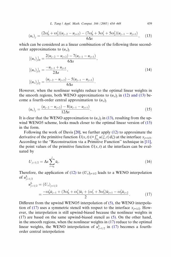
L. Tang / Appl. Math. Comput. 166 (2005) 434–448 439
ðuxÞj ¼ð2xj
0 þ xj2Þðuj�2 � ujþ2Þ � ð7xj
0 þ 3xj1 þ 5xj
2Þðuj�1 � ujþ1Þ6Dx
; ð13Þ
which can be considered as a linear combination of the following three second-
order approximations to (ux)j
½ðuxÞj�0 ¼2ðuj�2 � ujþ2Þ � 7ðuj�1 � ujþ1Þ
6Dx;
½ðuxÞj�1 ¼�uj�1 þ ujþ1
2Dx;
½ðuxÞj�2 ¼ðuj�2 � ujþ2Þ � 5ðuj�1 � ujþ1Þ
6Dx:
ð14Þ
However, when the nonlinear weights reduce to the optimal linear weights in
the smooth regions, both WENO approximations to (ux)j in (12) and (13) be-
come a fourth-order central approximation to (ux)j
ðuxÞj ¼ðuj�2 � ujþ2Þ � 8ðuj�1 � ujþ1Þ
12Dx: ð15Þ
It is clear that the WENO approximation to (ux)j in (13), resulting from the up-wind WENO5 scheme, looks much closer to the optimal linear version of (15)
in the form.
Following the work of Davis [20], we further apply (12) to approximate the
derivative of the primitive function U(x, t) (=R xx0uðn; tÞdn) at the interface xj+1/2.
According to the ‘‘Reconstruction via a Primitive Function’’ technique in [11],
the point values of the primitive function U(x, t) at the interfaces can be eval-
uated by
Ujþ1=2 ¼ DxXj
i¼i0
�ui: ð16Þ
Therefore, the application of (12) to (Ux)j+1/2 leads to a WENO interpolation
of uLjþ1=2
uLjþ1=2 ¼ ðUxÞjþ1=2
¼ �xj0�uj�1 þ ð3xj
0 þ xj1Þ�uj þ ðxj
1 þ 3xj2Þ�ujþ1 � xj
2�ujþ2
2: ð17Þ
Different from the upwind WENO5 interpolation of (5), the WENO interpola-
tion of (17) uses a symmetric stencil with respect to the interface xj+1/2. How-
ever, the interpolation is still upwind-biased because the nonlinear weights in
(17) are based on the same upwind-biased stencil as (5). On the other hand,
in the smooth regions, when the nonlinear weights in (17) reduce to the optimal
linear weights, the WENO interpolation of uLjþ1=2 in (17) becomes a fourth-
order central interpolation

440 L. Tang / Appl. Math. Comput. 166 (2005) 434–448
uLjþ1=2 ¼��uj�1 þ 7�uj þ 7�ujþ1 � �ujþ2
12: ð18Þ
Here both the stencil and coefficients are symmetric with respect to the inter-
face xj+1/2. This is why we refer the interpolation of (17) to as a central WENO4
interpolation.The central WENO4 interpolation of uRjþ1=2 can be found in a similar way
uRjþ1=2 ¼�xjþ1
0 �uj�1 þ ð3xjþ10 þ xjþ1
1 Þ�uj þ ðxjþ11 þ 3xjþ1
2 Þ�ujþ1 � xjþ12 �ujþ2
2:
ð19ÞDifferent from their upwind WENO5 counterparts, the central WENO4 inter-
polation of uRjþ1=2 in (19) is almost the same as the central WENO4 interpola-
tion of uLjþ1=2 in (17) except that the nonlinear weights may change from node tonode. When the nonlinear weights further reduce to the optimal linear weights,
which are constants,
uRjþ1=2 ¼ uLjþ1=2: ð20Þ
Therefore, in the smooth regions, no Riemann problem exists at the interfaces.
The second evolution (upwind) stage in the Godunov-type schemes can be
saved. The resulting spatial discretization is a simple and efficient central
scheme.
The above central WENO4 scheme is conceptually very neat. It takes full
advantage of both a central scheme in the smooth regions and an upwind
scheme in the non-smooth regions. Based on the local smoothness measures
of the solution, the scheme achieves an automatic transition between centraland upwind schemes. The upwind bias contained in the above central WENO4
scheme is the minimum for a stable and numerically non-oscillatory scheme in
the sense that upwinding is only introduced through the nonlinear weights in
the non-smooth regions.
It is noteworthy that the central WENO4 interpolation of uLjþ1=2 in (17) is
derived from the central WENO4 differencing of (ux)j in (12). Therefore, the
smoothness measures used in (17) should be determined based on the three
third-order polynomials used for construction of those second-order approxi-mations to (ux)j in (11) rather than the following three polynomial interpola-
tions of uLjþ1=2
ðuLjþ1=2Þ0 ¼��uj�1 þ 3�uj
2;
ðuLjþ1=2Þ1 ¼�uj þ �ujþ1
2;
ðuLjþ1=2Þ2 ¼3�ujþ1 � �ujþ2
2:
ð21Þ
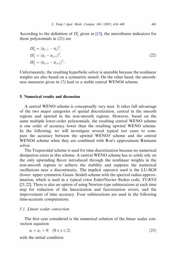
L. Tang / Appl. Math. Comput. 166 (2005) 434–448 441
According to the definition of ISjk given in [15], the smoothness indicators for
those polynomials in (21) are
ISj0 ¼ ð�uj�1 � �ujÞ2;
ISj1 ¼ ð�uj � �ujþ1Þ2;
ISj2 ¼ ð�ujþ1 � �ujþ2Þ2:
ð22Þ
Unfortunately, the resulting hyperbolic solver is unstable because the nonlinear
weights are also based on a symmetric stencil. On the other hand, the smooth-
ness measures given in (7) lead to a stable central WENO4 scheme.
5. Numerical results and discussion
A central WENO scheme is conceptually very neat. It takes full advantage
of the two major categories of spatial discretization, central in the smooth
regions and upwind in the non-smooth regions. However, based on the
same multiple lower-order polynomials, the resulting central WENO scheme
is one order of accuracy lower than the resulting upwind WENO scheme.
In the following, we will investigate several typical test cases to com-
pare the accuracy between the upwind WENO5 scheme and the central
WENO4 scheme when they are combined with Roe�s approximate Riemannsolver.
The Trapezoidal scheme is used for time discretization because no numerical
dissipation exists in this scheme. A central WENO scheme has to solely rely on
the only upwinding flavor introduced through the nonlinear weights in the
non-smooth regions to achieve the stability and suppress the numerical
oscillations near a discontinuity. The implicit operator used is the LU-SGS
(lower–upper symmetric Gauss–Seidel) scheme with the spectral radius approx-
imation, which is used in a typical rotor Euler/Navier–Stokes code, TURNS
[21,22]. There is also an option of using Newton-type subiterations at each time
step for reduction of the linearization and factorization errors, and the
improvement of time accuracy. Four subiterations are used in the following
time-accurate computations.
5.1. Linear scalar convection
The first case considered is the numerical solution of the linear scalar con-vection equation
ut þ ux ¼ 0 ð06 x6 2Þ ð23Þwith the initial condition

442 L. Tang / Appl. Math. Comput. 166 (2005) 434–448
uðx; 0Þ ¼
e� log 50 x�0:150:05ð Þ2 x0; 0:2;
1 0:3 < x < 0:4;
20x� 10 0:5 < x < 0:55;
12� 20x 0:556 x0; 0:6;ffiffiffiffiffiffiffiffiffiffiffiffiffiffiffiffiffiffiffiffiffiffiffiffi1� x�0:75
0:05
� �2q0:7 < x < 0:8;
0 otherwise;
8>>>>>>>>>><>>>>>>>>>>:
ð24Þ
which contains a smooth but narrow combination of a Gaussian function, asquare wave, a triangle wave, and a half ellipse, the same as in [23]. Each wave
spreads a distance of 10 cells on a coarser mesh of 200 cells and 20 cells on a
finer mesh of 400 cells. A CFL number of 0.4 is chosen for high time accuracy.
Fig. 1 presents the exact solution and the numerical results given by the
above two WENO schemes on the finer mesh after 500 time steps and on
the coarser mesh after 250 time steps. Here UWENO5 and CWENO4 stand
for Upwind WENO5 scheme presented in Section 3 and central WENO4
scheme presented in Section 4 respectively. It is found that although as ex-pected CWENO4 is slightly less accurate than UWENO5, the difference be-
tween the results given by these two methods is almost negligible, especially
for p = 1. The central WENO4 scheme seems more sensitive to the value of p
than the upwind WENO5 scheme. The difference between UWENO5 and
CWENO4 is slightly larger for p = 2 than for p = 1. Increasing p tends to damp
the peak values of the solution at those local extrema.
5.2. Sod’s shock-tube problem
The second selected case is the well-known Sod�s 1-D shock-tube problem
[24]. The governing equations are the 1-D Euler equations
o
ot
q
qu
e
0B@
1CAþ o
ox
qu
qu2 þ p
uðeþ pÞ
0B@
1CA ¼ 0; ð25Þ
and the initial data are
ðqL; uL; pLÞ ¼ ð1; 0; 1Þ; ðqR; uR; pRÞ ¼ ð0:125; 0; 0:1Þ: ð26ÞHere q, u, p and e are the density, velocity, pressure, and total energy per unit
volume respectively, and p = (c � 1)(e � qu2/2).Presented in Fig. 2 are the exact solution and the numerical results given by
the two WENO schemes on a uniform mesh of 100 cells over 0 6 x 6 1 after
125 time steps. For this case, it is found that the difference between the resultsgiven by UWENO5 and CWENO4 is negligible. The solutions are also not sen-
sitive to the choice of p.

-0.1
0
0.1
0.2
0.3
0.4
0.5
0.6
0.7
0.8
0.9
1
1.1
1.05 1.25 1.45 1.65 1.85
x
u
Exact
UWENO5
CWENO4
-0.1
0
0.1
0.2
0.3
0.4
0.5
0.6
0.7
0.8
0.9
1
1.1
1.05 1.25 1.45 1.65 1.85
x
u
Exact
UWENO5
CWENO4
(a)
(b)
Fig. 1. Linear scalar convection (CFL = 0.4): (a) p = 1, N = 400, 500 time steps; (b) p = 2, N = 400,
500 time steps; (c) p = 1, N = 200, 250 time steps; (d) p = 2, N = 200, 250 time steps.
L. Tang / Appl. Math. Comput. 166 (2005) 434–448 443
5.3. Woodward–Colella’s two interacting blast waves
The third selected case is Woodward–Colella�s problem in [25], which in-
volves the interaction of two blast waves. The initial data are the following:
(i) if 0 < x < 0.1, then
ðqL; uL; pLÞ ¼ ð1; 0; 1000Þ; ð27Þ(ii) if 0.1 < x < 0.9, then
ðqM; uM; pMÞ ¼ ð1; 0; 0:01Þ; ð28Þ

-0.1
0
0.1
0.2
0.3
0.4
0.5
0.6
0.7
0.8
0.9
1
1.1
1.05 1.25 1.45 1.65 1.85
x
u
Exact
UWENO5
CWENO4
-0.1
0
0.1
0.2
0.3
0.4
0.5
0.6
0.7
0.8
0.9
1
1.1
1.05 1.25 1.45 1.65 1.85
x
u
Exact
UWENO5
CWENO4
(c)
(d)
Fig. 1 (continued)
444 L. Tang / Appl. Math. Comput. 166 (2005) 434–448
(iii) if 0.9 < x < 1, then
ðqR; uR; pRÞ ¼ ð1; 0; 100Þ; ð29Þwhich presents one shock at x = 0.1 and the other at x = 0.9. The boundaries
at x = 0 and x = 1 are solid walls with a reflective boundary condition. After
a certain time, these two shocks collide with each other. At the final time step
of t = 0.038, the flow field involves two shocks and three contact discon-
tinuities.
Presented in Fig. 3 are the numerical solutions produced by UWENO5 and
CWENO4 on a uniform mesh of 400 cells at t = 0.038. There is no exact solu-
tion for this case. It is found that except in the middle region after the left shock
and before the right contact discontinuity, both UWENO5 and CWENO4
schemes produce very similar results. In that particular region, however, the

0
0.2
0.4
0.6
0.8
1
1.2
0.1 0.4 0.7 1
x
ρ
0
0.2
0.4
0.6
0.8
1
1.2
ρ
Exact
UWENO5
CWENO4
0.1 0.4 0.7 1
x
Exact
UWENO5
CWENO4
(a)
(b)
Fig. 2. Density distribution of Sod�s shock-tube problem (N = 100, CFL = 0.4, 125 steps): (a) p = 1
and (b) p = 2.
L. Tang / Appl. Math. Comput. 166 (2005) 434–448 445
results given by CWENO4 are not as smooth as those given by UWENO5,
especially in the distribution of the density and velocity for p = 2. While UWE-NO5 seems less sensitive to the choice of p, the results given by CWENO4 with
p = 1 look like smoother than those given by CWENO4 with p = 2 and are clo-
ser to the results given by UWENO5. Again, for the central WENO scheme,
increasing the value of p tends to reduce the peak values of the solutions at
the local extrama.
5.4. Shu–Osher’s problem
The fourth selected case is Shu–Osher�s problem in [13], which represents a
Mach 3 shock interacting with a sinusoidal density field. The initial data are
ðqL; uL; pLÞ ¼ ð3:86; 2:63; 10:33Þ; ðqR; uR; pRÞ ¼ ð1þ 0:2 sin 5x; 0; 1Þ:ð30Þ

0
1
2
3
4
5
6
0.4 0.5 0.6 0.7 0.8 0.9x
ρ
UWENO5CWENO4
0
1
2
3
4
5
6
0.4 0.5 0.6 0.7 0.8 0.9x
ρ
p=1 p=2
0.4 0.5 0.6 0.7 0.8 0.9x
0.4 0.5 0.6 0.7 0.8 0.9x
p=1 p=2
0
3
6
9
12
15
u
0
3
6
9
12
15
u
UWENO5CWENO4
(a)
(b)
(c)
0
50
100
150
200
250
300
350
400
450
0.4 0.5 0.6 0.7 0.8 0.9x
p
UWENO5CWENO4
0
50
100
150
200
250
300
350
400
450
0.4 0.5 0.6 0.7 0.8 0.9x
p
p=1 p=2
Fig. 3. Woodward–Colella�s blast waves problem (N = 400, Dt = 0.00005, t = 0.038): (a) density,
(b) velocity, and (c) pressure.
446 L. Tang / Appl. Math. Comput. 166 (2005) 434–448
Similar to the first case, in this problem, there are several extrema in the
smooth regions which present a good case for examination of the accuracy
of a shock-capturing scheme.
Again, no exact solution exists for this problem. Fig. 4 presents the numer-
ical results given by the two WENO schemes on the uniform meshes of 200 and400 cells at t = 1.8. It is found that the difference between the results given by
UWENO5 and CWENO4 is almost negligible. Increasing the value of p tends
to smear out the peak values of the solutions at those local extrema.

0
1
2
3
4
5
-3 -1 1 3x
ρ
UWENO5
CWENO40
1
2
3
4
5
-3 -1 1 3x
ρ
p=1 p=2
0
1
2
3
4
5
-3 -1 1 3x
0
1
2
3
4
5
-3 -1 1 3x
ρ
UWENO5
CWENO4
p=1 p=2
UWENO5
CWENO4
UWENO5
CWENO4
ρ
(a)
(b)
Fig. 4. Density distribution of Shu–Osher�s problem (Dt = 0.002, t = 1.8): (a) N = 400 and (b)
N = 200.
L. Tang / Appl. Math. Comput. 166 (2005) 434–448 447
6. Conclusions
There are two types of WENO schemes, upwind and central. A central
WENO scheme is conceptually very neat. It takes full advantage of the twomajor types of spatial discretization, central in the smooth regions and upwind
in the non-smooth regions. On the other hand, a central WENO scheme is one
order of accuracy lower than its upwind WENO counterpart. For most prob-
lems, the upwind and central WENO schemes produce very similar results.
However, for some tough cases, the solution given by the central WENO4
scheme is not as smooth as the one given by the upwind WENO5 scheme. A
central WENO scheme seems more sensitive to the choice of p. A better choice
for a central WENO scheme is p = 1.
Acknowledgements
This work is supported by NSF Grant DMI-0232255 and the technical mon-
itor is Dr. Juan E. Figueroa. The author would like to thank Prof. Chi-Wang
Shu for helpful discussions.

448 L. Tang / Appl. Math. Comput. 166 (2005) 434–448
References
[1] J.L. Steger, Implicit finite difference simulation of flow about two-dimensional geometries,
AIAA J. 16 (1978) 679.
[2] A. Jameson, W. Schmidt, E. Turkel, Numerical solution of the Euler equations by finite
volume methods using Runge–Kutta time stepping schemes, AIAA-81-1259, 1981.
[3] J.P. Boris, D.L. Book, Flux corrected transport, I SHASTA, a fluid transport algorithm that
works, J. Comput. Phys. 11 (1973) 38.
[4] D.L. Book, J.P. Boris, K. Hain, Flux-corrected transport II: generalizations of the method,
J. Comput. Phys. 18 (1975) 248.
[5] S.T. Zalesak, Fully multidimensional flux-corrected transport algorithms for fluids, J. Comput.
Phys. 31 (1979) 335.
[6] B. van Leer, Towards the ultimate conservative difference scheme. IV. A new approach to
numerical convection, J. Comput. Phys. 23 (1977) 276.
[7] A. Harten, On a class of high resolution total-variation-stable finite-difference schemes, SIAM
J. Numer. Anal. 21 (1984) 1.
[8] P.L. Roe, Some contributions to the modeling of discontinuous flows, Lect. Appl. Math. 22
(1985) 163.
[9] P.K. Sweby, High resolution schemes using flux limiters for hyperbolic conservation laws,
SIAM J. Numer. Anal. 21 (1984) 995.
[10] S.R. Chakravarthy, S. Osher, High resolution applications of the Osher upwind scheme for the
Euler equations, AIAA paper 83-1943, 1983.
[11] A. Harten, B. Engquist, S. Osher, S.R. Chakravarthy, Uniformly high order accurate
essentially non-oscillatory schemes, III, J. Comput. Phys. 71 (1987) 231.
[12] C.-W. Shu, S. Osher, Efficient implementation of essentially non-oscillatory shock capturing
schemes, J. Comput. Phys. 77 (1988) 439.
[13] C.-W. Shu, S. Osher, Efficient implementation of essentially non-oscillatory shock capturing
schemes, II, J. Comput. Phys. 83 (1989) 32.
[14] X.-D. Liu, S. Osher, T. Chan, Weighted essentially non-oscillatory schemes, J. Comput. Phys.
115 (1994) 200.
[15] G.-S. Jiang, C.-W. Shu, Efficient implementation of weighted ENO schemes, J. Comput. Phys.
126 (1996) 202.
[16] D.S. Balsara, C.-W. Shu, Monotonicity preserving weighted essentially non-oscillatory
schemes with increasingly high order of accuracy, J. Comput. Phys. 160 (2000) 405.
[17] L. Jiang, H. Shan, C.Q. Liu, Weighted compact scheme for shock capturing, Int. J. Comput.
Fluid Dyn. 15 (2001) 147.
[18] D. Levy, G. Puppo, G. Russo, Central WENO schemes for hyperbolic systems of conservation
laws, Math. Modell. Numer. Anal. (M2AN) 33 (1999) 547.
[19] J. Shi, C.-Q. Hu, C.-W. Shu, A technique of treating negative weights in WENO schemes,
J. Comput. Phys. 175 (2002) 108.
[20] S.F. Davis, Shock capturing with Pade method, Appl. Math. Comput. 89 (1998) 85.
[21] G.R. Srinivasan, J.D. Baeder, S. Obayashi, W.J. McCroskey, Flowfield of a lifting rotor in
hover––a Navier–Stokes simulation, AIAA J. 30 (1992) 2371.
[22] L. Tang, Improved Euler simulation of helicopter vortical flows, Ph.D. Thesis, University of
Maryland, College Park, 1998.
[23] A. Suresh, H.T. Huynh, Accurate monotonicity preserving scheme with Runge–Kutta time-
stepping, J. Comput. Phys. 136 (1997) 83.
[24] G. Sod, A survey of several finite difference methods for systems of nonlinear hyperbolic
conservation laws, J. Comput. Phys. 27 (1978) 1.
[25] P. Woodward, P. Colella, The numerical simulation of two-dimensional fluid flow with strong
shocks, J. Comput. Phys. 54 (1984) 115.


![WLS-ENO: Weighted-Least-Squares Based Essentially Non ...jiao/papers/wls-eno-fvm.pdf · ENO scheme [24] and its closely related WENO schemes [2]. In a nutshell, the ENO is a WENO](https://img.pdfslide.us/doc/110x75/6117dbe78dfbd9699074d533/wls-eno-weighted-least-squares-based-essentially-non-jiaopaperswls-eno-fvmpdf.jpg)


![Central-Upwind Schemes for Two-Layer Shallow Water Equationsgpetrova/KP_2l.pdf · Central-Upwind Schemes for Two-Layer Shallow Water ... we refer the reader to [2], ... Central-Upwind](https://img.pdfslide.us/doc/110x75/5abcf7377f8b9a24028e74bf/central-upwind-schemes-for-two-layer-shallow-water-gpetrovakp2lpdfcentral-upwind.jpg)