Embed Size (px)
Citation preview

Upstream greenhouse gas (GHG) emissions from Canadian oil sands asa feedstock for European refineries
Adam R. Brandt
Department of Energy Resources EngineeringStanford UniversityGreen Earth Sciences 065, 367 Panama St.Stanford, CA 94305-2220
Email: [email protected]: +1-650-724-8251
January 18, 2011

Brandt Upstream GHG emissions from oil sands production 2
1 Executive summary
Production of hydrocarbons from the Canadian oil sands reached approximately 1500kbbl/d in 2009, or almost 2% of global crude petroleum production. Due to the energyintensity of oil sands extraction and refining, fuel greenhouse gas (GHG) regulations mustassess the GHG emissions from oil-sands-derived fuels in comparison to emissions fromconventional oil production.
This report outlines the nature of oil sands extraction and upgrading processes, with anemphasis on factors affecting energy consumption. Next, it compares a variety of recentestimates of GHG emissions from oil sands, and outlines reasons for variation betweenestimates. Lastly, it outlines low, high and “most likely” estimates of GHG emissions fromoil sands, given results from previously produced estimates, and compare these emissionsto those of conventional fuels. This report focuses on the European context, and thereforeuses EU-specific emissions factors for transport and refining of fuels.
There is significant variation between current estimates of GHG emissions from oil-sands-derived fuels. This variation has a number of causes, including:
1. Differences in scope and methods of estimates: some studies model emissions fromspecific projects, while others generate average industry-wide emissions estimates.
2. Differences in assumed efficiencies of extraction and upgrading, especially with re-spect to the energy efficiency of steam-assisted gravity drainage (SAGD).
3. Differences in the fuel mix assumed to be consumed during oil sands extraction andupgrading.
4. Treatment of secondary non-combustion emissions sources, such as venting, flaringand fugitive emissions.
5. Treatment of ecological emissions sources, such as land-use change (LUC) associ-ated emissions.
These differences are discussed in some detail, although without access to originalmodel calculations it is difficult to determine all reasons for divergence in emissions es-timates.
Low, high and most likely emissions estimates for Canadian oil sands derived fuelsare shown in Figure 1. Low emissions are likely for natural-gas fired mining and upgrad-ing processes, while high emissions are likely from SAGD processes fueled with bitumenresidues. Figure 1 also shows the range of estimates for current conventional fuel streamsin the EU. For conventional crude streams, low and high ranges are supplied by the leastand most GHG-intensive petroleum streams consumed in the EU (i.e., Norway and Nige-ria, respectively).
Figure 1 shows that the lowest intensity oil sands process is less GHG intensive than themost intensive conventional fuel (as noted in recent reports by IHS-CERA, Jacobs Consul-tancy and others). Importantly though, the most likely industry-average GHG emissionsfrom oil sands are significantly higher than most likely industry-average emissions fromconventional fuels. The significant range between low and high estimates in both oil sands

Brandt Upstream GHG emissions from oil sands production 3
and conventional fuel streams is primarily due to variation in modeled process parame-ters, not due to fundamental uncertainty about the technologies.
Figure 2 shows the relative importance of upstream emissions from oil sands projectsby plotting output by oil sands project, cumulated and placed in order of low to highemissions. It also displays cumulated conventional oil consumption in the EU in order ofemissions intensity (see text for construction details). The key result is that while the high-est emissions conventional oil has higher upstream emissions than the lowest emissionsoil sands estimate, the production-weighted emissions profiles are significantly different.Despite uncertainty in these figures, GHG emissions from oil sands production as sig-nificantly different enough from conventional oil emissions that regulatory frameworksshould address this discrepancy with pathway-specific emissions factors that distinguishbetween oil sands and conventional oil processes.
The uncertainties that still remain with respect to modeling GHG emissions from theCanadian oil sands suggest the need for additional research. The most important uncer-tainties include:
1. Treatment of electricity cogeneration is variable across studies, and is uncertain be-cause of a lack of data on amounts of co-produced power, and difficulty in deter-mining the correct co-production credit for electricity exports.
2. Detailed treatment of refining is lacking in publicly available models, due to lack ofaccess to proprietary refining models.
3. Market considerations are lacking, which have important effects on co-product andby-product disposition, including the fate of produced coke.
This report was reviewed by a panel of outside experts, including: William Keesom,Jacobs Consultancy; Stefan Unnasch, Life Cycle Associates LLC.; Don O’Connor, S&T2
Consultants Inc.; and Joule Bergerson, University of Calgary.

Brandt Upstream GHG emissions from oil sands production 4
0
10
20
30
40
50
60
70
80
90
100
110
120
130
Weighted-‐average -‐ Most likely tar sands blend
Weighted-‐average EU convenBonal refinery feedstock
Well-‐to-‐whe
el life cycle GHG
emissions
(gCO
2 eq./M
J LHV
)
CombusBon*
Transport & distribuBon Refining*
VFF
Upgrading
ExtracBon
Figure 1: Oil sands emissions compared to conventional EU refinery feedstock emissions.Most likely estimates are base values of bars, low and high ranges are represented by errorbars. See report text for calculation details.

Brandt Upstream GHG emissions from oil sands production 5
0
20
40
60
80
100
120
140
0 0.2 0.4 0.6 0.8 1
Full fuel cycle (w
ell-‐to-‐whe
el) G
HG emissions
(g CO2 eq
./MJ o
f gasoline)
Normalized fracIon of producIon or imports
Oil sands ConvenIonal
Most likely value
Figure 2: Emissions as a function of cumulative normalized output, for oil sands projects(low and high estimates) and conventional oil imports to the EU. Only oil sands projectsthat produce refinery ready SCO are included as these full-fuel-cycle estimates utilize pre-calculated emissions estimates for EU refineries processing approximately 30 ◦API oil.Bounds on oil sands emissions are provided by (low) CNRL Horizon, (high) OPTI-Nexen,Long Lake SAGD + Residue gasification to SCO. The bounds on conventional oil emis-sions are provided by (low) Norway, (high) Nigeria. Due to uncertainty in Nigerian crudeoil emissions, two values are reported for Nigerian crude. See report text for calculationdetails.

Brandt Upstream GHG emissions from oil sands production 6
2 Introduction
As conventional oil production becomes increasingly constrained, transportation fuels arebeing produced from low-quality hydrocarbon resources (e.g. bitumen deposits) as well asfrom non-petroleum fossil fuel feedstocks (e.g. gas-to-liquid synthetic fuels). Greenhousegas (GHG) regulations such as the California Low Carbon Fuel Standard (CA LCFS) andEuropean Union Fuel Quality Directive must properly account for the GHG intensities ofthese new fuel sources.
Significant volumes of transport fuels are already produced using unconventional tech-nologies and from unconventional resources. These include enhanced oil recovery, oilsands, coal-to-liquids and gas-to-liquids synthetic fuels, and oil shale. US enhanced oil re-covery (EOR) projects produced 663 kbbl/d in 2010 [1]. About 40% of US EOR productionis from steam-induced heavy oil production in California and 60% is from gas injection(largely CO2 injection) [1]. Global EOR production is less certain due to poor data avail-ability, but exceeds 1200 kbbl/d [1].
Production of crude bitumen from the oil sands reached 1490 kbbl/d in 2009 [2, 3].Production of liquid products from oil sands, including raw bitumen and synthetic crudeoil (SCO), reached 1350 kbbl/d in 2009, due to volume loss upon upgrading of bitumen toSCO. This amount represents an increase from ≈ 600 kbbl/d in 2000 [4]. Current plans forexpansion of production capacity are significant, with over 7000 kbbl/d of capacity in allstages of construction and planning, as shown in Figure 3 [3].
This report studies upstream GHG emissions from Alberta oil sands production. Thegoal of this report is to comment on the comparability of previously published estimatesof GHGs from oil-sands-derived fuels, and to compile a range of emissions factors for oil-sands-derived fuel streams as inputs to a notional EU refinery.
First, this report provides an overview of the Alberta oil sands, with a focus on determi-nants of energy use and emissions from oil sands production. Next, previous estimates ofGHG emissions from oil sands production are reviewed and compared. Lastly, this reportuses published model results to estimate emissions from oil-sands-derived fuels processedin a notional European refinery.
***
Technical note: All units and prefixes used in this report are in SI units, with the exceptionof volumes of crude oil produced and steam injected, which will be reported in barrels(bbl). Crude oil density is generally reported in specific gravity (sg) rather than API grav-ity. Emissions per unit of energy will generally be reported per megajoule (MJ) on a lowerheating value (LHV) basis, except where the original source is unclear about the basis. Formost fuels of interest in this report, the potential error in GHG emissions estimates due tounspecified fuel heating value basis is ≈ 5-7%.

Brandt Upstream GHG emissions from oil sands production 7
3 Overview of oil sands production methods
Oil sands (also called tar sands) are more accurately called bituminous sands, as they con-tain natural bitumen [5]. Resource estimates for Canadian bitumen in place are between1.17 Tbbl [5] and 2.5 Tbbl [6]. Oil sands are a mixture of sand and other mineral matter(80-85%) water (5-10%) and bitumen (1-18%) [5]. Bitumen is a dense, viscous mixture ofhigh-molecular weight hydrocarbon molecules. Bitumen is either sold as a refinery feed-stock or upgraded to SCO and shipped to refineries.
3.1 Oil sands extraction
Bitumen can be produced through surface mining or in situ production methods. Surfacemining techniques require removal of vegetation and topsoil, removal of overburden (in-ert, non-hydrocarbon bearing mineral matter that lies above bitumen) and mining of thebitumen/sand mixture. The bitumen/sand mixture is transported to processing facilitieswhere it is mixed with hot water, screened and separated into bitumen and tailings (a wa-ter/sand mixture) [5]. A variety of in situ techniques exist, the most commonly appliedbeing steam-assisted gravity drainage (SAGD) and cyclic steam stimulation (CSS). Thesein situ processes are similar in concept to thermal EOR processes for heavy oil extraction:heat from injected steam reduces the viscosity of bitumen, allowing it to flow to the well-bore under existing pressure gradients or by gravity drainage [7].
3.1.1 Mining-based bitumen production
Overburden removal is typically performed with a truck-and-shovel operation [8]. Bi-tumen ore is mined with diesel or electric hydraulic shovels. Large haul trucks (dieselpowered) move the ore to central crushing and slurrying centers for hydrotransport viapipeline to extraction centers. Some mining and processing equipment is powered withelectricity co-produced on site from natural gas, upgrading process gas, or coke, with thegenerating fuel dependent on the operation [9]. In 2002, Syncrude reported comsuming1 Mbbl of diesel fuel for the production of 250,000 bbl/day of SCO, or about 62 MJ ofdiesel per bbl of SCO produced [9]. Estimates presented in the literature of mining energyconsumption vary across an order of magnitude from 50-580 MJ/bbl of SCO [6, 10].1
At the extraction facilities, bitumen froth (60%+ bitumen, remainder water) is sepa-rated from sand. This has been called an “expensive...and inflexible” process, requiringwarm water and consuming 40% of the energy used to produce a barrel of SCO [8]. In in-tegrated operations, upgrader by-products, including process gas and coke, provide heatand power for the separation process [9]. Consumption data from integrated operationsare shown in Figure 4, illustrating the variety of fuels consumed by projects [11].
After primary separation, the bitumen froth is treated to remove water and solids, us-ing naphtha or parrafinic solvents. This produces a bitumen ready for either dilution andsale or for upgrading to synthetic crude oil. Energy costs for separation of the bitumen areestimated at 150 MJ/bbl [10, 12].
1Given that the high end of this range (580 MJ/bbl SCO) represents some 10% of the energy content of theSCO, this is likely an overestimate of mining energy inputs.

Brandt Upstream GHG emissions from oil sands production 8
0
500
1000
1500
2000
2500
3000
3500
4000
Mining Athabasca in situ Cold lake in situ Peace River in situ
Pro
du
ctio
n c
apac
ity
(kb
bl/
d o
f b
itu
men
)
Announced
Disclosure
Withdrawn
Application
Approved
Construction
Operating
Figure 3: Oil sands production capacity, operational and proposed projects, by stage ofcompletion (current as of January, 2010) [3].
3.1.2 In-situ bitumen production
Oil sands are currently produced in situ using three techniques: cold production (generallysuitable for resources above ≈12 ◦API and so not considered further), cyclic steam stimu-lation (CSS), and steam assisted gravity drainage (SAGD) [8]. Thermal in situ productionvia CSS or SAGD is more energy intensive than mining-based production.
Thermal in situ recovery is made possible by the reduction in hydrocarbon viscositywith increases in temperature. After heating with steam, bitumen reaches a state where itwill flow to the well for production. SAGD and CSS differ primarily in the well configura-tion used for steam injection and bitumen extraction.
GHG emissions from in situ production result primarily from fuels combusted forsteam generation. The amount of energy required to convert water to steam for injec-tion depends on the steam pressure and steam quality, with cited values for 80% qualitysteam ranging from 320-380 MJ/bbl of cold water equivalent (CWE) turned to steam [7]. Akey indicator is the steam oil ratio (SOR), measured as volume of CWE steam injected pervolume of oil produced. Higher SORs, if all else is held equal, will result in larger GHGemissions from in situ production. Common SORs for in situ recovery projects range from2 to 5, with the production-weighted industry average being 3.2 in 2009 (see Table 1). SORsas high as 9.6 were reported in 2009, but these may represent transient effects due to re-quired initial buildup of reservoir temperature at the start of SAGD operations [13]. SORshave tended to improve over time with the maturation of SAGD technology. This can beexpected to continue, given the strong financial incentives (as well as regulatory require-ments) to reduce natural gas consumption. Such trends will likely have beneficial impactson GHG emissions from SAGD (which may be partially offset by declining resource qual-

Brandt Upstream GHG emissions from oil sands production 9
0%
10%
20%
30%
40%
50%
60%
70%
80%
90%
100%
Suncor Energy Inc.
Syncrude Canada Ltd.
- Mildred Lake
Albian Sands
Energy Inc.
Shell Canada Energy -Scotford Upgrader
CNRL -Horizon Oil
Sands Project
Total mining
Fuel
mix
by
faci
lity
Process gas Electricity Natural gas Coke
Figure 4: Approximate mining and upgrading fuel mixes for integrated (Suncor and Syn-crude) and stand-alone operations. Compiled from volumetric [m3] and mass [tonne] con-sumption rates by project as reported by ERCB [11]. ERCB does not report diesel con-sumption for haul trucks, allowing only an approximate fuel mix determination.
ity over time).Accounting for the above uncertainties, steam generation energy consumption for an
SOR range of 2.5 to 5 ranges from ≈ 950 to 2100 MJ/bbl of bitumen produced, assumingsteam generation equipment similar to California thermal EOR projects.2 This range isconservative, and is based on producing 80% quality steam for California thermal EOR viasteamflooding [7]. Energy consumption in SAGD projects is likely to be somewhat higher,due to the requirement for 100% quality steam [14], although this will be partially offsetby the newer age of the equipment in SAGD operations. To produce 100% quality steam,80% quality steam is first produced in once-through steam generators, and vapor-liquidseparators are used to reject solute-laden liquid phase water (“blowdown” water). Dueto the heat of vaporization of water and imperfect heat recovery from blowdown water,energy consumption is higher for 100% quality steam. Charpentier cites up to 450 MJ/bblof steam, while Butler cites ≈540 MJ/bbl for 100% quality steam generation [15, p. 7] [16].Electricity consumption for in situ production has been estimated as 30 MJ/bbl bitumen(8.25 kWh/bbl bitumen), but will vary with SOR due to dependence on pumping loads[8].
Steam generation for in situ production is generally fueled with natural gas. An ex-ception is the OPTI-Nexen Long Lake project, which consumes gasified bitumen residues[17, 18]. This converts a low-quality upgrading residue to fuel for the extraction process,
2Calculation method follows that of Brandt and Unnasch [7]. This low and high range assumes enthalpy ofsteam of 325 and 337.5 MJ/bbl, once-through steam generator with 85% and 80% efficient steam generation,LHV basis, and SORs of 2.5 and 5, respectively. Energy consumed per bbl of steam is 380-420 MJ/bbl steam.

Brandt Upstream GHG emissions from oil sands production 10
Table 1: Steam oil ratios (SORs) for in situ bitumen production (2009). A sample of large insitu projects is included, along with the average for all thermal in situ production [13].
Operator - Project Bitumen production Water injection SOR103 m3/d 103 m3/d m3 water/m3 oil
Imperial - Cold lake 22.4 78.5 3.50CNRL - Primrose 9.8 58.9 5.99EnCana - Foster creek 12.0 30.1 2.49Suncor - Firebag 7.8 24.3 3.13
Total thermal in situa 81.4 256.3 3.18a - Total values include summed bitumen production and steam injection for all projectsin ERCB databases labeled “Commercial” “Commercial-CSS”, “Commercial-SAGD”“Enhanced Recovery”, and “Experimental” [13]. Projects labeled “Primary” are not in-cluded due to likliehood that these represent primary production of heavy crude oils (i.e.,cold production).
avoiding purchases of natural gas and the associated operating expense volatility. How-ever, this configuration also significantly increases GHG emissions compared to natural-gas-fueled SAGD [18, 19].
3.2 Bitumen upgrading
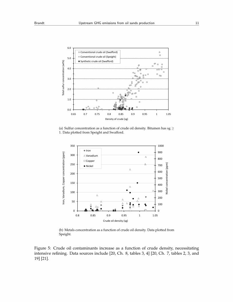
Because contaminants are concentrated in heavy hydrocarbon fractions, bitumen has sig-nificant sulfur and metals content, as shown in Table 2 and Figure 5. In addition, bitumenis carbon-rich, hydrogen-deficient, and contains a larger fraction of asphaltenes comparedto conventional crude oils (Table 2). Thus, bitumen requires more intensive upgrading andrefining than conventional crude oil.
Raw bitumen will not reliably flow through a pipeline at ambient temperatures. There-fore it must be modified before delivery. Bitumen can be transported after dilution with alighter hydrocarbon diluent (creating “dilbit,” or “synbit” if synthetic crude oil is used asthe diluent). Diluent can either be returned to the processing site or included with bitumento the refinery stream. If bitumen is not diluted, it must be upgraded into a synthetic crudeoil (SCO) before shipment.
Greenhouse gas emissions from upgrading have three causes:
1. Combustion of fuels for process heat, including process gas, natural gas or petroleumcoke.
2. Hydrogen production using steam reformation of natural gas, or less commonlyfrom gassification of petroleum coke or bitumen residues.
3. Combustion for electricity generation (whether on-site as part of a cogenerationscheme or off-site for production of purchased electricity).
Upgrading bitumen to SCO is performed in two stages. Primary upgrading separatesthe bitumen into fractions and reduces the density of the resulting SCO by increasing the
Brandt Upstream GHG emissions from oil sands production 11
0.0
1.0
2.0
3.0
4.0
5.0
6.0
0.65 0.7 0.75 0.8 0.85 0.9 0.95 1 1.05
Tota
l su
lfu
r co
nce
ntr
atio
n (
wt%
)
Density of crude (sg)
Conventional crude oil (Swafford)
Conventional crude oil (Speight)
Synthetic crude oil (Swafford)
(a) Sulfur concentration as a function of crude oil density. Bitumen has sg ≥1. Data plotted from Speight and Swafford.
0
100
200
300
400
500
600
700
800
900
1000
0
50
100
150
200
250
300
350
0.8 0.85 0.9 0.95 1 1.05
Nic
kel c
on
cen
trat
ion
(p
pm
)
Iro
n, V
anad
ium
, Co
pp
er c
on
cen
trat
ion
(p
pm
)
Crude oil density (sg)
Iron
Vanadium
Copper
Nickel
(b) Metals concentration as a function of crude oil density. Data plotted fromSpeight.
Figure 5: Crude oil contaminants increase as a function of crude density, necessitatingintensive refining. Data sources include [20, Ch. 8, tables 3, 4] [20, Ch. 7, tables 2, 3, and19] [21].

Brandt Upstream GHG emissions from oil sands production 12
Table 2: Bitumen and conventional oil properties [22, table 1], [23].
Property Conv. oil Athabasca Bitumen AthabascaSCO
Density [sg] 0.82-0.93 0.99-1.02 0.877
Elemental comp. [wt %] Carbon 86 83.1 87.53Hydrogen 13.5 10.6 12.32Sulfur 0.1-2 4.8 0.136Nitrogen 0.2 0.4 0.079Oxygen — 1.1 —
Metals [ppm] Vanadium ≤100 total 2500 ≤0.1Nickel 100 ≤0.1Iron 75 ≤0.1Copper 5 0.1
HC type [wt.%] Oils 95 49 98+Resins — 32 0.96Asphaltenes ≤ 5 19 0.06
hydrogen-to-carbon (H/C) ratio of the heavy fractions. Secondary upgrading treats result-ing SCO fractions to remove impurities such as sulfur, nitrogen and metals.
Primary upgrading changes the H/C ratio by adding hydrogen or rejecting carbonfrom the heavy fraction of the bitumen feedstock. The most common upgrading processesrely on coking to reject carbon [24]. Carbon is rejected from heavy bitumen fractions us-ing fluid or delayed coking processes [5]. Of the major integrated operations, Syncrudeutilizes fluid coking, while Suncor uses delayed coking. Coking generates upgraded SCOas well as byproducts of coke and process gas [8]. For example, Suncor’s delayed cokingupgrading resulted in 85% by energy content produced as SCO, 9% as process gas, and 6%as coke [11]. Natural gas or co-produced process gas is often used to drive coking, but in afluid coker a portion of the coke can be combusted to fuel the coking process.
In existing operations, coke disposition varies. In 2009, Suncor consumed 26% of pro-duced coke and exported another 7% for offsite use, while the rest was stockpiled or land-filled. In contrast, the CNRL Horizon project stockpiled all produced coke. Syncrudeoperations were intermediate in coke consumption levels [11]. The OPTI-Nexen projectavoids this need for coke disposal by gassifying upgrading residues (as asphaltenes) andgenerating no net coke output.
A competing upgrading approach relies on hydrogen addition for primary upgrading,as used by Shell at their Scotford upgrader [13], which uses an ebullating-bed catalytichydrotreating process. Treating the bitumen with hydrogen addition results in larger vol-umes of SCO produced from a given bitumen stream, and a high quality product. It alsorequires larger volumes of H2, with associated natural gas consumption and GHG emis-sions. The Scotford upgrader produced 82% of process outputs as SCO, 18% as processgas, and no coke (on an energy content basis) [11].
In secondary upgrading the heavier fractions of primary upgrading processes—which

Brandt Upstream GHG emissions from oil sands production 13
Table 3: Characteristics of bitumen-derived SCO products. Source: Batch Quality Reports,www.crudemonitor.ca [27]. Most recent assay is used for each crude stream, long-termaverages used for metals content.
API Density Sulfur Metals◦API kg/m3 wt% (Fe+Ni+V+Mo)
mg/l
Premium Albian Synthetic 34 854 0.05 6Suncor Synthetic A 32.2 864 0.2 7CNRL Light Sweet Synthetic 34.4 852 0.05 -Syncrude Synthetic 31.8 866 0.21 -
Albian Heavy Synthetic 19.1 939 2.9 163Suncor Synthetic H 19.5 937 3.07 15
Cold Lake Dilbit 21.3 925 3.76 224
contain the majority of the contaminants—are hydrotreated (i.e., treated through the ad-dition of H2 in the presence of heat, pressure, and a catalyst). This reduces sulfur concen-trations and improves the quality of the product. Blending of resulting streams produceslight refinery-ready SCO of 30-34 ◦API, 0.1 wt% sulfur and 500 ppm nitrogen [25]. HeavySCO streams, such as Suncor Synthetic H, are also produced, but in smaller quantities.Suncor Synthetic H has an API gravity of ≈20 and sulfur content of ≈3 wt.%. In chem-ical composition, dilbit looks similar to heavy synthetic blends. Characteristics of somemarketed SCO products are listed in Table 3.
Hydrogen consumption by hydrotreaters is significantly often in excess of 3 times thestoichiometric requirement for heteroatom removal, due to simultaneous hydrogenationof unsaturated hydrocarbons [25, p. 295]. Hydrogen consumed in secondary upgrading isgenerally produced via steam methane reformation of natural gas, regardless of primaryupgrading process [9]. Current expections include the OPTI-Nexen integrated SAGD toSCO project, which uses bitumen residues for H2 production. Consumption of H2 in up-grading processes ranges from 200-500 MJ/bbl of bitumen upgraded [26, p. 4-6].
Nearly all of the bitumen produced from mining is upgraded, while most of the in-situ-based production is shipped as a bitumen/diluent mixture to refineries in the PADDII region [8]. There is no fundamental physical or chemical reason that in situ producedbitumen cannot be upgraded [18].
3.3 SCO and bitumen refining
Non-upgraded bitumen supplied to refineries requires intensive refining, due to qualitydeficiencies cited above (Table 2). Refining of bitumen also produces a less desirable slateof outputs without extensive processing, due to high asphaltenes content.
Synthetic crude oil is a high-value product. Figure 5(a) shows that for a given den-sity, SCOs (dark markers) have low sulfur content compared to conventional crude oilsof similar density. Also, SCOs lack the typical “bottom” of a conventional crude oil (i.e.,residual products from distillation), because the components that would form the bottom

Brandt Upstream GHG emissions from oil sands production 14
of the SCO barrel are destroyed during upgrading. Figure 6(a) shows distillation curves forAthabasca bitumens, SCOs and Brent conventional crude. As the temperature increases,increasingly heavier fractions boil. As can be seen, over half of the mass of bitumen has notboiled by 550◦C, while all of SCO boils at temperatures ≤550◦C. Note that SCOs have lessheavy fraction than the conventional Brent crude marker (for this reason they are some-times called “bottomless”). Figure 6(b) shows the breakdown of products obtained undervacuum distillation, indicating the lack of residual bottom fraction in SCO [28].

Brandt Upstream GHG emissions from oil sands production 15
0
25
50
75
100
0 100 200 300 400 500 600
Frac
tio
n b
oile
d (
wt
%)
Temperature (deg. C)
SCO (Yui and Chung 2001)
SCO (Wang et al. 2007)
Brent crude (Rhodes 1995)
Athabasca Bitumen (Speight 2008)
Athabasca bitumen (Speight 2008)
(a) Distillation curves for Athabasca bitumen, Brent crude marker, andAthabasca bitumen SCO.
0
10
20
30
40
50
60
70
80
90
100
WTI Arab Light SCO
Frac
tio
nal
yie
ld (
vol%
)
Naphtha/LPG Distillate Vacuum gas oil Residuals
(b) Yields of product from crude separation/distillation. SCO yields lacklow-quality residual oils.
Figure 6: Qualities of SCO as compared to conventional crudes. Data sources include [5,tables 4.2, 4.4] [29] [30] [23].

Brandt Upstream GHG emissions from oil sands production 16
y = -0.77x + 86.39R² = 0.86
y = -0.09x + 15.13R² = 0.72
10
12
14
16
18
20
22
30
40
50
60
70
80
90
0 5 10 15 20 25 30 35 40
Ref
inin
g G
HG
Em
issi
on
s (g
CO
2e/
MJ
RB
OB
)
Ref
inin
g G
HG
Em
issi
on
s (k
g C
O2e/
bb
l oil)
Crude Gravity (°API)
kg/bbl crude
g GHGs / MJ RBOB
Figure 7: Fit of modeled GHG emissions to API gravity, from 11 crude streams modeledby Keesom et al. [7, 26]. Emissions on right axis per unit of reformulated blendstock foroxygenate blending (RBOB, i.e., raw gasoline before final blending).
Most LCA studies to date treat the refining of crude inputs (SCO and bitumen) in avery simple fashion [31, 32]. This is partly due to the absence of publicly-available modelsof refinery operations, and due to the fact that historical models (e.g., GREET have soughtto produce a national average result, without attention to refining differences betweenindividual crude blends). The most detailed study to date is the work of Keesom et al., whomodel the refining of SCO, bitumen, and diluent-bitumen mixtures using a commercialrefinery model [26]. Similar work was undertaken by Rosenfeld et al. [19].
Emissions can be approximately adjusted for crudes of differing density using the lin-ear fit from Brandt and Unnasch, which is based on the output from Keesom et al. model,shown in Figure 7 [7]. By the line of best fit, each API gravity decrease of 1◦ will increaserefining emissions by 0.09 gCO2 per MJ of gasoline blendstock produced.
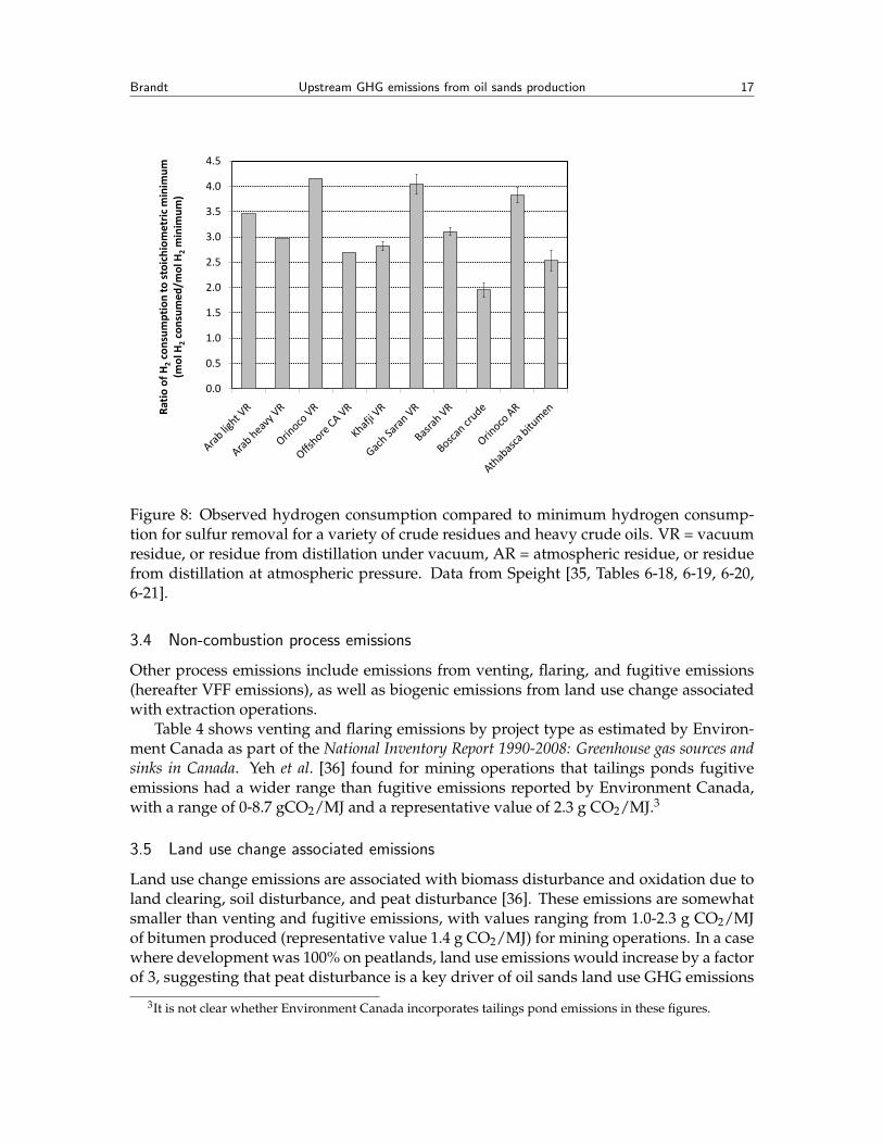
Also, streams that have different sulfur content than the nominal refinery feedstockcan be given a credit or debit based on the hydrogen consumption for desulfurization,assuming the hydrogen is generated from steam methane reforming. Observed hydrogenconsumption is generally in excess of that which would be expected based on the hydrogencontained in H2S stream removed from the feedstock crude, due to saturation of unsatu-rated hydrocarbons (e.g., olefins, aromatics) [33, p. 294]. Data from a variety of heavycrudes and residue are plotted in Figure 8, showing a similar relationship. Assuming that3 moles of H2 are consumed for every mole of H2S formed, and H2 is produced in a steammethane reformer, CO2 emissions will increase by ≈ 1.4 kg CO2 per kg S removed [34].
Brandt Upstream GHG emissions from oil sands production 17
0.0
0.5
1.0
1.5
2.0
2.5
3.0
3.5
4.0
4.5R
atio
of
H2
con
sum
pti
on
to
sto
ich
iom
etri
c m
inim
um
(m
ol H
2co
nsu
me
d/m
ol H
2m
inim
um
)
Figure 8: Observed hydrogen consumption compared to minimum hydrogen consump-tion for sulfur removal for a variety of crude residues and heavy crude oils. VR = vacuumresidue, or residue from distillation under vacuum, AR = atmospheric residue, or residuefrom distillation at atmospheric pressure. Data from Speight [35, Tables 6-18, 6-19, 6-20,6-21].
3.4 Non-combustion process emissions
Other process emissions include emissions from venting, flaring, and fugitive emissions(hereafter VFF emissions), as well as biogenic emissions from land use change associatedwith extraction operations.
Table 4 shows venting and flaring emissions by project type as estimated by Environ-ment Canada as part of the National Inventory Report 1990-2008: Greenhouse gas sources andsinks in Canada. Yeh et al. [36] found for mining operations that tailings ponds fugitiveemissions had a wider range than fugitive emissions reported by Environment Canada,with a range of 0-8.7 gCO2/MJ and a representative value of 2.3 g CO2/MJ.3
3.5 Land use change associated emissions
Land use change emissions are associated with biomass disturbance and oxidation due toland clearing, soil disturbance, and peat disturbance [36]. These emissions are somewhatsmaller than venting and fugitive emissions, with values ranging from 1.0-2.3 g CO2/MJof bitumen produced (representative value 1.4 g CO2/MJ) for mining operations. In a casewhere development was 100% on peatlands, land use emissions would increase by a factorof 3, suggesting that peat disturbance is a key driver of oil sands land use GHG emissions
3It is not clear whether Environment Canada incorporates tailings pond emissions in these figures.

Brandt Upstream GHG emissions from oil sands production 18
Table 4: Venting, flaring, and fugitive (VFF) emissions from mining and in situ production.Units: gCO2 eq./MJ bitumen production, LHV basis. Data are industry averages from[37].
Venting Flaring Fugitive
Mining 1.5 0.5 0.9In situ 0.5 0.3 0
[36]. In situ operations were found to have negligible land use emissions, ≈ 0.1 gCO2eq./MJ of crude produced.
4 Previous oil sands LCA results
A number of LCAs of oil sands production have been performed, although none are com-prehensive across all production stages with coverage of all oil sands production processes[38, 39, 26]. Over time, LCA studies have improved in quality and quantity of documen-tation, although gaps remain in the realm of publicly-available models (see discussionbelow).
The studies reviewed in this report are listed below. Descriptors in bold will hereafterbe used to refer to studies:
GREET The Greenhouse Gases, Regulated Emissions, and Energy Use in Transportation(GREET) Model, Argonne National Laboratory, Version 1.8d [40]. Most recentlydocumented in Summary of Expansions and Revisions in GREET1.8d Version [32], andalso documented in [23, 41, 42, 43].
GHGenius The GHGenius model v. 3.18. (S&T)2 Consultants for Natural ResourcesCanada [44]. Available with multiple volumes of documentation fromhttp://www.ghgenius.ca/.
Jacobs Keesom, W., S. Unnasch, et al. (2009). Life cycle assessment comparison of North Amer-ican and imported crudes. Chicago, IL, Jacobs Consultancy and Life Cycle Associatesfor Alberta Energy Resources Institute [26].
TIAX Rosenfeld, J., J. Pont, et al. (2009). Comparison of North American and imported crudeoil life cycle GHG emissions. Cupertino, CA, TIAX LLC. and MathPro Inc. for AlbertaEnergy Research Institute. [19].
NETL Gerdes, K. J. and T. J. Skone (2009). An evaluation of the extraction, transport andrefining of imported crude oils and the impact on life cycle greenhouse gas emissions. Pitts-burgh, PA, Office of Systems, Analysis and Planning, National Energy TechnologyLaboratory [45]. A companion report is also reviewed: Skone, T. J. and K. J. Gerdes(2008). Development of baseline data and analysis of life cycle greenhouse gas emissionsof petroleum-based fuels, Office of Systems, Analyses and Planning, National EnergyTechnology Laboratory [34].

Brandt Upstream GHG emissions from oil sands production 19
CERA IHS-CERA (2010). Oil sands, greenhouse gases, and US oil supply: Getting the numbersright. Cambridge, MA, Cambridge Energy Research Associates [46].
A comprehensive comparison of oil sands GHG studies (including references [47, 9, 44,40, 48, 24]) was produced by Charpentier et al. [15]. Other useful reviews are provided byMui et al. [49, 50]. We will not attempt to recreate the analysis of Charpentier et al. or Muiet al. but instead present their results to allow comparison with a broader set of studies.One study reviewed but not included above is the Oil sands technology roadmap [8], whichis of particular importance because it is the source for GREET energy inputs to oil sandsproduction [51].
Upstream (well-to-tank) GHG emissions results from the above studies are put on aconsistent basis and plotted in Figures 9, 10, and 11. See Appendix A and Table 8 forcalculation and comparison methods. Because tank-to-wheels (TTW) emissions are ap-proximately constant across studies, we will not address them further here.4
NETL and CERA results are not plotted in Figures 9, 10, and 11. NETL results are fora representative mixture of SCO and dilbit, produced using a combination of techniques,and therefore cannot be plotted on these plots, which are organized by production tech-nology. CERA results are not plotted because they are reported in kgCO2 per bbl of refinedproduct produced, and are therefore not comparable with other studies without makingsignificant assumptions.5
Figure 9 shows emissions estimates for mining-based processes with upgrading toSCO. In addition, the range of results compiled by Charpentier are plotted along withour main study results for comparison (see arrows) [15]. There is significant divergencebetween reviewed estimates, although there is less divergence between the studied esti-mates and the estimates reviewed by Charpentier et al. [15].6 In Section 5 we describereasons for these differences.
Figure 10 shows emissions estimates for in situ processes with upgrading to SCO.Again note that there is significant divergence between estimates. These estimates divergeprimarily due to different assumptions about fuel mixes consumed in production and up-grading of bitumen (see Section 5), as well as due to different treatment of cogeneration.
Figure 11 shows emissions estimates for pathways involving direct refining of bitumenwith no upgrading. Note the relatively higher refining emissions compared to SCO refin-ing in most cases, but the lower overall emissions compared to the in situ & upgradingcases.
4Small divergence between studies in TTW emissions does occur. For example, GHGenius TTW emissionsdiffer from GREET TTW emissions because GHGenius does not include carbon monoxide emissions in GHGtotals, while GREET assumes relatively rapid oxidation of CO to CO2 by calculating the mass-equivalentconversion of CO to CO2. Other similarly small changes, such as treatment of combusted engine lubricant,result in slightly different values between different models and different versions of the same model.
5See Appendix A for further discussion of this problem.6Charpentier’s review included assessments from Furimsky [9], which included future scenarios with very
low emissions - e.g., as low or lower than conventional oil production, which accounts for the wide spreadindicated by the arrow.

Brandt Upstream GHG emissions from oil sands production 20
0
5
10
15
20
25
30
35
40
45
50
55
GHGe
nius
GREET
Jacobs -‐ Mine & crack
TIAX
-‐ Mine & se
ll coke
TIAX
-‐ Mine & bury
coke
Charpe
nDer et a
l. (2009) ra
nge
Well-‐to-‐tank GHG
s (gCO2 eq
./MJ LHV
) DistribuDon
Refining
VFF
Transport
Upgrading
ExtracDon
Figure 9: Mining & upgrading emissions estimates. Emissions estimates from includedstudies [40, 44, 19, 26, 45] and other results compiled by Charpentier et al. [15]. All resultsconverted to units of gCO2 eq./MJ of refined fuel produced, reformulated gasoline, LHVbasis.

Brandt Upstream GHG emissions from oil sands production 21
0
5
10
15
20
25
30
35
40
45
50
55
GHGe
nius
GREET
Jacobs -‐ In situ &
cracker
Jacobs -‐ In situ &
hydrotrea@
ng
TIAX
-‐ Re
sidue
s fue
l
TIAX
-‐ NG fuel
Charpe
n@er et a
l. (2009) ra
nge
Well-‐to-‐tank GHG
s (gCO2 eq
./MJ LHV
)
Distribu@on
Refining
VFF
Transport
Upgrading
Extrac@on
Figure 10: In situ & upgrading emissions estimates. Emissions estimates from includedstudies [40, 44, 19, 26, 45] and other results compiled by Charpentier et al. [15]. All resultsconverted to units of gCO2 eq./MJ of refined fuel produced, reformulated gasoline, LHVbasis.

Brandt Upstream GHG emissions from oil sands production 22
0
5
10
15
20
25
30
35
40
45
50
55
GHGe
nius
GREET
Jacobs -‐ SA
GD to
bitumen
TIAX
-‐ SA
GD to
bitumen
1
TIAX
-‐ SA
GD to
bitumen
2
Charpe
nCer et a
l. (2009) ra
nge
Well-‐to-‐tank GHG
s (gCO2 eq
./MJ LHV
) DistribuCon
Refining
VFF
Transport
Upgrading
ExtracCon
Figure 11: In situ & production of diluted bitumen emissions estimates. Emissions esti-mates from included studies [40, 44, 19, 26, 45]. All results converted to units of gCO2eq./MJ of refined fuel produced, reformulated gasoline, LHV basis.
Brandt Upstream GHG emissions from oil sands production 23
5 Differences in model treatment of oil sands processes
Fully determining the causes of the differences between the above results is beyond thescope of this report (and likely impossible without access to original model calculations)[15]. However, differences between modeling approaches, data sources, and assumptionsare noted in this section so as to provide justification for calculation of low, high and “mostlikely” emissions from a notional EU refinery.
Many differences are due to the fact that some models attempt to assess emissionsfor the “average” oil-sands-derived fuel stream (GREET, GHGenius, NETL), while othersmodel specific project emissions (TIAX and Jacobs). As Charpentier et al. note, “the natureof the data used for the analysis varies significantly from theoretical literature values toproject-specific material and energy balances” [15, p. 7].
5.1 Surface mining
The primary determinants of emissions from mining are the fuel consumed per bbl ofraw bitumen produced and upgraded and the fuel mix consumed during upgrading. Thefuel mixes assumed by models and the observed industry average fuel mix for miningoperations are shown in Figure 12. Details for calculating these fuel mixes are shownin Appendix B, Table 10. These fuel mixes differ largely due to differences in processconfiguration assumed by each model.
GREET Estimates for diesel use are derived from Alberta Chamber of Resources data,which includes 54 MJ of electricity (15 kWh), 250 MJ of natural gas and 1.5 MJ dieselused per bbl of bitumen mined [51, p. 232]. This low diesel use (compare with rangenoted above of ≈50-500 MJ/bbl bitumen) is a possible difference between GREETresults and those of other oil sands LCAs.
GREET assumes no coke consumption, which is at odds with empirical fuel mixespresented in Figure 12, and other reports [9, 24]. Additionally, despite the fact thatGREET figures are based on ACR fuel use data, GREET emissions are 15.9 gCO2/MJrefined fuel delivered, while ACR emissions results range from ≈19-22 gCO2/MJ.7
This is likely due to the omission of coke combustion in the GREET model.8 Char-pentier previously noted these discrepancies, stating that “the energy balance inGREET appears to omit the diesel fuel used in mining and the coke used in upgrad-ing” [15, p. 7].
GHGenius GHGenius data are derived from CIEEDAC sources, and include emissions7These figures are only approximate comparisons, because ACR data are measured in kgCO2/bbl of SCO
produced and conversion factors to energetic units are not provided in ACR [8]. SCO density and energydensity were set to values for 31 ◦API oil to allow comparison.
8One possible explanation for the discrepancy is that the GREET energy inputs may have been derivedfrom Figure 7.2 in the ACR report [8], which is titled “Energy elements in the cost chain.” This figure includesnatural gas and electricity, but because coke is a byproduct fuel from upgrading in integrated operations, itdoes not show up in this cost figure. Calculated fuel mixes using the data from Figure 7.2 in align well withGREET fuel mixes, suggesting that this is possibly the error.

Brandt Upstream GHG emissions from oil sands production 24
0%
10%
20%
30%
40%
50%
60%
70%
80%
90%
100%
Mining Upgr. Mining Upgr. Integrated mining & upgr.
Average syntheBc for model
Upgr. -‐ Coker
Upgr. -‐ Eb-‐bed
ERCB
GREET GHGenius Jacobs Inudstry average
Mining and up
grading -‐ fue
l mix
Diesel Natural gas Electricity Coke Process gas
Figure 12: Fuel mix for mining and upgrading assumed by different models and industryaverage fuel mix. Fuel mix assumptions calculated from model inputs as described in text.Industry average fuel mix calculated from fuel consumption rates reported by ERCB for2009 mining and upgrading operations [11].
from off-site power and hydrogen production [52].9 A variety of fuel sources areassumed in the integrated case. Approximately 25% of the primary energy for inte-grated mining/upgrading operations being provided by coke, while less is assumedfor non-integrated mining and upgrading [44, worksheet “S”, cell AI14]. The over-all weighted fuel mix in GHGenius for mining and upgrading to synthetic crude as-sumes 16% of energy content from coke. Of the studied models, this figure is mostclosely in line with observed industry average mining fuel mix shown in Figure 12.
Jacobs Surface mining process model is not described in detail. Mining operation does notinclude coke combustion [26, Figure 3.8]. Process model represents an integratedoperation fueled with natural gas, therefore similar to the CNRL Horizon oil sandsproject (Figure 4) rather than an industry-wide average mining and upgrading fuelmix. This causes the Jacobs mining and upgrading emissions estimate to be lowerthan the GHGenius estimate.
TIAX Model represents the CNRL Horizon mining and upgrading project, which com-
9The source document for these estimates appears to have been removed from the CIEEDAC website,preventing a detailed review of the original sources for GHGenius mining figures. GHGenius technical docu-mentation provides ample documentation [52, 53].

Brandt Upstream GHG emissions from oil sands production 25
sumes natural gas and stockpiles coke generated during upgrading [19, Figure 3-12].This assessment therefore does not represent an industry-wide average estimate.The fuel mix shows a lack of coke combustion (Table 10).
NETL Model uses emissions reported by Syncrude for integrated mining and upgrad-ing operation [34, p. 12], as reported in Environment Canada facilities emissiondatabase [54]. As noted by Charpentier et al. there are difficulties in relying solelyon data reported by companies because of completeness and system boundary con-siderations (for example, upstream emissions from production of purchased elec-tricity or hydrogen are generally not reported).
CERA Estimate is based on meta-analysis of above studies and other studies also re-viewed by Charpentier et al. [15]. Methods of meta-analysis are not described indetail.
Much of the difference between mining GHG emissions estimates are therefore due todiffering fuel mix assumptions. This dependence has implications for future emissions, asfuture fuel mixes in mining operations are uncertain. Some argue that future projects willrely on coke as much as or more than current operations, due to decreasing availability oflow-cost natural gas [18, 24]. For example, Flint argues that natural-gas based expansion tovery large volumes of bitumen production is unlikely, and would lead to “unacceptable”aggregate natural gas consumption [24]. Others believe that unconventional gas resourceswill cause low natural gas prices to continue in the long term.
A shortcoming of existing studies is uneven attention to cogeneration of electric power.This is in part due to the complexity and ambiguity of accounting for emissions offsetsfrom cogenerated electric power. Jacobs is the only study to explicitly include cogenera-tion of electric power. GHGenius included co-generated power in an earlier version, buthas since removed it [53, p. 26]. GHGenius removed cogenerated electric power from in-tegrated mining and upgrading operations, based on lack of information in Syncrude andSuncor publications about power sales [53, p. 26]. ERCB data suggest that Suncor andSyncrude do export some electric power, with Syncrude Mildred lake facility exportingsome 10% of generated power, and Suncor exporting some 33% of generated power [11].This is a shortcoming of the GHGenius model, but will not result in extreme differences inemissions estimates. For example, Suncor exported some 4.1 PJ of electric power in 2009,compared to electricity consumption of 7.5 PJ and total energy consumption of 137.1 PJ[11]. This cogeneration credit should be included in future emissions estimates, but willlikely be small due to small magnitudes of electricity export.
5.2 In situ production
Because of relatively homogenous fuel mix consumed during in situ production, the pri-mary determinants of emissions from in situ production are the SOR and the energy con-sumed to produce each bbl of steam CWE. In some cases, the product of these two terms,or the energy consumed per bbl of crude bitumen produced is reported.
GREET In situ production emissions are on the low end of the range in Figure 10. Nat-ural gas consumption is approximately 1085 MJ/bbl [51, Table 1], or 70% of that

Brandt Upstream GHG emissions from oil sands production 26
estimated in GHGenius. This figure is at the lower bound of the range for in situproduction listed above (950 MJ/bbl - 2100 MJ/bbl bitumen).
GHGenius SORs of 3.2 and 3.4 assumed for SAGD and CSS, respectively [15, 53]. Thesefigures are in line with industry averages presented in Table 1. Natural gas con-sumption is 1325-1475 MJ/bbl of bitumen produced, for CSS and SAGD, respec-tively. These consumption rates are higher than those from Jacobs et al. for example,but within the range of potential natural gas consumption rates for in situ produc-tion listed above. Net export of cogenerated power is not included in the currentversion of GHGenius, although it can be modeled by inputing a negative electricitydemand into extraction demand.10
Jacobs Emissions are lower than GHGenius results, partially due to lower SOR assump-tion and partially due to cogeneration. Jacobs assumes SORs of 3 (compare to ob-served range in Table 1) [26, Table 3-10]. Energy content of steam is 325 MJ/bblCWE steam, while efficiency is 85% (LHV basis). This figure is at the low bound ofthe energy intensity range cited above. Consideration of higher energy consump-tion from 100% quality steam is not accounted for. Cogeneration of electric powerprovides an emissions offset [26, Table 3-10, Figure 3-8]. Because SAGD net cogen-eration exports are not reported in ERCB datasets, this figure is cannot be verified[13].
TIAX Natural gas consumption rates are at the low end of the above cited range, roughly700-1150 MJ/bbl bitumen for cases Christina Lake (SAGD) and Cold Lake (CSS)[19, Figures 3-14, 3-15]. The SAGD case has a low SOR of 2.5, and a low impliedenergy consumption of 275 MJ/bbl CWE of steam. These values are significantlylower than empirical values cited above [26, 55], driving the low emissions fromthe TIAX natural gas case. TIAX is the only report to consider integrated in situproduction with bitumen residue or coke firing. The TIAX case with coke consump-tion for steam generation (analogous to OPTI-Nexen Long Lake project) results inhigher emissions, as should be expect from carbon intensity of asphaltene residuegasification [19, Figure 3-13].
NETL Emissions calculated for Imperial Oil Cold Lake project using CSS [34, p. 12], as re-ported in Environment Canada facilities emission database [54]. In 2009, Cold Lakehad an SOR of 3.5 (see Table 1). As noted by Charpentier et al., there are difficulties inrelying on data reported by companies because of completeness and system bound-ary considerations (for example, upstream emissions from production of purchasedelectricity or hydrogen are generally not reported).
CERA Estimate is based on meta-analysis of above studies and other studies also re-viewed by Charpentier et al. [15]. SORs of 3-3.35 are used, which are in line withindustry average SORs. No other information is provided.
10Source: Personal communication, Don O’Connor. This method would assign the Alberta grid electric-ity GHG intensity to the emissions avoidance credit (due to power exports offsetting power demand on theAlberta grid).
Brandt Upstream GHG emissions from oil sands production 27
5.3 Upgrading emissions
Upgrading emissions are driven by the energy consumed per bbl of SCO produced, plusthe fuel mix used in upgrading. As with other emissions estimates above, the studies varyin their assumed energy intensity and the assumed fuel mix that provides this energy.
GREET Upgrading consumption values are low compared to other estimates (e.g., Ja-cobs). Consumption of natural gas equals ≈ 520 MJ natural gas/bbl SCO produced[51, Table 1]. No consumption of coke or process gas is recorded, which differs fromobserved fuel mixes shown in Figure 4.
GHGenius Consumption in upgrader is ≈ 990 MJ/bbl SCO [44, sheet “S”, column AG],with a mixture of fuels consumed (28% natural gas, 49% still gas, 15% coke, andremainder electricity). Detailed information on upgrading emissions and energyintensity is given in GHGenius documentation [53, Table 6-5]
Jacobs Consumption is ≈ 820 MJ/bbl SCO for coking, and 1050 MJ/bbl SCO for Eb-bed.Fuel mix includes both natural gas and process gas11, with no consumption of coke.This fuel mix therefore does not represent an industry average.
TIAX Study does not report upgrading consumption separately from mining or SAGDconsumption. This is because integrated operations are modeled and therefore pro-cess flows are not delineated by mining and upgrading stages [19, e.g., Figure 3-12].
NETL Additional description of upgrading is not provided in NETL studies [45, 34]. Up-grading emissions are included in emissions from Syncrude integrating mining andupgrading operation, as described above.
CERA Estimate is based on meta-analysis of above studies and other studies also re-viewed in Charpentier et al. [15]. Methods of meta-analysis are not described indetail.
Differences between Jacobs and GHGenius estimates are likely due to fuel mix dif-ferences, due to the similar energy consumption values. GREET energy consumption issignificantly lower than other studies with documentation for reasons for low energy use.Given observed consumption of coke in fluid coking operations, GHGenius estimates arelikely more representative of industry-wide upgrading intensity. GHG-intensive upgrad-ing using bitumen residues at OPTI-Nexen Long Lake is neglected in all models exceptTIAX.
5.4 Refining emissions
Refinery feedstock qualities differ by study, as shown in Table 5. Some studies do not stateexplicitly the quality of refinery feedstock. Note that these SCO characteristics align wellwith reported characteristics of SCO products (Table 3).
11Fuel mix is ≈50% each natural gas and process gas for the coking unit, 60% natural gas and 40% processgas in Eb-bed reactor [26].

Brandt Upstream GHG emissions from oil sands production 28
Table 5: Bitumen and synthetic crude oil properties by studya
API grav. Spec. grav. Sulfur Case◦API tonne/m3 wt.%
GHGeniusb Synthetic crude oil 31 0.871 0.2 Most likelyGHGeniusb Bitumen 8 1.014 4.7Jacobsc SCO - Eb. bed 23.12 - 0.13Jacobsc SCO - Delayed coker 29.01 - 0.4 LowJacobsc Bitumen 8.44 - 4.81TIAXd SCO - mining 32.2 - 0.16TIAXd SCO - in situ 39.4 - 0.001 HighTIAXd Dilbit 21.2 - 0.69a - No information is given on SCO quality in GREET or in Larson et al. [51]. Information onSCO and bitumen qualities is lacking in the NETL study, which cites API gravity of “20-33◦API” [45, p. 5]. The CERA study does not specific the quality of SCO used in calculations.b - Values from GHGenius, sheet “S”, row 95c - Values from Keesom et al., Table 5.2d - Values from Rosenfeld et al., Appendix D, Exhibit 3.1. No case of raw bitumen refiningis considered, in that diluent is considered refined along with delivered bitumen (hence APIgravity of 21.1, rather than ≈ 8 for raw bitumen.
GREET Model calculates refinery emissions from processing oil-sands-derived streamsas equivalent to processing conventional crude oil streams [51, p. 231] [40, sheet“Petroleum”, column O]. This assumption will not result in significant errors, be-cause GREET assumes mined and in situ bitumen are upgraded to SCO [40, sheet“Petroleum”]. As noted above, SCO refinery emissions are likely to be equivalentto or below conventional oil refining emissions, due to lack of “bottoms” and lowimpurity concentrations after upgrading (see Figures 5 and 6).
GHGenius Includes crude quality (density and wt.% sulfur) when accounting for refiningintensity, as of a 2007 update. This function is derived from MAPLE-C, a Canadianenergy modeling effort that contains a petroleum market module (PMM) [52, p. 13].The PMM contains more than 40 refinery processes. Regression analysis was used toderive a function from the results of MAPLE-C to represent refining energy (MJ/MJprocessed) as a quadratic function of crude density and sulfur content. It is unclearwhat ranges of refinery inputs are included in the inputs to this function. GHGe-nius results from this refining function for raw bitumen are notably higher thanthose reported from more detailed refinery modeling.12 Given that results frommore detailed refining modeling (e.g., TIAX, Jacobs) support an approximately lin-ear relationship between crude density and refining intensity, future work shouldinvestigate the differences between the GHGenius and other refining approaches.
12Charpentier et al. values derived from GHGenius for raw bitumen are converted to common baseline inTable 8. This author used the GHGenius model to model refining of raw bitumen of 8 ◦API and sulfur of 4wt.%, and found similar, though not identical results. If the model embedded in GHGenius was estimatedusing data for a narrower range of crude inputs, modeling crudes with high density and sulfur contents couldresult in overly high emissions estimates, due to quadratic (sulfur2 and sg2) terms.

Brandt Upstream GHG emissions from oil sands production 29
Jacobs Detailed calculation of refinery inputs and outputs is performed using a com-mercial refining simulation model. Results from the commercial refinery processmodel are presented in detail, with process throughputs and products breakdownprovided for SCO, bitumen, and dilbit [26, e.g., Table 5-3, 5-4]. Detailed utilitiesconsumption is presented for Arab Medium crude, but not for oil-sands-derivedstreams [26, e.g., Table 5-5]. Aggregate refining results from 11 crude streams mod-eled are used to generate Figure 7 in this report.
TIAX Model performs detailed calculation of refinery inputs and outputs, with extensivedocumentation. Model results include differential refining emissions based on thequality of the feedstock [19, Table 6-5]. For example, emissions from diluted bi-tumen streams (synbit and dilbit) are higher than those from SCO (15.2-16.9 gCO2eq./MJ for diluted bitumen vs. 10.1-12.4 gCO2 eq./MJ for SCO streams). This dif-ference aligns with what is to be expected from refining crudes of different qualities.
NETL Approach used by Gerdes et al. [45] is outlined in detail in Skone et al. [34]. A novelapproach using US nation-wide statistical data on refinery configurations, crudethroughputs, crude qualities, and utilization factors for different crude processingstages (e.g., distillation utilized capacity vs. fluid catalytic cracking utilized capac-ity) is developed. This approach is similar in framework to that taken by Wang et al.[31], although Skone et al. model process throughputs in more detail. This approachis used to derive a baseline emissions estimate for refining of average US feedstock[34]. It is also used to develop heuristic models for the effect of crude density andsulfur content on refining intensity, which are then used to estimate emissions froma variety of inputs to US refineries, including oil-sands-derived feedstocks [45, e.g.,Figures 2.7, 2.8].
CERA This study does not include enough information to evaluate the approach used tomodel refining of oil-sands-derived products.
In summary, the Jacobs model and TIAX model represent the most thorough efforts todate to model refinery emissions from refining oil-sands-derived feedstocks. The NETLmodel represents the most thorough treatment of the problem using public data. GHGe-nius results in somewhat higher refining emissions than other models.
A significant issue in refinery modeling is the different quality of SCO as comparedto conventional oil. As shown above, SCO lacks refinery bottoms. This will affect emis-sions both directly and indirectly from refining. Direct emissions effects would potentiallycause a decrease in emissions, due to less need for CO2 intensive upgrading processes. In-direct emissions effects could arise if significant amounts of SCO were imported to the EU.This would reduce the amount of residual oil available, which could have impacts on thebunker fuels, power generation, and industrial heat markets. This could have a positiveimpact if residual fuels were replaced with natural gas, and a negative impact if they werereplaced with coal. These issues are discussed in more detail below.

Brandt Upstream GHG emissions from oil sands production 30
5.5 Other process emissions
Emissions from venting, fugitive emissions and flaring (VFF) are unevenly addressed inthe above studies. GREET does not include non-combustion (e.g., VFF) emissions frombitumen extraction or upgrading [40, sheet “Petroleum”, columns G,J]. GHGenius doesinclude venting and flaring emissions [52]. Jacobs does not explictly include VFF emis-sions from oil sands production; it is not known if these emissions sources are includedin aggregate extraction emissions [26, Table 8.7]. TIAX does include VFF emissions, of 0.5to 3.3 gCO2eq./MJ [19, Table 6.3]. These emissions are from regulatory documents relatedto the Horizon oil sands mine. NETL does include venting and flaring generally [45, e.g.,Figures 2.1, 2.2], but does not describe method for estimating bitumen VFF emissions. It isunclear if CERA explicitly includes venting and flaring emissions.
Land use emissions are only considered in the GHGenius model, which calculates soiland biomass disturbance per ha and apportions this according to the type of operation(e.g., 100% disturbance on mined lands, no disturbance for SAGD) [44, sheet “S”, columnsZ-AB, AG-AI].
6 Comparability of studies
Given the above information, it is useful to summarize the comparability of referencedstudies. The comparability of studies with respect to oil sands emissions estimates is dis-cussed, followed by the comparability of studies in their treatment of conventional crudeoil. An important factor in the comparability and usefulness of studies is whether or notthe study results are indicative of the industry as a whole, or whether they are process-specific emissions estimates.
Process-specific emissions estimates and industry-average emissions estimates are use-ful in different contexts. For regulatory purposes for determining the potential over-all scale of differences in emissions between broad fuel types (e.g., conventional oil andoil sands) industry-wide production-weighted average emissions are more useful thanprocess-specific assessments. For regulating the GHG intensity of a given process or agiven import stream, process-specific emissions estimates are required.
6.1 Representativeness of oil sands results to industry-wide averages
The above studies can be compared on how representative their oil sands emissions resultsare of an industry-wide (e.g., production-weighted) emissions profile for oil sands.
GREET Model includes both mining and in situ production, and generates a consumption-weighted emissions profile for oil sands imported to the US, given differences be-tween in situ and mining processes [40].
GHGenius The model differentiates between the variety of oil sands production processes(e.g., integrated mining and upgrading vs. SAGD), and weights these processes bytheir relative importance in the oil sands sector [44, Sheet “S”]. This provides anassessment of industry-wide average emissions.

Brandt Upstream GHG emissions from oil sands production 31
Jacobs Models individual processes in detail, and does not provide an industry-wideemissions assessment. As noted above, Jacobs fuel mix assumptions are for individ-ual projects and are not representative of production-weighted average consump-tion.
TIAX Models individual processes in detail, and does not provide an industry-wide emis-sions assessment. Includes a variety of production technologies, including SAGDwith residue gasification. These assesments are not used to generate an industry-wide or production-weighted average.
NETL Reported industry values for Syncrude operations are used for mining and up-grading emissions. These values are therefore representative of a single oil sandsextraction and upgrading operation, not an industry-wide or production-weightedaverage.
CERA Includes a production-weighted value for average oil sands imported to the US[46, Figure 3], which allows for an industry-wide assessment of emissions from oilsands. Due to lack of documentation of meta-analysis methodology, it is not certainhow this value is computed.
6.2 Representativeness of comparison conventional crude oils
In addition to the comparability of oil sands emissions estimates, it is useful to assess thecomparability of emissions estimates for conventional crude oil. A key difficulty is that theemissions from a conventional oil production process will vary with process parameters,such as field depth, water cut, injectant type and volume for EOR, venting and flaringpractices, etc. Some of the reviewed studies modeled the emissions from a given crudetype or crude blend (i.e., from a given field or group of similar fields), while other studiesassess national-level averages.
Due to general methodological uncertainty, it is unclear (in most cases) whether na-tional average crude emissions can be considered indicative of the production-weightedaverage crude from those regions (e.g., is the NETL value of Mexico a representativeproduction-weighted average value for Mexico, or is it based on limited data from a fewprojects?) In a similar sense, it is not clear how to scale from crude blend-specific assess-ments to national averages (e.g., is Maya crude representative of all Mexican crude oils?).
National averages are useful for assessing the overall emissions profile for a given re-gion (given a suite of conventional oil imports) as calculated in the NETL report. However,regulatory processes will require detailed crude-specific emissions estimates: importersgenerally purchase marketed crude blends (e.g., Maya) or crudes from given fields. Theydo not purchase a national average crude (e.g., Mexican crude). For this reason, relianceon national averages is problematic for future regulation, and additional detailed analysisby crude oil type is required.
GREET The GREET model includes an assessment of average US crude oil, given typi-cal crude extraction characteristics and the refining profile of the US refining sec-tor. Therefore, conventional crude oil within GREET represents a nation-wide aver-

Brandt Upstream GHG emissions from oil sands production 32
age. Due to simplicity of modeling, details of crude operations or variation betweencrude type cannot be readily implemented in GREET.
GHGenius A variety of foreign feedstocks of varying quality, modeled by country of ori-gin, can be included in a model result as weighted inputs to a region of interest(e.g., Eastern US). Therefore, these conventional crude oil emissions effectively rep-resent nation/industry-wide averages, depending on the region selected. It is un-clear what weighting was used within country-level estimates, if any.
Jacobs Includes 7 marketed crude oil blends, including Arab Medium (Saudi Arabia),Kirkuk (Iraq), Bonny Light (Nigeria), Maya (Mexico), Bachaquero (Venzuela), Mars(US Gulf offshore), and Kern River(California) [26, p. 6]. These crude streams coverthe spectrum of crude oil qualities, from Bonny Light (light, low sulfur) to KernRiver (heavy, high-sulfur). These also cover the range of conventional productiontechnologies, including primary, secondary, and tertiary production methods (e.g.,including thermal oil recovery of Kern River crude). This detailed treatment allowsuseful comparison between marketed crude blends. No representative production-or consumption-weighted value is produced for national or industry averages ofthe constituent regions (e.g., Maya crude is not compared or converted to Mexicoaverage crude oil).
TIAX Includes 9 conventional crude oil streams (Alaska North Slope, Kern County HeavyOil, West Texas Intermediate, Bow River Heavy Oil (Canada) Saudi Arab Medium,Basrah Medium (Iraq), Escravos (Nigeria), Maya (Mexico) and Bachaquero (Venezuela)[19, Table 3-1]. This treatment of individual crude streams allows for detailed assess-ment of emissions from each stream, as in the Jacobs study. No production-weightedindustry/national average value is produced.
NETL Includes all major crudes imported to the US, aggregated by country of origin (rep-resenting 90% of crude oil inputs to US refineries in 2005) [34, p. 9]. Because thisassessment treats crude at the country rather than crude product level, there is someuncertainty associated with emissions from each crude basket. For example, resultsat this level of detail do not allow a crude importer or regulator to understand howMexican crude oil on average differs from the component crude streams that areimported, such as Maya crude. However, because all major imports to the US arecovered, and because they are aggregated in a production-weighed fashion, compa-rability to industry-wide average values as in GREET are possible.
CERA Assesses average US barrel consumed (2005) [46, Figure 3]. This consumption-weighed value can therefore be readily compared to the production-weighted valueof average oil sands imported to the US, but not directly to constituent conventionalcrude oil streams or project-level oil sands assessments [46, Figure 3].
6.3 Representativeness of refining emissions estimates and their comparability
Crude oil and oil sands refining is treated differently in each study, in some cases withsignificant methodological differences. The GREET model includes refining in a simple

Brandt Upstream GHG emissions from oil sands production 33
fashion, and refining energy intensity and emissions do not vary between conventionalpetroleum and SCO from oil sands. The GHGenius model, as well as studies from Jacobs,TIAX and NETL all incorporate crude quality metrics in their refining emissions assess-ments. As stated above, GHGenius and NETL use functions relating emissions to keyquality factors (i.e., API gravity and % sulfur). TIAX and NETL, on the other hand, relyon detailed petroleum refining models to assess each crude stream separately, as describedabove. The CERA study does not describe refining methodologies separately from otherprocess stages, although full life cycle figures are generated.
Due to differences in methodologies, refining estimates not be compared directly toeach other in a rigorous fashion. More study is required to assess the differences betweenthese refining models and their comparative accuracy.

Brandt Upstream GHG emissions from oil sands production 34
7 Recommendations for use of previous emissions estimates in EU GHGregulation
Given the above information about GHG estimates from the various models, recommen-dations can be made regarding the most acceptable models to use for estimating aggregateupstream emissions from oil sands imports into the EU fuels markets.
The two models reviewed above that are in the public domain are GREET and GH-Genius. Of these two public domain models, this report recommends that GHGenius beused to model emissions from oil-sands derived fuels. GREET emissions estimates are notrecommended due to the numerous concerns listed above.
The models with non-public models or calculation methods include Jacobs, TIAX,NETL, and CERA. Of these reports, the Jacobs work represents the most thorough andwell-documented work. The TIAX report is useful due to its coverage of a wider range ofproject types. NETL is also a useful reference, especially for its coverage of global crudeoils.
7.1 Emissions estimates for oil sands imports to nominal European refinery
This section describes GHG emissions from imports of oil sands to the European fuelsmarkets. We generate low, high and “most likely” results cases. These estimates assume EUstandard life cycle emissions factors for some process stages, which will be different in other regions.Please see Appendix A, Table 8 for the values as extracted from studies before modificationto standard EU downstream values.
Default values from EU well-to-wheels analysis are used for some stages. These EU-specific results are derived from JRC-EUCAR-CONCAWE (JEC) studies as used in EU fuelquality regulations in general [56, 57]. For our below calculated values, estimated valuesfor the following process stages are replaced with EU-specific default values:
• Refining and processing: 7.0 gCO2 eq./MJ
• Transport and distribution: 1.91 gCO2 eq./MJ
• Combustion: 73.38 gCO2 eq./MJ
Using these standard factors allows direct comparison with existing fuel cycle esti-mates, as produced by the JEC collaborative efforts.
Detailed results by study are presented in Table 8.
7.1.1 Low estimate life cycle emissions
From Table 8, the lower bound estimate of life cycle emissions for EU refinery feedstockwould be SCO derived from 100% mining and upgrading to SCO, as modeled by Jacobs.As the process modeled by Jacobs represents a natural-gas fueled operation, it most closelyrepresents the fuel mixes for the CNRL Horizon project, as shown in Figure 4. The totalemissions for this pathway are 98.2 gCO2/MJ LHV after substituting EU-specific estimatesfor downstream operations as noted above. Life cycle emissions credits from co-generated

Brandt Upstream GHG emissions from oil sands production 35
electric power are assigned to integrated surface mining with upgrading, as shown in Ja-cobs, Figure 3.8 (≈ 4 gCO2/MJ). Larger credits are assigned to SAGD projects, due to theirlarger amounts of power co-generated.
7.1.2 High estimate life cycle emissions
From Table 8, the higher bound estimate of life cycle emissions for EU refinery feedstockwould be 100% SAGD and integrated upgrading to SCO with bitumen residue gasification,as modeled by TIAX. As noted above, it most closely represents the OPTI-Nexen project.The total emissions for this pathway are 122.9 gCO2/MJ LHV using JEC EU-specific es-timates for downstream operations. This figure does not include co-generated electricpower, as the OPTI-Nexen project modeled does not include power export to the grid[19, p. 27].
7.1.3 “Most likely” estimate life cycle emissions with specified feedstock mix
The above fuel mixes with lowest and highest emissions do not represent realistic importmixes into the EU transport fuel system: it is improbable that imports to the EU would beonly from the projects with lowest or highest upstream GHG emissions. Also, in the faceof potential GHG regulations, it is unlikely that numerous projects having characteristicssimilar to the high case will be constructed. We therefore construct a ”most likely” mix thatrepresents a blend of product imports. GHGenius does not include co-generated electricityexported to the grid.
For a variety of reasons, we recommend the use of GHGenius for the “most likely”case:
• It is a public model undergoing active and continuous development, with significantattention paid to oil sands modeling. The public nature of the model is particularlyimportant for regulatory processes, which should utilize calculations that are readilyaccessible by all interested and regulated parties.
• Its model documentation is comprehensive and updated on a continuous basis.
• It includes all pathways, including mining and upgrading, integrated mining oper-ations, and SAGD.
• Its coverage is comprehensive, and its parameters reflect more closely industry av-erage figures, not project-specific figures. For example, its specified fuel mixes andother process parameters conform more closely to industry average values thanother models.
• Its treatment of SAGD has an assumed SOR that aligns closely with industry aver-ages as seen in ERCB data [13], and its per-bbl steam energy requirement is realisticgiven the high-quality steam flows needed for SAGD.
• GHGenius contains VFF emissions, as well as land use change emissions due tomining operations. It is important that these emissions be included in assessmentsof the GHG intensity of oil sands production [36].

Brandt Upstream GHG emissions from oil sands production 36
Potential areas for improvement in the GHGenius model (as noted above) include:
• Its treatment of electric power cogeneration should be examined in light of avail-able data on export electricity from mining and upgrading projects. Concerns aboutcogeneration are a common issue across the models reviewed above.
• Its treatment of refining should be examined in light of recent modeling results (e.g.,Jacobs) suggesting linear relationships between crude density and refining emis-sions intensity.
Because the estimates generated below for importing oil sands to the nominal EU re-finery utilize a standardized refining value (not the GHGenius refining value), the secondconcern listed above will not affect our estimates.
Our most likely case is calculated using the current production split between miningand in situ production:
• Approx. 45% in-situ
• Approx. 55% Mined
The results for the above low, high, and most likely scenarios are shown in Table 6.

Brandt Upstream GHG emissions from oil sands production 37
Tabl
e6:
Res
ults
for
spec
ified
refin
ery
mix
[gC
O2/
MJL
HV
].
Extr
acti
onU
pgra
ding
VFF
Refi
ning
*Tr
ansp
ort
and
Dis
trib
utio
n*C
ombu
stio
n*To
tal
Oil
sand
sem
issi
ons
esti
mat
es
Low
a7.
38.
60.
07.
01.
973
.498
.2H
igha
37.3
0.0
3.3
7.0
1.9
73.4
122.
9M
ostl
ikel
ya23
.50.
01.
57.
01.
973
.410
7.3
EUco
nven
tion
aloi
lem
issi
ons
esti
mat
es
Low
b1.
00.
00.
07.
01.
973
.483
.3H
ighb
21.1
0.0
0.0
7.0
1.9
73.4
103.
4M
ostl
ikel
yb4.
80.
00.
07.
01.
973
.487
.1a
-Cas
esde
fined
abov
e.Lo
wer
boun
dre
pres
ents
Jaco
bsm
inin
g&
upgr
adin
g.H
igh
boun
dre
pres
ents
TIA
Xin
tegr
ated
SAG
Dto
SCO
wit
hre
sidu
eco
nsum
ptio
nfo
rst
eam
and
hydr
ogen
.Mos
tlik
ely
case
repr
esen
tsw
eigh
ted
aver
age
GH
Gen
ius
resu
lts,
45%
insi
tuto
SCO
,55%
min
ing
toSC
O.A
llof
thes
ere
sult
sar
ede
rive
dfr
omTa
ble
8,w
ith
JEC
stan
dard
fact
ors
used
for
life
cycl
est
ages
mar
ked
wit
h*.
b-
Con
vent
iona
lEU
refin
ery
feed
stoc
k,w
ith
upst
ream
extr
acti
onem
issi
ons
aw
eigh
ted
aver
age
ofup
stre
amem
issi
ons
repo
rted
byN
ETL,
asin
Tabl
e7.
VFF
emis
sion
sar
ein
clud
edin
NET
Lup
stre
amem
issi
ons.
*-T
hese
proc
ess
stag
esar
eas
sign
edde
faul
tval
ues
from
JEC
WTW
stud
ies
for
the
EUfu
elsy
stem
[56,
57].
See
disc
ussi
onin
text
abov
e.

Brandt Upstream GHG emissions from oil sands production 38
7.1.4 Adjustment to EU refinery input stream
Given that our inputs for the most likely case come from the GHGenus model, and giventhe SCO properties from GHGenius in Table 3, there is no way to meet an average APIgravity target of 34 ◦API, which is the basis for the JEC refinery estimate used in Table 6.
Our modeled SCO streams differ from the nominal EU refinery input by being moredense (e.g., 31 vs. 34 ◦API for GHGenius case) and having less sulfur (0.2 wt% vs. 1.1wt.%). There will be some GHG impacts resulting from these differences, and detailedrefinery modeled would be required to model the total impacts.
For exploratory purposes, we can use the the simple linear model, developed abovein Figure 7 and adjacent text, to calculate a refining “penalty” associated with 3 degreesreduction in API gravity and 0.9 wt% reduction in sulfur content in GHGenius SCO ascompared to the nominal EU refinery feedstock. We calculate that the impact on refiningemissions of a switch to SCO will be small, on order 0.1 gCO2/MJ. For this reason, weinclude no adjustment factor in Table 6. To model this effect in detail, refinery processmodeling that accounts for EU refinery configuration and product output slate will berequired.
7.2 Comparison to current EU refinery input stream
Our low, high and most likely scenarios above for oil sands emissions can be comparedto similar low, high, and “most likely” estimates for the current EU refinery input stream.The results of this analysis are shown in Table 7. These resulting cases for the current EUrefinery inputs stream are compared with those from oil sands in Table 6.
Data on global crude oil streams and their upstream GHG emissions are difficult toobtain, and are a topic of significant current research. Here we use results from the NETLreport, “Development of Baseline Data and Analysis of Life Cycle Greenhouse Gas Emis-sions of Petroleum-Based Fuels” [34], which estimates emissions from a variety of globalcrude oils. The NETL report uses country-level oil production data from PE International(GaBi database) derive GHG emissions from oil production by source of imported crudeoil to the US. Since many of these crudes are also imported to the EU, these data can beused here.
Data are extracted from Figure 2.5 of the NETL report [34] and converted to MJ ofcrude oil equivalent using a standard conversion factor of 6.1 GJ/bbl of crude oil.13 Wethen apply country- or region-specific upstream emissions factors given 10-year weightedaverage crude imports to the EU. Where specific country values are not available fromNETL, average values are used (see footnotes to Table 7).
The results of comparing the current weighted-average EU refinery feedstock to low,high and most likely oil sands emissions are shown in Figure 13. Note that there is overlapbetween the most GHG-intensive crude oils (e.g., Nigeria) and the least GHG-intensiveoil sands production (e.g., mine and retort using natural gas, from Jacobs). This has beennoted by Jacobs, CERA, and other recent sources. Despite this overlap, there is significantdeviation between an average EU conventional fuel stream and an average oil sands fuel
13Crude oil energy density will vary with API gravity and other crude characteristics. Due to lack of dataon crude energy densities, we assume this common figure across all crude oils.
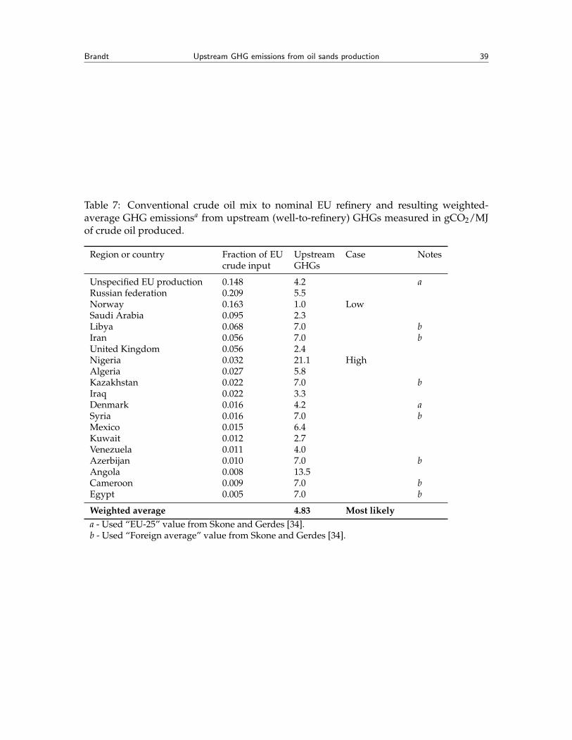
Brandt Upstream GHG emissions from oil sands production 39
Table 7: Conventional crude oil mix to nominal EU refinery and resulting weighted-average GHG emissionsa from upstream (well-to-refinery) GHGs measured in gCO2/MJof crude oil produced.
Region or country Fraction of EUcrude input
UpstreamGHGs
Case Notes
Unspecified EU production 0.148 4.2 aRussian federation 0.209 5.5Norway 0.163 1.0 LowSaudi Arabia 0.095 2.3Libya 0.068 7.0 bIran 0.056 7.0 bUnited Kingdom 0.056 2.4Nigeria 0.032 21.1 HighAlgeria 0.027 5.8Kazakhstan 0.022 7.0 bIraq 0.022 3.3Denmark 0.016 4.2 aSyria 0.016 7.0 bMexico 0.015 6.4Kuwait 0.012 2.7Venezuela 0.011 4.0Azerbijan 0.010 7.0 bAngola 0.008 13.5Cameroon 0.009 7.0 bEgypt 0.005 7.0 b
Weighted average 4.83 Most likelya - Used “EU-25” value from Skone and Gerdes [34].b - Used “Foreign average” value from Skone and Gerdes [34].
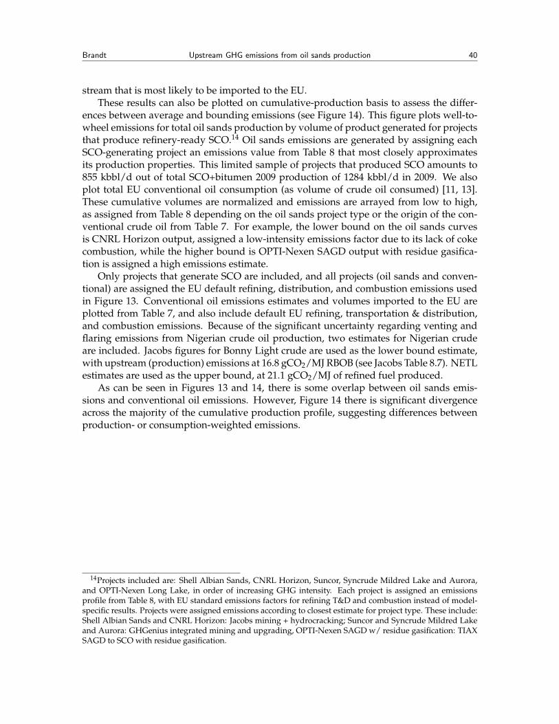
Brandt Upstream GHG emissions from oil sands production 40
stream that is most likely to be imported to the EU.These results can also be plotted on cumulative-production basis to assess the differ-
ences between average and bounding emissions (see Figure 14). This figure plots well-to-wheel emissions for total oil sands production by volume of product generated for projectsthat produce refinery-ready SCO.14 Oil sands emissions are generated by assigning eachSCO-generating project an emissions value from Table 8 that most closely approximatesits production properties. This limited sample of projects that produced SCO amounts to855 kbbl/d out of total SCO+bitumen 2009 production of 1284 kbbl/d in 2009. We alsoplot total EU conventional oil consumption (as volume of crude oil consumed) [11, 13].These cumulative volumes are normalized and emissions are arrayed from low to high,as assigned from Table 8 depending on the oil sands project type or the origin of the con-ventional crude oil from Table 7. For example, the lower bound on the oil sands curvesis CNRL Horizon output, assigned a low-intensity emissions factor due to its lack of cokecombustion, while the higher bound is OPTI-Nexen SAGD output with residue gasifica-tion is assigned a high emissions estimate.
Only projects that generate SCO are included, and all projects (oil sands and conven-tional) are assigned the EU default refining, distribution, and combustion emissions usedin Figure 13. Conventional oil emissions estimates and volumes imported to the EU areplotted from Table 7, and also include default EU refining, transportation & distribution,and combustion emissions. Because of the significant uncertainty regarding venting andflaring emissions from Nigerian crude oil production, two estimates for Nigerian crudeare included. Jacobs figures for Bonny Light crude are used as the lower bound estimate,with upstream (production) emissions at 16.8 gCO2/MJ RBOB (see Jacobs Table 8.7). NETLestimates are used as the upper bound, at 21.1 gCO2/MJ of refined fuel produced.
As can be seen in Figures 13 and 14, there is some overlap between oil sands emis-sions and conventional oil emissions. However, Figure 14 there is significant divergenceacross the majority of the cumulative production profile, suggesting differences betweenproduction- or consumption-weighted emissions.
14Projects included are: Shell Albian Sands, CNRL Horizon, Suncor, Syncrude Mildred Lake and Aurora,and OPTI-Nexen Long Lake, in order of increasing GHG intensity. Each project is assigned an emissionsprofile from Table 8, with EU standard emissions factors for refining T&D and combustion instead of model-specific results. Projects were assigned emissions according to closest estimate for project type. These include:Shell Albian Sands and CNRL Horizon: Jacobs mining + hydrocracking; Suncor and Syncrude Mildred Lakeand Aurora: GHGenius integrated mining and upgrading, OPTI-Nexen SAGD w/ residue gasification: TIAXSAGD to SCO with residue gasification.

Brandt Upstream GHG emissions from oil sands production 41
0
10
20
30
40
50
60
70
80
90
100
110
120
130
Weighted-‐average -‐ Most likely tar sands blend
Weighted-‐average EU convenBonal refinery feedstock
Well-‐to-‐whe
el life cycle GHG
emissions
(gCO
2 eq./M
J LHV
)
CombusBon*
Transport & distribuBon Refining*
VFF
Upgrading
ExtracBon
Figure 13: Weighted-average most likely oil sands emissions compared to weighted aver-age conventional EU refinery feedstock. Range of values for oil sands provided by low-high range shown above in Table 6. Range of values for conventional oil shown above inTable 7, for Norway (low) and Nigeria (high).

Brandt Upstream GHG emissions from oil sands production 42
0
20
40
60
80
100
120
140
0 0.2 0.4 0.6 0.8 1
Full fuel cycle (w
ell-‐to-‐whe
el) G
HG emissions
(g CO2 eq
./MJ o
f gasoline)
Normalized fracIon of producIon or imports
Oil sands ConvenIonal
Most likely value
Figure 14: Emissions as a function of cumulative normalized output, for oil sands projects(low and high estimates) and conventional oil imports to the EU. While there is some over-lap at the tails (highest conventional oil is higher than lowest oil sands) the production- orimport-weighted average emissions are significantly different. The bounds on oil sandsemissions are provided by (low) CNRL Horizon, (high) OPTI-Nexen, Long Lake SAGD+ Residue gasification. The bounds on conventional oil emissions are provided by (low)Norway, (high) Nigeria. Oil sands estimates are from Table 8, with EU standard emissionsfactors for refining T&D and combustion instead of model-specific results. Projects wereassigned emissions according to closest estimate for project type. These include: Shell Al-bian Sands and CNRL Horizon: Jacobs mining + hydrocracking; Suncor and Syncrude Mil-dred Lake and Aurora: GHGenius integrated mining and upgrading, OPTI-Nexen SAGDw/ residue gasification: TIAX SAGD to SCO with residue gasification.

Brandt Upstream GHG emissions from oil sands production 43
8 Uncertainties
Uncertainties remain in calculating life cycle GHG emissions from oil sands operationsand applying these factors to EU refinery inputs. Chief among these uncertainties are:
1. Treatment of cogenerated electric power is a concern in all studies. Given the CO2intensity of the Alberta grid, co-production credits from cogenerated power couldbe important. The Jacobs study addresses these issues, as did previous versions ofthe GHGenius model. More study of these issues is needed, ideally using observedelectric power export data from mining and in situ production projects.
2. Treatment of refining is a difficulty in public-domain studies such as GREET andGHGenius, due to a lack of access to proprietary refinery models. These refin-ery emissions will be specific to the region of refining and the type of crude oilrefined. Addressing the wide range between JEC emissions estimates and otherprocess model emissions estimates for refining should be a priority.
3. The interaction of markets with LCA results (addressed in “consequential” LCA) isnot studied in any model results. For example, coking of bitumen at a remote Al-berta upgrader and coking of bitumen at a more centrally-located refinery should, intheory, have roughly equivalent emissions profiles. However, because of the lack ofnearby markets for residual coke produced at remote Alberta upgraders, the pro-duced carbon is currently stockpiled in large quantities. A shift to shipment ofdiluted bitumen could cause coke generation to occur at existing refineries. Thiswould result in carbon in coke being produced closer to other markets and infras-tructure by which it would be consumed rather than stockpiled (note that refiner-ies currently do not stockpile coke). Thus, the total impacts (the full system conse-quences) from the two systems might differ, even though the engineering processesmight be very similar. A similar issue was raised above with regard to the emissionsimpacts of reducing the amount of residual fuels produced at refineries.

Brandt Upstream GHG emissions from oil sands production 44
9 Appendix A: Numerical results of comparison of WTW GHG studies
The numerical results used to derive Figures 10 and 9 are shown in Table 8. The source ofeach reference value is given in Table 9.
For consistency with previous works, results from Charpentier et al. are used for GH-Genius and GREET figures.

Brandt Upstream GHG emissions from oil sands production 45
Tabl
e8:
Wel
l-to
-tan
kre
sult
sfr
omin
clud
edst
udie
s.T
hese
resu
lts
have
notb
een
stan
dard
ized
for
EUm
arke
tcon
diti
ons.
All
resu
lts
adju
sted
togC
O2
eq./
MJ
ofre
fined
fuel
deliv
ered
,LH
Vba
sis.
Cas
eslis
tw
hich
path
way
ism
odifi
edfo
rin
clus
ion
as“l
ow”
(L)“
mos
tlik
ely”
(M)a
nd“h
igh”
(H)i
nTa
ble
6ab
ove.
Met
hods
desc
ribe
din
Tabl
e9.
Min
ing
and
upgr
adin
gEx
trac
tion
Upg
radi
ngTr
ansp
ort
VFF
Refi
ning
Dis
trib
utio
nC
ase
GH
Gen
ius
19.0
0.0
0.3
2.0
13.0
0.9
MG
REE
T15
.90.
00.
00.
014
.50.
0-
Jaco
bs-M
ine
+cr
acki
ng7.
38.
61.
10.
012
.60.
4L
TIA
X-M
ine
+se
llco
ke10
.10.
01.
20.
512
.40.
0-
TIA
X-M
ine
+bu
ryco
ke12
.40.
01.
20.
512
.40.
0-
Insi
tuan
dup
grad
ing
Extr
acti
onU
pgra
ding
Tran
spor
tV
FFR
efini
ngD
istr
ibut
ion
Cas
e
GH
Gen
ius
29.0
0.0
0.3
0.9
14.0
0.9
MG
REE
T19
.10.
00.
00.
014
.50.
0-
Jaco
bs-I
nsi
tu+
crac
ker
14.2
8.6
1.1
0.0
12.6
0.4
-Ja
cobs
-In
situ
+hy
drot
reat
ing
12.6
11.6
1.2
0.0
13.4
0.4
-TI
AX
-Res
idue
fuel
37.3
0.0
1.2
3.3
10.1
0.0
HTI
AX
-NG
fuel
23.4
0.0
1.2
3.3
10.1
0.0
-
Insi
tuw
itho
utup
grad
ing
Extr
acti
onU
pgra
ding
Tran
spor
tV
FFR
efini
ngD
istr
ibut
ion
Cas
e
Jaco
bs-M
ine
+cr
ack
11.8
0.0
0.3
0.6
26.4
0.9
-TI
AX
-Min
e+
sell
coke
15.8
0.0
0.0
0.0
14.5
0.0
-Ja
cobs
-SA
GD
tobi
tum
en13
.80.
01.
20.
017
.20.
4-
TIA
X-B
itum
enSA
GD
16.
70.
01.
23.
321
.50.
0-
TIA
X-B
itum
enSA
GD
210
.70.
01.
23.
321
.50.
0-
Mix
edEx
trac
tion
Upg
radi
ngTr
ansp
ort
VFF
Refi
ning
Dis
trib
utio
n-
NET
L-M
ixtu
reof
SCO
and
dilb
it21
.50.
01.
00.
012
.11.
0-

Brandt Upstream GHG emissions from oil sands production 46
Tabl
e9:
Not
eson
incl
uded
stud
ies
conv
ersi
onto
equi
vale
ntG
HG
emis
sion
sva
lues
.
Rep
ort
Sour
ceN
otes
GH
Gen
ius
Cha
rpen
tier
etal
.[15
,Sup
port
-in
gin
form
atio
n,Ta
ble
S2]
Con
vert
edfr
omgC
O2
eq.
per
kmto
gCO
2eq
.pe
rM
Jus
ing
GH
Gen
ius
vehi
cle
effic
ienc
yof
9.55
6l/
100
kman
dG
HG
eniu
sco
nver
sion
betw
een
HH
Van
dLH
V(S
heet
“E”)
.Thi
sis
done
tore
mai
nco
n-si
sten
twit
hC
harp
enti
erm
etho
dolo
gy,w
hich
isba
sed
onco
nver
sion
from
MJt
okm
usin
gG
HG
eniu
sfu
elen
ergy
dens
itie
san
dve
hicl
eef
ficie
ncie
s.C
harp
enti
erfig
ures
are
base
don
GH
Gen
ius
v.3.
13.
The
figur
esfo
rG
HG
eniu
sin
Cha
rpen
tier
pape
rar
eca
lcul
ated
asfo
llow
s(p
ers.
com
mun
icat
ion,
A.
Cha
rpen
tier
,Oct
ober
2010
):To
tale
mis
sion
sar
eeq
ualt
osh
eet“
Life
cycl
eR
esul
ts”
C17
less
co-p
rodu
ctem
issi
ons
cred
its
(C16
).O
n“I
nput
”sh
eet
the
follo
win
gch
ange
sar
em
ade:
regi
onis
chan
ged
toC
anad
aW
est(
G3)
,Inp
uton
D5
isch
ange
dto
100%
Can
ada
Wes
t.C
rude
oili
nput
isch
ange
dto
100%
SCO
(F65
).Fo
rm
inin
g,C
harp
enti
eras
sum
ed10
0%in
tegr
ated
oper
atio
n,0%
min
eto
upgr
ader
(she
et”S
”A
H-A
I6)
.Fo
rSA
GD
,ass
umed
bitu
men
toup
grad
ing
(”S”
AH
6),a
ssum
e50
%SA
GD
,50%
CC
S(”
S”Z
-AA
4).
GR
EET
Cha
rpen
tier
etal
.[15
,Sup
port
-in
gin
form
atio
n,Ta
ble
S2]
Con
vert
edfr
omgC
O2
eq.
per
kmto
gCO
2eq
.pe
rM
Jus
ing
GH
Gen
ius
vehi
cle
effic
ienc
yof
9.55
6l/
100
kman
dG
HG
eniu
sco
nver
sion
betw
een
HH
Van
dLH
V(S
heet
“E”)
.Thi
sis
done
tore
mai
nco
n-si
sten
twit
hC
harp
enti
erm
etho
dolo
gy,w
hich
isba
sed
onco
nver
sion
from
MJt
okm
usin
gG
HG
eniu
sfu
elen
ergy
dens
itie
san
dve
hicl
eef
ficie
ncie
s.
Jaco
bsK
eeso
met
al.[
26]
Val
ues
from
Tabl
e8.
7fo
ral
loil
sand
spr
oces
ses.
TIA
XR
osen
feld
etal
.[19
]V
alue
sfr
omTa
bles
6.3,
6.4,
and
6.5.
Whe
reap
plic
able
,res
ults
for
deliv
ery
toPA
DD
2ar
eus
ed.
CER
AC
ERA
[46]
Beca
use
figur
esar
ere
port
edin
kgC
O2
eq.p
erba
rrel
ofre
fined
prod
uct,
achi
evin
gdi
rect
lyco
mpa
ra-
ble
resu
lts
wit
hot
her
stud
ies
isdi
fficu
lt.R
efine
ryyi
eld
(e.g
.,M
Jofr
efine
ryou
tput
per
MJo
frefi
nery
inpu
ts)i
sno
tspe
cifie
d,so
data
are
notp
lott
ed.
NET
LG
erde
set
al.[
45]
and
Skon
eet
al.[
34]
Dat
afr
omG
erde
set
al.[
45]a
rede
rive
dfr
omea
rlie
r,m
ore
com
preh
ensi
vere
port
bySk
one
etal
.[34
].V
alue
foro
ilsa
nds
ista
ken
from
data
onIm
peri
alO
il-C
old
Lake
proj
ect(
crud
ebi
tum
en)a
ndfo
rSC
Ofr
omSy
ncru
de[3
4,Ta
ble
2.5]
.The
valu
eus
edis
am
ixtu
reof
thes
etw
oem
issi
ons
inte
nsit
ies,
and
the
brea
kdow
nin
emis
sion
sby
prod
ucts
tage
(ext
ract
ion,
tran
spor
t,up
grad
ing)
isno
trep
orte
d,m
akin
gco
mpa
riso
ndi
fficu
lt.F
orth
isre
ason
,val
ues
from
NET
Lar
eno
tplo
tted
inm
ain
resu
lts
figur
es
All
stud
ies
-TT
Wem
issi
ons
ane
glec
ted
beca
use
they
are
outs
ide
the
boun
dari
esof
this
stud
y.T
TWem
issi
ons
vary
slig
htly
betw
een
stud
ies.

Brandt Upstream GHG emissions from oil sands production 47
Tabl
e10
:Fue
lmix
for
sele
cted
stud
ies
(in
frac
tion
ofto
talf
ueli
nput
s).N
otal
lstu
dies
repo
rted
fuel
mix
es.
Min
ean
dup
grad
e
GR
EET
aG
HG
eniu
sbJa
cobs
cT
IAX
dIn
dust
ryav
erag
ee
Min
eU
pgr.
Min
eU
pgr.
Int.
min
e&
upgr
.In
dust
ryav
e.SC
O
Upg
r.-C
oker
Upg
r.-
Eb-b
edIn
t.m
ine
&up
gr.
Die
self
uel
0.01
0.00
0.16
0.00
0.05
0.04
0.00
0.00
0.05
0.00
Nat
ural
gas
0.82
0.97
0.82
0.28
0.21
0.44
0.51
0.62
0.42
0.44
Elec
tric
ity
0.17
0.03
0.02
0.08
0.01
0.03
0.00
0.00
0.02
0.05
Pet.
coke
0.00
0.00
0.00
0.15
0.27
0.16
0.00
0.00
0.0
0.13
Refi
nery
still
gas
0.00
0.00
0.00
0.49
0.45
0.33
0.49
0.38
0.51
0.40
a-V
alue
sfr
omG
REE
Tm
odel
1.8d
,wor
kshe
et“P
etro
leum
”,C
olum
nsF,
H40
-51.
b-V
alue
sfr
omG
HG
eniu
sm
odel
3.18
,wor
kshe
et“S
”.V
alue
sfo
rm
inin
g,SA
GD
,etc
.c
-Val
ues
from
Jaco
bsre
port
,Tab
le4-
6[2
6].
Jaco
bsdo
notr
epor
tfue
lmix
for
min
ing,
and
ther
efor
ela
ckdi
esel
cons
umpt
ion.
Jaco
bsre
port
assu
mes
elec
tric
ity
need
edfo
rpr
oces
sis
gene
rate
don
site
sono
nete
lect
rici
tyim
port
s.d
-Val
ues
from
TIA
Xre
port
,Fig
ure
3-12
,for
CN
RL
Hor
izon
proj
ect[
26].
e-
Val
ues
from
ERC
B,re
port
edby
proj
ect[
11].
Nat
ural
gas
isna
tura
lgas
purc
hase
dle
ssth
atex
port
ed.
Elec
tric
ity
is“p
lant
use”
cate
gory
.N
opo
wer
expo
rtis
incl
uded
.Pr
oces
sga
sis
proc
ess
gas
used
for
“fur
ther
proc
essi
ng”
(e.g
.,hy
drog
enge
nera
tion
),“f
uel/
plan
tus
e”an
d“fl
ared
/was
ted”
.C
oke
is“f
uel/
plan
tus
e”,w
ith
noin
clus
ion
coke
stoc
kpile
d(r
epre
sent
edin
ERC
Bfig
ures
asdi
ffer
ence
sin
open
ing
and
clos
ing
inve
ntor
y.ER
CB
data
dono
tinc
lude
dies
elco
nsum
ptio
n,so
dies
elus
edin
haul
truc
ksis
noti
nclu
ded.

Brandt Upstream GHG emissions from oil sands production 48
References
[1] Moritis, G. CO2 miscible, steam dominate enhanced oil recovery processes: EORsurvey. Oil & Gas Journal 2010, 108, 36+.
[2] Moritis, G. Continued Alberta oil sands production growth seen. Oil & Gas Journal2010, 2010, 42–46.
[3] DuPlessis, D. JPEC and Nippon oil mission. Technical report, Alberta Innovates, 2010.
[4] Williams, B. Heavy hydrocarbons playing key role in peak-oil debate, future energysupply. Oil & Gas Journal. 2003, 101, 20.
[5] Speight, J.G. Synthetic fuels handbook: properties, process, and performance; McGraw Hill:New York, 2008.
[6] Ordorica-Garcia, G.; Croiset, E.; Douglas, P.; Elkamel, A.; Gupta, M. Modeling theenergy demands and greenhouse gas emissions of the Canadian oil sands industry.Energy & Fuels 2007, 21, 2098–2111.
[7] Brandt, A.R.; Unnasch, S. Energy intensity and greenhouse gas emissions from Cali-fornia thermal enhanced oil recovery. Energy & Fuels 2010, DOI: 10.1021/ef100410f.
[8] ACR. Oil sands technology roadmap: Unlocking the potential, 2004.
[9] Furimsky, E. Emissions of carbon dioxide from tar sands plants in Canada. Energyand Fuels 2003, 17, 1541–1548.
[10] Johnson, H.R.; Crawford, P.M.; Bunger, J.W. Strategic significance of America’s oilshale resource: Volume I - Assessment of strategic issues. Technical report, AOCPetroleum Support Services, LLC, 2004.
[11] ERCB. ST39: Alberta Mineable Oil Sands Plant Statistics Monthly Supplement. Tech-nical report, Energy Resources Conservation Board, 2010.
[12] Johnson, H.R.; Crawford, P.M.; Bunger, J.W. Strategic significance of America’s oilshale resource: Volume II - Oil shale resources, technology and economics. Technicalreport, AOC Petroleum Support Services, LLC, 2004.
[13] ERCB. ST53: Alberta Crude Bitumen In Situ Production Monthly Statistics. Technicalreport, Energy Resources Conservation Board, 2010.
[14] Heins, W.; McNeill, R.; Albion, S. World’s first SAGD facility using evaporators, drumboilers, and zero discharge crystallizers to treat produced water. Journal of CanadianPetroleum Technology 2006, 45, 30–36.
[15] Charpentier, A.D.; Bergerson, J.; MacLean, H.L. Understanding the Canadian oilsands industry’s greenhouse gas emissions. Environmental Research Letters 2009, 4, 14.
[16] Butler, R.M. Application of SAGD, related processes growing in Canada. Oil & GasJournal 2001, 2001, 74–78.

Brandt Upstream GHG emissions from oil sands production 49
[17] Kerr, R.; Birdgeneau, J.; Batt, B.; Yang, P.; Nieuwenburg, G.; Rettger, P.; Arnold, J.;Bronicki, Y. The Long Lake Project - The first field integration of SAGD and upgrad-ing, 2002.
[18] Elliott, K. Examination of oil sands projects: Gasification, CO2 emissions, and supplycosts, 2008. SPE/PS/CHOA International Thermal Operations and Heavy Oil Sym-posium, Calgary, AB.
[19] Rosenfeld, J.; Pont, J.; Law, K.; Hirshfeld, D.; Kolb, J. Comparison of North Americanand imported crude oil life cycle GHG emissions. Technical report, TIAX LLC. andMathPro Inc. for Alberta Energy Research Institute, 2009.
[20] Speight, J.G. The chemistry and technology of petroleum; Chemical Industries, MarcelDekker: New York, 1994.
[21] Swafford, P. Understanding the quality of Canadian bitumen and synthetic crudes.Technical report, Spiral Software, 2009.
[22] Speight, J.G. Tar Sands. Kirk-Othmer Encylopedia of Chemical Technology 2000.
[23] Wang, J.; Zhao, S.; Xu, C.; Chung, K. Properties correlations and characterization ofAthabasca oil sands-derived synthetic crude oil. Petroleum Science 2007, 4, 84–90.
[24] Flint, L. Bitumen & very heavy crude upgrading technology: A review of long-termR&D opportunities. Technical report, LENEF Consulting Ltd., 2004.
[25] Gray, M.R. Upgrading petroleum residues and heavy oils; Chemical Industries, MarcelDekker: New York, 1994.
[26] Keesom, W.; Unnasch, S.; Moretta, J. Life cycle assessment comparison of NorthAmerican and imported crudes. Technical report, Jacobs Consultancy and Life CycleAssociates for Alberta Energy Resources Institute, 2009.
[27] Monitor, C. Crude quality data summary. www.crudemonitor.ca 2010, Various reports.
[28] Brierley, G.R.; Gembicki, V.A.; Cowan, T.M. Changing refinery configuration forheavy and synthetic crude processing. Technical report, UOP LLC, 2006.
[29] Rhodes, A.K. Brent blend, U.K. North Sea marker crude, assayed. Oil & Gas Journal1995, 1995.
[30] Yui, S.; Chung, K.H. Processing oilsands bitumen is Syncrude’s R&D focus. Oil & GasJournal 2001, 2001.
[31] Wang, M.Q. Estimation of energy efficiencies of U.S. petroleum refineries (plus asso-ciated spreadsheet). Technical report, Center for Transportation Research, ArgonneNational Laboratory, 2008.
[32] Wang, M. GREET Model 1.8d. Computer program, Argonne National Laboratory,2010.

Brandt Upstream GHG emissions from oil sands production 50
[33] Gray, D.; Tomlinson, G. Alternate routes for the production of fuels from coal andnatural-gas. Abstracts of Papers of the American Chemical Society 1994, 208, 108–FUEL.
[34] Skone, T.J.; Gerdes, K.J. Development of baseline data and analysis of life cycle green-house gas emissions of petroleum-based fuels. Technical report, Office of Systems,Analyses and Planning, National Energy Technology Laboratory, 2008.
[35] Speight, J.G. The desulfurization of heavy oils and residua, 2nd ed.; Marcel Dekker: NewYork, 1999.
[36] Yeh, S.; Jordann, S.M.; Brandt, A.R.; Turetsky, M.; Spatari, S.; Keith, D.W. Land usegreenhouse gas emissions from conventional oil production and oil sands. Environ-mental Science & Technology 2010, In press.
[37] Environment Canada. National inventory report 1990-2008: Greenhouse gas sourcesand sinks in Canada. Technical report, Environment Canada, 2010.
[38] Suncor. Suncor Energy Inc. 9th Annual Progress Report. Technical report, SuncorEnergy inc., 2003.
[39] Bergerson, J.; Keith, D.W. Life cycle assessment of oil sands technologies.InLCA/LCM Conference 2007, 2006.
[40] Wang, M. Summary of expansions and revisions in GREET1.8d. Technical report,Systems Assessment Section, Center for Transportation Research, Argonne NationalLaboratory,, 2010.
[41] Wang, M.; Huang, H. A full fuel-cycle analysis of energy and emissions impactsof transportation fuels produced from natural gas. Technical Report ANL/ESD-40,Argonnne National Laboratory, 1999.
[42] Wang, M.Q. The Greenhouse Gases, Regulated Emissions, and Energy Use in Trans-portation Model version 1.5. Technical report, Argonne National Laboratory, 1999.
[43] Wang, M. GREET Model 1.8b. Computer program, Argonne National Laboratory,2008.
[44] (S&T)2. GHGenius, model version 3.18. Technical report, (S&T)2 consultants, forNatural Resources Canada, 2010.
[45] Gerdes, K.J.; Skone, T.J. An evaluation of the extraction, transport and refining ofimported crude oils and the impact on life cycle greenhouse gas emissions. TechnicalReport DOE/NETL-2009/1362, Office of Systems, Analysis and Planning, NationalEnergy Technology Laboratory, 2009.
[46] CERA. Oil sands, greenhouse gases, and US oil supply: Getting the numbers right.Technical report, IHS-CERA, 2010.
[47] Brandt, A.R.; Farrell, A.E. Scraping the bottom of the barrel: Greenhouse gas emis-sion consequences of a transition to low-quality and synthetic petroleum resources.Climatic Change 2007, 84, 241–263.

Brandt Upstream GHG emissions from oil sands production 51
[48] McCann, T.; Magee, P. Crude oil greenhouse gas life cycle analysis helps assign valuesfor CO2 emissions trading. Oil & Gas Journal 1999, 97, 38–44.
[49] Mui, S.; Hannah, D.; Hwang, R. White paper: Life cycle analysis of greenhouse gasemissions from tar sands. Technical report, Natural Resources Defense Council, 2008.
[50] Mui, S.; Tonachel, L.; Shope, E. GHG emissions factors for high carbon intensity crudeoils. Technical report, Natural Resources Defense Council, 2010.
[51] Larson, R.; Wang, M.Q.; Wu, Y.; Vyas, A. Might Canadian oil sands promote hydrogenproduction for transportation? Greenhouse gas implications of oil sands recovery andupgrading. World Resource Review 2005, 17, 220–242.
[52] (S&T)2. 2007 Crude oil production update for GHGenius. Technical report, (S&T)2consultants, for Natural Resources Canada, 2007.
[53] (S&T)2. 2008 GHGenius update. Technical report, (S&T)2 consultants, for NaturalResources Canada, 2008.
[54] Canada, E. Reported facility GHG data. Technical report, Environment Canada, 2010.
[55] Brandt, A.R.; Plevin, R.J.; Farrell, A.E. Dynamics of the oil transition: modeling ca-pacity, depletion, and emissions. Energy 2010.
[56] JEC. Well-to-wheels analysis of future automotove fuels and powertrains in the Eu-ropean context - Version 2C - WTT appendix 1. Energy Policy 2007, In Press, CorrectedProof.
[57] JEC. Well-to-wheels analysis of future automotive fuels and powertrains in the Euro-pean context - Version 2C - TTW appendix 1. Technical report, Joint Research Centre-EUCAR-CONCAWE collaboration, 2007.