TBD ENGINEERING | MECHANICAL

04-2015 SUPPORTING DOCUMENTS | I Flexibility Sustainability Economy Community

SUPPORTING DOCUMENTS

REFERENCES

CODES AND HANDBOOKS 1. ASHRAE – 2011 ASHRAE HVAC Applications

2. ASHRAE – Standard 62.1 2013

3. ASHRAE – Standard 90.1 2013

4. ASHRAE – 2009 ASHRAE Fundamentals

5. Wisconsin Commercial Building Code

International Building Code 2009

National Electrical Code 2005

6. 2010 Florida Building Code

COMPUTER PROGRAMS Autodesk Revit 2014

Microsoft Excel 2013

Integrated Environmental Solutions (IES) Virtual Environment 2013

Trane Trace 700

Marley Update Selection Software Version 4.16.1

Bell and Gossett (Xylem Brand) ESP-Plus Selection Software

Xylem ESP Thermal Selection Software

REFERENCED IMAGES 7. Figure 4: Ferris, Jean L.G. The First Thanksgiving 1621. 1932. Private Collection. Beyond the Bubble. Stanford University. Web. 2 Jan. 2015.

8. Figure 10: Map of Milwaukee area courtesy of Bing Maps

9. Figure 18: Image of soybean availability across United States courtesy of AgWeb Soybean Harvest News

10. Figure SD 1: Well-X-Trol pressurized tank courtesy of Amtrol

11. Figure SD 3: Raft aquaponics image courtesy of aquaponics.com

12. Figure SD 7: BM-55/88 courtesy of Viessmann

13. Figure SD 17: Water Source Heat Pumps courtesy of Daikin

14. Drawing D2: Equipment Images Courtesy of Viessmann Group, Bell and Gossett, Haase Tanks, Hydroflex Systems, Maxim Heat Recovery Silencers, Clever and Brooks, Moyno

15. Drawing D1: Image Courtesy of Marley

ADDITIONAL RESOURCES

GREENHOUSE REFERENCES

16. Bucklin, R. A. "Fan and Pad Greenhouse Evaporative Cooling Systems1." EDIS New Publications RSS. University of Florida IFAS Extension, Dec. 1993. Web. 11 Oct. 2014.

17. Despommier, Dickson. "The Vertical Farm." The Vertical Farm RSS. N.p., n.d. Web. 02 Oct. 2014.

18. Torres, Ariana P., and Roberto G. Lopez. Measuring Daily Light Integral in a Greenhouse. Publication no. H0-238-W. Purdue University Extension, n.d. Web. 2 Oct. 2014.

AQUAPONICS REFERENCES

19. Baptista, Perry. "Water Use Efficiency in Hydroponics and Aquaponics."Bright Agrotech. Bright Agrotech, 4 June 2014. Web. 17 Oct. 2014.

TBD ENGINEERING | MECHANICAL

04-2015 SUPPORTING DOCUMENTS | II Flexibility Sustainability Economy Community

20. Chapman, John. "Interview with John Chapman on Aquaponics." Personal interview. 24 Oct. 2014.

21. Lennard, Wilson, PhD. "Aquaponic Media Bed Sizing Calculator - Metric."Aquaponic Media Bed Sizing Calculator – Metric Ver 2.0 Aquaponic Media Bed Sizing Calculator - Metric (2012): n. pag. Aquaponic Solutions. Wilson

Lennard, May 2012. Web. 17 Sept. 2014.

22. N.d. Different Methods of Aquaponics. Web. 29 Sept. 2014.

23. Rakocy, James E., Donald S. Bailey, R.C. Shultz, and Jason J. Danaher. A Commercial-Scale Aquaponic System Developed at the University of the Virgin Islands. Better Science, Better Fish, Better Life: Proceedings of the Ninth

International Symposium on Tilapia in Aquaculture, 22-24 April 2011, Shanghai, China. AQUAFISH Collaborative Research Support Program, 336-343

24. Rakocy, James. "Ten Guidelines for Aquaponics Systems." Aquaponics Journal 46 (2007): 14-17. Print.

25. Resh, Howard. "Welcome to Dr. Howard Resh, Hydroponic Services."Hydroponic Services. N.p., n.d. Web. 18 Oct. 2014.

26. Sanders, Douglas. "Lettuce Horticulture Information Leaflet." Lettuce. NC Cooperative Extension Resources, 16 Dec. 2014. Web. 27 Dec. 2014.

27. Wurts, William A. "Tilapia: A Potential Species for Kentucky Fish Farms."UK Ag. University of Kentucky College of Agriculture, Food and Environment, n.d. Web. 11 Oct. 2014.

ANAEROBIC DIGESTION REFERENCES

28. Curry, Nathan, and Pragasen Pillay. 2012. “Biogas Prediction and Design of a Food Waste to Energy System for the Urban Environment.” Renewable Energy 41 (May): 200–209. doi:10.1016/j.renene.2011.10.019.

29. Grimberg, S.J., Hilderbrandt, D., Kinnunen, M., Rogers, S., Anaerobic Digestion of Food Waste Through the Operation of a Mesophilic Two-Phase Pilot Scale Digester – Assessment of Variable Loadings on System Performance,

Bioresource Technology (2014), doi: http://dx.doi.org/10.1016/j.biortech.2014.09.001

30. Hilderbrandt, Daniel. Anaerobic Digestion of Food Waste through the Operation of a Mesophilic Two-Phase Pilot Scale Digester. Thesis Prepared for Clarkson University. 12 Dec. 2013.

31. Rapport, Joshua, Ruihong Zhang, Bryan Jenkins, and Robert Williams. 2008. “Current Anaerobic Digestion Technologies Used for Treatment of Municipal Organic Solid Waste”. California Integrated Waste Management Board.

COMBINED HEAT AND POWER REFERENCES

32. Energy Nexus Group. Technology Characterization: Reciprocating Engines. U.S. Environmental Protection Agency. Feb. 2012

33. Meckler, Milton, and Lucas B. Hyman. Sustainable On-site CHP Systems: Design, Construction, and Operations. New York: McGraw-Hill, 2010. Print.

34. Moriatry, Kristi. Feasibility Study of Anaerobic Digestion of Food Waste in St. Bernard, Louisiana. National Renewable Energy Laboratory. Jan. 2013.

35. U.S. Energy Information Administration. Wisconsin State Profile and Energy Estimates. 20 Jan. 2015. Web. 27 Mar. 2014.

36. U.S. Environmental Protection Agency. Catalog of CHP Technologies, Section 2: Technology Characterization – Reciprocating Internal Combustion Engines. Sept. 2014

37. U.S. Environmental Protection Agency. LFG Energy Benefits Calculator. 11 Jan. 2015. Web. 24 July 2014.

SOYBEAN OIL BIODIESEL REFERENCES

38. "AgWeb Soybean Harvest Map." AgWeb. Farm Journal, 1 Nov. 2014. Web. 1 Nov. 2014.

39. A. Bulent Koc, Mudhafer Abdullah and Mohammad Fereidouni (2011). Soybeans Processing for Biodiesel Production, Soybean – Applications and Technology, Prof. Tzi-Bun Ng (Ed.), ISBN: 978-953-307-207-4, InTech, Available

from: http://www.intechopen.com/books/soybean-applications-and-technology/soybeans-processing-for-biodiesel-production

40. Atadashi, I.M., M.K. Aroua, A.R. Abdul Aziz, and N.M.N. Sulaiman. Refining Technologies for the Purification of Crude Biodiesel. Tech. no. 4239-4251. Elsevier Ltd., 1 July 2011. Web. 13 Nov. 2014.

41. "Biodiesel Benefits and Considerations." Alternative Fuels Data Center: Biodiesel Benefits. U.S. Department of Energy, 2 Jan. 2015. Web. 5 Jan. 2015.

42. Hill, Jason, Erik Nelson, David Tilman, Stephen Polasky, and Douglas Tiffany. "Environmental, Economic, and Energetic Costs and Benefits of Biodiesel and Ethanol Biofuels." Environmental, Economic, and Energetic Costs and

Benefits of Biodiesel and Ethanol Biofuels. University of Minnesota, 25 July 2006. Web. 13 Dec. 2014.

43. "Soy Bean Oil Amounts Converter." Convert To. N.p., n.d. Web. 17 Dec. 2014.

44. United States Department of Agriculture. National Agricultural Statistics Service. Field Crops Usual Planting and Harvesting Dates. N.p.: n.p., n.d. Print.

TBD ENGINEERING | MECHANICAL

04-2015 SUPPORTING DOCUMENTS | III Flexibility Sustainability Economy Community

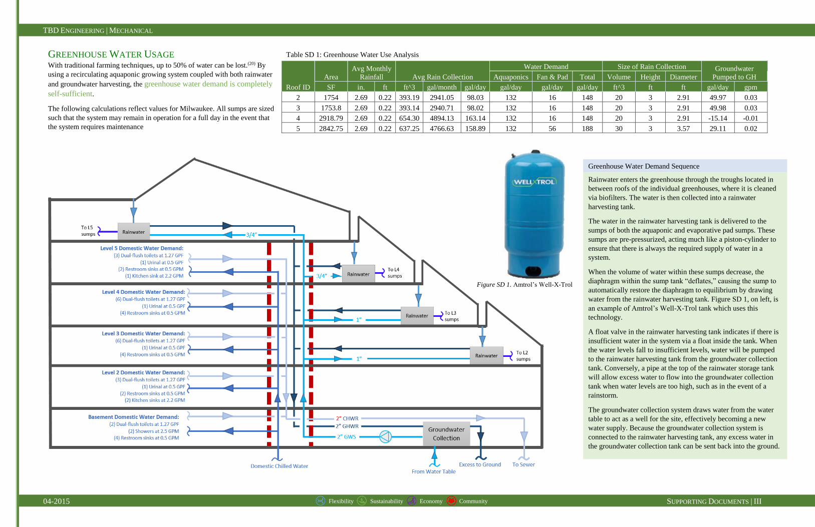
GREENHOUSE WATER USAGE With traditional farming techniques, up to 50% of water can be lost.(20) By

using a recirculating aquaponic growing system coupled with both rainwater

and groundwater harvesting, the greenhouse water demand is completely

self-sufficient.

The following calculations reflect values for Milwaukee. All sumps are sized

such that the system may remain in operation for a full day in the event that

the system requires maintenance

Roof ID

Area

Avg Monthly

Rainfall Avg Rain Collection

Water Demand Size of Rain Collection Groundwater

Pumped to GH Aquaponics Fan & Pad Total Volume Height Diameter

SF in. ft ft^3 gal/month gal/day gal/day gal/day gal/day ft^3 ft ft gal/day gpm

2 1754 2.69 0.22 393.19 2941.05 98.03 132 16 148 20 3 2.91 49.97 0.03

3 1753.8 2.69 0.22 393.14 2940.71 98.02 132 16 148 20 3 2.91 49.98 0.03

4 2918.79 2.69 0.22 654.30 4894.13 163.14 132 16 148 20 3 2.91 -15.14 -0.01

5 2842.75 2.69 0.22 637.25 4766.63 158.89 132 56 188 30 3 3.57 29.11 0.02

Greenhouse Water Demand Sequence

Rainwater enters the greenhouse through the troughs located in

between roofs of the individual greenhouses, where it is cleaned

via biofilters. The water is then collected into a rainwater

harvesting tank.

The water in the rainwater harvesting tank is delivered to the

sumps of both the aquaponic and evaporative pad sumps. These

sumps are pre-pressurized, acting much like a piston-cylinder to

ensure that there is always the required supply of water in a

system.

When the volume of water within these sumps decrease, the

diaphragm within the sump tank “deflates,” causing the sump to

automatically restore the diaphragm to equilibrium by drawing

water from the rainwater harvesting tank. Figure SD 1, on left, is

an example of Amtrol’s Well-X-Trol tank which uses this

technology.

A float valve in the rainwater harvesting tank indicates if there is

insufficient water in the system via a float inside the tank. When

the water levels fall to insufficient levels, water will be pumped

to the rainwater harvesting tank from the groundwater collection

tank. Conversely, a pipe at the top of the rainwater storage tank

will allow excess water to flow into the groundwater collection

tank when water levels are too high, such as in the event of a

rainstorm.

The groundwater collection system draws water from the water

table to act as a well for the site, effectively becoming a new

water supply. Because the groundwater collection system is

connected to the rainwater harvesting tank, any excess water in

the groundwater collection tank can be sent back into the ground.

Figure SD 1. Amtrol’s Well-X-Trol

Table SD 1: Greenhouse Water Use Analysis

TBD ENGINEERING | MECHANICAL

04-2015 SUPPORTING DOCUMENTS | IV Flexibility Sustainability Economy Community

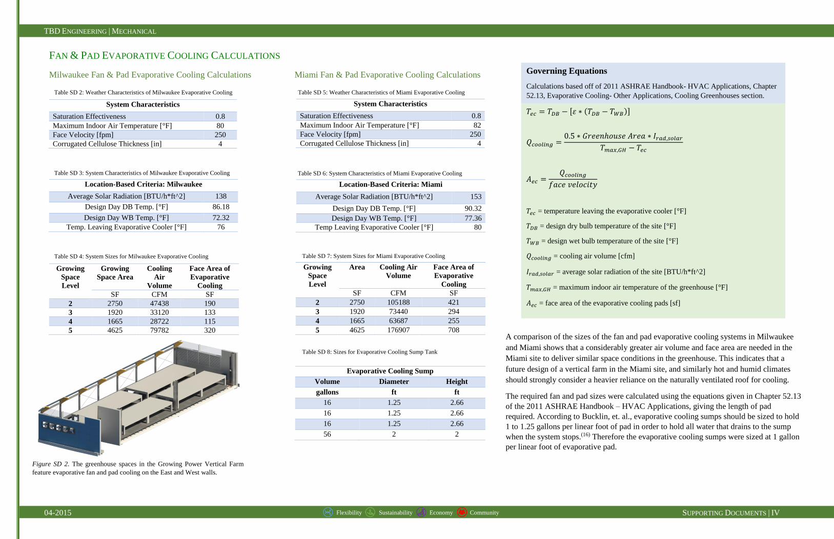
FAN & PAD EVAPORATIVE COOLING CALCULATIONS

Milwaukee Fan & Pad Evaporative Cooling Calculations Miami Fan & Pad Evaporative Cooling Calculations

System Characteristics

Saturation Effectiveness 0.8

Maximum Indoor Air Temperature [°F] 80

Face Velocity [fpm] 250

Corrugated Cellulose Thickness [in] 4

System Characteristics

Saturation Effectiveness 0.8

Maximum Indoor Air Temperature [°F] 82

Face Velocity [fpm] 250

Corrugated Cellulose Thickness [in] 4

Location-Based Criteria: Milwaukee

Average Solar Radiation [BTU/h*ft^2] 138

Design Day DB Temp. [°F] 86.18

Design Day WB Temp. [°F] 72.32

Temp. Leaving Evaporative Cooler [°F] 76

Location-Based Criteria: Miami

Average Solar Radiation [BTU/h*ft^2] 153

Design Day DB Temp. [°F] 90.32

Design Day WB Temp. [°F] 77.36

Temp Leaving Evaporative Cooler [°F] 80

Growing

Space

Level

Growing

Space Area

Cooling

Air

Volume

Face Area of

Evaporative

Cooling

SF CFM SF

2 2750 47438 190

3 1920 33120 133

4 1665 28722 115

5 4625 79782 320

Growing

Space

Level

Area Cooling Air

Volume

Face Area of

Evaporative

Cooling

SF CFM SF

2 2750 105188 421

3 1920 73440 294

4 1665 63687 255

5 4625 176907 708

Evaporative Cooling Sump

Volume Diameter Height

gallons ft ft

16 1.25 2.66

16 1.25 2.66

16 1.25 2.66

56 2 2

Table SD 5: Weather Characteristics of Miami Evaporative Cooling Table SD 2: Weather Characteristics of Milwaukee Evaporative Cooling

Table SD 6: System Characteristics of Miami Evaporative Cooling Table SD 3: System Characteristics of Milwaukee Evaporative Cooling

Table SD 4: System Sizes for Milwaukee Evaporative Cooling

A comparison of the sizes of the fan and pad evaporative cooling systems in Milwaukee

and Miami shows that a considerably greater air volume and face area are needed in the

Miami site to deliver similar space conditions in the greenhouse. This indicates that a

future design of a vertical farm in the Miami site, and similarly hot and humid climates

should strongly consider a heavier reliance on the naturally ventilated roof for cooling.

The required fan and pad sizes were calculated using the equations given in Chapter 52.13

of the 2011 ASHRAE Handbook – HVAC Applications, giving the length of pad

required. According to Bucklin, et. al., evaporative cooling sumps should be sized to hold

1 to 1.25 gallons per linear foot of pad in order to hold all water that drains to the sump

when the system stops.(16) Therefore the evaporative cooling sumps were sized at 1 gallon

per linear foot of evaporative pad.

Table SD 7: System Sizes for Miami Evaporative Cooling

𝑇𝑒𝑐 = 𝑇𝐷𝐵 − 𝜀 ∗ 𝑇𝐷𝐵 − 𝑇𝑊𝐵

𝑄𝑐𝑜𝑜𝑙𝑖𝑛𝑔 =0.5 ∗ 𝐺𝑟𝑒𝑒𝑛ℎ𝑜𝑢𝑠𝑒 𝐴𝑟𝑒𝑎 ∗ 𝐼𝑟𝑎𝑑,𝑠𝑜𝑙𝑎𝑟

𝑇𝑚𝑎𝑥,𝐺𝐻 − 𝑇𝑒𝑐

𝐴𝑒𝑐 =𝑄𝑐𝑜𝑜𝑙𝑖𝑛𝑔

𝑓𝑎𝑐𝑒 𝑣𝑒𝑙𝑜𝑐𝑖𝑡𝑦

𝑇𝑒𝑐 = temperature leaving the evaporative cooler [°F]

𝑇𝐷𝐵 = design dry bulb temperature of the site [°F]

𝑇𝑊𝐵 = design wet bulb temperature of the site [°F]

𝑄𝑐𝑜𝑜𝑙𝑖𝑛𝑔 = cooling air volume [cfm]

𝐼𝑟𝑎𝑑,𝑠𝑜𝑙𝑎𝑟 = average solar radiation of the site [BTU/h*ft^2]

𝑇𝑚𝑎𝑥,𝐺𝐻 = maximum indoor air temperature of the greenhouse [°F]

𝐴𝑒𝑐 = face area of the evaporative cooling pads [sf]

Governing Equations

Calculations based off of 2011 ASHRAE Handbook- HVAC Applications, Chapter

52.13, Evaporative Cooling- Other Applications, Cooling Greenhouses section.

Figure SD 2. The greenhouse spaces in the Growing Power Vertical Farm

feature evaporative fan and pad cooling on the East and West walls.

Table SD 8: Sizes for Evaporative Cooling Sump Tank

TBD ENGINEERING | MECHANICAL

04-2015 SUPPORTING DOCUMENTS | V Flexibility Sustainability Economy Community

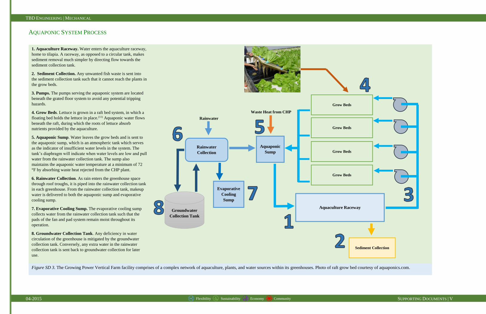
AQUAPONIC SYSTEM PROCESS

Grow Beds

Grow Beds

Grow Beds

Grow Beds

Aquaculture Raceway

Sediment Collection

Waste Heat from CHP

Aquaponic

Sump

Rainwater

Rainwater

Collection

Evaporative

Cooling

Sump

Groundwater

Collection Tank

1. Aquaculture Raceway. Water enters the aquaculture raceway,

home to tilapia. A raceway, as opposed to a circular tank, makes

sediment removal much simpler by directing flow towards the

sediment collection tank.

2. Sediment Collection. Any unwanted fish waste is sent into

the sediment collection tank such that it cannot reach the plants in

the grow beds.

3. Pumps. The pumps serving the aquaponic system are located

beneath the grated floor system to avoid any potential tripping

hazards.

4. Grow Beds. Lettuce is grown in a raft bed system, in which a

floating bed holds the lettuce in place.(11) Aquaponic water flows

beneath the raft, during which the roots of lettuce absorb

nutrients provided by the aquaculture.

5. Aquaponic Sump. Water leaves the grow beds and is sent to

the aquaponic sump, which is an atmospheric tank which serves

as the indicator of insufficient water levels in the system. The

tank’s diaphragm will indicate when water levels are low and pull

water from the rainwater collection tank. The sump also

maintains the aquaponic water temperature at a minimum of 72

°F by absorbing waste heat rejected from the CHP plant.

6. Rainwater Collection. As rain enters the greenhouse space

through roof troughs, it is piped into the rainwater collection tank

in each greenhouse. From the rainwater collection tank, makeup

water is delivered to both the aquaponic sump and evaporative

cooling sump.

7. Evaporative Cooling Sump. The evaporative cooling sump

collects water from the rainwater collection tank such that the

pads of the fan and pad system remain moist throughout its

operation.

8. Groundwater Collection Tank. Any deficiency in water

circulation of the greenhouse is mitigated by the groundwater

collection tank. Conversely, any extra water in the rainwater

collection tank is sent back to groundwater collection for later

use.

Figure SD 3. The Growing Power Vertical Farm facility comprises of a complex network of aquaculture, plants, and water sources within its greenhouses. Photo of raft grow bed courtesy of aquaponics.com.

TBD ENGINEERING | MECHANICAL

04-2015 SUPPORTING DOCUMENTS | VI Flexibility Sustainability Economy Community

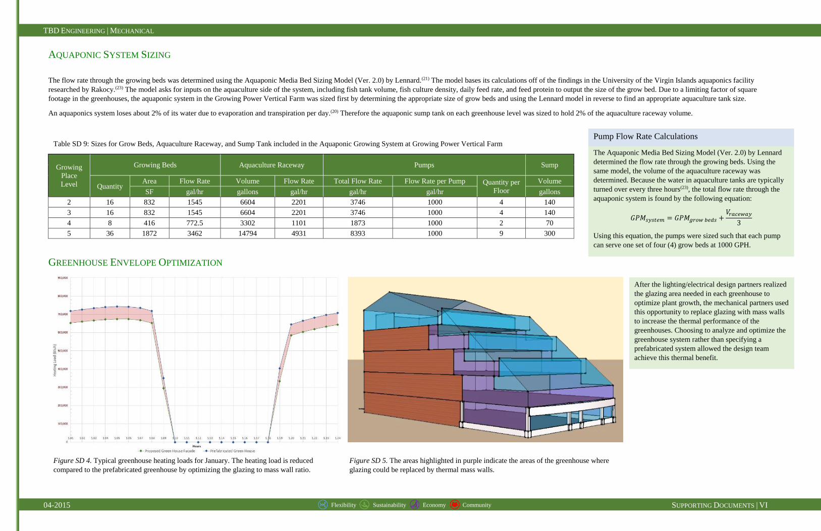
AQUAPONIC SYSTEM SIZING

The flow rate through the growing beds was determined using the Aquaponic Media Bed Sizing Model (Ver. 2.0) by Lennard.(21) The model bases its calculations off of the findings in the University of the Virgin Islands aquaponics facility

researched by Rakocy.(23) The model asks for inputs on the aquaculture side of the system, including fish tank volume, fish culture density, daily feed rate, and feed protein to output the size of the grow bed. Due to a limiting factor of square

footage in the greenhouses, the aquaponic system in the Growing Power Vertical Farm was sized first by determining the appropriate size of grow beds and using the Lennard model in reverse to find an appropriate aquaculture tank size.

An aquaponics system loses about 2% of its water due to evaporation and transpiration per day.(20) Therefore the aquaponic sump tank on each greenhouse level was sized to hold 2% of the aquaculture raceway volume.

Growing

Place

Level

Growing Beds Aquaculture Raceway Pumps Sump

Quantity Area Flow Rate Volume Flow Rate Total Flow Rate Flow Rate per Pump Quantity per

Floor

Volume

SF gal/hr gallons gal/hr gal/hr gal/hr gallons

2 16 832 1545 6604 2201 3746 1000 4 140

3 16 832 1545 6604 2201 3746 1000 4 140

4 8 416 772.5 3302 1101 1873 1000 2 70

5 36 1872 3462 14794 4931 8393 1000 9 300

GREENHOUSE ENVELOPE OPTIMIZATION

Table SD 9: Sizes for Grow Beds, Aquaculture Raceway, and Sump Tank included in the Aquaponic Growing System at Growing Power Vertical Farm

The Aquaponic Media Bed Sizing Model (Ver. 2.0) by Lennard

determined the flow rate through the growing beds. Using the

same model, the volume of the aquaculture raceway was

determined. Because the water in aquaculture tanks are typically

turned over every three hours(23), the total flow rate through the

aquaponic system is found by the following equation:

𝐺𝑃𝑀𝑠𝑦𝑠𝑡𝑒𝑚 = 𝐺𝑃𝑀𝑔𝑟𝑜𝑤 𝑏𝑒𝑑𝑠 +𝑉𝑟𝑎𝑐𝑒𝑤𝑎𝑦

3

Using this equation, the pumps were sized such that each pump

can serve one set of four (4) grow beds at 1000 GPH.

Pump Flow Rate Calculations

Figure SD 4. Typical greenhouse heating loads for January. The heating load is reduced

compared to the prefabricated greenhouse by optimizing the glazing to mass wall ratio.

After the lighting/electrical design partners realized

the glazing area needed in each greenhouse to

optimize plant growth, the mechanical partners used

this opportunity to replace glazing with mass walls

to increase the thermal performance of the

greenhouses. Choosing to analyze and optimize the

greenhouse system rather than specifying a

prefabricated system allowed the design team

achieve this thermal benefit.

Figure SD 5. The areas highlighted in purple indicate the areas of the greenhouse where

glazing could be replaced by thermal mass walls.

TBD ENGINEERING | MECHANICAL

04-2015 SUPPORTING DOCUMENTS | VII Flexibility Sustainability Economy Community

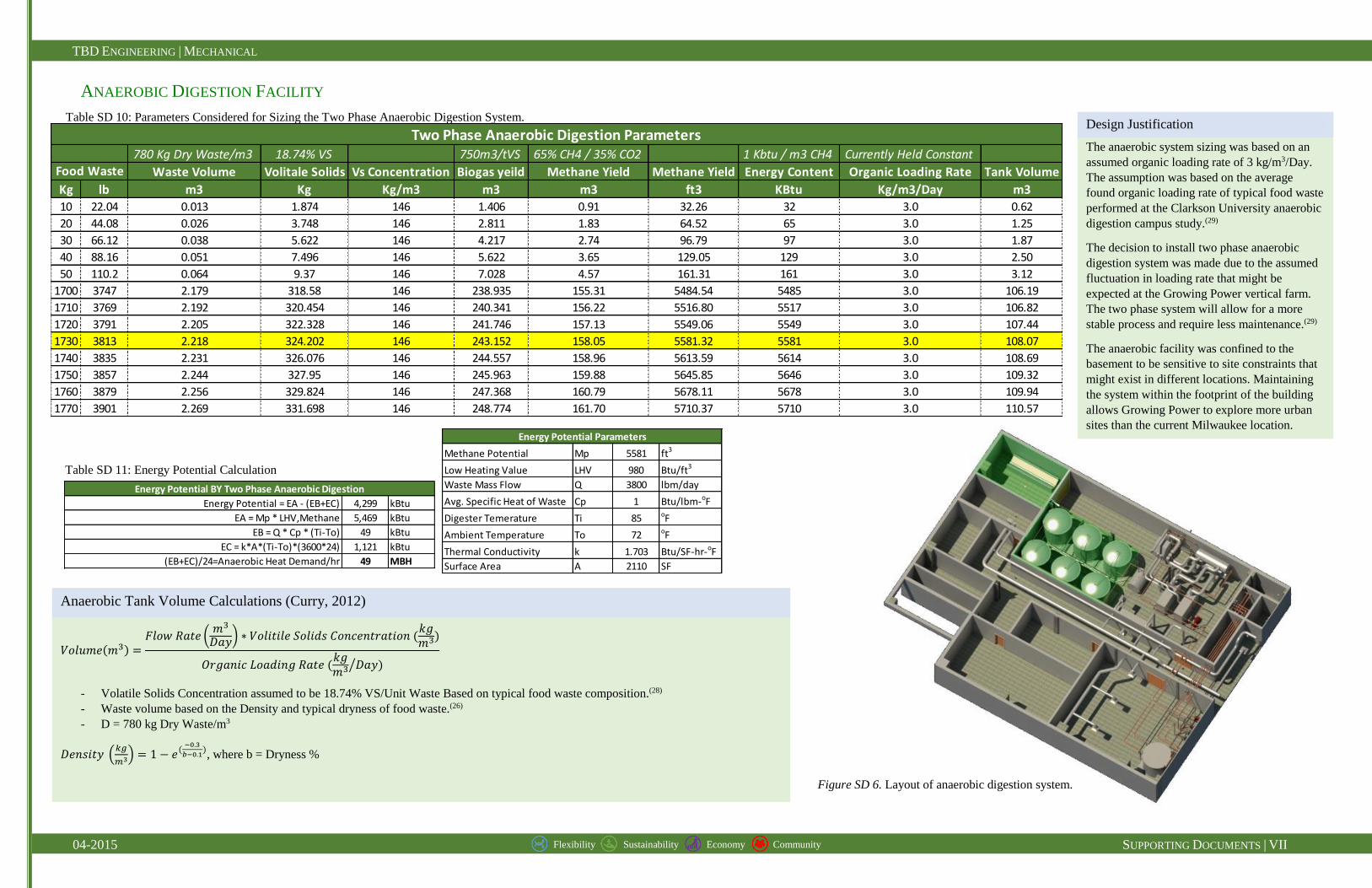
ANAEROBIC DIGESTION FACILITY

Table SD 10: Parameters Considered for Sizing the Two Phase Anaerobic Digestion System.

𝑉𝑜𝑙𝑢𝑚𝑒 𝑚3 =𝐹𝑙𝑜𝑤 𝑅𝑎𝑡𝑒

𝑚3

𝐷𝑎𝑦 ∗ 𝑉𝑜𝑙𝑖𝑡𝑖𝑙𝑒 𝑆𝑜𝑙𝑖𝑑𝑠 𝐶𝑜𝑛𝑐𝑒𝑛𝑡𝑟𝑎𝑡𝑖𝑜𝑛 𝑘𝑔𝑚3

𝑂𝑟𝑔𝑎𝑛𝑖𝑐 𝐿𝑜𝑎𝑑𝑖𝑛𝑔 𝑅𝑎𝑡𝑒 𝑘𝑔𝑚3 𝐷𝑎𝑦

- Volatile Solids Concentration assumed to be 18.74% VS/Unit Waste Based on typical food waste composition.(28)

- Waste volume based on the Density and typical dryness of food waste.(26)

- D = 780 kg Dry Waste/m3

𝐷𝑒𝑛𝑠𝑖𝑡𝑦 𝑘𝑔

𝑚3 = 1 − 𝑒 −0.3

𝑏−0.1 , where b = Dryness %

Anaerobic Tank Volume Calculations (Curry, 2012)

Table SD 11: Energy Potential Calculation

The anaerobic system sizing was based on an

assumed organic loading rate of 3 kg/m3/Day.

The assumption was based on the average

found organic loading rate of typical food waste

performed at the Clarkson University anaerobic

digestion campus study.(29)

The decision to install two phase anaerobic

digestion system was made due to the assumed

fluctuation in loading rate that might be

expected at the Growing Power vertical farm.

The two phase system will allow for a more

stable process and require less maintenance.(29)

The anaerobic facility was confined to the

basement to be sensitive to site constraints that

might exist in different locations. Maintaining

the system within the footprint of the building

allows Growing Power to explore more urban

sites than the current Milwaukee location.

Design Justification

Figure SD 6. Layout of anaerobic digestion system.

Methane Potential Mp 5581 ft3

Low Heating Value LHV 980 Btu/ft3

Waste Mass Flow Q 3800 lbm/day

Avg. Specific Heat of Waste Cp 1 Btu/lbm-oF

Digester Temerature Ti 85 oF

Ambient Temperature To 72 oF

Thermal Conductivity k 1.703 Btu/SF-hr-oF

Surface Area A 2110 SF

Energy Potential Parameters

4,299 kBtu

5,469 kBtu

49 kBtu

1,121 kBtu

49 MBH(EB+EC)/24=Anaerobic Heat Demand/hr

Energy Potential BY Two Phase Anaerobic Digestion

Energy Potential = EA - (EB+EC)

EA = Mp * LHV,Methane

EB = Q * Cp * (Ti-To)

EC = k*A*(Ti-To)*(3600*24)

780 Kg Dry Waste/m3 18.74% VS 750m3/tVS 65% CH4 / 35% CO2 1 Kbtu / m3 CH4 Currently Held Constant

Waste Volume Volitale Solids Vs Concentration Biogas yeild Methane Yield Methane Yield Energy Content Organic Loading Rate Tank Volume

Kg lb m3 Kg Kg/m3 m3 m3 ft3 KBtu Kg/m3/Day m3

10 22.04 0.013 1.874 146 1.406 0.91 32.26 32 3.0 0.62

20 44.08 0.026 3.748 146 2.811 1.83 64.52 65 3.0 1.25

30 66.12 0.038 5.622 146 4.217 2.74 96.79 97 3.0 1.87

40 88.16 0.051 7.496 146 5.622 3.65 129.05 129 3.0 2.50

50 110.2 0.064 9.37 146 7.028 4.57 161.31 161 3.0 3.12

1700 3747 2.179 318.58 146 238.935 155.31 5484.54 5485 3.0 106.19

1710 3769 2.192 320.454 146 240.341 156.22 5516.80 5517 3.0 106.82

1720 3791 2.205 322.328 146 241.746 157.13 5549.06 5549 3.0 107.44

1730 3813 2.218 324.202 146 243.152 158.05 5581.32 5581 3.0 108.07

1740 3835 2.231 326.076 146 244.557 158.96 5613.59 5614 3.0 108.69

1750 3857 2.244 327.95 146 245.963 159.88 5645.85 5646 3.0 109.32

1760 3879 2.256 329.824 146 247.368 160.79 5678.11 5678 3.0 109.94

1770 3901 2.269 331.698 146 248.774 161.70 5710.37 5710 3.0 110.57

Two Phase Anaerobic Digestion Parameters

Food Waste

TBD ENGINEERING | MECHANICAL

04-2015 SUPPORTING DOCUMENTS | VIII Flexibility Sustainability Economy Community

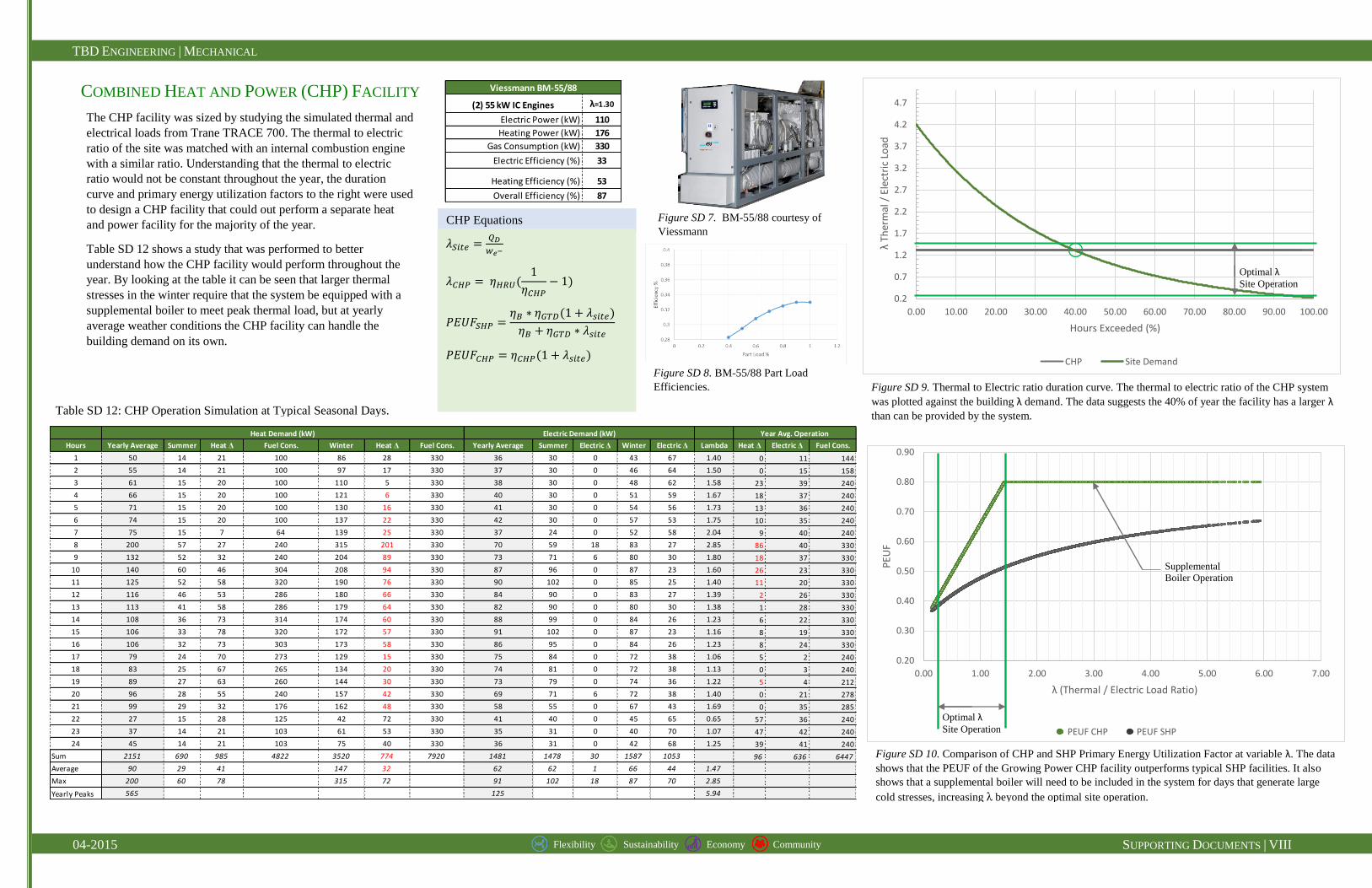
COMBINED HEAT AND POWER (CHP) FACILITY

0.20

0.30

0.40

0.50

0.60

0.70

0.80

0.90

0.00 1.00 2.00 3.00 4.00 5.00 6.00 7.00

PEU

F

λ (Thermal / Electric Load Ratio)

PEUF CHP PEUF SHP

0.2

0.7

1.2

1.7

2.2

2.7

3.2

3.7

4.2

4.7

0.00 10.00 20.00 30.00 40.00 50.00 60.00 70.00 80.00 90.00 100.00

λTh

erm

al /

Ele

ctri

c Lo

ad

Hours Exceeded (%)

CHP Site Demand

Optimal λ

Site Operation

Supplemental

Boiler Operation

Optimal λ

Site Operation

Table SD 12: CHP Operation Simulation at Typical Seasonal Days.

Figure SD 9. Thermal to Electric ratio duration curve. The thermal to electric ratio of the CHP system

was plotted against the building λ demand. The data suggests the 40% of year the facility has a larger λ

than can be provided by the system.

Figure SD 10. Comparison of CHP and SHP Primary Energy Utilization Factor at variable λ. The data

shows that the PEUF of the Growing Power CHP facility outperforms typical SHP facilities. It also

shows that a supplemental boiler will need to be included in the system for days that generate large

cold stresses, increasing λ beyond the optimal site operation.

Figure SD 8. BM-55/88 Part Load

Efficiencies.

The CHP facility was sized by studying the simulated thermal and

electrical loads from Trane TRACE 700. The thermal to electric

ratio of the site was matched with an internal combustion engine

with a similar ratio. Understanding that the thermal to electric

ratio would not be constant throughout the year, the duration

curve and primary energy utilization factors to the right were used

to design a CHP facility that could out perform a separate heat

and power facility for the majority of the year.

Table SD 12 shows a study that was performed to better

understand how the CHP facility would perform throughout the

year. By looking at the table it can be seen that larger thermal

stresses in the winter require that the system be equipped with a

supplemental boiler to meet peak thermal load, but at yearly

average weather conditions the CHP facility can handle the

building demand on its own.

CHP Equations

𝜆𝑆𝑖𝑡𝑒 =𝑄𝐷

𝑤𝑒−

𝜆𝐶𝐻𝑃 = 𝜂𝐻𝑅𝑈 1

𝜂𝐶𝐻𝑃− 1

𝑃𝐸𝑈𝐹𝑆𝐻𝑃 =𝜂𝐵 ∗ 𝜂𝐺𝑇𝐷 1 + 𝜆𝑠𝑖𝑡𝑒

𝜂𝐵 + 𝜂𝐺𝑇𝐷 ∗ 𝜆𝑠𝑖𝑡𝑒

𝑃𝐸𝑈𝐹𝐶𝐻𝑃 = 𝜂𝐶𝐻𝑃 1 + 𝜆𝑠𝑖𝑡𝑒

Figure SD 7. BM-55/88 courtesy of

Viessmann

Hours Yearly Average Summer Heat Δ Fuel Cons. Winter Heat Δ Fuel Cons. Yearly Average Summer Electric Δ Winter Electric Δ Lambda Heat Δ Electric Δ Fuel Cons.

1 50 14 21 100 86 28 330 36 30 0 43 67 1.40 0 11 144

2 55 14 21 100 97 17 330 37 30 0 46 64 1.50 0 15 158

3 61 15 20 100 110 5 330 38 30 0 48 62 1.58 23 39 240

4 66 15 20 100 121 6 330 40 30 0 51 59 1.67 18 37 240

5 71 15 20 100 130 16 330 41 30 0 54 56 1.73 13 36 240

6 74 15 20 100 137 22 330 42 30 0 57 53 1.75 10 35 240

7 75 15 7 64 139 25 330 37 24 0 52 58 2.04 9 40 240

8 200 57 27 240 315 201 330 70 59 18 83 27 2.85 86 40 330

9 132 52 32 240 204 89 330 73 71 6 80 30 1.80 18 37 330

10 140 60 46 304 208 94 330 87 96 0 87 23 1.60 26 23 330

11 125 52 58 320 190 76 330 90 102 0 85 25 1.40 11 20 330

12 116 46 53 286 180 66 330 84 90 0 83 27 1.39 2 26 330

13 113 41 58 286 179 64 330 82 90 0 80 30 1.38 1 28 330

14 108 36 73 314 174 60 330 88 99 0 84 26 1.23 6 22 330

15 106 33 78 320 172 57 330 91 102 0 87 23 1.16 8 19 330

16 106 32 73 303 173 58 330 86 95 0 84 26 1.23 8 24 330

17 79 24 70 273 129 15 330 75 84 0 72 38 1.06 5 2 240

18 83 25 67 265 134 20 330 74 81 0 72 38 1.13 0 3 240

19 89 27 63 260 144 30 330 73 79 0 74 36 1.22 5 4 212

20 96 28 55 240 157 42 330 69 71 6 72 38 1.40 0 21 278

21 99 29 32 176 162 48 330 58 55 0 67 43 1.69 0 35 285

22 27 15 28 125 42 72 330 41 40 0 45 65 0.65 57 36 240

23 37 14 21 103 61 53 330 35 31 0 40 70 1.07 47 42 240

24 45 14 21 103 75 40 330 36 31 0 42 68 1.25 39 41 240

Sum 2151 690 985 4822 3520 774 7920 1481 1478 30 1587 1053 96 636 6447

Average 90 29 41 147 32 62 62 1 66 44 1.47

Max 200 60 78 315 72 91 102 18 87 70 2.85

Yearly Peaks 565 125 5.94

Electric Demand (kW)Heat Demand (kW) Year Avg. Operation

λ=1.30

110

176

330

33

53

87

Gas Consumption (kW)

Overall Efficiency (%)

Viessmann BM-55/88

(2) 55 kW IC Engines

Electric Power (kW)

Electric Efficiency (%)

Heating Efficiency (%)

Heating Power (kW)

TBD ENGINEERING | MECHANICAL

04-2015 SUPPORTING DOCUMENTS | IX Flexibility Sustainability Economy Community

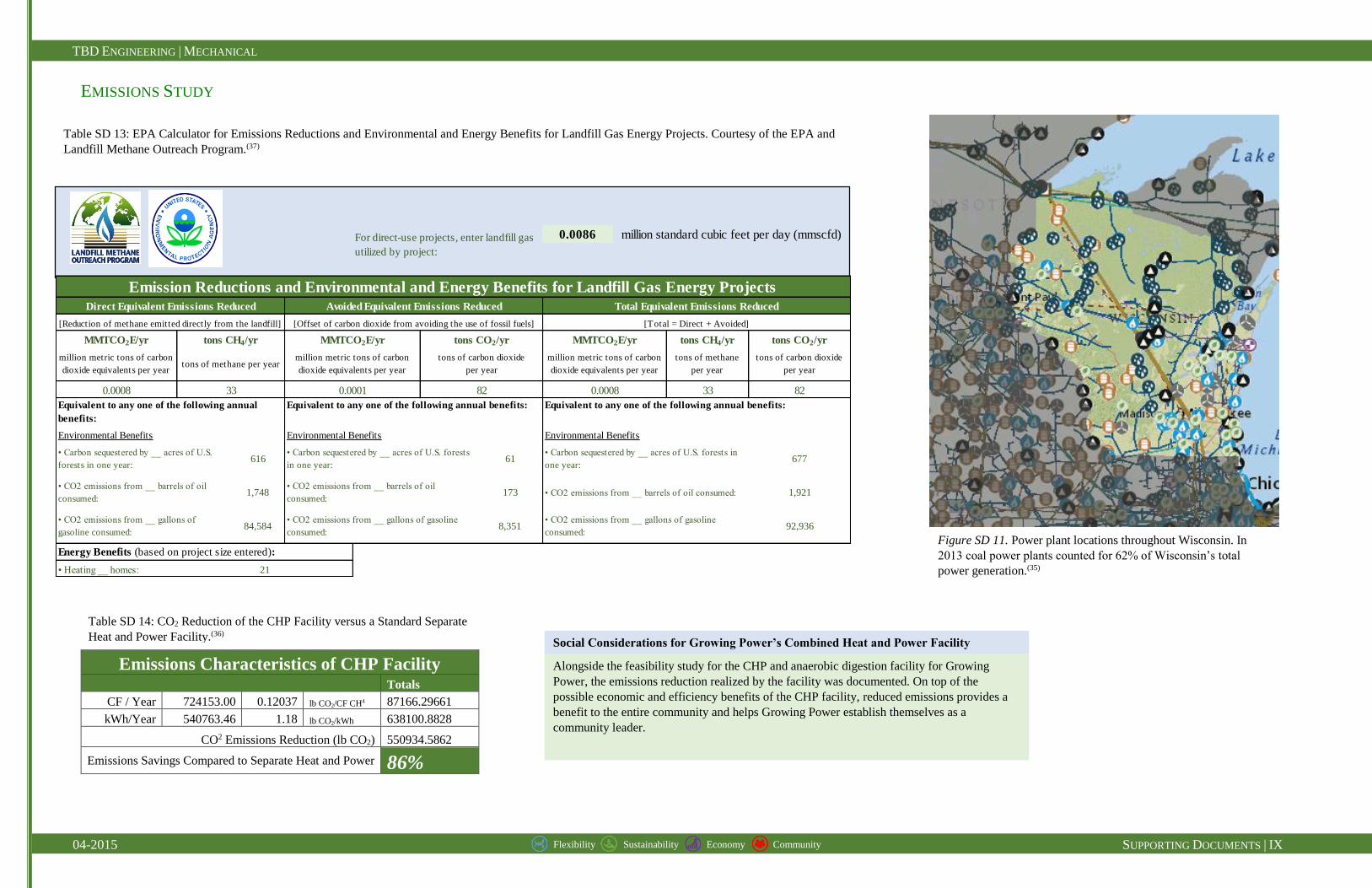
EMISSIONS STUDY

Emissions Characteristics of CHP Facility Totals

CF / Year 724153.00 0.12037 lb CO2/CF CH4 87166.29661

kWh/Year 540763.46 1.18 lb CO2/kWh 638100.8828

CO2 Emissions Reduction (lb CO2) 550934.5862

Emissions Savings Compared to Separate Heat and Power 86%

Table SD 13: EPA Calculator for Emissions Reductions and Environmental and Energy Benefits for Landfill Gas Energy Projects. Courtesy of the EPA and

Landfill Methane Outreach Program.(37)

Table SD 14: CO2 Reduction of the CHP Facility versus a Standard Separate

Heat and Power Facility.(36)

0.0086

tons CH4/yr tons CO2/yr

33 82

Environmental Benefits Environmental Benefits Environmental Benefits

• Heating __ homes:

Direct Equivalent Emissions Reduced Avoided Equivalent Emissions Reduced Total Equivalent Emissions Reduced

[Reduction of methane emitted directly from the landfill] [Offset of carbon dioxide from avoiding the use of fossil fuels] [Total = Direct + Avoided]

MMTCO2E/yr tons CH4/yr MMTCO2E/yr tons CO2/yr MMTCO2E/yr

tons of carbon dioxide

per year

0.0008 33 0.0001 82 0.0008

million metric tons of carbon

dioxide equivalents per yeartons of methane per year

million metric tons of carbon

dioxide equivalents per year

tons of carbon dioxide

per year

million metric tons of carbon

dioxide equivalents per year

tons of methane

per year

1,921

Equivalent to any one of the following annual

benefits:

Equivalent to any one of the following annual benefits:

• Carbon sequestered by __ acres of U.S.

forests in one year:616

• Carbon sequestered by __ acres of U.S. forests

in one year:61

• CO2 emissions from __ barrels of oil

consumed:1,748

• CO2 emissions from __ barrels of oil

consumed:173 • CO2 emissions from __ barrels of oil consumed:

Emission Reductions and Environmental and Energy Benefits for Landfill Gas Energy Projects

For direct-use projects, enter landfill gas

utilized by project:

Equivalent to any one of the following annual benefits:

Energy Benefits (based on project size entered):

21

million standard cubic feet per day (mmscfd)

• CO2 emissions from __ gallons of

gasoline consumed:84,584

• CO2 emissions from __ gallons of gasoline

consumed:8,351

• CO2 emissions from __ gallons of gasoline

consumed:92,936

• Carbon sequestered by __ acres of U.S. forests in

one year:677

Alongside the feasibility study for the CHP and anaerobic digestion facility for Growing

Power, the emissions reduction realized by the facility was documented. On top of the

possible economic and efficiency benefits of the CHP facility, reduced emissions provides a

benefit to the entire community and helps Growing Power establish themselves as a

community leader.

Social Considerations for Growing Power’s Combined Heat and Power Facility

Figure SD 11. Power plant locations throughout Wisconsin. In

2013 coal power plants counted for 62% of Wisconsin’s total

power generation.(35)

TBD ENGINEERING | MECHANICAL

04-2015 SUPPORTING DOCUMENTS | X Flexibility Sustainability Economy Community

ECONOMIC ANALYSIS

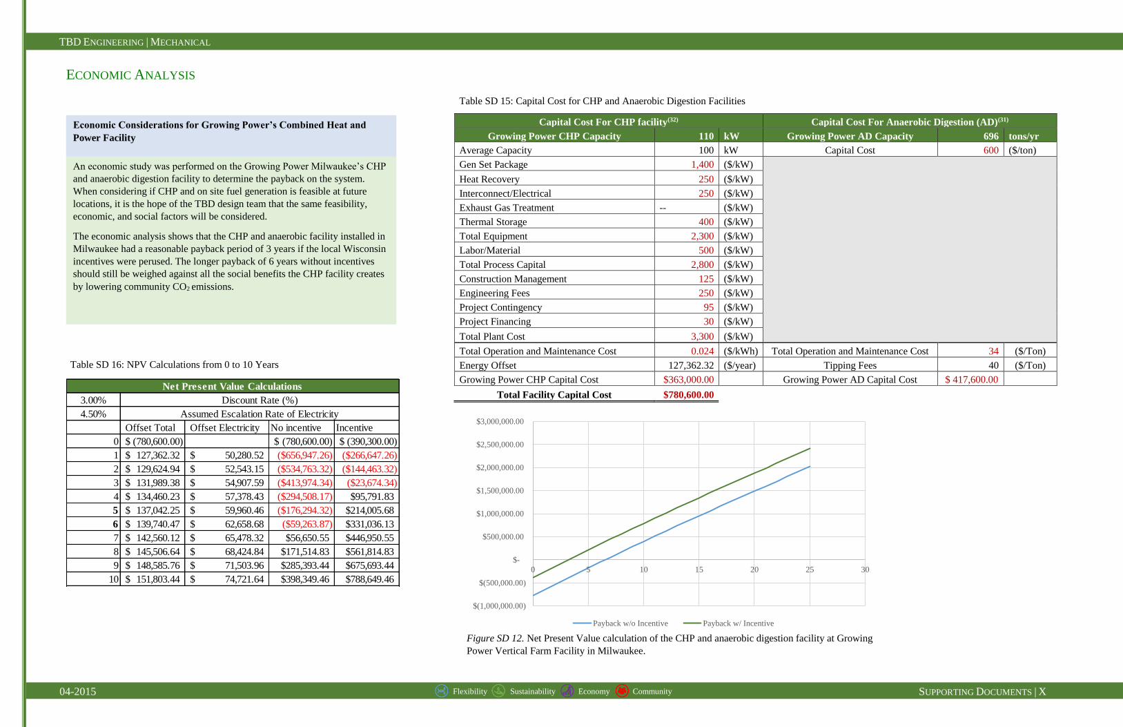
Capital Cost For CHP facility(32) Capital Cost For Anaerobic Digestion (AD)(31)

Growing Power CHP Capacity 110 kW Growing Power AD Capacity 696 tons/yr

Average Capacity 100 kW Capital Cost 600 ($/ton)

Gen Set Package 1,400 ($/kW)

Heat Recovery 250 ($/kW)

Interconnect/Electrical 250 ($/kW)

Exhaust Gas Treatment -- ($/kW)

Thermal Storage 400 ($/kW)

Total Equipment 2,300 ($/kW)

Labor/Material 500 ($/kW)

Total Process Capital 2,800 ($/kW)

Construction Management 125 ($/kW)

Engineering Fees 250 ($/kW)

Project Contingency 95 ($/kW)

Project Financing 30 ($/kW)

Total Plant Cost 3,300 ($/kW)

Total Operation and Maintenance Cost 0.024 ($/kWh) Total Operation and Maintenance Cost 34 ($/Ton)

Energy Offset 127,362.32 ($/year) Tipping Fees 40 ($/Ton)

Growing Power CHP Capital Cost $363,000.00 Growing Power AD Capital Cost $ 417,600.00

Total Facility Capital Cost $780,600.00 3.00%

4.50%

Offset Total Offset Electricity No incentive Incentive

0 (780,600.00)$ (780,600.00)$ (390,300.00)$

1 127,362.32$ 50,280.52$ ($656,947.26) ($266,647.26)

2 129,624.94$ 52,543.15$ ($534,763.32) ($144,463.32)

3 131,989.38$ 54,907.59$ ($413,974.34) ($23,674.34)

4 134,460.23$ 57,378.43$ ($294,508.17) $95,791.83

5 137,042.25$ 59,960.46$ ($176,294.32) $214,005.68

6 139,740.47$ 62,658.68$ ($59,263.87) $331,036.13

7 142,560.12$ 65,478.32$ $56,650.55 $446,950.55

8 145,506.64$ 68,424.84$ $171,514.83 $561,814.83

9 148,585.76$ 71,503.96$ $285,393.44 $675,693.44

10 151,803.44$ 74,721.64$ $398,349.46 $788,649.46

Net Present Value Calculations

Discount Rate (%)

Assumed Escalation Rate of Electricity

$(1,000,000.00)

$(500,000.00)

$-

$500,000.00

$1,000,000.00

$1,500,000.00

$2,000,000.00

$2,500,000.00

$3,000,000.00

0 5 10 15 20 25 30

Payback w/o Incentive Payback w/ Incentive

Figure SD 12. Net Present Value calculation of the CHP and anaerobic digestion facility at Growing

Power Vertical Farm Facility in Milwaukee.

Table SD 16: NPV Calculations from 0 to 10 Years

Table SD 15: Capital Cost for CHP and Anaerobic Digestion Facilities

An economic study was performed on the Growing Power Milwaukee’s CHP

and anaerobic digestion facility to determine the payback on the system.

When considering if CHP and on site fuel generation is feasible at future

locations, it is the hope of the TBD design team that the same feasibility,

economic, and social factors will be considered.

The economic analysis shows that the CHP and anaerobic facility installed in

Milwaukee had a reasonable payback period of 3 years if the local Wisconsin

incentives were perused. The longer payback of 6 years without incentives

should still be weighed against all the social benefits the CHP facility creates

by lowering community CO2 emissions.

Economic Considerations for Growing Power’s Combined Heat and

Power Facility

TBD ENGINEERING | MECHANICAL

04-2015 SUPPORTING DOCUMENTS | XI Flexibility Sustainability Economy Community

OVERALL MECHANICAL SYSTEM SCHEMATIC

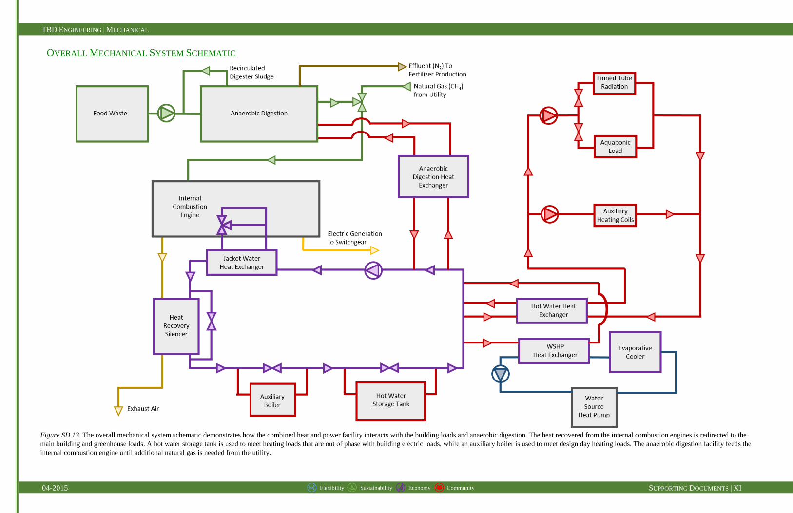
Figure SD 13. The overall mechanical system schematic demonstrates how the combined heat and power facility interacts with the building loads and anaerobic digestion. The heat recovered from the internal combustion engines is redirected to the

main building and greenhouse loads. A hot water storage tank is used to meet heating loads that are out of phase with building electric loads, while an auxiliary boiler is used to meet design day heating loads. The anaerobic digestion facility feeds the

internal combustion engine until additional natural gas is needed from the utility.

TBD ENGINEERING | MECHANICAL

04-2015 SUPPORTING DOCUMENTS | XII Flexibility Sustainability Economy Community

SOYBEAN OIL BIODIESEL PRODUCTION: AN ALTERNATIVE FOR FUTURE GROWING POWER VERTICAL FARM SITES

SIZING FOR A SOYBEAN OIL BIODIESEL PROCESS The following steps were taken to select equipment and size the required components of soybean oil biodiesel production.

1. Size the biodiesel generator for thermal demand of the building.

2. Use the generator data to determine the fuel input of biodiesel required to operate the generator.

3. Select a biodiesel processor that will produce biodiesel at a rate greater than or equal to the fuel input required in 2.

4. Use the biodiesel processor data to determine a soybean oil input volumetric flow rate required for the processor.

5. Select a soybean oil pressing unit that will produce the necessary volumetric flow rate of soybean oil as specified in 4.

6. Use the data from the soybean press to determine the amount of soybeans needed daily.

NaOH

Crude Biodiesel

Biodiesel to Biodiesel

Generator

Fish Feed to Aquaponic

System

Meal Mixing

Soybean Mash

Soybean Oil

Holding Tank

Soybean Oil Press

Soybean

Soybean Oil

Crude Glycerin

Biodiesel Processor:

Transesterification

Ethanol

Holding

Tank

Ethanol

Membrane

Biodiesel

Purification

Recovered Glycerin

NaOH

Holding

Tank

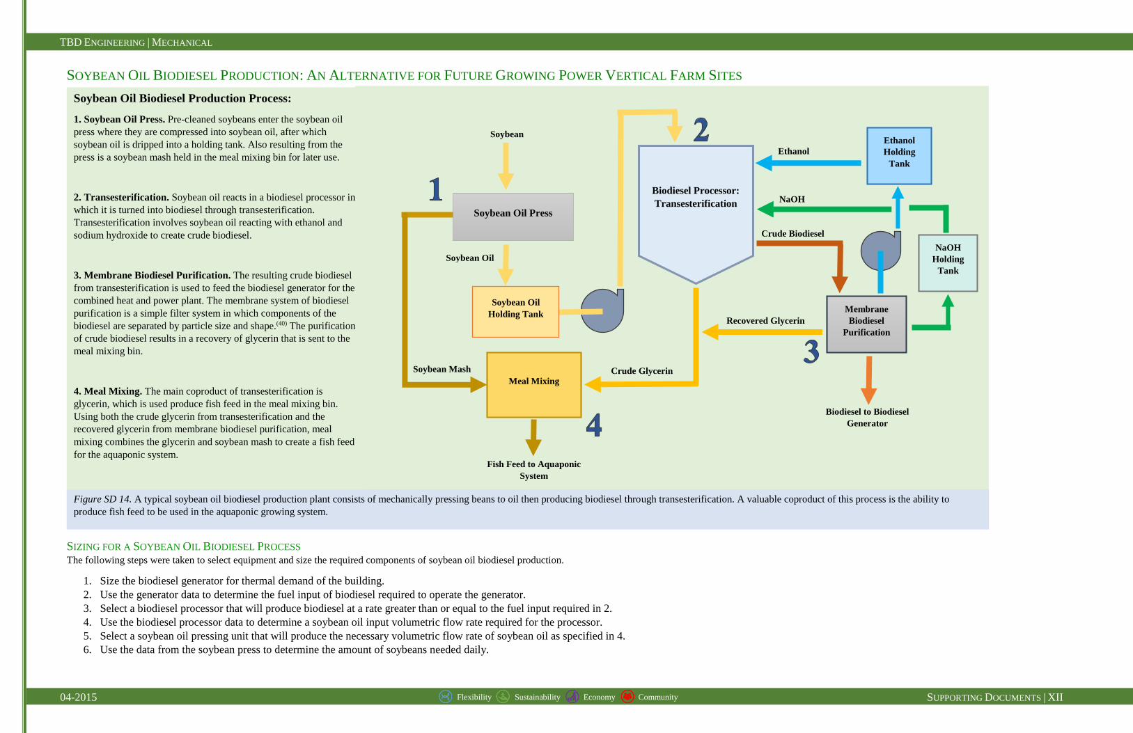
Figure SD 14. A typical soybean oil biodiesel production plant consists of mechanically pressing beans to oil then producing biodiesel through transesterification. A valuable coproduct of this process is the ability to

produce fish feed to be used in the aquaponic growing system.

Soybean Oil Biodiesel Production Process:

1. Soybean Oil Press. Pre-cleaned soybeans enter the soybean oil

press where they are compressed into soybean oil, after which

soybean oil is dripped into a holding tank. Also resulting from the

press is a soybean mash held in the meal mixing bin for later use.

2. Transesterification. Soybean oil reacts in a biodiesel processor in

which it is turned into biodiesel through transesterification.

Transesterification involves soybean oil reacting with ethanol and

sodium hydroxide to create crude biodiesel.

3. Membrane Biodiesel Purification. The resulting crude biodiesel

from transesterification is used to feed the biodiesel generator for the

combined heat and power plant. The membrane system of biodiesel

purification is a simple filter system in which components of the

biodiesel are separated by particle size and shape.(40) The purification

of crude biodiesel results in a recovery of glycerin that is sent to the

meal mixing bin.

4. Meal Mixing. The main coproduct of transesterification is

glycerin, which is used produce fish feed in the meal mixing bin.

Using both the crude glycerin from transesterification and the

recovered glycerin from membrane biodiesel purification, meal

mixing combines the glycerin and soybean mash to create a fish feed

for the aquaponic system.

TBD ENGINEERING | MECHANICAL

04-2015 SUPPORTING DOCUMENTS | XIII Flexibility Sustainability Economy Community

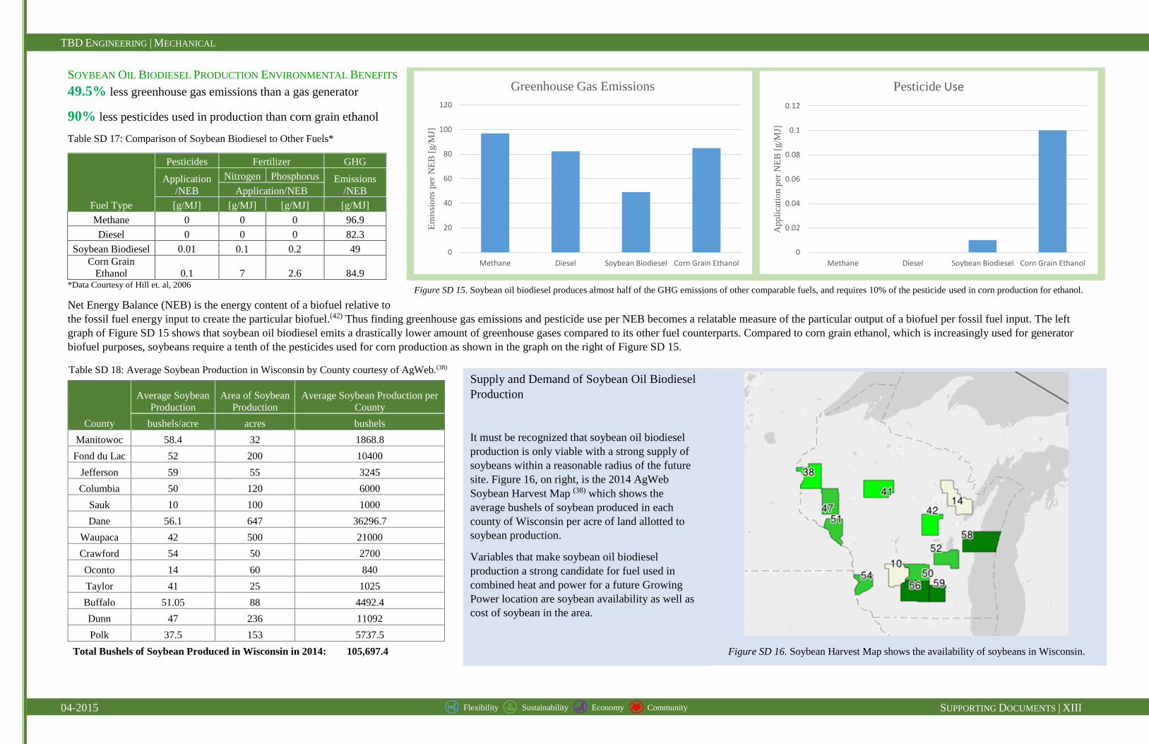
SOYBEAN OIL BIODIESEL PRODUCTION ENVIRONMENTAL BENEFITS

49.5% less greenhouse gas emissions than a gas generator

90% less pesticides used in production than corn grain ethanol

Table SD 17: Comparison of Soybean Biodiesel to Other Fuels*

Fuel Type

Pesticides Fertilizer GHG

Application

/NEB

Nitrogen Phosphorus Emissions

/NEB Application/NEB

[g/MJ] [g/MJ] [g/MJ] [g/MJ]

Methane 0 0 0 96.9

Diesel 0 0 0 82.3

Soybean Biodiesel 0.01 0.1 0.2 49

Corn Grain

Ethanol 0.1 7 2.6 84.9 *Data Courtesy of Hill et. al, 2006

Net Energy Balance (NEB) is the energy content of a biofuel relative to

the fossil fuel energy input to create the particular biofuel.(42) Thus finding greenhouse gas emissions and pesticide use per NEB becomes a relatable measure of the particular output of a biofuel per fossil fuel input. The left

graph of Figure SD 15 shows that soybean oil biodiesel emits a drastically lower amount of greenhouse gases compared to its other fuel counterparts. Compared to corn grain ethanol, which is increasingly used for generator

biofuel purposes, soybeans require a tenth of the pesticides used for corn production as shown in the graph on the right of Figure SD 15.

County

Average Soybean

Production

Area of Soybean

Production

Average Soybean Production per

County

bushels/acre acres bushels

Manitowoc 58.4 32 1868.8

Fond du Lac 52 200 10400

Jefferson 59 55 3245

Columbia 50 120 6000

Sauk 10 100 1000

Dane 56.1 647 36296.7

Waupaca 42 500 21000

Crawford 54 50 2700

Oconto 14 60 840

Taylor 41 25 1025

Buffalo 51.05 88 4492.4

Dunn 47 236 11092

Polk 37.5 153 5737.5

Total Bushels of Soybean Produced in Wisconsin in 2014: 105,697.4

0

20

40

60

80

100

120

Methane Diesel Soybean Biodiesel Corn Grain Ethanol

Em

issi

ons

per

NE

B [

g/M

J]

Greenhouse Gas Emissions

0

0.02

0.04

0.06

0.08

0.1

0.12

Methane Diesel Soybean Biodiesel Corn Grain Ethanol

Ap

pli

cati

on p

er N

EB

[g/M

J]

Pesticide Use

Figure SD 16. Soybean Harvest Map shows the availability of soybeans in Wisconsin.

Supply and Demand of Soybean Oil Biodiesel

Production

It must be recognized that soybean oil biodiesel

production is only viable with a strong supply of

soybeans within a reasonable radius of the future

site. Figure 16, on right, is the 2014 AgWeb

Soybean Harvest Map (38) which shows the

average bushels of soybean produced in each

county of Wisconsin per acre of land allotted to

soybean production.

Variables that make soybean oil biodiesel

production a strong candidate for fuel used in

combined heat and power for a future Growing

Power location are soybean availability as well as

cost of soybean in the area.

Figure SD 15. Soybean oil biodiesel produces almost half of the GHG emissions of other comparable fuels, and requires 10% of the pesticide used in corn production for ethanol.

Table SD 18: Average Soybean Production in Wisconsin by County courtesy of AgWeb.(38)

TBD ENGINEERING | MECHANICAL

04-2015 SUPPORTING DOCUMENTS | XIV Flexibility Sustainability Economy Community

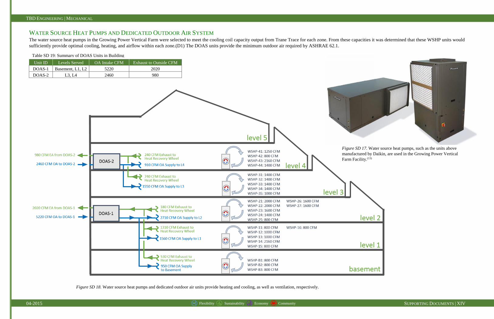
WATER SOURCE HEAT PUMPS AND DEDICATED OUTDOOR AIR SYSTEM The water source heat pumps in the Growing Power Vertical Farm were selected to meet the cooling coil capacity output from Trane Trace for each zone. From these capacities it was determined that these WSHP units would

sufficiently provide optimal cooling, heating, and airflow within each zone.(D1) The DOAS units provide the minimum outdoor air required by ASHRAE 62.1.

Unit ID Levels Served OA Intake CFM Exhaust to Outside CFM

DOAS-1 Basement, L1, L2 5220 2020

DOAS-2 L3, L4 2460 980

Figure SD 17. Water source heat pumps, such as the units above

manufactured by Daikin, are used in the Growing Power Vertical

Farm Facility.(13)

Figure SD 18. Water source heat pumps and dedicated outdoor air units provide heating and cooling, as well as ventilation, respectively.

Table SD 19: Summary of DOAS Units in Building

TBD ENGINEERING | MECHANICAL

04-2015 SUPPORTING DOCUMENTS | XV Flexibility Sustainability Economy Community

OCCUPANT COMFORT ANALYSIS

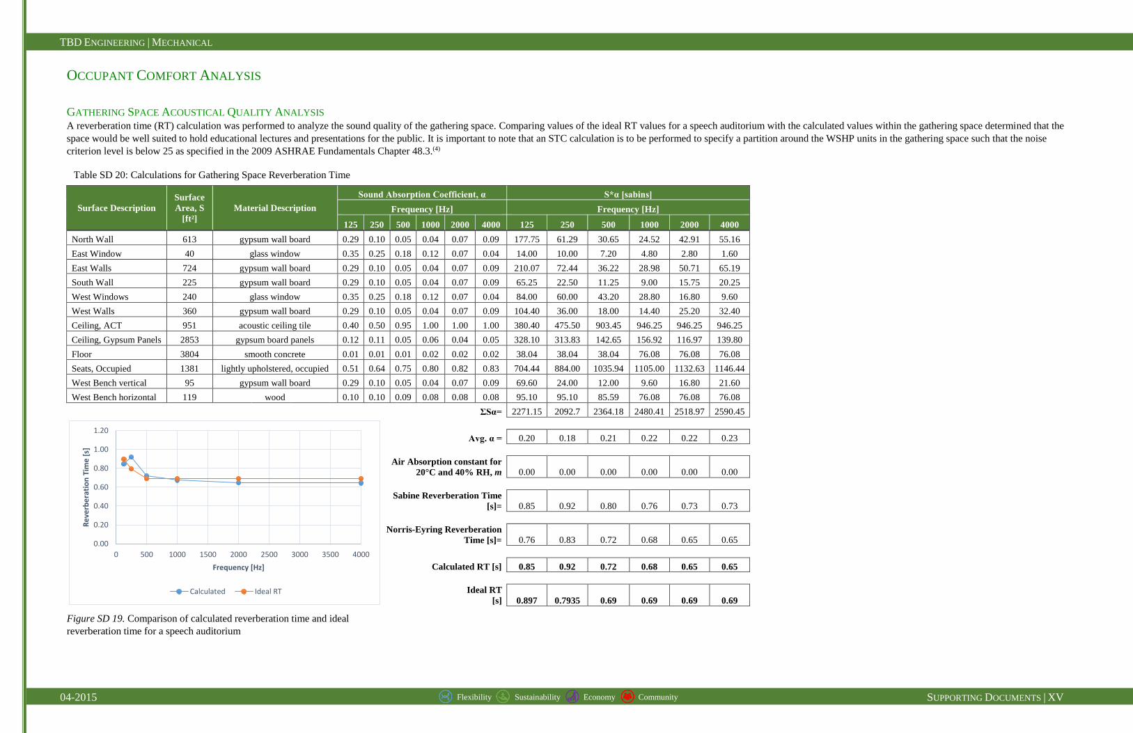
GATHERING SPACE ACOUSTICAL QUALITY ANALYSIS A reverberation time (RT) calculation was performed to analyze the sound quality of the gathering space. Comparing values of the ideal RT values for a speech auditorium with the calculated values within the gathering space determined that the

space would be well suited to hold educational lectures and presentations for the public. It is important to note that an STC calculation is to be performed to specify a partition around the WSHP units in the gathering space such that the noise

criterion level is below 25 as specified in the 2009 ASHRAE Fundamentals Chapter 48.3.(4)

Surface Description

Surface

Area, S

[ft²]

Material Description

Sound Absorption Coefficient, α S*α [sabins]

Frequency [Hz] Frequency [Hz]

125 250 500 1000 2000 4000 125 250 500 1000 2000 4000

North Wall 613 gypsum wall board 0.29 0.10 0.05 0.04 0.07 0.09 177.75 61.29 30.65 24.52 42.91 55.16

East Window 40 glass window 0.35 0.25 0.18 0.12 0.07 0.04 14.00 10.00 7.20 4.80 2.80 1.60

East Walls 724 gypsum wall board 0.29 0.10 0.05 0.04 0.07 0.09 210.07 72.44 36.22 28.98 50.71 65.19

South Wall 225 gypsum wall board 0.29 0.10 0.05 0.04 0.07 0.09 65.25 22.50 11.25 9.00 15.75 20.25

West Windows 240 glass window 0.35 0.25 0.18 0.12 0.07 0.04 84.00 60.00 43.20 28.80 16.80 9.60

West Walls 360 gypsum wall board 0.29 0.10 0.05 0.04 0.07 0.09 104.40 36.00 18.00 14.40 25.20 32.40

Ceiling, ACT 951 acoustic ceiling tile 0.40 0.50 0.95 1.00 1.00 1.00 380.40 475.50 903.45 946.25 946.25 946.25

Ceiling, Gypsum Panels 2853 gypsum board panels 0.12 0.11 0.05 0.06 0.04 0.05 328.10 313.83 142.65 156.92 116.97 139.80

Floor 3804 smooth concrete 0.01 0.01 0.01 0.02 0.02 0.02 38.04 38.04 38.04 76.08 76.08 76.08

Seats, Occupied 1381 lightly upholstered, occupied 0.51 0.64 0.75 0.80 0.82 0.83 704.44 884.00 1035.94 1105.00 1132.63 1146.44

West Bench vertical 95 gypsum wall board 0.29 0.10 0.05 0.04 0.07 0.09 69.60 24.00 12.00 9.60 16.80 21.60

West Bench horizontal 119 wood 0.10 0.10 0.09 0.08 0.08 0.08 95.10 95.10 85.59 76.08 76.08 76.08

ΣSα= 2271.15 2092.7 2364.18 2480.41 2518.97 2590.45

Avg. α = 0.20 0.18 0.21 0.22 0.22 0.23

Air Absorption constant for

20°C and 40% RH, m 0.00 0.00 0.00 0.00 0.00 0.00

Sabine Reverberation Time

[s]= 0.85 0.92 0.80 0.76 0.73 0.73

Norris-Eyring Reverberation

Time [s]= 0.76 0.83 0.72 0.68 0.65 0.65

Calculated RT [s] 0.85 0.92 0.72 0.68 0.65 0.65

Ideal RT

[s] 0.897 0.7935 0.69 0.69 0.69 0.69

0.00

0.20

0.40

0.60

0.80

1.00

1.20

0 500 1000 1500 2000 2500 3000 3500 4000

Re

verb

era

tio

n T

ime

[s]

Frequency [Hz]

Calculated Ideal RT

Figure SD 19. Comparison of calculated reverberation time and ideal

reverberation time for a speech auditorium

Table SD 20: Calculations for Gathering Space Reverberation Time