Updating and adjustment of the trade flows of an Input ... · Updating and adjustment of the trade flows of an Input-Output Table ... 2Departamento de Análisis Económico Aplicado

1

7th Annual Conference on Global Economic Analysis June 17-19, 2004 The World Bank, Washington, D.C., United States

Updating and adjustment of the trade flows of an Input-Output Table

D.R. Santos Peñate1, C. Manrique de Lara Peñate2

1Departamento de Métodos Cuantitativos en E. y G.

Universidad de Las Palmas de G.C., 35017 Las Palmas de G.C., Spain E-mail: [email protected]

2Departamento de Análisis Económico Aplicado Universidad de Las Palmas de G.C., 35017 Las Palmas de G.C., and CENTRA Spain

E-mail: [email protected]

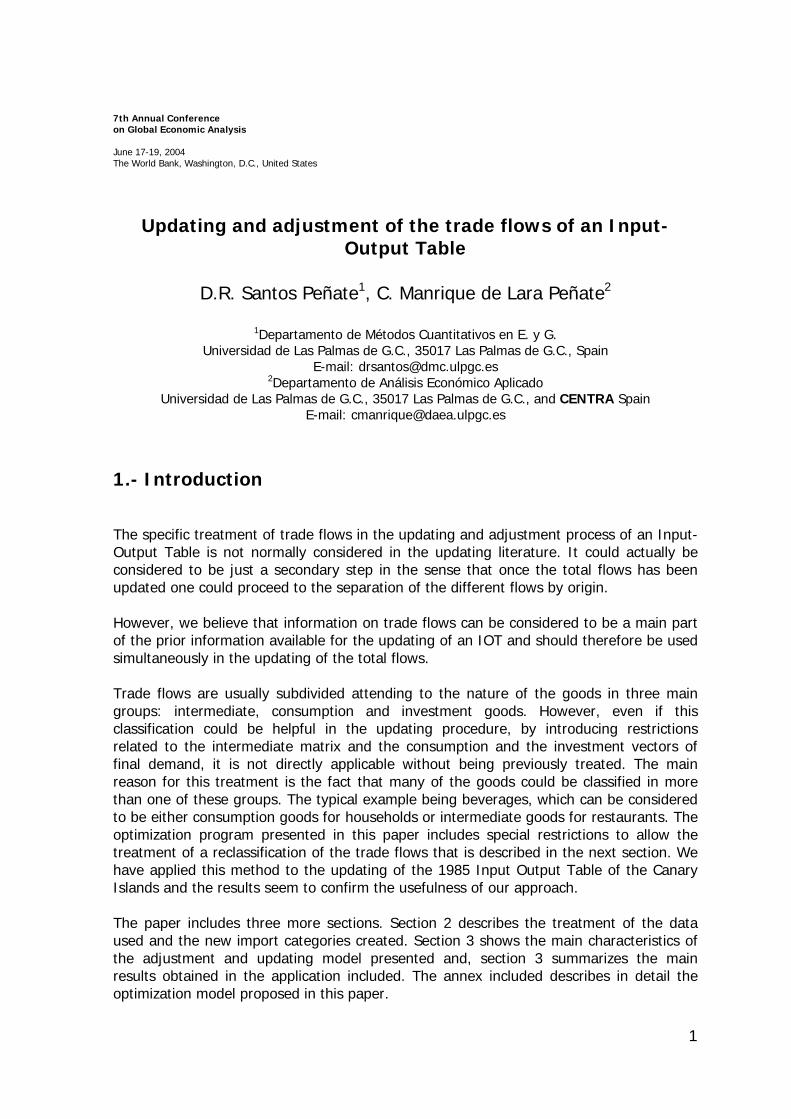
1.- Introduction The specific treatment of trade flows in the updating and adjustment process of an Input-Output Table is not normally considered in the updating literature. It could actually be considered to be just a secondary step in the sense that once the total flows has been updated one could proceed to the separation of the different flows by origin. However, we believe that information on trade flows can be considered to be a main part of the prior information available for the updating of an IOT and should therefore be used simultaneously in the updating of the total flows. Trade flows are usually subdivided attending to the nature of the goods in three main groups: intermediate, consumption and investment goods. However, even if this classification could be helpful in the updating procedure, by introducing restrictions related to the intermediate matrix and the consumption and the investment vectors of final demand, it is not directly applicable without being previously treated. The main reason for this treatment is the fact that many of the goods could be classified in more than one of these groups. The typical example being beverages, which can be considered to be either consumption goods for households or intermediate goods for restaurants. The optimization program presented in this paper includes special restrictions to allow the treatment of a reclassification of the trade flows that is described in the next section. We have applied this method to the updating of the 1985 Input Output Table of the Canary Islands and the results seem to confirm the usefulness of our approach. The paper includes three more sections. Section 2 describes the treatment of the data used and the new import categories created. Section 3 shows the main characteristics of the adjustment and updating model presented and, section 3 summarizes the main results obtained in the application included. The annex included describes in detail the optimization model proposed in this paper.

2

2.- Preparation of the data

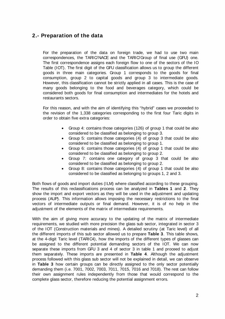
For the preparation of the data on foreign trade, we had to use two main correspondences, the TARIC/NACE and the TARIC/Group of final use (GFU) one. The first correspondence assigns each foreign flow to one of the sectors of the IO Table (IOT). The first digit of the GFU classification allows us to group the different goods in three main categories. Group 1 corresponds to the goods for final consumption, group 2 to capital goods and group 3 to intermediate goods. However, this classification cannot be strictly applied in all cases. This is the case of many goods belonging to the food and beverages category, which could be considered both goods for final consumption and intermediates for the hotels and restaurants sectors.

For this reason, and with the aim of identifying this “hybrid” cases we proceeded to the revision of the 1,338 categories corresponding to the first four Taric digits in order to obtain five extra categories:

• Group 4: contains those categories (126) of group 1 that could be also

considered to be classified as belonging to group 3. • Group 5: contains those categories (4) of group 3 that could be also


considered to be classified as belonging to group 2. • Group 7: contains one category of group 3 that could be also


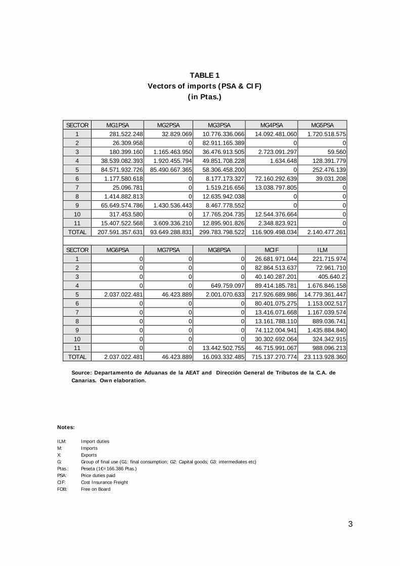
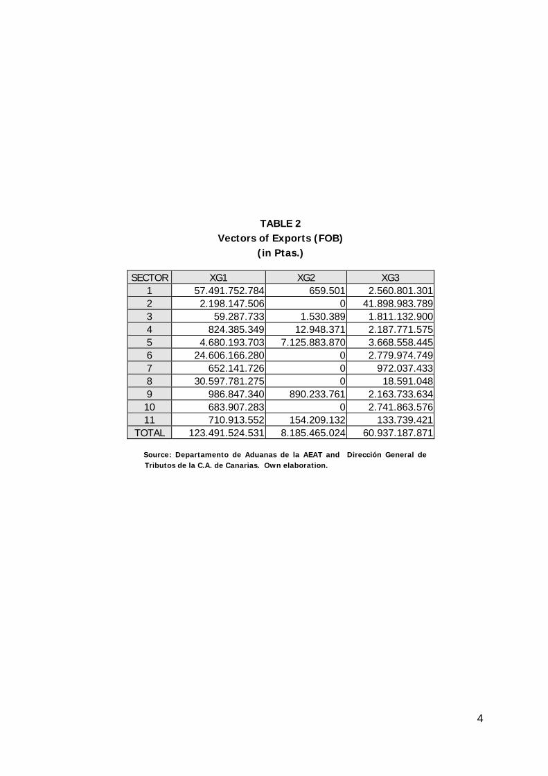
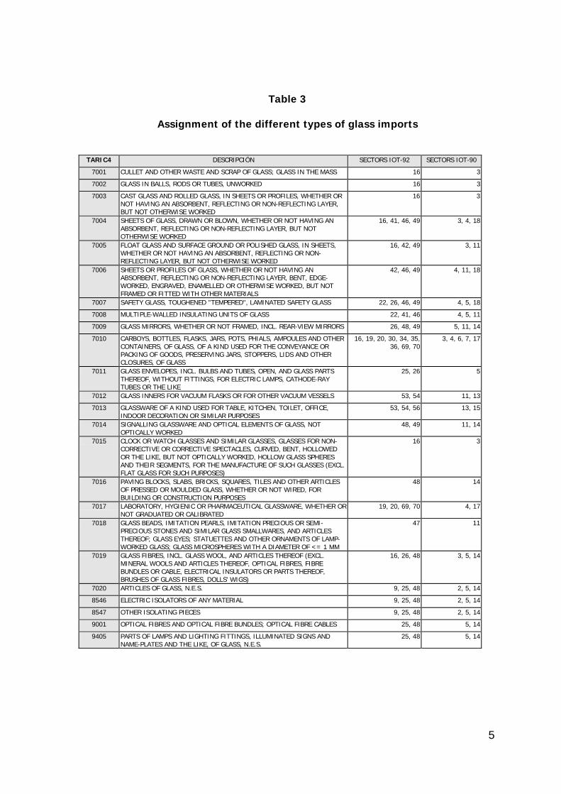
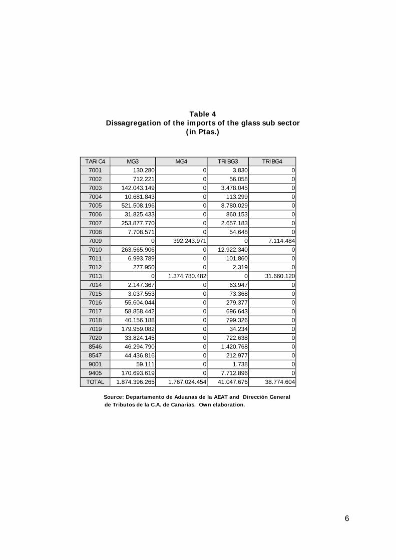
considered to be classified as belonging to groups 1, 2 and 3. Both flows of goods and import duties (ILM) where classified according to these grouping. The results of this reclassifications process can be analyzed in Tables 1 and 2. They show the import and export vectors as they will be used in the adjustment and updating process (AUP). This information allows imposing the necessary restrictions to the final vectors of intermediate outputs or final demand. However, it is of no help in the adjustment of the elements of the matrix of intermediate requirements. With the aim of giving more accuracy to the updating of the matrix of intermediate requirements, we studied with more precision the glass sub sector, integrated in sector 3 of the IOT (Construction materials and mines). A detailed scrutiny (at Taric level) of all the different imports of this sub sector allowed us to prepare Table 3. This table shows, at the 4-digit Taric level (TARIC4), how the imports of the different types of glasses can be assigned to the different potential demanding sectors of the IOT. We can now separate these imports from GFU 3 and 4 of sector 3 in table 1 and proceed to adjust them separately. These imports are presented in Table 4. Although the adjustment process followed with this glass sub sector will not be explained in detail, we can observe in Table 3 how certain groups can be directly assigned to the only sector potentially demanding them (i.e. 7001, 7002, 7003, 7011, 7015, 7016 and 7018). The rest can follow their own assignment rules independently from those that would correspond to the complete glass sector, therefore reducing the potential assignment errors.

3

TABLE 1 Vectors of imports (PSA & CIF)

(in Ptas.)

SECTOR MG1PSA MG2PSA MG3PSA MG4PSA MG5PSA 1 281.522.248 32.829.069 10.776.336.066 14.092.481.060 1.720.518.5752 26.309.958 0 82.911.165.389 0 03 180.399.160 1.165.463.950 36.476.913.505 2.723.091.297 59.5604 38.539.082.393 1.920.455.794 49.851.708.228 1.634.648 128.391.7795 84.571.932.726 85.490.667.365 58.306.458.200 0 252.476.1396 1.177.580.618 0 8.177.173.327 72.160.292.639 39.031.2087 25.096.781 0 1.519.216.656 13.038.797.805 08 1.414.882.813 0 12.635.942.038 0 09 65.649.574.786 1.430.536.443 8.467.778.552 0 010 317.453.580 0 17.765.204.735 12.544.376.664 011 15.407.522.568 3.609.336.210 12.895.901.826 2.348.823.921 0

TOTAL 207.591.357.631 93.649.288.831 299.783.798.522 116.909.498.034 2.140.477.261

SECTOR MG6PSA MG7PSA MG8PSA MCIF ILM 1 0 0 0 26.681.971.044 221.715.9742 0 0 0 82.864.513.637 72.961.7103 0 0 0 40.140.287.201 405.640.274 0 0 649.759.097 89.414.185.781 1.676.846.1585 2.037.022.481 46.423.889 2.001.070.633 217.926.689.986 14.779.361.4476 0 0 0 80.401.075.275 1.153.002.5177 0 0 0 13.416.071.668 1.167.039.5748 0 0 0 13.161.788.110 889.036.7419 0 0 0 74.112.004.941 1.435.884.84010 0 0 0 30.302.692.064 324.342.91511 0 0 13.442.502.755 46.715.991.067 988.096.213

TOTAL 2.037.022.481 46.423.889 16.093.332.485 715.137.270.774 23.113.928.360 Source: Departamento de Aduanas de la AEAT and Dirección General de Tributos de la C.A. de Canarias. Own elaboration.

Notes: ILM: Import duties M: Imports X: Exports G: Group of final use (G1: final consumption; G2: Capital goods; G3: intermediates etc) Ptas.: Peseta (1€=166.386 Ptas.) PSA: Price duties paid CIF: Cost Insurance Freight FOB: Free on Board

4

TABLE 2 Vectors of Exports (FOB)

(in Ptas.)

SECTOR XG1 XG2 XG3 1 57.491.752.784 659.501 2.560.801.301 2 2.198.147.506 0 41.898.983.789 3 59.287.733 1.530.389 1.811.132.900 4 824.385.349 12.948.371 2.187.771.575 5 4.680.193.703 7.125.883.870 3.668.558.445 6 24.606.166.280 0 2.779.974.749 7 652.141.726 0 972.037.433 8 30.597.781.275 0 18.591.048 9 986.847.340 890.233.761 2.163.733.634 10 683.907.283 0 2.741.863.576 11 710.913.552 154.209.132 133.739.421

TOTAL 123.491.524.531 8.185.465.024 60.937.187.871

Source: Departamento de Aduanas de la AEAT and Dirección General de Tributos de la C.A. de Canarias. Own elaboration.

5

Table 3

Assignment of the different types of glass imports

TARIC4 DESCRIPCIÓN SECTORS IOT-92 SECTORS IOT-90

7001 CULLET AND OTHER WASTE AND SCRAP OF GLASS; GLASS IN THE MASS 16 3

7002 GLASS IN BALLS, RODS OR TUBES, UNWORKED 16 3

7003 CAST GLASS AND ROLLED GLASS, IN SHEETS OR PROFILES, WHETHER OR NOT HAVING AN ABSORBENT, REFLECTING OR NON-REFLECTING LAYER, BUT NOT OTHERWISE WORKED

16 3

7004 SHEETS OF GLASS, DRAWN OR BLOWN, WHETHER OR NOT HAVING AN ABSORBENT, REFLECTING OR NON-REFLECTING LAYER, BUT NOT OTHERWISE WORKED

16, 41, 46, 49 3, 4, 18

7005 FLOAT GLASS AND SURFACE GROUND OR POLISHED GLASS, IN SHEETS, WHETHER OR NOT HAVING AN ABSORBENT, REFLECTING OR NON-REFLECTING LAYER, BUT NOT OTHERWISE WORKED

16, 42, 49 3, 11

7006 SHEETS OR PROFILES OF GLASS, WHETHER OR NOT HAVING AN ABSORBENT, REFLECTING OR NON-REFLECTING LAYER, BENT, EDGE-WORKED, ENGRAVED, ENAMELLED OR OTHERWISE WORKED, BUT NOT FRAMED OR FITTED WITH OTHER MATERIALS

42, 46, 49 4, 11, 18

7007 SAFETY GLASS, TOUGHENED "TEMPERED", LAMINATED SAFETY GLASS 22, 26, 46, 49 4, 5, 18

7008 MULTIPLE-WALLED INSULATING UNITS OF GLASS 22, 41, 46 4, 5, 11

7009 GLASS MIRRORS, WHETHER OR NOT FRAMED, INCL. REAR-VIEW MIRRORS 26, 48, 49 5, 11, 14

7010 CARBOYS, BOTTLES, FLASKS, JARS, POTS, PHIALS, AMPOULES AND OTHER CONTAINERS, OF GLASS, OF A KIND USED FOR THE CONVEYANCE OR PACKING OF GOODS, PRESERVING JARS, STOPPERS, LIDS AND OTHER CLOSURES, OF GLASS

16, 19, 20, 30, 34, 35, 36, 69, 70

3, 4, 6, 7, 17

7011 GLASS ENVELOPES, INCL. BULBS AND TUBES, OPEN, AND GLASS PARTS THEREOF, WITHOUT FITTINGS, FOR ELECTRIC LAMPS, CATHODE-RAY TUBES OR THE LIKE

25, 26 5

7012 GLASS INNERS FOR VACUUM FLASKS OR FOR OTHER VACUUM VESSELS 53, 54 11, 13

7013 GLASSWARE OF A KIND USED FOR TABLE, KITCHEN, TOILET, OFFICE, INDOOR DECORATION OR SIMILAR PURPOSES

53, 54, 56 13, 15

7014 SIGNALLING GLASSWARE AND OPTICAL ELEMENTS OF GLASS, NOT OPTICALLY WORKED

48, 49 11, 14

7015 CLOCK OR WATCH GLASSES AND SIMILAR GLASSES, GLASSES FOR NON-CORRECTIVE OR CORRECTIVE SPECTACLES, CURVED, BENT, HOLLOWED OR THE LIKE, BUT NOT OPTICALLY WORKED, HOLLOW GLASS SPHERES AND THEIR SEGMENTS, FOR THE MANUFACTURE OF SUCH GLASSES (EXCL. FLAT GLASS FOR SUCH PURPOSES)

16 3

7016 PAVING BLOCKS, SLABS, BRICKS, SQUARES, TILES AND OTHER ARTICLES OF PRESSED OR MOULDED GLASS, WHETHER OR NOT WIRED, FOR BUILDING OR CONSTRUCTION PURPOSES

48 14

7017 LABORATORY, HYGIENIC OR PHARMACEUTICAL GLASSWARE, WHETHER OR NOT GRADUATED OR CALIBRATED

19, 20, 69, 70 4, 17

7018 GLASS BEADS, IMITATION PEARLS, IMITATION PRECIOUS OR SEMI-PRECIOUS STONES AND SIMILAR GLASS SMALLWARES, AND ARTICLES THEREOF; GLASS EYES; STATUETTES AND OTHER ORNAMENTS OF LAMP-WORKED GLASS; GLASS MICROSPHERES WITH A DIAMETER OF <= 1 MM

47 11

7019 GLASS FIBRES, INCL. GLASS WOOL, AND ARTICLES THEREOF (EXCL. MINERAL WOOLS AND ARTICLES THEREOF, OPTICAL FIBRES, FIBRE BUNDLES OR CABLE, ELECTRICAL INSULATORS OR PARTS THEREOF, BRUSHES OF GLASS FIBRES, DOLLS' WIGS)

16, 26, 48 3, 5, 14

7020 ARTICLES OF GLASS, N.E.S. 9, 25, 48 2, 5, 14

8546 ELECTRIC ISOLATORS OF ANY MATERIAL 9, 25, 48 2, 5, 14

8547 OTHER ISOLATING PIECES 9, 25, 48 2, 5, 14

9001 OPTICAL FIBRES AND OPTICAL FIBRE BUNDLES; OPTICAL FIBRE CABLES 25, 48 5, 14

9405 PARTS OF LAMPS AND LIGHTING FITTINGS, ILLUMINATED SIGNS AND NAME-PLATES AND THE LIKE, OF GLASS, N.E.S.

25, 48 5, 14

6

Table 4 Dissagregation of the imports of the glass sub sector

(in Ptas.)

TARIC4 MG3 MG4 TRIBG3 TRIBG4 7001 130.280 0 3.830 0 7002 712.221 0 56.058 0 7003 142.043.149 0 3.478.045 0 7004 10.681.843 0 113.299 0 7005 521.508.196 0 8.780.029 0 7006 31.825.433 0 860.153 0 7007 253.877.770 0 2.657.183 0 7008 7.708.571 0 54.648 0 7009 0 392.243.971 0 7.114.484 7010 263.565.906 0 12.922.340 0 7011 6.993.789 0 101.860 0 7012 277.950 0 2.319 0 7013 0 1.374.780.482 0 31.660.120 7014 2.147.367 0 63.947 0 7015 3.037.553 0 73.368 0 7016 55.604.044 0 279.377 0 7017 58.858.442 0 696.643 0 7018 40.156.188 0 799.326 0 7019 179.959.082 0 34.234 0 7020 33.824.145 0 722.638 0 8546 46.294.790 0 1.420.768 0 8547 44.436.816 0 212.977 0 9001 59.111 0 1.738 0 9405 170.693.619 0 7.712.896 0

TOTAL 1.874.396.265 1.767.024.454 41.047.676 38.774.604

Source: Departamento de Aduanas de la AEAT and Dirección General de Tributos de la C.A. de Canarias. Own elaboration.

7

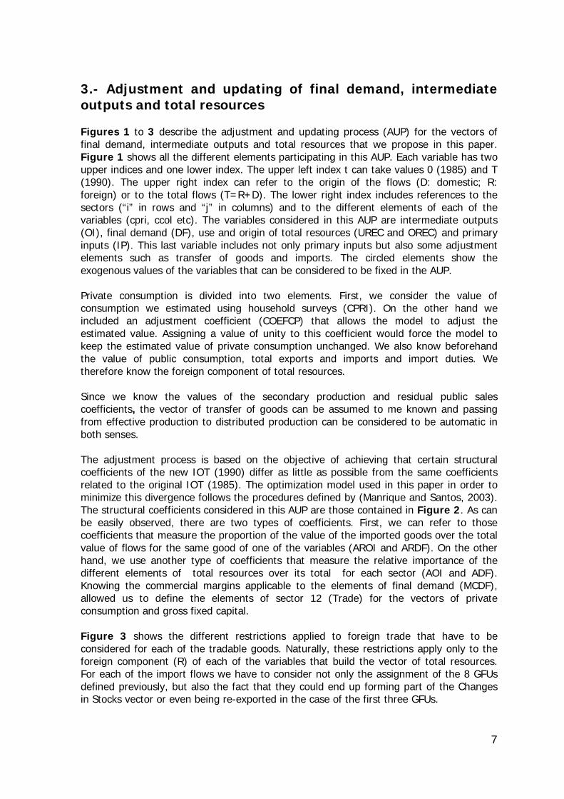
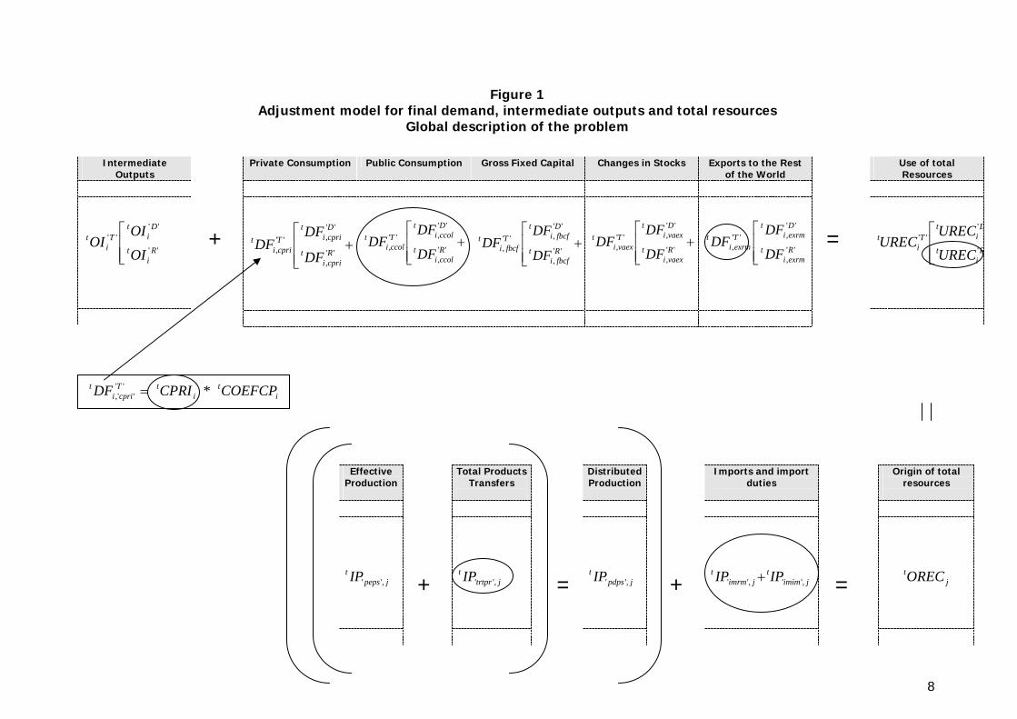
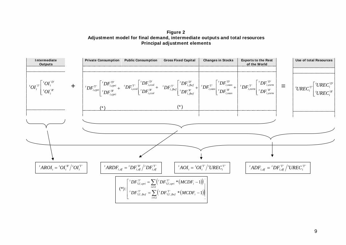
3.- Adjustment and updating of final demand, intermediate outputs and total resources Figures 1 to 3 describe the adjustment and updating process (AUP) for the vectors of final demand, intermediate outputs and total resources that we propose in this paper. Figure 1 shows all the different elements participating in this AUP. Each variable has two upper indices and one lower index. The upper left index t can take values 0 (1985) and T (1990). The upper right index can refer to the origin of the flows (D: domestic; R: foreign) or to the total flows (T=R+D). The lower right index includes references to the sectors (“i” in rows and “j” in columns) and to the different elements of each of the variables (cpri, ccol etc). The variables considered in this AUP are intermediate outputs (OI), final demand (DF), use and origin of total resources (UREC and OREC) and primary inputs (IP). This last variable includes not only primary inputs but also some adjustment elements such as transfer of goods and imports. The circled elements show the exogenous values of the variables that can be considered to be fixed in the AUP. Private consumption is divided into two elements. First, we consider the value of consumption we estimated using household surveys (CPRI). On the other hand we included an adjustment coefficient (COEFCP) that allows the model to adjust the estimated value. Assigning a value of unity to this coefficient would force the model to keep the estimated value of private consumption unchanged. We also know beforehand the value of public consumption, total exports and imports and import duties. We therefore know the foreign component of total resources. Since we know the values of the secondary production and residual public sales coefficients, the vector of transfer of goods can be assumed to me known and passing from effective production to distributed production can be considered to be automatic in both senses. The adjustment process is based on the objective of achieving that certain structural coefficients of the new IOT (1990) differ as little as possible from the same coefficients related to the original IOT (1985). The optimization model used in this paper in order to minimize this divergence follows the procedures defined by (Manrique and Santos, 2003). The structural coefficients considered in this AUP are those contained in Figure 2. As can be easily observed, there are two types of coefficients. First, we can refer to those coefficients that measure the proportion of the value of the imported goods over the total value of flows for the same good of one of the variables (AROI and ARDF). On the other hand, we use another type of coefficients that measure the relative importance of the different elements of total resources over its total for each sector (AOI and ADF). Knowing the commercial margins applicable to the elements of final demand (MCDF), allowed us to define the elements of sector 12 (Trade) for the vectors of private consumption and gross fixed capital. Figure 3 shows the different restrictions applied to foreign trade that have to be considered for each of the tradable goods. Naturally, these restrictions apply only to the foreign component (R) of each of the variables that build the vector of total resources. For each of the import flows we have to consider not only the assignment of the 8 GFUs defined previously, but also the fact that they could end up forming part of the Changes in Stocks vector or even being re-exported in the case of the first three GFUs.

8

Figure 1 Adjustment model for final demand, intermediate outputs and total resources

Global description of the problem

Private Consumption Public Consumption Gross Fixed Capital Changes in Stocks Exports to the Rest

of the World

+⎢⎢⎣

⎡''

,

'',''

, Rcprii

t

Dcprii

tTcprii

t

DF

DFDF

+⎢⎢⎣

⎡''

,

'',''

, Rccoli

t

Dccoli

tTccoli

t

DF

DFDF

+⎢⎢⎣

⎡''

,

'',''

, Rfbcfi

t

Dfbcfi

tTfbcfi

t

DF

DFDF

+⎢⎢⎣

⎡''

,

'',''

, Rvaexi

t

Dvaexi

tTvaexi

t

DF

DFDF

⎢⎢⎣

⎡''

,

'',''

, Rexrmi

t

Dexrmi

tTexrmi

t

DF

DFDF

Intermediate

Outputs

⎢⎢⎣

⎡''

''''

Ri

t

Di

tT

it

OI

OIOI

Use of total Resources

⎢⎢⎣

⎡'

'''

Ri

t

Di

tT

it

UREC

URECUREC

+ =

Origin of total

resources

jtOREC

Imports and import

duties

jimimt

jimrmt IPIP ,'','' +

DistributedProduction

jpdpst IP ,''

Effective

Production

jpepst IP ,''

=+

Total Products

Transfers

jtrtprt IP ,''

+ =

it

itT

cpriit COEFCPCPRIDF * ''

'', =

8

9


Principal adjustment elements

Private Consumption Public Consumption Gross Fixed Capital Changes in Stocks Exports to the Rest

of the World

+⎢⎢⎣

⎡''

,

'',''

, Rcprii

t

Dcprii

tTcprii

t

DF

DFDF

(*)

+⎢⎢⎣

⎡''

,

'',''

, Rccoli

t

Dccoli

tTccoli

t

DF

DFDF

+⎢⎢⎣

⎡''

,

'',''

, Rfbcfi

t

Dfbcfi

tTfbcfi

t

DF

DFDF

(*)

+⎢⎢⎣

⎡''

,

'',''

, Rvaexi

t

Dvaexi

tTvaexi

t

DF

DFDF

⎢⎢⎣

⎡''

,

'',''

, Rexrmi

t

Dexrmi

tTexrmi

t

DF

DFDF

Intermediate

Outputs

⎢⎢⎣

⎡''

''''

Ri

t

Di

tT

it

OI

OIOI

Use of total Resources

⎢⎢⎣

⎡''

''''

Ri

t

Di

tT

it

UREC

URECUREC

+ =

'''' Ti

tRi

ti

t OIOIAROI = '',

'',,

Tdfi

tRdfi

tdfi

t DFDFARDF = '''' Ti

tTi

ti

t URECOIAOI = '''',,

Ti

tTdfi

tdfi

t URECDFADF =

( )( )( )( )⎥⎥

⎥

⎦

⎤

⎢⎢⎢

⎣

⎡

−=

−=

∑

∑

≠

≠

12

'','12'

'','12'

12

'','12'

'','12'

1*

1*:(*)

ii

Tfbcf

tTfbcf

ti

iT

cpritT

cprit

MCDFDFDF

MCDFDFDF

10


Restriccions related to foreign trade

Type of imports

Private Consumption

(1)

Gross Fixed Capital

(2)

IntermediateOutputs

(3)

Changes in Stocks (1) (2) (3)

Exports To the Rest of the World (1) (2) (3) Parameters

MG1 X X X '1',iCM

MG2 X X X '2',iCM

MG3 X X X '3',iCM

MG4 X X X X '4',iCM

MG5 X X X X '5',iCM

MG6 X X X X '6',iCM

MG7 X X X X '7',iCM

MG8 X X X X X X '8',iCM

∑= '''',

Rvaexi

tDF ∑= '''',

Rexrmi

tDF

TOTAL '',Rcprii

tDF '',Rfbcfi

tDF ''Ri

tOI itVAEXRCX1 i

tVAEXRCX 2 itVAEXRCX3 i

t EXRCX1 itEXRCX2 i

tEXRCX3 Imp. Tot.

⎢⎢⎢⎢⎢

⎣

⎡

++

++≤

≥

'8','6','5',

'4','1',

'1',

1

iii

ii

i

i

CMCMCMCMCM

CM

CM

⎢⎢⎢⎢⎢

⎣

⎡

+

++≤

≥

'8','7',

'6','2',

'2',

2

ii

ii

i

i

CMCMCMCM

CM

CM

⎢⎢⎢⎢⎢

⎣

⎡

+

+++≤

≥

'8','7',

'5','4','3',

'3',

3

ii

iii

i

i

CMCMCMCMCM

CM

CM

it EXRCX1 i

tEXRCX2 itEXRCX3

it EXDCX1 i

tEXDCX2 itEXDCX3

TOTAL i

t EXTCX1 itEXTCX2 i

tEXTCX3 RESTRICCIÓN

'1',iCX '2',iCX '3',iCX

10

11

Therefore, the total of imports of group 1 (MG1) that is used as exogenous ( ,'1'iCM ), has

to be shared between the vectors of private consumption, changes in stocks and exports (cells marked with an X in the first row of figure 3). A similar distribution can be described for the two subsequent import groups (MG2 and MG3). The distribution process for the rest of the groups is somehow more complex because the assignment alternatives are greater. Imports belonging to group MG8, for example, have six of those alternatives. This is the case because both the vector of changes in stocks and exports had to be subdivides into three items, such that we could consider separately the goods for final consumption (VAEXRCX1, EXRCX1), capital goods (VAEXRCX2, EXRCX2) and intermediates (VAEXRCX3, EXRCX3). In order to be able to establish the basic foreign trade restrictions, we created three variables, CM1, CM2 and CM3. They allow us to group all different flows of consumption capital and intermediate goods that have been previously described. Cm1, for example, retains the private consumption, change in stocks and exports of the same type of goods (final consumption goods). The same occurs with CM2 and CM3. The elements of these variables are connected through similar arrows in Figure 3. Parameters CM can be used to establish the foreign trade restrictions as reflected in the lower part of Figure 3. Those boxes show the lower and upper limits to be imposed in terms of the parameters that have been described below. We should also describe parameters CX, that reflect the known values of total exports. These values reflect the available information on total exports for each sector of the three main groups of goods: final consumption goods ( ,'1'iCX ), capital goods ( ,'2 'iCX ) and

intermediates( ,'3'iCX ). However, the origin of these goods (domestic or foreign) cannot

be distinguished beforehand. The value of total exports (EXTCX) of goods of each type has to respect the CX parameters. On the other hand, those total exports can de divided between domestic goods (EXDCX) and foreign goods (EXRCX), which have been described as re-exports. These exports of foreign goods (EXRCX) has to respect the restrictions based on the CM parameters as described below.

12

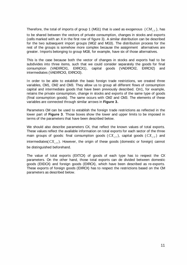
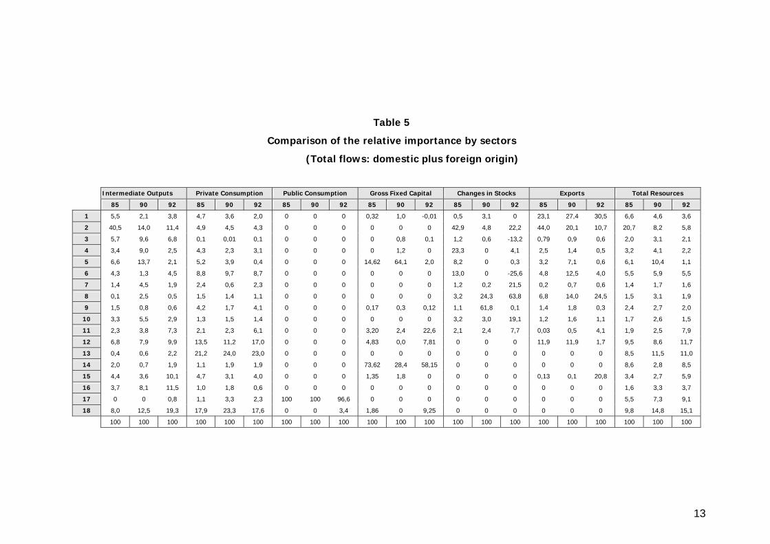
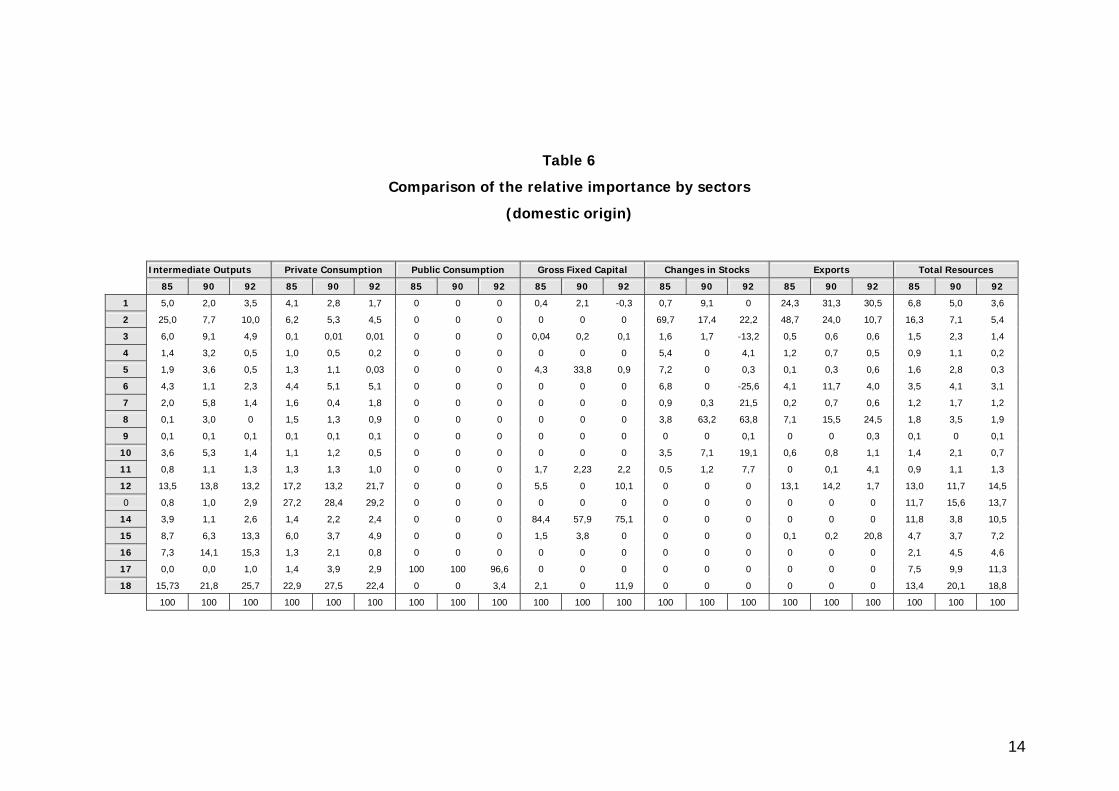
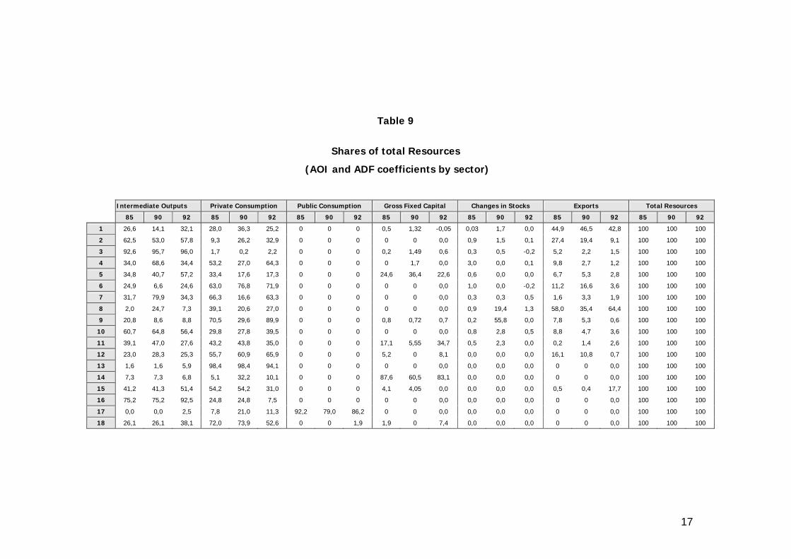
4.- Results obtained from the proposed adjustment and updating process The AUP described in the previous section was applied to the 1985 IOT of the Canary Islands (TIOCAN85) in order to obtain the IOT referred to the 1990 data (TIOCAN90). Since there exists an IOT of the Canary Islands for 1992, elaborated with direct methods, it was also used for comparisons with the 1990 estimated one. Tables 5 to 6 show the results obtained. The first three tables try to identify the structural parallelisms by sectors of the different vectors obtained. Without any doubt, the worst results are those related to Gross Fixed Capital and Changes of Stocks, due to their residual character. Beside these two cases, the structure of both IOT (85 and 90) show more then reasonable similarities. Most of the differences between TIOCAN90 and TIOCAN92 have their explanation in the different structure of the starting point (TIOCAN85). However, there are many cases in which the structure obtained by the TIOCAN90 is nearer to the 92 IOT than to the initial one (TIOCAN85). These results have their origin in the additional information used (e.g.: private consumption and exports) that is, logically, in many cases nearer to the TIOCAN92 than to the TIOCAN85. The differences observed in public consumption in Tables 5 and 6 are exclusively due to an aggregation problem. The classification by sectors of TIOCAN90 and TIOCAN92 did not allow an aggregation compatible with a perfect separation between the provision of private and public goods. On the other hand, the TIOCAN92 does not show any foreign entries neither for exports nor for changes in stocks. Therefore, the observed differences in this area are due to the differences in conception of both tables more than to a misbehavior of the proposed AUP. The basic elements of the updating process are of two types. First, the objective of the model is to maintain the shares of the different vectors of total resources. Expressed differently, it tries to minimize the differences between the AOI and ADF coefficients of both tables. On the other hand, the model tries to minimize the differences between the share of foreign flows for each of the cells of the different vectors, therefore minimizing the difference between the AROI and ARDF coefficients of both tables. The results obtained in terms of the first objective are summarized in Table 9, which shows very satisfactory results. The main differences appear in sectors 2,4,7 and 9 where we can observe important divergences. These differences can be explained describing the impact of the additional information included in the AUP. In this sense the most important piece of information is the one related to private consumption contained in Table 8. It shows how those sectors for which the relative importance of private consumption grows more significantly (2, 14 and 17) are those for which the relative importance seems to have achieved also the greatest levels in the updated IOT. The contrary occurs in sectors 4, 7 and 9. We can therefore conclude that the main differences observed are due to the initial data used more then to the model itself.

13

Table 5

Comparison of the relative importance by sectors

(Total flows: domestic plus foreign origin)

Intermediate Outputs Private Consumption Public Consumption Gross Fixed Capital Changes in Stocks Exports Total Resources

85 90 92 85 90 92 85 90 92 85 90 92 85 90 92 85 90 92 85 90 92

1 5,5 2,1 3,8 4,7 3,6 2,0 0 0 0 0,32 1,0 -0,01 0,5 3,1 0 23,1 27,4 30,5 6,6 4,6 3,6

2 40,5 14,0 11,4 4,9 4,5 4,3 0 0 0 0 0 0 42,9 4,8 22,2 44,0 20,1 10,7 20,7 8,2 5,8

3 5,7 9,6 6,8 0,1 0,01 0,1 0 0 0 0 0,8 0,1 1,2 0,6 -13,2 0,79 0,9 0,6 2,0 3,1 2,1

4 3,4 9,0 2,5 4,3 2,3 3,1 0 0 0 0 1,2 0 23,3 0 4,1 2,5 1,4 0,5 3,2 4,1 2,2

5 6,6 13,7 2,1 5,2 3,9 0,4 0 0 0 14,62 64,1 2,0 8,2 0 0,3 3,2 7,1 0,6 6,1 10,4 1,1

6 4,3 1,3 4,5 8,8 9,7 8,7 0 0 0 0 0 0 13,0 0 -25,6 4,8 12,5 4,0 5,5 5,9 5,5

7 1,4 4,5 1,9 2,4 0,6 2,3 0 0 0 0 0 0 1,2 0,2 21,5 0,2 0,7 0,6 1,4 1,7 1,6

8 0,1 2,5 0,5 1,5 1,4 1,1 0 0 0 0 0 0 3,2 24,3 63,8 6,8 14,0 24,5 1,5 3,1 1,9

9 1,5 0,8 0,6 4,2 1,7 4,1 0 0 0 0,17 0,3 0,12 1,1 61,8 0,1 1,4 1,8 0,3 2,4 2,7 2,0

10 3,3 5,5 2,9 1,3 1,5 1,4 0 0 0 0 0 0 3,2 3,0 19,1 1,2 1,6 1,1 1,7 2,6 1,5

11 2,3 3,8 7,3 2,1 2,3 6,1 0 0 0 3,20 2,4 22,6 2,1 2,4 7,7 0,03 0,5 4,1 1,9 2,5 7,9

12 6,8 7,9 9,9 13,5 11,2 17,0 0 0 0 4,83 0,0 7,81 0 0 0 11,9 11,9 1,7 9,5 8,6 11,7

13 0,4 0,6 2,2 21,2 24,0 23,0 0 0 0 0 0 0 0 0 0 0 0 0 8,5 11,5 11,0

14 2,0 0,7 1,9 1,1 1,9 1,9 0 0 0 73,62 28,4 58,15 0 0 0 0 0 0 8,6 2,8 8,5

15 4,4 3,6 10,1 4,7 3,1 4,0 0 0 0 1,35 1,8 0 0 0 0 0,13 0,1 20,8 3,4 2,7 5,9

16 3,7 8,1 11,5 1,0 1,8 0,6 0 0 0 0 0 0 0 0 0 0 0 0 1,6 3,3 3,7

17 0 0 0,8 1,1 3,3 2,3 100 100 96,6 0 0 0 0 0 0 0 0 0 5,5 7,3 9,1

18 8,0 12,5 19,3 17,9 23,3 17,6 0 0 3,4 1,86 0 9,25 0 0 0 0 0 0 9,8 14,8 15,1

100 100 100 100 100 100 100 100 100 100 100 100 100 100 100 100 100 100 100 100 100

14

Table 6


(domestic origin)


85 90 92 85 90 92 85 90 92 85 90 92 85 90 92 85 90 92 85 90 92

1 5,0 2,0 3,5 4,1 2,8 1,7 0 0 0 0,4 2,1 -0,3 0,7 9,1 0 24,3 31,3 30,5 6,8 5,0 3,6

2 25,0 7,7 10,0 6,2 5,3 4,5 0 0 0 0 0 0 69,7 17,4 22,2 48,7 24,0 10,7 16,3 7,1 5,4

3 6,0 9,1 4,9 0,1 0,01 0,01 0 0 0 0,04 0,2 0,1 1,6 1,7 -13,2 0,5 0,6 0,6 1,5 2,3 1,4

4 1,4 3,2 0,5 1,0 0,5 0,2 0 0 0 0 0 0 5,4 0 4,1 1,2 0,7 0,5 0,9 1,1 0,2

5 1,9 3,6 0,5 1,3 1,1 0,03 0 0 0 4,3 33,8 0,9 7,2 0 0,3 0,1 0,3 0,6 1,6 2,8 0,3

6 4,3 1,1 2,3 4,4 5,1 5,1 0 0 0 0 0 0 6,8 0 -25,6 4,1 11,7 4,0 3,5 4,1 3,1

7 2,0 5,8 1,4 1,6 0,4 1,8 0 0 0 0 0 0 0,9 0,3 21,5 0,2 0,7 0,6 1,2 1,7 1,2

8 0,1 3,0 0 1,5 1,3 0,9 0 0 0 0 0 0 3,8 63,2 63,8 7,1 15,5 24,5 1,8 3,5 1,9

9 0,1 0,1 0,1 0,1 0,1 0,1 0 0 0 0 0 0 0 0 0,1 0 0 0,3 0,1 0 0,1

10 3,6 5,3 1,4 1,1 1,2 0,5 0 0 0 0 0 0 3,5 7,1 19,1 0,6 0,8 1,1 1,4 2,1 0,7

11 0,8 1,1 1,3 1,3 1,3 1,0 0 0 0 1,7 2,23 2,2 0,5 1,2 7,7 0 0,1 4,1 0,9 1,1 1,3

12 13,5 13,8 13,2 17,2 13,2 21,7 0 0 0 5,5 0 10,1 0 0 0 13,1 14,2 1,7 13,0 11,7 14,5

0 0,8 1,0 2,9 27,2 28,4 29,2 0 0 0 0 0 0 0 0 0 0 0 0 11,7 15,6 13,7

14 3,9 1,1 2,6 1,4 2,2 2,4 0 0 0 84,4 57,9 75,1 0 0 0 0 0 0 11,8 3,8 10,5

15 8,7 6,3 13,3 6,0 3,7 4,9 0 0 0 1,5 3,8 0 0 0 0 0,1 0,2 20,8 4,7 3,7 7,2

16 7,3 14,1 15,3 1,3 2,1 0,8 0 0 0 0 0 0 0 0 0 0 0 0 2,1 4,5 4,6

17 0,0 0,0 1,0 1,4 3,9 2,9 100 100 96,6 0 0 0 0 0 0 0 0 0 7,5 9,9 11,3

18 15,73 21,8 25,7 22,9 27,5 22,4 0 0 3,4 2,1 0 11,9 0 0 0 0 0 0 13,4 20,1 18,8

100 100 100 100 100 100 100 100 100 100 100 100 100 100 100 100 100 100 100 100 100

15

Table 7


(foreign origin)


85 90 92 85 90 92 85 90 92 85 90 92 85 90 92 85 90 92 85 90 92

1 6,1 2,2 4,7 7,0 7,9 2,9 0 0 0 0 0 0,9 0 0 0 12,4 7,3 0 6,4 3,6 3,3

2 56,6 22,5 15,6 0,3 0,4 3,4 0 0 0 0 0 0 -48,3 -1,9 0 0 0 0 32,9 11,2 7,5

3 5,3 10,4 12,3 0,1 0 0,5 0 0 0 0 1,4 0 0 0 0 3,3 2,1 0 3,3 5,5 4,8

4 5,6 16,9 8,6 16,4 12,3 14,0 0 0 0 0 2,3 0 84,3 0 0 14,0 4,7 0 9,4 12,3 10,1

5 11,4 27,2 6,7 19,0 19,0 1,8 0 0 0 85,0 93,1 5,9 11,7 0 0 32,1 42,7 0 18,3 31,5 4,2

6 4,3 1,5 11,2 24,5 34,4 22,1 0 0 0 0 0 0 34,1 0 0 10,7 16,8 0 10,9 11,0 15,0

7 0,8 2,8 3,2 5,3 1,9 4,1 0 0 0 0 0 0 2,1 0,1 0 0,4 1,0 0 2,2 2,0 3,2

8 0,1 1,7 1,9 1,5 1,9 2,1 0 0 0 0 0 0 1,5 3,8 0 4,9 5,9 0 0,7 1,9 1,7

9 3,0 1,7 2,3 18,8 10,8 18,8 0 0 0 1,4 0,7 0,5 4,7 94,2 0 14,9 11,5 0 8,5 10,2 10,1

10 3,0 5,7 7,6 2,2 3,6 4,7 0 0 0 0 0 0 2,4 0,8 0 7,1 5,6 0 2,8 4,1 5,1

11 3,9 7,4 25,5 4,9 7,8 25,0 0 0 0 13,5 2,5 92,7 7,5 2,97 0 0,3 2,5 0 4,6 6,5 34,5

12 0 0 0 0 0 0 0 0 0 0 0 0 0 0 0 0 0 0 0 0 0

13 0 0 0 0 0 0 0 0 0 0 0 0 0 0 0 0 0 0 0 0 0

14 0 0 0 0 0 0 0 0 0 0 0 0 0 0 0 0 0 0 0 0 0

15 0 0 0,4 0 0 0,7 0 0 0 0 0 0 0 0 0 0 0 0 0 0 1

16 0 0 0 0 0 0 0 0 0 0 0 0 0 0 0 0 0 0 0 0 0

17 0 0 0 0 0 0 0 0 0 0 0 0 0 0 0 0 0 0 0 0 0

18 0 0 0 0 0 0 0 0 0 0 0 0 0 0 0 0 0 0 0 0 0

100 100 100 100 100 100 0 0 0 100 100 100 100 100 0 100 100 0 100 100 100

16

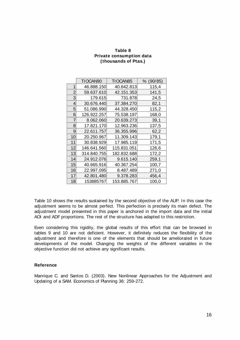
Table 8 Private consumption data

(thousands of Ptas.)

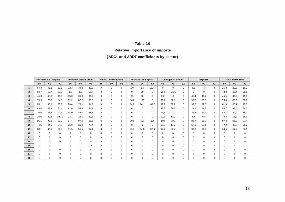
Table 10 shows the results sustained by the second objective of the AUP. In this case the adjustment seems to be almost perfect. This perfection is precisely its main defect. The adjustment model presented in this paper is anchored in the import data and the initial AOI and ADF proportions. The rest of the structure has adapted to this restriction.

Even considering this rigidity, the global results of this effort that can be browsed in tables 9 and 10 are not deficient. However, it definitely reduces the flexibility of the adjustment and therefore is one of the elements that should be ameliorated in future developments of the model. Changing the weights of the different variables in the objective function did not achieve any significant results.

Reference Manrique C. and Santos D. (2003). New Nonlinear Approaches for the Adjustment and Updating of a SAM. Economics of Planning 36: 259-272.

TIOCAN90 TIOCAN85 % (90/85) 1 46.888.150 40.642.813 115,4 2 59.637.610 42.151.353 141,5 3 179.615 731.878 24,5 4 30.676.440 37.384.270 82,1 5 51.086.990 44.328.450 115,2 6 126.922.257 75.538.197 168,0 7 8.062.060 20.639.273 39,1 8 17.821.170 12.963.236 137,5 9 22.611.757 36.355.996 62,2

10 20.250.967 11.309.143 179,1 11 30.838.929 17.985.119 171,5 12 146.641.560 115.831.051 126,6 13 314.840.755 182.832.688 172,2 14 24.912.076 9.615.140 259,1 15 40.665.916 40.367.254 100,7 16 22.997.095 8.487.489 271,0 17 42.801.480 9.378.283 456,4 18 153885767 153.885.767 100,0

17

Table 9

Shares of total Resources

(AOI and ADF coefficients by sector)


85 90 92 85 90 92 85 90 92 85 90 92 85 90 92 85 90 92 85 90 92

1 26,6 14,1 32,1 28,0 36,3 25,2 0 0 0 0,5 1,32 -0,05 0,03 1,7 0,0 44,9 46,5 42,8 100 100 100

2 62,5 53,0 57,8 9,3 26,2 32,9 0 0 0 0 0 0,0 0,9 1,5 0,1 27,4 19,4 9,1 100 100 100

3 92,6 95,7 96,0 1,7 0,2 2,2 0 0 0 0,2 1,49 0,6 0,3 0,5 -0,2 5,2 2,2 1,5 100 100 100

4 34,0 68,6 34,4 53,2 27,0 64,3 0 0 0 0 1,7 0,0 3,0 0,0 0,1 9,8 2,7 1,2 100 100 100

5 34,8 40,7 57,2 33,4 17,6 17,3 0 0 0 24,6 36,4 22,6 0,6 0,0 0,0 6,7 5,3 2,8 100 100 100

6 24,9 6,6 24,6 63,0 76,8 71,9 0 0 0 0 0 0,0 1,0 0,0 -0,2 11,2 16,6 3,6 100 100 100

7 31,7 79,9 34,3 66,3 16,6 63,3 0 0 0 0 0 0,0 0,3 0,3 0,5 1,6 3,3 1,9 100 100 100

8 2,0 24,7 7,3 39,1 20,6 27,0 0 0 0 0 0 0,0 0,9 19,4 1,3 58,0 35,4 64,4 100 100 100

9 20,8 8,6 8,8 70,5 29,6 89,9 0 0 0 0,8 0,72 0,7 0,2 55,8 0,0 7,8 5,3 0,6 100 100 100

10 60,7 64,8 56,4 29,8 27,8 39,5 0 0 0 0 0 0,0 0,8 2,8 0,5 8,8 4,7 3,6 100 100 100

11 39,1 47,0 27,6 43,2 43,8 35,0 0 0 0 17,1 5,55 34,7 0,5 2,3 0,0 0,2 1,4 2,6 100 100 100

12 23,0 28,3 25,3 55,7 60,9 65,9 0 0 0 5,2 0 8,1 0,0 0,0 0,0 16,1 10,8 0,7 100 100 100

13 1,6 1,6 5,9 98,4 98,4 94,1 0 0 0 0 0 0,0 0,0 0,0 0,0 0 0 0,0 100 100 100

14 7,3 7,3 6,8 5,1 32,2 10,1 0 0 0 87,6 60,5 83,1 0,0 0,0 0,0 0 0 0,0 100 100 100

15 41,2 41,3 51,4 54,2 54,2 31,0 0 0 0 4,1 4,05 0,0 0,0 0,0 0,0 0,5 0,4 17,7 100 100 100

16 75,2 75,2 92,5 24,8 24,8 7,5 0 0 0 0 0 0,0 0,0 0,0 0,0 0 0 0,0 100 100 100

17 0,0 0,0 2,5 7,8 21,0 11,3 92,2 79,0 86,2 0 0 0,0 0,0 0,0 0,0 0 0 0,0 100 100 100

18 26,1 26,1 38,1 72,0 73,9 52,6 0 0 1,9 1,9 0 7,4 0,0 0,0 0,0 0 0 0,0 100 100 100

18

Table 10

Relative importance of imports

(AROI and ARDF coefficients by sector)


85 90 92 85 90 92 85 90 92 85 90 92 85 90 92 85 90 92 85 90 92

1 54,3 45,1 30,6 32,3 34,3 30,8 0 0 0 1,9 1,9 -1504,4 0 0 0 5,1 4,3 0 25,8 20,8 18,3

2 68,7 68,7 33,9 1,5 1,5 16,7 0 0 0 0 00 0 -25,6 -25,6 0 0 0 0 42,8 36,4 25,1

3 46,3 46,3 45,0 35,0 35,0 95,2 0 0 0 90 90 0 0,0 0 0 40,4 40,4 0 45,6 46,6 45,3

4 79,9 79,9 84,5 82,2 82,2 96,0 0 0 0 100 100 0 82,1 82,1 0 55,0 55,0 0 78,8 80,2 90,8

5 85,1 85,1 80,8 80,4 76,1 94,3 0 0 0 74,1 74,1 66,2 32,2 32,2 0 97,0 97,0 0 81,3 80,1 77,5

6 49,4 49,4 61,4 61,0 55,4 54,1 0 0 0 0 0 0 59,5 59,5 0 21,6 21,6 0 53,7 49,4 54,0

7 26,5 26,5 42,3 48,0 48,0 38,3 0 0 0 0 0 0 42,1 42,1 0 21,2 21,2 0 40,7 29,9 38,7

8 29,6 29,6 100,0 22,1 22,1 39,6 0 0 0 0 0 0 10,2 10,2 0 6,8 6,8 0 13,3 16,2 18,0

9 96,1 96,1 93,2 97,4 97,4 98,5 0 0 0 100 100 100 100 100 0 99,7 99,7 0 97,3 98,9 97,4

10 44,5 44,5 64,3 36,0 36,0 73,4 0 0 0 0 0 0 17,2 17,2 0 57,1 57,1 0 42,9 42,0 65,3

11 83,1 83,1 86,5 51,5 51,5 87,1 0 0 0 54,0 54,0 92,4 82,7 82,7 0 93,3 86,6 0 64,5 67,7 86,5

12 0 0 0 0 0 0 0 0 0 0 0 0 0 0 0 0 0 0 0 0 0

13 0 0 0 0 0 0 0 0 0 0 0 0 0 0 0 0 0 0 0 0 0

14 0 0 0 0 0 0 0 0 0 0 0 0 0 0 0 0 0 0 0 0 0

15 0 0 1,1 0 0 3,6 0 0 0 0 0 0 0 0 0 0 0 0 0 0 1,7

16 0 0 0 0 0 0 0 0 0 0 0 0 0 0 0 0 0 0 0 0 0

17 0 0 0 0 0 0 0 0 0 0 0 0 0 0 0 0 0 0 0 0 0

18 0 0 0 0 0 0 0 0 0 0 0 0 0 0 0 0 0 0 0 0 0

Capítulo 5

19

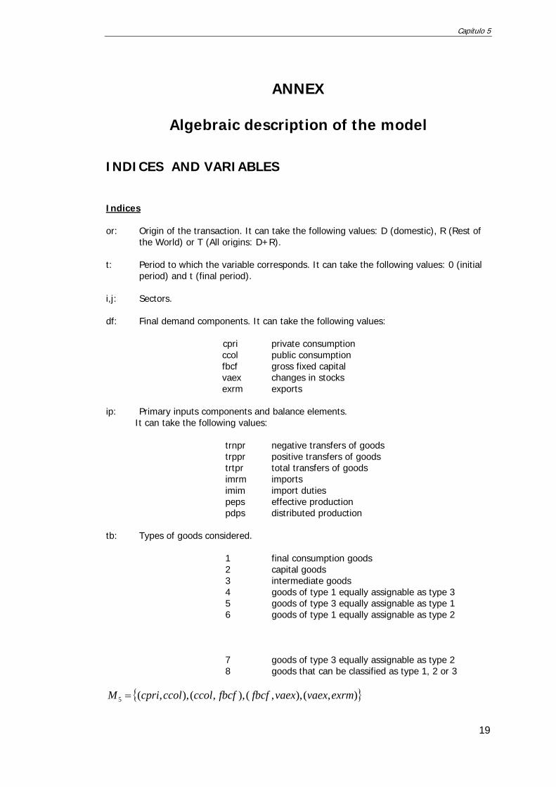
ANNEX

Algebraic description of the model INDICES AND VARIABLES Indices or: Origin of the transaction. It can take the following values: D (domestic), R (Rest of

the World) or T (All origins: D+R). t: Period to which the variable corresponds. It can take the following values: 0 (initial

period) and t (final period). i,j: Sectors. df: Final demand components. It can take the following values:

cpri private consumption ccol public consumption fbcf gross fixed capital vaex changes in stocks exrm exports

ip: Primary inputs components and balance elements. It can take the following values:

trnpr negative transfers of goods trppr positive transfers of goods trtpr total transfers of goods imrm imports imim import duties peps effective production pdps distributed production

tb: Types of goods considered. 1 final consumption goods 2 capital goods 3 intermediate goods 4 goods of type 1 equally assignable as type 3 5 goods of type 3 equally assignable as type 1 6 goods of type 1 equally assignable as type 2

7 goods of type 3 equally assignable as type 2 8 goods that can be classified as type 1, 2 or 3

{ }),(),,(),,(),,(5 exrmvaexvaexfbcffbcfccolccolcpriM =

Capítulo 5

20

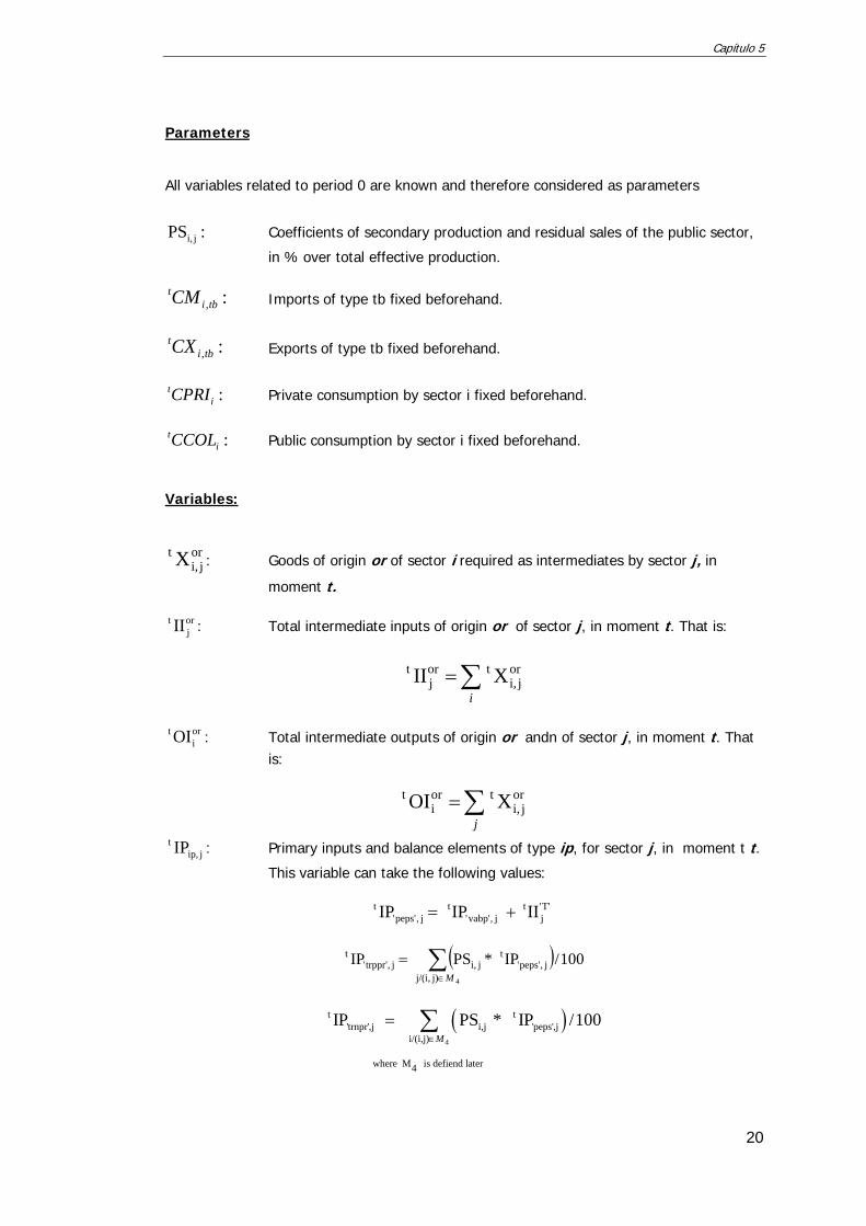
Parameters All variables related to period 0 are known and therefore considered as parameters

:PS ji, Coefficients of secondary production and residual sales of the public sector,

in % over total effective production.

:,tbitCM Imports of type tb fixed beforehand.

:,tbitCX Exports of type tb fixed beforehand.

:i

tCPRI Private consumption by sector i fixed beforehand.

:i

tCCOL Public consumption by sector i fixed beforehand.

Variables:

orji,

t X : Goods of origin or of sector i required as intermediates by sector j, in

moment t.

orj

t II : Total intermediate inputs of origin or of sector j, in moment t. That is:

∑=i

orji,

torj

t X II

ori

t OI : Total intermediate outputs of origin or andn of sector j, in moment t. That is:

∑=j

orji,

tori

t X OI

jip,t IP : Primary inputs and balance elements of type ip, for sector j, in moment t t.

This variable can take the following values:

II IP IP T''j

tj,vabp''

tj,peps''

t +=

( )∑

∈

=4j)j/(i,

j,peps''t

ji,j,trppr''t 100/IP * PS IP

M

( )4

t t'trnpr',j i,j 'peps',j

i/(i,j)

where M is defiend later4

IP PS * IP /100M∈

= ∑

Capítulo 5

21

j,trptr''t

j,trnpr''t

j,trtpr''t IP - IP IP =

j,trpr''t

j,peps''t

j,pdps''t IP IP IP +=

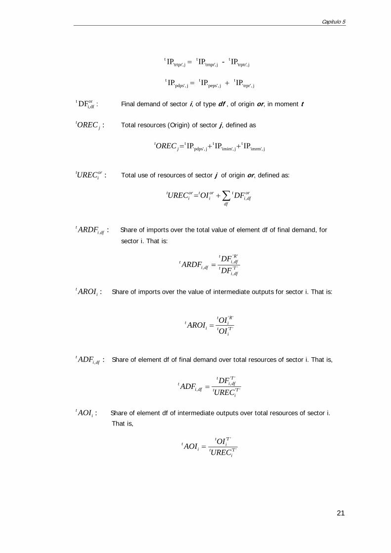
ordfi,

t DF : Final demand of sector i, of type df , of origin or, in moment t

:j

tOREC Total resources (Origin) of sector j, defined as

j,imrm''t

j,imim''t

j,pdps''t IPIPIP ++=j

tOREC

:ori

tUREC Total use of resources of sector j of origin or, defined as:

∑+=df

ordfi

tori

tori

t DFOIUREC ,

:.dfit ARDF Share of imports over the total value of element df of final demand, for

sector i. That is:

'',

'',

, Tdfi

t

Rdfi

t

dfit

DFDF

ARDF =

:i

t AROI Share of imports over the value of intermediate outputs for sector i. That is:

''

''

Ti

t

Ri

t

it

OIOIAROI =

:,dfit ADF Share of element df of final demand over total resources of sector i. That is,

''

'',

, Ti

t

Tdfi

t

dfit

URECDF

ADF =

:i

t AOI Share of element df of intermediate outputs over total resources of sector i.

That is,

''

''

Ti

t

Ti

t

it

URECOIAOI =

Capítulo 5

22

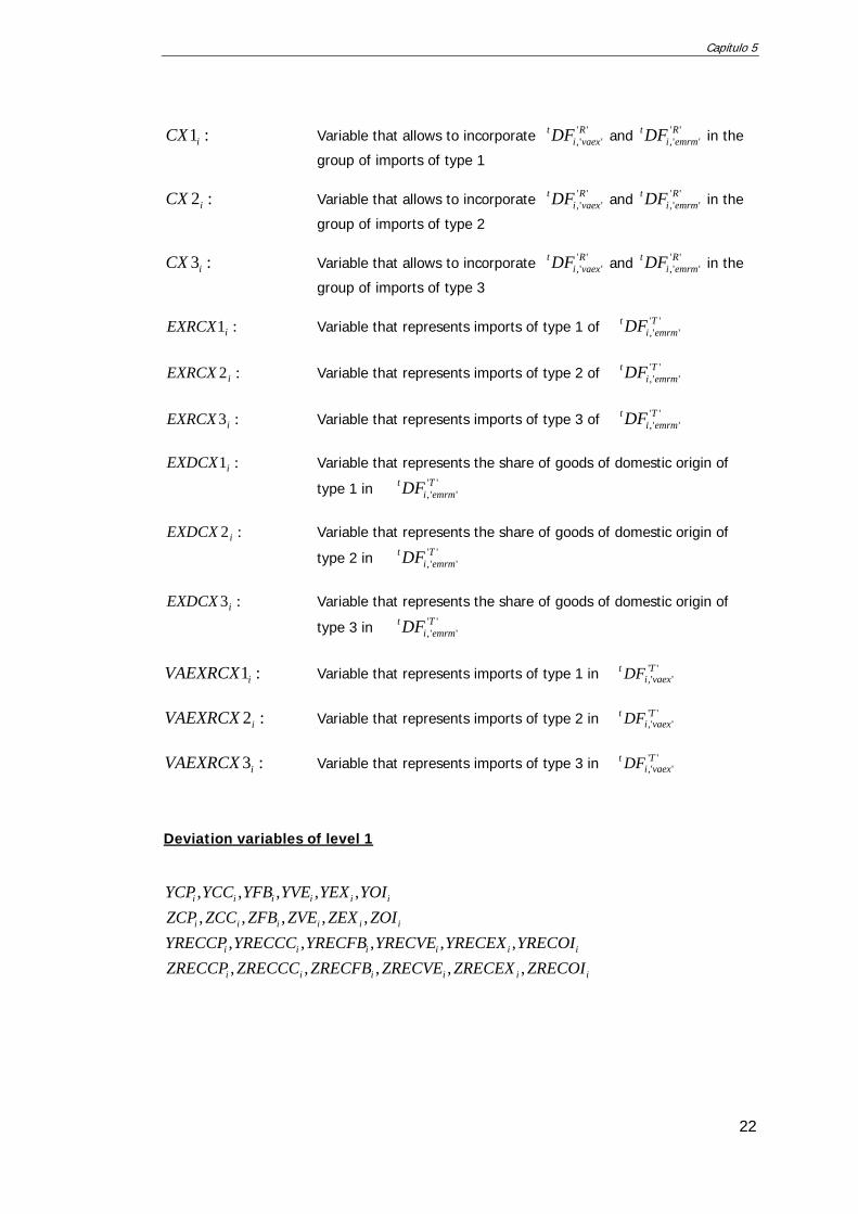
:1iCX Variable that allows to incorporate '''',

Rvaexi

tDF and '''',

Remrmi

tDF in the

group of imports of type 1


Rvaexi

tDF and '''',

Remrmi

tDF in the



Rvaexi

tDF and '''',

Remrmi

tDF in the


:1iEXRCX Variable that represents imports of type 1 of '''',

Temrmi

tDF

:2 iEXRCX Variable that represents imports of type 2 of ''

'',Temrmi

tDF

:3iEXRCX Variable that represents imports of type 3 of ''

'',Temrmi

tDF

:1iEXDCX Variable that represents the share of goods of domestic origin of

type 1 in '''',

Temrmi

tDF

:2 iEXDCX Variable that represents the share of goods of domestic origin of

type 2 in '''',

Temrmi

tDF

:3iEXDCX Variable that represents the share of goods of domestic origin of

type 3 in '''',

Temrmi

tDF

:1iVAEXRCX Variable that represents imports of type 1 in ''

'',Tvaexi

t DF


'',Tvaexi

t DF


'',Tvaexi

t DF

Deviation variables of level 1

iiiiii

iiiiii

iiiiii

iiiiii

ZRECOIZRECEXZRECVEZRECFBZRECCCZRECCPYRECOIYRECEXYRECVEYRECFBYRECCCYRECCP

ZOIZEXZVEZFBZCCZCPYOIYEXYVEYFBYCCYCP

,,,,,,,,,,

,,,,,,,,,,

Capítulo 5

23

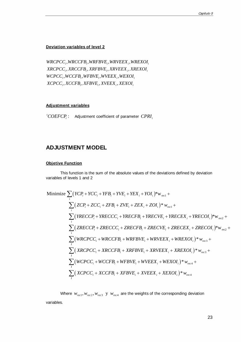
Deviation variables of level 2

,,,,,,,,

,,,,,,,,

iiiii

iiiii

iiiii

iiiii

XEXOIXVEEXXFBVEXCCFBXCPCCWEXOIWVEEXWFBVEWCCFBWCPCC

XREXOIXRVEEXXRFBVEXRCCFBXRCPCCWREXOIWRVEEXWRFBVEWRCCFBWRCPCC

Adjustment variables

:itCOEFCP Adjustment coefficient of parameter iCPRI

ADJUSTMENT MODEL Objetive Function This function is the sum of the absolute values of the deviations defined by deviation variables of levels 1 and 2

( )

( )

( )

rec1i

1

rec2i

Minimize *w

*w

i i i i i i

i i i i i i reci

i i i i i i

YCP YCC YFB YVE YEX YOI

ZCP ZCC ZFB ZVE ZEX ZOI * w

YRECCP YRECCC YRECFB YRECVE YRECEX YRECOI

ZRECC

+ + + + + +

+ + + + + +

+ + + + + +

∑

∑

∑( )

( )

( )

rec2i

3

3

*w

*

*

i i i i i i

i i i i i recI

i i i i i recI

P ZRECCC ZRECFB ZRECVE ZRECEX ZRECOI

WRCPCC WRCCFB WRFBVE WRVEEX WREXOI w

XRCPCC XRCCFB XRFBVE XRVEEX XREXOI w

+ + + + + +

+ + + + +

+ + + + +

∑

∑

∑( )

( )

4

4

*

*

i i i i i recI

i i i i i recI

WCPCC WCCFB WFBVE WVEEX WEXOI w

XCPCC XCCFB XFBVE XVEEX XEXOI w

+ + + + +

+ + + +

∑

∑

Where 4321 y ,, recrecrecrec wwww are the weights of the corresponding deviation

variables.

Capítulo 5

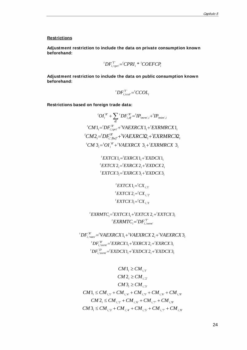
24

Restrictions Adjustment restriction to include the data on private consumption known beforehand:

it

itT

cpriit COEFCPCPRIDF *''

'', =

Adjustment restriction to include the data on public consumption known beforehand:

itT

ccolit CCOLDF =''

'',

Restrictions based on foreign trade data:

∑ +=+df

iimimt

iimrmtR

dfitR

it IPIPDFOI ,'',''

'',

''

it

itR

cpriit

it EXRMRCXVAEXRCXDFCM 111 ''

'', ++=

it

itR

fbcfit

it EXRMRCXVAEXRCXDFCM 222 ''

'', ++=

it

itR

it

it EXRMRCXVAEXRCXOICM 333 '' ++=

it

it

it EXDCXEXRCXEXTCX 111 +=

it

it


it

it


'1',1 it

it CXEXTCX =

'2',2 it

it CXEXTCX =

'3',3 it

it CXEXTCX =

it

it

it

it EXTCXEXTCXEXTCXEXRMTC 321 ++=

'''',

Texrmi

ti

t DFEXRMTC =

it

it

itR

vaexit VAEXRCXVAEXRCXVAEXRCXDF 321''

'', ++=

it

it

itR

exrmit EXRCXEXRCXEXRCXDF 321''

'', ++=

it

it

itD

exrmit EXDCXEXDCXEXDCXDF 321''

'', ++=

'1',1 ii CMCM ≥

'2',2 ii CMCM ≥

'3',3 ii CMCM ≥

'8','6','5','4','1',1 iiiiii CMCMCMCMCMCM ++++≤

'8','7','6','2',2 iiiii CMCMCMCMCM +++≤

'8','7','5','4','3',3 iiiiii CMCMCMCMCMCM ++++≤

Capítulo 5

25

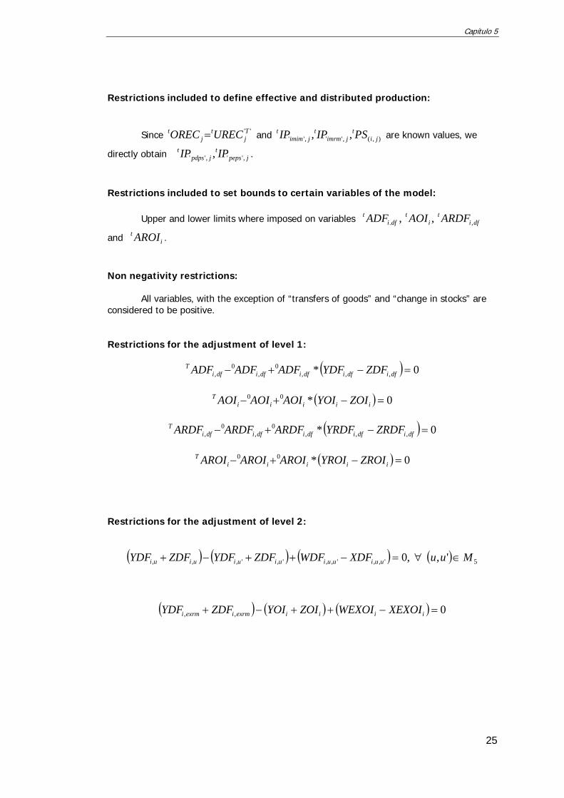
Restrictions included to define effective and distributed production:

Since ''Tj

tj

t URECOREC = and ),(,'','' ,, jit

jimrmt

jimimt PSIPIP are known values, we

directly obtain jpepst

jpdpst IPIP ,'','' , .

Restrictions included to set bounds to certain variables of the model:

Upper and lower limits where imposed on variables ,.dfit ADF ,i

t AOI dfit ARDF ,

and it AROI .

Non negativity restrictions: All variables, with the exception of “transfers of goods” and “change in stocks” are considered to be positive. Restrictions for the adjustment of level 1:

( ) 0* ,,,0

,0

, =−+− dfidfidfidfidfiT ZDFYDFADFADFADF

( ) 0*00 =−+− iiiii

T ZOIYOIAOIAOIAOI

( ) 0* ,,,

0,

0, =−+− dfidfidfidfidfi

T ZRDFYRDFARDFARDFARDF

( ) 0*00 =−+− iiiii

T ZROIYROIAROIAROIAROI

Restrictions for the adjustment of level 2:

( ) ( ) ( ) ( ) 5',,',,',',,, ', ,0 MuuXDFWDFZDFYDFZDFYDF uuiuuiuiuiuiui ∈∀=−++−+

( ) ( ) ( ) 0,, =−++−+ iiiiexrmiexrmi XEXOIWEXOIZOIYOIZDFYDF

Documents

Updating and adjustment of the trade flows of an Input ... · Updating and adjustment of the trade flows of an Input-Output Table ... 2Departamento de Análisis Económico Aplicado