ANSYS CFD v14

Update Seminar

© 2012 CAE Associates

ANSYS CFD v14 Meshing Update

© 2012 CAE Associates

Assembly Meshing

Assembly meshing is a top down meshing approach to mesh all parts Assembly meshing is a top-down meshing approach to mesh all parts— Use of virtual bodies (material points) to extract flow regions from dirty geometry— Support for:

M hi lid f h t b di• Meshing solids from sheet bodies• Conformal mesh between parts w/out having multi-body parts• Support for overlapping bodies

Assembly

Capping Face

Material point

3

point

Assembly Meshing

Assembly meshing replaces v13 CutCell Meshing at the GUI level Assembly meshing replaces v13 CutCell Meshing at the GUI level Supports both CutCell and Tetrahedral meshes CutCell meshing maintains characteristics from v13

— High fraction of hex and prismatic cells— Supports global size functions, feature capture,

tessellation, etc. controls— Operates on parts, multi-body parts, etc. with new

option to define virtual bodies— Patch independent:

Eli i t th d f i h t l d VT• Eliminates the need for pinch control and VT operations

Creates conformal meshes across parts in contactEliminates the need for m lti bod part generation in— Eliminates the need for multi-body part generation in CAD

Ability to create flow volumes from a “closed” set of bodies (sheet or solid)

4

bodies (sheet or solid)— Eliminates the need for Boolean/Fill operations in CAD

Assembly Meshing: Flow Volume Extraction

1 Define Coordinate system inside1. Define Coordinate system inside the Fluid Void

2. Insert a Virtual bodyAssign the proper Coordinate3. Assign the proper CoordinateSystem to the Material Point in the details of the Virtual Body Done4. Done

#2

#3

#1

#3

5

Assembly Meshing: Automatic Inflation

Inflation layers supported for Virtual Bodies Inflation layers supported for Virtual Bodies• Program controlled inflation acts only on Fluid Bodies

CutCell + Inflation Tetrahedron + Inflation

6

Assembly Meshing: Flow Volume Extraction

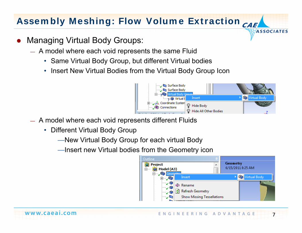
Managing Virtual Body Groups:a ag g tua ody G oups— A model where each void represents the same Fluid

• Same Virtual Body Group, but different Virtual bodies• Insert New Virtual Bodies from the Virtual Body Group IconInsert New Virtual Bodies from the Virtual Body Group Icon

— A model where each void represents different Fluids • Different Virtual Body GroupDifferent Virtual Body Group

—New Virtual Body Group for each virtual Body—Insert new Virtual bodies from the Geometry icon

7

Assembly Meshing: Keep Solid Mesh

Parts can be marked as fluids/solids

8

Assembly Meshing Leak Handling: Leakage Path

Find leaks using material points: Find leaks using material points:— Any time you are using material points (for internal flow), and it is leaking to the

outside, you can automatically see the leak-path together with the surface mesh

There is a small gap between the valve plug and the valve seat

9

Assembly Meshing Leak Handling:Closing Leaks up to 1/5 of min size

Contact sizing: Three simple steps1. Insert a Face-Face Contact between

the entities that are leaking

Pick the face of the valve plug (blue)and the edge of the valve seat (red)

the entities that are leaking• Face/Face or Face/Edge

2. Drag and drop the contact on top of the Mesh Iconthe Mesh Icon

• Creates a Contact sizing3. Adjust Contact sizing

• Should be bigger than the gap

#1

• Should be bigger than the gap— Limited to gaps up to 1/5 of

min-size4. Generate Mesh4. Generate Mesh

#2

#3

10

#3

Assembly Meshing: Finding Thin Sections

Why locate thin sections (3D bodies)? Why locate thin sections (3D bodies)?— Avoid Leakage— The assembly meshing method produces better quality meshes if thin baffles

and fins are well resolvedand fins are well resolved— By using the Find Thin Sections tool, these can be found in advance and

appropriate sizing can be applied

11

Assembly Meshing: Fluid Surfaces

Creating Fluid Surfaces for Flow Volume meshing Creating Fluid Surfaces for Flow Volume meshing— Description

• Pick all faces that make up the wetted surface of the flow volumeof the flow volume

— Applications• Mainly used when only flow volume is neededMainly used when only flow volume is needed

—No conjugate heat transfer

Advantage— Advantage• Faster• Less memory• Reduction of leakages• Reduction of leakages

— Approach• Insert Virtual Body

12

• Insert Virtual Body• Insert Fluid Surface (select faces)

Assembly Meshing: Fluid Surfaces

13

Assembly Meshing Export

CutCell— No support for CFX solver— No support for CFX solver

Tetrahedron: only integrated with FluentP d li t t t it bl f— Produces linear tets, not suitable for Mechanical solvers

— For CFX (unsupported work-around):• Set Physics to Fluent• Set Physics to Fluent • export the mesh in Fluent format• Import mesh into a CFX system

14

ANSYS CFD 14 ANSYS CFD v14 Update

© 2012 CAE Associates

ANSYS CFD v14 Update

CFX update

Fluent update

System Coupling Two-way FSI : Fluent and MechanicalTwo way FSI : Fluent and Mechanical

16

Rotating Machinery - Transient Blade Row

Highly efficient time accurateHighly efficient time accurate simulations with Transient Blade Row capability

— Several models available• Time Transformation (TT)

— Inlet Disturbance — Single Stage TRSg g

• Fourier Transformation (FT)— Inlet Disturbance — Single Stage TRS βg g— Blade Flutter β

Reference solution without a TBR method, requiring

Time Transformation solution, requiring only 3

Surface pressure distribution (top) and monitor point pressure (left) from an axial fan stage: Equivalent solution with Time Transformation at fraction of

180 deg model stator and 2 fan blades

17

solution with Time Transformation at fraction of computational effort

Rotating Machinery

Additional integrated turbo analysis capabilities (CFD-Post)

— Reduce need to export data and i l t t llmanipulate externally

— Directly assess stream-wise changes in span-wise distributions of circumferential averagesaverages

• Look at differences or ratios of existing variables, e.g. pressure ratio

— Further derived data possible with abilityFurther derived data possible with ability to define separate lines

Easier set-up of monitor points for rotating machinery βg y

— Specification in cylindrical coordinates

18

Interfaces

Easy simulation of opening and asy s u at o o ope g a dclosing

— Conditional GGIs that can open and close as the solution progresses

— Define condition as CEL function of solution

• e.g. After set time, based on l i l ( i l i lsolution values (single or integral

values)— Example applications

Membranes bursting windows• Membranes bursting, windows shattering, valves opening/closing

— Define as reversible (e.g. valve) or irreversible (e.g. burst membrane)irreversible (e.g. burst membrane)

Greater accuracy and speed with default interface settings

— Significantly faster more accurate

19

Significantly faster, more accurate direct intersection is now default

Immersed Solid

Improved accuracy with simplicity of Improved accuracy with simplicity of immersed solids

— Addition of boundary model for more li ti l it f i ithrealistic velocity forcing with

immersed solids• Track nodes nearest to immersed

solid

Boundary-fitted mesh

solid• Assume constant shear (laminar) or

use scalable wall function (turbulent) to modify forcing at immersed solid Immersed Solid (default)y g‘wall’

— Can improve immersed solid predictions significantly

Immersed Solid (default)

p g y• Continuing development for further

improvements and broader applications Immersed Solid with Boundary

Model

20

Multiphase – DPM

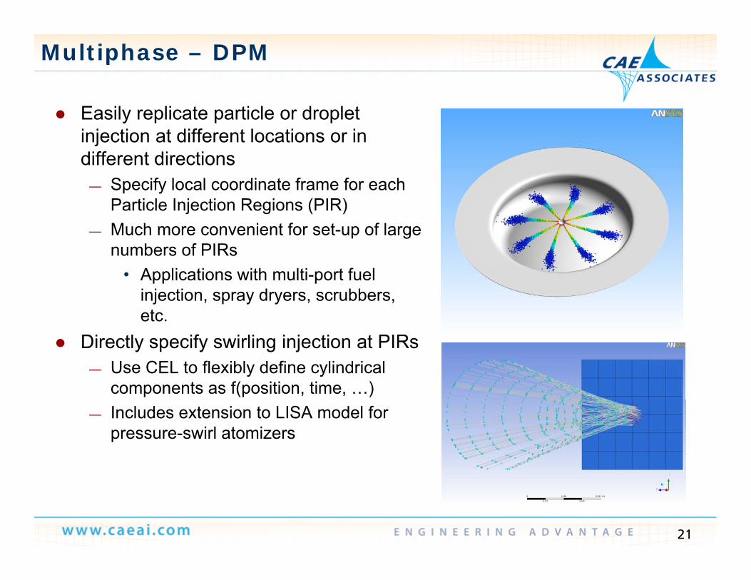
E il li t ti l d l t Easily replicate particle or droplet injection at different locations or in different directions

S if l l di t f f h— Specify local coordinate frame for each Particle Injection Regions (PIR)

— Much more convenient for set-up of large numbers of PIRsnumbers of PIRs

• Applications with multi-port fuel injection, spray dryers, scrubbers, etc.

Directly specify swirling injection at PIRs— Use CEL to flexibly define cylindrical

components as f(position, time, …)— Includes extension to LISA model for

pressure-swirl atomizers

21

Multiphase – Global Condensation

Ability to include global effect of wall Ability to include global effect of wall condensation without multi-phase details

— Single phase, multiple componentsSingle phase, multiple components• Mixture of one condensable and

one or more non-condensable species

Water condensation at heat exchanger wall (fluid-solid

interface)— Condensable component extracted

by sink terms at walls and CHT boundaries, as function of concentration through boundary

interface)

concentration through boundary layer

• Liquid film is not modeled— Key application: nuclear accident— Key application: nuclear accident

scenarios looking at containment pressure variation over time need to include macroscopic effect of

d i

22

condensation

Multiphase – Eulerian

C bi h h d i Combine phase change and varying dispersed phase size distributions for improved accuracy β

Homogeneous and inhomogeneous— Homogeneous and inhomogeneous MuSiG can be applied together with general phase change and RPI wall boiling models

= +

23

Simulation and comparison with experimental results from DEBORA Test Facility courtesy of HZDR (formerly FZD)

Mesh Motion

Further user control on deforming mesh to allow retention of optimal mesh Further user control on deforming mesh to allow retention of optimal mesh quality β

— Diffusion of boundary mesh motion can be defined to be anisotropic – i.e. preferential diffusion in different directionspreferential diffusion in different directions

Sample case: Deformation of an originally square

domain

Final mesh with isotropic diffusion: skewed

elements

Final mesh with anisotropic diffusion: improved mesh quality, greater range of

24

q y, g gmotion possible

ANSYS CFD v14 Update

CFX update

Fluent update

System Coupling Two-way FSI : Fluent and MechanicalTwo way FSI : Fluent and Mechanical

25

Higher Order Term Relaxation (HOTR)

What is HOTR: What is HOTR:— Under-relaxation applied to higher-order

discretization terms.

What does it do:— Improve solution convergence behavior— Can prevent apparent convergence stalling— Can prevent apparent convergence stalling— Improve solution startup robustness

How to use it: How to use it:— Activate it from the Solution Method task page

(DB & PB Solution methods)Extra Option available— Extra Option available

LimitationN t il bl f NITA

26

— Not available for NITA

HOTR Example - Plug Nozzle

DB Implicit solver SST-KO turb model DB Implicit solver, SST-KO turb. model

0.24 M quad cellsM=2.0

Difficult startup case— FMG-init— 1st-O spatial discretization for 200 iter— 2nd-O spatial discretization.

Mesh

High-Order Term Relaxation (HOTR) can accelerate the solution convergence, by allowing the solver to Mach Contoursg y gstart calculations at much more aggressive settings than without the use of HOTR

27

HOTR Example - Plug Nozzle

With and w/o HOTR @ CFL=35 With and w/o HOTR @ CFL=35 FMG performed for both the cases First Order for 200 iterations with CFL=5 Second Order solution started from the above First Order Solution.

With HOTR Without HOTR

1st Ord 2nd Ord 1st Ord 2nd Ord

28

Note: Without the additional stability from HOTR the case diverged @ CFL=35

HOTR Example - Plug Nozzle

Static Pressure Convergence

~900 iter to convergence w_HOTR @CFL=35 ~2000 iter to convergence w/o HOTR using max possible CFL=10

29

2000 iter to convergence w/o_HOTR using max possible CFL=10 Speedup in this case ~55%

Convergence Acceleration For Stretched Meshes (CASM)

What is CASM:— Accelerate the convergence of the DB-implicit

solution method on highly-stretched meshes. minlmaxl

g y— Convergence can be between 2 to 10 times

faster than without using CASM How does it work:

— Use local cell CFL value which is equal to Specified CFL value multiplied by a factor proportional to cell aspect ratio. Standard time step

— Optimize the solution advancement for implicit method

— Cell stretched perpendicular to flow skippedLi it ti

minlCFL

AVCFLt

f

CASM time step Limitations:

— Can be used with Solution-Steering but Manual schedule adjustment is required. (reduce max & min CFL values)

maxlCFLAR

AVCFLt

f

CASM time step

30

min CFL values)— Steady-State solution

Convergence Acceleration For Stretched Meshes (CASM)

How to use it:— Activate it from the Solution Method task page

A il bl ith d it b d i li it l— Available with density-based implicit solver (steady-state) only

— When CASM is use you typically do not need— When CASM is use you typically do not need to run the solver at very high CFL value. Range between 2 to 50 is sufficient for most flow cases.

— FMG initialization should be used before solving flow with CASM

31

CASM Example - Wing-Body Configuration

RAE Wing-Body Case #5 — M=0.8 AOA=2.0 deg

M h 6 5 M ll— Mesh: 6.5 M cells— max AR= 2.01E+04— Turb: SST-KO

2 d O fl NB d— 2nd-O flow NB-grads— CFL =20 Expl-relax=0.25— Double- Precision

Convergence:— Standard = 3000 iter— CASM = 300 iter Mesh:

— Hybrid Hex-Tet cells— Anisotropic mesh

32

— Viscous layer with very high stretching

CASM Example : Wing- Body Configuration

Comparing Convergence Between Standard and CASM.p g g

About 10 timesspeed up is observed in

CASM Standard

this test case.

CL StandardCASM

Cd StandardCASM

33

Dynamic Mesh

Fluent MDM improvements driven by Fluent MDM improvements driven by application needs

— Retain and remesh boundary layers during tetrahedral remeshing

T=0 T=25 T=50

during tetrahedral remeshing• Boundary layer settings from

original mesh• Example applications: internal p pp

combustion engines and FSI

— Improved robustness and usability for

Remeshing a tetrahedral mesh with boundary layers during a

simulation

dynamic mesh• Mesh smoothing• Cut cell remeshing• Parallel

34

Tetrahedral mesh with boundary layers after remeshing

Turbulence

Improved accuracy for turbulent flows Improved accuracy for turbulent flows with strong rotation and streamline curvature with one and two-equation modelsmodels

— Option to apply a correction term sensitive to rotation and curvature

— Accuracy comparable with the RSM, with y p ,less computational effort, for swirl-dominated flows Contours of curvature correction function

(fr) in a curved duct (k-omega SST turbulence model)

Improved accuracy for turbulence near porous jump interfaces β

— Use wall functions to include the effects of solid porous material on the near-wall turbulent flow on the fluid side of porous jump interfaces

35

Contours of velocity showing the impact of a porous jump on velocity in bordering cells

Turbulence

More accurate solution of high R ll b d d fl i Fl Re wall bounded flows using LES

— Algebraic Wall Modeled LES (WMLES) f l ti b d

Flow over a wall mounted hump

(WMLES) formulation based on Smagorinsky model

— Benefits gas turbine combustors and other internal flowand other internal flow applications

A mi ing la e ith esol ed t b lence

36

A mixing layer with resolved turbulence using SAS initiated by the forcing model

Multiphase – Free Surfaces

Coupled VOF after 500

Better robustness and faster convergence for free surface t d t t i

Coupled VOF after 500 iterations

steady-state cases using coupled VOF

• Improved in R14.0

Coupled P-V, Segregated VOF after 1400 iterations

37

Multiphase – Eulerian

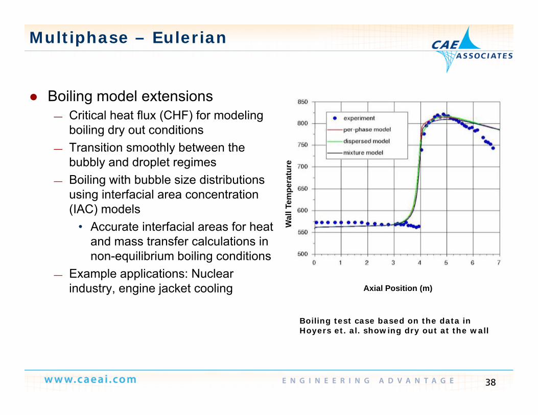
Boiling model extensions— Critical heat flux (CHF) for modeling

boiling dry out conditionsboiling dry out conditions — Transition smoothly between the

bubbly and droplet regimes— Boiling with bubble size distributions ra

ture

— Boiling with bubble size distributions using interfacial area concentration (IAC) models

• Accurate interfacial areas for heat Wal

l Tem

per

and mass transfer calculations in non-equilibrium boiling conditions

— Example applications: Nuclear industry engine jacket cooling A i l P iti ( )industry, engine jacket cooling Axial Position (m)

Boiling test case based on the data in Hoyers et. al. showing dry out at the wall

38

Multiphase – Eulerian Wall Film

Eulerian Wall Film Model for rain water management, deicing and other applications

— Available models:• Momentum coupling• DPM coupling

—Particle collection, splashing and shearing

• Heat transfer

The wall film on a car mirror withdroplets released due to wind shear

Contours of temperature

i l i

film airsolid

liquid water injected

in an Eulerian Wall Film with heat

transfer case

Q = 3000 W

KCQTfilm 75

40000103000

39

Cm Pfilm 400001.0

Multiphase – Population Balance

DQMOM Population Balance DQMOM Population Balance captures the segregation of poly-dispersed phases due to differential coupling with the continuous phase

DQMOM QMOM

g

coupling with the continuous phase

— Faster solution time than the Velocity big bubbles > velocity small bubbles

All bubbles move with same velocity

inhomogeneous discrete model — Multi-fluid model convects different

dispersed phase sizes using different velocitiesvelocities

— Example applications: Fluidized beds, gas solid flows, spray modeling, bubble columns

Bubble diameters for DQMOM (white) compared to QMOM (red)

Contours of volume fraction of the phase with

40

fraction of the phase with the largest diameters in a bubble column.

Multiphase – DEM

M d l d ti l t fl ith Model dense particulate flows with DEM

— DEM enabled as a collision model in the DPM d l l

NETL Fluidized Bed Simulations using DEM with DDPM 

DPM model panel— Use in combination with single phase and

DDPM simulationsWorks in parallel

12% fines0‐25 sec

— Works in parallel— Particle size distributions— Prediction of the packing limit

Head on collisions— Head-on collisions— Collisions with walls— Example applications: Bubbling and

circulating fluidized beds particle3% fines start‐up ‐15 sec circulating fluidized beds, particle

deposition in filtering devices, particle discharge devices (silos)

and 15‐30 sec 

Note that channeling is observed in the 15‐30 sec period

41

15 30 sec  period 

Reacting Flows

1D Reacting Channel Model 1D Reacting Channel Model— Model fluids reacting in thin

tubes, which exchange heat with an external flowwith an external flow

• Flow inside the tubes is simple (pipe profile), but the chemistry is complexthe chemistry is complex

• Flow outside the tubes is complex, but the chemistry is usuallychemistry is usually simple (equilibrium)

Example applications:

1D reacting channel model in Fluent

— Example applications: cracking furnace, fuel reformers, …

42

1D reacting channel geometry in Fluent

Shell Conduction

Shell conduction: Improved Shell conduction: Improved accuracy and ability to include combustion

— Non-premixed and partially-

Oxidizer(air)V=0.1 m/s, T = 300KMean Mixture Fraction=0

— Non premixed and partiallypremixed combustion models

— Example applications: Gas turbines, those with thin walls and

Fuel, V=1 m/sT= 300KMean Mixture Fraction=1

External Wall with convective BCh=2, Tinf= 300K

combustion

Improved shell conduction usability

Geometry and details for shell conduction with non-premixed combustion test case

— Updated documentation for wall temperature variables and shell zone and thin wall post-processingP t th t l ll— Post-process the external wall temperature if shell conduction is applied on a one-sided-wall

43

Temperature on a mid-geometry surface

AcousticsFWH source surface,R=1m

Validations and model extensions

— Convective effect for FW-H Acoustics

M=0.22D monopole with convection

acoustics solver• Option to include the

effect of far-field velocity on the generated sound

Acoustics directivity

Receivers, R=3m

on the generated sound for the Ffowcs-Williams & Hawkins solver

• Improves accuracy when OASPL – overall sound pressure level

p ymodeling aero-acoustics and external flows

M=0.4Moving receiver

Source

44

Sound pressure compared with analytic solution at approach and departure (Doppler effect different frequencies)

Adjoint Method

● Adjoint Solver for Fluent fully tested, documented, and supported at R14.0

— Provides information about a fluid system that is very difficult and expensive to gather otherwise

— Computes the derivative of an engineering quantity with respect to inputs for the systemEngineering quantities available

Shape sensitivity to down-force on a F1 car

Lift Force (N)Geometry Predicted Result— Engineering quantities available

• Down-force, drag, pressure drop

— Robust for large meshes

Geometry Predicted ResultOriginal ‐‐‐ 555.26Mod. 1 577.7 578.3Mod. 2 600.7 599.7Mod. 3 622 621.8

— Robust for large meshes• Tested up to ~15M cell

45

Shape sensitivity to lift on NACA 0012

ANSYS CFD v14 Update

CFX update

Fluent update

System Coupling Two-way FSI : Fluent and MechanicalTwo way FSI : Fluent and Mechanical

46

System Coupling 14.0

Facilitates simulations that require tightly integrated couplings of analysis Facilitates simulations that require tightly integrated couplings of analysis systems in the ANSYS portfolio

Extensible architecture for range of coupling scenarios (one- two- & n-way static data co-simulation )(one-, two- & n-way, static data, co-simulation…)

ANSYS Workbench user environment and workflow Stand-alone coupling service delivers coupling management and

mapping/interpolationmapping/interpolation Service and solvers communicate using proprietary TCP/IP client-server

Remote Procedure Call (RPC) library and Standard Interfaces

47

System Coupling 14.0

System Coupling Controls the Participant Solvers for Transient and System Coupling Controls the Participant Solvers for Transient and Steady/Static Solutions

— Solution update can ONLY be done via System Coupling componentSystem Coupling ensures that the time duration and time step settings are— System Coupling ensures that the time duration and time step settings are consistent across all participant solvers

48

Ball Valve

Fixed support

Flow outlet FSI interface

Fixed support

Flow inlet

49

Setup Transient/Static Structural Model

Setup structural solution, structural boundary conditions and Fluid-Solid

50

Interface

Setup Fluid Flow Model

Setup fluid solution, fluid boundary conditions and specify System Coupling Dynamic Mesh Zone for fluid-structure interaction motion

51

System Coupling Motion Type

System Coupling motion System Coupling motion identifies zones that may participate in System Coupling

— Allows user-defined motion to be combined with System Coupling motion

— Defaults to stationary motion type when not connected to System Coupling

52

Update Setup Cells for Transient/Static Structural and Fluid Flow

State of System Coupling setup cell will be— Upstream data is now available for SC Setup

53

System Coupling GUI

Chart MonitorsOutline Monitors

S l ti I f tiSolution Information Text MonitorsDetails

54

System Coupling Analysis Settings

Coupling End Time Coupling End Time— If both participants are transient— For General, Number of Steps is

user inputuser input

Coupling Step SizeIf both participants are transient— If both participants are transient

Minimum Number of Iterations per Coupling StepCoupling Step

Maximum Number of Iterations C li Stper Coupling Step

55

System Coupling Participants

Transient/Static Structural and Fluid Transient/Static Structural and Fluid Flow

— Region and variable information is generated automatically via Updategenerated automatically via Update when analysis systems are first connected to System Coupling

— For Fluent, all regions of type Wall are shown in SC Setup

— For Mechanical, all regions of type Fluid-Solid Interface are shown in SC Setup

56

Create Data Transfer Regions

Use Ctrl key to select a Fluent and Mechanical region pair and select Create Data Transfer from right-click pop-up menu

— Automatically fills in the details for the data transfer region

— Data transfers can be one-way (i.e. only transfer force or only transfer displacement) or two waydisplacement) or two-way

57

Data Transfer

Data Transfer defines the details for the Source Target and Data Data Transfer defines the details for the Source, Target and Data Transfer Controls

Participant— Participant— Region— Variable

Transfer At— Transfer At• Start of Iteration only

— Under Relaxation Factor— Convergence Target— Convergence Target

58

Execution Control

Co-Simulation Sequence Co-Simulation Sequence— Transient or Static Structural will

always be first in the co-simulation sequenceq

Debug Output— Different levels of debug output

for analysis and data transfersy Intermediate Results File Output

— Controls the intervals for writing restart file information

59

Executing System Coupling

Default chart monitorsDefault chart monitors show convergence history for all data transfers.

X-axis can be coupling time, step or iteration.

60

Solution Information

Build information— Build information— Complete summary of coupling

service input fileAnal sis details— Analysis details

— Participant summaries— Data transfer details— Mapping diagnostics— Time step and iteration summary— Solver field equation convergenceSolver field equation convergence

summary— Data transfer convergence

summarysu a y— Fluent/MAPDL solver output

61

Adding Charts and Variables

Add charts by selecting Create Convergence Chart Add charts by selecting Create Convergence Chart Variables can be added or removed from charts

— Data transfers, CFD and structural convergence normsCh t ti dit bl i th h t ithi Chart properties are editable in same manner as other charts within ANSYS Workbench

62

Post Processing System Coupling

Transient/Static Structural or Fluid Flow Results cell for solver specific Transient/Static Structural or Fluid Flow Results cell for solver-specific post-processing

Connect structural Solution cell directly to Fluent system Results cell or add a Results System (ANSYS CFD Post) for unified post processing ofadd a Results System (ANSYS CFD-Post) for unified post-processing of structural and fluid results

63

Ball Valve : Deformation

64

Ball Valve : Streamlines

65

Ball Valve : Fluid Pressure

66