Embed Size (px)
Citation preview
UU NN VV EE II LL II NN GG
TTHHEE RREETTIIRREEMMEENNTT
MM YY TT HH
Advanced Retirement Planning based on
Market History
Jim C. Otar
2
UNVEILING THE RETIREMENT MYTH Copyright © 2009 by Jim C. Otar.
All rights reserved. No part of this publication may be reproduced, stored in a retrieval system, or transmitted, in any form or by any means, electronic, mechanical, photocopying, recording, or otherwise, without the written permission of the publisher except in critical articles and reviews. For information, please contact Otar & Associates, 96 Willowbrook Road, Thornhill, Ontario, Canada, L3T 5P5, or send an email to: [email protected]
This publication is designed to provide basic information and general guidance concernng retirement income portfolios with an historical perspective. It is sold with the understanding that the publisher is not engaged in rendering legal, accounting, financial or other professional advice. Although the author has exhaustively researched all sources to ensure the accuracy and completeness of the information contained in this book, the author and the publisher assume no responsibility for errors, inaccuracies, omissions or any inconsistency herein. All comments and methods are based on available historical data at the time of writing. This book is for information purposes only and should not be construed as investment advice or as a recommendation for any investment method or as a recommendation to buy, sell, or hold any securities. Readers should use their own judgment. If legal or other expert assistance is required, the services of a competent professional should be sought for specific applications and individual circumstances.
The author and publisher disclaim any responsibility for any liability, loss or risk incurred as a consequence of the use or application of any of the contents of this book. The names and persons in examples, cases or problems in this book are fictitious. Any similarities to the events described and names of actual persons, living or dead, are purely coincidental.
Trademark Notice: Product or corporate names may be trademarks or registered trademarks, and are used only for identification and explanation, without intent to infringe. Care has been taken to trace ownership of copyright material contained in this book. The publisher will gladly receive any information that will enable them to rectify any reference or credit line in subsequent publications.
First edition published in 2009 Printed in Canada Cover picture: my loving parents and all their children, 1952 Visit www.retirementoptimizer.com for bulk orders or additional copies of this book.
Library and Archives Canada Cataloguing in Publication Otar, Jim C. Unveiling the retirement myth: advanced retirement planning based on market history / Jim C. Otar. Includes index. ISBN 978–0–9689634–2–5 1. Retirement income––Planning. 2. Stocks––Rate of return. 3. Investment analysis. 4. Portfolio management. I. Title. HG179.O838 2009 332.024'01 C2009–904683–0

3
To my parents, with whom I wish I had spent more time To Rita, who has always been beside me To those advisors who try to do their best for their clients

4
Author’s Preface
This book is based on my research of retirement planning involving one hundred and nine years of market history. It provides comprehensive analysis of methods and strategies for retirement planning. Detailed, step–by–step examples that are based on actual market history are included. These methods and strategies will take the reader to the next step, the advanced retirement planning. It will also help fellow advisors to reduce their exposure to liability when more and more retirees realize the devastating shortfalls of existing models. What you read will be depressing. The light at the end of the tunnel will not be visible until you start reading the zone strategy. There, you can find strategies for lifelong income, no matter how much you might have saved for your retirement. Jim C. Otar CFP, CMT, BASc, MEng Toronto, October 1, 2009 www.retirementoptimizer.com [email protected]
5
Table of Contents
Page
Acknowledgements .............................................................................. 7
How to Read this Book ...................................................................... 9
Introduction ...................................................................................... 11
Chapter 1: Time Value of Money .................................................. 15
Chapter 2: A Historical Perspective ............................................... 33
Chapter 3: Dividends ..................................................................... 46
Chapter 4: The “Importance” of Asset Allocation ......................... 51
Chapter 5: The “Magic” of Diversification .................................... 60
Chapter 6: Rebalancing .................................................................. 72
Chapter 7: Market Trends .............................................................. 83
Chapter 8: Mathematics of Loss .................................................... 90
Chapter 9: The Luck Factor ......................................................... 106
Chapter 10: Sequence of Returns .................................................. 109
Chapter 11: Inflation ...................................................................... 113
Chapter 12: Reverse Dollar Cost Averaging ................................. 120
Chapter 13: Time Value of Fluctuations ....................................... 125
Chapter 14: Efficient Frontier ....................................................... 137
Chapter 15: Monte Carlo Simulators ............................................. 142
Chapter 16: Optimum Asset Allocation – Distribution Stage ....... 156
Chapter 17: Sustainable Withdrawal Rate ..................................... 176
Chapter 18: How Much Alpha Do You Need? .............................. 189
Chapter 19: Optimum Asset Allocation – Accumulation Stage ... 196
Chapter 20: Effective Growth Rate .............................................. 209
Chapter 21: P/E Ratio as Predictor of Portfolio Life .................... 223
Chapter 22: Other Warning Signals of Diminishing Luck .............. 231
6
Chapter 23: Age Based Asset Allocation ...................................... 237
Chapter 24: Tactical Asset Allocation ........................................... 245
Chapter 25: Flexible Asset Allocation ........................................... 259
Chapter 26: Combo Asset Allocation ............................................ 275
Chapter 27: If You Miss the Best .................................................. 285
Chapter 28: Asset Selection & Monitoring: Fingerprinting ............ 294
Chapter 29: Portfolio Management Expenses ............................... 307
Chapter 30: Borrowing to Invest ................................................... 311
Chapter 31: Determinants of Portfolio’s Success .......................... 327
Chapter 32: Retirement Income Classes ....................................... 334
Chapter 33: Immediate Life Annuity ............................................ 340
Chapter 34: Variable Pay Annuity ................................................ 350
Chapter 35: Variable Annuity with GMWB ................................. 362
Chapter 36: Variable Annuity with GMIB ................................... 390
Chapter 37: Buy Term Annuity, Invest the Rest ........................... 408
Chapter 38: Asset Dedication ........................................................ 415
Chapter 39: Withdrawal Strategies based on Performance ............ 420
Chapter 40: Budgeting for Retirement ............................................ 433
Chapter 41: The Zone Strategy ........................................................ 437
Chapter 42: Green Zone Strategies .................................................. 457
Chapter 43: Gray Zone Strategies .................................................. 472
Chapter 44: Red Zone Strategies ................................................... 504
Chapter 45: The Final Word .......................................................... 510
Appendix A: Source Data ................................................................ 514
Appendix B: Retirement Cash Flow Worksheet ............................ 517
Index .................................................................................... 522

7
Acknowledgements In life, there are two kinds of luck: The first kind simply drops into your lap without you even asking for it. Many either do not experience it more than once in their entire lifetime or miss it altogether when it happens. The second kind of luck does not fall into your lap; it happens because of your hard work, tenacity, persistence, curiosity, and sometimes by you just being there. Fifty–eight years ago, I experienced the good luck of the first kind at birth: I was welcomed into this world by my wonderful parents. The values and the sense of humor they instilled in the early years of my childhood have been my greatest resource throughout my life. I thank them for their encouragement to complete this book. Thirty–two years ago, good luck of the first kind struck me again. I met Rita, my better half. She asked me a simple question in 1999, “Do we have enough money to retire?” That question triggered my first book on this topic in 2001. Six years ago, when I decided to re–write this expanded edition, she gave me unbounded encouragement. I thank her for that. I thank my older brother Yavuz for teaching me everything from how to ride a bicycle, to building radios, to the basics of economics, and how to fill out my first tax return. He gave me some of his unique combination of skepticism and self–confidence wrapped in one package. This attribute became my biggest asset for what I have been doing in the last fifteen years. I owe thanks to readers, advisors, friends, clients and editors of my articles, as well as sponsors of my live presentations. They asked numerous questions, gave me their feedback, suggested wonderful improvements to my retirement calculator, made my Wall–Street–bashing more compliant for my live presentations, and encouraged me to write more. I thank you all. In addition, a special thanks to Michael Baney for converting me from a “road worrier” to a “road warrior”. He is one of the finest people that I have met in this business. Finally, Boris Krivy did an excellent job of leaving my accent intact in my writings. I thank him for his fine editing.

8

9
How to Read this Book I am a typical engineer: I am skeptical of everything that I hear or read about, especially in the investment world. If I come across a strategy that looks interesting, then I like to work through the numbers until I can clearly see if and how it works. That is how I discovered nine years ago while writing “High Expectations & False Dreams”, that most research and innovative strategies you hear or read about, are just plain garbage.
This book is mostly a collection of my articles. I wanted to gather them all under one cover for your convenience. There are numerous tables and charts in each chapter. Some of the material might appear to be repetitious. For some readers, this can be overwhelming.
There are two kinds of readers: Those who like details and those who don’t.
If you like details, then read the entire book. Some topics are heavy. Do not be discouraged; you may need to read some chapters more than once.
If you dislike details or hate math, then you do not need to read the entire chapter. I designed many of the chapters in such a way that you can skip the details and still make sense of the topic. Here is how it works:
Chapter 2
A Historical Perspective
Most books become boring after the first couple of chapters. To keep you interested enough to read the rest of this book, this is a good place to shock you. I apologize beforehand for deflating some of your dreams. However, unless we go through this painful process of getting rid of some of the myths in my business, we cannot move forward. Therefore, in this chapter I will show you the current Gaussian mindset1 of retirement planning practice and its potential disastrous outcomes.
Currently, there are two popular ways of forecasting the adequacy of retirement assets: The first method is called Deterministic. The second one is the Monte Carlo simulation.
The deterministic method uses the formulae that we covered in Chapter 1, The Time Value of Money. After years of using it, more and more financial professionals are realizing that the deterministic method has serious flaws.
The Monte Carlo (MC) simulations are becoming more popular, I might add, regretfully so. They use probability models to overcome the weaknesses of the deterministic method. While MC’s are better than the deterministic method, they have their own flaws. I will cover the flaws of MC in Chapter 14. In this chapter, I will focus on the deterministic method only. I don’t want to over-shock you in one single chapter.
The Current Practice: Let’s start with an example: Bob is 65 years old. He is retiring this year. He expects to die
Conclusion:
You might ask “Over the last 100 years, the market index returned on the average 8.8% annually. Why is it then, if I withdraw 6% (i iti l ithd l t i d d t i fl ti ) th b bilit f i t f i hi h?” Th i littl
If you don’t like math, then just
read the beginning of the chapter until the first bold sub–
header.
Then skip to the end of the chapter
and read the “Conclusion”

10

11
Introduction In the old country, when I was little, my parents owned a small hobby farm. We had a flock of sheep, a dog, a few stray turtles and the neighbor’s donkey. My older brother raised chickens, ducks and geese for fun. Ali, the watchman, grew vegetables and looked after the sheep and the fruit trees.
I had occasional talks with Ali. One day, I don’t know how it started, I found myself discussing the merits of cabbage with him. He mentioned that cabbage, unlike okra, is a hardy plant, easy to grow, easy to pick, easy to sell. I started thinking about it. I calculated the cost of planting an acre of cabbage. Then I calculated the yield. Only then did I realize how much money I could make in just a few months.
I could probably plant a cabbage field every year and overcome my biggest phobia: asking my father for an allowance. The poor guy was already burdened up to his neck helping out the Crimean Tatars escaping from Russia, and they kept coming and coming. He was an accountant. Sometimes, his little office looked more like a refugee camp.
Wow! I was only eleven years old and thanks to this cabbage enterprise, I was set for life.
I shared my thoughts with Ali. He responded –trying not to discourage my enthusiasm, “you’ll never know how much money you’ll make until it is in your pocket. We may lose some seedlings to birds and sheep, but perhaps we can put a new fence around the sheep flock. That may solve the sheep problem. Then there is the neighbor’s donkey. They love cabbage; he may break his rope and eat our crop, but perhaps we can buy a stronger rope for the donkey and solve the donkey problem. Then there are the passers–by, especially the poor ones. They will certainly help themselves and you can never put them on a rope! As if this is not enough, on the harvest day the local deputy will undoubtedly show up and he would want to fill up his trunk with gifted cabbage!”
I did not like at all what Ali was saying. “These farmers are so stupid”, I said to myself, “that is why they must be so poor”. I always hated asking my father for allowance. This was my only way out, through the cabbage field. The next day, I cashed in all my life savings. I also broke my piggy–bank for additional funding, just in case. Ali and I went to the nursery and bought seedlings. You need lots of manure to grow cabbage. So, I bought a truck–load. Finally, I spent the last bit of my money on a new rope for the donkey and a new fence for the sheep. That was my risk management.
As tradition dictates, we planted several baskets of seedlings under the bright full moon. Then, I spread the entire mountain of manure carefully with my own bare hands around each seedling.
Weeks went by. It was a good season; the cabbage grew unbelievably well. We had less damage than we expected from birds, sheep, donkey and people. My dreams were coming true. No more asking my father for the weekly allowance!
But the winter was approaching fast. I asked Ali when we should harvest the cabbage. He gazed at the distant horizon for a long moment and then said, “We should wait two more weeks. The cabbage will weigh more then. You’ll make more money.”
12
Two weeks later, I went back to our hobby farm. On the way, I prepared myself mentally for the inevitable confrontation with the local deputy for his cut of my crop. Other than that, I was overflowing with joy, as I anticipated my new wealth.
When I arrived there, Ali did not look too happy. He said that there was a premature frost the night before. Now, the cabbage was useless. “Only the donkey can eat it now”, he added, “that is, if he cannot find anything better to eat”.
An unexpected unlucky event, just one day before the harvest, turned my dreams of financial freedom into financial ruin. As a result of that premature frost, I continued to feel a deep embarrassment weekly; each time I asked my father for my allowance. “Why did I listen to Ali? Why did I not harvest my cabbage one day earlier? Why? Why!”
Several years later, at age twenty, as hippies from the West were traveling to the East, I went in the opposite direction. I moved to Canada. I enrolled in the Faculty of Engineering at the University of Toronto. I made a living driving a taxi part–time during my student days. Finally, I no longer needed my father’s allowance.
The chances are, if that frost forty–seven years ago had come one day later, I would not have moved to Canada, have would have never met Rita, and you would not be reading this book. Remember, I mentioned earlier that there are two kinds of luck? Moving to Canada was good luck of the second kind. Many years later, I still cannot believe that happened at age twenty.
During the next ten years, over 90 million Americans and Canadians are hoping to retire. We have successfully landed robots on Mars and observed their amazing findings. We have successfully discovered cures for many diseases. We have found solutions to numerous other problems.
Yet our financial planning community still does not have the tools to give realistic answers to some of the most basic questions:
When can I retire? Do I have enough money to retire? How much do I need to save for my retirement? How long will my money last? Is there a shortfall? How much do I need to save between now and retirement?
You will find dozens of books in your local bookstore that attempt to answer these questions. Almost all of them use certain assumptions about future market growth and future inflation. You will find some of their arguments reasonable and logical. Others make outrageous claims. Most ignore one thing: averages do not apply to individuals.
When I changed my career from engineering to financial planning, I was appalled by the current design practice: we assume an "average" growth rate for the portfolio and then design a retirement plan accordingly.
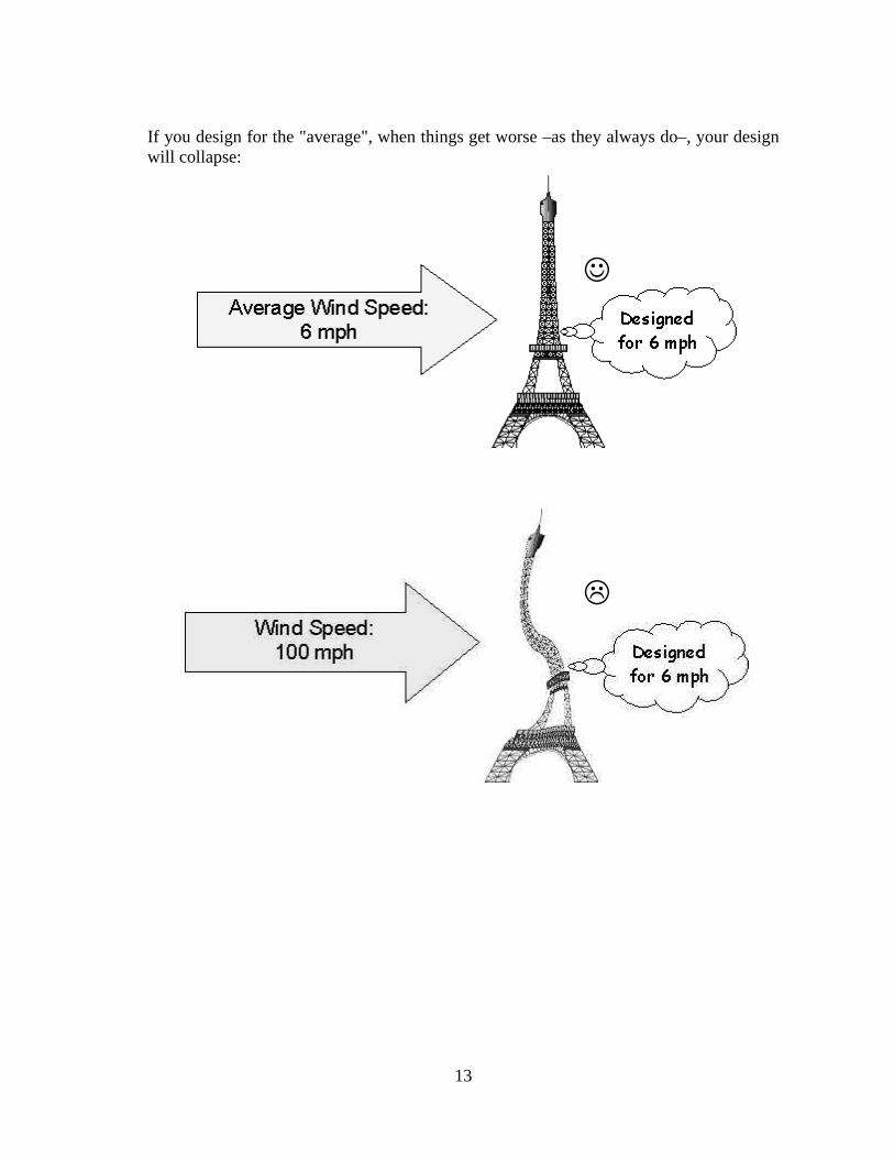
13
If you design for the "average", when things get worse –as they always do–, your design will collapse:
14
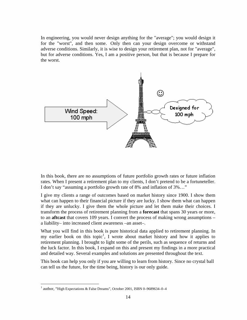
In engineering, you would never design anything for the "average"; you would design it for the "worst", and then some. Only then can your design overcome or withstand adverse conditions. Similarly, it is wise to design your retirement plan, not for "average", but for adverse conditions. Yes, I am a positive person, but that is because I prepare for the worst.
In this book, there are no assumptions of future portfolio growth rates or future inflation rates. When I present a retirement plan to my clients, I don’t pretend to be a fortuneteller. I don’t say “assuming a portfolio growth rate of 8% and inflation of 3%…”
I give my clients a range of outcomes based on market history since 1900. I show them what can happen to their financial picture if they are lucky. I show them what can happen if they are unlucky. I give them the whole picture and let them make their choices. I transform the process of retirement planning from a forecast that spans 30 years or more, to an aftcast that covers 109 years. I convert the process of making wrong assumptions –a liability– into increased client awareness –an asset–.
What you will find in this book is pure historical data applied to retirement planning. In my earlier book on this topic1, I wrote about market history and how it applies to retirement planning. I brought to light some of the perils, such as sequence of returns and the luck factor. In this book, I expand on this and present my findings in a more practical and detailed way. Several examples and solutions are presented throughout the text.
This book can help you only if you are willing to learn from history. Since no crystal ball can tell us the future, for the time being, history is our only guide.
1 author, “High Expectations & False Dreams”, October 2001, ISBN 0–9689634–0–4
90
Chapter 8
Mathematics of Loss
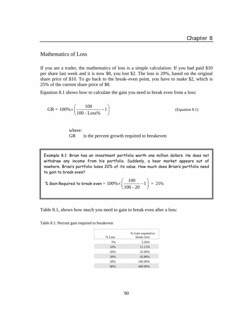
If you are a trader, the mathematics of loss is a simple calculation: If you had paid $10 per share last week and it is now $8, you lost $2. The loss is 20%, based on the original share price of $10. To go back to the break–even point, you have to make $2, which is 25% of the current share price of $8.
Equation 8.1 shows how to calculate the gain you need to break even from a loss:
GR = 100
100% 1100 - Loss%
(Equation 8.1)
where: GR is the percent growth required to breakeven
Example 8.1: Brian has an investment portfolio worth one million dollars. He does not withdraw any income from his portfolio. Suddenly, a bear market appears out of nowhere. Brian’s portfolio loses 20% of its value. How much does Brian’s portfolio need to gain to break even?
% Gain Required to break even = 100
100% 1100 - 20
= 25%
Table 8.1, shows how much you need to gain to break even after a loss: Table 8.1: Percent gain required to breakeven
% Loss % Gain required to
break even
5% 5.26%
10% 11.11%
20% 25.00%
30% 42.86%
50% 100.00%
80% 400.00%
91
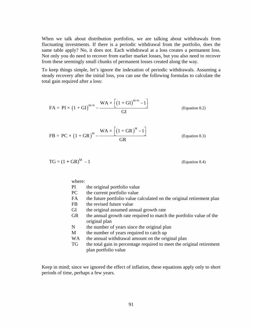
When we talk about distribution portfolios, we are talking about withdrawals from fluctuating investments. If there is a periodic withdrawal from the portfolio, does the same table apply? No, it does not. Each withdrawal at a loss creates a permanent loss. Not only you do need to recover from earlier market losses, but you also need to recover from these seemingly small chunks of permanent losses created along the way.
To keep things simple, let’s ignore the indexation of periodic withdrawals. Assuming a steady recovery after the initial loss, you can use the following formulas to calculate the total gain required after a loss:
FA = M+N
M+NWA × 1 + GI 1
PI × 1 + GIGI
(Equation 8.2)
FB = M
MWA × 1 + GR 1
PC × 1 + GRGR
(Equation 8.3)
TG = (1 + GR)M – 1 (Equation 8.4)
where: PI the original portfolio value PC the current portfolio value
FA the future portfolio value calculated on the original retirement plan FB the revised future value
GI the original assumed annual growth rate GR the annual growth rate required to match the portfolio value of the
original plan N the number of years since the original plan M the number of years required to catch up WA the annual withdrawal amount on the original plan
TG the total gain in percentage required to meet the original retirement plan portfolio value
Keep in mind; since we ignored the effect of inflation, these equations apply only to short periods of time, perhaps a few years.
92
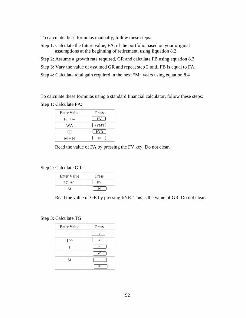
To calculate these formulas manually, follow these steps:
Step 1: Calculate the future value, FA, of the portfolio based on your original assumptions at the beginning of retirement, using Equation 8.2.
Step 2: Assume a growth rate required, GR and calculate FB using equation 8.3
Step 3: Vary the value of assumed GR and repeat step 2 until FB is equal to FA.
Step 4: Calculate total gain required in the next “M” years using equation 8.4
To calculate these formulas using a standard financial calculator, follow these steps:
Step 1: Calculate FA:
Enter Value Press
PI +/– PV
WA PYMT
GI I/YR
M + N N
Read the value of FA by pressing the FV key. Do not clear.
Step 2: Calculate GR:
Enter Value Press
PC +/– PV
M N
Read the value of GR by pressing I/YR. This is the value of GR. Do not clear.
Step 3: Calculate TG
Enter Value Press
/
100 +
1 =
yx
M –
=

93
Example 8.2
Steve retired 4 years ago. He then believed that stocks are for the long run. He had 100% equities in his portfolio. Originally, he had $1,000,000 in his portfolio. When he prepared his retirement plan four years ago, he assumed a long–term annual portfolio growth rate of 10%. He withdraws $60,000 annually from his portfolio.
Because of adverse market conditions and his periodic withdrawals totaling $240,000 over the last four years, his portfolio is now worth $610,000. Steve wants his portfolio to catch up with his original retirement plan in 3 years. Ignore inflation.
How much does Steve’s portfolio need to gain?
Step 1: Using a financial calculator, calculate FA
Enter Value Press 1,000,000 +/– PV
60,000 PYMT 10 I/YR 7 N
Read FA by pressing FV = 1,379,487. Do not clear.
Step 2: Calculate GR:
Enter Value Press 610,000 +/– PV
3 N
Read the value of GR by pressing I/YR = 39%. Do not clear.
Step 3: Calculate Total Gain using equation 8.4:
TG = [(1 + 39/100)3 – 1] x 100% = 169%
Steve’s portfolio needs to grow by 169% within the next 3 years to match his original retirement plan. Do you think this is possible?
Now, Steve thinks “Perhaps it is more realistic to expect a full recovery in five years instead of three”. Reworking numbers, Steve calculates that he needs a total gain of 238% over the next 5 years. Again, this is an unlikely return for a retirement portfolio.
Steve now understands the concept of mathematics of loss.
94
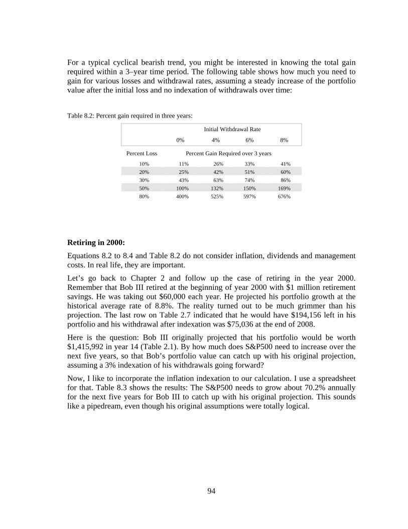
For a typical cyclical bearish trend, you might be interested in knowing the total gain required within a 3–year time period. The following table shows how much you need to gain for various losses and withdrawal rates, assuming a steady increase of the portfolio value after the initial loss and no indexation of withdrawals over time:
Table 8.2: Percent gain required in three years:
Initial Withdrawal Rate
0% 4% 6% 8%
Percent Loss Percent Gain Required over 3 years
10% 11% 26% 33% 41%
20% 25% 42% 51% 60%
30% 43% 63% 74% 86%
50% 100% 132% 150% 169%
80% 400% 525% 597% 676%
Retiring in 2000:
Equations 8.2 to 8.4 and Table 8.2 do not consider inflation, dividends and management costs. In real life, they are important.
Let’s go back to Chapter 2 and follow up the case of retiring in the year 2000. Remember that Bob III retired at the beginning of year 2000 with $1 million retirement savings. He was taking out $60,000 each year. He projected his portfolio growth at the historical average rate of 8.8%. The reality turned out to be much grimmer than his projection. The last row on Table 2.7 indicated that he would have $194,156 left in his portfolio and his withdrawal after indexation was $75,036 at the end of 2008.
Here is the question: Bob III originally projected that his portfolio would be worth $1,415,992 in year 14 (Table 2.1). By how much does S&P500 need to increase over the next five years, so that Bob’s portfolio value can catch up with his original projection, assuming a 3% indexation of his withdrawals going forward?
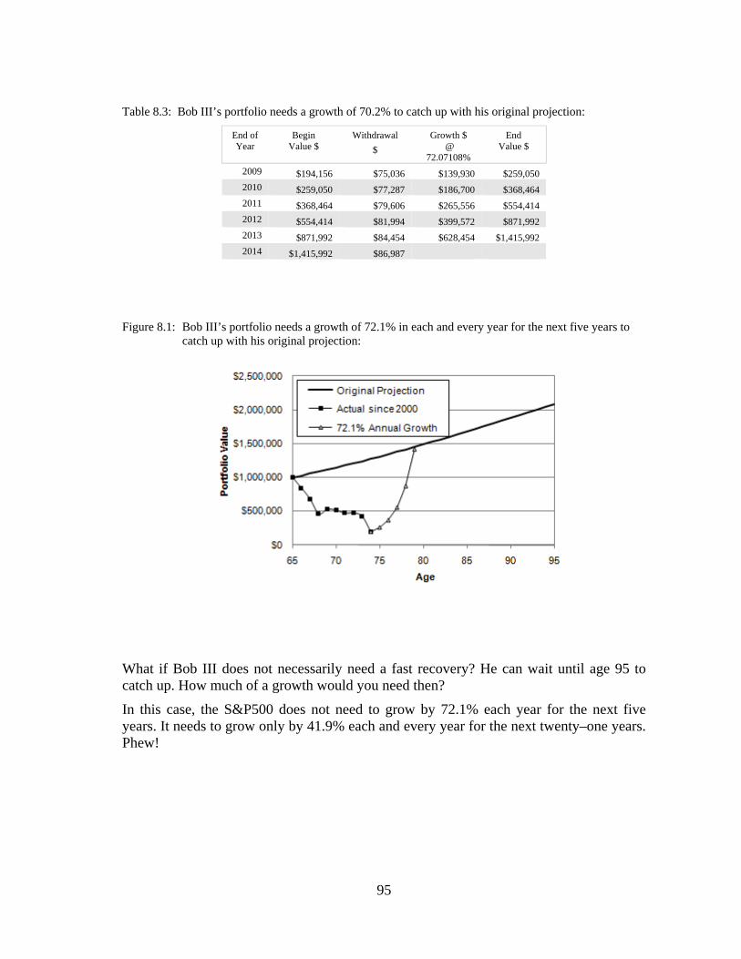
Now, I like to incorporate the inflation indexation to our calculation. I use a spreadsheet for that. Table 8.3 shows the results: The S&P500 needs to grow about 70.2% annually for the next five years for Bob III to catch up with his original projection. This sounds like a pipedream, even though his original assumptions were totally logical.
95
Table 8.3: Bob III’s portfolio needs a growth of 70.2% to catch up with his original projection:
End of Year
Begin Value $
Withdrawal
$
Growth $ @
72.07108%
End Value $
2009 $194,156 $75,036 $139,930 $259,050
2010 $259,050 $77,287 $186,700 $368,464
2011 $368,464 $79,606 $265,556 $554,414
2012 $554,414 $81,994 $399,572 $871,992
2013 $871,992 $84,454 $628,454 $1,415,992
2014 $1,415,992 $86,987
Figure 8.1: Bob III’s portfolio needs a growth of 72.1% in each and every year for the next five years to
catch up with his original projection:
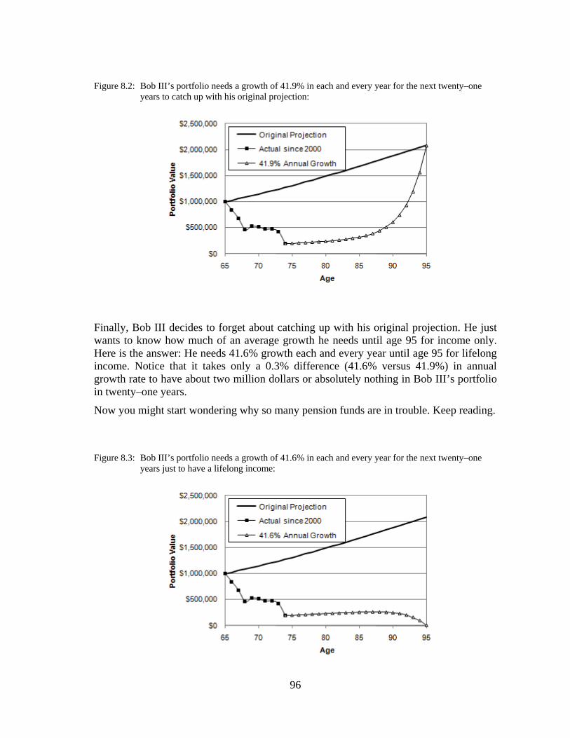
What if Bob III does not necessarily need a fast recovery? He can wait until age 95 to catch up. How much of a growth would you need then?
In this case, the S&P500 does not need to grow by 72.1% each year for the next five years. It needs to grow only by 41.9% each and every year for the next twenty–one years. Phew!
96
Figure 8.2: Bob III’s portfolio needs a growth of 41.9% in each and every year for the next twenty–one years to catch up with his original projection:
Finally, Bob III decides to forget about catching up with his original projection. He just wants to know how much of an average growth he needs until age 95 for income only. Here is the answer: He needs 41.6% growth each and every year until age 95 for lifelong income. Notice that it takes only a 0.3% difference (41.6% versus 41.9%) in annual growth rate to have about two million dollars or absolutely nothing in Bob III’s portfolio in twenty–one years.
Now you might start wondering why so many pension funds are in trouble. Keep reading.
Figure 8.3: Bob III’s portfolio needs a growth of 41.6% in each and every year for the next twenty–one
years just to have a lifelong income:
97
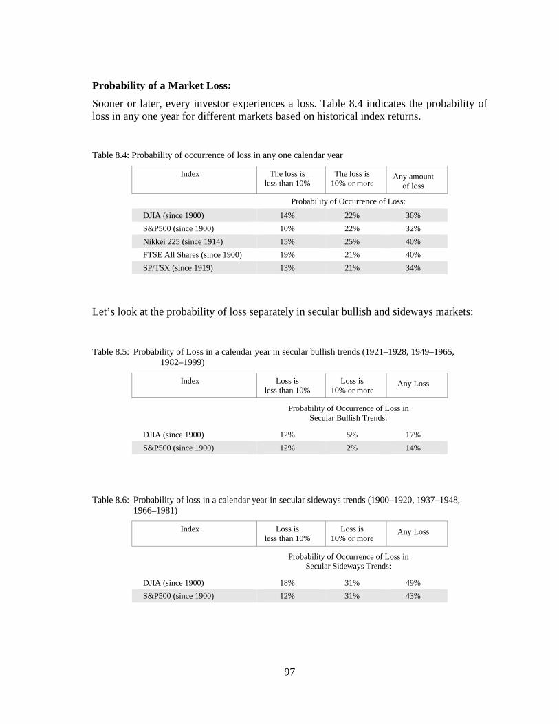
Probability of a Market Loss:
Sooner or later, every investor experiences a loss. Table 8.4 indicates the probability of loss in any one year for different markets based on historical index returns.
Table 8.4: Probability of occurrence of loss in any one calendar year
Index The loss is less than 10%
The loss is 10% or more
Any amount of loss
Probability of Occurrence of Loss:
DJIA (since 1900) 14% 22% 36%
S&P500 (since 1900) 10% 22% 32%
Nikkei 225 (since 1914) 15% 25% 40%
FTSE All Shares (since 1900) 19% 21% 40%
SP/TSX (since 1919) 13% 21% 34%
Let’s look at the probability of loss separately in secular bullish and sideways markets:
Table 8.5: Probability of Loss in a calendar year in secular bullish trends (1921–1928, 1949–1965, 1982–1999)
Index Loss is less than 10%
Loss is 10% or more
Any Loss
Probability of Occurrence of Loss in Secular Bullish Trends:
DJIA (since 1900) 12% 5% 17%
S&P500 (since 1900) 12% 2% 14%
Table 8.6: Probability of loss in a calendar year in secular sideways trends (1900–1920, 1937–1948, 1966–1981)
Index Loss is less than 10%
Loss is 10% or more
Any Loss
Probability of Occurrence of Loss in Secular Sideways Trends:
DJIA (since 1900) 18% 31% 49%
S&P500 (since 1900) 12% 31% 43%
98
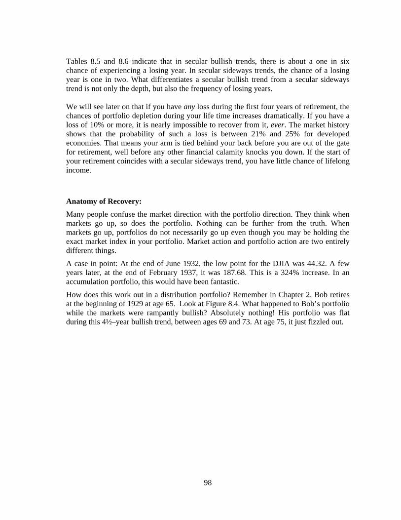
Tables 8.5 and 8.6 indicate that in secular bullish trends, there is about a one in six chance of experiencing a losing year. In secular sideways trends, the chance of a losing year is one in two. What differentiates a secular bullish trend from a secular sideways trend is not only the depth, but also the frequency of losing years. We will see later on that if you have any loss during the first four years of retirement, the chances of portfolio depletion during your life time increases dramatically. If you have a loss of 10% or more, it is nearly impossible to recover from it, ever. The market history shows that the probability of such a loss is between 21% and 25% for developed economies. That means your arm is tied behind your back before you are out of the gate for retirement, well before any other financial calamity knocks you down. If the start of your retirement coincides with a secular sideways trend, you have little chance of lifelong income.
Anatomy of Recovery:
Many people confuse the market direction with the portfolio direction. They think when markets go up, so does the portfolio. Nothing can be further from the truth. When markets go up, portfolios do not necessarily go up even though you may be holding the exact market index in your portfolio. Market action and portfolio action are two entirely different things.
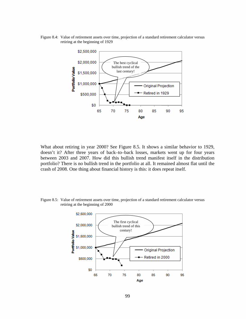
A case in point: At the end of June 1932, the low point for the DJIA was 44.32. A few years later, at the end of February 1937, it was 187.68. This is a 324% increase. In an accumulation portfolio, this would have been fantastic.
How does this work out in a distribution portfolio? Remember in Chapter 2, Bob retires at the beginning of 1929 at age 65. Look at Figure 8.4. What happened to Bob’s portfolio while the markets were rampantly bullish? Absolutely nothing! His portfolio was flat during this 4½–year bullish trend, between ages 69 and 73. At age 75, it just fizzled out.
99
Figure 8.4: Value of retirement assets over time, projection of a standard retirement calculator versus retiring at the beginning of 1929
What about retiring in year 2000? See Figure 8.5. It shows a similar behavior to 1929, doesn’t it? After three years of back–to–back losses, markets went up for four years between 2003 and 2007. How did this bullish trend manifest itself in the distribution portfolio? There is no bullish trend in the portfolio at all. It remained almost flat until the crash of 2008. One thing about financial history is this: it does repeat itself.
Figure 8.5: Value of retirement assets over time, projection of a standard retirement calculator versus retiring at the beginning of 2000
The first cyclical bullish trend of this
century!
The best cyclical bullish trend of the
last century!
100
After the first loss, the die is already cast. Even the strongest bullish trend cannot save a distribution portfolio from its eventual demise. A withdrawal rate of 4% prior to a market downturn jumps to 5% after a 20% loss and to 8% after a 50% loss.
Once the withdrawal rate exceeds 4%, a distribution portfolio does not go up when markets go up. If you watch your portfolio on a daily basis, you may see higher portfolio values after strong days and feel good about it. But at the end of the year, the most you can hope for is a flat portfolio value, even when markets might be soaring.
Here is how portfolios behave in various market trends:
MARKET TREND:
PORTFOLIO TREND:
Accumulation
Portfolio
Distribution Portfolio,
(Withdrawal rate over 4%)
Bearish Down Down
Sideways Sideways Down
Bullish Up Sideways or
Down
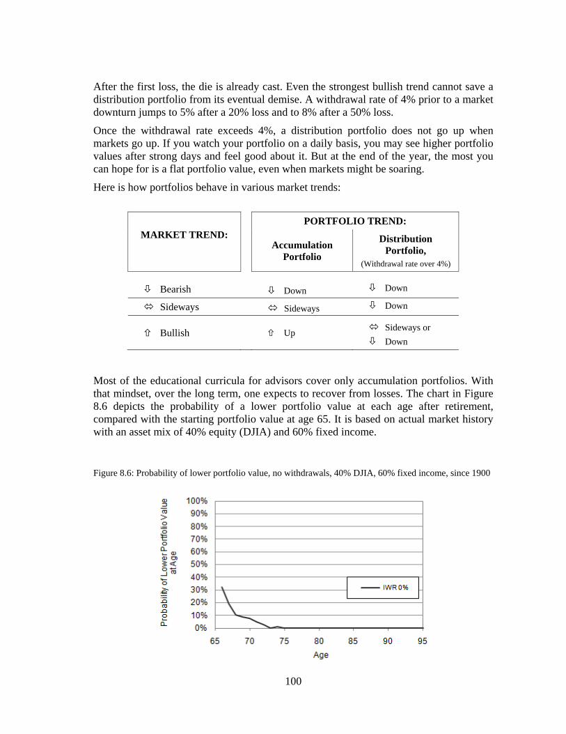
Most of the educational curricula for advisors cover only accumulation portfolios. With that mindset, over the long term, one expects to recover from losses. The chart in Figure 8.6 depicts the probability of a lower portfolio value at each age after retirement, compared with the starting portfolio value at age 65. It is based on actual market history with an asset mix of 40% equity (DJIA) and 60% fixed income.
Figure 8.6: Probability of lower portfolio value, no withdrawals, 40% DJIA, 60% fixed income, since 1900
101
The solid black line on the chart indicates that, if you have no withdrawals (IWR=0%), there was about a 32% chance of a lower portfolio value in the following year, at age 66. However, the portfolio inevitably recovered from the loss and the probability of a lower portfolio value came down to 0% at age 73. In other words, when there were no withdrawals, after eight years, you always had a higher portfolio value than the starting amount in a balanced portfolio.
What happens if there are withdrawals from the portfolio? Keep in mind, you don’t have to be retired for that. There are periodic withdrawals in accumulation portfolios too: fund fees, performance fees, management fees, trading costs and slippage, segregated fund guarantee costs, advisor fees, taxes and other leakages from your portfolio all create “withdrawals” continuously. These costs create de facto periodic withdrawals anywhere between 1% and 5%, depending on what you invest in, even in accumulation portfolios.
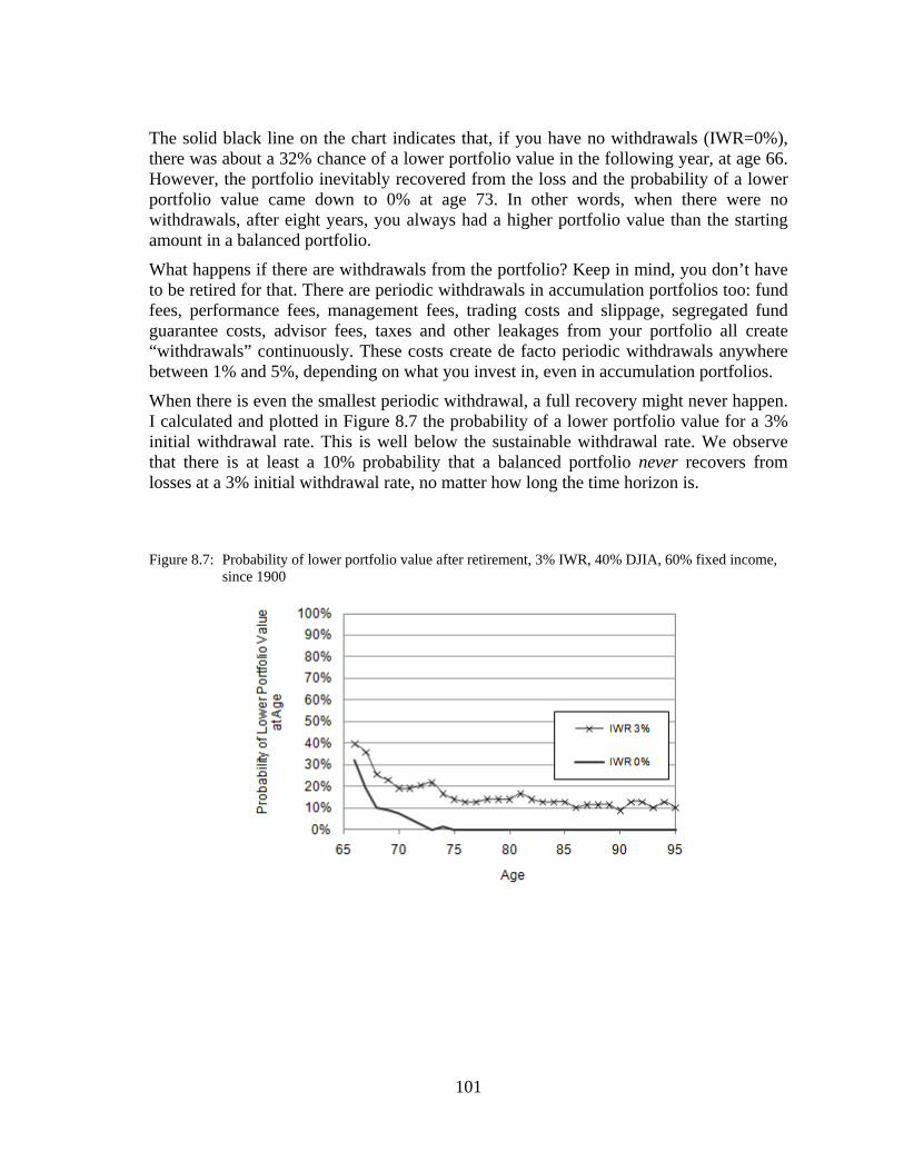
When there is even the smallest periodic withdrawal, a full recovery might never happen. I calculated and plotted in Figure 8.7 the probability of a lower portfolio value for a 3% initial withdrawal rate. This is well below the sustainable withdrawal rate. We observe that there is at least a 10% probability that a balanced portfolio never recovers from losses at a 3% initial withdrawal rate, no matter how long the time horizon is.
Figure 8.7: Probability of lower portfolio value after retirement, 3% IWR, 40% DJIA, 60% fixed income,
since 1900
102
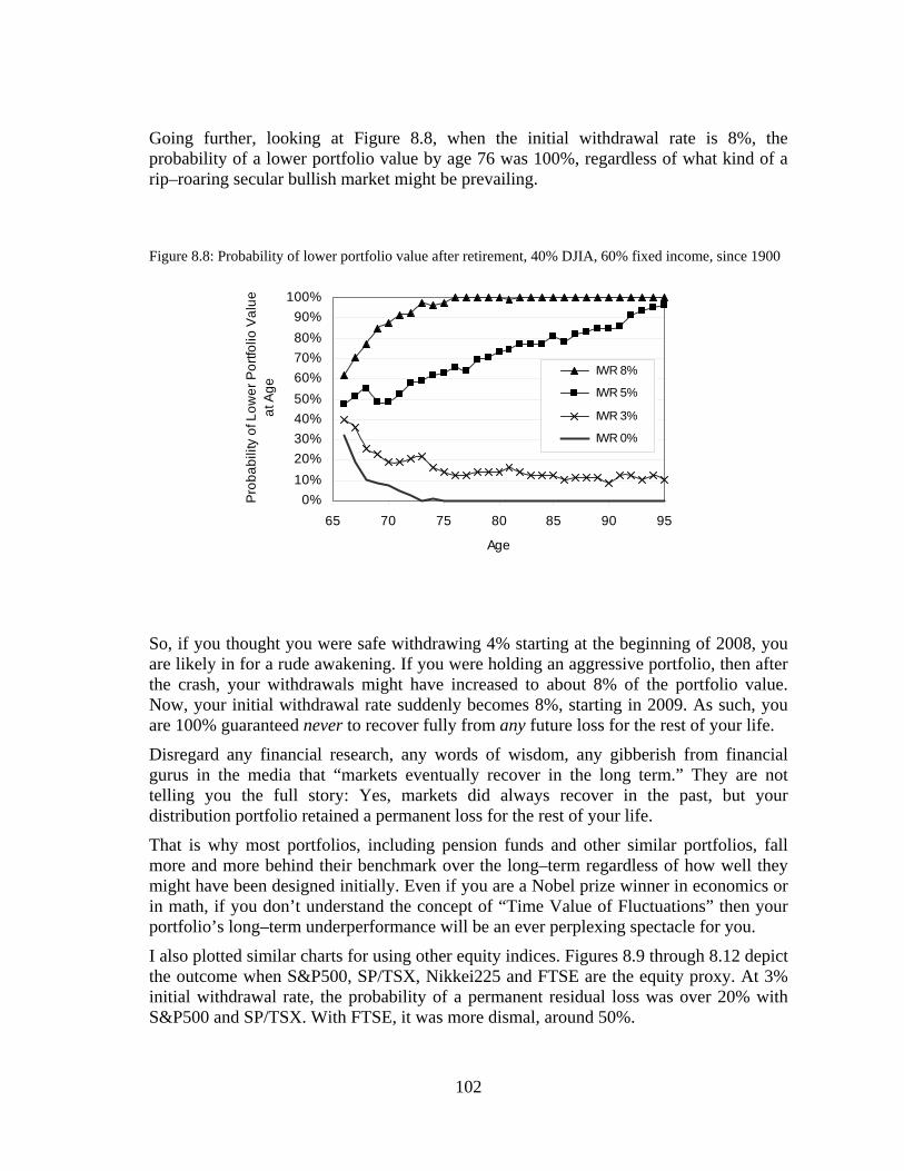
Going further, looking at Figure 8.8, when the initial withdrawal rate is 8%, the probability of a lower portfolio value by age 76 was 100%, regardless of what kind of a rip–roaring secular bullish market might be prevailing.
Figure 8.8: Probability of lower portfolio value after retirement, 40% DJIA, 60% fixed income, since 1900
So, if you thought you were safe withdrawing 4% starting at the beginning of 2008, you are likely in for a rude awakening. If you were holding an aggressive portfolio, then after the crash, your withdrawals might have increased to about 8% of the portfolio value. Now, your initial withdrawal rate suddenly becomes 8%, starting in 2009. As such, you are 100% guaranteed never to recover fully from any future loss for the rest of your life.
Disregard any financial research, any words of wisdom, any gibberish from financial gurus in the media that “markets eventually recover in the long term.” They are not telling you the full story: Yes, markets did always recover in the past, but your distribution portfolio retained a permanent loss for the rest of your life.
That is why most portfolios, including pension funds and other similar portfolios, fall more and more behind their benchmark over the long–term regardless of how well they might have been designed initially. Even if you are a Nobel prize winner in economics or in math, if you don’t understand the concept of “Time Value of Fluctuations” then your portfolio’s long–term underperformance will be an ever perplexing spectacle for you.
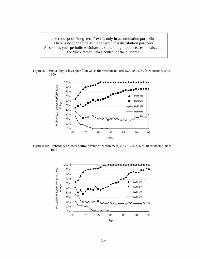
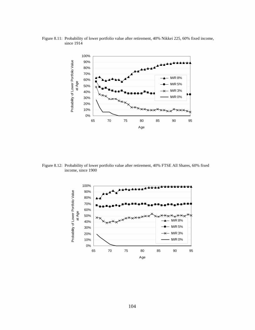
I also plotted similar charts for using other equity indices. Figures 8.9 through 8.12 depict the outcome when S&P500, SP/TSX, Nikkei225 and FTSE are the equity proxy. At 3% initial withdrawal rate, the probability of a permanent residual loss was over 20% with S&P500 and SP/TSX. With FTSE, it was more dismal, around 50%.
0%
10%
20%
30%
40%
50%
60%
70%
80%
90%
100%
65 70 75 80 85 90 95
Age
Pro
ba
bili
ty o
f Lo
we
r P
ort
folio
Va
lue
at A
ge
IWR 8%
IWR 5%
IWR 3%
IWR 0%
103
The concept of “long–term” exists only in accumulation portfolios. There is no such thing as “long term” in a distribution portfolio.
As soon as your periodic withdrawals start, “long–term” ceases to exist, and the “luck factor” takes control of the outcome.
Figure 8.9: Probability of lower portfolio value after retirement, 40% S&P500, 60% fixed income, since
1900
Figure 8.10: Probability of lower portfolio value after retirement, 40% SP/TSX, 60% fixed income, since 1919
0%
10%
20%
30%
40%
50%
60%
70%
80%
90%
100%
65 70 75 80 85 90 95
Age
Pro
babi
lity
of L
ower
Por
tfolio
Val
ue
at A
ge
IWR 8%
IWR 5%
IWR 3%
IWR 0%
0%
10%
20%
30%
40%
50%
60%
70%
80%
90%
100%
65 70 75 80 85 90 95
Age
Pro
babi
lity
of L
ower
Por
tfolio
Val
ue
at A
ge
IWR 8%
IWR 5%
IWR 3%
IWR 0%
104
Figure 8.11: Probability of lower portfolio value after retirement, 40% Nikkei 225, 60% fixed income, since 1914
Figure 8.12: Probability of lower portfolio value after retirement, 40% FTSE All Shares, 60% fixed income, since 1900
0%
10%
20%
30%
40%
50%
60%
70%
80%
90%
100%
65 70 75 80 85 90 95
Age
Pro
babi
lity
of L
ower
Por
tfolio
Val
ue
at A
ge IWR 8%
IWR 5%
IWR 3%
IWR 0%
0%
10%
20%
30%
40%
50%
60%
70%
80%
90%
100%
65 70 75 80 85 90 95
Age
Pro
babi
lity
of L
ower
Por
tfolio
Val
ue
at A
ge
IWR 8%
IWR 5%
IWR 3%
IWR 0%

105
Conclusion:
So you thought that “markets always go up in the long term!” That is fine. You can continue thinking that way. The thing is, while markets go up, your distribution portfolio will not follow it up. This minor detail can deplete it in a very short time.
If you are following a “buy–and–hold” strategy and the initial withdrawal rate exceeds 3%, there is a good chance that your portfolio might never recover fully, even from routine fluctuations. The losses become permanent, even in the presence of strong bullish trends or a multi–country diversification.
Do not lose, give away, donate, part with, gift, help out or misplace any retirement savings, especially during the early years of retirement. I have homework for you: every morning, take a blank piece of paper. Write on it:
Don’t lose today!
Read it to yourself throughout the day during your breaks. My best investment ever was a little sticky paper on my computer screen, where I do my occasional stock trades. It reads: “Greed kills”. I pay attention to it.
Sometimes, investors tell me that they watch their investments very carefully and closely. That is great. However, the most effective way of containing the risk is the “bet” size. It should be small enough so that if you lose half of that particular investment, your retirement plan should not be derailed. If the “bet” size is the cake, watching it closely is only the icing on that cake.
In a distribution portfolio, there are three different luck factors that create permanent losses:
Sequence of Returns Inflation, and Reverse Dollar Cost Averaging
In the next four chapters, we go into more detail about each of these topics.