Pattern Recognition Letters 32 (2011) 1532–1540

Contents lists available at ScienceDirect

Pattern Recognition Letters

journal homepage: www.elsevier .com/locate /patrec

Unsupervised multi-class segmentation of SAR images using triplet Markovfields models based on edge penalty

Yan Wu a,⇑, Ming Li b, Peng Zhang b, Haitao Zong a, Ping Xiao c, Chunyan Liu a

a School of Electronics Engineering, Xidian University, Xi’an 710071, Chinab National Key Lab. of Radar Signal Processing, Xidian University, Xi’an 710071, Chinac Shaanxi Bureau of Surveying and Mapping, No.334, Youyi east Road, Xi’an 710054, China

a r t i c l e i n f o

Article history:Received 21 October 2009Available online 18 April 2011Communicated by S. Aksoy

Keywords:SAR imageMulti-class segmentationTriplet Markov random field (TMF)New energy functionEdge penaltyMulti-region merging

0167-8655/$ - see front matter � 2011 Elsevier B.V. Adoi:10.1016/j.patrec.2011.04.009

⇑ Corresponding author.E-mail address: ywu@mail.xidian.edu.cn (Y. Wu).

a b s t r a c t

Non-Gaussian triplet Markov random fields (TMF) model is suitable for dealing with multi-class segmen-tation of nonstationary and non-Gaussian synthetic aperture radar (SAR) images. However, the segmen-tation of SAR images utilizing this model still fails to resolve the misclassifications due to the inaccuracyof edge location. In this paper, we propose a new unsupervised multi-class segmentation algorithm byfusing the traditional energy function of TMF model with the principle of edge penalty. Through the intro-duction of the penalty function based on local edge strength information, the new energy function couldprevent segment from smoothing across boundaries. Then we optimize the objective function that stemsfrom the new energy function to obtain an iterative multi-region merging Bayesian maximum posteriormode (MPM) segmentation equation for the new segmentation algorithm. The effectiveness of the pro-posed algorithm is demonstrated by application to simulated data and real SAR images.

� 2011 Elsevier B.V. All rights reserved.

1. Introduction

Since the nineties, along with the gradual improvement of thebasic research of synthetic aperture radar (SAR) imaging and thesuccessful development and application of many space-borneand airborne SAR systems, such as ERS21 and NASA/JPL Air SAR,a large number of high-quality SAR images have been received. Itis well known that SAR image influenced by speckle noise inher-ently has the characteristics of non-Gaussian and nonstationary.

SAR system mainly focuses on how to detect and identify tar-gets from SAR images which contain speckle noise. Recently, theimportant area of research is SAR image understanding. However,different from the optical imaging system, SAR is the coherentmicrowave imaging system and its image data reflects the localinteraction between imaging region and incident electromagneticwave, which is difficult to visually interpret. In order to obtainthe information about the SAR image region, we must interpretSAR image effectively.

SAR image segmentation technology is an important part ofinterpretation and recognition, which can provide the overallstructure of the image information. It establishes the basis of auto-matic target recognition (ATR) and promotes SAR applications. Inrecent years, this area has gradually become a research hotspot

ll rights reserved.

in both international and domestic (Tison et al., 2004; Destrempesand Mignotte, 2004; Benboudjema et al., 2007; Pieczynski andTebbache, 2000; Descombes et al., 1999). Hidden Markov fields(HMF) have been widely used for image segmentation, becausethey provide a powerful and formal way to introduce the informa-tion about the mutual influences among image pixels into the seg-mentation procedure. However, HMF is too simple to deal with alarge number of complex images (nonstationary image, texture im-age, strong noisy image). It does obtain satisfactory results (Poggiet al., 2005; Tran et al., 2005; Kumar and Hebert, 2006) when deal-ing with stationary images. But it is powerless to nonstationarySAR images. So far its own statistical model has been constantlyexpanded and improved, which allows us to deal with nonstation-ary images and correlated non-Gaussian noise better. One of theeffective extensions of HMF is the triplet Markov fields (TMF)(Benboudjema and Pieczynski, 2005), which describes the statisti-cal characteristic of SAR images better.

HMF model comprises two random fields X and Y, in which X isunobservable (or hidden), and must be estimated from the ob-served Y. The posterior distribution p(xjy) is a Markov distribution,which affords different Bayesian processing. However, when deal-ing with the segmentation of images containing numerous classeswith different textures, the simple form of the distribution p(yjx) isdissatisfactory and has to be replaced by a Markov field distribu-tion. Consequently, pairwise Markov field (PMF) model is pro-posed, which directly considers that the pair Z = (X,Y) is aMarkov field (Pieczynski and Tebbache, 2000). This implies that

Fig. 1. Possible nonstationarity of the distribution p(x, y) (a) observed Y and (b) fieldU = u.

Y. Wu et al. / Pattern Recognition Letters 32 (2011) 1532–1540 1533

both conditional distributions p(yjx) and p(xjy) are Markovian: Theformer fact allows one to better model complex noises and the lat-ter one still enables one to apply Bayesian segmentation. Then,TMF model which introduces a third random field U is proposedand the triplet T = (X, Y, U) is assumed to be Markovian(Benboudjema and Pieczynski, 2007; Benboudjema et al., 2007).One possible meaning for U is to define different homogeneitiesof (X,Y). This means that the Markov field distribution p(x, yju) isa nonstationary field and the m possible values of U describe m dif-ferent Markov stationarity of (X,Y). Consequently this model isvery suitable for dealing with the nonstationary SAR images whichusually contain complex textural configuration.

For nonstationary and non-Gaussian SAR images, the segmenta-tion method based on the TMF model is superior to the one basedon classical HMF model, however, the segmentation of SAR imagesbased on the TMF model still has small error blocks or single errorpixel in the smooth area due to the inaccurate edge location. Usu-ally edge appears as discontinuities in pixel intensity within theimage, so we introduce a penalty function based on local edgestrength into the TMF energy function, which could suppress theedge fuzzy and provide accurate edge location. Then an iterativemulti-region merging Bayesian maximum posterior mode (MPM)segmentation equation is educed for segmentation. Simulated dataand real SAR images are applied to validate the effectiveness of theproposed algorithm. Experimental results and analysis indicatethat compared with the segmentation algorithms based on theclassical HMF and the recent TMF models, the proposed algorithmeffectively improves the segmentation accuracy of the SAR imagewhile reducing the influence of multiplicative speckle noise, withthe weak edge location being more accurate especially.

2. Non-Gaussian triplet Markov fields model

Let S be the set of pixels. The HMF model contains two randomfields defined on S, X = (Xs)s2S and Y = (Ys)s2S. The random fieldsX = (Xs)s2S and Y = (Ys)s2S take their values in X = {x1, . . . ,xk} andR, respectively. The problem of the statistical segmentation is to re-cover unobservable X = (Xs)s2S from the observed Y = (Ys)s2S (Derinand Elliott, 1987; Poggi et al., 2005; Tran et al., 2005; Geman andGeman, 1984). Therefore, Y = (Ys)s2S can be seen as a noisy versionof X = (Xs)s2S.

In the classical HMF context, the distribution of (X,Y) is definedby some functions specified on cliques. Pairwise random field (X,Y)will be considered nonstationary in the probabilistic and spatialconfiguration sense when these functions depend on the positionof the cliques. The possible nonstationarity of the distributionp(x, y) of the pairwise field (X,Y) is managed by introducing a thirdrandom field U = (Us)s2S (Benboudjema et al., 2007), each Us takingits values from a finite set K = (k1, . . . ,km). Thus the m possible val-ues of Us can be interpreted as m different possible stationarities of(X,Y). Then we can say that pairwise random field (X,Y) is m-Mar-kov nonstationary (m-MNS) (Benboudjema and Pieczynski, 2007).When the third random field U = (Us)s2S is introduced, the tripletT = (X, U, Y) is a stationary Markov field because the distributionp(x, u, y) does not depend on the position of the cliques. Howeveran m-MNS field (X,Y) is nonstationary conditionally on U. That is tosay the Markov field distribution p(x,yju) and p(xju) will depend onthe position of the cliques. Consequently, the distribution p(xju) isnonstationary while the distribution p(x, u) is stationary.

Here, we describe the third random field U further. As shown inFig. 1, let K = (a, b), the nonstationarity of Fig. 1(a) can be seen inFig. 1(b). For the third random field U, it has its own physical inter-pretation. For example, the image can be segmented to two classes,houses and trees. And there are two regions in the scene, ‘‘town’’and ‘‘outside town’’, with both of the two classes existing in each

region. However the distribution of the trees or houses (the ran-dom field of classes) is different in ‘‘town’’ and ‘‘outside town’’,which results in the nonstationary of the whole scene. Here, therandom field U can be introduced to model ‘‘town’’ and ‘‘outsidetown’’ by two stationarities, u1 = a and u2 = b, thus modeling thetwo possibilities.

Following section will introduce the triplet Markov field model.First, let us consider the very classical Markov field X = (Xs)s2S

whose distribution is defined by the energy (Benboudjema andPieczynski, 2007):

WðxÞ ¼Xðs;tÞ2cH

aHð1� 2dðxs; xtÞÞ þXðs;tÞ2cv

avð1� 2dðxs; xtÞÞ; ð1Þ

where s and t are neighboring sites forming a pair-site clique, and cH

is the set of couples of pixels horizontally neighbors, cV is the set ofcouples of pixels vertically neighbors, and d(xs, xt) verifies as:

dðxs; xtÞ ¼1 if xs ¼ xt;

0 if xs – xt:

�ð2Þ

Furthermore, we assume that the random variables Y = (Ys)s2S

are independent conditionally on X = (Xs)s2S. In addition, we havep(ysjx) = p(ysjxs) for each s and xs. Thus, (X,Y) is a classical HMFwhose distribution is as follows (Benboudjema et al., 2007):

pðx; yÞ ¼ c exp �WðxÞ þXs2S

LogðpðysjxsÞÞ" #

: ð3Þ

Now, assume that this classical model is not stationary and itsdifferent possible stationarities can be described by the third ran-dom field U = (Us)s2S. Note that the random field U = (Us)s2S shouldbe simple enough (finite with less than ten elements) to makeBayesians processing possible. In TMF model, for simplicity andwithout loss of generality, we consider two different stationaritiesand the random field U = (Us)s2S takes its value from the set K = (a,b). We will assume that (X, U) is a Markov field and the distributionof Y conditional on (X, U) verifies the classical conditionpðyjx;uÞ ¼

Qs2SpðysjxsÞ . Then the distribution of T = (X, U, Y) is

Markovian. The distribution of the Markov field (X, U) is definedby the energy (Benboudjema et al., 2007; Benboudjema andPieczynski, 2007).

Wðx;uÞ ¼Xðs;tÞ2CH

a1Hð1� 2dðxs; xtÞÞ � ða2

aHd�ðus;ut; aÞ

þ a2bHd�ðus;ut; bÞÞð1� dðxs; xtÞÞ þ

Xðs;tÞ2CV

a1V ð1� 2dðxs; xtÞÞ

� ða2aVd�ðus;ut ; aÞ þ a2

bVd�ðus;ut ; bÞÞð1� dðxs; xtÞÞ; ð4Þ

where

1534 Y. Wu et al. / Pattern Recognition Letters 32 (2011) 1532–1540

d�ðus;ut; aÞ ¼1 if ðus ¼ ut ¼ a;

0 otherwise:

�

d�ðus;ut ; bÞ ¼1 if ðus ¼ ut ¼ b;

0 otherwise:

�ð5Þ

Finally, let us define the distribution of the triplet T = (X, U, Y) byBenboudjema and Pieczynski (2007)

pðx;u; yÞ ¼ c exp½�Wðx;uÞ þXs2S

LogðpðysjxsÞÞ�: ð6Þ

In fact, the distribution p(xju) is Markovian with the energyPc2Cf u

c ðxcÞ , where c = (s, t) is either a horizontal or vertical clique.For horizontal cliques, we have

f ucHðxcÞ ¼

a1Hð1� 2dðxs; xtÞÞ � a2

aHð1� dðxs; xtÞÞ us ¼ ut ¼ a;

a1Hð1� 2dðxs; xtÞÞ � a2

aHð1� dðxs; xtÞÞ us ¼ ut ¼ b;

a1Hð1� 2dðxs; xtÞÞ us – ut :

8><>:

ð7Þ

And for vertical cliques, we have

f ucV ðxcÞ ¼

a1V ð1� 2dðxs; xtÞÞ � a2

bV ð1� dðxs; xtÞÞ us ¼ ut ¼ a;

a1V ð1� 2dðxs; xtÞÞ � a2

bV ð1� dðxs; xtÞÞ us ¼ ut ¼ b;

a1V ð1� 2dðxs; xtÞÞ us–ut :

8><>:

ð8Þ

Furthermore let us consider the case that the random variablesY = (Ys)s2S are not independent given X = (Xs)s2S, and the distribu-tions p(ysjxs) would not be necessarily Gaussian (Lombardo andFarina, 1996). Assuming that there are K classes X = {x1, . . . ,xk},we want to have densities h1, . . . ,hk for the distributions: p(ys

jxs = x1), . . . ,p(ysjxs = xk). Of particular note, the K densitiesh1, . . . ,hk, possibly of different forms, can take any desired formand without loss of generality, Gamma-distribution has been takenin the experiments. Let G be the cumulative distribution functionof Gaussian zero-mean variable with variance one and letH1, . . . ,Hk be the cumulative distribution functions correspondingto h1, . . . ,hk.

Consider the following Markov random field (X,Y):

1. Take a Markov field X with the energy W;2. Y 0 ¼ Y 0s

� �s2S is assumed to be Gaussian Markov random field,

where each Y 0s is zero-mean and one-variance Gaussian randomvariable;

pðy0Þ ¼ c exp �12

Xs2S

ðy0sÞ2 �

Xðs;tÞ2C

b1y0sy0t

!" #

¼ c exp½�W 0ðy0Þ�: ð9Þ

3. For each s 2 S, set Ys ¼ H�1xs� G Y 0s� �

; We can get the distribu-tions of (X,Y) as follows:

pðx; yÞ ¼ c exp

"�WðxÞ �W 0ðuðx; yÞÞ

þXs2S

Log@ðG�1 � Hxs ðysÞÞ

@ys

����������#; ð10Þ

where uðx; yÞ ¼ y0 ¼ y0s� �

s2S and y0s ¼ G�1 � Hxs ðysÞ for each s 2 S.

Finally, the distribution of the triplet (X, U, Y) is defined by

pðx;u; yÞ ¼ c exp �Wðx;uÞ �W 0ðuðx; yÞÞ þXs2S

Log@ðG�1Hxs ðysÞÞ

@ys

����������

" #:

ð11Þ

Either classical HMF model given by Eq. (3) and or TMF modelsgiven by Eqs. (6) and (11) enable one to estimate p(xsjy). In HMF,this is classically done using the Gibbs sampler (Geman andGeman, 1984) and, in TMF this is done in two steps (Benboudjemaand Pieczynski, 2007): (1) estimate p(xs, usjy) by the Gibbs samplerand (2) calculate pðxsjyÞ ¼

Pus2Kpðxs;usjyÞ . Therefore, the Bayesian

MPM can be used in both HMF and TMF given by Eqs. (3) and (11),respectively.

3. Unsupervised multi-class segmentation of SAR images usingtriplet Markov fields models based on edge penalty

In this section we propose a new segmentation algorithm,which is applied to unsupervised multi-class segmentation ofSAR images. The new algorithm fuses traditional triplet Markovfield models and the principle of edge penalty. The edge criterioncan suppress the edge fuzzy and provide accurate edge location(Pham and Zung, 2004; Descombes et al., 1999) because it couldprevent the TMF algorithm from smoothing across boundaries.Consequently in the new algorithm, the local feature of edgestrength is incorporated into the TMF energy function. Instead ofpenalizing equally to all boundary site pairs, we implement anew penalty principle, that actualizes greater penalty to weakedges and lesser to strong ones, to successfully maintain the weakedges. Then we optimize the objective function that stems fromthe new energy function to obtain an iterative multi-region merg-ing Bayesian MPM segmentation equation for the new segmenta-tion algorithm. We will derive the new energy function based onedge penalty in Section 3.1, and obtain the final segmentation bythe Bayesian MPM using iterative region merging in Section 3.2. Fi-nally, we will detail the parameter estimation procedure of theproposed algorithm in Section 3.3.

3.1. Derivation of the new energy function based on edge penalty

For the multi-class segmentation of SAR images, especiallyincluding weak edges, the segmentation of images based on TMFmay not match the real objects well and even produces misclassi-fications in local place sometimes. If we introduce the local featureof edge strength into the TMF energy function, which maintainsthe local edge information well, we could obtain accurate segmen-tation results. Here we introduce how to incorporate the local fea-ture of edge strength into the TMF energy function.

We can change Eq. (4) to the following form:

Wðx;uÞ ¼Xðs;tÞ2CH

a1Hð1�2dðxs;xtÞÞ � ða1

aHd�ðus;ut ;aÞ

þ a2bHd�ðus;ut ;bÞÞð1� dðxs;xtÞÞ þ

Xðs;tÞ2CV

a1V ð1�2dðxs;xtÞÞ

� ða1aVd�ðus;ut ;aÞ þa2

bVd�ðus;ut;bÞÞð1� dðxs;xtÞÞ¼Xðs;tÞ2C

a1ð1�2dðxs;xtÞÞ � ða1ad�ðus;ut;aÞ

þ a2bd�ðus;ut;bÞÞð1� dðxs;xtÞÞ

¼Xðs;tÞ2C

a1ð1�2dðxs;xtÞÞ �Xðs;tÞ2C

ða1ad�ðus;ut ;aÞ

þ a2bd�ðus;ut;bÞÞð1� dðxs;xtÞÞ; ð12Þ

where a1 ¼ a1H;a1

V

� �; a1

a ¼ a1aH;a1

aV

� �; a2

b ¼ a2bH;a2

bV

� �. a1 with sub-

script H denotes the model parameter in the horizontal directionwhile the one with subscript V denotes the vertical parameter.They consist of the whole model parameters a1. It is the same as a1

a

and a2b .

The second term of Eq. (12) demonstrates the role of randomfield U = (Us)s2S in modeling energy function, we utilize V toexpress it:

Y. Wu et al. / Pattern Recognition Letters 32 (2011) 1532–1540 1535

Vðxs; xt ;us;utÞ ¼ a1ad�ðus; ut ; aÞ

�þ a2

bd�ðus;ut ; bÞ

�ð1� dðxs; xtÞÞ:

ð13Þ

Eq. (13) can be rewritten by:

Vðxs;xt ;us;utÞ ¼V1ðxs;xt ;us;utÞ ¼ a1

að1� dðxs;xtÞÞ; if ðus ¼ ut ¼ aÞ;V2ðxs;xt ;us;utÞ ¼ a2

bð1� dðxs;xtÞÞ; if ðus ¼ ut ¼ bÞ;0; otherwise:

8><>: ð14Þ

V1ðxs; xt ;us;utÞ ¼a1

a ; if ðxs – xtÞ;0; otherwise;

(

V2ðxs; xt ;us;utÞ ¼a2

b ; if ðxs – xtÞ;0; otherwise;

( ð15Þ

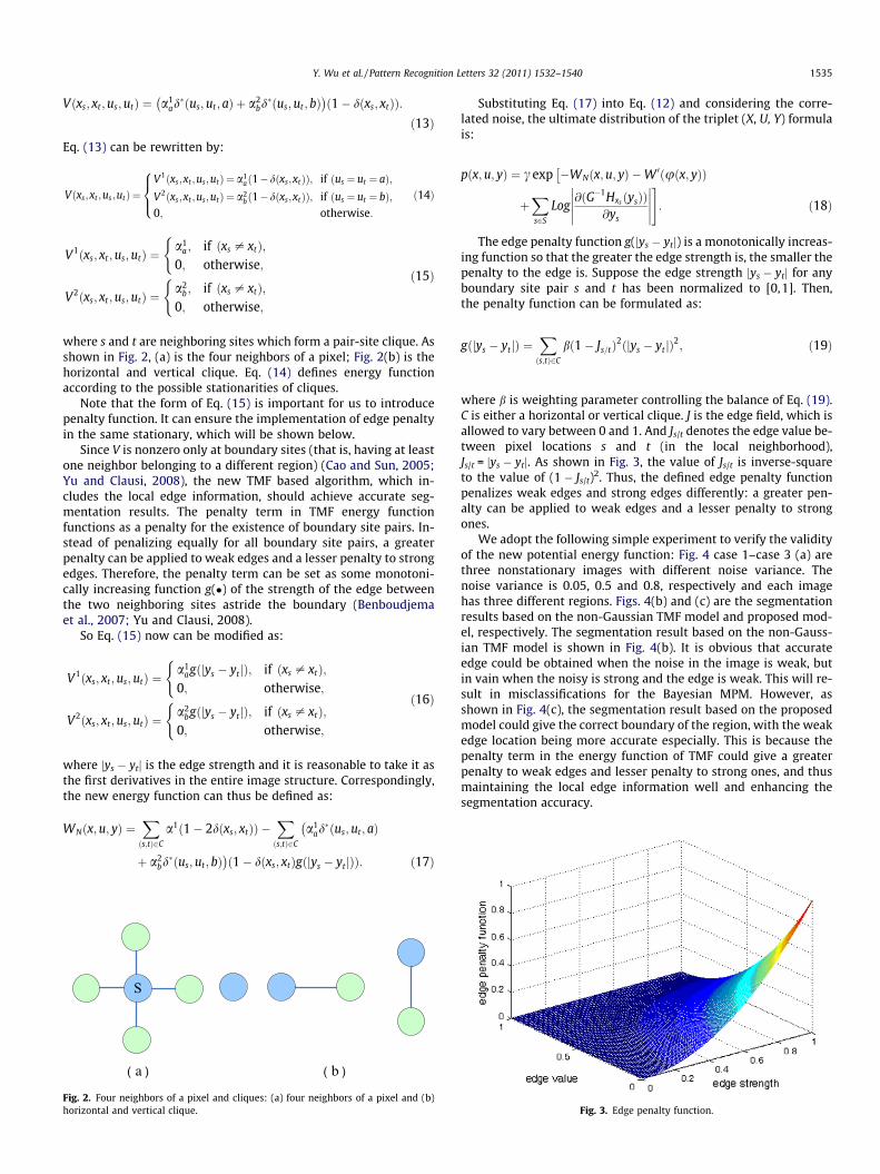
where s and t are neighboring sites which form a pair-site clique. Asshown in Fig. 2, (a) is the four neighbors of a pixel; Fig. 2(b) is thehorizontal and vertical clique. Eq. (14) defines energy functionaccording to the possible stationarities of cliques.

Note that the form of Eq. (15) is important for us to introducepenalty function. It can ensure the implementation of edge penaltyin the same stationary, which will be shown below.

Since V is nonzero only at boundary sites (that is, having at leastone neighbor belonging to a different region) (Cao and Sun, 2005;Yu and Clausi, 2008), the new TMF based algorithm, which in-cludes the local edge information, should achieve accurate seg-mentation results. The penalty term in TMF energy functionfunctions as a penalty for the existence of boundary site pairs. In-stead of penalizing equally for all boundary site pairs, a greaterpenalty can be applied to weak edges and a lesser penalty to strongedges. Therefore, the penalty term can be set as some monotoni-cally increasing function g(�) of the strength of the edge betweenthe two neighboring sites astride the boundary (Benboudjemaet al., 2007; Yu and Clausi, 2008).

So Eq. (15) now can be modified as:

V1ðxs; xt;us;utÞ ¼a1

agðjys � yt jÞ; if ðxs – xtÞ;0; otherwise;

(

V2ðxs; xt;us;utÞ ¼a2

bgðjys � yt jÞ; if ðxs – xtÞ;0; otherwise;

( ð16Þ

where jys � ytj is the edge strength and it is reasonable to take it asthe first derivatives in the entire image structure. Correspondingly,the new energy function can thus be defined as:

WNðx;u; yÞ ¼Xðs;tÞ2C

a1ð1� 2dðxs; xtÞÞ �Xðs;tÞ2C

a1ad�ðus; ut; aÞ

�þ a2

bd�ðus; ut; bÞ

�ð1� dðxs; xtÞgðjys � ytjÞÞ: ð17Þ

a b

Fig. 2. Four neighbors of a pixel and cliques: (a) four neighbors of a pixel and (b)horizontal and vertical clique.

Substituting Eq. (17) into Eq. (12) and considering the corre-lated noise, the ultimate distribution of the triplet (X, U, Y) formulais:

pðx;u; yÞ ¼ c exp �WNðx;u; yÞ �W 0ðuðx; yÞÞ�

þXs2S

Log@ðG�1Hxs ðysÞÞ

@ys

����������#: ð18Þ

The edge penalty function g(jys � ytj) is a monotonically increas-ing function so that the greater the edge strength is, the smaller thepenalty to the edge is. Suppose the edge strength jys � ytj for anyboundary site pair s and t has been normalized to [0,1]. Then,the penalty function can be formulated as:

gðjys � ytjÞ ¼Xðs;tÞ2C

bð1� Js=tÞ2ðjys � yt jÞ

2; ð19Þ

where b is weighting parameter controlling the balance of Eq. (19).C is either a horizontal or vertical clique. J is the edge field, which isallowed to vary between 0 and 1. And Js/t denotes the edge value be-tween pixel locations s and t (in the local neighborhood),Js/t = jys � ytj. As shown in Fig. 3, the value of Js/t is inverse-squareto the value of (1 � Js/t)2. Thus, the defined edge penalty functionpenalizes weak edges and strong edges differently: a greater pen-alty can be applied to weak edges and a lesser penalty to strongones.

We adopt the following simple experiment to verify the validityof the new potential energy function: Fig. 4 case 1–case 3 (a) arethree nonstationary images with different noise variance. Thenoise variance is 0.05, 0.5 and 0.8, respectively and each imagehas three different regions. Figs. 4(b) and (c) are the segmentationresults based on the non-Gaussian TMF model and proposed mod-el, respectively. The segmentation result based on the non-Gauss-ian TMF model is shown in Fig. 4(b). It is obvious that accurateedge could be obtained when the noise in the image is weak, butin vain when the noisy is strong and the edge is weak. This will re-sult in misclassifications for the Bayesian MPM. However, asshown in Fig. 4(c), the segmentation result based on the proposedmodel could give the correct boundary of the region, with the weakedge location being more accurate especially. This is because thepenalty term in the energy function of TMF could give a greaterpenalty to weak edges and lesser penalty to strong ones, and thusmaintaining the local edge information well and enhancing thesegmentation accuracy.

Fig. 3. Edge penalty function.

Fig. 4. The segmentation results of test images with different multiplicative speckle noise: (a) three test images corrupted by different noise variance (noise variance in case1, case 2 and case 3 is 0.05, 0.5 and 0.8, respectively); (b) segmentation results based on the non-Gaussian TMF model; and (c) segmentation results based on proposed model.

1536 Y. Wu et al. / Pattern Recognition Letters 32 (2011) 1532–1540

3.2. Iterative multi-region merging Bayesian MPM segmentation

The possible nonstationarity of the distribution p(x, y) of thepairwise field (X,Y) in the TMF model is managed by introducinga third random field U = (Us)s2S, each Us taking its values from ina finite set K = (k1, . . . ,km), which can describe m possible stationa-rities of (X,Y). The random field X = (Xs)s2S take its values inX = {x1, . . . ,xk}, which denote k real classes. The Bayesian MPMwhich minimizes the expected number of mislabeled sites, canbe used in TMF given by Eq. (18). However, the solution may trapinto local optimization. If the image is highly nonstationary, the lo-cal optimization are easily far away from the desired solution andthe convergence to such local minima is intolerable (Yu and Clausi,2008). Aiming at suppressing the unfavorable configurations sur-rounding the local minimum and increasing the relative area ofthe global minimum region, the unit is changed from a single pixelto a homogenous region (Yu and Clausi, 2005, 2007).

We define a simple merging criterion to judge whether the tworegions should be merged or not. The idea is intuitively simple. Pix-els or regions that have similar local statistics or texture measureare grouped together, and then labeling is performed on the ob-tained regions. The most common classes of local statistics or tex-ture measure are mean, mean Euclidean distance, variance (orstandard deviation), skew, kurtosis and entropy (Dekker, 2003).Standard deviation is utilized here. Examining each pair of regions,the difference in local statistics or texture measure between thetwo regions is set as the merging criterion for simplicity in this pa-per, compared to the merging criterion defined by energy differ-ence in Yu and Clausi (2008). Suppose two regions Ri and Rj arebeing investigated. Let RK = Ri [ Rj denotes the region obtained aftermerging. The merging criterion can be based on:

uij ¼ exp �1Lij

Ps2Ri

lnðriÞ��� �

Ps2Rj

lnðrjÞ���

n

0@

1A; ð20Þ

where ri is the standard deviation of region Ri and rj denotes thestandard deviation of region Rj, n is the number of iteration. Lij isthe public border of the two regions Ri and Rj.

For each n, we can find the maximum uij max for each pair of tworegions Ri and Rj using Eq. (20). If uijmax is more than the thresholdf, Ri and Rj can be merged, otherwise they cannot be merged. If Lij isbig and

Ps2Ri

lnðriÞ��� �

Ps2Rj

lnðrjÞ��� is small, uij will be large. As the

increasing of n, the change of uij will be slowly. The algorithm ofiterative region growing is described as follows:

1. For n = 0, construct an initial region adjacency graph (RAG) andassign each node with a random label.

2. Compute the value of merging criterion using Eq. (20) for eachpair of linked nodes with the same class label, and find the max-imum uij max.

3. If uij max is larger than the threshold f, merge the correspondingtwo nodes. (The initial value of f can be set as a large one, andwe can change its value during the iteration as follows:ft+1 = ft � 0.01.)

4. Perform the labeling on the new RAG. The process scans eachnode in the RAG randomly, and labels each node obtainedaccording to the result of MPM segmentation using Eq. (18). Ifthe number of iterations has not come to maximum, increasen and go back to step 2.

3.3. Parameter estimation

In the classical Markov random field context, aHMF ¼ ðaiHMFÞ is

the set of parameters defining distribution of X and should be setas a large value for simple scenes and small for complex scenes.Descombes et al. (1999) derived the following mathematical for-mulation through maximum likelihood estimation and utilized itto describe the relationship between aHMF and the boundarylength:

8i;NiðXÞ ¼X

i

NiðXÞPðXjaHMFÞ

¼X

i

NiðXÞ1

ZðaHMFÞexp �

Xi

aiHMFNiðXÞ

!; ð21Þ

where X is the random field of classes and Ni(X) is the total numberof pairs of neighboring sites with different labels. Eq. (21) demon-

Y. Wu et al. / Pattern Recognition Letters 32 (2011) 1532–1540 1537

strates that aHMF should choose the value according to the expecta-tion of the boundary length over configurations X. A Monte Carloscheme is then used to estimate aHMF.

For the new TMF model in this paper, we assume the parame-ters a ¼ ða1;a1

a ;a2bÞ are consistent over all possible configurations

X. And the parameters defining the distribution of (X, U, Y) willbe estimated as following:

1. Let us imagine that X, U and Y are observable. Thena ¼ ða1;a1

a ;a2bÞ can be estimated from X = x, U = u by Derin

et al.’s method (Derin and Elliott, 1987). And Y0 = y0 can becalculated from (X,Y) = (x, y) by Y 0s ¼ G�1 � Hxs ðysÞ, thus b1 canbe estimated from Y0 = y0 by the method described inBenboudjema and Pieczynski (2005). Finally, given a set ofstatistical distribution models, for each i = 1, . . . ,k, the parame-ter bi

r is utilized to choose the corresponding statistical distribu-tion model of each class (Benboudjema and Pieczynski, 2007).And bi

r can be estimated by the general method based on theKolmogorov distance, as described in Giordana and Pieczynski(1997).

2. As X, U are not observable, we have to use the sole Y = y. Wepropose the following iterative method, which is an extensionof the iterative conditional estimation (ICE) based on themethod used in Benboudjema and Pieczynski (2005). The itera-tive method runs as follows:

(a) Initialize the searched parameters and the densities associ-ated with the classes by some simple method, specific to agiven application.

(b) For each iteration, the next parameters and densities associ-ated with the classes are obtained from Y = y and currentparameters and densities in the following way:

Fig. 5.Gaussia

� Simulate (xn+1, un+1) according to p(x, ujy) based on thecurrent parameters;

� Use (xn+1, un+1) to estimate a, which gives the next an+1.� For each i = 1, . . . ,k, put Snþ1

i ¼ fs 2 Sjxnþ1i ¼ xig and use

ðynþ1s Þs2Snþ1

ito calculate the four moments of p(ysjxs = xi).

� Use the densities hnþ1i ðysÞ ¼ pðysjxs ¼ xiÞ to calculate the

cumulative functions Hnþ1i and ynþ10

s ¼ G�1Hnþ1xnþ1

sðysÞ. Use

ynþ10 ¼ ðynþ10s Þs2S to estimate b1, which gives the next bnþ1

1 .

(c) Stop the procedure when the estimates become steady,

according to some criterion specific to a given application.

We can use the Bayesian MPM above to derive the segmenta-tion equation:

SK

MPMðyÞ ¼ ðxK

sÞs2S; xK

s ¼ arg max pðxsjyÞ: ð22Þ

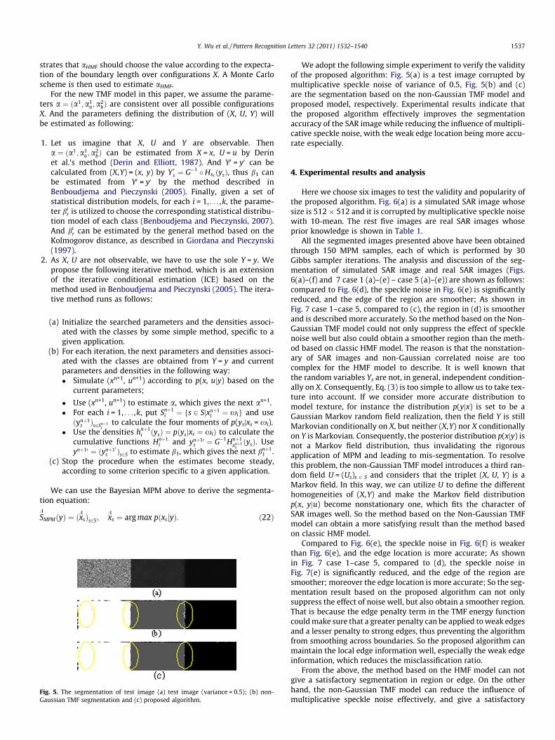
The segmentation of test image (a) test image (variance = 0.5); (b) non-n TMF segmentation and (c) proposed algorithm.

We adopt the following simple experiment to verify the validityof the proposed algorithm: Fig. 5(a) is a test image corrupted bymultiplicative speckle noise of variance of 0.5, Fig. 5(b) and (c)are the segmentation based on the non-Gaussian TMF model andproposed model, respectively. Experimental results indicate thatthe proposed algorithm effectively improves the segmentationaccuracy of the SAR image while reducing the influence of multipli-cative speckle noise, with the weak edge location being more accu-rate especially.

4. Experimental results and analysis

Here we choose six images to test the validity and popularity ofthe proposed algorithm. Fig. 6(a) is a simulated SAR image whosesize is 512 � 512 and it is corrupted by multiplicative speckle noisewith 10-mean. The rest five images are real SAR images whoseprior knowledge is shown in Table 1.

All the segmented images presented above have been obtainedthrough 150 MPM samples, each of which is performed by 30Gibbs sampler iterations. The analysis and discussion of the seg-mentation of simulated SAR image and real SAR images (Figs.6(a)–(f) and 7 case 1 (a)–(e) – case 5 (a)–(e)) are shown as follows:compared to Fig. 6(d), the speckle noise in Fig. 6(e) is significantlyreduced, and the edge of the region are smoother; As shown inFig. 7 case 1–case 5, compared to (c), the region in (d) is smootherand is described more accurately. So the method based on the Non-Gaussian TMF model could not only suppress the effect of specklenoise well but also could obtain a smoother region than the meth-od based on classic HMF model. The reason is that the nonstation-ary of SAR images and non-Gaussian correlated noise are toocomplex for the HMF model to describe. It is well known thatthe random variables Ys are not, in general, independent condition-ally on X. Consequently, Eq. (3) is too simple to allow us to take tex-ture into account. If we consider more accurate distribution tomodel texture, for instance the distribution p(yjx) is set to be aGaussian Markov random field realization, then the field Y is stillMarkovian conditionally on X, but neither (X,Y) nor X conditionallyon Y is Markovian. Consequently, the posterior distribution p(xjy) isnot a Markov field distribution, thus invalidating the rigorousapplication of MPM and leading to mis-segmentation. To resolvethis problem, the non-Gaussian TMF model introduces a third ran-dom field U = (Us)s 2 S and considers that the triplet (X, U, Y) is aMarkov field. In this way, we can utilize U to define the differenthomogeneities of (X,Y) and make the Markov field distributionp(x, yju) become nonstationary one, which fits the character ofSAR images well. So the method based on the Non-Gaussian TMFmodel can obtain a more satisfying result than the method basedon classic HMF model.

Compared to Fig. 6(e), the speckle noise in Fig. 6(f) is weakerthan Fig. 6(e), and the edge location is more accurate; As shownin Fig. 7 case 1–case 5, compared to (d), the speckle noise inFig. 7(e) is significantly reduced, and the edge of the region aresmoother; moreover the edge location is more accurate; So the seg-mentation result based on the proposed algorithm can not onlysuppress the effect of noise well, but also obtain a smoother region.That is because the edge penalty term in the TMF energy functioncould make sure that a greater penalty can be applied to weak edgesand a lesser penalty to strong edges, thus preventing the algorithmfrom smoothing across boundaries. So the proposed algorithm canmaintain the local edge information well, especially the weak edgeinformation, which reduces the misclassification ratio.

From the above, the method based on the HMF model can notgive a satisfactory segmentation in region or edge. On the otherhand, the non-Gaussian TMF model can reduce the influence ofmultiplicative speckle noise effectively, and give a satisfactory

Fig. 6. The segmentation results of simulation SAR image: (a) simulation SAR image (5-look); (b) manual segmentation; (c) estimated U = u with Non-Gaussian TMF; (d) HMFsegmentation; (e) non-Gaussian TMF segmentation; and (f) proposed algorithm.

Table 1The prior knowledge of the real SAR images.

Image Size Band Polarizationtype

Class ENL Image source

Case 1 256 � 256 X HH 3 19.458 Sandia NationalLaboratories

Case 2 256 � 256 X HH 4 4.3807 DLR and EADSAstriumCompany

Case 3 256 � 256 X HH 4 7.7528 A domesticairborne radarimaging data

Case 4 512 � 512 X HH 3 2.9908 A domesticairborne radarimaging data

Case 5 256 � 256 L HH 4 3.9185 Jet PropulsionLaboratory

1538 Y. Wu et al. / Pattern Recognition Letters 32 (2011) 1532–1540

segmentation in the meantime. However, there are still some de-fects such as misclassifications and inaccurate location of the weakedge. The proposed algorithm solves this problem effectively andachieves better segmentation results than the algorithm based onthe non-Gaussian TMF model.

The subjective evaluation of the segmentation results is givenabove, the objective evaluation criteria is as follows: the objectiveevaluation criteria contains three criteria: the variance RIvar, themean RImean and the logarithm of the normalized likelihood ratioD of the ratio image (Caves et al., 1998).

The ratio image is formed by dividing the original image by itssegmentation. The logarithm of the normalized likelihood ratio D isdefined as:

D ¼Xk

#¼1

n#n

D#; ð23Þ

where n# is the number of pixel that belongs to class # in the seg-mentation results, n is the total number of pixel of the observed im-

age, and D# is the logarithm of the normalized likelihood ratio ofclass # in the segmentation results. D# can be written as follows:

D# ¼1n#

Xi

lnIi

I#

� �¼ ln r#; ð24Þ

where Ii is the pixel intensity of observed image, I# is the mean ofclass #, and r# is the value of pixel that belongs to class # in the seg-mentation results. Substituting Eq. (24) into Eq. (23), we can obtain:

D ¼Xk

#¼1

n#n

ln r# ¼ ln r ð25Þ

D is allowed to be the value around zero. And only when all pix-els have the same intensity, it gets zeros. The smaller the value ofjDj is, the better the performance is. Heterogeneity is indicatedwhen jDj takes unusually large values.

The variance RIvar of the ratio image is defined as:

RIvar ¼Xk

#¼1

n# � 1n� 1

m#; ð26Þ

m# ¼n#

n# � 1ðr2# � r#2Þ; ð27Þ

where r2# and r#2 are the square value of the mean and mean of

the square of the class # in the ratio image, respectively. RIvar

describes the change of the pixel value in the ratio image. Thesmaller the value is, the better the performance of segmentationalgorithm is.

The mean RImean of the ratio image is defined as:

RImean ¼1n#

Xi

ri; ð28Þ

where ri is the pixel value of the ratio image. The ratio image is cor-rupted by a pure speckle noise which is generally a gamma distribu-tion. RImean describes the situation of the suppression to specklenoise, and the closer the value of RImean approaches 1, the betterthe suppression to speckle noise is.

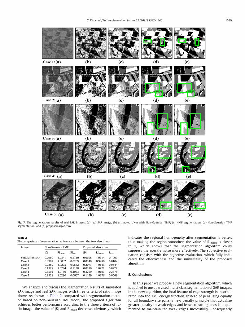
Fig. 7. The segmentation results of real SAR images: (a) real SAR image; (b) estimated U = u with Non-Gaussian TMF; (c) HMF segmentation; (d) Non-Gaussian TMFsegmentation; and (e) proposed algorithm.

Table 2The comparison of segmentation performance between the two algorithms.

Image Non-Gaussian TMF Proposed algorithm

jDj RImean RIvar jDj RImean RIvar

Simulation SAR 0.7960 1.0341 0.1730 0.6608 1.0314 0.1007Case 1 0.0961 1.0032 0.0209 0.0740 0.9986 0.0102Case 2 0.2269 1.0203 0.0672 0.2073 1.0143 0.0544Case 3 0.1327 1.0284 0.1138 0.0380 1.0221 0.0277Case 4 0.6591 1.0159 0.3953 0.3269 1.0103 0.2678Case 5 0.1521 1.0290 0.0667 0.1159 1.0276 0.0569

Y. Wu et al. / Pattern Recognition Letters 32 (2011) 1532–1540 1539

We analyze and discuss the segmentation results of simulatedSAR image and real SAR images with three criteria of ratio imageabove. As shown in Table 2, compared with segmentation meth-od based on non-Gaussian TMF model, the proposed algorithmachieves better performance according to the three criteria of ra-tio image: the value of jDj and RImean decreases obviously, which

indicates the regional homogeneity after segmentation is better,thus making the region smoother; the value of RImean is closerto 1, which shows that the segmentation algorithm couldsuppress the speckle noise more effectively. The subjective eval-uation consists with the objective evaluation, which fully indi-cated the effectiveness and the universality of the proposedalgorithm.

5. Conclusions

In this paper we propose a new segmentation algorithm, whichis applied to unsupervised multi-class segmentation of SAR images.In the new algorithm, the local feature of edge strength is incorpo-rated into the TMF energy function. Instead of penalizing equallyfor all boundary site pairs, a new penalty principle that actualizegreater penalty to weak edges and lesser to strong ones is imple-mented to maintain the weak edges successfully. Consequently

1540 Y. Wu et al. / Pattern Recognition Letters 32 (2011) 1532–1540

the proposed algorithm can locate the edge accurately, even understrong noise, thus significantly enhancing the accuracy of segmen-tation. The results of experiments on simulated data and real SARimages and analysis indicate that compared with the classicalHMF and the recent TMF based segmentation algorithm, the pro-posed algorithm effectively improves the segmentation accuracyof the SAR image while reducing the influence of multiplicativespeckle noise, with the weak edge location being more accurateespecially.

Acknowledgements

This work was supported by Program for Changjiang Scholarsand Innovative Research Team in University under Grant No. IRT0954, the National Natural Science Foundation of China (No.60872137), the National Defense Foundation of China (No.9140A01060408DZ0104) and the Aviation Science Foundation ofChina (20080181002).

References

Benboudjema, D., Pieczynski, W., 2005. Unsupervised image segmentation usingtriplet Markov fields. Comput. Vision Image Understand. 99 (3), 476–498.

Benboudjema, D., Pieczynski, W., 2007. Unsupervised statistical segmentation ofnonstationary images using triplet Markov fields. IEEE Trans. Pattern Anal.Machine Intell. 29 (8), 1367–1378.

Benboudjema, D., Tupin, F., Pieczynski, W., Sigelle, M., Nicolas, J.M., 2007.Unsupervised segmentation of SAR images using triplet Markov fields andFisher noise distributions. In: IEEE International Geoscience and RemoteSensing Symposium, pp. 3891–3893.

Cao, Yongfeng, Sun, Hong, 2005. An unsupervised segmentation method based onMPM for SAR images. IEEE Trans. Geosci. Remote Sens. Lett. 2 (1), 55–58.

Caves, R., Quegna, S., White, R., 1998. Quantitative comparison of the performanceof SAR segmentation algorithms. IEEE Trans. Image Process. 17 (11), 1534–1546.

Dekker, R.J., 2003. Texture analysis and classification of ERS SAR images for mapupdating of urban areas in the Netherlands. IEEE Trans. Geosci. Remote Sens. 41(9), 1950–1958.

Derin, H., Elliott, H., 1987. Modeling and segmentation of noisy and textured imagesusing Gibbs random fields. IEEE Trans. Pattern Anal. Machine Intell. 9 (1), 39–55.

Descombes, X., Morris, R.D., Zerubia, J., Berthod, M., 1999. Estimation of Markovrandom field prior parameters using Markov chain Monte Carlo maximumlikelihood. IEEE Trans. Image Process. 8 (7), 954–963.

Destrempes, F., Mignotte, M., 2004. A statistical model for contours in images. IEEETrans. Pattern Anal. Machine Intell. 26 (5), 238–626.

Geman, S., Geman, D., 1984. Stochastic relaxation, Gibbs distributions and theBayesian restoration of images. IEEE Trans. Pattern Anal. Machine Intell. 6 (6),721–741.

Giordana, N., Pieczynski, W., 1997. Estimation of generalized multisensory hiddenMarkov chains and unsupervised image segmentation. IEEE Trans. Pattern Anal.Machine Intell. 19 (5), 465–475.

Kumar, S., Hebert, M., 2006. Discriminative random fields. Internat. J. Comput.Vision 68 (2), 179–202.

Lombardo, P., Farina, A., 1996. Coherent radar detection against K-distributedclutter with partially correlated texture. Signal Process. 48 (1), 1–15.

Pham, L., Zung, D., 2004. Integrating intensity and boundary information for tissueclassification. In: Proc. 17th IEEE Symposium on Computer-Based MedicalSystems, pp. 216–220.

Pieczynski, W., Tebbache, A.-N., 2000. Pairwise Markov random fields andsegmentation of textured images. Machine Graphics Vision 9 (3), 705–718.

Poggi, G., Scarpa, G., Zerubia, J., 2005. Supervised segmentation of remote sensingimages based on a tree-structured MRF model. IEEE Trans. Geosci. Remote Sens.43 (8), 1901–1911.

Tison, C., Nicolas, J.M., Tupin, F., Maitre, H., 2004. A new statistical model forMarkovian classification of urban areas in high-resolution SAR images. IEEETrans. Geosci. Remote Sens. 42 (10), 2046–2057.

Tran, T.N., Wehrens, R., Buydens, L.M.C., 2005. Initialization of Markov random fieldclustering of large remote sensing image. IEEE Trans. Geosci. Remote Sens. 43(8), 1912–1919.

Yu, Qiyao, Clausi, D.A., 2005. Combining local and global features for imagesegmentation using iterative classification and region merging. In: Proc. SecondCanadian Conf. Computer and Robot Vision, pp. 579–586.

Yu, Qiyao, Clausi, D.A., 2007. SAR sea-ice image analysis based on iterative regiongrowing using semantics. IEEE Trans. Geosci. Remote Sens. 45 (12), 3918–3931.

Yu, Qiyao, Clausi, D.A., 2008. Image segmentation using edge penalties and regiongrowing. IEEE Trans. Pattern Anal. Machine Intell. 30 (12), 2126–2139.