Embed Size (px)
Citation preview
Unsupervised Learning
Unsupervised vs Supervised Learning:
• Most of this course focuses on supervised learning methodssuch as regression and classification.
• In that setting we observe both a set of featuresX1, X2, . . . , Xp for each object, as well as a response oroutcome variable Y . The goal is then to predict Y usingX1, X2, . . . , Xp.
• Here we instead focus on unsupervised learning, we whereobserve only the features X1, X2, . . . , Xp. We are notinterested in prediction, because we do not have anassociated response variable Y .
1 / 52
The Goals of Unsupervised Learning
• The goal is to discover interesting things about themeasurements: is there an informative way to visualize thedata? Can we discover subgroups among the variables oramong the observations?
• We discuss two methods:• principal components analysis, a tool used for data
visualization or data pre-processing before supervisedtechniques are applied, and
• clustering, a broad class of methods for discoveringunknown subgroups in data.
2 / 52
The Challenge of Unsupervised Learning
• Unsupervised learning is more subjective than supervisedlearning, as there is no simple goal for the analysis, such asprediction of a response.
• But techniques for unsupervised learning are of growingimportance in a number of fields:
• subgroups of breast cancer patients grouped by their geneexpression measurements,
• groups of shoppers characterized by their browsing andpurchase histories,
• movies grouped by the ratings assigned by movie viewers.
3 / 52
Another advantage
• It is often easier to obtain unlabeled data — from a labinstrument or a computer — than labeled data, which canrequire human intervention.
• For example it is difficult to automatically assess theoverall sentiment of a movie review: is it favorable or not?
4 / 52
Principal Components Analysis
• PCA produces a low-dimensional representation of adataset. It finds a sequence of linear combinations of thevariables that have maximal variance, and are mutuallyuncorrelated.
• Apart from producing derived variables for use insupervised learning problems, PCA also serves as a tool fordata visualization.
5 / 52
Principal Components Analysis: details
• The first principal component of a set of featuresX1, X2, . . . , Xp is the normalized linear combination of thefeatures
Z1 = φ11X1 + φ21X2 + . . .+ φp1Xp
that has the largest variance. By normalized, we mean that∑pj=1 φ
2j1 = 1.
• We refer to the elements φ11, . . . , φp1 as the loadings of thefirst principal component; together, the loadings make upthe principal component loading vector,φ1 = (φ11 φ21 . . . φp1)
T .
• We constrain the loadings so that their sum of squares isequal to one, since otherwise setting these elements to bearbitrarily large in absolute value could result in anarbitrarily large variance.
6 / 52
PCA: example
10 20 30 40 50 60 70
05
10
15
20
25
30
35
Population
Ad
Sp
en
din
g
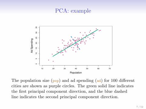
The population size (pop) and ad spending (ad) for 100 differentcities are shown as purple circles. The green solid line indicatesthe first principal component direction, and the blue dashedline indicates the second principal component direction.
7 / 52
Computation of Principal Components
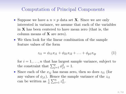
• Suppose we have a n× p data set X. Since we are onlyinterested in variance, we assume that each of the variablesin X has been centered to have mean zero (that is, thecolumn means of X are zero).
• We then look for the linear combination of the samplefeature values of the form
zi1 = φ11xi1 + φ21xi2 + . . .+ φp1xip (1)
for i = 1, . . . , n that has largest sample variance, subject tothe constraint that
∑pj=1 φ
2j1 = 1.
• Since each of the xij has mean zero, then so does zi1 (forany values of φj1). Hence the sample variance of the zi1can be written as 1
n
∑ni=1 z
2i1.
8 / 52
Computation: continued
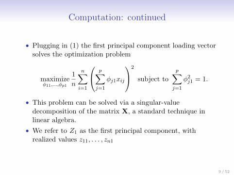
• Plugging in (1) the first principal component loading vectorsolves the optimization problem
maximizeφ11,...,φp1
1
n
n∑i=1
p∑j=1
φj1xij
2
subject to
p∑j=1
φ2j1 = 1.
• This problem can be solved via a singular-valuedecomposition of the matrix X, a standard technique inlinear algebra.
• We refer to Z1 as the first principal component, withrealized values z11, . . . , zn1
9 / 52
Geometry of PCA
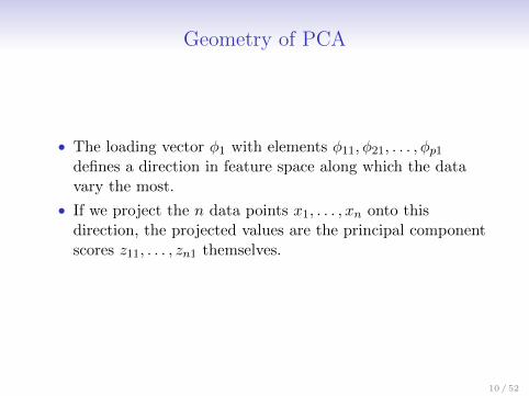
• The loading vector φ1 with elements φ11, φ21, . . . , φp1defines a direction in feature space along which the datavary the most.
• If we project the n data points x1, . . . , xn onto thisdirection, the projected values are the principal componentscores z11, . . . , zn1 themselves.
10 / 52
Further principal components
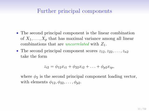
• The second principal component is the linear combinationof X1, . . . , Xp that has maximal variance among all linearcombinations that are uncorrelated with Z1.
• The second principal component scores z12, z22, . . . , zn2take the form
zi2 = φ12xi1 + φ22xi2 + . . .+ φp2xip,
where φ2 is the second principal component loading vector,with elements φ12, φ22, . . . , φp2.
11 / 52
Further principal components: continued
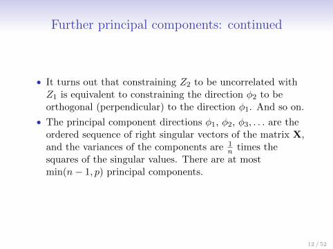
• It turns out that constraining Z2 to be uncorrelated withZ1 is equivalent to constraining the direction φ2 to beorthogonal (perpendicular) to the direction φ1. And so on.
• The principal component directions φ1, φ2, φ3, . . . are theordered sequence of right singular vectors of the matrix X,and the variances of the components are 1
n times thesquares of the singular values. There are at mostmin(n− 1, p) principal components.
12 / 52
Illustration
• USAarrests data: For each of the fifty states in the UnitedStates, the data set contains the number of arrests per100, 000 residents for each of three crimes: Assault, Murder,and Rape. We also record UrbanPop (the percent of thepopulation in each state living in urban areas).
• The principal component score vectors have length n = 50,and the principal component loading vectors have lengthp = 4.
• PCA was performed after standardizing each variable tohave mean zero and standard deviation one.
13 / 52
USAarrests data: PCA plot
−3 −2 −1 0 1 2 3
−3
−2
−1
01
23
First Principal Component
Second P
rincip
al C
om
ponent
Alabama Alaska
Arizona
Arkansas
California
ColoradoConnecticut
Delaware
Florida
Georgia
Hawaii
Idaho
Illinois
IndianaIowaKansas
KentuckyLouisiana
Maine Maryland
Massachusetts
Michigan
Minnesota
Mississippi
Missouri
Montana
Nebraska
Nevada
New Hampshire
New Jersey
New Mexico
New York
North Carolina
North Dakota
Ohio
Oklahoma
OregonPennsylvania
Rhode Island
South Carolina
South Dakota Tennessee
Texas
Utah
Vermont
Virginia
Washington
West Virginia
Wisconsin
Wyoming
−0.5 0.0 0.5
−0.5
0.0
0.5
Murder
Assault
UrbanPop
Rape
14 / 52
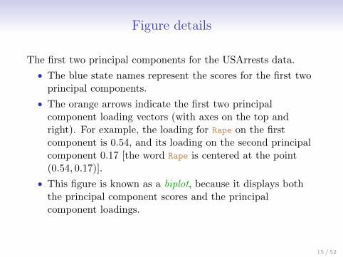
Figure details
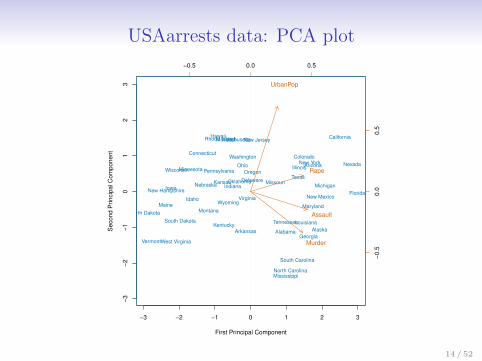
The first two principal components for the USArrests data.
• The blue state names represent the scores for the first twoprincipal components.
• The orange arrows indicate the first two principalcomponent loading vectors (with axes on the top andright). For example, the loading for Rape on the firstcomponent is 0.54, and its loading on the second principalcomponent 0.17 [the word Rape is centered at the point(0.54, 0.17)].
• This figure is known as a biplot, because it displays boththe principal component scores and the principalcomponent loadings.
15 / 52
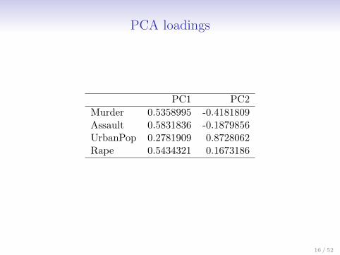
PCA loadings
PC1 PC2
Murder 0.5358995 -0.4181809Assault 0.5831836 -0.1879856UrbanPop 0.2781909 0.8728062Rape 0.5434321 0.1673186
16 / 52
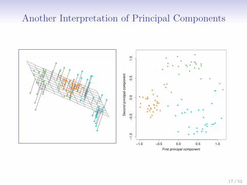
Another Interpretation of Principal Components
First principal component
Second p
rincip
al com
ponent
−1.0 −0.5 0.0 0.5 1.0
−1.0
−0.5
0.0
0.5
1.0
••
•
•
••
••
•
•
••
•
•
•
• ••
••
•
•
•• •
••
• •
• •
•
•
•
••
•
••
•
•
• •
• ••
•
•
••
•
•
•
•
• •
•
•
•
•
• •
•
• •
•
•
• •
•
•
••
•• •
•
••
• •
••
••
•
••
••
17 / 52
PCA find the hyperplane closest to the observations
• The first principal component loading vector has a veryspecial property: it defines the line in p-dimensional spacethat is closest to the n observations (using average squaredEuclidean distance as a measure of closeness)
• The notion of principal components as the dimensions thatare closest to the n observations extends beyond just thefirst principal component.
• For instance, the first two principal components of a dataset span the plane that is closest to the n observations, interms of average squared Euclidean distance.
18 / 52
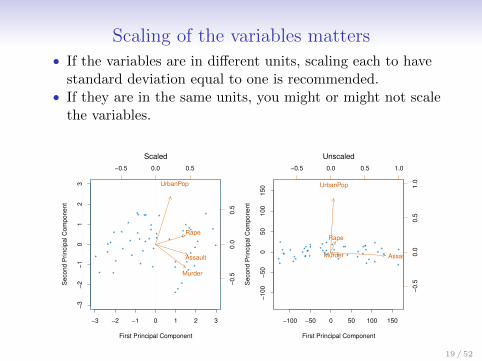
Scaling of the variables matters• If the variables are in different units, scaling each to have
standard deviation equal to one is recommended.• If they are in the same units, you might or might not scale
the variables.
−3 −2 −1 0 1 2 3
−3
−2
−1
01
23
First Principal Component
Second P
rincip
al C
om
ponent
* *
*
*
*
**
**
*
*
*
*
***
* *
* *
*
*
*
*
*
*
*
*
*
*
*
*
*
*
*
***
*
*
* *
*
*
*
*
*
*
*
*
−0.5 0.0 0.5
−0.5
0.0
0.5
Murder
Assault
UrbanPop
Rape
Scaled
−100 −50 0 50 100 150
−100
−50
050
100
150
First Principal Component
Second P
rincip
al C
om
ponent
* *
*
*
***
* **
*
*
*** *
* ** *
***
*
**
**
*
*
**
**
** **
*
***
**
*
**
*
**
−0.5 0.0 0.5 1.0
−0.5
0.0
0.5
1.0
Murder Assault
UrbanPop
Rape
Unscaled
19 / 52
Proportion Variance Explained
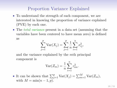
• To understand the strength of each component, we areinterested in knowing the proportion of variance explained(PVE) by each one.
• The total variance present in a data set (assuming that thevariables have been centered to have mean zero) is definedas
p∑j=1
Var(Xj) =
p∑j=1
1
n
n∑i=1
x2ij ,
and the variance explained by the mth principalcomponent is
Var(Zm) =1
n
n∑i=1
z2im.
• It can be shown that∑p
j=1 Var(Xj) =∑M
m=1 Var(Zm),with M = min(n− 1, p).
20 / 52
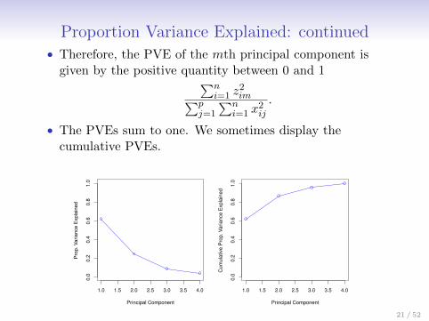
Proportion Variance Explained: continued• Therefore, the PVE of the mth principal component is
given by the positive quantity between 0 and 1∑ni=1 z
2im∑p
j=1
∑ni=1 x
2ij
.
• The PVEs sum to one. We sometimes display thecumulative PVEs.
1.0 1.5 2.0 2.5 3.0 3.5 4.0
0.0
0.2
0.4
0.6
0.8
1.0
Principal Component
Pro
p. V
ari
ance E
xpla
ined
1.0 1.5 2.0 2.5 3.0 3.5 4.0
0.0
0.2
0.4
0.6
0.8
1.0
Principal Component
Cum
ula
tive
Pro
p. V
ari
ance E
xpla
ined
21 / 52

How many principal components should we use?
If we use principal components as a summary of our data, howmany components are sufficient?
• No simple answer to this question, as cross-validation is notavailable for this purpose.
• Why not?
• When could we use cross-validation to select the number ofcomponents?
• the “scree plot” on the previous slide can be used as aguide: we look for an “elbow”.
22 / 52

How many principal components should we use?
If we use principal components as a summary of our data, howmany components are sufficient?
• No simple answer to this question, as cross-validation is notavailable for this purpose.
• Why not?• When could we use cross-validation to select the number of
components?
• the “scree plot” on the previous slide can be used as aguide: we look for an “elbow”.
22 / 52
Clustering
• Clustering refers to a very broad set of techniques forfinding subgroups, or clusters, in a data set.
• We seek a partition of the data into distinct groups so thatthe observations within each group are quite similar toeach other,
• It make this concrete, we must define what it means fortwo or more observations to be similar or different.
• Indeed, this is often a domain-specific consideration thatmust be made based on knowledge of the data beingstudied.
23 / 52
PCA vs Clustering
• PCA looks for a low-dimensional representation of theobservations that explains a good fraction of the variance.
• Clustering looks for homogeneous subgroups among theobservations.
24 / 52
Clustering for Market Segmentation
• Suppose we have access to a large number of measurements(e.g. median household income, occupation, distance fromnearest urban area, and so forth) for a large number ofpeople.
• Our goal is to perform market segmentation by identifyingsubgroups of people who might be more receptive to aparticular form of advertising, or more likely to purchase aparticular product.
• The task of performing market segmentation amounts toclustering the people in the data set.
25 / 52
Two clustering methods
• In K-means clustering, we seek to partition theobservations into a pre-specified number of clusters.
• In hierarchical clustering, we do not know in advance howmany clusters we want; in fact, we end up with a tree-likevisual representation of the observations, called adendrogram, that allows us to view at once the clusteringsobtained for each possible number of clusters, from 1 to n.
26 / 52
K-means clusteringK=2 K=3 K=4
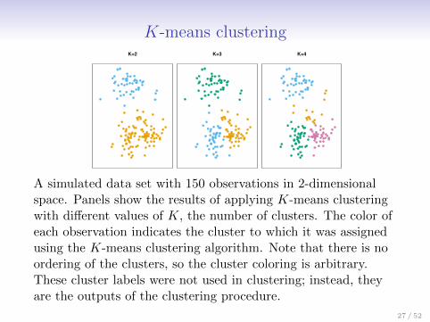
A simulated data set with 150 observations in 2-dimensionalspace. Panels show the results of applying K-means clusteringwith different values of K, the number of clusters. The color ofeach observation indicates the cluster to which it was assignedusing the K-means clustering algorithm. Note that there is noordering of the clusters, so the cluster coloring is arbitrary.These cluster labels were not used in clustering; instead, theyare the outputs of the clustering procedure.
27 / 52
Details of K-means clustering
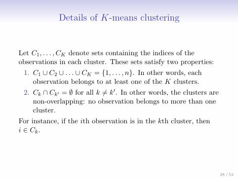
Let C1, . . . , CK denote sets containing the indices of theobservations in each cluster. These sets satisfy two properties:
1. C1 ∪ C2 ∪ . . . ∪ CK = {1, . . . , n}. In other words, eachobservation belongs to at least one of the K clusters.
2. Ck ∩ Ck′ = ∅ for all k 6= k′. In other words, the clusters arenon-overlapping: no observation belongs to more than onecluster.
For instance, if the ith observation is in the kth cluster, theni ∈ Ck.
28 / 52
Details of K-means clustering: continued
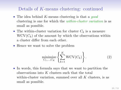
• The idea behind K-means clustering is that a goodclustering is one for which the within-cluster variation is assmall as possible.
• The within-cluster variation for cluster Ck is a measureWCV(Ck) of the amount by which the observations withina cluster differ from each other.
• Hence we want to solve the problem
minimizeC1,...,CK
{K∑k=1
WCV(Ck)
}. (2)
• In words, this formula says that we want to partition theobservations into K clusters such that the totalwithin-cluster variation, summed over all K clusters, is assmall as possible.
29 / 52
How to define within-cluster variation?
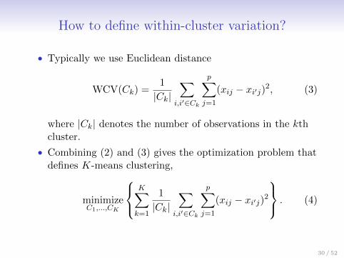
• Typically we use Euclidean distance
WCV(Ck) =1
|Ck|∑
i,i′∈Ck
p∑j=1
(xij − xi′j)2, (3)
where |Ck| denotes the number of observations in the kthcluster.
• Combining (2) and (3) gives the optimization problem thatdefines K-means clustering,
minimizeC1,...,CK
K∑k=1
1
|Ck|∑
i,i′∈Ck
p∑j=1
(xij − xi′j)2 . (4)
30 / 52
K-Means Clustering Algorithm
1. Randomly assign a number, from 1 to K, to each of theobservations. These serve as initial cluster assignments forthe observations.
2. Iterate until the cluster assignments stop changing:
2.1 For each of the K clusters, compute the cluster centroid.The kth cluster centroid is the vector of the p feature meansfor the observations in the kth cluster.
2.2 Assign each observation to the cluster whose centroid isclosest (where closest is defined using Euclidean distance).
31 / 52

Properties of the Algorithm
• This algorithm is guaranteed to decrease the value of theobjective (4) at each step. Why?
Note that
1
|Ck|∑
i,i′∈Ck
p∑j=1
(xij − xi′j)2 = 2∑i∈Ck
p∑j=1
(xij − x̄kj)2,
where x̄kj = 1|Ck|
∑i∈Ck
xij is the mean for feature j incluster Ck.
• however it is not guaranteed to give the global minimum.Why not?
32 / 52

Properties of the Algorithm
• This algorithm is guaranteed to decrease the value of theobjective (4) at each step. Why? Note that
1
|Ck|∑
i,i′∈Ck
p∑j=1
(xij − xi′j)2 = 2∑i∈Ck
p∑j=1
(xij − x̄kj)2,
where x̄kj = 1|Ck|
∑i∈Ck
xij is the mean for feature j incluster Ck.
• however it is not guaranteed to give the global minimum.Why not?
32 / 52
ExampleData Step 1 Iteration 1, Step 2a
Iteration 1, Step 2b Iteration 2, Step 2a Final Results
33 / 52
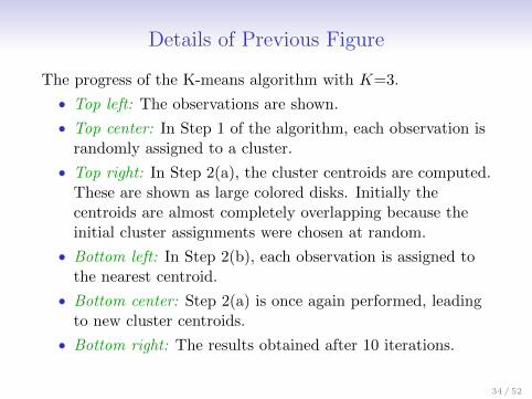
Details of Previous Figure
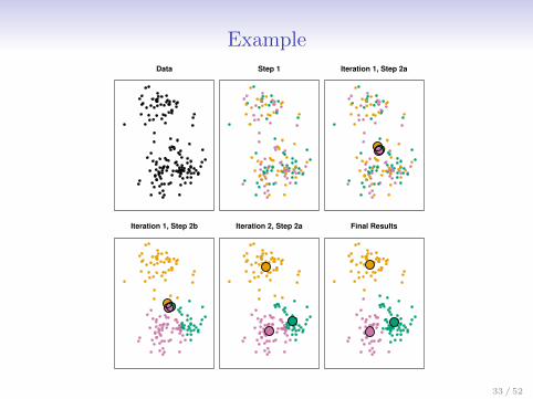
The progress of the K-means algorithm with K=3.
• Top left: The observations are shown.
• Top center: In Step 1 of the algorithm, each observation israndomly assigned to a cluster.
• Top right: In Step 2(a), the cluster centroids are computed.These are shown as large colored disks. Initially thecentroids are almost completely overlapping because theinitial cluster assignments were chosen at random.
• Bottom left: In Step 2(b), each observation is assigned tothe nearest centroid.
• Bottom center: Step 2(a) is once again performed, leadingto new cluster centroids.
• Bottom right: The results obtained after 10 iterations.
34 / 52
Example: different starting values320.9 235.8 235.8
235.8 235.8 310.9
35 / 52
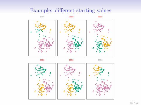
Details of Previous Figure
K-means clustering performed six times on the data fromprevious figure with K = 3, each time with a different randomassignment of the observations in Step 1 of the K-meansalgorithm.Above each plot is the value of the objective (4).Three different local optima were obtained, one of whichresulted in a smaller value of the objective and provides betterseparation between the clusters.Those labeled in red all achieved the same best solution, withan objective value of 235.8
36 / 52
Hierarchical Clustering
• K-means clustering requires us to pre-specify the numberof clusters K. This can be a disadvantage (later we discussstrategies for choosing K)
• Hierarchical clustering is an alternative approach whichdoes not require that we commit to a particular choice ofK.
• In this section, we describe bottom-up or agglomerativeclustering. This is the most common type of hierarchicalclustering, and refers to the fact that a dendrogram is builtstarting from the leaves and combining clusters up to thetrunk.
37 / 52
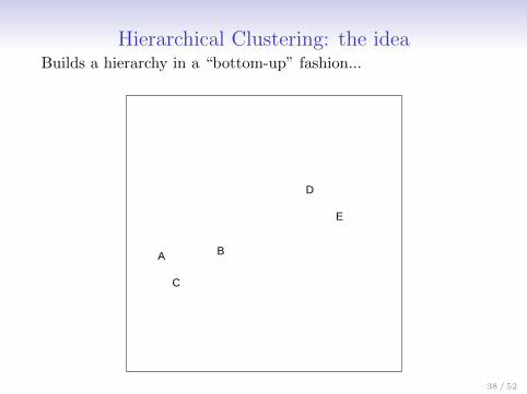
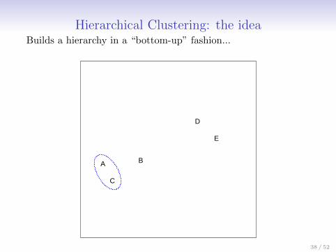
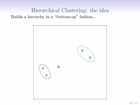
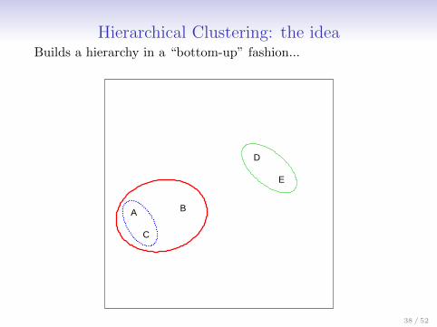
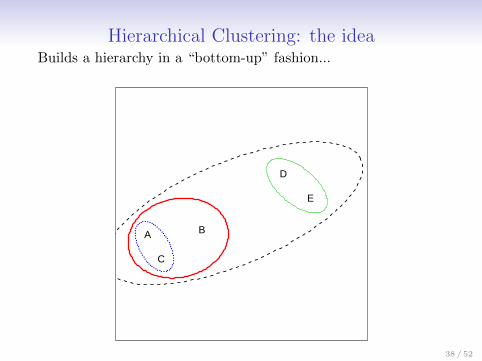
Hierarchical Clustering: the ideaBuilds a hierarchy in a “bottom-up” fashion...
A B
C
D
E
38 / 52
Hierarchical Clustering: the ideaBuilds a hierarchy in a “bottom-up” fashion...
A B
C
D
E
38 / 52
Hierarchical Clustering: the ideaBuilds a hierarchy in a “bottom-up” fashion...
A B
C
D
E
38 / 52
Hierarchical Clustering: the ideaBuilds a hierarchy in a “bottom-up” fashion...
A B
C
D
E
38 / 52
Hierarchical Clustering: the ideaBuilds a hierarchy in a “bottom-up” fashion...
A B
C
D
E
38 / 52
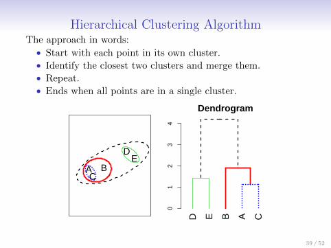
Hierarchical Clustering AlgorithmThe approach in words:
• Start with each point in its own cluster.• Identify the closest two clusters and merge them.• Repeat.• Ends when all points are in a single cluster.
A BC
DE
01
23
4
Dendrogram
D E B A C
39 / 52
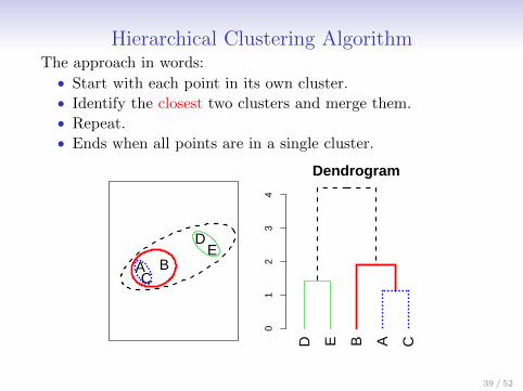
Hierarchical Clustering AlgorithmThe approach in words:
• Start with each point in its own cluster.• Identify the closest two clusters and merge them.• Repeat.• Ends when all points are in a single cluster.
A BC
DE
01
23
4
Dendrogram
D E B A C
39 / 52
An Example
−6 −4 −2 0 2
−2
02
4
X1
X2
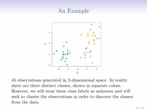
45 observations generated in 2-dimensional space. In realitythere are three distinct classes, shown in separate colors.However, we will treat these class labels as unknown and willseek to cluster the observations in order to discover the classesfrom the data.
40 / 52
Application of hierarchical clustering0
24
68
10
02
46
81
0
02
46
81
0
41 / 52
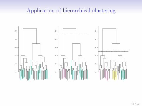
Details of previous figure
• Left: Dendrogram obtained from hierarchically clusteringthe data from previous slide, with complete linkage andEuclidean distance.
• Center: The dendrogram from the left-hand panel, cut at aheight of 9 (indicated by the dashed line). This cut resultsin two distinct clusters, shown in different colors.
• Right: The dendrogram from the left-hand panel, now cutat a height of 5. This cut results in three distinct clusters,shown in different colors. Note that the colors were notused in clustering, but are simply used for display purposesin this figure
42 / 52
Another Example
3
4
1 6
9
2
8
5 7
0.0
0.5
1.0
1.5
2.0
2.5
3.0
1
2
3
4
5
6
7
8
9
−1.5 −1.0 −0.5 0.0 0.5 1.0
−1
.5−
1.0
−0
.50
.00
.5
X1
X2
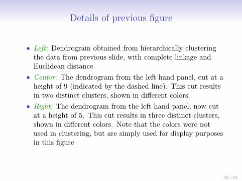
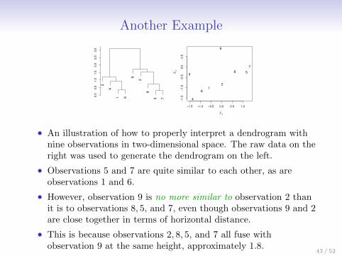
• An illustration of how to properly interpret a dendrogram withnine observations in two-dimensional space. The raw data on theright was used to generate the dendrogram on the left.
• Observations 5 and 7 are quite similar to each other, as areobservations 1 and 6.
• However, observation 9 is no more similar to observation 2 thanit is to observations 8, 5, and 7, even though observations 9 and 2are close together in terms of horizontal distance.
• This is because observations 2, 8, 5, and 7 all fuse withobservation 9 at the same height, approximately 1.8.
43 / 52
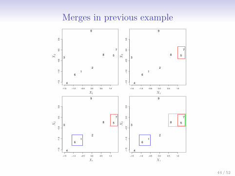
Merges in previous example
1
2
3
4
5
6
7
8
9
−1.5 −1.0 −0.5 0.0 0.5 1.0
−1
.5−
1.0
−0
.50
.00
.5
1
2
3
4
5
6
7
8
9
−1.5 −1.0 −0.5 0.0 0.5 1.0
−1
.5−
1.0
−0
.50
.00
.5
1
2
3
4
5
6
7
8
9
−1.5 −1.0 −0.5 0.0 0.5 1.0
−1
.5−
1.0
−0
.50
.00
.5
1
2
3
4
5
6
7
8
9
−1.5 −1.0 −0.5 0.0 0.5 1.0
−1
.5−
1.0
−0
.50
.00
.5
X1X1
X1X1
X2
X2
X2
X2
44 / 52
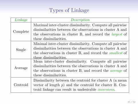
Types of Linkage
Linkage Description
Complete
Maximal inter-cluster dissimilarity. Compute all pairwisedissimilarities between the observations in cluster A andthe observations in cluster B, and record the largest ofthese dissimilarities.
Single
Minimal inter-cluster dissimilarity. Compute all pairwisedissimilarities between the observations in cluster A andthe observations in cluster B, and record the smallest ofthese dissimilarities.
Average
Mean inter-cluster dissimilarity. Compute all pairwisedissimilarities between the observations in cluster A andthe observations in cluster B, and record the average ofthese dissimilarities.
CentroidDissimilarity between the centroid for cluster A (a meanvector of length p) and the centroid for cluster B. Cen-troid linkage can result in undesirable inversions.
45 / 52
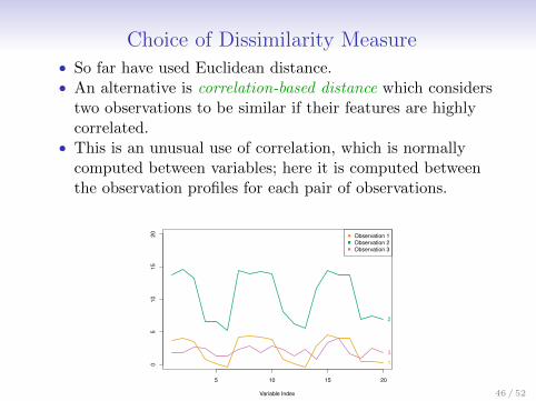
Choice of Dissimilarity Measure• So far have used Euclidean distance.• An alternative is correlation-based distance which considers
two observations to be similar if their features are highlycorrelated.
• This is an unusual use of correlation, which is normallycomputed between variables; here it is computed betweenthe observation profiles for each pair of observations.
5 10 15 20
05
10
15
20
Variable Index
Observation 1
Observation 2
Observation 3
1
2
3
46 / 52
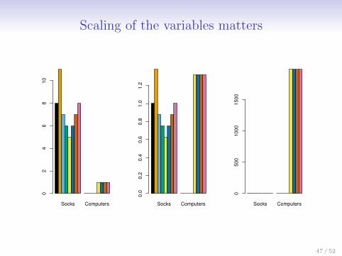
Scaling of the variables matters
Socks Computers
02
46
81
0
Socks Computers
0.0
0.2
0.4
0.6
0.8
1.0
1.2
Socks Computers
05
00
10
00
15
00
47 / 52
Practical issues
• Should the observations or features first be standardized insome way? For instance, maybe the variables should becentered to have mean zero and scaled to have standarddeviation one.
• In the case of hierarchical clustering,• What dissimilarity measure should be used?• What type of linkage should be used?
• How many clusters to choose? (in both K-means orhierarchical clustering). Difficult problem. No agreed-uponmethod. See Elements of Statistical Learning, chapter 13for more details.
48 / 52
Example: breast cancer microarray study
• “Repeated observation of breast tumor subtypes inindependent gene expression data sets;” Sorlie at el, PNAS2003
• Average linkage, correlation metric
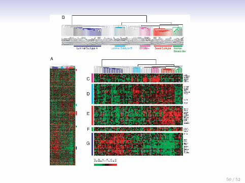
• Clustered samples using 500 intrinsic genes: each womanwas measured before and after chemotherapy. Intrinsicgenes have smallest within/between variation.
49 / 52
West et al. data sets (Table 4). We note that prediction accuraciesreported above are somewhat optimistic, as some of the genesused as predictors were used to define the test set groups in thefirst place.
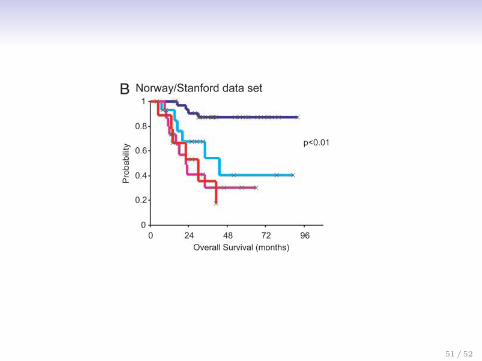
Tumor Subtypes Are Associated with Significant Difference in ClinicalOutcome. In our previous work, the expression-based tumor sub-types were associated with a significant difference in overall survivalas well as disease-free survival for the patients suffering from locallyadvanced breast cancer and belonging to the same treatmentprotocol (6). To investigate whether these subtypes were alsoassociated with a significant difference in outcome in other patientcohorts, we performed a univariate Kaplan–Meier analysis withtime to development of distant metastasis as a variable in the dataset comprising the 97 sporadic tumors taken from van’t Veer et al.
As shown in Fig. 5, the probability of remaining disease-free wassignificantly different between the subtypes; patients with luminalA type tumors lived considerably longer before they developedmetastatic disease, whereas the basal and ERBB2� groups showedmuch shorter disease-free time intervals. Although the method-ological differences prevent a definitive interpretation, it is notablethat the order of severity of clinical outcome associated with theseveral subtypes is similar in the two dissimilar cohorts. We couldnot carry out a similar analysis in the West et al. data because thenecessary follow-up data were not provided.
DiscussionBreast Tumor Subtypes Represent Distinct Biological Entities. Geneexpression studies have made it clear that there is considerablediversity among breast tumors, both biologically and clinically (5, 6,
Fig. 1. Hierarchical clustering of 115 tumor tissues and 7 nonmalignant tissues using the ‘‘intrinsic’’ gene set. (A) A scaled-down representation of the entire clusterof 534 genes and 122 tissue samples based on similarities in gene expression. (B) Experimental dendrogram showing the clustering of the tumors into five subgroups.Branches corresponding to tumors with low correlation to any subtype are shown in gray. (C) Gene cluster showing the ERBB2 oncogene and other coexpressed genes.(D) Gene cluster associated with luminal subtype B. (E) Gene cluster associated with the basal subtype. (F) A gene cluster relevant for the normal breast-like group. (G)Cluster of genes including the estrogen receptor (ESR1) highly expressed in luminal subtype A tumors. Scale bar represents fold change for any given gene relative tothe median level of expression across all samples. (See also Fig. 6.)
8420 � www.pnas.org�cgi�doi�10.1073�pnas.0932692100 Sørlie et al.
50 / 52
Another expectation from the concept that the tumor subtypesrepresent different biological entities is that genetic predispositionsto breast cancer might give rise preferentially to certain subtypes.This expectation is amply fulfilled by our finding in the data of van’t
Veer et al., which shows that the women carrying BRCA1-mutatedalleles all had tumors with the basal-like gene expression pattern.
Tumor Subtypes and Clinical Outcome. Consistent with the resultspreviously found in our data (6), we also found differences inclinical outcome associated with the different tumor subtypes in thedata set produced by van’t Veer et al. The outcomes, as measuredhere in time to development of distant metastasis, were strikinglysimilar to what we found previously: worst for basal (andERBB2�), best for luminal A, and intermediate for luminal Bsubtypes. Recently, two reports corroborating the poor outcome ofthe basal subtype solely based on immunohistochemistry withantibodies against keratins 5 and 17 and Skp2, strongly supports ourresults (24, 25). The finding that our gene cluster profile was ofsimilar prognostic importance in the van’t Veer et al. cohort asamong our patients is remarkable, taking into account differencesregarding disease stage (locally advanced versus stage I primaries)and patient age, but in particular, the fact that the Norwegianpatients had presurgical chemotherapy and all patients expressingESR1 received adjuvant endocrine treatment, whereas the patientsfrom van’t Veer et al. in general did not receive any systemicadjuvant treatment.
The observation that BRCA1 mutations are strongly associatedwith a basal tumor phenotype indicates a particularly poor prog-nosis for these patients. BRCA1-associated breast cancers areusually highly proliferative and TP53-mutated, and usually lackexpression of ESR1 and ERBB2 (20, 26). Status of BRCA1 infamilial cancers has failed to be an independent prognostic factorin several studies (reviewed in ref. 27), and is complicated byconfounding factors such as frequent screening and early diagnosis.
Molecular Marker Identification. In a mixture of biologically distinctsubtypes, it may well be that individual markers derived by super-vised analysis will under-perform what is possible if tumor subtypeswere separated before searching, in a supervised fashion, forprognostic indicators. Indeed, when we tested the prognostic impactof the 231 markers published by van’t Veer et al. on the Norwegiancohort, we found that they performed less well (47%) in predictingrecurrences within 5 years (see Materials and Methods). This may inpart be due to differences in the patient cohorts and treatments asdiscussed above.
Both van’t Veer et al. and West et al. showed the ability of gene
Fig. 4. Hierarchical clustering of gene expressiondata from West et al. (A) Scaled-down representationof the full cluster of 242 intrinsic genes across 49 breasttumors. (B) Dendrogram displaying the relative orga-nization of the tumor samples. Branches are coloredaccording to which subtype the corresponding tumorshowed the strongest correlation with. Gray branchesindicate tumors with low correlation (�0.1) to anyspecific subtype. (C) Luminalepithelial�estrogenrecep-tor gene cluster. (D) Basal gene cluster. (E) ERBB2�gene cluster. (See also Fig. 9, which is published assupporting information on the PNAS web site.)
Fig. 5. Kaplan–Meier analysis of disease outcome in two patient cohorts. (A)Time to development of distant metastasis in the 97 sporadic cases from van’tVeer et al. Patients were stratified according to the subtypes as shown in Fig. 2B.(B) Overall survival for 72 patients with locally advanced breast cancer in theNorway cohort. The normal-like tumor subgroups were omitted from both datasets in this analysis.
8422 � www.pnas.org�cgi�doi�10.1073�pnas.0932692100 Sørlie et al.51 / 52
Conclusions
• Unsupervised learning is important for understanding thevariation and grouping structure of a set of unlabeled data,and can be a useful pre-processor for supervised learning
• It is intrinsically more difficult than supervised learningbecause there is no gold standard (like an outcomevariable) and no single objective (like test set accuracy)
• It is an active field of research, with many recentlydeveloped tools such as self-organizing maps, independentcomponents analysis and spectral clustering.See The Elements of Statistical Learning, chapter 14.
52 / 52