JMLR: Workshop and Conference Proceedings 27:97–111, 2012 Workshop on Unsupervised and Transfer Learning

Unsupervised and Transfer Learning Challenge:a Deep Learning Approach

Gregoire Mesnil1,2 mesnilgr@iro.umontreal.ca

Yann Dauphin1 dauphiya@iro.umontreal.ca

Xavier Glorot1 glorotxa@iro.umontreal.ca

Salah Rifai1 rifaisal@iro.umontreal.ca

Yoshua Bengio1 bengioy@iro.umontreal.ca

Ian Goodfellow1 goodfeli@iro.umontreal.ca

Erick Lavoie1 lavoeric@iro.umontreal.ca

Xavier Muller1 mullerx@iro.umontreal.ca

Guillaume Desjardins1 desjagui@iro.umontreal.ca

David Warde-Farley1 wardefar@iro.umontreal.ca

Pascal Vincent1 vincentp@iro.umontreal.ca

Aaron Courville1 courvila@iro.umontreal.ca

James Bergstra1 bergstrj@iro.umontreal.ca1 Dept. IRO, Universite de Montreal. Montreal (QC), H2C 3J7, Canada2 LITIS EA 4108, Universite de Rouen. 76 800 Saint Etienne du Rouvray, France

Editor: I. Guyon, G. Dror, V. Lemaire, G. Taylor, and D. Silver

Abstract

Learning good representations from a large set of unlabeled data is a particularly chal-lenging task. Recent work (see Bengio (2009) for a review) shows that training deeparchitectures is a good way to extract such representations, by extracting and disentan-gling gradually higher-level factors of variation characterizing the input distribution. Inthis paper, we describe different kinds of layers we trained for learning representations inthe setting of the Unsupervised and Transfer Learning Challenge. The strategy of ourteam won the final phase of the challenge. It combined and stacked different one-layerunsupervised learning algorithms, adapted to each of the five datasets of the competition.This paper describes that strategy and the particular one-layer learning algorithms feedinga simple linear classifier with a tiny number of labeled training samples (1 to 64 per class).

Keywords: Deep Learning, Unsupervised Learning, Transfer Learning, Neural Networks,Restricted Boltzmann Machines, Auto-Encoders, Denoising Auto-Encoders.

1. Introduction

The objective of machine learning algorithms is to discover statistical structure in data.In particular, representation-learning algorithms attempt to transform the raw data intoa form from which it is easier to perform supervised learning tasks, such as classification.This is particularly important when the classifier receiving this representation as input is

c© 2012 G. Mesnil1,2 et al.

Mesnil1,2 et al.

linear and when the number of available labeled examples is small. This is the case herewith the Unsupervised and Transfer Learning (UTL) Challenge 1.

Another challenging characteristic of this competition is that the training (development)distribution is typically very different from the test (evaluation) distribution, because itinvolves a set of classes different from the test classes, i.e., both inputs and labels have adifferent nature. What makes the task feasible is that these different classes have thingsin common. The bet we make is that more abstract features of the data are more likely tobe shared among the different classes, even with classes which are very rare in the trainingset. Another bet we make with representation-learning algorithms and with Deep Learningalgorithms in particular is that the structure of the input distribution P (X) is stronglyconnected with the structure of the class predictor P (Y |X) for all of the classes Y . Itmeans that representations h(X) of inputs X are useful both to characterize P (X) and tocharacterize P (Y |X), which we will think of as parametrized through P (Y |h(X)). Anotherinteresting feature of this competition is that the input features are anonymous, so thatteams are compared based on the strength of their learning algorithms and not based ontheir ability to engineer hand-crafted features based on task-specific prior knowledge. Morematerial on Deep Learning can be found in a companion paper Bengio (2011).

The paper is organized as follows. The pipeline going from bottom (raw data) to top(final representation fed to the classifier) is described in Section 2. In addition to the scorereturned by the competition servers, Section 3 presents other criteria that guided the choiceof hyperparameters. Section 4 precisely describes the layers we chose to combine for each ofthe five competition datasets, at the end of the exploration phase that lasted from January2011 to mid-April 2011.

2. Method

We obtain a deep representation by stacking different single-layer blocks, each taken froma small set of possible learning algorithms, but each with its own set of hyper-parameters(the most important of which is often just the dimension of the representation). Whereasthe number of possible combinations of layer types and hyper-parameters is exponential asdepth increases, we used a greedy layer-wise approach (Bengio et al., 2007) for building eachdeep model. Hence, the first layer is trained on the raw input and its hyper-parametersare chosen with respect to the score returned by the competition servers (on the validationset) and different criteria to avoid overfitting to a particular subset of classes (discussed inSection 3). We then fix the ith layer (or keep only a very small number of choices) and searchfor a good choice of the i+ 1th layer, pruning and keeping only a few good choices. Depthis thus increased without an explosion in computation until the model does not improvesignificantly the performance according to our criteria.

The resulting learnt pipeline can be divided in three types of stages: preprocessing,feature extraction and transductive postprocessing.

1. http://http://www.causality.inf.ethz.ch/unsupervised-learning.php

98

Unsupervised and Transfer Learning Challenge: a Deep Learning Approach

2.1. Preprocessing

Before the feature extraction step, we preprocessed the data using various techniques. LetD = {x(j)}j=1,...,n be a training set where x(j) ∈ Rd.

Standardization One option is to standardize the data. For each feature, we compute

its mean µk = (1/n)∑n

j=1 x(j)k and variance σk. Then, each transformed feature x

(j)k =

(x(j)k − µk)/σk has zero mean and unit variance.

Uniformization (t-IDF) Another way to control the range of the input is to uniformizethe feature values by restricting their possible values to [0, 1] (and non-parametrically and

approximately mapping each feature to a uniform distribution). We rank all the x(j)k and

map them to [0, 1] by dividing the rank by the number of observations sorted. In the caseof sparse data, we assigned the same range value (0) for zeros features. One option is toaggregate all the features in these statistics and another is to do it separately for eachfeature.

Contrast Normalization On datasets which are supposed to correspond to images,each input d-vector is normalized with respect to the values in the given input vector(global contrast normalization). For each sample vector x(j) subtract its mean µ(j) =

(1/d)∑d

k=1 x(j)k and divide by its standard deviation σ(j) (also across the elements of the

vector). In the case of images, this would discard the average illumination and contrast(scale).

Whitened PCA The Karhulen-Loeve transform constantly improved the quality of therepresentation for each dataset. Assume the training set D is stored as a matrix X ∈MR(n, d). First, we compute the empirical mean µ = (1/n)

∑ni=1Xi. where Xi. denotes

row i of the matrix X, i.e., example i. We center the data X = X − µ and computethe covariance matrix C = (1/n)XT X. Then, we obtain the eigen-decomposition of thecovariance matrix C = V −1UV i.e U ∈ Rd contains the eigen-values and V ∈MR(d, d) thecorresponding eigen-vectors (each row corresponds to an eigen-vector). We build a diagonalmatrix U

′where U

′ii =

√Cii. By the end, the output of the whitened PCA is given by

Y = (X − µ)V U′. In our experiments, we used the PCA implementation of the scikits 2

toolbox.

Feature selection In the datasets where the input is sparse, a preprocessing that wefound very useful is the following: only the features active on the training (development)and test (resp. validation) datasets are retained for the test set (resp. validation) repre-sentations. We removed those whose frequency was low on both datasets (this introducesa new hyper-parameter that is the cut-off threshold, but we only tried a couple of values).

2.2. Feature extraction

Feature extraction is the core of our pipeline and has been crucial for getting the first ranksduring the challenge. Here we briefly introduce each method that has been used during thecompetition. See also Bengio (2011) along with the citations below for more details.

2. http://scikits.appspot.com/

99

Mesnil1,2 et al.

2.2.1. µ-ss-RBM

The µ-spike and slab Restricted Boltzmann Machine (µ-ssRBM) (Courville et al., 2011) isa recently introduced undirected graphical model that has demonstrated some promise asa model of natural images. The model is characterized by having both a real-valued slabvector and a binary spike variable associated with each hidden unit. The model possessessome practical properties such as being amenable to block Gibbs sampling as well as beingcapable of generating similar latent representations of the data to the mean and covarianceRestricted Boltzmann Machine (Ranzato and Hinton, 2010).

The µ-ssRBM describes the interaction between three random vectors: the visible vectorv representing the observed data, the binary “spike” variables h and the real-valued “slab”variables s. Suppose there are N hidden units and a visible vector of dimension D: v ∈ RD.The ith hidden unit (1 ≤ i ≤ N) is associated with a binary spike variable: hi ∈ {0, 1} anda real valued vector si ∈ RK , pooling over K linear filters. This kind of pooling structureallows the model to learn over which filters the model will pool – a useful property in thecontext of the UTL challenge where we cannot assume a standard “pixel structure” in theinput. The µ-ssRBM model is defined via the energy function

E(v, s, h) = −N∑i=1

vTWisihi +1

2vT

(Λ +

N∑i=1

Φihi

)v

+

N∑i=1

1

2sTi αisi −

N∑i=1

µTi αisihi −

N∑i=1

bihi +

N∑i=1

µTi αiµihi,

in which Wi refers to the ith weight matrix of size D×K, the bi are the biases associatedwith each of the spike variables hi, and αi and Λ are diagonal matrices that penalize largevalues of ‖si‖22 and ‖v‖22 respectively.

Efficient learning and inference in the µ-ssRBM is rooted in the ability to iterativelysample from the factorial conditionals P (h | v), p(s | v, h) and p(v | s, h) with a Gibbssampling procedure. For a detailed derivation of these conditionals, we refer the reader to(Courville et al., 2011). In training the µ-ssRBM, we use stochastic maximum likelihood(Tieleman, 2008) to update the model parameters.

2.2.2. Denoising Autoencoder

Traditional autoencoders map an input x ∈ Rdx to a hidden representation h (the learntfeatures) with an affine mapping followed by a non-linearity s (typically a sigmoid): h =f(x) = s(Wx + b). The representation is then mapped back to input space, initiallyproducing a linear reconstruction r(x) = W ′f(x) + br, where W ′ can be the transposeof W (tied weights) or a different matrix (untied weights). The autoencoder’s parametersθ = W, b, br are optimized so that the reconstruction is close to the original input x in thesense of a given loss function L(r(x), x) (the reconstruction error). Common loss functionsinclude squared error ‖r(x)− x‖2, squared error after sigmoid ‖s(r(x))− x‖2, and sigmoidcross-entropy −

∑i xi log s(ri(x)) + (1 − xi) log(1 − s(ri(x))). To encourage robustness of

the representation, and avoid trivial useless solutions, a simple and efficient variant wasproposed in the form of the Denoising Autoencoders (Vincent et al., 2008, 2010). Instead ofbeing trained to merely reconstruct its inputs, a Denoising Autoencoder is trained to denoise

100

Unsupervised and Transfer Learning Challenge: a Deep Learning Approach

artificially corrupted training samples, a much more difficult task, which was shown to forceit to extract more useful and meaningful features and capture the structure of the inputdistribution (Vincent et al., 2010). In practice, instead of presenting the encoder with aclean training sample x, it is given as input a stochastically corrupted version x. Theobjective remains to minimize reconstruction error L(r(x), x) with respect to clean samplex, so that the hidden representation has to help denoise. Common choices for the corruptioninclude additive Gaussian noise, and masking a fraction of the input components at randomby setting them to 0 (masking noise).

2.2.3. Contractive Autoencoder

To encourage robustness of the representation f(x) obtained for a training input x, Rifaiet al. (2011) propose to penalize its sensitivity to that input, measured as the Frobeniusnorm of the Jacobian Jf (x) of the non-linear mapping. Formally, if input x ∈ Rdx is mappedby an encoding function f to a hidden representation h ∈ Rdh , this sensitivity penalizationterm is the sum of squares of all partial derivatives of the extracted features with respectto input dimensions:

‖Jf (x)‖2F =∑ij

(∂hj(x)

∂xi

)2

.

Penalizing ‖Jf‖2F encourages the mapping to the feature space to be contractive in theneighborhood of the training data. The flatness induced by having small first derivativeswill imply an invariance or robustness of the representation for small variations of the input.

While such a Jacobian term alone would encourage mapping to a useless constant rep-resentation, it is counterbalanced in auto-encoder training by the need for the learnt repre-sentation to allow a good reconstruction of the training examples.

2.2.4. Rectifiers

Recent works investigated linear rectified activation function variants. Nair and Hinton(2010) used Noisy Rectified Linear Units (NReLU) (i.e. max(0, x+N(0, σ(x))) for RestrictedBoltzmann Machines. Compared to binary units, they observed significant improvementsin term of generalization performance for image classification tasks. Following this line ofwork, Glorot et al. (2011) used the rectifier activation function (i.e. max(0, x)) for deepneural networks and Stacked Denoising Auto-Encoders (SDAE) (Vincent et al., 2008, 2010)and obtained similarly good results.

This non-linearity has various mathematical advantages. First, it naturally createssparse representations with true zeros which are computationally appealing. In addition,the linearity on the active side of the activation function allows gradient to flow well on theactive set of neurons, possibly reducing the vanishing gradients problem.

In a semi-supervised setting similar to that of the Unsupervised and Transfer learningChallenge setup, Glorot et al. (2011) obtained state-of-the-art results for a sentiment anal-ysis task (the Amazon 4-task benchmark) for which the bag-of-words input were highlysparse.

But learning such embeddings for huge sparse vectors with the proposed approach is stillvery expensive. Even though the training cost only scales linearly with the dimension of

101

Mesnil1,2 et al.

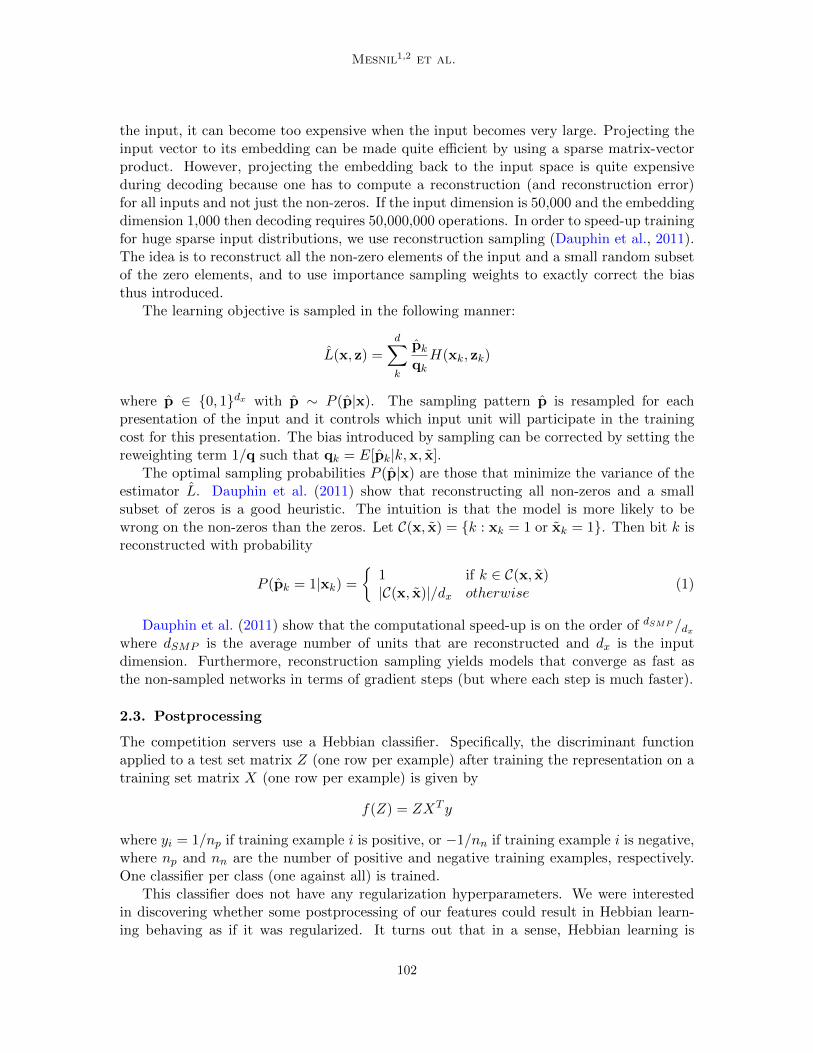
the input, it can become too expensive when the input becomes very large. Projecting theinput vector to its embedding can be made quite efficient by using a sparse matrix-vectorproduct. However, projecting the embedding back to the input space is quite expensiveduring decoding because one has to compute a reconstruction (and reconstruction error)for all inputs and not just the non-zeros. If the input dimension is 50,000 and the embeddingdimension 1,000 then decoding requires 50,000,000 operations. In order to speed-up trainingfor huge sparse input distributions, we use reconstruction sampling (Dauphin et al., 2011).The idea is to reconstruct all the non-zero elements of the input and a small random subsetof the zero elements, and to use importance sampling weights to exactly correct the biasthus introduced.

The learning objective is sampled in the following manner:

L(x, z) =

d∑k

pkqkH(xk, zk)

where p ∈ {0, 1}dx with p ∼ P (p|x). The sampling pattern p is resampled for eachpresentation of the input and it controls which input unit will participate in the trainingcost for this presentation. The bias introduced by sampling can be corrected by setting thereweighting term 1/q such that qk = E[pk|k,x, x].

The optimal sampling probabilities P (p|x) are those that minimize the variance of theestimator L. Dauphin et al. (2011) show that reconstructing all non-zeros and a smallsubset of zeros is a good heuristic. The intuition is that the model is more likely to bewrong on the non-zeros than the zeros. Let C(x, x) = {k : xk = 1 or xk = 1}. Then bit k isreconstructed with probability

P (pk = 1|xk) =

{1 if k ∈ C(x, x)|C(x, x)|/dx otherwise

(1)

Dauphin et al. (2011) show that the computational speed-up is on the order of dSMP /dxwhere dSMP is the average number of units that are reconstructed and dx is the inputdimension. Furthermore, reconstruction sampling yields models that converge as fast asthe non-sampled networks in terms of gradient steps (but where each step is much faster).

2.3. Postprocessing

The competition servers use a Hebbian classifier. Specifically, the discriminant functionapplied to a test set matrix Z (one row per example) after training the representation on atraining set matrix X (one row per example) is given by

f(Z) = ZXT y

where yi = 1/np if training example i is positive, or −1/nn if training example i is negative,where np and nn are the number of positive and negative training examples, respectively.One classifier per class (one against all) is trained.

This classifier does not have any regularization hyperparameters. We were interestedin discovering whether some postprocessing of our features could result in Hebbian learn-ing behaving as if it was regularized. It turns out that in a sense, Hebbian learning is

102

Unsupervised and Transfer Learning Challenge: a Deep Learning Approach

already maximally regularized. Fisher discriminant analysis can be solved as a linear re-gression problem (Bishop, 2006), and the L2 regularized version of this problem yields thisdiscriminant function:

gλ(Z) = Z(XTX + λI)XT y

where λ is the regularization coefficient. Note that

limλ→∞

gλ(Z)

||gλ(Z)||=

f(Z)

||f(Z)||.

Since scaling does not affect the final classification decision, Hebbian learning may be seenas maximally regularized Fisher discriminant analysis. It is possible to reduce Hebbianlearning’s implicit L2 regularization coefficient to some smaller λ by multiplying Z by(XTX + λI)−1/2), but it is not possible to increase it.

Despite this implicit regularization, overfitting is still an important obstacle to goodperformance in this competition due to the small number of training examples used. Wetherefore explored other means of avoiding overfitting, such as reducing the number offeatures and exploring sparse codes that would result in most of the features appearing inthe training set being 0. However, the best results and regularization where obtained by atransductive PCA.

2.3.1. Transductive PCA

A Transductive PCA is a PCA transform trained not on the training set but on the test(or validation) set. After training the first k layers of the pipeline on the training set, wetrained a PCA on top of layer k, either on the validation set or on the test set (depending onwhether we were submitting to the validation set or the test set). Regarding the notationused in 2.1, we apply the same transformation with X replaced by the representation ontop of layer k of the validation set or the test set i.e h(Xvalid).

This transductive PCA thus only retains variations that are the dominant ones in thetest or validation set. It makes sure that the final classifier will ignore the variationspresent in the training set but irrelevant for the test (or validation) set. In a sense, this is ageneralization of the strategy introduced in 2.1 of removing features that were not presentin the both training and test / validation sets. The lower layers only keep the directions ofvariation that are dominant in the training set, while the top transductive PCA only keepsthose that are significantly present in the validation (or test) set.

We assumed that the validation and test sets contained the same number of classesto validate the number of components on the validation set performance. In general, oneneeds at least k − 1 components in order to separate k classes by a set of one-against-allclassifiers. Transductive PCA has been decisive for winning the competition as it improvedconsiderably the performance on all the datasets. In some cases, we also used a mixedstrategy for the intermediate layers, mixing examples from all three sets.

2.3.2. Other methods

After the feature extraction process, we were able to visualize the data as a three-dimensionalscatter plot of the representation learnt. On some datasets, a very clear clustering pattern

103

Mesnil1,2 et al.

became visually apparent, though it appeared that several clouds came together in an am-biguous region of the latent space discovered.

In order to attempt to disambiguate this ambiguous region without making hard-threshold decisions, we fit a Gaussian mixture model with the EM algorithm and a smallnumber of Gaussian components chosen by visual inspection of these clouds. We then usedthe posterior probabilities of the cluster assignments as an alternate encoding.

K-means, by contrast with Gaussian mixture models, makes a hard decision as to clusterassignments. Many researchers were recently impressed when they found out that a certainkind of feature representation (the “triangle code”) based on K-means, combined withspecialized pre-processing, yielded state of the art performance on the CIFAR-10 imageclassification benchmark (Coates et al., 2011). Therefore, we tried K-means with a largenumber of means and the triangle code as a post-processing step.

In the end, though, none of our selected final entries included a Gaussian mixture modelor K-means, as the transductive PCA always worked better as a post-processing layer.

3. Criterion

The usual kind of overfitting is due to specializing to particular labeled examples. In thistransfer learning context, another kind of overfitting arose: overfitting a representationto particular classes. Since the validation set and test set have non-intersecting sets ofclasses, finding representations that work well on the validation set was not a guarantee forgood behavior on the test set, as we learned from our experience with the competition firstphase. Note also that the competition was focused on a particular criterion, the Area underthe Learning Curve (ALC)3 which gives much weight to the cases with very few labeledexamples (1, 2, or 4, per class, in particular, get almost half of the weight). So the questionwe investigated in the second and final phase (where some training set labels were revealed)was the following: does the ALC of a representation computed on a particular subset ofclasses correlate with the ALC of the same representation computed on a different set ofclasses?

Overfitting on a specific subset of classes can be observed by training a PCA separatelyon the training, validation and test sets on ULE (this data set corresponds to MNISTdigits). The number of components maximizing the ALC will be different, depending onthe choice of the subset of classes. Figure 1(a) illustrates the effect of the number ofcomponents retained on the training, validation and test ALCs. While the best number ofcomponents on the validation set would be 2, choosing this number of components for thetest set significantly degrades the test ALC.

During the first phase, we noticed the absence of correlation between the validationALC and test ALC computed on the ULE dataset. During the second phase, we tried toreproduce the competition setting using the labels available for transfer with the hope offinding a criteria that would guarantee generalization. The ALC was computed on everysubset of at least two classes found in the transfer labels and metrics were derived. Thosemetrics are illustrated in Figure 1(b). We observed that the standard deviation seems tobe inversely proportional to the generalization accuracy, therefore substracting it from themean ALC ensures that the choice of hyper-parameters is done in a range where the training,

3. http://www.causality.inf.ethz.ch/ul data/DatasetsUTLChallenge.pdf

104

Unsupervised and Transfer Learning Challenge: a Deep Learning Approach

validation and test ALCs are correlated. In the case of a PCA, optimizing the µ−σ criteriacorrectly returns the best number of PCA components, ten, where the training, validationand test ALCs are all correlated.

It appears that this criterion is a simple way to use the small amount of labels given tothe competitors for the phase 2. However, this criterion has not been heavily tested duringthe competition since we always selected our best models with respect to the validation ALCreturned by the competition servers. From the phase 1 to the phase 2, we only exploredthe space of the hyperparameters of our models using a finer grid.

(a) ALC on the three sets (b) Criterion

Figure 1: ULE Dataset Left: ALC on training, validation and test sets of PCA repre-sentations, with respect to the number of principal components retained. Right:Comparison between training, validation and test ALC and the criterion com-puted from the ALC, obtained on every subset of at least 2 classes present in thetransfer labels for different numbers of components of a PCA.

4. Results

For each of the five datasets, AVICENNA, HARRY, TERRY, SYLVESTER andRITA, the strategy retained for the final winning submission on the phase 2 is preciselydescribed. Training such a deep stack of layers from preprocessing to postprocessing takesat most 12 hours for each dataset once you have found the good hyperparameters. All ourmodels are implemented in Theano (Bergstra et al., 2010), a Python library that allowstransparent use of GPUs. During the competition, we used a cluster of GPUs, NvidiaGeForce GTX 580.

4.1. AVICENNA

Nature of the data It corresponds to arabic manuscripts and consists of 150, 205 trainingsamples of dimension 120.

Best Architecture For preprocessing, we fitted a whitened-PCA on the raw data andkept the first 75 components in order to eliminate the noise from the input distribution.

105

Mesnil1,2 et al.

AVICENNA SYLVESTER RITA HARRY TERRY0.0

0.2

0.4

0.6

0.8

1.0

ALC

VALID ALC by dataset and by step

RawPreprocFeat. Extr.Postproc

AVICENNA SYLVESTER RITA HARRY TERRY0.0

0.2

0.4

0.6

0.8

1.0

ALC

TEST ALC by dataset and by step

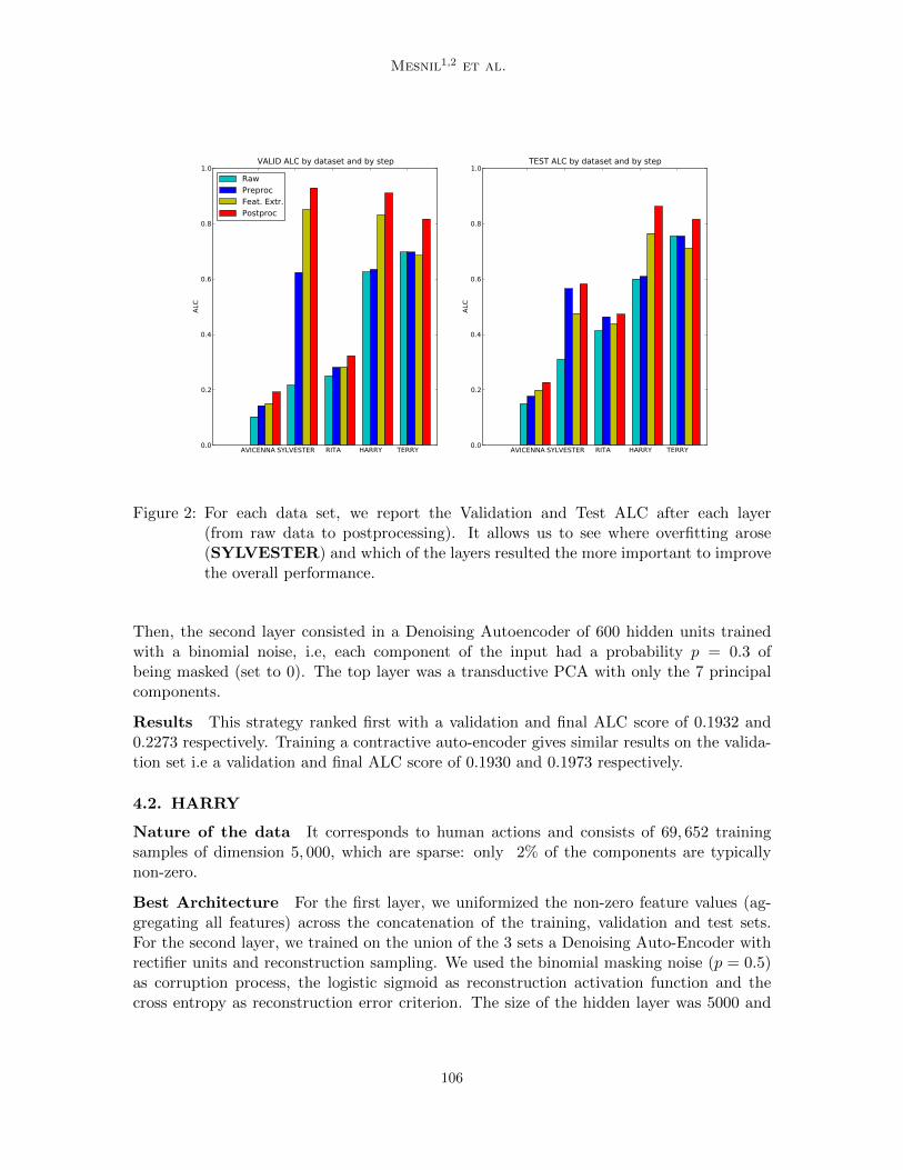
Figure 2: For each data set, we report the Validation and Test ALC after each layer(from raw data to postprocessing). It allows us to see where overfitting arose(SYLVESTER) and which of the layers resulted the more important to improvethe overall performance.

Then, the second layer consisted in a Denoising Autoencoder of 600 hidden units trainedwith a binomial noise, i.e, each component of the input had a probability p = 0.3 ofbeing masked (set to 0). The top layer was a transductive PCA with only the 7 principalcomponents.

Results This strategy ranked first with a validation and final ALC score of 0.1932 and0.2273 respectively. Training a contractive auto-encoder gives similar results on the valida-tion set i.e a validation and final ALC score of 0.1930 and 0.1973 respectively.

4.2. HARRY

Nature of the data It corresponds to human actions and consists of 69, 652 trainingsamples of dimension 5, 000, which are sparse: only 2% of the components are typicallynon-zero.

Best Architecture For the first layer, we uniformized the non-zero feature values (ag-gregating all features) across the concatenation of the training, validation and test sets.For the second layer, we trained on the union of the 3 sets a Denoising Auto-Encoder withrectifier units and reconstruction sampling. We used the binomial masking noise (p = 0.5)as corruption process, the logistic sigmoid as reconstruction activation function and thecross entropy as reconstruction error criterion. The size of the hidden layer was 5000 and

106

Unsupervised and Transfer Learning Challenge: a Deep Learning Approach

Figure 3: HARRY evaluation set after the transductive PCA, the data is nicely clustered,suggesting that the learned preprocessing has discovered the underlying classstructure.

we added an L1 penalty on the activation values to encourage sparsity of the representation.For the third layer, we applied a transductive PCA and kept 3 components.

Results We obtained the best validation ALC score of the competition. This was alsothe case for the final evaluation score with an ALC score of 0.861933, whereas the secondbest obtained 0.754497. Figure 3 shows the final data representation we obtained for thetest (evaluation) set.

4.3. TERRY

Nature of the data This is a natural language processing (NLP) task, with 217, 034training samples of dimension 41, 236, and a high level of sparsity: only 1% of the compo-nents are non-zero in average.

Best Architecture A setup similar to HARRY has been used for TERRY. For the firstlayer, we kept only the features that were active on both training and validation sets (andsimilarly with the test set, for preparing the test set representations). Then, we divided thenon-zero feature values by their standard deviation across the concatenation of the training,validation and test set. For the second layer, we trained on the three sets a Denoising Auto-Encoder with rectifier units and reconstruction sampling. We used binomial masking noise(p = 0.5) as corruption process, the logistic sigmoid as reconstruction activation functionand the squared error as reconstruction error criterion. The size of the hidden layer was5000 and we added an L1 penalty on the activation values to encourage sparsity of the

107

Mesnil1,2 et al.

representation. For the third layer, we applied a transductive PCA and kept the leading 4components.

Results We ranked second on this dataset with a validation and final score of 0.816752and 0.816009.

4.4. SYLVESTER

Nature of the data It corresponds to ecology data and consists of 572, 820 trainingsamples of dimension 100.

Best Architecture For the first layer, we extracted the meaningful features and dis-carded the apparent noise dimensions using PCA. We used the first 8 principal dimensionsas the feature representation produced by the layer because it gave the best performanceon the validation set. We also whitened this new feature representation by dividing eachdimension by its corresponding singular value (square root of the eigenvalue of the covari-ance matrix, or corresponding standard deviation of the component). Whitening gives eachdimension equal importance both for the classifier and subsequent feature extractors. Forthe second and third layers, we used a Contractive Auto-Encoder (CAE). We have selecteda layer size of 6 based on validation ALC. For the fourth layer, we again apply a transductivePCA.

(a) Raw Data (b) 1st Layer (c) 2nd Layer

(d) 3rd Layer (e) t-PCA

Figure 4: Validation performance increases with the depth of our feature hierarchy for theSYLVESTER dataset. ALC: Raw Data (0.2167), 1st Layer (0.6238), 2nd Layer(0.7878), 3rd Layer (0.8511), t-PCA(0.9316)

Figure 4 shows the evolution of the ALC curve for each layer of the hierarchy. Note thatat each layer, we only use the top-level features as the representation.

108

Unsupervised and Transfer Learning Challenge: a Deep Learning Approach

Results This yielded an ALC of 0.85109 for the validation set and 0.476341 for the test set.The difference in ALC may be explained by the fact that Sylvester is the only dataset wherethe test set contains more classes than the validation set and, and thus our assumpptionsof equal number of classes might have hurt test performance here.

4.5. RITA

Nature of the data It corresponds to the CIFAR RGB image dataset and consists of111, 808 training samples of dimension 7, 200.

Best Architecture The µ-ssRBM was initially developed as a model for natural images.As such, it was a natural fit for the RITA dataset. Their ability to learn the poolingstructure was also a clear advantage, since the max-pooling strategy typically used in visiontasks with convolutional networks LeCun et al. (1998) could no longer be employed due tothe obfuscated nature of the dataset.

For pre-processing, each image has been contrast-normalized. Then, we reduced thedimensionality of the training dataset by learning on the first 1, 000 principal components.For feature extraction, we chose the number of hidden units to be large enough (1000)while still being computationally efficient on GPUs. The learning rate of 10−3 and numberof training updates (110, 000 updates with minibatches of size 16) are chosen such thathidden units have sparse activations through pools of size 9, hovering around 10-25%. Thepost-processing was consistent with the other datasets: we used the transductive PCAmethod using only the first 4 principal components.

Results This yielded an ALC score of 0.286 and 0.437 for the validation and final testsets respectively. We also tried to stack 3 layers of contractive auto-encoders directly onthe raw data and it achieved a valid ALC of 0.3268. As it appeared actually transductive,we prefered to keep the µ-ssRBM in our competition entries because it was trained on thewhole training set.

5. Conclusion

The competition setting with different class labels in the validation and the test sets wasquite unusual. The similarity between two classes must be sufficient for transfer learning tobe possible. More formal assessments of class similarity might be useful in such settings. It isnot obvious that the similarity between the subsets of classes chosen for the different datasetsin the context of the competition is sufficient for an effective generalization, neither that thesimilarity between the subsets of classes found in the transfer labels is representative of thesimilarity between the classes found in the training, validation and test datasets. Finally,for assessing transfer across classes properly would require a larger number of classes. Ina future competition, we suggest that both similarity and representativeness (includingnumber of classes) should be ensured in a more formal or empirical way.

On all five tasks, we have found the idea of stacking different layer-wise representation-learning algorithms to work very well. One surprise was the effectiveness of PCA both asa first layer and a last layer, in a transductive setting. As core feature-learning blocks, thecontractive auto-encoder, the denoising auto-encoder and spike-and-slab RBM worked best

109

Mesnil1,2 et al.

for us on the dense datasets, while the sparse rectifier denoising auto-encoder worked beston the sparse datasets.

Acknowledgements

The authors acknowledge the support of the following agencies for research funding andcomputing support: NSERC, RQCHP, CIFAR. This is also funded in part by the FrenchANR Project ASAP ANR-09-EMER-001.

References

Yoshua Bengio. Learning deep architectures for AI. Foundations and Trends in MachineLearning, 2(1):1–127, 2009. Also published as a book. Now Publishers, 2009.

Yoshua Bengio. Deep learning of representations for unsupervised and transfer learning. InWorkshop on Unsupervised and Transfer Learning (ICML’11), June 2011.

Yoshua Bengio, Pascal Lamblin, Dan Popovici, and Hugo Larochelle. Greedy layer-wisetraining of deep networks. In Bernhard Scholkopf, John Platt, and Thomas Hoffman,editors, Advances in Neural Information Processing Systems 19 (NIPS’06), pages 153–160. MIT Press, 2007.

James Bergstra, Olivier Breuleux, Frederic Bastien, Pascal Lamblin, Razvan Pascanu, Guil-laume Desjardins, Joseph Turian, David Warde-Farley, and Yoshua Bengio. Theano:a CPU and GPU math expression compiler. In Proceedings of the Python for Scien-tific Computing Conference (SciPy), June 2010. URL http://www.iro.umontreal.ca/

~lisa/pointeurs/theano_scipy2010.pdf. Oral.

Christopher M. Bishop. Pattern Recognition and Machine Learning. Springer, 2006.

A. Coates, H. Lee, and A. Ng. An analysis of single-layer networks in unsupervised fea-ture learning. In Proceedings of the Thirteenth International Conference on ArtificialIntelligence and Statistics (AISTATS 2011), 2011.

Aaron Courville, James Bergstra, and Yoshua Bengio. Unsupervised models of images byspike-and-slab RBMs. In Proceedings of the Twenty-eight International Conference onMachine Learning (ICML’11), June 2011.

Yann Dauphin, Xavier Glorot, and Yoshua Bengio. Sampled reconstruction for large-scalelearning of embeddings. In Proceedings of the Twenty-eight International Conference onMachine Learning (ICML’11), June 2011.

Xavier Glorot, Antoire Bordes, and Yoshua Bengio. Deep sparse rectifier neural networks.In JMLR W&CP: Proceedings of the Fourteenth International Conference on ArtificialIntelligence and Statistics (AISTATS 2011), April 2011.

Y. LeCun, L. Bottou, Y. Bengio, and P. Haffner. Gradient based learning applied todocument recognition. IEEE, 86(11):2278–2324, November 1998.

110

Unsupervised and Transfer Learning Challenge: a Deep Learning Approach

V. Nair and G. E Hinton. Rectified linear units improve restricted Boltzmann machines. InProc. 27th International Conference on Machine Learning, 2010.

M. Ranzato and G. H. Hinton. Modeling pixel means and covariances using factorizedthird-order Boltzmann machines. In Proceedings of the Computer Vision and PatternRecognition Conference (CVPR’10), pages 2551–2558. IEEE Press, 2010.

Salah Rifai, Pascal Vincent, Xavier Muller, Xavier Glorot, and Yoshua Bengio. Contrac-tive auto-encoders: Explicit invariance during feature extraction. In Proceedings of theTwenty-eight International Conference on Machine Learning (ICML’11), June 2011.

Tijmen Tieleman. Training restricted Boltzmann machines using approximations to thelikelihood gradient. In William W. Cohen, Andrew McCallum, and Sam T. Roweis,editors, Proceedings of the Twenty-fifth International Conference on Machine Learning(ICML’08), pages 1064–1071. ACM, 2008.

Pascal Vincent, Hugo Larochelle, Yoshua Bengio, and Pierre-Antoine Manzagol. Extract-ing and composing robust features with denoising autoencoders. In William W. Cohen,Andrew McCallum, and Sam T. Roweis, editors, Proceedings of the Twenty-fifth Inter-national Conference on Machine Learning (ICML’08), pages 1096–1103. ACM, 2008.

Pascal Vincent, Hugo Larochelle, Isabelle Lajoie, Yoshua Bengio, and Pierre-Antoine Man-zagol. Stacked denoising autoencoders: Learning useful representations in a deep networkwith a local denoising criterion. Journal of Machine Learning Research, 11(3371–3408),December 2010.

111