Unsupervised Adversarially Robust Representation Learning

Unsupervised Adversarially Robust Representation Learning onGraphs

Jiarong Xu

Zhejiang University

[email protected]

Yang Yang

Zhejiang University

[email protected]

Junru Chen

Zhejiang University

[email protected]

Chunping Wang

FinVolution Group

[email protected]

Xin Jiang

University of California, Los Angeles

[email protected]

Jiangang Lu

Zhejiang University

[email protected]

Yizhou Sun

University of California, Los Angeles

[email protected]

ABSTRACTUnsupervised/self-supervised pre-training methods for graph rep-

resentation learning have recently attracted increasing research

interests, and they are shown to be able to generalize to various

downstream applications. Yet, the adversarial robustness of such

pre-trained graph learning models remains largely unexplored.

More importantly, most existing defense techniques designed for

end-to-end graph representation learning methods require pre-

specified label definitions, and thus cannot be directly applied to

the pre-training methods. In this paper, we propose an unsuper-

vised defense technique to robustify pre-trained deep graph models,

so that the perturbations on the input graph can be successfully

identified and blocked before the model is applied to different down-

stream tasks. Specifically, we introduce a mutual information-based

measure, graph representation vulnerability (GRV), to quantify the

robustness of graph encoders on the representation space. We then

formulate an optimization problem to learn the graph representa-

tion by carefully balancing the trade-off between the expressive

power and the robustness (i.e., GRV) of the graph encoder. The

discrete nature of graph topology and the joint space of graph

data make the optimization problem intractable to solve. To handle

the above difficulty and to reduce computational expense, we fur-

ther relax the problem and thus provide an approximate solution.

Additionally, we explore a provable connection between the ro-

bustness of the unsupervised graph encoder and that of models on

downstream tasks. Extensive experiments demonstrate that even

without access to labels and tasks, our model is still able to enhance

robustness against adversarial attacks on three downstream tasks

(node classification, link prediction, and community detection) by

an average of +16.5% compared with existing methods.

KEYWORDSgraph representation learning, robustness

1 INTRODUCTIONGraphs, a common mathematical abstraction for modeling pairwise

interactions between objects, are widely applied in numerous do-

mains, including bioinformatics, social networks, chemistry, and

finance. Owing to their prevalence, deep learning on graphs, such

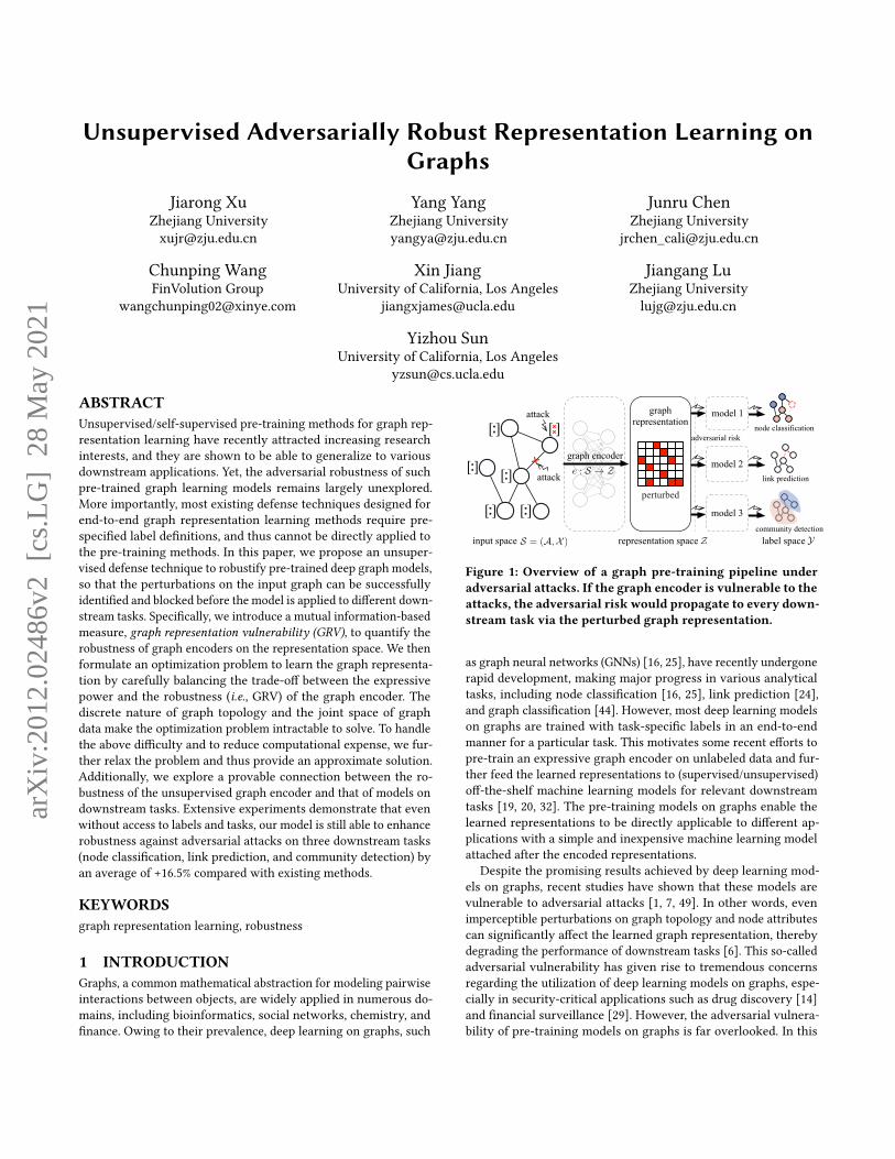
��graph

representation

adversarial risk

S = (A, X )<latexit sha1_base64="pUxN1beV0kbd5trQlh+wGo3n75Q=">AAACEXicbVDLSgMxFL3js9bXqEs3wSJUkDJTBd0IFTcuK/YF7VAyadqGZh4kGaEM8wtu/BU3LhRx686df2OmHXy0Hgice8695N7jhpxJZVmfxsLi0vLKam4tv76xubVt7uw2ZBAJQusk4IFouVhSznxaV0xx2goFxZ7LadMdXaV+844KyQK/psYhdTw88FmfEay01DWLHQ+rIcE8vk3QBfopL5Nj9F20kqOuWbBK1gRontgZKUCGatf86PQCEnnUV4RjKdu2FSonxkIxwmmS70SShpiM8IC2NfWxR6UTTy5K0KFWeqgfCP18hSbq74kYe1KOPVd3pjvKWS8V//PakeqfOzHzw0hRn0w/6kccqQCl8aAeE5QoPtYEE8H0rogMscBE6RDzOgR79uR50iiX7JNS+ea0UKllceRgHw6gCDacQQWuoQp1IHAPj/AML8aD8WS8Gm/T1gUjm9mDPzDevwCGdJzh</latexit>

Z<latexit sha1_base64="+XUzaIaOBF7K2eyZXZpYmz/rtd4=">AAAB83icbVDLSgMxFL2pr1pfVZdugkVwVWaqoMuCG5cV+sLOUDJppg3NZIYkI5Shv+HGhSJu/Rl3/o2ZdhbaeiBwOOde7skJEsG1cZxvVNrY3NreKe9W9vYPDo+qxyddHaeKsg6NRaz6AdFMcMk6hhvB+oliJAoE6wXTu9zvPTGleSzbZpYwPyJjyUNOibGS50XETCgR2eMcD6s1p+4sgNeJW5AaFGgNq1/eKKZpxKShgmg9cJ3E+BlRhlPB5hUv1SwhdErGbGCpJBHTfrbIPMcXVhnhMFb2SYMX6u+NjERaz6LATuYZ9aqXi/95g9SEt37GZZIaJunyUJgKbGKcF4BHXDFqxMwSQhW3WTGdEEWosTVVbAnu6pfXSbdRd6/qjYfrWrNd1FGGMziHS3DhBppwDy3oAIUEnuEV3lCKXtA7+liOllCxcwp/gD5/APcDkbA=</latexit>

Y<latexit sha1_base64="yibioAhXqoghUir83Mp9JnovUnQ=">AAAB83icbVDLSgMxFL2pr1pfVZdugkVwVWaqoMuCG5cV+pLOUDJppg3NZIYkI5Shv+HGhSJu/Rl3/o2ZdhbaeiBwOOde7skJEsG1cZxvVNrY3NreKe9W9vYPDo+qxyddHaeKsg6NRaz6AdFMcMk6hhvB+oliJAoE6wXTu9zvPTGleSzbZpYwPyJjyUNOibGS50XETCgR2eMcD6s1p+4sgNeJW5AaFGgNq1/eKKZpxKShgmg9cJ3E+BlRhlPB5hUv1SwhdErGbGCpJBHTfrbIPMcXVhnhMFb2SYMX6u+NjERaz6LATuYZ9aqXi/95g9SEt37GZZIaJunyUJgKbGKcF4BHXDFqxMwSQhW3WTGdEEWosTVVbAnu6pfXSbdRd6/qjYfrWrNd1FGGMziHS3DhBppwDy3oAIUEnuEV3lCKXtA7+liOllCxcwp/gD5/APV9ka8=</latexit>

graph encoder

attack

attack

input space representation space label space

model 2

node classification

link prediction

community detection

model 1

model 3

perturbed

e : S ! Z<latexit sha1_base64="Mqdbb7WpXzZtYQezqvOpmW62UZc=">AAACD3icbVDLSsNAFJ34rPUVdelmsCiuSlIFxVXBjcuKfWETymQ6bYdOZsLMRCkhf+DGX3HjQhG3bt35N07agNp64MLhnHu5954gYlRpx/myFhaXlldWC2vF9Y3NrW17Z7epRCwxaWDBhGwHSBFGOWloqhlpR5KgMGCkFYwuM791R6Sigtf1OCJ+iAac9ilG2khd+4hcQC9EeogRS25S6Ek6GGokpbj/0W/Trl1yys4EcJ64OSmBHLWu/en1BI5DwjVmSKmO60TaT5DUFDOSFr1YkQjhERqQjqEchUT5yeSfFB4apQf7QpriGk7U3xMJCpUah4HpzE5Us14m/ud1Yt0/9xPKo1gTjqeL+jGDWsAsHNijkmDNxoYgLKm5FeIhkghrE2HRhODOvjxPmpWye1KuXJ+WqvU8jgLYBwfgGLjgDFTBFaiBBsDgATyBF/BqPVrP1pv1Pm1dsPKZPfAH1sc3UZCc6g==</latexit>

��

��

��

��

Figure 1: Overview of a graph pre-training pipeline underadversarial attacks. If the graph encoder is vulnerable to theattacks, the adversarial risk would propagate to every down-stream task via the perturbed graph representation.

as graph neural networks (GNNs) [16, 25], have recently undergone

rapid development, making major progress in various analytical

tasks, including node classification [16, 25], link prediction [24],

and graph classification [44]. However, most deep learning models

on graphs are trained with task-specific labels in an end-to-end

manner for a particular task. This motivates some recent efforts to

pre-train an expressive graph encoder on unlabeled data and fur-

ther feed the learned representations to (supervised/unsupervised)

off-the-shelf machine learning models for relevant downstream

tasks [19, 20, 32]. The pre-training models on graphs enable the

learned representations to be directly applicable to different ap-

plications with a simple and inexpensive machine learning model

attached after the encoded representations.

Despite the promising results achieved by deep learning mod-

els on graphs, recent studies have shown that these models are

vulnerable to adversarial attacks [1, 7, 49]. In other words, even

imperceptible perturbations on graph topology and node attributes

can significantly affect the learned graph representation, thereby

degrading the performance of downstream tasks [6]. This so-called

adversarial vulnerability has given rise to tremendous concerns

regarding the utilization of deep learning models on graphs, espe-

cially in security-critical applications such as drug discovery [14]

and financial surveillance [29]. However, the adversarial vulnera-

bility of pre-training models on graphs is far overlooked. In this

arX

iv:2

012.

0248

6v2

[cs

.LG

] 2

8 M

ay 2

021

Conference’17, July 2017, Washington, DC, USA Jiarong Xu, Yang Yang, Junru Chen, Chunping Wang, Xin Jiang, Jiangang Lu, and Yizhou Sun

work, we show that graph pre-training models also suffer from the

adversarial vulnerability problem. Actually, owing to the compli-

cated and deep structure, the graph encoder is more vulnerable

to adversarial attacks than the simple machine learning models

used for downstream tasks in a graph pre-training pipeline [36]. As

Figure 1 shows, once the graph encoder is vulnerable to adversarial

attacks, the adversarial risk would propagate to every downstream

task via the perturbed representations.

Most efforts targeted on this adversarial vulnerability problem

focus on supervised, end-to-end models designed for a particular

application scenario [2, 23, 41, 50]. However, the dependency on

the supervised information largely limits the scope of their appli-

cation and usefulness. For example, these models do not perform

well on downstream tasks in which training labels are missing,

e.g., community detection in social networks. In addition, training

multiple models for different downstream tasks is both costly and

insecure [12]. In contrast, robust unsupervised pre-training models

can easily handle the above issues: adversarial attacks are identified

and blocked before propagating to downstream tasks. Moreover,

these models are applicable to a more diverse group of applications,

including node classification, link prediction, and community detec-

tion. And yet, robust pre-training models under the unsupervised

setting remains largely unexplored.

There are many interesting yet challenging questions in this

new field of research. Conventionally, the robustness of a model is

defined based on the label space [2, 17, 50], which is not the case

in our setting. Thus the first difficulty we meet is to quantify the

robustness of an unsupervised model (without the knowledge of

the true or predicted labels).

To overcome the above challenge, in this paper, we first intro-

duce the graph representation vulnerability (GRV), an information

theoretic-based measure used to quantify the robustness of a graph

encoder. We then formulate an optimization problem to study the

trade-off between the expressive power of a graph encoder and

its robustness to adversarial attacks, measured in GRV. However,

how to efficiently compute or approximate the objective of the

optimization problem becomes the next issue. First, it remains a

big problem on how to describe the ability of the attack strategies

or the boundary of perturbations, because adversarial attacks on

graphs perturb both the discrete graph topology and the continuous

node attributes. Second, the rigorous definition of the objective is

intractable.

To handle the above issues, we first quantify the ability of ad-

versarial attacks using Wasserstein distance between probability

distributions, and provide a computationally efficient approxima-

tion for it. We then adopt a variant of projected gradient descent

method to solve the proposed optimization problem efficiently. A

sub-optimal solution for the problem gives us a well-qualified, ro-

bust graph representation encoder.

Last but not least, we explore several interesting theoretical con-

nections between the proposed measure of robustness (GRV) and

the classifier robustness based on the label space. To show the

practical usefulness of the proposed model, we apply the learned

representations to three different downstream tasks, namely, node

classification, link prediction, and community detection. Exper-

imental results reveal that under adversarial attacks, our model

beats the best baseline by an average of +1.8%, +1.8%, and +45.8%

on node classification, link prediction, and community detection

task, respectively.

2 PRELIMINARIES AND NOTATIONSIn most cases, we use upper-case letters (e.g., 𝑋 and 𝑌 ) to denote

random variables and calligraphic letters (e.g., X and Y) to denote

their support, while the corresponding lower-case letters (e.g., 𝒙and 𝒚) indicate the realizations of these variables. We denote the

random variables of the probability distributions using subscripts

(e.g., `𝑋 and `𝑌 ) and the corresponding empirical distributions

with hat accents (e.g., ^𝑋 and ^𝑌 ). We use bold upper-case letters

to represent matrices (e.g., A). When indexing the matrices, A𝑖 𝑗

denotes the element at the 𝑖-th row and the 𝑗-th column, while A𝑖

represents the vector at the 𝑖-th row. We use (X, 𝑑) to denote themetric space, where 𝑑 :X ×X → R is a distance function on X. We

further denote byM(X) the set of all probability measures on X.We assume a generic unsupervised graph representation learning

setup. In brief, we are provided with an undirected and unweighted

graph G = (V,E) with the node set V = {𝑣1, 𝑣2, ..., 𝑣 |V |} and edge

set E ⊆ V × V = {𝑒1, 𝑒2, ..., 𝑒 |E |}. We are also provided with the

adjacency matrix A ∈ {0, 1} |V |× |V | of the graph G, a symmet-

ric matrix with elements A𝑖 𝑗 = 1 if (𝑣𝑖 , 𝑣 𝑗 ) ∈ E or 𝑖 = 𝑗 , and

A𝑖 𝑗 = 0 otherwise. We augment G with the node attribute matrix

X ∈ R |V |×𝑐 if nodes have attributes. Accordingly, we define our

input as 𝒔 = (𝒂, 𝒙) ∈ S; thus, we can conceive of 𝒙 as the attribute

matrix and 𝒂 as the adjacency matrix of G under a transductive

learning setting, while 𝒂 and 𝒙 are the adjacency matrix and at-

tribute matrix respectively of a node’s subgraph under an inductive

learning setting. We further define an encoder 𝑒 : S → Z, which

maps an input 𝒔 = (𝒂, 𝒙) ∈ S to a representation 𝑒 (𝒂, 𝒙) ∈ Z, and

a simple machine learning model 𝑓 : Z → Y that maps a repre-

sentation 𝒛 ∈ Z to a label 𝑓 (𝒛) ∈ Y. We go on to define 𝑔 = 𝑓 ◦ 𝑒as their composition, such that (𝑓 ◦ 𝑒) (𝒂, 𝒙) = 𝑓 (𝑒 (𝒂, 𝒙)). A table

of main notations is attached in the Appendix.

Mutual information. Recall that themutual information between

two random variables 𝑋 and 𝑌 is a measure of the mutual depen-

dence between them, and is defined as the Kullback–Leibler (KL)

divergence between the joint distribution 𝑝 (𝒙,𝒚) and the product

of the marginal distributions 𝑝 (𝒙)𝑝 (𝒚):I(𝑋 ;𝑌 ) = 𝐷KL

(𝑝 (𝒙,𝒚)∥𝑝 (𝒙)𝑝 (𝒚)

)=

∫Y

∫X𝑝 (𝒙,𝒚) log

(𝑝 (𝒙,𝒚)𝑝 (𝒙)𝑝 (𝒚)

)𝑑𝑥𝑑𝑦.

More specifically, it quantifies the “amount of information” obtained

about one random variable through observing the other random

variable. The successful application of mutual information to var-

ious unsupervised graph representation learning tasks has been

demonstrated by many authors [35, 37, 39].

Admissible perturbations on graphs. TheWasserstein distance

can be conceptualized as an optimal transport problem: we wish

to move transport the mass with probability distribution `𝑆 into

another distribution `𝑆′ at the minimum cost. Formally, the 𝑝-th

Wasserstein distance between `𝑆 and `𝑆′ is defined as

𝑊𝑝 = (`𝑆 , `𝑆′) =(

inf𝜋 ∈Π (`𝑆 ,`𝑆′ )

∫S2

𝑑 (𝒔, 𝒔 ′) 𝑑𝜋 (𝒔, 𝒔 ′))1/𝑝

,

Unsupervised Adversarially Robust Representation Learning on Graphs Conference’17, July 2017, Washington, DC, USA

where Π(`𝑆 , `𝑆′) denotes the collection of all measures on S × Swithmarginal `𝑆 and `𝑆′ , respectively. The choice of∞-Wasserstein

distance (i.e., 𝑝 = ∞) is conventional in learning graph representa-

tions [4].

Based on∞-Wasserstein distance, we can quantify the ability of

the adversarial attacks. An attack strategy is viewed as a perturbed

probability distribution around that of 𝑆 = (𝐴,𝑋 ), and then all

possible attack strategies stay in a ball around the genuine distribu-

tion `𝑆 :

B∞ (`𝑆 , 𝜏) = {`𝑆′ ∈ M(𝑆) :𝑊∞ (`𝑆 , `𝑆′) ≤ 𝜏},

where 𝜏 > 0 is a pre-defined budget.

3 GRAPHS REPRESENTATIONS ROBUST TOADVERSARIAL ATTACKS

In a widely adopted two-phase graph learning pipeline, The first

step is to pre-train a graph encoder 𝑒 (without the knowledge of true

labels), which maps the joint input space S (i.e., the graph topol-

ogyA and node attributesX) into some, usually lower-dimensional,

representation spaceZ. Then the encoded representation is used

to solve some target downstream tasks.

In this section, we explain how to obtain a well-qualified graph

representation robust to adversarial attacks. We first propose a

measure to quantify the robustness without label information in

§3.1. In §3.2, we formulate an optimization problem to explore the

trade-off between the expressive power and the robustness of the

graph encoder. We then describe every component in the proposed

optimization problem, and explain how we obtain a sub-optimal

solution efficiently in §3.3.

3.1 Quantifying the Robustness of GraphRepresentations

In this section, we propose the graph representation vulnerability(GRV) to quantify the robustness of an encoded graph representa-

tion. Intuitively, the learned graph representation is robust if its

quality does not deteriorate too much under adversarial attacks.

Now we introduce in detail how to measure the quality of repre-

sentations using MI, and how to describe the difference of repre-

sentation quality before and after adversarial attacks.

The use of mutual information. A fundamental challenge to

achieving a qualified graph representation is the need to find a

suitable objective that guides the learning process of the graph

encoder. In the case of unsupervised graph representation learning,

the commonly used objectives are random walk-based [15, 30] or

reconstruction-based [24]. These objectives impose an inductive

bias that neighboring nodes or nodes with similar attributes have

similar representations. However, the inductive bias is easy to break

under adversarial attacks [10, 23], leading to the vulnerability of

random walk-based and reconstruction-based encoders. As an al-

ternative solution, we turn to maximize the MI between the input

attributed graph and the representation output by the encoder, i.e.,I(𝑆; 𝑒 (𝑆)). In our case, maximizing the MI I(𝑆; 𝑒 (𝑆)) encouragesthe representations to be maximally informative about the input

graph and to avoid the above-mentioned inductive bias.

Graph representation vulnerability. In addition to the measure

of the quality of a graph representation, we also need to describe

the robustness of a representation. Intuitively, an encoder is robust

if the MI before and after the attack stay close enough. Thus, we

propose the graph representation vulnerability (GRV) to quantify

this difference:

GRV𝜏 (𝑒) = I(𝑆; 𝑒 (𝑆)) − inf`𝑆′ ∈B(`𝑆 ,𝜏)

I(𝑆 ′; 𝑒 (𝑆 ′)), (1)

where 𝑆 = (𝐴,𝑋 ) is the random variable following the benign data

distribution, and 𝑆 ′ = (𝐴′, 𝑋 ′) follows the adversarial distribution.The first term I(𝑆; 𝑒 (𝑆)) in (1) is the MI between the benign graph

data and the encoded representation, while the term I(𝑆 ′, 𝑒 (𝑆 ′))uses the graph data after attack. The attack strategy `𝑆★ that results

in the minimum MI is called the worst-case attack, and is defined as

`𝑆★ = argmin`𝑆′ ∈B(`𝑆 ,𝜏)

I(𝑆 ′; 𝑒 (𝑆 ′)) .

Hence by definition, the graph representation vulnerability (GRV)

describes the difference of the encoder’s behavior using benign

data and under the worst-case adversarial attack. A lower value

of GRV𝜏 (𝑒) implies a more robust encoder to adversarial attacks.

Formally, an encoder is called (𝜏,𝛾)-robust if GRV𝜏 (𝑒) ≤ 𝛾 .An analogy to the graph representation vulnerability (GRV) has

been studied in the image domain [48]. However, the extension

of [48] to the graph domain requires nontrivial effort. An image is

considered to be a single continuous space while a graph is a joint

space S = (A,X), consisting of a discrete graph-structure spaceAand a continuous feature space X. Moreover, the perturbations on

the joint space (A,X) is difficult to track because a minor change

in the graph topology or node attributes will propagate to other

parts of the graph via edges. This is different in the image domain,

where the distributions of all the pixels are assumed to be i.i.d.

Therefore, the discrete nature of graph topology and joint space

(A,X) make the worst-case adversarial attack extremely difficult

to estimate. Thus, the optimizationmethod we apply is substantially

different from that in [48]; see §3.2 and §3.3. Furthermore, more

complicated analysis is needed to verify our approach in theory;

see §4 for details.

3.2 Optimization ProblemThe trade-off between model robustness and the expressive power

of encoder has been well-studied by many authors [38, 47]. In

our case, this trade-off can be readily explored by the following

optimization problem

maximize ℓ1 (Θ) = I(𝑆; 𝑒 (𝑆)) − 𝛽GRV𝜏 (𝑒), (2)

where the optimization variable is the learnable parameters Θ of

the encoder 𝑒 , and 𝛽 > 0 is a pre-defined parameter.

However, in practice, the “most robust” encoder is usually not

the desired one (as it sacrifices too much in the encoder’s expres-

sive power). An intuitive example for the “most robust” encoder is

the constant map, which always outputs the same representation

whatever the input is. Hence, a “robust enough” encoder would be

sufficient, or even better. To this end, we add a soft-margin 𝛾 to

GRV, and obtain the following optimization problem

maximize ℓ2 (Θ) = I(𝑆; 𝑒 (𝑆)) − 𝛽max {GRV𝜏 (𝑒), 𝛾}. (3)


The second term is positive if GRV𝜏 > 𝛾 and the constant 𝛾 other-

wise. As a result, when the encoder is sufficiently robust, the second

term in ℓ2 vanishes, and thus Problem (3) turns to the standard MI

maximization using benign data. Furthermore, when 𝛽 = 1, Prob-lem (3) can be divided into two simple sub-problems, depending on

the value of GRV𝜏 (𝑒):maxΘ

inf`𝑆′ ∈B∞ (`𝑆 ,𝜏)

I(𝑆 ′; 𝑒 (𝑆 ′)), if GRV𝜏 > 𝛾

maxΘ

I(𝑆; 𝑒 (𝑆)), otherwise.(4)

In this case (𝛽 = 1), when GRV𝜏 (𝑒) > 𝛾 , the problem maximizes

the MI under the worst-case adversarial attack. In other words, the

robust encoder tries to maintain the mutual dependence between

the graph data and the encoded representation, under all kinds of

adversarial attacks. When the encoder is sufficiently robust (i.e.,GRV𝜏 (𝑒) ≤ 𝛾 ), the problem turns to maximize the expressive

power of graph encoder.

GNN as the parameterized encoder. The graph neural network

(GNN) has been extensively used as an expressive function for

parameterizing the graph encoder [24, 25]. In this paper, we adopt

a one-layer GNN: 𝑒 (A,X) = 𝜎 (D−1/2AD−1/2XΘ), where A is the

adjacency matrix with self-loops, D is the corresponding degree

matrix, 𝜎 is the ReLU function, and Θ is the learnable parameters.

3.3 Approximate SolutionIn this section, we discuss in detail how to obtain a sub-optimal

solution for Problem (4). Overall, the algorithm we use is a variant

of the classical gradient-basedmethods, as presented in Algorithm 1.

In every iteration, we first find out the distribution of the worst-

case adversarial attack, and thus we can calculate the value of

GRV. If GRV is larger than 𝛾 , we try to enhance the robustness in

this iteration, and apply one gradient descent step for the first sub-

problem in Problem (4). OtherwisewhenGRV𝜏 (𝑒) < 𝛾 , the encoder

is considered robust enough, and thus we focus on improving the

expressive power by one gradient descent move in the second sub-

problem in (4). As a small clarification, the stopping criterion in

Algorithm 1 follows the famous early-stopping technique [31].

However, there are still many kinds of difficulties in implement-

ing the algorithm. First of all, the mutual information I(𝑆, 𝑒 (𝑆)) isextremely hard to compute, mainly because 𝑆 = (𝐴,𝑋 ) is a jointrandom variable involving a high-dimensional discrete variable 𝐴.

In addition, the search space of the adversarial attacks, B∞ (`𝑆 , 𝜏),is intractable to quantify: There is no conventional or well-behaved

choice for the distance metric 𝑑 in such a complicated joint space,

and even when we know the metric, the distance between two

random variables is difficult to calculate. Apart from the above

challenges, the classical, well-known projected gradient descent

algorithm does not work in the joint space 𝑆 = (𝐴,𝑋 ), and thus

the worst-case adversarial attack `𝑆★ is no way to find. Therefore,

in this section, we further address the above issues in detail and

explain every component in Algorithm 1.

MI estimation. Directly computing I(𝑆; 𝑒 (𝑆)) in Problem (4) is

intractable, especially for a joint distribution 𝑆 = (𝐴,𝑋 ) whichincludes a high-dimensional discrete random variable 𝐴. Some au-

thors propose to maximize the average MI between a high-level

“global” representation and local regions of the input, and show

Algorithm 1 Optimization algorithm.

Input: Graph G = (A,X), learning rate 𝛼 .Output: Graph encoder parameters Θ.

1: Randomly initialize Θ.2: while Stopping condition is not met do3: `𝑆★ ← argmin`𝑆′ ∈B(`𝑆 ,𝜏) I(𝑆

′; 𝑒 (𝑆 ′)).4: GRV𝜏 (𝑒) ← I(𝑆; 𝑒 (𝑆)) − I(𝑆★; 𝑒 (𝑆★)).5: if GRV𝜏 (𝑒) > 𝛾 then6: Θ← Θ − 𝛼∇ΘI(𝑆★; 𝑒 (𝑆★)).7: else8: Θ← Θ − 𝛼∇ΘI(𝑆; 𝑒 (𝑆)).9: end if10: end while

Return: Θ.

great improvement in the quality of representations [18, 39]. In-

spired by recent work Deep Graph Infomax [39], we use a noise-

contrastive type objective as an approximation of the mutual infor-

mation (𝐼 ; 𝑒 (𝑆)):

ℓenc (𝑆, 𝑒) = E𝑆 [logD (𝒛, 𝒛G)] + E𝑆 [log (1 − D (��, 𝒛G))] , (5)

where 𝒛 denotes the local representation; 𝒛G = sigmoid (E𝑆 (𝒛))represents the global representation; 𝑆 is the random variable of

negative examples, and �� represents the realization of 𝑒 (𝑆). Thecritic function D(𝒛, 𝒛G) represents the probability score assigned

to a pair of local and global representations obtained from the natu-

ral samples (i.e., the original graph), whileD(��, 𝒛G) is that obtainedfrom negative samples. Common choices for the critic function Dinclude bilinear critics, separable critics, concatenated critics, or

even inner product critics [37]. Here, we select the learnable bilin-

ear critic as our critic function; i.e., DΦ = sigmoid(𝒛𝑇Φ𝒛G), whereΦ is a learnable scoring matrix. Finally, in practice, the expectation

over an underlying distribution is typically approximated by the ex-

pectation of the empirical distribution over 𝑛 independent samples

{(𝒂𝑖 , 𝒙𝑖 )}𝑖∈[𝑛] .Adversarial distribution estimation. Besides the estimation of

MI, another challenge involved in solving Problem (4) is how to find

the worst-case adversarial distribution `𝑆′ ∈ B∞ (`𝑆 , 𝜏). Here, wedivide the difficulties in find `𝑆★ into three categories, and explain

in detail how we solve them one by one.

First, it is difficult to choose an appropriate metric 𝑑 on the joint

input space S = (A,X) that faithfully measures the distance be-

tween each pair of point elements. For example, given any pair of

points 𝒔1 = (𝒂1, 𝒙1) and 𝒔2 = (𝒂2, 𝒙2) in the joint metric space

(A, 𝑑A ) and (X, 𝑑X), an intuitive choice for the distance between

𝒔1 and 𝒔2 would be the𝐿𝑝 -norm ∥(𝑑A (𝒂1, 𝒂2), 𝑑X (𝒙1, 𝒙2)

)∥𝑝 . How-

ever, this intuition fails in our case because the changes in graph

topology and that in node attributes are not in the same order of

magnitude. Thereby, we have to consider the perturbations in Aand X separately. With a little abuse of notation, we redefine the

perturbation bound as follows:

B∞ (`𝐴, `𝑋 , 𝛿, 𝜖) = {(`𝐴′, `𝑋 ′) ∈ M(A) ×M(X) |𝑊∞ (`𝐴, `𝐴′) ≤ 𝛿,𝑊∞ (`𝑋 , `𝑋 ′) ≤ 𝜖},


where the small positive numbers 𝛿 and 𝜖 play the role of pertur-

bation budget now. This is indeed a subset of the previous search

space B(`𝑆 , 𝜏).Moreover, although the search space has been restricted, the∞-

Wasserstein constrained optimization problem remains intractable:

We still have no clue about the underlying probability distribution.

Similar to what we did to estimate MI, we turn to replace the real

data distribution with an empirical one. Suppose we have a set of

i.i.d. samples {(𝒂𝑖 , 𝒙𝑖 )}𝑖∈[𝑛] (note that 𝑛 = 1 under a transductive

learning setting, based on which we can compute the empirical

distribution ( ^𝐴, ^𝑋 )). The empirical search space is defined as

B({𝒂𝑖 }𝑛𝑖=1, {𝒙

𝑖 }𝑛𝑖=1, 𝛿, 𝜖)

=

{( ^𝐴′, ^𝑋 ′)

�� ∥𝒂𝑖 ′ − 𝒂𝑖 ∥0 ≤ 𝛿, ∥𝒙𝑖 ′ − 𝒙𝑖 ∥∞ ≤ 𝜖, 𝑖 ∈ [𝑛]},

where ^𝐴′ and ^𝑋 ′ are the empirical distributions computed from

the perturbed samples {(𝒂𝑖 ′, 𝒙𝑖 ′)}𝑖∈[𝑛] . Here we use the cardinality(i.e., 𝐿0-norm) to measure the change in graph topology (i.e., 𝒂), andthe 𝐿∞-norm to measure the change in continuous node attributes

(i.e., 𝒙). (When node attributes are discrete, or even binary, we can

also use 𝐿0-norm for them.) Finally, we notice that the empirical

space B({𝒂𝑖 }𝑛

𝑖=1, {𝒙𝑖 }𝑛𝑖=1, 𝛿, 𝜖

)is again a subset of B∞ ( ^𝐴, ^𝑋 , 𝛿, 𝜖).

The last, yet the most challenging difficulty is how to efficiently

find the worst-case adversarial attack. We know that he projected

gradient descent (PGD) method can be used to find adversarial

examples in the image domain [27]. However, the idea that works

well for continuous optimization problems is not directly applicable

in our case as the graph topology is a kind of Boolean variables.

Inspired by [43], as a remedy for the discrete case, we adopt a graph

PGD attack for graph topology. We first find a convex hull of the

discrete feasible set, and apply the projected gradient method. A

binary sub-optimal solution 𝒂★ is then recovered using random

sampling. This variant of PGD helps us identify the worst-case

adversarial example efficiently.

4 THEORETICAL CONNECTION TO LABELSPACE

We expect our robust graph encoder is able to block perturbations

on graphs and benefits the downstream tasks. To this end, in this

section, we establish a provable connection between the robustness

of representations (measured by our proposed GRV) and the robust-

ness of the potential model built upon the representations. Despite

the generalization of our framework, we take node classification

tasks as an example in this section. First, we introduce a conven-

tional robustness, adversarial gap (AG), to measure the robustness

of downstream node classifier. Then, we explore some interesting

theoretical connections between GRV and AG.

Adversarial gap. We here introduce a conventional robustness

measure adversarial gap (AG) for node classification, which is built

on the label space.

Definition 1. Suppose we are under inductive learning setting,then 𝒂 and 𝒙 are the adjacency matrix and attribute matrix respec-tively of a node’s subgraph. Let (S, 𝑑) denote the input metric spaceand Y be the set of labels. For node classification model 𝑔 : S → Y,we define the adversarial risk of𝑔 with the adversarial budget 𝜏 ≥ 0

as follows:

AdvRisk𝜏 (𝑔) = E𝑝 (𝒔,𝑦) [∃ 𝒔 ′ = (𝒂′, 𝒙 ′) ∈ B(𝒔, 𝜏)s.t. 𝑔(𝒂′, 𝒙 ′) ≠ 𝑦]

Based on AdvRisk𝜏 (𝑔), the adversarial gap is defined to measurethe relative vulnerability of a given model 𝑔 w.r.t 𝜏 as follows:

AG𝜏 (𝑔) = AdvRisk𝜏 (𝑔) − AdvRisk0 (𝑔).

The smaller the value of AdvRisk or AG is, the more robust 𝑔 is.

Table 1 briefly summarize the robustness measures, including

AG, RV and GRV. The traditional model robustness, adversarial

gap (i.e., AG𝜖 (𝑔) and AG𝜏 (𝑔)), is based on the label space Y, whilethe MI-based robustness measures (i.e., RV∗ (𝑒) and GRV∗ (𝑒)) isbuilt upon the representation spaceZ. The prior work [48], which

defines RV𝜖 (𝑒) on a single input space X in the image domain has

shown that RV𝜖 (𝑒) has a clear connection with classifier robustness.The graph representation venerability GRV𝜏 (𝑒), however, definedas it is on a joint input space (A,X) in the graph domain, is different

from images due to the existence of both discrete and continuous

input data structures. In what follows, we explore some interesting

theoretic conclusions that an inherent relationship exists between

the graph representation vulnerability GRV𝜏 (𝑒) and the adversarialgap AG𝜏 (𝑔); this is based on some certain assumptions that is more

aligned with the graph representation learning.

In exploring the GRV’s connection to the label space Y, onesolution could be to simply assume that one of the input random

variables (i.e., 𝐴 or 𝑋 ) and the label random variable 𝑌 are indepen-

dent. We first consider the two special cases as follows:

• Topology-aware: given 𝑋 ⊥ 𝑌 , 𝑝 (𝑌 |𝐴,𝑋 ) = 𝑝 (𝑌 |𝐴)• Attribute-aware: given 𝐴 ⊥ 𝑌 , 𝑝 (𝑌 |𝐴,𝑋 ) = 𝑝 (𝑌 |𝑋 )

Here, we first work on these two special cases under the relevant

assumptions. We then illustrate a more general case in which 𝑌

is dependent on both 𝐴 and 𝑋 . Detailed proofs of the following

theorems can be found in the Appendix.

Special cases. We simplify the GNN-based encoder architecture as

𝒛 = 𝒂𝑇𝒙𝚯 to obtain a tractable surrogate model. Thus, the represen-

tation of each node depends only on its one-hop neighbors, so we

can obtain the corresponding column of A directly to compute the

representation for each node. Additionally, inspired by [28, 33] that

have defined the perturbations on the intermediate representations,

Table 1: Summary of robustness measures. Here, the adversar-ial gap (AG) is the robustness measure built on the label space Y,while representation vulnerability (RV) and graph representationvulnerability (GRV) are MI-based measures built on the representa-tion space Z. The subscript 𝜖 denotes the perturbation budget of 𝒙(i.e., the image) on the image domain, while the subscript 𝜏 denotesthe perturbation budget of (𝒂, 𝒙) on the graph domain.

Robustness

measure

Domain Input space Output

space

AG𝜖 (𝑔) Image Single X YAG𝜏 (𝑔) Graph Joint (A,X) YRV𝜖 (𝑒) Image Single X ZGRV𝜏 (𝑒) Graph Joint (A,X) Z


we opt to define the adversarial distribution w.r.t `𝐴𝑇𝑋 instead of

that w.r.t `𝐴 and `𝑋 respectively. This assumption is reasonable

owing to our focus on the robustness of our model rather than

the real attack strategies. Accordingly, we assume that the set of

adversarial distributions is B∞ (`𝐴𝑇𝑋 , 𝜌) = {`𝐴′𝑇𝑋 ′ ∈ M(H) :𝑊∞ (`𝐴𝑇𝑋 , `𝐴′𝑇𝑋 ′) ≤ 𝜌} where H = {𝒂𝑇𝒙 : ∀𝒂 ∈ A, 𝒙 ∈ X} inthe following two theorems.

In Theorems 4.1 and 4.2, we use 𝒂 ∈ {0, 1} |V | to denote a

column of A and 𝒙 = X. The subscript 𝜌 of GRV, AdvRisk and

AG represents that they are defined via B∞ (`𝐴𝑇𝑋 , 𝜌), while F =

{𝑓 : 𝑧 ↦→ 𝑦} denotes the set of non-trivial downstream classifiers,

𝑓 ∗ = argmin𝑓 ∈F AdvRisk𝜌 (𝑓 ◦ 𝑒) is the optimal classifier built

upon 𝑒 , and 𝐻𝑏 is the binary entropy function. Moreover, when

indexing 𝒂 and 𝒙 , 𝒂𝑖 denotes the 𝑖-th entry of 𝒂 and 𝒙𝑖 denotes the𝑖-th row of 𝒙 .

Theorem 4.1 (Topology-aware). Let (A, ∥ · ∥0) and (X, ∥ · ∥𝑝 )be the input metric spaces, Y = {−1, +1} be the label space andZ = {−1, +1} be the representation space. The set of encoders withΘ ∈ R |V | is as follows:

E = {𝑒 : (𝒂, 𝒙) ∈ S ↦→ sgn[𝒂𝑇𝒙𝚯] | ∥𝚯∥2 = 1}. (6)

Assume that all samples (𝒔,𝒚) ∼ `𝑆𝑌 are generated from 𝒚u.a.r.∼

𝑈 {−1, +1}, 𝒂𝑖 i.i.d.∼ Bernoulli(0.5+𝒚·(𝑝−0.5)) and 𝒙𝑖 i.i.d.∼ N(0, 𝜎2𝑰𝑐 )where 𝑖 = 1, 2, . . . , |𝑽 | and 0 < 𝑝 < 1. Then, given 𝜌 ≥ 0, for any𝑒 ∈ E, we have the following:

GRV𝜌 (𝑒) = 1 − 𝐻𝑏 (0.5 + AG𝜌 (𝑓 ∗ ◦ 𝑒)).

Next, consider a simpler case in which 𝒚 u.a.r.∼ 𝑈 {−1, +1} and 𝒂𝑖 i.i.d.∼Bernoulli(0.5 + 𝒚 · (𝑝 − 0.5)) hold, but 𝒙𝑖 = 1𝑐 , 𝑖 = 1, . . . , |𝑽 | andthe set of encoders follows such that E = {𝑒 : (𝒂, 𝒙) ↦→ sgn[(𝒂𝑇𝒙 −0.5|𝑽 |1𝑇𝑐 )𝚯] | ∥𝚯∥2 = 1}, which can be regarded as the non-attributecase. Then, given 𝜌 ≥ 0, for any 𝑒 ∈ E, we have

1 − 𝐻𝑏 (0.5 − 0.5AG𝜌 (𝑓 ∗ ◦ 𝑒)) ≤ GRV𝜌 (𝑒)≤ 1 − 𝐻𝑏 (0.5−AG𝜌 (𝑓 ∗ ◦ 𝑒)) . (7)

Theorem 4.1 reveals an explicit connection between GRV𝜌 (𝑒)and AG𝜌 (𝑓 ∗ ◦ 𝑒) achieved by the best classifier in the topology-

aware case. We note that 𝐻𝑏 (\ ) is concave on (0, 1) and that the

maximum of 𝐻𝑏 is attained uniquely at \ = 0.5. Thus, lower GRVis the sufficient and necessary condition of a smaller AG.

Theorem 4.2 (Attribute-aware). Let (A, ∥ · ∥0) and (X, ∥ · ∥𝑝 )be the input metric spaces, Y = {−1, +1} be the label space andZ =

{−1, +1} be the representation space. Suppose that the set of encodersis as in (6). Assume that the samples (𝒔,𝒚) ∼ `𝑆𝑌 are generated from

𝒚u.a.r.∼ 𝑈 {−1, +1}, 𝒂𝑖 𝑖 .𝑖 .𝑑.∼ Bernoulli(0.5) and 𝒙𝑖 𝑖 .𝑖 .𝑑.∼ N(𝒚 ·𝝁, 𝜎2𝐼𝑐 )

where 𝑖 = 1, 2, . . . , |𝑽 |. Then, given 𝜌 ≥ 0, for any 𝑒 ∈ E, we have:

GRV𝜌 (𝑒) = 1 − 𝐻𝑏 (0.5 − AG𝜌 (𝑓 ∗ ◦ 𝑒)) . (8)

Next, consider a simpler case in which 𝒚u.a.r.∼ 𝑈 {−1, +1}, 𝒙𝑖 𝑖 .𝑖 .𝑑.∼

N(𝒚 · 𝝁, 𝜎2𝐼𝑐 ) but 𝒂 ∈ {0, 1} |𝑽 |,∑ |𝑽 |𝑖=1 𝒂𝑖 = 𝑛0 + 𝑛1, where 𝑛0 =

|𝑽 |/4 + 𝒚 · (𝑝 − |𝑽 |/4), 𝑛1 = |𝑽 |/4 + 𝒚 · (𝑞 − |𝑽 |/4) and 𝑝 + 𝑞 =

|𝑽 |/2, 0 ≤ 𝑝, 𝑞 ≤ |𝑽 |/2, 𝑝, 𝑞 ∈ Z; that is, 𝒂𝑇𝒙 will aggregate 𝑛0samples with 𝒚 = +1 and 𝑛1 samples with 𝒚 = −1. Further supposethat the set of encoders is as presented in (6). Then, given 𝜌 ≥ 0, (7)also holds for any 𝑒 ∈ E.

Similarly, we have GRV𝜌 ∝ AG𝜌 in Theorem 4.2. Note that

Theorems 4.1 and 4.2 still hold when 𝒂 contains self-loops.

General case. In the general case, we can extend [48, Theorem

3.4] to the graph domain. Regardless of the encoder, the theorem

below provides a general lower bound of adversarial risk over any

downstream classifiers that involves both MI and GRV. We restate

the theorem below.

Theorem 4.3. [48]. Let (S, 𝑑) be the input metric space, Z bethe representation space and Y be the label space. Assume that thedistribution of labels `𝑌 over Y is uniform and 𝑆 is the randomvariable following the joint distribution of inputs `𝐴𝑋 . Further supposethat F is the set of downstream classifiers. Given 𝜏 ≥ 0,

inf𝑓 ∈F

AdvRisk𝜏 (𝑓 ◦ 𝑒) ≥ 1 − 𝐼 (𝑆; 𝑒 (𝑆)) − GRV𝜏 (𝑒) + log 2log |Y|

holds for any encoder 𝑒 .

Theorem 4.3 suggests that lower adversarial risk over all down-

stream classifiers cannot be achieved without either lower GRV

or higher MI between 𝑆 and 𝑒 (𝑆). It turns out that jointly optimiz-

ing the objective of maximizing 𝐼 (𝑆; 𝑒 (𝑆)) and that of minimizing

GRV𝜏 (𝑒) enables the learning of robust representations. Note that

Theorem 4.3 also holds in the graph classification task.

5 EXPERIMENTSIn this section, we demonstrate that our model capable of learn-

ing highly-qualified representations that are robust to adversarial

attacks. In the experiments, we train our model in a fully unsu-

pervised manner, then apply the output representations to three

graph learning tasks: namely, node classification, link prediction,

and community detection. We demonstrate that compared with

non-robust and other robust graph representation models, the pro-

posed model produces robust representations to defend adversarial

attacks (§ 5.2). Furthermore, the superiority of our model still hold

under different strengths of attacks (in §5.3) and under various

attach strategies (§5.4).

5.1 Experimental Setup

Datasets. We conduct experiments on three benchmark datasets:

Cora, Citeseer and Polblogs. The first two of these are well-known

citation networks in which nodes are documents and edges are the

citation links between two documents. Polblogs is a network of US

politics weblogs, where nodes are blogs and the connection between

two blogs forms an edge. As Polblogs is a dataset without node

attributes, the identity matrix is used to create its node attributes.

Baselines. The baseline models roughly fall into two categories.

• Non-robust graph representation learning: 1) Raw: raw fea-

tures concatenating the graph topology and the node attributes

(graph topology (only) for Polblogs); 2) DeepWalk [30]: a ran-

dom walk-based unsupervised representation learning method

that only considers the graph topology; 3) DeepWalk+X: con-

catenating the Deepwalk embedding and the node attributes;

4) GAE [24]: variational graph auto-encoder, an unsupervised

representation learning method; and 5) DGI [39]: another unsu-

pervised representation learning method based on MI.


Table 2: Summary of results for the node classification, link prediction and community detection tasks using polluted data.

Node classification (Acc%) Link prediction (AUC%) Community detection (NMI%)

Model

Dataset

Cora Citeseer Polblogs Cora Citeseer Polblogs Cora Citeseer Polblogs

Raw 57.4±3.0 49.7±1.6 73.9±0.9 60.5±0.1 50.2±0.5 89.0±0.4 9.7±7.5 1.0±0.5 0.2±0.1DeepWalk 56.2±1.1 16.5±0.9 80.4±0.5 55.4±0.8 50.3±0.3 89.2±0.7 34.6±0.6 11.1±1.0 0.4±0.5DeepWalk +X 59.3±0.4 26.5±0.5 - 55.9±0.6 50.9±0.3 - 34.2±3.7 11.1±1.3 -

GAE 14.0±1.2 16.2±1.1 49.9±1.2 52.4±1.4 50.9±1.8 50.5±1.3 10.9±2.1 1.4±1.7 9.2±1.0DGI 69.3±2.8 53.2±2.2 75.2±2.4 68.6±0.4 57.6±2.1 91.2±1.1 30.3±3.5 8.5±3.8 6.0±5.6Dwns_AdvT 59.2±1.2 25.0±1.0 80.7±0.5 56.0±0.7 50.7±0.4 89.5±0.8 35.0±0.7 11.5±1.0 0.9±0.7RSC 46.9±3.5 34.0±2.2 58.9±1.7 52.5±0.4 57.2±0.2 61.5±0.4 4.9±0.7 1.8±0.4 4.4±4.3DGI-EdgeDrop 56.0±4.3 49.0±4.5 79.8±1.7 66.2±0.8 61.3±0.9 89.3±1.6 30.1±6.8 7.34±0.8 9.0±7.8DGI-Jaccard 69.4±2.8 57.1±1.3 79.3±0.8 63.8±0.8 57.6±1.0 84.7±0.9 16.4±1.1 6.1±0.6 12.9±0.0DGI-SVD 68.1±8.0 56.1±16.4 81.6±0.7 60.1±0.8 54.7±1.3 85.2±0.7 16.2±0.9 6.5±0.8 13.0±0.0Ours-soft 69.4±0.7 57.5±2.0 79.7±2.1 68.1±0.3 58.2±1.3 90.3±0.5 39.2±8.8 23.5±1.9 12.6±9.6Ours 70.7±0.9 58.4±1.4 82.7±2.2 69.2±0.4 59.8±1.3 91.8±0.4 41.4±4.7 23.6±2.8 14.8±2.7

• Defense models: 1) Dwns_AdvT [8]: a defense model designed

for Deepwalk; 2) RSC [3]: a robust unsupervised representation

learning method via spectral clustering; 3) DGI-EdgeDrop [34]:

a defense model that works by dropping 10% of edges during

training DGI; 4) DGI-Jaccard [42]: DGI applied to a pruned ad-

jacency matrix in which nodes with low Jaccard similarity are

forced to be disconnected; and 5) DGI-SVD [10]: DGI applied to

a low-rank approximation of the adjacency matrix obtained by

truncated SVD.

We also include Ours-soft, an variant of our model which removes

soft margin on GRV.

Implementation details. In the training phase, we adopt the

graph PGD attack to construct adversarial examples of 𝒂 while the

PGD attack [27] to construct adversarial examples of 𝒙 . We set the

hyperparameters 𝛾 = 5e-3, 𝛿 = 0.4|E|, and 𝜖 = 0.1. For Polblogs,we do not perform attacks on the constructed node attributes.

In evaluation, we use the same attack strategy as in the training

phase. Note that DeepWalk and RSC both require the entire graph,

and thus we have to retrain them using polluted data. Due to the

imperceptible constraint on adversarial attacks, we set 𝛿 = 0.2|E|during evaluation. The evaluation is performed on three down-

stream tasks, and we explain the detailed settings below.

• Node classification: logistic regression is used for evaluation,

and only accuracy score is reported as the test sets are almost

balanced. For Cora and Citeseer, we use the same dataset splits

as in [25], but do not utilize the labels in the validation set. For

Polblogs, we allocate 10% of the data for training and 80% for

testing.

• Link prediction: logistic regression is used to predict whether a

link exists or not. Following conventions, we generate the positive

test set by randomly removing 10% of existing links and form

the negative test set by randomly sampling the same number of

nonexistent links. The training set consists of the remaining 90%

of existing links and the same number of additionally sampled

nonexistent links. We use the area under the curve (AUC) as the

evaluation metric on the link prediction task.

• Community detection: following the basic schemes for commu-

nity detection based on graph representation learning, we ap-

ply the learned representations to the K-means algorithm. The

normalized mutual information (NMI) is used as the evaluation

metric here.

We run 10 trials for all the experiments and report the average

performance and standard deviation.

5.2 Performance on Downstream TasksAfter adversarial attacks on graph topology and node attributes, our

model’s performance drops by an average of 13.6%, 1.0% and 47.3%

on the node classification, link prediction and community detection

task, respectively. It’s worth noting that, in community detection,

adversarial attacks can cause dramatic influence on model perfor-

mance because the community detection task itself is very sensitive

to the graph topology. Table 2 summarizes the performance of dif-

ferent models in three downstream tasks. From the table we see

that our model beats the best baseline by an average of +1.8% on

the node classification task, +1.8% on the link prediction task and

+45.8% on the community detection task. The difference between

the performance of our model and that of those non-robust graph

learning models indicates the importance of defending adversar-

ial attacks. Moreover, our model still stands out with huge lead

when compared with existing defense models. Last but not least,

the ablation study, i.e., comparing the last two rows in Table 2,

shows the superiority of the soft margin on GRV. With this penalty,

the model focuses on the representation capability on clean data

when the encoder is robust enough (i.e., RV𝜏 ≤ 𝛾 ), while carefullybalances the trade-off between the performance on clean data and

the robustness to polluted ones.

5.3 Performance under Different Rates ofPerturbation

We further compare our model with several strong competitors

under various perturbation rates.We use the node classification task

and the Cora dataset as an illustrative example.We vary the strength


Accu

racy

(%)

OursDGIDGI-JaccardDGI-SVD

1e-3 5e-3 1e-2 5e-2 1e-1 5e-1

62

66

70

74

78

Accu

racy��

Increasing perturbation rate ✏<latexit sha1_base64="V1gdxyRuEIgfVVDAlmoCIPTMGa8=">AAAB73icbVBNS8NAEJ3Ur1q/qh69LBbBU0mqoMeCF09SwX5AG8pmO2mXbjZxdyOU0D/hxYMiXv073vw3btsctPXBwOO9GWbmBYng2rjut1NYW9/Y3Cpul3Z29/YPyodHLR2nimGTxSJWnYBqFFxi03AjsJMopFEgsB2Mb2Z++wmV5rF8MJME/YgOJQ85o8ZKnR4mmotY9ssVt+rOQVaJl5MK5Gj0y1+9QczSCKVhgmrd9dzE+BlVhjOB01Iv1ZhQNqZD7FoqaYTaz+b3TsmZVQYkjJUtachc/T2R0UjrSRTYzoiakV72ZuJ/Xjc14bWfcZmkBiVbLApTQUxMZs+TAVfIjJhYQpni9lbCRlRRZmxEJRuCt/zyKmnVqt5FtXZ/Wanf5XEU4QRO4Rw8uII63EIDmsBAwDO8wpvz6Lw4787HorXg5DPH8AfO5w9Ru5Aw</latexit>

✏<latexit sha1_base64="V1gdxyRuEIgfVVDAlmoCIPTMGa8=">AAAB73icbVBNS8NAEJ3Ur1q/qh69LBbBU0mqoMeCF09SwX5AG8pmO2mXbjZxdyOU0D/hxYMiXv073vw3btsctPXBwOO9GWbmBYng2rjut1NYW9/Y3Cpul3Z29/YPyodHLR2nimGTxSJWnYBqFFxi03AjsJMopFEgsB2Mb2Z++wmV5rF8MJME/YgOJQ85o8ZKnR4mmotY9ssVt+rOQVaJl5MK5Gj0y1+9QczSCKVhgmrd9dzE+BlVhjOB01Iv1ZhQNqZD7FoqaYTaz+b3TsmZVQYkjJUtachc/T2R0UjrSRTYzoiakV72ZuJ/Xjc14bWfcZmkBiVbLApTQUxMZs+TAVfIjJhYQpni9lbCRlRRZmxEJRuCt/zyKmnVqt5FtXZ/Wanf5XEU4QRO4Rw8uII63EIDmsBAwDO8wpvz6Lw4787HorXg5DPH8AfO5w9Ru5Aw</latexit>

Accu

racy

(%)

OursDGIDGI-JaccardDGI-SVD

0.1 0.15 0.2 0.25 0.366

68

70

72

74

Accu

racy��

Increasing perturbation rate �<latexit sha1_base64="SFA26HczKSPDy+k01A8+XiD1cpk=">AAAB7XicbVBNS8NAEJ3Ur1q/qh69BIvgqSRV0GPBiyepYD+gDWWz2bRrN7thdyKU0v/gxYMiXv0/3vw3btsctPXBwOO9GWbmhangBj3v2ymsrW9sbhW3Szu7e/sH5cOjllGZpqxJlVC6ExLDBJesiRwF66SakSQUrB2ObmZ++4lpw5V8wHHKgoQMJI85JWilVi9iAkm/XPGq3hzuKvFzUoEcjX75qxcpmiVMIhXEmK7vpRhMiEZOBZuWeplhKaEjMmBdSyVJmAkm82un7plVIjdW2pZEd67+npiQxJhxEtrOhODQLHsz8T+vm2F8HUy4TDNkki4WxZlwUbmz192Ia0ZRjC0hVHN7q0uHRBOKNqCSDcFffnmVtGpV/6Jau7+s1O/yOIpwAqdwDj5cQR1uoQFNoPAIz/AKb45yXpx352PRWnDymWP4A+fzB5Z2jyw=</latexit>

�<latexit sha1_base64="SFA26HczKSPDy+k01A8+XiD1cpk=">AAAB7XicbVBNS8NAEJ3Ur1q/qh69BIvgqSRV0GPBiyepYD+gDWWz2bRrN7thdyKU0v/gxYMiXv0/3vw3btsctPXBwOO9GWbmhangBj3v2ymsrW9sbhW3Szu7e/sH5cOjllGZpqxJlVC6ExLDBJesiRwF66SakSQUrB2ObmZ++4lpw5V8wHHKgoQMJI85JWilVi9iAkm/XPGq3hzuKvFzUoEcjX75qxcpmiVMIhXEmK7vpRhMiEZOBZuWeplhKaEjMmBdSyVJmAkm82un7plVIjdW2pZEd67+npiQxJhxEtrOhODQLHsz8T+vm2F8HUy4TDNkki4WxZlwUbmz192Ia0ZRjC0hVHN7q0uHRBOKNqCSDcFffnmVtGpV/6Jau7+s1O/yOIpwAqdwDj5cQR1uoQFNoPAIz/AKb45yXpx352PRWnDymWP4A+fzB5Z2jyw=</latexit>

Figure 2: Accuracy of different models under various pertur-bation rates 𝛿 and 𝜖. The downstream task is node classifica-tion andwe use the Cora dataset for illustration. The shadedarea indicates the standard deviation (×0.1) over 10 runs.

Table 3: Defense against different attackers on Polblogs forthe node classification task.

Model

Attacker

Degree Betw Eigen DW

Raw 87.4±0.3 84.1±0.8 86.4±0.6 87.9±0.4DeepWalk 87.8±0.9 83.5±1.2 84.3±1.0 87.7±0.9DeepWalk +X 85.8±2.7 82.7±2.1 85.0±1.1 88.3±0.9GAE 83.7±0.9 81.0±1.6 81.5±1.4 85.4±1.1DGI 86.6±1.1 84.8±1.2 84.8±1.0 86.4±1.1Dwns_AdvT 88.0±1.0 84.1±1.3 84.6±1.0 88.0±0.8RSC 52.1±1.3 51.9±0.7 51.4±0.5 52.6±1.1DGI-EdgeDrop 87.1±0.3 87.0±0.6 80.5±0.5 86.3±0.3DGI-Jaccard 82.1±0.3 80.7±0.4 80.6±0.3 82.2±0.2DGI-SVD 86.5±0.2 85.6±0.2 86.1±0.2 85.3±0.3Ours-soft 88.5±0.7 85.7±1.5 86.2±0.4 88.7±0.7Ours 89.3±0.7 86.3±1.2 86.7±0.4 89.0±0.8

of adversarial attacks on the graph topology and the node attributes

by choosing different perburation rates 𝛿 and 𝜖 , respectively. As

shown in Figure 2, the performance of our model is consistently

superior to other competitors, both on average and in worst-case.

Note that the strong competitor DGI generates negative samples

in the training phase, and this might explain the robustness of the

DGI model. Comparably, the high standard deviation of DGI-SVD

might be attributed to the continuous low-rank approximation of

the adjacency matrix: the output of truncated SVD is no longer a

0–1 matrix, which violates the discrete nature of graph topology.

5.4 Performance under Other Attack StrategiesIn practice we do not know which kind of attack strategies the

malicious users is going to use. Thus it is interesting and important

to know the performance of our model across different types of

adversarial attacks. We adapt some common attack strategies to

the unsupervised setting and use them as baselines. 1) Degree: flip

edges based on the sum of the degree centrality of two end nodes;

2) Betw: flip edges based on the sum of the betweenness centrality

of two end nodes; 3) Eigen: flip edges based on the sum of the

eigenvector centrality of two end nodes; and 4) DW [1]: a black-

box attack method designed for DeepWalk. We set the size of the

sampled candidate set to 20K, as suggested in [1].

This time we consider the node classification task on Polblogs

dataset for illustration. This choice is convincing because all the

above attack strategies only vary the graph topology, which is the

only information we know about Polblogs dataset. Results in Table 3

shows the outstanding performance of our model as its superiority

persists in three attack strategies out of four. Comparison between

Table 2 and Table 3 shows that the graph PGD attack via MI is the

most effective attack strategy used here. This observation verifies

the idea of our model: We learn from the worst adversarial example

(i.e., the one deteriorates the performance most).

6 RELATEDWORKS

Unsupervised graph representation learning. The goal of un-supervised graph representation learning is to learn an encoder that

maps the input graph into a low-dimensional representation space.

Currently, the most popular algorithms for unsupervised graph

representation learning mainly rely on matrix factorization [40],

randomwalks [15, 30], and adjacencymatrix reconstruction [13, 24].

One alternative approach that has recently been advocated is that

of adopting the MI maximization principle [26, 35, 39]. This type of

methods have achieved massive gain in standard metrics across un-

supervised representation learning on graphs, and is even competi-

tive with supervised learning schemes. However, these MI-based

graph embeddings usually do not perform well with noisy or adver-

sarial data. This prompts further consideration of MI-based robust

representation learning on graphs.

Additionally, there exist some unsupervised graph learning mod-

els targeting the adversarial vulnerability problem. One line of them

tried to denoise the perturbed input based on certain hypothesis of

the crafted attacks [7, 10, 42], such as the fact that attackers tend to

link two nodes with different features. Another trend focused on

the robustness of a particular model, like Deepwalk [8] and spectral

clustering [3]. However, most of them can only operate on certain

task, but cannot be applied to various downstream tasks.

Robust models on graphs. Owing to the surge of adversar-

ial attacks on graphs, several countermeasures have been pro-

posed. Compared with pre/post-processing approaches, which are

supported by empirical observations on specific attacks or mod-

els (mostly on GNNs), such as input denoising [10, 42], adver-

sarial detection [3, 21, 45] and certifiable robustness guarantees

on GNNs [2, 22, 50], several recent attempts have been made to

formulate the graph defense problem as a minimax adversarial

game [5, 9, 11, 41, 43]. These approaches often resort to adversarial

training for optimization due to its excellent performance; however,

they typically require additional label information and are tailored

to attacks on GNNs. On the other hand, another line of works that

utilize a similar adversarial training strategy, do not depend on

label information. For instance, one cheap method of this kind in-

volves randomly dropping edges during adversarial training [7].

Moreover, in cases where no label information is exposed, there are

some existing works [8, 46] that have applied adversarial training

to unsupervised representation learning (for example, DeepWalk

and autoencoders). However, the robustness of unsupervised rep-

resentation learning via MI on graphs remains an inherent blind

spot.


The work that most closely resembles ours is that of [48], which

develops a notion of representation vulnerability based on theworst-

case MI in the image domain. However, it cannot address the ro-

bustness in the graph domain, mainly caused by the joint input

space and the discrete nature of graph topology. Moreover, the

adversarial perturbations of edges or node attributes are easy to

propagate to other neighbors via the relational information on a

graph, which makes the robustness even harder to enhance.

7 CONCLUSIONIn this paper, we study unsupervised adversarially robust represen-

tation learning on graphs. We propose the graph representation

vulnerability (GRV) to quantify the robustness of an unsupervised

graph encoder. Then we formulate an optimization problem to

study the trade-off between the expressive power of the encoder

and its robustness to adversarial attacks. After that we propose an

approximate solution which relies on a reduced empirical search

space. We further build sound theoretical connections between

GRV and one example downstream task, node classification. Ex-

tensive experimental results demonstrate the effectiveness of our

method on blocking perturbations on input graphs, sregardless of

the downstream tasks.

REFERENCES[1] Aleksandar Bojchevski and Stephan Günnemann. 2019. Adversarial attacks on

node embeddings via graph poisoning. In ICML. 695–704.[2] Aleksandar Bojchevski and Stephan Günnemann. 2019. Certifiable robustness to

graph perturbations. In NeurIPS.[3] Aleksandar Bojchevski, Yves Matkovic, and Stephan Günnemann. 2017. Robust

spectral clustering for noisy data: Modeling sparse corruptions improves latent

embeddings. In SIGKDD. 737–746.[4] Thierry Champion, Luigi De Pascale, and Petri Juutinen. 2008. The∞-wasserstein

distance: Local solutions and existence of optimal transport maps. SIAM (2008),

1–20.

[5] Jinyin Chen, Yangyang Wu, Xiang Lin, and Qi Xuan. 2019. Can adversarial

network attack be defended? arXiv preprint arXiv:1903.05994 (2019).[6] Liang Chen, Jintang Li, Jiaying Peng, Tao Xie, Zengxu Cao, Kun Xu, Xiangnan

He, and Zibin Zheng. 2020. A survey of adversarial learning on graph. arXivpreprint arXiv:2003.05730 (2020).

[7] Hanjun Dai, Hui Li, Tian Tian, Xin Huang, Lin Wang, Jun Zhu, and Le Song. 2018.

Adversarial attack on graph structured data. In ICML. 1115–1124.[8] Quanyu Dai, Xiao Shen, Liang Zhang, Qiang Li, and DanWang. 2019. Adversarial

training methods for network embedding. In WWW. 329–339.

[9] Zhijie Deng, Yinpeng Dong, and Jun Zhu. 2019. Batch virtual adversarial training

for graph convolutional networks. arXiv preprint arXiv:1902.09192 (2019).[10] Negin Entezari, Saba A Al-Sayouri, Amirali Darvishzadeh, and Evangelos E

Papalexakis. 2020. All you need is low (rank) defending against adversarial

attacks on graphs. In WSDM. 169–177.

[11] Fuli Feng, Xiangnan He, Jie Tang, and Tat-Seng Chua. 2019. Graph adversarial

training: Dynamically regularizing based on graph structure. TKDE (2019), 1–1.

[12] Matthias Feurer, Aaron Klein, Katharina Eggensperger, Jost Springenberg, Manuel

Blum, and Frank Hutter. 2015. Efficient and Robust Automated Machine Learning.

In NeurIPS.[13] Alberto García-Durán andMathias Niepert. 2017. Learning graph representations

with embedding propagation. In NeurIPS.[14] Justin Gilmer, Samuel S. Schoenholz, Patrick F. Riley, Oriol Vinyals, and George E.

Dahl. 2017. Neural message passing for quantum chemistry. In ICML. 1263–1272.[15] Aditya Grover and Jure Leskovec. 2016. node2vec: Scalable feature learning for

networks. In SIGKDD. 855–864.[16] William L. Hamilton, Zhitao Ying, and Jure Leskovec. 2017. Inductive represen-

tation learning on large graphs. In NeurIPS.[17] Han Xu Yao Ma Hao-Chen, Liu Debayan Deb, Hui Liu Ji-Liang Tang Anil, and K

Jain. 2020. Adversarial attacks and defenses in images, graphs and text: A review.

IJAC (2020), 151–178.

[18] R Devon Hjelm, Alex Fedorov, Samuel Lavoie-Marchildon, Karan Grewal, Phil

Bachman, Adam Trischler, and Yoshua Bengio. 2019. Learning deep representa-

tions by mutual information estimation and maximization. In ICLR.[19] Weihua Hu, Bowen Liu, Joseph Gomes, Marinka Zitnik, Percy Liang, Vijay Pande,

and Jure Leskovec. 2019. Strategies for pre-training graph neural networks. arXiv

preprint arXiv:1905.12265 (2019).[20] Ziniu Hu, Yuxiao Dong, Kuansan Wang, Kai-Wei Chang, and Yizhou Sun. 2020.

Gpt-gnn: Generative pre-training of graph neural networks. In SIGKDD. 1857–1867.

[21] Vassilis N. Ioannidis, Dimitris Berberidis, and Georgios B. Giannakis. 2019. Graph-

SAC: Detecting anomalies in large-scale graphs. arXiv preprint arXiv:1910.09589(2019).

[22] Hongwei Jin, Zhan Shi, Ashish Peruri, and Xinhua Zhang. 2020. Certified Robust-

ness of Graph Convolution Networks for Graph Classification under Topological

Attacks. In NeurIPS.[23] Wei Jin, Yao Ma, Xiaorui Liu, Xianfeng Tang, Suhang Wang, and Jiliang Tang.

2020. Graph structure learning for robust graph neural networks. In SIGKDD.66–74.

[24] Thomas N Kipf and Max Welling. 2016. Variational graph auto-Encoders. NIPSWorkshop on Bayesian Deep Learning (2016).

[25] Thomas N. Kipf and Max Welling. 2017. Semi-supervised classification with

graph convolutional networks. In ICLR.[26] Ralph Linsker. 1988. Self-organization in a perceptual network. Computer (1988),

105–117.

[27] Aleksander Madry, Aleksandar Makelov, Ludwig Schmidt, Dimitris Tsipras, and

Adrian Vladu. 2018. Towards deep learningmodels resistant to adversarial attacks.

In ICLR.[28] Takeru Miyato, Andrew M Dai, and Ian Goodfellow. 2017. Adversarial training

methods for semi-supervised text classification. In ICLR.[29] Ashwin Paranjape, Austin R. Benson, and Jure Leskovec. 2017. Motifs in temporal

networks. InWSDM. 601–610.

[30] Bryan Perozzi, Rami Al-Rfou, and Steven Skiena. 2014. Deepwalk: Online learning

of social representations. In SIGKDD. 701–710.[31] Lutz Prechelt. 1998. Early stopping-but when? In Neural Networks: Tricks of the

trade. 55–69.[32] Jiezhong Qiu, Qibin Chen, Yuxiao Dong, Jing Zhang, Hongxia Yang, Ming Ding,

Kuansan Wang, and Jie Tang. 2020. Gcc: Graph contrastive coding for graph

neural network pre-training. In SIGKDD. 1150–1160.[33] Liang Zhang Qiang Li Quanyu Dai, Xiao Shen and Dan Wang. 2019. Adversarial

Training Methods for Network Embedding. In WWW. 329–339.

[34] Yu Rong, Wenbing Huang, Tingyang Xu, and Junzhou Huang. 2020. DropEdge:

Towards Deep Graph Convolutional Networks on Node Classification.

[35] Fan-Yun Sun, Jordan Hoffman, Vikas Verma, and Jian Tang. 2020. InfoGraph: Un-

supervised and semi-supervised graph-level representation learning via mutual

information maximization. In ICLR.[36] Thomas Tanay and Lewis Griffin. 2016. A boundary tilting persepective on the

phenomenon of adversarial examples. arXiv preprint arXiv:1608.07690 (2016).[37] Michael Tschannen, Josip Djolonga, Paul K Rubenstein, Sylvain Gelly, and Mario

Lucic. 2020. On mutual information maximization for representation learning.

In ICLR.[38] Dimitris Tsipras, Shibani Santurkar, Logan Engstrom, Alexander Turner, and

Aleksander Madry. 2019. Robustness may be at odds with accuracy. In ICLR.[39] Petar Veličković, William Fedus, William L. Hamilton, Pietro Liò, Yoshua Bengio,

and R Devon Hjelm. 2019. Deep graph infomax. In ICLR.[40] Ulrike Von Luxburg. 2007. A tutorial on spectral clustering. Statistics and

computing (2007), 395–416.

[41] Xiaoyun Wang, Xuanqing Liu, and Cho-Jui Hsieh. 2019. GraphDefense: Towards

robust graph convolutional networks. arXiv preprint arXiv:1911.04429 (2019).[42] Huijun Wu, ChenWang, Yuriy Tyshetskiy, Andrew Docherty, Kai Lu, and Liming

Zhu. 2019. Adversarial examples on graph data: Deep insights into attack and

defense. In IJCAI.[43] Kaidi Xu, Hongge Chen, Sijia Liu, Pin-Yu Chen, Tsui-Wei Weng, Mingyi Hong,

and Xue Lin. 2019. Topology attack and defense for graph neural networks: An

optimization perspective. In IJCAI.[44] Keyulu Xu, Weihua Hu, Jure Leskovec, and Stefanie Jegelka. 2019. How Powerful

are Graph Neural Networks?. In ICLR.[45] Xiaojun Xu, Yue Yu, Bo Li, Le Song, Chengfeng Liu, and Carl Gunter. 2019.

Characterizing malicious edges targeting on graph neural networks. OpenReview(2019).

[46] Wenchao Yu, Cheng Zheng, Wei Cheng, Charu C Aggarwal, Dongjin Song, Bo

Zong, Haifeng Chen, andWeiWang. 2018. Learning deep network representations

with adversarially regularized autoencoders. In SIGKDD. 2663–2671.[47] Hongyang Zhang, Yaodong Yu, Jiantao Jiao, Eric P Xing, Laurent El Ghaoui, and

Michael I Jordan. 2019. Theoretically principled trade-off between robustness

and accuracy. arXiv preprint arXiv:1901.08573 (2019), 7472–7482.[48] Sicheng Zhu, Xinqi Zhang, and David Evans. 2020. Learning adversarially ro-

bust representations via Worst-Case mutual information maximization. In ICML.11609–11618.

[49] Daniel Zügner and Stephan Günnemann. 2019. Adversarial attacks on graph

neural networks via meta learning. In ICLR.[50] Daniel Zügner and Stephan Günnemann. 2019. Certifiable robustness and robust

training for graph convolutional networks. In SIGKDD. 246–256.


A APPENDIXA.1 Notations

Notation Description

G, A, X The input graph, the adjacency matrix and the node

attribute matrix ofG𝐴, 𝒂 The random variable representing structural informa-

tion and its realization

𝑋 , 𝒙 The random variable representing attributes and its

realization

𝑆 , 𝒔 The random variable (𝐴,𝑋 ) and its realization (𝒂, 𝒙)A, X, S, Z, Y The input space w.r.t graph topology, node attributes,

their joint, representations and labels.

`𝑋 The probability distribution of 𝑋

`𝑋 ′ The adversarial probability distribution of 𝑋 ′

^(𝑛)𝑋

The empirical distribution of 𝑋

^(𝑛)𝑋 ′ The adversarial empirical distribution of 𝑋 ′

𝑒 , 𝑓 , 𝑔 The encoder function, the classifier function and their

composition

A.2 Implementation DetailsWe conduct all experiments on a single machine of Linux system

with an Intel Xeon E5 (252GB memory) and a NVIDIA TITAN GPU

(12GB memory). All models are implemented in PyTorch1version

1.4.0 with CUDA version 10.0 and Python 3.7.

Implementations of our model. We train our proposed model

using the Adam optimizer with a learning rate of 1e-3 and adopt

early stopping with a patience of 20 epochs. We choose the one-

layer GNN as our encoder and set the dimension of its last layer as

512. The weights are initialized via Xavier initialization.

In the training phase, the step size of the graph PGD attack is

set to be 20 and the step size of PGD attack is set to be 1e-5. The

iteration numbers of both attackers are set to be 10. In the testing

phase, the step size of PGD attack is set to 1e-3. The iteration

numbers are set to 50 for both attacks. Others attacker parameters

are the same as that in the training phase. When evaluating the

learned representations via the logistic regression classifier, we set

its learning rate as 1e-2 and train 100 epochs.

Implementations of baselines. For all the baselines, we directlyadopt their implementations and keep all the hyperparameters as

the default values in most cases. Specifically, for GAE, we adopt

their graph variational autoencoder version. Since RSC and DGI-SVD are models designed for noisy graphs, we grid search their

most important hyperparameters when adopting RSC on benign

examples. For RSC on benign examples, the number of clusters is

128, 200, and 100 on Cora, Citeseer, and Polblogs, respectively. For

DGI-SVD on benign examples, the rank is set to be 500.

A.3 Additional Results

Empirical Connection between GRV and AG In §4, we es-

tablished a theoretical connection between the graph representa-

tion vulnerability (GRV) and adversarial gap (AG) under different

assumptions. Here, we also conduct experiments to corroborate

1https://github.com/pytorch/pytorch

Nat

ural

AC

C-A

dver

saria

l AC

C (%

)

GNN-256GNN-384GNN-512

20

30

40

101e2 3H�

RV

50

60

70

5H� 7H�

Adve

rsar

ial g

ap (%

)

GRV

Adve

rsar

ial A

CC

(%)

GNN-256GNN-384GNN-512

20

30

40

2e2 4H�

50

60

70

6H� 8H�Approximated �`2(⇥)

<latexit sha1_base64="Fpb2f6/URqvDJdo2XPm3PzZEP2o=">AAAB+HicbVBNS8NAEN34WetHox69LBahHixJFfRY9OKxQr+gCWGznbZLN5uwuxFq6C/x4kERr/4Ub/4bt20O2vpg4PHeDDPzwoQzpR3n21pb39jc2i7sFHf39g9K9uFRW8WppNCiMY9lNyQKOBPQ0kxz6CYSSBRy6ITju5nfeQSpWCyaepKAH5GhYANGiTZSYJcuPOA8qFW85gg0OQ/sslN15sCrxM1JGeVoBPaX149pGoHQlBOleq6TaD8jUjPKYVr0UgUJoWMyhJ6hgkSg/Gx++BSfGaWPB7E0JTSeq78nMhIpNYlC0xkRPVLL3kz8z+ulenDjZ0wkqQZBF4sGKcc6xrMUcJ9JoJpPDCFUMnMrpiMiCdUmq6IJwV1+eZW0a1X3slp7uCrXb/M4CugEnaIKctE1qqN71EAtRFGKntErerOerBfr3fpYtK5Z+cwx+gPr8wdcpZI/</latexit>

Adve

rsar

ial A

cc��

Approximated �`2(⇥)<latexit sha1_base64="9hmMM7bdFSelkKHL559yIZMWqUY=">AAAB+nicbVBNS8NAEN3Ur1q/Uj16CRahHixJFfRY8CKeKvQLmhA220m7dLMJuxulxP4ULx4U8eov8ea/cdvmoK0PBh7vzTAzL0gYlcq2v43C2vrG5lZxu7Szu7d/YJYPOzJOBYE2iVksegGWwCiHtqKKQS8RgKOAQTcY38z87gMISWPeUpMEvAgPOQ0pwUpLvlk+d4ExP6tPq25rBAqf+WbFrtlzWKvEyUkF5Wj65pc7iEkaAVeEYSn7jp0oL8NCUcJgWnJTCQkmYzyEvqYcRyC9bH761DrVysAKY6GLK2uu/p7IcCTlJAp0Z4TVSC57M/E/r5+q8NrLKE9SBZwsFoUps1RszXKwBlQAUWyiCSaC6lstMsICE6XTKukQnOWXV0mnXnMuavX7y0rjLo+jiI7RCaoiB12hBrpFTdRGBD2iZ/SK3own48V4Nz4WrQUjnzlCf2B8/gAufZNT</latexit>

Figure 3: Left. Connection between GRV and AG. Right. Connec-tion between adversarial accuracy and our approximation of ℓ2 (Θ) .Filled points, half-filled points, and unfilled points indicate ourmodels with 𝛿 = 0.4, 𝜖 = 0.1, our model with 𝛿 = 0.1, 𝜖 = 0.025,and the DGI model, respectively.

Accu

racy

(%)

0.2 0.3 0.4 0.5

73

71

70

72

690.6

(a) Budget of graph topology𝛼

Accu

racy

(%)

0.075 0.1 0.125 0.15

66

68

70

72

64

0.175

(b) Budget of node attributes 𝜖

Figure 4: Hyperparameter analysis.Ac

cura

cy (%

)

OursOurs-A

0.075 0.1 0.125 0.15

72

76

80

680.175

(a) Increasing perturbationrate on graph topology

Accu

racy

(%)

OursOurs-X

74

78

82

70

1e-3 5e-3 1e-2 5e-2 1e-1 5e-1

(b) Increasing perturbationrate on node attributes

Figure 5: The performance of our model against the perturbationsperformed on a single input space A or X compared with that on thejoint input space under increasing attack rate.

whether a similar connection still holds in more complicated scenar-

ios. Again, we take the node classification task on the Cora dataset

as our illustrative example. We compare somemetrics of three kinds

of encoders: GNNs of which the last layers have dimensions 512,

384, and 256, respectively. The left of Figure 3 presents a positive

correlation between the adversarial gap and the value of GRV. This

numerical results shows that GRV is indeed a good indicator for the

robustness of graph representations. Finally, as a supplementary ex-

periment, the right of Figure 3 plots the prediction accuracy under

polluted data versus our approximation of the objective function

ℓ2 (Θ) = I(𝑆; 𝑒 (𝑆)) − GRV𝜏 (𝑒) (with 𝛽 = 1). The figure shows apositive correlation between these two quantities, which verify the

use of ℓ2 (Θ) to enhance the adversarial accuracy.

Sensitivity of the budget hyperparameters. The budget hy-

perparameters 𝛿 and 𝜖 determine the number of changes made

to the original graph topology and node attributes respectively

when finding the worst-case adversarial distribution, and are thus

important hyperparameters in our proposed model. We use grid

search to find their suitable values in our model through numerical


experiments on Cora in Figure 4. Better performance can be ob-

tained when 𝛼 = 0.3 and 𝜖 = 0.15. We further observe that when

𝛼 and 𝜖 are small, the budgets are not sufficient enough to find the

worst-case adversarial distribution; while when 𝛼 and 𝜖 are big,

introducing too much adversarial attack will also lead to a decrease

in the performance to some extent.

Defending perturbations on the joint input space is morechallenging. In all the above-mentioned experiments, we fur-

ther evaluate our model’s robustness against the perturbations

performed on the joint space (A,X). Here, we consider the per-turbations performed on a single space A or X (i.e., Ours-A/X:our model against perturbations performed on A or X) under in-creasing attack rate as the setting of § 5.1, and present their results

in Figure 5. We can see that when facing with the perturbations

on the joint input space, the performance drops even more. This

indicates that defending perturbations on the joint input space is

more challenging, that is why we focus on the model robustness

against perturbations on the joint input space.

A.4 Proofs of TheoremsWe only show the proof details of Theorem 4.1. Theorem 4.2

follows in a similar way.

Proof of Theorem 4.1. For simplicity, we denote 𝑛 := |𝑽 |. Let 𝑅𝒚 be

the random variable following the Binomial distribution according

to 𝐴 (i.e., 𝑅𝒚 =∑𝑛𝑖=1𝐴𝑖 ∼ 𝐵(𝑛, 0.5 +𝒚(𝑝 − 0.5))) and its realization

𝒓𝒚 =∑𝑛𝑖=1 𝒂𝑖 . Let𝐻 be the random variable following the Gaussian

distribution according to A and X (i.e., 𝐻 = 𝐴𝑇𝑋 ∼ N(0, 𝑅𝒚𝜎2𝑰 )),then its realization 𝒉 = 𝒂𝑇𝒙 is exactly the aggregation operator of

GNNs. We first compute the explicit formulation of the representa-

tion vulnerability GRV𝜌 (𝑒). Note that I (𝑋 ;𝑌 ) = 𝐻 (𝑋 ) −𝐻 (𝑋 |𝑌 ) =𝐻 (𝑌 ) − 𝐻 (𝑌 |𝑋 ). For any given 𝑒 ∈ E, we have

GRV𝜌 (𝑒) = I (𝑆;𝑒 (𝑆)) − inf`𝐴′𝑇 𝑋 ′∼B∞ (`𝐴𝑇 𝑋

,𝜌 )I(𝑆′;𝑒

(𝑆′) )

= 𝐻𝑏 (0.5) − inf`𝐻 ′∼B∞ (`𝐻 ,𝜌 )

𝐻𝑏 (𝑒 (𝑆′)),

because 𝐻 (𝑒 (𝑆) |𝑆) = 0, and the distribution of 𝒉 = 𝒂𝑇𝒙 , informally

defined as 𝒉 ∼ 0.5N(0, 𝒓+1𝜎2𝑰 ) + 0.5N(0, 𝒓−1𝜎2𝑰 )), is symmetric

w.r.t. 0.We thus have,𝐻𝑏 (𝑒 (𝑆)) = −𝑃𝒔∼`𝑆 (𝒉Θ ≥ 0) log 𝑃𝒔∼`𝑆 (𝒉Θ ≥0) − 𝑃𝒔∼`𝑆 (𝒉Θ < 0) log 𝑃𝒔∼`𝑆 (𝒉Θ < 0) = 𝐻𝑏 (0.5). We note that

the binary entropy function𝐻𝑏 (\ ) = −\ log(\ )−(1−\ ) log(1−\ ) isconcave on (0, 1) and that the maximum of 𝐻𝑏 is attained uniquely

at \ = 0.5. To obtain the infimum of 𝐻𝑏 (𝑒 (𝑆 ′)), we should either

maximize or minimize 𝑃𝒔′∼`𝑆′ (𝒉′Θ ≥ 0).Boundof 𝑃𝒔′∼`𝑆′ (𝒉′Θ ≥ 0). To achieve the bound of 𝑃𝒔′∼`𝑆′ (𝒉′Θ ≥0), we first consider the bound of |Δ𝒉Θ| where Δ𝒉 = 𝒉′ − 𝒉 =

(𝒂+Δ𝒂)𝑇 (𝒙+Δ𝒙)−𝒂𝑇𝒙 . According to `𝐻 ′ ∼ B∞ (`𝐻 , 𝜌), we can get∥Δ𝐻 ∥𝑝 ≤ 𝜌 holds almost surely w.r.t. the randomness of 𝐻 and the

transport map defined by∞-Wasserstein distance. Then, according

to the Hölder’s inequality, we have |Δ𝒉Θ| ≤ ∥Δ𝒉∥𝑝 ∥Θ∥𝑞 ≤ 𝜌 ∥Θ∥𝑞 ,which indicates 𝑃𝒔∼`𝑆 ( |Δ𝒉Θ| ≤ 𝜌 ∥Θ∥𝑞) ≈ 1. We have,

𝑃𝒔∼`𝑆 (𝒉Θ − 𝜌 ∥Θ∥𝑞 ≥ 0)︸︷︷︸➀

≤ 𝑃𝒔′∼`𝑆′ (𝒉′Θ ≥ 0) ≤ 𝑃𝒔∼`𝑆 (𝒉Θ + 𝜌 ∥Θ∥𝑞 ≥ 0︸︷︷︸

➁

) .

Compute GRV𝜌 . Next, we will induce the more detailed formula-

tions of the two bounds above. The lower bound is

➀ =𝑃𝒉∼N(0,𝒓𝜎2𝑰 ),𝒓∼`𝑅 (𝒉Θ − 𝜌 ∥Θ∥𝑞 ≥ 0)

=𝑃𝑍∼N(0,1)𝑃𝒓∼`𝑅 (𝑍 ≥ 𝜌 ∥Θ∥𝑞/√𝒓𝜎 ∥Θ∥2) .

Then according to De Moivre-Laplace Central Limit Theorem, we

use Gaussian distribution to approximate Binomial distribution 𝒓𝒚

( e.g., 𝒓+ → N(𝑛𝑝, 𝑛𝑝𝑞) where 𝑞 = 1 − 𝑝). We have,

➀ =1

2𝑃𝑍∼N(0,1) [𝑃𝒓+∼𝐵 (𝑛,𝑝 ) (𝑍

√𝒓+𝜎 ∥Θ∥2 ≥ 𝜌 ∥Θ∥𝑞)

+ 𝑃𝒓−∼𝐵 (𝑛,1−𝑝 ) (𝑍√𝒓−𝜎 ∥Θ∥2 ≥ 𝜌 ∥Θ∥𝑞) ]

≈12𝑃𝑍∼N(0,1),𝑍>0 [𝑃𝑌∼N(0,1) (𝑌 ≥ 𝑀-

√𝑛𝑝

𝑞) + 𝑃𝑌∼N(0,1) (𝑌 ≥ 𝑀-

√𝑛𝑞

𝑝)

=:𝑃1/2 (0 ≤ 𝑃1 ≤ 1) .

where𝑀 =𝜌2 ∥Θ∥2𝑞/𝑍2𝜎2 ∥Θ∥22√

𝑛𝑝𝑞. Similarly, we have➁ ≈ 1/2+𝑃2/2 (0 ≤

𝑃2 ≤ 1) . Thus, GRV𝜌 (𝑒) = 𝐻𝑏 (1/2) −𝐻𝑏 (max{ |𝑃1/2− 1/2 |, |𝑃2/2 | } +1/2) .

Compute AG𝜌 . Given the formulation of GRV𝜌 , we further aim

to establish its connection to AG𝜌 . Here we induce the detailed

formulation of AG𝜌 . In our case, the only two classifiers to be

discussed are 𝑓1 (𝑧) = 𝑧 and 𝑓2 (𝑧) = −𝑧.For given 𝑒 ∈ E, we have AdvRisk𝜌 (𝑓1 ◦ 𝑒) as:

➂ :=AdvRisk𝜌 (𝑓1 ◦ 𝑒) = 𝑃 (𝒔,𝒚)∼`𝑆𝑌 [∃ 𝒔′ ∈ B(𝒉, 𝜌), s.t. sgn(𝒉′Θ) ≠ 𝒚 ]

=𝑃 (𝒔,𝒚)∼`𝑆𝑌 [ min𝒔′∈B(𝒉,𝜌 )

𝒚 · 𝒉′Θ ≤ 0]

=𝑃 (𝒔,𝒚)∼`𝑆𝑌 [𝒚 · 𝒉Θ ≤ − minΔ𝒔∈B(0,𝜌 )

𝒚 · Δ𝒉Θ] .

Because |Δ𝒉Θ| ≤ 𝜌 ∥Θ∥𝑞 , −minΔ𝒔∈B(0,𝜌) 𝒚 · Δ𝒉Θ = 𝜌 ∥Θ∥𝑞 holds

for any 𝒚. We have

➂ =1

2𝑃𝒉∼N(0,𝒓+𝜎2𝑰 ),𝒓+∼𝐵 (𝑛,𝑝 ) (𝒉Θ ≤ 𝜌 ∥Θ∥𝑞)

+12𝑃𝒉∼N(0,𝒓−𝜎2𝑰 ),𝒓+∼𝐵 (𝑛,𝑞) (𝒉Θ ≥ −𝜌 ≈ 1/2 + 𝑃2/2.

We also have AdvRisk𝜌=0 (𝑓1 ◦ 𝑒) as ➃ := AdvRisk𝜌=0 (𝑓1 ◦ 𝑒) =𝑃 (𝒔,𝒚)∼`𝑆𝑌 [𝒚 · 𝒉Θ ≤ 0] = 1/2. Thus, AG𝜌 (𝑓1 ◦ 𝑒) = ➂ −➃ = 𝑃2/2.

Similarly, for given 𝑒 ∈ E, we have AdvRisk𝜌 (𝑓2 ◦ 𝑒) as ➄ :=AdvRisk𝜌 (𝑓2 ◦𝑒) ≈ 1/2+𝑃2/2. We also have AdvRisk𝜌=0 (𝑓2 ◦𝑒) =1/2. We can get AG𝜌 (𝑓2 ◦ 𝑒) = ➄ −➅ = 𝑃2/2.

As a result, we have AG𝜌 (𝑓1 ◦ 𝑒) = AG𝜌 (𝑓2 ◦ 𝑒) = 𝑃2/2.Connection between GRV and AG. Now we aim to find the

connection between AG𝜌 and GRV𝜌 . Given their formulations de-

rived above, It is easy to show that 𝑃1 + 𝑃2 = 1 is equivalent to

1/2 − 𝑃1/2 = 𝑃2/2 and |𝑃1/2 − 1/2| = |𝑃2/2|. Then we have,

GRV𝜌 (𝑒) = 𝐻𝑏 (1/2) − 𝐻𝑏 (𝑃2/2 + 1/2) = 𝐻𝑏 (1/2) − 𝐻𝑏 (1/2 +AG𝜌 (𝑓 ∗ ◦ 𝑒)), which completes the proof.

Simpler case. Consider a simpler case that 𝒚u.a.r.∼ 𝑈 {−1, +1} and

𝒂𝑖i.i.d.∼ Bernoulli(0.5+𝒚 · (𝑝 − 0.5)) hold but 𝒙𝑖 = 1𝑐 , 𝑖 = 1, 2, . . . 𝑛,

and the set of encoders follows that E = {𝑒 : (𝒂, 𝒙) ↦→ sgn[(𝒂𝑇𝒙 −0.5𝑛1𝑇𝑐 )𝚯] | ∥𝚯∥2 = 1}. This simpler case removes the randomness

in 𝒙 . We let𝐻𝒚 = 𝐴𝑇𝑋 −0.5𝑛1𝑇𝑐 ∼ (𝑅𝒚 −0.5𝑛)𝑐 , then its realization𝒉 = 𝒂𝑇𝒙 − 0.5𝑛1𝑇𝑐 . We again use the De Moivre-Laplace Central


Limit Theorem to approximate 𝐻𝒚,

𝒉+ =𝒓+ − 0.5𝑛 → N((𝑛𝑝 − 𝑛

2)𝑐 , diag𝑐 (𝑛𝑝𝑞)),

𝒉− =𝒓− − 0.5𝑛 → N((𝑛𝑞 − 𝑛

2)𝑐 , diag𝑐 (𝑛𝑝𝑞)) .

Wenotice that𝑛𝑝−𝑛/2+𝑛𝑞−𝑛/2 = 0 and𝐻𝒚satisfies the conditions

of Gaussian Mixture model in [48]. Thus, we can directly reuse [48,

Theorem 3.4] by replacing 𝜽 ∗ with𝑛𝑝−𝑛/2 and 𝚺∗ with diag𝑐 (𝑛𝑝𝑞),which completes the proof. ■

Documents

Unsupervised Adversarially Robust Representation Learning