Embed Size (px)
Citation preview

ISSN: 2319-8753
International Journal of Innovative Research in Science, Engineering and Technology Vol. 2, Issue 5, May 2013
Copyright to IJIRSET www.ijirset.com 1389
Unstructured Finite Volume approach for 3-D
unsteady Thermo-Structural Analysis using
Bi-Conjugate Gradient Stabilized method
Bibin K.S 1, Ramarajan A
2
P.G student, Department of Mechanical Engineering, M.E.S college of Engineering, Kuttippuram, Kerala, India1
Asst. Professor, Department of Mechanical Engineering, M.E.S college of Engineering, Kuttippuram, Kerala, India2
Abstract: The structural members subjected to severe thermal environments are generally encountered in high speed
flows. The optimization of these structural members needs a coupled Fluid -Thermo-Structural analysis. As a first step
towards a coupled Fluid -Thermo-Structural analysis, an unsteady 3-D Thermo-Structural analysis is attempted in the
present work. As finite volume method is the most popular method for fluid flow analysis. The same methodology is
adopted for thermo-structural analysis in the present work. An implicit time stepping is adapted to achieve uniform
time stepping while solving heat conduction and structural dynamics equation. The implementation of implicit scheme
results in a system algebraic equations and are solved using Bi-Conjugate Gradient Stabilized (Bi-CGStab) method.
The space discretization is carried out using arbitrarily oriented tetrahedral elements and a new least square based
methodology is used for the evaluation of derivatives avoiding the reconstruction of variables at the nodes. As a first
step, an unstructured finite volume code for the solution of 3-D unsteady heat conduction equation is developed. The
code has been validated for various Neumann and Dirichlet boundary conditions. The results are compared with the
analytical solution available for semi-infinite body heat conduction and are found to be in good agreement. Then the
code is further extended for the unsteady structural dynamics equations and an integrated linear elastic Thermo-
Structural analysis was carried out for the case of internally heated hollow sphere. The unstructured finite volume
method in conjunction with Bi-CGStab solver results in an efficient unsteady Thermo-Structural solver and can be
easily extended for an integrated Fluid-Thermo-Structural analysis.
Keywords: Unstructured, Finite Volume Method, Unsteady, Thermo-Structural, Bi-CGStab method.
I. INTRODUCTION
The structural members subjected to severe thermal environments are generally encountered in high speed flows.
Design of such hypersonic vehicle structures depend on accurate prediction of the aero-thermal loads, structural
temperatures and their gradients, as well as structural deformation and stresses. So an integrated multi disciplinary
analysis procedure is required for accurate, timely prediction of coupled response of these structural members. To meet
the above analysis requirement for hypersonic vehicles the NASA Langley Research Center was developed an
integrated Fluid-Thermal-Structural (LIFTS) analyser using Finite element methods [3].
In this project work, the aim is to simulate coupled Thermo-Structural problem, by using the three-dimensional
unstructured finite volume method applying Bi-CGStab method [9] as the numerical solution tool. The work deals with
the unstructured finite volume method for the analysis because the method takes full advantages of an arbitrary mesh,
where large number of options are open for the definition of the control volumes around which the conservation laws
are expressed. In addition, by the direct discretization of the integral form of the conservation laws we can ensure that
the basic quantities mass, momentum and energy will remain conserved at discrete level. The finite volume method is
well established as well as an efficient method for solving fluid flow problems and can be extended to other problems
like heat transfer and structural analysis because the fact that the governing equations achieve similarity with fluid flow
problems. In this work, tetrahedron elements are used for the space discretization because of its flexibility in meshing
and will give very good results for all complex geometries. The unstructured finite volume method is well accepted as
the method for CFD, a computer code for the Thermo-Structural analysis using the same method is expected to pave
the way for an integrated Fluid-Thermo-Structural analysis methodology using this method.
II. MODELLING AND FORMULATION OF THERMO-STRUCTURAL ANALYSIS
A. Mathematical modelling
The governing equations for the unsteady heat conduction equation and structural dynamics are described in this
section A. The resulting equations are cast into a divergence form so that the finite volume method can be applied.
ISSN: 2319-8753
International Journal of Innovative Research in Science, Engineering and Technology Vol. 2, Issue 5, May 2013
Copyright to IJIRSET www.ijirset.com 1390
1) Governing equations for thermal analysis.
The general 3D heat conduction equation in Cartesian coordinates without heat generation is given by,
1........... 0z
TzK
zy
TyK
yx
TxK
xt
TPρC
Where, ρ is the density, Cp is the specific heat, Kx, Ky, Kz are the orthotropic conductivity along x, y and z directions.
Defining z
TzK
y
TyK
x
TxK
zqyqxq ,, the above equation can be written as,
2........... 0zqz
yqy
xqxt
TPρC
The above equation can be written in divergence form as follows,
3........... pρC 0.
q
t
T
2) Governing equations for Thermo-Structural analysis
The governing equation of structural dynamics is the equilibrium equations. Neglecting the body forces the equilibrium
equations are given by,
6........... 0z
τ
y
τ
x
τ
t
wρ
5........... 0z
τ
y
τ
x
τ
t
vρ
4........... 0z
τ
y
τ
x
τ
t
uρ
zzyzxz2
2
yzyyxy
2
2
xzxyxx2
2
Where u, v, w are the displacements in x, y and z directions, τxx, τyy, τzz, are the normal stress components, τxy, τxz, τyz
are the shear stress components.
The normal stress components can be written in terms of normal strain components as follows,
7........... )()().1(
)21(1initzzyyxxxx TT
E
8........... )()().1(
)21(1initzzxxyyyy TT
E
9........... )()().1(
)21(1inityyxxzzzz TT
E
Where Ԑxx, Ԑyy, Ԑzz are the strain components along x, y, z directions respectively, E = Young’s modulus, σ = Poisson’s
ratio,
21 eE , Where e is the coefficient of thermal expansion.
T is temperature at the specified location in the material and is obtained by solving the heat conduction equation.
Tinit is the initial temperature of the body.
The shear stress components can be written in terms of shear strain components as follows, 10........... xyxy .2
11........... xyxy .2
12........... xyxy .2
12
E , where µ is the lames constant and also known as shear modulus.
The strain components are given in a matrix form,
13...........
z
w
y
w
z
v
x
w
z
u
y
w
z
v
y
v
x
v
y
u
x
w
z
u
x
v
y
u
x
u
ij
2
1
2
1
2
1
2
1
2
1
2
1
Substituting the above strain-displacement relationships in stress-strain relationships and then substituting these stress-
strain relationships in the equilibrium equations, we get the equations in the divergence form as,
14........... 0t
Uρ
2
2
.
The above equations are similar to that of heat conduction equation and the finite volume method can be applied. The
unsteady Thermo-Structural analysis is performed in two steps at every time level. First the temperature distribution is
computed for the time step from the initial condition by solving the heat conduction equation with appropriate
ISSN: 2319-8753
International Journal of Innovative Research in Science, Engineering and Technology Vol. 2, Issue 5, May 2013
Copyright to IJIRSET www.ijirset.com 1391
boundary conditions. The temperature distribution obtained is used along with structural boundary conditions to obtain
the displacements u, v, and w by solving the structural dynamics equation for the same time step. The above
methodology is repeated for time marching. The solution methodology and details are given in the next section B.
B. Finite volume formulation
1) Finite volume formulation for thermal analysis
As explained in the previous section, for Thermo-Structural analysis first we need to solve the heat conduction equation
to get the temperature distribution in the body.
By integrating equation (3) we get,
15........... ρCp 0.
V
dVqt
T
0..0..
...
CVoffacesAll
ii
S
ii Snq
dt
dTVdSnq
dt
dTV pp ρCρC
For discretization we have used unstructured tetrahedron elements so the above equation can be written as,
16........... ρCp 0..
4
1
Snqdt
dTV i
i
2z2z2y2y2x2x1z1z1y1y1x1xi
ip .Sq.Sq.Sq.Sq.Sq.Sqdt
dTVρC
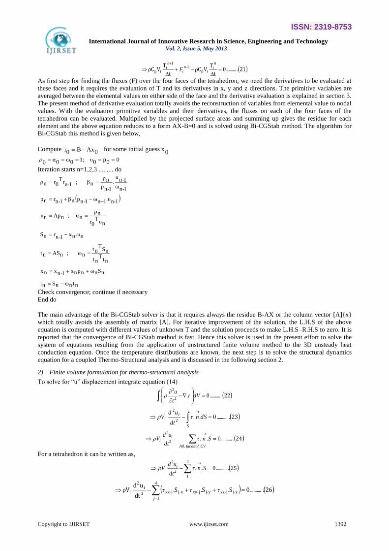
17........... 0...... 444444133333 zzyyxxzzyyxx SqSqSqSqSqSq
Where, Vi is the volume of element, S1x, S1y, S1z are the projected face area of the face-1 along x, y and z respectively,
S2x, S2y, S2z are the projected face area of the face-2 along x, y and z respectively, S3x, S3y, S3z are the projected face
area of the face-3 along x, y and z respectively and S4x, S4y, S4z are the projected face area of the face-4 along x, y and z
respectively. The different faces of the tetrahedron are shown in the Fig.1. The convention used is the face opposite to
node 1 is named as Face 1 and so on.
Fig.1. Different faces of a tetrahedron element
18........... .Sz
T.-.S
y
T.-S
x
T.-
dt
dTVρC z-j
jzy-j
j
yx-jj
xi
ip
4
1j
KKK
The above can written as follows,
19........... dt
dTVρC i
ip 0 iF
Explicit and implicit time stepping schemes can be used for the integration of these system of ordinary differential
equations. Explicit schemes are conditionally stable and many times the time steps become extremely small for many
practical problems. The advantage is that the residue can be explicitly evaluated from the values of the primitive
variables known at the previous time step. Though the implicit schemes are unconditionally stable, the residues are to
be computed on the current time level which involves the solution of the matrix system which is symmetric/non-
symmetric. The iterative solution technique, Bi-CGStab method can be used effectively here as it can be modified as an
element-by-element solver.
The above equation (19) is solved by pure implicit time integration (for implicit scheme “F” is evaluated for T in+1
i.e.
for the value at the next time step (t+Δt) as follows,
20........... t
TTVρC ii
ip 01
1
ni
nn
F
ISSN: 2319-8753
International Journal of Innovative Research in Science, Engineering and Technology Vol. 2, Issue 5, May 2013
Copyright to IJIRSET www.ijirset.com 1392
21........... t
TVρC
t
TVρC i
ipi
ip 01
1
nn
i
n
F
As first step for finding the fluxes (F) over the four faces of the tetrahedron, we need the derivatives to be evaluated at
these faces and it requires the evaluation of T and its derivatives in x, y and z directions. The primitive variables are
averaged between the elemental values on either side of the face and the derivative evaluation is explained in section 3.
The present method of derivative evaluation totally avoids the reconstruction of variables from elemental value to nodal
values. With the evaluation primitive variables and their derivatives, the fluxes on each of the four faces of the
tetrahedron can be evaluated. Multiplied by the projected surface areas and summing up gives the residue for each
element and the above equation reduces to a form AX-B=0 and is solved using Bi-CGStab method. The algorithm for
Bi-CGStab this method is given below,
Compute 0AxB0r for some initial guess0
x
00p0 υ1;0ω0α0
Iteration starts n=1,2,3 ......... do
ntnωnSnr
nSnωnpnα1-n xnx
ntΤ
nt
nSΤ
nt nω ;nAS nt
n.υnα1-nrnS
nυΤ
0r
nρ nα ;nAp nυ
1-n.υ1nω1-npnβ 1-nr np
1-nω
1-nα.
1-nρ
nρnβ ; 1-nr
Τ0rnρ
Check convergence; continue if necessary
End do
The main advantage of the Bi-CGStab solver is that it requires always the residue B-AX or the column vector [A]{x}
which totally avoids the assembly of matrix [A]. For iterative improvement of the solution, the L.H.S of the above
equation is computed with different values of unknown T and the solution proceeds to make L.H.S–R.H.S to zero. It is
reported that the convergence of Bi-CGStab method is fast. Hence this solver is used in the present effort to solve the
system of equations resulting from the application of unstructured finite volume method to the 3D unsteady heat
conduction equation. Once the temperature distributions are known, the next step is to solve the structural dynamics
equation for a coupled Thermo-Structural analysis and is discussed in the following section 2.
2) Finite volume formulation for thermo-structural analysis
To solve for “u” displacement integrate equation (14)
22...........
0.
2
2
dVt
u
23........... 0..2
2
dSndt
udV
S
ii
24........... 0..
...2
2
CVoffacesAll
ii Sn
dt
udV
For a tetrahedron it can be written as,
25........... 0..
4
12
2
Sndt
udV i
i
26........... .S.S.Sdt
udρV z-jj-xzy-jj-xyx-jj-xx2
i2
i 0
4
1
j
ISSN: 2319-8753
International Journal of Innovative Research in Science, Engineering and Technology Vol. 2, Issue 5, May 2013
Copyright to IJIRSET www.ijirset.com 1393
Where, τxx-j is the normal stress component along x-direction on face-j, τxy-j is the shear stress component along y-
direction on face-j, τxz-j is the shear stress component along z-direction on face-j and Sx-j, Sy-j, Sz-j are the projected face
area of the face-j along x, y, z-directions respectively.
The above equation can be written as,
27........... 0.2
4
12
2
j
zj
j
yj
j
xjrefj
j
ii S
x
w
z
uS
x
v
y
uSTT
x
u
dt
udV
Similarly we can write for “v” as,
28........... 0.2
4
12
2
j
zj
j
yjrefj
j
xj
j
ii S
y
w
z
vSTT
y
vS
x
v
y
u
dt
vdV
Similarly we can write for “w” as,
29........... 0.2
4
12
2
j
zjrefj
j
yj
j
xj
j
ii STT
z
wS
y
w
z
vS
x
w
z
u
dt
wdV
For the evaluation of “u “equation (27) can written as follows,
30........... ii
i Fdt
udV
2
2
The above equation can be solved implicitly. For Implicit scheme “F” is evaluated for uin+1
i.e. for the value at the next
time step (t+Δt),
31........... 02 1
2
11
ni
ni
ni
ni
i Ft
uuuV
32........... 02
2
11
2
1
t
uuVF
t
uV
ni
ni
in
i
ni
i
In the similar way we can evaluate v and w as follows,
33........... 02
2
11
2
1
t
vvVF
t
vV
ni
ni
in
i
ni
i
34........... 02
2
11
2
1
t
wwVF
t
wV
ni
ni
in
i
ni
i
The computation of fluxes over the four faces requires the evaluation of u, v and w its derivatives in x, y and z
directions. The primitive variables are averaged between the elemental values on either side of the face and the
derivative evaluation is explained in section 3. Once the computation of the fluxes over all the faces are completed, the
above equation reduces to a form AX-B=0 and is solved using Bi-CGStab method to get u, v and w.
3) Evaluation of derivatives
To calculate the flux terms, the first order derivatives like z
,y
,x
that appear in the implicit formulation are to be
evaluated at faces of the tetra element. The derivatives are calculated at face using Taylor series based least square
method. Let “Φ “be the variable (u, v, w or T) and from the Taylor series we can write Φ as,
z)z(z
y)y(y
x)x(xz)y,(x, ffff
ΦΦΦΦΦ (Higher order terms) .........(35)
Higher order terms are neglected since the value is small. If the values of the function are known at a points or
neighbours (i = 1 to n, n = total number of neighbours and the subscript “ f “ represents the face center value), we can
approximate the derivatives of the function at the reference node (face centered value) by solving a system of linear
equations. For such an approximation we select the points i = 1 to n, we are in the immediate neighbourhood of the
reference point. The above equation can be written in the form,
c.)z(zb.)y(y).x(xz)y,(x, ffff aΦΦ
Where,z
cy
bx
a
ΦΦΦ,,
36........... ΦΦ 0c.)z(zb.)y(y).x(x ffff a
The above equation is of the form,
czbyaxz)y,(x, Φ
The derivative evaluation for each face is to be unique as the face is shared by two elements on either side having two
cell-centre values of the variable which is insufficient to compute the derivatives. One option is to reconstruct the three
ISSN: 2319-8753
International Journal of Innovative Research in Science, Engineering and Technology Vol. 2, Issue 5, May 2013
Copyright to IJIRSET www.ijirset.com 1394
nodal values of the variables from the neighbouring cell centre values and then use them along with the two cell centre
values to get the derivatives. This is quite time and memory consuming process. Hence an efficient and unique
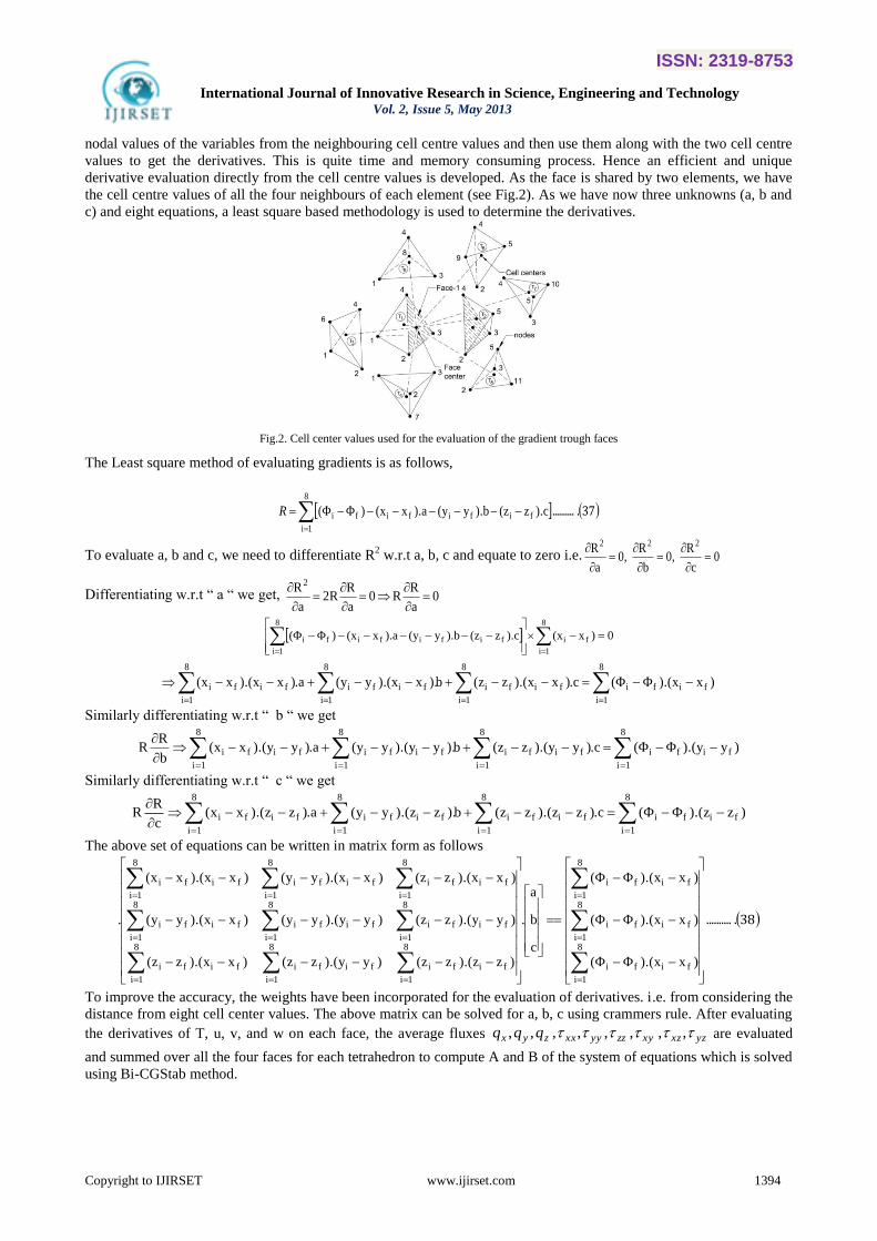
derivative evaluation directly from the cell centre values is developed. As the face is shared by two elements, we have
the cell centre values of all the four neighbours of each element (see Fig.2). As we have now three unknowns (a, b and
c) and eight equations, a least square based methodology is used to determine the derivatives.
Fig.2. Cell center values used for the evaluation of the gradient trough faces
The Least square method of evaluating gradients is as follows,
37........... ΦΦ
8
1i
fifififi ).cz(z).by(y).ax(x)(R
To evaluate a, b and c, we need to differentiate R2 w.r.t a, b, c and equate to zero i.e. 0
c
R0,
b
R0,
a
R 222
Differentiating w.r.t “ a “ we get, 0a
RR0
a
R2R
a
R2
0)x(x).cz(z).by(y).ax(x)(
8
1i
fi
8
1i
fifififi
ΦΦ
8
1i
fifi
8
1i
fifi
8
1i
fifi
8
1i
fifi )x).(x(.c)x).(xz(zb).x).(xy(y.a)x).(xx(x ΦΦ
Similarly differentiating w.r.t “ b “ we get
8
1i
fifi
8
1i
fifi
8
1i
fifi
8
1i
fifi )y).(y(.c)y).(yz(zb).y).(yy(y.a)y).(yx(xb
RR ΦΦ
Similarly differentiating w.r.t “ c “ we get
8
1i
fifi
8
1i
fifi
8
1i
fifi
8
1i
fifi )z).(z(.c)z).(zz(zb).z).(zy(y.a)z).(zx(xc
RR ΦΦ
The above set of equations can be written in matrix form as follows
38...........
ΦΦ
ΦΦ
ΦΦ
8
1i
fifi
8
1i
fifi
8
1i
fifi
8
1i
fifi
8
1i
fifi
8
1i
fifi
8
1i
fifi
8
1i
fifi
8
1i
fifi
8
1i
fifi
8
1i
fifi
8
1i
fifi
)x).(x(
)x).(x(
)x).(x(
c
b
a
.
)z).(zz(z)y).(yz(z)x).(xz(z
)y).(yz(z)y).(yy(y)x).(xy(y
)x).(xz(z)x).(xy(y)x).(xx(x
.
To improve the accuracy, the weights have been incorporated for the evaluation of derivatives. i.e. from considering the
distance from eight cell center values. The above matrix can be solved for a, b, c using crammers rule. After evaluating
the derivatives of T, u, v, and w on each face, the average fluxes yzxzxyzzyyxxzyx qqq ,,,,,,,, are evaluated
and summed over all the four faces for each tetrahedron to compute A and B of the system of equations which is solved
using Bi-CGStab method.
ISSN: 2319-8753
International Journal of Innovative Research in Science, Engineering and Technology Vol. 2, Issue 5, May 2013
Copyright to IJIRSET www.ijirset.com 1395
III. SOLUTION OF HEAT CONDUCTION AND INTEGRATED THERMO-STRUCTURAL ANALYSIS
A. Solution of unsteady heat conduction equation
As a first step the unstructured finite volume methodology described in the previous chapters, first applied to the
solution of 3-D unsteady heat conduction equation. To test the efficiency and accuracy of the code, a standard test case
of a one dimensional semi-infinite solid slab is considered for the validation of the heat conduction solver for various
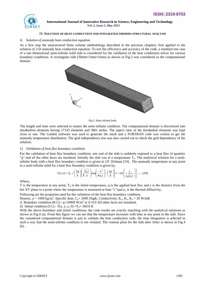
boundary conditions. A rectangular slab (50mm×5mm×5mm) as shown in Fig.3 was considered as the computational
domain.
Fig.3. Semi-infinite body
The length and time were selected to ensure the semi-infinite condition. The computational domain is discretized into
tetrahedron elements having 17143 elements and 3861 nodes. The aspect ratio of the tetrahedral elements was kept
close to one. The Gambit software was used to generate the mesh and a FORTRAN code was written to get the
unsteady temperature distribution. The grid independency test was also carried out to check the grid dependency of the
solution.
1) Validation of heat flux boundary condition
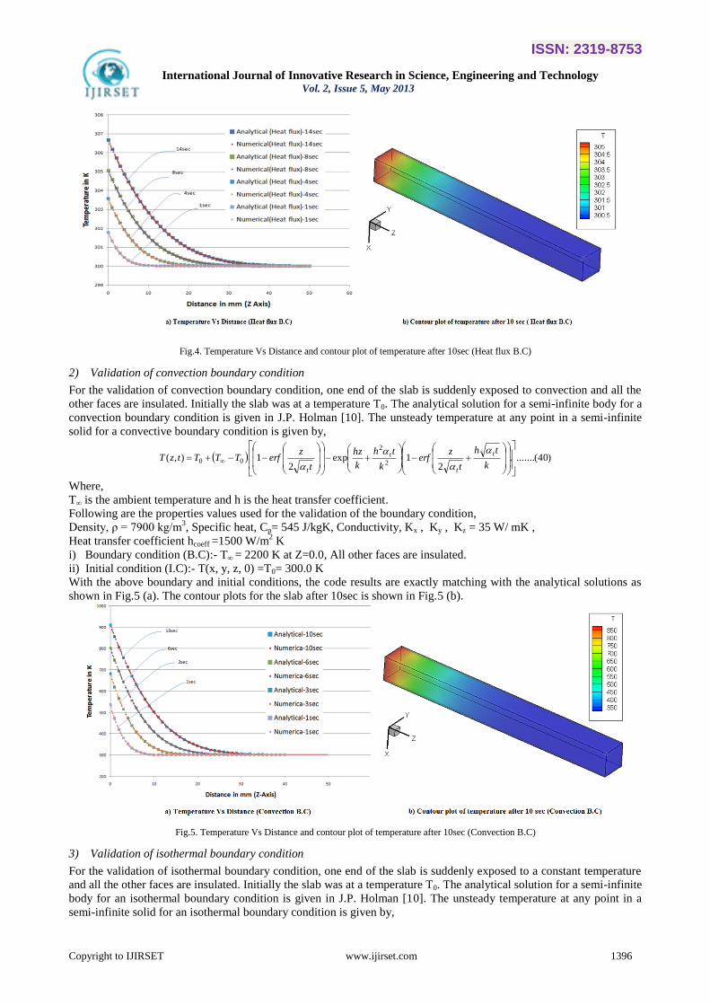
For the validation of heat flux boundary condition, one end of the slab is suddenly exposed to a heat flux of quantity
“q“ and all the other faces are insulated. Initially the slab was at a temperature T0. The analytical solution for a semi-
infinite body with a heat flux boundary condition is given in J.P. Holman [10]. The unsteady temperature at any point
in a semi-infinite solid for a heat flux boundary condition is given by,
)39(.......2
14
exp2
),(2
0
t
zerf
k
qz
t
zt
k
qTtzT
tt
t
Where,
T is the temperature at any point, T0 is the initial temperature, q is the applied heat flux and z is the distance from the
hot XY plane to a point where the temperature is measured at time “t “and t is the thermal diffusivity.
Following are the properties used for the validation of the heat flux boundary condition,
Density, ρ = 1000 kg/m3, Specific heat, Cp= 2000 J/kgK, Conductivity, Kx, Ky, Kz = 20 W/mK
i) Boundary condition (B.C):- q=10000 W/m2 at Z=0.0 All other faces are insulated.
ii) Initial condition (I.C):- T(x, y, z, 0) =T0= 300.0 K
With the above boundary and initial conditions, the code results are exactly matching with the analytical solutions as
shown in Fig.4 (a). From this figure we can see that the temperature increases with time at any point in the slab. Since
the considered computational domain is just to validate the heat conduction code, the time integration is selected in
such a way that the semi-infinite condition is not violated. The contour plots for the slab after 10sec is shown in Fig.4
(b).
ISSN: 2319-8753
International Journal of Innovative Research in Science, Engineering and Technology Vol. 2, Issue 5, May 2013
Copyright to IJIRSET www.ijirset.com 1396
Fig.4. Temperature Vs Distance and contour plot of temperature after 10sec (Heat flux B.C)
2) Validation of convection boundary condition
For the validation of convection boundary condition, one end of the slab is suddenly exposed to convection and all the
other faces are insulated. Initially the slab was at a temperature T0. The analytical solution for a semi-infinite body for a
convection boundary condition is given in J.P. Holman [10]. The unsteady temperature at any point in a semi-infinite
solid for a convective boundary condition is given by,
)40(........2
1exp2
1),(2
2
00
k
th
t
zerf
k
th
k
hz
t
zerfTTTtzT
t
t
t
t
Where,
T∞ is the ambient temperature and h is the heat transfer coefficient.
Following are the properties values used for the validation of the boundary condition,
Density, ρ = 7900 kg/m3, Specific heat, Cp= 545 J/kgK, Conductivity, Kx , Ky , Kz = 35 W/ mK ,
Heat transfer coefficient hcoeff =1500 W/m2 K
i) Boundary condition (B.C):- T∞ = 2200 K at Z=0.0, All other faces are insulated.
ii) Initial condition (I.C):- T(x, y, z, 0) =T0= 300.0 K
With the above boundary and initial conditions, the code results are exactly matching with the analytical solutions as
shown in Fig.5 (a). The contour plots for the slab after 10sec is shown in Fig.5 (b).
Fig.5. Temperature Vs Distance and contour plot of temperature after 10sec (Convection B.C)
3) Validation of isothermal boundary condition
For the validation of isothermal boundary condition, one end of the slab is suddenly exposed to a constant temperature
and all the other faces are insulated. Initially the slab was at a temperature T0. The analytical solution for a semi-infinite
body for an isothermal boundary condition is given in J.P. Holman [10]. The unsteady temperature at any point in a
semi-infinite solid for an isothermal boundary condition is given by,
ISSN: 2319-8753
International Journal of Innovative Research in Science, Engineering and Technology Vol. 2, Issue 5, May 2013
Copyright to IJIRSET www.ijirset.com 1397
)41(.......2
),( 0t
zerfTTTtzT ss
Where,
Ts is the temperature applied at one end of the boundary.
Following are the properties values used for the validation of the boundary condition,
Density, ρ = 1000 kg/m3, Specific heat Cp= 2000 J/kgK , Conductivity, Kx , Ky , Kz = 20 W/ mK
i) Boundary condition (B.C):- Ts =500 K at Z=0.0, All other faces are insulated.
ii) Initial condition (I.C):- T(x, y, z, 0) =T0= 300.0 K
With the above boundary and initial conditions, the code results are exactly matching with the analytical solutions as
shown in Fig.6 (a). The contour plots for the slab after 10sec is shown in Fig.6 (b).
Fig.6. Temperature Vs Distance and contour plot of temperature after 10sec (Isothermal B.C)
4) Summary of heat conduction simulations
The computer code developed for 3-D unsteady heat conduction equation is validated against the analytical solutions as
well as published numerical solutions for isothermal, heat flux, convective and radiation boundary conditions available
for the semi infinite slab for various boundary conditions. It was found that the solution methodology is accurate,
robust using Bi-CGStab solver. The code is now extended for the simultaneous solution of heat conduction equation
and structural dynamics equation for an integrated thermo structural analysis.
B. Solution of integrated thermo-structural analysis
As the results of the structural deformation are not affecting the heat conduction solution, the heat conduction and
thermo structural solution is solved in an uncoupled manner. From the initial condition the temperature distribution in
the body is computed for the first time step by solving the unsteady heat conduction equation. Using this temperature
distribution the equations for the displacements u, v, and w are solved. The above process is repeated till steady state is
achieved.
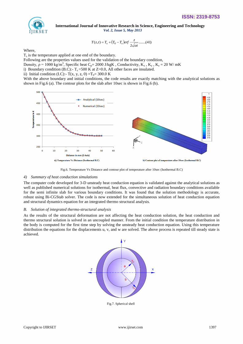
Fig.7. Spherical shell
ISSN: 2319-8753
International Journal of Innovative Research in Science, Engineering and Technology Vol. 2, Issue 5, May 2013
Copyright to IJIRSET www.ijirset.com 1398
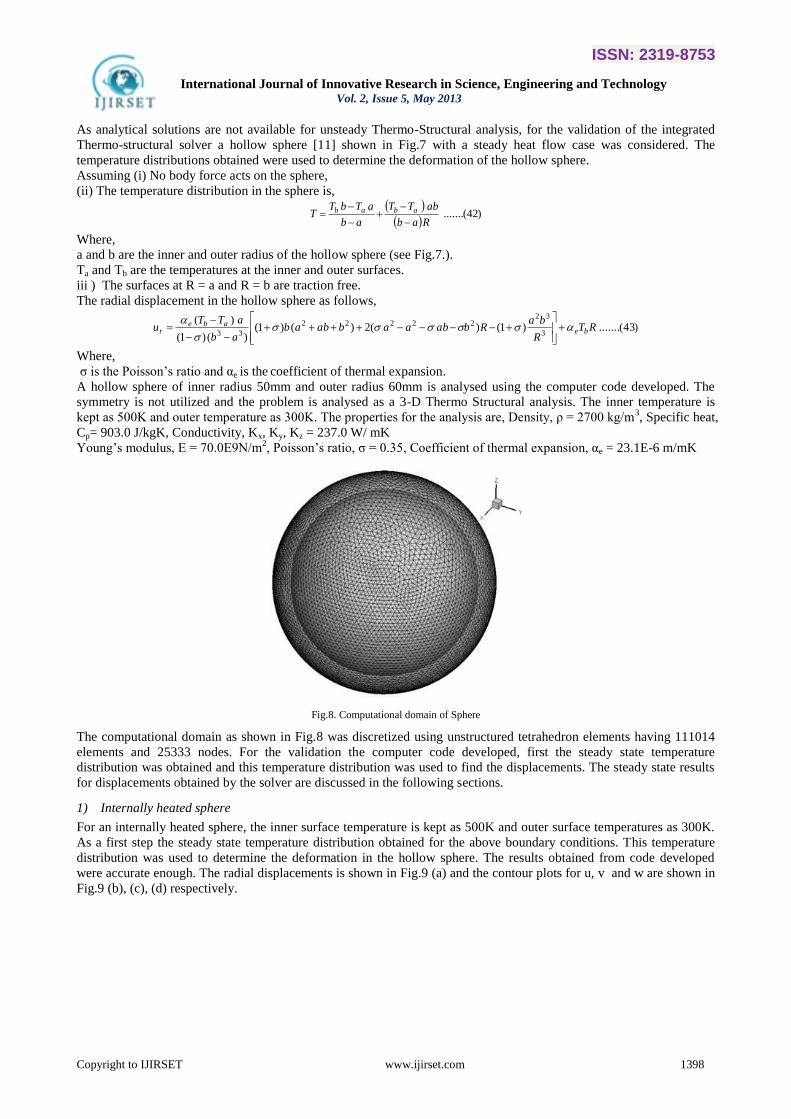
As analytical solutions are not available for unsteady Thermo-Structural analysis, for the validation of the integrated
Thermo-structural solver a hollow sphere [11] shown in Fig.7 with a steady heat flow case was considered. The
temperature distributions obtained were used to determine the deformation of the hollow sphere.
Assuming (i) No body force acts on the sphere,
(ii) The temperature distribution in the sphere is,
)42(.......Rab
abTT
ab
aTbTT abab
Where,
a and b are the inner and outer radius of the hollow sphere (see Fig.7.).
Ta and Tb are the temperatures at the inner and outer surfaces.
iii ) The surfaces at R = a and R = b are traction free.
The radial displacement in the hollow sphere as follows,
)43(.......)1()(2)()1()()1(
)(3
3222222
33RT
R
baRbabaababab
ab
aTTu be
aber
Where,
σ is the Poisson’s ratio and αe is the coefficient of thermal expansion.
A hollow sphere of inner radius 50mm and outer radius 60mm is analysed using the computer code developed. The
symmetry is not utilized and the problem is analysed as a 3-D Thermo Structural analysis. The inner temperature is
kept as 500K and outer temperature as 300K. The properties for the analysis are, Density, ρ = 2700 kg/m3, Specific heat,
Cp= 903.0 J/kgK, Conductivity, Kx, Ky, Kz = 237.0 W/ mK
Young’s modulus, E = 70.0E9N/m2, Poisson’s ratio, σ = 0.35, Coefficient of thermal expansion, αe = 23.1E-6 m/mK
Fig.8. Computational domain of Sphere
The computational domain as shown in Fig.8 was discretized using unstructured tetrahedron elements having 111014
elements and 25333 nodes. For the validation the computer code developed, first the steady state temperature
distribution was obtained and this temperature distribution was used to find the displacements. The steady state results
for displacements obtained by the solver are discussed in the following sections.
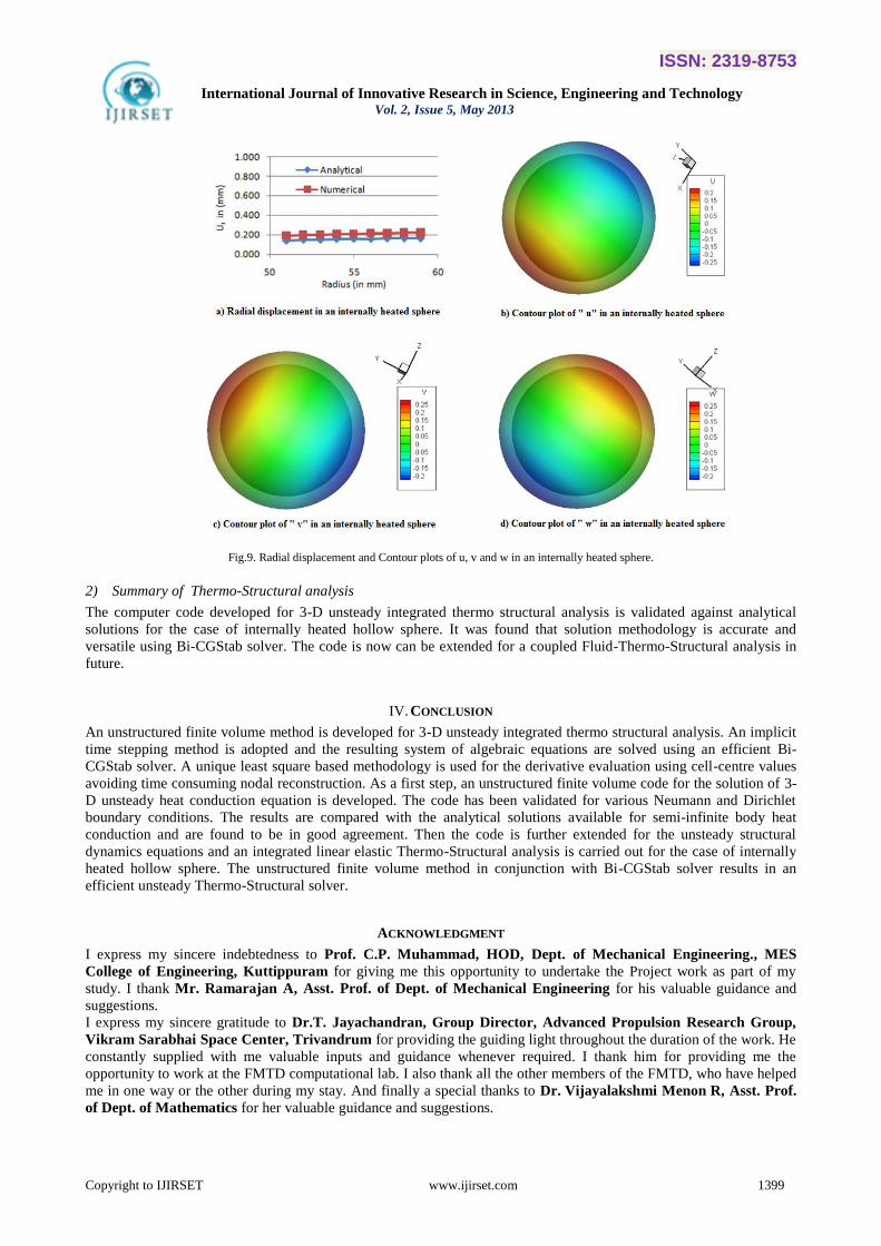
1) Internally heated sphere
For an internally heated sphere, the inner surface temperature is kept as 500K and outer surface temperatures as 300K.
As a first step the steady state temperature distribution obtained for the above boundary conditions. This temperature
distribution was used to determine the deformation in the hollow sphere. The results obtained from code developed
were accurate enough. The radial displacements is shown in Fig.9 (a) and the contour plots for u, v and w are shown in
Fig.9 (b), (c), (d) respectively.
ISSN: 2319-8753
International Journal of Innovative Research in Science, Engineering and Technology Vol. 2, Issue 5, May 2013
Copyright to IJIRSET www.ijirset.com 1399
Fig.9. Radial displacement and Contour plots of u, v and w in an internally heated sphere.
2) Summary of Thermo-Structural analysis
The computer code developed for 3-D unsteady integrated thermo structural analysis is validated against analytical
solutions for the case of internally heated hollow sphere. It was found that solution methodology is accurate and
versatile using Bi-CGStab solver. The code is now can be extended for a coupled Fluid-Thermo-Structural analysis in
future.
IV. CONCLUSION
An unstructured finite volume method is developed for 3-D unsteady integrated thermo structural analysis. An implicit
time stepping method is adopted and the resulting system of algebraic equations are solved using an efficient Bi-
CGStab solver. A unique least square based methodology is used for the derivative evaluation using cell-centre values
avoiding time consuming nodal reconstruction. As a first step, an unstructured finite volume code for the solution of 3-
D unsteady heat conduction equation is developed. The code has been validated for various Neumann and Dirichlet
boundary conditions. The results are compared with the analytical solutions available for semi-infinite body heat
conduction and are found to be in good agreement. Then the code is further extended for the unsteady structural
dynamics equations and an integrated linear elastic Thermo-Structural analysis is carried out for the case of internally
heated hollow sphere. The unstructured finite volume method in conjunction with Bi-CGStab solver results in an
efficient unsteady Thermo-Structural solver.
ACKNOWLEDGMENT
I express my sincere indebtedness to Prof. C.P. Muhammad, HOD, Dept. of Mechanical Engineering., MES
College of Engineering, Kuttippuram for giving me this opportunity to undertake the Project work as part of my
study. I thank Mr. Ramarajan A, Asst. Prof. of Dept. of Mechanical Engineering for his valuable guidance and
suggestions.
I express my sincere gratitude to Dr.T. Jayachandran, Group Director, Advanced Propulsion Research Group,
Vikram Sarabhai Space Center, Trivandrum for providing the guiding light throughout the duration of the work. He
constantly supplied with me valuable inputs and guidance whenever required. I thank him for providing me the
opportunity to work at the FMTD computational lab. I also thank all the other members of the FMTD, who have helped
me in one way or the other during my stay. And finally a special thanks to Dr. Vijayalakshmi Menon R, Asst. Prof.
of Dept. of Mathematics for her valuable guidance and suggestions.
ISSN: 2319-8753
International Journal of Innovative Research in Science, Engineering and Technology Vol. 2, Issue 5, May 2013
Copyright to IJIRSET www.ijirset.com 1400
REFERENCES
[1] Jameson. A and Marviplis. D, “Finite volume solution for 2D Euler equation on a regular mesh”, AIAA Journal vol.24, 4, pp.611-618, April
1986. [2] Y.D.Fryer, C. Bailey, M.Cross and C.H. Lai, “A control volume procedure for solving elastic stress strain equations on an unstructured mesh”,
Applications to mathematical modeling, 15, pp.639-645, 1991.
[3] Allan R.Wieting, Pramote Dechaumphai, Kim S.Bey at NASA Langley Research Center, Earl A. Thornton at Old Dominion University and Ken Morgan at University of Wales, “Application of integrated Fluid-Thermo-Structural Analysis Methods”, Thin-walled Structures, Elsevier
science Publishers Ltd, 1990.
[4] I. Demirdzic and D. Martinovic, “Finite volume method for thermo-elasto-plastic analysis”, Computational Methods Applied in Mechanics Engineering, 109, pp.331- 349, 1993.
[5] I.Demirdzic and M.Martinovic, “Finite volume method for elasto plastic stress analysis”, Computational Methods Applied in Mechanics
Engineering, 106, pp.330-349, 1991. [6] Demirdzic and S. Muzaferija, “Finite volume method for stress analysis in complex domain”, International Journal for Numerical Methods in
Engineering, 37, pp.3751-3766, 1994.
[7] H.Jasak and H.G. Weller, “Application of finite volume method and unstructured meshes to linear elasticity”, International Journal for
Numerical Methods in Engineering, 48, pp.267-287, 2000.
[8] G.H. Xia, Y.Zhao, J.H.Yeo. X.lv, “ A 3D implicit unstructured grid finite volume method for structural dynamics”, Comput Mech, 40,
pp.299–312 Published by Springer – Verlag, 2007. [9] Van der Vorst, H. A. "Bi-CGSTAB: A Fast and Smoothly Converging Variant of Bi-CG for the Solution of Nonsymmetric Linear
Systems". SIAM J.Sci. and Stat. Comput. 13 (2): pp.631–644, 1992.
[10] J.P. Holman, “Heat Transfer”, McGraw Hill, Tenth Edition ,Ny, 2010. [11] Allan F. Bower , “Applied Mechanics of Solids”, Published by Taylor and Francis, 2010.
BIOGRAPHY
Bibin K.S is doing M.Tech in Thermal systems at M.E.S college of Engineering, Kuttippuram,
Malappuram, Kerala. He did his B.E in Mechanical Engineering at East West Institute of
Technology, Bangalore, Karnataka, India. Also worked as a Design Engineer for SettyMech
Engineers Pvt.ltd, Mysore, Karnataka, India.
PHOTOGRAPH


![DIFFUSSION-THERMO AND CHEMICAL REACTION EFFECTS ON AN UNSTEADY MHD … · 2016-06-30 · tions in chemical engineering. Rao and Sivaiah [8] have studied chemical reaction effects](https://img.pdfslide.us/doc/110x75/5f1752039a3d711dbd69a8ba/diffussion-thermo-and-chemical-reaction-effects-on-an-unsteady-mhd-2016-06-30.jpg)