Unsteady Internal Forced-Convective Flow Under DynamicTime-Dependent Boundary Temperature

M. Fakoor-Pakdaman,∗ Mehran Ahmadi,† and Majid Bahrami‡

Simon Fraser University Surrey, British Columbia V3T 0A3, Canada

DOI: 10.2514/1.T4261

A new all-time analytical model is developed to predict transient internal forced-convection heat transfer underarbitrary time-dependentwall temperature. Slug flow condition is assumed for the velocity profile inside the tube.Thesolution to the time-dependent energy equation for a stepwall temperature is generalized for arbitrary time variationsin surface temperature using Duhamel’s theorem. A harmonic boundary temperature is considered, and newcompact closed-form relationships are proposed to predic: 1) fluid temperature distribution; 2) fluid bulk temper-ature; 3) wall heat flux; and 4) the Nusselt number. An optimum value is found for the dimensionless angularfrequency of the wall temperature to maximize the heat transfer rate of the studied unsteady forced-convectiveprocess. Such dimensionless parameter depends upon the imposed-temperature angular frequency, fluid thermo-physical properties, and tube geometrical parameters. A general surface temperature is considered, and thetemperature field inside the medium is obtained using a superposition technique. An independent numerical simula-tion is performed using ANSYS® Fluent. The comparison between the obtained numerical data and the presentanalytical model shows good agreement: a maximum relative difference less than 4.9%.

NomenclatureA = cross-sectional area, Eq. (13), m2

a = half-width of spacing between parallel plates, or circulartube radius, m

cp = heat capacity, J∕kg · KFo = Fourier number; αt∕a2J = Bessel function, Eq. (6a)k = thermal conductivity,W∕m · KNu = Nusselt number, ha∕Kn = positive integer, Eq. (6b)p = 0 for parallel plate and 1 for circular tube, Eqs. (3) and (14)Pr = Prandtl number (ν∕α)q!w = dimensionless wall heat fluxRe = Reynolds number, 2Ua∕νr = radial coordinate measured from circular tube center-

line, mT = temperature, KU = velocity magnitude, m∕su = velocity vector, Eq. (2)x = axial distance from the entrance of the heated section, my = normal coordinate measured from centerline of parallel

plate channel, mα = thermal diffusivity, m2∕sγ = function for circular tube [Eq. (6a)] or for parallel plate

[Eq. (6b)]Δφ = thermal lag (phase shift)ζ = dummy X variableη = dimensionless radial/normal coordinate for circular tube

equal to r∕a or for parallel plate equal to y∕aθ = dimensionless temperature; "T − T0#∕ΔTRλn = eigenvalues, Eq. (6)ν = kinematic viscosity, m2∕s

ξ = dummy Fo variableρ = fluid density, kg∕m3

ψ = arbitrary function of FoΩ = imposed-temperature angular frequency, rad∕sω = dimensionless temperature angular frequency,

Subscripts

m = mean or bulk valueR = reference values = step wall (surface) temperaturew = wall0 = inlet

I. Introduction

D EVELOPING an in-depth understanding of unsteady forced-convection heat transfer is crucial for optimal design and accu-

rate control of heat transfer in emerging sustainable energy applica-tions and next-generation heat exchangers. The origin of thermaltransients in sustainable energy applications include thevariable ther-mal load on 1) thermal solar panels in thermal energy storage (TES)systems [1–3]; 2) power electronics of solar/wind/tidal energy con-version systems [4,5]; and 3) power electronics and electric motor(PEEM) of hybrid electric vehicles (HEVs), electric vehicles (EVs),and fuel cell vehicles (FCVs) [6–9].Solar thermal systems are widely used in solar powerplants and

are being widely commercialized. Solar powerplants have seen about740 MW of generating capacity added between 2007 and the endof 2010, bringing the global total to 1095 MW [5]. Such growth isexpected to continue, as in the United States at least another 6.2 GWcapacity is expected tobe in operation by the endof 2013 [5].However,the growth of such technology is hindered by the inherent variability ofsolar energy subjected to daily variation, seasonal variation, andweather conditions [1,4,10]. To overcome the issue of the intermit-tency,TES systemsare used to collect thermal energy to smooth out theoutput and shift its delivery to a later time. Single-phase sensibleheating systems or latent heat storage systems using phase changematerials are used in TES; transient heat exchange occurs to charge ordischarge the storage material [11]. From the technical point of view,one of the main challenges facing TES systems is designing suitableheat exchangers towork reliably under unsteady conditions [11]: a keyissue that this research attempts to address.To assure reliable performance of electronic components, the

temperature of different components should be maintained below

Received 23 August 2013; revision received 23 November 2013; acceptedfor publication 9 January 2014; published online 21 April 2014. Copyright ©2013 by the American Institute of Aeronautics and Astronautics, Inc. Allrights reserved. Copies of this paper may be made for personal or internal use,on condition that the copier pay the $10.00 per-copy fee to the CopyrightClearance Center, Inc., 222 Rosewood Drive, Danvers, MA 01923; includethe code 1533-6808/14 and $10.00 in correspondence with the CCC.

*Laboratory for Alternative Energy Convection, School of MechatronicSystems Engineering, No. 4300, 250-13450 102nd Avenue; mfakoorp@sfu.ca.

†Laboratory for Alternative Energy Convection.‡Laboratory for Alternative Energy Convection; mbahrami@sfu.ca.

463

JOURNAL OF THERMOPHYSICS AND HEAT TRANSFERVol. 28, No. 3, July–September 2014

Dow

nloa

ded

by S

IMO

N F

RASE

R U

NIV

ERSI

TY o

n O

ctob

er 2

9, 2

014

| http

://ar

c.ai

aa.o

rg |

DO

I: 10

.251

4/1.

T426

1

recommended values. The temperature of power electronics can varysignificantly with the fluid flow and the applied heat flux over time[12]. Thus, it is important to investigate the transient thermal behaviorof these systems, especially during peak conditions [13]. Furthe-rmore, new application of transient forced convection has emergedbythe advent of HEVs, EVs, and FCVs. Since introduced, the sales ofsuch vehicles have grown at an average rate of more than 80% peryear.As ofOctober 2012,more than 5.8millionHEVs have been soldworldwide since their inception in 1997 [14]. Their hybrid powertrainand power electronics electric motors undergo a dynamic thermalload as a direct result of driving/duty cycle and environmentalconditions. Conventional cooling systems are designed based on anominal steady state, typically aworst-case scenario [15], whichmaynot properly represent the thermal behavior of various applications orduty cycles. This clearly indicates the enormity of the pending needfor in-depth understanding of the instantaneous thermal character-istics of the aforementioned thermal systems [16]. Successful andintelligent thermal design of such dynamic systems leads to thedesign of new efficient heat exchangers to enhance the overall effi-ciency and reliability of TES and PEEM cooling solutions, which inthe cases of the HEVs/EVs/FCVs means significant improvement invehicle efficiency/reliability and fuel consumption [15–18].In all the aforementioned applications, transient heat transfer

occurs in heat exchangers subjected to arbitrary time-dependentduct wall temperature. This phenomenon can be represented by anunsteady forced-convective tube flow, which is the ultimate goal ofthis study.Siegel pioneered the study of transient internal forced convection by

investigating a duct flow following a step change in wall heat flux ortemperature [19,20]. Later, SparrowandSiegel [21,22] used an integraltechnique to analyze transient heat transfer in the thermal entranceregion of a Poiseuille flow under step wall temperature/heat flux.Moreover, the tube wall temperature of channel flows for particulartypes of position/time-dependent heat fluxes was studied in the liter-ature [23–27]. A number of studies were conducted on effects ofperiodic inlet temperature on the heat transfer characteristics of a con-vective tube flowunder stepwall temperature [28–33].Most studies onunsteady internal forced convection are limited to homogeneous/constant boundary conditions at the tube wall, i.e., isothermal orisoflux; a summary of the available studies is presented in Table 1.Our literature review indicates the following:1) The effects of periodic/arbitrary time-dependent surface

temperatures on thermal performance of an internal forced-convectiveflow have not been investigated.2) There is no model to predict the fluid temperature distribution,

wall heat flux, and the Nusselt number of a tube flow under arbitrarytime-dependent surface temperatures.3) No study has been conducted to determine the optimum

conditions that maximize the convective heat transfer rate in tubeflows under harmonic boundary conditions.4) The parameters, including temperature amplitude, angular

frequency, and fluid thermal lag (phase shift), affecting the unsteadyinternal forced convection have not been presented in the literature.In previous work [34,35], a comprehensive study was carried

out on the thermal characteristics of a convective tube flow underdynamically varying heat flux. In the present study, a new analyticalall-time model is developed in Cartesian and cylindrical coordinatesto accurately predict 1) fluid temperature distribution; 2) fluid bulktemperature; 3) wall heat flux; and 4) the Nusselt number, for a tubeflow under arbitrary time-dependent temperature. New dimension-less variables are introduced that characterize transient forcedconvection inside a conduit under a time-dependent boundary tem-perature. An optimum condition is presented that maximizes the heattransfer rate of internal forced convection under a harmonic boundarytemperature. The present paper provides new insight on unsteadyheat transfer, and it serves as a platform and an engineering tool toinvestigate and develop intelligent transient thermal systems for awide variety of engineering applications.To develop the present analyticalmodel, the fluid flow response for

a step surface temperature is taken into account. Using Duhamel’stheorem [36], the thermal characteristics of the fluid flow are

determined analytically under a periodic time-dependent surfacetemperature. New dimensionless variables are introduced, and thesystem is optimized to maximize the heat transfer rate underharmonic boundary temperature.Any type of time-dependent surfacetemperature can be decomposed into sinusoidal functions using asine Fourier series transformation [36]. Thus, the present model forthe harmonic excitation is applied to find the temperature distributionof a tube flow under a general time-dependent boundary condition.

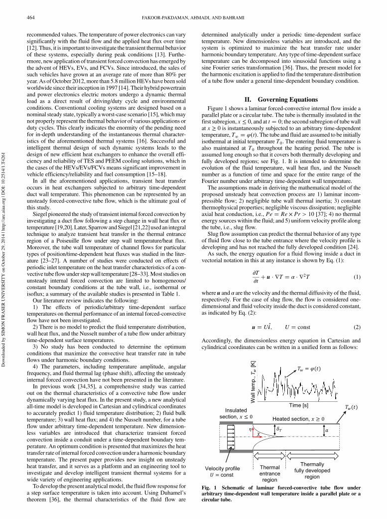
II. Governing EquationsFigure 1 shows a laminar forced-convective internal flow inside a

parallel plate or a circular tube. The tube is thermally insulated in thefirst subregion, x ≤ 0, and at t $ 0; the second subregion of tubewallat x ≥ 0 is instantaneously subjected to an arbitrary time-dependenttemperature, Tw $ φ"t#. The tube and fluid are assumed to be initiallyisothermal at initial temperature T0. The entering fluid temperature isalso maintained at T0 throughout the heating period. The tube isassumed long enough so that it covers both thermally developing andfully developed regions; see Fig. 1. It is intended to determine theevolution of the fluid temperature, wall heat flux, and the Nusseltnumber as a function of time and space for the entire range of theFourier number under arbitrary time-dependent wall temperature.The assumptions made in deriving the mathematical model of the

proposed unsteady heat convection process are 1) laminar incom-pressible flow; 2) negligible tube wall thermal inertia; 3) constantthermophysical properties; negligible viscous dissipation; negligibleaxial heat conduction, i.e., Pe $ Re × Pr > 10 [37]; 4) no thermalenergy sources within the fluid; and 5) uniform velocity profile alongthe tube, i.e., slug flow.Slug flow assumption can predict the thermal behavior of any type

of fluid flow close to the tube entrance where the velocity profile isdeveloping and has not reached the fully developed condition [24].As such, the energy equation for a fluid flowing inside a duct in

vectorial notation in this at any instance is shown by Eq. (1):

∂T∂t% u · ∇T $ α · ∇2T (1)

where u and α are the velocity and the thermal diffusivity of the fluid,respectively. For the case of slug flow, the flow is considered one-dimensional and fluid velocity inside the duct is considered constant,as indicated by Eq. (2):

u $ Ui; U $ const (2)

Accordingly, the dimensionless energy equation in Cartesian andcylindrical coordinates can be written in a unified form as follows:

Fig. 1 Schematic of laminar forced-convective tube flow underarbitrary time-dependent wall temperature inside a parallel plate or acircular tube.

464 FAKOOR-PAKDAMAN, AHMADI, AND BAHRAMI

Dow

nloa

ded

by S

IMO

N F

RASE

R U

NIV

ERSI

TY o

n O

ctob

er 2

9, 2

014

| http

://ar

c.ai

aa.o

rg |

DO

I: 10

.251

4/1.

T426

1

∂θ∂Fo% ∂θ

∂X$ 1

ηp∂∂η

!ηp

∂θ∂η

"(3)

It should be noted that superscript p takes the values of 0 and 1,respectively, for Cartesian and cylindrical coordinates. In fact, theformer is attributed to the fluid flow between parallel plates, and thelatter indicates the fluid flow inside a circular tube. The dimen-sionless variables are

θ $ T − T0

ΔTR; Fo $ αt

a2; X $ 2 xa

Re · Pr;

Rea $2Ua

υ; Pr $ υ

α; Nua $

ha

k

where ΔTR is the amplitude of the imposed temperature, Fo is theFourier number, andX is the dimensionless axial position. In addition,for parallel plate and circular tube, η $ y

a and η $ ra, respectively.

Equation (4) is subjected to the following boundary and initialconditions:

θ"0; η; Fo# $ 0 at X $ 0; Fo > 0; 0 ≤ η ≤ 1 (4a)

∂θ"X; 0; Fo#∂η

$ 0 at η $ 0; X > 0; Fo > 0 (4b)

θ"X; 1; Fo# $ ψ"Fo# at η $ 1; X > 0; Fo > 0 (4c)

θ"X; η; 0# $ 0 at Fo $ 0; X > 0; 0 ≤ η ≤ 1 (4d)

where ψ"Fo# is an arbitrary time-dependent temperature imposed onthe tube wall.

III. Model DevelopmentIn this section, a new all-time model is developed in Cartesian and

cylindrical coordinates, considering 1) short-time response; and2) long-time response. As such, the presented model predicts thetemperature distribution inside a convective tube flow under anarbitrary time-dependent temperature imposed on the tube wall.For a duct flow at uniform temperature T0, instantaneously

subjected to a step surface temperature, the temperature response isgiven in [19]:

θs $Tw − T0

ΔTR

#1 − 2

X∞

n$1γn"η# exp"−λ2nFo#

$(5)

1) In cylindrical coordinate, i.e., flow inside a circular tube,

γn"η# $J0"λnη#λnJ1"λn#

; and J0"λn# $ 0; λn > 0 (6a)

2) In Cartesian coordinate, i.e., flow between parallel plates,

γn"η#$"−1#n−1

λncos"λnη#; and λn$

2n−1

2π; n$1;2;3; ::: (6b)

where θs is the dimensionless temperature of the fluid under stepwalltemperature. J0 and J1 are the zero- and first-order Bessel functionsof the first kind, and λn are the eigenvalues in cylindrical or Cartesiancoordinates: Eqs. (6a) and (6b), respectively. The energy equation fora tube flow is linear; Eq. (4). This shows the applicability of asuperposition technique to extend the response of the fluid flow for astep surface temperature to the other general cases, as discussed in[25].As such, byusingDuhamel’s theorem [36], the thermal responsefor a step surface temperature [Eq. (6)] can be generalized for anarbitrary time variation in surface temperature [Eq. (4c)]:

θ$ T−T0

ΔTR$ 2

X∞

n$1λ2nγ"η#exp"−λ2nFo#×

ZFo

0

ψ"ξ#exp"λ2nξ#dξ (7)

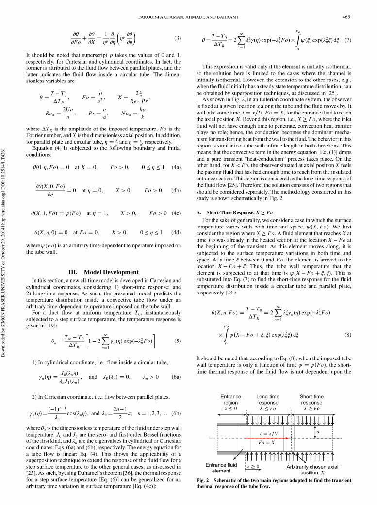
This expression is valid only if the element is initially isothermal,so the solution here is limited to the cases where the channel isinitially isothermal. However, the extension to the other cases, e.g.,when the fluid initially has a steady state temperature distribution, canbe obtained by superposition techniques, as discussed in [25].As shown in Fig. 2, in an Eulerian coordinate system, the observer

is fixed at a given location x along the tube and the fluid moves by. Itwill take some time, t $ x∕U,Fo $ X, for the entrance fluid to reachthe axial position X. Beyond this region, i.e., X ≥ Fo, where the inletfluid will not have enough time to penetrate, convection heat transferplays no role; hence, the conduction becomes the dominant mecha-nism for transferring heat from thewall to the fluid. Thebehavior in thisregion is similar to a tube with infinite length in both directions. Thismeans that the convective term in the energy equation [Eq. (1)] dropsand a pure transient “heat-conduction” process takes place. On theother hand, for X < Fo, the observer situated at axial position X feelsthe passing fluid that has had enough time to reach from the insulatedentrance section.This region is considered as the long-time response ofthe fluid flow [25]. Therefore, the solution consists of two regions thatshould be considered separately. The methodology considered in thisstudy is shown schematically in Fig. 2.

A. Short-Time Response, X ≥ FoFor the sake of generality, we consider a case in which the surface

temperature varies with both time and space, ψ"X;Fo#. We firstconsider the region where X ≥ Fo. A fluid element that reaches X attime Fo was already in the heated section at the location X − Fo atthe beginning of the transient. As this element moves along, it issubjected to the surface temperature variations in both time andspace. At a time ξ between 0 and Fo, the element is arrived to thelocation X − Fo% ξ. Thus, the tube wall temperature that theelement is subjected to at that time is ψ"X − Fo% ξ; ξ#. This issubstituted into Eq. (7) to find the short-time response for the fluidtemperature distribution inside a circular tube and parallel plate,respectively [24]:

θ"X; η; Fo# $ T − T0

ΔTR$ 2

X∞

n$1λ2nγn"η# exp"−λ2nFo#

×ZFo

0

ψ"X − Fo% ξ; ξ# exp"λ2nξ# dξ (8)

It should be noted that, according to Eq. (8), when the imposed tubewall temperature is only a function of time ψ $ ψ"Fo#, the short-time thermal response of the fluid flow is not dependent upon the

Fig. 2 Schematic of the two main regions adopted to find the transientthermal response of the tube flow.

FAKOOR-PAKDAMAN, AHMADI, AND BAHRAMI 465

Dow

nloa

ded

by S

IMO

N F

RASE

R U

NIV

ERSI

TY o

n O

ctob

er 2

9, 2

014

| http

://ar

c.ai

aa.o

rg |

DO

I: 10

.251

4/1.

T426

1

axial position. However, it is a function of time and the characteristicsof the imposed surface temperature.

B. Transition Time, X ! FoFor each axial position, the short-time and long-time responses are

equal atX $ Fo. This is the dimensionless transition time for a givenaxial position. Therefore, the time Fo $ X can be considered ademarcation between the short-time and long-time responses for eachaxial position. For instance, for an arbitrarily-chosen axial positionX $ 1.2, the dimensionless transition time is Fo $ 1.2.

C. Long-Time Response, X < FoNow, we consider the region where X < Fo. The element that

reaches X at time Fo has entered the channel at the time Fo − X andbegun to be heated. As time elapses from when the transition begins,this element will reach the location ζ at the time Fo − X% ζ. Thus,the surface temperature that the element is subjected to at that locationis ψ"ζ; Fo − X% ζ#. Substituting this into Eq. (7) results in Eq. (9),which represents the long-time response of the flow inside a circulartube or a parallel plate [24]:

θ"X; η; Fo# $ T − T0

ΔTR$ 2

X∞

n$1λ2nγn"η# exp"−λ2nFo#

×ZFo

0

ψ"ζ; Fo − X% ζ# exp"λ2nξ# dξ (9)

According to Eq. (9), the long-time thermal response of the fluid flowis a function of time, axial position, and characteristics of the imposedtube wall temperature.

IV. Harmonic Thermal TransientsIn this section, thermal response of a tube flow is obtained under a

harmonic wall temperature, prescribed as follows:

Tw $ T0 % ΔTR&1% sin"Ωt#' (10)

where ΔTR K and Ω rad∕s are the amplitude and the angularfrequency of the imposed wall temperature. The analytical model ispresented in form of 1) closed-form series solutions; and 2) approx-imate compact easy-to-use relationships.Any type of prescribed time-dependent wall temperature can be

decomposed into simple oscillatory functions using a Fourier seriestransformation [36]. Using a superposition technique, the results canbe extended to the cases with an arbitrary time-dependent walltemperature as a general boundary condition; see Sec. IV.H.

A. Exact Series SolutionsThe dimensionless form of Eq. (10) is as follows:

θw"ω; Fo# $Tw − T0

ΔTR$ 1% sin"ωFo# (11)

where ω $ Ωa2∕α is the dimensionless angular frequency. Substi-tuting Eq. (11) into Eqs. (8) and (9), after some algebraic manipula-tions, the short-time and long-time temperature distributions insidethe fluid are obtained. In this study,we considered the first 60 terms ofthe series solutions; using more terms does not affect the results up tofour decimal digits.1) Short-time fluid temperature distribution, X ≥ Fo,

θ"ω;η;Fo#$1%sin"ωFo#%2X∞

n$1γn"η#

×%&ωλ2n− "ω2%λ4n#'exp"−λ2nFo#−ω2 sin"ωFo#−ωλ2n cos"ωFo#

ω2%λ4n

&

(12a)

2) Long-time fluid temperature distribution, X ≤ Fo,

θ"ω; X; η; Fo# $ 1% sin"ωFo# % 2X∞

n$1γn"η# ×

8>>>><>>>>:

−λ2nω cos"ωFo# − ω2 sin"ωFo#ω2 % λ4n

−nλ4n sin&ω"Fo − X#' − λ2nω cos&ω"Fo − X#' − "ω2 % λ4n#

o× exp"−λ2nX#

ω2 % λ4n

9>>>>=>>>>;

(12b)

It should be noted that the definition of γn"η# and the eigenvaluesλn have been previously given byEqs. (6a) and (6b) for a circular tubeand a parallel plate, respectively. In addition, the fluid bulk temper-ature can be obtained by Eq. (13) [38]:

θm"ω; X; Fo# $1

A

ZZ

A

θ dA (13)

where A is the cross-sectional area of the tube at any arbitraryaxial position. After performing the integration in Eq. (13), thefollowing relationships are obtained to evaluate the fluid bulktemperature.Short-time dimensionless fluid bulk temperature, X ≥ Fo,

θm"ω; Fo# $ 1% sin"ωFo# % 2pX∞

n$1

×&ωλ2n − "ω2 % λ4n#' exp"−λ2nFo# − ω2 sin"ωFo#ωλ2n cos"ωFo#

λ2n"ω2 % λ4n#(14a)

Long-time dimensionless fluid bulk temperature, X ≤ Fo,

θm"ω; X; Fo# $ 1% sin"ωFo# % 2pX∞

n$1

8>>><>>>:

−λ2nω cos"ωFo# − ω2 sin"ωFo#λ2n"ω2 % λ4n#

−

fλ4n sin&ω"Fo − X#' % λ2nω cos&ω"Fo − X#' − "ω2 % λ4n#g × exp"−λ2nX#λ2n"ω2 % λ4n#

9>>>=>>>;

(14b)

466 FAKOOR-PAKDAMAN, AHMADI, AND BAHRAMI

Dow

nloa

ded

by S

IMO

N F

RASE

R U

NIV

ERSI

TY o

n O

ctob

er 2

9, 2

014

| http

://ar

c.ai

aa.o

rg |

DO

I: 10

.251

4/1.

T426

1

The eigenvalues λn for the fluid flow inside a circular tubeand a parallel plate can be obtained by Eqs. (6a) and (6b),respectively.The dimensionless heat flux at the tube wall can be evaluated by

q!w $∂θ∂η

''''η$1

(15)

Differentiating the fluid temperature [Eqs. (12a) and (12b)] at thetube wall, we obtain the following:Short-time dimensionless wall heat flux, X ≥ Fo,

q!w"ω;Fo# $−2X∞

n$1

×&ωλ2n − "ω2% λ4n#'exp"−λ2nFo#−ω2 sin"ωFo#−ωλ2n cos"ωFo#

ω2% λ4n(16a)

Long-time dimensionless wall heat flux, X ≤ Fo,

q!w"ω; X; Fo# $ −2X∞

n$1×ωλ2n sin"ωFo# − ω2 cos"ωFo# − fλ4n cos&ω"Fo − X#' % λ2nω sin&ω"Fo − X#'g × exp"−λ2nX#

ω2 % λ4n(16b)

In this study, the local Nusselt number is defined based on thedifference between the tube wall and fluid bulk temperatures; seeBejan [39]:

Nua"ω; X; Fo# $ha

k$ q!w

θw − θm$ q!w&1% sin"ωFo#' − θm

(17)

It should be noted that the characteristics length α for the Nusseltnumber is the half-width of a parallel plate in the Cartesian coordinateand the tube radius in the cylindrical coordinate. Therefore, the short-time Nusselt number can be obtained by substituting Eqs. (14a) and(14b) into Eq. (17); similarly, substituting Eqs. (16a) and (16b) intoEq. (17) indicates the long-time Nusselt number.To optimize the transient internal forced convection, we define

a new parameter, the average dimensionless wall heat flux, asfollows:

!q!w"ω# $1

Fo × X

ZFo

ξ$0

ZX

ζ$0

q!w dζ dξ (18)

where Fo is the Fourier number (dimensionless time), and X is anarbitrarily chosen axial position. Equation (18) shows the averageheat transfer rate over an arbitrary period of timeFo and length of thetube X. This will be discussed in more detail in Sec. VI.

B. Approximate Compact Relationships

Since using the series solutions presented in Section IV.E istedious, the following new compact easy-to-use relationships areproposed to predict 1) dimensionless fluid bulk temperature;2) dimensionless wall heat flux; and 3) Nusselt number, for fluidflow inside a parallel plate. As such, the MATLAB curve fittingtool was used to find the proposed compact relationships.

Therefore, analytical results for different dimensionless numberswere curve fitted to find the most appropriate form of the compactrelationships with minimum relative difference compared to theobtained series solutions. The proposed compact relationships arecompared with the exact series solutions in graphical formin Sec. VI.

1. Dimensionless Fluid Bulk Temperature

For ω ≥ π, the following compact relationships predict the exactseries solutions for the fluid bulk temperature [Eqs. (14a) and (14b)]by the maximum relative difference less than 9.1%.1) Compact short-time fluid bulk temperature, X ≥ Fo,

θm"ω; Fo# $1.078 × FoFo% 0.1951

%!

1.616

ω% 1.023

"

× exp

!−0.3748 × ω% 28.78

ω% 9.796× Fo

"% 0.0934 × ω% 2.86

ω% 1.802

× sin

!ωFo% −0.78ω2 % 17.8 × ω − 160.9

ω2 − 22.3 × ω% 200.7

"(19a)

2) Compact long-time fluid bulk temperature, X ≤ Fo,

θm"ω; X; Fo# $1.078 × XX% 0.1951

% 0.1167 × ω% 3.575

ω% 1.802

× sin

!ωFo% −0.78ω2 % 17.8 × ω − 160.9

ω2 − 22.3 × ω% 200.7

"(19b)

2. Dimensionless Wall Heat Flux

ForFo ≥ 0.05 andω ≥ π, the dimensionless wall heat flux can beobtained by the following compact relationships. The maximumrelative difference between the developed compact relationships[Eqs. (20a) and (20b)] and the exact series solutions [Eqs. (16a),(16b)] is less than 5.1%.1) Compact short-time wall heat flux, X ≥ Fo,

q!w"ω; Fo# $−0.206 × Fo% 0.449

Fo% 0.132% 14.73 × ω% 103.2

ω% 70.74

× sin

!ωFo% −0.77ω2 − 23.45 × ω% 215.3

ω2 − 30.51 × ω% 280.5

"(20a)

2) Compact long-time wall heat flux, X ≤ Fo,

q!w"ω;X;Fo#$ 3.037×exp"−4.626X#%−0.206×X%0.449

X%0.132

%14.73×ω%103.2

ω%70.74× sin

!ωFo%−0.77ω2−23.45×ω%215.3

ω2−30.51×ω%280.5

"

(20b)

3. Nusselt Number

Using the definition of the Nusselt number [Eq. (17)], a compactclosed-form relationship can also be obtained for Nusselt number.The short-time Nusselt number can be developed by substituting

FAKOOR-PAKDAMAN, AHMADI, AND BAHRAMI 467

Dow

nloa

ded

by S

IMO

N F

RASE

R U

NIV

ERSI

TY o

n O

ctob

er 2

9, 2

014

| http

://ar

c.ai

aa.o

rg |

DO

I: 10

.251

4/1.

T426

1

Eqs. (17a) and (20a) into Eq. (17). Similarly, the long-time Nusseltnumber can be obtained by substituting Eqs. (19b) and (20b)into Eq. (17).We believe that the form of the compact relationships presented in

this section reveals the nature of the transient problem herein underconsideration. This will be discussed in detail in Sec. VI.

V. Numerical StudyTo verify the presented analytical solution, an independent numer-

ical simulation of the planar flow inside a parallel plate is performedusing the commercial software ANSYS®Fluent. User-defined codesare written to apply the harmonic and arbitrary time-dependenttemperatures on the tubewall: Eqs. (10) and (22), respectively.Modelgeometry and boundary conditions are similar to what is shown inFig. 1. Furthermore, the assumptions stated in Sec. II are used in thenumerical analysis; however, the fluid axial conduction is notneglected in the numerical analysis. Grid independency of the resultsis tested for three different grid sizes: 20 × 100 and 40 × 200, as wellas 80 × 400. Finally, 40 × 200 is selected as the final grid size, sincethemaximum difference in the predicted values for the fluid tempera-ture by the two latter grid sizes is less than 1%. The geometrical andthermal properties used in the baseline case for the numericalsimulation are listed in Table 2. The maximum relative differencebetween the analytical results and the numerical data is less than4.9%, which is discussed in detail in Sec. VI.

VI. Results and DiscussionA. Harmonic Prescribed Temperature

Although the methodology developed in Sec. III is presented forCartesian and cylindrical coordinates, only the results for the formerare discussed in this section in a graphical form. The trends for thecylindrical coordinate are similar.Variations of the dimensionless centerline temperature against the

Fo number [Eqs. (12a) and (12b)] for a few axial positions along thetube are shown in Fig. 3 and compared with the numerical dataobtained in Sec. V. Periodic temperature is imposed on the tube wall;Eq. (11). The solid lines in Fig. 3 represent our analytical results, andthe markers show the obtained numerical data. There is an excellentagreement between the analytical results [Eqs. (12a) and (12b)] andthe obtained numerical data, with a maximum relative difference lessthan 4.9%.The following is shown in Fig. 3:1) The present model predicts an abrupt transition between the

short-time and long-time responses. The numerical results, however,indicate a smooth transition. This causes the numerical data to deviateslightly from the analytical results as the long-time response begins.Such transitions are demarcated by dashed lines on the figure.

2) The abrupt transition from short-time to long-time responsesis attributed to the analytical method that Siegel [19] used to solvethe transient energy equation for a step wall temperature. This isdiscussed in detail in [19].3) There is an initial transient period of “pure conduction” during

which all the curves follow along the same line, X ≥ Fo; Eq. (12a).4) When Fo $ X, each curve moves away from the common line,

i.e., pure conduction response, and adjusts toward a steady oscillatorybehavior at a long-time response; Eq. (12b). The wall temperaturesincrease for largerX values, as expected; this is due to the increase ofthe fluid energy (bulk temperature) along the axial direction.5) Increasing length-to-diameter ratio increases the axial position

number, which in turn increases the temperature inside the fluid.6) The higher the velocity inside the tube, the higher the Re

number, which in turn decreases the axial position number, X $"2x∕a#∕"Rea · Pr# and leads to lower temperature inside the fluid.Figure 4 shows the variations of the dimensionless fluid

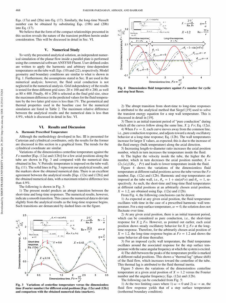
temperature at different radial positions across the tube versus theFonumber; Eqs. (12a) and (12b). Harmonic and step temperatures areimposed at the tube wall, i.e., θw $ 1% sin"πFo# and θw $ 1, re-spectively. As such, the short-time and long-time fluid temperaturesat different radial positions at an arbitrarily chosen axial position,X $ 1.2, are obtained using Eqs. (12a) and (12b).From Fig. 4, the following conclusions can be drawn:1) As expected at any given axial position, the fluid temperature

oscillates with time in the case of a prescribed harmonic wall tem-perature. For a step surface temperature,ω $ 0, the solution does notfluctuate over time.2) At any given axial position, there is an initial transient period,

which can be considered as pure conduction, i.e., the short-timeresponse for X ≥ Fo. However, as pointed out earlier, each axialposition shows steady oscillatory behavior for X ≤ Fo at the long-time response. Therefore, for the arbitrarily chosen axial position ofX $ 1.2, the long-time response begins at Fo $ 1.2 and shows thesame behavior all-time thereafter.3) For an imposed cyclic wall temperature, the fluid temperature

oscillates around the associated response for the step surface tem-peraturewith the sameangular frequency atwhich the system is excited.4) The shift between the peaks of the temperature profile is marked

at different radial positions. This shows a “thermal lag” (phase shift)of the fluid flow, which increases toward the centerline of the tube.This thermal lag is attributed to the fluid thermal inertia.Figure 5 shows the variations of the dimensionless centerline

temperature at a given axial position of X $ 1.2 versus the Fouriernumber and the angular frequency; Eqs. (12a) and (12b).The following can be concluded from Fig. 5:1) At the two limiting cases where 1) ω → 0 and 2) ω → ∞, the

fluid flow response yields that of a step surface temperature(isothermal boundary condition).

Fig. 3 Variations of centerline temperature versus the dimensionlesstime (Fourier number) for different axial positions [Eqs. (12a) and (12b)]and comparison with the obtained numerical data (markers).

Fig. 4 Dimensionless fluid temperature against Fo number for cyclicand step heat fluxes.

468 FAKOOR-PAKDAMAN, AHMADI, AND BAHRAMI

Dow

nloa

ded

by S

IMO

N F

RASE

R U

NIV

ERSI

TY o

n O

ctob

er 2

9, 2

014

| http

://ar

c.ai

aa.o

rg |

DO

I: 10

.251

4/1.

T426

1

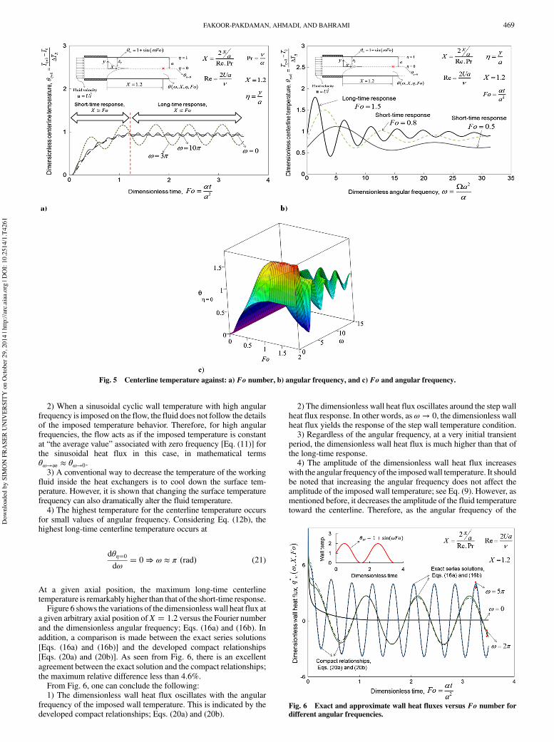
2) When a sinusoidal cyclic wall temperature with high angularfrequency is imposed on the flow, the fluid does not follow the detailsof the imposed temperature behavior. Therefore, for high angularfrequencies, the flow acts as if the imposed temperature is constantat “the average value” associated with zero frequency [Eq. (11)] forthe sinusoidal heat flux in this case, in mathematical termsθω→∞ ≈ θω→0.3) A conventional way to decrease the temperature of the working

fluid inside the heat exchangers is to cool down the surface tem-perature. However, it is shown that changing the surface temperaturefrequency can also dramatically alter the fluid temperature.4) The highest temperature for the centerline temperature occurs

for small values of angular frequency. Considering Eq. (12b), thehighest long-time centerline temperature occurs at

dθη$0dω$ 0 ⇒ ω ≈ π "rad# (21)

At a given axial position, the maximum long-time centerlinetemperature is remarkably higher than that of the short-time response.Figure 6 shows the variations of the dimensionless wall heat flux at

a given arbitrary axial position ofX $ 1.2 versus the Fourier numberand the dimensionless angular frequency; Eqs. (16a) and (16b). Inaddition, a comparison is made between the exact series solutions[Eqs. (16a) and (16b)] and the developed compact relationships[Eqs. (20a) and (20b)]. As seen from Fig. 6, there is an excellentagreement between the exact solution and the compact relationships;the maximum relative difference less than 4.6%.From Fig. 6, one can conclude the following:1) The dimensionless wall heat flux oscillates with the angular

frequency of the imposed wall temperature. This is indicated by thedeveloped compact relationships; Eqs. (20a) and (20b).

2) The dimensionless wall heat flux oscillates around the step wallheat flux response. In other words, asω → 0, the dimensionless wallheat flux yields the response of the step wall temperature condition.3) Regardless of the angular frequency, at a very initial transient

period, the dimensionless wall heat flux is much higher than that ofthe long-time response.4) The amplitude of the dimensionless wall heat flux increases

with the angular frequency of the imposedwall temperature. It shouldbe noted that increasing the angular frequency does not affect theamplitude of the imposed wall temperature; see Eq. (9). However, asmentioned before, it decreases the amplitude of the fluid temperaturetoward the centerline. Therefore, as the angular frequency of the

Fig. 5 Centerline temperature against: a) Fo number, b) angular frequency, and c) Fo and angular frequency.

Fig. 6 Exact and approximate wall heat fluxes versus Fo number fordifferent angular frequencies.

FAKOOR-PAKDAMAN, AHMADI, AND BAHRAMI 469

Dow

nloa

ded

by S

IMO

N F

RASE

R U

NIV

ERSI

TY o

n O

ctob

er 2

9, 2

014

| http

://ar

c.ai

aa.o

rg |

DO

I: 10

.251

4/1.

T426

1

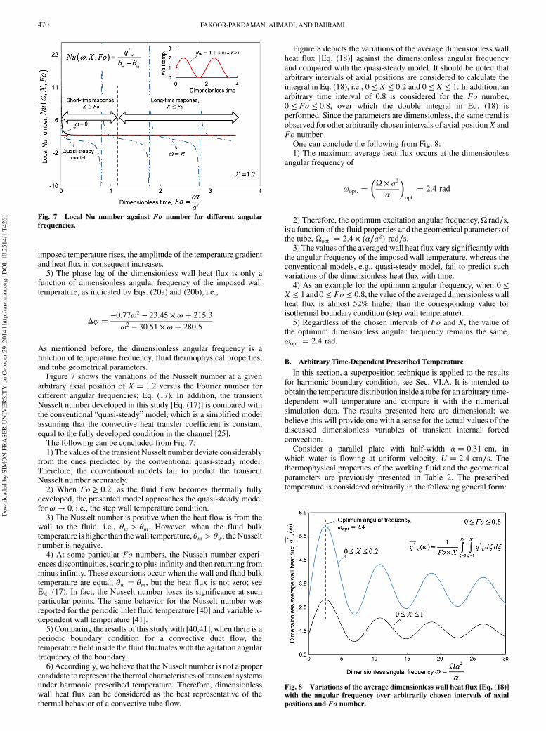
imposed temperature rises, the amplitude of the temperature gradientand heat flux in consequent increases.5) The phase lag of the dimensionless wall heat flux is only a

function of dimensionless angular frequency of the imposed walltemperature, as indicated by Eqs. (20a) and (20b), i.e.,

Δφ $ −0.77ω2 − 23.45 × ω% 215.3

ω2 − 30.51 × ω% 280.5

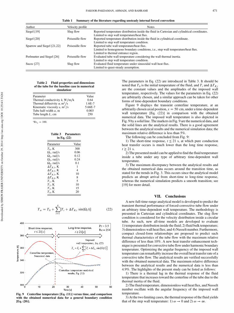
As mentioned before, the dimensionless angular frequency is afunction of temperature frequency, fluid thermophysical properties,and tube geometrical parameters.Figure 7 shows the variations of the Nusselt number at a given

arbitrary axial position of X $ 1.2 versus the Fourier number fordifferent angular frequencies; Eq. (17). In addition, the transientNusselt number developed in this study [Eq. (17)] is compared withthe conventional “quasi-steady” model, which is a simplified modelassuming that the convective heat transfer coefficient is constant,equal to the fully developed condition in the channel [25].The following can be concluded from Fig. 7:1) The values of the transient Nusselt number deviate considerably

from the ones predicted by the conventional quasi-steady model.Therefore, the conventional models fail to predict the transientNusselt number accurately.2) When Fo ≥ 0.2, as the fluid flow becomes thermally fully

developed, the presented model approaches the quasi-steady modelfor ω → 0, i.e., the step wall temperature condition.3) The Nusselt number is positive when the heat flow is from the

wall to the fluid, i.e., θw > θm. However, when the fluid bulktemperature is higher than thewall temperature, θm > θw, theNusseltnumber is negative.4) At some particular Fo numbers, the Nusselt number experi-

ences discontinuities, soaring to plus infinity and then returning fromminus infinity. These excursions occur when the wall and fluid bulktemperature are equal, θw $ θm, but the heat flux is not zero; seeEq. (17). In fact, the Nusselt number loses its significance at suchparticular points. The same behavior for the Nusselt number wasreported for the periodic inlet fluid temperature [40] and variable x-dependent wall temperature [41].5) Comparing the results of this studywith [40,41], when there is a

periodic boundary condition for a convective duct flow, thetemperature field inside the fluid fluctuates with the agitation angularfrequency of the boundary.6) Accordingly, we believe that the Nusselt number is not a proper

candidate to represent the thermal characteristics of transient systemsunder harmonic prescribed temperature. Therefore, dimensionlesswall heat flux can be considered as the best representative of thethermal behavior of a convective tube flow.

Figure 8 depicts the variations of the average dimensionless wallheat flux [Eq. (18)] against the dimensionless angular frequencyand compared with the quasi-steady model. It should be noted thatarbitrary intervals of axial positions are considered to calculate theintegral in Eq. (18), i.e., 0 ≤ X ≤ 0.2 and 0 ≤ X ≤ 1. In addition, anarbitrary time interval of 0.8 is considered for the Fo number,0 ≤ Fo ≤ 0.8, over which the double integral in Eq. (18) isperformed. Since the parameters are dimensionless, the same trend isobserved for other arbitrarily chosen intervals of axial positionX andFo number.One can conclude the following from Fig. 8:1) The maximum average heat flux occurs at the dimensionless

angular frequency of

ωopt: $!Ω × a2

α

"

opt:

$ 2.4 rad

2) Therefore, the optimum excitation angular frequency,Ω rad∕s,is a function of the fluid properties and the geometrical parameters ofthe tube, Ωopt: $ 2.4 × "α∕a2# rad∕s.3) The values of the averaged wall heat flux vary significantly with

the angular frequency of the imposed wall temperature, whereas theconventional models, e.g., quasi-steady model, fail to predict suchvariations of the dimensionless heat flux with time.4) As an example for the optimum angular frequency, when 0 ≤

X ≤ 1 and0 ≤ Fo ≤ 0.8, thevalue of the averageddimensionlesswallheat flux is almost 52% higher than the corresponding value forisothermal boundary condition (step wall temperature).5) Regardless of the chosen intervals of Fo and X, the value of

the optimum dimensionless angular frequency remains the same,ωopt: $ 2.4 rad.

B. Arbitrary Time-Dependent Prescribed Temperature

In this section, a superposition technique is applied to the resultsfor harmonic boundary condition, see Sec. VI.A. It is intended toobtain the temperature distribution inside a tube for an arbitrary time-dependent wall temperature and compare it with the numericalsimulation data. The results presented here are dimensional; webelieve this will provide one with a sense for the actual values of thediscussed dimensionless variables of transient internal forcedconvection.Consider a parallel plate with half-width α $ 0.31 cm, in

which water is flowing at uniform velocity, U $ 2.4 cm∕s. Thethermophysical properties of the working fluid and the geometricalparameters are previously presented in Table 2. The prescribedtemperature is considered arbitrarily in the following general form:

Fig. 8 Variations of the average dimensionless wall heat flux [Eq. (18)]with the angular frequency over arbitrarily chosen intervals of axialpositions and Fo number.

Fig. 7 Local Nu number against Fo number for different angularfrequencies.

470 FAKOOR-PAKDAMAN, AHMADI, AND BAHRAMI

Dow

nloa

ded

by S

IMO

N F

RASE

R U

NIV

ERSI

TY o

n O

ctob

er 2

9, 2

014

| http

://ar

c.ai

aa.o

rg |

DO

I: 10

.251

4/1.

T426

1

Tw $ T0 %X4

i$1&Ti % ΔTR;i sin"Ωit#' (22)

The parameters in Eq. (22) are introduced in Table 3. It should benoted that T0 is the initial temperature of the fluid, and Ti and ΔTR;iare the constant values and the amplitudes of the imposed walltemperature, respectively. The values for the parameters in Eq. (22)are arbitrarily chosen, and a similar approach can be taken for otherforms of time-dependent boundary conditions.Figure 9 displays the transient centerline temperature, at an

arbitrarily chosen axial position, x $ 50 cm, under a time-dependentwall temperature [Eq. (22)] in comparison with the obtainednumerical data. The imposed wall temperature is also depicted inFig. 9 by a solid line. Themarkers in Fig. 9 are the numerical data, andthe solid lines are the analytical results. There is a good agreementbetween the analytical results and the numerical simulation data; themaximum relative difference is less than 5%.The following can be concluded from Fig. 9:1) The short-time response, t ≤ 21 s, at which pure conduction

heat transfer occurs is much lower than the long time response,t ≥ 21 s.2) The presentedmodel can be applied to find the fluid temperature

inside a tube under any type of arbitrary time-dependent walltemperature.3) The maximum discrepancy between the analytical results and

the obtained numerical data occurs around the transition time, asstated for the trends in Fig. 3. This occurs since the analytical modelpredicts an abrupt arrival from short-time to long-time response,whereas the numerical simulation predicts a smooth transition; see[19] for more detail.

VII. ConclusionsA new full-time-range analytical model is developed to predict the

transient thermal performance of forced-convective tube flow underan arbitrary time-dependent wall temperature. The methodology ispresented in Cartesian and cylindrical coordinates. The slug flowcondition is considered for the velocity distribution inside a circulartube. As such, new all-time models are developed to evaluate1) temperature distribution inside the fluid; 2) fluid bulk temperature;3) dimensionless wall heat flux; and 4)Nusselt number. Furthermore,compact closed-form relationships are proposed to predict suchthermal characteristics of the tube flow with the maximum relativedifference of less than 10%. A new heat transfer enhancement tech-nique is presented for convective tube flow under harmonic boundarytemperature. Optimizing the angular frequency of the imposed walltemperature can remarkably increase the overall heat transfer rate of aconvective tube flow. The analytical results are verified successfullywith the obtained numerical data. The maximum relative differencebetween the analytical results and the numerical data is less than4.9%. The highlights of the present study can be listed as follows:1) There is a thermal lag in the thermal response of the fluid

temperature that increases toward the centerline of the tube due to thethermal inertia of the fluid.2) The fluid temperature, dimensionlesswall heat flux, andNusselt

number oscillate with the angular frequency of the imposed walltemperature.3)At the two limiting cases, the thermal response of the fluid yields

that of the step wall temperature: 1) ω → 0 and 2) ω → ∞.

Table 2 Fluid properties and dimensionsof the tube for the baseline case in numerical

simulationa

Parameter ValueThermal conductivity k, W∕m∕k 0.64Thermal diffusivity α, m2∕s 1.6E-7Kinematic viscosity ν, m2∕s 5.66E-7Tube half-width a, m 0.003Tube length L, cm 250

aRea $ 100.

Table 3 Parametersin Eq. (22)

Parameter ValueT0, K 300Ω1, rad∕s 0.06Ω2, rad∕s 0.12Ω3, rad∕s 0.24Ω4, rad∕s 0.1ΔTR;1, K 1ΔTR;2, K 4ΔTR;3, K 10ΔTR;4, K 8T1, K 5T2, K 10T3, K 15T4, K 20

Fig. 9 Centerline temperature [Eq. (11)] versus time, and comparisonwith the obtained numerical data for a general boundary condition[Eq. (20)].

Table 1 Summary of the literature regarding unsteady internal forced convection

Author Velocity profile NotesSiegel [19] Slug flow Reported temperature distribution inside the fluid in Cartesian and cylindrical coordinates.

Limited to step wall temperature/heat flux.Siegel [20] Poiseuille flow Reported temperature distribution inside the fluid in cylindrical coordinate.

Limited to step wall temperature condition.Sparrow and Siegel [21,22] Poiseuille flow Reported tube wall temperature/heat flux.

Limited to homogenous boundary conditions, i.e., step wall temperature/heat flux.Limited to thermal entrance region.

Perlmutter and Siegel [26] Poiseuille flow Evaluated tube wall temperature considering the wall thermal inertia.Limited to step wall temperature condition.

Sucec [27] Slug flow Evaluated fluid temperature under sinusoidal wall heat flux.Limited to quasi-steady assumption.

FAKOOR-PAKDAMAN, AHMADI, AND BAHRAMI 471

Dow

nloa

ded

by S

IMO

N F

RASE

R U

NIV

ERSI

TY o

n O

ctob

er 2

9, 2

014

| http

://ar

c.ai

aa.o

rg |

DO

I: 10

.251

4/1.

T426

1

4) There is an optimum value for the dimensionless angularfrequency of the imposed harmonic wall temperature that maximizesthe average dimensionless wall heat flux:

ωopt: $!Ω × a2

α

"

opt:

$ 2.43 rad

AcknowledgmentsThis work was supported by Automotive Partnership Canada,

grant no. APCPJ 401826-10. The authors would like to thank thesupport of the industry partner Future Vehicle Technologies, Inc.(British Columbia, Canada).

References[1] Agyenim, F., Hewitt, N., Eames, P., and Smyth, M., “A Review of

Materials, Heat Transfer and Phase Change Problem Formulation forLatent Heat Thermal Energy Storage Systems (Lhtess),”Renewable andSustainable Energy Reviews, Vol. 14, No. 2, Feb. 2010, pp. 615–628.doi:10.1016/j.rser.2009.10.015

[2] Cabeza, L. F., Mehling, H., Hiebler, S., and Ziegler, F., “Heat TransferEnhancement inWater whenUsed as PCM in Thermal Energy Storage,”Applied Thermal Engineering, Vol. 22, No. 10, July 2002, pp. 1141–1151.doi:10.1016/S1359-4311(02)00035-2

[3] Kurklo, A., “Energy Storage Applications in Greenhouses by Meansof Phase Change Materials (PCMs): A Review,” Renewable Energy,Vol. 13, No. 1, 1998, pp. 89–103.doi:10.1016/S0960-1481(97)83337-X

[4] Garrison, J. B., and Webber, E. M., “Optimization of an IntegratedEnergy Storage for a Dispatchable Wind Powered Energy System,”ASME 2012 6th International Conference on Energy Sustainability,American Soc. of Mechanical Engineers, Fairfield, NJ, 2012, pp. 1–11.

[5] Sawin, J. L., and Martinot, E., “Renewables Bounced Back in 2010,Finds REN21 Global Report,” Renewable Energy World, 2011, Dataavailable online at http://www.renewableenergyworld.com/rea/news/article/2011/09/renewables-bounced-back-in-2010-finds-ren21-global-report [retrieved 2014].

[6] Bennion, K., and Thornton, M., “Integrated Vehicle ThermalManagement for AdvancedVehicle Propulsion Technologies,”NationalRenewable Energy Lab. NREL/CP-540-47416, Golden, CO, 2010.

[7] Boglietti, A., Member, S., Cavagnino, A., Staton, D., Shanel, M.,Mueller, M., and Mejuto, C., “Evolution and Modern Approaches forThermal Analysis of Electrical Machines,” IEEE Transactions onIndustrial Electronics, Vol. 56, No. 3, 2009, pp. 871–882.doi:10.1109/TIE.2008.2011622

[8] Canders, W.-R., Tareilus, G., Koch, I., and May, H., “New Design andControl Aspects for Electric Vehicle Drives,” 2010 14th InternationalPower Electronics and Motion Control Conference (EPE/PEMC),IEEE Xplore, Sept. 2010, pp. S11-1, S11-8.doi:10.1109/EPEPEMC.2010.5606528

[9] Hamada, K., “Present Status and Future Prospects for Electronics inElectric Vehicles/Hybrid Electric Vehicles and Expectations for WideBandgap Semiconductor Devices,” Physica Status Solidi (B), Vol. 245,No. 7, July 2008, pp. 1223–1231.doi:10.1002/pssb.v245:7

[10] Hale, M., “Survey of Thermal Storage for Parabolic Trough PowerPlants,” National Renewable Energy Lab. NREL/SR-550-27925,Golden, CO, 2000, pp. 1–28.

[11] Sharma, A., Tyagi, V. V., Chen, C. R., and Buddhi, D., “Review onThermal Energy Storage with Phase Change Materials and Applica-tions,” Renewable and Sustainable Energy Reviews, Vol. 13, No. 2,Feb. 2009, pp. 318–345.doi:10.1016/j.rser.2007.10.005

[12] März, M., Schletz, A., Eckardt, B., Egelkraut, S., and Rauh, H., “PowerElectronics System Integration for Electric and Hybrid Vehicles,”Integrated Power Electronics Systems (CIPS), IEEE Xplore,March 2010, pp. 1–10, 16–18, Data available online at http://ieeexplore.ieee.org/stamp/stamp.jsp?tp=&=5730643&=5730626.

[13] Nerg, J., Rilla, M., and Pyrhönen, J., “Thermal Analysis of Radial-FluxElectricalMachines with a High Power Density,” IEEE Transactions onIndustrial Electronics, Vol. 55, No. 10, 2008, pp. 3543–3554.doi:10.1109/TIE.2008.927403

[14] “Cumulative Sales of TMC Hybrids Top 2 Million Units in Japan,”Toyota Motor Corporation, Japan, 2012, Data available online at

http://www.toyotabharat.com/inen/news/2013/april_17.aspx [retrieved2014].

[15] O’Keefe, M., and Bennion, K., “A Comparison of Hybrid ElectricVehicle Power Electronics Cooling Options,” IEEE Vehicle Power andPropulsionConference (VPPC), IEEEXplore, 2007, pp. 116–123, 9–12.doi:10.1109/VPPC.2007.4544110

[16] Bennion, K., and Thornton, M., “Integrated Vehicle Thermal Mana-gement for Advanced Vehicle Propulsion Technologies,” NationalRenewable Energy Lab. NREL/CP-540-47416, Golden, CO, 2010.

[17] Johnson, R. W., Evans, J. L., Jacobsen, P., Thompson, J. R. R., andChristopher, M., “The Changing Automotive Environment: High-Temperature Electronics,” IEEE Transactions on Electronics Packag-ing Manufacturing, Vol. 27, No. 3, July 2004, pp. 164–176.doi:10.1109/TEPM.2004.843109

[18] Kelly, K., Abraham, T., and Bennion, K., “Assessment of ThermalControl Technologies for Cooling Electric Vehicle Power Electronics,”National Renewable Energy Lab. NREL/CP-540-42267, Golden, CO,2008.

[19] Siegel, R., “Transient Heat Transfer for Laminar Slug Flow in Ducts,”Applied Mechanics, Vol. 81, No. 1, 1959, pp. 140–144.

[20] Siegel, R., “Heat Transfer for Laminar Flow in Ducts with ArbitraryTime Variations in Wall Temperature,” Journal of Applied Mechanics,Vol. 27, No. 2, 1960, pp. 241–249.doi:10.1115/1.3643945

[21] Sparrow, E. M., and Siegel, R., “Thermal Entrance Region of a CircularTube Under Transient Heating Conditions,” Third U.S. NationalCongress of Applied Mechanics, ASME Trans., 1958, pp. 817–826.

[22] Siegel, R., and Sparrow, E. M., “Transient Heat Transfer for LaminarForced Convection in the Thermal Entrance Region of Flat Ducts,”ASME Heat Transfer, Vol. 81, No. 1, 1959, pp. 29–36.

[23] Perlmutter, M., and Siegel, R., “Unsteady Laminar Flow in a Ductwith Unsteady Heat Addition,” Heat Transfer, Vol. 83, No. 4, 1961,pp. 432–439.doi:10.1115/1.3683662

[24] Siegel, R., “Forced Convection in a Channel with Wall Heat Capacityand with Wall Heating Variable with Axial Position and Time,”International Journal of Heat Mass Transfer, Vol. 6, No. 7, 1963,pp. 607–620.doi:10.1016/0017-9310(63)90016-4

[25] Siegel, R., and Perlmutter, M., “Laminar Heat Transfer in a ChannelwithUnsteady Flow andWall HeatingVaryingwith Position and Time,”Journal of Heat Transfer, Vol. 85, No. 4, 1963, pp. 358–365.doi:10.1115/1.3686125

[26] Perlmutter, M., and Siegel, R., “Two-Dimensional Unsteady Incom-pressible Laminar Duct Flowwith a Step Change inWall Temperature,”Journal of Heat Transfer, Vol. 83, No. 4, 1961, pp. 432–440.doi:10.1115/1.3683662

[27] Sucec, J., “Unsteady Forced Convection with Sinusoidal Duct WallGeneration: The Conjugate Heat Transfer Problem,” InternationalJournal of Heat and Mass Transfer, Vol. 45, No. 8, April 2002,pp. 1631–1642.doi:10.1016/S0017-9310(01)00275-7

[28] Kakac, S., Li, W., and Cotta, R. M., “Unsteady Laminar ForcedConvection inDuctswith PeriodicVariation of Inlet Temperature,”HeatTransfer, Vol. 112, No. 4, 1990, pp. 913–920.doi:10.1115/1.2910499

[29] Weigong, L., and Kakac, S., “Unsteady Thermal Entrance Heat Transferin Laminar Flow with a Periodic Variation of Inlet Temperature,”International Journal of Heat and Mass Transfer, Vol. 34, No. 10,Oct. 1991, pp. 2581–2592.doi:10.1016/0017-9310(91)90098-Y

[30] Kakac, S., and Yener, Y., “Exact Solution of the Transient ForcedConvection Energy Equation for Timewise Variation of Inlet Temper-ature,” International Journal of Heat Mass Transfer, Vol. 16, No. 12,1973, pp. 2205–2214.doi:10.1016/0017-9310(73)90007-0

[31] Cotta, R. M., and Özişik, M. N., “Laminar Forced Convection InsideDucts with Periodic Variation of Inlet Temperature,” InternationalJournal of Heat andMass Transfer, Vol. 29, Oct. 1986, pp. 1495–1501.doi:10.1016/0017-9310(86)90064-5

[32] Kakac, S., “AGeneral Analytical Solution to the Equation of TransientForced Convection with Fully Developed Flow,” International Journalof Heat Mass Transfer, Vol. 18, No. 12, 1975, pp. 1449–1454.doi:10.1016/0017-9310(75)90259-8

[33] Hadiouche, A., and Mansouri, K., “Application of Integral TransformTechnique to the Transient Laminar Flow Heat Transfer in the Ducts,”International Journal of Thermal Sciences, Vol. 49, No. 1, Jan. 2010,pp. 10–22.doi:10.1016/j.ijthermalsci.2009.05.012

472 FAKOOR-PAKDAMAN, AHMADI, AND BAHRAMI

Dow

nloa

ded

by S

IMO

N F

RASE

R U

NIV

ERSI

TY o

n O

ctob

er 2

9, 2

014

| http

://ar

c.ai

aa.o

rg |

DO

I: 10

.251

4/1.

T426

1

[34] Fakoor-Pakdaman, M., Andisheh-Tadbir, M., and Bahrami, M.,“Transient Internal Forced Convection Under Arbitrary Time-Dependent Heat Flux,” Proceedings of the ASME 2013 Summer HeatTransfer Conference HT2013, ASME-17148,Minneapolis, MN, 2013.

[35] Fakoor-Pakdaman, M., Andisheh-Tadbir, M., and Bahrami, M.,“Unsteady Laminar Forced-Convective Tube Flow Under DynamicTime-Dependent Heat Flux,” Journal of Heat Transfer, Vol. 136, No. 4,Nov. 2013, Paper 041706.doi:10.1115/1.4026119

[36] Kreyszig, E., Kreyzig, H., and Norminton, E. J., Advanced EngineeringMethematics, Wiley, New York, 2010, pp. 473–490.

[37] Campo, A., Morrone, B., and Manca, O., “Approximate AnalyticEstimate of Axial Fluid Conduction in Laminar Forced Convection

Tube Flows with Zero-to-Uniform Step Wall Heat Fluxes,” HeatTransfer Engineering, Vol. 24, No. 4, July 2003, pp. 49–58.doi:10.1080/01457630304027

[38] Incropera, F. P., Dewitt, D. P., Bergman, T. L., and Lavine, A. S.,Introduction to Heat Transfer, Wiley, New York, 2007, p. 458.

[39] Bejan, A., Convection Heat Transfer, Wiley, New York, 2004, p. 119.[40] Sparrow, E. M., and Farias, F. N. De., “Unsteady Heat Transfer in Ducts

With Time-Varying Inlet Tempearture and Participating Walls,”International Journal of Heat Mass Transfer, Vol. 11, No. 5, 1968,pp. 837–853.doi:10.1016/0017-9310(68)90128-2

[41] Kays,W.M., andCrawford,M. E.,ConvectiveHeat andMass Transfer,McGraw–Hill, New York, 1993, pp. 140–146.

FAKOOR-PAKDAMAN, AHMADI, AND BAHRAMI 473

Dow

nloa

ded

by S

IMO

N F

RASE

R U

NIV

ERSI

TY o

n O

ctob

er 2

9, 2

014

| http

://ar

c.ai

aa.o

rg |

DO

I: 10

.251

4/1.

T426

1