Unsteady Flamelet Modeling of Differential Diffusion inTurbulent Jet Diffusion Flames

HEINZ PITSCH*Center for Energy and Combustion Research, Department of Applied Mechanics and Engineering Sciences, 563

EBU II, 9500 Gilman Drive, University of California San Diego, MC 0411, La Jolla, CA 92093-0411, USA

An unsteady flamelet model, which will be called the Lagrangian Flamelet Model, has been applied to a steady,turbulent CH4/H2/N2–air diffusion flame. The results have been shown to be in reasonable agreement withexperimental data for axial velocity, mixture fraction, species mass fractions, and temperature. The applicationof three different chemical mechanisms leads to the promising conclusion that the state-of-the-art mechanismsyield almost identical results. To explain the still remaining differences from the experimental data, the effectsof differential diffusion are discussed. Three possible mechanisms leading to differential diffusion are proposed:Firstly, the occurrence of a laminar mixing layer in a region very close to the nozzle exit; secondly, the moleculardiffusivity being of the same order of magnitude as the turbulent eddy diffusivity; thirdly, a typical length scaleof the mixing layer thickness being smaller than the small turbulent eddies leading to a laminar sublayer. Byinvestigating the computational results for the considered configuration, the first mechanism has beenconcluded to be the only possibility. Further calculations have been performed, which account for differentialdiffusion by assuming the flow to be laminar very close to the nozzle and switching to unity Lewis numbersdownstream of the potential core. The results lead to a significant improvement of the agreement toexperimental data. It can be shown from the computational results and the experimental data that thedifferential diffusion effects arise from this laminar region. However, even though the Lewis numbers areassumed to be unity throughout the remaining part of the flow field these differential diffusion effects remainto a certain extent, even in the far downstream region, affecting for instance the centerline temperature byapproximately 100 K. This demonstrates that differential diffusion can cause a strong history effect in turbulentjet diffusion flames. © 2000 by The Combustion Institute

INTRODUCTION

Unsteady flamelet modeling of steady turbulentdiffusion flames has been demonstrated to yieldgood predictions for temperature and the con-centrations of chemical components includingOH and NO in the numerical simulation of anitrogen diluted H2/air jet diffusion flame [1]. Inthis study it has also been shown that it isimportant to account for unsteady effects, ifslow physical processes, such as radiation, orslow chemical processes, such as the formationof nitric oxides, are considered. In particular,unsteady effects appear if the time of flight of afluid particle is shorter than the time needed toachieve a steady-state solution.

The model presented in Ref. 1 relies on theassumption of unity Lewis numbers for thechemical species. However, it has been shown inmany experimental studies that effects of non-unity Lewis numbers can be observed close tothe nozzle in low Reynolds number [2–4] as wellas in high Reynolds number [3, 5, 6] turbulent

diffusion flames. Drake et al. [2, 4] obtainedfrom experiments in turbulent H2/air diffusionflames, differential diffusion effects in the con-centration profiles of H2 and N2, decreasingwith axial distance from the nozzle and withincreasing Reynolds number. Meier et al. [6]investigated nitrogen diluted, nonpremixed H2/air flames and found strong nonequal diffusioneffects by comparison of O-atom and H-atombased mixture fraction definitions accompaniedby noticeable superequilibrium temperatures.Because of the small Lewis number of thehydrogen molecule, nonequal diffusion effectsare more pronounced in hydrogen flames, espe-cially in the case of diluted fuel. However, alsoin hydrocarbon flames, where the Lewis num-bers of most of the involved chemical speciesare close to unity, the appearance of differentialdiffusion has been clearly demonstrated, forinstance, by Bergmann et al. [5] and Barlow andFrank [3]. Support for these findings has alsobeen given by the results of direct numericalsimulation (DNS) calculations [7–10].

Some authors have already suggested model-ing approaches in the frame of different com-*Corresponding author. E-mail: hpitsch@ames.ucsd.edu

COMBUSTION AND FLAME 123:358–374 (2000)0010-2180/00/$–see front matter © 2000 by The Combustion InstitutePII S0010-2180(00)00135-8 Published by Elsevier Science Inc.

bustion models. Bilger [11], for instance, sug-gested a model, which by perturbation about theequal diffusion case provided effective elementdiffusion coefficients. In a recent modelingstudy based on the conditional moment closure(CMC) combustion model, Nilsen and Kosaly[10] suggested an empirical relation as a closuremodel of a term in the CMC equations, whichrepresents differential diffusion effects. Bothstudies use DNS data to validate the proposedexpression. Chen and Chang [12] developed aclosure to incorporate differential diffusion ef-fects in various mixing models to be used inprobability density function (pdf) transportcombustion models.

The aim of this study is the numerical mod-eling of a turbulent CH4/H2/N2–air jet diffusionflame using an unsteady flamelet model and thecomparison of the results with experimentaldata. In addition, the effects of differentialdiffusion in turbulent nonpremixed flames andthe transition to equal diffusion for heat andmatter will be investigated, and a model will beproposed that is substantially different fromprevious suggestions.

MATHEMATICAL MODEL

Flow Field Solution

The diffusion flame configuration used in thisstudy has been experimentally investigated byBergmann et al. [5] and Hassel et al. [13]. Thefuel stream consists of 22.1% CH4, 33.2% H2,and 44.7% N2 in volumetric parts and is intro-duced into the flow field through a nozzle with adiameter of D 5 8 mm and a mean velocity of42.15 m/s. This leads to a fuel exit Reynoldsnumber of Re 5 15,200. The stoichiometricmixture fraction is Zst 5 0.167. A surroundingnozzle with a diameter of 140 mm supplies airwith an exit velocity of 0.3 m/s. The radialvelocity distribution of the fuel is assumed toobey the 1/7 power law.

The solution of the flow field is obtained byusing the FLUENT code. The original code hasbeen extended by the solution of the turbulentmean and the variance of the mixture fraction.The energy equation is solved in the form of anenthalpy equation, where the enthalpy is de-

fined to include the heat of formation of thechemical species, such that the transport equa-tion has no chemical source term. The appliedturbulence model is a standard k 2 e modelthat includes buoyancy effects and a correctionfor round jets as proposed by Pope [14]. Thecalculations have been performed in axisymmet-ric coordinates for a 1000 3 400 mm axial 3radial domain using a 191 3 77 cell nonequidis-tant grid.

Lagrangian Flamelet Model

The unsteady flamelet model applied in thisstudy has been described in detail in Ref. 1.Therefore, only a brief survey and some details,which are not given in Ref. 1 will be providedhere.

The flamelet model for nonpremixed com-bustion is a conserved scalar approach. Thescalar used to characterize the local mixture offuel and oxidizer is the mixture fraction Z,which is according to Ref. 15, for a two-feedsystem defined by the solution of the conserva-tion equation

r­Z­t

1 rv z ¹Z 2 ¹ z ~rDZ¹Z! 5 0 (1)

with the boundary conditions of Z 5 1 in thefuel stream and Z 5 0 in the oxidizer stream.DZ is the mixture fraction diffusivity, which isdefined as

DZ 5l

rcp, (2)

where l is the heat diffusivity, r the density, andcp the specific heat capacity at constant pres-sure. The mixture fraction definition given byEqs. 1 and 2 corresponds in the case of equalLewis numbers for all chemical species to anelement mixture fraction based definition as, forexample, given by Masri and Bilger [16], wherethe Lewis number of species i is defined as

Lei 5l

rDicp(3)

and Di is the molecular diffusivity of species i.Equations for the turbulent mean of the

mixture fraction Z and its variance Z02 are

359UNSTEADY FLAMELET MODELING

calculated for the whole flow field, where thetilde denotes Favre averaging. Using a pre-sumed pdf for the mixture fraction Z, whose

shape depends on the local values of Z and Z02,the turbulent mean values of the species massfractions Yi can be determined provided that aunique relationship among the species massfractions and the mixture fraction is known.

In flamelet modeling, this relation is given bythe solution of the flamelet equations, whichhave been given by Peters [17, 18] for unityLewis numbers of the chemical species as

r­Yi

­t2 r

x

2­2Yi

­Z2 2 mi 5 0 (4)

r­T­t

2 rx

2 S­2T­Z2 1

1cp

­cp

­Z­T­Z

1­T­Z O

k51

N

z S1 2cpk

cpD ­Yk

­Z D 11cp

S Ok51

N

hkmk 1 q-RD5 0. (5)

Here, t denotes the time, T the temperature, xthe scalar dissipation rate, q-R the rate of radi-ative heat loss per unit volume, and N is thenumber of chemical species. hk, cpk, and mk arethe enthalpy, the specific heat capacity at con-stant pressure, and the chemical production rateper unit volume of species k, respectively.

The scalar dissipation rate, appearing in Eqs.4 and 5 is defined as

x 5 2DZ~¹Z!2 (6)

and accounts for the influence of the flow fieldon the flame structure.

It has been mentioned earlier that it is impor-tant to describe the transient behavior of theflamelet if slow processes are involved. In theunsteady flamelet model described here, theflamelets are therefore allowed to undergochanges while they are convectively transportedthrough the considered flow configuration. Theflamelets are assumed to be introduced in theflow field at the nozzle exit. From there theytravel downstream with the axial velocity atstoichiometric mixture. Hence, the axial posi-tion x of the flamelet is uniquely related to thetime of flight t as

t 5 E0

x 1u~ x9!u~Z 5 Zst!

dx9. (7)

This approach corresponds to a Lagrangiantreatment of the flamelet development and willtherefore be called the Lagrangian FlameletModel in the following to distinguish it fromunsteady flamelet models applied to unsteadyflow situations as, for instance, in Refs. 19 and20. In this study one representative flamelet issolved simultaneously and coupled with the flowfield calculation.

The mixture fraction dependence of the sca-lar dissipation rate needed for the solution ofthe flamelet equations is modeled followingRef. 1 as

x 5 xstf~Z!, (8)

with

f~Z! 5Z2

Zst2

ln Zln Zst

. (9)

Nilsen and Kosaly [10] have shown from DNSof decaying turbulence in an initially nonpre-mixed system that a function similar to Eq. 9provides a good estimate for the mixture frac-tion dependence of the scalar dissipation rate.To accomplish a closure of the problem, thetemporal development of the scalar dissipationrate has to be obtained from the flow fieldsolution. Equation 8 shows that x depends onlyon its stoichiometric value and the mixturefraction and also that xst and Z are statisticallyindependent. Then, the turbulent mean of thescalar dissipation rate can be written as

x 5 Exst

x9stP~x9st! dx9st EZ

f~Z9!P~Z9! dZ9,

(10)

where P denotes the Favre averaged pdf. In Eq.10 the first integral defines the mean scalardissipation rate conditioned on Zst as

^xst& 5 Exst

x9stP~x9st! dx9st. (11)

If x is expressed in terms of the k 2 eturbulence model as [21]

360 H. PITSCH

x 5 cx

e

kZ02, (12)

with Eq. 10, the mean scalar dissipation rateconditioned on stoichiometric mixture becomes

^xst& 5

cx

e

kZ02

E0

1 Z2

Zst2

ln Zln Zst

P~Z! dZ

. (13)

The flamelet equations are solved using Eq. 8with

xst ; ^xst&, (14)

where ^xst& is the average of ^xst& over a partic-ular volume V. Note that because the closure ofthe flamelet equations has been achieved byusing the conditional averaged scalar dissipa-tion rate, the results of the solution of theflamelet equations are also assumed to be con-ditionally averaged quantities.

Since ^xst& is a quantity conditioned on stoi-chiometric mixture, the volume average is de-termined by weighting ^xst& with the instanta-neous area of stoichiometric mixture enclosedby the volume

^xst& 5

EA

^xst& dA9

EA

dA9

. (15)

Considering the volume V, it can be shown [22]that the integral of a positive function f(x, t)over the volume, weighted with the absolutevalue u¹w(x, t)u of a scalar field w(x, t), is equalto the sum of the surface integrals of thefunction f(x, t) over all isosurfaces c 5 w(x, t).This has been expressed by Kollmann and Chen[23] as

EV

f~x, t!u¹w~x, t!u dV9 5 E0

1EAw~c!

f~x, t! dA9 dc.

(16)

If the mixture fraction Z(x, t) is chosen for thescalar field function w(x, t) and the fine grainedpdf d[Zst 2 Z(x, t)] as the function f(x, t), the

surface of stoichiometric mixture can be ex-pressed as a function of the enclosing volume

EV

d~Zst 2 Z!u¹Z~x, t!u dV9 5 AZst(17)

and in the limit dV 3 0

dAst 5 u¹Z~x, t!ud~Zst 2 Z~x, t!! dV. (18)

The pdf of a function f can be defined by theensemble average of the fine grained pdf as [24]

P# ~f9! 5 d~f 2 f~x, t!!. (19)

Introducing Eq. 18 into Eq. 15 and calculating(u¹ZuuZ 5 Zst) from the definition of the scalardissipation rate Eq. 6 as

~u¹ZuuZ 5 Zst! 5 Î^xst&

2D, (20)

the use of Eq. 19 leads to

^xst& 5

EV

^xst&3/ 2r# P~Zst! dV9

EV

^xst&1/ 2r# P~Zst! dV9

. (21)

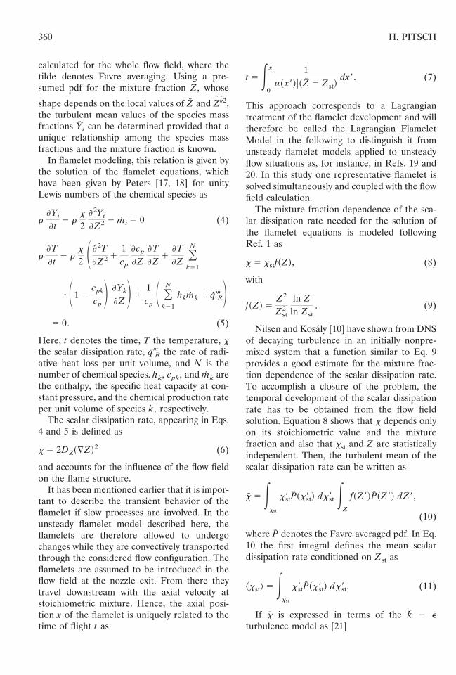
In the particular case considered here, ^xst&should denote a radial average and the integra-tion is performed in the limit dx 3 0. In anumerical simulation dx corresponds to theaxial spacing of the computational mesh. Theradial average of the scalar dissipation rateconditioned on stoichiometric mixture is shownin Fig. 1 as a function of the nozzle distance.The maximum value close to the nozzle isapproximately ^xst& 5 140 s21 and then de-creases strongly with increasing nozzle distance.At the point of the maximum centerline tem-perature, which is at approximately x/D 5 60,the scalar dissipation rate has already droppedto a value of ^xst& ' 0.6 s21.

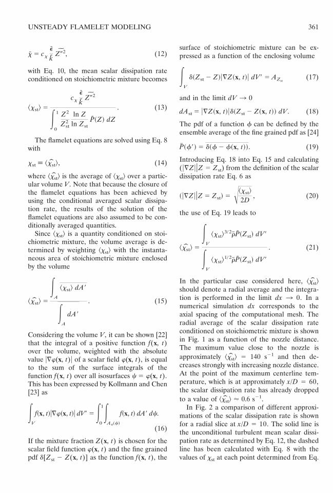
In Fig. 2 a comparison of different approxi-mations of the scalar dissipation rate is shownfor a radial slice at x/D 5 10. The solid line isthe unconditional turbulent mean scalar dissi-pation rate as determined by Eq. 12, the dashedline has been calculated with Eq. 8 with thevalues of xst at each point determined from Eq.

361UNSTEADY FLAMELET MODELING

13, and the dotted line is Eq. 8 with xst from Eq.21, which is the model used in the solution ofthe flamelet equations. All approximations yieldquite similar results for small values of themixture fraction, but in the very rich part theapproximations deviate from each other. Theunconditional mean is lower than the condi-tional mean scalar dissipation rate because ofthe ensemble averaging. Actually, the radialaverage (dotted line) should be equal to theconditional mean scalar dissipation rate(dashed line). The lower values indicate thatone particular flamelet does not extend in theradial direction. The radial average of the scalardissipation rate in conjunction with Eq. 8 recon-

structs the actual flamelet, whereas the othertwo approximations represent the values of aradial slice. However, it has been shown in Ref.15 that the impact of differences in the scalardissipation rate in the rich part is quite weak.

For the unsteady flamelet calculations, a re-duced 20-step mechanism has been used. Basedon the chemical mechanism given by Warnatz etal. [25] consisting of 295 elementary reactionsamong 34 chemical species, steady-state as-sumptions have been introduced for some rad-icals. The results obtained by using the reducedmechanism show essentially no differences fromcalculations employing the detailed reactionscheme.

Differential Diffusion

The Lagrangian Flamelet Model presented inthe previous section relies on the assumption ofunity Lewis numbers. In the following the pos-sibility of extending the model to account fornonequal Lewis numbers will be discussed.

It has been mentioned in the introductorydiscussion that differential diffusion effects ap-pear mainly very close to the nozzle and vanishfor high Reynolds numbers. The impact onflames in practical applications is therefore neg-ligible in most cases, although in flow situationsslightly above the transition Reynolds number,differential diffusion is more important than inthe diffusion flame investigated in the presentpaper. As mentioned earlier, this configurationhas been investigated experimentally by Berg-mann et al. [5], and differential diffusion effectshave been reported to be very pronouncedwithin a range extending from the nozzle toapproximately x/D 5 10.

In this section, three possible mechanisms,which would allow differential diffusion in tur-bulent flames are discussed and the individualimportance for the investigated flame will bedetermined. It will be concluded in the follow-ing that the first of these, the laminar near fieldflow, is the predominant mechanism responsiblefor differential diffusion in the investigatedflame. Although the remaining two mechanismswill be shown to be not important here, theyshould be discussed as possible alternatives indifferent flow situations.

Fig. 1. Radially averaged scalar dissipation rate conditionedon stoichiometric mixture as a function of nozzle distance(Eq. 21).

Fig. 2. Comparison of turbulent mean scalar dissipationrate (Eq. 12), conditional mean scalar dissipation rate (Eqs.8 and 13), and radially averaged conditional mean scalardissipation rate (Eqs. 8 and 21) at x/D 5 10 as a function ofthe mixture fraction.

362 H. PITSCH

Laminar Near Field Flow

It has been concluded from many studies thatthe near field of jet diffusion flames mightexhibit laminar structures within the mixinglayer, which would certainly make moleculardiffusion the dominant transport contributionwithin the mixing layer [5, 26–30].

Yule et al. [26] found from the investigationof transitional jets that diffusion flames have alaminarizing effect and an enlarged potentialcore when compared with nonreacting jets.

Schefer et al. [27] investigated the temporaldevelopment of turbulence–chemistry interac-tions in the near field of methane diffusionflames at a moderate jet-exit Reynolds numberof Re 5 7000. The obtained laser-induced flu-orescence (LIF) intensities of CH and CH4revealed laminar flame structures envelopingsemi-organized, large-scale vortical structures.Similar results have also been found by Chen etal. [28] in propane jet diffusion flames with highReynolds numbers up to Re ' 15,000. In addi-tion, it has been found from the analytic analysisof vorticity generation and destruction thatbuoyancy and volumetric expansion lead to asuppression of the vorticity in the fuel-richregime, which could explain the laminarizationof the near field region of jet diffusion flames.

Clemens and Paul [29] studied reacting andnonreacting nonpremixed jets. They also foundthe near field consisting of a laminar regionaround the reaction zone and organized vorticalstructures in the inner core. The laminarizationof the mixing layer and the separation of thevortical region from the reaction zone hassometimes been attributed to the lowering ofthe Reynolds number caused by the increasedviscosity due to the high temperature in thereaction zone. However, by comparison of reac-tive and nonreactive jets, it is shown in Ref. 29that the strong density gradients, in flamescaused by the heat release, are dominant inreducing the shear layer thickness and extend-ing the potential core.

In a numerical study of flow–chemistry inter-actions in the near field of nonpremixed jets,Soteriou [30] concluded that the initial separa-tion of the high vorticity region and the reactionzone is amplified by combustion-induced volu-metric expansion. Interestingly, it has been

found that the maximum vorticity can often belocated within the potential core, outside theregion of mixture fraction variation.

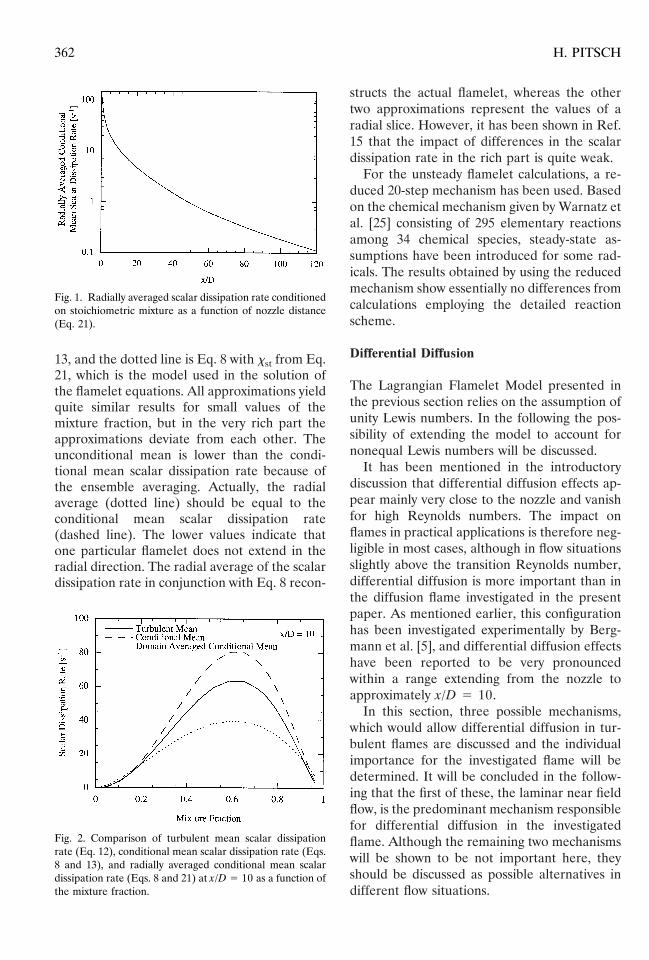
Hence, there is experimental, analytic, andnumerical evidence that even in high Reynoldsnumber flows in the near field of jet diffusionflames there exists a turbulent potential coresurrounded by a laminar mixing layer, whichincludes the reaction zone. It is obvious that thisregion is governed by molecular diffusion andwill be affected by nonunity Lewis numbers.Figure 3 shows experimentally obtained resultsby Bergmann et al. reproduced from Ref. 5 forthe CH4/H2/N2 flame investigated in the presentpaper. The left frame shows fluorescence inten-sity of NO seeded into the fuel. The brightregions represent the pure fuel forming thepotential core, which extends to approximately5 to 10 nozzle diameters downstream. Large-scale vortical structures can be obtained at theedges of the core which are formed in the shearlayer between the fuel and the surrounding

Fig. 3. LIF intensity of NO seeded into fuel and LIFintensity of OH in CH4/H2/N2–air jet diffusion flame ob-tained by Bergmann et al. [5].

363UNSTEADY FLAMELET MODELING

oxidizer. The OH fluorescence signal, given inthe right frame of Fig. 3, indicates that thereaction zone is still within a laminar environ-ment separated from the vortical region. Inter-actions among the turbulence-generating shearlayer and the region around the reaction zonestart at about x/D 5 5, still exhibiting almostunwrinkled layers until x/D 5 10. The differ-ential diffusion effects, which have been clearlydemonstrated to occur in this flame, are ex-plained in Ref. 5 by the absence of turbulencewithin the mixing layer in regions close to thenozzle. These effects are pronounced at x/D 55, and although turbulence develops in themixing layer thereafter, the effects of differen-tial diffusion remain even far downstream aswill be shown later in this paper.

Molecular Diffusivity

A second and very obvious possibility to allowmolecular diffusion effects emerging in turbulentflows is that the value of the molecular diffusivityDi of a particular species i is in the same order ofmagnitude as the turbulent diffusivity Dt. Notethat this argument actually includes the abovediscussed situation of a laminar flow region.However, the argument of a laminar mixinglayer in the near field of the nozzle is treatedseparately, because of the complete absence ofturbulence in this particular situation.

Because the molecular diffusivities of theindividual components can be considerably dif-ferent, these can be related to the mixturefraction diffusivity by using the Lewis numberand Eq. 2 as

Di 5DZ

Lei. (22)

The Lewis numbers of most species are close tounity. However, for the hydrogen radical, forinstance, the Lewis number is LeH ' 0.2. Theturbulent diffusivity can be related to the eddyviscosity nt by the turbulent Schmidt number

Sct 5nt

Dt, (23)

which is assumed to be close to unity. In theframe of the k 2 e model the turbulent eddyviscosity nt can be expressed as

nt 5 CD

k2

e(24)

with CD 5 0.09. For a simple comparison ofmolecular and turbulent diffusivity of the chem-ical components, the mixture fraction diffusivitycan then be compared to the turbulent eddydiffusivity calculated from Eqs. 23 and 24.

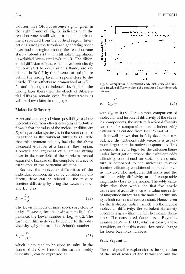
It is well known that in fully developed tur-bulence, the turbulent eddy viscosity is usuallymuch larger than the molecular quantities. Thisis demonstrated in Fig. 4 for the diffusion flameunder investigation, where the turbulent eddydiffusivity conditioned on stoichiometric mix-ture is compared to the molecular mixturefraction diffusivity conditioned on stoichiomet-ric mixture. The molecular diffusivity and theturbulent eddy diffusivity are of comparablemagnitude close to the nozzle. The eddy diffu-sivity rises then within the first five nozzlediameters of axial distance to a value one orderof magnitude larger than the molecular diffusiv-ity, which remains almost constant. Hence, evenfor the hydrogen radical, which has the highestmolecular diffusivity, the turbulent diffusivitybecomes larger within the first five nozzle diam-eters. The considered flame has a Reynoldsnumber of Re 5 15,000, which is clearly abovetransition, so that this conclusion could changefor lower Reynolds numbers.

Scale Separation

The third possible explanation is the separationof the small scales of the turbulence and the

Fig. 4. Comparison of turbulent eddy diffusivity and mix-ture fraction diffusivity along the contour of stoichiometricmixture.

364 H. PITSCH

mixing layer width. In the case that the charac-teristic mixing layer width lm is small comparedto the Kolmogorov scale hk, there exists alaminar sublayer which is governed by molecu-lar diffusion. In fact, the width of the mixinglayer is small very close to the nozzle andbroadens with increasing nozzle distance, whichwould correspond to the experimental findings.The transition to unity Lewis numbers wouldthen occur when the mixing layer width be-comes larger than the Kolmogorov scale and theturbulent eddies contribute to the transportwithin the mixing layer. Note that this does notviolate the flamelet assumption, because thesmall turbulent scales, which can disturb thelaminar structure of the mixing layer, can still bemuch larger than the reaction zone thickness,which is thin compared to the mixing layer.

For a rough estimate of the mixing layerthickness lm, this can be determined as a char-acteristic length scale related to the maximumscalar dissipation rate as

lm 5 Î2DZ

xmaxDZ. (25)

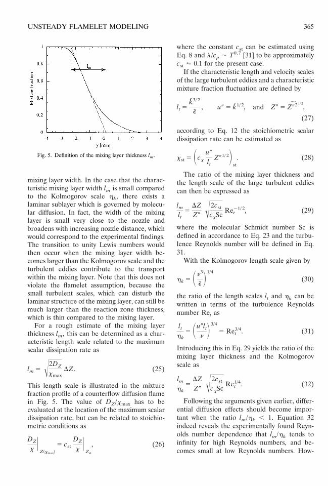
This length scale is illustrated in the mixturefraction profile of a counterflow diffusion flamein Fig. 5. The value of DZ/xmax has to beevaluated at the location of the maximum scalardissipation rate, but can be related to stoichio-metric conditions as

DZ

xU

Z~xmax!

5 cstDZ

xU

Zst

, (26)

where the constant cst can be estimated usingEq. 8 and l/cp ; T0.7 [31] to be approximatelycst ' 0.1 for the present case.

If the characteristic length and velocity scalesof the large turbulent eddies and a characteristicmixture fraction fluctuation are defined by

lt 5k3/ 2

e, u0 5 k1/ 2, and Z0 5 Z02 1/ 2

,

(27)

according to Eq. 12 the stoichiometric scalardissipation rate can be estimated as

xst 5 Scx

u0

ltZ01/ 2D

st. (28)

The ratio of the mixing layer thickness andthe length scale of the large turbulent eddiescan then be expressed as

lm

lt5

DZZ0 Î2cst

cxScRet

21/ 2, (29)

where the molecular Schmidt number Sc isdefined in accordance to Eq. 23 and the turbu-lence Reynolds number will be defined in Eq.31.

With the Kolmogorov length scale given by

hk 5 Sn3

eD1/4

(30)

the ratio of the length scales lt and hk can bewritten in terms of the turbulence Reynoldsnumber Ret as

lt

hk5 Su0lt

nD3/4

5 Ret3/4. (31)

Introducing this in Eq. 29 yields the ratio of themixing layer thickness and the Kolmogorovscale as

lm

hk5

DZZ0 Î2cst

cxScRet

1/4. (32)

Following the arguments given earlier, differ-ential diffusion effects should become impor-tant when the ratio lm/hk , 1. Equation 32indeed reveals the experimentally found Reyn-olds number dependence that lm/hk tends toinfinity for high Reynolds numbers, and be-comes small at low Reynolds numbers. How-

Fig. 5. Definition of the mixing layer thickness lm.

365UNSTEADY FLAMELET MODELING

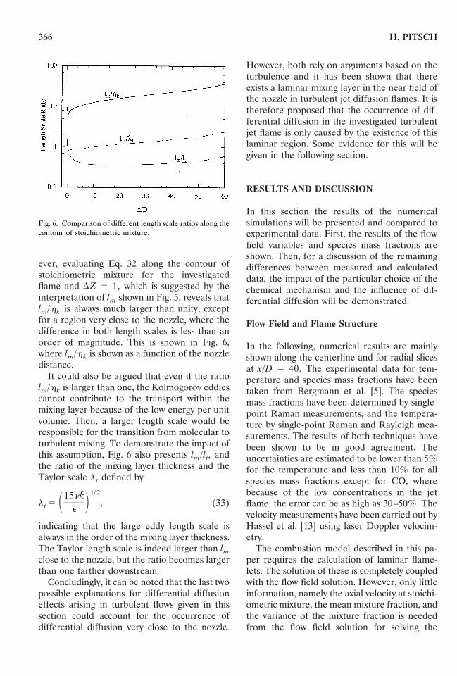
ever, evaluating Eq. 32 along the contour ofstoichiometric mixture for the investigatedflame and DZ 5 1, which is suggested by theinterpretation of lm shown in Fig. 5, reveals thatlm/hk is always much larger than unity, exceptfor a region very close to the nozzle, where thedifference in both length scales is less than anorder of magnitude. This is shown in Fig. 6,where lm/hk is shown as a function of the nozzledistance.

It could also be argued that even if the ratiolm/hk is larger than one, the Kolmogorov eddiescannot contribute to the transport within themixing layer because of the low energy per unitvolume. Then, a larger length scale would beresponsible for the transition from molecular toturbulent mixing. To demonstrate the impact ofthis assumption, Fig. 6 also presents lm/lt, andthe ratio of the mixing layer thickness and theTaylor scale lt defined by

lt 5 S15nke

D1/ 2

, (33)

indicating that the large eddy length scale isalways in the order of the mixing layer thickness.The Taylor length scale is indeed larger than lm

close to the nozzle, but the ratio becomes largerthan one farther downstream.

Concludingly, it can be noted that the last twopossible explanations for differential diffusioneffects arising in turbulent flows given in thissection could account for the occurrence ofdifferential diffusion very close to the nozzle.

However, both rely on arguments based on theturbulence and it has been shown that thereexists a laminar mixing layer in the near field ofthe nozzle in turbulent jet diffusion flames. It istherefore proposed that the occurrence of dif-ferential diffusion in the investigated turbulentjet flame is only caused by the existence of thislaminar region. Some evidence for this will begiven in the following section.

RESULTS AND DISCUSSION

In this section the results of the numericalsimulations will be presented and compared toexperimental data. First, the results of the flowfield variables and species mass fractions areshown. Then, for a discussion of the remainingdifferences between measured and calculateddata, the impact of the particular choice of thechemical mechanism and the influence of dif-ferential diffusion will be demonstrated.

Flow Field and Flame Structure

In the following, numerical results are mainlyshown along the centerline and for radial slicesat x/D 5 40. The experimental data for tem-perature and species mass fractions have beentaken from Bergmann et al. [5]. The speciesmass fractions have been determined by single-point Raman measurements, and the tempera-ture by single-point Raman and Rayleigh mea-surements. The results of both techniques havebeen shown to be in good agreement. Theuncertainties are estimated to be lower than 5%for the temperature and less than 10% for allspecies mass fractions except for CO, wherebecause of the low concentrations in the jetflame, the error can be as high as 30–50%. Thevelocity measurements have been carried out byHassel et al. [13] using laser Doppler velocim-etry.

The combustion model described in this pa-per requires the calculation of laminar flame-lets. The solution of these is completely coupledwith the flow field solution. However, only littleinformation, namely the axial velocity at stoichi-ometric mixture, the mean mixture fraction, andthe variance of the mixture fraction is neededfrom the flow field solution for solving the

Fig. 6. Comparison of different length scale ratios along thecontour of stoichiometric mixture.

366 H. PITSCH

laminar flamelet. Only if these data, which arean input rather than an output of the combus-tion model, are well predicted by the flow fieldsolver, can the combustion model be expectedto yield reasonable results. Therefore, the nu-merical solution for these quantities should becompared to the experimental data first.

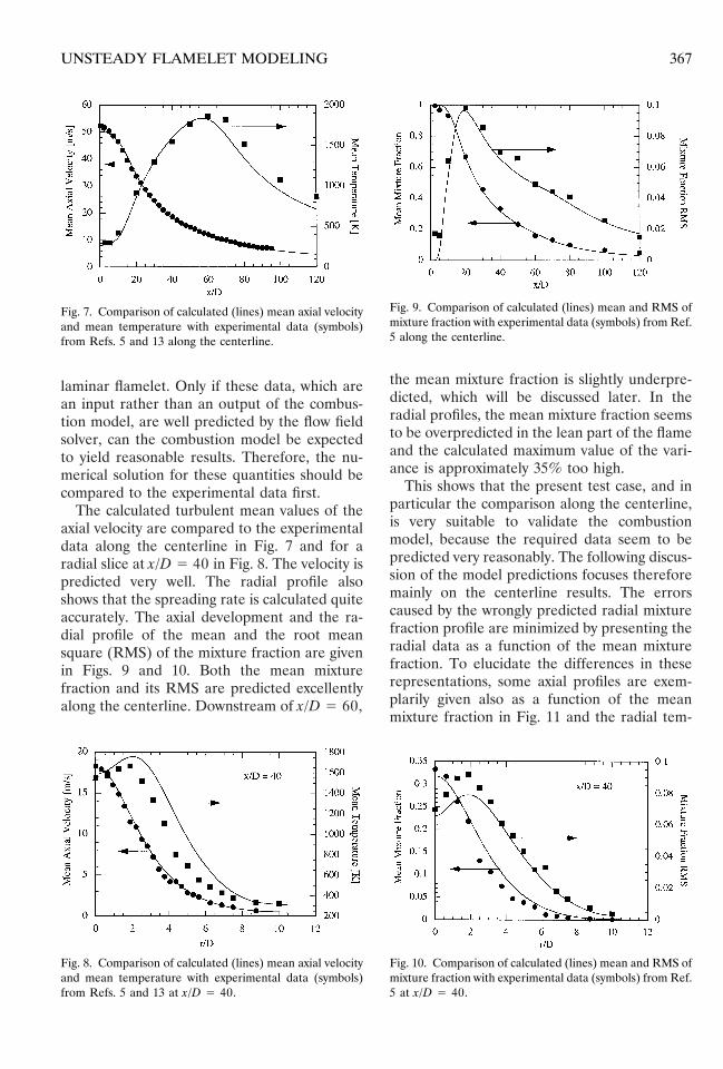
The calculated turbulent mean values of theaxial velocity are compared to the experimentaldata along the centerline in Fig. 7 and for aradial slice at x/D 5 40 in Fig. 8. The velocity ispredicted very well. The radial profile alsoshows that the spreading rate is calculated quiteaccurately. The axial development and the ra-dial profile of the mean and the root meansquare (RMS) of the mixture fraction are givenin Figs. 9 and 10. Both the mean mixturefraction and its RMS are predicted excellentlyalong the centerline. Downstream of x/D 5 60,

the mean mixture fraction is slightly underpre-dicted, which will be discussed later. In theradial profiles, the mean mixture fraction seemsto be overpredicted in the lean part of the flameand the calculated maximum value of the vari-ance is approximately 35% too high.

This shows that the present test case, and inparticular the comparison along the centerline,is very suitable to validate the combustionmodel, because the required data seem to bepredicted very reasonably. The following discus-sion of the model predictions focuses thereforemainly on the centerline results. The errorscaused by the wrongly predicted radial mixturefraction profile are minimized by presenting theradial data as a function of the mean mixturefraction. To elucidate the differences in theserepresentations, some axial profiles are exem-plarily given also as a function of the meanmixture fraction in Fig. 11 and the radial tem-

Fig. 7. Comparison of calculated (lines) mean axial velocityand mean temperature with experimental data (symbols)from Refs. 5 and 13 along the centerline.

Fig. 8. Comparison of calculated (lines) mean axial velocityand mean temperature with experimental data (symbols)from Refs. 5 and 13 at x/D 5 40.

Fig. 9. Comparison of calculated (lines) mean and RMS ofmixture fraction with experimental data (symbols) from Ref.5 along the centerline.

Fig. 10. Comparison of calculated (lines) mean and RMS ofmixture fraction with experimental data (symbols) from Ref.5 at x/D 5 40.

367UNSTEADY FLAMELET MODELING

perature profile is shown as a function of thephysical coordinate in Fig. 8.

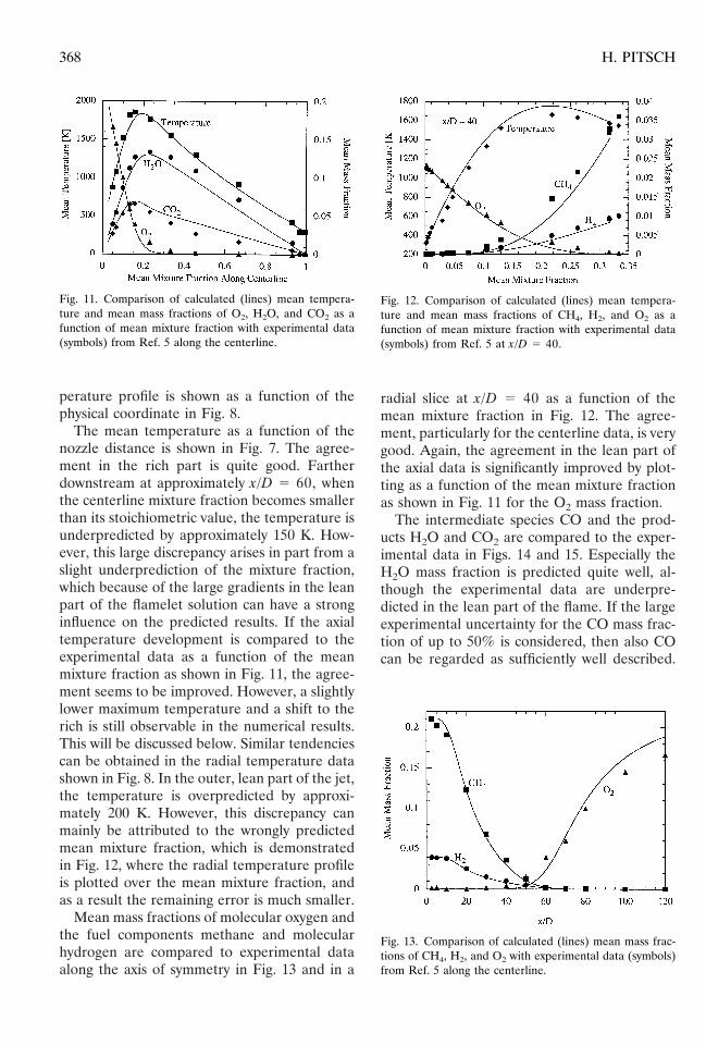
The mean temperature as a function of thenozzle distance is shown in Fig. 7. The agree-ment in the rich part is quite good. Fartherdownstream at approximately x/D 5 60, whenthe centerline mixture fraction becomes smallerthan its stoichiometric value, the temperature isunderpredicted by approximately 150 K. How-ever, this large discrepancy arises in part from aslight underprediction of the mixture fraction,which because of the large gradients in the leanpart of the flamelet solution can have a stronginfluence on the predicted results. If the axialtemperature development is compared to theexperimental data as a function of the meanmixture fraction as shown in Fig. 11, the agree-ment seems to be improved. However, a slightlylower maximum temperature and a shift to therich is still observable in the numerical results.This will be discussed below. Similar tendenciescan be obtained in the radial temperature datashown in Fig. 8. In the outer, lean part of the jet,the temperature is overpredicted by approxi-mately 200 K. However, this discrepancy canmainly be attributed to the wrongly predictedmean mixture fraction, which is demonstratedin Fig. 12, where the radial temperature profileis plotted over the mean mixture fraction, andas a result the remaining error is much smaller.

Mean mass fractions of molecular oxygen andthe fuel components methane and molecularhydrogen are compared to experimental dataalong the axis of symmetry in Fig. 13 and in a

radial slice at x/D 5 40 as a function of themean mixture fraction in Fig. 12. The agree-ment, particularly for the centerline data, is verygood. Again, the agreement in the lean part ofthe axial data is significantly improved by plot-ting as a function of the mean mixture fractionas shown in Fig. 11 for the O2 mass fraction.

The intermediate species CO and the prod-ucts H2O and CO2 are compared to the exper-imental data in Figs. 14 and 15. Especially theH2O mass fraction is predicted quite well, al-though the experimental data are underpre-dicted in the lean part of the flame. If the largeexperimental uncertainty for the CO mass frac-tion of up to 50% is considered, then also COcan be regarded as sufficiently well described.

Fig. 11. Comparison of calculated (lines) mean tempera-ture and mean mass fractions of O2, H2O, and CO2 as afunction of mean mixture fraction with experimental data(symbols) from Ref. 5 along the centerline.

Fig. 12. Comparison of calculated (lines) mean tempera-ture and mean mass fractions of CH4, H2, and O2 as afunction of mean mixture fraction with experimental data(symbols) from Ref. 5 at x/D 5 40.

Fig. 13. Comparison of calculated (lines) mean mass frac-tions of CH4, H2, and O2 with experimental data (symbols)from Ref. 5 along the centerline.

368 H. PITSCH

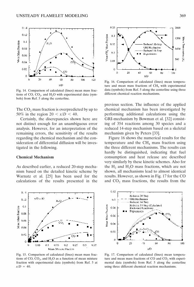
The CO2 mass fraction is overpredicted by up to50% in the region 20 , x/D , 40.

Certainly, the discrepancies shown here arenot distinct enough for an unambiguous erroranalysis. However, for an interpretation of theremaining errors, the sensitivity of the resultsregarding the chemical mechanism and the con-sideration of differential diffusion will be inves-tigated in the following.

Chemical Mechanism

As described earlier, a reduced 20-step mecha-nism based on the detailed kinetic scheme byWarnatz et al. [25] has been used for thecalculations of the results presented in the

previous section. The influence of the appliedchemical mechanism has been investigated byperforming additional calculations using theGRI-mechanism by Bowman et al. [32] consist-ing of 354 reactions among 30 species and areduced 14-step mechanism based on a skeletalmechanism given by Peters [33].

Figure 16 shows the numerical results for thetemperature and the CH4 mass fraction usingthe three different mechanisms. The results canhardly be distinguished, indicating that fuelconsumption and heat release are describedvery similarly by these kinetic schemes. Also forthe H2 and H2O mass fractions, which are notshown, all mechanisms lead to almost identicalresults. However, as shown in Fig. 17 for the COand CO2 mass fractions, the results from the

Fig. 14. Comparison of calculated (lines) mean mass frac-tions of CO, CO2, and H2O with experimental data (sym-bols) from Ref. 5 along the centerline.

Fig. 15. Comparison of calculated (lines) mean mass frac-tions of CO, CO2, and H2O as a function of mean mixturefraction with experimental data (symbols) from Ref. 5 atx/D 5 40.

Fig. 16. Comparison of calculated (lines) mean tempera-ture and mean mass fractions of CH4 with experimentaldata (symbols) from Ref. 5 along the centerline using threedifferent chemical reaction mechanisms.

Fig. 17. Comparison of calculated (lines) mean tempera-ture and mean mass fractions of CO and CO2 with experi-mental data (symbols) from Ref. 5 along the centerlineusing three different chemical reaction mechanisms.

369UNSTEADY FLAMELET MODELING

14-step mechanism depart from those of the20-step Warnatz mechanism and the GRImechanism, especially in the rich part of theflame, which extends from the nozzle to approx-imately x/D 5 60. Both, Warnatz’ mechanismand the GRI mechanism seem to yield muchmore accurate CO2 mass fractions. However, inRef. 33 kinetic rate data for the consideredbackward reactions are given explicitly. If thoseare computed from the equilibrium constants,the results of the 14-step mechanism are alsovery comparable to the other schemes. The COmass fraction seems to be improved by theresults of the 14-step mechanism. But since theexperimental uncertainty for CO is very high,the results of all mechanisms are still in thebounds of the experimental error.

Differential Diffusion

The experimental data obtained by Bergmannet al. [5] clearly reveal differential diffusioneffects close to the nozzle. These becomeweaker with increasing nozzle distance, but canstill be observed at x/D 5 20. In an earliersection it has been concluded that differentialdiffusion in the investigated jet flame is onlycaused by the existence of a laminar regionclose to the nozzle. This postulation should beconfirmed and investigated further in the fol-lowing.

In the context of differential diffusion it isimportant to clarify the applied definition of themixture fraction. In the frame of the flameletmodel as given in Ref. 15 the mixture fraction isdefined by the solution of a conservation equa-tion as given by Eq. 1. This definition is used forall calculations in the present paper. Because amixture fraction defined as such cannot beobtained from the experimental data, an ele-ment mixture fraction based definition, as forexample given by Masri and Bilger [16], has tobe used in order to compare the numericalresults with the experiments. However, the tur-bulent mean of this mixture fraction definitioncan be determined from flow field and flameletsolution very easily and is therefore applied inthe comparisons with experimental data in thissection. As mentioned earlier, for the equalLewis number approach there is no differencebetween both definitions.

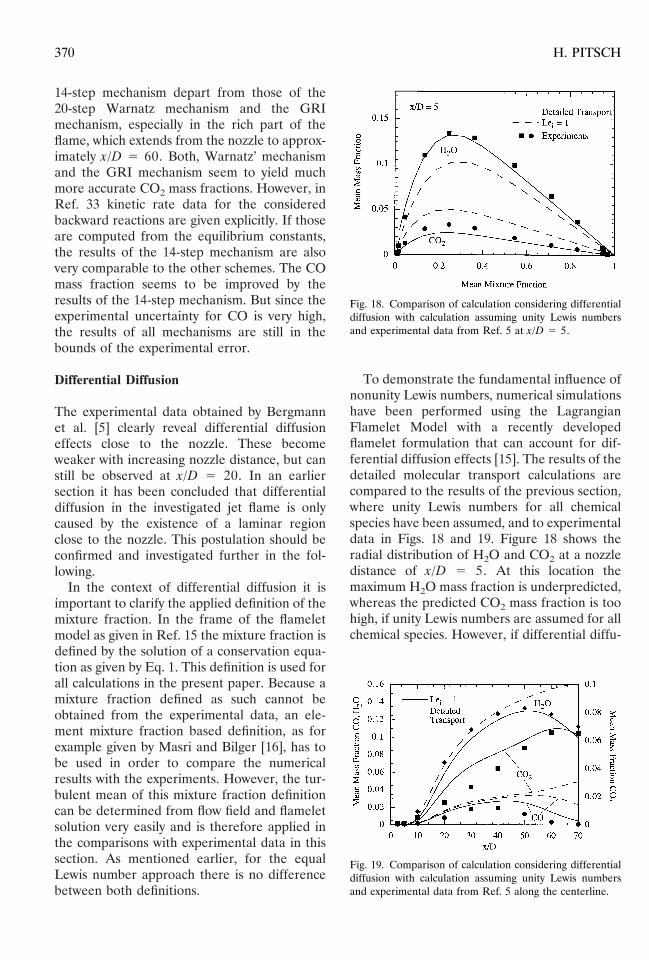
To demonstrate the fundamental influence ofnonunity Lewis numbers, numerical simulationshave been performed using the LagrangianFlamelet Model with a recently developedflamelet formulation that can account for dif-ferential diffusion effects [15]. The results of thedetailed molecular transport calculations arecompared to the results of the previous section,where unity Lewis numbers for all chemicalspecies have been assumed, and to experimentaldata in Figs. 18 and 19. Figure 18 shows theradial distribution of H2O and CO2 at a nozzledistance of x/D 5 5. At this location themaximum H2O mass fraction is underpredicted,whereas the predicted CO2 mass fraction is toohigh, if unity Lewis numbers are assumed for allchemical species. However, if differential diffu-

Fig. 18. Comparison of calculation considering differentialdiffusion with calculation assuming unity Lewis numbersand experimental data from Ref. 5 at x/D 5 5.

Fig. 19. Comparison of calculation considering differentialdiffusion with calculation assuming unity Lewis numbersand experimental data from Ref. 5 along the centerline.

370 H. PITSCH

sion is considered, both H2O and CO2 massfractions are significantly improved.

In Fig. 19 a comparison of the detailed trans-port calculations with the unity Lewis numberresults and the experimental data for H2O, CO,and CO2 is given along the axis of symmetry.Again, the results for H2O are improved closeto the nozzle by considering differential diffu-sion. Also for the CO2 mass fraction, the con-sideration of differential diffusion yields theright tendency, but the correction is too strong,leading to an underprediction of the CO2 massfraction. The CO profile is hardly influenced bydifferential diffusion in the region close to thenozzle. However, downstream of x/D ' 40 theresults of the differential diffusion calculationsdepart clearly from the experimental data forthe mass fractions of all three components,whereas the results obtained using the unityLewis number approach match the experimen-tal data quite well. These results seem to con-firm the experimental findings that differentialdiffusion is most important in the nozzle closeregion.

In order to validate the suggested model, anadditional calculation has been performed usingthe flamelet equations given in Ref. 15. For thiscalculation it has been assumed that as long asthe jet reveals a potential core, there is noturbulent diffusion of chemical species occur-ring within the mixing layer.

For this assumption the application of thestandard k 2 e model causes two problems.Firstly, this model cannot account for the lam-inar mixing layer region close to the nozzle.However, it has been shown that the velocityand also the mixture fraction field are wellpredicted. With respect to the scalar dissipationrate, recent work presenting k 2 e model andlarge-eddy simulation calculations for the samejet diffusion flame [34, 35] indicates that thepredictions for the scalar dissipation rate arenot very different even in the region close to thenozzle. The second problem is that the transi-tion point cannot be determined by the use ofthe k 2 e model. Because it is not the intentionof the present model to predict the transitionpoint, this value will be prescribed by the exam-ination of the experimental data for the presentstudy. However, both problems can probably becured by the use of large-eddy simulations.

From Fig. 3 the potential core region can beestimated to extend from the nozzle to approx-imately x/D 5 10. At this point, the laminar–turbulent transition is assumed to occur and thecalculation of the unsteady flamelet continuesdownstream with unity Lewis numbers for allspecies. This choice seems to be somewhatarbitrary, but it is strongly supported by elementmass fraction distributions discussed later in thispaper, which clearly show molecular transportbeing dominant up to a nozzle distance ofx/D 5 10. For the assumption of Lei 5 1, it canbe shown easily that the flamelet equationsgiven in Ref. 15 simplify to Eqs. 4 and 5.

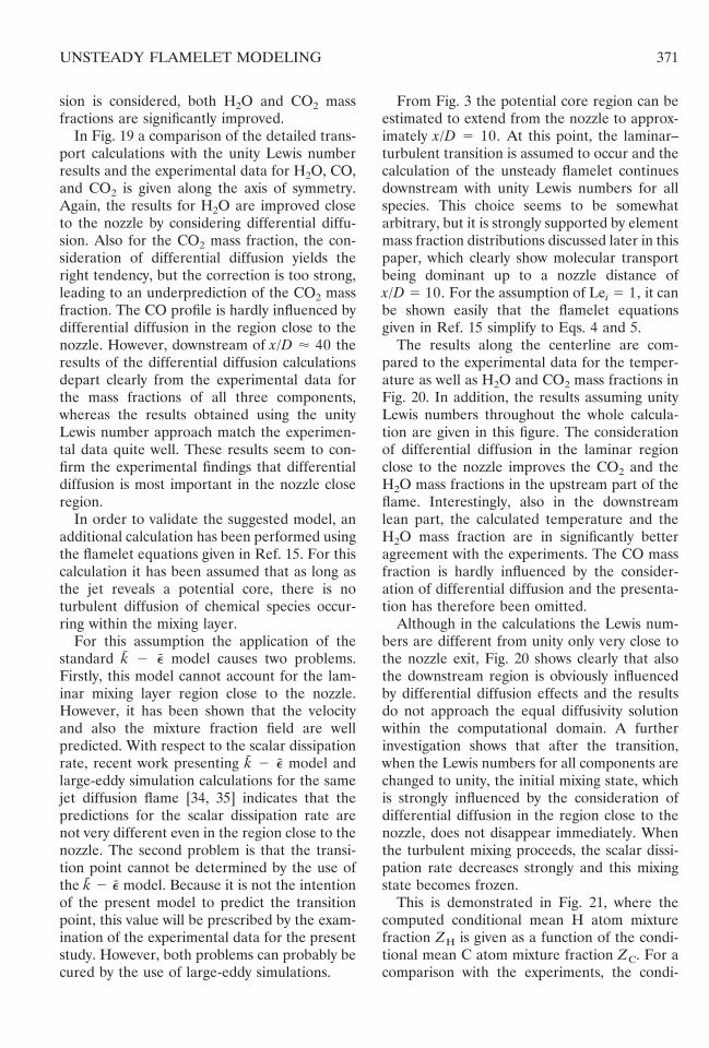
The results along the centerline are com-pared to the experimental data for the temper-ature as well as H2O and CO2 mass fractions inFig. 20. In addition, the results assuming unityLewis numbers throughout the whole calcula-tion are given in this figure. The considerationof differential diffusion in the laminar regionclose to the nozzle improves the CO2 and theH2O mass fractions in the upstream part of theflame. Interestingly, also in the downstreamlean part, the calculated temperature and theH2O mass fraction are in significantly betteragreement with the experiments. The CO massfraction is hardly influenced by the consider-ation of differential diffusion and the presenta-tion has therefore been omitted.

Although in the calculations the Lewis num-bers are different from unity only very close tothe nozzle exit, Fig. 20 shows clearly that alsothe downstream region is obviously influencedby differential diffusion effects and the resultsdo not approach the equal diffusivity solutionwithin the computational domain. A furtherinvestigation shows that after the transition,when the Lewis numbers for all components arechanged to unity, the initial mixing state, whichis strongly influenced by the consideration ofdifferential diffusion in the region close to thenozzle, does not disappear immediately. Whenthe turbulent mixing proceeds, the scalar dissi-pation rate decreases strongly and this mixingstate becomes frozen.

This is demonstrated in Fig. 21, where thecomputed conditional mean H atom mixturefraction ZH is given as a function of the condi-tional mean C atom mixture fraction ZC. For acomparison with the experiments, the condi-

371UNSTEADY FLAMELET MODELING

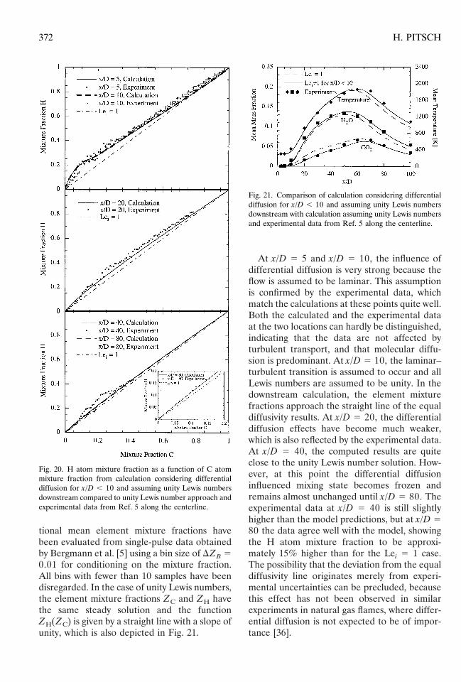
tional mean element mixture fractions havebeen evaluated from single-pulse data obtainedby Bergmann et al. [5] using a bin size of DZB 50.01 for conditioning on the mixture fraction.All bins with fewer than 10 samples have beendisregarded. In the case of unity Lewis numbers,the element mixture fractions ZC and ZH havethe same steady solution and the functionZH(ZC) is given by a straight line with a slope ofunity, which is also depicted in Fig. 21.

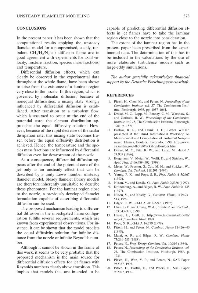
At x/D 5 5 and x/D 5 10, the influence ofdifferential diffusion is very strong because theflow is assumed to be laminar. This assumptionis confirmed by the experimental data, whichmatch the calculations at these points quite well.Both the calculated and the experimental dataat the two locations can hardly be distinguished,indicating that the data are not affected byturbulent transport, and that molecular diffu-sion is predominant. At x/D 5 10, the laminar–turbulent transition is assumed to occur and allLewis numbers are assumed to be unity. In thedownstream calculation, the element mixturefractions approach the straight line of the equaldiffusivity results. At x/D 5 20, the differentialdiffusion effects have become much weaker,which is also reflected by the experimental data.At x/D 5 40, the computed results are quiteclose to the unity Lewis number solution. How-ever, at this point the differential diffusioninfluenced mixing state becomes frozen andremains almost unchanged until x/D 5 80. Theexperimental data at x/D 5 40 is still slightlyhigher than the model predictions, but at x/D 580 the data agree well with the model, showingthe H atom mixture fraction to be approxi-mately 15% higher than for the Lei 5 1 case.The possibility that the deviation from the equaldiffusivity line originates merely from experi-mental uncertainties can be precluded, becausethis effect has not been observed in similarexperiments in natural gas flames, where differ-ential diffusion is not expected to be of impor-tance [36].

Fig. 20. H atom mixture fraction as a function of C atommixture fraction from calculation considering differentialdiffusion for x/D , 10 and assuming unity Lewis numbersdownstream compared to unity Lewis number approach andexperimental data from Ref. 5 along the centerline.

Fig. 21. Comparison of calculation considering differentialdiffusion for x/D , 10 and assuming unity Lewis numbersdownstream with calculation assuming unity Lewis numbersand experimental data from Ref. 5 along the centerline.

372 H. PITSCH

CONCLUSIONS

In the present paper it has been shown that thecomputational results applying the unsteadyflamelet model for a nonpremixed, steady, tur-bulent CH4/H2/N2–air diffusion flame are ingood agreement with experiments for axial ve-locity, mixture fraction, species mass fractions,and temperature.

Differential diffusion effects, which canclearly be observed in the experimental datathroughout the whole flame, have been shownto arise from the existence of a laminar regionvery close to the nozzle. In this region, which isgoverned by molecular diffusion, because ofnonequal diffusivities, a mixing state stronglyinfluenced by differential diffusion is estab-lished. After transition to a turbulent flow,which is assumed to occur at the end of thepotential core, the element distribution ap-proaches the equal diffusivity solution. How-ever, because of the rapid decrease of the scalardissipation rate, this mixing state becomes fro-zen before the equal diffusivity distribution isachieved. Hence, the temperature and the spe-cies mass fractions are influenced by differentialdiffusion even far downstream of the nozzle.

As a consequence, differential diffusion ap-pears after the end of the potential core of thejet only as an unsteady effect that can bedescribed by a unity Lewis number unsteadyflamelet model. Steady flamelet library modelsare therefore inherently unsuitable to describethese phenomena. For the laminar region closeto the nozzle, a previously developed flameletformulation capable of describing differentialdiffusion can be used.

The proposed mechanism leading to differen-tial diffusion in the investigated flame configu-ration fulfills several requirements, which areknown from experimental observations. For in-stance, it can be shown that the model predictsthe equal diffusivity solution for infinite dis-tance from the nozzle or infinite Reynolds num-ber.

Although it cannot be shown in the frame ofthis work, it seems to be very probable that theproposed mechanism is the main source fordifferential diffusion effects for jet flames withReynolds numbers clearly above transition. Thisimplies that models that are intended to be

capable of predicting differential diffusion ef-fects in jet flames have to take the laminarregion close to the nozzle into consideration.

The extent of the laminar region has in thepresent paper been prescribed from the exper-imental data. The determination of this has tobe included in the calculations by the use ofmore elaborate turbulence models such aslarge-eddy simulations.

The author gratefully acknowledges financialsupport by the Deutsche Forschungsgemeinschaft.

REFERENCES

1. Pitsch, H., Chen, M., and Peters, N., Proceedings of theCombustion Institute, vol. 27, The Combustion Insti-tute, Pittsburgh, 1998, pp. 1057–1064.

2. Drake, M. C., Lapp, M., Penney, C. M., Warshaw, S.,and Gerhold, B. W., Proceedings of the CombustionInstitute, vol. 18, The Combustion Institute, Pittsburgh,1981, p. 1521.

3. Barlow, R. S., and Frank, J. H., Poster W2E07,presented at the Third International Workshop onMeasurement and Computation of Turbulent Nonpre-mixed Flames, Boulder, Colorado, 1998, http://www.ca.sandia.gov/tdf/3rdWorkshop/Boulder.html.

4. Drake, M. C., Pitz, R. W., and Lapp, M., AIAA J.24:905 (1986).

5. Bergmann, V., Meier, W., Wolff, D., and Stricker, W.,Appl. Phys. B 66:489–502 (1998).

6. Meier, W., Prucker, S., Cao, M.-H., and Stricker, W.,Combust. Sci. Technol. 118:293 (1996).

7. Yeung, P. K., and Pope, S. B., Phys. Fluids A 5:2467(1993).

8. Nilsen, V., and Kosaly, G., Phys. Fluids 9:3386 (1997).9. Kronenburg, A., and Bilger, R. W., Phys. Fluids 9:1435

(1997).10. Nilsen, V., and Kosaly, G., Combust. Flame, 117:493–

513, 1999.11. Bilger, R. W., AIAA J. 20:962–970 (1982).12. Chen, J.-Y., and Chang, W.-C., Combust. Sci. Technol.,

133:343–375, 1998.13. Hassel, E., Geiß, S., http://www.tu-darmstadt.de/fb/

mb/ekt/flamebase.html, 1998.14. Pope, S. B., AIAA J. 16:279 (1978).15. Pitsch, H., and Peters, N., Combust. Flame 114:26–40

(1998).16. Masri, A. R., and Bilger, R. W., Combust. Flame

73:261–285 (1988).17. Peters, N., Prog. Energy Combust. Sci. 10:319 (1984).18. Peters, N., Proceedings of the Combustion Institute, vol.

21, The Combustion Institute, Pittsburgh, 1986, p.1231.

19. Pitsch, H., Wan, Y. P., and Peters, N., SAE Paper952357, 1995.

20. Pitsch, H., Barths, H., and Peters, N., SAE Paper962057, 1996.

373UNSTEADY FLAMELET MODELING

21. Jones, W. P., and Whitelaw, J. H., Combust. Flame48:1 (1982).

22. Maz’ja, V. G., Sobelev Spaces, Springer Verlag, Berlin,1985, p. 37.

23. Kollmann, W., and Chen, J. H., Proceedings of theCombustion Institute, vol. 21, The Combustion Insti-tute, Pittsburgh, 1994, pp. 777–784.

24. O’Brien, E. E., in Turbulent Reacting Flows (P. A.Libby and F. A. Williams, Eds.), Springer, 1980.

25. Warnatz, J., Maas, U., and Dibble, R. W., Combustion,Physical and Chemical Fundamentals, Modeling andSimulation, Experiments, Pollutant Formation, SpringerVerlag, 1996.

26. Yule, A. J., Chigier, N. A., Ralph, S., Boulderstone, R.,and Ventura, J., AIAA J. 19:752–760 (1980).

27. Schefer, R. W., Namazian, M., Filtopoulos, E. E. J.,and Kelly, J., Proceedings of the Combustion Institute,vol. 25, The Combustion Institute, Pittsburgh, 1994,pp. 1223–1231.

28. Chen, L.-D., Roquemore, W. M., Goss, L. P., andVilimpoc, V., Combust. Sci. Technol. 77:41–57 (1991).

29. Clemens, N. T., and Paul, P. H., Combust. Flame102:271–284 (1995).

30. Soteriou, M. C., Proceedings of the Combustion Insti-tute, vol. 27, The Combustion Institute, pp. 1213–1219Pittsburgh, 1998.

31. Smooke, M. D., and Giovangigli, V., in Reduced Ki-netic Mechanisms and Asymptotic Approximations forMethane–Air Flames (M. D. Smooke, Ed.), Springer,1991.

32. Bowman, C. T., Hanson, R. K., Davidson, D. F.,Gardiner, Jr., W. C., Lissianski, V., Smith, G. P.,Golden, D. M., Frenklach, M., and Goldenberg, M.,http://www.me.berkeley.edu/gri_mech/

33. Peters, N., in Reduced Kinetic Mechanisms for Applica-tions in Combustion Systems (Peters and Rogg, Eds.),Springer, 1993. Springer Verlag, Berlin (Peters, N. andRogg, B., Eds.)

34. Pitsch, H., and Riesmeier, E., Poster presented at theFourth International Workshop on Measurement andComputation of Turbulent Nonpremixed Flames,Darmstadt, 1999.

35. Pitsch, H., and Steiner, H., Poster presented at theFourth International Workshop on Measurement andComputation of Turbulent Nonpremixed Flames,Darmstadt, 1999.

36. Meier, W., Private communication, 1999.

Received 17 March 1999; revised 27 August 1999; accepted 15March 2000

374 H. PITSCH