J F / u d 'Mrth (19961. lo / 321, p p 157 187 Copyright '9 1996 Cambridge University Pi c s

157

Unsteadiness and convective instabilities in two-dimensional flow over a

backward-facing step

By L A M B R O S KAIKTSIS' , G E O R G E E M K A R N I A D A K I S 2 A N D S T E V E N A. O R S Z A G 3

'Institut fur Energietechnik, ETH-Zentrum, CH-8092 Zurich, Switzerland 'Center for Fluid Mechanics, Division of Applied Mathematics, Brown University,

Providence, RI 02912, USA 'Fluid Dynamics Research Center. Princeton University, Princeton, NJ 08544-0710, USA

(Received 6 June 1994 and in revised form 9 April 1996)

A systematic study of the stability of the two-dimensional flow over a backward- facing step with a nominal expansion ratio of 2 is presented up to Reynolds number Re = 2500 using direct numerical simulation as well as local and global stability analysis. Three different spectral element computer codes are used for the simulations. The stability analysis is performed both locally (at a number of streamwise locations) and globally (on the entire field) by computing the leading eigenvalues of a base flow state. The distinction is made between convectively and absolutely unstable mean flow. In two dimensions, i t is shown that all the asymptotic flow states up to Re = 2500 are time-independent in the absence of any external excitation, whereas the flow is convectively unstable, in a large portion of the flow domain, for Reynolds numbers in the range 700 < Re d 2500. Consequently, upstream generated small disturbances propagate downstream at exponentially amplified amplitude with a space-dependent speed. For small excitation disturbances, the amplitude of the resulting waveform is proportional to the disturbance amplitude. However, selective sustained external excitation (even at small amplitudes) can alter the behaviour of the system and lead to time-dependent flow. Two different types of excitation are imposed at the inflow: (1) monochromatic waves with frequency chosen to be either close to or very far from the shear layer frequency; and (ii) random noise. I t is found that for small-amplitude monochromatic excitation the flow acquires a time-periodic behaviour if perturbed close to the shear layer frequency, whereas the flow remains unaffected for high values of the excitation frequency. On the other hand, for the random noise as input, an unsteady behaviour is obtained with a fundamental frequency close to the shear layer frequency.

1. Introduction The flow over a backward-facing step has received much attention as a prototype

internal, separated flow. A detailed experimental study of mean flow quantities for a nominal expansion ratio (outlet to inlet height) of approximately 2 and for Reynolds numbers up to Re = 8000 is given by Armaly et ~ l . (1983) (see also references therein). Most computational studies up to now have focused on the low Reynolds number regime (Re ,< 1000). The well-defined nature of the problem as well as the availability

http

s://

doi.o

rg/1

0.10

17/S

0022

1120

9600

7689

Dow

nloa

ded

from

htt

ps://

ww

w.c

ambr

idge

.org

/cor

e. B

row

n U

nive

rsity

Lib

rary

, on

27 M

ar 2

018

at 1

9:30

:14,

sub

ject

to th

e Ca

mbr

idge

Cor

e te

rms

of u

se, a

vaila

ble

at h

ttps

://w

ww

.cam

brid

ge.o

rg/c

ore/

term

s.

158 L. Kaiktsis, G. E. Karniadakis and S. A. Orszag

of experimental data make step flow a benchmark problem for numerical methods (Gresho & Sani 1990).

In recent numerical work, however, discrepancies between various simulations have been reported regarding the time-asymptotic states of this flow for Reynolds number of order 1000 and beyond. For a given expansion ratio, the flow has been found to be steady or time-dependent depending on the specific numerical method and the selected resolution employed. Typically, simulation results based on low-order (relatively diffusive and/or dispersive) methods report steady (time-independent) states, whereas vortex and spectral methods report unsteady (time-dependent) flow. In particular, in two-dimensional simulations for a step expansion ratio close to 2, global unsteadiness has been computed for Reynolds numbers greater than 750 (Sethian & Ghoniem 1988) and 700 (Kaiktsis, Karniadakis & Orszag 1991), while steady flow results have been reported by Osswald, Ghia & Ghia (1983) for up to Re = 1474. More recently, a series of high-resolution numerical studies reported by Gresho et al. (1993) demonstrated that the step flow is stable to two-dimensional temporal perturbations for Reynolds numbers up to 800.

In laboratory experiments the flow appears to be three-dimensional above Re m 400 (Armaly et al. 1983). The reported normalized values for the reattachment length exhibit a peak at Re = 1200. The subsequent decrease of the primary recirculation zone length with Reynolds number increasing beyond Re 3 1200 can only be attributed to the action of Reynolds stresses. These Reynolds stresses must be present in the flow for Reynolds numbers lower than the one corresponding to the maximum value of the reattachment length. Therefore, the flow must become unsteady at some Re < 1200. More recent experimental results and corresponding stability calculations for an expansion ratio larger than 2 also suggest that the flow becomes unsteady for Reynolds number Re ,< 1000 (M. Gaster, private communications). For axisymmetric expansions, unsteadiness has been observed in the experimental work by Latornell & Pollard (1986), where, in particular, strong sensitivity to the inlet boundary conditions was observed.

Theoretically, the stability properties of step flow can be analysed qualitatively by considering the inviscid shear layer model examined by Huerre & Monkewitz (1985). If we denote by U1 and U2 the velocities of the two streams, then the absolute instability condition for that profile is R = (Ul - U2)/(U1 + U,) > 1.315, which is satisfied if U2 is sufficiently large and negative. If we consider a typical streamwise velocity profile in step flow within the primary separated zone (see figure 1) and substitute for U1 and Uz the maximum positive and negative velocities, respectively, we find that at Re = 700 the ratio R is slightly higher than 1.315 for all profiles in the region 7.6 < X < 9.4. However, the profile plotted in figure 1 is quite different from that of the shear layer model of Huerre & Monkewitz owing to the presence of channel walls. Furthermore, in a spatially developing flow, a sufficiently large ‘pocket’ of local absolute instability is necessary to generate global unsteadiness. This is expressed using the criterion of Chomaz, Huerre & Redekopp (1990) as

where the region of local absolute instability extends from x = X , to x = Xh and aogi(x) are the temporal ‘absolute growth-rates’ of the streamwise velocity profiles; wgi(x) correspond to vanishing group velocity (do/dklk, = 0), where both the frequency w and the wavenumber k are complex. It is clear from this simple argument that,

http

s://

doi.o

rg/1

0.10

17/S

0022

1120

9600

7689

Dow

nloa

ded

from

htt

ps://

ww

w.c

ambr

idge

.org

/cor

e. B

row

n U

nive

rsity

Lib

rary

, on

27 M

ar 2

018

at 1

9:30

:14,

sub

ject

to th

e Ca

mbr

idge

Cor

e te

rms

of u

se, a

vaila

ble

at h

ttps

://w

ww

.cam

brid

ge.o

rg/c

ore/

term

s.

Instuhilities in two-dimensional flow over a backward-facing step 159

t

1 5 i -0 2 0 0 2 04 0 6 0 8 1 0

FIGURE 1. Streamwise velocity profile at X = 8 (approximately 7.5 step heights downstream of the expansion cross-section); Re = 700.

U-velocity

especially in the region close to the channel expansion, local temporal stability analysis, although suggestive of an instability, cannot give a definitive solution to the global stability properties of step flow.

There are many possible reasons for the discrepancies between different simulation results, as well as between simulation and experiments. Insufficient spatial and temporal resolution, differences in the dispersive and diffusive properties of low- and high-order methods, and statistical noise associated with, e.g., viscous vortex methods, are perhaps the most important factors affecting computational results. Experimental results are affected by the omnipresent background noise, the three- dimensional character of the flow, and induced three-dimensionality effects due to the finite aspect ratio. All these factors, coupled with the stability characteristics of the flow below and above a critical Reynolds number (determined in the present problem primarily by the expansion ratio and the inlet boundary conditions) can contribute to the disagreements among the various studies.

In the present work, we investigate systematically the effects of various kinds of flow excitation and classify the stability regimes of the flow based on modern concepts of instability theory, e.g. the distinction between convectively and absolutely unstable flow (Bers 1975; Huerre & Monkewitz 1985, 1990; Triantafyllou, Triantafyllou & Chryssostomidis 1986; Deissler 1987). Our objective is three-fold: (i) to provide a clear understanding and classification of primary asymptotic two-dimensional flow states; (ii) to explain both experimental and numerical results in the context of instability theory; and (iii) to understand, in a more generic form, the nonlinear response of a convectively unstable flow system.

We use spectral element discretization algorithms for the numerical solution of the incompressible Navier-Stokes equations. These algorithms allow for a systematic variation of resolution parameters and, in particular, they allow resolution checks using two different convergence paths corresponding to h-type and p-type refinement. Three different spectral element codes were used (see below). The inflow boundary conditions can be specified as arbitrary functions of time so that the effects of sustained flow excitation at inflow can be compared to impulsive shear layer excitation at the step corner via a localized forcing. Many different cases are examined corresponding

http

s://

doi.o

rg/1

0.10

17/S

0022

1120

9600

7689

Dow

nloa

ded

from

htt

ps://

ww

w.c

ambr

idge

.org

/cor

e. B

row

n U

nive

rsity

Lib

rary

, on

27 M

ar 2

018

at 1

9:30

:14,

sub

ject

to th

e Ca

mbr

idge

Cor

e te

rms

of u

se, a

vaila

ble

at h

ttps

://w

ww

.cam

brid

ge.o

rg/c

ore/

term

s.

160 L. Kaiktsis, G. E. Karniadakis and S. A. Orszag

to different excitation forms of varying amplitude and frequency, while extensive resolution tests are performed to understand the stability properties of the discrete system and its relationship to the flow stability. It is demonstrated through direct numerical simulation and stability analysis that the flow is convectively unstable in a large portion of its domain around Re = 700 and that large growth of upstream disturbances is achieved at higher Reynolds numbers. For example, at Re = 1000, upstream disturbances are amplified by two orders of magnitude over a downstream distance of 30 step heights. This large spatial amplification can lead to time-dependent flow in the presence of even very small-amplitude sustained disturbances.

The paper is organized as follows. In $2 we summarize the governing equations and numerical techniques used here. In $3 we present the results of our two-dimensional simulations and in $4 we present the results of local and global stability analysis. Finally, in $5 we summarize our results and conclude in $6.

2, Problem definition and formulation

tions We consider incompressible Newtonian fluids governed by the Navier-Stokes equa-

+ vv2v + F in 9, - Dv - - -- Dt P

V . v = O in 9, (2b) where v(x, t) is the velocity field, p is the static pressure, p is the density, and v is the kinematic viscosity; F accounts for external body forces and is set equal to zero, unless otherwise indicated; D denotes total derivative, is . D = B / d t + v . V . The Reynolds number Re is defined as

Re = Um,,(2h)/v, (3) where h is the height of the inlet channel, and U,,, is the maximum velocity of the parabolic profile prescribed at the inflow boundary. Neumann boundary conditions (dv ldx = 0) are prescribed for the velocity at the outflow boundary. All lengths are non-dimensionalized with h, all velocities with U,,,, and pressure differences with p UL,,. All reported times are in non-dimensional (convective) units, T = (t UmaX)/h, and all frequencies are also non-dimensionalized as Strouhal numbers, i.e. St = (f h)/Uma,. Wavenumbers are non-dimensionalized with l/h, i.e. a = k h.

The numerical solution of the above system of equations is obtained in the domain 9 ; typical quadrilateral and triangular spectral element discretizations (corresponding to different outflow lengths) are shown in figures 2 and 3. The non-dimensional step height is S = 0.94231; thus the expansion ratio is r = 1.94231, exactly as in the experiments of Armaly et al. The expansion is placed one non-dimensional unit downstream of the inflow boundary; our previous investigation (Kaiktsis et al. 1991) has shown that the inflow channel length has a relatively small effect on the computed flow field for Re 3 200. The computational domain used in the low Reynolds number simulations (Re < 1000) extends to a total outflow length of 35 non-dimensional units. For the higher Reynolds number simulations as well as for stability calculations, domains with an outflow length of 60 and 100 units were used; comparisons with the different size domains are presented in Appendix C. The origin of the axes is taken at the middle of the inflow cross-section. This geometry is the same as that for the two-dimensional computations reported by Kaiktsis et al. (199 l), where calculations only on a quadrilateral relatively coarse mesh were performed. The spatial resolution

http

s://

doi.o

rg/1

0.10

17/S

0022

1120

9600

7689

Dow

nloa

ded

from

htt

ps://

ww

w.c

ambr

idge

.org

/cor

e. B

row

n U

nive

rsity

Lib

rary

, on

27 M

ar 2

018

at 1

9:30

:14,

sub

ject

to th

e Ca

mbr

idge

Cor

e te

rms

of u

se, a

vaila

ble

at h

ttps

://w

ww

.cam

brid

ge.o

rg/c

ore/

term

s.

Instubilities in two-dimensional f low over a backward-facing step 161

(0.0.5)

(0, --0.5)

( 1, -14423 1 )

B D E

t i x = 1 n=35

FIGURE 2. Quadrilateral spectral element mesh for flow over a backward-facing step, showing elements close to the expansion, and the entire mesh. Shown also are five points where velocity histories are recorded (see table 1).

( 1, -1.44231)

x = 1 x = 6 0

FIGURE 3. Triangular spectral element mesh for flow over a backward-facing step, showing elements close to the expansion, and the entire mesh. Within each triangle variables are represented as high-order Jacobi polynomial expansions.

used here is significantly higher than in that paper (see Appendix B for resolution tests).

The system of equations (2) is solved using three distinct codes: (i) a conforming quadrilateral-based spectral element code (Patera 1984; Karniadakis et al. 1993); (ii) a non-conforming quadrilateral spectral element code (Funaro, Quarteroni & Zanolli 1988; Mavriplis 1989; Henderson & Karniadakis 1993); and (iii) a conforming triangle-based spectral element code (Dubiner 1991 ; Sherwin & Karniadakis 1995). The time discretization is based on a second-order accurate mixed stiffly stable splitting scheme (Orszag, Israeli & Deville 1986; Karniadakis, Israeli & Orszag 1991).

3. Numerical simulations The computational domain (see figure 2) is broken up into K macro-elements;

within each element the field unknowns and data are expressed as tensor products of sixth-, eighth-, tenth- or twelfth-order Lagrangian interpolants (7 x 7, 9 x 9, 11 x 11,

http

s://

doi.o

rg/1

0.10

17/S

0022

1120

9600

7689

Dow

nloa

ded

from

htt

ps://

ww

w.c

ambr

idge

.org

/cor

e. B

row

n U

nive

rsity

Lib

rary

, on

27 M

ar 2

018

at 1

9:30

:14,

sub

ject

to th

e Ca

mbr

idge

Cor

e te

rms

of u

se, a

vaila

ble

at h

ttps

://w

ww

.cam

brid

ge.o

rg/c

ore/

term

s.

162 L. Kaiktsis, G. E. Karniadakis and S. A. Orszag

Point A B C D E

X 2.50 7.00 13.667 23.00 28.00 Y -0.50 -0.814 -1.128 -0.814 -0.50

TABLE 1. Coordinates of the principal observation points.

and 13 x 13 points in each macro-element). The number of elements K varies from 258 to 648 in the different runs with all domains. A time step of 0.005 is used in most of the simulations, corresponding to a frequency which is higher than typical natural frequences by three orders of magnitude (see below); temporal resolution tests are also performed and the results are included in Appendix B. The time-dependent system of equations (2) is marched in time until all variables converge to a stationary state. This state is then used as an initial condition for a still higher Reynolds number simulation.

In order to follow the temporal response of the flow, the time history of the calculated quantities is followed at a number of points in the computational domain. All points are located either at element corners or in the middle of a side, so that they remain fixed with increase of elemental resolution (p-refinement). We will refer to five of those points (marked on figure 2) as the principal observation points; their coordinates are given in table 1. Several simulation results are presented next corresponding to impulsive excitation as well as sustained excitation; the conforming quadrilateral spectral element code is used in most of these simulations.

3.1. Impulsive excitation 3.1.1. Shear layer forcing

To begin, we perform stability studies by disturbing the steady-state step flow with an external body force along the y-direction, Fy, located close to the step corner (1 < x < 1.25, -0.6 < y < -0.4). The type of impulsive shear layer forcing does not affect the qualitative behaviour of the perturbed flow (see Appendix A). The initially imposed disturbance is of the form

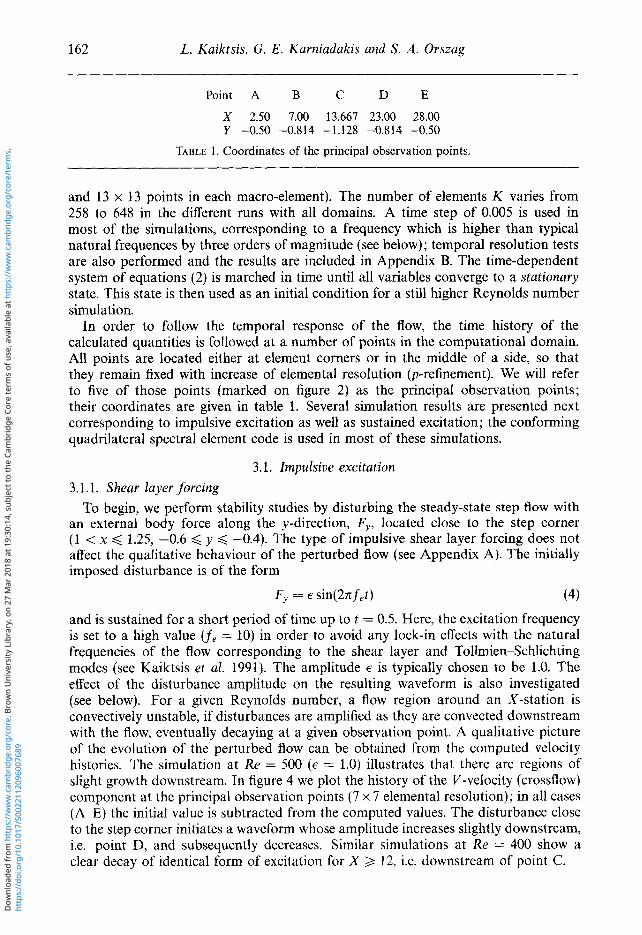
Fy = esin(2nf~) (4) and is sustained for a short period of time up to t = 0.5. Here, the excitation frequency is set to a high value (fe = 10) in order to avoid any lock-in effects with the natural frequencies of the flow corresponding to the shear layer and Tollmien-Schlichting modes (see Kaiktsis et al. 1991). The amplitude e is typically chosen to be 1.0. The effect of the disturbance amplitude on the resulting waveform is also investigated (see below). For a given Reynolds number, a flow region around an X-station is convectively unstable, if disturbances are amplified as they are convected downstream with the flow, eventually decaying at a given observation point. A qualitative picture of the evolution of the perturbed flow can be obtained from the computed velocity histories. The simulation at Re = 500 (e = 1.0) illustrates that there are regions of slight growth downstream. In figure 4 we plot the history of the V-velocity (crossflow) component at the principal observation points (7 x 7 elemental resolution); in all cases (A-E) the initial value is subtracted from the computed values. The disturbance close to the step corner initiates a waveform whose amplitude increases slightly downstream, i.e. point D, and subsequently decreases. Similar simulations at Re = 400 show a clear decay of identical form of excitation for X 3 12, i.e. downstream of point C.

http

s://

doi.o

rg/1

0.10

17/S

0022

1120

9600

7689

Dow

nloa

ded

from

htt

ps://

ww

w.c

ambr

idge

.org

/cor

e. B

row

n U

nive

rsity

Lib

rary

, on

27 M

ar 2

018

at 1

9:30

:14,

sub

ject

to th

e Ca

mbr

idge

Cor

e te

rms

of u

se, a

vaila

ble

at h

ttps

://w

ww

.cam

brid

ge.o

rg/c

ore/

term

s.

Instubillties in two-dimensional j o w over u backward-facing step 0.002 --77--7--7.

163

. I ,

!! O I , -7--77, ,

k- I

0 1 I +- - c

- 0 . 0 0 2 U ' ' 1 ' ' ' ' ' ' ' ' ' ' ' ' ' ' i '7 - 0.002 r-------y I 7 , I ' '

0

I , , , l , # , l L

i E 10 30 50 70 90

0 . 0 0 2 ' L ' ' 1 ' ' ' ' ' ' ' ' -1 -10

Time

FICURF 4. V-velocity (crossflow) time histories for Re = 500 (shear layer forcing).

A large part of the flow domain is convectively unstable at Re 3 700: As can be seen in figure 5 (dashed line, corresponding to E = 1.0, 9 x 9 elemental resolution), a disturbance is formed upstream which propagates with a space-dependent speed and with amplitude that is increasing at downstream locations. This behaviour is also typical for all the higher Reynolds number simulations we have carried out: a waveform initiated upstream is amplified downstream and exits the computational domain leaving steady laminar flow behind.

V-velocity time histories from simulations at Re = 1000, Re = 1500 and Re = 2000 with E = 1.0 (9 x 9 elemental resolution) are plotted in figures 6, 7 and 8. The simulations at Re = 1500 and Re = 2000 are performed for the long computational domain (X,,, = 60, see Appendix C). Notice that as the Reynolds number increases so do the levels of the response: the maximum response increases by about a factor 10 from Re = 400 to 700, another factor of 10 from Re = 700 to 1000, and another factor of 2 to 3 from Re = 1000 to 1500, nearly saturating as Re increases further. For Re 3 1500 the perturbed flow acquires nonlinear characteristics in the downstream channel region (for this level of excitation amplitude), with perturbations persisting for large times.

The two-dimensional results for Re 3 1500 exhibit unphysical features. For ex- ample, in the steady-state field at Re = 2000 plotted in figure 9, both the primary and secondary (upper wall) recirculation zones are significantly larger than those observed experimentally (Armaly et al. 1983). In particular, the length of the primary separation zone is 18.5 step heights in the simulation, in contrast with the experi- mental value of about 13.5 step heights. In this regime, the actual flow is strongly three-dimensional and unsteady (Armaly et al. 1983; Kaiktsis et ul. 1991). In the

http

s://

doi.o

rg/1

0.10

17/S

0022

1120

9600

7689

Dow

nloa

ded

from

htt

ps://

ww

w.c

ambr

idge

.org

/cor

e. B

row

n U

nive

rsity

Lib

rary

, on

27 M

ar 2

018

at 1

9:30

:14,

sub

ject

to th

e Ca

mbr

idge

Cor

e te

rms

of u

se, a

vaila

ble

at h

ttps

://w

ww

.cam

brid

ge.o

rg/c

ore/

term

s.

164 L. Kaiktsis, G. E. Karniadakis and S . A. Orszag

0.002[ ' ' ' 1 ' ' ' I ' ' ' I ' ' -,

-0.002' " ' I " ' I " ' I ' ~ ' I " ' I " 0.005 .)IB

-0.002-' * ' ' ' ' ' ' I ' ' ' I ' 1 w 0.005

s . h

I 5 -0.005 0.020

Time FIGURE 5. Y-velocity time histories normalized by excitation amplitude E for Re = 700

(shear layer forcing): -, E = 0.1; - - - -, E = 1.0; - - -, E = 2.0.

laboratory step flow there are apparently substantial Reynolds stresses that result in decreasing the size of the recirculation zones.

Next we study the spatial distribution of the perturbations. Consider the flow quantities V(x, y , t) defined as

vt, vka,y(x, Y ) = max[v/(x, Y , t ) - ~ ( x , Y,O)I (5a)

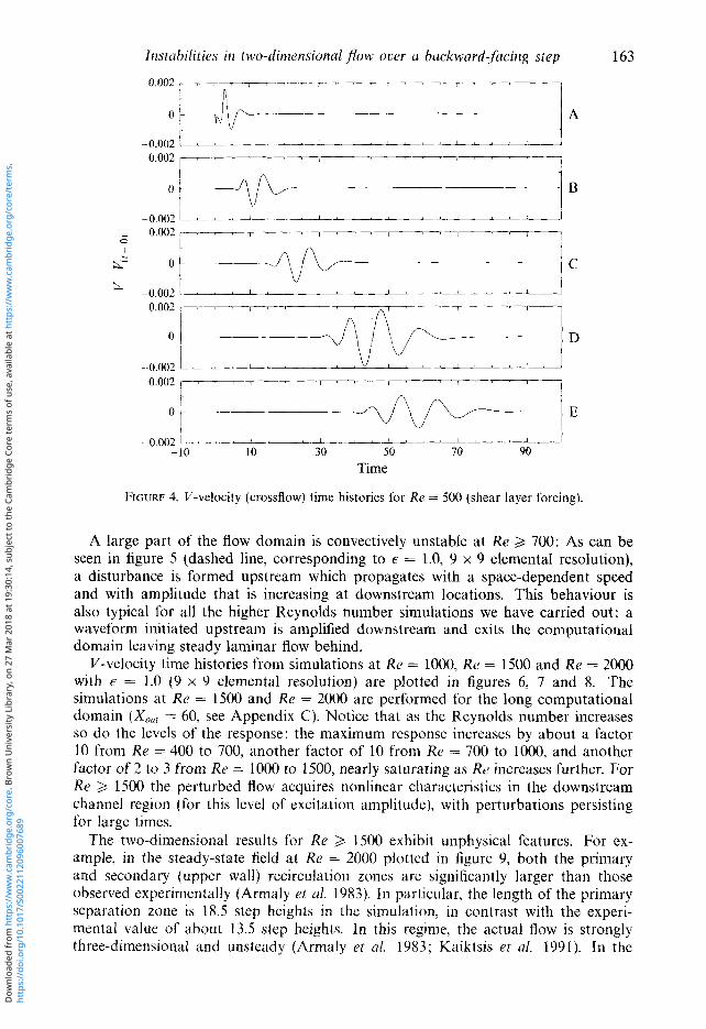
In figure 10 we plot the distribution of Uimp and Vimp for the U - (streamwise) and V - (crossflow) components of velocity at Re = 700 (e = 1.0, 9 x 9 elemental resolution). In both cases the global maxima are located around X NN 25. Thus, at Re = 700 the waveform fluctuations amplify for approximately 25 step heights downstream of the sudden expansion and decay gradually farther downstream. Note the different distribution of Uimp and Vimp in the downstream channel region: for a given channel cross-section the U:mp distribution exhibits two maxima close to the walls and is minimum at the channel centreline, while the distribution of VimP is maximum close to the centreline. Also note the slight amplification of the perturbations close to the outflow boundary; this numerical effect is due to the outflow boundary condition

http

s://

doi.o

rg/1

0.10

17/S

0022

1120

9600

7689

Dow

nloa

ded

from

htt

ps://

ww

w.c

ambr

idge

.org

/cor

e. B

row

n U

nive

rsity

Lib

rary

, on

27 M

ar 2

018

at 1

9:30

:14,

sub

ject

to th

e Ca

mbr

idge

Cor

e te

rms

of u

se, a

vaila

ble

at h

ttps

://w

ww

.cam

brid

ge.o

rg/c

ore/

term

s.

1 -0.200 ~ ' ' ' ' A A - 1 1 I I I I , , . I 1 , , I J

-10 10 30 50 70 90 Time

FIGURE 6. I/-velocity time histories for Re = 1000 (shear layer forcing).

-0 500 L--__ii-Li ' I , 1 I

-10 30 70 110 150 190 230 270 Time

FIGURE 7 V-velocity time histories for Re = 1500 (shear layer forcing).

165

http

s://

doi.o

rg/1

0.10

17/S

0022

1120

9600

7689

Dow

nloa

ded

from

htt

ps://

ww

w.c

ambr

idge

.org

/cor

e. B

row

n U

nive

rsity

Lib

rary

, on

27 M

ar 2

018

at 1

9:30

:14,

sub

ject

to th

e Ca

mbr

idge

Cor

e te

rms

of u

se, a

vaila

ble

at h

ttps

://w

ww

.cam

brid

ge.o

rg/c

ore/

term

s.

166 L. Kaiktsis, G . E. Karniadakis and S. A. Orszag

0.025

0

-0.500 o ~ D

. . -0.500' ' ' ' ' ' ' ' " " " ' I " ' I " ' I " ' I ' ' I

-10 30 70 110 150 190 230 270 Time

FIGURE 8. V-velocity time histories for Re = 2000 (shear layer forcing).

FIGURE 9. Steady-state streamlines at Re = 2000. (The streamwise dimension is compressed for clarity, the outflow is located at x = 60.) Shown in the background is the mesh triangulation used in this simulation.

but does not affect the results for X < 32 in the case of a computational domain extending to X = 35 (see Appendix C).

The study of the distribution of Uh,, and Vim, at different Reynolds numbers shows that the streamwise extent of the amplification region increases with Reynolds number. This is, of course, related to the base flow: as the Reynolds number increases, the size of the primary and upper-wall recirculation zones also increases; thus the region of unstable inflectional profiles is extended farther downstream. In table 2 we report the maximum value of Vimp and the corresponding point coordinates for different values of Reynolds number (shear layer forcing, e = 1.0). (The region X < 2.5 very close to the expansion is obviously not taken into account in the data processing, while the reported data are free of outflow length effects).

An important conclusion from these results is that one must be very careful in performing global temporal stability analyses of this flow in order to avoid misleading

http

s://

doi.o

rg/1

0.10

17/S

0022

1120

9600

7689

Dow

nloa

ded

from

htt

ps://

ww

w.c

ambr

idge

.org

/cor

e. B

row

n U

nive

rsity

Lib

rary

, on

27 M

ar 2

018

at 1

9:30

:14,

sub

ject

to th

e Ca

mbr

idge

Cor

e te

rms

of u

se, a

vaila

ble

at h

ttps

://w

ww

.cam

brid

ge.o

rg/c

ore/

term

s.

Instabilities in two-dimensional flow over a backward-facing step 167

0 Ub, 0.025

0 0.032

FIGURE 10. Colour-coded contours of U&p and Vimp at Re = 700 (shear layer forcing, short domain). (The x scale IS compressed by a factor of 4.)

Re Vc:mp X Y

400 0.00278 11.61 -0.53 500 0.00641 16.50 -0.50 700 0.03235 24.00 -0.52

1000 0.25545 31.16 -0.50

TABLE 2. Maximum values of Vimp and corresponding coordinates for different values of Reynolds number. Standard shear layer forcing, 9 x 9 elemental resolution.

results. Temporal stability analysis requires both upstream and downstream boundary conditions for the perturbations. For example, if at Re = 1000 the computational domain is less than approximately 35 units and the outflow perturbation amplitude is zero, the results are expected to be seriously affected.

The dependence of the waveform propagation speed on spatial location can be investigated by introducing a number of observation points along lines of constant X - or Y-coordinate. In figure 11 we plot the history of the I/-velocity components for a number of observation points located at one of the studied X-stations, namely at X = 28 ( R e = 700, c = 1.0, 9 x 9 elemental resolution). The Y-coordinates of these points are given in table 3. The waveform evidently arrives simultaneously

http

s://

doi.o

rg/1

0.10

17/S

0022

1120

9600

7689

Dow

nloa

ded

from

htt

ps://

ww

w.c

ambr

idge

.org

/cor

e. B

row

n U

nive

rsity

Lib

rary

, on

27 M

ar 2

018

at 1

9:30

:14,

sub

ject

to th

e Ca

mbr

idge

Cor

e te

rms

of u

se, a

vaila

ble

at h

ttps

://w

ww

.cam

brid

ge.o

rg/c

ore/

term

s.

168 L. Kaiktsis, G. E. Karniadakis and S. A . Orszag

0.0201 ' 1 ' I " ' I " ' I " 7 1 " ' I ' I

O I ----4P- l F -0.0201 " ' ' " I " ' I ' " " ' I "

-0.020' " ' " ' " " " ' ' " " I 0.010 s

k= I

L -0.010

O . O l O [ , 7 ' I " ' I " ' I " ' l " ' I ' \

-0.010' " ' ' I " " " I " " ' ' I 0.005

O O j J

-0.005 -10 10 30 50 70 90

Time FIGURE 11. V-velocity time histories for Re = 700; X = 28 (shear layer forcing).

Point F G H I .I

Y -0.333 -0.166 0 0.166 0.333

TABLE 3. Y-coordinates of observation points of figure 11.

at all points of constant X-coordinate and thus the waveform speed is independent of Y . (Study of numerical signals for observation points corresponding to the grid points closest to the upper and lower walls, i.e. Y = 0.3939, 0.446198, 0.4833, and Y = -1.3423, -1.3916, -1.4266, shows independence of propagation speed on Y- coordinate, even very close to the walls.) The dependence on X-location is checked by introducing a total of 80 observation points along the line of Y = -0.5 (along the inlet-channel lower wall). Based on the numerical signals, it is possible to estimate for each point the arrival time of the waveform. If P1 and P2 are two points located close together, with arrival times t l and t 2 respectively, and with X2 > X1, then the propagation speed can be approximated:

A systematic study shows that for each X-location the propagation speed is very close to the local maximum streamwise velocity, which decreases with increasing X-coordinate.

The effect of the disturbance amplitude on the perturbed flows is investigated by performing a number of simulations using 9 x 9 elemental resolution with f

http

s://

doi.o

rg/1

0.10

17/S

0022

1120

9600

7689

Dow

nloa

ded

from

htt

ps://

ww

w.c

ambr

idge

.org

/cor

e. B

row

n U

nive

rsity

Lib

rary

, on

27 M

ar 2

018

at 1

9:30

:14,

sub

ject

to th

e Ca

mbr

idge

Cor

e te

rms

of u

se, a

vaila

ble

at h

ttps

://w

ww

.cam

brid

ge.o

rg/c

ore/

term

s.

Instrrhilities in two-dimensional pow over a backward-facing step 169

0.15 .- c) m f a L- .$ 0.10

k

1 x 5 0.05

0 20 40 60 80 100 Amplitude

FIGURI: 12. Maximum positive perturbation ( VAax) versus excitation amplitude (6 ) at Re = 700 (shear layer forcing): (a) point A (upstream region) ( b ) point D (downstream region).

(see equation (4)) ranging from 0.1 to 100. Note that since the external forcing is imposed in a small region close to the step corner, values of f = 1 and higher will still result in relatively small velocity and pressure perturbations. Indeed, the resulting signals illustrate a nearly linear response to excitation amplitude E, for E < 2. In figure 5 we plot the history of the V-velocity components normalized by E, i.e. (( V ( x , y , t ) - V ( x , y , O))/e), at the principal observation points. Three values of excitation amplitude are included here, namely e = 0.1,1.0,2.0. For all points considered, the three normalized signals are nearly equal, indicating that indeed the response is almost linearly proportional to E . For E 3 2 the effect of the excitation amplitude is different in the upstream and downstream regions. In figure 12 we plot the maximum positive perturbation VA,, (see equation ( 5 ) ) versus the excitation amplitude at points A (in the upstream region) and D (in the downstream region). The amplitude of the waveform increases linearly with e in the upstream region, even at high values of e. In the downstream region a linear dependence is observed only for small values of e ; for very high values o f f the nonlinear response saturates. These results are very consistent with the convectively unstable character of the flow and the strong spatial amplification at Re 3 700.

http

s://

doi.o

rg/1

0.10

17/S

0022

1120

9600

7689

Dow

nloa

ded

from

htt

ps://

ww

w.c

ambr

idge

.org

/cor

e. B

row

n U

nive

rsity

Lib

rary

, on

27 M

ar 2

018

at 1

9:30

:14,

sub

ject

to th

e Ca

mbr

idge

Cor

e te

rms

of u

se, a

vaila

ble

at h

ttps

://w

ww

.cam

brid

ge.o

rg/c

ore/

term

s.

170 L. Kaiktsis, G. E . Karniadakis and S. A. Orszag

I I

k= k I 0

-0001 f ;-' ! C

' " I " 1 " ' 1 " ' 6 1 ' ' 1 ' -

-10 10 30 50 70 90 Time

FIGURE 13. V-velocity time histories for Re = 700 (inflow perturbations).

3.1.2. Inflow perturbations In order to explore the dependence of our results on the type of excitation, we

perform a number of simulations in which we introduce perturbations at the inflow boundary. In particular, we introduce a I/-velocity disturbance at the entire inflow boundary (with the exception of the two wall points) for a short period of time up to t = 0.5. The perturbation is chosen to be of the form

V(0, y , t ) = E U,,, sin(2nfet) (7) with fe = 10 and typically e = 0.01. In figure 13 we plot the history of the V-velocity components at the principal observation points for Re = 700 and E = 0.01 (9 x 9 elemental resolution). Clearly, the disturbances are amplified at the downstream locations. The distributions of UimP and ViYp (Kaiktsis 1995) are very similar to the ones corresponding to the shear layer excitation (see figure 10). The downstream maximum of Vimp is located at X = 26.32, Y = -0.52. The slightly earlier decay in the case of the standard shear layer forcing (see table 2 ) can be attributed to the higher effective forcing, resulting in a small deviation from linearity downstream. These results show that the system responds similarly to both shear layer forcing and inflow perturbations. Indeed, the downstream wavepackets shown in figures 5 and 13 are quite similar.

3.2. Sustained excitation In our earlier paper (Kaiktsis et al. 1991), simulation results obtained at lower resolutions than those of the present paper showed that global unsteadiness is possible for Re 3 700. The results for impulsive excitation reported above suggest that

http

s://

doi.o

rg/1

0.10

17/S

0022

1120

9600

7689

Dow

nloa

ded

from

htt

ps://

ww

w.c

ambr

idge

.org

/cor

e. B

row

n U

nive

rsity

Lib

rary

, on

27 M

ar 2

018

at 1

9:30

:14,

sub

ject

to th

e Ca

mbr

idge

Cor

e te

rms

of u

se, a

vaila

ble

at h

ttps

://w

ww

.cam

brid

ge.o

rg/c

ore/

term

s.

lnstuhilities in two-dimensional $ow over a backward-facing step 171

background noise, as introduced for example by the discretization error at low spatial resolution, acts as a disturbance which changes the character of the computed asymptotic flow states. At Re = 700, Kaiktsis et al. report a limit cycle of frequency f = f 2 = 0.104. In order to investigate the receptivity of the flow to different external frequencies, a number of forced simulations is performed at Re = 700 and Re = 1000 (9 x 9 elemental resolution). A V-velocity component, sustained in time, is introduced at the entire inflow boundary (with the exception of the two wall points), according to the relation V = F Urn,, sin(2nfet), with various values of f C ; two different values of 6

are used, lo-’ and For ft. < 0.5, the response of the flow is periodic in time at f = f e with fluctuations of finite amplitude. (Depending on the value of fe and spatial location, superharmonics of f r are also observed). In all cases, averaging is performed for a number of periods, l/fc, after the initial transients have died out. In figure 14 we plot profiles of the RMS fluctuation intensities along a representative Y -location (Re = 700, F = lo-’). It is clear that different flow regimes are sensitive to different external frequencies. In particular, upstream locations (X < 10) exhibit maximum fluctuations for f e z 0.15, while in the reattachement and early recovery regions (10 d X < 20) the fluctuations are maximal for f c z f l = 0.104; in the channel region farther downstream we get high fluctuations for 0.05 < f e < f z . In general, upstream locations are more sensitive to higher external frequencies, as compared to downstream locations. This result is in agreement with local temporal stability analysis calculations (Kaiktsis 1995), reporting a basic decrease of the frequency of the most unstable mode with increasing streamwise coordinate.

The overall effect of external excitation on the entire flow domain can be expressed in terms of a space-average RMS fluctuation intensity. Considering, for example, the V-velocity component, we define

where a prime denotes fluctuation, an overline denotes time-average, and A is the area of the computational domain. In figure 15 we plot the computed values of (UkMS), (Vk,,) and (PKMS) as a function of the excitation frequency, fe. Clearly, in all cases the distributions have a maximum around f e c f z . Thus, at Re = 700, f z seems to be the dominant frequency of the flow, which is imposed on the entire domain in the case of unsteady flow, driven by marginal spatial resolution (Kaiktsis et al. 1991); detailed tests, based on a systematic variation of spatial and temporal resolution, confirming this finding, are presented in Kaiktsis (1995).

At Re = 700 two simulations are performed at the high excitation frequencies fe = 1.0 and f e = 10, with F = lop2. At f e = 1.0, after the initial propagation of a waveform, the flow exhibits time-periodic behaviour o f f = f E in the upstream region, characterized by very low-amplitude fluctuations ; in the downstream region the flow equilibrates to a steady laminar state. At f e = 10 the flow state is practically a steady laminar state for the entire domain at large times.

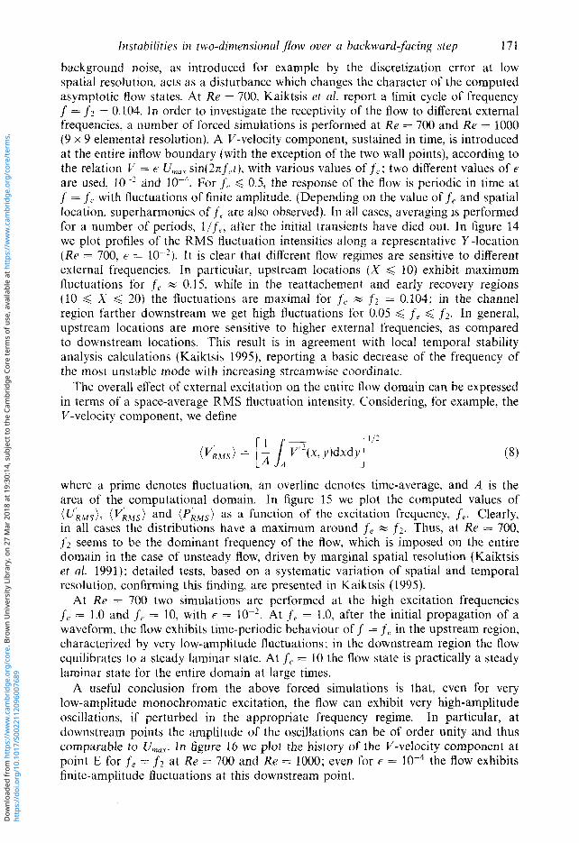
A useful conclusion from the above forced simulations is that, even for very low-amplitude monochromatic excitation, the flow can exhibit very high-amplitude oscillations, if perturbed in the appropriate frequency regime. In particular, at downstream points the amplitude of the oscillations can be of order unity and thus comparable to Urn,,. In figure 16 we plot the history of the V-velocity component at point E for f e = f z at Re = 700 and Re = 1000; even for 6 = the flow exhibits finite-amplitude fluctuations at this downstream point.

http

s://

doi.o

rg/1

0.10

17/S

0022

1120

9600

7689

Dow

nloa

ded

from

htt

ps://

ww

w.c

ambr

idge

.org

/cor

e. B

row

n U

nive

rsity

Lib

rary

, on

27 M

ar 2

018

at 1

9:30

:14,

sub

ject

to th

e Ca

mbr

idge

Cor

e te

rms

of u

se, a

vaila

ble

at h

ttps

://w

ww

.cam

brid

ge.o

rg/c

ore/

term

s.

172 L. Kaiktsis, G. E. Karniadakis and S . A. Orszag

0.10

0.08

$ 0.06

E? 0.04

0.02

0 0.06

0.04

0.02

Q X- coordinate

FIGURE 14. RMS fluctuation intensity profiles along the x-direction at Re = 700, Y = -1.12821 (sustained monochromatic inflow excitation, E = lo-*): -, fe = 0.025; ...... 3 f e - - 0.05. 1 - - - -, fe = 0.104; - - -, f e = 0.15; - - - -, f e = 0.20; - - -, f e = 0.25. (a) Streamwise component; (b) crossflow component.

In under-resolved simulations, finite spatial and temporal discretization errors may act as sustained disturbances. Discrete systems, in general, have a stronger tendency to instability and chaos than the continuous differential systems from which they arise. Based on the analysis of the monochromatic sustained excitation results, we expect that these discretization errors are equivalent to coherent forcing which yields maximum system response near a ‘resonant’ frequency. In order to further explore this phenomenon, we now study the opposite extreme of random excitation. In particular, we introduce a random V-disturbance, sustained in time, at each collocation point at the inflow, of the form V(O,y, t ) = E U,,, (1 - 2X); X is a random number between 0 and 1, generated by the CRAY random number generation routine of uniform distribution, based on a lagged Fibonacci series (Petersen 1988). Note that the details of the computed velocity histories and spectra may depend on the particular choice of the noise, which is white spatially. Alternatively, one may introduce such an excitation at the continuum level by defining an appropriate covariance function and project it onto the discrete spectral element basis. Although we did not attempt this in the present study, we expect that the primary frequency peaks in the spectra

http

s://

doi.o

rg/1

0.10

17/S

0022

1120

9600

7689

Dow

nloa

ded

from

htt

ps://

ww

w.c

ambr

idge

.org

/cor

e. B

row

n U

nive

rsity

Lib

rary

, on

27 M

ar 2

018

at 1

9:30

:14,

sub

ject

to th

e Ca

mbr

idge

Cor

e te

rms

of u

se, a

vaila

ble

at h

ttps

://w

ww

.cam

brid

ge.o

rg/c

ore/

term

s.

Instuhilities in two-dimensional flow over a backward-jacing step 173

0.06

a,

%? !G 0.02 P

0 0.1 0.2 0.3 Excitation frequency

FIGURE 15. Space-average RMS fluctuation intensities, versus excitation frey..zncy, f e , Re = 700: +, (uk,,); VRMS); *, ( L s ) .

are independent of the specific form of the random noise excitation. We perform several tests at Re = 700 and at Re = 1000 at different excitation amplitudes. We find that the flow behaviour at large times is time-dependent even at c = these amplitudes are significantly lower than those of the forced numerical experiments at f E = f z . In figure 17 we plot the numerical signal and power spectrum at point E (9 x 9 elemental resolution). The spectrum is characterized by a broad-band response in the range 0.05 d f’ ,< 0.15. A careful study o f spectra at all reference points shows a shift from higher to lower frequencies, with increasing streamwise coordinate. This result is consistent with the results of monochromatic excitation reported above and those of local stability analysis presented below. In the downstream channel region between points D and E the frequency content seems to be independent of the streamwise coordinate. A main frequency component f = 0.122 as well as a frequency approximately equal to fl are found at all reference points (see the power spectrum of point E).

4. Stability analysis The stability character of the flow can be examined independently by performing a

linear stability analysis at a number of streamwise locations. For Re = 700 we analyse the stability properties of streamwise velocity profiles at X = 2,3,5,10,15,20,25,27.5 and 30, corresponding to locations in the separated and recovery zone; the profiles in the region 3 < X < 20 are shown in figure 18. The convectively unstable character of the flow was investigated using the technique of mapping the complex wavenumber plane to the complex frequency plane, as developed by Triantafyllou (see Triantafyllou et a/ . 19861.

http

s://

doi.o

rg/1

0.10

17/S

0022

1120

9600

7689

Dow

nloa

ded

from

htt

ps://

ww

w.c

ambr

idge

.org

/cor

e. B

row

n U

nive

rsity

Lib

rary

, on

27 M

ar 2

018

at 1

9:30

:14,

sub

ject

to th

e Ca

mbr

idge

Cor

e te

rms

of u

se, a

vaila

ble

at h

ttps

://w

ww

.cam

brid

ge.o

rg/c

ore/

term

s.

174

0.2 ~

3 0.1

.I 0 0

-0.3 3 0.10

0.05

.3 0

g o L

0 0 3.

-0.05

-0.10 0 50 100 150 200

Time

FIGURE 16. V-velocity time histories at downstream point E for sustained inflow excitation at f e = f2: (a) c = lo-*, (b) E = lop4: -, Re = 700; ......, Re = 1000.

All profiles examined at Re = 700 were found to be convectively unstable for X < 27.5, in good agreement with the impulsive excitation results (note that all profiles up to X = 26 are inflectional). Thus a spatial stability analysis is appro- priate for this flow, which is complicated here by the non-parallel nature of the base flow. For slowly varying mean profiles, like those exhibited by zero-pressure- gradient boundary layers, and for small growth rates, Gaster’s transformation (Gaster 1962) (based on the analyticity of the eigenvalue dispersion relation) shows that there is a close relation between temporal and spatial modes. In the case of the step flow, this close relationship breaks down; it is therefore not sufficient to use temporal stability analysis alone to identify the stability properties of the step flow.

The local spatial stability analysis performed here is based on a code developed by Triantafyllou (G. S. Triantafyllou, private communications) in which the solution to the Orr-Sommerfeld equation is obtained using high-order finite differencing in an iterative manner, until a value of zero is obtained for the temporal growth rate. The results of this analysis are shown in table 4 in terms of the wavenumber, the spatial growth rate and the frequency of the most-unstable mode for all profiles considered.

http

s://

doi.o

rg/1

0.10

17/S

0022

1120

9600

7689

Dow

nloa

ded

from

htt

ps://

ww

w.c

ambr

idge

.org

/cor

e. B

row

n U

nive

rsity

Lib

rary

, on

27 M

ar 2

018

at 1

9:30

:14,

sub

ject

to th

e Ca

mbr

idge

Cor

e te

rms

of u

se, a

vaila

ble

at h

ttps

://w

ww

.cam

brid

ge.o

rg/c

ore/

term

s.

Instabilities in two-dimensional JRow over a backwardTfacing step 175

4 0.010

1 0.005 .- s 0 9 e, O F

s. > E

-0.010 F -0.005

t

0 200 400 600 Time

I r - - - - - 7 7 TT---

1 h 10

0 0.05 0.10 0.15 0.20 Frequency

FIGURE 17. ( a ) I/-velocity numerical signal and (h) associated power spectrum at downstream point E for random inflow ‘excitation ( R e = 700, E = 0.01).

It is seen that in the upstream region both the wavenumber and frequency decrease with increasing streamwise coordinate, while they remain approximately constant for X 3 15.

The effect of absolute instabilities can be examined by performing a linear global temporal stability analysis, where disturbances are introduced of the form u’(x, y, t ) = Z(x, y)eof, where is the complex global frequency; for positive growth rates (oR > 0), self-sustained oscillations are present independent of any form of impulsive or sus- tained excitation. The eigenvalue problem is solved using a spectral element code (see Barkley & Henderson 1996). Since the results plotted in figure 14 indicate that at Re = 700 perturbations may not be small even 30 step heights downstream of the sudden expansion, we choose a long domain with a total outflow length of 100 non-dimensional units. A modified Krylov method based on the upper Hessenberg system matrix (for efficiency) is used in this stability code. The real parts of the leading eigenvalues obtained at R e = 200,375,700 and 1000 are all negative and of decreasing magnitude, indicating global stability of the flow, in agreement with the results of our direct numerical simulations, and also in agreement with the results

http

s://

doi.o

rg/1

0.10

17/S

0022

1120

9600

7689

Dow

nloa

ded

from

htt

ps://

ww

w.c

ambr

idge

.org

/cor

e. B

row

n U

nive

rsity

Lib

rary

, on

27 M

ar 2

018

at 1

9:30

:14,

sub

ject

to th

e Ca

mbr

idge

Cor

e te

rms

of u

se, a

vaila

ble

at h

ttps

://w

ww

.cam

brid

ge.o

rg/c

ore/

term

s.

176

A , : .r ' \ _ < * ' . -

L. Kaiktsis, G. E. Karniadakis and S . A . Orszag

0.5

0 -

-0.5

-1.0

-

-

-

-, x = 3;

X-coordinate Wavenumber Growth rate Frequency

2 2.37 3 2.13 5 1.85

10 1.55 15 1.60 20 1.69 25 1.63 27.5 1.60 30 1.56

0.742 0.167 0.523 0.143 0.374 0.107 0.369 0.054 0.240 0.068 0.138 0.072 0.041 0.070 0.009 0.068

-0.030 0.066

TABLE 4. Fastest growing modes in space at Re = 700.

r i

0 5 10

FIGURE 19. Streamlines of base flow and leading eigenfunction at Re = 200.

http

s://

doi.o

rg/1

0.10

17/S

0022

1120

9600

7689

Dow

nloa

ded

from

htt

ps://

ww

w.c

ambr

idge

.org

/cor

e. B

row

n U

nive

rsity

Lib

rary

, on

27 M

ar 2

018

at 1

9:30

:14,

sub

ject

to th

e Ca

mbr

idge

Cor

e te

rms

of u

se, a

vaila

ble

at h

ttps

://w

ww

.cam

brid

ge.o

rg/c

ore/

term

s.

Instabilities in two-dimensional $ow over a backward-facing step 177

t

FIGURE 20. Streamlines of base flow and leading eigenfunction at Re = 375.

FIGURE 21. Instantaneous streamlines a t Re = 3000.

of Gresho et al. (1993). For higher Reynolds number it is difficult to obtain con- verged results, especially in the very long domain that we have used here. While the leading eigenvalue is real, the next eigenvalue appears as a complex-conjugate pair corresponding to a channel mode. For example, at Re = 200 the leading eigenvalue is (-0.07044; 0), the second and third are (-0.0892272; 0.02623104) and (-0.0892272 ; -0.02623 104). This complex-conjugate pair of eigenvalues corresponds to the least-stable channel mode; the second and third eigenfunctions are simply out of phase due to the translational symmetry in the channel part of the computational domain. The structure of the leading eigenmodes corresponding to Re = 200 and Re = 375 is shown in figures 19 and 20, superimposed on the corresponding base flow. It is clear from these plots that the dominant instability is due to the flow in the upstream region.

5. Summary In this paper we investigate the stability of backward-facing step flow, using two-

dimensional direct numerical simulation in conjunction with local and global stability analysis. Our results illustrate that a large part of the flow domain is convectively unstable for Reynolds numbers Re 3 700. This has been verified by following the evolution of upstream-generated disturbances (with both impulsive shear layer forcing and impulsive inflow excitation). Disturbances amplify downstream with different spatial distributions for the U - (streamwise) and I/- (crossflow) velocity components.

http

s://

doi.o

rg/1

0.10

17/S

0022

1120

9600

7689

Dow

nloa

ded

from

htt

ps://

ww

w.c

ambr

idge

.org

/cor

e. B

row

n U

nive

rsity

Lib

rary

, on

27 M

ar 2

018

at 1

9:30

:14,

sub

ject

to th

e Ca

mbr

idge

Cor

e te

rms

of u

se, a

vaila

ble

at h

ttps

://w

ww

.cam

brid

ge.o

rg/c

ore/

term

s.

178 L. Kaiktsis, G. E. Karniadakis and S. A. Orszag

0 U:, 0.071

0 0.098

FIGURE 22. Colour-coded contours of UimS and V:m, at Re = 700 (low spatial resolution, oscillatory flow). (The x scale is compressed by a factor of 4.)

For Reynolds numbers Re < 7827, for which plane Poiseuille flow is nonlinearly stable to two-dimensional disturbances (Herbert 1976; Orszag & Patera 1983), the two-dimensional step flow will relax to a steady laminar state far downstream (note that Re < 7827 as herein defined corresponds to Re < 2935 in Orszag & Patera 1983). Our two-dimensional simulations of step flow up to Re = 2500 demonstrate global stability to temporal perturbations. Thus bifurcation to self-sustained oscillations in two-dimensional flow is expected for 2500 < Re < 7827. It is very difficult using either direct numerical simulation or eigenvalue stability analysis to precisely identify this critical Reynolds number. Even at Re = 2500 we have to exercise particular care in the restarts of the simulation and use high resolution, in order to control round-off and discretization ‘noise’, which is acting as a source of excitation. At such high Reynolds numbers, disturbances due to a restart from a simulation at a lower Reynolds number may convect from the domain after a very long iteration time. With the time step kept sufficiently small to control temporal errors, this requirement translates to several hundred thousands of time steps. Preliminary simulation runs at Re = 3000, even at higher resolution, revealed an unsteady pattern (see figure 21). However, a more systematic study is necessary to assess such a claim; computationally this is currently quite expensive. In the physical laboratory the presence of background

http

s://

doi.o

rg/1

0.10

17/S

0022

1120

9600

7689

Dow

nloa

ded

from

htt

ps://

ww

w.c

ambr

idge

.org

/cor

e. B

row

n U

nive

rsity

Lib

rary

, on

27 M

ar 2

018

at 1

9:30

:14,

sub

ject

to th

e Ca

mbr

idge

Cor

e te

rms

of u

se, a

vaila

ble

at h

ttps

://w

ww

.cam

brid

ge.o

rg/c

ore/

term

s.

Instabilities in two-dimensional flow over a hackwardTjircing step 179

noise will trigger unsteadiness at lower Reynolds numbers via spatial amplification. This seems to explain the earlier transition (at Re < 1200) reported in Armaly et al. (1983).

Sustained external excitation even at small amplitudes leads to time-dependent behaviour at large times. Both monochromatic and random inflow excitations result in an oscillatory flow. For the monochromatic case, high amplitudes (for X ,< 35) are observed if the excitation frequency is close to the shear layer frequency, while very high values of excitation frequency leave the flow unaffected.

Extensive tests (see Appendices) have been performed to ensure the independence of our results of excitation type, of numerical resolution parameters, as well as of the length of the computational domain. In all cases, the asymptotic states of the two- dimensional flow are time independent up to Re = 2500 (in the absence of any external excitation or random noise). Thus, it seems plausible that the unsteadiness reported in previous work (as in Kaiktsis et al. 1991) is due to the fact that the discretization error introduced at coarser spatial resolution acts as as sustained disturbance, which changes the character of the computational results. With this enhanced forcing due to the discretization errors, the computations exhibit global unsteadiness which masks the convective instability of the flow. In such a case the flow is characterized by a continuous feed of disturbances, which propagate downstream. Interestingly enough, the lower-resolution simulations also preserve the basic physics of this flow; the spatial distribution of fluctuations of the globally unsteady flow is found to be similar to the distribution of disturbances of the convectively unstable flow. At Re = 700, Kaiktsis et (11. ( 1991) report oscillations at f = f 2 = 0.104. In figure 22 we present the distribution of the RMS fluctuation intensities of this Re = 700 simulation. Clearly, the spatial distribution of Uk,b,S and VkMS is very similar to the distribution of Ui,,,, and Vdml, (see figure 10).

As already mentioned, step flows appear to be unsteady at lower Reynolds num- bers in the physical laboratory (Armaly et al. 1983; Latornell & Pollard 1986). Clearly, the earlier transition observed experimentally can be partially attributed to the background noise, always present in laboratory experiments and the sensitivity to inlet conditions (Latornell & Pollard 1986). However, it is possible that the dis- crepancy is also related to the fact that the actual flow is three-dimensional, and thus transition (in both experiments and numerical simulations) can result from three- dimensionality effects. In fact, results of ongoing three-dimensional simulations show that at Re = 2000 the three-dimensional flow is unsteady (Kaiktsis 1995).

6. Conclusions Flow over a backward-facing step is a prototype of a complex shear-flow with

both free shear layer and wall-bounded effects. It has features reminiscent of typical wall-bounded flows (like plane Poiseuille flow), especially in the recovery region, and features common to free shear flows (like mixing layers), especially near the step corner. In our previous paper (Kaiktsis et al. 1991), we concen- trated on the description of the onset of three-dimensionality in the step flow due to secondary instability of the primary two-dimensional flow. In the present pa- per, we re-visit this flow to explore in more depth the character of the primary flow. In particular, it is interesting how unsteadiness appears in step flow; unlike wakes in which absolute instability leads to unsteadiness and a limit cycle (Kar- niadakis & Triantafyllou 1992), unsteadiness in step flow is created via convective

http

s://

doi.o

rg/1

0.10

17/S

0022

1120

9600

7689

Dow

nloa

ded

from

htt

ps://

ww

w.c

ambr

idge

.org

/cor

e. B

row

n U

nive

rsity

Lib

rary

, on

27 M

ar 2

018

at 1

9:30

:14,

sub

ject

to th

e Ca

mbr

idge

Cor

e te

rms

of u

se, a

vaila

ble

at h

ttps

://w

ww

.cam

brid

ge.o

rg/c

ore/

term

s.

180 L. Kaiktsis, G. E. Karniadakis and S. A. Orszag

instabilities through the sustained effects of noise. In that respect, this instabil- ity mechanism is similar to the one discovered in the work of Schatz, Barkley & Swinney (1995). This suggests that one must be careful in interpreting the re- sults of numerical simulations and stability analyses : some numerical simulations (like those based on vortex methods and lattice techniques, Sethian & Ghoniem 1988; Qian et al. 1993) have inherent random background noise that can generate unsteady-flow results; on the other hand, temporal stability analyses may miss com- pletely the convective instabilities responsible for time dependence in the presence of noise.

L.K. would like to acknowledge the financial support of the Swiss Federal Office of Energy (BEW), Grant EF-FOS(88)6. G.E.K. would like to acknowledge support by NSF Grants CTS-89-1422 and ECS-90-23362. S.A.O. would like to acknowledge support by ARPA/ONR under Contracts NOOO14-92-5-1796 and N00014-93-C-0216. The computations were performed on the Cray Y-MP/464 and on the Cray J90 of the Swiss Federal Institute of Technology in Zurich, on the NEC SX-3 of the CSCS at Manno, and on the Cray C90 of the Pittsburgh Supercomputing Center. We would like to thank Dr. A. Tomboulides for many useful ideas and discussions and for his assistance in some of the computations, Professor G. S. Triantafyllou and Dr D. Barkley for their assistance in the stability analysis computations, and Professor P. A. Monkewitz for his helpful comments and insight. We also acknowledge discussions with Professors G. L. Brown, S. H. Lam and I. G. Kevrekidis, and the comments by the JFM referees.

Appendix A. Effect of shear layer forcing type In this Appendix we investigate the effect of different types of impulsive shear layer

excitation on the perturbed flow. All tests are performed at Re = 700. First we check the effect of the direction of the forcing, by introducing the external body force along the x-direction, while maintaining its sinusoidal form, duration (0.5 time units) and regime applied (1 < x d 1.25, -0.6 < y d -0.4):

F, = E sin(2nf,t) (A 1)

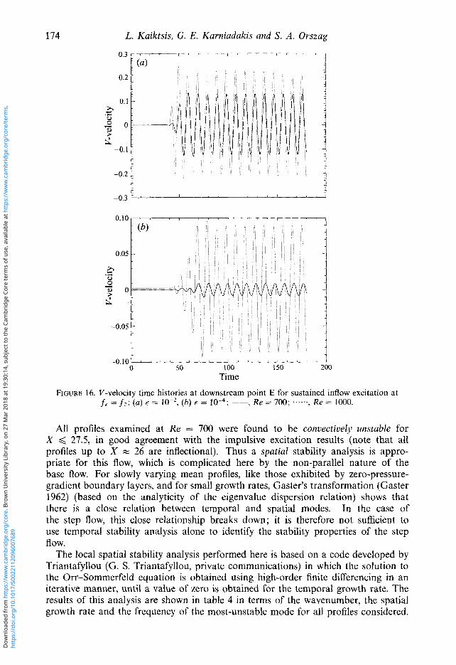
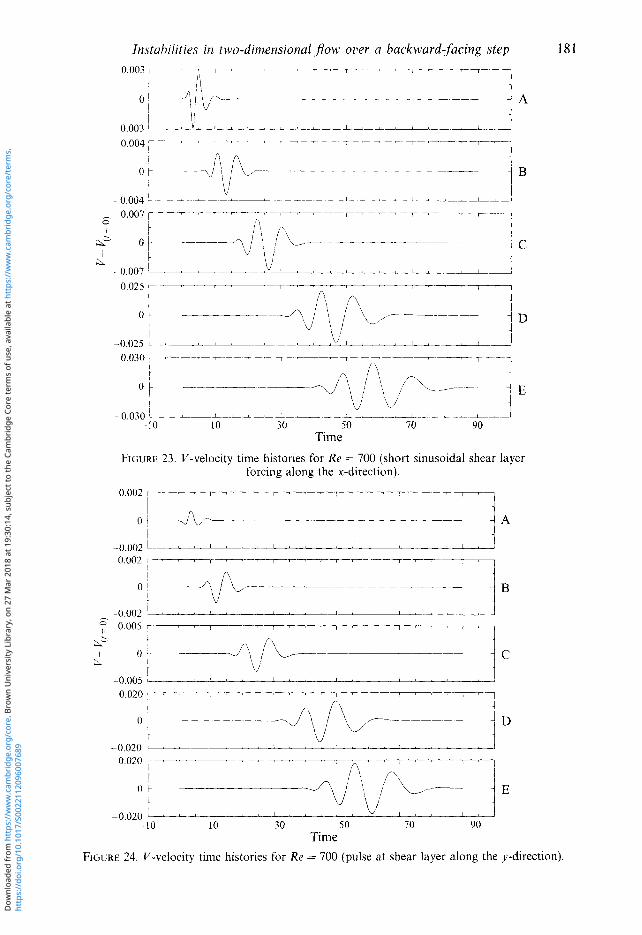
where f e = 10 and E = 1.0. The computed V-velocity time histories are presented in figure 23. Although forcing along the x-direction results in somewhat higher levels of perturbations, the system response is the same in terms of the propagation velocity of the induced waveform and in terms of the spatial distribution of disturbances, irrespective of the direction of the forcing introduced (compare figure 23 with dashed lines in figure 5) . In an additional check we introduce a pulse along the y-direction in the same region close to the step corner:

E if t < t , 0 otherwise.

For the same values of E and to, the pulse results in much higher levels of pertur- bations, as compared to the standard short sinusoidal forcing. Comparable response amplitudes are obtained if the pulse is characterized by smaller values of e and to. Figure 24 corresponds to a pulse with E = 0.1 and to = 0.05, i.e. both c and t, are equal to 10% of the values corresponding to the standard sinusoidal forcing. Clearly, the computed velocity histories are very similar to those of figure 5. In both cases

http

s://

doi.o

rg/1

0.10

17/S

0022

1120

9600

7689

Dow

nloa

ded

from

htt

ps://

ww

w.c

ambr

idge

.org

/cor

e. B

row

n U

nive

rsity

Lib

rary

, on

27 M

ar 2

018

at 1

9:30

:14,

sub

ject

to th

e Ca

mbr

idge

Cor

e te

rms

of u

se, a

vaila

ble

at h

ttps

://w

ww

.cam

brid

ge.o

rg/c

ore/

term

s.

-0.002 " ' 1 ' . ' 1 " ' I '

0 0 0 5 - ' ' -7-, , I , , , , , , , , , . , , ,

181

0 005 1

0020' ' ' ' 1 ' ' ' I ' ' ' ' ' ' ' I ' ' '

I , , , , , I , . , I

-0020 " " " ' I " ' I " ' I " ' 1 ' J

0.020. ' " I " ' I " ' 1 ' " I " ' I ' 1 n

10 10 30 50 70 90 0 0 2 0 ' ' ' ' ' ' ' ' ' ' ' I

Time FIGURP 24 I/-velocity time histories for Re = 700 (pulse at shear layer along the y-direction).

http

s://

doi.o

rg/1

0.10

17/S

0022

1120

9600

7689

Dow

nloa

ded

from

htt

ps://

ww

w.c

ambr

idge

.org

/cor

e. B

row

n U

nive

rsity

Lib

rary

, on

27 M

ar 2

018

at 1

9:30

:14,

sub

ject

to th

e Ca

mbr

idge

Cor

e te

rms

of u

se, a

vaila

ble

at h

ttps

://w

ww

.cam

brid

ge.o

rg/c

ore/

term

s.

182 L. Kaiktsis, G. E. Karniadakis and S. A. Orszag 0.010 T I T - - 9 7 - - ‘ 7 ? r n - - - p - m - ~ - -

(a) Y = O t 0.008

0.006

0.004 , 1

E 0.0020 U .3 * a -e z L

0.0015

d O.Oo10 z 0.0005

0

i ’ ,

1

t- i”

X-coordinate

FIGURE 25. Maximum positive perturbation (VmaX) profiles along the x-direction at Re = 700 for h-type refinement (inflow perturbations, 9 x 9 elemental resolution): -, 258 elements; - - - -, 512 elements, high node density in x-direction; - - -, 512 elements, high node density in y-direction.

studied in this Appendix the spatial distribution of Uimp and Vimp is very similar to the distribution produced by the standard shear layer forcing (figure 10). We conclude that the qualitative behaviour of the perturbed flow does not depend on the type of impulsive shear layer forcing.

http

s://

doi.o

rg/1

0.10

17/S

0022

1120

9600

7689

Dow

nloa

ded

from

htt

ps://

ww

w.c

ambr

idge

.org

/cor

e. B

row

n U

nive

rsity

Lib

rary

, on

27 M

ar 2

018

at 1

9:30

:14,

sub

ject

to th

e Ca

mbr

idge

Cor

e te

rms

of u

se, a

vaila

ble

at h

ttps

://w

ww

.cam

brid

ge.o

rg/c

ore/

term

s.

Instabilities in two-dimensional f low over a backward-facing step 183

0.010 -7-7- 7 -7 - 7 - 7 - 7 7-m [ (a) Y=O t

0.008 1 2

0.0°6 : a ' 0.004 i-4 s

0.002

6 J

E ; (b) Y=-O.5

.3 c

3 0004 [- a,

0003 L x' t 2 0.002 t

' -1 1

L g 0.0020 1- .- 4-3

m L e

s. 5 0.0015 1 a, a

L d o'oo'o

i

i

0 10 20 30 40 X- coordinate

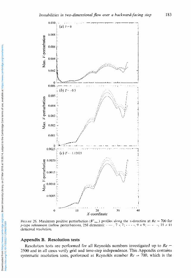
FIGUR~ 26. Maximum positive perturbation ( V"mai) profiles along the x-direction at Re = 700 for p-type refinement (inflow perturbations, 258 elements): - ~, 7 x 7; - - - -, 9 x 9; -- - -, 11 x 11 elemental resolution.

Appendix B. Resolution tests Resolution tests are performed for all Reynolds numbers investigated up to Re =

2500 and in all cases verify grid and time-step independence. This Appendix contains systematic resolution tests, performed at Reynolds number Re = 700, which is the

http

s://

doi.o

rg/1

0.10

17/S

0022

1120

9600

7689

Dow

nloa

ded

from

htt

ps://

ww

w.c

ambr

idge

.org

/cor

e. B

row

n U

nive

rsity

Lib

rary

, on

27 M

ar 2

018

at 1

9:30

:14,

sub

ject

to th

e Ca

mbr

idge

Cor

e te

rms

of u

se, a

vaila

ble

at h

ttps

://w

ww

.cam

brid

ge.o

rg/c

ore/

term

s.

184 L. Kaiktsis, G. E. Karniadakis and S . A . Orszag

one primarily investigated in this work. All computations are performed for the domain with total outflow length of 35 non-dimensional units, which is sufficient for Re < 1000 (see Appendix C). Based on those tests, we select the optimal temporal and spatial resolution parameters, which are also used for the lower Reynolds number simulations. A more detailed discussion of resolution tests is presented in Kaiktsis (1995).

To examine time resolution, we perform computations with an initial external forcing close to the step corner (e = l), as described in $3 . We select high (258 x 9 x 9, see below) resolution to minimize spatial errors. Three values of At are used, namely At = 0.003,0.005,0.01. For all reference points, all three values of At result in practically indistinguishable time responses (Kaiktsis 1995). Taking the simulation at At = 0.003 as the reference simulation, we find that the maximum absolute error in U’,,, and Vmax is of the order of 3 x lop4 in the case of At = 0.01, and of the order of in the case of At = 0.005. The maximum relative errors are 4% and 1% respectively. Note that the relative error should decrease with the response amplitude, and thus with the excitation amplitude. We conclude that the value of At = 0,005 is appropriate for the range of excitation amplitudes used in our computations.

To examine spatial resolution, we perform h- and p-type refinement tests. In par- ticular, for h-refinement, we perform computations on two additional computational meshes, obtained by splitting in half all elements either in the x- or in the y-direction. In each case this results in a total of 512 spectral elements, with 9 x 9 points in each element. For p-refinement, we keep the number of spectral elements constant (258 elements), using different polynomial degrees (7 x 7, 9 x 9, and 11 x 11 points in each macro-elemen t).

The sufficiency of spatial resolution is checked in two steps. In the first step, we compare the steady-state fields obtained using different spatial resolution. Careful examination of the results shows very small differences between the 258 x 7 x 7 and 258 x 9 x 9 simulations and practically no differences between the latter and all others (Kaiktsis 1995).

In the second step, we consider the waveform propagation. Here we initiate the waveform by introducing a V-velocity component at the entire inflow boundary (with the exception of the two wall points) for a short period of time up to t = 0.5, given by V = c Um,,sin(2nfet), with c = 0.01 and fe = 10. The value of the time step is At = 0.005. A careful study of numerical signals shows that the discrepancies between the 258 x 9 x 9 simulation and all others of higher resolution are small. This is also illustrated in figures 25 and 26, where we present profiles of the maximum positive V-velocity perturbation (VA,,) at representative y-locations, corresponding to h- and p-type refinement. Note that the maximum absolute error is of the order of

(higher than the corresponding temporal discretization error), while in all cases the form of the curves is the same and the maxima are located at exactly the same locations. Clearly, there is a small effect of the outflow boundary condition, which is more pronounced for the lowest-resolution (258 x 7 x 7) case.

Finally, all high Reynolds number cases (Re 3 1500) were simulated using all three spectral element codes (see 92); in all cases substantially identical results were obtained.

Appendix C. Outflow length effect The effect of the outflow length is investigated by performing computations on

a domain with an outflow length of 60 non-dimensional units. Results are then

http

s://

doi.o

rg/1

0.10

17/S

0022

1120

9600

7689

Dow

nloa

ded

from

htt

ps://

ww

w.c

ambr

idge

.org

/cor

e. B

row

n U

nive

rsity

Lib

rary

, on

27 M

ar 2

018

at 1

9:30

:14,

sub

ject

to th

e Ca

mbr

idge

Cor

e te

rms

of u

se, a

vaila

ble

at h

ttps

://w

ww

.cam

brid

ge.o

rg/c

ore/

term

s.

Instabilities in two-dimensional flow over a backward facing step 185

-A - - - -I---- - - - T --- 0 4 -

i . - 0 3 r ) 4-

r I t

0.4 1 i t I \

i t I

-02 L ~ - _- -I- - - .I X-coordinate

FIGURE 27. Streamwise velocity profiles along the x-direction ( Y = -1.12821) at (a) Re = 700, ( b ) Re = 1000, using 9 x 9 elemental resolution: ---, X,,, = 35; - - - -, X,,, = 60.

0 20 40 60

compared to those obtained with the standard domain of 35 units. In the X,,, = 60 case, the computational grid is exactly the same as that of the shorter domain up to X = 35. The rest of the domain is discretized maintaining the node density at X = 35 up to X = 60. This results in a total of 408 spectral elements. (An even longer domain with X,,, = 100 with a total number of 648 quadrilateral elements has been also used in the context of this work.)

The results demonstrate that a total outflow length of 35 units is sufficient for Re < 1000. In figure 27(a) we plot the streamwise velocity profiles at a representative y - location of the steady-state fields corresponding to the two outflow lengths (Re = 700, 9 x 9 elemental resolution). Clearly, for X < 35 the two fields practically coincide. In figure 28(a) we present the corresponding profiles of the maximum positive V-velocity perturbation (Vk,,) ; here we compare two simulations corresponding to the standard shear layer excitation, with E = 1 (9 x 9 elemental resolution). While the effect of the outflow boundary condition is clear for the short domain, the profiles are identical for X < 32.

The corresponding profiles of steady-state velocities and maximum positive perturbations for the same y-location are presented in figures 27(b) and 28(b). While the steady-

A similar test is performed at Re = 1000 (9 x 9 elemental resolution).

http

s://

doi.o

rg/1

0.10

17/S

0022

1120

9600

7689

Dow

nloa

ded

from

htt

ps://

ww

w.c

ambr

idge

.org

/cor

e. B

row

n U

nive

rsity

Lib

rary

, on

27 M

ar 2

018

at 1

9:30

:14,

sub

ject

to th

e Ca

mbr

idge

Cor

e te

rms

of u

se, a

vaila

ble

at h

ttps

://w

ww

.cam

brid

ge.o

rg/c

ore/

term

s.

186 L. Kaiktsis, G. E . Karniadakis and S. A. Orszag

X- coordinate

FIGURE 28. Maximum positive perturbation ( VmaX) profiles along the x-direction ( Y = -1.12821) at ( a ) Re = 700 ( b ) Re = 1000 (shear layer forcing): -, X,,, = 35; - - - -, X,,, = 60.

state fields are the same even very close to the outflow boundary, errors due to the outflow boundary condition are present in the perturbation profile corresponding to the short-domain simulation. Those errors are larger, than the ones at Re = 700; however the perturbation profiles still coincide for X < 32. The accuracy of the short-domain results close to the outflow boundary is quite remarkable, given that the perturbation distribution is maximum at X = 30.

REFERENCES

ARMALY, B. F., DURST, F., PEREIRA, J. C. F. & SCHONUNG, B. 1983 Experimental and theoretical investigation of backward-facing step Bow. J . Fluid Mech. 127, 473.

BARKLEY, D. & HENDERSON, R. D. 1996 Three-dimensional Floquet stability analysis of the wake of a circular cylinder. J . Fluid Mech. 322, 215.

BERS, A. 1975 Linear waves and instabilities. In Physique des Plasmas (ed. C. DeWitt, J. Peyraud), p. 11 7. Gordon and Breach.

CHOMAZ, J. M., HUERRE, P. & REDEKOPP, L. G. 1990 The effect of nonlinearity and forcing on global modes. In New Trends in Nonlinear Dynamics and Pattern-Forming Phenomena (ed. P. Coullet & P. Huerre), p. 259. Plenum.

http

s://

doi.o

rg/1

0.10

17/S

0022

1120

9600

7689

Dow

nloa

ded

from

htt

ps://

ww

w.c

ambr

idge

.org

/cor

e. B

row

n U

nive

rsity

Lib

rary

, on

27 M

ar 2

018

at 1

9:30

:14,

sub

ject

to th

e Ca

mbr

idge

Cor

e te

rms

of u

se, a

vaila

ble

at h

ttps

://w

ww

.cam

brid

ge.o

rg/c

ore/

term

s.

Instabilities in two-dimensional flow ouer a backward-fncing step 187

DEISSLER, R. J. 1987 Spatially growing waves, intermittency, and convective chaos in an open-flow

DUBINER, M. 1991 Spectral methods on triangles. J . Sci. Comput. 6, 345. FUNARO, D., QUARTERONI, A. & ZANOLLI, P. 1988 An iterative relaxation for domain decomposition

methods. SIAM J . Numer Anal. 25, 1213. GASTER, M. 1962 A note on the relation between temporally-increasing and spatially-increasing

disturbances in hydrodynamic stability. J . Fluid Mech. 14, 222. GRESHO, P. M., GARTLING, D. K., TORCZYNSKI, J. R., CLIFFE, K. A,, WINTERS, K. H., GARRAP, T. J.,

SPENCE, A. & GOODRICH, J. W. 1993 Is the steady viscous incompressible two-dimensional flow over a backward-facing step at Re = 800 stable? Intl J . Numer. Meth. Fluids 17, 501.

GRESHO, P. M. & SANI, R. L. 1990 Introducing four benchmark solutions. Intl J . Numer Meth. Fluids 11, 951.

HENDERSON, R. D. & KARNIADAKIS, G. E. 1993 Unstructured spectral element methods for the incompressible Navier-Stokes equations. Proc. Finite Elements in Fluids: New Trends and Ap- plications (ed. K. Morgan, E. Onate, J. Periaux & 0. C. Zienkiewicz). Pineridge.

HERBERT, T. 1976 Periodic secondary motions in a plane channel. Proc. Intl ConJ Numer. Meth. Fluid Dyn. (ed. A. I. van de Vooren & P. J. Zandbergen) p. 235. Springer.

HUERRE, P. & MONKEWITZ, P. A. 1985 Absolute and convective instabilities in free shear layers. J . Fluid Mech. 159, 151.

HUERRE, P. & MONKEWITZ, P. A. 1990 Local and global instabilities in spatially developing flows. Ann. Rev. Fluid Mech. 22, 413.

KAIKTSIS, L. 1995 Instability classification and transition in flow over a backward-facing step. PhD thesis, Institut fur Energietechnik, ETH-Zurich.

KAIKTSIS, L., KARNIADAKIS, G. E. & ORSZAG, S. A. 1991 Onset of three-dimensionality, equilibria, and early transition in flow over a backward-facing step. J . Fluid Mech. 231, 501.

KARNIADAKIS, G. E., ISRAELI, M. & ORSZAG, S. A. 1991 High-order splitting methods for the incompressible Navier-Stokes equations. J. Comput. Phys. 97, 414.

KARNIADAKIS, G. E., ORSZAG, S. A,, RONQUST, E. M. & PATERA, A. T. 1993 Spectral element and lattice gas methods for incompressible fluid dynamics. In Incompressible Fluid Dynamics (ed. M. D. Gunzburger & R. A. Nicolaides), chap. 8. Cambridge University Press.

KARNIADAKIS, G. E. & TRIANTAFYLLOU, G. S. 1992 Three-dimensional dynamics and transition to turbulence in the wake of bluff bodies. J. Fluid Mech. 238, 1.

LATORNELL, D. J. & POLLARD, A. 1986 Some observations of shear layer instabilities in laminar flow through axisymmetric sudden expansions. Phys. Fluids 29, 2828.

MAVRIPLIS, C. 1989 Non-conforming discretizations and a posteriori error estimators for adaptive spectral element techniques. PhD thesis, Massachusetts Institute of Technology.

ORSZAG, S. A., ISRAELI, M. & DEVILLE, M. 0. 1986 Boundary conditions for incompressible flows. J . Sci. Comput. 1, 15.

ORSZAG, S. A. & PATERA, A. T. 1983 Secondary instability of wall-bounded shear flows. J. Fluid Mech. 128, 341.

OSSWALD, G. A.. GHIA, K. N. & GHIA, U. 1983 Study of incompressible separated flow using an implicit time-dependent technique. In AIAA Sixth CFD Con$, Danvers, MA, p. 686.

PATERA, A. T. 1984 A spectral element method for fluid dynamics: Laminar flow in a channel expansion. J. Comput. Phys. 54, 468.

PETERSEN, W. P. 1988 Some vectorized random number generators for uniform, normal, and Poisson distributions for CRAY X-MP. J . Supercomput. 1, 321.

QIAN, Y. H., SUCCI, S., MASSAIOLI, F. & ORSZAG, S. A. 1993 A benchmark.for Lattice BGK model: flow over a backward-facing step. In Proc. Pattern Formation and Lattice-Gas Automata June 7-12, 1993. Waterloo, Canada. (ed. A. Lawniczak & R. Kapral).

SCHATZ, M. F., BARKLEY, D. & SWINNFY, H. L. 1995 Instability in a spatially periodic open flow. Phys. Fluids 7, 344.

SETHIAX, J. A. & GHONIEM, A. F. 1988 Validation of vortex methods. J . Comput. Phys. 74, 283. SHERWIN, S. J. & KARNIADAKIS, G. E. 1995 A triangular spectral element method; Applications to

the incompressible Navier-Stokes equations. Comput. Meth. Appl . Mech. Engng 123, 189. TRIANTAFYLLOU. G. S., TRIANTAFYLLOU, M. S. & CHRYSSOSTOMIDIS, C. 1986 On the formation of

vortex streets behind stationary cylinders. J . Fluid Mech. 170, 461.

system. Physica D 25, 233.

http

s://

doi.o

rg/1

0.10

17/S

0022

1120

9600

7689

Dow

nloa

ded

from

htt

ps://

ww

w.c

ambr

idge

.org

/cor

e. B

row

n U

nive

rsity

Lib

rary

, on

27 M

ar 2

018

at 1

9:30

:14,

sub

ject

to th

e Ca

mbr

idge

Cor

e te

rms

of u

se, a

vaila

ble

at h

ttps

://w

ww

.cam

brid

ge.o

rg/c

ore/

term

s.