UNR Joint Economics Working Paper Series Working Paper No. 10-004

The Effect of Government Purchases on Economic Growth in Japan

Federico Guerrero and Elliott Parker

Department of Economics / MS 0030 University of Nevada, Reno

Reno, NV 89557 (775) 784-6850│ Fax (775) 784-4728

email:guerrero@unr.edu; eparker@unr.edu

June, 2010

Abstract

We consider whether there is statistical evidence for a causal relationship between government expenditures and real GDP growth in postwar Japan. After studying the time-series properties of these variables, we find that government consumption and government investment both have a positive and causal effect on growth. This suggests that fiscal policy may not have been as ineffective during the last two decades of Japan’s stagnant growth as some have suggested, but may have helped to prevent an even more severe balance-sheet recession after the collapse of the Japanese bubble economy. JEL Classification: G32, G15, D92, E65, F39 Keywords: Long-term economic growth; Japan; Government size; Cointegration; Granger causality; Vector autoregression; Vector error correction model

The Effect of Government Purchases

on Economic Growth in Japan

Federico Guerrero and

Elliott Parker *

Associate Professor and Professor, respectively Department of Economics

University of Nevada, Reno

Revised June 14, 2010

Abstract: We consider whether there is statistical evidence for a causal relationship between government expenditures and real GDP growth in postwar Japan. After studying the time-series properties of these variables, we find that government consumption and government investment both have a positive and causal effect on growth. This suggests that fiscal policy may not have been as ineffective during the last two decades of Japan’s stagnant growth as some have suggested, but may have helped to prevent an even more severe balance-sheet recession after the collapse of the Japanese bubble economy.

JEL Classification: G32, G15, D92, E65, F39.

Keywords: long-term economic growth, Japan, government size, cointegration, Granger causality, vector autoregression, vector error correction model.

Contact Information:

Department of Economics /0030 University of Nevada, Reno Reno, NV 89557-0207 USA guerrero@unr.edu, eparker@unr.edu

* Corresponding Author

1

The Effect of Government Purchases on Economic Growth in Japan

Abstract: We consider whether there is statistical evidence for a causal relationship between government expenditures and real GDP growth in postwar Japan. After studying the time-series properties of these variables, we find that government consumption and government investment both have a positive and causal effect on growth. This suggests that fiscal policy may not have been as ineffective during the last two decades of Japan’s stagnant growth as some have suggested, but may have helped to prevent an even more severe balance-sheet recession after the collapse of the Japanese bubble economy.

1. Introduction

Other than China’s emergence as a major engine of economic growth, one of the most

stunning turnarounds in modern economic history is the lost generation of Japanese growth.

Japan was not only the largest economy in Asia, it was also a model for other regional

economies. In trying to restore growth after the asset bubble collapse of 1989, Japan’s Liberal

Democratic Party (LDP) used fiscal policy, especially through construction projects, to keep its

hold on the popular vote. However, such government spending does not appear to have led to a

fast-growing economy, at least not to the casual observer, even though central government debt

has now risen to 170 percent of GDP.

A common methodological pitfall in the literature that tries to uncover the causal links

between government spending and long-term economic growth is that they regularly conduct

Granger causality tests outside the cointegration framework.1 As is now well-known, this

problem may render many of their conclusions invalid (Granger, 1988). Furthermore, the papers

1 Ghali (1998) and Islam (2001) are among the exceptions.

2

that do place their Granger causality analyses within the cointegration framework do not tend to

implement a Vector Error Correction (VEC) model, which is the natural follow up in the case in

which the variables are cointegrated, given that the definitive test of causality lies with the error

correction term (Engle and Granger, 1987; Granger, 1988).2

In this paper, we examine the statistical evidence for the relationship between

government spending and GDP growth in Japan, using quarterly data from 1955 to 2009. Our

findings are in line with an evolving new consensus in the economics profession (see

Christiano, Eichenbaum, & Rebelo, 2009) that the fiscal multiplier for government purchases is

larger when interest rates are near the zero bound, and follow on similar work applied to the

United States (Guerrero & Parker, 2007). Our empirical exercises show a positive but modest

effect of government spending on real GDP in Japan. Thus, expansionary fiscal policy may

have played the role of avoiding a deeper economic depression than the one observed during

Japan’s lost decades.

2. Fiscal Policy and Economic Growth in Japan

From the early days of the Meiji restoration, Japan had a strong interventionist

government, but the relationship between government and big business was much more

collaborative than adversarial. Japanese postwar government policy helped transform the huge

Zaibatsus into bank-centered Keiretsu firms, with an “iron triangle” of firm leaders, LDP

politicians, and government technocrats setting most government trade, banking and finance

2 The only exception we could find is Ghali (1998), who implements VEC models in a setup with multiple cross-sections (ten advanced countries), but short time spans (quarterly data for the period 1970-94). Islam (2001) implements Johansen-Juselius’ weak exogeneity tests, but reports no VEC model.

3

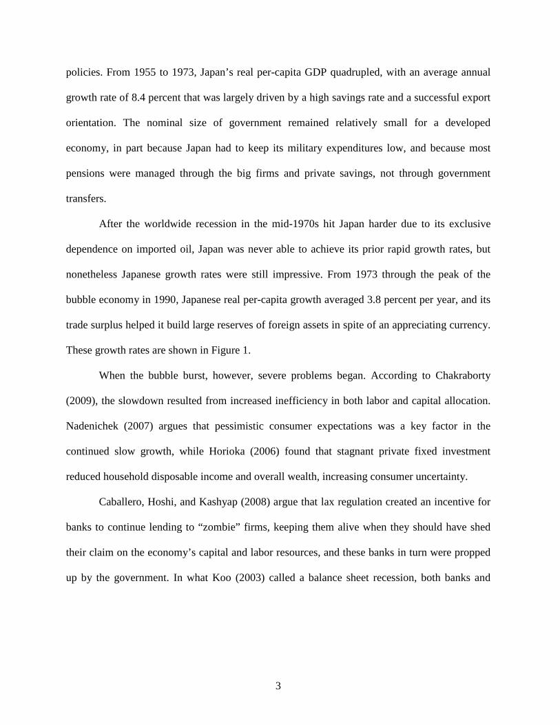
policies. From 1955 to 1973, Japan’s real per-capita GDP quadrupled, with an average annual

growth rate of 8.4 percent that was largely driven by a high savings rate and a successful export

orientation. The nominal size of government remained relatively small for a developed

economy, in part because Japan had to keep its military expenditures low, and because most

pensions were managed through the big firms and private savings, not through government

transfers.

After the worldwide recession in the mid-1970s hit Japan harder due to its exclusive

dependence on imported oil, Japan was never able to achieve its prior rapid growth rates, but

nonetheless Japanese growth rates were still impressive. From 1973 through the peak of the

bubble economy in 1990, Japanese real per-capita growth averaged 3.8 percent per year, and its

trade surplus helped it build large reserves of foreign assets in spite of an appreciating currency.

These growth rates are shown in Figure 1.

When the bubble burst, however, severe problems began. According to Chakraborty

(2009), the slowdown resulted from increased inefficiency in both labor and capital allocation.

Nadenichek (2007) argues that pessimistic consumer expectations was a key factor in the

continued slow growth, while Horioka (2006) found that stagnant private fixed investment

reduced household disposable income and overall wealth, increasing consumer uncertainty.

Caballero, Hoshi, and Kashyap (2008) argue that lax regulation created an incentive for

banks to continue lending to “zombie” firms, keeping them alive when they should have shed

their claim on the economy’s capital and labor resources, and these banks in turn were propped

up by the government. In what Koo (2003) called a balance sheet recession, both banks and

4

firms in the real sector became averse to debt, while savings were redirected toward liquid

assets with less risk.

For several years following the burst of the bubble, the newly-independent Bank of

Japan refused to relent on a tight money policy which had helped to pop the bubble, in part

because it hoped to force the Finance Ministry to reform the financial system; once it did relent,

it did so half-heartedly, with a zero-interest rate policy that did not account for the effect of

deflation on the real interest rate. Cargill and Parker (2004) demonstrated how deflation reduced

Japanese consumption while increasing money demand faster than the Bank of Japan was

willing to increase the supply.

If monetary policy was ineffectively used, then what about fiscal policy? When the

bubble burst, Japanese government purchases totaled about 20 percent of GDP, significantly

less than most other OECD countries. As Figure 1 shows, this ratio rose to 24 percent by 1999,

and then fell back to 22 percent before the recession of 2007-2009. In the first five years, the

growth was primarily in public investment. By 2007 this investment share had declined to

postwar lows, while public consumption rose from 13 percent of GDP in 1990 to 18 percent in

2007.

Cargill and Sakamoto (2008) argue that the LDP had traditionally used Keynesian fiscal

policy to respond to prior recessions, and that this approach was again used after 1990,

particularly with the Fiscal Investment and Loan Program (FILP), as an alternative to real

reforms that might have addressed underlying problems in firm behavior. As the stagnation of

the Japanese economy continued, the government became less and less fiscally conservative, at

5

least until the East Asian financial crisis of 1997, when there was an effort to increase taxes and

tighten spending.

Was fiscal policy ineffective? Perri (2001) used a general equilibrium simulation to

argue that the expansionary effects of fiscal policy in Japan were mostly canceled out by the

crowding-out effects. However, Kuttner and Posen (2001) examined the hypothesis that fiscal

policy was ineffective in Japan in the decade after the bubble collapsed, using a vector

autoregression approach. What they concluded was that fiscal policy was actually effective, as

savers appeared to passively accommodate it, but inadequate. Rising debt levels were not so

much caused by increases in expenditures, but rather by falling revenues to the continued

slowdown. Leightner and Inoue (2009) found that the effects of fiscal policy in Japan were

asymmetric, in that the multiplier for reductions in spending were larger than for increases.

Ono (2008) used a Granger-causality framework to examine the link between

government expenditures and government revenue, and found that the variables were linked

prior to the 1990s, while they became independent afterwards. As the economy slowed, there

was much less emphasis on constraining debt, and expenditures were no longer bound by the

taxes collected. As Tamada (2009) demonstrated, government spending in Japan had a

significant effect on voting patterns. This would suggest that government investment purchases

was less likely to have as significant of an economic return. But the ratio of these government

investments declined over the past decade, while overall government purchases remained

relatively steady, at least until the Great Recession of 2008-2009 led to a 7 percent decline in

Japan’s per-capita GDP.

6

3. The Effect of Government Spending on Growth

How should government spending in Japan have affected its growth? Poot (2000) argued

that there are at least seven separate effects of government spending on growth. These include,

among other factors, the provision of pure and quasi public goods, the distortionary effect of

taxes on resource allocation, and the comparative inefficiency of government control over

resources and production. The public choice literature focuses on the theoretical reasons for

inefficient provision of goods and services by the state, for reasons of inappropriate incentives,

insufficient information, and inadequate competition. The private sector, however, has its own

share of inefficiencies, and government spending may help to offset the effects of these market

failures.

In addition to the microeconomic affects, government expenditures may have a real

fiscal effect on aggregate demand in an economy with excess capacity, especially when

monetary policy is limited by deflation, fiscal crises, and the zero lower bound on interest rates.

On the other hand, increased government spending near full employment may crowd out the

private sector, especially when exchange rates float and monetary policy does not have to

accommodate fiscal expansion.

Christiano, Eichenbaum, and Rebelo (2009) have argued that the fiscal effects of

government spending can be large when interest rates are near the zero bound, as monetary

policy no longer follows a Taylor rule response. This argument is also consistent with that of

Leijonhufvud (2009) who, citing Minsky (1977), examined the leveraging and deleveraging

phases of the financial cycle to support the argument that private finance was the source of the

worldwide Great Recession.

7

Minsky (1986, ch. 2) explains why recessions accompanied by financial crises are

especially severe, and why fiscal policy becomes particularly important in stabilizing balance

sheets by augmenting low-quality assets with government bonds, by creating deficits in the

public sector to offset sudden, undesired surpluses in the private sector. An interventionist fiscal

policy may thus not create positive growth as much as it prevents a more significant recession.

Barro (1990) posited that the aggregate relationship between the size of government and

economic growth may be shaped like an inverted-U, with low growth resulting from both too

little and too much government, and the effect of government spending depends on the type of

spending. Defense spending, or investment in public infrastructure and education, may have

significantly different effects than transfers and public consumption.

On the empirical front, Landau (1983, 1986) found a negative effect of government

consumption on growth, while Ram (1986) found a positive effect. The international evidence

uncovered over the last two decades since these studies has remained decidedly mixed. In his

survey, Slemrod (1995) argues that the aggregate effect of government involvement is

negligible, though some types of taxes affect some behaviors significantly. Engen and Skinner

(1996) focus on the effect of taxes, and they find mildly negative effects for some taxes and

positive effects for others, but like much of the rest of the literature, the effects of larger

government are contradictory, ambiguous, and in the aggregate rather minimal.

Poot (2000) cited 41 studies in his survey, with seven finding a positive effect, twelve

finding a negative effect, and 23 inconclusive. Even more recently, Lee and Lin (2007) found a

negative effect of government that became insignificant once demographic factors were taken

into account. Plümper and Martin (2003) found a negative effect of government on growth

8

primarily in non-democratic countries, a result generally consistent with the findings of Guseh

(1997) and Scully (2001), which suggests that governments in democratic societies are more

likely to spend money on public investments, and less likely to divert public resources for

personal purposes.

4. The Time-Series Properties of Japanese Government Purchases and Growth

We start by defining Y as Japan’s real GDP, G as the real value of central and local

government purchases, Gc as the real value of government consumption, and Gi as the real

value of government investment (where G ≠ Gc + Gi precisely, due to discrepancies). The first

differences in these variables are defined as dY, dG, dGc, and dGi, and the growth rates are

defined as y, g, gc, and gi. These seasonally-adjusted, quarterly data were collected from the

Statistics Bureau of the Japanese Ministry of Internal Affairs and Communications. The sample

spans the period 1955:1-2009:3.

Figure 1.1 shows the time profile of the variables Y, G, Gc, and Gi in their levels, and it

is not obvious from this graph whether these variables can be regarded as trend stationary.

Similarly, Figure 1.2 displays the rates of growth y and g, and it is also not clear if these rates of

growth are either trend-stationary or difference-stationary.

As is well-known, running regressions involving I(1) variables may give rise to spurious

results and multiple inference and interpretations problems, given that the F-statistic does not

follow the tabulated values of Fisher’s F distribution (Granger & Newbold, 1974). Furthermore,

as Sims, Stock, and Watson (1990) make clear, the issue is not whether the data are integrated

9

per se, but rather whether the estimated coefficients or t-statistics of interest have a non-standard

distribution in the case when the regressors are in fact integrated.

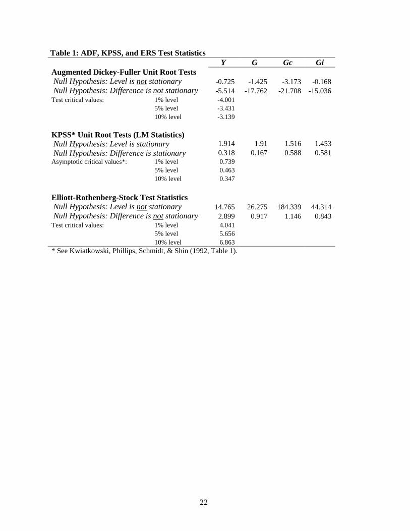
Table 1 contains the results for a battery of unit root tests including the Augmented

Dickey-Fuller (ADF) test, the Kwiatkowski, Phillips, Schmidt, and Shin (KPSS) test, and the

Elliott, Rothenberg, and Stock (ERS) test. The ADF test was specified to use a maximum

number of lags equal to 14 and the optimal number of lags was decided for each test using the

Schwartz Information Criterion. The KPSS test uses a spectral estimation method (in this case,

the Bartlett kernel) and the optimal number of lags used was chosen case-by-case using the

Newey-West bandwith, and the results were similar when we fixed the number of lags at 4 for

all tests. The ERS test also uses a spectral estimation procedure (AR spectral OLS, in this case),

the maximum number of lags allowed in the regressions was set equal to 14, and the optimal

number of lags was chosen in each test using the Schwartz Information Criterion.

Both the ADF and KPSS tests provide clear evidence that Y contains a unit root in its

level (i.e., it is an I(1) process), but apparently not in its first-difference (i.e., Y is first-difference

stationary).3 The ERS tests show the opposite result, suggesting that Y is trend-stationary in its

level, but displays a unit root in its first difference (we found some evidence that this last result

may be driven by a structural break in the year 1973, but the evidence is not conclusive). Using

tests that allowed for structural breaks in the real GDP series level, Cheung and Chinn (1986)

also rejected the unit root hypothesis (at the 10 percent significance level and using a different

dataset) for the level of Japan’s real GDP, and were among the first to show that Japan’s real

GDP can equally plausibly be thought of as trend-stationary.

3 For a more detailed discussion on different procedures to test for unit roots in the real GDP series the reader is referred to Cheung and Chinn (1986).

10

Similar conclusions arise in regards to the government expenditure variables. The ADF

and KPSS tests both reject the hypothesis of trend-stationarity in the variables’ levels, while not

rejecting the hypothesis of first difference-stationarity. The ERS tests arrive at the opposite

conclusion, namely the ERS tests find the government expenditure variables’ levels to be trend-

stationary whereas the first differences display unit roots.

Table 2 provides a summary of the variables’ stationarity and unit roots, and illustrates

two major points. First, a common specification in the literature is to regress real GDP growth

on the share of government purchases G/Y, and these shares are shown in Figure 2. But in this

case, these variables are not integrated of the same order as y, the growth rate of GDP.

Regressing a stationary dependent variable on independent variables which are not stationary is

an approach that Granger (1986: 216) argues “makes no sense as the independent and dependent

variables have such vastly different temporal properties.” Indeed, the expected coefficient(s)

from such a regression would be zero in such a case. Thus, we should not run regressions

combining these variables.

Second, real GDP and real government spending variables are not stationary in their

levels (i.e., not trend-stationary), according to both the ADF and the KPSS tests, but they are

stationary in their first differences. However, the opposite is true according to the ERS test, that

real GDP and real government spending are trend-stationary but their first differences display

unit roots (i.e., first differences are not stationary). This difficulty is not new; see, for example,

the pioneering work of Cheung and Chinn (1986) for the comparison of results between the

ADF and KPSS tests. Disentangling this ambiguity in tests results exceeds the scope of this

11

paper. Instead, we follow a pragmatic strategy in order to focus on the main goal of this paper,

which is to study the effectiveness of government spending to affect real GDP.

We thus take an agnostic approach regarding unit roots and proceed in two steps. First,

we run unrestricted VAR models in the variables’ levels. Second, we run the unrestricted VAR

models in the variables’ first differences. Finally, we conduct a cointegration analysis and

estimate a Vector Error Correction (VEC) model to extract causality implications from it.

5. An Unrestricted VAR Approach

As a first approach to analyzing the effect of the levels of G on Y, and of the growth

rates g on y, we estimated unrestricted Vector Auto-Regression (VAR) models from which we

extracted impulse-response results. An advantage of using an unrestricted VAR model is that it

implies a non-committal approach to the data in which issues of causation, timing, and

appropriate structural restrictions are temporarily left on hold, awaiting further analysis.

Since the impulse-response results are sensitive to the Cholesky-ordering of the

variables in the VAR, we first conduct Granger block-exogeneity tests on the variables’ levels

and first differences to gain some intuition on the most appropriate order of the variables. As

shown in Table 3 for 8, 9, and 10 lags, all the tests strongly suggest ordering the purchases

variables first and real GDP second.4

4 Eight, nine and ten lags are used in the Granger tests of Table 3, since using four lags created a significant number of inconclusive tests in the case of the variables in their rates of growth.

12

Unrestricted VAR models in the variables’ levels:

For the real levels of the variables, we follow the Final Prediction Error, the Akaike

Information Criterion, and the Hanna-Quinn Information Criterion, all of which suggest the use

of 4 lags as the optimal lag structure. Other, longer lag structures were also tried (again, 8 and 9

lags) and results were still generally in line with the ones reported.

In the first rows of Figures 3.1, 3.2, and 3.3, we show the impulse-response diagrams

from the VAR(4) model. For the levels of G, Gc, and Gi, government purchases, consumption,

and investment all have a significant effect on the level of GDP, while GDP does not appear to

increase government purchases, contrary to what we would expect from Wagner (1893).

On average, a one standard-deviation increase in real government spending leads, over a

period of two and a half years, to an approximately 40 point increase in real GDP, relative to an

index where 1955:1 GDP = 100. This is equivalent to an increase of 3.3 percent in Japan’s real

GDP of Japan at the end of the sample (2009:3). Interestingly, the smallest effect (10 points

accumulated over a period of 10 quarters) occurs for government consumption. Fiscal policy

shows some of its strongest effects in the form of government investment. This evidence is in

line with Koo (2008), who presented complementary evidence on the effectiveness of Japan’s

fiscal policy.

Unrestricted VAR models in the variables’ growth rates:

In considering the growth rates y, g, gc, and gi, we find that four of the five information criteria

used to determine the optimal lag structure still suggest the use of four lags, and we follow this

13

again. Granger tests of block exogeneity, shown in the bottom of Table 3, suggest ordering the

variables with g entering first, and y second.

The impulse-response diagrams are displayed in the bottom panels of Figures 3.1, 3.2,

and 3.3. A one standard deviation to the growth of real government purchases has a strongly

positive compounded effect on the growth of real GDP, adding one and a half percentage points

over a 10-quarter period. A similar shock to the rate of growth of real government consumption

increases real GDP growth by one full percentage point over a 10 quarter period, while a one-

standard-deviation shock to government investment has a slightly larger effect. These results

again support the argument that government purchases have had a positive effect on real GDP

in Japan during the postwar period.

The unrestricted VAR approach is not free of problems, however. Problems with this

approach include the potential for inefficient estimation due to over-parameterization (Zellner,

1988), and misspecification when the data are first-differenced and the variables are

cointegrated (Engle & Granger, 1987), as is potentially the case here. Hence, more analysis is

needed.

6. Cointegration Analysis

If the variables Y and G are cointegrated, causality tests conducted outside the

cointegration analysis framework may lead to incorrect causal inferences, since the error

correction term is omitted in the specifications used to test for Granger causality (see Granger,

1988, for additional discussion). Hence, to account for that difficulty we follow a two step

procedure in what follows. First, we check if the variables for GDP and government purchases

14

are cointegrated. Second, if the hypothesis that the series are not cointegrated is rejected, we

implement a Vector Error Correction (VEC) model in order to double check the results on block

exogeneity reported in Table 3. If cointegration test results show the presence of only one

cointegrating equation, the one in which G is the dependent variable and Y the explanatory one,

and the VEC model contains only one statistically significant error correction term in the

dynamic equations then, and only then, the block exogeneity test results reported below in Table

3 are valid (Granger, 1988).

In general, if two variables such as G and Y are both I(1), any combination of these

variables, such as Z = G – aY, will also be I(1), where Z is called the equilibrium error term.

However, there may exist a singularity a*, such that G - a*Y is I(0). If such a singularity exists,

G and Y are said to be cointegrated. This implies that in the long-run, although G and Y can be

arbitrarily high or low, they must be proportional to each other, with a factor of proportionality

a*. It is clearly possible for more than one equilibrium relation to govern the joint behavior of

the variables.

Johansen’s cointegration tests statistics are shown in Tables 4.1, with the results for the

variables in levels, and in Table 4.2, with the results for variables in growth rates. In general, the

variables in the levels contain only one cointegrating relation, with the exception being the case

of the pair of (Gi, Y), for which there tends to be a lack of cointegration (except for the case in

which the data are allowed no trend and the test includes only an intercept, but no trend). In the

growth rates, there tends to be two cointegrating relations (i.e., bi-directional causation) for the

growth variables in the overwhelming majority of the cases considered in the different

15

cointegration tests. The prevalence of a single cointegrating relationship in the case of the levels

raises the question of the direction of causation, which is addressed in the next section.

7. The Vector Error Correction Models

Engle and Granger (1987) have shown that if two variables are cointegrated, then there

must exist a VEC model linking these variables. Furthermore, the VEC model representation of

the bivariate system of cointegrated variables sheds light on the direction of causation between

those variables (Granger, 1988). Our VEC models for the variables in their levels is formulated

as follows:

tjt

T

jj

jt

T

jjtt

uyLd

gLcEbcgL

,11

,1

1,11

)1(

)1()1()1()1()1(

+−+

−++=−

−=

−=

−

∑

∑ (1)

tjt

T

jj

jt

T

jjtt

ugLd

yLcEbcyL

,21

,2

1,21

)1(

)1()2()2()2()1(

+−+

−++=−

−=

−=

−

∑

∑ (2)

where L is the lag operator, T is the number of lags to be included, and the error correction

terms are given by 1)( −tjE for j = 1, 2, which are the residuals from the OLS static regressions

of G on Y and vice versa, respectively. In equations (1) and (2), the VEC model allows for the

finding that G Granger-causes Y, or vice versa, so long as the corresponding error correction

term carries a statistically significant coefficient, even if the estimated dj coefficients are not

jointly statistically significant (Granger, 1988). If G and Y are cointegrated, then the error

16

correction terms are stationary I(0) processes. Conversely, if the residuals from the static

regressions involving G and Y are I(0), then G and Y are cointegrated (Engle & Granger, 1987).

The estimates of the VEC model contain important information regarding the long-run

relationship and the short-run dynamics involved in the relationship between G and Y. We chose

Johansen’s (1992) estimation procedure,5 and Table 5 displays the estimates. The error

correction terms leave no room for doubt: causation runs unidirectionally from real GDP to

government purchasing variables, and not the reverse. The impulse-response diagrams from

these VEC models clearly show that an increase in real government purchases still produces

positive effects on real GDP, as shown in Figures 4.1, 4.2, and 4.3.

One way to reconcile the causality results from the error correction terms of Table 5

with the ones displayed in the impulse-response diagrams in Figure 4 is by means of the

hypothesis that Japanese government officials have tended to react immediately to increases in

real GDP by contracting government spending, as displayed in the right-hand charts. This

introduces a systematic pattern of causation from real GDP to government spending, as

suggested by the error correction terms of Table 5 because a positive innovation to real GDP is

immediately followed by a reduction in government spending. Indeed, Koo (2008) has used a

similar explanation to account for the premature fiscal consolidations of 1997 and 2001 that

aborted strong economic recoveries that had been fueled by an activist fiscal policy in a context

of a zero lower bound constraint for short-term interest rates.

5 . See Guerrero and Parker (2007) for an illustration of Engle-Granger’s procedure for the case of the United States.

17

8. Conclusion

Our study examines whether government purchases in Japan helped or hurt GDP. This is

a very important issue for Japan after two lost decades of growth, in which Japan has failed to

return to a consistent growth path while debt has grown substantially.

Our dataset included quarterly data on GDP, government consumption, and government

investment from 1955 to 2009. This dataset permits a careful study of the time-series properties

of these variables for stationarity, cointegration, and Granger causality. Our results support

other evidence that government purchases had positive effects on growth. Government

investment was not that much more effective than consumption, which suggests that the fiscal

impact was at least as important as the effect of public infrastructure on potential GDP.

These results are consistent with the argument that fiscal policy may have worked in

Japan, but its observed effects, though consistently positive, were generally modest. The

financial crisis in Japan was severe, and the balance sheet troubles it created were long-lasting.

It was accompanied by a monetary policy that was tighter than it should have been in the

context, with deflation an unpleasant result. Expansionary fiscal policy may only have helped

ease the downturn. But that, as remarked by Koo (2008) and Leijonhufvud (2009), for example,

may be no small accomplishment.

18

References Barro, R.J. (1990), “Government spending in a simple model of endogenous growth”,

Journal of Political Economy, vol. 95, no. 5, pp. S103-125.

Caballero, R.J., T. Hoshi, & A.K. Kashyap (2008), "Zombie lending and depressed

restructuring in Japan”, American Economic Review, vol. 98, no. 5, pp. 1943-77.

Cargill, T.F., & E. Parker (2004), "Price deflation and consumption: central bank policy and

Japan's economic and financial stagnation”, Journal of Asian Economics, vol. 15, no. 3,

pp. 493-506.

Cargill, T.F., & T. Sakamoto (2008), Japan Since 1980. Cambridge University Press.

Chakraborty, S. (2009), “The boom and the bust of the Japanese economy: a quantitative

look at the period 1980–2000”, Japan and the World Economy, vol. 21, pp. 116–131.

Cheung, Y-W., & M.D. Chinn (1986), “Deterministic, stochastic and segmented trends in

aggregate output: A cross-country analysis. Oxford Economic Papers 48, pp. 134-162.

Christiano, L., M. Eichenbaum, & S. Rebelo (2009), “When is the government spending

multiplier large?”, NBER Working Paper No. 15394.

Engen, E., & J. Skinner (1996), “Taxation and economic growth”, National Tax Journal,

vol. 49, no. 4, pp. 617-42.

Engle, R.F., & C.W.J. Granger (1987), “Co-Integration and error correction: representation,

estimation, and testing”, Econometrica, vol. 55, no. 2, pp. 251-76.

Ghali, K.H. (1998), “Government size and economic growth: evidence from a multivariate

cointegration analysis”, Applied Economics, vol. 31, no. 8, pp. 975-987.

Granger, C.W.J., & P. Newbold (1974), “Spurious regressions in econometrics”, Journal of

Econometrics, vol. 2, no. 2, pp. 111-120.

Granger, C.W.J. (1986), “Developments in the study of cointegrated economic variables”,

Oxford Bulletin of Economics and Statistics, vol. 48, no. 3, pp. 213-228.

Granger, C.W.J. (1988), “Some recent developments in a concept of causality”, Journal of

Econometrics, vol. 39, no. 1-2, pp. 199-211.

Guerrero, F., & E. Parker (2007), "The effect of federal government size on long-term

economic growth in the United States, 1792-2004”, UNR Economics WP-07002.

19

Guseh, J.S. (1997), “Government size and economic growth in developing countries: a

political-economy framework”, Journal of Macroeconomics, vol. 19, no. 1, pp. 175-192.

Horioka, C.Y. (2006), “The causes of Japan’s ‘lost decade’: the role of household

consumption”, Japan and the World Economy, vol. 18, pp. 378–400.

Islam, A.M. (2001), “Wagner’s law revisited: cointegration and exogeneity tests for the

USA”, Applied Economics Letters, vol. 8, no. 8, pp. 509-515.

Johansen, S. (1992), “Determination of cointegration rank in the presence of a linear trend”,

Oxford Bulletin of Statistics, vol. 54, no. 3, pp. 383-397.

Koo, R.C. (2003), Balance Sheet Recession, Singapore, John Wiley & Sons (Asia).

Koo, R.C. (2008), The Holy Grail of Macroeconomics. Lessons from Japan’s Great

Recession, Singapore, John Wiley & Sons (Asia).

Kuttner, K.N., & A.S. Posen (2001), “Passive savers and fiscal policy: effectiveness in

Japan”, Working paper prepared for the CEPR-CIRJE-NBER Conference on Issues in

Fiscal Adjustment, Tokyo, Japan.

Kwiatkowski, D., P.C.B. Phillips, P. Schmidt, & Y. Shin (1992), “Testing the null

hypothesis of stationarity against the alternative of a unit root: how sure are we that

economic time series have a unit root?”, Journal of Econometrics, vol. 54, no. 1-3, pp.

159-178.

Landau, D. (1983), “Government expenditure and economic growth: a cross-country study”,

Southern Economic Journal, vol. 49, no. 3, pp. 783-792.

Landau, D. (1986), “Government and economic growth in the less developed countries: an

empirical study for 1960-80”, Economic Development and Cultural Change, vol. 35, no.

1, pp. 35-75.

Lee, B.S., & S. Lin (1994), “Government size, demographic changes, and economic

growth”, International Economic Journal, vol. 8, no. 1, pp. 91-108.

Leightner, J.E., & T. Inoue (2009), “Negative fiscal multipliers exceed positive multipliers

during Japanese deflation”, Applied Economics Letters, vol. 16, no. 13-15, pp. 1523-

1527.

20

Leijonhufvud, A. (2009), “Out of the corridor: Keynes and the crisis”, Cambridge Journal

of Economics, vol. 33, pp. 741–757.

MacKinnon, J.G., A.A. Haug, & L. Michelis (1999), Numerical distribution functions of

likelihood ratio tests for cointegration, Journal of Applied Econometrics, vol. 14, no. 5,

pp. 563-577.

Minsky, H.P. (1977), “A theory of systemic fragility”, in Altman, E. I. & Sametz, A. W.

(eds), Financial Crises: Institutions and Markets in a Fragile Environment, New York,

Wiley and Sons.

Minsky, H.P. (1986), Stabilizing an Unstable Economy, New York, McGraw-Hill.

Nadenichek, J. (2007), “Consumer confidence and economic stagnation in Japan”, Japan

and the World Economy, vol. 19, pp. 338–346.

Ono, H. (2008), “Government expenditure and government revenue nexus: Granger

causality test in the presence of threshold effects”, Empirical Economics Letters, vol. 7,

no. 4, pp. 377-386.

Perri, F. (2001), “The role of fiscal policy in Japan: a quantitative study”, Japan and the

World Economy, vol. 13, no. 4, pp. 387-404.

Peacock, A., & A. Scott (2000), “The curious attraction of Wagner's Law”, Public Choice,

vol. 102(1-2), pp. 1-17.

Perron, P. (1989), “The great crash, the oil price shock, and the unit root hypothesis”,

Econometrica, vol. 57, no. 6, pp. 1361-1401.

Plümper, T., & C.W. Martin (2003), “Democracy, government spending, and economic

growth: a political-economic explanation of the Barro-effect”, Public Choice, vol. 117,

no. 1-2, pp. 27-50.

Poot, J. (2000), “A synthesis of empirical research on the impact of government on long-run

growth”, Growth and Change 2000, vol. 31, no. 4, pp. 516-546.

Ram, R. (1986), “Government size and economic growth: a new framework and some

evidence from cross-section and time-series data”, American Economic Review, vol. 76,

no. 1, pp. 191-203.

21

Scully, G.W. (2002), “Economic freedom, government policy and the trade-off between

equity and economic growth”, Public Choice, vol. 113, no. 1-2, pp. 77-96.

Sims, C.A., C.A. Stock, & M.W. Watson (1990), “Inference in linear time series models

with unit roots”, Econometrica, vol. 58, no. 1, pp. 113-144.

Slemrod, J. (1995), “What do cross-country studies teach about government involvement,

prosperity, and economic growth?”, Brookings Papers on Economic Activity 1995, no. 2,

pp. 373-431.

Tamada, K. (2009), “The effect of election outcomes on the allocation of government

spending in Japan: evidence from the weather on election days”, Japanese Economy,

vol. 36, no. 1, pp. 3-26.

Wagner, A. (1893), Grundlegung der Politischen Okonomie, 3rd Edition, Leipzig, C.F.

Winter'sche Verlagshandlung.

Zellner, A. (1988), “Causality and causal laws in economics”, Journal of Econometrics, vol.

39, no. 1,2, pp. 7-28.

22

Table 1: ADF, KPSS, and ERS Test Statistics Y G Gc Gi Augmented Dickey-Fuller Unit Root Tests Null Hypothesis: Level is not stationary -0.725 -1.425 -3.173 -0.168 Null Hypothesis: Difference is not stationary -5.514 -17.762 -21.708 -15.036 Test critical values: 1% level -4.001 5% level -3.431 10% level -3.139 KPSS* Unit Root Tests (LM Statistics) Null Hypothesis: Level is stationary 1.914 1.91 1.516 1.453 Null Hypothesis: Difference is stationary 0.318 0.167 0.588 0.581 Asymptotic critical values*: 1% level 0.739

5% level 0.463 10% level 0.347

Elliott-Rothenberg-Stock Test Statistics Null Hypothesis: Level is not stationary 14.765 26.275 184.339 44.314 Null Hypothesis: Difference is not stationary 2.899 0.917 1.146 0.843 Test critical values: 1% level 4.041 5% level 5.656 10% level 6.863 * See Kwiatkowski, Phillips, Schmidt, & Shin (1992, Table 1).

23

Table 2: Summary of Stationarity Results Stationarity Results at 5% level ADF KPSS ERS Y NS NS S G NS NS (1) S Gc NS (1) NS S Gi NS NS S G/Y NS NS (1) S Gc/Y NS NS S Gi/Y NS NS S y S S NS g S NS (1) NS gc S S NS gi S S NS S = Stationary at 5% NS = Non-Stationary NS (1) = S at 10%

24

Table 3: Block Exogeneity and Granger tests Variables in Levels

Null Hypothesis: Lags of Y are not block-exogenous

Lags of G are not block-exogenous

Variable Obs F-stat p-value F-stat p-value

G 8 lags 211 4.16 0.000 0.68 0.710 9 lags 210 3.98 0.000 0.73 0.685 10 lags 209 3.87 0.000 0.74 0.684

Gc 8 lags 211 2.16 0.032 1.34 0.227

9 lags 210 2.03 0.039 1.71 0.089 10 lags 209 1.75 0.072 2.25 0.017

Gi 8 lags 211 1.57 0.136 1.29 0.248

9 lags 210 2.04 0.037 1.49 0.154 10 lags 209 2.23 0.018 1.38 0.193

Variables in Growth rates

Null Hypothesis: Lags of y are not block-exogenous

Lags of g are not block-exogenous

Obs F-stat p-value F-stat p-value

g 8 lags 210 4.99 0.000 1.20 0.296 9 lags 209 5.40 0.000 1.11 0.355 10 lags 208 1.47 0.115 1.11 0.354

gc 8 lags 210 4.48 0.000 2.02 0.046

9 lags 209 5.07 0.000 1.73 0.084 10 lags 208 4.13 0.000 1.47 0.155

gi 8 lags 210 2.81 0.006 1.77 0.085

9 lags 209 2.92 0.003 1.71 0.090 10 lags 208 2.56 0.006 1.70 0.083

25

Table 4.1: Bilateral Johansen’s Cointegration Tests for Variables in Levels Lags interval: 1 to 4 Selected (0.05 level*) Series: G and Y Number of Cointegrating Relations by Model Data Trend: None None Linear Linear Quadratic

Test Type No

Intercept Intercept Intercept Intercept Intercept

No Trend No

Trend No

Trend Trend Trend Trace 1 1 1 0 1 Max-Eig 1 1 1 1 1 Series: Gc and Y Number of Cointegrating Relations by Model Data Trend: None None Linear Linear Quadratic

Test Type No

Intercept Intercept Intercept Intercept Intercept

No Trend No

Trend No

Trend Trend Trend Trace 1 1 2 1 1 Max-Eig 1 1 2 1 1 Series: Gi and Y Number of Cointegrating Relations by Model Data Trend: None None Linear Linear Quadratic

Test Type No

Intercept Intercept Intercept Intercept Intercept

No Trend No

Trend No

Trend Trend Trend Trace 0 1 0 0 0 Max-Eig 0 1 0 0 0 *Critical values based on MacKinnon, Haug, & Michelis (1999).

26

Table 4.2: Bilateral Johansen’s Cointegration Tests for Variables in Growth Rates Lags interval: 1 to 4 Selected (0.05 level*) Series: g and y Number of Cointegrating Relations by Model Data Trend: None None Linear Linear Quadratic Test Type No Intercept Intercept Intercept Intercept Intercept

No Trend No

Trend No

Trend Trend Trend Trace 2 2 2 2 2 Max-Eig 2 2 2 2 2 Series: gc and y Number of Cointegrating Relations by Model Data Trend: None None Linear Linear Quadratic Test Type No Intercept Intercept Intercept Intercept Intercept

No Trend No

Trend No

Trend Trend Trend Trace 1 1 2 2 2 Max-Eig 1 1 2 2 2 Series: gi and y Number of Cointegrating Relations by Model Data Trend: None None Linear Linear Quadratic Test Type No Intercept Intercept Intercept Intercept Intercept

No Trend No

Trend No

Trend Trend Trend Trace 2 2 2 2 2 Max-Eig 2 2 2 2 2 *Critical values based on MacKinnon, Haug, & Michelis (1999).

27

Table 5: VEC between Measures of Government and GDP in Levels Gov't Purchases Gov't Consumption Gov't Investment Cointegrating Equation: G(-1) 1 1 1 Y(-1) -1.045 -1.560 -3.021 -0.025 -0.093 -0.966 [-41.00] [-16.75] [-3.13] Constant 25.753 406.861 1399.554 Error Correction Model: dG dY dGc dY dGi dY CointEq1 -0.097 -0.009 -0.022 0.000 0.006 0.001 -0.021 -0.013 -0.005 -0.004 -0.003 -0.001 [-4.51] [-0.71] [-4.73] [-0.07] [ 2.14] [ 1.36] dG(-1) -0.195 -0.050 -0.449 -0.097 0.022 -0.035 -0.070 -0.042 -0.070 -0.057 -0.071 -0.016 [-2.78] [-1.20] [-6.38] [-1.71] [ 0.31] [-2.20] dY(-1) 0.044 0.198 -0.180 0.026 0.028 0.174 -0.124 -0.074 -0.075 -0.060 -0.314 -0.072 [ 0.35] [ 2.69] [-2.40] [ 0.43] [ 0.09] [ 2.44] dY(-2) -0.066 0.126 -0.122 0.029 -0.088 0.143 -0.122 -0.072 -0.076 -0.061 -0.308 -0.070 [-0.54] [ 1.73] [-1.61] [ 0.48] [-0.29] [ 2.04] dY(-3) -0.487 0.199 0.046 0.217 -0.530 0.215 -0.130 -0.077 -0.089 -0.071 -0.321 -0.073 [-3.76] [ 2.58] [ 0.52] [ 3.04] [-1.65] [ 2.95] dY(-4) -0.164 -0.165 -0.207 0.222 0.229 -0.137 -0.145 -0.086 -0.093 -0.075 -0.349 -0.080 [-1.13] [-1.92] [-2.23] [ 2.98] [ 0.66] [-1.73] Constant 9.725 3.330 12.264 3.643 5.146 3.063 -1.562 -0.929 -1.616 -1.298 -3.428 -0.780 [ 6.23] [ 3.58] [ 7.59] [ 2.81] [ 1.50] [ 3.93] R-squared 0.159 0.135 0.259 0.142 0.043 0.155 Adj. R-squared 0.121 0.097 0.226 0.105 0.001 0.118 F-statistic 4.273 3.550 7.909 3.766 1.031 4.165 Akaike AIC 8.117 7.077 7.507 7.069 10.014 7.054 Schwarz SC 8.274 7.234 7.665 7.226 10.171 7.211 Included observations: 214 after adjustments Standard errors in (parentheses) and t-statistics in [brackets] Note: Insignificant lags are not shown

28

Figure 1.1: Real GDP and Government Purchases

-

50

100

150

200

250

1955 1958 1961 1964 1967 1970 1973 1976 1979 1982 1985 1988 1991 1994 1997 2000 2003 2006 2009

Quarterly Data

Ind

ex (

1985

:1 =

100

)

Y

Gc

Gi

G

GDP

Gov't Purchases

Gov't Investment

Gov't Consumption

Figure 1.2: Real Growth of GDP and Government Purchases

-14%

-10%

-6%

-2%

2%

6%

10%

1955 1958 1961 1964 1967 1970 1973 1976 1979 1982 1985 1988 1991 1994 1997 2000 2003 2006 2009

Quarterly Data

y

g

GDP

Gov't Purchases

29

Figure 2: Government Shares of GDP

0%

5%

10%

15%

20%

25%

1955 1958 1961 1964 1967 1970 1973 1976 1979 1982 1985 1988 1991 1994 1997 2000 2003 2006 2009

Quarterly Data

Sh

are

of

GD

P

Gc/Y Gi/Y G/Y

Gov't Purchases

Gov't Investment

Gov't Consumption

30

Figure 3.1: Accumulated Response for Government Purchases Cholesky One-Standard Deviations +/- Two Standard Errors (A) Accumulated Response of Y to G Accumulated Response of G to Y

(B) Accumulated Response of dY to dG Accumulated Response of dG to dY

31

Figure 3.2: Accumulated Response for Government Consumption Cholesky One-Standard Deviation Shocks +/- Two Standard Errors (A) Accumulated Response of Y to Gc Accumulated Response of Gc to Y

(B) Accumulated Response of dY to dGc Accumulated Response of dGc to dY

32

Figure 3.3: Accumulated Response for Government Investment Cholesky One-Standard Deviations +/- Two Standard Errors (A) Accumulated Response of Y to Gi Accumulated Response of Gi to Y

(B) Accumulated Response of dY to dGi Accumulated Response of dGi to dY

33

Figure 4: Accumulated Response for Government Purchases Accumulated Response of Y to G Accumulated Response of G to Y

Accumulated Response of Y to Gc Accumulated Response of Gc to Y

Accumulated Response of Y to Gi Accumulated Response of Gi to Y