Uni

vers

ity

of W

ashi

ngto

n

1

Boosting and predictive modeling

Yoav Freund

Columbia University

Uni

vers

ity

of W

ashi

ngto

n

2

What is “data mining”?

Lots of data - complex models

• Classifying customers using transaction logs.

• Classifying events in high-energy physics experiments.

• Object detection in computer vision.

• Predicting gene regulatory networks.

• Predicting stock prices and portfolio management.

Uni

vers

ity

of W

ashi

ngto

n

3

Leo BreimanStatistical Modeling / the two cultures

Statistical Science, 2001

• The data modeling culture (Generative modeling)– Assume a stochastic model (5-50 parameters).

– Estimate model parameters.

– Interpret model and make predictions.

– Estimated population: 98% of statisticians

• The algorithmic modeling culture (Predictive modeling)

– Assume relationship btwn predictor vars and response vars has a functional form (10^2 -- 10^6 parameters).

– Search (efficiently) for the best prediction function.

– Make predictions

– Interpretation / causation - mostly an after-thought.

– Estimated population: 2% 0f statisticians (many in other fields).

Uni

vers

ity

of W

ashi

ngto

n

4

Toy Example

• Computer receives telephone call

• Measures Pitch of voice

• Decides gender of caller

HumanVoice

Male

Female

Uni

vers

ity

of W

ashi

ngto

n

5

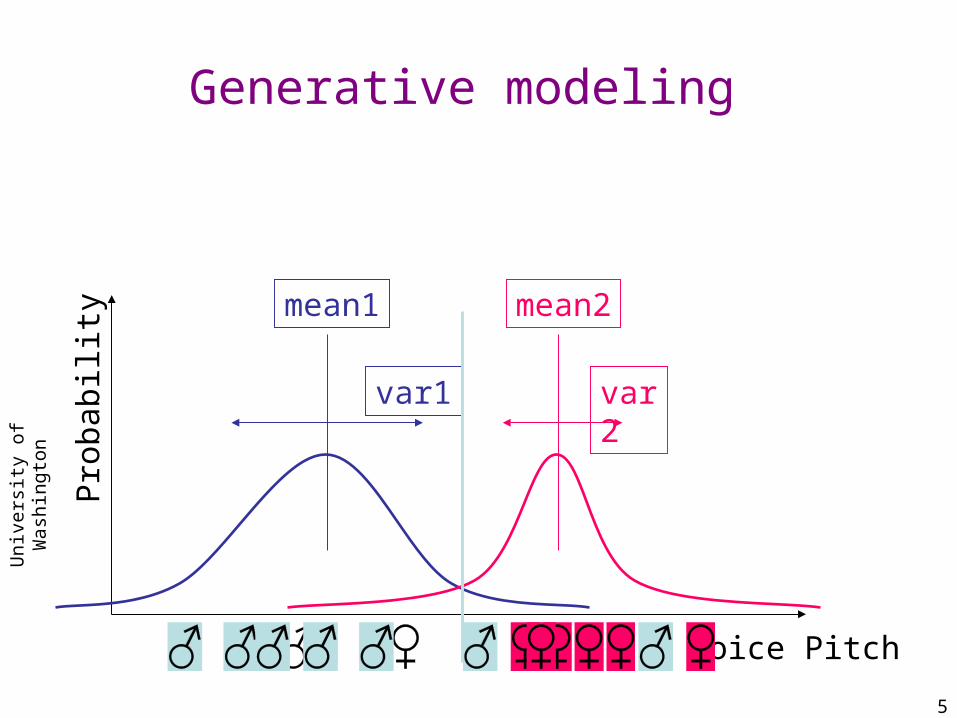
Generative modeling

Voice Pitch

Pro

babi

lity

mean1

var1

mean2

var2

Uni

vers

ity

of W

ashi

ngto

n

6

Discriminative approach

Voice Pitch

No.

of

mis

take

s

Uni

vers

ity

of W

ashi

ngto

n

7

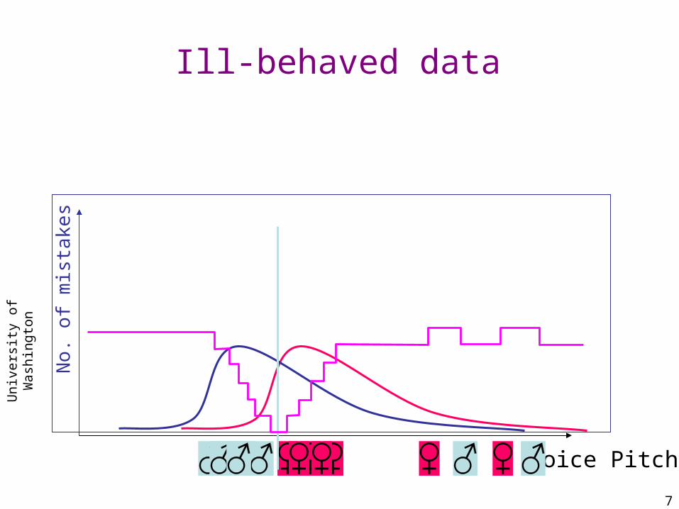
Ill-behaved data

Voice Pitch

Pro

babi

lity

mean1 mean2

No.

of

mis

take

s

Uni

vers

ity

of W

ashi

ngto

n

8

Plan of talk

• Boosting• Alternating Decision Trees• Data-mining AT&T transaction logs.• The I/O bottleneck in data-mining.• Resistance of boosting to over-fitting.• Confidence rated prediction.• Confidence-rating for object recognition.• Gene regulation modeling.• Summary

Uni

vers

ity

of W

ashi

ngto

n

9

Plan of talk

• Boosting: Combining weak classifiers.• Alternating Decision Trees• Data-mining AT&T transaction logs.• The I/O bottleneck in data-mining.• Resistance of boosting to over-fitting.• Confidence rated prediction.• Confidence-rating for object recognition.• Gene regulation modeling.• Summary

Uni

vers

ity

of W

ashi

ngto

n

10

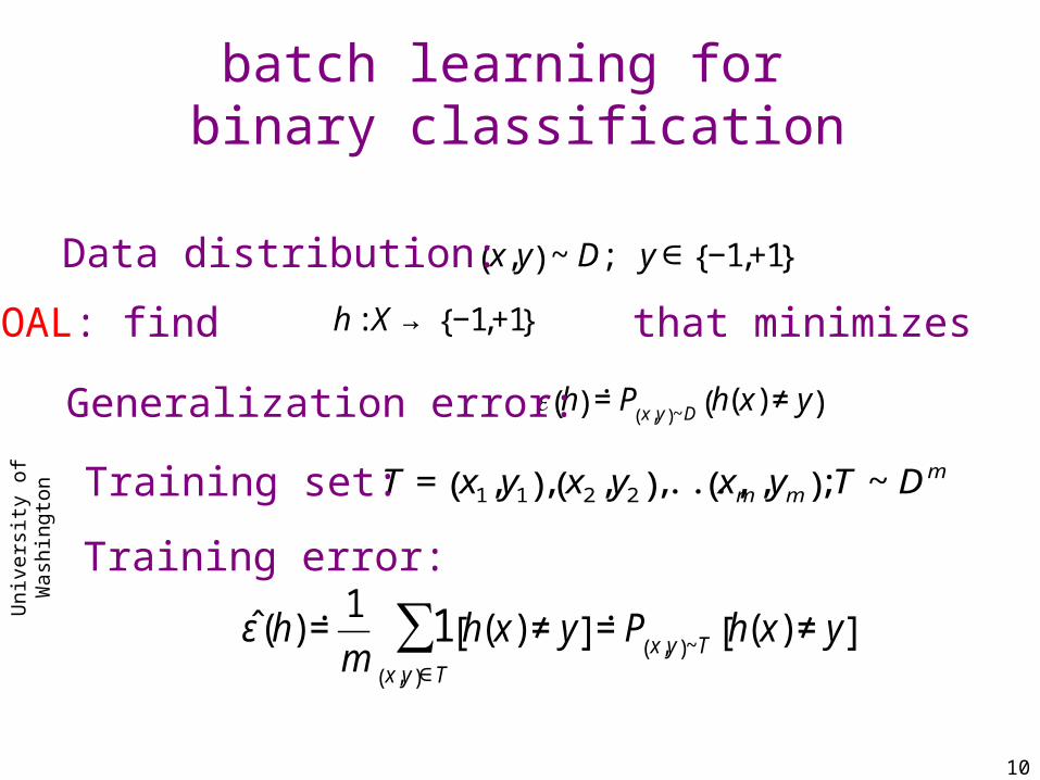
batch learning for binary classification

€

x,y( ) ~ D; y ∈ −1,+1{ }Data distribution:

€

ε h( ) ˙ = P x,y( )~D h(x) ≠ y( )Generalization error:

€

T = x1,y1( ), x2 ,y2( ),..., xm ,ym( ); T ~ DmTraining set:

€

ˆ ε (h) ˙ = 1

m1 h(x) ≠ y[ ]

x,y( )∈T

∑ ˙ = P x,y( )~T h(x) ≠ y[ ]

Training error:

GOAL: find that minimizes

€

h : X → −1,+1{ }

Uni

vers

ity

of W

ashi

ngto

n

11

A weighted training set

Feature vectors

Binary labels {-1,+1}

Positive weights

€

x1,y1,w1( ), x2 ,y2 ,w2( ),K , xm ,ym ,wm( )

Uni

vers

ity

of W

ashi

ngto

n

12

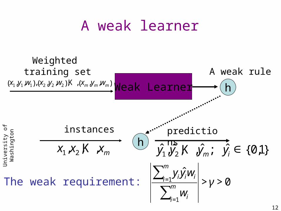
A weak learner

The weak requirement:

€

yiˆ y iwii=1

m

∑wii=1

m

∑> γ > 0

A weak rule

h

h

Weak Learner

Weighted training set

€

x1,y1,w1( ), x2 ,y2 ,w2( ),K , xm ,ym ,wm( )

instances

€

x1,x2 ,K ,xm

predictions

€

ˆ y 1, ˆ y 2 ,K , ˆ y m; ˆ y i ∈ {0,1}

Uni

vers

ity

of W

ashi

ngto

n

13

The boosting process

€

FT x( ) = α 1h1 x( ) +α 2h2 x( ) +L +α T hT x( )

Final rule:

€

fT (x) = sign FT x( )( )

weak learner

€

x1, y1,w11

( ), x2,y2,w21

( ),K , xn , yn,wn1

( )

€

x1,y1,w1T −1

( ), x2,y2,w2T −1

( ),K , xn ,yn,wnT −1

( )

€

hT

weak learner

€

x1, y1,1( ), x2, y2,1( ),K , xn , yn,1( )

€

h1

€

x1,y1,w12

( ), x2,y2,w22

( ),K , xn , yn,wn2

( )

€

h3

€

h2

Uni

vers

ity

of W

ashi

ngto

n

14

€

αt = ln wit

i:ht xi( )=1,yi =1∑ wi

t

i:ht xi( )=1,yi =−1∑ ⎛

⎝ ⎜ ⎞

⎠ ⎟

€

wit = exp −yiFt−1(xi )( )

Adaboost

€

F0 x( ) ≡ 0

€

Ft+1 = Ft +α tht€

Get ht from weak − learner

€

for t =1..T

Freund, Schapire 1997

Uni

vers

ity

of W

ashi

ngto

n

15

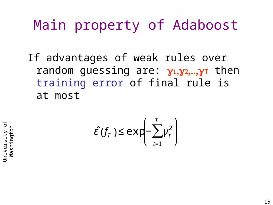
Main property of Adaboost

If advantages of weak rules over random guessing are: T then training error of final rule is at most

€

ˆ ε fT( ) ≤ exp − γ t2

t=1

T

∑ ⎛

⎝ ⎜

⎞

⎠ ⎟

Uni

vers

ity

of W

ashi

ngto

n

16

Boosting block diagram

WeakLearner

Booster

Weakrule

Exampleweights

Strong Learner AccurateRule

Uni

vers

ity

of W

ashi

ngto

n

17

Loss

CorrectMistakes

€

y Ft (x)

Adaboost as gradient-descent

Adaboost =

€

e−yFt (x )

0-1 loss

Logitboost=

€

ln 1+ e−yFt (x )( )

Brownboost=

€

1

21− erf

yFt x( ) + c − t

c − t

⎛

⎝ ⎜

⎞

⎠ ⎟

⎛

⎝ ⎜

⎞

⎠ ⎟

Uni

vers

ity

of W

ashi

ngto

n

18

Plan of talk

• Boosting• Alternating Decision Trees: a hybrid of boosting

and decision trees• Data-mining AT&T transaction logs.• The I/O bottleneck in data-mining.• Resistance of boosting to over-fitting.• Confidence rated prediction.• Confidence-rating for object recognition.• Gene regulation modeling.• Summary

Uni

vers

ity

of W

ashi

ngto

n

19

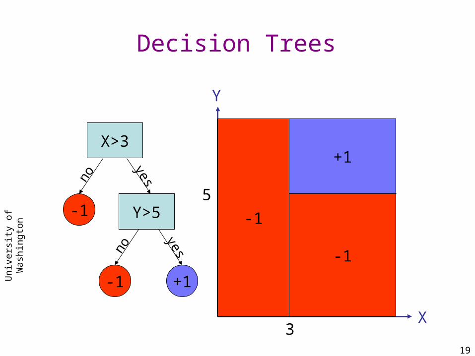
Decision Trees

X>3

Y>5-1

+1-1

no

yes

yesno

X

Y

3

5

+1

-1

-1

Uni

vers

ity

of W

ashi

ngto

n

20

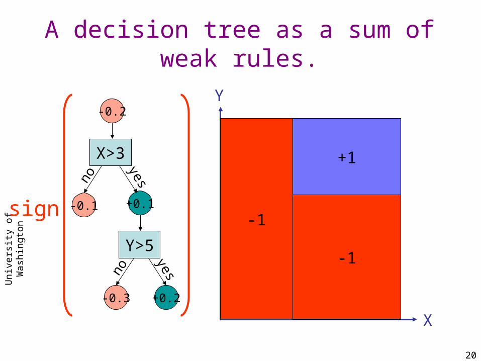
-0.2

A decision tree as a sum of weak rules.

X

Y-0.2

+0.2-0.3

Y>5

yesno

-0.1 +0.1

X>3

no

yes

+0.1-0.1

+0.2

-0.3

+1

-1

-1sign

Uni

vers

ity

of W

ashi

ngto

n

21

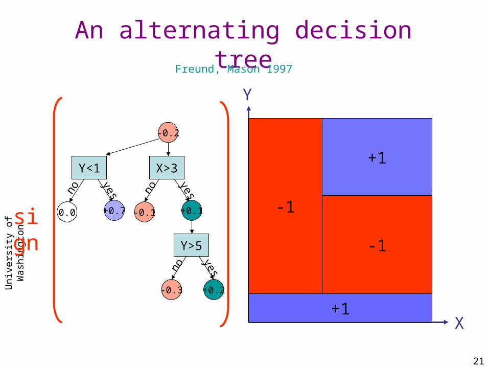
An alternating decision tree

X

Y

+0.1-0.1

+0.2

-0.3

sign

-0.2

Y>5

+0.2-0.3yesno

X>3

-0.1

no

yes

+0.1

+0.7

Y<1

0.0

no

yes

+0.7

+1

-1

-1

+1

Freund, Mason 1997

Uni

vers

ity

of W

ashi

ngto

n

22

Example: Medical Diagnostics

• Cleve dataset from UC Irvine database.

• Heart disease diagnostics (+1=healthy,-1=sick)

• 13 features from tests (real valued and discrete).

• 303 instances.

Uni

vers

ity

of W

ashi

ngto

n

23

AD-tree for heart-disease diagnostics

>0 : Healthy<0 : Sick

Uni

vers

ity

of W

ashi

ngto

n

24

Plan of talk

• Boosting• Alternating Decision Trees• Data-mining AT&T transaction logs.• The I/O bottleneck in data-mining.• Resistance of boosting to over-fitting.• Confidence rated prediction.• Confidence-rating for object recognition.• Gene regulation modeling.• Summary

Uni

vers

ity

of W

ashi

ngto

n

25

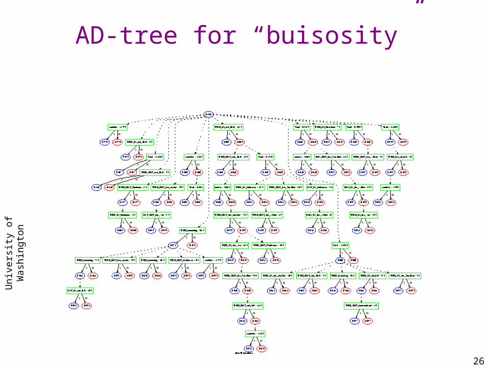
AT&T “buisosity” problem

• Distinguish business/residence customers from call detail information. (time of day, length of call …)

• 230M telephone numbers, label unknown for ~30%

• 260M calls / day

• Required computer resources:

Huge: counting log entries to produce statistics -- use specialized I/O efficient sorting algorithms (Hancock).Significant: Calculating the classification for ~70M customers.Negligible: Learning (2 Hours on 10K training examples on an off-line computer).

Freund, Mason, Rogers, Pregibon, Cortes 2000

Uni

vers

ity

of W

ashi

ngto

n

26

AD-tree for “buisosity”

Uni

vers

ity

of W

ashi

ngto

n

27

AD-tree (Detail)

Uni

vers

ity

of W

ashi

ngto

n

28

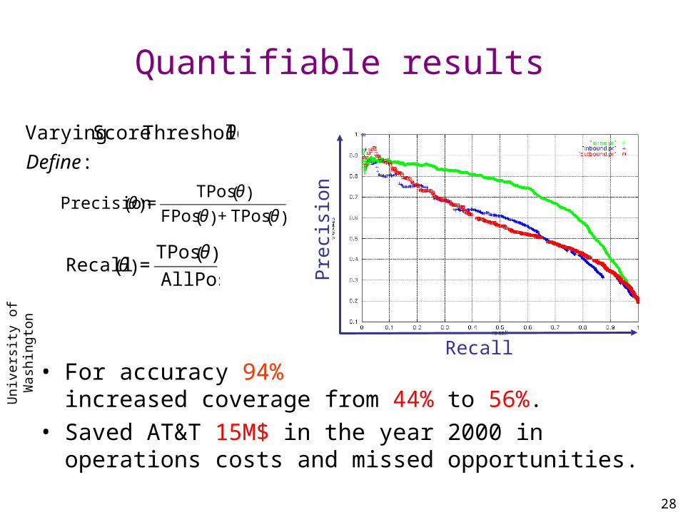
Quantifiable results

• For accuracy 94% increased coverage from 44% to 56%.

• Saved AT&T 15M$ in the year 2000 in operations costs and missed opportunities.

RecallP

reci

sion

€

Precision θ( ) =TPos θ( )

FPos θ( ) + TPos θ( )

€

Recall θ( ) =TPos θ( )AllPos

€

Varying Score Threshold θ

Define :

Uni

vers

ity

of W

ashi

ngto

n

29

Plan of talk

• Boosting• Alternating Decision Trees• Data-mining AT&T transaction logs.• The I/O bottleneck in data-mining.• Resistance of boosting to over-fitting.• Confidence rated prediction.• Confidence-rating for object recognition.• Gene regulation modeling.• Summary

Uni

vers

ity

of W

ashi

ngto

n

30

The database bottleneck

• Physical limit: disk “seek” takes 0.01 sec– Same time to read/write 10^5 bytes– Same time to perform 10^7 CPU operations

• Commercial DBMS are optimized for varying queries and transactions.

• Statistical analysis requires evaluation of fixed queries on massive data streams.

• Keeping disk I/O sequential is key.• Data Compression: improves I/O speed but

restricts random access.

Uni

vers

ity

of W

ashi

ngto

n

31

CS theory regarding very large data-sets

• Massive datasets: “You pay 1 per disk block you read/write ε per CPU operation. Internal memory can store N disk blocks”– Example problem: Given a stream of line segments (in

the plane), identify all segment pairs that intersect.– Vitter, Motwani, Indyk, …

• Property testing: “You can only look at a small fraction of the data”– Example problem: decide whether a given graph is bi-

partite by testing only a small fraction of the edges.– Rubinfeld, Ron, Sudan, Goldreich, Goldwasser, …

Uni

vers

ity

of W

ashi

ngto

n

32

Plan of talk

• Boosting• Alternating Decision Trees• Data-mining AT&T transaction logs.• The I/O bottleneck in data-mining.• Resistance of boosting to over-fitting.• Confidence rated prediction.• Confidence-rating for object recognition.• Gene regulation modeling.• Summary

Uni

vers

ity

of W

ashi

ngto

n

33

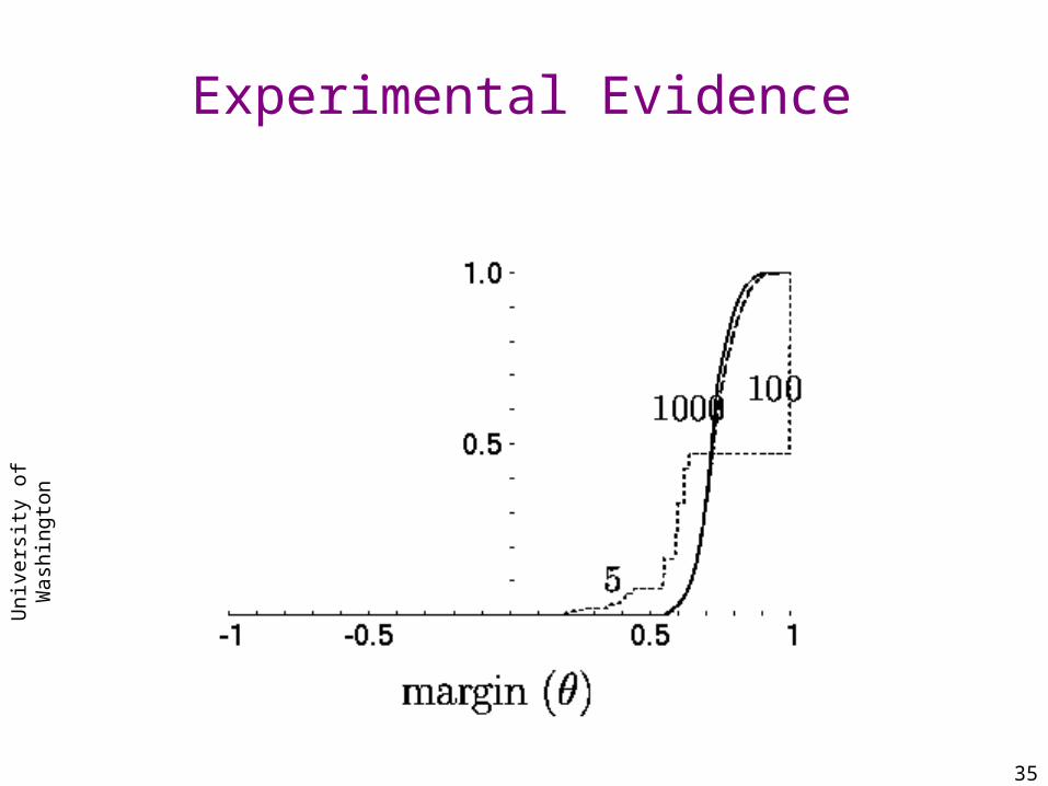
A very curious phenomenon

Boosting decision trees

Using <10,000 training examples we fit >2,000,000 parameters

Uni

vers

ity

of W

ashi

ngto

n

34

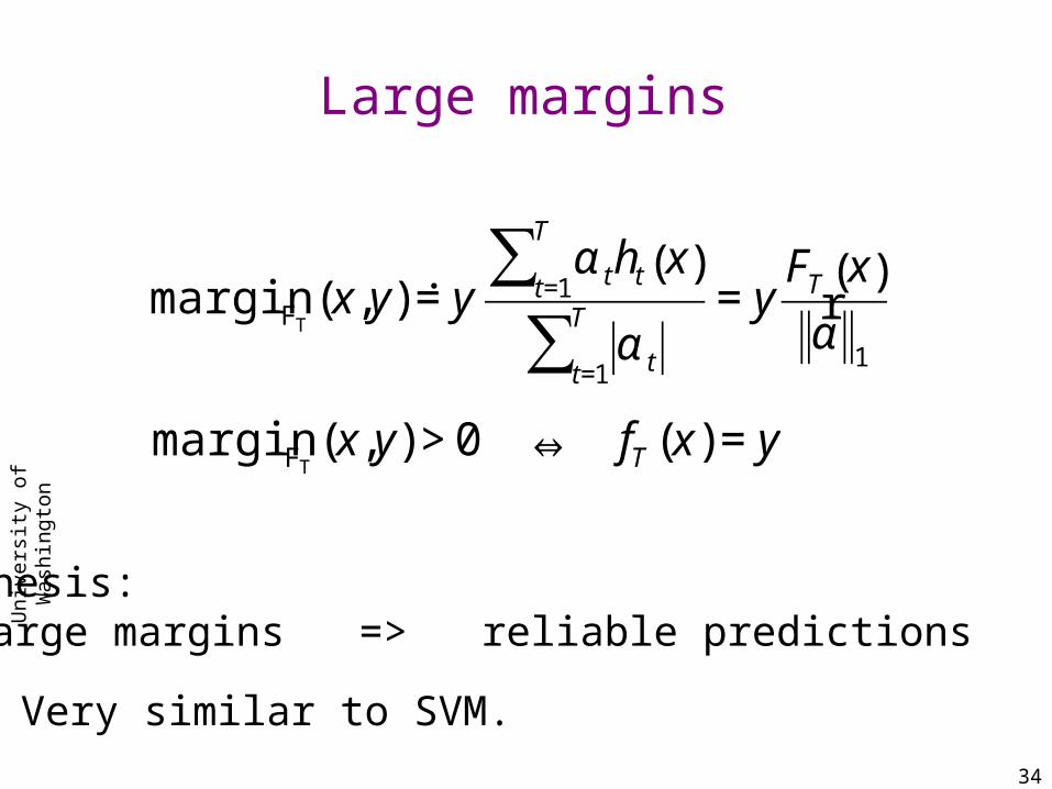
Large margins

€

marginFT(x,y) ˙ = y

α tht x( )t=1

T

∑α tt=1

T

∑= y

FT x( )r α

1

€

marginFT(x,y) > 0 ⇔ fT (x) = y

Thesis:large margins => reliable predictions

Very similar to SVM.

Uni

vers

ity

of W

ashi

ngto

n

35

Experimental Evidence

Uni

vers

ity

of W

ashi

ngto

n

36

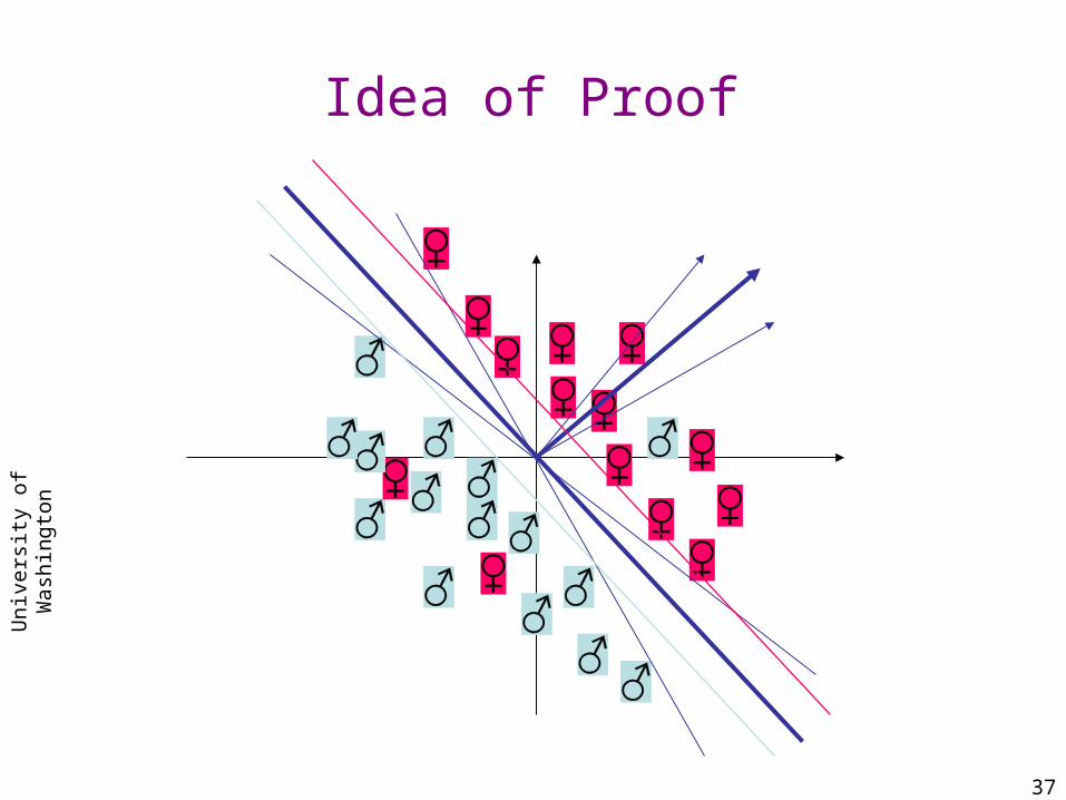
TheoremSchapire, Freund, Bartlett & Lee / Annals of statistics 1998

H: set of binary functions with VC-dimension d

C

€

= αihi | hi ∈ H , α i > 0, α i =1∑∑{ }

€

∀c ∈C,∀θ > 0, with probability1− δ w.r.t. T ~ Dm

€

P x,y( )~D sign c(x)( ) ≠ y[ ] ≤ P x,y( )~T marginc x,y( ) ≤ θ[ ]

€

+ ˜ O d / m

θ

⎛

⎝ ⎜

⎞

⎠ ⎟+O log

1

δ

⎛

⎝ ⎜

⎞

⎠ ⎟

€

T = x1,y1( ), x2 ,y2( ),..., xm ,ym( ); T ~ Dm

No dependence on no. of combined functions!!!

Uni

vers

ity

of W

ashi

ngto

n

37

Idea of Proof

Uni

vers

ity

of W

ashi

ngto

n

38

Plan of talk

• Boosting• Alternating Decision Trees• Data-mining AT&T transaction logs.• The I/O bottleneck in data-mining.• Resistance of boosting to over-fitting.• Confidence rated prediction.• Confidence-rating for object recognition.• Gene regulation modeling.• Summary

Uni

vers

ity

of W

ashi

ngto

n

39

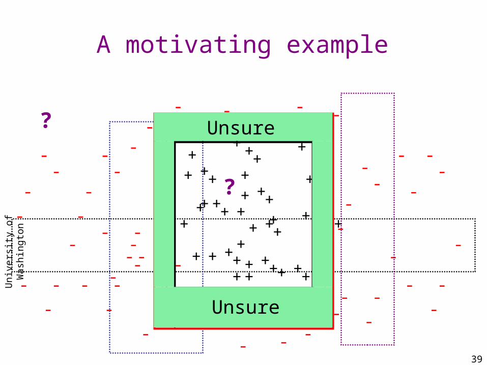
A motivating example

-

-

-+

+

+

++

+

++

++

-

-

-

-

-

-

-

-

-

--

-

-

-

-

-

--

-

-

-

-

-

-

--

-

-

-

-

-

--

-

--

-

-

-

-

-

-

+

++

+

++

+

+

++

+

++

+ +

++

+

+

+

+

+

++

+

++

+

+

++

+

++

+--

-

-- -

--

---

--

?

?

?

Unsure

Unsure

Uni

vers

ity

of W

ashi

ngto

n

40

The algorithm

€

η > 0, Δ > 0Parameters

€

w(h) ˙ = e−η ˆ ε h( )Hypothesis weight:

€

ˆ l η (x) ˙ = 1

ηln

w(h)h:h ( x)=+1

∑

w(h)h:h ( x)=−1

∑

⎛

⎝

⎜ ⎜ ⎜

⎞

⎠

⎟ ⎟ ⎟

Empirical Log RatioEmpirical Log Ratio::

€

ˆ p η ,Δ x( ) =

+1 if ˆ l x( ) > Δ

-1,+1{ } if ˆ l x( ) ≤ Δ

−1 if ˆ l x( ) < −Δ

⎧

⎨ ⎪

⎩ ⎪

Prediction rule:

Freund, Mansour, Schapire, Annals of Stat, August 2004

Uni

vers

ity

of W

ashi

ngto

n

41

Suggested tuning

€

P(abstain) = P x,y( )~Dˆ p (x) = −1,+1{ }( ) = 5ε h*

( ) +Oln 1 δ( ) + ln H( )

m1/2−θ

⎛

⎝ ⎜ ⎜

⎞

⎠ ⎟ ⎟

€

2) for m = Ω ln 1 δ( ) ln H( )( )1/θ ⎛

⎝ ⎜

⎞ ⎠ ⎟

Yields:

€

1) P mistake( ) = P x,y( )~D y ∉ ˆ p (x)( ) = 2ε h*( ) +O

ln m( )m1/2−θ

⎛

⎝ ⎜

⎞

⎠ ⎟

H is a finite set.

€

m=Size of training set

€

δ=Probability of failure

€

η =m1 2−θ ln H

€

Δ =lnH

δ

⎛

⎝ ⎜

⎞

⎠ ⎟ m1 2+θ

€

0 <θ < 14

Setting:

Uni

vers

ity

of W

ashi

ngto

n

42

Confidence Rating block diagram

Rater-Combiner

Confidence-ratedRule

CandidateRules

€

x1,y1( ), x2 ,y2( ),K , xm ,ym( )

Training examples

Uni

vers

ity

of W

ashi

ngto

n

43

Summary of Confidence-Rated Classifiers

• Frequentist explanation for the benefits of model averaging

• Separates between inherent uncertainty and uncertainty due to finite training set.

• Computational hardness: unknown other than in few special cases

• Margins from Boosting or SVM can be used as an approximation.

• Many practical applications!

Uni

vers

ity

of W

ashi

ngto

n

44

Plan of talk

• Boosting• Alternating Decision Trees• Data-mining AT&T transaction logs.• The I/O bottleneck in data-mining.• Resistance of boosting to over-fitting.• Confidence rated prediction.• Confidence-rating for object recognition.• Gene regulation modeling.• Summary

Uni

vers

ity

of W

ashi

ngto

n

45

Face Detection - Using confidence to save time

• Paul Viola and Mike Jones developed a face detector that can work in real time (15 frames per second).

Viola & Jones 1999

QuickTime™ and aYUV420 codec decompressor

are needed to see this picture.

Uni

vers

ity

of W

ashi

ngto

n

46

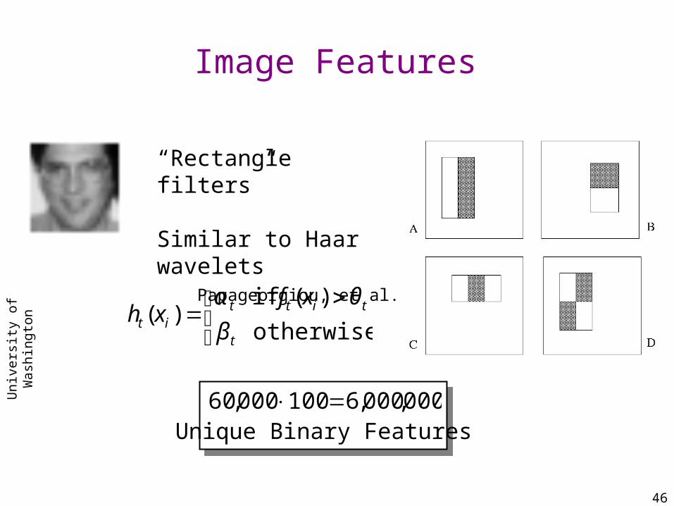
Image Features

“Rectangle filters”

Similar to Haar wavelets Papageorgiou, et al.

000,000,6100000,60 =×Unique Binary Features

⎩⎨⎧ >

=otherwise

)( if )(

t

tittit

xfxh

β

θα

Uni

vers

ity

of W

ashi

ngto

n

47

Example Classifier for Face Detection

ROC curve for 200 feature classifier

A classifier with 200 rectangle features was learned using AdaBoost

95% correct detection on test set with 1 in 14084false positives.

Not quite competitive...

Uni

vers

ity

of W

ashi

ngto

n

48

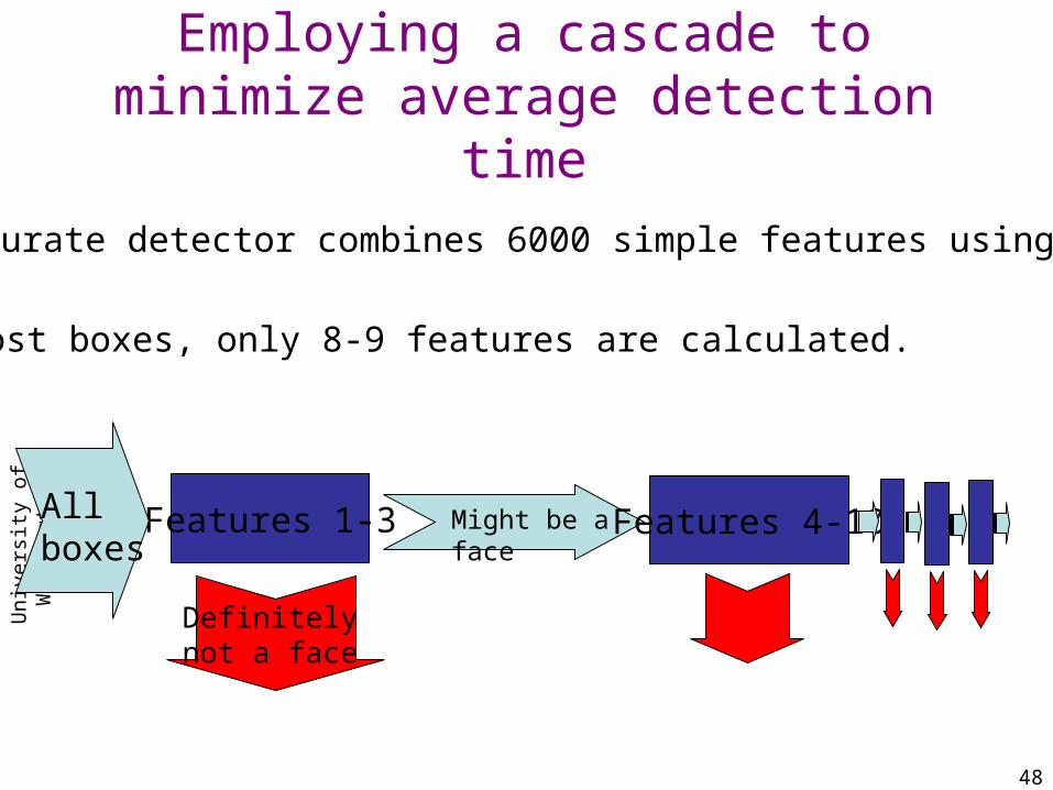
Employing a cascade to minimize average detection time

The accurate detector combines 6000 simple features using Adaboost.

In most boxes, only 8-9 features are calculated.

Features 1-3Allboxes

Definitely not a face

Might be a face

Features 4-10

Uni

vers

ity

of W

ashi

ngto

n

49

Using confidence to avoid labelingLevin, Viola, Freund 2003

Uni

vers

ity

of W

ashi

ngto

n

50

Image 1

Uni

vers

ity

of W

ashi

ngto

n

51

Image 1 - diff from time average

Uni

vers

ity

of W

ashi

ngto

n

52

Image 2

Uni

vers

ity

of W

ashi

ngto

n

53

Image 2 - diff from time average

Uni

vers

ity

of W

ashi

ngto

n

54

Co-training

HwyImages

Raw B/W

Diff Image

Partially trainedB/W basedClassifier

Partially trainedDiff basedClassifier

Confident Predictions

Confident Predictions

Blum and Mitchell 98

Uni

vers

ity

of W

ashi

ngto

n

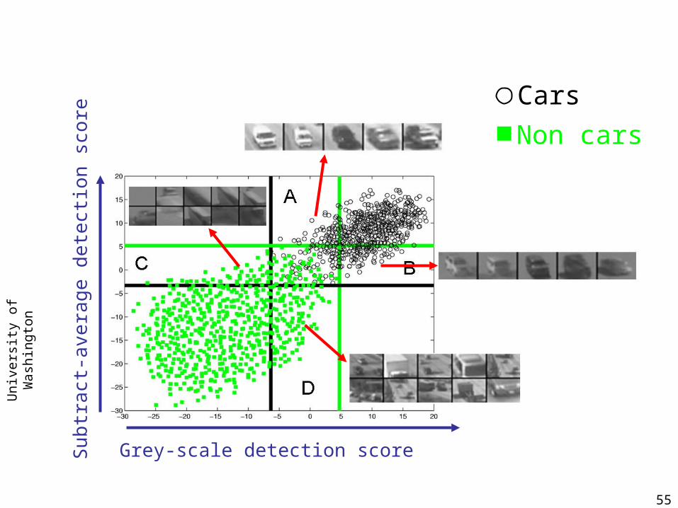
55

Grey-scale detection score

Sub

trac

t-av

erag

e de

tect

ion

scor

e

Non cars

Cars

Uni

vers

ity

of W

ashi

ngto

n

56

Co-Training Results

Raw Image detector Difference Image detector

Before co-training After co-training

Uni

vers

ity

of W

ashi

ngto

n

57

Plan of talk

• Boosting• Alternating Decision Trees• Data-mining AT&T transaction logs.• The I/O bottleneck in data-mining.• Resistance of boosting to over-fitting.• Confidence rated prediction.• Confidence-rating for object recognition.• Gene regulation modeling.• Summary

Uni

vers

ity

of W

ashi

ngto

n

58

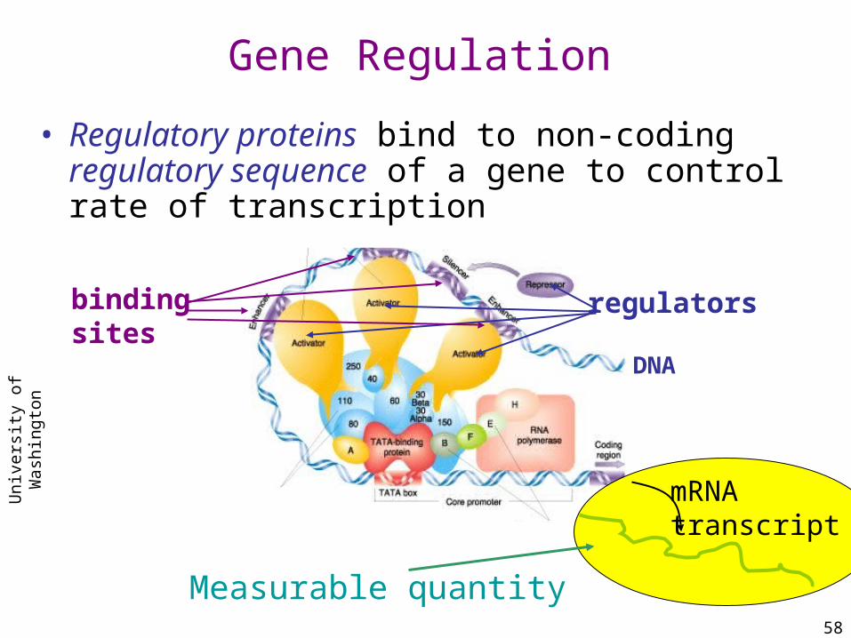
DNA

Measurable quantity

Gene Regulation

• Regulatory proteins bind to non-coding regulatory sequence of a gene to control rate of transcription

regulators

mRNAtranscript

bindingsites

Uni

vers

ity

of W

ashi

ngto

n

59

From mRNA to Protein

mRNAtranscript

Nucleus wall

ribosomeProteinfolding

Protein sequence

Uni

vers

ity

of W

ashi

ngto

n

60

Protein Transcription Factors

regulator

Uni

vers

ity

of W

ashi

ngto

n

61

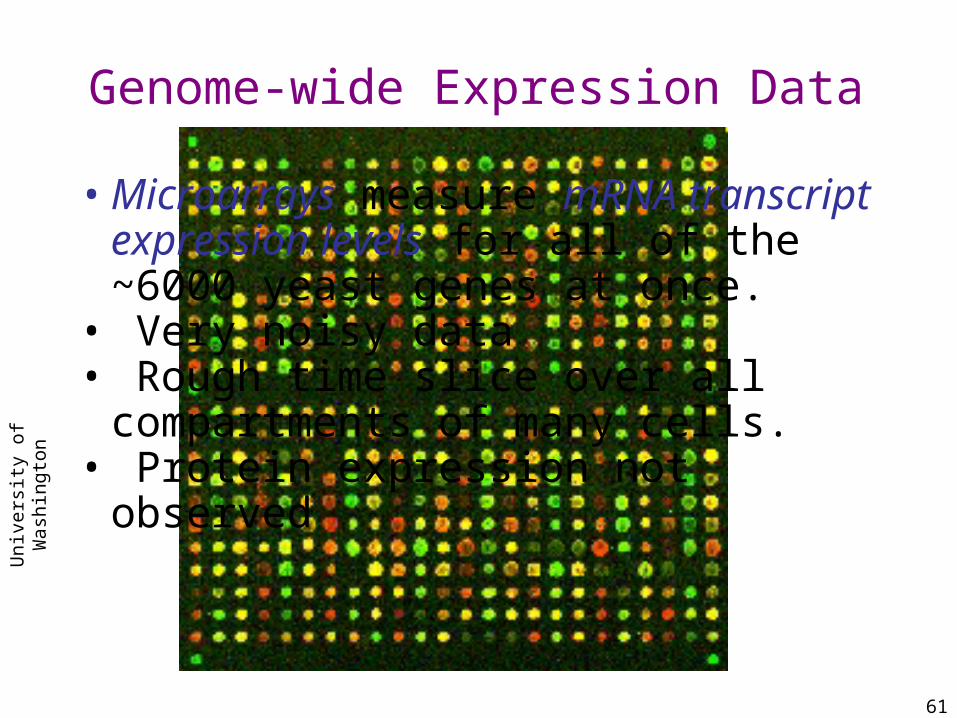
Genome-wide Expression Data

• Microarrays measure mRNA transcript expression levels for all of the ~6000 yeast genes at once.

• Very noisy data• Rough time slice over all

compartments of many cells.• Protein expression not observed

Uni

vers

ity

of W

ashi

ngto

n

62

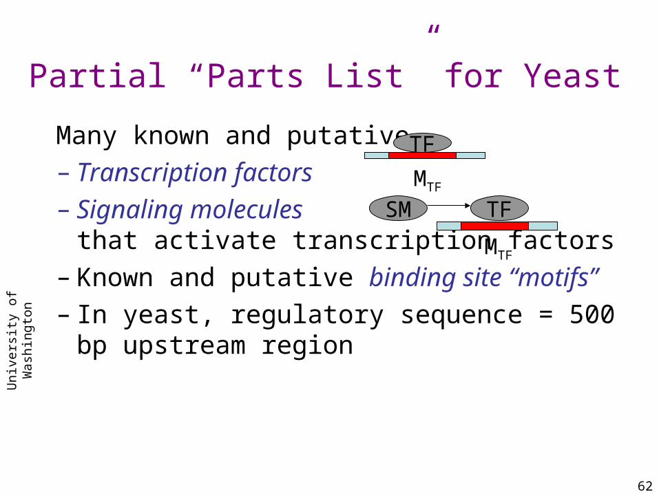
Partial “Parts List” for Yeast

Many known and putative – Transcription factors– Signaling molecules

that activate transcription factors– Known and putative binding site “motifs” – In yeast, regulatory sequence = 500 bp upstream

region

TFSM

MTF

TF

MTF

Uni

vers

ity

of W

ashi

ngto

n

63

Predict target gene regulatory response from regulator activity and binding site data

MicroarrayImage

R1 R2 RpR4R3 …..“Parent” gene expression G1

…

Target gene expression

G2

G3

G4

Gt

GeneClass: Problem Formulation

G1G2G3G4

Gt

Binding sites (motifs)in upstream region

…

M. Middendorf, A. Kundaje, C. Wiggins, Y. Freund, C. Leslie.Predicting Genetic Regulatory Response Using Classification. ISMB 2004.

Uni

vers

ity

of W

ashi

ngto

n

64

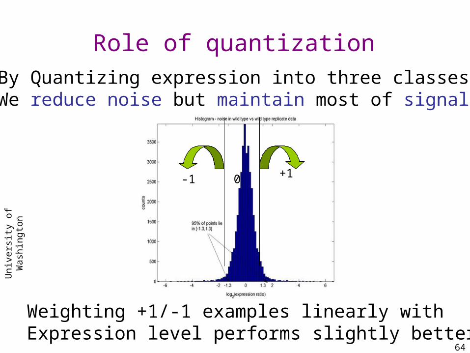
Role of quantization

-1 +10

By Quantizing expression into three classesWe reduce noise but maintain most of signal

Weighting +1/-1 examples linearly with Expression level performs slightly better.

Uni

vers

ity

of W

ashi

ngto

n

65

Problem setup

• Data point = Target gene X Microarray

• Input features:– Parent state {-1,0,+1}– Motif Presence {0,1}

• Predict output:– Target Gene {-1,+1}

Uni

vers

ity

of W

ashi

ngto

n

66

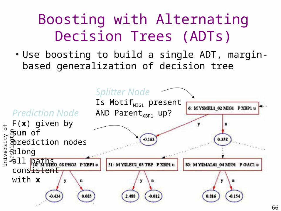
Boosting with Alternating Decision Trees (ADTs)

• Use boosting to build a single ADT, margin-based generalization of decision tree

Splitter NodeIs MotifMIG1 presentAND ParentXBP1 up?Prediction Node

F(x) given by sum of prediction nodes alongall paths consistent with x

Uni

vers

ity

of W

ashi

ngto

n

67

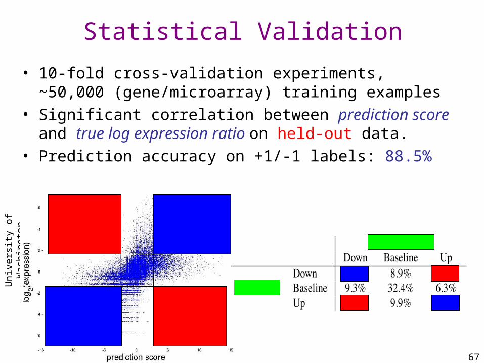
Statistical Validation

• 10-fold cross-validation experiments, ~50,000 (gene/microarray) training examples

• Significant correlation between prediction score and true log expression ratio on held-out data.

• Prediction accuracy on +1/-1 labels: 88.5%

Uni

vers

ity

of W

ashi

ngto

n

68

Biological InterpretationFrom correlation to causation

• Good prediction only implies Correlation.• To infer causation we need to integrate additional knowledge.• Comparative case studies: train on similar conditions (stresses),

test on related experiments• Extract significant features from learned model

– Iteration score (IS): Boosting iteration at which feature first appearsIdentifies significant motifs, motif-parent pairs

– Abundance score (AS): Number of nodes in ADT containing featureIdentifies important regulators

• In silico knock-outs: remove significant regulator and retrain.

Uni

vers

ity

of W

ashi

ngto

n

69

Case Study: Heat Shock and Osmolarity

Training set: Heat shock, osmolarity, amino acid starvation

Test set: Stationary phase, simultaneous heat shock+osmolarity

Results: Test error = 9.3% Supports Gasch hypothesis: heat shock and osmolarity

pathways independent, additive– High scoring parents (AS): USV1 (stationary phase and heat

shock), PPT1 (osmolarity response), GAC1 (response to heat)

Uni

vers

ity

of W

ashi

ngto

n

70

Case Study: Heat Shock and Osmolarity

Results: High scoring binding sites (IS):

MSN2/MSN4 STRE element Heat shock related: HSF1 and RAP1 binding sitesOsmolarity/glycerol pathways: CAT8, MIG1, GCN4Amino acid starvation: GCN4, CHA4, MET31

– High scoring motif-parent pair (IS):TPK1~STRE pair (kinase that regulates MSN2 via cellular localization) – indirect effect

TFMTF

PPMp

PMMp

Direct binding Indirect effect Co-occurrence

Uni

vers

ity

of W

ashi

ngto

n

71

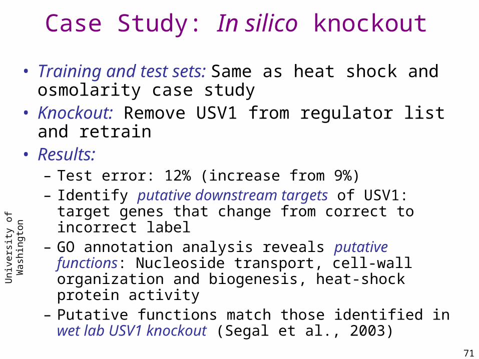
Case Study: In silico knockout

• Training and test sets: Same as heat shock and osmolarity case study

• Knockout: Remove USV1 from regulator list and retrain• Results:

– Test error: 12% (increase from 9%)– Identify putative downstream targets of USV1: target genes

that change from correct to incorrect label– GO annotation analysis reveals putative functions: Nucleoside

transport, cell-wall organization and biogenesis, heat-shock protein activity

– Putative functions match those identified in wet lab USV1 knockout (Segal et al., 2003)

Uni

vers

ity

of W

ashi

ngto

n

72

Conclusions: Gene Regulation

• New predictive model for study of gene regulation– First gene regulation model to make quantitative

predictions. – Using actual expression levels - no clustering.– Strong prediction accuracy on held-out experiments– Interpretable hypotheses: significant regulators,

binding motifs, regulator-motif pairs• New methodology for biological analysis: comparative

training/test studies, in silico knockouts

Uni

vers

ity

of W

ashi

ngto

n

73

Plan of talk

• Boosting• Alternating Decision Trees• Data-mining AT&T transaction logs.• The I/O bottleneck in data-mining.• Resistance of boosting to over-fitting.• Confidence rated prediction.• Confidence-rating for object recognition.• Gene regulation modeling.• Summary

Uni

vers

ity

of W

ashi

ngto

n

74

Summary

• Moving from density estimation to classification can make hard problems tractable.

• Boosting is an efficient and flexible method for constructing complex and accurate classifiers.

• I/O is the main bottleneck to data-mining– Sampling, data localization and parallelization help.

• Correlation -> Causation : still a hard problem, requires domain specific expertise and integration of data sources.

Uni

vers

ity

of W

ashi

ngto

n

75

Future work

• New applications: – Bio-informatics.– Vision / Speech and signal processing.– Information Retrieval and Information Extraction.

• Theory:– Improving the robustness of learning algorithms.– Utilization of unlabeled examples in confidence-rated

classification.– Sequential experimental design. – Relationships between learning algorithms and

stochastic differential equations.

Uni

vers

ity

of W

ashi

ngto

n

76

Extra

Uni

vers

ity

of W

ashi

ngto

n

77

Plan of talk

• Boosting• Alternating Decision Trees• Data-mining AT&T transaction logs.• The I/O bottleneck in data-mining.• High-energy physics.• . Resistance of boosting to over-fitting.• Confidence rated prediction.• Confidence-rating for object recognition.• Gene regulation modeling.• Summary

Uni

vers

ity

of W

ashi

ngto

n

78

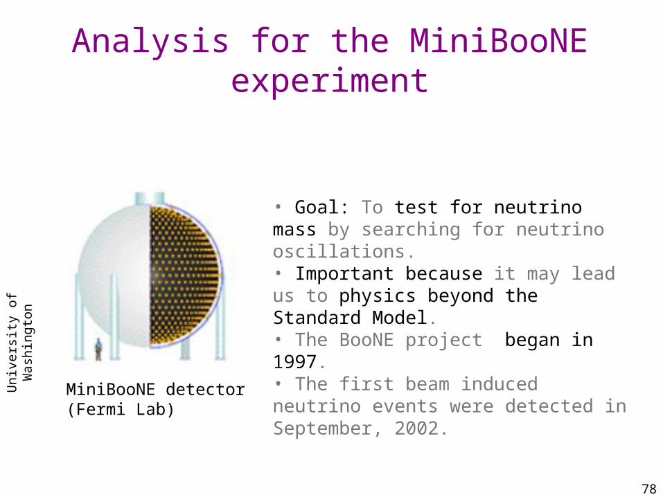
Analysis for the MiniBooNE experiment

• Goal: To test for neutrino mass by searching for neutrino oscillations. • Important because it may lead us to physics beyond the Standard Model. • The BooNE project began in 1997. • The first beam induced neutrino events were detected in September, 2002.

MiniBooNE detector(Fermi Lab)

Uni

vers

ity

of W

ashi

ngto

n

79

SimulationOf

MiniBooNEDetector

Reconstruction

Feature Vector(52 Reals)

52 inputs

26 Hidden

Neural Network

€

x > θ

€

ν e

Other

no

yes

Ion Stancu. UC Riverside

MiniBooNE Classification Task

Uni

vers

ity

of W

ashi

ngto

n

80

Uni

vers

ity

of W

ashi

ngto

n

81

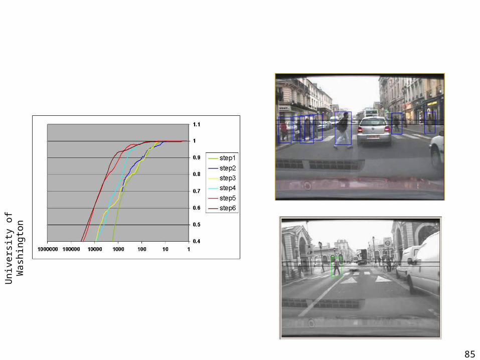
Results

Uni

vers

ity

of W

ashi

ngto

n

82

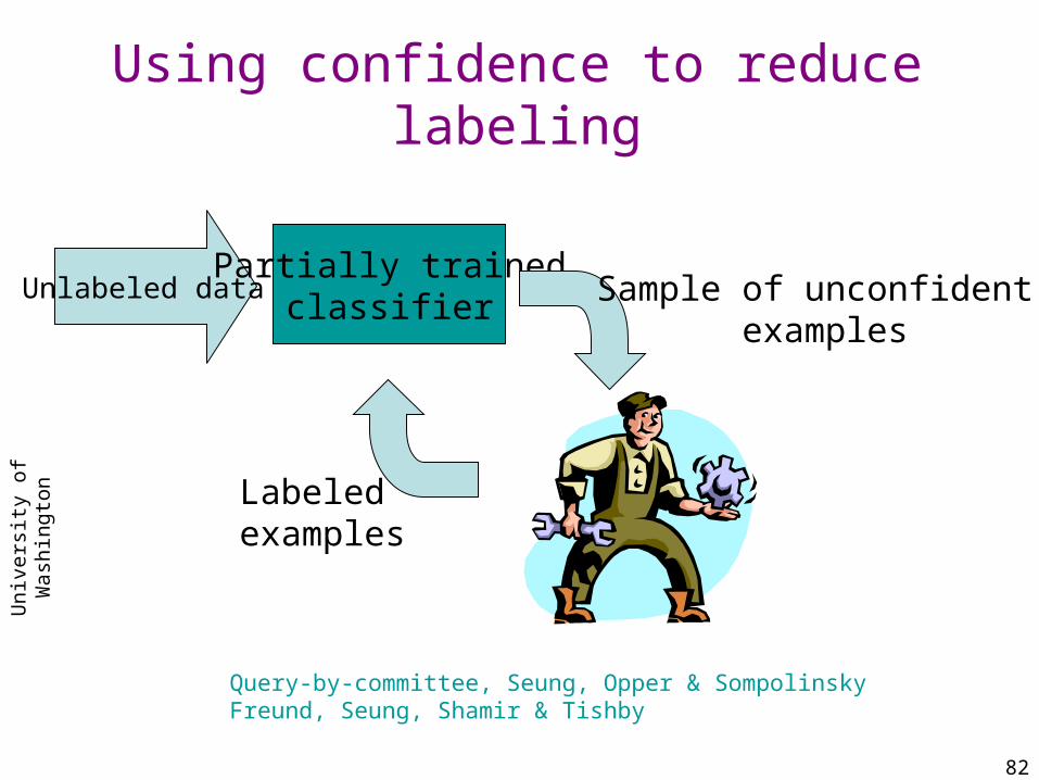
Using confidence to reduce labeling

Unlabeled dataPartially trained

classifier Sample of unconfident examples

Labeledexamples

Query-by-committee, Seung, Opper & SompolinskyFreund, Seung, Shamir & Tishby

Uni

vers

ity

of W

ashi

ngto

n

83

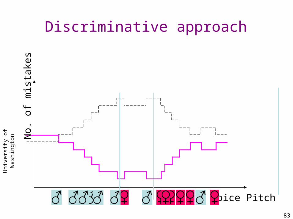
Discriminative approach

Voice Pitch

No.

of

mis

take

s

Uni

vers

ity

of W

ashi

ngto

n

84

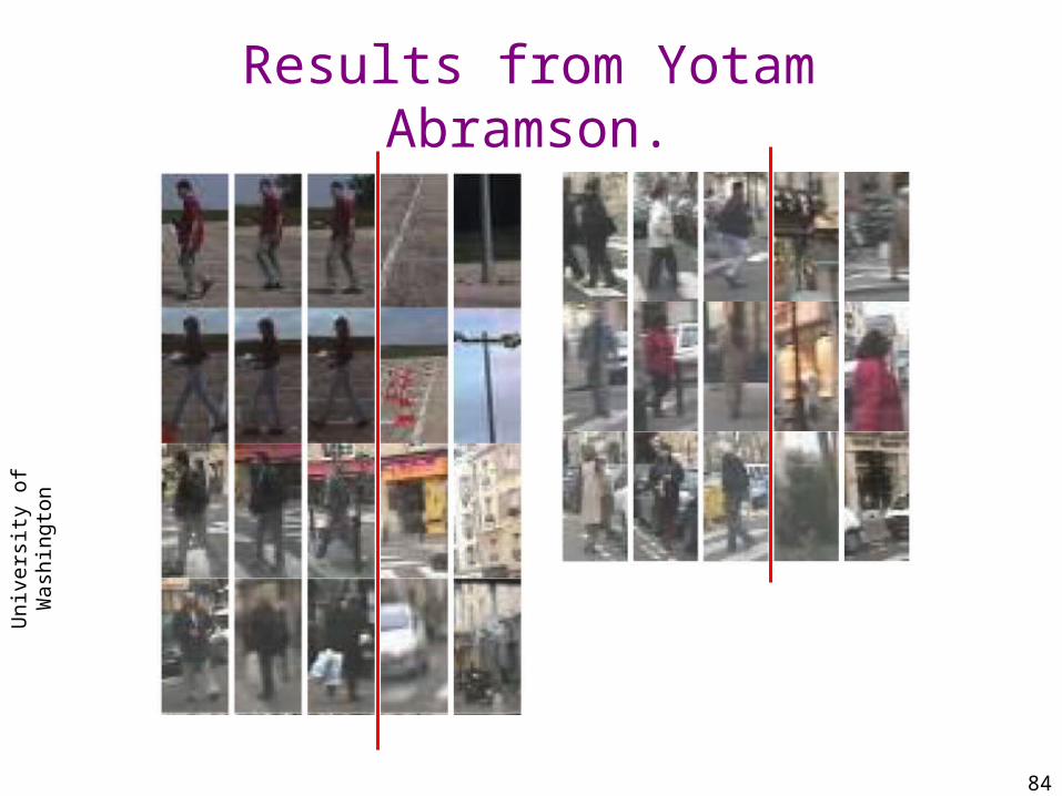
Results from Yotam Abramson.

Uni

vers

ity

of W

ashi

ngto

n

85