UNIVERSITY OF TROMSØ cruise report - Oceanoceanrep.geomar.de/20595/1/ECO2 cruise report UiT 2011 v2.pdfACKNOWLEDGEMENT ... long and one 75-m long section with a total of 14 streamers

1 NO-9037 Tromsø • [email protected] • http://uit.no • Switchboard: (+47) 77 64 40 00 • Fax: (+47) 77 64 49 00 Department of Geology • Phone 77 64 44 09 • Fax 77 64 56 00

Date: August 31, 2011

UNIVERSITY OF TROMSØ cruise report

Tromsø – Longyearbyen 01-07-11 to 14-07-11

R/V Helmer Hanssen

PART I

Sub-seabed CO2 Storage: Impact on Marine Ecosystems (ECO2) (A 7th Framework Programme EU project)

Institutt for Geologi, Dramsveien 201 Universitetet i Tromsø

Stefan Bünz (chief scientist)

2

Table of Contents

PARTICIPANT LIST ................................................................................................................ 3

INTRODUCTION AND OBJECTIVES ................................................................................... 4

SEISMIC METHODS ................................................................................................................ 6

The P-Cable 3D seismic system ............................................................................................. 6

Multi-component ocean bottom seismometer (OBS) ............................................................. 7

CTD and water sampling ........................................................................................................ 9

PRELIMINARY RESULTS .................................................................................................... 10

Swath bathymetry onboard processing ................................................................................ 10

P-Cable 3D seismic onboard QC and processing ................................................................. 12

NARRATIVE OF THE CRUISE ............................................................................................. 17

ACKNOWLEDGEMENT ....................................................................................................... 18

APPENDIX .............................................................................................................................. 19

CTD stations ......................................................................................................................... 19

OBS Stations ........................................................................................................................ 19

3D seismic line log ............................................................................................................... 20

3

PARTICIPANT LIST

Stefan Bünz (chief scientist)

University of Tromsø, Norway

Alexandros Tasianas


Sunil Vadakkepuliyambatta


Sergey Polyanov


Steinar Iversen University of Tromsø, Norway

Bjørn Runar Olsen University of Tromsø, Norway

Andre Frantzen Jensen


Espen Bergø


Ola Eriksen

P-Cable AS, Oslo, Norway

Dan Shehan

Geometrics, San Jose, USA

Antonio M.Calafat Frau

University of Barcelona, Spain

Joan Anton Salvadó i Estivill

IDAEA-CSIC, Spain

Marco Lo Martire

Polytechnic University of Marche, Ancona, Italy

Leonardo Langone

CNR-ISMAR, Bologna, Italy

Sánchez Vidal, Anna

University of Barcelona, Spain

Oriol Veres Cucurella University of Barcelona, Spain

Stephane Kunesch

CEFREM, Perpignan, France

Urvashi Keswani

Indian Institute of Technology Roorkee, India

Nivita Sehgal

Indian Institute of Technology Roorkee, India

4

INTRODUCTION AND OBJECTIVES

The ECO2 project sets out to assess the risks associated with the storage of CO2 below the

seabed. Carbon Capture and Storage (CCS) is regarded as a key technology for the reduction

of CO2 emissions from power plants and other sources at the European and international

level. The EU will hence support a selected portfolio of demonstration projects to promote, at

industrial scale, the implementation of CCS in Europe. Several of these projects aim to store

CO2 below the seabed. However, little is known about the short-term and long-term impacts

of CO2 storage on marine ecosystems even though CO2 has been stored sub-seabed in the

North Sea (Sleipner) for over 13 years and for one year in the Barents Sea (Snøhvit). Against

this background, the proposed ECO2 project will assess the likelihood of leakage and impact

of leakage on marine ecosystems. In order to do so ECO2 will study a sub-seabed storage site

in operation since 1996 (Sleipner, 90 m water depth), a recently opened site (Snøhvit, 2008,

330 m water depth), and a potential storage site located in the Polish sector of the Baltic Sea

(B3 field site, 80 m water depth) covering the major geological settings to be used for the

storage of CO2. Novel monitoring techniques will be applied to detect and quantify the fluxes

of formation fluids, natural gas, and CO2 from storage sites and to develop appropriate and

effective monitoring strategies. Field work at storage sites will be supported by modelling and

laboratory experiments and complemented by process and monitoring studies at natural CO2

seeps that serve as analogues for potential CO2 leaks at storage sites.

As part of the ECO2 project, the University of Tromsø committed to conduct a cruise to the

Snøhvit area in the SW Barents Sea (Figure 1). The main objective of the R/V Helmer

Hanssen cruise was to acquire high-resolution baseline data in order to determine geofluid

pathways and sites of gas hydrate formations and better understand fluid leakage mechanism

in the subsurface. Moreover, gas hydrates and shallow gas reservoirs are sites that are

potentially important for our understanding of natural methane storage and release systems.

Among the data sets to be acquired is high-resolution P-Cable 3D seismic data, a potential

novel technology for monitoring fluid migration in the subsurface. Furthermore, we will

acquire high-resolution bathymetric data and ocean-bottom seismic (OBS) data.

Many fluid and gas anomalies exists in the SW Barents Sea, particularly at the border

between the Polheim sub-platform, Loppa High and Hammerfest basin, where the Snøhvit

reservoir and storage site study area is located (Figure 1). The working areas are in approx.

300 – 400 m water depths. The Snøhvit hydrocarbon field has been operated by Statoil since

2008. The reservoir lies in Jurassic sandstones at about 2 km depth. Beneath the reservoir

formation, CO2 is stored in Triassic sediments of the Tubaen formation and later in the

bottom part of the Jurassic Stø formation. At Snøhvit, the analysis of conventional 3D seismic

data resulted in the definition of stratigraphic boundaries of the overburden structure and the

identification of faults, gas chimneys and shallow gas accumulations including the potential

occurrence of a gas-hydrate related bottom-simulating reflection (Figure 1). Faults both at the

Jurassic and Tertiary levels have been interpreted.

5

Figure 1: (top) Overview and location of the study area in the SW Barents Sea. (bottom) Perspective

view of the Snøhvit study area based on conventional 3D seismic data. The Main reservoir is in the

Jurassic Stø formation, whereas the CO2 is stored beneath in the Triassic Tubaen formation. The

shallow subsurface shows many amplitude anomalies that can be related to the presence of shallow

gas and gas hydrates.

6

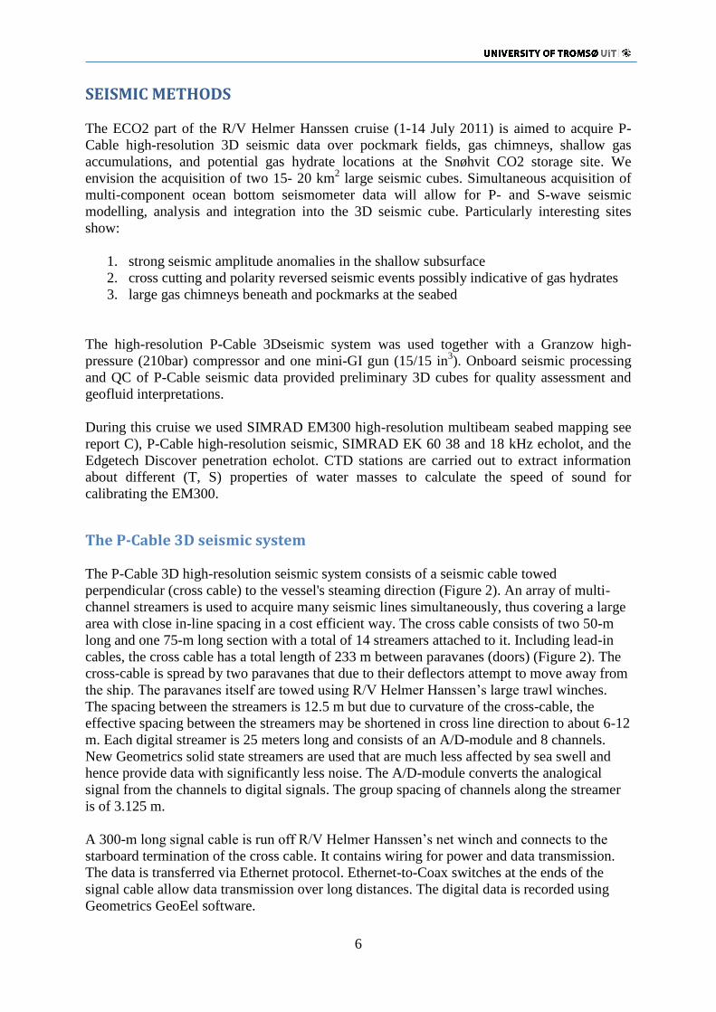
SEISMIC METHODS

The ECO2 part of the R/V Helmer Hanssen cruise (1-14 July 2011) is aimed to acquire P-

Cable high-resolution 3D seismic data over pockmark fields, gas chimneys, shallow gas

accumulations, and potential gas hydrate locations at the Snøhvit CO2 storage site. We

envision the acquisition of two 15- 20 km2 large seismic cubes. Simultaneous acquisition of

multi-component ocean bottom seismometer data will allow for P- and S-wave seismic

modelling, analysis and integration into the 3D seismic cube. Particularly interesting sites

show:

1. strong seismic amplitude anomalies in the shallow subsurface

2. cross cutting and polarity reversed seismic events possibly indicative of gas hydrates

3. large gas chimneys beneath and pockmarks at the seabed

The high-resolution P-Cable 3Dseismic system was used together with a Granzow high-

pressure (210bar) compressor and one mini-GI gun (15/15 in3). Onboard seismic processing

and QC of P-Cable seismic data provided preliminary 3D cubes for quality assessment and

geofluid interpretations.

During this cruise we used SIMRAD EM300 high-resolution multibeam seabed mapping see

report C), P-Cable high-resolution seismic, SIMRAD EK 60 38 and 18 kHz echolot, and the

Edgetech Discover penetration echolot. CTD stations are carried out to extract information

about different (T, S) properties of water masses to calculate the speed of sound for

calibrating the EM300.

The P-Cable 3D seismic system

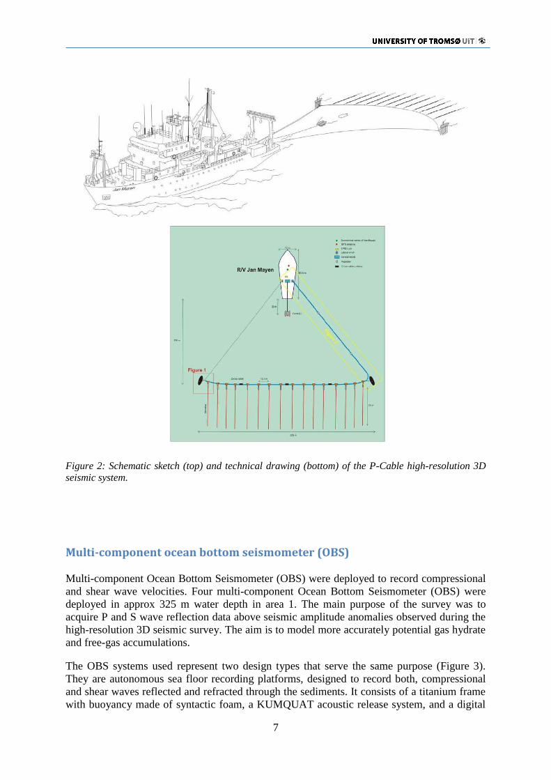
The P-Cable 3D high-resolution seismic system consists of a seismic cable towed

perpendicular (cross cable) to the vessel's steaming direction (Figure 2). An array of multi-

channel streamers is used to acquire many seismic lines simultaneously, thus covering a large

area with close in-line spacing in a cost efficient way. The cross cable consists of two 50-m

long and one 75-m long section with a total of 14 streamers attached to it. Including lead-in

cables, the cross cable has a total length of 233 m between paravanes (doors) (Figure 2). The

cross-cable is spread by two paravanes that due to their deflectors attempt to move away from

the ship. The paravanes itself are towed using R/V Helmer Hanssen’s large trawl winches.

The spacing between the streamers is 12.5 m but due to curvature of the cross-cable, the

effective spacing between the streamers may be shortened in cross line direction to about 6-12

m. Each digital streamer is 25 meters long and consists of an A/D-module and 8 channels.

New Geometrics solid state streamers are used that are much less affected by sea swell and

hence provide data with significantly less noise. The A/D-module converts the analogical

signal from the channels to digital signals. The group spacing of channels along the streamer

is of 3.125 m.

A 300-m long signal cable is run off R/V Helmer Hanssen’s net winch and connects to the

starboard termination of the cross cable. It contains wiring for power and data transmission.

The data is transferred via Ethernet protocol. Ethernet-to-Coax switches at the ends of the

signal cable allow data transmission over long distances. The digital data is recorded using

Geometrics GeoEel software.

7

Figure 2: Schematic sketch (top) and technical drawing (bottom) of the P-Cable high-resolution 3D

seismic system.

Multi-component ocean bottom seismometer (OBS) Multi-component Ocean Bottom Seismometer (OBS) were deployed to record compressional

and shear wave velocities. Four multi-component Ocean Bottom Seismometer (OBS) were

deployed in approx 325 m water depth in area 1. The main purpose of the survey was to

acquire P and S wave reflection data above seismic amplitude anomalies observed during the

high-resolution 3D seismic survey. The aim is to model more accurately potential gas hydrate

and free-gas accumulations.

The OBS systems used represent two design types that serve the same purpose (Figure 3).

They are autonomous sea floor recording platforms, designed to record both, compressional

and shear waves reflected and refracted through the sediments. It consists of a titanium frame

with buoyancy made of syntactic foam, a KUMQUAT acoustic release system, and a digital

8

data recorder in a separate pressure case1. A hydrophone and a 3-component geophone are

used to record the seismic wavefield. The Tromsø OBS has a 4.5 Hz geophone attached.

While the hydrophone is fixed to the frame of the OBS, the geophone is detached from it.

This design insures that the geophone is mechanically decoupled from the frame, to avoid

noise generated by the frame being recorded by the geophone. The whole system is rated for a

water depth of up to 6000 m.

The OBS is attached to a ground weight via the acoustic release system, to make it sink to the

sea floor after deployment. When the seismic experiment is completed, the OBS is released

from its ground weight by sending an acoustic code and it rises to the sea surface by its

buoyancy.

Flag

Swimming line with small float

Hydrophone

Registration Unit

Radio Transmitter

0.00.1

0.20.30.40.5 m

Hydrophone for the

Acoustic Release

Anchor Weight

Strobe

Acoustic Release

Release system for geohone

Geophone

Buoyancy

Figure 3: The old (bottom) and the new (top) Ocean Bottom Seismometer (OBS) system (UiT).

The OBS systems were prepared and programmed prior to deployment. The first channel

records the hydrophone data, while channel two, three and four are connected to horizontal

and vertical components of the geophone. The locations were selected based on seismic

anomalies in the conventional 3D seismic data. The station list is given in the appendix and

the positions of the OBS on the seafloor in area 1 is indicated in Figure 4.

9

CTD and water sampling

Conductivity-Temperature-Depth (CTD) is the oceanographer’s standard tool for determining oceanic

water masses. SeaBird’s (SBE) 911plus CTD was used for oceanographic measurements. Apart from

the standard temperature, conductivity and pressure (converted to depth), speed of sound, fluorescence

and turbidity can also be measured. A Rosette allows for the collection of up to 12 water samples per

CTD cast.

The temperature sensor is located at the base of the Rosette, thereby being the first sensor to measure

the undisturbed water mass on the downcast. Furthermore, water is pumped through a conductivity

tube, in which seawater conductivity is measured. Continuous pump operation is essential to prevent

boundary layers forming on the tube’s edges, and should data sets indicate fault malfunctions the data

sets are flagged or deleted. CTD data was acquired and processed using SBE’s in-house “SBE Data

Processing”.

10

PRELIMINARY RESULTS

Acquired data was processed onboard for Quality control and preliminary interpretations. This

included the multibeam and 3D seismic data. OBS data processing is more demanding and will be

done after the cruise.

Swath bathymetry onboard processing

Introduction

Swath bathymetry data were collected in the two survey areas during the cruise to the Snøhvit field in

the SW Barents Sea (Figure 1). Mapping of the seafloor in the study areas were carried out with a hull-

mounted, motion-compensated Kongsberg Simrad EM300 system. Both study areas cover an area of

approximately 3 x 10 km (Figures 4 and 5). The water depth in study areas ranges from 310 to 355 m.

Processing of bathymetric data

Line statistics showed that the raw depth data had a good quality, only the outer beams had somewhat

higher noise level. Kongsberg-Simrad Neptune software was used for processing of bathymetric data.

The processing of bathymetric data consisted of statistical data cleaning, what was done block by

block in BinStat. This function ensures an adaptive way of filtering and taking changes in the seabed

terrain into account. Both areas were divided into several blocks. The basic role for blocks was putting

a noise limit 2 and a STD limit 2. Noise limit 2 means that all depths with a distance from the plane

larger than 2/100 * mean depth of the cell were rejected. Furthermore, STD limit is most common

filtering parameter, and means that all depths with a distance from the plane larger than 2 * mean STD

were rejected. In addition, raw data were also cleaned manually with the ping graphic editor to

improve the accuracy on the depth data. After processing, the bathymetry data sets were exported from

Neptune as a 3-column XYZ ASCII file (Easting, Northing, depth) with positive depth values based

on a mean water datum. The XYZ bathymetry was gridded in the interactive visualization system

Fledermaus. Aweighted-moving average gridding type was chosen with weight diameter set to 3

(Fledermaus- Reference manual 2007). The good density of measurement point allowed a grid cell

size of 5 m x 5 m.

Morphological features interpretation

More or less linear and sinuous features are observed almost everywhere on the seafloor in both areas

(Figures 4 and 5). They are furrows with a small rise on both sides. The furrows are several km long

and up 400 m wide, but most of furrows are 1-2 km long and up to 100 m wide. They have a U-shape

in a vertical profile and their shape is slightly smooth. Their depths range between 3 and 5 m. The

dominant furrow orientation is ENE - WSW but the direction varies greatly. In some cases, the

furrows cross-cut each other and at the end point, the furrows create a headwall. Those features were

interpreted to be iceberg ploughmarks. Iceberg ploughmarks are formed when the keel of an iceberg is

exceeding the water depth and erodes soft sediments. Ploughmarks indicate that the region has been

influenced by glacial processes and are evidence of iceberg activity.

The seafloor in area 1 shows hundreds of small and a few large depressions (Figure 5). These

depression are typical expressions of fluid escape through the seafloor and are called pockmarks. Our

initial interpretation show two different pockmarks classes: hundreds of small pockmarks with

diameters of up to 20 m and depth of up to 1 m, and very few large pockmarks with diameters of up

700 m and depth of up to 10 m. Hydro-acoustic surveying did not detect any indications for gas

leakage from the seafloor. Further thorough interpretation of this data set and integration with the P-

Cable 3D and conventional 3D seismic data will commence after the processing on the latter has been

finalized.

11

Figure 4: Seafloor map of the multibeam data acquired in area 1 with a zoomed.in section of three

large pockmarks and a depth profile across them. OBS positions are indicated in the top map.

Figure 5: Seafloor map of the multibeam data acquired in area 2 with a zoomed.in section of the

largest ploughmark and a depth profile across it.

12

P-Cable 3D seismic onboard QC and processing

This report describes the onboard QC and processing of the 3D seismic data acquired with the P-Cable

system on board the R/V Helmer Hanssen. A geographical map of the working area is shown in

Figures 1. During this cruise data for two different 3D cubes were acquired and processed.

Area 1: We accomplished 31 planned seismic lines. Projected spacing between lines was 60 m

resulting in a block with an coverage of approximately 8 x 2 km (Figure 6). The block was

acquired over an area with few large and hundreds of small pockmarks, and a clinoform

system in the subsurface that shows multiple high-amplitude anomalies (Figures 7).

Area 2: Also here, we accomplished 30 planned seismic lines. Spacing between lines remained 60 m

resulting in a block with an coverage of approximately 8 x 2 km (Figure 8). The block was

acquired over an area that partly covers a large acoustic masking zone and BSR occurrence

interpreted to be related to a gas chimneys that might connect with the reservoir and storage

formations (Figure 9).

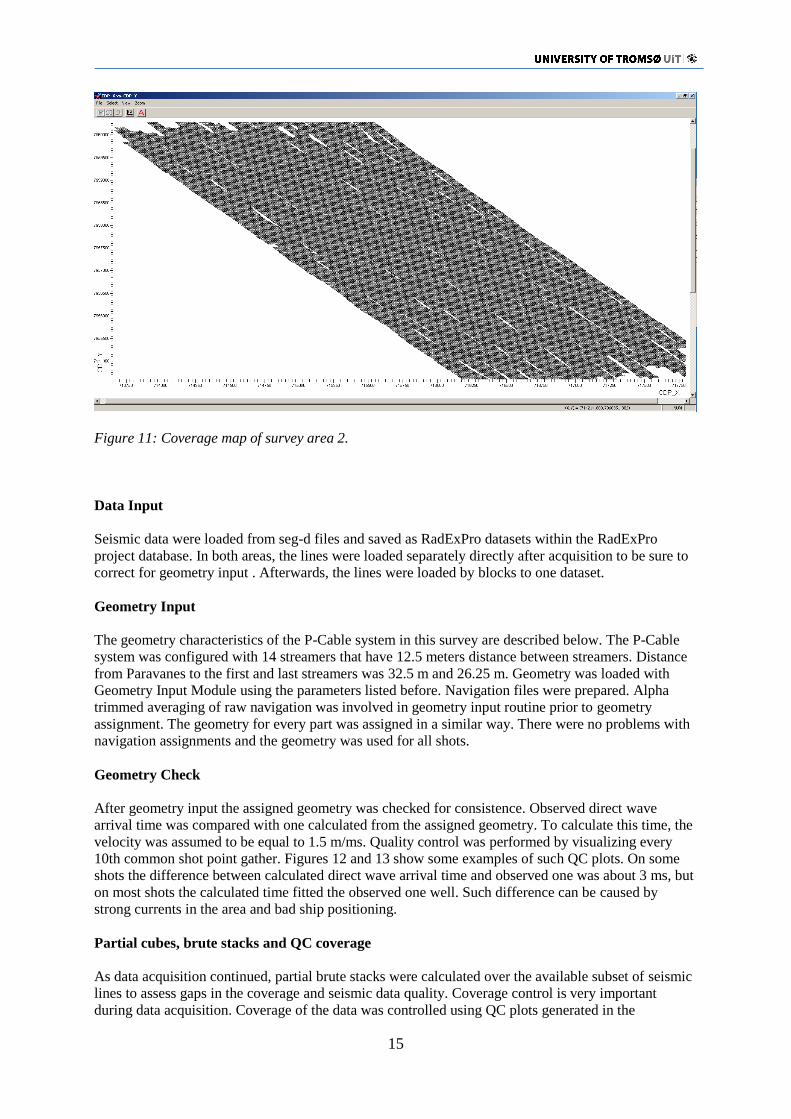
The CDP coverage for both areas is shown on Figures 10 and 11. As one can see there are some small

gaps in final coverage of both areas, bur particularly in area 2. A good coverage depends on ship

navigation and line tracking. In few instances the ship was off the planned line by up to 20 m, which

results in the gaps. However, these gaps mostly are only one bin size wide and thus, can be easily

infilled during processing. The navigation file processing and checking as well as data input, geometry

assignment and further data QC and processing are reported for both areas. The QC procedures and

seismic data processing were performed in the RadExPro Plus software. Brute stack cubes were

generated for both areas to assess the quality of the seismic data.

Figure 6: Seafloor map (Courtesy of Statoil) of parts of the Snøhvit area showing several hundreds of

small pockmarks. The blue box indicates the location of the P-Cable 3D seismic survey 1. Green

circles indicate location of OBS.

13

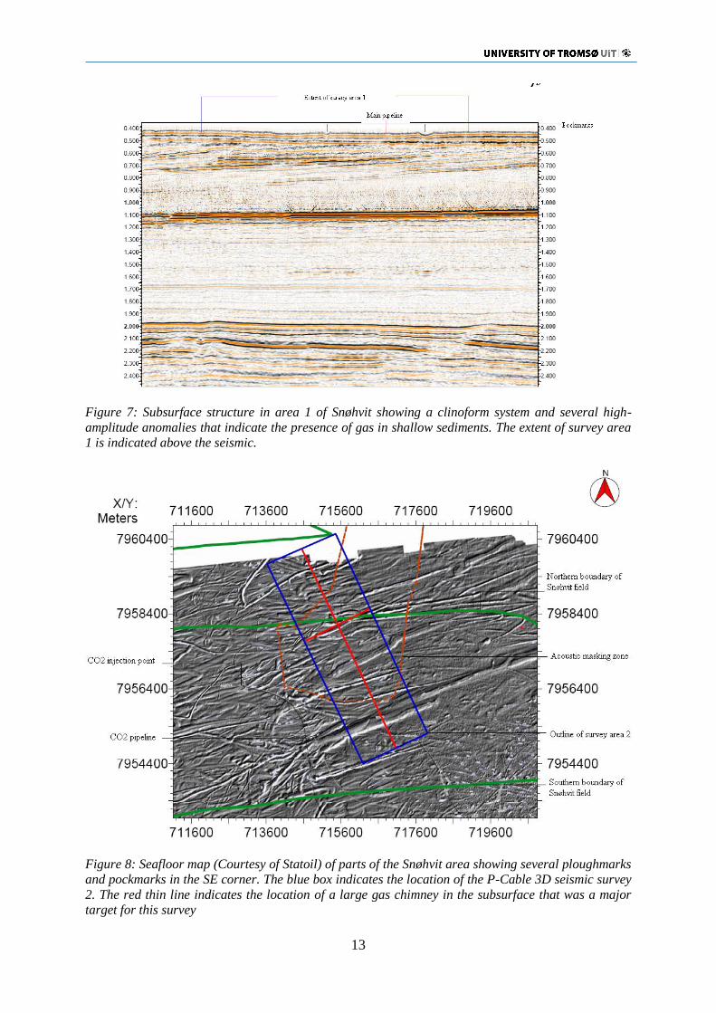
Figure 7: Subsurface structure in area 1 of Snøhvit showing a clinoform system and several high-

amplitude anomalies that indicate the presence of gas in shallow sediments. The extent of survey area

1 is indicated above the seismic.

Figure 8: Seafloor map (Courtesy of Statoil) of parts of the Snøhvit area showing several ploughmarks

and pockmarks in the SE corner. The blue box indicates the location of the P-Cable 3D seismic survey

2. The red thin line indicates the location of a large gas chimney in the subsurface that was a major

target for this survey

14

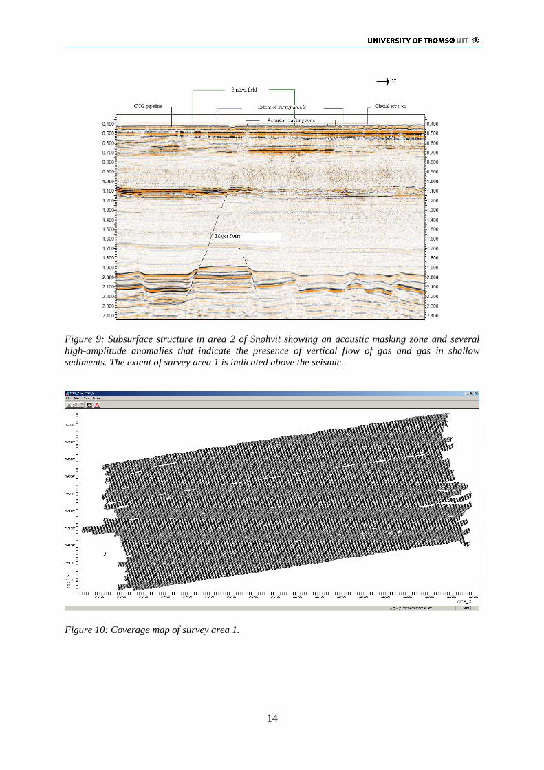
Figure 9: Subsurface structure in area 2 of Snøhvit showing an acoustic masking zone and several

high-amplitude anomalies that indicate the presence of vertical flow of gas and gas in shallow

sediments. The extent of survey area 1 is indicated above the seismic.

Figure 10: Coverage map of survey area 1.

15

Figure 11: Coverage map of survey area 2.

Data Input

Seismic data were loaded from seg-d files and saved as RadExPro datasets within the RadExPro

project database. In both areas, the lines were loaded separately directly after acquisition to be sure to

correct for geometry input . Afterwards, the lines were loaded by blocks to one dataset.

Geometry Input

The geometry characteristics of the P-Cable system in this survey are described below. The P-Cable

system was configured with 14 streamers that have 12.5 meters distance between streamers. Distance

from Paravanes to the first and last streamers was 32.5 m and 26.25 m. Geometry was loaded with

Geometry Input Module using the parameters listed before. Navigation files were prepared. Alpha

trimmed averaging of raw navigation was involved in geometry input routine prior to geometry

assignment. The geometry for every part was assigned in a similar way. There were no problems with

navigation assignments and the geometry was used for all shots.

Geometry Check

After geometry input the assigned geometry was checked for consistence. Observed direct wave

arrival time was compared with one calculated from the assigned geometry. To calculate this time, the

velocity was assumed to be equal to 1.5 m/ms. Quality control was performed by visualizing every

10th common shot point gather. Figures 12 and 13 show some examples of such QC plots. On some

shots the difference between calculated direct wave arrival time and observed one was about 3 ms, but

on most shots the calculated time fitted the observed one well. Such difference can be caused by

strong currents in the area and bad ship positioning.

Partial cubes, brute stacks and QC coverage

As data acquisition continued, partial brute stacks were calculated over the available subset of seismic

lines to assess gaps in the coverage and seismic data quality. Coverage control is very important

during data acquisition. Coverage of the data was controlled using QC plots generated in the

16

RadExPro. Locations of CDP points were displayed in the 3D CDP Binning tool. At the end of each

area coverage plots were made for all lines (figures ), and a brute stack cube for each area was

generated. The seismic data quality is generally very good. However, several additional processing

steps need to be run in the post-processing before the final version of the data is ready. These include,

tide and residual statics corrections, amplitude corrections, filtering and migration.

Figure 12: Geometry check plot with direct wave arrival and predicted theoretical arrival time (red

line).

Figure 13: Geometry check plot with direct wave arrival and predicted theoretical arrival time (red

line).

17

NARRATIVE OF THE CRUISE

Times in this report are given in local time (local time -2 hrs = UTC), 3D seismic data are

logged in UTC time and ship logs are given in UTC time. The weather for most of the cruise

provides a calm sea (Bft <3), fog and grey skies. Air temperatures were between 5 oC and 12 oC. During the cruise, five systems HighRes 3D reflection seismic, SIMRAD EM300 swath

bathymetry, CHIRP subbottom profiler, EK 60 38 and 18 kHz fishfinder, and GPS Navigation

are working parallel. In addition, OBS systems were deployed once in the Snøhvit area. We

started to prepare the cruise in Tromsø on July 1 with loading and assembling all seismic

equipment.

Friday, 01.07.

The scientific crew arrived during the morning hours. We started to load all equipment

onboard the ship. After the compressor container was lifted onboard we began assembling the

seismic equipment. The signal cable was spooled on one of Jan Mayens large winches. The

new cross cable was spooled on University of Tromsø’s versatile winch. Electronics and

computers for seismic data acquisition is set up in the laboratory. Loading and assembling

lasted until 1 hour after midnight.

Saturday, 02.07.

01:00 Departure from Tromsø heading north to the Snøhvit area.

09:00: During the transit to the working area, the OBS systems are prepared.

13:30 Arrival at the Snøhvit area. The cross cable has been modified to provide better

balance. However, the cross cable has not been operated after these modification and

therefore, further balancing is required.

15:00: The first deployment of the cross cable is without streamers and floatation are only

connected at the tri-point connections. The depth readings show that the cable is dipping

between 1 – 3 m beneath the sea surface. The desired cable depth is 1 m and hence we

connect three more floatation along the cross cable.

18:00: Another deployment test showed that the depth is now stable between 0,9 – 1,3 m,

which we deem acceptable given weather conditions and hydrodynamic nature of the cross

able.

19:30 We acquire a CTD cast in 314 m water depth.

22:00 The OBS seismographs are being synchronized and a last check is run.

23:00 OBS release systems are set up and mounted on the OBS frame.

Sunday, 03.07.

00:30 All OBS systems are ready for deployment.

01:10 OBS 1 deployed.

01:30 OBS 2 deployed



02:30 The P-cable system is prepared for deployment with streamers. 16 drop-lead-digitizer-

streamer assemblies are set up for a quick and efficient deployment operation.

03:00 We start to deploy the P-cable.

04:15 The system is in the water but there is leakage along the cable. Test showed that it is

most likely related to streamer 10.

05:00 The system is back on deck and we replace streamer assembly no. 10 with a spare one.

05:30 Another deployment operation starts.

18

06:30 The P-Cable system is in the water and working properly. We are running some pre-

survey test and configuration checks.

07:14 3D seismic line 1 starts.

12:02 Shortly before lunch we have completed line 4. Everything is working fine. The

weather is cloudy with light winds and waves of 0.5 m.

23:59 As the days ends we have almost finished line 14.

Monday, 04.07.

00:26 Line 15 starts.

02:00 A Statoil operated vessel is in the area and is doing inspections of seafloor installations.

Good communication assures that both survey vessels do not interfere with each other.

10:30 Shut down Geoeel (at shot 16861 on line 23) due to problems with triggers and leakage

on SPSU. Guns are being brought in for problems with the towing point. The cross cable was

also brought in for inspection of the signal cable attachment point. Modifications to the gun

array are required. We also identify a leaking streamer and replace it.

11:00 While maintenance work is going on, we decide to recover the OBS.

12:05 OBS 1 recovered.


14:10 OBS 3 recovered-


17:00 Maintenance work has finished and we start to deploy again.

18:22 We start again on line 23.

23:59 Acquiring line 27 as the day ends.

Tuesday, 05.07.

07:30 The last line of the first 3D seismic cube has just finished. The P-Cable system will stay

in the water as we slowly steam to the nearby area 2.

08:09 Line 1 in area 2 starts. Unchanged weather conditions provide relatively good

conditions for acquisition of 3D seismic data.

23:59 We are on line 14 as the day comes to an end

Wednesday, 06.07.

20:00 The last line (no 30) has just finished and we are recovering the P-Cable system.

22:00: Work at Snøhvit is concluded and we are heading towards working area 2 on the upper

continental slope of the SW-Barents Sea.

Thursday, 14.07.

09:00: Arrival in Longyearbyen. End of cruise.

ACKNOWLEDGEMENT

We thank the captain and his crew of R/V Helmer Hanssen of the University of Tromsø for

their excellent support during the 3D and multicomponent seismic survey. We are grateful to

the ECO2 project, a Collaborative Project funded under the European Commission's

Framework Seven Programme Topic OCEAN.2010.3 Sub-seabed carbon storage and the

marine environment, project number 265847 for providing financial support to carry out this

cruise to the SW Barents Sea.

19

APPENDIX

CTD stations

Date Time StationNr Latitude Longitude Depth

[m]

02.07.2011 19:41:58 294 71 38.71932 N 020 52.74085 E 313,94

OBS Stations

OBS

station

Deployment sites

Date / Time Longitude Latitude

1 02.07.2011 / 21 09.798’E 71 33.968’N

2 02.07.2011 / 21 11.856’E 71 33.961’N

3 02.07.2011 / 21 13.546’E 71 33.953’N

4 02.07.2011 / 21 17.460’E 71 33.939’N

20

3D seismic line log

Expedition: P-Cable Juli 2011 Survey: Snøhvit area 1. – Sheet #: 1 -

Times are UTC

3D line

number:

Date:

Start - end

Time (UTC):

Start - end

Shot point number

First - last

Shot point number

when crossing

planned start and

end of line

Comments

(sailing direction, ship speed, depth sensor, wind speed, air

temperature downtime, etc.)

1 03.07.11 05.14 – 06.19 710 -1481 784 - 1432

14 streamers, 2 x 30 cu in mini G guns. Speed: 4.3

kn, Heading: 93 deg., Wind: 4.5m/s 302 deg.,

Temp: 7.3 deg C

2 03.07.11 06.30 - 07.31 syst.

06.36 – 07.26 line 1482 - 2179 1525 - 2129


kn, Heading: 274 deg., Wind: 7.5 m/s 317 deg.,

Temp: 7.3 deg C

3 03.07.11 07.45 – 08.54 syst.

07.53 –08.50 line 2180 - 3000 2274 - 2949



Temp: 7.7 deg C

4 03.07.11 09.06– 10.06 syst.

09.09 – 10.02 line 3001 - 3723 3035 - 3677



Temp: 7.6 deg C

5 03.07.11 10.18 – 11.17 syst.

10.21 – 11.13 line 3724 - 4430 3765 - 4392



Temp: 8.1 deg C

6 03.07.11 11.27 – 12.34 syst.

11.31 – 12.30 line 4431 - 5228 4469 - 5183



Temp: 7.7 deg C

7 03.07.11 12.50 – 13.48 syst

12.51 – 13.45 line 5229 - 5931 5243 - 5893



Temp: 8.1 deg C

21

8 03.07.11 14.02 – 15.02 syst

14.05 – 14.58 line 5932 - 6649 5963 - 6608



Temp: 7.8 deg C

9

03.07.11

15.17 – 16.14 syst

15.18 – 16.11 line 6650 - 7340 6667 - 7303



Temp: 7.5 deg C

10 03.07.11 16.23 – 17.21 syst

16.27 – 17.18 line 7341 - 8040 7392 - 8003



Temp: 7.5 deg C

11 03.07.11 17.36 – 18. 32 syst

17.36– 18.30 line 8041 - 8702 8041 - 8676



Temp: 7.5 deg C

12 03.07.11 18.41 – 19.40 syst

18.45 – 19.38 line 8703 - 9410 8739 - 9377



Temp: 7.6 deg C

13 03.07.11 19.56 – 20.57 syst

19.59 – 20.55 line 9411 - 10141 9451 - 10114



Temp: 7.8 deg C

14 03.07.11 21.08 – 22.09 syst

21.11 – 22.06 line 10142 - 10865 10181 - 10840



Temp: 7.6 deg C

15 03.07.11 22.26 – 23.28 syst

22.29 – 23.24 line 10868 - 11607 10904 - 11558



Temp: 7.6 deg C

16 03.07.11 -

04.07.11

23.38 – 00.43 syst

23.43 – 00.39 line 11608 - 12380 11662 -12341



Temp: 7.6 deg C

22

17 04.07.11 00.55 – 01.51 syst

00.59 – 01.49 line 12381 - 13051 12421 - 13023



Temp: 7.1 deg C

18 04.07.11 02.06 – 03.08 syst

02.08 – 03.03 line 13052 - 13797 13083 - 13743



Temp: 7.3 deg C

19 04.07.11 03.22 – 04.21 syst

03.25 – 04.17 line 13798 - 14507 13833 - 14463



Temp: 7.6 deg C

20 04.07.11 04.38 – 05.36 syst

04.40 – 05.34 line 14508 - 15233 14531 - 15208



Temp: 7.3 deg C. Gather window show some noise

at end of line (channel 57) between shot 15095 and

15205 no noise in noise window.

21 04.07.11 05.55 – 06.50 syst

05.57 – 06.48 line 15234 - 15906 15259 - 15876



Temp: 7.8 deg C.

22 04.07.11 07.07 – 08.05 syst

07.10 – 08.03 line 15907 -16632 15942 - 16600



Temp: 7.5 deg C.

23 04.07.11 08.25 – syst

08.28 – line 16633 - 16663 -



Temp: 7.4 deg C.

Shut down geoeel (at shot 16861) due to problems

with triggers and leakage on SPSU.

24 04.07.11 10.00 – 10.15 syst

10.05 – line 17156 - 17337 17229 -

Guns are being brought in for problems with the

towing point. The cross cable was also brought in

for inspection of the signal cable attachment point.

23a 04.07.11 16.22 – 17.18 syst

16.24 – 17.16 line 17338 - 18009 17363 - 17998



Temp: 7.0 deg C. Reshot of line 23

23

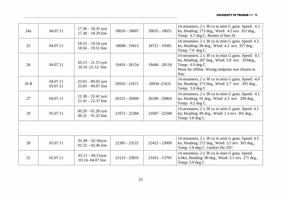
24a 04.07.11 17.36 – 18.32 syst

17.38 – 18.29 line 18010 - 18687 18035 - 18651



Temp: 6.7 deg C. Reshot of line 24

25 04.07.11 18.53 – 19.54 syst

18.56 – 19.51 line 18688 - 19415 18721 - 19381



Temp: 7.0 deg C.

26 04.07.11 20.13 – 21.15 syst

20.16 -21.12 line 19416 - 20154 19446 - 20118


kn, Heading: 267 deg., Wind: 5.0 m/s 333deg.,

Temp: 6.9 deg C.

Went far offline. Wrong endpoint was chosen in

Nav.

26 B 04.07.11

05.07.11

23.03 – 00.03 syst

23.05 – 00.07 line 20910 - 21671 20934 -21631



Temp: 5.8 deg C

27 04.07.11 21.38 – 22.41 syst

21.41 – 22.37 line 20155 - 20909 20189 - 20864



Temp: 6.2 deg C.

29 05.07.11 00.29 – 01.28 syst

00.31 – 01.25 line 21672 - 22384 21697 - 22348



Temp: 5.8 deg C.

28 05.07.11 01.49 – 02.50syst

01.52 – 02.46 line 22385 - 23122 22422 - 23069



Temp: 5.8 deg C. GeoEel file 29!!

31 05.07.11 03.11 – 04.11syst

03.14 -04.07 line 23123 - 23835 23161 - 13795

14 streamers, 2 x 30 cu in mini G guns. Speed:

4.0kn, Heading: 90 deg., Wind: 3.1 m/s 271 deg.,

Temp: 5.9 deg C

24

30 05.07.11 04.32 – 05.31syst

04.35 – 05.29 line 23836 - 24535 23867 - 24519

14 streamers, 2 x 30 cu in mini G guns. Speed:

4.1kn, Heading: 270 deg., Wind: 4.2 m/s 272 deg.,

Temp: 5.8 deg C

End Area 1

25

Start Area 2

3D line

number:

Date:

Start - end

Time (UTC):

Start - end

Shot point number

First - last

Shot point number

when crossing

planned start and

end of line

Comments

(sailing direction, ship speed, depth sensor, wind speed, air

temperature downtime, etc.)

1 05.07.11 06.09 – 7.03 syst

06.10 – 7.00 line 41 - 688 57 - 655



Temp: 6.2 deg C

2 05.07.11 07.38 – 08.33 syst

07.41 – 08.31 line 689 - 1340 717 - 1313



Temp: 6.6 deg C

3 05.07.11 08.55 – 09.50 syst

08.58 – 09.47 line 1341 - 2006 1376 - 1970



Temp: 7.9 deg C

4 05.07.11 10.36 – 11.28 syst

10.39 – 11.25 line 2007 -2633 2031 - 2590



Temp: 6.6 deg C (gun moved 20-25M further back)

5 05.07.11 11.46 – 12.39 syst

11.48 – 12.36 line 2634 - 3268 2652 - 3229



Temp: 6.6 deg C

6 05.07.11 12.59- 13.49 syst

13.01-13.36 line 3269-3857 3270-3840



Temp: 7.2 deg C

7 05.07.11 13.57 – 14.51 syst

13.58 – 14.50 line 3858-4420 3867 - 4404



Temp: 7.5 deg C

26

8 05.07.11 15.10 - 16.00syst

15.12 - 15.58 line 4421-5010 4446-4988



Temp: 7.4 deg C

9 05.07.11 16.12 – 17.05 syst

16.14 – 17.01 line 5011-5647 5037-5605



Temp: 7.7deg C

10 05.07.11 17.17– 18.10 syst

17.21 – 18.06 line 5648-6280 5690-6233



Temp: 7.0deg C (Missed few shots before file no.

5722)

11 05.07.11 18.22 – 19.16 syst

18.25 – 19.12 line 6281 - 6932 6317 -6878



Temp: 7.0deg C

12 05.07.11 19.28 – 20.22 syst

19.31 – 20.19 line 6968 - 7579 6933 - 7538



Temp: 6.7 deg C

13 05.07.11 20.37 – 21.30 syst

20.37 – 21.27 line 7580 - 8203 7580 - 8167



Temp: 6.3 deg C (System started right when ship

started line)

14 05.07.11 21.45 – 22.38 syst

21. 47– 22.34 line 8204 - 8825 8211 - 8781



Temp: 6.5 deg C (off course until line 8290)

15 05.07.11 22.49 – 23.44 syst

22.51 – 23.41 line 8826 - 9482 8850 - 9442



Temp: 5.9 deg C

16 05.07.11

06.07.11

23.59 – 00.48 syst

00.01 – 00.46 line 9483 - 10069 9514 - 10050



Temp: 6.9 deg C

27

17 06.07.11 01.02 – 02.00 syst

01.04 – 01.55line 10070 - 10768 10095 - 10703



Temp: 6.9 deg C

18 06.07.11 02.14 – 03.05 syst

02.16 – 03.03 line 10769 - 11375 10787 - 11353



Temp: 6.0 deg C

19 06.07.11 03.21 – 04.12 syst

03.23 – 04.10 line 11376 - 11982 11396 - 11961



Temp: 6.1 deg C

20 06.07.11 04.29 – 05.19 syst

04.30 – 05.16 line 11983 - 12579 11988 - 12541



Temp: 6.3 deg C

21 06.07.11 05.36 – 06.25 syst

05.36 – 06.23 line 12580 - 13172 12588 -13141



Temp: 6.2 deg C

22 06.07.11 06.47 – 07.42 syst

06.52 – 07.38 line 13173 - 13829 13228 - 13779



Temp: 6.1 deg C

23 06.07.11 08.00 – 09.00 syst

08.03– 08.56 line 13830 - 14546 13863 - 14502



Temp: 6.2 deg C

24 06.07.11 09.25 – 10.19 syst

09.28– 10.15 line 14547 - 15180 14580 - 15142



Temp: 6.3 deg C

25 06.07.11 10.36 – 11.36 syst

10.40 – 11.31 line 15181 - 15899 15231 - 15844



Temp: 6.6 deg C

26 06.07.11 12.01 – 12.51 syst

12.04 – 12.49 line 15900 - 16501 15935-16483



Temp: 6.4 deg C (30 meters off planned line during

28

some shots around file.no 15998)

27 06.07.11 13.09 – 14.02syst

13.12 – 13.59 line 16502 - 17144 16537 - 17104



Temp: 6.3 deg

28 06.07.11 14.25 –15.18 syst

14.28 – 15.16 line 17145- 17774 17182 - 17759



Temp: 7.1 deg

29 06.07.11 15.39 – 16.33 syst

15.40 – 16.31 line 17775 - 18418 17794 - 18394


kn, Heading: 347 deg., Wind: 9 m/s 272 deg.,

Temp: 6.8 deg

30 06.07.11 16.58 – 17.49 syst

16.59 – 17.48 line 18419 – 19035 18430 - 19020



Temp: 6.2 deg. Last line

End Area 2

Documents

UNIVERSITY OF TROMSØ cruise report - Oceanoceanrep.geomar.de/20595/1/ECO2 cruise report UiT 2011 v2.pdfACKNOWLEDGEMENT ... long and one 75-m long section with a total of 14 streamers