Embed Size (px)
Citation preview
University of Texas at Austin Petrophysical and Well-Log Simulator (3D UTAPWeLS)
Introduction User Guide __________________________________________________
Table of Contents Introduction to Version 4 of 3D UTAPWeLS ........................................................................................................................... 1
Main Window drop-down menus ............................................................................................................................................. 1 File Menu ............................................................................................................................................................................. 1
Settings Menu ...................................................................................................................................................................... 2
Help Menu ........................................................................................................................................................................... 3
Main Window Short-cut Icons ................................................................................................................................................. 5
Adding a well ....................................................................................................................................................................... 5
Changing Well Name ....................................................................................................................................................... 6 Well Interpreter drop down menus .......................................................................................................................................... 6
Loading a log into 3D UTAPWeLS .......................................................................................................................................... 9
Loading a LAS log file .......................................................................................................................................................... 9
Importing a DLIS file into 3D UTAPWeLS ......................................................................................................................... 10
Displaying log header ........................................................................................................................................................ 11
CSF: Wells, log sets and logs ............................................................................................................................................ 12 Working with the Track .......................................................................................................................................................... 13
Modeling and Focus Intervals............................................................................................................................................ 13
Track Editor ....................................................................................................................................................................... 14
Track editing tools ............................................................................................................................................................. 14
Displaying log .................................................................................................................................................................... 14 Example of a displayed log ................................................................................................................................................ 15
Track Display Editor .......................................................................................................................................................... 16
Mask and minor grid comparison ................................................................................................................................... 16
Well Interpreter overall view .................................................................................................................................................. 17
1
Introduction to Version 4 of 3D UTAPWeLS. The University of Texas at Austin Petrophysical and Well-Log Simulator
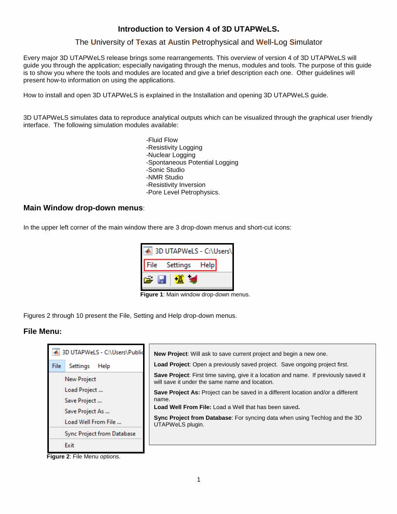
Every major 3D UTAPWeLS release brings some rearrangements. This overview of version 4 of 3D UTAPWeLS will guide you through the application; especially navigating through the menus, modules and tools. The purpose of this guide is to show you where the tools and modules are located and give a brief description each one. Other guidelines will present how-to information on using the applications. How to install and open 3D UTAPWeLS is explained in the Installation and opening 3D UTAPWeLS guide. 3D UTAPWeLS simulates data to reproduce analytical outputs which can be visualized through the graphical user friendly interface. The following simulation modules available:
-Fluid Flow -Resistivity Logging -Nuclear Logging -Spontaneous Potential Logging -Sonic Studio -NMR Studio -Resistivity Inversion -Pore Level Petrophysics.
Main Window drop-down menus:
In the upper left corner of the main window there are 3 drop-down menus and short-cut icons:
Figure 1: Main window drop-down menus.
Figures 2 through 10 present the File, Setting and Help drop-down menus. File Menu:
Figure 2: File Menu options.
New Project: Will ask to save current project and begin a new one.
Load Project: Open a previously saved project. Save ongoing project first.
Save Project: First time saving, give it a location and name. If previously saved it will save it under the same name and location.
Save Project As: Project can be saved in a different location and/or a different name. Load Well From File: Load a Well that has been saved.
Sync Project from Database: For syncing data when using Techlog and the 3D UTAPWeLS plugin.
2
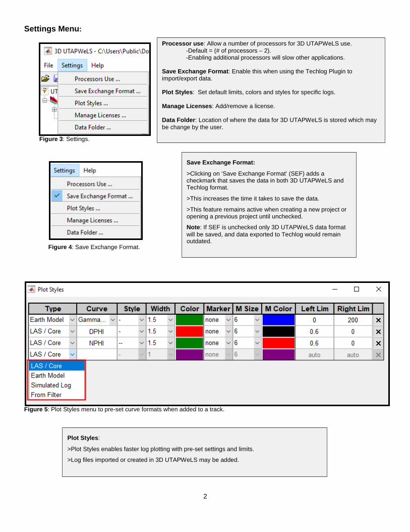
Settings Menu:
Figure 3: Settings.
Figure 4: Save Exchange Format.
Figure 5: Plot Styles menu to pre-set curve formats when added to a track.
Processor use: Allow a number of processors for 3D UTAPWeLS use. -Default = (# of processors – 2). -Enabling additional processors will slow other applications. Save Exchange Format: Enable this when using the Techlog Plugin to import/export data. Plot Styles: Set default limits, colors and styles for specific logs. Manage Licenses: Add/remove a license. Data Folder: Location of where the data for 3D UTAPWeLS is stored which may be change by the user.
Save Exchange Format:
>Clicking on ‘Save Exchange Format’ (SEF) adds a checkmark that saves the data in both 3D UTAPWeLS and Techlog format.
>This increases the time it takes to save the data.
>This feature remains active when creating a new project or opening a previous project until unchecked.
Note: If SEF is unchecked only 3D UTAPWeLS data format will be saved, and data exported to Techlog would remain outdated.
Plot Styles:
>Plot Styles enables faster log plotting with pre-set settings and limits.
>Log files imported or created in 3D UTAPWeLS may be added.

3
Settings Menu (cont.):
Figure 6: Managing licenses.
Figure 7: Data folder location.
Help Menu:
-The following figures relate to the Help pull-down menu followed by additional details for each item, in the box below Figure 11 describes the Help menu items.
Figure 8: Help drop down menu.
License Manager:
>To add a license, open the manager, click on the Add License File button, browse to the license and double click on it.
>To remove a license, open the license manager and highlight the license and click Remove Selected.
Data Folder location: >This folder contains some sample LAS files, and files related to simulations or calculations run through 3D UTAPWeLS. Its location can be changed using the three dots ‘…’ button.
Note: For some users, access to the AppData folder is restricted. Thus it will be necessary to place the Sim Data folder in a different location for UTAPWeLS access to the folder. Using the 3-dot button, browse to a different location to place the data storage folder (e.g. User Documents folder).
User = login name

4
Help Menu (cont.):
Figure 9: Show Log File Path.
Figure 10: Location of installation folder.
Help Menu: Show Log File Path: The file contains a log of the operations that have been performed with 3D UTAPWeLS and may help to determine the cause of a problem.
>If you run into an issue you want to report, click the ‘Show Log File Path’, use Ctrl+C and paste it into Windows Find. Save the file and send it to [email protected].
Show Installation Folder: Location of the software installation. Highlight the path, copy and paste into Windows search. The installation folder contains a logs folder which holds old logs. Logs are saved here when UTAPWeLS is closed.
About: Information about the version of 3D UTAPWeLS, the release date and contact info. Also which MATLAB application or runtime version is being used (Depends upon if the MATLAB-based (MB) or the Stand-alone (SA) version of 3D UTAPWeLS is installed, respectively.)
5
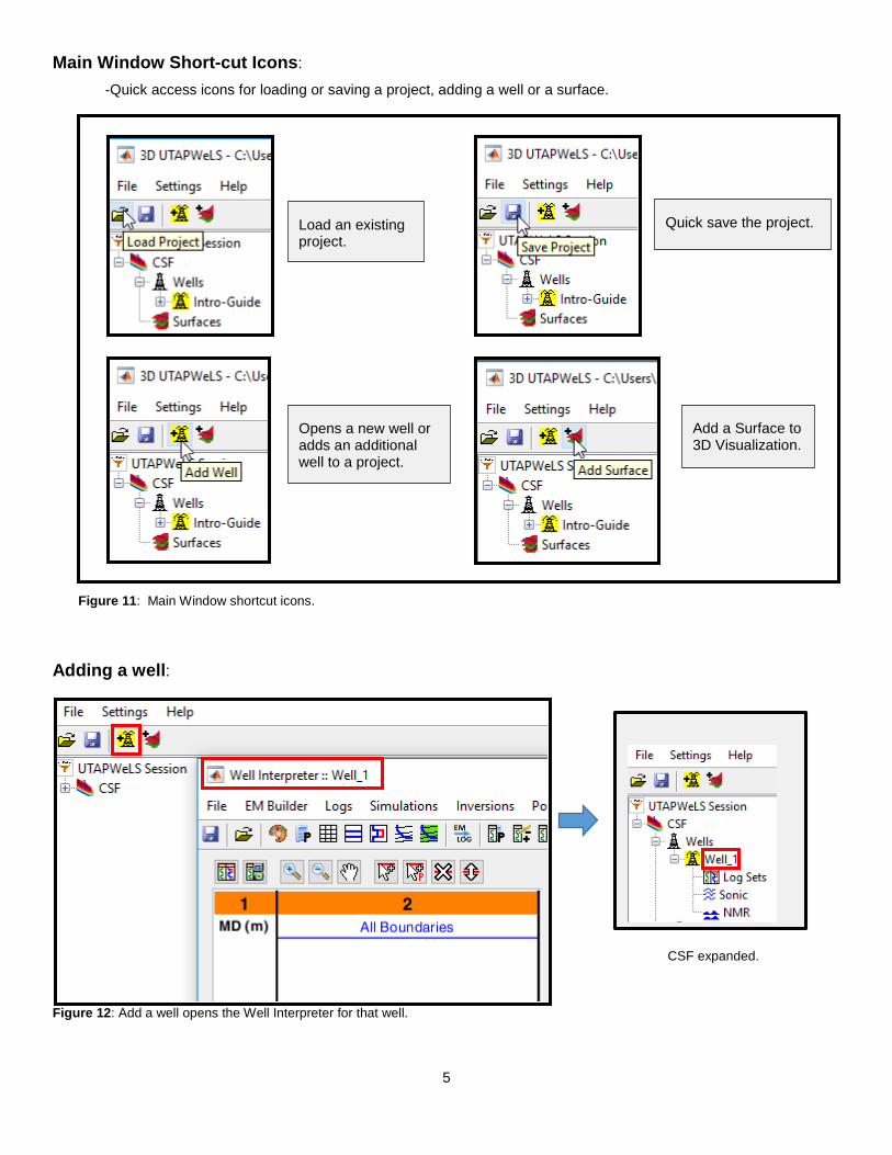
Main Window Short-cut Icons: -Quick access icons for loading or saving a project, adding a well or a surface.
Figure 11: Main Window shortcut icons.
Adding a well:
Figure 12: Add a well opens the Well Interpreter for that well.
Load an existing project.
Quick save the project.
Opens a new well or adds an additional well to a project.
Add a Surface to 3D Visualization.
CSF expanded.

6
Changing Well Name: The name of a well may be changed by right clicking on the well as described in the figures below:
Figure 13: Change well name.
Figure 14: Highlight existing name, rename and click OK.
Figure 15: Name also changes in the Well Interpreter.
Well Interpreter drop down menus:
Figure 16: Associations of the drop-down menus and icons in Well Interpreter. Not all items in drop-down menus have an icon.
>Please note that work is always ongoing to improve 3D UTAPWeLS which may result in changes to the menu selections and icons. >To check if a new version has been released visit the following website: http://faculty.engr.utexas.edu/formation/software.
>To change the well name:
-Right click on well name (i.e. Well_1).
-Open Properties and highlight the name.
-Rename the well and click OK.
7
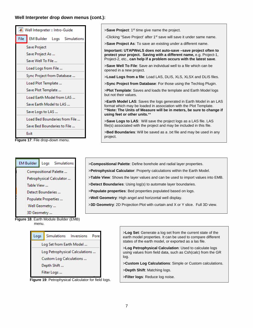
Well Interpreter drop down menus (cont.):
Figure 17: File drop-down menu.
Figure 18: Earth Module Builder (EMB)
menu.
Figure 19: Petrophysical Calculator for field logs.
>Save Project: 1st time give name the project.
-Clicking “Save Project’ after 1st save will save it under same name.
>Save Project As: To save an existing under a different name.
Important: UTAPWeLS does not auto-save –save project often to protect your project. Saving with a different name, e.g. Project-1, Project-2, etc., can help if a problem occurs with the latest save.
>Save Well To File: Save an individual well to a file which can be opened in a new project.
>Load Logs from a file: Load LAS, DLIS, XLS, XLSX and DLIS files.
>Sync Project from Database: For those using the Techlog Plugin.
>Plot Template: Saves and loads the template and Earth Model logs but not their values.
>Earth Model LAS: Saves the logs generated in Earth Model in an LAS format which may be loaded in association with the Plot Template. **Note: The Units of Measure will be in meters, be sure to change if using feet or other units.**
>Save Logs to LAS: Will save the project logs as a LAS file. LAS file(s) associated with the project and may be included in this file.
>Bed Boundaries: Will be saved as a .txt file and may be used in any project.
>Compositional Palette: Define borehole and radial layer properties.
>Petrophysical Calculator: Property calculations within the Earth Model.
>Table View: Shows the layer values and can be used to import values into EMB.
>Detect Boundaries: Using log(s) to automate layer boundaries.
>Populate properties: Bed properties populated based on logs.
>Well Geometry: High angel and horizontal well display.
>3D Geometry: 2D Projection Plot with curtain and X or Y slice. Full 3D view.
>Log Set: Generate a log set from the current state of the earth model properties. It can be used to compare different states of the earth model, or exported as a las file.
>Log Petrophysical Calculation: Used to calculate logs using values from field data, such as Csh(calc) from the GR log.
>Custom Log Calculations: Simple or Custom calculations.
>Depth Shift: Matching logs.
>Filter logs: Reduce log noise.
8
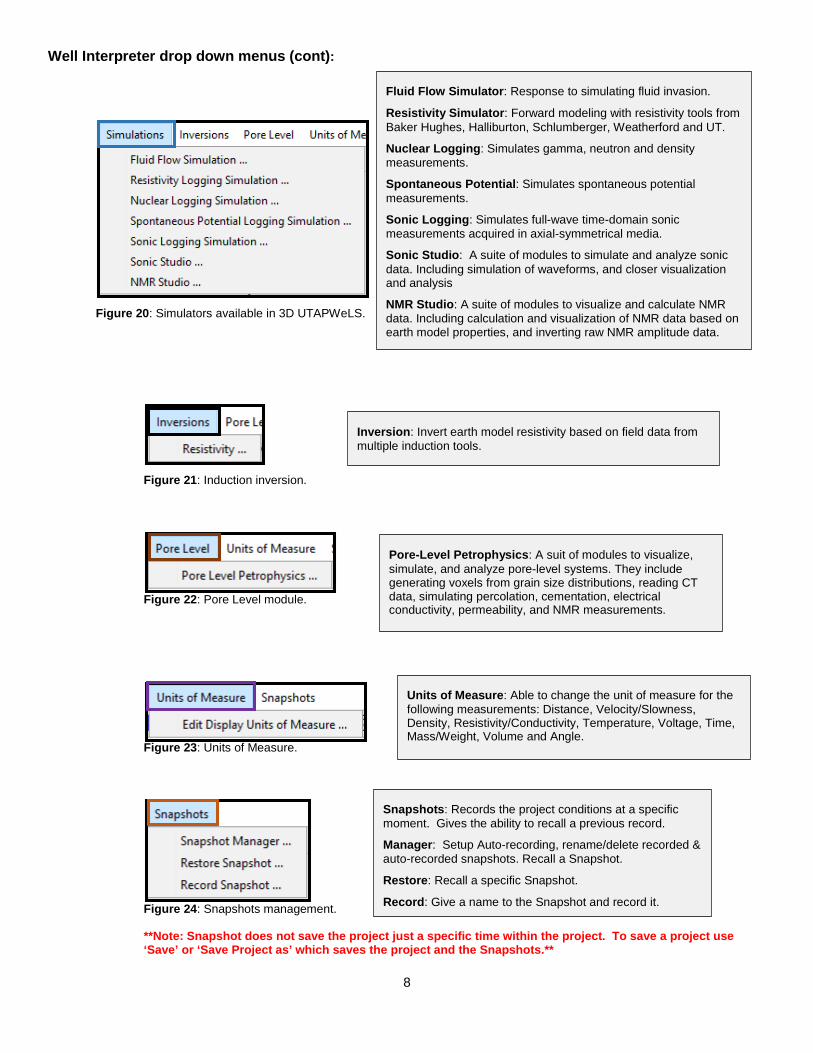
Well Interpreter drop down menus (cont):
Figure 20: Simulators available in 3D UTAPWeLS.
Figure 21: Induction inversion.
Figure 22: Pore Level module.
Figure 23: Units of Measure.
Figure 24: Snapshots management.
**Note: Snapshot does not save the project just a specific time within the project. To save a project use ‘Save’ or ‘Save Project as’ which saves the project and the Snapshots.**
Fluid Flow Simulator: Response to simulating fluid invasion.
Resistivity Simulator: Forward modeling with resistivity tools from Baker Hughes, Halliburton, Schlumberger, Weatherford and UT.
Nuclear Logging: Simulates gamma, neutron and density measurements.
Spontaneous Potential: Simulates spontaneous potential measurements.
Sonic Logging: Simulates full-wave time-domain sonic measurements acquired in axial-symmetrical media.
Sonic Studio: A suite of modules to simulate and analyze sonic data. Including simulation of waveforms, and closer visualization and analysis
NMR Studio: A suite of modules to visualize and calculate NMR data. Including calculation and visualization of NMR data based on earth model properties, and inverting raw NMR amplitude data.
Inversion: Invert earth model resistivity based on field data from multiple induction tools.
Pore-Level Petrophysics: A suit of modules to visualize, simulate, and analyze pore-level systems. They include generating voxels from grain size distributions, reading CT data, simulating percolation, cementation, electrical conductivity, permeability, and NMR measurements.
Units of Measure: Able to change the unit of measure for the following measurements: Distance, Velocity/Slowness, Density, Resistivity/Conductivity, Temperature, Voltage, Time, Mass/Weight, Volume and Angle.
Snapshots: Records the project conditions at a specific moment. Gives the ability to recall a previous record.
Manager: Setup Auto-recording, rename/delete recorded & auto-recorded snapshots. Recall a Snapshot.
Restore: Recall a specific Snapshot.
Record: Give a name to the Snapshot and record it.

9
Loading a log into 3D UTAPWeLS: Loading a LAS log file:
Figure 25: To upload a file into 3D UTAPWeLS by clicking on the ‘Load Logs from File’ icon.
Figure 26: Click on File icon to load a log file.
Figure 27: Importing logs into UTAPWeLS.
In addition to LAS files, DLIS and Core Data Excel (xls & xlsx) files can be imported. The following describes the method to import a DLIS file since it is slightly different than importing a LAS file.
>All logs are checked by default. Uncheck the logs not needed. (A depth log must be imported).
>The file header may be opened to show the header information and logs that will be loaded.
>Click on Import.
>Multiple log files may be loaded into a well.
>Click on the file icon to browse to the file to be loaded.
>Double click on the file and it will be added into the Import window as shown in Figure 33 below.
10
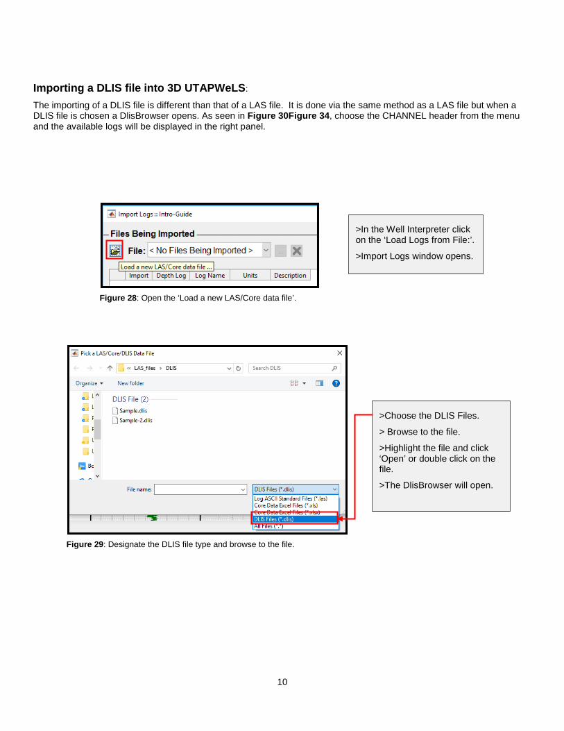
Importing a DLIS file into 3D UTAPWeLS:
The importing of a DLIS file is different than that of a LAS file. It is done via the same method as a LAS file but when a DLIS file is chosen a DlisBrowser opens. As seen in Figure 30Figure 34, choose the CHANNEL header from the menu and the available logs will be displayed in the right panel.
Figure 28: Open the ‘Load a new LAS/Core data file’.
Figure 29: Designate the DLIS file type and browse to the file.
>In the Well Interpreter click on the ‘Load Logs from File:’.
>Import Logs window opens.
>Choose the DLIS Files.
> Browse to the file.
>Highlight the file and click ‘Open’ or double click on the file.
>The DlisBrowser will open.
11
Importing a DLIS file into 3D UTAPWeLS (cont):
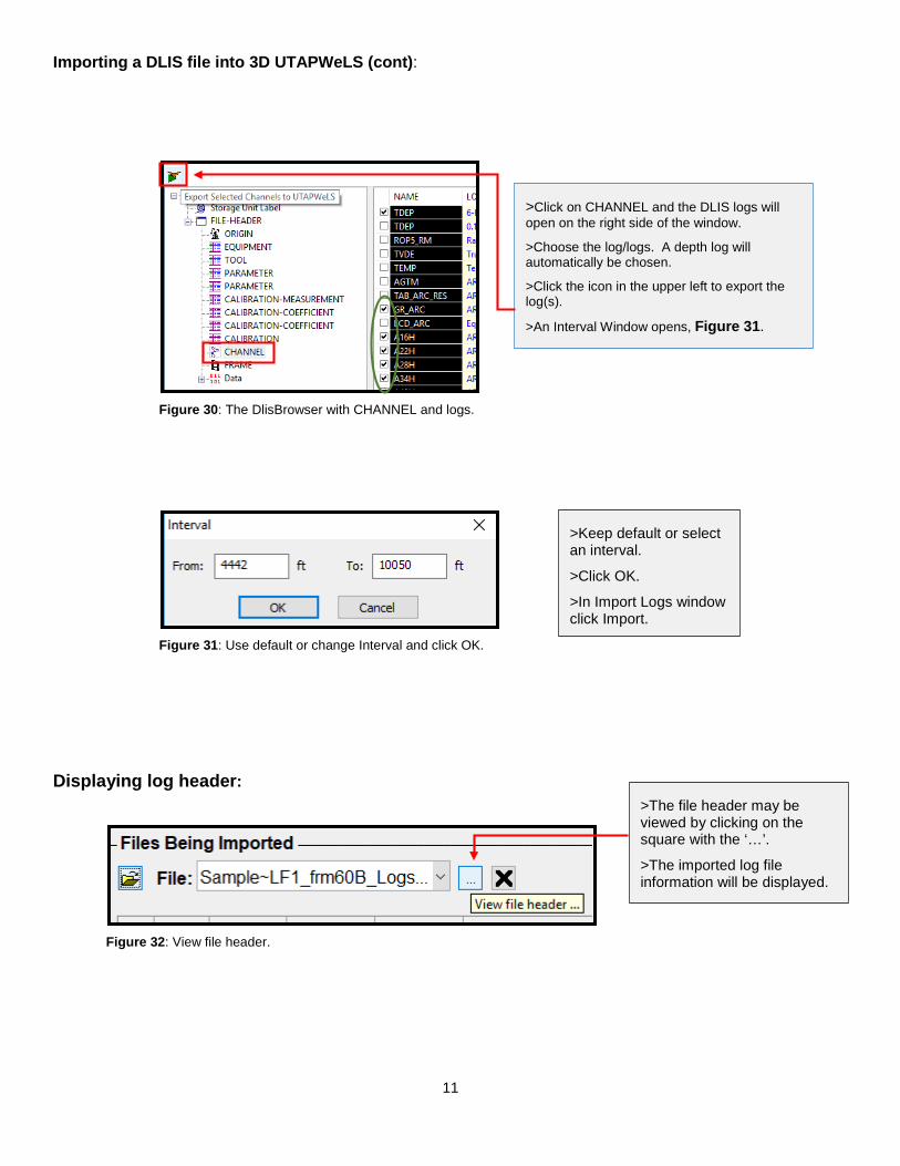
Figure 30: The DlisBrowser with CHANNEL and logs.
Figure 31: Use default or change Interval and click OK.
Displaying log header:
Figure 32: View file header.
>Keep default or select an interval.
>Click OK.
>In Import Logs window click Import.
>Click on CHANNEL and the DLIS logs will open on the right side of the window.
>Choose the log/logs. A depth log will automatically be chosen.
>Click the icon in the upper left to export the log(s).
>An Interval Window opens, Figure 31.
>The file header may be viewed by clicking on the square with the ‘…’.
>The imported log file information will be displayed.
12
CSF: Wells, log sets and logs:
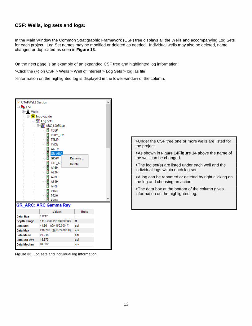
In the Main Window the Common Stratigraphic Framework (CSF) tree displays all the Wells and accompanying Log Sets for each project. Log Set names may be modified or deleted as needed. Individual wells may also be deleted, name changed or duplicated as seen in Figure 13.
On the next page is an example of an expanded CSF tree and highlighted log information:
>Click the (+) on CSF > Wells > Well of interest > Log Sets > log las file
>Information on the highlighted log is displayed in the lower window of the column.
Figure 33: Log sets and individual log information.
>Under the CSF tree one or more wells are listed for the project.
>As shown in Figure 14Figure 14 above the name of the well can be changed.
>The log set(s) are listed under each well and the individual logs within each log set.
>A log can be renamed or deleted by right clicking on the log and choosing an action.
>The data box at the bottom of the column gives information on the highlighted log.

13
Working with the Track:
Figure 34: Log file loaded into 3D UTAPWeLS.
Modeling and Focus Intervals:
A right click on the reference track opens a menu:
Figure 35: Choose Modeling and Focus Intervals.
Figure 36: Selecting the Modeling and Focus Intervals.
>After the log file is loaded into 3D UTAPWeLS, the GR log, if available, is displayed in the Reference Panel.
>A double left click in the Track opens Track Editor, see Figure 37. A double left click
within the track will open the Track Editor
> Modeling Interval: Area defined where the simulations run.
-Can be set by UTAPWeLS or user.
> Focus Interval: Change in size/view of the logs.
-Can be set by UTAPWeLS or user.

14
Working with the Track (cont.): Track Editor:
Figure 37: Track Editor window, ‘All Boundaries’ is default display plot.
Track editing tools:
Log Numeric Image Tool VDL
Shade NMR Sonic Vert. x-sect. STC
Figure 38: Track editing tools.
Use the editing tools to add a log, add shade, add numeric log values, results from NMR simulations, images, sonic waves, sonic tool simulated shot depth, create vertical cross-sections from fluid-flow results, variable-density log and slowness travel time coherence.
Displaying log:
Figure 39: Add log(s) to Track and how displayed.
>In the Track Editor one can:
-Add Tracks (also in drop down menu).
-Add log(s).
-Choose Linear or Logarithmic scale.
> Figure 38 below identifies additional tools.
>Log display values:
-Type: From a loaded file, Earth Model or simulated.
-Set: Which Log Set to use.
-Curve: Which log to display.
-Limits: Range of scale.
-Style: Solid line, dashed, etc.
-Width: Of the log displayed.
-Color: Variety to choose from.
-Marker: Used with some logs.
Add or modify Plot Styles, see Figure 5.
15
Example of a displayed log:
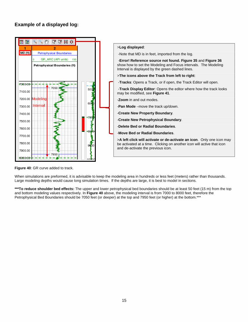
Figure 40: GR curve added to track.
When simulations are preformed, it is advisable to keep the modeling area in hundreds or less feet (meters) rather than thousands. Large modeling depths would cause long simulation times. If the depths are large, it is best to model in sections.
***To reduce shoulder bed effects: The upper and lower petrophysical bed boundaries should be at least 50 feet (15 m) from the top and bottom modeling values respectively. In Figure 40 above, the modeling interval is from 7000 to 8000 feet, therefore the Petrophysical Bed Boundaries should be 7050 feet (or deeper) at the top and 7950 feet (or higher) at the bottom.***
>Log displayed:
-Note that MD is in feet, imported from the log.
-Error! Reference source not found. Figure 35 and Figure 36 show how to set the Modeling and Focus intervals. The Modeling Interval is displayed by the green dashed lines.
>The icons above the Track from left to right:
-Tracks: Opens a Track, or if open, the Track Editor will open.
-Track Display Editor: Opens the editor where how the track looks may be modified, see Figure 41.
-Zoom in and out modes.
-Pan Mode –move the track up/down.
-Create New Property Boundary.
-Create New Petrophysical Boundary.
-Delete Bed or Radial Boundaries.
-Move Bed or Radial Boundaries.
>A left click will activate or de-activate an icon. Only one icon may be activated at a time. Clicking on another icon will active that icon and de-activate the previous icon.
Modeling
Interval

16
Track Display Editor:
Using the Track Display Editor enables some customization to the look of the tracks (style, font size, color etc.) and more.
Figure 41: Track Display Editor -modify the look of the track.
Mask and minor grid comparison:
Figure 42: Comparison with and without mask and minor grid.
>The Track Display Editor enables visual changes to the track:
-Compact or Expanded header view.
-Different font sizes.
-Show Track Titles/Numbers – unchecked removes the top bar.
-Change Text and Bar colors.
-Cursor Lines: Show/not show, different styles, color and width.
-Changing color of Modeling Lines.
-Highlight Layer: When Palette open.
-Track Header: highlight and color.
-Mask Depths: Level 1 – 100000; Number of digits shown and mask character. See Figure 42 below.
-Minor Grid: Display additional grid lines between the major grids. See Figure 42 below.
17
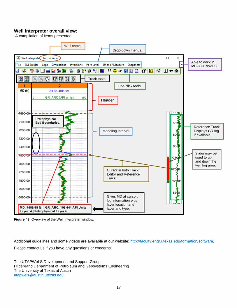
Well Interpreter overall view: -A compilation of items presented.
Figure 43: Overview of the Well Interpreter window.
Additional guidelines and some videos are available at our website: http://faculty.engr.utexas.edu/formation/software.
Please contact us if you have any questions or concerns.
The UTAPWeLS Development and Support Group Hildebrand Department of Petroleum and Geosystems Engineering The University of Texas at Austin [email protected]
Well name. Drop-down menus.
One-click tools.
Able to dock in MB-UTAPWeLS.
Gives MD at cursor, log information plus layer location and layer and type.
Reference Track Displays GR log if available.
Slider may be used to up and down the well log area.
Track tools.
Petrophysical Bed Boundaries.
Modeling Interval
Cursor in both Track Editor and Reference Track.
Header