University of Southern Queensland · University of Southern Queensland ... 50 kW Eddy Current brake50 kW Eddy Current ... Chapter 6 Chapter 6 –––– THE UPGRADED SYSTEM …

i

University of Southern Queensland

Faculty of Engineering & Surveying

50 kW Eddy Current brake50 kW Eddy Current brake50 kW Eddy Current brake50 kW Eddy Current brake

A dissertation submitted by

Rudolph Edouard Bavarin

in fulfilment of the requirements of

Courses ENG4111 and ENG4112 Research Project

Towards the degree of

Bachelor of Engineering (Electrical & Electronic)

Submitted: October, 2006

ii

ABSTRACT

The project involves the refurbishment of the “Heenan-dynamometer” located

underneath S block at the University of Southern Queensland.

The current system does not allow any computerized data acquisition. Upgrading

the electronic control unit using solid state power electronic devices will enable

users to perform better tests on engines and in the near future, it will allow the user

to acquire digital data via a computer.

The actual dynamometer control unit uses valve technology to rectify the AC

source and control the system output. The upgraded system will perform the same

operation however is will use solid state devices. In order to use the new system on

the dynamometer, a protective circuit based on pre-established conditions has

been designed.

iii


Faculty of Engineering and Surveying

ENG4111 & ENG4112 Research Project

Limitations of Use

The Council of tThe Council of tThe Council of tThe Council of the University of Southern Queensland, its Faculty of Engineering he University of Southern Queensland, its Faculty of Engineering he University of Southern Queensland, its Faculty of Engineering he University of Southern Queensland, its Faculty of Engineering and Surveying, and the staff of the University of Southern Queensland, do not and Surveying, and the staff of the University of Southern Queensland, do not and Surveying, and the staff of the University of Southern Queensland, do not and Surveying, and the staff of the University of Southern Queensland, do not accept any responsibility for the truth, accuracy or completeness of material accept any responsibility for the truth, accuracy or completeness of material accept any responsibility for the truth, accuracy or completeness of material accept any responsibility for the truth, accuracy or completeness of material contained within or associated withcontained within or associated withcontained within or associated withcontained within or associated with this dissertation. this dissertation. this dissertation. this dissertation. Persons using all or any part of this material do so at their own risk, and not at the Persons using all or any part of this material do so at their own risk, and not at the Persons using all or any part of this material do so at their own risk, and not at the Persons using all or any part of this material do so at their own risk, and not at the risk of the Council of the University of Southern Queensland, its Faculty of risk of the Council of the University of Southern Queensland, its Faculty of risk of the Council of the University of Southern Queensland, its Faculty of risk of the Council of the University of Southern Queensland, its Faculty of Engineering and Surveying or the staff of the University of Southern QuEngineering and Surveying or the staff of the University of Southern QuEngineering and Surveying or the staff of the University of Southern QuEngineering and Surveying or the staff of the University of Southern Queensland.eensland.eensland.eensland. This dissertation reports an educational exercise and has no purpose or validityThis dissertation reports an educational exercise and has no purpose or validityThis dissertation reports an educational exercise and has no purpose or validityThis dissertation reports an educational exercise and has no purpose or validity beyond this exercise. The sole purpose of the course pair entitled "Research beyond this exercise. The sole purpose of the course pair entitled "Research beyond this exercise. The sole purpose of the course pair entitled "Research beyond this exercise. The sole purpose of the course pair entitled "Research Project" is to contribute to the overall education within the student’s chosen degree Project" is to contribute to the overall education within the student’s chosen degree Project" is to contribute to the overall education within the student’s chosen degree Project" is to contribute to the overall education within the student’s chosen degree pppprogram. This document, the associated hardware, software, drawings, and other rogram. This document, the associated hardware, software, drawings, and other rogram. This document, the associated hardware, software, drawings, and other rogram. This document, the associated hardware, software, drawings, and other material set out in the associated appendices should not be used for any other material set out in the associated appendices should not be used for any other material set out in the associated appendices should not be used for any other material set out in the associated appendices should not be used for any other purpose: if they are so used, it is entirely at the risk of the user.purpose: if they are so used, it is entirely at the risk of the user.purpose: if they are so used, it is entirely at the risk of the user.purpose: if they are so used, it is entirely at the risk of the user.

Prof G Baker

Dean

Faculty of Engineering and Surveying

iv

CERTIFICATION

I certify that the ideas, designs and experimental work, results, analyses andI certify that the ideas, designs and experimental work, results, analyses andI certify that the ideas, designs and experimental work, results, analyses andI certify that the ideas, designs and experimental work, results, analyses and conclusions set out in this dissertation are entirely my own effort, except whereconclusions set out in this dissertation are entirely my own effort, except whereconclusions set out in this dissertation are entirely my own effort, except whereconclusions set out in this dissertation are entirely my own effort, except where otherwise indicated and acknowledged.otherwise indicated and acknowledged.otherwise indicated and acknowledged.otherwise indicated and acknowledged. I furthI furthI furthI further certify that the work is original and has not been previously submitted forer certify that the work is original and has not been previously submitted forer certify that the work is original and has not been previously submitted forer certify that the work is original and has not been previously submitted for assessment in any other course or institution, except where specifically stated.assessment in any other course or institution, except where specifically stated.assessment in any other course or institution, except where specifically stated.assessment in any other course or institution, except where specifically stated.

Rudolph Edouard Bavarin

Student Number: 005 000 1428

______________________________

Signature

______________________________

Date

v

ACKNOWLEDGMENTS

This project would not have been possible without the involvement, assistance and

moral support from several people.

I would like to thank my supervisor, Tony Ahfock for providing me with guidance

and knowledge throughout the year.

I would also like to thanks the electrical and mechanical technicians for their help

with respect to the practical side of this project.

Rudolph BAVARIN


November 2006

vi

TABLE OF CONTENTS

AbstractAbstractAbstractAbstract........................................................................................................................................................................................................................................................................................................................................................................................................................................................................ iiiiiiii

CertificationCertificationCertificationCertification ............................................................................................................................................................................................................................................................................................................................................................................................................................................ iviviviv

AcknowledgmentsAcknowledgmentsAcknowledgmentsAcknowledgments ........................................................................................................................................................................................................................................................................................................................................................................................................vvvv

Table of ContentsTable of ContentsTable of ContentsTable of Contents........................................................................................................................................................................................................................................................................................................................................................................................................vivivivi

List of FiguresList of FiguresList of FiguresList of Figures ............................................................................................................................................................................................................................................................................................................................................................................................................................ ixixixix

List of TablesList of TablesList of TablesList of Tables....................................................................................................................................................................................................................................................................................................................................................................................................................................xixixixi

Chapter 1 Chapter 1 Chapter 1 Chapter 1 –––– INTRODUCTION INTRODUCTION INTRODUCTION INTRODUCTION ................................................................................................................................................................................................................................................................................................................................ 1111

1.1 Justification for the project................................................................................. 1

1.2 Project aim and objectives ................................................................................ 1

1.3 Dissertation outline............................................................................................ 3

Chapter 2 Chapter 2 Chapter 2 Chapter 2 –––– BASIC PRINCIPLES BASIC PRINCIPLES BASIC PRINCIPLES BASIC PRINCIPLES............................................................................................................................................................................................................................................................................................................ 4444

2.1 Dynamometer.................................................................................................... 4

2.1.1 Dynamometer classification..................................................................... 4 2.1.2 The Heenan-dynamometer ...................................................................... 5

2.2 Electromagnetic principle ................................................................................ 10

2.2.1 The magnetic field of a current carrying conductor ................................ 10 2.2.2 Eddy current .......................................................................................... 13 2.2.3 Electromagnetic braking effect............................................................... 15

Chapter 3 Chapter 3 Chapter 3 Chapter 3 –––– RECTIFICATION RECTIFICATION RECTIFICATION RECTIFICATION ........................................................................................................................................................................................................................................................................................................................ 16161616

3.1 The power diode or rectifier diode ................................................................... 16

3.2 The Thyristor or Silicon Controlled Rectifier (SCR) ......................................... 17

3.3 Rectifiers configurations .................................................................................. 21

3.3.1 Half and full wave rectification ............................................................... 21 3.3.2 Half and fully controlled rectifier............................................................. 26

3.4 Testing on phase controlled rectifier................................................................ 26

3.4.1 The half controlled bridge rectifier.......................................................... 27 3.4.2 Fully controlled half wave rectifier with a free wheeling diode................ 31

Chapter 4 Chapter 4 Chapter 4 Chapter 4 –––– TEST AND DESIGN TEST AND DESIGN TEST AND DESIGN TEST AND DESIGN .................................................................................................................................................................................................................................................................................................... 33333333

4.1 Input and output location ................................................................................. 33

4.2 Preliminary tests.............................................................................................. 34

vii

Chapter 5 Chapter 5 Chapter 5 Chapter 5 –––– PROTECTIVE SYSTEM PROTECTIVE SYSTEM PROTECTIVE SYSTEM PROTECTIVE SYSTEM ............................................................................................................................................................................................................................................................................ 39393939

5.1 The existing protection system........................................................................ 39

5.1.1 The water pressure and ignition switches .............................................. 40 5.1.2 The connections of the coil ignition engine ............................................ 41 5.1.3 Resetting the DPCO relay...................................................................... 41 5.1.3 Over speed control ................................................................................ 42

5.2 Upgraded protection system............................................................................ 42

5.2.2 Over speeding protection device ........................................................... 43 5.2.3 Resetting the initial state of the circuit.................................................... 46 5.2.4 Protective circuit configuration............................................................... 47

Chapter 6 Chapter 6 Chapter 6 Chapter 6 –––– THE UPGRADED SYSTEM THE UPGRADED SYSTEM THE UPGRADED SYSTEM THE UPGRADED SYSTEM ........................................................................................................................................................................................................................................................ 48484848

6.1 The half control bridge rectifier ........................................................................ 48

6.1.1 AC to DC converter................................................................................ 48 6.1.2 Firing module for the P102W ................................................................. 51

6.2 Upgraded system: Manual torque control........................................................ 53

6.3 Laboratory testing on the upgraded system .................................................... 55

6.4 The new control unit of the Heenan dynamometer .......................................... 58

6.5 Test on the dynamometer................................................................................ 59

Chapter 7 Chapter 7 Chapter 7 Chapter 7 –––– OPEN LOOP AND CLOSE LOOP OPEN LOOP AND CLOSE LOOP OPEN LOOP AND CLOSE LOOP OPEN LOOP AND CLOSE LOOP.................................................................................................................................................................................................................... 60606060

7.1 The open loop systems ................................................................................... 60

7.2 The close loop system..................................................................................... 61

7.2.1 The reference signal .............................................................................. 63 7.2.2 The feed back signal.............................................................................. 63 7.2.3 The difference amplifier ......................................................................... 64 7.2.4 PID Controller ........................................................................................ 65

Chapter 8 Chapter 8 Chapter 8 Chapter 8 –––– DISCUSION AND CONCLUSION DISCUSION AND CONCLUSION DISCUSION AND CONCLUSION DISCUSION AND CONCLUSION .................................................................................................................................................................................................................... 67676767

8.1 Achievement of Objectives.............................................................................. 67

8.2 Further Work ................................................................................................... 68

8.3 Conclusion ...................................................................................................... 69

LIST OF REFERENCESLIST OF REFERENCESLIST OF REFERENCESLIST OF REFERENCES .................................................................................................................................................................................................................................................................................................................................................... 70707070

IIIIIIIIIIII APPENDICAPPENDICAPPENDICAPPENDICIEIEIEIESSSS

APPENDIX A APPENDIX A APPENDIX A APPENDIX A –––– PROJECT SPECIFICATION PROJECT SPECIFICATION PROJECT SPECIFICATION PROJECT SPECIFICATION ............................................................................................................................................................................................................................ 72727272

APPENDIX B APPENDIX B APPENDIX B APPENDIX B –––– M3MVR DATA SHEET M3MVR DATA SHEET M3MVR DATA SHEET M3MVR DATA SHEET ................................................................................................................................................................................................................................................................ 74747474

APPENDIX C APPENDIX C APPENDIX C APPENDIX C –––– P102W DATA SHEETP102W DATA SHEETP102W DATA SHEETP102W DATA SHEET.................................................................................................................................................................................................................................................................... 76767676

viii

APPENDIX D APPENDIX D APPENDIX D APPENDIX D –––– AFM11 DATA SHEET AFM11 DATA SHEET AFM11 DATA SHEET AFM11 DATA SHEET .................................................................................................................................................................................................................................................................... 83838383

APPENDIX E APPENDIX E APPENDIX E APPENDIX E –––– EQUIPEMENT COST EQUIPEMENT COST EQUIPEMENT COST EQUIPEMENT COST........................................................................................................................................................................................................................................................................ 86868686

APPENDIX F APPENDIX F APPENDIX F APPENDIX F –––– CONTROL UNIT BOX DESIGN CONTROL UNIT BOX DESIGN CONTROL UNIT BOX DESIGN CONTROL UNIT BOX DESIGN............................................................................................................................................................................................................ 88888888

ix

LIST OF FIGURES

Figure 2.1: Dynamometer cross section ................................................................ 6

Figure 2.2: Control desk of the dynamometer........................................................ 8

Figure 2.3: Torque vs. speed curve ....................................................................... 9

Figure 2.4: Magnetic field of a permanent magnet .............................................. 10

Figure 2.5: Magnetic field of a current carrying conductor ................................... 11

Figure 2.6: Magnetic field around a solenoid ....................................................... 11

Figure 2.7: Magnetic field generated within the dynamometer ............................ 12

Figure 2.8: Magnetic flux density through the rotor.............................................. 14

Figure 3.1: Diode circuit symbol .......................................................................... 16

Figure 3.2: Idealised diode characteristic ............................................................ 17

Figure 3.3: Thyristor circuit symbol...................................................................... 17

Figure 3.4: Typical thyristor characteristic ........................................................... 18

Figure 3.5: Half controlled half wave rectifier....................................................... 19

Figure 3.6: Gate trigger control circuit and waveforms ........................................ 20

Figure 3.7: Sinusoidal wave form ........................................................................ 21

Figure 3.8: Half wave rectification........................................................................ 22

Figure 3.9: Rectifier circuit with one diode........................................................... 22

Figure 3.10: Full wave rectification ...................................................................... 23

Figure 3.11: Diode Bridge rectifier ....................................................................... 24

Figure 3.12: Flow of current during positive cycle................................................ 24

Figure 3.13: Flow of current during negative cycle .............................................. 25

Figure 3.14: Half controlled bridge rectifier (SCR serie) ...................................... 26

Figure 3.15: Half controlled bridge rectifier (SCR parallel) .................................. 27

Figure 3.16: Half controlled bridge rectifier output ............................................... 28

Figure 3.17: fully controlled half wave rectifier output.......................................... 31

Figure 4.1: External wiring connection of the dynamometer ................................ 33

Figure 4.2: Signal obtained across connection C1 and C2 .................................. 36

x

Figure 4.3: Signal obtain across connection A1 and A2 ...................................... 37

Figure 4.4: Linearity between the output voltage and speed ............................... 38

Figure 5.1: Existing protective circuit ................................................................... 39

Figure 5.2: Double Pole Double Throw relay (DPDT).......................................... 41

Figure 5.3: Over speed protection used with initial design................................... 43

Figure 5.4: M3MVR and front panel.................................................................... 44

Figure 5.5: Timing diagram for over voltage monitoring ...................................... 45

Figure 5.6: M3MVR ............................................................................................. 46

Figure 5.7: DPCO-5532....................................................................................... 46

Figure 5.8: Protective circuit ................................................................................ 47

Figure 6.1: P102 W module ................................................................................. 48

Figure 6.2: Internal bridge rectifier configuration ................................................. 49

Figure 6.3: Heat sink ........................................................................................... 51

Figure 6.4: AFM-11.............................................................................................. 51

Figure 6.5: Control option for terminal 5,4 and 3 ................................................. 52

Figure 6.6: 5 kΩ potentiometer ........................................................................... 52

Figure 6.7: Transformer....................................................................................... 53

Figure 6.8: Upgraded control unit system............................................................ 54

Figure 6.9: Electronic input panel ........................................................................ 55

Figure 6.10: Testing configuration of the upgraded system................................. 55

Figure 6.11: Upgraded rectifier output ................................................................. 56

Figure 6.12: Protection circuit tested within the laboratory ................................. 57

Figure 6.13: Upgraded control unit ...................................................................... 58

Figure 7.1 Open loop system............................................................................... 60

Figure 7.2: Block diagram the close loop system ................................................ 62

Figure 7.3: Triggering module output................................................................... 63

Figure 7.4: Differential amplifier configuration ..................................................... 64

Figure 7.5: PID controller.................................................................................... 65

xi

LIST OF TABLES

Table 4.1: Tacho generator output voltage at a certain speed...............................38

Table 6.1: P102W ratings and characteristics .......................................................49

Table 6.2: Thermal and mechanical specification of the P102W module..............50

1

CHAPTER 1 – INTRODUCTION

1.1 1.1 1.1 1.1 Justification for the project Justification for the project Justification for the project Justification for the project

A dynamometer is an instrument used to measure the driving torque of a rotating

device coupled to it. The complete dynamometer system consists of a rotor made

of a high-permeable magnetic material which is enclosed within a stator. To

measure the torque generated by any rotating device coupled to the rotor, the

stator is held in position by a force transducer which measures the force

generated by the engine. In order to load the engine, the dynamometer needs a

DC source to excite the stator coil and generate a steady magnetic field.

The actual dynamometer uses valve technology to convert AC to an adjustable

DC source. The technology is obsolete and the dynamometer control circuit has to

be upgraded. The valve rectifier will be replaced using solid state power

electronic. To protect the dynamometer against overheating and the engine

against over speeding, an upgraded protective circuit will be designed.The area of

research for this project is limited to the design of solid state rectifier and an

understanding of magnetic principle involved in the dynamometer mechanism.

1.2 Project aim a1.2 Project aim a1.2 Project aim a1.2 Project aim and objectivesnd objectivesnd objectivesnd objectives

The University of Southern Queensland has a “Heenan-Dynamatic”

Dynamometer, type G.V.A.L which uses valve technology to control the

dynamometer. The actual control unit enables manual and automatic control of

the load.

2

These two different modes of operation are obtained through a selector switch.

When the switch is positioned on “governed engine”, the load is manually

controlled. On a contrary, when the switch is positioned on “Ungoverned engine”

engine, speed stabilisation is achieved.

This study focuses on the first mode of operation where manual control of the load

is achieved using solid state device.

Specific project objectives were:

• Research and document the basic principles of the dynamometer.

• Familiarize with the existing dynamometer.

• Carry out tests on the existing dynamometer that will help with the design of

the new DC supply.

• Design the new DC supply considering requirements such as open-

loop/close-loop speed control option.

• Construct the DC power supply and test the upgraded system.

3

1.3 Dissertation outline 1.3 Dissertation outline 1.3 Dissertation outline 1.3 Dissertation outline

Chapter 2 gives a brief overview of how dynamometers are generally classified

and briefly describes the “Heenan dynamometer”. It also outlines the fundamental

principle involved in the process used by the eddy current dynamometer.

Chapter 3 gives an overview of rectifier using solid state devices and

demonstrates by means of experiments, the basic principles involved in half

controlled rectification.

Chapter 4 describes the testing procedure used to locate the input and output

connections of the valve rectifier. It also defines the main characteristic of the

tacho generator which is located on the dynamometer shaft.

Chapter 5 explains the use of a protective circuit and briefly describes the

protective system used with the valve rectifier. Following that, it gives a

description of the selected devices used in the upgraded protection circuit.

Chapter 6 introduces the selected devices used for half controlled rectification and

describes the operation of the upgraded system.

Chapter 7 describes the open loop configuration of the upgraded control unit and

briefly explains how feed back control can be achieved.

4

CHAPTER 2 – BASIC PRINCIPLES

This chapter gives a brief overview of how dynamometers are generally classified

and briefly describes the “Heenan dynamometer”. It also outlines the fundamental

principle involved in the process used by the eddy current dynamometer.

2.1 Dynamometer2.1 Dynamometer2.1 Dynamometer2.1 Dynamometer

2.1.1 Dynamometer classification2.1.1 Dynamometer classification2.1.1 Dynamometer classification2.1.1 Dynamometer classification

Dynamometers are electro-mechanical instruments used to place a controlled

mechanical load on rotational devices. Basically this type of machine is used to

measure the generated power by the engine coupled to it. At the same time,

dynamometers are also used for several testing procedures that help to define an

engine’s characteristics and performance (Winther 1975). For example a

dynamometer can be use to test engine endurance and determine its fatigue life

under permanent stress conditions. From analysis of the results, preventive

maintenance schedules can be organized to maintain good engine running

conditions.

With most of the dynamometer, the torque-speed curves of the motor can be

plotted, and their motor drives can be tested over an intended operating range.

When dynamometers are used to determine the torque and the power required to

operate a coupled engine to it, they are generally classified as motoring or driving

dynamometer. Similarly, when they are driven by a rotating device they are

classified as an absorption dynamometer.

5

In addition to the previous classification, dynamometers can be classified as

engine dynamometer where the engine is coupled directly onto the shaft of the

dynamometer, or they can be classified as chassis dynamometers where the

power is measured through the power train of the vehicle. Finally, dynamometers

are classified by the type of absorption unit or absorber/driver that they use. Some

units that are capable of absorption can only be combined with a motor to

construct an absorber/driver or universal dynamometer (Winther 1975).

Types of absorption/driver units

• Water brake (absorption)

• Fan brake (absorption)

• Electric motor/generator (absorb or drive)

• Mechanical friction brake or Prony brake (absorption)

• Hydraulic brake (absorption)

• Eddy current or electromagnetic brake (absorption)

2.1.2 The Heenan2.1.2 The Heenan2.1.2 The Heenan2.1.2 The Heenan----dynamometer dynamometer dynamometer dynamometer

The dynamometer used for this project has been made by Heenan & Froude

limited. The Heenan dynamometer type G.V.A.L represented in figure 2.1 uses

the eddy current braking principle to apply a controlled load to the engine and

measure the torque generated by the engine.

6

The machine consists of an absorption unit called the stator which is carried upon

ball bearings so that it is free to swivel when braking occurs. The torque arm is

connected to the stator and a weighting scale is positioned so that it measures the

force exerted by the stator in attempting to rotate. The torque is the force indicated

by the scales multiplied by the length of the torque arm measured from the center

of the dynamometer. The rotor which is inside the stator is coupled to the tested

engine and is free to rotate at any speed depending on the dynamometer

operating mode.

Figure 2.Figure 2.Figure 2.Figure 2.1111: Dynamometer cross section: Dynamometer cross section: Dynamometer cross section: Dynamometer cross section

(Dynamometer handbook)

7

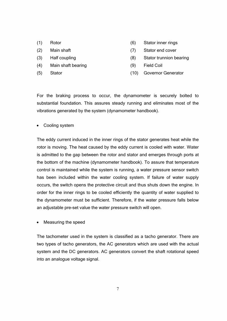
(1) Rotor (6) Stator inner rings

(2) Main shaft (7) Stator end cover

(3) Half coupling (8) Stator trunnion bearing

(4) Main shaft bearing (9) Field Coil

(5) Stator (10) Governor Generator

For the braking process to occur, the dynamometer is securely bolted to

substantial foundation. This assures steady running and eliminates most of the

vibrations generated by the system (dynamometer handbook).

• Cooling system

The eddy current induced in the inner rings of the stator generates heat while the

rotor is moving. The heat caused by the eddy current is cooled with water. Water

is admitted to the gap between the rotor and stator and emerges through ports at

the bottom of the machine (dynamometer handbook). To assure that temperature

control is maintained while the system is running, a water pressure sensor switch

has been included within the water cooling system. If failure of water supply

occurs, the switch opens the protective circuit and thus shuts down the engine. In

order for the inner rings to be cooled efficiently the quantity of water supplied to

the dynamometer must be sufficient. Therefore, if the water pressure falls below

an adjustable pre-set value the water pressure switch will open.

• Measuring the speed

The tachometer used in the system is classified as a tacho generator. There are

two types of tacho generators, the AC generators which are used with the actual

system and the DC generators. AC generators convert the shaft rotational speed

into an analogue voltage signal.

8

One of the main characteristics of tacho generators is to output a voltage that is

proportional in amplitude and frequency to the rotational speed. The generator is

mounted onto the dynamometer shaft. The output of the generator is

approximately 2 volts per 100 r.p.m (dynamometer handbook).

.

• The control desk

This control unit has been built within a sheet steel control desk and is free to

move at any distance from the dynamometer. This control unit is designed to

operate from a single phase AC source. Located on the top of the control desk is

the r.p.m indicating dial connected to the tachometer.

Figure 2.2: Control desk of the dynamometerFigure 2.2: Control desk of the dynamometerFigure 2.2: Control desk of the dynamometerFigure 2.2: Control desk of the dynamometer

• Governed and Ungoverned option

The actual electronic control system is arranged to provide a D.C. voltage rectified

from an A.C. mains supply. The control unit has been designed to produce two

9

desired torque/speed dynamometer characteristic under specific running

conditions. When the system is running under “governed” conditions, it provides a

constant D.C. current which flows through the coil irrespective to any speed rise of

the rotor. With this arrangement the dynamometer has a natural torque/speed

characteristic as depicted in figure 2.3.

Figure 2.3: Figure 2.3: Figure 2.3: Figure 2.3: TTTTorque vs. speedorque vs. speedorque vs. speedorque vs. speed curve curve curve curve


When set for a given current, the torque rises steeply and then becomes constant

irrespective of further speed increase. While the system runs under “ungoverned”

conditions, the speed of the engine is stabilised. No current flows within the

system until the speed has reached the controller preset value. Under this

condition any increase of the engine speed is immediately counteracted by an

increase of dynamometer load and if the engine speed drops, it will be

counteracted by a corresponding drop in the dynamometer load.

10

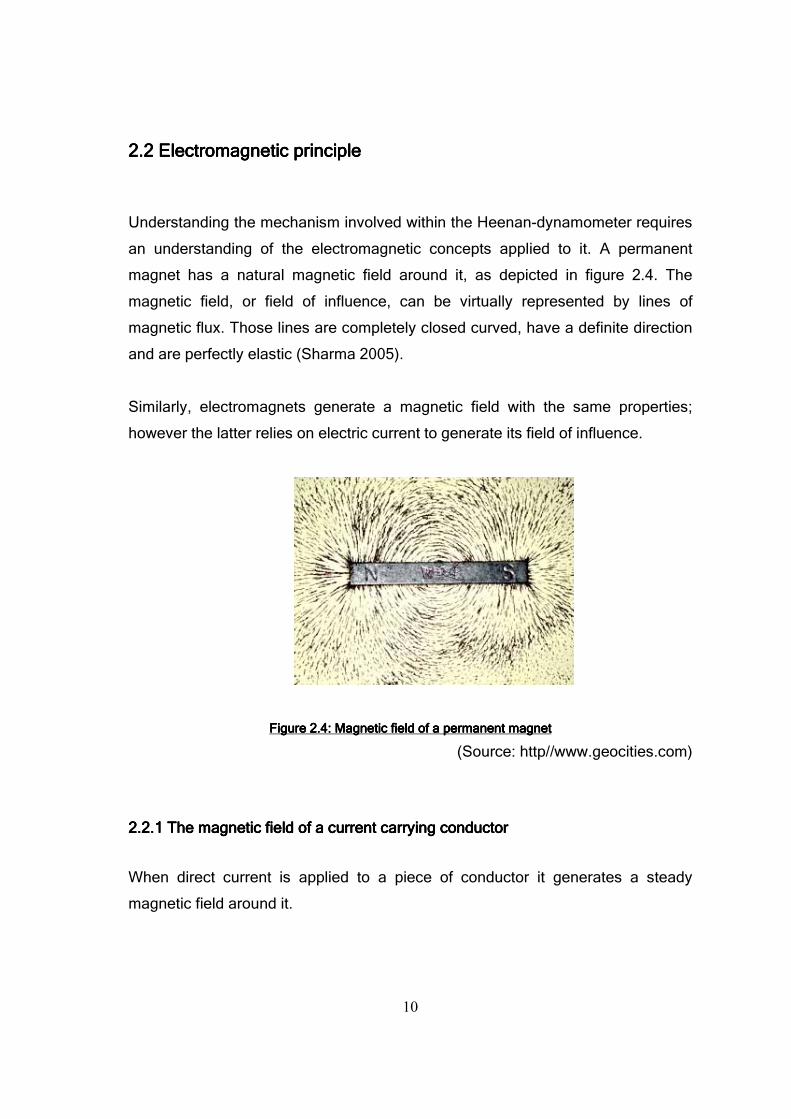
2.2 Electromagnetic principle2.2 Electromagnetic principle2.2 Electromagnetic principle2.2 Electromagnetic principle

Understanding the mechanism involved within the Heenan-dynamometer requires

an understanding of the electromagnetic concepts applied to it. A permanent

magnet has a natural magnetic field around it, as depicted in figure 2.4. The

magnetic field, or field of influence, can be virtually represented by lines of

magnetic flux. Those lines are completely closed curved, have a definite direction

and are perfectly elastic (Sharma 2005).

Similarly, electromagnets generate a magnetic field with the same properties;

however the latter relies on electric current to generate its field of influence.

Figure 2.4: Magnetic field of a permanent magnet Figure 2.4: Magnetic field of a permanent magnet Figure 2.4: Magnetic field of a permanent magnet Figure 2.4: Magnetic field of a permanent magnet

(Source: http//www.geocities.com)

2.2.1 T2.2.1 T2.2.1 T2.2.1 The magnetic field of a current carrying conductor he magnetic field of a current carrying conductor he magnetic field of a current carrying conductor he magnetic field of a current carrying conductor

When direct current is applied to a piece of conductor it generates a steady

magnetic field around it.

11

As represented in the figure 2.5, the surrounding field is generally represented by

concentric circles lying on a plane perpendicular to the conductor.

Figure 2.5: Magnetic field of a current carrying conductor Figure 2.5: Magnetic field of a current carrying conductor Figure 2.5: Magnetic field of a current carrying conductor Figure 2.5: Magnetic field of a current carrying conductor

(Source: http//www. bibleocean.com)

When two direct currents flowing in the same direction are applied to two parallel

conductors close to each other, the flux lines combine, and the two conductors

attract each other.

However, when two direct currents flowing in the opposite direction are applied to

two parallel conductors close to each other, the flux lines are crowded together in

the space between the conductor, and the two conductors repel each other. Thus,

when a direct current is applied to a solenoid, a magnetic field similar to the

permanent magnet magnetic field is generated as illustrated in figure 2.6.

Figure 2.6: MagFigure 2.6: MagFigure 2.6: MagFigure 2.6: Magnetic field around a solenoid netic field around a solenoid netic field around a solenoid netic field around a solenoid

(Source: http//www.schools.wikia.com)

12

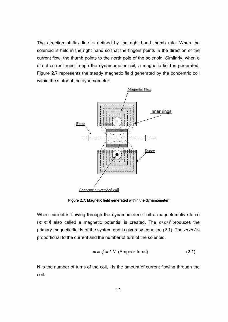
The direction of flux line is defined by the right hand thumb rule. When the

solenoid is held in the right hand so that the fingers points in the direction of the

current flow, the thumb points to the north pole of the solenoid. Similarly, when a

direct current runs trough the dynamometer coil, a magnetic field is generated.

Figure 2.7 represents the steady magnetic field generated by the concentric coil

within the stator of the dynamometer.

Figure 2.7: Magnetic field generated within the dynamometer Figure 2.7: Magnetic field generated within the dynamometer Figure 2.7: Magnetic field generated within the dynamometer Figure 2.7: Magnetic field generated within the dynamometer

When current is flowing through the dynamometer’s coil a magnetomotive force

(m.m.f) also called a magnetic potential is created. The m.m.f produces the

primary magnetic fields of the system and is given by equation (2.1). The m.m.f is

proportional to the current and the number of turn of the solenoid.

NIfmm ... = (Ampere-turns) (2.1)

N is the number of turns of the coil, I is the amount of current flowing through the

coil.

Inner rings

13

In the dynamometer system the number of turns is fixed, consequently the

magneto motive force will only be proportional to the amount of current through

the solenoid.

2.2.2 Eddy current 2.2.2 Eddy current 2.2.2 Eddy current 2.2.2 Eddy current

When a moving magnetic field intersects a conductor, or a moving conductor

intersects a magnetic field, current is induced. The relative motion causes a

circulating flow of electrons within the conductor. These currents, also called eddy

currents or Foucault currents, create electromagnets with magnetic fields that

oppose the change in the primary magnetic field.

The m.m.f generated by these eddy currents is proportional to the strength of the

original magnetic field, and also to the speed at which the magnetic field or the

conductor is moving. These eddy currents are induced to the inner rings of the

stator (see figure 2.7) when the rotor starts spinning within the magnetic field. The

rotor is of high permeability steel and makes with the stator the magnetic circuit of

the system. Because of this property, the flux lines are uniformly concentrated at

the rotor pole tips to take full advantage of the available area. As a result, the

density of the magnetic flux is not the same all around the rotor. Figure 2.8

illustrates the rotor pole tips and the concentration of the magnetic flux due to the

magnetic property of the rotor.

The flux density is a vector quantity, and its magnitude is given by equation (2.2).

In the SI system the unit of the magnetic flux density is Weber per meter square.

AB

Φ= )/( 2mWb (2.2)

At the pole tips of the rotor the density of the magnetic flux is large because the

fluxes are squashed into a small area. Everywhere else on the rotor the magnetic

flux density will be weaker.

14

Flux line

Figure 2.8Figure 2.8Figure 2.8Figure 2.8: : : : Magnetic flux density through the rotorMagnetic flux density through the rotorMagnetic flux density through the rotorMagnetic flux density through the rotor

Because of the steady nature of the magnetic field, the rotor will not be affected by

any change of magnetic flux density. Therefore no current will be induced on the

rotor. However, while the rotor is moving, the inner rings of the stator are subject

to a change in magnetic field density.

According to Faraday’s law, whenever there is a relative motion between a

conductor and a magnetic field, an electromotive force is induced in the conductor

and is proportional to the rate of change at which the field is cut (Sharma 2005). In

this case, the inner rings are held stationary and they are subject to varying

magnetic fields produced by the rotation of the slotted rotor within the primary

magnetic field. These electromotive forces are localized with the inner rings and

generate eddy currents due to the resistive nature of the material. Fleming’s Right

hand rule can be used to define the direction of the induced electromotive force.

However, in accordance to Lenz’s law, represented by equation (2.3), the eddy

currents will always tend to oppose the change in field inducing it.

tNemf∆∆

−=φ (2.3)

Where N is the number of turn and t∆

∆φis the change in flux with respect to time.

15

2.2.3 El2.2.3 El2.2.3 El2.2.3 Electromagnetic braking effect ectromagnetic braking effect ectromagnetic braking effect ectromagnetic braking effect

The magnetic fields created by the induced eddy current are called the secondary

magnetic fields and they attempt to cancel the magnetic field causing it. This

phenomenon generates new forces within the dynamometer. One force which

acts upon the stator and another force which opposes the first acts upon the rotor,

and thus decelerate its motion.

The force acting upon the stator forces it to rotate in the same direction as the

rotation of the rotor. The absorption unit is securely bolted to a substantial

foundation but is able to swivel clockwise or anti-clockwise depending on the force

acting upon it. This tendency to follow the rotor rotation is counteracted by means

of a lever arm connected to a sensitive torque measuring apparatus. When the

stator swivels, the force applied to it is transferred to the measuring apparatus.

The stator is forced to follow the motion of the rotor but is not able to do so. As a

result, opposing forces are created within the dynamometer. The force applied on

the rotor is referred as braking force of the dynamometer and is controlled by the

amount of current flowing trough the field coil.

16

CHAPTER 3 – RECTIFICATION

The actual dynamometer rectifier is obsolete and uses valve rectifier technology.

To update the system with new power electronics, it is convenient for the

University of Southern Queensland to change the valve rectifier with solid state

devices. This chapter includes an overview of rectifier using solid state devices

and demonstrates by means of experiment the basic principles for controlled

rectification.

3.1 The power diode or rectifier diode3.1 The power diode or rectifier diode3.1 The power diode or rectifier diode3.1 The power diode or rectifier diode

A diode is a two terminal device that allows an electric current to flow in one

direction but essentially blocks it in the opposite direction. The diode circuit

symbol is represented in figure 3.1. A semiconductor diode consists of a PN

junction and the two terminals are called the anode and the cathode. Current flows

from anode to cathode within the diode as shown by the arrow of the circuit

symbol.

Figure 3.1: Diode circuit symbol Figure 3.1: Diode circuit symbol Figure 3.1: Diode circuit symbol Figure 3.1: Diode circuit symbol

When the voltage across the diode is negative the diode is said to be reversed

biased and behaves as an open switch assuming ideal diode characteristics.

When the voltage is positive, the diode is forward biased and works as a close

switch (Afhock 2005). Figure 3.2 illustrates the ideal operating characteristics of a

practical power diode.

17

Figure 3.2: Idealised Figure 3.2: Idealised Figure 3.2: Idealised Figure 3.2: Idealised diode characteristicdiode characteristicdiode characteristicdiode characteristic

3.2 3.2 3.2 3.2 The ThyriThe ThyriThe ThyriThe Thyristor or Silicon Cstor or Silicon Cstor or Silicon Cstor or Silicon Controlled ontrolled ontrolled ontrolled RRRRectifierectifierectifierectifier (SCR) (SCR) (SCR) (SCR)

A thyristor is a semiconductor device that has the same characteristics as the

diode. Thyristors are often called silicon controlled rectifiers and compare to the

diode the thyristor is a three terminal device. The main terminals of the thyristor

are the anode and the cathode. The third terminal is referred as a gate. Figure 3.3

illustrate the thyristor circuit symbol.

Figure 3.3: Thyristor circuit symbolFigure 3.3: Thyristor circuit symbolFigure 3.3: Thyristor circuit symbolFigure 3.3: Thyristor circuit symbol

In the case that the thyristor is connected in series with a load through an AC

source, no current flows through the circuit until the thyristor as received a

triggering signal at the gate terminal.

Anode Cathode

Gate

18

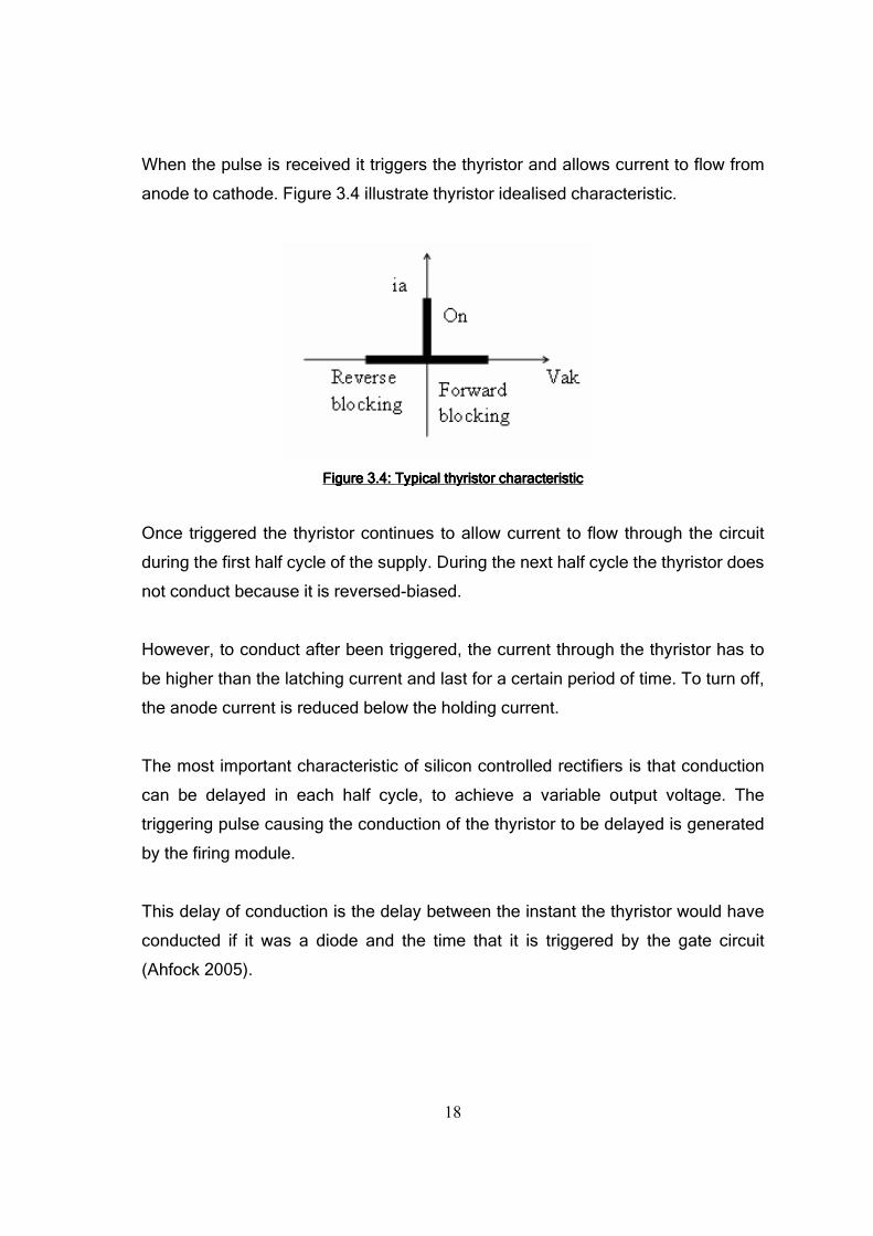
When the pulse is received it triggers the thyristor and allows current to flow from

anode to cathode. Figure 3.4 illustrate thyristor idealised characteristic.

Figure 3.4: Typical thyristor characteristicFigure 3.4: Typical thyristor characteristicFigure 3.4: Typical thyristor characteristicFigure 3.4: Typical thyristor characteristic

Once triggered the thyristor continues to allow current to flow through the circuit

during the first half cycle of the supply. During the next half cycle the thyristor does

not conduct because it is reversed-biased.

However, to conduct after been triggered, the current through the thyristor has to

be higher than the latching current and last for a certain period of time. To turn off,

the anode current is reduced below the holding current.

The most important characteristic of silicon controlled rectifiers is that conduction

can be delayed in each half cycle, to achieve a variable output voltage. The

triggering pulse causing the conduction of the thyristor to be delayed is generated

by the firing module.

This delay of conduction is the delay between the instant the thyristor would have

conducted if it was a diode and the time that it is triggered by the gate circuit

(Ahfock 2005).

19

0 0.002 0.004 0.006 0.008 0.01 0.012 0.014 0.016 0.018 0.02-0.8

-0.6

-0.4

-0.2

0

0.2

0.4

0.6

0.8

Measu

rem

ent

Time in millisecond

delay angle

AC source

Figure 3.5 illustrates the delay of conduction also called the delay angle.

Figure 3.5: Half controlled half wave rectifier Figure 3.5: Half controlled half wave rectifier Figure 3.5: Half controlled half wave rectifier Figure 3.5: Half controlled half wave rectifier

• The firing module

The firing circuit must be designed so that it will only give a firing pulse during the

time that the thyristor is forward biased. If the gate pulse is applied at the

beginning of the half-cycle, the complete half-cycle will be applied to the load. If

the gate pulse is applied anywhere else during the half-cycle, only a portion of the

half-cycle is applied to the load. It is therefore possible to control the load voltage

by controlling the gate pulse position.

This method of control is called linear firing angle control. To make sure that each

triggering pulses occur at a precise phase angle, the line supply voltage is

stepped down through a transformer and then sent to the triggering module. As

the signal has been stepped down it is still in phase with the mains source voltage.

20

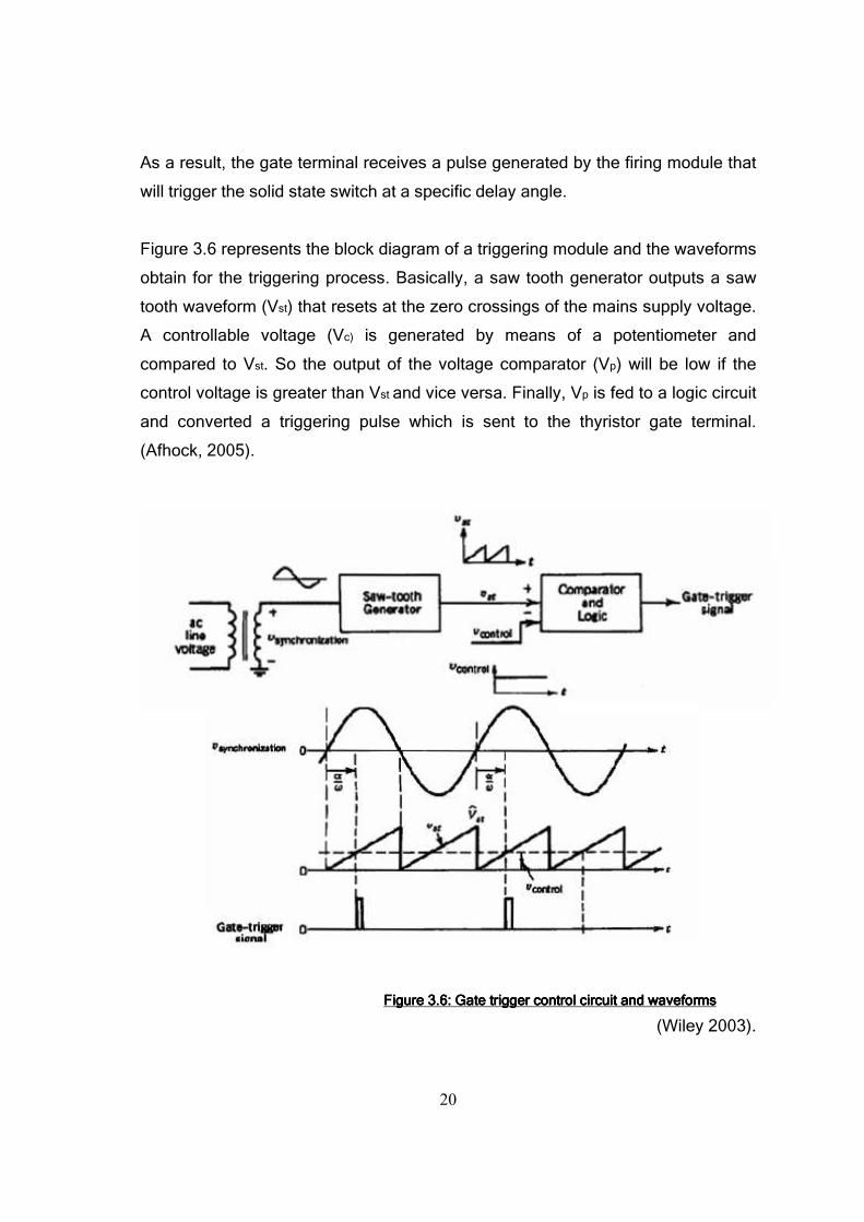
As a result, the gate terminal receives a pulse generated by the firing module that

will trigger the solid state switch at a specific delay angle.

Figure 3.6 represents the block diagram of a triggering module and the waveforms

obtain for the triggering process. Basically, a saw tooth generator outputs a saw

tooth waveform (Vst) that resets at the zero crossings of the mains supply voltage.

A controllable voltage (Vc) is generated by means of a potentiometer and

compared to Vst. So the output of the voltage comparator (Vp) will be low if the

control voltage is greater than Vst and vice versa. Finally, Vp is fed to a logic circuit

and converted a triggering pulse which is sent to the thyristor gate terminal.

(Afhock, 2005).

Figure 3.6: Gate trigger control circuit and waveforms Figure 3.6: Gate trigger control circuit and waveforms Figure 3.6: Gate trigger control circuit and waveforms Figure 3.6: Gate trigger control circuit and waveforms

(Wiley 2003).

21

3.3 Rectifiers configurations 3.3 Rectifiers configurations 3.3 Rectifiers configurations 3.3 Rectifiers configurations

The coil of the dynamometer requires direct current to generate a steady magnetic

field for the braking process to occur. Consequently, conversion of AC to DC must

be achieved.

3.3.1 Half and full wave rectification 3.3.1 Half and full wave rectification 3.3.1 Half and full wave rectification 3.3.1 Half and full wave rectification

The process of converting AC to DC is called rectification. The majority of the DC

loads respond to the mean value of a periodic wave form. To obtain the mean

value of a periodic signal, the integral of the signal during one period is divided by

the period in which it occurs. The waveform obtained from the mains is similar to a

sinusoidal signal represented in figure 3.7. When using the mean value formula on

a sinusoidal signal, the result will be zero as the net area for one period is equal to

zero.

Figure 3.7: Sinusoidal wave form Figure 3.7: Sinusoidal wave form Figure 3.7: Sinusoidal wave form Figure 3.7: Sinusoidal wave form

Nevertheless, by means of solid state technology it is possible to change the form

of the input signal and obtain an applicable mean value of the supplied voltage for

the device to operate in DC mode. There are two main manipulations that can be

achieved when rectifying a sinusoidal signal. The half wave rectification or the full

wave rectification.

• Half wave rectification

The process of removing one half of the input signal to establish a DC level is

called half wave rectification.

22

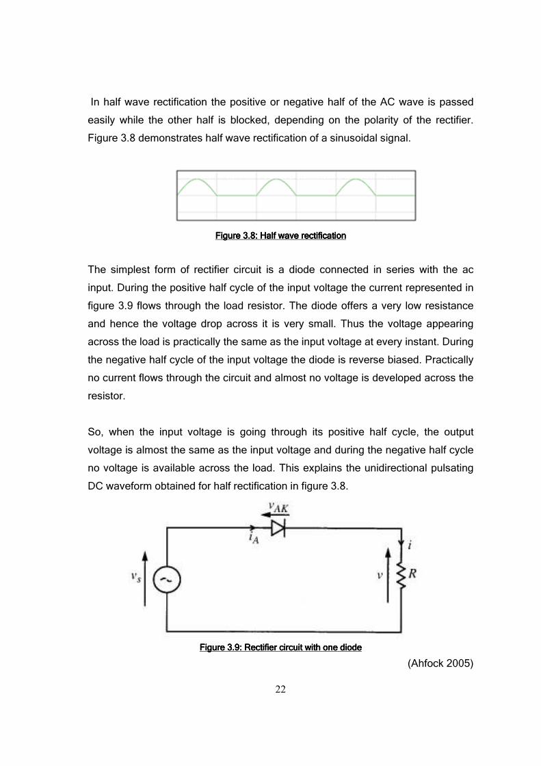
In half wave rectification the positive or negative half of the AC wave is passed

easily while the other half is blocked, depending on the polarity of the rectifier.

Figure 3.8 demonstrates half wave rectification of a sinusoidal signal.

Figure 3.8: Half wave rectification Figure 3.8: Half wave rectification Figure 3.8: Half wave rectification Figure 3.8: Half wave rectification

The simplest form of rectifier circuit is a diode connected in series with the ac

input. During the positive half cycle of the input voltage the current represented in

figure 3.9 flows through the load resistor. The diode offers a very low resistance

and hence the voltage drop across it is very small. Thus the voltage appearing

across the load is practically the same as the input voltage at every instant. During

the negative half cycle of the input voltage the diode is reverse biased. Practically

no current flows through the circuit and almost no voltage is developed across the

resistor.

So, when the input voltage is going through its positive half cycle, the output

voltage is almost the same as the input voltage and during the negative half cycle

no voltage is available across the load. This explains the unidirectional pulsating

DC waveform obtained for half rectification in figure 3.8.

Figure 3.9: Rectifier circuit with one diode Figure 3.9: Rectifier circuit with one diode Figure 3.9: Rectifier circuit with one diode Figure 3.9: Rectifier circuit with one diode

(Ahfock 2005)

23

This rectifier configuration is classified as uncontrolled rectification. In half wave

rectification the AC source only works to supply power to the load once every half-

cycle, meaning that much of its capacity is unused. However, half-wave

rectification is the simple way to reduce power to a resistive load.

The Average voltage or the DC content of the voltage across the load is given by:

[ ]

ππ

π

ωπ

ωϖωπ

π

π

π

π

peakpeakavav

peak

av

peak

av

peakav

I

R

V

R

VI

VV

tV

V

tdtdtVV

===

=

−=

+= ∫∫

.

cos2

)(.0)(sin.2

1

0

2

0

• Full wave rectification

Figure 3.10 illustrates full wave rectification of the same sinusoidal signal. The

negative or positive portions of the alternating signal are reversed and thus

produce an entirely positive or negative signal waveform depending on how the

diodes are connected.

Figure 3.10: Full wave rectification Figure 3.10: Full wave rectification Figure 3.10: Full wave rectification Figure 3.10: Full wave rectification

24

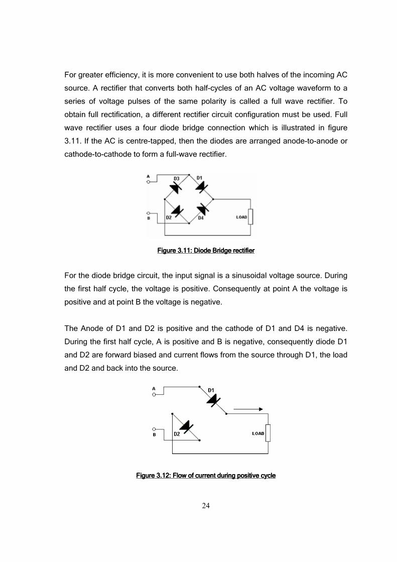
For greater efficiency, it is more convenient to use both halves of the incoming AC

source. A rectifier that converts both half-cycles of an AC voltage waveform to a

series of voltage pulses of the same polarity is called a full wave rectifier. To

obtain full rectification, a different rectifier circuit configuration must be used. Full

wave rectifier uses a four diode bridge connection which is illustrated in figure

3.11. If the AC is centre-tapped, then the diodes are arranged anode-to-anode or

cathode-to-cathode to form a full-wave rectifier.

Figure 3.11: Diode Bridge rectifier Figure 3.11: Diode Bridge rectifier Figure 3.11: Diode Bridge rectifier Figure 3.11: Diode Bridge rectifier

For the diode bridge circuit, the input signal is a sinusoidal voltage source. During

the first half cycle, the voltage is positive. Consequently at point A the voltage is

positive and at point B the voltage is negative.

The Anode of D1 and D2 is positive and the cathode of D1 and D4 is negative.

During the first half cycle, A is positive and B is negative, consequently diode D1

and D2 are forward biased and current flows from the source through D1, the load

and D2 and back into the source.

Figure 3.12: Flow of curreFigure 3.12: Flow of curreFigure 3.12: Flow of curreFigure 3.12: Flow of current during positive cycle nt during positive cycle nt during positive cycle nt during positive cycle

25

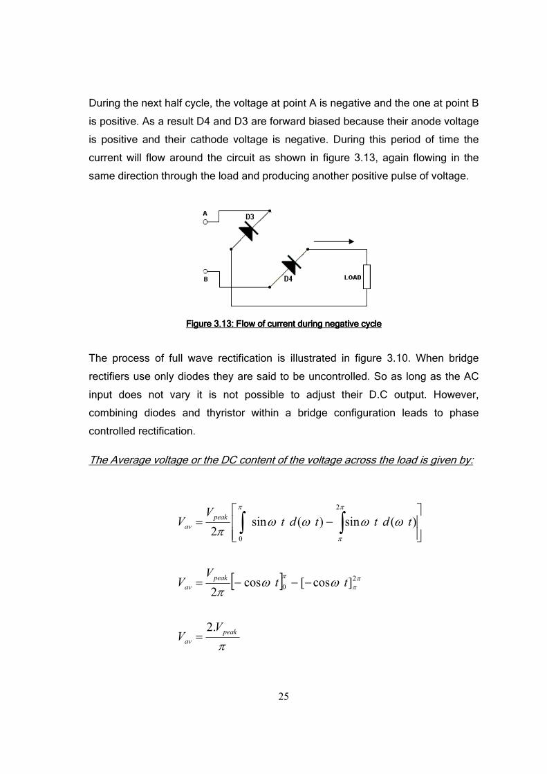
During the next half cycle, the voltage at point A is negative and the one at point B

is positive. As a result D4 and D3 are forward biased because their anode voltage

is positive and their cathode voltage is negative. During this period of time the

current will flow around the circuit as shown in figure 3.13, again flowing in the

same direction through the load and producing another positive pulse of voltage.

Figure 3.13: Flow of current during negative cycle Figure 3.13: Flow of current during negative cycle Figure 3.13: Flow of current during negative cycle Figure 3.13: Flow of current during negative cycle

The process of full wave rectification is illustrated in figure 3.10. When bridge

rectifiers use only diodes they are said to be uncontrolled. So as long as the AC

input does not vary it is not possible to adjust their D.C output. However,

combining diodes and thyristor within a bridge configuration leads to phase

controlled rectification.

The Average voltage or the DC content of the voltage across the load is given by:

[ ]

π

ωωπ

ωωωωπ

ππ

π

π

π

π

peak

av

peak

av

peak

av

VV

ttV

V

tdttdtV

V

.2

]cos[cos2

)(sin)(sin2

2

0

2

0

=

−−−=

−= ∫∫

26

SCR1

D2 D1

3.3.2 3.3.2 3.3.2 3.3.2 Half Half Half Half and fully controlled rectifier and fully controlled rectifier and fully controlled rectifier and fully controlled rectifier

By using different combinations of diode and thyristor it is possible to obtain

different classes of rectifiers. Mainly because of the thyristor characteristic of

being able to be phased controlled, rectifier are said to be fully controlled when

using four thyristors within a bridge configuration.

The fully controlled bridge is usually used when it is necessary to regenerate

power form the load. The most widely used rectifier configuration is the half-

controlled bridge illustrated in figure 3.14. The main advantage of using half

controlled rectification is to provide the load an adjustable D.C output voltage that

varies with respect to the delay angle.

For most of the applications using half controlled rectifiers, the control is only

possible during positive output voltage from the mains, and no control is possible

when the mains cycles are negative.

Figure 3.14: Half controlled bridge rectifier (SCR serie)Figure 3.14: Half controlled bridge rectifier (SCR serie)Figure 3.14: Half controlled bridge rectifier (SCR serie)Figure 3.14: Half controlled bridge rectifier (SCR serie)

3.4 Testing on phase controlled rectifier 3.4 Testing on phase controlled rectifier 3.4 Testing on phase controlled rectifier 3.4 Testing on phase controlled rectifier

A series of tests on a half controlled rectifier provided by the engineering faculty

have been conducted in order to understand the process of rectification using this

configuration. In the following experiments two different rectifier configurations

have been used.

SCR2

Load

27

D1 SCR1

SCR2

D2

Most of the power electronic applications operate at a relative high voltage and in

such cases the voltage drop across the SCR tends to be irrelevant for such

application. So, most of the time, the conduction voltage drop across the device is

assumed to be zero for circuit analysis. Similarly, it is also valid to assume that

the current through the thyristor is zero when it is not conducting.

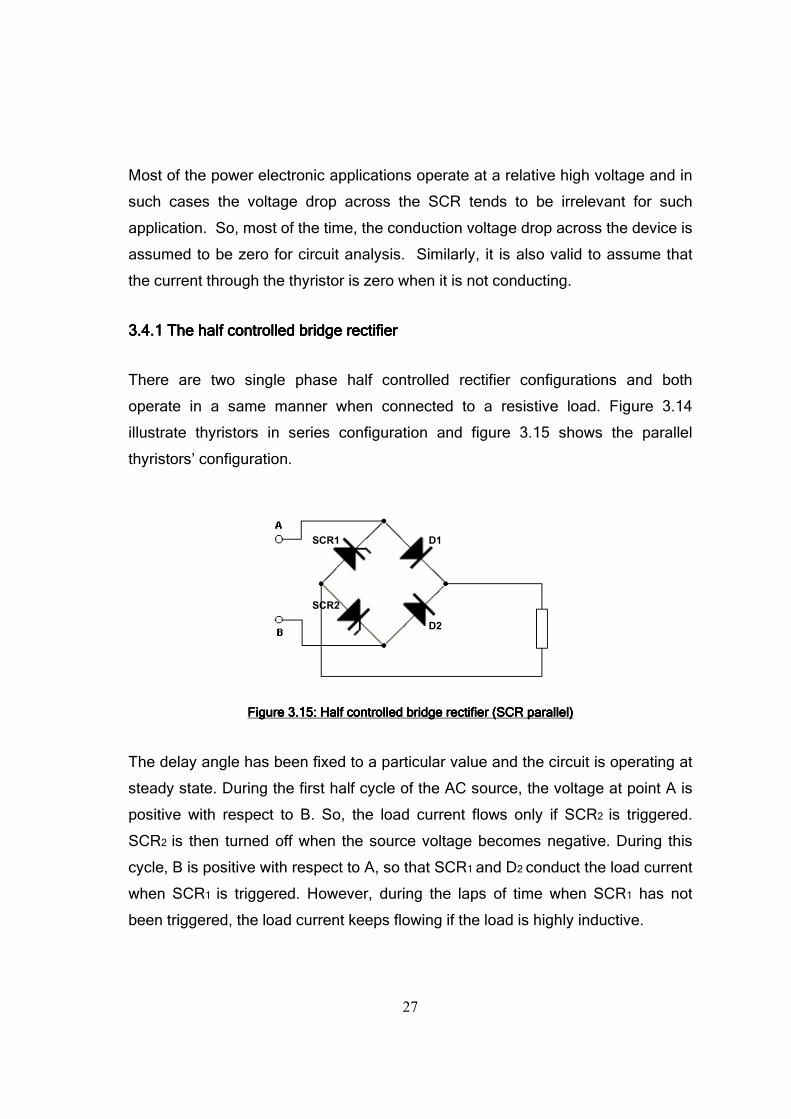
3.4.1 3.4.1 3.4.1 3.4.1 The half controlled bridge rectifierThe half controlled bridge rectifierThe half controlled bridge rectifierThe half controlled bridge rectifier

There are two single phase half controlled rectifier configurations and both

operate in a same manner when connected to a resistive load. Figure 3.14

illustrate thyristors in series configuration and figure 3.15 shows the parallel

thyristors’ configuration.

Figure 3.15: Half controlled bridge rectifier (SCR parallel) Figure 3.15: Half controlled bridge rectifier (SCR parallel) Figure 3.15: Half controlled bridge rectifier (SCR parallel) Figure 3.15: Half controlled bridge rectifier (SCR parallel)

The delay angle has been fixed to a particular value and the circuit is operating at

steady state. During the first half cycle of the AC source, the voltage at point A is

positive with respect to B. So, the load current flows only if SCR2 is triggered.

SCR2 is then turned off when the source voltage becomes negative. During this

cycle, B is positive with respect to A, so that SCR1 and D2 conduct the load current

when SCR1 is triggered. However, during the laps of time when SCR1 has not

been triggered, the load current keeps flowing if the load is highly inductive.

28

0 0.002 0.004 0.006 0.008 0.01 0.012 0.014 0.016 0.018 0.02-0.8

-0.6

-0.4

-0.2

0

0.2

0.4

0.6

0.8RESISTIVE AND INDUCTIVE LOAD

Mea

sure

me

nts

Time in millisecond

Main voltage

Load current

Rectified voltage

This inductive current has two circuits where it can flow, one made by the SCR2,

the source and D1 and a second, made by SCR1 and D1. Because of the low

impedance of the second circuit, the current continue to flow through SCR1 and D1

while the voltage is negative.

The back e.m.f from the inductive load drives current through the bridge without

containing any of the reverse supply voltage. During this time interval the load

current decays exponentially. Thyristor SCR1 is then triggered in the next half

cycle and the cycle repeats. Figure 3.16 illustrates the output of a half controlled

bridge rectifier connected to an inductive load.

Figure 3.16: Half controlled bridge rectifier output Figure 3.16: Half controlled bridge rectifier output Figure 3.16: Half controlled bridge rectifier output Figure 3.16: Half controlled bridge rectifier output

29

This half control rectifier configuration is good when the load is not too inductive

and with a time constant much lower than one half cycle of the supply. On a

contrary, if the load is highly inductive with a time constant greater than one half-

cycle of the supply, it will become more difficult to turn off the load current just by

not sending any pulse to the gate.

If the trigger pulses are removed after that a thyristor has been triggered, this

thyristor will continue to conduct as usual for the rest of the half cycle of the

supply. Then, the other thyristor will not turn on because no triggering pulse will be

sent to assure conduction. The circuit will continue to operate indefinitely with the

first triggered thyristor conducting on complete alternate half cycle and acting as a

flywheel diode on the other half cycles. In this case, the only way to interrupt this

cycle will be to stop the mains supply. Nevertheless, to ensure that the circuit

operates satisfactorily a free wheeling diode can be added in parallel to the load.

Consequently, at the end of each half cycle of the supply the load current is

transferred directly to this diode. The free wheeling diode ensures that there is no

risk that a thyristor will continue to conduct over another half cycle. (ed. Mullard

1970).

The average output voltage of the bridge as a function of firing angle:

[ ]

]cos1[

]cos[cos

cos

)(sin

απ

αππ

ωπ

ωωπ

π

α

π

α

+=

−−

=

−=

= ∫

peak

av

peak

av

peak

av

peak

av

VV

VV

tV

V

tdtV

V

30

The RMS load current during α < wt < π :

][)sin()(

)(tan

1

][)sin()(

1

2

ταπ

ταϖ

βππ

τβ

ωτ

τ

βωω

−−

−

−−

×+−×=

=

=

+×=

×+−×=

eAZ

Vi

and

R

L

RZ

where

eAtZ

Vti

peak

load

tpeak

load

TheRMS load current during π < wt < π + α :

][)()( τπϖ

πω−

−+=

t

loadload iti

When the load current is repetitive

τπ

τπ

τα

βαβπ

βπαπ

βαα

παα

−

−−

−

−−−×=

+×−×=+

+−×=

+=

eZ

VA

eAeZ

Vi

AZ

Vi

ii

peak

peak

load

peak

load

loadload

1

)sin()][sin(

)sin()(

)sin()(

)()(

31

0 0.002 0.004 0.006 0.008 0.01 0.012 0.014 0.016 0.018 0.02-0.8

-0.6

-0.4

-0.2

0

0.2

0.4

0.6

0.8RESISTIVE AND INDUCTIVE LOAD

Mea

sure

me

nts

Time in millisecond

Once A is known, the total RMS value of line current and the RMS value of its

fundamental component can be estimated.

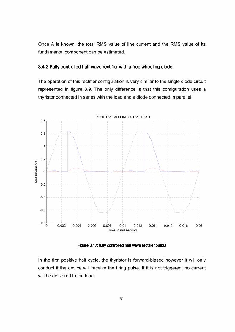
3.4.2 Fully controlled half wave rectifier with a free wheeling diode 3.4.2 Fully controlled half wave rectifier with a free wheeling diode 3.4.2 Fully controlled half wave rectifier with a free wheeling diode 3.4.2 Fully controlled half wave rectifier with a free wheeling diode

The operation of this rectifier configuration is very similar to the single diode circuit

represented in figure 3.9. The only difference is that this configuration uses a

thyristor connected in series with the load and a diode connected in parallel.

Figure 3.17: fully controlled half wave rectifier output Figure 3.17: fully controlled half wave rectifier output Figure 3.17: fully controlled half wave rectifier output Figure 3.17: fully controlled half wave rectifier output

In the first positive half cycle, the thyristor is forward-biased however it will only

conduct if the device will receive the firing pulse. If it is not triggered, no current

will be delivered to the load.

32

As explained earlier, when the thyristor is triggered in the forward-bias state, it

starts conducting and the positive source keeps the device in conduction until the

source voltage becomes negative. At that instant, the current through the circuit is

not zero because there is some energy that has been stored in the inductor.

The inductor discharges this energy during the negative cycle of the mains source

through the free wheeling diode. So, when the free wheeling diode conducts, the

thyristor remains reverse-biased, because the source voltage is negative. In the

absence of the free wheeling diode, the inductor would keep the thyristor in

conduction during the negative cycle of the source voltage until the load is fully

discharged.

33

CHAPTER 4 – TEST AND DESIGN

The updated half wave rectifier has to be tested on the dynamometer.

Subsequently, tests will be implemented in order to localise where the upgraded

rectifier will be connected.

4.1 Input and output location4.1 Input and output location4.1 Input and output location4.1 Input and output location

Originally, the protective circuit of the initial circuit was supposed to be reused with

the upgraded rectifier circuit. However, this task was requiring meticulous

investigations and thus more time. Therefore, it was more convenient to re-design

the whole unit control and keep the valve circuit intact. As a result, the entire valve

system was disconnected so that if the upgraded system fails to operate, the initial

electronic unit will still be able to operate the plant. The first approach was to

determine the input and output connections of the circuit.

Figure 4.1: External wiring connection of the dynamometer Figure 4.1: External wiring connection of the dynamometer Figure 4.1: External wiring connection of the dynamometer Figure 4.1: External wiring connection of the dynamometer


34

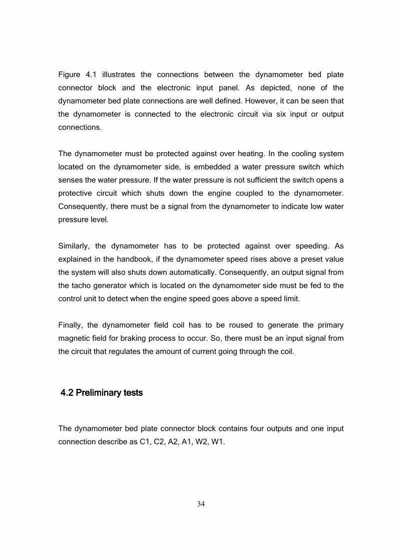
Figure 4.1 illustrates the connections between the dynamometer bed plate

connector block and the electronic input panel. As depicted, none of the

dynamometer bed plate connections are well defined. However, it can be seen that

the dynamometer is connected to the electronic circuit via six input or output

connections.

The dynamometer must be protected against over heating. In the cooling system

located on the dynamometer side, is embedded a water pressure switch which

senses the water pressure. If the water pressure is not sufficient the switch opens a

protective circuit which shuts down the engine coupled to the dynamometer.

Consequently, there must be a signal from the dynamometer to indicate low water

pressure level.

Similarly, the dynamometer has to be protected against over speeding. As

explained in the handbook, if the dynamometer speed rises above a preset value

the system will also shuts down automatically. Consequently, an output signal from

the tacho generator which is located on the dynamometer side must be fed to the

control unit to detect when the engine speed goes above a speed limit.

Finally, the dynamometer field coil has to be roused to generate the primary

magnetic field for braking process to occur. So, there must be an input signal from

the circuit that regulates the amount of current going through the coil.

4.2 Preliminary tests 4.2 Preliminary tests 4.2 Preliminary tests 4.2 Preliminary tests

The dynamometer bed plate connector block contains four outputs and one input

connection describe as C1, C2, A2, A1, W2, W1.

35

The information contained within the handbook does not define any of these

connections; subsequently assumptions were made before implementing tests on

the dynamometer.

At first, connection C1 and C2 were assumed to refer to the coil connection and

therefore enables a signal to go from the electronic circuit to the field coil. Then, it

was assumed that connection W1 and W2 were assumed to refer to the water

pressure switch located within the dynamometer. And finally, connection A1 and

A2 were assumed to be the analogue signal generated by the tacho generator to

prevent the engine to over speed.

Connection IG.1, IG.2, and IG.3 are defined as the engine ignition connection and

are used to safeguard the engine in case of overspending, or failure of water or

electricity supplies. The main power supply is defined by the L and N connections

to operate the whole system.

To verify the assumptions about connections C1, C2, A2, A1, W2, W1, a series of

tests were implemented on the dynamometer bed plate connections.

• Test at terminals C1and C2

The input signal of the excited coil must be a rectified version of the main source

voltage. The best approach to ensure that C1 and C2 are the dynamometer coil

input connections a digital oscilloscope was connected across them. Figure 4.2

illustrates the signal obtain across these connections.

As depicted, the signal is half rectified and therefore must be the output of the

valve rectifier. As a result, C1 and C2 are defined to be the dynamometer coil

connection.

36

- 0.02 5 -0.02 -0 .01 5 -0.0 1 -0 .005 0 0 .005 0.01 0. 015 0.02 0. 025-0 .1

0

0 .1

0 .2

0 .3

0 .4

0 .5

0 .6

0 .7O utpu t fro m c onn ectio n C 1 an d C 2

rect

ifie

d V

olta

ge w

ave

form

Ti me i n m illise cond

Figure 4.2: Signal obtaFigure 4.2: Signal obtaFigure 4.2: Signal obtaFigure 4.2: Signal obtained across connection C1 and C2ined across connection C1 and C2ined across connection C1 and C2ined across connection C1 and C2

• Test at terminals W1 and W2

As explained before, W1 and W2 are assumed to be the water pressure switch

connection of the protective circuit. Consequently, these connections must be

connected at both ends of the switch represented in figure 5.1.

A perfect switch, by definition, will have 0 Ω when closed and it will have infinite

resistance when opened. To check the resistance between these two connections,

an ammeter was connected across them.

The result obtained demonstrated that when there is not water flowing within the

cooling system, the resistance across W1 and W2 is infinite. On the contrary, when

the water tape is open, the resistance is approximately equal to 0.3 Ω. This test

has proven that connection W1 and W2 are the water pressure switch connection.

37

- 3 - 2 - 1 0 1 2 3

x 10-3

- 0 .1

- 0 .0 8

- 0 .0 6

- 0 .0 4

- 0 .0 2

0

0 .02

0 .04

0 .06

0 .08

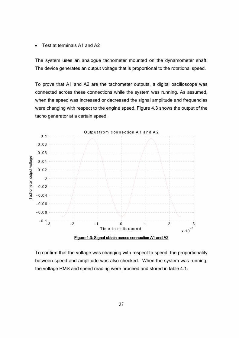
0 .1O utp u t f r o m c on n e c t io n A 1 a n d A 2

Tach

om

ete

r outp

ut vo

ltag

e

T ime in m i llis e co n d

• Test at terminals A1 and A2

The system uses an analogue tachometer mounted on the dynamometer shaft.

The device generates an output voltage that is proportional to the rotational speed.

To prove that A1 and A2 are the tachometer outputs, a digital oscilloscope was

connected across these connections while the system was running. As assumed,

when the speed was increased or decreased the signal amplitude and frequencies

were changing with respect to the engine speed. Figure 4.3 shows the output of the

tacho generator at a certain speed.

Figure 4.3: Figure 4.3: Figure 4.3: Figure 4.3: Signal obtain Signal obtain Signal obtain Signal obtain across across across across connection connection connection connection AAAA1 and 1 and 1 and 1 and AAAA2222

To confirm that the voltage was changing with respect to speed, the proportionality

between speed and amplitude was also checked. When the system was running,

the voltage RMS and speed reading were proceed and stored in table 4.1.

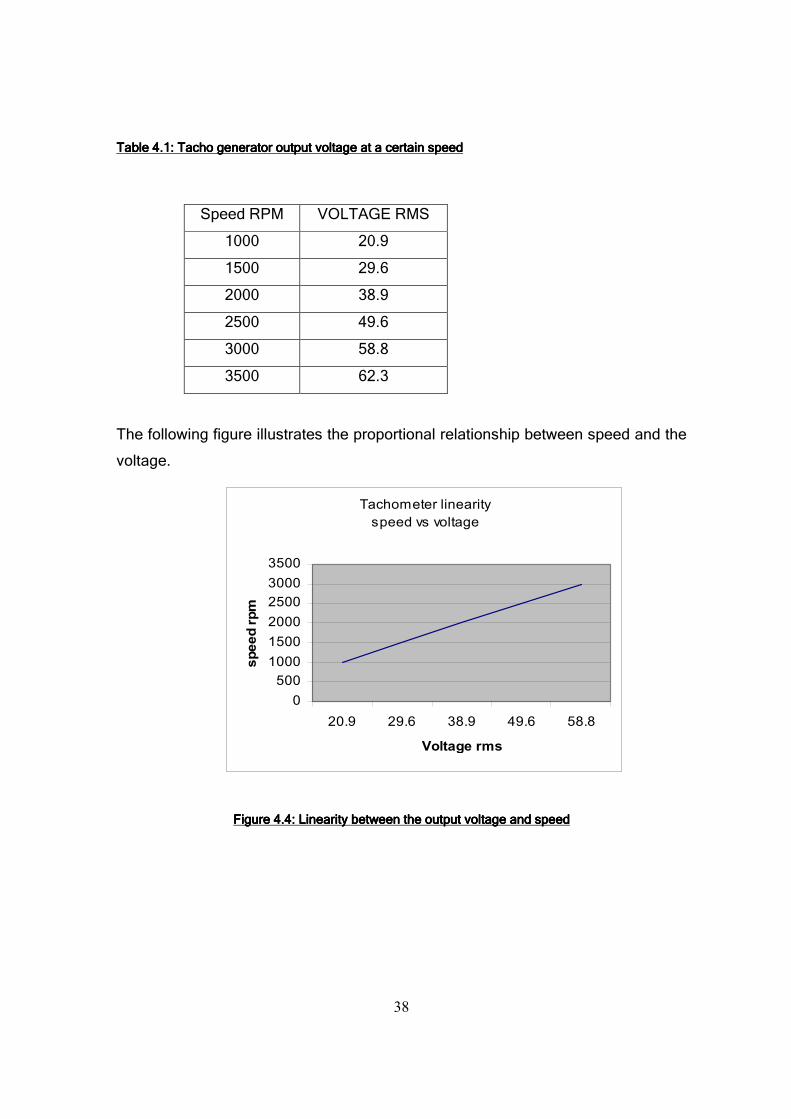
38

Tachometer linearity

speed vs voltage

0

500

1000

1500

2000

2500

3000

3500

20.9 29.6 38.9 49.6 58.8

Voltage rms

speed rpm

Table 4.1: Tacho generator output voltage at a certain speed Table 4.1: Tacho generator output voltage at a certain speed Table 4.1: Tacho generator output voltage at a certain speed Table 4.1: Tacho generator output voltage at a certain speed

The following figure illustrates the proportional relationship between speed and the

voltage.

Figure 4.4: Linearity between the output voltage and speed Figure 4.4: Linearity between the output voltage and speed Figure 4.4: Linearity between the output voltage and speed Figure 4.4: Linearity between the output voltage and speed

Speed RPM VOLTAGE RMS

1000 20.9

1500 29.6

2000 38.9

2500 49.6

3000 58.8

3500 62.3

39

CHAPTER 5 – PROTECTIVE SYSTEM

Protection of the plant while it is operating is essential. The whole plant has to be

protected against over speeding and overheating. At the same time, the user must

be safe and has to be protected against any independent emergency. This chapter

explains the use of a protective circuit and briefly describes the protective system

used with the valve rectifier. Following that, it gives a description of the selected

devices used for protection.

5.1 The existing protection system 5.1 The existing protection system 5.1 The existing protection system 5.1 The existing protection system

The circuit depicted in figure 5.1 represents the actual protective circuit that

safeguards the engine and the dynamometer in the event of water failure, over

speeding or failure of the power supply.

Figure 5.1: Existing protective circuit Figure 5.1: Existing protective circuit Figure 5.1: Existing protective circuit Figure 5.1: Existing protective circuit


40

5.1.1 The water pressure a5.1.1 The water pressure a5.1.1 The water pressure a5.1.1 The water pressure and ignition switchesnd ignition switchesnd ignition switchesnd ignition switches

• The water pressure switch

Cooling the dynamometer inner rings is essential to safeguard the dynamometer

because considerable damage would be done if the instrument overheated. The

heat generated by the induced current would melt the stator inner rings if they are

not cooled properly.

As explained in the dynamometer handbook, each brake power absorbed

generates 42.4 B.Th.U per minute, nearly all of which passes into the cooling

water. Consequently, the water pressure must be sufficient to ensure the

temperature of the stator inner rings does not rise above 140 degrees Celsius.

To sense the water pressure in the cooling system, a specific protective device is

used. It is referred in to the handbook as the water pressure switch. The switch is

embedded within the dynamometer cooling system and is connected to the

electronic unit by means of the connections W1 and W2. When water is running

through the dynamometer with enough pressure, the water pressure switch closes

a protective circuit so that the system is safe to run. On the contrary, if the water

pressure is not sufficient to cool the inner rings, the switch opens the protective

circuit so that the system is shut down or cannot start.

• The ignition switch

This ignition switch is a manually-operated switch and has to be closed for the

combustion engine to start. The main purpose of this switch, however, is to

safeguard the system or the user in the event of an independent emergency.

41

5.1.2 The connections of the coil ignition engin5.1.2 The connections of the coil ignition engin5.1.2 The connections of the coil ignition engin5.1.2 The connections of the coil ignition engineeee

IG.1, IG.2 and IG.3 are the three terminals from the electronic input panel

connected with the engine ignition system. The Low Tension connections of the

coil ignition engine are connected in series with terminal IG.1, IG.2 and IG.3. These

terminals are connected to the second ‘change-over contact’ of a double pole

double throw relay as depicted in figure 5.2.

To stop the engine when a fault occurs, the change over contact has to be on IG.1

and IG.2. For the engine to start, IG.2 and IG.3 must be connected. The Double

Pole Change Over (D.P.C.O) relay has two rows of change-over terminals and is

actuated by a single coil.

Figure 5.2: Double Pole Double Throw relay (DPDT)Figure 5.2: Double Pole Double Throw relay (DPDT)Figure 5.2: Double Pole Double Throw relay (DPDT)Figure 5.2: Double Pole Double Throw relay (DPDT)

(Handbook, 1881)

5.1.3 Resetting the DPCO relay 5.1.3 Resetting the DPCO relay 5.1.3 Resetting the DPCO relay 5.1.3 Resetting the DPCO relay

To reset the relay, a momentary push button switch is connected to the first

change-over contact of the relay. Referring to figure 5.1, if the water switch, the

ignition switch and the RL1 internal switch are closed, then by pressing and

depressing the reset button the relay becomes energized, so that contacts IG.2

becomes connected to IG.3.

42

As a result, the engine is ready to be started and the whole system is safe to

operate. For the engine to start, the entire set of switches that constitute the

protection system have to be closed. If any of the switches open while the system

operates the engine is turned off automatically. For example, if the water pressure

is insufficient, the water pressure switch will open. Consequently, the coil of the

relay will be de- energized and the relay will return to its initial state where IG.2 is

connected to IG.1.

5.1.3 Over speed control 5.1.3 Over speed control 5.1.3 Over speed control 5.1.3 Over speed control

The function of the first relay RL1, represented in figure 5.2, is to stop the prime

mover if the load generated by the dynamometer fails. When the load fails it is

commonly due to either a failure of the main supply or a fault occurring within the

excitation unit. If a sudden failure of the load occurs, the speed of the engine will

rise so quickly that considerable damages would occur to the prime mover.

In figure 5.1, valve V8 is biased off by adjusting the potentiometer P3. The position

of P3 determines the speed at which the plant should shut down. V8 will remain

biased off until the rectified signal from the tacho generator exceeds the bias

condition. In the case that the rectified D.C signal exceeds the over speed cut out

adjustor limit, V8 will allow current to pass and will energised the coil of RL1. As a

result, Relay one open the protective circuit and de-energises Relay two (RL2)

which closes contacts IG.1 and IG2 (Dynamometer handbook).

5.2 Upgraded protection system 5.2 Upgraded protection system 5.2 Upgraded protection system 5.2 Upgraded protection system

An upgraded version of the initial protective system has been designed and tested

onto the dynamometer. The circuit uses the latest technology available from

Farnell’s catalogue 2005.

43

The circuit guarantees that the engine stops automatically in the event of

insufficient water pressure, over speeding or a fault occurring in the excitation unit.

For design simplicity and convenience, the water pressure sensor has been re-

used.

5.2.25.2.25.2.25.2.2 Over speeding protection device Over speeding protection device Over speeding protection device Over speeding protection device

As explained earlier, the circuit must prevent over speeding for engine protection.

When the speed of the dynamometer shaft rises above a preset value, the prime

mover must stop. The most suitable device for this operation is the Multifunction

Voltage Relay also called the M3MVR. As a result, the section of the initial

protective circuit represented in figure 5.3 is replaced by using only this device.

Figure 5.3: Over speed protection used with initial design Figure 5.3: Over speed protection used with initial design Figure 5.3: Over speed protection used with initial design Figure 5.3: Over speed protection used with initial design


The M3MVR automatically adjusts for AC or DC supply. The relay can be used for

either under voltage monitoring or over voltage monitoring. For this application the

device is used for over voltage monitoring. The tripping mode of the relay must be

selected at the time of installation by means of a rear mounted switch. Figure 5.4

illustrates the M3MVR relay.

44

Figure 5.Figure 5.Figure 5.Figure 5.4444: : : : M3MVR and front panel M3MVR and front panel M3MVR and front panel M3MVR and front panel

(Source: http://www.broycecontrol.com)

For this application, the M3MVR is used to track if the voltage output from the

tacho generator goes above a preset voltage. As soon as the M3MVR receives an

analogue signal with a peak value above the limit, the internal switch opens and

thus opens the protective circuit, stopping the engine.

When the relay has triggered it can be reset by either momentarily removing the

power supply or turning the latch switch to the off position.

The main advantage offered by this relay is that if a spike is generated by the tacho

generator the relay will not respond to this high voltage. In order for the relay to trip,

the analogue signal should stay above the preset over voltage limit for a pre-

defined interval of time. The time (t), in figure 5.5 represents the tripping time delay.

The relay can be set to delay tripping, for 100 ms or 1 second, using the front

mounted delay switch.

45

Figure 5.5: Timing diagram for over voltage monitoring Figure 5.5: Timing diagram for over voltage monitoring Figure 5.5: Timing diagram for over voltage monitoring Figure 5.5: Timing diagram for over voltage monitoring

(Source: http://www.broycecontrol.com)

If the relay is monitoring close to its tripping point, it might continuously pull in and

drop out as the voltage continually passes through the set point. To overcome this

problem, an adjustable hysteresis level has been incorporated to the relay. This

causes the relay to re-energise at a point which is at either 2% or 10% below the

set point level. The choice of hysteresis level can be made using the front mounted

switch (see figure 5.4). The M3MVR is able to monitor two different ranges of

voltages.

M3MVR technical specifications:

Supply voltage (nominal): 18 – 240 V AC 50/60 Hz

Min./max limits : 15 – 265 V AC 48/63 Hz

Power consumption: 3 VA

Output contact ratings: 8 A, 250V AC

Input impedance: 10 MΩ

Monitoring ranges:

Range 1 1 to 26.5 V AC

Range 2 10 to 265 V AC

Maximum input voltage: 1000V

46

Figure 5.6 represents the section of the upgraded protection circuit that will protect

the engine against over speeding.

Figure 5.6: M3MVRFigure 5.6: M3MVRFigure 5.6: M3MVRFigure 5.6: M3MVR

5.2.3 Resetting the initial state of the circuit 5.2.3 Resetting the initial state of the circuit 5.2.3 Resetting the initial state of the circuit 5.2.3 Resetting the initial state of the circuit

The most suitable relay to control the state of the engine and thus guarantee

protection of the whole system is the DPCO-5532, illustrated in figure 5.7. This

miniature general purpose relay is called an "ice cube" relay in reference to its

transparent enclosure and size. The transparency allows inspection of the

contacts, coil, and swing arms for evidence of overheating.

Figure 5.7: DPCOFigure 5.7: DPCOFigure 5.7: DPCOFigure 5.7: DPCO----5532553255325532

Contacts specifications:

Contact configuration: 2 Change over, DPDT.

Rated current/Maximum peak current: 10 A.

Rated voltage/Maximum switching voltage: 250 V AC.

Tacho

M3MVR

47

DPCO

Coil specification:

Voltage, coil AC nominal: 230 V.

Coil resistance: 17 Ω.

This relay is the core of the protection system. When its coil is energised, it

maintains circuit protection, and when the coil is de-energised the relay shuts down

the engine by means of IG.1, IG.2 and IG.3.

5.2.4 Protective circuit configuration 5.2.4 Protective circuit configuration 5.2.4 Protective circuit configuration 5.2.4 Protective circuit configuration

While designing the new protective circuit, it was more convenient to refer most of

the design to the old circuit. The upgraded protective system is depicted in figure

5.8. The water switch closes as soon as there is enough water pressure in the

cooling system. When the ignition switch is manually closed, the system is ready

to operate and an indicator indicates that the plant is ready. However, before

starting the engine the reset button has to be pressed and depressed so that the

relay “DPCO – 5532” becomes energized and closes contacts IG.2 and IG.3.

Figure 5.8: Protective circuitFigure 5.8: Protective circuitFigure 5.8: Protective circuitFigure 5.8: Protective circuit

Tacho

M3MVR

48

CHAPTER 6 – THE UPGRADED SYSTEM

Upgrading the rectifying system has required a selection of specific devices. This

chapter introduces the selected devices used for rectification and describes the

operation of the upgraded system.

6666.1 .1 .1 .1 The half control bridge rectifier The half control bridge rectifier The half control bridge rectifier The half control bridge rectifier

6.1.16.1.16.1.16.1.1 AC to DC converter AC to DC converter AC to DC converter AC to DC converter

Silicon controlled rectifiers are available in a variety of integrated circuit packages

which have different number of pins. After a meticulous search for the most

suitable device, the integrated power circuits P102W was selected to convert the

AC source to DC. This device consists of power thyristors and power diodes

configured in a single package as illustrated in figure 6.1. As depicted in the

following figure, the module is mounted on an alumina substrate to provide a

completely isolated assembly.

Figure 6.1: P102 WFigure 6.1: P102 WFigure 6.1: P102 WFigure 6.1: P102 W module module module module

(Source: http:// www.farnell.com)

49

Figure 6.2 illustrates the internal configuration of the module and shows that the

module has a free wheeling diode connected in parallel to the load of the module.

Figure 6.2: Figure 6.2: Figure 6.2: Figure 6.2: IIIInternal bridge rectifier configuration nternal bridge rectifier configuration nternal bridge rectifier configuration nternal bridge rectifier configuration

(Source: http://www.irf.com)

Table 6.1 details all the major ratings and characteristics of the P102W module.

Table 6.1Table 6.1Table 6.1Table 6.1: P102W ratings and characteristics: P102W ratings and characteristics: P102W ratings and characteristics: P102W ratings and characteristics

(Source: http://www.irf.com)

50

• Heat sink

When the internal diodes or thyristors are forward biased, there is a current flowing

through it, as well as a voltage across it. Semi conductor power losses are

dissipated in the form of heat, which must be transferred away from the switching

junction (William1992). An excessive amount of heat can be damaging or

destructive to the module. In order to control the module temperature, the device is

mounted on a specific heat sink which ensures a good thermal equilibrium between

the junction temperature and the ambient temperature. The following table details

the thermal and mechanical specification of the rectifier module.

Table Table Table Table 6.6.6.6.2: Thermal and mechanical specification of the P102W module.2: Thermal and mechanical specification of the P102W module.2: Thermal and mechanical specification of the P102W module.2: Thermal and mechanical specification of the P102W module.

(Source: http://www.irf.com , 2006)

The thermal resistance of the heat sink depends on its size, its construction and its

orientation. Figure 6.3 illustrates the heat sink where the rectifying module is

mounted.

51

FFFFigure 6igure 6igure 6igure 6.3.3.3.3: Heat sink : Heat sink : Heat sink : Heat sink

The heats sink has a thermal resistance of 0.85°C/W and is made of aluminium. It

utilise finned surface area on both side of the module mounting surface in order to

provide maximum heat dissipation.

6.1.26.1.26.1.26.1.2 Firing module for Firing module for Firing module for Firing module for the P102Wthe P102Wthe P102Wthe P102W

The selected trigger module illustrated in figure 6.4 uses variable phase angle

control with adjustable signal matching, integral current limit input and adjustable

soft start.

Figure 6.Figure 6.Figure 6.Figure 6.4444: AFM: AFM: AFM: AFM----11111111

(Source: http://www.powercontrollers.net/components/firing_circuit)

52

As depicted in figure 6.5, the module offers four different ways to control the phase

angle generated by the firing module. Control can be achieved via an input signal,

a relay, a manual potentiometer or a DC input signal. The module offers an

adjustable current limit option that can be used when designing the close loop

system.

Figure 6.Figure 6.Figure 6.Figure 6.5555: Control option for terminal 5,4 and 3: Control option for terminal 5,4 and 3: Control option for terminal 5,4 and 3: Control option for terminal 5,4 and 3

(Farnell, 2005)

• The control potentiometer

Although, there are different methods available to control the angle of conduction,

the use of a manual potentiometer is one of the most suitable options to manually

control the load generated by the dynamometer. A 5kΩ potentiometer illustrated in

figure 6.6 is connected to the firing module.

Figure 6.Figure 6.Figure 6.Figure 6.6666: : : : 5 k5 k5 k5 kΩΩΩΩ potentiometerpotentiometerpotentiometerpotentiometer

(Source: http://www.farnellinone.com)

53

• Supply step down transformer

In order to operate the triggering module and the multifunction relay, the mains

source has to be step down to 24 V AC. The transformer illustrated in figure 6.4 is a

step down transformer that converts 230 V AC to 24 V AC. As illustrated in picture

6.7 the transformer provides two secondary voltages.

Figure 6.Figure 6.Figure 6.Figure 6.7777: Transformer : Transformer : Transformer : Transformer

(Source: http://www.farnellinone.com)

Transformer characteristics :

Power, AC: 12VA

Voltages, secondary: 0-24, 0-24

Voltage, single primary: 230 V

Power, per secondary winding: 6VA

Regulation: 12%

(Appendix E details the cost of these devices )

6666.2.2.2.2 Upgraded Upgraded Upgraded Upgraded system:system:system:system: Manual torque control Manual torque control Manual torque control Manual torque control

As explained earlier, the new control unit must supply the dynamometer field coil

with an adjustable DC source. However, the whole system has to be protected and

safe to use.

54

The upgraded system consists of the protection circuit and the upgraded rectifier.

Figure 6.8 illustrates the block diagram representation of the upgraded system.

Figure 6.Figure 6.Figure 6.Figure 6.8888: Upgra: Upgra: Upgra: Upgraded ded ded ded control unit control unit control unit control unit system system system system

The control potentiometer is connected directly to the firing module to ensure

manual load control. Once the potentiometer is set to a certain position, the firing

module generates a pulse signal which occurs at a specific delay angle. As a

result, the P102W produces a constant level of direct current to the field coil and

thus generate a load that will quickly become constant irrespective of further

engine speed rise.

The new control unit is connected to the electronic input panel illustrated in Figure

6.9 These connections are located within the initial control desk.

55

Figure 6.Figure 6.Figure 6.Figure 6.9999: E: E: E: Electronic input panel lectronic input panel lectronic input panel lectronic input panel

6.3 Laboratory testing on the upgraded system 6.3 Laboratory testing on the upgraded system 6.3 Laboratory testing on the upgraded system 6.3 Laboratory testing on the upgraded system

Before implementing any testing onto the dynamometer, the new circuit was tested

in laboratory to verify if the circuit was working properly. Figure 6.10 illustrates the

testing configuration of the upgraded system.

Figure 6.Figure 6.Figure 6.Figure 6.10: Tes10: Tes10: Tes10: Testing configuration of the upgraded system ting configuration of the upgraded system ting configuration of the upgraded system ting configuration of the upgraded system

Variac

1:1 Transfo

6A fuse Oscilloscope

Upgraded

circuit

Load

56

-0.025 -0.02 -0.015 -0.01 -0.005 0 0.005 0.01 0.015 0.02 0.025-400

-300

-200

-100

0

100

200

300

400RESISTIVE AND INDUCTIVE LOAD

Measure

ments

Time in millisecond

The first test was performed to verify if rectification was occurring. To replace the

dynamometer coil, an inductive load was connected in series with a resistive load.

The output wave form of the source voltage and the rectified signal was obtained

via a digital oscilloscope (Tektronix TDS 420A). Figure 6.11 illustrates the rectifier

output at a specific angle of conduction.

Figure 6.11Figure 6.11Figure 6.11Figure 6.11: : : : Upgraded Upgraded Upgraded Upgraded rectifier outputrectifier outputrectifier outputrectifier output

The second series of tests was organised to check the reset condition of the

protective circuit and if the system shuts down in the event of over speeding.

Figure 6.12 illustrate the circuit configuration tested within the laboratory.

The reset condition of the protective circuit has been verified by ensuring that no

voltage was across the DPCO coil before the reset button was pressed. Thus,

when the reset button was pressed and depressed, 230 V AC appeared through

the same coil and a red lamp lights to indicate that the plant is ready. The reset

option works as expected so further testings were carried out to verify over

speeding protection.

57

The reset button has been pressed and depressed so that the system is now

protected. If the internal switch of the M3MVR opens, the magnetic field of the

DPCO coil collapses and thus connection IG.2 connects to IG.1in order to shut

down the engine.

To ensure full system protection against over speeding within the laboratory, the

main AC source was connected to a variac to obtain variable AC source that will

replace the tacho generator output in the laboratory. The signal from the variac

was fed to the monitored input connection of the M3MVR relay with the intention of

tracking if the voltage goes above a predefined value. When the monitored signal

goes above the voltage limit, the internal switch of the relay opens the protective

circuit, so that the DPCO relay switches back to its initial state and thus stop the

engine.

To guarantee that the DPCO had switched back to its initial state, the resistance

across the second internal switch of the DPCO relay was measured via an ampere

meter. When the whole system is protected, the resistance across IG2 and IG1 is

very high. On the other hand, when the system is not protected or when a fault

occurs, the resistance across these terminals is very low because IG.2 connects

back to IG.1.

Figure Figure Figure Figure 6.6.6.6.12121212: Protection circuit tested within the laboratory: Protection circuit tested within the laboratory: Protection circuit tested within the laboratory: Protection circuit tested within the laboratory

M3MVR

DPCO

58

6.4 The new control unit of the Heenan dynamometer6.4 The new control unit of the Heenan dynamometer6.4 The new control unit of the Heenan dynamometer6.4 The new control unit of the Heenan dynamometer

The new control gear is mounted within a metallic box which may be situated at

any convenient distance from the dynamometer. Figure 6.13 represents the

upgraded control unit for the Heenan dynamometer. The box is earthed to provide

an alternative path for a fault current so that the user is protected. All internal

connections are covered with heat shrink so that the user is safe to touch any

internal wires however this is not recommended. Perspex has been used on the

top of the box for educational purpose and at the same time to see the status of the

firing module.

Figure 6.Figure 6.Figure 6.Figure 6.13131313: : : : UUUUpgraded contrpgraded contrpgraded contrpgraded control unit ol unit ol unit ol unit

As depicted in the above figure, the M3MVR and the DPCO are located on the

front of the control box. This configuration allows any user to select the controlling

options offered by the M3MVR and at the same time it allows the control of the

internal contact of DPCO relay. Both relay are mounted on a DIN rail from inside.

(Appendix F details the design of the control unit box)

M3MVRM3MVRM3MVRM3MVR

DPCODPCODPCODPCO

IndicatorIndicatorIndicatorIndicator (plant is ready)

PotentiometerPotentiometerPotentiometerPotentiometer

Reset buttonReset buttonReset buttonReset button

59

6666.5 Test on the dynamometer.5 Test on the dynamometer.5 Test on the dynamometer.5 Test on the dynamometer

Testing the upgraded control unit on the dynamometer was not achieved because

the contact ratings of the DPCO relay were inappropriate for this application. While

connecting the upgraded control unit to the dynamometer, it was realised that the

actual relay (RL2) connected to the ignition coil was extremely big compare to the

DPCO relay. As a result, it was assumed that the new relay will not withstand the

inductive current coming from the coil.

The coil of the engine is operated by a 20 V DC battery so that when connection

IG.2 is connected to IG.3 the coil current is flowing trough the inductor. Therefore,

a magnetic field exists in the region surrounding the inductor. The energy

transferred form the DC supply is now stored in the inductor. Consequently, when

the switch opens the impedance across it increase and consequently a very high

voltage is required across the switch if current is to continue to flow trough it. As a

result damage will be caused to the internal switch of the under rated relay.

60

G(s)

Input Output

CHAPTER 7 – OPEN LOOP AND CLOSE LOOP

The valve control system has two mode of operation. These two modes of

operation are selected by means of an external selector switch located on the

control desk. When the switch selects “Governed engines” operating mode, the

dynamometer acts as an open loop system and when the switch selects

“Ungoverned engines”, the control unit operated as a close loop system. This

chapter describes the open loop configuration of the upgraded control unit and

briefly explains how feed back control can be achieved.

7.1 The open loop systems7.1 The open loop systems7.1 The open loop systems7.1 The open loop systems

An open loop system is a control system that does not use its output to correct the

process of the system. The system is given a predefined input signal and the

output signal must behave in a predefined manner (Nise 2003). Thus, the open

loop controller of the dynamometer system will essentially be a potentiometer that

will generate different level of current to the dynamometer’s coil.

FFFFigure igure igure igure 7.17.17.17.1 Open loop system Open loop system Open loop system Open loop system

The design of the open loop of the dynamometer system contains a half controlled

bridge rectifier, a firing module and its potentiometer. The bridge rectifier is the

input transducer that converts the main AC source to a DC source. The firing

module is the device that generates the triggering gate current at a specific time.

By shifting the firing point, by means of the potentiometer, the half controlled bridge

61

rectifier will produce different level of exciting current to the dynamometer’s coil.

Consequently, the load imposed to the coupled engine will be different at different

potentiometer position. While operating with the open loop system, the DC current

flowing in the dynamometer coil is constant irrespective of the dynamometer’s

speed.

7777.2 The close loop system .2 The close loop system .2 The close loop system .2 The close loop system

Systems that use a feedback signal are called closed-loop control systems. The

reason for using feedback control with the dynamometer is to provide engine speed

stabilisation. In cases such as the testing of an internal combustion engine, speed

stabilisation of the engine is necessary to measure many engine performances at a

specific speed. For example, when designing an engine it is relevant to know how

much fuels the engine consumes at a specific speed. Similarly, using the

dynamometer to stabilise the speed of the engine facilitates the tunning of the

engine.

To maintain the speed of the engine, the load of the dynamometer must be

adjusted whenever the engine speed is changing. As explained earlier, the load

generated by the dynamometer is proportional to the amount of current flowing

through the field coil. As a result, speed control can be achieved by varying the

amount of current generated by the AC to DC converter.

In order to adjust the DC output of the converter, the conduction angle has to be

varied automatically in response to any change of the engine speed. In this case,

the feedback signal is used to adjust the output of the driven system. The motor

speed is measured by means of the tacho generator and the signal is fed back to a

comparator. The second input signal of the comparator is called the reference

speed signal and is generated by means of a controlling potentiometer.

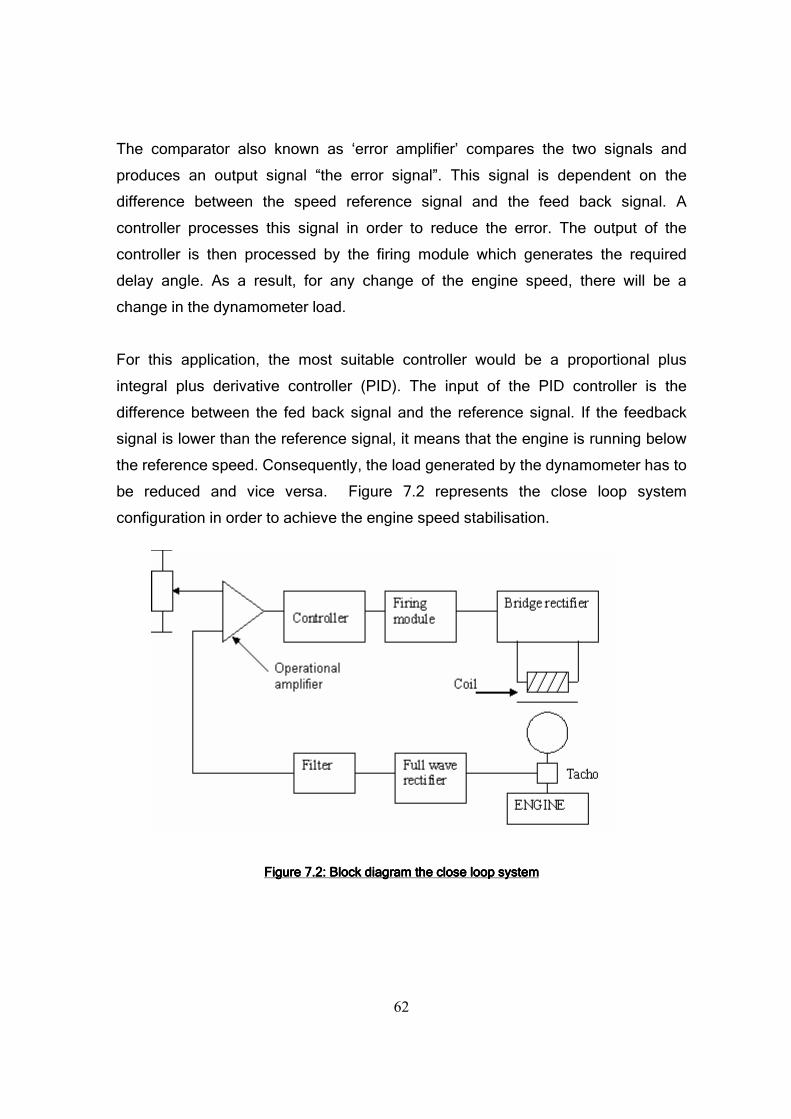
62

The comparator also known as ‘error amplifier’ compares the two signals and

produces an output signal “the error signal”. This signal is dependent on the

difference between the speed reference signal and the feed back signal. A

controller processes this signal in order to reduce the error. The output of the

controller is then processed by the firing module which generates the required

delay angle. As a result, for any change of the engine speed, there will be a

change in the dynamometer load.

For this application, the most suitable controller would be a proportional plus

integral plus derivative controller (PID). The input of the PID controller is the

difference between the fed back signal and the reference signal. If the feedback

signal is lower than the reference signal, it means that the engine is running below

the reference speed. Consequently, the load generated by the dynamometer has to

be reduced and vice versa. Figure 7.2 represents the close loop system

configuration in order to achieve the engine speed stabilisation.

Figure 7.2: Figure 7.2: Figure 7.2: Figure 7.2: BBBBlock diagram the close loop system lock diagram the close loop system lock diagram the close loop system lock diagram the close loop system

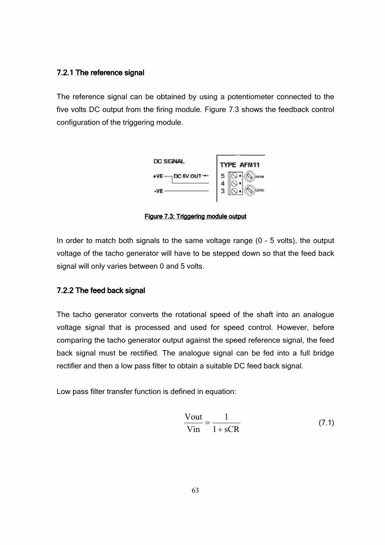
63

7.2.1 The reference signal 7.2.1 The reference signal 7.2.1 The reference signal 7.2.1 The reference signal

The reference signal can be obtained by using a potentiometer connected to the

five volts DC output from the firing module. Figure 7.3 shows the feedback control

configuration of the triggering module.

Figure 7.3: Triggering module outputFigure 7.3: Triggering module outputFigure 7.3: Triggering module outputFigure 7.3: Triggering module output

In order to match both signals to the same voltage range (0 – 5 volts), the output

voltage of the tacho generator will have to be stepped down so that the feed back

signal will only varies between 0 and 5 volts.

7.2.7.2.7.2.7.2.2222 The feed back signal The feed back signal The feed back signal The feed back signal

The tacho generator converts the rotational speed of the shaft into an analogue

voltage signal that is processed and used for speed control. However, before

comparing the tacho generator output against the speed reference signal, the feed

back signal must be rectified. The analogue signal can be fed into a full bridge

rectifier and then a low pass filter to obtain a suitable DC feed back signal.

Low pass filter transfer function is defined in equation:

sCR1

1

Vin

Vout

+= (7.1)

64

7.2.3 The difference amplifier 7.2.3 The difference amplifier 7.2.3 The difference amplifier 7.2.3 The difference amplifier

The reference signal and the feed back signal are compared to obtain the error

signal that will drive the controller. The most suitable amplifier configuration for this

task is the difference amplifier.

This op amp configuration amplifies the difference between two input voltages

however the ratio of R1/R2 must be equal to the ratio R3/R4 to produce the

required error voltage. Equation 7.2 expresses output voltage in terms of R1, R2,

V2 and V1.

)12(1

2VV

R

RVout −×= (7.2)

Vout is referred as the error signal. Figure 7.4 gives the basic circuit configuration

of a differential amplifier.

FigureFigureFigureFigure 7. 7. 7. 7.4444: D: D: D: Differential amplifier configuration ifferential amplifier configuration ifferential amplifier configuration ifferential amplifier configuration

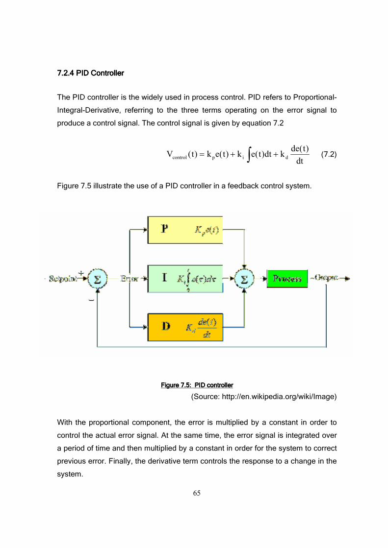
65

7.2.7.2.7.2.7.2.4444 PID PID PID PID CCCController ontroller ontroller ontroller

The PID controller is the widely used in process control. PID refers to Proportional-

Integral-Derivative, referring to the three terms operating on the error signal to

produce a control signal. The control signal is given by equation 7.2

∫ ++=dt

)t(dekdt)t(ek)t(ek)t(V dipcontrol (7.2)

Figure 7.5 illustrate the use of a PID controller in a feedback control system.

Figure 7.Figure 7.Figure 7.Figure 7.5555: PID controller : PID controller : PID controller : PID controller

(Source: http://en.wikipedia.org/wiki/Image)

With the proportional component, the error is multiplied by a constant in order to

control the actual error signal. At the same time, the error signal is integrated over

a period of time and then multiplied by a constant in order for the system to correct

previous error. Finally, the derivative term controls the response to a change in the

system.

66

With the derivative term the controller can anticipate what action is needed by

estimating the rate of change of the error signal (Parr 1996). As a result, when the

error signal is changing rapidly, the controller adds more corrective actions to the

plant.

67

CHAPTER 8 – DISCUSION AND CONCLUSION

8.1 Achievement of Objectives 8.1 Achievement of Objectives 8.1 Achievement of Objectives 8.1 Achievement of Objectives

The aim of this project was to upgrade the existing eddy-current dynamometer by

replacing its current valve operated DC source with a power electronic system.

Most of the objectives put forward at the start of this project were fulfilled, however,

some of them changed during the year.

The protective circuit of the initial circuit was supposed to be re-used with the

upgraded system. However, with a meticulous analysis of the circuit configuration it

became apparent that this option was going to be time consuming and would result

in a deterioration of the initial control unit. As a result, it was preferable to

disconnect the entire system and design the whole circuit with updated devices.

The first new objective was to upgrade the protection circuit to ensure the

safeguards of the dynamometer. As a result, an updated version of the initial

protection circuit has been designed and tested in the laboratory. The new

protection circuit works perfectly in the laboratory but has not been tested onto the

dynamometer because the selected DPCO relay has been under-rated.

As well as this new objective, only a brief description of the closed loop control

configuration has been investigated so as to introduce the concept of engine speed

stabilisation to a future student.

68

8.2 Further Work 8.2 Further Work 8.2 Further Work 8.2 Further Work

It was realised that the selected relay which is connected to the ignition coil was

not suitable for this application. Two propositions were offered to solve this

problem.

The first was to use the initial protection circuit with the upgraded rectifier.This

option is time consuming and will degrade the initial circuit ,however, is a realisable

option.

The second option was to run the valve rectifier circuit and sense the current from

the ignition coil while the engine was turned off by means of RL2 (see figure 5.1).

By knowing the peak value of inductive current while the magnetic field of the coil

collapses, a well rated diode can be selected and then connected in parallel to the

ignition coil. This diode will act as a free wheeling diode so that the inductive

current will remain within the coil.

Chapter seven introduces the closed loop configuration of the system and briefly

explains how speed stabilisation can be achieved. The feed back control system

requires further analysis and more investigation of system stabilisation. As a result,

this project leads to the design of the closed loop control system.

With further work, the upgraded control unit will provide two different modes of

operation. The first mode of operation, presented in this study, provides manual

load control in order to test and record engine performance. The second mode of

operation will enable engine speed stabilisation.

In the near future, it will be possible to connect the control unit to a computer in

order to acquire digital data. The actual torque measuring apparatus will be

replaced by a load cell so that test data can be transmitted to a data acquisition

system rather than being recorded manually.

69

8888.3 Conclusio.3 Conclusio.3 Conclusio.3 Conclusion n n n

This study provides a description of the process involved in eddy current braking

and more specifically it defines how the Heenan dynamometer braking process

occurs. Moreover, the dissertation describes the process of rectification and how it

has been achieved in order to generate an adjustable DC source from a single

phase AC source. Also, the paper provides a comprehensive chapter on how the

dynamometer, the control unit and the engine are protected and gives a description

of the protection devices used in the upgraded protective circuit. Following that, a

description of the devices selected for half control rectification is given. The final

topic briefly describes how engine speed stabilisation can be achieved using the

open loop system.

70

LIST OF REFERENCES

Ahfock, T 2005, ELE3805 Power Electronics Principles & Applications Study Book

1 & 2, University of Southern Queensland, Toowoomba.

Farnell 2005, Farnell In one Electronic Engineering, A Premier Farnell Company,

NSW Australia.

Fisher, M 1991, Power electronic, PWS –KENT, Boston.

Nise, N 2005, Control Systems Engineering, Jhon wiley & son, California.

Parr, E 1996, Control Engineering, Butterworth Heinemann, London.

Sharma, R 2005, Electrical Technology Study Book 1, University of Southern

Queensland, Toowoomba.

Winther, J 1975, Dynamometer Handbook of Basic Theory and Applications,

Cleveland, Ohio: Eaton Corporation.

Williams, B 1992, Devices, Drivers, Applications and passive components,

MACMILLAN, London.

71

IIIIIIIIIIII APPENDICIESAPPENDICIESAPPENDICIESAPPENDICIES

72

APPENDIX A – PROJECT SPECIFICATION

73

74

APPENDIX B – M3MVR DATA SHEET

75

76

APPENDIX C – P102W DATA SHEET

77

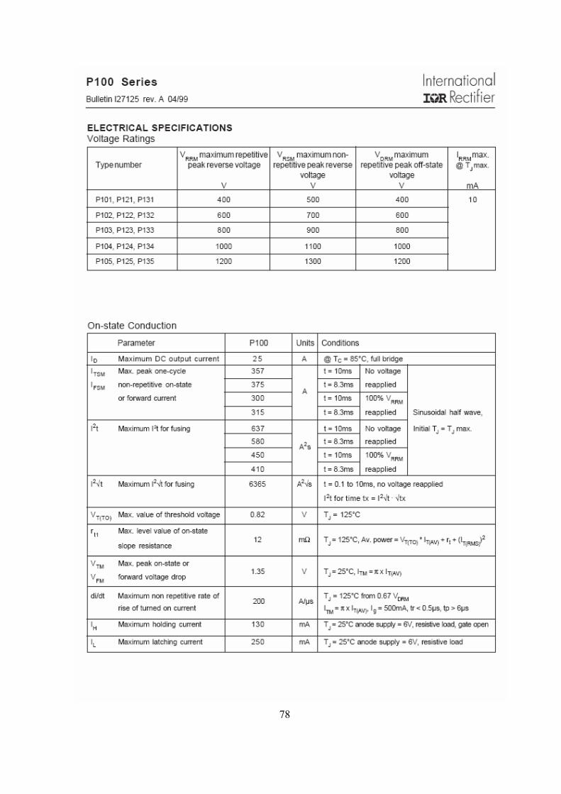
78

79

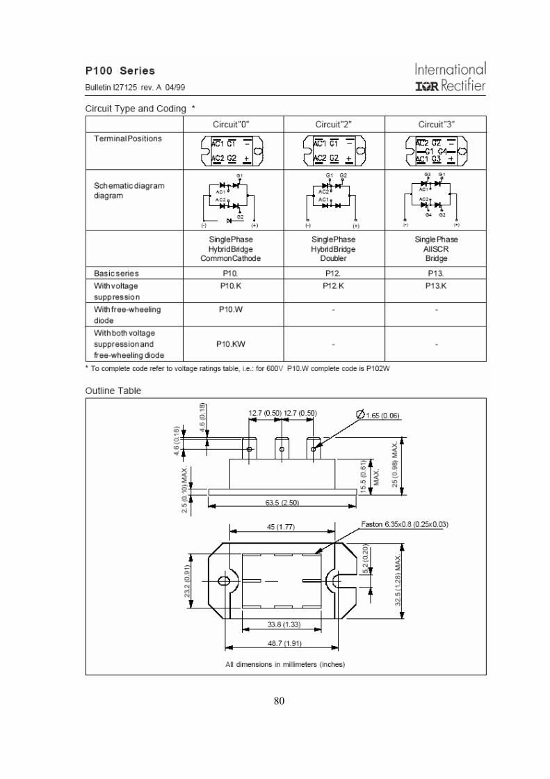
80

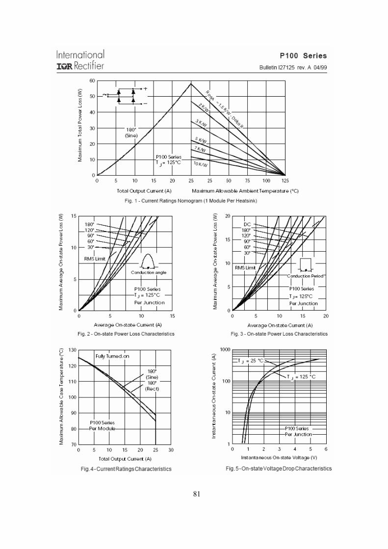
81

82

83

APPENDIX D – AFM11 DATA SHEET

84

85

86

APPENDIX E – EQUIPEMENT COST

87

Name : BAVARIN Rudolph Date : 8/08/2006

Discipline : BENG ELE

Project : 50kW Eddy current Braking

farnell 2005

Order

code Part number Description Qty price cost Page

178-756 AFM-11 Trigger module 1 273.7 273.68 1/837

351076 CLR11069S5K0K potentiometer 5K 1 35.59 35.59 1/742

890-935 1/4 fine aluminium (grub screw) potentiometer knob 1 6.01 6.01 2/303

362-530 P102W B2HKF config thyristor diode bridge 1 121.3 121.34 1/831

696-547 12VA-12% regulation Transformer Clamp mounting 1 19.28 19.28 2/1016

427-4527 M3MVR Multifunction voltage relay 1 245 245 2/526

443-4470 green SPNO Momentary 1 17.26 17.26 2/752

560-650 DPCO - 5532 series 10 A relay 1 20.12 20.12 2/593

335-4131 double surface 1.15 heat sink 1 42.29 42.29 1/863

Total 780.57

88

APPENDIX F – CONTROL UNIT BOX DESIGN

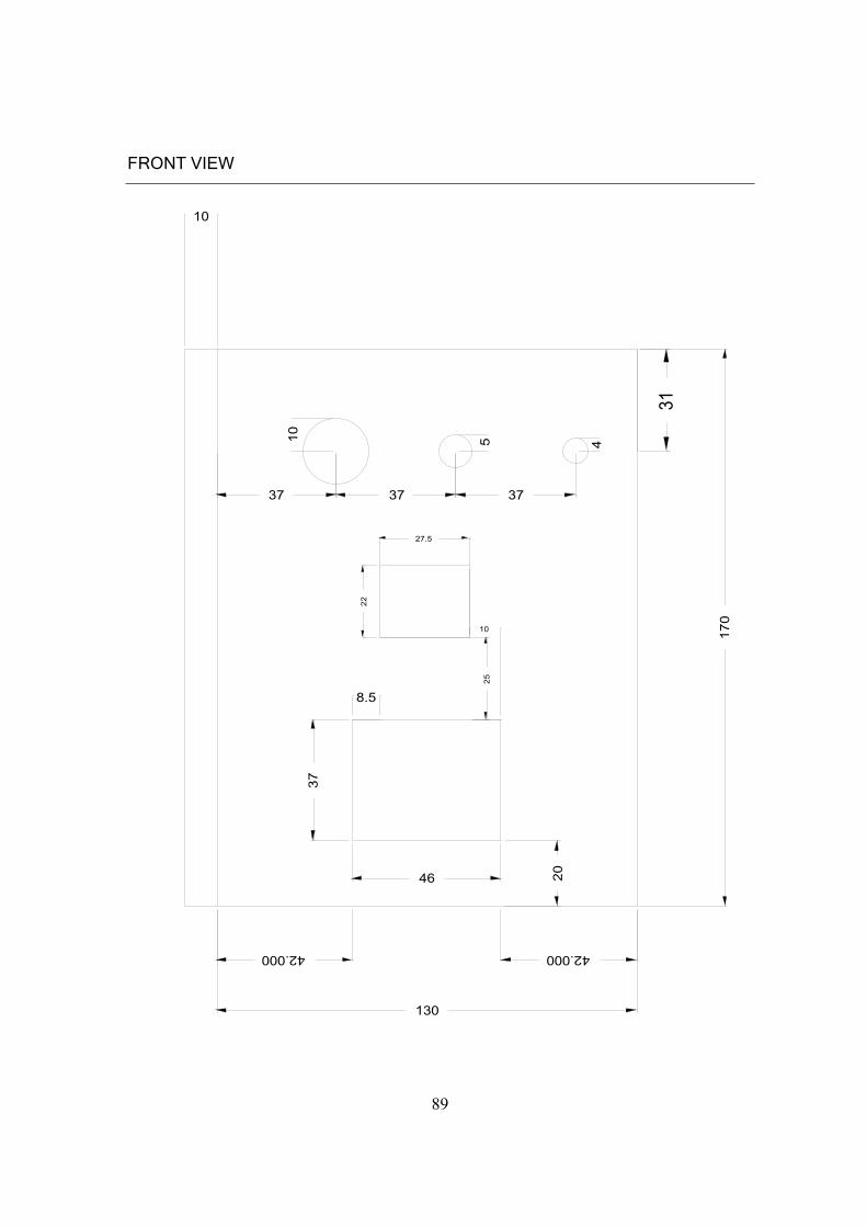
89

170

8.5

42.00042.000

20

130

46

37

37 37 37

10

5 4

10

31

27.5

25

10

22

FRONT VIEW

90

30

16

7

7

7

7

7

7

BACK VIEW

91

17

5

110

45

SIDE VIEW

Documents

University of Southern Queensland · University of Southern Queensland ... 50 kW Eddy Current brake50 kW Eddy Current ... Chapter 6 Chapter 6 –––– THE UPGRADED SYSTEM …