Embed Size (px)
Citation preview
University of Southampton Research Repository
ePrints Soton
Copyright © and Moral Rights for this thesis are retained by the author and/or other copyright owners. A copy can be downloaded for personal non-commercial research or study, without prior permission or charge. This thesis cannot be reproduced or quoted extensively from without first obtaining permission in writing from the copyright holder/s. The content must not be changed in any way or sold commercially in any format or medium without the formal permission of the copyright holders.
When referring to this work, full bibliographic details including the author, title, awarding institution and date of the thesis must be given e.g.
AUTHOR (year of submission) "Full thesis title", University of Southampton, name of the University School or Department, PhD Thesis, pagination
http://eprints.soton.ac.uk

UNIVERSITY OF SOUTHAMPTON
Modelling of reactive absorption in
gas-liquid flows on structured packing
by
Jason J. Cooke
Thesis for the degree of Doctor of Philosophy
in the
Faculty of Engineering and the Environment
School of Engineering Sciences
May 2016


UNIVERSITY OF SOUTHAMPTON
ABSTRACT
FACULTY OF ENGINEERING AND THE ENVIRONMENT
SCHOOL OF ENGINEERING SCIENCES
Doctor of Philosophy
MODELLING OF REACTIVE ABSORPTION IN GAS-LIQUID FLOWS
ON STRUCTURED PACKING
by Jason J. Cooke
Carbon capture & storage (CCS) is at the technological forefront in the challenge of
reducing carbon emissions. The most viable approach to implementing CCS within
existing coal and natural gas power stations is the post-combustion capture of CO2 by
absorption into amine solutions within packed column absorbers.
CFD modelling is an important aspect in the design and optimisation of this process.
However, significant challenges arise due to the large range of spatial scales and the
complexity of the physics being modelled. Therefore, simplification of the problem
is required to complete such simulations using the computational resources currently
available.
This thesis explores some of the approaches used to model flow within packed columns.
It concludes that, with current computing resources, standard modelling approaches
are not viable for large scale simulations of CCS. This led to the development of the
Enhanced Surface Film (ESF) model. The ESF approach was able to simulate chemically
enhanced absorption of gaseous species into thin liquid films. The method significantly
reduced the computational resources required and is a significant step to enable future
researchers to model larger domains in CCS.
The ESF approach has wide ranging applications due to the ubiquitous nature of liquid
films across the industrial and environmental sectors. In many industries the dynamics
of thin liquid films play a crucial role in the overall performance. Further applications
may include thin film microreactors, surface coating, biofluids and medical applications.


Acknowledgements
First of all, I would like to thank my supervisors, Dr Lindsay-Marie Armstrong and Dr.
Edward Richardson, for all of their support and invaluable advice.
I am eternally grateful to my girlfriend, Florinela for all of her support, love and friend-
ship over the years. I am happy, and I’m sure she will be, that I will be able to spend
my weekends with her now that this thesis is complete. Last but not least, I would like
to thank my family for everything they have done for me and for helping me to achieve
my goals.
I also acknowledges the use of the IRIDIS High Performance Computing Facility, and
associated support services at the University of Southampton, in the completion of this
work.
v


Declaration of Authorship
I, Jason J. Cooke, declare that this thesis and the work presented in it are my own and
has been generated by me as the result of my own original research.
MODELLING OF REACTIVE ABSORPTION IN GAS-LIQUID FLOWS ON STRUC-
TURED PACKING
I confirm that:
• This work was done wholly or mainly while in candidature for a research degree
at this University.
• Where any part of this thesis has previously been submitted for a degree or any
other qualification at this University or any other institution, this has been clearly
stated.
• Where I have consulted the published work of others, this is always clearly at-
tributed.
• Where I have quoted from the work of others, the source is always given. With
the exception of such quotations, this thesis is entirely my own work.
• I have acknowledged all main sources of help.
• Where the thesis is based on work done by myself jointly with others, I have made
clear exactly what was done by others and what I have contributed myself.
• Parts of this work have been published as given in the list of publications.
Signed:
Date:
vii


Publications
Journal Articles
Cooke, J., Armstrong, L., Luo, K. & Gu, S. (2014) Adaptive Mesh Refinement of Gas-
Liquid Flow on an Inclined Plane. Journal of Computers & Chemical Engineering, 60,
297-306.
Conference Papers
Cooke, J., Gu, S., Armstrong, L. & Luo, K. (2012) Gas-Liquid Flow on Smooth and
Textured Inclined Planes. World Academy of Science, Engineering and Technology, 68,
1712-1719.
ix


Contents
Acknowledgements v
Declaration of Authorship vii
Publications ix
Nomenclature xxi
1 Introduction 1
1.1 Carbon Capture and Storage (CCS) . . . . . . . . . . . . . . . . . . . . . 1
1.2 CCS with Packed Columns . . . . . . . . . . . . . . . . . . . . . . . . . . 1
1.3 Motivation for Research . . . . . . . . . . . . . . . . . . . . . . . . . . . . 3
1.4 Novel Research . . . . . . . . . . . . . . . . . . . . . . . . . . . . . . . . . 6
1.5 Structure of this thesis . . . . . . . . . . . . . . . . . . . . . . . . . . . . . 6
2 Literature Review 9
2.1 CCS with Packed Columns . . . . . . . . . . . . . . . . . . . . . . . . . . 9
2.2 Computational Fluid Dynamics Modelling . . . . . . . . . . . . . . . . . . 10
2.2.1 Microscale . . . . . . . . . . . . . . . . . . . . . . . . . . . . . . . . 15
2.3 Thin Liquid Films . . . . . . . . . . . . . . . . . . . . . . . . . . . . . . . 17
2.3.1 Full Film Dynamics . . . . . . . . . . . . . . . . . . . . . . . . . . 18
2.3.2 Thin-film long-wave approximation . . . . . . . . . . . . . . . . . . 20
2.3.3 Weighted Integral Boundary Layer Method . . . . . . . . . . . . . 21
2.3.4 Contact Line Dynamics . . . . . . . . . . . . . . . . . . . . . . . . 22
2.4 Mass Transfer and Reaction Kinetics . . . . . . . . . . . . . . . . . . . . . 23
2.4.1 The Stagnant Film Model . . . . . . . . . . . . . . . . . . . . . . . 23
2.4.2 The Higbie Penetration Model . . . . . . . . . . . . . . . . . . . . 25
2.4.3 Chemically Enhanced Absorption . . . . . . . . . . . . . . . . . . . 27
2.4.4 Modelling of Mass Transfer . . . . . . . . . . . . . . . . . . . . . . 30
3 CFD Modelling 35
3.1 Introduction . . . . . . . . . . . . . . . . . . . . . . . . . . . . . . . . . . . 35
3.2 General Governing Equations . . . . . . . . . . . . . . . . . . . . . . . . . 35
3.2.1 Continuity Equation . . . . . . . . . . . . . . . . . . . . . . . . . . 36
3.2.2 Momentum Equations . . . . . . . . . . . . . . . . . . . . . . . . . 36
3.3 Multiphase Flow . . . . . . . . . . . . . . . . . . . . . . . . . . . . . . . . 36
3.3.1 Mass Transfer Modelling . . . . . . . . . . . . . . . . . . . . . . . . 38
3.4 Discretisation of the domain . . . . . . . . . . . . . . . . . . . . . . . . . . 40
xi

xii CONTENTS
3.5 The Scalar-Transport Equation . . . . . . . . . . . . . . . . . . . . . . . . 40
3.5.1 Discretising the Diffusion Term . . . . . . . . . . . . . . . . . . . . 40
3.5.2 Discretising the Source Term . . . . . . . . . . . . . . . . . . . . . 41
3.5.3 Discretising the Advection Term . . . . . . . . . . . . . . . . . . . 41
3.5.3.1 Central Differencing . . . . . . . . . . . . . . . . . . . . . 42
3.5.3.2 Upwind Differencing . . . . . . . . . . . . . . . . . . . . . 42
3.5.4 Temporal Discretisation . . . . . . . . . . . . . . . . . . . . . . . . 42
3.6 Discretisation of the Navier-Stokes Equations . . . . . . . . . . . . . . . . 44
3.6.1 The Pressure Equation . . . . . . . . . . . . . . . . . . . . . . . . . 44
3.6.2 PISO Algorithm . . . . . . . . . . . . . . . . . . . . . . . . . . . . 45
3.7 Adaptive Mesh Refinement . . . . . . . . . . . . . . . . . . . . . . . . . . 46
4 Microscale Hydrodynamics 47
4.1 Introduction . . . . . . . . . . . . . . . . . . . . . . . . . . . . . . . . . . . 47
4.2 Numerical Methodology . . . . . . . . . . . . . . . . . . . . . . . . . . . . 48
4.2.1 Modelling and Governing Equations . . . . . . . . . . . . . . . . . 48
4.2.1.1 Important Parameters . . . . . . . . . . . . . . . . . . . . 48
4.2.2 Computational Domain . . . . . . . . . . . . . . . . . . . . . . . . 49
4.2.3 Simulation Set-Up . . . . . . . . . . . . . . . . . . . . . . . . . . . 50
4.3 Results and Discussion . . . . . . . . . . . . . . . . . . . . . . . . . . . . . 53
4.3.1 Validation . . . . . . . . . . . . . . . . . . . . . . . . . . . . . . . . 53
4.3.2 Smooth Plate . . . . . . . . . . . . . . . . . . . . . . . . . . . . . . 55
4.3.3 Textured Plate . . . . . . . . . . . . . . . . . . . . . . . . . . . . . 58
4.4 Conclusion . . . . . . . . . . . . . . . . . . . . . . . . . . . . . . . . . . . 61
5 Adaptive Mesh Refinement at the Microscale 63
5.1 Introduction . . . . . . . . . . . . . . . . . . . . . . . . . . . . . . . . . . . 63
5.1.1 Numerical Modelling . . . . . . . . . . . . . . . . . . . . . . . . . . 64
5.1.1.1 Adaptive Grid Refinement . . . . . . . . . . . . . . . . . 64
5.1.2 Computational Domain . . . . . . . . . . . . . . . . . . . . . . . . 65
5.1.3 Simulation Set-Up . . . . . . . . . . . . . . . . . . . . . . . . . . . 67
5.2 Standard Grid Refinement . . . . . . . . . . . . . . . . . . . . . . . . . . . 69
5.2.1 Results & Discussion . . . . . . . . . . . . . . . . . . . . . . . . . . 69
5.3 Adaptive Grid Refinement . . . . . . . . . . . . . . . . . . . . . . . . . . . 70
5.3.1 Refinement at the Interface . . . . . . . . . . . . . . . . . . . . . . 70
5.3.2 Results . . . . . . . . . . . . . . . . . . . . . . . . . . . . . . . . . 70
5.3.3 Full-Film Refinement . . . . . . . . . . . . . . . . . . . . . . . . . . 74
5.3.4 Improvements to Interface Refinement . . . . . . . . . . . . . . . . 77
5.4 Conclusion . . . . . . . . . . . . . . . . . . . . . . . . . . . . . . . . . . . 78
6 Enhanced Surface Film Model 81
6.1 Introduction . . . . . . . . . . . . . . . . . . . . . . . . . . . . . . . . . . . 81
6.2 Governing Equations . . . . . . . . . . . . . . . . . . . . . . . . . . . . . . 83
6.2.1 Full 3-D Navier-Stokes Equation . . . . . . . . . . . . . . . . . . . 83
6.2.2 Tools for Depth Integration . . . . . . . . . . . . . . . . . . . . . . 83
6.2.3 Depth-Averaged Navier-Stokes Equations . . . . . . . . . . . . . . 84
6.2.3.1 Surface Tension . . . . . . . . . . . . . . . . . . . . . . . 86

CONTENTS xiii
6.2.4 Closure Models . . . . . . . . . . . . . . . . . . . . . . . . . . . . . 88
6.2.4.1 Shear Stress . . . . . . . . . . . . . . . . . . . . . . . . . 88
6.2.4.2 Depth-Averaged Pressure . . . . . . . . . . . . . . . . . . 89
6.2.4.3 Momentum Dispersion . . . . . . . . . . . . . . . . . . . 89
6.3 Numerical Methodology . . . . . . . . . . . . . . . . . . . . . . . . . . . . 90
6.3.1 Geometry & Mesh . . . . . . . . . . . . . . . . . . . . . . . . . . . 90
6.3.2 Simulation Set-up . . . . . . . . . . . . . . . . . . . . . . . . . . . 91
6.4 Analysis . . . . . . . . . . . . . . . . . . . . . . . . . . . . . . . . . . . . . 92
6.4.1 VOF . . . . . . . . . . . . . . . . . . . . . . . . . . . . . . . . . . . 93
6.4.2 Surface Film Model . . . . . . . . . . . . . . . . . . . . . . . . . . 95
6.4.2.1 Surface Tension . . . . . . . . . . . . . . . . . . . . . . . 95
6.4.2.2 Dispersion . . . . . . . . . . . . . . . . . . . . . . . . . . 99
6.4.2.3 Viscous Terms and Wall Shear Stress . . . . . . . . . . . 101
6.4.2.4 Depth-Averaged Pressure . . . . . . . . . . . . . . . . . . 103
6.5 Results & Discussion . . . . . . . . . . . . . . . . . . . . . . . . . . . . . . 103
6.5.1 Comparison of Simulation CPU-Time . . . . . . . . . . . . . . . . 109
6.6 Conclusion . . . . . . . . . . . . . . . . . . . . . . . . . . . . . . . . . . . 111
7 Surface Film Modelling with Mass Transport and Chemical Reaction113
7.1 Introduction . . . . . . . . . . . . . . . . . . . . . . . . . . . . . . . . . . . 113
7.2 Mass Transfer with the ESF Model . . . . . . . . . . . . . . . . . . . . . . 114
7.2.1 Liquid Film Exposure Time . . . . . . . . . . . . . . . . . . . . . . 116
7.2.1.1 Residence Time Equation . . . . . . . . . . . . . . . . . . 117
7.2.1.2 Reactions Kinetics with the ESF Model . . . . . . . . . . 118
7.3 Simulations with Mass Transfer . . . . . . . . . . . . . . . . . . . . . . . . 119
7.3.1 1-Dimensional Mass Transfer . . . . . . . . . . . . . . . . . . . . . 119
7.3.1.1 Computational Domain & Simulation Set-up . . . . . . . 120
7.3.1.2 Results & Discussion . . . . . . . . . . . . . . . . . . . . 121
7.3.2 2-Dimensional Mass Transfer . . . . . . . . . . . . . . . . . . . . . 121
7.3.2.1 Computational Domain . . . . . . . . . . . . . . . . . . . 122
7.3.2.2 Simulation Set-up . . . . . . . . . . . . . . . . . . . . . . 123
7.3.2.3 Results & Discussion . . . . . . . . . . . . . . . . . . . . 126
7.3.3 3-Dimensional Mass Transfer . . . . . . . . . . . . . . . . . . . . . 131
7.3.3.1 Computational Domain & Simulation Set-up . . . . . . . 132
7.3.3.2 Results & Conclusions . . . . . . . . . . . . . . . . . . . . 133
7.4 Chemically Enhanced Mass Transfer in a Wetted-Wall Column . . . . . . 136
7.4.1 Computational Domain . . . . . . . . . . . . . . . . . . . . . . . . 136
7.4.2 Simulation Set-up . . . . . . . . . . . . . . . . . . . . . . . . . . . 136
7.4.3 Results & Discussion . . . . . . . . . . . . . . . . . . . . . . . . . . 139
7.5 Chemically Enhanced Absorption of CO2 on a Partially Wetted Plate . . 142
7.5.1 Computational Domain . . . . . . . . . . . . . . . . . . . . . . . . 142
7.5.2 Simulation Set-up . . . . . . . . . . . . . . . . . . . . . . . . . . . 142
7.5.3 Results & Discussion . . . . . . . . . . . . . . . . . . . . . . . . . . 144
7.6 Conclusion . . . . . . . . . . . . . . . . . . . . . . . . . . . . . . . . . . . 147
8 Conclusion 149
8.1 Hydrodynamic Modelling of Thin Films . . . . . . . . . . . . . . . . . . . 149

xiv CONTENTS
8.2 Mass Transfer and Reaction Kinetics . . . . . . . . . . . . . . . . . . . . . 151
8.3 Future Work . . . . . . . . . . . . . . . . . . . . . . . . . . . . . . . . . . 152
A Microscale Hydrodynamics 155
A.1 Mesh Independence Checks . . . . . . . . . . . . . . . . . . . . . . . . . . 155
A.1.1 Smooth Plate . . . . . . . . . . . . . . . . . . . . . . . . . . . . . . 155
A.1.2 Textured Plate . . . . . . . . . . . . . . . . . . . . . . . . . . . . . 155
B Derivation of Depth-Averaged Navier-Stokes Equations 159
B.0.1 Tools for Depth Integration . . . . . . . . . . . . . . . . . . . . . . 159
B.0.1.1 The kinematic boundary condition at the free surface . . 159
B.0.1.2 The kinematic boundary condition at the plate surface . 160
B.0.1.3 The Leibniz theorem and fundamental theorem of inte-gration . . . . . . . . . . . . . . . . . . . . . . . . . . . . 160
B.0.2 The continuity equation . . . . . . . . . . . . . . . . . . . . . . . . 160
B.0.3 The momentum equations . . . . . . . . . . . . . . . . . . . . . . . 161
B.0.4 Depth-averaged pressure and surface tension . . . . . . . . . . . . 164
C Mass Transfer with AMR-VOF 167
C.1 Computational Domain and Grid . . . . . . . . . . . . . . . . . . . . . . . 167
C.1.1 Results . . . . . . . . . . . . . . . . . . . . . . . . . . . . . . . . . 168
Bibliography 171
List of Figures
1.1 CO2 absorber and stripper (image adapted from L. Raynal, P. A. Bouil-lon, A. Gomez, and P. Broutin, “From MEA to demixing solvents andfuture steps; a roadmap for lowering the cost of post-combustion carboncapture,” Chemical Engineering Journal, vol. 171, pp. 742-752, 2011 [1]) . 2
1.2 Example of stainless steel unstructured packing IMTP 50 (images adaptedfrom P. Alix and L. Raynal, “Liquid distribution and liquid hold-up inmodern high capacity packings,” Chemical Engineering Research and De-sign, vol. 86, no. 6, pp. 585-591, 2008. [2]) . . . . . . . . . . . . . . . . . . 2
1.3 Example of metallic structured packing MellapakPlus 252.Y. (images adaptedfrom P. Alix and L. Raynal, “Liquid distribution and liquid hold-up inmodern high capacity packings,” Chemical Engineering Research and De-sign, vol. 86, no. 6, pp. 585− 591, 2008. [2]) . . . . . . . . . . . . . . . . 3
2.1 The two-film model for mass transfer . . . . . . . . . . . . . . . . . . . . . 24
2.2 Representation of the Higbie Penetration Model . . . . . . . . . . . . . . . 26
3.1 Definition of contact angle, θw, unit vector normal to wall, nnnw and unitvector tangential to wall, tttw . . . . . . . . . . . . . . . . . . . . . . . . . . 38
4.1 Computational domain and mesh for smooth plate . . . . . . . . . . . . . 50
4.2 Computational domain and mesh for textured plate . . . . . . . . . . . . 51
4.3 The specific wetted area against Rel . . . . . . . . . . . . . . . . . . . . . 53
4.4 Comparison of film velocity profile against the Nusselt solution at Rel = 224 55
4.5 Comparison of specific wetted area for a range of Rel at inclination anglesof 30o and 60o . . . . . . . . . . . . . . . . . . . . . . . . . . . . . . . . . . 56
4.6 Thickness of liquid film at Rel = 156.85 0.01 seconds after release . . . . . 57
4.7 Thickness of liquid film at Rel = 156.85 0.08 seconds after release . . . . . 57
4.8 Thickness of liquid film at Rel = 156.85 0.12 seconds after release . . . . . 57
4.9 Thickness of liquid film at Rel = 156.85 at steady state . . . . . . . . . . 58
4.10 Specific wetted area, aw and specific interfacial area, ai against Rel forthe smooth and textured plate (θ = 60o) . . . . . . . . . . . . . . . . . . . 58
4.11 Thickness of liquid film at Rel = 134.44 and θ = 60o (left: Smooth plate,right: Textured plate) . . . . . . . . . . . . . . . . . . . . . . . . . . . . . 59
4.12 Interfacial velocity contours of liquid film at Rel = 179.26 and θ = 60o
(left: Smooth plate, right: Textured plate) . . . . . . . . . . . . . . . . . . 61
4.13 Velocity vectors within the liquid film along the plane y = 0.02 m atRel = 179.26 and θ = 60o (top: Smooth plate, bottom: Textured plate) . 61
5.1 AMR refinement of a single computational cell in 2D for 2 levels of re-finement . . . . . . . . . . . . . . . . . . . . . . . . . . . . . . . . . . . . . 65
xv

xvi LIST OF FIGURES
5.2 Computational domain and refined static mesh . . . . . . . . . . . . . . . 66
5.3 Comparison of the static mesh with a snapshot of the partial-film AMRmesh at t = 0.36s and Rel = 156.85 (blue line is the gas-liquid interface) . 67
5.4 Closer view of comparison of the static mesh with the t = 0.36s snapshotof the partial-film AMR mesh at Rel = 156.85 (blue line is the gas-liquidinterface) . . . . . . . . . . . . . . . . . . . . . . . . . . . . . . . . . . . . 67
5.5 Comparison of Static Grid Simulation with Literature . . . . . . . . . . . 69
5.6 The specific wetted area against Rel for AMR at the interface . . . . . . . 71
5.7 Contour plot of gas-liquid interface at Rel = 44.8 (Partial-film mesh) . . . 71
5.8 Contour plot of gas-liquid interface at Rel = 58.3 (Partial-film mesh) . . . 72
5.9 Contour plot of gas-liquid interface at Rel = 71.7 (Partial-film mesh) . . . 72
5.10 Contour plot of gas-liquid interface at Rel = 44.8 for static grid (left) andPartial-film grid (right) . . . . . . . . . . . . . . . . . . . . . . . . . . . . 73
5.11 Comparison of specific wetted area and specific interfacial area againstRel for the partial-film AMR simulation . . . . . . . . . . . . . . . . . . . 73
5.12 Flow within the gas phase for Rel = 156.85 at steady state. . . . . . . . . 74
5.13 The specific wetted area against Rel for various degrees of AMR . . . . . 75
5.14 Cutting plane used for interface plots . . . . . . . . . . . . . . . . . . . . . 76
5.15 Interface plots along cutting plane at steady state . . . . . . . . . . . . . . 77
6.1 Definition of contact angle, θw, unit vector normal to wall, nnnw and unitvector tangential to wall, tttw . . . . . . . . . . . . . . . . . . . . . . . . . . 86
6.2 Computational domain used in the VOF approach . . . . . . . . . . . . . 90
6.3 Computational domain used in thin film approach - side view . . . . . . . 91
6.4 3D VOF Interface Contour Plot with cut planes (Rel = 156.85) . . . . . . 94
6.5 Budget Plot of Numerical Integration of 3D y-momentum equation terms- Central position . . . . . . . . . . . . . . . . . . . . . . . . . . . . . . . . 94
6.6 Budget Plot of Numerical Integration of 3D y-momentum equation terms- Oblique position . . . . . . . . . . . . . . . . . . . . . . . . . . . . . . . 95
6.7 Budget Plot of Numerical Integration of 3D y-momentum equation terms- Stagnation position . . . . . . . . . . . . . . . . . . . . . . . . . . . . . . 95
6.8 Budget Plot of Numerical Integration of 3D y-momentum Convection andMomentum Dispersion - Central position . . . . . . . . . . . . . . . . . . 96
6.9 Budget Plot of Numerical Integration of 3D y-momentum Convection andMomentum Dispersion - Oblique position . . . . . . . . . . . . . . . . . . 96
6.10 Budget Plot of Numerical Integration of 3D y-momentum Convection andMomentum Dispersion - Stagnation position . . . . . . . . . . . . . . . . . 97
6.11 Film depth at steady state for AMR-VOF (left) and Surface Film Model(right) . . . . . . . . . . . . . . . . . . . . . . . . . . . . . . . . . . . . . . 100
6.12 Film depth at steady state for AMR-VOF (left) and Surface Film Model(right) . . . . . . . . . . . . . . . . . . . . . . . . . . . . . . . . . . . . . . 100
6.13 Budget Plot comparing the Closed and Modelled Surface Tension of they-momentum equations for range of δn- Oblique position . . . . . . . . . . 101
6.14 Budget Plot comparing the Closed and Modelled Surface Tension of they-momentum equations for range of δn- Stagnation position . . . . . . . . 101
6.15 Budget Plot comparing the Closed and Modelled Viscous Terms of they-momentum equations - Central position . . . . . . . . . . . . . . . . . . 102

LIST OF FIGURES xvii
6.16 Budget Plot comparing the Closed and Modelled Viscous Terms of they-momentum equations - Oblique position . . . . . . . . . . . . . . . . . . 102
6.17 Budget Plot comparing the Closed and Modelled Viscous Terms of they-momentum equations - Stagnation position . . . . . . . . . . . . . . . . 103
6.18 Budget Plot comparing the Closed and Modelled Depth Average PressureTerm (hp) - Central position . . . . . . . . . . . . . . . . . . . . . . . . . 104
6.19 Budget Plot comparing the Closed and Modelled Depth Average PressureTerm (hp) - Oblique position . . . . . . . . . . . . . . . . . . . . . . . . . 104
6.20 Budget Plot comparing the Closed and Modelled Depth Average PressureTerm (hp) - Stagnation position . . . . . . . . . . . . . . . . . . . . . . . . 105
6.21 Comparison of wetted area for Surface Film Model with standard AMR-VOF and Experimental Data . . . . . . . . . . . . . . . . . . . . . . . . . 106
6.22 Film depth at Rel = 156.85 (Left: AMR-VOF, Centre: Surface FilmModel [3], Right: ESF Model) . . . . . . . . . . . . . . . . . . . . . . . . . 106
6.23 Film depth for AMR-VOF and Surface Film Model at various Rel . . . . 107
6.24 Budget Plot of Numerical Integration of ESF depth-averaged, y-momentumequation terms - Central position . . . . . . . . . . . . . . . . . . . . . . . 108
6.25 Budget Plot of Numerical Integration of 3D y-momentum equation terms- Central position . . . . . . . . . . . . . . . . . . . . . . . . . . . . . . . . 108
6.26 Budget Plot of Numerical Integration of ESF depth-averaged, y-momentumequation terms - Oblique position . . . . . . . . . . . . . . . . . . . . . . . 109
6.27 Budget Plot of Numerical Integration of 3D y-momentum equation terms- Oblique position . . . . . . . . . . . . . . . . . . . . . . . . . . . . . . . 109
6.28 Budget Plot of Numerical Integration of ESF depth-averaged, y-momentumequation terms - Stagnation position . . . . . . . . . . . . . . . . . . . . . 110
6.29 Budget Plot of Numerical Integration of 3D y-momentum equation terms- Stagnation position . . . . . . . . . . . . . . . . . . . . . . . . . . . . . . 110
7.1 Mesh of the 1-D domain . . . . . . . . . . . . . . . . . . . . . . . . . . . . 120
7.2 Liquid and gas distribution in 1-D domain . . . . . . . . . . . . . . . . . . 121
7.3 Species concentration in 1-D domain for He = 0.1 . . . . . . . . . . . . . 121
7.4 1-dimensional species distribution for He = 0.1,e = 0.05, C0L = 0 and
C0G = 1 . . . . . . . . . . . . . . . . . . . . . . . . . . . . . . . . . . . . . . 122
7.5 Mesh of the 2-D domain (VOF) . . . . . . . . . . . . . . . . . . . . . . . . 123
7.6 Mesh of the 2-D domain (Surface Film) . . . . . . . . . . . . . . . . . . . 124
7.7 Comparison of velocity profile with Nusselt profile . . . . . . . . . . . . . 126
7.8 Comparison kL,local against the Higbie Penetration Theory . . . . . . . . . 128
7.9 Comparison kL,local against the Higbie Penetration Theory (Close to inlet) 128
7.10 Concentration contours. (Left: VOF, right:ESF) . . . . . . . . . . . . . . 129
7.11 Plot of concentration profile along the central vertical slice. . . . . . . . . 129
7.12 Comparison of exposure time plotted against distance from liquid inlet . . 130
7.13 Slice locations in VOF domain . . . . . . . . . . . . . . . . . . . . . . . . 131
7.14 Plot of concentration gradient at various locations . . . . . . . . . . . . . 131
7.15 Plot of exposure time at interface contour - Partially Wetted Plate. Left:VOF tH,RT , right: ESF tH,RT . . . . . . . . . . . . . . . . . . . . . . . . . 134
7.16 Plot of exposure time at central slice - Partially Wetted Plate . . . . . . . 134
7.17 Plot of exposure time at oblique slice - Partially Wetted Plate . . . . . . . 135
7.18 Plot of exposure time at stagnation slice - Partially Wetted Plate . . . . . 135
xviii LIST OF FIGURES
7.19 Wetted-Wall Column Apparatus (Puxty et al. [4]) . . . . . . . . . . . . . 137
7.20 Wetted wall column domain adapted from Puxty et al. [4] . . . . . . . . 138
7.21 CO2 absorption flux as a function of applied partial pressure (313K) . . . 141
7.22 CO2 absorption flux as a function of applied partial pressure (333K) . . . 141
7.23 CO2 concentration slices on partially wetted plate. . . . . . . . . . . . . . 144
7.24 CO2 concentration contours on the film surface for partially wetted plate 144
7.25 Hatta number for the partially wetted plate . . . . . . . . . . . . . . . . . 145
7.26 Enhancement factor for the first order irreversible reaction between CO2
and MEA for the partially wetted plate . . . . . . . . . . . . . . . . . . . 145
7.27 Velocity on partially wetted plate . . . . . . . . . . . . . . . . . . . . . . . 146
7.28 CO2 concentration contours on partially wetted plate (Dg = 100×DCO2g ). 147
7.29 CO2 concentration slices on partially wetted plate (Dg = 100×DCO2g ). . . 147
A.1 Specific wetted area against time for smooth plate θ = 60o . . . . . . . . . 156
A.2 Specific wetted area against time for smooth plate θ = 30o . . . . . . . . . 156
A.3 Specific wetted area against time for textured plate θ = 60o . . . . . . . . 157
C.1 Initial AMR-VOF Grid 12096 cells. . . . . . . . . . . . . . . . . . . . . . . 168
C.2 Final AMR-VOF Grid 6.7 million cells. . . . . . . . . . . . . . . . . . . . 168
C.3 Close view of AMR-VOF Grid 6.7 million cells. (α1) . . . . . . . . . . . . 169
C.4 Close view of AMR-VOF Grid 6.7 million cells. (CO2) . . . . . . . . . . . 169

List of Tables
4.1 Phase Properties . . . . . . . . . . . . . . . . . . . . . . . . . . . . . . . . 52
4.2 Specific wetted area for smooth and textured plate at θ = 60o . . . . . . . 60
5.1 Computational Meshes . . . . . . . . . . . . . . . . . . . . . . . . . . . . . 68
5.2 Phase Properties . . . . . . . . . . . . . . . . . . . . . . . . . . . . . . . . 68
5.3 Simulation time & actual time to convergence . . . . . . . . . . . . . . . . 75
5.4 Percentage change from original initial grid to coarser initial grid (AMR) 78
6.1 Equation terms . . . . . . . . . . . . . . . . . . . . . . . . . . . . . . . . . 85
6.2 Phase Properties . . . . . . . . . . . . . . . . . . . . . . . . . . . . . . . . 92
6.3 Range of fluid properties for determination of δn. (Fluid 0 is baseline -water) . . . . . . . . . . . . . . . . . . . . . . . . . . . . . . . . . . . . . . 98
6.4 Test Fluid Properties . . . . . . . . . . . . . . . . . . . . . . . . . . . . . . 99
6.5 Wetted area for various fluids . . . . . . . . . . . . . . . . . . . . . . . . . 99
6.6 CPU Time . . . . . . . . . . . . . . . . . . . . . . . . . . . . . . . . . . . 111
7.1 Phase Properties . . . . . . . . . . . . . . . . . . . . . . . . . . . . . . . . 125
7.2 Phase Properties . . . . . . . . . . . . . . . . . . . . . . . . . . . . . . . . 133
7.3 Phase Properties . . . . . . . . . . . . . . . . . . . . . . . . . . . . . . . . 138
7.4 Average KG Data Comparison . . . . . . . . . . . . . . . . . . . . . . . . 142
xix


Nomenclature
Aw Wetted area
aw Specific wetted area
Ai Interfacial area
ai Specific interfacial area
AMP Isobutanolamine
AMR Adaptive mesh refinement
b Reactants mole ratio
C Concentration
Ca Capillary number
CCS Carbon Capture and Storage
CFD Computational Fluid Dynamics
CSF Continuum surface force
D Diffusion coefficient
DEA Diethanolamine
DTSF Diffusion through Stagnant Film
E Enhancement factor
Ei Instantaneous enhancement factor
ESF Enhanced Surface Film
G Gas-phase
H Characteristic thickness
Ha Hatta number
He Henry’s constant
HETP Bed height equivalent to a theoretical plate
int Liquid interface
IPCC Intergovernmental Panel on Climate Change
k Reaction constant
kavg Average mass transfer coefficient
kG Gas-side mass transfer coefficient
kL Liquid-side mass transfer coefficient
KG Overall mass transfer coefficient
L Characteristic length
L Liquid-phase
xxi
xxii NOMENCLATURE
LBM Lattice Boltzmann Method
LMPD Log mean pressure difference
MEA Monoethanolamine
MDEA Methyldiethanolamine
EMCD Equi-Molar Counter Diffusion
N Flux
p Depth-averaged pressure
r Forward reaction rate
Re Reynolds number
REUs Representative elementary units
RST Reynolds Stress Transport
tH Liquid-film exposure time
tH,SV Liquid-film exposure time (Calculated using surface velocity)
tH,RT Liquid-film exposure time (Calculated using residence-time equation)
τ Residence time
u Depth-averaged velocity
u′′
Deviation from depth-averaged velocity
We Weber number
VOF Volume-of-fluid
α Volume fraction
αf Wetted fraction
δ Delta function
δG Two-film theory gas film thickness
δL Two-film theory liquid film thickness
δn Threshold film thickness
∆x Cell length
ε Lubrication parameter
κ Curvature
σ Surface tension
Θ Contact time
θ Plate inclination angle
θw Static contact angle

Chapter 1
Introduction
1.1 Carbon Capture and Storage (CCS)
Clean coal technologies encompass a wide range of engineering solutions developed to
reduce the level of pollutant gases released into the environment. A fairly recent de-
velopment within this field, namely Carbon Capture & Storage (CCS), involves pre-
combustion or post-combustion processes to separate CO2 from carbon-rich fossil fuels.
The resulting CO2 is then stored to prevent it from entering the atmosphere. This
research will focus on the CFD modelling of post-combustion capture of CO2 utilising
amine solutions within packed columns.
1.2 CCS with Packed Columns
CCS using packed columns involves the capture of CO2 using an amine solution, usually
monoethanolamine (MEA). Aqueous MEA undergoes a reversible reaction with CO2,
whereby the chemical equilibrium and mass transfer rates are dependent upon many
factors. CO2 is removed from exhaust gases in the absorber, where cooled MEA flows
counter-current to the gas flow. CO2 is subsequently removed from the solution in a
stripper using a counter-current flow of steam [5]. The amine solution is heated by the
stream to shift the chemical equilibrium of the system. The regenerated MEA is cooled
before re-entering the cycle. A diagram of a typical absorber and stripper configuration
for carbon capture is shown in Figure 1.1.
Packed columns are used to enhance heat and mass transfer by providing large gas-liquid
interfacial areas. Packing materials within the packed columns come in two distinct
categories; structured and unstructured. Structured packing is optimal since it provides
high mass transfer efficiency and low pressure drop within the columns.
1
2 Chapter 1 Introduction
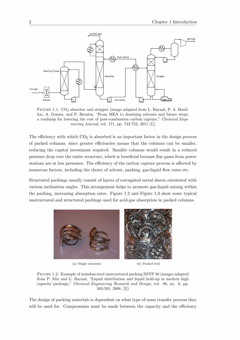
Figure 1.1: CO2 absorber and stripper (image adapted from L. Raynal, P. A. Bouil-lon, A. Gomez, and P. Broutin, “From MEA to demixing solvents and future steps;a roadmap for lowering the cost of post-combustion carbon capture,” Chemical Engi-
neering Journal, vol. 171, pp. 742-752, 2011 [1])
The efficiency with which CO2 is absorbed is an important factor in the design process
of packed columns, since greater efficiencies means that the columns can be smaller,
reducing the capital investment required. Smaller columns would result in a reduced
pressure drop over the entire structure, which is beneficial because flue gases from power
stations are at low pressures. The efficiency of the carbon capture process is affected by
numerous factors, including the choice of solvent, packing, gas-liquid flow rates etc.
Structured packings usually consist of layers of corrugated metal sheets orientated with
various inclination angles. This arrangement helps to promote gas-liquid mixing within
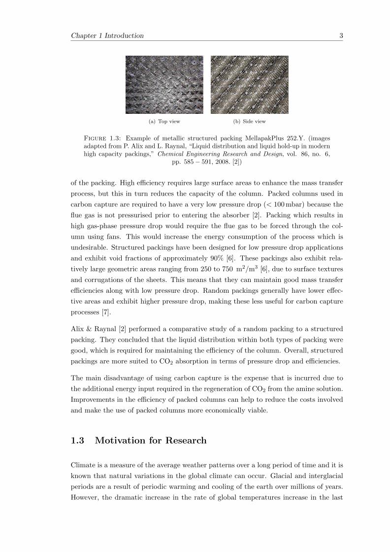
the packing, increasing absorption rates. Figure 1.2 and Figure 1.3 show some typical
unstructured and structured packings used for acid-gas absorption in packed columns.
(a) Single elements (b) Packed bed
Figure 1.2: Example of stainless steel unstructured packing IMTP 50 (images adaptedfrom P. Alix and L. Raynal, “Liquid distribution and liquid hold-up in modern highcapacity packings,” Chemical Engineering Research and Design, vol. 86, no. 6, pp.
585-591, 2008. [2])
The design of packing materials is dependent on what type of mass transfer process they
will be used for. Compromises must be made between the capacity and the efficiency
Chapter 1 Introduction 3
(a) Top view (b) Side view
Figure 1.3: Example of metallic structured packing MellapakPlus 252.Y. (imagesadapted from P. Alix and L. Raynal, “Liquid distribution and liquid hold-up in modernhigh capacity packings,” Chemical Engineering Research and Design, vol. 86, no. 6,
pp. 585− 591, 2008. [2])
of the packing. High efficiency requires large surface areas to enhance the mass transfer
process, but this in turn reduces the capacity of the column. Packed columns used in
carbon capture are required to have a very low pressure drop (< 100 mbar) because the
flue gas is not pressurised prior to entering the absorber [2]. Packing which results in
high gas-phase pressure drop would require the flue gas to be forced through the col-
umn using fans. This would increase the energy consumption of the process which is
undesirable. Structured packings have been designed for low pressure drop applications
and exhibit void fractions of approximately 90% [6]. These packings also exhibit rela-
tively large geometric areas ranging from 250 to 750 m2/m3 [6], due to surface textures
and corrugations of the sheets. This means that they can maintain good mass transfer
efficiencies along with low pressure drop. Random packings generally have lower effec-
tive areas and exhibit higher pressure drop, making these less useful for carbon capture
processes [7].
Alix & Raynal [2] performed a comparative study of a random packing to a structured
packing. They concluded that the liquid distribution within both types of packing were
good, which is required for maintaining the efficiency of the column. Overall, structured
packings are more suited to CO2 absorption in terms of pressure drop and efficiencies.
The main disadvantage of using carbon capture is the expense that is incurred due to
the additional energy input required in the regeneration of CO2 from the amine solution.
Improvements in the efficiency of packed columns can help to reduce the costs involved
and make the use of packed columns more economically viable.
1.3 Motivation for Research
Climate is a measure of the average weather patterns over a long period of time and it is
known that natural variations in the global climate can occur. Glacial and interglacial
periods are a result of periodic warming and cooling of the earth over millions of years.
However, the dramatic increase in the rate of global temperatures increase in the last

4 Chapter 1 Introduction
50 years is unprecedented over millennia [8]. The Intergovernmental Panel on Climate
Change (IPCC) [8] has estimated that the global temperature has risen by 0.65-1.06 oC
between the period 1880-2012 and they state that it is 95-100% certain that human
influences were the dominant cause global warming between 1951-2010.
Greenhouse gases are comprised mainly of carbon dioxide, methane, sulphur dioxide,
nitrous oxide and fluorinated gases. The layer of greenhouse gases in the atmosphere
absorbs heat which is reflected from the surface of the earth. This process increases
the temperature of the earth and prevents the thermal radiation of the sun from being
reflected back into space. It is known that naturally present greenhouse gases in the
atmosphere are vital to the survival of life on the planet by maintaining a habitable
climate.
Global manmade emissions of greenhouse gases has increased significantly over the last
100 years. According to Marland et al. [9], carbon emission have risen by about 90%
between 1970 and 2011, increasing from approximately 4000 million metric tons of car-
bon to 9500 million metric tons of carbon per annum. Carbon dioxide emissions from
fossil fuels and industrial processes account for 65% of total greenhouse gas emissions [8].
Therefore, the recent increase in carbon emissions has caused a significant increase in
greenhouse gases within the atmosphere. The rising level of greenhouse gases in the
atmosphere will increase the warming of the earth, which has been observed in temper-
ature data, the reduction in arctic sea-ice and rising sea levels [8]. Furthermore, rising
global temperatures can cause positive feedback, where CO2 can be desorbed from the
ocean as a direct result of higher oceanic temperatures. This is because the equilibrium
between the concentration of CO2 in the air and in the ocean is shifted by changes in
temperature.
According to the IPCC [8], without climate change mitigation there could be an increase
in global temperatures of 3.7-4.8 oC by the year 2100. This would significantly increase
the adverse effects of higher global temperature, such as rising sea levels and unpre-
dictable weather events. In order to reverse the effects of manmade global warming
mitigation is required to reduce the levels of greenhouse gas emissions into the atmo-
sphere.
Power and heat generation from the burning of coal, natural gas and oil is the largest
source of global greenhouse gas emissions, accounting for 25% of emissions in 2010 [8].
Therefore, mitigation of carbon emissions from these sources could greatly reduce the
impact of manmade emissions on climate change. Carbon Capture & Storage is one
of the various methods that can be used to reduce the carbon footprint of the energy
sector. These large, point sources of carbon dioxide can be targeted by CCS technologies
to reduce the level of emission. This research will help to provide cost-effective solutions
to the capture of CO2 from flue gases emitted from both coal and natural gas power
stations.

Chapter 1 Introduction 5
Agriculture, forestry and land use accounted for 24% of global greenhouse gas emissions
in 2010, whilst industrial sources and transportation accounted for 21% and 14%, respec-
tively. These sources of emissions are usually much smaller on an individual basis and
so are less suited to current CCS technologies. For example, an individual car or factory
will represent a tiny fraction of the total emissions for their respective sectors. Therefore,
research is better focussed on the power and heat generation sector where an individual
investment into CCS technology will represent a greater reduction in greenhouse gas
emissions.
Stabilisation of CO2 emissions at the current level would not result in the stabilisation of
CO2 concentration in the atmosphere, it would in fact continue to increase [8]. In order
to stabilise or reduce the level of CO2 in the atmosphere the level of emissions would
need to be reduced significantly, by as much as 80% [8]. Therefore, in order to make
a significant impact on mitigation of greenhouse gases in the atmosphere, CCS in the
energy production sector would need to reduce emissions by a similarly large amount.
There are a vast range of CCS technologies, using methods including chemical and
physical absorption, adsorption, cryogenics and membranes [10]. The advantage of post-
combustion carbon capture methods, like those employed with packed columns, is that
they can be retro-fitted to current coal/gas-fired power stations. This significantly re-
duces the capital investment, since no major modifications need to be made to existing
power stations.
However, at the present time, these technologies consume large amounts of energy and
they drain the electrical energy being produced by the power stations. As a result, this
reduces the overall efficiency of power stations causing a surge in operating costs, which
would inevitably be passed onto customers. This research topic is not just about devel-
oping the technology to remove the maximum volume of carbon dioxide, it also involves
aspects of design optimisation to reduce the overall operating costs. In fact, reducing
the energy consumption of carbon capture via packed columns would be considered the
most important factor from an industrial and economic viewpoint.
Due to the fact that the flue gas is at a relatively low pressure, of the same order as
atmospheric pressure, packed columns are required to have very low pressure drops over
the whole column height. Otherwise, the gas would need to be pressurised prior to
the absorption process, which would further increase operating costs. Therefore, packed
columns need to be designed to take this into account, whilst maintaining high gas-liquid
interfacial areas to ensure adequate absorption rates.
CFD modelling provides a method to simulate the processes which occur within packed
columns. However, at the present moment, there are major difficulties in modelling the
process as a whole. This is due to the large range of spatial scales and the significant
impact of small-scale features on the column efficiencies. Difficulties also arise in mass
transfer modelling, which is a crucial element of the process.

6 Chapter 1 Introduction
1.4 Novel Research
The work detailed in this Thesis represents an extension of knowledge in the fields of
CFD and CCS. As a result of initial investigations it was concluded that an alternative
approach was required to model thin films in CCS, due to computational limitations.
Thus, the Enhanced Surface Film (ESF) model was developed and implemented in Open-
FOAM. This development was based on the depth-averaged Navier-Stokes equations,
and was aimed at simulating thin liquid films that occur within packed columns. The
ESF solver models surface tension using the continuum surface force (CSF) model [11].
The application of the CSF model to the depth-averaged equations required the devel-
opment of an additional model for the threshold film thickness. It was shown that the
ESF approach was able to accurately predict the hydrodynamics of thin films across a
range of fluids, including water, acetone and glycerol at various flow rates.
The ESF model was extended to include physical mass transfer, utilising Higbie pen-
etration theory [12] to simulate interfacial mass transfer. The surface-age required by
Higbie penetration theory was determined by the development a residence-time transport
equation, applicable to depth-averaged flow. This allowed the mass transfer coefficient
to predicted, in parallel with the hydrodynamics of the liquid film.
The final addition made by this work was the inclusion of chemically enhanced mass
transfer with the ESF model. This was achieved using the Enhancement factor model
and allowed both 1st and 2nd order reaction kinetics to be simulated in addition to
interfacial mass transfer and film hydrodynamics. The ESF model not only has applica-
tions within CCS, but also across a range of industries where the efficiency of equipment
is dependent on the structure of thin liquid films.
1.5 Structure of this thesis
Chapter 1: Introduction
This chapter gives an introduction to carbon capture, detailing the carbon capture
process within packed columns. An overview of motivation for the research in this field
is then given.
Chapter 2: Literature Review
An extensive literature review is performed, focussing on the computational fluid dy-
namics modelling research. This includes single-phase flows and multi-phase flows with
mass transfer and reaction kinetics.

Chapter 1 Introduction 7
Chapter 3: CFD Modelling
This chapter gives an introduction to CFD modelling and provides the governing equa-
tions for the simulations used throughout this thesis. An overview of the discretisation
process of the finite volume method in given. The chapter also details the approach
that is used to map solutions between different meshes, required during adaptive mesh
refinement techniques.
Chapter 4: Microscale Hydrodynamics
The results of multi-phase flow simulations at the microscale are detailed in this chapter.
Flow on the packing surfaces is simplified to flow down an inclined plane. A novel surface
texture pattern was designed and tested in terms of wetted area.
Chapter 5: Adaptive Mesh Refinement at the Microscale
This chapter gives the results of adaptive mesh refinement at the microscale. Comparison
of the results are made with those using a highly refined static mesh and experimental
data from the literature.
Chapter 6: Enhanced Surface Film Model
The development of the Enhanced Surface Film (ESF) model is detailed. The model is
tested and validated against experimental data. Simulations are performed for a range
of fluids, including water, acetone and glycerol.
Chapter 7: Surface Film Modelling with Mass Transport & Chemical
Reaction
In this chapter the ESF model is extended to included mass transfer. This allows gas
separation processes to be modelled along with the hydrodynamics of thin liquid films.
Chemically enhanced absorption is also implemented using the Enhancement factor ap-
proach. The final model is validated against experimental data of CO2 absorption in a
wetted wall column. The ESF model is then used to simulate CO2 absorption into a
partially wetted film.

8 Chapter 1 Introduction
Chapter 8: Conclusion
The final conclusions are made, along with suggestions for future research. This includes
additional application of the ESF model and further extensions that could be made to
it.
Chapter 2
Literature Review
This chapter reviews the body of literature in the area of carbon capture using packed
columns. Initially, a broad discussion of packed columns is detailed, leading onto the
computational fluid dynamics modelling work which has researched. This involves work
investigating the variety of scales within the absorbers. Since thin liquid films are an
important feature of carbon capture using packed columns a review of theoretical works
on thin film is detailed. Research into mass transfer is then discussed. Finally, literature
detailing the inclusion of reaction kinetics into the models is reviewed.
2.1 CCS with Packed Columns
The use of experiments to analyse proposed advances in technology is very expensive,
especially at full-scale. Despite this, several pilot-plant studies have been performed
in the literature [13, 14] studying the effects of variations of parameters, such as liquid
flow rates, gas flow rates, packing types and CO2 loadings. Many other experimental
investigation have been reported in the literature, including the determination of the
effects of packing texture on liquid-side mass transfer, pressure drop through structured
packing and liquid hold-up in packed columns [15–17]. However, these mainly focus on
reduced-scale equipments and it is important to understand that results and correlations
derived at this scale may not necessarily apply or may include further errors at full-scale.
Computational modelling provides an alternative research tool to experimental inves-
tigations, since the cost is significantly reduced. Simulations can easily be repeated
with different parameters, such as packing geometry, without the expense involved in
manufacturing test samples. Process simulation tools and rate-based modelling have
been used in the literature to study mass transfer efficiencies of packed columns [18].
However, these types of models do not directly take into account the internal structure
and the packing and the complex hydrodynamics inherent in packed columns.
9
10 Chapter 2 Literature Review
It is important to model the hydrodynamics because flow patterns can have a distinct
effect on the absorption and reaction characteristics. This type of detailed modelling also
provides information that is out of the reach of experimental investigations, which can
be crucial in the understanding and the optimisation of the processes involved in CO2
absorption within packed columns. Computational fluid dynamics is a computational
modelling approach which enables simulations to be performed with the inclusion of
hydrodynamics and reaction kinetics.
As noted by some authors [19], the use and applicability of more rigorous models is
dependent upon the situations being modelled. In some circumstances a simplified
approach may adequately model the physical problem and the use of more rigorous
models can unnecessarily increase the complexity of the problem. This emphasises the
importance of evaluating each problem on the basis of simplifications that can be made.
2.2 Computational Fluid Dynamics Modelling
Computational fluid dynamics modelling is a numerical method used to solve fluid flow
problems. It involves discretising the governing equations and the flow domain to form
a set of algebraic equations, which are then solved using computational algorithms.
The major difficulty that arises when modelling carbon capture through packed columns
is the large range of spatial scales that exist throughout the process. To accurately
model the whole system, near wall effects must be accounted for, requiring detailed
modelling of the liquid films. However, absorbers and strippers have characteristic sizes
on the scale of meters and so even with the current computing power it is extremely
time-consuming to resolve all of these spatial scales simultaneously during a numerical
simulation. Furthermore, the inclusion of reaction kinetics into the model introduces
additional complexity. To overcome these difficulties researchers make approximations or
simplifications to models that allow simulations to be performed, including reducing the
problem to single-phase flow or segmenting the problem into ranges of spatial scales [20].
According to Øi [19], the modelling of CO2 absorption using packed columns can be
subdivided into the following processes; absorption and reaction kinetics, the gas-liquid
equilibrium, gas-liquid flows and pressure drop. As mentioned in section 1.2, the pressure
drop encountered through a packed column is a crucial factor in the design of packed
columns. A large pressure drop is undesirable and would reduce the overall efficiency
of the system, due to the increased energy consumption because of the requirement
for gas pumping, or due to the decreased CO2 absorption as a result of column height
compromises. Computational fluid dynamics is a suitable tool that can be used to
determine the pressure drop within the packed columns.

Chapter 2 Literature Review 11
Single-phase models have been used to evaluate pressure drop, since it is assumed that
the dry pressure drop can be simply correlated to the wet pressure drop, due to the same
pressure loss mechanisms. Larachi et al. [21] and Petre et al. [22] evaluated the pressure
drop within a column by reducing the whole packing layer into small mesoscale sections,
known as representative elementary units (REUs). The pressure drop contributions from
each of these elements was determined by relation with the loss coefficients of the flow.
Simulations with REUs are less computationally expensive and combinations of these
REUs can be used to evaluate the overall pressure drop within the column.
The main energy losses occur due to the collision of flows in the criss-crossing channels
of the packing and due to the sudden change in direction between successive layers of
packing [21,22]. It has been observed that increasing the inclination angle of the packing
from the standard 900 to 1350 resulted in reduced turbulence and smoother flow through
the packing transition layers.
Attempts have been made to increase the capacity (reduce the pressure drop) of struc-
tured packing by making modifications to the packing itself. Saleh et al. [23] used an
Eulerian-Eulerian approach to model dry and wet pressure drop in MellapakPlus 752.Y
structured packing. This method was considered appropriate because they aimed to
determine the pressure drop where sharp resolution of the gas-liquid interfacial region
was not considered important. In this particular packing the channels are bent around
to vertical at the inlet and outlet regions. Simulations showed that these modifications
reduced the dry pressure drop by as much as 10% and the wet pressure drop by 11.5%.
The addition of a flat sheet between the layers of packing was also studied by Saleh
et al. [23] and they found that the dry pressure drop decreased for the whole range of
F-factors tested. The additional plates separated the criss-crossing channels, removing
the pressure drop created by opposing flows within the channels. This also had the
advantage of increasing the wetted area of the packing, which should in theory increase
mass transfer and therefore increase CO2 absorption efficiencies, as long as the observed
increase in wetted also resulted in an increase in the interfacial area.
Pressure drop results directly from energy losses throughout the packing. Olujic et
al. [24] noted that only a small fraction of the energy lost in the packing goes towards
enhancing the mass transfer. Pressure loss sources, such as gas-gas interactions at the
criss-crossing sections of packing, have little contribution to the mass transfer efficiency.
Therefore, by reducing these types of pressure losses the overall pressure drop within the
column can be reduced without adversely affecting the efficiency of the column. Sheets
placed between the packing layers can eliminate these pressure loses. However, in reality,
adverse effects of these sheets, such as liquid maldistribution, reduced gas mixing and
liquid rivulet formation could reduce the mass transfer efficiency significantly, especially
below the loading point [24].

12 Chapter 2 Literature Review
Some authors have developed new packing geometries in order to optimise the capacity
of columns. Wen et al. [25] developed a novel structured packing design, with the
premise of decreasing the pressure drop whilst maintaining mass transfer efficiencies. The
novel design comprised of vertical sheets, with spacers punched and bent from the sheet
itself to reduce build costs. The spacers were used to maintain the structural integrity
of the packing, help to promote good liquid distribution and to induce turbulence to
increase mixing of the gas and liquid phases. CFD simulations were used to optimise
the designs, in terms of liquid distribution. Finalised designs were constructed and
compared experimentally with a commercial packing, Gempak 2.5A (Koch-Glitsch Inc.),
with the same surface area (250 m2/m3). It was found that the novel packing reduced
the pressure drop by as much as 45%, with at least 23% higher capacity and similar
performance in terms of mass transfer efficiency. Therefore, the new design was able
to reduce the pressure drop, whilst maintaining good efficiency. However, the surface
area of this novel design is at the lower range of the surface areas found in structured
packings and the observed results may not scale well to larger surface areas. Further
investigation is required in this area.
Raynal et al. [26] performed a combination of CFD simulations to determine the wet
pressure drop through a packed bed during co-current flow. Firstly, 3-dimensional single-
phase simulations were performed in order to determine the dry pressure drop. Secondly,
2-dimensional multi-phase calculations were used to determine the liquid hold-up within
a section of packing. Finally, the wet pressure drop was evaluated from a combination
of the dry pressure drop and the liquid hold-up within the packing.
Raynal et al. [26] also questioned the use of REUs to calculate pressure drop within
a whole section of packing. Using the criss-crossing channel REU [21, 22] the authors
were able to show that the pressure drop was highly dependent upon the inlet and outlet
lengths, before and after the crossing region. This was attributed to the large proportion
of the area of the domain that was composed of inlet and outlet boundaries, meaning that
the boundary conditions had a significant impact on the solution. The authors stated
that REUs can be used to provide qualitative comparisons between different packing
geometries, but should not be used to derive macroscopic flow characteristics.
To overcome the difficulties that arise by deriving macroscopic quantities (such as pres-
sure drop) from combinations of REUs, the work of Raynal et al. [27] and Raynal and
Royon-Lebeaud [20] proposed a novel elementary unit, being the smallest periodic ele-
ment within the packing. This allowed periodic boundary conditions to be imposed on
the open parts of the element, avoiding the challenges faced by REUs. However, the
use of periodic elements is also questionable in regions where the flow is not periodic in
nature, such as near the column walls. The multiple-scale approach was utilised in these
papers. Firstly, 2-dimensional VOF simulations were performed at the micro-scale to
determine the interfacial velocity and liquid hold-up. These results were then used at the
Chapter 2 Literature Review 13
mesoscale (periodic elements) to determine the pressure drop within the column. Single-
phase simulations were performed and the liquid was indirectly taken into account by
transforming the gas superficial velocity into an interstitial velocity. The liquid hold-up
was used to derive the interstitial velocity. The velocity at the interface was also taken
into account by applying moving wall boundary conditions to the walls of the periodic
element. The pressure drop data was then used at the macroscale, by representing the
packing as a porous media where the associated pressure loss coefficient was derived
from the mesoscale pressure drop data.
Fernandes et al. [28, 29] performed CFD simulations to calculate dry and wet pressure
drop within structured packing. Pressure drop is calculated from the results of CFD
simulations of gas flow through the structured packing. Dry pressure drop involves
simulations of gas flow only, whereas wet pressure drop includes the effect of liquid
flow within the structured packing. Dry pressure drop calculations were made using
two different domains. The first domain consisted of the region between two layers
of the corrugated sheets and the second consisted of a full section of packing. It was
found that the larger scale simulations, on a full section of packing, produced results
closer to experimental data. Wet pressure drops were performed in a similar method to
that previously. This again shows that the choice of computational domain is crucial.
Segmentation of the domain into periodic elements can reduce computational effort
considerably (due to the smaller number of cells required), but this can induce errors
due to the inherent simplifications being made.
Due to the turbulent nature of the gas flow within packed columns the choice of turbu-
lence model is important. This is particularly relevant during simulations to determine
the pressure drop. Various papers in the literature have reviewed different turbulence
models [26,30]. It was found that more advanced models, such as the RNG k− ε or the
SST k−ω models were more appropriate than standard k−ε models. However, all these
models rely on the eddy viscosity concept as a closure model for the Reynold’s stress
terms that arise in the Reynold’s averaged Navier-Stokes equations. An assumption of
the eddy viscosity concept is that the eddy viscosity and turbulence is isotropic. How-
ever, due to the complex flow through structured packing the flow is highly anisotropic
and therefore, the applicability of the eddy viscosity concept to these flows is highly
limited. On the other hand, Reynolds stress transport (RST) models apply a second-
order closure by solving transport equations for the Reynolds stress terms. Therefore,
RST models should be more applicable to flows within structured packing, since the
limitation of isotropic eddy viscosity is avoided.
Other aspects of packed columns which can be analysed using CFD are gas and liquid
distributors. The distribution of gas and liquid throughout the packed column is of
great importance, considering that maldistribution can reduce the column efficiency.
It has been shown, during a macro-scale simulation using the multiple-scale method,
that a simple horizontal inlet provides the best gas distribution when compared to a

14 Chapter 2 Literature Review
vertical pipe inlet with or without a baffle [27]. In relation to this, it is also important
to consider the orientation of the layers of packing with respect to the inlet flow. It
has been shown for a particular inlet configuration that the orientation of the layers can
have a noticeable effect on the homogeneity of the gas flow [20]. Wehrli et al. [31] used
CFD to investigate more complex gas distributors and their effect on the inlet flow.
Beugre et al. [32] used a different approach to conventional CFD to study the hydrody-
namics within structured packing. They used the Lattice Boltzmann Method (LBM) to
simulate the single-phase flow between two sheets of packing. Good agreement was ob-
served with experimental data. Comparisons with conventional CFD approaches showed
that the LBM was able to capture more of the variety of flow behaviours seen during tur-
bulent flow. However, the authors pointed out that this was at a higher computational
cost and is the major disadvantage of this method.
Wen et al. [33] used a two-component single-phase model to simulate flow within struc-
tured packing and the distribution of CO2 from a point source. This approach was able
to show the anisotropic nature of structured packing and how CO2 spreads throughout
the column. However, the absorption process can not be modelled using a single-phase
approach and therefore, multiphase approaches must be used for accurate modelling of
CO2 absorption.
Multiphase models have been used extensively in the literature to study the hydrody-
namics of packed columns, including single- and two-fluid models. Two-fluid models
consider the gas and liquid phases to be two distinct, separate fluids. Constitutive equa-
tions are then required to take account of the influence of each phase on the other,
such as interfacial drag [34]. However, in situations where the location and structure of
the interface is important, such as during reactive absorption, these models encounter
difficulties due to the diffuse nature of the interface. Large concentration gradients can
exist at the interface, which are not accurately modelled when the interface is diffuse.
One-fluid multiphase models, such as the volume-of-fluid (VOF) method, enable good
reconstruction of the interface to be made. However, these types of simulations are
mainly restricted to the flow at the microscale, due to the requirement to have large
numbers of cells in the interfacial region for accuracy. Hydrodynamics at the microscale
will be detailed further in section 2.2.1.
Mahr & Mewes [35, 36] proposed an alternative method to simulate two-phase flow
within packed columns at the macroscale. The proposed method used the elementary
cell method, whereby the elementary cell is taken to be the smallest periodic element
of packing. All variables of the flow field are then averaged over this elementary cell.
It is assumed that the flow entering and leaving each cell is similar and so the intricate
flow behaviour inside the cell does not need to be accounted for. Due to the preferential
spreading of fluid in the direction of the corrugations, the liquid phase is split into two
distinct phases, each with a preference for either of the two corrugation directions. This
Chapter 2 Literature Review 15
allows the highly anisotropic nature of structured packing to be accounted for in the
elementary cell method. CFD calculations were then performed using two liquid phases
and a single gas phase. This enabled simulations to be performed at the macroscale,
whilst taking into account the anisotropic nature of structured packing. However, this
approach neglects to model the flow within the periodic elements where mass transfer
may be effected, since the rate of absorption is highly dependent on the local structure
of the interface which is neglected in this approach.
2.2.1 Microscale
Liquid films are an important feature throughout many areas of engineering, ranging
from falling film microreactors [37,38] to Carbon Capture & Storage. It is important to
determine the fluid dynamics of liquid films because the efficiency of CO2 absorption is
closely related to the structure of the liquid films within the packing materials. Liquid
films can exhibit a range of flow regimes, including full-film, rivulet and droplet flow. The
formation and structure of these features is dependent upon various flow parameters,
such as liquid flow rate, plate surface texture, plate geometry etc.
Previous experimental studies have been undertaken to investigate the effect of surface
texture on liquid-side mass transfer during liquid film flows [15]. It was found that a
textured surface, typically found in commercial packing materials, can increase the mass
transfer by as much as 80% in comparison to a smooth plate [15]. CFD investigations
have been performed of heat and mass transfer on structured packing [34,39,40]. How-
ever, these papers do not examine the effect of surface texture on heat and mass transfer,
exclusively investigating smooth corrugated packing materials.
Haroun et al. [41] performed direct numerical simulations of gas-liquid flow on two-
dimensional structured surfaces using a modified VOF approach. Szulczewska et al. [42]
also used the VOF method to study liquid film flow using a two-dimensional approach.
They studied the dependency of the interfacial area on the gas and liquid flow rates
during counter-current flow. However, liquid films can exhibit highly three-dimensional
structures, such as rivulets, and these can not be observed when using a two-dimensional
model.
There have been many papers in the literature specifically looking at liquid films in an
effort to understand the hydrodynamic behaviour of packed columns and other gas-liquid
contactors at the micro-scale. Lan et al. [43] used a combined experimental and three-
dimensional, isothermal CFD approach to study thin film flow on inclined planes. They
focused on the effects that surface tension, contact angle, film flow rate and inclination
angle had on the film velocity, width and thickness. However, this investigation did not
specifically focus on liquid films within packed columns and so surface texture was not
taken into account.

16 Chapter 2 Literature Review
Johnson et al. [44] performed an experimental investigation of thin film flow down an
inclined plane. Specifically, they investigated the moving contact line and the formation
of rivulets. This included the effect of flow parameters on the wavelength of the rivulets
that form.
The analysis of counter-current gas-liquid flow at the micro-scale is of particular impor-
tance in the understanding of the processes involved in packed columns. Counter-current
gas flow has been observed to increase the thickness and fluctuation of liquid films [45].
Furthermore, thin films may be susceptible to break-up and hence, thicker films are
more suitable when this flow arrangement is used [46].
Microscale surface texture on packed columns has been found to have a large effect on
the structure of liquid films [46]. Valluri et al. [47] developed an analytical model for
film flow over sinusoidal and doubly sinusoidal surfaces at moderate Reynolds numbers.
A CFD approach was used to assess the viability of the model. The analytical model
was shown to provide good correlation with the CFD results for Rel < 30.
Full films provide the greatest efficiency because the large surface area is conducive
to CO2 absorption. The formation of rivulets, or any other phenomena which could
reduce the interfacial area of a film flowing on structured packing, could hinder heat
and mass transfer. These three-dimensional phenomena have been successfully modelled
using the VOF approach and it has been shown that the structure of a film is highly
dependent upon the geometry and the choice of boundary conditions during numerical
simulations [48,49].
Following on from this, Iso and Chen [50] examined the transition behaviour between
the different flow regimes exhibited on inclined plates. Three-dimensional, isothermal
VOF simulations were used to analyse the transition between rivulet flow and full film
flow. It was observed that a hysteresis phenomena occurred, depending on whether the
liquid flow rate was increasing or decreasing, suggesting that the flow is also affected by
historic flow patterns.
This emphasises the importance of performing time-dependent simulations to accurately
resolve the film flow features. Iso and Chen [50] also showed that a particular surface
texture on the packing material was able to increase the wetted area, which could en-
hance heat and mass transfer if interfacial area also increased. However, it is important
to examine the negative effects of surface texture, which may hinder heat and mass
transfer. For example, sinusoidal structures of certain amplitudes have been shown to
cause recirculation in the film, resulting in regions of stagnant fluid [46, 47]. These
regions will reduce the efficiency of CO2 absorption within packed columns.
Hoffmann et al. [49] performed an experimental investigation of film flow down an in-
clined plane to provide validation for their CFD simulations. The experiment consisted
of a small steel plate of 0.06m in length by 0.05m in width, with steel walls at the sides.

Chapter 2 Literature Review 17
This setup was chosen to be representative of a small section of structured packing. The
inclination angle was chosen to be either 45o or 60o to the horizontal, which represents
common inclination angles used in commercial structured packing [49]. The liquid at
the top of the plate was introduced by an overflowing weir to ensure a uniform film at
the inlet. Various flow rates were tested and the wetted area of the plate was determined
from pictures taken during the experiment.
Iso et al. [51] also performed a similar experiment to validate their CFD results. A single
inclination angle of 60o was chosen and a range of liquid flow rates were tested. The
plate was longer than that of Hoffmann et al. [49], but the measurement region was the
same size (i.e. 0.06m in length). They also measured the wetted area of the plate.
The experimental results of Hoffmann et al. [49] and Iso et al. [51] will be used to provide
validation for the initial simulations in this thesis. It is noted that the experimental
results report the wetted area, rather than the interfacial area of the liquid film. The
interfacial area is important for mass transfer, since mass transfer occurs through the
interfacial area of the film surface. However, determination of the interfacial area in an
experiment is difficult to achieve and was not considered important for the validation of
the hydrodynamics of liquid film flow.
An alternative approach to modelling thin films is to solve the depth-averaged Navier-
Stokes equations. These surface film models provide much greater flexibility for mod-
elling realistic absorption equipment due to the reduction in computational requirements.
The application of this approach has been used in many areas of research. These include
thin film microreactors [37, 38], surface coatings [52, 53], biofluids and medical applica-
tions [54,55]. Another such application is within internal combustion engines where thin
films are an important feature that can effect both the efficiency of combustion and the
resulting emissions.
2.3 Thin Liquid Films
Thin liquid films are an important feature in gas absorption equipment and so an in-
depth understanding of thin film flows is important in the modelling of acid-gas absorp-
tion within structured packing. Oron et al. [56] and Craster & Matar [57] performed
in-depth reviews on the theoretical literature focussing on the dynamics and stability of
thin liquid films.
The following discussion looks at two different flow situations. The first of these is
full film flow where the substrate is completely covered by the liquid film. Here the
instabilities arise at the film surface, which can lead to the formation of long-wave
structures. Secondly, a discussion of contact line dynamics is given. Here the substrate
is partially covered by the film, resulting in the formation of a contact line between the
18 Chapter 2 Literature Review
fluid interface and the underlying solid surface. This gives rise to instabilities that can
occur at the contact line, which can result in the formation of rivulets. Contact line
dynamics is of particular importance to the work performed in this thesis. Both of these
mechanisms can have a significant effect on mass transfer.
2.3.1 Full Film Dynamics
Full film dynamics involves situations where the fluid film completely covers a substrate,
or in other words, there exists no contact line between the fluid and solid surface. The
effect of contact lines and resulting instabilities of those contact lines will be discussed
in the following section.
The interface between a liquid film and the surrounding gas is a deformable interface [56],
and therefore any instability on an initially flat interface can create surface waves. It
has been shown that these interfaces exhibit long wavelength deformations, where the
wavelength of the deformation is much larger than the film thickness [58]. According
to Oron et al. [56], wave steepening at higher flow rate can even result in transitions
to quasiperiodic or chaotic structures, which can eventually lead to film rupture. This
behaviour can have a significant impact on the overall flow structure and the resulting
rate of mass transfer through a liquid film interface.
According to Kalliadasis et al. [58] there are three main mechanisms that have a direct
impact of long-wave instabilities. If an initially flat surface is exposed to a long-wave
perturbation the crest and troughs of the wave will be acted on by gravity. It is known
that the net streamwise flow rate in a film increase with fluid depth [58]. Therefore,
gravity will draw fluid from the centre of the crest towards the front of the crest, causing
the interface to rise upwards. Fluid is also drawn from the rear of the crest which causes
the interface to fall downwards. The result of this is that the initial perturbation moves
downstream with a phase velocity larger than the fluid velocity [58]. The streamwise
gravity does not cause the perturbation to grow in size.
The second mechanism that affects long-wave instabilities is inertia which causes fluid
to accumulate underneath the crest of the moving perturbation [58]. This is due to the
fact that the surface waves move at a greater velocity than the underlying fluid. This
causes perturbations to grow in size as they move downstream.
The third mechanism is the cross-stream component of gravity, which causes hydrostatic
pressure within the film [58]. Therefore, this mechanism is only relevant in inclined flows
and is not present in vertically falling films. The larger depth of fluid at the crests causes
an increase in hydrostatic pressure. This increase in pressure pushes fluid from the crests
to the troughs, effectively stabilising the flow [58].

Chapter 2 Literature Review 19
Long waves are always present on the surface of vertically falling films and these wave
structures can significantly influence mass transfer across a fluid interface [59]. In small
length films these long waves are of an ordered, 2D nature, at moderate liquid film
Reynolds numbers [59]. Vertically falling films have been shown to be unstable at all
Reynolds numbers and due to these instabilities, small perturbations to an initially
smooth film will grow in size to form 2D waves [59]. As the amplitude of these waves
grow, the 2D waves become unstable and break into 3D waves structures. Alekseenko et
al. [59] developed a model equation to describe the nonlinear, nonstationary waves that
occur on thin film interfaces.
Alekseenko et al. [60] performed an experimental study of 3D solitary wave formation
in gravity-driven film flow down a vertically inclined plane. They state that quite a
long distance is required to reach the fully developed wavy regime with 3D solitary wave
formation, due to the nonlinear nature of the wave formation. To excite the formation
of 3D solitary waves Alekseenko et al. [60] used a pulse jetlet to create point, surface
perturbations. The development of the waves downstream was monitored at a range
of low liquid film Reynolds numbers. From this experimental work the features of 3D
solitary waves are easily observed; a steep leading edge along with small capillary waves
ahead of this leading edge.
Due to the small plate dimensions used throughout this thesis it may be possible that
there is not the required distance for solitary waves to grow to a significant level. Park &
Nosoko [61] performed an experimental investigation of film flow down a vertical plane,
without forcing at the inlet, at Reynolds number, Re = 32.7. They observed that the
film was initially flat for the first 5cm, which subsequently developed 2D waves. These
2D waves then developed into 3D surface waves at a distance of approximately 15cm from
the inlet. This further suggests that the simulations in this thesis will not see significant
development of surface waves due to the small size of domain. The simulations in this
thesis are also performed on inclined plates and so the resulting hydrostatic pressure
within the film will dampen wave formation [58].
There are various methods that are available to simplify the governing, Navier-Stokes
equations for thin film flow. The applicability of which will depend on the flow conditions
being modelled. The main approaches are the thin-film long-wave approximation and
the weighted integral boundary layer method. These will be discussed in the following
sections.
The first attempt to simplify the governing Navier-Stokes equations for film flow was
Nusselt [62]. Nusselt was able to derive a parabolic velocity profile for film flow under
the assumption of a constant film thickness. However, this approach is unable to model
the development of waves on the surface of the film.

20 Chapter 2 Literature Review
2.3.2 Thin-film long-wave approximation
The thin-film long-wave approximation is an approach used to reduce the dimensionality
of the Navier-Stokes equations. It relies on the fact that the cross-stream scale is much
smaller than the streamwise or span-wise scales [58].
Initially, the governing Navier-Stokes equations and associated boundary conditions are
non-dimensionalised using suitable scaling [57]. These scaling parameters are derived
from the disparity between the characteristic thickness, H and the characteristic length
scale along the film, L. The assumption is that H << L, which is the case for the flow of
thin films over a substrate. A small parameter, ε ≡ H/L can then be introduced which is
used to eliminate terms that vary slowly across and along the thin film [57]. The resulting
equations are known as the boundary layer equations. These equations are simpler
than the original Navier-Stokes equations, but they are of the same dimensionality [63].
Therefore, these equations are less computationally expensive, but are still very complex.
Further simplification can be made by the use of the long-wave approximation.
According to Craster & Matar [57], the long-wave approximation is performed by taking
the lubrication parameter, ε = H/L to be asymptotically small. This allows a pertur-
bation expansion to be performed by expanding the variables in powers of ε. Assuming
that the Reynolds number, Re = O(1) then the inertial terms can be neglected from
the equations. Substitution of the asymptotic series into the non-dimensionalised gov-
erning equations allows a solution to be found for the first-order velocity and pressure.
These are then substituted into the the first order kinematic boundary condition at the
free surface, resulting in an evolution equation for the film thickness. The final result
of this perturbation analysis is a single non-linear partial differential equation for the
film thickness. This equation is much simpler than the original Navier-Stokes equations
that describe the flow. The first-order film evolution equation can then be used to per-
formed stability analysis by introducing a normal mode perturbation of the base-state
film thickness [58].
The resulting film evolution equation is accurate for non-inertial flow, such is the case
when gravity terms are of comparable magnitude to the viscous terms. However, the
model breaks down when the Reynolds number is greater than O(1), leading to finite-
time blow-up of the solution [58]. According to Kalliadasis et al. [58], this is due to the
fact that the velocity field is slaved to the kinematics of the free surface because only
the film evolution equation is solved. Therefore, the long-wave approximation is limited
to low Reynolds number film flow and is not suitable for modelling flow in the inertial
regime where the Reynolds number is higher than than O(1).
The flow regimes modelled within this thesis and those that occur within structured
packing are at relatively high Reynolds numbers. Here the inertial terms are significant

Chapter 2 Literature Review 21
and so the long-wave approximation would not be suitable to model these types of film
flows.
2.3.3 Weighted Integral Boundary Layer Method
When inertial effects are important, at higher Reynolds numbers, an alternative ap-
proach is the integral boundary layer method. Shkadov [64] developed the integral
boundary layer method by integrating the boundary layer equations over the film depth.
This leads to two governing equations where all variables are enslaved to the film thick-
ness and the flow rate. The resulting equations require closure models for the wall shear
stress and the momentum transport. Shkadov [64] developed these closure models by
assuming a self-similar parabolic velocity profile. However, the integral boundary layer
method of Shkadov does not predict well the critical Reynolds number for the onset of
unstable long waves on the film. Indeed, for a vertically falling film it does not predict
the correct critical Reynolds number and for inclined film flow the critical Reynolds
number is 20% away from the correct value [58].
Ruyer-Quil & Manneville [63, 65] improved the integral boundary layer method by de-
veloping a model based on the weighted residual method. The velocity field was defined
by polynomial test functions, rather than the self-similar parabolic velocity profile used
by Shkadov. These works also improved the closure model of the wall shear stress,
leading to a shear stress which is first order accurate. This was shown to improve the
main deficiency of Shkadov’s integral boundary layer method. The weighted integral
boundary layer method of Ruyer-Quil & Manneville was able to accurately predict the
critical Reynolds number for the onset of unstable long waves on the free surface.
Tseluiko & Kalliadasis [66] utilised the weight integral boundary layer method to study
counter-current flow down an inclined channel. They made a number of assumptions
that allowed the turbulent gas flow to be isolated from the liquid flow by replacing
the gas-liquid interface with a no-slip wavy wall. This model was subsequently used to
examine flooding flow within the channel.
Vellingiri et al. [67] also used the weighted integral boundary layer method to study
counter-current gas-liquid flow using a similar approach to Tseluiko & Kalliadasis [66].
They used this approach to examine absolute and convective instabilities on the film.
The authors found that the weighted integral boundary layer method gave good agree-
ment with the full governing equations and was in better agreement than the long-wave
approximation, as would be expected.
The works of Tseluiko & Kalliadasis [66] and Vellingiri et al. [67] examine situations
involving very high gas flow rates, where the film velocity could be neglected. However,
this assumption is not valid when the liquid and gas flow velocities are of a comparable

22 Chapter 2 Literature Review
magnitude. Lavelle et al. [68] sought to improve this restriction by coupling a low-
dimensional model for the liquid phase with the full Navier-Stokes equations for the
gas phase. This involved solving the liquid phase using the long-wave film model and
coupling this with the gas-phase using a moving mesh technique. The advantage of
this approach is that there is no restriction on the thickness of the gaseous phase and
the position of this interface is taken account of within the gas-phase as a result of the
moving mesh technique. The approach was able to accurately predict surface waves at
the gas-liquid interface. However, the effect of contact line dynamics on the liquid films
was not included.
A similar approach to modelling thin films is used in this thesis, whereby the liquid
and gas domains are separated. Within the gas domain the full Navier-Stokes equations
are solved and within the liquid domain the depth-averaged Navier-Stokes equations are
solved.
2.3.4 Contact Line Dynamics
A contact line is the position where a fluid interface comes into contact with the solid
substrate over which the fluid flows. The contact line is also unstable to perturbations
and so flows with contact lines can exhibit interesting dynamics. When a fluid is released
onto an inclined plane the contact line will initially be straight in the spanwise direction
to the flow [56]. According to Oron et al. [56], a ridge will form at the contact line
caused by an induced high pressure at the contact line, which deforms the interface to
produce the ridge. The induced high pressure is created by recirculation as fluid flows
from the film surface to the contact line and then to the plate.
Instabilities at the contact line will cause the contact line to develop into a series of fingers
or rivulets [56]. These fingers will develop into either triangular periodic waves or straight
fingers parallel with the streamwise direction, depending on the flow conditions [56].
According to Oron et al. [56], the fingering instabilities will develop with a certain
frequency across the plate.
Troian et al. [69] performed a study of contact line instabilities using the lubrication
approximation. They performed a linear stability analysis and found that an initially
straight contact line is unstable to perturbations over a range of wave numbers. The
most unstable wavelength is given by λ = 14l, where l = h(3Ca)−13 . The parameter l is
a length scale where surface tension and gravitational forces balance and h is the film
thickness. Ca is the capillary number given by, Ca = µUσ , where µ is the fluid viscosity,
U is the characteristic velocity and σ is the surface tension.
The simulations performed in this thesis involve moving contact lines, produced by fluid
flowing down an inclined plane. Due to contact line instabilities, the initially straight
contact line is likely to form rivulets with a certain frequency across the width of the

Chapter 2 Literature Review 23
plate. However, these simulations also include walls at the sides of the plate in order to
compare directly with the experimental data of Hoffmann et al. [49] and Iso et al.. These
side walls are likely to have an influence on the resulting pattern of rivulet formation,
due to the contact angle at the side walls. The stability analyses in the literature do
not typically include the effect of side walls, so a direct comparison with the theoretical
analysis of Troian et al. [69] may not be possible.
2.4 Mass Transfer and Reaction Kinetics
The determination of mass transfer across gas-liquid interfaces can be achieved by using
either numerical models or by direct numerical simulation. Numerical models have
been developed throughout the literature to provide a description of the mass transfer
process and to enable approximations of the physical process to be made. The stagnant
film model [70] is a classical example which gives a qualitative understanding to the
absorption process. However, this approach is limited to its application since it assumes
that the liquid and gas films at the interface are stagnant. Improvements to this model
have been made to include dynamic absorption of species at the interface. These include
the Higbie penetration model [12] and the Danckwerts surface renewal model [71]. The
following sections describe the stagnant film model and the Higbie penetration model.
The Higbie penetration model is often selected over the Dankwerts surface renewal model
since it is easier to implement and provides a good description of dynamic absorption
at the interface.
The Higbie penetration model can be used to derive mass transfer coefficients using data
from CFD simulations. However, these numerical models can give no indication of the
actual distribution of species throughout the domain. Direct numerical simulation is a
method whereby the evolution of species within the domain is determined as part of a
CFD simulation using species transport equations. This approach enables mass transfer
coefficients to be determined from the distribution of species near the interface and
gives a much greater understanding of the physical processes involved. Direct numerical
simulation approaches from the literature are detailed further in the following sections.
2.4.1 The Stagnant Film Model
Mass transfer at the microscale can be described by the two-film theory developed by
Whitman [70]. This is a simplified model since it assumes stagnant films, which is not the
case in packed columns. However, it suitably explains the mass transfer characteristics
from a qualitative viewpoint.
The two-film model assumes that there exists a thin interface between the gaseous and
liquid phases and that there is a thin layer either side of the interface known as the liquid

24 Chapter 2 Literature Review
and gas films, with thickness’s δL and δG, respectively. These films separate the interface
from the liquid and gas bulk (see Figure 2.1). Mass transfer through the interface is
limited by resistance within the gas or liquid films, the main contribution during acid-gas
absorption coming from the liquid film resistance [72]. The concentration of the solute
j, CG,j is considered to be constant in the gas bulk, falling linearly through the gas
film region until it reaches the concentration at the interface, CintG,j [73]. Equilibrium is
assumed at the interface, whereby the concentration in the liquid film, CintL,j is determined
by a relation such as Henry’s law, given by:
CintG,j = Hej CintL,j , (2.1)
where Hej is Henry’s constant for species j. Henry’s constant is temperature dependent
considering that the solubility of a gas is affected by temperature. The temperature
dependence of Henry’s constant can be taken account of by the equation given by Ver-
steeg & Dijck [74]. The concentration drops further until it reaches the concentration in
the liquid bulk, CL,j . The flux of species j through the interface, N intj can therefore be
given by:
N intj = ρkG(CG,j − CintG,j) = ρkL(CintL,j − CL,j), (2.2)
where kG and kL are the mass transfer coefficients for the gas and liquid films, respec-
tively.
Figure 2.1: The two-film model for mass transfer
From this representation it is easy to derive expressions for the gas and liquid mass
transfer coefficients in terms of the diffusivities of the species and the thicknesses of the
gas and liquid films:
kG =DG,j
δGkL =
DL,j
δL, (2.3)
where DG,j is the diffusivity of species j in the gaseous phase and DL,j is the diffusivity
of species j in the liquid phase. However, this approach only provides a qualitative

Chapter 2 Literature Review 25
description of the mass transfer process and can not be used to determine the mass
transfer coefficients, since this model does not provide a method to estimate the film
thicknesses [75].
2.4.2 The Higbie Penetration Model
The stagnant film model assumes that mass transfer takes place by steady-state molec-
ular diffusion through the interface. However, in many physical situations mass transfer
occurs under dynamic conditions, where the diffusion of species through the interface is
time-dependent. The Higbie penetration model [12] assumes that unsteady mass trans-
fer occurs when fluid elements are in contact with the interface. Equilibrium is assumed
between the liquid-side and gas-side species concentration at the gas-liquid interface and
each fluid element is assumed to spend equal time at the interface (see Figure 2.2). It is
reasonable to assume equilibrium at the interface because the interface is infinitesimally
thin and therefore, equilibrium at the interface is achieved almost instantaneously. This
is also the case for the stagnant film model. Under these conditions, the convection
terms in the diffusion equation can be neglected [75], resulting in the following equation
in the liquid phase,∂Cj∂t
= DL,j∂2Cj∂x2
, (2.4)
with boundary conditions:
t = 0, x > 0 : Cj = C∞L,j
t > 0, x = 0 : Cj = CintL,j ,
where the interface is located at x = 0 and the liquid phase is located at x > 0.
The solution of this partial differential equation is given by:
CintL,j − CjCintL,j − C∞L,j
= erf
(x
2√DL,jt
), (2.5)
where erf(x) is the error function defined by:
erf(x) =2√π
∫ x
0exp(−z2)dz. (2.6)
The mass flux of species j, Nj [Kg m−2 s−1] is given by:
Nj = −ρDL,j
(∂Cj∂x
)x=0
, (2.7)

26 Chapter 2 Literature Review
considering that mass transfer in gas absorption is by unidirectional diffusion [75]. An
expression for the rate of mass transfer at time t can be found by substituting Equa-
tion 2.5 into Equation 2.7, giving:
Nj(t) = ρ
√DL,j
πt(CintL,j − C∞L,j). (2.8)
The resulting liquid-side mass transfer coefficient is given by:
kL(t) =
√DL,j
πt, (2.9)
and the average mass transfer coefficient over the contact time, Θ is given by:
kL,avg =1
Θ
∫ Θ
0kL(t)dt = 2
√DL,j
πΘ. (2.10)
Figure 2.2: Representation of the Higbie Penetration Model
It can be seen from Figure 2.2 that the Higbie penetration theory solves for time-
dependent mass transfer resulting in curved concentration profiles, whilst the stagnant
film model gives a steady-state linear concentration profile (Figure 2.1). The thick-
ness of the liquid-side film is therefore time-dependent, increasing as the exposure time
increases, and is given by 2√DL,jt. Higbie penetration theory is a model used in cir-
cumstances where the concentration profile is not to be resolved and allows the mass
transfer rate to be determined, as long as the interfacial concentration and the bulk
concentration are known. For the Enhanced Surface Film approach developed in this
thesis the concentration in the liquid phase is not resolved, however, the concentration
in the gas-phase is resolved, using direct numerical simulation. Henry’s law is used to
determine the concentration at the liquid side of the interface and the bulk concentra-
tion is assumed to be negligible, due to the small diffusion coefficient of CO2 in the
liquid phase. This allows Higbie penetration theory to be used within the liquid phase

Chapter 2 Literature Review 27
to determine the rate of mass transfer through the interface, without resorting to direct
numerical simulation of the liquid-phase concentration (see Chapter 7).
The disadvantages of these models is that they both rely on the presence bulk regions
adjacent to the gas and liquid films. In situations involving very thin liquid films the
concentration boundary layer may stretch all the way to the wall. In these instances,
models which rely on the presence of a liquid bulk are hindered and may become less
accurate. The influence of liquid bulk on mass transfer has been studied by van Elk [76].
Direct numerical simulation methods are not restricted by the presence or lack of a liquid
bulk and so may be more applicable to these situations.
2.4.3 Chemically Enhanced Absorption
As mentioned previously, mass transfer by physical absorption may be limited by the
liquid-film resistance, especially during acid-gas absorption [72]. In these circumstances,
chemically enhanced absorption is a method by which the liquid-film mass transfer
coefficient can be increased [72], hence increasing the overall absorption of species from
the gas to the liquid phase. However, the extent to which chemical reactions enhance
mass transfer is dependent upon the rates of reaction of the system.
According to Kohl & Nielson [72], for slow reactions the absorption is still limited by
the liquid-film resistance, since absorbed molecules diffuse into the bulk of the liquid
before reactions occur. For fast reactions the absorbed molecules react within the liquid
film, thereby enhancing additional absorption of species into the liquid from the gaseous
phase. Large increases in the liquid-film absorption coefficient can lead to the overall
absorption rate being limited by gas-film resistance. Turbulence in the flow can also
enhance mass transfer by mixing the gas and liquid phases.
The optimal acid gas absorbents for CO2 capture in packed columns are known as
amines. These were first developed and patented by Bottoms [77] in 1930. An amine
has the general formula NR1R2R3, where R1, R2 and R3 can either be organic groups
of molecules or single hydrogen atoms [19]. Amines are classified as primary, secondary
and tertiary depending upon the number of organic groups bonded to the nitrogen atom
(i.e. one organic group is primary, two is secondary and three is tertiary). Amines
can also be classified as alkanolamines if a hydroxyl group is present within any of the
organic groups. The hydroxyl group increases the solubility of the amines in aqueous
solutions [78]. Examples of industry-used amines include monoethanolamine (MEA),
diethanolamine (DEA), methyldiethanolamine (MDEA) and isobutanolamine (AMP).
The generally accepted mechanism for the reaction of aqueous primary and secondary
alkanolamines with CO2 is the zwitterion mechanism [79,80]. An intermediate zwitterion
is formed by the reaction of the alkanolamine with CO2, followed by the deprotonation of
the zwitterion by a base, B to form a carbamate [81]. The base, B represents the bases

28 Chapter 2 Literature Review
present in the solution, which, in the case of an aqueous solution, are the amine itself,
H2O and OH− ions. The reaction mechanism for a general alkanolamine, R1R2NH
with CO2 is given by:
CO2 +R1R2NHk2−⇀↽−k1
R1R2N+HCOO− (2.11)
R1R2N+HCOO− +B
kB−−−⇀↽−−−k−B
R1R2NCOO− +BH+. (2.12)
Under the assumption of a quasi-steady concentration of the zwitterion, the overall for-
ward reaction rate can be determined by the following equation (see [78] for derivation):
r =k2[CO2][R1R2NH]
1 +k1
ΣkB[B]
(2.13)
An asymptotic analysis of the overall forward reaction rate reveals the variation of the
reaction orders with respect to the amine, that have been observed in experimental
investigations. As performed by Versteeg & van Swaaij [81], if the second term of the
denominator of equation 2.13 is � 1, then the overall forward reaction rate is given by:
r = k2[CO2][R1R2NH]. (2.14)
This describes simple second-order reaction kinetics, which is first order with respect
to the amine and CO2. On the other hand, if the second term of the denominator of
equation 2.13 is � 1, then the overall forward reaction rate is given by:
r = k2[CO2][R1R2NH]ΣkB[B]
k1(2.15)
This equation describes a reaction which can lie between first and second order with
respect to the amine, in agreement with experimental data. Aqueous MEA solution
are typically found to be first order with respect to the amine and hence, the overall
forward reaction rate can be determined using equation 2.14. The rate constant of the
reaction between monoethanolamine and CO2 can be found using the equation derived
by Versteeg & Dijck [74]. This equations takes into account the temperature dependence
of the reaction rate constant, which is important for simulations of packed columns.
The industry standard alkanolamine based solvent is 30wt% aqueous MEA. The concen-
tration of primary amines is usually limited to 30%wt because they are highly corrosive.
MEA and other primary amines provide fast reaction rates with CO2, but are limited
to an approximate amine to CO2 mole ratio of 2:1, due to the low rate of hydrolysis to
form bicarbonates [72]. These reduce the capacity of primary amines to absorb CO2,
considering they are limited by the stoichiometry of the reactions and also limited by
compromises in concentration to avoid excessive corrosion.

Chapter 2 Literature Review 29
Tertiary amines do not react directly with CO2 to form a carbamate. They react by
protonation of the amine via hydrolysis and ionisation of the dissolved CO2 [72]. This
process means that tertiary amines have a greater capacity than other amines, due to
an amine to CO2 mole ratio of 1:1. Tertiary amines, such as MDEA are advantageous
because they have low regeneration energies when compared to primary or secondary
amines [19]. However, the rate of reaction of CO2 by hydrolysis is much slower than
the rate of reaction via carbamate formation [72, 82–85]. This means that the overall
reaction rate of CO2 with tertiary amines is slower than that of primary or secondary
amines.
Couchaux et al. [86] performed a review of the kinetics of CO2 reactions with amines.
If the amine concentration is in excess, then the overall reaction can be considered
first order with respect to CO2, with a pseudo first order reaction rate constant, k0.
According to Couchaux et al. [86], in these circumstances k0 depends on the nature of
the amine, it concentration and temperature. For the same amine concentration and
temperature, the pseudo first order reaction rate constant for the primary amine, MEA
is 3 orders of magnitude larger than that of the tertiary amine, MDEA.
The reaction rate of CO2 with MEA can be calculated using the equation of Versteeg
& Dijck [74], to ensure that the temperature dependence of the reaction rate is taken
account of, given by,
kMEA = 4.4× 10¹¹ e−5400/T L mol−1s−1, (2.16)
whereas the reaction rate of CO2 with MDEA can be calculated using the equation of
Kierzkowska-Pawlak and Chacuk [87], given by,
kMDEA = 2.07× 10⁹ e−5912.7/T L mol−1s−1. (2.17)
Therefore, for an amine concentration of 1 mol L−1 at a temperature of 313K, the pseudo
first order reaction rate constant for MEA is, k0,MEA = 14152.5 s−1 whilst for MDEA
it is, k0,MDEA = 12.9 s−1. The pseudo first order reaction rate constant for MEA is 3
orders of magnitude larger than that of MDEA, in agreement with the observations of
Couchaux et al. [86].
Recently, the development of mixed amines has helped to combine the advantageous
properties of tertiary amines with those of primary and secondary amines. Due to
the slower reaction rate of tertiary amines with CO2, the addition of a small amount of
primary or secondary amines can significantly increase the reaction rate with CO2, whilst
maintaining the high capacity and low regeneration energies of the overall amine mixture
[88]. The simulations performed in this thesis focus exclusively on CO2 and MEA
reactions, considering that MEA is the industry standard amine for acid-gas absorption.

30 Chapter 2 Literature Review
Puxty et al. [4] and Aboudheir et al. [89] performed experimental investigations of CO2
absorption into aqueous monoethanolamine solution. Their aims were to determine the
rate of mass transfer of CO2 in a wetted wall column. The wetted wall column provides
a controlled experimental setup to determine rates of mass transfer. This is because the
flow rates of liquid and gas can be easily controlled and the interfacial area of the film
is easily determined. The overall mass transfer coefficient for CO2 being absorbed into
a thin film of aqueous monoethanolamine was determined for 313K and 333K. These
results will be used for validation of the simulations in this thesis.
2.4.4 Modelling of Mass Transfer
Mass transfer efficiency within packed columns can be described by the bed height equiv-
alent to a theoretical plate (HETP). HETP can be expressed in terms of the gas- and
liquid-phase superficial velocities, the gas- and liquid-phase mass transfer coefficients,
the effective interfacial area and the stripping factor. These terms are often derived
through correlations and a review of some of these is given in the review paper by Wang
et al. [90]. However, these correlations are often based on experimental data or theoret-
ical predictions, meaning that they must be used with caution. For situations involving
different parameters, or different assumptions to the original experiments or theoretical
predictions, the validity of the correlations is questionable.
Rate based models can be used to simulate packed columns using detailed reaction
kinetics [18]. Further details of rate based models can be found in the review by Øi [19].
However, these types of models do not directly take into account the structure of packings
and their effect on heat and mass transfer, relying on correlations for mass-transfer
coefficients, specific wetted areas, liquid hold-up, and pressure drop [91]. Experimental
investigations can be performed to determine these correlations, but this restricts the
variation in parameters that can be made, due to the inherent costs involved.
Kloker et al. [91] combined CFD simulations with rate-based reaction kinetics. In this
way, correlations were provided by the CFD results, allowing extensive variations in
packing geometries to be easily investigated. The disadvantage of this approach is
the distribution of species within the columns, during reactive absorption, cannot be
resolved. This is important in determining the effect of changes of packing geometry on
column efficiencies.
The computational modelling of mass transfer within packed columns requires a multi-
phase approach, since the mass transfer process takes place across the interfacial bound-
ary between the liquid and gas phases. In order to fully capture the physics of the
problem it is important to be able to resolve the interfacial region, especially when the
absorption process is enhanced by reactions within the liquid film region. This makes
the VOF method particularly attractive for these applications because good resolution

Chapter 2 Literature Review 31
of the interface can be achieved. However, traditional VOF models do not account for
the movement of species through the interface.
Physical and reactive absorption can be modelled using various approaches, using single-
fluid and two-fluid models. Two-fluid models require correlations of mass transfer, whilst
one-fluid models (also known as direct numerical simulations) can directly resolve the
absorption process, without the need for correlations. The latter method is more accu-
rate and can be used over a wider range of problems, since correlations are specific to
particular laboratory set-ups. The most widely used single-fluid, multi-phase approach
is the VOF model.
Khosravi Nikou et al. [34] used a two-fluid approach to determine the pressure drop, heat
and mass transfer within a section of structured packing. The authors simulated flow
between two sheets of the packing, Flexipac 1Y. Constitutive equations were used to
account for the influences of each fluid on the other, in terms of mass and heat transfer
across the interface. The simulated results were compared with experimental data and it
was found that the pressure drop, HETP and temperature profile were predicted well by
the model with mean absolute relative errors of 20.7%, 12.9% and 2.8% respectively. The
disadvantage of using a two-fluid approach is that it creates a diffuse interface between
the gas and liquid phases. Haroun et al. [92] have shown that during CO2 absorption
there is a very thin concentration boundary layer close to the gas-liquid interface and so
the two-fluid model may not be able to fully resolve mass transfer across the interface.
To the best of the authors knowledge, the first publication to combine mass transfer with
a VOF approach was written by Ohta & Suzuki [93] in 1996. They studied mass transfer
from a bubble rising in a column during solvent extraction processes. The standard
VOF model was supplemented with a species transport equation, under the assumption
that mass transfer did not have an effect on the flow field. Davidson & Rudman [94]
also performed a VOF-type simulation to determine mass and heat transfer across a
deformable interface. However, these methods were only applicable in situations where
the concentration of species was continuous across the interface, i.e. Hej = 1.
Bothe et al. [95] improved upon previous studies, allowing a discontinuity of concentra-
tion across the interface, governed by Henry’s law. The authors incorporated Henry’s
law into the concentration field to create a new scalar, c, which is continuous across the
interface. In the liquid phase c = Cl, whereas in the gaseous phase c = Cg/He. This
then allows simulations to be performed with previous methods, using the new scalar to
avoid problems with discontinuity. However, this approach creates a discontinuity in the
local diffusive species flux across the interface, which has been avoiding by modifying
the local gas diffusivity near the interface, Dg = HeDg. This ensures continuity of local
diffusive species flux across the interface, but it also artificially modifies the diffusivity
in the interface region causing inaccuracies in the diffusivity at the interface.

32 Chapter 2 Literature Review
Yang & Mao [96] used the level-set method (an analogous approach to the VOF method)
to simulate mass transfer with He 6= 1. A similar approach was used to that of Bothe
et al. [95], in that a transformed concentration field, c was used in the species trans-
port equations. In the gaseous phase c = Cg He0.5 and in the liquid phase c = ClHe
0.5,
thereby forming a continuous concentration field across the interface. Again, this creates
a discontinuity in the local diffusive species flux at the interface, which can be rectified
by artificially modifying the diffusivities close to the interface. Yang & Mao made trans-
formations to the diffusivity to rectify this problem. However, these transformations
introduce further complexity into the problem.
Haroun et al. [41, 97] used direct numerical simulation to extend the functionality of
the VOF method to include species transport, using an additional species transport
equation. The difficulty that arises when using this method is the discontinuity of
concentration at the interface between the two phases, for Hej 6= 1. This occurs due
to the differences in the solubility of species in each of the phases. The VOF method
is a one-fluid method and hence, the species transport equation must be adapted to
deal with this discontinuity in concentration at the interface. Haroun et al. [41, 97]
included an addition solubility flux term in the species transport equation, which was
able to resolve the jump in concentration at the interface and ensure continuity of flux
at the interface. This term is dependant on the gradient of the volume fraction and
so is negligible away from the interface. They observed that high diffusivity ratios or
large curvatures of the interface can create spurious concentration fluxes, analogous to
the problem of spurious currents well known in the VOF approach. These spurious
fluxes were damped dramatically by using harmonic interpolation for diffusivity, rather
than the usual linear interpolation used in the VOF method, and by using a smoothing
function for the volume fraction calculation.
One of the limitations of the methods proposed so far is they have made the assumption
of a constant distribution coefficient, Hej . However, the distribution coefficient can
depend on state variables, such as temperature, and so this dependence needs to be
modelled to gain a more accurate solution [98]. Ganguli & Kenig [98] used a level-set
method integrated with mass transfer to study the diffusion of oxygen from a rising gas
bubble in liquid. The boundary conditions at the interface given by Henry’s law and
the continuity of local diffusive species flux were incorporated directly into the model by
using source terms in the species transport equations. Two boundary conditions means
that two species transport equations need to be solved, one for the gas phase and one
for the liquid phase. The source terms in the equations were multiplied by a factor, α
which was set to be very large close to the interface and zero away from it. Therefore,
away from the interface the modified species transport equations reduced to the standard
transport equations and at the boundary the equations were approximately equal to the
interface boundary conditions, due to the large value of α.

Chapter 2 Literature Review 33
A unique approach developed by Chasanis et al. [38] involved a combination of two-phase
and single-phase simulations. They were analysing the mass transfer characteristics
within a falling-film micro-contactor. Initially, numerical calculations of the two-phase
flow were performed using the level-set method, in order to determine the location of
the gas-liquid interface. The domain was then subdivided along the interface location
into two separate gas and liquid domains. Finally, single-phase flow was investigated
in each domain, including mass transfer across the fixed interfacial boundary. This
method significantly reduced computational effort and provided good agreement with
experimental data in the literature. However, this method is only valid at very low
concentrations of solute in the gaseous phase, since the effect of absorption on the
hydrodynamics is neglected. At higher CO2 concentrations this method may introduce
significant errors.
Mass transfer in gas-liquid, multi-component systems can proceed by two main mech-
anisms; Equi-Molar Counter Diffusion (EMCD) and Diffusion through Stagnant Film
(DTSF) [99]. EMCD generally applies to distillation-type mass transfer problems where
mass transfer occurs equally in both directions through the interface. Whereas, DTSF
is more suited to absorption since it describes cases in which a single component has
non-zero flux through the interface. It also directly takes into account the diffusion
velocity at the interface caused by mass transfer.
Hassanvand & Hashemabadi [99] investigated DTSF using two different approaches. The
first approach involved the addition of a source term to the volume fraction continuity
equation to take account of the effect of mass transfer on the hydrodynamics of the
flow, the source term being only applied at the interface. A standard transport equation
for species concentration was used and an internal boundary condition was applied at
the interface in order to take account of the concentration jump. The second method
involved a modification to the species transport equation, which indirectly took account
of the diffusion velocity caused by mass transfer. This approach is similar to the method
used by Haroun et al. [41, 97], apart from the use of an internal boundary condition to
take account of the discontinuity of concentration at the interface. It has been shown
that the second method provided more accurate results than the first when comparisons
were made to analytical solutions of some simple flows.
Initial investigations into mass transfer in this thesis utilise the method of Haroun et al.
[41,97] to implement mass transfer into the VOF approach. This was selected because of
its simple formulation and also its ability to effectively resolve the jump in concentration
at the interface and ensure continuity of flux at the interface. The restriction of constant
Henry coefficient was not considered limiting because the simulations were performed at
constant temperatures. This is a valid assumption due to the small size of the domain,
where temperature variations would be minimal. Simulations of larger domains with
the VOF approach may require an alternative approach with variable Henry constant if
the solubilities are significantly affected by changes in temperature along the column.

34 Chapter 2 Literature Review
The inclusion of mass transfer and reaction kinetics into the VOF method can signif-
icantly increase the strain on computational resources. In order to simulate reaction
kinetics, simplifications can be made to the domain to offset these additional problems.
Wetted wall columns allow simulations to be made on a geometry which is far simpler
than structured packing and enables computations to be made more easily. Comparisons
can be made with experimental data of acid-gas absorption using wetted wall columns
to validate developed models [4, 89,100].

Chapter 3
CFD Modelling
This chapter introduces the CFD modelling used in this thesis. Firstly, the general
governing equations of fluid flow are listed. Secondly, the equations used to simulate
multiphase flow are detailed, along with the adaptations made to the VOF method to
include mass transfer. An overview of the finite volume discretisation is then given. The
changes required for adaptive mesh refinement calculations are also detailed.
3.1 Introduction
Computational fluid dynamic modelling is a computational approach used to solve the
governing equations of fluid flow with numerical methods. Firstly, the governing equa-
tions are defined by derivation from first principles. Finally, the flow domain and equa-
tions are discretised to form a set of algebraic equations, which can then be solved
numerically with the aid of a computer. The CFD software, OpenFOAM [101, 102] is
used to perform the simulations in this thesis. OpenFOAM is an open-source set of
C++ libraries used to solve fluid flow problems. The advantage over commercial CFD
software is that the underlying code can be easily accessed and adapted to suit the
particular problem being investigated.
3.2 General Governing Equations
The governing equations of fluid flow are derived from first principles. If the continuum
assumption can be satisfied, then the fluid can be considered a continuous medium. This
allows the solution of the flow variables to be represented by a set of partial differential
equations. These partial differential equations are derived by considering a small element
of fluid and by applying the principles of conservation of mass, momentum and energy.
35

36 Chapter 3 CFD Modelling
Throughout the investigations in this thesis, the isothermal assumption is made and
therefore, the energy equation can be neglected.
3.2.1 Continuity Equation
For a single-phase flow the continuity equation is derived from the conservation of mass
and is given by:∂ρ
∂t+∇ · (ρuuu) = 0, (3.1)
where ρ is the fluid density and uuu is the fluid velocity field. For an incompressible flow,
as is the case throughout this thesis, the continuity equation reduces to:
∇ · uuu = 0. (3.2)
3.2.2 Momentum Equations
In single-phase flow the momentum equation (also known as the Navier-Stokes equation)
is derived from the principle of conservation of momentum. For the case of incompress-
ible flow the Navier-Stokes equations and is given by:
ρ
(∂uuu
∂t+ uuu · ∇uuu
)= −∇p+ µ∇2uuu+ ρggg +FsFsFs, (3.3)
where p is the fluid pressure,µ is the dynamic viscosity, ggg is the gravitational vector and
FsFsFs is any additional sources of momentum, such as surface tension.
The Navier-Stokes equations can be further simplified for thin film flow by integrating
the governing equations over the fluid depth. These are known as the depth-averaged
Navier-Stokes equations and the derivation will be performed in Chapter 6.
3.3 Multiphase Flow
The main CFD approaches for multiphase flows are based on one- or two-fluid models.
Two-fluid models require constitutive equations to account for the interaction between
the two fluids. On the other hand, one-fluid models require methods to reconstruct the
interface between the two phases, a popular approach being the volume-of-fluid (VOF)
method [103].
The VOF method in OpenFOAM (known as interFOAM) can be used to solve multiphase
flow of incompressible, isothermal, immiscible fluids. A single momentum equation is
solved for the mixture and the fluid properties of each phase are combined to form
fluid properties of this mixture. The interface between the phases is resolved using an

Chapter 3 CFD Modelling 37
interface capturing technique. This is achieved by solving a transport equation for the
volume fraction.
The volume fraction, αi is used to determine the volume of phases within each compu-
tational cell. The total volume fraction for a cell is defined to be 1 and therefore, the
volume fraction for each phase can lie in the range 0 ≤ αi ≤ 1. If a cell is completely
filled with the ith phase then αi = 1 and if a cell is completely devoid of the ith phase
then αi = 0. The interface region can be constructed using the values of αi in the
cells across the domain. For a two-phase system, as is the case in this thesis, the volume
fraction is determined for one phase and the other phase is tracked trivially, α2 = 1−α1.
Fluid properties such as the density, ρ and the dynamic viscosity, µ are defined in each
cell as a function of volume fraction and are given by:
ρ = α1ρ1 + (1− α1)ρ2, (3.4)
µ = α1µ1 + (1− α1)µ2, (3.5)
where the subscripts relate to the individual properties of each phase.
The volume fractions throughout the domain can be determined by solving transport
equations for αi. In a two-phase flow a single transport equation for α1 is required, since
α2 can be determined trivially. The transport equation for α1 used in the interFOAM
solver is defined by [104]:
∂α1
∂t+∇ · (uuuα1) +∇ · (urururα1(1− α1)) = 0, (3.6)
where ururur is a suitable velocity field selected to compress the α1 field around the interface
[105]. This is beneficial because it reduces the numerical smearing of the interface
which increases the accuracy of simulations utilising this interface capturing technique.
Equation 3.6 is the continuity equation for α1, with the notable addition of the 3rd term.
As described by Rusche [104], this is an artificial compression term used to provide
interface compression without the use of a compressive differencing scheme, with the
advantage that the solution for α1 is bounded between 0 and 1, as required by the
definition of volume fraction. Due to the form of this extra term it is only significant in
the interfacial region, where it is required and hence, has negligible effect on the solution
throughout the rest of the domain.
Surface tension in multiphase flow is modelled by the inclusion of a source term in
the momentum equation. The contribution to the balance of momentum from surface
tension, FsFsFs is modelled using the continuum surface force model (CSF) model [11] and
is given by:
FsFsFs = (σκ(xxx)nnn+∇‖σ)δ, (3.7)

38 Chapter 3 CFD Modelling
Figure 3.1: Definition of contact angle, θw, unit vector normal to wall, nnnw and unitvector tangential to wall, tttw
where σ is the surface tension, nnn (see equation 3.8 and 3.10) is the unit normal vector
to the interface pointing into the liquid phase, κ(xxx) (see equation 3.9) is the curvature
of the interface, ∇‖ is the surface gradient and δ is the surface delta function. The delta
function is usually taken as equal to δ = 1|∇α| . The second term of the surface tension
force is significant in cases where the surface tension coefficient is a function of either
temperature or concentration. However, in this thesis the term has been neglected since
it was assumed that the concentration of species had little effect on the value of the
surface tension coefficient and isothermal simulations were performed.
nnn =∇α|∇α|
, (3.8)
κ(xxx) = −∇ ·nnn. (3.9)
In cells adjacent to a wall boundary the definition of the unit normal vector is adjusted
in order to take account of the liquid contact angle. The method in this thesis used a
constant wall contact angle, θw and the unit normal vector is defined as [46]:
nnn = −nwnwnwcos(θw)− twtwtwsin(θw), (3.10)
where nwnwnw is the unit vector normal to the wall and twtwtw is the unit vector tangential to
the wall (see Figure 3.1). Here again, nnn points into the liquid phase.
Therefore, for the cases studied in this thesis where the surface tension coefficient is
constant the surface tension force is given by,
FsFsFs = σκ(xxx)∇α. (3.11)
3.3.1 Mass Transfer Modelling
The inclusion of mass transfer in the VOF model can be achieved in a variety of ways.
The authors preliminary investigations into mass transfer modelling (see chapter 7) use
the method devised by Haroun et al. [97]. This approach is a direct numerical simulation
method and so does not require any additional models, such as Higbie penetration theory,
to resolve the mass transfer process. It uses an additional set of equations to determine

Chapter 3 CFD Modelling 39
the evolution of species concentration throughout the domain, given by,
∂Ci∂t
+∇ · (uuuCi) = ∇ · (Di∇Ci + Φi) +Wi, (3.12)
and Φi is defined by:
Φi = −(Di
Ci(1−Hei)α+Hei(1− α)
∇α), (3.13)
where Ci is the concentration of the ith species, Di is the diffusivity of the ith species
and Wi is the production term for the ith species. In this thesis, the VOF formulation of
mass transfer is only used to model physical mass transfer and therefore the production
term, Wi is neglected. The lengthy derivation of the above equation along with the
resulting additional flux term is given in the thesis by Haroun [106].
Equation 3.12 is a modified scalar transport equation with an additional solubility flux
term to account for discontinuities in the concentration field at the interface between
two immiscible fluids [97]. These mass transfer equations can account for the continuity
of fluxes at the interface: ∑L,G
jijiji ·nnnδi = 0, (3.14)
and the discontinuity in concentration of species at the interface given by:
CintG,i = HeiCintL,i . (3.15)
Henry’s law is an equilibrium condition which could take some time to achieve equi-
librium. The gas bulk and liquid bulk concentrations may take a long time to reach
equilibrium. However, the interface concentrations will reach equilibrium very quickly
so it is reasonable to assume equilibrium of concentration at the gas-liquid interface.
In accordance with Haroun et al. [97], the diffusivity is calculated using a harmonic
formulation, rather than the standard linear formulation of the VOF method. The
harmonic diffusivity is given by:
Di =Di,LDi,G
α1Di,G + (1− α1)Di,L. (3.16)
Haroun et al. [97] demonstrated that this approach reduces spurious fluxes that arise in
the species concentration as a result of interface curvature. The thesis of Haroun [106]
shows that the choice of harmonic diffusion over linear diffusion does not affect the
structure of the species transport equation.

40 Chapter 3 CFD Modelling
3.4 Discretisation of the domain
The domain is discretised into a number of control volumes, which may be structured or
unstructured depending upon the preference for the problem being solved. Many CFD
solvers store variables at nodes at the centre of these computational cells. It is assumed
that variables are linear within a control volume. Therefore, it is important that control
volumes are small enough to capture the physics of the problem and to suitably describe
regions of large gradients. The governing equations of fluid flow are also discretised
to produce numerical approximations of the flow fields at these nodes. Details of the
discretisation of the governing equations are given in the following sections.
3.5 The Scalar-Transport Equation
The scalar-transport equation is a generic equation which describes the transport of a
physical quantity, φ, due to advection and diffusion processes. In differential form the
equation is given by:
∂ρφ
∂t+∇ · (ρuuuφ)−∇ · (ρΓφ∇φ) = Sφ(φ), (3.17)
where Γφ is the diffusivity of φ. The first term in equation 3.17 is the temporal derivative,
the second term is the convection term, the third term is the diffusion term and the fourth
term is the source term. This governing equation is discretised over each control volume
within the domain and so for a particular cell with volume, V the following equation
must be satisfied [107]:∫ t+∆t
t
[∫V
∂ρφ
∂tdV +
∫V∇ · (ρuuuφ)dV −
∫V∇ · (ρΓφ∇φ)dV
]dt =
∫ t+∆t
t
[∫VSφ(φ)dV
]dt.
(3.18)
The spatial discretisation of the terms in equation 3.18 are given in the following sections.
3.5.1 Discretising the Diffusion Term
Using Gauss’ theorem the volume integral of the diffusion term can be transformed into
a surface integral over the boundary of the volume. This can then be approximated by
a summation over the faces of the control volume given by:∫V∇ · (ρΓφ∇φ)dV =
∮ρΓφ∇φ · dAAA =
∑f
(ρΓφ)fAAA · (∇φ)f . (3.19)

Chapter 3 CFD Modelling 41
The gradient of φ at the face is calculated using central differencing and for orthogonal
meshes:
AAA · (∇φ)f = |AAA|φN − φP|xxx|
, (3.20)
where φP is the value of the scalar at the cell centre, φN is the value of the scalar at the
centre of the cell adjacent to the current cell face, f . The vector, xxx is the vector between
the two cell centres. For non-orthogonal meshes an alternative approach is required, but
it not detailed here because orthogonal meshes have been used throughout this project.
3.5.2 Discretising the Source Term
The source term Sφ(φ) can depend on the solution, φ and so is represented as a function
of φ. The source term is linearised as follows:
Sφ(φ) = bp + spφ, sp ≤ 0, (3.21)
and so: ∫VSφ(φ)dV = bpVp + spVpφp. (3.22)
The condition of sp ≤ 0 arises from the requirement of negative feedback to ensure
numerical stability of the problem.
3.5.3 Discretising the Advection Term
Again using Gauss’ theorem the volume integral of the advective term can be trans-
formed into a surface integral over the boundary of the control volume. Using the
same approach as with the diffusion term, the surface integral can be approximated by
a summation over the individual faces of the control volume centred about point, P .
Therefore: ∫V∇ · (ρuuuφ)dV =
∮(ρuuuφ) · dAAA =
∑f
AAA · (ρuuuφ)f =∑f
Cφf , (3.23)
where the mass flux through the face, C = AAA · (ρuuu)f .
The value of the scalar at the face, φf needs to be approximated by the values of φ at
the adjacent cell centres in order to discretise the advection term. An advection scheme
is needed to compute these values. The following sections are given as examples of
advection schemes that can be used, central differencing and upwind. They are detailed
to give information to the reader about the nature of advection schemes.

42 Chapter 3 CFD Modelling
3.5.3.1 Central Differencing
Central differencing approximates the cell-face value, φf by averaging the values at the
nodes on either side of the face, assuming that φ is linear between these two nodes. This
gives [107]:
φf = FiφP + (1− Fi)φN , (3.24)
where the interpolation factor, Fi is the ratio of the distances between the cell face and
its adjacent nodes (dP,f and dN,f ):
Fi =dP,fdN,f
. (3.25)
Central differencing is second order accurate for φf , but can produce non-physical oscil-
lations in the solution for advection dominated flows. This is due to the non-transportive
nature of the scheme. Transportive schemes are upstream-biased and assign a higher
weighting to the upstream node to account for the directionality of the advection process,
since properties are transported in the direction of the flow.
3.5.3.2 Upwind Differencing
Upwind differencing is a transportive scheme and the cell-face value, φf is approximated
by the value of φ at the upwind node, φU . Therefore,
φf =
{φP if C ≥ 0
φN if C < 0(3.26)
Due to the transportive nature of the upwind differencing scheme it is bounded and
so does not produce unphysical oscillations in the solution. However, this scheme is
only first order accurate. Many advances have been made on these two basic schemes
to increase the accuracy, boundedness and stability of the advection schemes. Further
information about more advanced schemes can be found in [108].
3.5.4 Temporal Discretisation
This section gives examples of temporal discretisation schemes that can be used in CFD
simulations. They are detailed to give information to the reader about the nature of
temporal discretisation schemes. The spatial discretisation of the terms in equation 3.18
have been determined and can be reduced into canonical form as follows:∑f
Cφf −∑f
(ρΓφ)fAAA · (∇φ)f − (bpVp + spVpφp) = aPφP −∑N
aNφN − bp, (3.27)

Chapter 3 CFD Modelling 43
and so the substitution of equation 3.27 into equation 3.18 gives:
∫ t+∆t
t
[(∂ρφ
∂t
)P
V
]dt+
∫ t+∆t
t
[aPφP −
∑N
aNφN − bp
]dt = 0. (3.28)
This equation is of the form:∫ t+∆t
t
(dψ
dt
)dt =
∫ t+∆t
tFdt, (3.29)
and so:∆ψ
∆t= F av. (3.30)
Hence,
ψn = ψn−1 + F av∆t. (3.31)
Therefore, the new value of ψ at the new time step (ψn = ψ(t+ ∆t)) can be calculated
from the old value of ψ at the old time step (ψn−1 = ψ(t)). However, the value of
the average derivative, F av is not known until the solution is known and so must be
estimated. Estimations are made by temporal differencing schemes. The following
temporal differencing schemes are given as information to the reader about the nature
of the differencing schemes.
Forward differencing (Euler method) estimates the value of the average derivative as its
value at the old time step, F av = Fn−1. This method is easy to implement because it is
explicit. However, it is only first order accurate in time and time-step restrictions must
be imposed to ensure stability.
Backward differencing (Backward Euler) estimates the value of the derivative at the end
of the time step, F av = Fn. In CFD calculations this removes the limit to the time-
step, but is still first order accurate. It is an implicit scheme and so iteration must be
performed to determine the solution.
The Crank-Nicolson scheme is a centred differencing scheme and approximates the av-
erage derivative by, F av = 12(Fn + Fn+1). The advantage of this scheme is that it is
second order accurate in time. However, time-step restrictions need to be imposed in
CFD to ensure stability.
Using implicit temporal discretisation methods, equation 3.28 can be rewritten in canon-
ical form as:
kPφnP +
∑N
kNφnN = jP , (3.32)
where the coefficients kP , N and jP are determined from the discretisation process.
This equation is solved for each cell in the domain and due to the relation between the

44 Chapter 3 CFD Modelling
equations, a matrix equation is formed:
|A||Φ| = |j|, (3.33)
where |Φ| is the vector of node values, |j| is the vector of source terms and |A| is a sparse
matrix containing the coefficients of the canonical equations. This matrix equation is
solved computationally in an iterative manner (see [108] for further information) to
determine solutions to the differential governing equations of fluid flow.
3.6 Discretisation of the Navier-Stokes Equations
The Navier-Stokes equations are similar in form to the generic scalar transport equation.
However, the equations for momentum differ in the fact that they are non-linear, coupled
and must satisfy conservation of mass. Due to the coupled nature of the equations they
must be solved together. In the OpenFOAM incompressible flow solvers, the mass
and momentum equations are solved iteratively in a sequential manner, known as a
segregated approach.
Pressure terms are present in the Navier-Stokes equations and this creates pressure-
velocity coupling. In compressible flows the pressure equation is determined from an
equation of state. Whereas, in incompressible flows a pressure equation is determined
from the requirement of mass conservation. The momentum equation gives a relation
between the velocity field and pressure field within a flow. The pressure equation is
derived by substituting this into the continuity equation.
3.6.1 The Pressure Equation
According to Jasak [107], the pressure equation is derived using a semi-discretised version
of the momentum equation:
aPUPUPUP = HHH(UUU)−∇P, (3.34)
where the term HHH(UUU) is given by:
HHH(UUU) = −∑N
aNUNUNUN +U0U0U0
∆t. (3.35)
and so the velocity can be expressed as:
UPUPUP =HHH(UUU)
aP− 1
aP∇p, (3.36)

Chapter 3 CFD Modelling 45
and the cell-face velocities are given by:
UfUfUf =
(HHH(UUU)
aP
)f
−(
1
aP
)f
(∇p)f . (3.37)
Thus, substituting equation 3.37 into the discretised form of the continuity equation will
give the pressure equation. The discretised form of the continuity equation is given by:
∇ ·UUU =∑f
AAA ·UfUfUf , (3.38)
and so the pressure equation is [107]:
∇ ·(
1aP∇p)
= ∇ ·(HHH(UUU)aP
)=∑
f AAA ·(HHH(UUU)ap
)f,
(3.39)
which gives after discretisation of the left hand term:
∑f
AAA ·
[(1
aP
)f
(∇p)f
]=∑f
AAA ·(HHH(UUU)
ap
)f
. (3.40)
The face flux, C is given by:
C = AAA ·UfUfUf = AAA ·
[(HHH(UUU)
aP
)f
−(
1
aP
)f
(∇p)f
](3.41)
3.6.2 PISO Algorithm
The PISO algorithm [109] is a pressure-correction method used during transient CFD
simulations. Pressure-correction methods are used to derive velocity and pressure fields
that satisfy both the momentum equation and continuity. The following steps outline
the PISO algorithm [107]:
• Momentum predictor step - Solve the momentum equation using the pressure
field from the previous time-step. This gives an approximation to the velocity
field.
• Pressure solution - Solve the pressure equation using the approximate velocity
field.
• Explicit velocity correction step - The velocity field is corrected using the new
pressure field to give a conservative velocity field. The mass flux is also calculated
at this step.
• Repeat from step 2 for the specified number of PISO corrector loops.

46 Chapter 3 CFD Modelling
3.7 Adaptive Mesh Refinement
Adaptive mesh refinement is a method whereby initial solutions are found on a coarse
mesh, which is then refined in specified regions to improve the accuracy of the initial
solution. The solution from the coarse mesh are mapped onto the refined mesh. Variables
stored at cell centres can be easily mapped, but the mapping of face fluxes requires an
alternative approach to ensure continuity. According to Jasak [107], variables stored
at cell centres (φP ) at the point, P in the new mesh can be mapped from the original
coarse mesh using the equation:
φP = φT + ppp · (∇φ)T , (3.42)
where ppp = xP − xT is the position difference between the cell centre, P and the nearest
cell centre, T in the original mesh.
For a static non-changing mesh the pressure equation (Equation 3.39) ensures that the
face fluxes satisfy continuity. The face fluxes are then calculated using Equation 3.41.
To ensure that the mapped solution satisfies continuity the face fluxes are not mapped
directly. The fields ap and HHH(UUU) defined at cell centres are first interpolated to the new
refined mesh. The pressure equation is then solved on the new mesh, which ensures
continuity of the solution. The face fluxes can then be determined for the new mesh.
For VOF simulations the condition for refinement is usually based on the volume fraction,
α. The volume fraction is defined to be α = 1 in the liquid phase and α = 0 in the gas
phase with the interface located at α = 0.5. In reality, due to numerical diffusion the
interface is not located at exactly α = 0.5 and is in fact spread over the width of a few
cells. Therefore, for adaptive mesh refinement at the interface the refinement is usually
carried out between a range of volume fractions about the value α = 0.5. In this thesis
the range was chosen to be 0.2 < α < 0.8 to ensure that adequate refinement was made
about the interface. This fairly wide range was selected because if mass transfer was
included in the simulations, adequate refinement in the vicinity of the interface would
be required to capture concentration gradients at the interface.

Chapter 4
Microscale Hydrodynamics
This chapter focuses on the hydrodynamics of packed columns at the microscale. The
first section of this chapter looks at gravity-driven film flow over smooth surfaces. The
results are validated by comparison with experimental data from the literature and the
Nusselt theory. Multiple inclination angles are investigated to determine the effect of
the inclination angle on the wetted area. The second part of this chapter details the
results of film flow over a textured plate. Comparisons are made between the smooth
and textured plate, in terms of wetted area, interfacial area, interfacial velocities and
thickness of the liquid films.
4.1 Introduction
This investigation involved simulating flow at the microscale. The intricate fluid flow
behaviour throughout packing was simplified to film flow over an inclined plane. By
reducing the number of parameters and complexity of the problem in this way, a detailed
analysis of the film flow was performed. The findings in this chapter could be used as
the basis for an optimisation study in order to determine the optimum packing structure
for CCS.
It is important to determine the fluid dynamics of liquid films because the efficiency of
CO2 absorption is closely related to the structure of the liquid films within the packing
materials. Liquid films can exhibit a range of flow regimes, including full-film, rivulet and
droplet flow. The formation of these features is dependent upon various flow parameters,
such as liquid flow rate, plate surface texture, plate geometry etc.
The efficiency of CO2 absorption in packed columns is highly dependent on the structure
of the liquid films within the column. In particular, a unique surface texture pattern
for the structured packing was devised in order to increase the interfacial surface area
and hence, increase mass transfer rates. To study the characteristics of liquid films
47

48 Chapter 4 Microscale Hydrodynamics
OpenFOAM is utilised to solve two-phase, isothermal film flow using the volume-of-fluid
method.
The model was validated using existing experimental data and the Nusselt theory. It
was found that smaller plate inclination angles, with respect to the horizontal plane,
resulted in larger wetted areas on smooth plates. However, only a slight improvement
in the wetted area was observed. Simulations were also performed using a ridged plate
and it was observed that these surface textures significantly increase the interfacial area
of the plate at the respective flow rates. This was mainly attributed to the effect of the
ridges on the contact line of the film. Rivulet formations on the ridged plate were also
flattened out and spread across a larger proportion of the plate width.
4.2 Numerical Methodology
4.2.1 Modelling and Governing Equations
This investigation used the solver interFOAM, enabling the solution of three-dimensional,
multiphase, isothermal flow to be calculated, where reactions were neglected. The flow
through packed columns is highly complex due to the multiphase, multiscale and reac-
tive nature of the system. At present, this can only be accomplished by some form of
simplification or decomposition of scales [20].
This investigation focuses on the micro-scale, where liquid film flow within packed
columns can be approximated by flow down an inclined plane. Reaction kinetics were
neglected in order to further simplify the approach. These simplifications allowed film
flow to be studied in detail, examining the effects of variation of parameters and of
surface texture on the wetted area and other characteristics of the flow.
4.2.1.1 Important Parameters
The liquid film Reynolds number, Rel is an important non-dimensional parameter in
the analysis of liquid-film flow and is defined by [50]:
Rel =ρl · Vl · δ
µl, (4.1)
where Vl is the average liquid film inlet velocity defined as
Vl =Qlδ · w
. (4.2)
The Rel number is a ratio of momentum forces to viscous forces in a flow. Another
important parameter in flows with surface tension is the Weber number, We which is a
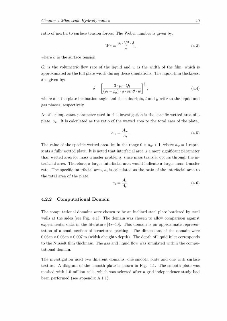
Chapter 4 Microscale Hydrodynamics 49
ratio of inertia to surface tension forces. The Weber number is given by,
We =ρl · V 2
l · δσ
, (4.3)
where σ is the surface tension.
Ql is the volumetric flow rate of the liquid and w is the width of the film, which is
approximated as the full plate width during these simulations. The liquid-film thickness,
δ is given by:
δ =
[3 · µl ·Ql
(ρl − ρg) · g · sinθ · w
] 13
, (4.4)
where θ is the plate inclination angle and the subscripts, l and g refer to the liquid and
gas phases, respectively.
Another important parameter used in this investigation is the specific wetted area of a
plate, aw. It is calculated as the ratio of the wetted area to the total area of the plate,
aw =AwAt
. (4.5)
The value of the specific wetted area lies in the range 0 < aw < 1, where aw = 1 repre-
sents a fully wetted plate. It is noted that interfacial area is a more significant parameter
than wetted area for mass transfer problems, since mass transfer occurs through the in-
terfacial area. Therefore, a larger interfacial area would indicate a larger mass transfer
rate. The specific interfacial area, ai is calculated as the ratio of the interfacial area to
the total area of the plate,
ai =AiAt. (4.6)
4.2.2 Computational Domain
The computational domains were chosen to be an inclined steel plate bordered by steel
walls at the sides (see Fig. 4.1). The domain was chosen to allow comparison against
experimental data in the literature [48–50]. This domain is an approximate represen-
tation of a small section of structured packing. The dimensions of the domain were
0.06 m× 0.05 m× 0.007 m (width×height×depth). The depth of liquid inlet corresponds
to the Nusselt film thickness. The gas and liquid flow was simulated within the compu-
tational domain.
The investigation used two different domains, one smooth plate and one with surface
texture. A diagram of the smooth plate is shown in Fig. 4.1. The smooth plate was
meshed with 1.0 million cells, which was selected after a grid independence study had
been performed (see appendix A.1.1).

50 Chapter 4 Microscale Hydrodynamics
Figure 4.1: Computational domain and mesh for smooth plate
The textured plate maintained the same overall dimensions as the smooth plate and
consisted of ridges running along the 0.06 m length. The ridges were 0.2 mm high,
0.4 mm wide and spaced 0.8 mm apart from each other. Usually structured packings
have surface texture on a microscopic scale, which influences the contact angle between
the fluid and the surface. This introduces difficulties in the specification of the contact
angle in a CFD simulation and additional experimental investigations must be performed
to determine the correct value for the contact angle. Therefore, the ridges were chosen
to be of a similar scale to the liquid film thickness. This approach would allow the effect
of larger scale surface textures to be examined. A diagram of the textured plate is shown
in Fig. 4.2. The grid for the ridged plate consisted of 2.5 million cells, selected after a
grid independence study (see appendix A.1.2).
All computational grids in this chapter use structured non-uniform hexahedral cells, so
as to maintain a high degree of accuracy whilst using the VOF method. This approach
resulted in a rather large number of cells for the textured plate domain, considering the
level of refinement required around the ridges to fully resolve the flow. However, it was
important to maintain the level of accuracy achieved by using structured grids. Due to
the increased area of the textured plate it was important to introduce a correction to
the specific wetted area calculation, so that direct comparisons could be made between
the smooth and textured plate. The correction involved neglecting plate surfaces that
were perpendicular to the film surface (e.g. side walls of the ridges), since inclusion of
these surfaces would give a larger value for the wetted area.
4.2.3 Simulation Set-Up
The simulations were performed using various flow parameters. For the smooth plane,
multiple inclination angles, θ were selected in order to determine the effect of inclination
angle on the film flow. Simulations were run at angles, θ = 30o and θ = 60o. The velocity
of the liquid film at the inlet was altered to give a range of Rel. During this investigation

Chapter 4 Microscale Hydrodynamics 51
Figure 4.2: Computational domain and mesh for textured plate
counter-current flow of gas was neglected to allow comparison with literature data. In
accordance with Hoffman et al. [48] and Iso & Chen [50] turbulence was not considered
since Rel < 230 and the flow could be considered to be in the laminar or pseudo laminar
regime. It is noted that for falling liquid films the onset of turbulence can occur at
Rel = 75 due to wall-induced turbulence [110]. However, fully turbulent flow is not
reach until Rel > 400 [110] and so the laminar version of the governing equations were
used in this chapter.
For the textured plate, the inclination angle was fixed at θ = 60o for all simulations and
the only varied parameter was the Rel. The ridges on the textured plate had the effect of
reducing the area of the liquid inlet and hence, the liquid flow velocity was increased in
order to maintain equivalent Rel. This allowed direct comparisons to be made between
the results of the smooth and textured plates.
Simulations were conducted as time-dependent runs, stepping to steady or pseudo-steady
states. All simulations were run using a variable time-step to keep the Courant number
below 1.0. This resulted in time steps of the order 1×10⁻⁵s. The two timescales present
in these simulations are the viscous time-scale, τv = L2
ν and the advection time-scale,
τa = LU , where L is the characteristic length scale or the cell size, ν is the kinematic
viscosity and U is the characteristic velocity. In these simulations the smallest viscous
timescale was approximately 16.2 times larger than the advection time scale, which
confirms the choice of time-step based on the courant number, Cr = UτaL .
The simulations which resulted in the partially wetted regime were run until a steady
state was reached. This was confirmed by monitoring the specific wetted area as a
function of time. The dynamic viscosity and density of the constituent phases are given
in Table 4.1. The surface tension was set to σ = 0.0728 N ·m−1 and a static contact
angle of θw = 70o was selected [50] .
The initial conditions for the simulations were that the domain was initially filled with
gas, α = 0 and the velocity was zero everywhere. The plate surface and side walls were

52 Chapter 4 Microscale Hydrodynamics
Table 4.1: Phase Properties
Phase µ [ Pa · s] ρ [ Kg ·m−3]
Liquid 8.899× 10⁻⁴ 997
Gas 1.831× 10⁻⁵ 1.185
no-slip walls with a constant static contact angle of θw = 70o. The liquid inlet was
set to a constant velocity with volume fraction, α = 1. The remaining gas inlet and
outlet were set to fixed pressure boundaries. The atmospheric open boundary was set
to free-slip boundary condition.
The use of a no-slip boundary condition on the walls appears to be incompatible with
dynamic contact line phenomena. The contact line is expected to move along the plate,
but this contradicts the no-slip condition. This results in a stress singularity at the
contact line [111]. Slip models can be used to remove the stress singularity at the
contact line. These models allow slip at the contact line, whilst the no-slip boundary
condition is applied elsewhere at the wall. The Navier-slip condition specifies the slip
velocity at the contact line as being proportional to the shear stress, and is of the form,
u|z=0 = β∂u
∂z|z=0, (4.7)
where the wall is located at z = 0, β is the slip length and u|z=0 is the slip velocity. The
use of slip models then requires the slip length, β to be defined.
In the CFD simulations performed in this thesis fields are stored at cell centres. This
means that numerical slip is imposed due to the fact that the velocity in the cell centre
adjacent to the no-slip wall is not zero. If the mesh size is ∆z in the cell adjacent to the
wall, then a numerical slip length of 12∆z is imposed. According to Renardy et al. [112],
for most applications the value of the slip length, β is of a much smaller magnitude than
the mesh size. In these cases the numerical slip is greater than any imposed slip length,
β. Walther et al. [113] state that the slip length of water on hydrophobic surfaces is
of the order of 30nm, whilst for water on hydrophilic surface it is of the order of 9nm.
These slip lengths are much smaller than the grid sizes used in this thesis and so the
numerical slip is dominant. Therefore, the no-slip boundary condition is applied without
any slip model, since a Navier-slip model with the appropriate slip length would have
negligible effect in comparison to numerical slip.
The numerical slip means that the amount of slip at the contact line is dependent on
the grid size. Therefore, the solution may be dependent on the grid size, if the contact
line dynamics is the dominant process. However, grid refinement studies showed that
finer mesh resolution had little effect on the overall solution at steady state. It may be
due to the fact that the simulations were run until a steady state was reached. Here,
the contact line was not in motion along the wall and so there is no paradox. Only

Chapter 4 Microscale Hydrodynamics 53
the time-dependence of the solution would be effected. Furthermore, the results were
validated against experimental data to ensure that they were accurate, despite the above
mentioned deficiencies in the numerical approach.
4.3 Results and Discussion
4.3.1 Validation
Validation of the methods used in this chapter were performed by comparison with
previous studies in the literature and with the predictions of the Nusselt theory. Sim-
ulations were performed using the smooth plate with various liquid inlet velocities at
an inclination angle of θ = 60o. The results are shown in Fig. 4.3, where the specific
wetted area of the plate was plotted against Rel. To provide comparative data, existing
experimental results from the literature [48, 49] are also plotted in Fig. 4.3. As men-
tioned previously, it is noted that interfacial area is a more significant parameter than
wetted area, since mass transfer occurs through the interfacial area. However, wetted
area was used for validation because the experimental results, used to compare with
the simulated results [48, 49], were given in terms of wetted area. A comparison of the
interfacial area to the wetted area is given in section 4.3.3.
0
0.2
0.4
0.6
0.8
1
1.2
0 50 100 150 200 250
Specific
wetted a
rea A
w/A
t [-]
Reynolds number Rel [-]
Simulation on smooth plateExp. Data Hoffmann et al. (2005)Exp. Data Hoffmann et al. (2006)
Figure 4.3: The specific wetted area against Rel
It is noted that the numerical method under-estimates the wetted area at lower Rel, but
is able to correctly predict the wetted area at larger Rel. This may be due to the fact
that a constant velocity boundary condition was used at the liquid inlet, rather than
the Nusselt profile. Therefore, the film would have to flow a certain distance down the
plate before the proper Nusselt velocity profile was established. At lower Rel the rivulets

54 Chapter 4 Microscale Hydrodynamics
formed at a position relatively close to the inlet. Here, the Nusselt velocity profile did
not have sufficient time to develop and so this may have had an effect on the resulting
position of the contact line. Whereas, at higher Rel the rivulets were formed further
down the plate, where the full velocity profile had sufficient time to established. It is
also noted that the experimental data has a wide spread of data. This is probably due
to the fact that the dynamics of the liquid film is sensitive to external factors, such as
the smoothness of the plate surface. Small imperfections on the plate surface can effect
the contact angle between the film and the plate, impacting the resulting wetted area.
Despite these uncertainties, there is fairly good agreement between the the numerical
and the experimental data and the numerical results follow the general trend observed
in experiment.
The Nusselt theory [62] provides a theoretical prediction of the velocity profile within
a liquid film during gravity-driven flow down an inclined plane. This theory is a model
for gravity-driven film flow under the assumption of either 2D flow or in the case of an
infinitely wide film. Therefore, side-wall effects are neglected. This is approximately
true in the centre of the film where side-walls effects have negligible effect on the flow.
The Nusselt theory predicts that the fluid velocity in the flow direction (y-coordinate
direction), v(z) is given by:
v(z) =(ρl − ρg)gsin(θ)
µl
(zδN −
z2
2
), (4.8)
where ρl is the liquid phase density, ρg is the gas-phase density, g is the gravitational
constant, θ is the inclination angle of the plate, µl is the liquid viscosity, δN is the
Nusselt film thickness and z is the plate normal distance. The Nusselt film thickness,
δN is given by,
δN =
(3µlQl
(ρl − ρg)gsin(θ)
) 13
, (4.9)
where Ql is the liquid volumetric flow rate per unit width. The Nusselt velocity predic-
tion was used to provide further validation of the computational approach used through-
out this chapter. The simulation was performed at Rel = 224 and inclination angles of
θ = 30o and θ = 60o. At this liquid film Reynolds number a full film had developed
on the plate with no contact line. This is appropriate considering that the Nusselt the-
ory neglects contact line effects. The film velocity profile was extracted from a central
position on the plate in order to minimise the side-wall effects, which are also not con-
sidered in the Nusselt theory. A position 0.5 mm above the outlet (far from the inlet)
was selected to ensure that the film was fully developed. Figure 4.4 shows the compar-
ison between the predictions of the Nusselt theory and the data obtained using CFD
simulations.
Figures 4.3 and 4.4 show that the numerical methods used in this chapter produced
results in good correlation with previous experimental data and theoretical predictions.

Chapter 4 Microscale Hydrodynamics 55
0
5e-05
0.0001
0.00015
0.0002
0.00025
0.0003
0.00035
0.0004
0.00045
0.0005
0 0.1 0.2 0.3 0.4 0.5 0.6 0.7 0.8
Film
thic
kness z
[m
]
Velocity v [ms-1
]
Simulation, θ=60o
Nusselt Solution, θ=60o
Simulation, θ=30o
Nusselt Solution, θ=30o
Figure 4.4: Comparison of film velocity profile against the Nusselt solution at Rel =224
Therefore, it can be assumed that these methods can be used with confidence in further
simulations to accurately solve for film flow on inclined planes.
4.3.2 Smooth Plate
The inclination angle of surfaces within packed columns is an important choice to make
when designing packing materials. The performance of packed columns depends on the
inclination angle in a number of ways. As noted by Petre et al. [22], shallow angles of
inclination (with respect to the horizontal) result in large pressure drops when compared
to steeper inclination angles. During the carbon capture process the pressure drop
through the column needs to be kept to a minimum, considering that the flue gas is
at a relatively low pressure. The smaller the pressure drop, the taller the column can
be, resulting in a greater volume of CO2 absorption. From a pressure drop perspective,
large inclination angles are optimal. However, it is also important to examine the effect
that the inclination angle has on the resulting wetted area of the packing materials.
The wetted area was simulated for a range of Rel for inclination angles of 30o and 60o.
The results are plotted in Fig. 4.5. It can be seen that smaller inclination angles result
in larger wetted areas, across the whole range of Rel tested. If the increased wetted area
results in an increase in interfacial area this would make a positive contribution to heat
and mass transfer, but a higher pressure drop would be encountered. Further investiga-
tion will need to be performed to analyse whether any advantage gained by an increased
interfacial surface area is offset by the increased pressure drop. The increased wetted
area for the smaller inclination angle is probably due to the fact that the wall normal
component of gravity is larger and therefore, hydrostatic pressure is larger. Increased

56 Chapter 4 Microscale Hydrodynamics
hydrostatic pressure within thin films has been shown to increase the stability of the
interface [58]. In particular, the contact line ridge will be smaller and so is more stable
against transverse perturbations. Therefore, the contact line will move further down the
plate before contact line instabilities grow large enough to cause rivulet formation. This
would result in larger wetted areas, as has been observed in the data.
0
0.2
0.4
0.6
0.8
1
0 50 100 150 200 250
Specific
wetted a
rea A
w/A
t [-]
Reynolds number Rel [-]
Smooth plate θ=60o
Smooth plate θ=30o
Figure 4.5: Comparison of specific wetted area for a range of Rel at inclination anglesof 30o and 60o
It is known that rivulet formation is caused by instabilities of the gas-liquid interface
and of the contact line. In these simulations the perturbation of the interface, which
creates the instabilities leading to rivulet formation, is likely to be created by the side
walls of the plate. After the initial release of liquid onto the plate, surface tension causes
the fluid to move up the side walls to adhere to the contact angle of the wall, as can
be seen in Fig. 4.6. Fig. 4.6 plots the film interface contour and associated film depth
0.01s after the release of the liquid onto the plate, for the case of Rel = 156.85.
In accordance with the observations of Oron et al. [56], when the fluid is released onto
the inclined plane the contact line is initially straight in the spanwise direction. There
is also a ridge formed at the contact line due to the induced high pressure at the contact
line [56] (see Fig. 4.6). This contact line is unstable to perturbations and will form
rivulets, which can be observed in Fig. 4.9. In this case a single rivulet is formed.
Observing Fig. 4.6, if we denote the initial film depth at the contact line ridge as, hl,
the film depth at the side-walls is greater than hl. This in turn causes the film depth to
reduce to below hl in the regions between the side-walls and the centre of the plate, as
can be seen in Fig. 4.6. This perturbation of the film interface grows in time, eventually
resulting in the rivulet formation. This growth can be seen in Figures 4.7-4.8 which plot
the liquid interface 0.08s and 0.12s after the release of the liquid onto the plate, for the

Chapter 4 Microscale Hydrodynamics 57
Rel = 156.85 case. The liquid film eventually reaches a steady state where the contact
line becomes stationary and there is no movement of the liquid interface (see Fig. 4.9).
Figure 4.6: Thickness of liquid film at Rel = 156.85 0.01 seconds after release
Figure 4.7: Thickness of liquid film at Rel = 156.85 0.08 seconds after release
Figure 4.8: Thickness of liquid film at Rel = 156.85 0.12 seconds after release
It is noted that there is very little wave formation in the film prior to the contact line. In
the region preceding the contact line ridge, the film is very flat, apart from the curvature
near the side walls. The lack of wave formation is probably due to the small size of the
plate, meaning that instabilities at the interface do not have sufficient time to grow.
This is in agreement with the experiments of Park & Nosoko [61] who also found that

58 Chapter 4 Microscale Hydrodynamics
Figure 4.9: Thickness of liquid film at Rel = 156.85 at steady state
an initially flat liquid interface required sufficient time before perturbations grew into
2D or 3D surface waves.
4.3.3 Textured Plate
This section discusses the results of film flow over inclined planes with surface textures.
The ridged surface of the plate was devised in order to increase the wetted and interfacial
area of the plate. Fig. 4.10 shows a comparison of the specific wetted and interfacial
areas of the smooth plate and the ridged plate for a range of Rel at θ = 60o. It was
observed that the addition of ridges, running parallel to the flow direction, significantly
increased the wetted area of the plate at all Rel < 200. The observed increase in wetted
area also resulted in an increase in the interfacial area at respective Rel.
0
0.2
0.4
0.6
0.8
1
0 50 100 150 200 250
Specific
wetted (
inte
rfacia
l) a
rea A
w/A
t (A
i/At) [-
]
Reynolds number Rel [-]
Smooth plate awSmooth plate ai
Textured plate awTextured plate ai
Figure 4.10: Specific wetted area, aw and specific interfacial area, ai against Rel forthe smooth and textured plate (θ = 60o)

Chapter 4 Microscale Hydrodynamics 59
At low-range and mid-range Rel, rivulet flow, induced by surface tension forces and
instabilities at the interface, cause a reduction in the wetted area. As can be seen in
Fig. 4.11, rivulets can form with a thickness of several times that of the preceding film
flow. It can be seen in Fig. 4.11 that ridges on the plate help to spread the rivulet over
a much larger area across the width of the plate, thus increasing the wetted area. This
is likely due to the ridges interfering with the contact line at the leading edge. The film
interface must form the correct contact angle at all walls within these ridges.
The break up of the leading edge of the film observed within the channels is likely to
be unphysical and a deficiency of the VOF method. Since the location of the interface
in the VOF method is spread across a few cells, the approach breaks down when the
number of cells is insufficient to resolve the interface. It was observed that in these
simulations the interface was spread over approximately 3 cells. However, there are only
6 cells across the width of each channel. Therefore, it is concluded that the channeling
flow observed within the ridges is caused by a numerical deficiency, rather than being
physically accurate. Extra refinement within the channels could alleviate this problem,
but the resulting increase in computational load would prove limiting. Adaptive mesh
refinement at the interface is an approach that is likely to improve the inaccuracies of
the computation within the channels.
Figure 4.11: Thickness of liquid film at Rel = 134.44 and θ = 60o (left: Smoothplate, right: Textured plate)
It is interesting to note that the textured surface has a much larger effect on the wet-
ted area at the lower range of Rel tested. Table 4.2 shows the percentage increase in
the wetted area from the smooth plate to the textured plate. It will be important to
determine the effects of these ridges on other aspects of the system. For example, in a
packed column, these ridges may prevent the transport of MEA throughout the liquid
film, resulting in CO2 rich regions near the film surface and CO2 lean regions within the
ridges. If MEA transport is inhibited, then the CO2 absorption rate may be reduced,
cancelling out the advantages created by the increased interfacial area. The exact nature
of these effects is only speculative and is out of the scope of this investigation.
It is crucial to remember that idealisations have been made in order to reduce the
complexity of the problem. In reality, the Rel and the film structure will depend upon
many factors, such as liquid flow rate, the distribution of liquid throughout the columns,

60 Chapter 4 Microscale Hydrodynamics
corrugation angle, inclination angle of the packing, etc. Further mesoscale simulations
will need to be performed to determine the exact liquid distribution over the packing.
This chapter shows that the addition of ridges should improve the wetted and interfacial
area of full-scale packing up to a limiting Rel. The limiting Rel will be dependent on
the specific problem being investigated and it can be defined as the point at which full
film flow occurs.
Rel [-] Asmoothw /At [-] Atexturedw /At [-] Increase in WettedArea [%]
0 0 0 0
44.81 0.164787 0.400508 143.05
80.67 0.238929 0.486207 103.49
112.04 0.348422 0.608895 74.76
134.44 0.449249 0.69194 54.02
156.85 0.610955 0.958555 56.89
168.05 0.729229 1 37.13
179.26 0.923153 1 8.32
201.66 1 1 0
224.07 1 1 0
Table 4.2: Specific wetted area for smooth and textured plate at θ = 60o
Fig. 4.12 shows the interfacial velocity magnitude for the smooth and textured plates
at Rel = 179.26 and θ = 60o and Fig. 4.13 shows a close-up view of the velocity
vectors within this film along the plane y = 0.02 m. It is observed that the ridges on
the plate create alternate layers of varying interfacial velocities along the surface of the
film. This is attributed to the reduction in film thickness, due to the presence of the
ridges. Fig. 4.13 shows that the addition of ridges along the plate does not result
in regions of stagnant fluid within the channels. Furthermore, the variation in velocity
throughout the film and the film surface may assist in the heat and mass transfer process,
since different layers of fluid within the film move at different velocities. However, as
mentioned previously, the impact of these structures on the CO2 absorption process will
have to be assessed in future investigations.
Packing materials also have a corrugation angle (usually 45o) as well as an inclination
angle. The corrugation angle was neglected in this chapter, but it is predicted that
the effect of this would be to cause liquid to accumulate at the sides of the plate. The
channels on the textured packing may help to prevent such accumulation of liquid and
help to produce more evenly distributed films.
Also, it has been assumed that the liquid inlet spans across the whole width of the plate.
However, in reality this may not be the case, especially well within the packed column.

Chapter 4 Microscale Hydrodynamics 61
Figure 4.12: Interfacial velocity contours of liquid film at Rel = 179.26 and θ = 60o
(left: Smooth plate, right: Textured plate)
Figure 4.13: Velocity vectors within the liquid film along the plane y = 0.02 m atRel = 179.26 and θ = 60o (top: Smooth plate, bottom: Textured plate)
In the case of a point source of liquid the channels may even reduce the wetted area.
This will have to be investigated further and modifications to the design could help to
increase the wetted area for various inlet conditions.
4.4 Conclusion
In this chapter the VOF method was used to study isothermal liquid film flow down
inclined planes. Initially, simulations were performed on a smooth plate and the effect
of inclination angle on the wetted area was studied for a range of Rel. The methods used
throughout this chapter were validated using existing experimental data and theoretical
predictions. Also, it is noted that the experimental results for wetted area have large
variation. Future research could focus on performing more experimental analysis of thin
film flow down inclined plates to determine more accurately the relation between Rel
and wetted area.
It was found that a decrease in the inclination angle resulted in larger wetted areas
at the respective Rel. However, the increases observed were minimal. The advantage
gained from using small inclination angles in packed columns is the increase in gas-liquid
interfacial area, which should enhance heat and mass transfer. However, negative side-
effects of shallow inclination angles, such as larger pressure drops, may negate these
improvements.

62 Chapter 4 Microscale Hydrodynamics
A unique surface texture pattern on an inclined plate was also investigated. It was found
that the addition of vertical ridges, of the same scale as the liquid film thickness, resulted
in much larger interfacial areas at equivalent Rel. It is reasonable to assume that an
increase in interfacial area should enhance CO2 absorption within packed columns.

Chapter 5
Adaptive Mesh Refinement at the
Microscale
This chapter focusses on the use of adaptive mesh refinement (AMR) as a method to
improve the accuracy of VOF simulations performed in Chapter 4, whilst maintaining
or reducing the computational requirements. This is of significant importance in future
investigations where the complexity of the problems may be increased, in terms of the
scale of the domain and a reduced level of simplifications. Local adaptive mesh refine-
ment is used to ensure improved resolution of the geometrical grids at the gas-liquid
interface.
5.1 Introduction
The interface between a gas and a liquid phase should, in theory, have a thickness in the
order of the distance between molecules [114]. This scale is significantly smaller than
can be resolved in VOF simulations, so the interface is at least spread over 1 cell width.
However, numerical diffusion of the volume fraction widens the reconstructed interface
to a thickness of a few cells. Therefore, it is obvious that in order to accurately resolve
the interface the cells must be as small as possible in the interfacial region. Due to the
changing nature of the interface, standard VOF requires highly refined grids throughout
the domain to ensure proper resolution at the interface, as it progresses through the
domain. This can significantly affect the computational requirements.
An approach which attempts to address this problem is local adaptive mesh refinement.
Local AMR allows for dynamic refinement of the mesh in regions of high error and
un-refinement in regions of low error [107]. In terms of the VOF method, refinement is
made at the interface in order to ensure that the mesh can accurately resolve it. As the
interface moves through the domain, successive mesh refinement and un-refinement can
63

64 Chapter 5 Adaptive Mesh Refinement at the Microscale
take place. Refinement is achieved using the addition of computational nodes, known
as h-refinement [107].
The AMR approach has been used successfully in many different applications, from
single-phase flows to multiphase flows. Jasak and Gosman [115] developed an AMR
procedure based on a-posteriori error estimates and solution gradients. They used this
approach to solve supersonic flow of an ideal gas flowing over a forward facing step
resulting in strong shock wave formations. Shock waves exhibit large gradients and so
require high cell densities to be resolved accurately. Jasak and Gosman showed that the
use of AMR was able to suitably resolve these shocks.
In terms of multiphase flows, Theodorakakos and Bergeles [114] evaluated the effective-
ness of AMR with the VOF method on various test cases. Simulations were performed
on the convection of bubbles under prescribed flow velocities and droplet impact was also
studied. They concluded that the AMR approach was able to reduce the computational
time for simulations, whilst gaining very good accuracy of the interfacial region. In par-
ticular, they observed that a very small transition region between the gas and the liquid
phases could be achieved, which is physically more realistic. Numerical diffusion of the
interface was reduced, which addresses one of the disadvantages of the VOF method.
There have also been investigations using the VOF approach with AMR to study droplet
impact onto thin liquid films [116, 117]. This approach is particularly useful in these
situations because of the range of scales observed, for example, during the breakup of the
crown of fluid formed after impact. These examples show that significant improvements
can be made to the VOF method with the inclusion of local AMR.
This chapter uses the local AMR approach in an effort to improve upon the results
gained using a static grid. Improvements are expected in terms of simulation accuracy
and computational effort. Comparisons are made between the solutions obtained using
AMR and those obtained using highly refined static meshes. It was observed that local
AMR produced results with much better correlation to experimental data. However, it
was shown that in order to reduce the computational requirements, careful consideration
is required in the choice of AMR parameters, such an initial grid resolution or number of
refinement levels. Inadequate selection of AMR parameters can even result in increased
computational load.
5.1.1 Numerical Modelling
5.1.1.1 Adaptive Grid Refinement
Adaptive grid refinement is a method used to dynamically alter the mesh density
throughout the domain. For example, in regions of high gradients, large numbers of
cells are required to accurately resolve the solution. In principle, this can be achieved

Chapter 5 Adaptive Mesh Refinement at the Microscale 65
Figure 5.1: AMR refinement of a single computational cell in 2D for 2 levels ofrefinement
by producing an initial grid where mesh density is high in these specific regions, whilst
being of low density in regions of less importance.
In the VOF method it is important to accurately resolve the interfacial region between
two phases. The accuracy of the interface can be improved by using high densities of
cells around the interfacial region. However, the location of the interface is not known a
priori and so using a static grid method would require a high density mesh throughout
the domain, creating excessive simulation run-times.
Adaptive Mesh Refinement allows one to initiate the simulation using a relatively coarse
grid, which is then successively refined and un-refined according the specific location of
the interface. This enables accurate resolution of the interface, whilst keeping run-time
to a minimum. The only overhead is created by the process of mesh adaptation.
In this investigation the solver interDymFoam was used for the AMR simulations. This
is an extension of the standard VOF solver, interFoam, to include dynamic manipulation
of the computational grid. A dictionary file is used to specify the parameters for the
grid manipulation. Grid refinement can be performed at specific time-step intervals and
can be based on specific flow fields, for example, volume fraction. Cells are refined if
this field is within a specified refinement range. If the value of the field within these
cells moves outside of this range, the cells are un-refined back to the initial mesh. The
grid refinement is performed by adding computational nodes along the mid-points of cells
within the specified refinement regions [116]. Hence, a 3-dimensional hexahedral cell will
be split into 8 new cells. Figure 5.1 shows the refinement of a single, 2D computational
cell, with 2 levels of refinement. The arrow indicates an individual refinement step. The
criteria for grid refinement used in this chapter is explained in the section 5.1.3.
5.1.2 Computational Domain
The computational domain was chosen to be the smooth inclined steel plate used in
Chapter 4 (see Fig. 5.2). The domain dimensions were kept at 0.06 m×0.05 m×0.007 m
(width×height×depth). The depth of liquid at the inlet was set by the Nusselt film
depth.

66 Chapter 5 Adaptive Mesh Refinement at the Microscale
Figure 5.2: Computational domain and refined static mesh
This investigation used two different approaches to the meshing procedure (see Table.
5.1). Firstly, simulations were run using a structured, non-uniform, hexahedral static
mesh, whereby mesh independence checks (see appendix A.1.1) were performed to de-
termine an adequately fine grid resolution. The mesh is shown in Fig. 5.2, consisted of
1.0 million cells and will be denoted as the static mesh.
Secondly, simulations were run using the local AMR method, using two different condi-
tions on the refinement (see Table 5.1). Refinement around the interface with volume
fractions in the range, 0.2 < α < 0.8 is denoted as the partial-film mesh, whereas refine-
ment around the interface and the whole film region with volume fractions in the range,
0.2 < α < 1.0 is denoted as the full-film mesh. An initial mesh was selected with 192000
structured non-uniform hexahedral cells. A grid independence study was performed to
determine an adequate limit on the number of refinement levels. Levels of 2 and 3 were
tested and the refinement level of 2 was found to be most appropriate. The extra level of
refinement generated much larger cell numbers within the domain causing the run-time
to increase approximately 20 times. However, the difference in the calculated specific
wetted area was only 2.72%.
Figure 5.3 shows a comparison of the mesh used in the static grid and partial-film AMR
grid simulations. The sections of mesh were selected from the plate surface at time,
t = 0.36s with Rel = 156.85. On the left, it can be seen that the static mesh is finer
throughout the whole domain, whereas on the right it can be seen that the AMR mesh
is refined just around the gas-liquid interface, denoted by the blue line. Figure 5.4 shows
a closer view of the static mesh and the AMR mesh. Here it can be seen that the static
mesh is highly refined throughout the domain, even in regions where it is not required.

Chapter 5 Adaptive Mesh Refinement at the Microscale 67
Figure 5.3: Comparison of the static mesh with a snapshot of the partial-film AMRmesh at t = 0.36s and Rel = 156.85 (blue line is the gas-liquid interface)
Figure 5.4: Closer view of comparison of the static mesh with the t = 0.36s snapshotof the partial-film AMR mesh at Rel = 156.85 (blue line is the gas-liquid interface)
On the other hand, the AMR mesh is much more highly refined at the interface, where
high grid density is required for accurate resolution of the interface. In other parts of the
domain, the mesh is coarser, which helps to maintain reasonable simulation run-times.
5.1.3 Simulation Set-Up
For all simulations a constant inclination angle of θ = 60o was chosen to allow compar-
isons with current data in the literature. A range of Rel were tested by suitably altering

68 Chapter 5 Adaptive Mesh Refinement at the Microscale
Table 5.1: Computational Meshes
Mesh Name Initial MeshDensity
RefinementConditions
Static Mesh 1.0× 10⁶ -
Partial-FilmMesh
1.92× 10⁵ 0.2 < α < 0.8
Full-Film Mesh 1.92× 10⁵ 0.2 < α < 1.0
Table 5.2: Phase Properties
Phase µ [ Pa · s] ρ [ Kg ·m−3]
Liquid 8.899× 10⁻⁴ 997
Gas 1.831× 10⁻⁵ 1.185
the velocity of the liquid film at the inlet. During this investigation counter-current flow
of gas was neglected to again allow comparison with previous data in the literature. In
accordance with Hoffman et al. [48] and Iso & Chen [50] turbulence was not considered
since Rel < 230 and the flow could be considered to be in the laminar or pseudo lam-
inar regime. It is noted that for falling liquid films the onset of turbulence can occur
at Rel = 75 due to wall-induced turbulence [110]. However, fully turbulent flow is not
reach until Rel > 400 [110] and so laminar versions of the governing equations have been
used in this chapter.
Time-dependent simulations were carried out using a variable time-step to ensure a
Courant number below 1.0, resulting in time-steps of approximately 1 × 10⁻⁵s. Sim-
ulations were allowed to run until a steady or pseudo-steady state was reached. This
was assured by monitoring the specific wetted area of the plates as a function of time.
During the AMR simulations the mesh adaptation was performed every 5 time steps.
The two timescales present in these simulations are the viscous time-scale, τv = L2
ν and
the advection time-scale, τa = LU , where L is the characteristic length scale or the cell
size, ν is the kinematic viscosity and U is the characteristic velocity. In these simula-
tions the smallest viscous timescale is approximately 9.7 times larger than the advection
time scale, based on the smallest cell size after maximum refinement of the grid. This
confirms the choice of time-step based on the courant number, Cr = UτaL .
The dynamic viscosity and density of the constituent phases are given in Table 5.2. The
surface tension was set to σ = 0.0728 N ·m−1 and a static contact angle of θw = 70o
was selected [50].
The initial conditions for the simulations were that the domain was initially filled with
gas, α = 0 and the velocity was zero everywhere. The plate surface and side walls were
no-slip walls with a constant static contact angle of θw = 70o [50]. The liquid inlet was
set to a constant velocity with volume fraction, α = 1. The remaining gas inlet and

Chapter 5 Adaptive Mesh Refinement at the Microscale 69
0
0.2
0.4
0.6
0.8
1
1.2
0 50 100 150 200 250 300
Specific
wetted a
rea A
w/A
t [-]
Reynolds number Rel [-]
Static MeshExp. Data Hoffmann et al. (2005,2006)
Simulation Data Iso and Chen (2011)Simulation Data Hoffmann et al. (2006)
Figure 5.5: Comparison of Static Grid Simulation with Literature
outlet were set to fixed pressure boundaries. The atmospheric open boundary was set to
free-slip boundary condition. Here again the slip length is much smaller than the grid
size and so the no-slip condition is applied without a slip model. Numerical slip caused
by locating the velocity fields at cell centres alleviates the contact line paradox.
5.2 Standard Grid Refinement
5.2.1 Results & Discussion
Comparison of the results obtained with the smooth static grid from Chapter 4 were
made with other CFD data from the literature. Figure 5.5 shows a plot of the results of
various of the simulations, along with the experimental data of Hoffmann et al. [48,49]. It
is observed that improvements have been made in terms of the accuracy of the simulated
data, possibly due to the much finer grid resolutions used in this thesis. At higher Rel the
wetted area is correctly predicted, but at lower Rel the approach still under-estimates the
wetted area in comparison to experimental data. Despite these improvements, significant
differences between simulated and real-world phenomena are still observed.

70 Chapter 5 Adaptive Mesh Refinement at the Microscale
5.3 Adaptive Grid Refinement
5.3.1 Refinement at the Interface
It was postulated that the differences between the data of CFD simulations and real-
world data, especially at lower Rel, were caused by inefficiencies of the VOF method.
Since some improvement was observed by using a higher density grid resolution across
the domain, it was assumed that further improvement could possibly be made by increas-
ing the grid resolution at the interface. This should increase the accuracy of interface
reconstruction. Local AMR was used to achieve the desired increase in grid resolution at
the interface, whilst maintaining reasonable run-times by using a coarse mesh in regions
of less physical interest.
5.3.2 Results
In order to assess the improvements made by using local AMR at the gas-liquid interface,
the wetted area against Rel was plotted (see Fig. 5.6). Figure 5.6 also displays the
experimental data of Hoffmann et al. [48,49] and the CFD data obtained using the static
grid from section 5.2.1. It is noted that the results from local AMR were improved at the
lower and higher ranges of liquid film Reynolds numbers. An important observation is
the fact that local AMR provides results in much greater correlation with experimental
data in the range 50 < Rel < 100. In this region the specific wetted area initially falls
before rising again, a behaviour which is expressed in the experimental data. Simulations
with a highly refined static mesh were unable to replicate this behaviour, indicating the
importance of using local AMR at lower Rel.
It would be expected that as the liquid film Reynolds number increases the wetted area
would also increase. However, as noted previously, it can be seen that betweenRel = 44.8
and Rel = 58.3 the wetted area plateaus, falling at Rel = 71.7 and then rising in the
assumed manner as further increases in Rel are made. This can be explained by the flow
phenomena observed at each of these Rel. At Rel = 44.8, the flow forms 4 rivulets (see
Fig. 5.7), reducing to 3 rivulets at Rel = 58.3 (see Fig. 5.8) and forming a single rivulet
at Rel = 71.7 (see Fig. 5.9). At these lower Rel, the increasing flow rate changes the
behaviour of the flow. As the rivulets combine, the wetted area stays constant, or even
falls. It can be assumed that the Rel where a single rivulet is formed is in the region
58.3 < Rel < 71.7, which may explain the cluster of experimental points in this range
(see Fig. 5.6).
By comparing the interface contours of simulations using the static grid and the partial-
film grid it is possible to see why the static grid under-estimates at lower Rel and does
not correlate properly with the experimental data. Fig 5.10 shows the interface contours
at Rel = 44.8. It can be seen that the static grid only resolves a single rivulet, whilst

Chapter 5 Adaptive Mesh Refinement at the Microscale 71
0
0.2
0.4
0.6
0.8
1
1.2
0 50 100 150 200 250
Specific
wetted a
rea A
w/A
t [-]
Reynolds number Rel [-]
Static GridHoffmann et al. (2005)Hoffmann et al. (2006)
Partial-Film
Figure 5.6: The specific wetted area against Rel for AMR at the interface
Figure 5.7: Contour plot of gas-liquid interface at Rel = 44.8 (Partial-film mesh)
the partial-film grid resolves 4. This may be attributed to the fact that the partial-film
AMR grid is much finer at the gas-liquid interface. If perturbations at the interface
near the contact line are small, these may not have been resolved in the static grid.
Therefore, these perturbations can grow in the AMR case, resulting in the formation of
more rivulets. However, in the static grid case the mesh may not have been fine enough
to resolve the perturbation, resulting in less rivulet formation. The surface area of a
single rivulet is smaller than that of 4 rivulets, as can be observed in the data.
It is interesting to note that the results with adaptive mesh refinement indicate a slightly

72 Chapter 5 Adaptive Mesh Refinement at the Microscale
Figure 5.8: Contour plot of gas-liquid interface at Rel = 58.3 (Partial-film mesh)
Figure 5.9: Contour plot of gas-liquid interface at Rel = 71.7 (Partial-film mesh)
larger wetted area across the majority of Rel when compared to the static grid, but they
are broadly in agreement. This shows that the choice of a no-slip wall condition with
numerical slip is not significantly mesh dependent. For the AMR grid the cells at the
interface are significantly smaller than those of the static grid. This means that in the
AMR simulations the slip length is much smaller, which would result in a smaller slip
velocity at the no-slip wall. However, there is not a significant difference in the wetted
area and overall shape of the interface from mid to high Rel.
As mentioned previously, when mass transfer is to be modelled, the interfacial area
is more significant than the wetted area. Mass transfer occurs through the gas-liquid
interface and therefore, the rate of mass transfer is dependent on the interfacial area.
Figure 5.11 compares the interfacial area against the wetted area for a range of Rel. It
is observed that the interfacial area is much larger than the wetted area at the lower
range of Rel. This is a direct effect of the contact line dynamics where high curvature

Chapter 5 Adaptive Mesh Refinement at the Microscale 73
Figure 5.10: Contour plot of gas-liquid interface at Rel = 44.8 for static grid (left)and Partial-film grid (right)
0
0.2
0.4
0.6
0.8
1
1.2
0 50 100 150 200 250
Specific
wetted (
inte
rfacia
l) a
rea A
w/A
t (A
i/At) [-
]
Reynolds number Rel [-]
Wetted AreaInterfacial Area
Figure 5.11: Comparison of specific wetted area and specific interfacial area againstRel for the partial-film AMR simulation
of the interface results in an increase in interfacial area, in comparison to the wetted
area. This exemplifies the importance of determining the interfacial area, rather than
the wetted area when mass transfer is of consideration.
The flow within the gas phase is shown in Figure 5.12 for the case of Rel = 156.85 at
steady state. In these simulations the gas-phase is not forced at the gas inlet. The flow
within the gas-phase is generated by the effect of shear force on the gas by the flowing

74 Chapter 5 Adaptive Mesh Refinement at the Microscale
Figure 5.12: Flow within the gas phase for Rel = 156.85 at steady state.
liquid film. It is observed that the flow of the liquid film has a significant influence of
the gas phase, especially in regions near the gas-liquid contact line.
5.3.3 Full-Film Refinement
It has been shown that local AMR about the interface was more able to replicate the
physical phenomena of the real-world flow. However, there was still an under-estimation
of the wetted area at lower Rel. It was considered that improvements may be made
by refining the whole film, rather than just at the interface. The film within packed
columns and on inclined plates is relatively thin. Therefore, shear layers at the wall may
require extra refinement to be resolved accurately, especially if these shear layers have
a significant impact on the interface, due to their close proximity.
AMR simulations were performed to determine the wetted area across a range of Rel,
refining the whole liquid film. Comparisons were made with the results of AMR simu-
lations with refinement only around the interface (see Fig. 5.13).
It is observed that the results using the two methods are fairly consistent across the
whole range of Rel tested. Table 5.3 shows the run-times for each simulation. Data that
is not available is denoted by “−” in the table. For the full-film simulation data was not
obtained for Rel = 201.66 due to excessive simulation run-times at these high Rel.
Local AMR throughout the whole liquid film was shown to exhibit insignificant im-
provements. Run-times of the simulations were increased across the range of Rel tested,
with large increases seen at higher Rel. It is obvious that under the situations tested
in this investigation, local AMR throughout the whole of the liquid film was an over-
complication resulting in dramatically increased run-times, with negligible improvement
in accuracy. Therefore, local AMR about the interface is optimal. This finding is also
important when scaling up the problem to determine the hydrodynamics within larger
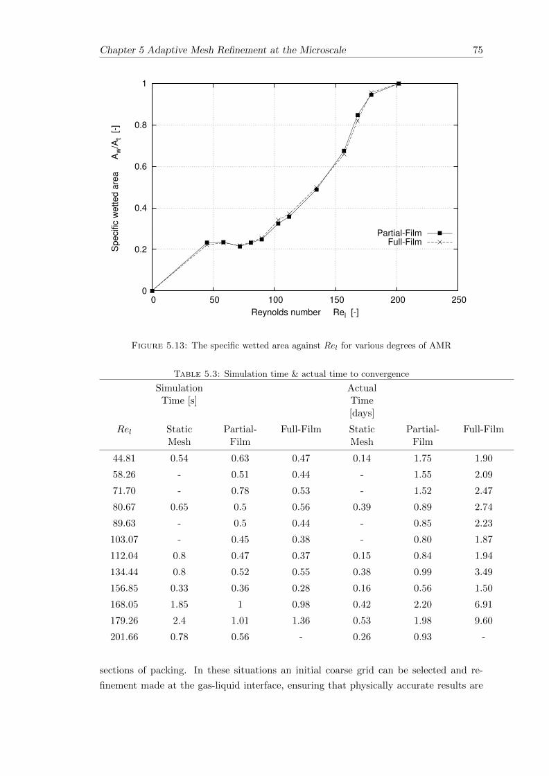
Chapter 5 Adaptive Mesh Refinement at the Microscale 75
0
0.2
0.4
0.6
0.8
1
0 50 100 150 200 250
Specific
wetted a
rea A
w/A
t [-]
Reynolds number Rel [-]
Partial-FilmFull-Film
Figure 5.13: The specific wetted area against Rel for various degrees of AMR
Table 5.3: Simulation time & actual time to convergence
SimulationTime [s]
ActualTime[days]
Rel StaticMesh
Partial-Film
Full-Film StaticMesh
Partial-Film
Full-Film
44.81 0.54 0.63 0.47 0.14 1.75 1.90
58.26 - 0.51 0.44 - 1.55 2.09
71.70 - 0.78 0.53 - 1.52 2.47
80.67 0.65 0.5 0.56 0.39 0.89 2.74
89.63 - 0.5 0.44 - 0.85 2.23
103.07 - 0.45 0.38 - 0.80 1.87
112.04 0.8 0.47 0.37 0.15 0.84 1.94
134.44 0.8 0.52 0.55 0.38 0.99 3.49
156.85 0.33 0.36 0.28 0.16 0.56 1.50
168.05 1.85 1 0.98 0.42 2.20 6.91
179.26 2.4 1.01 1.36 0.53 1.98 9.60
201.66 0.78 0.56 - 0.26 0.93 -
sections of packing. In these situations an initial coarse grid can be selected and re-
finement made at the gas-liquid interface, ensuring that physically accurate results are

76 Chapter 5 Adaptive Mesh Refinement at the Microscale
Figure 5.14: Cutting plane used for interface plots
achieved, whilst maintaining reasonable simulation run-times.
Despite the fact that the differences in specific wetted areas between the two types of
AMR simulations was minimal, it was important to examine the structure of the liquid
film to determine whether any major differences occurred. To determine the film depths
down the plate a slice was taken (x = 0.017m), as shown in Fig. 5.14.
Figure 5.15 shows a comparative plot of the film depths for the full- and partial-film
simulations at steady state along this slice. It was observed that the full-film simulations
were able to resolve small waves preceding the contact line ridge. These were damped
out in the partial-film simulations. This may be an important consideration to make
when absorption is added to the model. Interfacial absorption is dependent on the shape
of the interface and so the ripples observed may have an effect on the absorption of CO2
across the interface. However, the observed differences in film interface structure is very
minimal and so may not have a significant impact on the absorption of species across it.
If absorption and reaction kinetics are added to the AMR-VOF approach an important
consideration needs to be made. In these cases, refinement is also required to resolve the
large CO2 concentration gradients in the vicinity of the interface. Here, adaptive mesh
refinement could be determined by the gradient of concentration as well as the location
of the interface.
In terms of packed columns, surface texture on structured packing has been shown to
increase the wetted area [50, 118], as well as have an impact on the structure of the
films [46]. In theory, this should enhance heat and mass transfer across the interface if
an increase in the interfacial area is also observed. This has been confirmed by Kohrt
et al. [15] who performed an experimental investigation to determine liquid-side mass
transfer during flow over an inclined plate. The addition of a textured surface to a
smooth plate increased the mass-side transfer by as much as 80%. It has also been

Chapter 5 Adaptive Mesh Refinement at the Microscale 77
0
0.0002
0.0004
0.0006
0.0008
0.001
0.0012
0.015 0.02 0.025 0.03 0.035 0.04 0.045 0.05 0.055 0.06
Film
Thic
kness z [m
]
Plate Length y [m]
Partial-FilmFull-Film
Figure 5.15: Interface plots along cutting plane at steady state
shown that certain surface structures can cause regions of recirculation in the film [46,47].
These regions of stagnant fluid would reduce the efficiency of CO2 absorption.
These investigations raise the question of grid refinement at the surface of the packing.
If these structures have such an influence on the flow dynamics, then it is reasonable
to assume that grid densities must be high enough to resolve these effects. Therefore,
adaptive mesh refinement close to the plate surface may be required in these cases, to
adequately resolve these surface structures.
5.3.4 Improvements to Interface Refinement
It can be seen in Table 5.3 that the Partial-film simulations using local AMR at the
interface increased the run-times, especially at Rel = 44.81. These increases in run-time
are acceptable considering the increases in accuracy gained. However, it was considered
that, with careful consideration of AMR parameters, improvements might be made to
the run-times, whilst maintaining the desired accuracy.
Further simulations were run using a much coarser initial grid of only 32640 cells, in
comparison to the 192000 used originally. An extra level of refinement was used at the
interface to try to maintain the accuracy. Simulations were run at Rel = 44.81 and
Rel = 156.85 using this new set-up.
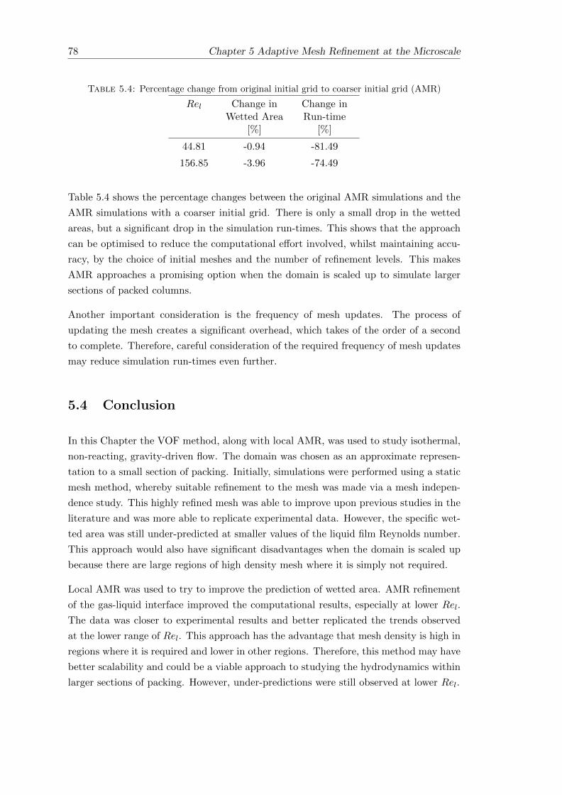
78 Chapter 5 Adaptive Mesh Refinement at the Microscale
Table 5.4: Percentage change from original initial grid to coarser initial grid (AMR)
Rel Change inWetted Area
[%]
Change inRun-time
[%]
44.81 -0.94 -81.49
156.85 -3.96 -74.49
Table 5.4 shows the percentage changes between the original AMR simulations and the
AMR simulations with a coarser initial grid. There is only a small drop in the wetted
areas, but a significant drop in the simulation run-times. This shows that the approach
can be optimised to reduce the computational effort involved, whilst maintaining accu-
racy, by the choice of initial meshes and the number of refinement levels. This makes
AMR approaches a promising option when the domain is scaled up to simulate larger
sections of packed columns.
Another important consideration is the frequency of mesh updates. The process of
updating the mesh creates a significant overhead, which takes of the order of a second
to complete. Therefore, careful consideration of the required frequency of mesh updates
may reduce simulation run-times even further.
5.4 Conclusion
In this Chapter the VOF method, along with local AMR, was used to study isothermal,
non-reacting, gravity-driven flow. The domain was chosen as an approximate represen-
tation to a small section of packing. Initially, simulations were performed using a static
mesh method, whereby suitable refinement to the mesh was made via a mesh indepen-
dence study. This highly refined mesh was able to improve upon previous studies in the
literature and was more able to replicate experimental data. However, the specific wet-
ted area was still under-predicted at smaller values of the liquid film Reynolds number.
This approach would also have significant disadvantages when the domain is scaled up
because there are large regions of high density mesh where it is simply not required.
Local AMR was used to try to improve the prediction of wetted area. AMR refinement
of the gas-liquid interface improved the computational results, especially at lower Rel.
The data was closer to experimental results and better replicated the trends observed
at the lower range of Rel. This approach has the advantage that mesh density is high in
regions where it is required and lower in other regions. Therefore, this method may have
better scalability and could be a viable approach to studying the hydrodynamics within
larger sections of packing. However, under-predictions were still observed at lower Rel.

Chapter 5 Adaptive Mesh Refinement at the Microscale 79
Finally, local AMR was used to refine the whole film region to examine whether the
close proximity of the plate surface had any affect on the results. It was found that
simulation run-times were increased for all Rel tested, as would be expected. However,
the computational results showed marginal differences and so it was concluded that
local AMR should only be applied at the interface. Also, at larger Rel the run-times
were significantly increased because the volume of the fluid film became larger, requiring
more refinement. This shows that the approach of refining the whole film region would
encounter difficulties scaling to larger domains, such as larger sections of structured
packed.
Future investigations could focus on optimisation of the initial mesh density, the number
of refinement levels and the frequency of mesh refinement in order to keep run-times to
a minimum, whilst maintaining good accuracy.


Chapter 6
Enhanced Surface Film Model
Current approaches to modelling post-combustion carbon capture using computational
fluid dynamics are hindered by the multiscale, multiphase characteristics. This chapter
develops a novel Enhanced Surface Film (ESF) model, to simulate thin-film flow down
an inclined plane, with a view to extending this method to be used in the carbon capture
field. This modelling technique produced results inline with the established volume-of-
fluid method, whilst giving a speed-up of 150 times.
6.1 Introduction
Thin film flows are ubiquitous across industrial and environmental sectors. Examples
include thin film microreactors [37, 38], surface coatings [52, 53], biofluids and medical
applications [54,55]. In the majority of these applications the dynamics of the thin liquid
film play a crucial role to the overall performance.
Unfortunately, thin film flows are complex as their dynamics lead to numerous char-
acteristics that can prevent even distributions over surfaces, such as rivulet formation,
rippling effects and even rupture flows. If research is to continue into improving the
performance of applications that exhibit such flows, then there needs to be a significant
advancement in not only understanding the physics behind the flows, but also predicting
the complex characteristics that are commonly seen.
An example of thin filmed flow in industry which is explored in this chapter is the absorp-
tion of CO2 into liquid alkanolamines for use in the carbon capture industry [2,5,6,20,26].
Currently the liquid amines flow over inclined structured packing plates but the forma-
tion of droplets and rivulets reduces the coverage over the surface, thus requiring more
structured packing to compensate. Before the process can be optimised to maximise
the surface area of the liquid on the plate and subsequently improve performance at the
larger scale we need to be better equipped to predict the complex dynamics.
81

82 Chapter 6 Enhanced Surface Film Model
With increasing computational capabilities, computational modelling is proving a valu-
able tool in predicting and optimising flow dynamics and overall processes without the
additional cost and time of performing numerous experimental studies. Unfortunately
the large range of spatial scales within packed columns can greatly inhibit the practical
application of computational fluid dynamics to these situations. CFD solves numerical
models to capture the flow dynamics over finite volumes, however, this leads to signifi-
cant scaling issues as small-scale features cannot be resolved simultaneously with large
scale dynamics. Numerous approaches have been used to model the flow of liquid over an
inclined plate including the VOF model [43,48–50] and surface film modelling [3,119,120].
The volume-of-fluid approach is the favoured method for simulating a liquid film over
a plate or structured packing [26, 41, 42] as it tracks the interface between the liquid
and the air. Unfortunately, the scale of the interface is such smaller than the depth
of the film itself and the averaging nature of CFD models incur inaccuracies as to its
exact location. Refining all the cells which process the numerical modelling can tend
to improve results but at the expense of increase computational exhaustivity and still
are unable to capture this interface exactly. As has been shown in the previous chapter,
adaptive mesh refinement [107,116,117,121] to perform extensive refinement only in the
region of the interface can significantly improve the accuracy and simulation times, but
these simulations times are still much too large for effective scale-up to larger domains.
In order to combat the scalability issues of VOF and AMR-VOF an alternative approach
has been developed in this chapter. Using the depth-averaged Navier-Stokes equations
the number of computational cells required within the liquid film is significantly reduced.
The majority of simulations with the depth-averaged Navier-Stokes equations focus on
flow regimes where the contact angle can be neglected. This simplifies the surface tension
to the capillary pressure. However, in many film flow simulations the contact angle has
a significant effect, causing rivulets to form which significantly reduce the interfacial
surface area of the film. Meredith et al. [3] devised a method to include contact angle
effect in the formulation of the surface film model. Using Young’s Law, which states that
forces along the contact line are balanced at equilibrium, and the balance of tangential
surface forces due to interfacial tension, they derived an expression for the surface-
tangential force normal to the contact line in terms of the surface tension coefficient
and the contact angle. This surface-tangential force is then applied at the contact line,
the interface between wet and dry regions of the flow. The contact line is defined as
the minimum liquid thickness below which the film flow cannot exert enough force to
overcome the contact angle force [3]. However, the contact-angle stress derived from
this model includes a constant which is used to match the model with experimentally
observed data. Therefore, experiments must be run in order to successfully use this
model.
This chapter develops an enhanced surface film model which incorporates new models to
account for the surface tension and contact-line phenomena. Firstly, we will demonstrate

Chapter 6 Enhanced Surface Film Model 83
that previous assumptions to simplify and neglect terms such as contact angle, surface
tension and momentum dispersion were incorrect and develop new models based on data
obtained from high refinement AMR-VOF. Comparisons are performed, to determine
the accuracy and efficiency of this novel method, with existing approaches such as the
standard VOF model and an existing surface film model.
6.2 Governing Equations
The surface film approach used in this thesis makes use of the depth-averaged Navier-
Stokes equations. Initially, the full 3-D Navier-Stokes equations are listed, along with the
mathematical tools required for depth-integration of the equations. Finally, the depth-
averaged Navier-Stokes equation are given, along with the required closure models.
6.2.1 Full 3-D Navier-Stokes Equation
The incompressible Navier-Stokes equation for a 3-dimensional fluid and domain are
determined by the conservation of mass and the conservation of momentum. If the
velocity of the fluid is denoted by uuu = [u, v, w] and the fluid is incompressible, the
conservation of mass leads to the continuity equation given by:
∇ · uuu = 0. (6.1)
The conservation of momentum is given by:
ρ
(∂uuu
∂t+ uuu · ∇uuu
)= −∇p+ µ∇2uuu+ ρggg +FFF st, (6.2)
where ρ is the density, p is the pressure, µ is the kinematic viscosity, ggg is the gravitational
force and FFF st is the surface tension force.
The assumption is made that the density is constant. The inclusion of mass transfer
into the ESF model in the following chapter will involve non-constant densities, since
the density is dependent on the distribution of species within the fluid film. However,
in CCS the concentration of aqueous amine is much larger than the concentration of
absorbed CO2. Therefore, the choice of constant density is a reasonable assumption for
the physical situations being modelled in the following chapter.
6.2.2 Tools for Depth Integration
Important tools for the depth integration of the Navier-Stokes equations are the Leibniz
theorem, the fundamental theorem of integration, the kinematic boundary condition at

84 Chapter 6 Enhanced Surface Film Model
the free surface of the liquid and the kinematic boundary condition at the surface of the
plate along which the fluid flows. It is assumed that the depth-integration is performed
in the z-direction from z(t, x, y) = z0 to z(t, x, y) = zo + h, where h is the film depth
and z0 is the z-coordinate location of the underlying substrate. For a flat substrate this
is usually assigned to the z-coordinate, z0 = 0. The kinematic boundary condition at
the free surface is given by:
w|z0+h =∂h
∂t+ u|z0+h
∂(z0 + h)
∂x+ v|z0+h
∂(z0 + h)
∂y. (6.3)
The kinematic boundary condition at the plate surface is derived by assuming that there
is no mass flux perpendicular to the plate and is given by:
w|z0 = u|z0∂z0
∂x+ v|z0
∂z0
∂y. (6.4)
The Leibniz theorem is stated as:
∂
∂x
∫ z0+h
z0
udz =
∫ z0+h
z0
∂u
∂xdz + u|z0+h
∂(z0 + h)
∂x− u|z0
∂z0
∂x, (6.5)
when u = u(x, y, z) and the fundamental theorem of integration is stated as:∫ z0+h
z0
∂u
∂zdz = u|z0+h − u|z0 . (6.6)
6.2.3 Depth-Averaged Navier-Stokes Equations
The depth-averaging of the Navier-Stokes equations is applicable under the assumptions
that the vertical velocity component is much smaller than the horizontal components
and the pressure is linear with respect to the depth. Depth integrating equation 6.1 (see
Appendix B for full derivation) over the z-direction from z = 0 to z = h and dividing
by ρ = const leads to a continuity equation for the height of the free surface:
∂h
∂t+∇s · (huuu) = 0, (6.7)
where h is the film depth, uuu = (u, v) is the depth-averaged velocity and ∇s is the 2D
nabla given by,
∇s =
(∂
∂x,∂
∂y
). (6.8)
The derivation of the continuity equation does not contain any unclosed terms that
require modelling, so therefore, this is an exact representation of the depth-averaged
continuity equation.
Depth integration of the momentum equations (equation 6.2) leads to:
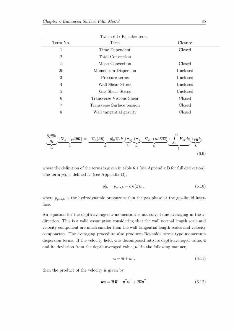
Chapter 6 Enhanced Surface Film Model 85
Table 6.1: Equation terms
Term No. Term Closure
1 Time Dependent Closed
2 Total Convection -
2i Mean Convection Closed
2ii Momentum Dispersion Unclosed
3 Pressure terms Unclosed
4 Wall Shear Stress Unclosed
5 Gas Shear Stress Unclosed
6 Transverse Viscous Shear Closed
7 Transverse Surface tension Closed
8 Wall tangential gravity Closed
∂ρuuuh
∂t︸ ︷︷ ︸1.
+∇s · (ρhuuuuuu)︸ ︷︷ ︸2.
= −∇s(hp) + p|h∇sh︸ ︷︷ ︸3.
+τττw︸︷︷︸4.
+τττ g︸︷︷︸5.
+∇s · (µh∇uuu)︸ ︷︷ ︸6.
+
∫ h
0FFF stdz︸ ︷︷ ︸
7.
+ρgggh︸ ︷︷ ︸8.
,
(6.9)
where the definition of the terms is given in table 6.1 (see Appendix B for full derivation).
The term p|h is defined as (see Appendix B),
p|h = pgas,h − σκ(xxx)nz, (6.10)
where pgas,h is the hydrodynamic pressure within the gas phase at the gas-liquid inter-
face.
An equation for the depth-averaged z-momentum is not solved due averaging in the z-
direction. This is a valid assumption considering that the wall normal length scale and
velocity component are much smaller than the wall tangential length scales and velocity
components. The averaging procedure also produces Reynolds stress type momentum
dispersion terms. If the velocity field, uuu is decomposed into its depth-averaged value, uuu
and its deviation from the depth-averaged value, uuu′′
in the following manner,
uuu = uuu+ uuu′′, (6.11)
then the product of the velocity is given by,
uuuuuu = uuu uuu+ uuu′′uuu′′
+ 2uuuuuu′′. (6.12)

86 Chapter 6 Enhanced Surface Film Model
Figure 6.1: Definition of contact angle, θw, unit vector normal to wall, nnnw and unitvector tangential to wall, tttw
Taking the depth-averaged value (mean value) of this product gives,
uuuuuu = uuu uuu+ uuu′′uuu′′ + 2uuuuuu′′ , (6.13)
uuuuuu = uuu uuu+ uuu′′uuu′′ +���*0
2uuuuuu′′ . (6.14)
Therefore, term 2 in equation 6.9 can be written as,
∇s · (ρhuuuuuu)︸ ︷︷ ︸2.
= ∇s · (ρhuuuuuu)︸ ︷︷ ︸2i.
+∇s · (ρhuuu′′uuu′′).︸ ︷︷ ︸2ii.
. (6.15)
The solution of the above depth-averaged equations along with the continuity equation
and appropriate closure models allows one to solve for fluid depth, h and depth-averaged
velocity, uuu using a CFD approach.
6.2.3.1 Surface Tension
Surface tension is an important term in the modelling of film flow, particularly at the
leading edge of the film where surface tension and contact line instabilities can cause the
formation of rivulets. In the majority of the literature on thin-film modelling, surface
tension is included in the governing equations through a contribution in the pressure
term, as the capillary pressure. This is suitable for regimes where the plate is fully cov-
ered by the liquid film and therefore, no contact line exists at the underlying substrate.
In partially-wetted regimes the contact angle between the liquid and solid surface causes
results in the surface tension deviating from the capillary pressure. This effect must be
included in the governing equations to accurately model partially wetted flow regimes.
Meredith et al. [3] included this influence as an additional body force in the momentum
equations. They defined a threshold film thickness, below which the surface was consid-
ered dry. This body force was applied at the interface between the wet and dry regions.
However, this approach requires a fitting constant to match with experimental data and,
for the simulations performed in this thesis, we were not able to get good agreement
with VOF techniques (see Chapter 6.5).
This approach developed in this thesis applies the continuum surface force (CSF) model
[11], developed for 3D VOF simulations, to the surface film approach. The contribution

Chapter 6 Enhanced Surface Film Model 87
to the balance of momentum from surface tension, FFF st is defined in the CSF model by:
FFF st = σκ(xxx)nnnδ, (6.16)
where σ is the surface tension, nnn is the unit normal vector of the interface pointing into
the liquid phase, δ is the Dirac Delta Function and κ(xxx) is the curvature of the interface,
given by:
κ(xxx) = −∇ ·nnn. (6.17)
In cells adjacent to a wall boundary the definition of the unit normal vector, nnn pointing
into the fluid, is adjusted in order to take account of the liquid contact angle. For a
constant wall contact angle, θw, the unit normal vector pointing into the liquid phase
at the contact line is defined by [46]:
nnn = −nnnwcos(θw)− tttwsin(θw), (6.18)
where nnnw is the unit vector normal to the wall and tttw is the unit vector tangential to
the wall (see Fig. 6.1).
A consistent approach has been adopted in this thesis to model the depth-averaged
surface tension in the ESF model. Assuming that the z-component of velocity is much
smaller than the horizontal components, the depth-averaged pressure is given by (see
Appendix B for derivation),
p = pgas,h +1
2ρghcos(θ)− σκ(t, x, y)nz, (6.19)
where pgas,h is the hydrodynamic pressure within the gas phase at the gas-liquid inter-
face.
The horizontal components of surface tension will be included directly as momentum
source terms in equation 6.9. Therefore, according to the derivation in Appendix B,∫ h
0FFF stdz =
1
2σκnnn. (6.20)
To calculate the normal of the interface (where the interface is defined as z = h(x, y)),
we define the function f(x, y, z) = z − h(x, y). The interface normal pointing into the
liquid phase is then given by:
nnn = − ∇f|∇f |
=hxx+ hyy − z
(1 + h2x + h2
y)0.5, (6.21)
where the subscripts denote differentiation with respect to the coordinate directions and
x, y and z are the unit coordinate vectors.

88 Chapter 6 Enhanced Surface Film Model
For consistency with the 3D CSF model (equation 6.18), the interface normal vector
must be fixed to ensure the correct contact angle. This requires the definition of a
threshold liquid thickness where the definition of the interface normal switches (see
section 6.4.2.1), called δn.
The unit vector tangential to the wall is also normal to the contact line and therefore
can be defined by:
tttw =−hxx− hyy(h2x + h2
y)0.5, (6.22)
and so the interface normal close to the wall is given by:
nnnδ = −nnnwcos(θw)− tttwsin(θw) = −zcos(θw) +hxx+ hyy
(h2x + h2
y)0.5sin(θw). (6.23)
To switch the definition of the interface normal at the threshold liquid thickness we
defined ω as:
ω =
{1 if h ≥ δn0 if h < δn
(6.24)
Therefore, the interface normal, nnntotal, including the effect of the contact angle close to
the wall, is given by:
nnntotal = ωnnn+ (1− ω)nnnδ. (6.25)
The curvature can then be calculated as:
κ(xxx) = −∇ ·nnntotal. (6.26)
6.2.4 Closure Models
6.2.4.1 Shear Stress
For laminar flow on a flat plate the wall shear stress can be defined from the Nusselt
velocity profile [3]. According to Meredith et al. [3], if the velocity at the wall is zero
and the velocity gradients at the gas interface are negligible, then the following velocity
profile can be assumed:
u(z) =3u
h
(z − z2
2h
), (6.27)
where u is the depth-averaged film velocity, z is the wall normal coordinate and h is the
film depth. The wall shear stress can be derived from this assumed velocity profile and
is given by [3]:
τw,i ≈ −µ3uih, (6.28)
where µ is the viscosity of the liquid.

Chapter 6 Enhanced Surface Film Model 89
The assumption of a parabolic velocity profile is valid for wavy film flow [3] and so for
the Rel numbers observed throughout this thesis this assumption should be accurate in
the majority of the flow field. However, in partially wetted flow the assumption of a
parabolic velocity profile may not be accurate. The flow near the fluid front will deviate
from the parabolic profile due to the contact line. According to Oron et al. [56], in
the frame of reference of the contact line the flow recirculates, moving along the free
surface to the contact line and then along the plate surface. Here the above expression
may not accurately predict the actual wall shear stress and could introduce inaccuracies
in the modelling approach. The relative importance of the wall shear stress terms and
accuracy of the proposed model will be determined in the following sections.
Meredith et al [3] modelled the gas shear stress using the following expression,
τg ≈ −Cρg|ug − u|u, (6.29)
where C is a fitting constant and ug is the gas phase velocity. However, the gas-phase
will have negligible effect on the liquid-phase flow and so the gas shear stress terms will
be neglected in the ESF formulation. This approximation is shown to be the case in the
following sections.
6.2.4.2 Depth-Averaged Pressure
As mentioned above, the depth-averaged pressure is derived from the wall-normal mo-
mentum equation. Due to the assumptions of the thin-film equations, the wall-normal
velocity is considered negligible. By including only the wall-normal component of the
surface tension force in the pressure formulation (tangential surface tension forces are
included as source terms in the thin-film equations), the depth-averaged pressure is given
by,
p = pgas,h +1
2ρghcos(θ)− σκ(t, x, y)nz. (6.30)
6.2.4.3 Momentum Dispersion
The momentum dispersion terms are difficult to model since they require knowledge of
the velocity profiles and also knowledge of the deviation of the velocity from the depth-
averaged velocity within the flow. Since the depth-averaged Navier-Stokes equations
only solve for the depth-averaged velocity, it is not possible to calculate the deviation
of the velocity from the average during surface film simulations. Therefore, a model is
required to determine the momentum dispersion terms. The standard approach for thin
film flow is to neglect these terms. However, neglecting the momentum dispersion terms
may not be valid in film flow down an inclined plate, so the relative magnitude of the
momentum dispersion terms will be determined in section 6.4.1.
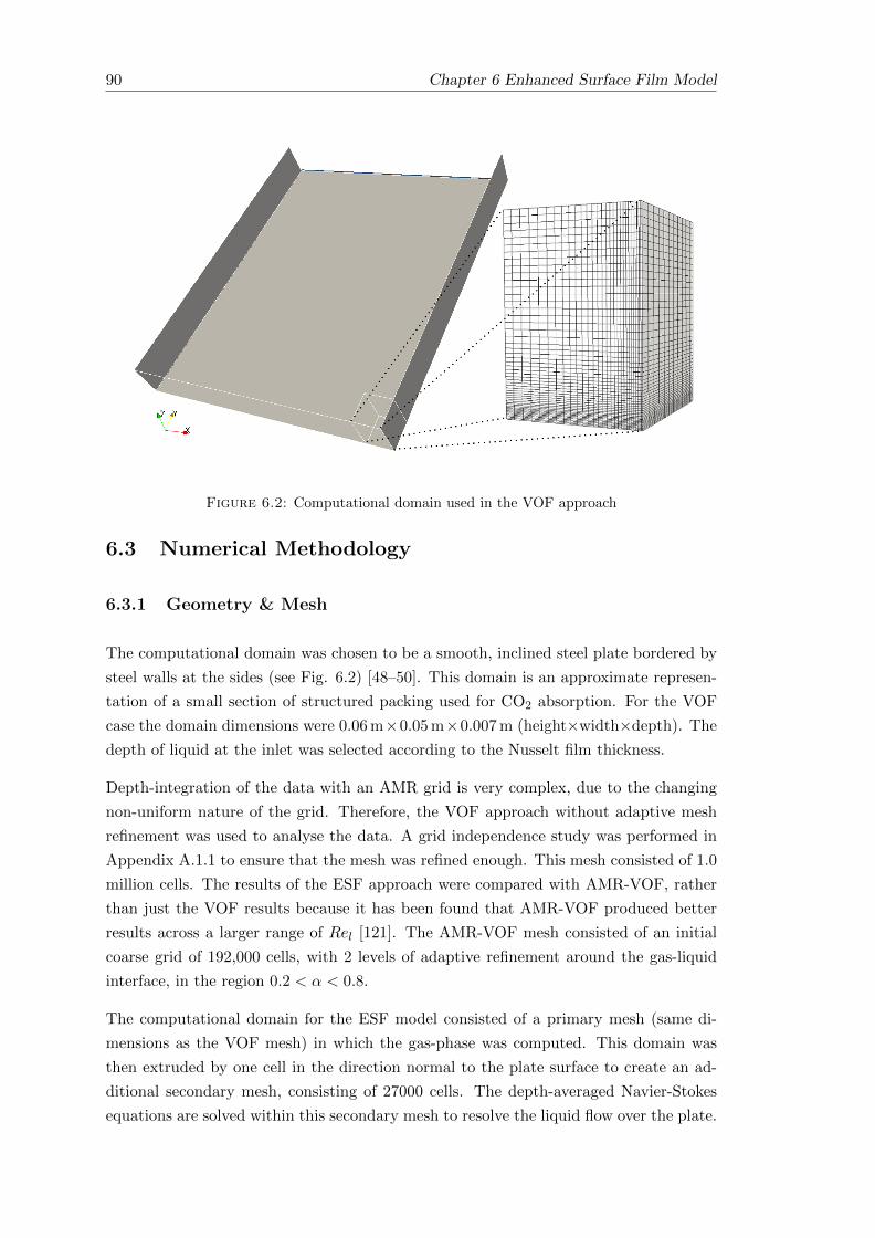
90 Chapter 6 Enhanced Surface Film Model
Figure 6.2: Computational domain used in the VOF approach
6.3 Numerical Methodology
6.3.1 Geometry & Mesh
The computational domain was chosen to be a smooth, inclined steel plate bordered by
steel walls at the sides (see Fig. 6.2) [48–50]. This domain is an approximate represen-
tation of a small section of structured packing used for CO2 absorption. For the VOF
case the domain dimensions were 0.06 m×0.05 m×0.007 m (height×width×depth). The
depth of liquid at the inlet was selected according to the Nusselt film thickness.
Depth-integration of the data with an AMR grid is very complex, due to the changing
non-uniform nature of the grid. Therefore, the VOF approach without adaptive mesh
refinement was used to analyse the data. A grid independence study was performed in
Appendix A.1.1 to ensure that the mesh was refined enough. This mesh consisted of 1.0
million cells. The results of the ESF approach were compared with AMR-VOF, rather
than just the VOF results because it has been found that AMR-VOF produced better
results across a larger range of Rel [121]. The AMR-VOF mesh consisted of an initial
coarse grid of 192,000 cells, with 2 levels of adaptive refinement around the gas-liquid
interface, in the region 0.2 < α < 0.8.
The computational domain for the ESF model consisted of a primary mesh (same di-
mensions as the VOF mesh) in which the gas-phase was computed. This domain was
then extruded by one cell in the direction normal to the plate surface to create an ad-
ditional secondary mesh, consisting of 27000 cells. The depth-averaged Navier-Stokes
equations are solved within this secondary mesh to resolve the liquid flow over the plate.

Chapter 6 Enhanced Surface Film Model 91
Figure 6.3: Computational domain used in thin film approach - side view
A side-view of the computational domain is shown in Fig. 6.3, which shows the cells
within the secondary mesh and the extent of the primary mesh.
6.3.2 Simulation Set-up
For all simulations a constant inclination angle of θ = 60o was chosen to allow compar-
isons with current data in the literature. A range of Rel were tested by suitably altering
the velocity of the liquid film at the inlet. During this investigation counter-current flow
of gas was neglected to again allow comparison with published data. In accordance with
Hoffman et al. [48] and Iso & Chen [50] turbulence was not considered since Rel < 230
and the flow could be considered to be in the laminar or pseudo laminar regime. It
is noted that for falling liquid films the onset of turbulence can occur at Rel = 75
due to wall-induced turbulence [110]. However, fully turbulent flow is not reach until
Rel > 400 [110] and so the laminar governing equations have been used in this chapter.
Time-dependent simulations were carried out using a variable time-step to ensure a
Courant number below 0.2, resulting in time-steps of approximately 8 × 10⁻⁵s for the
surface film simulations. Simulations were allowed to run until a steady or pseudo-steady
state was reached. This was assured by monitoring changes in the specific wetted area
of the plates as a function of time. The two timescales present in these simulations
are the viscous time-scale, τv = L2
ν and the advection time-scale, τa = LU , where L
is the characteristic length scale or the cell size, ν is the kinematic viscosity and U is
the characteristic velocity of the simulation. In these simulations the smallest viscous
timescale was approximately 21.6 times larger than the advection time scale, which
confirms the choice of time-step based on the courant number, Cr = UτaL .
The dynamic viscosity and density of the constituent phases are given in Table 6.2. The
surface tension was set to σ = 0.0728 N ·m−1 and a static contact angle of θw = 70o
was selected.

92 Chapter 6 Enhanced Surface Film Model
Table 6.2: Phase Properties
Phase µ [ Pa · s] ρ [ Kg ·m−3]
Liquid 8.899× 10⁻⁴ 997
Gas 1.831× 10⁻⁵ 1.185
These simulations did not calculate the flow within the gas-phase domain considering
that the aim was to simulate the film flow. The influence of the gas flow on the fluid flow
from the gas-phase shear stress is negligible. For simulations involving mass transfer in
the following chapter the gas-phase domain is solved.
The initial conditions for the simulations were that the depth-averaged domain was
initially devoid of fluid, with the film depth, h = 0 and zero depth-averaged velocity
everywhere. The velocity boundary condition at the plate was set to no-slip condition.
This is not a direct boundary condition on the depth-averaged velocity and is instead
used to determine the wall shear stress. In the case of a moving plate the shear stress
would be increased or decrease depending on the wall velocity direction. In reality, the
boundary condition for the depth-averaged velocity at the plate is a free-slip condition
because the grid in the depth-averaged domain is only one cell deep. The depth-averaged
velocity boundary condition for the side-walls was set to the no-slip condition. The
liquid inlet was set to a fixed value depth-averaged velocity with a fixed value for the
fluid depth, representing the depth-averaged Nusselt velocity and Nusselt film thickness.
For the side-walls the film depth, h was set to a fixed gradient boundary condition to
ensure the correct contact angle was imposed at these side-walls. The outlet was set to
zero gradient for both depth-averaged velocity and film depth. The free boundary at
the top of the domain was set to a slip condition for depth averaged velocity and zero
gradient for film depth.
In the case of the ESF model the contact line paradox is avoided because there is no
explicit no-slip condition for velocity at the plate wall. Instead this approach solves for
the depth-averaged velocity and the influence of the plate wall is taken account of by
the wall shear stress calculation.
6.4 Analysis
This section provides an analysis of the surface film approach and the associated closure
models. Initially, the results from 3D VOF simulations were integrated over the depth of
the liquid film and budget plots were made to determine the relative importance of each
of the terms in the surface film model. This approach revealed which terms must be
included and which could be neglected in the implementation of the surface film model.

Chapter 6 Enhanced Surface Film Model 93
Secondly, an evaluation of the applicability of the CSF model to the thin film approach
was made by comparing the depth-integrated surface tension from 3D VOF simulations
with the ESF surface tension. A model for δmin is derived and thoroughly tested on
different fluids with varying properties.
Finally, the closure models used in the surface film approach were tested by comparison
with the associated terms of the 3D VOF simulations. This allowed the suitability of
the closure models to be determined for thin films on inclined plates. Throughout the
analysis, terms of the surface film equations are evaluated using the depth-averaged
values from the 3D VOF simulations (e.g. film depth, average velocity etc.).
6.4.1 VOF
The results of 3D VOF simulations of film flow down an inclined plane from the pre-
vious chapters were integrated over the thickness of the film to determine the relative
significance of the terms in the surface film model. The integration was performed on
the results after they had reached a pseudo steady-state, determined by the fact the the
interface remained in a fixed location and wetted area was steady. A numerical integra-
tion was performed by calculating the individual terms in the governing equations. Due
to the structured nature of the grid, columns of cells in the wall normal direction could
be numerically integrated to find the depth-averaged value of the individual equation
terms. The depth-averaged value was found by summing up the values within the cells
over each of the columns, weighted by the volume fraction and cell size in the wall normal
direction. The time-dependent terms were calculated by continuing the simulation for a
single time-step. These terms should effectively be zero. However, the VOF simulations
reached only a pseudo steady-state and so these terms may not be exactly zero for the
single time-step calculated.
A mid-range Rel was chosen where multiple flow regimes are observed (see figure 6.4).
Close to the inlet a Nusselt profile flow is observed, but further down the plate a rivulet
forms due to instabilities at the contact line. Slices were taken parallel to the y-axis at
3 important positions within the flow; a central slice, a slice through the oblique rivulet
contact line and a slice through the stagnation point of the flow (see fig. 6.4). These
positions were chosen because they show different flow structures where the relative
magnitudes of the terms may differ. Figures 6.5-6.7 show budget plots of the integrated
3D terms. It is noted that the numerical integral of the 3D convection terms inherently
includes the dispersive Reynolds stresses.
It can be seen that in Figure 6.5 that the time derivative is not equal to zero in the
region where the rivulet combines into a thin ribbon a fluid. This is due to the fact that
the simulations were run until a pseudo-steady state was reached and, whilst the total
flow structure and wetted area remained constant, fluctuations in this region still occur.

94 Chapter 6 Enhanced Surface Film Model
Figure 6.4: 3D VOF Interface Contour Plot with cut planes (Rel = 156.85)
-40
-30
-20
-10
0
10
20
30
0 0.01 0.02 0.03 0.04 0.05
Equation T
erm
s [K
gm
-1s
-2]
Distance from Outlet y [m]
1. Time Derivative2. Total Convection
3. Pressure Gradient4. 5. 6. Viscous Terms
7. Surface Tension8. Gravity
Total
Figure 6.5: Budget Plot of Numerical Integration of 3D y-momentum equation terms- Central position
These budget plots show that all terms appear to be significant. However, the convection
term is comprised of the mean convection (term 2i.) and momentum dispersion (term
2ii.) and the viscous term is comprised of wall shear (term 4.), gas shear (term 5.)
and transverse shear stresses (term 6.). In order to asses the magnitude of these terms
further budget plots are made below.
To determine whether the dispersive Reynolds stresses (term 2ii. in equation 6.15) are
important, budgets showing the total integrated convection, the mean convection and
the momentum dispersion terms are shown in figures 6.8-6.10. It is easy to see that
these dispersion terms are not negligible in the rivulet regions of the flow. Therefore, it
is may not be correct to neglect these terms without a loss of accuracy.

Chapter 6 Enhanced Surface Film Model 95
-15
-10
-5
0
5
10
0.02 0.025 0.03 0.035 0.04 0.045
Equation T
erm
s [K
gm
-1s
-2]
Distance from Outlet y [m]
1. Time Derivative2. Total Convection
3. Pressure Gradient4. 5. 6. Viscous Terms
7. Surface Tension8. Gravity
Total
Figure 6.6: Budget Plot of Numerical Integration of 3D y-momentum equation terms- Oblique position
-20
-15
-10
-5
0
5
10
15
0.035 0.036 0.037 0.038 0.039 0.04 0.041 0.042 0.043 0.044 0.045
Equation T
erm
s [K
gm
-1s
-2]
Distance from Outlet y [m]
1. Time Derivative2. Total Convection
3. Pressure Gradient4. 5. 6. Viscous Terms
7. Surface Tension8. Gravity
Total
Figure 6.7: Budget Plot of Numerical Integration of 3D y-momentum equation terms- Stagnation position
6.4.2 Surface Film Model
6.4.2.1 Surface Tension
The surface tension model used in this thesis is an application of the Continuum Surface
Force (CSF) model to the depth-averaged Navier-Stokes equations. The CSF model
alters the definition of the interface normal close to the wall to take account of the
contact angle between the fluid and the solid surface. The difference between the 3D and

96 Chapter 6 Enhanced Surface Film Model
-60
-50
-40
-30
-20
-10
0
10
20
30
40
0 0.005 0.01 0.015 0.02 0.025 0.03 0.035 0.04
Equation T
erm
s [K
gm
-1s
-2]
Distance from Outlet y [m]
2. Total Convection2i Mean Convection
2ii Momentum Dispersion
Figure 6.8: Budget Plot of Numerical Integration of 3D y-momentum Convection andMomentum Dispersion - Central position
-10
-8
-6
-4
-2
0
2
4
6
8
10
12
0.02 0.025 0.03 0.035 0.04 0.045
Equation T
erm
s [K
gm
-1s
-2]
Distance from Outlet y [m]
2. Total Convection2i Mean Convection
2ii Momentum Dispersion
Figure 6.9: Budget Plot of Numerical Integration of 3D y-momentum Convection andMomentum Dispersion - Oblique position
depth-averaged implementations of the CSF model is the specification of the transition
in the definition of the interface normal.
In the depth-averaged implementation of the CSF model a threshold thickness, δn is
specified, which allows the definition of the interface normal to be adjusted so that it
matches the contact angle close to the fluid-solid contact line. The effect of the value of
δn can be seen in the budget plots of surface tension along the oblique and stagnation
slices. As shown in Figures 6.13-6.14, neglecting the threshold thickness results in a
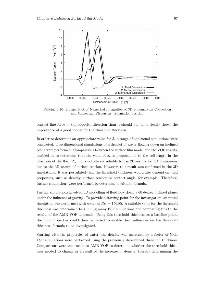
Chapter 6 Enhanced Surface Film Model 97
-4
-2
0
2
4
6
8
10
12
0.036 0.038 0.04 0.042 0.044 0.046 0.048 0.05
Equation T
erm
s [K
gm
-1s
-2]
Distance from Outlet y [m]
2. Total Convection2i Mean Convection
2ii Momentum Dispersion
Figure 6.10: Budget Plot of Numerical Integration of 3D y-momentum Convectionand Momentum Dispersion - Stagnation position
contact line force in the opposite direction than it should be. This clearly shows the
importance of a good model for the threshold thickness.
In order to determine an appropriate value for δn a range of additional simulations were
completed. Two dimensional simulations of a droplet of water flowing down an inclined
plane were performed. Comparisons between the surface film model and the VOF results,
enabled us to determine that the value of δn is proportional to the cell length in the
direction of the flow, ∆x. It is not always reliable to use 2D results for 3D phenomena
due to the 3D nature of surface tension. However, this result was confirmed in the 3D
simulations. It was postulated that the threshold thickness would also depend on fluid
properties, such as density, surface tension or contact angle, for example. Therefore,
further simulations were performed to determine a suitable formula.
Further simulations involved 3D modelling of fluid flow down a 60 degree inclined plane,
under the influence of gravity. To provide a starting point for the investigation, an initial
simulation was performed with water at Rel = 156.85. A suitable value for the threshold
thickness was determined by running many ESF simulations and comparing this to the
results of the AMR-VOF approach. Using this threshold thickness as a baseline point,
the fluid properties could then be varied to enable their influences on the threshold
thickness formula to be investigated.
Starting with the properties of water, the density was increased by a factor of 50%.
ESF simulations were performed using the previously determined threshold thickness.
Comparisons were then made to AMR-VOF to determine whether the threshold thick-
ness needed to change as a result of the increase in density, thereby determining the
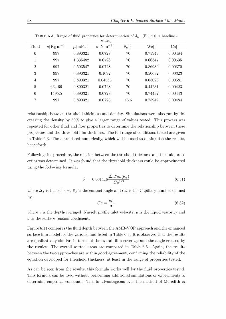
98 Chapter 6 Enhanced Surface Film Model
Table 6.3: Range of fluid properties for determination of δn. (Fluid 0 is baseline -water)
Fluid ρ[ Kg m−3] µ[ mPa s] σ[ N m−1] θw[o] We[-] Ca[-]
0 997 0.890321 0.0728 70 0.75949 0.00484
1 997 1.335482 0.0728 70 0.66347 0.00635
2 997 0.593547 0.0728 70 0.86939 0.00370
3 997 0.890321 0.1092 70 0.50632 0.00323
4 997 0.890321 0.04853 70 0.65023 0.00581
5 664.66 0.890321 0.0728 70 0.44231 0.00423
6 1495.5 0.890321 0.0728 70 0.74432 0.00443
7 997 0.890321 0.0728 46.6 0.75949 0.00484
relationship between threshold thickness and density. Simulations were also run by de-
creasing the density by 50% to give a larger range of values tested. This process was
repeated for other fluid and flow properties to determine the relationship between these
properties and the threshold film thickness. The full range of conditions tested are given
in Table 6.3. These are listed numerically, which will be used to distinguish the results,
henceforth.
Following this procedure, the relation between the threshold thickness and the fluid prop-
erties was determined. It was found that the threshold thickness could be approximated
using the following formula,
δn = 0.031416∆xTan(θw)
Ca1/3(6.31)
where ∆x is the cell size, θw is the contact angle and Ca is the Capillary number defined
by,
Ca =uµ
σ, (6.32)
where u is the depth-averaged, Nusselt profile inlet velocity, µ is the liquid viscosity and
σ is the surface tension coefficient.
Figure 6.11 compares the fluid depth between the AMR-VOF approach and the enhanced
surface film model for the various fluid listed in Table 6.3. It is observed that the results
are qualitatively similar, in terms of the overall film coverage and the angle created by
the rivulet. The overall wetted areas are compared in Table 6.5. Again, the results
between the two approaches are within good agreement, confirming the reliability of the
equation developed for threshold thickness, at least in the range of properties tested.
As can be seen from the results, this formula works well for the fluid properties tested.
This formula can be used without performing additional simulations or experiments to
determine empirical constants. This is advantageous over the method of Meredith et

Chapter 6 Enhanced Surface Film Model 99
Table 6.4: Test Fluid Properties
Fluid ρ[ Kg m−3] µ[ mPa s] σ[ N m−1] θw[o] We[-] Ca[-]
Water 997 0.890321 0.0728 70 0.75949 0.00484
Acetone 791 0.331 0.0229 40 0.30567 0.00320
Glycerol 1227 19.5 0.0671 56 0.04814 0.01977
Table 6.5: Wetted area for various fluids
Fluid AMR-VOF Aw[%]
SF Aw [%] Difference [%]
1 68.04 63.43 -6.78
2 64.66 65.27 0.94
3 42.90 44.69 4.17
4 54.02 56.28 4.18
5 42.86 43.92 2.47
6 54.37 57.74 6.20
7 72.29 72.51 0.30
Acetone 51.48 53.23 3.40
Glycerol 44.01 44.74 1.66
al. [3] because simulations do not need to be compared with experiment to determine
an appropriate value for the threshold film thickness.
In order to test the accuracy and reliability of the derived threshold thickness formula,
additional 3D simulations were performed. This included modelled the flow of ace-
tone and glycerol down the same inclined steel plate. These fluids have wide ranging
properties (Table 6.4), even compared to the test-cases used to determine the formula.
Therefore, they are a good test of the models’ reliability across a wider range of cases.
It can be seen in Figure 6.12 and Table 6.5 that, again, the results are within good
agreement. This further strengthens the validation of the model, since it has been
derived on one set of fluid and successfully tested on another separate set of different
fluids.
6.4.2.2 Dispersion
It can be seen from the Figures 6.8-6.10 that the dispersive stresses are large close to
the leading edge of the film. Observations of the velocity field from the VOF simula-
tions reveal that the momentum dispersion stresses arise due to the recirculating flow
structures created at the static contact line. However, it is difficult to distinguish the
exact effect of these stresses on the overall flow characteristics. Modelling of these terms
is out of the scope of this thesis. Furthermore, the differences in the results between the

100 Chapter 6 Enhanced Surface Film Model
(a) Fluid 1 (b) Fluid 2
(c) Fluid 3 (d) Fluid 4
(e) Fluid 5 (f) Fluid 6
(g) Fluid 7
Figure 6.11: Film depth at steady state for AMR-VOF (left) and Surface Film Model(right)
(a) Acetone (b) Glycerol
Figure 6.12: Film depth at steady state for AMR-VOF (left) and Surface Film Model(right)
ESF model and VOF will give insight into the magnitude of the momentum dispersion
terms.

Chapter 6 Enhanced Surface Film Model 101
-20
-15
-10
-5
0
5
10
0.02 0.025 0.03 0.035 0.04
Equation T
erm
s [K
gm
-1s
-2]
Distance from Outlet y [m]
7. Surface TensionSurface Film Model deltamin=0
deltamin=0.8e-5deltamin=0.2e-4deltamin=0.4e-4deltamin=0.8e-4deltamin=0.2e-3
Figure 6.13: Budget Plot comparing the Closed and Modelled Surface Tension of they-momentum equations for range of δn- Oblique position
-30
-25
-20
-15
-10
-5
0
5
10
15
0.035 0.036 0.037 0.038 0.039 0.04 0.041 0.042 0.043 0.044 0.045
Equation T
erm
s [K
gm
-1s
-2]
Distance from Outlet y [m]
7. Surface TensionSurface Film Model deltamin=0
deltamin=0.8e-5deltamin=0.75e-4deltamin=0.8e-4deltamin=0.2e-3
Figure 6.14: Budget Plot comparing the Closed and Modelled Surface Tension of they-momentum equations for range of δn- Stagnation position
6.4.2.3 Viscous Terms and Wall Shear Stress
The total viscous terms in the Navier-Stokes equations are depth integrated in the
following manner:∫ h
0µ
(∂2u
∂x2+∂2u
∂y2+∂2u
∂z2
)dz︸ ︷︷ ︸
Closed Total Viscous Term
= τw,y︸︷︷︸4.
+τg,y︸ ︷︷ ︸5.
+∂
∂x
(µh∂u
∂x
)+
∂
∂y
(µh∂u
∂y
)︸ ︷︷ ︸
6.
(6.33)
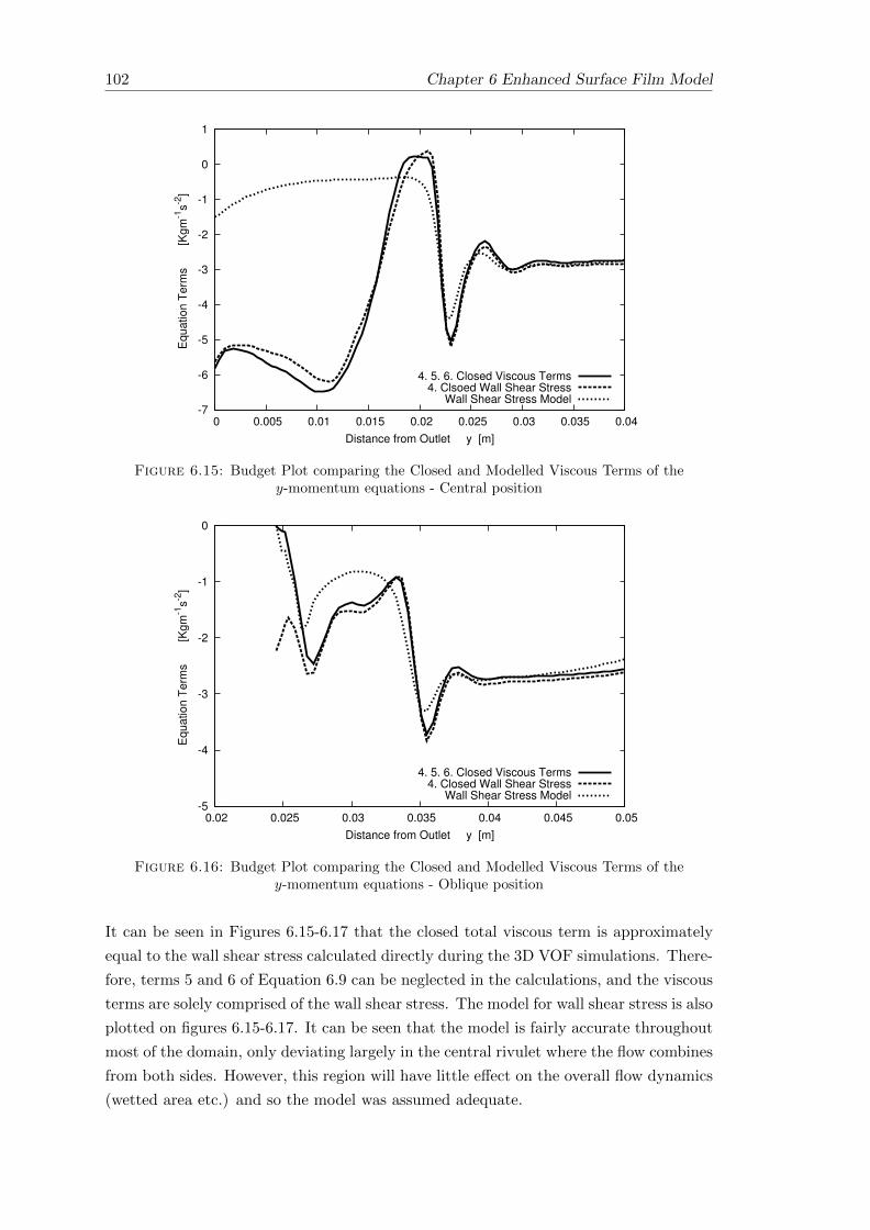
102 Chapter 6 Enhanced Surface Film Model
-7
-6
-5
-4
-3
-2
-1
0
1
0 0.005 0.01 0.015 0.02 0.025 0.03 0.035 0.04
Equation T
erm
s [K
gm
-1s
-2]
Distance from Outlet y [m]
4. 5. 6. Closed Viscous Terms4. Clsoed Wall Shear Stress
Wall Shear Stress Model
Figure 6.15: Budget Plot comparing the Closed and Modelled Viscous Terms of they-momentum equations - Central position
-5
-4
-3
-2
-1
0
0.02 0.025 0.03 0.035 0.04 0.045 0.05
Equation T
erm
s [K
gm
-1s
-2]
Distance from Outlet y [m]
4. 5. 6. Closed Viscous Terms4. Closed Wall Shear Stress
Wall Shear Stress Model
Figure 6.16: Budget Plot comparing the Closed and Modelled Viscous Terms of they-momentum equations - Oblique position
It can be seen in Figures 6.15-6.17 that the closed total viscous term is approximately
equal to the wall shear stress calculated directly during the 3D VOF simulations. There-
fore, terms 5 and 6 of Equation 6.9 can be neglected in the calculations, and the viscous
terms are solely comprised of the wall shear stress. The model for wall shear stress is also
plotted on figures 6.15-6.17. It can be seen that the model is fairly accurate throughout
most of the domain, only deviating largely in the central rivulet where the flow combines
from both sides. However, this region will have little effect on the overall flow dynamics
(wetted area etc.) and so the model was assumed adequate.

Chapter 6 Enhanced Surface Film Model 103
-5
-4
-3
-2
-1
0
1
0.036 0.038 0.04 0.042 0.044 0.046 0.048 0.05
Equation T
erm
s [K
gm
-1s
-2]
Distance from Outlet y [m]
4. 5. 6. Closed Viscous Terms4. Closed Wall Shear Stress
Wall Shear Stress Model
Figure 6.17: Budget Plot comparing the Closed and Modelled Viscous Terms of they-momentum equations - Stagnation position
6.4.2.4 Depth-Averaged Pressure
The pressure terms in the depth-averaged Navier-Stokes equations are approximate,
since the pressure is not solved during the simulation and is estimated based on the
assumptions of the depth-averaged approach. Again, taking streamwise slices through
the central, oblique and stagnation positions comparisons are made between the depth-
averaged pressure (hp) derived from the surface film model and the depth-averaged
pressure from the 3D VOF simulations. Figures 6.18-6.20 show the comparisons. It
is noted that the depth-averaged pressure model is in good agreement with the VOF
derived depth-averaged pressure in most regions of the flow. Again, there is a deviation
where the flow combines into a single rivulet, which is probably due to the fact that in
this region the assumptions of the depth-averaged model are invalid. Particularly, there
will be a large deviation from the Nusselt velocity profile in this region. However, as
stated previously errors in this region will have little effect on the overall wetted area
and interfacial area of the flow, which is of interest to mass transfer studies.
6.5 Results & Discussion
This section outlines the results from simulations of liquid film flow down an inclined
plate using the depth-averaged ESF model. A range of Rel were used to enable compari-
son with 3D AMR-VOF simulations of the same physical problem. The wetted area was
plotted using data from both types of simulations, along with experimental data [48,49].
A comparison of simulation run-times for each method was made.

104 Chapter 6 Enhanced Surface Film Model
-0.05
0
0.05
0.1
0.15
0.2
0.25
0.3
0 0.01 0.02 0.03 0.04 0.05 0.06
Equation T
erm
s [K
gs
-2]
Distance from Outlet y [m]
Closed Average PressureDepth-Averaged Pressure Model
Figure 6.18: Budget Plot comparing the Closed and Modelled Depth Average Pres-sure Term (hp) - Central position
-0.02
-0.015
-0.01
-0.005
0
0.005
0.01
0.015
0.02
0.025
0.02 0.025 0.03 0.035 0.04
Equation T
erm
s [K
gs
-2]
Distance from Outlet y [m]
Closed Average PressureDepth-Averaged Pressure Model deltamin=0
deltamin=0.8e-5deltamin=0.2e-4deltamin=0.4e-4deltamin=0.8e-4deltamin=0.2e-3
Figure 6.19: Budget Plot comparing the Closed and Modelled Depth Average Pres-sure Term (hp) - Oblique position
Figure 6.21 shows a graph of the wetted areas for a range of Rel using the enhanced
surface film model, 3D AMR-VOF and experimental data [48,49]. The ESF model was
able to accurately simulate film flow down an inclined plate across a range of Rel. At
low Rel there is a good agreement between the surface film approach and the AMR-
VOF results, whilst at mid-range Rel the wetted area is slightly over-predicted and at
higher Rel the wetted area is slightly under-predicted. However, the ESF model matched
well with experimental data and it is concluded that the approach is a suitable way to
model film flow down an inclined plane, even without the inclusion of a momentum

Chapter 6 Enhanced Surface Film Model 105
-0.015
-0.01
-0.005
0
0.005
0.01
0.015
0.02
0.025
0.035 0.036 0.037 0.038 0.039 0.04 0.041 0.042 0.043 0.044 0.045
Equation T
erm
s [K
gs
-2]
Distance from Outlet y [m]
Closed Average PressureDepth-Averaged Pressure Model deltamin=0
deltamin=0.8e-5deltamin=0.75e-4deltamin=0.2e-3
Figure 6.20: Budget Plot comparing the Closed and Modelled Depth Average Pres-sure Term (hp) - Stagnation position
dispersion model. This suggests that the momentum dispersion terms have less effect,
than previously thought, on the overall wetted area for these particular simulations. The
deviation between the ESF model and AMR-VOF is acceptable given the assumptions
that are made in the approach.
The biggest difference between the ESF and AMR-VOF was at the high Rel. At these
Rel, once the initial rivulet formed, the contact line moved slowly down the plate until
reaching a steady state position. This slow traversal of the contact line did not occur
to the same degree in the ESF model. An explanation for this may be the effect of the
momentum dispersion terms, because they become more significant, in comparison to
surface tension, as Rel increases.
The OpenFOAM-2.3.0 solver, reactingParcelFilmFoam is an implementation of Meredith
et al.’s [3] surface film model. This includes a model for surface tension where the
contact-angle stress is multiplied by a constant in order to fit with experimental data.
However, despite varying this fitting constant, the solver was unable to replicate the
results of the domain tested in the chapter. For all cases tested, at Rel = 156.85, the
flow was unable to maintain a partially wetted state (Figure 6.22). It is observed that
the ESF model developed in this thesis gave results in greater correlation to the standard
AMR-VOF approach, which in turn is in greater correlation with experimental data.
Figure 6.23 compares the film depth for a range of Rel computed using the ESF model
and AMR-VOF. The enhanced surface film model produced results very similar to the
AMR-VOF approach, in terms of flow characteristics and film depth. It is noted that
for Rel = 58.26 the ESF model shows break-up up of the rivulets into droplets. These
break-up events are likely to be mesh effects. Here the rivulets are very thin and so the

106 Chapter 6 Enhanced Surface Film Model
0
0.2
0.4
0.6
0.8
1
1.2
0 50 100 150 200 250
Specific
wetted a
rea A
w/A
t [-]
Reynolds number Rel [-]
Hoffmann et al. (2005)Hoffmann et al. (2006)
AMR GridSurface Film Model
Figure 6.21: Comparison of wetted area for Surface Film Model with standard AMR-VOF and Experimental Data
Figure 6.22: Film depth at Rel = 156.85 (Left: AMR-VOF, Centre: Surface FilmModel [3], Right: ESF Model)
mesh was probably not refined enough, across the width of the rivulets, resulting in a
numerical break-up event. Further refinement of the grid should enable the rivulets to
be more accurately resolved and prevent break-up for cases where thin rivulets form.
It is noted that good agreement is achieved between the ESF model and AMR-VOF
approach, despite the fact the the dispersion terms have been neglected from the ESF
model. In order to assess the reasons for this, the terms of the depth-averaged equations
used in the ESF model are analysed along the central, oblique and stagnation slices (Fig-
ures 6.24, 6.26, 6.28). The figures only show the significant terms; the total convection,
pressure gradient, wall shear stress, surface tension and gravity. These significant terms
are also evaluated from the results of VOF simulations, to provide comparative data,
and are shown in Figs. 6.25, 6.27, 6.29.
It is observed that the convection term in the ESF model does differ from the depth-
averaged convection term derived from the VOF model. This is expected since the
momentum dispersion terms were neglected. However, it can also be seen that these

Chapter 6 Enhanced Surface Film Model 107
(a) Rel = 58.26 Left: AMR-VOF, Right: ESF
(b) Rel = 71.7 Left: AMR-VOF, Right: ESF
(c) Rel = 112.04 Left: AMR-VOF, Right: ESF
(d) Rel = 156.85 Left: AMR-VOF, Right: ESF
(e) Rel = 179.26 Left: AMR-VOF, Right: ESF
Figure 6.23: Film depth for AMR-VOF and Surface Film Model at various Rel

108 Chapter 6 Enhanced Surface Film Model
-80
-60
-40
-20
0
20
40
60
0 0.01 0.02 0.03 0.04 0.05
Equation T
erm
s [K
gm
-1s
-2]
Distance from Outlet y [m]
2. Total Convection3. Pressure Gradient4. Wall Shear Stress
7. Surface Tension8. Gravity
Figure 6.24: Budget Plot of Numerical Integration of ESF depth-averaged, y-momentum equation terms - Central position
-80
-60
-40
-20
0
20
40
60
0 0.01 0.02 0.03 0.04 0.05
Equation T
erm
s [K
gm
-1s
-2]
Distance from Outlet y [m]
2. Total Convection3. Pressure Gradient
4. 5. 6. Viscous Terms7. Surface Tension
8. Gravity
Figure 6.25: Budget Plot of Numerical Integration of 3D y-momentum equation terms- Central position
differences are balanced out by the gradient of pressure term and, close to the contact
line, the surface tension terms.
The neglected dispersion terms appears not to have a significant effect on the results
in the simulations tested within this thesis. However, these terms may become more
significant for scale-up due to the increased Rel. Therefore, any future work involving
scale-up will have to determine an appropriate model for the dispersion terms.

Chapter 6 Enhanced Surface Film Model 109
-15
-10
-5
0
5
10
15
0.02 0.025 0.03 0.035 0.04 0.045
Equation T
erm
s [K
gm
-1s
-2]
Distance from Outlet y [m]
2. Total Convection3. Pressure Gradient4. Wall Shear Stress
7. Surface Tension8. Gravity
Figure 6.26: Budget Plot of Numerical Integration of ESF depth-averaged, y-momentum equation terms - Oblique position
-15
-10
-5
0
5
10
15
0.02 0.025 0.03 0.035 0.04 0.045
Equation T
erm
s [K
gm
-1s
-2]
Distance from Outlet y [m]
2. Total Convection3. Pressure Gradient
4. 5. 6. Viscous Terms7. Surface Tension
8. Gravity
Figure 6.27: Budget Plot of Numerical Integration of 3D y-momentum equation terms- Oblique position
6.5.1 Comparison of Simulation CPU-Time
One of the main reasons for choosing to use a surface film approach for modelling film
flow over an inclined plane is the computational speed-up achieved in comparison to
alternative methods. Three-dimensional VOF methods using static grids require large
numbers of computational cells throughout the entire domain to ensure that suitable
resolution is achieved to adequately resolve the liquid interface. This results in fairly
large simulation run-times, even on the small domains used in this thesis. Scaling up

110 Chapter 6 Enhanced Surface Film Model
-15
-10
-5
0
5
10
0.03 0.032 0.034 0.036 0.038 0.04 0.042 0.044
Equation T
erm
s [K
gm
-1s
-2]
Distance from Outlet y [m]
2. Total Convection3. Pressure Gradient4. Wall Shear Stress
7. Surface Tension8. Gravity
Figure 6.28: Budget Plot of Numerical Integration of ESF depth-averaged, y-momentum equation terms - Stagnation position
-15
-10
-5
0
5
10
0.03 0.032 0.034 0.036 0.038 0.04 0.042 0.044
Equation T
erm
s [K
gm
-1s
-2]
Distance from Outlet y [m]
2. Total Convection3. Pressure Gradient
4. 5. 6. Viscous Terms7. Surface Tension
8. Gravity
Figure 6.29: Budget Plot of Numerical Integration of 3D y-momentum equation terms- Stagnation position
to simulate large-scale flow over the structured packings used in carbon capture would
be prohibitive in terms of the computational requirements. AMR simulations can help
alleviate some of the computational requirements, by concentrating grid points in regions
of numerical interest. However, simulation run-times would still be prohibitive at larger
scales.
Table 6.6 compares the CPU time for simulations using the ESF model, the VOF ap-
proach and the AMR-VOF approach. It is clear that the ESF model vastly reduces

Chapter 6 Enhanced Surface Film Model 111
Table 6.6: CPU Time
CPU-Time [hrs/sec] CPU-Time [hrs/sec] CPU-Time [hrs/sec]
Rel Static Grid AMR Grid Surface-Film Model
44.81 149.73 1598.50 1.56
58.26 - 1755.33 1.51
71.70 - 1121.67 1.60
80.67 349.73 1021.72 1.48
89.63 - 984.80 1.66
103.07 - 1029.84 1.50
112.04 107.55 1025.08 1.57
134.44 274.92 1097.63 1.45
156.85 287.21 900.93 0.94
168.05 129.78 1269.18 1.05
179.26 127.61 1129.49 0.99
201.66 192.99 953.54 1.14
the number of computational cells required and therefore, reduces the computational
requirements for simulations, thereby making scale-up to mesoscale domains much more
achievable. The approach was approximately 150 times quicker than standard VOF
and 850 times quicker than AMR-VOF. The AMR-VOF results stated used two level of
refinement about this liquid interface, however, it was shown previously that by using a
very coarse initial grid and 3 levels of refinement around the liquid interface, the AMR
run-times could be reduced by up to 80%. Even with this increase in efficiency, the ESF
model is still vastly quicker than the standard approaches to modelling film flow.
6.6 Conclusion
In this investigation a surface film model was developed to simulate isothermal, non-
reacting, gravity-driven flow down an inclined plane. The domain was chosen as an
approximation to a small section of packing material used in CO2 absorption. The results
from three-dimensional VOF simulations were used to determine significant terms of the
depth-averaged Navier-Stokes equations, and to verify the accuracy of modelled terms
which arise due to the spatial averaging process in the derivation of these terms.
The ESF model developed in this chapter was able to replicate the results of more
conventional VOF simulations. In particular, the transition from multiple rivulets to
single rivulets was modelled well, and the wetted area across a range of Rel matched well
with previous numerical studies and experimental data. The deviation from previous
numerical studies is attributed to the simplifications of the approach and the neglected

112 Chapter 6 Enhanced Surface Film Model
momentum dispersion terms. The neglected dispersion terms appear not to have a
significant impact on the results for the simulations tested in this chapter. However, these
terms may become more significant for scale-up due to the increased Rel. Therefore,
any future work involving scale-up will have to determine an appropriate model for the
dispersion terms.
The main problem with using the VOF method for studying CO2 absorption within
packed columns is the prohibitive computational run-times required for larger domains.
The main advantage of this method over other approaches is the significant reduction in
computational requirements (of the order 150 times quicker). Therefore, this will allow
the computational domains to be scaled-up and will allow simulations to be performed
on larger sections of packing, whilst maintaining reasonable CPU-times. However, as
mentioned previously, an appropriate model for the dispersion terms may have to be
developed for scale-up. The ESF approach will also be of benefit in other industrial sec-
tors where the modelling of thin film flow is vital to the understanding of the underlying
processes and the subsequent optimisation studies that are often required.
The next chapters of this thesis will focus on the the addition of species absorption and
reaction modelling to the ESF model. This will represent a significant step forward in
the use of depth-averaged approaches for the modelling acid-gas absorption.

Chapter 7
Surface Film Modelling with
Mass Transport and Chemical
Reaction
7.1 Introduction
The ability to model species mass transfer is a vital component in the numerical sim-
ulation of carbon capture via packed columns. In particular, the absorption of CO2
from the gaseous phase to the liquid phase is seen as a challenging prospect. Despite
these challenges, several papers in the literature state methods of including species mass
transfer within the framework of the VOF model. However, to the best of the author’s
knowledge, there is no literature detailing the inclusion of interfacial mass transfer and
reaction kinetics with a depth-averaged approach.
This chapter details the implementation and validation of mass transfer with the en-
hanced surface film model. Due to the lack of experimental data for physical absorption,
an alternative approach from the literature was used as validation. The method devel-
oped by Haroun et al. [97] was selected and coded into the interFOAM (VOF) solver to
create a new solver capable of modelling species transport. This approach was validated
by Haroun et al., however, further validation is performed here to ensure that new solver
was correctly implemented in OpenFOAM.
The method of Haroun et al. [97] was selected due to its simple formulation, being a single
additional flux term in the species transport equation. The limitation of this method
is that it requires a constant value for Henry’s constant, He. However, simulations
performed in this thesis are isothermal and so He will be constant over the domain.
Initially, the developed code, capable of simulating mass transfer using the VOF method,
was validated using a 1-dimensional model, whereby the simulated results were compared
113

114 Chapter 7 Surface Film Modelling with Mass Transport and Chemical Reaction
against the exact analytical solution [97]. Secondly, validation was performed using a
2-dimensional approach, whereby the results were compared against the mass transfer
coefficient derived from Higbie Penetration Theory.
The mass transfer implementation in the ESF model was then validated against the
VOF approach, in a wetted wall column set-up. Comparisons were made in terms of
concentration profiles and the surface age.
Physical mass transfer is only present in a small subset of real-world absorption equip-
ment and so it was important to also include reaction kinetics in the ESF model. Chem-
ically enhanced mass transfer involves the absorption of a gaseous component into the
liquid phase, accompanied by a chemical reaction. This reaction is used to greatly en-
hance the rate of absorption of many absorption systems, including CO2 capture in
packed columns.
Thus, this chapter also details the implementation of reactive mass transfer with the
ESF model, where validation is performed against the experimental data of Puxty et
al. [4]. It will be shown that the ESF approach, with the inclusion of mass transfer, is
more viable than VOF for realistic 3D simulations of gaseous absorption into a liquid
film.
The validated model is ultimately used to model CO2 absorption into an MEA solution
in the partially wetted regime. This combines all the elements developed throughout
this thesis, including thin-film hydrodynamics, mass transfer, reaction kinetics, and com-
putes all of these aspects simultaneously in a very economical simulation. It exemplifies
that this approach is viable for 3D simulations and clearly demonstrates that this ESF
model could be extended to larger, more realistic problems in CCS with appropriate
modifications.
7.2 Mass Transfer with the ESF Model
In order to include mass transfer within the ESF model it was required to solve a species
transport equation in the gaseous domain. The inclusion of a sink term accounted for
the mass transfer from the gaseous phase into the liquid phase, through the gas-liquid
interface.
As detailed in Chapter 6, the surface-film approach solves equations in two separate
domains, a 3D gaseous domain and a 2D depth-averaged fluid domain. In order to track
the concentration of CO2 (or other gaseous component to be absorbed), an additional
species transport equation was included (equation 7.1), and solved for, in the gaseous
domain,

Chapter 7 Surface Film Modelling with Mass Transport and Chemical Reaction 115
∂Cj∂t
+∇ · (uuuCj)−∇2(DCj ,gCj) = SCj , (7.1)
where Cj is the concentration of species, j, DCj ,g is the diffusion coefficient of species
j in the gaseous phase and SCj is the source/sink of species j. In these simulations
the density in the gaseous phase has been treated as a constant. This is only valid
when the concentration of the absorbed species is low, the temperature differences are
small and the flow is incompressible. This is a reasonable assumption to make since
the concentration of CO2 is flue gas is low, especially in carbon capture at gas-powered
plants. At the scale of the simulations performed in this thesis the temperature range
can also be considered small enough to warrant a constant density assumption. The
flow configurations considered are also in the incompressible regime.
The source term in equation 7.1 is the rate of mass transfer of species j from the gas
phase to the liquid phase. Considering that the surface film model solves on two separate
domains, this source term can be applied in cells adjacent to the interface between these
two domains. The liquid domain in the surface film model is depth-averaged, with only
one cell in the film depth. Therefore, the concentration profile within the liquid phase
can not be resolved. Therefore, Higbie penetration theory is utilised to model the liquid
phase mass transfer process, which ultimately enables the rate of mass transfer through
the interface to be determined.
According to two-film theory [70], the rate of mass transfer through a gas-liquid interface
can be given by equation 2.2, stated again as,
N intj = kL(CintL,j −��
�*0CL,j). (7.2)
It is assumed that the concentration in the liquid bulk, CL,j is approximately zero.
This is a reasonable assumption considering the small diffusion coefficient of CO2 in the
liquid phase, resulting in a very thin concentration boundary layer within the film at
the liquid-side of the interface. This condition is exemplified in the 2D simulations of
gas absorption using the VOF approach later in this chapter.
Henry’s law provides an equilibrium condition at the interface, given by,
CintG,j = Hej CintL,j , (7.3)
which allows the mass transfer rate through the interface to specified by,
N intj = kL
CintG,j
Hej, (7.4)

116 Chapter 7 Surface Film Modelling with Mass Transport and Chemical Reaction
and therefore, the source term in equation 7.1 is specified by,
SCj = −A kLCintG,j
Hej, (7.5)
where A is the interfacial area through which mass transfer can occur. This is taken
as equal to the cell-face area at the boundary between the adjacent domains. However,
a more accurate representation could be achieved by correcting this area by the slope
of the interface. This would give a more accurate representation of the interfacial area,
which would improve future simulations.
This equation is a valid approximation to the rate of mass transfer through a gas-liquid
interface if the concentration gradient on the gaseous side of the interface can be resolved
with adequate grid in the gaseous domain. Since, the diffusion coefficient in the gaseous
phase is of the order of 100 times greater than in the liquid phase (for CO2 in air and
CO2 in aqueous MEA), resolution of the concentration gradient on the gas-side of the
interface is much more achievable than the liquid-side of the interface.
The mass transfer coefficient in the liquid phase, kL can be obtained from Higbie Pene-
tration Theory [12],
kL(t) =
√DCj ,L
πtH. (7.6)
As detailed in section 2.4.2, the exposure time, tH is the amount of time that each fluid
element spends at the gas-liquid interface.
7.2.1 Liquid Film Exposure Time
Many articles in the literature which make use of Higbie Penetration Theory define the
exposure time as the ratio of liquid surface velocity to the distance from the inlet,
tH,SV =yinlet|Us|
, (7.7)
where yinlet is the distance from the liquid inlet and |Us| is the magnitude of the velocity
at the liquid surface, at a particular point in space. The subscript, SV in the exposure
time, tH,SV indicates that the exposure time is calculated using the surface velocity.
This approach gives viable approximation to the exposure time in simple flow config-
urations, such as wetted-wall column flow. However, no consideration is made to the
history of the flow, since it is calculated at specific locations in space and time. It is also
difficult to apply this approach to situations with complicated flow patterns, where the
distance travelled by a fluid particle is not simply equivalent to the straight-line distance
between the current position and the inlet. This situation arises, to a certain degree, in
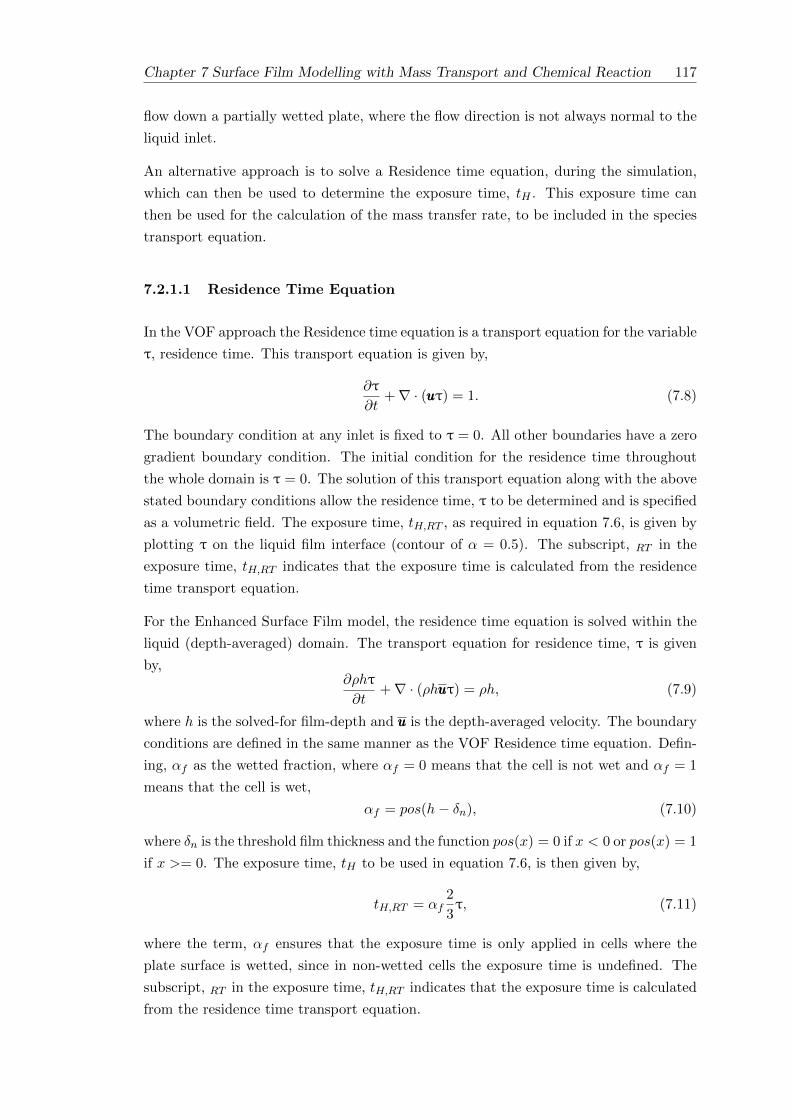
Chapter 7 Surface Film Modelling with Mass Transport and Chemical Reaction 117
flow down a partially wetted plate, where the flow direction is not always normal to the
liquid inlet.
An alternative approach is to solve a Residence time equation, during the simulation,
which can then be used to determine the exposure time, tH . This exposure time can
then be used for the calculation of the mass transfer rate, to be included in the species
transport equation.
7.2.1.1 Residence Time Equation
In the VOF approach the Residence time equation is a transport equation for the variable
τ, residence time. This transport equation is given by,
∂τ
∂t+∇ · (uuuτ) = 1. (7.8)
The boundary condition at any inlet is fixed to τ = 0. All other boundaries have a zero
gradient boundary condition. The initial condition for the residence time throughout
the whole domain is τ = 0. The solution of this transport equation along with the above
stated boundary conditions allow the residence time, τ to be determined and is specified
as a volumetric field. The exposure time, tH,RT , as required in equation 7.6, is given by
plotting τ on the liquid film interface (contour of α = 0.5). The subscript, RT in the
exposure time, tH,RT indicates that the exposure time is calculated from the residence
time transport equation.
For the Enhanced Surface Film model, the residence time equation is solved within the
liquid (depth-averaged) domain. The transport equation for residence time, τ is given
by,∂ρhτ
∂t+∇ · (ρhuuuτ) = ρh, (7.9)
where h is the solved-for film-depth and uuu is the depth-averaged velocity. The boundary
conditions are defined in the same manner as the VOF Residence time equation. Defin-
ing, αf as the wetted fraction, where αf = 0 means that the cell is not wet and αf = 1
means that the cell is wet,
αf = pos(h− δn), (7.10)
where δn is the threshold film thickness and the function pos(x) = 0 if x < 0 or pos(x) = 1
if x >= 0. The exposure time, tH to be used in equation 7.6, is then given by,
tH,RT = αf2
3τ, (7.11)
where the term, αf ensures that the exposure time is only applied in cells where the
plate surface is wetted, since in non-wetted cells the exposure time is undefined. The
subscript, RT in the exposure time, tH,RT indicates that the exposure time is calculated
from the residence time transport equation.

118 Chapter 7 Surface Film Modelling with Mass Transport and Chemical Reaction
Validation of the ESF version of exposure time, tH,RT will be made by comparison
with the VOF exposure time, tH,RT and the usual approach of equation 7.7, tH,SV .
Comparisons will be made on a 2D domain (wetted-wall column) and a 3D domain
(partially-wetted plate).
7.2.1.2 Reactions Kinetics with the ESF Model
The absorption of gases, such as CO2, into liquid films is limited by the small diffusion
coefficient of those gases in the liquid phase. This is often, as in the case of CO2, much
smaller than the diffusion coefficient in the gaseous phase, which results in the rate of
absorption being limited by the liquid-side resistance.
In order to increase the rate of absorption, chemical reactions can reduce the concen-
tration of CO2 in the liquid film, thus reducing the liquid film resistance. In the case of
CO2 absorption, aqueous monoethanolamine is the baseline solvent used to enhance the
rate of absorption.
The modelling of reactions, along with the hydrodynamics and mass transfer adds addi-
tional complexity to the simulations, but it must be included to ensure that simulations
of industry relevant absorption equipment can be completed accurately.
The approach used in this chapter is the Enhancement factor model [122]. The En-
hancement factor, E is defined as the ratio of the rate of absorption into the liquid film
with reaction to the rate of absorption without chemical reaction. This allows all of
the effects of chemical reaction to be confined to one parameter, E. The rate of ab-
sorption without reaction is known from the previous sections, so determination of the
enhancement factor is all that is required to model chemically enhanced absorption.
The Enhancement factor is expressed as a function of the Hatta number, Ha for both
first and second order reactions. The Hatta number is a dimensionless number which
relates the rate of reaction in a liquid film to the rate of diffusion through the film. For
example, in the case of CO2 absorbing from the gaseous phase into the liquid phase and
thus reacting with MEA in the liquid phase, the Hatta number would be given by,
Ha2 =k CbulkMEA,L DCO2,L
k2L
, (7.12)
where k is the rate of chemical reaction between CO2 and MEA, CbulkMEA,L is the concen-
tration of MEA in the bulk of the liquid phase, DCO2,L is the diffusion coefficient of CO2
in the liquid phase and kL (given by equation 7.6) is the rate of mass transfer of CO2 into
the liquid film that would occur without any reaction. According to Danckwerts [122],
for an irreversible, first order reaction the Enhancement factor is given by,
E =√
1 +Ha2. (7.13)

Chapter 7 Surface Film Modelling with Mass Transport and Chemical Reaction 119
The enhancement factor takes a different form for irreversible, second-order reaction
kinetics and an approximate solution developed by Decoursey [123], is given by:
E =M
2(Ei − 1)+
(M2
4(Ei − 1)2+
EiM
(Ei − 1)+ 1
)1/2
, (7.14)
where M = Ha2 and Ei is the enhancement factor for an instantaneous irreversible
reaction, given by:
Ei = 1 +DMEA,LC
bulkMEA,L
bDCO2,LCintCO2,L
, (7.15)
where DMEA,L is the diffusion coefficient of MEA in the liquid phase, b is the number of
moles of MEA required to react with one mole of CO2, and CintCO2,Lis the concentration
of CO2 at liquid-side of the interface.
Whichever order of reaction is selected the enhancement factor is included in the ESF
model within the source term of equation 7.1, so that SCj is given by,
SCj = −E A kLCintG,j
Hej. (7.16)
The assumption of a first-order reaction can be made due to the fast reaction kinetics
and the relatively low concentrations of CO2 in the gas stream. This assumption will
be tested in the following sections.
7.3 Simulations with Mass Transfer
To provide validation of physical mass transfer in the ESF model, the approach of
Haroun et al. [41,97] was implemented into OpenFOAM. This was primarily due to the
lack of experimental data for physical mass transfer and would allow the mass transfer
model used in this thesis to be validated. Further validation is performed in the final
sections of this chapter, where reaction kinetics are included in the model. In this case,
experimental data does exist for chemically enhanced absorption in wetted wall columns.
Initially, one-dimensional simulations were performed and validated against an exact
solution to the governing equations of mass transfer. Secondly, two-dimensional sim-
ulations were performed and validated against the Higbie Penetration Theory of mass
transfer.
7.3.1 1-Dimensional Mass Transfer
As stated by Haroun et al. [97], the case of one-dimensional mass transfer can be val-
idated against an exact numerical solution. Under this simplification no flow occurs

120 Chapter 7 Surface Film Modelling with Mass Transport and Chemical Reaction
and the species transport equation is simplified to a one-dimensional diffusion problem
through a static gas-liquid interface. The exact steady-state solution for the concentra-
tion along the x-axis is given by:
CL =C0G −HeC0
L
He+ DLDG
x
e+ C0
L 0 ≤ x ≤ e, (7.17)
CG =C0G −HeC0
L
HeDGDL
+ 1
x− 2e
e+ C0
G e ≤ x ≤ 2e, (7.18)
where C denotes concentration, He is Henry’s constant, y = e is the location of the
gas-liquid interface and the subscripts L and G correspond to the liquid and gas phases,
respectively.
7.3.1.1 Computational Domain & Simulation Set-up
The computational domain was chosen to be one-dimensional along the x-axis with
a length of 0.1m. The domain was subdivided into 150 cells, considered more than
adequate for this particular simulation. A diagram of the mesh can be observed in
Figure 7.1.
Figure 7.1: Mesh of the 1-D domain
In accordance with the validation performed by Haroun et al. [97], the diffusivity ratio
was chosen to be DG/DL = 10 and the interface is located at x = e. The author of
this thesis imposed the values, e = 0.05 and initial conditions of C0L = 0 mol m−3 and
C0G = 1 mol m−3. The boundary condition for concentration at the left wall was set to
a fixed value of C = 0 mol m−3, whilst for the right wall it was set to a fixed value of
C = 1 mol m−3. Due to the 1-dimensional nature of the domain, the interface would
remain fixed and the gas/liquid phases would remain stagnant. Therefore, the properties
of the fluids are arbitrary and Henry’s constant was chosen to be He = 0.1.
The simulations were run as time-dependent with a time-step of 1× 10⁻⁵s until steady
state was reached. The only time-scale present in this simulation was the diffusion
time-scale, τv = L2
D , where L is the characteristic length scale or the cell size, D is
the diffusion coefficient. The smallest diffusion time-scale was approximately 2× 10⁻⁵s,
which confirms the choice of time step.

Chapter 7 Surface Film Modelling with Mass Transport and Chemical Reaction 121
7.3.1.2 Results & Discussion
Initial validation of the absorption-VOF code was performed by using one of the valida-
tion cases of Haroun et al. [97]. Figure 7.2 shows a plot of the volume fraction, α1. It
can be seen that the interface is located at a central position with the liquid phase on
the left and the gaseous phase on the right of the interface. As mentioned previously, the
fluids will remain stagnant throughout the simulation and therefore, this distribution of
volume fraction will remain constant.
Figure 7.2: Liquid and gas distribution in 1-D domain
Figure 7.3 shows the contour fractions of species concentration throughout the domain.
Initially, the species is fully confined to the gaseous phase (see Figure 7.3(a)). The
converged solution is shown in Figure 7.3(b) and it can be seen that mass transfer has
taken place across the interface in accordance with Henry’s law at the interface.
(a) Initial species concentration (b) Converged species concentration
Figure 7.3: Species concentration in 1-D domain for He = 0.1
Figure 7.4 plots the converged species concentration along the x-axis. The simulated
results are compared to the exact solution. It can be seen that there is very good
agreement between the simulated and analytical solutions, verifying the correct imple-
mentation of the method. The method was able to capture well the discontinuity in
species concentration at the interface region, with good resolution of the concentration.
7.3.2 2-Dimensional Mass Transfer
Simulations were performed of 2D mass transfer on a 2D set-up of a wetted-wall column.
Initially, the OpenFOAM implementation of the VOF approach of Haroun et al. [41,
97] was validated by comparing the calculated mass transfer coefficient with that of
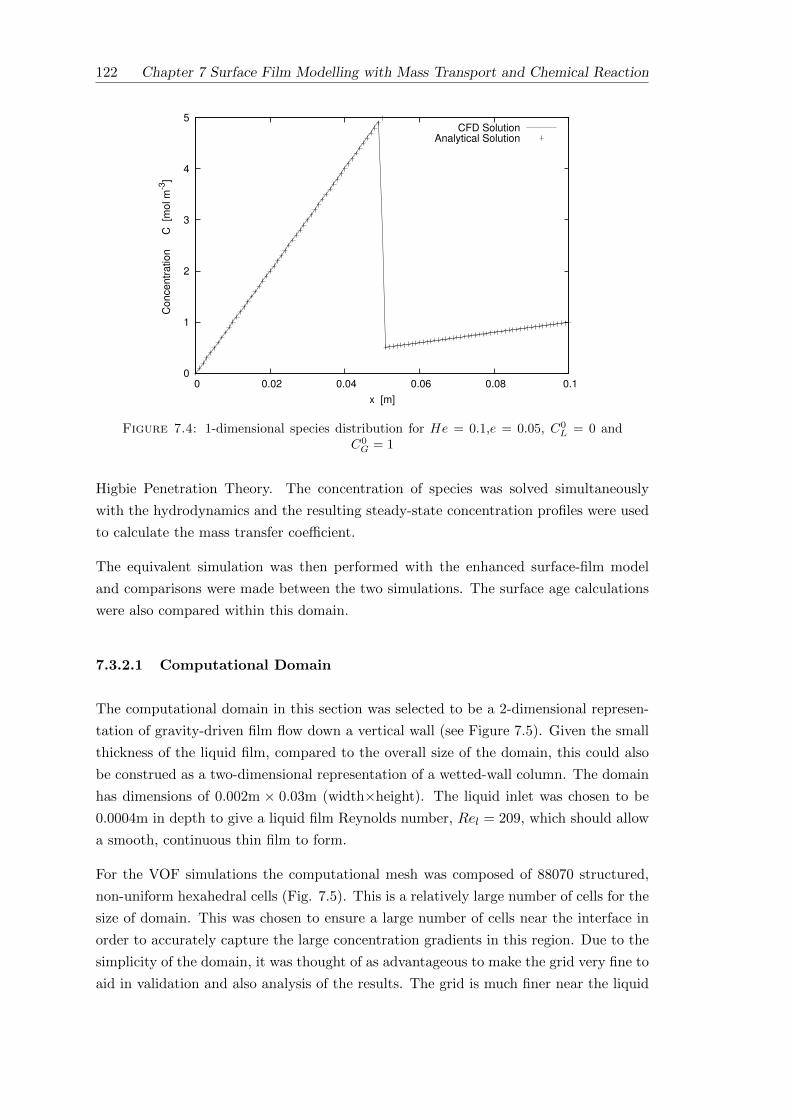
122 Chapter 7 Surface Film Modelling with Mass Transport and Chemical Reaction
0
1
2
3
4
5
0 0.02 0.04 0.06 0.08 0.1
Concentr
ation C
[m
ol m
-3]
x [m]
CFD SolutionAnalytical Solution
Figure 7.4: 1-dimensional species distribution for He = 0.1,e = 0.05, C0L = 0 and
C0G = 1
Higbie Penetration Theory. The concentration of species was solved simultaneously
with the hydrodynamics and the resulting steady-state concentration profiles were used
to calculate the mass transfer coefficient.
The equivalent simulation was then performed with the enhanced surface-film model
and comparisons were made between the two simulations. The surface age calculations
were also compared within this domain.
7.3.2.1 Computational Domain
The computational domain in this section was selected to be a 2-dimensional represen-
tation of gravity-driven film flow down a vertical wall (see Figure 7.5). Given the small
thickness of the liquid film, compared to the overall size of the domain, this could also
be construed as a two-dimensional representation of a wetted-wall column. The domain
has dimensions of 0.002m × 0.03m (width×height). The liquid inlet was chosen to be
0.0004m in depth to give a liquid film Reynolds number, Rel = 209, which should allow
a smooth, continuous thin film to form.
For the VOF simulations the computational mesh was composed of 88070 structured,
non-uniform hexahedral cells (Fig. 7.5). This is a relatively large number of cells for the
size of domain. This was chosen to ensure a large number of cells near the interface in
order to accurately capture the large concentration gradients in this region. Due to the
simplicity of the domain, it was thought of as advantageous to make the grid very fine to
aid in validation and also analysis of the results. The grid is much finer near the liquid

Chapter 7 Surface Film Modelling with Mass Transport and Chemical Reaction 123
inlet, where the gradients are largest, expanding down the plate as the concentration
boundary layer grows.
Figure 7.5: Mesh of the 2-D domain (VOF)
The ESF approach was also modelled on the same domain. This computational mesh
consisted 8800 cells in the gaseous domain and 400 cells in the fluid domain (see Fig.
7.6). In this case a mesh independence check was performed to ensure the grid was fine
enough to accurately resolve the flow features. Due to the large diffusion coefficient in the
gaseous domain, the mesh could be fairly coarse, whilst still capturing the concentration
gradients.
7.3.2.2 Simulation Set-up
To ensure the set-ups were as similar as possible it was important for the liquid inlet
in the VOF case to have the correct velocity profile, considering that this is implicit in
the surface film model. This is important because the rate of mass transfer across the
interface is dependent on the velocity at the interface, which is affected by the velocity
profile.

124 Chapter 7 Surface Film Modelling with Mass Transport and Chemical Reaction
Figure 7.6: Mesh of the 2-D domain (Surface Film)
Therefore, for the VOF case, the simulation was initially run without mass transfer to
set-up the velocity field within the domain. The velocity at the liquid inlet was mapped
from a position further down the domain in a region where the velocity profile was fully
developed. The mapping procedure ensured that the liquid mass flow rates between
the cases were the same. Mass transfer was then included in the VOF model using the
converged, fully-developed velocity field. The initial conditions for the ESF case were
that the depth-averaged domain was initial devoid of fluid with h = 0 and zero velocity
everywhere. In the gas-phase domain the velocity was initially zero everywhere.
For both cases, the average velocity at the liquid inlet in the direction of the flow was
set to UL = −0.5232 ms−1, according to equations 7.19 & 7.20. Again for both cases,
the outlet and gas inlet were set to fixed pressure boundaries and the right boundary
was set to a free-slip atmospheric boundary condition. The left wall was set to a no-slip
boundary. For the ESF case the velocity in the gas domain at the boundary between
the depth-averaged domain was mapped from the liquid interface velocity calculated
in the depth-average domain. The concentration of CO2 at the gas inlet was set to,
CG = 1 mol m−3 and Henry’s constant was set to an arbitrary value, He = 0.5.
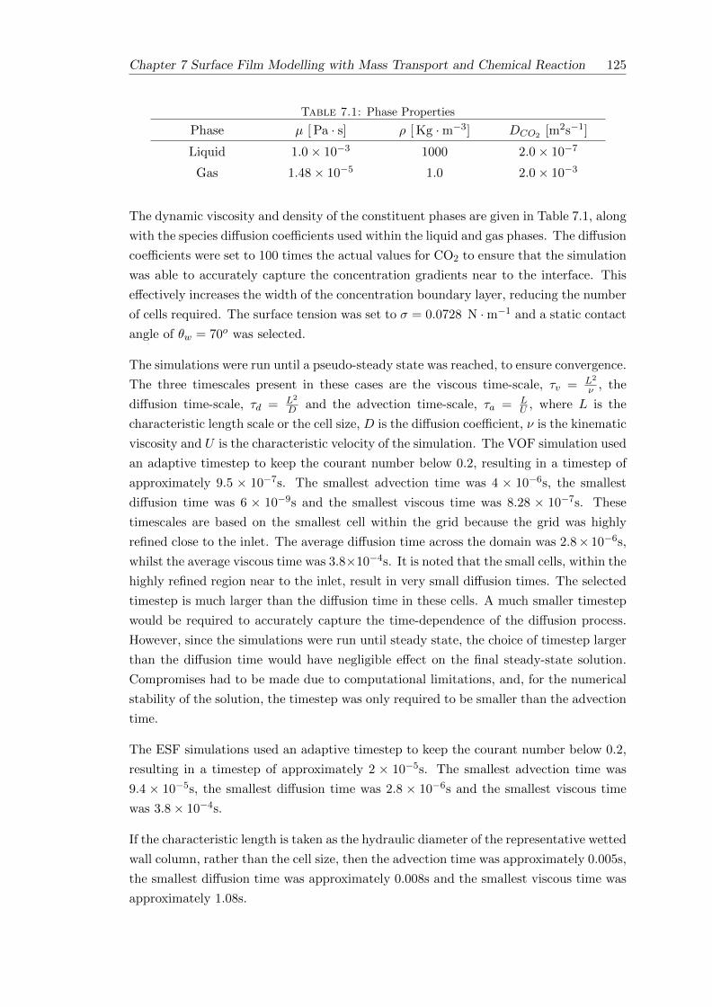
Chapter 7 Surface Film Modelling with Mass Transport and Chemical Reaction 125
Table 7.1: Phase Properties
Phase µ [ Pa · s] ρ [ Kg ·m−3] DCO2 [m2s−1]
Liquid 1.0× 10⁻³ 1000 2.0× 10⁻⁷
Gas 1.48× 10⁻⁵ 1.0 2.0× 10⁻³
The dynamic viscosity and density of the constituent phases are given in Table 7.1, along
with the species diffusion coefficients used within the liquid and gas phases. The diffusion
coefficients were set to 100 times the actual values for CO2 to ensure that the simulation
was able to accurately capture the concentration gradients near to the interface. This
effectively increases the width of the concentration boundary layer, reducing the number
of cells required. The surface tension was set to σ = 0.0728 N ·m−1 and a static contact
angle of θw = 70o was selected.
The simulations were run until a pseudo-steady state was reached, to ensure convergence.
The three timescales present in these cases are the viscous time-scale, τv = L2
ν , the
diffusion time-scale, τd = L2
D and the advection time-scale, τa = LU , where L is the
characteristic length scale or the cell size, D is the diffusion coefficient, ν is the kinematic
viscosity and U is the characteristic velocity of the simulation. The VOF simulation used
an adaptive timestep to keep the courant number below 0.2, resulting in a timestep of
approximately 9.5 × 10⁻⁷s. The smallest advection time was 4 × 10⁻⁶s, the smallest
diffusion time was 6 × 10⁻⁹s and the smallest viscous time was 8.28 × 10⁻⁷s. These
timescales are based on the smallest cell within the grid because the grid was highly
refined close to the inlet. The average diffusion time across the domain was 2.8× 10⁻⁶s,
whilst the average viscous time was 3.8×10⁻⁴s. It is noted that the small cells, within the
highly refined region near to the inlet, result in very small diffusion times. The selected
timestep is much larger than the diffusion time in these cells. A much smaller timestep
would be required to accurately capture the time-dependence of the diffusion process.
However, since the simulations were run until steady state, the choice of timestep larger
than the diffusion time would have negligible effect on the final steady-state solution.
Compromises had to be made due to computational limitations, and, for the numerical
stability of the solution, the timestep was only required to be smaller than the advection
time.
The ESF simulations used an adaptive timestep to keep the courant number below 0.2,
resulting in a timestep of approximately 2 × 10⁻⁵s. The smallest advection time was
9.4 × 10⁻⁵s, the smallest diffusion time was 2.8 × 10⁻⁶s and the smallest viscous time
was 3.8× 10⁻⁴s.
If the characteristic length is taken as the hydraulic diameter of the representative wetted
wall column, rather than the cell size, then the advection time was approximately 0.005s,
the smallest diffusion time was approximately 0.008s and the smallest viscous time was
approximately 1.08s.

126 Chapter 7 Surface Film Modelling with Mass Transport and Chemical Reaction
7.3.2.3 Results & Discussion
Initially, for the VOF simulations, the velocity field was set-up within the domain, with-
out mass transfer. The resulting velocity profile was compared against the predictions
of the Nusselt Theory [62]. According to Nusselt, gravity-driven film flow will develop
a parabolic velocity profile given by:
U(x) = UL,effx(2e− x)
e2, (7.19)
where the interface lies at x = e and the interfacial velocity, UL,eff is given by:
UL,eff =3UL
2=ρLge
2
2µL. (7.20)
The average velocity in the liquid film is denoted by UL.
Figure 7.7 shows a comparison between the simulated velocity profile and the profile
prediction by Nusselt theory. It can be seen that the results are in good agreement with
the theoretical prediction.
-0.8
-0.7
-0.6
-0.5
-0.4
-0.3
-0.2
-0.1
0
0 0.0005 0.001 0.0015 0.002
Velo
city U
(x)
[m
s-1
]
Depth x [m]
SimulationNusselt Solution
Figure 7.7: Comparison of velocity profile with Nusselt profile
Species transport was then included, where the concentration of CO2 is denoted as C.
The CO2 was introduced at the gas inlet with a concentration of CG = 1 mol m−3 and
the concentration at the liquid inlet was kept at CL = 0 mol m−3.

Chapter 7 Surface Film Modelling with Mass Transport and Chemical Reaction 127
According to Haroun et al. [97], the liquid-side local mass transfer coefficient can be
calculated numerically within the CFD code by solving the following equation:
kCFDL,local = −(D∇C + Φ) · nL
∆CL,local, (7.21)
where nL is the normal to the interface pointing into the liquid, ∆CL,local is the local con-
centration difference between the interface concentration and a reference concentration
in the liquid phase close to the wall and Φ is the solubility flux defined in Equation 3.13.
The calculated mass transfer coefficient can then be compared with Higbie Penetration
Theory (see Equation 2.9). The exposure time in this equation is determined from the
CFD data,
tH,SV =yinlet|Us|
, (7.22)
where yinlet is the distance from the liquid inlet and |Us| is the velocity at the gas-liquid
interface. Therefore, the local mass transfer coefficient in the liquid phase, as determined
by the Higbie Penetration Theory, is given by:
kHigbieL,local =
√DC,L
πtH=
√DC,L|Us|πyinlet
. (7.23)
The liquid-side mass transfers coefficient at the interface is plotted against the vertical
y-axis (see Figure 7.8). Comparison is made with the theoretical value for the liquid-
side mass transfer coefficient derived from the Higbie Penetration Theory. Figure 7.9
shows the mass transfer coefficient close to the inlet, where gradients are very large. It
is observed that the numerical results are in good correlation with Higbie Penetration
Theory.
Comparisons between the VOF and ESF approach can be made in terms of the con-
centration profiles within the domain. Figure 7.10 shows the concentration contours
within the domains. It is noted that qualitatively the results are in good agreement. A
vertical slice was then taken through the centre of the domain and the concentration
along this slice is plotted in Figure 7.11. Again, good agreement is observed between
the two approaches, providing further validation for the ESF approach.
The Residence time equation for the VOF model is simply a transport equation for
the Residence time, τ with the appropriate boundary conditions, as described in section
7.2.1.1. By plotting this variable on the contour of volume fraction, α = 0.5 it is possible
to determine the exposure time, tH,RT that is used in the Higbie Penetration model of
mass transfer.
The Residence time equation for the surface film model is slightly more complex due
to the depth averaged nature of the liquid domain (Equation 7.9 and 7.11). In order
to validate the exposure time, tH,RT determined using this approach, comparisons were

128 Chapter 7 Surface Film Modelling with Mass Transport and Chemical Reaction
-0.1
0
0.1
0.2
0.3
0.4
0.5
0.6
0 0.005 0.01 0.015 0.02 0.025 0.03
Mass T
ransfe
r C
oeffic
ient k
L,loca
l [m
s-2
]
Distance y [m]
CFDHigbie
Figure 7.8: Comparison kL,local against the Higbie Penetration Theory
0
0.1
0.2
0.3
0.4
0.5
0.6
0.029 0.0292 0.0294 0.0296 0.0298 0.03
Mass T
ransfe
r C
oeffic
ient k
L,lo
ca
l [m
s-2
]
Distance y [m]
CFDHigbie
Figure 7.9: Comparison kL,local against the Higbie Penetration Theory (Close to inlet)
made against the exposure time determined by the VOF model and with the usual
approach of Equation 7.7, denoted as tH,SV , were the subscript, SV indicates that the
exposure time was calculated from the surface velocity. Figure 7.12 plots these three
approaches against the vertical y-axis, where the liquid inlet is at y = 0.03m and the
outlet is at y = 0m.

Chapter 7 Surface Film Modelling with Mass Transport and Chemical Reaction 129
Figure 7.10: Concentration contours. (Left: VOF, right:ESF)
0.91
0.92
0.93
0.94
0.95
0.96
0.97
0.98
0.99
1
0 0.005 0.01 0.015 0.02 0.025 0.03
Concentr
ation C
O2 [m
ol m
-3]
Position y [m]
VOFESF
Figure 7.11: Plot of concentration profile along the central vertical slice.
It can be seen that the surface age predictions are all in agreement. This is positive vali-
dation, however, comparison still needs to be made on more complex flows. Comparison
of the surface age predictions on a 3D partially wetted plate will be performed in the
following section.
The simulations performed so far highlight a significant problem with the use of standard
approaches to modelling acid-gas absorption into thin liquid films. VOF integrated with

130 Chapter 7 Surface Film Modelling with Mass Transport and Chemical Reaction
0
0.005
0.01
0.015
0.02
0.025
0.03
0.035
0.04
0 0.005 0.01 0.015 0.02 0.025 0.03
Tim
e t H
[s
]
Position y [m]
VOF tH,RTVOF tH,SVESF tH,RT
Figure 7.12: Comparison of exposure time plotted against distance from liquid inlet
mass transfer will work well for certain situations, but may not be applicable to areas
of interest in carbon capture.
The small size of the 2D domain tested, using VOF, allowed many grid points to be
used to ensure that the concentration gradient close to the interface was accurately re-
solved. Figure 7.14 plots the concentration at various horizontal slices along the column
(0.0001m, 0.0004m, 0.0016m, 0.0064m and 0.0256m from the liquid inlet - see Fig. 7.13).
It can be seen that the concentration gradient on the liquid-side of the interface is very
thin, due to the small diffusion coefficient in the liquid. It is noted that the film is
located in the region from x = 0m to approximately x = 0.0004m, whilst the x-axis in
Fig. 7.14 starts at x = 0.0003m. In order to accurately resolve this gradient the grid
was composed of 88070 cells. This implies that for fully 3D simulations the number of
cells required to resolve the concentration field would be prohibitively large. This is all
with a diffusion coefficient in the liquid of 2.0 × 10⁻⁷ m2s−1, 100 times larger than the
actual diffusion coefficient of CO2 in aqueous MEA. For cases with the correct diffusion
coefficient a larger number of cells would be required to accurately capture the smaller
concentration boundary layer that exists on the liquid-side of the interface.
The ESF model does not have this restriction because it does not explicitly model the
concentration within the liquid film. It only requires enough cells to accurately resolve
the concentration gradients within the gaseous domain where the diffusion coefficients
are much larger, hence requiring less cells. Therefore, the ESF model not only speeds-up
purely hydrodynamic simulations, but this improvement will be further enhanced when
mass transfer is included.

Chapter 7 Surface Film Modelling with Mass Transport and Chemical Reaction 131
Figure 7.13: Slice locations in VOF domain
0
0.2
0.4
0.6
0.8
1
1.2
1.4
1.6
1.8
2
0.0003 0.00032 0.00034 0.00036 0.00038 0.0004 0.00042 0.00044
Concentr
ation C
O2 [m
ol m
-3]
Position x [m]
0.0001m0.0004m0.0016m0.0064m0.0256m
Figure 7.14: Plot of concentration gradient at various locations
7.3.3 3-Dimensional Mass Transfer
The ESF mass transfer model has been validated in two-dimensions by comparison
against direct numerical simulation VOF techniques. However, it is concluded that it is
not viable to complete 3D simulations of mass transfer with the VOF approach because
too many cells would be required to capture the thin concentration layer close to the
interface (see Appendix C). A mesh fine enough to simulate the partially wetted plate,
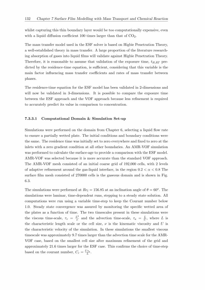
132 Chapter 7 Surface Film Modelling with Mass Transport and Chemical Reaction
whilst capturing this thin boundary layer would be too computationally expensive, even
with a liquid diffusion coefficient 100 times larger than that of CO2.
The mass transfer model used in the ESF solver is based on Higbie Penetration Theory,
a well-established theory in mass transfer. A large proportion of the literature research-
ing absorption of gases into liquid films will validate against Higbie Penetration Theory.
Therefore, it is reasonable to assume that validation of the exposure time, tH,RT pre-
dicted by the residence-time equation, is sufficient, considering that this variable is the
main factor influencing mass transfer coefficients and rates of mass transfer between
phases.
The residence-time equation for the ESF model has been validated in 2-dimensions and
will now be validated in 3-dimensions. It is possible to compare the exposure time
between the ESF approach and the VOF approach because less refinement is required
to accurately predict its value in comparison to concentration.
7.3.3.1 Computational Domain & Simulation Set-up
Simulations were performed on the domain from Chapter 6, selecting a liquid flow rate
to ensure a partially wetted plate. The initial conditions and boundary conditions were
the same. The residence time was initially set to zero everywhere and fixed to zero at the
inlets with a zero gradient condition at all other boundaries. An AMR-VOF simulation
was performed to calculate the surface-age to provide a comparison with the ESF model.
AMR-VOF was selected because it is more accurate than the standard VOF approach.
The AMR-VOF mesh consisted of an initial coarse grid of 192,000 cells, with 2 levels
of adaptive refinement around the gas-liquid interface, in the region 0.2 < α < 0.8 The
surface film mesh consisted of 270000 cells is the gaseous domain and is shown in Fig.
6.3.
The simulations were performed at Rel = 156.85 at an inclination angle of θ = 60o. The
simulations were laminar, time-dependent runs, stepping to a steady state solution. All
computations were run using a variable time-step to keep the Courant number below
1.0. Steady state convergence was assured by monitoring the specific wetted area of
the plates as a function of time. The two timescales present in these simulations were
the viscous time-scale, τv = L2
ν and the advection time-scale, τa = LU , where L is
the characteristic length scale or the cell size, ν is the kinematic viscosity and U is
the characteristic velocity of the simulation. In these simulations the smallest viscous
timescale was approximately 9.7 times larger than the advection time scale for the AMR-
VOF case, based on the smallest cell size after maximum refinement of the grid and
approximately 21.6 times larger for the ESF case. This confirms the choice of time-step
based on the courant number, Cr = UτaL .

Chapter 7 Surface Film Modelling with Mass Transport and Chemical Reaction 133
Table 7.2: Phase Properties
Phase µ [ Pa · s] ρ [ Kg ·m−3]
Liquid 8.899× 10⁻⁴ 997
Gas 1.831× 10⁻⁵ 1.185
The dynamic viscosity and density of the constituent phases are given in Table 7.2. The
surface tension was set to σ = 0.0728 N ·m−1 and a static contact angle of θw = 70o
was selected [50].
7.3.3.2 Results & Conclusions
Comparisons are made between the exposure time, tH,RT predictions of both modelling
approaches, derived from the residence time equation. These results are compared with
the exposure time, tH,SV calculated using the film surface velocity and distance from
the inlet. Contour plots are used to give an overall view of the exposure time and slices
through these contours are taken at the stagnation position, oblique position and central
position. These allow more detailed comparisons to be made.
Figure 7.15 shows a comparison of the exposure time, tH,RT plotted on the liquid inter-
face contour, for the VOF model and ESF model, calculated by solving the residence
time transport equations. The two approaches result in a very similar distribution of
exposure time across the film, especially in regions near the stagnation position.
The exposure time calculated during the AMR-VOF is shifted in time, due to the fact
that at the liquid inlet the velocity was set to constant value, rather than a velocity
profile. This initial constant velocity transitions to the Nusselt profile shortly after
entering the domain. This modelling approximation is required because it is difficult to
apply a Nusselt velocity profile at the inlet, especially during AMR simulations where cell
numbers and locations are adapted in response to the liquid interface. This means that
the interfacial velocity is initially lower than it should be prior to the Nusselt velocity
profile being established. This approximation has little effect on the overall shape of the
film and the wetted area. However, it does affect the evolution of the exposure time, in
the observed way.
This effect can also be observed in Figures 7.16-7.18, which plot the exposure time along
slices at the central position, oblique position and the stagnation position. The exposure
time, tH,RT is calculated using the VOF and ESF residence time equations, along with
the exposure time, tH,SV calculated using the film surface velocity and distance from
the inlet.

134 Chapter 7 Surface Film Modelling with Mass Transport and Chemical Reaction
Figure 7.15: Plot of exposure time at interface contour - Partially Wetted Plate. Left:VOF tH,RT , right: ESF tH,RT
It is observed that for the ESF simulations tH,RT is more accurate than tH,SV . This is
especially significant in Figure 7.18, where the ESF tH,SV significantly over-predicts the
exposure time close to the gas-liquid-solid contact line.
0
0.05
0.1
0.15
0.2
0.25
0 0.01 0.02 0.03 0.04 0.05 0.06
Tim
e t H
[s
]
Position y [m]
VOF tH,RTVOF tH,SVESF tH,RTESF tH,SV
Figure 7.16: Plot of exposure time at central slice - Partially Wetted Plate
It is observed from all of the results that when using the ESF model it is more accurate to
solve a residence time transport equation to determine the exposure time, rather than
relying on a direct calculation of the exposure time from the interfacial velocity and
distance from the inlet. This is particularly the case in regions where the film deviates
from the Nusselt solution. One of the assumptions made to calculate the exposure time,

Chapter 7 Surface Film Modelling with Mass Transport and Chemical Reaction 135
0
0.02
0.04
0.06
0.08
0.1
0.12
0.14
0.015 0.02 0.025 0.03 0.035 0.04 0.045 0.05 0.055 0.06
Tim
e t H
[s
]
Position y [m]
VOF tH,RTVOF tH,SVESF tH,RTESF tH,SV
Figure 7.17: Plot of exposure time at oblique slice - Partially Wetted Plate
0
0.1
0.2
0.3
0.4
0.5
0.6
0.7
0.8
0.9
0.03 0.035 0.04 0.045 0.05 0.055 0.06
Tim
e t H
[s
]
Position y [m]
VOF tH,RTVOF tH,SVESF tH,RTESF tH,SV
Figure 7.18: Plot of exposure time at stagnation slice - Partially Wetted Plate
tH,RT from the depth-average residence time equation is that the velocity profile within
the liquid film is a Nusselt profile. However, this is not always the case and the interfacial
velocity can be under- or over-predicted in certain regions of the flow. This has little
effect on the total wetted/interfacial area because the surface velocity is not integral to

136 Chapter 7 Surface Film Modelling with Mass Transport and Chemical Reaction
the solution. However, if this is used to calculate mass transfer then this will introduce
errors into the solution for species transport.
7.4 Chemically Enhanced Mass Transfer in a Wetted-Wall
Column
Puxty et al. [4] performed a comparison of CO2 absorption into aqueous ammonia solu-
tions and aqueous MEA solutions. The analysis was performed on a wetted wall column,
which provides good validation of both, the mass transfer model and the reaction kinetics
used in the enhanced surface film model.
7.4.1 Computational Domain
The computational domain consisted of wetted-wall column with a counter-current flow
set-up, meaning that the solvent and gas flow in opposite directions. The apparatus
consisted of an internal stainless steel column with an effective height of 8.21cm and di-
ameter of 1.27cm in a vertical orientation [4]. The solvent solution was pumped through
the centre of this column, over-flowing at the top to form a thin film along the sides of
the column. The internal column was surrounded by a jacketed glass column, with an
internal diameter of 2.54cm. This allowed the apparatus to remain at a constant fixed
temperature. A diagram of the apparatus is shown in Fig 7.19.
The depth of liquid film flowing down the sides of the column was much smaller than
the diameter of the internal column. This means that the assumption of 2D flow can
be made, rather than solving on an axisymmetric mesh. Therefore, the problem was
simplified to a rectangular 2D domain of width 0.635cm and height 8.21cm. This defined
the gaseous region, which was subsequently extruded by one cell in the negative x-
direction to form the separate depth-averaged fluid domain (see Fig. 7.20).
This grid consisted of 52544 structured, non-uniform hexahedral cells in the gaseous
region, and 821 cells in the fluid region. Due to the small size of the domain, a fairly
large number of cells could be chosen to ensure that the concentration gradients in the
gaseous domain were captured accurately.
7.4.2 Simulation Set-up
To accurately replicate the results of Puxty et al.’s [4] experimental data, it was ensured
that all parameters of the problem closely resembled their set-up. In particular, it was
important to simulate counter-current flow. This can easily be performed with the
surface film model, due to the fact that two separate domains are used. Whereas, with a

Chapter 7 Surface Film Modelling with Mass Transport and Chemical Reaction 137
Figure 7.19: Wetted-Wall Column Apparatus (Puxty et al. [4])
VOF type simulation it would be much more complicated. This is due to the fact that at
the bottom boundary of the domain, the gas and liquid would flow in opposite directions.
It is effectively an inlet for the gas phase, but an outlet for the liquid phase. This presents
problems for the specification of the boundary condition where a combination of inlet
and outlet conditions must be applied.
The aqueous MEA solution was at a concentration of 5 mol L−1 (30% wt/wt), and flowed
through the system at a flow rate of 220 mL min−1. As stated by Puxty et al. [4], this
flow rate ensured the formation of a continuous, smooth flowing liquid film within the
apparatus. A loading of 0 moles of CO2 per mole of amine was selected.
The gaseous phase consisted of a binary mixture of N2 and CO2 with inlet CO2 concen-
trations of 1.25, 2.5, 4, 5 and 6 mol m−3. The gas flow rate through the apparatus was
set at 5 L min−1.
The initial conditions were zero velocity everywhere and the depth-averaged domain was
initially devoid of liquid with h = 0. All walls were set to no-slip boundaries with fixed
pressure conditions at the outlets. The residence time was initially zero everywhere, fixed
to zero at the inlets and zero gradient at all other boundaries. In the gaseous domain
the concentration was set to fixed value boundaries at the inlet. The velocity boundary

138 Chapter 7 Surface Film Modelling with Mass Transport and Chemical Reaction
Figure 7.20: Wetted wall column domain adapted from Puxty et al. [4]
Table 7.3: Phase Properties
Phase µ [ Pa · s] ρ [ Kg ·m−3]
Liquid 1.600263× 10⁻³ 1003.3
Gas 1.830825× 10⁻⁵ 1.185
condition in the gas-phase domain at the boundary with the depth-averaged domain was
mapped from the film interfacial velocity calculated within the depth-averaged domain.
The dynamic viscosity and density of the constituent phases are given in Table 7.3. The
surface tension was set to σ = 0.0728 N ·m−1 and a static contact angle of θw = 70o
was selected [50]. The simulations were run until a steady state was reached.
The computations were run at two different temperatures, 313K and 333K, due to the
fact that temperatures within CCS absorber columns usually range between 313K an

Chapter 7 Surface Film Modelling with Mass Transport and Chemical Reaction 139
333K [124]. Henry’s constant was set to,
He =
(1
RT
)2.82× 10⁶e−2044/T , (7.24)
to take account of the temperature dependence of He, where R is the universal gas
constant. The diffusivity of CO2 in the liquid phase was calculated using the expression
of Versteeg & Dijck [74], given by:
DCO2,L = 2.35× 10⁻⁶e−2199/T m2s−1. (7.25)
The diffusion coefficient of CO2 in the gas phase was set to DCO2,g = 1.785×10⁻⁵ m2s−1
at 313K and DCO2,g = 1.997 × 10⁻⁵ m2s−1 at 333K [125]. The reaction rates were
calculated using the equation of Versteeg & Dijck [74], to ensure that the temperature
dependence of the reaction rate was taken account of, given by,
k = 4.4× 10¹¹ e−5400/T L mol−1s−1. (7.26)
The computations were run until steady state with an initial time step of 2 × 10⁻⁴s
with an adaptive time-step to keep the Courant number below 1.0. The four timescales
present in these simulations were the viscous time-scale, τv = L2
ν , the diffusion time-
scale, τd = L2
D , the advection time-scale, τa = LU and the reaction timescale, τr = 1
Ck
where L is the characteristic length scale or the cell size, D is the diffusion coefficient,
ν is the kinematic viscosity, U is the characteristic velocity of the simulation, C is the
concentration of CO2 and k is the reaction rate constant. The smallest diffusion time
was approximately 5 × 10⁻⁴s, whilst the smallest viscous time scale was 6 × 10⁻⁴s.
The smallest reaction time scale for the simulations performed was 0.00418s, whilst the
smallest advection time scale was approximately 2.5 × 10⁻⁴s. This confirms the choice
of time-step based on the courant number, Cr = UτaL .
If the characteristic length is taken as the hydraulic diameter of the wetted wall column,
rather than the cell size, then the advection time was approximately 0.038s, the smallest
diffusion time was approximately 8.08s and the smallest viscous time was approximately
10.44s.
7.4.3 Results & Discussion
According to Puxty et al. [4], the overall mass transfer coefficient, KG during absorption
processes is a combination of the liquid-side and gas-side mass transfer coefficients, as
well as the enhancement due to chemical reaction. The absorption flux is given by,
NCO2 = KG(PCO2 − P ∗CO2), (7.27)

140 Chapter 7 Surface Film Modelling with Mass Transport and Chemical Reaction
where PCO2 is the partial pressure of CO2 in the bulk of the gas and P ∗CO2is the
equilibrium CO2 partial pressure.
Puxty et al. [4] state that at constant CO2 loading, the equilibrium partial pressure is a
constant. Therefore, by measuring the CO2 absorption flux, NCO2 and the corresponding
applied partial pressure, PCO2 , for various partial pressures, the overall mass transfer
coefficient can be determined by a linear regression. The applied partial pressure is
calculated as the log mean of the inlet and outlet CO2 partial pressures, given by
PCO2 =(P inCO2,bulk
− P ∗,inCO2)− (P outCO2,bulk
− P ∗,outCO2)
Ln((P inCO2,bulk− P ∗,inCO2
)/(P outCO2,bulk− P ∗,outCO2
)). (7.28)
Following this methodology, Puxty et al. [4] performed linear regressions of the data
according to the formula,
NCO2 = KG . PCO2 + d. (7.29)
resulting in the determination of the values of KG and d for a range of conditions. This
data was used in order to compare the results of the ESF model which included mass
transfer and reaction kinetics.
Figures 7.21 and 7.22 plot the CO2 absorption flux against applied CO2 partial pressure
at 313K and 333K, respectively. The CFD results of the ESF model are compared
against the expression in equation 7.29 and the coefficients derived from regression of
experimental data. First and second order reaction kinetics were performed to test the
assumption that first order reaction kinetics is appropriate.
It is observed that the CFD results are in good agreement with the experimentally de-
rived correlation and that the value of KG is independent of the applied partial pressure,
as expected. From the results it can be concluded that 1st order reaction kinetics are
valid for this simulation, due to the low concentration of CO2 in the gas stream and the
fast reaction rates involved.
Table 7.4 compares the average KG data derived from this work and the average KG
derived from the work of Puxty et al. [4] and Aboudheir et al. [89]. This further confirms
the validity of the models used in the ESF approach. The values obtained from the
experimental data of Aboudheir et al. [89] were performed at much higher applied partial
pressures, which could explain why the results for KG are slightly higher. This was
probably due to the heat of reaction at the liquid film caused by the use of higher
applied partial pressures [4].

Chapter 7 Surface Film Modelling with Mass Transport and Chemical Reaction 141
-5
0
5
10
15
20
25
30
0 2 4 6 8 10
CO
2 A
bsorp
tion F
lux, N
CO
2 [m
mol s
-1 m
-2]
PCO2 [kPa]
Puxty et al [4]First Order
Second Order
Figure 7.21: CO2 absorption flux as a function of applied partial pressure (313K)
-5
0
5
10
15
20
25
30
35
40
0 2 4 6 8 10
CO
2 A
bsorp
tion F
lux, N
CO
2 [m
mol s
-1 m
-2]
PCO2 [kPa]
Puxty et al [4]First Order
Second Order
Figure 7.22: CO2 absorption flux as a function of applied partial pressure (333K)

142 Chapter 7 Surface Film Modelling with Mass Transport and Chemical Reaction
Table 7.4: Average KG Data Comparison
Source KG [ ms−1] (313K) KG [ ms−1] (333K)
This Work (1st Order) 0.01072 0.02222
This Work (2nd Order) 0.01150 0.02353
Puxty et al [4] 0.01152 0.02247
Aboudheir et al [89] 0.01341 0.02464
7.5 Chemically Enhanced Absorption of CO2 on a Par-
tially Wetted Plate
In the previous chapters, the implementation of the enhanced surface film model has
been validated against experimental data. The inclusion of mass transfer has been vali-
dated by comparison with theoretical solutions and refined ARM-VOF simulations. The
inclusion of reaction kinetics into the model has been validated against the experimen-
tal data of a wetted wall column, and the residence-time equation approach has been
validated against the AMR-VOF residence-time equation.
To conclude this thesis, all the elements will be combined to perform a 3D simulation of
CO2 absorption into a partially wetted film of aqueous MEA. This is a major advance-
ment in the field and is an approach which promises much greater scalability, due to
the speed of simulations, especially in comparison to alternative methods such as VOF,
where large scale simulations are simply not possible with current computing capacities.
7.5.1 Computational Domain
The physical situation being modelled was gravity driven flow down an inclined plane.
Therefore, the domain was the same that was used in Chapter 6. In summary, this
consisted of a stainless steel plate of dimensions 0.05m in width and 0.06m in length.
The plate was inclined at 60 degrees to the horizontal plane. The gaseous side of the
domain consisted of 270000 cells and the liquid domain consisted of 27000 cells.
7.5.2 Simulation Set-up
The simulation performed was of CO2 absorption into a falling liquid film of 5 mol L−1
aqueous MEA solution at 313K. The resulting properties of the gas and liquid phases
are shown in Table 7.3. The diffusion coefficient of CO2 in the liquid phase was given by
equation 7.25, with the diffusion coefficient in the gas phase given by, DCO2,g = 1.785×10⁻⁵ m2s−1 [125]. Henry’s constant was specified by equation 7.24. The simulations were
repeated with a gas-side diffusion coefficient 100 times greater than the actual value for

Chapter 7 Surface Film Modelling with Mass Transport and Chemical Reaction 143
CO2. This was to enable qualitative evaluation of the flow and mass transfer, since the
concentration contours are easier to visualise.
The liquid flow rate was selected to ensure a partially wetted plate, Rel = 88.53. The
flow of gas was chosen to be co-current to the liquid film, with a flow rate of 4.2 L min−1.
The inlet concentration of CO2 was selected to be CinCO2= 5 mol m−3.
The initial conditions were zero velocity everywhere and the depth-averaged domain was
initially devoid of liquid with h = 0. All walls were set to no-slip boundaries with fixed
pressure conditions at the outlets. The top boundary in the gas domain was set to a wall
condition with no-slip. At the plate side-walls within the depth-averaged domain a fixed
gradient condition was set on the film depth, h to ensure the correct contact angle was
formed. The residence time was initially zero everywhere fixed to zero at the inlets and
zero gradient at all other boundaries. In the gaseous domain the concentration was set
to fixed value boundaries at the inlet. The velocity boundary condition in the gas-phase
domain at the boundary with the depth-averaged domain was mapped from the film
interfacial velocity calculated in the depth-averaged domain.
The reaction was modelled using 1st order kinetics, as this was shown to be accurate
for the physical situation, with the reaction rate given by equation 7.26. The film
exposure time, tH,RT was calculated using the residence-time equation. The solution of
the liquid film, the gas phase, species concentration and reaction kinetics were performed
simultaneously. The simulation was also run without chemical reaction, to provide a
comparison between physical absorption and reactive absorption of CO2.
The computations were run until steady state with an initial time step of 1 × 10⁻⁴s
with an adaptive time-step to keep the Courant number below 0.2. The four timescales
present in these simulations were the viscous time-scale, τv = L2
ν , the diffusion time-
scale, τd = L2
D , the advection time-scale, τa = LU and the reaction timescale, τr = 1
Ck
where L is the characteristic length scale or the cell size, D is the diffusion coefficient, ν
is the kinematic viscosity, U is the characteristic velocity of the simulation, C is the con-
centration of CO2 and k is the reaction rate constant. The smallest diffusion time-scale
was approximately 0.0062s, whilst the smallest viscous time scale was approximately
0.0072s. The smallest reaction time scale for the simulations performed was 0.0141s,
whilst the smallest advection time scale is approximately 3.6× 10⁻⁴s. This confirms the
choice of time-step based on the courant number, Cr = UτaL .
If the characteristic length is taken as the Nusselt film depth for the inlet flow rate, rather
than the cell size, then the advection time was approximately 0.00038s, the smallest
diffusion time was approximately 0.01s and the smallest viscous time was approximately
0.012s.

144 Chapter 7 Surface Film Modelling with Mass Transport and Chemical Reaction
7.5.3 Results & Discussion
Figure 7.23 shows the film depth in the liquid domain. It can be seen that the film is
in the partially wetted regime, as expected. The slices plot the concentration of CO2
within the gaseous domain. They are taken through a central position and the stagnation
position. The effect of mass transfer can be seen in the reduction of CO2 concentration
near the liquid interface. Figure 7.24 shows a contour plot of CO2 concentration at
the interface between the gas and liquid domains. In effect, this represents the CO2
concentration at the liquid interface.
Figure 7.23: CO2 concentration slices on partially wetted plate.
Figure 7.24: CO2 concentration contours on the film surface for partially wetted plate
Figures 7.25-7.26 show the Hatta number and enhancement factor for this case at the
steady state solution. It is observed that the reaction between CO2 and MEA signif-
icantly enhances the rate of absorption from the gas phase into the liquid film. Since
the Hatta number is large, the enhancement factor is approximately equal to the Hatta
number in the majority of the domain.
The same slices, through a central position and the stagnation position, are used in Fig.
7.27 to plot the velocity magnitude within the gaseous domain. The velocity field that

Chapter 7 Surface Film Modelling with Mass Transport and Chemical Reaction 145
Figure 7.25: Hatta number for the partially wetted plate
Figure 7.26: Enhancement factor for the first order irreversible reaction between CO2
and MEA for the partially wetted plate
is plotted in the depth-averaged domain represents the surface velocity of the film. It
is noted that because the film surface velocity is greater than the gas inlet velocity, the
film causes an increase in the gas velocity near to the interface. It can also be seen
that where there is no film present, the gas velocity is zero at the plate surface. This
demonstrates the coupling between the gas-phase velocity and the liquid-phase velocity
in the ESF model.
Comparisons are also made between physical absorption and chemically enhanced ab-
sorption for this case. The total absorption rate in the case of physical absorption
was 4.996 × 10⁻⁶ mol s−1, whilst in the case of chemically enhanced absorption it was
3.228× 10⁻⁴ mol s−1. This means that the CO2 absorption rate with chemical reaction
was 63.6 times greater than that of physical absorption. Despite the fact that absorp-
tion of CO2 into aqueous MEA is always accompanied by a chemical reaction, this
result clearly demonstrates the advantage of using a chemically reacting system over an
alternative non-reacting system.

146 Chapter 7 Surface Film Modelling with Mass Transport and Chemical Reaction
Figure 7.27: Velocity on partially wetted plate
It is noted that the simulations performed of chemical absorption in this thesis rely on
simplified 1-step mechanisms for the reaction between MEA and CO2. In reality, the
reaction mechanism between MEA and CO2 is very complex, consisting of many inter-
mediate reaction steps. The full reaction mechanism can be represented as having 12
intermediate steps [89]. For a full description of the reaction all of these would need
to be included in the model, with appropriate rate constants for the individual steps.
However, as noted by Aboudheir et al. [89], the overall reaction can be represented by a
single-step reaction between CO2 and MEA using a general reaction rate constant. This
approach has been used in this thesis and it should accurately represent the overall reac-
tion between CO2 and monoethanolamine. The addition of more reaction steps should
increase the accuracy of the simulations, especially if the distribution of intermediate
product has an influence on the overall reaction rate. Future research will focus on the
addition of more reaction steps to better represent the reaction scheme.
In order to qualitatively view the effect of chemical absorption, the simulation was
repeated with a gas-side diffusion coefficient 100 times greater than the actual value for
CO2. This enabled the concentration contours to be viewed more easily (Figs. 7.28-7.29),
due to the process being diffusion dominated. The concentration is observed to drop
near the liquid surface, as expected. Near to the inlet region, where full-film flow occurs
across the width of the plate, the concentration contours are similar to a 2D model.
This is expected since in this region the film is essentially 2D in nature. However, as
the film moves down the plate and the rivulet begins to form, the CO2 concentration
profile also deviates. The concentration is seen to depend significantly on the location
of the interface.
The total simulation time, for the reactive absorption of CO2 into MEA, was 18489
seconds, which equates to 7 cpu hours per second of simulation. This completion time
is significantly quicker than the the VOF simulations, which only modelled the hydro-
dynamics of the flow.

Chapter 7 Surface Film Modelling with Mass Transport and Chemical Reaction 147
Figure 7.28: CO2 concentration contours on partially wetted plate (Dg = 100 ×DCO2
g ).
Figure 7.29: CO2 concentration slices on partially wetted plate (Dg = 100×DCO2g ).
7.6 Conclusion
This chapter initially detailed the inclusion and validation of physical mass transfer
into the enhanced surface film model. The results were validated against the method
of Haroun et al. [97], due to the lack of experimental data for physical mass transfer.
The implementation of Haroun et al.’s method into OpenFOAM was validated against
analytical and theoretical solutions.
The enhanced surface film model was shown to be as accurate as the VOF approach
in the situations tested, with the use of much reduced computational grid. This is
mainly due to the fact that, in these situations, the diffusion coefficient of the trans-
ferred species is much larger in the gas-phase than it is in the liquid-phase. The ESF
model does not explicitly solve for concentration in the liquid, meaning that it requires
less computational grid to resolve the flow, resulting in a reduction in computational
requirements.

148 Chapter 7 Surface Film Modelling with Mass Transport and Chemical Reaction
The residence-time equation developed for use in the enhanced surface film model was
validated against a VOF model of residence time. It was found that the usual approach
of calculating the exposure time, tH,SV using the interfacial velocity and distance from
the inlet was less accurate than deriving the exposure time, tH,RT from a residence-time
equation. This is more so in regions where the ESF model was unable to accurately
derive surface velocities from depth-averaged velocities, such as near the contact-line. It
was concluded that the enhanced surface film model, using the residence-time equation,
was sufficiently accurate to calculate physical mass transfer into liquid films, whilst
significantly improving simulation run-times.
The main disadvantage of this approach is that it assumes that the concentration in
the liquid bulk is negligible. Despite this, in many systems the concentration boundary
layer is confined to a small region close to the liquid film interface, so it may not be
a large disadvantage. However, if a lot of mixing occurs within the liquid film, due to
turbulence, for example, then this would have to be taken account of in the model.
This chapter also described the novel implementation of chemically enhanced absorption
within the enhanced surface film model. Validation was performed against experimental
data of a wetted-wall column. The values of the overall mass transfer coefficient, KG
were within an acceptable range of the experimental data.
The next step combined all of the elements developed in this thesis to model a situation of
real relevance to the carbon capture industry. This involved simulating CO2 absorption
into a thin film of aqueous monoethanolamine. The domain selected was a small-scale
representation of flow within an absorber column filled with structured packing.
The final model was able to simulate, simultaneously, the liquid film hydrodynamics,
the gas flow, the species transport and the chemically enhanced absorption of CO2 into
the film. The results clearly show the applicability of this novel approach to the CCS
industry. The main advantage of this method is the economy of computational resources,
due to the much reduced grid in comparison to the VOF approach. Further research
into this area is clearly of benefit, to scale-up simulations to model much larger, more
realistic sections of packing within absorber columns.
Improvements to the model will need to be made in order for successful scale-up to be
made. These include the addition of a suitable model for momentum dispersion terms
which may become more important at larger scales. The use of a moving mesh technique,
as performed by Lavelle et al. [68], in the gas phase could also improve the accuracy
of the approach. In particular, this would improve the accuracy of the gas phase flow
and also the mass transfer through the interface because the interface would be more
accurately modelled.

Chapter 8
Conclusion
This chapter provides a summary of the work developed within this thesis. This includes
a review of the major contributions and the final conclusions that can be drawn. Finally,
suggestions for future development of this work are listed, along with the wide ranging
applicability of this work.
8.1 Hydrodynamic Modelling of Thin Films
Thin liquid films are a major aspect of carbon capture within packed column absorbers
and they can have a significant impact on the efficiency of the processes. This char-
acteristic is not limited to carbon capture, in fact, many industrial sectors rely on the
thin-film for their efficient operation.
One of the main factors affecting the efficiency of gas absorption into a liquid film is the
interfacial area available for absorption. This thesis initially focussed on a method to
increase the wetted and interfacial areas of films on packing materials. The introduction
of vertical grooves on a steel plate was found to significantly increase the wetted area and
interfacial area, especially at lower liquid flow rates. These simulations were performed
with the VOF method and it was found that despite a significantly reduced domain, in
comparison to the size of absorber columns, the simulations were very computationally
expensive.
Adaptive mesh refinement is a modelling approach which can be used to either increase
accuracy in certain regions of interest, or reduce the computational requirements by
reducing the number of cells in regions that are of little interest. AMR was used with
the VOF model to simulate thin film flow down an inclined plane. An initial coarse
mesh was used, which was then refined around the gas-liquid interface. It was found
that AMR-VOF produced results in better agreement with experimental data in the
literature. However, these simulations took longer to complete due to the overall increase
149

150 Chapter 8 Conclusion
in the number of cells, despite the cells being more effectively distributed. The act of
adapting the mesh, as the interface moves through the domain, also introduces additional
overhead.
Careful consideration of the AMR-VOF parameters eventually enabled the AMR-VOF
simulation to be completed in less computational time. This highlights that the use of
AMR-VOF does not necessarily reduce the computational requirements and that the
AMR parameters (such as initial mesh density and number of refinement levels) need
to be chosen carefully to ensure fast, accurate simulations. Despite these tools, these
type of simulations were still computationally expensive and scaling up the size of the
domain would prove difficult. This would be further complicated by the addition of mass
transfer and reaction kinetics.
From the outset of this work it was understood that the complexity of modelling carbon
capture within packed columns would require the development of a novel approach, espe-
cially in modelling larger scales. Furthermore, it was confirmed in this work that even at
scales much smaller than absorber columns, the VOF or AMR-VOF approaches would
struggle to model the underlying mass transfer processes accurately. This is due to the
large number of computational cells required to accurately resolve the large concentra-
tion gradients that exist close to the interface within the liquid-phase. Simulations using
these types of fully three-dimensional approaches are too computationally intensive and
this significantly hinders their applicability in the real-world application of CCS.
The Enhanced Surface Film (ESF) model developed within this thesis is an extension
of the thin-film depth-averaged model. Surface tension is one of the significant forces
affecting the flow of thin films, and can cause rivulet formation which reduce the effi-
ciencies of devices which rely on thin-films for gas separation. The implementation of
the CSF surface tension model along with the surface film approach allowed accurate
simulations of thin film flow to be performed. This required the development of a model
for the threshold thickness, a parameter required in the depth-averaged version of the
CSF model.
The threshold thickness model was able to accurately simulate thin-film flow for various
fluids with a wide variety of physical properties, from acetone to glycerol. Validation of
the model was made by comparison with experimental data and highly refined AMR-
VOF simulations. The results of the ESF model were within an acceptable range of
the AMR-VOF results and matched well with experimental data. The significant flow
features, such as rivulets and droplets were also captured by the model.
The limitation of the ESF model is the fact that the momentum dispersion terms are
not included, due to the difficulties in modelling these non-linear depth-averaged terms.
However, it was found that neglecting these terms did not effect the results largely, in
terms of wetted area, due to them being balanced by other terms in the equations. It is
proposed that at the larger Rel, the inclusion of a momentum dispersion model may have

Chapter 8 Conclusion 151
improved the results further. This is because at the larger Rel the film contact line moved
very slowly down the plate after the initial rivulet is formed. The slow moving contact
line was not observed with the current ESF model, resulting in an under-predication of
the wetted area at higher Rel. A model for momentum dispersion is an important focus
of future research in this area because it was shown in budget plots that these terms
are not insignificant. Furthermore, the momentum dispersion terms would probably be
more significant in larger domains at higher Rel. A suitable model for the momentum
dispersion terms will need to be determined for future scale-up of the ESF approach.
8.2 Mass Transfer and Reaction Kinetics
Mass transfer is a vital component in gas absorption equipment, such as in packed
columns. The basic principle of these apparatus is the separation of a gaseous species by
absorption into a thin film of solvent. The modelling of this process has been performed
along with the VOF approach in the literature [41,97]. Haroun et al.’s [41,97] approach
was implemented into OpenFOAM in order to provide additional validation of methods
developed in this thesis.
However, simulations using this implementation highlighted further problems with the
use of the VOF approach for the modelling of these processes. Particularly in carbon
capture, the diffusion coefficient of CO2 in the liquid phase very small and is two orders of
magnitude smaller than that in the gaseous phase. The resulting concentration boundary
layer on the liquid side of the interface is very small and requires many cells in this region
to accurately capture this gradient. It was concluded that, even for the relatively small
domains used in thesis, the VOF model with mass transfer would be too computationally
expensive to simulate, when using the correct diffusion coefficients for CO2.
The inclusion of mass transfer in the ESF model was a major development in this field
of research. In order to account for mass transfer, sink terms were introduced in the
gas phase where the mass transfer coefficient was calculated using Higbie Penetration
Theory. This theory requires the definition of a film exposure time. In order to track
the evolution of the exposure time throughout the domain, a depth-averaged version of
the residence-time transport equation was developed and included in the ESF model.
This allows the exposure time to be determined at any location on the surface of the
film at any moment in time.
It was found that the mass transfer implementation of the ESF model was able to accu-
rately solve for the hydrodynamics of thin films and the physical mass transfer through
the gas-liquid interface, simultaneously. The limitation of this approach is that it as-
sumes that the concentration in the bulk of the liquid film is negligible. Improvements
to this could be made in future research. However, at present this is not seen as a major
disadvantage because in many applications the concentration of absorbed species is very

152 Chapter 8 Conclusion
low in the liquid bulk. This is due to the fact that the concentration is the gas bulk is
usually low and the diffusion coefficient in the liquid phase is small. Chemical reactions
in the liquid film also reduce the amount of absorbed species that can diffuse into the
liquid bulk, since they are transformed into reaction products.
A natural extension of the mass transfer ESF solver, was to include chemically enhanced
absorption. This is another advancement in this field of research. This was included
using the Enhancement factor model, which is the ratio of the rate absorption with
chemical reaction to the rate of absorption without chemical reaction. The Enhancement
factor is usually defined in terms of the Hatta number, Ha, a non-dimensional number.
First and Second order reactions were tested in a two-dimensional representation of a
wetted-wall column. This involved CO2 absorbing into a liquid film composed of aque-
ous monoethanolamine. The model was validated against experimental data from the
literature and it was found that the ESF model was able to accurately model chemically
enhanced absorption. The prediction of the overall mass transfer coefficients were very
similar to literature data for temperature values of 313k and 333k.
First order reactions kinetics gave similar results to second order reaction kinetics. This
was expected since the concentration of CO2 in the gas phase was low, as is the case
in natural gas power station flue gas. The rate of reaction between CO2 and mo-
noethanolamine is also very fast, meaning that the assumption of first order reaction
kinetics is valid. The work detailed in this thesis has proven that this is the case, for
the set-up tested.
The final part of this thesis was to combine all of the elements developed for the ESF
model. A simulation was performed of CO2 absorption into a film of aqueous mo-
noethanolamine. The flow rate of the liquid phase was chosen so that it was in the
partially wetted regime. The model was able to simulate this domain with relative ease,
the simulation only using 2.17 cpu hours per second of simulation. All of the aspects,
such as the solution of hydrodynamics, mass transfer and reaction kinetics were solved
simultaneously. Despite the limitations and assumptions of the ESF model, this clearly
shows that this is a promising approach to simulating carbon capture on larger domains.
Therefore, future research could focus on using the model to solve for larger sections of
packing materials, even at the mesoscale.
8.3 Future Work
The ESF model in its present state can be used to model a variety of apparatus in
numerous industries. The performance and efficiency of many apparatus is dependent
on the structure of thin liquid films. Therefore, potential applications include thin
Chapter 8 Conclusion 153
film microreactors, surface coating, biofluids and medical applications. It would be
interesting to test the ESF model in other applications, such as these.
In terms of CCS, the size of the simulations could be scaled-up to model more realistic
representations of the absorber columns. This could be made possible by the ESF
model. Simulations of the mesoscale with the inclusion of surface film modelling and
mass transfer would present an interesting challenge. A prerequisite to this research
would be the development of a model for the momentum dispersion terms to properly
account for momentum dispersion at higher Rel.
The ESF model could also be extended from it current form to increase its accuracy.
As mentioned previously, this could be achieved in terms of the hydrodynamics by
developing a model for the momentum dispersion terms. In terms of mass transfer, the
model could be extended to allow for a non-zero species concentration in the liquid bulk,
or gas loadings greater than zero. This would allow a greater variety of carbon capture
situations to be modelled including cases with larger values of CO2 loading. Finally, a
moving mesh technique could be introduced to improve the coupling between the gas
and liquid phases.


Appendix A
Microscale Hydrodynamics
A.1 Mesh Independence Checks
Mesh independence checks were carried out to ensure the results were not effected by
the choice of meshes during the investigation of flow down an inclined plane using VOF.
It was observed that the wetted area of the plate was highly dependent upon the flow
parameters and therefore, this variable was used as a good indication to mesh depen-
dency. These checks were performed for the smooth plate and textured plate and are
detailed below.
A.1.1 Smooth Plate
Due to the range of plate inclination angles it was important to ensure grid independent
results for all angles. Simulations were run initially with a mesh of 0.6 million cells,
increasing the number of cells in subsequent calculations until no significant difference
in the solution was observed. Fig. A.1 and Fig. A.2 plot the specific wetted area against
time for θ = 60o and θ = 30o, respectively. It can be seen that there was very little
difference in the solutions when using meshes of 0.8, 1.0 and 1.2 million cells. It was
established that a cell count of 1.0 million cells allowed mesh dependency errors to be
minimised for the range of inclination angles, whilst keeping run times to a reasonable
level.
A.1.2 Textured Plate
Simulations were run initially with approximately 1.4 million cells, increasing the num-
ber of cells in subsequent calculations until no significant difference in the solution was
observed. Fig. A.3 plots the specific wetted area against time for the various compu-
tational meshes. It can be seen that the solutions obtained with meshes of 2.0 and 2.5
155
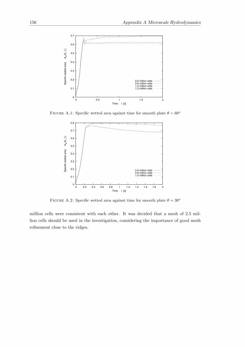
156 Appendix A Microscale Hydrodynamics
0
0.1
0.2
0.3
0.4
0.5
0.6
0.7
0 0.5 1 1.5 2
Specific
wetted a
rea A
w/A
t [-]
Time t [s]
0.6 million cells0.8 million cells1.0 million cells1.2 million cells
Figure A.1: Specific wetted area against time for smooth plate θ = 60o
0
0.1
0.2
0.3
0.4
0.5
0.6
0.7
0.8
0 0.2 0.4 0.6 0.8 1 1.2 1.4 1.6 1.8 2
Specific
wetted a
rea A
w/A
t [-]
Time t [s]
0.6 million cells0.8 million cells1.0 million cells
Figure A.2: Specific wetted area against time for smooth plate θ = 30o
million cells were consistent with each other. It was decided that a mesh of 2.5 mil-
lion cells should be used in the investigation, considering the importance of good mesh
refinement close to the ridges.

Appendix A Microscale Hydrodynamics 157
0
0.1
0.2
0.3
0.4
0.5
0.6
0.7
0.8
0.9
1
0 0.5 1 1.5 2
Specific
wetted a
rea A
w/A
t [-]
Time t [s]
1.4 million cells2.0 million cells2.5 million cells
Figure A.3: Specific wetted area against time for textured plate θ = 60o


Appendix B
Derivation of Depth-Averaged
Navier-Stokes Equations
This appendix shows the full derivation of the depth-averaged Navier-Stokes equations,
followed by the derivation of the surface tension terms used in the ESF model. Initially,
a recap is given of the tools used for the depth integration of the equations.
B.0.1 Tools for Depth Integration
Important tools for the depth integration of the Navier-Stokes equations are the Leibniz
theorem, the fundamental theorem of integration, the kinematic boundary condition at
the free surface and the kinematic boundary condition at the surface of the plate along
which the liquid flows. It is assumed that the depth integration is performed in the
z-direction from z(t, x, y) = z0 to z(t, x, y) = zo + h, where h is the film height and z0 is
the z-coordinate location of the underlying substrate. Since the simulations in this thesis
were performed on a flat plate, z0 = 0. The velocity field is denoted as uuu = [u, v, w].
B.0.1.1 The kinematic boundary condition at the free surface
If the surface is denoted by zs = z0+h, then the kinematic boundary condition is derived
by taking the derivative of zs = zs(t, x, y),
w|z0+h =DzsDt
=∂(z0 + h)
∂t+∂x
∂t
∂(z0 + h)
∂x+∂y
∂t
∂(z0 + h)
∂y, (B.1)
which gives,
w|z0+h =���7
0∂z0
∂t+∂h
∂t+ u|z0+h
∂(z0 + h)
∂x+ v|z0+h
∂(z0 + h)
∂y, (B.2)
159
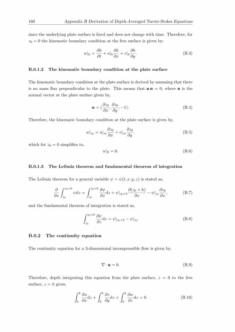
160 Appendix B Derivation of Depth-Averaged Navier-Stokes Equations
since the underlying plate surface is fixed and does not change with time. Therefore, for
z0 = 0 the kinematic boundary condition at the free surface is given by:
w|h =∂h
∂t+ u|h
∂h
∂x+ v|h
∂h
∂y. (B.3)
B.0.1.2 The kinematic boundary condition at the plate surface
The kinematic boundary condition at the plate surface is derived by assuming that there
is no mass flux perpendicular to the plate. This means that uuu.nnn = 0, where nnn is the
normal vector at the plate surface given by,
nnn = (∂z0
∂x,∂z0
∂y,−1). (B.4)
Therefore, the kinematic boundary condition at the plate surface is given by,
w|z0 = u|z0∂z0
∂x+ v|z0
∂z0
∂y. (B.5)
which for z0 = 0 simplifies to,
w|0 = 0. (B.6)
B.0.1.3 The Leibniz theorem and fundamental theorem of integration
The Leibniz theorem for a general variable ψ = ψ(t, x, y, z) is stated as,
∂
∂x
∫ z0+h
z0
ψdz =
∫ z0+h
z0
∂ψ
∂xdz + ψ|z0+h
∂(z0 + h)
∂x− ψ|z0
∂z0
∂x, (B.7)
and the fundamental theorem of integration is stated as,∫ z0+h
z0
∂ψ
∂zdz = ψ|z0+h − ψ|z0 . (B.8)
B.0.2 The continuity equation
The continuity equation for a 3-dimensional incompressible flow is given by,
∇ · uuu = 0. (B.9)
Therefore, depth integrating this equation from the plate surface, z = 0 to the free
surface, z = h gives, ∫ h
0
∂u
∂xdz +
∫ h
0
∂v
∂ydz +
∫ h
0
∂w
∂zdz = 0. (B.10)

Appendix B Derivation of Depth-Averaged Navier-Stokes Equations 161
Using the Leibniz theorem gives,
∂
∂x
∫ h
0udz − u|h
∂h
∂x+
∂
∂y
∫ h
0vdz − v|h
∂h
∂y+ w|h − w|0 = 0. (B.11)
Substituting the kinematic boundary condition at the free surface and at the plate
surface gives,∂
∂x
∫ h
0udz +
∂
∂y
∫ h
0vdz +
∂h
∂t= 0. (B.12)
The depth averaged velocity, u and v are defined by,∫ h
0udz = uh,
∫ h
0vdz = vh, (B.13)
and so the depth-averaged continuity equation is given by,
∂h
∂t+∂(uh)
∂x+∂(vh)
∂y= 0. (B.14)
In vector calculus form the continuity equation is given by,
∂h
∂t+∇s · (huuu) = 0, (B.15)
where h is the film depth, uuu = (u, v) is the depth-averaged velocity and ∇s is the 2D
nabla given by,
∇s =
(∂
∂x,∂
∂y
). (B.16)
B.0.3 The momentum equations
The Navier-Stokes equation for a 3-dimensional incompressible flow are determined by
the conservation of momentum. If the velocity of the fluid is denoted by uuu = [u, v, w]
and the fluid is incompressible, the conservation of momentum leads to,
ρ
(∂uuu
∂t+ uuu · ∇uuu
)= −∇p+ µ∇2uuu+ ρggg +FFF st, (B.17)
where ρ is the density, p is the pressure, µ is the kinematic viscosity, ggg is the gravitational
force and FFF st is the surface tension force. The depth integration will be performed on
the x-momentum equation and an analogous approach can be used for the y-momentum
equation. The x-momentum equation can be written as,
ρ
(∂u
∂t+ u
∂u
∂x+ v
∂u
∂y+ w
∂u
∂z
)= −∂p
∂x+∂τxx∂x
+∂τxy∂y
+∂τxz∂z
+ ρgx + F stx , (B.18)
where τ is the deviatoric stress tensor, gx represents the x-component of gravity and F stx
represents the x-component of the body force FFF st.

162 Appendix B Derivation of Depth-Averaged Navier-Stokes Equations
Depth integration of equation B.18 from z = 0 to z = h will be done in parts to ensure
that the derivation is easy to follow. Firstly, the temporal derivative and convection
terms will be integrated using the Leibniz theorem and the fundamental theorem on
integration,∫ h
0
(∂u
∂t+ u
∂u
∂x+ v
∂u
∂y+ w
∂u
∂z
)dz =
∂
∂t
∫ h
0udz − u|h
∂h
∂t
+∂
∂x
∫ h
0u2dz − u2|h
∂h
∂x
+∂
∂y
∫ h
0uvdz − (uv)|h
∂h
∂y
+ (uw)|h − (uw)|0
(B.19)
Rearranging this equation into the form,∫ h
0
(∂u
∂t+ u
∂u
∂x+ v
∂u
∂y+ w
∂u
∂z
)dz =
∂
∂t
∫ h
0udz +
∂
∂x
∫ h
0u2dz +
∂
∂y
∫ h
0uvdz
− u|h(∂h
∂t+ u|h
∂h
∂x+ v|h
∂h
∂y− w|h
)− u|0(w|0),
(B.20)
and using the kinematic boundary conditions allows the final two terms to be removed
as they are equal to zero, resulting in the following,∫ h
0ρ
(∂u
∂t+ u
∂u
∂x+ v
∂u
∂y+ w
∂u
∂z
)dz =
∂ρhu
∂t+∂ρhuu
∂x+∂ρhuv
∂y. (B.21)
The pressure derivative term will be depth integrated as follows using the Leibniz theo-
rem, ∫ h
0−∂p∂x
dz = − ∂
∂x
∫ h
0pdz + p|h
∂h
∂x, (B.22)
and therefore, ∫ h
0−∂p∂x
dz = −∂hp∂x
+ p|h∂h
∂x(B.23)
where p is the depth-averaged pressure and p|h will be defined in the following section.
The viscous terms will be integrated using the Leibniz theorem and the fundamental
theorem of integration as follows,∫ h
0
(∂τxx∂x
+∂τxy∂y
+∂τxz∂z
)dz =
∂
∂x
∫ h
0τxxdz − τxx|h
∂h
∂x
+∂
∂y
∫ h
0τxydz − τxy|h
∂h
∂y
+ τxz|h − τxz|0.
(B.24)

Appendix B Derivation of Depth-Averaged Navier-Stokes Equations 163
Rearranging this equation into the form,∫ h
0
(∂τxx∂x
+∂τxy∂y
+∂τxz∂z
)dz =
∂
∂x
∫ h
0τxxdz +
∂
∂y
∫ h
0τxydz
− τxx|h∂h
∂x− τxy|h
∂h
∂y+ τxz|h
− τxz|0.
(B.25)
and defining the wall shear stress, τwallx ,
τwallx = −τxz|0, (B.26)
and the gas shear stress, τ gasx ,
τ gasx = −τxx|h∂h
∂x− τxy|h
∂h
∂y+ τxz|h, (B.27)
allows the depth-integrated viscous terms to be written as,∫ h
0
(∂τxx∂x
+∂τxy∂y
+∂τxz∂z
)dz =
∂hτxx∂x
+∂hτxy∂y
+ τ gasx + τwallx . (B.28)
The gravity term is depth-integrated as follows,∫ h
0ρgxdz = ρgxh. (B.29)
Combining these derivations gives the final depth-averaged Navier-Stokes momentum
equation for the x-component as,
∂ρhu
∂t+∂ρhuu
∂x+∂ρhuv
∂y= −∂hp
∂x+p|h
∂h
∂x+∂hτxx∂x
+∂hτxy∂y
+τ gasx +τwallx +ρgxh+
∫ h
0F stx dz.
(B.30)
In vector calculus form this gives,
∂ρuuuh
∂t+∇s·(ρhuuuuuu) = −∇s(hp)+p|h∇sh+∇s·(µh∇uuu)+τττ g+τττw+ρgggh+
∫ h
0FFF stdz, (B.31)
where ∇s is the 2D nabla given by,
∇s =
(∂
∂x,∂
∂y
). (B.32)
Closure models for the gas-shear stress, τττ g and wall shear stress, τττw are needed and are
detailed in Chapter 6.

164 Appendix B Derivation of Depth-Averaged Navier-Stokes Equations
B.0.4 Depth-averaged pressure and surface tension
The z-component of the incompressible 3-dimensional Navier-Stokes equations is given
by,
ρ
(∂w
∂t+ u
∂w
∂x+ v
∂w
∂y+ w
∂w
∂z
)= −∂p
∂z+ µ
(∂2w
∂x2+∂2w
∂y2+∂2w
∂z2
)+ ρgz + σκ(xxx)nzδ,
(B.33)
where δ is the Dirac delta function localising the surface tension force to the interface.
The curvature, κ and normal, nz can be calculated using the height, h and so have
no dependence on the z-coordinate. This equation is applicable to the whole domain
including both the liquid and gaseous phases. The z-component of the surface tension
force can be included in the pressure derivative by integrating it with respect to the
z-coordinate, ∫σκ(xxx)nzδdz = σκ(xxx)nzH, (B.34)
where H is the Heaviside step function. This function is defined as being zero for z < h
and 1 for z > h. Therefore, the pressure derivative term can be defined by,
− ∂(p− σκ(xxx)nzH)
∂z. (B.35)
This shows that the z-component of the surface tension force introduces a pressure jump
at the interface between the liquid and gas phase. Within the gas phase, if we take the
limit z → h+, this gives the pressure on the gas-side of the interface and is given by,
pgas = pgas,h − σκ(xxx)nz, (B.36)
since the Heaviside function is defined to be equal to 1 in the limit z → h+. Here, pgas,h
is the hydrodynamic pressure in the gas-phase at the interface.
Now, under the assumption that the characteristic horizontal length scale is much larger
than the vertical length scale and that the characteristic vertical velocity is much smaller
than the horizontal velocity component, the z-momentum equation (Equation B.33)
within the liquid film only can be reduced to,
0 = −∂p∂z− ρgcos(θ) + σκ(t, x, y)nzδ. (B.37)
Integrating this equation in z gives an expression for the pressure,
p(z) =
∫(−ρgcos(θ) + σκ(t, x, y)nzδ)dz
= −ρgzcos(θ) + σκ(t, x, y)nzH + c(x, y),
(B.38)

Appendix B Derivation of Depth-Averaged Navier-Stokes Equations 165
This defines the pressure in the liquid phase. Taking the limit z → h− and defining
p(z = h) = pgas, the constant of integration can be determined,
p(z = h) = −ρghcos(θ) + c(x, y) = pgas = pgas,h − σκ(xxx)nz, (B.39)
since the Heaviside function is defined to be equal to 0 in the limit z → h− at the
interface. The constant of integration is then given by,
c(x, y) = pgas,h − σκ(xxx)nz + ρghcos(θ) (B.40)
Therefore, the pressure in the liquid phase is given by,
p(z) = pgas,h + ρg(h− z)cos(θ)− σκ(t, x, y)nz. (B.41)
Integrating p(x) with respect to z from z = 0 to z = h defines the depth-averaged
pressure by,
p =1
h
∫ h
0(pgas,h + ρg(h− z)cos(θ)− σκ(t, x, y)nz)dz
p = pgas,h +1
2ρghcos(θ)− σκ(t, x, y)nz.
(B.42)
The horizontal components of surface tension are included directly as momentum source
terms in equation B.31. Therefore, for the x-component:∫ h
0F stx dz =
∫ h
0σκnxdz,
=1
2σκnx,
(B.43)
since the integration of the Dirac delta function, located at the interface, from z = 0 to
z = h is equal to 12 . A similar procedure can be used for the y-component.


Appendix C
Mass Transfer with AMR-VOF
This appendix outlines the attempts made to simulate acid-gas absorption using the
VOF method with adaptive mesh refinement. It was shown in Chapter 7 that during
acid-gas absorption, a thin concentration boundary layer is formed on the liquid-side
of the gas-liquid interface. In order to resolve this thin concentration boundary layer a
large number of cells is required in this region.
It was concluded that the AMR-VOF approach would not be possible on domains of
practical interest, due to the very large number of computational cells required. This
conclusion was confirmed and is detailed in the following.
C.1 Computational Domain and Grid
The domain was selected as a microscale representation of gravity-driven flow over
structured packing (see Chapter 5). In order to take full advantage of adaptive mesh
refinement, an initial very coarse grid was constructed, which would then be heavily
refined about the gas-liquid interface. The domain was also divided along the centre-
line (x = 0.025m), with the introduction of a symmetry plane, to further reduce the
computational requirements.
The initial grid consisted of 12096 cells and is shown in Figure C.1. The adaptive
refinement was performed for volume fractions in the range, 0.2 > α > 0.8 and 5 levels
of refinement were selected. The grid refinement was chosen to occur every 75 time
steps. This was selected to reduce the overhead involved with physically adapting the
grid, whilst maintaining the stability of the simulation. Too large a value resulted in
instabilities, due to the fact that changes to the mesh lagged behind the evolution of
the interface. The time-step was limited to give a courant number below 0.7, resulting
in time-steps of approximately 3× 10⁻⁶ seconds. The simulation was run in parallel on
100 processors on the Southampton Iridis3 cluster.
167

168 Appendix C Mass Transfer with AMR-VOF
Figure C.1: Initial AMR-VOF Grid 12096 cells.
Figure C.2: Final AMR-VOF Grid 6.7 million cells.
C.1.1 Results
The final converged solution resulted in a grid of 6.7 million cells and is shown in Figs.
C.2-C.4. It can be seen that even with 5 levels of adaptive mesh refinement the number
of cells close to the interface is not adequate to accurately resolve the thin concentration
layer, especially for CO2. Even for a fluid with a liquid diffusion coefficient 100 times
greater than CO2, the grid did not provide enough points to resolve the concentration
boundary layer (see Figure 7.14).
The simulation was completed in 136 hours on 100 processors. This clearly shows that
the use of ARM-VOF is not a viable approach to simulating acid-gas absorption, where
thin concentration layers are present at the gas-liquid interface. Further levels of refine-
ment would be required to accurately resolve the concentration gradients at the interface,
which would increase the simulation run-times to much more unmanageable levels.

Appendix C Mass Transfer with AMR-VOF 169
Figure C.3: Close view of AMR-VOF Grid 6.7 million cells. (α1)
Figure C.4: Close view of AMR-VOF Grid 6.7 million cells. (CO2)
An unresolved grid increases the amount of diffusion through the interface, increasing
the absorption flux of acid-gas into the liquid film. It was observed that, for the ESF
case the mass transfer through the interface was 26.77% lower in comparison to the
AMR-VOF model, as expected, due to the lack of resolution in the AMR-VOF grid.


Bibliography
[1] L. Raynal, P. A. Bouillon, A. Gomez, and P. Broutin, “From MEA to demixing
solvents and future steps; a roadmap for lowering the cost of post-combustion
carbon capture,” Chemical Engineering Journal, vol. 171, pp. 742–752, 2011.
[2] P. Alix and L. Raynal, “Liquid distribution and liquid hold-up in modern high
capacity packings,” Chemical Engineering Research and Design, vol. 86, no. 6, pp.
585–591, 2008.
[3] K. Meredith, A. Heather, J. de Vries, and Y. Xin, “A numerical model for partially-
wetted flow of thin liquid films,” Computational Methods in Multiphase Flow, VI,
pp. 239–250, 2011.
[4] G. Puxty, R. Rowland, and M. Attalla, “Comparison of the rate of CO¡ sub¿
2¡/sub¿ absorption into aqueous ammonia and monoethanolamine,” Chemical En-
gineering Science, vol. 65, no. 2, pp. 915–922, 2010.
[5] S. Freguia and G. T. Rochelle, “Modeling of CO2 capture by aqueous mo-
noethanolamine,” AIChE Journal, vol. 49, no. 7, pp. 1676–1686, 2003.
[6] L. Raynal, J. P. Ballaguet, and C. Barrere-Tricca, “Determination of mass transfer
characteristics of co-current two-phase flow within structured packing,” Chemical
Engineering Science, vol. 59, no. 22-23, pp. 5395–5402, 2004.
[7] V. Bessou, D. Rouzineau, M. Prevost, F. Abbe, C. Dumont, J. P. Maumus, and
M. Meyer, “Performance characteristics of a new structured packing,” Chemical
Engineering Science, vol. 65, no. 16, pp. 4855–4865, 2010.
[8] “Intergovernment panel on climate change (IPCC),” http://www.ipcc.ch/, 2014.
[9] G. Marland, T. Boden, R. Andres, A. Brenkert, and C. Johnston, “Global, re-
gional, and national fossil fuel CO2 emissions,” Trends: A Compendium of Data
on Global Change, pp. 37 831–6335, 2007.
[10] E. Chen, “Carbon Dioxide Absorption into Piperazine Promoted Potassium Car-
bonate using Structured Packing,” Ph.D. dissertation, The University of Texas at
Austin, December 2007.
171
172 BIBLIOGRAPHY
[11] J. Brackbill, D. Kothe, and C. Zemach, “A continuum method for modeling surface
tension,” Journal of Computational Physics, vol. 100, no. 2, pp. 335–354, 1992.
[12] R. Higbie, “The rate of absorption of pure gas into a still liquid during short peri-
ods of exposure,” Transactions of the American Institute of Chemical Engineers,
vol. 31, pp. 36–60, 1935.
[13] E. R. Dugas, “Pilot plant study of carbon dioxide capture by aqueous mo-
noethanolamine,” Ph.D. dissertation, The University of Texas at Austin, May
2006.
[14] H. Mangalapally and H. Hasse, “Pilot plant study of post-combustion carbon diox-
ide capture by reactive absorption: Methodology, comparison of different struc-
tured packings, and comprehensive results for monoethanolamine,” Chemical En-
gineering Research and Design, vol. 89, pp. 1216–1228, 2011.
[15] M. Kohrt, I. Ausner, G. Wozny, and J. U. Repke, “Texture influence on liquid-side
mass transfer,” Chemical Engineering Research and Design, vol. 89, pp. 1405–1413,
2011.
[16] A. Zakeri, A. Einbu, and H. F. Svendsen, “Experimental investigation of pressure
drop in structured packings,” Chemical Engineering Science, vol. 73, no. 0, pp.
285 – 298, 2012.
[17] A. Muzen and M. C. Cassanello, “Liquid holdup in columns packed with structured
packings: Countercurrent vs. cocurrent operation,” Chemical Engineering Science,
vol. 60, no. 22, pp. 6226–6234, 2005.
[18] J. M. Plaza, D. V. Wagener, and G. T. Rochelle, “Modeling CO2 capture with
aqueous monoethanolamine,” Energy Procedia, vol. 1, no. 1, pp. 1171–1178, 2009.
[19] L. Øi, “CO2 removal by absorption: challenges in modelling,” Mathematical and
Computer Modelling of Dynamical Systems, vol. 16, no. 6, pp. 511–533, 2010.
[20] L. Raynal and A. Royon-Lebeaud, “A multi-scale approach for CFD calculations
of gas-liquid flow within large size column equipped with structured packing,”
Chemical Engineering Science, vol. 62, no. 24, pp. 7196–7204, 2007.
[21] F. Larachi, C. F. Petre, I. Iliuta, and B. Grandjean, “Tailoring the pressure drop
of structured packings through CFD simulations,” Chemical Engineering and Pro-
cessing: Process Intensification, vol. 42, no. 7, pp. 535 – 541, 2003.
[22] C. F. Petre, F. Larachi, I. Iliuta, and B. P. A. Grandjean, “Pressure drop through
structured packings: Breakdown into the contributing mechanisms by CFD mod-
eling,” Chemical Engineering Science, vol. 58, no. 1, pp. 163–177, 2003.

BIBLIOGRAPHY 173
[23] A. Rafati Saleh, S. H. Hosseini, S. Shojaee, and G. Ahmadi, “CFD Studies of Pres-
sure Drop and Increasing Capacity in MellapakPlus 752.Y Structured Packing,”
Chemical Engineering & Technology, vol. 34, no. 9, pp. 1402–1412, 2011.
[24] Z. Olujic, H. Jansen, B. Kaibel, T. Rietfort, and E. Zich, “Stretching the capacity
of structured packings,” Industrial & Engineering Chemistry Research, vol. 40,
no. 26, pp. 6172–6180, 2001.
[25] X. Wen, A. Afacan, K. Nandakumar, and K. Chuang, “Development of a Novel
Vertical-Sheet Structured Packing,” Chemical Engineering Research and Design,
vol. 83, no. 5, pp. 515 – 526, 2005.
[26] L. Raynal, C. Boyer, and J. Ballaguet, “Liquid holdup and pressure drop deter-
mination in structured packing with CFD simulations,” The Canadian Journal of
Chemical Engineering, vol. 82, no. 5, pp. 871–879, 2004.
[27] L. Raynal, F. Ben Rayana, and A. Royon-Lebeaud, “Use of CFD for CO2 absorbers
optimum design: from local scale to large industrial scale,” Energy Procedia, vol. 1,
no. 1, pp. 917–924, 2009.
[28] J. Fernandes, P. Simoes, J. Mota, and E. Saatdjian, “Application of CFD in the
study of supercritical fluid extraction with structured packing: Dry pressure drop
calculations,” The Journal of Supercritical Fluids, vol. 47, no. 1, pp. 17–24, 2008.
[29] J. Fernandes, P. F. Lisboa, P. C. Simoes, J. P. B. Mota, and E. Saatdjian, “Ap-
plication of CFD in the study of supercritical fluid extraction with structured
packing: Wet pressure drop calculations,” The Journal of Supercritical Fluids,
vol. 50, no. 1, pp. 61–68, 2009.
[30] W. Said, M. Nemer, and D. Clodic, “Modeling of dry pressure drop for fully-
developed gas flow in structured packing using CFD simulations,” Chemical En-
gineering Science, vol. 66, pp. 2107–2117, 2011.
[31] M. Wehrli, S. Hirschberg, and R. Schweizer, “Influence of Vapour Feed Design
on the Flow Distribution Below Packings,” Chemical Engineering Research and
Design, vol. 81, no. 1, pp. 116 – 121, 2003.
[32] D. Beugre, S. Calvo, M. Crine, D. Toye, and P. Marchot, “Gas flow simulations in a
structured packing by lattice Boltzmann method,” Chemical Engineering Science,
vol. 66, no. 17, pp. 3742 – 3752, 2011.
[33] X. Wen, S. Akhter, A. Afacan, K. Nandakumar, and K. T. Chuang, “CFD model-
ing of columns equipped with structured packings: I. Approach based on detailed
packing geometry,” Asia-Pacific Journal of Chemical Engineering, vol. 2, no. 4,
pp. 336–344, 2007.

174 BIBLIOGRAPHY
[34] M. R. Khosravi Nikou, M. R. Ehsani, and M. Davazdah Emami, “CFD Simu-
lation of Hydrodynamics, Heat and Mass Transfer Simultaneously in Structured
Packing,” International Journal of Chemical Reactor Engineering, vol. 6, p. A91,
2008.
[35] B. Mahr and D. Mewes, “CFD Modelling and Calculation of Dynamic Two-Phase
Flow in Columns Equipped with Structured Packing,” Chemical Engineering Re-
search and Design, vol. 85, no. 8, pp. 1112 – 1122, 2007.
[36] B. Mahr and D. Mewes., “Two-phase flow in structured packings: Modeling and
calculation on a macroscopic scale,” AIChE Journal, vol. 54, no. 3, pp. 614–626,
2008.
[37] C. D. Ho, H. Chang, H. J. Chen, C. L. Chang, H. H. Li, and Y. Y. Chang, “CFD
simulation of the two-phase flow for a falling film microreactor,” International
Journal of Heat and Mass Transfer, vol. 54, pp. 3740–3748, 2011.
[38] P. Chasanis, A. Lautenschleger, and E. Y. Kenig, “Numerical investigation of
carbon dioxide absorption in a falling-film micro-contactor,” Chemical Engineering
Science, vol. 65, no. 3, pp. 1125–1133, 2010.
[39] J. Chen, C. Liu, X. Yuan, and G. Yu, “CFD simulation of flow and mass transfer
in structured packing distillation columns,” Chinese Journal of Chemical Engi-
neering, vol. 17, no. 3, pp. 381–388, 2009.
[40] Y. Y. Xu, S. Paschke, J. U. Repke, J. Q. Yuan, and G. Wozny, “Computational
Approach to Characterize the Mass Transfer between the Counter-Current Gas-
Liquid Flow,” Chemical Engineering & Technology, vol. 32, no. 8, pp. 1227–1235,
2009.
[41] Y. Haroun, D. Legendre, and L. Raynal, “Direct numerical simulation of reac-
tive absorption in gas-liquid flow on structured packing using interface capturing
method,” Chemical Engineering Science, vol. 65, no. 1, pp. 351–356, 2010.
[42] B. Szulczewska, I. Zbicinski, and A. Gorak, “Liquid flow on structured packing:
CFD simulation and experimental study,” Chemical Engineering & Technology,
vol. 26, no. 5, pp. 580–584, 2003.
[43] H. Lan, J. Wegener, B. Armaly, and J. Drallmeier, “Developing laminar gravity-
driven thin liquid film flow down an inclined plane,” Journal of Fluids Engineering,
vol. 132, p. 081301, 2010.
[44] M. Johnson, R. Schluter, M. Miksis, and S. Bankoff, “Experimental study of rivulet
formation on an inclined plate by fluorescent imaging,” Journal of Fluid Mechan-
ics, vol. 394, pp. 339–354, 1999.

BIBLIOGRAPHY 175
[45] Y. Y. Xu, S. Paschke, J. U. Repke, J. Q. Yuan, and G. Wozny, “Portraying
the Countercurrent Flow on Packings by Three-Dimensional Computational Fluid
Dynamics Simulations,” Chemical Engineering & Technology, vol. 31, no. 10, pp.
1445–1452, 2008.
[46] F. Gu, C. J. Liu, X. G. Yuan, and G. C. Yu, “CFD simulation of liquid film
flow on inclined plates,” Chemical Engineering & Technology, vol. 27, no. 10, pp.
1099–1104, 2004.
[47] P. Valluri, O. K. Matar, G. F. Hewitt, and M. A. Mendes, “Thin film flow over
structured packings at moderate Reynolds numbers,” Chemical Engineering Sci-
ence, vol. 60, no. 7, pp. 1965–1975, 2005.
[48] A. Hoffmann, I. Ausner, J. U. Repke, and G. Wozny, “Fluid dynamics in multi-
phase distillation processes in packed towers,” Computers & Chemical Engineering,
vol. 29, no. 6, pp. 1433–1437, 2005.
[49] A. Hoffmann., I. Ausner, J. U. Repke, and G. Wozny, “Detailed investigation of
multiphase (gas-liquid and gas-liquid-liquid) flow behaviour on inclined plates,”
Chemical Engineering Research and Design, vol. 84, no. 2, pp. 147–154, 2006.
[50] Y. Iso and X. Chen, “Flow Transition Behavior of the Wetting Flow Between the
Film Flow and Rivulet Flow on an Inclined Wall,” Journal of Fluids Engineering,
vol. 133, p. 091101, 2011.
[51] Y. Iso, J. Huang, M. Kato, S. Matsuno, and K. Takano, “Numerical and Ex-
perimental Study on Liquid Film Flows on Packing Elements in Absorbers for
Post-combustion CO2 Capture,” Energy Procedia, vol. 37, pp. 860 – 868, 2013.
[52] L. Schwartz and D. Weidner, “Modeling of coating flows on curved surfaces,”
Journal of Engineering Mathematics, vol. 29, no. 1, pp. 91–103, 1995.
[53] R. V. Roy, A. J. Roberts, and M. E. Simpson, “A lubrication model of coating
flows over a curved substrate in space,” Journal of Fluid Mechanics, vol. 454, pp.
235–261, 3 2002.
[54] R. J. Braun and A. Fitt, “Modelling drainage of the precorneal tear film after a
blink,” Mathematical Medicine and Biology, vol. 20, no. 1, pp. 1–28, 2003.
[55] J. Grotberg, “Pulmonary flow and transport phenomena,” Annual Review of Fluid
Mechanics, vol. 26, no. 1, pp. 529–571, 1994.
[56] A. Oron, S. H. Davis, and S. G. Bankoff, “Long-scale evolution of thin liquid
films,” Rev. Mod. Phys., vol. 69, pp. 931–980, Jul 1997.
[57] R. V. Craster and O. K. Matar, “Dynamics and stability of thin liquid films,” Rev.
Mod. Phys., vol. 81, pp. 1131–1198, Aug 2009.

176 BIBLIOGRAPHY
[58] S. Kalliadasis, C. Ruyer-Quil, B. Scheid, and M. G. Velarde, Falling liquid films.
Springer Science & Business Media, 2011, vol. 176.
[59] S. V. Alekseenko, V. Y. Nakoryakov, and B. G. Pokusaev, “Wave formation on a
vertical falling liquid film,” AIChE Journal, vol. 31, no. 9, pp. 1446–1460, 1985.
[60] S. V. Alekseenko, V. A. Antipin, V. V. Guzanov, S. M. Kharlamov, and D. M.
Markovich, “Three-dimensional solitary waves on falling liquid film at low reynolds
numbers,” Physics of Fluids, vol. 17, no. 12, 2005.
[61] C. Park and T. Nosoko, “Three-dimensional wave dynamics on a falling film and
associated mass transfer,” AIChE Journal, vol. 49, no. 11, pp. 2715–2727, 2003.
[62] W. Nusselt, “Die Oberflchenkondensation des Wasserdampfes,” Zeitschrift des
Vereines Deutscher Ingenieure, vol. 60, pp. 541–546 and 569–575, 1916.
[63] C. Ruyer-Quil and P. Manneville, “Modeling film flows down inclined planes,”
European Physical Journal B, vol. 6, no. 2, pp. 277–292, NOV 1998.
[64] V. Y. Shkadov, “Wave flow regimes of a thin layer of viscous fluid subject to
gravity,” Fluid Dynamics, vol. 2, no. 1, pp. 29–34, 1967.
[65] C. Ruyer-Quil and P. Manneville, “Improved modeling of flows down inclined
planes,” European Physical Journal B, vol. 15, no. 2, pp. 357–369, MAY 2000.
[66] D. Tseluiko and S. Kalliadasis, “Nonlinear waves in counter-current gas-liquid film
flow,” Journal of Fluid Mechanics, vol. 673, pp. 19–59, APR 2011.
[67] R. Vellingiri, D. Tseluiko, and S. Kalliadasis, “Absolute and convective instabilities
in counter-current gas-liquid film flows,” Journal of Fluid Mechanics, vol. 763, pp.
166–201, 1 2015.
[68] G. Lavalle, J.-P. Vila, G. Blanchard, C. Laurent, and F. Charru, “A numerical re-
duced model for thin liquid films sheared by a gas flow,” Journal of Computational
Physics, vol. 301, pp. 119 – 140, 2015.
[69] S. Troian, E. Herbolzheimer, S. Safran, and J. Joanny, “Fingering instabilities of
driven spreading films,” EPL (Europhysics Letters), vol. 10, no. 1, p. 25, 1989.
[70] W. Whitman, “Preliminary experimental confirmation of the two-film theory of
gas absorption,” Chem. Metall. Eng., vol. 29, pp. 146–148, 1923.
[71] P. Danckwerts, “Significance of liquid-film coefficients in gas absorption,” Indus-
trial & Engineering Chemistry, vol. 43, no. 6, pp. 1460–1467, 1951.
[72] A. Kohl and R. Nielsen, Gas purification 5th ed. Houston: Gulf Publishing
Company, 1997.

BIBLIOGRAPHY 177
[73] M. Baniadam, J. Fathikalajahi, and M. R. Rahimpour, “Incorporation of Eulerian-
Eulerian CFD framework in mathematical modeling of chemical absorption of acid
gases into methyl diethanol amine on sieve trays,” Chemical Engineering Journal,
vol. 151, no. 1-3, pp. 286–294, 2009.
[74] G. Versteeg, L. Dijck, and W. Swaaij, “On the kinetics between co2 and alka-
nolamines both in aqueous and non-aqueous solutions. an overview.” Chemical
Engineering Communications, vol. 144, pp. 113–158, 1996.
[75] K. Asano, Mass Transfer: From Fundamentals to Modern Industrial Applications.
John Wiley & Sons, 2007.
[76] E. P. van Elk, “Gas-liquid reactions: influence of liquid bulk and mass transfer on
process performance,” Ph.D. dissertation, Universiteit Twente, Oct 2001.
[77] R. Bottoms, “Process for separating acid gases,” Dec. 2 1930, US Patent 1,783,901.
[78] O. Bavbek and E. Alper, “Reaction mechanism and kinetics of aqueous solutions
of primary and secondary alkanolamines and carbon dioxide,” Turkish Journal of
Chemistry, vol. 23, pp. 293–300, 1999.
[79] M. Caplow, “Kinetics of carbamate formation and breakdown,” Journal of the
American Chemical Society, vol. 90, no. 24, pp. 6795–6803, 1968.
[80] P. Danckwerts, “The reaction of CO2 with ethanolamines,” Chemical Engineering
Science, vol. 34, no. 4, pp. 443–446, 1979.
[81] G. Versteeg and W. Swaaij, “On the kinetics between CO2 and alkanolamines
both in aqueous and non-aqueous solutions–I. Primary and secondary amines,”
Chemical Engineering Science, vol. 43, no. 3, pp. 573–585, 1988.
[82] A. Kidnay, W. Parrish, and D. McCartney, Fundamentals of Natural Gas Process-
ing, Second Edition, ser. Mechanical engineering. CRC Press, 2011.
[83] T. Letcher, Future Energy: Improved, Sustainable and Clean Options for our
Planet. Elsevier Science, 2013.
[84] A. Bahadori, Natural Gas Processing: Technology and Engineering Design. Else-
vier Science, 2014.
[85] M. Goel, Carbon Capture, Storage and, Utilization: A possible climate change
solution for energy industry. Energy and Resources Institute, 2014.
[86] G. Couchaux, D. Barth, M. Jacquin, A. Faraj, and J. Grandjean, “Kinetics of
carbon dioxide with amines. i. stopped-flow studies in aqueous solutions. a review,”
Oil & Gas Science and Technology–Revue d?IFP Energies nouvelles, vol. 69, no. 5,
pp. 865–884, 2014.

178 BIBLIOGRAPHY
[87] H. Kierzkowska-Pawlak and A. Chacuk, “Kinetics of carbon dioxide absorption
into aqueous mdea solutions,” Ecol. Chem. Eng. S, vol. 17, no. 4, pp. 463–475,
2010.
[88] B. Mandal, M. Guha, A. Biswas, and S. Bandyopadhyay, “Removal of carbon
dioxide by absorption in mixed amines: modelling of absorption in aqueous
MDEA/MEA and AMP/MEA solutions,” Chemical Engineering Science, vol. 56,
no. 21-22, pp. 6217 – 6224, 2001, proceedings of the 5th International Conference
on Gas-Liquid and Gas-Liquid-Solid Reactor Engineering.
[89] A. Aboudheir, P. Tontiwachwuthikul, A. Chakma, and R. Idem, “Kinetics of the
reactive absorption of carbon dioxide in high CO2-loaded, concentrated aqueous
monoethanolamine solutions,” Chemical Engineering Science, vol. 58, no. 2324,
pp. 5195 – 5210, 2003.
[90] G. Wang, X. Yuan, and K. Yu, “Review of Mass-Transfer Correlations for Packed
Columns*,” Industrial & Engineering Chemistry Research, vol. 44, no. 23, pp.
8715–8729, 2005.
[91] M. Kloker, E. Kenig, and A. Gorak, “On the development of new column internals
for reactive separations via integration of CFD and process simulation,” Catalysis
Today, vol. 79, pp. 479–485, 2003.
[92] Y. Haroun, L. Raynal, and D. Legendre, “Mass transfer and liquid hold-up deter-
mination in structured packing by CFD,” Chemical Engineering Science, vol. 75,
pp. 342 – 348, 2012.
[93] M. Ohta and M. Suzuki, “Numerical analysis of mass transfer from a free motion
drop in a solvent extraction process,” Solvent Extraction Research and Develop-
ment, vol. 3, pp. 138–149, 1996.
[94] M. R. Davidson and M. Rudman, “Volume-of-fluid calculation of heat or mass
transfer across deforming interfaces in two-fluid flow,” Numerical Heat Transfer
Part B: Fundamentals, vol. 41, no. 3-4, pp. 291–308, 2002.
[95] D. Bothe, M. Koebe, K. Wielage, and H. Warnecke, “VOF simulations of mass
transfer from single bubbles and bubble chains rising in the aqueous solutions,” in
Proceedings of FEDSM, vol. 3, 2003, pp. 6–11.
[96] C. Yang and Z. Mao, “Numerical simulation of interphase mass transfer with the
level set approach,” Chemical Engineering Science, vol. 60, no. 10, pp. 2643–2660,
2005.
[97] Y. Haroun, D. Legendre, and L. Raynal, “Volume of fluid method for interfacial
reactive mass transfer: Application to stable liquid film,” Chemical Engineering
Science, vol. 65, no. 10, pp. 2896–2909, 2010.

BIBLIOGRAPHY 179
[98] A. A. Ganguli and E. Y. Kenig, “A CFD-based approach to the interfacial mass
transfer at free gas-liquid interfaces,” Chemical Engineering Science, vol. 66, pp.
3301–3308, 2011.
[99] A. Hassanvand and S. H. Hashemabadi, “Direct numerical simulation of interphase
mass transfer in gas-liquid multiphase systems,” International Communications in
Heat and Mass Transfer, vol. 38, pp. 943–950, 2011.
[100] J. Liu, S. Wang, B. Zhao, H. Tong, and C. Chen, “Absorption of carbon dioxide
in aqueous ammonia,” Energy Procedia, vol. 1, no. 1, pp. 933–940, 2009.
[101] OpenCFD, OpenFOAM: The Open Source CFD Toolbox. User Guide Version
2.0.1. OpenCFD Ltd., Reading UK, 2011.
[102] OpenCFD., OpenFOAM: The Open Source CFD Toolbox. Programmer’s Guide
Version 2.0.1. OpenCFD Ltd., Reading UK, 2011.
[103] C.W. Hirt and B.D. Nichols, “Volume of fluid (VOF) method for the dynamics of
free boundaries,” Journal of Computational Physics, vol. 39, no. 1, pp. 201 – 225,
1981.
[104] H. Rusche, “Computational Fluid Dynamics of Dispersed Two-Phase Flows at
High Phase Fractions,” Ph.D. dissertation, Imperial College, University of London,
Dec 2002.
[105] E. Berberovic, N. P. van Hinsberg, S. Jakirlic, I. V. Roisman, and C. Tropea, “Drop
impact onto a liquid layer of finite thickness: Dynamics of the cavity evolution,”
Physical Review E, vol. 79, no. 3, p. 036306, 2009.
[106] Y. Haroun, “Etude du transfert de masse reactif gaz-liquide le long de plans cor-
rugues par simulation numerique avec suivi d’interface,” Ph.D. dissertation, Insti-
tut National Polytechnique de Toulouse, 2008.
[107] H. Jasak, “Error analysis and estimation for the finite volume method with appli-
cations to fluid flows.” Ph.D. dissertation, Imperial College London (University of
London), 1996.
[108] J. H. Ferziger and M. Peric, Computational methods for fluid dynamics, 3rd ed.
Springer Berlin, 2002.
[109] R. I. Issa, “Solution of the implicitly discretised fluid flow equations by operator-
splitting,” Journal of Computational physics, vol. 62, no. 1, pp. 40–65, 1986.
[110] G. F. Dietze, W. Rohlfs, K. Nhrich, R. Kneer, and B. Scheid, “Three-dimensional
flow structures in laminar falling liquid films,” Journal of Fluid Mechanics, vol.
743, pp. 75–123, 3 2014.

180 BIBLIOGRAPHY
[111] C. Huh and L. Scriven, “Hydrodynamic model of steady movement of a solid/liq-
uid/fluid contact line,” Journal of Colloid and Interface Science, vol. 35, no. 1,
pp. 85–101, 1971.
[112] M. Renardy, Y. Renardy, and J. Li, “Numerical simulation of moving contact line
problems using a volume-of-fluid method,” Journal of Computational Physics, vol.
171, no. 1, pp. 243–263, 2001.
[113] J. Walther, R. Jaffe, T. Werder, T. Halicioglu, and P. Koumoutsakos, “On the
boundary condition for water at a hydrophobic, dense surface,” Center for Tur-
bulence Research, Proceedings of the Summer Program, 2002.
[114] A. Theodorakakos and G. Bergeles, “Simulation of sharp gas–liquid interface using
VOF method and adaptive grid local refinement around the interface,” Interna-
tional Journal for Numerical Methods in Fluids, vol. 45, no. 4, pp. 421–439, 2004.
[115] H. Jasak and A. Gosman, “Automatic resolution control for the finite-volume
method, Part 2: Adaptive mesh refinement and coarsening,” Numerical Heat
Transfer: Part B: Fundamentals, vol. 38, no. 3, pp. 257–271, 2000.
[116] P. Brambilla and A. Guardone, “Automatic tracking of corona propagation in
three-dimensional simulations of non-normal drop impact on a liquid film,” Com-
puting, pp. 1–10, 2013.
[117] N. Nikolopoulos, A. Theodorakakos, and G. Bergeles, “Three-dimensional numer-
ical investigation of a droplet impinging normally onto a wall film,” Journal of
Computational Physics, vol. 225, no. 1, pp. 322–341, 2007.
[118] J. Cooke, S. Gu, L. Armstrong, and K. Luo, “Gas-Liquid Flow on Smooth and Tex-
tured Inclined Planes,” World Academy of Science, Engineering and Technology,
vol. 68, pp. 1712–1719, 2012.
[119] J. A. Diez and L. Kondic, “Computing three-dimensional thin film flows including
contact lines,” Journal of Computational Physics, vol. 183, no. 1, pp. 274–306,
2002.
[120] A. A. King, L. J. Cummings, S. Naire, and O. E. Jensen, “Liquid film dynamics
in horizontal and tilted tubes: Dry spots and sliding drops,” Physics of Fluids
(1994-present), vol. 19, no. 4, p. 042102, 2007.
[121] J. Cooke, L. Armstrong, K. Luo, and S. Gu, “Adaptive Mesh Refinement of Gas-
Liquid Flow on an Inclined Plane,” Computers and Chemical Engineering, vol. 60,
pp. 297–306, 2014.
[122] P. Danckwerts, Gas-Liquid-Liquid Reaction. McGraw-Hill, New York., 1970.
BIBLIOGRAPHY 181
[123] W. DeCoursey, “Absorption with chemical reaction: development of a new relation
for the danckwerts model,” Chemical Engineering Science, vol. 29, no. 9, pp. 1867–
1872, 1974.
[124] M. Wanga, A. Lawala, P. Stephenson, J. Sidders, C. Ramshawa, and H. Yeunga,
“Post-combustion co2 capture with chemical absorption: A state-of-the-art re-
view,” Chemical Engineering Research and Design, vol. 89, no. 9, pp. 1609–1624,
2011.
[125] H. D. Baehr and K. Stephan, Heat and Mass Transfer, 2nd ed. Springer , Berlin,
2006.