Embed Size (px)
Citation preview

University of Southampton Research Repository
ePrints Soton
Copyright © and Moral Rights for this thesis are retained by the author and/or other copyright owners. A copy can be downloaded for personal non-commercial research or study, without prior permission or charge. This thesis cannot be reproduced or quoted extensively from without first obtaining permission in writing from the copyright holder/s. The content must not be changed in any way or sold commercially in any format or medium without the formal permission of the copyright holders.
When referring to this work, full bibliographic details including the author, title, awarding institution and date of the thesis must be given e.g.
AUTHOR (year of submission) "Full thesis title", University of Southampton, name of the University School or Department, PhD Thesis, pagination
http://eprints.soton.ac.uk

UNIVERSITY OF SOUTHAMPTON
Gravity, spinors
and gauge-natural bundles
Paolo Matteucci, M.Sc.Faculty of Mathematical Studies
A thesis submitted for the degree of Doctor of Philosophy
February 2003

UNIVERSITY OF SOUTHAMPTON
ABSTRACT
FACULTY OF MATHEMATICAL STUDIES
MATHEMATICS
Doctor of Philosophy
GRAVITY, SPINORS AND GAUGE-NATURAL BUNDLES
by Paolo Matteucci, M.Sc.
The purpose of this thesis is to give a fully gauge-natural formulation of gravitation theory,
which turns out to be essential for a correct geometrical formulation of the coupling
between gravity and spinor fields. In Chapter 1 we recall the necessary background
material from differential geometry and introduce the fundamental notion of a gauge-
natural bundle. Chapter 2 is devoted to expounding the general theory of Lie derivatives,
its specialization to the gauge-natural context and, in particular, to spinor structures.
In Chapter 3 we describe the geometric approach to the calculus of variations and the
theory of conserved quantities. Then, in Chapter 4 we give our gauge-natural formulation
of the Einstein (-Cartan) -Dirac theory and, on applying the formalism developed in the
previous chapter, derive a new gravitational superpotential, which exhibits an unexpected
freedom of a functorial origin. Finally, in Chapter 5 we complete the picture by presenting
the Hamiltonian counterpart of the Lagrangian formalism developed in Chapter 3, and
proposing a multisymplectic derivation of bi-instantaneous dynamics.
Appendices supplement the core of the thesis by providing the reader with useful
background information, which would nevertheless disrupt the main development of the
work. Appendix A is devoted to a concise account of categories and functors. In Ap-
pendix B we review some fundamental notions on vector fields and flows, and prove a
simple, but useful, proposition. In Appendix C we collect the basic results that we need
on Lie groups, Lie algebras and Lie group actions on manifolds. Finally, Appendix D
consists of a short introduction to Clifford algebras and spinors.

At miei genitori

Contents
Acknowledgements vii
Introduction 1
1 Background differential geometry 4
1.1 Preliminaries and notation 4
1.2 Fibre bundles 6
1.3 More on principal bundles 10
1.3.1 Bundle of linear frames and G-structures 16
1.4 Associated bundles 18
1.5 Principal connections 20
1.5.1 Linear connections 25
1.6 Natural bundles 27
1.7 Jets 31
1.8 Horizontal and vertical differential 32
1.8.1 Examples 36
1.9 First order jet bundle 37
1.10 Gauge-natural bundles 39
1.10.1 Examples 44
2 General theory of Lie derivatives 47
2.1 Generalized notion of a Lie derivative 48
2.2 Lie derivatives and Lie algebras 55
2.3 Reductive G-structures and their prolongations 57
IV

Contents
2.4 Split structures on principal bundles 61
2.5 Lie derivatives on reductive G-structures: the Lie derivative of spinor fields 69
2.6 G-tetrads and G-tensors 78
2.6.1 Holonomic gauge 85
2.6.2 Lie derivative of a G-connection 87
2.7 Critical review of some Lie derivatives 91
2.7.1 Penrose's Lie derivative of "spinor fields" 91
2.7.2 Gauge-covariant Lie derivative of G-tensor valued g-forms . . . . 94
2.7.3 Hehl et a/.'s (1995) "ordinary" Lie derivative 95
3 Gauge-natural field theories 97
3.1 Variational principle 97
3.1.1 Classical approach 97
3.1.2 Geometric formulation on gauge-natural bundles 100
3.2 Symmetries and conserved quantities 105
3.2.1 Energy-momentum tensors 114
3.3 Examples 121
3.3.1 Classical mechanics 122
3.3.2 Scalar fields 123
3.3.3 Proca fields 124
3.3.4 Yang-Mills and Maxwell fields 126
3.3.5 General relativity 130
4 Gauge-natural gravitation theory 134
4.1 Motivation 134
4.2 Spin-tetrads, spin-connections and spinors 136
4.3 Riemann-Cartan geometry on spin manifolds 139
4.4 Einstein-Cartan-Dirac theory 142
4.4.1 Natural approach 147
4.5 Einstein-Dirac theory 148
4.5.1 First order Einstein-Hilbert gravity 150
4.6 The indeterminacy 150
v

Contents
4.7 Comparison with Giachetta et a/.'s (1997) approach 152
5 Multisymplectic derivation of bi-instantaneous dynamics 153
5.1 Motivation 153
5.2 Multisymplectic formulation of a field theory 154
5.3 Transition from the multisymplectic to the instantaneous formalism . . . 160
5.4 Bi-instantaneous dynamics 165
5.5 Future work 173
Conclusions and perspectives 175
A Categories and functors 177
A.I Categories 177
A.2 Functors 180
B Vector fields and flows 182
B.I General definitions 182
B.2 A simple proposition 185
C Lie groups and Lie algebras 187
C.I Lie groups 187
C.2 Lie algebras 189
C.3 Lie group actions on manifolds 193
D Clifford algebras and spinors 194
D.I Clifford algebra, 7 matrices and spin group 194
D.2 Spin structures and spinors 196
D.3 2-spinors 198
Bibliography 200
Index 210
VI

Acknowledgements
It is a pleasure to acknowledge the supervision and constant encouragement
of Prof. James A. Vickers throughout all the stages of this research project.
The author would also like to express his deep gratitude to Dr. Marco Go-
dina, University of Turin, Italy, for guidance and useful discussions on the
more strictly geometrical aspects of the project. Moreover, some of the re-
sults presented in this thesis are, in many respects, the climax of a long-term
research project carried out over several years by the mathematical physics
group of the Department of Mathematics of the University of Turin, whose
indirect contribution to this work is hereby gratefully acknowledged. In partic-
ular, the recent doctoral theses of Dr. Lorenzo Fatibene (1999) and Dr. Marco
Raiteri (2000) have proved to be invaluable sources of background material.
Finally, the author gladly acknowledges an EPSRC research studentship and
a Faculty Research Studentship from the University of Southampton for fi-
nancial support throughout his doctorate.
vi 1

Introduction
Vos igitur, doctrnae et sapientiae filii, perquirite in hoc libro colli-gendo nostram dspersam intentionem quam in diversis locis propo-suimus et quod ocultatum est a nobis in uno loco, manifestus fecimusillud in alio, ut s.pientibus vobis patefiat.
H. C. AGRIPPL VON NETTESHEIM, De occulta philosophia, III, lxv
It is commonly accepted nowadays thatthe appropriate mathematical arena for classical
field theory is that of fibre bundles or, nore precisely, of their jet prolongations (c/., e.g.,
Atiyah 1979; Trautman 1980; SaundersigSg; Giachetta et al. 1997). What is less often
realized or stressed is that, in physics, lbre bundles are always considered together with
some special class of morphisms, i.e. as dements of a particular category. In other words,
fields are always considered together wih a particular class of transformations.
The category of natural bundles wasintroduced about thirty years ago and proved to
be an extremely fruitful concept in differential geometry. But it was not until recently,
when a suitable generalization was intDduced, that of gauge-natural bundles, that the
relevance of this functorial approach t< physical applications began to be clearly per-
ceived. The notion of naturality traditicially relates to the idea of coordinate invariance,
or "covariance". The more recent introcuction of gauge invariance into physics gives rise
to the very idea of gauge-natural bundLs.
Indeed, every classical field theory an be regarded as taking place on some jet pro-
longation of some gauge-natural (vectoror affine) bundle associated with some principal
bundle over a given base manifold (Eckig8i; Kolaf et al. 1993; Fatibene 1999).
On the other hand, it is well known feat one of the most powerful tools of Lagrangian
field theory is the so-called "Noether their em". It turns out that, when phrased in modern
geometrical terms, this theorem cruciallj involves the concept of a Lie derivative, and here
is where the aforementioned functorial approach is not only useful, but also intrinsically

Introduction
unavoidable. By using the general theory of Lie derivatives, one can see that the concept
of Lie differentiation is, crucially, a category-dependent one, and it makes a real difference
in taking the Lie derivative of, say, a vector field if one regards the tangent bundle as a
purely natural bundle or, alternatively, as a more general gauge-natural bundle associated
with some suitable principal bundle (c/. Chapter 2).
In Chapter 4 we shall show that this functorial approach is essential for a correct
geometrical formulation of the Einstein (-Cartan) -Dirac theory and, at the same time,
yields an unexpected freedom in the concept of conserved quantities. As we shall see,
this freedom originates from the very fact that, when coupled with Dirac fields, Einstein's
general relativity can no longer be regarded as a purely natural theory, because, in order
to incorporate spinors, one must enlarge the class of morphisms of the theory.
This is the general idea which underlies the present work. An interesting by-product
of this analysis is the successful systematization of the long-debated concept of a Lie
derivative of spinor fields. A synopsis of the thesis follows.
In Chapter 1 we recall the necessary background material from differential geometry
and introduce the fundamental notion of a gauge-natural bundle. Chapter 2 is devoted to
expounding the general theory of Lie derivatives, its specialization to the gauge-natural
context and, in particular, to spinor structures. In Chapter 3 we describe the geometric
approach to the calculus of variations and the theory of conserved quantities. Then,
in Chapter 4 we give our gauge-natural formulation of the Einstein (-Cartan) -Dirac
theory and, on applying the formalism developed in the previous chapter, derive a new
gravitational superpotential. Finally, in Chapter 5 we complete the picture by presenting
the Hamiltonian counterpart of the Lagrangian formalism developed in Chapter 3, and
proposing a multisymplectic derivation of "bi-instantaneous" dynamics, i.e. dynamics
with two evolution directions.
Appendices supplement the core of the thesis by providing the reader with useful
background information, which would nevertheless disrupt the main development of the
work. Appendix A is devoted to a concise account of categories and functors. In Ap-
pendix B we review some fundamental notions on vector fields and flows, and prove a
simple, but useful, proposition. In Appendix C we collect the basic results that we need
on Lie groups, Lie algebras and Lie group actions on manifolds. Finally, Appendix D

Introduction
consists of a short introduction to Clifford algebras and spinors.
Most of the material contained in Chapters 2 and 4 is original and is partly based on
Godina & Matteucci (2002), Godina et al. (2000, 2001) and Matteucci (2002). The rest
of the thesis consists of the author's original reformulation of standard material, often
supplemented by explicit calculations which would be difficult to find elsewhere in the
literature. Furthermore, §5.4 is original.

Chapter 1
Background differential geometry
Ubi materia, ibi geometria.J. KEPLER, De fundamentis astrologiae certioribus, XX, 26
"Ia[isv Tiou OTI TW oXw xai. navel Sioiaei f][Hdevoq xe YZ(x>y.expiac,xai [xrr
PLATO, Res publica, VII, ix, 527c
In this chapter we shall give a concise outline of some non-trivial concepts of differential
geometry used throughout the thesis. In particular, we shall introduce the fundamental
notion of a gauge-natural bundle.
1.1 Preliminaries and notation
Throughout the thesis, all maps are assumed to be of class C°°, while manifolds are
real, finite-dimensional, Hausdorff, second-countable and, hence, paracompact, unless
otherwise stated. The adjectives "differentiable" and "smooth" are regarded as synonyms
of C°° and used interchangeably.
The canonical pairing between 1-forms and vector fields will be denoted by (-, •), and
the interior product of a vector field with a p-form by J (c/., e.g., Abraham et al. 1989).
The space of vector fields on a manifold M is denoted by X(M), the space of (dif-
ferential) p-forms on M by fip(M). The tangent [cotangent] space at a point x G M is
denoted by TXM [T*M\. The tangent [cotangent] bundle of M is denoted by TM [T*M\.
The tangent map induced by a smooth map tp: M —> N between manifolds is defined
to be the linear mapping Txcp: TXM —•*• TV(X)N such that \Tx<p(v)j(f) = v(f o tp) for all
4

Chapter 1. Background differential geometry
x G M, v G TXM, f G C°°{N; R) (cf. Appendix B). We shall denote by Tip: TM -+ TN
the total mapping given by Tip\xxM = Txip. If ip: M —> A is a diffeomorphism, i.e. if
it is smooth and has a smooth inverse f/?"1: Af —» M, then we can define the induced
cotangent map1 T*ip := ((T^c/?)"1)*: T^M —> T*,X^N and the corresponding total map-
ping T*c/?: T*M —> T*Ar. In this case, we can also define the push-forward cp*£ G X(A/")
of a vector field £ £ X(M) by <p as <p*£ := T99 0 ^ 0 y?"1, whereas, in order to define the
pull-back ip*u € QP(M) of a p-form CJ e QP(N) by (/?, c/?: M —> Ar need only be a smooth
map. Indeed, for v G TXM, this is given by'i
(V7*CJ)X(Y, • • •, v) = u^x)(Txip o v,..., Txip o t>).
Lower-case Greek indices are assumed to be (holonomic) coordinate indices on M
and run from 0 to dimM — 1. Lower-case Latin indices are assumed to be anholonomic
indices on TXM = ]RdlinM and run from 0 to dim M — 1. Lower-case Gothic indices are
assumed to label the fibre coordinates of a generic fibre bundle B over M {cf. §1.2).
Finally, upper-case calligraphic letters denote Lie algebra indices running from 1 to the
dimension of the algebra, whereas primed and unprimed upper-case italic letters denote
2-spinor indices running from 0' to 1' and from 0 to 1, respectively.
Let (<9M := d/dx^\x) be the natural basis of TXM corresponding to a set of local
coordinates (xx) around a point x G M. and (dxM := dxM|x) its dual basis. Define
d S / 1 1 . . . ^ : = ^ t J ( - - - j ( ^ 1 J d s ) . . - ) , (1.1.1)
where k — 0 ,1 , . . . , m — 1, m := dim M, and ds := dx° A • • • A dx"1'1. The set (dsM1...MJ
forms a basis of the vector space [\m~kT*M. On exploiting the formal properties of the
1Note that in many texts the cotangent map is defined to be the inverse of this map. Our definition,though, is the more useful one in a functorial context such as the one of this thesis.

Chapter 1. Background differential geometry
interior product and the fact that QP(M) = {0} for p > m, one easily finds that
dxp A dsM = Sp^ ds,
dxp A d6> = {K dsp - 5% ds,,),
dz" A ds^a = ( ^ d s ^ - 5pv ds^a
(1.1.2a)
(1.1.26)
(1.1.2c)
Furthermore, one has
A • • • A dr""'A A U X
where eAn...Mm := m!(5°rMl •••t)m^1Mmi. Throughout, we use Bourbaki's (1967) convention
on the exterior product, whereby a A / j = a ® / 3 — / 3 ® « for any two 1-forms a and (5
on iV/.
1.2 Fibre bundles
Let M be an m-dimensional manifold and (xA)" T01 a set of coordinates on a chart (U, tp)
of A/, U being an open subset of M and (/?:[/—> E m a local homeomorphism. In the
sequel, we shall often denote any such chart simply by (U, xA), or even just (xx) if there
is no danger of confusion. Moreover, we shall denote by the same symbol xx both the
map (f(U) —>• M and the composite map U —> <p{U) -^ E, as customary.
A fibred manifold is a triple (B,M,ir), where B and M are two manifolds (called
the bundle or total space and the base, respectively) and TX: B —> M is a differentiable,
surjective map of constant rank r = diinil/, called the projection. The preimage Bx :=
7T~l(x) of a point x G M is a submanifold of B, called the fibre over x. A fibred chart
(V,xx,ya) of I? is a chart such that (TT(V), XX) is a chart of M. A fibred atlas is an atlas
of fibred charts; its transition functions read2
x'x =
"Here and in the sequel a notation like f(z^) is to be understood as a shorthand for

Chapter 1. Background differential geometry
Definition 1.2.1. We call a quadruple {B,M, vr; F) a {differentiable) fibre bundle
over M if (B, M, vr) is a fibred manifold and F is a manifold, called the standard (or
typical) fibre, such that for any x G M there exist a chart (U, tp) of M with x E U and a
diffeomorphism 0: Tr^f/) —> U x F such that prx o tp = 7r, prx denoting the projection
of £/ x F onto the first factor, i.e. onto U. Furthermore, if two charts of M (Ua,(pa)
and {Up, ipp) have a non-empty intersection, then the following diagram is required to be
commutative
l{Ua C\Up\ua n Up) - ^ (U
ipa and ipp being the diffeomorphisms associated with Ua and U3, respectively. The pairs
{{Ua, Wo)}, or simply the maps {i>a}, are called the {local) trivializations of the bundle.
Every fibre Bx is naturally diffeomorphic to the standard fibre F. The maps
are called the transition functions of the bundle: for any x G Ua H Up they define a
diffeomorphism ipa0{x) of F into itself by
feF.
The dimension of B, of course, turns out to be the sum of the dimensions of M
and F. When no confusion can arise, a fibre bundle {B, M, n; F) will be denoted simply by
(5 , M, TT) or even B, just as the underlying fibred manifold or its total space, respectively.
A fibre bundle of the form (M x F, M, prx; F) is called a trivial bundle.
Let now G be a Lie group, i.e. a group which is also a (differentiable) manifold and
where the composition and inversion maps are differentiable3. Let G act on the standard
3For a concise introduction to Lie groups and Lie algebras see Appendix C.

Chapter 1. Background differential geometry
fibre F of the bundle (B, M, TT; F) in such a way that, for any transition function ipap,
•ipap{x, f) = (x, aa0(x) • / ) , (1-2.1)
aag(x) being an element of G and '•' denoting the (left) action of G on F. Then we
say that (B, M, n; F; G) is a fibre bundle with structure group G or, for short, a
G-bundle. The maps aag: Un f! Ug —> G are called the transition functions with values
in G and enjoy the following properties:
a0a(x) = aap(x)~l,
aa0(x)ag1(x) = aai(x)
for any x <E Ua fl Ug D C/7 ^ 0 , juxtaposition denoting group multiplication.
A G-bundle (B, M, TT; F; G) is called:
• a principal (fibre) bundle, if F = G, and the action of G on itself is simply the
group multiplication (on the left);
• a vector bundle, if F is a vector space V, and G is isomorphic to a subgroup of
the general linear group GL(V), acting on V in the standard way,
• an affine bundle (modelled on a vector bundle E [over A/]), if F is an affine
space A modelled on the standard fibre of E, and G is isomorphic to a subgroup of
the general affine group GA(A), acting on A in the standard way.
For instance, the tangent bundle TM of an m-dimensional manifold M can be regarded
as a vector bundle over M with standard fibre Rm and structure group GL(m, E) since
the transition functions are linear on every fibre.
Let (B, M, -K) be a fibred manifold and tp: M' —> M a smooth map between manifolds.
By the pull-back of B by cp we shall mean the fibred manifold ((p*B, M^prJ with total
space p*B := { (x1, y) e M' x B \ n(y) = ip(x') } . If (B', M, 7r') is another fibred manifold
over the same base M, then we can also define the fibred product (B XM B',M,TT) of
(B,M,n) and (B',M,n') as the fibred manifold (n*B,M,n o p r j . If (B,M,TT) and

Chapter 1. Background differential geometry
(£>', M, vr') are actually vector bundles, we shall usually write B ®M B' for B xM B',
which is consistent since (B ®M B')X = Bx@ B'x for all x G M.
Now, let (£?, M, 7r) and (B1, M', it') be two fibred manifolds; a fibred {manifold)
morphism, <& {over if) is the pair (</>,$), where <p G C°°(M,M'), $ G C°°{BJB') and
7r' O $ = <£> o 7T. Equivalently, the following diagram is commutative.
M - ^ M'
A fibred isomorphism is a fibred morphism where both ip and $ are diffeomorphisms.
A fibred automorphism is a fibred isomorphism where (£?', A/', 7r') = {B, M,n). A 6a5e-
preserving {fibred) morphism is a fibred morphism where M' = M and </? = idjvf. If
a fibred manifold has an additional structure (of a vector, principal bundle, etc.), its
morphisms are defined in such a way that the fibre structure is preserved: so, for instance,
a "vector bundle morphism" is linear when restricted to the fibres.
A {local) section a of a fibred manifold (B, M, n) is a differentiate map from U C M
to B such that TT O a = id^. A global section is a section defined on the whole of M.
All fibre bundles possess local sections, but not all bundles possess global sections, e.g.
a principal bundle admits a global section iff it is trivial4, whereas (smooth) vector and
affine bundles possess an infinite number of global sections provided the dimension of
their standard fibres is greater than one0. In particular, a vector bundle admits the
so-called zero section 0: M —> B given by 0(x) = 0x G Bx for all x G M.
The vertical {tangent) bundle (VB, B, v%) of a fibred manifold {B. M, IT) is defined
to be the submanifold ker(TTr) C TB such that VyB — ker(T?/7r) for any y G B. The
4Indeed, for any trivialization (Ua,'ipa) of a principal bundle (P, M,n;G;G), we can define the localsection aa: x € Ua t—> (Ja(x) := •tp~1(x, e), where e denotes the identity of G. Then, if ipa is global (andhence the bundle is trivial), so is aa. Conversely, if <ja is global, so is tpa : aa(x)-a ^ ^ a ( a a ( i ) - a ) = (x, a),where a is an element of G and '•' denotes the right action of G on P (see the next section).
"Indeed, if {(Ua,ipa)} is a vector or affine bundle atlas, any smooth mapping ipn from Ua to thestandard fibre defines a local section x i—> ip~l(x,tpa(x)) on Ua. Then, if {fa} is a partition of unitysubordinated to {Ua}, a global section is readily given by x i—» a fa(x)'ip^1(x,ifa(x)).

Chapter 1. Background differential geometry
elements of the fibre (at y)
VyB = {v€ TyB | Tyn(v) = 0 G TAy)M }
are called vertical vectors (at y) and can be regarded as vectors tangent to B which are
also tangent to the fibres of (B, M,w). A vertical vector field is a differentiable map
T: M —> VB such that TT o i/B o T = idM- Locally,
dya „'y
(xx,ya) being local fibred coordinates around a point ip~l(x,y) G 5 .
Vertical vector fields are just a particular instance of a larger class of vector fields,
called ''projectable vector fields". A projectable vector field H G £(£?) over a vector
field £ G 3£(M) is a vector field on B such that
O E. = £ O 7T
or, locally,
whenever £ = £M<9M|X and S = Sf^d^x + 3ada\y, (xx,ya) being local fibred coordinates
around a point ip~l(x,y) G 5- (In the sequel, we shall tend to omit the points at which
natural basis vectors are evaluated.)
1.3 More on principal bundles
In the sequel, we shall denote a principal bundle (P, M, IT; G; G) simply by (P, M, n; G),
or even P(M, G) whenever we do not need to specify the projection IT.
Any principal bundle P(M,G) admits a (canonical) right action R: P x G -* P
or, equivalently, Ra = R(-,a): P —> P locally given by
10

Chapter 1. Background differential geometry
which turns out to be independent of the trivialization used. Indeed, if {ipp} is another
trivialization of P(M, G), then certainly
• I ~ 1 ( r h \ — •' ~ l ( r ( r ) b )
for some transition function apa, whence the diagram
ip~l{x,b) {Ra)" >'iP^{x,ba)
v)b) . >• ipg (x, aj3a{x)ba)(Ru)g
is commutative, and globality follows. If u G P, we shall often simply write u • a for Rau.
The right action is obviously vertical, i.e. u • a G Px for all u G Px and a G G, it is /ree,
i.e. u • a = u, u G P, implies a = e, e denoting the unit element of G, and is transitive on
the fibres, i.e., if u,u' G Px, then u' = u • a for some a G G.
A homomorphism of a principal bundle (P, M, 7r; G) into another principal bundle
(P', M',7r'; G') consists of a differentiable mapping $ : P —* P' and a Lie group homo-
morphism / : G —r G' such that $(w-a) = $(w)-/(a) for all u G P, a G G. Hence, $ maps
fibres into fibres and induces6 a differentiable mapping ip: M —> M' by (^(x) = ir'((p(u)),
u being any point in P such that 7i(u) = x. A homomorphism $ : P — P' is called an
embedding if </?: M —> M' is an embedding7 and / : G —-> G' is injective. In such a case,
we can identify P with $(P) , G with /(G) and M with ip(M), and P is said to be a
subbundle of P'. If M' = A/ and <p = idjv/, P is called a reduced subbundle or a reduction
of P', and we also say that G' "reduces" to the subgroup G.
A homomorphism $: P —> P' is called an isomorphism if there exists a homomor-
phism of principal bundles *!*: P' —> P such that vl> o $ = idp and $ o ^ = idp>. An
isomorphism $: P —> P is called an automorphism,.
In the sequel, we shall need only a restricted class of principal bundle morphisms.
bOne can convince oneself that this is true by following almost exactly the same argument as the oneused in the proof of Proposition 1.3.4 below.
7We recall that a mapping ip: M —> M' is an embedding if it is injective, and Txip: TXM —» T^^M'is injective for all x G M.
11

Chapter 1. Background differential geometry
Definition 1.3.1. Let P(M, G) and P'(M', G) be two principal G-bundles. A principal
morphism from P to P' is a principal bundle homomorphism <E>: P —> P' such that
/ = idc
The class of all principal G-bundles over m-dimensional manifolds together with the
class of all principal morphisms between any two of them forms a category in the sense
of Definition A.1.18, which we shall denote by PBm(G). In particular, we have
Definition 1.3.2. Let P(M,G) be a principal bundle. A (principal) automorphism
of P is a G-equivariant diffeomorphism of P onto itself, i.e. a diffeomorphism $: P —> P
such that $(w • a) = $(u) • a for all u G P, a G G.
We shall denote by Aut(P) the group of all automorphisms of P.
Definition 1.3.3. Let E be a vector field on P generating the one-parameter group {&t}-
Then, E is called a (right) G-invariant vector field if $ t is an automorphism of P
for all t G R.
Now, if E is a G-invariant vector field generating the one-parameter group {$t} on P,
differentiating the expression (&t(u) • a = <frt(u • a) with respect to t at t = 0 yields
TRa o Ej(it) = (E
for all u <E P and a G G, or, equivalently,
for all a G G, i.e. E is indeed "(right) G-invariant" (cf. §C2).
We shall denote by Xo(P) the Lie algebra of G-invariant vector fields of P.
Proposition 1.3.4. Let (P, M,n;G) be a principal bundle. Each automorphism $ G
Aut(P) induces a unique diffeomorphism <p: M —>• M such that ix o $ = cp o vr.
Proof. Since the right action of G on P is transitive on the fibres, if u,u' G Px, then
v! — u • a for some a G G. Therefore, for such u and u'
• a)) = TT($(U) • a) =
12

Chapter 1. Background differential geometry
where the second equality follows from the fact that $ is a principal automorphism, and
the third one from the transitivity of the right action. Therefore, if we define <p(x) to
equal TT(CE>(V)), this is independent of the choice of v!. It remains to show that ip is a
diffeomorphism. So, let o be any (local) section of P defined in a neighbourhood U of x.
Then, <p\u = n o $ o a, demonstrating that ip is smooth at x: analogously one shows
that p~l is smooth. Finally, ip is unique because IT is surjective. D
Locally, we can aways express an automorphism $ of P as
$(x,a) = (<p(x)J(x)a) (1.3.1)
for all (x,a) G U x G, U C M, where <p: M —• M is the unique diffeomorphism such
that 7 ro$ = !/)o 7r as per the previous proposition, and / : U -+ G is a local map.
Indeed, if ipa: ir~1(Ua) —> Ua x G is a local trivialization of P(M,G), then, owing to
Proposition 1.3.4 (and the fact that G is a group), there must exist some c E G such that
$(ip-1(x,a)) = *l,-1(<p(x),ac) (1.3.2)
for all ip^(x,a) E P. Furthermore, there certainly exists a local map f: Ua x G —* G
such that f(x, a) = c. Now, from the definition of a right action and that of a principal
automorphism it follows that
${ijj-l(x,ab)) = ^{iP^{x,a) • b) = ^ ( C ' M ) • b
for all i])~l(x,a) G P and b E G. Using (1.3.2) and the definition of Rb once again, the
previous identity can be rewritten as
•ti;~1(^{x),abf{x,ab)) = t/;~1((p(x),af(x,a)b).
This, in turn, implies that
bf(x,ab) = f(x,a)b
13

Chapter 1. Background differential geometry
or, multiplying on the left by b \
f(x,ab) = b~l f(x,a)b,
whence, setting a = e,
= b~1f(x)b,
where / : Ua —> G is a local map such that fix) = f(x,e). But then, substituting
fix,a) = a~lfix)a for c into (1.3.2), we recover precisely (1.3.1). •
Corollary 1.3.5. Let PiM,G) be a principal bundle. Then, every G-invariant vector
field E on P is projectable over a unique vector field £ on the base manifold M.
Proof. From Proposition 1.3.4, if {$ t} denotes the flow of E, then there is a unique
diffeomorphism ipt: M —>• M such that IT O $ t = <pt o re. If we differentiate this expression
with respect to t at t = 0 and define £ G X(M) as -§ift , then we get
TiT O E = ^ O 7T,
and realize that £ is the required vector field.
Every G-invariant vector field H on P admits the following local representation:
•
5(x, a) =
for all (x,a) <E U xG, U C M, where £(:c)
vector fields on G given by (c/. §C2)
(1.3.3)
and (p^) is a basis of right-invariant
= TeRaEA
at any a G G, (e^) being a basis of TeG = g. Indeed, in accordance with (1.3.1) and
taking Corollary 1.3.5 into account, the flow of E must be locally expressible as
$t(z,a) = (<pt(x),ft{x)a) = iftix),Raftix)).
14

Chapter 1. Background differential geometry
Differentiating this expression with respect to t at t = 0, we get
Z(x,a) = £{x) + TeRaEe(x), (1.3.4)
where
e TeG ^ g.t=o
Hence, on wrriting Ee(x) =: EA(X)SJX, we recover precisely (1.3.3). •
In the sequel, we shall need the transformation rule for a G-invariant vector field E un-
der a change of local trivialization, i.e. the transformation rule for (1.3.3) or, equivalently,
(1.3.4). Now, in accordance with (1.2.1), we can express any change of trivialization on P
by some transition function ihap: Ua C\Up x G —> Ua D Up x G satisfying
i'a3{x, a) = (x, aal3(x)a) = (x, Raaa0(x)) = (x, La^(x)a) (1.3.5)
for all x G Ua D Up, a G G, and some aa@: Ua Pi Up —>• G. Accordingly, the trivialization
change on TP induced by (1.3.5) will be represented by the transition function
T{x,a)^ai3: Tx{Ua n Up) ® TaG -+ Tx{Ua D Up) © TaG.
Then, all that is left to do is to evaluate T(Xia)ipap on £(x) + TeRaEe(x), which is:
T(x,ayiljap(i{x) + TeRaEe{x)) = £(z) + Tx{Ra o aap) o i{x) + TaLaag{x) o TeRaZe(x).
Now, the second term on the r.h.s. of this expression can be obviously rewritten as
Tx(Ra o aap) o £(x) = Tcla.i{x)Ra o Txaap o £(x)
— TeRaai3(x)a O Tan(3(x)Ranfi(x)-i O Tx(lap O f;(x),
15

Chapter 1. Background differential geometry
whereas for third one we have:
TaLaap{x) oTeRaEe(x) = Te(Laali{x) o Ra) o Ee(x)
= Te(Ra o Rang(x) o Raa0{x)-i o Laap{x)) o Ee(x)
= TeRaali(x)a ° AdaQ/3(x)Ee(x),
Ad denoting the adjoint representation of G (cf. §C.2). Thus, we are finally left with
T(x,a)lpap{£(.x) + TeRaEe(x)) = £(x)
+ TeRaa0{x)a o (Tanil{x)Ran.3{x)-i o Txaa0 o £(x) + Adaag{x)Ee(x)). (1.3.6)
Specializing this result to the situation when £ = 0, we obtain
aYe(x)) = TeRan0ix)a o Adaal3(x)Ye{x) (1.3.7)
as the transformation rule for any vertical G-invariant vector field T on P. Making use
of (1.3.3), replacing a with b and then setting a(x) := aap(x), we can rewrite (1.3.6)
and (1.3.7) in a slightly more evocative form, as
E(x, a{x)b) = ( x ) ^ + {Ta{x)Ra{x)^ o (x)d^a(x) + Ada{x)Ee{x))ApA(a(x)b) (1.3.8)
and
T(x, a{x)b) = {Ada{x)re(x))ApA{a{x)b), (1.3.9)
respectively.
1.3.1 Bundle of linear frames and G-structures
Definition 1.3.6. Let M be an m-dimensional manifold and S j the set of all bases of
TXM = JRm, x G M. Let LM denote the disjoint union LIxeM x- Since "Bx is isomorphic
to GL(m, R) for all x € M, LM(M, GL(m, R)) is a principal bundle known as the bundle
of linear frames over M.
If ([/, xx) is a chart on M, a local trivialization of LM over U is given by the chart
16

Chapter 1. Background differential geometry
(n 1(U);xx,u'J'a = e^), where the coordinates (eaM) are the components, relative to the
basis (dp), of the vectors (ea) forming a basis of TXM, i.e.
Definition 1.3.7. Let G be a Lie subgroup of GL(m,R). By a G-structure on M we
shall mean a subbundle P(M, G) of LM.
According to the previous definition, the principal bundles (over M) LM, CSO(M,g) and
SO(M,g) with structure groups GL(m,R), CSO(p,g)e = SO{p,q)e x R+ and SO{p,q)e,
respectively, where g is an otherwise unspecified metric tensor on M of signature (p. q)
and p + q = m (cf. §C.l), are all examples of G-struetures on M.
Now, in accordance with (1.3.3), a G-invariant vector field on a G-structure P(M, G)
will be locally written as
^ — S ufJ. i —* bfJa i (1.3.10)
where (pab) is a basis of G-invariant vector fields in their fundamental representation on
gl(m, ]R), i.e. in their lowest dimensional faithful (linear) representation on gl(rn, R). If
(x^,uab) denote local fibred coordinates around a point %rl(x, a) G P, then
dpa (a) = u c ° a-
Indeed, in these coordinates, the natural basis of TeG = g reads (d/du%\e), whence
pa\a) =
— TeRa5caS d-Q^F,
having set abc := u6
c o a. •
Analogously, a vertical G-invariant vector field on a G-structure P(M, G) will be
locally expressible as
T = TahPa
b. (1.3.11)

Chapter 1. Background differential geometry
Hence, transformation rules (1.3.8) and (1.3.9) specialized to (1.3.10) and (1.3.11) read
aab := (a~l)%, and
b = CL c I , ; a (,, (1.0.lOJ
respectively. In particular, on LM one can choose aatl =• 8a\L corresponding to the change
of basis <9M —> ea = e</'<9M. ||eaM|| := ||^a/x||-1- Then (1.3.12) becomes
and, correspondingly,
Remark 1.3.8. Note that, in general, (1.3.14) and (1.3.14') do not make sense on any
G-structure other than LM. This is because the e^ 's cannot be regarded as local coordi-
nates on any proper Lie subgroup of GL(rn, R). In Chapter 2, though, we shall introduce
the important concept of a G-tetrad, thanks to which we shall be able to regard (1.3.14)
and (1.3.14') as the transformations between a GL(m, R)-invariant vector field on LAI and
the corresponding (G-invariant) Kosmann vector field on a given G-structure P(M, G)
(provided G is a reductive Lie subgroup of G: cf. Corollary 2.4.14 and Definition 2.3.1
below).
1.4 Associated bundles
Let P{M, G) be a principal bundle and A: G x F ^ F a left action of G on a manifold F.
The associated (fibre) bundle P xA F, or simply (P x F)/G, is the G-bundle over M
with standard fibre F whose total space is the quotient of P x F with respect to the
equivalence relation
(u', / ' ) ~ (w, / ) <=> 3a E G | v! = u-a and / ' = or1 • / := A(a~\ / ) , (1.4.1)

Chapter 1. Background differential geometry
which is clearly a right action of G on P x F. The equivalence classes will be denoted
by [u, f}\. Indeed, if ipa: TT~l(Ua) —> Ua x G is a local trivialization of P(M, G), we can
define a local trivialization (ip\)a '• K^1 {Ua) —"> Ua x F of P X\ F as
for all (x, / ) e Ua x F, e denoting the unit element of G. The map g: PxF-^Px\F:
(u, f) i—• [w, f]\ is known as the quotient map.
As an example, consider the following left action of GL(m.R) on Mm:
\ • P T /'^n IB i v IR>m ^ 1Wm
A . (JU(TTI, K ) X M —> JK
(1.4.2)A: (a\,va) ^ v'a := a\vh
If we choose a set of adapted coordinates (xA,uMa = ea
M) on L ¥ , a corresponding set of
coordinates on the associated bundle LM X\ Wm is given by the quotient map
(1.4.3)
It is then immediate to realize that LM x^Rm = TM, i.e. that LM xARm is (canonically)
isomorphic to the tangent bundle of M: indeed, (1.4.2) and (1.4.3) simply state that a
point in LM xx Rm is an object which transforms like a vector in the classical sense.
Analogously, one can show that the cotangent bundle and, more generally, any tensor
(density) bundle over M may be regarded as a (vector) bundle associated with LM.
Note, though, that, if we have a metric tensor g on M of signature (p,q), we could
also consider the action' Y : SO{p,q)e x R m - ^ r
(1.4.4)A': (ac
b,va) ^v'a := a\vb
and the associated fibre bundle SO(M, g) X\r Mm would be still isomorphic to TM. Hence
we see that the tangent bundle and, more generally, any tensor (density) bundle over M
could be equally well regarded as a (vector) bundle associated with SO(M,g).
19

Chapter 1. Background differential geometry
1.5 Principal connections
Definition 1.5.1. Let P(M,G) be a principal bundle. A principal connection on P
is a fibre G-equivariant projection x : TP —+ VP such that x o x = x and i m x = KP.
Here, "G-equi variant" means that TRa o x = x o TRa for all a E G.
It follows that HP := ker x is a constant-rank vector subbundle of TP, called the horizon-
tal bundle. We have a decomposition TP = HP®VP and TUP = HUP®VUP for all u G ? .
Then, x is also called the vertical projection and the projection x : = idrp — x, which
is also G-equivariant and satisfies X ° X = X and im x = ker x, is called the horizontal
projection.
Equivalently, x can be viewed as 1-form in Q}(P,TP), which, owing to its G-equiv-
ariance, locally must be of the form
(1.5.1)
(TT"4) denoting the basis of (right) G-invariant forms on G dual to (PA)- Analogously, x
must locally read
X = dx" ® {dp - uJA^{x)pA). (1.5.2)
Given a G-invariant vector field 3 on P locally given by (1.3.3), we can then define its
horizontal and vertical parts as
E :— H J x
and
E : = H J % = E - 5 J X ,
respectively. Locally,
(1-5.4)
Remark 1.5.2. Note that, although the general definition of a vertical vector field on P
is independent of the choice of a connection (cf. §1-2), both the horizontal and the vertical
20

Chapter 1. Background differential geometry
part of a G-invariant vector field on P depend on the particular connection chosen. In
this context, a vertical (G-invariant) vector field on P could be defined as a (G-invariant)
vector field (on P) which coincides with its vertical part for any connection ~x on P.
Regarding \ as 1-form on M, which we shall denote by the same letter, we can define
the horizontal lift £ of a vector field £ £ X(M) onto P a s ( : = ( J X - Locally,
(1.5.5)
Let now P xA F be a fibre bundle associated with P. We can define a horizontal lift
of a vector field £ e X(M) onto P xx F induced by £ as
U[u, f]x) := T{uJ)q(i(u) + 0F(/)), (1.5.6)
q: P x F —> P X\ F denoting the quotient map, and QF the zero vector field on F. This
horizontal lift implicitly defines a 1-form XA on P xA F' with values in T(P xA F) by
£ J XA := £A- Such a 1-form is known as the induced connection on P X\ F. Also, wTe
can define the covariant derivative Vco~ of a section <r: M -+ P X\ F with respect to
a vector field £ 6 X(M) as
Vc<7 := 7V o f - |A o o\ (1.5.7)
Furthermore, if F is a (finite-dimensional) vector space V and A: G —* GL(V) is a repre-
sentation of G on V, we can define the covariant exterior derivative Da of a p-form a
on M with values in the vector bundle P x \ V by the formula
, (1-5.
£ G 3C(A/), a hat over a vector field denoting that it must be omitted. Of course, for a
(F xA V)-valued 0-form a on M, we have £ j Da = Da(f) = V5a.
Now, let Q denote the Lie algebra of G and let (u, £e) G F x g. It is clear that the
( ~ \ lid
T(ufi)R\{Qu,ie) defines a vector bundle isomorphism F x g ^> VP
21

Chapter 1. Background differential geometry
over P, i.e. VP is trivial as a vector bundle over P. Therefore we have that UJ(V) :=
(TeLu)~l x(v) is in g for all v G TlLP, Lu denoting the partial mapping R(u, •): G —> P.
In this way, we get a g-valued 1-form UJ G Q1(P;Q), known as the connection l-form.
Proposition 1.5.3. If x E Q(P;VP) is a principal connection on a principal bundle
P(M,G), then the connection 1-form satisfies the follovjing properties:
(i) u(TeLu£,e) = £e for all £e G g;
(ii) ((Ra)*u)(v) = Ada-ia;(u) for all aeG and v G TUP.
Conversely, a 1-forrn UJ G (^(Pjg) satisfying (i) defines a l-form x G O^FjVF) 6y
>f(w) = TeLuLj(v), which is a principal connection iff (ii) is satisfied.
Proof. The proof of the proposition readily follows from direct computation.
(i) From the definition of UJ and the vertically of TeLu£, one obtains:
i eLuu)(i eLu£e) = *c(l eLuqe) = leLuqe
for all ^e G g. Since TeLu: g —»• V^P is an isomorphism, the result follows.
(ii) First, note that (c/. §C.l)
(Ra o Lu)b = -Rau • b = u • aa^1ba = u • ala-\b = (Lu.a o Ia-\)b.
for all a, 6 G G, u G P. Hence (cf. §C.2),
(Tui?a o TeLu)^e = T e(^, o Zu)^e = Te(Lu.a o /a_i)^e = TeLu.a o Ado-i^e (1.5.9)
for all ( e G § . Now, from the definition of u we have that
TeLu.a o (i?a)*w o v = TeLu.au(TuRav) = x(TuRav) (1.5.10a)
for all t> G TUP. On the other hand, using (1.5.9), the definition of u and the
G-equivariance of x,
TeLu.a o Ada-iu;(u) = (TuRa o TeLu)a;(t;) = TuRa*(v) = >c(TuRav). (1.5.106)
22

Chapter 1. Background differential geometry
Now, from (1.5.10) and the fact that TeLu.a: g —* Vu.aP is an isomorphism the
result easily follows.
This completes the proof. •
Now, let (P, M, 7r; G) be a principal bundle. Let {Ua} be an open covering of M
with a family of trivializations -0Q: n'l(Ua) —• Ua x G and the corresponding family
of transition functions anp: Ua n Up —* G. For each a, let aa: Ua —>• P be the section
on LrQ denned by <rQ(x) = tp~l(x, e), x E Ua, e denoting the identity of G. Let 9 be the
(left-invariant g-valued) canonical (or Maurer-Cartan) l-form on G defined by
for all £e G TeG = g or, equivalently,
6(v) = TaLa-iv
for all v G TaG. For each non-empty intersection Ua C\ Up, define a g-valued l-form on
Ua n Up as
and, for each a, define a g-valued l-form uja on Ua as
Then, we have the following
Proposition 1.5.4. On Ua C\ Up, the forms 9ap and toa are related by the formula
up = Ada-iwQ + 9ap. (1.5.11)-,f3
Conversely, for every family of g-valued 1-forms {uJa} each defined on Ua and satis-
fying (1.5.11), there is a unique connection l-form to which gives rise to {wa} in the
described manner.
23

Chapter 1. Background differential geometry
Proof. This is a classical proposition: we shall give Kobayashi & Nomizu's (1963) proof
in a slightly modernized notation. If Uar\Up is non-empty, then o~p(x) = o~a{x) -aap{x) =
RUa (X)O~a(x) = Laa(x-)aap(x) for all x G Ua D [7/j since the right action is transitive on the
fibres. Now,
Txap{v) = Tx(aa • aalS){v)
= Taa(x)Ran[j{x) o Txaa(v) + Tang{x)Laa{x) o Txaap{v) (1.5.12)
for all v G Tx(Ua D Us). Applying u on both sides of (1.5.12) yields
ujp(v) = hdacxi3{x)-iua{v)+6a0(v), (1.5.13)
which is clearly equivalent to (1.5.11). Indeed, as far as the l.h.s. of (1.5.13) is concerned,
we obviously have
u(Txo-p{v)} = a*u{v) = ujp(v).
As for the first term on the r.h.s.. it follows directly from Proposition 1.5.3(M). Finally,
let £ be the left-invariant vector field on G which equals Txaap(v) at a := aap(x) so that
Qap(v) = 9{Txaal3(v)) = TaLa-i£(a) = ^(e) G g. Now, set u := aa(x) • aa0(x). With these
substitutions the second term on the r.h.s. of (1.5.12) can be rewritten as
TaLu.a-i£(a) = Ta(Lu o La~i)£,(a) = TeLu o TaLa-i^(a).
On applying u> to this expression and using Proposition 1.5.3(z), we find precisely 9ap(v),
as required. This concludes the proof of the first part of the proposition.
The converse can be easily verified by following back the process of obtaining {ua}
from u. •
Locally, setting a := o,a/g, we can rewrite transformation rule (1.5.11) as
u'\{x) = (Ad^j-O-WU*) + ( ^ i a w - ' ^ a ^ ) ) - 4 , (1.5.14)
where the UJ^^S are precisely the ones appearing in (1.5.1) and (1.5.2).
24

Chapter 1. Background differential geometry
1.5.1 Linear connections
Definition 1.5.5. A principal connection on the bundle of linear frames LM is called a
linear connection on M.
Now, if P(M, G) is a G-structure on M, then, in the notation of §1.3.1, transformation
rule (1.5.14) will read
^ b/j, — a c<Jy,a b + a CUJ a 6-
In particular, on LM, if we make the choice a^a = eaM, then we have
«;% = e\d^ + 0 aprv6" (1.5.15)
as the transformation rule for a linear connection on M corresponding to a change from
holonomic to anholonomic coordinates8. Similarly to (1.3.14) above, (1.5.15) does not
make sense on any G-structure other than LM. Also in this case, though, after the
introduction of the notion of G-tetrad in Chapter 2, it will be possible to regard (1.5.15)
as the transformation rule between a principal connection on a G-structure and a linear
connection on M {cf. Remark 1.3.8).
Clearly, in the case of a change of holonomic coordinates (xA) \—> (x'x), (1.5.15)
specializes to the well known transformation rule
FP r'p ux u x u-i ux ox n ^ 1 « ^
We conclude by giving the local expressions for x o n LM, i.e.
Pab = O'^d/dO^, or [cf. (1.5.15)]
8The use of a different kernel letter to denote a linear connection ''in holonomic coordinates" is duein part to historical reasons, and in part to reasons which will become apparent in the sequel. Notealso that in order to adhere to the conventions of most relativists, our TP
VIJ/ differs from Kobayashi &Nomizu's (1963) by the order of subscripts, and from Kolaf et a/.'s (1993) by a sign.
25

Chapter 1. Background differential geometry
ppv = ea"d/dea
p, and for xx on TM = LM xA Rm, i.e.
ea = e^dy., or
ya = O^y11, obtained on using (1.5.6). Hence, on applying (1.5.7), we find
or, equivalently,
rf = 9"'^, as the local expression of the covariant derivative of a vector field q 6 X(M)
with respect to another vector field £ G X(M): this calculation can be easily generalized
to any tensor (density) field on M. Note also that, if we define a torsion tensor T on M
as
(O £-^>S-[U'], (1-5.17)
we can implicitly define the transpose \ °f the linear connection x by means of the
associated covariant derivative operator V on TM given by
which is well defined, and locally reads
Vcr/ = H d X + ^ V / > a (1.5.18)
or, equivalently,
%/ - e(d»vp + rp^nu)dP,
where uiabfl := 9c
lMebutuaCu and f ,, := rp
MIy. The connection x IS then called torsionless or
symmetric if r = 0 or, equivalently, x — X- In this case, of course, we also have V = V
26

Chapter 1. Background differential geometry
and FPM[/ = Tp
vtl. Finally, if (M,g) is a (pseudo-) Riemannian manifold (cf. §D.2), a
linear connection x o n M is called the Levi-Civita (or Riemannian) connection if it is
symmetric and metric, i.e.
0, (1.5.19)
' V denoting the associated covariant derivative operator on \/2T*M, and 'V' the sym-
metrized tensor product. In this case, x 1S unique.
1.6 Natural bundles
Many of the fibre bundles one normally uses in physics—such as the tangent, cotangent
and. more generally, any tensor (density) bundle—are nearly always considered together
with a special class of morphisms. according to which all fibred coordinate changes are
induced by some coordinate changes on the base. E.g., in the case of the tangent bundle,
equipped with fibred coordinates {xx,ylx), once the base coordinate change xx i—• x'x :—
is given, the fibred coordinate change
(1.6.1a)
(1.6.16)
is uniquely determined [here, {{J^ '•= d(px/dx^\\ denotes the Jacobian matrix of transfor-
mation (1.6.1a)]. Analogously, in the case of the cotangent bundle, equipped with fibred
coordinates (xA,yM), for the same base coordinate change we have
xx ^ x'
x = (^A(^), (1.6.2a)
yM h-> y; = $M(xA, yv) := ( r x ) ^ y v . (1.6.26)
Fibre bundles of this kind are called "bundles of geometric objects" or—when con-
sidered together with this special class of morphisms—"natural (fibre) bundles". In the
latter /tinctorial sense9, they were first introduced by Nijenhuis (1972) (see also Salvioli
1972; Ferraris & Francaviglia 1983a; Kolaf et al. 1993). Their precise definition follows.
9For a short account on categories and functors see Appendix A.

Chapter 1. Background differential geometry
Definition 1.6.1. Let FMbe the category of fibred manifolds and fibre-respecting mor-
phisms, and Mfm the category of rn-dimensional manifolds and local diffeomorphisms.
Let Ob(-) denote the class of the objects of a given category. A natural bundle is a
functor &: Mfm -> i^M such that:
(i) every manifold M G Ob(M/m) is transformed into a fibred manifold (jFM, M, n) G
Oh(FM);
(ii) every local diffeomorphism 99: M —• M' between two manifolds M, M' G Ob(Mfm)
is transformed into a fibre-respecting morphism J^ip: ^FM —> ^M' over Lp\
(111) for every open subset U C M, M G Ob(M/m), ,#Lr = TT~1(C/) and the inclusion
1: U —± M is transformed into the inclusion J^/,: Tr"^^/) —> &M.
A section of (.j?M, M, ir) is called a natural object or, sometimes, a field of geometric
objects. If (J^A/, A/, 71") has an additional structure of a vector [affine] bundle and its
morphisms {i^V} are vector [affine] bundle morphisms, then it is called natural vector
[afjine] bundle.
Remark 1.6.2. It should be clear from its very definition that a natural bundle J£~ au-
tomatically induces a fibre bundle structure on the fibred manifold (J TV/, M, TT), thereby
justifying its name. Indeed, one can show that for any rn-dimensional manifold M the
quadruple (J*M, M, TT; 0Rm) is a fibre bundle over M, ,^0W
n denoting the fibre of ^ M m
over 0 G Km (cf. Kolaf et al. 1993, §14.2). In any case, in §1.10 we shall see an explicit
construction of (gauge-) natural bundles as fibre bundles associated with a particular
class of principal bundles (and morphisms thereon).
Remark 1.6.3. Nijenhuis's (1972) original definition of a natural bundle contained the
following additional (regularity) condition:
(iv) if M, M' and M" are three objects in Mfm and <p: M" x M —> M' is a smooth
map such that for all x G M" the maps ipx := tp(x, •): M -^ M' are local diffeo-
morphisms, then the map ,#</?: M" x &M —> &M' defined as ,^ip(x, •) := <?yx is
smooth.
28

Chapter 1. Background differential geometry
Epstein & Thurston (1979) proved that this condition actually follows from the previous
three.
From Definition 1.6.1 it follows immediately that the tangent [cotangent] bundle TM
[T*M] of an m-dimensional manifold M is a natural (vector) bundle (over M). Indeed,
it is a functor
T: M ->• TM [T*: M -» T*M]
given by
(i) T{U) := TU [T*{U) := T*U] for any open submanifold U of M;
{11) T{ip) := Tip [T*(ip) := T*ip = ((7V)"1)*] for any local diffeomorphism <p of M.
Analogously, it is immediate to realize that any tensor (density) bundle is a natural
(vector) bundle.
Remark 1.6.4. In the sequel, we shall often not distinguish between a natural bundle J^,
the fibred manifold (J^M, M, 7r), or even the total space J^M itself. What is important
to realize, though, is that J^ is a junctor, i.e. the object (.j£~M, M, TT) together with a
•particular class of "naturally induced" morphisms.
Definition 1.6.5. Given a vector field £ G X(M) and a natural bundle J^, we can define
the natural lift ,3-^ e X(^M) of £ as
.->.- VT-W > (1 .6 .3)a t t=o
where {</?t} is the flow of £.
Roughly speaking, i^£ is obtained by differentiating the bundle transition functions
with respect to the parameter time t. We shall explain this by means of two fundamental
examples: the natural lifts onto the tangent and cotangent bundles.
The transition functions of the tangent [cotangent] bundle are essentially given by
eqs. (1.6.1) [(1.6.2)]. Set then
x'x := rf(x») = xx + ifA(z") + °X(t2) « xx = iptt{xffi) = x'x - t^(x'") + Ox(t2)
29

Chapter 1. Background differential geometry
and
0,(t2)
On substituting these expressions into (1.6.16) [(1.6.26)], we get
+ + tdve + dv
On differentiating the previous equation with respect to t at t = 0, one gets immediately
(1.6.4)
orr\ r\
which is the natural lift of £ onto the tangent [cotangent] bundle.
Remark 1.6.6. This derivation is easily extended to any tensor (density) bundle.
Proposition 1.6.7. Let £ and q be two vector fields on M. Then,
Proof (Kolaf et al. 1993). First, note that J£" induces a smooth mapping between the
appropriate spaces of local diffeomorphisms, which are infinite-dimensional manifolds.
Then, apply & to the curves (B.2.1) of Appendix B to get:
o ^ ot=0
= 0,
t=0
t=o
which proves the proposition. •
30

Chapter 1. Background differential geometry
1.7 Jets
Definition 1.7.1. Two curves 7,5: R —> M are said to have contact of order k
at zero if, for every smooth function / : M —> M, all derivatives up to order k of the
difference / o 7 — / o 8 vanish at 0 £ 1.
In such a case, we write 7 ^^ 8. Obviously, ~fc is an equivalence relation.
Definition 1.7.2. Two maps ip, <//: M —> N are then said to determine the same k-jet
at x G A/ if, for every curve 7: M —> A/ such that 7(0) = x, the curves </? o 7 and ^ ' 0 7
have contact of order /c at zero, and we shall write jkip = jktp'-
Now, let (B, M, TT) be a fibred manifold.
Definition 1.7.3. The set JkB of all fc-jets of the local sections of (B, M, TT) has a natural
topology of a fibred manifold over A/, denoted by (Jfc£>, M, 7rfc) and called the k-th order
jet prolongation of (£?, A/, TT).
Remark 1.7.4. If (5 , A/, TT) is a bundle, so is (JkB, M. yrfc).
The adapted fibred chart on JkB induced by the chart (V, xx, ya) on B will be denoted
by (JkV, xx, j/aM), where /x is a multi-index of length \fi\ such that 0 ^ \/J,\ < A;. Moreover,
we shall set <9aM := 8/8ya^ for |/J.| 0, and 8^ := (9Ms o • • • o <9Ml for /x = (/i s , . . . , fx{).
If <r: M —> B is a section of (B,M,TT), its A>£/i order jet prolongation is the section
jfccr of (Jfc5, M, ?rfc) locally given by
!/>A:=9/ (1.7.1)
where 1 ^ |/x| ^ k and aa := ya o a. Vice versa, a section of (JkB, M,nk) which
is the fc-th order jet prolongation of some section a: M —> B is called a holonomic
section. Furthermore, if $ : B —> 5 ' is a fibred morphism between two fibred manifolds
(B,M,TT) and (B',M',TT') over a diffeomorphism >: M —> A/', we define its /c-i/i order
jet prolongation Jfc<2>: 5 —> B' by requiring
31

Chapter 1. Background differential geometry
for all sections a: M —> B. It is easy to realize that, with (1.7.2), Jk: FM -+ FM
becomes a functor in the sense of Definition A.2.1, and hence a natural bundle known
as the k-th order jet bundle. We shall denote by vr£ the canonical projections from
JkB to JhB for k > h and set J°B := B. It is easy to see that (JkB, Jk~lB, ir^) is a
(natural) affine bundle modelled on the vector bundle \JkT*M ®jk-iB VB, 'Vfc' denoting
the k-th symmetric tensor product.
1.8 Horizontal and vertical differential
A form to G Qp(JkB), k ^ 1, is called a contact p-form if
(jka)*u = 0 (1.8.1)
for any section a of (B,M,n). Contact 1-forms are linear combinations of the basis
contact forms (f?aM) of JkB, defined as
0 ^ |/x| k-1 [cf., e.g., (1.8.3) and (1.8.21) below]. By a horizontalp-form on (B, M, TT)
we shall mean any form u € flp(B) such that
1 ' p
{T} being vertical vector fields (cf. §1-2). Locally, a horizontal p-form u reads
a; = -uni a dxai A • • • A dxar (1.8.2)pi
Horizontal p-forms span a subspace Vl^(B) of Cip(B).
32

Chapter 1. Background differential geometry
If a; 6 Qi(B), on JlB we can decompose it as follows:
(TTQ)*^1 = LJ^ dx^1 + uja dya
= (LJli + uaya
fi)dx» + uada, (1.8.3)
namely we can express (TTQ)*LJ as the sum of a contact 1-form ioai}a and a horizontal
1-form on JlB,
/^):=(^ + u;a^)d^, (1.8.4)
called the horizontal part of to. Such a definition can be extended to 1-forms on any jet
prolongation of B, i.e. to forms LJ €E Q1(JkB). If
tc = ijjv dxu + cj aM dya^
is a 1-form on JkB, one defines the operator h: 9}(JkB) -»• nl0{Jk+lB) as
/i(a;) := (c^ + wa" y0^) dx". (1.8.5)
It is possible to extend the previous definition also to 0-forms, i.e. to smooth functions
from JkB to R. by setting
=f, (1.8.6)
for any / £ Q°(JkB) = C°°(JfcS;lR). Finally, we can extend the definition of h to any
p-form by using the fact that there exists a unique linear operator
h: Vf(JkB) -> D,p0(
that coincides with the previous definitions for p = 0 and p = 1, and satisfies the property
h(u A x) = h{tu) A /i(x) (1.8.7)
for any two forms CJ e x- Furthermore, the contact part k(u) of a form UJ G
33

Chapter 1. Background differential geometry
defined as
is always a contact form. Therefore,
by (1.8.1), where, on the l.h.s., we simply wrote u for (TT£+1)*CJ, it being hereafter under-
stood that a form UJ G Qp(JkB) need first be pulled back onto Jk+lB to be decomposed
into its horizontal and contact parts [cf. (1.8.3)].
The horizontal differential dH: %{JkB) -* Qp0+1{Jk+lB) is defined as
dnu := h{du). (1.8.9)
for any u G S~2Q( JkB) and is such that
dH(w A X) = dH-' A \ + (-l)pw A dH/\- (1.8.10)
If we define the formal (or total) derivative du: Q°{JkB) - • tt°(Jk+lB) as
dj^dj + y'^da'f, (1.8.11)
for any function / G i~l°(JkB). then we have
(1.8.12)
and
dMd,/ = d.d^f. (1.8.13)
More generally, if w G f$(Jfc.B), one has [cf. (1.8.2)]
dH^ = 4 c W n - a P dx^ A dxa i A • • • A dxQp. (1.8.14)
34

Chapter 1. Background differential geometry
Thus, property (1.8.13) entails
dHdHcu = 0 (1.8.15)
if CJ is a horizontal form (or a function).
Now, it turns out that any p-form on JkB can be expressed as a linear combination
of exterior products of horizontal forms and basis contact forms. Therefore, if we define
and require that dn be linear and satisfy property (1.8.10) for any pair of forms u and X-,
the definition of horizontal differential can be uniquely extended to any p-form. Fur-
thermore, because of the way in which we denned the horizontal differential on contact
forms and of its properties on horizontal forms, identity (1.8.15) holds also for any p-form
to e ttp(JkB).
Finally, note that horizontal differential and formal derivative are defined in such a
way that, if c is a section of a fibred manifold (B, M, vr), then
for any w £ Q?{JkB), and
(dM / )o/+V = c y / o j V ) (1.8.16)
for any / ett°(JkB). Moreover,
hod = dRoh. (1.8.17)
We can now define the vertical differential dv : W{JkB) -> Qp+l(Jk+lB) as the
difference between the standard and the horizontal differential, i.e.
d v w:=dw-d H u> (1.8.18)
for any u G Qp(JkB). It is immediate to see that the vertical differentials of the base
coordinates (xA) vanish and the vertical differentials of the coordinates {ya(i) are nothing
but the base contact forms ($aM). Furthermore, the vertical differential of any p-forin is
35

Chapter 1. Background differential geometry
always a contact form, and the horizontal part of a vertical differential always vanishes.
Finally, from the properties of the standard and the horizontal differential it follows that
the vertical differential is linear and moreover one has
dv(o; A x) = dvoJ A x + (~1)P^ A dvX
for any u € Qp(JkB) and
dydyCJ = 0.
1.8.1 Examples
For the reader's convenience, we shall now give some examples of formal derivatives,
horizontal and vertical differentials which often recur in this thesis. First of all, consider
the formal derivative of ya. On applying (1.8.11), we obtain immediately
On using (1.8.12), we also have
dHya = d^yadx» = y^dx». (1.8.20)
Hence, on applying (1.8.18), we get effortlessly
dvya = dya - dH?/ = dya - y% dx^ (1.8.21)
which is nothing but the basis contact form $Q, as anticipated. •
Now, we have already seen that for a form UJ G V}{B) decomposition (1.8.3) holds.
The contact part of ui is given by
k{u) = uai)a = uja{dya - y\ da;").
36

Chapter 1. Background differential geometry
Let us verify important property (1.8.1), then. By virtue of (1.7.1) we have
V * = 0,
as claimed. So, property (1.8.8) holds, but we can also check it directly. Indeed, the
horizontal part of u is given by (1.8.4). Thus,
by (1.7.1). On the other hand,
(A)*" = (jV)*(^dx^ + uadya) = [u^o-)+^a(a)d^a}dx»
directly from the fact that ya o a = aa. O
Finally, let us check property (1.8.17). Let u G (B) be as in (1.8.3). Now, the
horizontal part of u is given by (1.8.4). Its horizontal differential is
yalw) dxu A
Adi"
by virtue of (1.8.5) and the symmetry of y%. On the other hand,
h(du) = h{dvu)p dxv A dx" + dvua dxu A dya + db^'a dyb A dya)
= (dvUp + ya^duuja + y^y^dbUJa) dxu A dx"
= (cWv + yaM d ^ a ) dx" A dx",
where we used properties (1.8.7) and (1.8.6), eq. (1.8.20) and definition (1.8.11). •
1.9 First order jet bundle
In section §1.7 we introduced the concept of the k-th. order jet bundle over a fibre manifold
(5 , M, TT). In the sequel, we shall be mainly concerned with first order jets. Fibred
37

Chapter 1. Background differential geometry
coordinates on JlB will be denoted by (xx, ya, yalx) and the transition functions are clearly
given by the transformation rule for first order derivatives, namely
x'x = x'x(xfM)
dxv (dy'a dy'a b
where we used (1.8.11). Therefore, if we have a vector field E, on B, i.e. locally
we can compute its natural lift J 1 ^ according to Definition 1.6.5. Set then
(1.9.2a)
(1.9.26)
(1.9.2c)
Now, substitute eqs. (1.9.2) into (1.9.1) to get
where we used (1.8.19). Differentiating the last equation with respect to t at t = 0 gives
or
" " " ax-M + - 5y" + t d / i " ^ " M^ ]dy
38

Chapter 1. Background differential geometry
1.10 Gauge-natural bundles
The category of natural bundles is not large enough to encompass all fibre bundles ap-
pearing in classical field theory. In particular, principal bundles, which constitute the
geometrical arena of gauge theory, are not, in general, natural bundles. To this end, a
suitable generalization of the notion of a natural bundle must be given: this was accom-
plished by Eck (1981), who introduced the concept of a "gauge-natural bundle".
We shall now give both the axiomatic and the constructive definition of such a functor.
This section closely follows Kolaf et al. (1993), notably §15 and Chapter XII.
Definition 1.10.1. Let G be a Lie group, and PBm(G) the category of principal G-bun-
dles over m-dimensional manifolds and principal morphisms defined in §1.3. A gauge-
natural bundle is a functor &: PBm(G) —> FM such, that:
(i) every principal bundle (P, Al,ir;G) G Ob(PBm(G)) is transformed into a fibred
manifold (^P. M, ff) G Ob(FM):
(ii) every principal morphism $ : P —> P' between two principal bundles P(M,G),
P'(M', G) G Oh(PBrn(G)) over a local diffeomorphism ip: M -> M' is transformed
into a fibred morphism J*"<&: &P —> 3?P' over cp;
(lit) for every principal bundle (P, M, TT; G) £ Ob(PBm(G)) and every open subset U C
M the inclusion t: 7r~1(f/) —> P is transformed into the inclusion ^ 1: 7r^1(L'r) —>•
A section of (J^P, M, TT) is called a gauge-natural object.
The choice G = {e}, where e denotes the unit element of G, reproduces, of course, the
natural bundles on Mfin as defined in §1.6.
We shall now give a different characterization of (gauge-) natural bundles as fibre
bundles associated with a particular class of principal bundles (together with a special
class of morphisms). To this end, we need first to introduce a few preliminary concepts.
Definition 1.10.2. The set
a: Wm -> R"\ a(0) = 0, locally invertible }
39

Chapter 1. Background differential geometry
equipped with the jet composition j^a O JQCX' := j k (a o a') is a Lie group called the k-th
differential group and denoted by Gkm.
For k = 1 we have, of course, the identification Glm = GL(m, M).
Definition 1.10.3. Let M be an m-dimensional manifold. The principal bundle over M
with group Gkm is called the bundle of k-frames [over M) and will be denoted by
LkM.
For k = 1 we have, of course, the identification LlM = LM, where LM is the bundle of
linear frames over M (cf. §1.3.1).
Definition 1.10.4. Let G be a Lie group. Then, by the space of (m, h)-velocities
of G we shall mean the set
mG •= \Joa a- M "^ G l -
Thus, T^G denotes the set of /i-jets with "'source" at the origin 0 G Mm and "target"
in G, and can be given the structure of a (Lie) group. Indeed, let S,T G T'^G be any
elements. We define a (smooth) multiplication in T^nG as
lii: (S = jhoa, T = j
where (ab)(x) := a(x)b(x) = u(a(x), b(x)) is the group multiplication in G. The mapping
(S,T) i—> S1 -T is associative; moreover, the element j^e , e denoting both the unit element
in G and the constant mapping from Rm onto e, is the unit element of T^G, and JQ<X~1 ,
where a~1(x) := a(x)~1 (the inversion being taken in the group G), is the inverse element
of jfta.
Definition 1.10.5. Consider a principal bundle P(M,G). Let k and h be two natural
numbers such that k ^ h. Then, by the (A;, h)-principal prolongation of P we shall
mean the bundle
Wk'HP : = LkM x M JhP. (1.10.1)
40

Chapter 1. Background differential geometry
A point of Wrk>hP is of the form (Joe,j^a), where e: Rm —> M is locally invertible and
such that e(0) = x, and a: M —> P is a local section around the point x 6 M.
Unlike JhP, Wk'hP is a principal bundle over M, and its structure group is
W^hG is called the (m; k, h)-principal prolongation of G. The group multiplication on
VV '/lG is defined by the following rule:
i i r v ") n \ f~*~~) ( i i~i i h ) \ ' —i / Q e x l o U i / ''ZJ \ I c\ f s y J o ) ' —
The right action of W%hG on Wk-hP is then defined by
(1.10.2)
'•' denoting the canonical right action of G on P.
In the case /z = 0, we have a direct product of Lie groups W^fG := G^ x G and the
usual fibred product Wk'°P = LkM x M P of principal bundles.
Definition 1.10.6. Let $ : P — P be an automorphism over a diffeomorphism (p: M —>
A/ (c/. §1.3). We define an automorphism of Wk'hP associated with $ as
• WkMP —> Wk'hP(1.10.3)
o a o "1))
Proposition 1.10.7. The bundle morphism Wk'h& preserves the right action, thereby
being a principal automorphism.
41

Chapter 1. Background differential geometry
Proof. We have:
j*e,£v) 0 (Jo* Jo") = (Jo(v ° 4 j ' ( $ ° o- o p"1)) 0'-v £- \ >-* ^ - . , 1 s\ ' u I / " I ^ ^-s s^- ^>. I s-\ "*- i /-~% s*^ /-^ . A ^ N / / ^ ^ ^ - S ^ - \ "^
J
where in the first equality we used (1.10.3), in the second one (1.10.2), and in the last
one both. Therefore. Wk'h$> preserves the right action. By Definition 1.3.2 this means
that Wk'h$ is a principal automorphism of Wk'hP. •
By virtue of (1.10.1) and (1.10.3) Wk'h turns out to be a functor from the category of
principal G-bundles over m-dimensional manifolds and local isomorphisms to the category
of principal W^G-bundles. Now. let P\ := Wk'hP X\ F be a fibre bundle associated
with P(M, G) via an action A of W^hG on a manifold F. There exists a canonical
representation of the automorphisms of P induced by (1.10.3). Indeed, if $ : P —•> P is an
automorphism over a diffeomorphism cp: M —*• M, then we can define the corresponding
induced automorphism <&\ as
(1.10.4)
which is well-defined since it is independent of the representative (u, f) E P x F. Indeed,
if (u1, / ' ) G [u, f}\, then by (1.4.1) u' = u • a and / ' = a'1 • f for some a G G. Therefore,
{Wk-H(u'),f']x = [Wk>h$(u • a), a~l • f]x
where the second equality follows from Proposition 1.10.7, and the third one from us-
ing (1.4.1) once again. •
42

Chapter 1. Background differential geometry
This construction yields a functor -\ from the category of principal G-bundles to the
category of fibred manifolds and fibre-respecting mappings.
Definition 1.10.8. A gauge-natural bundle of order (k.h) over M associated with
P(M, G) is any such functor.
It can be shown that this constructive definition of gauge-natural bundles is indeed equiv-
alent to the axiomatic definition given above (c/. Kolaf et al. 1993, §51): notably, -\ = JF,
where the symbol ' = ' is to be understood in the sense of a natural isomorphism as per
Definition A.2.4. This important result is usually expressed by saying that gauge-natural
bundles have finite order.
Now, we saw earlier that natural bundles are gauge-natural bundles with G — {e}.
Indeed, we have the following
Definition 1.10.9. Let <p: M —>• M be a diffeomorphism. We define an automorphism
of LkM associated with <p, called its natural lift onto LkM, by
Lk<p: LkM -> LkM(1.10.5)k ^ J
Then, Lk turns out to be a functor from the category of m-dimensional manifolds
and local diffeomorphisms to the category of principal G^-bundles. Now, given any fibre
bundle associated with LkM and any diffeomorphism on M, we can define a corresponding
induced automorphism along the lines of (1.10.4). This construction yields a functor from
the category of m-dimensional manifolds to the category of fibred manifolds.
Definition 1.10.10. A natural bundle of order k over M is any such functor.
Remark 1.10.11. Unless explicitly stated otherwise, in the sequel we shall always as-
sume that LkM is equipped with the principal bundle structure naturally induced by the
differentiate structure of the base manifold M, i.e. that LkM itself is a natural bundle
over M. This is, of course, possible because we can always identify a principal bundle
P(M,G) with its associated bundle P\ := P X\G, where A is the left action of G on
itself. Hence, we can regard LkM as a principal bundle associated with itself, whose only
automorphisms are of the type (1.10.5).
43

Chapter 1. Background differential geometry
Definition 1.10.12. Let PA be a gauge-natural bundle associated with a principal bundle
P(M, G) and let S be a G-invariant vector field on P. By the gauge-natural lift of E
onto PA we shall mean the vector field EA G X(P\) defined as
EA := —($ t)A , (1.10.6)t=o
{$t} denoting the flow of E.
Remark 1.10.13. Of course, if PA is a (purely) natural bundle, the gauge-natural lift of
any vector field in X(M) reduces to its natural lift as defined in §1.6.
Proposition 1.10.14. Let E and H be two G-invariant vector fields on a principal bundle
P{M,G). Then,
L~A, HA] = [.=., H]A-
Proof. It is enough to realize that the argument we used in proving Proposition 1.6.7 goes
through unmodified if we replace M with P, and £ and r\ with E and H, respectively. •
1.10.1 Examples
We shall now give some important examples of (gauge-) natural bundles.
Example 1.10.15 (Bundle of tensor density fields). A first fundamental example
of a natural bundle is given, of course, by the bundle wTrsM of tensor density fields of
weight w over an m-dimensional manifold M. Indeed, wTrsM is a vector bundle associated
with LlM via the following left action of Glm = W^°{e} ~ GL(m, R) on the vector space
r;(Mm) [cf. (1.4.2)]:
f"'1,! • •" «%, (det a)"™
For w — 0 we recover the bundle of tensor fields over M. This is a definition of wTrsM
which is appropriate for physical applications, where one usually considers only those
(active) transformations of tensor fields that are naturally induced by some transforma-
tions on the base manifold (cf. §1-6). Somewhat more unconventionally, though, we can
44

Chapter 1. Background differential geometry
regard wTrsM as a gauge -natural vector bundle associated with W°'°(LM). Also, in §1.4
we saw that wTrsM could be equally well regarded as a (gauge-natural vector) bundle
associated with SO(M, g). Of course, the three bundles under consideration are the same
as objects, but their morphisms are different. In Chapter 2 we shall see that this implies,
in particular, that we have (at least) three different notions of a Lie derivative for a tensor
(density) field.
Example 1.10.16 (Bundle of principal connections). Let P(M,G) be a principal
bundle, and (Ada)As the coordinate expression of the adjoint representation of G. Set
A :— (W1)* ® g, where g denotes the Lie algebra of G, and consider the action
£: x A -* A(1.10.7)
where (aA,aBi) denote natural coordinates on T^G: a generic element j$f E T^G is
represented by a = / (0) E G, i.e. aA = fA{0), and aBl = (dl(a~lf(x))\x=0)
13. Comparing
with (1.5.14) and noting that, there, we did not take into account transformations of
the 1-form index /i, it is immediate to realize that the sections of Wl'lP xeA are in 1-1
correspondence with the principal connections on P. A section of Wl'lP XeA will be
called a G - connection. Clearly, Wl'lP xe A is a gauge-natural affine bundle of order
(1,1).
Example 1.10.17 (Bundle of linear connections). Of course, a GL(m, lR)-connection
in the sense of the previous example is nothing but a linear connection on M. It is
interesting to note, though, that in this case, i.e. when P = LM, a principal connection
can be seen as a section of a (purely) natural bundle. Indeed, consider the following
action of G2m W;n°{e) on T1
2(Mm) = (Rm)* <g> gl(m,R)
: G2 x T12
h alm,an
pq) wl]k a\al
jk
(1.10.8)
which is clearly equivalent to (1.10.7) when G = GL(m,R) [cf. (1.5.15) and (1.5.16)].
Thus, L2M x^ T12(Rm) can, and shall, be regarded as a natural afrme bundle of or-
45

Chapter 1. Background differential geometry
der 2. A section of l?M x^-T12(M
m) will be called a natural linear connection on M.
Again, as in Example 1.10.15, the bundle of natural linear connections and the bundle of
GL(m, R)-connections are the same as objects, but their morphisms are different.
Example 1.10.18 (Bundle of G-invariant vector fields). Let V := Rm © g, and
consider the following action:
(1.10.9)
Comparing with (1.3.8) and noting that, there, we did not take into account transfor-
mations of the £M's, it is easy to realize that the sections of the gauge-natural (vector)
bundle Wl'lP xA V are in 1-1 correspondence with the G-invariant vector fields on P.
Example 1.10.19 (Bundle of vertical G-invariant vector fields). Take g as the
standard fibre and consider the following action:
A W ^ G x g f l(1.10.10)
A: ((aJk,aB,aCL),wA) ^ (Ada)
ABwB
Comparing with (1.3.9), it is immediate to realize that the sections of Wl'lP X\ g are in
1-1 correspondence with the vertical G-invariant vector fields on P. Of course, in this
example, we could more simply think of vertical G-invariant vector field as sections of the
vector bundle P xAdg associated with P = W°'°P, i.e. of a gauge-natural vector bundle of
order (0, 0). Then, giving action (1.10.10) amounts to regarding the original G-manifold g
as a W^1 G-manifold via the canonical projection of Lie groups W^G —• G. It is also
meaningful to think of action (1.10.10) as setting vl — 0 in (1.10.9), and hence one sees
that the first jet contribution, i.e. cr4,, disappears.
46

Chapter 2
General theory of Lie derivatives
Para ver una cosa hay que comprenderla.J. L. BORGES, There are more things
This chapter contains recent original results in the general theory of Lie derivatives, most
of which were first presented in Godina & Matteucci (2002). This work was specifically
motivated by the desire to gain a better understanding of the long-debated concept of a
Lie derivative of spinor fields.
Indeed, it has now become apparent that there has been some confusion regarding this
notion, both in the mathematical and the physical literature. Lichnerowicz was the first
one to give a correct definition of a Lie derivative of spinor fields, although with respect
to infinitesimal isometries only. The local expression given by Lichnerowicz (1963) is1
£& •= rVoV' - -^a&f^V: (*)
where Va£f, = V[a^j, as £ is assumed to be a Killing vector field.
After a first attempt to extend Lichnerowicz's definition to generic infinitesimal trans-
formations (Kosmann 1966), Kosmann put forward a new definition of a Lie derivative
of spinor fields in her doctoral thesis under Lichnerowicz's supervision (1972). Indeed, in
her previous work she had just extended tout court Lichnerowicz's definition to the case
of a generic vector field £, without antisymmetrizing Va£&. Therefore, the local expression
appearing in Kosmann (1966) could not be given any clear-cut geometrical meaning. The
1The reader is referred to Appendix D for some preliminaries on spinor theory and notation.
47

Chapter 2. General theory of Lie derivatives
remedy was then realized to be retaining Lichnerowicz's local expression (*) for a generic
vector field £, but explicitly taking the antisymmetric part of Va£,b only (Kosmann 1972).
Several papers on the subject followed, including particularly Binz & Pferschy's (1983)
and Bourguignon & Gauduchon's (1992). Furthermore, among the physics community
much interest has been attracted by Penrose & Rindler's (1986) definition, despite its
being restricted to infinitesimal coriformal isometries (see §2.7.1 below).
In this chapter we shall investigate whether the definition of a Lie derivative of spinor
fields can be placed in the more general framework of the theory of Lie derivatives of
sections of fibred manifolds (and, more generally, of differentiable maps between two
manifolds) stemming from Trautman's (1972) seminal paper and further developed by
Janyska & Kolaf (1982).
A first step in this direction was already taken by Fatibene et al. (1996), who success-
fully placed Kosmann's (1972) definition in the framework of the theory of Lie derivatives
of sections of gauge-natural bundles by introducing a new geometric concept, which the
authors called the ''Kosmann lift".
The aim of this work is to provide a more transparent geometric explanation of the
Kosmann lift and, at the same time, a generalization to reductive G-structures. Indeed,
the Kosmann lift is but a particular case of this interesting generalization.
2.1 Generalized notion of a Lie derivative
Definition 2.1.1. Let N and N' be two manifolds and / : N —>• N' a map between them.
By a vector field along f we shall mean a map £: TV —> TN' such that T^I o ( = / ,
Tjv: TN' —> N' denoting the canonical tangent bundle projection.
Definition 2.1.2. Let A*. Ar/ and / be as above, and let rj and rf be two vector fields
on N and A", respectively. Then, by the generalized Lie derivative £(,hn')f of f
with respect to rj and q' we shall mean the vector field along / given by
Av,«)f-=Tf°V-v'°f- (2.1.1)
If {(ft} and {ip'l } denote the flows of rj and •//, respectively, then one readily verifies
48

Chapter 2. General theory of Lie derivatives
thatd i
M)f = -foi^-t ° f (2.1.1')t=o
Indeed, on performing the differentiation on the r.h.s. of (2.1.1') and recalling the defini-
tion of a tangent map and a flow of a vector field (cf. §§1.1 and B.I), one gets
<Pt)t=0
TiciN{x)f o
for allx G iV, i.e. (2.1.1). D
The concept of a generalized Lie derivative was first introduced by Trautman (1972)
and further developed by Kolaf (1982) and Janyska & Kolaf (1982) (see also Kolaf et al.
1993, Chapter XI).
Consider now two fibred manifolds (B, M, IT) and (B', M, n'). a base-preserving mor-
phism $ : B —> B', and two projectable vector fields 77 e X(5) and 7/ € X(B') over the
same vector field ^ G X(M). Then, from (2.1.1) and the fact that $ is base-preserving,
TTT' = TTT' O
= T ( T T ' O $ ) o 17 - TTT ' O 77' o $
o 77 — o ?r' o
= TIT 0-/7 — 0 idjv/ o yr
Therefore,
VB'. (2.1.2)
Remark 2.1.3. One says that a fibred manifold (B,M,TT) admits a vertical splitting
if there exists a linear bundle isomorphism 0*3 • VB —> B xM B (covering the identity
of £?), where (B,M,ff) is a vector bundle. In particular, a vector bundle (E,M,TT)
admits a canonical vertical splitting ap: VE —> E xMf?. Indeed, if fE; TE —> E denotes
49

Chapter 2. General theory of Lie derivatives
the (canonical) tangent bundle projection restricted to VE, y is a point in E such that
y = TE(V) for a given v £ VE, and 7: M. —> f?y = 7r""1(7r(?/)) is a curve such that 7(0) = y
and j'o7 = t1, then O>E is given by a_e(t') := (y,w), where w := limt_>o 7(7(0 —7(0)).
Analogously, an affine bundle (A,M,ir) modelled on a vector bundle (A,M,TX) admits a
canonical vertical splitting a A'- VA - > A X I U A, defined exactly as before with the caveat
that now ~/(t) - 7(0) £ Ay for all t £ R.
So, if we specialize (2.1.2) to the case in which (B', M, n') admits a vertical splitting
«g': VB' —> B' xM B', we have that the second component of £{rhrf) is a map
£{T)rf)$: B-+B', (2.1.3)
which we shall call the (restricted) Lie derivative of $ with respect to 77 and rf.
Now, let (B, M, IT) a fibred manifold, 2 £ X(B) a projectable vector field over a vector
field £ £ X(M), and a: M —> B a section of B. Then, from (2.1.1),
TIT O £(£^<J = TTT O (TCT O £ — H o cr)
= T(7T o a) o £ — T7T o E o cr
= Tidjv/ o(-(o7TOff
= id.TM ° £ ~ £ ° idjv/
= £ - £ = 0™.
Therefore,
£Ba ;= %>E)o-: M -»• VB. (2.1.4)
iW is called the generalized Lie derivative of a with respect to E. If (B, M, n)
admits a vertical splitting Qg: VB -^ B xM B, then, as before, we shall call the second
component
£~,a: M —> B (2.1.5)
of £=a the (restricted) Lie derivative of a with respect to E. In this case, if
(xx,ya) are local fibred coordinates on B and aa := ya o a, by virtue of (2.1.1) we can
50

Chapter 2. General theory of Lie derivatives
locally write2
4d = ( (V-S"o^ , (2.1.6)
^dfj. and ^<9M + 3ada being the local expressions of £ and E, respectively. Also, on using
the fact that the second component of £-=a is the derivative of <fr_t o a o ipt at t = 0 in
the classical sense, one can re-express the restricted Lie derivative in the form
X-cr = hm . (2.1.5)
An important property of £30" is that it commutes with j f c . Indeed, if {tpt} and {$f}
denote the flows of £ and E, respectively, from (2.1.1') and (1.7.2) it follows that
vt, 4=0
t=0
as claimed. In local coordinates this reads of course3
(2.1.7)
A;. •We can now specialize formula (2.1.4) to the case of gauge-natural bundles in a
straightforward manner.
Definition 2.1.4. Let P\ be a gauge-natural bundle associated with some principal
bundle P(M, G), E a G-invariant vector field on P projecting over a vector field £ on M,
and a: M —> P> a section of PA- Then, by the generalized (gauge-natural) Lie
2Of course, the r.h.s. of (2.1.6) is also the local expression of £~,cr in the general case, but, as such,it does not define a global object unless (B, M, IT) admits a vertical splitting, in which case the globalobject in question is precisely £=u.
3Identity (2.1.7) might look surprising at first sight, but one can convince oneself that it is indeedthe right answer by considering that the only sensible way to take the Lie derivative of the /c-th partialderivative of a section of some fibre bundle is to regard such partial derivative as the local expression ofthe /c-th order jet prolongation of the given section, whence (2.1.7) naturally follows.
51

Chapter 2. General theory of Lie derivatives
derivative of a with respect to :- we shall mean the map
4=0-: A/-» VPA, iW :=Tcro«f-EAoo-, (2.1.8)
where EA is the gauge-natural lift of E onto P\ as per Definition 1.10.12. Equivalently,
d(2.1.8')
t=o
{'~Pt} and {$ t} denoting the flows of f and E, respectively.
In particular, if 3FM is a natural bundle over M and i^£ G 3C(J£M) denotes the
natural lift of a vector field f G 3£(A/), we shall write
La := £,?t:cr: M -> V&M, (2.1.9)
which will be simply called the generalized Lie derivative of a with respect to f. Of
course, if P\ \^M\ admits a vertical splitting, we can define the notion of a (restricted)
Lie derivative corresponding to (2.1.8) [(2.1.9)] in the usual fashion. In particular, on
specializing (2.1.9) to the case of tensor (density) bundles over A/, one recovers the
standard definition of a Lie derivative given in classical textbooks (c/., e.g, Schouten 1954;
Yano 1957). For instance, in the case of the tangent [cotangent] bundle, applying (2.1.6)
with E = Ti [E = T*£] gives [cf. (1.6.4)]
which is indeed the usual coordinate expression for the Lie derivative of a vector field 77
with rf := yu o r; [1-form a with av := yv o Q]. Alternatively, using (2.1.5'), we find
Tcp^t o>no (pt-vei) = hm = hm
a = lim = Inn*—0 t t-*o
which is the corresponding classical intrinsic expression.
52

Chapter 2. General theory of Lie derivatives
Remark 2.1.5. We stress that the concept of a (generalized or restricted) gauge-natural
Lie derivative is, crucially, a category-dependent one. In confirmation of this, recall that
in Example 1.10.15 we mentioned the fact that we have (at least) three different notions
of a Lie derivative of a vector field r] E X(M), depending on whether we regard TM
as natural bundle (associated with LM), a gauge-natural bundle associated with LM,
or a gauge-natural bundle associated with SO(M, g)4 We have just obtained both the
coordinate and the intrinsic expression for the Lie derivative of r\ corresponding to the
first case. As for the other two, note for a start that, unlike in the first case, we cannot
take the Lie derivative of r/ with respect to another vector field £ on M, but we can only
take the Lie derivative of r\ wTith respect to a GL(m,R)-invariant [SO(p, <y)e-invariant]
vector field 2 on LM [SO(M.g)} projecting on £. This is because the bundles under
consideration are not natural, and we cannot functorially lift £ onto them, but only H.
Then, on applying Definition 2.1.4 and taking (1.10.6), (1.4.2) [(1.4.4)] and (1.3.10) into
account, we find [see also (2.2.1) below]
(2.1.10)
where ||Ea6(x)|j G gl(m,R) [||Ha
fe(x)|| G so{p,q)]. Of course, on using (1.3.14) we could
re-express (2.1.10) in holonomic coordinates, but this would not change the fact that
||Ea;,(x)|| is a generic element of gl(m,M.) [so(p,q)], a priori unrelated to the ^(x)'s.°
In the sequel we shall also need the following
Definition 2.1.6. We call formal generalized Lie derivative the (global) base-
preserving morphism (over M) £-=y: JlB —>• VB intrinsically defined by
(2.1.11)
4Note that the three bundles under consideration are isomorphic as vector bundles, not as functors.5In order to re-express (2.1.10) in holonomic coordinates in the case TM = SO(M,g) Xy Rm using
a relation formally identical with (1.3.14), we need the concept of an SO(p, q)e-tetrad, which shall beintroduced in §2.6 below.
53

Chapter 2. General theory of Lie derivatives
where £^a is given by (2.1.8). Locally,
4y = (W,,-S°)A (2.1.11')
Thus, the formal generalized Lie derivative £=y is but the generalized Lie derivative
operator £•= regarded as a fibred morphism.
There is an important relation between vertical differential and formal (generalized)
Lie derivative. Indeed,
JlE J dvya = JXE J (d|/a - y% dx^1)
= a - ev,,= ~hv\ (2.1.12)
JlE being given by (1.9.3) with EM = ^. Another important property of the formal Lie
derivative is that it commutes with the formal derivative. Indeed, on applying (2.1.11')
to yaM, we obtain
a n a cu a '—a
where we used (1.9.3) with EM = £^. On the other hand, taking the formal derivative
of (2.1.11') gives
= €y%» - (d^a - yavd^v) = £sy% (2.1.14)
as claimed.6 D
6Of course, this could also be deduced directly from (2.1.7), (1.8.16) and (2.1.11).
54

Chapter 2. General theory of Lie derivatives
2.2 Lie derivatives and Lie algebras
Definition 2.2.1. Let £ be a vector bundle over a manifold M. Then, TE is a vector
bundle over TM. A projectable vector field E E X(E) over a vector field £ G X(M) is
called a linear vector field if E: E —> TE is a linear morphism of E into TE over the
base map £: M —>• TA/. Locally,
(2.2.1)
for all •0^1(x, y) £ £\
Analogously, we can give
Definition 2.2.2. Let A be an affine bundle over a manifold M. Then, TA is an affine
bundle over TM. A projectable vector field E G X(.4) over a vector field £ G £(A/) is
called an affine vector field if E: .4 —> TA is an affine morphism of A into TA over the
base map £: M —>• TA/. Locally7,
E(rr, y) = ^(x)d,t + {Eab(x)yb + Ea(x))da = E(.x, y) + ~.a(x)da (2.2.2)
for all il)~l(x,y) G A.
Now, let E and H be two linear vector fields on a vector bundle E over a manifold M.
Then, using (2.2.1) (and the analogous one for H), we find
[E, H] = [£, vfd^ + ( r ^ m - rfd^\ + EcbE
ac - Ec
bEac)y
bda,
whence of course
ab + E c
6H ac - Ec
bEac)a
b.
7For consistency with (2.2.1), in (2.2.2) and the rest of this section (ya) will always denote fibrecoordinates on the vector bundle E, on which A is assumed to be modelled, rather than on A itself.
55

Chapter 2. General theory of Lie derivatives
On the other hand,
+ H c6~>6) - (E ^ H)
= £[s,H}<Ja- (2.2.3)
Similarly, let, E and H be two affine vector fields on an affine bundle A over M. Then,
using (2.2.2) (and the analogous one for H), we find
[E. H] = [E, H] + (ed^W1 - rfdpE* + EbW\ - rlbEab)da,
whence
- ( e ^ H a - rfd,Ea + Efem - H6Ea6
On the other hand, if we define (consistently) [iW. £^\ to equal £•=£# — £•&£•=,
[£z, £nK = (£s£u<ra ~ 4 H a ) - (E ~ H)
= {£^£noa - ^d^Ea + Ea6H
6) - (S ^ H)
= £{t,Hfa- (2-2.4)
Now, by its very definition, every gauge-natural lift E\ of a G-invariant vector field E
on a principal bundle P(M, G) onto an associated gauge-natural vector [affine] bundle P\
over M is a linear [affine] vector field [cf., e.g., (2.1.10)]. Therefore,
[•£=, £n] = [i-EAi ^H.\] = 4sA,HAj = £[E.,H]x — 4S .H] ' (2.2.5)
where the second identity follows from (2.2.3) [(2.2.4)] and the third one from Proposi-
tion 1.10.14. Hence, £ is a Lie algebra homomorphism from Xc{P) to E n d C 0 0 ^ ) -
Furthermore, if J^£ denotes the natural lift of a vector field £ on M onto a natural
vector [affine] bundle JPM, then
[£^, £v] = [£.?t, £:?,,} = £[.<?z,?v] = £.9{t,,ri\ = £[s,r,\, (2.2.6)
56

Chapter 2. General theory of Lie derivatives
where the second identity follows from (2.2.5) and the third one from Proposition 1.6.7.
Hence, £ is here a Lie algebra homomorphism from X(M) to EndC°°(J^M).
Finally, it should be mentioned that (2.2.5) and (2.2.6) can be derived from a very
general formula first proven by Kolaf (1982) (see also Kolaf et al. 1993, §50). Our main
aim here was to show that a "bracket formula" holds for (gauge-) natural Lie derivatives in
the context of (gauge-) natural vector and affine bundles, which constitute the geometrical
arena of classical field theory.
2.3 Reductive G-structures and their prolongations
Definition 2.3.1. Let H be a Lie group and G a Lie subgroup of H. Denote by f) the
Lie algebra of H and by g the Lie algebra of G. We shall say that G is a reductive Lie
subgroup of H if there exists a direct sum decomposition
t) = g © m,
where m is an Adc-mvariant vector subspace of f), i.e. Adam C m for all a G G.
Remark 2.3.2. A Lie algebra f) and a Lie subalgebra g satisfying these properties form a
so-called reductive pair (cf. Choquet-Bruhat & DeWitt-Morette 1989, p. 103). Moreover,
Ad^m C m implies (TeAd)gm = adgm = [g,rn] C m, and, conversely, if G is connected,
[g,m] C m implies Ad^m c m (cf. §C2).
Example 2.3.3. Consider a subgroup G C H and suppose that an Adc-invariant metric
K can be assigned on the Lie algebra E) (e.g., if H is a semisimple Lie group, K could
be the Killing-Cartan form, given by K(£e,r}e) — tr(ad^e oadr,J for all E,e,r]e e t): indeed,
this form is Ad//-invariant and, in particular, also Adc-invariant). Set
m : = g 1 = { & G \) \ K { & , r)e) = 0\/rjeeg}.
Obviously, f) can be decomposed as the direct sum f) = g©m and it is easy to show that,
under the assumption of Adc-invariance of K, the vector subspace m is also Adc-invari-
57

Chapter 2. General theory of Lie derivatives
Example 2.3.4 (The unimodular group). The unimodular group SL(m,R) is an
example of a reductive Lie subgroup of GL(m.R). To see this, first recall that its Lie
algebra sl(m,R) is formed by all m x m traceless matrices (c/. §C2). If M is any matrix
in g[(m, R), the following decomposition holds:
M = U + —tr(M)l,m
where I :— idgi^jj) and U is traceless. Indeed,
tr(U) = tr(M) - — tr(M) tr(l) = 0.m
Accordingly, the Lie algebra g((m, R) can be decomposed as follows:
gl(m,R) = sl(m,R) © R.
In this case, m is the set Rl = R of all real multiples of I, which is obviously adjoint-
invariant under SL(m, R). Indeed, if S is an arbitrary element of SL(m, R), for any a G R
one has
Ads(al) = S(al)S^1 = alSS"1 = a\.
This proves that R is adjoint-invariant under SL(m,R), and SL(m, R) is a reductive Lie
subgroup of GL(m, R). D
Given the importance of the following example for the future developments of the
theory, we shall state it as
Proposit ion 2.3.5. The (pseudo-) orthogonal group SO(p, q), p + q = m, is a reductive
Lie subgroup o/GL(m,lR).
Proof. Let 77 denote the standard metric of signature (p,q), p + q = m, on Rm (c/. §C.l)
and M be any matrix in gl(m,R). Denote by MT the adjoint ("transpose") of M with
respect to 77, defined by requiring ?7(MT^,f/) = 77(11, Mi/) for all v,v' G Rm. Of course,
any traceless matrix can be (uniquely) written as the sum of an antisymmetric matrix
58

Chapter 2. General theory of Lie derivatives
and a symmetric traceless matrix. Therefore,
sl(m,R) = so(p,q)®V,
so(p, q) denoting the Lie algebra of the (pseudo-) orthogonal group SO(JD, q) for 77, formed
by all matrices A in gl(m, R) such that AT = —A, and V the vector space of all matrices V
in sl(m,R) such that VT = V. Now, let 0 be any element of SO(p, q) and set V : =
AdoV ~ OVCT1 for any V G V. We have
V/T = (0V0T)T = V
because VT = V and 0" 1 = 0 T . Moreover,
tr(V') =tr(O)tr(V)tr(O^1) = 0
since V is traceless. So, V is in V, thereby proving that V is adjoint-invariant under
SO(p,q). Therefore, SO(p, q) is a reductive Lie subgroup of SL(m,R) and, hence, also a
reductive Lie subgroup of GL(m, R) by virtue of Example 2.3.4. •
Definition 2.3.6. A reductive G-structure on a principal bundle Q(A/, H) is a prin-
cipal subbundle P(M, G) of Q(M, H) such that G is a reductive Lie subgroup of H.
Now, since later on we shall consider the case of spinor fields, it is convenient to give
the following general
Definition 2.3.7. Let P(M,G) be a principal bundle and p: T —> G a central homo-
morphism of a Lie group T onto G, i.e. such that its kernel is discrete8 and contained
in the centre of F (Greub & Petry 1978: Haefiiger 1956). A T-structure on P(M,G)
is a principal bundle map (,: P —* P which is equivariant under the right actions of the
structure groups, i.e.
C(u-a ) = ((u) • p(a)
for all u e P and a G T.
8We recall that a group G is called discrete if every subset of G is open, e.g. a finite group.
59

Chapter 2. General theory of Lie derivatives
Equivalently, we have the following commutative diagrams
p^p p^
M -rr-> M P —^ P
Ra and Ra denoting the canonical right actions on P and P, respectively. This means
that for u G P, both u and £(«) lie over the same point, and £, restricted to any fibre,
is a "copy" of p, i.e. it is equivalent to it. The existence condition for a F-structure can
be formulated in terms of Cech cohomology {cf. Haefliger 1956; Greub & Petry 1978;
Lawson & Michelsohn 1989).
Remark 2.3.8. Recall that, if X and Y are two topological spaces and X is arcwise
connected and arcwise locally connected, a map / : Y —> X is called a covering if f(Y) =
X and, for each x G X. there is an arcwise connected neighbourhood U of x such that
each component of f~l{U) is open in Y and maps topologically onto U under / . The
space Y is then called a covering space. It can be shown that a covering space Y admits
a fibre bundle structure with a discrete structure group {cf. Steenrod 1951, §14.3). Then,
the bundle map Q: P —> P is a covering, and P a covering space.
Proposition 2.3.9. Let (,: P —> P be a V-structure on P{M,G). Then, every G-invari-
ant vector field E on P admits a unique (F-invariant) lift E onto P.
Proof. Consider a G-invariant vector field E, its flow being denoted by {<&4}. For each
( 6 R, $j is an automorphism of P. Moreover, £: P —> P being a covering space, it is
possible to lift $ t to a (unique) bundle map l>4: P -H> P in the following way. For any
point u G P, consider the (unique) point £(£) = u. From the theory of covering spaces
it follows that, for the curve j u : R —> P based at u, that is 7u(0) = u, and defined by
7u(i) := $t(ti), there exists a unique curve %: M. —> P based at u such that C o 7^ = 7^
(c/. Steenrod 1951, §14). It is possible to define a principal bundle map *&t: P —> P
covering $ t by setting $t('u) := 7u(£)- The one-parameter group of automorphisms {$ t}
of P defines a vector field E{u) := ^[$ t('u)]| for all u G P. •11—u
60

Chapter 2. General theory of Lie derivatives
Proposition 2.3.10. Let (: P —> P be a T-structure on P(M,G). Then, every T-vn-
variant vector field E on P is projectable over a unique G-invariant vector field E on P.
Proof. Consider a F-invariant vector field E on P. Denote its flow by {<&{}• Each <§t
induces a unique automorphism $ t : P —> P such that ( o $ ( = $ ( o ( and, hence, a
unique vector field E on P given by E(u) :— -~[<Pt(u)}\ for all u G P. D
Corollary 2.3.11. Let (: P —> P be a T-structure on P(M,G). There is a bisection
between G-invariant vector fields on P and T-invariant vector fields on P.
2,4 Split structures on principal bundles
Recall that a principal connection on a principal bundle P(M, G) induces a decomposition
TP = HPQVP of the tangent bundle (cf. §1.5). This is, of course, a well-known example
of a "split structure" on a principal bundle. We shall now give the following general
definition, due—for pseudo-Riemannian manifolds—to a number of authors (Walker 1955,
1958; Cattaneo-Gasparini 1963; Gray 1967: Fava 1968) and more generally to Gladush &
Konoplya (1999).
Definition 2.4.1 (Godina & Matteucci 2002). An r-split structure on a principal
bundle P(M, G) is a system of r fibre G-equivariant linear operators {xl '• TP —> TP}rl=1 of
constant rank, equivalently viewed as 1-forms {xl £ ^{PiTP)}^, with the properties:
X'oXJ=*'¥, J2x' = TP. (2.4.1)
We introduce the notations:
EJ^imxL, ni:=dimSlu, (2.4.2)
where im x\ ls the image of the operator x% a t a point u of P, i.e. E^ = { v E TUP
Xu°v = v } . Owing to the constancy of the rank of the operators {x*}> the numbers {n^}
do not depend on the point u of P. It follows from the very definition of an r-split
61

Chapter 2. General theory of Lie derivatives
structure that we have a G-equivariant decomposition of the tangent space:
rT P = £P)E2 dimT P =
Obviously, the bundle TP is also decomposed into r vector subbundles {S*} so that
V
TP = 0 E \ El = U E*,. (2.4.3)
Remark 2.4.2. Let A/ be a manifold. Recall that, given a vector subspace Ex of TXAI for
each x G M, the disjoint union E := IIieJv/ -Ex is called a distribution on M. Let XE{AI)
denote the set of all locally defined vector fields £ on M such that £(z) G Ex whenever
defined. Then, we say that £ is a smooth distribution if Xg(AI) spans E. Finally, an
integral manifold of a smooth distribution E is a connected submanifold N of M such
that TXN = Ex for all x G N, and E is called integrable if each point of M is contained in
some integral manifold of E. Now, in general, the r vector subbundles {£ l —• P} defined
above are anholonornic, i.e. non-integrable, and are not vector subbundles of VP. For a
principal connection, i.e. for the case TP = HP®VP, the vector bundle VP is integrable.
Proposition 2.4.3. An equivariant decomposition of TP into r vector subbundles {E1}
as given by (2.4.3), with TuRa{jy-u) = S*u.a, induces a system ofr fibre G-equivariant linear
operators {\l'• TP —> TP}^=1 of constant rank satisfying properties (2.4.1) and (2.4.2)(1).
Proof. It is immediate to realize (2.4.3) imply (2.4.1) and (2.4.2)(1). The only thing that
we have to prove is the G-equivariance of the xl's> but this follows from G-equivariance
of the £j/s. •
Proposition 2.4.4. Given an r-split structure on a principal bundle P(M,G), every
G-invariant vector field E on P splits into r G-invariant vector fields \3\ such that
S = ©-=1 E and 3(u) G Elu for all u G P and i G { 1 , . . . , r}.
i i
Remark 2.4.5. The vector fields IE\ are compatible with the {S1}, i.e. they are sections
JE: P -> E1} of the vector bundles {£' -> P}.
Proof of Proposition 2.4.4. If we set 3(u) = x« ° " ( u ) f°r a n u £ P and i G { 1 , . . . , r},
then it follows immediately from (2.4.2)(1) and (2.4.3)(1) that E splits as 0,-=1 E. Again,
62

Chapter 2. General theory of Lie derivatives
the only thing we have to check is the G-invariance of the ,r,'s. But now, from thei
G-equivariance of the x*'s and the G-invariance of H,
TuRaoE{u)=TuRaoXloE(u)
= TuRa o xlu o Tu.aRa~i o TuRa o E(u)
= Xu ° E(u " a) = -(u • a)
for all u G P, a G G and i G { 1 , . . . , r} , which is the thesis. D
Example 2.4.6. Comparing with §1.5, we see that, for the split structure induced by
a principal connection on a principal bundle P(M, G), we have r = 2, x1 = X, X2 = >c-
E1 = HP, S2 = VP, E = E and E = E.
Corollary 2.4.7. Let P(KL G) be a reductive G-structure on a principal bundle Q(M, H)
and let ip: P —• Q be the canonical embedding. Then, any given r-split structure on
Q(M,H) induces an r-split structure restricted to P(M,G), i.e. an equivariant decom-
position of ip(TQ) = P xQ TQ = {(u,v) G P x TQ | TQ(V) = iP(u)} such that
ip(TQ) = 0'j=1ip(E*), and any H-invariant vector field E on Q restricted to P splits
into r G-invariant sections of the pull-back bundles {ip(Ez) = P X Q S 1 } , i.e. E\p = ©j= 1 Ei
with E(u) G fip(S2)) for all uE P and iE {1 , . . . , r).i V / u
Proof. The first part of the corollary is obvious. The second part follows immediately
from Proposition 2.4.4 once one realizes that the restriction to P of any (if-invariant)
vector field E on Q is a section of iP(TQ) —>• P. •
Remark 2.4.8. Note that the pull-back iP is a natural operation, i.e. it respects the split-
ting iP(TQ) = 0 [ = 1 zp(E*). In other words, the pull-back of a splitting for Q is a splitting
of the pull-backs for P. Furthermore, although the vector fields \E: P —*• ?P(£ZH are< i >
G-invariant sections of their respective pull-back bundles, by virtue of Proposition 2.4.4
they are //-invariant if regarded as vector fields on the corresponding subsets of Q, i.e.- In the
Pas sections {En- Q —> Ez) such that En ° ip = Tip o E. Equivalently, E = E
I i J i i " i i
sequel, we shall not formally distinguish between E and En.i i
Now, in order to proceed any further, we first need a different characterization of
principal bundles.
63

Chapter 2. General theory of Lie derivatives
Definition 2.4.9 (Kobayashi & Nomizu 1963). Let M be a manifold and G a Lie
group. A principal bundle over M with structure group G consists of a manifold P
and an action of G on P satisfying the following conditions:
(i) G acts freely on P on the right: (u, a) G P x G (—> u • a G P;
(n) A/ is the quotient space of P by the equivalence relation induced by G, i.e. M
coincides with the space of orbits P/G (cf. §C3), and the canonical projection
7T: P —>• Af is smooth;
(m) P is locally trivial, i.e. every point x of A/ has a neighbourhood f/Q such that there
is a diffeomorphism (/:a: Tr^f/a) —•> t/a x G such that 4!a(u) = (ir(u). fa(u)) for all
•u G /r^fX^), / a : T T " ^ ^ ) —> G being a mapping satisfying fa(u • a) — fa(u)a for
all u e n-l(Ua), a G G.
It is easy to see that this definition of a principal bundle is completely equivalent to
the one given in §1.2: condition (i) defines the canonical right action on P introduced
in §1.3, condition (ii) amounts to saying that (P, M, n) is a fibred manifold, whereas
condition (Hi) can be used to define the transition functions aap\ Ua O Up —> G with
values in G by aa$(x) = /a(7r"1(a;))/a(7r^1(a:))~1 for all x G Ua C\ Up. The reader is
referred to Kobayashi & Nomizu (1963), Chapter I, §5, for more detail.
Now, in §1.10 we saw that Wh'hP is a principal bundle over M. Consider in particular
Wx'lP, the (1, l)-principal prolongation of P. The fibred manifold Wl'lP —* M coincides
with the fibred product LlM xM JlP over M. We have two canonical principal bundle
morphisms prx: Wl^P —> IXA/ and pr2: Wl'lP —> P (cf. Kolaf et al. 1993). In particular,
pr2: WhlP -^ P is a Glm xi g ® Mm-principal bundle, G^ xi g ® Rm being the kernel of
W^lG -^ G. Indeed, recall from group theory that, if / : G —> G' is a group epimorphism,
then G' = G/ker / . Therefore, if TTQ'^ denotes the canonical projection from W^G to G,
then G = VV^^G/kerTTQO- Hence, recalling the previous definition of a principal bundle,
we have:
G = M = P/G = ^ r t i
from which we deduce that pro: VF l j lP —> P is a (ker 7ro'o)-principal bundle. It remains
to show that k e r ^ o = G}n xi g <8> Rm, but this is obvious if we consider that kerTTo'o is
64

Chapter 2. General theory of Lie derivatives
coordinatized by (a4,eB ,a^) (c/., e.g., Example 1.10.16). •
The following lemma recognizes rp: TP —> P as a vector bundle associated with the
principal bundle Wl'lP —> P.
Lemma 2.4.10. The vector bundle Tp: TP -+ P is isomorphic to the vector bundle
T U P := (WhlP x V)/(Gln x 0<g>Rm) over P, where V := Rm®5 is the left Glm x. g®Mm-
manifold with action given by:
A: (Gl x ig®Rm ) x V-» V(2.4.4)
A: ( B c 4) y ^ ^^
Proof. It is easy to show that the tangent bundle TG of a Lie group G is again a Lie
group, and, if P(M,G) is a principal bundle, so is TP(TM,TG) (cf, e.g, Kolaf et al.
1993, §10). Now, the canonical right action R on P induces a canonical right action
on TP simply given by TR. It is then easy to realize that the space of orbits TP/G,
regarded as vector bundle over A/, is canonically isomorphic to the bundle of G-invariant
vector fields on P (cf. §1.3). Hence, taking Example 1.10.18 into account, we have:
TP/(W^G/Glm ^ g » Km) = TP/G = {Wl-lP x
from which it follows that Tp: TP —• P is a [gauge-natural vector] bundle [of order (0, 0)]
associated with pr2: Wl-lP —> P. Action (2.4.4) is nothing but action (1.10.9) restricted
to Glm x g <g> Rm. •
Lemma 2.4.11. VP —* P is a trivial vector bundle associated with W1^? —>• P.
Proof. We already know that VP —> P is a trivial vector bundle (cf. §1.5). To see that it
is associated with Wl'xP —> P, we follow the same argument as before, this time taking
into account Example 1.10.19. We then have:
= VP/G = (W^P x
whence the result follows. •
65

Chapter 2. General theory of Lie derivatives
Lemma 2.4.12. Let P(M, G) be a reductive G-structure on a principal bundle Q(M, H)
and if. P —> Q the canonical embedding. Then, iP(TQ) = P XQ TQ IS a vector bundle
over P associated with WVilP-* P.
Proof. It follows immediately from Lemma 2.4.10 once one realizes that iP(TQ) is by
definition a vector bundle over P with fibre Rm © t) and the same structure group as
TP -» P (see also Figure 2.4.1 below). •
From the above lemmas it follows that another important example of a split structure
on a principal bundle is given by the following
Theorem 2.4.13. Let P(M, G) be a reductive G-structure on a principal bundle Q(M, H)
and let ip\ P —> Q be the canonical embedding. Then, there exists a canonical decompo-
sition of iP(TQ) —> P such that
i*{TQ)^TP®PM{P),
i.e. at each u G P one has
TUQ = TUP © Mu,
M.u being the fibre over u of the subbundle Ai(P) —> P of iP(VQ) —* P. The bundle
M(P) is defined as M{P) := {WulP x m)/(Glm x g 8 Mm), where m is the (trivial left)
Glm * 0 ® Rm-manifold.
Proof. From Lemma 2.4.12 and the fact that G is a reductive Lie subgroup of H (Defi-
nition 2.3.1) it follows that
iP{TQ) ^ {\Vl'lP x [Wn © i)))/{Glm X. g <8) Rm)
= [WulP x (Rm © Q))/(Glm x, g ® Rm) ©P (WLlP x m)/(Gl
m x g ® Rm)
= TP®pM{P).
The trivial Glm x g ® Km-manifold m corresponds to action (1.10.10) of Example 1.10.19
with W^G restricted to G^ x g ® Rn\ and g restricted to m. Of course, since the group
Glm x g®Km acts trivially on m, it follows that Ai(P) is trivial, i.e. isomorphic to P x m,
because Wl>lP/(G]n x g ® Rm) = P. D
66

Chapter 2. General theory of Lie derivatives
From the above theorem two corollaries follow, which are of prime importance for the
concepts of a Lie derivative we shall introduce in the next section.
Corollary 2.4.14. Let P(M.G) and Q(M,H) be as in the previous theorem. The re-
striction S|p of an H-invariant vector field E on Q to P splits into a G-invariant vector
field SK on P} called the Kosmann vector field associated with E, and a "transverse"
vector field EG, called the von Goden vector field associated with E.
The situation is schematically depicted in Figure 2.4.1 [Q is represented as a straight
line, and P as the half-line stretching to the mark; TQ is represented as a parallelepiped
over Q, i%(TQ) as the part of it corresponding to P, whereas TP is the face of i%(TQ)
facing the reader].
/
/
/
( H K ) .
V
i*P(TQ) /
/(-G)« TP
/
/TQ
P
u Q
Figure 2.4.1: Kosmann and von Goden vector fields.
Corollary 2.4.15. Let P(M, G) be a classical G-structure, i.e. a reductive G-structure on
the bundle LM of linear frames over M. The restriction L£\p to P —» M of the natural
lift L£ onto LM of a vector field £ on M splits into a G-invariant vector field on P called
the generalized Kosmann lift of £ and denoted simply by £K, and a "transverse" vector
field called the von Goden lift of £ and denoted by £G-
Remark 2.4.16. The last corollary still holds if, instead of LM, one considers the A:-th
order frame bundle LkM and hence a classical G-structure of order k, i.e. a reductive
G-subbundle P of LkM.
67

Chapter 2. General theory of Lie derivatives
Example 2.4.17 (Kosmann lift). A fundamental example of a G-structure on a man-
ifold M is given, of course, by the bundle SO(M, g) of its (pseudo-) orthonormal frames
with respect to a metric g of signature (p, q), where p + q = m = dim M. SO (A/, g) is a
principal bundle (over M) with structure group G = SO(p, q)e. Now, combining (1.6.3)
and (1.10.5), we can define the natural lift LE, of a vector field £ on M onto LM as
(2.4.5)t=o
{^t} denoting the flow of £. If (pab) denotes a (local) basis of right GL(m,lR)-invariant
vector fields on LM reading (pab = ub
cd/duac) in some local chart {x1*,uab) and (ea =:
e^dfj) is a local section of LM (cf. §1.3.1), then L£ has the local expression
where £ =: £aea =: ^ c ^ and
(LOab := Q%{dvi
(>ehv - $,vdveb"). (2.4.6)
Indeed, on locally expanding ( t as ^f(xA) = xM + t^(xx) + OA'(t2) and applying (2.4.5),
we immediately find [L^Y^ = ct£M. Hence, on using (1.3.14), we recover precisely (2.4.6).
If we now let (ea) and (x^,u%) denote a local section and a local chart of SO(A/,g),
respectively, then the generalized Kosmann lift £K o n SO(M, g) of a vector field £ on M,
simply called its Kosmann lift (Fatibene et al. 1996), locally reads
£K = Saea + (LO[ab\Aa\ (2.4.7)
where (Aab) is a basis of right SO(/;, g)e-invariant vector fields on SO(M, g) locally reading
(Aab = rjc^a6%pcd), {Li)ab := r]ac(Li)cb, and (r/ac) denote the components of the standard
Minkowski metric of signature (p,q) (cf. §C.l).
Now, combining Proposition 2.3.9 and Theorem 2.4.13 yields the following result,
which, in particular, will enable us to extend the concept of a Kosmann lift to the
important context of spinor fields.

Chapter 2. General theory of Lie derivatives
Corollary 2.4.18. Let £: P —> P be a T-structure over a classical G-structure P(M, G).
Then, the generalized Kosmann lift £K of a vector field £ on M lifts to a unique (T-in-
variant) vector field £K on P, which projects on £K-
2.5 Lie derivatives on reductive G-structures: the
Lie derivative of spinor fields
Remark 2.5.1 (Notation). Let P(M,G) be a principal bundle and recall Defini-
tion 2.1.4. For each F-structure £: P —* P on P, we shall simply write £-=u := £ecr: M —>
Px for the corresponding (restricted) gauge-natural Lie derivative, Px denoting a gauge-
natural bundle associated with P admitting a canonical vertical splitting VPX = Px xMPx
and a: M —> Px one of its sections, which makes sense since 3 admits a unique (F-in-
variant) lift E onto P (Proposition 2.3.9).
Of course, we can now further specialize to the case of classical G-structures and, in
particular, give the following
Definition 2.5.2. Let P\ be a gauge-natural bundle associated with some classical
G-structure P(M,G), £K the generalized Kosmann lift (on P) of a vector field £ on M,
and a: M —*• P\ a section of P\. Then, by the generalized Lie derivative of a with
respect to £K we shall mean the generalized gauge-natural Lie derivative £$Kcr of a with
respect to £K in the sense of Definition 2.1.4.
Consistently with (2.1.5) and Remark 2.5.1, we shall simply write £cKa: M —• Px for
the corresponding restricted Lie derivative, whenever defined, and £^Ka := £?ra: M —>
Px for the (restricted) Lie derivative of a section o~ of a gauge-natural bundle Px associated
with some F-structure (: P —> P (and admitting a canonical vertical splitting), which
makes sense since £K admits a unique (F-invariant) lift £K onto P (Corollary 2.4.18).
Example 2.5.3 (Lie derivative of spinor fields. I). In Example 2.4.17 we men-
tioned that a fundamental example of a G-structure on a manifold M is given by the
bundle SO(M, g) of its (pseudo-) orthonormal frames. An equally fundamental exam-
ple of a F-structure on SO(M,g) is given by the corresponding spin bundle Sp'm(M,g)
69

Chapter 2. General theory of Lie derivatives
with structure group F = Spin(p, q)e (cf. §D.2). Now, it is obvious that spinor fields
can be regarded as sections of a suitable gauge-natural bundle over M. Indeed, if 7 is
the linear representation of Spin(p, q)e on the vector space Cm induced by a given choice
of 7 matrices, then the associated vector bundle Spin(M, g)^ := Spin(M, g) x^ Cm is
a gauge-natural bundle of order (0,0) whose sections represent spinor fields (cf. §D.2).
Therefore, in spite of what is sometimes believed, a Lie derivative of spinors (in the sense
of Definition 2.1.4) always exists, no matter what the vector field £ on M is. By virtue
of (2.1.10) and (D.1.6), such a Lie derivative locally reads
£•=$ = CeaV + -S a f c 7a7 6^ (2.5.1)
for any spinor field -ip, (Ea& = E[afcj) denoting the components of an SO(p, (/)e-invariant
vector field E = £aea + EabAab on SO(M,g), £ =: £aea, and eaip the "Pfaff derivative"
of ;/' along the local section (ea =: ea^d^) of SO(M,g) induced by some local section of
Spin(M, g). This is the most general notion of a (gauge-natural) Lie derivative of spinor
fields and the appropriate one for most situations of physical interest (cf. Godina et al.
2001; Matteucci 2002): the generality of E might be disturbing, but is the unavoidable
indication that Spin(M, g);f is not a natural bundle.
If we wish nonetheless to remove such a generality, we must choose some canonical
(not natural) lift of £ onto SO(M,g). The conceptually (not mathematically) most
"natural" choice is perhaps given by the Kosmann lift (recall Example 2.4.17 and use
Corollary 2.4.18). The ensuing Lie derivative locally reads
(2.5.2)
Of course, if ' V and 'V' denote the covariant derivative operators associated with the con-
nection on Spin(M, g) and the transposed connection on TM, respectively, induced by a
given principal connection on SO (A/, <?), it easy to see that, on using (D.2.4) and (1.5.18),
the previous expression can be recast into the form
(2.5.2')
70

Chapter 2. General theory of Lie derivatives
which, in the case of a symmetric connection where V = V, reproduces exactly Kos-
mann's (1972) definition.
Remark 2.5.4. An easy calculation shows that the Kosmann lift [onto SO(M, g)] satisfies
the "quasi-naturality" condition (cf. Bourguignon & Gauduchon 1992; Fatibene 1999)
[?K,r/K] = [e,r?]K + K(e,r/), (2.5.3)
where K(^,rj) is a vertical vector field on SO (M.g) locally given by
K(e.T?) [ ( ^ ) , ( £ T / 5 ) ] ^ a .
denoting the endomorphism corresponding to £^g. Then, if we set £f :— £^K, we
have
[£c , £ v ] = [ £ i K , £ , , K ] = - % K , 7 7 K ] = £lZ,n]K+K(Z,r,) = £\Z,ri\ ~ K A ( £ , ? ? ) , (2.5.4)
where the second identity follows from (2.2.5), the third one from (2.5.3), and K\(£,ri)
is the gauge-natural lift of K(£, 77) onto the given gauge-natural vector (or affine) bun-
dle SO{ALg)x -> M [Spin(Af,g)A -> M] associated with SO(M,g) [Spin(M,g)]. A
glance at (2.5.4) reveals that £K will be a Lie algebra homomorphism from X(M) to
EndC°°(SO(A/,g)A) [EndCoo(Spin(A/,g)A)] for a gauge-natural vector (or affine) bundle
SO(M,g)\ [Spin(M, g)\] only if £ and/or 77 are conformal Killing vector fields (cf. §B.l).
Thus, £K can be regarded as a Lie algebra homomorphism from the Lie algebra of con-
formal Killing vector fields on M to EndC°°(SO(M, g)x) [EndCoc(Spin(M,g)A)]. Note
that, on a (purely) natural bundle, [£f, £^] — £^v], since £^K must then reduce to the
ordinary (natural) Lie derivative £^, for which (2.2.6) holds.
Remark 2.5.5. We stress that, although in this case its local expression would be
identical with (2.5.2), £^K is not the "metric Lie derivative" introduced by Bourguignon &
Gauduchon (1992). To convince oneself of this it is enough to take the Lie derivative of the
metric g, which is a section of the natural bundle \/2T*M, 'V' denoting the symmetrized
tensor product. Since the (restricted) Lie derivative £^K in the sense of Definition 2.5.2
71

Chapter 2. General theory of Lie derivatives
must reduce to the ordinary one on natural objects, it holds that
On the other hand, if £^K coincided with the operator £ | defined by Bourguignon &
Gauduchon (1992), the right-hand side of the above identity should equal zero (Bour-
guignon & Gauduchon 1992, Proposition 15), thereby implying that £ is a Killing vector
field, contrary to the fact that £ is completely arbitrary. Indeed, in order to recover
Bourguignon and Gauduchon's definition, another concept of a Lie derivative must be
introduced.
We shall start by recalling two classical definitions due to Kobayashi (1972).
Definition 2.5.6. Let P(M,G) be a (classical) G-structure. Let ipbea diffeomorphism
of M onto itself and Llip its natural lift onto LM. If LlLp maps P onto itself, i.e. if
Llip{P) C P, then tp is called an automorphism of the G-structure P.
Definition 2.5.7. Let P(M, G) be a G-structure. A vector field £ on M is called an
infinitesimal automorphism of the G-structure P if it generates a local one-
parameter group of automorphisms of P.
We can now generalize these concepts to the framework of reductive G-structures as
follows.
Definition 2.5.8. Let P be a reductive G-structure on a principal bundle Q(M, H) and
$ a principal automorphism of Q. If $ maps P onto itself, i.e. if <&(P) C P, then <& is
called a generalized automorphism of the reductive G-structure P.
Clearly, since $ is if-equivariant by definition, its restriction $|p: P —> P to P is G-equiv-
ariant, and hence is a principal automorphism of P. Then, each element of Aut(P), i.e.
each principal automorphism of P, is automatically a generalized automorphism of the
reductive G-structure P. Analogously, we have
Definition 2.5.9. Let P be a reductive G-structure on a principal bundle Q(M,H).
An //-invariant vector field S on Q is called a generalized infinitesimal automor-
phism of the reductive G-structure P if it generates a local one-parameter group of
generalized automorphisms of P.
72

Chapter 2. General theory of Lie derivatives
Clearly, the restriction ,=,|p of ,=, to P is a G-invariant vector field on P, and, on the
other hand, each element of Xc(P), i.e. each G-invariant vector field on P, is, trivially,
a generalized infinitesimal automorphism of the reductive G-structure P. Kobayashi's
classical definitions are then recovered on setting Q = LM, H = GL(m,M), $ = Lx(f
and E = L£.
Proposition 2.5.10. Let P(M,G) be a reductive G-structure on a principal bundle
Q(M,H). An H-invariant vector field E on Q is a generalized infinitesimal automor-
phism of the reductive G-structure P if and only if E is tangent to P at each point of P.
Proof. Let {$ t} be the flow of E. Then, from Definition 2.5.9 it follows that $ t is
a generalized automorphism of P for all t. Hence, $ t maps P into itself, and this is
clearly equivalent to E being tangent to P at each point of P. This result generalizes
Proposition 1.1 of Kobayashi & Nomizu (1969), Chapter X, which is easily recovered on
setting E = L£. •
We then have the following important
Lemma 2.5.11. Let P be a reductive G-structure on a principal bundle Q(M, H) and E
a generalized infinitesimal automorphism of the reductive G-structure P. Then, the flow
{$t} of S, it being H-invariant, induces on each gauge-natural bundle Q\ associated
with Q a one-parameter group {{<&t)\} of global automorphisms.
Proof. Since E is by assumption a generalized infinitesimal automorphism, it is by defini-
tion an ^/-invariant vector field on Q. Therefore, its flow {$t} is a one-parameter group
of //-equivariant maps on Q. Then, if Q\ = VVk'hQ xA F. we set
(u, f) E Q x F, and are back to the situation of formula (1.10.4). •
Corollary 2.5.12. Let P and Q(M,H) be as in the previous lemma, and let S be an
H-invariant vector field on Q. Then, the flow { ($K)*} of the generalized Kosmann vector
field EK associated with E induces on each gauge-natural bundle Q\ associated with Q a
one-parameter group I ( (^K)*) \ of global automorphisms.
3

Chapter 2. General theory of Lie derivatives
Proof. Recall that, although the generalized Kosmann vector field •=.« is a G-invariant
vector field on P, it is //-invariant if regarded as a vector field on the corresponding
subset of Q (cf. Remark 2.4.8 and Corollary 2.4.14). Therefore, its flow {($K)t} is a
one-parameter group of //-equivariant automorphisms on the subset P of Q.
We now want to define a one-parameter group of automorphisms { ( ( $ K ) M ) of Q\ —
Wk'hQ xA F. Let [u, f}\ e Q\, u e Q and f e F, and let u\ be a point in P such
that n(ui) = TT(U), TV: Q —> M denoting the canonical projection. There exists a unique
ai G H such that u = u\ • aL. Set then
We must show that, given another point uo E P such that u = u2 • a2 for some (unique)
cio £ H, we have
Indeed, since the action of H is free and transitive on the fibres, from u = U\ • a\ and
u = U'i • a-2 it follows that ai = aa-2 or a = aia^1 or a2 = a~lcii. But then
t(u2), a2f]x = [ ^ • ' ' ( ^ K ) * ^ ! • a), (a-'cn) • f]
= [WkM(<S>K)t(u1),a1-f]x,
as claimed. It is then easy to see that the so-defined ((<&K)t) does not depend on the
chosen representative. D
By virtue of the previous corollary, we can now give the following
Definition 2.5.13. Let P be a reductive G-structure on a principal bundle Q(M,H),
G ^ {e}, and EE an //-invariant vector field on Q projecting over a vector field £ on M.
Let Q\ be a gauge-natural bundle associated with Q and a: M —> Q\ a section of Q\.
Then, by the generalized G-reductive Lie derivative of a with respect to E we
74

Chapter 2. General theory of Lie derivatives
shall mean the map
{ft} denoting the flow of £.
The corresponding notions of a restricted Lie derivative and a (generalized or re-
stricted) Lie derivative on an associated F-structure (which will still be called "G-reduc-
tive" and denoted by the superscript G) can be defined in the usual way.
Remark 2.5.14. Of course, since EK is by definition a G-invariant vector field on P,
Definition 2.5.13 makes sense also when a is a section of a gauge-natural bundle P\
associated with P. for which one does not even need Corollary 2.5.12.
Remark 2.5.15. When Q = P (and H = G), EK is just E, and we recover the notion
of a (generalized) Lie derivative in the sense of Definition 2.1.4, but, as G is required not
to equal the trivial group {e}, Q\ is never allowed to be a (purely) natural bundle.
By its very definition, the (restricted) G-reductive Lie derivative does not reduce, in
general, to the ordinary (natural) Lie derivative on fibre bundles associated with LkM.
This fact makes it unsuitable in all those situations where one needs a unique operator
which reproduce "standard results" when applied to "'standard objects".
In other words, £§ is defined with respect to some pre-assigned (generalized) symme-
tries. We shall make this statement explicit in Proposition 2.5.17 below, which provides
a generalization of a well-known classical result.
Let then K be a tensor over the vector space M.m (i.e., an element of the tensor algebra
over Mm) and G the group of linear transformations of Rm leaving K invariant. Recall
that each reduction of the structure group GL(m, R) to G gives rise to a tensor field K
on M. Indeed, we may regard each u G LM as a linear isomorphism of lRm onto TXM,
where x = n(u) and IT: LM —> M denotes, as usual, the canonical projection. Now, if
P(M, G) is a G-structure. at each point x of M we can choose a frame u belonging to
P such that n(u) = x. Since u is a linear isomorphism of Rm onto the tangent space
TXM, it induces an isomorphism of the tensor algebra over Mm onto the tensor algebra
over TXM. Then Kx is the image of K under this isomorphism. The invariance of K by G
implies that Kx is defined independent of the choice of u in iv~l(x). Then, the following
proposition is evident.
75

Chapter 2. General theory of Lie derivatives
Proposition 2.5.16 (Kobayashi 1972). Let K be a tensor over the vector space Mm and
G the group of linear transformations ofM™ leaving K invariant. Let P be a G-structure
on M and K the tensor field on M defined by K and P. Then,
(i) a diffeomorphism <p: M —> M is an automorphism of the G-structure P iff ^ leaves
K invariant:
(ii) a vector field £ on M is an infinitesimal automorphism of P iff £cK = 0.
An analogous result for generalized automorphisms of P follows.
Proposition 2.5.17. With the same hypotheses as the previous proposition,
(i) an automorphism $ : LAI —> LAI is a generalized automorphism of the G-struc-
ture P iff $ leaves K invariant;
(ii) a GL(m,K)-invariant vector field E on LAI is an infinitesimal generalized auto-
morphism of P iff £^K = 0;
(iii) £§K = 0 for any GL(m, R) -invariant vector field E on LAI.
Proof. First, note that, here, K is regarded as a section of a (/au^e-natural, not simply
natural, bundle over M (cf. Example 1.10.15). Then, since K is G-invariant, an auto-
morphism $ : LAI —-*• LAI will leave K unchanged if and only if it maps P onto itself
and is G-equivariant on P, i.e. iff it is a generalized automorphism of P, whence (i) fol-
lows. Part {ii) is just the infinitesimal version of {1), whereas {iii) follows from (M) and
Definition 2.5.13 since EK is by definition a G-invariant vector field on P and hence, in
particular, a generalized automorphism of P. The choice E = L£ reproduces Kobayashi's
(1972) classical result, which can therefore be stated in a (purely) natural setting, as in
Proposition 2.5.16. •
Corollary 2.5.18. Let E be a GL{m,R)-invariant vector field on LAI, and let g be a
metric tensor on M of signature {p,q). Then, <£W <? = 0.
Proof. It follows immediately from Proposition 2.5.17{iii). At the end of §2.6 we shall
also give an explicit proof of this result using local coordinates. •
76

Chapter 2. General theory of Lie derivatives
Corollary 2.5.18 suggests that Bourguigiion & Gauduchon's (1992) metric Lie deriva-
tive might be a particular instance of an SO(p, g)e-reductive Lie derivative. This is
precisely the case, as explained in the following fundamental
Example 2.5.19 (Lie derivative of spinor fields. II). We know that the Kosmann
lift £K onto SO(M. g) of a vector field £ on M is an SO(p, (?)e-invariant vector field on
SO(M.g), and hence its lift £K onto Spin(M, g) is a Spin(p, g)e-invariant vector field.
As the spinor bundle Spin(A/, g)j is a vector bundle associated with Spin(M, g), the
SO(p, g)e-reductive Lie derivative £L^ -ip of a spinor field '0 coincides with £$Kip, i.e.
locally with expression (2.5.2) or (2.5.2'). Indeed, in this case we have, with an obvious
notation, Q = LM, H = GL(m,R), P = SO(M,g), G = SO(M.g), P = Spm{M,g),
F = Spin(p, q)e and P~x = Spin(A/, g)^ (cf. Definition 2.5.13 and Remark 2.5.14).
Now recall that, in order to evaluate the SO(p, c/)e-reductive Lie derivative £L? g of g,
we must regard g as a gauge-natural, not simply natural, object. Then, if g = g
in some natural chart, we have the local expression
= 0,
as required by Corollary 2.5.18, the (£K)PI>'S having been obtained from the (£i<)afe =
?7ac(L£)[cfe]'s on using (2.4.6) and (1.3.14'). This is, of course, quite different from the
usual {natural) Lie derivative
= ^
where the metric is regarded as a purely natural object. Hence, we can identify Bour-
guignon & Gauduchon's (1992) metric Lie derivative £^ with £L^ .
ll

Chapter 2. General theory of Lie derivatives
2.6 G-tetrads and G-tensors
In the following sections we shall review a number of definitions of Lie derivatives of
spinors and related objects, which have appeared in the literature. To this end, we need
first to introduce a few preliminary concepts.
Remark 2.6.1 (Terminology). From now on, we shall only consider (classical) G-struc-
tures which are "reductive", i.e. where G is a reductive Lie subgroup of GL(m.M) (cf.
Definition 2.3.1). On the other hand, note that all the G-structures mentioned in §1.3.1
and encountered so far, i.e. LM, CSO(M, g) and SO(M, g), are in fact reductive. Indeed,
we know that SO(p, q)e is a reductive Lie subgroup of GL(M, R) (Proposition 2.3.5), and
that GL(Af, R) is (trivially) a reductive Lie subgroup of itself. As for CSO(p, q)e, on recall-
ing that cso(p, q) = so(p, q)®R (cf. §C2) and hence noticing that gl(m, R) = cso(p, q)®V,
where V is as in Proposition 2.3.5, an argument similar to the one used in proving that
proposition shows that CSO(p, q)e is indeed a reductive Lie subgroup of GL(m, R). Also,
note that, when considered as a GL(m, Restructure, LM will be regarded as gauge-
natural bundle, not just as a (purely) natural one (see, instead, Remark 1.10.11).
Definition 2.6.2. Let P(M.G) be a G-structure on an m-dimensional manifold M and
consider the following left action of W^°G on the manifold GL(m,R)
p: W^°G x GL(m,R) -> GL(m,M)(2.6.1)
p: ((ak()a
mn),P)) ^ (3a
3 := ^ a l -
together with the associated bundle Pp := Wl'°P xp GL(m,M). Pp is a fibre bundle
associated with Wl'QP, i.e. a gauge-natural bundle of order (1, 0). A section of Pp will be
called a G-tetrad9 (or a G-frame) and usually denoted by 0. Its components will be
denoted by (0a/1) to stress the fact that the second index transforms naturally, whereas
the first one, in general, does not. Also, we shall denote by (ea^) the components of the
"inverse" of 6, i.e. locally 9atl(x)ea
l'(x) = 5^ and 9afl(x)eb^(x) = 5a
b for all x e M.
Whenever M admits a spin structure (cf. §D.2), the following definition also makes
9The name "tetrad" (in German, "Vierbein") is a slight abus de langage here, it not being completelyjustified but for in = 4.
78

Chapter 2. General theory of Lie derivatives
sense.
Definition 2.6.3. Let A be the epimorphism which exhibits Spin(p, q)e as a two-fold
covering of SO(p, q)e (cf. §D.l) and consider the following left action of W^°Sp'm(p,q)e
on GL(m, R), p + q = m (and m even),
p: W£°Spin(p, q)e x GL(m,R) -»• GL(m,
p: ((aA>,Smn.),/^) ^ ^ :
together with the associated bundle Spin(M, g)p := l/F1'°Spin(A/, 5) xpGL(m, R). Clearly,
Spin(M, g)p is a fibre bundle associated with l'F1'°Spin(M, g), i.e. a gauge-natural bundle
of order (1,0). A section of Spin(Af, g)p will be called a spin-frame-induced tetrad
or, for short, a spin-tetrad.
In the sequel we shall manly refer to G-tetrads, but it is hereafter understood that, when-
ever a result holds for an SO(p, g)e-tetrad (and M admits a spin structure), analogous
conclusions can be drawn for a spin-tetrad. Also, one could easily generalize the concept
of a G-tetrad to the case of {general) reductive G-structures, but we shall not need to do
so here.
The concept of a G-tetrad also admits the following straightforward generalization.
Definition 2.6.4. Let P(M,G) be a G-structure on M and consider the following left
rr+Pt• s+q
act ion of the group W^°G on the vector space T s ' ^ ( R m ) , r,p, s,q G { 0 , 1 , . . . , m}.
P • wm G x i s.+g (JK ) —> i s+q [K )
a\ • • • a \ a \ • • • a\tl^r^{a}^ • • • ( a ) ^ . ( d ) \ • • • (d)\(deta)-"(deta)~w
together with the associated bundle v'wT{{[:p
q]Pp := WlfiP xp T^(Rm). v'wT{[;pq]Pp
is a vector bundle associated with W1>°P, i.e. a gauge-natural vector bundle of or-
der (1,0). A section of v'wT{f\Pp will be called a G-tensor density field of type
{(r,s), (p,q)} and weight (v,w) (on P). In particular, a G-tensor density field T of
weight (0,0) will be simply called a G-tensor (field), and its components will be usu-
ally denoted by (T^ 1 "^ 1 "^p). Also, a G-tensor field of type {(r, s), (0, q)} such that
79

Chapter 2. General theory of Lie derivatives
Tbi "'bsvi y, = ^Ti'"ui,! v I w^ ^ e c a^ e ( i a G-tensor valued q-form, and a G-tensor of
type {(1, 0), (0, 0)} will be called a G-vector {field).
Of course, °'°T[J;°JPP = Pp and 0>wT^Pp ^ "T^M. Thus, a G-tetracl can be regarded
as a G-vector valued 1-form, whereas a tensor density field on M of type (p, <?) and
weight w can be viewed as a G-tensor density field of type {(0,0), (p,q)} and weight
(0,t6'). SO(1, 3)e-tensors are particularly important for general relativity, wrhere they are
usually known as Lorentz tensors.
G-tetrads provide a way to transform G-tensors of type {(r, s), (p, q)} to G-tensors of
type {(r + 1, s), (p—l,q)} and vice versa [and G-tensors of type {(r, s), (p, q)} to G-tensors
of type {(r, s + l),(p,q — 1)} and vice versa]. Explicitly,
rpai...ara...iJ.p no. rpa\...arn\...p,v <-pip,...arj.i\...\.Lv fMrpiai...arni...fj,p , / « « *-.1b1...bsv1...vq •— a Hllbi...bsvi...vq ' J fc!..^.,!/!...^ •— e a i -t bi...bs^...uq ' e l C - ^.D./J
Remark 2.6.5. Note that, although so far we have adopted either an (abstract) index-
free notation or a (concrete) index notation, formulae like the ones above could be in-
terpreted within an "abstract index notation"' (cf. Penrose &: Rindler 1984) since all the
objects in question are sections of vector bundles, and hence transform "tensorially".
In this framework, Greek and Latin indices would no longer denote holonomic and an-
holonomic coordinates, respectively, but only natural and gauge (-natural) vector bundle
objects. In this context, G-tetrads can be regarded as a sort of "functorial Kronecker 5's".
Now, let P(M, G) be a G-structure, and let ' V denote the covariant derivative opera-
tor associated with the connection on Pp induced by a G-connection UJ on P and a natural
linear connection F on LM {cf. Examples 1.10.16 and 1.10.17, respectively). Then, wTe
have the following local expression for the covariant derivative of a G-tetrad 0:
In the sequel, we shall always require that 9 satisfy the compatibility condition {with V),
i.e.
= 0, (2.6.3)
80

Chapter 2. General theory of Lie derivatives
which locally implies
ujab = Qa
vd ebu + 9a Yp
u ebu, (2.6.4)
formally identical with (1.5.15), but here the u/^ ' s are not the F ^ ' s in anholonomic
coordinates, but the components of a G-connection u on P, a priori unrelated to the
linear connection F on LM.
In the case P = SO(M.g), we have defined a metric tensor g on M, and let (g^) be
its components in some natural chart. Then, we can define a (non-degenerate symmetric)
SO(p, g)e-tensor g of type {(0, 2), (0, 0)} by
9ab = e./e^g^, (2.6.5)
gab denoting the components of g is some suitable basis [equivalently, one could inter-
pret (2.6.5) abstractly]. Now we know that g must transform as an SO(p, g)e-tensor of
type {(0,2), (0,0)}: hence,
gab ^ g'ab = LcaL
dbgcd (2.6.6)
for some L £ SO(p, q)e. But then we can always choose coordinates such that gab = rjabl
where r/ is the standard Minkowski metric defined in §C.l: in the sequel, we shall always
assume that this choice has been made, i.e.
Vab = Sa^e^g^, (2.6.7)
the inverse transformation being of course
9^ = 0%e\Vab. (2.6.8)
In Chapter 4 we shall adopt a different view, where the metric g is regarded as being
determined a posteriori via (2.6.8) by a given (free) spin-tetrad, the latter being in turn
determined by Einstein's field equations.
Remark 2.6.6. Of course, given a metric tensor g on M, we can always construct a (non-
degenerate symmetric) G-tensor g via (2.6.5) even for a generic G-structure P(M, G), the
81

Chapter 2. General theory of Lie derivatives
inverse transformation being•6
9^ = 0\6Wb, (2.6.9)
but now, since (2.6.6) will hold for some L G G with G ^ SO(p, q)e (in general), then we
cannot make the predefined choice gab = rja^.
Remark 2.6.7. From now on, G-tensor Greek [Latin] indices are assumed to be lowered
by g^y [gab] and raised by gup [gbc], gvp [gbc] denoting the inverse of g^ [gab], a n d we shall
use the same kernel letter as in (2.6.2). Then, one readily verifies that
0a» = eaM and, equivalently, ebfl = 0b^. (2.6.10)
Note that, in the case of an SO(p, g)e-structure, compatibility condition (2.6.3) implies
metricity condition (1.5.19) [cf. (2.6.8)], whereas for a generic G-structure this is not
necessarily true since, in general, Vg ^ 0 [cf. (2.6.9)]. Throughout this thesis, though,
we shall always assume metricity, i.e.
V 5 = 0, (2.6.11)
whence also Vg = 0. The fact that the compatibility condition for an SO(p, g)e-tetrad
is equivalent to the metricity of F is consistent with the standard result saying that a
metric linear connection can always be reduced to a principal connection on SO(M,g)
[cf. (2.6.4)].
Of course, we can easily compute the gauge-natural Lie derivative of a G-tensor
with respect to a G-invariant vector field E on P projecting on a vector field £ on M
[cf. (1.3.10)]. E.g., for a G-vector field r/, it locally reads [cf. (2.1.10)]
• £sVa = ^d^rf - HV/" (2.6.12)
and, for a G-tetrad 9,
£~0\ = CdJ\ - Sa6^ + d^d\. (2.6.13)
In the sequel, it will be often convenient to express such Lie derivatives in a "covariantized
form" in order to exploit conditions like (2.6.3) or (2.6.11). To do so, recall first the local
82

Chapter 2. General theory of Lie derivatives
expression (1.5.4) of the vertical part of a G-invariant vector field on a principal bundle P.
Specialized to the case of a G-structure, this reads
(2.6.14)
On making use of this expression it is easy to see that, e.g., (2.6.12) and (2.6.13) can be
recast into the form
and
(' 0a V7 Cvtia ~Z:a Qb /o a 1 q/\^zv fi = VM4 t> „ — c bO M , {Z.0.16 j
respectively, where in the latter we also took (2.6.3) into account. In this form, these
expressions lend themselves to a reinterpretation in terms of abstract index notation,
since the vertical part of a vector field transforms tensorially [cf. (1.3.13)], and G-tensors
are sections of (gauge-natural) vector bundles (cf. Remark 2.6.5 above).
Now we would like to compute the G-reductive Lie derivative of a G-tensor: we can do
this directly for G-tensors of type {(r, s), (0.0)}, for which it coincides with the gauge-
natural one (cf. Remark 2.5.15). In order to compute the G-reductive Lie derivative
of a G-tensor of arbitrary type, we first need to regard W1'°P as W°'°(W1'°P), i.e. to
think of LM as a generic gauge-natural bundle rather than a purely natural one (cf.
Proposition 2.5.17 and Example 2.5.19). Then, as we do not want to consider a generic
W^i°G-invariant vector field on W1'°P, but one constructed out of a GL(m, R)-invariant
vector field 3 on LM projecting on a vector field £ on M, we shall define
n G rri p Vym' G rp
•£= 1 '•— X 3 K e ( ; S K J '
where 5K ©^ SK is the W^n°G-invariant vector field on Wl'°P constructed out of the
Kosmann vector field SK on P associated with E. The definition makes sense because SK
is a G-invariant vector field on P, but is GL(m, M)-invariant when regarded as a vector
field on the corresponding subset of LM (cf. Remark 2.4.8). If
83

Chapter 2. General theory of Lie derivatives
is the local expression of ,=,{< on P, the local expression of CK ©£ —K is given by
where (p^) [(pab)} is a local basis of GL(m, M)-invariant [G-invariant] vector fields on LM
[P]. Of course, the (EK)Vs are related to the (EK)Vs via (1.3.14) and (1.3.14'), i.e.
(EK)n6 = ehvilxd^Qa
v + Oaf,(EK)tJ'l/eb
u (2.6.15)
and
but here the <9aM's [ea
M's] must be regarded as the components of [the inverse of] a
G-tetrad, transforming a G-invariant vector field on P into a GL(m, R)-invariant vector
field on LM. So, we see, for instance, that the local expression of the GL(m, M)-reductive
Lie derivative of a vector field rj on M with respect to a GL(m,M)-invariant vector field
E = EK on LM is
which coincides, of course, with (the local expression of) its gauge-natural Lie deriva-
tive .£=//, provided we consider r/ as a gauge-natural, not simply natural, object (cf.
Remark 2.1.5). Wre already had an example of this behaviour in Example 2.5.19: natural
object are transformed in a gauge-natural way rather than in the usual natural way. This
is also why we questioned the applicability of reductive Lie derivatives to concrete phys-
ical situations in which the given physical entity happens to be represented by a natural
object. Also, it should not go unnoticed that the G-reductive Lie derivative of a G-tetrad
is identically zero. Indeed.
pGna cv'A tia (z: \o, nb , / ~ \v nafc('(i = S Up? v ~ l -Kj 6(7 fj, + {—K) i±u v
by (2.6.15).
Wre conclude by giving a coordinate (or abstract index) proof of Corollary 2.5.18. Let
then 5K be the vertical part of the Kosmann vector field associated with a GL(m, K)-in-
84

Chapter 2. General theory of Lie derivatives
variant vector field :=, on LM with respect to some metric linear connection, e.g. the Levi-
Civita connection associated with g. In covariantized form and using (2.6.11), (1.3.13)
and (2.6.10) (2), we obtain
„,pSO(p,q)K n / " \ <~>tia (z: \ fib
•£-3. 5 V — A ^ K j ( ^ ) = Z& Ml"KJ(a6)C/ „
but (EK)«6 = (—K)[O6] because EK is SO(p, (/) "-invariant, whence the result follows. •
2.6.1 Holonomic gauge
We have just seen that the G-reductive Lie derivative of a G-tetrad is identically zero.
Consider now the gauge-natural Lie derivative of a GL(m, R)-tetrad with respect to the
natural lift LE, onto LM of a vector field £ on M. On using (2.4.6), we readily get
£Li9 = 0.
This is obvious because, in this particular case, the GL(m, R)-invariant vector field on LM
with respect to which the Lie derivative is taken is required to coincide with the natural
lift of £. Accordingly,
(2.6.16)
for any GL(m,R)-tensor T with components (T^""^""). Identity (2.6.16) is a sort of
"naturality condition", since applying £i^ to a section of T^'^LMp turns out to be the
same as applying the ordinary (i.e. natural) Lie derivative to the corresponding section of
M and then transvecting the result with as many GL(m, R)-tetrads
as necessary to map it back to T^s ,LMp. Vice versa, note that, if we require
£36 = 0 (2.6.17)
85

Chapter 2. General theory of Lie derivatives
for a GL(m, R)-tetrad 6 and a generic GL(m, lR)-invariant vector field 2 on LM projecting
on a vector field £ on M, on using (2.6.3) and recalling (2.4.6), we find precisely
E\ = Vbe = (LOab i.e. E = Li, (2.6.18)
where the use of the transposed linear connection indicates that, for the moment, we are
allowing for non-symmetric (metric) connections.
Therefore, we can ask ourselves what happens if we require (2.6.17) to hold for
any G-tetrad and any G'-invariant vector field E on a generic G-structure P. In line
with (2.6.16), we shall call condition (2.6.17) the holonomic gauge or, for reasons
which will become apparent in a moment, the G-Killing equation10.
Now, on using (2.6.13') and recalling (2.4.7), it is almost immediate to realize that, if
condition (2.6.17) is imposed, then
=>ab =
But now, unlike in the G-reductive case, £cK must reduce to £^ on natural objects.
Therefore, from (2.6.17) and (2.6.8) we automatically get
£cg^u = £/rKg^ = 0, (2.6.19)
i.e. imposing the holonomic gauge on an SO(p,q)e-tetrad amounts to setting E = £K and
requiring £ to be Killing (cf. §B.l). Similarly, in the case of a CSO(p, q)e-structure, we
find
A, ~ 1 ~ - 1 - „-ab = - V [ a & i H Vc£
cgah = m)[ah] H mycgab = (£,p)ab i-e. ^ = £P,
where ^p is the generalized Kosmann lift of £ onto CSO(A/, g), called, for reasons that
will become apparent in the sequel, the Peurose lift {of E). Also, from (2.6.17) and (2.6.9)
°This name was suggested by Marco Godina.
86

Chapter 2. General theory of Lie derivatives
and using the fact that ^ = £p [or simply recalling that ^ is CSO(p, ^-invariant]11,
2
where, as before, 'V' denotes the covariant derivative associated with the transpose of
a (not necessarily symmetric) metric linear connection. Thus, imposing the holonomic
gauge on a CSO(p,q)e-tetrad amounts to setting E = £p and requiring £ to be conformal
Killing (c/., again, §B.f).
2.6.2 Lie derivative of a G-connection
Although a G-connection on a principal bundle P{M, G) is not a G-tensor even when P
is a G-structure since it is section of a gauge-natural affine bundle {cf. Example 1.10.16),
we shall give here the local expression of its Lie derivative for future reference. We
shall start with the case of a generic principal bundle, and then specialize to the case of
G-structures.
So, let E be a G-invariant vector field on P locally reading
for all ip~l(x, a) E P, projecting on a vector field £ on M, locally reading £(x) = (x)dIM
for all x G A/. Then, if Pg := Wl^P xeA denotes the bundle of G-connections on P (cf.
Example 1.10.16), the induced vector field Eg £ -E(-P ) will locally read
where
=.\ = -{d^wAv - (adnj^u^ + d^EA), (2.6.20)
(u'"4^) are local fibre coordinates on Pe and Ee(x) = EA(x)ejL, {ej) being a basis of g.
xIn the same way we could have proven (2.6.19), i.e. without assuming (2.6.8).
87

Chapter 2. General theory of Lie derivatives
Indeed, we have
JL fA(r)dt-lt \x)
t=0
t = 0
t=0
{$J denoting the flow of E (cf. §1.3). Hence, setting a%(x) = dtf(x)/dx^1, a(x) = $t(x)
and LJ'\(X) := -u/^oc^x) = (($( :)A)'4^(^) for any section u; of Pc, we can rewrite (1.10.7)
as
Differentiating this equation with respect to t at £ = 0 then gives
i.e. precisely (2.6.20). •
Therefore, by virtue of (2.1.8) and (2.6.20) the Lie derivative of a (9-connection LJ is
-3.^ fj, — q
or
-H1* /i — ? C tU ^ + C^^ LJ ^ — c BC r: a/' n + a^^ , (Z.O.ZZ)
where we introduced the structure constants (CABC = C^[BC]) °f the Lie algebra g [with
respect to the basis {SA)\, intrinsically defined by &dSBec = [SB-.EA — CABC^A {cf- §C.2).
On a G-structure, formula (2.6.22) becomes
\ Pi C11 . ,a i ,« z:c , ,c Fz:a i Pi z r a
^ + C^? ^ 61/ + ^ CM— b — W bn— c + CM— 6
in the fundamental representation of the Lie algebra g of G on gl(m, R).
Now we know that, P^ being an affine bundle, £^u must be a section of the asso-
ciated vector bundle P(_ (cf. Remark 2.1.3). Therefore, we would like to recast (2.6.22)
and (2.6.23) into a form which made their tensorial character explicit.
88

Chapter 2. General theory of Lie derivatives
To this end, first note that the bundle of vertical G-invariant vector fields is isomorphic
to the vector bundle P xAd g (c/. Example 1.10.19). Define then the (P xAd g)-valued
curvature 2-form Q associated with u> by
(2.6.24)
for all (,?) 6 X(M), £ and r) being the horizontal lifts of £ and r\ with respect to cu,
respectively. Locally,
O"V = %u\ - duu}\ + cABC UJB^C
U. (2.6.25)
Now, since (P xAd g) is a vector bundle associated with P. it makes sense to consider
covariant exterior derivatives of (P xAd g)-valued p-forms (cf. §1-5). In particular,
Hence, on using (2.6.23) and (1.5.4), we easily find the desired expression
£^\ = Ctt\ + V^A (2.6.27)
for the Lie derivative of a G-connection on a principal bundle P(M, G). Analogously, on
using (2.6.23) and (2.6.14), it is easy to verify that
4 u a 6 = i J Vab + VEa
b, (2.6.28)
£Buab := £Eu>%dx^, 0,% := 1/2 tta
ba^ dxa A dx^, or equivalents
£=.*%» = 6apeb
vRpva^
a + V^Ea6, (2.6.28')
where we used the fact that ^iabafJ. = daP^b'Rpvon, {^aba^) being the components of ft
and (Rpvu,j) the components of the curvature 2-form12 associated with the (compati-
12The corresponding tensor of type (1,3) is, of course, the well-known Riemann tensor (of M: of.,e.g., Wald 1984).
89

Chapter 2. General theory of Lie derivatives
ble) natural linear connection F: the two sets are related because of (2.6.4). On start-
ing from (2.6.28'), a rather lengthy but straightforward calculation, which makes use
of (2.6.4), (2.1.7), (2.6.3) and (2.6.14), gives
— P-.V — Rp Fa 4-XI XI
a formula that has been known for a long time (c/., e.g., Schouten 1954; Yano 1957), and
is usually obtained directly from (1.5.16) or (1.10.8) on applying the standard definition
of a Lie derivative of natural objects.
Now, recall that the conventional notations £3.1^%^ and £^Tpuli actually stand for
(£^UJ)%^ and ( i ^ F ) ^ , respectively, where F is a natural linear connection (cf. Exam-
ple 1.10.17). Of course, UJPV)X = F^M, i.e. the components of u; with respect to a holonomic
basis coincide with the components of F with respect to the same basis [cf. (2.6.4)], but
in general 4 ^ % 7 i ^ F ^ , i.e. the components of £=UJ with respect to a holonomic basis
do not coincide, in general, with the components of £^T with respect to the same basis.
Until the general theory of Lie derivatives was developed, there lacked the mathematical
framework for evaluating the Lie derivative of a (general) G-connection, and it was only
possible to evaluate £^T. Classical textbooks do sometimes give the expression £(Y%^
for the Lie derivative of a natural linear connection in anholonomic coordinates, but this
is of course different from £=1^%^ even when u is a GL(m, R)-connection on LM since
the morphisms are different {cf. Example 1.10.17).
Formula (2.6.28) will play a key role in the derivation of the gravitational superpo-
tential in Chapter 4 in exactly the same way as formula (2.6.29) plays a key role in the
previous purely natural formulations of gravity (cf. §3.3.5). As the primary object of our
gauge-natural gravitation theory will be a spin-tetrad, we will be forced to take (2.6.28)
instead of (2.6.29) as the appropriate formula for the Lie derivative of a connection,
whether this is regarded as a variable itself (as in a "metric-affine" formulation) or a
combination of spin-tetrads (as in a purely "metric" one).
90

Chapter 2. General theory of Lie derivatives
2.7 Critical review of some Lie derivatives
As anticipated in §2.6, we shall now review some definitions of Lie derivatives of spinor
fields and G-tensors which have appeared in the literature in recent years, one of the most
noteworthy being of course Bourguignon & Gauduchon's (1992), which has been already
analysed in §2.5. All Lie derivatives reviewed in this section are of the gauge-natural, not
the G-reductive type, since all the authors under consideration aim at denning operators
which suitably reduce to the standard one on natural objects.
112.7.1 Penrose's Lie derivative of "spinor fields
We shall now give a reinterpretation of Penrose & Rindler's (1986) definition of a Lie
derivative of spinor fields in the light of the general theory of Lie derivatives. This
definition has become quite popular among the physics community despite its being
restricted to infinitesimal conformal isometries, and was already thoroughly analysed
by Delaney (1993)- Although his analysis is correct for all practical purposes, Delaney
fails to understand the true reasons of the aforementioned restriction because these are,
crucially, of a functorial nature, and only a functorial analysis can unveil them.
Throughout this section we shall assume m = dimM = 4, and ' V will denote the
covariant derivative operator corresponding to the Levi-Civita connection associated with
the given metric g. Also, we shall use a covariantized form for all our Lie derivatives so
that our formulae can be reinterpreted in an abstract index fashion, if so desired. We
refer the reader to §D.3 for the basics of the 2-spinor formalism.
Penrose & Rindler's Lie derivative £f 0 of a 2-spinor field d> (locally) reads
(2.7.1)
(cf. Penrose & Rindler 1986, §6.6) or, in 4-spinor formalism,
(2.7.2)
for some suitable 4-spinor ip, and, in the authors' formulation, only holds if £ is conformal
Killing. From (2.7.2) we immediately note that the (particular) lift of £ with respect to
91

Chapter 2. General theory of Lie derivatives
which the Lie derivative is taken is not SO(p, g) "-invariant, but rather CSO(p, (^-invari-
ant, i.e., strictly speaking £fijj is not a Lie derivative of a spinor field, but of a conformal
spinor field. Furthermore, it is easy to realize that the given lift is actually the Penrose
lift defined in §2.6.1.
Now, the Penrose lift £p of a vector field £ is just a particular instance of a generalized
Kosmann lift, and one should be able to take the Lie derivative of a conformal spinor field
with respect to £p no matter what £ is (cf. Definition 2.5.2 and Example 2.5.3). The fact
that formula (2.7.1) above is stated to hold only for conformal Killing vector fields then
suggests that an additional condition has been (tacitly) imposed. From the discussion in
§2.6.1 we deduce that this condition must be the holonomic gauge.
This is actually the impression one gets from Huggett & Tod (1994). who from the
2-dimensionality of S(M, g) deduce that, for all Lie derivatives £^ of spinor fields, the
following should hold
£s9ab = £=.(£ AB£ A1 B>) = (A + X)gab. (2.7.3)
This is true: actually, in the strictly spinorial case A = 0 since gab = r]ab, but what is not
necessarily true is that
= (A
unless we impose precisely the holonomic gauge13: this implies nice property (2.6.16),
but has the strong drawback of restricting ourselves to infinitesimal conformal isometries.
This is probably the simplest way to interpret Penrose's Lie derivative in terms of the
general theory of Lie derivatives.
This is not, though, the way Penrose & Rindler (1986) arrive at formula (2.7.1). Using
the fact that a (complex) bivector field K, i.e. a section of f\2TMc, can be represented
spinorially as K, ® K ® e, K being a section of S(M, g), they write
cBA'B'\ cr-X7 ( A BA'B'. A B A ' B ' \ cr-X7 ( A B A ' B ' \ n R _£>' B'y ra A^D^A'B'y fi) / 9 7 ,, \
K K, £ ) = 4 V C ( K K £ ) — K K t Vdt, — K h, £ Vdk, • [Z.SA)
laNote that, even in an abstract index type notation, we cannot suppress the CSO(p, q)e-tetradt; sincethe Lie derivative is a category-dependent operator, and the CSO(p, ij)e-tetrads here serve the purposeof reminding us that, ultimately, we still want g to be a natural object as far as Lie differentiation isconcerned.
92

Chapter 2. General theory of Lie derivatives
assuming that K ® K ® £ transforms with the usual natural lift. In §D.3, though, we
mentioned that, in this kind of vector bundle isomorphisms, TMC (or TM) is assumed
to be a gauge-natural vector bundle associated with SO(M, g), not a natural bundle
(associated with LM). Hence, if we want (2.7.4) to make any sense at all from the point
of view of the general theory of Lie derivatives, we must interpret £f K as a £i^K on a
vector bundle associated with a GL(4, Restructure, not as £^K: in any case, K will not
transform with SL(2,C), as a standard spinor.
Now, a little algebra (Penrose & Rindler 1986, p. 102) shows that (2.7.4) implies
v/(A'cB') _ n ( 9 7 c\
which is readily seen to be equivalent to the conformal Killing equation (cf. §B.l). But
now recall from §2.6.1 that £i^K identically satisfies the holonomic gauge, and, unlike
in the SO(p, q)e- or the CSO(p. g)e-case, this did not imply any further restriction, so we
might wonder why we ended up with (2.7.5). Note that, even starting from a general
GL(4, R)-invariant vector field E (projecting on £), i.e.
P (*-AisBrA'B'\ Cc\7 I\-AL.-BrA'B'\ vD R^D'B'—a ,_A n_.4'.D'~6
one finds oneself restricted to cso(l,3), i.e.
-(AB) — U ' {Z.(.tO)
whereas the same argument applied in the strictly spinorial case [i.e. to an SO(p, q)e-m-
variant vector field] leads to the trivial identity
0 = 0,
i.e. to no restriction whatsoever.
The reason why (2.7.5) or, more generally, (2.7.6) appears is due to the particular
vector space we are using to represent these "GL(4, R)-spinors". Indeed, note that,
93

Chapter 2. General theory of Lie derivatives
although we can represent a GL(4, M)-invariant vector field z. spinorially, explicitly
') + Ecc'ABA'B' + (EE E + E c c s £ + (EceA'B' + ECc{A'BI)eAB), (2.7.7)
we cannot "move" a section of S(M, g) with E because the largest group that can act on
a 2-dimensional complex vector space is GL(2, C) and
dimgl(4,R) = 4 • 4 = 16 8 = (2 • 2)2 = dimHg((2,C),
unlike in the strictly spinorial case, where
dimso(l,3) = l i i z i l = 6 = (2 • 2 - 1)2 = dimRsl(2,C).
If we nevertheless attempt to do so, we get the 9 conditions (2.7.6).
One could still wonder why we get 9 equations instead of 8. The reason is that, as we
can also easily see from (2.7.7), the irreducible decomposition of gl(4,M) is
g[(4,R) = s o ( l , 3 ) © M © V
V being the vector space of all traceless symmetric matrices, and no combination of the
dimensions of the terms on the r.h.s. adds up to 8, so that we are left with cso(l,3) =
so(l,3) © K. This also explains why it is only possible to determine the real part of A
(corresponding to the term ECc of the general case) in (2.7.3), as already observed by
Penrose & Rindler (1986), p. 102.
2.7.2 Gauge-covariant Lie derivative of G-tensor valued
q- forms
Let P(M,G) be a G'-structure. The (connection-dependent) gauge-covariant Lie
derivative L^a of a G-tensor valued g-form a on P with respect to a vector field £
on M is denned to be (Mason & Frauendiener 1990; Woodhouse 1991; Hehl et al. 1995)
ft), (2.7.8)
94

Chapter 2. General theory of Lie derivatives
where "D' denotes the covariant exterior derivative operator associated with a G-connec-
tion UJ on P. Locally,
tT~\ Cl\ .. .dT J Q.1 ...CLr I CLi A C. .<Xr i i CL-i- A <1\ ...C
^ab\...bs : = d a 6 i . . . 6 s + u c A a 6 i ;bs + • • • + u ' c A a^ 1 ___6s
C A t l i . . . a r C A <l\...CLr /O 7 fl\
-ublAaclhs Wk.Aai,1..; (2.7.9)
[c/. (1.5.8)], where we set
< . f := ^ <: . t , , . . , ( / dx"1 A • • • A dx"', (2.7.10)
^^i 6^i z> ~ aV 'b'\y v I denoting the components of a in some suitable chart.
On recalling the definition of a gauge-natural Lie derivative and that of the horizontal
lift £ of a vector field on M onto P (cf. §1.5), it is now easy to see that
(2.7.11)
i.e. the gauge-covariant Lie derivative of a G-tensor valued q-form a with respect to a
vector field £ 6 X(M) is nothing but the gauge-natural Lie derivative of a with respect
to the horizontal lift of £. On a standard g-form a on M this Lie derivative reduces, of
course, to the standard (natural, connection-independent) Lie derivative
(2.7.12)
whereas on a G-vector field r/ it reproduces its covariant derivative (associated with u)
with respect to £, i.e.
consistently with (1.5.7) and (2.1.8).
2.7.3 Hehl et a/.'s (1995) "ordinary" Lie derivative
Hehl et al. (1995) define the "ordinary" Lie derivative of a GL(m,IR)-tensor valued
95

Chapter 2. General theory of Lie derivatives
g-form a with respect to a vector field £ on M as
L a\...aT .=
where we used the abbreviated notation (2.7.10), a^1"' '' ^ = Q; 1'" ' „ i denoting the
components of a in some suitable chart. On using (2.7.11) and recalling (2.6.18), we
readily find that
which is nothing but the gauge-natural Lie derivative of a with respect to the natural
lift of £. Of course. £i^ is well-defined on any GL(rn, R)-tensor, and therefore we can
effortlessly extend the domain of Lc simply by setting
(2.7.13)
This Lie derivative is used quite often in physics nowadays. In principle, there is nothing
wrong with this, but it must be noted that it is just a f/atu/e-natural Lie derivative with
respect to a particular lift. Therefore, one should not claim that results found on making
use of (2.7.13) are generally valid.
96

Chapter 3
Gauge-natural field theories
Je me suis propose de reduire la theorie de cette Science, etl'art de resoudre les problemes qui s'y rapportent, a des formulesgenerales, dont le simple developpement donne toutes les equationsnecessaires pour la solution de chaque probleme.
J.-L. LAGRANGE, Mecanique Analytique. Avertissement
This chapter can be regarded as an introduction to the geometric formulation of the
calculus of variations and the theory of conserved quantities in a gauge-natural context
(see also Fatibene 1999; Fatibene & Francaviglia 2001; Fatibene et al. 2001).
In this connection, it is probably worth stressing that the reformulation of well-known
classical results, such as Noether's (1918) theorems, in modern geometrical terms is not
just a nice exercise of differential geometry, but provides one with tools that have proved
to be extremely powerful in tackling problems which had remained unsolved until very
recently (c/., e.g., Francaviglia 1990; Giachetta et al. 1997).
3.1 Variational principle
3.1.1 Classical approach
In this section we shall describe the classical approach to the Lagrangian formulation of
a field theory. We shall follow mainly Wald (1984).
We have a field theory whenever a (physical) system can be described in terms of
two sets of variables: dependent (field variables or simply fields) and independent. The
behaviour of the system is known whenever the values of the fields as functions of the
97

Chapter 3. Gauge-natural field theories
independent variables are known. The fields are connected to the independent variables
through one or more equations (the field equations or equations of'motion), which specify
their dynamics.
In this sense, classical mechanics is a field theory: time is the independent variable,
the coordinates defining the system configuration are the fields, and the Euler-Lagrange
equations are the field equations. Also electromagnetism is a field theory: space-time
coordinates are the independent variables, the six components of the electric and magnetic
fields are the field variables, and the Maxwell equations are the field equations.
In physics, the field equations are generally deduced from a variational principle.
Consider a field theory involving an otherwise unspecified field -ip = 'tp(x) over an m-di-
mensional manifold M. Usually, M is taken to be a 4-dimensional Lorentzian manifold,
but this is of no particular interest here. Let £/[(JJ] be a functional of •(/-', i.e. a map
from the field configurations on M into the (real or complex) numbers, and let (ilja) de-
note the components of iv with respect to some suitable basis. Let {0A} be a smooth
one-parameter family of field configurations starting from ipQ which satisfy appropriate
boundary conditions, and let (0") denote the components of ip\ for each A. We call
S-Wa:=C),/,a
dipx
dX(3.1.1)
A=0
a variation of i/ja. Suppose that cle//dA at A = 0 exists for all such one-parameter families
starting from ijjQ. Moreover, suppose that d^//dA can be written in the form
where Xa = Xa(%) is smooth in x, but otherwise unspecified, and D is a compact sub-
manifold of M. Then we say that srf is functionally differentiable at ipo- We call Xa the
functional derivative of sz/ and denote it as
Xa=-
98

Chapter 3. Gauge-natural field theories
Consider now a functional stf of the form
JD
where L is a scalar density depending on the point x, the field ib and a finite number of
its derivatives, i.e.
and ds := dx° A • • • A dxm~l is the standard volume element on M. Suppose that srf is
functionally differentiable and that the field configurations ib which extremize =c/,
= 0. (3.1.2)
are precisely the ones which are solutions of the field equations for ip. Then srf is called
an action and L a Lagrangian density.
Let us find now an explicit expression for (3.1.2) when L depends on the derivatives
of the field only up to the first order, and 5ipa = 0 on the boundary 3D of D. In such a
case we have:
dA A=0f
dXJD
L(x,
/JD
where
d\= du
A=0 dx
(3.1.3)
(3.1.4)A=0
On substituting this expression into (3.1.3) and integrating by parts, we obtain
D
dLd,,
(dLD \diba
dLa
bib ds
[D
I do
dL(3.1.5)
where in the second line we used Stokes's theorem and dsM := <9M J ds (cf. §1.1). Now,
the second integral in (3.1.5) vanishes since 5'iba = 0 on 3D. Therefore, condition (3.1.2)
99

Chapter 3. Gauge-natural field theories
reduces to the vanishing of the first integral in (3.1.5) or, equivalently,
|^-W£—0, (3.1.6)
since both D and 8va are arbitrary. Eqs. (3.1.6) are called the Euler-Lagrange equations.
Remark 3.1.1. At this stage, the geometric framework is not quite clear. Moreover,
observe a few notational inconsistencies, e.g. in (3.1.6). In the denominator of the second
term on the l.h.s, d^Wa has a "formal" meaning, i.e. it is the "variable" with respect to
which we are differentiating the Lagrangian density and must not be regarded as the
partial derivative of if>a(x). Furthermore, the operator <9M in the numerator is ambiguous
too: in principle, it could be regarded as either a partial derivative with respect to x11 or
a total derivative to which the chain rule applies. The latter is the meaning it actually
has, but only once dLjd'd^ is evaluated on a solution of the field equations, otherwise
•ipa and x are to be regarded as independent variables. Indeed, recall classical mechanics,
where the Euler-Lagrange equations read
dL d dL ,^ - ^ T T - = 0, 3.1.7)dq1 dtdu1 v ;
and ul = dq1 /dt only on the equations of motion, and the time derivative appearing
in (3.1.7) is, with reason, a total one.
3.1.2 Geometric formulation on gauge-natural bundles
A field theory can be phrased in geometrical terms by means of a fibred manifold
(B, M, 7r), the base M representing the space of independent variables, the total space B
representing the space of fields, and the projection n associating with each point x G M
(independent variable) the set Bx :~ ir~[(x) of all possible values of the fields at x.
The system behaviour is given by a (usually only local) section a of (B,M,n). Such
a section is the geometric equivalent of the field ijj of the previous section. Therefore,
the space of all possible fields is the space of all local sections of (B, M, n). We call the
sections that are solutions of the field equations critical, whereas (£?, A/, TT) is known as
the configuration bundle of the theory.
100

Chapter 3. Gauge-natural field theories
Now, although the calculus of variations could be entirely developed on fibred mani-
folds (c/., e.g., Giachetta et al. 1997), for our present purposes these are far too general
objects. Therefore, in the sequel the configuration bundle of the theory will be assumed
to be a gauge-natural bundle P\ associated with some principal bundle P(M,G) (cf.
§1.10). P is then called the structure bundle (of the theory). Indeed, gauge-natural
bundles form a category large enough to encompass all known classical field theories
(cf. Eck 1981; Kolaf et al. 1993; Fatibene 1999). At the same time, this specialization
to gauge-natural bundles will enable us to give a more concrete characterization of the
physical systems under consideration.
The basic ingredient of a geometric (Lagrangian) field theory is its Lagrangian, i.e.
a base-preserving morphism
£ : JkP\ -> AmT*M, (3.1.8)
f\mT*M being the vector bundle of m-forms on M and m the dimension of M, or, equiv-
alently, a horizontal rn-form £ G ft™(JfcP\) (cf. §1.8). The i:k-th order jet bundle" JkPx,
whose precise definition was given in §1.7, can be thought of simply as the space of the
field variables together with all their derivatives up to the k-th order. We stress that, in
this geometric approach, the fields and their derivatives (together with the independent
variables, of course) are to be regarded as coordinates on JkP\. Indeed, one of the main
advantages of this formalism is that jets of fibre bundles (when sections are identified by
a finite number of terms of their Taylor series) form smooth finite-dimensional manifolds.
Therefore, the dynamics of field systems is defined on a finite-dimensional configuration
space.
The integer k is called the order of the Lagrangian. In the rest of this thesis, we shall
be mainly concerned with first order Lagrangians; therefore, as a rule, in the sequel we
shall only discuss the first order case in some detail, limiting ourselves to simply state the
corresponding results for higher order Lagrangians. Indeed, most physical theories are
described by first order Lagrangians, one remarkable exception being general relativity
in the Einstein-Hilbert approach (cf. §§3.3.5 and 4.5). A geometric field theory based on
a k-th order Lagrangian is called a k-th order field theory.
101

Chapter 3. Gauge-natural field theories
The variation of the field (3.1.1) is geometrically represented by a vertical1 vector
field T on JlP\ (cf. §1.2). The variation of a (first order) Lagrangian £ is then simply
defined as the Lie derivative of £ with respect to the pair of vector fields (JLT, 0) in
the sense of formula (2.1.3), where JXT denotes the first oder jet prolongation of T, i.e.
locally
Jlt = T a -^ - + d , T a - ^ - , (3.1.9)dya dy%
(Ta) denoting the components of T [cf. (1.9.3)]. Thus, we have
= <dC, J'T) = (^-Ja + ^r^Ta) ds, (3.1.10)
where L is the scalar density intrinsically defined by the local decomposition
& = Lds, (3.1.11)
where ds is as in §1.1. Observe that the notation is consistent since
dva
ya = (dya, J'T) = ^ T b = Ta = -£rya,
i.e. Ta <-+ 5ipa and ^(jiT>0) •-> 6 {cf. §3.1.1).
On applying the Leibniz rule to the second term on the r.h.s. of (3.1.10), the variation
of L can be rewritten as2
(dC, . /T ) = (e(L),T) + dH(/0C), T), (3.1.12)
where e(£) is the Euler-Lagrange morphism, locally given by
= dya ® ea(H) := (^ - ^^f\ & ® ds, (3.1.13)
xWe are just considering variations of the field, not of the point x 6 M at which it is evaluated.The "full variation" of the Lagrangian enters the discussion of conserved quantities and is given by (thesecond component of) (3.2.4) below.
2More precisely, the l.h.s. of (3.1.12) should read (TT?)*(d£, JlT) {cf. §1.7 and (3.1.15) below].
102

Chapter 3. Gauge-natural Geld theories
andO T
= / / dya <g> d6V := — - dya <g> d V , (3.1.14)
{dya} denoting the fibre basis of V*P\ := (VP\)* defined by requiring (dya,db) = 5%.
Identity (3.1.12) is called the first variation formula and the /0M's the (first order)
momenta. This calculation can be generalized (in a straightforward but rather technical
way) to the k-th order case. Indeed, we have the following
Proposition 3.1.2. Let L be a k-th order Lagrangian on a gauge-natural bundle P\,
k ^ 1. There exist a global morphism / ( £ ,F ) : J2k-lPx -^ V*Jk~lPx <g> Am'1T*M and a
unique global morphism e(£): J2kP\ —>• V*P\ <g> [\mT*M such that
(7ifc j (QAJ, J I ) = {e{L), I ; + d H \ / ( ^ , 1 J, <v 1 / (o . l . l o j
/or any vertical vector field T on PA- Locally,
/ \/ a r O 7* \
. . [ (J -Li x ^ / , i ! , J . O LJ \ — n .
Proof. See, e.g., Kolaf ei a/. (1993), §49.3. D
In the sequel, we shall use the classical notation oX for (7r^fc)*(d£, JkT) = (7r|fc)*£(jfcTi0)£
whenever no confusion can arise. Unlike e(H). f(L,F) is not uniquely determined and
depends in general on a linear connection F on M. In the case k = 1,2, though, this
dependence disappears3 and f(L,T) = / (£ ) locally reads
dL 3L \ -, dL -,ds,,.
where dy^ is defined by requiring {dyau, dhp) = 5\5P
U [compare with (3.1.14) above]. The
global morphism / (£ ,F) is called the Poincare-Cartan morphism.
Let us now come back to the first order case. On following now the same line of
JMore precisely, / ( X , r ) is uniquely determined for m = 1 (any k) and k = 1 (any m). For m ^ 2and k ^ 2 uniqueness is lost, but for k = 2 (any m) there still is a unique canonical choice.
103

Chapter 3. Gauge-natural field theories
argument that led from (3.1.5) to (3.1.6), the field equations are found to be
e (£ )o / 2 a = 0 (3.1.16)
for any critical section o: M —> P\, or, locally,
(^-d^of^O, (3.1.16')
by virtue of (3.1.13) and consistently with (3.1.6). The field equations are second-order:
indeed, the second term in brackets on l.h.s. of (3.1.16') depends in general on the fields,
and their first and second derivatives. On the other hand, the momenta depend in general
on the fields and their first derivatives.
The term appearing as a horizontal differential in (3.1.15) [or (3.1.12)] is called the
"'boundary term'', since in the formula of the variation of the action it goes over to an
integral on the boundary of the domain D. If two Lagrangians differ by a boundary
term, then the corresponding field equations turn out to be the same, in which case the
Lagrangians are said to be (dynamically) equivalent. Indeed, let
L' :=L + dH/3,
where £ is a £>th order Lagrangian on P\ and (5 is a horizontal (m — l)-form on JkP\
such that dn/3 £ Q™(JkP\). Then, L' is also a k-Va order Lagrangian on PA- Moreover,
SC = 5L + 5dm3
, T) + dH(/0C, T), Jk~lT) + 5dH/3,
where we used (3.1.15) and set 5 := £/jkTOy However, the operators 5 and dn commute.
This can be seen in various ways: from the identification of 8 with the variation defined in
§3.1.1, and hence from (3.1.4); in local coordinates, from expression (3.1.10); on applying
the covariant functor J1 to (2.1.3). Therefore,
5C = (e(£), T) + daft/CC, T), Jk"lT) + 5p). (3.1.17)
104

Chapter 3. Gauge-natural field theories
However, by virtue of Proposition 3.1.2, for each Lagrangian £/, there is a unique Euler-
Lagrange morphism e(L') such that a decomposition like (3.1.17) holds. Hence,
as claimed. •
Proving the converse, i.e. that all Lagrangians equivalent to a given one differ from
one another by a boundary term, represents one of the most difficult problems of the
geometric calculus of variations and, in the A>th order case, was only recently solved by
Krupka & Musilova (1998). In the present, gauge-natural, context, their result can be
rephrased as follows.
Theorem 3.1.3. Two k-th order Lagrangians £ and £/ on a gauge-natural bundle P\
are equivalent iff, locally, they differ from each other by the horizontal part of the exterior
differential of an (m — l)-form x on Jk~lP\.
In the first order case, this result admits a further refinement, whereby two first order
Lagrangians on P\ are equivalent iff they differ from each other by the horizontal part of
a (global) closed rn-form on P\ (Krupka 1974).
3.2 Symmetries and conserved quantities
Roughly speaking, a "symmetry" of a physical system is a correspondence associating
with any possible history of the system another such history of the same system. More
precisely, we can give the following
Definition 3.2.1. Let PA be a gauge-natural bundle associated with some principal bun-
dle P(AL G) over an m-dimensional manifold M, as in the previous section. A configu-
ration bundle automorphism (<p, $), i.e. an automorphism $ of P\ over a diffeomorphism
if: M —> M, is called a symmetry of a geometric field theory described by a fc-th order
Lagrangian £ : JkPx -* /\mT*M if
1) = 0
105

Chapter 3. Gauge-natural Geld theories
for any critical section a: M —> P\.
Now, since L: JkPx -> /\mT*M and e(£): J2fcPA -+ V*PA ® AmT*M, for any configu-
ration bundle automorphism (</?, $) we must have4
e(AmTV"1 o ^ o Jfc$) = (V*®-1 <g> A'^TV"1) o e(£) o J2fc$, (3.2.1)
where 1/*$ := T*$\v.Px.
Definition 3.2.2. A configuration bundle automorphism (if, $) is called a generalized
invariant transformation if it leaves the Euler-Lagrange morphism associated with a
A:-th order Lagrangian £ on Px unchanged, i.e. if (V*®-1® AmT>~1)oe(X)oJ2fc$ = e(£) .
In the sequel we shall deal with a more restricted class of symmetries, which is nonethe-
less large enough to encompass most cases of physical interest.
Definition 3.2.3. A configuration bundle automorphism (<£,<&) is called an invari-
ant transformation (or a Lagrangian symmetry) for a A>th order Lagrangian
L: JkPx -> AmT*M if it leaves £ unchanged, i.e. if A ^ V " 1 ° £ ° ^ ' $ = £•
It follows immediately from (3.2.1) and Definition 3.2.3 that any invariant transformation
is a generalized invariant transformation. In its turn, any generalized invariant transfor-
mation is a symmetry. Indeed, from (1.7.2) and Definition 3.2.2 it follows that
o a o l) = e(£) o
AmT*<p)
which clearly vanishes if e(£) o j2ka = 0. D
Now, the infinitesimal version of Definition 3.2.3 is the following.
Definition 3.2.4. A vector field EE generating a one-parameter groirp {<&t} of invariant
transformations is called an infinitesimal invariant transformation (or an in-
finitesimal Lagrangian symmetry).
4Remember the "direction" of our cotangent maps as defined in §1.1.
106

Chapter 3. Gauge-natural field theories
Definition 3.2.5. Let Aut(PA) denote the group of all induced automorphisms of P\
[cf. (1.10.4)]. We shall say that a k-th order Lagrangian on PA is Aut(P\)-invariant
if any induced automorphism of PA is a Lagrangian symmetry (and any induced vector
field on PA is an infinitesimal Lagrangian symmetry).
We are now in a position to refine our definition of a geometric field theory on a
gauge-natural bundle PA-
Definition 3.2.6. A k-th order gauge-natural (Lagrangian) field theory is a
geometric field theory on a gauge-natural bundle P\ in which the fields are represented
by (local) sections of PA and the equations of motion can be formally written as
(3.2.2)
for some suitable Aut(P\)-invariant k-th order Lagrangian £ on P\ and some (critical)
section a: M —> P\. Whenever an identity holds only modulo equation (3.2.2), we shall
call it a weak identity (as opposed to strong), or say that it holds ''on shell", and use the
symbol "~' instead of the equals sign. In particular, we shall write equation (3.2.2) itself
simply as e(£) ~ 0.
All known classical Lagrangian field theories such as all standard gravitational field the-
ories (including, in particular, Einstein's general relativity and the Einstein-Cartan the-
ory), electromagnetism, the Yang-Mills theory, bosonic and fermionic matter field the-
ories, topological field theories—as well as all their possible mutual couplings—are La-
grangian field theories on some suitable gauge-natural (vector or affine) bundle (cf. Eck
1981; Kolaf et al. 1993; Fatibene 1999).
Remark 3.2.7. Note that, if one starts from Definition 3.2.6, there is no need to intro-
duce the concepts of an action or a variation, and one can work completely within the
boundaries of a finite-dimensional formalism.
Proposition 3.2.8. Let E.\ be a vector field on P\ induced by a G-vnvariant vector
field 5 on P projecting on a vector field £ on M, and, L an Aut(P\)-invariant k-th order
107

Chapter 3. Gauge-natural field theories
Lagrangian on P\. Then,
f * J f c 4 ? / ) = d H ( £ j £ ) . (3.2.3)
Proof. The result readily follows from Definition 3.2.4 and the properties of the formal
generalized Lie derivative, taking into account the isomorphism JkVP\ = VJkP\ locally
given by the identification (x\ ya,yb, y^, (f)v) ^ (xx,ya,y^,yb, (y°J := (y0).). In the
first order case, one explicitly proceeds as follows. By Definition 3.2.3 a one-parameter
group of (induced) Lagrangiari symmetries {<pt, ($*)A} satisfies
On differentiating this expression with respect to t at t = 0, one gets
4 ^ A , A " . T . 0 £ = TX o JkEx - AmT*e o £ = 0. (3.2.4)
EA being the infinitesimal counterpart of {($t)>} and ^ its projection on M. Specializing
now to the case k = 1, (the second component of) formula (3.2.4) can be locally rewritten
as
= ed^L + EadaL + (dAiEa - y\d£")da»L + d^L, (3.2.5)
where we used (1.9.3). Consider now the expressions for the formal generalized Lie
derivative of ya and yajJil given by (2.1.11') and (2.1.13), respectively. On inserting these
two expressions into (3.2.5) and recalling that [cf. (1.8.11)]
we get immediately
= daL £3ya + da»L £^y\, (3.2.6)
which is nothing but the coordinate expression of (3.2.3) in the first order case. •
108

Chapter 3. Gauge-natural Held theories
Identity (3.2.3) is known as the fundamental identity. Combining (3.1.12) and
(3.2.3) we get
dnE(H,E) = W(Jl,E), (3.2.7)
where we set
, E) := - e J £ + (/(£, r>, Jk~%y) (3.2.8)
and
W{L,E):=-(e{C)Jsy). (3.2.9)
, H) is called the Noether current and \V(L< E) the work form. For a first order
theory, formula (3.2.8) explicitly reads
, H) = (-L£" + / / 4 y Q ) d6V, (3.2.10)
where we are assuming (3.1.11), as usual. Formula (3.2.7) is the generalization of the
(first) Noether (1918) theorem to the geometric framework of jet prolongations of
gauge-natural bundles. Indeed, if we define
we have
and, whenever a is a critical section,
,E,CT) = 0. (3.2.11)
Thus, given an infinitesimal Lagrangian symmetry E\, we have a whole class of currents
E(L, E, a) (one for each solution a), which are closed (m — l)-forms on M. We stress that
109

Chapter 3. Gauge-natural field theories
the Noether current E(£>,?,) is defined at the bundle level and is canonically associated
with the Lagrangian L. It is only at a later stage that it is evaluated on a section
a: M —> P\, thereby giving E(£j,Z,a).
Remark 3.2.9. Note that Noether theorem is an identity [a strong one in the sense
of (3.2.7) or a weak one in sense of (3.2.11)] ensuing solely from the Aut(F\)-invariance
of the Lagrangian. In the classical terminology, E(L,Z) is known as a first integral (of
the motion).
Since E{L,Z,a) is an (m — l)-form on M, it can be integrated over an (m — 1)-
dimensional region S, namely a compact submanifold E c—• M with boundary 9S.
Definition 3.2.10. The real functional
Qs(£,E,a):= J^E(H,Z,a) (3.2.12)
is called the conserved quantity (or charge) along a with respect to E and E.
Clearly, if a is a critical section, and two compact (m — l)-submanifolds E .S ' c—> M
form the homological boundary 3D of a compact m-dimensional domain D C M, from
(3.2.12), Stokes's theorem and (3.2.11) we readily obtain
, E, a) - QE(£, E, cr) = / E , ^ (£ , E, a) -
= /Dd£;(£,E,(T) = 0. (3.2.13)
Remark 3.2.11. In classical mechanics (cf. §3.3.1 below), M = R, E(L, E, a) is a 0-form,
i.e. an R-valued function on M, and E, E' are just two points t, t' G 1R. Therefore (3.2.13)
becomes
QAH,E,a) = Qt(L,Z,a),
i.e. Q t (£ ,S ,a) is indeed a quantity conserved in time along any solution a: t <—> (t,ql =
o-'(t)) of the field equations. This motivates the name of a "conserved quantity" for
QE(<C, E, a) in the general case.
110

Chapter 3. Gauge-natural field theories
Since E(L>, n, a) is closed on shell, in field theories where m > 1 we may ask ourselves
whether it is also exact, i.e. whether there exists an (m — 2)-form U(£j,E,a) on M such
that
Z,cr). (3.2.14)
If this happens to be the case, then we can express Qs(£, E, a) as an (m — 2)-dimensional
integral over the boundary 5E of E. Indeed, on using (3.2.14) and Stokes's theorem, we
have
(3.2.15)
Actually, it is possible to prove the following fundamental
Theorem 3.2.12 (Fatibene 19995). Let P( := WulPxeA denote the bundle of G-con-
nections on a principal bundle P(M,G) and L2Mi := L2M x^ 7112(R
m) the bundle of
(natural) linear connections on M (cf. Examples 1.10.16 and 1.10.17). Now, let P\ be a
gauge-natural bundle associated with P and suppose there exist two base-preserving mor-
phisms u!: JkP\ —> Pe and T: JkP\ —> L2M^ associating with each section a: M —> Px a
G- connection LJ O jka on P and a linear connection T o jka on M, respectively. Then,
the Noether current is exact on shell for all k-th order gauge-natural field theories on P\,
regardless of the topology of M.
We shall not prove Theorem 3.2.12 in the general case, but shall limit ourselves to ex-
plicitly show that it holds true for all the theories we shall deal with. We stress that this
important result can only be achieved since Noether's theorem has been formulated in
terms of fibred morphisms rather than directly in terms of forms on M. In particular,
we shall give the following
°The proof closely follows the analogous one for natural field theories due to Robutti (1984) (see alsoFerraris et al. 1986, 1987). The existence of the morphisrns in question is a technical condition requiredfor ensuring a global decomposition of the Noether current (see also §3.2.1 below). It is interestingto note, though, that in many theories of physical interest a G-connection and/or a linear connectionnaturally appear as dynamical variables.

Chapter 3. Gauge-natural field theories
Definition 3.2.13. If the Noether current E(£J,ZL) can be written as
£(£, E) = £(£, E) + dHU(L, S), (3.2.16)
where E(L,E,a) := (j'2k~1a)*E(L, E) vanishes for any critical section a, then we shall
call Z?(XL,E) and f/(XL,E) the reduced (Noether) current and the superpotential
associated with XL, respectively. Whenever the splitting (3.2.16) holds, then it is immedi-
ate to see that [/(XL,E,cr) := (j2fc~1a)*(7(£, E) satisfies equation (3.2.14) for any critical
section a.
We stress that Noether currents and superpotentials have an indirect physical meaning, in
that they provide the corresponding conserved quantities upon integration. What is really
physically meaningful, though, are the values of these integrals, which only depend on
the cohomology class, not on the chosen representative. In other words, Noether currents
are defined modulo exact (m — l)-forms, superpotentials modulo closed (m — 2)-forms.
Finally, one might be interested in what happens to Noether currents and superpo-
tentials (and, hence, to the conserved quantities) when the Lagrangian XL of the theory is
replaced by an equivalent Lagrangian XL', which, by virtue of Definition 3.2.2, is the same
as asking what the conserved quantities associated with a generalized invariant transfor-
mation XL t—> XL' are. From Theorem 3.1.3 it follows that, locally, XL' = XL + h(dx), where
X is an (m — l)-form on Jk~lP\. Now, comparison between (3.1.15) and (3.2.8) tells us
that we can read off the Noether current associated with XL' from its first variation, which
will be given by (3.1.17) if we just set (3 := h(x)- Explicitly,
', E) = E(L, 3)
where we used (1.8.17). But (3 is in Q™~i(JkP\) by definition; accordingly, £=f3 = £^(3
£ J dup + dn(C J P), whence
[/(£', S) = C/(£,E)+£_!/?, (3.2.17)
(£', S, a) = QE(XL, E, a) + &E(£ j /?). (3.2.18)
112

Chapter 3. Gauge-natural Held theories
Of course, these results will only have a local validity in general. In the sequel, though, we
shall either deal with equivalent Lagrangians differing from each other by global boundary
terms, or else our considerations will not rely on globality issues.
Remark 3.2.14. As E(Z,E,a) can be locally written as
E{L,E,<r) = Ell(£J,E,<T)dsll, (3.2.19)
where the £>"s are the components of a vector density, equation (3.2.11) becomes
d^E'1 = 0,
which, whenever M is the ordinary space-time manifold and x° =: ct, reads
ot
where we set g := E°/c and y.= (E1, E2, E's). So, whenever we can identify the parame-
ter t with time, we get the usual (differential) equation of continuity with density o and
current j .
Remark 3.2.15. Consider a first order gauge-natural field theory described by a La-
grangian £ : JlP\ —>• /\mT*M. Then, the Noether E(L,E) associated with £ and E is
locally given by (3.2.10), where fa^ = da^L [cf. (3.1.14)]. Now, since the gauge-natural
lift E\ of E onto PA is a projectable vector field, it is always possible to choose fibred coor-
dinates (xM,ya) = (t,x\ya)1^Tll on P\ adapted to E\, i.e. such that E\ = d/dt. Then, the
formal generalized Lie derivative £-~ya reduces to the formal derivative yao with respect to
the coordinate x° = t. Consider now an m-dimensional region D C M contained in the
domain of the chart (£, xl) and assume that D is sliced by a family of (m— l)-dimensional
hypersurfaces Et at constant t. Then, from (3.2.12) it follows that the conserved quantity
associated with S and Et along a solution a of the field equations is
jlads0
113

Chapter 3. Gauge-natural field theories
If we identify the coordinate t with time, this formula reproduces the standard ADM
energy for first order theories (Arnowitt et al. 1959, i960, 1962), and Ha := fa°yao — L is
recognized to be the (Lagrangian counterpart of the) Harniltonian density of the theory
(see also §5.3).
3.2.1 Energy-momentum tensors
Let P\ be a gauge-natural bundle of order (r, s) associated with a principal bundle
P(M, G) and let c^, + E"4/?^ be the local representation of a G-invariant vector field E
on P. Then, from (2.1.8), (1.10.6), and hence ultimately from (1.10.3), we see that the
gauge-natural Lie derivative of a section a: M —> P\ with respect to E is a hnear partial
differential operator of order r and s in £M and E"4, respectively. Hence, from (3.2.8) it
follows that the Noether current associated with a A,--th order gauge-natural field theory
on P\ can be expressed as a linear combination of partial derivatives of and E*4 up to
order r + k — 1 and s + k — 1, respectively.
Suppose now the hypotheses of Theorem 3.2.12 are satisfied. Then, we can choose
the systems
as the generators of the modules spanned by
respectively. Clearly, the former systems generate the same modules as the latter. As
far as linear independence is concerned, it enough to notice that there always exists a
coordinate system for which V(M1 • • • VM<;) = <9m - • • <9Mq at a given point. Also note that
symmetrization is required because of the commutation relation [cf. (2.6.24) and (1.5.17)]
and the analogous ones for the E^'s and/or higher order covariant derivatives.
114

Chapter 3. Gauge-natural field theories
Let us now concentrate on the case r = 1 = k, s = 0, which encompasses many
natural field theories, e.g. any first order tensor field theory (cf. Example 1.10.15). For
simplicity's sake, in the remainder of this section we shall also assume that the given
linear connection (morphism) on M is torsionless. Thus, from the above considerations
we know that, if E(L, E) = E(L, £) denotes the Noether current of the theory, then the
following decomposition must hold
(3.2.21)
where, by construction, (E\) and (£'A<T/U) are the components of two tensor densities of
weight +1 known as the canonical energy-momentum tensor densities. For the
same reasons, from (3.2.7) it follows that the work form must be expressible as
W{L, 0 = (W^ + W^V^e + Wx%W{xVa)n ds, (3.2.22)
where again, by construction, (W^), (WAM) and (W^^ = W^Xa\) are the components of
three tensor densities of weight +1 known as the stress energy-momentum tensor
densities. Decompositions (3.2.21) and (3.2.22) [for arbitrary k,r,s] underlie the proof
of Theorem 3.2.12. But, now, from (3.2.21), (1.8.14) and (1.1.2a) it follows that
0 =^ + ^E\R^Xa)e + (E% + VxE
x\)Vae + Ex^ViXVa)e] ds
(3.2.23)
where we used (3.2.20) with r = 0 and replaced formal derivatives with (formal) covariant
derivatives since
d^ = d^v^ + r%y - r%F = v ^ (3.2.24)
for any vector density V of weight +1 and any symmetric connection Y. On using (3.2.7),
115

Chapter 3. Gauge-natural field theories
(3.2.23) and (3.2.22), and taking into account the arbitrariness of the £M's, we then find
W» = VA£AM + \EX%R%X(T, (3.2.25a)
W% = E% + VXEX%, (3.2.256)
V (3.2.25c)
Suppose now that our configuration bundle is the fibred product (over M) of a natural
bundle J?M, coordinatized by (xx,yfM), and the symmetric tensor product \J2T*M, coor-
dinatized by {xx,g^): in other words, a (non-degenerate) section of \J"T*M is a metric
on M. Then, identity (3.2.7) takes the form
dA(-L£A + / / % " + rX£i9^) ds = -e^)£,if - e^{L)£^glxu (3.2.26)
where we took into account (3.2.10) and (3.2.9). Of course, if the sections of J TV/ were
the only dynamical variables, then
ds = -
For convenience's sake, in the remainder of this section we shall denote by E(L,^) and
W(L,£) the J^M-part only of the Noether current and the work form, respectively, i.e.
W(L, 0 := dxi-L^ + //£&») ds.
Similarly, the symbol '~ ' will be used for identities holding modulo e / i(£) ojla — 0 only.
Of course, identities (3.2.25) will still be valid, but, in general, (3.2.11) will not, unless £
is a Killing vector field for g (cf. §B.l). Indeed, (3.2.26) can now be rewritten as
0 « -e""(£)A& " dx{rx£^g) ds, (3.2.27)
whence the statement is clear. Now, recall (B.1.4) and expand the r.h.s. of (3.2.27) to
116

Chapter 3. Gauge-natural field theories
0 ~ \\H\R%W + (H% + VXHX%)Vae + Hx\V{xVa)e] ds, (3.2.28)
where we set
E - 2 ^ - = 2(fagvfi^ = H{^\ (3.2.29)
r) I'lluX _ Q 9 L - \ ( )
and used (3.2.24) and (3.2.20). ' V hereafter denoting the (formal) covariant derivative
operator associated with the Levi-Civita connection (morphism) relative to g. Thus,
combining (3.2.28) with (3.2.25) yields
2-ff (IuR'/nXa ~ WV = ^A^ /i + 2-^ "v^^oi (3.2.30a)
H\ + VXHX% « IV'% = ^ + VAEA% (3.2.306)
ffA<TM « Wx\ = E[Xa\. (3.2.30c)
By definition, (H^u) and (Hx^) are the components of two tensor densities of weight +1
known as the (Hilbert) energy-momentum tensor densities. Of course, since now
we have a metric g at our disposal, we could divide all the tensor densities introduced
so far by yjg, i.e. the square root of the absolute value of the determinant of g, thereby
transforming each of them into a tensor field6. In particular, ( T ^ := H^/y/g) are the
components of the well-known (Hilbert) energy-momentum tensor (field), whilst
(tx^ := E\/\fg) and (tXa^ := EXa^/^/g) are the components of the first and the second
canonical energy-momentum tensor (field), respectively.
Nowr, from (3.2.306) we deduce that
(3.2.31)
6This amounts to choosing a volume form 9E on M. Locally, 9E = J7jds.
117

Chapter 3. Gauge-natural field theories
Furthermore, from the first Bianchi identity,
it follows that we can rewrite (3.2.30a) as
V{xVa]Hx% « -VXE\ + V[AVa]£
AV (3.2.32)
Then, on covariantly differentiating (3.2.306) and using (3.2.30c) and (3.2.32), we imme-
diately find
VvW w 0 « V .T^ , (3.2.33)
i.e. the first Hilbert energy-momentum tensor (density) is conserved on shell.
Now, we would like to express H^v in terms of the canonical energy-momentum den-
sities only. To this end, we shall repeat the procedure which led to (3.2.30) on using
the triple (xA, g^v', rapp) instead of (xA, g^, gap,P) as coordinates for Jl\J2T*M, where the
P^p's denote the Christoffel symbols associated with g. This is, of course, always possible
since, as is well known, the transformation rule between the first derivatives of g and the
Christoffel symbols is invertible. Thus, on starting from
(3.2.34)
and using (B.1.4) and (2.6.29), one easily finds
9L
(3.2.35a)
(3.2.356)
indices having been lowered and raised (here and in the sequel) by means of (g^) and
its inverse (g"p), respectively. Now, from the well-known relation
-
118

Chapter 3. Gauge-natural field theories
it follows that
QL o dL
(3.2.36)
Combining (3.2.35c) with (3.2.36) then gives
Finally, substituting this expression into (3.2.31) yields the desired relation
or, equivalently,
T^ K. t'w + Vx{tx{^] + t^x] - r [ v l) , (3.2.37)
which is nothing but the Belinfante-Rosenfeld formula (Belinfante 1940: Rosen-
feld 1940). The derivation we have presented here is similar to Kijowski & Tulczyjew's
(1979). For a generalization to arbitrary r we refer the interested reader to Gotay &
Marsden (1992).
Remark 3.2.16. Note that formulae like (3.2.33) and (3.2.37) hold also for generic s
since all the identities concerning the Hilbert energy-momentum tensor only involve the
natural part of the theory. In other words, they only involve the coefficients of the £^'s,
not of the EA's.
Remark 3.2.17. Earlier on we noted that, in general, (3.2.11) does not hold, unless
4 is a Killing vector field for g, owing to (3.2.27). This happens, of course, because
the procedure leading to (3.2.11) holds only whenever all fields and all Lagrangians are
taken into account. Indeed, the metric, "enters" our Lagrangian L by assumption, but its
behaviour (i.e. dynamics) is not described by £. In gravitation theory, gravity is usually
described by the Einstein-Hilbert Lagrangian, while the matter fields are described by a
suitable "matter Lagrangian", e.g. the Lagrangian £ of the present case. According to
119
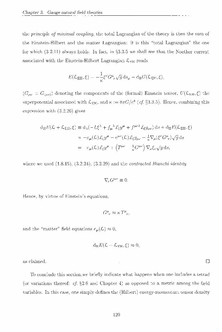
Chapter 3. Gauge-natural field theories
the principle of minimal coupling, the total Lagrangian of the theory is then the sum of
the Einstein-Hilbert and the matter Lagrangian: it is this "total Lagrangian" the one
for which (3.2.11) always holds. In fact, in §3.3.5 we shall see that the Noether current
associated with the Einstein-Hilbert Lagrangian £EH reads
( 0 V
(G^ = G^v)) denoting the components of the (formal) Einstein tensor, U(£JEH,0 the
superpotential associated with £EH> and K := SKG/C4 (cf. §3.3.5). Hence, combining this
expression with (3.2.26) gives
)y/gds
where we used (1.8.15), (3.2.24), (3.2.29) and the contracted Bianchi identity
= 0.
Hence, by virtue of Einstein's equations,
and the "matter" field equations eAi(XL) ~ 0,
as claimed. D
To conclude this section,we briefly indicate what happens when one includes a tetrad
(or variations thereof: cf. §2.6 and Chapter 4) as opposed to a metric among the field
variables. In this case, one simply defines the (Hilbert) energy-momentum tensor density
120

Chapter 3. Gauge-natural field theories
as
and the above procedure goes through unmodified. Of course, eHtJjU := gvp9ap
eHtia will
not be symmetric in general. Yet, when a tetrad appears in the Lagrangian only through
the metric, then it is known that eHIJ'v is symmetric. Indeed, on using (2.6.8) we get
oHf" = -gvpe%^- = -9up0aP^-^ = ~g^ea
pHQ0(Vab9
b^a + Vba6bJ^) = H>",
(3.2.38)
which shows that eH*11' is symmetric (and its definition consistent). A caveat, though:
despite the fact that (3.2.38) is formally correct, it is dangerous in general to try to
gain information about the conserved quantities, associated with a Lagrangian whose
primary variable is a tetrad, from the metric, even if the former enters the Lagrangian
only through the latter. This is because the definition of a Noether current involves
explicitly a Lie derivative [formula (3.2.8)], which is, crucially, a category-dependent
operator (Remark 2.1.5), and, whereas the metric is (usually regarded as) a natural
object, a tetrad is not necessarily—in particular, in the Einstein (-Cartan) -Dirac theory
the (spin-) tetrad in question cannot be considered as such (cf. Chapter 4).
3.3 Examples
We shall now give a number of examples to illustrate how Noether's theorem is applied to
some important field theories in actual fact. Except for classical mechanics, we shall al-
ways assume that the given base manifold M can be equipped with a pseudo-Riemannian
metric g (cf. §B.l). In particular, we shall assume that Proca, Yang-Mills and Maxwell
fields are dynamically coupled with g, whose dynamics is then described by the standard
Einstein-Hilbert Lagrangian, as per §3.3.5. Therefore, we should more properly speak of
"Einstein-Proca", "Einstein-Yang-Mills" and "Einstein-Maxwell" field theories.
121

Chapter 3. Gauge-natural field theories
3.3.1 Classical mechanics
In classical mechanics the configuration bundle is (diffeomorphic to) the trivial7 bundle
( R x Q , l , prx; Q), where Q is a manifold. Since any trivial bundle can be regarded as a
suitable {e}-bundle (c/.. e.g., Steenrod 1951, §4.1), and hence as a bundle associated with
a suitable principal {e}-bundle (c/., e.g., Kolaf et al. 1993, §10.8), classical mechanics is
indeed—in this minimal sense, at least—a gauge-natural field theory. Somewhat more
interestingly, if there is a group G acting on Q, as is often the case, then R x Q can
be regarded as a G-bundle, and the Lagrangian is required to be invariant with respect
to the (lifted) G-action—again, a gauge-natural setting. In any case, the Lagrangian is
assumed to be first order: explicitly,
: Jy(R x Q) R x TQ -»• T*R
: (t, {q\ u1)) H-> £ (*, (q\ -^)) =: L(t, q\ ul) dt
Given a projectable vector field S = d/dt + E.ld/dql o n R x Q , symmetry condition (3.2.3)
reads
ul
where dt = d/dt denotes the formal derivative on J'(1R x Q) = I x TQ and we used
(2.1.14). On specializing (2.1.11') to the present context, it is immediate to see that
£sql ~ ul — El, and hence (3.3.1) is equivalent to
(3.3.2)
Now, the first order jet prolongation of E is
E^J'EEI + ^ U ? ^ , (3.3.3)at oql oul
A well-known topology theorem states that every bundle over a contractible base is trivial (cf., e.g.,Steenrod 1951, Corollary 11.6).
122

Chapter 3. Gauge-natural field theories
consistently with formula (1.9.3). On comparing (3.3.3) to (3.3.2), we see that the pro-
jectable vector field E is a Lagrangian symmetry iff E(L) = 0. The conserved quantity
associated with L is given by formula (3.2.10) and turns out to be
(3.3.4)
On evaluating (3.3.4) on a critical section cr: i i— (t,al(t) := ql o a(t)), one recovers the
well-known conservation law
E(L)=0
In particular, E = d/dt is a Lagrangian symmetry iff dL/dt = 0, and the associated
conserved current is
which is nothing but the so-called "generalized energy" of the system. Indeed, if the
system is conservative, then E = T + V, where T and V are the kinetic and potential
energy, respectively.
3.3.2 Scalar fields
Let M be an m-dimensional manifold admitting pseudo-Riemannian metrics on itself. A
collection {ya}™=1 of n (R-valued) scalar fields on M can be regarded as a section of the
(natural) trivial bundle M x W1 over M. Then, Lie derivative (2.1.11') is simply
£zya =
which, substituted into (3.2.10), gives
J, E) = E(£J, £) = ^t^y/gds^, (3.3.5)
123

Chapter 3. Gauge-natural field theories
for any first order (natural) Lagrangian £ on M x En . Here,
^V, - L5^) (3.3.6)
is the (first) canonical energy-momentum tensor defined in §3.2.1. Since the second
canonical energy-momentum tensor is identically zero [compare (3.3.5) to (3.2.21)], from
(3.2.37) it follows that the canonical energy-momentum tensor coincides with the (Hil-
bert) energy-momentum tensor and, hence, is covariantly conserved because of (3.2.33),
and symmetric because of (3.2.29)—an attribute that is hardly obvious from (3.3.6).
3.3.3 Proca fields
As in the previous section, M shall denote an m-dimensional manifold admitting pseudo-
Riemannian metrics on itself. The first simple example of a theory admitting a non-
everywhere vanishing superpotential is the one describing a constrained spin 1 massive
Boson field a on A/, the so-called "Proca field". If (xA, yM, y^) denote local natural
coordinates on JlT*M, the Proca Lagrangian is the fibre-preserving morphism
\J2T*M x M JlT*M -+ f\4T*M(3.3.7)
([Xfl]a^ - \m2axax)
where Q^ := y\ o j ' a , a\^ := y\^ o jxa, m is a real constant, and, as usual, indices are
lowered and raised by means of g^ and its inverse gvp', respectively. The Proca equations
of motion are obtained by varying L with respect to a. They are
(3-3.8)
Remark 3.3.1. Note that, if we take, as we shall, V to be the covariant derivative
operator associated with the Levi-Civita connection relative to g, then partial derivatives
can be replaced by covariant derivatives both in (3.3.7) and (3.3.8)—thereby eliminating
the annoying factor of /g from both sides of the equation, namely
2
124

Chapter 3. Gauge-natural field theories
Now, the formal generalized Lie derivative of y\ is simply
Therefore, on applying formula (3.2.10), we have
+ d A ( / A ^ D , (3-3.9)
where, of course.M. (3.3.10)
Hence,
is recognized to be the superpotential associated to the Lagrangian £, provided the first
term on r.h.s. of (3.3.9) vanishes on shell (cf. Remark 3.2.17). Let us check that this is
actually the case, as we know it must from the general theory. We have
where we used (3.3.10) and set f//iA := fx^yu^y/9- Now, the term in square brackets is
clearly symmetric in \i and is, and, on taking also into account formula (3.3.20) below, it
is easy to see that it equals the energy-momentum tensor density, whilst the second term
125

Chapter 3. Gauge-natural field theories
vanishes on shell because of (3.3.8). Therefore, £/(Xp,£) is indeed the superpotential
associated with £ P (cf. Remark 3.2.17).
Remark 3.3.2. On differentiating (3.3.10) and using (3.3.8) and (3.2.24), we can easily
verify that
Vxax = 0.
On using this result and the symmetry properties of the Riemann tensor (cf. §2.6.2), we
could check that equation (3.3.8) can be recast into the form
R,^x '•— g^RaSa\ (cf- Kijowski Ik Tulczyjew 1979). In flat space (which entails R^x = 0)
this reduces to the usual Klein-Gordon (vector) equation. This is why we call the Proca
field a "constrained" field.
3.3.4 Yang-Mills and Maxwell fields
Let P(M, G) be principal bundle, g a metric tensor on M, and Q an Ad^-invariant metric
on G, i.e. such that Q(Ada^e, Ada'r]e) = Q(^e,r]e) for all a G G, E,e,r)e G TeG = g. Then,
we can define an interior product of any two (P x^d fl)-valued p-forms a and ft on i\I,
locally given by
( (a , 0)) = aAfll...IJ,pf3
Bl/1..Mp GAB gfnUl • • • gp'pVv•
Now, let P( :— Wl-lP xeA be the bundle of G-connections introduced in Example 1.10.16.
Then the first order Lagrangian
1
on \J"T*M x M JlPg, F being the curvature 2-form associated with a G-connection A on P
(cf. §2.6.2), is called the Yang-Mills Lagrangian (relative to A). Unlike the Proca
and the scalar field Lagrangian above, and the Einstein-Hilbert Lagrangian of the next
section, which are all (purely) natural Lagrangians, the Yang-Mills Lagrangian is a truly
gauge-natural one.
126

Chapter 3. Gauge-natural Geld theories
In order to find the Noether current E(HYM, ^) associated with £YM> let us first
compute its first variation OXYM [hi the sense of (3.1.10) or (3.1.15)]. We have:
6A%ACV + f^Sg^) ds%
A\A\) + 2(fAtiVcA
BCAcl/ - dvfB^)8A\ + f^Jg^} ds, (3.3.11)
where
M. _ 9LYM — J_ (1 pA rp a/3 _ pA p p\ rz _ V^T^I T a/3r^4 i/^y r jiprAv ) V a — 2 /""•
Comparing, now, (3.3.11) with (3.1.12), we realize that8
ds, (3.3.13a)
® dsv, (3.3.136)
where, in the first equation, ' V denotes the (formal) covariant derivative operator with
respect to the connection on /\2T*M®M {P xAd£l) canonically induced by the Levi-Civita
connection on M and the G-connection A on P (cf. §§1.5 and 2.6.2). The first term on the
r.h.s. of (3.3.13a) vanishes on shell by virtue of Einstein's equation (cf. Remark 3.2.17).
So does the second one because of the Yang-Mills equations of motion,
V,, V w 0.
Now, comparison between (3.1.15) and (3.2.8) [or even, in the first order case, be-
tween (3.1.12) and (3.2.10)] tells us that wre can read off the Noether current associated
8In (3.3.11) the vertical vector field T on \J2T*MxM Pe is locally represented by Sg^d^
127

Chapter 3. Gauge-natural Geld theories
with £> from its first variation (3.3.11). Explicitly,
(3.3.14)
where we used (3.3.12) and (2.6.27) to obtain the first equality, and (3.3.136) to obtain
the second one. Now, the first term on the r.h.s. of (3.3.14) vanishes on shell by virtue of
the Einstein and the Yang-Mills equations. As for the second term, first recall that for
any bivector density U of weight +1 and any symmetric connection T we have
W " = dM1" + V^U"" + VpM™ ~ VpM1"' = dJJ^. (3.3.15)
Hence, the second term on the r.h.s. of (3.3.14) can be regarded as the (formal) divergence
of U^ = -1/(4TT) ^AFA^^g, and
(3.3.16)
is recognized to be the superpotential associated with the Yang-Mills Lagrangian. At
first, the seeming indeterminacy of this superpotential might look puzzling (the E^'s are
arbitrary functions), so that some have preferred to impose by hand the horizontal lift
°f £ (c/- §1-5), i.e. set E = £, whence, of course,
and
(c/., e.g., Kijowski & Tulczyjew 1979). However, we can convince ourselves that (3.3.16)
is the "right answer" by specializing to the electromagnetic case, of which Yang-Mills
theory can be thought of as the non-commutative generalization.
Indeed, electromagnetism is just a Yang-Mills theory with structure group U(l), the
(Abelian) group of all unimodular complex numbers, i.e. U(l) = { eld : 9 € M } = S1
128

Chapter 3. Gauge-natural held theories
(c/., e.g., Atiyah 1979). Since its Lie algebra u(l) = iR (cf. §C2) is 1-dimensional, we
can omit Lie algebra indices everywhere. Furthermore, U(l) being Abelian, its unique
structure constant is zero. Then, the Lagrangian for electromagnetism, or the Maxwell
Lagrangian, is
where
F = dA
is the electromagnetic field with components [cf. (2.6.25)]
r pv = O^AV — O^Afj,,
and [cf. (1.5.2)]
is the U(l)-connection serving as the electromagnetic potential. Then, the (source-free)
Maxwell equations read
VVF^ « 0,
whereas the Noether current is
V 4TT / 47T
Therefore, the superpotential associated with Lu turns out to be
U(£J\I,E) := EF^U\fg~dsuv- (3.3.17)
Now, we know that, in general, a vertical G-invariant vector T on a principal bundle
P(M,G) transforms via the adjoint representation of G (cf. §1.3 and Example 1.10.19).
But U(l) is Abelian, and hence E is unchanged under gauge transformations, i.e. vertical
automorphisms of the structure bundle. Therefore, without loss of generality, we can
choose E = 1. In any (4-dimensional) Lorentzian manifold where it is possible to single
out a globally defined timelike vector field and, hence, in particular, in Minkowski space-
129

Chapter 3. Gauge-natural field theories
time (R4,??), we can consider the conserved quantity
associated with a (constant time) spacelike region E with boundary <9E (and a critical
section of \J2T*M xM Pe). Then, with our conventions, (El := -FOl(a))f=1 can be
identified with the components of the electric field, and from (3.3.17) we obtain9
Q(£M,E.<7) = — I E-ndS.4TT JdT,
i.e. precisely the total charge contained in E
3.3.5 General relativity
Let (A/, g) be a 4-Lorentzian manifold. In its standard Lagrangian formulation general
relativity is described by the Einstein-Hilbert Lagrangian
EH : J'2V2T*M -> A4T*A/x (3.3.18)
EH: fg >-> &m{fg) •= -7rV99^R^uds,IK
where K = 8nG/c4 and R^ = i?aMQ^, (Ra^au) being the components of the curvature
2-form (or Riemann tensor) associated with the Levi-Civita connection relative to g (cf.
§2.6.2). Of course, as we are thinking of g as a dynamical variable whose values will be
ultimately determined by the (Einstein) equations of motion, M should be more precisely
thought of as a 4-dimensional manifold satisfying all the topological requirements needed
to admit Lorentzian metrics on itself, so that (M, g) is a Lorentzian manifold for any solu-
tion g of the field equations. For the same reasons, the configuration bundle of the theory
is, strictly speaking, the (natural vector) bundle Lor (A/) of (non-degenerate) Lorentzian
metrics on M rather than simply \J2T*M. All this will be hereafter understood.
9Here, E = Eldi, n is the outward normal to <9S, and dS its surface element.
130

Chapter 3. Gauge-natural field theories
The variation of £EH is
^Sg^ + g^SR^) ds
ds - dH (^•'y/gSu^dso), (3.3.19)
where we used the relation
bjg~=—\fyg^giLlJ (3.3.20)
and set
The Einstein equations of motion are then
or, in the presence of matter fields (c/. §3.2.1),
From (3.3.19) (and taking into account the fact that the configuration bundle is a
natural vector bundle) we deduce that the Noether current associated with £EH is
0 = £J£EH V^4«V d s «
On making use, now, of (2.6.29), after a little algebra we get to the expression
£(£EH,0 = -
whence
C ^ ^ f ^ v ^ ) l (3.3.21)K \K J
131

Chapter 3. Gauge-natural field theories
is recognized to be the superpotential associated with XLEHJ and Remark 3.2.17 is now fully
justified. £ / ( X E H , 0 was originally derived in a Hamiltonian (multisymplectic) framework
by Kijowski (1978) (see also Kijowski & Tulczyjew 1979), and is a half of the well-known
Komar (1959) potential, thereby suffering from similar drawbacks (c/., e.g., Katz 1985).
Note, though, that the Einstein-Hilbert Lagrangian is degenerate. Indeed, according
to the general theory, the field equations associated with a second order Lagrangian should
be fourth order (Proposition 3.1.2), but Einstein equations are clearly second order, as
if ^EH were first order. Indeed, as Einstein himself (1916) realized, it is possible to
decompose the Einstein-Hilbert Lagrangian into a (formal) divergence and an equivalent
first order Lagrangian (cf. Theorem 3.1.3). Explicitly,
gtf^^/g) ds,
where
Now, we know that, although equivalent Lagrangians give rise, by their very definition,
to the same equations of motion, the associated conserved quantities are, in general,
different [cf. (3.2.18)], so that we could hope that using &E instead of £EH would improve
the situation. Unfortunately, since F is not a tensor, £ E is n°t covariant, and hence nor
are the ensuing conserved quantities.
Following an earlier idea of Rosen (1940). we can then introduce a background (sym-
metric linear) connection F in order to obtain a covariant splitting of £EH- Explicitly,
- dH (
where1
FF "~ 2K[
132

Chapter 3. Gauge-natural field theories
and we set
a pa _ paH per • '-per L per i
-a
a _ -au' [J,
-a Ya — (t)a P -4- f)a F' )
R denoting the curvature 2-form associated with F. Then, from (3.2.17) it follows that
the superpotential associated with £ F F is
This derivation is due to Ferraris & Francaviglia (1990), although superpotential (3.3.22)
had already been found by Katz (1985) in an ad hoc way. The good news is that this
superpotential overcomes the drawbacks of Komar's (1959) potential. In particular, with
a suitable (but generally obvious) choice of background connection, it reproduces:
• the Schwarzschild mass parameter ms for the Schwarzschild solution,
• the correct mass ms — e2/2r for the Reissner-Nordstrom solution,
• the correct angular momentum £ = niga, for the the Kerr solution,
• the ADM mass at spacelike infinity,
• the Bondi mass at null infinity.
Finally, we should mention that quite recently Noether's theorem was successfully used
to provide a general definition of entropy for stationary black holes (Fatibene et al. 1999a,
19996, 2000, and references therein), to obtain the first law of thermodynamics for rigidly
rotating horizons (Allemandi et al. 2001), and to give a general definition of energy for
the iV-body problem in (1 + l)-dimensional gravity (Mann et al. 2000).
133

Chapter 4
Gauge-natural gravitation theory
L'universo e infinito perche deve consentire as-solutamente tutto quello che e permesso, perchetutto quello che e permesso e obbligatorio.
T. REGGE, in: P. Levi & T. Regge, Dialogo
This chapter is a reformulation of results that first appeared in Godina et al. (2001) and
Matteucci (2002).
4.1 Motivation
The Einstein-Dirac theory is the (classical) field theory describing a spin 1/2 massive
Fermion field minimally coupled with Einstein's gravitational field in a curved space-
time. The Einstein-Cartan-Dirac theory is a modification of the Einstein-Dirac theory,
which allows for the presence of torsion as a possible "source" of spin (c/. §4.3 below).
In this chapter we shall show that the functorial approach of gauge-natural bundles
and the general theory of Lie derivatives developed in Chapters 2 and 3 is essential for
a correct geometrical formulation of the Einstein (-Cartan) -Dirac theory and, at the
same time, yields an unexpected indeterminacy in the concept of conserved quantities.
In the Einstein-Cartan-Dirac case, such an indeterminacy can be regarded as the well-
known indeterminacy which occurs in gauge theory (Noether 1918; Giachetta et al. 1997;
Fatibene 1999; Barnich & Brandt 2002), although there are serious conceptual risks
involved in dismissing this "metric-affine" theory of gravitation as a standard "gauge
theory" (Trautman 1980; Giachetta et al. 1997). This is certainly not the case, though,
134

Chapter 4. Gauge-natural gravitation theory
for the Einstein-Dirac theory proper, which can by no means be viewed as such. We
shall show that, in both cases, this indeterminacy actually arises from the very fact that,
when coupled with Dirac fields, Einstein's general relativity can no longer be regarded as
a purely natural theory, because, in order to incorporate spinors, one must enlarge the
class of morphisms of the theory.
Indeed, it is well-known that there are no representations of the group GL(4,R)
of the automorphisms of M4 which behave like spinors under the subgroup of Lorentz
transformations. Therefore, if one aims at considering the coupling between general
relativity and Fermion fields, one is forced to resort to the so-called "tetrad formalism"
(c/., e.g., Weinberg 1972). Yet, there seems to have been a widespread misunderstanding
of the full mathematical (and physical) significance of this. Leaving all the technicalities
to the later sections, it will suffice here to briefly recall how the concept of a tetrad is
usually introduced.
On relying on the "principle of equivalence'', which mathematically is tantamount to
the simple statement that every manifold is locally flat, at every point x of space-time
one can erect a set of coordinates (Xa) that are locally inertial at x. The components of
the metric in any general non-inertial coordinate system are then1
9^{x) = eatl{x)9b
l/(x)rjab, (4.1.1)
where ||TU|| := diag(l, - 1 , - 1 , -1) (cf. §C.l) and
a*.(4.1-2)
Thus, if we change our general non-inertial coordinates from (xM) to (rr'M), 9\ will change
according to the rulec)ru
^ - n = ^ V (4.1.3)
Therefore, (#aM) must be regarded as the components of four l-forrns (9a), not of a single
tensor field 6. This set of four 1-forms is what is known as a tetrad.
At this stage the Latin index a is just a "label" and, for any a, 6a is indeed a natural
and in the rest of this chapter both Latin and Greek indices range from 0 to 3.
135

Chapter 4. Gauge-natural gravitation theory
object. But the reason why a tetrad was introduced in the first place is precisely that
we then wanted to "switch on" that Latin index in order to incorporate spinors into our
formalism. This means that 9a^ will have to additionally change according to the rule
9<\(x) -* L\(x)9b^x), (4.1.4)
where L(x) is the (space-time-dependent) Lorentz transformation induced (modulo a
sign) by a given spinorial transformation S under the group epimorphism A: Spin(l, 3)e
->SO(l,3)e (cf. §D.l).
This is precisely the point that has been too often overlooked. Unlike (4.1.3), trans-
formation law (4.1.4) does not descend from definition (4.1.2), but is a requirement we
have imposed a posteriori. In other words, we have changed the definition of 6*"M in such
a way that now (9afJ) must be regarded as the components of a non-natural object 9.
There is another important point that has been traditionally overlooked, which is of
pre-eminent physical significance. Recall, indeed, that spinor fields can be denned on a
manifold M only if M admits a "spin structure". Now, the standard definition of a spin
structure involves fixing a metric on M (cf. §D.2), a framework which is certainly well-
suited to a situation in which the gravitational field is considered unaffected by spinors,
but is otherwise unable to describe the complete interaction and feedback between gravity
and spinor fields (van den Heuvel 1994; Slawianowski 1996). To this end, the concept of
a free spin structure must be introduced.
Ultimately, the solution to both the aforementioned problems lies in suitably denning
the bundle of which 9 is to be a section. This leads to the concept of a spin-tetrad, which
turns out to be a gauge-natural object (Fatibene et al. 1998; Godina et al. 2000, 2001;
Matteucci 2002).
4.2 Spin-tetrads, spin-connections and spinors
To the best of our knowledge, the concept of a "free spin structure" was originally intro-
duced (with a different purpose) by Plymen & West bury (1987) (see also Swift 1988). It
was then rediscovered by van den Heuvel (1994) for the very reason mentioned in §4.1
136

Chapter 4. Gauge-natural gravitation theory
and further analysed by Fatibene et al. (1998) and Fatibene & Francaviglia (1998). The
notion of a "spin-tetrad" as a section of a suitable gauge-natural bundle over M was first
proposed by Fatibene et al. (1998).
Definition 4.2.1. Let M be a 4-dimensional manifold admitting Lorentzian metrics of
signature —2, i.e. satisfying the topological requirements which ensure the existence on
it of Lorentzian structures [SO(1, 3)e-reductions], and let A be the epimorphism which
exhibits Spin(l, 3)e as the twofold covering of SO(1, 3)e. A free spin structure on M
consists of a principal bundle ix: E —> M with structure group Spin(l,3)e and a map
A: E -+ LM such that
AoRs = R'{ioA){s) o A V5 G Spin(l, 3)e,
IT O A = 7T,
R and R' denoting the canonical right actions on E and LM, respectively, 1: SO(l,3)e
—•>• GL(4,R) the canonical injection of Lie groups, and IT': LM —> M the canonical
projection (cf. Definition D.2.1). Equivalently, the diagrams
LM.-—»• LMR(i.oA)(S)
are commutative. We shall call the bundle map A a spin-frame on S.
This definition of a spin structure induces metrics on M. Indeed, given a spin-frame
A: E —> LM, we can define a metric g via the reduced subbundle SO(M,g) := A(E) of
LM. In other words, the (dynamic) metric g = gA is defined to be the metric such that
frames in A(S) C LM are g-orthonormal frames. It is important to stress that in our
picture the metric g is built up a posteriori, after a spin-frame has been determined by
the field equations in a way which is compatible with the (free) spin structure one has
used to define spinors.
Now, if we want to regard spin-frames as dynamical variables in a Lagrangian field
137

Chapter 4. Gauge-natural gravitation theory
theory, we should be able to represent them as (global) sections of a suitable configuration
bundle. This motivates the following
Definition 4.2.2. Let A be as in Definition 4.2.1 and consider the following left actionto
of the group W4' Spin(l,3)e on the manifold GL(4,
x GL(4,R) -> GL(4,
together with the associated bundle T,p := Wh0T, xp GL(4,R). Ep is a fibre bundle
associated with PFL0S, i.e. a gauge-natural bundle of order (1,0). A section of Ep will
be called a spin-tetrad (cf. §2.6 for the corresponding metric-dependent definition).
If (9ap) denote the components of a spin-tetrad 9 in some local chart, then the components
(9nv) °f the induced metric g in the associated chart read
(4.2.1)
formally identical with equation (4.1.1), but with both (4.1.3) and (4.1.4) built in.
Recall now how a G-connection was defined (Example 1.10.16) and consider the fol-
lowing
Definition 4.2.3. Let so(l,3) = spin(l,3) denote the Lie algebra of SO(l,3)e and con-
sider the following left action of the group W41'1Spin(l, 3)e on the vector space (R4)* <g>
so( l ,3)
£: W4uSpin(l ,3) ex ((R4)* <g> so(l, 3)) -> (R4)* <g> so(l, 3)
where we are using the notation of Example 1.10.16 with a := A(5(0)) and (A(S))lJfc :=
(ydk(a'lA(S(x))\x=0))). Clearly, the associated bundle S^ := Wl>lH xe ((R4)* ®5o(l, 3))
is a gauge-natural (affine) bundle of order (1, 1) isomorphic to the bundle of SO(1, 3)e-con-
nections over M (cf. Example 1.10.16). A section of S^ will be called a spin-connection.
138

Chapter 4. Gauge-natural gravitation theory
Note that also spinors can be regarded as sections of a suitable gauge-natural bundle
over M. Indeed, if 7 is the linear representation of Spin(l,3)e on the vector space C4
induced by the given choice of 7 matrices, then the associated vector bundle S^ := Sx^C4
is a gauge-natural (vector) bundle of order (0, 0) whose sections represent spinors (or,
more precisely, spin-vector fields: cf. §D.2).
Note also that, in the present picture, the spmor connection UJ corresponding to a
given spin-connection LJ may be denned in terms of to as
A' := XeA denoting the Lie algebra isomorphism between spin(l,3) and so(l,3) [cf.
(D.2.2)]. Locally, the components (u^) of a) read
ab;
(ujaCfJi =: ujah^r]hc) denoting the components of a; [cf. (D.2.3) and (D.I.2)].
4.3 Riemann-Cartan geometry on spin manifolds
Throughout the rest of this chapter we shall use Cartan's language of vector (bundle)-
valued differential forms (on M), which will prove to be an elegant and compact way to
express our findings. To this end, let Ep := S XpR4 denote the vector bundle associated
with S via the action' p: Spin(l,3)e x 1R4 -> R4
p: (Sjk,/?)»$'' :=A(S))^
Then, a spin-tetrad can be equivalently regarded as a Ep-valued 1-form on M locally
reading
(4.3.1)
(fa) denoting a local fibre basis of Up. Furthermore, by gl(Ep) we shall mean the vector
bundle over M given by the value at Ep of the canonical extension of the functor g[ to the
category of vector bundles and their homomorphisms (cf. Kolaf et al. 1993, §6.7). Finally,
139

Chapter 4. Gauge-natural gravitation theory
if {ujabfl) are the components of a spin-connection in some local chart, it is convenient to
introduce the notation (cf. §2.6.2)
Now, let ' V be the covariant derivative operator with respect to the connection
on T^M naturally induced by a (natural) linear connection F on M (cf. Example 1.10.17),
T?M denoting the (p, g)-tensor bundle over M (cf. Example 1.10.15). Classically, Rie-
mann-Cartan geometry is characterized by two conditions: the covariant constancy of
the metric,
Vg = 0, (4.3.2)
just as in ordinary Riemannian geometry, and the presence of a (not necessarily zero)
torsion tensor r (cf. §1.5.1).
In the present gauge-natural setting we can introduce analogous concepts serving a
similar purpose. In particular, if 9 is a spin-tetrad in the sense of Definition 4.2.2 and g
is the metric induced by 9 via (4.2.1), equation (4.3.2) can be derived by the condition
V0 = O, (4.3.3)
where, here, ' V denotes the covariant derivative operator with respect to the connection
on S p canonically induced by the connections F and u on LM and £, respectively (cf.
§2.6). Accordingly, we can define a torsion 2-form as the Ep-valued 2-form, which we
shall denote again by r, given by the expression
r :=
or, equivalently,
r : = r " ® / a , ra := <D9a = d9" + uab A 9\ (4.3.4)
'CD' denoting the covariant exterior derivative operator (cf. §1.5) and 9 being as in (4.3.1).
Moreover, we can define a contortion 1-form as the gl(Ep)-valued 1-form measuring
the deviation of the spin-connection u from the Riemannian (or "Levi-Civita") spin-
140

Chapter 4. Gauge-natural gravitation theory
connection u> [cf. (4.3.6) below]:
K :=
(Fab) denoting a local fibre basis of gl(Sp). The components of the associated tensor field
then read
Rabc = _}_(Tabc + r6ca _ ^ ^ (435)
(rade =: Tabcrji,ci7}ce) denoting the components of the tensor associated to the torsion 2-
form. Finally, note that a curvature 2-form associated with ui may be defined as the
gl(Ep)-valued 2-forni
ac A
(cf. §2.6.2), and that the components of the Riemannian spin-connection 6UJ read (cf.,
e.g., Choquet-Bruhat 1987)
(4.3.6)
Latin and Greek indices being lowered or raised by r\ and g, respectively, or their inverses.
In the sequel, we shall need the (gauge-natural) Lie derivatives, with respect to a
Spin(l, 3)e-invariant vector field H on E, of a spin-tetrad, a spin-connection, a spinor and
its Dirac adjoint. Locally, they read
£~0\ = %C0a, - ^ Q 6 ^ , (4.3.7a)
£^ab = ZjWb + <D^a
b, (4.3.76)
£z4> = Cd.iJ + \Sablabrb = T V . 0 + \^abiabip, (4.3.7c)
£=.!> = J&P = r v , - 0 - \^abhab, (4.3.7rf)
respectively, (£M, H"c =: fEabrjhc) denoting the components of the SO(1, 3)e-invariant vector
field on E/Z2 induced by E [cf. (2.6.13'), (2.6.28) and (2.5.1)].
We are now in a position to apply the theory of conserved quantities developed in
141

Chapter 4. Gauge-natural gravitation theory
Chapter 3 to the Einstein (-Cartan) -Dirac theory. We shall do so separately for the
Einstein-Cartan-Dirac case and the Einstein-Dirac one. Calculations will be "formal",
unless otherwise stated, i.e. they will involve local coordinates, rather than sections, of
the bundles under consideration. For the sake of simplicity, we shall nevertheless use the
names of the corresponding sections. With a slight abuse of notation, we shall also use
the symbols ' V and 'D' for their formal counterparts, defined in the usual manner (c/.,
e.g., Definition 2.1.6).
4.4 Einstein-Cartan-Dirac theory
Our main reference for the Einstein-Cartan-Dirac theory is Choquet-Bruhat (1987).
In the light of the new geometric framework developed in §4.2, the Einstein- Cartan
Lagrangian can be defined as the base-preserving morphism
where K := 8TTG/C4, £a(, := e J (ea J E) and S is the standard volume form on M locally
given by detj|(9|| dx° A • • • A dxs. Here ||#|| stands for the matrix of the components of 6
and we have set ea : = e</<9M, ||eaM|| denoting the inverse of ||#||. The Dirac Lagrangian
reads instead
Sp x M S, xM J% - . A4T*M
where a := he. According to the principle of minimal coupling, the total Lagrangian of
the theory will be simply assumed to be L := £ E C + &D- A vertical vector field on the
configuration bundle will then read
r -
where (0a/l), (cu^jW^^) and (</>'4, /ipA
H,) denote fibre coordinates on Sp, J [E^ and
142

Chapter 4. Gauge-natural gravitation theory
respectively. If we set locally
56a : = 56\ dx", 5u% : = SLU V dx»,
5'ip := 5ipA / A , 5ip := Stjj,
(/A) denoting a local fibre basis of £.,,, then the first variation formula for £ is
abOLJ = I — - G ;, + I fc I z^a A ott + I ^ - JJz.afe — <bai L c A oc
+ dH [ - ^ S o 6 A 5a,'afc - if (5inaip - y
where G denotes the Einstein tensor associated with Q, (cf. §3.3.5), S a := ea J E and we
set
( D ) ^ ) ( a ^ ' 7a + mi/)
e(£D) := 7{L^) = e'(£D) + ^ V /
identity (D.1.3) having been used in the last but one equality. Thus, the Einstein-Cartan-
Dirac equations are
(-'ab ~ K-L ab:
0.
The first two equations are called the first and the second Einstein-Cartan (-Dirac)
equation, respectively, whereas the last one is known as the (Cartan-) Dirac equation.
T is the energy-momentum, tensor of the theory (as usual: cf. §3.2.1), and S the spin
momentum tensor. Now, making use of (4.3.4), the second Einstein-Cartan equation can
143

Chapter 4. Gauge-natural gravitation theory
be put into the form
TC A S ~ 2KS (,CS
or equivalently
ra6c « 2ft-5afcc, (4.4.2)
which in turn implies that the torsion tensor is completely antisymmetric on shell. There-
fore, so is the contortion tensor. Indeed, from (4.3.5) and (4.4.2)
j^abc ^ T<ibc ^ _Kgabc
Hence, the Dirac equation reduces to e'(£o) ~ 0. which implies Tab « Qab. To sum up.
the above system of equations is completely equivalent to the following
rabc « 2«Sa6c,
i7aVa?/> — mip ~ 0.
Now, we know that we can read off the Noether current associated with £ from its
first variation (4.4.1) (c/., e.g., §3.3.4). Explicitly,
1 L ia/ y I / ^ . (J t I /sj / j ^A / \ d£s"C& ( Ju'ZZ'UJ / Kp '11/ / <i^~^'\y j / if, .
After some manipulation, which makes use (inter alia) of (4.3.76)-(4.3.7d) and the fact
that GabEa = - 1 / 2 iTc A (eb j Sac), £•(£, E) can be recast as
^ , E ) = ^ (--Gab + nJEa + - ( -DEa 6-5a 6
cS cj+dH(--^Ea 6j ,
so that the superpotential associated with L turns out to be
U{L, E) = [7(£EC, E) := - ~ S a 6 E a 6 , (4.4.3)IK
a result which appeared in Godina et al. (2001) for the first time. Therefore, the Dirac
144

Chapter 4. Gauge-natural gravitation theory
Lagrangian does not seem to contribute to the total superpotential. From this fact one
might mistakenly conclude that the Dirac fields do not contribute to the total conserved
quantities. This conclusion would be wrong because, although the Dirac Lagrangian
does not contribute directly to the superpotential, in order to obtain the corresponding
conserved quantities, one needs to integrate the superpotential on a solution, which in
turn depends on the Dirac Lagrangian via its energy-momentum tensor and the second
Einstein-Cartan equation.
Note that in the case of the Kosmann lift we have2 (cf. §2.6.1)
2a6 = (£K)<I6 = — V[a£&], (4.4.4)
which, substituted into (4.4.3), gives
U(iZEC^K) = ~Va^ab, (4.4.5)
i.e. (half of) the well-known Komar (1959) potential, in accordance with the result found
by Ferraris et al. (1994) in a purely natural context (cf. §3.3.5). This is also the lift
implicitly used by Godina et al. (2000) in the 2-spinor formalism.
Let now (craAA') denote the Infeld-van der Waerden symbols, which express the iso-
morphism between Re[S(M) ® S(M)] and TM in the orthonormal basis induced by the
spin-frame chosen (cf. §D.3), and consider the following lift3:
e = ea»aaAA/\
A\A\ Eab = (CwU := -4a[aAA> ab]
BB> Re(\B,VBA,\A), (4.4.6)
which will be referred to as the Witten lift. Then
£/(£EC,£W) = ReW = - -Re(iA4 /DA4 /\9AA'), (4.4.7)
which is the (real) Nester-Witten 2-form (Nester 1981; Penrose & Rindler 1986). Indeed,
2Here, the symbol Va stands for the operator eaaX7a.
3Here, the symbol VAA' stands for cra/iA'eaCrV<7.
145

Chapter 4. Gauge-natural gravitation theory
we have :
+ cc
+ cc
AVb\A6a A6b + cc
= 2i\A,'D\A A 0AA> + CC, (4.4.8)
where we used the identities (cf. Penrose & Rindler 1984)
*/1 Ra6 A *Dab ** Aab ,\ab * AABA'B' ; A ABB'A'Aab-D — Aab D , A = —A , A = \A
for any two bivectors Aab and i?afe. Inserting (4.4.8) into (4.4.3) gives (4.4.7), as claimed.
If we wish, it is also possible to define a complexified Witten lift as
e = ea»aaAA,\A\A', Eab = (&) a 6 := -Aa[a
AA'ab]BB'\B<VBA,\A. (4.4.9)
Then, the relevant superpotential is
L'( EC,ew) = W := ~-\A,?)\AA6AA\ (4.4.10)K
which is the (complex) Nester-Witten 2-form (Penrose & Rindler 1986; Mason & Frau-
endiener 1990). From the viewpoint of physical applications (proof of positivity of the
Bondi or ADM mass, quasi-local definitions of momentum and angular momentum in
general relativity, etc.), it is immaterial whether one uses (4.4.10) or its real part (4.4.7),
as its imaginary part turns out to be —1/ndY{(\A\A>0a), which vanishes upon integration
over a closed 2-surface.
Note, though, that (4.4.10) appears to relate more directly to Penrose quasi-local 4-mo-
mentum, when suitable identifications are made (cf. Penrose & Rindler 1986, p. 432).
4With the exception of formula (4.4.9) below, we shall suppress hereafter the Infeld-van der Waerdensymbols and adopt the standard identification a = A A1, b = BB', etc., as is customary in the currentliterature (cf. §D.3).
146

Chapter 4. Gauge-natural gravitation theory
Remark 4.4.1. Note also that—modulo an inessential numerical factor—the Kosmann
lift is (the real part of) the dual of the (complexified) Witten lift, in the sense that
as can be easily checked on starting from equations (4.4.4) and (4.4.9)(2). whenever, of
course, £ = A A .
4.4.1 Natural approach
Suppose for a moment that we deliberately neglect the gauge-natural nature of the
Einstein-Cartan-Dirac theory. This means that we shall temporarily regard the Einstein-
Cartan Lagrangian as a purely natural Lagrangian, i.e. a first order Lagrangian on a
(purely) natural bundle. In particular, the spin-connection u> will be replaced by a nat-
ural linear connection F (cf. Example 1.10.17). As such, F is a natural object, whose
components ( F ^ ) are related, because of the compatibility condition V# = 0, to the
components (u;a&M) of u via the familiar formula
^ bp. = v p(alj,ebH + 1 e f e j , (4.4.11)
wThere antisymmetrization in {a, 6} is understood on the r.h.s. of (4.4.11) (cf. §2.6).
Note that we cannot regard the Dirac Lagrangian itself as a natural Lagrangian because
spinors cannot be suitably replaced by any (physically equivalent) natural objects: this is
precisely why we chose a gauge-natural formulation in the first place, and why we expect
to encounter some sort of restrictions now.
The local expression for the Lie derivative of F is given by formula (2.6.29), i.e.
P "PP DP C& I V7 V7 CP (A A 1 O\
L(Y yUil = ixva^t, + VnVvq • (4.4.12)
Thus, the Noether current is now of the form
147

Chapter 4. Gauge-natural gravitation theory
where we setb )da
peb" dx'1.
The important point to note here is that, although (FpUfJ.) may be regarded as the compo-
nents of UJ in the holonomic basis, (££Ypu^l) are not, in general, the components of £-=u in
that basis. Accordingly, the second term on the right-hancl side of identity (4.4.13) can-
not be claimed to be the most general expression for ( / ( £ E C ) , £=.<JJ)I but naturality must
indeed be assumed. In fact, if we now proceeded in the same way as before, we would then
find that consistency with the second Einstein-Cartan equation requires 'Eab = — Vta£6',
i.e. precisely the Kosmann lift, and thus we would recover the purely natural result.
4.5 Einstein-Dirac theory
Our main reference for the Einstein-Dirac theory is Lichnerowicz (1964). The procedure
for obtaining the conserved quantities is completely analogous to the Einstein-Cartan-
Dirac case: therefore, we shall limit ourselves to present the results and briefly comment
on them, pointing out the possible differences. In the sequel, the symbol '|A=O' affixed to
a quantity shall mean that the latter is formally identical with the quantity denoted by
the same letter in §4.4, but with all (explicit or implicit) occurrences of a; replaced by %.
Then, the Einstein-Hilbert Lagrangian is nothing but
(4.5.1)) : = &EC\K=O
whereas the Dirac Lagrangian is regarded here as the base-preserving morphism
Remark 4.5.1. On using (4.2.1) and exploiting the relationship between Q and R (cf.
§2.6.2), it is easy to see that £EH coincides, as an object, with the Einstein-Hilbert
Lagrangian introduced in §3.3.5, but here £-EH is regarded as a gauge-natural, not simply
natural, Lagrangian.
148

Chapter 4. Gauge-natural gravitation theory
According to the principle of minimal coupling, the total Lagrangian of the Einstein-
Dirac theory will simply be £ := £EH + £ D , its variation reading
-KeGa
b + 6Tab) Ea A S9b
+ dH [~^£«b A59uab bcZah A 56r - f
where
b\
(4.5.2)
(4.5.3)
\ := f
Thus, the Einstein-Dirac equations are
f
0.
Note that, although the invariance of the Dirac Lagrangian with respect to Lorentz
transformations requires Tab to be symmetric on shell (Weinberg 1972; Choquet-Bruhat
1987), the manipulation required for going from (4.5.2) to (4.5.3) is highly non-trivial:
the interested reader is referred to Lichnerowicz (1964) for an elegant proof.
Following the same procedure as before, we find that the Noether current associated
with is
E) = - e J - ^Lab A £J \SabJlah A £30C - ff (i
149

Chapter 4. Gauge-natural gravitation theory
so that the superpotential associated with £ is recognized to be
(®r ^ \ 'ZTQ.fcv i cc nab sp i » r \ \{LJ,Z.) .— — — n L,ab + ~q J c^ab, (4.5.4J
and we note that, unlike in the Einstein-Cartan-Dirac case, the Dirac Lagrangian enters
the superpotential directly, but recall that we have no second Einstein-Cartan equation
here. Note also that the "vertical contribution" (i.e. all terms in Ea6) coming from the
Dirac Lagrangian consistently vanishes off shell. For the same reason, no inconsistency
of the type of §4.4.1 can arise here. This fact, though, by no means disproves the gauge-
riaturality of the theory, which is well-motivated on both physical and mathematical
grounds.
4.5.1 First order Einstein-Hilbert gravity
Remarkably, Lagrangian (4.5.1) can be split into a horizontal differential plus a first
order covariant Lagrangian locally reading
£ F F := - ^ ( f U - Qac A Qcb) A Ea6
where Qab := dn^afc + ^ac A (i'% and Qab := u?a6 — a;afc, a; being a background (non-
dynamical) spin-connection. It is easy to see that £ F F is but the gauge-natural counter-
part of Ferraris & Francaviglia's (1990) Lagrangian introduced in §3.3.5: in particular,
Q% = 9aaeb
tiqaIJ,l,dxL'. Then, from (3.2.17) it follows that the superpotential associated
with -CFF is
[7(£FF, E) := C/(£EHj E) + ~ £ J (Qafe A Sa6), (4.5.5)
where, of course, C/(£EH,E) := - 1 / ( 2 K ) Ea6Ea6 = C/(£Ec,H).
4.6 The indeterminacy
Both (4.4.3) and (4.5.4) reveal that, in this gauge-natural formulation of gravity coupled
with Dirac fields, the superpotential is essentially indeterminate because no condition can
150

Chapter 4. Gauge-natural gravitation theory
be imposed a priori on the vertical part of n. Therefore, we can state our main result as
follows.
Theorem 4.6.1. Any conserved charge associated with the gravitational field is intrinsi-
cally indeterminate.
Note that, because of (3.2.17), this indeterminacy does not depend on the particular
Lagrangians chosen [cf., e.g., (4.5.5)]: for this reason and the functorial nature of this
indeterminacy we have called it "intrinsic". This important result can be regarded either
as a limit for the theory or as an additional flexibility. In any case, it cannot be overlooked.
If we look back at the examples of §3.3, we realize that, in the case of (scalar and)
Yang-Mills fields, the contribution to the conserved quantities associated with a vector
field £ on M comes from its horizontal lift (with respect to the G-connection A), whereas
the vertical contribution seems to be related to the "gauge charges", such as the electric
charge in the case of electromagnetism (cf. §3.3.4). For the Proca fields and standard gen-
eral relativity, the horizontal lift (possibly with respect to the Levi-Civita connection F) is
no longer enough if we wish to include the contribution coming from the superpotentials,
and we are thus led to consider the natural lift of £. Finally, here, as we already noted in
§4.4, in order to recover the purely natural results, we should impose the Kosmann lift,
which is canonical, but not natural, i.e. it is only one of the possible lifts of £ onto £,
and is not functorially induced by £. Remarkably, when £ is null, another possibility is
given by the (complexified) Witten lift, which is also related to quasi-local definitions
of momentum and angular momentum in general relativity (Ludvigsen & Vickers 1983;
Dougan & Mason 1991).
From a physical point of view, it might be disturbing to think, that, when the spino-
rial contribution is removed, the (gravitational part of the) theory should automati-
cally revert to its purely natural counterpart, thereby reproducing the well-known (non-
indeterminate) results of §3.3.5. This could mean either that some (possibly physical)
justification has to be found to impose the Kosmann lift by hand5 or, conversely, as we
believe, that a gauge-natural formulation is the appropriate one for gravity for the very
5In this connection, it is interesting to note that, in the triad-affine formulation of the (2 + ^-dimen-sional BTZ black hole solution, the Kosmann lift is precisely what is needed to recover the "one-quarter-area law" for the entropy of the black hole (Fatibene et al. 19996).
151

Chapter 4. Gauge-natural gravitation theory
reason that it is the most general one6, irrespectively of the nature of the theory it is
possibly coupled with.
4.7 Comparison with Giachetta et a/.'s (1997) ap-
proach
We conclude by briefly commenting on a different approach to the same problem ad-
dressed in this chapter, developed by Sardanashvily and collaborators (cf. Giachetta et al.
1997 and references therein). We must say first of all that they consider the "metric-
affine" case only, so that, strictly speaking, a comparison between the two approaches
is possible only for the Einstein-Cartan-Dirac theory (although it would be relatively
straightforward to extend the discussion to incorporate Einstein-Dirac gravity as well).
Indeed, even though they do not explicitly work in a gauge-natural setting, they seem
to be well aware of the problems of the traditional approach mentioned in §4.1. The
solution they propose is to rely on spontaneous symmetry breaking. Although this is
admittedly a quantum phenomenon, the description of Einstein-Cartan gravity in terms
of Higgs fields has some justification (cf., e.g., Trautman 1980).
From our point of view and very roughly speaking, what this does is to split the
gauge-naturality of the theory into its purely gauge and purely natural part, so that
the gravitational contribution is still represented by a linear connection and gives rise
to the usual Komar potential, whereas the indeterminate vertical contribution appears
now as a further additive term, it being "decoupled". The authors, though, reject this
indeterminacy and impose the Kosmann lift by hand. The final net result is
It is obvious then that, in this case, their approach is, in effect, completely equivalent
to the one presented here. But, if really the Kosmann lift has to be imposed by hand,
then we dare favour our formulation because it is conceptually simpler and does not
invoke quantum phenomena.
6Note that, even if we were to couple Einstein (-Cartan) gravity with "C/4-spinors" (Buchdahl 1989,1992; Godlewski 2002), so(i,3) is in some sense "maximal" since, ultimately, the superpotential of thetheory must be a 2-form.
152

Chapter 5
Multisymplectic derivation of
bi-instantaneous dynamics
Meantime mathematicians will judge, whether in sacrificing a part ofthe simplicity of that geometrical conception on which the theoriesof LAGRANGE and POISSON are founded, a simplicity of anotherkind has not been introduced, which was wanting in those admirabletheories.
W. R. HAMILTON, Second essay on a general method in dynamics
The purpose of this chapter is to give a geometrical derivation of bi-instantaneous dynam-
ics in the sense of Hayward (1993). This will be done by appealing to the multisymplectic
(Hamiltonian) formalism.
5.1 Motivation
The standard 3+1 Hamiltonian analysis of the gravitational field, or "ADM formalism",
due to Arnowitt et al. (1959, i960, 1962) formulates gravitational dynamics in terms
of the evolution of spacelike hypersurfaces. In many cases, however, particularly in
problems where gravitational radiation is important, it is desirable to consider a foliation
by characteristic or null hypersurfaces. The geometry of a space-time foliated by null
hypersurfaces is rather awkward to describe owing to the absence of a natural rigging
vector and the degeneracy of the metric on a null surface. However, if one further
decomposes the null surfaces into families of spacelike 2-surfaces, one obtains a special
case of the 2+2 formalism in which no such degeneracies occur. The 2+2 formalism
153

Chapter 5. Multisymplectic derivation of bi-instantaneous dynamics
decomposes space-time into two families of spacelike 2-surfaces. We can view this as a
constructive procedure in which an initial 2-dimensional submanifold is chosen in a bare
manifold together with two vector fields which transvect the submanifold everywhere.
The two vector fields can then be used to drag the initial 2-surface out into two foliations
of 3-surfaces. The character of these 3-surfaces will depend in turn on the character
of the two vector fields. Since, once a metric is introduced, the two vector fields may
each separately be null, timelike or spacelike, then this gives rise to six different types of
decomposition. The two most important cases are double-null foliations and null-timelike
foliations. An elegant way of describing this decomposition is to introduce a manifestly
covariant formalism in which one uses projection operators and Lie derivatives in the
normal directions. This approach gives rise to the covariant 2+2 formalism of d'Inverno
and collaborators (d'Inverno & Stachel 1978: d'Inverno & Smallwood 1980; Smallwood
1983)-
Since in general relativity space-time is represented by a (Lorentzian) 4-dimensional
manifold, it follows that, geometrically, the 2+2 approach lies exactly in between the
standard 3+1 and the multisymplectic formalism presented in the following section.
5.2 Multisymplectic formulation of a field theory
We shall now recall the basic ingredients of the multisymplectic (Hamiltonian) formalism.
This section closely follows Gotay et al. (1998), §§2B and 3A-B, to which the reader is
referred for more detail and an extensive bibliography.
First of all, we need to introduce the field-theoretic analogue of the cotangent bundle.
Let then B denote the configuration bundle of a, first order1 field theory. As in Chapter 3,
we could develop our formalism for a generic fibre bundle B over an m-dimensional
manifold M, but hereafter we shall restrict attention to the case in which B is a gauge-
natural bundle PA associated with some principal bundle P(M.G). We define the dual
jet bundle JlP\ to be the vector bundle over P\ whose fibre at y G (P\)x is the set of
lrThe formalism presented in this section can be generalized to the higher order case, but we shall notneed to do so here. The interested reader is referred to Ferraris & Francaviglia (19836), Gotay (1991a)and references therein.
154

Chapter 5. Multisymplectic derivation of bi-instantaneous dynamics
affine maps from JyP\ to l\mT*M. A section of JXP\ is therefore an affine bundle map
of JlP\ to /\mT*M covering the projection n: P\ —> M. Fibre coordinates on JlP\ are
(p,Pa^), which correspond to the affine map given in coordinates by
? / W ( P + P a V J d s . (5.2.1)
Analogous to the canonical 1- and 2-forms on a cotangent bundle, there are canonical
forms on JlP{- To define these, another description of JlP\ will be convenient. Namely,
let A A := /\mT*P\ denote the bundle of m-forms on P\, with fibre over y G PA denoted
by (AA)j, and with projection TTA: A A —> P\. Let Z\ be the subbundle of AA whose fibre
is given by
(ZA), := { z G (AA), | f ' j f J ^ = 0 Vt>, t/ G V;PA }• (5.2.2)
Elements of Z\ can be be written uniquely as
z^pds+p^dy" Ads^. (5.2.3)
Hence, fibre coordinates for Zx are also (p ,p / ) and we note that Zx = T*PAA(Am~1r*M).
Z\, which is clearly a gauge-natural bundle over M, is called the (homogeneous) Le-
gendre bundle (c/., e.g., Giachetta et al. 1997).
Equating the coordinates (xx,ya,p,pbfJ') of Z\ and of JlP£ defines a vector bundle
isomorphism
$: Zx -»• J ^ ; . (5.2.4)
Intrinsically, $ is defined by
$(z )oy :=y*~GA m T;M, (5.2.5)
where 2 G {Z\)y, y E JlyP\ and .x = 7r(y). To see this, note that, if y has fibre coordinates
(y^), then
* and y* dya = y% dx" (5.2.6)
155

Chapter 5. Multisymplectic derivation of bi-instantaneous dynamics
and so
* + PSdyaAdSli) = (p + PoV/*)ds, (5.2.7)
where we used (1.1.2a).
We shall now construct canonical forms on Z\ and then use the isomorphism between
JlP\ and Z\ to transfer these to JlP\- We first define the canonical m-form 0A on A A
by
v J • • • J v J 0 \ (z) = TTTA O v J • • • J Tn\ O v J z1 m ' l (5.2.8)
where z G A^ and v,..., v G T.A\. Define the canonical (m + l)-form Q& on A\ by1 m
QA := -dGA . (5.2.9)
Note that, if m = 1, then AA = T*P\ and 0,\ is the standard canonical 1-form. If
i: Z\ —> AA denotes the inclusion, the canonical m-form 0 on Z\ is defined by
G : = i * 6 A (5.2.10)
and the canonical (m + 1)-form 0 on Z\ is defined by
Q := - d 0 = t*QA. (5.2.11)
The pair (Z\, Q) is called multiphase space or covariant phase space. It is an exam-
ple of a multisymplectic manifold, i.e. a manifold equipped with a closed non-degenerate
(m + l)-form.
From (5.2.3), (5.2.8), (5.2.9), (5.2.10) and (5.2.11), one finds that the coordinate
expression for 0 is
e = pa»dya Ads^+pds, (5.2.12)
and so
Q = dya A dpa^ A dsM - dp A ds. (5.2.13)
Now, we shall construct the covariant Legendre transform for a first order La-
156

Chapter 5. Multisymplectic derivation of bi-instantaneous dynamics
grangian £ : JlP\ —> [\mT*M. This is a fibre-preserving morphism
FC: JlPx
over Px, which has the coordinate expressions
(5.2.14)
for the multimomenta (pa^) and the covariant Hamiltonian H := —p, the /aM's
being defined by (3.1.14). An intrinsic definition follows.
If y e JyP\, then ¥L(-j) is to be an affine map from J*PX to /\mT*M where y G (P\)x.
Define ¥L(y) to be the first order vertical Taylor approximation to £, i.e.:
o y' :=dt
Sl(y - y (5.2.15)t=o
where y' £ J]P\- To derive the coordinate expressions (5.2.14), suppose that, locally,
y = {xx,ya,ya^ and y' = (xA, ya, y'a^). Then the right-hand side of (5.2.15) reads
which is an affine function of y'a^ with linear and constant pieces given by the first
and second equation of (5.2.14), respectively. Hence (5.2.14) is indeed the coordinate
description of EC. Then, the so-called (Poincare-) Cartan form is the m-form 0£
on JlP\ intrinsically defined as
*e, (5.2.16)
where 0 is the canonical m-form on Z\. Indeed, (5.2.12) and (5.2.14) yield
Qc = /aM dya A dsM + (L - fSy'J ds
where the second equality follows from (1.8.21). If f& denotes the contact 1-form uniquely
associated with the Poincare-Cartan morphism /(C), i.e. locally f^ = fa'J"da A dsM =
157

Chapter 5. Multisymplectic derivation of bi-instantaneous dynamics
fa1 dyya A dsM, then of course
Qz = -C + /c ,
a formula which also holds in the £>th order case, although, in general, 0£ will be global
but not unique (cf. §3.1.2). It is now easy to see that the Noether current E(£J, E) defined
in §3.2 can be written as
[cf. (3.2.10) and (2.1.12)]: again, this formula can be generalized to the k-th order case
by replacing JXE with J2k^l'E. It is not surprising, then, that the so-called (special)
covariant momentum map J: Z\ —> X*G(P) ® /\m~1T*Z\, defined by
for all G-invariant vector field S G SCG(P) on P, encodes all the essential information
about the conserved quantities associated with the given (first order) field theory. (Here,
E^ denotes gauge-natural lift of H onto Z\.)
Remark 5.2.1. Our definition of a covariant momentum map differs slightly from the
original one due to Gotay et al. (1998), but is more suitable for our gauge-natural setting.
Indeed, in such a setting one has automatically defined a Lie group G and vector fields
on (P\ and) Z\ functorially induced by G-invariant vector fields on P.
Finally, in analogy with classical mechanics, we expect the dynamics of the theory to
be encoded in the canonical (m + l)-form Q. Indeed, if we define
Qc := (F£)*fi = -de*, ,
then we have the following result.
Theorem 5.2.2. Let a be a critical section of P\. Then,
(A)*(~J^) = 0 (5.2.17)
for any vector field H on JlP\.
158

Chapter 5. Multisymplectic derivation of bi-instantaneous dynamics
Proof. To prove the theorem, first observe that any tangent vector on JlP\ can be decom-
posed into a component tangent to the image of j V and a vertical vector on JlP\ —> M.
Similarly, any vertical vector on JlP\ —> M can be decomposed into a jet extension of
some vertical vector on P\ and a vertical vector JlP\ —> P\. Assume then that EE is
tangent to the graph of j V in JlP\\ that is, E = Tjlcr o £ for some vector field £ on M.
Then,
(j V)*(s J n£) = (A)* ( ( T A O 0 J
which vanishes since (jlo~)*£}ji is an (m + l)-form on the m-dimensional manifold M.
Assume now that E is a vertical vector field on JlP\ —> -PA- Then, locally,
A calculation using the coordinate expression of Q,c, i.e.
Qr = dtf A d / / A (dsM - / a V , J A ds, (5.2.18)
shows that
which clearly vanishes when pulled back by the jet of a section of P\ because of (1.7.1)
and (1.1.2a). Finally, one readily computes in coordinates that, along j1o~,
(5.2.19)
for all vertical vector fields T on P\. Thus, (5.2.17) implies (3.1.16). On the other hand,
(5.2.19) combined with the above remarks on decompositions of vector fields shows that
(3.1.16) implies (5.2.17). •
159

Chapter 5. Multisymplectic derivation of bi-instantaneous dynamics
5.3 Transition from the multisymplectic to the in-
stantaneous formalism
In this section we shall summarize the procedure devised by Gotay (19916) for the tran-
sition from the multisymplectic to the instantaneous (i.e. ADM) Hamiltonian formalism
(see also Giachetta et al. 1997; Gotay et al. 1999).
Let PA be a gauge-natural bundle over an m-dimensional manifold M and let E c M
be a compact (rn — l)-dimensional Cauchy (i.e. non-characteristic) hypersurface without
boundary for a (first order) gauge-natural field theory on PA. Let O AIE be the space of all
(smooth) sections of PA restricted to E. Note that, when completed in the appropriate
Sobolev topology, the space CPAJE becomes a smooth infinite-dimensional manifold. Also,
in the sequel we shall always assume to have chosen coordinates (x^)™!^ = {^°,^l)i^[1
on M adapted to S, in the sense that E is locally given by x° = 0.
The tangent space Ta'P\\z at a section a: S —>• PA|S is defined as the set of sections T
of the vertical bundle VTAIS —> E which cover a, i.e. such that uPx o T = a (cf. §1.2).
Similarly, the cotangent space T^CPAIS consists of the section of the bundle V*S ®pA|E
Am~1T*E —> E which cover a. The natural pairing of an element a E T*7\\^ with an
element v 6 Ta7\\j: is then given by integration:
(a,v) := / (a{x),v{x)), x S.
Now, let Z\\-£. denote the restriction of the Legendre bundle Z\ to S. Of course, the space
2,A|S of its sections is endowed with the induced fibration %A|E ~> AIE- Let a G Z\\-£
and u, v G TaZ\ v. We can then define the canonical 1- and 2-form on Z\\% by
/
andr
V J U A QJ: = / O- ( V J U J Q ) = —./E
respectively, 0 and 0 being the canonical forms on Z\ defined in the previous section.
In general, though, Q^, fails to be symplectic because of a non-trivial kernel. Indeed,
160

Chapter 5. Multisymplectic derivation of bi-instantaneous dynamics
ker Os = span{9/9p, d/dpa1} by inspection. For this reason, fiv is called presymplectic.
To overcome this difficulty, we define a vector bundle morphism R%: &\|v —> T*TA|E by
(Rx(*),v) := J^TTZ o a)*(v J a), (5.3.1)
7T2 : ZA -^ -PA being the canonical projection and v an element of T ^ O O ^ A I E - In adapted
coordinates, a G Z\ ^ takes the form
a = pa^dya Ads^+pds, (5.3.2)
and so we may locally write
= Pa ds0
v is obviously a surjective submersion with
ker i?v = { a G 2.A|S : cr = pal dya ® dsi + pds, i = 1 , . . . , m — 1 }.
Proposition 5.3.1 (Gotay 19916). 77ie quotient map Z\\^/kevRy, =
—> T*T A |E induced by Rr is a symplectic diffeomorphism, ie. Z is canonically
isomorphic to T*TA|S, and the inherited symplectic form, on the former is isomorphic to
the canonical one on the latter.
Explicitly,
fiv = R*LUEj
where OY, and LO^ are the canonical 1- and 2-form on T*TA|S, respectively, defined in the
usual manner, i.e.
(-0,7r) denot ing a point in T*CPA|E, V an element of T(^j7r)T*CPA|s, a n d TT<J>A : T*CPA|E
161

Chapter 5. Multisymplectic derivation of bi-instantaneous dynamics
being the cotangent bundle projection. Locally,
u?.{4>, vr) = /sd-0a A d7ra <g> ds0.
Now, to discuss dynamics, namely how fields evolve in time, we need to introduce the
concept of a "slicing", which is a way to define a global notion of "time". It is important
to note that in this concept are encoded both the idea of a foliation of M by means of a
one-parameter family of lower dimensional hypersurfaces and that of a fibration through
a parameter time t.
Definition 5.3.2. A slicing of an m-dimensional manifold M consists of a "reference"
(m — l)-dimensional Cauchy hypersurface S and a diffeomorphism SM : S x ]R —> M.
For t G R, we shall write Et for s,u(£ x {£}). Also, we shall usually denote by £ the
generator of SM, i-e. £ := (sJv/)*(9/9t), which is then said to be an infinitesimal slicing
of M.
Given a bundle B over M and a slicing SM of M, a compatible slicing of i? is a
bundle £?£ over £ and a bundle isomorphism SB '• BY. x 1R —* 5 such that the diagram
commutes, the vertical arrows denoting the appropriate bundle projections. We shall
write Bt for SB(BT. X {t}). Also, the generator E of s^ is given by E := (sB)*(d/dt),
which is then a compatible infinitesimal slicing ot B. It is easy two see that E!
is compatible with £ iff it projects onto £. Since we shall deal only with gauge-natural
bundles P\ associated with G-principal bundles P and shall consider only gauge-natural
lifts 3\ of G-invariant vector fields S on P as infinitesimal slicings of P\, these will always
be compatible with the infinitesimal slicings £ of M on which they happen to project. In
other words, we shall call E.\ an infinitesimal slicing of P\ if its projection £ on M is an
infinitesimal slicing of M.
162

Chapter 5. Multisymplectic derivation of bi-instantaneous dynamics
Now, fix an infinitesimal slicing E\ of the configuration bundle PA of a first order
gauge-natural field theory described by a Lagrangian L: JlP\ -» f\mT*M. The corre-
sponding "slice" (P\)t of P\ is, of course, a gauge-natural bundle over the "slice" S t of M
corresponding to the projection £ of EA on M. Let then £=yt'- {JlP\)t —> {VP\)t de-
note the restriction of the formal generalized Lie derivative to (-PA)* (C/. Definition 2.1.6).
Explicitly,
£=.'!Jt o J1XG = £Ecr(x)
for all a G CPA and x E T.t. For future convenience, set
for all a 6 3V Hence define a bundle map /5E: ( J ^ A ) * -> JH^A)* X (VPA)t over (PA)t by
(ktilv) = ti&Mx)) (5.3.3)
for all ( J G T A and x G E t. In coordinates adapted to Et, (5.3.3) reads
Furthermore, if the coordinates on PA are arranged so that d/dx°\(px-)t = £, then of
course ?/a = y°o, which is to say that, if £ is transverse to Et, then /?= is a bundle
isomorphism. In this case, 0= is called the jet decomposition map1 and its inverse
the jet reconstruction map. Clearly, both maps can be extended to maps of sections.
Indeed, from (5.3.3) it follows that
(5.3.4)
where i-%: E t —> M is the inclusion. In fact, in (5.3.4) j^-tp is completely determined
by ip. On the other hand, ip is a section of V(P\)t covering 'ip, and so defines an element
of T^{7\)t, (7\)t denoting the space of sections of (P\)t- Therefore, /?= induces an
isomorphism of ji(7\)t with T('J}\)t, j1(7\)t denoting the collection of restrictions of
holonomic sections of JlP\ to E t.
163

Chapter 5. Multisymplectic derivation of bi-instantaneous dynamics
We are now in a position to define the instantaneous Lagrangian L^: T(7\)t
by
for ('ip,'ip) G T(CPA)t, where jla o zs is the reconstruction of (jliip)'ijj). In coordinates
adapted to S t , it reads
The instantaneous Lagrangian L s has an instantaneous Legendre transform
defined in the usual way as the fibre derivative of L=. In adapted coordinates,
7T = 7r ady a ® d s 0 ,
where
We call
) t) C
the instantaneous primary constraint set. Constraint analysis is one of the most
interesting (and difficult) aspects of Haniiltonian dynamics, and is beyond the scope of
the present discussion2. On <J?t, wre can define the instantaneous Hamiltonian H=
by
tfs(V,70 = (n,ii>) ~ LZ(IIJ,IP).
In coordinates,
2The interested reader is referred to Gotay et al. (1999).
164

Chapter 5. Multisymplectic derivation of bi-instantaneous dynamics
We have
; H Z J 6 ) (5.3.5)
for any a G R^1 (•$, IT) fl F£/(j1(5>A)t) and any gauge-natural lift E^ of E onto Z\, where
RT. '•— Rzt denotes the symplectic reduction morphism defined by (5.3.1). We already
know that (5.3.5) must be true because it is so for its Lagrangian counterpart (cf. Re-
mark 3.2.15 and §5.2). Explicitly,
(3z J 9) = ,kt[Pa°(ed^a - Ea) - (pSd^'+p)?] ds
as claimed. D
Finally, if we denote by the same symbol uiv := u-£t the pull-back onto $ t of the
canonical 2-form on T*(7\)t, dynamics can be described by the classical equation
(5.3.6)
which is to be solved for (the flow of) the evolution vector field X. The local expression
of (5.3.6) is known, of course, as Hamilton's equations. Explicitly,
-\r 5 M^a - a Sipa '
where locally X = Xada + Xada, da := d/di/ja, da := d/dTia.
5.4 Bi-instantaneous dynamics
Dynamics with two evolution directions, or bi-instantaneous dynamics, is essentially anal-
ogous to dynamics with one evolution direction, but, for each configuration field, there
are two velocity fields, and consequently two momentum fields. The initial surfaces are
165

Chapter 5. Multisymplectic derivation of bi-instantaneous dynamics
two (usually null) intersecting hypersurfaces of codimension 1, JV- and ,/V+, and their
(compact, orientable) intersection 5?. Alternatively, one could consider any Cauchy hy-
persurface E of codimension 1 consisting of a one-parameter family of hypersurfaces of
codimension 2 stretching between JY_ and JY+. The latter is the framework of Epp (1995),
and is essentially analogous to the instantaneous formalism described in the previous sec-
tion. Here, we are interested in developing a characteristic description of bi-instantaneous
Hamiltonian dynamics along the lines of Hay ward (1993).
The idea is to start with a (degenerate) multisymplectic structure on the z'-th hy-
persurface .JYI, i = —,+, and then mimic the procedure we followed in the previous
section for the transition from the multisymplectic to the instantaneous Hamiltonian de-
scription. As before, in the sequel we shall always assume to have chosen coordinates
( x ^ S / = {x\xa)™Z<l on M adapted to jVL, jV+ and y , in the sense that jY_, JV+
and y are locally given by x+ = 0, x~ = 0 and x+ = 0 = x~, respectively.
Now, let P{ be the restriction of a gauge-natural bundle P\ over M to the z'-th hyper-
surface jVi, and let P)\,</ denote its restriction to 5^'. As usual, 7\\y will denote the space
of all the sections of P{\.^- Accordingly, Z\ shall denote the (homogeneous) Legendre
bundle over P{ (and ^ ) , Z\\/y its restriction to J?, and Z\\y the space of its sections.
Then, in analogy with the instantaneous case, we can define the canonical 1- and 2-forms
on Z\\y> by
U J G V = / a (UJ&) (5.4.1a).In
and/' *t ; jujQy= / a ('«J uj 12 ) = — d6y, (5.4.16)
respectively, 0" and O1 being the canonical forms on Z\ defined as in §5.2. As before, we
define a vector bundle morphism Rlt/: Zl
x\y —> (T*9A|,^)2 : = T*^ \y®<j>-\,,^y+ T*7\\y
by
(vja), (5.4.2)
.yTrt: Z\ —* P\ being the canonical projection, v an element of T^oa^Wy: a n ( i k • T7\
T7X\.'y t n e canonical vector bundle embedding. In
166

Chapter 5. Multisymplectic derivation of bi-instantaneous dynamics
adapted coordinates. R^(cr) reads
where dS := dz j els and ds := dx1 A dx'2 A • • • A dxm - 1 . As before, we have
(5.4.3a)
(5.4.36)
where 6> . and LJ'X are the canonical 1- and 2-forms on (T*7\\.y)2, respectively, defined
by
O y),
UJ c/> \— — d v c/i.
(5.4.4a)
(5.4.46)
(•(/>, 7r ,7r+) denoting a point in (T*yA|,^)2, v an element of T(¥,i7r-7r+)(7n*TA|,r)2i and
TT.J,Z : {T*7\\y)'2 —>• !P\|,y- being the canonical projection. Locally,
7 T , d5,
7T+) = j ; r d ' ( / ; a A d7Tla
Indeed, let u E T^Z^j.y- By definition of pull-back (cf. §1.1) and (5.4.4a),
However, since Rl7 covers the identity,
Tfjn O Rlyj = 7Tj,

Chapter 5. Multisymplectic derivation of bi-instantaneous dynamics
where nl: Z\\,y —» 7\\^ is the canonical projection. Hence,
Therefore,
yi o TR%9, o v = TTXI o v = TTTJ O V.
where we used (5.4.2). However, by definition of 0 \ TT*(T = &ocr [cf. (5.2.8) and (5.2.10)].
Thus, by (5.4.1a)
which proves (5.4.3a), whereas (5.4.36) follows from (5.4.16), (5.4.3a) and (5.4.46). •
Remark 5.4.1. As a mathematical curiosity, notice that, if we let
endomorphism associated with u]?., i — —, +, then we would find
\iJyJ)ii — J ° \X ~ V) & a<;>3;;
denote the
where
\
/0 \n 0 ] 0 0 .
/~ : = - U 0 0 , / + : = 0 0 0
o o o) y-\n o o/
x,y G y and n := dimFA — dim M. Each (CJ.V)* defines an infinite-dimensional /-struc-
ture (Yano 1963: Yano & Kon 1984). Moreover,
Now, to discuss dynamics, wTe need to modify the concept of a "slicing" introduced
earlier on since we have two "times" here. Explicitly, we shall require that there exists a
diffeomorphism §M : . / x l 2 —? M, where 5? is a compact, orientable (m — 2)-dimensional
168

Chapter 5. Multisymplectic derivation of bi-instantaueous dynamics
and M is our m-dimensional space-time. Following the literature on the subject, we shall
call the pair (y .%) a double-null slicing.
For (x~, x+) G R2, we shall write S^ for % ( y x {(x~, x+)}). Also, we shall usually
denote by £ and r\ the generators of % , i.e. £ := (sM)*{d/dx~) and 77 := (%f):t;(<9//c'x+).
The concept of compatible double-null slicings of (gauge-natural) bundles over M can
then be defined along the lines of the previous section, as well as their infinitesimal
counterparts.
Fix now an infinitesimal double-null slicing (E^,HA) of the configuration bundle P\
of a first order gauge-natural field theory described by a Lagrangian L: JlP\ — f\mT*AI.
The corresponding "slice" (P\)m of P\ is, of course, a gauge-natural bundle over the
"slice" J?1^ of M corresponding to the projections £ and 77 of 3\ and HA, respectively. In
analogy with the instantaneous case, we can define two operators £^\)^ and £\{U~ by
for all a G CPA and x G ,5^, and we shall set
The construction of the jet decomposition map proceeds as before. Explicitly, we define
it to be the map ,%H: {JlP\)^ -»• ' ( ^ ) T x ( ^ ^ A ) T X ( V P A ) T such that
for all a € TA and x G J ^ . In coordinates adapted to y^, this reads
Hence, we can define the bi-instantaneous Lagrangian LH,H : (T{7x)^)2 —> M by
169

Chapter 5. Multisymplectic derivation of bi-instantaneous dynamics
for ('(/',-(/'_, i[}+) £ ( T ( J > A ) ^ ) 2 , where jlo o iy> is the reconstruction of (j'V> '0- , '0+) and
i,r: ^ T —* A/ is the inclusion. In coordinates adapted to y^, it reads
£ E , H ( < M - , - 0 + ) = 2
where (consistently) clS = d s _ + = dx2 A ••• A di'"1^1. The bi-instantaneous Lagran-
gian £3 H has ti bi-instantaneous Legendre transform
defined in the usual manner. In adapted coordinates,
ixl = iral dya 0 dS,
where
In analogy with instantaneous case, we shall call
2) C
the bi-instantaneous primary constraint set. On $T , we can then define the
bi-instantaneous Hamiltonian H=^u by
In coordinates,
/' / ( ^ V ° ~ 2L(j'Vv0-, 0+)£h??+1) d5.
Finally, if we denote by the same symbol ioly := u)%
:/ the pull-back onto <&^ of the i-th
170

Chapter 5. Multisymplectic derivation of bi-instantaneous dynamics
canonical 2-form on (T*(03\)T)2, dynamics can be described by the equation
XiJu*r = dHE,ii, (5.4.5)
which is to be solved for the z'-th evolution vector field X{. Locally, (5.4.5) reads
X% J Jy = [Xiada + XJd'j} J l^&lPb A d7rbl <g> dS
= d .H = f^ ( ^ dr + §f dV) ® dS,
which implies
which are precisely the bi-instantaneous Hamilton equations (Hayward 1993).
From these we see that the trace-free part of (Xia:i) is not determined. This is related to a
qualitatively new feature of bi-instantaneous dynamics, namely that the above Hamilton
equations do not by themselves give the full (first-order) field equations, but need to be
supplemented by an additional condition, such as the integrability condition
[E,H] = 0. (5.4.6)
(c/.. e.g., Hayward 1993). Of course, equation (5.4.6) implies [£,77] = Tn o [E, H] = 0,
which in turn implies that, locally, £ — S^-d^ and 77 = 5^+8^, IT: P —> M denoting here
the canonical projection. By virtue of Proposition 1.10.14 condition (5.4.6) also entails
[EA,H>] = 0, which in turn implies [£•=, £n] = 0 on any (gauge-natural) vector or affine
bundle P\ —> i\I because of (2.2.5). This result is often very useful in practice.
To illustrate how this works in actual fact, we shall give the following simple
Example 5.4.2 (Klein-Gordon scalar field in Minkowski space-time). The dy-
namics of an R-valued Klein-Gordon scalar field (/» in Minkowski space-time (IR4,77) is
171

Chapter 5. Multisymplectic derivation of bi-instantaneous dynamics
described by the Klein-Gordon Lagrangian
£>KC,'- J (
- m2ip2)
indices being lowered and raised by r\ and r/"1, respectively. The corresponding Euler-
Lagrange equations are readily found to be
Kc) o j2tp = -(d^d" + m'2)i' = 0. (5.4.7'
Now, any infinitesimal double-null slicing (~,A, HA) of the natural vector bundle M4 x R —>
R4 is simply given by an infinitesimal slicing (£, rj) of the basis M4. The bi-instantaneous
Klein-Gordon Lagrangian then reads
= 2 -da
Thus, the bi-instantaneous Legendre transform is
7T =dip
whence the bi-instantaneous Hamiltonian reads
c[-r+]7r - + jpd ip - -mr-ip- dS
and the Hamilton equations are
rTT P+ \TT
Now, here integrability condition (5.4.6) simply reduces to [£, r/] = 0. As we saw, this
entails, on one hand, £ = S^-d^ and r/ = <5M+5M, which acquires a canonical meaning here
172

Chapter 5. Multisymplectic derivation of bi-instantaneous dynamics
since we are in M4. On the other hand, on using £M = <5 _ and rf = 5M+. it yields
Thus, the Hamilton equations together with the integrability condition give
•\\l_ K, 7 T + , (/.'_ £3 7T~, 7T~__ Si 7T++ £3 —-{da8
a + m2)ip,
and the initial data are 0 on ,5^ , 7r~ on yK. and n+ on /f _. On recalling, now, the explicit
expression for £ and r/, it is easy to realize that these equations are indeed equivalent to
Euler-Lagrangian equations (5.4.7).
5.5 Future work
As we saw, integrability condition (5.4.6) is extremely useful in simplifying calculations,
but, geometrically speaking, represents a very strong requirement. Although we believe
that some sort of "compatibility condition'' between the vector fields 3\ and H> is nec-
essary, we are currently investigating how to relax the integrability condition in actual
fact (Matteucci & Vickers 2003).
Also, it is natural to ask whether a suitable definition of Poisson brackets can be given
in the context of bi-instantaneous dynamics. An obvious candidate for the "z-th Poisson
bracket" would be
where the 'z-th Hamiltonian vector field' (Xj)l with respect to the functional) / in
Coc((r*TA |, r)2;K) is defined to be the vector field on (T*7A |,r)
2 such that
[cf. (5.4.5)]. Unfortunately, these brackets, though geometrically well-defined, are alge-
braically awkward, i.e. they do not possess any clear-cut symmetry. In particular, they
are not antisymmetric and do not form a Lie algebra.
173

Chapter 5. Multisymplectic derivation of bi-instantaneous dynamics
In this connection, we believe that only a correct understanding—still lacking at
present—of the concept of Poisson brackets in multisymplectic geometry could provide
full insight into this matter.
174

Conclusions and perspectives
Die ganze Zahl schuf der Hebe Gott, alles Ubrige ist Men-schenwerk.
L. KRONECKER, in: F. Cajori, A history of mathematics
In a remarkable paper published in 1972, Andrzej Trautman introduced the notion of
a generalized Lie derivative, and, arguably for the first time, formulated the theory of
conserved quantities for first order Lagrangians in the elegant and concise language of
modern differential geometry. He wrote:
A GENERAL lesson to be drawn from the development of the theory of relativityis that it is desirable to analyse in detail the various structures inherent in themathematical models used to describe physical phenomena. [...] With respect todifferential-geometric notions, the custom of expressing everything in coordinatesprevailed for a long time. [...] a steady and stubborn use of coordinates makesit difficult to separate and describe the various geometrical structures associatedwith physical theories. An important example of such a situation is provided bythe variational principles of physics.
In a later and equally remarkable paper, Trautman (rg8o) reviewed the important role
fibre bundles play in present-day physics, especially in connection with the Einstein-
Cartan theory. In particular, he observed:
The most important difference between gravitation and other gauge theories isdue to the soldering of the bundle of frames LAI to the base manifold M. Thebundle LM is constructed in a natural and unique way from M, whereas a noncon-tractible M may be the base of inequivalent bundles with the same structure group.[...] What is the structure group G of the gravitational principal bundle PI Sincespace-time M is four dimensional, if P = LM then G = GL(4,K). But one couldequally well take for P the bundle AM of affine frames; in this case G is the affinegroup. [...] If one assumes—as usually one does—that to and g are compatible,then the structure group of LM or AM can be restricted to the Lorentz or thePoincare group, respectively.
In many respects, this thesis is the ideal continuation of that work, and sheds some new
light on the issues raised by Trautman by using Trautman's very formalism. In particular,
175

Conclusions and perspectives
his definition of a generalized Lie derivative turned out to be the key to understand and
systematize the hoary problem of Lie differentiation of spinor fields, and hence suggest
that the theory of conserved quantities associated with the gravitational field coupled
with Dirac fields could be properly analysed only in a truly gauge-natural context.
In §4.6 we observed that the Kosmann lift, which arises almost "naturally" in the
theory of the Lie derivatives of spinors, seems to play a privileged role in the theory
of conserved quantities too. It would be interesting to investigate to what extent this is
true, and whether other lifts could be more suitable in the description of different physical
situations.
In Chapter 5 we saw that gauge-naturality and generalized Lie derivatives arise nat-
urally in both multisymplectic geometry and the intrinsic formulation of instantaneous
and bi-instantaneous dynamics. As we mentioned in §5.5, there are several interesting
open problems in this area, and there seems to be much to be gained in the study of field
theory from the rich geometric structure of the multisymplectic formalism.
176

Appendix A
Categories and functors
In the sequel, we shall regard the concept of a class as primitive. Intuitively, a class is a
collection whose elements are sets and/or elements of sets.
A.I Categories
Definition A. 1.1. The elements of a class are called objects.
Definition A.1.2. Let X and X' be two classes. By a map (between classes) we shall
mean a rule assigning to each object in X an object in X'.
Definition A.1.3. A class X is called a set if there exists at least another class ^ such
that X G y.
Definition A.1.4. Let X and Y be two sets. By a map (between sets) with dommn X
and codomain Y we shall mean a rule assigning to each element x G X an element
f(x) 6 Y. Then, we shall write f: X ^ Y or f: x ^ f(x).
Definition A.1.5. A map (between sets) / is said to equal another map (between
sets) g, and we write / = g. if / and a have the same domain, the same codomain and
the same value f(x) = g(x) for any element x of their common domain.
Definition A.1.6. Let X be a set. The map
id*: X -+X
id* : x i—» id*(x) := x
177

Appendix A. Categories and functors
is called the identity (map) on X.
Definition A.1.7. Let X, Y, Z three sets and f: X —> Y, g: Y ^> Z two maps. By the
composite map of g and / we shall mean the map
gof:X->Z
go f: x H-> (go f)(x) := g(f(x))
D e f i n i t i o n A . 1 . 8 . A m a p f : X — Y is s a i d t o b e injective (or a n injection or
"into") whenever x\ ^ x-2 in X implies f(xi) ^ f(xo) in V.
Definition A.1.9. A map / : A" —> Y is said to be surjective (or a surjection or
"onto") whenever for each y G Y there exists at least an x G A such that /(re) = '(/.
Definition A.1.10. A map / : X —> F is said to be bijective (or a bijection or "one-
to-one") if it is both injective and surjective, i.e. whenever for each y EY there exists
only one x G A such that /(x) = i/.
Definition A.1.11. Let X and F be two sets and / : A —>• F and g: F —» A' two maps.
If 5 ° / = idx, 5 is said to be a left-sided inverse of / . li f o g = idy, p is said to be
a right-sided inverse of / . If g is both a left-sided and a right-sided inverse of / . it is
called a two-sided inverse of / .
Theorem A.1.12. A map with non-empty domain is an injection iff it has a left-sided,
inverse, and is a surjection iff it has a right-sided inverse.
Corollary A.1.13. Let X andY be two sets and f: X —?Y a map. Then, the following
statements are equivalent:
(i) / is a bijection;
(ii) / has both a left-sided and a right-sided inverse;
(iii) / has a two-sided inverse.
In this case, any two inverses (left-sided, right-sided or two-sided) coincide. Such a
unique inverse of f (denoted by f~1) is bijective and, furthermore,
178

Appendix A. Categories and functors
Definition A.1.14. The unique inverse / 1 of / as defined in the previous corollary is
called the inverse (map) of / , and / is said to be invertible.
Definition A. 1.15. By the direct product X\ x X2 x • • • x Xn of n sets Xi,X2,..., Xn
we shall mean the set of all ordered n-tuples of elements of Xi,X2, • • •, Xn, respectively,
i.e. the set
Xi x X2 x • • • x Xn :— { (xi, x 2 , . . . , xn) \ Xi G A ' i , x 2 G X2,..., x n G Xn } .
Definition A.1.16. Let n be a natural number, X a set and
X x • •• • x Xj if n / 0,rt times
{1} ifn = 0
the n-th direct product of X with itself. By an n-ary operation we shall mean a map
f:Xn-*X.
Definition A.1.17. Let X and X' be twTo sets equipped with an n-ary operation h: Xn
—> X and an n-ary operation h!: (X')n —> X'\ respectively. By a morphism or, more
precisely, a homomorphism1 (of n-ary operations) we shall mean a map / : X —> X'
such that
(/ o h) (xu x2,..., xn) == K (f(Xl), f(x2),..., f(xn))
for all Xi,x2,... ,xn E X.
We shall denote the set of all morphisms between X and X' by Mov(X,X'). We
shall say that a morphism / : X —>• X' is a monomorphism if the map / is an injection,
an epimorphism if it is a surjection, an isomorphism if it is a bijection and f~l is a
morphism.
A morphism / : X —> X is called an endomorphism (of X) or, if it is bijective. an
automorphism (of X).
lrThe term "morphism", although less precise, is commonly used in the general cane, whereas the term"homomorphism" is mainly used for linear maps between vector spaces.
179

Appendix A. Categories and functors
Definition A.1.18. By a category we shall mean a pair X := (Ob(X), Mor(X)),
where Ob(X) is a class and Mor(X) is the class formed by all the sets Mor(X, Y),
X, Y G Ob(X), satisfying the following two conditions:
(i) id Y G Mor(X,X) for all X G Ob(X);
(n) if / G Mor(A',F) and g G Mor(Y, Z), then g o / G Mor(X, Z) for all X,Y,Z G
Ob(X).
The objects of Ob(X) are simply called the objects of the category X, whereas the
objects of Mor(X) are said to be the morphisms of X.
In this thesis, three main categories are considered: the category Mfrn of ra-dimen-
sional manifolds and local diffeomorphisms, the category FM of fibred manifolds and
fibre-respecting morphisms and, finally, the category PBm(G) of principal G-bundles
over ni-dimensional manifolds and principal bundle morphisms. It is easy to realize that
these are indeed categories in the sense of Definition A. 1.18.
A.2 Functors
Definition A.2.1. Let X and X' be two categories. By a (covariant) functor from X
to X' we shall mean a map J2": X —> X' assigning" to each object X in X an object <^{X)
in X' and to each morphism / : X —> Y in X a morphism ^(f): J?(X) —> ^(Y) in X'',
and satisfying the following two conditions:
(i) ^ ( id x ) = id.^(x) for all X G Ob(X);
(M) &{gof) = 3?{g)o#{f) for all / G Mor(X,y), g G Mor(y,Z), X, Y, Z G Ob(X).
In this thesis, two important kinds of functors are considered: natural and gauge-
natural functors (cf. Chapter 1).
Definition A.2.2. Let X and X' be two categories. By a contravariant functor
from X to X' we shall mean a map c£: X —• X ' assigning to each object, X in X an
object J^"(X) in X ' and to each morphism / : X —> Y in X a morphism ^ ( / ) : &(Y) —>
<&(X) in X ' , and satisfying condition (i) of Definition A.2.1 and, instead of condition (ii),
the following one:
180

Appendix A. Categories and functors
nf) &{Q o /) = &(f) o &{Q) for all / G Mor(X, Y), g 6 Mor(r, Z), I , F ; Z e Ob(X).
Definition A.2.3. Let J^,^: X —* X' two functors. By a natural transformation
from J " to ^ we shall mean a map r : J^ —> £# assigning to each object A" in X a
morphism rx : <^(X) —•> f(A') in X ' such that, for any morphism / : X —> Y in X ,
ry o J^"(/) = ^ ( / ) o rx. Equivalently, the following diagram is commutative.
An analogous definition exists for contravariant functors. A natural transformation
r : j£" —> ^ is also known as a functor morphism,.
Definition A.2.4. Let r, X , X', J£" and Sf be as in the previous definition. If r^ is
invertible in X ' for all A e Ob(X), we call r a natural isomorphism (or a natu-
ral equivalence), and we note that the inverses { (TX)^ 1 } form a natural isomorphism
r - i . < _ . j^~^ j n this case, we write J£~ = r 5f or, when clear from the context, & = $f.
181

Appendix B
Vector fields and flows
In this appendix we collect together a number of classical results on vector fields and
flows, which will prove useful in the rest of the thesis.
B.I General definitions
Definition B.I.I . A vector field £ on a manifold M is a smooth section of the tangent
bundle, so £: M —> TM is smooth and TM o £ = id v/, T"M : TM —> M denoting the
(canonical) tangent bundle projection.
We shall denote the set of all vector fields on M by X(M). With pointwise addition and
scalar multiplication X(M) becomes an infinite-dimensional vector space.
Proposition B.I.2. X(M) coincides canonically with the space of all derivations of the
algebra C°°(M;R) of smooth functions from, M to R, i.e. with the space of all R-linear
operators D: C°°(M;R) -> C°°(M;R) such that D(fg) = D(f)g + fD(g) for all f,g £
C°°(iV/;M).
Proof. See, e.g., Kolaf et al. (1993), p. 16. •
Definition B.1.3. The M-bilinear mapping [-, •]: £(M) x X(M) -> X{M) defined as
182

Appendix B. Vector fields and Bows
for all ( ,f j£ X(M) and / G C°°(M;R) is called the commutator (or Lie bracket)
of £ and 77, and turns X(M) into a Lie algebra (cf. Definition C.2.1).
Definition B.I.4. Let / C I be an interval and 7: / —> A/ a smooth curve on a
manifold M defined on /, and set A/(t) = ^i(t) :— Tn(l). Then, we shall say that 7 is
an integral curve of a vector field £ <E J £ ( M ) if 'j(t) = £(7(£)) for all t E I. In this case,
we shall say that 7 is maximal if either / = R or 7 leaves M in finite (parameter) time t
in the past, in the future, or both.
Theorem B.I.5 (Picard-Lindelof). Let £ be a vector field on M. Then, for any x
in M there is an open interval Ix containing 0 and an integral curve ^x: Ix —• M for £
based at x, i.e. such that 7x(0) — x. If j x is 'maximal, then it is unique.
Definition B.I.6. Let £ be a vector field on M and write <ft(x) = <P^{t, x) := -yx(t), where
Ix '• Ix —> M is the maximal integral curve of £ constructed in the previous theorem. The
mapping ^ or, equivalently, the set of maps {<Pt}teir will be called the flow of the vector-
field f.
In the rest of this thesis, we shall tend to omit the superscript £ whenever it is clear
which is the vector field whose flow we shall be considering.g.
Theorem B.I .7 . For each vector field £ on M the mapping tp^: D^ -^ M, where D^ :=
UreA/(^x x {x}) is an open neighbourhood ofO x M m K x M, is smooth. Then, we have
in the following sense: if the r.h.s. exists, then the l.h.s. exists and we have equality; if
t and s are both non-negative or both non-positive, and if the l.h.s. exists, then also the
r.h.s. exists and we have equality.
Definition B.I.8. Let £ be a vector field on M. Its flow c^ is called global or complete
if Dc defined in the previous theorem equals R x M. Then, ipt is a diffeomorphism of M
for alH G M and £ is called a complete vector field.
Now, recall that the support supp^ of a vector field £ on M is the closure of the set
{x G M I £(x) ^ 0}.
183

Appendix B. Vector fields and Hows
Proposition B.I.9. Every vector field with compact support on M is complete.
Corollary B.I.10. On a compact manifold every vector field is complete.
From Theorem B.1.7 and Definition B.1.6 it follows immediately that
<p\ o <p\ = (pt+s, (B.I.la)
(p*0 = idM, (B.I. lb)
whence also
i.e. {(ft} is a (local) one-parameter group of diffeomorphisms of M. From Definitions B.1.6
and B.1.4 it also follows that
f$p\{x) = £ o <p\{x) (B.1.2)
and, in particular.d
(B.1.3)t=o
gwhich could be taken as the definition of the vector field £ given the mappin
Definition B. l . l l . By a pseudo-Riemannian manifold we shall mean a pair (M, g),
where M is a manifold and g is a (non-degenerate) metric tensor on M of signature (p. q),
p + q = m :— dim M. We shall say that a pseudo-Riemannian manifold is Riemannian
[Lorentzian] if p = m (and g = 0) [p — 1 (and q = m — 1)].
Definition B.I.12. Let (M,g) be a (pseudo-) Riemannian manifold. A diffeomorphism
<>: A/ —> A/ is called an isometry [a conformal isometry] if ( *g = ^ [ *^ = fi2^,
Q E C°°(A/;R+)].
Definition B.I.13. Let (A/, g) be a (pseudo-) Riemannian manifold. A vector field £
on M generating a one-parameter family of isometries [conformal isometries] is called a
Killing vector field [conformal Killing vector field}.
It is easy to see that the condition for a vector field £ to be Killing translates into the
Killing equation
£^g = 0
184

Appendix B. Vector fields and Sows
(cf. §2.1), which, if ' V denotes the covariant derivative operator associated with the
Levi-Civita connection (cf. §1.5.1), can be locally written as
(B.1.4)
where g = g^ dxM V dx", £ — d^ and £M : = ivgVii in some natural chart. Similarly, the
condition for a vector field £ to be conformal Killing has the following local expression:
Hern
(B.1.5)
m = dim M.
B.2 A simple proposition
We shall now give a direct proof of a simple proposition, which will prove useful in
Chapter 1. For its generalization see, e.g.. Theorem 3.16 of Kolaf et al. (1993).
Proposition B.2.1. Let £ and rj be two vector fields on M. Then,
t=0
(B.2.la)
(B.2.16)
Proof. By virtue of (B.I.16) and (B.1.3) the first order expansion of ip\(x) around t = 0
reads
4 (2, (B.2.2)
and analogously for (pt(x)- Hence [omitting the points (of M) at which maps are evalu-
ated], we find
, r ' r,:nt n .rP
dt t = 0
d
dtidM + 0(t2)) = 0,
t=o
which is nothing but (B.2.la). To prove (B.2.16), we need a second order expansion
of (f^{x) and ip^(x) since we need to compute a second derivative here, all higher order
185

Appendix B. Vector fields and flows
terms again vanishing owing to the fact that the expression is evaluated at t = 0. Taking
the derivative of (B.I.2), applying the chain rule and using (B.I.3). we then get
(B.2.3)t=o
Therefore, by virtue of (B.2.2) and (B.2.3) the second order expansion of ipt(x) around
t = 0 reads
<pt{x) =x + t£(x) + t%t(x)t o £(x) + O(t3),
and analogously for (f'l{x). Hence, we readily find
• s nri 5 1
t=o
as claimed.
t=o
•
186

Appendix C
Lie groups and Lie algebras
In this appendix we collect together some standard results on Lie groups, Lie algebras
and Lie group actions on manifolds. The reader is referred to Kolaf et al. (1993), §§4-5,
for a concise, yet entirely self-contained, introduction to the same concepts, and for all
the proofs of the results presented herein.
C.I Lie groups
Definition C.I.I. A Lie group G is a (smooth) manifold and a group such that the
multiplication ji: G x G —>• G is smooth.
Then, it can be shown that also the inversion t: G —•> G is smooth. Throughout,
we shall use a multiplicative notation, whereby multiplication in G is denoted by jux-
taposition, i.e. /i(a,b) =: ab, and i{a) =: a^1 for all a, 6 G G. Furthermore, we shall
denote by e the identity of G. By the dimension of G we shall mean the dimension of
the underlying (finite-dimensional) manifold. By the left translation La by an element
a G G we shall mean the diffeomorphism La: G —> G such that La: b 1—> Lab := ab
for all b G G. Analogously, by the right translation Ra by an element a G G we shall
mean the diffeomorphism Ra: G —* G such that Ra: b 1—• Rab := ba for all b E G. It
follows immediately that La o Lb = Lab, Ra o Rb = Rba: L^1 — La~\, R~l = i?a-i and
La o Rb = Rbo La-
Let K = R, C. Examples of Lie groups we shall encounter in this thesis are the general
187

Appendix C. Lie groups and Lie algebras
linear group GL(V) of all automorphisms (i.e. invertible linear mappings) of a finite-
dimensional vector space V into itself [in particular, we shall set GL(m,K) := GL(Km)],
the special linear group SL(m, K) of all mxrn invertible matrices with unit determinant,
the pseudo-orthogonal group O(p,q) of all linear isometries of (Rm,?7), where r/ is the
standard Minkowski metric of signature (p,q), p + q — m, on Mm, i.e.
||T?a6jj := diag(l,. . . , 1 , - 1 , . . -1 ) .p times q times
We shall also denote by SO(p, q) the special pseudo-orthogonal group formed by all el-
ements of O(p,q) with unit determinant, and by SO(p, q)e its connected component
with the identity. Finally, we shall also need the pseudo-conformal group CSO(p.q) :=
SO(p.q) x JR+ of all conformal isometries of (M.m,r)). as well as the general affine group
GA(m,K) := GL(m, K) x IK™ formed by all matrices A of the form
A e GL(m,K), v E Km.
Definition C.I.2. Let if be a Lie group. A subgroup G of H is called a Lie subgroup
if G itself is a Lie group and the inclusion i: G —> H is smooth.
Proposition C.I.3. Let G be a closed subgroup of a Lie group H. Then, G is a Lie
subgroup and a submanifold of H.
Thus, for instance, SO(p,q) is a Lie subgroup of SL(m,R), which is in turn a Lie
subgroup of GL(m,M).
Definition C.I.4. By the centre of a Lie group G we shall mean the Lie subgroup C
of G formed by all elements a e G such that ab = ba for all b E G.
Definition C.I.5. By a Lie group homomorphism between two Lie groups G and H
we shall mean a smooth mapping ip: G —> H such that cp(ab) = <p(a)<p(b) for all a, b G G.
As usual, we shall speak of Lie group isomorphism, endomorphism or automorphism,
if ip is invertible, H = G, or tp is an invertible endomorphism, respectively. For a € G,
188

Appendix C. Lie groups and Lie algebras
define Ia: G —> G by Iab := abcT1 = (La o Ra~i)b = (Ra-i o La)b. Then, Ia is clearly an
automorphism of G, called the inner automorphism (or conjugation) by a.
Definition C.I.6. Let (R, +) denote the (Lie) group of real numbers with addition. By
a one-parameter subgroup of a Lie group G we shall mean a Lie group homomorphism
tp: (R, +) —> G, i.e. a smooth curve <p in G such that p(0) = e and y(s + i) = p(s)ip(t)
(cf. §B.l).
Definition C.I.7. By a reai [compZea;] representation of a Lie group G on a real
[complex] (finite-dimensional) vector space V we shall mean a Lie group homomorphism
p: G —> GL(V). A representation is said to be faithful if it is injective.
C.2 Lie algebras
Definition C.2.1. Let V be a vector space on a field IK = R, C endowed with a binary
operation
' [•,•]: V x V-> V
called the commutator (or Lze bracket) of i; and t/, satisfying the following properties:
(i) [v, av' + 0v"] = a[t-, ?/] + /3[f, v"] for all a . j S e K and v, v', v" G V,
(ii) [v,v'] = -[v',v], for all v,v' e V,
(m) [v, [v\ v")] + [v1, [v", v}] + [v", [v, v1]} = 0, for all v, v', v" € V.
Then, the pair (V, [•, •]) or, for short, simply V is called a Lie algebra (on IK).
Properties (i) and (ii) simply express the linearity and antisymmetry of the commu-
tator1, whereas (in) is known as the Jacobi identity. As a first example of a Lie algebra,
recall the (infinite-dimensional) Lie algebra X(M) of all vector fields on a manifold M
encountered in Definition B.1.3. By the dimension of a Lie algebra we shall mean the
dimension of the underlying (finite-dimensional) vector space.
^o te that (i) and (ii) imply linearity also in the first argument.
189

Appendix C. Lie groups and Lie algebras
Definition C.2.2. By a Lie subalgebra of a Lie algebra V we shall mean a vector
subspace S of W such that [v,v;] G § for all v,v' G S.
Definition C.2.3. By an ideal of a Lie algebra V we shall mean a Lie subalgebra J of V
such that [v, v'} G 3 for all v G V, v' G 1
Definition C.2.4. By the centre of a Lie algebra V we shall mean the ideal G of V
formed by all elements v' G V such that [v, v'] = 0 for all v G V.
Definition C.2.5. By a Lie algebra homomorphism between two Lie algebras V
and W we shall mean a linear mapping <p: V —-> W such that <p([v, v'}) = [<p(v), <p(v')] for
all v, v' E V.
As an example, it easy to show that the push-forward ip* by a diffeomorphism ip: M —>•
N is a Lie algebra homomorphism X(M) —> X(Ar).
Now, a vector field ^ on G is called left-invariant if (La)*£ = ^ for all a £ G. Since
the push-forward is a Lie algebra homomorphism, the space XL(G) of all left invariant
vector field on G is closed under the Lie bracket, and hence it is a Lie subalgebra of X(G).
Furthermore, any left-invariant vector field is uniquely determined by its value £(e) G TeG
at the identity. Indeed. <f(a) = (LQ-i)*£(a) = TeLa^(e) for all a G G. Thus, Xi(G) is
linearly isomorphic to TeG, and the commutator on X^(G) induces a Lie algebra structure
on TeG, which is known as the Lie algebra of the Lie group G and will be denoted
by 8-
Analogously, a vector field £ on G is called right-invariant if (Ra)*£ = £ for all
a E G. Right-invariant vector fields form a Lie subalgebra XR(G) oiX(G), which is again
isomorphic to g. In particular, we can define a basis (p^) of right-invariant vector fields
on G by
pA(a) = TeRaeA
for all a € G, (e^J^i being a basis of TeG. Indeed, since Ra: G —> G is a diffeomorphism
for all a G G, TeRa: TeG —> TaG must be a linear isomorphism for all a G G, so that
(p^i(a)) is a basis of TaG for all a G G. It remains to show that the pAs are right-invariant.
190

Appendix C. Lie groups and Lie algebras
We have
= Tba^Ra o pA o Ra^(b)
= (Tba-iRa o TeRba-i)eA
= Te(RaoRba-1)£A
= TeRbeA = pA(b)
for all a, b G G, demonstrating that the pAs are indeed right-invariant. •
Now, let G be a group of matrices, e.g. GL(m, R) or any of its Lie subgroups, and
let f: (1R, +) — G a one-parameter subgroup of G generated by a left-invariant vector
field £. Then, we have (cf. §B.l)
!?=£(¥>(*))
— T— J-e
where £e := ^(e) G TeG. This equation has a unique solution satisfying the initial
condition cp(O) = e, which is
<p(t) =
exp denoting the exponential mapping of matrices given by the well-known expression
exp(tA) = J2T=o tk/kl Afc for all matrix A. This argument motivates the following
Definition C.2.6. Let G be a Lie group and g its Lie algebra. The mapping exp: g —> G
defined by exp£e := ^p{l), where if is the one-parameter subgroup of G with dip/dt\t=0 =
£e, is called the exponential mapping.
Proposition C.2.7. The exponential mapping is a diffeomorphism from a neighbourhood
of 0 & Q to a neighbourhood of e G G. If G is connected and U is an open subset of g
containing 0, then exp U equals G. If G is not connected, then exp U equals the connected
component Ge of G containing e.
Thanks to the exponential mapping, we can now easily find the relationship between
the Lie groups listed in the previous section and their respective Lie algebras: as a rule,
191

Appendix C. Lie groups and Lie algebras
we shall denote a Lie algebra with the lower-case gothic version of the letter combination
denoting the corresponding Lie group.
As an exercise, we shall compute the Lie algebra so(p, q) of SO(p, q), which, by Propo-
sition C.2.7, is the same as the Lie algebra of O(p,q) or SO(p, q)e. Now, an element
O £ SO(p, q) is characterized by the condition OT = O"1, where OT denotes the adjoint
("transpose") of 0 with respect to r\ denned by requiring r](0Tv,v') = n(v,Ov') for all
v,v' G K're- Then, using the exponential mapping, we certainly have
exp 0 = 1 = (exp A)T exp A = exp(AT + A)
for some A £ so(p,q) such that exp A = 0, I denoting the identity of SO(p.q). Hence,
AT = —A, and we deduce that so(p,q) is the Lie algebra formed by all antisymmetric
(real) matrices. Analogously, we deduce that sl(m, K) is formed by all traceless (real
or complex) matrices, that cso(p,q) = 5o(p,q) © M, and go(m, K) = g[(m,K) © Km
(semi-direct sum). g[(m,K) denoting the Lie algebra of all endomorphisms of Km.
Definition C.2.8. By a real [complex] representation of a Lie algebra "W on a real
[complex] (finite-dimensional) vector space V we shall mean a Lie algebra homomorphism
p': W —> Ql(V), Ql(V) denoting the Lie algebra of all endomorphism of V. A representation
is said to be faithful if it is injective.
Proposition C.2.9. Let <p: G —> G' be a Lie group homomorphism, and let g and g'
denote the Lie algebras of G and G', respectively. Then, TeLp: g —> g' is a Lie algebra
homomorphism.
Now, for a G G define the mapping Ada: g —» g as Ada := TeIa, which turns out
to be a Lie algebra homomorphism by virtue of the previous proposition. Moreover,
Ad: G —> GL(g) given by Ad(a) := Ada is a representation of G, called the adjoint
representation of G. Finally, we define the adjoint representation ad: g —> gl(g)
of g as ad := TeAd. We then have the following important proposition, the proof of
which is straightforward for a matrix group.
192

Appendix C. Lie groups and Lie algebras
Proposition C.2.10. It holds
ad^Ve := ad(£e) o r/e = [£e, r/e]
for all £e, ?7e e g.
C.3 Lie group actions on manifolds
Definition C.3.1. A left [right] action of a Lie group G on a manifold M is a smooth
mapping L: G x A/ —> M [ .ft: A/ x G —• M] such that Lao Lb = Lab [Ra o Rb = Rba]
and Le = id^; [Re — idjv/], where Zax := L(a,x) =: a • x [-Rax := R(x, a) —: x • a] for all
a e G, x e M.
A G-manifold is a manifold A/ together with a left or right action of a Lie group G
on M. Given a left [right] action of a Lie group G on A/, by the orbit through a point
x E M we shall mean the set G • x := L(G, x) = { x' G M j 3a G G : x' = a • x } C M
[x • G := i?(x, G) = { x' G M | 3a G G : x' = x • a } C A/]. Of course, an orbit is an
equivalence class of points in M. Accordingly, the space of orbits of M will be denoted
by A//G.
The action is called transitive if M is one orbit, i.e. for all x,x' G M there is some
a G G such that a-x = x' [x-a = x'}. The action is called free if a• x = a'• x [x-a = x• a'] for
some x G M implies a = a'. Finally, the action is called effective if La = La> [Ra = Ra>]
implies a = a'.
193

Appendix D
Clifford algebras and spinors
This appendix consists of a summary of the basic concepts of the theory of spinors.
D.I Clifford algebra, 7 matrices and spin group
A Clifford algebra C£(V) on a (real) m-dimensional vector space V equipped with a
scalar product (v, v') \—> g(v, v') of signature (p, q), p + q = m, is an associative algebra
such that there exists a linear map 7 from "V into a subset of C£(V) generating C£(V) and
satisfying the property
-y{v)>y{v') +-y{v')i(v) = -2g(v,v')e,
e denoting the unit element of C£(V). The Clifford algebra on an m-dimensional vector
space has dimension 2m. It can be realized by an algebra of linear maps of a complex
vector space of dimension 2/<m//2' into itself, I(rn/2) denoting the integral part of m/2.
Henceforth, we shall always assume that m is even.
By 7 matrices we shall mean a set. of m such linear maps, represented by matrices,
associated with the vectors of an orthonormal frame of V.
If we denote by (r/tt;;) the components of g in such a frame (cf. §C.l), then the 7 ma-
trices, which we shall denote by (7a), satisfy the fundamental relation
7a 76 + 7fe7a = - 2r/afc, (D. 1.1)
194

Appendix D. Clifford algebras and spinors
where the identity matrix is implied on the right-hand side. We shall also define
7ai...a f c : = ^ 7 [ o i •••lak\- ( D . I . 2 )
In fact, it turns out that we need to consider only antisymmetrized products. This is
because, on applying (D.f.f) iteratively, we find
la lb = lab — Vab,
1'alblc = labc - liable ~ Vbcla + Vcalb,
and so forth. Moreover, substituting the former into the latter relation yields'•is
7afc7e + 7c7a6 = 27afcc, (D.I .3)
an identity which proves useful in Chapter 4. Furthermore, it can be shown that the
7 matrices satisfy the following properties:
—7a if a G {0, . . . , p } ,la = [
ya if a E {p
'f' denot ing " t ransposi t ion" (i.e. adjunction by g) a n d complex conjugation. From (D . I . I )
and (D.1.4) it follows immediately tha t , in the par t icu la r case (p = l,q = m - 1),
707a7o — ~la
for all a E { 1 , . . . . m}.
Finally, by the spin group Spin(p,q) we shall mean the (Lie) subgroup of GL(m,C)
consisting of those elements S such that there exists an L E SO(p, q) satisfying
SlaS^ = Labih, (D.1.5a)
L = \\Lab\\, and such that
det(S) = 1. (D.I. 5b)
195

Appendix D. Clifford algebras and spinors
Relations (D.1.5) define an epimorphism from Spin(p, q) onto SO(p,q). It can be shown
that Spin(p, q) [Spin(p, q)e] is the twofold covering of SO(p, q) [SO(p, q)e], the superscript e
denoting the connected component with the unit. In particular, Spin(p, q)e is simply
connected.
The Lie group epimorphism A: Spin(p, q)e —> SO(p, q)e induces a Lie algebra isomor-
phism A' := TeA: spin(p, q) —> so(p,q). On differentiating (D.I.5a) and taking (D.1.56)
into account, we find that (A')^(A) is given by
(A')-i(A) = -]f\ablab (D.1.6)
4
for all A e so(p,q), A = ||Aac =: Aabqbc\\.
D.2 Spin structures and spinors
Definition D.2.1. Let (M,g) denote a (pseudo-) Riemannian manifold, i.e. a mani-
fold M equipped with a metric tensor g of signature (p, q) (cf. §B.l). A spin structure
on (M,g) is a pair (Spin(iW,g), A), where
(i) Spin(A/, g) is principal bundle over M with structure group Spin(p. q)e called the
spin bundle;
(ii) A: Spin(M,g) —* SO(M,g) is a principal morphism with respect to the Lie group
epimorphism A: Spin(p, q)e --^ SO(p,g)e, i.e. the following diagrams are commuta-
tive:
Spin( A/, g) '- SO(M, g) Spin(M, g) - ^ Spin(M, g)
M SO(A/, g) — *- SO(A/, g)
Note that there are topological obstructions for a (pseudo-) Riemannian manifold
(M,g) to be a spin manifold, i.e. for (M,g) to admit a spin structure (cf., e.g., Lawson
& Michelsohn 1989). In the rest of this thesis, we shall tacitly assume that all manifolds
196

Appendix D. Clifford algebras and spinors
under consideration satisfy all the conditions required for this to be possible. Indeed, for
rn = 4 these conditions are satisfied by all physically admissible space-times.
Also, in Chapter 4 we shall give a slightly different definition of a spin structure,
which avoids any reference to a metric g on M, and is hence more suitable for general
relativity, where the metric is supposed not to be given a priori, but to be determined a
posteriori by Einstein's field equations.
Definition D.2.2. Let 7 be the linear representation of Spin(p, q)e on the vector space
Cm, p + q = m, induced by a given choice of 7 matrices. By a spinor field (or, more
precisely, a spin-vector field) we shall mean a section 0 of the associated vector bundle
/ , ^ := Spin{M,g) x^ Cm.
Now, let h: Cm x Cm —> C be the 7-invariant scalar product on Cm given by
h(^{S)vrf{S)v') = h{v,v') for all S G Spin{p,q)e, v.v' G Cm. Denote by v .-> v the
anti-isomorphism Cm —> (Cm)* induced by h defined by vv' = h(v,v'). If ip is a spin-
vector field, the spin-covector field ip given by 'ip(x) = ip(x) f° r a ^ x ^ M is called the
Dirac adjoint of if). In the case (p = l,q = m — 1), tp{x) locally reads
where, as usual, ip^(x) stands for (ip(x))^.
We can also define the spinor connection u, understood as a spin(p, g)-valued 1-form
on Spin(M, g), corresponding to a given principal connection to on SO(M, <?), understood
as a so(p, q)-valued I-form on SO(M,g) (cf. §1-5), as
u •= (A'y1 OA*LJ. (D.2.2)
By virtue of (D.I.6), the components (u>M) of Co then read
COn = --UJahalab^ (D.2.3)4
(uacix =: Luab^qbc) denoting the components of to (cf. §1.5.1). From identity (D.2.3) it
follows that the local expressions of the covariant derivative of a spinor and its Dirac
197

Appendix D. Clifford algebras and spinors
adjoint are
VM '0 = dn,'ip wafcu7a6'0, (D.2.4)4
_ 1 ~ ,
D.3 2-spinors
Throughout this section, M will denote a 4-dimensional spin manifold. Now, in the case
•m = 4, we have the notable Lie group isomorphism Spin(l,3)e = SL(2,C), and the
corresponding Lie algebra isomorphism spin(l,3) = sl(2,C). Therefore, the following
definition makes sense.
Definition D.3.1. Let A be the standard action of SL(2,C) on the vector space C2. By
a 2-spinor field (or, more precisely, a 2-spin-vector field) we shall mean a section </>
of the associated vector bundle S(M,g) := Spin(M, g) xA C2.
From S(M,g) we can construct in a canonical fashion three more bundles. Indeed,
let S(M,gf := S{M,g) <g> C be the complexification of S(M,g). On S(M)gf there
is a conjugation defined, and we let S(M.g) be the conjugate of S(M,g) in S(M,g)c.
Finally, we let S*(M,g) and S*(M,g) denote the (complex-linear) duals of the vector
bundles S(M,g) and S(M,g), respectively.
A (4-) spinor field (/; c a n be then represented by a pair (</>, 0') formed by 2-spinor
fields (f> and <fi', sections of S(M,g) and S(M,g), respectively. We refer to Penrose &
Rindler (1984, 1986) for more detail. Here, we shall just mention the notable vector
bundle isomorphisms TM£ := TM 0 C ^ S{M, g) <g> S(M, g) and TM = Re(S(JW, g) ®
S(M,g)), induced by the group epimorphism A: Spin(l,3)e ^ SL(2,C) -> SO(l,3)e and
the isomorphism C4 = C2©C2 . In local anholonomic coordinates, we can represent these
vector bundle isomorphisms by means of the (globally invariant, hermitian) Infeld-van
der Waerden symbols (aaAA') as va = aa
AArvAA' (cf. §1.1), or simply as va = vAA' with the
standard identification a ^ AA', where vAA' := vAA' — vAA> for the latter isomorphism.
Observe that, here, TMC and TM are tacitly regarded as vector bundles associated with
SO(M,g), not LM (cf. §1.4 and Example 1.10.15): this fact has crucial implications for
198

Appendix D. Clifford algebras and spinors
the theory of Lie derivatives (cf. Remark 2.1.5 and §2.7.1).
Finally, note, that owing to its 2-dimensionality, there is—modulo rescalings—only
one symplectic (i.e. closed non-degenerate) 2-form e on S(M,g), whose components will
be denoted by (EAB)- We shall also set 6A>B' '•= £~AB, as customary. The 2-forms e
and e induce an inner product on S(M,g) and S(M,g), respectively, and we shall use
the standard conventions
0A := 0BeBA and eACeBc =
With these conventions, Clifford equation (D.I.I) can be recast into the form
A1 Ob B + °V A'&a B — ~^B Hah-
199

Bibliography
Abraham, R., Marsden, J. E. & Ratiu, T. (1989). Manifolds, tensor' analysis, and appli-
cations. Applied Mathematical Sciences 75. New York: Springer-Verlag, 2nd ed.
Allemandi, G., Francaviglia, M. & Raiteri, M. (2001). 'The first law of isolated horizons
via Noether theorem'. E-print: arXiv:gr-qc/0110104.
Arnowitt, R., Deser, S. & Misner, C. W. (1959). 'Dynamical structure and definition of
energy in general relativity'. Phys. Rev. (2) 116, 1322-30.
Arnowitt, R., Deser, S. & Misner, C. W. (i960). 'Canonical variables for general relativ-
ity'. Phys. Rev. (2) 117, 1595-1602.
Arnowitt, R., Deser, S. & Misner, C. W. (1962). 'The dynamics of general relativity'.
In L. Witten (Ed.), Gravitation: an introduction to current research, pp. 227-65. New
York: Wiley.
Atiyah, M. F. (1979). Geometry of Yang-Mills fields. Lezioni Fermiane. Pisa: Scuola
Normale Superiore.
Barnich, G. k. Brandt, F. (2002). 'Covariant theory of asymptotic symmetries, conserva-
tion laws and central charges'. Nuclear Phys. B 633(1-2), 3-82.
Belinfante, F. J. (1940). 'On the current and the density of the electric charge, the energy,
the linear momentum and the angular momentum of arbitrary fields'. Physica 7, 449-
74.
Binz, E. & Pferschy, R. (1983). 'The Dirac operator and the change of the metric'. C. R.
Math. Rep. Acad. Set. Canada 5(6), 269-74.
200

Bibliography
Bourbaki, N. (1967). Varietes differentielles et analytiques. Fascicule de resultats 33.
Paris: Hermann.
Bourguignon, J.-P. & Gauduchon, P. (1992). 'Spineurs, operateurs de Dirac et variations
de metriques'. Comm. Math. Phys. 144(3), 581-99.
Buchdahl, H. A. (1989). 'On the compatibility of relativistic wave-equations in Riemann-
Cartan spaces'. J. Math. Phys. 30(3), 700-5.
Buchdahl, H. A. (1992). 'On gauge-invariant and phase-invariant spinor analysis. II'.
J. Math. Phys. 33(1), 64-7.
Cattaneo-Gasparini, I. (1963). 'Connessioni adattate a una struttura quasi prodotto'.
Ann. Mat. Pura Appl. (4) 63, 133-50.
Choquet-Bruhat, Y. (1987). 'Spin 1/2 fields in arbitrary dimensions and the Einstein-
Cartan theory'. In W. Rindler & A. Trautman (Eds.), Gravitation and geometry.
A volume in honour of Ivor Robinson, Monogr. Textbooks Phys. Sci. 4, pp. 83-106.
Napoli: Bibliopolis.
Choquet-Bruhat, Y. & DeWitt-Morette, C. (1989). Analysis, manifolds, and physics.
Part II: 92 applications. Amsterdam: Elsevier.
Delaney, P. (1993). 'Spinors and symmetries'. MSc thesis, National University of Ireland.
d'Inverno, R. A. & Smallwood, J. (1980). 'Covariant 2 + 2 formulation of the initial value
problem in general relativity'. Phys. Rev. D (3) 22(6), 1233-47.
d'Inverno, R. A. & Stachel, J. (1978). 'Conformal two-structure as the gravitational
degrees of freedom in general relativity'. J. Math. Phys. 19(12), 2447-60.
Dougan, A. & Mason, L. (1991). 'Quasilocal mass constructions with positive energy".
Phys. Rev. Lett. 67(16), 2119-22.
Eck, D. J. (1981). 'Gauge-natural bundles and generalized gauge theories'. Mem. Amer.
Math. Soc. 33(247).
201

Bibliography
Einstein, A. (1916). 'Hamiltonscb.es Prinzip und allgemeine Relativitatstheorie'. Konigl.
Preufi. Akad. Wiss. (Berlin). Sitzungsber., 1111-6.
Epp, R. J. (1995). 'The symplectic structure of general relativity the double-null (2+2)
formalism'. E-print: arXiv:gr-qc/9511060.
Epstein, D. B. A. k Thurston, W. P. (1979). 'Transformation groups and natural bundles'.
Proc. London Math. Soc. (3) 38(2), 219-36.
Fatibene, L. (1999). Formalisms gauge-naturale per le teorie di campo classiche. Tesi di
Dottorato, Universita degli Studi di Torino.
Fatibene, L., Ferraris, M., Francaviglia. M. k Godina, M. (1996). 'A geometric definition
of Lie derivative for spinor fields". In J. Janyska, I. Kolaf k J. Slovak (Eds.), Proc. 6th
International Conference on Differential Geometry and its Applications (Brno, 1995),
pp. 549-58. Brno: Masaryk University.
Fatibene, L., Ferraris, M., Francaviglia, M. k Godina, M. (1998). 'Gauge formalism for
general relativity and fermionic matter". Gen. Rel. Grav. 30(9), 1371-89.
Fatibene, L., Ferraris, M., Francaviglia, M. k Raiteri, M. (1999a). 'Remarks on conserved
quantities and entropy of BTZ black hole solutions. Part I: the general setting'. Phys.
Rev. D 60, 124012.
Fatibene, L., Ferraris, M., Francaviglia, M. k Raiteri, M. (19996). 'Remarks on conserved
quantities and entropy of BTZ black hole solutions. Part II: BCEA theory'. Phys.
Rev. D 60, 124013.
Fatibene, L., Ferraris, M, Francaviglia, M. k Raiteri, M. (2000). 'The entropy of the
Taub-Bolt solution'. Ann. Physics 284(2), 197-214.
Fatibene, L. k Francaviglia, M. (1998). 'Deformations of spin structures and gravity'.
Ada Phys. Polon. B 29(4), 915-28.
Fatibene, L. k Francaviglia, M. (2001). 'Natural and gauge-natural field theories'. In
Geometry Seminars, 2000 (Bologna, 1999/2000), pp. 123-50. Bologna: Univ. Stud.
Bologna.
202

Bibliography
Fatibene, L., Francaviglia, M. & Palese, M. (2001). 'Conservation laws and variational
sequences in gauge-natural theories'. Math. Proc. Cambridge Philos. Soc. 130(3), 555-
69.
Fava, F. (1968). 'Distribuzioni e strutture indotte'. Atti Accad. Sci. Torino Cl. Sci. Fis.
Mat. Natur. 102, 93-120.
Ferraris, M. & Francaviglia, M. (1983a). 'A constructive approach to bundles of geometric
objects on a differentiable manifold'. J. Math. Phys. 24(1), 120-4.
Ferraris, M. & Francaviglia, M. (19836). 'On the global structure of Lagrangian and
Hamiltonian formalisms in higher order calculus of variations'. In M. Modugno (Ed.),
Proceedings of the international meeting on geometry and physics (Florence, 1982), pp.
43-70. Bologna: Pitagora Editrice.
Ferraris, M. & Francaviglia, M. (1990). 'Covariant first-order Lagrangians, energy-density
and superpotentials in general relativity'. Gen. Rel. Grav. 22(9), 965-85.
Ferraris, M., Francaviglia. M. & Mottini, M. (1994). 'Conserved quantities of the gravi-
tational field in tetrad notation'. Rend. Mat. Appl. (7) 14(3), 457-81.
Ferraris, M., Francaviglia, M. k, Robutti, O. (1986). 'Energy and superpotentials in
gravitational field theories'. In M. Modugno (Ed.), Atti del 6° Convegno Nazionale di
Relativitd Generate e Fisica della Gravitazione, pp. 137-50. Bologna: Pitagora Editrice.
Ferraris, M., Francaviglia, M. & Robutti, O. (1987). 'On the notion of energy and the
existence of superpotentials in gravitational theories'. In Y. Choquet-Bruhat, B. Coll,
R. Kramer & A. Lichnerowicz (Eds.), Geometric et physique, Proc. Journees Rela-
tivistes (Marseille, 1985), pp. 112-25. Paris: Hermann.
Francaviglia, M. (1990). Relativistic theories (the variational formulation). Lectures given
at the 13th Summer School in Mathematical Physics (Ravello, 1988). Roma: Quaderni
del C.N.R.
Giachetta, G., Mangiarotti, L. & Sardanashvily, G. (1997)- New Lagrangian and Hamil-
tonian methods in field theory. Singapore: World Scientific.
203

Bibliography
Gladush, V. D. & Konoplya, R. A. (1999). 'Split structures in general relativity and the
Kaluza-Klein theories'. J. Math. Phys. 40(2), 955-79.
Godina, M. & Matteucci, P. (2002). 'Reductive G-structures and Lie derivatives'. E-print:
arXiv:math.DG/0201235. J. Geom. Phys. (to appear).
Godina, M., Matteucci, P., Fatibene, L. & Francaviglia, M. (2000). 'Two-spinor formu-
lation of first order gravity coupled to Dirac fields'. Gen. Rel. Grav. 32(1), 145-59.
Godina, M., Matteucci, P. & Vickers, J. A. (2001). 'Metric-affme gravity and the Nester-
Witten 2-form'. J. Geom. Phys. 39(4), 265-75.
Godlewski, P. (2002). 'Bitetrad as geometrodynamical variable for GL(2, C)-invariant
models of mutually interacting gravitational and bispinor fields'. Rep. Math. Phys.
49(1), 39-62.
Gotay, M. J. (1991a). 'A multisymplectic framework for classical field theory and the
calculus of variations. I. Covariant Hamiltonian formalism'. In M. Francaviglia (Ed.),
Mechanics, analysis and geometry: 200 years after Lagrange, North-Holland Delta Ser.,
pp. 203-235. Amsterdam: North-Holland.
Gotay, M. J. (19916). 'A multisymplectic framework for classical field theory and the
calculus of variations. II. Space + time decomposition'. Differential Geom. Appl. 1(4),
375-90.
Gotay, M. J., Isenberg, J. & Marsden, J. E. (1998). 'Momentum maps and clas-
sical relativistic fields. Part I: Covariant field theory'. E-print: arXiv:physics.
math-ph/9801019.
Gotay, M. J., Isenberg, J. & Marsden, J. E. (1999). 'Momentum maps and classical
relativistic fields. Part II: Canonical Analysis of Field Theories'. Unpublished lecture
notes.
Gotay, M. J. & Marsden, J. E. (1992). 'Stress-energy-momentum tensors and the
Belinfante-Rosenfeld formula'. Contemp. Math. 132, 367-91.
204

Bibliography
Gray, A. (1967). 'Pseudo-Riemannian almost product manifolds and submersions'.
J. Math. Mech. 16, 715-37.
Greub, W. & Petry, H.-R. (1978). 'On the lifting of structure groups'. In Differential ge-
ometrical methods in mathematical physics, II (Proc. Conf., Univ. Bonn, Bonn, 1977),
Lecture Notes in Math. 676, pp. 217-46. Berlin: Springer-Verlag.
Haefliger, A. (1956). 'Sur l'extension du groupe structural d'un espace fibre'. C. R. Acad.
Sci. Pans 243, 558-60.
Hayward, S. A. (1993). 'Dual-null dynamics'. Ann. Inst. H. Pomcare. Phys. Theor.
59(4), 399-419.
Hehl, F. W., McCrea, J. D., Mielke, E. W. & Ne'eman, Y. (1995). 'Metric-affine gauge
theory of gravity: field equations, Noether identities, world spinors, and breaking of
dilation invariance'. Phys. Rep. 258, 1-171.
Huggett, S. A. & Tod, K. P. (1994). An introduction to twistor theory. London Math.
Soc. Student Texts 4. Cambridge: Cambridge University Press, 2nd ed.
Janyska, J. & Kolaf, I. (1982). 'Lie derivatives on vector bundles'. In O. Kowalski (Ed.),
Proceedings of the Conference on Differential Geometry and its Applications (Nove
Mesto na Morave, 1980), pp. 111-6. Prague: Univ. Karlova.
Katz, J. (1985). 'A note on Komar's anomalous factor'. Class. Quantum Grav. 2(3),
423-5.
Kijowski, J. (1978). 'On a new variational principle in general relativity and the energy
of the gravitational field'. Gen. Rel. Grav. 9(10), 857-77.
Kijowski, J. & Tulczyjew, W. M. (1979). A symplectic framework for field theories.
Lecture Notes in Physics 107. Berlin: Springer-Verlag.
Kobayashi. S. (1972). Transformation groups in differential geometry. Berlin: Springer-
Verlag.
205

Bibliography
Mann, R. B., Potvin, G. & Raiteri, M. (2000). 'Energy for iV-body motion in two
dimensional gravity'. Class. Quantum Grav. 17(23), 4941-58.
Mason, L. J. & Frauendiener, J. (1990). 'The Sparling 3-form, Ashtekar variables and
quasi-local mass'. In T. N. Bailey & R. J. Baston (Eds.), Twisters in mathematics and
physics, London Math. Soc. Lecture Notes 156, pp. 189-217. Cambridge: Cambridge
University Press.
Matteucci, P. (2002). 'Einstein-Dirac theory on gauge-natural bundles'. E-print:
arXiv:gr-qc/0201079. Rep. Math. Phys. (to appear).
Matteucci, P. & Vickers, J. A. (2003). 'Multisymplectic derivation of bi-instantaneous
dynamics'. In preparation.
Nester, J. M. (1981). "A new gravitational energy expression with a simple positivity
proof. Phys. Lett. 83A, 241-2.
Nijenhuis, A. (1972). 'Natural bundles and their general properties. Geometric objects
revisited'. In Differential geometry (in honor of Kentaro Yano), pp. 317-34. Tokyo:
Kinokuniya.
Noether, E. (1918). Tnvariante Variationsprobleme'. Nachr. v. d. Ges. d. Wiss. zu
Gottingen, 235-57.
Penrose, R. & Rindler, W. (1984). Spinors and space-time. Vol. 1: Two-spinor calculus
and relativistic fields. Cambridge: Cambridge University Press.
Penrose, R. & Rindler, W. (1986). Spinors and space-time. Vol. 2: Spinor and twistor
methods in space-time geometry. Cambridge: Cambridge University Press.
Plymen, R. J. &; Westbury, B. W. (1987). 'Complex conformal rescaling and spin-
structure'. Bull. London Math. Soc. 19(4), 363-70.
Raiteri, M. (2000). Dual Lagrangians and conserved quantities in relativistic field theories.
Tesi di Dottorato, Universita degli Studi di Torino.
207

Bibliography
Robutti, O. (1984). Tensori energetici e superpotenziali nelle teorie geometriche di carnpo.
Tesi di Laurea, Universita degli Studi di Torino.
Rosen, N. (1940). 'General relativity and flat space. P. Phys. Rev. 57, 147-50.
Rosenfeld, L. (1940). 'Sur le tenseur d'impulsion-energie'. Acad. Roy. Belgique. Cl. Sci.
Mem. Coll. in 8° 18(6).
Salvioli, S. E. (1972). 'On the theory of geometric objects'. J. Diff. Geom. 7, 257-78.
Saunders, D. J. (1989). The geometry of jet bundles. London Math. Soc. Lecture Notes
142. Cambridge: Cambridge University Press.
Schouten, J. A. (1954). Ricci-calculus. An introduction to tensor analysis and its ge-
ometrical applications. Grundlehren der Mathematischen Wissenschaften 10. Berlin:
Springer-Verlag, 2nd ed.
Slawianowski, J. J. (1996). 'U(2, 2)-invariant spinorial geometrodynamics'. Rep. Math.
Phys. 38(3), 375-97.
Smallwood, J. (1983). 'Orthogonal 2 + 2 decomposition of space-time'. J. Math. Phys.
24(3), 599-605.
Steenrod, N. (1951). The topology of fibre bundles. Princeton Mathematical Series 14.
Princeton: Princeton University Press.
Swift, S. T. (1988). Spvnors, embeddings and gravity. PhD thesis, University of Southamp-
ton.
Trautman, A. (1972). 'Invariance of Lagrangian systems'. In L. O'Raifeartaigh (Ed.),
General relativity. Papers in honour of J. L. Synge, pp. 85-99. Oxford: Clarendon
Press.
Trautman, A. (1980). 'Fiber bundles, gauge fields, and gravitation'. In A. Held (Ed.),
General relativity and gravitation. One hundred years after the birth of Albert Einstein,
vol. 1, pp. 287-308. New York: Plenum Press.
208

Bi bliography
van den Heuvel, B. M. (1994). 'Energy-momentum conservation in gauge theories'.
J. Math. Phys. 35(4), 1668-87.
Wald, R. M. (1984). General relativity. Chicago: The University of Chicago Press.
Walker, A. G. (1955). 'Connexions for parallel distributions in the large'. Quart. J. Math.,
Oxford Ser. (2) 6, 301-8.
Walker, A. G. (1958). 'Connexions for parallel distributions in the large. IF. Quart.
J. Math., Oxford Ser. (2) 9, 221-31.
Weinberg, S. (1972). Gravitation and cosmology: principles and applications of the general
theory of relativity. New York: Wiley.
Woodhouse, N. M. J. (1991). Geometric quantization. Oxford: Oxford University Press,
2nd ed.
Yano, K. (1957). The theory of Lie derivatives and its applications. Amsterdam: North-
Holland.
Yano, K. (1963). "On a structure defined by a tensor field / of type (1, 1) satisfying
f + f = Q\ Tensor (N.S.) 14, 99-109.
Yano, K. & Kon, M. (1984). Structures on manifolds. Singapore: World Scientific.
209

Index
Numbers refer to the page(s) where the given item is treated extensively, not to all of its
occurrences. A number in italics refers to the page where the item is denned.
abstract index notation 80, 83
action 99
adjoint representation
of a Lie algebra 192
of a Lie group 192
A D M formalism . . . 114, 153, 160-165
affine bund le 8
affine vector field 55
associated bundle 18
B
base-preserving morphism 9
B e l i n f a n t e - R o s e n f e l d f o r m u l a . . . . 119
B i a n c h i i d e n t i t y 118
contracted 120
bracket formula 57
bundle 7, 6-10
affine 8
associated 18
configuration 100
gauge-natural 39, 39-46
Legendre
natural .
principal
structure
155
. . 28, 27-30
8, 10-16, 64
101
vector 8
vertical 9
bundle of fc-frames 40
bundle of linear frames . . . 16, 40, 43
C
canonical 1-form 23
canonical m-form 156
canonical (m + l)-form 156
Cartan form see Poincare-Cartan form
category 180
centre
of a Lie algebra 190
of a Lie group 188
Clifford algebra 194
commutator 183, 189
compatibility condition 80
complete vector field 183
210

Index
configuration bundle 100
conformal isometry 184
conformal Killing vector field . . . . 184
connect ion
induced 21
principal 20
connection 1-form 22
conserved quantity 110
contact p-form 32
continuity
equation of 113
cotangent map 5
covariant derivative 21
covariant exterior derivative 21
covariant Legendre t ransform . . . . 156
covariant m o m e n t u m m a p 158
covering 60
covering space 60
critical section 100
curvature 2-form 89
D
diffeomorphism 5
differential
horizontal 34, 32-37
vertical 35, 32-37
dimension
of a Lie algebra 189
of a Lie group 187
Dirac adjoint 191
Dirac Lagrangian 142, 148
discrete group 59
distribution 62
smooth 62
integrable 62
dual jet bundle 154
E
Einstein-Cartan Lagrangian 142
Einstein-Hilbert Lagrangian . 130, 148
embedding 11
energy-momentum tensor . . . 114-121
canonical 115, 111
(Hilbert) Ill, 120
stress 115
equation of continuity 113
equivalent Lagrangian 104
Euler-Lagrange equations . . 100, 104
Euler-Lagrange morphism 102
exponential mapping 191
F
fibre bundle see bundle
fibred manifold 6
fibred morphism 9
base-preserving 9
fibred product 8
first integral 110
first variation formula 103
flow of a vector field 183
formal derivative 34
free spin structure 131
functor 180
211

Index
contravariant 180
(covariant) 180
fundamental identity 109
G
7 matrix 194
F-structure 59
gauge transformation 129
gauge-natural bundle 39, 39-46
of order (A:, h) 43
gauge-natural lift 44
G-bundle 8
G-connection ^5
G-invariant vector field 12
G-manifold 193
G-structure 17, 78
of order k 67
reductive 59
G-tensor 19
geometric field theory 101
H
Hamilton's equations 165
bi-instantaneous 171
Hamiltonian 114
bi-instantaneous 170
covariant 157
instantaneous 164
horizontal bundle 20
horizontal differential 34, 32-37
horizontal lift 21
horizontal part of a vector field . . . 20
horizontal p-form 32
horizontal projection 20
I
ideal 190
induced connection 21
Infeld-van der Waerden symbols . . 198
inner automorphism 189
integrability condition 171
integral curve 183
integral manifold 62
invariant transformation 106
infinitesimal 106
isometry 184
conformal 184
J
jet bundle 32
dual 154
jet decomposition map 163
jet prolongation 31
jet reconstruction map 163
K
Killing vector field 184
Killing-Cartan form 57
Klein-Gordon Lagrangian 172
Kosmann lift 68
generalized 67
Kosmann vector field 67
L
Lagrangian 101
212

Index
bi-instantaneous 169
Dirac 142, 148
Einstein-Cartan 142
Einstein-Hilbert 130, 148
equivalent 104
instantaneous 164
Klein-Gordon 172
Maxwell 129
order of 101
Proca 124
Yang-Mills 126
Lagrangian density 99
Lagrangian symmetry 106
infinitesimal 106
left-invariant vector field 190
left translation 187
Legendre bundle 155
Legendre transform
bi-instantaneous 170
covariant 156
instantaneous 164
Lie algebra 189
of a Lie group 190
Lie algebra homomorphism 190
Lie bracket see commutator
Lie derivative
formal 53
generalized 48, 50, 52
(gauge-natural) 52
(restricted) 50
Lie group 187
Lie group action 193
effective 193
free 193
transitive 193
Lie group homomorphism 188
Lie subalgebra 190
lift
gauge-natural 44
horizontal 21
Kosmann 68
generalized 67
natural 29
onto LkM 43
Penrose 86
linear connection 25
Levi-Civita 21
natural 46
symmetric 26
transposed 26
linear vector field 55
Lorentz tensor 80
Lorentzian manifold 184
M
Maurer-Cartan 1-form . . see canonical
1-form
Maxwell Lagrangian 129
Minkowski metric 188
morphism 179
fibred 9
base-preserving 9
213

Index
multimomenta 157
multiphase space 156
multisymplectic manifold 156
N
natural bundle 28. 27-30
of order k 43
natural isomorphism 181
natural lift 29
onto LkM 43
natural transformation 181
Noether current 109
reduced 112
Noether theorem 109
O
one-parameter subgroup 189
orbit 193
order of a field theory 101
order of a Lagrangian 101
P
Penrose lift 86
Pfaff derivative 70
Poincare-Cartan form 151
Poincare-Cartan morphism 103
primary constraint set
bi-instantaneous 170
instantaneous 164
principal automorphism 12
principal bundle 8, 10-16, 64
principal connection 20, 20-27, 45-46
principal morphism 12
principal prolongation 40
Proca Lagrangian 124
projectable vector field 10
prolongation
jet 31
principal 40
p s e u d o - R i e m a n n i a n m a n i f o l d . . . . 184
p u l l - b a c k 5
of a fibred manifold 8
push-forward 5
Q
quotient map 19
R
reduction 11
reductive G-structure 59
reductive Lie subgroup 57
reductive pair 57
representation
of a Lie algebra 192
faithful 192
fundamental 17
of a Lie group 189
faithful 189
Riemann tensor 89
Riemannian manifold 184
right action 10
right-invariant vector field 190
right translation 187
right-invariant vector field 14
214

Index
ssection
critical 100
global 9
holonomic 31
(local) 9
zero 9
slicing 162
compatible 162
double-null 169
infinitesimal 162
compatible 162
space of orbits 193
spin bundle 196
spin-connection 138
spin-frame 137
spin group 195
spin manifold 196
spin structure 196
free 137
spin-tetrad 79, 138
spinor field 197
strong identity 107
structure bundle 101
structure constants 88
subbundle 11
reduced 11
superpotential 112
support of a vector field 183
symmetry 105
Lagrangian 106
infinitesimal 106
T
tangent map 4
torsion tensor 26
total derivative . see formal derivative
2-spinor 198
V
variation 98
vector bundle 8
vector field 182
affine 55
complete 183
G-invariant 12
Killing 184
conformal 184
linear 55
projectable 10
support of 183
vertical 10
vertical differential 35, 32-37
vertical part of a vector field 20
vertical projection 20
vertical (tangent) bundle 9
vertical vector field 10
W
weak identity 107
Y
Yang-Mills Lagrangian 126
215


![[Apuntes] Spinors](https://img.pdfslide.us/doc/110x75/55005f854a7959da6c8b5143/apuntes-spinors.jpg)