Embed Size (px)
Citation preview

University of Southampton Research Repository
ePrints Soton
Copyright © and Moral Rights for this thesis are retained by the author and/or other copyright owners. A copy can be downloaded for personal non-commercial research or study, without prior permission or charge. This thesis cannot be reproduced or quoted extensively from without first obtaining permission in writing from the copyright holder/s. The content must not be changed in any way or sold commercially in any format or medium without the formal permission of the copyright holders.
When referring to this work, full bibliographic details including the author, title, awarding institution and date of the thesis must be given e.g.
AUTHOR (year of submission) "Full thesis title", University of Southampton, name of the University School or Department, PhD Thesis, pagination
http://eprints.soton.ac.uk

UNIVERSITY OF SOUTHAMPTON
Faculty of Human and Social Sciences
Dynamic Modelling of Blood Glucose Concentration inPeople With Type 1 Diabetes
by
Sean Michael Ewings
Thesis submitted for the degree of Doctor of PhilosophyDecember 2012


UNIVERSITY OF SOUTHAMPTON
ABSTRACT
FACULTY OF SOCIAL AND HUMAN SCIENCES
Mathematics
Doctor of Philosophy
DYNAMIC MODELLING OF BLOOD GLUCOSE CONCENTRATION INPEOPLE WITH TYPE 1 DIABETES
by Sean Michael Ewings
The behaviour of blood glucose concentration (BGC) in free-living conditions is not
well understood in people with type 1 diabetes; in particular, the effect of different
types of activity experienced in everyday life has not been fully investigated. Bet-
ter understanding of the effect of major disturbances to BGC can improve treatment
regimes and delay or prevent complications associated with diabetes. The current re-
search investigates approaches to modelling BGC, based on blood glucose, physical
activity, food and insulin data collected from a Diabetes UK study.
Exploratory analysis of the study data found that BGC is non-stationary and ex-
hibits strong autocorrelation, which varies among and within individuals. Analysis
of BGC in the frequency domain also highlights indistinct low-frequency periodicities.
However, BGC measurements alone are not enough to predict BGC over several hours
using autoregressive models.
Dynamic linear models are used to model BGC empirically using inputs from mea-
sured physical activity, and estimates of glucose and insulin absorption after food intake
and injections, respectively, derived from physiological models in the literature. Dy-
namic linear models are used for parameter learning and predicting BGC over several
hours: the models show some capability for predicting BGC for up to one hour, in
particular highlighting periods of low and high BGC, but parameter estimates do not
comply with established physiological knowledge.
A new semi-empirical compartmental model is developed to impose a structure
that incorporates well-established physiology. A set of differential equations are con-
verted into a probabilistic Bayesian framework, suitable for simultaneous, model-wide
parameter estimation and prediction. A simulation study is conducted to determine
the feasibility of using Markov chain Monte Carlo methods as a means for parameter
estimation, and test performance in the predictive space. The methods show an ability
to estimate a subset of the parameters simultaneously with good coverage, robustness
to parameter misspecification, and insensitivity to specification of prior distributions.
The current research represents a new paradigm for analysing mathematical mod-
els of BGC, and highlights important practical and theoretical issues not previously
addressed in the quest for an artificial pancreas as treatment for type 1 diabetes.


Contents
1 Introduction 1
1.1 Type 1 Diabetes . . . . . . . . . . . . . . . . . . . . . . . . . . . . . . . 1
1.1.1 Treatment . . . . . . . . . . . . . . . . . . . . . . . . . . . . . . 2
1.1.1.1 Insulin Therapy . . . . . . . . . . . . . . . . . . . . . . 3
1.1.2 Hyperglycaemia . . . . . . . . . . . . . . . . . . . . . . . . . . . 5
1.1.3 Hypoglycaemia . . . . . . . . . . . . . . . . . . . . . . . . . . . 5
1.2 Type 2 Diabetes . . . . . . . . . . . . . . . . . . . . . . . . . . . . . . . 6
1.3 Other Types of Diabetes . . . . . . . . . . . . . . . . . . . . . . . . . . 7
1.4 Motivation . . . . . . . . . . . . . . . . . . . . . . . . . . . . . . . . . . 7
1.5 Research Overview and Contributions . . . . . . . . . . . . . . . . . . . 9
1.5.1 Thesis Structure . . . . . . . . . . . . . . . . . . . . . . . . . . 10
1.6 Summary . . . . . . . . . . . . . . . . . . . . . . . . . . . . . . . . . . 11
2 Research Background 13
2.1 Metabolic Processes . . . . . . . . . . . . . . . . . . . . . . . . . . . . . 13
2.1.1 Role of Food . . . . . . . . . . . . . . . . . . . . . . . . . . . . . 15
2.1.2 Role of the Pancreas . . . . . . . . . . . . . . . . . . . . . . . . 16
2.1.3 Role of the Liver . . . . . . . . . . . . . . . . . . . . . . . . . . 17
2.1.4 Role of the Kidneys . . . . . . . . . . . . . . . . . . . . . . . . . 17
2.1.5 Role of the Brain . . . . . . . . . . . . . . . . . . . . . . . . . . 18
2.1.6 Role of Muscles . . . . . . . . . . . . . . . . . . . . . . . . . . . 18
2.1.7 Role of Hormones . . . . . . . . . . . . . . . . . . . . . . . . . . 18
2.1.8 Role of Fatty Acids . . . . . . . . . . . . . . . . . . . . . . . . . 18
2.1.9 Role of Glucose Transporters . . . . . . . . . . . . . . . . . . . 19
2.1.10 Implication of Type 1 Diabetes . . . . . . . . . . . . . . . . . . 20
2.2 Exercise Physiology . . . . . . . . . . . . . . . . . . . . . . . . . . . . . 20
2.2.1 Whole-Body Changes . . . . . . . . . . . . . . . . . . . . . . . . 20
2.2.2 Adenosine Triphosphate . . . . . . . . . . . . . . . . . . . . . . 21
2.2.3 Carbohydrates as a Source of Energy . . . . . . . . . . . . . . . 21
2.2.4 Fats (lipids) as a Source of Energy . . . . . . . . . . . . . . . . 22
2.2.5 Other Sources of Energy . . . . . . . . . . . . . . . . . . . . . . 22
i
2.2.6 Hormonal Response to Exercise . . . . . . . . . . . . . . . . . . 22
2.2.7 Implication of Type 1 Diabetes . . . . . . . . . . . . . . . . . . 23
2.3 Other Factors Affecting BGC . . . . . . . . . . . . . . . . . . . . . . . 24
2.3.1 Renal Clearance . . . . . . . . . . . . . . . . . . . . . . . . . . . 24
2.3.2 Temporal Effects . . . . . . . . . . . . . . . . . . . . . . . . . . 24
2.3.3 Miscellaneous . . . . . . . . . . . . . . . . . . . . . . . . . . . . 24
2.4 Physiological Review: Summary . . . . . . . . . . . . . . . . . . . . . . 25
2.5 Modelling Techniques . . . . . . . . . . . . . . . . . . . . . . . . . . . . 26
2.5.1 Compartmental Modelling . . . . . . . . . . . . . . . . . . . . . 26
2.5.2 Glucose Tolerance Tests . . . . . . . . . . . . . . . . . . . . . . 26
2.5.3 Continuous Glucose Monitors . . . . . . . . . . . . . . . . . . . 26
2.5.4 Percentage of Maximal Oxygen Consumption . . . . . . . . . . 27
2.6 Diabetes Modelling . . . . . . . . . . . . . . . . . . . . . . . . . . . . . 27
2.6.1 Glucose-Insulin Dynamics: Bergman’s Minimal Model . . . . . . 27
2.6.2 Glucose-Insulin Dynamics: Other Compartmental Models . . . . 30
2.6.3 Glucose-Insulin Dynamics and Physical Activity . . . . . . . . . 31
2.6.4 Empirical Modelling of BGC . . . . . . . . . . . . . . . . . . . . 32
2.6.5 Artificial Pancreas . . . . . . . . . . . . . . . . . . . . . . . . . 33
2.7 Modelling Review: Summary . . . . . . . . . . . . . . . . . . . . . . . . 35
3 Data Collection and Exploratory Analysis 37
3.1 Diabetes UK Study . . . . . . . . . . . . . . . . . . . . . . . . . . . . . 37
3.2 Blood Glucose Concentration Data . . . . . . . . . . . . . . . . . . . . 38
3.2.1 MiniMed Calibration . . . . . . . . . . . . . . . . . . . . . . . . 39
3.3 Physical Activity Data . . . . . . . . . . . . . . . . . . . . . . . . . . . 40
3.4 Food Diary . . . . . . . . . . . . . . . . . . . . . . . . . . . . . . . . . 43
3.4.1 Modelling the Digestive System . . . . . . . . . . . . . . . . . . 43
3.5 Insulin Diary . . . . . . . . . . . . . . . . . . . . . . . . . . . . . . . . 45
3.5.1 Modelling Insulin Injection . . . . . . . . . . . . . . . . . . . . . 46
3.6 Modelling Limitations . . . . . . . . . . . . . . . . . . . . . . . . . . . 47
3.7 Data Collection: Summary . . . . . . . . . . . . . . . . . . . . . . . . . 49
3.8 Time Series Methods . . . . . . . . . . . . . . . . . . . . . . . . . . . . 49
3.8.1 Stochastic Processes . . . . . . . . . . . . . . . . . . . . . . . . 50
3.8.2 Stochastic Processes in the Time Domain . . . . . . . . . . . . . 50
3.8.2.1 Autocovariance and Autocorrelation . . . . . . . . . . 51
3.8.2.2 Simple Stochastic Models . . . . . . . . . . . . . . . . 51
3.8.2.3 Autoregressive Moving-Average Models . . . . . . . . . 51
3.8.2.4 Extensions of ARMA models . . . . . . . . . . . . . . 52
3.8.3 Estimation in the Time Domain . . . . . . . . . . . . . . . . . . 52
ii
3.8.4 Stochastic Processes in the Frequency Domain . . . . . . . . . . 53
3.8.5 Estimation in the Frequency Domain . . . . . . . . . . . . . . . 54
3.8.6 Analysis of the Periodogram . . . . . . . . . . . . . . . . . . . . 56
3.8.6.1 Smoothing the Periodogram . . . . . . . . . . . . . . . 57
3.8.6.2 Tapering . . . . . . . . . . . . . . . . . . . . . . . . . 57
3.8.7 Autoregressive Spectral Estimation . . . . . . . . . . . . . . . . 58
3.9 BGC Variation in the Time Domain . . . . . . . . . . . . . . . . . . . . 58
3.9.1 BGC AR Model . . . . . . . . . . . . . . . . . . . . . . . . . . . 62
3.9.2 BGC AR Prediction . . . . . . . . . . . . . . . . . . . . . . . . 63
3.9.2.1 Results . . . . . . . . . . . . . . . . . . . . . . . . . . 65
3.9.3 Conclusions . . . . . . . . . . . . . . . . . . . . . . . . . . . . . 65
3.10 BGC Variation in the Frequency Domain . . . . . . . . . . . . . . . . . 67
3.10.1 Results . . . . . . . . . . . . . . . . . . . . . . . . . . . . . . . . 67
3.10.2 Conclusions . . . . . . . . . . . . . . . . . . . . . . . . . . . . . 69
3.11 Summary . . . . . . . . . . . . . . . . . . . . . . . . . . . . . . . . . . 69
4 Dynamic Modelling of Blood Glucose Concentration 71
4.1 Dynamic Linear Models . . . . . . . . . . . . . . . . . . . . . . . . . . 71
4.1.1 Structure of a DLM . . . . . . . . . . . . . . . . . . . . . . . . . 72
4.1.2 Updating Procedure . . . . . . . . . . . . . . . . . . . . . . . . 73
4.1.3 Unknown System Error Variance . . . . . . . . . . . . . . . . . 74
4.1.4 Unknown Observation Error Variance . . . . . . . . . . . . . . . 75
4.1.4.1 Time-Varying Observation Error Variance . . . . . . . 77
4.1.5 K -step Forecasting . . . . . . . . . . . . . . . . . . . . . . . . . 78
4.1.6 Filtering and Smoothing . . . . . . . . . . . . . . . . . . . . . . 79
4.1.7 Reference Analysis . . . . . . . . . . . . . . . . . . . . . . . . . 81
4.2 DLM of Blood Glucose Concentration . . . . . . . . . . . . . . . . . . . 82
4.2.1 First-order Polynomial Model . . . . . . . . . . . . . . . . . . . 83
4.2.2 One-Step Regression DLM . . . . . . . . . . . . . . . . . . . . . 85
4.2.2.1 Results . . . . . . . . . . . . . . . . . . . . . . . . . . 85
4.2.2.2 Double-Discount DLM . . . . . . . . . . . . . . . . . . 86
4.2.2.3 Sensitivity Analysis . . . . . . . . . . . . . . . . . . . . 89
4.2.2.4 Model Diagnostics . . . . . . . . . . . . . . . . . . . . 91
4.2.2.5 Filtered DLM of BGC . . . . . . . . . . . . . . . . . . 95
4.2.2.6 Conclusions . . . . . . . . . . . . . . . . . . . . . . . . 98
4.3 Sampling the DLM of Blood Glucose Concentration . . . . . . . . . . . 99
4.3.1 Full, Individual Conditional Sampling . . . . . . . . . . . . . . . 99
4.3.1.1 Results . . . . . . . . . . . . . . . . . . . . . . . . . . 101
4.3.2 Full, Joint Conditional Sampling . . . . . . . . . . . . . . . . . 101
iii

4.3.2.1 Results . . . . . . . . . . . . . . . . . . . . . . . . . . 104
4.3.2.2 Conclusions . . . . . . . . . . . . . . . . . . . . . . . . 104
4.4 Many-Step Regression DLM . . . . . . . . . . . . . . . . . . . . . . . . 104
4.4.1 12-Step BGC Prediction . . . . . . . . . . . . . . . . . . . . . . 108
4.4.2 24-Step BGC Prediction . . . . . . . . . . . . . . . . . . . . . . 108
4.4.3 48-Step BGC Prediction . . . . . . . . . . . . . . . . . . . . . . 111
4.4.4 Conclusions . . . . . . . . . . . . . . . . . . . . . . . . . . . . . 111
4.5 Summary . . . . . . . . . . . . . . . . . . . . . . . . . . . . . . . . . . 111
4.5.1 Discussion . . . . . . . . . . . . . . . . . . . . . . . . . . . . . . 116
5 Stochastic Modelling of Glucose-Insulin Dynamics in Free-Living Con-
ditions for People with Type 1 Diabetes 119
5.1 Development of the Minimal Model . . . . . . . . . . . . . . . . . . . . 120
5.1.1 Stochastic Minimal Model . . . . . . . . . . . . . . . . . . . . . 121
5.1.2 Physical Activity Minimal Model . . . . . . . . . . . . . . . . . 122
5.2 PA Model and Free-Living Data . . . . . . . . . . . . . . . . . . . . . . 124
5.2.1 Results . . . . . . . . . . . . . . . . . . . . . . . . . . . . . . . . 125
5.2.2 Modified PA Model . . . . . . . . . . . . . . . . . . . . . . . . . 127
5.3 Stochastic Modified PA Model . . . . . . . . . . . . . . . . . . . . . . . 131
5.3.1 Posterior Distribution of the SPA model . . . . . . . . . . . . . 134
5.4 Simulation Study of MCMC and the SPA Model . . . . . . . . . . . . . 136
5.4.1 Practical MCMC Considerations . . . . . . . . . . . . . . . . . 136
5.4.1.1 Initialisation . . . . . . . . . . . . . . . . . . . . . . . 138
5.4.1.2 Tuning . . . . . . . . . . . . . . . . . . . . . . . . . . . 139
5.4.2 Results . . . . . . . . . . . . . . . . . . . . . . . . . . . . . . . . 139
5.4.3 Model Verification . . . . . . . . . . . . . . . . . . . . . . . . . 141
5.4.3.1 Results . . . . . . . . . . . . . . . . . . . . . . . . . . 142
5.4.4 Robustness . . . . . . . . . . . . . . . . . . . . . . . . . . . . . 146
5.4.4.1 Results . . . . . . . . . . . . . . . . . . . . . . . . . . 149
5.4.5 Conclusions . . . . . . . . . . . . . . . . . . . . . . . . . . . . . 149
5.5 Summary . . . . . . . . . . . . . . . . . . . . . . . . . . . . . . . . . . 150
6 Conclusions and Future Work 151
6.1 Conclusions . . . . . . . . . . . . . . . . . . . . . . . . . . . . . . . . . 151
6.1.1 Contributions . . . . . . . . . . . . . . . . . . . . . . . . . . . . 151
6.2 Future Work . . . . . . . . . . . . . . . . . . . . . . . . . . . . . . . . . 153
6.3 Summary . . . . . . . . . . . . . . . . . . . . . . . . . . . . . . . . . . 154
A Bayesian Methods 157
iv

B Double-Discount DLM Structure 159
C Sampling-Based Methods 161
C.1 Monte Carlo Integration . . . . . . . . . . . . . . . . . . . . . . . . . . 161
C.2 Markov Chains . . . . . . . . . . . . . . . . . . . . . . . . . . . . . . . 162
C.2.1 Metropolis-Hastings Algorithm . . . . . . . . . . . . . . . . . . 162
C.2.2 Gibbs Sampling . . . . . . . . . . . . . . . . . . . . . . . . . . . 163
C.3 Implementing MCMC . . . . . . . . . . . . . . . . . . . . . . . . . . . 164
C.3.1 Proposal Density . . . . . . . . . . . . . . . . . . . . . . . . . . 164
C.3.2 Verification . . . . . . . . . . . . . . . . . . . . . . . . . . . . . 164
References 167
v

List of Tables
2.1 Metabolic processes relating to BGC. The first three are anabolic processes (com-
plex substances formed from simpler substances), and the remaining are catabolic
pathways (complex substances broken down into simpler ones). . . . . . . . . . . 14
2.2 Selected organs, tissues and cells involved in blood glucose production and uptake. . 15
2.3 Function of various hormones on BGC. . . . . . . . . . . . . . . . . . . . . . 19
2.4 Function of glucose transporters. . . . . . . . . . . . . . . . . . . . . . . . . 19
2.5 Parameters of the minimal model. . . . . . . . . . . . . . . . . . . . . . . . . 28
3.1 Variables recorded by the SenseWear armband. . . . . . . . . . . . . . . . . . 41
3.2 Examples of approximate METs for various activities; values taken from Ainsworth
et al. (2000). . . . . . . . . . . . . . . . . . . . . . . . . . . . . . . . . . . 41
3.3 Parameters of the Lehmann and Deutsch (1992) digestion model. . . . . . . . . . 44
3.4 Parameters of the Tarin et al. (2005) insulin model. . . . . . . . . . . . . . . . 47
3.5 AIC of autoregressive models for change in BGC. . . . . . . . . . . . . . . . . 62
4.1 FOP model error properties for selected values of discount factor, λ; all values
rounded to 3sf. Mean squared error (MSE), mean absolute deviation (MAD) and
log-likelihood ratio (LLR) as defined in section 4.1.3. Starred (*) entries, where
given, indicate minimum values for MAD and MSE, and the maximum value for LLR. 85
4.2 One-step regression model error properties for selected values of discount factor, λ; all
values rounded to 3sf. Mean squared error (MSE), mean absolute deviation (MAD)
and log-likelihood ratio (LLR) as defined in section 4.1.3. Starred (*) entries, where
given, indicate minimum values for MAD and MSE, and the maximum value for LLR. 86
4.3 Reference model error properties for selected values of discount factor, λ; all values
rounded to 3sf. Mean squared error (MSE), mean absolute deviation (MAD) and
log-likelihood ratio (LLR) as defined in section 4.1.3. Starred (*) entries, where
given, indicate minimum values for MAD and MSE, and the maximum value for LLR. 91
5.1 Relationship of model and equation parameters for the minimal model. . . . . . . 120
5.2 Parameters for the Roy and Parker (2007) model. Parameters pi are assumed known
and taken from the original Bergman et al. (1979) model. The set of parameters ai
are fitted using various studies; see Roy and Parker (2007) and references within. . 125
vi

5.3 Parameter values used to generate BGC time series for simulation study. . . . . . 137
5.4 CRPS values under scenarios given in section 5.4.4. . . . . . . . . . . . . . . . 149
vii

List of Figures
2.1 Glucose production from exogenous sources and the metabolic pathways. . . . . . 14
2.2 Internal glucose storage and utilisation. . . . . . . . . . . . . . . . . . . . . . 15
2.3 Diagram of the pancreas; image reproduced from http://www.webmd.com/digestive-
disorders/picture-of-the-pancreas, last accessed 02/10/12 . . . . . . . . . . . . . 16
2.4 Minimal model of blood glucose metabolism; G represents BGC, Ip is plasma insulin
concentration, Ia is active insulin concentration and parameters k1, . . . , k6 represent
rates of exchange between compartments. Reproduced from Bergman et al. (1979). 28
2.5 Two-compartment glucose subsystem of Dalla Man et al. (2007). Variables and
parameters as described in text. . . . . . . . . . . . . . . . . . . . . . . . . . 30
2.6 Basic structure of artificial pancreas . . . . . . . . . . . . . . . . . . . . . . . 34
3.1 Example of Guardian BGC measurements over 24 hours. . . . . . . . . . . . . . 39
3.2 Example of the one-step change in BGC time series, with times of calibration, for an
individual in the DUK study. . . . . . . . . . . . . . . . . . . . . . . . . . . 40
3.3 Activity armband output over a 24-hour period for an individual in the DUK study:
(i) skin temperature; (ii) longitudinal acceleration. . . . . . . . . . . . . . . . 42
3.4 Metabolic equivalent units (METs) over a 24-hour period for an individual in the
DUK study. . . . . . . . . . . . . . . . . . . . . . . . . . . . . . . . . . . 42
3.5 Estimated glucose absorption over a 24-hour period for one individual in the DUK
study using the Lehmann and Deutsch model. . . . . . . . . . . . . . . . . . . 45
3.6 Estimated insulin absorption over a 24-hour period for one individual in the DUK
study using the Tarin et al. model. . . . . . . . . . . . . . . . . . . . . . . . 48
3.7 Glucose and insulin absorption over a 24-hour period for one individual in the DUK
study using the Lehmann and Deutsch and Tarin et al. models, respectively. . . . 48
3.8 Subject A’s measured BGC time series. . . . . . . . . . . . . . . . . . . . . . 59
3.9 Autocorrelation coefficient against respective lag for BGC of Subject A. Dotted lines
represent theoretical 95% confidence intervals given by ± 2√n
. . . . . . . . . . . . 60
3.10 Autocorrelation coefficient against respective lag for BGC for two different individ-
uals in the DUK study. Dotted lines represent theoretical 95% confidence intervals
given by ± 2√n
. . . . . . . . . . . . . . . . . . . . . . . . . . . . . . . . . . 60
3.11 One-step changes in BGC time series for Subject A. . . . . . . . . . . . . . . . 61
viii
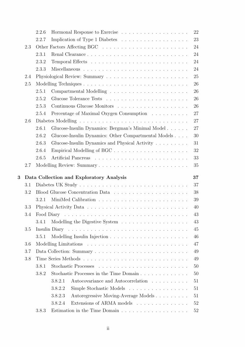
3.12 Sample autocorrelation function for change in BGC of Subject A. Dotted lines rep-
resent theoretical 95% confidence intervals given by ± 2√n
. . . . . . . . . . . . . 61
3.13 Sample partial autocorrelation function for change in BGC of Subject A. Dotted
lines represent theoretical 95% confidence intervals given by ± 2√n
. . . . . . . . . 62
3.14 AR(1) model residuals for change in BGC of Subject A. . . . . . . . . . . . . . 63
3.15 Correlogram of the AR(1) model residuals for change in BGC of Subject A. . . . . 64
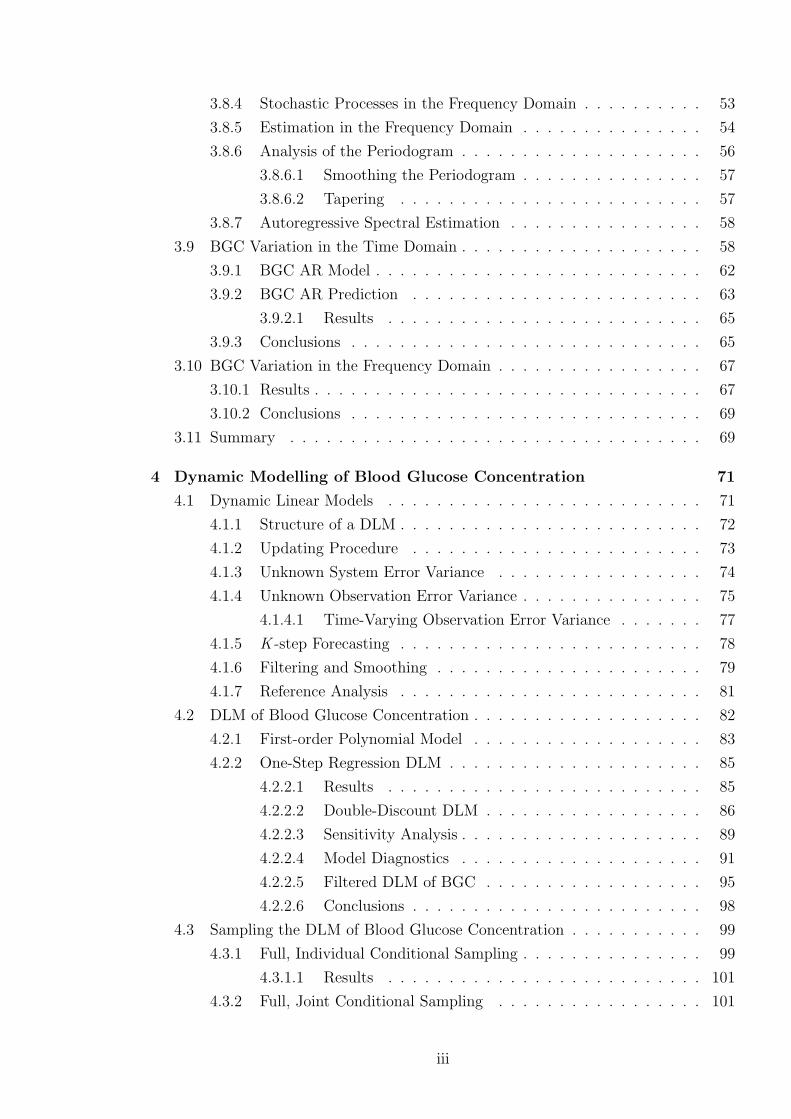
3.16 Measured BGC and one-step (five minutes) ahead prediction for BGC using ARIMA(1,1,0)
model for Subject A. . . . . . . . . . . . . . . . . . . . . . . . . . . . . . . 65
3.17 Measured BGC and 48-step (four hours) ahead prediction for BGC using ARIMA(1,1,0)
model for Subject A. . . . . . . . . . . . . . . . . . . . . . . . . . . . . . . 66
3.18 Periodogram for change in BGC of Subject A with taper proportion 0.1 and Daniell
smoothers of spans 7 and 11. . . . . . . . . . . . . . . . . . . . . . . . . . . 68
3.19 Periodogram for change in BGC of Subject A using ASE. . . . . . . . . . . . . 68
4.1 Measured BGC and FOP DLM predicted BGC for λ=0.01 and λ=1. . . . . . . . 84
4.2 One-step (five minutes) ahead prediction of BGC and measured BGC, with 95%
credible intervals. Extreme values of intervals omitted for clarity. . . . . . . . . . 87
4.3 Predicted BGC (solid line) and 95% credible intervals for standard DLM (δ = 1; blue
lines) and double discount model (δ as described in the text, representing increased
uncertainty at time 21.12; red lines). . . . . . . . . . . . . . . . . . . . . . . 88
4.4 METs parameter estimates for varying discount factor: (i) λ = 1; (ii) λ = 0.96; (iii)
λ = 0.5; (iv) λ = 0.1. . . . . . . . . . . . . . . . . . . . . . . . . . . . . . 89
4.5 METs parameter estimates for varying initial values: (i) θ = (0, 0, 0, 0); (ii) θ =
(100, 100, 100, 100); (iii) θ = (−100,−100,−100,−100); (iv) θ = (100,−100, 100,−100). 90
4.6 Measured BGC and predicted BGC for reference analysis approach, with 95% cred-
ible intervals. . . . . . . . . . . . . . . . . . . . . . . . . . . . . . . . . . 92
4.7 Time series of reference model forecast variance. . . . . . . . . . . . . . . . . . 92
4.8 Time series of filter model one-step BGC prediction errors. . . . . . . . . . . . . 93
4.9 Partial autocorrelation function of filter model errors. . . . . . . . . . . . . . . 93
4.10 Reference model errors against measured BGC. . . . . . . . . . . . . . . . . . 94
4.11 Reference filter model output for BGC and measured BGC. . . . . . . . . . . . 95
4.12 Parameter estimates for the reference filter model: (i) constant parameter; (ii) car-
bohydrate parameter; (iii) insulin parameter; (iv) METs parameter. . . . . . . . 96
4.13 Predicted BGC in the absence of insulin based on filter model results. . . . . . . . 97
4.14 Predicted BGC and measured BGC using parameter predictions from previous 24-
hour period. . . . . . . . . . . . . . . . . . . . . . . . . . . . . . . . . . . 98
4.15 Representative MCMC output for full, individual conditional distribution sampling
of DLM parameters: (i) the constant parameter at time t = 1 and (ii) t = 800; (iii)
the carbohydrate parameter at t = 100; (iv) the insulin parameter at time t = 500. . 102
ix

4.16 MCMC output for observation error precision, φ, under full, individual conditional
distribution sampling of DLM parameters. . . . . . . . . . . . . . . . . . . . . 103
4.17 Representative MCMC trace plots, sampled values for: (i) constant parameter at
time t=0; (ii) carbohydrate parameter at time t=50; (iii) insulin parameter at time
t=100; (iv) METs parameter at time t=500. . . . . . . . . . . . . . . . . . . 105
4.18 MCMC trace plot for observation error precision, φ. . . . . . . . . . . . . . . . 105
4.19 Means (solid lines) and 95% quantiles (dotted lines) from MCMC output for: (i)
constant parameter; (ii) carbohydrate parameter; (iii) insulin parameter; (iv) METs
parameter. . . . . . . . . . . . . . . . . . . . . . . . . . . . . . . . . . . . 106
4.20 12-steps (one hour) ahead predicted BGC (solid line) and measured BGC (dotted
line): (i) time series g[1], as given in (4.4.1); (ii) time series g[12]. . . . . . . . . . 109
4.21 24-hour window of compiled 12-step predicted BGC from all time series, g[n], and
measured BGC. Red circles indicate points in time series g[1]. . . . . . . . . . . . 109
4.22 (i) Function I(1)t (·) (4.4.2) applied to 12-step predicted BGC (black dots) and mea-
sured BGC (red dots); (ii) function I(2)t (·) applied to 12-step predicted and measured
BGC. . . . . . . . . . . . . . . . . . . . . . . . . . . . . . . . . . . . . . 110
4.23 Parameter estimates for 12-step predictive model: (i) constant parameter; (ii) car-
bohydrate parameter; (iii) insulin parameter; (iv) METs parameter. . . . . . . . 110
4.24 24-steps (two hours) ahead predicted BGC (solid line) and measured BGC (dotted
line): (i) time series g[1], as given in (4.4.1); (ii) time series g[24]. . . . . . . . . . 112
4.25 24-hour window of compiled 24-step predicted BGC from all time series, g[n], and
measured BGC. Red circles indicate points in time series g[1]. . . . . . . . . . . . 112
4.26 (i) Function I(1)t (·) (4.4.2) applied to 24-step predicted BGC (black dots) and mea-
sured BGC (red dots): (ii) function I(2)t (·) applied to 24-step predicted and measured
BGC. . . . . . . . . . . . . . . . . . . . . . . . . . . . . . . . . . . . . . 113
4.27 Parameter estimates for 24-step predictive model: (i) constant parameter; (ii) car-
bohydrate parameter; (iii) insulin parameter; (iv) METs parameter. . . . . . . . 113
4.28 48-steps (four hours) ahead predicted BGC (solid line) and measured BGC (dotted
line): (i) time series g[1], as given in (4.4.1); (ii) time series g[48]. . . . . . . . . . 114
4.29 24-hour window of compiled 48-step predicted BGC from all time series, g[n], and
measured BGC. Red circles indicate points in time series g[1]. . . . . . . . . . . . 114
4.30 (i) Function I(1)t (·) (4.4.2) applied to 48-step predicted BGC (black dots) and mea-
sured BGC (red dots); (ii) function I(2)t (·) applied to 48-step predicted and measured
BGC. . . . . . . . . . . . . . . . . . . . . . . . . . . . . . . . . . . . . . 115
4.31 Parameter estimates for 48-step predictive model: (i) constant parameter; (ii) car-
bohydrate parameter; (iii) insulin parameter; (iv) METs parameter. . . . . . . . 115
5.1 Minimal model of glucose-insulin kinetics: (i), model of glucose metabolism; (ii),
model of insulin kinetics. Reproduced from Bergman et al. (1979, 1981). . . . . . 120
x
5.2 Directed acyclic graph of the Andersen and Højbjerre (2005) model. . . . . . . . 123
5.3 Glucose (i) and insulin absorption (ii) (from the digestion and insulin models) and
relative PVOmax2 (iii) for Subject A. . . . . . . . . . . . . . . . . . . . . . . 126
5.4 PA model predicted of BGC and measured BGC for Subject A. . . . . . . . . . . 126
5.5 Integrated exercise intensity from the PA model for Subject A. . . . . . . . . . . 127
5.6 Hepatic contribution to BGC from the PA model for Subject A. . . . . . . . . . 127
5.7 Blood insulin concentration from the PA model for Subject A. . . . . . . . . . . 128
5.8 BGC profiles for two different basal glucose values, Gb=4.44mmol/l and Gb=4.17mmol/l.128
5.9 Renal clearance for a range of BGC. Recreated from Arleth et al. (2000). . . . . . 130
5.10 The modified physical activity model for glucose-insulin kinetics, where PA indicates
the relationships affected by physical activity. . . . . . . . . . . . . . . . . . . 130
5.11 Measured BGC and modified PA model results for BGC. . . . . . . . . . . . . . 131
5.12 Directed acyclic graph of the extended model. . . . . . . . . . . . . . . . . . . 134
5.13 (i) Estimated glucose and (ii) insulin absorption (from the digestion and insulin
models) and (iii) relative PVOmax2 for one day of Subject A’s records. . . . . . . . 137
5.14 MCMC trace plot for p5 from a long chain. . . . . . . . . . . . . . . . . . . . 140
5.15 MCMC trace plots for p1 based on three different starting values: (i) p(0)1 = 0, (ii)
p(0)1 = −10 (iii) p(0)
1 = −3.35 (the true value, as indicated by the red line in each plot).141
5.16 Measured BGC and MCMC output. . . . . . . . . . . . . . . . . . . . . . . . 142
5.17 Means and 95% credible intervals for p1 from each Markov chain in the simulation
study; the horizontal line represents the value of p1 used to generate the simulations. 143
5.18 Means and 95% credible intervals for p2 from each Markov chain in the simulation
study; the horizontal line represents the value of p2 used to generate the simulations. 143
5.19 Means and 95% credible intervals for p10 from each Markov chain in the simulation
study; the horizontal line represents the value of p10 used to generate the simulations. 144
5.20 Means and 95% credible intervals for τi from each Markov chain in the simulation
study; the horizontal line represents the value of τi used to generate the simulations. 145
5.21 Means and 95% credible intervals for τg∗ from each Markov chain in the simulation
study; the horizontal line represents the value of τg∗ used to generate the simulations. 145
5.22 Means and 95% credible intervals for each missing observation under scenario A. . . 147
5.23 Means and 95% credible intervals for each missing observation under scenario B. . . 147
5.24 Means and 95% credible intervals for each missing observation under scenario C (first
block). . . . . . . . . . . . . . . . . . . . . . . . . . . . . . . . . . . . . 148
5.25 Means and 95% credible intervals for each missing observation under scenario C
(second block). . . . . . . . . . . . . . . . . . . . . . . . . . . . . . . . . . 148
xi

Declaration of Authorship
I, SEAN MICHAEL EWINGS, declare that the thesis entitled
DYNAMIC MODELLING OF BLOOD GLUCOSE CONCENTRATION IN
PEOPLE WITH TYPE 1 DIABETES
and the work presented in it are my own and has been generated by me as the result
of my own original research.
I confirm that:
1. This work was done wholly or mainly while in candidature for a research degree
at this University;
2. Where any part of this thesis has previously been submitted for a degree or any
other qualification at this University or any other institution, this has been clearly
stated;
3. Where I have consulted the published work of others, this is always clearly at-
tributed;
4. Where I have quoted from the work of others, the source is always given. With
the exception of such quotations, this thesis is entirely my own work;
5. I have acknowledged all main sources of help;
6. Where the thesis is based on work done by myself jointly with others, I have
made clear exactly what was done by others and what I have contributed myself;
7. None of this work has been published before submission.
Signed . . . . . . . . . . . . . . . . . . . . . . . . . . . . . . . . . . . . . . . . . . . . . . . . . . . . . . . . . . . . . . . . . . . . . . . . . .
Date . . . . . . . . . . . . . . . . . . . . . . . . . . . . . . . . . . . . . . . . . . . . . . . . . . . . . . . . . . . . . . . . . . . . . . . . . . . .
xii
Acknowledgements
I would firstly like to thank my supervisors, Dr. Sujit Sahu and Dr. Andy Chipperfield,
for their guidance, enthusiasm and encouragement throughout. I am also grateful for
the support of EPSRC and the work of Diabetes UK and all those involved in the
study, particularly Dr. John Joseph Valletta.
I owe a very large thank you to my family, Paul, Maeve, Fiona and Holly, and
fiancee, Izi; their unwavering belief and support was invaluable and I cannot thank
them enough.
Finally, a thank you also to all the brilliant people at the university I have shared
offices and cake with through the years; it has been an enormous pleasure.

List of Abbreviations
AIC Akaike information criterion
AIDA Automated Insulin Dosage Advisor
AP Artificial pancreas
AR Autoregressive
ARIMA Autoregressive integrated moving average
ARMA Autoregressive moving average
ASE Autoregressive spectral estimation
ATP Adenosine triphosphate
BGC Blood glucose concentration
CGM Continuous Glucose Monitor
CRPS Continuous ranked probability score
CSII Continuous subcutaneous insulin infusion
DCCT Diabetes Care and Control Trial
DAG Directed acyclic graph
DE Differential equation
DIAS Diabetes Advisory System
DKA Diabetic ketoacidosis
DLM Dynamic linear model
DP Dormand-Prince
DUK Diabetes UK
EDIC Epidemiology of Diabetes Interventions and
Complications
FFA Free fatty acid
FOP First-order polynomial
GI Glycaemic index
GL Glycaemic load
GLUT Glucose transporter
HbA1c Glycated haemoglobin
IF Interstitial fluid
IVGTT Intravenous glucose tolerance test
xiv

KADIS Karlsburger Diabetes Management System
LLR Log-likelihood ratio
MA Moving average
MAD Mean absolute deviation
MCMC Markov chain Monte Carlo
MDI Multiple daily injections
MET Metabolic equivalent of task
MH Metropolis-Hastings
MM Minimal Model
MPC Model predictive control
MSE Mean squared error
OGTT Oral glucose tolerance test
PA model Physical activity minimal model
PCr Phosphocreatine
PDM Principal dynamic mode
PID Proportional-integral-derivative
PVOmax2 Percentage of maximal oxygen consumption
SCMH Single-component Metropolis-Hastings
SGLT Sodium-glucose transport protein
TG Triglyceride
xv

Chapter 1
Introduction
Diabetes mellitus (usually referred to as diabetes) is a chronic metabolic disorder char-
acterised by prolonged high blood glucose concentration (hyperglycaemia). Glucose
is a vital energy source for the body, particularly the brain, and its concentration in
blood is maintained within strict limits by various hormones. Insulin is crucial in this
process, as it is the only hormone that allows cells to take up glucose from the blood to
meet energy requirements. Diabetes is caused by reduced sensitivity to, or insufficient
secretion of, insulin. Defective insulin response results in hyperglycaemia, which is
associated with increased morbidity and mortality.
Worldwide prevalence of all forms of diabetes is approximately 180 million (World
Health Organisation, 2008), which is estimated to more than double by 2030 (Wild
et al., 2004). There is no cure, and day-to-day management is the responsibility of
the individual. Serious short- and long-term health complications are common due
to the unpredictable nature of treatment. Greater understanding of how different
factors affect blood glucose concentration (BGC) can help improve current treatment
programmes, and decrease the mental, physical and financial burden on individuals
and health services.
There are two predominant forms of diabetes, type 1 and type 2; the current work
is primarily focused on type 1 diabetes. This chapter discusses its causes, treatment
and complications, leading to the motivation for the current project and its potential
contributions to understanding and managing diabetes. The chapter also introduces
key concepts used throughout the thesis.
1.1 Type 1 Diabetes
Type 1 diabetes1 is a chronic autoimmune disease where an individual loses the ability
to produce insulin. The hormone is normally created in β-cells found in regions of the
1also referred to as insulin-dependent or juvenile-onset diabetes, though these are no longer definingcharacteristics.
1

pancreas called the islets of Langerhans. In people with type 1 diabetes, the β-cells are
destroyed, leaving no means for the uptake and utilisation of blood glucose (glucose
metabolism); the individual is thus deprived of a vital source of energy.
The β-cells are destroyed by the body’s own immune system, specifically by a T-cell
mediated response (Roep, 2003). The autoimmune reaction may be triggered by an
infection, where the body’s attack on virus-infected cells is also directed against β-
cells. There is evidence that enterovirus infections are linked to type 1 diabetes more
strongly than other environmental factors (Hyoty, 2002). Other research has focused
on genetic predisposition to type 1 diabetes; genetic susceptibility stems from genes in
the human leukocyte antigen region (Donner et al., 1997). An ongoing collaborative
article from the Online Mendelian Inheritance in Man website2 documents other work
studying genetic factors in type 1 diabetes.
Type 1 diabetes tends to present in people under the age of 30. The onset can
be quick, from a few days to a few weeks. When insulin-producing mechanisms are
destroyed, a number of physiological processes become unregulated. This results in the
over-production of ketones, which increase blood acidity (a process known as diabetic
ketoacidosis, DKA). Left untreated, type 1 diabetes will result in coma and eventually
death.
Type 1 diabetes accounts for approximately 15% of known cases of diabetes in the
UK, equivalent to around 250-300,000 people. The incidence of type 1 diabetes over
the period 1996-2005 remained relatively constant in the UK (Gonzalez et al., 2009);
however, there is evidence of increasing incidence around the world in 0-14 year-olds
(Onkamo et al., 1999), and other studies have found increasing prevalence in different
countries, e.g., Akesen et al. (2011); Ehehalt et al. (2012).
1.1.1 Treatment
There is currently no widely available cure for any form of diabetes. A pancreas
transplant is a highly invasive and expensive procedure, requiring a post-transplant
lifetime of immunosuppressant drugs. Pancreas transplants are usually only carried
out in individuals that are undergoing/have undergone other organ transplants. Islet
cell transplant is less invasive, where cells from donor pancreases are infused into the
individual to replace the lost insulin function. The method has produced promising
preliminary results (Shapiro et al., 2000), with the development of the Edmonton Pro-
tocol (Shapiro et al., 2006) designed to investigate the potential of a standardised
approach to treatment in an international, multi-centre trial. However, the method is
still hampered by the need for immunosuppressants and potentially multiple donors
for one individual’s treatment.
2http://www.ncbi.nlm.nih.gov/omim/222100, last accessed 12/01/2012
2

Developments in stem cell research offer a route for curing diabetes that potentially
eliminates the need for immunosuppressants. Promising results have been seen in small,
preliminary studies, e.g., Couri et al. (2009), though traditional stem cell therapy does
not overcome the underlying problems of autoimmunity. However, particular forms of
stem cells have been shown to change immune activity; Zhao et al. (2012) presented
results from a small trial demonstrating reduced autoimmunity maintained over several
months. Stem cell research in diabetes is, however, in its infancy, and any potential
cure remains in the distant future.
Current treatment regimes for diabetes are based on careful management of BGC.
For people without diabetes, BGC ranges between ∼4-7 mmol/l (also reported as ∼75-
120 mg/dl, where 18 mmol/l ∼ 1 mg/dl; the units mmol/l will be used here) in the
fasting state, with post-prandial (after meal) peaks up to ∼10 mmol/l. For people
with type 1 diabetes, the aim is to maintain BGC within these ranges through insulin
therapy (discussed in section 1.1.1.1).
Assessing insulin requirements to maintain healthy BGC (euglycaemia) is an in-
dividualised practice, dependent on various physiological and lifestyle factors. Age,
gender, body mass index and duration of diabetes all relate to insulin needs (Muis
et al., 2006); other important factors include insulin sensitivity (the body’s ability to
respond to insulin) and hormonal secretion (e.g., the response to physical or mental
stress). It is well established that food and physical activity are the dominant external
factors affecting the behaviour of BGC (as discussed later). The individual must assess
their insulin needs according to these external factors, and their own experience, on an
injection-by-injection basis. Choosing an appropriate insulin dosage is usually aided
by a small number of finger-prick blood tests each day; these provide a measure of
BGC at a particular moment in time, but offer no indication of stability or direction
of change.
Long-term control of BGC is assessed during routine visits to a care facility, using a
number of different methods. In particular, a blood test for glycated haemoglobin
(HbA1c) offers an indication of BGC over the preceding 2-3 months. The HbA1c
blood test measures the extent to which glucose molecules have attached themselves to
haemoglobin on red blood cells, where elevated readings suggest recurrent or prolonged
hyperglycaemia.
1.1.1.1 Insulin Therapy
Treatment with exogenous insulin began in the early 1920’s, when Fredrick Banting
and colleagues identified insulin and extracted it from animals for human injection. Di-
abetes was no longer an abruptly fatal illness, but early patients suffered pain, swelling
and other allergic reactions, as well as unpredictable BGC (Bliss, 1982). Animal in-
sulin has since been superseded by synthetic human insulin (also known as insulin
3

analogues), which rarely cause an allergic response; such insulin can also be altered to
achieve different absorption and metabolism. A history of the major advancements in
insulin production is discussed in Teuscher (2007).
Currently, the most common treatment programme is the multiple daily injection
(MDI), or basal-bolus, regime, where exogenous insulin is delivered into the subcuta-
neous tissue using insulin pens or syringes. The programme is designed to mimic the
response of a healthy pancreas, but at the cost of more insulin injections per day: a
once-daily injection of basal insulin allows low-level metabolism of glucose throughout
the day, while a bolus of fast-acting insulin is taken with each meal to help metabolise
exogenous glucose. The amount of insulin taken with meals is based on an estimate
of the amount of carbohydrate being consumed (carbohydrate counting) and recent
and/or impending exercise.
Continuous subcutaneous insulin infusion (CSII), where insulin is delivered via a
pump device and cannula, also aims to mimic the action of a healthy pancreas. While
the cannula must be replaced every few days, the method helps to reduce the number
of injections needed. In England and Wales, insulin pumps are generally only available
to those experiencing severe difficulties in reaching and maintaining HbA1c targets,
as indicated by the National Institute of Health and Clinical Excellence guidelines3.
Pump use is limited due to cost and the training required for the user to successfully
implement the regime (Pickup and Keen, 2001). However, the benefits of this method of
treatment have been demonstrated: a meta-analysis showed improved HbA1c and mean
BGC compared to conventional therapy, with no increase in adverse effects (Weissberg-
Benchell et al., 2003).
CSII may be open- or closed-loop. In an open-loop system, the user is still respon-
sible for selecting appropriate doses of insulin based on finger-prick blood tests, as with
the MDI regime. A closed-loop system is the ideal as it removes the individual from the
maintenance of euglycaemia. However, the system requires a BGC monitor to be worn
continuously, and computational software to relay the information from the monitor
as signals for action from the insulin pump. The combination of pump, monitor and
software is often referred to as an artificial pancreas; this is discussed further in section
1.4.
For both MDI and CSII, insulin is delivered into subcutaneous tissue. This repre-
sents a compromise for insulin delivery; the tissue is easily accessible, but represents
a “compartmental mismatch” (Buse et al., 2002): diffusion and absorption from sub-
cutaneous tissue does not faithfully recreate the conditions associated with a healthy
pancreas, with regard to the ratio of insulin concentration in the periphery and liver.
However, other methods for insulin delivery are not widely used. Intravenous delivery
is used in the health care environment, but is difficult outside of this. Inhaled insulin is
3http://www.nice.org.uk/Guidance/TA151#documents, last accessed 11/01/2012
4

not generally available, in part due to fears over long-term complications of the lungs.
Oral administration of insulin is currently not possible as it is broken down by digestive
juices, rendering it unusable.
Whichever treatment programme is used, the ultimate aim is to achieve eugly-
caemia. Due to the complex nature of BGC, maintaining euglycaemia is a daily chal-
lenge. Establishing a suitable insulin regimen is essentially a trial-and-error process for
every individual, even with the support of a professional health care team. It is hugely
important that BGC is maintained within the physiologically desirable range, as poor
control of BGC can lead to a number of short- and long-term complications, discussed
in the following two sections.
1.1.2 Hyperglycaemia
Extreme hyperglycaemia over a short period of time can cause life-threatening DKA.
Frequent and prolonged hyperglycaemia damages blood vessels and results in a num-
ber of complications over a longer period of time. The Diabetes Care and Control
Trial (DCCT; a 9-year clinical study) demonstrated that intensive blood glucose con-
trol4 can reduce the risk of eye, kidney and nerve damage in the longer-term (DCCT
Research Group, 1993). The follow-up study, the Epidemiology of Diabetes Interven-
tions and Complications (EDIC), also showed that intensive control can reduce the
risk of cardiovascular events, such as heart attack and stroke (DCCT/EDIC Study Re-
search Group, 2005). Treatment aims to maintain euglycaemia and hence avoid these
complications, but is itself associated with problems.
1.1.3 Hypoglycaemia
Hypoglycaemia, or low BGC, is a side effect of insulin therapy. The inexact nature of
treatment means that BGC may fall below normal levels (generally 4 mmol/l is consid-
ered to be the threshold for hypoglycaemia). The brain is then starved of its primary
energy source, and the individual will experience a hypoglycaemic reaction. Symp-
toms, and their severity, depend on the individual’s recent history of hypoglycaemic
reactions, and the severity of the hypoglycaemia. Failure to deal with hypoglycaemia
may result in unconsciousness, and potentially death.
In a healthy pancreas, low BGC will stimulate the secretion of glucagon from pan-
creatic α-cells and a concomitant suppression of insulin; this stimulates the liver to
release glucose into the blood. However, injected insulin cannot be suppressed, and
4The “intensive control” trialled by the DCCT involved upwards of four finger-prick blood tests aday, at least three injections of insulin per day (which could be adjusted according to food, physicalactivity and current BGC), monthly visits to a health care team, and more frequent contact viatelephone to review their regimen. The control group consisted of people on one or two injections perday.
5

will continue to encourage blood glucose uptake and suppress the release of glucagon.
Furthermore, glucagon response may be diminished over time in people with diabetes,
weakening the body’s ability to counteract hypoglycaemia (Liu et al., 1993). The
secretion of epinephrine, which helps stimulate hepatic glucose release and triggers
symptoms of hypoglycaemia, may also be attenuated in the presence of nerve damage.
Recent hypoglycaemic events may result in loss of awareness of future events, as
hypoglycaemia lowers glycaemic thresholds for autonomic and symptomatic response
(LeRoith et al., 2003). Thus, when several hypoglycaemic events occur over a short
period of time, the body will only begin to respond to more severe hypoglycaemia, if
at all. This can impact upon quality of life, due to fear of unexpected hypoglycaemia.
The DCCT trial showed that while intensive control helped to reduce HbA1c, it also
resulted in a three-fold increase in hypoglycaemic events. It appears that by making
a concentrated effort to avoid hyperglycaemia, individuals run an increased risk of
hypoglycaemia.
Other side effects of treatment are relatively uncommon. Repeated injections in
the same site can lead to hard lumps (hyperlipotrophy) forming under the skin, which
can disrupt insulin absorption; it is recommended that injection sites are rotated to
avoid unpredictable absorption, which can result in hypo- or hyperglycaemia (Saez-de
Ibarra and Gallego, 1998).
1.2 Type 2 Diabetes
Type 2 diabetes5 is generally associated with genetic and lifestyle factors, particularly
obesity and sedentary lifestyle (Zimmet, 1982; Ohlson et al., 1988; Hu, 2003). Defective
insulin response manifests in the form of lowered insulin sensitivity (where tissues are
less responsive to insulin, thus diminishing the body’s capacity to metabolise blood
glucose) and/or relatively-reduced insulin secretion. Onset is gradual and can go un-
noticed for many years, with potentially 40% of type 2 diabetes cases unidentified
(Thomas et al., 2005).
Type 2 diabetes tends to present in adults over the age of 40, though changes in
lifestyle has resulted in increased incidence in younger adults and children are increasing
(Fagot-Campagna et al., 2001). It is estimated that more than 2.5 million people in
the UK have type 2 diabetes. The Centers for Disease Control and Prevention (part of
the US health service) note that the number of Americans with type 2 diabetes tripled
in the period 1980 to 2006, from 5.6 million to 16.8 million, and led them to label it
“an epidemic”6.
5also referred to as non-insulin dependent or adult-onset diabetes, though these are no longerdefining characteristics.
6http://www.cdc.gov/nccdphp/publications/aag/ddt.htm, last accessed 12/01/2012
6
Generally, the first course of treatment is to make lifestyle changes, as dietary
improvements and increased physical activity can help improve insulin sensitivity. If
this is unsatisfactory, oral drugs may be prescribed. Failure to achieve euglycaemia with
these approaches means exogenous insulin may be required, as with type 1 diabetes.
1.3 Other Types of Diabetes
There are various other types of diabetes, which are generally less common. Gestational
diabetes can occur in pregnant women when the increased insulin demands placed
on the body during pregnancy are not met. Gestational diabetes is temporary and
the problem usually resolves itself after the baby is born. However, it needs careful
management during the course of pregnancy to ensure the short- and long-term health
of mother and child. Other rarer forms of diabetes also exist, such as secondary diabetes
mellitus, caused by any drug or disease that damages the pancreas or β-cells.
The current project will focus on type 1 diabetes; however this does not discount
applicability to other types of diabetes, particularly those that require exogenous in-
sulin.
1.4 Motivation
Diabetes is a major public health issue. The National Diabetes Audit (NHS Informa-
tion Centre, 2011), based on English GP practices, estimated there were 24,000 more
deaths in the diabetes population compared to the general population in the 2007-08
cohort. Soedamah-Muthu et al. (2006) reported mortality rates of 8 per 1,000 person-
years in the type 1 diabetes group, compared to 2.15 per 1,000 person-years in the
control group. It is a growing worldwide problem, and the burden on health services is
already substantial. The National Health Service in the UK spends approximately 10%
of its budget annually on treatment for all forms of diabetes (Diabetes UK, 2008). The
American Diabetes Association estimates similar levels of spending in U.S. healthcare,
corresponding to $147bn in 20077. Thus, diabetes attracts a great amount of research
interest that will only escalate given its increasing prevalence.
For those with diabetes, maintaining euglycaemia is a daily challenge, with insulin
needs having to be balanced against various lifestyle factors. The repercussions of poor
BGC control can present in the short- and long-term, and may result in eye, nerve
and kidney damage, as well as cardiovascular events such as heart attack and stroke.
Effective treatment can prevent, delay or slow the progress of these complications.
7http://www.diabetesarchive.net/advocacy-and-legalresources/cost-of-diabetes.jsp, last accessed13/09/2012
7

The DCCT study demonstrated that intensive treatment can be effective in pre-
venting longer-term complications, albeit at the risk of more frequent hypoglycaemic
episodes. However, not all aspects of the treatment are realistic in the long-term; in
particular, the weekly and monthly consultations with various health care specialists
are generally not viable due to time and financial constraints. Thus, effective treatment
must rely more on the individual or on other more cost-effective methods. To this end,
much work has focused on understanding the factors which affect BGC and how they
manifest.
It is well established that food, insulin and physical activity are the major factors
affecting BGC. In the diabetes literature, much recent work has focused on describing
glucose-insulin dynamics in the blood under these external disturbances. Many of the
underlying modelling strategies used in such work are attributable to landmark research
undertaken by Bergman and colleagues (Bergman et al., 1979, 1981; Toffolo et al.,
1980), who developed a “minimal model” to be used for estimating insulin sensitivity
(the work was predominantly concerned with type 2 diabetes). The minimal model
compartmentalised the body by separating out the most important features of the
body’s response to a glucose load, though originally made no consideration of food
intake, insulin injections or physical activity.
Compartmental models (discussed in section 2.5.1) have long been a popular ap-
proach to describing glucose-insulin dynamics, with prominent examples found in
Sorensen (1985), and computer packages AIDA (Lehmann and Deutsch, 1992) and
DIAS (Hejlesen et al., 1997). These models have been extended to account for pro-
cesses that were previously overlooked, e.g., the models of Bergman et al. and Sorensen
have been extended by Derouich and Boutayeb (2002) and Hernandez-Ordonez and
Campos-Delgado (2008), respectively, to include the effects of physical activity. More
recently, compartmental models have been used in the development of software as part
of an artificial pancreas. It is interesting to note, however, that in a review of diabetes
modelling, experienced authors Lehmann and Deutsch suggest that “compartmental
model-based computational techniques may have relatively little utility for generat-
ing glycaemic prediction and offering decision support in routine clinical practice”
(Lehmann and Deutsch, 1998).
The concept of the artificial pancreas generates much of the current diabetes mod-
elling literature, despite the fact that the necessary insulin pump and BGC monitor
are not part of the current standard treatment protocol for diabetes. Furthermore,
the various proposed control algorithms in the literature have only been tested using
simulated BGC profiles. The approach has yet to demonstrate long-term efficacy, cost-
effectiveness, and most crucially, safety. In contrast, there appears to be much less
focus on improving the MDI treatment regime that is most commonly used in diabetes
management.
8
Despite advances in understanding glucose metabolism, diabetes research is still
hampered by a lack of free-living data.8 Data collected in a clinical setting may have
very limited relevance to the daily life of an individual. This is particularly notable in
the case of physical activity; attempts to adequately incorporate activity into models of
glucose-insulin dynamics have been based on data collected from unrealistic, simplified
and/or artificial experiments, or from non-diabetic subjects. A number of different
approaches to quantifying exercise have been proposed, each with their own advantages
and limitations. The percentage of maximum oxygen uptake (PVOmax2 ; discussed in
section 2.5.4) has been used in a number of studies, e.g., Lenart and Parker (2002) and
Hernandez-Ordonez and Campos-Delgado (2008), and is based on the approximate
linear relationship between oxygen consumption and energy expenditure. However,
measuring PVOmax2 requires specialist equipment only found in a clinical environment.
Breton (2008) proposed the use of heart rate as an indication of exercise duration and
intensity. This has only been trialled within a very strict clinical environment, and has
yet to be used in the free-living environment.
Recently developed devices, such as the BodyMedia SenseWear armband (Andre
et al., 2006) which estimates physical activity as a multiple of resting metabolic rate,
offer an opportunity to quantify both the duration and intensity of activity outside of
the clinical setting. As such, these devices can be a crucial component in understanding
how activity affects BGC in free-living conditions. It is worth highlighting the impor-
tance of people with diabetes being able to safely incorporate physical activity into
their daily routine; the benefits in the general population are well-documented, and
regular physical activity is also associated with better glycaemic control and enhanced
insulin sensitivity for people with diabetes (Waden et al., 2005; Herbst et al., 2006;
Riddell and Iscoe, 2006).
1.5 Research Overview and Contributions
The proposed research seeks to combine data from SenseWear devices with detailed,
free-living data on BGC, food and insulin for the purpose of improving current treat-
ment regimes, without recourse to continuous glucose monitors and insulin pumps, and
potential treatment regimes based on an artificial pancreas. The research will draw on
knowledge from a number of separate disciplines relevant to diabetes; this includes
work that describes the digestion of food, absorption of injected insulin, and the effects
of physical activity.
The current work has two main aims: the first is to investigate more precisely how
the effects of physical activity manifest in the behaviour of BGC; this has the potential
8Free-living data is a term used throughout to refer to data that is collected from an individual’severyday environment without impediment
9
to help those with diabetes safely incorporate physical activity into daily life, and enjoy
the health benefits without the dangers of hypo- or hyperglycaemia. The second aim
is to build a model that can accurately predict BGC over periods of several hours.
Prediction over four hours (or more) are of particular interest, as this represents a
reasonable amount of time between finger-prick tests as part of the MDI regime. Such
a model could then be included in current treatment regimes by guiding the insulin
therapy decision-making process.
An appropriate predictive and/or descriptive model of BGC would help reduce the
risk of the short- and long-term complications associated with diabetes, and reduce the
burden on individuals and health services. The proposed work thus offers the potential
for a relatively inexpensive and immediate improvement in diabetes care. Furthermore,
better understanding of the role of physical activity would further develop the push
for an artificial pancreas, by providing a more physiologically-accurate representation
of the glucoregulatory system under the stimuli experienced by individuals with type
1 diabetes in their normal daily environment.
1.5.1 Thesis Structure
The thesis is divided as follows:
• Chapter 2 reviews relevant literature in physiology and mathematical modelling.
The work highlighted here helps guide modelling strategies used throughout the rest
of the current work;
• Chapter 3 discusses in detail the unique data which drives the current project.
Practical modelling issues regarding the food and insulin data are highlighted and
overcome with the use of physiological models taken from the literature. The chapter
also introduces and uses simple time series analysis methods, including analysis in the
time and frequency domains, to better understand the nature of free-living BGC data.
The exploratory measures inform the more complex modelling strategies used in later
chapters;
• Chapter 4 uses dynamic linear models, not previously used in diabetes modelling,
to predict BGC from food, insulin and physical activity data. These models are also
used to explore the role of physical activity in the behaviour of BGC. Long-term pre-
dictions of BGC (over several hours) take the form of either forecasting the profile of
BGC or forecasting periods of hypo- and hyperglycaemia. The models presented here
are one of few empirical approaches used to predict the behaviour of BGC;
10
• Chapter 5 uses a more detailed semi-empirical compartmental model to further
investigate the role of physical activity in the behaviour of BGC. The chapter describes
the potential problems in many of the current diabetes modelling strategies with regard
to free-living data, highlighting the danger of building models based on inappropriate
data from non-diabetic subjects or simulations. A new model, with food, insulin and
physical activity inputs, is presented to overcome limitations of current models. The
performance of the new model is tested using the free-living data previously described.
The chapter presents a simulation study designed to test the feasibility of a Bayesian
approach and modern, computationally-intensive statistical methods to simultaneously
estimate model parameters, and predict BGC. This is the first time the descriptive ca-
pabilities of compartmental models have been tested with free-living data;
• Chapter 6 summarises the work of the previous chapters and makes recommen-
dations for future work in the area.
1.6 Summary
Type 1 diabetes is a worldwide problem, whose treatment and associated complications
represent a great cost to individuals and health services. Current treatment methods
such as MDI are limited due to the variable nature of BGC, and intensive treatment
to limit hyperglycaemia results in more frequent hypoglycaemic episodes. The devel-
opment of an artificial pancreas is ongoing, and attempts to model BGC are limited
by a lack of appropriate and relevant data, particularly with regard to physical activ-
ity. New technology, such as the BodyMedia SenseWear R© device, provide a means
of quantifying activity in free-living conditions, and hence may be used to assess and
model the effect of exercise on BGC. This opens the possibility of data-driven models
for BGC using food intake, insulin and physical activity as explanatory variables, and
testing compartmental models developed using artificial data.
11

Chapter 2
Research Background
The following chapter is a review of research in diabetes, and other relevant fields,
that provides context to the current work. The chapter is split into two sections: the
first is a review of the literature on relevant physiology and the effect of diabetes on
the body’s internal processes, and the second is a review of the diabetes modelling
literature. Understanding the relevant underlying physiology is vital for modelling the
behaviour of blood glucose concentration (BGC), particularly if the model is to be
accurate, viable and interpretable by potential end-users, i.e., clinicians and people
with diabetes. The second section presents the motivations and objectives of research
related to the current work, and how modelling approaches are guided by the physiology
presented in the first section. The review includes discussion of limitations in the
research and how the current work may improve the body of knowledge.
Physiological Review
This section looks at the different factors that affect BGC, and how diabetes impacts
on these. The roles of various organs, tissues, cells and hormones and their relation-
ships (collectively called the glucoregulatory system) are discussed with respect to their
influence on blood glucose homeostasis (self-regulation). The second half of this sec-
tion focuses on the body’s response to physical activity, highlighting the practical and
theoretical difficulties in modelling this response.
2.1 Metabolic Processes
Blood glucose is a vital source of energy for the body, whose regulation is maintained
via various metabolic pathways, summarised in Table 2.1. Glucose in the body is
derived from digestion of the nutrients carbohydrate, fat and protein; Figure 2.1 shows
the processes by which the body converts food to glucose. Reserves of glucose are
13
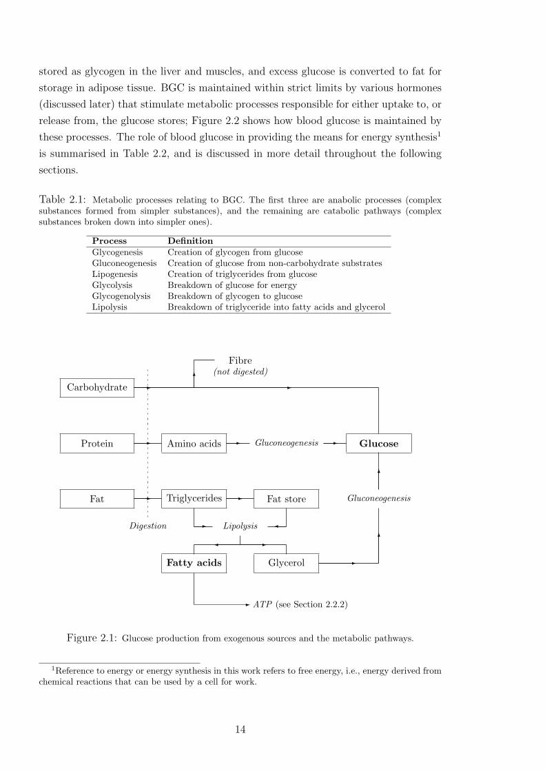
stored as glycogen in the liver and muscles, and excess glucose is converted to fat for
storage in adipose tissue. BGC is maintained within strict limits by various hormones
(discussed later) that stimulate metabolic processes responsible for either uptake to, or
release from, the glucose stores; Figure 2.2 shows how blood glucose is maintained by
these processes. The role of blood glucose in providing the means for energy synthesis1
is summarised in Table 2.2, and is discussed in more detail throughout the following
sections.
Table 2.1: Metabolic processes relating to BGC. The first three are anabolic processes (complexsubstances formed from simpler substances), and the remaining are catabolic pathways (complexsubstances broken down into simpler ones).
Process DefinitionGlycogenesis Creation of glycogen from glucoseGluconeogenesis Creation of glucose from non-carbohydrate substratesLipogenesis Creation of triglycerides from glucoseGlycolysis Breakdown of glucose for energyGlycogenolysis Breakdown of glycogen to glucoseLipolysis Breakdown of triglyceride into fatty acids and glycerol
Digestion
Glucose
Fat - Triglycerides
-
- Fat store
Lipolysis
-
Glycerol -
Gluconeogenesis
6
6
Fatty acids
- ATP (see Section 2.2.2)
Protein - Amino acids - Gluconeogenesis -
Carbohydrate - -6
Fibre(not digested)
Figure 2.1: Glucose production from exogenous sources and the metabolic pathways.
1Reference to energy or energy synthesis in this work refers to free energy, i.e., energy derived fromchemical reactions that can be used by a cell for work.
14

Glucose -
-
-
Lipogenesis -
Glycogenesis -
Glycolysis -
Triglycerides (adipose tissue)
Pyruvate (intracellular)
6
ATP (see Section 2.2.2)
(Anaerobic)Lactate
?
Cori cycle
?
Glycogen (liver, muscles)
Glycogenolysis
6
Figure 2.2: Internal glucose storage and utilisation.
Table 2.2: Selected organs, tissues and cells involved in blood glucose production and uptake.
Organ/tissue/cell Source or sink Via processBrain Sink Insulin-independent uptakeLiver Source / sink Glycogenolysis, gluconeo. / GlycogenesisKidneys Source / sink Gluconeogenesis / FiltrationIntestines Source DigestionMuscles Sink GlycogenesisAdipose tissue Source / sink Lipolysis / LipogenesisRed blood cells Sink Insulin-independent uptake
2.1.1 Role of Food
Carbohydrates are the most accessible source of energy for the body, and are generally
split into three types: monosaccharides (e.g., glucose), disaccharides (e.g., lactose), and
polysaccharides (also known as complex carbohydrates, e.g., starch). The digestion
of carbohydrate, from mouth to intestines, is the process by which the body breaks
down the more chemically complex carbohydrates into simpler monosaccharides. These
molecules can then be absorbed into the bloodstream and used as a source of energy
by various cells, organs and tissues.
The type of carbohydrate ingested determines the rate of digestion, and thus how
quickly it increases BGC. The glycaemic index (GI) was developed by Jenkins et al.
(1981) as a way of grouping foods that displayed similar effects on BGC. High GI
foods, e.g., honey, raise BGC relatively quickly, while low GI foods, e.g., pasta, exhibit
a slower, longer effect on BGC. The index was designed to help people with type 2
diabetes avoid rapid increases in BGC, and hence reduce the strain on impaired insulin
production/action.
The glycaemic load (GL) extends the idea of the GI by also considering the quan-
15
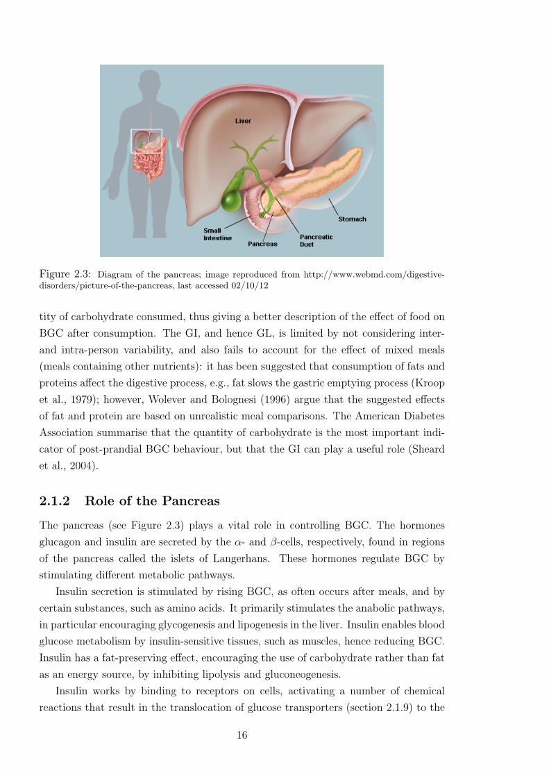
Figure 2.3: Diagram of the pancreas; image reproduced from http://www.webmd.com/digestive-disorders/picture-of-the-pancreas, last accessed 02/10/12
tity of carbohydrate consumed, thus giving a better description of the effect of food on
BGC after consumption. The GI, and hence GL, is limited by not considering inter-
and intra-person variability, and also fails to account for the effect of mixed meals
(meals containing other nutrients): it has been suggested that consumption of fats and
proteins affect the digestive process, e.g., fat slows the gastric emptying process (Kroop
et al., 1979); however, Wolever and Bolognesi (1996) argue that the suggested effects
of fat and protein are based on unrealistic meal comparisons. The American Diabetes
Association summarise that the quantity of carbohydrate is the most important indi-
cator of post-prandial BGC behaviour, but that the GI can play a useful role (Sheard
et al., 2004).
2.1.2 Role of the Pancreas
The pancreas (see Figure 2.3) plays a vital role in controlling BGC. The hormones
glucagon and insulin are secreted by the α- and β-cells, respectively, found in regions
of the pancreas called the islets of Langerhans. These hormones regulate BGC by
stimulating different metabolic pathways.
Insulin secretion is stimulated by rising BGC, as often occurs after meals, and by
certain substances, such as amino acids. It primarily stimulates the anabolic pathways,
in particular encouraging glycogenesis and lipogenesis in the liver. Insulin enables blood
glucose metabolism by insulin-sensitive tissues, such as muscles, hence reducing BGC.
Insulin has a fat-preserving effect, encouraging the use of carbohydrate rather than fat
as an energy source, by inhibiting lipolysis and gluconeogenesis.
Insulin works by binding to receptors on cells, activating a number of chemical
reactions that result in the translocation of glucose transporters (section 2.1.9) to the
16

cell membrane. The transporters aid the movement of glucose in the blood across cell
membranes. Once insulin has effected its action, it may be degraded by the cell or
released back into the blood where it is cleared by the liver or kidneys.
The effect of insulin on blood glucose uptake varies according to circumstance:
insulin-independent uptake dominates during fasting, but insulin-dependent uptake
becomes more prominent after meals. Hovorka et al. (2001) note that this results in
nonlinear insulin action: raising basal insulin levels by 50% during fasting has a small
effect on total glucose uptake, but the same increase during times of insulin-dependent
dominance has a far greater effect on uptake.
Glucagon has the opposite effect of insulin. Its release is stimulated by low BGC,
and inhibited by insulin. Glucagon stimulates the liver to release glucose via the
catabolic pathways glycogenolysis (primarily) and gluconeogenesis; it thus helps to
raise BGC. Conversely, glucagon secretion encourages secretion of insulin, so that the
body is able to metabolise recently liberated glucose.
2.1.3 Role of the Liver
Insulin stimulates the liver to convert glucose to glycogen for storage; this is the single
largest pool of stored glucose in the body. When fasting, the liver helps maintain eu-
glycaemia by releasing glucose into the blood via glycogenolysis and gluconeogenesis.
The ratio at which these metabolic pathways provide glucose depends on the glycogen
stores in the liver. Glycogenolysis is generally the dominant method of glucose pro-
duction, but during/after exercise, or after long periods of fasting, the glycogen stores
in the liver become depleted; gluconeogenesis is then the primary pathway for glucose
production. Gluconeogenesis is slower to produce glucose than glycogenolysis, and may
result in demand outstripping production and a subsequent decrease in BGC.
Hepatic glycogen depletion results in increased post-prandial glucose uptake in the
liver to replenish stores. If hepatic glycogen stores are full, excess glucose in the liver
is used in the synthesis of fatty acids. These are released in to the blood where they
may then be stored in other tissue as triglycerides. When glucose reserves are low, the
liver can produce ketones by metabolising fatty acids. At low levels, ketones are not
harmful and can be used by the brain and kidneys as an alternative source of energy.
2.1.4 Role of the Kidneys
Net renal glucose output is small in the fasting state, but the kidneys have been shown
to be a significant organ in the uptake and release of blood glucose. Stumvoll et al.
(1995) reported that the kidneys account for around 20% (average) of blood glucose
uptake, and approximately 28% (average) of glucose released into the blood in their
sample of healthy individuals. During epinephrine infusion (up to levels designed to
17
mimic those seen during hypoglycaemia), the kidneys increased output to account
for 40% of glucose appearance. This increase accounted for almost all of the raised
glucose appearance. Stumvoll et al. (1995) note that there seems to be little scope for
glycogen storage in the kidneys, so glucose production is assumed to be dominated by
gluconeogenesis.
2.1.5 Role of the Brain
The brain relies on the constant supply of blood glucose for its source of energy, and
accounts for approximately 50% of basal glucose uptake (Naylor et al., 1995). Glucose
uptake in the brain is insulin-independent. The brain cannot use fatty acids for creating
energy, though during fasting it can use ketones to reduce demand on blood glucose.
2.1.6 Role of Muscles
Muscles store glucose as glycogen, thus providing an immediate energy source at the
onset of exercise. If glycogen stores become depleted, muscular blood glucose uptake
increases; increased uptake may also be seen post-exercise as the stores of glycogen are
replenished. Muscles do not release glucose into the blood, but during exercise may
release gluconeogenic precursors; in particular, pyruvate is converted in to alanine (an
amino acid) and released in to the blood. It is then transported to the liver, where
it is converted back into pyruvate and then glucose. Increased production of alanine
also occurs when glucose stores are low and the muscle begins to break down protein
reserves for energy. Lactate is also released by muscle and transported to the liver,
where it may be converted to glucose as part of the Cori cycle.
2.1.7 Role of Hormones
In addition to insulin and glucagon, a number of other hormones aid blood glucose
homeostasis; their roles are summarised in Table 2.3. It is worth noting that insulin is
the only hormone that always reduces BGC. The role of hormones is discussed more
thoroughly by Ganong (2005) and Pocock and Richards (2006).
2.1.8 Role of Fatty Acids
Fat is stored in adipose tissue, predominantly in the form of triglycerides (TGs); these
consist of fatty acids bound by glycerol. When TGs are broken down (lipolysis) they
release the fatty acids (becoming free fatty acids, FFAs) and glycerol in to the blood.
FFAs are then oxidised for energy in muscle(s) or the liver, while glycerol may be
converted to glucose in the liver. At rest, FFAs dominate muscle energy synthesis as
fat yields more energy by mass (∼9.4kcal/g) than carbohydrate (∼4.2kcal/g) or protein
18
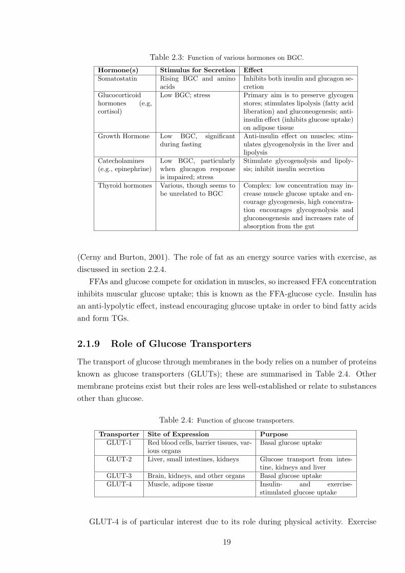
Table 2.3: Function of various hormones on BGC.
Hormone(s) Stimulus for Secretion EffectSomatostatin Rising BGC and amino
acidsInhibits both insulin and glucagon se-cretion
Glucocorticoidhormones (e.g,cortisol)
Low BGC; stress Primary aim is to preserve glycogenstores; stimulates lipolysis (fatty acidliberation) and gluconeogenesis; anti-insulin effect (inhibits glucose uptake)on adipose tissue
Growth Hormone Low BGC, significantduring fasting
Anti-insulin effect on muscles; stim-ulates glycogenolysis in the liver andlipolysis
Catecholamines(e.g., epinephrine)
Low BGC, particularlywhen glucagon responseis impaired; stress
Stimulate glycogenolysis and lipoly-sis; inhibit insulin secretion
Thyroid hormones Various, though seems tobe unrelated to BGC
Complex: low concentration may in-crease muscle glucose uptake and en-courage glycogenesis, high concentra-tion encourages glycogenolysis andgluconeogenesis and increases rate ofabsorption from the gut
(Cerny and Burton, 2001). The role of fat as an energy source varies with exercise, as
discussed in section 2.2.4.
FFAs and glucose compete for oxidation in muscles, so increased FFA concentration
inhibits muscular glucose uptake; this is known as the FFA-glucose cycle. Insulin has
an anti-lypolytic effect, instead encouraging glucose uptake in order to bind fatty acids
and form TGs.
2.1.9 Role of Glucose Transporters
The transport of glucose through membranes in the body relies on a number of proteins
known as glucose transporters (GLUTs); these are summarised in Table 2.4. Other
membrane proteins exist but their roles are less well-established or relate to substances
other than glucose.
Table 2.4: Function of glucose transporters.
Transporter Site of Expression PurposeGLUT-1 Red blood cells, barrier tissues, var-
ious organsBasal glucose uptake
GLUT-2 Liver, small intestines, kidneys Glucose transport from intes-tine, kidneys and liver
GLUT-3 Brain, kidneys, and other organs Basal glucose uptakeGLUT-4 Muscle, adipose tissue Insulin- and exercise-
stimulated glucose uptake
GLUT-4 is of particular interest due to its role during physical activity. Exercise
19

encourages the translocation of GLUT-4, which helps enhance glucose uptake in mus-
cles independently of insulin (Coderre et al., 1995; Goodyear and Kahn, 1998). Thorell
et al. (1999) also hypothesise that the redistribution of GLUT-4 accounts for increased
glucose uptake post-exercise (discussed in section 2.2).
Sodium-dependent glucose transporters (SGLT) aid the function of the GLUTs in
the kidneys (SGLT1 and SGLT2) and intestines (SGLT1). In particular, the trans-
porters in the kidney help reclaim filtered glucose. The amount of glucose that can be
reclaimed is limited by the renal glucose threshold (RGT; discussed further in section
2.3.1).
2.1.10 Implication of Type 1 Diabetes
The lack of endogenous insulin production in people with type 1 diabetes means that
blood glucose cannot be metabolised by the insulin-sensitive cells and tissues, and thus
parts of the body are starved of their primary source of energy. The lack of insulin also
means there is no inhibition of glucagon secretion (and hence hepatic glucose release),
and no regulation of the breakdown of TGs to FFAs. This results in extreme and
prolonged hyperglycaemia and increased FFA circulation. The liver converts excess
FFA into ketones, resulting in life-threatening DKA.
Exogenous insulin delivery, as part of diabetes treatment regimes, is designed to
replace the lost function of the pancreas. However, the body’s inability to regulate in-
jected insulin means various physiological processes are sub-optimal. Insulin injections
also fail to faithfully recreate the conditions of pancreatic insulin release, in particular
the ratio of peripheral insulin to hepatic insulin (Buse et al., 2002). This may explain
the lower hepatic glycogen stores in people with diabetes observed by Petersen et al.
(2005), as well as dysfunctional glucagon response to carbohydrate consumption, where
glucagon suppression was not observed after meals (Dinneen et al., 1995).
2.2 Exercise Physiology
Describing the body’s response to exercise, and how this affects BGC, is a primary aim
of the current work. It is therefore important to understand the underlying physiology,
the effect of different durations, intensities and types of exercise, and the impact of
diabetes on the physiology. The remainder of this section focuses on the role of blood
glucose in providing energy for activity.
2.2.1 Whole-Body Changes
The onset of exercise triggers a number of physiological responses. Blood flow is redis-
tributed through vasodilation and vasoconstriction (widening and narrowing of blood
20
vessels, respectively), with increased flow to the exercising muscle(s), heart and lungs,
and a decrease to the liver and kidneys. Increased heart rate and hyperventilation aids
delivery and removal of substances involved in cellular respiration. Various metabolic
processes are stimulated to power activity, with the aim of maintaining the supply of
the energy-rich compound adenosine triphosphate.
2.2.2 Adenosine Triphosphate
The breakdown of adenosine triphosphate (ATP) and the subsequent chemical reactions
release free energy, which contracts skeletal muscle and thus powers exercise. Stores of
ATP in the body are limited and it must be replenished continuously during exercise.
Carbohydrate and lipid metabolism dominate ATP synthesis, while oxidation of protein
(more precisely amino acids) generally provides <5% of energy (Riddell and Iscoe,
2006). Amino acids are, however, essential to production of phosphocreatine (PCr),
another energy-rich compound. PCr is predominantly stored in muscle and is crucial
for anaerobic ATP production during very short-term (less than 10 seconds) exercise.
It is replenished through ingestion of the necessary amino acids.
The roles of carbohydrate and lipid metabolism in ATP replenishment depend on
the duration and intensity of physical activity, and the behaviour of BGC depends on
how the body uses these sources of energy.
2.2.3 Carbohydrates as a Source of Energy
During exercise, muscle glycogen is broken down into glucose, and then into pyruvate
(see Figure 2.2, section 2.1). With sufficient oxygen, the pyruvate is fed into the citric
acid cycle (also known as Krebs’ cycle). The citric acid cycle creates a small amount
of energy, as well as producing important substrates for the electron transport chain.
This chain produces the majority of energy in aerobic respiration (Pocock and Richards,
2006).
When there is insufficient oxygen, the body will be unable to oxidise all the pyruvate
derived from the breakdown of glucose. Excess pyruvate is instead converted to lactate
and released into the blood. Lactate may then be taken up by the liver to be converted
to glucose (via gluconeogenesis; see section 2.2.5), which is then released into the
blood. The gluconeogenic stage in the liver is energy consuming, and hence anaerobic
respiration is suitable only for short periods of time.
As muscle glycogen stores become depleted, the muscle may take up glucose from
the blood to be used as a source of energy. Glucose levels in the blood are maintained
by hepatic glucose release. Furthermore, blood glucose is important in replenishing the
muscle glycogen stores post-exercise. The liver replenishes its own glycogen stores via
gluconeogenesis and increased glucose uptake after carbohydrate intake.
21

During high-intensity exercise, carbohydrates are the main source of energy; under
such high energy demand, the body seeks to extract the maximum amount of energy
from the available oxygen, and the use of carbohydrates is marginally more efficient
than using fats (Cerny and Burton, 2001). FUrthermore, glycogen stores local to the
exercising muscle(s) are readily available for immediate use as an energy source.
2.2.4 Fats (lipids) as a Source of Energy
During low- and medium-intensity exercise, fat is the main source of energy. Deriving
energy from fat stores is not as immediate as from carbohydrate: TGs must be broken
down and transported from their storage site (predominantly adipose tissue) to the
required cells. Furthermore, lipolysis is aerobic and oxygen uptake does not always
increase immediately at the onset of exercise, initially limiting the rate at which energy
from fats can be provided. However, due to the large stores in the body, triglycerides
can provide energy for long periods of physical activity.
The hormonal response to exercise (further discussed in section 2.2.6) helps to
stimulate the breakdown of TGs and the release of the resulting fatty acids and glycerol
into the blood. The increase of fatty acids in the bloodstream counters a corresponding
decrease in BGC (Cerny and Burton, 2001). Fatty acids are broken down to feed the
citric acid cycle and electron transport chain, while glycerol may be converted to glucose
in the liver via gluconeogenesis.
2.2.5 Other Sources of Energy
Gluconeogenesis is the process of converting non-carbohydrate substrates into glu-
cose. This takes place in the liver (predominantly), kidneys and intestines. As noted
previously, lactate and glycerol - both gluconeogenic substrates - are created in the
breakdown of other energy sources. Various amino acids may also be used as a source
of energy, particularly during times of fasting. Fatty acid metabolism in the liver pro-
duces ketones, which may be used by the heart and brain as a source of energy. The
brain is particularly dependent on ketones during periods of low BGC as it cannot
derive energy from fatty acids.
2.2.6 Hormonal Response to Exercise
The hormonal response to exercise is complex, depending on type, intensity and du-
ration. Generally, the secretion of certain hormones (e.g., cortisol, glucagon, growth
hormone, epinephrine and norepinephrine) increases to stimulate gluconeogenesis and
glycogenolysis, which help to increase BGC. Catecholamines become the primary con-
trollers of BGC during high-intensity exercise, and the ratio of glucagon to insulin
22

becomes less important (Marliss and Vranic, 2002).
Insulin secretion does not increase during exercise despite increased glucose uptake
and may instead be inhibited by raised catecholamine levels, thereby sensitising the
liver to glucagon and encouraging lipolysis. Insulin delivery is instead aided by the in-
creased blood flow to the exercising muscle(s); furthermore, glucose uptake into skeletal
muscle is aided by relocation of the glucose transporter GLUT-4.
Mild hyperglycaemia has been observed in healthy subjects during high-intensity
exercise, which increases post-exercise (Marliss and Vranic, 2002). High blood in-
sulin concentration (hyperinsulinaemia) then ensues, creating favourable conditions
for glycogen replenishment in the muscles and liver. Replenishment may also continue
after the next carbohydrate-containing meal, so the effects of exercise can last much
longer than the duration of the exercise.
2.2.7 Implication of Type 1 Diabetes
Excess or deficiency of injected insulin - i.e., insulin unregulated by the body - can result
in hypo- or hyperglycaemia. Hypoglycaemia may be caused by any of the following
circumstances, alone or in combination:
• hyperinsulinaemia, which suppresses glucagon secretion (and hence hepatic glu-
cose release) and lipolysis;
• attenuated epinephrine and cortisol secretion (reducing stimulus for glycogenol-
ysis and gluconeogenesis) as reported in people with diabetes (Petersen et al.,
2005; Riddell and Iscoe, 2006);
• over-reliance on gluconeogenesis for hepatic glucose release (a slower process of
glucose production than glycogenolysis), as reported in people with diabetes (Pe-
tersen et al., 2005);
• decreased insulin diffusion path due to vasodilation, resulting in accelerated ab-
sorption and action of insulin.
Conversely, hypoinsulinaemia may cause hyperglycaemia, during or post-exercise, due
to:
• failure to suppress glucagon secretion (and hence hepatic glucose release) and
breakdown of fat stores;
• inability of muscles to uptake blood glucose, resulting in increased glucose de-
mand (despite hyperglycaemia);
• prevention of glycogen-store repletion in muscles and the liver.
23

Insulin requirements must be considered carefully before and after exercise. Different
intensities and durations of exercise result in different responses from the body, which
affect BGC in different ways. Furthermore, the effects of exercise may last longer than
its duration.
2.3 Other Factors Affecting BGC
2.3.1 Renal Clearance
When BGC passes a threshold, the kidneys can no longer reclaim all filtered glucose
due to saturation of the SGLT. Excess glucose is then passed in the urine (glucosuria).
The threshold varies from person-to-person and over time within the individual, though
a modal value seems to be around 9-10 mmol/l (Johansen et al., 1984). The presence
of glucose in the urine is thus an indication of current or recent hyperglycaemia, and
generally only occurs in those with diabetes. Renal clearance is a function of glomerular
filtration rate (GFR), the flow of filtered fluid through the kidney.
2.3.2 Temporal Effects
Van Cauter et al. (1997) note that there appears to be evidence that glucose toler-
ance changes during the day, and in particular that there is reduced insulin sensitivity
and glucose metabolism later in the day. Van Cauter et al. also discuss the “dawn
phenomenon”, where hyperglycaemia occurs pre-breakfast due to increased insulin re-
quirements. Why this occurs is not fully understood, though it appears to be related
to growth hormone secretion. Hejlesen et al. (1996) suggest that a post-hypoglycaemia
rebound effect exists in individuals with recently-diagnosed type 1 diabetes (<2 years),
resulting in hyperglycaemia. As noted previously, glucagon secretion may become di-
minished over time, so this rebound effect may depend on the duration of diabetes.
2.3.3 Miscellaneous
The diffusion and absorption of injected insulin may vary according to a number of fac-
tors. Temperatures at 35oC and 85oC (sauna) have been shown to increase absorption
rates for certain types of insulin (Koivisto, 1980; Koivisto et al., 1981), as has local
massage (Berger et al., 1982). Like exercise, heat and massage stimulate vasodilation
in the affected muscle and tissue, and hence can decrease the insulin diffusion path.
There are significant differences between absorption rates for insulin injected into
the leg, arm and lower torso (Henriksen et al., 1993; Bantle et al., 1993). Injections in
the leg can result in slower absorption than in the arm, while injections in the lower
torso display varied but increased absorption compared to other injection sites (Frid
24

and Linde, 1993). Correct injection technique is also important to avoid unpredictable
insulin absorption (Hicks et al., 2011).
When insulin therapy commences, the body may, for a short period of time (days or
weeks), exhibit some self-regulation of BGC. This is known as the “honeymoon period”
(Abdul-Rasoul et al., 2006; Akirav et al., 2008).
Quality of sleep can affect brain and tissue glucose metabolism (Scheen and van
Cauter, 1998). Stress, caused by illness or lifestyle, and the corresponding hormonal
response can lead to raised hepatic glucose release.
Smoking can lead to temporary vasoconstriction, which may affect insulin delivery.
It has been reported that smokers’ insulin requirements are greater than non-smokers’
(Klemp et al., 1982). Alcohol has been observed to reduce blood glucose for up to 12
hours after evening intake (Ploughmann et al., 2003).
2.4 Physiological Review: Summary
This section described how the complex glucoregulatory system maintains BGC within
strict limits, minimising deviation and effectively damping the effect of external im-
pulses such as food and exercise. Understanding this system, and how diabetes affects
it, informs the modelling approaches used in the current work and other diabetes lit-
erature.
BGC homeostasis depends on various organs, tissues, cells and hormones individ-
ually and collectively performing different roles in order to supply energy to all parts
of the body, whether for cell repair, general function and maintenance, or for physical
activity. Insulin plays a crucial role in blood glucose homeostasis, being the only hor-
mone that is geared towards lowering BGC by encouraging uptake in insulin-sensitive
cells and tissues. When insulin-producing mechanisms are destroyed, as in type 1 di-
abetes, the body’s ability to regulate BGC is terminally impaired. Exogenous insulin
is then required, but balancing the body’s needs with meal and exercise disturbances
is an inherently complex process. This balance is particularly difficult to achieve when
considering the effects of physical activity.
Modelling Review
The second section of this chapter reviews techniques and models used in diabetes
research, including descriptions of glucose-insulin dynamics and exercise physiology. A
number of these techniques and models provide a basis for work presented in later chap-
ters. The section offers a critique of modelling approaches in the diabetes literature,
suggesting where the current work can enhance the body of knowledge.
25
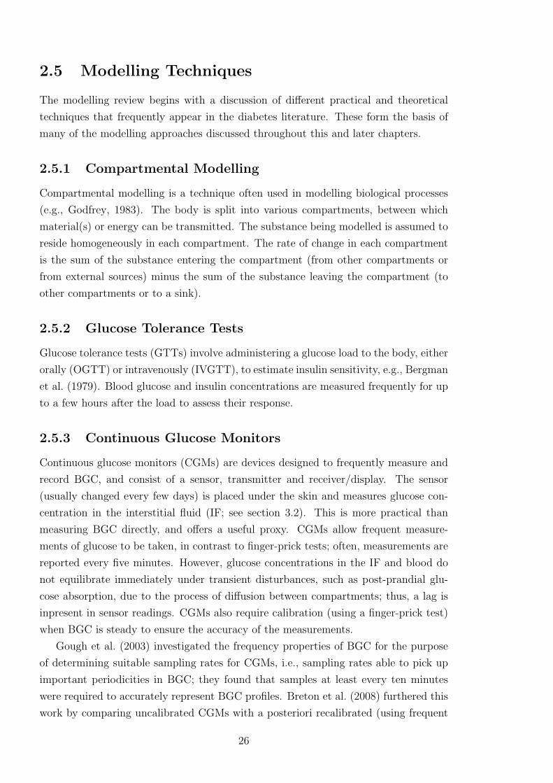
2.5 Modelling Techniques
The modelling review begins with a discussion of different practical and theoretical
techniques that frequently appear in the diabetes literature. These form the basis of
many of the modelling approaches discussed throughout this and later chapters.
2.5.1 Compartmental Modelling
Compartmental modelling is a technique often used in modelling biological processes
(e.g., Godfrey, 1983). The body is split into various compartments, between which
material(s) or energy can be transmitted. The substance being modelled is assumed to
reside homogeneously in each compartment. The rate of change in each compartment
is the sum of the substance entering the compartment (from other compartments or
from external sources) minus the sum of the substance leaving the compartment (to
other compartments or to a sink).
2.5.2 Glucose Tolerance Tests
Glucose tolerance tests (GTTs) involve administering a glucose load to the body, either
orally (OGTT) or intravenously (IVGTT), to estimate insulin sensitivity, e.g., Bergman
et al. (1979). Blood glucose and insulin concentrations are measured frequently for up
to a few hours after the load to assess their response.
2.5.3 Continuous Glucose Monitors
Continuous glucose monitors (CGMs) are devices designed to frequently measure and
record BGC, and consist of a sensor, transmitter and receiver/display. The sensor
(usually changed every few days) is placed under the skin and measures glucose con-
centration in the interstitial fluid (IF; see section 3.2). This is more practical than
measuring BGC directly, and offers a useful proxy. CGMs allow frequent measure-
ments of glucose to be taken, in contrast to finger-prick tests; often, measurements are
reported every five minutes. However, glucose concentrations in the IF and blood do
not equilibrate immediately under transient disturbances, such as post-prandial glu-
cose absorption, due to the process of diffusion between compartments; thus, a lag is
inpresent in sensor readings. CGMs also require calibration (using a finger-prick test)
when BGC is steady to ensure the accuracy of the measurements.
Gough et al. (2003) investigated the frequency properties of BGC for the purpose
of determining suitable sampling rates for CGMs, i.e., sampling rates able to pick up
important periodicities in BGC; they found that samples at least every ten minutes
were required to accurately represent BGC profiles. Breton et al. (2008) furthered this
work by comparing uncalibrated CGMs with a posteriori recalibrated (using frequent
26

finger-prick tests) measurements, and highlighted the different frequency properties
of blood and interstitial glucose, suggesting frequent calibrations were necessary to
accurately determine BGC.
Klonoff (2005) discuss in detail the testing, problems and benefits of CGMs. In
particular, they note the reluctance of insurance companies or governments to fund
CGMs. However, Tamborlane et al. (2008) report improvements in HbA1c when using
continuous monitors.
2.5.4 Percentage of Maximal Oxygen Consumption
VOmax2 represents an individual’s maximal oxygen consumption, usually determined in
a clinical setting by incremental exercise on a treadmill or stationary bicycle. PVOmax2
represents relative intensity of exercise as a percentage of VOmax2 . Oxygen consumption
is approximately proportional to the work done by the body, so PVOmax2 provides a
measure of how hard the body is working and can be used as a method of quantifying
exercise intensity.
2.6 Diabetes Modelling
Some of the earliest work in the diabetes modelling literature was dedicated to describ-
ing blood glucose-insulin dynamics using compartmental models. These models were
generally used for estimating insulin sensitivity and glucose effectiveness (the ability
of blood glucose to suppress endogenous glucose production and encourage blood glu-
cose uptake). More recently, advances in technology have presented the opportunity
for an artificial pancreas (section 2.6.5), and contemporary literature has focused on
designing the control algorithm component. Many control algorithms rely on whole-
body models describing glucose-insulin dynamics; such models have built on the early
compartmental models to include the effect of digestion, insulin injection and physical
activity.
2.6.1 Glucose-Insulin Dynamics: Bergman’s Minimal Model
One of the earliest models of glucose-insulin dynamics was developed in a series of pa-
pers by Bergman and colleagues (Bergman et al., 1979; Toffolo et al., 1980; Bergman
et al., 1981). They proposed the minimal model (MM) based on results from IVGTTs.
The model was tailored for clinical use by providing a non-invasive method for esti-
mating insulin sensitivity. The MM consists of compartments for blood glucose, blood
insulin and “remote” (or active) insulin, with concentrations denoted by G, Ip and Ia,
respectively, and compartments representing the liver and the periphery; the model
structure is given in Figure 2.4. The remote insulin compartment distinguished the
27
MM from previous models, e.g., Bolie, 1961, by removing the assumption that glucose
metabolism was dependent on blood insulin. Instead, blood insulin must first enter the
remote compartment before effecting its action on blood glucose, hence representing
the process of blood insulin binding to insulin-sensitive cells.
Ip(t) -k2
Ia(t) - (Insulin degradation)k3
G(t)-k5
g -k1
Liver Periphery?
k4
?
k6
Figure 2.4: Minimal model of blood glucose metabolism; G represents BGC, Ip is plasma insulinconcentration, Ia is active insulin concentration and parameters k1, . . . , k6 represent rates of exchangebetween compartments. Reproduced from Bergman et al. (1979).
The MM was chosen from a number of contenders posited by Bergman et al. (1979),
based on its parsimonious nature and the identifiability and physiological meaning of
parameters. The model describes the relationship between blood glucose, blood insulin
and insulin action. Insulin action is given by X(t) = (k4 + k6)Ia(t), and represents the
effect of insulin in the remote compartment on blood glucose uptake. The model is
described by a pair of differential equations:
G(t) = [p1 −X(t)]G(t) + p4
X(t) = p2X(t) + p3Ip(t),(2.6.1)
where model parameters p1, . . . , p4 are described in Table 2.5. Glucose effectiveness is
given by p1, and insulin sensitivity is given by −p3/p2.
Table 2.5: Parameters of the minimal model.
Relationship Descriptionp1 = −(k1 + k5) Rate constant of insulin-independent glucose uptakep2 = −k3 Rate of decreasing ability to uptake glucosep3 = k2(k4 + k6) Rate constant of insulin-dependent glucose uptakep4 = H0 Hepatic balance extrapolated to zero BGC
The rate of change of glucose is derived from the difference between hepatic glucose
balance, H, and peripheral uptake, U :
G = H − U,
28

where hepatic balance is determined by
H = H0 − (k5 + k6Ia)G,
and peripheral glucose uptake is determined by insulin-dependent and -independent
rates of uptake,
U = (k1 + k4Ia)G.
The model was later appended (Toffolo et al., 1980; Bergman et al., 1981) with a third
differential equation describing blood insulin:
I(t) = p5(G(t)− p6)t− p7I(t), (2.6.2)
where p5 is the rate of insulin release by β-cells, p6 is the threshold of glucose above
which this release begins, and p7 is the rate constant of insulin degradation.
Parameter estimation of the MM requires two stages: first, a known insulin time
course is supplied to (2.6.1) to estimate the parameters p1, . . . , p4, and second, a glucose
time course is supplied to estimate parameters in (2.6.2). De Gaetano and Arino (2000)
note that considering the MM as a complete system results in unrealistic behaviour.
The authors instead propose a “dynamic model”, which retains most features of the
minimal model but allows simultaneous estimation of all parameters. Andersen and
Højbjerre (2005) presented a Bayesian approach to overcome issues with full model
parameter estimation. They extended their Bayesian network to a population-based
model.
Various works (e.g. Regittnig et al., 1999; Cobelli et al., 1998, 1999) argue the min-
imal model is too simplistic, leading to poor estimates of insulin sensitivity. A second
glucose compartment was suggested to account for differences in glucose concentration
between blood and slowly-equilibrating tissue during glucose disturbances. An example
of such a model, proposed by Dalla Man et al. (2007), is shown in Figure 2.5; the two
glucose compartments represent glucose masses in the blood and quickly-equilibrating
tissue (Gp) and slowly-equilibrating tissue (Gt), with exchange between glucose com-
partments determined by rates k1 and k2. The extended model of Dalla Man et al.
also represents well the additional considerations needed to tailor the MM for use in
type 1 diabetes and enhance its theoretical plausibility. The model includes glucose
uptake separated into insulin-independent uptake from the plasma (Uii) and insulin-
dependent uptake from tissue (Uid), appearance of glucose from meals (CHO), and
renal clearance of excess glucose (R).
The original MM is further limited by providing only whole body measures of insulin
sensitivity. Hovorka et al. (2001) used an IVGTT to separate the effects of insulin on
glucose, establishing its action on distribution, disposal and production.
29

-HGP?
CHO
Gp
?
R
?
Uii
-k1
k2
Gt
?
Uid
Figure 2.5: Two-compartment glucose subsystem of Dalla Man et al. (2007). Variables and param-eters as described in text.
2.6.2 Glucose-Insulin Dynamics: Other Compartmental Mod-
els
There have been numerous other attempts to model glucose-insulin dynamics, many
building on the work of Bergman and colleagues. As glucose-insulin models have devel-
oped, there has been interest in accounting for external influences, such as meals, and
generalising to the wider diabetes population, by accounting for insulin injections. Hov-
orka (2005a) presents a comprehensive review of models that rely on either infrequent
or continuous blood glucose measurements. It is worth noting that few of the models
reviewed account for physical activity; predominantly, inputs are BGC measurements,
meal intake and insulin type and dose.
Compartmental glucose-insulin models form the foundation of various computer
packages designed for clinicians and patients. Generally these are designed for scenario
analysis, where different insulin regimes may be tested in silico to see the effect on
BGC. The Karlsburger Diabetes Management System (KADIS; Salzsieder et al., 1990;
Salzsieder and Rutscher, 1998) involves subsystems for glucose and insulin linked by
four state variables, blood glucose and insulin concentration, net endogenous glucose
balance, and insulin action equivalent of exercise.
The Automated Insulin Dosage Advisor (AIDA) package (Lehmann and Deutsch,
1991), freely available online2, offers a number of case studies for educational pur-
poses. The model takes into account meal intake, insulin absorption and action,
insulin-independent glucose uptake, net hepatic balance and renal clearance, but fails
to explicitly account for the effects of physical activity.
The Diabetes Advisory System (DIAS; Hejlesen et al., 1997) is structurally similar
to AIDA, but instead models the liver’s uptake and release separately. Again, there is
no description of the effect of exercise. The model has, however, shown some success
in providing advice on insulin dose in modest studies (Cavan et al., 1999). DIAS has
been modified by Arleth et al. (2000) to account for the role of glucose transporters.
2http://www.2aida.net/welcome/, last accessed 17/08/12
30
The revised model differentiates between glucose uptake by muscles and other organs,
which may allow a further extension to account for physical activity.
GlucoSim (Agar et al., 2005) uses the compartmental model developed by Puckett
(1992) as part of an educational simulator. The software allows input for food and
insulin, as well as very limited options for input of physical activity. The simulator
uses the data to produce profiles of blood glucose and insulin for up to 24 hours.
Sorensen (1985) developed a physiological, compartmental model to simulate glu-
cose metabolism in “normal” man, i.e., no diabetes. The model is more comprehensive
than most, comprising lung/heart, brain, gut and kidney compartments in addition to
the liver and periphery, with 19 differential equations describing the model. The model
pancreas was removed in order to simulate type 1 diabetes, allowing development of
a control algorithm for use in closed-loop control. However, removing the pancreas
entirely not only eliminates endogenous insulin secretion but also glucagon secretion,
which is unrealistic. Hepatic glycogen stores are also not considered.
None of the above models account for the role of other hormones (except the
Sorensen model which accounts for glucagon), fatty acids (unlike Roy and Parker
(2006), a model based on the MM) or amino acids. Many models also fail to con-
sider inter- and intra-patient variability.
2.6.3 Glucose-Insulin Dynamics and Physical Activity
Attempts to include physical activity as an input to a glucose-insulin model are gener-
ally presented as extensions of existing glucose-insulin models. Derouich and Boutayeb
(2002) extended Bergman’s minimal model by adding parameters to each of the three
differential equations governing the glucose-insulin system. However, the parameters
do not relate to the intensity and duration of exercise. Roy and Parker (2007) also ex-
tended the minimal model by including terms relating to the changes in insulin removal,
glucose uptake and hepatic release during activity (measured using PVOmax2 ). Parame-
ter estimates are based on fitting the model against data from healthy volunteers. The
DIAS computer package models exercise as insulin action equivalent (Salzsieder and
Rutscher, 1998), but this is physiologically inaccurate as exercise can increase BGC.
Lenart and Parker (2002) and Hernandez-Ordonez and Campos-Delgado (2008)
extended Sorensen’s physiological model to account for physical activity. Energy ex-
penditure was measured using PVOmax2 as well as percentage of active muscle mass.
The model of Lenart and Parker (2002) showed good agreement with BGC data (from
healthy volunteers) for up to 90 minutes of low- and medium-intensity exercise (30%
and 60% PVOmax2 respectively). However, due to unrealistic assumptions, such as infi-
nite hepatic glycogen stores, the model performed poorly after 90 minutes. Hernandez-
Ordonez and Campos-Delgado (2008) extended the Lenart and Parker framework by
31
incorporating glycogen depletion and subsequent replenishment during the next ab-
sorptive stage.
Breton (2008) presented an alternative method for incorporating exercise into the
minimal model. The intensity and duration of exercise is estimated by heart rate, which
is correlated with oxygen uptake, itself correlated with energy expenditure. Thus, heart
rate presents a surrogate measure for energy expenditure that may more realistically
be measured in free-living conditions. The model includes terms for increased glucose
uptake due to physical activity and longer-term changes in insulin action. Dalla Man
et al. (2009) adopt the approach of Breton, testing three models (differing through the
effect of physical activity on insulin-independent glucose uptake and insulin sensitivity)
via simulation. A lack of data hinders the assumptions and conclusions of the model.
An alternative approach to measuring and quantifying physical activity is the use
of recently-developed devices such as the BodyMedia R© armband, which allow activity
data to be collected from free-living conditions with minimal impact on the individual.
Such armbands are able to measure and record a number of different variables, such as
directional accelerations (movement) and skin temperature, and use these to estimate
METs, a measure of energy expenditure relative to resting metabolic rate (discussed
further in chapter 3). Rollins et al. (2008) used such a device to record the activity
of an individual with type 2 diabetes. Data from several variables measured by the
armband were used as inputs in a Wiener model of BGC. Valletta et al. (2009) used
data from a continuous glucose monitor and the armband in a Gaussian process model.
It was found that the assumption of stationarity (constant mean and variance) of BGC
was not correct, hence limiting the accuracy of model predictions.
2.6.4 Empirical Modelling of BGC
Empirical models in diabetes are less prevalent given the problems in collecting relevant,
sufficiently detailed data. Empirical models are particularly restricted by the difficulty
in collecting data relating to internal processes in the body, e.g., the liver is a very
inaccessible organ for the purposes of frequent testing, and hence processes such as
glycogenolysis and gluconeogenesis are difficult or impossible to measure. Empirical
models have thus been reliant on those variables that can be easily and safely measured,
which itself has been limited until recent technological advances in CGMs.
One of the few data-true approaches to investigating insulin sensitivity was proposed
by Marmarelis (2004). The methods are based on Volterra models, using principal
dynamic mode (PDM) formulation; two PDMs were obtained to represent glucolepsis
and glucogenesis (Marmarelis, 2004, section 6.4), where glucolepsis is defined as the
insulin-assisted glucose uptake and glucogenesis as the production of glucose due to
increased insulin.
32

Empirical models based on BGC measurements in standard treatment regimes are
restricted due to the infrequent nature of testing. Bellazzi et al. (1999) used Bayesian
analysis to determine trends and daily patterns for BGC measured only a few times
per day. The model is a burden computationally, meaning real-time analysis is not
possible. Yamaguchi et al. (2006) used data mining to predict fasting BGC and trend
fluctuations for morning BGC.
The development of CGMs allows for more frequent measurements of BGC. Bremer
and Gough (1999) investigated the behaviour of BGC from a number of studies using
frequent sampling. BGC data from individuals with type 1 diabetes was seen to be
nonstationary (non-constant mean and variance). Nonstationarity implies some form
of temporal dependency between observations and presents problems for many conven-
tional time series analysis. Differencing the data (subtracting successive observations)
removed much of the nonstationarity in the mean, and the newly-created variable was
used to construct autoregressive models; the linear models were unable to accurately
predict over even relatively short time periods (30 minutes). Sparacino et al. (2007),
however, showed that even a simple first-order polynomial or first-order autoregres-
sive model could predict hypoglycaemic episodes 30 minutes in advance using a CGM.
Model parameters were allowed to vary in time to compensate for the nonstationarity
of BGC.
2.6.5 Artificial Pancreas
The artificial pancreas (AP) represents the end goal of much diabetes research, as it can
automate the process of maintaining euglycaemia. Figure 2.6 shows the conceptual ba-
sis of an AP, where a CGM relays information to a control algorithm that subsequently
determines the release of insulin from a pump.
Much work has been dedicated to developing a control algorithm to be used as part
of an AP. The control algorithm aims to minimise the difference between measured
and reference (or target) BGC. Control algorithms are designed only for short-term
prediction, often employing receding horizon control. Many control algorithms also
rely on dynamic models of the process(es) to be controlled, hence the continued interest
in models of blood glucose dynamics such as those described in the previous sections.
Various control methods have been proposed, and what follows is a very brief
overview of more recent approaches:
• proportional-derivative-integral control (PID), e.g., Gantt et al. (2007) use
a PI controller with asymmetric cost function to punish hypoglycaemia more than
hyperglycaemia; Marchetti et al. (2008) use a PID controller with feed-forward
component to announce meals and help limit post-prandial peaks in BGC;
• model predictive control (MPC), e.g., Abu-Rimleh and Garcia-Gabin (2010)
33

PumpInsulin
6
InsulinSubcutaneous -
GlucoseBlood -
MonitorGlucose
?
ModelGlucose
AlgorithmControl
Figure 2.6: Basic structure of artificial pancreas
use multiple MPCs to deal with the nonlinearities of the glucoregulatory system;
Lee and Bequette (2009) use meal detection and meal size estimation algorithms
to deal with unannounced meals; Hovorka et al. (2004) use nonlinear MPC; Soru
et al. (2012) use MPC with a focus on an individualised control algorithm;
• adaptive control, e.g., Eren-Oruklu et al. (2009) use an empirical approach
using an autoregressive moving average (ARMA) model. Linear, low-order mod-
els are fitted as it is assumed that nonlinearities are rendered less significant by
frequent glucose measurements;
• pseudo self-evolving cerebellar model algorithm controller (PSECMAC),
e.g., Teddy et al. (2010) use the PSECMAC network, a computational model of
the human cerebellum (part of the brain), to capture the dynamics of a healthy
insulin secretion profile;
• H∞ control, e.g., Parker et al. (2000) suggest the method is particularly ro-
bust by accounting for intra-patient variability and meal disturbances; Quiroz
and Femat (2010) use H∞ theory to design a controller with biosignals to indi-
cate exercise disturbance (via the relationship between glucose and lactate) and
hypoglycaemia (via the relationship between glucose and adrenaline);
• run-to-run strategy, e.g., Palerm et al. (2008) suggest a variable basal insulin
infusion rate to account for changes in insulin sensitivity, with emphasis on clinical
heuristics to design the strategy.
More detailed explanation of these methods may be found in the respective references.
Further discussion may also be found in the various reviews of approaches to the AP in
the literature, e.g., Naylor et al. (1995) on the risks and challenges of an artificial pan-
creas, El Youssef et al. (2009) on the history of closed-loop control algorithms, Bellazzi
et al. (2001) on closed- and partially closed-loop strategies for subcutaneous insulin de-
livery, Parker et al. (2001) on closed-loop, intravenous insulin delivery, Kameth et al.
(2006) on open- and closed-loop, feed-forward and feed-back approaches, and Hovorka
(2005b) on approaches for frequent and infrequent BGC measurements.
34

The main problem regarding an AP is safety; any algorithm must be able to main-
tain euglycaemia during disturbances such as meals and exercise, which has yet to be
demonstrated in free-living individuals. The majority of control algorithms have only
been tested on data derived from the compartmental models previously described, pre-
dominantly the Hovorka et al. (2001) model (and the extension of Wilinska et al.,
2005), and hence remain untested on the stimuli individuals experience in a free-living
environment.
2.7 Modelling Review: Summary
The section presented a review of literature relevant to the current work. The review
has highlighted a gap in the literature regarding modelling BGC using free-living data;
in particular, compartmental models have not been tested using data that better reflects
the real experiences of people in day-to-day life. Furthermore, empirical models that do
not require simplified compartmental models of the human body are limited in number,
due to the practical difficulties in collecting relevant data.
35

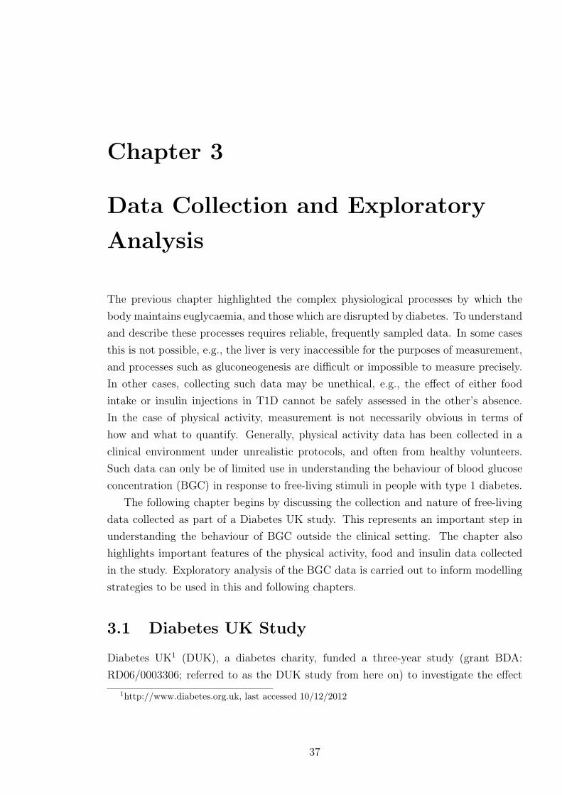
Chapter 3
Data Collection and Exploratory
Analysis
The previous chapter highlighted the complex physiological processes by which the
body maintains euglycaemia, and those which are disrupted by diabetes. To understand
and describe these processes requires reliable, frequently sampled data. In some cases
this is not possible, e.g., the liver is very inaccessible for the purposes of measurement,
and processes such as gluconeogenesis are difficult or impossible to measure precisely.
In other cases, collecting such data may be unethical, e.g., the effect of either food
intake or insulin injections in T1D cannot be safely assessed in the other’s absence.
In the case of physical activity, measurement is not necessarily obvious in terms of
how and what to quantify. Generally, physical activity data has been collected in a
clinical environment under unrealistic protocols, and often from healthy volunteers.
Such data can only be of limited use in understanding the behaviour of blood glucose
concentration (BGC) in response to free-living stimuli in people with type 1 diabetes.
The following chapter begins by discussing the collection and nature of free-living
data collected as part of a Diabetes UK study. This represents an important step in
understanding the behaviour of BGC outside the clinical setting. The chapter also
highlights important features of the physical activity, food and insulin data collected
in the study. Exploratory analysis of the BGC data is carried out to inform modelling
strategies to be used in this and following chapters.
3.1 Diabetes UK Study
Diabetes UK1 (DUK), a diabetes charity, funded a three-year study (grant BDA:
RD06/0003306; referred to as the DUK study from here on) to investigate the effect
1http://www.diabetes.org.uk, last accessed 10/12/2012
37
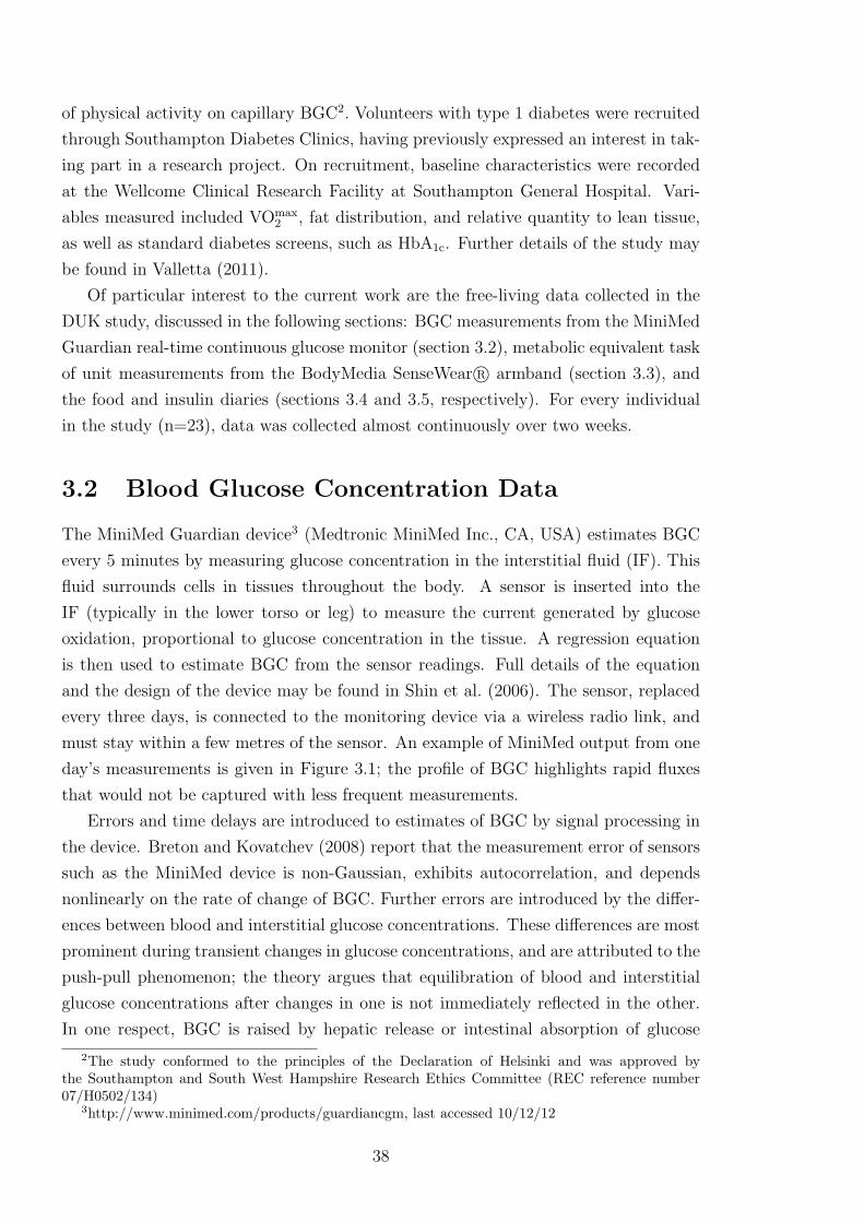
of physical activity on capillary BGC2. Volunteers with type 1 diabetes were recruited
through Southampton Diabetes Clinics, having previously expressed an interest in tak-
ing part in a research project. On recruitment, baseline characteristics were recorded
at the Wellcome Clinical Research Facility at Southampton General Hospital. Vari-
ables measured included VOmax2 , fat distribution, and relative quantity to lean tissue,
as well as standard diabetes screens, such as HbA1c. Further details of the study may
be found in Valletta (2011).
Of particular interest to the current work are the free-living data collected in the
DUK study, discussed in the following sections: BGC measurements from the MiniMed
Guardian real-time continuous glucose monitor (section 3.2), metabolic equivalent task
of unit measurements from the BodyMedia SenseWear R© armband (section 3.3), and
the food and insulin diaries (sections 3.4 and 3.5, respectively). For every individual
in the study (n=23), data was collected almost continuously over two weeks.
3.2 Blood Glucose Concentration Data
The MiniMed Guardian device3 (Medtronic MiniMed Inc., CA, USA) estimates BGC
every 5 minutes by measuring glucose concentration in the interstitial fluid (IF). This
fluid surrounds cells in tissues throughout the body. A sensor is inserted into the
IF (typically in the lower torso or leg) to measure the current generated by glucose
oxidation, proportional to glucose concentration in the tissue. A regression equation
is then used to estimate BGC from the sensor readings. Full details of the equation
and the design of the device may be found in Shin et al. (2006). The sensor, replaced
every three days, is connected to the monitoring device via a wireless radio link, and
must stay within a few metres of the sensor. An example of MiniMed output from one
day’s measurements is given in Figure 3.1; the profile of BGC highlights rapid fluxes
that would not be captured with less frequent measurements.
Errors and time delays are introduced to estimates of BGC by signal processing in
the device. Breton and Kovatchev (2008) report that the measurement error of sensors
such as the MiniMed device is non-Gaussian, exhibits autocorrelation, and depends
nonlinearly on the rate of change of BGC. Further errors are introduced by the differ-
ences between blood and interstitial glucose concentrations. These differences are most
prominent during transient changes in glucose concentrations, and are attributed to the
push-pull phenomenon; the theory argues that equilibration of blood and interstitial
glucose concentrations after changes in one is not immediately reflected in the other.
In one respect, BGC is raised by hepatic release or intestinal absorption of glucose
2The study conformed to the principles of the Declaration of Helsinki and was approved bythe Southampton and South West Hampshire Research Ethics Committee (REC reference number07/H0502/134)
3http://www.minimed.com/products/guardiancgm, last accessed 10/12/12
38
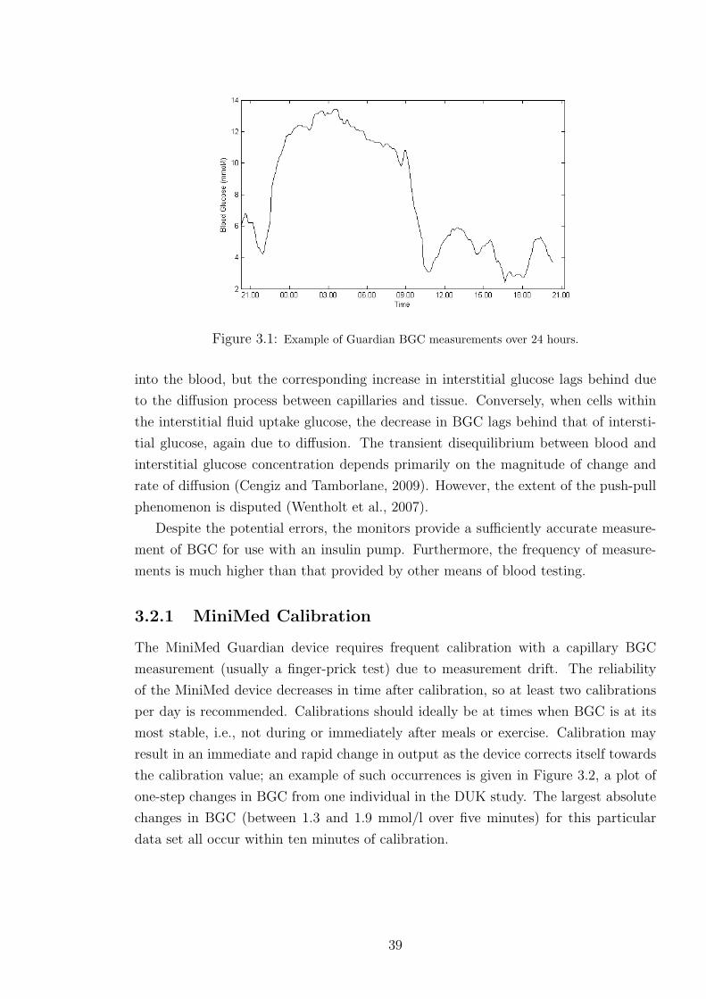
Figure 3.1: Example of Guardian BGC measurements over 24 hours.
into the blood, but the corresponding increase in interstitial glucose lags behind due
to the diffusion process between capillaries and tissue. Conversely, when cells within
the interstitial fluid uptake glucose, the decrease in BGC lags behind that of intersti-
tial glucose, again due to diffusion. The transient disequilibrium between blood and
interstitial glucose concentration depends primarily on the magnitude of change and
rate of diffusion (Cengiz and Tamborlane, 2009). However, the extent of the push-pull
phenomenon is disputed (Wentholt et al., 2007).
Despite the potential errors, the monitors provide a sufficiently accurate measure-
ment of BGC for use with an insulin pump. Furthermore, the frequency of measure-
ments is much higher than that provided by other means of blood testing.
3.2.1 MiniMed Calibration
The MiniMed Guardian device requires frequent calibration with a capillary BGC
measurement (usually a finger-prick test) due to measurement drift. The reliability
of the MiniMed device decreases in time after calibration, so at least two calibrations
per day is recommended. Calibrations should ideally be at times when BGC is at its
most stable, i.e., not during or immediately after meals or exercise. Calibration may
result in an immediate and rapid change in output as the device corrects itself towards
the calibration value; an example of such occurrences is given in Figure 3.2, a plot of
one-step changes in BGC from one individual in the DUK study. The largest absolute
changes in BGC (between 1.3 and 1.9 mmol/l over five minutes) for this particular
data set all occur within ten minutes of calibration.
39

Figure 3.2: Example of the one-step change in BGC time series, with times of calibration, for anindividual in the DUK study.
3.3 Physical Activity Data
The SenseWear R© armband (BodyMedia Inc., PA, USA) measures a number of physio-
logical variables, listed in Table 3.1, and uses these to estimate metabolic equivalent of
task (METs, kcal/kg/hr). METs provide a person-specific measure of energy expendi-
ture as a multiple of resting metabolic rate (RMR). RMR is the energy expenditure at
rest (at room temperature and in a post-absorptive state), and represents the energy
required to maintain function of the vital organs. The armband estimates METs using
a proprietary algorithm that has been validated in numerous studies4 against the gold-
standard of indirect calorimetry (which uses oxygen uptake as a surrogate for calories
burnt). Measurements from the armband are recorded every minute in the DUK study.
Examples of METs for different activities are given in Table 3.2.
A series of papers (Liden et al., 2002, 2001; Sunseri et al.) detail the components
of the device and their respective functions. The papers demonstrate the device’s
reliability and repeatability, as well as the practical advantages of the device compared
to other methods for determining energy expenditure. In particular, the design of
the device allows it to be worn continuously (except in wet conditions) with minimal
impact on the mobility of the individual, meaning free-living data can be measured.
This is particularly important for the applicability of the results from this study to
4review available from http://www.bodymedia.com/Professionals/Whitepapers/The-Development-of-the-SenseWear-armband, last accessed 06/08/12
40

Table 3.1: Variables recorded by the SenseWear armband.Variable DescriptionMetabolic equivalent of task(METs)
Measure of energy expenditure
Transverse acceleration aver-age (TAA)
Measured by two-axis accelerometer and providesinformation on body position and movement (av-erage over time interval)
Transverse accelerationmean absolute deviation(TAM)
As above but records mean absolute deviation
Transverse accelerationpeaks (TAP)
As above but records peak during time interval
Longitudinal acceleration av-erage
Measurement perpendicular to TAA
Longitudinal accelerationmean absolute deviation
As above but for TAM
Longitudinal accelerationpeaks
As above but for TAP
Near body temperature Average ambient temperature
Skin temperature Average temperature of the skin
Heat flux Heat dissipated by the body (average) along aconductive path between skin and vent in thearmband
Galvanic skin resistance Measures conductivity of the skin using two sen-sors; relates to physical and emotional stimuli
Table 3.2: Examples of approximate METs for various activities; values taken from Ainsworth et al.(2000).
Activity METsSleeping 0.9Lying down 1Walking (2mph) 2.5Bicycling (general) 8Running (6-10mph) 10-16
41
the wider population. Older versions of the device have been shown to underestimate
certain types of exercise (Crawford, 2004), though this limitation has been overcome
to a great extent by the use of exercise-specific algorithms.
Examples of armband data captured from a volunteer are given in Figures 3.3 and
3.4. The first figure shows skin temperature over a 24-hour period, with drops after
activity due to sweating, and longitudinal acceleration, which is relatively stable during
the night when the individual is asleep. The second figure shows the highly variable
nature of METs, which fluctuates rapidly during the day but is relatively stable during
the night. Such behaviour is relatively typical of other individuals in the DUK study;
patterns and magnitudes vary, but METs is always highly variable during waking hours.
Figure 3.3: Activity armband output over a 24-hour period for an individual in the DUK study: (i)skin temperature; (ii) longitudinal acceleration.
Figure 3.4: Metabolic equivalent units (METs) over a 24-hour period for an individual in the DUKstudy.
42
3.4 Food Diary
Food intake was recorded in a diary by each participant in the DUK study. The type
and amount of food was recorded, as well as time of consumption, and subsequently
the nutritional content was estimated using either reported nutritional information
or food databases (Kellow et al., 2007). The process is subject to intra- and inter-
patient variable errors with regard to potential non-reporting of food consumption
and estimating portion size; however, many individuals with type 1 diabetes have had
training for carbohydrate counting, and are thus experienced in such matters. The
method of data collection is appropriate in terms of the applicability of this study’s
outcomes to the wider type 1 diabetes population, who generally use carbohydrate
counting as part of the MDI regime.
The food intake data from the DUK study offer no dynamical description of how
food intake affects BGC. A model of the digestive process may be used to better
represent how food intake effects BGC.
3.4.1 Modelling the Digestive System
The breakdown of food begins in the mouth and continues via the oesophagus and
stomach until the food is in a suitable form (i.e., relatively small molecules such as
glucose) to be absorbed from the intestines into the blood. Jenkins et al. (1981)
described the concept of the glycaemic index, which is used to group foods that display
similar effects on BGC (depending on rate of absorption). However, Worthington
(1997) argues that there are several fundamental flaws, in particular that the index
offers no dynamical description of the rate of appearance of glucose in the blood after
food intake. As such, a simple one-compartmental model was proposed, albeit one
validated against a single individual and for only two foods. The model involves two
parameters specific to food, the glycaemic value (ratio of glucose weight to total food
weight) and fractional turnover rate (related to rate-limiting metabolic processes).
Lehmann and Deutsch (1992) proposed a more comprehensive model for the diges-
tive system, which will be used in the current work. The model converts carbohydrate
consumed into a profile of glucose absorption from the gut. The rate of change of
glucose in the gut is described by
d(Ggut)
dt= Gempt − kabsGgut (3.4.1)
43

where Gempt is the rate of gastric emptying and kabs is the rate constant of glucose
absorption into the blood. Gastric emptying is modelled as a trapezoidal function:
Gempt =
kmax
Tasct, for t < Tasc
kmax, Tasc < t ≤ Tasc + Tmax
kmax − kmax
Tdes(t− Tasc − Tmax), Tasc + Tmax ≤ t < Tmax
+Tasc + Tdes
0, otherwise,
(3.4.2)
with
kmax =2D
Tasc + 2Tmax + Tdes
. (3.4.3)
Parameter values, units and descriptions are given in Table 3.3. The duration of the
maximal gastric emptying (Tmax) is defined as a function of the carbohydrate ingested,
but is zero when the amount of carbohydrate is small (emptying is a triangular function
in this case). The rate of gastric emptying increases in proportion to the amount of
carbohydrate consumed, before reaching the maximal (and constant) rate of emptying.
Once almost all of the carbohydrate has been consumed, the rate begins to slow.
Glucose absorption through the intestinal tract, Gin, is assumed to be linear and is
given by
Gin = kabsGgut. (3.4.4)
Further description of these parameters and their relationships is given in Lehmann
and Deutsch (1992).
Table 3.3: Parameters of the Lehmann and Deutsch (1992) digestion model.Parameter Value Descriptionkabs 1 h−1 Rate constant of glucose absorption from the gutkmax 120 mmol/h Maximal rate of gastric emptyingTasc 0.5 h Duration of ascending gastric emptyingTdes 0.5 h Duration of descending gastric emptyingTmax h Duration of maximal gastric emptyingt h Time since start of meal
The estimated carbohydrate intake from the food diaries in the DUK study may
be input to the model (as D) to estimate profiles of post-prandial glucose absorption
in to the blood; Figure 3.5 shows recorded carbohydrate consumption and estimated
glucose absorption every five minutes over a 24-hour period for one individual as an
example of the digestion model’s function. The large peaks correspond to meals, and
smaller peaks to snacks.
The Lehmann and Deutsch (1992) digestion model is physiologically incorrect as it
treats the digestive process as a single stage process, when it is really biphasic (Siegel
44

Figure 3.5: Estimated glucose absorption over a 24-hour period for one individual in the DUK studyusing the Lehmann and Deutsch model.
et al., 1988). Dalla Man et al. (2006) tested the above model against a newly-proposed
nonlinear model, and found their model better described data from OGTT and mixed
meals in volunteers with varying glucose tolerance; however, differences between model
estimations were not substantial. The Lehmann and Deutsch (1992) model has been
used in various other models in the literature, e.g., Wong et al. (2009), due to its
parsimonious nature and ease of use.
3.5 Insulin Diary
Volunteers in the DUK study also recorded information regarding each insulin injec-
tion, specifically time of injection, dose, and type of insulin. As with the food diaries,
these records offer no dynamical description of the effect of insulin on BGC. Under-
standing the behaviour of blood insulin concentration requires frequent blood samples
and specialist equipment, and is hence not feasible in free-living conditions. A model
describing the process of insulin absorption can provide an alternative to invasive blood
samples, by offering important information on the appearance of insulin in the blood.
45
3.5.1 Modelling Insulin Injection
A model of insulin absorption must be able to capture the differing absorption profiles
for the various types of insulin used in diabetes care. Short/rapid-acting insulin, usually
taken with food, is absorbed quickly after injection but may only act for up to four
hours, while longer-lasting insulin may last beyond 24 hours to provide basal release
of insulin throughout the day. Nucci and Cobelli (2000) provide a critical review of
a number of proposed models for insulin kinetics; generally, compartmental models
are favoured, often with two compartments corresponding to subcutaneous tissue and
blood. The review pinpointed two models that performed well, notably the model
described by Trajanoski et al. (1993). This model is an extension of that by Mosekilde
et al. (1989), and has itself been extended by Tarin et al. (2005). The latter presents
a generic model that is able to describe insulin absorption for a number of different
insulin types, in particular glargine, whose long-lasting, peakless action has not been
well described by other models; hence, this model is used in the current work.
Mosekilde et al. (1989), and their modelling descendants, assume that insulin re-
sides in the subcutaneous tissue in dimeric, hexameric (according to molecular weight)
and immobile, bound states. The model divides tissue into rings around the point of
injection, into which the insulin diffuses. Tarin et al. (2005) changed the role of the
bound state, allowing insulin in this state to break up into the hexameric form at a
rate proportional to the concentration of the bound state.
The relationships between the three states of insulin in Tarin et al. (2005) are
described by a series of coupled differential equations, which account for diffusion,
hexameric-dimeric dissociation, bound-hexameric conversion and absorption of dimeric
insulin:
δcd(t, r)
δt= P (ch(t, r)−Qcr(t, r)3)−Bdcd(t, r) +D∆2cd(t, r)
δch(t, r)
δt= −P (ch(t, r)−Qcd(t, r)3) + κcb(t, r)(ch,max − ch(t, r))
+D∆2ch(t, r) (3.5.1)
δcb(t, r)
δt= −κcb(t, r)(ch,max − ch(t, r)) + dbD∆2cb(t, r),
where parameters are described in Table 3.4. Exogenous insulin flow in to the blood,
Iex(t), is then given by
Iex(t) = Bd
∫Vsc
cd(t, r) dV, (3.5.2)
where Vsc is the volume of the subcutaneous tissue. The integrand involves only the
cd term, as only insulin in the dimeric state is assumed to pass into the blood. The
equations given in (3.5.1) have no closed-form solution, so they must be discretised in
time and space (the full equations are given in Tarin et al., 2005). The Tarin et al.
46
model has been used throughout the diabetes literature, e.g., by the computer package
AIDA (Lehmann et al., 2007).
Table 3.4: Parameters of the Tarin et al. (2005) insulin model.Parameter Descriptioncd dimeric insulin concentrationch hexameric insulin concentrationcb bound insulin concentrationP dimeric production rateQ hexameric-dimeric equilibrium constantBd absorption rate of dimeric insulinD diffusion constantκ bound-hexameric conversion factorch,max bound-hexameric saturation constantdb reduction factor for diffusion constant of bound state
The insulin records of volunteers in the DUK study may be input to the model
to estimate the profile of insulin absorption in to the blood. An example using one
individual’s insulin records is given in Figure 3.6, with estimates found every five
minutes. The plot shows the profiles of two types of insulin: that of long-lasting insulin
glargine, whose peakless action can last up to 26 hours to provide a basal release of
insulin for low-level glucose metabolism, and that of short-acting insulin Novorapid,
whose relatively quick action lasts only a few hours to compensate for post-prandial
glucose absorption.
The profiles of estimated glucose and insulin absorption, for one individual over a 24-
hour period, are given together in Figure 3.7. The plot shows peaks for the absorption
of short-acting insulin just before peaks of glucose absorption. This highlights the
delayed effect of blood insulin on BGC, as insulin must first bind to receptors on cells
before effecting their action. The plot also shows the action of long-lasting insulin
overnight when no food is consumed.
3.6 Modelling Limitations
The Lehmann and Deutsch (1992) digestion model and Tarin et al. (2005) insulin
absorption model (referred to as the digestion model and insulin model, respectively,
from here on) are approximations to complex biological processes and introduce errors
due to various simplifications:
i) neither model is subject-specific. They therefore do not differentiate between indi-
viduals who may have different physiological responses to the food and insulin
inputs;
ii) the digestion model does not account for any protein and/or fat consumed, nor the
47

Figure 3.6: Estimated insulin absorption over a 24-hour period for one individual in the DUK studyusing the Tarin et al. model.
Figure 3.7: Glucose and insulin absorption over a 24-hour period for one individual in the DUKstudy using the Lehmann and Deutsch and Tarin et al. models, respectively.
48

GI of the food. This may lead to under- or over-estimation of the rate of glucose
appearance;
iii) the digestion model does not account for the biphasic nature of the digestive pro-
cess. This may lead to poor estimation for the non-linear gastric emptying of
liquids;
iv) the insulin model does not take into account injection site (position or quality).
Hence it may under- or over-estimate the appearance and amount of insulin in
the blood.
Despite these limitations, it is believed that the models provide important information
on how ingested carbohydrate and injected insulin appear in the blood, and hence
affect BGC. Such information is beyond that provided by the raw data recorded in the
food and insulin diaries.
3.7 Data Collection: Summary
The data collected in the DUK study drive the current project and its objectives.
Food intake, insulin and physical activity represent the three major external factors
affecting BGC, and the data and modelling approaches presented here allow analysis
of uninterrupted time series over several days, on a range of individuals. The data
can be used to build the most detailed empirical model of BGC yet, for descriptive
and predictive purposes. This would ideally be able to provide accurate BGC profiles
given the inputs of food, insulin and activity, and thus be appropriate for use within
the MDI treatment regime. Furthermore, many of the more complex, compartmental
models that claim to account for physical activity are based on only very simplified
descriptions of physical activity. The current work aims to test how such models
perform when supplied with free-living data.
The remainder of the chapter uses simple time series methods to explore the DUK
data, with the aim of better understanding the behaviour of blood glucose and soliciting
useful information that may inform or supplement more complex models.
3.8 Time Series Methods
The nature of BGC is such that neighbouring observations are highly correlated, and
may not be considered independent (Bremer and Gough, 1999). In such cases, time
series methods are preferred to standard statistical regression. In the following section,
basic descriptive techniques for time series data are described. The remainder of the
chapter uses such techniques to explore BGC data from the DUK study. Understanding
49
the nature of BGC can aid the modelling process, e.g., BGC may exhibit circadian
behaviour (naturally occurring oscillations), or short- and/or long-term correlation
that can be accounted for in a more comprehensive model. Given the limited amount
of free-living data in the diabetes literature, the exploratory analysis offers an insight
to the behaviour of BGC outside the clinical environment.
3.8.1 Stochastic Processes
A stochastic, or random, process is the collective name for time series which involve
some non-deterministic form. An observed time series, y1, ..., yn = yt, can be consid-
ered to be one realisation of a series of random variables, Y1, ..., Yn = Yt (the notation
here applies to a series considered at discrete time intervals only). The series yt is
therefore considered to be a sample from the population of all possible observable time
series, known as the ensemble. Rather than using sample properties to make infer-
ences upon the population, it is the properties of the probabilistic model underlying
the process that are of interest.
A stochastic process is said to be strictly stationary when the joint distribution of
a time series does not change in time. This is often formally expressed in terms of the
joint cumulative distribution, FY (Tong, 1993):
for any t1, ..., tn, with n ∈ N, and any k ∈ Z
FYt1 ,Yt2 ,...,Ytn(y1, y2, . . . , yn) = FYt1+k,Yt2+k,...,Ytn+k
(y1, y2, . . . , yn).
A process is weakly stationary if the first two moments of the joint distribution (de-
scribed in section 3.8.2.1) are constant in time. This less restrictive definition is gener-
ally sufficient to study other properties of a process. Analysis of stationary time series
is well-established (e.g., Chatfield, 1992; Priestley, 1981). Often, where possible, non-
stationary time series are subject to certain techniques to make the series stationary,
e.g., see section 3.8.2.4.
3.8.2 Stochastic Processes in the Time Domain
Analysis in the time domain relates to studying functions with respect to time, as
opposed to the frequency domain (as described in section 3.8.4). The joint distribution
of Yt is one method of describing a process over time, but will generally be too
complex to handle. An alternative is to instead consider only the first two moments of
the distribution. This is generally sufficient to explore the properties of a time series.
50

3.8.2.1 Autocovariance and Autocorrelation
The mean, variance and autocovariance describe the first two moments of a time se-
ries, where the mean and variance are the standard functions relating to expectations.
Autocovariance is the covariance of a time series with itself at different time lags, and
is given by
γk = γ(Yt, Yt+k) = E[(Yt − E[Yt])(Yt+k − E[Yt+k])
]. (3.8.1)
This may be used to determine the autocorrelation coefficient at lag k:
ρk = γk/γ0, (3.8.2)
where γ0 is the variance of the time series. The autocorrelation is a measure of the linear
association between Yt and Yt+k, and has similar properties to the standard correlation
function, e.g., |ρk| ≤ 1. The correlogram is a plot of the autocorrelation coefficients
as a function of lag k, and can highlight a number of important features of a time
series such as short- and long-term dependence between observations. For a stationary
process, the mean and variance are constant and the autocovariance depends only on
the absolute time difference.
Methods for estimating these functions rely on ergodic theorems. The theorems
show that (in most cases) the sample estimates of the moments converge in mean
square error to the ensemble moments as n → ∞. The theorems are discussed with
regards to the mean and autocovariance in Priestley (1981), with further references
within, and are not considered further here.
3.8.2.2 Simple Stochastic Models
The simplest stochastic model is the purely random series, made up of a sequence of
independent and identically distributed (iid) variables. A process, Yt, is a random walk
if it can be written as Yt = Yt−1 + Zt, where Zt is an iid process. This simple model
forms the basis for the more sophisticated stochastic models described in the following
sections, throughout which it is assumed Zt is an iid process.
3.8.2.3 Autoregressive Moving-Average Models
An autoregressive process of order j, represented by AR(j), is based on a linear com-
bination of the j previous values of the time series:
Yt = α1Yt−1 + α2Yt−2 + . . .+ αjYt−j + Zt. (3.8.3)
Fitting an AR process involves determining a suitable order, j, and estimating the
parameters, αi. The estimated coefficient of an AR(j) process at lag i, αi, is known as
51
the partial autocorrelation, and represents the sample correlation between the variable
and itself at lag i that is not accounted for by lags 1 to i − 1; the plot of i against αi
is the partial autocorrelation function.
A moving average process of order k, represented by MA(k), is based on a linear
combination of a purely random process:
Yt = Zt + β1Zt−1 + . . .+ βkZt−k. (3.8.4)
Again, fitting such a model requires estimating the order, k, and the parameters, βi.The combination of AR and MA models is an ARMA(j, k) model.
3.8.2.4 Extensions of ARMA models
In some cases, non-stationary series can be made stationary by differencing, represented
by the difference operator, ∇:
xt = ∇yt = yt − yt−1, (3.8.5)
and taking d differences gives:
xt = ∇dyt =d∑i=0
(−1)i(d
i
)yt−i. (3.8.6)
An ARMA model applied to data such as xt is an autoregressive integrated moving
average model, represented by ARIMA(j, d, k).
3.8.3 Estimation in the Time Domain
Analysis of the autocorrelation function is referred to as analysis in the time domain.
The sample autocovariance at lag k may be constructed in a similar way to estimating
a population variance from a sample:
γk = ck =1
n
n−k∑t=1
(yt − y)(yt+k − y). (3.8.7)
The divisor n gives this estimator a larger bias compared to n−k (though is asymptot-
ically unbiased), but tends to result in a lower mean square error (Jenkins and Watts,
1968). The sample autocorrelation coefficient at lag k is then given by:
ρk = rk = ck/c0, (3.8.8)
52

where c0 is the (biased) estimator of the variance. One could use the estimator of γk
with smaller bias (i.e., use divisor n− k) but again the estimator with larger bias has
preferable properties, e.g., it ensures that |rk| ≤ 1 (Priestley, 1981).
Theoretically, for a purely random process, ρk = 0, except at lag zero. It can be
shown that asymptotically and under weak conditions (Kendall et al., 1983):
rk ∼ N(−1/n, 1/n), (3.8.9)
with approximate 95% confidence intervals given by:
− 1
n± 2√
n. (3.8.10)
For large n, this may be further approximated by ±2/√n. Autocorrelation coefficients
outside this range suggest non-randomness.
The sample partial autocorrelation coefficients may be determined by fitting AR
models of increasing order. The estimated coefficients can be plotted against order,
with values outside ±2/√n suggesting statistically significant correlation at the 5%
level. A purely AR(j) process will show significant partial correlation up to lag j.
The coefficients of an AR model can be determined using the Yule-Walker equations
(Chatfield, 1992, chapter 3), which use the relationship between the parameters and
autocorrelation function. The equations are given by
ρk = α1ρk−1 + . . .+ αjρk−j, for k ∈ N.
Models of successively higher order may also be compared on some suitable measure;
a general method for aiding model selection is Akaike’s Information Criterion (AIC),
which allows comparison of models using the maximised likelihood (L) and a penalty
for including more parameters (p):
AIC(p) = −2 ln(L) + 2p. (3.8.11)
Lower values indicate a preferable model.
3.8.4 Stochastic Processes in the Frequency Domain
To complement analysis in the time domain, the frequency properties of a series may
be analysed. This is called analysis in the frequency domain (or spectral analysis, or
harmonic analysis) and is based on techniques estimating the spectral density function.
The spectral density function represents the contribution of different frequencies to the
variation in a series. Spectral analysis is based on Fourier analysis, extending its use on
53

deterministic functions of time to stochastic functions. Much theory exists regarding
Fourier and spectral analysis which will not be discussed here; the reader is directed
to Chatfield (1992), Bloomfield (1976), and Priestley (1981) for increasingly detailed
discussions of these techniques.
A key tool in frequency domain analysis is the Fourier transform (FT). This converts
a given function of time, f(t), t ∈ R, in to a function of frequency, F(ω):
F (ω) =
∫ ∞−∞
f(t) exp(−iωt)dt, (3.8.12)
where ω is frequency in radians per unit time. The integral can be considered as a
summation when a time series is observed only at discrete points.
The spectral density function is the Fourier transform of the autocovariance coef-
ficients (Chatfield, 1992, chapter 7). The autocovariance function is an even function,
so the FT may be simplified to:
F (ω) =1
π
[γ0 + 2
∞∑k=1
γk cos(ωk)]. (3.8.13)
The spectral density function uses the same information as the autocovariance function,
but summarises the second-order properties in a different form. By comparing the be-
haviour of a function to sinusoidal curves of different frequencies, important structural
behaviour regarding periodicities may be highlighted. It is worth noting that spectral
analysis should be performed on stationary series, as any trends in the data tend to
dominate estimation and may obscure important periodicities.
3.8.5 Estimation in the Frequency Domain
Fourier analysis involves reconstructing a function as the sum of sine and cosine terms,
known as the Fourier series representation. This representation may be thought of as
repeatedly fitting a simple sinusoidal model,
Yt = µ+ a cos(ωt) + b sin(ωt) + Zt,
for t = 1, . . . , n, across the range of Fourier frequencies, ω. Parameter estimation is
simplified by considering frequencies that are multiples of 2π/n, i.e., ωk = 2kπ/n, in
the range [0,n/2]; frequencies outside this range are aliased due to the periodic nature
of sinusoids (Bloomfield, 1976). The Fourier series representation is given by:
54
for t = 1, . . . , n,
yt =
n/2∑k=0
[ak cos(ωkt) + bk sin(ωkt)
], (3.8.14)
with parameter estimates (Chatfield, 1992, chapter 7)
a0 = y
an/2 =1
n
n∑t=1
(−1)tyt
ak =2
n
n∑t=1
yt cos(ωkt)
bk =2
n
n∑t=1
yt sin(ωkt),
for k = 1, . . . , n/2 − 1, where b0 = bn/2 = 0 (as sin(ω0) = sin(ωn/2) = 0). There are n
parameters to estimate, and so a series may be completely represented by its Fourier
representation (i.e., no error term). The variability of a time series at a given Fourier
frequency, k, is called the kth harmonic, with associated amplitude v2k = a2
k + b2k.
The contribution of a frequency to the variability may be found by considering the
breakdown of the total sum of squares. It can be shown that the contribution to the
sum of squares for the kth harmonic is given by (Chatfield, 1992, chapter 7):
n
2v2k, for k 6= n/2,
a2kn, for k = n/2.
The sum of squares may then be written as:
n∑t=1
(yt − y)2 =n
2
n2−1∑
k=1
v2k + na2
n/2
⇒ 1
n
n∑t=1
(yt − y)2 =1
2
n2−1∑
k=1
v2k + a2
n/2,
and so the kth harmonic contributes v2k/2 to the overall variance (except for k = n/2
when the contribution is a2n/2). Rather than plot v2
k/2 against frequency to obtain a
spectrum, it is more appropriate to consider v2k/2 as the contribution to the variance
in the range ωk ± π/n. This gives a more realistic estimation of the spectral density
function which is usually continuous (recall that the range [0, π] was discretised to
multiples of 2π/n). This gives a histogram where the variance contribution is centred
on ωk, with width 2π/n. The heights of the histogram bars, I(ω), are found by dividing
55
the variance contribution by the width:
I(ωk) =nv2k/4π, for k = 1, . . . , n/2− 1
I(ωn/2) =na2n/2/π, k = n/2.
The plot of I(ω) against ω is called the periodogram. Often I(ω) is instead plotted
against fr = ω/2π, where fr corresponds to the number of cycles completed per unit
time, a more natural definition of frequency than the Fourier frequencies, ωk (sometimes
referred to as angular frequencies to distinguish them from fr).
3.8.6 Analysis of the Periodogram
As noted previously, the spectral density function is the FT of the autocovariance
coefficients. Given that I(ω) is the FT of the sample autocovariance coefficients, it
would seem to be the natural estimator of f(ω). However, there are a number of
problems with using the periodogram to estimate the spectral density function:
i) I(ω) is not a consistent estimator of f(ω) as it can be shown that V ar[I] 9 0 as
n→∞ (Diggle, 1990);
ii) the sample autocovariance coefficients may only be calculated up to n. The spectral
density is a Fourier transform of the infinite sequence of autocovariance coeffi-
cients, so the estimator I(ω) suffers from an abrupt truncation at lag n;
iii) the estimated autocorrelations rk become less reliable as k increases due to the
lack of data to calculate higher lags;
iv) periodogram ordinates are only estimated at the discrete Fourier frequencies. Pe-
riods that exist at non-Fourier frequencies are ignored, and so the variance ex-
plained by such periods may “leak” into neighbouring Fourier frequencies. This
may result in spurious peaks in the periodogram;
v) periodogram ordinates I(ω) are asymptotically uncorrelated and so the periodogram
may fluctuate rapidly.
Problem iv) may be partially countered by ensuring a suitable sampling rate. For
a given time span, a higher sampling rate will result in more frequencies that can
be explored, equivalent to improving resolution. The following sections give a brief
overview of methods that can help to overcome some of these issues; full theory and
discussion may be sought in the respective references.
56

3.8.6.1 Smoothing the Periodogram
Problems i) and v) can be overcome by smoothing the periodogram ordinates. Perhaps
the simplest smoothing technique is the Daniell smoother (Daniell, 1946), a moving
average applied to the periodogram ordinates. The modified Daniell smoother applies
a halved weight to the end-points of the moving average:
for j ∈ N,
f(ωk) =
k+j∑i=k−j
κiI(ωi),
where
κi =
12(j−1)
, for i = k ± j1j, for i ∈ [k − j + 1, k + j − 1],
(3.8.15)
with adjustments made for the end frequencies 0 and π by considering the periodogram
to be symmetric about these frequencies. The choice of the span, 2j, decides the number
of periodogram ordinates used in weighting and hence the degree of smoothing; it is
recommended to try values around j = n/80 (Chatfield, 1992, chapter 7). The Daniell
smoother introduces bias to the estimator if the spectrum is not linear over the interval
(k− j, k+ j), but this is not so important if the spectrum is smooth or if 2j n. The
smoother may be applied several times. Note that after smoothing, the area under the
periodogram no longer directly represents the variance of the time series.
3.8.6.2 Tapering
Tapering is a method used primarily to reduce bias in the periodogram and resolve
the issue of leakage, by smoothing the ends of the data toward zero. The theory
behind it is discussed thoroughly in Bloomfield (1976) and Priestley (1981). The use
of tapering has been labelled “controversial” (Chatfield, 1992, p. 120), and it has
been noted there is little to be gained from tapering if using a smoothing window
(Priestley, 1981). Furthermore, by tapering the data, the effective data is reduced
and hence variance of the estimated spectrum will increase. However, if a smoothing
window with discontinuities is used (such as the Daniell smoother), tapering can give
a better-behaved Fourier transform (Priestley, 1981).
A split cosine bell is suggested as a convenient taper (Bloomfield, 1976). This taper
is smooth, and the majority of data can be left unaffected. The weights, λt, are applied
57

to the raw data before the Fourier transform, and are given by:
λt =
12
(1− cos[ π
m(t− 1
2)]), t = 1, . . . ,m
1, t = m+ 1, . . . , n−m12
(1− cos[ π
m(n− t+ 1
2)]), t = n−m+ 1, . . . , n.
(3.8.16)
The value of m is chosen so that the proportion of tapered data, p = 2m/n, is some
appropriate value; a value of p = 0.1 is suggested (Bloomfield, 1976).
3.8.7 Autoregressive Spectral Estimation
An alternative to the spectral estimates in the preceding sections is autoregressive
spectral estimation (ASE). This is of use when the data may be adequately explained
by an AR model of the form given in equation 3.8.3, section 3.8.2.4. An AR model
describes the entire process and is not limited to sample data, nor certain frequencies.
However, by imposing global assumptions, some errors may be incurred. ASE is based
on the fact that the spectral density function for an AR(j) process can be calculated
by (Priestley, 1981):
f(ω) =σ2Z
2π|1− α1e
iω − . . .− αjeijω|−2.
3.9 BGC Variation in the Time Domain
The methods described in sections 3.8.2 and 3.8.3 are now applied to an individual’s
(Subject A) BGC measurements, gt, and may be seen as being relatively represen-
tative (unless stated otherwise) of BGC time series from other individuals in the DUK
study. The data recorded spans almost three days (n=845) without interruption, as
shown in Figure 3.8.
The autocorrelation coefficients for BGC were calculated using equation 3.8.8, sec-
tion 3.8.5. The maximum lag was chosen to be 432, which corresponds to one-and-a-half
days. The plot suggests non-stationary behaviour as the autocorrelation coefficients do
not come down to zero except at very high lags (Figure 3.9). Thus, observations above
(or below) the mean are followed by a large number of other observations above (or
below) the mean. The data are consistent with that presented elsewhere, e.g., Bremer
and Gough (1999); Sparacino et al. (2007). Data for other individuals in the DUK
study also suggest high autocorrelation, but in varying patterns; Figure 3.10 shows the
difference between two other individuals.
Trends in BGC dominate the correlogram so it is useful to consider methods for
making the data stationary. One common method is differencing, as described in
58
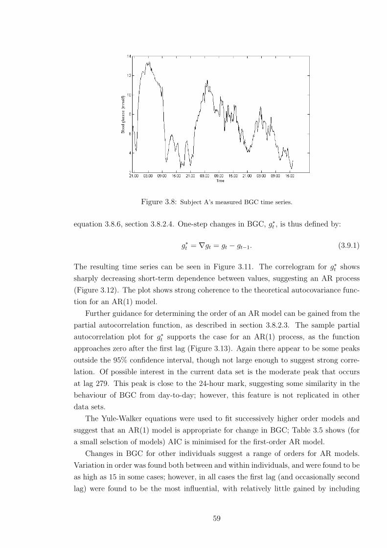
Figure 3.8: Subject A’s measured BGC time series.
equation 3.8.6, section 3.8.2.4. One-step changes in BGC, g∗t , is thus defined by:
g∗t = ∇gt = gt − gt−1. (3.9.1)
The resulting time series can be seen in Figure 3.11. The correlogram for g∗t shows
sharply decreasing short-term dependence between values, suggesting an AR process
(Figure 3.12). The plot shows strong coherence to the theoretical autocovariance func-
tion for an AR(1) model.
Further guidance for determining the order of an AR model can be gained from the
partial autocorrelation function, as described in section 3.8.2.3. The sample partial
autocorrelation plot for g∗t supports the case for an AR(1) process, as the function
approaches zero after the first lag (Figure 3.13). Again there appear to be some peaks
outside the 95% confidence interval, though not large enough to suggest strong corre-
lation. Of possible interest in the current data set is the moderate peak that occurs
at lag 279. This peak is close to the 24-hour mark, suggesting some similarity in the
behaviour of BGC from day-to-day; however, this feature is not replicated in other
data sets.
The Yule-Walker equations were used to fit successively higher order models and
suggest that an AR(1) model is appropriate for change in BGC; Table 3.5 shows (for
a small selsction of models) AIC is minimised for the first-order AR model.
Changes in BGC for other individuals suggest a range of orders for AR models.
Variation in order was found both between and within individuals, and were found to be
as high as 15 in some cases; however, in all cases the first lag (and occasionally second
lag) were found to be the most influential, with relatively little gained by including
59

Figure 3.9: Autocorrelation coefficient against respective lag for BGC of Subject A. Dotted linesrepresent theoretical 95% confidence intervals given by ± 2√
n.
Figure 3.10: Autocorrelation coefficient against respective lag for BGC for two different individualsin the DUK study. Dotted lines represent theoretical 95% confidence intervals given by ± 2√
n.
60
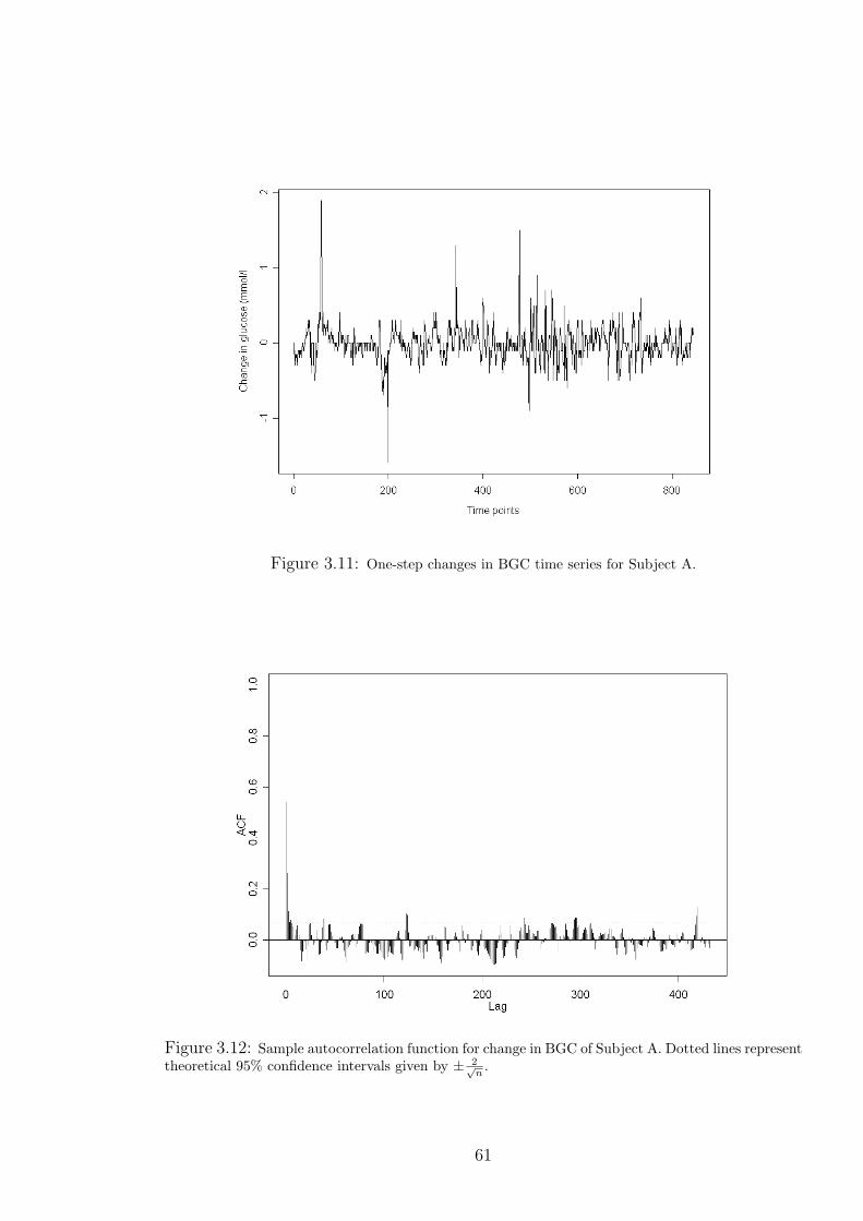
Figure 3.11: One-step changes in BGC time series for Subject A.
Figure 3.12: Sample autocorrelation function for change in BGC of Subject A. Dotted lines representtheoretical 95% confidence intervals given by ± 2√
n.
61
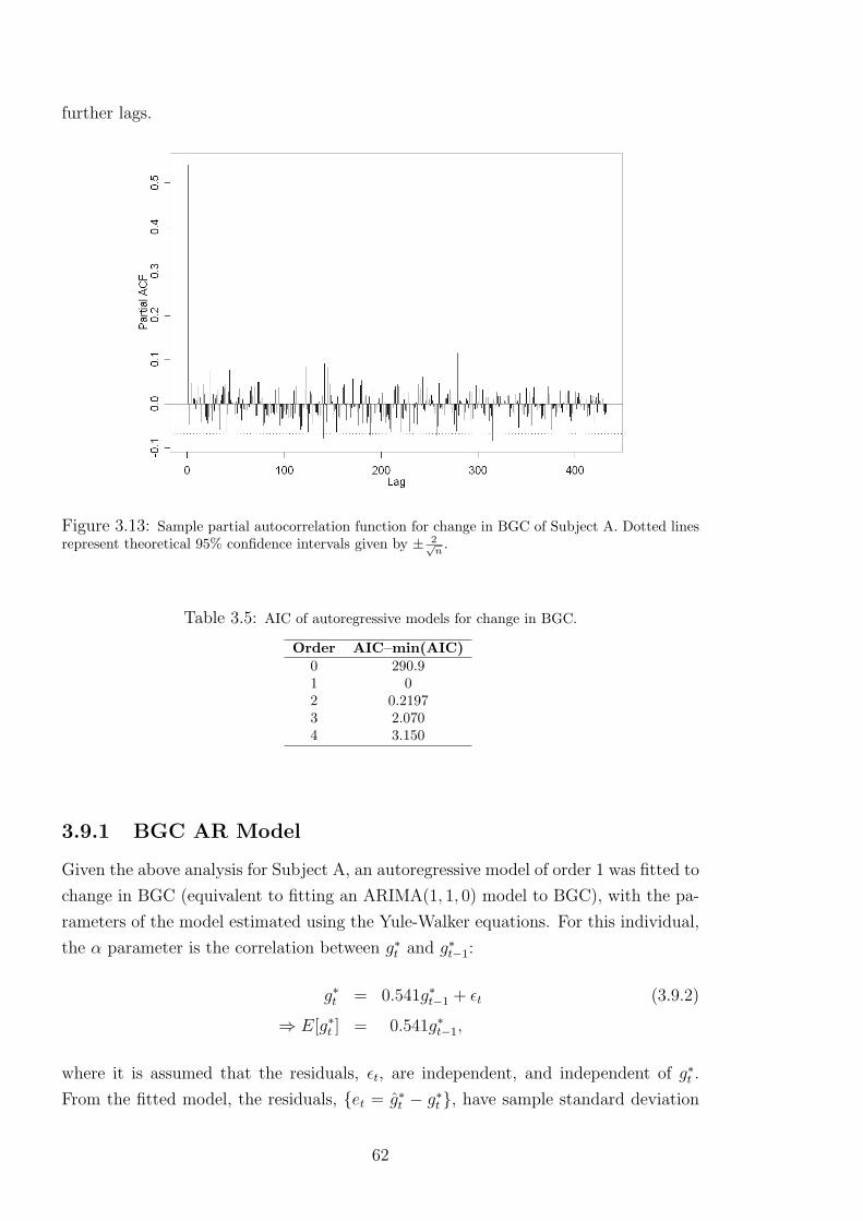
further lags.
Figure 3.13: Sample partial autocorrelation function for change in BGC of Subject A. Dotted linesrepresent theoretical 95% confidence intervals given by ± 2√
n.
Table 3.5: AIC of autoregressive models for change in BGC.
Order AIC–min(AIC)0 290.91 02 0.21973 2.0704 3.150
3.9.1 BGC AR Model
Given the above analysis for Subject A, an autoregressive model of order 1 was fitted to
change in BGC (equivalent to fitting an ARIMA(1, 1, 0) model to BGC), with the pa-
rameters of the model estimated using the Yule-Walker equations. For this individual,
the α parameter is the correlation between g∗t and g∗t−1:
g∗t = 0.541g∗t−1 + εt (3.9.2)
⇒ E[g∗t ] = 0.541g∗t−1,
where it is assumed that the residuals, εt, are independent, and independent of g∗t .
From the fitted model, the residuals, et = g∗t − g∗t , have sample standard deviation
62

s2e = 0.0371 and approximately zero mean. Residual analysis does not suggest any
temporal dependence, except perhaps the tendency for pairs of large positive-negative
values, e.g., around time point 200 (Figure 3.14).
Figure 3.14: AR(1) model residuals for change in BGC of Subject A.
The residual correlogram also does not suggest any temporal dependence of the
residuals; Figure 3.15 shows most autocorrelation coefficients are within the 95% in-
tervals. In addition the partial autocorrelation function (not shown) does not suggest
any violation of the assumptions.
3.9.2 BGC AR Prediction
Using the above model of g∗t , it is of interest to assess predictive performance. The
conditional expectation is given by
E[g∗t+1|g∗t , ..., g∗0] =E[g∗t+1|g∗t ]
=0.541g∗t ,
so the one-step ahead forecast at time t is
g∗t+1 = 0.541g∗t . (3.9.3)
63

Figure 3.15: Correlogram of the AR(1) model residuals for change in BGC of Subject A.
Similarly, for the k-step ahead forecast:
E[g∗t+k|g∗t , ..., g∗0]
= E[g∗t+k|g∗t ]
= 0.541g∗t+k−1
= 0.5412g∗t+k−2
...
= 0.541kg∗t .
Given a positive (negative) reading at time n all future estimates g∗n+k will also be
positive (negative) and will decay to zero as k increases; this suggests the AR model
will be poor for long-term prediction.
The data used to build the AR model may be considered as a training set, and
the model may be tested on a second set to assess its predictive ability. The test
set measurements were taken from the same individual starting on the same day as
the training set finished. The model was set to predict one and 48 time steps ahead,
equivalent to five minutes and four hours respectively, where four hours represents a
reasonable time between finger-prick tests as part of the MDI treatment regime. In
each case, the predictions for change in BGC were used to then predict actual BGC.
64

3.9.2.1 Results
The one-step AR(1) model shows good predictive capability; Figure 3.16 shows pre-
dictions follow the peaks and troughs of measured BGC well. However, five-minute
ahead predictions are of little or no relevance to a clinician or individual looking to
make longer-term predictions for BGC.
Figure 3.16: Measured BGC and one-step (five minutes) ahead prediction for BGC usingARIMA(1,1,0) model for Subject A.
The 48-step AR(1) model highlights the limited predictive capabilities of AR mod-
els. Predicted change in BGC quickly tends to zero the more steps ahead the prediction
is made, and so misses the peaks and troughs in the data; Figure 3.17 shows the 48-step
model predictions are essentially the original BGC time series shifted. Similar results
were seen for other individuals in the DUK study, regardless of AR model order. AR
models are thus inadequate for long-term prediction, and more sophisticated methods
are required to model BGC over several hours.
3.9.3 Conclusions
Changes in BGC appear to behave like an AR process, and hence exhibits short-term
trend; this is certainly noticeable in the case of Subject A, whose BGC rapidly increases
at night and experiences other short-term peaks and troughs. Although consecutive
changes in BGC are highly correlated, there is little scope for using this information
to predict the behaviour of BGC over several hours. Long-term predictive models of
65

Figure 3.17: Measured BGC and 48-step (four hours) ahead prediction for BGC using ARIMA(1,1,0)model for Subject A.
66
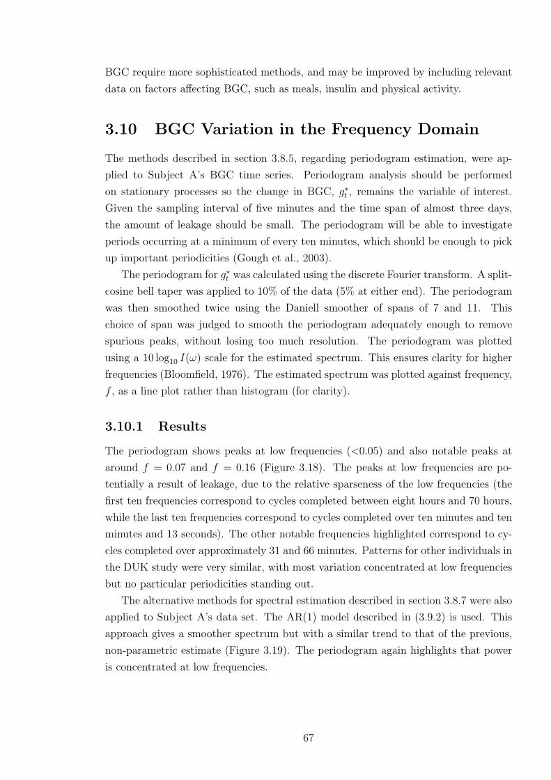
BGC require more sophisticated methods, and may be improved by including relevant
data on factors affecting BGC, such as meals, insulin and physical activity.
3.10 BGC Variation in the Frequency Domain
The methods described in section 3.8.5, regarding periodogram estimation, were ap-
plied to Subject A’s BGC time series. Periodogram analysis should be performed
on stationary processes so the change in BGC, g∗t , remains the variable of interest.
Given the sampling interval of five minutes and the time span of almost three days,
the amount of leakage should be small. The periodogram will be able to investigate
periods occurring at a minimum of every ten minutes, which should be enough to pick
up important periodicities (Gough et al., 2003).
The periodogram for g∗t was calculated using the discrete Fourier transform. A split-
cosine bell taper was applied to 10% of the data (5% at either end). The periodogram
was then smoothed twice using the Daniell smoother of spans of 7 and 11. This
choice of span was judged to smooth the periodogram adequately enough to remove
spurious peaks, without losing too much resolution. The periodogram was plotted
using a 10 log10 I(ω) scale for the estimated spectrum. This ensures clarity for higher
frequencies (Bloomfield, 1976). The estimated spectrum was plotted against frequency,
f , as a line plot rather than histogram (for clarity).
3.10.1 Results
The periodogram shows peaks at low frequencies (<0.05) and also notable peaks at
around f = 0.07 and f = 0.16 (Figure 3.18). The peaks at low frequencies are po-
tentially a result of leakage, due to the relative sparseness of the low frequencies (the
first ten frequencies correspond to cycles completed between eight hours and 70 hours,
while the last ten frequencies correspond to cycles completed over ten minutes and ten
minutes and 13 seconds). The other notable frequencies highlighted correspond to cy-
cles completed over approximately 31 and 66 minutes. Patterns for other individuals in
the DUK study were very similar, with most variation concentrated at low frequencies
but no particular periodicities standing out.
The alternative methods for spectral estimation described in section 3.8.7 were also
applied to Subject A’s data set. The AR(1) model described in (3.9.2) is used. This
approach gives a smoother spectrum but with a similar trend to that of the previous,
non-parametric estimate (Figure 3.19). The periodogram again highlights that power
is concentrated at low frequencies.
67
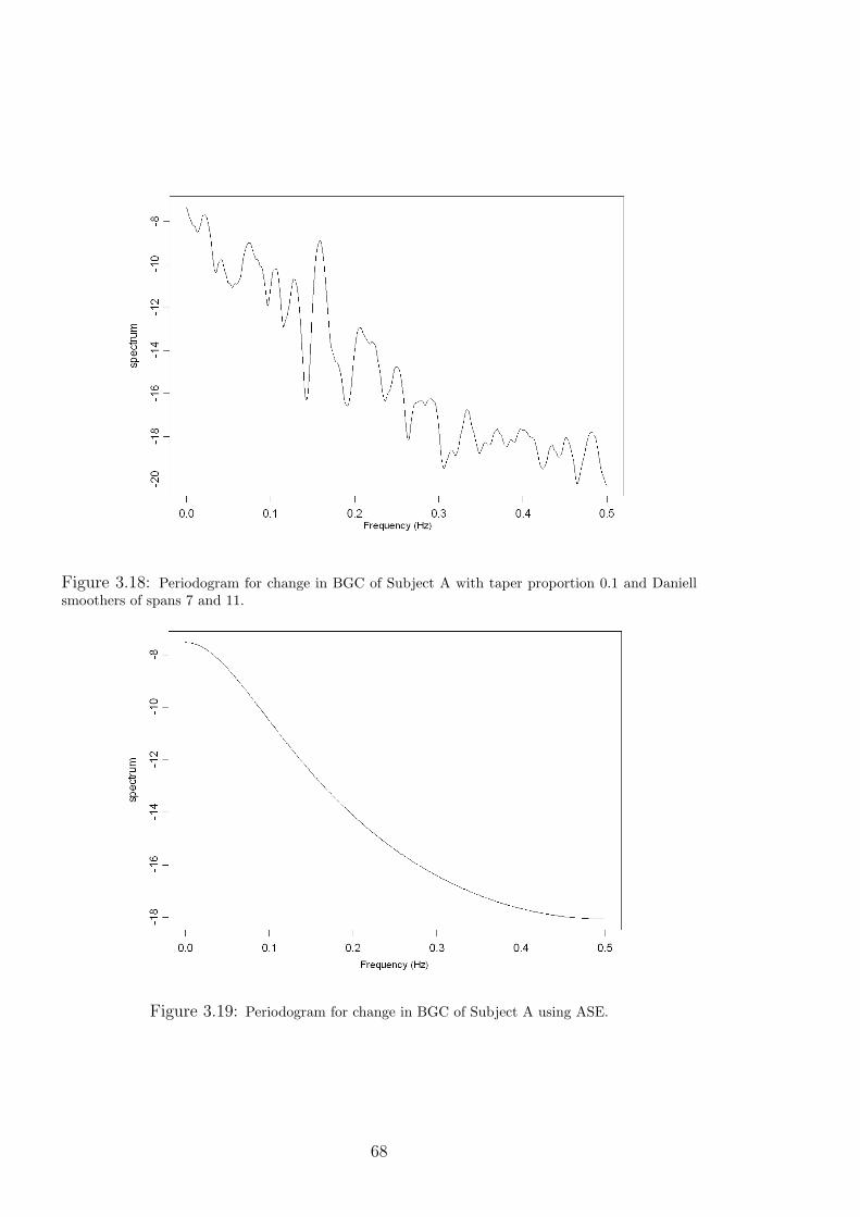
Figure 3.18: Periodogram for change in BGC of Subject A with taper proportion 0.1 and Daniellsmoothers of spans 7 and 11.
Figure 3.19: Periodogram for change in BGC of Subject A using ASE.
68
3.10.2 Conclusions
It appears that change in BGC exhibits some indistinct oscillations over periods of
several hours, and potentially days. This is most likely to be due to lifestyle factors,
e.g., timing of meals and sleep, rather than naturally occurring biological rhythms,
which may be indistinguishable under the greater influence of food and insulin.
The BGC plot of Subject A shows repeated cases of mild, night-time hypergly-
caemia, and compensatory decreases in the morning. It is possible that the insulin–
carbohydrate ratio, used by the individual to calculate insulin dose with meals, is not
appropriate for the evening meal, resulting in an underestimation of the required in-
sulin. This may be due to changes in insulin sensitivity or other physiological changes,
but may also be explained by miscounting of carbohydrate content in the meal, in-
appropriate insulin profile with respect to the glycaemic index of the food, or other
external influences, e.g., stress.
3.11 Summary
Free-living data from the Diabetes UK study, relating to BGC, physical activity, food
and insulin, have been presented, and practical modelling issues regarding these data
have been highlighted. The information from the food and insulin diaries has been
converted from discrete inputs to continuous processes using models in the literature, to
describe the appearance of glucose and insulin in the blood and hence better understand
their effect on BGC. It was also found that physical activity data fluctuates greatly
during the day, creating new challenges for models in the literature trained and/or
validated on simplified representations of activity.
Exploratory analysis of the DUK data showed that BGC is non-stationary. Simple
time series analysis suggests temporal dependence between changes in BGC, but simple
models could not use this information to predict over long periods of time. Frequency
analysis did not highlight any important periodicities in changes in BGC. Thus, BGC
alone does not itself offer useful information on future behaviour of blood glucose over
periods of several hours. The inclusion of explanatory variables such as food intake,
insulin, and METs in more complex models may help to improve predictive performance
of BGC.
69


Chapter 4
Dynamic Modelling of Blood
Glucose Concentration
The previous chapter highlighted the need for more sophisticated methods to predict
the behaviour of blood glucose concentration (BGC), which account for food, insulin
and physical activity. This chapter introduces dynamic linear models (DLMs) and ap-
plies them to the DUK study data. DLMs are empirical models not previously used
in the diabetes literature. It is hypothesised they can be a useful tool for investigating
the role of physical activity in the behaviour of BGC by assessing their relationship
over time, in the presence of food and insulin injection disturbances, using dynamic re-
gression models. Understanding the effects of physical activity on BGC can help those
with diabetes incorporate physical activity safely into their daily routine. DLMs may
also be used to predict BGC over several hours, based on future profiles of glucose and
insulin absorption, and physical activity. A suitable predictive model could be incorpo-
rated in the current treatment regime of MDI by guiding the insulin therapy decision
process, and hence help limit hypo- and hyperglycaemia and associated complications.
The chapter begins by describing the structure of DLMs and features relevant to the
current work. A simple DLM is used as a starting point to build more complex DLMs
that account for explanatory variables and other features of the data.
4.1 Dynamic Linear Models
Linear models are used to determine the dependence of an (n×1) response vector, y, on
a linear combination of explanatory variables, xi, for i = 1, ..., p, using a (p× 1) vector
of regression parameters, θ. Dynamic linear models (DLMs) add flexibility by allowing
the values of the parameters to vary in time, and are hence able to track changes in
mean and variance inherent in non-stationary time series. DLMs as presented in this
chapter were originally proposed by Harrison and Stevens (1976), using the work of
71

Kalman (1963).
DLMs are a general class of models that apply the Bayesian paradigm to time
series, making use of the convenient features of Bayesian methods for descriptive and
predictive purposes. Bayesian methods provide a structure for updating statistical
inference as data becomes available, and are described further in appendix A for those
unfamiliar with this approach.
DLMs have been used in a number of areas, including biology, e.g., modelling
growth hormone levels (Bolstad, 1988), but not in diabetes modelling. The advantages
of DLMs in the context of the current work will be highlighted throughout the following
sections, which discuss their theory and structure.
4.1.1 Structure of a DLM
The basic regression DLM structure consists of the observation and system equations,
and initial information on the parameters. The observation equation relates the time
series of interest (the response, Yt, for t = 1, . . . , T , assumed univariate here) to a set
of p known explanatory variables, X t:
Yt = XTt θt + εt, εt ∼ N(0, σ2
t ), (4.1.1)
where θt is the (p×1) vector of regression parameters, εt is the scalar observation error,
and σ2t is the scalar observation error variance. Successive Yt are assumed to be condi-
tionally independent given θ. The observation errors are assumed to be independent
and normally distributed with zero mean. The variance of the error distribution may
vary across time to account for changes in measurement accuracy.
The system equation describes the dependence of parameter values on their previous
values:
θt = Gtθt−1 + ωt, ωt ∼ N(0,Ωt), (4.1.2)
where Gt is the (p×p) system matrix, ωt is the (p×1) vector of system errors, and Ωt
is the (p × p) variance-covariance matrix of system errors. Parameters are allowed to
change in time to account for possible changing conditions in the system. The system
errors are again assumed to be independent and normally distributed with zero mean.
Furthermore, the system errors are assumed to be independent of the observation
errors and the initial information. Finally, the two equations are augmented by initial
information of the form:
(θ0|D0) ∼ N(m0,C0),
where (θ0|D0) represents the conditional distribution of the parameters given all known
prior information, D0; more generally, Dt represents all known information up to and
including time t. The initial information is characterised by some appropriate mean,
72

m0, and variance, C0, which must be specified to initialise the model.
4.1.2 Updating Procedure
Based on the structure of the initial information and the observation and system equa-
tions, predictions and parameter inference may be updated as new data is collected.
The updating procedure is in closed-form due to conjugacy of the prior distribution,
and DLMs thus provide a structure for rapid, non-computationally intensive time series
analysis. If X t, Gt, and the error variances, σ2t and Ωt, are assumed known, then the
DLM updating procedure is as follows:
Assume the posterior distribution for the parameters at time t− 1 is:
(θt−1|Dt−1) ∼ N(mt−1,Ct−1).
By (4.1.2), θt is a linear combination of normal variables, so the prior distribution for
the parameters at time t is given by
(θt|Dt−1) ∼ N(at,Rt), (4.1.3)
where
at = Gtmt−1,
and
Rt = GtCt−1GTt + Ωt.
The marginal distribution for Yt defines the probability function assigned to the one-
step forecast at time t. By (4.1.1), Yt is a linear combination of normal variables, so
the one-step ahead forecast distribution is given by
(Yt|Dt−1) ∼ N(ft, Qt),
where
ft = XTt at,
and
Qt = XTt RtX t + σ2
t .
The one-step ahead point forecast is given by the mean of the distribution, ft, with
associated uncertainty given by the variance, Qt. A credible interval for the mean may
be calculated from the forecast distribution. Upon observing yt, the forecast error is
determined by the difference between the observed value and the forecast: et = yt− ft.The prior distribution for the parameters may then be updated by applying Bayes’
73
Theorem to θt:
p(θt|Dt) = p(θt|Yt = yt, Dt−1) ∝ p(θt|Dt−1)p(Yt|θt, Dt−1),
and by (4.1.1) and (4.1.3),
p(θt|Dt−1) ∝ exp[−1/2(θt − at)TR−1(θt − at)]
and
p(Yt|θt, Dt−1) ∝ exp[−1/2(Yt − ft)2/Qt].
Rearranging these exponentials it can be shown that
p(θt|Dt) ∝ exp[−(θt −mt)TC−1
t (θt −mt)/2],
where
mt = at +Atet,
and
Ct = Rt −AtATt Qt,
with the adaptive vector, At, given by
At = RtX t/Qt.
The posterior distribution of the parameters a time t may then be written as
(θt|Dt) ∼ N(mt,Ct).
The posterior mean, mt, is a combination of the prior mean and the forecast error,
weighted by At. The weight assigned to the error depends on the size of the prior
variance, Rt, relative to the forecast error, Qt.
4.1.3 Unknown System Error Variance
In the above, it is assumed that the error variances, σ2t and Ωt, are known; this may
be unrealistic without any prior knowledge of the system. While the observation error
variance, σ2, may be incorporated into the updating process of the DLM (as discussed
in section 4.1.4), including the system error variance matrix, Ωt, in the process can lead
to problems (Pole et al., 1994). Furthermore, specifying this matrix can be difficult for
a number of reasons:
i) it is not invariant to the scale of measurement of the covariates, X;
74
ii) it can lead to ambiguities, as an uncountable number of different models with the
same forecast distribution may be specified that differ only in Ωt (West and
Harrison, 1997, chapter 5).
A solution is to use a method known as discounting. Consider a process which at
a given time, t, has precision C−1t−1 associated with θt−1. The precision associated
with Gtθt−1 is (GtCt−1GTt )−1 = P−1
t . If Ωt = 0 then P t also describes the precision
associated with θt. However, the uncertainty in the system equation means that R−1t ,
the actual precision associated with θt, is reduced by the term Ωt relative to P−1t . This
loss of precision may be applied directly to P t using a multiplicative factor, λ, known
as the discount factor. The variance of θt is now given by Rt = 1λP t. From this it can
be seen that Ωt = 1−λλP t. The system equation in (4.1.2) is thus amended to
θt = Gtθt−1 + ωt, ωt ∼ N(0,1− λλ
P t). (4.1.4)
For most practical purposes, λ will lie in the range (0.9, 1] with unity representing
Ωt = 0 (West and Harrison, 1997, chapter 6).
The discount factor may be determined by comparing model performance for a
suitable range of values of the discount factor. Model performance may be measured
in a number of ways, often based on measures of the forecast errors; two common
measures are MSE and MAD (section C.3.2, Appendix C):
MSE =1
T
T∑t=1
e2t ; MAD =1
T
T∑t=1
|et|.
Small values of each are preferred. A likelihood function for λ may also be constructed
from the forecast distributions evaluated at each observation:
L(λ|Y , D0) = p(Y |λ,D0) =T∏t=1
p(Yt|Dt−1), (4.1.5)
where Y = (Y1, . . . , YT ). The likelihood takes into account the forecast variance, unlike
MSE or MAD. The likelihood is often used to form a log-likelihood ratio (LLR), where
alternative models are compared to some baseline model.
4.1.4 Unknown Observation Error Variance
Assuming that the observation error variance is unknown but constant (σ2t = σ2), the
closed-form, conjugate updating procedure for the DLM may be retained by scaling
the system error variance, Ωt, and the initial prior variance, C0, by σ2. Conjugacy
is then achieved with an inverse gamma prior distribution on σ2. This is equivalent
75
to a gamma distribution1, G(·, ·), on the precision, φ = σ−2. The gamma distribution
is commonly used in Bayesian analysis for reflecting uncertainty on strictly positive
values.
Prior information must be specified for the precision, φ, so the initial information
is appended by
(φ|D0) ∼ G(n0/2, d0/2),
where the shape parameter, n0, and the inverse scale, d0, are to be specified. Note that
E[φ|D0] = n0/d0 = 1/S0 is the prior point estimate of the observation error precision.
At time t, the prior distribution of φ is given by
(φ|Dt−1) ∼ G(nt−1/2, dt−1/2), (4.1.6)
with the point prior estimate of (σ2|Dt−1) given by St−1 = dt−1/nt−1. After observing
yt, the prior distribution may be updated via Bayes’ Theorem to
(φ|Dt) ∼ G(nt/2, dt/2), (4.1.7)
where nt = nt−1 + 1, dt = dt−1 + e2t/Q∗t , and Q∗t represents the unscaled forecast
variance, i.e., Qt/σ2.
Ignoring the time subscript and dependence on D for convenience, the joint distri-
bution of Y and φ is the product of a normal and a gamma distribution:
p(Y, φ) = p(Y |φ)p(φ)
∝ φ1/2 exp(−φ(Y − f)2/2Q∗)
× φn/2−1 exp(−φd/2).
The marginal distribution for Y is given by p(Y, φ)/p(φ|Y ), where p(φ|Y ) represents
the updated gamma distribution given by (4.1.7). Algebraic manipulation gives a T-
distribution for p(Y ), denoted by Tn(·, ·) for n degrees of freedom. This argument
extends to the multivariate normal case for p(θt, φ), with θt following a multivariate
T-distribution.
Defining Ω∗t to be the part of the matrix Ωt that does not depend on σ2, and like-
wise for C∗t , R∗t =GtC
∗t−1G
Tt + Ω∗t and Q∗t =X tR
∗tX t + 1, the updating procedure
unconditional on σ2 is now as follows:
1The gamma parameterisation used here and throughout specifies that if X ∼ G(α, β) thenp(X;α, β) ∝ Xα−1 exp(−Xβ).
76
Assume the posterior distribution for the parameters at time t− 1 is given by
(θt−1|Dt−1) ∼ Tnt−1(mt−1,Ct−1), (4.1.8)
for some location, mt−1, and scale matrix, Ct−1. This is updated to the prior distri-
bution at time t,
(θt|Dt−1) ∼ Tnt−1(at,Rt), (4.1.9)
where at = Gtmt−1 and Rt = St−1(GtC∗t−1G
Tt + Ω∗t ) = St−1R
∗t . The forecast distri-
bution is given by
(Yt|Dt−1) ∼ Tnt−1(ft, Qt), (4.1.10)
where ft = XTt at and Qt = St−1(1 + XT
t R∗tX t) = St−1Q
∗t . After observing yt, the
one-step forecast error is as defined previously, the prior distribution for φ is updated
to obtain the updated estimate, St, and the prior distribution for the parameters is
updated to
(θt|Dt) ∼ Tnt(mt,Ct), (4.1.11)
where mt = at + Atet, Ct = St(R∗t − AtA
Tt Q∗t ) = StC
∗t , and nt = nt−1 + 1. The
adaptive vector, At, is as defined previously.
4.1.4.1 Time-Varying Observation Error Variance
The above procedure can be extended to include temporal changes in observation
variance. This is relevant if it is thought that the observation error is subject to
change, e.g., due to variation in measurement accuracy. Changes in variance may be
included in the conjugate, closed-form updating procedure using discounting (West
and Harrison, 1997, chapter 10). This involves introducing a stage between (4.1.6) and
(4.1.7), prior to observing yt. Appending a time subscript to (4.1.6) so that
(φt−1|Dt−1) ∼ G(nt−1/2, dt−1/2) (4.1.12)
represents all information on φ at time t−1, additional uncertainty may be introduced
at time t as follows:
Define
φt = γtφt−1/δ, (4.1.13)
where γt follows a beta distribution, Beta(·, ·), independent of φ, given by
γt ∼ Beta(δnt−1/2, (1− δ)nt−1/2), (4.1.14)
whose shape parameters are determined by the parameters in (4.1.12) and discount
77

factor, δ. By (4.1.12) and (4.1.13), the variable φt is a product of beta and gamma
distributions and so follows a gamma distribution. The amended information on φ is
given by
(φt|Dt−1) ∼ G(δnt−1, δdt−1). (4.1.15)
The value of the discount factor, δ, is restricted to the range (0, 1]. Unity implies no
loss of information, equivalent to the model described in section 4.1.4. Note that under
(4.1.15):
E(φt|Dt−1) = nt−1/dt−1
= 1/St−1
= E(φt−1|Dt−1),
and
V (φt|Dt−1) = nt−1/δd2t−1
= (1/δ)V (φt−1|Dt−1),
so the point estimate of (σ2t |Dt−1) is the same but with increased uncertainty. The
updating procedure in section 4.1.4 still applies, with only the following changes:
(φt|Dt−1) ∼ G(δnt−1/2, δdt−1/2)
(Yt|Dt−1) ∼ Tδnt−1(ft, Qt)
nt = δnt−1 + 1
dt = δdt−1 + St−1e2t/Qt.
The degrees of freedom for the forecast distribution are thus reduced by a factor of
δ. Additional uncertainty can be supplied to the model at individual time-points by
decreasing δ momentarily. The introduction of a discount factor for the observation
variance, σ2, is relatively superficial; there is no change in the forecast, only a change in
the estimate of φ. Although the discount factor is designed to increase uncertainty in
predictions, it may artificially reduce the prediction interval depending on the forecast
error (see appendix B).
4.1.5 K -step Forecasting
The updating procedure as presented allows for one-step ahead prediction. Given
observations up to time t, the distribution of the parameters for k steps ahead may be
78

determined by repeated application of the system equation, and is given by:
(θt+k|Dt) ∼ N [at(k),Rt(k)],
where
at(k) = Gt+kat(k − 1)
and
Rt(k) = Gt+kRt(k − 1)GTt+k + Ωt+k
are calculated recursively.
The forecast distribution for k steps ahead is determined from the observation
equation, and is given by:
(Yt+k|Dt) ∼ N [ft(k), Qt(k)],
where
ft(k) = XTt+kat(k)
and
Qt(k) = XTt+kRt(k)X t+k + σ2
t+k.
The starting values are defined at time t by:
at(0) = mt
Rt(0) = Ct.
If σ2t is unknown, it is replaced by St in the above structure. For unknown Ωt, the
discounting approach requires some care: if P t+k = Gt+kRt(k − 1)GTt+k, it can be
shown that Rt(k) ∝ Ct/λk, hence the information in Ct has exponential decay rather
than the arithmetic decay associated with the additive process of one-step forecasts.
A suggested approach is to define
Ωt(k) = Ωt+1 =1
λP t+1, (4.1.16)
so that Ωt+1 is the forecast of the system error variance at all times until the next
observation, when it can then be updated (West and Harrison, 1997, chapter 6).
4.1.6 Filtering and Smoothing
Interest in a system may not be solely in predictive performance. DLMs may also be
used to monitor the behaviour of the parameters through time, where inferences on
the parameters at time t may be revised in the wake of observed data after this time;
79
this process is known as filtering. Given observed data up to time T , the k-step filtered
distribution, p(θT−k|DT ), for k = 1, . . . , T − 1, may be found by evaluating
p(θT−k|DT ) =
∫p(θT−k|θT−k+1, DT )p(θT−k+1|DT )dθT−k+1.
Defining M t = CtGTt+1R
−1t+1, the filtered distributions are given by
(θT−k|DT ) ∼ N [aT (−k),RT (−k)],
where
aT (−k) = mT−k +MT−k[aT (−k + 1)− aT−k+1]
and
RT (−k) = CT−k +MT−k[RT (−k + 1)−RT−k+1]MTT−k.
The full proof by induction for the filtered distributions may be found in West and
Harrison (1997, chapter 4). The proof makes use of the following important result,
invoked later in this chapter:
(θT−k|θT−k+1, DT−k) ∼ N [hT (k),HT (k)], (4.1.17)
where
hT (k) = mT−k +MT−k(θT−k+1 − aT−k+1)
and
HT (k) = CT−k −MT−kRT−k+1MTT−k.
The filtered distributions may also be used to retrospectively assess the behaviour
of the mean of the time series, µt = XTt θt, with the k-step smoothed distributions,
p(µT−k|DT ). By simple extension from the above results, the k-step smoothed distri-
bution is given by
(µT−k|DT ) ∼ N(fT (−k),XTT−kRT (−k)XT−k), (4.1.18)
where
fT (−k) = XTT−kaT (−k).
For the case of unknown, constant observation variance, σ2, the filtered distributions
are adjusted to
θT−k|DT ∼ TnT[aT (−k), (ST/ST−k)RT (−k)],
80

and the k-step smoothed distributions become
(µT−k|DT ) ∼ TnT(fT (−k), (ST/ST−k)X
TT−kRT (−k)XT−k).
4.1.7 Reference Analysis
A further concession to a lack of prior knowledge of the system may be achieved with
the use of non-informative, improper prior distributions to initialise the model, where
the prior distribution for the parameter set, p(θ1|D0), need not be specified in terms of
the hyperparameters, m0 and C0. For unknown observation error variance, the joint
prior distribution of θ1 and φ may instead be defined by
p(θ1, φ|D0) ∝ φ.
More generally, the prior distribution at time t may be expressed as
p(θt, φ|Dt−1) ∝ φ1+(t−1)/2 exp−φ/2(θTt Atθt − 2θT
t at + τt−1),
with starting values A1 = 0, a1 = 0 and τ0 = 0. After observing yt, this updates to
p(θt, φ|Dt) ∝ φ1+t/2 exp−φ/2(θTt Btθt − 2θT
t bt + τt),
where bt = at +X tYt, Bt = At +X tXTt and τt = τt−1 + Y 2
t . The prior distributions
for the next time point are determined from the relationships
at = (G−1t )Tbt−1
and
At = (G−1t )TBt−1G
−1t .
Posterior distributions will remain improper until at least (but generally not beyond)
time t = t∗ = p+ 1, where p is the dimension of θ. At time t∗ + 1 the analysis reverts
to the usual updating procedure described previously, where the prior distribution of
the parameters is given by
(θt∗+1|Dt∗) ∼ N(mt∗+1,Ct∗+1),
where mt∗+1 = Bt∗+1bt∗+1 and Ct∗+1 = St∗+1Bt∗+1.
The above method is a simplified approach that assumes, for t ∈ [1, t∗], the system
error variance, Ω, is equal to the zero matrix; this is justified by the fact that the
amount of information collected during the reference period does not allow for the
detection of changes in parameters. Full proof and discussion of the procedure may be
81
found in West and Harrison (1997, chapter 4).
4.2 DLM of Blood Glucose Concentration
Although the glucose-insulin dynamical system is non-linear, it is hypothesised that
DLMs are able to model BGC given the inputs of glucose and insulin absorption and
physical activity. These inputs represent the biggest challenges to BGC regulation,
and it is to be investigated whether the effect of these can be captured in an empirical
model. Using a linear modelling approach is, at the very least, a useful basis for
exploring non-linear systems; this is certainly true when, as with the glucoregulatory
system, nonlinearities may be unknown, and potentially time- and subject-specific.
Furthermore, linear models may be suitable in a non-linear system over limited time
frames. The methods proposed have not previously been applied in diabetes modelling.
DLMs have a number of favourable properties for modelling BGC: time-varying
parameters may capture effects such as changes in insulin sensitivity through the day,
time-varying error variances account for changes in measurement accuracy of CGMs,
the models can be individualised (hence taking into account inter-patient variability)
and a rapid, computationally efficient updating procedure allows for on-line prediction.
DLMs also allow scope for modelling BGC with differing aims. The first is to assess
the role of physical activity (using METs) and its effect on BGC. This may be achieved
by monitoring the behaviour of the model parameters using filtering (as described in
section 4.1.6). The second aim is to assess the capability of DLMs for long-term
prediction (at least four hours). It has been established, e.g., chapter 3 and Sparacino
et al. (2007), that BGC can be predicted in the short term purely from recent values
of itself, using relatively simple time series methods. The current approach is aimed at
longer-term prediction based on the major inputs of consumed carbohydrates, injected
insulin and physical activity, with less reliance on frequent BGC measurements. This
has the potential to enhance an individual’s control of their BGC by predicting profiles
for different insulin doses, and thus suggesting the most appropriate dose. Such an
approach could improve the predominant current treatment regime of MDI.
The structure of DLMs assumes a normally distributed response variable. BGC does
not necessarily satisfy this assumption given that it is a strictly positive value (and is
likely to have some unknown physiological limit above this). In such a situation, it is
common to transform the response, e.g., using natural logarithms. To maintain the
desired linear structure, it is then required to take logarithms of the covariates also.
However, carbohydrate intake and insulin absorption may be zero. Instead it is argued
here that the natural restriction of BGC will have minimal impact on the assumptions
of the DLM, and hence BGC will be not be transformed.
A number of variants of the basic DLM structure are now applied to an individual’s
82

BGC measurements. Analysis will initially focus on one-step ahead prediction and
parameter behaviour, before considering long-term forecasts.
4.2.1 First-order Polynomial Model
The first model fitted is the simplest DLM, the first-order polynomial (FOP) DLM,
with θt = µt representing an overall level of the process, and Gt = Xt = 1:
Yt = µt + εt, εt ∼ N(0, σ2)
µt = µt−1 + ωt, ωt ∼ N(0,Ω).
The error variances, σ2 and Ω, are assumed constant but unknown. The methods
described in sections 4.1.3 and 4.1.4 , regarding a gamma prior distribution and dis-
counting, are used for the respective variances. The prior information is given by:
(µ0|D0) ∼ T1(Y0, 10)
(φ|D0) ∼ G(2, 1),
where Y0 is the finger-prick measurement used to calibrate the CGM at the start of the
measurement period. The values for (φ|D0) were chosen to give a weakly informative
prior distribution; likewise, the variance of (µ0|D0) is chosen to be deliberately large.
This model was used for one-step (5 minutes) ahead predictions.
As noted in section 4.1.3, the discount factor for Ω cannot be included in the
updating procedure. Hence the model was fit repeatedly for λ ∈ (0, 1] in increments
of 0.01. For the LLR, the baseline model for comparison will be λ = 1, equivalent to
W t = 0; the LLR for an alternative discount factor, λ∗, is thus given by:
LLR(λ∗) = log
[L(λ = 1|Y )
L(λ∗|Y )
]. (4.2.1)
The results from the FOP model suggest that MSE and MAD are minimised, and
LLR maximised, as λ → 0, or equivalently, Ωt → ∞; selected results for MSE, MAD
and LLR are shown in Table 4.1, and plots of one-step predictions for λ = 0.01 and
λ = 1, shown in Figure 4.1, highlight the difference in model performance. As λ→ 0,
parameter estimates change greatly with each new observation, and the posterior mean
for µ is almost entirely decided by the most recent observation, Yt. Despite good
performance when predicting one step ahead, such a model is of little practical use for
predicting many steps ahead, when correlation between observations far apart in time
is much less. The model may be improved by the inclusion of covariates.
83
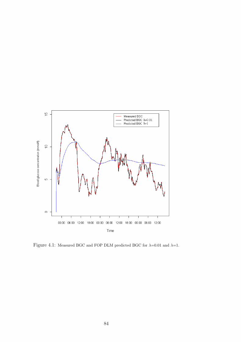
Figure 4.1: Measured BGC and FOP DLM predicted BGC for λ=0.01 and λ=1.
84
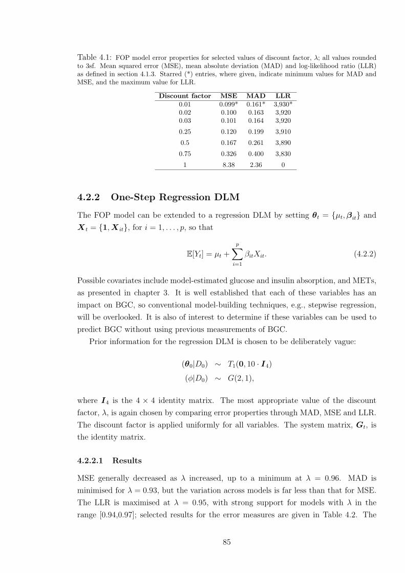
Table 4.1: FOP model error properties for selected values of discount factor, λ; all values roundedto 3sf. Mean squared error (MSE), mean absolute deviation (MAD) and log-likelihood ratio (LLR)as defined in section 4.1.3. Starred (*) entries, where given, indicate minimum values for MAD andMSE, and the maximum value for LLR.
Discount factor MSE MAD LLR0.01 0.099* 0.161* 3,930*0.02 0.100 0.163 3,9200.03 0.101 0.164 3,920
0.25 0.120 0.199 3,910
0.5 0.167 0.261 3,890
0.75 0.326 0.400 3,830
1 8.38 2.36 0
4.2.2 One-Step Regression DLM
The FOP model can be extended to a regression DLM by setting θt = µt,βit and
X t = 1,X it, for i = 1, . . . , p, so that
E[Yt] = µt +
p∑i=1
βitXit. (4.2.2)
Possible covariates include model-estimated glucose and insulin absorption, and METs,
as presented in chapter 3. It is well established that each of these variables has an
impact on BGC, so conventional model-building techniques, e.g., stepwise regression,
will be overlooked. It is also of interest to determine if these variables can be used to
predict BGC without using previous measurements of BGC.
Prior information for the regression DLM is chosen to be deliberately vague:
(θ0|D0) ∼ T1(0, 10 · I4)
(φ|D0) ∼ G(2, 1),
where I4 is the 4 × 4 identity matrix. The most appropriate value of the discount
factor, λ, is again chosen by comparing error properties through MAD, MSE and LLR.
The discount factor is applied uniformly for all variables. The system matrix, Gt, is
the identity matrix.
4.2.2.1 Results
MSE generally decreased as λ increased, up to a minimum at λ = 0.96. MAD is
minimised for λ = 0.93, but the variation across models is far less than that for MSE.
The LLR is maximised at λ = 0.95, with strong support for models with λ in the
range [0.94,0.97]; selected results for the error measures are given in Table 4.2. The
85

model with λ = 0.96 is preferred as the most suitable compromise between these error
measures. This value of discount factor means the model places far less emphasis on
new observations compared to the first-order polynomial model.
Table 4.2: One-step regression model error properties for selected values of discount factor, λ; allvalues rounded to 3sf. Mean squared error (MSE), mean absolute deviation (MAD) and log-likelihoodratio (LLR) as defined in section 4.1.3. Starred (*) entries, where given, indicate minimum values forMAD and MSE, and the maximum value for LLR.
Discount factor MSE MAD LLR0.5 3.97×10⁴ 12.4 -1.10×10⁸
0.8 699 1.43 -1.78×10⁵
0.9 30.3 0.693 -1,290
0.95 1.95 0.726 1,540*0.96 1.34* 0.800 1,5000.97 1.46 0.927 1,3600.98 2.02 1.11 1,1100.99 3.05 1.37 697
1 5.55 1.88 0
The chosen model shows reasonable predictive capability, barring one or two consid-
erable deviations from measured BGC (Figure 4.2). The larger deviations correspond
to sudden increases in magnitude and variation of METs when the individual ceases
to sleep/lie down. These sudden fluctuations also correspond to jumps in uncertainty
about the forecast. Predicted BGC is far smoother when the individual is sleeping or
lying down at night.
The 95% credible intervals contain the measured BGC almost entirely. In partic-
ular they are able to highlight the most extreme period of hyperglycaemia. However
the intervals are not narrow enough to highlight periods of hypoglycaemia or mild
hyperglycaemia with great certainty.
4.2.2.2 Double-Discount DLM
As noted in section 3.2, calibration of the CGM can lead to rapid changes in BGC
readings. To compensate for this, the discounting procedure described in section 4.1.4.1
is applied to the one-step model, so that the observation error variance is no longer
constant. At times immediately after calibration, the discount factor, δ, is decreased to
0.9 before increasing uniformly to 1 over the next five time points, hence introducing
added uncertainty into the model. This half-hour window was chosen to match the
times when the largest changes in BGC occurred post-calibration. Use of the discount
factor introduces added uncertainty into the model at times when rapid changes in BGC
readings may be related to influences beyond those of the covariates. This is reflected
in wider prediction credible intervals, but no change in BGC prediction; Figure 4.3
shows an example of the effect of introducing a second discount factor.
86

Figure 4.2: One-step (five minutes) ahead prediction of BGC and measured BGC, with 95% credibleintervals. Extreme values of intervals omitted for clarity.
87

Figure 4.3: Predicted BGC (solid line) and 95% credible intervals for standard DLM (δ = 1; bluelines) and double discount model (δ as described in the text, representing increased uncertainty attime 21.12; red lines).
88

4.2.2.3 Sensitivity Analysis
Sensitivity of the model to starting inputs must be assessed to test the model’s ability
to cope with misinformation. All initial inputs, and the discount factor, may be varied
to assess how they affect model performance.
Altering the value of the discount factor affects the behaviour of parameter esti-
mates, as the representative example in Figure 4.4 demonstrates; in particular, chang-
ing the discount factor effects the magnitude of estimates. Decreasing the discount
factor is equivalent to increasing the variance of the prior distribution for θt. This also
results in greater uncertainty about the forecast values.
Figure 4.4: METs parameter estimates for varying discount factor: (i) λ = 1; (ii) λ = 0.96; (iii)λ = 0.5; (iv) λ = 0.1.
Varying the starting values for parameters has very little effect on the one-step fore-
casts and parameter estimates; Figure 4.5 shows consistency of the METs parameter
estimate for different values of m0. Hence the model results are not unduly affected
by the mean values used to initialise the model.
In contrast, model performance depends greatly on the matrix entries for C0, sug-
gesting user misspecification of the matrix can affect results adversely. The model copes
well with diagonal matrices, but performance deteriorates when off-diagonal entries are
89

Figure 4.5: METs parameter estimates for varying initial values: (i) θ = (0, 0, 0, 0); (ii) θ =(100, 100, 100, 100); (iii) θ = (−100,−100,−100,−100); (iv) θ = (100,−100, 100,−100).
90

non-zero. To overcome this limitation the model was rerun using the reference analysis
approach described in section 4.1.7. The model is therefore guided by the data rather
than user input. However, model performance is still susceptible to change depending
on when the model analysis (and hence reference period) begins.
Assessment of reference model errors for different values of the discount factor again
suggests that λ = 0.96 is appropriate; results are given in Table 4.3. Comparison of
error measures suggest that the reference DLM performs slightly worse than the first-
order polynomial model, but better than the standard DLM.
Table 4.3: Reference model error properties for selected values of discount factor, λ; all valuesrounded to 3sf. Mean squared error (MSE), mean absolute deviation (MAD) and log-likelihood ratio(LLR) as defined in section 4.1.3. Starred (*) entries, where given, indicate minimum values for MADand MSE, and the maximum value for LLR.
Discount factor MSE MAD LLR0.5 4.00×10⁴ 12.5 -1.10×10⁸
0.8 703 1.42 -1.82×10⁵
0.9 30.4 0.683 -1,260
0.95 1.92 0.716 1,550*0.96 1.30* 0.789 1,5100.97 1.40 0.917 1,3800.98 1.96 1.11 1,1200.99 3.00 1.36 705
1 5.52 1.88 0
The reference model is able to predict one-step ahead with accuracy, but is suscep-
tible to sharp spikes in prediction upon waking (Figure 4.6). The prediction variance
is generally relatively small and stable, except for occasional spikes corresponding with
the sudden increase in METs upon waking (Figure 4.7).
4.2.2.4 Model Diagnostics
Model assumptions may be assessed by determining the behaviour of the errors. Plots of
the errors suggest some minor violations of the assumptions of temporal independence;
the error time series in Figure 4.8 suggests some temporal dependence, with runs of
consecutive positive or negative errors. The partial autocorrelation function of errors,
as shown in Figure 4.9, also suggest some short-term dependence. The assumption of
constant variance of the errors appears valid; Figure 4.10 suggests a random spread of
errors about 0 across the range of BGC, though there is some evidence of consistent
underestimation for larger values of BGC.
91

Figure 4.6: Measured BGC and predicted BGC for reference analysis approach, with 95% credibleintervals.
Figure 4.7: Time series of reference model forecast variance.
92

Figure 4.8: Time series of filter model one-step BGC prediction errors.
Figure 4.9: Partial autocorrelation function of filter model errors.
93

Figure 4.10: Reference model errors against measured BGC.
94

4.2.2.5 Filtered DLM of BGC
Parameter inference may be improved by using all collected data for an individual. This
is achieved by filtering the one-step DLM, as detailed in section 4.1.6. The reference
model was used for filtering.
The filtered model shows good adherence to the measured BGC (Figure 4.11). How-
ever, the parameters show unrealistic behaviour; the insulin parameter is occasionally
positive and the carbohydrate parameter occasionally negative (Figure 4.12). It is
therefore difficult to draw reliable conclusions about the METs parameter.
The parameter for the constant term tracks measured BGC relatively closely, leav-
ing little variation to be explained by the covariates. This lack of covariate influence
may be highlighted in a “what if” analysis. For example, predicted BGC using the
filtered model results barely alter if the insulin input is kept constant at zero (Figure
4.13). Given the carbohydrate input, it would be expected that a lack of insulin would
result in extreme hyperglycaemia; the ingested carbohydrate would increase BGC, and
the absence of insulin would fail to restrict hepatic glucose release, further increasing
BGC.
Figure 4.11: Reference filter model output for BGC and measured BGC.
95

Figure 4.12: Parameter estimates for the reference filter model: (i) constant parameter; (ii) carbo-hydrate parameter; (iii) insulin parameter; (iv) METs parameter.
96
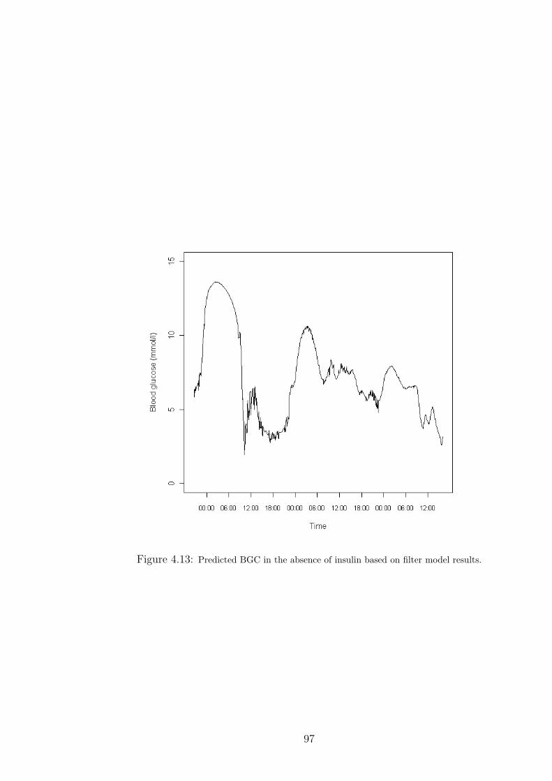
Figure 4.13: Predicted BGC in the absence of insulin based on filter model results.
97
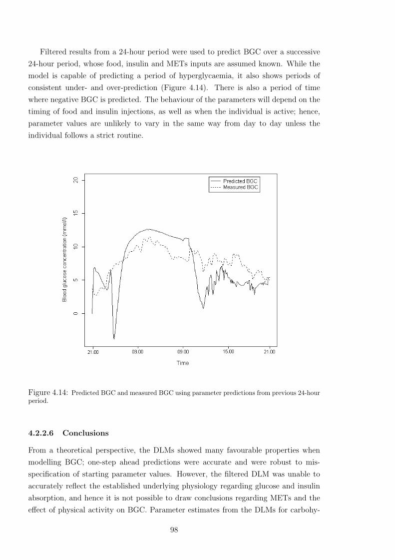
Filtered results from a 24-hour period were used to predict BGC over a successive
24-hour period, whose food, insulin and METs inputs are assumed known. While the
model is capable of predicting a period of hyperglycaemia, it also shows periods of
consistent under- and over-prediction (Figure 4.14). There is also a period of time
where negative BGC is predicted. The behaviour of the parameters will depend on the
timing of food and insulin injections, as well as when the individual is active; hence,
parameter values are unlikely to vary in the same way from day to day unless the
individual follows a strict routine.
Figure 4.14: Predicted BGC and measured BGC using parameter predictions from previous 24-hourperiod.
4.2.2.6 Conclusions
From a theoretical perspective, the DLMs showed many favourable properties when
modelling BGC; one-step ahead predictions were accurate and were robust to mis-
specification of starting parameter values. However, the filtered DLM was unable to
accurately reflect the established underlying physiology regarding glucose and insulin
absorption, and hence it is not possible to draw conclusions regarding METs and the
effect of physical activity on BGC. Parameter estimates from the DLMs for carbohy-
98

drate and insulin do not agree with established knowledge, suggesting the models would
be unsuitable for a “what if” analysis and hence could not aid the MDI regime. The
disparity between model estimates and established physiology may be due to issues
with parameter identification. This is a particular problem in diabetes modelling; it
is not possible to safely excite individual inputs (particularly food and insulin) while
keeping others constant, thus the individual effects of simultaneously-excited inputs
are obscured.
4.3 Sampling the DLM of Blood Glucose Concen-
tration
Another approach to parameter learning is to sample the full posterior distribution of
parameters,
p(ΘT , σ2,Ω) =
T∏i=0
[p(θi)|σ2,Ω]p(σ2)p(Ω),
where ΘT = (θ0,θ1, . . . ,θT ) is the full set of regression parameters. The poste-
rior distribution is complex, making parameter learning difficult; in such situations,
computationally-intensive methods such as Markov chain Monte Carlo (MCMC) are
often used (Gilks et al., 1996). MCMC methods provide a general approach for sam-
pling from probability distributions, and are discussed in appendix C for those unfa-
miliar with this approach. MCMC will be used here to simulate from the posterior
distribution of the parameters.
4.3.1 Full, Individual Conditional Sampling
One method for sampling the parameter vector, Θ, is to sample from the full, individual
conditional distribution, p(θi|Y T ,Θ·−i, φ,Ωt), where Θ·−i = (θ0, . . . ,θi−1,θi+1, . . . ,θT ).
Given the structure of the DLM, neighbouring values of θi will be correlated; hence,
sampling from these distributions will generally result in slower mixing compared to
sampling from the joint distribution (Chib and Greenberg, 1996). However, this ap-
proach allows a little more flexibility in terms of defining the error variances, as there
is no need to use a discount factor for Ωt. Assuming Ω, a (p× p) matrix, is constant,
the conjugate prior distribution is given by an inverse Wishart distribution with pa-
rameters υ and Σ, representing the degrees of freedom and an inverse scale matrix,
respectively. The distribution is denoted by Ω ∼ IWp(υ,Σ), where
p(Ω) =|Σ|υ/2|Ω|−υ+p+1 exp[−1
2trace(ΣΩ−1)]
2υp/2Γp(υ/2),
99
with Γp(·) representing the p-variate gamma function. The inverse Wishart is the
multivariate generalisation of the inverse gamma distribution. The prior distribution
for φ = σ−2, assumed constant, is a gamma distribution.
Setting ψ = Θ, σ2,Ω, the full, joint posterior distribution for the parameter set
is given by the product of the likelihood (the observation and system equations) and
prior distributions:
p(ψ|y) ∝ p(ψ) · p(y|ψ)
∝T∏t=1
φ1/2 exp[−φ2
(yt − xTt θt)
2]
×T∏t=1
|Ω|−1/2 exp[−1
2(θt − θt−1)
TΩ−1(θt − θt−1)]
× exp[−1
2(θ0 −m0)
TC−10 (θ0 −m0)]
× (φ)n−1 exp(−dφ)
× |Ω|−(υ+p+1)/2 exp(−trace(ΣΩ−1)/2). (4.3.1)
After observing the data, the conditional posterior distribution for φ is updated to
φ|(y,θ0,Θ,Ω) ∼ G(n+ T/2, d+1
2
T∑t=1
(yt − xTt θt)
2). (4.3.2)
The conditional posterior distribution for Ω is
Ω|(y,θ0,Θ, φ) ∼ IWp(υ + T,Σ +T∑t=1
(θt − θt−1)T(θt − θt−1)).
The initial regression parameters are updated to
θ0|(y,Θ, τ 2t , λ
2t ) ∼ N(b0,B0)
where
B−10 = λ2
1W−1 +C−1
0 ,
B−10 b0 = λ2
1W−1θ1 +C−1
0 m0.
For t = 1, . . . , T − 1, the regression parameters have a posterior distribution given by
θt|(y,θ0,Θ−t, τ2t , λ
2t ) ∼ N(bt,Bt)
100

where
B−1t = τ 2
t xtxTt + λ2
tW−1 + λ2
t+1W−1,
B−1t bt = τ 2
t ytxt + λ2tW
−1θt−1 + λ2t+1W
−1θt+1.
For t = T , the posterior distribution is
θT |(y,θ0,Θ−T , τ2t , λ
2t ) ∼ N(bT ,BT )
where
B−1T = τ 2
TxTxTT + λ2
TW−1,
B−1T bT = τ 2
TyTxT + λ2TW
−1θT−1.
The posterior distributions are all of standard form, hence Gibbs sampling may be
used. Under Gibbs sampling methods, samples are drawn from the full conditional
distribution, p(ψ|y). For parameter ψi this involves considering only terms involving
ψi. Defining ψ−i = (ψ1, . . . , ψi−1, ψi+1, . . . , ψk), this is equivalent to sampling from
p(ψ|y,ψ−i). Conjugacy of the priors and the likelihood ensures closed distributions.
Gibbs sampling also allows for component-wise updating, where components may be
of differing dimensions. In this case the regression parameters will be considered as
one component, and the variances, σ2 and Ω, as individual components.
4.3.1.1 Results
The output for the full, individual conditional approach shows varied results. Mixing
is good for Θ at early time points but becomes considerably worse as t increases, as
seen in the trace plots in Figure 4.15. The poor mixing remains after 20,000 iterations.
This is likely to be due to the correlation between the parameters. Mixing is, however,
good for the error variances; Figure 4.16 shows the trace plot for the observation error
variance.
4.3.2 Full, Joint Conditional Sampling
An alternative approach to sampling the regression parameters is proposed by Carter
and Kohn (1994). This approach simulates the θi, for i = 0, . . . , T , from their full,
joint conditional distribution, p(Θ|y, σ2t ,Ωt). Dropping the dependence on the error
variances for convenience, the joint distribution may be written as
p(Θ|Y T ) = p(θT |Y T )T−1∏i=0
p(θi|Y i,θi+1),
101
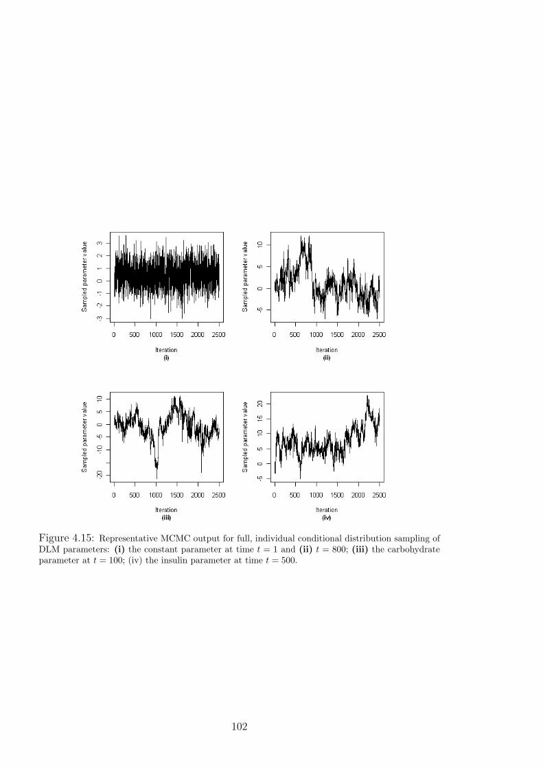
Figure 4.15: Representative MCMC output for full, individual conditional distribution sampling ofDLM parameters: (i) the constant parameter at time t = 1 and (ii) t = 800; (iii) the carbohydrateparameter at t = 100; (iv) the insulin parameter at time t = 500.
102

Figure 4.16: MCMC output for observation error precision, φ, under full, individual conditionaldistribution sampling of DLM parameters.
103
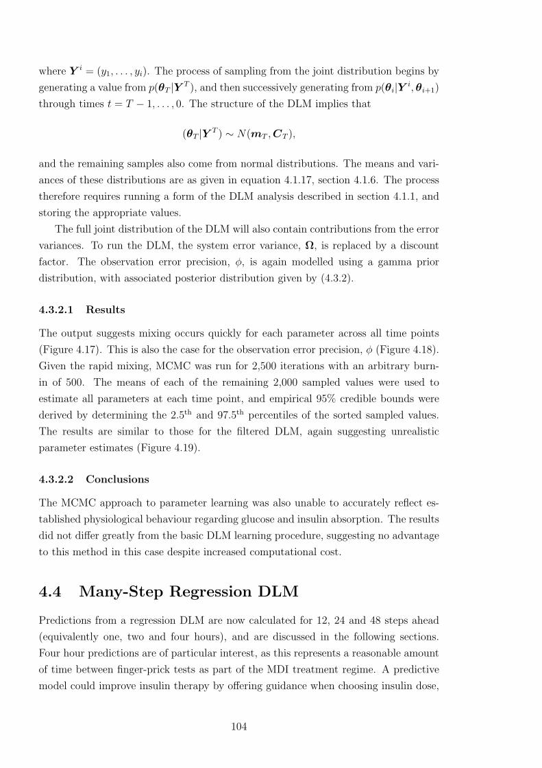
where Y i = (y1, . . . , yi). The process of sampling from the joint distribution begins by
generating a value from p(θT |Y T ), and then successively generating from p(θi|Y i,θi+1)
through times t = T − 1, . . . , 0. The structure of the DLM implies that
(θT |Y T ) ∼ N(mT ,CT ),
and the remaining samples also come from normal distributions. The means and vari-
ances of these distributions are as given in equation 4.1.17, section 4.1.6. The process
therefore requires running a form of the DLM analysis described in section 4.1.1, and
storing the appropriate values.
The full joint distribution of the DLM will also contain contributions from the error
variances. To run the DLM, the system error variance, Ω, is replaced by a discount
factor. The observation error precision, φ, is again modelled using a gamma prior
distribution, with associated posterior distribution given by (4.3.2).
4.3.2.1 Results
The output suggests mixing occurs quickly for each parameter across all time points
(Figure 4.17). This is also the case for the observation error precision, φ (Figure 4.18).
Given the rapid mixing, MCMC was run for 2,500 iterations with an arbitrary burn-
in of 500. The means of each of the remaining 2,000 sampled values were used to
estimate all parameters at each time point, and empirical 95% credible bounds were
derived by determining the 2.5th and 97.5th percentiles of the sorted sampled values.
The results are similar to those for the filtered DLM, again suggesting unrealistic
parameter estimates (Figure 4.19).
4.3.2.2 Conclusions
The MCMC approach to parameter learning was also unable to accurately reflect es-
tablished physiological behaviour regarding glucose and insulin absorption. The results
did not differ greatly from the basic DLM learning procedure, suggesting no advantage
to this method in this case despite increased computational cost.
4.4 Many-Step Regression DLM
Predictions from a regression DLM are now calculated for 12, 24 and 48 steps ahead
(equivalently one, two and four hours), and are discussed in the following sections.
Four hour predictions are of particular interest, as this represents a reasonable amount
of time between finger-prick tests as part of the MDI treatment regime. A predictive
model could improve insulin therapy by offering guidance when choosing insulin dose,
104

Figure 4.17: Representative MCMC trace plots, sampled values for: (i) constant parameter at timet=0; (ii) carbohydrate parameter at time t=50; (iii) insulin parameter at time t=100; (iv) METsparameter at time t=500.
Figure 4.18: MCMC trace plot for observation error precision, φ.
105
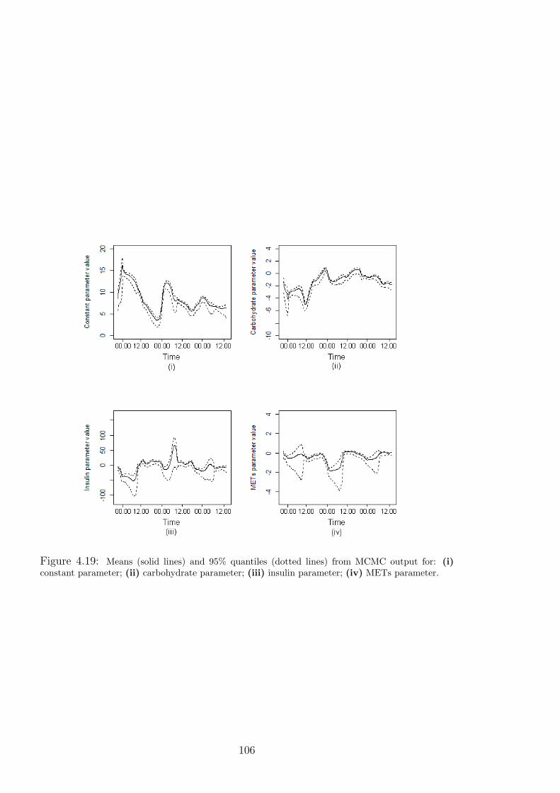
Figure 4.19: Means (solid lines) and 95% quantiles (dotted lines) from MCMC output for: (i)constant parameter; (ii) carbohydrate parameter; (iii) insulin parameter; (iv) METs parameter.
106

and help avoid hypo- or hyperglycaemia.
For k = 12, 24, 48-step ahead predictions, the full set of BGC measurements (the
ensemble; t = 1, . . . , T ) is split into k time series, whose BGC measurements are k
steps (5k minutes) apart:
for n = 1, . . . , k,
g[n] = gn, gn+k, . . . , gn+tkk, (4.4.1)
where tk is such that tkk ≤ T < (tk + 1)k. For each time series, g[n], a one-step single-
discount DLM (as in section 4.2.2) is run (note that these DLMs will be referred to as
many-step DLMs in reference to the fact they are forecasting 5k minutes ahead). To
initiate each time series, a one-step single-discount DLM is applied to the ensemble,
from time t = 1 to t = k; these results are filtered (as in section 4.2.2.5), and the
filtered distributions are used as the initial distributions, p(θ[n]|D0), for the associated
time series, g[n].
Forecast performance may be assessed by comparing measured and forecast BGC
both within each time series and by considering forecasts from each time series con-
currently. Two new indices are also presented to assess forecast performance; these
are introduced to determine a model’s ability to predict hypo- and hyperglycaemia.
Though a model may not be able to accurately predict the future profile of BGC, it
would still be of value if it can accurately determine periods of hypo- or hyperglycaemic
(collectively referred to from here on as glycaemic excursions). Index 1 is defined as
I(1)t (gt) =
−1, for gt < 4 mmol/l
0, for 4 mmol/l ≤ gt ≤ 8 mmol/l
+1, for gt > 8 mmol/l ,
(4.4.2)
and thus separates BGC into ranges for hypoglycaemia, euglycaemia and hypergly-
caemia, respectively. The ability of the model to predict glycaemic excursions may
be assessed by comparing I(1)t (gt) (measured BGC) with I
(1)t (ft) (model forecasts of
BGC). The predictive ability of the model may be further assessed by Index 2, defined
as
I(2)t (gt) =
0, if I
(1)t (gt) = I
(1)t (ft)
1, if |I(1)t (gt)− I(1)
t (ft)| = 1
2, if |I(1)t (gt)− I(1)
t (ft)| = 2 ,
(4.4.3)
and so highlights agreement and large discrepancies between measured and predicted
BGC.
107

4.4.1 12-Step BGC Prediction
The discount factor for the 12-step (one hour) predictive model is chosen to be 0.66
based on the error measures MAD, MSE and LLR (results not shown). Figure 4.20
shows predictions for time series g[1] and g[12], and suggests the model is generally able
to match the profile of measured BGC; however, there are some large discrepancies
between predictions and measurements, caused by the increase in METs upon waking.
Considered as a single time series, the 12-step predictions generally matches the profile
of measured BGC, albeit with consistent under- or overestimation across consecutive
time points. Early in the day, predictions become unstable due to the sudden increase
in METs upon waking. Indices 1 and 2 suggest the model is generally able to dis-
tinguish between euglycaemia and glycaemic excursions; Figure 4.22, plot (i) suggests
the model is able to determine glycaemic excursions, albeit with a lag when predicting
hyperglycaemia, and Figure 4.22, plot (ii) suggests predicted and measured BGC are
in the same glycaemic range for the majority of the time series.
Parameter estimates for the 12-step model appear to vary between time series; Fig-
ure 4.23 shows oscillations for each parameter, suggesting marked differences between
estimates depending on when the time series begins. Parameter estimates do not com-
ply with established physiological knowledge, as the insulin parameter is predominantly
positive and the carbohydrate parameter predominantly negative. This suggests the
model is unable to adequately describe the effect food and insulin has on BGC, perhaps
due to the inputs’ simultaneous excitations; hence, the model would not be suitable
for guiding insulin dosing.
4.4.2 24-Step BGC Prediction
The discount factor for the 24-step (two hours) predictive model is chosen to be 0.98
based on the error measures (results not shown). Figure 4.24 shows predicted and
measured BGC for time series g[1] and g[24], which suggests mixed predictive results
across time series; plot (i) shows g[1] fails to recreate the profile of measured BGC, in
particular the predictions miss the hyperglycaemia during the first night, while plot
(ii) shows better predictive performance, albeit with evidence of a lag in the predic-
tions with regard to the hyperglycaemia during the first night. Figure 4.25 shows the
compiled time series, and suggests there are particular problems with time series g[1]
through the night as it consistently underestimates measured BGC; it is unclear why
this problem appears to affect only this time series. Predictions during the day fluc-
tuate due to the influence of METs, and are generally unable to reflect the profile of
measured BGC. Index 1 suggests that 24-step predictions are able to determine periods
of hyperglycaemia, but fail to pick up periods of hypoglycaemia (Figure 4.26, plot (i)).
Index 2 suggests there is moderate agreement between predictions and measurements
108
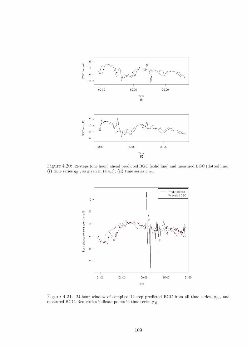
Figure 4.20: 12-steps (one hour) ahead predicted BGC (solid line) and measured BGC (dotted line):(i) time series g[1], as given in (4.4.1); (ii) time series g[12].
Figure 4.21: 24-hour window of compiled 12-step predicted BGC from all time series, g[n], andmeasured BGC. Red circles indicate points in time series g[1].
109
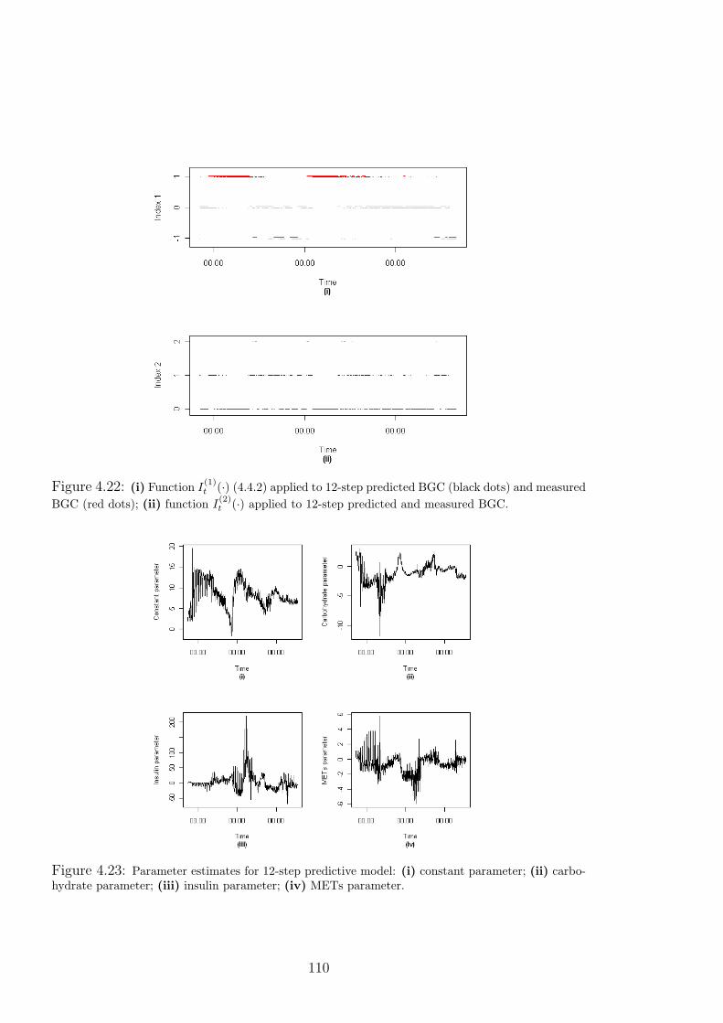
Figure 4.22: (i) Function I(1)t (·) (4.4.2) applied to 12-step predicted BGC (black dots) and measured
BGC (red dots); (ii) function I(2)t (·) applied to 12-step predicted and measured BGC.
Figure 4.23: Parameter estimates for 12-step predictive model: (i) constant parameter; (ii) carbo-hydrate parameter; (iii) insulin parameter; (iv) METs parameter.
110

in terms of the range of BGC, with small discrepancies in prediction also fairly common
and large discrepancies relatively rare (Figure 4.26, plot (ii)). Parameter estimates os-
cillate, as with the 12-step model, suggesting estimates are dependent on when the time
series begins. Furthermore, parameter estimates again fail to comply with established
knowledge, as the carbohydrate parameter is predominantly negative (Figure 4.27).
4.4.3 48-Step BGC Prediction
The discount factor for this model is chosen to be 0.85 based on the error measures
(results not shown). Figure 4.28 shows predictions and measurements for time series
g[1] and g[48], which suggest a lag between predictions and measurements. Predictions
appear to be unable to determine the larger changes in BGC and consistently over-
estimate BGC during the first day. For g[48], there is a negative prediction which is
physiologically non-viable. Figure 4.29 shows reasonable predictive performance dur-
ing the night, again with the exception of g[1]. During the day, predicted BGC is
occasionally greatly below measured BGC, most likely due to the nature of METs.
Index 1 suggests the fluctuating nature of the predictions leads to an overestimation
of glycaemic events (Figure 4.30, plot (i)); however, the model is able to determine
periods of hyperglycaemia, albeit for longer durations than the measured BGC. Index
2 suggests moderate agreement between predictions and measurements with regard to
the glycaemic ranges of BGC (Figure 4.30, plot (ii)). As with the previous many-step
predictive models, parameter estimates oscillate and the carbohydrate parameter is
negative (Figure 4.31).
4.4.4 Conclusions
Many-step DLMs were unable to accurately reflect the profile of measured BGC. The
12-step model suggested reasonable predictive performance, particularly when predic-
tions and measurements of BGC were compared using the indices; however, predictions
were unstable in the mornings due to the sudden increase in METs upon waking. Pa-
rameter estimates also failed to comply with established knowledge, suggesting the
model is unable to offer appropriate guidance for insulin dosage. The 24-step and 48-
step models were generally unable to predict the profile of measured BGC, and the
indices suggested that the models were also unable to accurately predict the range of
measured BGC for any length of time.
4.5 Summary
DLMs were used to predict BGC using food intake, insulin, and physical activity as
explanatory variables, with two aims: firstly, to understand the effect of physical ac-
111
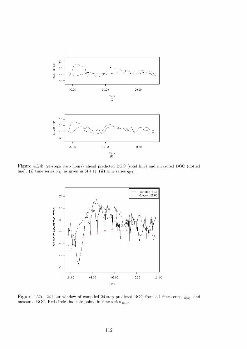
Figure 4.24: 24-steps (two hours) ahead predicted BGC (solid line) and measured BGC (dottedline): (i) time series g[1], as given in (4.4.1); (ii) time series g[24].
Figure 4.25: 24-hour window of compiled 24-step predicted BGC from all time series, g[n], andmeasured BGC. Red circles indicate points in time series g[1].
112

Figure 4.26: (i) Function I(1)t (·) (4.4.2) applied to 24-step predicted BGC (black dots) and measured
BGC (red dots): (ii) function I(2)t (·) applied to 24-step predicted and measured BGC.
Figure 4.27: Parameter estimates for 24-step predictive model: (i) constant parameter; (ii) carbo-hydrate parameter; (iii) insulin parameter; (iv) METs parameter.
113
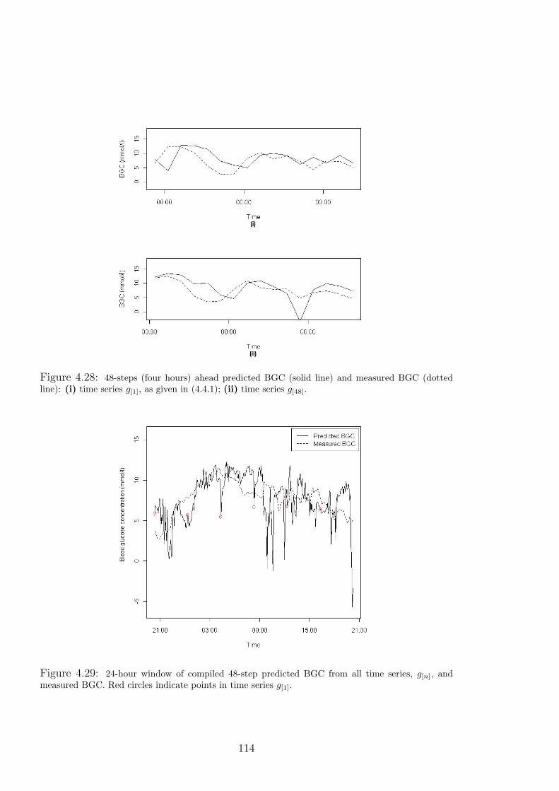
Figure 4.28: 48-steps (four hours) ahead predicted BGC (solid line) and measured BGC (dottedline): (i) time series g[1], as given in (4.4.1); (ii) time series g[48].
Figure 4.29: 24-hour window of compiled 48-step predicted BGC from all time series, g[n], andmeasured BGC. Red circles indicate points in time series g[1].
114
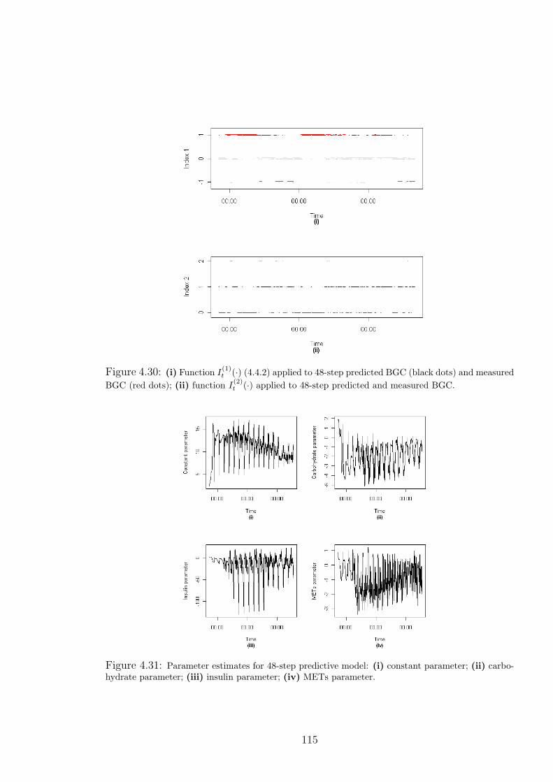
Figure 4.30: (i) Function I(1)t (·) (4.4.2) applied to 48-step predicted BGC (black dots) and measured
BGC (red dots); (ii) function I(2)t (·) applied to 48-step predicted and measured BGC.
Figure 4.31: Parameter estimates for 48-step predictive model: (i) constant parameter; (ii) carbo-hydrate parameter; (iii) insulin parameter; (iv) METs parameter.
115
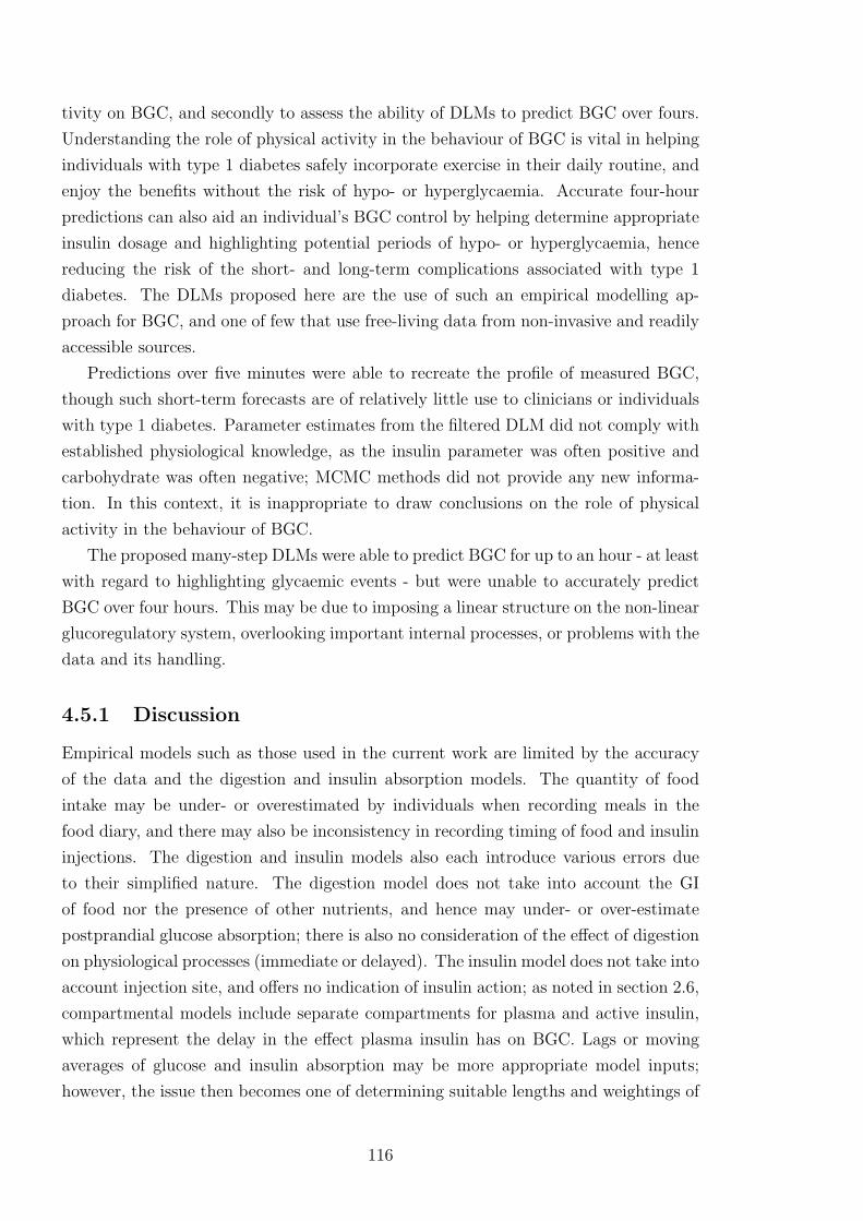
tivity on BGC, and secondly to assess the ability of DLMs to predict BGC over fours.
Understanding the role of physical activity in the behaviour of BGC is vital in helping
individuals with type 1 diabetes safely incorporate exercise in their daily routine, and
enjoy the benefits without the risk of hypo- or hyperglycaemia. Accurate four-hour
predictions can also aid an individual’s BGC control by helping determine appropriate
insulin dosage and highlighting potential periods of hypo- or hyperglycaemia, hence
reducing the risk of the short- and long-term complications associated with type 1
diabetes. The DLMs proposed here are the use of such an empirical modelling ap-
proach for BGC, and one of few that use free-living data from non-invasive and readily
accessible sources.
Predictions over five minutes were able to recreate the profile of measured BGC,
though such short-term forecasts are of relatively little use to clinicians or individuals
with type 1 diabetes. Parameter estimates from the filtered DLM did not comply with
established physiological knowledge, as the insulin parameter was often positive and
carbohydrate was often negative; MCMC methods did not provide any new informa-
tion. In this context, it is inappropriate to draw conclusions on the role of physical
activity in the behaviour of BGC.
The proposed many-step DLMs were able to predict BGC for up to an hour - at least
with regard to highlighting glycaemic events - but were unable to accurately predict
BGC over four hours. This may be due to imposing a linear structure on the non-linear
glucoregulatory system, overlooking important internal processes, or problems with the
data and its handling.
4.5.1 Discussion
Empirical models such as those used in the current work are limited by the accuracy
of the data and the digestion and insulin absorption models. The quantity of food
intake may be under- or overestimated by individuals when recording meals in the
food diary, and there may also be inconsistency in recording timing of food and insulin
injections. The digestion and insulin models also each introduce various errors due
to their simplified nature. The digestion model does not take into account the GI
of food nor the presence of other nutrients, and hence may under- or over-estimate
postprandial glucose absorption; there is also no consideration of the effect of digestion
on physiological processes (immediate or delayed). The insulin model does not take into
account injection site, and offers no indication of insulin action; as noted in section 2.6,
compartmental models include separate compartments for plasma and active insulin,
which represent the delay in the effect plasma insulin has on BGC. Lags or moving
averages of glucose and insulin absorption may be more appropriate model inputs;
however, the issue then becomes one of determining suitable lengths and weightings of
116

lags for these inputs.
Physical activity presents an even greater modelling challenge, as the effect of ac-
tivity may be immediate and/or last several hours, depending on the type, duration
and intensity of activity. The use of lags or moving averages may represent the ef-
fects of activity in a more physiologically-appropriate manner, but requires choice of
appropriate time intervals, which are likely to vary depending on type, duration and
intensity of activity. It is also apparent that the high variability of METs during the
day resulted in highly fluctuating predictions. This problem could be overcome by
smoothing METs; however, this requires finding suitable weights and time windows for
smoothing, and risks losing important information.
Modelling BGC during the night with the proposed form of DLMs also presents its
own problems. The food, insulin and METs inputs are generally very stable at night
(and close to zero in the case of carbohydrate) and effects that are unaccounted for,
such as hepatic glucose release, become much more prominent, and may be erroneously
attributed to one or more of the inputs.
Empirical models based only on easily measurable inputs may be improved by more
accurate representations of glucose and insulin absorption after meals and injections,
respectively, and better understanding of the physiological processes affected by these
disturbances. Furthermore, METs requires better handling, whether through smooth-
ing, lags or otherwise, in order to better represent the effect of physical activity on
BGC. Non-linear dynamic models would be more physiologically representative, but
would be difficult to construct given that non-linearities in the glucoregulatory system
are not well understood, and potentially time- and subject-specific.
The roles of food, insulin and physical activity may be better captured in a model
with a physiological basis. The semi-empirical compartmental models discussed in
sections 2.6.1 and 2.6.2 are more physiologically representative of the glucoregulatory
system than a DLM, albeit at the cost of greater complexity. However, such models
may be able to better reflect the role of food, insulin and physical activity in the
behaviour of BGC.
117


Chapter 5
Stochastic Modelling of
Glucose-Insulin Dynamics in
Free-Living Conditions for People
with Type 1 Diabetes
The previous chapter highlighted the difficulties in building empirical models of blood
glucose concentration (BGC). The focus of this chapter remains on investigating the
role of physical activity, now through semi-empirical compartmental models. The
work draws on the decades of research stimulated by the minimal model proposed
by Bergman et al. (1979, 1981).
This chapter begins with a description of the minimal model and its various ex-
tensions, in particular the work of Andersen and Højbjerre (2005) and the physical
activity minimal model of Roy and Parker (2007) (referred to as the PA model from
here). The focus then moves onto testing the viability of combining the PA model with
free-living data. The PA model, like the vast majority of models in the diabetes litera-
ture, is tested only on clinical or simulated data that do not accurately reflect the daily
experience of individuals. Using the DUK study data (as discussed in chapter 3), the
first aim is to explore the practical issues of using frequently-sampled, highly-variable
free-living data on the PA model; this is the first attempt to combine free-living data
on BGC, food intake, insulin and physical activity with such models.
New methods for analysing compartmental models are then presented as a more re-
alistic representation of the underlying physiology. Markov chain Monte Carlo methods
are tested as a tool for estimating all model parameters using a simulation study.
119
5.1 Development of the Minimal Model
The minimal model (MM) was discussed in section 2.6.1; to recap, the MM is a com-
partmental model used to describe blood glucose-insulin kinetics, whose structure is
given in Figure 5.1. The variables G(t) [mg/dl], Ip(t) [µU/ml], and Ia(t) [µU/ml] repre-
sent the concentrations of blood glucose, blood insulin, and remote (or active) insulin,
respectively. The equations used to describe glucose-insulin kinetics are
dG(t)
dt= G = [p1 −X(t)]G(t) + p4
X = p2X(t) + p3Ip(t)
Ip = p5(G(t)− p6)t− p7Ip(t),
(5.1.1)
where X = (k4 + k6)Ia(t) [min−1] describes the insulin action in the remote compart-
ment. The relationships between model and equation parameters (ki and pi, respec-
tively) are described in Table 5.1.
Ip(t) -k2
Ia(t) -k3
G(t)-
k6
g -k1
Liver Periphery?
k4
?
k5
(i)
Ip(t)-k7(G− a)t
-−k8Ip(t)
(ii)
Figure 5.1: Minimal model of glucose-insulin kinetics: (i), model of glucose metabolism; (ii), modelof insulin kinetics. Reproduced from Bergman et al. (1979, 1981).
Table 5.1: Relationship of model and equation parameters for the minimal model.
Parameter Units Descriptionp1 = −(k1 + k5) min−1 Rate of insulin-independent glucose uptakep2 = −k3 min−1 Rate of decreasing ability to uptake glucosep3 = k2(k4 + k6) ml/µU/min2 Rate constant of insulin-dependent glucose uptakep4 = H0 mg/dl/min Hepatic balance extrapolated to zero BGCp5 = k7 µU/mg/min2 Rate of insulin release by β-cellsp6 = a mg/dl Threshold for insulin releasep7 = k8 min−1 Rate of insulin clearance
120

Originally, the MM was used to determine insulin sensitivity in people with type 2
diabetes. Analysis involves two stages: firstly, a known insulin time course is supplied
to the glucose model (Figure 5.1 (i)) for parameter estimation; secondly, a glucose time
course is supplied to estimate parameters in the insulin model (Figure 5.1 (ii)). Con-
sidering the model as one unified system can lead to unrealistic behaviour (De Gaetano
and Arino, 2000). Various generalisations and improvements have been posited in the
literature to extend the MM and/or overcome its limitations; of particular interest here
is the extension proposed by Roy and Parker (2007) to include the physical activity
of exercise, and the stochastic, population model proposed by Andersen and Højbjerre
(2005), discussed in the following sections.
5.1.1 Stochastic Minimal Model
It is argued here that a stochastic model of blood glucose-insulin dynamics would
better reflect the uncertainty inherent in complex biological systems, and hence would
be a more physiologically-viable representation of the glucoregulatory system when
compared to a set of deterministic differential equations. Andersen and Højbjerre
(2005) approached the minimal model with a similar perspective; their reformulation
of the MM converts the deterministic differential equations (DEs) into a Bayesian
network, where modern sampling techniques may then be used for parameter estimation
based on an IVGTT and subsequent blood samples. The reformulation uses vague
prior distributions, based on previous studies, to allow unified analysis of the model,
and proceeds as follows:
i) rewrite (5.1.1) in terms of the natural logarithms of the (positive) latent processes:
g(t) = ln[G(t)], x(t) = ln[X(t)] and i(t) = ln[Ip(t)] (note that Ip will be rep-
resented by I from here on, and Ia from the original MM is only considered in
terms of X);
ii) add a stochastic term to each equation to account for measurement and process
variability: stochastic terms are Wiener processes representing the integral of
Gaussian white noise;
iii) convert the DEs to integral equations by integration over a small time frame;
iv) approximate integrals to determine an iterative set of equations;
v) determine conditional distributions for the log-transformed latent processes: the
means of the distributions are determined by the MM, and the precisions by the
Wiener process;
vi) model observations as Gaussian to account for measurement errors: the means of
the distribution are given by the underlying latent process.
121

Using blood glucose as an example, the reformulation converts the DEs into the form:
(gtk |gtk−1, xtk−1
, τg) ∼ N(fg,t(gtk−1, xtk−1
), (∇t)τ−1g ),
where
fg,t(gtk−1, xtk−1
) = gtk−1−∇tp1[1−Gb exp(−gtk−1
)] + exp(xtk−1);
note that p1 has changed sign from the original MM, Gb = p4/p1 is basal glucose, τg
is the precision associated with the Wiener process, and ∇t = tk − tk−1 represents the
time span over which the approximations are made.
Parameters p1, . . . , p6 are assumed to have log-normal prior distributions, and
precisions are assumed to have gamma prior distributions. The parameters of these
distributions may also be assigned prior distributions to extend the reformulation to a
population model. A directed acyclic graph (DAG) is used to represent the relation-
ships between variables, g, x, i, and blood glucose and insulin observations, go, io(Figure 5.2); vertices represent variables at given time points (here square boxes are
the unobserved, latent processes and the circles represent observed processes), while di-
rected edges describe the dependencies between variables. The posterior distribution of
all unknown parameters is analysed using MCMC methods, allowing for simultaneous,
model-wide parameter estimation.
The approach presented by Andersen and Højbjerre is aimed at improving analysis
of the minimal model, and hence is concerned only with type 2 diabetes. The methods
are geared specifically toward estimating the insulin sensitivity and glucose effectiveness
parameters based on intermittent blood samples collected for up to four hours. The
approach has therefore only been tested on data collected in a clinical setting over a
limited time frame, with no attempt to extend the model to include the influence of
digestion, insulin injection or physical activity.
5.1.2 Physical Activity Minimal Model
Roy and Parker (2007) generalised and adapted the original minimal model for use in
type 1 diabetes by including terms for exogenous insulin, meals and physical activity.
Six DEs were included to account for the effects of physical activity: one accounting
for PVOmax2 (E; see section 2.5.4), one for integrated activity intensity (A), and one
each for the activity-induced effects on hepatic glucose production (H; mg/kg/min),
glucose uptake (U ; mg/kg/min), insulin clearance (Z; µU/ml/min), and decline in rate
of glycogenolysis (K; mg/kg/min).
The blood glucose DE of the MM is modified by including the influence of the
122

...
...
...
...
...
...
gtk−1
xtk−1
itk−1
gtk
xtk
itk
gtk+1
xtk+1
itk+1
gotk
iotk
-
-
-
-
-
-
6
?
AAAAAAAAU
AAAAAAAAU
Figure 5.2: Directed acyclic graph of the Andersen and Højbjerre (2005) model.
processes H, K and U , and glucose absorption from food (MG; mg/min):
G(t) =− p1(G(t)−Gb)−X(t)G(t)
+ (W/VG)[H(t)−K(t)− U(t)] +MG(t)/VG,(5.1.2)
where W is weight (kg), and VG is the glucose distribution space (dl). The blood
insulin DE is modified by the influence of Z and insulin absorption after injection (MI ;
µU/min):
I(t) =− p2I(t) + p3MI(t)− Z(t). (5.1.3)
Insulin action is given by
X(t) =− p4X(t) + p5(I(t)− Ib), (5.1.4)
where Ib is basal insulin. Physical activity intensity, measured by PVOmax2 , is modelled
by a DE to describe the delay in reaching a steady state value at the onset of activity
(therefore mimicking the delay in increased oxygen uptake and heart rate):
E(t) =− p6E(t) + p7ME(t), (5.1.5)
where ME is the actual intensity of activity above basal level (8% VOmax2 ). Parameter
values of p6 = p7 = 0.8 were chosen to acheive an appropriate settling time of five
minutes. The DEs representing the new processes H, U and Z are given by
H(t) = p8E(t)− p9H(t),
U(t) = p10E(t)− p11U(t),
Z(t) = p12E(t)− p13Z(t).
(5.1.6)
123
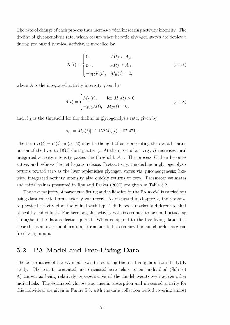
The rate of change of each process thus increases with increasing activity intensity. The
decline of glycogenolysis rate, which occurs when hepatic glycogen stores are depleted
during prolonged physical activity, is modelled by
K(t) =
0, A(t) < Ath
p14, A(t) ≥ Ath
−p15K(t), ME(t) = 0,
(5.1.7)
where A is the integrated activity intensity given by
A(t) =
ME(t), for ME(t) > 0
−p16A(t), ME(t) = 0,(5.1.8)
and Ath is the threshold for the decline in glycogenolysis rate, given by
Ath = ME(t)[−1.152ME(t) + 87.471].
The term H(t)−K(t) in (5.1.2) may be thought of as representing the overall contri-
bution of the liver to BGC during activity. At the onset of activity, H increases until
integrated activity intensity passes the threshold, Ath. The process K then becomes
active, and reduces the net hepatic release. Post-activity, the decline in glycogenolysis
returns toward zero as the liver replenishes glycogen stores via gluconeogenesis; like-
wise, integrated activity intensity also quickly returns to zero. Parameter estimates
and initial values presented in Roy and Parker (2007) are given in Table 5.2.
The vast majority of parameter fitting and validation in the PA model is carried out
using data collected from healthy volunteers. As discussed in chapter 2, the response
to physical activity of an individual with type 1 diabetes is markedly different to that
of healthy individuals. Furthermore, the activity data is assumed to be non-fluctuating
throughout the data collection period. When compared to the free-living data, it is
clear this is an over-simplification. It remains to be seen how the model performs given
free-living inputs.
5.2 PA Model and Free-Living Data
The performance of the PA model was tested using the free-living data from the DUK
study. The results presented and discussed here relate to one individual (Subject
A) chosen as being relatively representative of the model results seen across other
individuals. The estimated glucose and insulin absorption and measured activity for
this individual are given in Figure 5.3, with the data collection period covering almost
124
Table 5.2: Parameters for the Roy and Parker (2007) model. Parameters pi are assumed knownand taken from the original Bergman et al. (1979) model. The set of parameters ai are fitted usingvarious studies; see Roy and Parker (2007) and references within.
Parameter Value Units Initial valuesp1 0.035 min−1 G(0)=Gb
p2 0.142 min−1 I(0)=Ibp3 0.098 ml−1 X(0)=0p4 0.05 min−1 E(0)=0p5 0.000028 ml/µU/min2 H(0)=0p6 0.8 min−1 U(0)=0p7 0.8 min−1 Z(0)=0p8 0.00158 mg/kg/min2 K(0)=0p9 0.056 min−1 A(0)=0p10 0.00195 mg/kg/min2
p11 0.0485 min−1
p12 0.00125 µU/ml/minp13 0.075 min−1
p14 0.0108 mg/kg/min2
p15 0.1667 minp16 1000 PVOmax
2
Gb 80 mg/dlVG 117 dlIb [not defined] µU/ml
three days.
Measured physical activity was converted from METs to relative PVOmax2 (rPVOmax
2 )
by
rPVOmax2 = max
(0,
METs
METsmax
× 100− 8
),
where METsmax is the maximum METs achievable by the individual (equivalent to
VOmax2 ), and basal activity (∼ 8%VOmax
2 , equivalently ∼ 1 METs) is adjusted to zero.
The DEs were solved numerically using the Dormand-Prince (DP) method (Dormand
and Prince, 1980) implemented in Simulink1. DP is a fourth/fifth-order solver which
achieves an appropriate balance between speed and accuracy.
5.2.1 Results
The model was unable to accurately reflect the behaviour of BGC, even predicting
negative concentration (Figure 5.4). A number of other unfavourable results were also
found, due, in particular, to the differences between artificial and free-living physical
activity. Free-living physical activity data are far more variable than the data used to
build the PA model, and rarely return to basal level for an extended period of time
during the day. This results in the integrated exercise, A, increasing throughout the
day (Figure 5.5), and a great over-estimation of the decline in rate of glycogenolysis.
1http://www.mathworks.co.uk/products/simulink/, last accessed 29/11/2012
125

Figure 5.3: Glucose (i) and insulin absorption (ii) (from the digestion and insulin models) andrelative PVOmax
2 (iii) for Subject A.
Subsequently, the model estimates frequent negative contribution from the liver (Figure
5.6), when instead the process K was originally intended to merely dampen the effect
of process H. Such excessive hepatic glucose uptake contradicts what would reasonably
be expected given that the individual did not pass 50% VOmax2 , and did not maintain
an activity level far above basal level for any extended period of time.
Figure 5.4: PA model predicted of BGC and measured BGC for Subject A.
The model also returned negative values for blood insulin concentration (Figure
5.7) and insulin action. This is predominantly due to the activity-stimulated insulin
clearance rate, Z. Insulin clearance increases above the insulin absorbed after injection,
resulting in negative blood insulin; negative insulin action then follows.
126
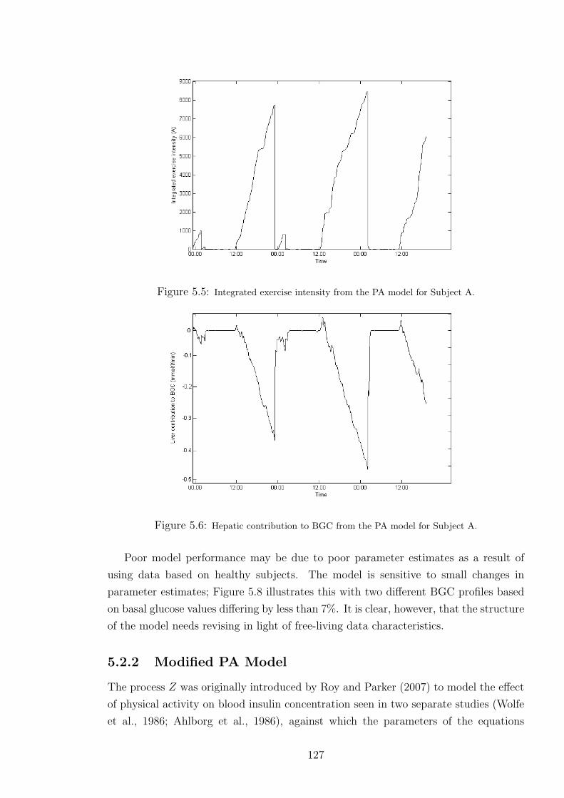
Figure 5.5: Integrated exercise intensity from the PA model for Subject A.
Figure 5.6: Hepatic contribution to BGC from the PA model for Subject A.
Poor model performance may be due to poor parameter estimates as a result of
using data based on healthy subjects. The model is sensitive to small changes in
parameter estimates; Figure 5.8 illustrates this with two different BGC profiles based
on basal glucose values differing by less than 7%. It is clear, however, that the structure
of the model needs revising in light of free-living data characteristics.
5.2.2 Modified PA Model
The process Z was originally introduced by Roy and Parker (2007) to model the effect
of physical activity on blood insulin concentration seen in two separate studies (Wolfe
et al., 1986; Ahlborg et al., 1986), against which the parameters of the equations
127

Figure 5.7: Blood insulin concentration from the PA model for Subject A.
Figure 5.8: BGC profiles for two different basal glucose values, Gb=4.44mmol/l and Gb=4.17mmol/l.
in (5.1.6) were fitted and validated. The two studies were both based on healthy
subjects, where the observed decrease in blood insulin concentration may be explained
by decreased insulin secretion rather than increased clearance. Indeed, Zajadacz et al.
(2009) reported no change in insulin clearance during activity, and Petersen et al.
(2005) reported no decrease in blood insulin in subjects with diabetes during medium
intensity exercise. Hence, the process Z may be modelling a non-existent phenomenon
in type 1 diabetes and is therefore removed from the model.
The basal insulin term, Ib, is also removed from the insulin action DE. In the
context of an individual with type 1 diabetes, the notion of a basal insulin level is not
physiologically accurate. The model implies that, should blood insulin concentration
drop below basal level, the flow of blood insulin into the remote compartment will
decrease; however, the body can not regulate exogenous insulin. In addition, the basal
128

insulin term means that, in hypoinsulinaemic conditions, the insulin action can become
negative.
Absorbed insulin (MI) in the blood insulin DE is scaled by insulin distribution
space, given by VI (ml), as presented by Roy (2008, chapter 2). Absorbed insulin is
therefore assumed to dissipate throughout the bloodstream, in a similar manner to
that of absorbed glucose (MG) in the blood glucose DE.
To account for the effect of renal glucose clearance, a new term is added to the
blood glucose differential equation. Renal clearance, as discussed in section 2.3.1,
may have significant impact on BGC during hyperglycaemia (a common occurrence in
type 1 diabetes), when BGC exceeds the threshold for glucose reabsorption. A term
describing renal clearance, taken from Arleth et al. (2000), is therefore added to the
blood glucose DE. Renal clearance, R, is given by a moving average (MA) of a function
of glomerular filtration rate, f , and blood glucose:
R = MA[max(0, f ·G− r)],
where r is the maximum glucose transport rate above which reabsorption of glucose is
no longer total. The moving average is of width 7 mmol/l to match literature values
of the renal clearance threshold. This smooths the transition from no clearance to full
clearance. The values r = 125 mmol/h and f = 7.5 l/h are also both taken from the
literature. Figure 5.9 shows the renal clearance across a range of BGC according to
this model.
Finally, due to the disproportionate and physiologically unrealistic influence of the
process K, the decline of glycogenolysis rate will not be considered further. The model
thus only represents short- to medium-term physical activity at mild to moderate
intensity, where the depletion of hepatic glycogen stores has little or no effect on hepatic
glucose release. The full modified model, shown in Figure 5.10, is believed to be a
better reflection of the underlying physiology under these conditions. The model now
comprises six DEs:
G(t) =− p1[G(t)−Gb] + (W/VG)[H(t)− U(t)−R(t)]
−X(t)G(t) +MG(t)/VG
I(t) =− p2I(t) + p3MI(t)/VI
X(t) =− p4X(t) + p5I(t)
E(t) = p6ME(t)− p7E(t)
H(t) = p8E(t)− p9H(t)
U(t) = p10E(t)− p11U(t)
(5.2.1)
The modified PA model is still unable to accurately recreate measured BGC profiles,
129
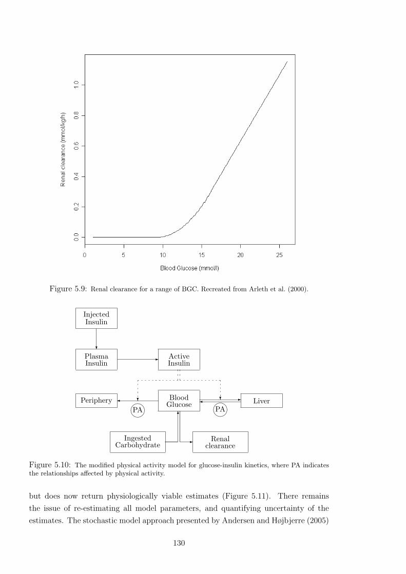
Figure 5.9: Renal clearance for a range of BGC. Recreated from Arleth et al. (2000).
?
InjectedInsulin
-PlasmaInsulin
? ?
ActiveInsulin
LiverPeriphery -BloodGlucose PAPA6
IngestedCarbohydrate
- Renalclearance
Figure 5.10: The modified physical activity model for glucose-insulin kinetics, where PA indicatesthe relationships affected by physical activity.
but does now return physiologically viable estimates (Figure 5.11). There remains
the issue of re-estimating all model parameters, and quantifying uncertainty of the
estimates. The stochastic model approach presented by Andersen and Højbjerre (2005)
130

allows for simultaneous estimation of all model parameters in a Bayesian framework.
A stochastic model is advocated here as it is more physiologically representative of the
body.
Figure 5.11: Measured BGC and modified PA model results for BGC.
5.3 Stochastic Modified PA Model
A stochastic version of the modified PA model is now presented (SPA model); the
methods are applied here using the blood glucose DE as an example. The latent
processes are first converted on to the log scale2; setting g(t) = ln[G(t)], . . . , u(t) =
ln[U(t)], gives
g(t) = G(t)/G(t) = G(t) exp[−g(t)]
= −p11−Gb exp[−g(t)] − exp[x(t)] +MG(t) exp[−g(t)]/VG
+ (W exp[−g(t)]/VG)exp[h(t)]− exp[u(t)]−R(t).
The DE is appended with a stochastic term, represented by a Wiener process, wg(t),
with associated precision, τg, to model possible deviations. By convention, such a
2Theoretically, the processes H and U can be zero, where the logarithm is undefined. However, theform of the differential equations mean these processes cannot return to zero, only become so smallas to be practically zero.
131

stochastic DE is written as:
dg(t) =− p11−Gb exp[−g(t)] − exp[x(t)]
+ (W exp[−g(t)]/VG)exp[h(t)]− exp[u(t)]−R(t)
+MG(t) exp[−g(t)]/VG
dt+ (τ−1/2g )dwg(t).
This is converted to an integral equation by integrating over a small time frame, t to
t+ δ, for small δ > 0, assumed constant here:
g(t+ δ)− g(t) =
∫ t+δ
t
− p11−Gb exp[−g(t)] − exp[x(t)]
+ W exp[−g(t)]/VGexp[h(t)]− exp[u(t)]−R(t)
+MG(t) exp[−g(t)]/VG
dt+ εg(t),
where εg(t) = τ−1/2g [wg(t + δ) − wg(t)]. The integral is approximated by the product
of the width and the integrand evaluated at the lower limit (Euler approximation;
Butcher, 2008). The model is now concerned with discrete time rather than continuous,
hence a change in notation of the form g(t) = gt and εg(t) = εg,t. The change in BGC
over the time span δ is now given by
gt+1 − gt = δ−p1[1−Gb exp(−gt)]− exp(xt)
+ [W exp(−gt)/VG][exp(ht)− exp(ut)−Rt] (5.3.1)
+MG,t exp(−gt)/VG+ εg,t+1.
Standard results for a Wiener process gives εg,t+1 ∼ N(0, δτ−1g ). Setting
fg,t+1 = gt + δ−p1[1−Gb exp(−gt)]− exp(xt)
+ [W exp(−gt)/VG][exp(ht)− exp(ut) (5.3.2)
−Rt] +MG,t exp(−gt)/VG
gives gt+1 = fg,t+1 + εg,t+1, and hence
(gt+1|gt, xt, ht, ut) ∼ N(fg,t+1, δτ−1g ), (5.3.3)
132

ignoring for convenience the dependence of latent processes on the equation parameters.
Following the same procedure for each DE in (5.2.1) gives
(it+1|it) ∼N(fi,t+1, δτ−1i )
(xt+1|xt, it) ∼N(fx,t+1, δτ−1x )
(et+1|et) ∼N(fe,t+1, δτ−1e )
(ht+1|ht, et) ∼N(fh,t+1, δτ−1h )
(ut+1|ut, et) ∼N(fu,t+1, δτ−1u ),
(5.3.4)
wherefi,t+1 =it + δ[−p2 + p3MI,t exp(−it)/VI ]
fx,t+1 =xt + δ[−p4 + p5 exp(−xt) exp(it)]
fe,t+1 =zt + δ[p6ME,t exp(−et)− p7]
fh,t+1 =ht + δ[p8 exp et exp(−ht)− p9]
fu,t+1 =ut + δ[p10 exp et exp(−ut)− p11].
(5.3.5)
The log of BGC measurements, g∗t , are assumed to have measurement error modelled
by white noise, with expectation equal to the underlying latent process:
g∗t |(gt, τg∗) ∼ N(gt, τ−1g∗ ). (5.3.6)
The DAG of the SPA model is given in Figure 5.12, and shows the conditional rela-
tionships between the latent processes.
The final stage of the process requires setting prior distributions for the equation
parameters and precisions. The positive equation parameters, p1, . . . , p11, Gb, VG, VI,are assumed to have a log-normal prior distribution, e.g.,
p1 ∼ lnN(µp1 , τ−1p1
), (5.3.7)
where if X ∼ lnN(µ, τ−1) then
f(x) =τ 1/2
x√
2πexp
[−τ(lnx− µ)2
2
],
with E[X] = exp[µ + 1/(2τ)] and V [X] = [exp(τ−1) − 1] exp(2µ + τ−1). The pre-
cisions, τg∗ , τg, . . . , τu, are assumed to have a conditionally conjugate gamma prior
distribution (for modelling convenience), e.g.,
τg ∼ G(ατg , βτg). (5.3.8)
133

...
...
...
...
...
...
...
...
...
...
...
...
et−1 et et+1
ut−1
ht−1
gt−1
ut
ht
gt
ut+1
ht+1
gt+1
xt−1
it−1
xt
it
xt+1
it+1
g∗t
-
-
-
-
-
-
-
-
-
-
-
-
-
-
@@@@@R
@@@@@R
@@@@@R
@@@@@R
?
Figure 5.12: Directed acyclic graph of the extended model.
5.3.1 Posterior Distribution of the SPA model
For convenience, the equation parameters, precisions and latent processes are split into
three groups:
Ω1 =p1, p2, p3, p4, p5, p6, p7, p8, p9, p10, p11, Gb, VG, VI,
Ω2 =τg, τi, τx, τh, τu, τe, τg∗,
Φ =g, i, x, h, u, e,
with the full collection denoted by θ = Ω1,Ω2,Φ. By Bayes’ Theorem the full, joint
posterior distribution of all unobserved quantities is given by
p(θ|g∗) ∝ p(g∗|θ)p(θ)
∝ p(g∗|θ)p(Φ|Ω1,Ω2)p(Ω1)p(Ω2), (5.3.9)
where g∗ = g∗1, . . . , g∗T. The first part of the likelihood, p(g∗|θ), is determined by
(5.3.6):
p(g∗|θ) =T∏t=1
p(g∗t |gt, τg∗) ∝ (τg∗)T/2 exp[(−τg∗/2)
T∑t=1
(g∗t − gt)2].
134
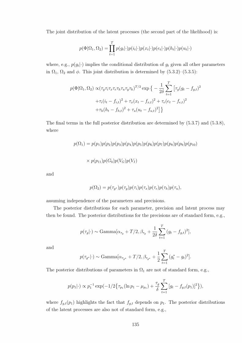
The joint distribution of the latent processes (the second part of the likelihood) is:
p(Φ|Ω1,Ω2) =T∏t=1
p(gt|·)p(it|·)p(xt|·)p(et|·)p(ht|·)p(ut|·)
where, e.g., p(gt|·) implies the conditional distribution of gt given all other parameters
in Ω1, Ω2 and φ. This joint distribution is determined by (5.3.2)–(5.3.5):
p(Φ|Ω1,Ω2) ∝(τgτiτxτeτhτuτyτk)T/2 exp
− 1
2δ
T∑t=1
[τg(gt − fg,t)2
+τi(it − fi,t)2 + τx(xt − fx,t)2 + τe(et − fe,t)2
+τh(ht − fh,t)2 + τu(ut − fu,t)2]
The final terms in the full posterior distribution are determined by (5.3.7) and (5.3.8),
where
p(Ω1) = p(p1)p(p2)p(p3)p(p4)p(p5)p(p6)p(p7)p(p8)p(p9)p(p10)
× p(p11)p(Gb)p(VG)p(VI)
and
p(Ω2) = p(τg∗)p(τg)p(τi)p(τx)p(τe)p(τh)p(τu),
assuming independence of the parameters and precisions.
The posterior distributions for each parameter, precision and latent process may
then be found. The posterior distributions for the precisions are of standard form, e.g.,
p(τg|·) ∼ Gamma[ατg + T/2, βτg +1
2δ
T∑t=1
(gt − fg,t)2],
and
p(τg∗|·) ∼ Gamma[ατg∗ + T/2, βτg∗ +1
2
T∑t=1
(g∗t − gt)2].
The posterior distributions of parameters in Ω1 are not of standard form, e.g.,
p(p1|·) ∝ p−11 exp(−1/2
τp1(ln p1 − µp1) +
τgδ
T∑t=1
[gt − fg,t(p1)]2
),
where fg,t(p1) highlights the fact that fg,t depends on p1. The posterior distributions
of the latent processes are also not of standard form, e.g.,
135
for time t=0,
p(i0|·) ∝ exp(− 1
2δτi[i1 − fi,1(i0)]2 + τx[x1 − fx,1(i0)]2);
for time t=1,. . . ,T-1,
p(it|·) ∝ exp(− 1
2δτi(it − fi,t)2+τi[it+1 − fi,t+1(it)]
2
+τx[xt+1 − fx,t+1(it)]2);
except at time t=T,
p(iT |·) ∝ exp− 1
2δ[τi(iT − fi,T )2].
5.4 Simulation Study of MCMC and the SPA Model
Markov chain Monte Carlo (MCMC) methods (discussed in appendix C) are a well-
established approach for analysing highly complex distributions (Gilks et al., 1996),
such as the posterior distribution of the SPA model. A simulation study was run to
test the viability of using MCMC methods to estimate the parameters of the SPA
model. Parameters in Ω1 were fixed to the values reported by Roy and Parker (2007)3,
and the precisions in Ω2 were also fixed; values are given in Table 5.3. Glucose and
insulin absorption, as estimated by the digestion and insulin models, from one day of
Subject A’s records were used as the inputs MG and MI , respectively, and the same
day’s physical activity (METs) measurements were used as the input ME; these inputs
are given in Figure 5.13. The conditional distributions presented in (5.3.3) and (5.3.4)
were used to simulate values of the latent processes, g, i, x, e, h, u, every five minutes
for one day (288 time points). Blood glucose “observations” were then simulated using
(5.3.6). Given this series of observations, MCMC methods were used to estimate the
parameters in Ω1 and Ω2.
5.4.1 Practical MCMC Considerations
Given the complexity of the model, with regard to the number of processes and pa-
rameters, the computational burden is large; to reduce this burden, the process E, and
associated parameters, p6 and p7, were treated as known. The process E describes the
body’s delayed response to physical activity, i.e., the delayed increase in heart rate and
oxygen uptake, and introduces a lag on the impact of activity on other processes; its
3The value of parameter p3 was altered as the value presented in Roy and Parker (2007) led to anunstable blood insulin time series.
136

Table 5.3: Parameter values used to generate BGC time series for simulation study.
Parameter Value Parameter Valuep1 0.035 Gb 80p2 0.142 VG 117p3 0.0001 VI 1760p4 0.05 τg 5p5 0.000028 τi 5p6 0.8 τx 5p7 0.8 τh 5p8 0.00158 τu 5p9 0.056 τg∗ 5p10 0.00195p11 0.0485
Figure 5.13: (i) Estimated glucose and (ii) insulin absorption (from the digestion and insulinmodels) and (iii) relative PVOmax
2 for one day of Subject A’s records.
intended behaviour is therefore well understood, and it is dependent only on armband
measurements. The parameters p6 and p7 were set to 0.8, as in Roy and Parker (2007),
and the DE for E was solved using Simulink. Solutions at each time point were treated
as known in the rest of the model.
The remaining latent processes and parameters in Ω1 were updated using the single-
component Metropolis-Hastings algorithm, while precisions were updated using Gibbs
sampling. The normal distribution was chosen to be the proposal density for each
137
parameter in Ω1, Ω2 and Φ, with the mean determined by the current state of the chain,
i.e., for parameter θi, the proposal distribution at iteration j, q(·|θ(j−1)i ), is N(θ
(j−1)i , λi),
for given variance, λi, which may be tuned appropriately to return desirable acceptance
rates. For sampling convenience, the equation parameters in Ω1 = ω(1)i , for i =
1, . . . , 12, were transformed using natural logarithms. This brings the scale of the
parameters on to the whole real line, and ensures that a normal proposal distribution
will give realistic candidates. The transformed parameters follow a normal distribution:
αi = ln(ω(1)i )⇒ p(αi) = pωi
(αi)|dωi/dαi|
⇒ αi ∼ N(µαi, τ−1αi
),
The relationships in (5.3.2) and (5.3.5) are altered accordingly, e.g.,
fi,t+1 =it + δ[− exp(α2) + exp(α3)MI,t exp(−it)].
The posterior distributions of the unknown parameters are not of standard form, e.g.,
p(α1|·) ∝ exp(−1
2
τα1(α1 − µα1)
2 +T∑t=1
τg[gt − fg,t(expα1)]2
).
Generally, visual inspection of MCMC output will be used here as a guide to perfor-
mance. Convergence to the stationary distribution, and hence burn-in length, is often
identifiable from a trace plot of the output. Mixing can also be determined from a
trace plot, as the properties of a well-mixing chain are generally well established, e.g.,
see Gilks et al. (1996, p. 6) for a simple demonstration. Comparison between trace
plots of chains with different starting points can give further indication of mixing and
convergence.
5.4.1.1 Initialisation
To run MCMC, prior distributions for parameters in Ω1 and Ω2 must be specified, as
well as starting values for the chain (which constitute iteration zero). The means of the
prior distributions for the equation parameters were chosen to be the values reported
by Roy and Parker (2007), and the variances were chosen to be relatively large, e.g.,
α1 = ln(p1) ∼ N(ln(0.035), 1).
The prior distributions of the precisions are given by
τg ∼ G(2, 1),
138
a weakly-informative prior distribution without the problems associated with a gamma
distribution of the form G(ε, ε) as ε→ 0 (Gelman, 2006).
Starting values for the equation parameters and precisions were chosen to be the
means of their respective priors, e.g., α(0)1 = ln(0.035) and τ
(0)g = 2. The latent processes
were given arbitrary starting values across all time points: ∀t, gt = ln(Gb) = ln(80),
it = −5, xt = −5, ht = −5, and ut = −5.
5.4.1.2 Tuning
A series of pilot studies, using chains of length 5,000–10,000, were run to determine
suitable variances of the proposal distributions. Variances were repeatedly tuned in
order to return acceptance rates of between 0.15 and 0.5. It was found that the high
correlation between successive time points in the latent processes led to occasional poor
mixing; blocking of correlated parameters can help overcome this limitation, though
blocking whole latent processes led to very slow convergence in this case and so was
not pursued.
The pilot studies highlighted the difficulty of estimating all processes and parame-
ters. In particular, a number of parameter estimates were highly negative, suggesting
the parameters are zero on the original scale. This feature remained in a long chain;
Figure 5.14 shows the trace plot for p5 from a chain of length 50,000 with burn-in
20,000. It was later established that the poor parameter estimates appeared to bias
estimates of other parameters. To account for this, three parameters in Ω1 with highly
negative estimates were not included in the MCMC estimation procedure. These pa-
rameters, Gb, VG and VI , represent basal glucose, glucose distribution space, and insulin
distribution space, respectively, and are physical attributes that may be estimated us-
ing other methods, e.g., Hirota et al. (1999). Further pilot studies also suggested that
parameters p3, p5, a2 and a4 were also highly negative. These were also omitted from
the MCMC estimation procedure. For the remaining parameters, trace plots suggested
a burn-in of 5,000 was acceptable for estimation; Figure 5.15 shows trace plots for p1
using three over-dispersed starting values. Chains of length 10,000 suggested posterior
estimation of BGC agreed well with simulated BGC; Figure 5.16 shows estimated BGC
closely matches the profile of simulated BGC.
5.4.2 Results
Fifty data sets were simulated, and for each set a Markov chain, of size 10,000 with
burn-in of 5,000, was run. The delayed average (equation C.1, section C.2, Appendix C)
was calculated for each chain to estimate parameters in Ω1 and Ω2. Corresponding 95%
credible intervals were found by determining the 2.5th and 97.5th precentiles according
to ascending order of the sampled values. Coverage was assessed by comparison of
139

Figure 5.14: MCMC trace plot for p5 from a long chain.
credible intervals from all chains against the true parameter value (expressed as a
percentage of intervals containing the true value). Comparison of the true parameter
value against its respective MCMC sample means (across all chains) was used to identify
bias in parameter estimates, where consistent under- or overestimation of a parameter
suggests downward or upward bias, respectively.
Figures 5.17–5.19 show means and credible intervals for parameters p1, p2 and p10,
respectively, ordered by lower bound of the credible interval. Figure 5.17 suggests very
good coverage of parameter p1 with the majority (90%) of credible intervals containing
the parameter value used to generate the simulated BGC. Coverage for p2 is 0%, with
consistent underestimation (Figure 5.18); this implies there may be issues with param-
eter identification, where different values of p2 can give rise to the same distribution of
observations. Coverage for p10 is far better, though still short of ideal (Figure 5.19);
this may be due to an inadequate burn-in period, where non-convergence of the chain
leads to poor paramter estimation. However, time restrictions meant a larger simula-
tion study could not be conducted to thoroughly investigate this. Results similar to
those of p10 were seen for parameters p4 and p8.
Figures 5.20 and 5.21 show means and credible intervals for precisions τi and τg∗ ,
140

Figure 5.15: MCMC trace plots for p1 based on three different starting values: (i) p(0)1 = 0, (ii)
p(0)1 = −10 (iii) p(0)
1 = −3.35 (the true value, as indicated by the red line in each plot).
respectively, ordered by lower bound of the credible interval. The results for τi are
typical of those seen for τx, τh and τu, with 100% coverage but a tendency for over-
estimation (Figure 5.20). The results for τg∗ show equally good coverage but with no
obvious bias (Figure 5.21), and is similar to the results seen for τg.
5.4.3 Model Verification
MCMC methods may be further assessed by monitoring performance in the predictive
space; this was achieved by removing a selection of BGC measurements (to be used as
verification values) according to a number of scenarios:
• scenario A 25 randomly-selected measurements;
• scenario B one-hour block during early morning (when asleep);
• scenario C one-hour block after breakfast, and three-hour block after an evening
meal and into the night.
141

Figure 5.16: Measured BGC and MCMC output.
The MCMC methods used in the previous section were extended to sample from the dis-
tribution of BGC measurements (equation 5.3.6); Gibbs sampling was used as the con-
ditional posterior distribution of BGC measurements is a normal distribution. Chains
of size 20,000, including burn-in of 5,000, were run to determine the ability of MCMC
to predict measured BGC. Starting values of the missing observations were chosen to
be Gb = 4.44mmol/l.
5.4.3.1 Results
For each scenario, MCMC sample means and 95% credible intervals were calculated
for each missing BGC measurement. Figure 5.22 suggests good predictive performance
under scenario A (random missing measurements), with the credible intervals all con-
taining the true value, and no obvious prediction bias. Figure 5.23 shows the result for
scenario B, with the credible intervals again containing the simulated BGC entirely.
However, the intervals are so wide as to be of limited use in practical terms; for ex-
ample an interval of (2,6) is equivalent to BGC in the range ∼(0.5,22)mmol/l, which
spans much of the hypo- and hyperglycaemic range. The MCMC sample means also
142
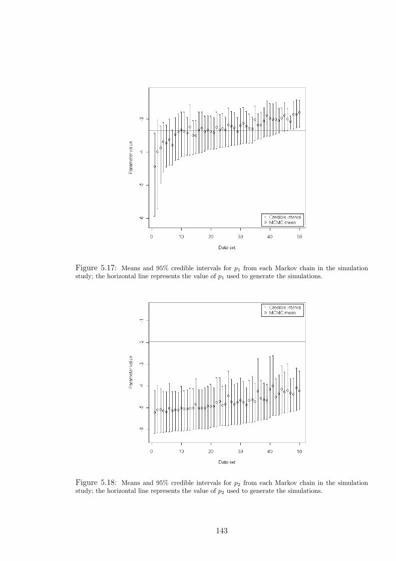
Figure 5.17: Means and 95% credible intervals for p1 from each Markov chain in the simulationstudy; the horizontal line represents the value of p1 used to generate the simulations.
Figure 5.18: Means and 95% credible intervals for p2 from each Markov chain in the simulationstudy; the horizontal line represents the value of p2 used to generate the simulations.
143

Figure 5.19: Means and 95% credible intervals for p10 from each Markov chain in the simulationstudy; the horizontal line represents the value of p10 used to generate the simulations.
144

Figure 5.20: Means and 95% credible intervals for τi from each Markov chain in the simulationstudy; the horizontal line represents the value of τi used to generate the simulations.
Figure 5.21: Means and 95% credible intervals for τg∗ from each Markov chain in the simulationstudy; the horizontal line represents the value of τg∗ used to generate the simulations.
145
do not appear to pick up the fluctuating nature of the simulated BGC. Figure 5.24
and 5.25 show the results for scenario C, split into blocks of verification values; these
suggest that the credible intervals contain the simulated BGC almost entirely (one
interval does not) but are again relatively wide. There are large discrepancies between
simulated BGC and MCMC predictions at the start of both blocks of missing values,
but improved performance later in the blocks.
5.4.4 Robustness
Predictive performance may also be assessed by testing robustness to specification of
prior distributions or misspecification of parameters. Misleading prior distributions
may affect MCMC output by directing posterior distribution estimates away from the
true value and toward subjective information supplied by the prior distribution; hence,
MCMC estimates could be inaccurate without some form of reliable prior knowledge.
Furthermore, model performance must also be robust to parameter misspecification
to ensure MCMC estimates are reliable; parameters that are fixed during the MCMC
estimation procedure may have been estimated using other methods, and hence con-
tain error that could bias MCMC estimates. Predictive performance was assessed over
25 randomly-selected BGC simulated values across a number of arbitrarily-determined
scenarios, involving either (misleading) informative prior distributions, parameter mis-
specification, or a combination:
• scenario 1 (baseline scenario) all fixed parameters kept at simulation values, prior
distributions as specified in section 5.4.1.1. Other scenarios are as scenario 1
except where specified;
• scenario 2 overestimation of basal glucose (simulation value of 4.44mmol/l; fixed
value of 5mmol/l);
• scenario 3 ten-fold overestimation of a2 (0.056; 0.56) and underestimation of in-
sulin distribution space (1760ml; 1500ml);
• scenario 4 ten-fold underestimation of p11 (0.0485; 0.00485), prior distribution for
p10 given by N(1, 0.1);
• scenario 5 all fixed parameters kept at simulation values, with prior distributions
τg ∼ G(10, 10) and τi ∼ G(0.1, 0.1);
• scenario 6 prior distribution p1 ∼ N(0.35, 3);
• scenario 7 all equation parameter prior distributions set to N(5, 0.01), 100-fold
overestimation of p5 (0.000028; 0.0028), ten-fold underestimation of p9 (0.056;
0.0056) and overestimation of glucose distribution space (117dl; 140dl).
146

Figure 5.22: Means and 95% credible intervals for each missing observation under scenario A.
Figure 5.23: Means and 95% credible intervals for each missing observation under scenario B.
147

Figure 5.24: Means and 95% credible intervals for each missing observation under scenario C (firstblock).
Figure 5.25: Means and 95% credible intervals for each missing observation under scenario C (secondblock).
148
The continuous ranked probability score (CRPS; section C.3.2, Appendix C) was used
to compare the MCMC samples under each scenario.
5.4.4.1 Results
Estimated CRPS for each of the scenarios is given in Table 5.4. CRPS is relatively
consistent across the scenarios, suggesting the model is robust to misspecification of
parameters and/or different specification of prior distributions. In particular, all sce-
narios performed at a similar level to scenario 1, suggesting, at worst, only a minor
loss of predictive performance compared to the standard set-up.
Table 5.4: CRPS values under scenarios given in section 5.4.4.
Scenario CRPS1 0.3952 0.3973 0.4104 0.3935 0.3936 0.4007 0.412
5.4.5 Conclusions
The feasibility of using MCMC methods to analyse the proposed Bayesian network
has been demonstrated. MCMC was unable to identify all parameters simultaneously,
but was able to estimate most parameters with good coverage. Precisions had 100%
coverage, but there was evidence of upward bias for the precisions of processes i, x, h
and u. The parameter p1 was generally well estimated by MCMC with good coverage
and no obvious bias; parameters p4, p8 and p10 had lower coverage, though MCMC
sample means were for the most part within 10% of the true value. Again, there was
no obvious bias in estimates. MCMC estimates of parameter p2 were, in contrast,
downwardly biased, with consistent underestimation of the parameter. This may be
due to the complex form of the posterior distribution causing issues with parameter
identification, where different values of p2 can give rise to the same observation distri-
butions. Parameter p2 relates to clearance of blood insulin, and affects the distribution
of BGC observations via the active insulin and blood glucose equations. It is possible
that the effect of p2 is attributed to other parameters in this pathway, so its role is
attenuated and hence underestimated by MCMC. It is interesting to note that only one
parameter from Ω1 in each of the original DEs (5.2.1) could be adequately estimated.
Again, this may be due to issues with parameter identification.
149
MCMC methods were verified by testing performance in the predictive space under
a number of scenarios with missing BGC values; credible intervals almost entirely
contained the simulated BGC, although MCMC means did not always reproduce the
fluctuating nature of the simulated BGC. MCMC methods also appeared to be robust
to specification of prior distributions and parameter misspecification, suggesting the
methods can produce reliable estimates even if misleading information is included in
the estimation procedure.
5.5 Summary
In this chapter, modern, computationally-intensive statistical methods for analysis of a
glucose-insulin compartmental model were presented. The methods were proposed as
a new approach to analysing compartmental models in the diabetes literature, which
play an important role in the development of the artificial pancreas. A new compart-
mental model was derived from the physical activity minimal model presented by Roy
and Parker (2007), with modifications to enhance the physiological plausibility and to
ensure the model was valid for data collected in free-living conditions. The modified
model was converted to a Bayesian network (the SPA model), which expresses the
relationship of a number of physiological processes via conditional probability distri-
butions, to better reflect the uncertainty inherent in the glucoregulatory system. The
network was analysed using MCMC methods, a well-established approach for analysing
highly complex distributions.
A simulation study was run to determine the ability of the proposed approach to
estimate parameters of the SPA model and predict missing BGC observations, where
fifty data sets were generated to test MCMC coverage across parameter estimates.
MCMC was implemented using both Gibbs sampling (where conditional posterior dis-
tributions were of standard form) and the Metropolis algorithm. It was found that
MCMC was unable to accurately determine estimates for all parameters, perhaps due
to issues with parameter identification (which may be caused by model formulation).
Parameters whose estimates were far removed from their true value were removed from
the MCMC estimation procedure; for the remaining parameters, MCMC was generally
able to produce good estimates. Precisions were generally overestimated but had to-
tal coverage, while coverage for other parameters was lower but with no obvious bias
in most cases. MCMC performance in the predictive space was tested under a num-
ber of scenarios, involving parameter misspecification and misleading informative prior
distributions; variation in performance was relatively small (as measured by CRPS)
suggesting robustness to situations where incorrect information is supplied to the esti-
mation procedure.
150

Chapter 6
Conclusions and Future Work
6.1 Conclusions
This thesis investigated the use of free-living data and new modelling techniques to
improve current and potential treatment regimes for type 1 diabetes. The disease is
associated with increased morbidity and mortality due to the imperfections of insulin
therapy; better understanding of blood glucose concentration (BGC) under typical
daily stimuli can improve BGC control by either providing support and education
for individuals or helping realise the goal of an artificial pancreas. The current work
presented a unique, free-living data set from a Diabetes UK study, and used mathemat-
ical and statistical methods for the purpose of building generic and personalised models
capable of describing and/or predicting BGC. Time series of BGC were analysed to
determine any short- or long-term structure that might be exploited for predictive pur-
poses. Predictive models of BGC, based on food, insulin and physical activity, were
tested over four hours to determine their suitability for inclusion in the MDI regime, as
a tool for describing the profile of BGC between finger-prick tests. Finally, a descriptive
model derived from the literature was tested using free-living data, raising important
practical and theoretical modelling issues for an artificial pancreas, and new methods
were proposed for parameter estimation and analysis of semi-empirical compartmental
models.
6.1.1 Contributions
Chapter 2 presented a review of diabetes literature, highlighting the lack of free-living
data and empirical modelling approaches. In this context, the data from the Dia-
betes UK study, as presented in chapter 3, offered a unique opportunity to explore
the behaviour of BGC under the influence of food intake, insulin injections and phys-
ical activity in free-living conditions. Analysis of BGC in the time domain confirmed
results presented previously in the literature, with regard to the non-stationarity and
151
short-term dependence of BGC measurements. Short-term dependence was found to
vary between and within individuals. An AR model was used to describe BGC, with
predictions based only on previous measurements of BGC. The model was able to pre-
dict accurately over five minutes, but failed to capture BGC dynamics over several
hours. Analysis in the frequency domain investigated for the first time the possibility
of exploiting periodicities in BGC for predictive purposes. The spectral densities of
BGC time series were approximated using a periodogram; variation in BGC was found
to be concentrated at lower frequencies, but no notable periodicities were evident.
Chapter 4 introduced DLMs as a new method for modelling BGC, due to their abil-
ity to describe non-stationary time series, and account for time-varying parameters and
varying measurement accuracy. Food and insulin diary records were used to estimate
glucose and insulin absorption profiles, respectively, using physiological models in the
literature, and used as inputs to the DLMs, along with physical activity armband mea-
surements. DLMs were used to predict the profile of BGC for up to four hours ahead.
They were found to be suitable for short-term prediction, and able to detect periods of
hypo- and hyperglycaemia. However, predictions over four hours were inaccurate, due
to the linear structure of the models and/or the inability of the model to account for
the effect of other physiological processes. Furthermore, it was found that parameter
estimates did not comply with established physiological behaviour. This may be due to
modelling the effect of glucose and insulin absorption on BGC as immediate, with no
longer-term influence on stimulating/suppressing metabolic processes. In this context,
it was not appropriate to make inference regarding the role of physical activity.
Chapter 5 considered a more physiologically-representative compartmental model
as a tool for descriptive modelling of BGC. A glucose-insulin model (PA model) com-
posed of differential equations (DEs) was taken from the literature and tested using
the free-living data, and was found to return physiologically-unrealistic results. This
highlights potential flaws in compartmental models based on data from healthy sub-
jects, whose performance has not been tested with free-living data. This suggests that
control algorithms (designed to be included in an artificial pancreas) developed and
tested using simulations from other compartmental models are not realistically chal-
lenged with such data. A modified version of the PA model was presented for further
use; the new model included inputs for food, insulin and physical activity, as well as a
term for renal clearance. The set of DEs was converted to a Bayesian network (SPA
model) to better represent the underlying physiology, with the relationships between
physiological processes determined by conditional distributions. MCMC was then pro-
posed as a method for analysing the complex posterior distribution of the SPA model.
A simulation study found that MCMC methods were able to estimate most parameters
in the SPA model with good coverage. MCMC performance in the predictive space
was found to be robust to the specification of prior distributions and misspecification
152

of parameters.
6.2 Future Work
The role of physical activity in the behaviour of BGC is highly complex; this is par-
ticularly true for individuals with type 1 diabetes, whose response is complicated by
unregulated insulin. Under- or overdosing of insulin compromises the entire glucoreg-
ulatory system, and the level of impairment depends on the discrepancy between the
current and ideal plasma insulin concentrations. Thus, the response to physical activ-
ity will vary depending on plasma insulin concentration as well as the characteristics
(type, intensity, duration) of physical activity. The role of blood insulin concentration
for different activity characteristics, both immediate and longer-lasting, needs to be
established to better represent the role of physical activity in the behaviour BGC.
Empirical models of BGC, such as those used in the current work, require accurate
descriptions of post-prandial glucose absorption, insulin absorption and physical activ-
ity. However, taking into account all the effects of these external influences detracts
from the advantage of DLMs, given their rapid computation, and simple and easily-
understood nature. It is possible the performance of DLMs (from both a predictive
and descriptive perspective) may be improved by the introduction of lags to better
reflect the physiology; this is certainly true in the case of insulin, where absorption
into the blood is a precursor to its actual effect on BGC. The Tarin et al. (2005) model
may also be used to describe plasma, hepatic and interstitial insulin concentrations
(albeit without consideration of the effects of exercise), which may offer more relevant
information to a DLM.
The current work highlighted a number of practical and theoretical issues related
to free-living data. In particular, the physical activity data was found to be highly
fluctuating. It is yet to be understood which features of such data must be captured
in order to better understand the behaviour of BGC. For example, highly fluctuating
data may be smoothed, but this may lose peaks (and troughs) which have physiological
importance.
The SPA model presented in chapter 5 does not take into account the decline in rate
of glycogenolysis during prolonged activity; the process was removed from the original
PA model as it caused physiologically unrealistic results with free-living data. Further
work may investigate new approaches for including this process in the model, and hence
extend the model’s practical use to long periods of exercise where the effect of depleting
the liver’s glycogen stores becomes more apparent. The decline in glycogenolysis rate,
as modelled by Roy and Parker (2007), is dependent on integrated activity passing
a certain threshold, whereas it may be more realistic to have this threshold depend
on both energy expenditure and energy intake from food. The processes H and U ,
153

representing hepatic glucose release and muscular glucose uptake due to activity, may
be better represented by a mixture model, where the processes take a value of zero
with probability p or follow a log-normal distribution with probability 1− p.Sequential Monte Carlo (SMC) methods are an alternative method to MCMC for
analysing the posterior distribution of the SPA model. Doucet et al. (2001) suggest that
SMC is better suited to estimation of recursive problems, as it considers the sequence of
conditional distributions rather than the entire posterior distribution. Once a suitable
estimation procedure is found, the SPA model, as presented in (chapter 5), may be
applied to individuals from the DUK study. The behaviour of latent variables may be
explored and compared to expected behaviour according to established physiology.
The stochastic approach advocated in chapter 5 may also be extended to a popula-
tion model. The relationship of parameter estimates and physical characteristics may
also be explored, using the all the data collected in the DUK study; e.g., the propor-
tion or distribution of fat in the body may be related to certain parameters. With
longer-term assessment, the effects of changes in lifestyle could be related to changes
in parameter estimates.
6.3 Summary
The contributions of the current work to the body of knowledge may be summarised
as:
• a unique free-living data set was presented, highlighting the highly fluctuating
nature of physical activity data;
• frequency analysis of BGC data did not present any exploitable periodicities for
the purposes of predicting BGC;
• DLMs were presented as an empirical approach to modelling BGC, using glucose
and insulin absorption (estimated by models in the literature), and physical ac-
tivity data as explanatory variables. The results suggest that predicting BGC
over periods of several hours is not possible using the current inputs;
• compartmental models based on simulated data, or data from healthy volunteers,
may not be able to handle free-living data, and can return physiologically non-
viable estimates. This suggests that proposed control algorithms, as part of an
artificial pancreas, are not being realistically challenged by current models;
• a new compartmental model of the body was presented, bringing together models
of digestion, insulin absorption, and renal clearance;
154

• a stochastic version of the new compartmental model was also presented, to better
reflect the underlying physiology. Bayesian methods were used to simultaneously
estimate model parameters and define person-specific models;
• MCMC methods for parameter estimation and BGC prediction were tested in a
simulation study. The methods were suitable for a subset of parameters, and
predictions of BGC were robust to misleadingly informative prior distributions
and parameter misspecification.
155


Appendix A
Bayesian Methods
Bayesian methodology differs to classical statistical approaches by treating unknown
parameters as random variables, with appropriate probability distributions used to
represent uncertainty. The methods make use of Bayes’ Theorem, which states that,
for a given set of data, y = (y1, . . . , yn), with a probability density function, pY (y;θ),
described by an unknown parameter set, θ = (θ1, ..., θp):
pθ(θ|Y = y) =pY (y|θ)pθ(θ)∫
θpY (y|θ)pθ(θ)dθ
.
The normalising constant in the denominator is the marginal distribution, pY (y). It
does not involve θ and so is not of particular interest compared to the form of the
numerator. Instead, the above is often presented as
pθ(θ|Y = y) ∝ pY (y|θ)pθ(θ). (A.1)
The term pθ(θ) is the prior distribution of the parameter set. This represents all known
information about the parameters prior to observing the data, y. The term pY (y|θ) is
the likelihood function of the parameter set given the data. The left-hand side of (A.1)
is the posterior distribution of the parameters. This represents the updated information
on the parameters having observed the data. New information on parameters, e.g.,
from further observations, can easily be assimilated into previous knowledge using the
relationship between the prior and posterior distributions.
The choice of prior distribution allows subjective input into the process, and may
incorporate any previously established information. Vague prior distributions may
be used if little or no information is known a priori. When the prior and posterior
distributions are of the same functional form, i.e., from the same family of distribution,
the prior distribution is said to be conjugate to the likelihood. In such a setting
only the parameters of the prior distribution change in the updating procedure, hence
simplifying computation.
157


Appendix B
Double-Discount DLM Structure
Given the single-discount approach described in section 4.1.4.1 and equation 4.1.3,
let any changes due to a second discount factor be denoted with the superscript (δ).
Furthermore, assume δ = 1 for up to and including time t − 1, and δt ∈ (0, 1). Then
the point estimate of σ2t in the double-discount model is
S(δ)t =
δtdt−1 + St−1e2t/Qt
δtnt−1 + 1,
differing from the single-discount model only by the scaling of nt−1 and dt−1 by δt. The
posterior estimate for the variance of the parameters is also different:
C(δ)t = (S
(δ)t /St−1)(Rt −AtA
Tt Qt)
= (S(δ)t /St)Ct. (B.1)
Let N t = (1/St−1)(Rt − AtATt Qt), which is the same for the single- and double-
discount model. At time t + 1 the above changes feed into the prior variance for the
parameters and the forecast variance:
R(δ)t+1 = (1/λ)C
(δ)t
= (1/λ)S(δ)t N t,
Q(δ)t+1 = XT
t+1R(δ)t+1X t+1 + S
(δ)t
= S(δ)t [(1/λ)XT
t+1N tX t+1 + 1].
The adaptive vector, At+1, however, remains unchanged:
A(δ)t+1 = R
(δ)t+1X t+1/Q
(δ)t+1
= [(1/λ)S(δ)t N tX t+1]/S
(δ)t [(1/λ)XT
t+1N tX t+1 + 1]
= At+1,
159

as the S(δ)t terms cancel. Hence
C(δ)t+1 = (S
(δ)t+1/S
(δ)t )(R
(δ)t+1 −A
(δ)t+1(A
(δ)t+1)
TQ(δ)t+1)
= S(δ)t+1(1/λ)N t −A(δ)
t+1(A(δ)t+1)
T[(1/λ)XTt+1N tX t+1 + 1]
= (S(δ)t+1/St+1)Ct,
exactly as in (B.1) but for t+ 1. Note that St < S(δ)t if
dt−1 + (dt−1/nt−1)(e2t/Qt)
nt−1 + 1<
δdt−1 + (dt−1/nt−1)(e2t/Qt)
δnt−1 + 1
⇔ δ(e2t/Qt − 1) < e2t/Qt − 1
⇔ |et/√Qt| > 1.
The structure of the DLM implies that (et|Dt−1) ∼ Tnt−1(0, Qt), and so et/√Qt, the
standardised error, follows a standard Tnt−1 distribution. If the standardised error
is outside the range (−1, 1), which for large enough n is equivalent to one standard
deviation from the mean, then the model adapts by increasing the point estimate of
the observation error variance. Otherwise the point estimate will decrease, and hence
artificially decreases the prediction interval of the forecast.
160
Appendix C
Sampling-Based Methods
Bayesian inference involves assessing the properties of posterior distributions, which
may involve evaluating very complex integrals. For example, determining the expecta-
tion of a function of the parameters, g(θ), requires finding
E[g(θ|Y )] =
∫g(θ)p(θ)p(Y |θ)dθ∫p(θ)p(Y |θ)dθ
,
whose analytic evaluation, even approximately, may be impossible. A common ap-
proach to this problem is to use sampling based methods such as Markov Chain Monte
Carlo (MCMC).
C.1 Monte Carlo Integration
Monte Carlo integration uses random samples to evaluate integrals. For a given sample,
θ(i), for i = 1, ..., n, from p(θ|Y ), the expectation of g(θ|Y ) is estimated by the sample
mean:
E[g(θ|Y )] ≈ 1
n
n∑i=1
g(θ(i)).
Given independence of the θ(i), the desired accuracy of the approximation may be
achieved by choosing an appropriate value for n. However, it is not always possible to
draw independent θ(i). Dependent samples may instead be used to derive estimates of
the characteristics of the population distribution if they are approximately distributed
as the desired distribution; Markov chains are a method for achieving this.
161

C.2 Markov Chains
A sequence, θ(i), for i = 1, . . . , n, is a Markov chain if it is generated from a distri-
bution, p(·|·), known as the transition kernel, with the property
p(θ(i+1)|θ(i), θ(i−1), . . . , θ(1), θ(0)) = p(θ(i+1)|θ(i)).
Under appropriate conditions, the chain will forget its initial value, θ(0), and converge
to a unique stationary distribution, π(·) (Gilks et al., 1996). A Markov chain thus
generates dependent samples from π(·) as n increases. Taking into account the time
taken for the chain to forget its initial state (burn-in), the expectation is approximated
by the delayed average,1
n−m
n∑i=m+1
g(θ(i)), (C.1)
where values prior to burn-in time, m, are discarded. Markov chains may be con-
structed in a number of ways, discussed in the following sections. Monte Carlo estima-
tion based on a Markov chain is known as MCMC.
C.2.1 Metropolis-Hastings Algorithm
The Metropolis-Hastings (MH) algorithm is a general method for constructing a Markov
chain with the desired stationary distribution. Defining π(θ) to be the distribution of
interest, q(·) to be a proposal distribution, and the acceptance probability, α, as:
α(θ, Z) = min(
1,π(Z)q(θ|Z)
π(θ)q(Z|θ)
),
the algorithm proceeds as follows:
i) define iteration 0 (arbitrary starting point, θ(0)), and set i = 0;
ii) sample candidate, Z, from the proposal distribution, q(·);
iii) sample u from a standard uniform distribution, U(0, 1);
iv) set θ(i+1) = Z if α(θ(i), Z) > u, else θ(i+1) = θ(i);
v) i = i+ 1, return to step ii).
The algorithm is the Hastings (1970) generalisation of the method proposed in Metropo-
lis et al. (1953). Originally the Metropolis approach considered only symmetric pro-
posal distributions, where q(θ|Z) = q(Z|θ), giving an acceptance probability of
α(θ, Z) = min(
1,π(Z)
π(θ)
). (C.2)
162

The MH method works for any proposal distribution, q(·), but certain choices offer
preferable results in terms of convergence (time taken to reach the stationary distribu-
tion) and mixing (how quickly samples explore the support of the stationary distribu-
tion). Hence identifying appropriate forms for the proposal distributions can minimise
computation. Further details and wider discussion of the Metropolis-Hastings algo-
rithm may be found in Gilks et al. (1996).
Often it is preferable to update θ component-wise rather than as a whole. This
is known as single-component Metropolis-Hastings (SCMH). If the vector θ is di-
vided into d components of possibly differing dimensions, θ = θ1, ..., θd, then an
iteration of SCMH involves d updating steps. Defining θ(i)j to be the state of pa-
rameter θj at the end of iteration i, step j of the (i + 1)th iteration involves up-
dating θ(i)j . A candidate, Zj, is generated from a proposal, qj(Zj|θ(i)
j ,θ(i+1)−j ), where
θ(i+1)−j = θ(i+1)
1 , ..., θ(i+1)j−1 , θ
(i)j+1, ..., θ
(i)h is the vector of most recently sampled values of
θ. The acceptance probability is given by
α(Zj; θ(i)j ,θ
(i+1)−j ) = min
(1,π(Zj|θ(i+1)
−j )qj(θ(i)j |Zj,θ
(i+1)−j )
π(θ(i)j |θ
(i+1)−j )qj(Zj|θ(i)
j ,θ(i+1)−j )
). (C.3)
The term π(θ(i)j |θ
(i+1)−j ) is the full conditional distribution of θ
(i)j conditioning on θ
(i+1)−j ,
given by
π(θ(i)j |θ
(i+1)−j ) =
π(θ)∫π(θ)dθ
(i)j
. (C.4)
The form of θ(i+1)−j presented here implies the elements of θ are updated sequentially,
though this need not necessarily be the case. Correlated parameters may be updated as
a group using SCMH to improve convergence and mixing, a process known as blocking.
C.2.2 Gibbs Sampling
The Gibbs sampler (Geman and Geman, 1984) is a special case of SCMH with proposal
distribution
qj(Zj|θj,θ−j) = π(Zj|θ−j), (C.5)
where π(Zj|θ−j) is the full conditional distribution as in (C.4). Gibbs sampling involves
sampling from the full conditional distribution, and is most suitable when this is easily
done. Substituting (C.5) into (C.3) gives an acceptance probability of one, hence Gibbs
candidates are always accepted. Again, the order of updating may be random and need
not necessarily involve all components during each iteration.
163
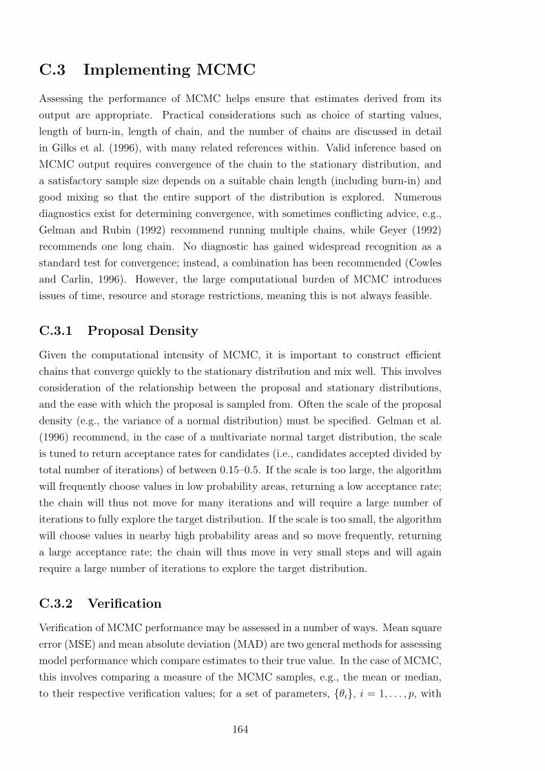
C.3 Implementing MCMC
Assessing the performance of MCMC helps ensure that estimates derived from its
output are appropriate. Practical considerations such as choice of starting values,
length of burn-in, length of chain, and the number of chains are discussed in detail
in Gilks et al. (1996), with many related references within. Valid inference based on
MCMC output requires convergence of the chain to the stationary distribution, and
a satisfactory sample size depends on a suitable chain length (including burn-in) and
good mixing so that the entire support of the distribution is explored. Numerous
diagnostics exist for determining convergence, with sometimes conflicting advice, e.g.,
Gelman and Rubin (1992) recommend running multiple chains, while Geyer (1992)
recommends one long chain. No diagnostic has gained widespread recognition as a
standard test for convergence; instead, a combination has been recommended (Cowles
and Carlin, 1996). However, the large computational burden of MCMC introduces
issues of time, resource and storage restrictions, meaning this is not always feasible.
C.3.1 Proposal Density
Given the computational intensity of MCMC, it is important to construct efficient
chains that converge quickly to the stationary distribution and mix well. This involves
consideration of the relationship between the proposal and stationary distributions,
and the ease with which the proposal is sampled from. Often the scale of the proposal
density (e.g., the variance of a normal distribution) must be specified. Gelman et al.
(1996) recommend, in the case of a multivariate normal target distribution, the scale
is tuned to return acceptance rates for candidates (i.e., candidates accepted divided by
total number of iterations) of between 0.15–0.5. If the scale is too large, the algorithm
will frequently choose values in low probability areas, returning a low acceptance rate;
the chain will thus not move for many iterations and will require a large number of
iterations to fully explore the target distribution. If the scale is too small, the algorithm
will choose values in nearby high probability areas and so move frequently, returning
a large acceptance rate; the chain will thus move in very small steps and will again
require a large number of iterations to explore the target distribution.
C.3.2 Verification
Verification of MCMC performance may be assessed in a number of ways. Mean square
error (MSE) and mean absolute deviation (MAD) are two general methods for assessing
model performance which compare estimates to their true value. In the case of MCMC,
this involves comparing a measure of the MCMC samples, e.g., the mean or median,
to their respective verification values; for a set of parameters, θi, i = 1, . . . , p, with
164
a measure of the associated MCMC sample, f(θi), and respective verification values,
yi,
MSE =1
p
p∑i=1
(f(θi)− yi)2
and
MAD =1
p
p∑i=1
|f(θi)− yi|.
The continuous ranked probability score (CRPS) accounts for the entire predictive
distribution rather than a single measure of an MCMC sample. CRPS compares the
cumulative distribution function (cdf) of a set of MCMC samples to that of a verifica-
tion value, and is defined as
CRPS(F, y) = −∫ ∞−∞
[F (θ)− I(θ ≥ y)]2dθ,
where F (·) is the cdf of the MCMC samples and I(x) is an indicator function taking
the value of one if the argument, x, is true, and zero otherwise. This may be evaluated
as (Gneiting and Raftery, 2007)
CRPS(F, y) =1
2EF |θ(i) − θ(j)| − EF |θ(i) − y|,
where θ(i) and θ(j) are two independent samples of a random variable with common
cdf, F (·). This may be approximated by
ˆCRPS(F, y) =1
n
n∑i=1
|θ(i) − y| − 1
2n2
n∑i=1
n∑j=1j 6=i
|θ(i) − θ(j)|, (C.1)
for a chain of length n. For p verification values, the overall CRPS is given by
ˆCRPSp =1
p
p∑i=1
CRPS(Fi, yi). (C.2)
Smaller values of CRPS are preferred as this indicates the predictive cdf is closer to
the observed cdf.
165


References
Abdul-Rasoul, M., Habib, H. and Al-Khouly, M. (2006) ‘The honeymoon phase’ in
children with type 1 diabetes mellitus: frequency, duration, and influential factors.
Pediatric Diabetes, 7, 101–107.
Abu-Rimleh, A. and Garcia-Gabin, W. (2010) Feedforward-feedback multiple predic-
tive controllers for glucose regulation in type 1 diabetes. Computer Methods and
Programs in Biomedicine, 99, 113–123.
Agar, B. U., Erzen, M. and Cinar, A. (2005) Glucosim: Educational software for virtual
experiments with patients with type 1 diabetes. In Proceedings of the 2005 IEEE
Engineering in Medicine and Biology Society, 27th Annual Conference.
Ahlborg, G., Wahren, J. and Felig, P. (1986) Splanchnic and peripheral glucose and
lactate metabolism during and after prolonged arm exercise. Journal of Clinical
Investigation, 77, 690–699.
Ainsworth, B. E., Haskell, W. L., Whitt, M. C., Irwin, M. L., Swartz, A. M., Strath,
S. J., O’Brien, W. L., R., B. J. D., Schmitz, K. H., Emplaincourt, P. O., Jacobs Jnr.,
D. R. and Leon, A. S. (2000) Compendium of physical activities: an update of
activity codes and MET intensities. Medicine & Science in Sports & Exercise, 32,
S498S504.
Akesen, E., Turan, S., Guran, T., Atay, Z., Save, D. and Bereket, A. (2011) Prevalence
of type 1 diabetes mellitus in 6-18-yr-old school children living in Istanbul, Turkey.
Pediatric Diabetes, 12, 567–571.
Akirav, E., Kushner, J. A. and Herold, K. C. (2008) Beta-cell mass and type 1 diabetes:
Going, going, gone? Diabetes, 57, 2883–2888.
Andersen, K. E. and Højbjerre, M. (2005) A population-based Bayesian approach to
the minimal model of glucose and insulin homeostasis. Statistics in Medicine, 24,
2381–2400.
Andre, D., Pelletier, R., Farringdon, J., Safier, S., Talbott, W., Stone, R., Vyas, N.,
Trimble, J., Wolf, D., Vishnubhatla, S., Boehmke, S., Stivoric, J. and Teller, A.
167
(2006) The development of the SensewearTM armband, a revolutionary energy as-
sessment device to assess physical activity. Body Media Inc.
Arleth, T., Andreassen, S., Federici, M. O. and Benedetti, M. M. (2000) A model of the
endogenous glucose balance incorporating the characteristics of glucose transporters.
Computer Methods and Programs in Biomedicine, 62, 219–234.
Bantle, J. P., Neal, L. and Frankamp, L. M. (1993) Effects of the anatomical region
used for insulin injections on glycaemia in type 1 diabetes subjects. Diabetes Care,
16, 1592–1597.
Bellazzi, R., Larizza, C., Magni, P., Montani, S. and Nicolao, G. D. (1999) Intelli-
gent analysis of clinical time series by combining structural filtering and temporal
abstractions. Artificial Intelligence in Medicine, 1620, 261–270.
Bellazzi, R., Nucci, G. and Cobelli, C. (2001) The subcutaneous route to insulin-
dependent diabetes therapy. IEEE Engineering in Medicine and Biology, 51, 54–64.
Berger, M., Cuppers, H. J., Hegner, H., Jorgens, V. and Berchtold, P. (1982) Absorp-
tion kinetics and biologic effects of subcutaneously injected insulin preparations.
Diabetes Care, 5, 77–91.
Bergman, R. N., Ider, Y. Z., Bowden, C. R. and Cobelli, C. (1979) Quantitative
estimation of insulin sensitivity. American Physiological Society, 236, 667–677.
Bergman, R. N., Phillips, L. S. and Cobelli, C. (1981) Physiologic evaluation of factors
controlling glucose tolerance in man. Journal of Clinical Investigation, 68, 1456–
1467.
Bliss, M. (1982) The Discovery of Insulin. University of Chicago Press.
Bloomfield, P. (1976) Fourier Analysis of Time Series: An Introduction. John Wiley
& Sons.
Bolie, V. W. (1961) Coefficients of normal blood glucose regulation. Journal of Applied
Physiology, 16, 783–788.
Bolstad, W. M. (1988) The multiprocess dynamic linear model with biased perturba-
tions: A real time model for growth hormone level. Biometrika, 75, 685–692.
Bremer, T. and Gough, G. A. (1999) Is blood glucose predictable from previous values?
A solicitation for data. Diabetes, 48, 445–451.
Breton, M. and Kovatchev, B. (2008) Analysis, modeling, and simulation of the accu-
racy of continuous glucose sensors. Journal of Diabetes and Science Technology, 2,
853–862.
168
Breton, M. D. (2008) Physical activity - the major unaccounted impediment to closed
loop control. Journal of Diabetes Science and Technology, 2, 169–174.
Breton, M. D., Shields, D. P. and Kovatchev, B. P. (2008) Optimum subcutaneous
glucose sampling and Fourier analysis of continuous glucose monitors. Journal of
Diabetes Science and Technology, 2, 495–500.
Buse, J. B., Weyer, C. and Maggs, D. G. (2002) Amylin replacement with pramlintide
in type 1 and type 2 diabetes: A physiological approach to overcome barriers with
insulin therapy. Clinical Diabetes, 20, 137–144.
Butcher, J. C. (2008) Numerical Methods for Ordinary Differential Equations. Wiley,
second edn.
Carter, C. K. and Kohn, R. (1994) On Gibbs sampling for state space models.
Biometrika, 81, 541–553.
van Cauter, E., Polonsky, K. S. and Scheen, A. J. (1997) Roles of circadian rhythmicity
and sleep in human glucose regulation. Endocrine Reviews, 18, 716–738.
Cavan, D. A., Hejlesen, O. K., Hovorka, R., Evans, J. A., Metcalfe, J. A., Cavan, M. L.,
Halim, M., Andreassen, S., Carson, E. R. and Sonksen, P. H. (1999) Preliminary
experience of the DIAS computer model in providing insulin dose advice to patients
with insulin dependent diabetes. Computer Methods and Programs in Biomedicine,
56, 157–164.
Cengiz, E. and Tamborlane, W. V. (2009) A tale of two compartments: Interstitial
versus blood glucose monitoring. Diabetes Technology & Therapeutics, 11, S11–S16.
Cerny, F. J. and Burton, H. W. (2001) Exercise Physiology for Health Care Profession-
als. Human Kinetics Europe Ltd.
Chatfield, C. (1992) The Analysis of Time Series. Chapman & Hall.
Chib, S. and Greenberg, E. (1996) Markov chain Monte Carlo simulation methods in
econometrics. Econometric Theory, 12, 409–431.
Cobelli, C., Bettini, F., Caumo, A. and Quon, M. J. (1998) Overestimation of minimal
model glucose effectiveness in presence of insulin response is due to undermodeling.
Endocrinology and Metabolism, 275, 1031–1036.
Cobelli, C., Caumo, A. and Omenetto, M. (1999) Minimal model SG overestimation
and SI underestimation: improved accuracy by a Bayesian two-compartment model.
Endocrinology and Metabolism, 277, 481–488.
169
Coderre, L., Kandror, K. V., Vallega, G. and Pilch, P. F. (1995) Identification and char-
acterization of an exercise-sensitive pool of glucose transporters in skeletal muscle.
Journal of Biological Chemistry, 270, 27584–27588.
Couri, C. E. B., Oliveira, M. C. B., Stracieri, A. B. P. L., Moraes, D. A., Pieroni,
F., Barros, G. M. N., Madeira, M. I. A., Malmegrim, K. C. R., Foss-Freitas, M. C.,
Simoes, B. P., Martinez, E. Z., Foss, M. C., Burt, R. K. and Voltarelli, J. C. (2009)
C-peptide levels and insulin independence following autologous nonmyeloablative
hematopoietic stem cell transplantation in newly diagnosed type 1 diabetes mellitus.
Journal of the American Medical Association, 301, 1573–1579.
Cowles, M. K. and Carlin, B. P. (1996) Markov chain Monte Carlo convergence diag-
nostics: A comparative review. Journal of the American Statistical Association, 91,
883–904.
Crawford, K. (2004) Validation of the Sensewear Pro 2 Armband to Assess Energy Ex-
penditure of Adolescents During Various Modes of Activity. Ph.D. thesis, University
of Pittsburgh.
Dalla Man, C., Breton, M. D. and Cobelli, C. (2009) Physical activity into the meal
glucose-insulin model of type 1 diabetes: In Silico studies. Journal of Diabetes
Science and Technology, 3, 56–67.
Dalla Man, C., Camilleri, M. and Cobelli, C. (2006) A system model of oral glucose
absorption: Validation on gold standard data. IEEE Transactions on Biomedical
Engineering, 53, 2472–2478.
Dalla Man, C., Rizza, R. A. and Cobelli, C. (2007) Meal simulation model of the
glucose-insulin system. IEEE Transactions on Biomedical Engineering, 54, 1740–
1749.
Daniell, P. J. (1946) Discussion on the symposium on autocorrelation in time series.
Supplement to the Journal of the Royal Statistical Society, 8, 88–90.
DCCT Research Group, . (1993) The effect of intensive treatment of diabetes on the de-
velopment and progression of long-term complications in insulin-dependent diabetes
mellitus. New England Journal of Medicine, 329, 977–986.
DCCT/EDIC Study Research Group, . (2005) Intensive diabetes treatment and cardio-
vascular disease in patients with type 1 diabetes. New England Journal of Medicine,
353, 2643–2653.
De Gaetano, A. and Arino, O. (2000) Mathematical modelling of the intravenous glu-
cose tolerance test. Journal of Mathematical Biology, 40, 136–138.
170
Derouich, M. and Boutayeb, A. (2002) The effect of physical exercise on the dynamics
of glucose and insulin. Journal of Biomechanics, 35, 911–917.
Diabetes UK (2008) Diabetes. Beware the silent assassin. Tech. rep., Diabetes UK.
Diggle, P. J. (1990) Time Series: A Biostatistical Introduction. Oxford Science.
Dinneen, S., Alzaid, A., Turk, D. and Rizza, R. (1995) Failure of glucagon suppression
contributes to postprandial hyperglycaemia in IDDM. Diabetologia, 38, 337–343.
Donner, H., Rau, H., Walfish, P. G., Braun, J., Siegmund, T., Finke, R., Herwig, J.,
Usadel, K. H. and Badenhoop, K. (1997) CTLA4 alanine-17 confers genetic suscep-
tibility to Graves’ disease and to type 1 diabetes mellitus. The Journal of Clinical
Endocrinology and Metabolism, 82, 143–146.
Dormand, J. R. and Prince, P. J. (1980) A family of embedded Runge-Kutta formulae.
Journal of Computational and Applied Mathematics, 6, 19–26.
Doucet, A., de Freitas, N. and Gordon, N. (2001) Sequential Monte Carlo Methods in
Practice. Springer, first edn.
Ehehalt, S., Dietz, K., Willasch, A. M. and Neu, A. (2012) Prediction model for the
incidence and prevalence of type 1 diabetes in childhood and adolescence: evidence
for a cohort-dependent increase within the next two decades in Germany. Pediatric
Diabetes, 13, 15–20.
El Youssef, J., Castle, J. and Ward, W. K. (2009) A review of closed-loop algorithms
for glycemic control in the treatment of type 1 diabetes. Algorithms, 2, 518–532.
Eren-Oruklu, M., Cinar, A., Quinn, L. and Smith, D. (2009) Adaptive control strategy
for regulation of blood glucose levels in patients with type 1 diabetes. Journal of
Process Control, 19, 1333–1346.
Fagot-Campagna, A., Narayan, K. M. V. and Imperatore, G. (2001) Type 2 diabetes
in children. BMJ, 322, 377–378.
Frid, A. and Linde, B. (1993) Clinically important differences in insulin absorption
from abdomen in IDDM. Diabetes Research and Clinical Practice, 21, 137–141.
Ganong, W. F. (2005) Review of Medical Physiology. McGraw-Hill Medical, 22nd edn.
Gantt, J. A., Rochelle, K. A. and Gatzke, E. P. (2007) Type 1 diabetic patient insulin
delivery using asymmetric PI control. Chemical Engineering Communications, 194,
586–602.
171

Gelman, A. (2006) Prior distributions for variance parameters in hierarchical models.
Bayesian Analysis, 1, 515–533.
Gelman, A., Roberts, G. O. and Gilks, W. R. (1996) Efficient Metropolis jumping
rules. In Bayesian Statistics 5 (eds. J. M. Bernardo, J. O. Berger, A. P. Dawid and
A. F. M. Smith), 599–607. Oxford University Press.
Gelman, A. and Rubin, D. B. (1992) Inference from iterative simulation using multiple
sequences. Statistical Science, 7, 457–472.
Geman, S. and Geman, D. (1984) Stochastic relaxation, Gibbs distributions, and the
Bayesian restoration of images. IEEE Transactions on Pattern Analysis and Machine
Intelligence, 6, 721–741.
Geyer, C. J. (1992) Practical Markov chain Monte Carlo. Statistical Science, 7, 473–
483.
Gilks, W. R., Richardson, S. and Spiegelhalter, D. J. (1996) Markov Chain Monte
Carlo in Practice. Chapman & Hall.
Gneiting, T. and Raftery, A. E. (2007) Strictly proper scoring rules, prediction, and
estimation. Journal of the American Statistical Association, 102, 359–378.
Godfrey, K. (1983) Compartmental Models and Their Application. Academic Press Inc.
Gonzalez, E. L. M., Johansson, S., Wallander, M.-A. and Garcia-Rodriguez, L. A.
(2009) Trends in the prevalence and incidence of diabetes in the UK: 1996-2005.
Journal of Epidemiology and Community Health, 63, 332–336.
Goodyear, L. J. and Kahn, B. B. (1998) Exercise, glucose transport, and insulin sen-
sitivity. Annual Review of Medicine, 49, 235–261.
Gough, D. A., Kreutz-Delgado, K. and Bremer, T. M. (2003) Frequency characteriza-
tion of blood glucose dynamics. Annals of Biomedical Engineering, 31, 91–97.
Harrison, P. J. and Stevens, C. F. (1976) Bayesian forecasting. Journal of the Royal
Statistical Society. Series B (Methodological), 38, 205–247.
Hastings, W. K. (1970) Monte Carlo sampling methods using Markov chains and their
applications. Biometrika, 57, 97–109.
Hejlesen, O. K., Andreassen, S., Cavanb, D. A. and Hovorka, R. (1996) Analysing
the hypoglycaemic counter-regulation: a clinically relevant phenomenon? Computer
Methods and Programs in Biomedicine, 50, 231–240.
172
Hejlesen, O. K., Andreassen, S., Hovorka, R. and Cavan, D. A. (1997) DIAS - the dia-
betes advisory system: an outline of the system and the evaluation results obtained
so far. Computer Methods and Programs in Biomedicine, 54, 49–58.
Henriksen, J. E., Djurhuus, M. S., Vaag, A., Thyme-Ronn, P., Knudsen, D., Hother-
Nielsen, O. and Beck-Nielsen, H. (1993) Impact of injection sites for soluble insulin
on glycaemic control in type 1 (insulin-dependent) diabetic patients treated with a
multiple insulin injection regime. Diabetologia, 36, 752–758.
Herbst, A., Bachran, R., Kapellen, T. and Holl., R. W. (2006) Effects of regular physical
activity on control of glycemia in pediatric patients with type 1 diabetes mellitus.
Archives of Pediatrics and Adolescent Medicine, 160, 573577.
Hernandez-Ordonez, M. and Campos-Delgado, D. U. (2008) An extension to the com-
partmental model of type 1 diabetic patients to reproduce exercise periods with
glycogen depletion and replenishment. Journal of Biomechanics, 41, 744–752.
Hicks, D., Kirkland, F., Pledger, J., Burmiston, S. and Basi, M. (2011) Helping people
with diabetes to manage their injectable therapies. Primary Health Care, 21, 28–31.
Hirota, K., Ishihara, H., Tsubo, T. and Matsuki, A. (1999) Estimation of the initial
distribution volume of glucose by an incremental plasma glucose level at 3 min after
i.v. glucose in humans. British Journal of Clinical Pharmacology, 47, 361–364.
Hovorka, R. (2005a) Management of diabetes using adaptive control. International
Journal of Adaptive Control and Signal Processing, 19, 309–325.
— (2005b) Management of diabetes using adaptive control. International Journal of
Adaptive Control and Signal Processing, 19, 309–325.
Hovorka, R., Canonico, V., Chassin, L. J., Haueter, U., Massi-Benedetti, M., Federici,
M. O., Pieber, T. R., Schaller, H. C., Schaupp, L., Vering, T. and Wilinska, M. E.
(2004) Nonlinear predictive control of glucose concentration in subjects with type 1
diabetes. Physiological Measurement, 25, 905–920.
Hovorka, R., Shoajee-Moradie, F., Carroll, P. V., Chassin, L. J., Gowrie, I. J., Jackson,
N. C., Tudor, R. S., Umpleby, A. M. and Jones, R. H. (2001) Partitioning glucose dis-
tribution/transport, disposal, and endogenous production during IVGTT. American
Journal of Physiology - Endocrinology and Metabolism, 282, E997–E1007.
Hu, F. B. (2003) Sedentary lifestyle and risk of obesity and type 2 diabetes. Lipids,
38, 103–108.
Hyoty, H. (2002) Enterovirus infections and type 1 diabetes. Annals of Medicine, 34,
138–147.
173
Saez-de Ibarra, L. and Gallego, F. (1998) Factors related to lipohypertrophy in insulin-
treated diabetic patients: role of educational intervention. Practical Diabetes Inter-
national, 15, 9–11.
Jenkins, D. J. A., Wolever, T. M. S., Taylor, R. H., Barker, H., Fielden, H., Baldwin,
J. M., Bowling, A. C., Newman, H. C., Jenkins, A. L. and Goff, D. V. (1981)
Glycemic Index of foods: a physiological basis for carbohydrate exchange. The
American Journal of Clinical Nutrition, 34, 362–366.
Jenkins, G. M. and Watts, D. G. (1968) Spectral Analysis and its Applications. Holden-
Day.
Johansen, K., Svendsen, R. A. and Lorup, B. (1984) Variations in renal threshold for
glucose in type 1 (insulin-dependent) diabetes mellitus. Diabetologia, 26, 180–182.
Kalman, R. E. (1963) New methods in Wiener filtering theory. In Proceedings of
the First Symposium on Engineering Application of Random Function Theory and
Probability (eds. J. L. Bogdanoff and F. Kozin). New York: Wiley.
Kameth, S., George, V. I. and Vidyasagar, S. (2006) A review of control algorithms for
non invasive monitoring. Journal of Automatic Control and Systems Engineering, 6,
17–22.
Kellow, J., Costain, L. and Walton, R. (2007) The Calorie, Carb & Fat Bible 2008.
Weight Loss Resources Ltd.
Kendall, M. G., Stuart, A. and Ord, J. K. (1983) Advanced Theory of Statistics (Volume
3). Griffin.
Klemp, P., Staberg, B., Madsbad, S. and Kolendorf, K. (1982) Smoking reduces insulin
absorption from subcutaneous tissue. British Medical Journal, 284, 237.
Klonoff, D. C. (2005) Continuous glucose monitoring: Roadmap for 21st century dia-
betes therapy. Diabetes Care, 28, 1231–1239.
Koivisto, V. A. (1980) Sauna-induced acceleration in insulin absorption from subcuta-
neous injection site. British Medical Journal, 280, 1411–1413.
Koivisto, V. A., Fortney, S., Hendler, R. and Felig, P. (1981) A rise in ambient tem-
perature augments insulin absorption in diabetic patients. Metabolism, 30, 402–405.
Kroop, H. S., Long, W. B., Alavi, A. and Hansell, J. R. (1979) Effect of water and fat
on gastric emptying of solid meals. Gastroenterology, 77, 997–1000.
174

Lee, H. and Bequette, B. W. (2009) A closed-loop artificial pancreas based on model
predictive control: Human-friendly identification and automatic meal disturbance
rejection. Biomedical Signal Processing and Control, 4, 347–354.
Lehmann, E. D. and Deutsch, T. (1991) A physiological model of glucose-insulin in-
teraction. In Proceedings of the 13th Annual International Conference of the IEEE
Engineering in Medicine and Biology Society, IEEE Press.
— (1992) A physiological model of glucose-insulin interaction in type 1 diabetes mel-
litus. Journal of Biomedical Engineering, 14, 235–242.
— (1998) Compartmental models for glycaemic prediction and decision-support in
clinical diabetes care: promise and reality. Computer Methods and Programs in
Biomedicine, 56, 193–204.
Lehmann, E. D., Tarin, C., Bondia, J., Teufel, E. and Deutsch, T. (2007) Incorporat-
ing a generic model of subcutaneous insulin absorption into the AIDA v4 diabetes
simulator. Journal of Diabetes Science and Technology, 1, 423–435.
Lenart, P. J. and Parker, R. S. (2002) Modeling exercise effects in type 1 diabetes. In
15th Triennial World Congress, Barcelona, Spain.
LeRoith, D., Taylor, S. I. and Olefsky, J. M. (2003) Diabetes Mellitus: A Fundamental
and Clinical Text. Lippincott Williams and Wilkins, third (revised) edn.
Liden, C., Wolowicz, M., Stivoric, J., Teller, A., Vishnubhatla, S., Pelletier,
R. and Farringdon, J. (2002) Accuracy and reliability of the Sensewear arm-
band as an energy expenditure assessment device. Internal analysis document;
http://www.welnia.com/docs/Accuracy.pdf.
Liden, C., Wolowicz, M., Stivoric, J., Teller, A., Vishnubhatla, S., Pelletier, R., Far-
ringdon, J. and Boehmke, S. (2001) Benefits of the Sensewear armband over other
physical activity and energy expenditure measurement techniques. Internal analysis
document.
Liu, D., Adamson, U., Lins, P. E. and Clausen-Sjobom, N. (1993) An analysis of the
glucagon response to hypoglycaemia in patients with type 1 diabetes and in healthy
subjects. Diabetic Medicine, 10, 246–254.
Marchetti, G., Barolo, M., Jovanovic, L., Zisser, H. and Seborg, D. E. (2008) A
feedforward-feedback glucose control strategy for type 1 diabetes mellitus. Jour-
nal of Process Control, 18, 149–162.
Marliss, E. B. and Vranic, M. (2002) Intense exercise has unique effects on both insulin
release and its roles in glucoregulation. Diabetes, 51, S271–S283.
175

Marmarelis, V. Z. (2004) Nonlinear Dynamic Modelling of Physiological Systems.
Wiley-Interscience.
Metropolis, N., Rosenbluth, A. W., Rosenbluth, M. N. and Teller, A. H. (1953) Equa-
tion of state calculations by fast computing machines. Journal of Chemical Physics,
21, 1087–1092.
Mosekilde, E., Jensen, K. S., Binder, C., Pramming, S. and Thorsteinsson, B. (1989)
Modeling absorption kinetics of subcutaneous injected soluble insulin. Journal of
Pharmacokinetics and Biopharmaceutics, 17, 67–87.
Muis, M. J., Bots, M. L., Bilo, H. J. G., Hoogma, R. P. L. M., Hoekstra, J. B. L.,
Grobbee, D. E. and Stolk, R. P. (2006) Determinants of daily insulin use in type 1
diabetes. Journal of Diabetes and Its Complications, 20, 356–360.
Naylor, J. N., Hodel, A. S., Morton, B. and Schumacher, D. (1995) Automatic control
issues in the development of an artificial pancreas. In Proceedings of the American
Control Conference, Seattle, Washington.
NHS Information Centre (2011) National diabetes audit mortality analysis 2007-2008.
Tech. rep., National Health Service.
Nucci, G. and Cobelli, C. (2000) Models of subcutaneous insulin kinetics. a critical
review. Computer Methods and Programs in Biomedicine, 62, 249–257.
Ohlson, L.-O., Larsson, B., Bjrrntorp, P., Eriksson, H., Svirdsudd, K., Welin, L., Tib-
blin, G. and Wilhelmsen, L. (1988) Risk factors for type 2 (non-insulin-dependent)
diabetes mellitus. Thirteen and one-half years of follow-up of the participants in a
study of Swedish men born in 1913. Diabetologia, 31, 798–805.
Onkamo, P., Vaananen, S., Karvonen, M. and Tuomilehto, J. (1999) Worldwide in-
crease in incidence of type 1 diabetes - the analysis of the data on published incidence
trends. Diabetologia, 42, 1395–1403.
Palerm, C. C., Zisser, H., Jovanovic, L. and Doyle III, F. J. (2008) A run-to-run control
strategy to adjust basal insulin infusion rates in type 1 diabetes. Journal of Process
Control, 18, 258–265.
Parker, R. S., Doyle, F. J., Ward, J. H. and Peppas, N. A. (2000) Robust H-infinity
glucose control in diabetes using a physiological model. AIChE Journal, 46, 2537–
2549.
Parker, R. S., III, F. J. D. and Peppas, N. A. (2001) The intravenous route to blood
glucose control. IEEE Engineering in Medicine and Biology, 51, 65–73.
176

Petersen, K. F., Price, T. B. and Bergeron, R. (2005) Regulation of net hepatic
glycogenolysis and gluconeogenesis during exercise: Impact of type 1 diabetes. The
Journal of Clinical Endocrinology & Metabolism, 89, 46564664.
Pickup, J. and Keen, H. (2001) Continuous subcutaneous insulin infusion in type 1
diabetes. BMJ, 322, 1262–1263.
Ploughmann, S., Hejlesen, O., Turner, B., Kerr, D. and Cavan, D. (2003) The effect of
alcohol on blood glucose in type 1 diabetes-metabolic modelling and integration in a
decision support system. International Journal of Medical Informatics, 70, 337–344.
Pocock, G. and Richards, C. D. (2006) Human Physiology: The basis of medicine.
Oxford Core Texts, third edn.
Pole, A., West, M. and Harrison, J. (1994) Applied Bayesian Forecasting and Time
Series Analysis. Chapman & Hall, first edn.
Priestley, M. B. (1981) Spectral Analysis and Time Series (Volume 1). Academic Press
Inc.
Puckett, W. R. (1992) Dynamic Modeling of Diabetes Mellitus. University of Wisconsin
- Madison.
Quiroz, G. and Femat, R. (2010) Theoretical blood glucose control in hyper- and hypo-
glycemic and exercise scenarios by means of an H∞ algorithm. Journal of Theoretical
Biology, 263, 154–160.
Regittnig, W., Trajanoski, Z., Leis, H.-J., Ellmerer, M., Wutte, A., Sendlhofer, G.,
Schaupp, L., Brunner, G. A., Wach, P. and Pieber, T. R. (1999) Plasma and inter-
stitial glucose dynamics after intravenous glucose injection. Diabetes, 48, 1070–1081.
Riddell, M. C. and Iscoe, K. E. (2006) Physical activity, sport, and pediatric diabetes.
Pediatric Diabetes, 7, 60–70.
Roep, B. O. (2003) The role of T-cells in the pathogenesis of type 1 diabetes: From
cause to cure. Diabetologia, 46, 305–321.
Rollins, D. K., Bhandari, N. and Kotz, K. R. (2008) Critical modeling issues for success-
ful feedforward control of blood glucose in insulin dependent diabetics. In American
Control Conference, Seattle, Washington, 832-837.
Roy, A. (2008) Dynamic Modeling of Free Fatty Acid, Glucose, and Insulin During
Rest and Exercise in Insulin Dependent Diabetes Mellitus Patients. Ph.D. thesis,
University of Pittsburgh.
177
Roy, A. and Parker, R. S. (2006) Dynamic modeling of free fatty acid, glucose, and
insulin: An extended “minimal model”. Diabetes Technology & Therapeutics, 8,
617–626.
— (2007) Dynamic modeling of exercise effects on plasma glucose and insulin levels.
Journal of Diabetes Science and Technology, 1, 338–347.
Salzsieder, E., Albrecht, G., Fischer, U., Rutscher, A., Stephen, R. L. and Stoewhas, H.
(1990) Assessment of individual pharmacokinetics and pharmacodynamics of insulin
and its therapeutic consequences based on a model of the glucose-insulin system. In
Annual International Conference of the IEEE Engineering in Medicine and Biology
Society, vol. 12, no. 3.
Salzsieder, E. and Rutscher, A. (1998) Identification of the parameters of a glu-
cose/insulin control model based on individually monitored self-control data in di-
abetes care. Proceedings of the 20th Annual International Conference of the IEEE
Engineering in Medicine and Biology Society, 20, 3123–3125.
Scheen, A. J. and van Cauter, E. (1998) The roles of time of day and sleep quality
in modulating glucose regulation: Clinical implications. Hormone Research, 49,
191–201.
Shapiro, A. M. J., Lakey, J. R. T., Ryan, E. A., Korbutt, G. S., Toth, E., Warnock,
G. L., Kneteman, N. M. and Rajotte, R. V. (2000) Islet transplantation in seven
patients with type 1 diabetes mellitus using a glucocorticoid-free immunosuppressive
regimen. New England Journal of Medicine, 343, 230–238.
Shapiro, A. M. J., Ricordi, C., Hering, B. J., Auchincloss, H., Lindblad, R., Robert-
son, R. P., Secchi, A., Brendel, M. D., Berney, T., Brennan, D. C., Cagliero, E.,
Alejandro, R., Ryan, E. A., DiMercurio, B., Morel, P., Polonsky, K. S., Reems,
J. A., Bretzel, R. G., Bertuzzi, F., Froud, T., Kandaswamy, R., Sutherland, D. E.,
Eisenbarth, G., Segal, M., Preiksaitis, J., Korbutt, G. S., Barton, F. B., Viviano,
L., Seyfert-Margolis, V., Bluestone, J. and Lakey, J. R. (2006) International trial of
the Edmonton protocol for islet transplantation. New England Journal of Medicine,
355, 1318–1330.
Sheard, N. F., Clark, N. G., Brand-Miller, J. C., Franz, M. J., Pi-Sunyer, F. X., Mayer-
Davis, E., Kulkarni, K. and Geil, P. (2004) Dietary carbohydrate (amount and type)
in the prevention and management of diabetes. Diabetes Care, 27, 2266–2271.
Shin, J. J., Holtzclaw, K. R., Dangui, N. D., Kanderian Jnr, S., Mastrototaro, J. J.
and Hong, P. I. (2006) Real time self-adjusting calibration algorithm. United States
Patent; Patent No. US 7,029,444 B2; April 18, 2006.
178
Siegel, J. A., Urbain, J. L., Adler, L. P., Charkes, N. D., Maurer, A. H., Krevsky, B.,
Knight, L. C., Fisher, R. S. and Malmud, L. S. (1988) Biphasic nature of gastric
emptying. Gut, 29, 85–89.
Soedamah-Muthu, S. S., Fuller, J. H., Mulnier, H. E., Raleigh, V. S., Lawrenson,
R. A. and Colhoun, H. M. (2006) All-cause mortality rates in patients with type
1 diabetes mellitus compared with a non-diabetic population from the UK general
practice research database, 1992-1999. Diabetologia, 49, 660–666.
Sorensen, J. T. (1985) A Physiological Model of Glucose Metabolism in Man and its
use to Design and Assess Improved Insulin Therapies for Diabetes. Massachusetts
Institute of Technology.
Soru, P., De Nicolao, G., Toffanin, C., Dalla Man, C., Cobelli, C. and Magni, L. (2012)
MPC based artificial pancreas: Strategies for individualization and meal compensa-
tion. Annual Reviews in Control, 36, 118–128.
Sparacino, G., Zanderigo, F., Corazza, S., Maran, A., Facchinetti, A. and Cobelli, C.
(2007) Glucose concentration can be predicted ahead in time from continuous glucose
monitoring sensor time-series. IEEE Transactions on Biomedical Engineering, 54,
931–937.
Stumvoll, M., Chintalapudi, U., Perriello, G., Welle, S., Gutierrez, O. and Gerich, J.
(1995) Uptake and release of glucose by the human kidney. Postabsorptive rates and
responses to epinephrine. Journal of Clinical Investigation, 96, 2528–2533.
Sunseri, M., Liden, C., Farringdon, J., Pelletier, R., Safier, S.,
Stivoric, J., Teller, A. and Vishnubhatla, S. () The Sensewear arm-
band as a sleep detection device. Internal analysis document;
http://www.welnia.com/docs/SenseWearasSleepDetectionDevice.pdf.
Tamborlane, W. V., Beck, R. W., Bode, B. W., Buckingham, B., Chase, H. P., Clemons,
R., Fiallo-Scharer, R., Fox, L. A., Gilliam, L. K., Hirsch, I. B., Huang, E. S., Kollman,
C., Kowalski, A. J., Laffel, L., Lawrence, J. M., Lee, J., Mauras, N., O’Grady, M.,
Ruedy, K. J., Tansey, M., Tsalikian, E., Weinzimer, S., Wilson, D. M., Wolpert,
H., Wysocki, T. and Xing, D. (2008) Continuous glucose monitoring and intensive
treatment of type 1 diabetes. New England Journal of Medicine, 359, 1464–1476.
Tarin, C., Teufel, E., Pic, J., Bondia, J. and Pfleiderer, H.-J. (2005) Comprehensive
pharmacokinetic model of insulin glargine and other insulin formulations. IEEE
Transactions on Biomedical Engineering, 52, 1994–2005.
179
Teddy, S. D., Quek, C., Lai, E. M.-K. and Cinar, A. (2010) PSECMAC intelligent in-
sulin schedule for diabetic blood glucose management under nonmeal announcement.
IEEE Transactions on Neural Networks, 21, 361–380.
Teuscher, A. (2007) Insulin - A Voice for Choice. S Karger AG.
Thomas, M. C., Walker, M. K., Emberson, J. R., Thomson, D. A., Lawlor, D. A.,
Ebrahim, S. and Whincup, P. H. (2005) Prevalence of undiagnosed type 2 diabetes
and impaired fasting glucose in older British men and women. Diabetic Medicine,
22, 789–793.
Thorell, A., Hirshman, M. F., Nygren, J., Jorfeldt, L., Wojtaszewski, J. F. P., Dufresne,
S. D., Horton, E. S., Ljungqvist, O. and Goodyear, L. J. (1999) Exercise and in-
sulin cause GLUT-4 translocation in human skeletal muscle. Endocrinology and
Metabolism, 277, E733–E741.
Toffolo, G., Bergman, R. N., Finegood, D. T., Bowden, C. R. and Cobelli, C. (1980)
Quantitative estimation of β-cell sensitivity to glucose in the intact organism: A
minimal model of insulin kinetics in the dog. Diabetes, 29, 979–990.
Tong, H. (1993) Non-linear Time Series. Oxford Science Publications.
Trajanoski, Z., Wach, P., Kotanko, P., Ott, A. and Skraba, F. (1993) Pharmacokinetic
model for the absorption of subcutaneously injected soluble insulin and monomeric
insulin analogues. Biomedizinische Technik, 38, 224–231.
Valletta, J. J. (2011) Dynamic modelling of the effect of physical activity on capillary
blood glucose concentration in people with type 1 diabetes. PhD Thesis.
Valletta, J. J., Chipperfield, A. J. and Byrne, C. D. (2009) Gaussian process modelling
of blood glucose response to free-living physical activity data in people with type 1
diabetes. In Conference Proceedings of IEEE Engineering in Medicine and Biology
Society, 4913–4916.
Waden, J., Tikkanen, H., Forsblom, C., Fagerudd, J., Pettersson-Fernholm, K., Lakka,
T., Riska, M., Groop, P.-H. and on behalf of the FinnDiane Study Group (2005)
Leisure time physical activity is associated with poor glycemic control in type 1
diabetic women. Diabetes Care, 28, 777–782.
Weissberg-Benchell, J., Antisdel-Lomaglio, J. and Seshadri, R. (2003) Insulin pump
therapy: a meta-analysis. Diabetes Care, 26, 1079–1087.
Wentholt, I. M. E., Hart, A. A. M., Hoekstra, J. B. L. and DeVries, J. H. (2007)
Relationship between interstitial and blood glucose in type 1 diabetes patients: Delay
180
and the push-pull phenomenon revisited. Diabetes Technology & Therapeutics, 9,
169–175.
West, M. and Harrison, J. (1997) Bayesian Forecasting and Dynamic Models. Springer.
Wild, S., Roglic, G., Green, A., Sicree, R. and King, H. (2004) Global prevalence of
diabetes: Estimates for the year 2000 and projections for 2030. Diabetes Care, 27,
1047–1053.
Wilinska, M. E., Chassin, L. J., Schaller, H. C., Schaupp, L., Pieber, T. R. and Hovorka,
R. (2005) Insulin kinetics in type-1 diabetes: Continuous and bolus delivery of rapid
acting insulin. IEEE Transactions in Biomedical Engineering, 52, 3–12.
Wolever, T. M. S. and Bolognesi, C. (1996) Prediction of glucose and insulin responses
of normal subjects after consuming mixed meals varying in energy, protein, fat,
carbohydrate and glycemic index. The Journal of Nutrition, 126, 2807–2812.
Wolfe, R. R., Nadel, E. R., Shaw, J. H., Stephenson, L. A. and Wolfe, M. H. (1986)
Role of changes in insulin and glucagon in glucose homeostasis in exercise. Journal
of Clinical Investigation, 77, 900–907.
Wong, X.-W., Chase, J. G., Compte, A. J. L., Hann, C. E., Lin, J. and Shaw, G. M.
(2009) An adaptive clinical type 1 diabetes control protocol to optimize conventional
self-monitoring blood glucose and multiple daily-injection therapy. International
Journal of Adaptive Control and Signal Processing, 23, 408–434.
World Health Organisation (2008) World Health Organisation factsheet, no. 312.
http://www.who.int/mediacentre/factsheets/fs312/en/.
Worthington, D. R. L. (1997) Minimal model of food absorption in the gut. Informatics
for Health and Social Care, 22, 35–45.
Yamaguchi, M., Kaseda, C., Yamazaki, K. and Kobayashi, M. (2006) Prediction of
blood glucose level of type 1 diabetics using response surface methodology and data
mining. Medical and Biological Engineering and Computing, 44, 451–457.
Zajadacz, B., Skarpanska-Stejnborn, A., Brzenczek-Owczarzak, W., Juszkiewicz, A.,
Naczk, M. and Adach, Z. (2009) The influence of physical exercise on alterations in
concentrations of neuropeptide Y, leptin and other selected hormonal and metabolic
parameters in sportspeople. Biology of Sport, 26, 309–324.
Zhao, Y., Jiang, Z., Zhao, T., Ye, M., Hu, C., Yin, Z., Li, H., Zhang, Y., Diao, Y., Li,
Y., Chen, Y., Sun, X., Fisk, M. B., Skidgel, R., Holterman, M., Prabhakar, B. and
Mazzone, T. (2012) Reversal of type 1 diabetes via islet cell regeneration following
181

immune modulation by cord blood-derived multipotent stem cells. BMC Medicine,
10.
Zimmet, P. (1982) Type 2 (non-insulin-dependent) diabetes - an epidemiological
overview. Diabetologia, 22, 399–411.
182


![Bgc Flyer 1 20110112 [Agc]](https://img.pdfslide.us/doc/110x75/5470a5c7b4af9f9d0a8b4814/bgc-flyer-1-20110112-agc.jpg)