Embed Size (px)
Citation preview

UNIVERSITY OF MINNESOTA
This is to certify that I have examined this copy of Master's thesis by
Rashmi Kankaria
and found that it is complete and satisfactory in all respects,and that any and all revisions required by the final
examining committee have been made.
Dr. Richard Maclin---------------------------------
Name of Faculty Adviser
----------------------------------
Signature of Faculty Adviser
--------------------Date
GRADUATE SCHOOL

A Tool for Constructing and Visualizing Tree Augmented Bayesian Networks forSurvey Data
A THESISSUBMITTED TO THE FACULTY OF THE GRADUATE SCHOOL
OF THE UNIVERSITY OF MINNESOTABY
Rashmi Kankaria
IN PARTIAL FULFILLMENT OF THE REQUIREMENTSFOR THE DEGREE OFMASTER OF SCIENCE
August 2004

Acknowledgments
I am grateful to my adviser Dr. Richard Maclin for giving me an opportunity towork under him and guiding me. I wish to thank him for pushing me when he realized Iwas falling back.
I would like to thank Dr. Tim Van Wave for his helpful suggestions and advicefrom time to time and for his interest and involvement in this thesis.
I would also like to thank my committee members, Dr. Turner and Dr. Hasan forseeing over my thesis and for their suggestions.
I would also thank Linda Meek, Lori Lucia, Jim Luttinen and the faculty atComputer Science Department at UMD for their support.
I take this opportunity to thank all my friends in Duluth and abroad. Last butnever the least, I thank my parents.
i

Contents
1. Introduction ............................................................................................................... 1
1.1 Machine Learning and Bayesian Theory ............................................................ 11.2 Thesis Statement ................................................................................................ 21.3 Thesis Outline .................................................................................................... 3
2. Background ............................................................................................................... 4
2.1 Bayes Theorem ................................................................................................... 42.2 The Bayes Optimal Classifier ............................................................................. 62.3 The Naive Bayes Classifier ................................................................................ 82.4 Bayesian Networks ............................................................................................ 11
2.4.1 Concept of Conditional Independence ....................................................... 112.4.2 Representation ............................................................................................ 122.4.3 Inference .................................................................................................... 172.4.4 Learning Bayesian Network Structure ...................................................... 19
3. The Bridge to Health Dataset .................................................................................. 23
3.1 The Bridge to Health Survey Dataset ................................................................ 233.2 Data Collection .................................................................................................. 233.3 Statistical Weighting of Data ............................................................................. 243.4 Data Description ................................................................................................ 253.5 Class variables: Features of Interest .................................................................. 27
4. The Construct-TAN algorithm [Friedman et al, 1997] ........................................ 29
4.1 Bayesian Networks as Classifiers ...................................................................... 294.2 The Construct-TAN algorithm .......................................................................... 32
5. Our Bayesian Toolbox ............................................................................................. 36
5.1 Motivation ......................................................................................................... 365.2 Design of the Tool ............................................................................................. 37
5.2.1 Representation of the Network .................................................................. 375.2.2 Structure Leaning ...................................................................................... 375.2.3 Inference .................................................................................................... 385.2.4 Software issues .......................................................................................... 38
5.3 Working of the Tool with an Example .............................................................. 39
ii

5.4 Features ............................................................................................................. 415.5 Discussion ......................................................................................................... 41
6. Experiments and Analysis ...................................................................................... 43
6.1Data Preprocessing ............................................................................................. 43
6.1.1 Feature Elimination .................................................................................... 446.1.2 Handling Missing Values in Dataset .......................................................... 456.1.3 Handling Continuous Values in Dataset .................................................... 45
6.2 Two-Fold Cross Validation Testing .................................................................. 466.3 Bayesian Learning for Q5_12: Diagnosed elevated cholesterol ........................ 48
6.3.1 Bayesian Network Structure ....................................................................... 486.3.2 Top Ten Associations Amongst Variables ................................................. 486.3.3 Top Ten Parent Nodes ................................................................................ 506.3.4 Bayesian Multinets ..................................................................................... 51
6.4 Bayesian Learning for Other Class Variables .................................................... 536.4.1 Bayesian Learning for Q15NEW2: A mental health status variable ......... 546.4.2 Bayesian Learning for DBDPANX2 with Class Value 'yes' .................... 566.4.3 Bayesian Learning for Q69A with Class Value 'yes' ................................ 56
7. Related Work ........................................................................................................... 58
7.1 Survey Data using Bayesian Modeling .............................................................. 587.2 TAN algorithm for Classification ...................................................................... 587.3 Bayes Net Toolbox ............................................................................................ 597.4 Other Related Work ........................................................................................... 59
8. Future Work ............................................................................................................. 61
8.1 Practical Aspects ............................................................................................... 618.2 Theoretical Aspects ........................................................................................... 62
9. Conclusions ............................................................................................................... 64
Bibliography ................................................................................................................... 66
iii

List of Figures
Figure 2.1(a) An example of naive Bayes classifier ........................................................ 12
Figure 2.1(b) A simple Bayesian network ....................................................................... 12
Figure 2.2 General network 1 with three nodes and directed edges ............................... 13
Figure 2.3 General network 2 with three nodes and directed edges ............................... 13
Figure 2.4 A Bayesian network with eight nodes ............................................................ 14
Figure 2.5 A Bayesian network with eight nodes with CPT's ......................................... 16
Figure 4.1 An augmented naive Bayesian classifier......................................................... 30
Figure 4.2 Tree Augmented Network (TAN) .................................................................. 31
Figure 5.1 Tree augmented network for class variable CHRONIC.................................. 40
Figure 6.1 TAN for structure learning of class variable Q5_12....................................... 50
Figure 6.2 Top 10% links for the class variable Q5_12................................................... 51
Figure 6.3 TAN network with top 10% edges for Q5_12 having value 1....................... 53
Figure 6.4 TAN network with top 10% edges Q5_12 having value 2............................ 54
Figure 6.5 A part of the structure for Q15NEW2 having value 1.................................... 54
Figure 6.6 A part of the structure for Q15NEW2 having value 1..................................... 55
Figure 6.7 A part of the structure for DBDPANX2 having value 31............................... 55
Figure 6.8 A part of the structure for Q69A (Interesting associations)............................ 56
Figure 6.9 A part of the structure for Q69A (top 10% connections)................................ 57
iv

List of Tables
Table 2.1 Training Examples used for naive Bayes classification ................................... 9
Table 3.1 Mental health status variables used as class variables ..................................... 26
Table 3.2 Cardiovascular disease risk factors used as class variables ............................. 27
Table 4.1 Construct-tree procedure ................................................................................. 32
Table 4.2 Construct-TAN procedure ............................................................................... 34
Table 5.1 Prim's Algorithm ............................................................................................. 39
Table 6.1 Two-fold cross-validation results for MHS (TAN vs. naive Bayes) ............... 47
Table 6.2 Two-fold cross-validation results for CVD (TAN vs. naive Bayes) ............... 47
Table 6.3 List of top 10 associations to predict the class Q5_12 .................................... 49
Table 6.4 List of top 10 parents to predict Q5_12 ........................................................... 52
v

Abstract
Bayesian learning is an effective method to learn the structure of data in variety of
applications. In this thesis, we use the Construct-TAN algorithm [Friedman et al, 1997],
an algorithm that learns a Bayesian network, to create a tool that learns the structure of
epidemiological datasets and visualizes their structure effectively. To test our methods,
we identify interesting relations between cardiovascular disease risk factors and mental
health status variables, from the BTH 2000 dataset. In comparing the accuracy of our
system with a naive Bayes learner, we find that the accuracy of our system is very high.
Our interface allows a user to visually inspect and manipulate the resulting Bayesian
network to better understand interactions in the dataset. We believe that our work brings
new insights to relationships between cardiovascular diseases and mental health status
problems. It may also provide a platform for developing more visually intensive tools
that can improve visualization of survey data.
vi

Chapter 1: Introduction
To better understand the overall health of the United States, there has been a
significant growth in the collection of data with regards to people's health in the form of
surveys. Several government organizations as well as non-government organizations
conduct surveys and collect information regarding various aspects of a person's lifestyle
related to health. This data can prove very useful in giving information about various
diseases. In this thesis we use Bayesian learning techniques on an epidemiological survey
dataset, to identify useful relationships between the variables that form the dataset and, in
particular, examine relationships between cardiovascular disease risk factors and mental
health status variables.
Heart disease and stroke, one of the main components of cardiovascular disease,
are the first and third leading causes of death for both men and women in the United
States, accounting for almost 40% of all deaths [NCCDPH, 2004]. Another staggering
statistic is that 64 million Americans (almost one-fourth of the population) live with
cardiovascular disease and over 6 million hospitalizations each year are due to
cardiovascular disease [NCCDPH, 2004]. According to the Surgeon General's 1999
report [SGR, 1999] almost 54 million Americans suffer from some kind of mental illness.
Depression and anxiety disorders — the two most common mental illnesses — each
affect 19 million American adults annually [NMHA, 2001]. Also, this is important as
depression greatly increases the risk of developing heart disease. People with depression
are four times more likely to have a heart attack than those with no history of depression
[NMHA, 2001]. In this thesis we present a Bayesian toolbox which we have used to
explore relationships between variables pertaining to cardiovascular health and mental
health in a regional population.
1.1 Machine Learning and Bayesian Theory
Machine Learning involves the development of methods that will allow machines
1

to imitate the process of human learning. According to Dietterich [1999],
Machine learning is said to occur in a
program that can modify some aspect of itself,
often referred to as its state, so that on a
subsequent execution with the same input, a
different output is produced.
Unsupervised learning, supervised learning, neural networks, decision trees and Bayesian
learning are a few of the sub-fields of Machine Learning.
Bayesian theory is an important part of machine learning. This area of machine
learning has become highly researched and Bayesian theory has been used in fields such
as diagnosis [Rodrigues et al, 2000], expert systems [Stephen and Steven, 1986] and
planning learning [Stavrulaki et al, 2003]. In this thesis we use Bayes nets to find
probabilistic models to explain relationships in health survey data. There are several
reasons why we focus on Bayesian methods. Bayesian methods provide various structure
learning algorithms. They use probability theory as a foundation and can handle
uncertainty. Finally, Bayesian networks provide a way to visualize results. We want to
find the relationship amongst various variables in our data, and Bayesian methods
provide a very good way of doing that.
1.2 Thesis Statement
In this thesis we use Bayesian learning techniques to find useful structures in a
survey dataset. We built a toolbox of methods which lets the user create a Bayesian
network, learn its structure and allow him/her to understand the relationship between
different variables which are a part of the network. One of the main aims of this thesis is
to show how the tool can be used to find relationships between cardiovascular disease
variables and the mental health status variables in our dataset.
2

1.3 Thesis Outline
This thesis is organized as follows. Chapter 2 reviews the basics of Bayesian
networks and how to learn from them. Chapter 3 introduces the Bridge to Health Survey
dataset which is used to find relationships between cardiovascular disease risk factors and
mental health status variables and also other features in the dataset. Chapter 4 outlines
how Bayesian networks can be used for classification and structure learning. In the same
section, we discuss the Construct-TAN algorithm [Friedman et al, 1997], which is the
basis of the design of our toolbox. In Chapter 5 we describe the toolbox with regards to
its representation and functionality. Chapter 6 describes our experiments to verify the
effectiveness of our tool. Chapter 7 discusses related work in development of Bayesian
networks. Chapter 8 discusses the future work that could follow the current research.
Chapter 9 concludes the thesis.
3

Chapter 2: Background
In this chapter, we present the background for this work. We will first provide a
brief introduction to Bayes theorem and some preliminary definitions. We then talk about
the Bayesian optimal classification and the naive Bayes classifier. Finally we talk about
Bayesian networks in detail.
2.1 Bayes Theorem
Bayes theorem is a mathematical formula used for calculating conditional
probabilities. Bayes theorem provides a method to calculate the probability of a
hypothesis h based on its prior probability, the probabilities of observing various data
given the hypothesis, and the observed data itself. Bayes theorem is
P h /D=P D /hP h
P D
where
P(h) = the prior probability of hypothesis h, which is the probability of
hypothesis h without knowing the training data D
P(D) = the prior probability of the training data D, which is the probability of
the training data D depending on the data distribution of all the instances
in the data
P(D/h) = the probability of observing data D given that hypothesis h holds, also
called the likelihood of data D given h
P(h/D) = the probability that hypothsis h holds given data D, also called the
posterior probability of h given D
The posterior probability P(h/D) reflects the influence of the training data D on
4

the hypothesis h, in contrast to the prior probability P(h), which is independent of D.
Bayes theorem is the basis of Bayesian learning methods because it provides a way to
calculate the posterior probability of a classification from the prior probability, P(D) and
P(D/h). Thus we observe that P(h/D) increases with P(h) and with P(D/h) and decreases
as P(D) increases, because the more probable it is that D will be observed independent of
h, the less evidence D provides in support of h.
Consider an example to illustrate Bayes theorem. Assume that a doctor knows that a
particular kind of throat cancer causes the patient to have a severe sore throat 40% of the
time. A doctor also knows that the prior probability that the patient has throat cancer is
0.001%, and the prior probability that any patient has severe sore throat is 5%. Let t be a
proposition that the patient has throat cancer and s be a proposition that the patient has
sore throat, then
P(s / t) = 40/100 = 0.4
P(t) = 1/10,000 = 0.00001
P(s) = 1/20 = 0.05
P(t / s) = P(s / t) P(t) / P(s)
= 0.4 * 0.0001 / 0.05
= 0.00008
This means that a doctor can expect that 1 in 12500 patients with a sore throat to
have throat cancer. Even though throat cancer is strongly associated with sore throat, the
probability of throat cancer in the patient remains small. The reason behind this is that the
prior probability of having a sore throat is much higher than that of having throat cancer.
The maximum a posteriori (MAP) hypothesis hMAP is any hypothesis h∈H that is
most probable from a given set of hypotheses H given the training data D. This
maximally probable hypothesis can be determined using Bayes theorem by calculating
the posterior probability of each candidate hypothesis as
5

hMAP=argmaxh∈H P h /D
hMAP=argmaxh∈H
P D /hP hP D (2.1)
hMAP=argmaxh∈H P D /hP h (2.2)
Note that P(D) is dropped in Equation (2.2) as the prior, P(D) will be same for all
the hypotheses and can be ignored.
The maximum likelihood (ML) hypothesis hML is any hypothesis h∈H that
maximizes the likelihood of the training data D. The assumption here is that every
hypothesis in H is equally probable, that is, P hi=P h j for all hi , h j∈H.
hML=argmaxh∈H P D /hP h (2.3)
hML≃argmax P D /h (2.4)
The MAP hypothesis hMAP and the ML hypothesis hML are the same when the prior
probability P(h) is distributed uniformly over all hypotheses in H. If the prior probability
of h is uniformly distributed, the MAP hypothesis is the one with lower error rate on
instance(s) of the evaluation data. The ML hypothesis has a lower error rate if one
assumes the future instance(s) of the evaluation data follows the same distribution
as the training data D.
2.2 The Bayes Optimal Classifier
Consider this problem. There are four possible hypotheses h1, h2, h3, h4 with probabilities
given a dataset D as,
P(h1 / D) = 0.2 P(h2 / D) = 0.4
P(h3 / D) = 0.3 P(h4 / D) = 0.1
6

Given a new instance x,
h1(x) = neg h2(x) = pos
h3(x) = neg h4(x) = neg
We can then ask the question, what is the most probable classification of x?
Obviously hMAP = h2 which will classify the instance x as positive. However the
probability of x being classified negative taking into account all of the hypotheses is 0.6,
which is higher than the most probable classification probability 0.4, which classifies the
instance x to be positive. This indicates that we could improve the overall classification
by calculating the most probable classification of the new instance by combining the
probabilities of all hypotheses and weighting them by their posterior probabilites.
P v j /D=∑h∈H
P v j /hP h /D
P v j /D is the probability that correct classification of the new instance is vj
where vj is some class from a set of class values V [Mitchell, 1997].
The Bayes optimal classification calculates the class probability in this type of case as
argmaxv j∈V P v j /D
argmaxv j∈V ∑
hi∈H
P v j /hiP hi /D
Revisiting the same problem,
P(h1/ D) = 0.2 P(neg / h1) = 1 P(pos / h1) = 0
P(h2/ D) = 0.4 P(neg / h2) = 0 P(pos / h2) = 1
P(h3/ D) = 0.3 P(neg / h3) = 1 P(pos / h3) = 0
P(h4/ D) = 0.1 P(neg / h4) = 1 P(pos / h4) = 0
therefore
7
∑hi∈H
P pos /hiP hi /D=0.4
∑hi∈H
P neg /hiP hi /D=0.6
and so
argmaxv j∈V ∑hi∈H
P v j /hiP hi /D=neg
where V = { pos, neg}.
However Bayes optimal classification is generally impossible and in restricted
cases computationally expensive because we cannot generate all possible classifiers in
effiecient manner.
2.3 The Naive Bayes Classifier
Classification is an important task in data analysis and pattern recognition. The
naive Bayes classifier [Domingos and Pazzani, 1997] and its variants are among the most
successful known algorithms for learning to classify text documents [Kim et al, 2003],
filtering email [Sahami et al, 1998], galaxy classification [Bazell and Aha, 2001] and
even emotion recognition [Sebe et al, 2002]. Despite its simplicity and robust nature, its
performance is comparable to that of state-of-the art classifiers like neural networks and
decision tree learning. It has also exhibited high accuracy and speed when applied to
large databases.
The naive Bayes classifier assigns the most likely class label C to instances
described by a set of attribute values A1...An. The naive Bayes classifier is based on an
assumption that all the attributes Ai are conditionally independent given the class label C.
Hence the probability of observing the conjunction A1…An is just the product of
8
Table 2.1: Training Examples used in our example of naive Bayes
classification. The three attributes are Smoker, Hypertensive and Weight and are
used to predict the class variable, Heart disease.
Patient no. Smoker Hypertensive Weight Heart disease
1 Chain-Smoker No Above 150 Lb. Yes
2 Chain-Smoker No Above 150 Lb. No
3 Chain-Smoker No Above 150 Lb. Yes
4 Non-Smoker No Above 150 Lb. No
5 Non-Smoker No Below 150 Lb. Yes
6 Non-Smoker Yes Below 150 Lb. No
7 Non-Smoker Yes Below 150 Lb. Yes
8 Non-Smoker Yes Above 150 Lb. No
9 Chain-Smoker Yes Below 150 Lb. No
10 Chain-Smoker No Below 150 Lb. Yes
probabilities for the individual attributes, which are calculated from the training data.
P C /A=P C ∏i
P Ai /C
C NB=argmax P C ∏i
P Ai /C
Thus the naive Bayes learning method involves a learning step in which the
various P(C) and P(Ai/C) terms are estimated, based on their frequencies over the training
data. There is no explicit search through the space of possible hypothesis. The hypothesis
is formed by counting the frequency of various combinations within the training
examples.
Table 2.1 considers the case for training examples for the class label Heart Disease.We
want to predict whether a new patient who is a chain-smoker, hypertensive and above
9

150 Lb., has heart disease or not. The calculated conditional probabilities are shown
below.
P(Chain-Smoker/Has heart Disease) = # of patients who are Chain-Smokers and have
heart Disease/# of patients who have Heart Disease
= 3/5
= 0.6
P(Chain-Smoker/Has Heart Disease) = 0.6 P(Chain-Smoker/No Heart Disease) = 0.4
P(Hypertensive/Has Heart Disease) = 0.2 P(Hypertensive/No Heart Disease) = 0.6
P (Above 150 Lb/Has Heart Disease) = 0.4 P (Above 150 Lb/No Heart Disease) = 0.6
P(Has Heart Disease) = 0.5 P(No Heart Disease) = 0.5
Our task is to predict whether our new patient {Smoker = chain-smoker,
hypertensive = yes , weight = above 150 Lb} has Heart Disease or not.
C NB=argmaxC j∈yes , noP C ∏i
P Ai /C j
C NB=argmaxC j∈ yes , no P chain−smoker /C j∗P hypertensive /C j∗P above150 Lb./C j
P( chain-smoker & hypertensive & above 150 Lb. & has heart disease) =
P(chain-smoker/has heart disease) * P(hypertensive/has hearth disease) *
P(above150 Lb./has heart disease) * P(has heart disease) = 0.6 * 0.2 * 0.4 * 0.5 = 0.024
P( chain-smoker & hypertensive & above 150 Lb. & no heart disease) =
P(chain-smoker/no heart disease) * P(hypertensive/no hearth disease) *
P(above150 Lb/no heart disease) * P(no heart disease) = 0.4 * 0.6 * 0.6 * 0.5 = 0.072
Thus the naive Bayes classifier classifies the given instance with class label
Heart disease = no, based on the probability calculations learned from the training data.
10

2.4 Bayesian Networks
The naive Bayes classifier makes a strong assumption about independence of
attributes, given the class label C. This assumption simplifies the calculations and
reduces the complexity of classifier but it is overly restrictive. Also if we think intuitively
about the conditional independence, we cannot ignore that there may exist correlations
among attributes which should be accounted for. Relaxing the assumption of conditional
independence could lead to more accurate classification.
Bayesian Networks (BNs), also referred as Bayes Nets or Belief Networks, are
popular in Machine Learning beacuse they can handle incomplete datasets for
predictions. Also they allow one to learn about causal relationships amongst attributes.
Further, they facilitate the combination of domain knowledge and data and offer an
efficient and principled approach to avoiding the overfitting of data in combination with
Bayesian statistical techniques [Heckerman 1995].
Figure 2.1(a) shows a typical naive Bayes network while Figure 2.1(b) shows a
typical Bayesian network. The naive Bayes network has the strong assumption of
conditional independence amongst the attributes B, C and D as there are no edges among
them. This means that the likelihood of occurence of attribute B given A is independent
of the likelihood of occurence of attribute C given A. All the attributes are dependent on
class variable A as there is an edge from A to them. This conditional independence
assumptions amongst the attributes are relaxed in case of Bayesian network (see Figure
2.1(b)). This means that the likelihood of occurence of C given A is also dependent on
the liklihood of occurence of B given A.
2.4.1 Concept of Conditional Independence
Two discrete random variables X and Y are said to be independent if
P(X) = P (X / Y). It can be alternatively stated as P(X, Y) = P(X) P(Y). In the case of
11

(a) (b)
Figure 2.1(a) An example of naive Bayes classifier with strong independenceassumption amongst nodes B, C and D with no edges and Figure 2.1(b) showssimple Bayesian network with relaxed independence assumptions amongst nodes B,C and D as there are edges from B to C and C to D.
three discrete random variables X, Y, and Z we can say that X and Y are conditionally
independent given the value of Z if the probability distribution of X is independent of the
value of Y given a value of Z, that is P (X / Y, Z) = P(X / Z). Extending this definition for
the sets of variables, we can say that X 1. .. X m is conditionally independent of Y 1. ..Y n
given the set of variables Z 1. .. Z p if
P X1 ... X m /Y 1. ..Y n , Z 1 ... Z p=P X 1 ... X m /Z 1 ... Z p
Consider Figure 2.2. In this network, nodes B and C are both dependent however
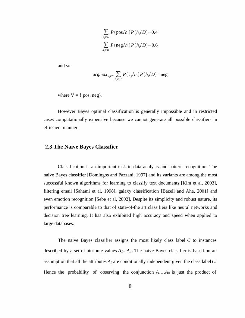
B is independent of C given A that is P C /B , A=P C /A . Consider Figure 2.3. In this
network, nodes A and B are both independent however A is dependent on B given C.
2.4.2 Representation
Figure 2.5 shows an example of a Bayesian network structure S and local
probability distributions P of all nodes in the form of conditional probability tables.
12
A
B C D
A
B C D
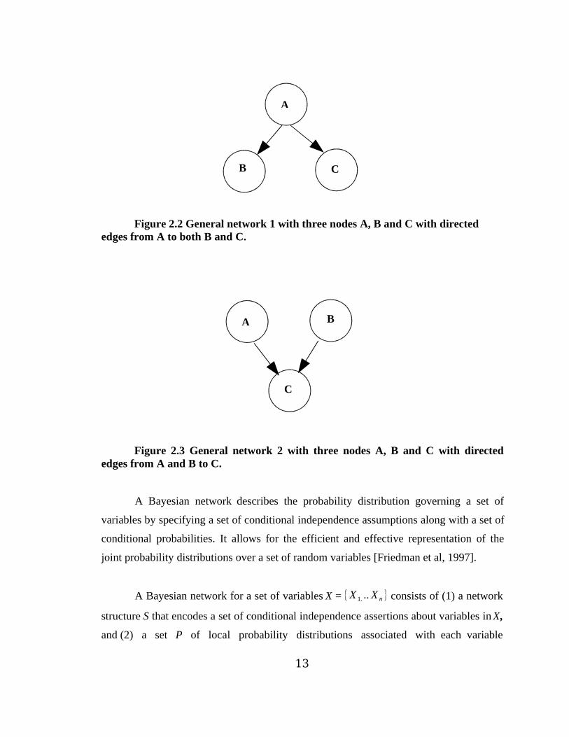
Figure 2.2 General network 1 with three nodes A, B and C with directededges from A to both B and C.
Figure 2.3 General network 2 with three nodes A, B and C with directededges from A and B to C.
A Bayesian network describes the probability distribution governing a set of
variables by specifying a set of conditional independence assumptions along with a set of
conditional probabilities. It allows for the efficient and effective representation of the
joint probability distributions over a set of random variables [Friedman et al, 1997].
A Bayesian network for a set of variables X = {X 1. .. X n } consists of (1) a network
structure S that encodes a set of conditional independence assertions about variables in X,
and (2) a set P of local probability distributions associated with each variable
13
A
B C
A
C
B

Figure 2.4 A Bayesian network with eight nodes A, B, C, D, E, F, G and H.With respect to node E, nodes A and B are non descendants, nodes C and D areparents while nodes F and G are descendants. Node H is a parent of node G.
[Heckerman, 1995]. These two are the components of the joint probability distribution
for X.
Each vertex in S is a random variable from X, and each edge represents a
correlation between the variables. The lack of an edge between two nodes encodes
conditional independence between the two nodes. This network structure S is essentially
an acyclic graph whose vertices correspond to variables in X. The local probability
distributions P are represented as a table for each variable given its parents known as
conditional probability table.
A Bayesian network encodes the Markov Assumption. Any variable X i is
14
C D
E
F G
H
BA

conditionally independent of its non descendants, given its parents.
P X 1 ... X n=∏i=1
n
P X i /Parents X i , where Parents X i is set of parents of X i .
Consider Figure 2.4. For node E, nodes A and B are non descendants while nodes
C and D are parents and nodes F and G are descendants. Node E is independent of A, B
given C, D.
In general, a Markov blanket of some node X is a minimal set of variables that
make the variable X independent from all the other variables in the network. It is a union
of three sets – the parents of X, the children of X and the parents of the children of X.
Figure 2.5 shows a more complete Bayesian network for our test problem. Before
explaining the Bayesian network in Figure 2.6, we will explain the variables denoted by
nodes in the figure.
Q48NEVER Had Blood Pressure Checked? {never, yes}
ALCWDBNO Accomplished less, careless work, and felt downhearted and blue
without being depressed or anxious {yes, no}
Q5_15 Diagnosed Depression {yes, no}
Q5_10 Diagnosed Stroke Related Problem {yes, no}
Q39 Limited in the kind of work {yes, no}
Q5_9 Diagnosed Heart Trouble {yes, no}
Q48NEVER directly affects the probability of ALCWDBNO. The value of Q5_15 to be
yes or the value of Q39 to be yes for limited in the kind of work depends only on the state
of ALCWDBNO as both the variables Q5_15 and Q39 are in the Markov blanket of
ALCWDBNO.
The table associated with each of the nodes is called a Conditional Probability
15

Figure 2.5 An example of typical Bayesian structure and local probabilitydistributions in the form of Conditional Probability Tables for each node.
Table (CPT). The CPT of the variables Q5_15, Q5_10 and Q39 have two rows each.
Each of the row corresponds to a value of the variable ALCWDBNO. Each column of
the CPT corresponds to the particular variables value. For example, if we look at the first
row of the CPT of Q5_15, the probability of Q5_15 = yes when ALCWDBNO = yes is
0.9 and the probability of Q5_15 to have value no when ALCWDBNO= yes is 0.1.
Again, in the second row, the probability of Q5_15 = yes when ALCWDBNO is no is
0.05 and the probability of Q5_15 to have value no when ALCWDBNO = no is 0.95. As
we can see, each row of the CPT must add up to 1. Each row in CPT contains the
conditional probability of each node value for the conditioning case. A conditioning case
is just a possible combination of values for the parent node. All the root nodes (like
16
P (48N)
Q39
Q5_9
Q39
yes
no 0.45
P (Q5_9)
0.20
ALC
yes
no
ALC
yes
no 0.25
P (Q39)
0.55
0.30Q48NEVER
ALCWDBNO
Q5_15Q5_10
Q48N
yes
never 0.15
P (ALC)
0.60
ALC
yes
no 0.55
P (Q5_10)
0.10
0.05
P(Q5_15)
0.90
0.95
P(-Q5_15)
0.10

Q48NEVER), with no parents are represented with prior probabilities of each possible
value of that variable.
2.4.3 Inference
After a Bayesian network is created from the data and prior knowledge about the
variables, we need to determine various probabilities of our interest from this network
which may not be available directly from the net. Thus we need to compute this
probability distribution for any subset of variables of interest given the values of any
subset of remaining variables.
There are several variants of probabilistic inference algorithms developed for
Bayesian networks. Overall they all can be categorized in two main kinds of inference:
(1) exact, and (2) approximate.
Exact inference of probabilities for an arbitrary Bayesian network is NP hard
[Mitchell, 1997]. Exact inference is possible when all nodes of Bayesian network have
linear Gaussian distributions [Mitchell, 1997]. There are two main types of exact
inference algorithms, those that work only on directed acyclic graph (DAG) models and
those that work on both directed and undirected graphs.
The DAG-only inference algorithms exploit the chain-rule decomposition of the
joint probability,
P X =P X 1P X 2/X 1P X 3/X 1 , X 2 ...
and the “push sums inside products” approach to remove the irrelevant nodes. This kind
of algorithm is called the variable elimination algorithm. This results in a single marginal
probability P X i /X j .
17

Algorithms that work on both undirected and directed graphs are generally
defined in terms of message passing on a tree. The tree can be directed or undirected and
the messages can be passed sequentially or in parallel. One of the advantages of message
passing algorithms is that they use dynamic programming to avoid redundant
computations used by variable elimination algorithms when computing all the marginal
probabilities simultaneously. A few good examples of message passing algorithms are
Pearl's algorithm [1988] and the Hugin/JLO algorithm [Jensen et al, 1990]
There are a couple of reasons why it is difficult to use exact inference in all cases.
In cases when exact inference is mathematically possible, the computation time to get the
exact solution is often very long. There are also cases when there is no possible
closed-form solution. In both such cases, approximate inference is often employed. There
are few different types of approximate inference algorithms that are used.
Sampling Methods are one of the techniques that are used to perform approximate
inference. Importance sampling is one the simplest kinds of these methods. In importance
sampling random samples are drawn from prior probabilities [Cheng and Druzdzel,
2000]. One of the most popular approximation approaches is the Markov Chain Monte
Carlo (MCMC) method, in which the random samples are drawn from the posterior
probabilities. Other methods include Gibbs sampling [MacKay, 1998] and the
Metropolis-Hasting algorithm [Neal, 1993].
Another kind of approximation methods are the variation methods. One example
of these is the mean-field approximation method [Jordan et al, 1998]. This method
exploits the law of large numbers to approximate large sums of random variables by their
means. The mean-field algorithm produces a lower bound on the likelihood of the
approximations.
Belief Propagation algorithms [Berrou et al, 1993] apply the message passing
algorithm to the original graph even if it has loops. These algorithms are closely related
to the variation methods and have been used to do approximate Bayesian inference in
18
algorithms like the Expectation Propagation algorithm.
2.4.4 Learning Bayesian Network Structure
Why do we need to learn Bayesian networks? Sometimes we do not know the
structure of a network or only know parts of the structure. Also, the graph structure
provides us a method to gather new knowledge by providing an insight into the domain
of our problem.
There are two main kinds of learning: parameter learning and structure learning.
In parameter learning, there can be two cases: one in which the network structure is
known and there are no hidden/missing variables and another in which the network
structure is known but there are hidden/missing variables.
In the first case, where the network structure is known in advance and all the
variables are fully observable, the task of parameter learning is to estimate the conditional
probability table entries. This is a simple task. There have been various algorithms that
have been proposed for such a case. If the network structure is a directed acyclic graph,
the problem decomposes fully, since we can construct the conditional probability tables
independently of each other. When the network is undirected, methods like Iterative
Proportional Fitting (IPF) and the generalized iterative scaling algorithm [Darrech and
Ratcliff, 1972] can be used.
In the case where the network structure is known but not all of the variables'
values are observable (missing and/or hidden values in dataset), learning is more
difficult. In this case, a locally optimal solution is preferred. Algorithms such as the
Expectation Maximization (EM) algorithm [Lauritzer, 1995] can be used to find such a
locally optimal solution. There are other methods that can also be used, such as the
“bound and collapse” method [Ramoni and Sebastini, 1997] and gradient based methods
[Koller et al, 1997]. However, the EM algorithm is generally preferred over these because
of its simplicity and the fact that it deals with constraints automatically. The EM
19

algorithm can be sped up by combining it with gradient methods [Jamshidian and
Jennrich, 1993].
When the underlying structure of data D is not known, we must perform Structure
Learning. The Structure Learning task can be informally stated as: Given a training
dataset D, find a network B that best matches D, where D is a set of independent
instances. There are two different approaches to graphical probabilistic model learning
(structure learning) from data [Cheng et al, 1997]: (1) dependency-analysis-based
methods, and (2) search and score methods.
A dependency-analysis-based methods depend on the assumption that the
underlying network which is studied has many dependencies amongst the nodes.
Algorithms based on this approach try to discover the relevant set of these dependencies
and independences in the network from the training data and use them to infer the
structure of network. Dependency relationships are calculated using some form of
Conditional Independence (CI) tests. This is also called the constraint based approach. A
few algorithms based on this approach are the Boundary DAG algorithm [Pearl, 1988],
the Wermuth-Lauritzen Algorithm [Wermuth and Lauritzen, 1983], the Constructor
algorithm [Fung and Crawford, 1990], the SRA algorithm [Srinivas et al, 1990], and the
SGS algorithm [Sprites et al, 1990].
Although the dependency-based method has advantages, such as being more
efficient for sparse networks and often finding the correct structure when the probability
distribution of data satisfies certain assumption, it can be unreliable when the CI tests
have large condition sets (number of different conditions in data). Moreover, this
approach often requires an exponential number of CI tests.
The more popular approach is the search and score method. This approach
attempts to find the structure that can fit the data best using a search process. All the
search and score methods attempt to search a graph that maximizes the selected scoring
function. Algorithms falling in this category generally start with a simple graph without
20

any edges and then use some search method to add/delete edges recursively. The score
method is used to measure the goodness of each explored graph from the space of
feasible solutions. This process continues until they do not get a candidate which defines
the data in a better way. Thus each algorithm is characterized by a specific search
procedure and scoring function. The scoring function is based on different criteria such as
the Bayesian scoring method [Cooper and Herskovits, 1992; Heckerman et al, 1995;
Ramoni and Sebastini, 1997], the entropy based method [Herskovits and Cooper, 1990],
the minimum description length (MDL) method [Suzuki 1996; Friedman and
Goldszmidt, 1996; Lam and Bacchus, 1994] and the minimum message length method
[Wallace et al, 1996]. We discuss a few of these algorithms briefly below.
The Chow-Liu Tree Construction Algorithm [Chow and Liu, 1968] is used to do
structure learning and is a variant of the [Friedman and Goldszmidt, 1996] algorithm.
This algorithm uses two different kinds of scores to learn a Bayesian network. It used
both the minimum description length (MDL) score and the Bayesian score. It is effective
algorithm since it learns the Bayesian network and the local structure of the conditional
probability tables at the same time. When we add a new edge using this algorithm, it
chooses the direction which gives the better score as the direction for the edge.
The K2 Algorithm [Cooper and Herskovits, 1992] was the first serious attempt at
learning a Bayesian belief network. It is one of the first search and scoring based
algorithms for learning a Bayesian belief network. The working of this algorithm is very
simple in that it takes as input a dataset and a node order, and constructs a belief network
structure as the output. This algorithm uses a Bayesian scoring method and computes the
conditional probabilities by the brute force method.
The MDL length method [Suzuki 1996] addressed the issue of learning Bayes
networks using the minimum description length (MDL) principle. The MDL principle
basically selects a rule that takes both simplicity and fit to the data into account and
achieves the best results. This algorithm uses a formula for description length and applies
a branch and bound technique to find the network structure. The branch and bound
21

technique thus developed determines whether a branch needs to be searched more by
calculating a lower bound after adding an arc to the structure. This algorithm is very
different from other search and score algorithms in that it does not use a heuristic and it
also guarantees that we find an optimal structure.
The Construct-TAN algorithm [Friedman et al, 1997] that we use to do our
structure learning is a variant of the tree augmented naive Bayes [Friedman and
Goldszmidt, 1996] algorithm. It uses both the minimum description length (MDL) score
and the Bayesian score to learn the network. It is also a good algorithm since it learns the
Bayesian network and the local structure of the conditional probability tables at the same
time [Friedman et al, 1997]. When we add a new edge using this algorithm, it chooses the
direction which gives the better score as the direction for the edge. The toolbox we have
implemented is based on this algorithm. The Construct-TAN algorithm is explained in
detail in Chapter 4.
22

Chapter 3: The Bridge to Health Dataset
This chapter is organized as follows. Section 3.1 introduces the Bridge to Health
survey data, followed by Section 3.2 which explains in detail the method by which data
was collected. Section 3.3 describes the statistical weighting of data. The next subsection
describes the data, while the last section, 3.5, lists variables of interest, cardiovascular
disease risk factors and mental health status variables.
3.1 The Bridge to Health Survey Dataset
The Bridge to Health survey was a regional health status assessment carried out
between November 1999 and February 2000. This population-based survey was mainly
conducted to gather information on health indicators. The Bridge to Health Survey
dataset is a local (county level) survey data of more than 6200 adult residents in a
sixteen-county region in Northeastern Minnesota and Northwestern Wisconsin
[Block et al, 2000].
3.2 Data Collection
The Bridge to Health 2000 survey (BTH 2000) data was collected through 6251
computer-aided telephone interviews by the Survey Research Center of Division Health
Services Research and Policy located in the School of Public Health at the University of
Minnesota for Bridge to Health Collaborative. One adult (above the age of 18) from each
sampled household was selected to participate in the survey. Out of 8559 eligible
households contacted by phone between November 1999 and February 2000, 6251
interviews were completed with the response rate of over 74% [Block et al, 2000].
The BTH 2000 collected data on lifestyle behaviors, health care access, disease
prevalence, preventive health practices, injury prevention and violence, preventive
screening and tobacco-alcohol use. The BTH 2000 Questionnaire had 101 questions for
23

which the responses of the interviewees were recorded. The questions were designed to
gather information about the general health of an individual as perceived by himself and
as diagnosed by a doctor.
Most of the questions had a choice of response as YES/NO. An example question
is
In the last year, have you had a flue shot?
- Yes
- No
But some questions were more descriptive, with the choices as in
How much of the time during the past four weeks, have you felt downhearted and
blue?
- All the time
- Most of the time
- A good bit of the time
- Some of the time
- A little of the time
- None of the time
- Refused
- Don't know
3.3 Statistical Weighting of Data
The BTH 2000 dataset was required to be weighted because of the differences in
household size, differences in the size of the population in each of the 18 strata
(counties), and differences in response rates between men and women and people of
different ages [Block et al, 2000]. The statistical weighting was already done by [Block et
al, 2000] before we used the data for our research. However the process of weighting the
24

data is crucial and so I would like to mention it here. The first step involved weighing the
data by the inverse of the selection probability within the household (that is, the number
of adults age 18 and older living in the household). The next step was to weigh the data
by the actual size of the adult population in each of the strata divided by the number of
respondents from each stratum. The third step was to post-stratify the data based on the
1998 U.S. Census estimates of the age and gender distributions for adults with each of the
strata. The last step was to divide the weights by a numeric constant, which forced the
weighted total sample size to be equal to the total number of respondents in the sample.
3.4 Data Description
BTH 2000 has 6251 records, each one representing the response of an
interviewee. Each record has 334 features.
These features are either the direct responses of the interviewees, new/recoded
variables or maintenance variables. The new or recoded variables were added to facilitate
research of the dataset. These variables are calculated from the direct responses either to
make them more specific or more general. Some of the continuous variables were made
discrete. The various features can be categorized as follows:
1. General information such as the sex, age, education, height, weight or marital status
of a person.
2. Physical health status variables such as chronic conditions, overweight issues and
person suffering from particular diseases.
3. Mental health status variables such as anxiety, panic attacks, depression and
accomplished less due to mental health.
4. Diagnosed diseases such as allergies, asthma, back problems, cancer, diabetes,
digestive disorder, high blood pressure and high cholesterol.
25

Table 3.1 Mental health status variables used as class variables to create tree
augmented networks using Construct-TAN algorithm.
Variable name Description Response
Q15NEW2 Diagnosed depression 1: Yes
10: No
Q16NEW2 Diagnosed anxiety 2: Yes
20: No
DEPRANX2 Diagnosed depression andanxiety
2: Yes
5: No
ALDPANX2 Accomplished less withoutdepression or anxiety
31: Yes
33: No
CWDPANX2 Careless work withoutdepression or anxiety
31: Yes
34; No
DBDPANX2 Feel downhearted or bluewithout depression oranxiety
31; Yes
35: No
5. Preventive care such as consumption of fruits and vegetables, avoidance of certain
food due to toothache and flu vaccination.
6. Preventive screening such as mammogram, pap-smear test, prostate examination
and colon screening.
7. Injury prevention and violence such as seat-belt use, safety equipment in home and
victims of violence or crime against property.
8. Tobacco-Alcohol use such as cigarette smoking, smoking in the home, attitudes
towards smoking regulations and alcohol consumption patterns.
9. Health care access such as health insurance coverage and failure to receive medical
care.
10. Recoded variables such as combination/recalculation of direct responses.
11. Data maintenance variables.
26

3.5 Class Variables: Features of Interest
In this research, we are interested in finding the correlations between the variables
given a particular (class) variable and analyzing the structure created by the Construct-
TAN algorithm (explained in Chapter 5). Table 3.1 lists all the cardiovascular disease
risk factors and Table 3.2 lists all the mental health status variables used as class
variables for structure learning.
Table 3.2 Cardiovascular disease risk factors used as class variables to create tree
augmented networks using Construct-TAN algorithm.
Variable name Description Response
Q5_11 Diagnosed high bloodpressure
1: Yes
2: No
Q5_12 Diagnosed elevatedcholesterol
1: Yes
2: No
Q48REC Blood Pressure checked inlast 2 years
1: Within past 2 years
2: Not within past 2 years
Q49REC2 Cholesterol checked in last2 years
1: Within past 2 years
2: Not within past 2 years
OVERWGT2 Overweight or notoverweight based on BMI
0: Not overweight
1: Overweight
BMICUTS Normal weight, overweight,obese based on BMI
0: Not overweight
1: Overweight
2: Obese
EXCERREC Moderate or vigorousexercise 3X per week
1: Exercise less than 3 timesper week
2: Exercise more than 3times per week
Q69A Current smoker 1: Yes
2: No
27
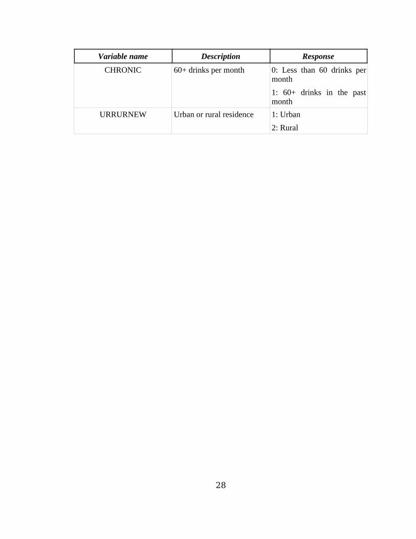
Variable name Description Response
CHRONIC 60+ drinks per month 0: Less than 60 drinks permonth
1: 60+ drinks in the pastmonth
URRURNEW Urban or rural residence 1: Urban
2: Rural
28

Chapter 4: The Construct-TAN algorithm [Friedman et al,
1997]
In this chapter we present the algorithm that we used to create our Bayesian
networks. The tool we describe in Chapter 5 is based on the Construct-TAN [Friedman et
al, 1997] algorithm.
4.1 Using Bayesian Networks for Classification
As we have already seen in the background section, a naive Bayes classifier
learns from training data D the conditional probability of each attribute Ai given the class
variable C (note that all variables in training data D except C are called attributes).
Classification is then done by applying Bayes rule to compute the probability of C given
the particular instance of A1...An and then predicting the class with the highest posterior
probability.
But in general, the strong assumption of conditional independence between the
attributes given the class variable C is not realistic for real world datasets. The
classification using naive Bayes could be skewed (and yet good) because of the fact that
it neglects the correlation between attributes in highly interrelated network.
In our classifier, we start with the connections from the class variable C to every
attribute Ai. This gives the class variable a special status in the network. The connection
from C to each Ai ensures that, in the learned network, the probability P(C/ A1...An) will
take all attributes in account [Friedman et al, 1997]. Thus we start with a naive Bayes
network and change it by adding edges amongst the attributes maintaining the acyclic
nature of the graph. These additional edges signify a correlation amongst variables in the
structure. Thus the newly created classifier is called as augmented naive Bayes classifier.
29
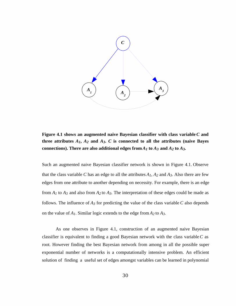
Figure 4.1 shows an augmented naive Bayesian classifier with class variable C and
three attributes A1, A2 and A3. C is connected to all the attributes (naive Bayes
connections). There are also additional edges from A1 to A3 and A2 to A3.
Such an augmented naive Bayesian classifier network is shown in Figure 4.1. Observe
that the class variable C has an edge to all the attributes A1, A2 and A3. Also there are few
edges from one attribute to another depending on necessity. For example, there is an edge
from A1 to A3 and also from A2 to A3. The interpretation of these edges could be made as
follows. The influence of A3 for predicting the value of the class variable C also depends
on the value of A1. Similar logic extends to the edge from A2 to A3.
As one observes in Figure 4.1, construction of an augmented naive Bayesian
classifier is equivalent to finding a good Bayesian network with the class variable C as
root. However finding the best Bayesian network from among in all the possible super
exponential number of networks is a computationally intensive problem. An efficient
solution of finding a useful set of edges amongst variables can be learned in polynomial
30
C
A1 A
2
A3

Figure 4.2 A Tree Augmented Network (TAN) with class variable C and three
attributes nodes A1, A2 and A3. C is connected to all the attributes. There are also
directed edges from A1 to A2 and A2 to A3.
time by imposing restrictions on allowable interactions amongst the variables. This
results in a new network called a Tree Augmented Network or TAN.
In a TAN, the network is restricted in that the class variable has no parents and
each attribute has as parents the class variable C and at most one other attribute. The
edges in a TAN are called augmented edges. One should notice that each attribute in
TAN can have one augmented edge pointing to it.
Figure 4.2 shows a tree augmented network where class variable C is connected to
all the attributes A1, A2 and A3. Also there are edges from one attribute to another
depending on necessity. For example, there is an edge from A1 to A2 and also from A2 to
A3. Note that the TAN cannot have any attribute node with more that one attribute as its
parent. In Figure 4.2, both A1 and A2 have only one attribute as parent. However an
augmented naive Bayesian network can have nodes with more than one attribute as their
31
C
A1 A
2
A3

parents. In Figure 4.1, A3 has two parents A1 and A2. This is where an augmented naive
Bayesian network differs from a TAN.
4.2 The Construct-TAN algorithm
Chow and Liu [1968] developed a procedure (shown in Table 4.1) for
constructing of TAN (learning the appropriate set of edges in the network). This
procedure reduces the problem of building a Bayesian network to finding a maximal
weighted spanning tree in a graph. This means the problem of finding such a tree is to
select a subset of arcs from a graph such that the selected arcs constitute a tree and the
sum of weights attached to the selected arcs is maximized [Friedman et al, 1997].
Table 4.1: The Construct-tree procedure of CL [Chow and Liu, 1968]
1. Compute IP (Xi ; Xj) between each pair of variables, i is not equal to j
2. Build a complete undirected graph in which the vertices are the variables in X.
Annotate the weight of an edge connecting Xi to Xj by IP (Xi ; Xj)
3. Build a maximum weighted spanning tree
4. Transform the resulting undirected tree to a directed tree one by choosing a root
variable and setting the direction of all edges to be outward from it
I pX ;Y = ∑
x∈X , y∈Y
P x , y logP x , y
P x P y (4.1)
The function IP (Xi ; Xj) is called the mutual information (MI) function and is
shown in equation (4.1). This function characterizes the mutual information between the
32

two variables X and Y. The MI between two variables X and Y can tell us whether the two
variables are dependent or not and if they are, then how close the relationship is. If MI
has a smaller value than a particular threshold t, then the two variables are called
conditionally independent. The time complexity of this procedure is O f 2∗n , where f is
the total number of variables in the data D.
The Construct-TAN [Friedman et al, 1997] algorithm, shown in Table 4.2, on
which my tool is designed, is based on the procedure Construct-tree
[Chow and Liu, 1968], with a slight modification. The Construct-TAN algorithm is a five
step procedure to build a tree augmented network for a given class node C. The first step
determines the weight of each edge between two nodes of the network. The weighting
function is called conditional mutual information function as shown in equation (4.2).
This function calculates the mutual information between two attributes given the value of
class variable C. The CMI between the two variables X and Y can tell us whether the two
variables are dependent or not, given the value of another variable C . The dependency of
the variables X and Y is determined with respect to the value of C. If CMI has a smaller
value than a particular threshold t, then the two variables are conditionally independent
given C. The next step constructs a undirected graph with all attributes (all nodes other
than the class node) and the weights are assigned to all the edges. The next step builds a
maximum-weighted spanning tree. In the toolbox, we have implemented Prim's algorithm
[Tenenbaum et al, 1995] for building the spanning tree. The fourth step converts
the undirected graph to directed one.
I P X ;Y /C = ∑
x∈X , y∈Y ,c∈C
P x , y , c logP x , y /c
P x /cP y /c (4.2)
33

Table 4.2: The Construct-TAN procedure explained from [Friedman et al, 1997]
1. Compute IP (Ai ; Aj / C) between each pair of variables, where i is not equal to j
2. Build a complete undirected graph in which the vertices are the attributes A1 ,...,
An. Annotate the weight of an edge connecting Ai to Aj by IP (Ai ; Aj / C).
3. Build a maximum weighted spanning tree.
4. Transform the resulting undirected tree to a directed one by choosing a root variable
and setting the direction of all edges to be outward from it.
5. Construct a TAN model by adding a vertex labeled by C and adding an arc from C
to each Ai.
Our implementation of this step selects the variable next to class variable in the
comma separated data file as the root node. The last step adds the class node to the graph.
The time complexity of this procedure is also O f 2∗n where f is the total number of
variables in the data D.
The two methods, Construct-tree and Construct-TAN, although they appear
similar, have a few differences as follows.
• Construct-tree is a four step method to build a general tree of all the variables in the
data while Construct-TAN is a five step algorithm to build a specialized tree with a
class node as parent of all the remaining nodes.
• A tree built by the Construct-tree method has one node (root node) with no parents and
all the other nodes with only one parent. On the other hand, the network built by
34

Construct-TAN has one node with no parent (class node), one node with only one
parent ( root node with class node as parent) and all the other nodes with two parents
( class node and some other node in the tree).
35

Chapter 5: Our Bayesian Toolbox
This chapter describes the toolbox that we developed using the Construct-TAN
algorithm. In this section, first we will discuss the motivation to create such a tool for our
survey data. Then we will discuss the representation used while creating this toolbox, the
interface design of the tool. In the next section, we will demonstrate the working of the
tool with an example TAN. Finally we enumerate the capabilities of the tool.
5.1 Motivation
There are various machine learning techniques that can be used to discover
various kinds of relationships amongst features in our data. However we wanted a
technique that would be: (1) accurate, (2) able to learn Bayesian network structures,
(3) efficient, and (4) effective for visualization.
We want to do structure learning using the Construct-TAN algorithm as it gives a
probable network by doing heuristic search over the space of network structures. The
structure that is created using our tool should describe the data very closely. There should
be a measure by which this structure can be validated. We use cross validation technique
to test the accuracy of the network created.
The tool thus developed should not only learn the structure of data but also
displays as a network of nodes and edges efficiently thus making speed an important
factor in the design of the tool. The algorithm used to develop the network is very
efficient and learns the data fast. Last but not the least, the tool should provide an
effective way to visualize the network and. The tool thus incorporated what was desired.
36

5.2 Design of the Tool
This section discusses the design of the tool. It explains how the structure learning
and inference methods are implemented in the tool, the representation of the network
built by the tool and software issues related to the tool.
5.2.1 Representation of the Network
The network is in the form of a DAG, more specifically a tree augmented
network. The structure created by the tool has a class node which is connected to all the
other nodes in the graph. However the number of attributes in our dataset is very large
(over 100) and to show the edges (directed from the class node to the attributes) would
make the network crowded and unreadable. Hence we do not show all of these edges in
the resulting network.
5.2.2 Structure Learning
The Construct-TAN algorithm constructs the network. As preprocessing of data
handles the elimination of missing values in the data and discretization of data, the
structure learning algorithm is implemented on data which is fully observed with no
hidden, no missing value variables. The input to the tool is an ordinary database table in
the comma separated variable file format. The first field of the data is treated as a class
variable, the next as the root variable. Each record is a complete instantiation of all the
variables in the domain. The conditional mutual information of variables is computed
using the relative frequencies from the database. The Construct-TAN algorithm, as
described in Chapter 4, is applied to the data and its structure is determined. The resulting
network is then displayed in a JAVA applet.
37

5.2.3 Inference
Because all the variables in the dataset are discrete, inference is practically viable
for implementation. Because of the simple approach of the algorithm, an inference
algorithm could be implemented in terms of a product of potentials. A potential is an
object variable which helps to execute the inference algorithm efficiently. In our case, the
potential is represented as the conditional probability table of a node, given all possible
states of its parents. The tree which is created by the tool is a spanning tree, and therefore
for each node the number of parents is at most two. Inference in TAN can then be
simplified as shown in equation (5.2). Equation (5.1) shows a generalized formula for
inference learning.
P C /X 1 ... X n=∏i=1
n
P X i /Parents X i (5.1)
where Parents X i are the parents of node Xi. There are only two parents of node X in
TAN , the class node C and some other node Y.
P C /X 1 ... X n=∏i=1
n
P X i /Y ,C (5.2)
The inference algorithm is easy to implement and enables optimization at
implementation level. In the case of inference, the inputs to the tool are the training data
file which learns the structure of the data and the testing data file for inference.
5.2.4 Software Issues
The tool has been implemented in JAVA because of the various functions JAVA
provides. JAVA has rich set of built-in data structures, facilities for drawing graphs and
use of applets to display the network. The use of JAVA as a programming language
makes the tool runnable on any JAVA-enabled browser.
38

5.3 Working of the Tool with an Example
Consider a training data file to develop a network for the class variable
CHRONIC using our tool.
CHRONIC,SEX,Q36,Q37,Q38,Q39,Q40,Q41,Q44,Q45,Q46,Q48,...0,2,3,100,2,2,2,2,5,2,5,1,...0,2,3,100,2,2,2,2,2,3,6,1,...0,1,3,100,2,2,2,2,1,3,6,1,...0,1,3,100,2,2,2,2,2,3,6,1,...0,2,1,1,2,2,100,100,2,100,5,1,...0,2,3,100,2,2,2,2,2,4,5,1,......
The training data file has 3115 records and 54 variables including the class
variable CHRONIC. The training data file and the testing data file are both comma
separated files. The top row lists the variable names which are represented as nodes in
the TAN. The first variable (CHRONIC) is considered as the class variable for which the
structure is built. The next variable (SEX) is the root variable which has only one parent,
the class variable. All the other rows (except the first one) contain the values of all the
nodes. The network thus created by the tool is shown in Figure 5.1. It shows the tree
augmented network for the class variable CHRONIC. All the variables other than the
class variable are represented as nodes in the network. The edges are weighted by the
conditional mutual information value (see equation 4.2). Our tool searches the space of
all possible networks and builds a network which is a maximum-weighted spanning tree.
The algorithm we implemented for building the spanning tree is Prim's algorithm. It is
described below.
Table 5.1: Prims Algorithm
1. Create a tree T containing a single vertex v, chosen arbitrarily from the graph G. v is
known as the root node.
2. Create a set S containing all the edges in G.
39

3. Remove from S an edge e with maximum weight that connects a vertex in the T with
a vertex u in G. Add edge e and vertex u to the tree.
4. Repeat step 3 until every edge in S connects two vertices in T .
Figure 5.1 Tree augmented network for class variable CHRONIC
40

5.4 Features
The toolbox has various features incorporated into it right now. The tool builds a
TAN with the following features: (1) it is web enabled, (2) time efficient, (3) the network
spaces itself in given area, (4) the network can be frozen for examination, (5) nodes are
distanced according to their association with each other, and (6) the user can choose a
percentage of edges.
5.5 Discussion
Although there are many Bayes Network tools which are freely available that can
provide some similar functionality to our tool, almost all of them had a restriction on the
size of the dataset that one can use. We wanted to create a tool which did not put any
restrictions on the dataset one can use.
Another drawback with many tools is that they use some kind of node ordering
requirement. Node Ordering is a type of domain knowledge used by many Bayesian
network learning algorithms that satisfies a causal or temporal order of the nodes of the
graph. Most algorithms either assume that there is a node ordering requirement or they
prefer to use it. We wanted to make a tool which did not necessarily have this
requirement of node ordering. That is the reason we chose the Construct-TAN algorithm
described earlier; it does not require any node ordering.
Most of the visual tools that are available online have a constraint on the number
of nodes in the graph. We did not want any constraints on the number of nodes that are
present in the graph. We wanted to visualize all variables in the dataset and then analyze
from their structure using some measures.
Finally, there is a dearth of publicly available learning tools for real world data
mining datasets and applications. Real world data mining datasets have hundreds of
41

variables and thousands to millions of records in them. Most of the tools we found had
restrictions on data size and hence were not really meant for any real world application.
They ran on at most 40 features and 5000 records. I had a dataset that consisted of over
300 features and hence we wanted to create a tool that would handle this size of data
efficiently.
42

Chapter 6: Experiments and Analysis
In this chapter, we present the experiments to verify the usefulness of the tool we
constructed. In the first section, we describe how the data was preprocessed. The data
preprocessing technique was carried out in two phases: (1) feature elimination, and (2)
handling of missing values in the dataset. We compare the effectiveness of the network
we create using the tool with the naive Bayes classifier in Section 6.2. Section 6.3
describes the results obtained from our tool for class variable Q5_12: Diagnosed elevated
cholesterol in detail. Finally, in Section 6.4 we show several example TANs created by
our tool and provide some analysis.
6.1 Data Preprocessing
The BTH 2000 dataset (presented in Chapter 3) is a large dataset with 6251
records and 334 variables. The focus of this thesis was to demonstrate that our tool could
find relationships between the cardiovascular disease risk factors and mental health status
variables and to analyze the kind of correlations that exist between the variables (see
table 3.1 and 3.2) along with other variables. When the original dataset with 334 features
was assessed, it was observed that there were many features which were irrelevant to our
purpose. There are several variables like maintenance variables in the dataset used as
sanity checks of data and to statistically weigh the data. For example variables like ID
(the respondent's ID number), SRVYMODE (Mode of survey), STATEWT (sample
weights for state level analysis) and COUNTYWT (sample weights for county level
analysis) are maintenance variables. The original dataset also contained several recoded
variables. BMICUTS (body mass index cuts) is a recoded variable of BMI (body mass
index) with a new definition. There are several other variables which are recoded and
suffixed with “new” or “rec”. For example variable Q48 (had blood pressure check?) is
recoded as Q48REC (has blood pressure checked in last 2 years) and Q48NEVER ( never
had blood pressure checked). There were also some other variables which were
43

categorized variables of another variable and thus conveyed similar information. For
example Q92A1 (drink and drive: car or truck), Q92B1 (drink and drive: boat) ,
Q92C1 (drink and drive: snowmobile) and Q92D1 (drink and drive: other) were
summarized by one variable Q96 (drink and drive). So there were several variables in
BTH 2000 which conveyed very little or no information of the variables of our interest.
Bayesian structure learning with all entire set of variables would have been
computationally and memory-wise costly. Also the extracted structure would be overly
crowded and hard to decipher. Hence a preprocessing of BTH 2000 dataset was necessary
to make the Bayesian learning process efficient.
The data had to be converted from SPSS format to the format that we could be
easily manipulate. The dataset was converted to a comma separated format as an input to
our tool while it was converted to C4.5 format to test it against a naive Bayes classifier.
6.1.1 Feature Elimination
The purpose of the feature elimination process was to select an appropriate set of
features that could predict the output variable (that is, either a cardiovascular disease risk
factor or mental health status variable, see Tables 3.1 and 3.2). The feature elimination
process tried to identify the contribution of each variable to predict the class variable and
identify its rank compared to others. It recursively discarded those features which even
when eliminated from the dataset would not affect the desired accuracy. We used C4.5 as
the classification mechanism to predict the class variable. Each variable from the dataset
was categorized as probably irrelevant or very likely relevant variable. A probably
irrelevant variable is a variable which conveys little or no information about the class
variable we are trying to predict. For example, YNGKIDS (number of young kids in the
household), CRIMEREC (crime record of the interviewee) have no relevance to class
variable Q5_11 (Diagnosed Hypertension). Also any variable which carry no extra
information about the class variable was considered as probably irrelevant. For example,
consider a class variable BMICUTS, variable BMI very much has the same information
44

and so could be conveniently not considered. The inclusion of such variables might have
created a bias in the learning algorithm as they will show high correlation between the
class variable and hence overshadow the variables of interest. To classify the variables in
each of the above classes, all the variables were dropped one at a time and the change in
accuracy value of the classification of class variable was noted.
Out of the 334 variables in the BTH 2000 dataset, 76 variables were determined to
have little potential bearing with class variables and removed as irrelevant, 86 were
removed by feature elimination process. Sixty more variables (considered either
irrelevant or recoded) from the remaining 172 variables were with the help of an domain
expert, Dr. Timothy Van Wave [2004] who reviewed the dataset for us.
6.1.2 Handling Missing Values in Dataset
After the feature elimination process the dataset had 110 variables and 6251
records. 61,196 data points out of total 687,610 data points had missing value
(represented as '$null$' in the dataset) meaning 8.9% of data was missing. While carrying
out experiments to do inference learning as well as structure learning of this dataset, all
the missing values were replaced with a unique value representing 'unknown'. Records
with a missing value for the class variable however were removed from the data set
before using the dataset. Thus the data after this process was cleaned for missing data
points by simple substitution for null values.
6.1.3 Handling Continuous Values in Dataset
The initial set of experiments using the dataset with 110 variables made the
learning process very slow due to the presence of a few continuous-valued variables
(variables with more than 10 values). A further assessment of the dataset was then done
to handle these variables. Four variables (Q7B, HHSIZE, PCS12 and MCS12) were
discretized by range while three variables (DOLLARS, AGE, BMI) were dropped from
45

the dataset. The complete preprocessing process was examined by our domain expert,
Dr. Van Wave.
After the data preprocessing phase, there are a further assumptions that we have
made about the data. They are: (1) all the variables of the dataset have discrete values, (2)
all missing values for all the variables are handled, (3) the records occur independently
given the underlying probabilistic distribution of the data, and (4) the volume of data is
large enough.
6.2 Two-Fold Cross Validation Testing
N-fold cross validation is a well known technique for testing of dataset for a given
method. In our experiments, we verify the effectiveness of the TAN created by the
Construct-TAN algorithm against the naive Bayes classifier. The two-fold cross
validation divides the data in two folds. The instances are randomly divided amongst the
two folds. One of the two folds is then trained using the structure learning algorithm.
Then the learned structure is then tested against the other fold and accuracy of the
classifier is calculated using confusion matrix of the predicted values of the classifier
against the actual values of the classifier. The same procedure is repeated considering the
second fold to be the train data and the first fold to be the test data. Average accuracy is
thus calculated. Table 6.3 and 6.4 show the two fold cross validation results for all the
class variables from Tables 3.1 and 3.2 for both TAN and naive Bayes classifier.
Tables 6.1 and 6.2 show two-fold cross validation results for both mental health
status variables and cardiovascular risk factors using Construct-TAN networks and naive
Bayes networks. These results show that the Construct-TAN networks outperform the
naive Bayes networks for all the mental health status variables, in some cases
significantly, and for the cardiovascular risk factors the Construct-TAN networks either
perform similarly to the naive Bayes networks or in some cases significantly outperform
the naive Bayes networks. This is not entirely surprising as a Construct-TAN network is
46

Table 6.1 Two-fold cross-validation results for both TAN and naive Bayes forMental Health Status variables.
Class Variable TAN naive Bayes
Q15NEW2 99.01% 96.65%
Q16NEW2 98.86% 92.92%
DEPRANX2 99.60% 96.52%
ALDPANX2 99.94% 97.21%
CWDPANX2 98.81% 97.04%
DBDPANX2 99.77% 99.47%
Table 6.2 Two fold cross-validation results for both TAN and naive Bayes forCardiovascular Disease Risk factors.
Class Variable TAN naive Bayes
BMICUTS 92.81% 93.23%
EXCERREC 99.64% 99.93%
Q69A 93.13% 88.66%
CHRONIC 88.90% 81.68%
URRURNEW 99.77% 99.90%
Q5_11 86.85% 87.51%
Q5_12 86.77% 87.95%
Q48REC 97.76% 97.60%
Q49REC2 98.13% 98.65%
OVERWGT2 99.61% 97.86%
capable of taking into account the same probability estimates as a naive Bayes network,
but it also shows that in many cases, the learned connections in the resulting TAN can
significantly increase performance.
47
6.3 Bayesian Learning for Q5_12: Diagnosed elevated cholesterol
Q5_12, diagnosed elevated cholesterol, is a cardiovascular disease risk factor (see
Table 3.1). In this section, the Bayesian learning for Q5_12 using our tool is discussed in
detail. Bayesian learning for all the class variables from Tables 3.1 and 3.2 are discussed
in brief in the next section.
The main goal of all the experiments conducted is to find the interesting subset of
variables from the list of variables which have strong correlation amongst them as well as
with the class variable Q5_12. We also intend to find the meaningful links between the
variables of interest and analyze them.
6.3.1 Bayesian Network Structure
The tree augmented network created by the tool is shown in the Figure 6.1. The
TAN created has 106 nodes and 105 edges. In TAN, the class variable (Q5_12) is
connected to all the other nodes in the network. These edges indicate that the class node
is a parent of all the nodes. But these edges are not weighted. Our TAN has more than
one hundred nodes in the graph and so if we would have shown edges from the class
node to all the nodes, it would have made the network crowded. Also it would have made
observing meaningful links between the other nodes difficult, and so the network we
display does not show the class node.
6.3.2 Top Ten Associations Amongst Variables
The TAN was also analyzed to find interesting links between the variables of our
interest. Using the slider in the toolbox, we varied the percentage of links we want to
concentrate on. Figure 6.2 shows the top 10% of the links. The mental health status
variables which appeared in the diagram are highlighted with red color while
48

cardiovascular disease risk factors are highlighted using blue color. Various randomly
selected datasets with at least 3000 records were trained and the structures were studied
to find the top links amongst the variables. The top 20 associations between the variables
of all networks were compared and the common associations were ranked according to
their occurrences in all the networks. The most common top ten associations for
predicting the value of Q5_12 are listed in Table 6.3.
Table 6.3 List of top 10 associations to predict the class Q5_12.
Parent Child
STATE Q5_5
Q56 OVERWGT2
Q56 BMICUTS
CHRONIC Q52REC
STATE Q5_6
CHRONIC Q51REC
STATE Q5_8
OVERWGT2 Q66A
OVERWGT2 Q65A
CHRONIC POVEREC
49

Figure 6.1 TAN for structure learning of class variable Q5_12: Diagnosedelevated Cholesterol.
6.3.3 Top Ten Parent Nodes
We use the same datasets to find the variables which are associated with a larger
number of other variables. If any node in the network has a parent node, it means that the
value of that child node used to predict the value of class variable is influenced by the
value of its parent node and taken into account while classifying the class variable. So we
50

Figure 6.2 Top 10% links for the class variable Q5_12.
can intuitively think that if a node is a parent of many other nodes in the network, its
contribution in prediction of the class variable is significant. If we are interested in
finding the links between two variables, the parents of both the variables also play a
crucial part. An example of this is Figure 6.1. Table 6.2 lists the top 10% of the nodes
which are parents of another nodes in the structure. Another use of identifying such
parent nodes is to find the nodes at the top of the spanning tree. The nodes from Table 6.2
are highlighted in Figure 6.1. Table 6.2 shows that many nodes of interest like
ALCWDBNO, CHRONIC and ALDPANX2 appear in the list of top parent nodes.
6.3.4 Bayesian Multinets
The TAN shown in Figure 6.1 shows the relationship between all the nodes to be
the same for all the different values of the class variable Q5_12. The two values
(responses, see Table 3.1) of the class variable Q5_12 are 1 (yes) and 2 (no). Different
51

Table 6.4 List of top 10 parents to predict Q5_12
PARENT NODE NOTES
ALCWDBNO Accomplished less and careless work without depression and
anxiety. (Mental health status recoded variable)
CHRONIC Chronic drinker. (Cardiovascular risk factor)
SEATBLT2 Seatbelt used
ALDPANX2 Accomplished less without depression and anxiety. (Mental health
status variable)
Q56 Have in home; smoke detector.
STATE Minnesota/Wisconsin
OVERWGT2 Overweight according to new BMI definition. (Cardiovascular
risk factor)
Q16NEW2 Diagnosed Anxiety (Mental health status variable)
Q5_8 Diagnosed heart trouble
ALDBNODA Accomplished less without downhearted blues and without
depression and anxiety. (Mental health status variable)
values of a class variable could have a different structure and hence a different set of
augmenting edges. The collection of all the networks with a different value of class
variable is called a multinet. We created multinets by partitioning the data according to
the values of the class variable.
Figure 6.3 shows a local network for Q5_12 having the value 1. The figure shows
cardiovascular disease risk factors like OVERWGT2 and BMICUTS. Since Q5_12
means whether a patient is diagnosed with elevated cholesterol, we can see in the
network that general health variables like Q48NEVER (BP never checked) , GENHLTH
(general health of a person) and Q4REC (general health compared to others) appear in
the top ten percent of meaningful edges. Also we observe an interesting relationship
between Q41 (careless work due to emotional problems), Q46REC (felt downhearted and
blue – recoded) and Q5_17 (diagnosed with other mental problems). The top parent node
52

for this network is Q35 ( moderate activity because of health).
Figure 6.4 shows a local network for those values in which Q5_12: diagnosed
elevated cholesterol has the value no. This network does not give us much information
about other interesting variables related to the class variable because not being diagnosed
with high cholesterol does not really tell us about other health problems that the person
may have. However, the network does confirm directed links between BMICUTS, Q56
and OVERWGT2 which appear in all the networks for Q5_12.
6.4 Bayesian Learning for other variables
There were many class variables that we experimented our tool with. We varied
the parameters like the value of class variable and percentage of edges. In this section we
present some of the interesting results that we got and their analysis.
Figure 6.3 shows the local TAN network with top 10% edges of Q5_12:
diagnosed elevated cholesterol being diagnosed with having elevated cholesterol.
53

Figure 6.4 shows the local TAN network with top 10% edges of Q5_12:diagnosed elevated cholesterol being diagnosed with not having elevated cholesterol.
6.4.1 Bayesian Learning for Q15NEW2: diagnosed depression
Figure 6.5 shows a part of the TAN created for class variable Q15NEW2 with
class value 'yes'. The variable OVERWGT2 is connected to Q5_15 (Diagnosed
depression). Q5_15 is the parent of the maximum number of variables in this structure
and hence influences the classification of the class variable significantly. Q5_15 is shown
to be correlated to Q16NEW2 and OVERWGT2.
Figure 6.5 shows a part of the structure for Q15NEW2 with class value 'yes' .The nodes having interesting connections are circled with red and blue.
54

Figure 6.6 shows a part of the structure for Q15NEW2 with class 'yes'. Thenodes having interesting connections are circled with red and blue.
Figure 6.7 shows a part of the structure created for the class variableDBDPANX2 with class value 'yes'.
Figure 6.6 shows that BMITVW (obese or not) is highly correlated to many mental health
status variables like CWDPANX2, ALDPANX2 and DBDPANX2. The same variable is
also connected to heart disease related recoded variable Q48REC (Blood Pressure
checked in last two years).
55

6.4.2 Bayesian Learning for DBDPANX2 with Class Value 'yes'
Figure 6.7 shows correlation amongst several mental health status variables and
cardiovascular risk factors. Both Q27NEW and Q5_15 are top ranking parent nodes and
are connected to various variables of interest. Q46REC (felt downhearted and blue) is a
self assessed mental health status variables and variables like CWDPANX2,
ALDPANX2 are recoded using this variable. The link between Q46REC and Q49REC2
shows association between self assessed mental health status variable and risk factor for
heart diseases.
6.4.3 Bayesian Learning for Q69A with class value 'yes'
Figure 6.9 shows the top 10% connections in the network build for the class
variable having value 1. The variable SMOKECIG (Cigarette smoking status) show high
correlation with variables ALDBNODA and CWDBNODA (recoded mental health status
variables). In a fully connected network, as shown in figure 6.8, SMOKECIG shows
connections with CHRONIC and EXCERREC as well.
Figure 6.8 shows a part of network build for Q69A (Current smoker) withclass value 'yes'. The network shows variable SMOKECIG connected to variousother mental health status variables in the system
56

Figure 6.9 shows a part of network build for Q69A (Current smoker) withclass value 'yes'. The network shows the top 10% connections amongst variables inthe network.
57

Chapter 7: Related Work
In this chapter, we discuss other research that is related to what we present in this
thesis and discuss how our research differs. Section 7.1 discusses a technique which
classifies survey data using Bayesian modeling. Section 7.2 presents an example of the
usage of the TAN algorithm for classification of gene expression data. Finally we discuss
a similar Bayesian network toolbox in section 7.3. The last section discusses other
related work.
7.1 Survey Data using Bayesian Modeling
Sebastiani and Ramoni [2001] use Bayesian modeling techniques to analyze a
data set extracted from a British General Household survey. They believe that instead of
presenting the statistical findings via contingency tables relating two or three variables at
a time, building a model to show association between large numbers of variables would
give a better picture of data. Their approach, the K2 algorithm as proposed by Cooper
and Herskovitz [1992], searches for a model within a subset of networks (rather than all
possible networks) in which there would be significant directed associations. The
modeling of the data was carried out with the program Bayesware Discoverer [BD, 2004]
which implements the model search approach described earlier. Bayesian modeling was
done on thirteen variables indicative of the composition of British households. The
dataset used for Bayesian modeling was limited to only thirteen variables. In our analysis
of data, we have included all the features from the dataset (over a hundred) which could
be potentially useful.
7.2 TAN algorithm for Classification
Mittal et al, [2004] in their work use TANs as a classification method to classify a
protein into different structural and fold classes. Their implementation framework is
58

called BAYESPROT, in which they have incorporated two methods, feature
discretization and a Mean Probability Voting (MPV) scheme, in addition to the TAN
classifier. The preprocessing of data is done by extracting attributes from the dataset and
converting them into features of six different categories, and then a feature discretization
method is used to discretize the values of features. Frequency discretization is applied to
two significant categories, namely Composition and Secondary Structure, separately
while all the other categories discretized together. The TAN Bayes classifier routine is
then applied to each set of features separately and then finally MVP scheme is used to
predict the Structure class and Fold class value individually. In their work, the TAN was
used mainly for classification. However our thesis exploits the structural information
extracted from the TAN algorithm as well.
7.3 Bayes Net Toolbox
The Bayes net toolbox (BNT) is an open source package implemented in
MATLAB for probabilistic models [Murphy 2003]. Major features of the BNT include
support for exact and approximate inference, support for both dynamic and static
Bayesian networks, parameter learning and structure learning. It also supports various
types of conditional probability distributions. The visualization aspect of BNT is limited
to MATLAB graphs and some plotting routines. The support is too basic for the size of
data we are representing in our tool.
7.4 Other Related Work
Dr. Van Wave [2004] in his secondary analysis of the BTH 2000 dataset suggests
that significant associations exist between self-assessed and physician-diagnosed mental
health status variables and heart disease risk factors. In his research, two-way
contingency table analysis was used to evaluate the statistical relationship between the
mental health status variables and cardiovascular risk factors. Pearson's Chi-Square and
Odds ratios were used to estimate the independence between the above mentioned
59

variables. He suggests that early intervention addressing poor mental health status and
recognized heart disease risk factors may work together to reduce heart disease risk more
effectively. His work is significant to our thesis in many ways. His analysis of the BTH
2000 dataset with promising results inspired us to identify the association between the
above mentioned variables in broader perspective, considering all the other variables of
the dataset. In this work we focus on analyzing the BTH 2000 dataset using the Bayesian
methods.
Takale [2004] in his thesis has developed a predictive model to identify the
predictors of mental health status (MHS) variables and cardiovascular disease risk factors
(CRF). In his thesis, he has built a genetic algorithm based system employing decision
trees to identify good, small subsets of features having high classification accuracy. The
predictive model also establishes relationships within the data, especially between MHS
and CRF. The predictive model identifies a subset of the dataset with high accuracy to
classify the class variable whereas our thesis identifies dependencies between all the
variables in the dataset.
60

Chapter 8: Future Work
In this chapter we discuss future enhancements that could be made to our current
work. In the first section we talk about the work that can be done with regards to the tool
that we created. We then talk about the changes that can be made to the theoretical
aspects of the algorithm that we employ.
8.1 Practical Aspects
In this section we talk about possible enhancements that can be made to the
toolbox that we created. The following are the suggested enhancements that can be made
to the tool: (1) support for various data formats, (2) support for continuous variables and
missing values, (3) make more interactive, (4) provide more visualization, (5) incorporate
various inference algorithms, and (6) make an API available.
There are various different data formats available online. A few examples of data
formats are BIF, BNET and HUGIN. We can add facilities to read the data in these
formats. Another feature that can be added is to save the results that we get in a user
chosen format.
Currently we do not use continuous variables in our data. Future enhancements
can incorporate the use of such variables. Also, we could handle missing values better,
instead of just replacing them with a fixed value like we do now.
The toolbox could be made more interactive. We could add features like
displaying the conditional probability tables related to each node when a user clicks on
the node. We can also provide other information such as the data distribution for a
particular node. We can provide the option of zooming on a particular area of the
network. These enhancements can make the tool more interactive and produce more
61

effective visualization.
Another aspect which we can improve is the way we do inference. We can let the
user choose which inference algorithm he/she wants to use to do inference. We would
need to implement more inference algorithms in our code to provide such a functionality.
Finally we can make the API of our code available online so that other users that
are creating applications similar to ours can interface their code with ours.
8.2 Theoretical Aspects
In this section we will talk about what changes could be made to the algorithm
that we used to create our tool. The following are the suggested enhancements that can be
made to the current system: incorporate other algorithms to do structure learning and
learn model with hidden variables.
One possible future enhancement to the current system could be to incorporate
other structure learning algorithms or even create some hybrid algorithm that uses both
our current algorithm and some other algorithm to learn the structure.
We assume that the survey dataset is fully observable, that is there are no hidden
variables in the system other than those in the dataset. So Bayesian learning is done to
find the structure of the data. However there could be some hidden variables which are
not represented in the structure. Sometimes it is convenient to introduce hidden variables
in the system. If these variables are identified, they could represent the structure of the
data more compactly, improve structure accuracies, and also save some computation
time. Parameter learning methods for networks with hidden variables have been
developed [Russell et al, 1995]. Any future work can involve considering hidden
variables while creating the network.
62

We can embed an algorithm for estimating statistical confidence like the one
suggested by Friedman [2000]. Currently, the tool has a choice of viewing the given
percentage of Markov related features. However, if we are able to determine the order of
confidence relations amongst the features, we can incorporate this structure into our tool.
63

Chapter 9: Conclusions
Bayesian learning is an effective method to learn the structure of data in a variety
of applications. We used Bayesian learning to learn the structure of the BTH 2000
dataset, given a class variable from the features of interest, and to identify meaningful
links in the data. The same dataset was also used to find such links in the data using
statistical methods like Pearson's Chi Square and odds ratio by Dr. Van Wave [2004].
Our approach of using the Bayesian learning is an extension to the simple statistical
methods.
We implemented the Construct-TAN algorithm in our tool and displayed the
resulting Bayesian structure and added simple features to our tool to visualize the
structures effectively. We also implemented inference learning to verify the effectiveness
of our tool.
Experiments with our toolbox showed that the accuracy of the TAN built by our
tool was comparable to that of a naive Bayesian network created using the same dataset.
We observed that the accuracy of TAN is generally well above 80%. Various structures
with different parameters were studied to identify links in the dataset between the
features of interest, and the results were discussed with the domain expert, Dr. Tim Van
Wave, who found them to be meaningful.
The tool seems to be a good direction to incorporate Bayesian theory to not only
learn the structure of data but also to visualize it effectively. Such tools find applications
to learn from large survey dataset available. This work can be considered as the starting
point for other works which can incorporate more features like visualization of a subset
of data, facility of changing (fixed value) the value of class variable and seeing the
structure formed at runtime. We also believe that this tool will help in understanding the
relationship between cardiovascular and mental health diseases. It will help the
concerned authorities to identify various risk factors related to both kinds of diseases and
64

try and reduce such cases.
65

Bibliography
[Bazell and Aha, 2001] Bazell D. and Aha D. 2001. Ensembles of Classifiers for
Morphological Galaxy Classification, Astrophysical Journal, 548, 219-223.
[BD, 2004] http://www.bayesware.com/products/discoverer/student.html 2004.
Bayesware Discoverer.
[Berrou et al, 1993] Berrou, C., Glavieux, A. and Thitimajashima, P. 1993. Near Shannon
Limit Error-Correcting Coding and Decoding: Turbo Codes. Proceedings of the IEEE
International Communication Conference.
[Block et al, 2000] Block, D., Kinney, A., Sundberg, L., Peterson, J., Kelly, G. and
Bridge To Health Collaborative. 2000. Bridge to Health Survey 2000: Northeastern
Minnesota and Northwestern Wisconsin Regional Health Status Survey. Available from
Community Health Department, St. Mary's/Duluth Clinic Health System, 407 E Third
Street, Duluth.
[Cheng and Druzdzel, 2000] Cheng J. and Druzdzel M. 2000. AIS-BN: An Adaptive
Importance Sampling Algorithm for Evidential Reasoning in Large Bayesian networks.
Journal of AI Research, 13:155-188.
[Cheng et al, 1997] Cheng, J., Bell, D., Liu, W. 1997. Learning Bayesian Networks from
Data: An Efficient Approach Based on Information Theory. In proceedings of ACM
CIKM'97.
[Chow and Liu, 1968] Chow, C. and Liu, C. 1968. Approximating Discrete Probability
Distributions with Dependence Trees. IEEE Transactions on Information Theory, Vol.
14, Pg 462-467.
66

[Cooper and Herskovits, 1992] Cooper, G. and Herskovits, E. 1992. A Bayesian Method
for the Induction of Probabilistic Networks from Data. Machine Learning, 9, 309-347.
[Darrech and Ratcliff, 1972] Darrech J. and Ratcliff D., 1972. Iterative Scaling for Log
Linear Models. Annals of Mathematical Statistics, 43[5]: 1470-1480.
[Dietterich, 1999] Dietterich, T. 1999. Machine Learning. In Rob Wilson and Frank Keil
(Eds.) The MIT Encyclopedia of the Cognitive Sciences, MIT Press.
[Domingos and Pazzani, 1997] Domingos, P. and Pazzani, M. 1997. Beyond
Independence: Conditions for the Optimality of the Simple Bayesian Classifier. Machine
Learning, 29, 103-130.
[Friedman and Goldszmidt, 1996] Friedman, N. and Goldszmidt, M. 1996. Building
Classifiers Using Bayesian Networks, Thirteenth National Conference on Artificial
Intelligence.
[Friedman et al, 1997] Friedman, N., Geiger, D. and Goldszmidt, M. 1997 Bayesian
Network Classifiers. Machine Learning, 29:131-163.
[Friedman et al, 2000] Friedman, N., Linial, M., Nachman, I., and Pe'er, D. 2000. Using
Bayesian networks to analyze expression data. J. Comput Biol, vol 7, 601-620.
[Fung and Crawford, 1990] Fung, R.M. and Crawford, S.L., 1990. Constructor: A
System for the Induction of Probabilistic Models, Proceedings of the Seventh National
Conference on Artificial Intelligence.
[Heckerman 1995] Heckerman D., 1995. A Tutorial on Learning with Bayesian
Networks. MSR-TR-95-06, Microsoft Research.
[Heckerman et al, 1995] Heckerman, D., Geiger, D. and Chickering, D. 1995. Learning
Bayesian Networks: The Combination of Knowledge and Statistical Data. Machine
67

Learning, 20, 197-243.
[Herskovits and Cooper, 1990] Herskovits, E. and Cooper, G. 1990. Kutató: An Entropy
Driven System for the Construction of Probabilistic Expert Systems from Databases. In
Proceedings of the Sixth Conference on Uncertainty in Artificial Intelligence.
[Jamshidian and Jennrich, 1993] Jamshidian M. and Jennrich R. 1993. Conjugate
Gradient Acceleration of the EM Algorithm. JASA, 88[421]:221-228.
[Jensen et al, 1990] Jensen F., Lauritzen S. and Olesen K. 1990. Bayesian Updating in
Causal Probabilistic Networks by Local Computations. Computation Statistics Quarterly,
4:269-282.
[Jordan et al, 1998] Jordan, M., Ghahramani, Z., Jaakkola, T. and Saul,L. 1998. An
Introduction to Variational Methods for Graphical Models. Learning in Graphical
Models. MIT Press.
[Kim et al, 2002] Kim S., Seo H. and Rim H. 2003. Poisson Naive Bayes for Text
Classification with Feature Weighting. International Workshop on Information Retrieval
with Asian Languages.
[Koller et al, 1997] Koller, D., Binder, J., Russell, S., and Kanazawa, K., 1997. Adaptive
Probabilistic Networks with Hidden Variables. Machine Learning, 29:213-244.
[Lam and Bacchus, 1994] Lam, W. and Bacchus, F. 1994. Learning Bayesian Belief
Networks. An Approach Based on the MDL Principle. Computational Intelligence, 10,
269-293.
[Lauritzer, 1995] Lauritzer, S. 1995. The EM Algorithm for Graphical Association
Models with Missing Data. Computational Statistics and Data Analysis, 19:191-201.
68

[MacKay, 1998] MacKay, D. 1998. Introduction to Mote-Carlo Methods. Learning in
Graphical Models. MIT Press.
[Mittal et al, 2004] Mittal, A., Chinaswamy, A. and Sung, W. 2004. Protein Structure and
Fold Prediction Using Tree-Augmented Bayesian Classifier. In Pacific Symposium on
Biocomputing.
[Mitchell, 1997] Mitchell, T. 1997. Machine Learning, McGraw Hill.
[Murphy, 2001] Murphy, K. 2001. The Bayes Net Toolbox for MATLAB. Computing
Science and Statistics, vol 33.
[Murphy, 2003] Murphy, K. 2003. Bayes Net Toolbox v5 for MATLAB.
[NCCDPH, 2004] www.cdc.gov. 2004. National Center for Chronic Disease Prevention
and Health Promotion.
[Neal, 1993] Neal, R. 1993. Probabilistic Inference Using Markov Chain Monte Carlo
Methods. Technical Report, University of Toronto.
[NMHA, 2001] http://www.nmha.org/infoctr/factsheets/15.cfm 2001. National Mental
Health Association. Mental Illness and the Family: Mental Health Statistics.
[Pearl 1988] Pearl J., 1988. Probabilistic Reasoning in Intelligent Systems: Networks of
Plausible Inference, Morgan Kaufmann.
[Ramoni and Sebastini, 1997] Ramoni, M. and Sebastini, P. 1997. Learning Bayesian
Networks from Incomplete Databases. UAI.
[Rodrigues et al , 2000] Rodrigues, M., Liu, Y., Bottaci, L. and Rigas, D. 2000.
Learning and Diagnosis in Manufacturing Processes Through an Executable Bayesian
69

Network. 13th International Conference on Industrial and Engineering Applications of
Artificial Intelligence and Expert Systems IEA/AIE-2000.
[Rusell et al, 1995] Rusell, S., Binder, J., Koller, D., and Kanazawa, K. 1995. Local
Learning in Probabilistic Networks with Hidden Variables. In Proceedings of the
Fifteenth International Joint Conference on Artificial Intelligence, pp. 1146-1152
Montreal, Canada.
[Sahami et al, 1998] Sahami M., Dumais S., Heckerman, D. and Horvitz E. 1998. A
Bayesian Approach to Filtering Junk E-Mail. In Learning for Text Categorization,
Papers from the 1998 Workshop. AAAI Technical Report WS-98-05.
[Sebastiani and Ramoni, 2001] Sebastiani, P. and Ramoni, M. 2001. On the Use of
Bayesian Networks to Analyze Survey Data. Research in Official Statistics, 4(1), 53-64.
[Sebe et al, 2002] Sebe N., Lew M., Cohen I., Gary A. and Huang T. 2002. Emotion
Recognition Using Cauchy Naive Bayes Classifier. International Conference on Pattern
Recognition, Volume 1.
[SGR, 1999] http://www.surgeongeneral.gov/library/mentalhealth/home.html 1999.
Mental Health: A Report of the Surgeon General.
[Spirtes et al, 1990] Spirtes, P., Glymour, C. and Scheines, R. 1990. Causality from
Probability. Proceedings of Advanced Computing for the Social Sciences, Williamsburg,
VA.
[Srinivas et al, 1990] Srinivas, S., Russell, S. and Agogino, A. 1990. Automated
Construction of Sparse Bayesian Networks from Unstructured Probabilistic Models and
Domain Information. In Henrion, M., Shachter. R.D., Kanal, L.N. and Lemmer, J.F.
[Eds], Uncerta.
70

[Stavrulaki et al, 2003] Stavrulaki, E., Fong D. and Lin D. 2003. Two-Resource
Stochastic Capacity Planning Employing a Bayesian Methodology. Journal of the
Operational Research Society. pp. 1198-1208.
[Stephen and Steven, 1986] Stephen, B. and Steven, N. 1986. Knowledge Engineering
Within a Generalized Bayesian Framework. Proceedings of the 2nd Annual Conference
on Uncertainty in Artificial Intelligence (UAI-86).
[Suzuki, 1996] Suzuki, J. 1996. Learning Bayesian Belief Networks Based on the
Minimum Description Length Principle: An Efficient Algorithm Using the B&B
Technique. In Proceedings of the Thirteenth International Conference on Machine
Learning, 462-470.
[Takale, 2004] Takale, A. 2004. Constructing Predictive Models to Assess the
Importance of Variables in Epidemiological Data Using A Genetic Algorithm System
employing Decision Trees. Submitted as Master's Thesis, Computer Science
Department ,University of Minnesota, Duluth.
[Tenenbaum et al, 1995] Tenenbaum, A., Langsam Y. and Augustein, M. 1995. Data
Structures Using C and C++. Second Edition. Prentice Hall.
[Van Wave, 2004] Van Wave, T. 2004. Secondary Analysis of Bridge to Health Survey
2000 Dataset Using Statistical Methods. Unpublished Work. Department of Family
Medicine, University of Minnesota Duluth.
[Wallace et al, 1996] Wallace, C., Korb, K. and Dai H. 1996. Causal Discovery via
MML. Proceedings of the Thirteenth International Conference on Machine Learning
ICML'96, pp. 516-524.
[Wermuth and Lauritzen, 1983] Wermuth, N. and Lauritzen, S. 1983. Graphical and
Recursive Models for Contingency Tables. Biometrika, 72, 537-552.
71