Embed Size (px)
Citation preview

1
AN INTEGRATED MODEL OF REGIONAL AND LOCAL RESIDENTIAL SORTING WITH APPLICATION TO AIR
QUALITY
Timothy L. Hamilton^
University of Richmond
Daniel J. Phaneuf
University of Wisconsin
Version Date: April 2015
Acknowledgements:
This research was conducted while the authors were Special Sworn Status researchers of the US
Census Bureau at the Triangle Census Research Data Center. Any opinions and conclusions expressed
herein are those of the authors and do not necessarily represent the views of the U.S. Census Bureau. All
results have been reviewed to ensure that no confidential information is disclosed.
^ Address for correspondence. Prof. Timothy Hamilton, Department of Economics, University of Richmond, VA
23173. Email: [email protected]

2
An Integrated Model of Regional and Local Residential Sorting with Application to Air Quality
ABSTRACT
We examine the interconnectedness of demand for regionally and locally varying public goods
using a residential sorting model. We propose a version of the model that describes household choices at
the city (MSA) level and, conditional on city, the neighborhood (census tract) level. We use a two-stage
budgeting argument to develop an empirically feasible sorting model that allows us to estimate
preferences for regionally varying air quality while accounting for sorting at the local level. Our
conceptual and empirical approach nests previous sorting models as special cases, allowing us to assess
the importance of accounting for multiple spatial scales in our predictions for the cost of air pollution.
Furthermore our preferred specification connects the city and neighborhood sorting margins to the upper
and lower elements of a nested logit model, thereby establishing a useful correspondence between two
stage budgeting and nested logit estimation. Empirically we find that estimates from a conventional
model of sorting across MSAs imply a smaller marginal willingness to pay for air quality than estimates
from our proposed model. We discuss how the difference is attributable in part to the omitted variable
problems arising when tract level sorting is ignored.
Keywords: residential sorting, air pollution, value of public goods, hedonic price analysis

1
1) Introduction
Residential sorting models have become prevalent in urban, public and environmental economics
as a tool for valuing local public goods.1 Estimates are obtained by observing location decisions in which
households make tradeoffs between wage earnings, home prices and local amenities such as air quality
and education. The objective is to characterize the utility function parameters and the equilibrating
mechanisms, thereby providing a platform for counterfactual welfare analysis. Thus sorting models offer
important capabilities relative to hedonic price models, which only characterize the market level
equilibrium. The added capabilities do not come for free, however, in that numerous assumptions are
needed to implement a residential sorting model. Among the most important of these is how the analyst
divides the landscape into discrete, mutually exclusive choice alternatives.
The division of the landscape in existing sorting models has occurred at what we label the macro
level (e.g. Bayer et al.; 2009; Bayer et al., 2011; Bishop, 2012) or micro level (e.g. Sieg et al. 2004;
Klaiber and Phaneuf, 2010; Kuminoff, 2012). The former examines which city people locate to from a
collection of metropolitan areas across the country, while the latter examines the specific location choice
within a city or region. The scale of analysis is determined by the objectives of the study, in that public
good levels can vary at the local (e.g. open space; school quality) or regional/national (e.g. certain types
of air quality) level. Thus all sorting models of which we are aware begin with a decision on the spatial
scale of analysis – macro or micro – and then examine households’ behavior exclusively at that level.2
This, however, ignores the reality that location choices occur at both scales. At the macro level
households select a metropolitan area or region, which conditions the set of specific neighborhoods
available at the micro level. The macro choice may depend on labor market considerations and regionally
1 Recent examples include Sieg et al. (2004) and Tra (2010) for air quality; Bayer et al. (2007) for school quality;
Walsh (2007) and Klaiber and Phaneuf (2010) for landscape amenities; and Bayer et al. (2012) for racial
composition.
2 A potential exception to this is Kuminoff (2012), who models the joint choice of residential location and labor
market using a vertical sorting model. The choice set includes school district and PMSA combinations defined over
the San Francisco and Sacramento metropolitan areas.

2
varying geographical aspects such as climate; the micro (or neighborhood) choice might depend on school
quality or access to landscape amenities. Although distinctive, it is possible that the two choice levels are
interconnected, so that variation in access to local public goods might affect households’ valuations for
regionally varying amenities. In addition, it is worth noting that household migration within metropolitan
areas is considerably more prevalent than household migration across metropolitan areas, and thus likely
to contain useful information regarding preferences.
In this paper we examine the extent to which these two levels of choice are connected, and what
the connections might mean for how we use sorting models to value public goods. We begin by
developing a horizontal sorting model that formally reflects both the macro and micro components of
choice.3 We show how a two-stage budgeting assumption allows us to separately analyze the two choices
and then link them in a single model. In particular, the micro level choice sets and choice behavior are
aggregated into a quality adjusted price index, which is then used as a characteristic of the macro
locations. This provides a structurally consistent means of considering the joint role of regional and local
public goods in household decisions. We then propose an empirical version of this model at the macro
level that can be estimated with data on micro level location decisions and macro level public goods.
Importantly, though our approach accounts for local public goods and housing prices, we do not need to
measure amenities at the local level. Rather, the model allows us to account for these local attributes
simply based on observed local sorting.
We test how micro level choices affect macro level valuation using, in our preferred specification,
a nested logit model that allows us to estimate the marginal willingness to pay for regionally varying air
quality. We focus on air quality both for its policy relevance and because air quality is the focus in Bayer
et al. (2009), which we use as our baseline model. We establish an analog between two-stage budgeting
3 Horizontal and vertical sorting models are distinguished by whether households rank the bundle of public goods at
a location differentially (horizontal) or similarly (vertical). Klaiber and Phaneuf (2010) is an example of the former,
while Sieg et al. (2004) is an example of the latter. Horizontal sorting models use the discrete choice format in
which the preference function contains a random term that varies over individuals and choice alternatives.

3
in theory and the nested logit model in practice, whereby the ‘inclusive value’ from the micro level (lower
nest) choice is shown to be equivalent to the quality augmented price index in the macro level (upper
nest) choice. Thus an added contribution of our paper is to establish a new interpretation for the nested
logit framework. We compare the estimates from our preferred model with those from conventional
sorting models, models that account for less preference heterogeneity than our preferred model, and
conditional logit versions of our two-stage budgeting model.
We find sizeable differences in our estimates of the cost of air pollution when micro-level sorting
is considered. In our preferred model the elasticity of willingness to pay with respect to air quality is
0.49. By way of comparison we find an elasticity of 0.31 using the Bayer et al. (2009) macro-only model,
which largely replicates their findings. At median levels of income and air pollution these estimates
translate to annual marginal willingness to pay predictions of $371 and $2324, respectively. One
explanation for this is that differences arise because neighborhood sorting behavior acts as an omitted
variable, which is correlated with air pollution in the macro level regressions. We also find that our
nested logit model of two stage sorting leads to a higher marginal willingness to pay compared to the
conditional logit model typically used in horizontal sorting models. Taken together our results suggest
that the macro and micro dimensions of sorting behavior are connected in ways that can have
economically significant effects on valuation measures, meaning that the micro dimension should be
controlled for even when the emphasis is on regionally varying public goods. A more general lesson is
that attention should be paid to the multiple spatial scales at which households make decisions, the
multiple spatial scales at which location-specific public goods vary, and ways of reconciling differences
that might arise between the two.
2) Conceptual Basis
In consumer choice theory, two-stage budgeting postulates a budget allocation process in which
4 Marginal willingness to pay values are measured in 1990 dollars.

4
expenditures are first assigned to broad groups of consumption categories, and then allocated to
individual goods within each group. Blackorby and Russell (1997) show that two-stage budgeting is
consistent with utility maximization when the first stage satisfies price aggregation and the second stage
satisfies decentralisability. The former implies expenditures are allocated to aggregate commodity groups
based on group specific price indices and total expenditure. The latter implies commodity demands
depend only on group specific prices and group expenditures. When price aggregation and
decentralisability are satisfied the consumer’s two-stage optimization problem is identical to optimizing
over all goods. The practical benefit of this result is that one can individually analyze choices at different
levels of aggregation, while maintaining consistency with consumer choice theory. Thus when the
assumption can be justified, two-stage budgeting is a useful tool for applied demand analysis.
We propose that the two-stage residential location decision can be effectively modeled using a
preference structure that is consistent with two-stage budgeting. The stages are defined based on the
geographical scale at which decisions occur. More specifically, budget allocation in the first stage
involves dividing expenditures between housing and non-housing consumption at the optimal macro
location. In our model we will look at location choices among metropolitan statistical areas (MSAs), and
so we refer to this as the MSA level choice. In the second stage expenditures on housing are divided
between ‘housing services’ – e.g. the size and quality of the structure – and neighborhood amenities at the
optimal micro location. As we discuss below, existing macro-level sorting applications use functional
specifications that are consistent with two-stage budgeting, but limit attention to the first stage decision.
Our model therefore nests the Bayer et al. (2009) structure as a special case. Our micro choice set
consists of the collection of census tracts in each MSA, and so we use the label ‘census tract’s for
neighborhoods throughout the paper.5
5 Our use of census tracts as neighborhoods is based on the US Census Bureau’s definition of a tract as “[a]
relatively homogeneous unit with respect to population characteristics, economic status, and living conditions [that]
averages about 4,000 inhabitants.” Examples of other recent analyses using census tracts as neighborhood-like units
include Galiani et al. (2012), Gamper-Rabindran and Timmins (2013), and Kuminoff and Pope (2013). These

5
To examine two-stage budgeting formally, we write the conditional utility maximization problem
for individual i in census tract j of MSA m as
,
max ( , , , , , , ; ) . . .ijm jm m jm m ijm jm imC H
U U C H X Y s t C p H I (1)
The notation in (1) is defined as follows. Numeraire consumption is denoted by C and consumption of
housing services is denoted by H. There are two types of location specific attributes entering preferences.
The vector Xjm refers to observed characteristics specific to tract j in MSA m, while the vector Ym refers to
observed characteristics that vary over MSAs. The difference between MSA and local characteristics
arises from the tract level variability in amenities. The central tendency of an amenity within a given
MSA is captured by Ym, while Xjm captures tract-level deviations from MSA levels. In a similar way the
scalars jm and m refer to tract-varying and MSA-varying unobserved characteristics, respectively, and
individual unobserved idiosyncratic shocks are given byijm. The term is a vector of utility function
parameters. The scalar pjm is the price of a homogenous unit of housing services in tract j of MSA m, and
it varies across the entire micro and macro landscape based on location specific characteristics. We
assume that pjm contains MSA and tract specific components such that pjm=m×jm or equivalently
ln ln ln ,jm m jmp (2)
where m varies only across MSAs and jm varies at the tract level within each MSA. The component m
can be interpreted as the base MSA price, while jm is the price adjustment arising from the variation in
tract-level amenities. Finally, based on the notion that an MSA is a single labor market, income Iim varies
only across MSAs for a given person. Absent additional structure the optimization problem in (1) gives
rise to a conditional indirect utility function of the form
( , , , , , , ; ), 1,..., , 1,..., ,ijm im jm m jm jm m ijm mV V I p Y X j J m M (3)
examples notwithstanding, there are disadvantages to using census tracts as neighborhoods. Their boundaries may
imperfectly correspond to the spatial extent of local public good provision, and their count in a given MSA may not
be an accurate representation of the actual variability in local public good levels. Investigating the definition of
neighborhoods in micro sorting models is an important part of this research agenda, but beyond the scope of the
current paper.

6
where Jm is the number of census tracts in MSA m. The MSA/tract combination j,m is an optimal location
if Vijm≥Vikn for all feasible combinations of k,n≠j,m. Thus the choice implied by (3) involves a single
choice from among the J1+…+JM alternatives.
Adding structure to the problem allows us to rewrite (3) in a way that is conducive to estimation
in multiple stages. In particular, a sufficient condition for two-stage budgeting is that the conditional
indirect utility function can be expressed as a function of price indices that correspond to the consumption
groups. We define three consumption groups for our problem: non-housing (numeraire) consumption C,
MSA-level public goods Y, and a composite group Q. The latter is an aggregate of tract-level public
goods X and housing services H. With two-stage budgeting we can rewrite (3) as
( , , , , , ; ), 1,..., ,iim im m m m m imV V I Y m M (4)
where
1 1 1 1 1| |( ,..., , ,..., , ,..., , ,..., )m m m m
i im m m J m m J m J m i m iJ mX X (5)
is an index for individual i in MSA m, and we have divided the idiosyncratic error term into two
components so that ηijm=ηij|m+ηim. Note that (5) aggregates the prices and characteristics of the individual
commodities – i.e. the census tracts – in the composite group Q, and that it implicitly imbeds the optimal
choice of a tract conditional on MSA m. Since Xjm is fixed from the individual’s perspective the index is
conditional on its value rather than an explicit price; for this reason we refer to (5) as a quality augmented
price index. The price for the Y group is simply the MSA location price m, and the price of C is
normalized to one. In this formulation of the problem MSA m is the optimal location if Vim≥Vin for all
n≠m, where the optimal choice of a census tract conditional on an MSA is reflected in ( ).im A spatial
equilibrium arises in this setup via a population of households sorting across the landscape, selecting a
tract and accepting employment in their chosen MSA to maximize the utility. Given a fixed supply of
housing and an exogenous, location-specific demand for labor a set of spatially varying home prices and
wages are determined in equilibrium. Home prices and wages capitalize the local public good features of
the landscape, such as pollution levels, school quality, and access to cultural amenities. We propose that

7
equations (4) and (5) can provide the basis for a micro-consistent, macro level sorting model, conditional
on the spatial equilibrium observed in the data.
Functional Forms
To derive an empirical model we need to specify a functional form for (1). Following Bayer et al.
(2009) we assume the conditional optimization problem is
,
max exp( ) . . ,C Y H X
ijm m jm im jm m ijm jm imC H
U C Y H X MC s t C p H I (6)
where MCim is a term that captures the moving costs household i incurs when it locates to MSA m. Since
Ym and Xjm are vectors, the parameters associated with them are also vectors; correspondingly the
parameters associated with C and H are scalars. For ease of exposition in what follows, however, we
refer to all four of these terms as scalars. Maximizing (6) with respect to C and H subject to the budget
constraint results in the familiar conditional indirect utility function
ln ln ln ln ln ln ,ijm I im Y m im X jm H m jm jm m ijmV I Y MC X (7)
where a fixed (and therefore irrelevant) constant term is dropped, and I=C+H.
An additively separable indirect utility function as shown in equation (7) has been the basis for all
recent empirical horizontal sorting models, and so our choice of utility function in (6) does not add new
assumptions to common practice in this literature.6 However, the following proposition establishes that
its form is consistent with two stage budgeting.
Proposition 1:
When household preferences follow the form of equation (6), two-stage budgeting holds and the
household’s location choice can be modeled as a two-step process in which a macro-level location is
chosen, followed by a micro-level location within that macro location. More specifically, it is
6 Note that with the restrictions X=0, jm=1, jm=0, and Jm=1, equation (7) collapses to the specification used in
Bayer et al. (2009).

8
theoretically consistent to estimate a macro level model,
ln ln ln ln ,iim I im Y m im H m m m imV I Y MC (8)
where
|max{ ln ln }
m
im H jm X jm jm ij m
j JX
(9)
is a quality augmented price index for the micro-level location attributes (proof shown in Appendix A).
3) An Empirical Two-Stage Sorting Model
In this section we discuss the steps we take to specify an estimable version of the model described
above. To begin we consider the representation in (7) and assume for the moment that the decision
consists of a single choice from among the J1+…+JM available alternatives. We account for observable
preference heterogeneity by allowing preference parameters to be type-specific
, , , , ,kr r r I Y H X (10)
where the superscript k denotes a discrete household type. In our empirical model, a household type is
defined based on education level and the presence of children in the household.7 Because we wanted to
keep the number of discrete household types relatively small8, we have used these characteristics to define
the eight unique household types that are described in table 1.
We next assume that the unobserved utility shock in (7) has cumulative distribution function
1 1
( ) exp exp / ,
mmJM
i ijm m
m j
F
(11)
where ijm is an element of
7 We choose the presence of children to control for any altruistic effects in which individuals may value air quality
due to its impact on their children. Evidence from nonmarket valuation literature (e.g. Bowland and Beghin, 2001)
suggests that education is also an indicator of preferences for environmental goods.
8 This is based on our use of secure-access US Census micro data for components of our analysis, which for
confidentiality reasons caused us to favor relatively coarse definitions of observable heterogeneity.

9
1 211 1, 21 2 1 ,...,,..., ,..., ,..., .
Mi i iJ i iJ i M iJ M (12)
This is the generalized extreme value (GEV) distribution that gives rise to a nested logit model with M
nests and Jm alternatives contained in each nest m. The parameter m determines the degree of correlation
that exists between any two elements within the same nest. Specifically, ijm and ijn for m≠n are
independent by construction, while the correlation between ijm and ikm is based on the value of m.
Lower values of m imply a higher correlation between elements, while m=1 implies independence. In
this latter case (11) reduces to an Extreme Value distribution and the conditional logit model used in most
horizontal sorting models arises. A GEV distribution is intuitive in our context in that it allows the
unobserved components of utility to be correlated for census tracts within a given MSA, but maintains
independence between tracts in different MSAs. The assumption of a GEV distribution implies the
probability of observing household i selecting tract j in MSA m is
1
1
1 1
exp / exp /Pr ,
exp /
mm
n
J
ijm m iqm mq
ijmM Jn
iqn nn q
v v
v
(13)
where vijm is the right hand side of (7), absent the idiosyncratic shock.
A familiar property of the nested logit model is that the choice probability can be decomposed
into the product of a conditional and a marginal probability, so that (13) becomes Prijm=Prij|m×Prim, where
Prij|m is the probability that individual i selects tract j in MSA m, conditional being in MSA m, and Prim the
probability that he selects MSA m. We make the additional assumption that m=k for m=1,…,M, which
implies identical correlation among idiosyncratic shocks within a given nest for a given household type k,
across all nests in the landscape. The correlation level can, however, vary across the household types.
We use this restriction for two reasons. First, it reduces the number of -parameters that we need to
estimate from M (the size of the macro choice set) to K (the number of household types). Second, as we
show below, it facilitates our ability to use data on local sorting to construct our quality augmented price
index. The m=k assumption allows us to write the marginal and conditional probabilities as

10
1
exp ln ln lnPr
exp ln ln ln
k k k k kI im Y m H m m m
im M k k k k kI in Y n H n n nn
I Y IV
I Y IV
(14)
and
|
1 1
exp ln / expPr ,
exp ln / expm m
k k k kH jm X jm jm jm
ij m J Jk k k kH jl X lm lm lml l
X
X
(15)
respectively, where kmIV is type k specific and given by
1
ln exp .mJ
k km jm
j
IV
(16)
Thus the assumption that k is constant across all M allows us to subsume it into the fixed effect in (15).
Consistency with utility maximization requires that 0<k≤1 (McFadden, 1977).
Constructing the quality augmented price index
Expressions (14), (15), and (16) are useful for both the theoretical and empirical aspects of our
model. Note that the terms entering (15) nearly match those in equation (9), with the difference being the
scale term k and the absence of the idiosyncratic shock. More specifically, equation (16) is the expected
value of im , where the dependence on k, local prices, and local public goods is subsumed into the fixed
effects. That is, we define ( )k im mE , where the expectation is over all households i of type k in
location m, and note that k km mIV for a household i of type k. With this we can rewrite (14) as
1
exp ln ln lnPr , 1,..., ,
exp ln ln ln
k k k k kI im Y m H m m m
im M k k k k kI in Y n H n n nn
I YM
I Y
(17)
which we can interpret as the probability statement for a micro-consistent, macro sorting model. This
suggests an operational strategy in which we use data on micro location choices to first recover estimates
of km , and then estimate the parameters in (17) using macro level choices. Econometrically this is
equivalent to sequentially estimating a nested logit model in which the top level choice involves selecting

11
an MSA and the bottom level choice involves selecting a tract within an MSA. Therefore, when
individuals’ behavior conforms to two-stage budgeting, a nested logit model becomes a convenient means
of estimating the first budgeting stage, and one can interpret the inclusive value as a quality augmented
price index over the goods or attributes that vary within a nest. It should be emphasized, however, that
two-stage budgeting is not driven by the nested logit structure; indeed for k=1 the model collapses to a
multinomial logit. The budgeting process arises entirely from household preferences and, with certain
distributional assumptions on the idiosyncratic shocks, can be modeled using any type of discrete choice
model.
There are three points to add to this discussion. First, we are assuming that the analysis is not
concerned with separating the effects of jm and Xjm on local sorting; instead the objective is to account for
their combined effect on macro sorting behavior.9 Second, a common concern with sequential nested
logit models is that the scale of utility in the constructed inclusive value covariates can be different across
nests, making values of the expected utilities non-comparable in the upper level analysis. However, since
the tract utility function is estimated as a fixed effect that does not contain cross-nest restrictions, the
usual normalization via k is absorbed in the parameter value. Finally, there is an issue of normalization
that needs to be discussed. The ordinal nature of utility means that kjm can only be identified relative to a
base alternative for each m and for each k. Depending on the normalization used this means the vector of
’s for different MSAs m and n may not be comparable.
To deal with the issue of normalization we employ an effects coding strategy in place of the usual
practice of restricting one of the alternative specific constants to be zero. In particular, we use the
normalization
9 For a macro-level model, observation and collection of data across a large number of high spatial resolution
locations is usually not possible. However, an analysis of a subset of MSAs at the micro level is consistent within
the context of this model.

12
1
0mJ
kjm
j
(18)
for each k in each MSA, where Jm is the number of tracts included for MSA m. The structure of the
conditional probability in (15) implies that each tract fixed effect can then be calculated as
1
ln ,
kjmk
jm km q j qm
s
J s
(19)
where kjms is the share of type k individuals in MSA m that choose tract j. In discrete choice models
generally, effects coding implies we need to compare the parameter estimates to a grand mean. In our
case this means we can interpret kjm as the deviation from average MSA level utility that a type k
household receives from tract j in MSA m. Thus the tract alternative specific constants reflect variability
in prices and amenities within an MSA. Said another way, if the tracts within a given MSA are identical
for type k households up to their idiosyncratic shocks we will observe 1k
jm ms J for all j; this implies that
0kjm for j=1,…,Jm. Intuitively, a lack of variability in tract level amenities in MSA m means that the
opportunity to select from the collection of census tracts within that MSA does not affect the (MSA level)
average utility in a substantial way.
There is one caveat to this statement. In computing the quality augmented price index for our
empirical model we use the expectation in (16), meaning that lnk
m mIV J when 0kjm for all tracts in
the MSA choice set. Thus the household level unobservable term – which accounts for idiosyncratic
variation in households’ preferences for each census tract – implies that the index is increasing in the
number of available tracts, even when there is no observable variability in the type-level census tract
shares. This means that households’ idiosyncratic error terms provide an additional source of tract
differentiation, so that an increase in the number of available tracts increases the attractiveness of an
MSA, by increasing the idiosyncratic variability available to the household. More generally, k
mIV is
increasing in both the size of the choice set and the amount of variability in the characteristics of the tract

13
choice elements.
A micro consistent macro sorting model
Proposition 1 and the subsequent discussion suggest we can estimate a micro consistent macro
sorting model by first constructing the price indices using type-specific tract choice share data, and then
including the price index as an explanatory variable in a macro sorting model. More specifically, we are
interested in estimating the parameters of the first stage sorting utility function
1ln ln ln ln .k kim I im Y m H m im m m imV I Y MC (20)
In (20) we restrict the macro-level parameters to be constant across all household types, while
maintaining heterogeneity in the parameters describing micro-level sorting. As a robustness check in the
empirical section we explore additional sources of heterogeneity.
The macro sorting model defined in (20) nests three different models, based on the parameter
value for k. When k=0 the two-stage model collapses to a standard single stage sorting model based
only on MSA level prices and attributes. When k=1 two-stage budgeting holds and the micro level
sorting plays a role in how the macro model is estimated. The error distribution, however, collapses to an
extreme value distribution so that the conditional logit model describes the choices over the J1+…+JM
choices. Finally, when 0<k<1 the error distribution is generalized extreme value, and the nested logit
model arises in which tracts within a given MSA have correlated utilities.
Caveats and limitations
An advantage of our two-stage sorting model is that it enables us to use information on local
sorting to better characterize MSA-level sorting. This comes, however, at the cost of adding the
additional assumption that households are fully informed about all MSA- and tract-level characteristics
across the choice set, whereas a macro-only model limits this assumption to MSA-level characteristics.
This stronger assumption is largely unavoidable within the McFadden framework, where the alternative

14
specific idiosyncratic errors are known by households and random only from the perspective of the
observer. Related to this, as we saw above when discussing the dependence of the inclusive value on Jm,
a characteristic of the discrete choice framework with choice-specific errors is that expected utility
depends on the size of the choice set.10 By dramatically expanding the dimension of the choice set we
have assumed a much broader range of substitution possibilities than may exist in reality. Finally, by
using the same choice set for all households, we have implicitly assumed that all households can afford all
of the available options. While this is a characteristic of most horizontal sorting models, in our case the
assumption is stronger because the number of choice alternatives is larger.
While these choice set assumptions are largely unavoidable, our restriction that the coefficient on
the inclusive value term in (20) is constant for a type k household across all MSAs is based on tractability
and convenience of interpretation. The ability to subsume k into the fixed effect in (16) enables our
intuitive use of the micro sorting information in a nested logit framework, and limiting the dimension of
the -parameter estimates to K rather than M facilitates interpretation of the estimates in (20).
Nonetheless this restriction is strong and unlikely to be empirically supported vis-à-vis a more general
specification. This said, our sense is that our relatively restrictive nested logit model is more general than
the typically-applied conditional logit, and therefore provides a reasonable starting point for exploring
two-stage sorting behavior.
4) Data
Primary data sources
Our analysis uses data from several sources. We use confidential census micro-data to estimate
the price index from the second stage of sorting, and public use census data to estimate the macro sorting
model. Data on particulate matter emissions from EPA’s National Emissions Inventory were used to
10 See Berry and Pakes (2007) for a discussion regarding the impact of the size of the choice space on an
individual’s utility.

15
characterize air quality at the MSAs in our choice set. Other MSA-level variables (e.g. economic activity,
expenditures by local governments) were assembled from various sources. In this section we describe
how these various sources were combined to allow estimation of our two stage sorting model.
The micro sorting component of our model requires information recording census tract location
decisions for different types of households across the country. The US Census long form, a decennial
census distributed to approximately 1 in 6 households, is our source for this information. We obtained
access to this confidential data through the Triangle Census Data Research Center, which allowed
observation of individual heads of household at the census block level of spatial resolution. In addition to
location we make use of data on the person’s education and household composition to define the
household types included in our analysis, as shown in table 1. We estimate the micro sorting stage using
1990 and 2000 subsamples of household heads between the ages of 23 and 40 who live in one of 229
MSAs in the continental United States. Following Bayer et al. (2009), we make this restriction so as to
focus on households that are in life stages defined by the potential for mobility in the housing and labor
markets, rather than older household who are likely to be more settled in a location and/or job. This
implies that our inference is conditional on the subset of the population that we draw our data from.
As noted above, our neighborhood definition for the micro level choice is a census tract. For the
locations included in our analysis the mean tract population in 1990 is 3,791 and 4,387 for 2000. Since
census tracts are not constant across years we use the 1990 definitions for our tracts and use information
in the 2000 data to link household locations back to their corresponding 1990 tracts. This approach
eliminates econometric problems that may arise from the endogenous designation of new census tracts.
In total we analyze the micro sorting behavior across 40,416 census tracts using 8,587,816 individuals in
1990 and 7,619,164 in 2000.
The macro sorting component of our model requires information on MSA-level choices by
household heads, in addition to data on earnings and past migration. These data are obtained from the
Integrated Public Use Microdata Series (IPUMS), managed by the University of Minnesota. The 1990
and 2000 IPUMS data include a 5% sample of census long form observations that identify households in

16
their current MSA as well as their birth and previous locations. We also observe the individual attributes
necessary to perform earnings regressions and predictions. Based on the availability of data and
consistency across years, a subset of 229 MSAs (among 290 in 1990 and 301 in 2000) was defined as the
macro-level choice set. Table A1 in the appendix lists the subset of MSAs included in our analysis as
well as the number of census tracts in each, where we see that the number of tracts per MSA ranges from
27 to 2,457, thereby providing considerable variation for the second stage of sorting.. The MSA choice
set covers 71% (171,413,984) of the U.S. population in 1990 and 70% (190,474,896) in 2000.
Furthermore, the sample accounts for 91% and 86% of the nation's urban population in 1990 and 2000,
respectively. As in the micro-level analysis, we restrict the sample to household heads between the ages
of 23 and 40. After implementing the household and geographic restrictions, as well as removing
individuals with missing variable observations from census surveys, we randomly select 20 percent of the
available data as our estimation sample, which consists of 39,058 household heads in 1990 and 37,165
household heads in 2000.
Our application to air quality uses the same approach to pollution measurement as Bayer et al
(2009). Particulate emissions from 1990 and 2000 were obtained from the EPA National Emissions
Inventory. The emissions were transformed into location and time specific estimates of PM10
concentrations (particulate matter small than 10 micrometers) that are used as our measure of air quality.
The transformation was done using a source/receptor matrix developed by EPA contractors (Latimer,
1996) to describe pollution dispersion in the atmosphere. The matrix includes a unique transfer
coefficient for each source and receptor combination for particulate matter and sulfur dioxide emissions.
Emissions for both pollutants are observed at 5903 sources, measured separately as ground level county
emissions (3080 locations), emissions from stacks below 250 meters (1885 locations), emissions from
stacks 250-500 meters high (373 locations), and emissions from stacks higher than 500 meters (565
locations). The 3080 receptors of the matrix correspond to counties, which are then averaged to obtain
MSA concentrations. Concentrations of PM10 are measured as micrograms per cubic meter (μg/m3). In
1990 they ranged from 2.87 μg/m3 in Tucson, AZ to 108.5 μg/m3 in Longview-Marshall, TX. However,

17
the data are somewhat concentrated around the median of 33.88 μg/m3, with the 20th percentile at 17.74
μg/m3 and the 80th percentile at 48.92 μg/m3. Similarly, PM10 concentrations in 2000 were between 2.35
μg/m3 and 85.31 μg/m3, representing Tucson, AZ and Jackson, TN, respectively. The median 2000
concentration is 29.05 μg/m3. Table 2 summarizes our PM10 concentration predictions. Importantly for
our identification strategy, there is considerable variation in concentrations across MSAs and over time.
Other MSA level variables that we investigate include indicators for crime, economic activity,
and cultural and recreational opportunities. We use MSA-level gross domestic product (GDP) as a
measure of the level of economic activity, along with percent of the population employed. Per capital real
GDP is reported by the Bureau of Economic Analysis and employment data comes from the Bureau of
Labor Statistics. Other economic data include government expenditures and percent of revenue from
property taxes, both obtained from the County and City Data Books for 1988 and 2000, maintained by the
University of Virginia Library. Crime data is also taken from this source. Public transportation
infrastructure, healthcare, and cultural amenities are measured based on MSA rankings developed in
Boyer and Savageau (1993) and D’Agostino and Savageau (2000). Finally, the US Census Bureau
provides MSA demographic composition data related to age, race, education and family structure, which
may be used as attributes of each location. These aggregate estimates are taken from the 1990 summary
file 3 and 2000 summary file 3, respectively. Table 2 reports summary statistics for each of these MSA
level variables.
Price and income analysis
Estimation of our macro level model requires estimates of the price of housing services at the
MSA level (m) and the potential income of household heads at each of the 229 macro locations (Iim). To
compute prices and impute incomes we use hedonic approaches that closely follow Sieg et al. (2002) and
Bayer et al. (2009). From the budget constraint in (1) and the definition of the price of housing services
in (2) we can write the market price for house i in tract j of MSA m as

18
exp( ),ijm m jm i ijmP H (21)
where ijm is a house specific idiosyncratic shock. We define Hi as a function that maps the structural
characteristics of a property hi into a continuous index of housing services given by Hi=exp(hi).
Substituting this into the price equation and taking logs we have
ln ln ln
ln ,
ijm m jm i ijm
m i im
P h
h
(22)
where im=lnjm+ijm. We use a sample of self-reported housing prices drawn from the IPUMS data to
estimate (22) with a full set of MSA-specific fixed effects; transformations of the fixed effects are used to
obtain estimates of m for m=1,…,229. Details on this are provided in Appendix B, and summary
statistics for the MSA level housing services prices are included in table 3.
The subscript m on income in equation (1) illustrates our assumption that each MSA is a separate
labor market that conveys potential earning to each household head. Estimation therefore requires data on
potential income at each MSA in the choice set for each person in the sample. Actual income, however,
is only observed in the labor market where the person chose to locate. Since this is an optimal choice
observed income likely reflects unobserved, place-specific factors that interact with unobservable, person-
specific characteristics to determine earnings at the chosen location. This is akin to a spatial version of
the Roy (1951) income sorting problem, and it suggests that a simple regression of income on individual
characteristics will result in biased predictions for earnings at alternative locations.
A semi-parametric correction for this problem is proposed by Dahl (2002) and implemented by
Bayer et al. (2009). We also follow this strategy and conduct our income predictions using the wage
regression
2
1 ( , 1: 2) 2 ( , 1: 2)l Pn r Pr ,kimim i P k R R P k R RI Z (23)
where kimI is the observed income for person i of type k in MSA m, Zi is a vector of individual’s observed
attributes, and Pr(k,R1:R2) is the empirical frequency in which an individual of type k migrated from region
R1 to R2. In our empirical specification, R1 is the individual’s birth region (one of nine regions in the

19
continental United States) and R2 is the individual’s current region of residency.11 The intuition for
including Pr(∙) is that information on the migration propensity of observationally similar people can proxy
for the unobserved determinants of person i's income, and thereby improve the accuracy of estimated
coefficients on Zi. Additional details on our wage regressions are included in Appendix B.
5) Estimation
Estimation of the price index for each of the 229 MSAs was conducted in the Census Data
Research Center using the confidential micro data. By observing the proportion of type k people in MSA
m that reside in census tract j we are able to compute kjms for each household type. These shares are used
to compute the normalized alternative specific constants using (18), and equation (19) is used to compute
the index (inclusive value) for each MSA. Since we observe a household selecting from a single set of
tracts in their chosen MSA, we observe the index value for only a single MSA for each household. Thus
the index value that a household faces in all other MSAs is calculated using the type k households
residing in the household’s non-chosen locations.
These predictions were cleared for release from the Data Center and use in our subsequent
analysis by census officials. Table 3 shows summary statistics for the predicted price indices. Rows 2
through 8 display the mean and standard deviation of the index across all MSAs, separately for each
individual type. Since tract fixed effects are normalized across years in the same way as across space,
these indices are comparable in both dimensions. The last two columns display statistics based on the
change in the index. The average size of the index change is fairly small, but high standard deviations
imply a significant amount of variation in the tract-level amenities between 1990 and 2000. It is also
interesting to note that while index means are of a similar magnitude as the log price of housing services,
the explanatory variable in a typical macro sorting model, standard deviations are much higher,
11 The time lag between residence in the birth region and residence in the (potentially) new region, and the migration
patterns in between, cannot be gauged from the available data.

20
suggesting we are able to exploit additional variability in our two stage model.
With the quality augmented price indices available for all MSAs and all household types we
estimate models of the form
1ln ln ,k kim m I im im m imV I MC (24)
where
lnln , 1,..., .Hm Y m mmY m M (25)
We consider two different forms for MCim. First, we follow Bayer et al. (2009) and use
,bs brim bs i br iMC D D (26)
where 1bsiD if MSA m is outside of individual i's birth state and 1br
iD if MSA m is outside of
individual i's birth region. Second, we consider a specification that accounts for variation in moving costs
based on the presence of children in a household (a potential constraint on migration). For this we use
( ) ( ),bs br bs brim bs i br i bs i i br i i
c cMC D D D D D D (27)
where 1ciD if there are children under the age of 18 living in household i.
Macro sorting results
We estimate the parameters in (24) and (25) using the methods from Berry et al. (1995) in which
the component of utility that is constant within an MSA (m) is first estimated as a fixed effect in the logit
model, and then decomposed using a linear regression. We combine the data from 1990 and 2000 and
estimate the fixed effects for each MSA for each year. To control for the endogeneity of price when
estimating the linear equation in (25) we follow Bayer et al. (2009) and move the term lnH m to the
left hand side of the equation, setting 0.25.H 12 In addition, we estimate the model in first differences to
12 The structure of the model implies that this parameter is equal to the share of income spent on housing. The value
0.25 is calculated from our sample of households, and differs only slightly from the sample statistic of 0.2 used in
Bayer et al. (2009). In robustness checks (available upon request) we examine second stage regressions using a

21
control for time-constant MSA unobservable characteristics. Finally, all of the specifications considered
use an instrumental variable (IV) approach to control for correlation between changes in MSA-level
unobserved characteristics and changes in PM10 concentrations. Following Bayer et al. (2009), we use the
source-receptor matrix discussed earlier to construct an instrument for PM10. In particular, concentrations
are calculated using only emissions from sources greater than 50km distant from a particular receptor.
Since MSA concentrations are aggregated from county concentrations, if a source is within 50km from
any county in an MSA, then that source is dropped in calculating concentrations for all counties in that
MSA. The validity of this instrument rests on the notion that weather and geography create correlation
between distant sources and local receptors, but local unobservable variables such as economic activity
are uncorrelated with distant pollution sources.
We consider specifications in which k=0 for all k (a standard sorting model), k=1 for all k (a
conditional logit version of our two-stage sorting model), and when 0<k<1 is freely estimated. We refer
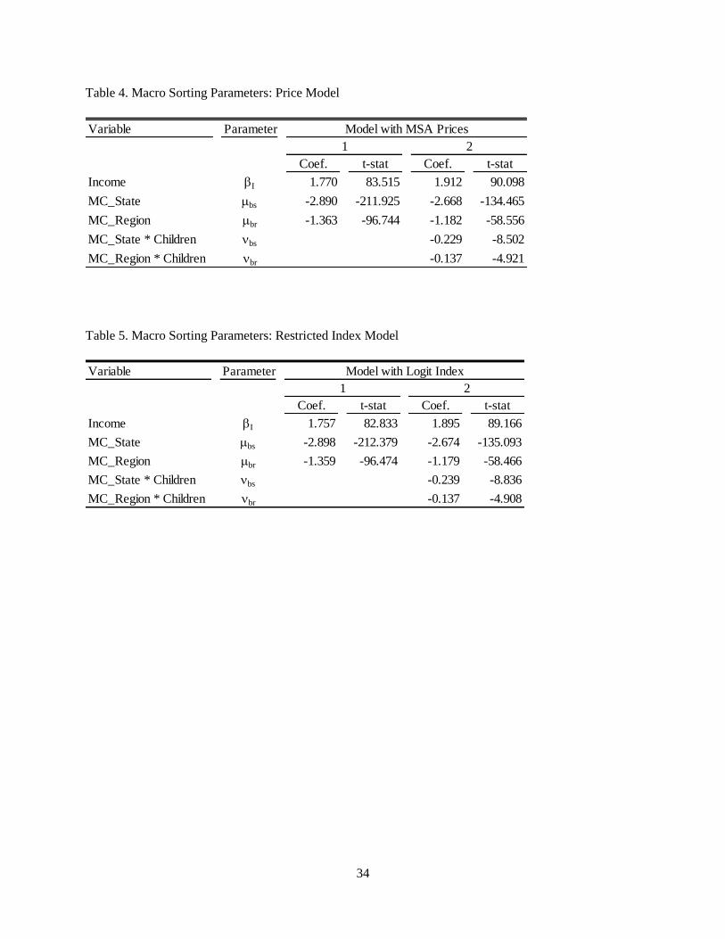
to these as the price (or baseline model), restricted index, and unrestricted index model, respectively.
Table 4 shows coefficient estimates for the parameters in (24), absent the fixed effects, for the price
model. The results for specification 1 mirror those presented in Bayer et al. (2009) in that there is a
positive marginal utility of income and a negative utility shift when MSA is outside of one’s birth state
and region. In specification 2 we find evidence of heterogeneous migration costs in that the presence of
children increases the disutility from leaving one’s geographical roots. Tables 5 and 6 display the utility
function parameter estimates for the restricted and unrestricted index models, respectively. The results
for the moving cost parameters are nearly identical to what is found in the price model; this is expected in
that our specification for moving costs is only relevant at the macro level. The marginal utility of income
is also similar between the price and restricted index model, but smaller for the unrestricted index model.
The remaining estimates in table 6 correspond to the parameters on the nested logit inclusive
value term, and reflect the degree of correlation among the idiosyncratic tract level utility shocks.
wide variety of values for H, and find our comparisons are qualitatively unchanged across the range. Our results
are also quantitatively unchanged for other feasible values of the share of income spent on housing.

22
Equivalently, k is the type k specific marginal utility of the choices available at the sub-MSA level.
Recall that a greater degree of variability in tract characteristics results in a larger value for km and hence
a larger utility level for MSA m. Our estimates range between 0.44 and 0.88 across both specifications
and all household types.
We decompose the MSA/year fixed effects using a first differenced IV regression that includes
our pollution measure, other MSA attributes described in table 2, and dummy variables for the 9 census
regions in the country. Table 7 reports results for all three models with the homogenous moving costs
specification. While these coefficients are not directly comparable due to potential differences in the
scale of utility in the three models, we note that the coefficient on pollution is significantly negative in all
three specifications, as expected. In the next subsection we compare marginal willingness to pay
estimates for the three models, where we will see that the larger coefficient on pollution in the third and
fourth columns does indeed suggest a larger disutility of pollution in the index models vis-à-vis the price
model.
Table 8 contains the decomposition results for the models that include heterogeneity in moving
costs. The cross-model comparison follows the pattern we saw in table 7. However, we find an
economically significant decrease in the magnitude of pollution costs when we compare each
heterogeneous moving cost model to its homogenous counterpart. Indeed, the pollution coefficient is
statistically insignificant for the price and restricted index models.
What can we learn from a comparison of the coefficient estimates from the three models and two
moving cost specifications? First, though it is not the main emphasis of this paper, we find that it is
important to account for heterogeneity in moving costs in macro level sorting models. In the homogenous
moving costs specification the higher disutility of migration among households with children manifests as
a larger disutility of pollution. Intuitively the homogenous migration cost model predicts that households
that remain in relatively clean MSAs do so to avoid pollution, when in fact this may be partially due to
their higher cost of migration. Second, our index models – particularly the unrestricted version – capture

23
an additional tradeoff margin compared to the price model. The former quantifies tradeoffs among MSA
level prices, MSA level characteristics, and the choices available at the tract level, while the latter limits
attention to tradeoffs between prices and characteristics at the macro level.
Mechanically, the inclusion of the price index in our two stage sorting model takes variation out
of the MSA-level fixed effect m; in the conventional model this variation remains in the fixed effects and
is contained in m in the regression equation (25). This introduces the potential for an omitted variable
bias in the fixed effect decomposition for the price model. Specifically, our summary statistics show that
PM10 concentrations and values for the price index are positively correlated.13 As such we obtain an
upwardly biased estimate of the coefficient on PM10 (a smaller negative number) when the variability
associated with the price index remains in the error term. In terms of tradeoffs, a more diverse set of
choice options at the tract level partially compensates for worse air quality.
Willingness to pay for clean air
The magnitudes of the regression coefficients in tables 4 through 8 do not have a direct economic
interpretation. However, we can use the ratios of parameters to compute the marginal willingness to pay
for a unit reduction in PM10. Since both income and PM10 are measured in log form the marginal
willingness to pay is given by
10
.iPM
I
IMWTP
PM
(28)
The model uses annual income, implying MWTP is an annual value, and so our predictions reflect a
household’s willingness to pay per year for changes in PM10 concentrations. 14 Table 9 reports point
13 Across eight type-specific indices, the correlation between changes in the index and changes in pollution
concentrations from 1990 to 2000 ranges from 0.05 to 0.20, with an average of 0.12.
14 In equilibrium wages at different points in the landscape will also capitalize the level of pollution, meaning that
the formula for marginal willingness to pay needs to include an additive term for the marginal change in wages from
a marginal change in pollution, to be formally correct. Bayer et al. (2009) found the wage gradient for pollution to

24
estimates of MWTP computed at the median observed income ($25,683) and PM10 concentrations (33.87)
from the sample. We find that MWTP decreases substantially in all three models when one considers the
additional moving costs for households with children, falling from 20% to 30%. Furthermore, the impact
of accounting for tract level sorting can be seen by comparing estimates in columns across the three rows.
Including the tradeoff between PM10, prices, and the characteristics of the micro choice set (rather than
only average MSA prices) results in an economically significant higher cost of pollution. An additional
increase in the cost of air pollution is evident in the unrestricted index model that allows for a higher
degree of heterogeneity in tract-level sorting. Finally, our estimates show that MWTP increases by 59%
when moving from a conventional price model with homogenous moving costs to the unrestricted index
model with heterogeneous moving costs.
Table 10 shows estimates of MWTP from a heterogeneous moving costs model, which also
includes additional accounting for household type preference heterogeneity. In particular, equation (24)
is augmented to include interactions between dummy variables for household type and air quality, and
equation (25) is used to identify the common component of preferences. Parameter estimates for this
model are shown in appendix table A5. Across all household types, we see an increase in the estimated
MWTP for the two-stage model, relative to the baseline mode, as was the case in table 9. The general
impact of accounting for local amenities appears to hold when we allow for greater preference
heterogeneity.
To gain a more intuitive understanding of our MWTP estimates, consider an approximate
calculation using the MSAs of Raleigh-Durham-Chapel Hill, NC, which has PM10 concentrations of 57.09
𝜇𝑔/𝑚3, and Charlottesville, VA, which has PM10 concentrations of 45.39 𝜇𝑔/𝑚3. These PM10
concentrations roughly correspond to the 50% and 75% percentiles, respectively, in the sample of MSAs.
The pollution change from Charlottesville to Raleigh-Durham-Chapel Hill offers a 26% reduction in PM10
concentrations (11.8 𝜇𝑔/𝑚3). Using estimates from the unrestricted index model with heterogeneous
be statistically zero and therefore did not include it in their estimates. We have also left this component out to assure
comparability with their findings.

25
moving costs in table 9, this difference corresponds to a 19% increase in a household's willingness to pay
for clean air. Therefore, based on a median income of $31,397 in Charlottesville, VA, the move offers
$2,919 in benefits derived from less pollution.
6) Conclusion
Our objective in this paper has been to examine whether the multiple levels of spatial sorting
behavior associated with city (MSA) and neighborhood (tract) choices are interconnected in an
empirically important way. For our application to air quality we find that the answer is yes. Our
structural approach allowed us to isolate the role played by tract level characteristics in determining
household’s city level choices. Intuitively we find that the diversity of available neighborhoods is an
important characteristic of MSAs, and that ignoring this as a determinant of sorting behavior can lead to
potentially biased estimates of the value of location specific amenities via an omitted variable bias
mechanism. To isolate this effect we used a two stage sorting model and a sequential estimation approach
that provided a new interpretation of the nested logit model in a sorting context. While the nested logit
offered a convenient estimation tool, we stress that the two-stage model is driven by the choice of
specification for consumer preferences, not the choice of error distribution. Nonetheless the error
distribution is the primary driver of the econometric structure of the model. Thus our key innovation was
the use of a quality augmented price index at the MSA level, derived from observation of tract choice
shares for different types of households, and operationalized using the two components of the nested logit
probability expression. Including the index in estimation allowed us to account for adjustment margins
related to MSA level air pollution, housing prices, and tract attributes. In our application, air quality and
tract choice variability were negatively correlated (i.e. pollution and the price index were positively
correlated), meaning that households were able to offset poor air quality in part by the corresponding
higher tract choice variability. Controlling for this additional substitution possibility increased our point
estimates of marginal willingness to pay 59% in our preferred specification, relative to the Bayer et al.
(2009) model. More generally, the bias is a function of unobserved amenities at a fine spatial scale.

26
These unobserved (to the analyst) amenities affect consumer behavior, but are not accounted for in the
conventional economic approach. We have presented empirical estimates relative to those of Bayer et al.
(2009) in an effort to isolate the impact of a single feature of location choice models. Thus our goal has
been to calculate the change in MWTP estimates due to the addition of this modeling dimension. Of
course, other features of sorting models that we share with Bayer et al. (2009) will affect value estimates.
Given the relatively large MWTP values reported in both studies, future research should continue to
investigate the full set of assumptions that are necessary to identify amenity preferences from sorting
behavior. We return to this point below.
A broader lesson that emerges from this research is that heterogeneity in the spatial units that we
define as the elements of choice in residential sorting models can matter for how the model’s primitive
parameters are estimated. If interest centers on modeling choices at one spatial scale, but variability in
location-specific features occurs at a smaller scale, the type of bias we have isolated in the macro/micro
context may become an issue. On the other hand, spatial variability in locational features that occurs at a
scale larger than the spatial unit of choice is unlikely to result in this type of bias, since the elements of
choice will have uniform values for the higher-level attribute. This suggests micro-level sorting models
are not likely to suffer from the same omitted attribute bias as their macro-level counterparts. These
observations are closely related to the issue of spatial fixed effects that Abbott and Klaiber (2011) discuss
in the context of first stage hedonic model estimation. In their case the issue is that “…consistent
estimates with spatial fixed effects require that the effects be defined over spatial scales at or below the
scale of variation of the correlated omitted variables” (p. 1332). A version of the multi-scale sorting
model that we have presented in this paper offers a solution to this problem from a structural sorting
perspective.
An additional contribution in this paper is our characterization of moving costs. Previous
research has shown the importance of including moving costs in choice models that have a spatial
dimension. In this paper, we allow for heterogeneity in moving costs. Our results suggest a higher cost
of moving for households with children. This specification significantly reduces the MWTP for clean air.

27
In a framework with homogeneous moving costs, a portion of these costs are attributed to poor air quality,
increasing the MWTP for clean air.
We close by returning to the topic of further research. First, our results confirm the findings from
Bayer et al. (2009) that the non-market value of particulate matter can be identified from variation in
pollution and housing prices across cities. However, both studies rely on assumptions of perfect
information among household about amenities across the landscape for estimation, which may not be
tenable for choices at the MSA scale. Thus research on sorting models generally should consider how
imperfect information about location attributes affects estimates. Tra (2010) offers evidence that sorting
behavior is also affected by air pollution variability that is more localized, such as ground level ozone. At
this spatial scale it may be more plausible to assume households are well informed about spatially varying
amenities. However, our two-stage model controls for this lower level variability but does not exploit or
quantify it as part of the estimated marginal willingness to pay. It would be informative to examine how
estimates gleaned from macro and micro sorting margins compare. This may help gauge the plausibility
of different revealed preference assumptions about the geographical extent of households’ knowledge of
location specific amenities. For example, are household perceptions of the spatial variation in air quality
stronger across MSAs, or across neighborhoods within MSAs?
This said, our discussion above suggests that in contexts where a specific amenity varies at both
the regional and local level, it is perhaps preferable to measure preferences based on the micro stage, in
that the scale of analysis aligns more directly with the scale of variability in the amenity. This also allows
the analyst to avoid the difficult issue of predicting counterfactual incomes in different labor markets.
When the scale of variability in the amenity of interest requires a macro-level approach, it would be
useful to explore alternative means of controlling for micro-sorting induced bias by identifying
instruments that plausibly meet the broader set of exclusion assumptions that our findings imply.

28
7) References
Abbott, Joshua K. and H. Allen Klaiber, “An embarrassment of riches: confronting omitted variable bias
and multi-scale capitalization in hedonic price models,” Review of Economics and Statistics 93(4):
1331-1342.
Albouy, David, 2009. “Are big cities really bad places to live? Improving quality of life estimates across
cities,” NBER Working Paper 14472.
Bayer, Patrick, Shakeeb Kahn, and Christopher Timmins, 2011. “Nonparametric identification and
estimation in a Roy model with common nonpecuniary returns,” Journal of Business and Economic
Statistics 29(2): 201-215.
Bayer, Patrick, McMillan, Robert and Rueben, Kim, 2005. “An equilibrium model of sorting in an urban
housing market,” NBER Working Paper 10865.
Bayer, Patrick, Ferreira, Fernando, and Robert McMillian, 2007. “A unified framework for measuring
preferences for schools and neighborhoods,” Journal of Political Economy 115(4): 588-638.
Bayer, Patrick, Keohane, Nathaniel and Timmins, Christopher, 2009. “Migration and hedonic valuation:
The case of air quality,” Journal of Environmental Economics and Management 58(1): 1-14.
Bayer, Patrick and Robert McMillian, 2012. “Teibout sorting and neighborhood stratification,” Journal of
Public Economics 96: 1129-43.
Berry, Steven, Levinsohn, James and Pakes, Ariel, 1995. “Automobile prices in market equilibrium,”
Econometrica 63(4): 841-800.
Berry, Steven and Pakes, Ariel, 2007. “The Pure Characteristics Demand Model,” International Economic
Review 48(4): 1193:1225.
Bishop, Kelly C., 2012. “A dynamic model of location choice and hedonic valuation,” unpublished
manuscript.
Blackorby, Charles and Russell, R. Robert, 1997. “Two-stage budgeting: An extension of Gorman’s
theorem,” Economic Theory 9: 185-193.
Blackorby, Charles, Primont, Daniel and Russell, R. Robert, 1978. Duality, Separability, and Functional

29
Structure: Theory and Economic Applications. Elsevier North-Holland.
Blomquist, Glenn C., Berger, Marc C. and Hoehn, John P., 1988. “New estimates of quality of life in
urban areas,” The American Economic Review 78(1): 89-107.
Bowland, Bradley J. and Beghin, John C., 2001. “Robust estimates of value of a statistical life for
developing economies,” Journal of Policy Modeling 23(4): 385-396.
Boyer, Richard and Savageau, David, 1993. Places Rated Almanac. Prentice Hall General Reference.
D’Agostino, Ralph and Savageau, David, 2000. Places Rated Almanac. Hungry Minds.
Dahl, Gordon B., 2002. “Mobility and the return to education: Testing a Roy model with multiple
markets,” Econometrica 70(6): 2367-2420.
Galiani, Sebastian, Alvin Murphy, and Juan Pantano, 2012. “ Estimating neighborhood choice models:
lessons from a housing assistant experiment,” unpublished manuscript.
Gamper-Rabindran, Shanti and Christopher Timmins, 2013. “Does cleanup of hazardous waste sites raise
housing values? Evidence of spatially localized benefits,” Journal of Environmental Economics and
Management 65: 345-360.
Gorman, W.M., 1965. “Consumer budgets and prices indices,” unpublished manuscript.
Gorman, W.M., 1995. The Collected Works of W.M. Gorman, Vol 1. Oxford University Press.
Klaiber, H. Allen and Phaneuf, Daniel J., 2010. “Valuing open space in a residential sorting model of the
twin cities,” Journal of Environmental Economics and Management 2(60): 57-77.
Kuminoff, Nicolai and Jaren Pope, 2013. “The value of residential land and structures during the great
housing boom and bust,” Land Economics 89: 1-29.
Kuminoff, Nicolai, 2012. “Partial identification of preferences in a dual-market sorting equilibrium,”
unpublished manuscript.
Latimer, Douglas, 1996. “Particulate matter source-receptor relationships between all point and area
sources in the United States and PSD class I area receptors,” report prepared for US EPA.
Poterba, James M. 1992. “Taxation and housing: Old questions, new answers,” American Economic
Reivew 82(2): 237-242.

30
Roy, A.D., 1951. “Some thoughts on the distribution of earnings,” Oxford Economic Review 3: 135-146.
Sieg, Holger, V. Kerry Smith, H. Spencer Banzhaf, and Randy Walsh, 2002. “Inter-jurisdictional housing
prices in locational equilibrium,” Journal of Urban Economics 52: 131-153.
Sieg, Holger, V. Kerry Smith, H. Spencer Banzhaf, and Randy Walsh, 2004. “Estimating the general
equilibrium benefits of large changes in spatially delineated public goods,” International Economic
Review 45(4): 1047-1077.
Tra, Constant I., 2010. “A discrete choice equilibrium approach to valuing large environmental changes,”
Journal of Public Economics 94: 183-196.
Walsh, Randy, 2007. “Endogenous open space amenities in a locational equilibrium,” Journal of Urban
Economics 61(2): 319-344.

31
Table 1. Type Definitions
Type Definition (presence of children and education)
Type 1 No children in household, No high school degree
Type 2 No children in household, High school degree or some college
Type 3 No children in household, Bachelor's degree
Type 4 No children in household, Graduate or professional degree
Type 5 Children in household, No high school degree
Type 6 Children in household, High school degree or some college
Type 7 Children in household, Bachelor's degree
Type 8 Children in household, Graduate or professional degree

32
Table 2. MSA Attribute Summary Statistics
Variable Description Mean Std. Dev. Mean Std. Dev. Mean Std. Dev.
PM10 PM10 Concentration (μg/m3) 34.562 18.082 29.746 15.344 -4.816 5.807
Crime Crime rate (per 1000 people) 0.590 0.189 0.464 0.155 -0.126 0.144
Prop_Tax Percent of tax revenue from property taxes 75.443 16.510 74.034 16.107 -1.409 5.606
Gov_ExpLocal government expenditures per capita
(thousands of dollars)1291.531 314.211 1506.258 369.016 214.727 243.688
White Percent of population that is white 0.836 0.104 0.792 0.114 -0.045 0.029
Heatlh Health Ranking 152.916 91.345 147.674 89.682 -5.243 43.216
Art Arts Ranking 149.456 89.821 146.385 90.355 -3.071 52.914
Trans Transportation Ranking 147.172 88.095 141.682 88.743 -5.490 69.882
Employment Percent of population employed 0.460 0.047 0.473 0.114 0.013 0.112
Manuf_Est Number of manufacturing establishments 1136.594 2200.280 1123.741 1972.251 0.051 0.144
Population Population (millions of people) 0.731 1.147 0.813 1.227 0.113 0.098
1990 2000 Change

33
Table 3. Price and Index Summary Statistics
Variable Description Mean Std. Dev. Mean Std. Dev. Mean Std. Dev.
ln(ρ) log price of housing services 8.146 0.304 8.448 0.258 0.302 0.139
Γ1
MSA Index: Type 1 5.730 1.099 5.974 1.165 0.244 0.409
Γ2
MSA Index: Type 2 5.583 1.266 5.443 1.315 -0.139 0.681
Γ3
MSA Index: Type 3 5.911 1.067 5.925 1.101 0.014 0.364
Γ4
MSA Index: Type 4 5.522 1.045 5.747 1.066 0.225 0.270
Γ5
MSA Index: Type 5 5.390 1.014 5.743 1.037 0.353 0.298
Γ6
MSA Index: Type 6 5.476 1.169 5.312 1.260 -0.164 0.585
Γ7
MSA Index: Type 7 5.658 1.116 5.892 1.229 0.234 0.440
Γ8
MSA Index: Type 8 5.278 1.091 5.738 1.135 0.460 0.310
1990 2000 Change
34
Table 4. Macro Sorting Parameters: Price Model
Variable Parameter
Coef. t-stat Coef. t-stat
Income I 1.770 83.515 1.912 90.098
MC_State bs -2.890 -211.925 -2.668 -134.465
MC_Region br -1.363 -96.744 -1.182 -58.556
MC_State * Children bs -0.229 -8.502
MC_Region * Children br -0.137 -4.921
Model with MSA Prices
1 2
Table 5. Macro Sorting Parameters: Restricted Index Model
Variable Parameter
Coef. t-stat Coef. t-stat
Income I 1.757 82.833 1.895 89.166
MC_State bs -2.898 -212.379 -2.674 -135.093
MC_Region br -1.359 -96.474 -1.179 -58.466
MC_State * Children bs -0.239 -8.836
MC_Region * Children br -0.137 -4.908
Model with Logit Index
1 2

35
Table 6. Macro Sorting Parameters: Unrestricted Index Model
Variable Parameter
Coef. t-stat Coef. t-stat
Income I 1.555 58.776 1.673 63.330
MC_State bs -2.894 -211.887 -2.670 -134.273
MC_Region br -1.358 -96.376 -1.173 -58.132
MC_State * Children bs -0.230 -8.512
MC_Region * Children br -0.145 -5.200
MSA Index: 1
1
0.661 6.763 0.659 0.718 7.305 0.672
MSA Index: 2
2
-0.043 -1.767 0.489 0.005 0.202 0.501
MSA Index: 3
3
1.086 23.080 0.748 1.137 23.874 0.757
MSA Index: 4
4
1.871 15.360 0.867 1.955 15.302 0.876
MSA Index: 5
5
0.634 10.346 0.653 0.724 11.524 0.673
MSA Index: 6
6
-0.242 -11.762 0.440 -0.191 -9.403 0.452
MSA Index: 7
7
0.238 6.001 0.559 0.293 7.357 0.573
MSA Index: 8
8
0.707 10.867 0.670 0.771 11.614 0.684
Model with Gamma Index
1 2

36
Table 7. Second Stage Regression: Fixed Effects From Sorting Model with Homogeneous Moving Costs
Baseline Restricted Index Unrestricted Index
Δ ln(PM10) -0.5420** -0.6757** -1.1079***
(0.2575) (0.3373) (0.3935)
Δ Crime 0.0095 -0.1439 0.2372
(0.1960) (0.2568) (0.2996)
Δ Prop_Tax -0.0034 -0.0058 -0.0131
(0.0056) (0.0074) (0.0086)
Δ Gov_Exp 0.0002 0.0002 0.0005***
(0.0001) (0.0002) (0.0002)
Δ White 3.1864*** 5.1255*** 0.005
(1.1946) (1.5652) (1.8259)
Δ Health -0.0003 0.0003 -0.0002
(0.0007) (0.0009) (0.0011)
Δ Art -0.0020*** -0.0023*** -0.0026***
(0.0005) (0.0007) (0.0008)
Δ Trans -0.0001 0.0005 -0.0001
(0.0004) (0.0005) (0.0006)
Δ Employment 0.0534 0.1551 0.3509
(0.2446) (0.3205) (0.3739)
Δ ln(Manuf_Est) 0.1481 0.6068* 0.1895
(0.2707) (0.3546) (0.4137)
Δ ln(Population) 0.4873 -0.4574 0.3959
(0.4487) (0.5878) (0.6858)
Regional Dummies yes yes yes
R-Squared 0.185 0.224 0.245
Observations 229 229 229
Dependent Variable: Δθ
+ .25Δln(ρ)

37
Table 8. Second Stage Regression: Fixed Effects From Sorting Model with Heterogeneous Moving Costs
Baseline Restricted Index Unrestricted Index
Δ ln(PM10) -0.4063 -0.5527 -0.8185**
(0.2598) (0.3411) (0.3533)
Δ Crime -0.0732 -0.2071 0.2546
(0.1978) (0.2596) (0.2690)
Δ Prop_Tax -0.004 -0.0066 -0.0137*
(0.0057) (0.0074) (0.0077)
Δ Gov_Exp 0.0002 0.0002 0.0004***
(0.0001) (0.0002) (0.0002)
Δ White 3.2833*** 5.2307*** 1.0668
(1.2054) (1.5826) (1.6394)
Δ Health -0.0003 0.0004 -0.0002
(0.0007) (0.0009) (0.0010)
Δ Art -0.0020*** -0.0022*** -0.0023***
(0.0005) (0.0007) (0.0007)
Δ Trans -0.0002 0.0004 0.0000
(0.0004) (0.0005) (0.0006)
Δ Employment 0.0246 0.1246 0.3434
(0.2468) (0.3241) (0.3357)
Δ ln(Manuf_Est) 0.1533 0.6255* 0.189
(0.2731) (0.3586) (0.3714)
Δ ln(Population) 0.4183 -0.5223 0.3885
(0.4527) (0.5944) (0.6157)
Regional Dummies yes yes yes
R-Squared 0.164 0.199 0.214
Observations 229 229 229
Dependent Variable: Δθ
+ .25Δln(ρ)

38
Table 9. MWTP for Reduction in PM10 Concentrations:
No MC Interaction With MC Interaction
Baseline Model $232.22 $161.14
Restricted Index Model $291.62 $221.16
Unrestricted Index Model $540.08 $371.05
Table 10. Heterogeneous MWTP for Reduction in PM10 Concentrations (with heterogeneous MC)
Baseline Restricted Index Unrestricted Index
Type 1 $123.38 $235.08 $439.46
Type 2 $163.39 $224.80 $365.49
Type 3 $107.06 $153.76 $323.94
Type 4 $35.95 $117.07 $321.63
Type 5 $250.04 $295.14 $490.36
Type 6 $181.74 $216.41 $351.19
Type 7 $132.28 $186.24 $341.21
Type 8 $66.37 $160.12 $341.63

39
Table 11. MWTP for Reduction in PM10 Concentrations with Varying H (with MC Interaction)
H Baseline Restricted Index Unrestricted Index
0.10 $153.75 $213.70 $357.27
0.15 $156.21 $216.19 $361.86
0.20 $158.68 $218.67 $366.46
0.25 $161.14 $221.16 $371.05
0.30 $163.60 $223.65 $375.64
0.35 $166.07 $226.13 $380.24
0.40 $168.53 $228.62 $384.83
0.45 $170.99 $231.10 $389.43
0.50 $173.46 $233.59 $394.02

40
Appendix A: Conditions for two stage budgeting
We now show that the common functional form shown in equation (6) satisfies the conditions for
two stage-budgeting, and therefore provides an opportunity to use additional structure in characterizing
the household’s optimization problem. We focus here on a heuristic demonstration; a more detailed
derivation is available in the Online Appendix. Once again partition the set of all goods into the three
groups consumption C, the MSA level amenities Y, and the composite housing good Q, consisting of
housing services H and local amenities X. The primary concern in proving the existence of two-stage
budgeting in our context is to show that dividing the entire set of commodities into these groups is
consistent with utility maximization. In particular, we will show that this grouping satisfies price
aggregation and decentralisability, the necessary and sufficient conditions for two-stage budgeting. For
the following discussion, we assume that consumer have continuous preferences for the amenity goods X
and Y. This allows for the use of derivatives for optimization over these goods.
Focusing first on price aggregation, the maximization problem defined in equation (6) results in
the following expenditures for C and H:
, , .r rim im
C H
E I r C H
(A1)
For expenditures on Y, consider a hedonic framework and define a marginal implicit price for Y as
/ .H
imE Y The optimal expenditures on Y can be written as
,H
Y im Yim im im
C H
EE Y I
Y
(A2)
so that expenditures on MSA amenities are also a fixed share of income. Thus commodity group
expenditures do not depend on the prices for individual goods, suggesting price aggregation is satisfied.
In equation (A2) H
imE refers to expenditures on housing, which implicitly includes expenditures on X.
Turning to decentralisability, we need to show that within group expenditures are independent of
prices of goods in other commodity groups. For the utility function in (6) the first order conditions result

41
in demand relationships ( ) C
imC E for numeraire consumption and ( ) /H
im jmH E p for housing services.
From (A2) it is clear that demand for Y is similar to that of C and H, in that it depends only on preference
parameters and total Y expenditures. The demand for X, like Y, is based on an implicit marginal price
derived from a hedonic interpretation
1
,H
imXijm im
C H
EX I
X
(A3)
so that the demand for X depends on total expenditures on H and the implicit price of X.
Decentralisability is therefore satisfied as the demand for each commodity depends only on group
expenditures and own-group prices. In general, the model assumes that any tradeoffs between Y and H or
Y and X are captured in the tradeoff between Y and total expenditures devoted to H and X. Having shown
that the optimization problem satisfies price aggregation and decentralisability, two-stage budgeting can
be applied to the choice problem.
Equation (7) is written to reflect a choice among all tracts in all MSAs. However, as shown
above, the form of the optimization problem allows the location choice to be modeled in two stages. The
first stage determines expenditures for the three broad groups and is equivalent to a choice among MSAs.
Such a correspondence is evident from equation (A1), where we see that expenditures on the three groups
vary only at the MSA level. Therefore, the optimization problem can be modeled first as a choice among
MSAs. To see this rewrite the conditional indirect utility function as
ln ln ln ln ,i
im I im Y m H m m m imV I Y (A4)
where once again 𝜂𝑖𝑗𝑚 = 𝜂𝑖𝑚 + 𝜂𝑖𝑗|𝑚 and
|max{ ln ln }
m
i
m H jm X jm jm ij mj J
X
(A5)
reflects the optimal allocation of housing services based on tract variation and tract-level public goods,
which corresponds to the second stage of the two-stage budgeting process.
It is theoretically consistent to write equations (A4) and (A5) with the full price of housing
services included as part of the index. Due to the linear nature of (A4) and (A5) combined with a two-

42
stage budgeting framework in which m does not vary across tracts, however, Hlnm can simply be
removed from the index so that it directly enters the MSA-level function. We do this for two reasons.
First, m is estimable in a hedonic framework and leads to a feasible strategy for identifying behavior in
the first stage of budgeting. Second, having it explicitly enter the macro choice function allows for a
direct comparison to conventional sorting models that ignore tract variability in local public goods.

43
Appendix B: MSA level price and income
The variable definitions used for the housing price hedonic model are shown in table A2. The
price that serves as the dependent variable in (22) is the annual cost of housing. For units that are rented,
this value is simply the annual rent plus utilities and fees. For owned units, however, an annual rent must
be imputed from the housing value. Rents are calculated in a manner similar to Albouy (2009) and
Blomquist (1988), following methods described in Poterba (1992). In equilibrium, the ratio of the rental
value to the house price is the user cost of owner-occupied housing. This ratio is equal to the sum of the
nominal interest rate, property tax rate, risk premium, maintenance costs and depreciation, less the
inflation rate. Since property taxes are observed and treated as an additional cost, the property tax rate is
omitted from calculation of the user cost of owner-occupied housing. Following Poterba (1992), we
assign maintenance costs and depreciation each to be 2% and the risk premium on home ownership at 4%.
The nominal interest rate is the average commitment rate on new fixed mortgages and the inflation rate is
calculated as a five year average of the CPI inflation rate. The respective values for the interest rate and
inflation are 10.13 and 4.12 for 1990 and 8.05 and 2.54 for 2000. The resulting rent to value ratio is
11.48 for 1990 and 11.50 for 2000. Given a rent to value ratio of 11.5, a $100,000 house takes on an
annual housing cost of $8,695, equivalent to an apartment with monthly rent of $725.
This hedonic is estimated on a sample of 262,735 households for 1990 and 233,095 households
for 2000 across the 229 MSAs, obtained from the IPUMS dataset. Note that the set of households used
for the MSA hedonic estimation is not the same as the set of households used for the macro sorting
model. Both data sets are subsets of the same set of household observations, but different selection
criteria lead to different sets of observations.
Equation (22) estimates an MSA-specific price for each year. Coefficients on housing services
parameters are reported in Table A3. The hedonic regression gives highly significant and expected
results. Price increases for homes that have larger living quarters, are more recently built, and on larger
plots of land. In addition, single family detached homes and apartment units are more expensive than
attached single family homes. The mean and standard deviation for MSA prices in each year are reported

44
in table 3.
Our income regression uses as its dependent variable is the log of weekly income, as reported on
the US Census long form. The sample includes 874,809 total observations for 1990 and 749,618 total
observations for 2000, with a range of MSA populations of 465-45,921 (mean of 3,976) and 390-34,476
(mean of 3,637) for each year, respectively. Regressors include gender, marital status, race/ethnicity, age,
part-time employment, citizenship, education, and industry, as well as type-specific migration
probabilities to account for nonrandom sorting. These variables are located in table A4. Observations
include employed household heads not in the military and not disabled. A separate wage hedonic is run
for each MSA using (23), controlling for effects related to labor demand and allowing the income effect
of individual traits to vary across locations.
Income is predicted for each individual in each MSA for 1990 and 2000. Note that the migration
probabilities act only as controls for consistent estimates, and so are not included when predicting
income. The weekly wage prediction is multiplied by the individual's number of weeks worked to obtain
the final income prediction, 𝐼𝑖𝑚. Regression results are shown in table A4. Since the empirical analysis
involves 229 sets of coefficients representing each MSA/labor market, only summary measures are
reported. Elements of the table refer to summary statistics across the 229 regressions. Coefficient means
all have expected signs, with positive wage premiums for individuals who are male, married, white, older,
educated, U.S. citizens, full time workers, and are in management positions. In some cases, the minimum
coefficient estimate may be negative for a variable that has a positive (and expected positive) mean
coefficient estimate. Similarly, the maximum coefficient estimate may be positive for a variable that has
an negative (and expected negative) mean coefficient estimate. The fact that such results show up for
some MSAs is likely a function of supply and demand idiosyncrasies in local labor markets. The last two
rows report coefficients on type specific migration probabilities and migration probabilities squared.
There is very little interpretation that follows these parameters, but their significance suggests that the
approach is valid.
These regression coefficients are then used to predict annual incomes for each individual in each

45
MSA. Given different labor market forces in each MSA and compensating differentials for non-market
goods, variation is expected across locations. One way to demonstrate the amount of variation in income
predictions, and thus the degree to which they may influence the macro model, is to look at the average
wage variation across locations. For year 1990, the standard deviation for an individual's wage
predictions across the set of MSAs has 10%, 50% and 90% percentiles of 2,695, 4,415 and 6,720,
respectively. Without making a direct comparison to values at particular percentiles, these standard
deviations should be considered relative to mean income prediction 10%, 50% and 90% percentiles of
13,226, 24,857, and 38,210, respectively. To be clear, the preceding means and standard deviations are
summaries of individuals' summary statistics. Significant variation is also evident for year 2000. Mean
predicted income has 10%, 50% and 90% percentiles of 17,164, 34,522 and 54,167, respectively, with
standard deviation 10%, 50% and 90% percentiles of 3,833, 7,233 and 13,458, respectively.

46
MSA Name # of Tracks
80 Akron, OH PMSA 166
120 Albany, GA MSA 35
160 Albany-Schenectady-Troy, NY MSA 229
200 Albuquerque, NM MSA 183
220 Alexandria, LA MSA 34
240 Allentown-Bethlehem-Easton, PA MSA 140
280 Altoona, PA MSA 34
440 Ann Arbor, MI PMSA 169
450 Anniston, AL MSA 28
460 Appleton-Oshkosh-Neenah, WI MSA 80
480 Asheville, NC MSA 45
500 Athens, GA MSA 41
520 Atlanta, GA MSA 660
560 Atlantic-Cape May, NJ PMSA 87
600 Augusta-Aiken, GA-SC MSA 88
640 Austin-San Marcos, TX MSA 255
680 Bakersfield, CA MSA 137
720 Baltimore, MD PMSA 623
760 Baton Rouge, LA MSA 120
860 Bellingham, WA MSA 27
870 Benton Harbor, MI MSA 48
880 Billings, MT MSA 27
920 Biloxi-Gulfport-Pascagoula, MS MSA 79
960 Binghamton, NY MSA 65
1000 Birmingham, AL MSA 196
1020 Bloomington, IN MSA 29
1040 Bloomington-Normal, IL MSA 41
1080 Boise City, ID MSA 72
1120 Boston, MA-NH PMSA 701
1150 Bremerton, WA PMSA 51
1160 Bridgeport, CT PMSA 110
1240 Brownsville-Harlingen-San Benito, TX MSA 86
1280 Buffalo-Niagara Falls, NY MSA 300
1320 Canton-Massillon, OH MSA 87
1360 Cedar Rapids, IA MSA 43
1400 Champaign-Urbana, IL MSA 41
1440 Charleston-North Charleston, SC MSA 117
1520 Charlotte-Gastonia-Rock Hill, NC-SC MSA 300
1540 Charlottesville, VA MSA 34
1560 Chattanooga, TN-GA MSA 96
1600 Chicago, IL PMSA 1860
1620 Chico-Paradise, CA MSA 42
1640 Cincinnati, OH-KY-IN PMSA 404
1660 Clarksville-Hopkinsville, TN-KY MSA 42
1680 Cleveland-Lorain-Elyria, OH PMSA 706
1720 Colorado Springs, CO MSA 111
1740 Columbia, MO MSA 29
1760 Columbia, SC MSA 121
1800 Columbus, GA-AL MSA 74
1840 Columbus, OH MSA 370
1880 Corpus Christi, TX MSA 78
1920 Dallas, TX PMSA 687
1930 Danbury, CT PMSA 47
1950 Danville, VA MSA 28
1960 Davenport-Moline-Rock Island, IA-IL MSA 99
2000 Dayton-Springfield, OH MSA 241
2020 Daytona Beach, FL MSA 84
2030 Decatur, AL MSA 33
2040 Decatur, IL MSA 36
2080 Denver, CO PMSA 509
2120 Des Moines, IA MSA 101
2160 Detroit, MI PMSA 1266
2180 Dothan, AL MSA 34
2240 Duluth-Superior, MN-WI MSA 83
2290 Eau Claire, WI MSA 32
2320 El Paso, TX MSA 124
2360 Erie, PA MSA 72
2400 Eugene-Springfield, OR MSA 78
2440 Evansville-Henderson, IN-KY MSA 76
2520 Fargo-Moorhead, ND-MN MSA 40
2560 Fayetteville, NC MSA 51
2580 Fayetteville-Springdale-Rogers, AR MSA 60
2640 Flint, MI PMSA 131
2650 Florence, AL MSA 31
2670 Fort Collins-Loveland, CO MSA 56
2680 Fort Lauderdale, FL PMSA 269
2700 Fort Myers-Cape Coral, FL MSA 116
2710 Fort Pierce-Port St. Lucie, FL MSA 60
2720 Fort Smith, AR-OK MSA 40
2760 Fort Wayne, IN MSA 128
2840 Fresno, CA MSA 175
2900 Gainesville, FL MSA 43
2920 Galveston-Texas City, TX PMSA 61
3000 Grand Rapids-Muskegon-Holland, MI MSA 225
3060 Greeley, CO PMSA 36
3120 Greensboro--Winston-Salem--High Point, NC MSA 263
3160 Greenville-Spartanburg-Anderson, SC MSA 210
3200 Hamilton-Middletown, OH PMSA 73
3240 Harrisburg-Lebanon-Carlisle, PA MSA 140
3280 Hartford, CT MSA 289
3290 Hickory-Morganton-Lenoir, NC MSA 68
3350 Houma, LA MSA 42
3360 Houston, TX PMSA 769
3480 Indianapolis, IN MSA 339
3520 Jackson, MI MSA 37
3560 Jackson, MS MSA 103
3600 Jacksonville, FL MSA 197
3610 Jamestown, NY MSA 34
3620 Janesville-Beloit, WI MSA 36
3660 Johnson City-Kingsport-Bristol, TN-VA MSA 105
3680 Johnstown, PA MSA 68
3710 Joplin, MO MSA 32
3720 Kalamazoo-Battle Creek, MI MSA 115
3760 Kansas City, MO-KS MSA 492
3800 Kenosha, WI PMSA 30
3840 Knoxville, TN MSA 139
3880 Lafayette, LA MSA 81
3920 Lafayette, IN MSA 45
3960 Lake Charles, LA MSA 41
3980 Lakeland-Winter Haven, FL MSA 110
4000 Lancaster, PA MSA 94
4040 Lansing-East Lansing, MI MSA 117
4080 Laredo, TX MSA 32
4100 Las Cruces, NM MSA 32
4120 Las Vegas, NV-AZ MSA 323
4280 Lexington, KY MSA 108
4320 Lima, OH MSA 44
4360 Lincoln, NE MSA 58
4400 Little Rock-North Little Rock, AR MSA 140
4480 Los Angeles-Long Beach, CA PMSA 2038
4520 Louisville, KY-IN MSA 241
4600 Lubbock, TX MSA 61
4640 Lynchburg, VA MSA 53
4680 Macon, GA MSA 72
4720 Madison, WI MSA 91
4760 Manchester, NH PMSA 43
4800 Mansfield, OH MSA 45
4890 Medford-Ashland, OR MSA 36
4900 Melbourne-Titusville-Palm Bay, FL MSA 92
4920 Memphis, TN-AR-MS MSA 272
4940 Merced, CA MSA 47
5000 Miami, FL PMSA 342
5080 Milwaukee-Waukesha, WI PMSA 415
5120 Minneapolis-St. Paul, MN-WI MSA 742
5160 Mobile, AL MSA 137
5170 Modesto, CA MSA 89
5190 Monmouth-Ocean, NJ PMSA 257
5200 Monroe, LA MSA 41
5240 Montgomery, AL MSA 78
5280 Muncie, IN MSA 31
5360 Nashville, TN MSA 247
5400 New Bedford, MA PMSA 48
5480 New Haven-Meriden, CT PMSA 124
5560 New Orleans, LA MSA 393
5600 New York, NY PMSA 2457
5720 Norfolk-Virginia Beach-Newport News, VA-NC MSA 363
5790 Ocala, FL MSA 46
5910 Olympia, WA PMSA 34
Table A1: Macro (MSA) Choice Set

47
5920 Omaha, NE-IA MSA 218
5960 Orlando, FL MSA 325
6080 Pensacola, FL MSA 77
6120 Peoria-Pekin, IL MSA 87
6160 Philadelphia, PA-NJ PMSA 1311
6200 Phoenix-Mesa, AZ MSA 675
6280 Pittsburgh, PA MSA 702
6400 Portland, ME MSA 55
6440 Portland-Vancouver, OR-WA PMSA 421
6480 Providence-Fall River-Warwick, RI-MA MSA 259
6520 Provo-Orem, UT MSA 84
6560 Pueblo, CO MSA 50
6600 Racine, WI PMSA 39
6640 Raleigh-Durham-Chapel Hill, NC MSA 210
6680 Reading, PA MSA 82
6690 Redding, CA MSA 33
6720 Reno, NV MSA 66
6740 Richland-Kennewick-Pasco, WA MSA 36
6760 Richmond-Petersburg, VA MSA 252
6780 Riverside-San Bernardino, CA PMSA 583
6800 Roanoke, VA MSA 49
6820 Rochester, MN MSA 34
6840 Rochester, NY MSA 268
6880 Rockford, IL MSA 93
6920 Sacramento, CA PMSA 354
6960 Saginaw-Bay City-Midland, MI MSA 101
6980 St. Cloud, MN MSA 34
7040 St. Louis, MO-IL MSA 524
7080 Salem, OR PMSA 63
7120 Salinas, CA MSA 80
7160 Salt Lake City-Ogden, UT MSA 282
7240 San Antonio, TX MSA 314
7320 San Diego, CA MSA 594
7360 San Francisco, CA PMSA 380
7400 San Jose, CA PMSA 341
7480 Santa Barbara-Santa Maria-Lompoc, CA MSA 86
7490 Santa Fe, NM MSA 41
7500 Santa Rosa, CA PMSA 86
7510 Sarasota-Bradenton, FL MSA 141
7520 Savannah, GA MSA 75
7560 Scranton--Wilkes-Barre--Hazleton, PA MSA 183
7600 Seattle-Bellevue-Everett, WA PMSA 527
7610 Sharon, PA MSA 34
7680 Shreveport-Bossier City, LA MSA 94
7720 Sioux City, IA-NE MSA 29
7800 South Bend, IN MSA 69
7840 Spokane, WA MSA 106
7880 Springfield, IL MSA 55
7920 Springfield, MO MSA 78
8000 Springfield, MA MSA 119
8040 Stamford-Norwalk, CT PMSA 84
8050 State College, PA MSA 29
8120 Stockton-Lodi, CA MSA 119
8160 Syracuse, NY MSA 209
8200 Tacoma, WA PMSA 158
8240 Tallahassee, FL MSA 57
8280 Tampa-St. Petersburg-Clearwater, FL MSA 544
8320 Terre Haute, IN MSA 41
8400 Toledo, OH MSA 163
8440 Topeka, KS MSA 41
8480 Trenton, NJ PMSA 73
8520 Tucson, AZ MSA 198
8560 Tulsa, OK MSA 248
8600 Tuscaloosa, AL MSA 45
8680 Utica-Rome, NY MSA 92
8780 Visalia-Tulare-Porterville, CA MSA 76
8840 Washington, DC-MD-VA-WV PMSA 1032
8880 Waterbury, CT PMSA 52
8920 Waterloo-Cedar Falls, IA MSA 37
8940 Wausau, WI MSA 27
8960 West Palm Beach-Boca Raton, FL MSA 265
9040 Wichita, KS MSA 137
9140 Williamsport, PA MSA 27
9160 Wilmington-Newark, DE-MD PMSA 142
9200 Wilmington, NC MSA 42
9240 Worcester, MA-CT PMSA 113
9260 Yakima, WA MSA 34
9280 York, PA MSA 82
9320 Youngstown-Warren, OH MSA 157
9340 Yuba City, CA MSA 30
9360 Yuma, AZ MSA 32
Table A1 continued:

48
Table A2: Variable Definitions
Variable Mean Description
male 0.7422 Sex (Male=1, Female=0)
married 0.6004 Marital status (Married=1, Single=0)
nonwhite 0.1605 Race (Nonwhite=1, White=0)
age 32.060 Age
nohs 0.0786 No high school degree
hs 0.6298 High school degree/Some college
bach 0.2058 Bachelor's degree
grad 0.0858 Graduate or professional degree
cit1 0.9122 Born as a U.S. Citizen
cit2 0.0314 Naturalized U.S. Citizen
ptime 0.0791 Part time worker (Part time=1, Full time=0)
occ1 0.4305 Management occupation
occ2 0.2984 Service or Sales occupation
occ3 0.2711 Farming/Production/Other occupation
room2 0.0439 2 rooms in dwelling
room3 0.0973 3 rooms in dwelling
room4 0.1476 4 rooms in dwelling
room5 0.1986 5 rooms in dwelling
room6 0.1954 6 rooms in dwelling
room7 0.1298 7 rooms in dwelling
room8 0.0848 8 rooms in dwelling
room9 0.0822 9+ rooms in dwelling
bedroom2 0.1347 2 bedrooms in dwelling
bedroom3 0.2658 3 bedrooms in dwelling
bedroom4 0.3904 4 bedrooms in dwelling
bedroom5 0.1488 5 bedrooms in dwelling
bedroom6 0.0327 6+ bedrooms in dwelling
yr1 0.0186 Dwelling built 0-1 yrs ago
yr2 0.0764 Dwelling built 2-5 yrs ago
yr3 0.0784 Dwelling built 6-10 yrs ago
yr4 0.1748 Dwelling built 11-20 yrs ago
yr5 0.1701 Dwelling built 21-30 yrs ago
yr6 0.1548 Dwelling built 31-40 yrs ago
yr7 0.1166 Dwelling built 41-50 yrs ago
yr8 0.1372 Dwelling built 51-60 (51+ for 1990) yrs ago
yr9 0.1551 Dwelling built 61+ yrs ago
acre1 0.8744 Dwelling on 0-1 acre lot
acre2 0.0980 Dwelling on 1-3 acre lot
acre3 0.0276 Dwelling on 3+ acre lot
own 0.6430 Dwelling is owned by resident
bld1 0.6354 1 family house, detached
bld2 0.1156 1 family house, attached
bld3 0.2490 Multiple family building

49
Table A3: MSA Housing Hedonic
Coefficient t-statistic Coefficient t-statistic
room2 0.0585 *** 3.33 0.0597 *** 4.49
room3 0.0855 *** 4.47 0.0551 *** 4.01
room4 0.1490 *** 7.54 0.0809 *** 5.60
room5 0.2305 *** 11.46 0.1415 *** 9.59
room6 0.3531 *** 17.36 0.2394 *** 15.94
room7 0.4982 *** 24.20 0.3686 *** 24.20
room8 0.6392 *** 30.64 0.4868 *** 31.40
room9 0.8346 *** 39.63 0.6858 *** 43.58
bedroom2 0.0950 *** 5.80 0.0759 *** 6.42
bedroom3 0.2050 *** 11.65 0.1909 *** 15.08
bedroom4 0.2024 *** 11.19 0.2101 *** 16.01
bedroom5 0.2246 *** 12.10 0.2798 *** 20.60
bedroom6 0.2622 *** 13.33 0.3614 *** 24.36
yr2 -0.0047 -0.49 -0.0202 *** -2.32
yr3 -0.1285 *** -13.50 -0.0803 *** -9.23
yr4 -0.2036 *** -22.50 -0.1814 *** -22.11
yr5 -0.2771 *** -30.37 -0.2838 *** -34.89
yr6 -0.3488 *** -38.03 -0.3264 *** -39.59
yr7 -0.4021 *** -42.22 -0.3537 *** -42.66
yr8 -0.4276 *** -46.63 -0.4134 *** -47.56
yr9 - - -0.3952 *** -47.64
acre1 -0.0526 *** -12.97 -0.1214 *** -32.12
acre3 0.0808 *** 11.13 0.0846 *** 9.86
bld1 0.0925 *** 21.98 0.0687 *** 17.60
bld3 0.0533 *** 11.56 0.0224 *** 5.31
R-Squared 0.54 0.60
Observations 262,735 233,095
1990 2000Dependent Variable:
ln(price)

50
Table A4: Income Regression: Summary of Coefficients for 229 MSAs
Mean Minimum Maximum Mean Minimum Maximum
constant 2.8742 -0.0127 4.5345 3.4088 1.6046 5.3569
male 0.2617 0.0580 0.4621 0.2267 0.1062 0.3965
married 0.0856 -0.0764 0.2065 0.1043 -0.0113 0.2833
nonwhite -0.1442 -0.4383 0.1416 -0.1204 -0.5630 0.1791
ln(age) 0.8533 0.4159 1.3611 0.8072 0.2576 1.3338
nohs -0.1744 -0.5439 0.4094 -0.1961 -0.5220 0.1896
bach 0.2255 -0.0006 0.5191 0.2570 0.0169 0.5122
grad 0.4111 0.0120 0.9656 0.4097 0.0839 0.7416
cit1 0.1455 -0.5785 3.0109 0.1102 -0.5250 0.7293
cit2 0.1518 -0.8594 3.1850 0.1085 -2.3121 1.3304
ptime -0.5974 -0.9942 -0.2654 -0.6602 -1.0074 -0.1694
occ2 -0.1673 -0.3281 0.0248 -0.1738 -0.3260 0.0005
occ3 -0.1076 -0.3027 0.1072 -0.1498 -0.4272 0.0845
roy 0.0334 -30.9152 19.8122 -0.1104 -28.2410 30.3966
roy2 1.3994 -821.2247 819.1582 1.6300 -498.5059 563.7523
Observations 3,976 465 45,921 3,637 390 34,476
Dependent Variable:
ln(weekly income)
1990 2000
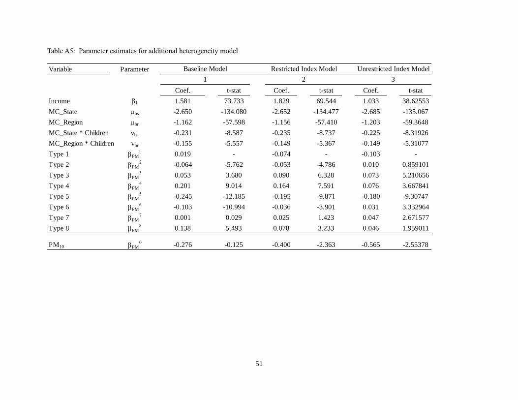
51
Table A5: Parameter estimates for additional heterogeneity model
Variable Parameter
Coef. t-stat Coef. t-stat Coef. t-stat
Income I 1.581 73.733 1.829 69.544 1.033 38.62553
MC_State bs -2.650 -134.080 -2.652 -134.477 -2.685 -135.067
MC_Region br -1.162 -57.598 -1.156 -57.410 -1.203 -59.3648
MC_State * Children bs -0.231 -8.587 -0.235 -8.737 -0.225 -8.31926
MC_Region * Children br -0.155 -5.557 -0.149 -5.367 -0.149 -5.31077
Type 1 PM1 0.019 - -0.074 - -0.103 -
Type 2 PM2 -0.064 -5.762 -0.053 -4.786 0.010 0.859101
Type 3 PM3 0.053 3.680 0.090 6.328 0.073 5.210656
Type 4 PM4 0.201 9.014 0.164 7.591 0.076 3.667841
Type 5 PM5 -0.245 -12.185 -0.195 -9.871 -0.180 -9.30747
Type 6 PM6 -0.103 -10.994 -0.036 -3.901 0.031 3.332964
Type 7 PM7 0.001 0.029 0.025 1.423 0.047 2.671577
Type 8 PM8 0.138 5.493 0.078 3.233 0.046 1.959011
PM10 PM0 -0.276 -0.125 -0.400 -2.363 -0.565 -2.55378
1 2 3
Unrestricted Index ModelRestricted Index ModelBaseline Model


![HANGING SCALES/CRANE SCALES - Aviga HFO 159 page 166 1020,-from € Hanging scales/Crane scales Lisa Mayer Product specialist Hanging scales/Crane scales Tel. +49 [0] 7433 9933 - 219](https://img.pdfslide.us/doc/110x75/5afd22507f8b9a68498c727e/hanging-scalescrane-scales-hfo-159-page-166-1020-from-hanging-scalescrane.jpg)