UNIVERSITY OF PATRAS

SCHOOL OF ENGINEERING

DEPARTMENT OF CIVIL ENGINEERING

ENVIRONMENTAL DATA MANAGEMENT AND DECISION SUPPORT

FOR RIVER BASINS

Application in Alfeios River

PhD Thesis

Eleni S. BEKRI

Dipl. Civil Engineer, MSc

PATRAS 2015

The authors thank the European Social Fund (ESF), Operational Program for EPEDVM and

particularly the Program Herakleitos II, for financially supporting this work.

“Since all measurements and observations are nothing more than approximations

to the truth, the same must be true of all calculations resting upon them,

and the highest aim of all computations made concerning concrete phenomena must be approximate, as nearly as practicable, to the truth.

But this can be accomplished in no other way than by a suitable combination of more observations than the number absolutely requisite for the determination of

the unknown quantities.”

Gauss, K.G. (1963) Theory of Motion of Heavenly Bodies, New York, Dover.

Dedicated

to my husband Panagiotis

and to my two daughters Aimilia and Konstantina

…When you bend down and look at the waters of the Alfeios river

near Olympia,

their clarity is such

that your face and soul are mirrored in them...

The nature becomes here spirit.

The clarity of waters becomes clarity of thought …

Panayiotis Kanellopoulos (1902-1986)

Professor of Sociology

Prime Minister of Greece

i

ΕΚΤΕΝΗΣ ΠΕΡΙΛΗΨΗ

Εισαγωγή

Η αναγκαιότητα για την ανάπτυξη και την εφαρµογή σχεδίων διαχείρισης

υδρολογικών λεκανών έχει εισαχθεί στην Ευρώπη µε την Κοινοτική Οδηγία για το Νερό

2000/60/EC (WFD, 2000). Ένα από τα θεµελιώδη στάδια αυτών των σχεδίων είναι τα

προγράµµατα παρακολούθησης της ποσότητας και της ποιότητας των υδατικών πόρων

τους. Αυτά τα προγράµµατα είναι απαραίτητα µεταξύ άλλων για τον καθορισµό µιας

συνολικής εικόνας της κατάστασης των υδάτων και για τον προσδιορισµό όχι µόνο του

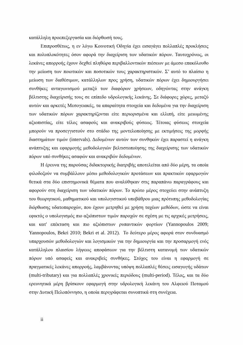
επιπέδου καθορισµένων ρύπων αλλά και του ρυπαντικού τους φορτίου. Το φορτίο qij µιας

ρυπαντικής ουσίας j σε µία επιλεγµένη διατοµή i ενός ποταµού µπορεί να υπολογιστεί

έµµεσα µέσω του συνδυασµού παράλληλων µετρήσεων της υδατικής παροχής Qi και της

συγκέντρωσης του εν λόγω ρύπου cij από την σχέση:

(E.1)

Για µία καθολική και πλήρης εικόνα της κατάσταση των υδάτων, ποιοτικές και

ποσοτικές µετρήσεις πρέπει να πραγµατοποιηθούν σχεδόν ταυτόχρονα σε κατάλληλα

επιλεγµένες διατοµές καλύπτοντας όλο το εξεταζόµενο ποτάµι και τους παραποτάµους

του. Ωστόσο, τροχοπέδη αποτελεί η απουσία τέτοιων οργανωµένων και συστηµατικών

µόνιµων σταθµών µετρήσεων υδατικών χαρακτηριστικών από πολλά ποτάµια ανά τον

κόσµο. Σε αυτήν την περίπτωση κινητά όργανα µέτρησης (π.χ. µυλίσκοι)

χρησιµοποιούνται για τον υπολογισµό της επιφανειακής ταχύτητας ροής µε ταυτόχρονη

εκτίµηση της υγρής διατοµής. Πληθώρα κινητών µεθόδων µετρήσεων παροχής έχουν

αναπτυχθεί και εφαρµοστεί (WMO 1980). Παρά ταύτα, ο διαθέσιµος χρόνος για την

πραγµατοποίηση αυτών των µετρήσεων σε πολλαπλές διατοµές σε όλο το εύρος ενός

υδατορρεύµατος είναι σηµαντικά µικρότερος σε σχέση µε τον απαιτούµενο για τις

προαναφερόµενες µεθόδους µετρήσεων πεδίου. Γι’ αυτόν τον λόγο καθώς και σε

περιπτώσεις µειωµένου οικονοµικού προϋπολογισµού για προγράµµατα παρακολούθησης,

αντιπροτείνεται η χρήση ταχέων µετρήσεων υδατοπαροχής χαµηλού κόστους και

αξιοπιστίας, όπως αυτές του επιπλέοντος αντικειµένου, αναδυόµενων φυσαλλίδων αέρα

και ανηρτηµένης σφαίρας (Yannopoulos, 1995; Yannopoulos et al., 2000; Yannopoulos et

al., 2008). Ωστόσο, για χρήση αυτών των µετρήσεων υδατοπαροχών απαιτείται η

ijiij cQq =

ii

κατάλληλη προεπεξεργασία και διόρθωσή τους.

Επιπροσθέτως, η εν λόγω Κοινοτική Οδηγία έχει εισαγάγει πολλαπλές προκλήσεις

και πολυπλοκότητες όσον αφορά την διαχείριση των υδατικών πόρων. Ταυτοχρόνως, οι

λεκάνες απορροής έχουν δεχθεί πληθώρα περιβαλλοντικών πιέσεων µε άµεσο επακόλουθο

την µείωση των ποιοτικών και ποσοτικών τους χαρακτηριστικών. Σ’ αυτό το πλαίσιο η

µείωση των διαθέσιµων, κατάλληλων προς χρήση, υδατικών πόρων έχει δηµιουργήσει

συνθήκες ανταγωνισµού µεταξύ των διαφόρων χρήσεων, οδηγώντας στην ανάγκη

βέλτιστης διαχείρισής τους σε επίπεδο υδρολογικής λεκάνης. Σε διάφορες χώρες, µεταξύ

αυτών και αρκετές Μεσογειακές, τα απαραίτητα στοιχεία και δεδοµένα για την διαχείριση

των υδατικών πόρων χαρακτηρίζονται είτε περιορισµένα και ελλιπή, είτε µειωµένης

αξιοπιστίας, είτε τέλος ασαφούς και ανακριβούς φύσεως. Τέτοιας φύσεως στοιχεία

µπορούν να προσεγγιστούν στο στάδιο της µοντελοποίησης µε εκτιµήσεις της µορφής

διαστηµάτων τιµών (intervals). ∆εδοµένων αυτών των συνθηκών έχει παραστεί η ανάγκη

ανάπτυξης και εφαρµογής µεθοδολογιών βελτιστοποίησης της διαχείρισης των υδατικών

πόρων υπό συνθήκες ασαφών και ανακριβών δεδοµένων.

Η έρευνα της παρούσας διδακτορικής διατριβής αποτελείται από δύο µέρη, τα οποία

φιλοδοξούν να συµβάλλουν µέσω µεθοδολογικών προτάσεων και πρακτικών εφαρµογών

θετικά στα δύο επιστηµονικά θέµατα που αναλύθηκαν στις παραπάνω παραγράφους και

αφορούν στη διαχείριση των υδατικών πόρων. Το πρώτο µέρος στοχεύει στην ανάπτυξη

του θεωρητικού, µαθηµατικού και υπολογιστικού υποβάθρου µιας πρότυπης µεθοδολογίας

διόρθωσης υδατοπαροχών, που έχουν µετρηθεί µε χρήση ταχέων µεθόδων, ώστε να είναι

εφικτός ο υπολογισµός πιο αξιόπιστων τιµών παροχών σε σχέση µε τις αρχικές µετρήσεις,

και κατ' επέκταση και πιο αξιόπιστων ρυπαντικών φορτίων (Yannopoulos 2009;

Yannopoulos, Bekri 2010; Bekri et al. 2012). Το δεύτερο µέρος αφορά στον συνδυασµό

υπαρχουσών µεθοδολογιών και λογισµικών για την δηµιουργία και την προσαρµογή ενός

κατάλληλου πλαισίου λήψεως αποφάσεων για την βέλτιστη κατανοµή των υδατικών

πόρων υπό ασαφείς και ανακριβείς συνθήκες. Στόχος του είναι η εφαρµογή σε

πραγµατικές λεκάνες απορροής, λαµβάνοντας υπόψη πολλαπλές θέσεις εισαγωγής υδάτων

(multi-tributary) και για πολλαπλές χρονικές περιόδους (multi-period). Τέλος, και τα δύο

ερευνητικά µέρη βρίσκουν εφαρµογή στην υδρολογική λεκάνη του Αλφειού Ποταµού

στην ∆υτική Πελοπόννησο, η οποία περιγράφεται συνοπτικά στη συνέχεια.

Συνοπτική Περιγραφή Λεκάνης Αλφειού Ποταµού

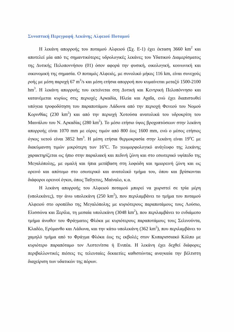
Η λεκάνη απορροής του ποταµού Αλφειού (Σχ. Ε-1) έχει έκταση 3660 km2 και

αποτελεί µία από τις σηµαντικότερες υδρολογικές λεκάνες του Υδατικού ∆ιαµερίσµατος

της ∆υτικής Πελοποννήσου (01) όσον αφορά την φυσική, οικολογική, κοινωνική και

οικονοµική της σηµασία. Ο ποταµός Αλφειός, µε συνολικό µήκος 116 km, είναι συνεχούς

ροής µε µέση παροχή 67 m3/s και µέση ετήσια απορροή που κυµαίνεται µεταξύ 1500-2100

hm3. Η λεκάνη απορροής του εκτείνεται στη ∆υτική και Κεντρική Πελοπόννησο και

κατανέµεται κυρίως στις περιοχές Αρκαδία, Ηλεία και Αχαΐα, ενώ έχει διαπιστωθεί

υπόγεια τροφοδότηση του παραποτάµου Λάδωνα από την περιοχή Φενεού του Νοµού

Κορινθίας (230 km2) και από την περιοχή Χοτούσα ανατολικά του υδροκρίτη του

Μαινάλου του Ν. Αρκαδίας (280 km2). Το µέσο ετήσιο ύψος βροχοπτώσεων στην λεκάνη

απορροής είναι 1070 mm µε εύρος τιµών από 800 έως 1600 mm, ενώ ο µέσος ετήσιος

όγκος υετού είναι 3852 hm3. Η µέση ετήσια θερµοκρασία στην λεκάνη είναι 19οC µε

διακύµανση τιµών µικρότερη των 16οC. Το γεωµορφολογικό ανάγλυφο της λεκάνης

χαρακτηρίζεται ως ήπιο στην παραλιακή και πεδινή ζώνη και στο εσωτερικό υψίπεδο της

Μεγαλόπολης, µε οµαλή και ήπια µετάβαση στη λοφώδη και ηµιορεινή ζώνη και ως

ορεινό και απότοµο στο εσωτερικό και ανατολικό τµήµα του, όπου και βρίσκονται

διάφοροι ορεινοί όγκοι, όπως Ταΰγετος, Μαίναλο, κ.α.

Η λεκάνη απορροής του Αλφειού ποταµού µπορεί να χωριστεί σε τρία µέρη

(υπολεκάνες), την άνω υπολεκάνη (250 km2), που περιλαµβάνει το τµήµα του ποταµού

Αλφειού στο οροπέδιο της Μεγαλόπολης µε κυριότερους παραποτάµους τους Λούσιο,

Ελισσώνα και Ξερίλα, τη µεσαία υπολεκάνη (3048 km2), που περιλαµβάνει το ενδιάµεσο

τµήµα άνωθεν του Φράγµατος Φλόκα µε κυριότερους παραποτάµους τους Σελινούντα,

Κλαδέο, Ερύµανθο και Λάδωνα, και την κάτω υπολεκάνη (362 km2), που περιλαµβάνει το

χαµηλό τµήµα από το Φράγµα Φλόκα έως τις εκβολές στον Κυπαρισσιακό Κόλπο µε

κυριότερο παραπόταµο τον Λεστενίτσα ή Ενιπέα. Η λεκάνη έχει δεχθεί διάφορες

περιβαλλοντικές πιέσεις τις τελευταίες δεκαετίες καθιστώντας αναγκαία την βέλτιστη

διαχείριση των υδατικών της πόρων.

iv

Σχήµα Ε-1. Η υδρολογική λεκάνη του Αλφειού Ποταµού αποτελούµενη από 11

υπολεκάνες σε διάφορες αποχρώσεις του γκρι. Με κόκκινες κουκίδες

δίδονται οι διατοµές εξόδου των υπολεκανών (που συµπίπτουν µε τις

διατοµές µετρήσεων). Με διακεκοµµένες γραµµές παρουσιάζονται οι

τέσσερις κόµβοι.

Η γεωλογική δοµή της λεκάνης του Αλφειού είναι σύνθετη και πολύπλοκη. Τις

ορεινές περιοχές σχηµατίζουν πετρώµατα Άλπεων (Μεσοζωικής περιόδου), τις ηµιορεινές

και λοφώδεις περιοχές σχηµατίζουν µεταλπικά πετρώµατα (Τριτογενούς περιόδου) και τις

χαµηλού υψοµέτρου κοιλάδες δοµούν πρόσφατες αποθέσεις ιζηµάτων (Τεταρτογενούς

περιόδου). Το έδαφος στη λεκάνη του Αλφειού συνίσταται από αλουβιακές αποθέσεις,

αποτελούµενες από άµµους, χαλίκια και κροκάλες, καθώς επίσης και από νεογενή ιζήµατα

που χαρακτηρίζονται από ασυνέχεια και ανοµοιογένεια, µε επακόλουθο την εµφάνιση

επάλληλων υπό πίεση υδροφόρων οριζόντων. Σε µερικές περιοχές παρατηρούνται

αυξηµένα επίπεδα σιδήρου και µαγγανίου, που καθιστούν τα υπόγεια νερά ακατάλληλα για

ύδρευση.

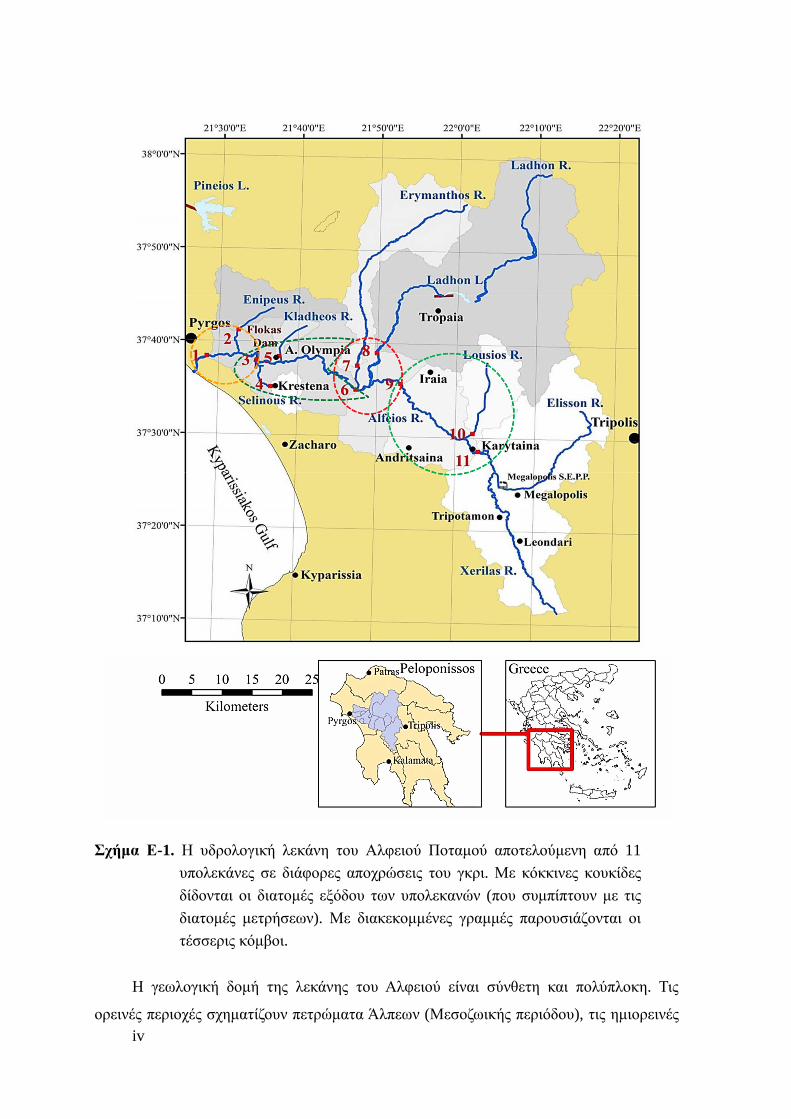
Τα πιο σηµαντικά κατασκευαστικά έργα που αφορούν τη διαχείριση των υδατικών

πόρων του Αλφειού Ποταµού φαίνονται στον ακόλουθο πίνακα. Οι βασικές χρήσεις νερού

στην λεκάνη περιλαµβάνουν: (1) την παραγωγή υδροηλεκτρικής ενέργειας στον Λάδωνα

σε συνδυασµό µε τον αντίστοιχο ταµιευτήρα και το φράγµα, (2) την άρδευση κυρίως γύρω

από το Φράγµα του Φλόκα (20 km ανάντη της εκβολής του ποταµού στον Κυπαρισσιακό

κόλπο), (3) την παραγωγή υδροηλεκτρικής ενέργειας στο µικρό υδροηλεκτρικό

εργοστάσιο του Φλόκα και (4) την ύδρευση της περιοχής του Πύργου και των όµορων

∆ήµων από τον παραπόταµο του Αλφειού Ποταµού, Ερύµανθο.

Πίνακας Ε.1 Έργα Υποδοµής στην υδρολογική λεκάνη του Αλφειού Ποταµού

Έτος Έργο - ∆ραστηριότητα

1951 Φράγµα βαρύτητας Παραποτάµου Λάδωνα στα Τρόπαια (τεχνητή λίµνη: επιφάνεια 4 km2, ωφέλιµος όγκος αποθήκευσης 46.2×106 m3, λεκάνη απορροής 749 km2, ύψος φράγµατος 50 m).

1955 Υδροηλεκτρικός σταθµός Λάδωνα 8620 m κατάντη του φράγµατος (δύο υδροστρόβιλοι × 34.5 MW τύπου FRANCIS).

1965 Κατασκευή αναχωµάτων στην κάτω λεκάνη του Ποταµού Αλφειού (µήκος × πλάτος 8,6 km × 250 m).

1967

Έναρξη οργανωµένης αµµοχαλικοληψίας από κοίτη Ποταµού Αλφειού στην κάτω υπολεκάνη. Αποξήρανση λιµνών Αγουλινίτσας και Μουριάς.

Αρδευτικά έργα στην κάτω λεκάνη του Αλφειού (160 km2).

Αρδευτικό Φράγµα Φλόκα (φράγµα εκτροπής για άρδευση µέγιστης παροχής 13 m3/s περίπου). Έργα προστασίας (κυρίως αναχώµατα) στη µεσαία λεκάνη του Αλφειού (περιοχή Αρχαίας Ολυµπίας).

1971 Λειτουργία ατµοηλεκτρικού σταθµού (ΑΗΣ) ∆ΕΗ στην περιοχή της Μεγαλόπολης (δύο µονάδες × 150 MW).

1975 Λειτουργία µίας επί πλέον µονάδας 300 MW στον ΑΗΣ Μεγαλόπολης. 1989 Λειτουργία µίας επί πλέον µονάδας 300 MW στον ΑΗΣ Μεγαλόπολης. 2002 Εκτροπή κοίτης ποταµού Αλφειού στην περιοχή Μεγαλόπολης για εξόρυξη λιγνίτη. 2000 Μικρό υδροηλεκτρικό εργοστάσιο στην Λαµπεία (∆ίβρη) µε µέγιστη ικανότητα 1.3MW 2010 Μικρό υδροηλεκτρικό εργοστάσιο στο Φράγµα Φλόκα µε µέγιστη ικανότητα 6,594MW

2011 Εγκατάσταση καθαρισµού νερού και σύστηµα διανοµής από τον Ερύµανθο Ποταµό για την ύδρευση του Πύργου και των όµορων δήµων µε συνολική ικανότητα 2,000 m3/h και7,000 κατοίκων.

vi

Πρώτο µέρος: Μεθοδολογία διόρθωσης ταχέων µετρήσεων υδατοπαροχής

Εισαγωγή

Προτείνεται µια πρότυπη µεθοδολογία διόρθωσης ταχέων µετρήσεων υδατοπαροχής

στην παρούσα διδακτορική διατριβή µε στόχο τον υπολογισµό πιο αξιόπιστων παροχών σε

σχέση µε τις αρχικές µετρήσεις, και κατ’ επέκταση πιο αξιόπιστων ρυπαντικών φορτίων. Η

µεθοδολογία στηρίζεται στις εξισώσεις διατήρησης του όγκου του νερού καθώς και της

µάζας του ρύπου εφαρµοζόµενες ταυτοχρόνως, τόσο σε όλους τους µονούς ανεξάρτητους

κόµβους ισορροπίας ενός ποταµού, όσο και σε όλους τους δυνατούς συνδυασµούς

διαδοχικών κόµβων (ανά δύο, ανά τρείς, κτλ.). Απαραίτητη προϋπόθεση για την εφαρµογή

της είναι να υπάρχουν διαθέσιµες παράλληλες µετρήσεις υδατοπαροχής και ρυπαντικών

ουσιών ή φυσικών δεικτών σε αντιπροσωπευτικές διατοµές καθ’ όλο το µήκος του κυρίως

ποταµού και των παραποτάµων του.

Το βασικό εννοιολογικό πλαίσιο της προτεινόµενης µεθοδολογίας είναι παρόµοιο µε

αυτό του επιστηµονικού πεδίου του «συνταιριάσµατος δεδοµένων» (data reconciliation),

αφού επιδιώκεται η διόρθωση των αρχικών µετρήσεων βάσει των αρχών διατήρησης του

όγκου και της µάζας. Οι κλασσικές τεχνικές του «συνταιριάσµατος δεδοµένων»

περιλαµβάνουν συνήθως την επίλυση µε την χρήση στατιστικών προσεγγίσεων, οι οποίες

προϋποθέτουν γνωστή την ακρίβεια των µετρήσεων. Οι βασικές δυσκολίες της

στατιστικής αυτής γνώσης είναι ότι η περιγραφή των διαδικασιών και των

αλληλεπιδράσεών τους, που επηρεάζουν τις µετρήσεις, δεν είναι πάντα απολύτως γνωστές,

καθώς και ότι η στατιστική ακρίβεια των µετρήσεων δεν µπορεί να ποσοτικοποιηθεί µε

ακρίβεια. Ωστόσο, σε πολλές περιπτώσεις, υπάρχει η εµπειρική γνώση για τις µετρήσεις

και το σφάλµα µέτρησής τους, η οποία παρά το γεγονός ότι δεν είναι ακριβής, µπορεί να

διατυπωθεί υπό µορφή διαστηµάτων τιµών. Η παρούσα µεθοδολογία δεν απαιτεί την ρητή

γνώση της στατιστικής κατανοµής των σφαλµάτων µέτρησης των παροχών, καθώς

χρησιµοποιεί διαστήµατα τιµών (intervals) εκφράζοντας τα άνω και κάτω όρια τιµών τους

µέσω σφαλµάτων (error bounds), ώστε να προσδιορίσει το επιτρεπόµενο εύρος τιµών των

διορθωµένων παραµέτρων µε βάση τις αρχικές µετρήσεις.

Η λογική αυτή χρησιµοποιείται στο επιστηµονικό υποπεδίο του «συνταιριάσµατος

δεδοµένων», το οποίο αναφέρεται στην βιβλιογραφία ως «εκτίµηση συστήµατος

παραµέτρων µε χρήση ορίων σφαλµάτων» (parameter set estimation from bounded error

data) (Milanese and Belforte, 1982; Ragot and Maquin, 2005). Σε αυτή την περίπτωση

γίνεται η υπόθεση ότι όλοι οι τύποι σφαλµάτων ανήκουν σε γνωστό πεδίο τιµών και ότι το

σφάλµα µέτρησης είναι δεσµευµένο και οριοθετηµένο (bounded). Όπως αναλύεται στις εν

λόγω εργασίες, λόγω της έλλειψης ακρίβειας καθώς και της επιρροής θορύβου, δεν είναι

εφικτός ο υπολογισµός των τιµών των παραµέτρων µε ακρίβεια, αλλά φαίνεται πιο

λογικός ο υπολογισµός ενός πεδίου τιµών µέσα στο οποίο εµπεριέχονται και οι

πραγµατικές τιµές του συστήµατος. Πιο συγκεκριµένα, µια παρόµοιας λογικής εργασία µε

την παρούσα προτεινόµενη µεθοδολογία είναι αυτή των Mandel et al. (1998) από τον

τοµέα των χηµικών µηχανικών. Όλες οι µεταβλητές εκφράζονται ως διαστήµατα

εµπιστοσύνης καταλήγοντας σε άνω και κάτω όρια τιµών. Επιπροσθέτως, µια ανώτατη και

κατώτατη επιτρεπόµενη απόκλιση από την ισορροπία της µάζας λαµβάνεται υπόψη,

συµπληρώνοντας το σύστηµα των περιορισµών. Όλες αυτές οι πληροφορίες στηρίζονται

στην εµπειρική γνώση της διαδικασίας και του πιθανότερου πεδίου διακύµανσης των

τιµών των εξεταζόµενων παραµέτρων. Το διαµορφωµένο σύστηµα ανισοτήτων επιλύεται

µε την χρήση της τεχνικής του Γραµµικού Μητρώου Ανισοτήτων (Linear Matrix

Inequality), η οποία καθορίζει αν το εν λόγω σύστηµα ανισοτήτων έχει εφικτή και δυνατή

λύση και υπολογίζει µία λύση του.

Βασικές διαφορές της παρούσας µεθοδολογίας είναι, πρώτον, η διάταξη του

µαθηµατικού προβλήµατος µε την µορφή προβλήµατος βελτιστοποίησης και όχι

συστήµατος ανισοτήτων (όπως θ’ αναλυθεί ακολούθως) και, δεύτερον, ότι το σύστηµα των

περιορισµών περιλαµβάνει επιπροσθέτως την έκφραση των ανισοτήτων των πεδίων τιµών

της κάθε µεταβλητής έχοντας αντικαταστήσει την εν λόγω µεταβλητή από την ισοδύναµη

έκφρασή της µέσω των εξισώσεων διατήρησης του όγκου και της µάζας, εκφρασµένων όχι

µόνο για την ισορροπία του µονού ανεξάρτητου κόµβου, αλλά και όλων των δυνατών

συνδυασµών ισορροπίας των διαδοχικών κόµβων. Με αυτόν τον τρόπο οι διορθωµένες

τιµές ικανοποιούν στο µέγιστο δυνατό βαθµό όλες τις εν λόγω εξισώσεις.

∆ιακριτοποίηση λεκάνης απορροής και προϋποθέσεις εφαρµογής της µεθοδολογίας

Η παρούσα µεθοδολογία βασίζεται στη διακριτοποίηση µιας υδρολογικής λεκάνης

µέσω του ορισµού διαδοχικών κόµβων καλύπτοντας όλο το µήκος του κυρίως ποταµού

καθώς και των παραποτάµων. Ο κάθε κόµβος αποτελείται από κατάλληλα επιλεγµένες

διατοµές, στις οποίες λαµβάνουν χώρα µετρήσεις ποιοτικών και ποσοτικών

χαρακτηριστικών. Επιπλέον κάθε κόµβος συνδέεται µε τον γειτονικό του µέσω της κοινής

τους εφαπτόµενης διατοµής, η οποία για τον ανάντη κόµβο αποτελεί διατοµή εξόδου και

viii

για τον κατάντη διατοµή εισόδου. Οι θέσεις των διατοµών είναι επιλεγµένες έτσι, ώστε να

εξασφαλίζεται ότι οι διατοµές βρίσκονται αρκετά κοντά µεταξύ τους ώστε να

ελαχιστοποιούνται οι ενδιάµεσες εισροές υδάτων. Παράλληλα, οι διατοµές πρέπει να

απέχουν κατάλληλη απόσταση µεταξύ τους, ώστε να επιτρέπουν την επίτευξη συνθηκών

πλήρους ανάµειξης των συγκεντρώσεων των ρύπων από ενδιάµεσες σηµειακές πηγές

ρύπανσης, εξασφαλίζοντας στις θέσεις των εν λόγω διατοµών οµοιοµορφία πλευρικών και

κατακόρυφων συγκεντρώσεων.

Επιπλέον, για την εφαρµογή της µεθοδολογίας γίνεται η παραδοχή ότι οι συνθήκες

κατά τις οποίες πραγµατοποιήθηκαν οι µετρήσεις αναφέρονται στις µέσες υδραυλικές

συνθήκες ροής που συνήθως επικρατούν στην περιοχή µελέτης υπό µόνιµες (steady-state)

συνθήκες ροής (Schmidt, 2002) (όπως π.χ. µε απουσία µεταβατικών φαινοµένων ροής,

µεταβαλλόµενης αντιρροής, αλλαγές στην γεωµετρία των διατοµών µετρήσεων, κτλ.).

Περιορισµοί µε βάση την διατήρηση του όγκου νερού

Στην παρούσα µεθοδολογία η εξίσωση διατήρησης του όγκου νερού σ’ ένα µονό

ανεξάρτητο κόµβο k (Σχήµα Ε-2) στον οποίο συµπεριλαµβάνονται Ν εν συνόλω διατοµές

(i=1,N) µπορεί να γραφτεί ως εξής, αγνοώντας σε αυτό το στάδιο την παρουσία

σφαλµάτων µέτρησης (Yannopoulos and Bekri, 2010):

Nk

N

ii QQQQ ++= ∑

−

=λ

1

21 (Ε.2)

Οι µετρηµένες ποσότητες της παροχής σε µία διατοµή i (1,N) συµβολίζονται

αντιστοίχως ως Qi. Σε κάθε µονό ανεξάρτητο κόµβο λαµβάνεται υπόψη µία άγνωστη, µη

άµεσα µετρηµένη ποσότητα. Αυτός ο άγνωστος όρος αναφέρεται ως λανθάνουσα

ποσότητα, αφού δεν έχει µετρηθεί άµεσα. Γίνεται, δε, η υπόθεση ότι αντιστοιχεί σε

απορροή από την υπολεκάνη που βρίσκεται ανάµεσα στις διατοµές εξόδου των

υπολεκανών, των οποίων η απορροή εισρέει στον κόµβο (διατοµές µε i=2,Ν) και της

διατοµής εξόδου (διατοµή µε i=1) από τον κόµβο k. Η επιφάνειά της στο Σχήµα Ε-2

αντιστοιχεί στην χρωµατισµένη επιφάνεια µε κίτρινο. Η παροχή από την λανθάνουσα

επιφάνεια δεν µπορεί να υπολογιστεί µε ακρίβεια, αλλά µόνο µία χονδρική εκτίµηση είναι

δυνατή µε βάση τις επιφάνειες των υπολοίπων υπολεκανών απορροής και της συνολικής

επιφάνειας που περικλείεται από τον εξεταζόµενο κόµβο. Τέλος, το µοντέλο υπολογισµού

της λανθάνουσας παροχής Qλk βασίζεται στην διατήρηση του όγκου του νερού σε επίπεδο

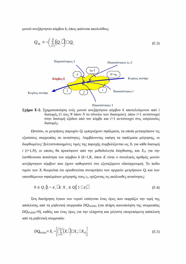
µονού ανεξάρτητου κόµβου k, όπως φαίνεται ακολούθως:

( ) 12

QQQN

iik +

−= ∑

=λ (Ε.3)

Σχήµα Ε-2. Σχηµατοποίηση ενός µονού ανεξάρτητου κόµβου k αποτελούµενου από i διατοµές (1 έως N όπου Ν το σύνολο των διατοµών), όπου i=1 αντιστοιχεί στην διατοµή εξόδου από τον κόµβο και i>1 αντιστοιχεί στις εισρέουσες διατοµές.

Ωστόσο, οι µετρήσεις παροχών Qi εµπεριέχουν σφάλµατα, τα οποία µετατρέπουν τις

εξισώσεις ισορροπίας σε ανισότητες. Λαµβάνοντας υπόψη τα σφάλµατα µέτρησης, οι

διορθωµένες/ βελτιστοποιηµένες τιµές της παροχής συµβολίζονται ως Xi για κάθε διατοµή

i (i=1,N), οι οποίες θα προκύψουν από την µεθοδολογία διόρθωσης, και Xλk για την

λανθάνουσα ποσότητα του κόµβου k (k=1,K, όπου Κ είναι ο συνολικός αριθµός µονών

ανεξάρτητων κόµβων που έχουν καθοριστεί στο εξεταζόµενο υδατόρρευµα). Το πεδίο

τιµών των Xi θεωρείται ότι οριοθετείται συναρτήσει των αρχικών µετρήσεων Qi και των

υποτιθέµενων σφαλµάτων µέτρησής τους εi, ορίζοντας τις ακόλουθες ανισότητες:

( ) ( )iiiii QXQ εε +≤≤−≤ 110 (Ε.4)

Στη διατήρηση όγκου του νερού εισάγεται ένας όρος που εκφράζει την τιµή της

απόκλισης από τη µηδενική ισορροπία DQNODEk (για πλήρη ικανοποίηση της ισορροπίας

DQNODEk=0), καθώς και ένας όρος για την ελάχιστη και µέγιστη επιτρεπόµενη απόκλιση

από τη µηδενική ισορροπία:

( )

++

−= ∑

−

=N

N

iiNODEk XXXXDQ λ

1

21 (Ε.5)

Κυρίως ποτάµι

Παραπόταµος 1

Παραπόταµος 2

Παραπόταµος i

Παραπόταµος nk-2

Κυρίως ποτάµι Κόµβος k

x

DevQDQDevQ NODEk +≤≤− (Ε.6)

Μπορούµε να εκφράσουµε την σχέση (Ε.4) αντικαθιστώντας σε αυτή το ισοδύναµο

των διορθωµένων παροχών Xi από την σχέση (Ε.5). Με αυτό τον τρόπο προστίθενται στο

σύστηµα των περιορισµών ανισότητες για κάθε διατοµή του ποταµού µε βάση την

ισορροπία του όγκου του νερού εκφρασµένη, τόσο για τους µονούς ανεξάρτητους κόµβους

όσο και για όλους τους δυνατούς συνδυασµούς διαδοχικών κόµβων. Για παράδειγµα, για

τη διατοµή εξόδου X1 (Σχήµα Ε-2) και για την περίπτωση έκφρασης της εξίσωσης

διατήρησης για τον µονό κόµβο προκύπτει η εξής διπλή ανισότητα:

( ) ( ) ( )112

11 11 εε λ +≤+

+≤− ∑

=QXXDQQ

N

iiNODEk (Ε.7)

Αντιστοίχως η σχέση (Ε-7) γράφεται για την εν λόγω διατοµή i=1 τόσες φορές όσες

οι εξισώσεις διατήρησης του όγκου νερού, οι οποίες περιλαµβάνουν την εν λόγω διατοµή.

Περιορισµοί µε βάση την διατήρηση της µάζας του ρύπου

Προχωρούµε ακολούθως στην ανάλυση του δεύτερου συνόλου περιορισµών, που

βασίζονται στην διατήρηση της µάζας του ρύπου. Στην προτεινόµενη µεθοδολογία

λαµβάνονται υπόψη οι συγκεντρώσεις m τον αριθµό κατάλληλα επιλεγµένων ρυπαντικών

ουσιών ή φυσικών δεικτών, οι οποίοι έχουν µετρηθεί µε αρκετά καλή ακρίβεια, και

συνεπώς έχουν αρκετά χαµηλά και γνωστά σφάλµατα µέτρησης. Επιπλέον, µπορούν να

επιλεχθούν µόνο ρύποι ή φυσικοί δείκτες, οι οποίοι µπορούν να θεωρηθούν σταθεροί και

συντηρητικοί και δεν θα υποστούν διάσπαση ή οποιαδήποτε άλλη αντίδραση (φυσική,

βιολογική ή χηµική) κατά την πορεία του ρύπου µέσα στην περιοχή του κόµβου/ κόµβων

που έχουν οριστεί στην παρούσα µεθοδολογία. Είναι αξιοσηµείωτο το γεγονός ότι όταν οι

ρύποι ή οι φυσικοί δείκτες µετρώνται µε µεγάλη ακρίβεια, η ακρίβεια µέτρησης των

παροχών είναι η κρισιµότερη παράµετρος στον υπολογισµό των φορτίων ρύπανσης και

αποτελούν τη µεγαλύτερη πηγή σφαλµάτων (NNSMP, 2008).

Μέσα σ’ αυτό το πλαίσιο, οι εξισώσεις ισορροπίας της µάζας, αγνοώντας τα

σφάλµατα µέτρησης, για τον µονό ανεξάρτητο κόµβο k (Σχήµα Ε-2) γράφονται ως εξής:

( ) NNj

N

iijij

Nj

N

iijj

cQcQcQcQ

qqqq

++=

⇔++=

∑

∑

−

=

−

=

λλ

λ

1

211

1

21 (Ε.8)

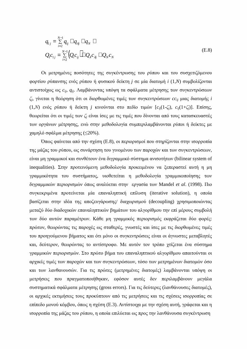
Οι µετρηµένες ποσότητες της συγκέντρωσης του ρύπου και του συσχετιζόµενου

φορτίου ρύπανσης ενός ρύπου ή φυσικού δείκτη j σε µία διατοµή i (1,N) συµβολίζονται

αντιστοίχως ως cij, qij. Λαµβάνοντας υπόψη τα σφάλµατα µέτρησης των συγκεντρώσεων

ζj, γίνεται η θεώρηση ότι οι διορθωµένες τιµές των συγκεντρώσεων ccij µιας διατοµής i

(1,Ν) ενός ρύπου ή δείκτη j κινούνται στο πεδίο τιµών [cij(1-ζj), cij(1+ζj)]. Επίσης,

θεωρείται ότι οι τιµές των ζj είναι ίσες µε τις τιµές που δίνονται από τους κατασκευαστές

των οργάνων µέτρησης, ενώ στην µεθοδολογία συµπεριλαµβάνονται ρύποι ή δείκτες µε

χαµηλό σφάλµα µέτρησης (≤20%).

Όπως φαίνεται από την σχέση (Ε.8), οι περιορισµοί που στηρίζονται στην ισορροπία

της µάζας του ρύπου, ως συνάρτηση του γινοµένου των παροχών και των συγκεντρώσεων,

είναι µη γραµµικοί και συνθέτουν ένα διγραµµικό σύστηµα ανισοτήτων (bilinear system of

inequalities). Στην προτεινόµενη µεθοδολογία προκειµένου να ξεπεραστεί αυτή η µη

γραµµικότητα του συστήµατος, υιοθετείται η µεθοδολογία γραµµικοποίησης των

διγραµµικών περιορισµών όπως αναλύεται στην εργασία των Mandel et al. (1998). Πιο

συγκεκριµένα προτείνεται µία επαναληπτική επίλυση (iterative solution), η οποία

βασίζεται στην ιδέα της αποζευγάρωσης/ διαχωρισµού (decoupling) χρησιµοποιώντας

µεταξύ δύο διαδοχικών επαναληπτικών βηµάτων του αλγορίθµου την επί µέρους συµβολή

των δύο αυτών παραµέτρων. Κάθε µη γραµµικός περιορισµός εκφράζεται δύο φορές:

πρώτον, θεωρώντας τις παροχές ως σταθερές, γνωστές και ίσες µε τις διορθωµένες τιµές

του προηγούµενου βήµατος και ότι µόνο οι συγκεντρώσεις είναι οι άγνωστες µεταβλητές

και, δεύτερον, θεωρώντας το αντίστροφο. Με αυτόν τον τρόπο χτίζεται ένα σύστηµα

γραµµικών περιορισµών. Στο πρώτο βήµα του επαναληπτικού αλγορίθµου απαιτούνται οι

αρχικές τιµές των παροχών και των συγκεντρώσεων, τόσο των µετρηµένων διατοµών όσο

και των λανθανουσών. Για τις πρώτες (µετρηµένες διατοµές) λαµβάνονται υπόψη οι

µετρήσεις που πραγµατοποιήθηκαν, εφόσον αυτές δεν περιλαµβάνουν µεγάλα

συστηµατικά σφάλµατα µέτρησης (gross errors). Για τις δεύτερες (λανθάνουσες διατοµές),

οι αρχικές εκτιµήσεις τους προκύπτουν από τις µετρήσεις και τις σχέσεις ισορροπίας σε

επίπεδο µονού κόµβου, όπως η σχέση (Ε.3). Αντίστοιχα µε την σχέση αυτή, γράφεται και η

ισορροπία της µάζας του ρύπου, η οποία επιλύεται ως προς την λανθάνουσα συγκέντρωση

xii

( )λ

λ Q

cQcQcQc

NN

N

iijij

j

−−=

∑−

=

1

211 (Ε.9)

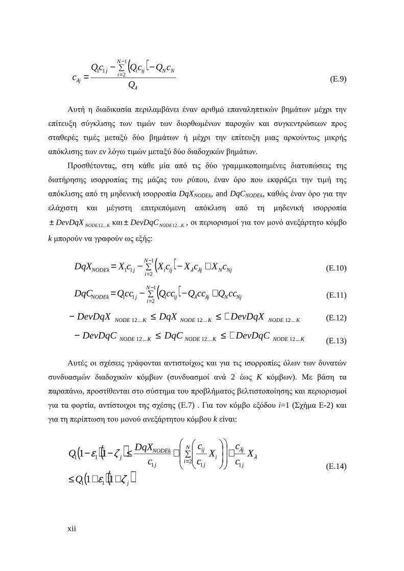
Αυτή η διαδικασία περιλαµβάνει έναν αριθµό επαναληπτικών βηµάτων µέχρι την

επίτευξη σύγκλισης των τιµών των διορθωµένων παροχών και συγκεντρώσεων προς

σταθερές τιµές µεταξύ δύο βηµάτων ή µέχρι την επίτευξη µιας αρκούντως µικρής

απόκλισης των εν λόγω τιµών µεταξύ δύο διαδοχικών βηµάτων.

Προσθέτοντας, στη κάθε µία από τις δύο γραµµικοποιηµένες διατυπώσεις της

διατήρησης ισορροπίας της µάζας του ρύπου, έναν όρο που εκφράζει την τιµή της

απόκλισης από τη µηδενική ισορροπία DqXNODEk, and DqCNODEk, καθώς έναν όρο για την

ελάχιστη και µέγιστη επιτρεπόµενη απόκλιση από τη µηδενική ισορροπία

KNODEDevDqX ...12± και KNODEDevDqC ...12± , οι περιορισµοί για τον µονό ανεξάρτητο κόµβο

k µπορούν να γραφούν ως εξής:

( ) NjNj

N

iijijNODEk cXcXcXcXDqX +−−= ∑

−

=λλ

1

211 (E.10)

( ) NjNj

N

iijijNODEk ccQccQccQccQDqC +−−= ∑

−

=λλ

1

211 (E.11)

KNODEKNODEKNODE DevDqXDqXDevDqX ...12...12...12 +≤≤− (E.12) KNODEKNODEKNODE DevDqCDqCDevDqC ...12...12...12 +≤≤− (E.13) Αυτές οι σχέσεις γράφονται αντιστοίχως και για τις ισορροπίες όλων των δυνατών

συνδυασµών διαδοχικών κόµβων (συνδυασµοί ανά 2 έως K κόµβων). Με βάση τα

παραπάνω, προστίθενται στο σύστηµα του προβλήµατος βελτιστοποίησης και περιορισµοί

για τα φορτία, αντίστοιχοι της σχέσης (Ε.7) . Για τον κόµβο εξόδου i=1 (Σχήµα Ε-2) και

για τη περίπτωση του µονού ανεξάρτητου κόµβου k είναι:

( )( )

( )( )j

j

jN

ii

j

ij

j

NODEkj

Q

Xc

cX

c

c

c

DqXQ

ζε

ζε λλ

++≤

+

+≤−− ∑

=

11

11

11

12

1111

(Ε.14)

( )( )

( )( )j

j

jN

ii

j

ij

j

NODEkj

Q

Qc

ccQ

c

cc

c

DqCQ

ζε

ζε λλ

++≤

+

+≤−− ∑

=

11

11

11

12

1111 (E.15)

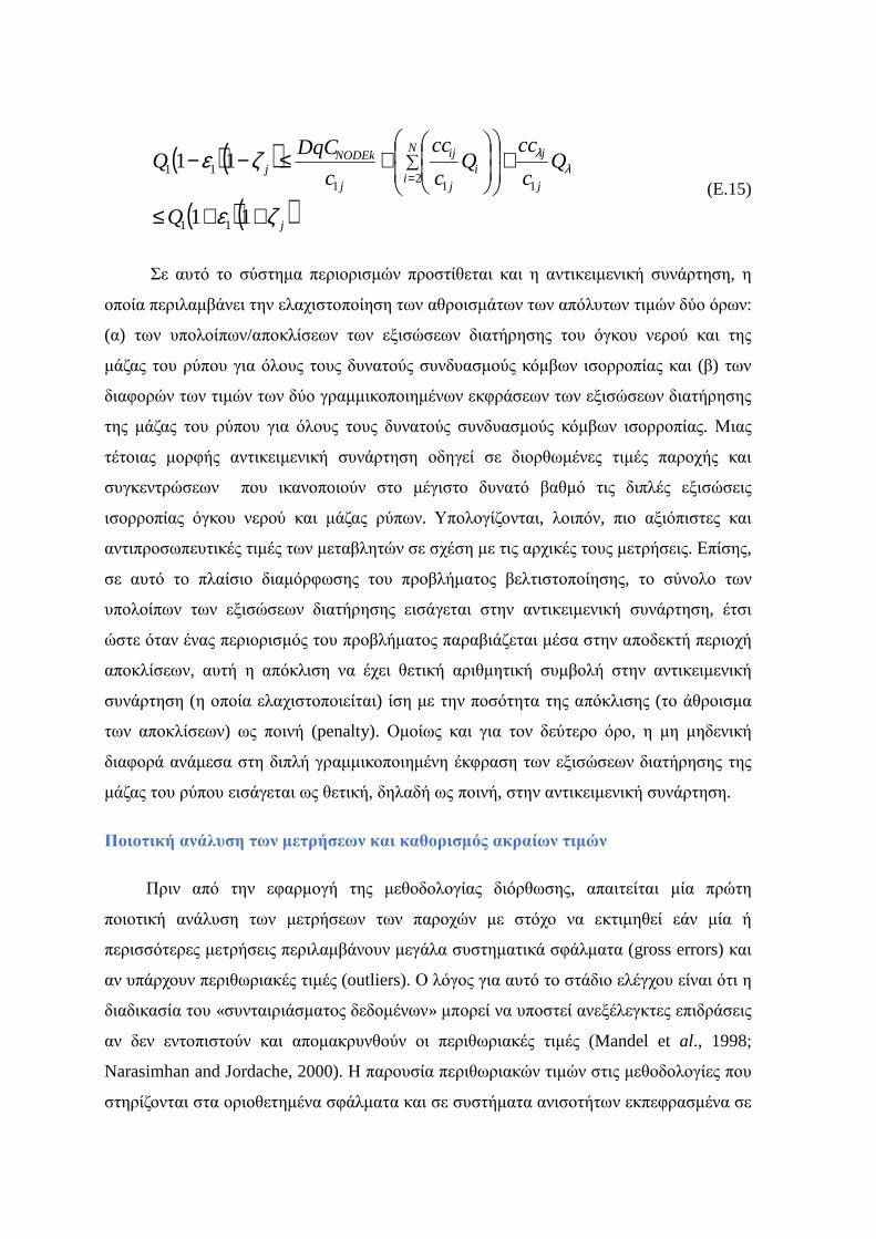
Σε αυτό το σύστηµα περιορισµών προστίθεται και η αντικειµενική συνάρτηση, η

οποία περιλαµβάνει την ελαχιστοποίηση των αθροισµάτων των απόλυτων τιµών δύο όρων:

(α) των υπολοίπων/αποκλίσεων των εξισώσεων διατήρησης του όγκου νερού και της

µάζας του ρύπου για όλους τους δυνατούς συνδυασµούς κόµβων ισορροπίας και (β) των

διαφορών των τιµών των δύο γραµµικοποιηµένων εκφράσεων των εξισώσεων διατήρησης

της µάζας του ρύπου για όλους τους δυνατούς συνδυασµούς κόµβων ισορροπίας. Μιας

τέτοιας µορφής αντικειµενική συνάρτηση οδηγεί σε διορθωµένες τιµές παροχής και

συγκεντρώσεων που ικανοποιούν στο µέγιστο δυνατό βαθµό τις διπλές εξισώσεις

ισορροπίας όγκου νερού και µάζας ρύπων. Υπολογίζονται, λοιπόν, πιο αξιόπιστες και

αντιπροσωπευτικές τιµές των µεταβλητών σε σχέση µε τις αρχικές τους µετρήσεις. Επίσης,

σε αυτό το πλαίσιο διαµόρφωσης του προβλήµατος βελτιστοποίησης, το σύνολο των

υπολοίπων των εξισώσεων διατήρησης εισάγεται στην αντικειµενική συνάρτηση, έτσι

ώστε όταν ένας περιορισµός του προβλήµατος παραβιάζεται µέσα στην αποδεκτή περιοχή

αποκλίσεων, αυτή η απόκλιση να έχει θετική αριθµητική συµβολή στην αντικειµενική

συνάρτηση (η οποία ελαχιστοποιείται) ίση µε την ποσότητα της απόκλισης (το άθροισµα

των αποκλίσεων) ως ποινή (penalty). Οµοίως και για τον δεύτερο όρο, η µη µηδενική

διαφορά ανάµεσα στη διπλή γραµµικοποιηµένη έκφραση των εξισώσεων διατήρησης της

µάζας του ρύπου εισάγεται ως θετική, δηλαδή ως ποινή, στην αντικειµενική συνάρτηση.

Ποιοτική ανάλυση των µετρήσεων και καθορισµός ακραίων τιµών

Πριν από την εφαρµογή της µεθοδολογίας διόρθωσης, απαιτείται µία πρώτη

ποιοτική ανάλυση των µετρήσεων των παροχών µε στόχο να εκτιµηθεί εάν µία ή

περισσότερες µετρήσεις περιλαµβάνουν µεγάλα συστηµατικά σφάλµατα (gross errors) και

αν υπάρχουν περιθωριακές τιµές (outliers). Ο λόγος για αυτό το στάδιο ελέγχου είναι ότι η

διαδικασία του «συνταιριάσµατος δεδοµένων» µπορεί να υποστεί ανεξέλεγκτες επιδράσεις

αν δεν εντοπιστούν και αποµακρυνθούν οι περιθωριακές τιµές (Mandel et al., 1998;

Narasimhan and Jordache, 2000). Η παρουσία περιθωριακών τιµών στις µεθοδολογίες που

στηρίζονται στα οριοθετηµένα σφάλµατα και σε συστήµατα ανισοτήτων εκπεφρασµένα σε

xiv

διαστήµατα τιµών, όπως η παρούσα µεθοδολογία, καθώς και αυτή των Ragot and Maquin

(2004), οδηγεί σε µη εφικτή λύση, λόγω του ότι οι ανισότητες δεν είναι πλέον συµβατές

µεταξύ τους και δεν έχουν κοινή περιοχή τιµών κατά την κοινή τους επίλυση.

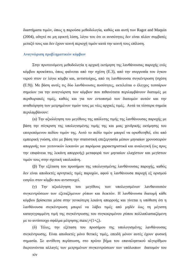
Αναγνώριση προβληµατικών κόµβων

Στην προτεινόµενη µεθοδολογία η αρχική εκτίµηση της λανθάνουσας παροχής ενός

κόµβου προκύπτει, όπως φαίνεται από την σχέση (Ε.3), από την ισορροπία του όγκου

νερού στον εν λόγω κόµβο και, αντιστοίχως, από τη λανθάνουσα συγκέντρωση (σχέση

(Ε.9)). Με βάση αυτές τις δύο λανθάνουσες ποσότητες, εκτελείται ο έλεγχος τεσσάρων

σηµείων για την αναγνώριση των κόµβων που πιθανότατα περιλαµβάνουν διατοµές µε

περιθωριακές τιµές, καθώς και για τον εντοπισµό των διατοµών αυτών και την

αναθεώρηση των µετρηµένων τιµών τους µε νέες αρχικές τιµές. Αυτά τα τέσσερα σηµεία

περιλαµβάνουν:

(α) Την αξιολόγηση του µεγέθους της απόλυτης τιµής της λανθάνουσας παροχής µε

βάση την σύγκριση της υπολογισµένης τιµής της και µιας χονδρικής εκτίµησης του

επιτρεπόµενου πεδίου τιµών της. Αυτό το πεδίο τιµών µπορεί να οριοθετηθεί, είτε από

εµπειρική γνώση, είτε µε βάση την στατιστική επεξεργασία µέσων µηνιαίων χρονοσειρών

απορροής των γειτονικών λεκανών µε παρόµοια χαρακτηριστικά και αναλογική (ως προς

την επιφάνεια της λεκάνη απορροής) µεταφορά των µηνιαίων ελαχίστων και µεγίστων

τιµών τους στην σχετική υπολεκάνη.

(β) Την εξέταση του προσήµου της υπολογισµένης λανθάνουσας παροχής, καθώς

δεν είναι αποδεκτές αρνητικές τιµές παροχών, αφού η λανθάνουσα παροχή εξ ορισµού

εισρέει στον κόµβο που αντιστοιχεί.

(γ) Την αξιολόγηση του µεγέθους των υπολογισµένων λανθανουσών

συγκεντρώσεων των εξεταζόµενων ρύπων και δεικτών. Η λανθάνουσα διατοµή κάθε

κόµβου βρίσκεται µέσα στην γενικότερη λεκάνη απορροής και γίνεται η υπόθεση ότι η

λανθάνουσα συγκέντρωση µπορεί να λάβει τιµές από µηδέν έως τη µέγιστη

καταγεγραµµένη τιµή της συγκέντρωσης του συγκεκριµένου ρύπου πολλαπλασιαζόµενη

µε το αντίστοιχο σφάλµα µέτρησης maxcj×(1+ζj).

(δ) Τέλος, την εξέταση του προσήµου της υπολογισµένης λανθάνουσας

συγκέντρωσης. Είναι αποδεκτές µόνο θετικές τιµές, επειδή µόνον αυτές έχουν φυσική

σηµασία. Σε αντίθετη περίπτωση, στο πρώτο βήµα του επαναληπτικού αλγορίθµου

διερευνώνται αλλαγές των µετρηµένων συγκεντρώσεων των υπόλοιπων διατοµών του

κόµβου εντός των επιτρεποµένων ορίων τους, ώστε να προκύψει εφικτή λύση του

προβλήµατος βελτιστοποίησης.

Κατά την εφαρµογή του προτεινόµενου αλγορίθµου στον Αλφειό Ποταµό,

προστίθεται ακόµη ένα σηµείο ελέγχου, το οποίο αφορά την ηλεκτρική αγωγιµότητα. Η

αγωγιµότητα έχει µετρηθεί µε δύο διαφορετικά όργανα µέτρησης και η κάθε µία

λαµβάνεται ως ξεχωριστός δείκτης. Ωστόσο σε κάθε διατοµή, οι δύο αυτές τιµές της

ηλεκτρικής αγωγιµότητας δεν µπορεί να διαφέρουν περισσότερο από 15% µεταξύ τους,

επειδή εκφράζουν εκτιµήσεις της ίδιας παραµέτρου. Για αυτόν τον λόγο, πριν ακόµη

εφαρµοστεί ο έλεγχος των τεσσάρων σηµείων, που προαναφέρθηκε, απαιτείται ο έλεγχος

των µετρήσεων αγωγιµότητας. Σε περίπτωση µη ικανοποίησης της συνθήκης του ±15%, οι

αρχικές τιµές των συγκεντρώσεων των διατοµών του κόµβου προσαρµόζονται κατάλληλα

εντός των επιτρεποµένων ορίων τους ώστε να ικανοποιούν την εν λόγω συνθήκη.

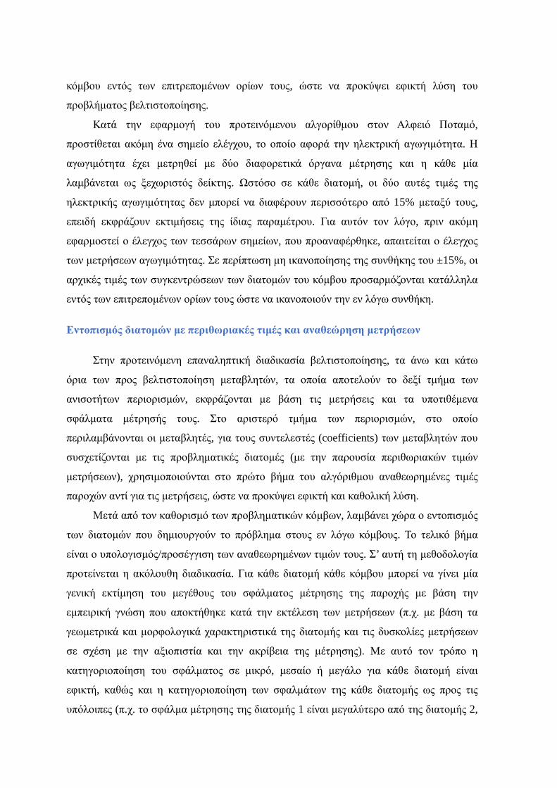
Εντοπισµός διατοµών µε περιθωριακές τιµές και αναθεώρηση µετρήσεων

Στην προτεινόµενη επαναληπτική διαδικασία βελτιστοποίησης, τα άνω και κάτω

όρια των προς βελτιστοποίηση µεταβλητών, τα οποία αποτελούν το δεξί τµήµα των

ανισοτήτων περιορισµών, εκφράζονται µε βάση τις µετρήσεις και τα υποτιθέµενα

σφάλµατα µέτρησής τους. Στο αριστερό τµήµα των περιορισµών, στο οποίο

περιλαµβάνονται οι µεταβλητές, για τους συντελεστές (coefficients) των µεταβλητών που

συσχετίζονται µε τις προβληµατικές διατοµές (µε την παρουσία περιθωριακών τιµών

µετρήσεων), χρησιµοποιούνται στο πρώτο βήµα του αλγόριθµου αναθεωρηµένες τιµές

παροχών αντί για τις µετρήσεις, ώστε να προκύψει εφικτή και καθολική λύση.

Μετά από τον καθορισµό των προβληµατικών κόµβων, λαµβάνει χώρα ο εντοπισµός

των διατοµών που δηµιουργούν το πρόβληµα στους εν λόγω κόµβους. Το τελικό βήµα

είναι ο υπολογισµός/προσέγγιση των αναθεωρηµένων τιµών τους. Σ’ αυτή τη µεθοδολογία

προτείνεται η ακόλουθη διαδικασία. Για κάθε διατοµή κάθε κόµβου µπορεί να γίνει µία

γενική εκτίµηση του µεγέθους του σφάλµατος µέτρησης της παροχής µε βάση την

εµπειρική γνώση που αποκτήθηκε κατά την εκτέλεση των µετρήσεων (π.χ. µε βάση τα

γεωµετρικά και µορφολογικά χαρακτηριστικά της διατοµής και τις δυσκολίες µετρήσεων

σε σχέση µε την αξιοπιστία και την ακρίβεια της µέτρησης). Με αυτό τον τρόπο η

κατηγοριοποίηση του σφάλµατος σε µικρό, µεσαίο ή µεγάλο για κάθε διατοµή είναι

εφικτή, καθώς και η κατηγοριοποίηση των σφαλµάτων της κάθε διατοµής ως προς τις

υπόλοιπες (π.χ. το σφάλµα µέτρησης της διατοµής 1 είναι µεγαλύτερο από της διατοµής 2,

xvi

κ.τ.λ.). Οι διατοµές µε τα µεγαλύτερα σφάλµατα είναι αυτές που οι µετρήσεις τους

τίθενται προς αναθεώρηση. Γι’ αυτές τις διατοµές πρέπει να προσδιοριστούν άνω και κάτω

όρια του εύρους διακύµανσης των τιµών τους για τους µήνες που πραγµατοποιήθηκαν οι

µετρήσεις. Αυτό µπορεί να γίνει, όπως στην περίπτωση του Αλφειού Ποταµού, µε χρήση

της στατιστικής ανάλυσης µηνιαίων χρονοσειρών απορροής ή µε εµπειρική γνώση. Με

βάση αυτό γίνεται η υπόθεση ότι οι αναθεωρηµένες τιµές των παροχών των

προβληµατικών διατοµών βρίσκονται µέσα σε αυτά τα εκτιµηµένα πεδία τιµών και

λαµβάνονται τρεις τιµές προς εξέταση: η ελάχιστη, η µέση (ή και εναλλακτικά η µέτρηση,

αν είναι µέσα στο πεδίο τιµών) και η µέγιστη τιµή. Με βάση αυτές τις τρεις τιµές,

εξετάζονται όλοι οι δυνατοί συνδυασµοί τιµών για τον εν λόγω κόµβο και είτε γίνονται

αποδεκτοί, είτε απορρίπτονται, αναλόγως µε την συµβατότητά τους ή µη, µε βάση τα

τέσσερα προαναφερόµενα σηµεία ελέγχου των λανθανουσών ποσοτήτων (µέγεθος και

πρόσηµο).

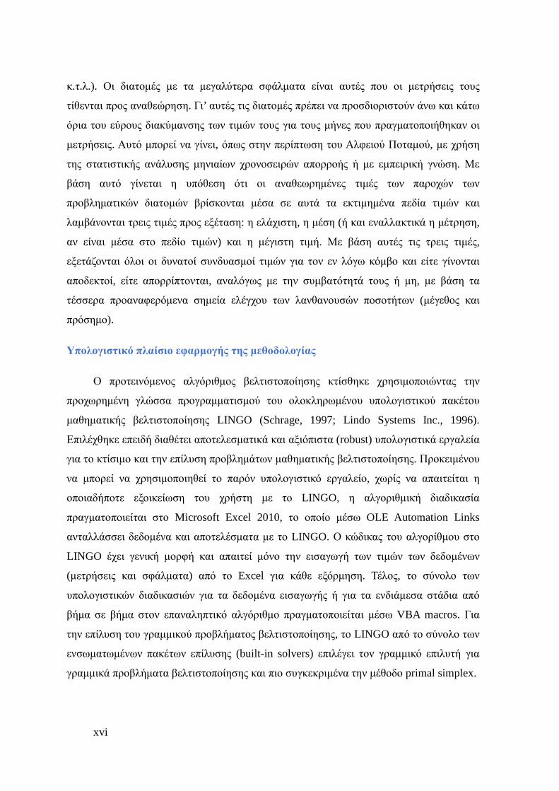
Υπολογιστικό πλαίσιο εφαρµογής της µεθοδολογίας

Ο προτεινόµενος αλγόριθµος βελτιστοποίησης κτίσθηκε χρησιµοποιώντας την

προχωρηµένη γλώσσα προγραµµατισµού του ολοκληρωµένου υπολογιστικού πακέτου

µαθηµατικής βελτιστοποίησης LINGO (Schrage, 1997; Lindo Systems Inc., 1996).

Επιλέχθηκε επειδή διαθέτει αποτελεσµατικά και αξιόπιστα (robust) υπολογιστικά εργαλεία

για το κτίσιµο και την επίλυση προβληµάτων µαθηµατικής βελτιστοποίησης. Προκειµένου

να µπορεί να χρησιµοποιηθεί το παρόν υπολογιστικό εργαλείο, χωρίς να απαιτείται η

οποιαδήποτε εξοικείωση του χρήστη µε το LINGO, η αλγοριθµική διαδικασία

πραγµατοποιείται στο Microsoft Excel 2010, το οποίο µέσω OLE Automation Links

ανταλλάσσει δεδοµένα και αποτελέσµατα µε το LINGO. Ο κώδικας του αλγορίθµου στο

LINGO έχει γενική µορφή και απαιτεί µόνο την εισαγωγή των τιµών των δεδοµένων

(µετρήσεις και σφάλµατα) από το Excel για κάθε εξόρµηση. Τέλος, το σύνολο των

υπολογιστικών διαδικασιών για τα δεδοµένα εισαγωγής ή για τα ενδιάµεσα στάδια από

βήµα σε βήµα στον επαναληπτικό αλγόριθµο πραγµατοποιείται µέσω VBA macros. Για

την επίλυση του γραµµικού προβλήµατος βελτιστοποίησης, το LINGO από το σύνολο των

ενσωµατωµένων πακέτων επίλυσης (built-in solvers) επιλέγει τον γραµµικό επιλυτή για

γραµµικά προβλήµατα βελτιστοποίησης και πιο συγκεκριµένα την µέθοδο primal simplex.

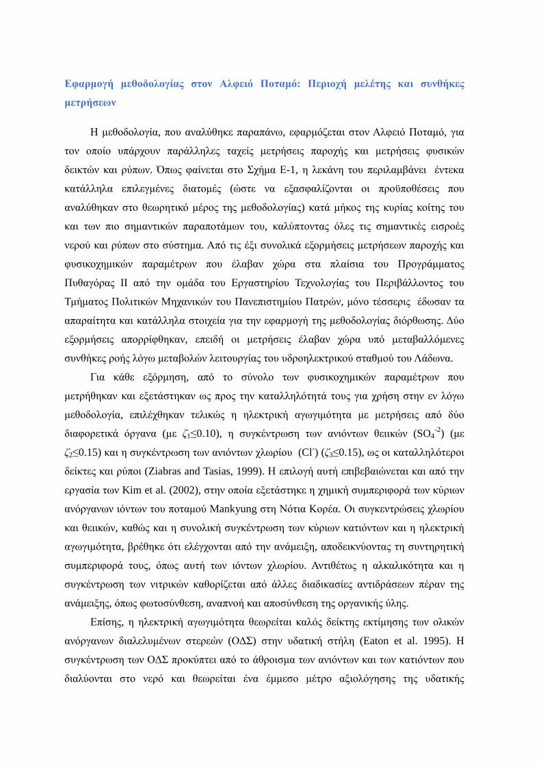
Εφαρµογή µεθοδολογίας στον Αλφειό Ποταµό: Περιοχή µελέτης και συνθήκες

µετρήσεων

Η µεθοδολογία, που αναλύθηκε παραπάνω, εφαρµόζεται στον Αλφειό Ποταµό, για

τον οποίο υπάρχουν παράλληλες ταχείς µετρήσεις παροχής και µετρήσεις φυσικών

δεικτών και ρύπων. Όπως φαίνεται στο Σχήµα Ε-1, η λεκάνη του περιλαµβάνει έντεκα

κατάλληλα επιλεγµένες διατοµές (ώστε να εξασφαλίζονται οι προϋποθέσεις που

αναλύθηκαν στο θεωρητικό µέρος της µεθοδολογίας) κατά µήκος της κυρίας κοίτης του

και των πιο σηµαντικών παραποτάµων του, καλύπτοντας όλες τις σηµαντικές εισροές

νερού και ρύπων στο σύστηµα. Από τις έξι συνολικά εξορµήσεις µετρήσεων παροχής και

φυσικοχηµικών παραµέτρων που έλαβαν χώρα στα πλαίσια του Προγράµµατος

Πυθαγόρας ΙΙ από την οµάδα του Εργαστηρίου Τεχνολογίας του Περιβάλλοντος του

Τµήµατος Πολιτικών Μηχανικών του Πανεπιστηµίου Πατρών, µόνο τέσσερις έδωσαν τα

απαραίτητα και κατάλληλα στοιχεία για την εφαρµογή της µεθοδολογίας διόρθωσης. ∆ύο

εξορµήσεις απορρίφθηκαν, επειδή οι µετρήσεις έλαβαν χώρα υπό µεταβαλλόµενες

συνθήκες ροής λόγω µεταβολών λειτουργίας του υδροηλεκτρικού σταθµού του Λάδωνα.

Για κάθε εξόρµηση, από το σύνολο των φυσικοχηµικών παραµέτρων που

µετρήθηκαν και εξετάστηκαν ως προς την καταλληλότητά τους για χρήση στην εν λόγω

µεθοδολογία, επιλέχθηκαν τελικώς η ηλεκτρική αγωγιµότητα µε µετρήσεις από δύο

διαφορετικά όργανα (µε ζ1≤0.10), η συγκέντρωση των ανιόντων θειικών (SO4-2) (µε

ζ2≤0.15) και η συγκέντρωση των ανιόντων χλωρίου (Cl-) (ζ3≤0.15), ως οι καταλληλότεροι

δείκτες και ρύποι (Ziabras and Tasias, 1999). Η επιλογή αυτή επιβεβαιώνεται και από την

εργασία των Kim et al. (2002), στην οποία εξετάστηκε η χηµική συµπεριφορά των κύριων

ανόργανων ιόντων του ποταµού Μankyung στη Νότια Κορέα. Οι συγκεντρώσεις χλωρίου

και θειικών, καθώς και η συνολική συγκέντρωση των κύριων κατιόντων και η ηλεκτρική

αγωγιµότητα, βρέθηκε ότι ελέγχονται από την ανάµειξη, αποδεικνύοντας τη συντηρητική

συµπεριφορά τους, όπως αυτή των ιόντων χλωρίου. Αντιθέτως η αλκαλικότητα και η

συγκέντρωση των νιτρικών καθορίζεται από άλλες διαδικασίες αντιδράσεων πέραν της

ανάµειξης, όπως φωτοσύνθεση, αναπνοή και αποσύνθεση της οργανικής ύλης.

Επίσης, η ηλεκτρική αγωγιµότητα θεωρείται καλός δείκτης εκτίµησης των ολικών

ανόργανων διαλελυµένων στερεών (Ο∆Σ) στην υδατική στήλη (Eaton et al. 1995). Η

συγκέντρωση των Ο∆Σ προκύπτει από το άθροισµα των ανιόντων και των κατιόντων που

διαλύονται στο νερό και θεωρείται ένα έµµεσο µέτρο αξιολόγησης της υδατικής

xviii

ποιότητας. Η ηλεκτρική αγωγιµότητα είναι ανάλογη της συγκέντρωσης Ο∆Σ και µπορεί

να χρησιµοποιηθεί στις εξισώσεις ισορροπίας της µάζας ως ένας ρύπος.

Κατά την εφαρµογή της επαναληπτικής διαδικασίας βελτιστοποίησης, παρατηρείται

ότι σε κάθε βήµα του αλγόριθµου η τιµή της αντικειµενικής συνάρτησης µειώνεται µέχρι

το σηµείο που µηδενίζεται εντελώς. Μετά από αυτό το βήµα, παρατηρείται ότι η

διαδικασία εγκλωβίζεται ανάµεσα σε δύο λύσεις που εµφανίζονται εναλλασσόµενες σε

διαδοχικά βήµατα. Σε αυτή την περίπτωση απαιτείται η εισαγωγή επιπρόσθετων

περιορισµών που οριοθετούν τη διαφορά τιµών των βελτιστοποιηµένων µεταβλητών

µεταξύ δύο διαδοχικών βηµάτων (step bounds) (Edgar et al., 2001). Με αυτό τον τρόπο

οδηγείται ο αλγόριθµος στην αναζήτηση λύσης σε πιο κοντινή περιοχή τιµών. Σ’ αυτή την

εργασία η τιµή των ορίων του επιτρεπόµενου βήµατος καθορίζεται µε δοκιµές.

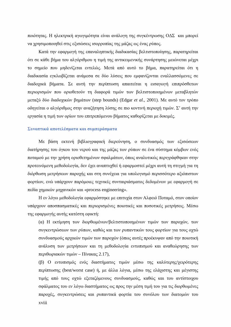
Συνοπτικά αποτελέσµατα και συµπεράσµατα

Με βάση εκτενή βιβλιογραφική διερεύνηση, ο συνδυασµός των εξισώσεων

διατήρησης του όγκου του νερού και της µάζας των ρύπων σε ένα σύστηµα κόµβων ενός

ποταµού µε την χρήση οριοθετηµένων σφαλµάτων, όπως αναλυτικώς περιγράφθηκαν στην

προτεινόµενη µεθοδολογία, δεν έχει αναπτυχθεί ή εφαρµοστεί µέχρι αυτή τη στιγµή για τη

διόρθωση µετρήσεων παροχής και στη συνέχεια για υπολογισµό περισσότερο αξιόπιστων

φορτίων, ενώ υπάρχουν παρόµοιες τεχνικές συνταιριάσµατος δεδοµένων µε εφαρµογή σε

πεδία χηµικών µηχανικών και «process engineering».

Η εν λόγω µεθοδολογία εφαρµόστηκε µε επιτυχία στον Αλφειό Ποταµό, στον οποίον

υπάρχουν αποσπασµατικές και περιορισµένες ποιοτικές και ποσοτικές µετρήσεις. Μέσω

της εφαρµογής αυτής κατέστη εφικτή:

(α) Η εκτίµηση των διορθωµένων/βελτιστοποιηµένων τιµών των παροχών, των

συγκεντρώσεων των ρύπων, καθώς και των ρυπαντικών τους φορτίων για τους οχτώ

συνδυασµούς αρχικών τιµών των παροχών (όπως αυτές προέκυψαν από την ποιοτική

ανάλυση των µετρήσεων και τη µεθοδολογία εντοπισµού και αναθεώρησης των

περιθωριακών τιµών – Πίνακας 2.17),

(β) Ο εντοπισµός ενός διαστήµατος τιµών µέσω της καλύτερης/χειρότερης

περίπτωσης (best/worst case) ή, µε άλλα λόγια, µέσω της ελάχιστης και µέγιστης

τιµής από τους οχτώ εξεταζόµενους συνδυασµούς, καθώς και του αντίστοιχου

σφάλµατος του εν λόγω διαστήµατος ως προς την µέση τιµή του για τις διορθωµένες

παροχές, συγκεντρώσεις και ρυπαντικά φορτία του συνόλου των διατοµών του

κυρίως ποταµού και των παραποτάµων του, στις οποίες έχουν πραγµατοποιηθεί οι

µετρήσεις, και

(γ) η εκτίµηση των άγνωστων µη άµεσα µετρήσιµων λανθανουσών παραµέτρων,

που περιλαµβάνουν την παροχή, τις συγκεντρώσεις και τα ρυπαντικά φορτία σε κάθε

οριζόµενο κόµβο.

Επιπροσθέτως, η µεθοδολογία έδωσε ικανοποιητικά αποτελέσµατα µε σηµαντικά

χαµηλότερα σφάλµατα για τις διορθωµένες παροχές. Με βάση τα αποτελέσµατα (Πίνακας

2.21) επιτεύχθηκε ο περιορισµός των σφαλµάτων των τιµών των διορθωµένων παροχών

για όλες τις διατοµές όπου υπήρχαν µετρήσεις. Το σχετικό σφάλµα ως προς την µέση τιµή

του διαστήµατος κυµαίνεται από 2% έως 5%, ήτοι πολύ περιορισµένο διάστηµα τιµών και

µε χαµηλά σφάλµατα σε σχέση µε το αντίστοιχο που προκύπτει από τις µετρήσεις και τα

θεωρούµενα σφάλµατά τους (5% και 100%). Για τις διορθωµένες τιµές των

συγκεντρώσεων, τα υπολογισµένα διαστήµατα τιµών είναι µειωµένα, αλλά όχι σηµαντικά,

αφού τα σφάλµατα µέτρησης των συγκεντρώσεων είναι a priori πολύ µικρά µε βάση τις

προϋποθέσεις της µεθοδολογίας. Το σχετικό σφάλµα των διορθωµένων λανθανουσών

παροχών είναι σηµαντικά µεγαλύτερο και µε ευρύτερο διάστηµα τιµών (2%, 74%) σε

σχέση µε αυτό των διατοµών µε µετρήσεις. Παρ’ όλα αυτά, αξίζει να σηµειωθεί ότι ο

καθορισµός της υποθετικής άγνωστης, µη άµεσα µετρήσιµης λανθάνουσας ποσότητας,

καθώς και η εκτίµηση των διορθωµένων τιµών της, έστω και αν είναι σχετικά ανακριβής,

είναι πολύ σηµαντική και χρήσιµη, αφού η άµεση µέτρηση είναι αδύνατη.

Πέραν τούτου, µε βάση τα αποτελέσµατα αξίζει να τονιστεί ότι ο συνδυασµός των

εξισώσεων διατήρησης του όγκου του νερού και της µάζας του ρύπου για τους επί µέρους

κόµβους και σε όλους τους δυνατούς συνδυασµούς πολλαπλών διαδοχικών κόµβων,

κατέληξε σε σηµαντική µείωση των ακρότατων τιµών των διαστηµάτων των παροχών σε

όλες τις διατοµές του Αλφειού Ποταµού. Το σύνολο των διαστηµάτων τιµών που

προέκυψαν για τις δύο βασικές µεταβλητές του προβλήµατος βελτιστοποίησης, της

παροχής και της συγκέντρωσης, βρίσκονται σε πλήρη συµβατότητα µε τα αποτελέσµατα

της ποιοτικής ανάλυσης. Για την διατοµή 8 στον Λάδωνα Ποταµό, η τιµή της µέσης

ηµερήσιας παροχής του υδροηλεκτρικού σταθµού του Λάδωνα (=36.75m3/s, Πίνακας 2.7,

σελ. 50) περιλαµβάνεται µέσα στο υπολογισµένο διάστηµα τιµών της διορθωµένης

παροχής στη εν λόγω διατοµή (35.7, 38.25)m3/s, γεγονός το οποίο αποτελεί έναν έµµεσο

τρόπο επαλήθευσης της εγκυρότητας των αποτελεσµάτων της µεθοδολογίας διόρθωσης.

Με βάση τις διορθωµένες παροχές και συγκεντρώσεις (Πίνακα 2.21 και Πίνακες

xx

2.28 – 2.30) για τους οκτώ συνδυασµούς αρχικών τιµών των παροχών (Πίνακας 2.17),

υπολογίστηκαν οκτώ τιµές διορθωµένων ρυπαντικών φορτίων για κάθε διατοµή και για

κάθε εξεταζόµενο ρύπο ή δείκτη (Πίνακες 2.34-2.36). Για λόγους σύγκρισης, οι ελάχιστες

και µέγιστες τιµές των ρυπαντικών φορτίων µε βάση τις µετρήσεις και τα θεωρούµενα

σφάλµατά τους καθορίστηκαν από το διάστηµα (Qi(1-εi)×cij(1-ζj)Qi, Qi(1+εi)×cij(1+ζj)).

Από αυτά τα αποτελέσµατα προκύπτει το γενικό συµπέρασµα ότι τα διορθωµένα

ρυπαντικά φορτία έχουν σηµαντικά χαµηλότερα σφάλµατα, δηλαδή τα διαστήµατα τιµών

τους είναι πολύ περιορισµένα σε σχέση µε αυτά που προκύπτουν από τις µετρήσεις για

όλες τις µετρηµένες διατοµές.

Προχωρώντας τώρα στην αξιολόγηση των λανθανόντων ρυπαντικών φορτίων (που

αντιστοιχούν στις τιµές των µη µετρηµένων λανθανουσών παροχών), το σχετικό σφάλµα

τους για το σύνολο των εξεταζόµενων ρύπων/δεικτών είναι αρκετά υψηλό και αντίστοιχης

τάξης µεγέθους µε αυτά που προέκυψαν για τα διορθωµένα ρυπαντικά φορτία µε βάση τις

µετρήσεις για τις µετρηµένες διατοµές. Οι πιο υψηλές τιµές των ρυπαντικών φορτίων

εµφανίζονται στις διατοµές 6, 3 and 1 κατά µήκος του κυρίως ποταµού, γεγονός που

αιτιολογείται από το ότι δέχονται τις εισροές από τις ανάντη υπολεκάνες του Αλφειού

Ποταµού και των αντιστοίχων παραποτάµων του. Οι υψηλότερες τιµές των λανθανόντων

φορτίων για τα ολικά διαλελυµένα στερεά έχουν υπολογιστεί στον δεύτερο και τον

τέταρτο κόµβο, ενώ για τα θειικά στον δεύτερο και τον τρίτο κόµβο. Περαιτέρω

διερεύνηση του υπολογισµού των ρυπαντικών φορτίων ως γινοµένου δύο µεταβλητών,

ώστε να επιτρέπει την καλύτερη δυνατή στατιστική τους ανάλυση, αποτελεί πιθανό στόχο

µελλοντικών ερευνών.

Η άµεση επιβεβαίωση της προτεινόµενης µεθοδολογίας διόρθωσης µέσω της

σύγκρισής της µε ακριβείς µετρήσεις παροχής δεν είναι δυνατή λόγω απουσίας των

απαιτούµενων µετρήσεων. Γι’ αυτό τον λόγο, η εγκυρότητα της µεθοδολογίας

εξασφαλίζεται µε έµµεση επαλήθευση των αποτελεσµάτων µε αυτά που προκύπτουν από

την µη γραµµική επίλυση των εξισώσεων διατήρησης της µάζας εκάστου ρύπου. Το µη

γραµµικό πακέτο του LINGO χρησιµοποιείται προκειµένου να βρεθούν οι εν λόγω λύσεις.

Στην περίπτωση της διαµόρφωσης της παρούσας µεθοδολογίας διατηρώντας τις µη

γραµµικές ανισότητες, δεν απαιτείται η εισαγωγή αρχικών τιµών για τις παροχές και τις

συγκεντρώσεις, παρά µόνο οι αρχικές τιµές των λανθανουσών ποσοτήτων, για τις οποίες

δεν υπάρχουν µετρήσεις και χρησιµοποιούνται οι οχτώ συνδυασµοί τιµών που προέκυψαν.

Με βάση αυτήν τη σύγκριση συµπεραίνεται ότι τα διαστήµατα τιµών που προκύπτουν από

το µη γραµµικό µοντέλο βρίσκονται σε παρόµοια, αλλά όχι ακριβώς ίδια περιοχή τιµών µε

αυτές του γραµµικού µοντέλου. Για παράδειγµα, στην διατοµή 8 στον Λάδωνα, η επίλυση

του γραµµικού προβλήµατος βελτιστοποίησης δίνει τις τιµές διορθωµένων παροχών (Min,

Mean, Max)=(36.84, 38.03, 38.99)m3/s και η αντίστοιχη περιοχή του µη γραµµικού

µοντέλου είναι (Min, Mean, Max)=(35.70, 36.34, 38.25)m3/s. Το διάστηµα τιµών της

γραµµικής επίλυσης εµπεριέχεται µέσα στο αντίστοιχο της µη γραµµικής, αποδεικνύοντας

την συνέπεια και την συµβατότητα των αποτελεσµάτων τους. Γενικώς, τα διαστήµατα

τιµών από τη µη γραµµική προσέγγιση είναι λίγο πιο διευρυµένα.

Ακολούθως, έλαβε χώρα έλεγχος γραµµικότητας του συστήµατος που συνθέτουν οι

µετρήσεις (Qi) και οι διορθωµένες τιµές (Xi) µέσω του στατιστικού ελέγχου υποθέσεων της

κατανοµής t (Hypothesis t-test paired with two tails), µε στόχο τη διερεύνηση ισχύος της

γραµµικής σχέσεως. Η µηδενική υπόθεση εκφράζεται µε βάση την κλίση της ευθείας που

προκύπτει από τη γραµµική παρεµβολή µεταξύ των Qi (x-άξονας) και Xi (y-άξονας) (Η0:

β1=1), ενώ η εναλλακτική υπόθεση είναι Η1: β1ǂ1. Με βάση τις διορθωµένες τιµές των

παροχών για τους οκτώ συνδυασµούς που εξετάστηκαν, δεν απορρίπτεται η µηδενική

υπόθεση Η0 σε επίπεδο σηµαντικότητας 0.01. Και οι οκτώ τιµές της κλίσης β1 από την

γραµµική παρεµβολή είναι πολύ κοντά στη µονάδα µε διάστηµα τιµών (0.951, 0.980) για

το γραµµικό µοντέλο και (0.951, 0.991) για το µη γραµµικό. Συνεπώς, συµπερασµατικά οι

πληθυσµοί µετρήσεων και εκτιµήσεων, που προκύπτουν από την εν λόγω µεθοδολογία,

είναι αναλόγως ισοδύναµοι, και συνεπώς οι λύσεις της µεθοδολογίας είναι συµβατές και

σε συµφωνία µε τις µετρήσεις.

Τέλος, σε κάθε περίπτωση κρίνεται αναγκαίο και προτείνεται ως µελλοντικό

αντικείµενο µελέτης, η περαιτέρω διερεύνηση της άµεσης σύγκρισης της µεθοδολογίας

διόρθωσης µε µετρήσεις ακριβείας. Η εφαρµογή του προτεινόµενου µαθηµατικού και

µεθοδολογικού πλαισίου δεν περιορίζεται µόνο σε ποτάµια µε ή χωρίς παραποτάµους,

αλλά σε οποιαδήποτε άλλη εφαρµογή που περιλαµβάνει τη δυνατότητα παράλληλων

µετρήσεων παροχών και µάζας ή συγκεντρώσεων ρύπων και µπορούν να εκφραστούν µε

εξισώσεις διατήρησής τους. Συνεπώς, η παρούσα µεθοδολογία θα µπορούσε να

αποτελέσει ένα χρήσιµο, αποτελεσµατικό και απαραίτητο εργαλείο για την εφαρµογή

προγραµµάτων παρακολούθησης ποιοτικών και ποσοτικών χαρακτηριστικών, µε στόχο

την αύξηση της αξιοπιστίας σε αποδεκτά επίπεδα της εκτίµησης γρήγορων µετρήσεων

παροχών, των συγκεντρώσεων και των ρυπαντικών φορτίων.

xxii

∆εύτερο µέρος: Βέλτιστη κατανοµή υδατικών πόρων υπό αβέβαιες συνθήκες

συστήµατος

Εισαγωγή

Η βέλτιστη κατανοµή των υδατικών πόρων συνιστά πολλαπλή πρόκληση λόγω των

διαφόρων αβεβαιοτήτων και ασαφειών, που συσχετίζονται µε το υδατικό σύστηµα, τις

παραµέτρους του και τους παράγοντες που το επηρεάζουν, καθώς και µε τις

αλληλεπίδράσεις τους. Αυτές οι αβεβαιότητες σε πολλές περιπτώσεις είναι αποτέλεσµα

διαφόρων πολυπλοκοτήτων σχετικά µε την ποιότητα των πληροφοριών (Li et al., 2009).

Τα τυχαία χαρακτηριστικά των φυσικών διαδικασιών (π.χ. βροχόπτωση και κλιµατική

αλλαγή) και των συνθηκών του συστήµατος (π.χ. υδατικές εισροές, υδατική παροχή,

ικανότητες αποθήκευσης και περιβαλλοντικές απαιτήσεις), τα σφάλµατα στις εκτιµήσεις

των παραµέτρων των µοντέλων (π.χ. παράµετροι για τα οφέλη και το κόστος), η ασάφεια

της αντικειµενικής συνάρτησης και των περιορισµών συνιστούν πηγές αβεβαιότητας.

Αυτές οι αβεβαιότητες µπορεί να περιλαµβάνονται, είτε στο δεξί σκέλος (ως σταθερές),

είτε στο αριστερό σκέλος (ως µεταβλητές µε τις σταθερές τους) των περιορισµών καθώς

και στην αντικειµενική συνάρτηση.

Κάποιες από αυτές τις µεταβλητές µπορεί να εκφραστούν µε την µορφή τυχαίων

µεταβλητών (random variables). Ταυτοχρόνως, κάποια τυχαία γεγονότα µπορούν να

ποσοτικοποιηθούν υπό την µορφή διαστηµάτων τιµών (intervals), είτε µε ντετερµινιστικά

είτε µε ασαφή άνω και κάτω όρια, οδηγώντας σε πολλαπλούς τύπους αβεβαιοτήτων (Li et

al., 2010). Οι παραδοσιακές µέθοδοι βελτιστοποίησης αδυνατούν να συµπεριλάβουν

µεταβλητές µη ντετερµινιστικές, µε άµεση συνέπεια να τίθενται εν αµφιβόλω τα

αποτελέσµατά τους, όταν τα δεδοµένα εισαγωγής του µοντέλου είναι αβέβαια (Li et al.,

2009; Fan and Huang, 2012; Suo et al., 2013). Για αυτόν το λόγο, έχουν αναπτυχθεί νέες

τεχνικές, όπως ο στοχαστικός προγραµµατισµός (stochastic programming), ο

προγραµµατισµός ασαφούς λογικής (fuzzy programming) και ο προγραµµατισµός µε

διαστήµατα τιµών (interval-parameter programming), καθώς και ο υβριδικός συνδυασµός

τους. Πληθώρα τέτοιων µεθοδολογιών έχουν προταθεί για διάφορους συνδυασµούς

αβεβαιοτήτων και εφαρµογών (Suo et al., 2013; Huang et al., 1992; Huang and Loucks,

2000; Maqsood et al., 2005; Li et al., 2006; Nie et al., 2007; J. Environmental

Management, 2007; Yeomans, 2008; Li and Huang, 2009; Li and Huang, 2011; Yeomans,

2008; Li and Huang, 2009; Li and Huang, 2011; Fu et al., 2013; Liu et al., 2014; Miao et

al., 2014; Li et al., 2008).

Πολλά προβλήµατα βέλτιστης κατανοµής υδατικών πόρων απαιτούν την σταδιακή

λήψη αποφάσεων µέσα στον χρονικό ορίζοντα που εξετάζονται. Αυτά τα προβλήµατα

µπορούν να εκφραστούν ως προβλήµατα στοχαστικού προγραµµατισµού δύο σταδίων

(two-stage programming TSP), στα οποία µία απόφαση λαµβάνεται πριν γίνουν γνωστές οι

τιµές των τυχαίων µεταβλητών, και στην συνέχεια, αφότου λάβουν χώρα τα τυχαία

συµβάντα και γίνουν γνωστές οι τιµές τους, µία δεύτερη απόφαση λαµβάνεται µε στόχο

την ελαχιστοποίηση των «ποινών» (penalties) που πιθανόν να εµφανιστούν λόγω

οποιουδήποτε προβλήµατος (Loucks et al., 1981). Στις πρακτικές εφαρµογές του TSP,

κάποιες αβεβαιότητες έχουν καθοριστεί µέσω συναρτήσεων πιθανοτήτων και κάποιες

άλλες ως σταθερές τιµές για τις οποίες θ’ ακολουθήσει ανάλυση µετα-βελτιστοποίησης

(post-optimality analyses) (Huang and Loucks, 2000). Το βήµα αυτό είναι αναγκαίο επειδή

(1) η ποιότητα της πληροφορίας, όσον αφορά την αβεβαιότητα σε πολλά πρακτικά

προβλήµατα, δεν είναι αρκετά καλή για να εκφραστεί µε την µορφή συνάρτησης

πιθανοτήτας, και (2) η επίλυση ενός µεγάλου TSP µοντέλου µε όλες τις αβέβαιες

µεταβλητές εκπεφρασµένες ως συναρτήσεις πιθανοτήτων είναι πολύ δύσκολη και

πολύπλοκη, ακόµη και στην περίπτωση που αυτές οι συναρτήσεις είναι διαθέσιµες.

Το δεύτερο µέρος αυτής της διδακτορικής διατριβής έχει ως στόχο να προτείνει ένα

πλαίσιο για τη λήψη αποφάσεων (DS) όσον αφορά την βέλτιστη κατανοµή των υδατικών

πόρων υπό συνθήκες αβεβαιότητας σε ένα πραγµατικό και σύνθετο υδατικό σύστηµα µε

πολλαπλές υδατικές εισροές (multi-tributary) και πολλαπλές περιόδους (multi-period) στον

Αλφειό Ποταµό. ∆ύο υβριδικές µεθοδολογίες χρησιµοποιούνται γι’ αυτό το σκοπό:

πρώτον, µία ανακριβής τεχνική στοχαστικού προγραµµατισµού δύο σταδίων (an inexact

two-stage stochastic programming technique (ITSP)) µε διαστήµατα τιµών µε

ντετερµινιστικά (καθορισµένα) άνω και κάτω όρια (Huang and Loucks, 2000), και

δεύτερον, µία παρόµοιας λογικής µεθοδολογία, αλλά πιο εκλεπτυσµένη και εξελιγµένη,

στην οποία τα όρια των διαστηµάτων των τιµών είναι ασαφή (FBISP) (Li et al., 2009). Και

οι δύο µέθοδοι βασίζονται στην ιδέα ότι στα πρακτικά προβλήµατα κάποιες αβεβαιότητες

µπορούν να εκφραστούν σαν ασαφή διαστήµατα, αφού οι µηχανικοί και οι µελετητές

θεωρούν συνήθως πιο εύκολο τον καθορισµό ενός εύρους διακυµάνσεων παρά

πιθανοτικών κατανοµών.

Η ITSP είναι µία υβριδική µέθοδος ανακριβούς βελτιστοποίησης (inexact

optimization), η οποία προτάθηκε µε στόχο να ξεπεραστούν οι δυσκολίες που σχετίζονται

xxiv

µε τις αναλύσεις µεταβελτιστοποίησης και να ενσωµατωθούν αβεβαιότητες, που δεν

µπορούν να εκφραστούν µε τη µορφή συναρτήσεων πιθανοτήτων. Από την άλλη µεριά η

FBISP περιλαµβάνει τους πιο σηµαντικούς τύπους έκφρασης της αβεβαιότητας

(πιθανότητες, ασαφή λογική και διαστήµατα τιµών) και βασίζεται στον συνδυασµό τριών

τεχνικών βελτιστοποίησης: (α) Στοχαστικό προγραµµατισµό πολλαπλών σταδίων (multi-

stage stochastic programming), (β) ασαφή προγραµµατισµό (χρησιµοποιώντας ανάλυση

κορυφών για ασαφή σύνολα - vertex analysis for fuzzy sets) και (γ) προγραµµατισµό

παραµετρικών διαστηµάτων τιµών (interval parameter programming - IPP). Κάθε τεχνική

συµβάλλει µε τον δικό της τρόπο στην ενίσχυση της ικανότητας της µεθοδολογίας να

ενσωµατώνει την αβεβαιότητα σε διάφορες µορφές. Επιπροσθέτως, η συµπεριφορά των

υπευθύνων (decision makers), όσον αφορά στο ρίσκο µιας απόφασης, λαµβάνεται υπόψη

στην FBISP, µέσω δύο διαφορετικών τρόπων επίλυσης του υπολογιστικού αλγορίθµου

βελτιστοποίησης (α) µία αρνητική προσέγγιση της ανάληψης επικινδυνότητας ή

απαισιόδοξη ή συντηρητική (risk-adverse or pessimistic) και (β) µία θετική προσέγγιση

της ανάληψης επικινδυνότητας ή αισιόδοξη (risk-prone or optimistic). Ο όρος

«επικινδυνότητα», που χρησιµοποιείται για να χαρακτηρίσει τους δύο τρόπους επίλυσης,

δεν υποννοεί την µέτρηση της επικινδυνότητας µε την αυστηρή µαθηµατική του έννοια,

αλλά περισσότερο την πρόθεση των υπευθύνων να αναλάβουν επικινδυνότητα ή όχι να

πληρώσουν υψηλότερες ποινές (ή να αποδεχτούν το κόστος) σε περίπτωση που επιλέξουν

την αισιόδοξη λύση του αβέβαιου συστήµατος υπό απαιτητικές µη ευνοϊκές συνθήκες ή να

υπάρχει µειωµένο κέρδος από την κατανοµή των υδατικών πόρων στην περίπτωση

επιλογής της απαισιόδοξης λύσης υπό ευνοϊκές συνθήκες.

Συνοπτική παρουσίαση του µαθηµατικού υπόβαθρου της ITSP

Το µαθηµατικό υπόβαθρο του ITSP µοντέλου παρουσιάζεται µε συνοπτικό τρόπο µε

βάση την εργασία των Huang and Loucks (2000). Αρχικώς, γίνεται η θεώρηση µιας

υπόθεσης εργασίας, στην οποία ο διαχειριστής των υδατικών πόρων έχει την αρµοδιότητα

κατανοµής του νερού σε διάφορες χρήσεις από πολλαπλές πηγές ύδατος. Μπορεί να

αναπαρασταθεί λοιπόν το πρόβληµα βελτιστοποίησης ως πρόβληµα µεγιστοποίησης της

οικονοµικής δραστηριότητας στη περιοχή. Με βάση ένα σχέδιο στόχων διανοµής του

νερού για κάθε χρήση, αν πράγµατι επιτευχθεί ο στόχος που έχει τεθεί, επιτυγχάνονται

καθαρά κέρδη για την τοπική κοινωνία. Στην αντίθετη περίπτωση (µη µηδενικών

ελλείψεων νερού), ο επιθυµητός στόχος νερού θα πρέπει να ικανοποιηθεί µέσω

εναλλακτικών και πιο δαπανηρών πηγών ύδατος, καταλήγοντας σε ποινές (κόστος) για την

τοπική κοινωνία (Loucks et al., 1981).

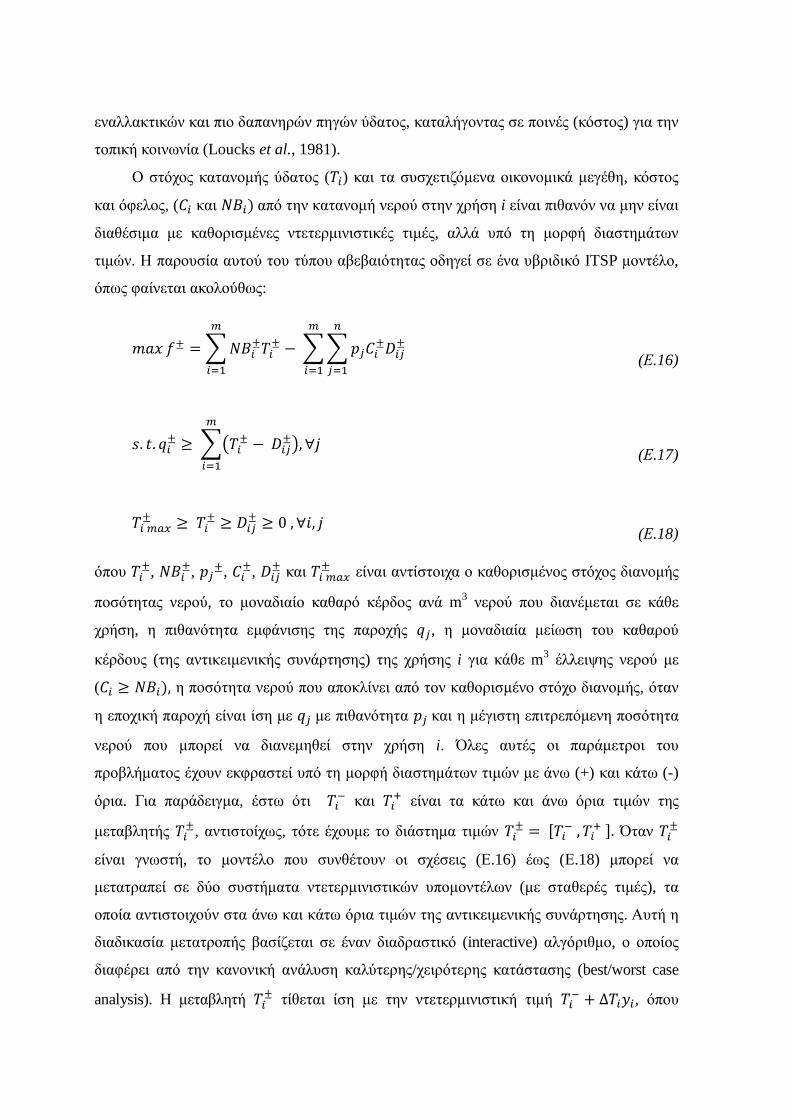
Ο στόχος κατανοµής ύδατος () και τα συσχετιζόµενα οικονοµικά µεγέθη, κόστος

και όφελος, ( και )από την κατανοµή νερού στην χρήση i είναι πιθανόν να µην είναι διαθέσιµα µε καθορισµένες ντετερµινιστικές τιµές, αλλά υπό τη µορφή διαστηµάτων

τιµών. Η παρουσία αυτού του τύπου αβεβαιότητας οδηγεί σε ένα υβριδικό ITSP µοντέλο,

όπως φαίνεται ακολούθως:

± = ±± −±±

(Ε.16)

. . ± ≥± −±, ∀

(Ε.17)

!"± ≥± ≥ ± ≥ 0, ∀$, (Ε.18)

όπου ±, ±, ±, ±, ± και !"± είναι αντίστοιχα ο καθορισµένος στόχος διανοµής

ποσότητας νερού, το µοναδιαίο καθαρό κέρδος ανά m3 νερού που διανέµεται σε κάθε

χρήση, η πιθανότητα εµφάνισης της παροχής , η µοναδιαία µείωση του καθαρού κέρδους (της αντικειµενικής συνάρτησης) της χρήσης i για κάθε m3 έλλειψης νερού µε

( ≥ ), η ποσότητα νερού που αποκλίνει από τον καθορισµένο στόχο διανοµής, όταν

η εποχική παροχή είναι ίση µε µε πιθανότητα και η µέγιστη επιτρεπόµενη ποσότητα

νερού που µπορεί να διανεµηθεί στην χρήση i. Όλες αυτές οι παράµετροι του

προβλήµατος έχουν εκφραστεί υπό τη µορφή διαστηµάτων τιµών µε άνω (+) και κάτω (-)

όρια. Για παράδειγµα, έστω ότι % και & είναι τα κάτω και άνω όρια τιµών της

µεταβλητής ±, αντιστοίχως, τότε έχουµε το διάστηµα τιµών ± = '%, &(. Όταν ±

είναι γνωστή, το µοντέλο που συνθέτουν οι σχέσεις (Ε.16) έως (Ε.18) µπορεί να

µετατραπεί σε δύο συστήµατα ντετερµινιστικών υποµοντέλων (µε σταθερές τιµές), τα

οποία αντιστοιχούν στα άνω και κάτω όρια τιµών της αντικειµενικής συνάρτησης. Αυτή η

διαδικασία µετατροπής βασίζεται σε έναν διαδραστικό (interactive) αλγόριθµο, ο οποίος

διαφέρει από την κανονική ανάλυση καλύτερης/χειρότερης κατάστασης (best/worst case

analysis). Η µεταβλητή ± τίθεται ίση µε την ντετερµινιστική τιµή % + Δ+, όπου

xxvi

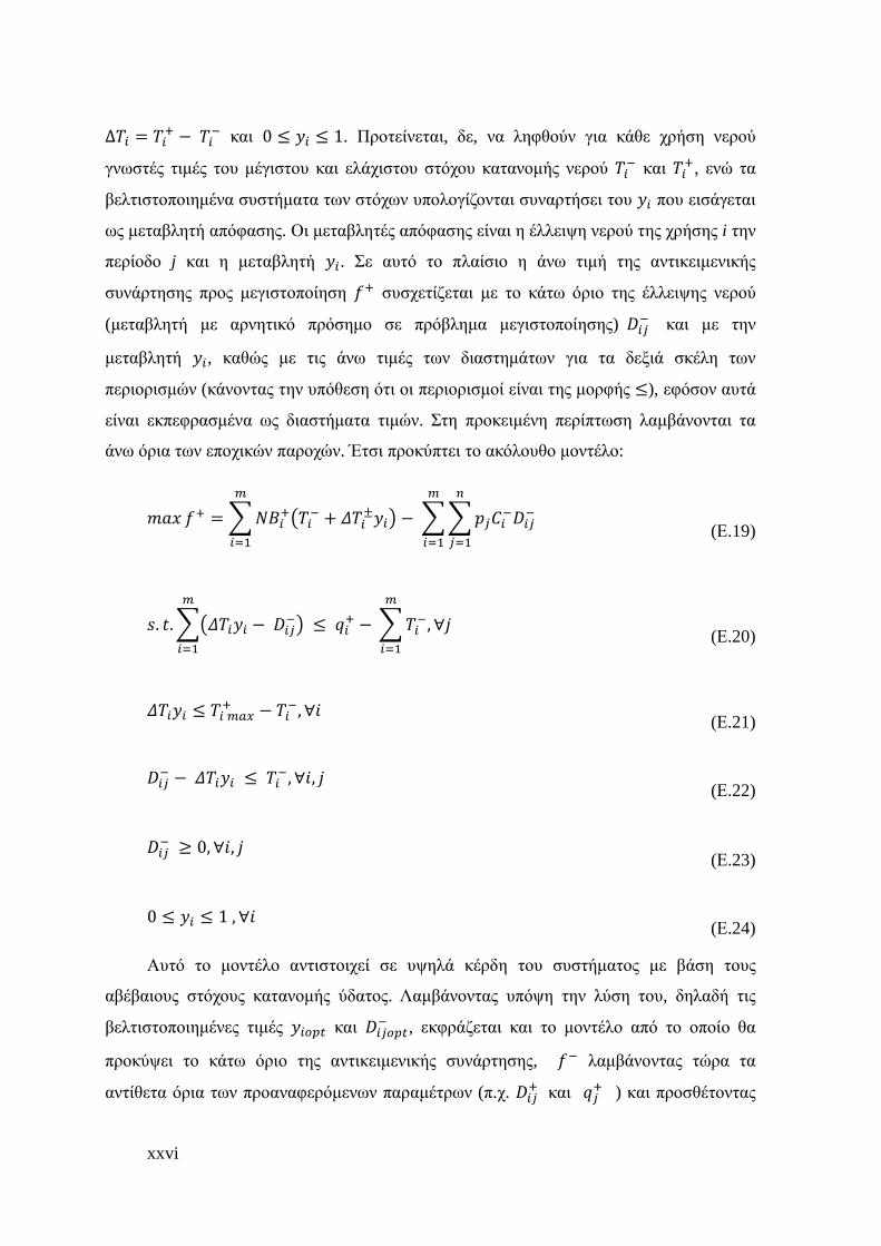
Δ = & − % και 0 ≤ + ≤ 1. Προτείνεται, δε, να ληφθούν για κάθε χρήση νερού

γνωστές τιµές του µέγιστου και ελάχιστου στόχου κατανοµής νερού % και &, ενώ τα

βελτιστοποιηµένα συστήµατα των στόχων υπολογίζονται συναρτήσει του + που εισάγεται ως µεταβλητή απόφασης. Οι µεταβλητές απόφασης είναι η έλλειψη νερού της χρήσης i την

περίοδο j και η µεταβλητή +. Σε αυτό το πλαίσιο η άνω τιµή της αντικειµενικής

συνάρτησης προς µεγιστοποίηση & συσχετίζεται µε το κάτω όριο της έλλειψης νερού

(µεταβλητή µε αρνητικό πρόσηµο σε πρόβληµα µεγιστοποίησης)% και µε την µεταβλητή +, καθώς µε τις άνω τιµές των διαστηµάτων για τα δεξιά σκέλη των

περιορισµών (κάνοντας την υπόθεση ότι οι περιορισµοί είναι της µορφής ≤), εφόσον αυτά

είναι εκπεφρασµένα ως διαστήµατα τιµών. Στη προκειµένη περίπτωση λαµβάνονται τα

άνω όρια των εποχικών παροχών. Έτσι προκύπτει το ακόλουθο µοντέλο:

& = &% + .±+ −%%

(Ε.19)

. ..+ −% ≤ & − %, ∀

(Ε.20)

.+ ≤ !"& − %, ∀$(Ε.21)

% − .+ ≤ %, ∀$, (Ε.22)

% ≥ 0, ∀$, (Ε.23)

0 ≤ + ≤ 1, ∀$ (Ε.24)

Αυτό το µοντέλο αντιστοιχεί σε υψηλά κέρδη του συστήµατος µε βάση τους

αβέβαιους στόχους κατανοµής ύδατος. Λαµβάνοντας υπόψη την λύση του, δηλαδή τις

βελτιστοποιηµένες τιµές +/01 και /01% , εκφράζεται και το µοντέλο από το οποίο θα

προκύψει το κάτω όριο της αντικειµενικής συνάρτησης, % λαµβάνοντας τώρα τα

αντίθετα όρια των προαναφερόµενων παραµέτρων (π.χ. & και & ) και προσθέτοντας

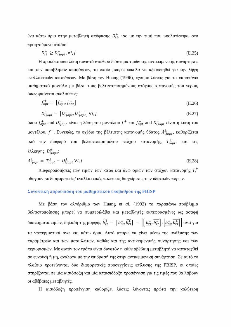
ένα κάτω όριο στην µεταβλητή απόφασης &, ίσο µε την τιµή που υπολογίστηκε στο

προηγούµενο στάδιο:

& ≥ /01% , ∀$, (Ε.25)

Η προκύπτουσα λύση συνιστά σταθερό διάστηµα τιµών της αντικειµενικής συνάρτησης

και των µεταβλητών αποφάσεων, το οποίο µπορεί εύκολα να αξιοποιηθεί για την λήψη

εναλλακτικών αποφάσεων. Με βάση τον Huang (1996), έχουµε λύσεις για το παραπάνω

µαθηµατικό µοντέλο µε βάση τους βελτιστοποιηµένους στόχους κατανοµής του νερού,

όπως φαίνεται ακολούθως:

/01± = 2/01% , /01& 3 (Ε.26)

/01± = 2/01% , /01& 3∀$, (Ε.27)

όπου /01& and /01% είναι η λύση του µοντέλου & και /01% and /01& είναι η λύση του

µοντέλου, %. Συνεπώς, το σχέδιο της βέλτιστης κατανοµής ύδατος,4/01± , καθορίζεται

από την διαφορά του βελτιστοποιηµένου στόχου κατανοµής, /01± , και της

έλλειψης,/01± :

4/01± =/01± −/01± ∀$, (Ε.28)

∆ιαφοροποιήσεις των τιµών των κάτω και άνω ορίων των στόχων κατανοµής ±

οδηγούν σε διαφορετικές/ εναλλακτικές πολιτικές διαχείρισης των υδατικών πόρων.

Συνοπτική παρουσιάση του µαθηµατικού υπόβαθρου της FBISP

Με βάση τον αλγόριθµο των Huang et al. (1992) το παραπάνω πρόβληµα

βελτιστοποίησης µπορεί να συµπεριλάβει και µεταβλητές εκπεφρασµένες ως ασαφή

διαστήµατα τιµών, δηλαδή της µορφής 561±7 = 2561%7,561&73 = 89561% , 561% : , 9561& , 561& :; αντί για

τα ντετερµιστικά άνω και κάτω όρια. Αυτό µπορεί να γίνει µέσω της ανάλυσης των

παραµέτρων και των µεταβλητών, καθώς και της αντικειµενικής συνάρτησης και των

περιορισµών. Με αυτόν τον τρόπο είναι δυνατόν η κάθε αβέβαιη µεταβλητή να καταταχθεί

σε ευνοϊκή ή µη, ανάλογα µε την επιδρασή της στην αντικειµενική συνάρτηση. Σε αυτό το

πλαίσιο προτείνονται δύο διαφορετικές προσεγγίσεις επίλυσης της FBISP, οι οποίες

στηρίζονται σε µία αισιόσοξη και µία απαισιόδοξη προσέγγιση για τις τιµές που θα λάβουν

οι αβέβαιες µεταβλητές.

Η αισιόδοξη προσέγγιση καθορίζει λύσεις λύνοντας πρώτα την καλύτερη

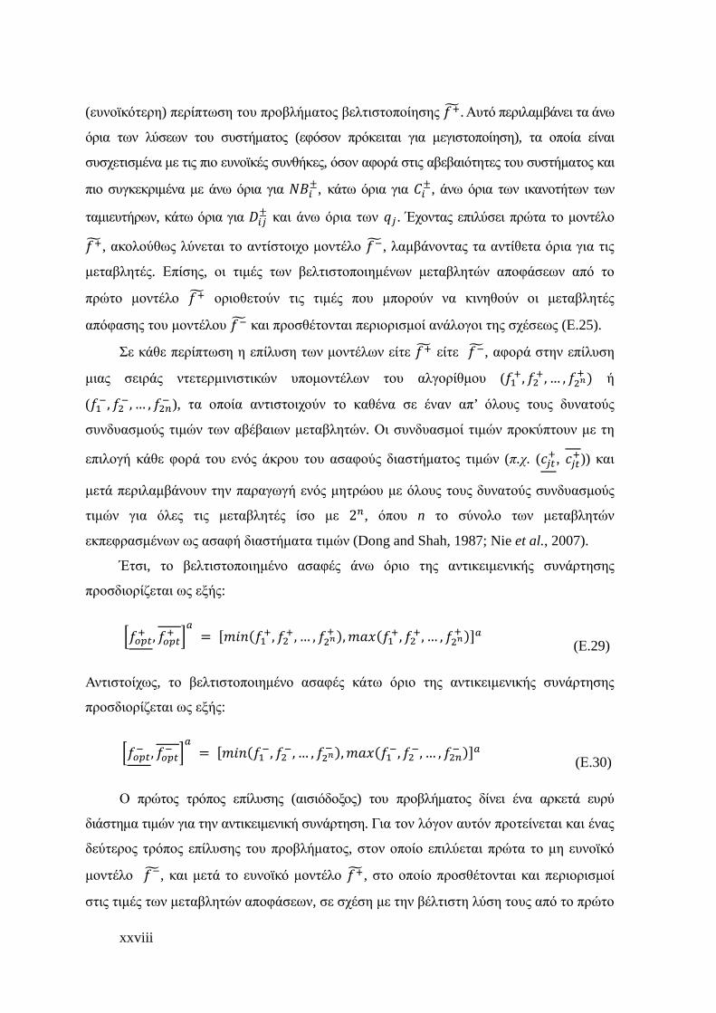
xxviii

(ευνοϊκότερη) περίπτωση του προβλήµατος βελτιστοποίησης &7 . Αυτό περιλαµβάνει τα άνω

όρια των λύσεων του συστήµατος (εφόσον πρόκειται για µεγιστοποίηση), τα οποία είναι

συσχετισµένα µε τις πιο ευνοϊκές συνθήκες, όσον αφορά στις αβεβαιότητες του συστήµατος και

πιο συγκεκριµένα µε άνω όρια για ±, κάτω όρια για ±, άνω όρια των ικανοτήτων των

ταµιευτήρων, κάτω όρια για ± και άνω όρια των . Έχοντας επιλύσει πρώτα το µοντέλο

&7 , ακολούθως λύνεται το αντίστοιχο µοντέλο %7 , λαµβάνοντας τα αντίθετα όρια για τις

µεταβλητές. Επίσης, οι τιµές των βελτιστοποιηµένων µεταβλητών αποφάσεων από το

πρώτο µοντέλο &7 οριοθετούν τις τιµές που µπορούν να κινηθούν οι µεταβλητές

απόφασης του µοντέλου %7 και προσθέτονται περιορισµοί ανάλογοι της σχέσεως (Ε.25).

Σε κάθε περίπτωση η επίλυση των µοντέλων είτε &7 είτε %7 , αφορά στην επίλυση

µιας σειράς ντετερµινιστικών υποµοντέλων του αλγορίθµου (&, <&, … , <>& ) ή

(%, <%, … , <% ), τα οποία αντιστοιχούν το καθένα σε έναν απ’ όλους τους δυνατούς

συνδυασµούς τιµών των αβέβαιων µεταβλητών. Οι συνδυασµοί τιµών προκύπτουν µε τη

επιλογή κάθε φορά του ενός άκρου του ασαφούς διαστήµατος τιµών (π.χ. (?1&, ?1&)) και

µετά περιλαµβάνουν την παραγωγή ενός µητρώου µε όλους τους δυνατούς συνδυασµούς

τιµών για όλες τις µεταβλητές ίσο µε 2, όπου n το σύνολο των µεταβλητών

εκπεφρασµένων ως ασαφή διαστήµατα τιµών (Dong and Shah, 1987; Nie et al., 2007).

Έτσι, το βελτιστοποιηµένο ασαφές άνω όριο της αντικειµενικής συνάρτησης

προσδιορίζεται ως εξής:

9/01& , /01& :! = '$AB&, <&, … , <>& ),B&, <&, … , <>& )(!(Ε.29)

Αντιστοίχως, το βελτιστοποιηµένο ασαφές κάτω όριο της αντικειµενικής συνάρτησης

προσδιορίζεται ως εξής:

9/01% , /01% :! = '$AB%, <%, … , <>% ),B%, <%, … , <% )(!(Ε.30)

Ο πρώτος τρόπος επίλυσης (αισιόδοξος) του προβλήµατος δίνει ένα αρκετά ευρύ

διάστηµα τιµών για την αντικειµενική συνάρτηση. Για τον λόγον αυτόν προτείνεται και ένας

δεύτερος τρόπος επίλυσης του προβλήµατος, στον οποίο επιλύεται πρώτα το µη ευνοϊκό

µοντέλο %7 , και µετά το ευνοϊκό µοντέλο &7 , στο οποίο προσθέτονται και περιορισµοί

στις τιµές των µεταβλητών αποφάσεων, σε σχέση µε την βέλτιστη λύση τους από το πρώτο

στάδιο του αλγορίθµου.

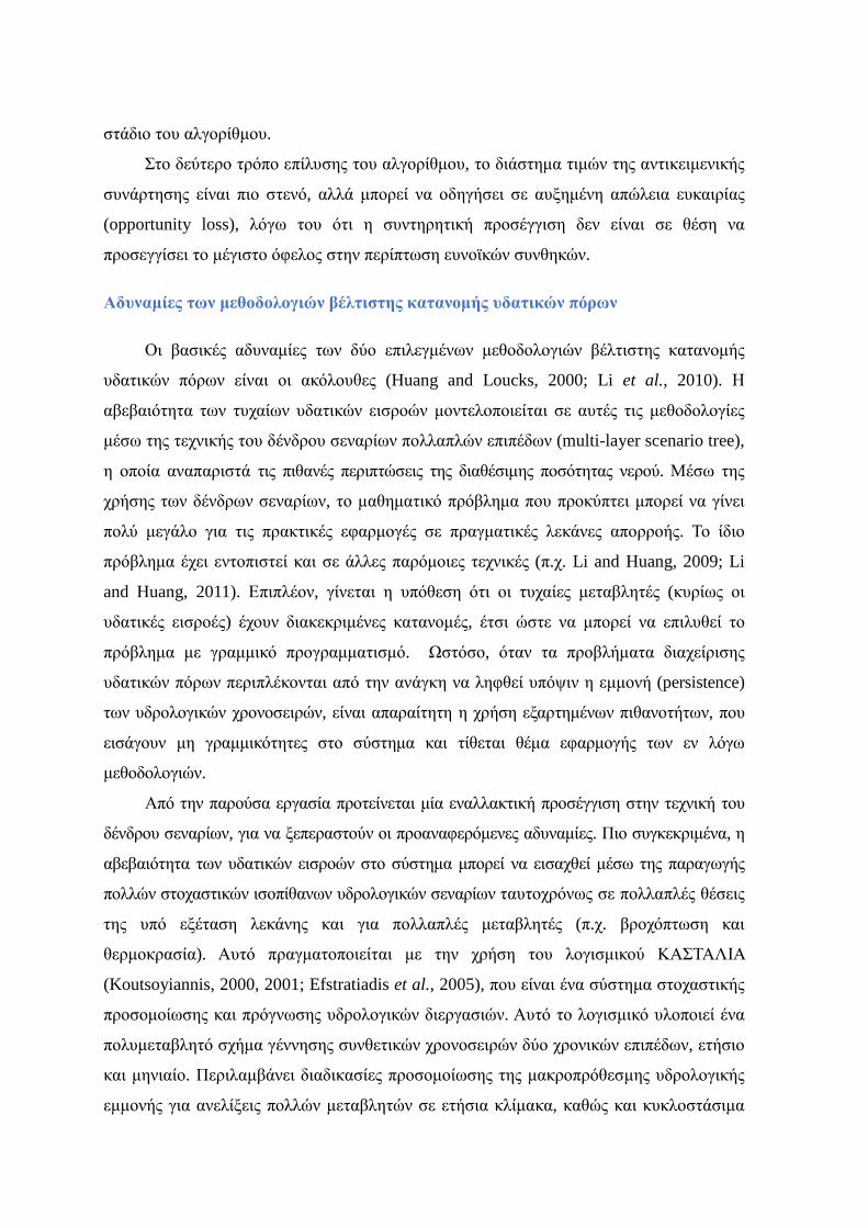
Στο δεύτερο τρόπο επίλυσης του αλγορίθµου, το διάστηµα τιµών της αντικειµενικής

συνάρτησης είναι πιο στενό, αλλά µπορεί να οδηγήσει σε αυξηµένη απώλεια ευκαιρίας

(opportunity loss), λόγω του ότι η συντηρητική προσέγγιση δεν είναι σε θέση να

προσεγγίσει το µέγιστο όφελος στην περίπτωση ευνοϊκών συνθηκών.

Αδυναµίες των µεθοδολογιών βέλτιστης κατανοµής υδατικών πόρων

Οι βασικές αδυναµίες των δύο επιλεγµένων µεθοδολογιών βέλτιστης κατανοµής

υδατικών πόρων είναι οι ακόλουθες (Huang and Loucks, 2000; Li et al., 2010). Η

αβεβαιότητα των τυχαίων υδατικών εισροών µοντελοποιείται σε αυτές τις µεθοδολογίες

µέσω της τεχνικής του δένδρου σεναρίων πολλαπλών επιπέδων (multi-layer scenario tree),

η οποία αναπαριστά τις πιθανές περιπτώσεις της διαθέσιµης ποσότητας νερού. Μέσω της

χρήσης των δένδρων σεναρίων, το µαθηµατικό πρόβληµα που προκύπτει µπορεί να γίνει

πολύ µεγάλο για τις πρακτικές εφαρµογές σε πραγµατικές λεκάνες απορροής. Το ίδιο

πρόβληµα έχει εντοπιστεί και σε άλλες παρόµοιες τεχνικές (π.χ. Li and Huang, 2009; Li

and Huang, 2011). Επιπλέον, γίνεται η υπόθεση ότι οι τυχαίες µεταβλητές (κυρίως οι

υδατικές εισροές) έχουν διακεκριµένες κατανοµές, έτσι ώστε να µπορεί να επιλυθεί το

πρόβληµα µε γραµµικό προγραµµατισµό. Ωστόσο, όταν τα προβλήµατα διαχείρισης

υδατικών πόρων περιπλέκονται από την ανάγκη να ληφθεί υπόψιν η εµµονή (persistence)

των υδρολογικών χρονοσειρών, είναι απαραίτητη η χρήση εξαρτηµένων πιθανοτήτων, που

εισάγουν µη γραµµικότητες στο σύστηµα και τίθεται θέµα εφαρµογής των εν λόγω

µεθοδολογιών.

Από την παρούσα εργασία προτείνεται µία εναλλακτική προσέγγιση στην τεχνική του

δένδρου σεναρίων, για να ξεπεραστούν οι προαναφερόµενες αδυναµίες. Πιο συγκεκριµένα, η

αβεβαιότητα των υδατικών εισροών στο σύστηµα µπορεί να εισαχθεί µέσω της παραγωγής

πολλών στοχαστικών ισοπίθανων υδρολογικών σεναρίων ταυτοχρόνως σε πολλαπλές θέσεις

της υπό εξέταση λεκάνης και για πολλαπλές µεταβλητές (π.χ. βροχόπτωση και

θερµοκρασία). Αυτό πραγµατοποιείται µε την χρήση του λογισµικού ΚΑΣΤΑΛΙΑ

(Koutsoyiannis, 2000, 2001; Efstratiadis et al., 2005), που είναι ένα σύστηµα στοχαστικής

προσοµοίωσης και πρόγνωσης υδρολογικών διεργασιών. Αυτό το λογισµικό υλοποιεί ένα

πολυµεταβλητό σχήµα γέννησης συνθετικών χρονοσειρών δύο χρονικών επιπέδων, ετήσιο

και µηνιαίο. Περιλαµβάνει διαδικασίες προσοµοίωσης της µακροπρόθεσµης υδρολογικής

εµµονής για ανελίξεις πολλών µεταβλητών σε ετήσια κλίµακα, καθώς και κυκλοστάσιµα

xxx

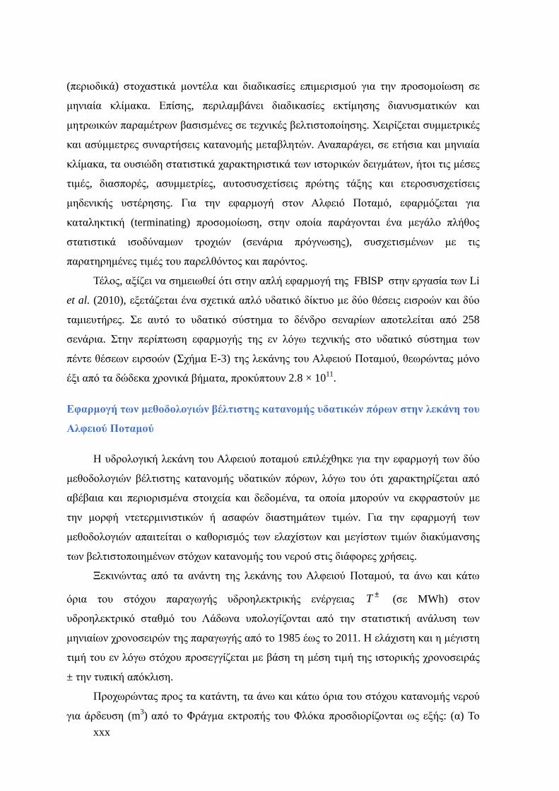
(περιοδικά) στοχαστικά µοντέλα και διαδικασίες επιµερισµού για την προσοµοίωση σε

µηνιαία κλίµακα. Επίσης, περιλαµβάνει διαδικασίες εκτίµησης διανυσµατικών και

µητρωικών παραµέτρων βασισµένες σε τεχνικές βελτιστοποίησης. Χειρίζεται συµµετρικές

και ασύµµετρες συναρτήσεις κατανοµής µεταβλητών. Αναπαράγει, σε ετήσια και µηνιαία

κλίµακα, τα ουσιώδη στατιστικά χαρακτηριστικά των ιστορικών δειγµάτων, ήτοι τις µέσες

τιµές, διασπορές, ασυµµετρίες, αυτοσυσχετίσεις πρώτης τάξης και ετεροσυσχετίσεις

µηδενικής υστέρησης. Για την εφαρµογή στον Αλφειό Ποταµό, εφαρµόζεται για

καταληκτική (terminating) προσοµοίωση, στην οποία παράγονται ένα µεγάλο πλήθος

στατιστικά ισοδύναµων τροχιών (σενάρια πρόγνωσης), συσχετισµένων µε τις

παρατηρηµένες τιµές του παρελθόντος και παρόντος.

Τέλος, αξίζει να σηµειωθεί ότι στην απλή εφαρµογή της FBISP στην εργασία των Li

et al. (2010), εξετάζεται ένα σχετικά απλό υδατικό δίκτυο µε δύο θέσεις εισροών και δύο

ταµιευτήρες. Σε αυτό το υδατικό σύστηµα το δένδρο σεναρίων αποτελείται από 258

σενάρια. Στην περίπτωση εφαρµογής της εν λόγω τεχνικής στο υδατικό σύστηµα των

πέντε θέσεων ειρσοών (Σχήµα Ε-3) της λεκάνης του Αλφειού Ποταµού, θεωρώντας µόνο

έξι από τα δώδεκα χρονικά βήµατα, προκύπτουν 2.8 × 1011.

Εφαρµογή των µεθοδολογιών βέλτιστης κατανοµής υδατικών πόρων στην λεκάνη του

Αλφειού Ποταµού

Η υδρολογική λεκάνη του Αλφειού ποταµού επιλέχθηκε για την εφαρµογή των δύο

µεθοδολογιών βέλτιστης κατανοµής υδατικών πόρων, λόγω του ότι χαρακτηρίζεται από

αβέβαια και περιορισµένα στοιχεία και δεδοµένα, τα οποία µπορούν να εκφραστούν µε

την µορφή ντετερµινιστικών ή ασαφών διαστηµάτων τιµών. Για την εφαρµογή των

µεθοδολογιών απαιτείται ο καθορισµός των ελαχίστων και µεγίστων τιµών διακύµανσης

των βελτιστοποιηµένων στόχων κατανοµής του νερού στις διάφορες χρήσεις.

Ξεκινώντας από τα ανάντη της λεκάνης του Αλφειού Ποταµού, τα άνω και κάτω

όρια του στόχου παραγωγής υδροηλεκτρικής ενέργειας ±T (σε MWh) στον

υδροηλεκτρικό σταθµό του Λάδωνα υπολογίζονται από την στατιστική ανάλυση των

µηνιαίων χρονοσειρών της παραγωγής από το 1985 έως το 2011. Η ελάχιστη και η µέγιστη

τιµή του εν λόγω στόχου προσεγγίζεται µε βάση τη µέση τιµή της ιστορικής χρονοσειράς

± την τυπική απόκλιση.

Προχωρώντας προς τα κατάντη, τα άνω και κάτω όρια του στόχου κατανοµής νερού

για άρδευση (m3) από το Φράγµα εκτροπής του Φλόκα προσδιορίζονται ως εξής: (α) Το

κάτω όριο ορίζεται ίσο µε την µέγιστη δυνατή µηνιαία ζήτηση σε νερό του παρόντος

σχήµατος καλλιεργειών στην περιοχή που αρδεύεται από το εν λόγω φράγµα, και (β) το

άνω όριο ορίζεται ίσο µε την µέγιστη θεωρητική ζήτηση για πλήρη κάλυψη της

αρδευόµενης περιοχής, όπως αυτή δίνεται στο τεύχος µελέτης του µικρού υδροηλεκτρικού

σταθµού στο Φράγµα Φλόκα. Για τον υπολογισµό της µέγιστης µηνιαίας ζήτησης σε

αρδευτικό νερό µε βάση τις παρούσες καλλιέργειες, χρησιµοποιήθηκε το λογισµικό του

FAO CROPWAT 8.0, βάσει του οποίου υπολογίστηκαν οι απαιτήσεις σε νερό άρδευσης

για κάθε καλλιέργεια, λαµβάνοντας υπόψη τη στρεµµατική αναλογία της κάθε

καλλιέργειας στην περιοχή για το σύνολο των υδρολογικών σεναρίων, που εξετάζονται σε

αυτή την εφαρµογή. Οι µέγιστες µηνιαίες τιµές, που προέκυψαν από το σύνολο των

υδρολογικών σεναρίων, εισάγονται ως κάτω όριο του στόχου διανοµής αρδευτικού νερού.

Όσον αφορά τον µικρό υδροηλεκτρικό σταθµό στον Φλόκα, τα άνω και κάτω όρια του

στόχου διανοµής νερού για παραγωγή υδροηλεκτρικής ενέργειας (MWh) προσεγγίζονται

µε παρόµοιο τρόπο, όπως και για την παραγωγή υδροηλεκτρικής ενέργειας στο Λάδωνα. Πιο

συγκεκριµένα, µε βάση τις µηνιαίες χρονοσειρές παραγωγής υδροηλεκτρικής ενέργειας στον

Φλόκα από την αρχή της λειτουργίας του (2011) µέχρι το Σεπτέµβριο 2015, λαµβάνει χώρα

η στατιστική επεξεργασία τους. Η µέση τιµή ± την τυπική απόκλιση της εν λόγω

χρονοσειράς αποτελούν τα κάτω και άνω όρια του στόχου διανοµής νερού της παρούσας

χρήσης.

Τέλος, λαµβάνεται υπόψη µία µηνιαία διανοµή νερού από τον Ερύµανθο Ποταµό ίση

µε 0.6m3/s για την ικανοποίηση της ζήτησης σε πόσιµο νερό για την πόλη του Πύργου και

των όµορων δήµων. Λόγω της έλλειψης στοιχείων καθώς και λόγω της πρόσφατης

λειτουργίας του (τέθηκε σε λειτουργία το έτος 2013), αυτή η χρήση νερού δεν

ενσωµατώνεται στον αλγόριθµο µε την µορφή µεταβλητής απόφασης αλλά ως γνωστή και

δεδοµένη εκτροπή νερού από τον Ερύµανθο. Αξίζει να σηµειωθεί ότι η προσθήκη της και

η διερεύνηση των µοναδιαίων τιµών από τα οφέλη και τις ζηµιές της µη ικανοποίησης

αυτής της χρήσης αποτελεί θέµα µελλοντικής έρευνας.

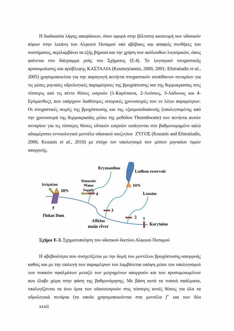
Η σχηµατοποίηση του υδρολογικού δικτύου του Αλφειού Ποταµού και των

παραποτάµων του αναπαριστάται στο Σχήµα Ε-3, στο οποίο περιλαµβάνονται οι πέντε

βασικές θέσεις εισροών υδατοπαροχών στο σύστηµα. Οι θέσεις αυτές επιλέχτηκαν λόγω του

ότι αντιπροσωπεύουν τις πιο σηµαντικές υπολεκάνες, για τις οποίες υπάρχουν διαθέσιµα

υδρολογικά στοιχεία (µέσες µηνιαίες χρονοσειρές βροχόπτωσης, θερµοκρασίας και

απορροής).

xxxii

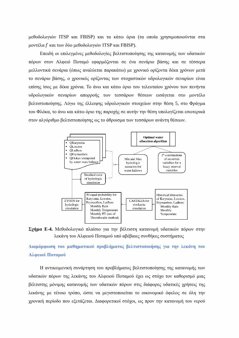
Η διαδικασία λήψης αποφάσεων, όσον αφορά στην βέλτιστη κατανοµή των υδατικών

πόρων στην λεκάνη του Αλφειού Ποταµού υπό αβέβαιες και ασαφείς συνθήκες του

συστήµατος, περιλαµβάνει τα εξής βήµατα και την χρήση των ακόλουθων λογισµικών, όπως

φαίνεται στο διάγραµµα ροής του Σχήµατος (Ε.4). Το λογισµικό στοχαστικής

προσοµοίωσης και πρόβλεψης ΚΑΣΤΑΛΙΑ (Koutsoyiannis, 2000, 2001; Efstratiadis et al.,

2005) χρησιµοποιείται για την παραγωγή πενήντα στοχαστικών ισοπίθανων σεναρίων για

τις µέσες µηνιαίες υδρολογικές παραµέτρους της βροχόπτωσης και της θερµοκρασίας στις

τέσσερις από τις πέντε θέσεις εισροών (1-Καρύταινα, 2-Λούσιος, 3-Λάδωνας και 4-

Ερύµανθος), που υπάρχουν διαθέσιµες ιστορικές χρονοσειρές των εν λόγω παραµέτρων.

Οι στοχαστικές σειρές της βροχόπτωσης και της εξατµισοδιαπνοής (υπολογισµένης από

την χρονοσειρά της θερµοκρασίας µέσω της µεθόδου Thornthwaite) των πενήντα αυτών

σεναρίων για τις τέσσερις θέσεις υδτικών εισροών εισάγονται στο βαθµονοµηµένο απλό

αδιαµέριστο εννοιολογικό µοντέλο υδατικού ισοζυγίου ΖΥΓΟΣ (Kozanis and Efstratiadis,

2006; Kozanis et al., 2010) µε στόχο τον υπολογισµό των µέσων µηνιαίων τιµών

απορροής.

Σχήµα Ε-3. Σχηµατοποίηση του υδατικού δικτύου Αλφειού Ποταµού

Η αβεβαιότητα που συσχετίζεται µε την δοµή του µοντέλου βροχόπτωσης-απορροής

καθώς και µε την επιλογή των παραµέτρων του λαµβάνεται υπόψη µέσω του υπολογισµού

των τυπικών σφαλµάτων µεταξύ των µετρηµένων απορροών και των προσοµοιωµένων

που έλαβε χώρα στην φάση της βαθµονόµησης. Με βάση αυτά τα τυπικά σφάλµατα,

υπολογίζονται τα άνω όρια των υδατοεισροών στις τέσσερις αυτές θέσεις για όλα τα

υδρολογικά σενάρια (τα οποία χρησιµοποιούνται στα µοντέλα f+ και των δύο

µεθοδολογιών ITSP και FBISP) και τα κάτω όρια (τα οποία χρησιµοποιούνται στα

µοντέλα f- και των δύο µεθοδολογιών ITSP και FBISP).

Επειδή οι επιλεγµένες µεθοδολογίες βελτιστοποίησης της κατανοµής των υδατικών

πόρων στον Αλφειό Ποταµό εφαρµόζονται σε ένα σενάριο βάσης και σε τέσσερα

µελλοντικά σενάρια (όπως αναλύεται παρακάτω) µε χρονικό ορίζοντα δέκα χρόνων µετά

το σενάριο βάσης, ο χρονικός ορίζοντας των στοχαστικών υδρολογικών σεναρίων είναι

επίσης ίσος µε δέκα χρόνια. Το άνω και κάτω όριο του τελευταίου χρόνου των πενήντα

υδρολογικών σεναρίων απορροής των τεσσάρων θέσεων εισάγεται στο µοντέλο

βελτιστοποίησης. Λόγω της έλλειψης υδρολογικών στοιχείων στην θέση 5, στο Φράγµα

του Φλόκα, το άνω και κάτω όριο της παροχής σε αυτήν την θέση υπολογίζεται εσωτερικά

στον αλγόριθµο βελτιστοποίησης ως το άθροισµα των τεσσάρων ανάντη θέσεων.

Σχήµα Ε-4. Μεθοδολογικό πλαίσιο για την βέλτιστη κατανοµή υδατικών πόρων στην λεκάνη του Αλφειού Ποταµού υπό αβέβαιες συνθήκες συστήµατος

∆ιαµόρφωση του µαθηµατικού προβλήµατος βελτιστοποιήσης για την λεκάνη του

Αλφειού Ποταµού

Η αντικειµενική συνάρτηση του προβλήµατος βελτιστοποίησης της κατανοµής των

υδατικών πόρων της λεκάνης του Αλφειού Ποταµού έχει ως στόχο τον καθορισµό µιας

βέλτιστης µόνιµης κατανοµής των υδατικών πόρων στις διάφορες υδατικές χρήσεις της

λεκάνης µε τέτοιο τρόπο, ώστε να µεγιστοποιείται το οικονοµικό όφελος σε όλη την

χρονική περίοδο που εξετάζεται. ∆ιαφορετικοί στόχοι, ως προν την κατανοµή του νερού

xxxiv

στις διάφορες χρήσεις, συσχετίζονται µε διαφορετικές στρατηγικές διαχείρισης των

υδατικών πόρων, καθώς και µε διαφορετικές οικονοµικές επιπτώσεις, όσον αφορά στην

πιθανοτική ποινή και την απώλεια ευκαιρίας (probabilistic penalty and opportunity loss).

Η αντικειµενική συνάρτηση έχει την µορφή της σχέσης (Ε.16). Η ποινή (penalty)

συσχετίζεται µε την µη ορθή κατανοµή και διαχείριση των υδατικών πόρων και

περιλαµβάνει (α) ποινή λόγω της έλλειψης νερού σε σχέση µε την ζήτηση καθώς και λόγω

υπερχειλίσεων, εξ αιτίας παραγωγής υδροηλεκτρικής ενέργειας, και (β) ποινή στην

περίπτωση έλλειψης νερού σε σχέση µε την ζήτηση, εξ αιτίας χρήσεως νερού για άρδευση.

Το πρόβληµα βελτιστοποίησης επιλύεται για χρονικό ορίζοντα ενός έτους µε µηνιαίο

βήµα, δηλαδή περιλαµβάνει δώδεκα στάδια.

Το µαθηµατικό πρόβληµα βελτιστοποίησης της κατανοµής των υδατικών πόρων της

λεκάνης του Αλφειού Ποταµού περιλαµβάνει το ακόλουθο σύστηµα περιορισµών:

(1) Εξισώσεις διατήρησης του όγκου νερού σε κάθε χρονικό βήµα/στάδιο στον Φράγµα

του Λάδωνα, στο Φράγµα του Φλόκα και στον υδροηλεκτρικό σταθµό του Φλόκα,

(2) Περιορισµοί ελάχιστης και µέγιστης αποθηκευτικής ικανότητας του ταµιευτήρα του

Λάδωνα,

(3) Περιορισµοί ελάχιστης και µέγιστης ικανότητας παροχής των τουρµπινών του

υδροηλεκτρικού σταθµού του Λάδωνα και του Φλόκα,

(4) Περιορισµοί ελάχιστης απαιτούµενης περιβαλλοντικής παροχής κατάντη των δύο

υδροηλεκτρικών σταθµών,

(5) Περιορισµός για την παροχή της ιχθυόσκαλας στο Φράγµα του Φλόκα,

(6) Περιορισµός ελάχιστης µηνιαίας ζήτησης αρδευτικού νερού από το Φράγµα του

Φλόκα,

(8) Περιορισµός για την εκτροπή σταθερής παροχής νερού από τον Ερύµανθο για την

ικανοποίηση της ζήτησης πόσιµου νερού.

Η εξάτµιση από την επιφάνεια του ταµιευτήρα του Λάδωνα (m3) υπολογίζεται µέσω

του γινοµένου του µηνιαίου ρυθµού εξάτµισης (m) και της µέσης επιφάνειας του

ταµιευτήρα στην αρχή (επιφάνεια ταµιευτήρα του προηγούµενου βήµατος) και στο τέλος

του χρονικού βήµατος (επιφάνεια ταµιευτήρα του τρέχοντος βήµατος).

Τέλος, οι µη γραµµικές εξισώσεις, όπως π.χ. η σχέση που συνδέει την παροχή των

τουρµπινών µε την παραγωγή υδροηλεκτρικής ενέργειας, αντικαθιστώνται µε τις

γραµµικές µορφές τους µέσω γραµµικής παρεµβολής. Η αβεβαιότητα που εισάγεται στο

σύστηµα από αυτή την απλοποίηση δεν λαµβάνεται υπόψη στη διαδικασία

βελτιστοποίησης. Ωστόσο, αξίζει να σηµειωθεί ότι για όλες τις γραµµικοποιηµένες

εξισώσεις ο συντελεστής R2 από τη γραµµική παρεµβολή λαµβάνει τιµές ≥0.9.

Ανάλυση του µοναδιαίου κέρδους και της µοναδιαίας ποινής για την παραγωγή

υδροηλεκτρικής ενέργειας

Η τιµή πώλησης της υδροηλεκτρικής ενέργειας δεν είναι σταθερή και καθορισµένη

λόγω της απελευθέρωσης της αγοράς ενέργειας. Στην Ελλάδα, η τιµή αυτή εξαρτάται από

την ωριαία οριακή τιµή του συστήµατος ενέργειας, η οποία αντανακλά την τιµή κέρδους

της ενέργειας από τους παραγωγούς. Επιπλέον, επηρεάζεται πρώτον, από τον συνδυασµό

των προσφερόµενων τιµών πώλησης από τον κάθε παραγωγό και την δυνατότητα

παραγωγής της κάθε µονάδας παραγωγής, και δεύτερον, από την ωριαία ζήτηση ενέργειας

του συστήµατος. Με βάση την εµπειρική γνώση του Μηχανικού, υπεύθυνου για την

λειτουργία του υδροηλεκτρικού σταθµού του Λάδωνα, προσδιορίστηκαν η ελάχιστη και η

µέγιστη τιµή του µοναδιαίου κέρδους του υδροηλεκτρικού σταθµού υπό ευνοϊκές

συνθήκες (συσχετιζόµενες µε το µέγιστο δυνατό κέρδος από την παραγωγή

υδροηλεκτρικής ενέργειας) και υπό µη ευνοϊκές συνθήκες (συσχετιζόµενες µε το ελάχιστο

δυνατό κέρδος από την παραγωγή υδροηλεκτρικής ενέργειας). Αυτές οι τέσσερις τιµές

χρησιµοποιούνται για την δηµιουργία του άνω και κάτω ασαφούς ορίου για την µοναδιαία

τιµή κέρδους από την διανοµή ενός κυβικού µέτρου νερού για την παραγωγή

υδροηλεκτρικής ενέργειας στον Λάδωνα. Οι τιµές αυτές επιβεβαιώνονται και από µία

µελέτη που αναλύει στατιστικά τις ωριαίες οριακές τιµές ενέργειας στην Ελλάδα

(Stefanakos, 2009). Λόγω της έλλειψης περαιτέρω στοιχείων, δεν λαµβάνεται κάποια

ασαφής συνάρτηση συµµετοχής (membership function) για την εν λόγω µεταβλητή, παρά

µόνο οι ακραίες τιµές µε ασαφή άνω και κάτω όρια.

Η σκιώδης τιµή (shadow price) της ποινής, που αφορά στην παραγωγή

υδροηλεκτρικής ενέργειας στον Λάδωνα, αποτελείται από δύο µέρη: (1) Την ποινή σε

περίπτωση έλλειψης νερού, σε σχέση µε αυτήν που απαιτείται για την ικανοποίηση του

στόχου παραγωγής υδροηλεκτρικής ενέργειας, και (2) την ποινή από τις υπερχειλίσεις από

το Φράγµα του Λάδωνα, για τιµές µεγαλύτερες από την περιβαλλοντική παροχή, µε στόχο

να µειωθεί η ευκαιρία απώλειας (opportunity loss). Η µέγιστη τιµή της µοναδιαίας ποινής

λαµβάνεται ίση µε την µέγιστη δυνατή και καταγεγραµµένη τιµή πώλησης, σύµφωνα µε

την Ρυθµιστική Αρχή Ενέργειας (150€/MWh). Οι υπόλοιπες τιµές των ασαφών ορίων

υπολογίζονται µε βάση την εµπειρική γνώση του Μηχανικού στο υδροηλεκτρικό

xxxvi

εργοστάσιο του Λάδωνα.

Οι τιµές του µοναδιαίου κέρδους για την παραγωγή υδροηλεκτρικής ενέργειας στο

µικρό υδροηλεκτρικό εργοστάσιο του Φλόκα υπολογίζονται απλούστερα µε βάση την

σταθερή και προκαθορισµένη τιµή πώλησης για τα µικρά υδροηλεκτρικά. Η µοναδιαία

ποινή ορίζεται ως διάστηµα τιµών µε ντετερµινιστικά όρια ίσα µε τις τιµές του άνω

ασαφούς ορίου που υπολογίστηκε για τον υδροηλεκτρικό σταθµό του Λάδωνα.

Ανάλυση του µοναδιαίου κέρδους και της µοναδιαίας ποινής για την αρδευτική

χρήση

Η µηνιαία αρδευτική ζήτηση αποτελείται από δύο µέρη: (1) Μία προκαθορισµένη

και σταθερή τιµή που έχει συµφωνηθεί µεταξύ της ∆.Ε.Η. και του Γ.Ο.Ε.Β. Αλφειού-

Πηνειού, και (2) µία επιπρόσθετη ποσότητα νερού, η οποία εξαρτάται από το είδος των

καλλιεργειών και τις τυχαίες υδατικές εισροές στο Φράγµα του Φλόκα. Οι συνολικές

απαιτήσεις σε αρδευτικό νερό υπολογίζονται µε το λογισµικό του FAO, CROPWAT 8.0. Το

µοναδιαίο κέρδος από την διανοµή νερού στην άρδευση ερµηνεύεται ως το πιθανό καθαρό

κέρδος από την αγροτική παραγωγή των υπαρχουσών καλλιεργειών. Για τον υπολογισµό

του λαµβάνονται υπόψη τα ακρότατα (ελάχιστη και µέγιστη τιµή) της τιµής πώλησης των

αγροτικών προϊόντων, του κόστους της παραγωγής, του κόστους χρέωσης του αρδευτικού

καναλιού του ΓΟΕΒ και του κόστους χρέωσης των ΤΟΕΒ. Αυτές οι τιµές συνδυάζονται µε

το άνω και κάτω όριο τιµών των υδατικών εισροών στο Φράγµα του Φλόκα για τον τελικό

υπολογισµό των ασαφών ορίων του µοναδιαίου κέρδους. Τέλος, η τιµή της µοναδιαίας

ποινής για τις ελλείψεις νερού των αρδευτικών αναγκών υπολογίζεται µε βάση την

οικονοµική απώλεια του αγροτικού εισοδήµατος, λόγω της µείωσης της αγροτικής

παραγωγής από την έλλειψη νερού.

Μελλοντικά αγροτικά και υδατικά σενάρια

Το πρόγραµµα «Η βιωσιµότητα της Eυρωπαϊκής Αρδευόµενης Γεωργίας υπό το

πρίσµα της Κοινοτική Οδηγίας Πλαίσιο για το Νερό και την Ατζέντα 2000 (WADI)»

επικεντρώνεται στις αλλαγές της Eυρωπαϊκής γεωργικής πολιτικής και των υδάτων,

δεδοµένου ότι επηρεάζουν την οικονοµική, κοινωνική και περιβαλλοντική

αποτελεσµατικότητα της άρδευσης των κρατών µελών. Σκοπός του ήταν να διερευνήσει

τις επιπτώσεις της αλλαγής πολιτικής στον τοµέα της άρδευσης στην Ισπανία, την Ελλάδα,

την Ιταλία και το Ηνωµένο Βασίλειο, µε ιδιαίτερη έµφαση στην Κοινοτική Οδηγία

Πλαίσιο για τα ύδατα (WFD) και τη µεταρρύθµιση της Κοινής Γεωργικής Πολιτικής

(CAP). Η γεωργική πολιτική το 2001, όπως καθορίζεται από την CAP, λαµβάνεται ως

σενάριο αναφοράς. Αυτό το έτος αναφοράς χρησιµοποιείται για να παρέχει ένα σχετικό

σηµείο αναφοράς για τον καθορισµό των µελλοντικών σεναρίων. Αυτό το σενάριο

επεκτείνεται 10 έτη µετά το έτος αναφοράς (2001-2010), µε βάση τις προβλέψεις των

γεωργικών αγορών και των τιµών από την ΕΕ, τον Οργανισµό Οικονοµικής Συνεργασίας

και Ανάπτυξης (ΟΟΣΑ) και άλλες πηγές. Οι εκτιµήσεις των κυριότερων παραµέτρων για

κάθε µελλοντικό σενάριο χρησιµοποιούνται ως δεδοµένα εισόδου στα µοντέλα

βελτιστοποίησης, προκειµένου να καταστεί δυνατή η αξιολόγηση της επίδραση των

αλλαγών της αγροτικής πολιτικής καθώς και της πολιτικής διαχείρισης των υδατικών

πόρων της ΕΕ στα οφέλη του υδροσυστήµατος.

Για την καλύτερη κατανόηση του περιεχοµένου και της φιλοσοφίας των

µελλοντικών σεναρίων, τα τέσσερα γεωργικά και υδατικά WADI σενάρια περιγράφονται

εν συντοµία. Το σενάριο «Παγκόσµιων Αγορών» (World Markets) συσχετίζεται µε την

ιδιωτική κατανάλωση και ένα πολύ ανεπτυγµένο και ολοκληρωµένο παγκόσµιο εµπορικό

σύστηµα. Το σενάριο «Παγκόσµιας Αειφορίας» (Global Sustainability) δίνει έµφαση στις

κοινωνικές και οικολογικές αξίες που συνδέονται µε τα παγκόσµια θεσµικά όργανα και το

εµπορικό σύστηµα συναλλαγών. Κεντρικό ρόλο στο εν λόγω σενάριο παίζουν η ενεργός

συµµετοχή στη δηµόσια πολιτική και τη διεθνή συνεργασία, τόσο εντός της Ευρωπαϊκής

Ένωσης, όσο και σε παγκόσµιο επίπεδο. Το σενάριο «Περιφερειακή Επιχείρηση»

(Provincial Enterprise) επικεντρώνει στην ιδιωτική κατανάλωση εντός εθνικού και

περιφερειακού επιπέδου για να απεικονίσει τοπικές προτεραιότητες και συµφέροντα. Το

σενάριο «Τοπική ∆ιοίκηση» (Local Stewardship) δίνει βαρύτητα στις ισχυρές τοπικές και

περιφεριακές κυβερνήσεις µε έµφαση στις κοινωνικές αξίες, την αυτάρκεια και την

διατήρηση των φυσικών πόρων και του περιβάλλοντος.

Αποτελέσµατα και συµπεράσµατα

Η προτεινόµενη µεθοδολογία έχει ως σκοπό, αφενός, να καθορίσει τον επιθυµητό

στόχο κατανοµής των υδατικών πόρων µε ελαχιστοποίηση του κινδύνου της οικονοµικής

ποινής και της απώλειας ευκαιριών, και αφετέρου να καθορίσει ένα βελτιστοποιηµένο

σχέδιο κατανοµής του νερού, εξασφαλίζοντας την µεγιστοποίηση του καθαρού κέρδους

του συστήµατος σε όλη την χρονική περίοδο που εξετάζεται. Υπολογίζονται

ντετερµινιστικά ή ασαφή άνω και κάτω όρια για τους στόχους βέλτιστης κατανοµής του

xxxviii

νερού και των πιθανοτικών κατανοµών νερού και των ελλείψεων, καθώς και για τα

συνολικά οφέλη του συστήµατος για τις κύριες χρήσεις των υδάτων. Τα αποτελέσµατα που

προέκυψαν δείχνουν ότι οι µεταβολές στους στόχους κατανοµής των υδατικών πόρων

µπορούν να εκφράσουν διαφορετικές στρατηγικές για τη διαχείριση των υδατικών πόρων

και να οδηγήσουν σε διαφορετικές οικονοµικές επιπτώσεις σε συνθήκες αβεβαιότητας.

Τα κυριότερα αποτελέσµατα από την εφαρµογή της ITSP και της FBISP για την

βέλτιστη κατανοµή των υδατικών πόρων του Αλφειού Ποταµού είναι τα ακόλουθα:

(1) Οι τιµές των µηνιαίων βελτιστοποιηµένων στόχων για την κατανοµή του νερού

συγκρίνονται µε τις µέγιστες αποδεκτές τιµές τους για όλες τις χρήσεις µε στόχο τον

καθορισµό των συµβιβασµών (tradeoffs) και των προτεραιοτήτων, όσον αφορά την

κατανοµή του νερού. Από τους βελτιστοποιηµένους στόχους των τριών κύριων υδατικών

χρήσεων, συµπεραίνεται ότι η υψηλότερη προτεραιότητα για την κατανοµή του νερού

δίνεται στην άρδευση, δεδοµένου ότι έχει το υψηλότερο µοναδιαίο όφελος (unit benefit),

ταυτοχρόνως όµως και την µεγαλύτερη µοναδιαία ποινή (unit penalty). Οι επόµενες

προτεραιότητες αποδίδονται στην παραγωγή υδροηλεκτρικής ενέργειας στο Φράγµα του

Φλόκα και τέλος στην παραγωγή υδροηλεκτρικής ενέργειας στο Φράγµα του Λάδωνα.

(2) Οι βελτιστοποιηµένοι συνολικοί ετήσιοι στόχοι κατανοµής νερού που προκύπτουν

για τα διάφορα µελλοντικά αγροτικά και υδατικά WADI σενάρια, συγκρινόµενοι µε αυτούς

από το σενάριο βάσης, δεν έχουν σηµαντικές διαφοροποιήσεις, καθώς η βασική επίδραση

αυτών των σεναρίων βρίσκεται στο καθαρό κέρδος του συστήµατος. Με βάση την σύγκριση

των συνολικών καθαρών οφελειών του συστήµατος από τα τέσσερα µελλοντικά σενάρια µε

το βασικό σενάριο, η µεγαλύτερη αύξηση παρατηρείται στο σενάριο«Τοπική ∆ιοίκηση»

(Local Stewardship)και η µοναδική µείωση κέρδους στο σενάριο «Παγκόσµιων Αγορών»

(World Warket).

(3) Όσον αφορά την άρδευση, στα περισσότερα υδρολογικά σενάρια, η ετήσια

έλλειψη αρδευτικού νερού είναι µηδενική, καθώς η προκύπτουσα διανοµή του νερού για

άρδευση ισούται µε τον βελτιστοποιηµένο στόχο διανοµής. Για τα ελάχιστα υδρολογικά

σενάρια µε µη µηδενική έλλειψη, αν οι αγρότες δεν έχουν κάποια εναλλακτική υδατική

πηγή τροφοδοσίας, είναι πολύ πιθανή η µείωση της αγροτικής παραγωγής. Αυτές οι

ελλείψεις παρατηρούνται τον Αύγουστο και τον Σεπτέµβριο, γεγονός που εξηγείται από

τον συνδυασµό των χαµηλών υδατικών παροχών για αυτούς τους µήνες µε την αυξηµένη

αρδευτική ζήτηση. Από την άλλη, η παραγωγή υδροηλεκτρικής ενέργειας στον Λάδωνα

και στον Φλόκα για τα περισσότερα υδρολογικά σενάρια αποκλίνει από τους

βελτιστοποιηµένους στόχους. Κατά συνέπεια, παρατηρούνται µη µηδενικές ελλείψεις στα

περισσότερα υδρολογικά σενάρια και για τους δύο σταθµούς. Για την παραγωγή

υδροηλεκτρικής ενέργειας στον Λάδωνα, η υψηλότερη έλλειψη σηµειώνεται από τον

Ιανουάριο έως τον Απρίλιο (µε την υψηλότερη να καταγράφεται τον Μάιο). Αυτό

εξηγείται, επειδή, για να ικανοποιηθεί η αρδευτική ζήτηση τους µήνες από περίπου Μάιο

έως Σεπτέµβριο, απαιτείται η αποθήκευση των εισροών στον ταµιευτήρα του Λάδωνα από

Ιανουάριο έως Απρίλιο. Αυτή την περίοδο εντοπίζεται µία σύγκρουση ανάµεσα στις δύο

αυτές χρήσεις. Αντιστοίχως για την υδροηλεκτική παραγωγή στον Φλόκα, η υψηλότερη

έλλειψη σηµειώνεται κατά την αρδευτική περίοδο από τον Ιούνιο έως Οκτώβριο (µε την

υψηλότερη να καταγράφεται τον Οκτώβριο), δείχνοντας µία σύγκρουση των δύο χρήσεων.

Το µικρό υδροηλεκτρικό του Φλόκα τίθεται σε λειτουργία µόνο εφόσον έχει ικανοποηθεί

πλήρως η αρδευτική ζήτηση και, βάσει αυτού, προκύπτουν ελλείψεις νερού για την εν

λόγω χρήση, όταν η παροχή στην θέση του Φράγµατος του Φλόκα δεν επαρκεί.

(4) Από την σύγκριση των αποτελεσµάτων των δύο µεθοδολογιών, FBISP και ITSP,

προκύπτει ότι τα αποτελέσµατα είναι συµβατά και συνεπή µεταξύ τους. Ωστόσο, η

ενσωµάτωση της ασαφούς φύσεως των αβεβαιοτήτων στην FBISP οδηγεί σε µία πιο

αναλυτική και εκλεπτυσµένη προσέγγιση της επίδρασης των αβεβαιοτήτων στην ελάχιστη

και µέγιστη τιµή των διαστηµάτων τιµών των αποτελεσµάτων.

Τέλος, η προτεινόµενη µεθοδολογία επιτυγχάνει να εφαρµόσει τις δύο επιλεγµένες

µεθοδολογίες βέλτιστης κατανοµής των υδατικών πόρων για πρώτη φορά σε µια πραγµατική

λεκάνη µε πολλαπλές θέσεις υδατικών εισροών και πολλαπλών χρονικών βηµάτων

ξεπερνώντας τις δυσκολίες που καταγράφονται από τους συγγραφείς για την εφαρµογή τους σε

µεγάλης κλίµακας λεκάνες.

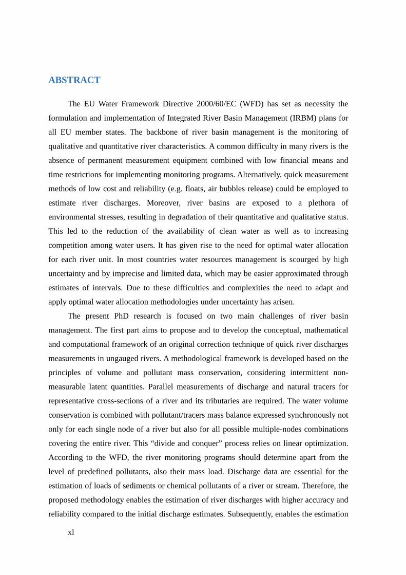
xl

ABSTRACT

The EU Water Framework Directive 2000/60/EC (WFD) has set as necessity the

formulation and implementation of Integrated River Basin Management (IRBM) plans for

all EU member states. The backbone of river basin management is the monitoring of

qualitative and quantitative river characteristics. A common difficulty in many rivers is the

absence of permanent measurement equipment combined with low financial means and

time restrictions for implementing monitoring programs. Alternatively, quick measurement

methods of low cost and reliability (e.g. floats, air bubbles release) could be employed to

estimate river discharges. Moreover, river basins are exposed to a plethora of

environmental stresses, resulting in degradation of their quantitative and qualitative status.

This led to the reduction of the availability of clean water as well as to increasing

competition among water users. It has given rise to the need for optimal water allocation

for each river unit. In most countries water resources management is scourged by high

uncertainty and by imprecise and limited data, which may be easier approximated through

estimates of intervals. Due to these difficulties and complexities the need to adapt and

apply optimal water allocation methodologies under uncertainty has arisen.

The present PhD research is focused on two main challenges of river basin

management. The first part aims to propose and to develop the conceptual, mathematical

and computational framework of an original correction technique of quick river discharges

measurements in ungauged rivers. A methodological framework is developed based on the

principles of volume and pollutant mass conservation, considering intermittent non-

measurable latent quantities. Parallel measurements of discharge and natural tracers for

representative cross-sections of a river and its tributaries are required. The water volume

conservation is combined with pollutant/tracers mass balance expressed synchronously not

only for each single node of a river but also for all possible multiple-nodes combinations

covering the entire river. This “divide and conquer” process relies on linear optimization.

According to the WFD, the river monitoring programs should determine apart from the

level of predefined pollutants, also their mass load. Discharge data are essential for the

estimation of loads of sediments or chemical pollutants of a river or stream. Therefore, the

proposed methodology enables the estimation of river discharges with higher accuracy and

reliability compared to the initial discharge estimates. Subsequently, enables the estimation

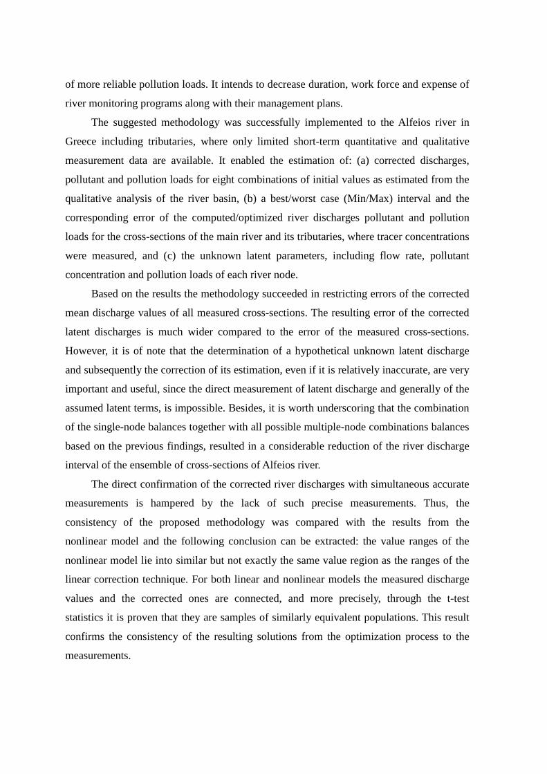
of more reliable pollution loads. It intends to decrease duration, work force and expense of

river monitoring programs along with their management plans.

The suggested methodology was successfully implemented to the Alfeios river in

Greece including tributaries, where only limited short-term quantitative and qualitative

measurement data are available. It enabled the estimation of: (a) corrected discharges,

pollutant and pollution loads for eight combinations of initial values as estimated from the

qualitative analysis of the river basin, (b) a best/worst case (Min/Max) interval and the

corresponding error of the computed/optimized river discharges pollutant and pollution

loads for the cross-sections of the main river and its tributaries, where tracer concentrations

were measured, and (c) the unknown latent parameters, including flow rate, pollutant

concentration and pollution loads of each river node.

Based on the results the methodology succeeded in restricting errors of the corrected

mean discharge values of all measured cross-sections. The resulting error of the corrected

latent discharges is much wider compared to the error of the measured cross-sections.

However, it is of note that the determination of a hypothetical unknown latent discharge

and subsequently the correction of its estimation, even if it is relatively inaccurate, are very

important and useful, since the direct measurement of latent discharge and generally of the

assumed latent terms, is impossible. Besides, it is worth underscoring that the combination

of the single-node balances together with all possible multiple-node combinations balances

based on the previous findings, resulted in a considerable reduction of the river discharge

interval of the ensemble of cross-sections of Alfeios river.

The direct confirmation of the corrected river discharges with simultaneous accurate

measurements is hampered by the lack of such precise measurements. Thus, the

consistency of the proposed methodology was compared with the results from the

nonlinear model and the following conclusion can be extracted: the value ranges of the

nonlinear model lie into similar but not exactly the same value region as the ranges of the

linear correction technique. For both linear and nonlinear models the measured discharge

values and the corrected ones are connected, and more precisely, through the t-test

statistics it is proven that they are samples of similarly equivalent populations. This result

confirms the consistency of the resulting solutions from the optimization process to the

measurements.

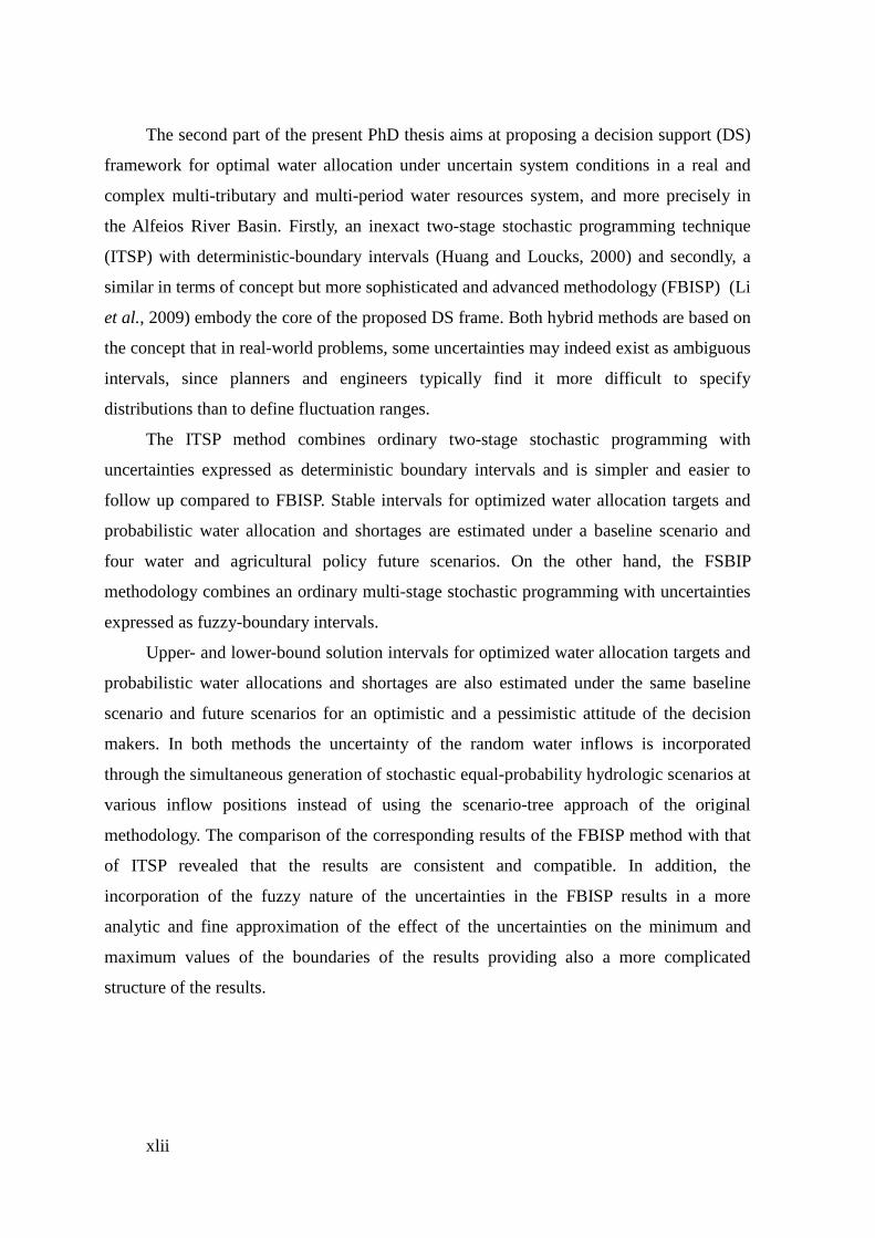
xlii

The second part of the present PhD thesis aims at proposing a decision support (DS)

framework for optimal water allocation under uncertain system conditions in a real and

complex multi-tributary and multi-period water resources system, and more precisely in

the Alfeios River Basin. Firstly, an inexact two-stage stochastic programming technique

(ITSP) with deterministic-boundary intervals (Huang and Loucks, 2000) and secondly, a

similar in terms of concept but more sophisticated and advanced methodology (FBISP) (Li

et al., 2009) embody the core of the proposed DS frame. Both hybrid methods are based on

the concept that in real-world problems, some uncertainties may indeed exist as ambiguous

intervals, since planners and engineers typically find it more difficult to specify

distributions than to define fluctuation ranges.

The ITSP method combines ordinary two-stage stochastic programming with

uncertainties expressed as deterministic boundary intervals and is simpler and easier to

follow up compared to FBISP. Stable intervals for optimized water allocation targets and

probabilistic water allocation and shortages are estimated under a baseline scenario and

four water and agricultural policy future scenarios. On the other hand, the FSBIP

methodology combines an ordinary multi-stage stochastic programming with uncertainties

expressed as fuzzy-boundary intervals.

Upper- and lower-bound solution intervals for optimized water allocation targets and

probabilistic water allocations and shortages are also estimated under the same baseline

scenario and future scenarios for an optimistic and a pessimistic attitude of the decision

makers. In both methods the uncertainty of the random water inflows is incorporated

through the simultaneous generation of stochastic equal-probability hydrologic scenarios at

various inflow positions instead of using the scenario-tree approach of the original

methodology. The comparison of the corresponding results of the FBISP method with that

of ITSP revealed that the results are consistent and compatible. In addition, the

incorporation of the fuzzy nature of the uncertainties in the FBISP results in a more

analytic and fine approximation of the effect of the uncertainties on the minimum and

maximum values of the boundaries of the results providing also a more complicated

structure of the results.

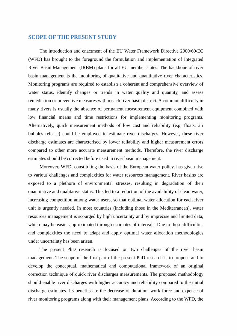
SCOPE OF THE PRESENT STUDY

The introduction and enactment of the EU Water Framework Directive 2000/60/EC

(WFD) has brought to the foreground the formulation and implementation of Integrated

River Basin Management (IRBM) plans for all EU member states. The backbone of river

basin management is the monitoring of qualitative and quantitative river characteristics.

Monitoring programs are required to establish a coherent and comprehensive overview of

water status, identify changes or trends in water quality and quantity, and assess

remediation or preventive measures within each river basin district. A common difficulty in

many rivers is usually the absence of permanent measurement equipment combined with

low financial means and time restrictions for implementing monitoring programs.

Alternatively, quick measurement methods of low cost and reliability (e.g. floats, air

bubbles release) could be employed to estimate river discharges. However, these river

discharge estimates are characterised by lower reliability and higher measurement errors

compared to other more accurate measurement methods. Therefore, the river discharge

estimates should be corrected before used in river basin management.

Moreover, WFD, constituting the basis of the European water policy, has given rise

to various challenges and complexities for water resources management. River basins are

exposed to a plethora of environmental stresses, resulting in degradation of their

quantitative and qualitative status. This led to a reduction of the availability of clean water,

increasing competition among water users, so that optimal water allocation for each river

unit is urgently needed. In most countries (including those in the Mediterranean), water

resources management is scourged by high uncertainty and by imprecise and limited data,

which may be easier approximated through estimates of intervals. Due to these difficulties

and complexities the need to adapt and apply optimal water allocation methodologies

under uncertainty has been arisen.

The present PhD research is focused on two challenges of the river basin

management. The scope of the first part of the present PhD research is to propose and to

develop the conceptual, mathematical and computational framework of an original

correction technique of quick river discharges measurements. The proposed methodology

should enable river discharges with higher accuracy and reliability compared to the initial

discharge estimates. Its benefits are the decrease of duration, work force and expense of

river monitoring programs along with their management plans. According to the WFD, the

xliv

river monitoring programs should determine apart from the level of predefined pollutants,

also their mass load. Discharge data are essential for the estimation of loads of sediments

or chemical pollutants of a river or stream (NCSU, 2008). Based on the corrected river

discharges the computation of more reliable pollution loads should be enabled by the

developed methodology.

For the application of this methodology the Alfeios River Basin in Western

Peloponnisos in Greece has been selected. The first reason for this is the availability

exclusively of limited short-term measurement data for the assessment of its water quality

and quantity. Moreover, permanent gauge stations along the main river and its tributaries,

except for the direct or indirect discharge measurements at the hydroelectric power

generation stations, are absent. The second reason is that for the Alfeios catchment quick

river discharge measurements together with measurements of various pollutant/ natural

tracers are available enabling the testing of the correction technique. Finally, the Alfeios

river is hailed as an important watershed due to its great natural, ecological, social and

economic value for Western Greece, since it has the longest watercourse and the highest

flow-rate in the Peloponnisos region.

The second part of the present PhD thesis aims at proposing a decision support (DS)

framework for optimal water allocation under uncertain system conditions in a real and

complex multi-tributary and multi-period water resources system, and more precisely into

the Alfeios River Basin. Firstly, an inexact two-stage stochastic programming technique

(ITSP) with deterministic-boundary intervals (Huang and Loucks, 2000) and secondly, a

similar in terms of concept but more sophisticated and advanced methodology (FBISP)

with fuzzy- instead of deterministic-boundary intervals (Li et al., 2009) constitute the core

of the proposed DS frame. Both hybrid methods are based on the concept that in real-world

problems, some uncertainties may indeed exist as ambiguous intervals, since planners and

engineers typically find it more difficult to specify distributions than to define fluctuation

ranges.

A further reason for the selection of the Alfeios Riber Basin for the application of the

two optimal water allocation methods under uncertain and vague system condition is that

Alfeios is a river basin, combining various water uses, including (a) irrigation, which plays

a vital social, economic and environmental role associated among others with agricultural

income and with water, food and energy efficiency, (b) hydropower generation and (c)

drinking water supply. In Alfeios River Basin, as in many countries including

Mediterranean, water resources management has been focused up to now on an essentially

supply-driven approach. It is characterized by a lack of effective operational strategies.

Authority responsibility relationships are fragmented, and law enforcement and policy

implementations are weak, facts that lead to difficulties in gathering the necessary data for

water resources management or, even worse, to data loss. In some cases, river monitoring,

which is crucial for water quantity and quality assessment, if present, is inefficient with

intermittent periods with no measurements resulting in unreliable and/or short-term data. In

this case, some sources of obtaining hydrologic, technical, economic and environmental

data required for water resources management come from making additional periodic

measuring expeditions, indirectly such as from expert knowledge. Data of this type with a

high degree of uncertainty may be easily defined as fluctuation ranges and, therefore,

simulated as intervals with lower and upper (deterministic or fuzzy) bounds without the

need for any distributional or probabilistic information. Therefore, the ITSP and the FBSIP

method can be used for optimal water allocation in Alfeios River Basin.

xlvi

STRUCTURE OF THE PHD THESIS

The present PhD thesis is composed of five chapters covering the total of the

research and a thorough description of the selected river basin for the application of the

studied methodologies, the Alfeios River Basin in Greece. In the first chapter the the

Alfeios River Basin is depicted. More precisely, the characteristics (natural, socio-

economic and administrative/institutional) of the river basin are identified and presented,

and the related literature is critically reviewed.

The second chapter is dedicated to the correction technique of quick river discharge

measurements. It contains the theoretical background information necessary for the

building and formulation of the correction technique. An analytic state of the art for the

error correction techniques of river flow rate measurement is included in order to highlight

the originality of the proposed methodology and to depict the origins of its conceptual

development. Then, the methodological and mathematical framework is described in

details. The application of the suggested methodology in the Alfeios River Basin is based

on four measuring expeditions. The complete and analytic results of one of the four

measuring expeditions are presented here, whereas the results of the others are given

synoptically in the Appendixes. At the end of the chapter discussion and conclusions are

included.

The third and the fourth chapters are devoted to the demonstration of a decision

support framework for optimal water allocation under uncertainty in a real and complex

multi-tributary and multi-period water resources system, in the Alfeios hydrosystem. More

precisely, the third chapter describes the first of two selected hybrid methodologies of

optimal water allocation, the ITSP with deterministic boundaries as developed by Huang

and Loucks (2000). It includes the presentation of the mathematical background of the

ITSP as provided by its developers. Then, the simplified schematization of the Alfeios

hydrosystem for the application of the optimal water allocation methodology is shortly

described. A specific subsection focuses on the incorporation of the water inflow dynamics

through the simultaneous stochastic generation of equal-probability hydrologic scenarios at

various locations in the Alfeios River Basin, since it underscores the originality of this

research part. The benefit and penalty concept of the optimization process for the two main

water uses (hydropower and irrigation) are also analyzed in depth. The WADI future

agriculture and water scenarios are shortly introduced. The formulation of the optimization

problem for the Alfeios hydrosystem is also included. At last the analytic results and their

interpretation, as well as discussion and conclusions are provided. In order to facilitate the

understanding of the steps of the proposed process and their interactions, a flow chart is

also included.

The second methodology, being the FBISP method as proposed by Li et al. (2010b),

is described and discussed in the fourth chapter. The reason for organizing these two

chapters as described above is to facilitate a deeper understanding of this type of

methodology through the application of the first method, which is simpler and easier

regarding follow up. This chapter includes the presentation of the mathematical

background of the FBISP as well as the limitations of the applied methodology and the

proposed changes. The mathematical formulation of the optimization problem for the

Alfeios hydrosystem is also depicted. The steps of the proposed process and the used

software programs are presented schematically in the form of a flow chart. The detailed

results, their interpretation and a comparison with the first methodology are provided. This

chapter closes with discussion and conclusions.

The fifth and last chapter includes a summary of the whole PhD thesis synoptically

presenting the main conclusions of the two parts of the present research work. It is

completed with the presentation of the original contributions and a complete list of

publications based on this PhD research as well as with proposals for future work.

xlviii

ACKNOWLEDGEMENTS

The present Phd Thesis with the title “Environmental Data Management and

Decision Support for River Basins: Application in the Alfeios River” has been completed

within the frame of the MSc program of study “Water Resources and Environmental

Management” for PhDs at the Environmental Engineering Laboratory of the Department of

Civil Engineering of the University of Patras in Greece. Mr. Panayotis Yannopoulos,

Professor at the Department of Civil Engineering of the University of Patras, is responsible

for the continuous supervision, guidance and consultations, enhancing and enriching the

overall concept of the research topics of the present PhD thesis. I would like to express my

deep gratitude to my supervisor for his total contribution to my research through his

constructive criticism, for his implicit help and support and also for the trust and

understanding he has shown during the difficult periods of this PhD research. I would also

like to thank the other two members of the three-members consulting committee, Mr.

Vasileios Kaleris and Mr. Stylianos Tsonis, Professors at the same department, for their

valuable contributions and invested time for consultation and for evaluation of this

research work.

This research has been co-financed by the European Union (European Social Fund—

ESF) and Greek national funds through the Operational Program “Education and Lifelong

Learning” of the National Strategic Reference Framework (NSRF)—Research Funding

Program: Heracleitus II: Investing in knowledge society through the European Social

Fund. Within the framework of this program, a part of this PhD research has been

undertaken in cooperation with the Technische Universität München (TUM) in Germany,

and more precisely with Mr. Markus Disse, Professor at the Chair of Hydrology and River

Basin Management of the Civil Engineering Deparment of TUM. I would like to express

my deep gratitude to Professor Disse for his enthousiastic involvement in this program

despite the difficulties due to the fact that all administrative processes were mainly

available in Greek, for his total contribution to my research through his constructive

criticism, for his help and support and for providing me the possibility to complete a part

of my PhD, as described in the proposal of Heracleitus II program, at his Chair.

Moreover, I would like to thank Mr. Anastasios Stamou, Professor from the

Department of Water Resources and Environmental Engineering of the National Technical

University of Athens and member of the seven-members examination committee for his

valuable time and his constructive comments concerning the qualitative analysis of the

river discharge measurements, Mr. Polychronis Economou, Ass. Professor at the

Department of Civil Engineering of the University of Patras and member of the seven-

members examination committee, for his help, consultation and contribution to the

statistical part of my research, and Mr. Dimitrios Koutsoyiannis, Professor from the

Department of Water Resources and Environmental Engineering of the National Technical

University of Athens and member of the seven-members examination committee, for the

information provided for the software developed from his research team and used in this

research.

Finally, I would like to express my gratitude to all people that provided precious and

necessary information for the completion of this research. For this reason I would like to

thank firstly, Mr. Dimitris Demetracopoulos, Mr. Ioannis Argyrakis, Mr. Ioannis Mavros

and Mr. Ioannis Stathas from the Hellenic Public Power Corporation for providing

valuable operational data for Ladhon HPS, secondly, the HYDROCRITES University

Network and the TUM (Germany) for their support, thirdly, the anonymous reviewers for

their insightful and helpful comments, fourthly, Mr. Apostolis Labadaris, Mr. Christos

Potamias, Mr. Nikos Panagiotopoulos, Mr. Anastasios Altanis, Mr. Vasileios Tzifas, Mrs

Mariniki Tzifa, and fifthly, all friends and colleagues from both universities for providing

help and moral support. Finally, I would like to express my deepest gratitude firstly, to my

husband, Panagiotis, and my two daughters, Aimilia and Konstantina, for supporting me

continuously mainly moraly, and also for accepting my physical and sometimes mental

absence during this stressfull period, since without their implicit and explicit help,

understanding and presence this PhD would have never been completed, and secondly, to

my parents and parents in law for their support and help.

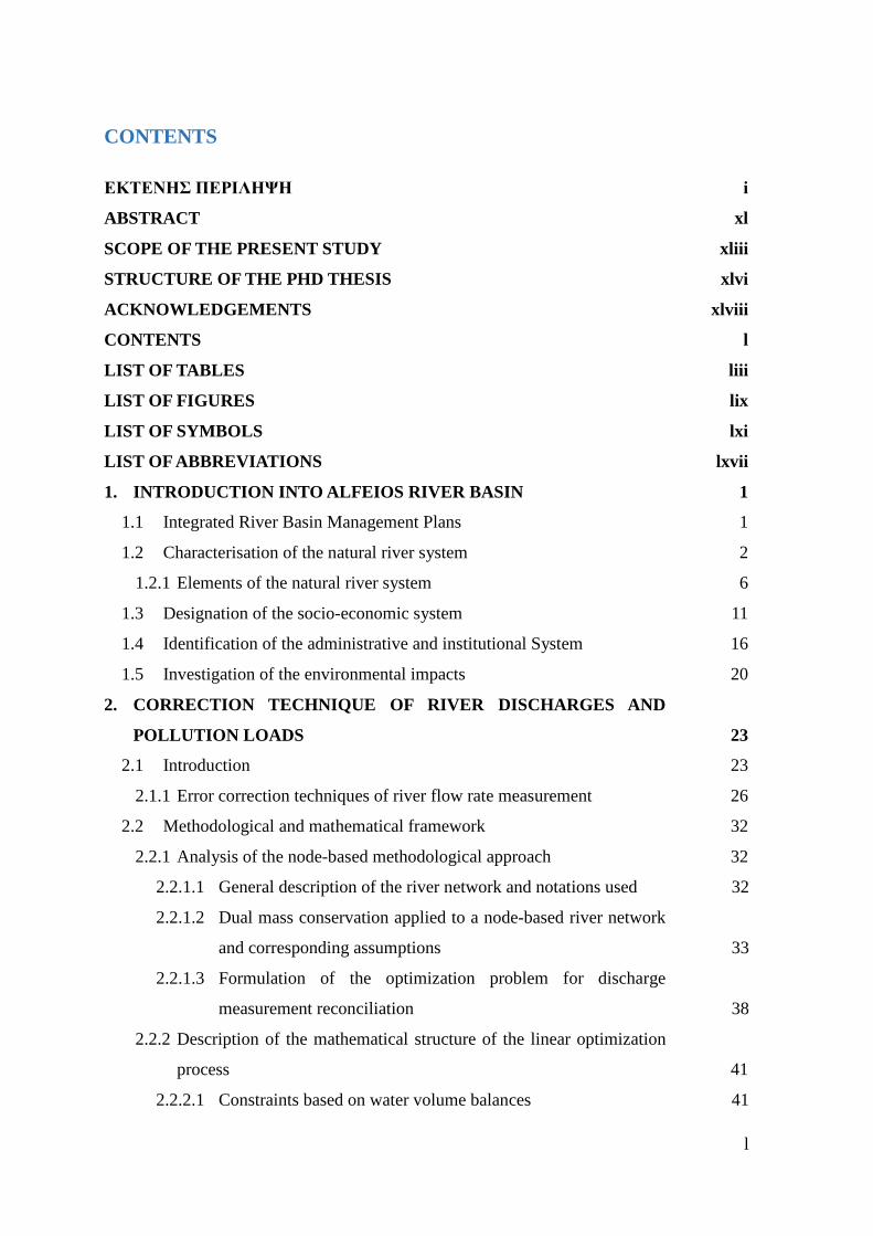
l

CONTENTS

ΕΚΤΕΝΗΣ ΠΕΡΙΛΗΨΗ i

ABSTRACT xl

SCOPE OF THE PRESENT STUDY xliii

STRUCTURE OF THE PHD THESIS xlvi

ACKNOWLEDGEMENTS xlviii

CONTENTS l

LIST OF TABLES liii

LIST OF FIGURES lix

LIST OF SYMBOLS lxi

LIST OF ABBREVIATIONS lxvii

1. INTRODUCTION INTO ALFEIOS RIVER BASIN 1

1.1 Integrated River Basin Management Plans 1

1.2 Characterisation of the natural river system 2

1.2.1 Elements of the natural river system 6

1.3 Designation of the socio-economic system 11

1.4 Identification of the administrative and institutional System 16

1.5 Investigation of the environmental impacts 20

2. CORRECTION TECHNIQUE OF RIVER DISCHARGES AND

POLLUTION LOADS 23

2.1 Introduction 23

2.1.1 Error correction techniques of river flow rate measurement 26

2.2 Methodological and mathematical framework 32

2.2.1 Analysis of the node-based methodological approach 32

2.2.1.1 General description of the river network and notations used 32

2.2.1.2 Dual mass conservation applied to a node-based river network

and corresponding assumptions 33

2.2.1.3 Formulation of the optimization problem for discharge

measurement reconciliation 38

2.2.2 Description of the mathematical structure of the linear optimization

process 41

2.2.2.1 Constraints based on water volume balances 41

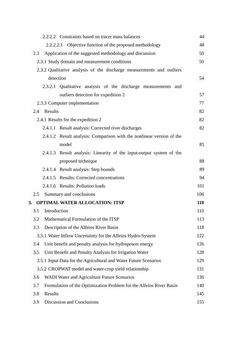
2.2.2.2 Constraints based on tracer mass balances 44

2.2.2.2.1 Objective function of the proposed methodology 48

2.3 Application of the suggested methodology and discussion 50

2.3.1 Study domain and measurement conditions 50

2.3.2 Qualitative analysis of the discharge measurements and outliers

detection 54

2.3.2.1 Qualitative analysis of the discharge measurements and

outliers detection for expedition 2 57

2.3.3 Computer implementation 77

2.4 Results 82

2.4.1 Results for the expedition 2 82

2.4.1.1 Result analysis: Corrected river discharges 82

2.4.1.2 Result analysis: Comparison with the nonlinear version of the

model 85

2.4.1.3 Result analysis: Linearity of the input-output system of the

proposed technique 88

2.4.1.4 Result analysis: Step bounds 89

2.4.1.5 Results: Corrected concentrations 94

2.4.1.6 Results: Pollution loads 101

2.5 Summary and conclusions 106

3. OPTIMAL WATER ALLOCATION: ITSP 110

3.1 Introduction 110

3.2 Mathematical Formulation of the ITSP 113

3.3 Description of the Alfeios River Basin 118

3.3.1 Water Inflow Uncertainty for the Alfeios Hydro-System 122

3.4 Unit benefit and penalty analysis for hydropower energy 126

3.5 Unit Benefit and Penalty Analysis for Irrigation Water 128

3.5.1 Input Data for the Agricultural and Water Future Scenarios 129

3.5.2 CROPWAT model and water-crop yield relationship 131

3.6 WADI Water and Agriculture Future Scenarios 136

3.7 Formulation of the Optimization Problem for the Alfeios River Basin 140

3.8 Results 145

3.9 Discussion and Conclusions 155

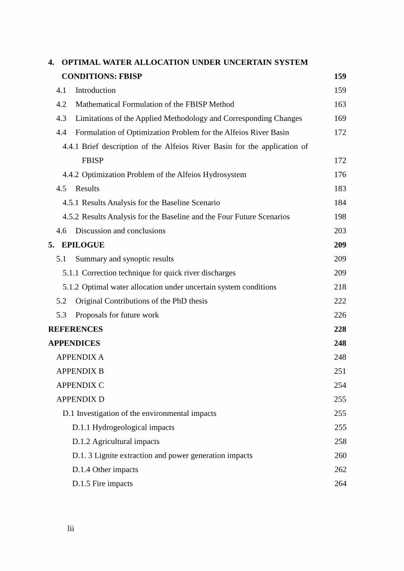
lii

4. OPTIMAL WATER ALLOCATION UNDER UNCERTAIN SYSTEM

CONDITIONS: FBISP 159

4.1 Introduction 159

4.2 Mathematical Formulation of the FBISP Method 163

4.3 Limitations of the Applied Methodology and Corresponding Changes 169

4.4 Formulation of Optimization Problem for the Alfeios River Basin 172

4.4.1 Brief description of the Alfeios River Basin for the application of

FBISP 172

4.4.2 Optimization Problem of the Alfeios Hydrosystem 176

4.5 Results 183

4.5.1 Results Analysis for the Baseline Scenario 184

4.5.2 Results Analysis for the Baseline and the Four Future Scenarios 198

4.6 Discussion and conclusions 203

5. EPILOGUE 209

5.1 Summary and synoptic results 209

5.1.1 Correction technique for quick river discharges 209

5.1.2 Optimal water allocation under uncertain system conditions 218

5.2 Original Contributions of the PhD thesis 222

5.3 Proposals for future work 226

REFERENCES 228

APPENDICES 248

APPENDIX A 248

APPENDIX B 251

APPENDIX C 254

APPENDIX D 255

D.1 Investigation of the environmental impacts 255

D.1.1 Hydrogeological impacts 255

D.1.2 Agricultural impacts 258

D.1. 3 Lignite extraction and power generation impacts 260

D.1.4 Other impacts 262

D.1.5 Fire impacts 264

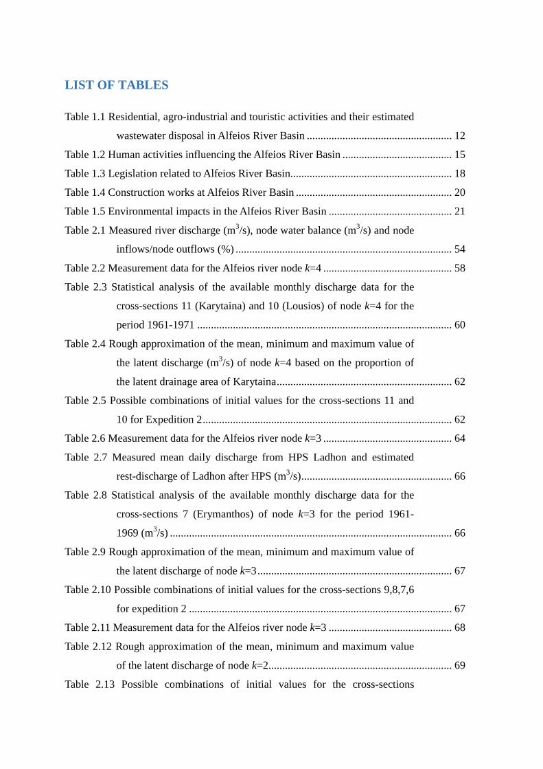
LIST OF TABLES

Table 1.1 Residential, agro-industrial and touristic activities and their estimated

wastewater disposal in Alfeios River Basin ..................................................... 12

Table 1.2 Human activities influencing the Alfeios River Basin ........................................ 15

Table 1.3 Legislation related to Alfeios River Basin........................................................... 18

Table 1.4 Construction works at Alfeios River Basin ......................................................... 20

Table 1.5 Environmental impacts in the Alfeios River Basin ............................................. 21

Table 2.1 Measured river discharge (m3/s), node water balance (m3/s) and node

inflows/node outflows (%) ............................................................................... 54

Table 2.2 Measurement data for the Alfeios river node k=4 ............................................... 58

Table 2.3 Statistical analysis of the available monthly discharge data for the

cross-sections 11 (Karytaina) and 10 (Lousios) of node k=4 for the

period 1961-1971 ............................................................................................. 60

Table 2.4 Rough approximation of the mean, minimum and maximum value of

the latent discharge (m3/s) of node k=4 based on the proportion of

the latent drainage area of Karytaina ................................................................ 62

Table 2.5 Possible combinations of initial values for the cross-sections 11 and

10 for Expedition 2 ........................................................................................... 62

Table 2.6 Measurement data for the Alfeios river node k=3 ............................................... 64

Table 2.7 Measured mean daily discharge from HPS Ladhon and estimated

rest-discharge of Ladhon after HPS (m3/s) ....................................................... 66

Table 2.8 Statistical analysis of the available monthly discharge data for the

cross-sections 7 (Erymanthos) of node k=3 for the period 1961-

1969 (m3/s) ....................................................................................................... 66

Table 2.9 Rough approximation of the mean, minimum and maximum value of

the latent discharge of node k=3 ....................................................................... 67

Table 2.10 Possible combinations of initial values for the cross-sections 9,8,7,6

for expedition 2 ................................................................................................ 67

Table 2.11 Measurement data for the Alfeios river node k=3 ............................................. 68

Table 2.12 Rough approximation of the mean, minimum and maximum value

of the latent discharge of node k=2................................................................... 69

Table 2.13 Possible combinations of initial values for the cross-sections

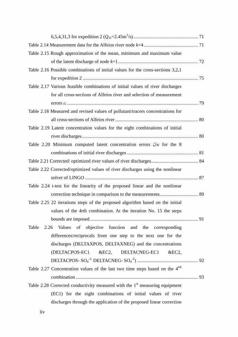
liv

6,5,4,31,3 for expedition 2 (Q31=2.45m3/s) ...................................................... 71

Table 2.14 Measurement data for the Alfeios river node k=4 ............................................. 71

Table 2.15 Rough approximation of the mean, minimum and maximum value

of the latent discharge of node k=1................................................................... 72

Table 2.16 Possible combinations of initial values for the cross-sections 3,2,1

for expedition 2 ................................................................................................ 75

Table 2.17 Various feasible combinations of initial values of river discharges

for all cross-sections of Alfeios river and selection of measurement

errors εi ............................................................................................................. 79

Table 2.18 Measured and revised values of pollutant/tracers concentrations for

all cross-sections of Alfeios river ..................................................................... 80

Table 2.19 Latent concentration values for the eight combinations of initial

river discharges ................................................................................................. 80

Table 2.20 Minimum computed latent concentration errors ζλκ for the 8

combinations of initial river discharges ........................................................... 81

Table 2.21 Corrected/ optimized river values of river discharges ....................................... 84

Table 2.22 Corrected/optimized values of river discharges using the nonlinear

solver of LINGO .............................................................................................. 87

Table 2.24 t-test for the linearity of the proposed linear and the nonlinear

correction technique in comparison to the measurements ................................ 89

Table 2.25 22 iterations steps of the proposed algorithm based on the initial

values of the 4rth combination. At the iteration No. 15 the steps

bounds are imposed. ......................................................................................... 91

Table 2.26 Values of objective function and the corresponding

differences/reciprocals from one step to the next one for the

discharges (DELTAXPOS, DELTAXNEG) and the concentrations

(DELTACPOS-EC1 &EC2, DELTACNEG-EC1 &EC2,

DELTACPOS- SO4-2, DELTACNEG- SO4

-2) ................................................... 92

Table 2.27 Concentration values of the last two time steps based on the 4rth

combination ...................................................................................................... 93

Table 2.28 Corrected conductivity measured with the 1st measuring equipment

(EC1) for the eight combinations of initial values of river

discharges through the application of the proposed linear correction

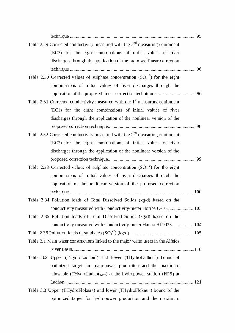
technique .......................................................................................................... 95

Table 2.29 Corrected conductivity measured with the 2nd measuring equipment

(EC2) for the eight combinations of initial values of river

discharges through the application of the proposed linear correction

technique .......................................................................................................... 96

Table 2.30 Corrected values of sulphate concentration (SO4-2) for the eight

combinations of initial values of river discharges through the

application of the proposed linear correction technique .................................. 96

Table 2.31 Corrected conductivity measured with the 1st measuring equipment

(EC1) for the eight combinations of initial values of river

discharges through the application of the nonlinear version of the

proposed correction technique .......................................................................... 98

Table 2.32 Corrected conductivity measured with the 2nd measuring equipment

(EC2) for the eight combinations of initial values of river

discharges through the application of the nonlinear version of the

proposed correction technique .......................................................................... 99

Table 2.33 Corrected values of sulphate concentration (SO4-2) for the eight

combinations of initial values of river discharges through the

application of the nonlinear version of the proposed correction

technique ........................................................................................................ 100

Table 2.34 Pollution loads of Total Dissolved Solids (kg/d) based on the

conductivity measured with Conductivity-meter Horiba U-10 ...................... 103

Table 2.35 Pollution loads of Total Dissolved Solids (kg/d) based on the

conductivity measured with Conductivity-meter Hanna HI 9033 .................. 104

Table 2.36 Pollution loads of sulphates (SO4-2) (kg/d) ...................................................... 105

Table 3.1 Main water constructions linked to the major water users in the Alfeios

River Basin. ...................................................................................................... 118

Table 3.2 Upper (THydroLadhon+) and lower (THydroLadhon−) bound of

optimized target for hydropower production and the maximum

allowable (THydroLadhonMax) at the hydropower station (HPS) at

Ladhon. ........................................................................................................... 121

Table 3.3 Upper (THydroFlokas+) and lower (THydroFlokas−) bound of the

optimized target for hydropower production and the maximum

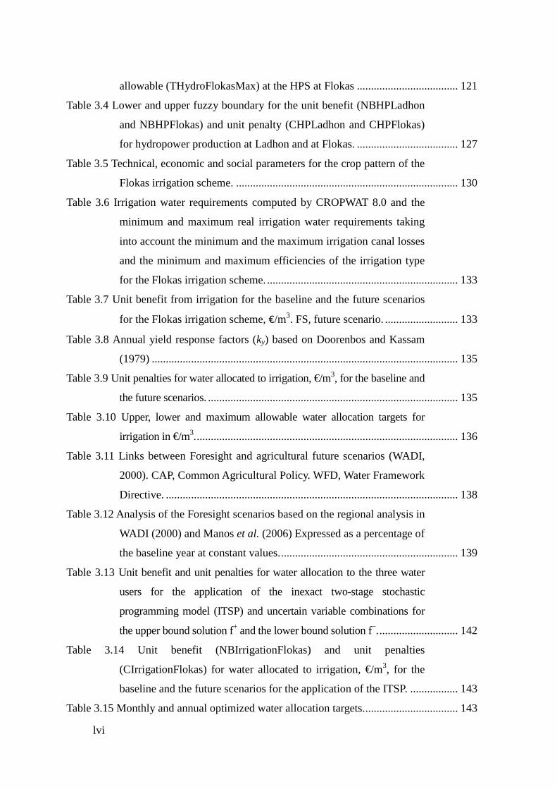
lvi

allowable (THydroFlokasMax) at the HPS at Flokas .................................... 121

Table 3.4 Lower and upper fuzzy boundary for the unit benefit (NBHPLadhon

and NBHPFlokas) and unit penalty (CHPLadhon and CHPFlokas)

for hydropower production at Ladhon and at Flokas. .................................... 127

Table 3.5 Technical, economic and social parameters for the crop pattern of the

Flokas irrigation scheme. ............................................................................... 130

Table 3.6 Irrigation water requirements computed by CROPWAT 8.0 and the

minimum and maximum real irrigation water requirements taking

into account the minimum and the maximum irrigation canal losses

and the minimum and maximum efficiencies of the irrigation type

for the Flokas irrigation scheme. .................................................................... 133

Table 3.7 Unit benefit from irrigation for the baseline and the future scenarios

for the Flokas irrigation scheme, €/m3. FS, future scenario. .......................... 133

Table 3.8 Annual yield response factors (ky) based on Doorenbos and Kassam

(1979) ............................................................................................................. 135

Table 3.9 Unit penalties for water allocated to irrigation, €/m3, for the baseline and

the future scenarios. ......................................................................................... 135

Table 3.10 Upper, lower and maximum allowable water allocation targets for

irrigation in €/m3. ............................................................................................. 136

Table 3.11 Links between Foresight and agricultural future scenarios (WADI,

2000). CAP, Common Agricultural Policy. WFD, Water Framework

Directive. ........................................................................................................ 138

Table 3.12 Analysis of the Foresight scenarios based on the regional analysis in

WADI (2000) and Manos et al. (2006) Expressed as a percentage of

the baseline year at constant values. ............................................................... 139

Table 3.13 Unit benefit and unit penalties for water allocation to the three water

users for the application of the inexact two-stage stochastic

programming model (ITSP) and uncertain variable combinations for

the upper bound solution f+ and the lower bound solution f−. ............................ 142

Table 3.14 Unit benefit (NBIrrigationFlokas) and unit penalties

(CIrrigationFlokas) for water allocated to irrigation, €/m3, for the

baseline and the future scenarios for the application of the ITSP. ................. 143

Table 3.15 Monthly and annual optimized water allocation targets. ................................. 143

Table 3.16 Total net benefit (€) from all water uses. OF, objective function. ................... 147

Table 3.17 Annual water allocation and shortage for irrigation at Flokas (m3). ............... 147

Table 3.18 Annual hydropower production and shortage at the HPS at Ladhon

and at Flokas (MWh). ..................................................................................... 150

Table 3.19 Annual water allocation and shortage for irrigation and annual

hydropower production and shortage at the HPS at Ladhon and at

Flokas (MWh) for optimized targets equal to ±T , −T , +T . ........................ 154

Table 4.1 Upper- (THydroLadhon+) and lower- (THydroLadhon−) bounds of

optimized target for hydropower production at HPS at Ladhon. ................... 174

Table 4.2 Upper- and lower-water allocation targets for irrigation in EUR/m3. ............... 174

Table 4.3 Upper- (THydroFlokas+) and lower- (THydroFlokas−) bounds of

optimized target for hydropower production at HPS at Flokas. ..................... 175

Table 4.4 Lower- and upper- fuzzy-boundary intervals for the unit benefit and

unit penalty for hydropower production EUR/MWh at Ladhon and

at Flokas. ........................................................................................................ 182

Table 4.5 Lower- and upper- fuzzy-boundary intervals for the unit benefit from

irrigation for the baseline and the WADI future scenarios for Flokas

irrigation scheme EUR/m3. ............................................................................. 182

Table 4.6 Lower- and upper- fuzzy-boundary intervals for the unit penalties for

water deficits to irrigation EUR/m3 for the baseline and the future

scenarios. ........................................................................................................ 183

Table 4.7 Total annual net benefit (EUR) for all water uses. ............................................ 185

Table 4.8 Total annual benefit and penalties (EUR) for irrigation at Flokas. ................... 186

Table 4.9 Total annual benefit and penalties (EUR) for hydropower production

at Ladhon HPS. ............................................................................................... 186

Table 4.10 Total annual benefit and penalties (EUR) for hydropower

production at Flokas HPS. .............................................................................. 188

Table 4.11 Optimized target for total annual water volumes for irrigation (m3). .............. 188

Table 4.12 Annual Shortage for irrigation (m3 × 106). ...................................................... 190

Table 4.13 Annual Allocation for irrigation (m3 × 106). ................................................... 190

Table 4.14 Annual target, shortage and allocation for irrigation (m3) for the

hydrologic scenario 19. .................................................................................. 191

Table 4.15 Optimized target for total annual hydropower production at HPS

lviii

Flokas (MWh). ............................................................................................... 193

Table 4.16 Optimized target for total annual hydropower production at HPS

Flokas (MWh). ............................................................................................... 195

Table 4.17 Maximum allowable (THydroFlokasPlus) and Optimized (Optimized

THydroFlokas) monthly targets of hydropower production at

Flokas HPS (MWh). ....................................................................................... 195

Table 4.18 Optimized annual target for hydropower production at HPS Ladhon

(MWh). ........................................................................................................... 195

Table 4.19 Maximum allowable (THydro-LadhonPlus) and minimum

(MinOptimized THydroFlokas) and maximum (MaxOptimized

THydroFlokas) optimized monthly targets of hydropower production

at Flokas HPS (MWh) and their ratios in (%) for the first solution

method (optimistic). ......................................................................................... 196

Table 4.20 Maximum allowable (THydro-LadhonPlus) and minimum

(MinOptimized THydroFlokas) and maximum (MaxOptimized

THydroFlokas) optimized monthly targets of hydropower

production at Flokas HPS (MWh) and their ratios in (%) for the

second solution method (pessimistic). ............................................................ 196

Table 4.21 Interconnections between total net benefit and optimized total target

for the four options and for both solution methods. ....................................... 197

Table 4.22 Optimized total annual water allocation target of the four future

scenarios as ratio of the baseline (%). ............................................................ 201

Table 4.23 Total annual net benefit (EUR) of the four future scenarios as ratio

of the baseline (%). ......................................................................................... 201

Table 4.24 Annual net benefit (EUR) for irrigation and ratios (%) of annual net

benefit of the four future scenarios compared to baseline. ............................. 202

Table 5.1 Original contributions of the present PhD thesis ............................................... 223

Table 5.2 List of publications and conferences during the present PhD thesis ................. 225

LIST OF FIGURES

Figure 1.1 Alfeios River Basin ............................................................................................. 4

Figure 1.2 Digital Elevation Model for Alfeios River Basin ................................................ 5

Figure 1.3 Short- and long-term population projection for Alfeios River Basin

(Source: Hellenic Statistical Authority, 2009) ................................................. 14

Figure 1.4 Land uses (%) of Alfeios River Basin (Source: Skoulikidis et al.,

2009) ................................................................................................................. 14

Figure 2.1 Representation of a single node k composed of nk=6 cross-sections ................. 31

Figure 2.2 Representation of a river composed of two consecutive nodes: the

first downstream node k=1 with 4 tributaries and a total number of

cross-sections nk=1= 6 and the second and last node k=K=2 with 4

tributaries and nk=2= 6. For the second node, the single node

enumeration is provided in green. .................................................................... 34

Figure 2.3 Geographical depiction of the eleven cross-sections of Alfeios river

basin with parallel quantitative and qualitative measurements. ....................... 52

Figure 2.4 Solution space of ∧∧

21, XX for the water balance and correction

constraints ......................................................................................................... 55

Figure 2.5 Block diagram of the proposed correction algorithm ........................................ 88

Figure 3.1 The simplified schematic of the Alfeios River Basin. ..................................... 123

Figure 3.2 Methodological framework for optimal water allocation of Alfeios

River Basin. .................................................................................................... 125

Figure 3.3 Box plots of the annual probabilistic water allocation and shortage

for the irrigation in m3 and for the hydropower production at

Ladhon and Flokas in MWh for the baseline for the f+ .................................. 152

Figure 4.1 Methodological framework for optimal water allocation of Alfeios

River Basin ..................................................................................................... 181

Figure 4.2 Interconnections between total net benefit and optimized total target

for the four options and for both solution methods. ....................................... 197

Figure 4.3 Box plots for the four options of total net optimized benefits in EUR

for the baseline and the four future scenarios (FS1: Future Scenario

1; FS2: Future Scenario 2; FS3: Future Scenario 3; FS4: Future

lx

Scenario 4). ..................................................................................................... 202

Figure 4.4 Box plots for the four options of annual net optimized benefits for

irrigation in EUR for the baseline and the four future scenarios

(FS1: Future Scenario 1; FS2: Future Scenario 2; FS3: Future

Scenario 3; FS4: Future Scenario 4). .............................................................. 203

LIST OF SYMBOLS

Greek symbols

slope coefficient from linear regression between surface

area of Ladhon reservoir and storage volume

εi maximum relative error of the river discharge

measurements Qi

ζj measurement error for the concentration cij for a

pollutant/tracer j (1,m)

λ index for the latent term

Latin symbols

Ai drainage area corresponding to the cross-section i of a

river node k (<)

41CD surface area of Ladhon reservoir in period t under

scenarios k1 (<)

5 intercept coefficient from linear regression between

surface area of Ladhon reservoir and storage volume

561% 7 and 561&7 fuzzy lower- and upper-bound of the right-hand side of

constrains considered as fuzzy-boundary interval

561±7 = 2561%7,561&73 = 89561% , 561% : , 9561& , 561& :; 561% and 561% lower- and upper-bound of the lower fuzzy bound of

561±7 = 2561%7,561&73 = 89561% , 561% : , 9561& , 561& :; 561& AE561& lower- and upper-bound of the upper fuzzy bound of

561±7 = 2561%7,561&73 = 89561% , 561% : , 9561& , 561& :; ? area-based conversion factor

cij concentration of a pollutant/tracer j at a river cross-section

i

cλjk latent concentration of a pollutant/tracer j of a river node k

lxii

ccij corrected/optimized concentration of a pollutant/tracer j at

a cross-section i (1,N)

ccλjk corrected concentration of a pollutant/tracer j for the latent

term of each node k (1,K)

±DevDqCNODE12…K minimum and maximum admissible deviation from the

zero-balance of the residual KNODEDqC ...12 expressing the

pollutant mass conservation written for a combination of K

successive nodes

±DevDqXNODE12…K minimum and maximum admissible deviation from the

zero-balance of the residual KNODEDqX ...12 expressing the

pollutant mass conservation written for a combination of K

successive nodes

±DevQNODE12…K minimum and maximum admissible deviation from the

zero-balance of the residual KNODEDQ ...12 expressing the

water volume conservation written for a combination of K

successive nodes

DqCNODE12…K residual of the pollutant mass conservation (in comparison

to zero balance) written for a combination of K successive

nodes when the balance is written assuming that the

concentrations are the unknown variables and the river

discharges are known

DQNODE12..K residual of the water volume conservation (in comparison

to zero balance) written for a combination of K successive

nodes

DqXNODE12…K residual of the pollutant mass conservation (in comparison

to zero balance) written for a combination of K successive

nodes when the balance is written assuming that the

concentrations are known and the river discharges are the

unknown variables

E slope coefficient from linear regression between

hydropower production of Ladhon reservoir and water

volume released through the turbines

F slope coefficient from linear regression between

hydropower production of Ladhon reservoir and water

volume released through the turbines

F1± average evaporation rate for Ladhon reservoir in period t

(m)

G1± evaporation loss of Ladhon reservoir in period t (H)

slope coefficient from linear regression between

hydropower production of Flokas and water volume

released through the turbines ± Upper and lower solution values of the objective function

of the optimal water allocation of the ITSP methodology /01& upper-bound solution of the objective function of the

optimal water allocation using the ITSP methodology /01% lower-bound solution of the objective function of the

optimal water allocation using the ITSP methodology

/01& upper-bound of the first (optimistic) solution method of

the objective-function value of the FBISP methodology /01& lower-bound of the first (optimistic) solution method of

the objective-function value using the FBISP methodology /01% lower-bound of the second (pessimistic) solution method

of the objective-function value using the FBISP

methodology

/01% lower-bound of the second (pessimistic) solution method

of the objective-function value using the FBISP

methodology I slope coefficient from linear regression between

hydropower production of Flokas HPS and water volume

released through the turbines

JK1CD± monthly hydropower production for t = 1, 2, …, T; in

period t under scenarios k1 for the water user i with i = 1, 2

corresponding to Ladhon and Flokas, respectively

k river node used for the water volume and mass pollutant

balance

lxiv

ky annual yield response factor

L1 number of flow scenarios in period t

± net benefit per unit of water allocated to each water use i-

(EUR/H) for irrigation and (EUR/MNℎ) for hydropower

NODE12…K index of the residual term from the zero balance written

for the K successive nodes combination

KG± penalty per unit of water not delivered for each water user

i—(EUR/H) for irrigation and (EUR/MNℎ) for

hydropower

1CD probability of occurrence of scenario Pin period t

Qi river discharge measurement at a river cross-section i

(m3/s)

qij pollutant load of a pollutant j at a river cross-section i

Qλk river discharge at the latent cross-section λ of a node k

(m3/s)

qλjk pollutant load of a pollutant/tracer j of the latent cross-

section λ of a river node k

Q1CD± water inflow level into stream j in period t under scenario

P (H)

R1CD± Water release flow from the turbines of Ladhon reservoir

in period t under scenario P (H)

RS± maximum storage capacity of Ladhon reservoir (H)

RST± minimum storage capacity of Ladhon reservoir (H)

sn scenario n

S1CD± storage level in Ladhon reservoir in period t under

scenario P (H)

SK1CD± spill volume over Ladhon Dam in period t under scenario P (H) time period

±T optimized water allocation targets (H)

1UVW lower-bound of the optimized target for the water user i in

period t - (H) for irrigation and (MWh) for hydropower

1U!"W upper-bound of the optimized target for the water user i in

period t - (H) for irrigation and (MWh) for hydropower

1 ± Upper- and lower-(deterministic) bound of water

allocation target that is promised to the user i in period t

(H)

JKCD± annual hydropower production in period t under scenarios

k1 for the water user i with i = 1, 2 corresponding to

Ladhon and Flokas, respectively

TX± maximum capacity of turbines at Ladhon HPS (H)

TT± minimum capacity of turbines at Ladhon HPS (H)

YX± maximum capacity of turbines at Flokas HPS (H)

YT± minimum capacity of turbines at Flokas HPS (H)

NZ1CD± irrigation shortage volume in period t under scenarios P

(H)

NZ[1CD± water volume residual at Flokas after having allocated the

irrigation water in period t under scenarios P (H)

NYT1CD± water volume flowing through the fish ladder at Flokas

dam in period t under scenarios P (H)

N\Y1CD± water volume flowing through the turbines at Flokas HPS

in period t under scenarios k1 (H)

WVFOabD± spill volume at Flokas dam in period t under scenarios P

(H)

Xi corrected/optimized river discharges for each cross-section

i (1,N)

Xλk corrected/optimized river discharges at the latent cross-

section of a river node k (1,K) 1& upper-bound of the water allocation target (first-stage

decision variables) in period t with B = 1,2, … . , ) 1%, lower-bound of the water allocation target (first-stage

decision variables) in period t +1C& upper-bound of the water shortage of water use j by which

the water-allocation target is not met in period t for the

lxvi

scenario k (recourse decision variable)

(P = 1, 2, … . , L1AE = 1, 2, … . , <) +1C% lower-bound of the water shortage of water use j by which

the water-allocation target is not met in period t for the

scenario k (recourse decision variable)

(P = 1, 2, … . , L1AE = 1, 2, … . , <)

LIST OF ABBREVIATIONS

ADCP Acoustic Doppler Current Profiler

AOM Organic Matter Of Anthropogenic Origin

asl above sea level

BOD5 Biological Oxygen Demand

BWC Best/Worst Case

CAP Common Agricultural Policy

CCP Chance-Constrained Programming

DO Dissolved Oxygen

DS Decision Support

DVR Data Validation and Reconciliation

EC1 Conductivity measured with Conductivity-meter Horiba U-10

EC2 Conductivity measured with Conductivity-meter Hanna HI 9033

ET0 Reference Evapotranspiration

FAO Food and Agricultural Organization of United Nations

FBISP Fuzzy-Boundary Interval-Stochastic Programming

FP Fuzzy Programming

FPS Feasible Parameter Set

FPS Sample Average Approximation

FS1 Future Scenario 1

FS2 Future Scenario 2

FS3 Future Scenario 3

FS4 Future Scenario 4

GOEB General Irrigation Organization

HMA Hellenic Ministry of Agriculture

HMEPPPW Hellenic Ministry of the Environment, Physical Planning and Public

Works

HNCMR Hellenic National Centre for Marine Research

HPPC Hellenic Public Power Corporation

HPS Hydropower Station

HSA Hellenic Statistical Authority

IPP Interval-Parameter Programming

lxviii

IRBM Integrated River Basin Management

ISO International Organization for Standardization

ITSP Inexact Two-Stage Stochastic Programming

JDM Joint Ministerial Decision

OF Objective Function

MLC Megalopolis Lignite Centre

MLR Maximum Likelihood Rectification

MRDF Ministry of Rural Development and Food

MSP Multistage Stochastic Programming

OCDE Organization for Economic Co-operation and Development

PAH Polycyclic Aromatic hydrocarbons

PAR(1) Periodic First-Order Autoregression

PCA Principal Component Analysis

PDF Probability Density Function

QBR Qualitat del Bosc de Ribera

RAE Regulatory Authority of Energy

RES Renewable Energy Sources

RHS River Habitat Survey

SEPP Stream Electric Power Plant

SMA Symmetric Moving Average

SMA Symmetric Moving Average

SP Stochastic Programming

TSP Two-Stage Stochastic Programming

USCS Unified Soil Classified Service

WADI Water Framework Directive and Agenda

WFD Water Framework Directive

WHO World Health Organization

WLS Weighted Least Squares

Greek

ΓΟΕΒ Γενικός Οργανισµός Έγγειων Βελτιώσεων

∆ΕΗ ∆ηµόσια Επιχείρηση Ηλεκτρισµού

ΤΟΕΒ Τοπικός Οργανισµός Έγγειων Βελτιώσεων

Specific Abbreviations

CHPFlokas Upper Fuzzy Boundary for the Penalty for

Hydropower Production at Flokas (€/m3)

CHPLadhon Lower Fuzzy Boundary for the Unit Penalty for

Hydropower Production at Ladhon (€/m3)

CIrrigationFlokas Unit Penalties for Water Allocated to Irrigation at

Flokas (€/m3)

MaxOptimized THydroFlokas Maximum Optimized Monthly Targets of

Hydropower Production at Flokas HPS (MWh)

MinOptimized THydroFlokas Minimum Optimized Monthly Targets of

Hydropower Production at Flokas HPS (MWh)

NBIrrigationFlokas Unit benefit for Water Allocated to Irrigation at

Flokas (€/m3)

NBHPFlokas Fuzzy Upper Boundary for the Unit Benefit for

Hydropower Production at Flokas HPS (€/m3)

NBHPLadhon Fuzzy Lower Boundary for the Unit Benefit for

Hydropower Production at Ladhon HPS (€/m3)

Optimized THydroFlokas Optimized Monthly Targets of Hydropower

Production at Flokas HPS (MWh)

THydroFlokas Upper Bound of the Optimized Target for

Hydropower Production at Flokas HPS (MWh)

THydroFlokas Lower Bound of the Optimized Target for

Hydropower Production at Flokas HPS (MWh)

THydroFlokasMax Maximum Allowable Bound of the Optimized

Target of Hydropower Production at Flokas HPS

(MWh)

THydroFlokasPlus Maximum Allowable Monthly Targets of

Hydropower Production at Flokas HPS (MWh)

THydroLadhon− Lower Bound of Optimized Target for

Hydropower Production at Ladhon HPS (MWh)

THydroLadhon+ Upper Bound of Optimized Target for

Hydropower Production at Ladhon HPS (MWh)

lxx

THydroLadhonMax Maximum Allowable Bound of Optimized Target

for Hydropower (MWh)

THydroLadhonPlus Maximum Monthly Targets of Hydropower

Production at Ladhon HPS (MWh)

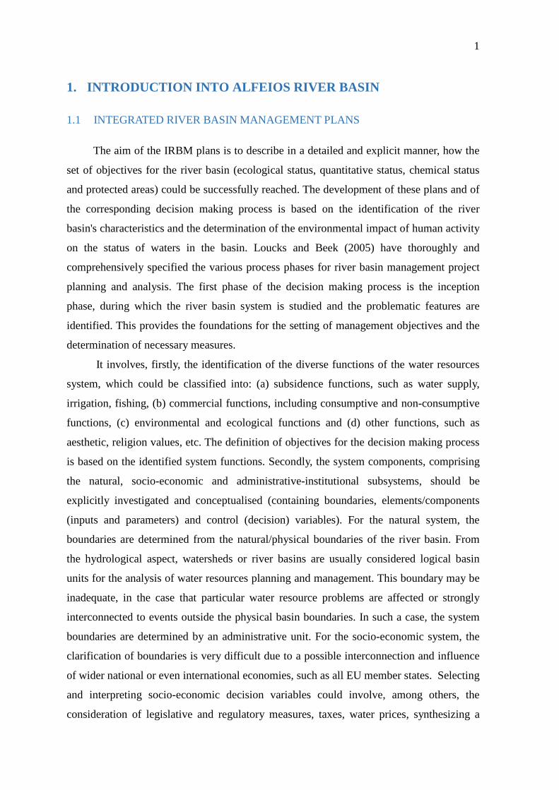
1

1. INTRODUCTION INTO ALFEIOS RIVER BASIN

1.1 INTEGRATED RIVER BASIN MANAGEMENT PLANS

The aim of the IRBM plans is to describe in a detailed and explicit manner, how the

set of objectives for the river basin (ecological status, quantitative status, chemical status

and protected areas) could be successfully reached. The development of these plans and of

the corresponding decision making process is based on the identification of the river

basin's characteristics and the determination of the environmental impact of human activity

on the status of waters in the basin. Loucks and Beek (2005) have thoroughly and

comprehensively specified the various process phases for river basin management project

planning and analysis. The first phase of the decision making process is the inception

phase, during which the river basin system is studied and the problematic features are

identified. This provides the foundations for the setting of management objectives and the

determination of necessary measures.

It involves, firstly, the identification of the diverse functions of the water resources

system, which could be classified into: (a) subsidence functions, such as water supply,

irrigation, fishing, (b) commercial functions, including consumptive and non-consumptive

functions, (c) environmental and ecological functions and (d) other functions, such as

aesthetic, religion values, etc. The definition of objectives for the decision making process

is based on the identified system functions. Secondly, the system components, comprising

the natural, socio-economic and administrative-institutional subsystems, should be

explicitly investigated and conceptualised (containing boundaries, elements/components

(inputs and parameters) and control (decision) variables). For the natural system, the

boundaries are determined from the natural/physical boundaries of the river basin. From

the hydrological aspect, watersheds or river basins are usually considered logical basin

units for the analysis of water resources planning and management. This boundary may be

inadequate, in the case that particular water resource problems are affected or strongly

interconnected to events outside the physical basin boundaries. In such a case, the system

boundaries are determined by an administrative unit. For the socio-economic system, the

clarification of boundaries is very difficult due to a possible interconnection and influence

of wider national or even international economies, such as all EU member states. Selecting

and interpreting socio-economic decision variables could involve, among others, the

consideration of legislative and regulatory measures, taxes, water prices, synthesizing a

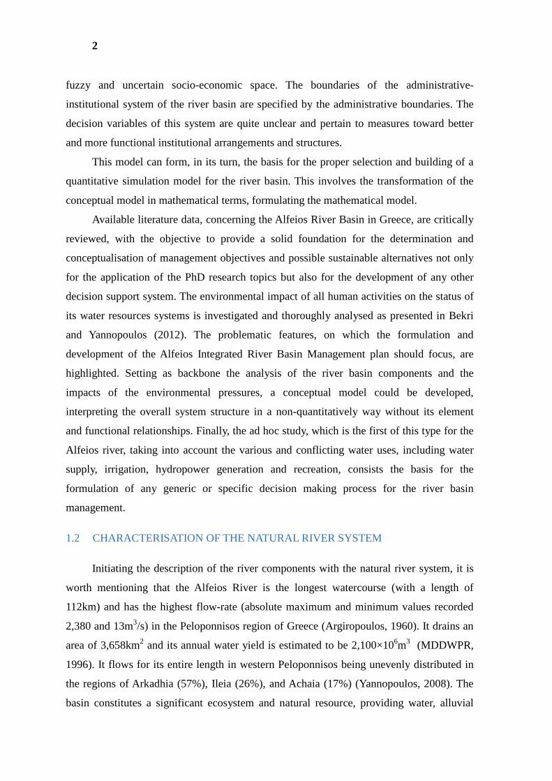
2

fuzzy and uncertain socio-economic space. The boundaries of the administrative-

institutional system of the river basin are specified by the administrative boundaries. The

decision variables of this system are quite unclear and pertain to measures toward better

and more functional institutional arrangements and structures.

This model can form, in its turn, the basis for the proper selection and building of a

quantitative simulation model for the river basin. This involves the transformation of the

conceptual model in mathematical terms, formulating the mathematical model.

Available literature data, concerning the Alfeios River Basin in Greece, are critically

reviewed, with the objective to provide a solid foundation for the determination and

conceptualisation of management objectives and possible sustainable alternatives not only

for the application of the PhD research topics but also for the development of any other

decision support system. The environmental impact of all human activities on the status of

its water resources systems is investigated and thoroughly analysed as presented in Bekri

and Yannopoulos (2012). The problematic features, on which the formulation and

development of the Alfeios Integrated River Basin Management plan should focus, are

highlighted. Setting as backbone the analysis of the river basin components and the

impacts of the environmental pressures, a conceptual model could be developed,

interpreting the overall system structure in a non-quantitatively way without its element

and functional relationships. Finally, the ad hoc study, which is the first of this type for the

Alfeios river, taking into account the various and conflicting water uses, including water

supply, irrigation, hydropower generation and recreation, consists the basis for the

formulation of any generic or specific decision making process for the river basin

management.

1.2 CHARACTERISATION OF THE NATURAL RIVER SYSTEM

Initiating the description of the river components with the natural river system, it is

worth mentioning that the Alfeios River is the longest watercourse (with a length of

112km) and has the highest flow-rate (absolute maximum and minimum values recorded

2,380 and 13m3/s) in the Peloponnisos region of Greece (Argiropoulos, 1960). It drains an

area of 3,658km2 and its annual water yield is estimated to be 2,100×106m3 (MDDWPR,

1996). It flows for its entire length in western Peloponnisos being unevenly distributed in

the regions of Arkadhia (57%), Ileia (26%), and Achaia (17%) (Yannopoulos, 2008). The

basin constitutes a significant ecosystem and natural resource, providing water, alluvial

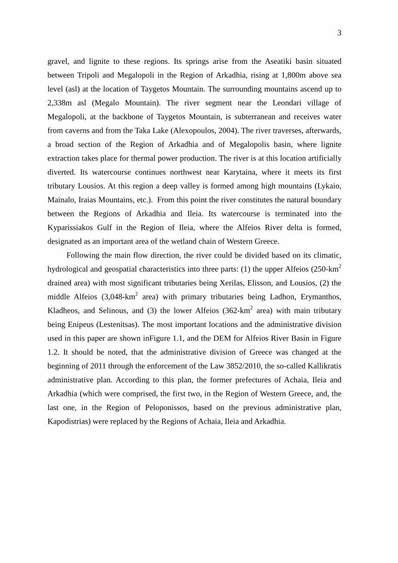
3

gravel, and lignite to these regions. Its springs arise from the Aseatiki basin situated

between Tripoli and Megalopoli in the Region of Arkadhia, rising at 1,800m above sea

level (asl) at the location of Taygetos Mountain. The surrounding mountains ascend up to

2,338m asl (Megalo Mountain). The river segment near the Leondari village of

Megalopoli, at the backbone of Taygetos Mountain, is subterranean and receives water

from caverns and from the Taka Lake (Alexopoulos, 2004). The river traverses, afterwards,

a broad section of the Region of Arkadhia and of Megalopolis basin, where lignite

extraction takes place for thermal power production. The river is at this location artificially

diverted. Its watercourse continues northwest near Karytaina, where it meets its first

tributary Lousios. At this region a deep valley is formed among high mountains (Lykaio,

Mainalo, Iraias Mountains, etc.). From this point the river constitutes the natural boundary

between the Regions of Arkadhia and Ileia. Its watercourse is terminated into the

Kyparissiakos Gulf in the Region of Ileia, where the Alfeios River delta is formed,

designated as an important area of the wetland chain of Western Greece.

Following the main flow direction, the river could be divided based on its climatic,

hydrological and geospatial characteristics into three parts: (1) the upper Alfeios (250-km2

drained area) with most significant tributaries being Xerilas, Elisson, and Lousios, (2) the

middle Alfeios (3,048-km2 area) with primary tributaries being Ladhon, Erymanthos,

Kladheos, and Selinous, and (3) the lower Alfeios (362-km2 area) with main tributary

being Enipeus (Lestenitsas). The most important locations and the administrative division

used in this paper are shown inFigure 1.1, and the DEM for Alfeios River Basin in Figure

1.2. It should be noted, that the administrative division of Greece was changed at the

beginning of 2011 through the enforcement of the Law 3852/2010, the so-called Kallikratis

administrative plan. According to this plan, the former prefectures of Achaia, Ileia and

Arkadhia (which were comprised, the first two, in the Region of Western Greece, and, the

last one, in the Region of Peloponissos, based on the previous administrative plan,

Kapodistrias) were replaced by the Regions of Achaia, Ileia and Arkadhia.

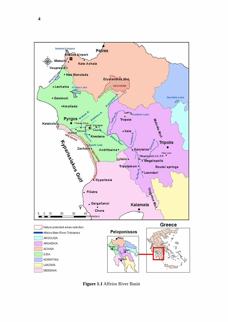
4

Figure 1.1 Alfeios River Basin

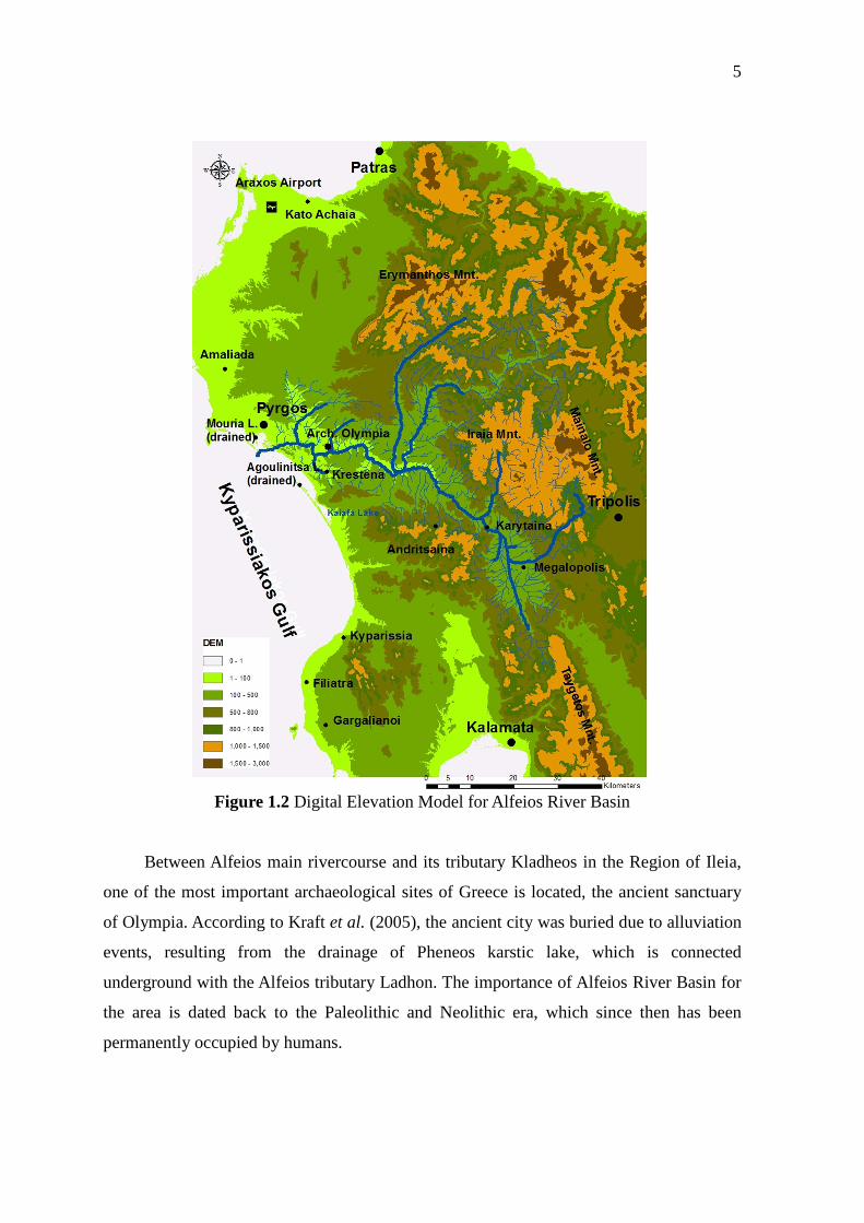
5

Figure 1.2 Digital Elevation Model for Alfeios River Basin

Between Alfeios main rivercourse and its tributary Kladheos in the Region of Ileia,

one of the most important archaeological sites of Greece is located, the ancient sanctuary

of Olympia. According to Kraft et al. (2005), the ancient city was buried due to alluviation

events, resulting from the drainage of Pheneos karstic lake, which is connected

underground with the Alfeios tributary Ladhon. The importance of Alfeios River Basin for

the area is dated back to the Paleolithic and Neolithic era, which since then has been

permanently occupied by humans.

6

1.2.1 ELEMENTS OF THE NATURAL RIVER SYSTEM

The following elements of the natural river system are studied and analysed in detail:

(a) Soil conditions: The Alfeios River lies exclusively in the External Balkanides

emerging from the Dinarides-Hellenides Mountain. The soil of the river catchment area

consists of alluvial and sandstone deposits, as well as Neogene deposits characterized by

discontinuity and heterogeneity. Basin hydrogeology is based on karstic systems, ferrous

and manganese content, which makes the groundwater unsuitable for potable use.

Geologically, the catchment area consists of Alpine deposits belonging to the Ionian, Pilos-

Gavrovo, and Olonos- Pindos Zones, which have been overthrusted to the Tripolis and the

central Peloponnisos zones (MDDWPR, 1996). The following geomorphological

characteristics could be identified in the three river divisions: (a) at the first upper

mountainous section, mainly erosion is observed due to the high river flow and strong

relief, (b) at the second middle section, both erosion and deposition take place due to the

relatively normal flow velocity and medium relief, and (c) at the third lower plain section

near the river mouth, deposition takes place due to the gentle relief, where the ground is

almost flat. The deposited materials are fine grained in the lower river part, and increasing

in size as one moves to the middle river section. In the main river axis, at the region of

Archaia Olympia, the height of debris deposition is estimated to reach 15-20m, while at the

river estuary 60-70m (Center of Environmental Education of Krestena, 2010).

(b) Climatic conditions: The prevailing climate in the coastal and flat areas is the

marine Mediterranean climate, whereas in the interior it changes to continental and

mountainous types. Precipitation averages 1,100mm annually, ranging from 800-1,600mm

with occurrences of 80-120 days. The annual basin mean air temperature is 19°C with a

range of variation usually less than 16°C (MDDWPR, 1996). Through the creation of

temperature profile for the Alfeios River Basin using multitemporal thermal satellite

images (Nikolakopoulos et al., 2007) it is concluded that the presence of water creates

lanes of lower temperature around the river branches. The sea temperature is 10-12°C

lower than the land temperature, while the area around the big artificial lake of Ladhon is

characterised by significantly lower temperature.

(c) Biological characteristics/ecosystem: According to the ichthyo-geographic

classification of Economidis & Banarescu (1991), the Alfeios River belongs to the West

Balkans and more precisely to the Ionian subdivision, which encompasses the drainages

7

between Thyamis and Evrotas, representing a long-term isolated area with a high

proportion of endemic species (Economou et al., 1999). The types of vegetation, traced in

the basin, include sand dune, halophytic, humid grasslands, reed-beds, shrubs with

tamarisk, salix, alnus and platanus species. Garrigue (phrygana) vegetation and Aleppo

pine stands are limited, while there are some stone pine representatives (Dafis et al., 1996).

In the aquatic ecosystem, increased habitation levels of Mugil cephalus (cephalos), Rutilu

rutilus (tsironi), and Anguilla Anguilla (cheli); moderate levels of cyprinus (cyprinos),

Paraphoxinus epirotius (tsima), Salmotrutta (thalassopestrofa), Barbus peloponnesius

(chamosouris), and freshwater Mugil cephalus (cephalos); and relatively low levels of

Valencia letourneuxi (zournas) and Salaria fluviatilis (potamosaliara) have been identified

(HMEPPPW, 1997). Downstream of Flokas dam (Figure 1.1), mediterranean Alosa

(Caspialosa) caspia and several other species, met in semisaline (brackish) waters and

seawaters have been also recorded. It is worth mentioning, that the Alfeios lowland

riparian forest has been replaced by Eucalyptus plantations. According to Androutsopoulou

(2010), the ecological state of the Alfeios tributaries, Erymanthos and Lousios, could be

considered as very good based on the results from the application of the methods of QBR

(Qualitat del Bosc de Ribera) and RHS (River Habitat Survey).

The following regions and water bodies of the river basin are listed as NATURA

protected sites (European Commission, 2003). Firstly, the modern city of Olympia in the

Region of Ileia (GR2330004) has been selected not due to the presence of rare and

endemic plant taxa or interesting vegetation types, but rather for its national and

international significance as an archaeological/cultural site, corresponding to the location

of Archaia Olympia, as well as for its interesting fauna. The broad touristic interest for this

area poses an enormous danger to its ecological balance and preservation, since the

development of touristic facilities and the unplanned construction of buildings are major

environmental stresses (NTUA, 2011). Besides, the marine area of Kyparissiakos Gulf

extending from Cape Katakolo till Kyparissia city (GR2330008), an area enclosing Kaiafa,

the lagoon of Kotychi and the forest of Strofylia, Zacharo and Kakovato (GR2330005),

and Erymanthos Mountain (GR2320012) have been also approved as NATURA sites.

(d) Physical and chemical processes-water quality: Geological and climatic

conditions and anthropogenic interventions are the major factors, affecting the hydro-

chemical regime of a river. The Alfeios River belongs to the hydro-chemical zone 3, being

a carbonate type river with high precipitation (Skoulikidis et al., 2006). According to

8

Skoulikidis et al. (2006) the river basin could be hydro-chemically characterised by two

basic water categories: a) surface waters and b) well and ground-waters. The hydro-

chemical difference between these two categories arise from the fact that the surface waters

are highly affected by the lignite geological formation of Megalopolis basin, and for the

rest of the region (Ladhon) by high sulphate concentrations, leading to water with high

hardness and conductivity. The Alfeios River has the second highest sulphate concentration

behind Evros River in Greece due to gypsum dissolution and lignite mining and

combustion (Skoulikidis et al., 2006). Moreover, surface waters have generally low values

of chloride and chemical pollutants. On the other hand, the well and ground-waters are

characterised by high nitrate, nitrite and phosphate concentrations owing to the pollution

accumulation. The sulphate concentration is low in contrast to the chloride concentration,

which is increased due to the higher contact time of liquid-solid phase in groundwater. The

calcium and magnesium concentration levels are almost similar to both water categories

because of the high concentration of these two elements in riverine water, stemming from

the lignite reactions with limestone and dolomite rocks.

Only limited short-term measurement data are available for the assessment of the

Alfeios River water quality and quantity. It is worth emphasizing the absence of permanent

gauge stations along the main river and its tributaries, except for the direct or indirect

discharge measurements at the hydroelectric power generation stations. A first estimate of

the river water quality and of the impact of the operation of the Megalopolis Stream

Electric Power Plant (SEPP) on the ecosystem has been reported by Dalezios et al. (1977).

This study was based on a 2-day (March 5-6, 1977) sampling and analysis in terms of total

solids, visibility and sulphates at 14 locations along the entire river span, and mirrored

local public opinion. Irregular (at 1- or 2-month, or longer intervals) water-quality

monitoring programs have been conducted at Flokas dam and three other locations in the

Megalopolis basin by the Hellenic Ministry of Agriculture (HMA, 1997, 2001) between

1983-1998 for examining the satisfaction of the water quality criteria for irrigation

purposes. For the assessment of the environmental impact on the Alfeios River water

quality and ecosystem, the Environmental Engineering Laboratory of the Civil Engineering

Department of the University of Patras, Greece, has conducted four 1-day (August 20,

1991, December 13, 1992, May 1, 1993, October 18, 1993) field and laboratory

measurements of physicochemical water characteristics (Vossos et al., 1993; Yannopoulos

and Tsivoglou, 1992), taking samples at 10 different locations. Additionally, Bakalis et al.

9

(1995) have reported water-quality measurements in the upper Alfeios area conducted

during a 2-day period (January 11–12, 1995). Meteorological and hydrometric data are

available by the Hellenic Public Power Corporation (HPPC), undertaking long-term

discharge measurements at several river locations (mainly at railway and road bridges). In

the Alfeios basin, HPPC has installed and operates 18 meteorological stations and 5

hydrometric stations. Moreover, the Directorate of Water and Physical Resources of the

Hellenic Ministry of Development has published since 1987 registered meteorological and

hydrometric station data. Another study of the surface River water quality was conducted

by the Hellenic National Centre for Marine Research (HNCMR, 2001) between summer

2000-spring 2001. Additional water quality measurements are reported by the University of

Athens (1993-1994), the University of Patras (1996-1999 and 2006-2007), the University

of the Aegean (1998-1999) and the Hellenic Ministry of the Environment, Physical

Planning and Public Works (HMEPPPW) (2004-2005). The seasonal water quality of

Alfeios River and its longitudinal changes have been studied by Iliopoulou-Georgudaki et

al. (2003), who implemented an alternative approach, using a number of biotic and abiotic

parameters. Samples were obtained from four sites along Alfeios River: (1) Routsi

(Springs), (2) Karytaina-35 km downstream, (3) Linaria, a further-45km and (4) Alfeiousa,

-15km downstream. The Alfeios water quality was found to vary from good to very good

with the exception of the chemical status of Karytaina, which was bad in autumn 1998 with

high values of ammonia (3mg/L), conductivity and total dissolved solids due to effluents

from Megalopolis SEPP, which are discharged close to the sampling site. The chemical

status obtained in Karytaina at the other timepoints was estimated as good. In some cases

high values of nitrates (up to 22mg/L) and sulphates (100mg/L) were measured, which

were attributed to the chemical effluents from the waste treatment of the Megalopolis

SEPP.

Taking into account the above-mentioned data, the following conclusions could be

drawn. In the Alfeios River Basin, the pollutant concentrations of surface water are higher

than the maximum allowable values according to the Directive 75/440/EOK for potable

use. This fact has been underscored by many researchers (e.g., Smyrniotis (1982)) and

seems to arise mainly from the nature of soil conditions, governing the region, and not

necessarily from pollution. The overall water quality status (chloride, sodium adsorption

ratio, conductivity) satisfies the basic requirements for irrigation of agricultural crops.

Only the river sections, receiving directly heavy polluted leachate, resulting from

10

cultivated fields, are inappropriate for irrigation. Alfeios River, according to the

classification system of Skoulikidis et al. (2006), is in good status for nitrate, nitrite and

ammonia with average values 0.69mg/L as N-NO3, <5.5µg/L as N-NO2 and <54µg/L as N-

NH4 respectively. Moreover, aquatic quality slightly deteriorates below Megalopolis to

improve again downstream. Additionally, the riverwater has a low total phosphorus

concentration (<16µg/L). Consequently, the nutrient level in Alfeios is described as of

good to high quality. The tributaries Elisson, Lousios, Ladhon are also characterised by a

high water quality status.

The surface water temperature does not exceed the maximum allowable of 30oC, the

pH ranges between 6.5 and 9, and the conductivity between 300 and 1,000µS/cm (only few

measurements exceeded the 1,000µS/cm). The dissolved oxygen (DO) onsite

measurements (ranging between 9 and 12mg/L) were higher than the instantaneous

minimum value of 5mg/L required for all life stages other than buried embryo and alevin

for water column data (U.S.E.P.A., 1986). Alfeios River is a well oxygenated river, and this

fact is verified from the mean values of DO estimated for this river in framework of the

Master Plan for Water Resources Management of Greece (MDDWPR, 1996) resulting to

degree of saturation above 70%, being the lower limit value for drinking water quality of

the water category A1.

For the Greek rivers, in general, the compounds of the List II of the Directive

76/464/EC and other toxic elements have low concentrations of VOCs and insecticides,

whereas the concentrations of herbicides and metals seem to range in moderate levels.

Elevated concentrations occur in some cases due to a combination of factors, resulting

from intense agricultural applications, meteorological events, industrial effluents, mining

activity and the geochemical background (Lekkas et al., 2004). S-triazines, amide

herbicides and organophosphorus insecticides are the most frequently detected

agrochemicals in Greece. Regarding herbicides, the following forms have been mostly

detected: atrazine, simazine (withdrawn since 2004 in Greece), metolachlor, alachlor and

prometryne (Lekkas et al., 2004; Konstantinou et al., 2006). Moreover, despite the high

geochemical background, riverine heavy metal levels are generally low (Lekkas et al.,

2004). For Alfeios River, the level of microorganisms (excluding pesticides) does not

exceed the maximum allowable limit of Greek legislation-Joint Ministerial Decision

(JDM) 2/1-2-2001 (Greek Legislation, 2001), and most of these are not detectable in

samples. Several organophosphorus insecticides were reported in Alfeios River. The level

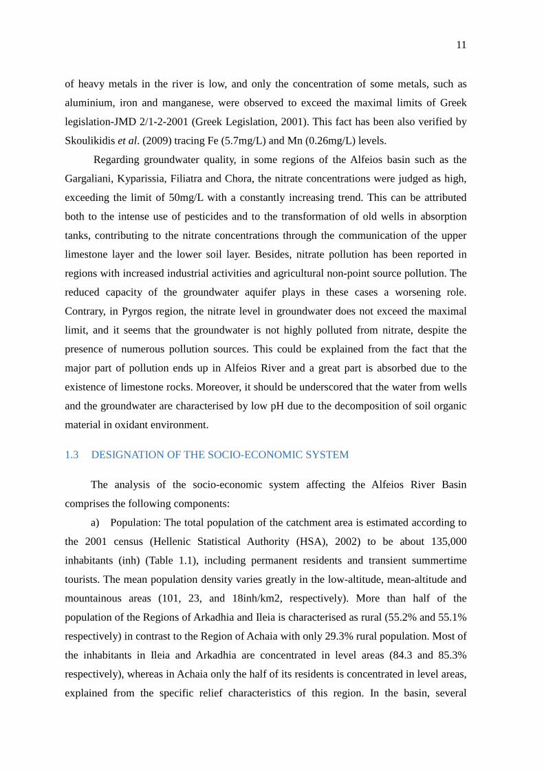
11

of heavy metals in the river is low, and only the concentration of some metals, such as

aluminium, iron and manganese, were observed to exceed the maximal limits of Greek

legislation-JMD 2/1-2-2001 (Greek Legislation, 2001). This fact has been also verified by

Skoulikidis et al. (2009) tracing Fe (5.7mg/L) and Mn (0.26mg/L) levels.

Regarding groundwater quality, in some regions of the Alfeios basin such as the

Gargaliani, Kyparissia, Filiatra and Chora, the nitrate concentrations were judged as high,

exceeding the limit of 50mg/L with a constantly increasing trend. This can be attributed

both to the intense use of pesticides and to the transformation of old wells in absorption

tanks, contributing to the nitrate concentrations through the communication of the upper

limestone layer and the lower soil layer. Besides, nitrate pollution has been reported in

regions with increased industrial activities and agricultural non-point source pollution. The

reduced capacity of the groundwater aquifer plays in these cases a worsening role.

Contrary, in Pyrgos region, the nitrate level in groundwater does not exceed the maximal

limit, and it seems that the groundwater is not highly polluted from nitrate, despite the

presence of numerous pollution sources. This could be explained from the fact that the

major part of pollution ends up in Alfeios River and a great part is absorbed due to the

existence of limestone rocks. Moreover, it should be underscored that the water from wells

and the groundwater are characterised by low pH due to the decomposition of soil organic

material in oxidant environment.

1.3 DESIGNATION OF THE SOCIO-ECONOMIC SYSTEM

The analysis of the socio-economic system affecting the Alfeios River Basin

comprises the following components:

a) Population: The total population of the catchment area is estimated according to

the 2001 census (Hellenic Statistical Authority (HSA), 2002) to be about 135,000

inhabitants (inh) (Table 1.1), including permanent residents and transient summertime

tourists. The mean population density varies greatly in the low-altitude, mean-altitude and

mountainous areas (101, 23, and 18inh/km2, respectively). More than half of the

population of the Regions of Arkadhia and Ileia is characterised as rural (55.2% and 55.1%

respectively) in contrast to the Region of Achaia with only 29.3% rural population. Most of

the inhabitants in Ileia and Arkadhia are concentrated in level areas (84.3 and 85.3%

respectively), whereas in Achaia only the half of its residents is concentrated in level areas,

explained from the specific relief characteristics of this region. In the basin, several

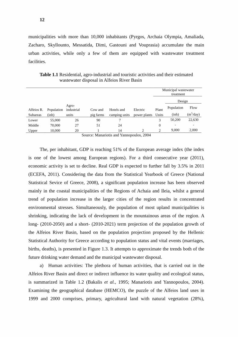
12

municipalities with more than 10,000 inhabitants (Pyrgos, Archaia Olympia, Amaliada,

Zacharo, Skyllounto, Messatida, Dimi, Gastouni and Vouprasia) accumulate the main

urban activities, while only a few of them are equipped with wastewater treatment

facilities.

Table 1.1 Residential, agro-industrial and touristic activities and their estimated wastewater disposal in Alfeios River Basin

Municipal wastewater

treatment

Design

Alfeios R. Population Agro-industrial Cow and Hotels and Electric Plant

Population Flow

Subareas (inh) units pig farms camping units power plants Units (inh) (m3/day)

Lower 55,000 26 90 7 3 50,200 22,630

Middle 70,000 27 51 24 0 - -

Upper 10,000 20 1 14 2 2 9,000 2,000

Source: Manariotis and Yannopoulos, 2004

The, per inhabitant, GDP is reaching 51% of the European average index (the index

is one of the lowest among European regions). For a third consecutive year (2011),

economic activity is set to decline. Real GDP is expected to further fall by 3.5% in 2011

(ECEFA, 2011). Considering the data from the Statistical Yearbook of Greece (National

Statistical Sevice of Greece, 2008), a significant population increase has been observed

mainly in the coastal municipalities of the Regions of Achaia and Ileia, whilst a general

trend of population increase in the larger cities of the region results in concentrated

environmental stresses. Simultaneously, the population of most upland municipalities is

shrinking, indicating the lack of development in the mountainous areas of the region. A

long- (2010-2050) and a short- (2010-2021) term projection of the population growth of

the Alfeios River Basin, based on the population projection proposed by the Hellenic

Statistical Authority for Greece according to population status and vital events (marriages,

births, deaths), is presented in Figure 1.3. It attempts to approximate the trends both of the

future drinking water demand and the municipal wastewater disposal.

a) Human activities: The plethora of human activities, that is carried out in the

Alfeios River Basin and direct or indirect influence its water quality and ecological status,

is summarized in Table 1.2 (Bakalis et al., 1995; Manariotis and Yannopoulos, 2004).

Examining the geographical database (HEMCO), the puzzle of the Alfeios land uses in

1999 and 2000 comprises, primary, agricultural land with natural vegetation (28%),

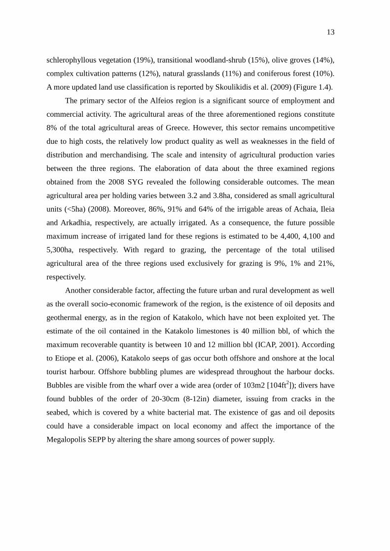
13

schlerophyllous vegetation (19%), transitional woodland-shrub (15%), olive groves (14%),

complex cultivation patterns (12%), natural grasslands (11%) and coniferous forest (10%).

A more updated land use classification is reported by Skoulikidis et al. (2009) (Figure 1.4).

The primary sector of the Alfeios region is a significant source of employment and

commercial activity. The agricultural areas of the three aforementioned regions constitute

8% of the total agricultural areas of Greece. However, this sector remains uncompetitive

due to high costs, the relatively low product quality as well as weaknesses in the field of

distribution and merchandising. The scale and intensity of agricultural production varies

between the three regions. The elaboration of data about the three examined regions

obtained from the 2008 SYG revealed the following considerable outcomes. The mean

agricultural area per holding varies between 3.2 and 3.8ha, considered as small agricultural

units (<5ha) (2008). Moreover, 86%, 91% and 64% of the irrigable areas of Achaia, Ileia

and Arkadhia, respectively, are actually irrigated. As a consequence, the future possible

maximum increase of irrigated land for these regions is estimated to be 4,400, 4,100 and

5,300ha, respectively. With regard to grazing, the percentage of the total utilised

agricultural area of the three regions used exclusively for grazing is 9%, 1% and 21%,

respectively.

Another considerable factor, affecting the future urban and rural development as well

as the overall socio-economic framework of the region, is the existence of oil deposits and

geothermal energy, as in the region of Katakolo, which have not been exploited yet. The

estimate of the oil contained in the Katakolo limestones is 40 million bbl, of which the

maximum recoverable quantity is between 10 and 12 million bbl (ICAP, 2001). According

to Etiope et al. (2006), Katakolo seeps of gas occur both offshore and onshore at the local

tourist harbour. Offshore bubbling plumes are widespread throughout the harbour docks.

Bubbles are visible from the wharf over a wide area (order of 103m2 [104ft2]); divers have

found bubbles of the order of 20-30cm (8-12in) diameter, issuing from cracks in the

seabed, which is covered by a white bacterial mat. The existence of gas and oil deposits

could have a considerable impact on local economy and affect the importance of the

Megalopolis SEPP by altering the share among sources of power supply.

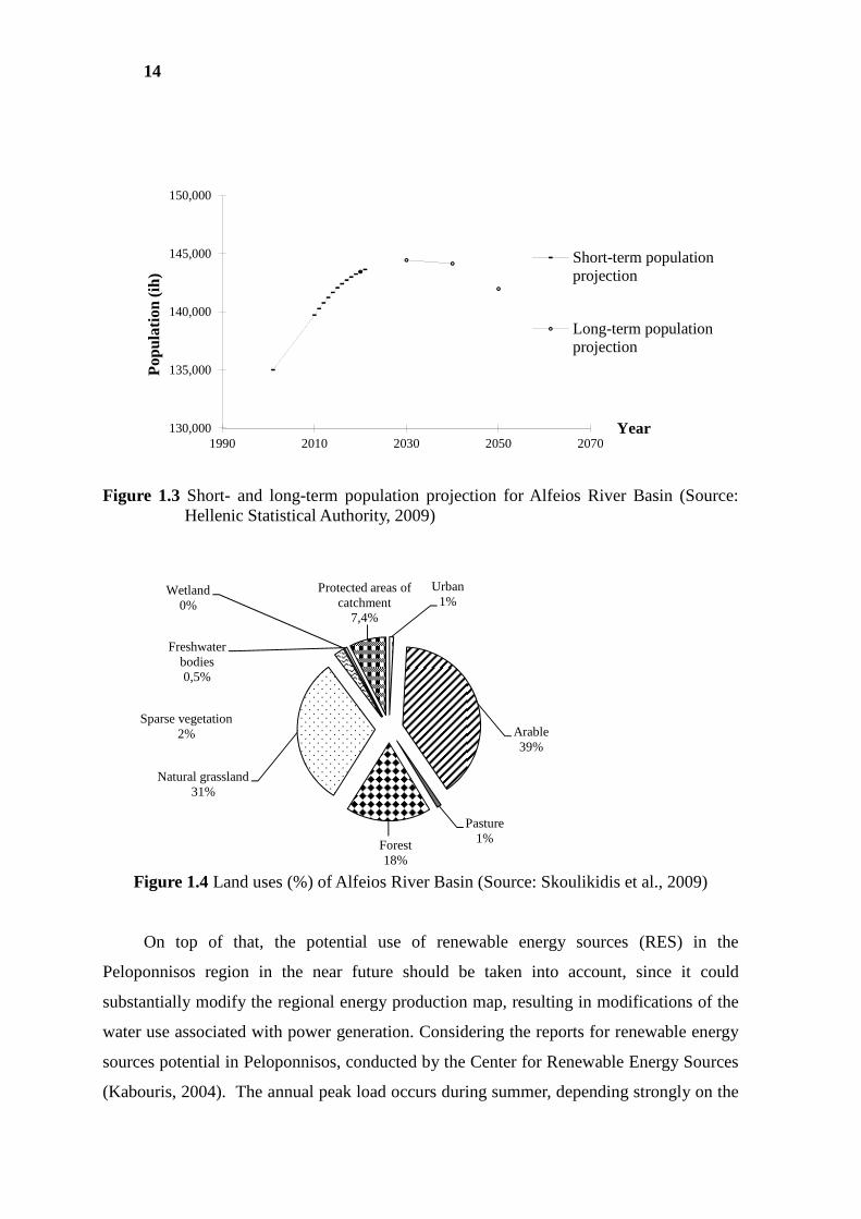
14

Figure 1.3 Short- and long-term population projection for Alfeios River Basin (Source: Hellenic Statistical Authority, 2009)

Figure 1.4 Land uses (%) of Alfeios River Basin (Source: Skoulikidis et al., 2009)

On top of that, the potential use of renewable energy sources (RES) in the

Peloponnisos region in the near future should be taken into account, since it could

substantially modify the regional energy production map, resulting in modifications of the

water use associated with power generation. Considering the reports for renewable energy

sources potential in Peloponnisos, conducted by the Center for Renewable Energy Sources

(Kabouris, 2004). The annual peak load occurs during summer, depending strongly on the

130,000

135,000

140,000

145,000

150,000

1990 2010 2030 2050 2070

Pop

ulat

ion

(ih)

Year

Short-term populationprojection

Long-term populationprojection

Urban 1%

Arable39%

Pasture1%Forest

18%

Natural grassland31%

Sparse vegetation2%

Wetland0%

Freshwater bodies0,5%

Protected areas of catchment

7,4%

15

weather conditions. The existing generation facilities comprise mainly two power plants:

(a) the Megalopolis SEPP (with total installed capacity of 850MW) and (b) the large

hydropower plant of Ladhon, with two generators of nominal capacity 30 or 15MW each,

and annual capacity factor range from 9% to 15%. There are also two small hydropower

plants outside the Alfeios River Basin, Glafkos and Tsivlos. The total thermal and hydro

production from these units was assessed for 2002 to be 5,135 and 200GWh, respectively.

The total theoretical maximum and minimum wind potential of Peloponnisos is estimated

at about 4,755MW and 2,857MW. Additionally, the hydro-potential of Peloponnisos is

quite significant, while two different hydro-areas are distinguished: (a) the first area, in the

north, comprising wet basins with promising flows for small hydro-developments, and (b)

the dry area, at the south-south west, presenting only local sites with flows and heads for

mini-hydro projects. The maximal hydro-potential is about 140MW. Part of this potential is

already exploited by the operation of Ladhon (68MW) and small hydroplants (70.10WM in

2003), belonging both to the HPPC and private investors. Last but not least, the biomass

potential, mainly resulting from residues of agriculture and wood, is estimated to be of

great significance, since in the Alfeios basin a notable number of agro-industrial units

operates. The total available biomass energy for the Regions of Achaia and Ileia, including

mainly the Alfeios basin, is about 2,688,273GJ.

Table 1.2 Human activities influencing the Alfeios River Basin

1. Irrigated and rainfed agricultural activities, fertilization and grazing

11. Construction and operation of transportation infrastructure (roads, railway bridges)

2. Forest burning and exploitation without replanting

12. Continuous and extensive urbanisation in the deltaic area

3. Hunting and trampling 13. Discontinuous urbanisation, dispersed rural habitation

4. Sand and gravel extraction 14. Agro-industrial units, livestock production units 5. Polderization and land reclamation 15. Tourist facilities and recreational activities 6. Drainage of areas surrounding the river delta 16. Lignite mining in Megalopolis basin 7. Embankments, canalization, river diversion and other river-modifying structures

17. Operation of stream electric power production plant in Megalopolis

8. Water-level management at dam locations 18. Public and private hydroelectric power stations 9. Dumping and disposal of dredged materials 19. Municipal untreated or partially treated

wastewater disposal 10. Landfilling and disposal of inert materials

Source: (Bakalis et al., 1995; Manariotis and Yannopoulos, 2004; Dafis et al., 1996) Various “green” touristic and recreational activities are added to the socio-economic

mosaic of the Alfeios River Basin. The area is equipped with accommodation and catering

16

facilities of high quality, and is gifted with the combination of maritime, mountainous and

lowland areas. Attractive activities include climbing, mountain biking, walking tours, river

trekking (Trekking Hellas) amongst trails of dense vegetation going parallel to the Lousios

River, being one of the most stirring Greek sites. Moreover, rafting (i.e., in Erymanthos

River), sea sports, canoe-kayak, sailing, diving are only some of the supplementary

activities already provided in the river basin.

Finally, attempting to synthesize the socio-economic profile of the broader region

of the Alfeios watershed, it is worth taking into consideration the following future

perspectives of the region of Western Greece. This region is an essential transport hub,

which has led to an intense development of international sea transport and trade to and

from its main port, Patras (HMEPPPW, 2008). The prospects for further touristic

developments and related industry are also favourable. As far as future policies are

concerned, a lot of emphasis is expected to be put on innovation at regional level. Given

the importance of the service sector in Western Greece, the provision of specific service

innovation measures seems to be a priority for national and regional innovation strategic

planning. The development of this sector could be interpreted as a potential reduction of

the industrial wastewater disposal, and simultaneously as a pole of attraction of more

educated individuals, which could demonstrate a stronger willingness to actively

participate in the water resources management process. On the other hand, because of the

proximity to countries both within the EU (internal boundaries) and non-EU countries on

its borders, the region of Western Greece experiences considerable immigration and

repatriation, posing an enormous burden, which could be translated also into direct and

indirect negative environmental stresses in its water resources system.

1.4 IDENTIFICATION OF THE ADMINISTRATIVE AND INSTITUTIONAL

SYSTEM

The general regulating frame for water resources management and protection in

Greece, as an EU-member, is predominantly determined by the European water policy. The

most important breakthrough, the transposition of the European WFD into the Greek

legislation, has led to an institutional organisation with a new Central Water Agency, 13

Regional Water Directorates, a National Water Committee (interministerial political body),

and national and regional water councils (consultative bodies). River basin management

within this administrative scheme falls into the responsibility of the 13 Regional Water

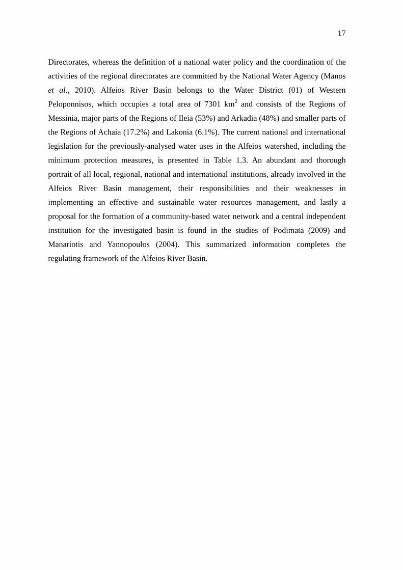
17

Directorates, whereas the definition of a national water policy and the coordination of the

activities of the regional directorates are committed by the National Water Agency (Manos

et al., 2010). Alfeios River Basin belongs to the Water District (01) of Western

Peloponnisos, which occupies a total area of 7301 km2 and consists of the Regions of

Messinia, major parts of the Regions of Ileia (53%) and Arkadia (48%) and smaller parts of

the Regions of Achaia (17.2%) and Lakonia (6.1%). The current national and international

legislation for the previously-analysed water uses in the Alfeios watershed, including the

minimum protection measures, is presented in Table 1.3. An abundant and thorough

portrait of all local, regional, national and international institutions, already involved in the

Alfeios River Basin management, their responsibilities and their weaknesses in

implementing an effective and sustainable water resources management, and lastly a

proposal for the formation of a community-based water network and a central independent

institution for the investigated basin is found in the studies of Podimata (2009) and

Manariotis and Yannopoulos (2004). This summarized information completes the

regulating framework of the Alfeios River Basin.

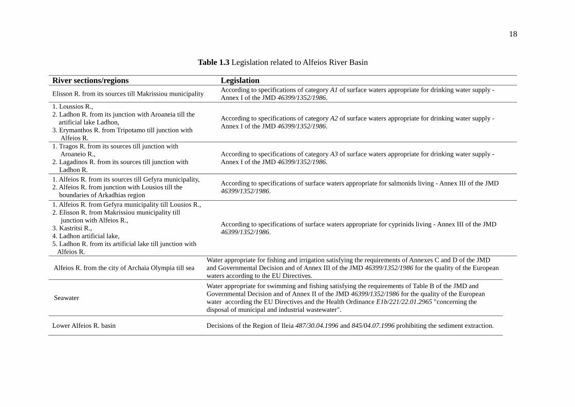
18

Table 1.3 Legislation related to Alfeios River Basin

River sections/regions Legislation

Elisson R. from its sources till Makrissiou municipality According to specifications of category A1 of surface waters appropriate for drinking water supply - Annex I of the JMD 46399/1352/1986.

1. Loussios R., 2. Ladhon R. from its junction with Aroaneia till the

artificial lake Ladhon, 3. Erymanthos R. from Tripotamo till junction with Alfeios R.

According to specifications of category A2 of surface waters appropriate for drinking water supply - Annex I of the JMD 46399/1352/1986.

1. Tragos R. from its sources till junction with Aroaneio R., 2. Lagadinos R. from its sources till junction with Ladhon R.

According to specifications of category A3 of surface waters appropriate for drinking water supply - Annex I of the JMD 46399/1352/1986.

1. Alfeios R. from its sources till Gefyra municipality, 2. Alfeios R. from junction with Lousios till the boundaries of Arkadhias region

According to specifications of surface waters appropriate for salmonids living - Annex III of the JMD 46399/1352/1986.

1. Alfeios R. from Gefyra municipality till Lousios R., 2. Elisson R. from Makrissiou municipality till junction with Alfeios R., 3. Kastritsi R., 4. Ladhon artificial lake, 5. Ladhon R. from its artificial lake till junction with Alfeios R.

According to specifications of surface waters appropriate for cyprinids living - Annex III of the JMD 46399/1352/1986.

Alfeios R. from the city of Archaia Olympia till sea Water appropriate for fishing and irrigation satisfying the requirements of Annexes C and D of the JMD and Governmental Decision and of Annex III of the JMD 46399/1352/1986 for the quality of the European waters according to the EU Directives.

Seawater

Water appropriate for swimming and fishing satisfying the requirements of Table B of the JMD and Governmental Decision and of Annex II of the JMD 46399/1352/1986 for the quality of the European water according the EU Directives and the Health Ordinance E1b/221/22.01.2965 "concerning the disposal of municipal and industrial wastewater".

Lower Alfeios R. basin Decisions of the Region of Ileia 487/30.04.1996 and 845/04.07.1996 prohibiting the sediment extraction.

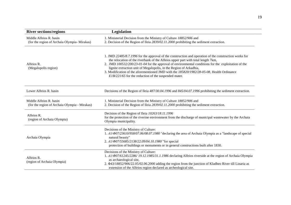
19

River sections/regions Legislation

Middle Alfeios R. basin (for the region of Archaia Olympia- Mirakas)

1. Ministerial Decision from the Ministry of Culture 18852/906 and 2. Decision of the Region of Ileia 2839/02.11.2000 prohibiting the sediment extraction.

Alfeios R. (Megalopolis region)

1. JMD 22485/8.7.1996 for the approval of the construction and operation of the construction works for the relocation of the riverbank of the Alfeios upper part with total length 7km,

2. JMD 100532/200/23-01-04 for the approval of environmental conditions for the exploitation of the lignite extraction unit of Megalopolis, in the Region of Arkadhia,

3. Modification of the aforementioned JMD with the 185820/1982/28-05-08, Health Ordinance E1B/221/65 for the reduction of the suspended mater.

Lower Alfeios R. basin Decisions of the Region of Ileia 487/30.04.1996 and 845/04.07.1996 prohibiting the sediment extraction.

Middle Alfeios R. basin (for the region of Archaia Olympia - Mirakas)

1. Ministerial Decision from the Ministry of Culture 18852/906 and 2. Decision of the Region of Ileia 2839/02.11.2000 prohibiting the sediment extraction.

Alfeios R. (region of Archaia Olympia)

Decision of the Region of Ileia 10263/18.11.1996 for the protection of the riverine environment from the discharge of municipal wastewater by the Archaia Olympia municipality.

Archaia Olympia

Decisions of the Ministry of Culture: 1. Α1/Φ07/23610/958/07.06/08.07.1980 "declaring the area of Archaia Olympia as a "landscape of special

natural beauty" 2. Α1/Φ07/55685/2138/22.09/04.10.1980 "for special protection of buildings or monuments or in general constructions built after 1830.

Alfeios R. (region of Archaia Olympia)

Decisions of the Ministry of Culture: 1. Α1/Φ07/61245/2286/ 19.12.1985/31.1.1986 declaring Alfeios riverside at the region of Archaia Olympia

as archaeological site, 2. Φ43/18852/906/22.05/02.06.2000 adding the region from the junction of Kladheo River till Linaria as

extension of the Alfeios region declared as archeological site.

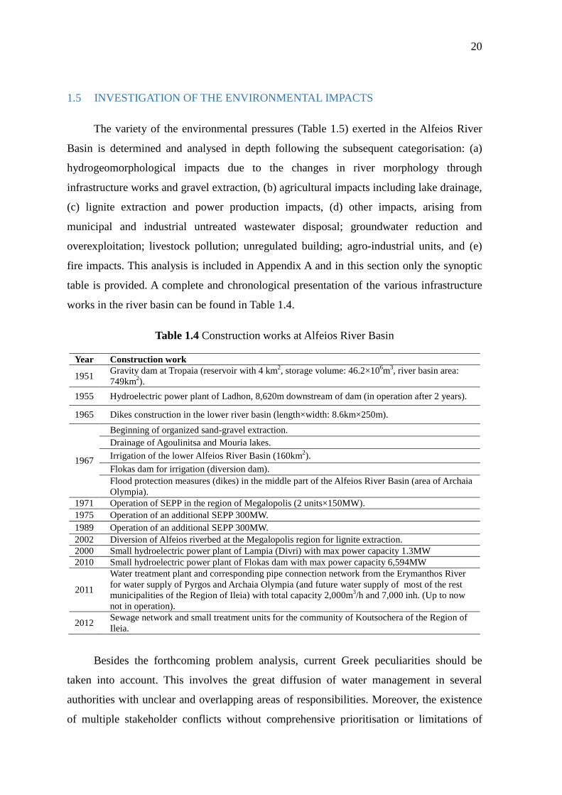
20

1.5 INVESTIGATION OF THE ENVIRONMENTAL IMPACTS

The variety of the environmental pressures (Table 1.5) exerted in the Alfeios River

Basin is determined and analysed in depth following the subsequent categorisation: (a)

hydrogeomorphological impacts due to the changes in river morphology through

infrastructure works and gravel extraction, (b) agricultural impacts including lake drainage,

(c) lignite extraction and power production impacts, (d) other impacts, arising from

municipal and industrial untreated wastewater disposal; groundwater reduction and

overexploitation; livestock pollution; unregulated building; agro-industrial units, and (e)

fire impacts. This analysis is included in Appendix A and in this section only the synoptic

table is provided. A complete and chronological presentation of the various infrastructure

works in the river basin can be found in Table 1.4.

Table 1.4 Construction works at Alfeios River Basin

Year Construction work

1951 Gravity dam at Tropaia (reservoir with 4 km2, storage volume: 46.2×106m3, river basin area: 749km2).

1955 Hydroelectric power plant of Ladhon, 8,620m downstream of dam (in operation after 2 years).

1965 Dikes construction in the lower river basin (length×width: 8.6km×250m).

1967

Beginning of organized sand-gravel extraction. Drainage of Agoulinitsa and Mouria lakes.

Irrigation of the lower Alfeios River Basin (160km2).

Flokas dam for irrigation (diversion dam). Flood protection measures (dikes) in the middle part of the Alfeios River Basin (area of Archaia Olympia).

1971 Operation of SEPP in the region of Megalopolis (2 units×150MW). 1975 Operation of an additional SEPP 300MW. 1989 Operation of an additional SEPP 300MW. 2002 Diversion of Alfeios riverbed at the Megalopolis region for lignite extraction. 2000 Small hydroelectric power plant of Lampia (Divri) with max power capacity 1.3MW 2010 Small hydroelectric power plant of Flokas dam with max power capacity 6,594MW

2011

Water treatment plant and corresponding pipe connection network from the Erymanthos River for water supply of Pyrgos and Archaia Olympia (and future water supply of most of the rest municipalities of the Region of Ileia) with total capacity 2,000m3/h and 7,000 inh. (Up to now not in operation).

2012 Sewage network and small treatment units for the community of Koutsochera of the Region of Ileia.

Besides the forthcoming problem analysis, current Greek peculiarities should be

taken into account. This involves the great diffusion of water management in several

authorities with unclear and overlapping areas of responsibilities. Moreover, the existence

of multiple stakeholder conflicts without comprehensive prioritisation or limitations of

21

water uses is another complexity factor. Irregular and inadequate pollution monitoring

programs and low financial resources pose more difficulties. There is also a great lack of

environmental education and citizen awareness of environmental issues. And finally, some

attempts towards IRBM practices - such as control of gravel extraction or changes in

agricultural management - were hampered by the lack of monitoring systems for the actual

and continuous verification of the water bodies’ status.

Table 1.5 Environmental impacts in the Alfeios River Basin

A. Hydrogeological stresses Impacts

- from the construction and operation of Flokas and Ladhon dam

- from gravel and sediment extraction along the river

- Effects on the natural deltaic evolution (retreat of coastline; deltaic shore erosion, etc.)

- Reduction of riverwidth - Reduction of fluvial sediment fluxes - Changes in the riverine flora - High capital for stabilisation works of dam and

bridges foundations due to scoring effects - Groundwater overexploitation; groundwater table

drop; saline intrusion - Overall ecosystem deterioration

B. Agricultural stresses Impacts

- from agricultural activities - from the drainage of Agoulinitsa

and Mouria lakes

- Destruction of biotopes - Eutrophication conditions and deoxydation - High concentration of ammonia - Sediment contamination from extensive use of

fertilisers and waste dumping - Nitrate, nitrite and phosphate pollution

C. Lignite extraction & power production stresses Impacts

- from lignite extraction site and SEPP of Megalopolis

- Geomorphological changes (river embankment, levees, diversion of river course, etc.)

- Reduction of riverine flora and deterioration of riverine areas

- Crop damages - Water and air pollution

D. Other stresses Impacts

- from untreated municipal and industrial wastewater disposal;

- from trampling and unregulated building near Alfeios delta;

- from agro-industrial and other industrial units;

- from wildfires

- Water quality pollution - Degradation of flora and fauna - Geomorphological changes - Aesthetic and landscape changes - Non-point source pollution

- Economic losses due to infrastructure, touristic facilities and agricultural damages

22

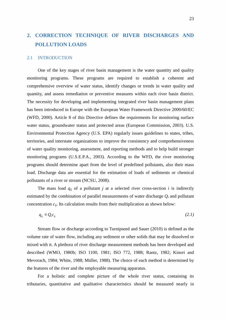
23

2. CORRECTION TECHNIQUE OF RIVER DISCHARGES AND

POLLUTION LOADS

2.1 INTRODUCTION

One of the key stages of river basin management is the water quantity and quality

monitoring programs. These programs are required to establish a coherent and

comprehensive overview of water status, identify changes or trends in water quality and

quantity, and assess remediation or preventive measures within each river basin district.

The necessity for developing and implementing integrated river basin management plans

has been introduced in Europe with the European Water Framework Directive 2000/60/EC

(WFD, 2000). Article 8 of this Directive defines the requirements for monitoring surface

water status, groundwater status and protected areas (European Commission, 2003). U.S.

Environmental Protection Agency (U.S. EPA) regularly issues guidelines to states, tribes,

territories, and interstate organizations to improve the consistency and comprehensiveness

of water quality monitoring, assessment, and reporting methods and to help build stronger

monitoring programs (U.S.E.P.A., 2003). According to the WFD, the river monitoring

programs should determine apart from the level of predefined pollutants, also their mass

load. Discharge data are essential for the estimation of loads of sediments or chemical

pollutants of a river or stream (NCSU, 2008).

The mass load qij of a pollutant j at a selected river cross-section i is indirectly

estimated by the combination of parallel measurements of water discharge Qi and pollutant

concentration cij. Its calculation results from their multiplication as shown below:

(2.1)

Stream flow or discharge according to Turnipseed and Sauer (2010) is defined as the

volume rate of water flow, including any sediment or other solids that may be dissolved or

mixed with it. A plethora of river discharge measurement methods has been developed and

described (WMO, 1980b; ISO 1100, 1981; ISO 772, 1988; Rantz, 1982; Kinori and

Mevorach, 1984; White, 1988; Müller, 1988). The choice of each method is determined by

the features of the river and the employable measuring apparatus.

For a holistic and complete picture of the whole river status, containing its

tributaries, quantitative and qualitative characteristics should be measured nearly in

ijiij cQq =

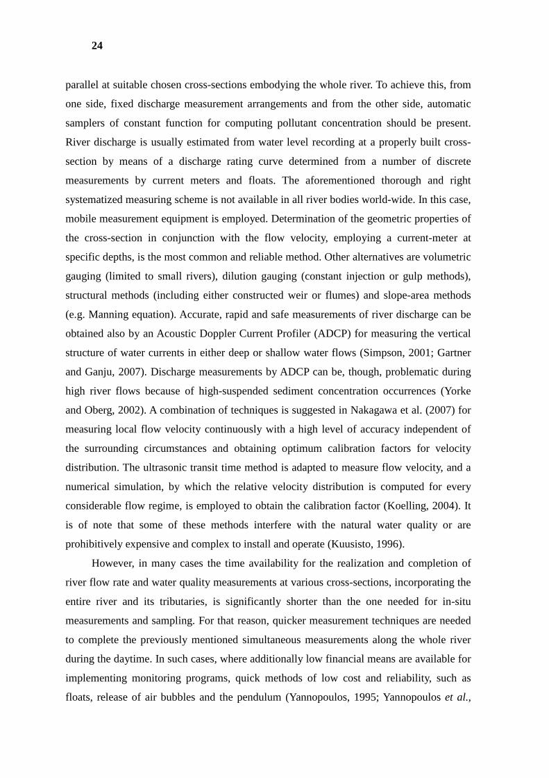
24

parallel at suitable chosen cross-sections embodying the whole river. To achieve this, from

one side, fixed discharge measurement arrangements and from the other side, automatic

samplers of constant function for computing pollutant concentration should be present.

River discharge is usually estimated from water level recording at a properly built cross-

section by means of a discharge rating curve determined from a number of discrete

measurements by current meters and floats. The aforementioned thorough and right

systematized measuring scheme is not available in all river bodies world-wide. In this case,

mobile measurement equipment is employed. Determination of the geometric properties of

the cross-section in conjunction with the flow velocity, employing a current-meter at

specific depths, is the most common and reliable method. Other alternatives are volumetric

gauging (limited to small rivers), dilution gauging (constant injection or gulp methods),

structural methods (including either constructed weir or flumes) and slope-area methods

(e.g. Manning equation). Accurate, rapid and safe measurements of river discharge can be

obtained also by an Acoustic Doppler Current Profiler (ADCP) for measuring the vertical

structure of water currents in either deep or shallow water flows (Simpson, 2001; Gartner

and Ganju, 2007). Discharge measurements by ADCP can be, though, problematic during

high river flows because of high-suspended sediment concentration occurrences (Yorke

and Oberg, 2002). A combination of techniques is suggested in Nakagawa et al. (2007) for

measuring local flow velocity continuously with a high level of accuracy independent of

the surrounding circumstances and obtaining optimum calibration factors for velocity

distribution. The ultrasonic transit time method is adapted to measure flow velocity, and a

numerical simulation, by which the relative velocity distribution is computed for every

considerable flow regime, is employed to obtain the calibration factor (Koelling, 2004). It

is of note that some of these methods interfere with the natural water quality or are

prohibitively expensive and complex to install and operate (Kuusisto, 1996).

However, in many cases the time availability for the realization and completion of

river flow rate and water quality measurements at various cross-sections, incorporating the

entire river and its tributaries, is significantly shorter than the one needed for in-situ

measurements and sampling. For that reason, quicker measurement techniques are needed

to complete the previously mentioned simultaneous measurements along the whole river

during the daytime. In such cases, where additionally low financial means are available for

implementing monitoring programs, quick methods of low cost and reliability, such as

floats, release of air bubbles and the pendulum (Yannopoulos, 1995; Yannopoulos et al.,

25

2000; Yannopoulos et al., 2008) could be employed for river discharge measurements.

For the determination of river water quality characteristics, in-situ field

measurements of physical and chemical parameters, such as temperature, conductivity

(salinity), dissolved oxygen, pH, turbidity, fluorescence, BOD5, nutrients and metals, are

taking place in parallel with water sampling for laboratory analysis (Kuusisto, 1996).

Considerations that influence the parameter to sample include the study objectives, the

type of water resource, the use of the water body, the type of point and non-point source of

pollution, the difficulty or cost in analysis of the variable, and the water quality problem

(USDA, 2003). The sampling equipment is selected according to the type of water body

and to the sample requirements for performing the analyses of the monitoring program. For

such in-situ measurements, a variety of single-parameter and multi-parameter field-

measurement instruments are available. They use various technologies to measure the same

water characteristic, requiring differing calibration, maintenance and measurement

methods (Wilde, 2008). Standards for water quality monitoring could be “any relevant

CEN/ISO standards or such other national or international standards, which will ensure the

provision of data of an equivalent scientific quality and comparability” (WFD, 2000).

Water sampling and laboratory measurements of samples can be made according to the

Standard Methods for examination of water and wastewater (Eaton et al., 1995; APHA,

1999), avoiding any contamination or changes in the relevant chemical properties of the

sample. River and stream samples should be taken from mid-stream or a flowing part of

the stream, where good mixing conditions have been established.

It is worth mentioning that numerous measurements and samples will be needed to

accurately and reliably capture the true value of the measured parameter. There is often a

conflict between the number of observations a program can afford and the number needed

to obtain an accurate and reliable load estimate. For this reason, it is useful from one side,

to investigate the propagation of error in measurements, and from the other side, to develop

and integrate techniques and procedures to correct the measured values or even try to

derive more reliable values.

The present work aims to develop a methodology based on a correction concept of

quick river discharge measurements for the estimation of more reliable values of pollution

loads in ungauged rivers (Yannopoulos, 2009; Yannopoulos and Bekri, 2010; Bekri et al.,

2013; Yannopoulos and Bekri, 2010; Bekri et al., 2013). The water volume conservation is

combined with pollutant/tracers mass balance in a river node and in the entire river, when

26

parallel measurements of river flow rate and natural tracers are available for representative

cross-sections of a river and its tributaries. The proposed methodology computes river

discharge values, and subsequently pollution loads, of higher accuracy and reliability

compared to the initial discharge estimates, measured by the aforementioned quick

methods. It relies on linear optimization, taking into account hypothetical unknown latent

quantities. Moreover, this methodology enables the determination of a non-measurable

unknown latent discharge at a river node, at the point where the main river meets one or

more tributaries. It attempts to reduce time, complexity, personnel and cost of river

monitoring programs, as well as of water resources management plans. The method was

applied and tested to the Alfeios River Basin, in Greece, where only limited short-term

quantitative and qualitative measurement data are available (Yannopoulos and Bekri,

2010).

2.1.1 ERROR CORRECTION TECHNIQUES OF RIVER FLOW RATE MEASUREMENT

Various methods have been developed for estimating the uncertainty in discharge

measurements including hydrographer estimates (Rantz, 1982) and statistical error

propagation techniques (Carter and Anderson, 1963; WHO, 1980; Herschy, 1985, 1971;

ISO 748, 1979; Sauer and Meyer, 1992). Error correction techniques are generally very

cost-effective and therefore, efficient for data assimilation. A thorough review of processes

for estimating discharge measurements errors was published by Dickinson (1967), updated

by Pelletier (1988) and lately by McMillan et al. (2012). It is worth emphasizing that no

amount of computer processing or statistical analysis will correct a completely wrong

measurement. According to ISO (1993) guide, measurement uncertainty has been defined

as a non-negative parameter characterizing the dispersion of the quantity values being

attributed to a measure and based on the information used. Based on Miller (1983)

definition of measuring accuracy, the accuracy or the error of river discharge measurement

may be expressed as the difference between the measured and the true value, which is not

known and can only be ascertained by weighing or volumetric measurements. Although the

error in a result is by definition unknown, the uncertainty may be estimated, if the

distribution of the measured values about the true mean is known. An estimate of the true

value has therefore to be made by calculating the uncertainty in the measurement, as the

range in which the true value is expected to lie expressed as confidence level.

The uncertainty of individual river discharge measurements includes random and

27

systematic errors in the cross-sectional area related to errors in measurement of width,

depth, errors in mean stream velocity arising from velocity distributions, turbulence and

other factors, errors associated with the computation procedure and errors caused by

change in stage during the measurements, boundary effects, ice, obstructions, wind,

incorrect equipment, incorrect measurements techniques, poor distribution of

measurements verticals, carelessness and other factors (Sauer and Meyer, 1992). Moreover,

the uncertainty related to real hydraulic conditions at time t for river discharge

measurements, potentially differing from the reference flow regime, is related to additional

sources of errors including transient flow effects (hysteresis) and variable hydraulic

conditions (backwater effects in non-uniform flows, seasonal vegetation changes, changes

in reach or control section geometry) (Le Coz, 2012).

The most commonly used statistical term in estimation of river flow measurement

uncertainty is the standard deviation. In general, the uncertainty in the measurements of an

independent variable is estimated by computing the standard deviation from a sufficient

high number of observations, usually more than thirty. This is quite difficult in a gauging

station, and therefore the estimate of the true value could be made through examination of

all possible error sources, as analysed above. To apply the theory of statistics in river

discharge measurements, it is assumed that the observations are independent random

variables from a statistically uniform distribution. In general, two possible approaches to

estimating measurement uncertainty can be used, either separately or as complementary

techniques. The first approach, the so-called bottom-up approach, includes a detailed

analysis of the contributing errors from each of the methodological elements and then a

combination of these uncertainties into an overall discharge error (Di Baldassarre and

Montanari, 2009; Sauer and Meyer, 1992). This general overall approach of summing

individual errors can lead to an underestimation of the measurement uncertainty due to the

risk of overlooking an important contributing element. The second approach of estimating

measurement uncertainty, the top-down approach uses data from the analysis of certified

reference materials, routine control samples, or interlaboratory trials. It is worth noticing

that the estimation of uncertainty using these methods is most likely to yield accurate

estimates of discharge measurement uncertainty, only if the measurement conditions are

similar to those experienced in the empirical or laboratory studies. The limitations of the

methods dealing with uncertainties in a statistical framework has been recognized by the

ISO (1993) guide, which expressed uncertainties by distinguishing two different categories

28

of uncertainties according to method used to estimate their numerical values: Type A,

method of evaluation of uncertainty by the statistical analysis of series of observations, and

Type B, evaluation of uncertainty by means other than the statistical analysis of series of

observations (Shrestha and Simonovic, S.,P., 2010).

Another interesting scientific domain aiming at correcting measurement errors due to

measurement noise is the data validation and reconciliation (DVR) (Kuehn and Davidson,

1961; Mah et al., 1976; Himmelblau, 1978; Maquin et al., 1991). It finds application

mainly in industry sectors where either measurements are not accurate or even non-

existing, like for example in the upstream sector where flow meters are difficult or

expensive to position (Delava et al., 1999), or where accurate data is of high importance,

for example for security reasons in nuclear power plants (Langenstein et al., 2004). It

improves the accuracy of process data by adjusting the measured values so that they satisfy

the process constraints. In general, data reconciliation can be formulated by a weighted

least squares optimization problem or maximum likelihood objective function, where the

measurement errors are minimized with process model constraints. The data reconciliation

techniques not only reconcile the raw measurements, but also estimate unmeasured process

variables or model parameters, provided that they are observable. Usually, the kind of

constraints included is mass and energy balance constraints as deterministic valid physical

laws and in some cases other inequality relations imposed by feasibility of process

operations. Empirical or other types of equations involving many unmeasured parameters

are not recommended to be used as constraints, since they are at best known only

approximately. Forcing the measured variables to obey inexact relations can cause

inaccurate data reconciliation solution and incorrect gross error diagnosis. The reconciled

estimates are expected to be more accurate than the measurements and, more importantly,

are also consistent with the known relationships between process variables as defined by

the constraints.

The most commonly used criterion/ objective function to select the optimal solution

in data reconciliation is the weighted least squares (WLS) deviations of the corrected

discharges from their measured values. Generally, it is assumed that the error variances for

all the measurements are known and the weights are chosen to be the inverse of these

variances. In this case, more accurate measurements are given larger weights in order to

force their adjustments to be as small as possible. As analysed in Özyurt and Pike (2004),

different objective functions besides the WLS can be used for data reconciliation. The

29

WLS objective function assumes measurement errors from a distribution with zero mean

and known variance. For any possible deviation from this assumption, another objective

function, which does not require this assumption, can be a better candidate. This is

especially the case when the measurements contain some gross errors, which contaminate

the estimates for other measured variables. Tjoa and Biegler (1991) showed that using

nonlinear programming along with a method based on a contaminated Normal (Gaussian)

objective function instead of the least squares objective function, any gross error present in

the measurements could be replaced with reconciled values, and an iterative procedure was

not required. By establishing an analogy between maximum likelihood rectification (MLR)

and robust regression, Johnston and Kramer (1995) reported the feasibility and better

performance of the robust estimators as the objective function in the data reconciliation

problem, especially when the data contain gross errors. Subsequently, different types of

robust estimators and their performance in data reconciliation were reported (Albuquerque

and Biegler, 1996; Arora and Biegler). These studies have shown the potential of robust

statistics developed by Huber (1981), which attempts accurate estimation of statistical

parameters in the presence of gross errors. In Özyurt and Pike (2004), a comparison of

various maximum likelihood functions derived from normal, contaminated normal and

Cauchy distribution as well as the fair, logistic, Lorentzian and Hampel function, has been

undertaken, concluding that Lorentzian function is the most insensitive to gross errors

when data reconciliation is conducted with them.

The basic concept of our proposed methodology is similar as in data reconciliation,

since they both aim at correcting the raw measurements based on the principles of mass

conservation without knowing the precise values. Classical approaches for data validation

are usually solved by statistical approaches, which are relevant when an explicit

characterization of the measurement errors is available. As extensively analyzed in most

correction error methods, in addition to knowledge of the measurements and the

knowledge of the model of the process, which is used as constraints for the estimation,

knowledge of the precision of the measurements, which is involved in the weight functions

and affects the different corrective terms, is also requested (Abdollahzadeh et al., 1996).

The main difficulties for this are that the processes are not always perfectly described and

the measurement precision cannot be precisely quantified. In many cases the user has only

an experimental knowledge, which even inaccurate can be used in the form of inequalities.

The proposed methodology does not request the knowledge of any statistical assumption

30

for the error distribution, since intervals in terms of error bounds are used in order to

express the allowable range of the corrected values of each parameter based on their

measured values and assumed measurement errors.

This concept of expressing the measurement error as interval is similar to the one

used in the so-called parameter set estimation from bounded error data (Milanese and

Belforte, 1982). In this case it is assumed that all types of errors belong to a known set and

that the measurement error is bounded. It includes the determination of the set of constant

parameter values, called Feasible Parameter Set (FPS), which is compatible with all the

available observations, taking into account the errors bounds and the model constraints

(Maquin et al., 1991). As analysed in these scientific works, because of uncertainty and

noise influence it is not feasible to calculate the exact parameter values, but it seems

reasonable to compute a domain in which the real values of the system are contained. The

feasible set may have a complicated shape and its exact description may be intractable. To

overcome this difficulty, the exact FPS is restricted to a simpler domain. For linear models,

the FPS is a convex polytope which can be approximated by ellipsoids (Fogel and Huang,

1982) or orthotopes (Milanese and Belforte, 1982; Milanese et al., 1996) containing it.

As mentioned in Ragot and Maquin (2004) a few works has been published in this

area. In Himmelblau (1985) the use of bounds for the estimation with an interval

formulation is attempted. More recently, in Mandel et al. (1998) and Ragot et al. (1997)

the linear matrix inequality approach enables the formulation of more general bounded

estimation problems and their corresponding admissible solutions. In Ragot and Maquin

(2004), a two-step strategy is proposed. The first step includes the reduction of the

parameter to be estimated to those which are redundant, thus measured. The second step

involves the formulation of the problem in inequalities taking into account the error

bounds. A geometric shape is selected, such as a box with a centre and a width for each

parameter, and the corresponding range is expressed based on these two variables and the

measurement error bounds. The set of the inequalities is solved in respect of expressing the

interval of each parameter in association with the centre and the width. If the measurement

variance is known then the maximisation of the size of the box expressed by the width of

each parameter subject to the model constraints could be selected as objective function.

The main conceptual difference of this bounded error data reconciliation technique with

the present methodology is that the proposed methodology does not request the knowledge

of the variance of the measurements, since it is very difficult to make the sufficient number

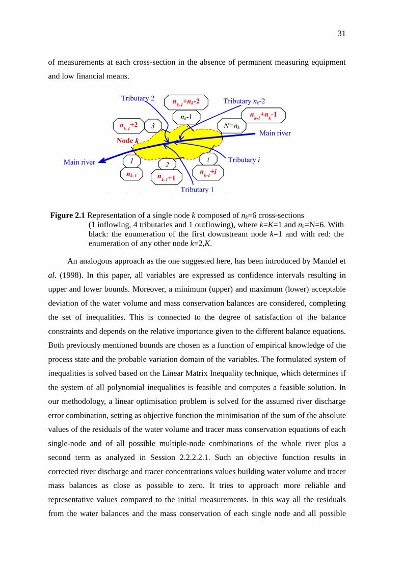
31

of measurements at each cross-section in the absence of permanent measuring equipment

and low financial means.

An analogous approach as the one suggested here, has been introduced by Mandel et

al. (1998). In this paper, all variables are expressed as confidence intervals resulting in

upper and lower bounds. Moreover, a minimum (upper) and maximum (lower) acceptable

deviation of the water volume and mass conservation balances are considered, completing

the set of inequalities. This is connected to the degree of satisfaction of the balance

constraints and depends on the relative importance given to the different balance equations.

Both previously mentioned bounds are chosen as a function of empirical knowledge of the

process state and the probable variation domain of the variables. The formulated system of

inequalities is solved based on the Linear Matrix Inequality technique, which determines if

the system of all polynomial inequalities is feasible and computes a feasible solution. In

our methodology, a linear optimisation problem is solved for the assumed river discharge

error combination, setting as objective function the minimisation of the sum of the absolute

values of the residuals of the water volume and tracer mass conservation equations of each

single-node and of all possible multiple-node combinations of the whole river plus a

second term as analyzed in Session 2.2.2.2.1. Such an objective function results in

corrected river discharge and tracer concentrations values building water volume and tracer

mass balances as close as possible to zero. It tries to approach more reliable and

representative values compared to the initial measurements. In this way all the residuals

from the water balances and the mass conservation of each single node and all possible

Figure 2.1 Representation of a single node k composed of nk=6 cross-sections (1 inflowing, 4 tributaries and 1 outflowing), where k=K=1 and nk=N=6. With black: the enumeration of the first downstream node k=1 and with red: the enumeration of any other node k=2,K.

32

node combinations are introduced into the objective function. When a constraint

considering their allowable values is violated, there is a positive contribution to the

objective function equal to the amount of violations or the sum of infeasibilities. A further

comparison of the two resembling methodologies is provided in the description of the

recommended methodology.

Finally, it is of note that from a thorough literature review, the combination of water

volume and properly selected natural tracers mass conservation in a river network with the

use of bounded error data reconciliation, as analysed in the introduced methodology, has

not been applied up to the present to correct river discharge measurements and compute

more reliable pollution loads, whereas similar data reconciliation techniques are proposed

in chemical engineering domain.

2.2 METHODOLOGICAL AND MATHEMATICAL FRAMEWORK

2.2.1 ANALYSIS OF THE NODE -BASED METHODOLOGICAL APPROACH

2.2.1.1 GENERAL DESCRIPTION OF THE RIVER NETWORK AND NOTATIONS USED

Based on preliminary scientific work of Yannopoulos (2009) and Yannopoulos and

Bekri (2010) which included only an oversimplified application of the initial mathematical

background and the corresponding theoretical idea for a single-node balance of Alfeios

river, whereas assuming the tracer concentrations known, the improved and thoroughly

revised general methodological framework is presented in this paper. As depicted in for a

single node k of a river composed of nk (nk≥2) cross-sections, the following cross-sections

contribute to the node: an inflowing cross-section N=nk, nk-2 tributaries, if any, and an

outflowing cross-section 1. Covering the entire length of a river of interest, it is possible to

define K consecutive nodes, beginning from the river estuaries (k=1) towards its sources

(k=K). This is shown in Figure 2.2. for a river composed of two nodes, thus K=2. It is

worth noticing that two adjacent nodes k and k+1 are connected through a common cross-

section, which for the upstream node k+1 is outflowing and for the downstream node k is

inflowing (in Figure 2.2 the common node is the node nk=1).

The enumeration of the cross-sections i, for building the multiple-node optimization

subsystem, including the combination of two subsequent cross-sections up to the

combination of numerous subsequent nodes covering the whole river, starts from river

estuaries and ends to the river sources (which is in accordance to the direction of

33

enumeration of the single node). More precisely, as shown in Figure 2.2, it starts with i=1

from the cross-section flowing out of the first node k=1 into the sea situated at river

estuaries cross-section. Then, moving upstream up to the last cross-section situated at the

river sources with i=N. The number of total cross-sections of the entire river, N, is

connected with the separate enumeration of the total cross-section of each single node, nk

(with k=1,K), with the relationship ( )∑=

−−=K

kk KnN

1

1 . The last term in parenthesis is used

to subtract the effect of the double counting of the common nodes between two adjacent

cross-sections. In example for a river with two nodes, with the first node having 2

tributaries and the second node 1, we would have for the first node nk=1=4 (input, 2

tributaries and output) and nk=2=3 (input, 1 tributary and output). The total number of

cross-sections of the system of the two nodes N=4+3-1=6, subtracting the common

outflowing cross section of node 1 and inflowing cross-section of node 2.

2.2.1.2 DUAL MASS CONSERVATION APPLIED TO A NODE -BASED RIVER NETWORK AND

CORRESPONDING ASSUMPTIONS

In order to apply the analyzed methodology, parallel measurements of the river

discharge and pollutant concentrations should be available. It is assumed that the position

of each cross-section i is properly selected in order to ensure that the cross-sections are

situated close enough to minimize any intermediate water inflow. On the other hand, the

cross-sections should be located far away from each other to allow for complete cross-

sectional mixing conditions, verifying homogenous vertical and lateral pollutant

concentrations from point pollution sources at each cross-section.

For the application of the proposed methodology, it is possible to take into account

the mass conservation of various pollutant/natural tracers, as long as they could be

considered stable and conservative, thus not subject to decay or reaction (physical,

biological or chemical) within the previously-analyzed system boundaries of a river

(Figure 2.1 and Figure 2.2). The use of tracers, as water quality signatures, has been

recognized as the most productive method in hydrology for determining water budgets and

streamflow generation processes (Peters, 1994). According to Peters (1994) environmental

tracers, such as naturally-occurring isotopes (18O, D), solutes (Cl-, Br-, SO4-2) and other

physical and chemical characteristics (temperature, specific conductance and alkalinity), to

track the movement of water has gained widespread acceptance. Moreover, tracers can

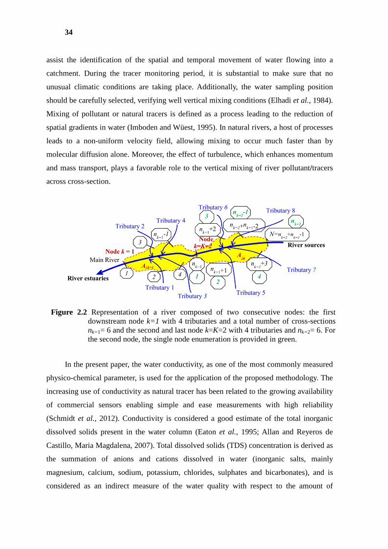
34

assist the identification of the spatial and temporal movement of water flowing into a

catchment. During the tracer monitoring period, it is substantial to make sure that no

unusual climatic conditions are taking place. Additionally, the water sampling position

should be carefully selected, verifying well vertical mixing conditions (Elhadi et al., 1984).

Mixing of pollutant or natural tracers is defined as a process leading to the reduction of

spatial gradients in water (Imboden and Wüest, 1995). In natural rivers, a host of processes

leads to a non-uniform velocity field, allowing mixing to occur much faster than by

molecular diffusion alone. Moreover, the effect of turbulence, which enhances momentum

and mass transport, plays a favorable role to the vertical mixing of river pollutant/tracers

across cross-section.

In the present paper, the water conductivity, as one of the most commonly measured

physico-chemical parameter, is used for the application of the proposed methodology. The

increasing use of conductivity as natural tracer has been related to the growing availability

of commercial sensors enabling simple and ease measurements with high reliability

(Schmidt et al., 2012). Conductivity is considered a good estimate of the total inorganic

dissolved solids present in the water column (Eaton et al., 1995; Allan and Reyeros de

Castillo, Maria Magdalena, 2007). Total dissolved solids (TDS) concentration is derived as

the summation of anions and cations dissolved in water (inorganic salts, mainly

magnesium, calcium, sodium, potassium, chlorides, sulphates and bicarbonates), and is

considered as an indirect measure of the water quality with respect to the amount of

Figure 2.2 Representation of a river composed of two consecutive nodes: the first downstream node k=1 with 4 tributaries and a total number of cross-sections nk=1= 6 and the second and last node k=K=2 with 4 tributaries and nk=2= 6. For the second node, the single node enumeration is provided in green.

35

dissolved ions, since it does not provide analytical information neither for the nature and

the exact relationship of the present ions, nor for the water characteristic parameters. It

plays, therefore, the role of general water quality indicator. The conductivity value is

directly proportional to the TDS concentration. It is therefore, possible to use conductivity

measurements in the pollutant conservation equation instead of the TDS concentration. The

approximate conversion of water conductivity (usually expressed in mS/cm) into TDS

concentration (in ppm) is undertaken through a factor ranging from 0.5 up to 0.9 depending

on the chemical composition of the TDS (APHA, 1999). Moreover, the chloride and the

sulphate ions are also included in the process. In Kim et al. (2002), the chemical behavior

of major inorganic ions in the streams of the Mankyung river area (South Korea) was

investigated. It was revealed that concentrations of chloride and sulphate, the total

concentration of major cations, and electrical conductivity in the stream were controlled by

mixing, indicating their conservative behavior similar to chloride. Alkalinity and

concentration of nitrate, however, were regulated by various reactions such as mixing,

photosynthesis, respiration and decomposition of organic matter.

In the introduced methodology, it is considered that the concentrations of m properly

selected (as described above) pollutants have been estimated with a sufficient accuracy,

and therefore, resulting in an adequately low and known error. It is notable that when

pollutant or natural tracers are measured very precisely, accuracy of discharge

measurements becomes the most critical component of the pollutant load computation and

the largest source of error (NCSU, 2008).

Moreover, it is assumed that the measurement conditions refers to the mean

hydraulic conditions usually prevailing in the considered flow (Schmidt et al., 2012), being

steady state (no transient effects) and usual hydraulic controls (i.e. no varying backwater

effects, no change in channel roughness or the geometry of the controlling cross-section).

Within this framework and taking into account water compressibility, it is possible to

express the mass conservation for the water volume and the pollutant load for one single-

node and all possible multiple-node combinations for the entire river. The balance

relationships for a single node (Figure 2.1) with cross-sections i (1,N) have been presented

analytically in Yannopoulos and Bekri (2010).

N

N

ii QQQQ ++= ∑

−

=λ

1

21 (2.2)

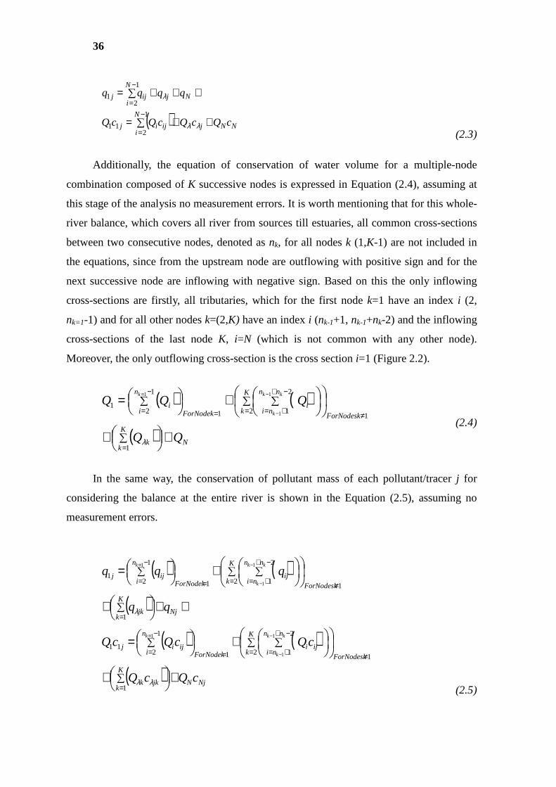
36

( ) NNj

N

iijij

Nj

N

iijj

cQcQcQcQ

qqqq

++∑=

⇔++∑=

−

=

−

=

λλ

λ

1

211

1

21

(2.3)

Additionally, the equation of conservation of water volume for a multiple-node

combination composed of K successive nodes is expressed in Equation (2.4), assuming at

this stage of the analysis no measurement errors. It is worth mentioning that for this whole-

river balance, which covers all river from sources till estuaries, all common cross-sections

between two consecutive nodes, denoted as nk, for all nodes k (1,K-1) are not included in

the equations, since from the upstream node are outflowing with positive sign and for the

next successive node are inflowing with negative sign. Based on this the only inflowing

cross-sections are firstly, all tributaries, which for the first node k=1 have an index i (2,

nk=1-1) and for all other nodes k=(2,K) have an index i (nk-1+1, nk-1+nk-2) and the inflowing

cross-sections of the last node K, i=N (which is not common with any other node).

Moreover, the only outflowing cross-section is the cross section i=1 (Figure 2.2).

( ) ( )

( ) N

K

kk

ForNodesk

K

k

nn

nii

ForNodek

n

ii

QQ

QQQkk

k

k

+

+

+

=

∑

∑ ∑∑

=

≠=

−+

+==

−

=

−

−

=

1

12

2

11

1

21

1

1

1

λ

(2.4)

In the same way, the conservation of pollutant mass of each pollutant/tracer j for

considering the balance at the entire river is shown in the Equation (2.5), assuming no

measurement errors.

( ) ( )

( )

( ) ( )

( ) NjN

K

kjkk

ForNodesk

K

k

nn

niiji

ForNodek

n

iijij

Nj

K

kjk

ForNodesk

K

k

nn

niij

ForNodek

n

iijj

cQcQ

cQcQcQ

qq

qqq

kk

k

k

kk

k

k

+

+

+

=

⇔+

+

+

=

∑

∑ ∑∑

∑

∑ ∑∑

=

≠=

−+

+==

−

=

=

≠=

−+

+==

−

=

−

−

=

−

−

=

1

12

2

11

1

211

1

12

2

11

1

21

1

1

1

1

1

1

λλ

λ

(2.5)

37

In Equations (2.4) and (2.5) the measured quantities of river discharge, of the

pollutant concentration and the resulting pollutant mass (pollution load) of a

pollutant/tracer j at each cross-section i (1,N) are symbolized respectively as Qi, cij, qij.

In the proposed methodology for each node k, an unknown, not-directly measured

water quantity is taken into account. This unknown quantity is referred to as “latent”, since

it is impossible to directly measure it. This latent term is declared with the Greek index λ

and the corresponding water and pollution quantities as Qλk, qλjk, cλjk. The latent discharge

of the node k is assumed to correspond to runoff of a catchment area Aλk, which is included

between all considered inflowing cross-sections and the outflowing cross-section around

the node k. The runoff from this area, which is illustrated with yellow in Figure 2.1 and

Figure 2.2, is missing from the water balance of the node k taking into account the nk cross-

sections. This is explained as follows. The flow rate, which is measured at each cross-

section i flowing into the node, sums up the drainage area of the corresponding

subcatchment up to the given cross-section. On the other hand, the flow rate, measured at

the cross-section flowing out of the node, sums up the entire area of the whole catchment

up to the given cross-section including the yellow area, which is not considered from the

inflowing cross-sections. The exact area for the latent quantity cannot be computed with

certainty and only a rough approximation given the various subcatchment areas and the in-

between area can be made.

Besides the consideration of the unaccounted areas, this latent quantity is assumed to

enclose also any other additional unknown interaction between the surface water bodies

or/and their interplay with the groundwater, which is assumed to be very small based on

the assumptions for the application of the proposed methodology. Based on this latent term

definition, the latent discharge flows into the node, thus having a positive sign +Qλk in

Equation (2.4) and (2.5). It should be mentioned that the need for considering a latent term

is also verified from the theory of data reconciliation. More precisely, in cases where

significant losses are present, it is proposed to avoid considering the mass balances or

alternatively to include an unknown loss term in the balance equation which can be

estimated as part of the reconciliation equations. In river systems, even if the cross-sections

are properly selected as previously assumed, there is an unknown water quantity flowing in

a considered node, which is taken into consideration by the latent term.

According to the above definition of the latent term Qλk of each node k, its first initial

estimation are approximated by the Equation (2.6) based on the water volume balance of

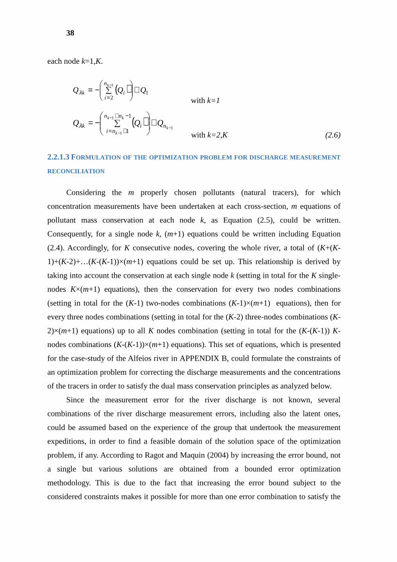
38

each node k=1,K.

( ) 12

1

QQQkn

iik +

∑−=

=

=λ with k=1

( )1

1

1

1

1−

−

−

+

∑−=

−+

+= k

kk

k

n

nn

niik QQQλ with k=2,K (2.6)

2.2.1.3 FORMULATION OF THE OPTIMIZATION PROBLEM FOR DISCHARGE MEASUREMENT

RECONCILIATION

Considering the m properly chosen pollutants (natural tracers), for which

concentration measurements have been undertaken at each cross-section, m equations of

pollutant mass conservation at each node k, as Equation (2.5), could be written.

Consequently, for a single node k, (m+1) equations could be written including Equation

(2.4). Accordingly, for K consecutive nodes, covering the whole river, a total of (K+(K-

1)+(K-2)+…(K-(K-1))×(m+1) equations could be set up. This relationship is derived by

taking into account the conservation at each single node k (setting in total for the K single-

nodes K×(m+1) equations), then the conservation for every two nodes combinations

(setting in total for the (K-1) two-nodes combinations (K-1)×(m+1) equations), then for

every three nodes combinations (setting in total for the (K-2) three-nodes combinations (K-

2)×(m+1) equations) up to all K nodes combination (setting in total for the (K-(K-1)) K-

nodes combinations (K-(K-1))×(m+1) equations). This set of equations, which is presented

for the case-study of the Alfeios river in APPENDIX B, could formulate the constraints of

an optimization problem for correcting the discharge measurements and the concentrations

of the tracers in order to satisfy the dual mass conservation principles as analyzed below.

Since the measurement error for the river discharge is not known, several

combinations of the river discharge measurement errors, including also the latent ones,

could be assumed based on the experience of the group that undertook the measurement

expeditions, in order to find a feasible domain of the solution space of the optimization

problem, if any. According to Ragot and Maquin (2004) by increasing the error bound, not

a single but various solutions are obtained from a bounded error optimization

methodology. This is due to the fact that increasing the error bound subject to the

considered constraints makes it possible for more than one error combination to satisfy the

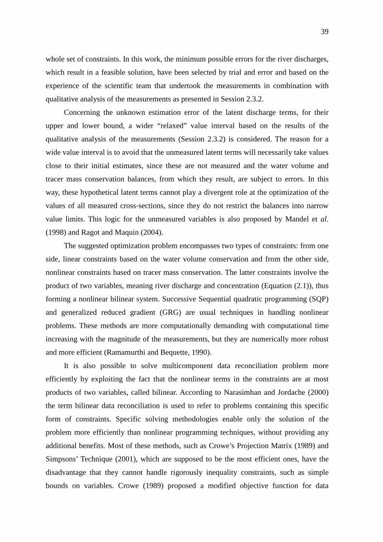
39

whole set of constraints. In this work, the minimum possible errors for the river discharges,

which result in a feasible solution, have been selected by trial and error and based on the

experience of the scientific team that undertook the measurements in combination with

qualitative analysis of the measurements as presented in Session 2.3.2.

Concerning the unknown estimation error of the latent discharge terms, for their

upper and lower bound, a wider “relaxed” value interval based on the results of the

qualitative analysis of the measurements (Session 2.3.2) is considered. The reason for a

wide value interval is to avoid that the unmeasured latent terms will necessarily take values

close to their initial estimates, since these are not measured and the water volume and

tracer mass conservation balances, from which they result, are subject to errors. In this

way, these hypothetical latent terms cannot play a divergent role at the optimization of the

values of all measured cross-sections, since they do not restrict the balances into narrow

value limits. This logic for the unmeasured variables is also proposed by Mandel et al.

(1998) and Ragot and Maquin (2004).

The suggested optimization problem encompasses two types of constraints: from one

side, linear constraints based on the water volume conservation and from the other side,

nonlinear constraints based on tracer mass conservation. The latter constraints involve the

product of two variables, meaning river discharge and concentration (Equation (2.1)), thus

forming a nonlinear bilinear system. Successive Sequential quadratic programming (SQP)

and generalized reduced gradient (GRG) are usual techniques in handling nonlinear

problems. These methods are more computationally demanding with computational time

increasing with the magnitude of the measurements, but they are numerically more robust

and more efficient (Ramamurthi and Bequette, 1990).

It is also possible to solve multicomponent data reconciliation problem more

efficiently by exploiting the fact that the nonlinear terms in the constraints are at most

products of two variables, called bilinear. According to Narasimhan and Jordache (2000)

the term bilinear data reconciliation is used to refer to problems containing this specific

form of constraints. Specific solving methodologies enable only the solution of the

problem more efficiently than nonlinear programming techniques, without providing any

additional benefits. Most of these methods, such as Crowe’s Projection Matrix (1989) and

Simpsons’ Technique (2001), which are supposed to be the most efficient ones, have the

disadvantage that they cannot handle rigorously inequality constraints, such as simple

bounds on variables. Crowe (1989) proposed a modified objective function for data

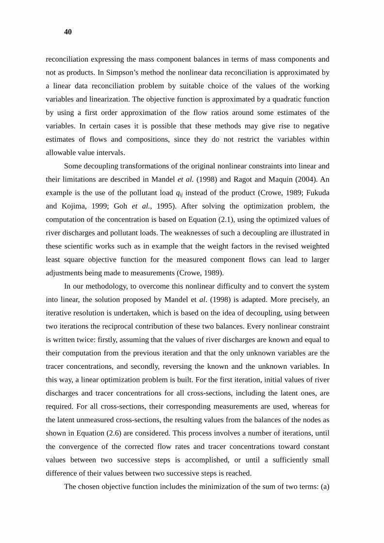
40

reconciliation expressing the mass component balances in terms of mass components and

not as products. In Simpson’s method the nonlinear data reconciliation is approximated by

a linear data reconciliation problem by suitable choice of the values of the working

variables and linearization. The objective function is approximated by a quadratic function

by using a first order approximation of the flow ratios around some estimates of the

variables. In certain cases it is possible that these methods may give rise to negative

estimates of flows and compositions, since they do not restrict the variables within

allowable value intervals.

Some decoupling transformations of the original nonlinear constraints into linear and

their limitations are described in Mandel et al. (1998) and Ragot and Maquin (2004). An

example is the use of the pollutant load qij instead of the product (Crowe, 1989; Fukuda

and Kojima, 1999; Goh et al., 1995). After solving the optimization problem, the

computation of the concentration is based on Equation (2.1), using the optimized values of

river discharges and pollutant loads. The weaknesses of such a decoupling are illustrated in

these scientific works such as in example that the weight factors in the revised weighted

least square objective function for the measured component flows can lead to larger

adjustments being made to measurements (Crowe, 1989).

In our methodology, to overcome this nonlinear difficulty and to convert the system

into linear, the solution proposed by Mandel et al. (1998) is adapted. More precisely, an

iterative resolution is undertaken, which is based on the idea of decoupling, using between

two iterations the reciprocal contribution of these two balances. Every nonlinear constraint

is written twice: firstly, assuming that the values of river discharges are known and equal to

their computation from the previous iteration and that the only unknown variables are the

tracer concentrations, and secondly, reversing the known and the unknown variables. In

this way, a linear optimization problem is built. For the first iteration, initial values of river

discharges and tracer concentrations for all cross-sections, including the latent ones, are

required. For all cross-sections, their corresponding measurements are used, whereas for

the latent unmeasured cross-sections, the resulting values from the balances of the nodes as

shown in Equation (2.6) are considered. This process involves a number of iterations, until

the convergence of the corrected flow rates and tracer concentrations toward constant

values between two successive steps is accomplished, or until a sufficiently small

difference of their values between two successive steps is reached.

The chosen objective function includes the minimization of the sum of two terms: (a)

41

the sum of the absolute values of the residuals of the water volume and tracer mass

conservation equations written for each single node and also for all possible multiple-node

combinations covering the whole river and (b) the sum of the absolute values of the

differences between the mass balance residuals, when the mass balance is written assuming

that the concentrations are known and the river discharges are the unknown variables, and

the mass balance residuals, when the mass balance is written, assuming the concentrations

are unknown and the river discharges are the known. Concerning the first term, such an

objective function results in correcting river discharge and tracer concentrations values,

building water volume and tracer mass balances as close as possible to zero. Therefore,

more reliable and representative values of the river discharge and also of the tracer

concentrations at each cross-section are computed, which fulfill simultaneously the entire

set of the constraints and at the same time minimize the residuals of the water volume and

tracer mass balances. Concerning the second term, since the pollutant mass balance is

expressed twice in order to keep the optimization problem in the linear space, the solution

of the optimization problem should verify that the difference of the two expressions tends

to zero.

2.2.2 DESCRIPTION OF THE MATHEMATICAL STRUCTURE OF THE LINEAR OPTIMIZAT ION

PROCESS

2.2.2.1 CONSTRAINTS BASED ON WATER VOLUME BALANCES

In this session, the mathematical structure of the proposed optimization problem will

be presented. The water volume and tracer mass conservation as shown in Equations (2.4)

and (2.5) have been expressed without incorporating any measurement errors. Let’s now

accept that there are measurements errors. The river discharges, corrected/optimized by the

suggested methodology, are indicated as Xi for each cross-section i (1,N) and Xλk for the

latent term of each node k (1,K). The corrected values Xi are supposed to be bounded based

on the measured values Qi and their unknown absolute maximum relative error denoted as

εi, within the ranges [Qi(1-εi), Qi(1+εi)], as shown in Equation (2.7). Under the above

conditions, the following dual (upper and lower bound) constraints for each corrected Χi

and Xλk are given:

( ) ( )iiiii QXQ εε +≤≤−≤ 110 (2.7)

42

In the water volume conservation for a combination of K successive nodes, as

expressed in Equation (2.4), the measurement errors are taken into account and the

following equality constraint (Equation (2.8)) are added into the optimization problem.

Now the corrected river discharges Χi and Xλk and a term for their residual DQNODE12..K, (for

equal to zero, no deviation for the zero balance is expressed) are entered. This type of

equality constraints are written for all possible single-node and multiple-node

combinations (every 1,K nodes combinations), as analytically described in APPENDIX C.

The index of the residual term reveals the balance of the nodes-combination, as i.e. for the

balance of the whole river the index is symbolized as NODE12…K, for the balance of the

nodes 2 and 3 as NOD23, for the balance of the nodes 1, 2 and 3 as NODE123, etc.

( ) ( )

( )

+

+

+

−=∑

∑ ∑∑

=

≠=

−+

+==

−

=

−

−

=

N

K

kk

ForNodesk

K

k

nn

nii

ForNodek

n

ii

KNODE

XX

XXXDQ

kk

k

k

1

12

2

11

1

2

1...12

1

1

1

λ (2.8) For the K nodes combinations, corresponding to the balance of the whole river, an

upper and lower bound ±DevQNODE12…K for the residual KNODEDQ ...12 is defined in order to

specify the minimum and maximum admissible deviation from the zero-balance for the

whole river.

DevQDQDevQ KNODE +≤≤− ...12 (2.9) Moreover, it is possible to rewrite the dual inequality constraint (2.7), by replacing

for each cross-section, the optimized discharge Χi (i=1,N and λk) with its equivalent as

derived from the balance equality (2.8). Firstly, for each outflowing cross-section nk of

each node k (2,K) except of the first one and secondly, separately for the outflowing cross-

section i=1 of the first node (k=1), as shown in Figure 2.2, the following constraints can be

written:

( ) ( )

( )11

1

111

1

101

1

−−

−

−−−

+≤

+

+≤−−≤ ∑−+

+=

kk

kk

kkk

nn

k

nn

niiNODEknn

Q

XXDQQ

ε

ε λ with k=2,K

43

( ) ( )( )111

2111

1

101

ε

ε

λ +≤+

+≤−≤

=

== ∑

=

QX

XDQQ

k

n

iiNODEk

k

with k=1 (2.10)

According to the constraints (2.10) similar inequality constraints for each outflowing

cross-section are added taking into account the water volume conservation of the

combination of two, three up to K successive nodes based on the balance Equation (2.8),

such as for example for the outflowing cross-section i=1 by considering all K successive

nodes (whole river):

( ) ( ) ( )

( ) ( )111

12

2

11

1

2...1211

1

101

1

1

ε

ε

λ +≤

+

∑+

∑

∑+

∑+≤−≤

=

≠=

−+

+==

−

=

−

−

=

QXX

XXDQQ

N

K

kk

ForNodesk

K

k

nn

nii

ForNodek

n

iiKNODE

kk

k

k

(2.11) Respectively, the following constraints can be written for each inflowing cross-

section i (nk-1+1,nk+nk-1-1) at each node k=2,K except of the first one, and separately for

the first node k=1with inflowing cross-sections denoted as i=2,nk=1:

( ) ( )

( )iik

nn

isnssNODEknii

QX

XDQXQkk

kk

ε

ε

λ +≤−

−−≤−≤ ∑−+

≠∧+=

−

−−

1

101

1

1

11 with k=2,K

( ) ( )( )iik

n

isssNODEkii

QX

XDQXQk

ε

ε

λ +≤−

−−≤−≤

=

≠∧== ∑

=

1

10

1

211

1

with k=1 (2.12)

According to the constraints (2.12), similar inequality constraints for each inflowing

cross-section are added taking into account the water volume conservation of the

combinations of two, three up to K successive nodes based on the balance Equation (2.8).

For the latent discharge Qλk of each node k=2,K except of the first one and separately

for the first node k=1, the following constraints can be written:

( )

( ) ( )kk

nn

nii

NODEknkk

QX

DQXQ

kk

k

k

λλ

λλ

ε

ε

+≤

−

−+≤−≤

∑−+

+=

−

−

−

1

10

1

1

1

1

1 with k=2,K

44

( )

( ) ( )112

1111

1

10

1

===

===

+≤

−

−+≤−≤

∑=

kk

n

ii

NODEkkk

QX

DQXQ

k

λλ

λλ

ε

ε with k=1 (2.13)

According to the constraints (2.13), similar inequality constraints for each latent

cross-section are added taking into account the water volume conservation of the

combinations of two, three up to K successive nodes based on the balance equation (2.8).

2.2.2.2 CONSTRAINTS BASED ON TRACER MASS BALANCES

Proceeding now to the constraints based on the pollutant mass conservation, it is

worth emphasizing that the pollutant concentration is assumed to have a known and very

small absolute maximum relative error (as thoroughly analyzed in Session 2.2.1.2). This

measurement error is denoted for each selected pollutant/tracer j (1,m) as ζj. It is taken

equal to the value provided by the manufacturer of the measuring equipment and only the

tracers with suitably small error, which is assumed to be less than 20%, are accepted. The

pollutant concentration values are supposed to lie within the narrow range [cij(1-ζj),

cij(1+ζj)]. The pollutant mass conservation is used in this methodology from one hand side,

to correct the concentration values, and from the other side, to further force the correction

of the discharge measurement values to an even more restricted solution space in order to

satisfy both water volume and mass conservation.

In the tracer mass conservation for a combination of K successive nodes, as

expressed in Equation (2.5), let’s take now into account the measurement errors. In this

case, the corrected river discharges Χi and Xλk and the corrected tracer concentrations ccij

and ccλjk, are entered. As previously mentioned, each nonlinear constraint, including the

product of river discharge with concentration is expressed twice in a linear form. When the

balance (Equation (2.14)) is written assuming that the concentrations are known and the

river discharges are the unknown variables (as described in Session 2.1.3), a term for their

residual DqXNODE12..K, is added. When the balance (Equation (2.15)) is written by reversing

the two known and unknown variables, a term for their residual DqCNODE12..K, is included.

The following equality constraints are written in the optimization problem:

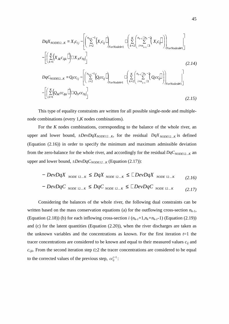
45

( ) ( )

( )

+

∑−

∑

∑+

∑−=

=

≠=

−+

+==

−

=

−

−

=

NjN

K

kjkk

ForNodesk

K

k

nn

niiji

ForNodek

n

iijijKNODE

cXcX

cXcXcXDqXkk

k

k

1

12

2

11

1

211...12

1

1

1

λλ(2.14)

( ) ( )

( )

+

∑−

∑

∑+

∑−=

=

≠=

−+

+==

−

=

−

−

=

NjN

K

kjkk

ForNodesk

K

k

nn

niiji

ForNodek

n

iijijKNODE

ccQccQ

ccQccQccQDqCkk

k

k

1

12

2

11

1

211...12

1

1

1

λλ (2.15) This type of equality constraints are written for all possible single-node and multiple-

node combinations (every 1,K nodes combinations).

For the K nodes combinations, corresponding to the balance of the whole river, an

upper and lower bound, ±DevDqXNODE12…K, for the residual KNODEDqX ...12 is defined

(Equation (2.16)) in order to specify the minimum and maximum admissible deviation

from the zero-balance for the whole river, and accordingly for the residual KNODEDqC ...12 an

upper and lower bound, ±DevDqCNODE12…K (Equation (2.17)):

KNODEKNODEKNODE DevDqXDqXDevDqX ...12...12...12 +≤≤− (2.16) KNODEKNODEKNODE DevDqCDqCDevDqC ...12...12...12 +≤≤− (2.17) Considering the balances of the whole river, the following dual constraints can be

written based on the mass conservation equations (a) for the outflowing cross-section nk-1,

(Equation (2.18)) (b) for each inflowing cross-section i (nk-1+1,nk+nk-1-1) (Equation (2.19))

and (c) for the latent quantities (Equation (2.20)), when the river discharges are taken as

the unknown variables and the concentrations as known. For the first iteration t=1 the

tracer concentrations are considered to be known and equal to their measured values cij and

cλjk. From the second iteration step t≥2 the tracer concentrations are considered to be equal

to the corrected values of the previous step, 1−tijcc :

46

( )( )

( )( )jnnkjn

jk

nn

nii

jn

ij

jn

KNODEjnn

kk

k

kk

k kk

kk

QXc

c

Xc

c

c

DqXQ

ζε

ζε

λλ ++≤+

∑

+≤−−

−−−

−

− −−−−

−+

+=

11

11

11

1

1

1 11

11

1

1

...12

(2.18)

( )( )

( )( )jiikij

jk

nn

isnss

ij

sj

ij

KNODEn

ij

jnjii

QXc

c

Xc

c

c

DqXX

c

cQ

kk

kk

k

ζε

ζε

λλ ++≤−

∑

−−≤−−

−+

≠∧+=

−

−−

−

11

111

1

...12 1

11

1

(2.19)

( )( )

( )( )jkk

nn

nii

jk

ij

jk

KNODEn

jk

jnjkk

Q

Xc

c

c

DqXX

c

cQ

kk

kk

k

ζε

ζε

λλ

λλλλλ

++≤

∑

−−+≤−−

−+

+=

−

−−

−

11

111

1

...12 1

11

1

(2.20) And accordingly for the first node k=1:

( )( ) ( )( )jk

j

jkn

ii

j

ij

j

KNODEj QX

c

cX

c

c

c

DqXQ

k

ζεζε λλ ++≤+

∑

+≤−− =

=

=

=1111 111

1

1

2 11

...1211

1

(2.21)

( )( )

( )( )jii

kij

jkn

isss

ij

sj

ij

KNODE

ij

jjii

Q

Xc

cX

c

c

c

DqXX

c

cQ

k

ζε

ζε λλ

++≤

−

∑

−−≤−− =

=

≠∧=

=

11

11 11

2

...121

1 1

(2.22)

( )( )

( )( )jkk

n

ii

jk

ij

jk

KNODE

jk

jjkk

Q

Xc

c

c

DqXX

c

cQ

k

ζε

ζε

λλ

λλλλλ

++≤

∑

−−+≤−−

==

= =====

=

11

11

11

2 11

...121

1

111

1

(2.23) According to the Equations (2.18) to (2.20) the corresponding constraints with river

discharges taken as known variables and the concentrations as unknown are expressed

below. For the first iteration t=1 the river discharges are equal to their measurements Qi for

all measured cross-sections and to their estimated values Qλk for all latent and from the

second iteration step t≥2 equal to the corrected values of the previous step, 1−tiX :

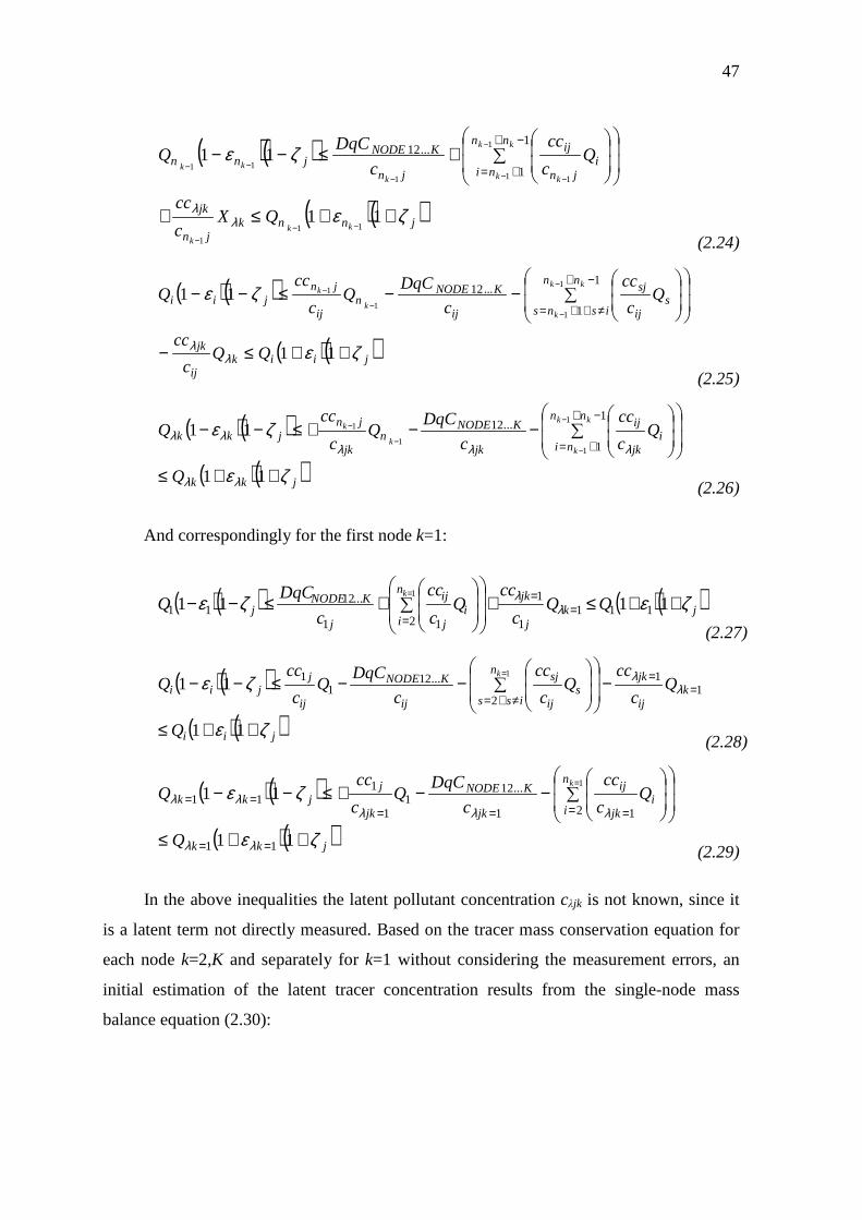
47

( )( )

( )( )jnnkjn

jk

nn

nii

jn

ij

jn

KNODEjnn

kk

k

kk

k kk

kk

QXc

cc

Qc

cc

c

DqCQ

ζε

ζε

λλ ++≤+

∑

+≤−−

−−−

−

− −−−−

−+

+=

11

11

11

1

1

1 11

11

1

1

...12

(2.24)

( )( )

( )( )jiikij

jk

nn

isnss

ij

sj

ij

KNODEn

ij

jnjii

QQc

cc

Qc

cc

c

DqCQ

c

ccQ

kk

kk

k

ζε

ζε

λλ ++≤−

∑

−−≤−−

−+

≠∧+=

−

−−

−

11

111

1

...12 1

11

1

(2.25)

( )( )

( )( )jkk

nn

nii

jk

ij

jk

KNODEn

jk

jnjkk

Q

Qc

cc

c

DqCQ

c

ccQ

kk

kk

k

ζε

ζε

λλ

λλλλλ

++≤

∑

−−+≤−−

−+

+=

−

−−

−

11

111

1

...12 1

11

1

(2.26) And correspondingly for the first node k=1:

( )( ) ( )( )jk

j

jkn

ii

j

ij

j

KNODEj QQ

c

ccQ

c

cc

c

DqCQ

k

ζεζε λλ ++≤+

∑

+≤−− =

=

=

=1111 111

1

1

2 11

...1211

1

(2.27)

( )( )

( )( )jii

kij

jkn

isss

ij

sj

ij

KNODE

ij

jjii

Q

Qc

ccQ

c

cc

c

DqCQ

c

ccQ

k

ζε

ζε λλ

++≤

−

∑

−−≤−− =

=

≠∧=

=

11

11 11

2

...121

1 1

(2.28)

( )( )

( )( )jkk

n

ii

jk

ij

jk

KNODE

jk

jjkk

Q

Qc

cc

c

DqCQ

c

ccQ

k

ζε

ζε

λλ

λλλλλ

++≤

∑

−−+≤−−

==

= =====

=

11

11

11

2 11

...121

1

111

1

(2.29) In the above inequalities the latent pollutant concentration cλjk is not known, since it

is a latent term not directly measured. Based on the tracer mass conservation equation for

each node k=2,K and separately for k=1 without considering the measurement errors, an

initial estimation of the latent tracer concentration results from the single-node mass

balance equation (2.30):

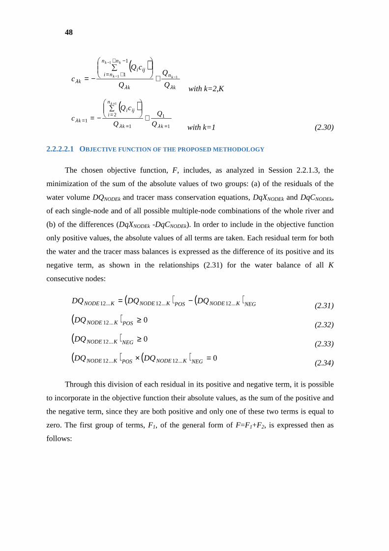
48

( )

k

n

k

nn

niiji

k Q

Q

Q

cQ

c k

kk

k

λλλ

1

1

1

1

1 −

−

− +

∑

−=

−+

+=

with k=2,K

( )

1

1

1

21

1

==

== +

∑

−=

=

kk

n

iiji

k Q

Q

Q

cQ

c

k

λλλ with k=1 (2.30)

2.2.2.2.1 OBJECTIVE FUNCTION OF THE PROPOSED METHODOLOGY

The chosen objective function, F, includes, as analyzed in Session 2.2.1.3, the

minimization of the sum of the absolute values of two groups: (a) of the residuals of the

water volume DQNODEk and tracer mass conservation equations, DqXNODEk and DqCNODEk,

of each single-node and of all possible multiple-node combinations of the whole river and

(b) of the differences (DqXNODEk -DqCNODEk). In order to include in the objective function

only positive values, the absolute values of all terms are taken. Each residual term for both

the water and the tracer mass balances is expressed as the difference of its positive and its

negative term, as shown in the relationships (2.31) for the water balance of all K

consecutive nodes:

( ) ( )NEGKNODEPOSKNODEKNODE DQDQDQ ...12...12...12 −= (2.31) ( ) 0...12 ≥POSKNODEDQ (2.32) ( ) 0...12 ≥NEGKNODEDQ (2.33) ( ) ( ) 0...12...12 =× NEGKNODEPOSKNODE DQDQ (2.34) Through this division of each residual in its positive and negative term, it is possible

to incorporate in the objective function their absolute values, as the sum of the positive and

the negative term, since they are both positive and only one of these two terms is equal to

zero. The first group of terms, F1, of the general form of F=F1+F2, is expressed then as

follows:

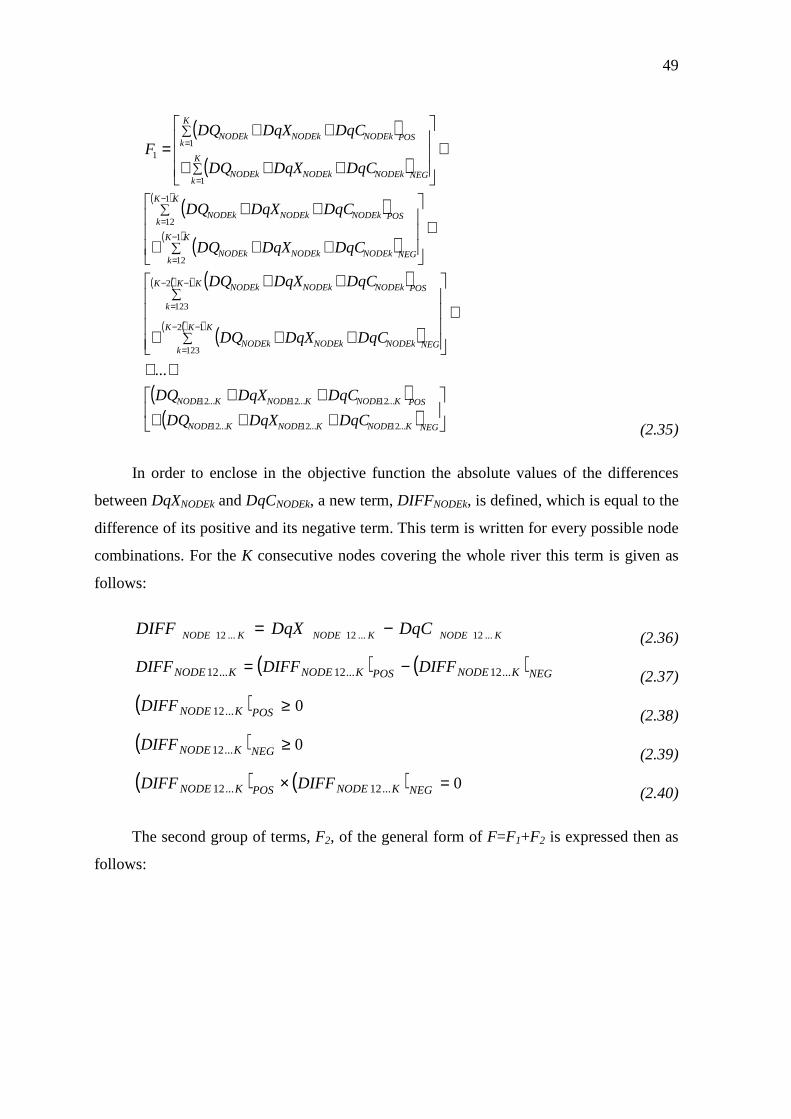
49

( )

( )

( )( )

( )( )

( )( )( )

( )( )( )

( )( )

+++++

++

+

+++

++

+

+++

++

+

+++

++=

∑

∑

∑

∑

∑

∑

−−

=

−−

=

−

=

−

=

=

=

NEGKNODEKNODEKNODE

POSKNODEKNODEKNODE

KKK

kNEGNODEkNODEkNODEk

KKK

k

POSNODEkNODEkNODEk

KK

kNEGNODEkNODEkNODEk

KK

kPOSNODEkNODEkNODEk

K

kNEGNODEkNODEkNODEk

K

kPOSNODEkNODEkNODEk

DqCDqXDQ

DqCDqXDQ

DqCDqXDQ

DqCDqXDQ

DqCDqXDQ

DqCDqXDQ

DqCDqXDQ

DqCDqXDQF

...12...12...12

...12...12...12

12

123

12

123

1

12

1

12

1

11

...

(2.35) In order to enclose in the objective function the absolute values of the differences

between DqXNODEk and DqCNODEk, a new term, DIFFNODEk, is defined, which is equal to the

difference of its positive and its negative term. This term is written for every possible node

combinations. For the K consecutive nodes covering the whole river this term is given as

follows:

KNODEKNODEKNODE DqCDqXDIFF ...12...12...12 −= (2.36)

( ) ( )NEGKNODEPOSKNODEKNODE DIFFDIFFDIFF ...12...12...12 −= (2.37) ( ) 0...12 ≥POSKNODEDIFF (2.38)

( ) 0...12 ≥NEGKNODEDIFF (2.39)

( ) ( ) 0...12...12 =× NEGKNODEPOSKNODE DIFFDIFF (2.40)

The second group of terms, F2, of the general form of F=F1+F2 is expressed then as

follows:

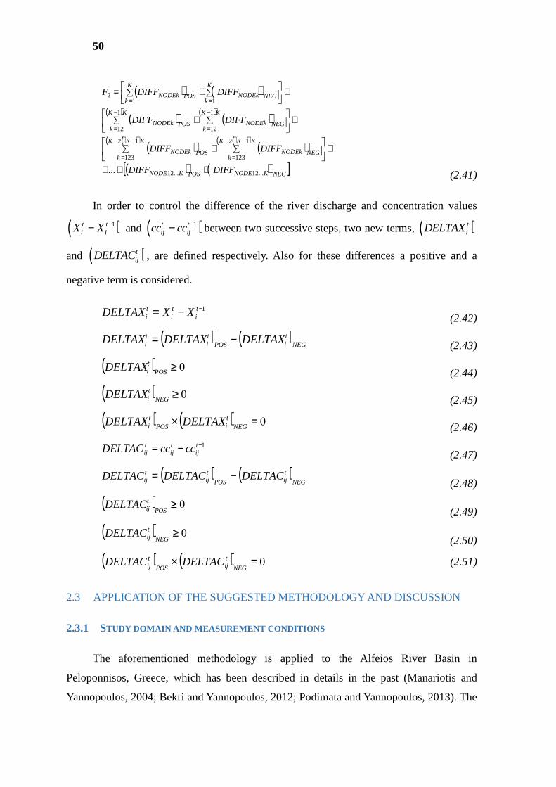
50

( ) ( )

( )( )

( )( )

( )( )( )

( )( )( )

( ) ( )[ ]NEGKNODEPOSKNODE

KKK

kNEGNODEk

KKK

kPOSNODEk

KK

kNEGNODEk

KK

kPOSNODEk

K

kNEGNODEk

K

kPOSNODEk

DIFFDIFF

DIFFDIFF

DIFFDIFF

DIFFDIFFF

...12...12

12

123

12

123

1

12

1

12

112

... +++

+

∑∑ +

+

∑∑ +

+

∑∑ +=

−−

=

−−

=

−

=

−

=

==

(2.41)

In order to control the difference of the river discharge and concentration values

( )1t ti iX X −− and ( )1t t

ij ijcc cc−− between two successive steps, two new terms, ( )tiDELTAX

and ( )tijDELTAC , are defined respectively. Also for these differences a positive and a

negative term is considered.

1−−= ti

ti

ti XXDELTAX (2.42)

( ) ( )NEGtiPOS

ti

ti DELTAXDELTAXDELTAX −= (2.43)

( ) 0≥POStiDELTAX (2.44)

( ) 0≥NEGtiDELTAX (2.45)

( ) ( ) 0=× NEGtiPOS

ti DELTAXDELTAX (2.46)

1−−= tij

tij

tij ccccDELTAC (2.47)

( ) ( )NEG

tijPOS

tij

tij DELTACDELTACDELTAC −= (2.48)

( ) 0≥POS

tijDELTAC (2.49)

( ) 0≥NEG

tijDELTAC (2.50)

( ) ( ) 0=×NEG

tijPOS

tij DELTACDELTAC (2.51)

2.3 APPLICATION OF THE SUGGESTED METHODOLOGY AND DISCUSSION

2.3.1 STUDY DOMAIN AND MEASUREMENT CONDITIONS

The aforementioned methodology is applied to the Alfeios River Basin in

Peloponnisos, Greece, which has been described in details in the past (Manariotis and

Yannopoulos, 2004; Bekri and Yannopoulos, 2012; Podimata and Yannopoulos, 2013). The

51

simultaneous discharge measurements using quick techniques and water sampling included

eleven cross-sections along the main river and its tributaries, as shown in Figure 2.3. The

measurement cross-sections comprised either road bridges or dams, where access to the

entire river length was possible. Six expeditions took place in 2006 and 2007 within the

framework of the research program Pythagoras II-Environment (Yannopoulos et al., 2007;

Yannopoulos, 2008), one for each year season, excepting summer 2007 due to extended

and disastrous fires.

For the application of the suggested technique, four nodes of junctions were

properly defined, in order to satisfy the previously mentioned distance requirement,

covering the entire river length and its tributaries. The node k=1 located near river estuary

encompasses the cross-sections 1, 2 and 3 and entails one tributary, Enipeus river. The

node k=2, enclosing the cross-sections 3, 4, 5 and 6, has its lower bound at the Flokas

Diversion Dam for irrigation purposes, and includes two tributaries, Kladheos river and

Selinous river with low to minor contribution to the node’s water volume balance. The next

upstream adjoining node k=3, composed of the cross-sections 6, 7, 8 and 9, contains two

tributaries, Ladhon river, covering almost the one third of the total catchment, and

Erymanthos river. The last node k=4 close to river sources, which includes the cross-

sections 9, 10 and 11, involves only one tributary, Lousios river.

From the six expeditions, only four yielded sufficient and suitable data for the

application of the proposed methodology requirements for the whole-river approach. The

expeditions 3 and 7 were carried out under unstable flow conditions due to sudden

alterations of the operation of the Ladhon Hydroelectric Power Station (HPS) during the

measurement process, which violates the predefined steady-state conditions for the

application of the proposed methodology. This can be observed in Table Table 2.1, where

for the expedition 3 the water balances of the nodes k=1 (water balance=12.67

corresponding to 64% of the maximum inflow value Q3) and k=3 (water balance=-22.68

corresponding to 64% of the maximum inflow value Q8) is unacceptably high due to the

effect of the sudden change of the water releases from HPS Ladhon. For the expedition 7

only the node k=1 (water balance=20.92 corresponding to 66% of the maximum inflow

value Q3) has been affected by this flow rate alterations. It is worth noticing that for all

nodes the water balance does not exceed the 30% of the maximum inflow, whereas for the

prementioned nodes it exceeds 60%, which cannot be justified from the latent drainage

area which corresponds to this water balance.

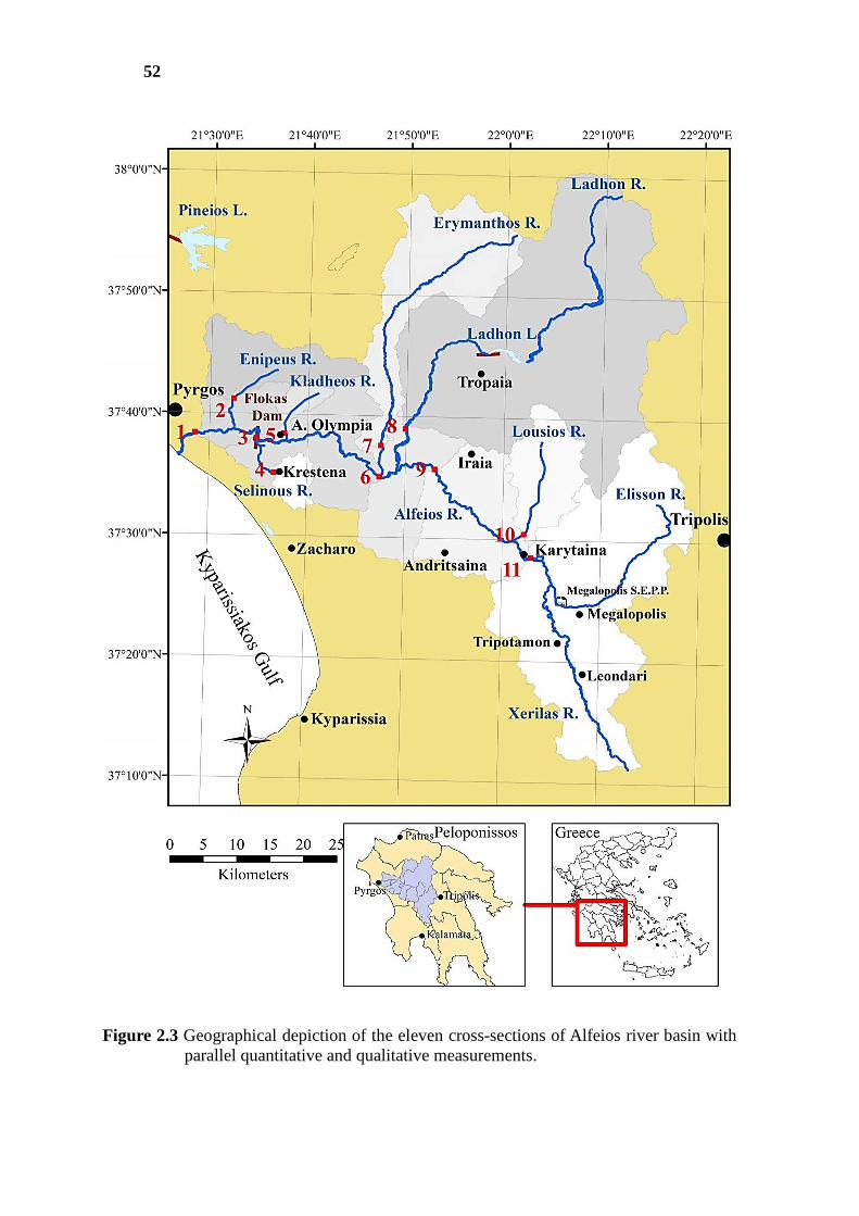
52

Figure 2.3 Geographical depiction of the eleven cross-sections of Alfeios river basin with parallel quantitative and qualitative measurements.

53

For both expeditions, the real water releases from Ladhon HPS have been compared

with the water balances differences and the time of the measurements at each node,

verifying the observed steady-state flow violations. Therefore, it is of note that in order to

effectively apply the proposed methodology, it is important to previously verify the weekly

water releases plan of the Ladhon HPS and select the days for which the operation of HPS

is steady during the measurements at the cross-section at Ladhon river and the cross-

sections at Alfeios river situated between Ladhon and river estuaries (being cross-sections

8,6,3,1).

For each expedition, the following natural tracers have been tested and selected as

the most appropriate based on the requirements of the considered methodology (Ziabras

and Tasias, 1992): (a) Water conductivity, with measurements in the field corresponding to

a satisfactory accuracy (ζ1≤0.10), (b) Sulphate ions concentration (SO4-2), with

measurements derived from laboratorial analysis of water sampling, corresponding again

to an satisfying accuracy (ζ2≤0.15), (c) Chloride ions concentration (Cl-), with

measurements derived from laboratorial analysis of water sampling, corresponding to an

adequate accuracy (ζ3≤0.15). Due to the fact that the chlorine ions have not been measured

at every cross-section, they are not used. The river discharge measurements included the

estimation of the geometrical characteristics of the cross-section along with the surface

maximum velocity employing a floating object. Additionally, the pendulum method has

been used for several cross-sections, while the release of air bubbles has been employed at

cross-sections, where either the flow depth was irregular or the flow permitted bubbles to

be clearly viewed. The duration of every expedition was one day in order to avoid or to

reduce the effect of a possible change of the steady-state flow conditions. Additionally, the

date of each expedition has been properly selected based on the available weather data,

excluding dates directly after short or long rainy periods, attempting to measure the mean

steady-state flowing conditions without bias. Every expedition started with measurements

at the first cross-section close to estuaries of Alfeios and then moving upstream up to the

very last cross-section close to the river sources.

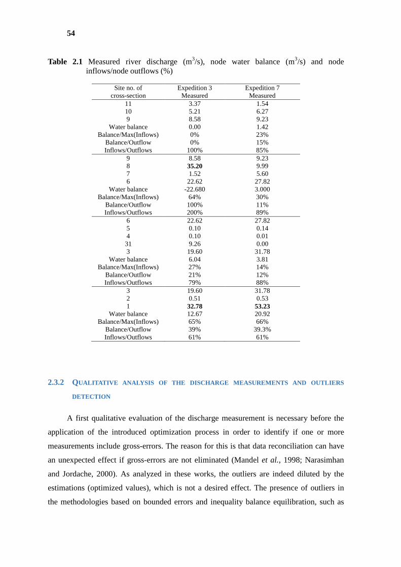
54

Table 2.1 Measured river discharge (m3/s), node water balance (m3/s) and node inflows/node outflows (%)

Site no. of Expedition 3 Expedition 7 cross-section Measured Measured

11 3.37 1.54 10 5.21 6.27 9 8.58 9.23

Water balance 0.00 1.42 Balance/Max(Inflows) 0% 23%

Balance/Outflow 0% 15% Inflows/Outflows 100% 85%

9 8.58 9.23 8 35.20 9.99 7 1.52 5.60 6 22.62 27.82

Water balance -22.680 3.000 Balance/Max(Inflows) 64% 30%

Balance/Outflow 100% 11% Inflows/Outflows 200% 89%

6 22.62 27.82 5 0.10 0.14 4 0.10 0.01 31 9.26 0.00 3 19.60 31.78

Water balance 6.04 3.81 Balance/Max(Inflows) 27% 14%

Balance/Outflow 21% 12% Inflows/Outflows 79% 88%

3 19.60 31.78 2 0.51 0.53 1 32.78 53.23

Water balance 12.67 20.92 Balance/Max(Inflows) 65% 66%

Balance/Outflow 39% 39.3% Inflows/Outflows 61% 61%

2.3.2 QUALITATIVE ANALYSIS OF THE DISCHARGE MEASUREMENTS AND OUTLIERS

DETECTION

A first qualitative evaluation of the discharge measurement is necessary before the

application of the introduced optimization process in order to identify if one or more

measurements include gross-errors. The reason for this is that data reconciliation can have

an unexpected effect if gross-errors are not eliminated (Mandel et al., 1998; Narasimhan

and Jordache, 2000). As analyzed in these works, the outliers are indeed diluted by the

estimations (optimized values), which is not a desired effect. The presence of outliers in

the methodologies based on bounded errors and inequality balance equilibration, such as

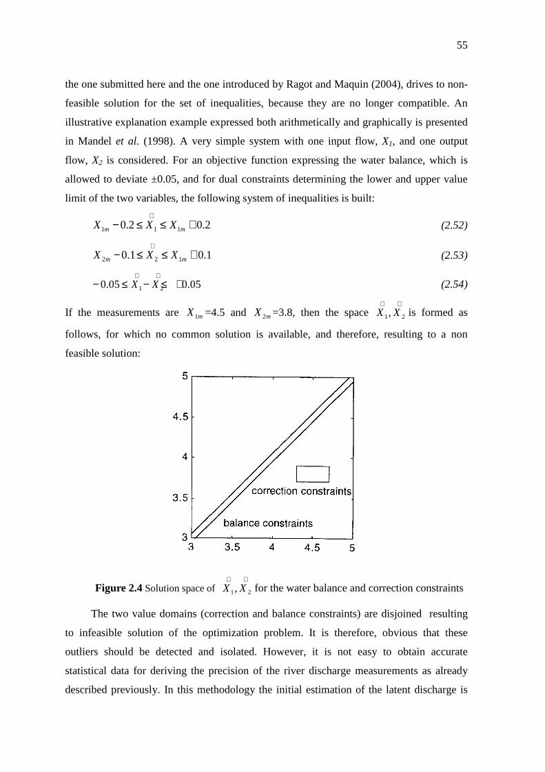
55

the one submitted here and the one introduced by Ragot and Maquin (2004), drives to non-

feasible solution for the set of inequalities, because they are no longer compatible. An

illustrative explanation example expressed both arithmetically and graphically is presented

in Mandel et al. (1998). A very simple system with one input flow, X1, and one output

flow, X2 is considered. For an objective function expressing the water balance, which is

allowed to deviate ±0.05, and for dual constraints determining the lower and upper value

limit of the two variables, the following system of inequalities is built:

2.02.0 111 +≤≤−∧

mm XXX (2.52)

1.01.0 122 +≤≤−∧

mm XXX (2.53)

05.005.0 21 +≤−≤−∧∧

XX (2.54)

If the measurements are mX1 =4.5 and mX2 =3.8, then the space ∧∧

21, XX is formed as

follows, for which no common solution is available, and therefore, resulting to a non

feasible solution:

Figure 2.4 Solution space of ∧∧

21, XX for the water balance and correction constraints

The two value domains (correction and balance constraints) are disjoined resulting

to infeasible solution of the optimization problem. It is therefore, obvious that these

outliers should be detected and isolated. However, it is not easy to obtain accurate

statistical data for deriving the precision of the river discharge measurements as already

described previously. In this methodology the initial estimation of the latent discharge is

56

derived from the water balance of each node using the measurements of the river

discharge.

There are four points to be checked for the identification of a probable cross-section

with gross-error and for the subsequent revision of tis measured value. Firstly, the

magnitude of the latent discharge should be assessed. The comparison of the computed

latent value with a rough estimation of the maximum possible latent discharge value based

on the hydrologic characteristics of the river and its tributaries or on expert

understanding/knowledge of the examined hydrologic system (as analyzed below) could be

used. This comparison can reveal if the discharge measurement errors are very high, which

is an indication of the presence of gross-errors. In case of gross-errors, the corresponding

“problematic“ discharge measurements should not be taken into account. Secondly, the

examination of the sign of water balance of each node, from which the latent discharge is

computed, is required since no negative water or/and mass pollutant balances are

acceptable. If the resulting latent discharge is negative and small, then only small changes

in one or more of the measurements are made within their ranges. Otherwise, important

revisions are required.

Thirdly, the magnitude of the computed latent concentration based on the mass

pollutant balance of the examined node is explored. The latent cross-section is situated

within the catchment area and therefore, the assumption is made that the latent

concentration can vary between zero and the maximum registered concentration of each

pollutant plus the measurement error. For the Alfeios river these upper limits for

electroconductivity concentrations are set equal to 1.3×1.15=1.5 µS/cm/1000 and for 24−SO

0.15×1.15=0.17 mg/l/1000. Fourthly, the sign of the computed latent concentration based

on the mass pollutant balance of the examined node is investigated. Only positive

concentration values are reasonable and accepted. If negative values are derived, small

changes of the measured concentration values within their narrow ranges are undertaken in

order to derive an initial solution with positive concentrations. In the application of the

proposed methodology in the Alfeios river, electroconductivity has been measured with

two measuring equipment. These two measurements should not differ more than 15% from

each other. For this reason before applying the optimization process this check should be

also done. In case of higher deviations, the initial values of these concentrations should be

properly adjusted within their allowable value range based on their measurement error

ζ=10%.

57

In the iterative optimization process, the lower and upper bounds of the optimization

variables (which are the right-hand sides of the constraints) are written based on the

measurements and their assumed measurements errors. In the left-hand side of the

constraints, where the optimization variables are included, revised values at the cross-

sections with gross-errors are used as initial values instead of their measurements at the

first step of the optimization process in order to ensure a global feasible solution at the first

step of the algorithm.

After the identification of the node(s) including cross-sections with gross-errors, the

identification of the “problematic” cross-sections should take place and the

computation/approximation of their revised values. In this methodology the following

process for these points is suggested. For each node an evaluation of the magnitude of the

river discharge measurement error of each cross-section should be made based on the

measuring knowledge of the team that undertook the measurements (i.e. based on the

geometric and morphological characteristics of the cross-section and the difficulties of

measuring associated with the reliability of the measurement). In this way the

categorisation of the measurement errors to small, medium and high result for each cross-

section of the node is enabled. The cross-sections with the assumed highest measurements

errors are supposed to be subject to revision. For these cross-sections an upper and lower

bound for the river discharge values for the month of the measuring expedition should be

identified. This can be done by using the statistical analysis of historical timeseries, if

available, or expert knowledge. The revised values are assumed to lie within this estimated

value range and equal to three values: the minimum, mean (or the measured value if it lies

within the computed range) and maximum value. Based on this all possible combinations

of the revised initial values of river discharges are examined and assessed in terms of their

feasibility according to the four prementioned check points for the latent terms (magnitude

and sign).

Based on these four points the qualitative analysis for the four nodes and the four

expeditions follows.

2.3.2.1 QUALITATIVE ANALYSIS OF THE DISCHARGE MEASUREMENTS AND OUTLIERS

DETECTION FOR EXPEDITION 2

(a) Node k=4: Beginning from river springs and moving downstream towards

estuary (Figure 2.3), at the node k=4 the measurement position 11 of the Alfeios river is

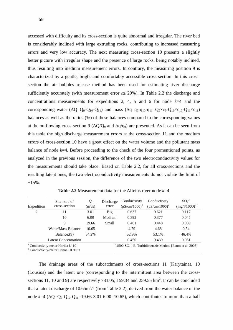
58

accessed with difficulty and its cross-section is quite abnormal and irregular. The river bed

is considerably inclined with large extruding rocks, contributing to increased measuring

errors and very low accuracy. The next measuring cross-section 10 presents a slightly

better picture with irregular shape and the presence of large rocks, being notably inclined,

thus resulting into medium measurement errors. In contrary, the measuring position 9 is

characterized by a gentle, bright and comfortably accessible cross-section. In this cross-

section the air bubbles release method has been used for estimating river discharge

sufficiently accurately (with measurement error ε≤ 20%). In Table 2.2 the discharge and

concentrations measurements for expeditions 2, 4, 5 and 6 for node k=4 and the

corresponding water (∆Q=Q9-Q10-Q11) and mass (∆q=q9-q10-q11=Q9×c9-Q10×c10-Q11×c11)

balances as well as the ratios (%) of these balances compared to the corresponding values

at the outflowing cross-section 9 (∆Q/Q9 and ∆q/q9) are presented. As it can be seen from

this table the high discharge measurement errors at the cross-section 11 and the medium

errors of cross-section 10 have a great effect on the water volume and the pollutant mass

balance of node k=4. Before proceeding to the check of the four prementioned points, as

analyzed in the previous session, the difference of the two electroconductivity values for

the measurements should take place. Based on Table 2.2, for all cross-sections and the

resulting latent ones, the two electroconductivity measurements do not violate the limit of

±15%.

Table 2.2 Measurement data for the Alfeios river node k=4

Site no. i of cross-section

Qi Discharge error

Conductivity Conductivity SO42-

Expedition (m3/s) (µS/cm/1000)1 (µS/cm/1000)2 (mg/l/1000)3

2 11 3.01 Big 0.637 0.621 0.117

10 6.00 Medium 0.392 0.377 0.045

9 19.66 Small 0.461 0.448 0.059

Water/Mass Balance 10.65 4.79 4.68 0.54

Balance:(9) 54.2% 52.9% 53.1% 46.4%

Latent Concentration 0.450 0.439 0.051 1 Conductivity-meter Horiba U-10 2 Conductivity-meter Hanna HI 9033

3 4500-SO42- E. Turbidimentric Method [Eaton et al. 2005]

The drainage areas of the subcatchments of cross-sections 11 (Karytaina), 10

(Lousios) and the latent one (corresponding to the intermittent area between the cross-

sections 11, 10 and 9) are respectively 783.05, 159.34 and 259.55 km2. It can be concluded

that a latent discharge of 10.65m3/s (from Table 2.2), derived from the water balance of the

node k=4 (∆Q=Q9-Q10-Q11=19.66-3.01-6.00=10.65), which contributes to more than a half

59

(54.2%) of the outflowing water quantity, is not reasonable and cannot be justified from the

drainage area. This is a proof of the presence of gross-errors. Firstly, the problematic cross-

sections should be identified and secondly, their measured values should be revised. For

the first point, the estimation of the magnitude of the discharge measurement error for the

three cross-sections (11,10,9), as described at the beginning of this session, is used to

identify the problematic cross-sections. For the node k=4, the cross-section 11 (Karytaina)

has the highest measurement error, the cross-section 10 has a medium error, whereas at the

cross-section 9 measurements are undertaken with high accuracy. Based on this analysis

the original measurement of cross-section 11 or/and 10 should not be taken into account,

but should be revised at the initial solution. This is verified by the fact that by solving the

optimization algorithm with the initial values equal to the measurements, no feasible

solution is found.

For the second point related to the estimation of the revised initial values for the

problematic measurements, a statistical analysis of the available historical river discharge

timeseries can be employed as follows. In our case the measured monthly discharges at the

cross-sections 11 and 10 by the Hellenic Public Power Corporation for a 10-year period

(1961-1971) can provide some useful information (Table 2.3). Expedition 2 took place on

the 9th of April 2006 and according to Table 2.3 the mean value of the river discharge in

this month for the cross-section 11 is 6.00m3/s ranging from 0.66 and 11.34m3/s. The

measured river discharge of 3.01m3/s for the cross-section 11 lies within the estimated

range but is relatively low. For the cross-section 10 the corresponding mean values is

7.04m3/s, which is close to the measured value (6.00m3/s), and varies between 4.67 and

9.40m3/s. Since the exact values of the river discharges are not known, various initial

values can be examined to check the feasibility of the solution of the algorithm. Three

values are taken into account as initial probable revised values for the cross-sections 11

and 10 in order to cover the entire value range. These are the two extreme values

(minimum and maximum) and the mean one for the cross-sections 11 and 10. All possible

combinations of these values are examined except of the ones resulting to negative latent

values or to latent values outside the probable value range of latent discharge approximated

as shown below.

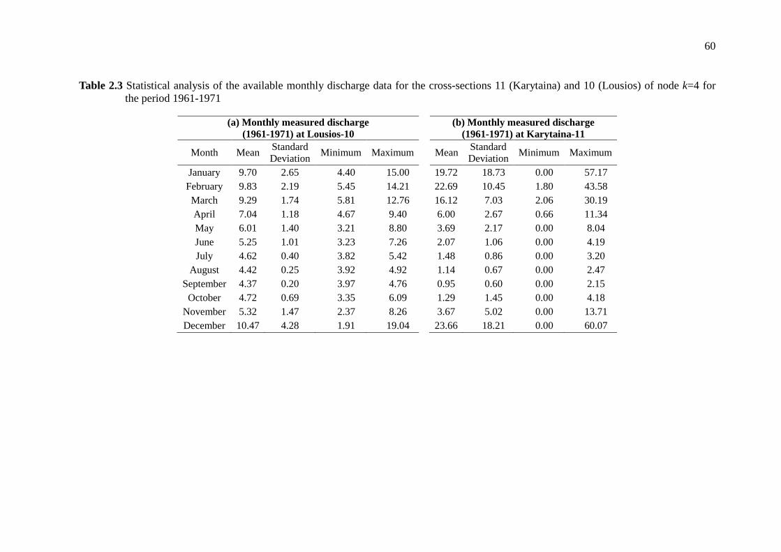
60

Table 2.3 Statistical analysis of the available monthly discharge data for the cross-sections 11 (Karytaina) and 10 (Lousios) of node k=4 for the period 1961-1971

(a) Monthly measured discharge (1961-1971) at Lousios-10

(b) Monthly measured discharge (1961-1971) at Karytaina-11

Month Mean Standard Deviation

Minimum Maximum

Mean Standard Deviation

Minimum Maximum

January 9.70 2.65 4.40 15.00

19.72 18.73 0.00 57.17 February 9.83 2.19 5.45 14.21

22.69 10.45 1.80 43.58

March 9.29 1.74 5.81 12.76

16.12 7.03 2.06 30.19 April 7.04 1.18 4.67 9.40

6.00 2.67 0.66 11.34

May 6.01 1.40 3.21 8.80

3.69 2.17 0.00 8.04 June 5.25 1.01 3.23 7.26

2.07 1.06 0.00 4.19

July 4.62 0.40 3.82 5.42

1.48 0.86 0.00 3.20 August 4.42 0.25 3.92 4.92

1.14 0.67 0.00 2.47

September 4.37 0.20 3.97 4.76

0.95 0.60 0.00 2.15 October 4.72 0.69 3.35 6.09

1.29 1.45 0.00 4.18

November 5.32 1.47 2.37 8.26

3.67 5.02 0.00 13.71 December 10.47 4.28 1.91 19.04

23.66 18.21 0.00 60.07

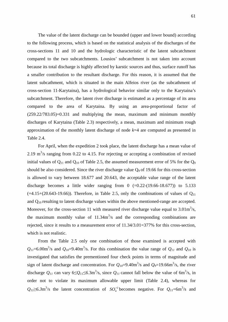
61

The value of the latent discharge can be bounded (upper and lower bound) according

to the following process, which is based on the statistical analysis of the discharges of the

cross-sections 11 and 10 and the hydrologic characteristic of the latent subcatchment

compared to the two subcatchments. Lousios’ subcatchment is not taken into account

because its total discharge is highly affected by karstic sources and thus, surface runoff has

a smaller contribution to the resultant discharge. For this reason, it is assumed that the

latent subcathment, which is situated in the main Alfeios river (as the subcathment of

cross-section 11-Karytaina), has a hydrological behavior similar only to the Karytaina’s

subcatchment. Therefore, the latent river discharge is estimated as a percentage of its area

compared to the area of Karytaina. By using an area-proportional factor of

(259.22/783.05)=0.331 and multiplying the mean, maximum and minimum monthly

discharges of Karytaina (Table 2.3) respectively, a mean, maximum and minimum rough

approximation of the monthly latent discharge of node k=4 are computed as presented in

Table 2.4.

For April, when the expedition 2 took place, the latent discharge has a mean value of

2.19 m3/s ranging from 0.22 to 4.15. For rejecting or accepting a combination of revised

initial values of Q11 and Q10 of Table 2.5, the assumed measurement error of 5% for the Q9

should be also considered. Since the river discharge value Q9 of 19.66 for this cross-section

is allowed to vary between 18.677 and 20.643, the acceptable value range of the latent

discharge becomes a little wider ranging from 0 (=0.22-(19.66-18.677)) to 5.133

(=4.15+(20.643-19.66)). Therefore, in Table 2.5, only the combinations of values of Q11

and Q10 resulting to latent discharge values within the above mentioned-range are accepted.

Moreover, for the cross-section 11 with measured river discharge value equal to 3.01m3/s,

the maximum monthly value of 11.34m3/s and the corresponding combinations are

rejected, since it results to a measurement error of 11.34/3.01=377% for this cross-section,

which is not realistic.

From the Table 2.5 only one combination of those examined is accepted with

Q11=6.00m3/s and Q10=9.40m3/s. For this combination the value range of Q11 and Q10 is

investigated that satisfies the prementioned four check points in terms of magnitude and

sign of latent discharge and concentration. For Q10=9.40m3/s and Q9=19.66m3/s, the river

discharge Q11 can vary 6≤Q11≤6.3m3/s, since Q11 cannot fall below the value of 6m3/s, in

order not to violate its maximum allowable upper limit (Table 2.4), whereas for

Q11≥6.3m3/s the latent concentration of 24−SO becomes negative. For Q11=6m3/s and

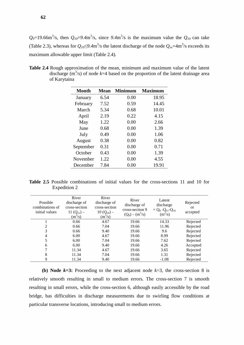
62

Q9=19.66m3/s, then Q10=9.4m3/s, since 9.4m3/s is the maximum value the Q10 can take

(Table 2.3), whereas for Q10≤9.4m3/s the latent discharge of the node Qλκ=4m3/s exceeds its

maximum allowable upper limit (Table 2.4).

Table 2.4 Rough approximation of the mean, minimum and maximum value of the latent discharge (m3/s) of node k=4 based on the proportion of the latent drainage area of Karytaina

Month Mean Minimum Maximum January 6.54 0.00 18.95 February 7.52 0.59 14.45 March 5.34 0.68 10.01 April 2.19 0.22 4.15 May 1.22 0.00 2.66 June 0.68 0.00 1.39 July 0.49 0.00 1.06

August 0.38 0.00 0.82 September 0.31 0.00 0.71 October 0.43 0.00 1.39

November 1.22 0.00 4.55 December 7.84 0.00 19.91

Table 2.5 Possible combinations of initial values for the cross-sections 11 and 10 for Expedition 2

Possible combinations of

initial values

River discharge of cross-section

11 (Q11) – (m3/s)

River discharge of cross-section

10 (Q10) – (m3/s)

River discharge of

cross-section 9 (Q9) – (m3/s)

Latent discharge

= Q9 -Q11-Q10

(m3/s)

Rejected or

accepted

1 0.66 4.67 19.66 14.33 Rejected 2 0.66 7.04 19.66 11.96 Rejected 3 0.66 9.40 19.66 9.6 Rejected 4 6.00 4.67 19.66 8.99 Rejected 5 6.00 7.04 19.66 7.62 Rejected 6 6.00 9.40 19.66 4.26 Accepted 7 11.34 4.67 19.66 3.65 Rejected 8 11.34 7.04 19.66 1.31 Rejected 9 11.34 9.40 19.66 -1.08 Rejected

(b) Node k=3: Proceeding to the next adjacent node k=3, the cross-section 8 is

relatively smooth resulting in small to medium errors. The cross-section 7 is smooth

resulting in small errors, while the cross-section 6, although easily accessible by the road

bridge, has difficulties in discharge measurements due to swirling flow conditions at

particular transverse locations, introducing small to medium errors.

63

Before proceeding to the check of the four prementioned points the difference of the

two electroconductivity values for the cross-sections and the latent one should be

undertaken. Based on Table 2.6, for all cross-sections except of the latent, the two

electroconductivity measurements do not violate the limit of ±15%. For the latent cross-

sections, the second latent concentration, CEC2, should lie between (0.167×0.85,

0.167×1.15)=(0.142,0.193) µS/cm/1000 based on the condition of ±15% deviation from the

first electroconductivity measurement, CEC1, condition which is not satisfied for

CEC1=0.167µS/cm/1000 and CEC2=-0.010µS/cm/1000. Since the latent concentrations are

negative and subject to revision, the adaptations of the electroconductivity concentrations

are made based on the combinations of initial values for the cross-sections of the examined

node.

Following the same qualitative analysis for the third node, for expedition 2 no

indication of gross-error is observed based on the low absolute water balance difference

(1.04) from Table 2.6. As mentioned previously, the signs of the water and pollutant mass

balances should be checked. The water balance, although low as absolute value, is

negative. It seems that there is either an overestimation of one or more of the inflowing

cross-sections or an underestimation of the outflowing cross-section. Both cases are

examined. The measured mean daily water release of the HPS Ladhon for the four

expeditions (2,4,5,6) are available. These river discharges correspond to a drainage area of

769km2 which is smaller than the area covered by the cross-section 8 (1,123km2).

Moreover, the discharge from the area of Ladhon’s subcatchment between these two cross-

sections has only a small contribution to the total river discharge, since it is mainly affected

by karstic sources. This small contribution (corresponding to an area of 1,123-

769=354km2) is mainly composed of surface runoff and for this reason an area-based

factor is used to transfer the river discharge values from the HPS Ladhon downstream to

the cross-section 8 based on the river discharge of Erymanthos (cross-section 7), which is a

neighboring subcatchment mainly affected by surface runoff. The results are presented in

Table 2.7. Ladhon’s discharge at cross-section 8 for expedition 2 is overestimated since its

measured value is 42m3/s and the mean daily release from Table 2.7 is 36.75m3/s

(measurement error ε=12.5%). The revised initial discharge values for this cross-section

are computed based on the minimum, mean and maximum values of the latent discharge as

described below.

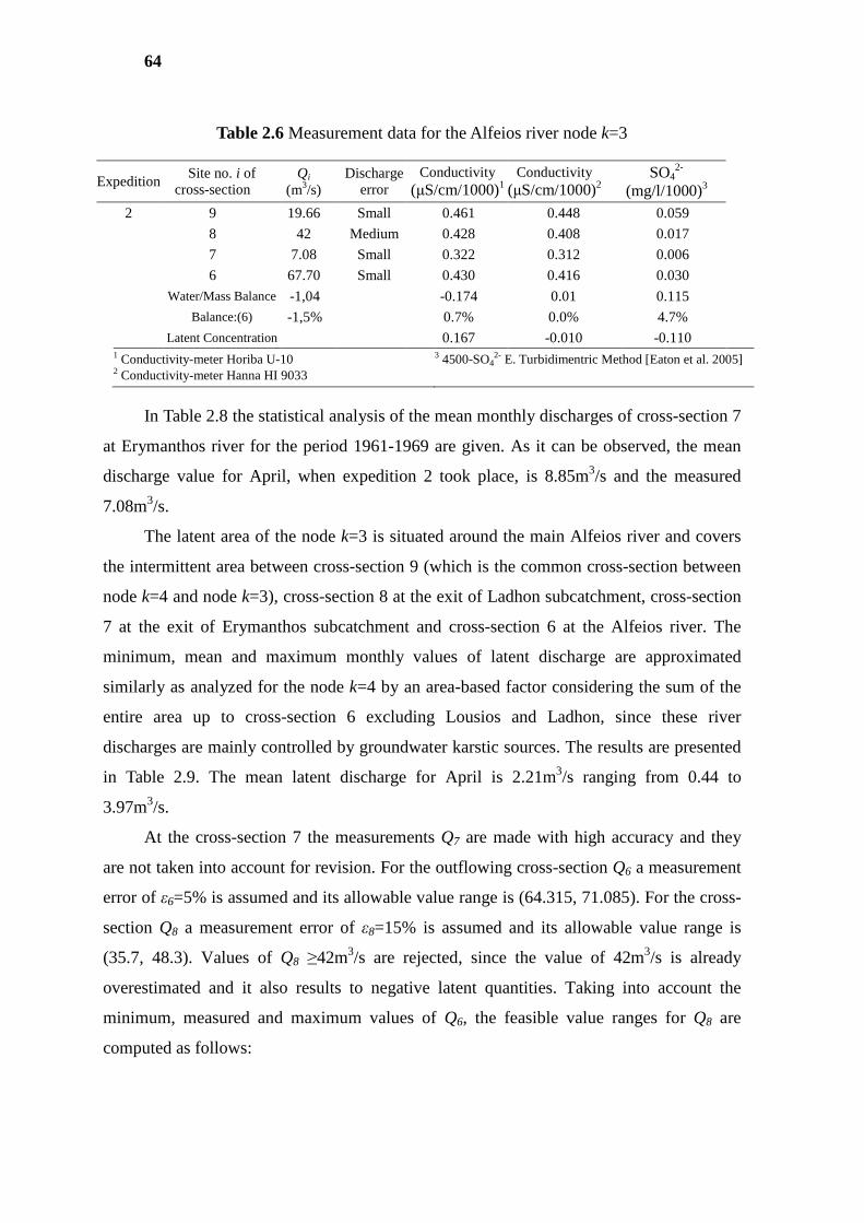
64

Table 2.6 Measurement data for the Alfeios river node k=3

Expedition Site no. i of

cross-section Qi

(m3/s) Discharge

error Conductivity

(µS/cm/1000)1 Conductivity

(µS/cm/1000)2 SO4

2-

(mg/l/1000)3 2 9 19.66 Small 0.461 0.448 0.059

8 42 Medium 0.428 0.408 0.017

7 7.08 Small 0.322 0.312 0.006

6 67.70 Small 0.430 0.416 0.030

Water/Mass Balance -1,04 -0.174 0.01 0.115

Balance:(6) -1,5% 0.7% 0.0% 4.7%

Latent Concentration 0.167 -0.010 -0.110 1 Conductivity-meter Horiba U-10 2 Conductivity-meter Hanna HI 9033

3 4500-SO42- E. Turbidimentric Method [Eaton et al. 2005]

In Table 2.8 the statistical analysis of the mean monthly discharges of cross-section 7

at Erymanthos river for the period 1961-1969 are given. As it can be observed, the mean

discharge value for April, when expedition 2 took place, is 8.85m3/s and the measured

7.08m3/s.

The latent area of the node k=3 is situated around the main Alfeios river and covers

the intermittent area between cross-section 9 (which is the common cross-section between

node k=4 and node k=3), cross-section 8 at the exit of Ladhon subcatchment, cross-section

7 at the exit of Erymanthos subcatchment and cross-section 6 at the Alfeios river. The

minimum, mean and maximum monthly values of latent discharge are approximated

similarly as analyzed for the node k=4 by an area-based factor considering the sum of the

entire area up to cross-section 6 excluding Lousios and Ladhon, since these river

discharges are mainly controlled by groundwater karstic sources. The results are presented

in Table 2.9. The mean latent discharge for April is 2.21m3/s ranging from 0.44 to

3.97m3/s.

At the cross-section 7 the measurements Q7 are made with high accuracy and they

are not taken into account for revision. For the outflowing cross-section Q6 a measurement

error of ε6=5% is assumed and its allowable value range is (64.315, 71.085). For the cross-

section Q8 a measurement error of ε8=15% is assumed and its allowable value range is

(35.7, 48.3). Values of Q8 ≥42m3/s are rejected, since the value of 42m3/s is already

overestimated and it also results to negative latent quantities. Taking into account the

minimum, measured and maximum values of Q6, the feasible value ranges for Q8 are

computed as follows:

65

(1) For Q6=64.315m3/s the minimum value of Q8 not violating all analyzed

conditions is equal to its minimum allowable value of 35.7m3/s. For this value combination

for the latent cross-sections, the second latent concentration, CEC2, should lie between

(0.643×0.85, 0.643×1.15)=(0.483,0.653)µS/cm/1000 based on the condition of ±15%

deviation from the first electroconductivity measurement, CEC1, condition which is

satisfied for CEC1=0.643µS/cm/1000 and CEC2=0.568µS/cm/1000. The maximum value of

Q8 is equal to 36.99m3/s, which results to Qλk=0.585, Cλk=0.877 for electroconductivity

with measurement equipment 1, Cλk=0.940 for electroconductivity with measurement

equipment 2 and Cλk=0.168 for 24−SO . For values Q8 ≥37m3/s, the values Cλk≥0.17 for

24−SO , which are not acceptable. Therefore, for Q6=64.315m3/s then 35.7≤Q8≤36.99m3/s.

(2) For Q6=67.70m3/s the minimum value of Q8 not violating all analyzed conditions is

equal to 36.99m3/s. For values <36.99m3/s the latent discharge exceeds its maximum

allowable value of 3.97m3/s.

For this value combination for the latent cross-sections, the second latent concentration,

CEC2, should lie between (0.877×0.85, 0.877×1.15)=(0.745,1.008)µS/cm/1000 based on the

condition of ±15% deviation from the first electroconductivity measurement, CEC1,

condition which is not satisfied for CEC1=0.877µS/cm/1000 and CEC2=1.160µS/cm/1000.

For this reason the measured values of CEC2 of one or more cross-sections of the node k=4

should be adapted within their value ranges in order to fulfill this condition. The general

aim is to make as few modifications as possible, avoiding transferring the modifications to

the other nodes upstream and downstream. For this reason we start from the cross-sections

which are not common between two successive nodes, in this case 8 and 7. No significant

improvement is derived. Now the common cross-sections 9 and 6 should be checked. Since

the common inflowing cross-section 9 will affect also the node k=4, for which the analysis

has already been undertaken without the need to modify the concentrations, the cross-

section 6 is selected to be tested for modifications. By trial and error, it is concluded that

for values between 0.413≤(CEC2)6≤0.415µS/cm/1000 the condition is satisfied. More

precisely, for the lower limit of (CEC2)6= 0.413µS/cm/1000, then (CEC2)λk=

0.775µS/cm/1000, which lies in the allowable range of (0.745,1.008)µS/cm/1000. For

smaller values i.e. (CEC2)6= 0.412µS/cm/1000, then (CEC2)λk= 0.665µS/cm/1000, which

violates the condition. For the upper limit of (CEC2)6= 415µS/cm/1000, then (CEC2)λk=

0.995µS/cm/1000, which lies in the allowable range. For higher values i.e. (CEC2)6=

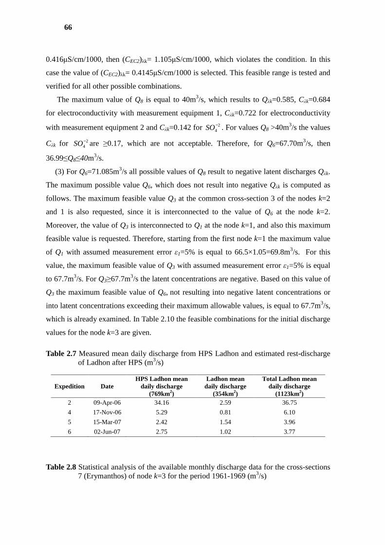
66

0.416µS/cm/1000, then (CEC2)λk= 1.105µS/cm/1000, which violates the condition. In this

case the value of (CEC2)λk= 0.4145µS/cm/1000 is selected. This feasible range is tested and

verified for all other possible combinations.

The maximum value of Q8 is equal to 40m3/s, which results to Qλk=0.585, Cλk=0.684

for electroconductivity with measurement equipment 1, Cλk=0.722 for electroconductivity

with measurement equipment 2 and Cλk=0.142 for 24−SO . For values Q8 >40m3/s the values

Cλk for 24−SO are ≥0.17, which are not acceptable. Therefore, for Q6=67.70m3/s, then

36.99≤Q8≤40m3/s.

(3) For Q6=71.085m3/s all possible values of Q8 result to negative latent discharges Qλk.

The maximum possible value Q6, which does not result into negative Qλk is computed as

follows. The maximum feasible value Q3 at the common cross-section 3 of the nodes k=2

and 1 is also requested, since it is interconnected to the value of Q6 at the node k=2.

Moreover, the value of Q3 is interconnected to Q1 at the node k=1, and also this maximum

feasible value is requested. Therefore, starting from the first node k=1 the maximum value

of Q1 with assumed measurement error ε1=5% is equal to 66.5×1.05=69.8m3/s. For this

value, the maximum feasible value of Q3 with assumed measurement error ε1=5% is equal

to 67.7m3/s. For Q3≥67.7m3/s the latent concentrations are negative. Based on this value of

Q3 the maximum feasible value of Q6, not resulting into negative latent concentrations or

into latent concentrations exceeding their maximum allowable values, is equal to 67.7m3/s,

which is already examined. In Table 2.10 the feasible combinations for the initial discharge

values for the node k=3 are given.

Table 2.7 Measured mean daily discharge from HPS Ladhon and estimated rest-discharge of Ladhon after HPS (m3/s)

Expedition Date HPS Ladhon mean

daily discharge (769km2)

Ladhon mean daily discharge

(354km2)

Total Ladhon mean daily discharge

(1123km2) 2 09-Apr-06 34.16 2.59 36.75

4 17-Nov-06 5.29 0.81 6.10

5 15-Mar-07 2.42 1.54 3.96

6 02-Jun-07 2.75 1.02 3.77

Table 2.8 Statistical analysis of the available monthly discharge data for the cross-sections 7 (Erymanthos) of node k=3 for the period 1961-1969 (m3/s)

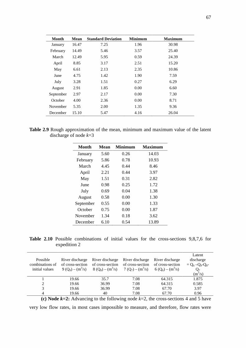
67

Month Mean Standard Deviation Minimum Maximum January 16.47 7.25 1.96 30.98

February 14.49 5.46 3.57 25.40

March 12.49 5.95 0.59 24.39

April 8.85 3.17 2.51 15.20

May 6.61 2.13 2.35 10.86

June 4.75 1.42 1.90 7.59

July 3.28 1.51 0.27 6.29

August 2.91 1.85 0.00 6.60

September 2.97 2.17 0.00 7.30

October 4.00 2.36 0.00 8.71

November 5.35 2.00 1.35 9.36

December 15.10 5.47 4.16 26.04

Table 2.9 Rough approximation of the mean, minimum and maximum value of the latent discharge of node k=3

Month Mean Minimum Maximum

January 5.60 0.26 14.03 February 5.86 0.78 10.93 March 4.45 0.44 8.46 April 2.21 0.44 3.97 May 1.51 0.31 2.82 June 0.98 0.25 1.72 July 0.69 0.04 1.38

August 0.58 0.00 1.30 September 0.55 0.00 1.33 October 0.75 0.00 1.87

November 1.34 0.18 3.62 December 6.10 0.54 13.89

Table 2.10 Possible combinations of initial values for the cross-sections 9,8,7,6 for expedition 2

Possible combinations of

initial values

River discharge of cross-section 9 (Q9) – (m3/s)

River discharge of cross-section 8 (Q8) – (m3/s)

River discharge of cross-section 7 (Q7) – (m3/s)

River discharge of cross-section 6 (Q6) – (m3/s)

Latent discharge

= Q6 –Q9-Q8-Q7

(m3/s) 1 19.66 35.7 7.08 64.315 1.875 2 19.66 36.99 7.08 64.315 0.585 3 19.66 36.99 7.08 67.70 3.97 4 19.66 40 7.08 67.70 0.96

(c) Node k=2: Advancing to the following node k=2, the cross-sections 4 and 5 have

very low flow rates, in most cases impossible to measure, and therefore, flow rates were

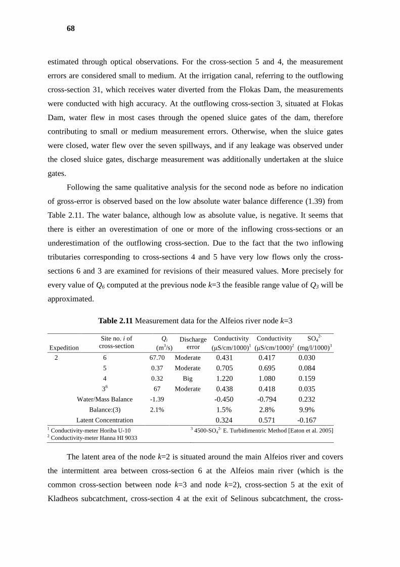
68

estimated through optical observations. For the cross-section 5 and 4, the measurement

errors are considered small to medium. At the irrigation canal, referring to the outflowing

cross-section 31, which receives water diverted from the Flokas Dam, the measurements

were conducted with high accuracy. At the outflowing cross-section 3, situated at Flokas

Dam, water flew in most cases through the opened sluice gates of the dam, therefore

contributing to small or medium measurement errors. Otherwise, when the sluice gates

were closed, water flew over the seven spillways, and if any leakage was observed under

the closed sluice gates, discharge measurement was additionally undertaken at the sluice

gates.

Following the same qualitative analysis for the second node as before no indication

of gross-error is observed based on the low absolute water balance difference (1.39) from

Table 2.11. The water balance, although low as absolute value, is negative. It seems that

there is either an overestimation of one or more of the inflowing cross-sections or an

underestimation of the outflowing cross-section. Due to the fact that the two inflowing

tributaries corresponding to cross-sections 4 and 5 have very low flows only the cross-

sections 6 and 3 are examined for revisions of their measured values. More precisely for

every value of Q6 computed at the previous node k=3 the feasible range value of Q3 will be

approximated.

Table 2.11 Measurement data for the Alfeios river node k=3

Site no. i of cross-section

Qi Discharge error

Conductivity Conductivity SO42-

Expedition (m3/s) (µS/cm/1000)1 (µS/cm/1000)2 (mg/l/1000)3

2 6 67.70 Moderate 0.431 0.417 0.030 5 0.37 Moderate 0.705 0.695 0.084 4 0.32 Big 1.220 1.080 0.159 36 67 Moderate 0.438 0.418 0.035 Water/Mass Balance -1.39 -0.450 -0.794 0.232 Balance:(3) 2.1% 1.5% 2.8% 9.9% Latent Concentration 0.324 0.571 -0.167

1 Conductivity-meter Horiba U-10 2 Conductivity-meter Hanna HI 9033

3 4500-SO42- E. Turbidimentric Method [Eaton et al. 2005]

The latent area of the node k=2 is situated around the main Alfeios river and covers

the intermittent area between cross-section 6 at the Alfeios main river (which is the

common cross-section between node k=3 and node k=2), cross-section 5 at the exit of

Kladheos subcatchment, cross-section 4 at the exit of Selinous subcatchment, the cross-

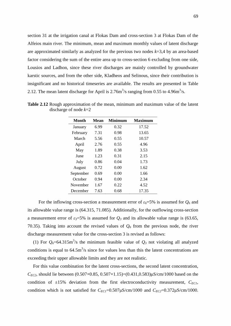
69

section 31 at the irrigation canal at Flokas Dam and cross-section 3 at Flokas Dam of the

Alfeios main river. The minimum, mean and maximum monthly values of latent discharge

are approximated similarly as analyzed for the previous two nodes k=3,4 by an area-based

factor considering the sum of the entire area up to cross-section 6 excluding from one side,

Lousios and Ladhon, since these river discharges are mainly controlled by groundwater

karstic sources, and from the other side, Kladheos and Selinous, since their contribution is

insignificant and no historical timeseries are available. The results are presented in Table

2.12. The mean latent discharge for April is 2.76m3/s ranging from 0.55 to 4.96m3/s.

Table 2.12 Rough approximation of the mean, minimum and maximum value of the latent discharge of node k=2

Month Mean Minimum Maximum

January 6.99 0.32 17.52 February 7.31 0.98 13.65 March 5.56 0.55 10.57 April 2.76 0.55 4.96 May 1.89 0.38 3.53 June 1.23 0.31 2.15 July 0.86 0.04 1.73

August 0.72 0.00 1.62 September 0.69 0.00 1.66 October 0.94 0.00 2.34

November 1.67 0.22 4.52 December 7.63 0.68 17.35

For the inflowing cross-section a measurement error of ε6=5% is assumed for Q6 and

its allowable value range is (64.315, 71.085). Additionally, for the outflowing cross-section

a measurement error of ε3=5% is assumed for Q3 and its allowable value range is (63.65,

70.35). Taking into account the revised values of Q6 from the previous node, the river

discharge measurement value for the cross-section 3 is revised as follows:

(1) For Q6=64.315m3/s the minimum feasible value of Q3 not violating all analyzed

conditions is equal to 64.5m3/s since for values less than this the latent concentrations are

exceeding their upper allowable limits and they are not realistic.

For this value combination for the latent cross-sections, the second latent concentration,

CEC2, should lie between (0.507×0.85, 0.507×1.15)=(0.431,0.583)µS/cm/1000 based on the

condition of ±15% deviation from the first electroconductivity measurement, CEC1,

condition which is not satisfied for CEC1=0.507µS/cm/1000 and CEC2=0.372µS/cm/1000.

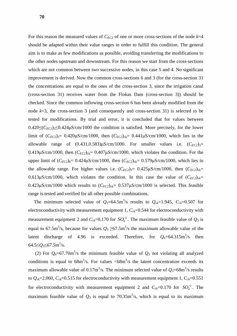
70

For this reason the measured values of CEC2 of one or more cross-sections of the node k=4

should be adapted within their value ranges in order to fulfill this condition. The general

aim is to make as few modifications as possible, avoiding transferring the modifications to

the other nodes upstream and downstream. For this reason we start from the cross-sections

which are not common between two successive nodes, in this case 5 and 4. No significant

improvement is derived. Now the common cross-sections 6 and 3 (for the cross-section 31

the concentrations are equal to the ones of the cross-section 3, since the irrigation canal

(cross-section 31) receives water from the Flokas Dam (cross-section 3)) should be

checked. Since the common inflowing cross-section 6 has been already modified from the

node k=3, the cross-section 3 (and consequently and cross-section 31) is selected to be

tested for modifications. By trial and error, it is concluded that for values between

0.420≤(CEC2)3≤0.424µS/cm/1000 the condition is satisfied. More precisely, for the lower

limit of (CEC2)3= 0.420µS/cm/1000, then (CEC2)λk= 0.441µS/cm/1000, which lies in the

allowable range of (0.431,0.583)µS/cm/1000. For smaller values i.e. (CEC2)3=

0.419µS/cm/1000, then (CEC2)λk= 0.407µS/cm/1000, which violates the condition. For the

upper limit of (CEC2)6= 0.424µS/cm/1000, then (CEC2)λk= 0.579µS/cm/1000, which lies in

the allowable range. For higher values i.e. (CEC2)3= 0.425µS/cm/1000, then (CEC2)λk=

0.613µS/cm/1000, which violates the condition. In this case the value of (CEC2)λk=

0.423µS/cm/1000 which results to (CEC2)λk= 0.537µS/cm/1000 is selected. This feasible

range is tested and verified for all other possible combinations.

The minimum selected value of Q3=64.5m3/s results to Qλk=1.945, Cλk=0.507 for

electroconductivity with measurement equipment 1, Cλk=0.544 for electroconductivity with

measurement equipment 2 and Cλk=0.170 for 24−SO . The maximum feasible value of Q3 is

equal to 67.5m3/s, because for values Q3 ≥67.5m3/s the maximum allowable value of the

latent discharge of 4.96 is exceeded. Therefore, for Q6=64.315m3/s then

64.5≤Q3≤67.5m3/s.

(2) For Q6=67.70m3/s the minimum feasible value of Q3 not violating all analyzed

conditions is equal to 68m3/s. For values <68m3/s the latent concentration exceeds its

maximum allowable value of 0.17m3/s. The minimum selected value of Q3=68m3/s results

to Qλk=2.060, Cλk=0.515 for electroconductivity with measurement equipment 1, Cλk=0.551

for electroconductivity with measurement equipment 2 and Cλk=0.170 for 24−SO . The

maximum feasible value of Q3 is equal to 70.35m3/s, which is equal to its maximum

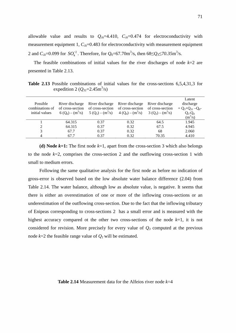
71

allowable value and results to Qλk=4.410, Cλk=0.474 for electroconductivity with

measurement equipment 1, Cλk=0.483 for electroconductivity with measurement equipment

2 and Cλk=0.099 for 24−SO . Therefore, for Q6=67.70m3/s, then 68≤Q3≤70.35m3/s.

The feasible combinations of initial values for the river discharges of node k=2 are

presented in Table 2.13.

Table 2.13 Possible combinations of initial values for the cross-sections 6,5,4,31,3 for expedition 2 (Q31=2.45m3/s)

Possible combinations of

initial values

River discharge of cross-section 6 (Q6) – (m3/s)

River discharge of cross-section 5 (Q5) – (m3/s)

River discharge of cross-section 4 (Q4) – (m3/s)

River discharge of cross-section 3 (Q3) – (m3/s)

Latent discharge

= Q3+Q31 –Q6-Q5-Q4

(m3/s) 1 64.315 0.37 0.32 64.5 1.945 2 64.315 0.37 0.32 67.5 4.945 3 67.7 0.37 0.32 68 2.060 4 67.7 0.37 0.32 70.35 4.410

(d) Node k=1: The first node k=1, apart from the cross-section 3 which also belongs

to the node k=2, comprises the cross-section 2 and the outflowing cross-section 1 with

small to medium errors.

Following the same qualitative analysis for the first node as before no indication of

gross-error is observed based on the low absolute water balance difference (2.04) from

Table 2.14. The water balance, although low as absolute value, is negative. It seems that

there is either an overestimation of one or more of the inflowing cross-sections or an

underestimation of the outflowing cross-section. Due to the fact that the inflowing tributary

of Enipeas corresponding to cross-sections 2 has a small error and is measured with the

highest accuracy compared ot the other two cross-sections of the node k=1, it is not

considered for revision. More precisely for every value of Q3 computed at the previous

node k=2 the feasible range value of Q1 will be estimated.

Table 2.14 Measurement data for the Alfeios river node k=4

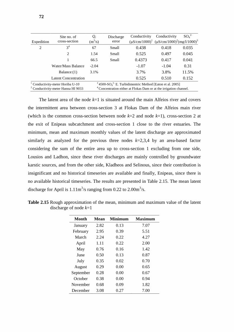
72

Site no. of cross-section

Qi Discharge error

Conductivity Conductivity SO42-

Expedition (m3/s) (µS/cm/1000)1 (µS/cm/1000)2 (mg/l/1000)3

2 34 67 Small 0.438 0.418 0.035 2 1.54 Small 0.525 0.497 0.045 1 66.5 Small 0.4373 0.417 0.041 Water/Mass Balance -2.04 -1.07 -1.04 0.31 Balance:(1) 3.1% 3.7% 3.8% 11.5% Latent Concentration 0.525 0.510 0.152

1 Conductivity-meter Horiba U-10 2 Conductivity-meter Hanna HI 9033

3 4500-SO42- E. Turbidimentric Method [Eaton et al. 2005]

4 Concentration either at Flokas Dam or at the irrigation channel.

The latent area of the node k=1 is situated around the main Alfeios river and covers

the intermittent area between cross-section 3 at Flokas Dam of the Alfeios main river

(which is the common cross-section between node k=2 and node k=1), cross-section 2 at

the exit of Enipeas subcatchment and cross-section 1 close to the river estuaries. The

minimum, mean and maximum monthly values of the latent discharge are approximated

similarly as analyzed for the previous three nodes k=2,3,4 by an area-based factor

considering the sum of the entire area up to cross-section 1 excluding from one side,

Lousios and Ladhon, since these river discharges are mainly controlled by groundwater

karstic sources, and from the other side, Kladheos and Selinous, since their contribution is

insignificant and no historical timeseries are available and finally, Enipeas, since there is

no available historical timeseries. The results are presented in Table 2.15. The mean latent

discharge for April is 1.11m3/s ranging from 0.22 to 2.00m3/s.

Table 2.15 Rough approximation of the mean, minimum and maximum value of the latent discharge of node k=1

Month Mean Minimum Maximum

January 2.82 0.13 7.07 February 2.95 0.39 5.51 March 2.24 0.22 4.27 April 1.11 0.22 2.00 May 0.76 0.16 1.42 June 0.50 0.13 0.87 July 0.35 0.02 0.70

August 0.29 0.00 0.65 September 0.28 0.00 0.67 October 0.38 0.00 0.94

November 0.68 0.09 1.82 December 3.08 0.27 7.00

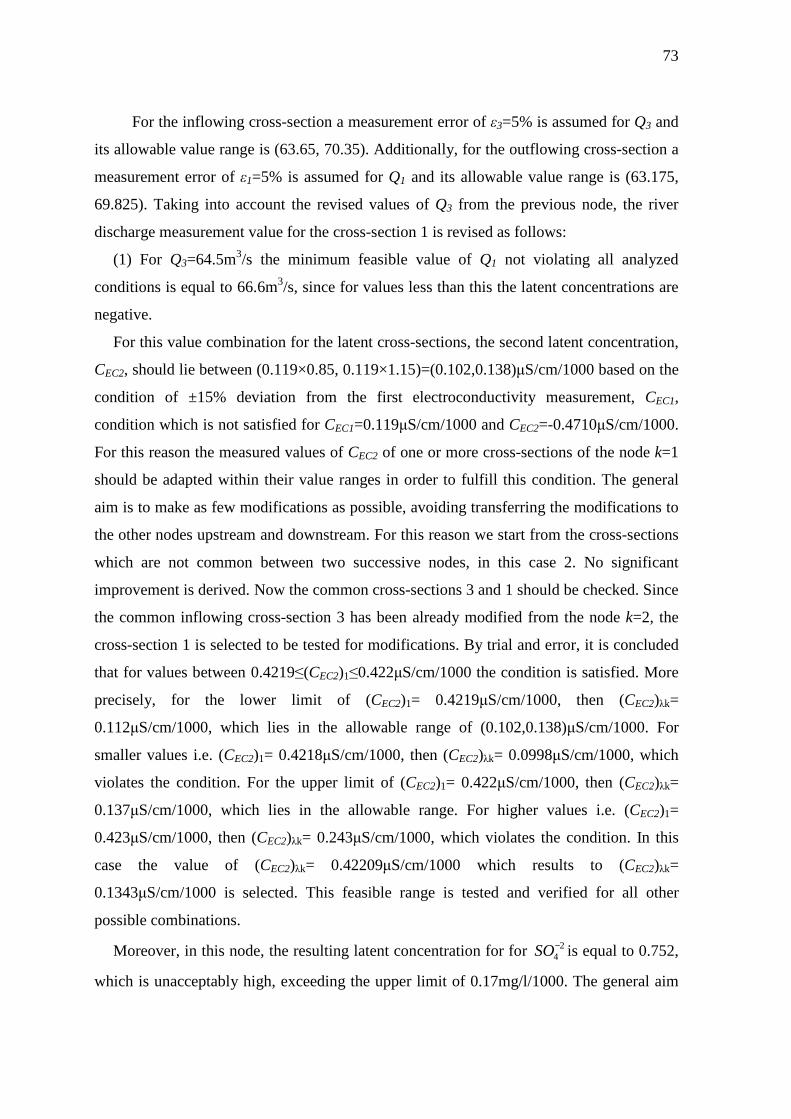
73

For the inflowing cross-section a measurement error of ε3=5% is assumed for Q3 and

its allowable value range is (63.65, 70.35). Additionally, for the outflowing cross-section a

measurement error of ε1=5% is assumed for Q1 and its allowable value range is (63.175,

69.825). Taking into account the revised values of Q3 from the previous node, the river

discharge measurement value for the cross-section 1 is revised as follows:

(1) For Q3=64.5m3/s the minimum feasible value of Q1 not violating all analyzed

conditions is equal to 66.6m3/s, since for values less than this the latent concentrations are

negative.

For this value combination for the latent cross-sections, the second latent concentration,

CEC2, should lie between (0.119×0.85, 0.119×1.15)=(0.102,0.138)µS/cm/1000 based on the

condition of ±15% deviation from the first electroconductivity measurement, CEC1,

condition which is not satisfied for CEC1=0.119µS/cm/1000 and CEC2=-0.4710µS/cm/1000.

For this reason the measured values of CEC2 of one or more cross-sections of the node k=1

should be adapted within their value ranges in order to fulfill this condition. The general

aim is to make as few modifications as possible, avoiding transferring the modifications to

the other nodes upstream and downstream. For this reason we start from the cross-sections

which are not common between two successive nodes, in this case 2. No significant

improvement is derived. Now the common cross-sections 3 and 1 should be checked. Since

the common inflowing cross-section 3 has been already modified from the node k=2, the

cross-section 1 is selected to be tested for modifications. By trial and error, it is concluded

that for values between 0.4219≤(CEC2)1≤0.422µS/cm/1000 the condition is satisfied. More

precisely, for the lower limit of (CEC2)1= 0.4219µS/cm/1000, then (CEC2)λk=

0.112µS/cm/1000, which lies in the allowable range of (0.102,0.138)µS/cm/1000. For

smaller values i.e. (CEC2)1= 0.4218µS/cm/1000, then (CEC2)λk= 0.0998µS/cm/1000, which

violates the condition. For the upper limit of (CEC2)1= 0.422µS/cm/1000, then (CEC2)λk=

0.137µS/cm/1000, which lies in the allowable range. For higher values i.e. (CEC2)1=

0.423µS/cm/1000, then (CEC2)λk= 0.243µS/cm/1000, which violates the condition. In this

case the value of (CEC2)λk= 0.42209µS/cm/1000 which results to (CEC2)λk=

0.1343µS/cm/1000 is selected. This feasible range is tested and verified for all other

possible combinations.

Moreover, in this node, the resulting latent concentration for for 24−SO is equal to 0.752,

which is unacceptably high, exceeding the upper limit of 0.17mg/l/1000. The general aim

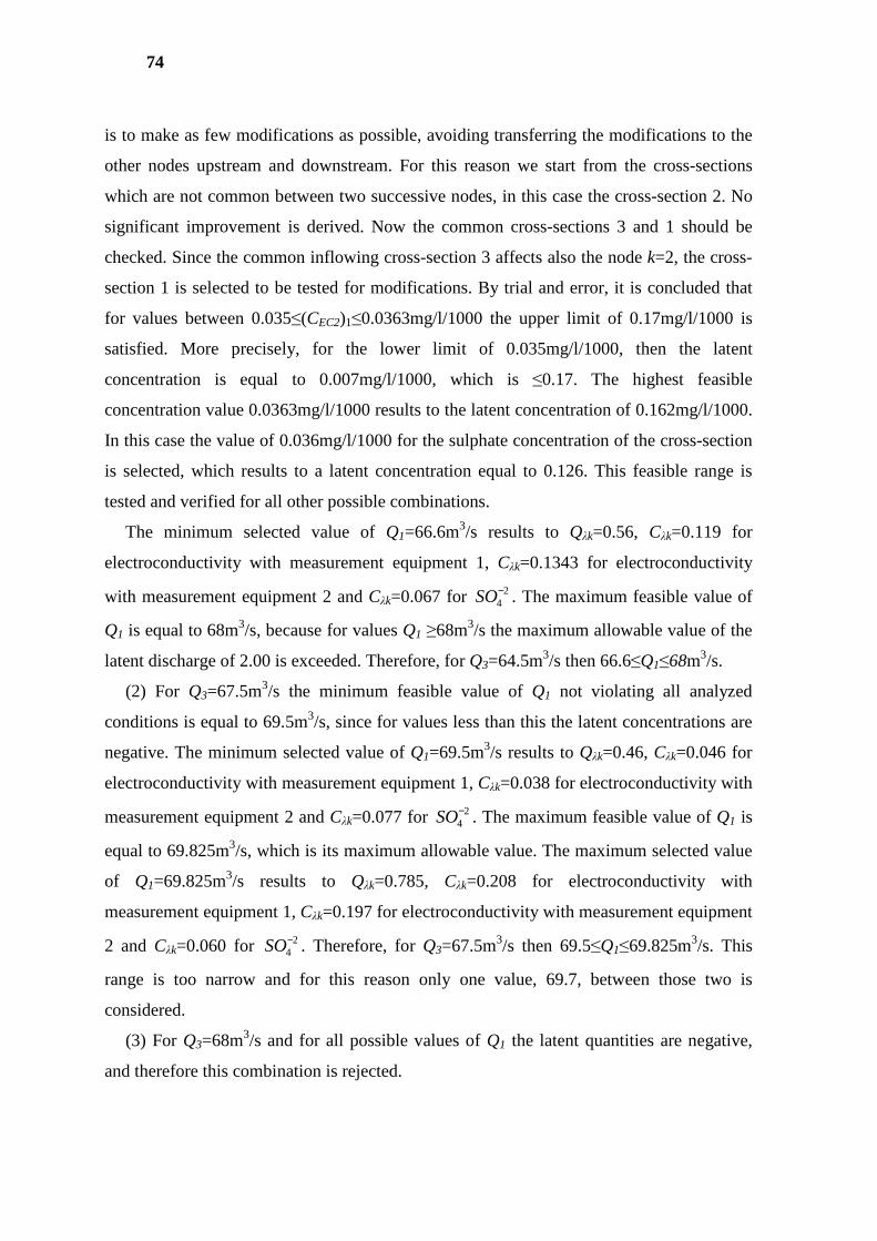
74

is to make as few modifications as possible, avoiding transferring the modifications to the

other nodes upstream and downstream. For this reason we start from the cross-sections

which are not common between two successive nodes, in this case the cross-section 2. No

significant improvement is derived. Now the common cross-sections 3 and 1 should be

checked. Since the common inflowing cross-section 3 affects also the node k=2, the cross-

section 1 is selected to be tested for modifications. By trial and error, it is concluded that

for values between 0.035≤(CEC2)1≤0.0363mg/l/1000 the upper limit of 0.17mg/l/1000 is

satisfied. More precisely, for the lower limit of 0.035mg/l/1000, then the latent

concentration is equal to 0.007mg/l/1000, which is ≤0.17. The highest feasible

concentration value 0.0363mg/l/1000 results to the latent concentration of 0.162mg/l/1000.

In this case the value of 0.036mg/l/1000 for the sulphate concentration of the cross-section

is selected, which results to a latent concentration equal to 0.126. This feasible range is

tested and verified for all other possible combinations.

The minimum selected value of Q1=66.6m3/s results to Qλk=0.56, Cλk=0.119 for

electroconductivity with measurement equipment 1, Cλk=0.1343 for electroconductivity

with measurement equipment 2 and Cλk=0.067 for 24−SO . The maximum feasible value of

Q1 is equal to 68m3/s, because for values Q1 ≥68m3/s the maximum allowable value of the

latent discharge of 2.00 is exceeded. Therefore, for Q3=64.5m3/s then 66.6≤Q1≤68m3/s.

(2) For Q3=67.5m3/s the minimum feasible value of Q1 not violating all analyzed

conditions is equal to 69.5m3/s, since for values less than this the latent concentrations are

negative. The minimum selected value of Q1=69.5m3/s results to Qλk=0.46, Cλk=0.046 for

electroconductivity with measurement equipment 1, Cλk=0.038 for electroconductivity with

measurement equipment 2 and Cλk=0.077 for 24−SO . The maximum feasible value of Q1 is

equal to 69.825m3/s, which is its maximum allowable value. The maximum selected value

of Q1=69.825m3/s results to Qλk=0.785, Cλk=0.208 for electroconductivity with

measurement equipment 1, Cλk=0.197 for electroconductivity with measurement equipment

2 and Cλk=0.060 for 24−SO . Therefore, for Q3=67.5m3/s then 69.5≤Q1≤69.825m3/s. This

range is too narrow and for this reason only one value, 69.7, between those two is

considered.

(3) For Q3=68m3/s and for all possible values of Q1 the latent quantities are negative,

and therefore this combination is rejected.

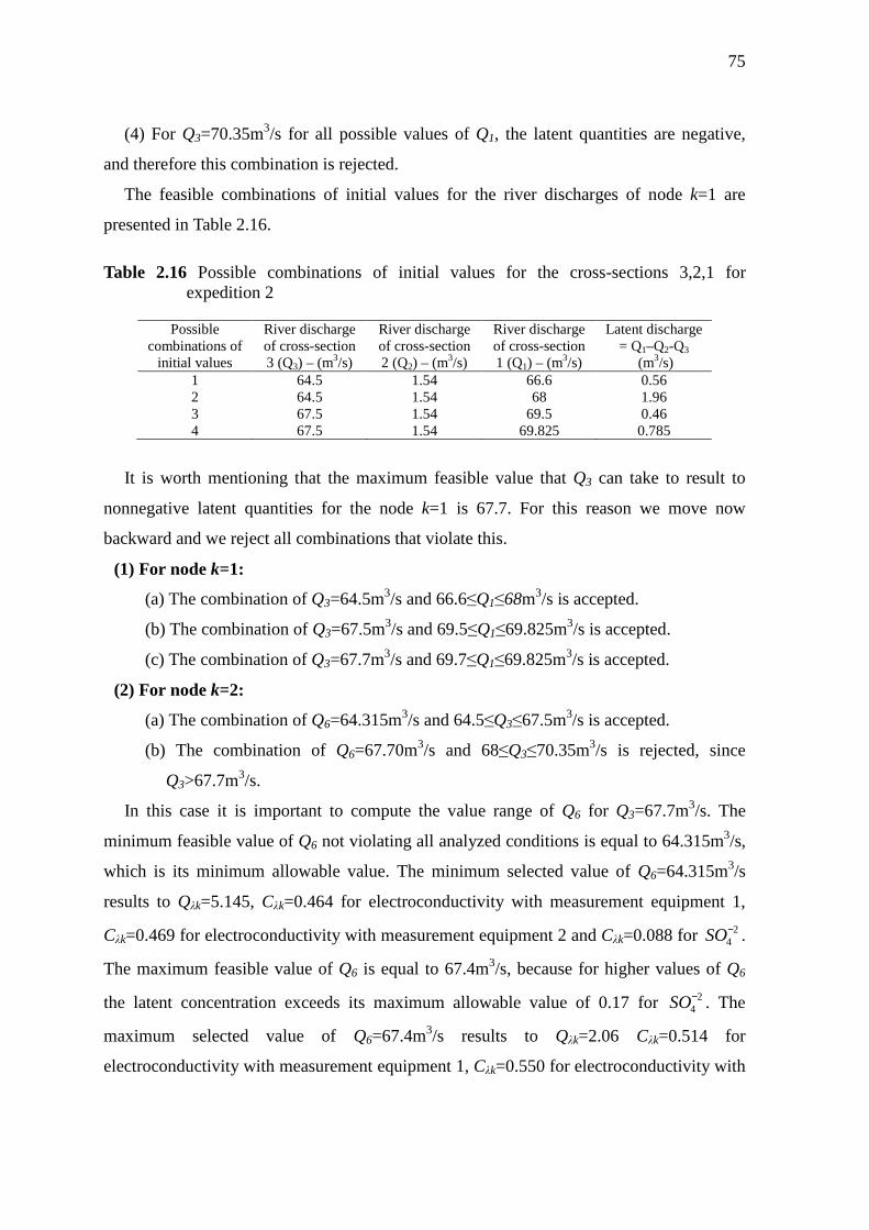
75

(4) For Q3=70.35m3/s for all possible values of Q1, the latent quantities are negative,

and therefore this combination is rejected.

The feasible combinations of initial values for the river discharges of node k=1 are

presented in Table 2.16.

Table 2.16 Possible combinations of initial values for the cross-sections 3,2,1 for expedition 2

Possible combinations of

initial values

River discharge of cross-section 3 (Q3) – (m3/s)

River discharge of cross-section 2 (Q2) – (m3/s)

River discharge of cross-section 1 (Q1) – (m3/s)

Latent discharge = Q1–Q2-Q3

(m3/s) 1 64.5 1.54 66.6 0.56 2 64.5 1.54 68 1.96 3 67.5 1.54 69.5 0.46 4 67.5 1.54 69.825 0.785

It is worth mentioning that the maximum feasible value that Q3 can take to result to

nonnegative latent quantities for the node k=1 is 67.7. For this reason we move now

backward and we reject all combinations that violate this.

(1) For node k=1:

(a) The combination of Q3=64.5m3/s and 66.6≤Q1≤68m3/s is accepted.

(b) The combination of Q3=67.5m3/s and 69.5≤Q1≤69.825m3/s is accepted.

(c) The combination of Q3=67.7m3/s and 69.7≤Q1≤69.825m3/s is accepted.

(2) For node k=2:

(a) The combination of Q6=64.315m3/s and 64.5≤Q3≤67.5m3/s is accepted.

(b) The combination of Q6=67.70m3/s and 68≤Q3≤70.35m3/s is rejected, since

Q3>67.7m3/s.

In this case it is important to compute the value range of Q6 for Q3=67.7m3/s. The

minimum feasible value of Q6 not violating all analyzed conditions is equal to 64.315m3/s,

which is its minimum allowable value. The minimum selected value of Q6=64.315m3/s

results to Qλk=5.145, Cλk=0.464 for electroconductivity with measurement equipment 1,

Cλk=0.469 for electroconductivity with measurement equipment 2 and Cλk=0.088 for 24−SO .

The maximum feasible value of Q6 is equal to 67.4m3/s, because for higher values of Q6

the latent concentration exceeds its maximum allowable value of 0.17 for 24−SO . The

maximum selected value of Q6=67.4m3/s results to Qλk=2.06 Cλk=0.514 for

electroconductivity with measurement equipment 1, Cλk=0.550 for electroconductivity with

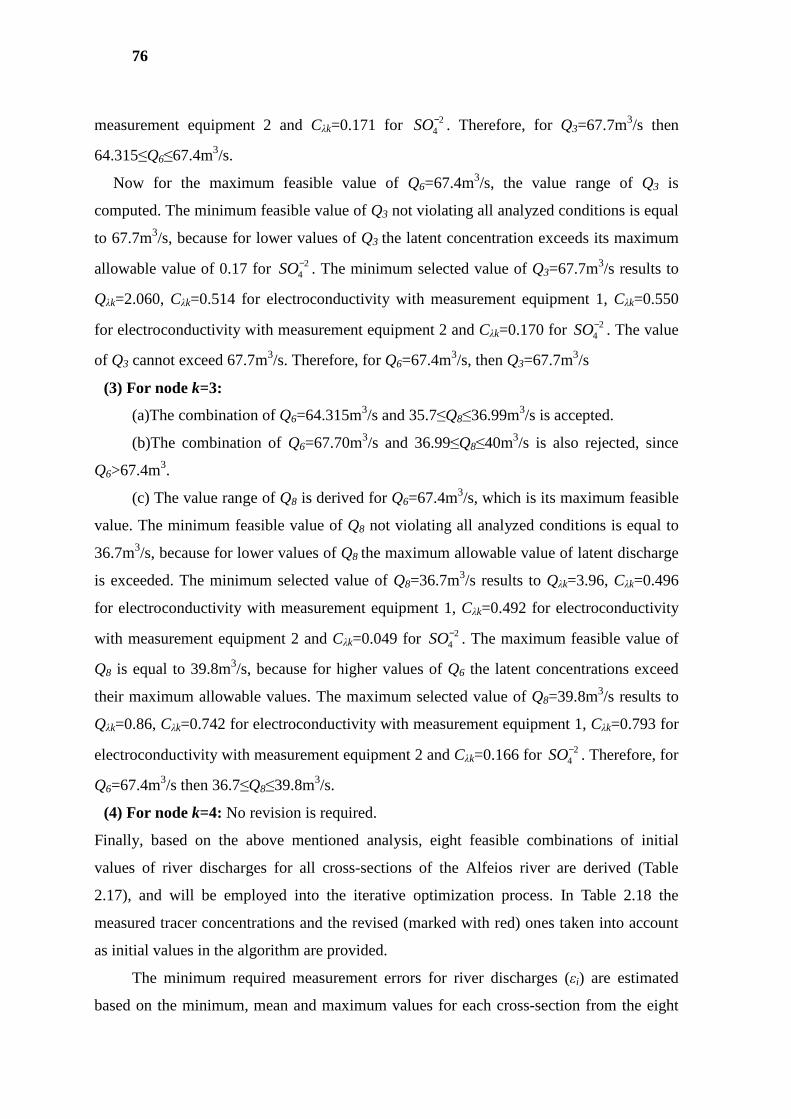
76

measurement equipment 2 and Cλk=0.171 for 24−SO . Therefore, for Q3=67.7m3/s then

64.315≤Q6≤67.4m3/s.

Now for the maximum feasible value of Q6=67.4m3/s, the value range of Q3 is

computed. The minimum feasible value of Q3 not violating all analyzed conditions is equal

to 67.7m3/s, because for lower values of Q3 the latent concentration exceeds its maximum

allowable value of 0.17 for 24−SO . The minimum selected value of Q3=67.7m3/s results to

Qλk=2.060, Cλk=0.514 for electroconductivity with measurement equipment 1, Cλk=0.550

for electroconductivity with measurement equipment 2 and Cλk=0.170 for 24−SO . The value

of Q3 cannot exceed 67.7m3/s. Therefore, for Q6=67.4m3/s, then Q3=67.7m3/s

(3) For node k=3:

(a)The combination of Q6=64.315m3/s and 35.7≤Q8≤36.99m3/s is accepted.

(b)The combination of Q6=67.70m3/s and 36.99≤Q8≤40m3/s is also rejected, since

Q6>67.4m3.

(c) The value range of Q8 is derived for Q6=67.4m3/s, which is its maximum feasible

value. The minimum feasible value of Q8 not violating all analyzed conditions is equal to

36.7m3/s, because for lower values of Q8 the maximum allowable value of latent discharge

is exceeded. The minimum selected value of Q8=36.7m3/s results to Qλk=3.96, Cλk=0.496

for electroconductivity with measurement equipment 1, Cλk=0.492 for electroconductivity

with measurement equipment 2 and Cλk=0.049 for 24−SO . The maximum feasible value of

Q8 is equal to 39.8m3/s, because for higher values of Q6 the latent concentrations exceed

their maximum allowable values. The maximum selected value of Q8=39.8m3/s results to

Qλk=0.86, Cλk=0.742 for electroconductivity with measurement equipment 1, Cλk=0.793 for

electroconductivity with measurement equipment 2 and Cλk=0.166 for 24−SO . Therefore, for

Q6=67.4m3/s then 36.7≤Q8≤39.8m3/s.

(4) For node k=4: No revision is required.

Finally, based on the above mentioned analysis, eight feasible combinations of initial

values of river discharges for all cross-sections of the Alfeios river are derived (Table

2.17), and will be employed into the iterative optimization process. In Table 2.18 the

measured tracer concentrations and the revised (marked with red) ones taken into account

as initial values in the algorithm are provided.

The minimum required measurement errors for river discharges (εi) are estimated

based on the minimum, mean and maximum values for each cross-section from the eight

77

combinations of this qualitative analysis. More precisely, they are computed as [1-

(Min/Mesurement)] or [(Max/Measurement)-1] and are presented in the column named

“Computed εi” of Table 2.17. At the last column of this table the selected measurement

errors “Selected εi” are given after rounding the computed εi. For the cross-sections with

computed errors equal to zero, a revision of the zero value with a more representative error

is undertaken based on the characterization of the magnitude of the measurement error and

the measuring conditions during the given expedition. For most of the cross-sections with

low to medium error, a 5% measurement error has been specified.

For the estimation of the unknown error of the latent concentrations, a wider

“relaxed” value interval is considered. It is based on the values of the latent concentrations

from the eight combinations. More precisely, in Table 2.19 the latent concentrations are

provided for the 8 combinations of initial river discharges (for all single nodes) together

with their corresponding minimum, mean and maximum values. In Table 2.20 the relative

measurement errors of concentrations (ζj) for the latents are computed as [1-(Min/Mean)]

or [(Max/Mean)-1] and presented in the column named “Computed εi”. A further rounding

as described above and the revision of their values is also included and the selected ζλκ.

2.3.3 COMPUTER IMPLEMENTATION

For implementing the proposed methodology, the LINGO optimization software

(Schrage, 1997; Lindo Systems Inc., 1996) has been selected, since it is a very efficient and

robust tool for building and solving mathematical optimization models. In order to increase

the flexibility and the ease of the proposed methodology, LINGO has been properly

combined with Microsoft Excel in order to import and export input and output data to and

from M. Excel. This is enabled through OLE Automation Links from Excel. In this case

LINGO allows to place a LINGO command script in a range in an Excel spreadsheet, and

then pass the script to LINGO by means of OLE Automation. Most of the inputs

computational processes necessary for the calculation of the coefficients of the objective

function and constraints and the right- and left-hand side of the constraints of the

optimization algorithm and also the iterative process are introduced into M. Excel through

VBA macros, which communicate with LINGO in order to exchange data and run the

algorithm at every step.

The proposed optimization algorithm, as analyzed above, was built using the

advanced programming language of LINGO. In this way a generic code has been written,

78

enabling in this way for every case-study only the introduction of the necessary input

values (measurements and measurements errors) from M. Excel. At every step of the

iterative process M. Excel calls LINGO, which imports the input values, runs the

optimization algorithm and exports the results in M. Excel. The solution of the last step is

transferred in M. Excel in the input cells of the next step of the iteration, etc. LINGO

includes a set of fast built-in solvers for most classes of optimization models. For the

introduced methodology it uses firstly a direct solver and then its linear solver for a

continuous linear optimization problem, which is based on the primal simplex. The dual

simplex solver as well as the barrier for large-scale sparse optimization problems are also

available. According to Schrage (1997) through the use of the direct solver, LINGO

substitutes out all the fixed variables and constraints from the model. The remaining

reduced set of constraints and variables are then classified as being either linear or

nonlinear. LINGO’s solver status window, which by default opens every time you solve a

model, gives a count of the linear and nonlinear variables and constraints in a model.

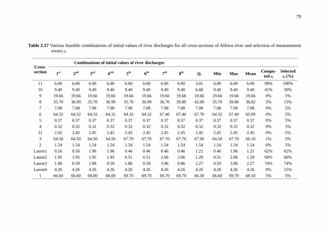
79

Table 2.17 Various feasible combinations of initial values of river discharges for all cross-sections of Alfeios river and selection of measurement errors εi

Cross-section

Combinations of initial values of river discharges

1st 2nd 3rd 4rth 5th 6th 7th 8th Qi Min Max Mean Compu-ted εi

Selectedεi (%)

11 6.00 6.00 6.00 6.00 6.00 6.00 6.00 6.00 3.01 6.00 6.00 6.00 99% 100%

10 9.40 9.40 9.40 9.40 9.40 9.40 9.40 9.40 6.68 9.40 9.40 9.40 41% 50%

9 19.66 19.66 19.66 19.66 19.66 19.66 19.66 19.66 19.66 19.66 19.66 19.66 0% 5%

8 35.70 36.99 35.70 36.99 35.70 36.99 36.70 39.80 42.00 35.70 39.80 36.82 5% 15%

7 7.08 7.08 7.08 7.08 7.08 7.08 7.08 7.08 7.08 7.08 7.08 7.08 0% 5%

6 64.32 64.32 64.32 64.32 64.32 64.32 67.40 67.40 67.70 64.32 67.40 65.09 0% 5%

5 0.37 0.37 0.37 0.37 0.37 0.37 0.37 0.37 0.37 0.37 0.37 0.37 0% 5%

4 0.32 0.32 0.32 0.32 0.32 0.32 0.32 0.32 0.32 0.32 0.32 0.32 0% 5%

31 2.45 2.45 2.45 2.45 2.45 2.45 2.45 2.45 2.45 2.45 2.45 2.45 0% 5%

3 64.50 64.50 64.50 64.50 67.70 67.70 67.70 67.70 67.00 64.50 67.70 66.10 1% 5%

2 1.54 1.54 1.54 1.54 1.54 1.54 1.54 1.54 1.54 1.54 1.54 1.54 0% 5%

Latent1 0.56 0.56 1.96 1.96 0.46 0.46 0.46 0.46 1.21 0.46 1.96 1.21 62% 62%

Latent2 1.95 1.95 1.95 1.95 0.51 0.51 2.06 2.06 1.29 0.51 2.06 1.29 60% 60%

Latent3 1.88 0.59 1.88 0.59 1.88 0.59 3.96 0.86 2.27 0.59 3.96 2.27 74% 74%

Latent4 4.26 4.26 4.26 4.26 4.26 4.26 4.26 4.26 4.26 4.26 4.26 4.26 0% 15%

1 66.60 66.60 68.00 68.00 69.70 69.70 69.70 69.70 66.50 66.60 69.70 68.50 5% 5%

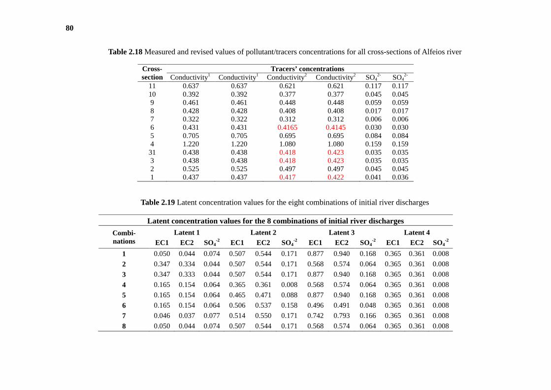
80

Table 2.18 Measured and revised values of pollutant/tracers concentrations for all cross-sections of Alfeios river

Cross-section

Tracers’ concentrations Conductivity1 Conductivity1 Conductivity2 Conductivity2 SO4

2- SO42-

11 0.637 0.637 0.621 0.621 0.117 0.117 10 0.392 0.392 0.377 0.377 0.045 0.045 9 0.461 0.461 0.448 0.448 0.059 0.059 8 0.428 0.428 0.408 0.408 0.017 0.017 7 0.322 0.322 0.312 0.312 0.006 0.006 6 0.431 0.431 0.4165 0.4145 0.030 0.030 5 0.705 0.705 0.695 0.695 0.084 0.084 4 1.220 1.220 1.080 1.080 0.159 0.159 31 0.438 0.438 0.418 0.423 0.035 0.035 3 0.438 0.438 0.418 0.423 0.035 0.035 2 0.525 0.525 0.497 0.497 0.045 0.045 1 0.437 0.437 0.417 0.422 0.041 0.036

Table 2.19 Latent concentration values for the eight combinations of initial river discharges

Latent concentration values for the 8 combinations of initial river discharges

Combi-nations

Latent 1 Latent 2 Latent 3 Latent 4 EC1 EC2 SO4

-2 EC1 EC2 SO4-2 EC1 EC2 SO4

-2 EC1 EC2 SO4-2

1 0.050 0.044 0.074 0.507 0.544 0.171 0.877 0.940 0.168 0.365 0.361 0.008

2 0.347 0.334 0.044 0.507 0.544 0.171 0.568 0.574 0.064 0.365 0.361 0.008

3 0.347 0.333 0.044 0.507 0.544 0.171 0.877 0.940 0.168 0.365 0.361 0.008

4 0.165 0.154 0.064 0.365 0.361 0.008 0.568 0.574 0.064 0.365 0.361 0.008

5 0.165 0.154 0.064 0.465 0.471 0.088 0.877 0.940 0.168 0.365 0.361 0.008

6 0.165 0.154 0.064 0.506 0.537 0.158 0.496 0.491 0.048 0.365 0.361 0.008

7 0.046 0.037 0.077 0.514 0.550 0.171 0.742 0.793 0.166 0.365 0.361 0.008

8 0.050 0.044 0.074 0.507 0.544 0.171 0.568 0.574 0.064 0.365 0.361 0.008

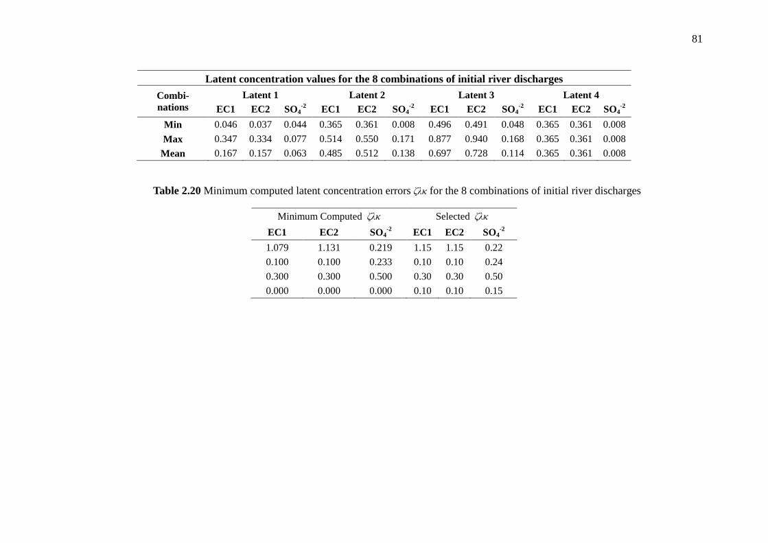
81

Latent concentration values for the 8 combinations of initial river discharges

Combi-nations

Latent 1 Latent 2 Latent 3 Latent 4 EC1 EC2 SO4

-2 EC1 EC2 SO4-2 EC1 EC2 SO4

-2 EC1 EC2 SO4-2

Min 0.046 0.037 0.044 0.365 0.361 0.008 0.496 0.491 0.048 0.365 0.361 0.008

Max 0.347 0.334 0.077 0.514 0.550 0.171 0.877 0.940 0.168 0.365 0.361 0.008

Mean 0.167 0.157 0.063 0.485 0.512 0.138 0.697 0.728 0.114 0.365 0.361 0.008

Table 2.20 Minimum computed latent concentration errors ζλκ for the 8 combinations of initial river discharges

Minimum Computed ζλκ Selected ζλκ

EC1 EC2 SO4-2 EC1 EC2 SO4

-2

1.079 1.131 0.219 1.15 1.15 0.22

0.100 0.100 0.233 0.10 0.10 0.24

0.300 0.300 0.500 0.30 0.30 0.50

0.000 0.000 0.000 0.10 0.10 0.15

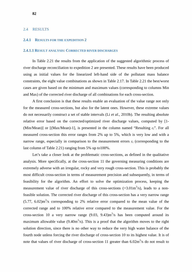
82

2.4 RESULTS

2.4.1 RESULTS FOR THE EXPEDITION 2

2.4.1.1 RESULT ANALYSIS : CORRECTED RIVER DISCHARGES

In Table 2.21 the results from the application of the suggested algorithmic process of

river discharge reconciliation to expedition 2 are presented. These results have been produced

using as initial values for the linearized left-hand side of the pollutant mass balance

constraints, the eight value combinations as shown in Table 2.17. In Table 2.21 the best/worst

cases are given based on the minimum and maximum values (corresponding to columns Min

and Max) of the corrected river discharge of all combinations for each cross-section.

A first conclusion is that these results enable an evaluation of the value range not only

for the measured cross-sections, but also for the latent ones. However, these extreme values

do not necessarily construct a set of stable intervals (Li et al., 2010b). The resulting absolute

relative error based on the corrected/optimized river discharge values, computed by [1-

(Min/Mean)] or [(Max/Mean)-1], is presented in the column named “Resulting εi”. For all

measured cross-section this error ranges from 2% up to 5%, which is very low and with a

narrow range, especially in comparison to the measurement errors εi (corresponding to the

last column of Table 2.21) ranging from 5% up to100%.

Let’s take a closer look at the problematic cross-sections, as defined in the qualitative

analysis. More specifically, at the cross-section 11 the governing measuring conditions are

extremely adverse with an irregular, rocky and very rough cross-section. This is probably the

most difficult cross-section in terms of measurement precision and subsequently, in terms of

feasibility for the algorithm. An effort to solve the optimization process, keeping the

measurement value of river discharge of this cross-sections (=3.01m3/s), leads to a non-

feasible solution. The corrected river discharge of this cross-section has a very narrow range

(5.77, 6.02)m3/s corresponding to 2% relative error compared to the mean value of the

corrected range and to 100% relative error compared to the measurement value. For the

cross-section 10 a very narrow range (9.03, 9.43)m3/s has been computed around its

maximum allowable value (9.40m3/s). This is a proof that the algorithm moves to the right

solution direction, since there is no other way to reduce the very high water balance of the

fourth node unless forcing the river discharge of cross-section 10 to its highest value. It is of

note that values of river discharge of cross-section 11 greater than 6.02m3/s do not result to

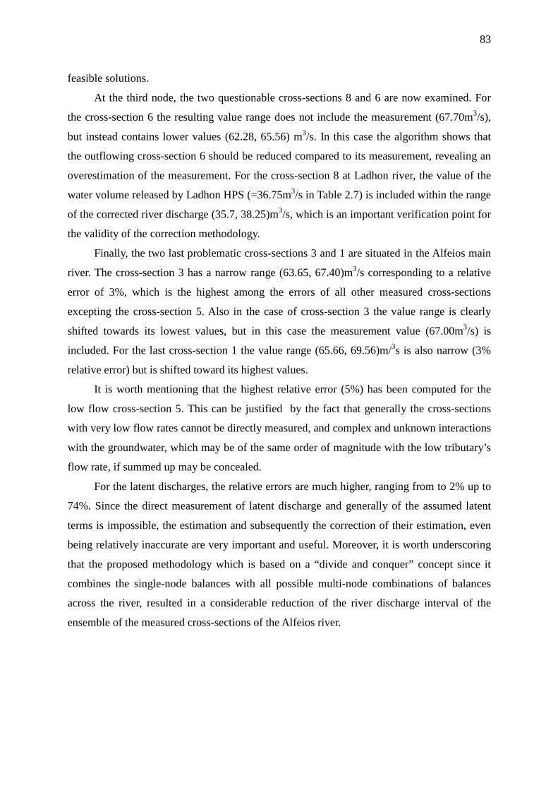
83

feasible solutions.

At the third node, the two questionable cross-sections 8 and 6 are now examined. For

the cross-section 6 the resulting value range does not include the measurement (67.70m3/s),

but instead contains lower values (62.28, 65.56) m3/s. In this case the algorithm shows that

the outflowing cross-section 6 should be reduced compared to its measurement, revealing an

overestimation of the measurement. For the cross-section 8 at Ladhon river, the value of the

water volume released by Ladhon HPS (=36.75m3/s in Table 2.7) is included within the range

of the corrected river discharge (35.7, 38.25)m3/s, which is an important verification point for

the validity of the correction methodology.

Finally, the two last problematic cross-sections 3 and 1 are situated in the Alfeios main

river. The cross-section 3 has a narrow range (63.65, 67.40)m3/s corresponding to a relative

error of 3%, which is the highest among the errors of all other measured cross-sections

excepting the cross-section 5. Also in the case of cross-section 3 the value range is clearly

shifted towards its lowest values, but in this case the measurement value (67.00m3/s) is

included. For the last cross-section 1 the value range (65.66, 69.56)m/3s is also narrow (3%

relative error) but is shifted toward its highest values.

It is worth mentioning that the highest relative error (5%) has been computed for the

low flow cross-section 5. This can be justified by the fact that generally the cross-sections

with very low flow rates cannot be directly measured, and complex and unknown interactions

with the groundwater, which may be of the same order of magnitude with the low tributary’s

flow rate, if summed up may be concealed.

For the latent discharges, the relative errors are much higher, ranging from to 2% up to

74%. Since the direct measurement of latent discharge and generally of the assumed latent

terms is impossible, the estimation and subsequently the correction of their estimation, even

being relatively inaccurate are very important and useful. Moreover, it is worth underscoring

that the proposed methodology which is based on a “divide and conquer” concept since it

combines the single-node balances with all possible multi-node combinations of balances

across the river, resulted in a considerable reduction of the river discharge interval of the

ensemble of the measured cross-sections of the Alfeios river.

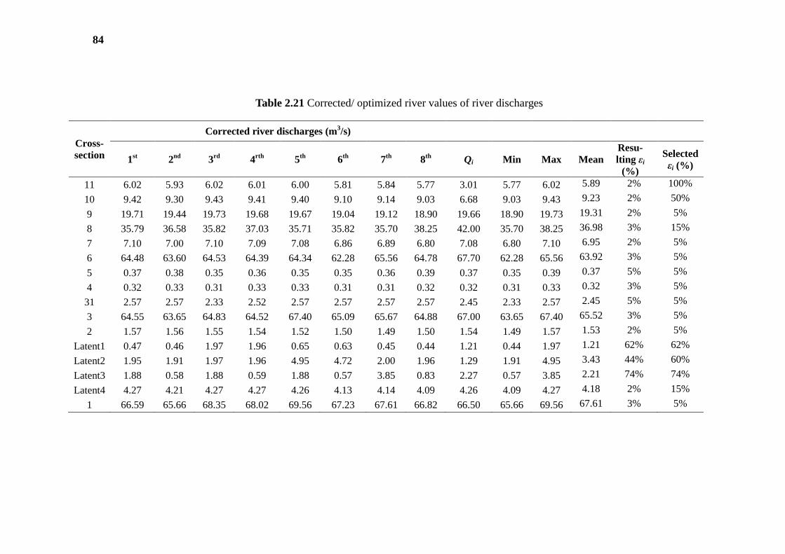
84

Table 2.21 Corrected/ optimized river values of river discharges

Cross-section

Corrected river discharges (m3/s)

1st 2nd 3rd 4rth 5th 6th 7th 8th Qi Min Max Mean Resu-lting εi

(%)

Selectedεi (%)

11 6.02 5.93 6.02 6.01 6.00 5.81 5.84 5.77 3.01 5.77 6.02 5.89 2% 100%

10 9.42 9.30 9.43 9.41 9.40 9.10 9.14 9.03 6.68 9.03 9.43 9.23 2% 50%

9 19.71 19.44 19.73 19.68 19.67 19.04 19.12 18.90 19.66 18.90 19.73 19.31 2% 5%

8 35.79 36.58 35.82 37.03 35.71 35.82 35.70 38.25 42.00 35.70 38.25 36.98 3% 15%

7 7.10 7.00 7.10 7.09 7.08 6.86 6.89 6.80 7.08 6.80 7.10 6.95 2% 5%

6 64.48 63.60 64.53 64.39 64.34 62.28 65.56 64.78 67.70 62.28 65.56 63.92 3% 5%

5 0.37 0.38 0.35 0.36 0.35 0.35 0.36 0.39 0.37 0.35 0.39 0.37 5% 5%

4 0.32 0.33 0.31 0.33 0.33 0.31 0.31 0.32 0.32 0.31 0.33 0.32 3% 5%

31 2.57 2.57 2.33 2.52 2.57 2.57 2.57 2.57 2.45 2.33 2.57 2.45 5% 5%

3 64.55 63.65 64.83 64.52 67.40 65.09 65.67 64.88 67.00 63.65 67.40 65.52 3% 5%

2 1.57 1.56 1.55 1.54 1.52 1.50 1.49 1.50 1.54 1.49 1.57 1.53 2% 5%

Latent1 0.47 0.46 1.97 1.96 0.65 0.63 0.45 0.44 1.21 0.44 1.97 1.21 62% 62%

Latent2 1.95 1.91 1.97 1.96 4.95 4.72 2.00 1.96 1.29 1.91 4.95 3.43 44% 60%

Latent3 1.88 0.58 1.88 0.59 1.88 0.57 3.85 0.83 2.27 0.57 3.85 2.21 74% 74%

Latent4 4.27 4.21 4.27 4.27 4.26 4.13 4.14 4.09 4.26 4.09 4.27 4.18 2% 15%

1 66.59 65.66 68.35 68.02 69.56 67.23 67.61 66.82 66.50 65.66 69.56 67.61 3% 5%

85

2.4.1.2 RESULT ANALYSIS : COMPARISON WITH THE NONLINEAR VERSION OF THE MODEL

A further test of consistency of the proposed methodology is to compare its results

with the corresponding results using a nonlinear solver. Successive Sequential Quadratic

programming (SQP) and generalized reduced gradient (GRG) are usual techniques in

handling nonlinear problems. These methods are more computationally demanding with

computational time increasing with the magnitude of the measurements, but they are

numerically more robust and more efficient (Ramamurthi and Bequette, 1990). The first-

order necessary conditions for problems with inequality constraints are called the Kuhn-

Tucker conditions (KTC). In order to verify that the solution of these method is not only a

local optimum but also a global one the convexity should be checked (Edgar et al., 2001).

It is very difficult to tell if an inequality constraint or objective function is convex or not.

Hence it is often uncertain if a point satisfying the KTC is a local or global optimum, or

even a saddle point. For problems with few variables we can sometimes find all KTC

solutions analytically and pick the one with the best objective function value. Otherwise,

most numerical algorithms terminate when the KTC are satisfied within some tolerance.

This is a significant drawback of the nonlinear methods, that can be balanced by a linear

approach, such as the one proposed in this research.

For the nonlinear processing of the proposed methodology, the previously described

mathematical optimization problem is taken into account with the only difference that the

nonlinear constraints are not linearized. But instead they are taken in their original forms

with the products of river discharge and concentration having both variables as unknowns.

In this case the relevant inequalities are nonlinear. By using the default nonlinear solver in

LINGO, who among others embodies the method of successive linearization and steepest

descent, the nonlinear problem is solved finding not a global but a local optimum of the

optimization. The results from the nonlinear solver are presented in tabular form in Table

2.22. For the running of the nonlinear algorithm the initial values are not required since the

nonlinear pollutant mass load constraints are not written in their linearized form. In this

case only the measurements are taken into account and from each combination the values

of river discharge and concentration for the latent cross-sections are introduced as the only

differentiation among the combinations.

A first note is that these results lie into similar but not exactly the same value region

as the linear correction technique. In example for the cross-section 8, the linear method

86

results to (Min, Mean. Max)=(36.84, 38.03, 38.99)m3/s and the nonlinear method to (Min,

Mean. Max)=(35.70, 36.34, 38.25)m3/s for the cross-section 1. The linear value range is

enclosed within the nonlinear value range. Generally, the nonlinear range is wider. The

resulting absolute relative error based on the corrected/optimized river discharge values,

computed by the relationships [1-(Min/Mean)] or [(Max/Mean)-1], is presented in the

column named “Resulting εi”. For all measured cross-section this error ranges is wider

compared to the ranges of the linearized approach. It varies from 1% up to 9%, which is

low and is slightly higher in comparison to the linear resulting relative errors εi (Table

2.21) ranging from 2% up to5%. For the latent discharges, the relative errors are high as in

the linearized methodology, ranging from to 0% up to 62%. Finally, by focusing on the

corrected river discharge values of Table 2.22 for each problematic cross-section, the

conclusions are in accordance and similar to the in depth analyzed results from the

linearized algorithm.

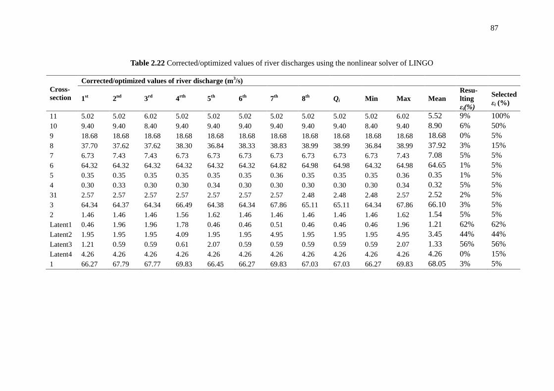
87

Table 2.22 Corrected/optimized values of river discharges using the nonlinear solver of LINGO

Cross-section

Corrected/optimized values of river discharge (m3/s)

1st 2nd 3rd 4rth 5th 6th 7th 8th Qi Min Max Mean Resu-lting εi(%)

Selected εi (%)

11 5.02 5.02 6.02 5.02 5.02 5.02 5.02 5.02 5.02 5.02 6.02 5.52 9% 100% 10 9.40 9.40 8.40 9.40 9.40 9.40 9.40 9.40 9.40 8.40 9.40 8.90 6% 50% 9 18.68 18.68 18.68 18.68 18.68 18.68 18.68 18.68 18.68 18.68 18.68 18.68 0% 5% 8 37.70 37.62 37.62 38.30 36.84 38.33 38.83 38.99 38.99 36.84 38.99 37.92 3% 15% 7 6.73 7.43 7.43 6.73 6.73 6.73 6.73 6.73 6.73 6.73 7.43 7.08 5% 5% 6 64.32 64.32 64.32 64.32 64.32 64.32 64.82 64.98 64.98 64.32 64.98 64.65 1% 5% 5 0.35 0.35 0.35 0.35 0.35 0.35 0.36 0.35 0.35 0.35 0.36 0.35 1% 5% 4 0.30 0.33 0.30 0.30 0.34 0.30 0.30 0.30 0.30 0.30 0.34 0.32 5% 5% 31 2.57 2.57 2.57 2.57 2.57 2.57 2.57 2.48 2.48 2.48 2.57 2.52 2% 5% 3 64.34 64.37 64.34 66.49 64.38 64.34 67.86 65.11 65.11 64.34 67.86 66.10 3% 5% 2 1.46 1.46 1.46 1.56 1.62 1.46 1.46 1.46 1.46 1.46 1.62 1.54 5% 5% Latent1 0.46 1.96 1.96 1.78 0.46 0.46 0.51 0.46 0.46 0.46 1.96 1.21 62% 62% Latent2 1.95 1.95 1.95 4.09 1.95 1.95 4.95 1.95 1.95 1.95 4.95 3.45 44% 44% Latent3 1.21 0.59 0.59 0.61 2.07 0.59 0.59 0.59 0.59 0.59 2.07 1.33 56% 56% Latent4 4.26 4.26 4.26 4.26 4.26 4.26 4.26 4.26 4.26 4.26 4.26 4.26 0% 15% 1 66.27 67.79 67.77 69.83 66.45 66.27 69.83 67.03 67.03 66.27 69.83 68.05 3% 5%

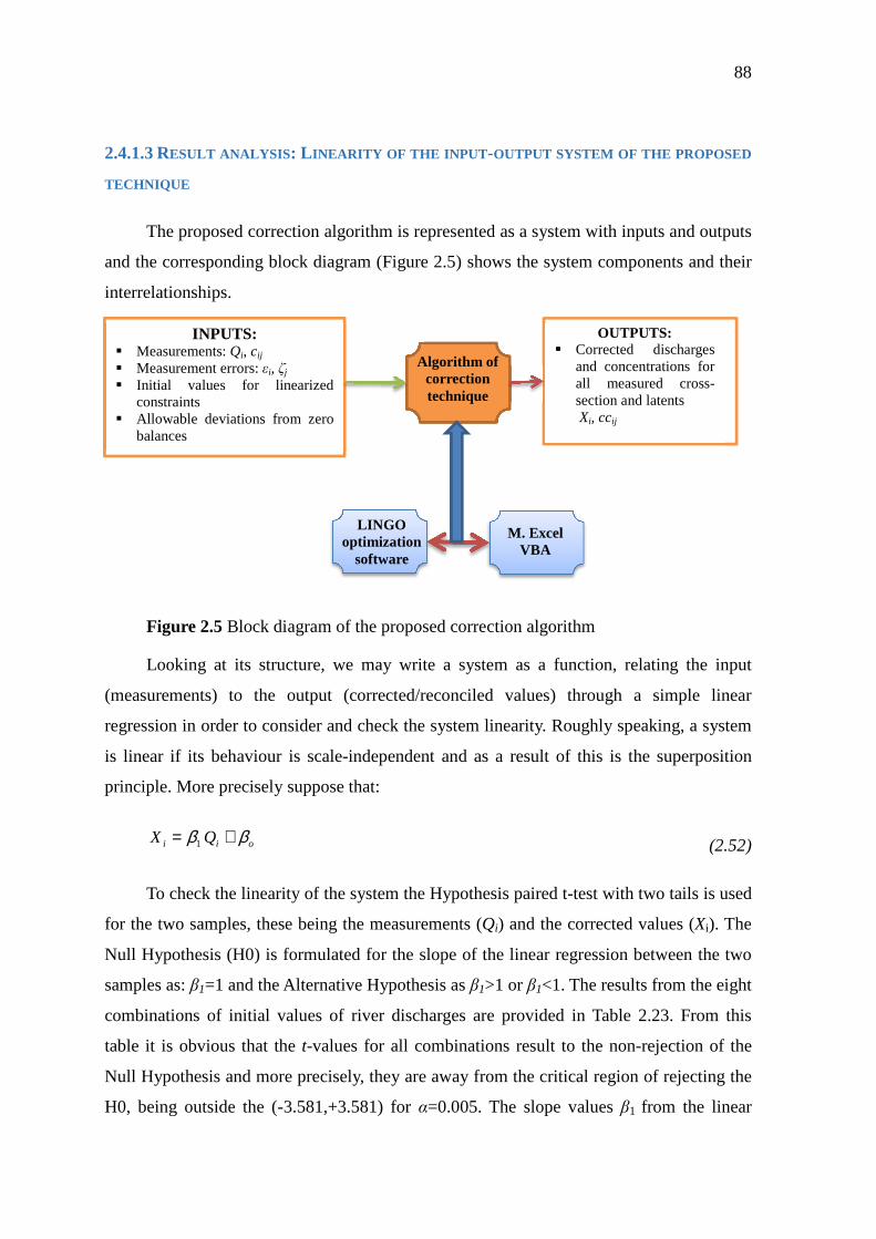
88

2.4.1.3 RESULT ANALYSIS : L INEARITY OF THE INPUT -OUTPUT SYSTEM OF THE PROPOSED

TECHNIQUE

The proposed correction algorithm is represented as a system with inputs and outputs

and the corresponding block diagram (Figure 2.5) shows the system components and their

interrelationships.

Figure 2.5 Block diagram of the proposed correction algorithm

Looking at its structure, we may write a system as a function, relating the input

(measurements) to the output (corrected/reconciled values) through a simple linear

regression in order to consider and check the system linearity. Roughly speaking, a system

is linear if its behaviour is scale-independent and as a result of this is the superposition

principle. More precisely suppose that:

oii QX ββ += 1 (2.52)

To check the linearity of the system the Hypothesis paired t-test with two tails is used

for the two samples, these being the measurements (Qi) and the corrected values (Xi). The

Null Hypothesis (H0) is formulated for the slope of the linear regression between the two

samples as: β1=1 and the Alternative Hypothesis as β1>1 or β1<1. The results from the eight

combinations of initial values of river discharges are provided in Table 2.23. From this

table it is obvious that the t-values for all combinations result to the non-rejection of the

Null Hypothesis and more precisely, they are away from the critical region of rejecting the

H0, being outside the (-3.581,+3.581) for α=0.005. The slope values β1 from the linear

INPUTS:

Measurements: Qi, cij Measurement errors: εi, ζj Initial values for linearized

constraints Allowable deviations from zero

balances

Algorithm of correction technique

LINGO optimization

software

M. Excel VBA

OUTPUTS: Corrected discharges

and concentrations for all measured cross-section and latents Xi, ccij

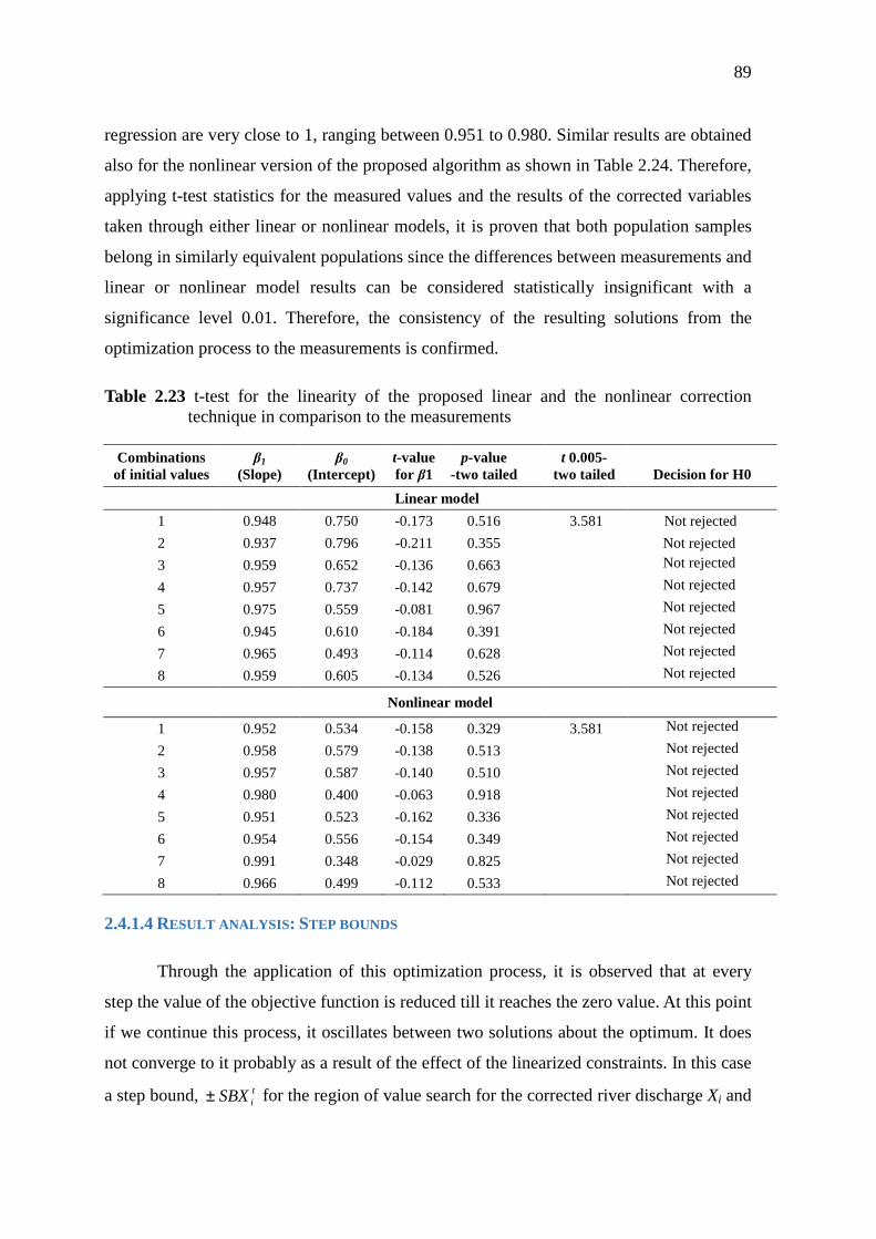
89

regression are very close to 1, ranging between 0.951 to 0.980. Similar results are obtained

also for the nonlinear version of the proposed algorithm as shown in Table 2.24. Therefore,

applying t-test statistics for the measured values and the results of the corrected variables

taken through either linear or nonlinear models, it is proven that both population samples

belong in similarly equivalent populations since the differences between measurements and

linear or nonlinear model results can be considered statistically insignificant with a

significance level 0.01. Therefore, the consistency of the resulting solutions from the

optimization process to the measurements is confirmed.

Table 2.23 t-test for the linearity of the proposed linear and the nonlinear correction technique in comparison to the measurements

Combinations of initial values

β1

(Slope) β0

(Intercept) t-value for β1

p-value -two tailed

t 0.005- two tailed

Decision for H0

Linear model

1 0.948 0.750 -0.173 0.516 3.581 Not rejected

2 0.937 0.796 -0.211 0.355

Not rejected

3 0.959 0.652 -0.136 0.663

Not rejected

4 0.957 0.737 -0.142 0.679

Not rejected

5 0.975 0.559 -0.081 0.967

Not rejected

6 0.945 0.610 -0.184 0.391

Not rejected

7 0.965 0.493 -0.114 0.628

Not rejected

8 0.959 0.605 -0.134 0.526

Not rejected

Nonlinear model

1 0.952 0.534 -0.158 0.329 3.581 Not rejected

2 0.958 0.579 -0.138 0.513

Not rejected

3 0.957 0.587 -0.140 0.510

Not rejected

4 0.980 0.400 -0.063 0.918

Not rejected

5 0.951 0.523 -0.162 0.336

Not rejected

6 0.954 0.556 -0.154 0.349

Not rejected

7 0.991 0.348 -0.029 0.825

Not rejected

8 0.966 0.499 -0.112 0.533

Not rejected

2.4.1.4 RESULT ANALYSIS : STEP BOUNDS

Through the application of this optimization process, it is observed that at every

step the value of the objective function is reduced till it reaches the zero value. At this point

if we continue this process, it oscillates between two solutions about the optimum. It does

not converge to it probably as a result of the effect of the linearized constraints. In this case

a step bound, tiSBX± for the region of value search for the corrected river discharge Xi and

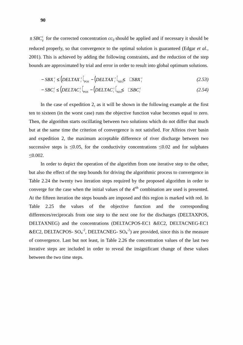
90

tijSBC± for the corrected concentration ccij should be applied and if necessary it should be

reduced properly, so that convergence to the optimal solution is guaranteed (Edgar et al.,

2001). This is achieved by adding the following constraints, and the reduction of the step

bounds are approximated by trial and error in order to result into global optimum solutions.

( ) ( ) tiNEG

tiPOS

ti

ti SBXDELTAXDELTAXSBX +≤−≤− (2.53)

( ) ( ) tiNEG

tiPOS

ti

ti SBCDELTACDELTACSBC +≤−≤− (2.54)

In the case of expedition 2, as it will be shown in the following example at the first

ten to sixteen (in the worst case) runs the objective function value becomes equal to zero.

Then, the algorithm starts oscillating between two solutions which do not differ that much

but at the same time the criterion of convergence is not satisfied. For Alfeios river basin

and expedition 2, the maximum acceptable difference of river discharge between two

successive steps is ≤0.05, for the conductivity concentrations ≤0.02 and for sulphates

≤0.002.

In order to depict the operation of the algorithm from one iterative step to the other,

but also the effect of the step bounds for driving the algorithmic process to convergence in

Table 2.24 the twenty two iteration steps required by the proposed algorithm in order to

converge for the case when the initial values of the 4rth combination are used is presented.

At the fifteen iteration the steps bounds are imposed and this region is marked with red. In

Table 2.25 the values of the objective function and the corresponding

differences/reciprocals from one step to the next one for the discharges (DELTAXPOS,

DELTAXNEG) and the concentrations (DELTACPOS-EC1 &EC2, DELTACNEG-EC1

&EC2, DELTACPOS- SO4-2, DELTACNEG- SO4

-2) are provided, since this is the measure

of convergence. Last but not least, in Table 2.26 the concentration values of the last two

iterative steps are included in order to reveal the insignificant change of these values

between the two time steps.

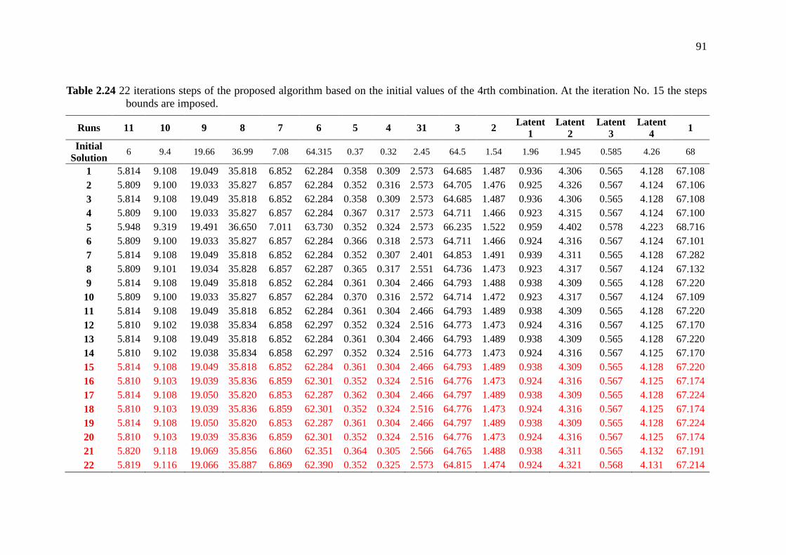
91

Table 2.24 22 iterations steps of the proposed algorithm based on the initial values of the 4rth combination. At the iteration No. 15 the steps bounds are imposed.

Runs 11 10 9 8 7 6 5 4 31 3 2 Latent 1

Latent 2

Latent 3

Latent 4 1

Initial Solution

6 9.4 19.66 36.99 7.08 64.315 0.37 0.32 2.45 64.5 1.54 1.96 1.945 0.585 4.26 68

1 5.814 9.108 19.049 35.818 6.852 62.284 0.358 0.309 2.573 64.685 1.487 0.936 4.306 0.565 4.128 67.108 2 5.809 9.100 19.033 35.827 6.857 62.284 0.352 0.316 2.573 64.705 1.476 0.925 4.326 0.567 4.124 67.106 3 5.814 9.108 19.049 35.818 6.852 62.284 0.358 0.309 2.573 64.685 1.487 0.936 4.306 0.565 4.128 67.108 4 5.809 9.100 19.033 35.827 6.857 62.284 0.367 0.317 2.573 64.711 1.466 0.923 4.315 0.567 4.124 67.100 5 5.948 9.319 19.491 36.650 7.011 63.730 0.352 0.324 2.573 66.235 1.522 0.959 4.402 0.578 4.223 68.716 6 5.809 9.100 19.033 35.827 6.857 62.284 0.366 0.318 2.573 64.711 1.466 0.924 4.316 0.567 4.124 67.101 7 5.814 9.108 19.049 35.818 6.852 62.284 0.352 0.307 2.401 64.853 1.491 0.939 4.311 0.565 4.128 67.282 8 5.809 9.101 19.034 35.828 6.857 62.287 0.365 0.317 2.551 64.736 1.473 0.923 4.317 0.567 4.124 67.132 9 5.814 9.108 19.049 35.818 6.852 62.284 0.361 0.304 2.466 64.793 1.488 0.938 4.309 0.565 4.128 67.220 10 5.809 9.100 19.033 35.827 6.857 62.284 0.370 0.316 2.572 64.714 1.472 0.923 4.317 0.567 4.124 67.109 11 5.814 9.108 19.049 35.818 6.852 62.284 0.361 0.304 2.466 64.793 1.489 0.938 4.309 0.565 4.128 67.220 12 5.810 9.102 19.038 35.834 6.858 62.297 0.352 0.324 2.516 64.773 1.473 0.924 4.316 0.567 4.125 67.170 13 5.814 9.108 19.049 35.818 6.852 62.284 0.361 0.304 2.466 64.793 1.489 0.938 4.309 0.565 4.128 67.220 14 5.810 9.102 19.038 35.834 6.858 62.297 0.352 0.324 2.516 64.773 1.473 0.924 4.316 0.567 4.125 67.170 15 5.814 9.108 19.049 35.818 6.852 62.284 0.361 0.304 2.466 64.793 1.489 0.938 4.309 0.565 4.128 67.220 16 5.810 9.103 19.039 35.836 6.859 62.301 0.352 0.324 2.516 64.776 1.473 0.924 4.316 0.567 4.125 67.174 17 5.814 9.108 19.050 35.820 6.853 62.287 0.362 0.304 2.466 64.797 1.489 0.938 4.309 0.565 4.128 67.224 18 5.810 9.103 19.039 35.836 6.859 62.301 0.352 0.324 2.516 64.776 1.473 0.924 4.316 0.567 4.125 67.174 19 5.814 9.108 19.050 35.820 6.853 62.287 0.361 0.304 2.466 64.797 1.489 0.938 4.309 0.565 4.128 67.224 20 5.810 9.103 19.039 35.836 6.859 62.301 0.352 0.324 2.516 64.776 1.473 0.924 4.316 0.567 4.125 67.174 21 5.820 9.118 19.069 35.856 6.860 62.351 0.364 0.305 2.566 64.765 1.488 0.938 4.311 0.565 4.132 67.191 22 5.819 9.116 19.066 35.887 6.869 62.390 0.352 0.325 2.573 64.815 1.474 0.924 4.321 0.568 4.131 67.214

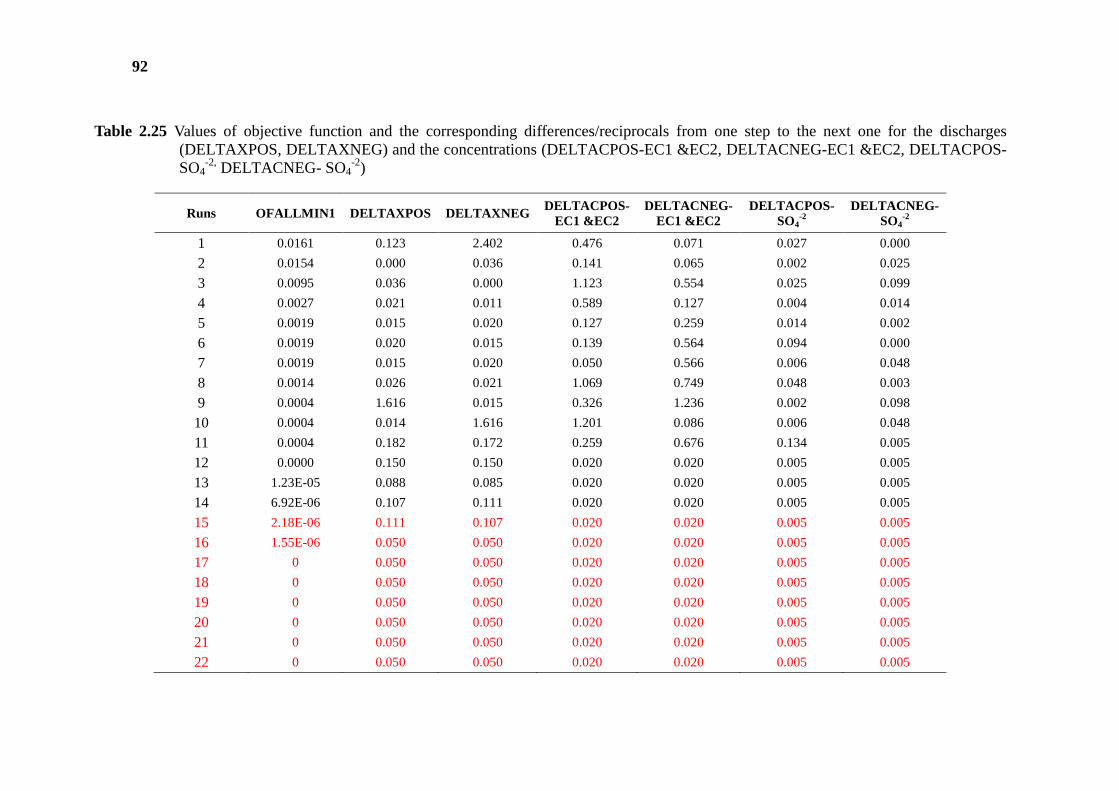
92

Table 2.25 Values of objective function and the corresponding differences/reciprocals from one step to the next one for the discharges (DELTAXPOS, DELTAXNEG) and the concentrations (DELTACPOS-EC1 &EC2, DELTACNEG-EC1 &EC2, DELTACPOS- SO4

-2, DELTACNEG- SO4-2)

Runs OFALLMIN1 DELTAXPOS DELTAXNEG DELTACPOS-EC1 &EC2

DELTACNEG- EC1 &EC2

DELTACPOS- SO4

-2 DELTACNEG-

SO4-2

1 0.0161 0.123 2.402 0.476 0.071 0.027 0.000

2 0.0154 0.000 0.036 0.141 0.065 0.002 0.025

3 0.0095 0.036 0.000 1.123 0.554 0.025 0.099

4 0.0027 0.021 0.011 0.589 0.127 0.004 0.014

5 0.0019 0.015 0.020 0.127 0.259 0.014 0.002

6 0.0019 0.020 0.015 0.139 0.564 0.094 0.000

7 0.0019 0.015 0.020 0.050 0.566 0.006 0.048

8 0.0014 0.026 0.021 1.069 0.749 0.048 0.003

9 0.0004 1.616 0.015 0.326 1.236 0.002 0.098

10 0.0004 0.014 1.616 1.201 0.086 0.006 0.048

11 0.0004 0.182 0.172 0.259 0.676 0.134 0.005

12 0.0000 0.150 0.150 0.020 0.020 0.005 0.005

13 1.23E-05 0.088 0.085 0.020 0.020 0.005 0.005

14 6.92E-06 0.107 0.111 0.020 0.020 0.005 0.005

15 2.18E-06 0.111 0.107 0.020 0.020 0.005 0.005

16 1.55E-06 0.050 0.050 0.020 0.020 0.005 0.005

17 0 0.050 0.050 0.020 0.020 0.005 0.005

18 0 0.050 0.050 0.020 0.020 0.005 0.005

19 0 0.050 0.050 0.020 0.020 0.005 0.005

20 0 0.050 0.050 0.020 0.020 0.005 0.005

21 0 0.050 0.050 0.020 0.020 0.005 0.005

22 0 0.050 0.050 0.020 0.020 0.005 0.005

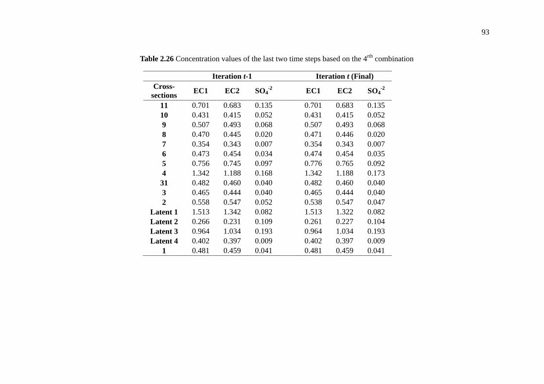
93

Table 2.26 Concentration values of the last two time steps based on the 4rth combination

Iteration t-1 Iteration t (Final) Cross-

sections EC1 EC2 SO4

-2

EC1 EC2 SO4-2

11 0.701 0.683 0.135

0.701 0.683 0.135 10 0.431 0.415 0.052

0.431 0.415 0.052

9 0.507 0.493 0.068

0.507 0.493 0.068 8 0.470 0.445 0.020

0.471 0.446 0.020

7 0.354 0.343 0.007

0.354 0.343 0.007 6 0.473 0.454 0.034

0.474 0.454 0.035

5 0.756 0.745 0.097

0.776 0.765 0.092 4 1.342 1.188 0.168

1.342 1.188 0.173

31 0.482 0.460 0.040

0.482 0.460 0.040 3 0.465 0.444 0.040

0.465 0.444 0.040

2 0.558 0.547 0.052

0.538 0.547 0.047 Latent 1 1.513 1.342 0.082

1.513 1.322 0.082

Latent 2 0.266 0.231 0.109

0.261 0.227 0.104 Latent 3 0.964 1.034 0.193

0.964 1.034 0.193

Latent 4 0.402 0.397 0.009

0.402 0.397 0.009 1 0.481 0.459 0.041

0.481 0.459 0.041

94

2.4.1.5 RESULTS: CORRECTED CONCENTRATIONS

Finnaly, the corrected/ optimized concentrations from the application of the proposed

linear methodology to the expedition 2 are presented in Table 2.27 for conductivity (EC1)

in Table 2.28 for conductivity (EC2) and in Table 2.29 for sulphate (SO4-2). For

comparison reasons in Table 2.30,Table 2.31 and Table 2.32 the corresponding

concentration of the three natural tracers are given based on the solution of the nonlinear

version of the proposed methodology using the LINGO optimization software.

As analyzed for the corrected river discharges, minimum and maximum values,

which do not necessarily construct a set of stable intervals, are computed and included in

the prementioned tables. For all measured cross-section the resulting relative error ranges

from 2% to 10% for EC1, from 0% to 10% for EC2 and from 8% to 15% for SO4-2,

showing that only in some cross-sections the proposed process reduces the concentration

errors. For the latent concentrations are very high. More precisely the resulting relative

error ranges from 23% to 100% for EC1, from 71% to 100% for EC2 and from 11% to

100% for SO4-2,

For the corresponding results based on the nonlinear model, the resulting relative

error ranges from 5% to 10% for EC1, from 0% to 10% for EC2 and from 0% to 15% for

SO4-2. The resulting relative error for the latent concentrations ranges from 10% to 100%

for EC1, from 10% to 100% for EC2 and from 15% to 100% for SO4-2.

Generally the resulting error range are wider for the nonlinear solver, but in both

linear and nonlinear the error values are low.

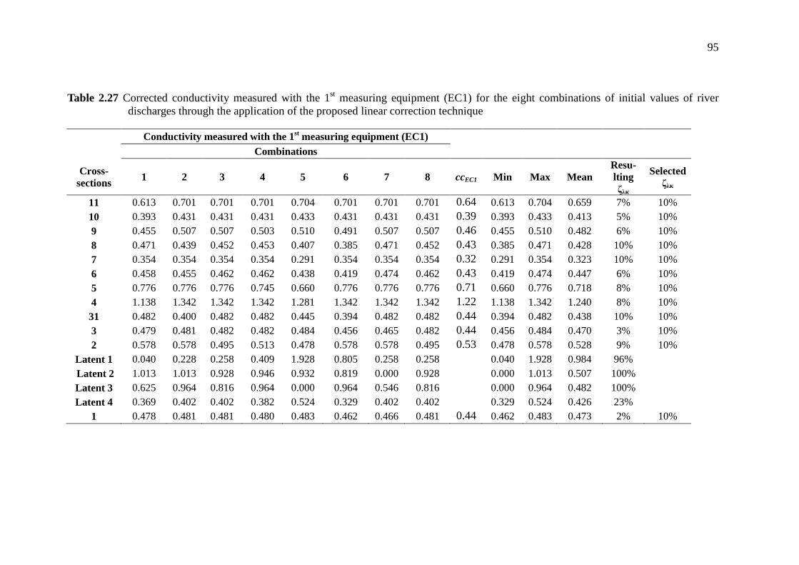
95

Table 2.27 Corrected conductivity measured with the 1st measuring equipment (EC1) for the eight combinations of initial values of river discharges through the application of the proposed linear correction technique

Conductivity measured with the 1st measuring equipment (EC1)

Combinations

Cross-sections 1 2 3 4 5 6 7 8 ccEC1 Min Max Mean

Resu-lting ζλκ

Selected ζλκ

11 0.613 0.701 0.701 0.701 0.704 0.701 0.701 0.701 0.64 0.613 0.704 0.659 7% 10% 10 0.393 0.431 0.431 0.431 0.433 0.431 0.431 0.431 0.39 0.393 0.433 0.413 5% 10% 9 0.455 0.507 0.507 0.503 0.510 0.491 0.507 0.507 0.46 0.455 0.510 0.482 6% 10% 8 0.471 0.439 0.452 0.453 0.407 0.385 0.471 0.452 0.43 0.385 0.471 0.428 10% 10% 7 0.354 0.354 0.354 0.354 0.291 0.354 0.354 0.354 0.32 0.291 0.354 0.323 10% 10% 6 0.458 0.455 0.462 0.462 0.438 0.419 0.474 0.462 0.43 0.419 0.474 0.447 6% 10% 5 0.776 0.776 0.776 0.745 0.660 0.776 0.776 0.776 0.71 0.660 0.776 0.718 8% 10% 4 1.138 1.342 1.342 1.342 1.281 1.342 1.342 1.342 1.22 1.138 1.342 1.240 8% 10% 31 0.482 0.400 0.482 0.482 0.445 0.394 0.482 0.482 0.44 0.394 0.482 0.438 10% 10% 3 0.479 0.481 0.482 0.482 0.484 0.456 0.465 0.482 0.44 0.456 0.484 0.470 3% 10% 2 0.578 0.578 0.495 0.513 0.478 0.578 0.578 0.495 0.53 0.478 0.578 0.528 9% 10%

Latent 1 0.040 0.228 0.258 0.409 1.928 0.805 0.258 0.258 0.040 1.928 0.984 96%

Latent 2 1.013 1.013 0.928 0.946 0.932 0.819 0.000 0.928 0.000 1.013 0.507 100%

Latent 3 0.625 0.964 0.816 0.964 0.000 0.964 0.546 0.816 0.000 0.964 0.482 100%

Latent 4 0.369 0.402 0.402 0.382 0.524 0.329 0.402 0.402 0.329 0.524 0.426 23%

1 0.478 0.481 0.481 0.480 0.483 0.462 0.466 0.481 0.44 0.462 0.483 0.473 2% 10%

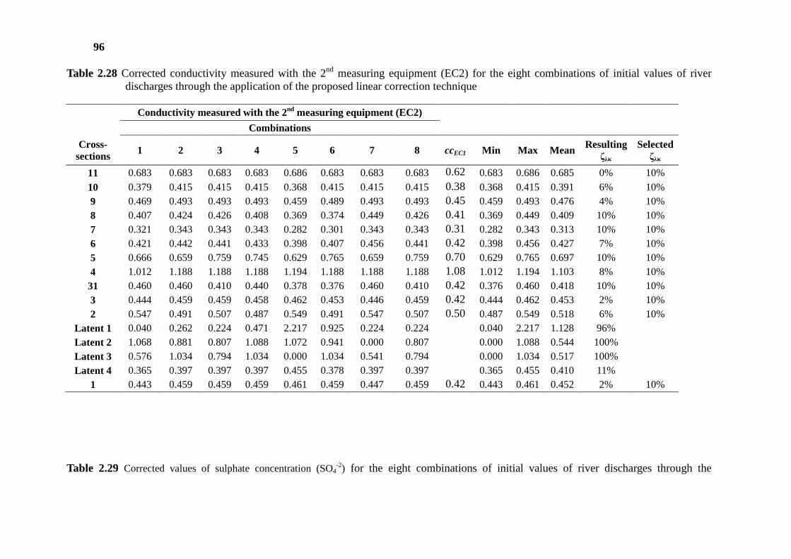
96

Table 2.28 Corrected conductivity measured with the 2nd measuring equipment (EC2) for the eight combinations of initial values of river discharges through the application of the proposed linear correction technique

Conductivity measured with the 2nd measuring equipment (EC2)

Combinations

Cross-sections 1 2 3 4 5 6 7 8 ccEC1 Min Max Mean Resulting

ζλκ Selected

ζλκ

11 0.683 0.683 0.683 0.683 0.686 0.683 0.683 0.683 0.62 0.683 0.686 0.685 0% 10%

10 0.379 0.415 0.415 0.415 0.368 0.415 0.415 0.415 0.38 0.368 0.415 0.391 6% 10% 9 0.469 0.493 0.493 0.493 0.459 0.489 0.493 0.493 0.45 0.459 0.493 0.476 4% 10% 8 0.407 0.424 0.426 0.408 0.369 0.374 0.449 0.426 0.41 0.369 0.449 0.409 10% 10% 7 0.321 0.343 0.343 0.343 0.282 0.301 0.343 0.343 0.31 0.282 0.343 0.313 10% 10% 6 0.421 0.442 0.441 0.433 0.398 0.407 0.456 0.441 0.42 0.398 0.456 0.427 7% 10% 5 0.666 0.659 0.759 0.745 0.629 0.765 0.659 0.759 0.70 0.629 0.765 0.697 10% 10% 4 1.012 1.188 1.188 1.188 1.194 1.188 1.188 1.188 1.08 1.012 1.194 1.103 8% 10% 31 0.460 0.460 0.410 0.440 0.378 0.376 0.460 0.410 0.42 0.376 0.460 0.418 10% 10% 3 0.444 0.459 0.459 0.458 0.462 0.453 0.446 0.459 0.42 0.444 0.462 0.453 2% 10% 2 0.547 0.491 0.507 0.487 0.549 0.491 0.547 0.507 0.50 0.487 0.549 0.518 6% 10%

Latent 1 0.040 0.262 0.224 0.471 2.217 0.925 0.224 0.224 0.040 2.217 1.128 96%

Latent 2 1.068 0.881 0.807 1.088 1.072 0.941 0.000 0.807 0.000 1.088 0.544 100%

Latent 3 0.576 1.034 0.794 1.034 0.000 1.034 0.541 0.794 0.000 1.034 0.517 100%

Latent 4 0.365 0.397 0.397 0.397 0.455 0.378 0.397 0.397 0.365 0.455 0.410 11%

1 0.443 0.459 0.459 0.459 0.461 0.459 0.447 0.459 0.42 0.443 0.461 0.452 2% 10%

Table 2.29 Corrected values of sulphate concentration (SO4-2) for the eight combinations of initial values of river discharges through the

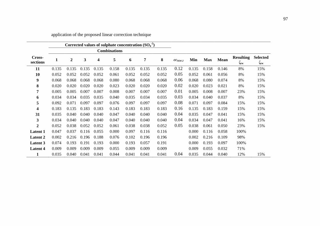
97

application of the proposed linear correction technique

Corrected values of sulphate concentration (SO4-2)

Combinations

Cross-sections 1 2 3 4 5 6 7 8 ccSO4-2 Min Max Mean Resulting

ζλκ Selected

ζλκ

11 0.135 0.135 0.135 0.135 0.158 0.135 0.135 0.135 0.12 0.135 0.158 0.146 8% 15% 10 0.052 0.052 0.052 0.052 0.061 0.052 0.052 0.052 0.05 0.052 0.061 0.056 8% 15% 9 0.068 0.068 0.068 0.068 0.080 0.068 0.068 0.068 0.06 0.068 0.080 0.074 8% 15% 8 0.020 0.020 0.020 0.020 0.023 0.020 0.020 0.020 0.02 0.020 0.023 0.021 8% 15% 7 0.005 0.005 0.007 0.007 0.008 0.007 0.007 0.007 0.01 0.005 0.008 0.007 23% 15% 6 0.034 0.034 0.035 0.035 0.040 0.035 0.034 0.035 0.03 0.034 0.040 0.037 8% 15% 5 0.092 0.071 0.097 0.097 0.076 0.097 0.097 0.097 0.08 0.071 0.097 0.084 15% 15% 4 0.183 0.135 0.183 0.183 0.143 0.183 0.183 0.183 0.16 0.135 0.183 0.159 15% 15% 31 0.035 0.040 0.040 0.040 0.047 0.040 0.040 0.040 0.04 0.035 0.047 0.041 15% 15% 3 0.034 0.040 0.040 0.040 0.047 0.040 0.040 0.040 0.04 0.034 0.047 0.041 16% 15% 2 0.052 0.038 0.052 0.052 0.061 0.038 0.038 0.052 0.05 0.038 0.061 0.050 23% 15%

Latent 1 0.047 0.037 0.116 0.055 0.000 0.097 0.116 0.116 0.000 0.116 0.058 100%

Latent 2 0.002 0.216 0.196 0.188 0.076 0.102 0.196 0.196 0.002 0.216 0.109 98%

Latent 3 0.074 0.193 0.191 0.193 0.000 0.193 0.057 0.191 0.000 0.193 0.097 100%

Latent 4 0.009 0.009 0.009 0.009 0.055 0.009 0.009 0.009 0.009 0.055 0.032 71%

1 0.035 0.040 0.041 0.041 0.044 0.041 0.041 0.041 0.04 0.035 0.044 0.040 12% 15%

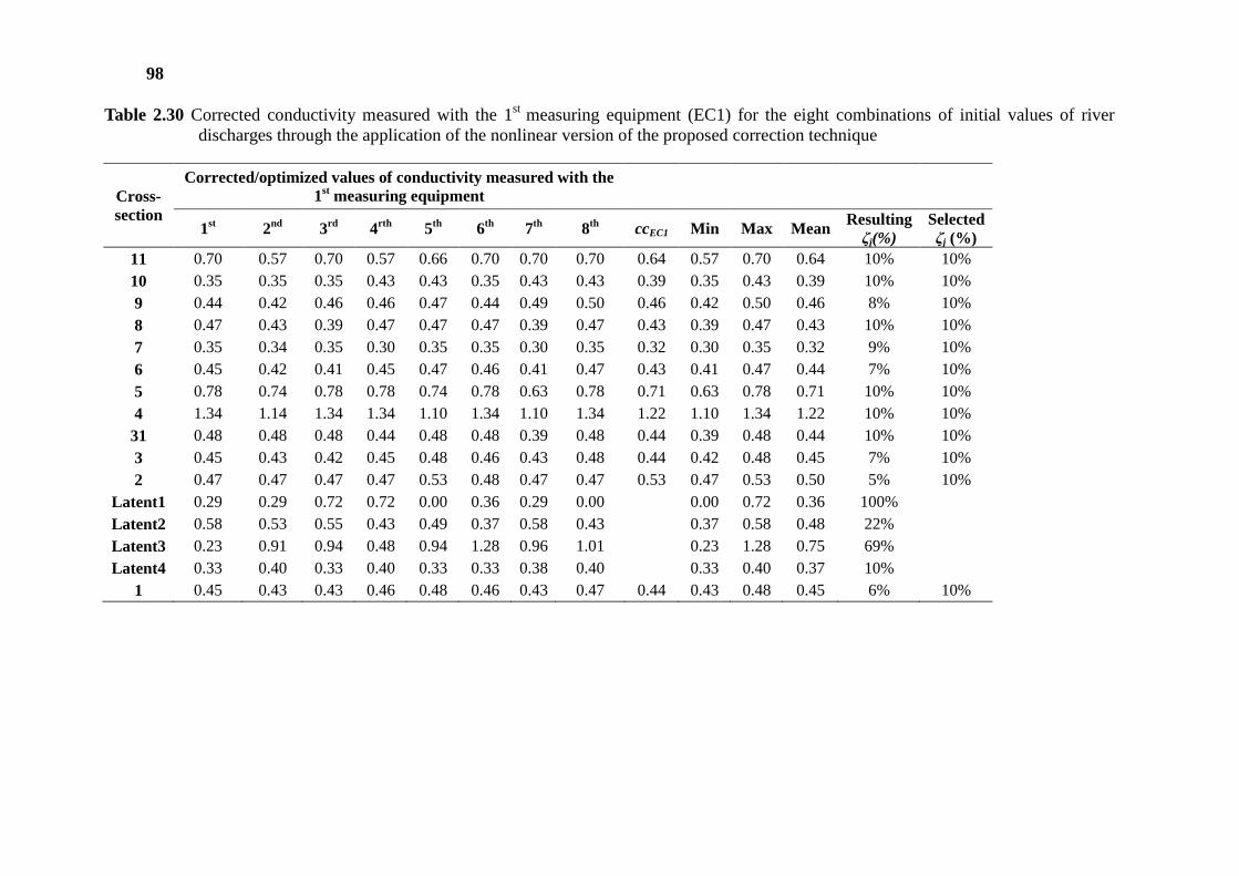
98

Table 2.30 Corrected conductivity measured with the 1st measuring equipment (EC1) for the eight combinations of initial values of river discharges through the application of the nonlinear version of the proposed correction technique

Cross-section

Corrected/optimized values of conductivity measured with the 1st measuring equipment

1st 2nd 3rd 4rth 5th 6th 7th 8th ccEC1 Min Max Mean Resulting ζj(%)

Selected ζj (%)

11 0.70 0.57 0.70 0.57 0.66 0.70 0.70 0.70 0.64 0.57 0.70 0.64 10% 10% 10 0.35 0.35 0.35 0.43 0.43 0.35 0.43 0.43 0.39 0.35 0.43 0.39 10% 10% 9 0.44 0.42 0.46 0.46 0.47 0.44 0.49 0.50 0.46 0.42 0.50 0.46 8% 10% 8 0.47 0.43 0.39 0.47 0.47 0.47 0.39 0.47 0.43 0.39 0.47 0.43 10% 10% 7 0.35 0.34 0.35 0.30 0.35 0.35 0.30 0.35 0.32 0.30 0.35 0.32 9% 10% 6 0.45 0.42 0.41 0.45 0.47 0.46 0.41 0.47 0.43 0.41 0.47 0.44 7% 10% 5 0.78 0.74 0.78 0.78 0.74 0.78 0.63 0.78 0.71 0.63 0.78 0.71 10% 10% 4 1.34 1.14 1.34 1.34 1.10 1.34 1.10 1.34 1.22 1.10 1.34 1.22 10% 10% 31 0.48 0.48 0.48 0.44 0.48 0.48 0.39 0.48 0.44 0.39 0.48 0.44 10% 10% 3 0.45 0.43 0.42 0.45 0.48 0.46 0.43 0.48 0.44 0.42 0.48 0.45 7% 10% 2 0.47 0.47 0.47 0.47 0.53 0.48 0.47 0.47 0.53 0.47 0.53 0.50 5% 10%

Latent1 0.29 0.29 0.72 0.72 0.00 0.36 0.29 0.00

0.00 0.72 0.36 100%

Latent2 0.58 0.53 0.55 0.43 0.49 0.37 0.58 0.43

0.37 0.58 0.48 22%

Latent3 0.23 0.91 0.94 0.48 0.94 1.28 0.96 1.01

0.23 1.28 0.75 69%

Latent4 0.33 0.40 0.33 0.40 0.33 0.33 0.38 0.40

0.33 0.40 0.37 10%

1 0.45 0.43 0.43 0.46 0.48 0.46 0.43 0.47 0.44 0.43 0.48 0.45 6% 10%

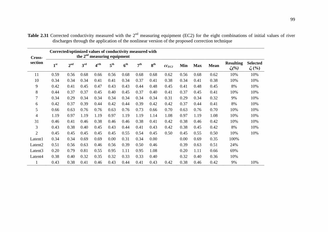
99

Table 2.31 Corrected conductivity measured with the 2nd measuring equipment (EC2) for the eight combinations of initial values of river discharges through the application of the nonlinear version of the proposed correction technique

Cross-section

Corrected/optimized values of conductivity measured with the 2nd measuring equipment

1st 2nd 3rd 4rth 5th 6th 7th 8th ccEC2 Min Max Mean Resulting ζj(%)

Selected ζj (%)

11 0.59 0.56 0.68 0.66 0.56 0.68 0.68 0.68 0.62 0.56 0.68 0.62 10% 10% 10 0.34 0.34 0.34 0.41 0.41 0.34 0.37 0.41 0.38 0.34 0.41 0.38 10% 10% 9 0.42 0.41 0.45 0.47 0.43 0.43 0.44 0.48 0.45 0.41 0.48 0.45 8% 10% 8 0.44 0.37 0.37 0.45 0.40 0.45 0.37 0.40 0.41 0.37 0.45 0.41 10% 10% 7 0.34 0.29 0.34 0.34 0.34 0.34 0.34 0.34 0.31 0.29 0.34 0.32 9% 10% 6 0.42 0.37 0.39 0.44 0.42 0.44 0.39 0.42 0.42 0.37 0.44 0.41 8% 10% 5 0.66 0.63 0.76 0.76 0.63 0.76 0.73 0.66 0.70 0.63 0.76 0.70 10% 10% 4 1.19 0.97 1.19 1.19 0.97 1.19 1.19 1.14 1.08 0.97 1.19 1.08 10% 10% 31 0.46 0.41 0.46 0.38 0.46 0.46 0.38 0.41 0.42 0.38 0.46 0.42 10% 10% 3 0.43 0.38 0.40 0.45 0.43 0.44 0.41 0.43 0.42 0.38 0.45 0.42 8% 10% 2 0.45 0.45 0.45 0.45 0.45 0.55 0.54 0.45 0.50 0.45 0.55 0.50 10% 10%

Latent1 0.34 0.34 0.69 0.69 0.00 0.31 0.34 0.00

0.00 0.69 0.35 100%

Latent2 0.51 0.56 0.63 0.46 0.56 0.39 0.50 0.46

0.39 0.63 0.51 24%

Latent3 0.20 0.79 0.81 0.55 0.95 1.11 0.95 1.08

0.20 1.11 0.66 69%

Latent4 0.38 0.40 0.32 0.35 0.32 0.33 0.33 0.40

0.32 0.40 0.36 10%

1 0.43 0.38 0.41 0.46 0.43 0.44 0.41 0.43 0.42 0.38 0.46 0.42 9% 10%

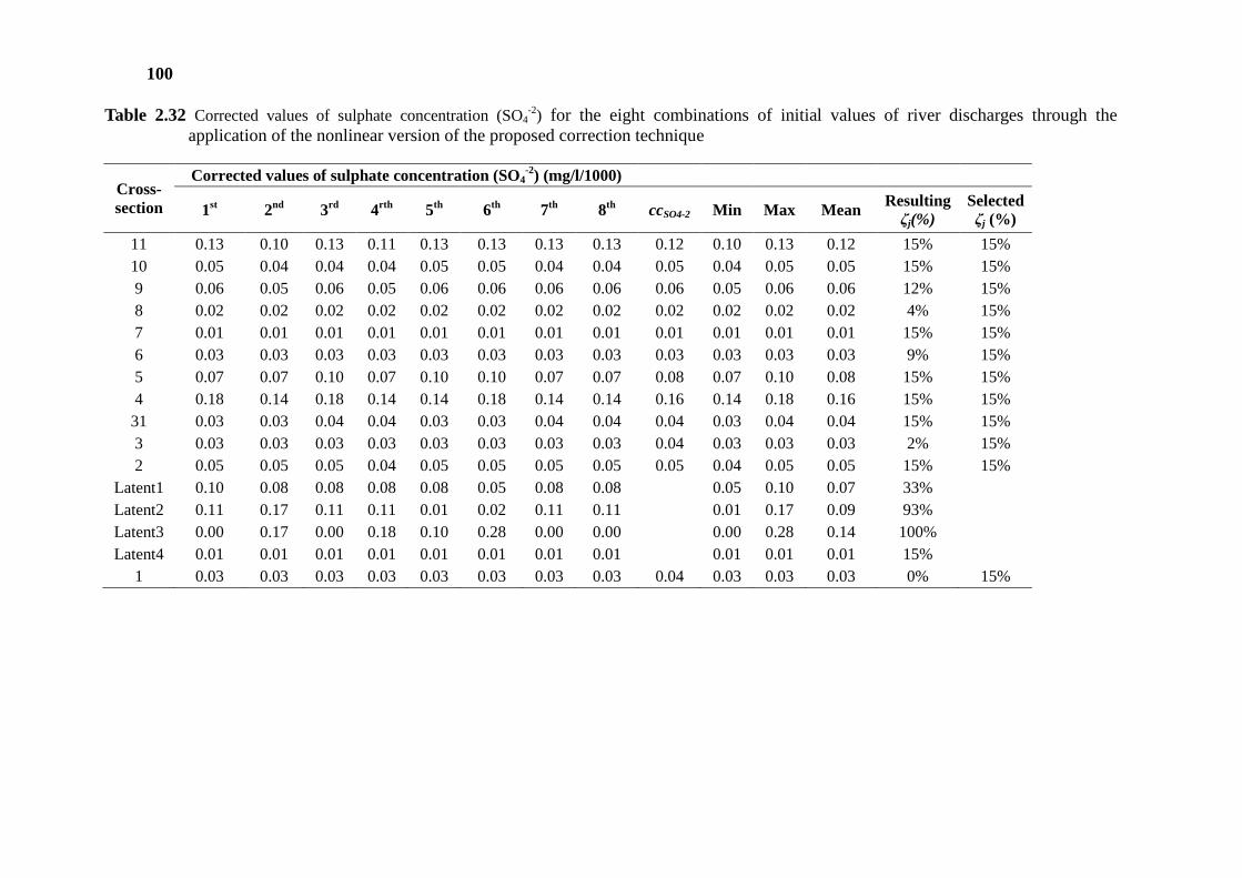
100

Table 2.32 Corrected values of sulphate concentration (SO4-2) for the eight combinations of initial values of river discharges through the

application of the nonlinear version of the proposed correction technique

Cross-section

Corrected values of sulphate concentration (SO4-2) (mg/l/1000)

1st 2nd 3rd 4rth 5th 6th 7th 8th ccSO4-2 Min Max Mean Resulting ζj(%)

Selected ζj (%)

11 0.13 0.10 0.13 0.11 0.13 0.13 0.13 0.13 0.12 0.10 0.13 0.12 15% 15% 10 0.05 0.04 0.04 0.04 0.05 0.05 0.04 0.04 0.05 0.04 0.05 0.05 15% 15% 9 0.06 0.05 0.06 0.05 0.06 0.06 0.06 0.06 0.06 0.05 0.06 0.06 12% 15% 8 0.02 0.02 0.02 0.02 0.02 0.02 0.02 0.02 0.02 0.02 0.02 0.02 4% 15% 7 0.01 0.01 0.01 0.01 0.01 0.01 0.01 0.01 0.01 0.01 0.01 0.01 15% 15% 6 0.03 0.03 0.03 0.03 0.03 0.03 0.03 0.03 0.03 0.03 0.03 0.03 9% 15% 5 0.07 0.07 0.10 0.07 0.10 0.10 0.07 0.07 0.08 0.07 0.10 0.08 15% 15% 4 0.18 0.14 0.18 0.14 0.14 0.18 0.14 0.14 0.16 0.14 0.18 0.16 15% 15% 31 0.03 0.03 0.04 0.04 0.03 0.03 0.04 0.04 0.04 0.03 0.04 0.04 15% 15% 3 0.03 0.03 0.03 0.03 0.03 0.03 0.03 0.03 0.04 0.03 0.03 0.03 2% 15% 2 0.05 0.05 0.05 0.04 0.05 0.05 0.05 0.05 0.05 0.04 0.05 0.05 15% 15%

Latent1 0.10 0.08 0.08 0.08 0.08 0.05 0.08 0.08

0.05 0.10 0.07 33%

Latent2 0.11 0.17 0.11 0.11 0.01 0.02 0.11 0.11 0.01 0.17 0.09 93%

Latent3 0.00 0.17 0.00 0.18 0.10 0.28 0.00 0.00 0.00 0.28 0.14 100%

Latent4 0.01 0.01 0.01 0.01 0.01 0.01 0.01 0.01 0.01 0.01 0.01 15%

1 0.03 0.03 0.03 0.03 0.03 0.03 0.03 0.03 0.04 0.03 0.03 0.03 0% 15%

101

2.4.1.6 RESULTS: POLLUTION LOADS

Based on the corrected river discharges and concentrations for the eight

combinations of initial values of river discharges, it is possible to compute more reliable

corrected pollution loads for the total dissolved solids and the sulphates.

As analyzed in Section 2.2.1.2, the water conductivity, as one of the most commonly

measured physico-chemical parameter, is used for the application of the proposed

methodology. Conductivity is considered a good estimate of the total inorganic dissolved

solids present in the water column (Eaton et al., 1995). Total dissolved solids (TDS)

concentration is derived as the summation of anions and cations dissolved in water. The

conductivity value is directly proportional to the TDS concentration. The approximate

conversion of water conductivity (usually expressed in µS/cm) into TDS concentration (in

ppm) is undertaken through a factor ranging from 0.5 up to 0.9 depending on the chemical

composition of the TDS (APHA, 1999). Usually, a value of 0.65 is used and taken into

account in this application.

From the eight values of pollution loads for each cross-section the minimum and

maximum values are derived for each pollutant. As previously mentioned, this does not

necessarily constitute a stable value range. Based on the mean value of the minimum and

maximum value, it is possible to compute the resulting relative error based on the

corrected/optimized pollution load values, computed by the relationships [1-(Min/Mean)]

or [(Max/Mean)-1]. For comparison reasons, the minimum and maximum pollution load

values derived from the range of the measurements Qi and cij and their measurement errors

(εi, ζj) are also presented. More precisely, in Table 2.33 the pollution loads of the total

dissolved solids in kg/d based on the conductivity measured with Conductivity-meter

Horiba U-10 are provided, in Table 2.34 the pollution loads of total dissolved solids in kg/d

based on the conductivity measured with Conductivity-meter Hanna HI 9033 are given and

finally, in Table 2.35 the pollution loads for the sulphates are presented.

From these tabular results, it can be concluded that generally the proposed

methodology enables the computation of pollution load with significantly lower resulting

error, revealing a very narrow value range for all measured cross-sections. More precisely,

considering the measured cross-sections the relative error for the pollution loads of the

total dissolved solids in Table 2.33 varies between 5% and 15%, while the corresponding

error range based on the measurements and their measurement errors ranges between 10%

102

and 120%. The relative error for the pollution loads of the total dissolved solids in Table

2.34 is bounded between 2% and 15% from the application of the proposed methodology

and from 16% to 120% derived from the raw measurements for the measured cross-

section. Finally, the relative error for the pollution loads of the sulphates from the proposed

methodology is higher than the previous ones and ranges from 10% to 25%, whereas the

relative error from the measurements is very high (21%-130%).

Proceeding now to the latent cross-sections (being nonmeasured cross-sections and

therefore no relative error is computed based on the measurements), the relative errors for

all pollutants are significantly higher and very close but smaller than the relative error

ranges computed from the measurements for the measured cross-sections. For the pollution

loads of the total dissolved solids in Table 2.33 the relative error ranges between 12% and

100%, in Table 2.34 between 13% and 100% and in Table 2.35 between 72% and 100%.

Moreover, it is worth noticing that the pollutant loads derived from Qi ×cij are for all

cases very close to the minimum values of the pollutant loads computed from the proposed

methodology. The highest pollutant loads are observed in the cross-sections 6, 3 and 1 of

the main Alfeios River, since it receives all water contributions from the upstream

catchment and the tributaries. Their values range from 1467 to 1888kg/d for conductivity

(EC1) and from 1391 to 1800kg/d (EC2), whereas for the sulphates from 120 to 179kg/d.

The highest pollutant loads for TDS are computed at the latent cross-sections of the second

and fourth node, and for the sulphates at the second and third node. A further investigation

of the pollutant loads and their statistical analysis based on the corrected river discharges

and concentrations are proposed for future work.

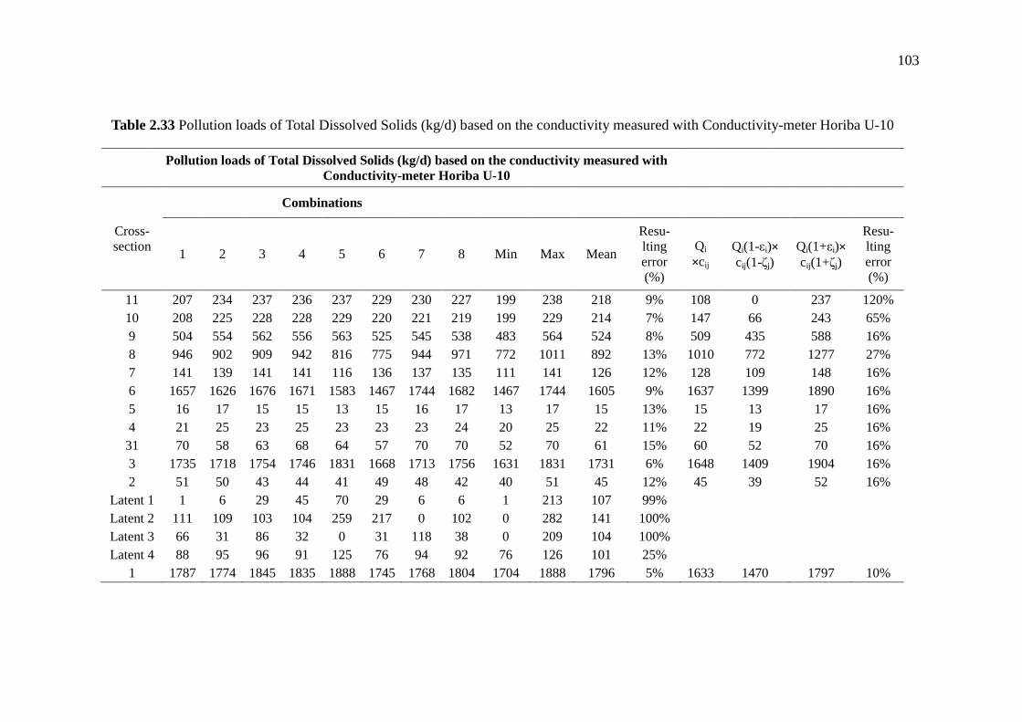
103

Table 2.33 Pollution loads of Total Dissolved Solids (kg/d) based on the conductivity measured with Conductivity-meter Horiba U-10

Pollution loads of Total Dissolved Solids (kg/d) based on the conductivity measured with Conductivity-meter Horiba U-10

Cross-section

Combinations

1 2 3 4 5 6 7 8 Min Max Mean

Resu-lting error (%)

Qi

×cij Qi(1-εi)× cij(1-ζj)

Qi(1+εi)× cij(1+ζj)

Resu-lting error (%)

11 207 234 237 236 237 229 230 227 199 238 218 9% 108 0 237 120% 10 208 225 228 228 229 220 221 219 199 229 214 7% 147 66 243 65% 9 504 554 562 556 563 525 545 538 483 564 524 8% 509 435 588 16% 8 946 902 909 942 816 775 944 971 772 1011 892 13% 1010 772 1277 27% 7 141 139 141 141 116 136 137 135 111 141 126 12% 128 109 148 16% 6 1657 1626 1676 1671 1583 1467 1744 1682 1467 1744 1605 9% 1637 1399 1890 16% 5 16 17 15 15 13 15 16 17 13 17 15 13% 15 13 17 16% 4 21 25 23 25 23 23 23 24 20 25 22 11% 22 19 25 16% 31 70 58 63 68 64 57 70 70 52 70 61 15% 60 52 70 16% 3 1735 1718 1754 1746 1831 1668 1713 1756 1631 1831 1731 6% 1648 1409 1904 16% 2 51 50 43 44 41 49 48 42 40 51 45 12% 45 39 52 16%

Latent 1 1 6 29 45 70 29 6 6 1 213 107 99%

Latent 2 111 109 103 104 259 217 0 102 0 282 141 100%

Latent 3 66 31 86 32 0 31 118 38 0 209 104 100%

Latent 4 88 95 96 91 125 76 94 92 76 126 101 25%

1 1787 1774 1845 1835 1888 1745 1768 1804 1704 1888 1796 5% 1633 1470 1797 10%

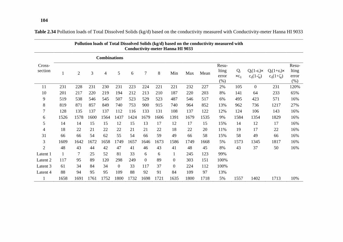
104

Table 2.34 Pollution loads of Total Dissolved Solids (kg/d) based on the conductivity measured with Conductivity-meter Hanna HI 9033

Pollution loads of Total Dissolved Solids (kg/d) based on the conductivity measured with Conductivity-meter Hanna HI 9033

Cross-section

Combinations

1 2 3 4 5 6 7 8 Min Max Mean

Resu-lting error (%)

Qi

×cij Qi(1-εi)× cij(1-ζj)

Qi(1+εi)× cij(1+ζj)

Resu-lting error (%)

11 231 228 231 230 231 223 224 221 221 232 227 2% 105 0 231 120% 10 201 217 220 219 194 212 213 210 187 220 203 8% 141 64 233 65% 9 519 538 546 545 507 523 529 523 487 546 517 6% 495 423 571 16% 8 819 871 857 849 740 753 900 915 740 964 852 13% 962 736 1217 27% 7 128 135 137 137 112 116 133 131 108 137 122 12% 124 106 143 16% 6 1526 1578 1600 1564 1437 1424 1679 1606 1391 1679 1535 9% 1584 1354 1829 16% 5 14 14 15 15 12 15 13 17 12 17 15 15% 14 12 17 16% 4 18 22 21 22 22 21 21 22 18 22 20 11% 19 17 22 16% 31 66 66 54 62 55 54 66 59 49 66 58 15% 58 49 66 16% 3 1609 1642 1672 1658 1749 1657 1646 1673 1586 1749 1668 5% 1573 1345 1817 16% 2 48 43 44 42 47 41 46 43 41 48 45 8% 43 37 50 16%

Latent 1 1 7 25 52 81 33 6 6 1 245 123 99%

Latent 2 117 95 89 120 298 249 0 89 0 303 151 100%

Latent 3 61 34 84 34 0 33 117 37 0 224 112 100%

Latent 4 88 94 95 95 109 88 92 91 84 109 97 13%

1 1658 1691 1761 1752 1800 1732 1698 1721 1635 1800 1718 5% 1557 1402 1713 10%

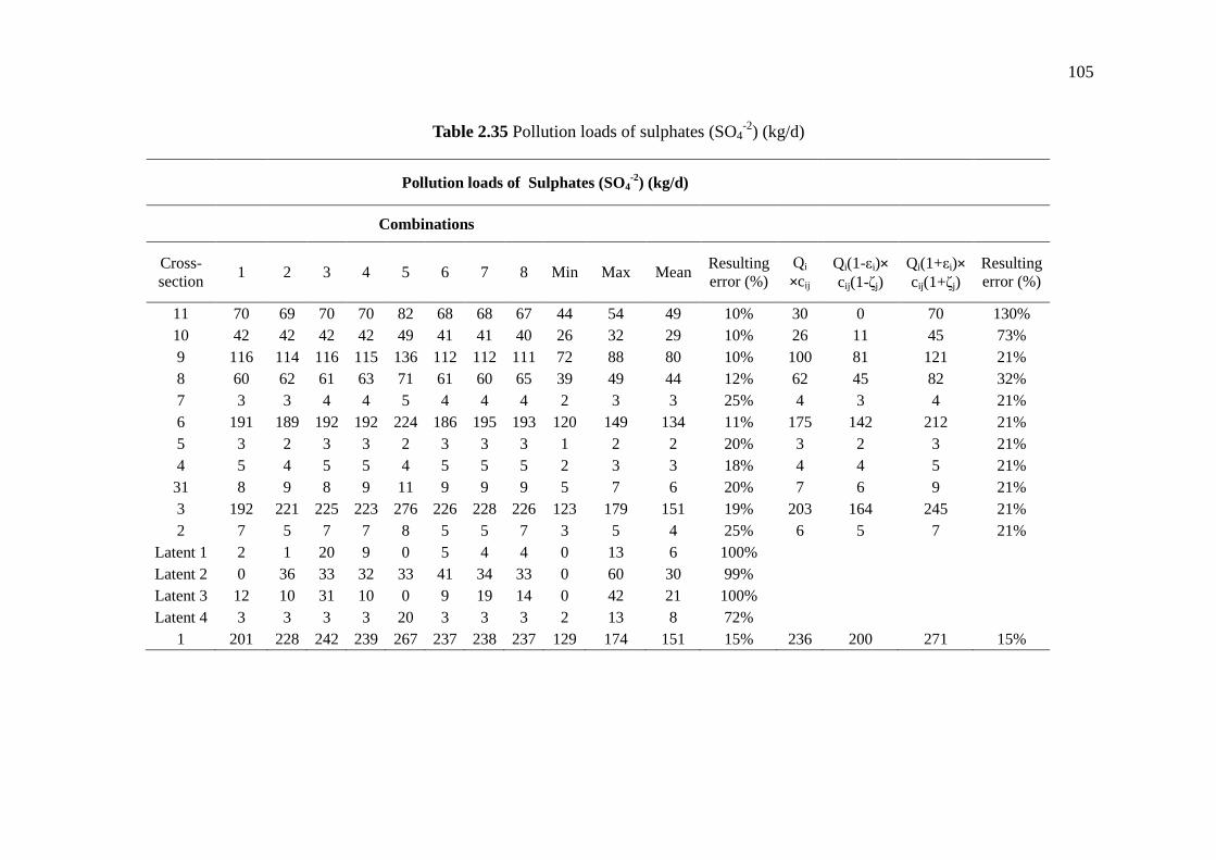
105

Table 2.35 Pollution loads of sulphates (SO4-2) (kg/d)

Pollution loads of Sulphates (SO4

-2) (kg/d)

Combinations

Cross-section

1 2 3 4 5 6 7 8 Min Max Mean Resulting error (%)

Qi

×cij Qi(1-εi)× cij(1-ζj)

Qi(1+εi)× cij(1+ζj)

Resulting error (%)

11 70 69 70 70 82 68 68 67 44 54 49 10% 30 0 70 130% 10 42 42 42 42 49 41 41 40 26 32 29 10% 26 11 45 73% 9 116 114 116 115 136 112 112 111 72 88 80 10% 100 81 121 21% 8 60 62 61 63 71 61 60 65 39 49 44 12% 62 45 82 32% 7 3 3 4 4 5 4 4 4 2 3 3 25% 4 3 4 21% 6 191 189 192 192 224 186 195 193 120 149 134 11% 175 142 212 21% 5 3 2 3 3 2 3 3 3 1 2 2 20% 3 2 3 21% 4 5 4 5 5 4 5 5 5 2 3 3 18% 4 4 5 21% 31 8 9 8 9 11 9 9 9 5 7 6 20% 7 6 9 21% 3 192 221 225 223 276 226 228 226 123 179 151 19% 203 164 245 21% 2 7 5 7 7 8 5 5 7 3 5 4 25% 6 5 7 21%

Latent 1 2 1 20 9 0 5 4 4 0 13 6 100%

Latent 2 0 36 33 32 33 41 34 33 0 60 30 99%

Latent 3 12 10 31 10 0 9 19 14 0 42 21 100%

Latent 4 3 3 3 3 20 3 3 3 2 13 8 72%

1 201 228 242 239 267 237 238 237 129 174 151 15% 236 200 271 15%

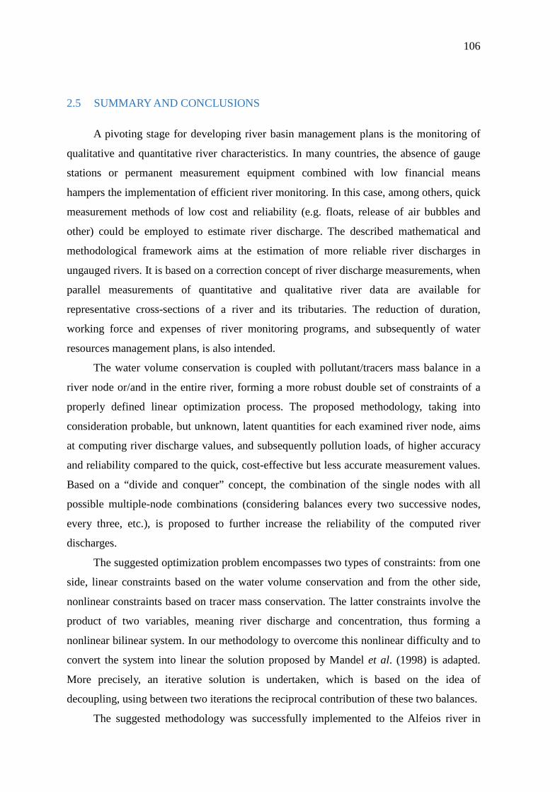
106

2.5 SUMMARY AND CONCLUSIONS

A pivoting stage for developing river basin management plans is the monitoring of

qualitative and quantitative river characteristics. In many countries, the absence of gauge

stations or permanent measurement equipment combined with low financial means

hampers the implementation of efficient river monitoring. In this case, among others, quick

measurement methods of low cost and reliability (e.g. floats, release of air bubbles and

other) could be employed to estimate river discharge. The described mathematical and

methodological framework aims at the estimation of more reliable river discharges in

ungauged rivers. It is based on a correction concept of river discharge measurements, when

parallel measurements of quantitative and qualitative river data are available for

representative cross-sections of a river and its tributaries. The reduction of duration,

working force and expenses of river monitoring programs, and subsequently of water

resources management plans, is also intended.

The water volume conservation is coupled with pollutant/tracers mass balance in a

river node or/and in the entire river, forming a more robust double set of constraints of a

properly defined linear optimization process. The proposed methodology, taking into

consideration probable, but unknown, latent quantities for each examined river node, aims

at computing river discharge values, and subsequently pollution loads, of higher accuracy

and reliability compared to the quick, cost-effective but less accurate measurement values.

Based on a “divide and conquer” concept, the combination of the single nodes with all

possible multiple-node combinations (considering balances every two successive nodes,

every three, etc.), is proposed to further increase the reliability of the computed river

discharges.

The suggested optimization problem encompasses two types of constraints: from one

side, linear constraints based on the water volume conservation and from the other side,

nonlinear constraints based on tracer mass conservation. The latter constraints involve the

product of two variables, meaning river discharge and concentration, thus forming a

nonlinear bilinear system. In our methodology to overcome this nonlinear difficulty and to

convert the system into linear the solution proposed by Mandel et al. (1998) is adapted.

More precisely, an iterative solution is undertaken, which is based on the idea of

decoupling, using between two iterations the reciprocal contribution of these two balances.

The suggested methodology was successfully implemented to the Alfeios river in

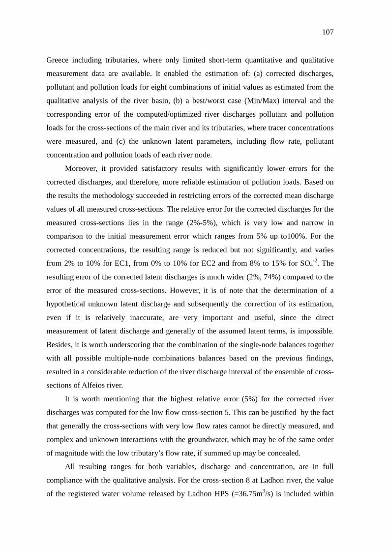
107

Greece including tributaries, where only limited short-term quantitative and qualitative

measurement data are available. It enabled the estimation of: (a) corrected discharges,

pollutant and pollution loads for eight combinations of initial values as estimated from the

qualitative analysis of the river basin, (b) a best/worst case (Min/Max) interval and the

corresponding error of the computed/optimized river discharges pollutant and pollution

loads for the cross-sections of the main river and its tributaries, where tracer concentrations

were measured, and (c) the unknown latent parameters, including flow rate, pollutant

concentration and pollution loads of each river node.

Moreover, it provided satisfactory results with significantly lower errors for the

corrected discharges, and therefore, more reliable estimation of pollution loads. Based on

the results the methodology succeeded in restricting errors of the corrected mean discharge

values of all measured cross-sections. The relative error for the corrected discharges for the

measured cross-sections lies in the range (2%-5%), which is very low and narrow in

comparison to the initial measurement error which ranges from 5% up to100%. For the

corrected concentrations, the resulting range is reduced but not significantly, and varies

from 2% to 10% for EC1, from 0% to 10% for EC2 and from 8% to 15% for SO4-2. The

resulting error of the corrected latent discharges is much wider (2%, 74%) compared to the

error of the measured cross-sections. However, it is of note that the determination of a

hypothetical unknown latent discharge and subsequently the correction of its estimation,

even if it is relatively inaccurate, are very important and useful, since the direct

measurement of latent discharge and generally of the assumed latent terms, is impossible.

Besides, it is worth underscoring that the combination of the single-node balances together

with all possible multiple-node combinations balances based on the previous findings,

resulted in a considerable reduction of the river discharge interval of the ensemble of cross-

sections of Alfeios river.

It is worth mentioning that the highest relative error (5%) for the corrected river

discharges was computed for the low flow cross-section 5. This can be justified by the fact

that generally the cross-sections with very low flow rates cannot be directly measured, and

complex and unknown interactions with the groundwater, which may be of the same order

of magnitude with the low tributary’s flow rate, if summed up may be concealed.

All resulting ranges for both variables, discharge and concentration, are in full

compliance with the qualitative analysis. For the cross-section 8 at Ladhon river, the value

of the registered water volume released by Ladhon HPS (=36.75m3/s) is included within

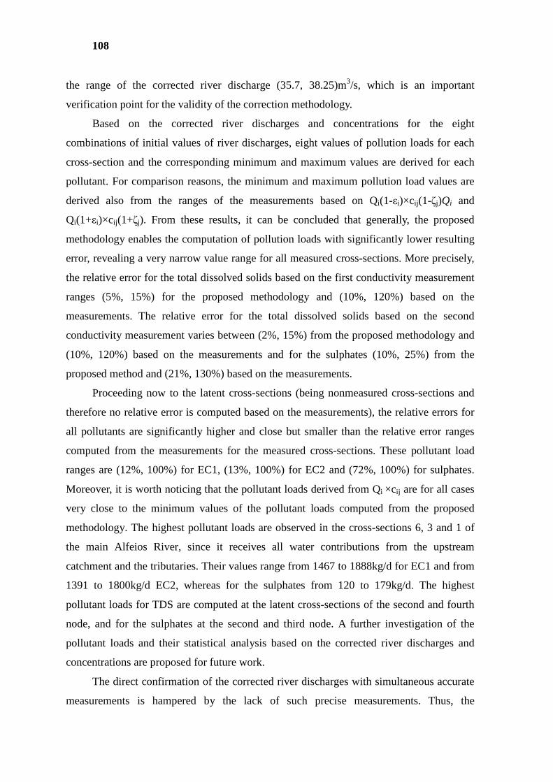
108

the range of the corrected river discharge (35.7, 38.25)m3/s, which is an important

verification point for the validity of the correction methodology.

Based on the corrected river discharges and concentrations for the eight

combinations of initial values of river discharges, eight values of pollution loads for each

cross-section and the corresponding minimum and maximum values are derived for each

pollutant. For comparison reasons, the minimum and maximum pollution load values are

derived also from the ranges of the measurements based on Qi(1-εi)×cij(1-ζj)Qi and

Qi(1+εi)×cij(1+ζj). From these results, it can be concluded that generally, the proposed

methodology enables the computation of pollution loads with significantly lower resulting

error, revealing a very narrow value range for all measured cross-sections. More precisely,

the relative error for the total dissolved solids based on the first conductivity measurement

ranges (5%, 15%) for the proposed methodology and (10%, 120%) based on the

measurements. The relative error for the total dissolved solids based on the second

conductivity measurement varies between (2%, 15%) from the proposed methodology and

(10%, 120%) based on the measurements and for the sulphates (10%, 25%) from the

proposed method and (21%, 130%) based on the measurements.

Proceeding now to the latent cross-sections (being nonmeasured cross-sections and

therefore no relative error is computed based on the measurements), the relative errors for

all pollutants are significantly higher and close but smaller than the relative error ranges

computed from the measurements for the measured cross-sections. These pollutant load

ranges are (12%, 100%) for EC1, (13%, 100%) for EC2 and (72%, 100%) for sulphates.

Moreover, it is worth noticing that the pollutant loads derived from Qi ×cij are for all cases

very close to the minimum values of the pollutant loads computed from the proposed

methodology. The highest pollutant loads are observed in the cross-sections 6, 3 and 1 of

the main Alfeios River, since it receives all water contributions from the upstream

catchment and the tributaries. Their values range from 1467 to 1888kg/d for EC1 and from

1391 to 1800kg/d EC2, whereas for the sulphates from 120 to 179kg/d. The highest

pollutant loads for TDS are computed at the latent cross-sections of the second and fourth

node, and for the sulphates at the second and third node. A further investigation of the

pollutant loads and their statistical analysis based on the corrected river discharges and

concentrations are proposed for future work.

The direct confirmation of the corrected river discharges with simultaneous accurate

measurements is hampered by the lack of such precise measurements. Thus, the

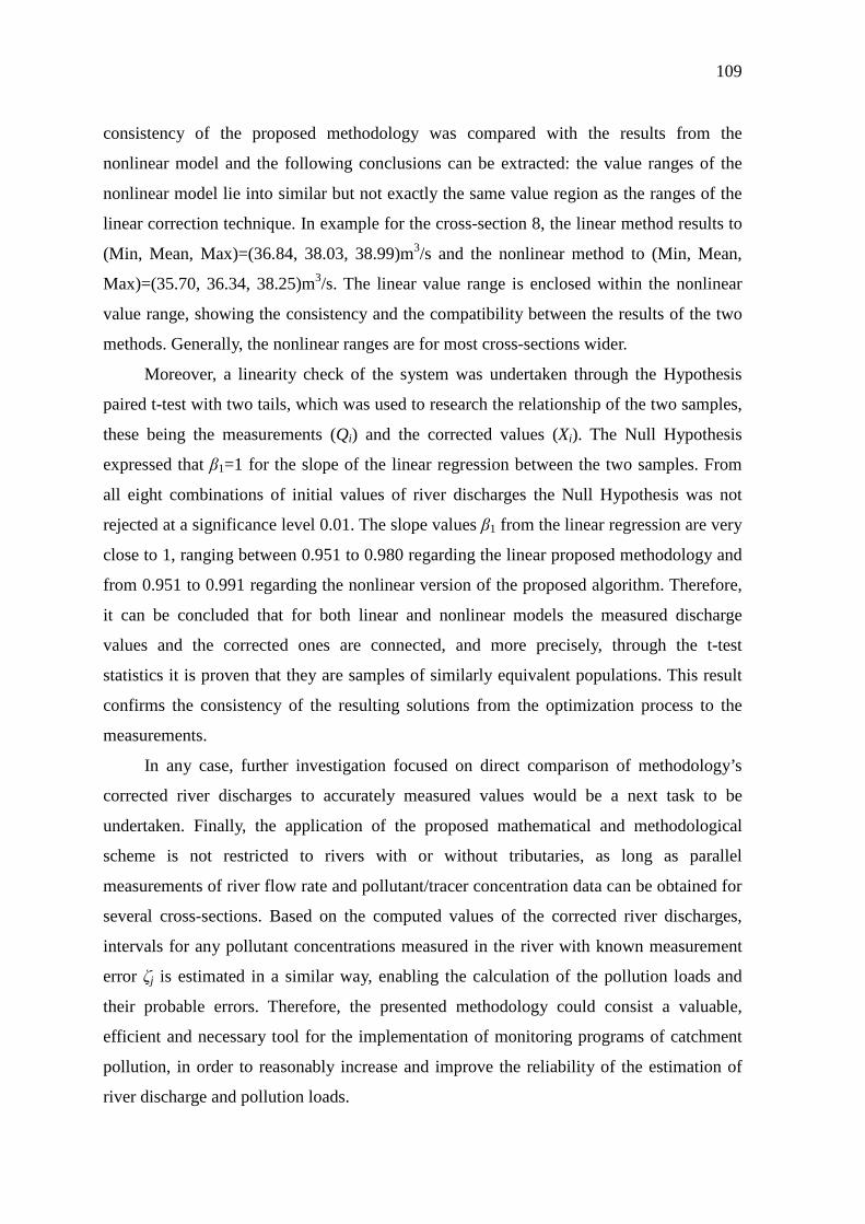
109

consistency of the proposed methodology was compared with the results from the

nonlinear model and the following conclusions can be extracted: the value ranges of the

nonlinear model lie into similar but not exactly the same value region as the ranges of the

linear correction technique. In example for the cross-section 8, the linear method results to

(Min, Mean, Max)=(36.84, 38.03, 38.99)m3/s and the nonlinear method to (Min, Mean,

Max)=(35.70, 36.34, 38.25)m3/s. The linear value range is enclosed within the nonlinear

value range, showing the consistency and the compatibility between the results of the two

methods. Generally, the nonlinear ranges are for most cross-sections wider.

Moreover, a linearity check of the system was undertaken through the Hypothesis

paired t-test with two tails, which was used to research the relationship of the two samples,

these being the measurements (Qi) and the corrected values (Xi). The Null Hypothesis

expressed that β1=1 for the slope of the linear regression between the two samples. From

all eight combinations of initial values of river discharges the Null Hypothesis was not

rejected at a significance level 0.01. The slope values β1 from the linear regression are very

close to 1, ranging between 0.951 to 0.980 regarding the linear proposed methodology and

from 0.951 to 0.991 regarding the nonlinear version of the proposed algorithm. Therefore,

it can be concluded that for both linear and nonlinear models the measured discharge

values and the corrected ones are connected, and more precisely, through the t-test

statistics it is proven that they are samples of similarly equivalent populations. This result

confirms the consistency of the resulting solutions from the optimization process to the

measurements.

In any case, further investigation focused on direct comparison of methodology’s

corrected river discharges to accurately measured values would be a next task to be

undertaken. Finally, the application of the proposed mathematical and methodological

scheme is not restricted to rivers with or without tributaries, as long as parallel

measurements of river flow rate and pollutant/tracer concentration data can be obtained for

several cross-sections. Based on the computed values of the corrected river discharges,

intervals for any pollutant concentrations measured in the river with known measurement

error ζj is estimated in a similar way, enabling the calculation of the pollution loads and

their probable errors. Therefore, the presented methodology could consist a valuable,

efficient and necessary tool for the implementation of monitoring programs of catchment

pollution, in order to reasonably increase and improve the reliability of the estimation of

river discharge and pollution loads.

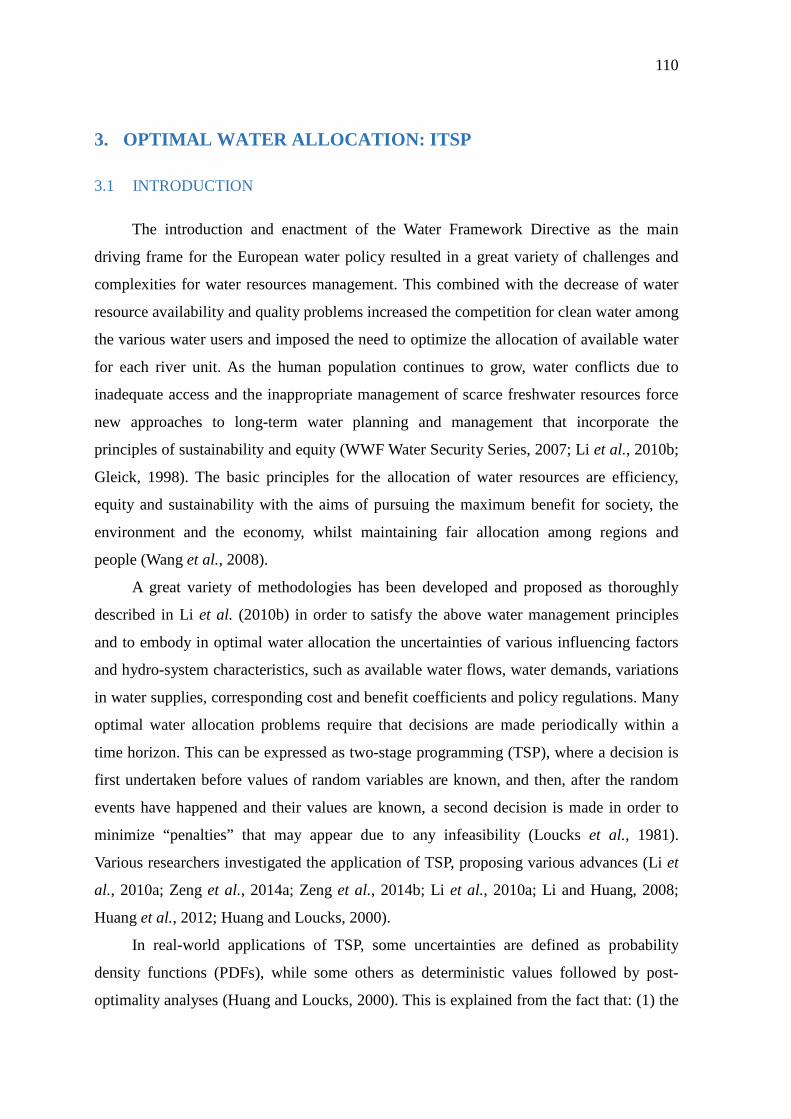
110

3. OPTIMAL WATER ALLOCATION: ITSP

3.1 INTRODUCTION

The introduction and enactment of the Water Framework Directive as the main

driving frame for the European water policy resulted in a great variety of challenges and

complexities for water resources management. This combined with the decrease of water

resource availability and quality problems increased the competition for clean water among

the various water users and imposed the need to optimize the allocation of available water

for each river unit. As the human population continues to grow, water conflicts due to

inadequate access and the inappropriate management of scarce freshwater resources force

new approaches to long-term water planning and management that incorporate the

principles of sustainability and equity (WWF Water Security Series, 2007; Li et al., 2010b;

Gleick, 1998). The basic principles for the allocation of water resources are efficiency,

equity and sustainability with the aims of pursuing the maximum benefit for society, the

environment and the economy, whilst maintaining fair allocation among regions and

people (Wang et al., 2008).

A great variety of methodologies has been developed and proposed as thoroughly

described in Li et al. (2010b) in order to satisfy the above water management principles

and to embody in optimal water allocation the uncertainties of various influencing factors

and hydro-system characteristics, such as available water flows, water demands, variations

in water supplies, corresponding cost and benefit coefficients and policy regulations. Many

optimal water allocation problems require that decisions are made periodically within a

time horizon. This can be expressed as two-stage programming (TSP), where a decision is

first undertaken before values of random variables are known, and then, after the random

events have happened and their values are known, a second decision is made in order to

minimize “penalties” that may appear due to any infeasibility (Loucks et al., 1981).

Various researchers investigated the application of TSP, proposing various advances (Li et

al., 2010a; Zeng et al., 2014a; Zeng et al., 2014b; Li et al., 2010a; Li and Huang, 2008;

Huang et al., 2012; Huang and Loucks, 2000).

In real-world applications of TSP, some uncertainties are defined as probability

density functions (PDFs), while some others as deterministic values followed by post-

optimality analyses (Huang and Loucks, 2000). This is explained from the fact that: (1) the

111

quality of information in terms of uncertainty in many practical problems is not good

enough to be expressed as PDFs; and (2) the solution of a large TSP model with all

uncertain parameters being expressed as PDFs is very difficult and complex, even if these

functions are available. Alternatively, methods of post-optimality analysis (such as

sensitivity analysis and parametric programming) may be used or best/worst case (BWC)

models may be formulated. However, sensitivity analysis is most suitable for problems

with few uncertain parameters. If a significant number of parameters is expressed as

intervals, various possible combinations of the deterministic values within the intervals

should be tested. For large-scale problems, programming this number of combinations may

become extremely large (Budnick et al., 1988). Despite the fact that parametric

programming may help with reducing the number of combinations, it assumes that

simultaneous variations occur in the model parameters, which may not be true for real-world

applications. In BWC analysis, optimal solutions are determined under best and worst

conditions, without necessarily forming stable sets of intervals, and are useful for evaluating

the capacity of the system to realize the desired goal. BCW analysis is really a special type of

sensitivity analysis for evaluating the responses of model solutions under two extreme

conditions.

In order to overcome the above complications in data availability and the solution

method, Huang and Loucks (2000) proposed an inexact two-stage stochastic programming

model (ITSP). It is a hybrid method of inexact optimization and TSP (Matloka, 1992) able

to handle uncertainties, which cannot be expressed as PDFs. In real-world problems, some

uncertainties may indeed exist as ambiguous intervals, since planners and engineers

typically find it more difficult to specify distributions than to define fluctuation ranges.

In the present work, an optimal water allocation method under uncertain system

conditions is searched for the Alfeios River Basin in Greece. Alfeios is an important river

basin in the Peloponnese region in Greece (Bekri and Yannopoulos, 2012; Bekri et al.,

2013, 2014) combining various water uses. These include irrigation, playing a vital social,

economic and environmental role associated among others with agricultural income and

with water, food and energy efficiency, hydropower generation and drinking water supply.

In Alfeios River Basin, as in most Mediterranean countries, water resources management

has been focused up to now on an essentially supply-driven approach. It is characterized by

a lack of effective operational strategies. Authority responsibility relationships are

fragmented, and law enforcement and policy implementations are weak, facts that lead to

112

the difficulty of gathering the necessary data for water resources management or, even

worse, to data loss. In some cases, river monitoring, which is crucial for water quantity and

quality assessment, if present, is either inefficient with intermittent periods with no

measurements or, due to low financial means, the monitoring programs are short and

undertaken by a small number of personnel, leading to unreliable and/or short-term data. In

this case, some sources of obtaining hydrologic, technical, economic and environmental

data required for water resources management come from making additional periodic

measuring expeditions, indirectly from expert knowledge, from informal information of the

local population or from more general data concerning a wider geographical location (i.e.,

country level) from national, European or international databases. Data of this type with a

high degree of uncertainty may be easily defined as fluctuation ranges and, therefore,

simulated as intervals with lower and upper (deterministic or fuzzy) bounds without the

need for any distributional or probabilistic information. Therefore, the ITSP method can be

used for optimal water allocation in Alfeios River Basin.

This chapter describes the first part of two methodologies, which aim at analyzing

and applying two similar optimization techniques, in terms of their basic concepts, for

optimal water allocation under uncertain system conditions in a real and complex multi-

tributary and multi-period water resources system, the Alfeios River Basin. The second

methodology, described and discussed in chapter 3.9, extends the ITSP in order to take into

account fuzzy boundaries (instead of deterministic) for the variables expressed as intervals,

since some intervals are fuzzy in nature. The reason for organizing these two chapters as

described above is to facilitate a deeper understanding of this type of methodology through

the application of the first method, which is simpler and easier regarding follow up.

The results obtained from this methodology include (1) the optimized water

allocation target with a minimized risk of economic penalty from shortages and

opportunity loss from spills and (2) an optimized water allocation plan (identification of

water allocation and shortages based on the optimized water allocation targets) with a

maximized system benefit over a multi-period planning horizon. These types of results are

derived as deterministic upper and lower bounds. The system dynamics in terms of

decisions for water allocation is mirrored through the consideration of the various equal

probability hydrologic scenarios, which have been stochastically generated simultaneously

at the positions of the water inflows. The total net system benefits and the benefits and

penalties of each main water use for Alfeios are studied and analyzed based on the

113

application of the ITSP method for a baseline scenario and four water and agricultural

future scenarios developed within the Sustainability of European Irrigated Agriculture

under Water Framework Directive and Agenda 2000 (WADI) project (WADI, 2000; Manos

et al., 2006; Berkhout and Hertin, 2002; Bekri et al., 2015a; HMSO, 2002). These future

scenarios cover various possible technical, environmental and socio-economic aspects of

the future space for different EU water and agricultural policies, having an impact mainly

on agriculture, but also on water resources management. Changes of crop patterns, yields,

subsidies, farmer income, variable input costs, market prices per agricultural product,

fertilizers and water and hydropower prices are some of the variables described in the

narratives of these scenarios, which, in turn, serve as inputs to the optimization algorithm

for the evaluation and the estimation of their effect on the water allocation pattern and the

system benefits. Finally, for applying the abovementioned optimal water allocation

methodology, benefit analysis of each water use, or even better, the determination of

economic water value for each water use, identifying the unit benefit and unit penalties of

each m3 of water allocated to each one of the water uses, is undertaken for the Alfeios

River.

3.2 MATHEMATICAL FORMULATION OF THE ITSP

The mathematical background of the ITSP model presented in this section is based

on Huang and Loucks (2000). Let us consider a problem, where a water manager should

supply water from various sources to multiple users. The water manager can build the

optimization problem as the maximization of the expected value of economic activity in

the region. For a water allocation target set for each water user, if this water target is

provided, it results in net benefits to the local economy. In the opposite case (nonzero

shortages), the desired water target should be obtained from alternative and more

expensive water sources, resulting in penalties on the local economy (Loucks et al., 1981).

Since the total water available is a random variable, the problem can be built as a

two-stage stochastic programming model. To solve this problem with linear programming,

the distribution of Q must be approximated by a discrete function. Letting Q take values

with probability for = 1,2, … . , A, we have (Loucks et al., 1981):

114

G c d

e =

(3.1)

where = the fixed allocation target for water that is promised to water user i, !"

= the maximum allowable allocation amount to user i, = the reduction of the net benefit

to user i per unit of water not delivered ( ≥ ),= the net benefit to user i per unit

of water allocated, f = the net system benefits, i = the water user, m = the number of water

users,G' ( = the expected value of a random variable and is the amount by which

water allocation target is not met when the seasonal flow is with probability . The

water allocation target () and the economic data ( and ) may not be available as

deterministic values, but as intervals. This leads to a hybrid ITSP model as follows:

± = ±± −±±

(3.2a)

. . ± ≥± −±, ∀

(3.2b)

!"± ≥± ≥ ± ≥ 0, ∀$, (3.2c)

where ±, ±, ±, ±, ± and !"± are interval parameters/variables. For

example, letting % and & be lower and upper bounds of ±, respectively, we have

± = '%, &(. When ± are known, Model (3.2) can be transformed into two sets of deterministic

submodels, which correspond to the upper and lower bounds of the desired objective

function value. This transformation process is based on an interactive algorithm, which is

different from normal best/worst case analysis. The resulting solution provides stable intervals

for the objective function and decision variables, which can be easily interpreted for generating

decision alternatives. The detailed transformation process is as follows.

The first step is to determine values for cost coefficients and decision variables

corresponding to the desired bound of the objective function value. For Model (3.2), & is

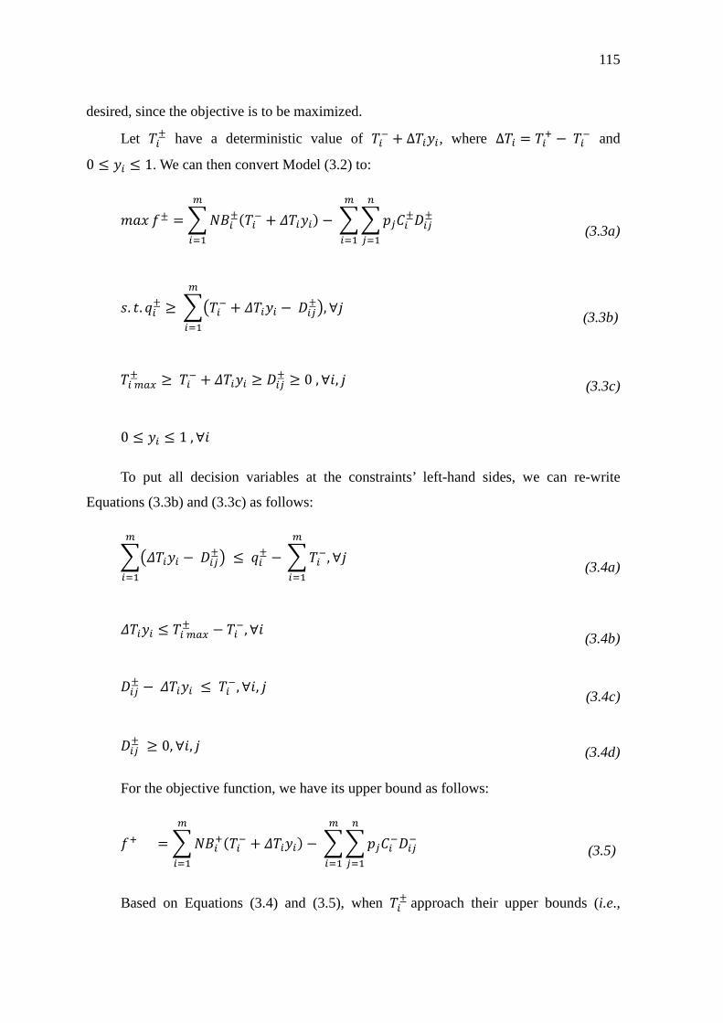
115

desired, since the objective is to be maximized.

Let ± have a deterministic value of % + Δ+, where Δ = & − % and 0 ≤ + ≤ 1. We can then convert Model (3.2) to:

± = ±B% + .+) −±±

(3.3a)

. . ± ≥% + .+ −±, ∀

(3.3b)

!"± ≥% + .+ ≥ ± ≥ 0, ∀$, (3.3c)

0 ≤ + ≤ 1, ∀$To put all decision variables at the constraints’ left-hand sides, we can re-write

Equations (3.3b) and (3.3c) as follows:

.+ −± ≤ ± − %, ∀

(3.4a)

.+ ≤ !"± − %, ∀$(3.4b)

± − .+ ≤ %, ∀$, (3.4c)

± ≥ 0, ∀$, (3.4d)

For the objective function, we have its upper bound as follows:

& = &B% + .+) −%%

(3.5)

Based on Equations (3.4) and (3.5), when ±approach their upper bounds (i.e.,

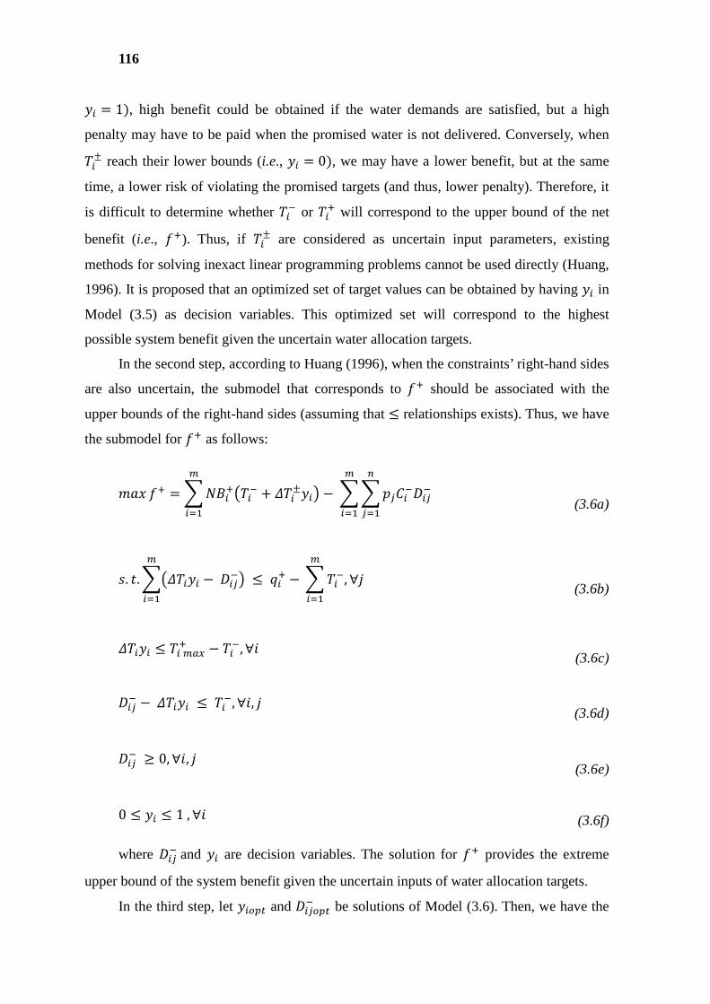
116

+ = 1), high benefit could be obtained if the water demands are satisfied, but a high

penalty may have to be paid when the promised water is not delivered. Conversely, when

± reach their lower bounds (i.e., + = 0), we may have a lower benefit, but at the same

time, a lower risk of violating the promised targets (and thus, lower penalty). Therefore, it

is difficult to determine whether % or & will correspond to the upper bound of the net

benefit (i.e., &). Thus, if ± are considered as uncertain input parameters, existing

methods for solving inexact linear programming problems cannot be used directly (Huang,

1996). It is proposed that an optimized set of target values can be obtained by having + in

Model (3.5) as decision variables. This optimized set will correspond to the highest

possible system benefit given the uncertain water allocation targets.

In the second step, according to Huang (1996), when the constraints’ right-hand sides

are also uncertain, the submodel that corresponds to & should be associated with the

upper bounds of the right-hand sides (assuming that ≤ relationships exists). Thus, we have

the submodel for & as follows:

& = &% + .±+ − %%

(3.6a)

. ..+ −% ≤ & − %, ∀

(3.6b)

.+ ≤ !"& − %, ∀$(3.6c)

% − .+ ≤ %, ∀$, (3.6d)

% ≥ 0, ∀$, (3.6e)

0 ≤ + ≤ 1, ∀$ (3.6f)

where %and + are decision variables. The solution for & provides the extreme

upper bound of the system benefit given the uncertain inputs of water allocation targets.

In the third step, let +/01 and /01% be solutions of Model (3.6). Then, we have the

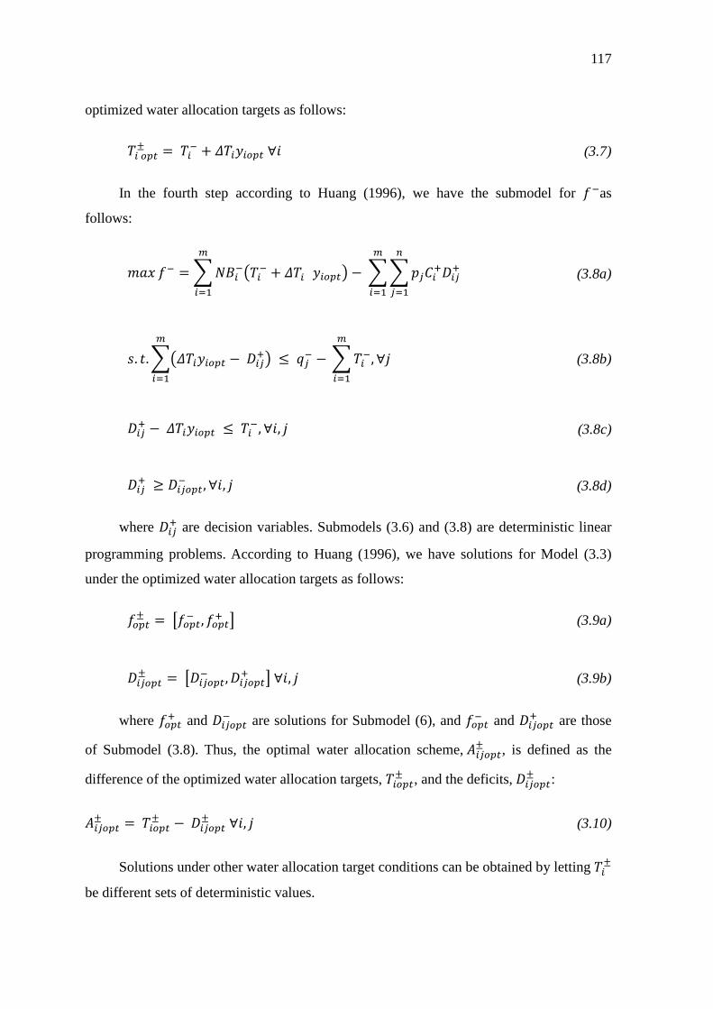
117

optimized water allocation targets as follows:

/01± =% + .+/01∀$ (3.7)

In the fourth step according to Huang (1996), we have the submodel for %as

follows:

% = %% + . +/01 −&&

(3.8a)

. ..+/01 −& ≤ % − %, ∀

(3.8b)

& − .+/01 ≤ %, ∀$, (3.8c)

& ≥ /01% , ∀$, (3.8d)

where & are decision variables. Submodels (3.6) and (3.8) are deterministic linear

programming problems. According to Huang (1996), we have solutions for Model (3.3)

under the optimized water allocation targets as follows:

/01± = 2/01% , /01& 3 (3.9a)

/01± = 2/01% , /01& 3∀$, (3.9b)

where /01& and /01% are solutions for Submodel (6), and /01% and /01& are those

of Submodel (3.8). Thus, the optimal water allocation scheme,4/01± , is defined as the

difference of the optimized water allocation targets, /01± , and the deficits,/01± :

4/01± =/01± −/01± ∀$, (3.10)

Solutions under other water allocation target conditions can be obtained by letting ±

be different sets of deterministic values.

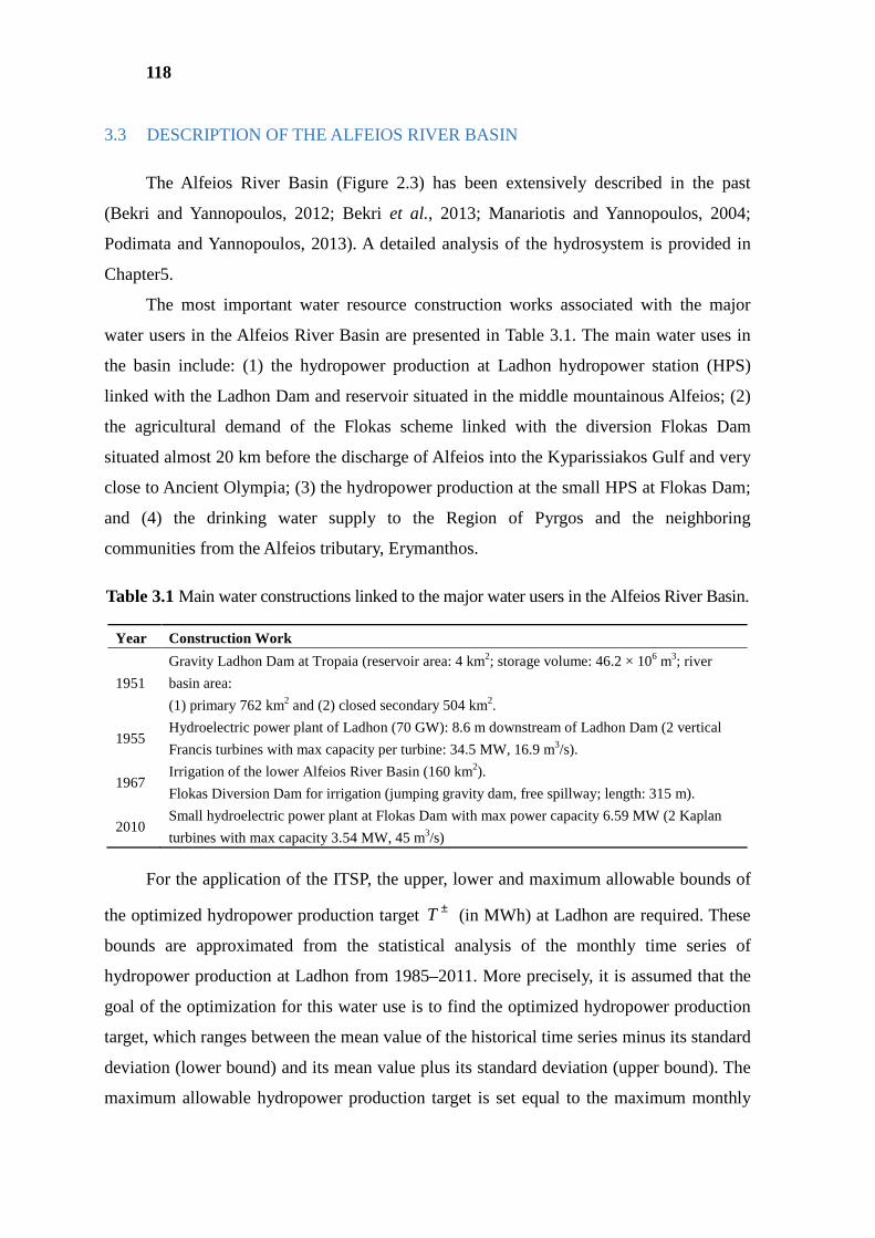
118

3.3 DESCRIPTION OF THE ALFEIOS RIVER BASIN

The Alfeios River Basin (Figure 2.3) has been extensively described in the past

(Bekri and Yannopoulos, 2012; Bekri et al., 2013; Manariotis and Yannopoulos, 2004;

Podimata and Yannopoulos, 2013). A detailed analysis of the hydrosystem is provided in

Chapter5.

The most important water resource construction works associated with the major

water users in the Alfeios River Basin are presented in Table 3.1. The main water uses in

the basin include: (1) the hydropower production at Ladhon hydropower station (HPS)

linked with the Ladhon Dam and reservoir situated in the middle mountainous Alfeios; (2)

the agricultural demand of the Flokas scheme linked with the diversion Flokas Dam

situated almost 20 km before the discharge of Alfeios into the Kyparissiakos Gulf and very

close to Ancient Olympia; (3) the hydropower production at the small HPS at Flokas Dam;

and (4) the drinking water supply to the Region of Pyrgos and the neighboring

communities from the Alfeios tributary, Erymanthos.

Table 3.1 Main water constructions linked to the major water users in the Alfeios River Basin.

Year Construction Work

1951

Gravity Ladhon Dam at Tropaia (reservoir area: 4 km2; storage volume: 46.2 × 106 m3; river

basin area:

(1) primary 762 km2 and (2) closed secondary 504 km2.

1955 Hydroelectric power plant of Ladhon (70 GW): 8.6 m downstream of Ladhon Dam (2 vertical

Francis turbines with max capacity per turbine: 34.5 MW, 16.9 m3/s).

1967 Irrigation of the lower Alfeios River Basin (160 km2).

Flokas Diversion Dam for irrigation (jumping gravity dam, free spillway; length: 315 m).

2010 Small hydroelectric power plant at Flokas Dam with max power capacity 6.59 MW (2 Kaplan

turbines with max capacity 3.54 MW, 45 m3/s)

For the application of the ITSP, the upper, lower and maximum allowable bounds of

the optimized hydropower production target ±T (in MWh) at Ladhon are required. These

bounds are approximated from the statistical analysis of the monthly time series of

hydropower production at Ladhon from 1985–2011. More precisely, it is assumed that the

goal of the optimization for this water use is to find the optimized hydropower production

target, which ranges between the mean value of the historical time series minus its standard

deviation (lower bound) and its mean value plus its standard deviation (upper bound). The

maximum allowable hydropower production target is set equal to the maximum monthly

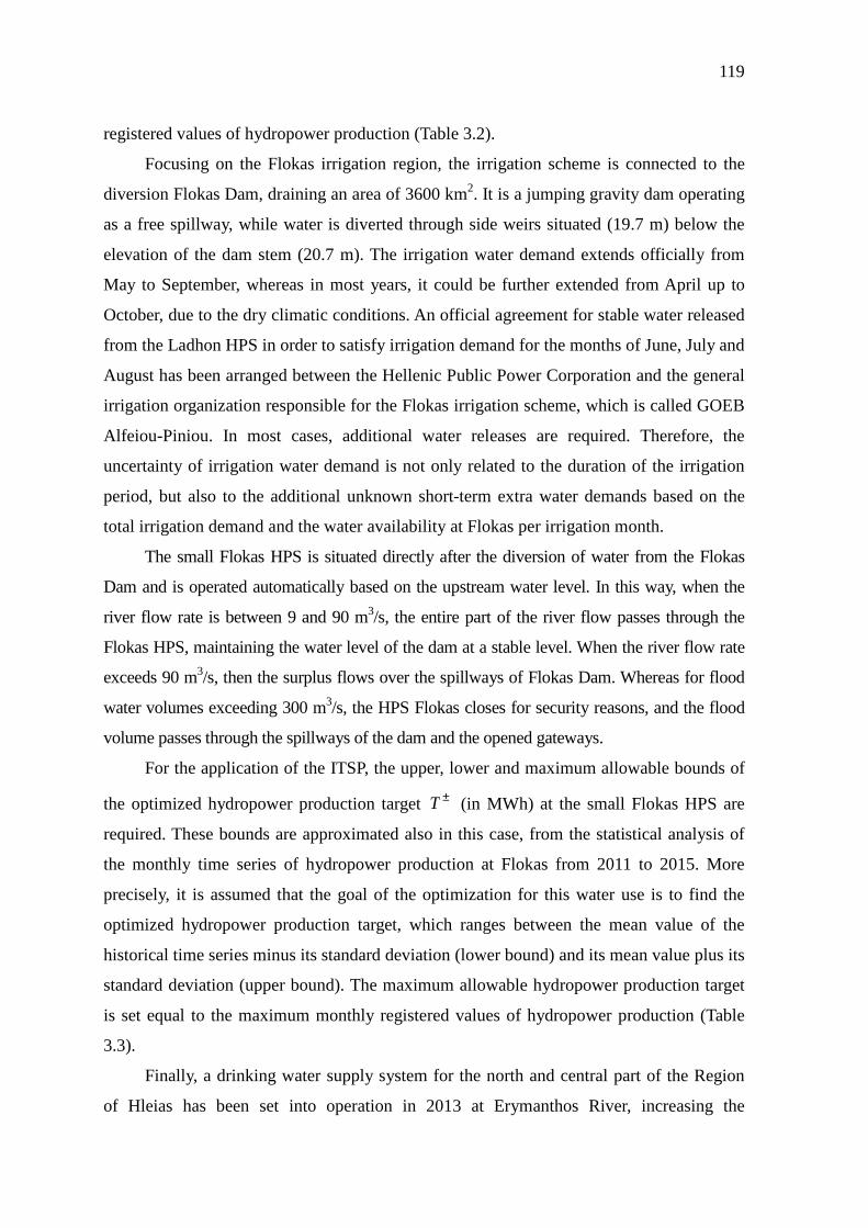
119

registered values of hydropower production (Table 3.2).

Focusing on the Flokas irrigation region, the irrigation scheme is connected to the

diversion Flokas Dam, draining an area of 3600 km2. It is a jumping gravity dam operating

as a free spillway, while water is diverted through side weirs situated (19.7 m) below the

elevation of the dam stem (20.7 m). The irrigation water demand extends officially from

May to September, whereas in most years, it could be further extended from April up to

October, due to the dry climatic conditions. An official agreement for stable water released

from the Ladhon HPS in order to satisfy irrigation demand for the months of June, July and

August has been arranged between the Hellenic Public Power Corporation and the general

irrigation organization responsible for the Flokas irrigation scheme, which is called GOEB

Alfeiou-Piniou. In most cases, additional water releases are required. Therefore, the

uncertainty of irrigation water demand is not only related to the duration of the irrigation

period, but also to the additional unknown short-term extra water demands based on the

total irrigation demand and the water availability at Flokas per irrigation month.

The small Flokas HPS is situated directly after the diversion of water from the Flokas

Dam and is operated automatically based on the upstream water level. In this way, when the

river flow rate is between 9 and 90 m3/s, the entire part of the river flow passes through the

Flokas HPS, maintaining the water level of the dam at a stable level. When the river flow rate

exceeds 90 m3/s, then the surplus flows over the spillways of Flokas Dam. Whereas for flood

water volumes exceeding 300 m3/s, the HPS Flokas closes for security reasons, and the flood

volume passes through the spillways of the dam and the opened gateways.

For the application of the ITSP, the upper, lower and maximum allowable bounds of

the optimized hydropower production target ±T (in MWh) at the small Flokas HPS are

required. These bounds are approximated also in this case, from the statistical analysis of

the monthly time series of hydropower production at Flokas from 2011 to 2015. More

precisely, it is assumed that the goal of the optimization for this water use is to find the

optimized hydropower production target, which ranges between the mean value of the

historical time series minus its standard deviation (lower bound) and its mean value plus its

standard deviation (upper bound). The maximum allowable hydropower production target

is set equal to the maximum monthly registered values of hydropower production (Table

3.3).

Finally, a drinking water supply system for the north and central part of the Region

of Hleias has been set into operation in 2013 at Erymanthos River, increasing the

120

complexity of the water allocation pattern. A monthly water flow rate of 0.6 m3/s needs to

be diverted from Erymanthos to the water treatment plant and then to the neighboring

communities extending up to the city of Pyrgos. Due to the short operation period, this

water use, which has the highest priority among the others, is not incorporated into the

optimization process as a variable. It is introduced instead as a steady and known water

abstraction demand, while for each month, the deficit, if any, based on the considered

streamflow at Erymanthos is computed.

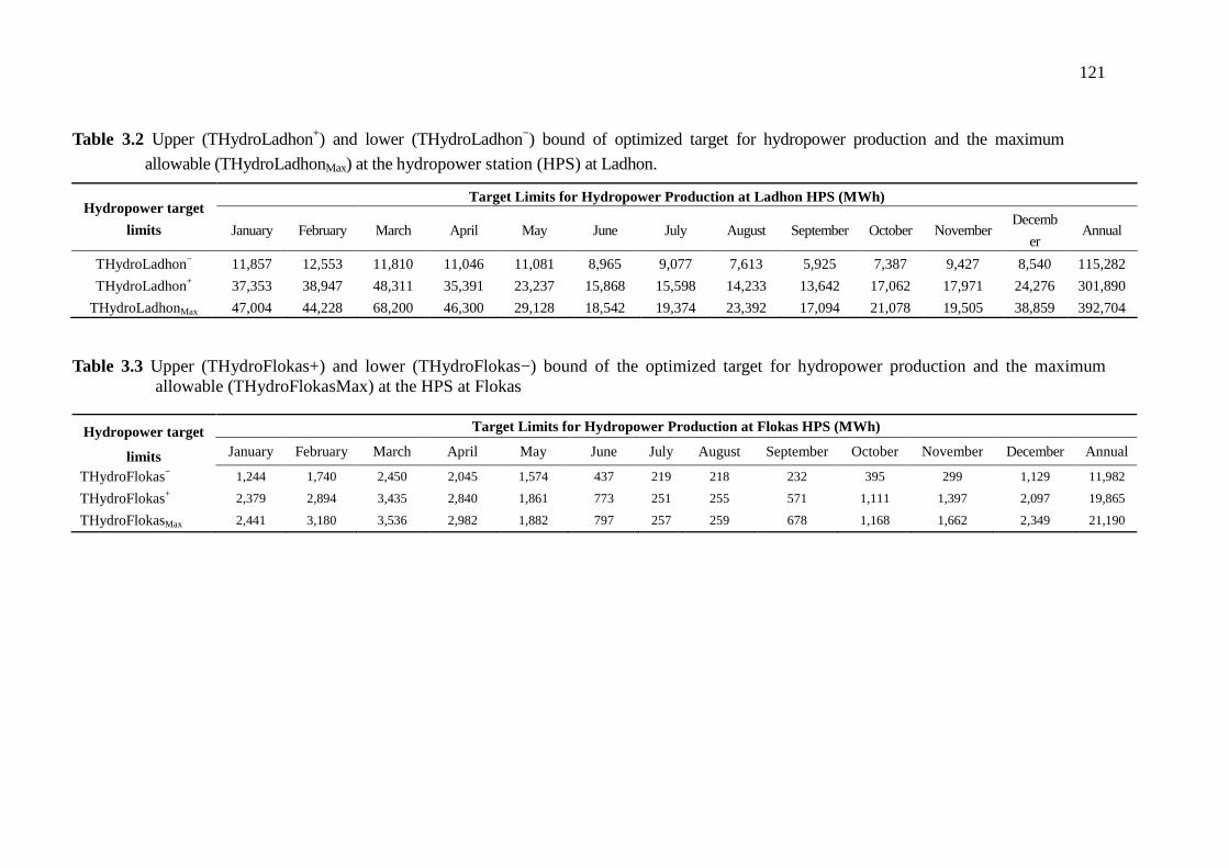
121

Table 3.2 Upper (THydroLadhon+) and lower (THydroLadhon−) bound of optimized target for hydropower production and the maximum

allowable (THydroLadhonMax) at the hydropower station (HPS) at Ladhon.

Hydropower target

limits

Target Limits for Hydropower Production at Ladhon H PS (MWh)

January February March April May June July August September October November Decemb

er Annual

THydroLadhon− 11,857 12,553 11,810 11,046 11,081 8,965 9,077 7,613 5,925 7,387 9,427 8,540 115,282

THydroLadhon+ 37,353 38,947 48,311 35,391 23,237 15,868 15,598 14,233 13,642 17,062 17,971 24,276 301,890

THydroLadhonMax 47,004 44,228 68,200 46,300 29,128 18,542 19,374 23,392 17,094 21,078 19,505 38,859 392,704

Table 3.3 Upper (THydroFlokas+) and lower (THydroFlokas−) bound of the optimized target for hydropower production and the maximum

allowable (THydroFlokasMax) at the HPS at Flokas

Hydropower target

limits

Target Limits for Hydropower Production at Flokas HPS (MWh)

January February March April May June July August September October November December Annual

THydroFlokas− 1,244 1,740 2,450 2,045 1,574 437 219 218 232 395 299 1,129 11,982

THydroFlokas+ 2,379 2,894 3,435 2,840 1,861 773 251 255 571 1,111 1,397 2,097 19,865

THydroFlokasMax 2,441 3,180 3,536 2,982 1,882 797 257 259 678 1,168 1,662 2,349 21,190

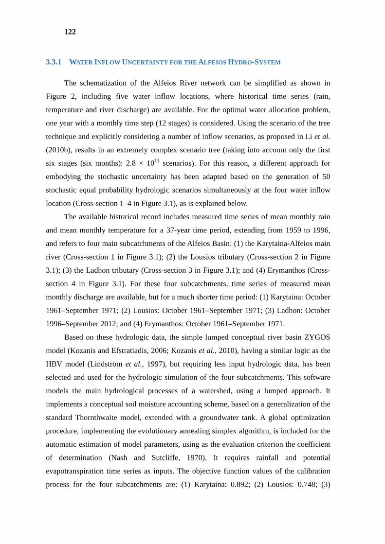
122

3.3.1 WATER INFLOW UNCERTAINTY FOR THE ALFEIOS HYDRO-SYSTEM

The schematization of the Alfeios River network can be simplified as shown in

Figure 2, including five water inflow locations, where historical time series (rain,

temperature and river discharge) are available. For the optimal water allocation problem,

one year with a monthly time step (12 stages) is considered. Using the scenario of the tree

technique and explicitly considering a number of inflow scenarios, as proposed in Li et al.

(2010b), results in an extremely complex scenario tree (taking into account only the first

six stages (six months): 2.8 × 1011 scenarios). For this reason, a different approach for

embodying the stochastic uncertainty has been adapted based on the generation of 50

stochastic equal probability hydrologic scenarios simultaneously at the four water inflow

location (Cross-section 1–4 in Figure 3.1), as is explained below.

The available historical record includes measured time series of mean monthly rain

and mean monthly temperature for a 37-year time period, extending from 1959 to 1996,

and refers to four main subcatchments of the Alfeios Basin: (1) the Karytaina-Alfeios main

river (Cross-section 1 in Figure 3.1); (2) the Lousios tributary (Cross-section 2 in Figure

3.1); (3) the Ladhon tributary (Cross-section 3 in Figure 3.1); and (4) Erymanthos (Cross-

section 4 in Figure 3.1). For these four subcatchments, time series of measured mean

monthly discharge are available, but for a much shorter time period: (1) Karytaina: October

1961–September 1971; (2) Lousios: October 1961–September 1971; (3) Ladhon: October

1996–September 2012; and (4) Erymanthos: October 1961–September 1971.

Based on these hydrologic data, the simple lumped conceptual river basin ZYGOS

model (Kozanis and Efstratiadis, 2006; Kozanis et al., 2010), having a similar logic as the

HBV model (Lindström et al., 1997), but requiring less input hydrologic data, has been

selected and used for the hydrologic simulation of the four subcatchments. This software

models the main hydrological processes of a watershed, using a lumped approach. It

implements a conceptual soil moisture accounting scheme, based on a generalization of the

standard Thornthwaite model, extended with a groundwater tank. A global optimization

procedure, implementing the evolutionary annealing simplex algorithm, is included for the

automatic estimation of model parameters, using as the evaluation criterion the coefficient

of determination (Nash and Sutcliffe, 1970). It requires rainfall and potential

evapotranspiration time series as inputs. The objective function values of the calibration

process for the four subcatchments are: (1) Karytaina: 0.892; (2) Lousios: 0.748; (3)

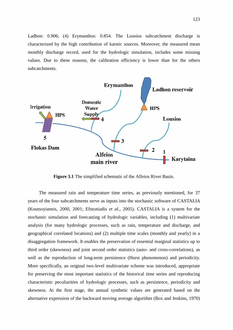
123

Ladhon: 0.906; (4) Erymanthos: 0.854. The Lousios subcatchment discharge is

characterized by the high contribution of karstic sources. Moreover, the measured mean

monthly discharge record, used for the hydrologic simulation, includes some missing

values. Due to these reasons, the calibration efficiency is lower than for the others

subcatchments.

Figure 3.1 The simplified schematic of the Alfeios River Basin.

The measured rain and temperature time series, as previously mentioned, for 37

years of the four subcatchments serve as inputs into the stochastic software of CASTALIA

(Koutsoyiannis, 2000, 2001; Efstratiadis et al., 2005). CASTALIA is a system for the

stochastic simulation and forecasting of hydrologic variables, including (1) multivariate

analysis (for many hydrologic processes, such as rain, temperature and discharge, and

geographical correlated locations) and (2) multiple time scales (monthly and yearly) in a

disaggregation framework. It enables the preservation of essential marginal statistics up to

third order (skewness) and joint second order statistics (auto- and cross-correlations), as

well as the reproduction of long-term persistence (Hurst phenomenon) and periodicity.

More specifically, an original two-level multivariate scheme was introduced, appropriate

for preserving the most important statistics of the historical time series and reproducing

characteristic peculiarities of hydrologic processes, such as persistence, periodicity and

skewness. At the first stage, the annual synthetic values are generated based on the

alternative expression of the backward moving average algorithm (Box and Jenkins, 1970)

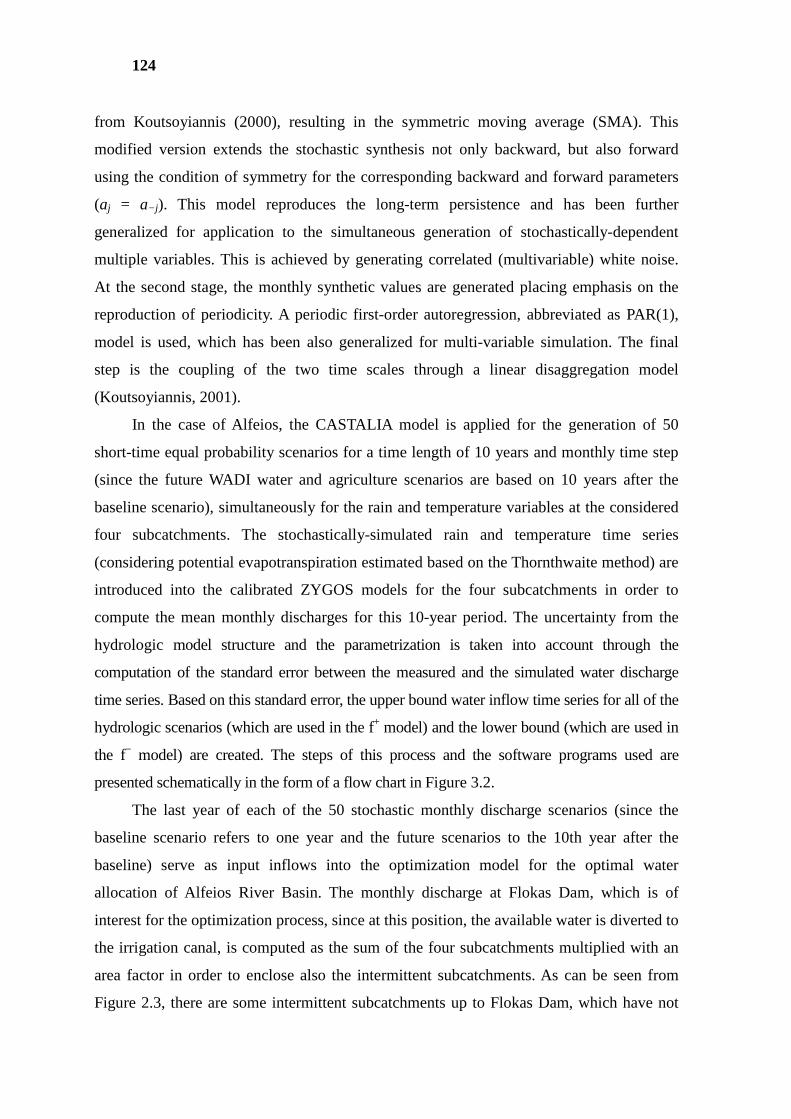
124

from Koutsoyiannis (2000), resulting in the symmetric moving average (SMA). This

modified version extends the stochastic synthesis not only backward, but also forward

using the condition of symmetry for the corresponding backward and forward parameters

(aj = a−j ). This model reproduces the long-term persistence and has been further

generalized for application to the simultaneous generation of stochastically-dependent

multiple variables. This is achieved by generating correlated (multivariable) white noise.

At the second stage, the monthly synthetic values are generated placing emphasis on the

reproduction of periodicity. A periodic first-order autoregression, abbreviated as PAR(1),

model is used, which has been also generalized for multi-variable simulation. The final

step is the coupling of the two time scales through a linear disaggregation model

(Koutsoyiannis, 2001).

In the case of Alfeios, the CASTALIA model is applied for the generation of 50

short-time equal probability scenarios for a time length of 10 years and monthly time step

(since the future WADI water and agriculture scenarios are based on 10 years after the

baseline scenario), simultaneously for the rain and temperature variables at the considered

four subcatchments. The stochastically-simulated rain and temperature time series

(considering potential evapotranspiration estimated based on the Thornthwaite method) are

introduced into the calibrated ZYGOS models for the four subcatchments in order to

compute the mean monthly discharges for this 10-year period. The uncertainty from the

hydrologic model structure and the parametrization is taken into account through the

computation of the standard error between the measured and the simulated water discharge

time series. Based on this standard error, the upper bound water inflow time series for all of the

hydrologic scenarios (which are used in the f+ model) and the lower bound (which are used in

the f− model) are created. The steps of this process and the software programs used are

presented schematically in the form of a flow chart in Figure 3.2.

The last year of each of the 50 stochastic monthly discharge scenarios (since the

baseline scenario refers to one year and the future scenarios to the 10th year after the

baseline) serve as input inflows into the optimization model for the optimal water

allocation of Alfeios River Basin. The monthly discharge at Flokas Dam, which is of

interest for the optimization process, since at this position, the available water is diverted to

the irrigation canal, is computed as the sum of the four subcatchments multiplied with an

area factor in order to enclose also the intermittent subcatchments. As can be seen from

Figure 2.3, there are some intermittent subcatchments up to Flokas Dam, which have not

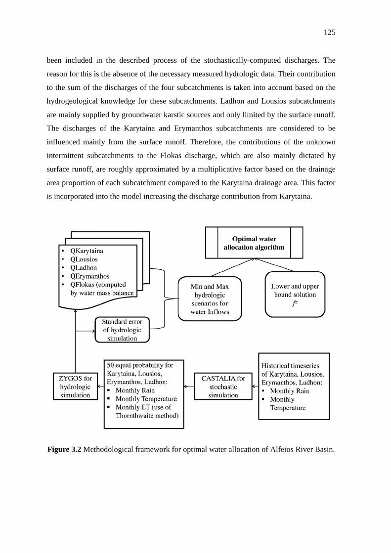
125

been included in the described process of the stochastically-computed discharges. The

reason for this is the absence of the necessary measured hydrologic data. Their contribution

to the sum of the discharges of the four subcatchments is taken into account based on the

hydrogeological knowledge for these subcatchments. Ladhon and Lousios subcatchments

are mainly supplied by groundwater karstic sources and only limited by the surface runoff.

The discharges of the Karytaina and Erymanthos subcatchments are considered to be

influenced mainly from the surface runoff. Therefore, the contributions of the unknown

intermittent subcatchments to the Flokas discharge, which are also mainly dictated by

surface runoff, are roughly approximated by a multiplicative factor based on the drainage

area proportion of each subcatchment compared to the Karytaina drainage area. This factor

is incorporated into the model increasing the discharge contribution from Karytaina.

Figure 3.2 Methodological framework for optimal water allocation of Alfeios River Basin.

126

3.4 UNIT BENEFIT AND PENALTY ANALYSIS FOR HYDROPOWER ENERGY

In order to estimate the unit benefit from water allocated to hydropower energy and

the corresponding shadow unit penalty, it is worth taking into account the changes in the

energy market in Greece based on the illustrative paper of Bunn and Karakatsani (2008).

As described in this work, until recently, electricity was a monopoly in most countries,

including Greece, often government owned, and, if not, highly regulated. As such,

electricity prices reflected the government’s social and industrial policy, and any price

forecasting that was undertaken was really focused on thinking about underlying costs. In

this respect, it tended to be over the longer term, taking a view on fuel prices, technological

innovation and generation efficiency. This energy market liberalization has been in effect

in Greece since 19 February 2001 with the Law 2773/22.12.1999.

From the above analysis, it is clear that the selling price of hydropower energy, as

part of the energy market, has not been fixed and steady since the energy market

liberalization. For Greece, it depends on the hourly marginal energy price of the energy

system. This price, reflecting the energy price gained by the energy producers, is

influenced by, firstly, the combination of the selling price offers and the energy production

of each energy production unit and, secondly, by the hourly energy demand of the system.

Based on the estimations of the chief engineer responsible for the operation of Ladhon

HPS, who was asked to provide minimum and maximum values for the unit benefit from

hydropower production at Ladhon under favorable (associated with the maximum benefit

from hydropower production) and under unfavorable (associated with the minimum benefit

from hydropower production) conditions, an upper and a lower fuzzy boundary interval are

defined for the unit benefit from hydropower energy at Ladhon HPS. Due to the absence of

the membership function for this fuzzy variable, only the extreme values have been

considered in the analysis. Moreover, a study that analyzes statistically the values of the

hourly marginal energy prices as provided by the independent Regulatory Authority of

Energy (RAE) (which is the organization that controls and regulates the Hellenic energy

system) has drawn duration curves of the hourly marginal energy selling prices

(Stefanakos, 2009). Three zones have been identified based on the operation mode of an

energy production unit: base, intermittent and peak. Alternatively, the unit benefit intervals

could be derived by making the assumption that the upper bound solution corresponds to

the interval values of the intermittent zone of the year with the highest mean hourly

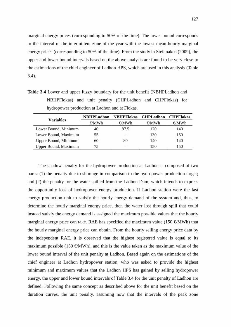
127

marginal energy prices (corresponding to 50% of the time). The lower bound corresponds

to the interval of the intermittent zone of the year with the lowest mean hourly marginal

energy prices (corresponding to 50% of the time). From the study in Stefanakos (2009), the

upper and lower bound intervals based on the above analysis are found to be very close to

the estimations of the chief engineer of Ladhon HPS, which are used in this analysis (Table

3.4).

Table 3.4 Lower and upper fuzzy boundary for the unit benefit (NBHPLadhon and

NBHPFlokas) and unit penalty (CHPLadhon and CHPFlokas) for

hydropower production at Ladhon and at Flokas.

Variables NBHPLadhon NBHPFlokas CHPLadhon CHPFlokas

€/MWh €/MWh €/MWh €/MWh

Lower Bound, Minimum 40 87.5 120 140 Lower Bound, Maximum 55 – 130 150 Upper Bound, Minimum 60 80 140 140 Upper Bound, Maximum 75 – 150 150

The shadow penalty for the hydropower production at Ladhon is composed of two

parts: (1) the penalty due to shortage in comparison to the hydropower production target;

and (2) the penalty for the water spilled from the Ladhon Dam, which intends to express

the opportunity loss of hydropower energy production. If Ladhon station were the last

energy production unit to satisfy the hourly energy demand of the system and, thus, to

determine the hourly marginal energy price, then the water lost through spill that could

instead satisfy the energy demand is assigned the maximum possible values that the hourly

marginal energy price can take. RAE has specified the maximum value (150 €/MWh) that

the hourly marginal energy price can obtain. From the hourly selling energy price data by

the independent RAE, it is observed that the highest registered value is equal to its

maximum possible (150 €/MWh), and this is the value taken as the maximum value of the

lower bound interval of the unit penalty at Ladhon. Based again on the estimations of the

chief engineer at Ladhon hydropower station, who was asked to provide the highest

minimum and maximum values that the Ladhon HPS has gained by selling hydropower

energy, the upper and lower bound intervals of Table 3.4 for the unit penalty of Ladhon are

defined. Following the same concept as described above for the unit benefit based on the

duration curves, the unit penalty, assuming now that the intervals of the peak zone

128

correspond to the unit penalty, can be derived. In this case, the derived intervals are lower,

ranging from 70 to 110 €/MWh. Since the penalties should be much higher than the unit

benefits to force the algorithm to reduce the penalties, the estimations of the chief engineer

at Ladhon are used in this study.

The unit benefit and penalty of the small Flokas HPS are approximated in a simpler

way, since small hydroelectric power stations are not included in the regulations of the

liberalization of the energy market described above. Small HPSs are considered renewable

energy systems, and each country is obliged to buy the hydropower energy produced at a

steady price. Based on the monthly selling price data of Flokas HPS, the unit benefit is

approximated as a single interval (meaning that no upper and lower bound intervals are

defined); this value ranges as presented in Table 3.4. The unit shadow penalty is

approximated as a single interval and is taken as equal to the upper bound solution of the

unit penalty of Flokas HPS, as shown in Table 3.4.

3.5 UNIT BENEFIT AND PENALTY ANALYSIS FOR IRRIGATION WATER

The present monthly irrigation water demand scheme is composed of two parts, as

previously analyzed in detail: (1) a regulated and stable irrigation demand pattern, referring

only to the required water volume releases from Ladhon Reservoir, which is derived from

the official agreement between Hellenic Public Power Corporation and GOEB; and (2) an

extra uncertain irrigation demand at the Flokas Dam site based on the actual crop patterns

and the water inflows at this position. The total irrigation requirements for the crop pattern

of Flokas are estimated for each stochastic hydrologic scenario using the FAO software

CROPWAT 8.0. The unit benefit for water allocated to irrigation is interpreted as the

probable net income from the agricultural production of the Flokas crop pattern, taking into

account the farmer income, the cost of production, the cost of the irrigation canal

(associated with the water charge to the farmers from the general irrigation organization,

GOEB) and the organizational structure of local irrigation organizations (the charges of the

local irrigation organizations). Finally, the unit penalty from the irrigation deficits is based

on the crop yield reduction and the corresponding net farmer income loss. The process of

the computation of the unit benefit, the unit penalty and the irrigation requirements is

analyzed in the following sections.

129

3.5.1 INPUT DATA FOR THE AGRICULTURAL AND WATER FUTURE SCENARIOS

The necessary input data for the examined agricultural and water future scenarios

(Table 3.5) include: (1) crop pattern details, such as crop pattern, area per crop, annual

yields, irrigation canal information, irrigation type used, etc.; (2) crop cultivation

information: time and technical information of crop production, such as the purchase costs

of seeds, fertilizers and pesticides, labor types, hours and costs, technical and economic

data for the machinery needed for agricultural production based either on annual operation

costs or, if available on purchase, maintenance and insurance costs, fuel type and costs,

etc.; and (3) prices of agricultural products in order to estimate the possible agricultural

income and also the corresponding profits from crop production: selling prices at the

producer price, cost of inputs, rents of agricultural land uses, subsidies and information for

the Common Agricultural Policy (CAP) determining the subsidies. Most of the above data,

including the cost of production of the main crops cultivated within the Flokas irrigated

area, have been estimated based on literature data, as described below. The main sources

are, on the one hand, scientific works (Soldatos et al., 2009; Villiotis, 2008; Liofagou,

2005) based on agricultural engineers in cooperation with farmers and, on the other hand,

statistical data from national and international databases, such as Eurostat, Ministry of

Rural Development and Food, Hellenic Statistical Authority (HSA) (2002), the Food and

Agricultural Organization of United Nations (FAO) and last, but not least, from

agricultural magazines and the web (i.e., (Agronews)). In any case, when local data were

available, these have been integrated into the analysis. Moreover, the crop areas and crop

pattern, as well as the irrigation canal data of the Flokas Irrigation Region are based on the

local data covering a time period from 2007 to 2013, as provided by the local agricultural

organization of the corresponding regions being A and B Pyrgos, Epitalion and Pelopion.

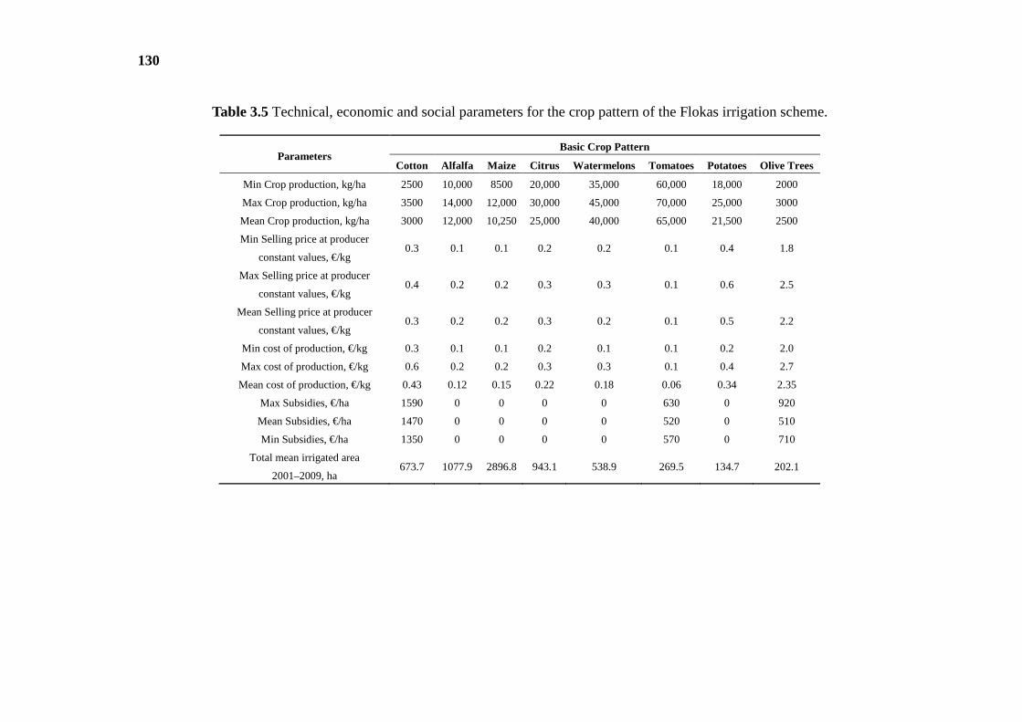
130

Table 3.5 Technical, economic and social parameters for the crop pattern of the Flokas irrigation scheme.

Parameters Basic Crop Pattern

Cotton Alfalfa Maize Citrus Watermelons Tomatoes Potatoes Olive Trees

Min Crop production, kg/ha 2500 10,000 8500 20,000 35,000 60,000 18,000 2000

Max Crop production, kg/ha 3500 14,000 12,000 30,000 45,000 70,000 25,000 3000

Mean Crop production, kg/ha 3000 12,000 10,250 25,000 40,000 65,000 21,500 2500

Min Selling price at producer

constant values, €/kg 0.3 0.1 0.1 0.2 0.2 0.1 0.4 1.8

Max Selling price at producer

constant values, €/kg 0.4 0.2 0.2 0.3 0.3 0.1 0.6 2.5

Mean Selling price at producer

constant values, €/kg 0.3 0.2 0.2 0.3 0.2 0.1 0.5 2.2

Min cost of production, €/kg 0.3 0.1 0.1 0.2 0.1 0.1 0.2 2.0

Max cost of production, €/kg 0.6 0.2 0.2 0.3 0.3 0.1 0.4 2.7

Mean cost of production, €/kg 0.43 0.12 0.15 0.22 0.18 0.06 0.34 2.35

Max Subsidies, €/ha 1590 0 0 0 0 630 0 920

Mean Subsidies, €/ha 1470 0 0 0 0 520 0 510

Min Subsidies, €/ha 1350 0 0 0 0 570 0 710

Total mean irrigated area

2001–2009, ha 673.7 1077.9 2896.8 943.1 538.9 269.5 134.7 202.1

131

3.5.2 CROPWAT MODEL AND WATER -CROP YIELD RELATIONSHIP

In order to estimate the irrigation water requirements of the present Flokas crop

pattern for the 50 stochastic hydrologic scenarios, the FAO software, CROPWAT 8.0, has

been used. CROPWAT 8.0 software can calculate evapotranspiration, crop water

requirements, scheme water supply and irrigation scheduling. The first input parameter of

the model, the reference evapotranspiration (ET0), representing the potential evaporation of

a well-watered grass crop, is computed externally by using the Thornthwaite method from

the mean monthly temperature of the last simulated year of each stochastic hydrologic

scenario. The second parameter to enter into the model is the rainfall, which is taken as

equal to the mean monthly rainfall of the last simulated year of each stochastic hydrologic

scenario. The effective rainfall is estimated internally in CROPWAT, using the USDA Soil

Conservation Service empirical formula developed by the Unified Soil Classified Service

(USCS), and is not based on more accurate data, such as from the hydrologic simulation of

the Flokas subbasin due to the absence of the necessary data (the absence of measured

discharge data).

Additionally, the crop characteristics of the Flokas irrigation scheme are required as

the third parameter of the model. Information, such as the length of the growth periods,

crop factors, rooting depths, etc., have been collected and entered into CROPWAT for each

crop. In the absence of regional data, CROPWAT 8.0 provides the possibility for several

crops’ data based on the selected FAO publications. These data have been adjusted to the

specific conditions of Greece and more precisely to the Region of Hleias. For crops that

have various planting dates, such as alfalfa, depending on the number of its cuts, more than

one planting date is defined. In Table 6, the Flokas total irrigation water demand (m3) for

one of the 50 stochastic hydrologic scenarios is presented, including the total irrigation

water demands in m3 for each crop: (1) estimated by CROPWAT 8.0; (2) estimated by

CROPWAT 8.0, but taking also into account the minimum losses of the Flokas irrigation

canal (20%) and the maximum efficiency of each irrigation type used (surface irrigation:

0.75; sprinklers: 0.80; and drip irrigation: 0.95); and (3) estimated by CROPWAT 8.0, but

taking also into account the maximum losses of the Flokas irrigation canal (30%) and the

minimum efficiency of each irrigation type used (surface irrigation: 0.5; sprinklers: 0.6;

and drip irrigation: 0.8).

The unit benefit from each m3 of water allocated to irrigation is based on the data of

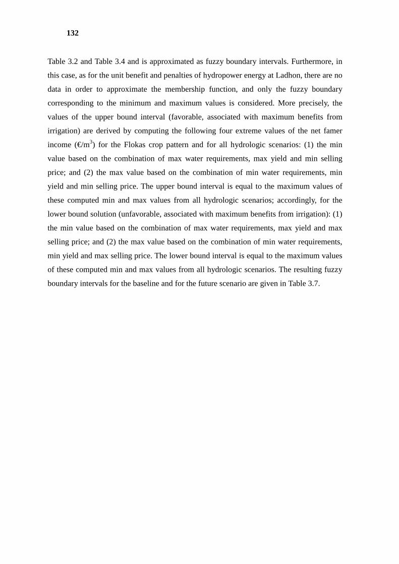
132

Table 3.2 and Table 3.4 and is approximated as fuzzy boundary intervals. Furthermore, in

this case, as for the unit benefit and penalties of hydropower energy at Ladhon, there are no

data in order to approximate the membership function, and only the fuzzy boundary

corresponding to the minimum and maximum values is considered. More precisely, the

values of the upper bound interval (favorable, associated with maximum benefits from

irrigation) are derived by computing the following four extreme values of the net famer

income (€/m3) for the Flokas crop pattern and for all hydrologic scenarios: (1) the min

value based on the combination of max water requirements, max yield and min selling

price; and (2) the max value based on the combination of min water requirements, min

yield and min selling price. The upper bound interval is equal to the maximum values of

these computed min and max values from all hydrologic scenarios; accordingly, for the

lower bound solution (unfavorable, associated with maximum benefits from irrigation): (1)

the min value based on the combination of max water requirements, max yield and max

selling price; and (2) the max value based on the combination of min water requirements,

min yield and max selling price. The lower bound interval is equal to the maximum values

of these computed min and max values from all hydrologic scenarios. The resulting fuzzy

boundary intervals for the baseline and for the future scenario are given in Table 3.7.

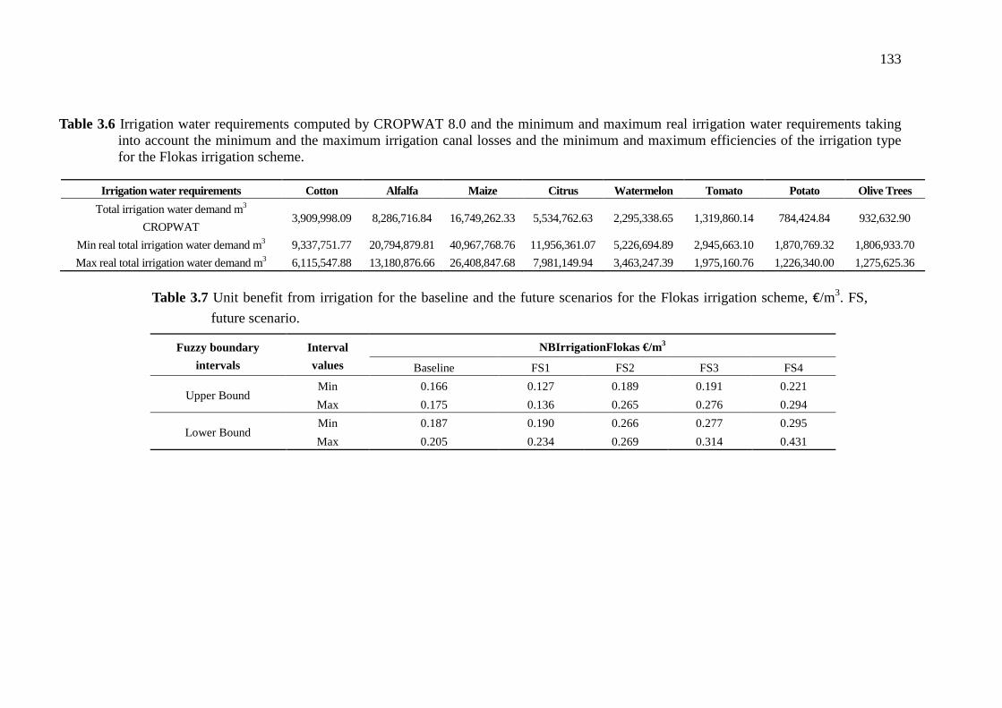
133

Table 3.6 Irrigation water requirements computed by CROPWAT 8.0 and the minimum and maximum real irrigation water requirements taking into account the minimum and the maximum irrigation canal losses and the minimum and maximum efficiencies of the irrigation type for the Flokas irrigation scheme.

Irrigation water requirements Cotton Alfalfa Maize Citrus Watermelon Tomato Potato Olive Trees

Total irrigation water demand m3

CROPWAT 3,909,998.09 8,286,716.84 16,749,262.33 5,534,762.63 2,295,338.65 1,319,860.14 784,424.84 932,632.90

Min real total irrigation water demand m3 9,337,751.77 20,794,879.81 40,967,768.76 11,956,361.07 5,226,694.89 2,945,663.10 1,870,769.32 1,806,933.70

Max real total irrigation water demand m3 6,115,547.88 13,180,876.66 26,408,847.68 7,981,149.94 3,463,247.39 1,975,160.76 1,226,340.00 1,275,625.36

Table 3.7 Unit benefit from irrigation for the baseline and the future scenarios for the Flokas irrigation scheme, €/m3. FS,

future scenario.

Fuzzy boundary

intervals

Interval

values

NBIrrigationFlokas €/m 3

Baseline FS1 FS2 FS3 FS4

Upper Bound Min 0.166 0.127 0.189 0.191 0.221

Max 0.175 0.136 0.265 0.276 0.294

Lower Bound Min 0.187 0.190 0.266 0.277 0.295

Max 0.205 0.234 0.269 0.314 0.431

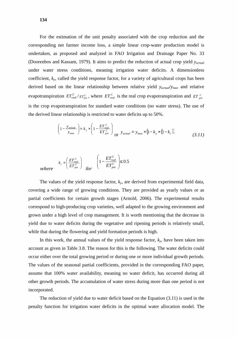
134

For the estimation of the unit penalty associated with the crop reduction and the

corresponding net farmer income loss, a simple linear crop-water production model is

undertaken, as proposed and analyzed in FAO Irrigation and Drainage Paper No. 33

(Doorenbos and Kassam, 1979). It aims to predict the reduction of actual crop yield yactual

under water stress conditions, meaning irrigation water deficits. A dimensionless

coefficient, ky, called the yield response factor, for a variety of agricultural crops has been

derived based on the linear relationship between relative yield yactual/ymax and relative

evapotranspiration CrealET / C

potET , where CrealET is the real crop evapotranspiration and CpotET

is the crop evapotranspiration for standard water conditions (no water stress). The use of

the derived linear relationship is restricted to water deficits up to 50%.

−×=

− C

pot

Creal

yactual

ET

ETk

y

y11

max or ( )( )ryactual kkyy −×−×= 11max

(3.11)

where

= C

pot

Creal

r ET

ETk for 5.01 ≤

−

Cpot

Creal

ET

ET

The values of the yield response factor, ky, are derived from experimental field data,

covering a wide range of growing conditions. They are provided as yearly values or as

partial coefficients for certain growth stages (Arnold, 2006). The experimental results

correspond to high-producing crop varieties, well adapted to the growing environment and

grown under a high level of crop management. It is worth mentioning that the decrease in

yield due to water deficits during the vegetative and ripening periods is relatively small,

while that during the flowering and yield formation periods is high.

In this work, the annual values of the yield response factor, ky, have been taken into

account as given in Table 3.8. The reason for this is the following. The water deficits could

occur either over the total growing period or during one or more individual growth periods.

The values of the seasonal partial coefficients, provided in the corresponding FAO paper,

assume that 100% water availability, meaning no water deficit, has occurred during all

other growth periods. The accumulation of water stress during more than one period is not

incorporated.

The reduction of yield due to water deficit based on the Equation (3.11) is used in the

penalty function for irrigation water deficits in the optimal water allocation model. The

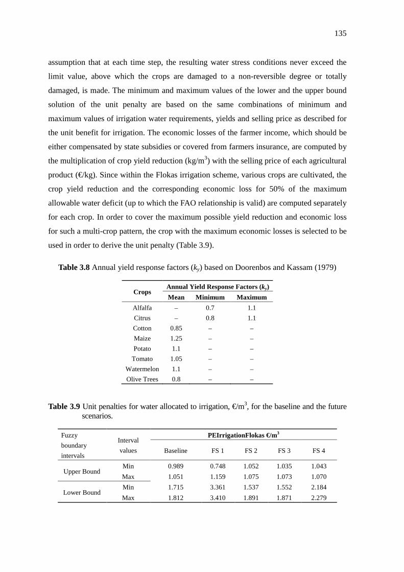
135

assumption that at each time step, the resulting water stress conditions never exceed the

limit value, above which the crops are damaged to a non-reversible degree or totally

damaged, is made. The minimum and maximum values of the lower and the upper bound

solution of the unit penalty are based on the same combinations of minimum and

maximum values of irrigation water requirements, yields and selling price as described for

the unit benefit for irrigation. The economic losses of the farmer income, which should be

either compensated by state subsidies or covered from farmers insurance, are computed by

the multiplication of crop yield reduction (kg/m3) with the selling price of each agricultural

product (€/kg). Since within the Flokas irrigation scheme, various crops are cultivated, the

crop yield reduction and the corresponding economic loss for 50% of the maximum

allowable water deficit (up to which the FAO relationship is valid) are computed separately

for each crop. In order to cover the maximum possible yield reduction and economic loss

for such a multi-crop pattern, the crop with the maximum economic losses is selected to be

used in order to derive the unit penalty (Table 3.9).

Table 3.8 Annual yield response factors (ky) based on Doorenbos and Kassam (1979)

Crops Annual Yield Response Factors (ky)

Mean Minimum Maximum

Alfalfa – 0.7 1.1

Citrus – 0.8 1.1

Cotton 0.85 – –

Maize 1.25 – –

Potato 1.1 – –

Tomato 1.05 – –

Watermelon 1.1 – –

Olive Trees 0.8 – –

Table 3.9 Unit penalties for water allocated to irrigation, €/m3, for the baseline and the future

scenarios.

Fuzzy

boundary

intervals

Interval

values

PEIrrigationFlokas €/m3

Baseline FS 1 FS 2 FS 3 FS 4

Upper Bound Min 0.989 0.748 1.052 1.035 1.043

Max 1.051 1.159 1.075 1.073 1.070

Lower Bound Min 1.715 3.361 1.537 1.552 2.184

Max 1.812 3.410 1.891 1.871 2.279

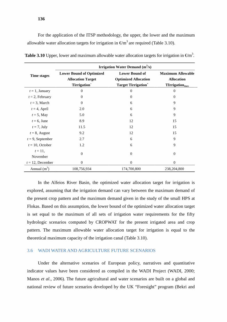
136

For the application of the ITSP methodology, the upper, the lower and the maximum

allowable water allocation targets for irrigation in €/m3 are required (Table 3.10).

Table 3.10 Upper, lower and maximum allowable water allocation targets for irrigation in €/m3.

Time stages

Irrigation Water Demand (m 3/s)

Lower Bound of Optimized

Allocation Target

Tirrigation −

Lower Bound of

Optimized Allocation

Target Tirrigation +

Maximum Allowable

Allocation

TIrrigation max

t = 1, January 0 0 0

t = 2, February 0 0 0

t = 3, March 0 6 9

t = 4, April 2.0 6 9

t = 5, May 5.0 6 9

t = 6, June 8.9 12 15

t = 7, July 11.5 12 15

t = 8, August 9.2 12 15

t = 9, September 2.7 6 9

t = 10, October 1.2 6 9

t = 11,

November 0 0 0

t = 12, December 0 0 0

Annual (m3) 108,756,934 174,700,800 238,204,800

In the Alfeios River Basin, the optimized water allocation target for irrigation is

explored, assuming that the irrigation demand can vary between the maximum demand of

the present crop pattern and the maximum demand given in the study of the small HPS at

Flokas. Based on this assumption, the lower bound of the optimized water allocation target

is set equal to the maximum of all sets of irrigation water requirements for the fifty

hydrologic scenarios computed by CROPWAT for the present irrigated area and crop

pattern. The maximum allowable water allocation target for irrigation is equal to the

theoretical maximum capacity of the irrigation canal (Table 3.10).

3.6 WADI WATER AND AGRICULTURE FUTURE SCENARIOS

Under the alternative scenarios of European policy, narratives and quantitative

indicator values have been considered as compiled in the WADI Project (WADI, 2000;

Manos et al., 2006). The future agricultural and water scenarios are built on a global and

national review of future scenarios developed by the UK “Foresight” program (Bekri and

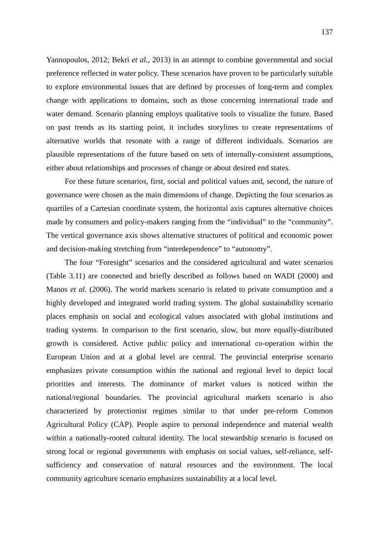
137

Yannopoulos, 2012; Bekri et al., 2013) in an attempt to combine governmental and social

preference reflected in water policy. These scenarios have proven to be particularly suitable

to explore environmental issues that are defined by processes of long-term and complex

change with applications to domains, such as those concerning international trade and

water demand. Scenario planning employs qualitative tools to visualize the future. Based

on past trends as its starting point, it includes storylines to create representations of

alternative worlds that resonate with a range of different individuals. Scenarios are

plausible representations of the future based on sets of internally-consistent assumptions,

either about relationships and processes of change or about desired end states.

For these future scenarios, first, social and political values and, second, the nature of

governance were chosen as the main dimensions of change. Depicting the four scenarios as

quartiles of a Cartesian coordinate system, the horizontal axis captures alternative choices

made by consumers and policy-makers ranging from the “individual” to the “community”.

The vertical governance axis shows alternative structures of political and economic power

and decision-making stretching from “interdependence” to “autonomy”.

The four “Foresight” scenarios and the considered agricultural and water scenarios

(Table 3.11) are connected and briefly described as follows based on WADI (2000) and

Manos et al. (2006). The world markets scenario is related to private consumption and a

highly developed and integrated world trading system. The global sustainability scenario

places emphasis on social and ecological values associated with global institutions and

trading systems. In comparison to the first scenario, slow, but more equally-distributed

growth is considered. Active public policy and international co-operation within the

European Union and at a global level are central. The provincial enterprise scenario

emphasizes private consumption within the national and regional level to depict local

priorities and interests. The dominance of market values is noticed within the

national/regional boundaries. The provincial agricultural markets scenario is also

characterized by protectionist regimes similar to that under pre-reform Common

Agricultural Policy (CAP). People aspire to personal independence and material wealth

within a nationally-rooted cultural identity. The local stewardship scenario is focused on

strong local or regional governments with emphasis on social values, self-reliance, self-

sufficiency and conservation of natural resources and the environment. The local

community agriculture scenario emphasizes sustainability at a local level.

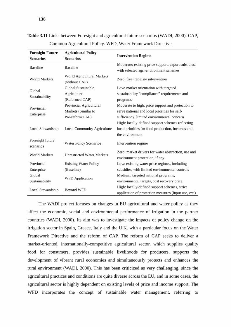
138

Table 3.11 Links between Foresight and agricultural future scenarios (WADI, 2000). CAP,

Common Agricultural Policy. WFD, Water Framework Directive.

Foresight Future

Scenarios

Agricultural Policy

Scenarios Intervention Regime

Baseline Baseline Moderate: existing price support, export subsidies,

with selected agri-environment schemes

World Markets World Agricultural Markets

(without CAP) Zero: free trade, no intervention

Global

Sustainability

Global Sustainable

Agriculture

(Reformed CAP)

Low: market orientation with targeted

sustainability “compliance” requirements and

programs

Provincial

Enterprise

Provincial Agricultural

Markets (Similar to

Pre-reform CAP)

Moderate to high: price support and protection to

serve national and local priorities for self-

sufficiency, limited environmental concern

Local Stewardship Local Community Agriculture

High: locally-defined support schemes reflecting

local priorities for food production, incomes and

the environment

Foresight future

scenarios Water Policy Scenarios Intervention regime

World Markets Unrestricted Water Markets Zero: market drivers for water abstraction, use and

environment protection, if any

Provincial

Enterprise

Existing Water Policy

(Baseline)

Low: existing water price regimes, including

subsidies, with limited environmental controls

Global

Sustainability WFD Application

Medium: targeted national programs,

environmental targets, cost recovery price.

Local Stewardship Beyond WFD High: locally-defined support schemes, strict

application of protection measures (input use, etc.)

The WADI project focuses on changes in EU agricultural and water policy as they

affect the economic, social and environmental performance of irrigation in the partner

countries (WADI, 2000). Its aim was to investigate the impacts of policy change on the

irrigation sector in Spain, Greece, Italy and the U.K. with a particular focus on the Water

Framework Directive and the reform of CAP. The reform of CAP seeks to deliver a

market-oriented, internationally-competitive agricultural sector, which supplies quality

food for consumers, provides sustainable livelihoods for producers, supports the

development of vibrant rural economies and simultaneously protects and enhances the

rural environment (WADI, 2000). This has been criticized as very challenging, since the

agricultural practices and conditions are quite diverse across the EU, and in some cases, the

agricultural sector is highly dependent on existing levels of price and income support. The

WFD incorporates the concept of sustainable water management, referring to

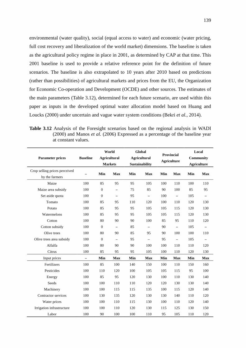
139

environmental (water quality), social (equal access to water) and economic (water pricing,

full cost recovery and liberalization of the world market) dimensions. The baseline is taken

as the agricultural policy regime in place in 2001, as determined by CAP at that time. This

2001 baseline is used to provide a relative reference point for the definition of future

scenarios. The baseline is also extrapolated to 10 years after 2010 based on predictions

(rather than possibilities) of agricultural markets and prices from the EU, the Organization

for Economic Co-operation and Development (OCDE) and other sources. The estimates of

the main parameters (Table 3.12), determined for each future scenario, are used within this

paper as inputs in the developed optimal water allocation model based on Huang and

Loucks (2000) under uncertain and vague water system conditions (Bekri et al., 2014).

Table 3.12 Analysis of the Foresight scenarios based on the regional analysis in WADI (2000) and Manos et al. (2006) Expressed as a percentage of the baseline year at constant values.

Parameter prices Baseline

World

Agricultural

Markets

Global

Agricultural

Sustainability

Provincial

Agriculture

Local

Community

Agriculture

Crop selling prices perceived

by the farmers – Min Max Min Max Min Max Min Max

Maize 100 85 95 95 105 100 110 100 110

Maize area subsidy 100 0 – 75 85 90 100 85 95

Set aside quota 100 0 – 95 – 100 – 105 –

Tomato 100 85 95 110 120 100 110 120 130

Potato 100 85 95 95 105 105 115 120 130

Watermelons 100 85 95 95 105 105 115 120 130

Cotton 100 80 90 90 100 85 95 110 120

Cotton subsidy 100 0 – 85 – 90 – 105 –

Olive trees 100 80 90 85 95 90 100 100 110

Olive trees area subsidy 100 0 – 95 – 95 – 105 –

Alfalfa 100 80 90 90 100 100 110 110 120

Citrus 100 85 95 95 105 100 110 120 130

Input prices – Min Max Min Max Min Max Min Max

Fertilizers 100 85 100 140 150 100 110 150 160

Pesticides 100 110 120 100 105 105 115 95 100

Energy 100 85 95 120 130 100 110 130 140

Seeds 100 100 110 110 120 120 130 130 140

Machinery 100 100 115 115 135 100 115 120 140

Contractor services 100 130 135 120 130 130 140 110 120

Water prices 100 100 110 115 130 100 110 120 140

Irrigation infrastructure 100 100 110 120 130 115 125 130 150

Labor 100 90 100 100 110 95 105 110 120

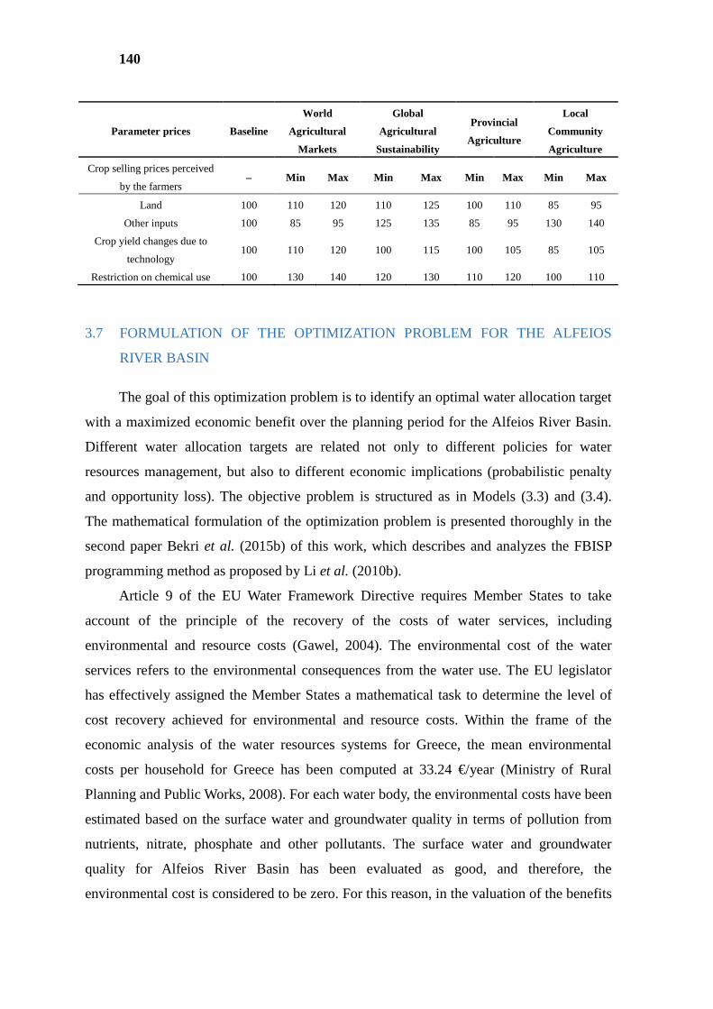
140

Parameter prices Baseline

World

Agricultural

Markets

Global

Agricultural

Sustainability

Provincial

Agriculture

Local

Community

Agriculture

Crop selling prices perceived

by the farmers – Min Max Min Max Min Max Min Max

Land 100 110 120 110 125 100 110 85 95

Other inputs 100 85 95 125 135 85 95 130 140

Crop yield changes due to

technology 100 110 120 100 115 100 105 85 105

Restriction on chemical use 100 130 140 120 130 110 120 100 110

3.7 FORMULATION OF THE OPTIMIZATION PROBLEM FOR THE ALFEIOS

RIVER BASIN

The goal of this optimization problem is to identify an optimal water allocation target

with a maximized economic benefit over the planning period for the Alfeios River Basin.

Different water allocation targets are related not only to different policies for water

resources management, but also to different economic implications (probabilistic penalty

and opportunity loss). The objective problem is structured as in Models (3.3) and (3.4).

The mathematical formulation of the optimization problem is presented thoroughly in the

second paper Bekri et al. (2015b) of this work, which describes and analyzes the FBISP

programming method as proposed by Li et al. (2010b).

Article 9 of the EU Water Framework Directive requires Member States to take

account of the principle of the recovery of the costs of water services, including

environmental and resource costs (Gawel, 2004). The environmental cost of the water

services refers to the environmental consequences from the water use. The EU legislator

has effectively assigned the Member States a mathematical task to determine the level of

cost recovery achieved for environmental and resource costs. Within the frame of the

economic analysis of the water resources systems for Greece, the mean environmental

costs per household for Greece has been computed at 33.24 €/year (Ministry of Rural

Planning and Public Works, 2008). For each water body, the environmental costs have been

estimated based on the surface water and groundwater quality in terms of pollution from

nutrients, nitrate, phosphate and other pollutants. The surface water and groundwater

quality for Alfeios River Basin has been evaluated as good, and therefore, the

environmental cost is considered to be zero. For this reason, in the valuation of the benefits

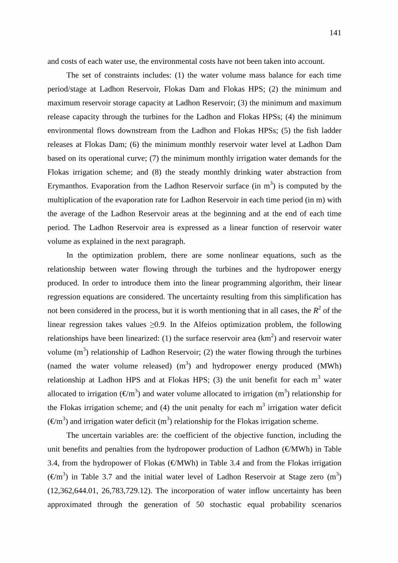
141

and costs of each water use, the environmental costs have not been taken into account.

The set of constraints includes: (1) the water volume mass balance for each time

period/stage at Ladhon Reservoir, Flokas Dam and Flokas HPS; (2) the minimum and

maximum reservoir storage capacity at Ladhon Reservoir; (3) the minimum and maximum

release capacity through the turbines for the Ladhon and Flokas HPSs; (4) the minimum

environmental flows downstream from the Ladhon and Flokas HPSs; (5) the fish ladder

releases at Flokas Dam; (6) the minimum monthly reservoir water level at Ladhon Dam

based on its operational curve; (7) the minimum monthly irrigation water demands for the

Flokas irrigation scheme; and (8) the steady monthly drinking water abstraction from

Erymanthos. Evaporation from the Ladhon Reservoir surface (in m3) is computed by the

multiplication of the evaporation rate for Ladhon Reservoir in each time period (in m) with

the average of the Ladhon Reservoir areas at the beginning and at the end of each time

period. The Ladhon Reservoir area is expressed as a linear function of reservoir water

volume as explained in the next paragraph.

In the optimization problem, there are some nonlinear equations, such as the

relationship between water flowing through the turbines and the hydropower energy

produced. In order to introduce them into the linear programming algorithm, their linear

regression equations are considered. The uncertainty resulting from this simplification has

not been considered in the process, but it is worth mentioning that in all cases, the R2 of the

linear regression takes values ≥0.9. In the Alfeios optimization problem, the following

relationships have been linearized: (1) the surface reservoir area (km2) and reservoir water

volume (m3) relationship of Ladhon Reservoir; (2) the water flowing through the turbines

(named the water volume released) (m3) and hydropower energy produced (MWh)

relationship at Ladhon HPS and at Flokas HPS; (3) the unit benefit for each m3 water

allocated to irrigation (€/m3) and water volume allocated to irrigation (m3) relationship for

the Flokas irrigation scheme; and (4) the unit penalty for each m3 irrigation water deficit

(€/m3) and irrigation water deficit (m3) relationship for the Flokas irrigation scheme.

The uncertain variables are: the coefficient of the objective function, including the

unit benefits and penalties from the hydropower production of Ladhon (€/MWh) in Table

3.4, from the hydropower of Flokas (€/MWh) in Table 3.4 and from the Flokas irrigation

(€/m3) in Table 3.7 and the initial water level of Ladhon Reservoir at Stage zero (m3)

(12,362,644.01, 26,783,729.12). The incorporation of water inflow uncertainty has been

approximated through the generation of 50 stochastic equal probability scenarios

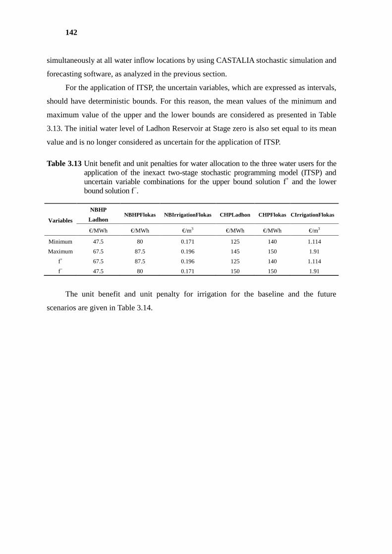
142

simultaneously at all water inflow locations by using CASTALIA stochastic simulation and

forecasting software, as analyzed in the previous section.

For the application of ITSP, the uncertain variables, which are expressed as intervals,

should have deterministic bounds. For this reason, the mean values of the minimum and

maximum value of the upper and the lower bounds are considered as presented in Table

3.13. The initial water level of Ladhon Reservoir at Stage zero is also set equal to its mean

value and is no longer considered as uncertain for the application of ITSP.

Table 3.13 Unit benefit and unit penalties for water allocation to the three water users for the application of the inexact two-stage stochastic programming model (ITSP) and uncertain variable combinations for the upper bound solution f+ and the lower bound solution f−.

Variables

NBHP

Ladhon NBHPFlokas NBIrrigationFlokas CHPLadhon CHPFlokas CIrrigationFlokas

€/MWh €/MWh €/m3 €/MWh €/MWh €/m3

Minimum 47.5 80 0.171 125 140 1.114

Maximum 67.5 87.5 0.196 145 150 1.91

f+ 67.5 87.5 0.196 125 140 1.114

f− 47.5 80 0.171 150 150 1.91

The unit benefit and unit penalty for irrigation for the baseline and the future

scenarios are given in Table 3.14.

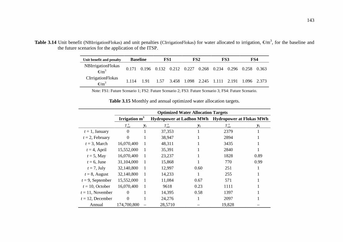
143

Table 3.14 Unit benefit (NBIrrigationFlokas) and unit penalties (CIrrigationFlokas) for water allocated to irrigation, €/m3, for the baseline and the future scenarios for the application of the ITSP.

Unit benefit and penalty Baseline FS1 FS2 FS3 FS4 NBIrrigationFlokas

€/m3 0.171 0.196 0.132 0.212 0.227 0.268 0.234 0.296 0.258 0.363

CIrrigationFlokas €/m3

1.114 1.91 1.57 3.458 1.098 2.245 1.111 2.191 1.096 2.373

Note: FS1: Future Scenario 1; FS2: Future Scenario 2; FS3: Future Scenario 3; FS4: Future Scenario.

Table 3.15 Monthly and annual optimized water allocation targets.

Optimized Water Allocation Targets Irrigation m 3 Hydropower at Ladhon MWh Hydropower at Flokas MWh

±optT yi ±

optT yi ±optT yi

t = 1, January 0 1 37,353 1 2379 1 t = 2, February 0 1 38,947 1 2894 1 t = 3, March 16,070,400 1 48,311 1 3435 1 t = 4, April 15,552,000 1 35,391 1 2840 1 t = 5, May 16,070,400 1 23,237 1 1828 0.89 t = 6, June 31,104,000 1 15,868 1 770 0.99 t = 7, July 32,140,800 1 12,997 0.60 251 1

t = 8, August 32,140,800 1 14,233 1 255 1 t = 9, September 15,552,000 1 11,084 0.67 571 1 t = 10, October 16,070,400 1 9618 0.23 1111 1

t = 11, November 0 1 14,395 0.58 1397 1 t = 12, December 0 1 24,276 1 2097 1

Annual 174,700,800 – 28,5710 – 19,828 –

144

145

3.8 RESULTS

For each of the two models solved (f+ and f−) as described above, (1) the optimized

water allocation target for each time stage (the twelve months of the examined year), as

well as for total annual (as the summation of the values of the twelve time stages), (2) the

probabilistic shortages and allocations for each one of the 50 hydrologic scenarios and for

each of the three water users for each time stage (the twelve months of the examined year),

as well as for the total annual (as the summation of the values of the twelve time stages)

and (3) the total benefits and the benefits and penalties for each of the three water users are

derived. The analysis of these results concerns the baseline scenario and also the effect of

the different water and agriculture policies represented by the four future scenarios on the

benefits and penalties of the baseline scenario.

The results derived from this methodology for the objective function, meaning the

net benefits from the water allocated to the three water users, as well as the non-zero water

allocation and shortages are expressed as intervals. The resulting solutions provide stable

intervals for the objective function and decision variables, which can be easily interpreted

for generating decision alternatives (Huang and Loucks, 2000). The values of +optf and −

optf

depict the two extreme conditions of the total net benefit of the system, ranging between

their upper and lower bounds. This solution process may result in extremely high system

benefits under favorable conditions, but it may also lead to high penalties in the case of

shortages in relation to the corresponding water allocation targets. This uncertainty

produces broad intervals between the upper and the lower bounds of ±optf .

From the solution of the model f+ for the Alfeios River Basin, the optimized water

allocation targets for the three water uses are computed and presented in Table 3.15. Based

on the yi values, the monthly optimized water allocation target values for irrigation are

equal to the maximum possible allocation, TIrrigation+. For the hydropower production at

Ladhon, the monthly optimized hydropower production target values are equal to the

maximum possible, THydroLadhon+, for all months except June (60% of its maximum

value), September (67% of its maximum value), October (23% of its maximum value) and

November (58% of its maximum value). For the hydropower production at Flokas, the

monthly optimized hydropower production target values are equal to the maximum

possible allocation, THydroLadhon+, for all months, except May (89% of its maximum

value) and June (99% of its maximum value). From these results, it is concluded that the

146

highest priority is set to irrigation, since it has the highest unit benefit, but at the same time

also the highest unit penalty. The next two priorities are set to the hydropower production

at Flokas, and last, but not least, to the hydropower production at Ladhon, which has the

smallest unit benefit.

The optimized water allocation targets are the same also for the four WADI future

scenarios. The four WADI future scenarios mirror four different possible water and

agricultural policy alternatives in comparison to the baseline scenario, which may have an

impact on the optimal water allocation. The differences between the future scenarios

include, among others, changes of hydropower energy prices, water prices, selling prices of

the agricultural products, yield functions, subsidies, farmer income variable costs, labor

and fertilizers. Therefore, the main impact of these scenarios is on the net benefits from the

system.

In Table 3.16, (1) the total maximized net benefits (€) based on the optimized water

allocation targets for the three water uses and (2) the maximized benefits (€) and penalties

(€) of each water use for the baseline and the future scenarios are presented. The total

maximized net benefits of the hydro-system range between (131,565,871, 99,636,682) for

the baseline scenario. From this table, it is verified that for the lower bound model f−, the

benefits are lower and the penalties are higher in comparison to the corresponding results

from the upper bound model f+. The ratios of the benefits and penalties from the four future

scenarios in comparison to the baseline are also given in Table 3.16. It is worth mentioning

that the highest increase of the total system benefits is observed for the local stewardship

scenario ranging from 52%–59% for the total net system benefit (objective function value).

The only decrease of the net benefits compared to the benefits of the baseline scenario occurs

for the world market scenario (9%–24%).

The results for the annual shortage and the annual allocation (Table 3.17) for

irrigation, as computed by the optimization algorithm for the 50 hydrologic equal

probability scenarios, are provided. In most hydrologic scenarios, the water allocation is

equal to the desired target, therefore resulting in zero annual shortages. There are only a

few hydrologic scenarios with nonzero shortages. Among these scenarios, Hydrologic

Scenario 19 is the worst shortage condition. In this case, the annual water allocation

interval is (114,297,023, 1,528,400,127) in m3 and the corresponding shortage interval

(21,860,788, 60,403,777) in m3. By computing the shortage to target ratio, which varies

from 12.5%–34.6%, it is indicated that the shortage is serious. In this case, if the farmers

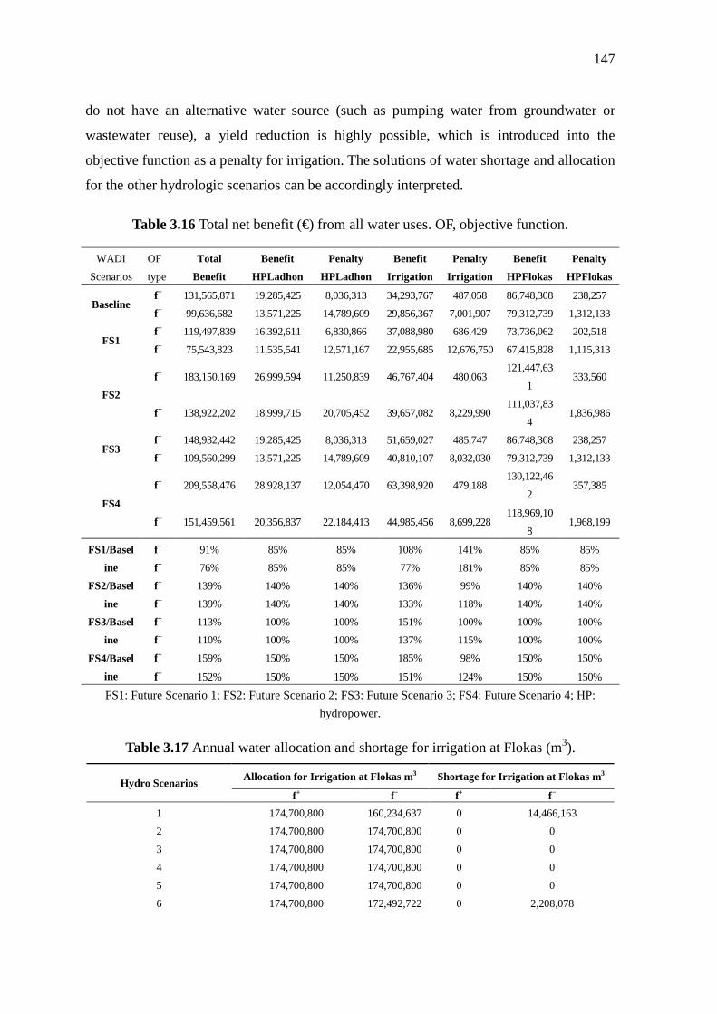
147

do not have an alternative water source (such as pumping water from groundwater or

wastewater reuse), a yield reduction is highly possible, which is introduced into the

objective function as a penalty for irrigation. The solutions of water shortage and allocation

for the other hydrologic scenarios can be accordingly interpreted.

Table 3.16 Total net benefit (€) from all water uses. OF, objective function.

WADI

Scenarios

OF

type

Total

Benefit

Benefit

HPLadhon

Penalty

HPLadhon

Benefit

Irrigation

Penalty

Irrigation

Benefit

HPFlokas

Penalty

HPFlokas

Baseline f+ 131,565,871 19,285,425 8,036,313 34,293,767 487,058 86,748,308 238,257

f− 99,636,682 13,571,225 14,789,609 29,856,367 7,001,907 79,312,739 1,312,133

FS1 f+ 119,497,839 16,392,611 6,830,866 37,088,980 686,429 73,736,062 202,518

f− 75,543,823 11,535,541 12,571,167 22,955,685 12,676,750 67,415,828 1,115,313

FS2

f+ 183,150,169 26,999,594 11,250,839 46,767,404 480,063 121,447,63

1 333,560

f− 138,922,202 18,999,715 20,705,452 39,657,082 8,229,990 111,037,83

4 1,836,986

FS3 f+ 148,932,442 19,285,425 8,036,313 51,659,027 485,747 86,748,308 238,257

f− 109,560,299 13,571,225 14,789,609 40,810,107 8,032,030 79,312,739 1,312,133

FS4

f+ 209,558,476 28,928,137 12,054,470 63,398,920 479,188 130,122,46

2 357,385

f− 151,459,561 20,356,837 22,184,413 44,985,456 8,699,228 118,969,10

8 1,968,199

FS1/Basel

ine

f+ 91% 85% 85% 108% 141% 85% 85%

f− 76% 85% 85% 77% 181% 85% 85%

FS2/Basel

ine

f+ 139% 140% 140% 136% 99% 140% 140%

f− 139% 140% 140% 133% 118% 140% 140%

FS3/Basel

ine

f+ 113% 100% 100% 151% 100% 100% 100%

f− 110% 100% 100% 137% 115% 100% 100%

FS4/Basel

ine

f+ 159% 150% 150% 185% 98% 150% 150%

f− 152% 150% 150% 151% 124% 150% 150%

FS1: Future Scenario 1; FS2: Future Scenario 2; FS3: Future Scenario 3; FS4: Future Scenario 4; HP:

hydropower.

Table 3.17 Annual water allocation and shortage for irrigation at Flokas (m3).

Hydro Scenarios Allocation for Irrigation at Flokas m 3 Shortage for Irrigation at Flokas m3

f+ f− f+ f−

1 174,700,800 160,234,637 0 14,466,163

2 174,700,800 174,700,800 0 0

3 174,700,800 174,700,800 0 0

4 174,700,800 174,700,800 0 0

5 174,700,800 174,700,800 0 0

6 174,700,800 172,492,722 0 2,208,078

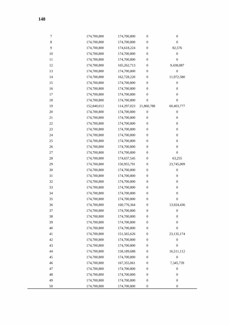
148

7 174,700,800 174,700,800 0 0

8 174,700,800 174,700,800 0 0

9 174,700,800 174,618,224 0 82,576

10 174,700,800 174,700,800 0 0

11 174,700,800 174,700,800 0 0

12 174,700,800 165,262,713 0 9,438,087

13 174,700,800 174,700,800 0 0

14 174,700,800 162,728,220 0 11,972,580

15 174,700,800 174,700,800 0 0

16 174,700,800 174,700,800 0 0

17 174,700,800 174,700,800 0 0

18 174,700,800 174,700,800 0 0

19 152,840,012 114,297,023 21,860,788 60,403,777

20 174,700,800 174,700,800 0 0

21 174,700,800 174,700,800 0 0

22 174,700,800 174,700,800 0 0

23 174,700,800 174,700,800 0 0

24 174,700,800 174,700,800 0 0

25 174,700,800 174,700,800 0 0

26 174,700,800 174,700,800 0 0

27 174,700,800 174,700,800 0 0

28 174,700,800 174,637,545 0 63,255

29 174,700,800 150,955,791 0 23,745,009

30 174,700,800 174,700,800 0 0

31 174,700,800 174,700,800 0 0

32 174,700,800 174,700,800 0 0

33 174,700,800 174,700,800 0 0

34 174,700,800 174,700,800 0 0

35 174,700,800 174,700,800 0 0

36 174,700,800 160,776,364 0 13,924,436

37 174,700,800 174,700,800 0 0

38 174,700,800 174,700,800 0 0

39 174,700,800 174,700,800 0 0

40 174,700,800 174,700,800 0 0

41 174,700,800 151,565,626 0 23,135,174

42 174,700,800 174,700,800 0 0

43 174,700,800 174,700,800 0 0

44 174,700,800 158,189,688 0 16,511,112

45 174,700,800 174,700,800 0 0

46 174,700,800 167,355,061 0 7,345,739

47 174,700,800 174,700,800 0 0

48 174,700,800 174,700,800 0 0

49 174,700,800 174,700,800 0 0

50 174,700,800 174,700,800 0 0

149

The results for the annual shortage and the annual hydropower production at Flokas

and Ladhon, as computed by the optimization algorithm for the 50 hydrologic equal

probability scenarios, are presented in Table 3.18. In most hydrologic scenarios, the

hydropower production is not equal to the desired target, therefore resulting in nonzero

annual shortages for both hydropower stations. There are only a few hydrologic scenarios

with zero shortages. Among these scenarios, Hydrologic Scenario 19 is the worst shortage

condition for the HPS at Ladhon. In this case, the annual hydropower production interval is

(25,943, 45,515) in MWh and the corresponding shortage interval (240,195, 259,767) in

MWh. By computing the shortage to target ratio, which varies from 84% to 90.9%, it is

indicated that the shortage is serious. Hydrologic Scenario 28 is the worst shortage

condition for the small HPS at Flokas. In this case, the annual hydropower production

interval is (5191, 12,729) in MWh and the corresponding shortage interval from the

desired target (7099, 14,637) in MWh. By computing the shortage to target ratio, which

varies from 35.8% to 73.8%, it is indicated that the shortage is serious.

The statistical analysis of the monthly water allocations and corresponding shortages

(due to the high amount of data) for all stages (twelve months) for the 50 hydrologic

scenarios is graphically presented in Figure 3.3 for the model f+ and the baseline scenarios

through the use of box plots for Alfeios River Basin in western Greece. Some very

interesting comments from these figures are given as follows. For the irrigation, the

shortages take place in August and September. This can be explained by the facts that the

flow rate at Flokas Dam for these two months is very low and that the irrigation demand is

increased. For the hydropower production at Ladhon, the highest shortages occur from

January–April (with the highest in March). This can be justified by the fact that the highest

priority in terms of the satisfaction of the desired target is set on irrigation. In order to

satisfy the irrigation demand, which starts mainly from May (having only a very low

demand also in April), the water volume flowing into the Ladhon Reservoir from

December–April should be stored and not released. Therefore, there is a conflict between

the two uses for this time period. Finally, for the hydropower production at Flokas, the

highest shortages occur from June–October (with the highest in October), which is the

irrigation period, revealing a conflict between the two uses. The operation of the small

HPS at Flokas is only set in operation after having satisfied irrigation, and this leads to the

shortages for these months.

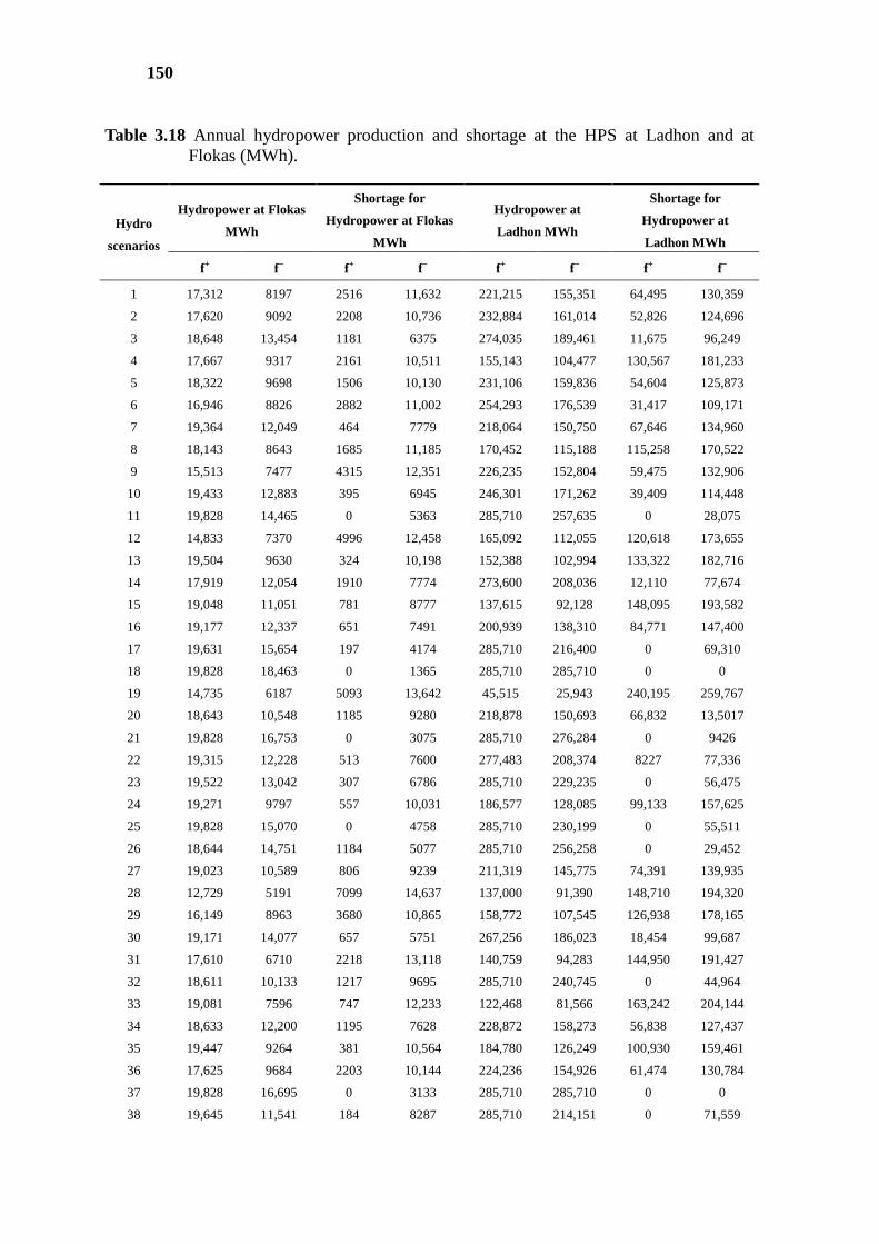
150

Table 3.18 Annual hydropower production and shortage at the HPS at Ladhon and at Flokas (MWh).

Hydro

scenarios

Hydropower at Flokas

MWh

Shortage for

Hydropower at Flokas

MWh

Hydropower at

Ladhon MWh

Shortage for

Hydropower at

Ladhon MWh

f+ f− f+ f− f+ f− f+ f−

1 17,312 8197 2516 11,632 221,215 155,351 64,495 130,359

2 17,620 9092 2208 10,736 232,884 161,014 52,826 124,696

3 18,648 13,454 1181 6375 274,035 189,461 11,675 96,249

4 17,667 9317 2161 10,511 155,143 104,477 130,567 181,233

5 18,322 9698 1506 10,130 231,106 159,836 54,604 125,873

6 16,946 8826 2882 11,002 254,293 176,539 31,417 109,171

7 19,364 12,049 464 7779 218,064 150,750 67,646 134,960

8 18,143 8643 1685 11,185 170,452 115,188 115,258 170,522

9 15,513 7477 4315 12,351 226,235 152,804 59,475 132,906

10 19,433 12,883 395 6945 246,301 171,262 39,409 114,448

11 19,828 14,465 0 5363 285,710 257,635 0 28,075

12 14,833 7370 4996 12,458 165,092 112,055 120,618 173,655

13 19,504 9630 324 10,198 152,388 102,994 133,322 182,716

14 17,919 12,054 1910 7774 273,600 208,036 12,110 77,674

15 19,048 11,051 781 8777 137,615 92,128 148,095 193,582

16 19,177 12,337 651 7491 200,939 138,310 84,771 147,400

17 19,631 15,654 197 4174 285,710 216,400 0 69,310

18 19,828 18,463 0 1365 285,710 285,710 0 0

19 14,735 6187 5093 13,642 45,515 25,943 240,195 259,767

20 18,643 10,548 1185 9280 218,878 150,693 66,832 13,5017

21 19,828 16,753 0 3075 285,710 276,284 0 9426

22 19,315 12,228 513 7600 277,483 208,374 8227 77,336

23 19,522 13,042 307 6786 285,710 229,235 0 56,475

24 19,271 9797 557 10,031 186,577 128,085 99,133 157,625

25 19,828 15,070 0 4758 285,710 230,199 0 55,511

26 18,644 14,751 1184 5077 285,710 256,258 0 29,452

27 19,023 10,589 806 9239 211,319 145,775 74,391 139,935

28 12,729 5191 7099 14,637 137,000 91,390 148,710 194,320

29 16,149 8963 3680 10,865 158,772 107,545 126,938 178,165

30 19,171 14,077 657 5751 267,256 186,023 18,454 99,687

31 17,610 6710 2218 13,118 140,759 94,283 144,950 191,427

32 18,611 10,133 1217 9695 285,710 240,745 0 44,964

33 19,081 7596 747 12,233 122,468 81,566 163,242 204,144

34 18,633 12,200 1195 7628 228,872 158,273 56,838 127,437

35 19,447 9264 381 10,564 184,780 126,249 100,930 159,461

36 17,625 9684 2203 10,144 224,236 154,926 61,474 130,784

37 19,828 16,695 0 3133 285,710 285,710 0 0

38 19,645 11,541 184 8287 285,710 214,151 0 71,559

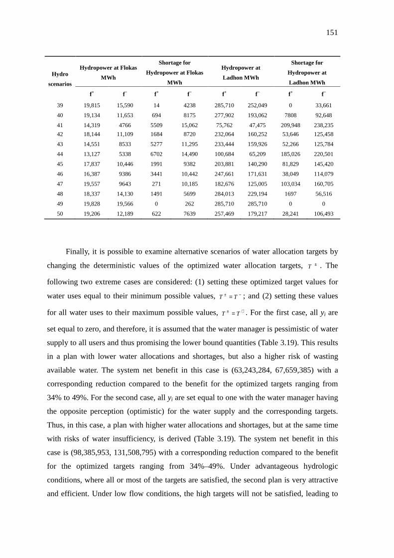
151

Hydro

scenarios

Hydropower at Flokas

MWh

Shortage for

Hydropower at Flokas

MWh

Hydropower at

Ladhon MWh

Shortage for

Hydropower at

Ladhon MWh

f+ f− f+ f− f+ f− f+ f−

39 19,815 15,590 14 4238 285,710 252,049 0 33,661

40 19,134 11,653 694 8175 277,902 193,062 7808 92,648

41 14,319 4766 5509 15,062 75,762 47,475 209,948 238,235

42 18,144 11,109 1684 8720 232,064 160,252 53,646 125,458

43 14,551 8533 5277 11,295 233,444 159,926 52,266 125,784

44 13,127 5338 6702 14,490 100,684 65,209 185,026 220,501

45 17,837 10,446 1991 9382 203,881 140,290 81,829 145,420

46 16,387 9386 3441 10,442 247,661 171,631 38,049 114,079

47 19,557 9643 271 10,185 182,676 125,005 103,034 160,705

48 18,337 14,130 1491 5699 284,013 229,194 1697 56,516

49 19,828 19,566 0 262 285,710 285,710 0 0

50 19,206 12,189 622 7639 257,469 179,217 28,241 106,493

Finally, it is possible to examine alternative scenarios of water allocation targets by

changing the deterministic values of the optimized water allocation targets, ±T . The

following two extreme cases are considered: (1) setting these optimized target values for

water uses equal to their minimum possible values, −± = TT ; and (2) setting these values

for all water uses to their maximum possible values, +± = TT . For the first case, all yi are

set equal to zero, and therefore, it is assumed that the water manager is pessimistic of water

supply to all users and thus promising the lower bound quantities (Table 3.19). This results

in a plan with lower water allocations and shortages, but also a higher risk of wasting

available water. The system net benefit in this case is (63,243,284, 67,659,385) with a

corresponding reduction compared to the benefit for the optimized targets ranging from

34% to 49%. For the second case, all yi are set equal to one with the water manager having

the opposite perception (optimistic) for the water supply and the corresponding targets.

Thus, in this case, a plan with higher water allocations and shortages, but at the same time

with risks of water insufficiency, is derived (Table 3.19). The system net benefit in this

case is (98,385,953, 131,508,795) with a corresponding reduction compared to the benefit

for the optimized targets ranging from 34%–49%. Under advantageous hydrologic

conditions, where all or most of the targets are satisfied, the second plan is very attractive

and efficient. Under low flow conditions, the high targets will not be satisfied, leading to

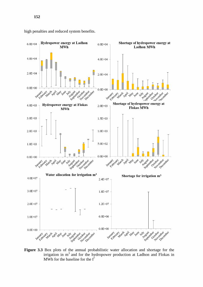
152

high penalties and reduced system benefits.

Figure 3.3 Box plots of the annual probabilistic water allocation and shortage for the irrigation in m3 and for the hydropower production at Ladhon and Flokas in MWh for the baseline for the f+

153

.

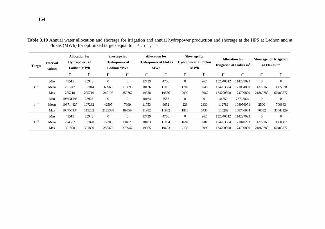
154

Table 3.19 Annual water allocation and shortage for irrigation and annual hydropower production and shortage at the HPS at Ladhon and at Flokas (MWh) for optimized targets equal to ±T , −T , +T .

Target Interval

values

Allocation for

Hydropower at

Ladhon MWh

Shortage for

Hydropower at

Ladhon MWh

Allocation for

Hydropower at Flokas

MWh

Shortage for

Hydropower at Flokas

MWh

Allocation for

Irrigation at Flokas m 3

Shortage for Irrigation

at Flokas m3

f+ f− f+ f− f+ f− f+ f− f+ f− f+ f−

±T

Min 45515 25943 0 0 12729 4766 0 262 152840012 114297023 0 0

Mean 221747 167014 63963 118696 18126 11081 1702 8748 174263584 171034880 437216 3665920

Max 285710 285710 240195 259767 19828 19566 7099 15062 174700800 174700800 21860788 60403777

−T

Min 106631595 25923 0 0 10164 5552 0 0 44750 73713804 0 0

Mean 108714427 107282 42507 7999 11753 9652 229 2330 112782 108056071 2500 700863

Max 108756934 115282 2125338 89359 11982 11982 1818 6430 115282 108756934 70532 35043129

+T

Min 45515 25943 0 0 12729 4766 0 262 152840012 114297023 0 0

Mean 224587 167870 77303 134020 18183 11084 1682 8781 174263584 171040293 437216 3660507

Max 301890 301890 256375 275947 19865 19603 7136 15099 174700800 174700800 21860788 60403777

155

3.9 DISCUSSION AND CONCLUSIONS

As analyzed in Huang and Loucks (2000), compared to the existing approaches for

resolving water resource management problems, the ITSP has advantages in data

availability, solution algorithms and computational requirements. In practical water

resource problems, the quality of information is in many cases quite uncertain and not

good enough to be expressed as a deterministic number or probability distribution. In this

case, it may be easier to obtain estimates of upper and lower bounds and to introduce them

into the optimization problem as interval numbers. The ITSP accepts this type of variable.

It is worth mentioning that even if the probability distributions of all uncertain variables

were available, it would be extremely difficult to solve a large multi-stage programming

model. The ITSP can efficiently communicate the intervals in a two-stage stochastic

optimization problem.

The Alfeios River Basin in Greece is selected for applying the ITSP method for

optimal water allocation, because it is characterized by uncertain and limited data, which

can be expressed easily as intervals, since the quality of the information is not good enough

to be presented as probability distributions. This is also a common problem met in other

Mediterranean countries. The total net benefits and the benefits and penalties of the main

water uses for Alfeios (hydropower energy and irrigation) are studied and analyzed within

the framework of the four WADI water and agricultural future scenarios through

investigation of technical, environmental and socio-economic aspects.

The hydropower energy market of Greece, crop patterns, yield functions, subsidies,

farmer income variable costs, market prices per agricultural product and fertilizers changes

are taken into account for the valuation and the estimation of their effect on the

hydropower energy and irrigation benefits of the hydro-system.

In terms of the results from this methodology, its goal is, from one side, to spot the

desired water allocation target with a minimized risk of economic penalty and opportunity

loss and, from the other side, to determine an optimized water allocation plan with a

maximized system benefit over a multi-period planning horizon. Deterministic upper and

lower bound intervals for the optimal water allocation targets and the probabilistic water

allocations and shortages, as well as for the total system benefits for the main water uses

are identified. The dynamics in terms of decisions for water allocation are mirrored

through the consideration of the various equal probability hydrologic scenarios. The results

156

acquired show that variations in water allocation targets could express different strategies

for water resources management and, thus, produce varied economic implications under

uncertainty.

The major results through the application of the ITSP methods to optimal water

resources allocation in the Alfeios River Basin are the following:

(1) The monthly optimized water allocation target values are equal to: (i) the

maximum possible allocation, TIrrigation+, for irrigation, (ii) the maximum possible

allocation, THydroLadhon+, for all months except June and September–November for the

hydropower production at Ladhon and (iii) the maximum possible allocation,

THydroLadhon+, for all months except May and June for the hydropower production at

Flokas. This sets the highest priority to irrigation with the highest unit benefit and, at the

same time, also the highest unit penalty. Then follows the hydropower production at Flokas

and last, but not least, the hydropower production at Ladhon with the smallest unit benefit.

(2) The optimized water allocation targets for the four WADI future scenarios

are the same as the ones for the baseline scenario, since the main impact of these scenarios

is on the net system benefits. Based on the comparison of the total system benefits from the

four future scenarios to the baseline, the highest increase is observed for the local

stewardship scenario and the only decrease for the world market scenario.

(3) For irrigation, in most hydrologic scenarios, annual water shortages are

zero, since the water allocation is equal to the optimized water allocation target. There are

only a few hydrologic scenarios with nonzero shortages, for which, if the farmers do not

have an alternative water source, a yield reduction is highly possible. These shortages

occur in August and September, which can be justified by the low flow rate at Flokas Dam

for these two months in combination with the increased irrigation demand. On the other

hand, the hydropower production at Ladhon and Flokas in most hydrologic scenarios

deviates from the optimized target, therefore resulting in nonzero annual shortages for both

hydropower stations. For the hydropower production at Ladhon, the highest shortages take

place from January–April (with the highest in March), since in order to satisfy completely

the most important water use, that being irrigation (starting mainly from May), the water

volume flowing into the Ladhon Reservoir from December–April should be stored and not

released. A conflict between the two uses for this time period is observed. For the

hydropower production at Flokas, the highest shortages occur during the irrigation period

from June–October (with the highest in October), showing a conflict between the two uses.

157

The small HPS at Flokas is only set in operation after the satisfaction of irrigation demand,

driving toward water shortages for these months if the available water at Flokas Dam is not

adequate.

According to Huang and Loucks (2000), some problems associated with the

application of the ITSP to large-scale real-world problems are the following. For large-

scale problems, including regulating reservoirs, the optimization formulations become very

complicated. In some water resources management problems, the complexity of

considering the persistence in hydrologic time series is present. Therefore, water

availability should be quantified through conditional probabilities. This may lead to non-

linearities in system responses. The second difficulty is related to the dynamics of the

hydro-systems. The evolution of a water problem in time involves many time stages. More

than three stages lead to a very complicated and large optimization model, in fact too big to

justify its use. The third problem is met in oversized models, which are complicated and

large. In this case, other methods, such as inexact multi-stage programming, nonlinear

ITSP and other more sophisticated hybrid processes, should be used.

An attempt to overcome some of the abovementioned weaknesses has been made

here by incorporating the water inflow uncertainty (system dynamics) through the

simultaneous generation of stochastic equal probability hydrologic scenarios considering

stochastically-dependent multiple variables at various locations of water inflows in the

river basin. This is enabled by using CASTALIA software for stochastic simulation and

forecasting of hydrologic variables, combining not only multivariate analysis, but also

multiple time scales (monthly and yearly) in a disaggregation framework. This software

permits the preservation of essential marginal statistics up to third order and joint second

order statistics (auto- and cross-correlations) and the reproduction of long-term persistence

(Hurst phenomenon) and periodicity.

In this application, twelve time periods/stages, one for each month of the examined

year, have been defined (whereas in Huang and Loucks (2000), only one stage has been

considered). Fifty equal probability hydrologic scenarios (in Huang and Loucks (2000),

only three flow scenarios: low, medium and high) have been generated. Such a formulation

of the ITSP problem includes 12 × 50 = 600 variables for probabilistic shortages and water

allocation for each water use. From the analysis of the results, it is clear that due to the

space limitations, the monthly results cannot be presented in tabular form and analyzed as

thoroughly as in Huang and Loucks (2000) due to their high number. Alternatively, the

158

monthly shortages and water allocations could be analyzed statistically for the 50

hydrologic equal probability scenarios through the building of box plots separately for each

month. It is worth mentioning that an increase of the number of the hydrologic scenarios

generated would increase the quality of this statistical analysis, but it would make the

analysis of the results even more complicated, setting also the matter of the use of this

methodology to a more complex time horizon. The development of more complex models

based on ITSP is proposed in order to increase its applicability even further to a higher

number of stages.

159

4. OPTIMAL WATER ALLOCATION UNDER UNCERTAIN

SYSTEM CONDITIONS: FBISP

4.1 INTRODUCTION

Optimal water allocation of a river basin poses great challenges for engineers due to

various uncertainties associated with the hydrosystem, its parameters and its impact factors

as well as their interactions. These uncertainties are often associated with various

complexities in terms of information quality (Li et al., 2009). The random characteristics

of natural processes (i.e., precipitation and climate change) and stream conditions (i.e.,

stream inflow, water supply, storage capacity, and river-quality requirement), the errors in

estimated modeling parameters (i.e., benefit and cost parameters), and the vagueness of

system objectives and constraints are all possible sources of uncertainties. These

uncertainties may exist in both left- and right-hand sides of the constraints as well as

coefficients of the objective function. Some uncertainties may be expressed as random

variables. At the same time, some random events can only be quantified as discrete intervals

with fuzzy boundaries, leading to multiple uncertainties presented as different formats in the

system's components (Li et al., 2010b). Traditional optimization techniques can embody

various characteristics but only as deterministic values. In various real-world problems,

results generated by these traditional optimization techniques could be rendered highly

questionable if the modeling inputs could not be expressed with precision (Li et al., 2009;

Fan and Huang, 2012; Suo et al., 2013). For these reasons conventional deterministic

optimization approaches have given their place to stochastic (SP), fuzzy (FP) and interval-

parameter programming (IPP) approaches and their hybrid combinations in order to face

up these difficulties. Various methodologies have been developed and proposed (Suo et al.,

2013; Huang et al., 1992; Huang and Loucks, 2000; Maqsood et al., 2005; Li et al., 2006;

Nie et al., 2007; Yeomans, 2008; Li and Huang, 2009; Li and Huang, 2011; Yeomans,

2008; Li and Huang, 2009; Li and Huang, 2011; Fu et al., 2013; Liu et al., 2014; Miao et

al., 2014; Li et al., 2008) in order to embody in optimal water allocation uncertainties of

various influencing factors and hydrosystem characteristics.

SP can handle uncertainties expressed as random variables with known probability

distributions and at the same time connect efficiently the pre-regulated policies and the

associated economic implications caused by improper policies (Li et al., 2010b). Stedinger

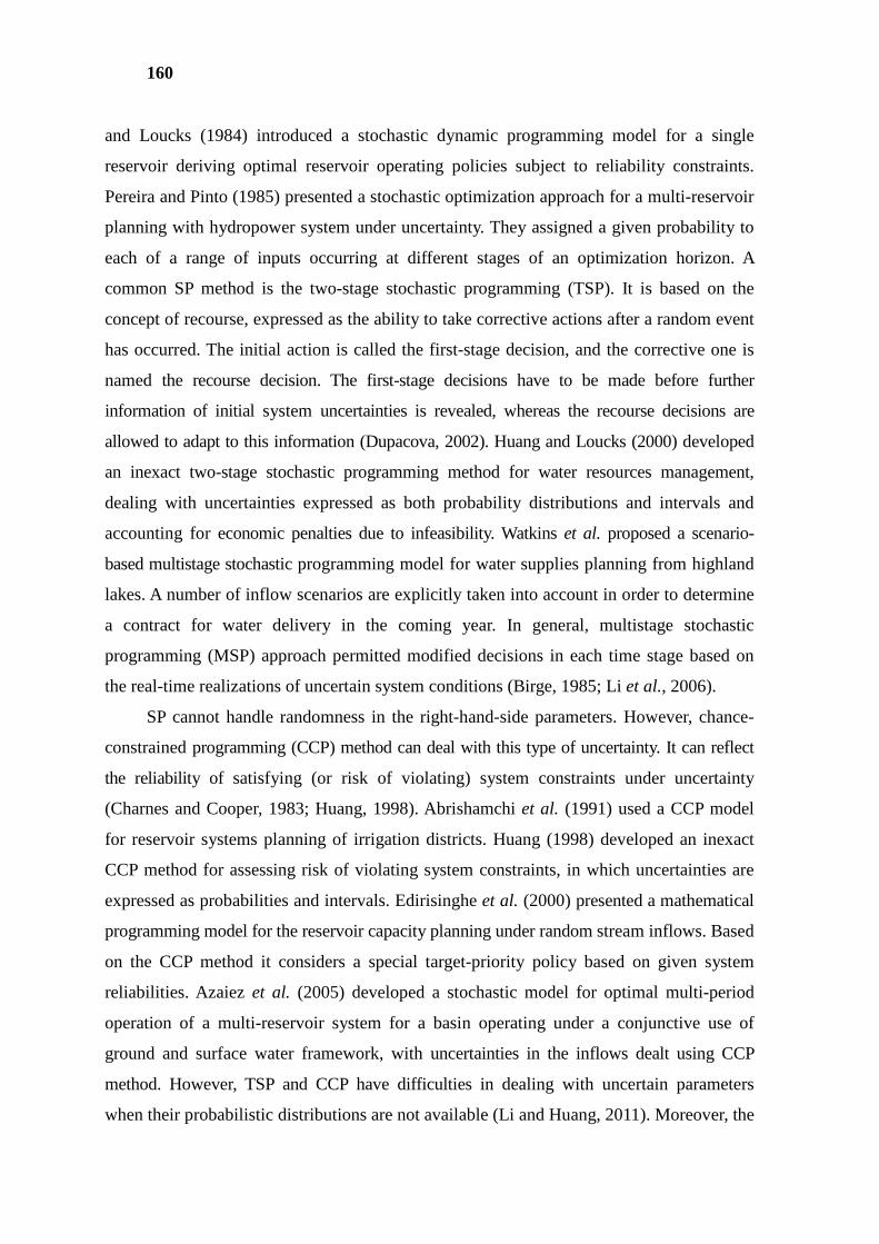
160

and Loucks (1984) introduced a stochastic dynamic programming model for a single

reservoir deriving optimal reservoir operating policies subject to reliability constraints.

Pereira and Pinto (1985) presented a stochastic optimization approach for a multi-reservoir

planning with hydropower system under uncertainty. They assigned a given probability to

each of a range of inputs occurring at different stages of an optimization horizon. A

common SP method is the two-stage stochastic programming (TSP). It is based on the

concept of recourse, expressed as the ability to take corrective actions after a random event

has occurred. The initial action is called the first-stage decision, and the corrective one is

named the recourse decision. The first-stage decisions have to be made before further

information of initial system uncertainties is revealed, whereas the recourse decisions are

allowed to adapt to this information (Dupacova, 2002). Huang and Loucks (2000) developed

an inexact two-stage stochastic programming method for water resources management,

dealing with uncertainties expressed as both probability distributions and intervals and

accounting for economic penalties due to infeasibility. Watkins et al. proposed a scenario-

based multistage stochastic programming model for water supplies planning from highland

lakes. A number of inflow scenarios are explicitly taken into account in order to determine

a contract for water delivery in the coming year. In general, multistage stochastic

programming (MSP) approach permitted modified decisions in each time stage based on

the real-time realizations of uncertain system conditions (Birge, 1985; Li et al., 2006).

SP cannot handle randomness in the right-hand-side parameters. However, chance-

constrained programming (CCP) method can deal with this type of uncertainty. It can reflect

the reliability of satisfying (or risk of violating) system constraints under uncertainty

(Charnes and Cooper, 1983; Huang, 1998). Abrishamchi et al. (1991) used a CCP model

for reservoir systems planning of irrigation districts. Huang (1998) developed an inexact

CCP method for assessing risk of violating system constraints, in which uncertainties are

expressed as probabilities and intervals. Edirisinghe et al. (2000) presented a mathematical

programming model for the reservoir capacity planning under random stream inflows. Based

on the CCP method it considers a special target-priority policy based on given system

reliabilities. Azaiez et al. (2005) developed a stochastic model for optimal multi-period

operation of a multi-reservoir system for a basin operating under a conjunctive use of

ground and surface water framework, with uncertainties in the inflows dealt using CCP

method. However, TSP and CCP have difficulties in dealing with uncertain parameters

when their probabilistic distributions are not available (Li and Huang, 2011). Moreover, the

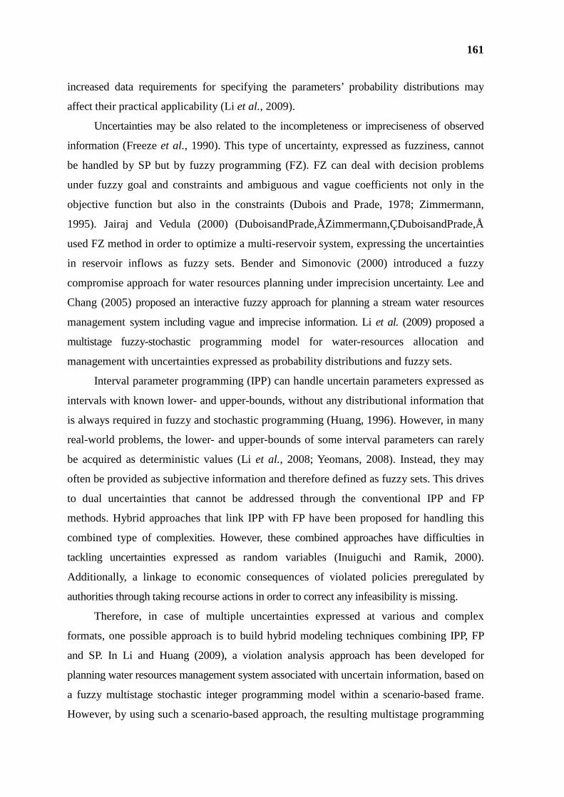
161

increased data requirements for specifying the parameters’ probability distributions may

affect their practical applicability (Li et al., 2009).

Uncertainties may be also related to the incompleteness or impreciseness of observed

information (Freeze et al., 1990). This type of uncertainty, expressed as fuzziness, cannot

be handled by SP but by fuzzy programming (FZ). FZ can deal with decision problems

under fuzzy goal and constraints and ambiguous and vague coefficients not only in the

objective function but also in the constraints (Dubois and Prade, 1978; Zimmermann,

1995). Jairaj and Vedula (2000) (DuboisandPrade,ÅZimmermann,ÇDuboisandPrade,Å

used FZ method in order to optimize a multi-reservoir system, expressing the uncertainties

in reservoir inflows as fuzzy sets. Bender and Simonovic (2000) introduced a fuzzy

compromise approach for water resources planning under imprecision uncertainty. Lee and

Chang (2005) proposed an interactive fuzzy approach for planning a stream water resources

management system including vague and imprecise information. Li et al. (2009) proposed a

multistage fuzzy-stochastic programming model for water-resources allocation and

management with uncertainties expressed as probability distributions and fuzzy sets.

Interval parameter programming (IPP) can handle uncertain parameters expressed as

intervals with known lower- and upper-bounds, without any distributional information that

is always required in fuzzy and stochastic programming (Huang, 1996). However, in many

real-world problems, the lower- and upper-bounds of some interval parameters can rarely

be acquired as deterministic values (Li et al., 2008; Yeomans, 2008). Instead, they may

often be provided as subjective information and therefore defined as fuzzy sets. This drives

to dual uncertainties that cannot be addressed through the conventional IPP and FP

methods. Hybrid approaches that link IPP with FP have been proposed for handling this

combined type of complexities. However, these combined approaches have difficulties in

tackling uncertainties expressed as random variables (Inuiguchi and Ramik, 2000).

Additionally, a linkage to economic consequences of violated policies preregulated by

authorities through taking recourse actions in order to correct any infeasibility is missing.

Therefore, in case of multiple uncertainties expressed at various and complex

formats, one possible approach is to build hybrid modeling techniques combining IPP, FP

and SP. In Li and Huang (2009), a violation analysis approach has been developed for

planning water resources management system associated with uncertain information, based on

a fuzzy multistage stochastic integer programming model within a scenario-based frame.

However, by using such a scenario-based approach, the resulting multistage programming

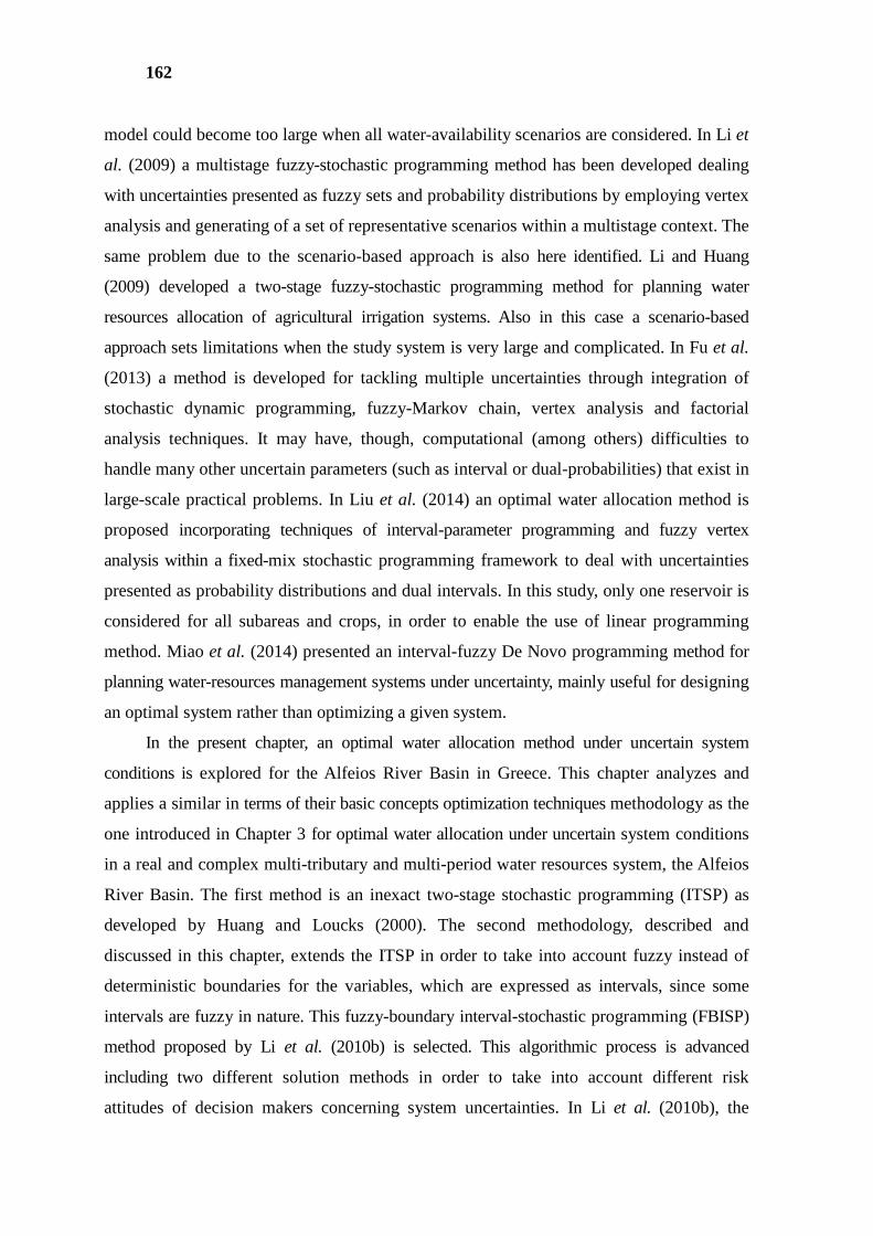
162

model could become too large when all water-availability scenarios are considered. In Li et

al. (2009) a multistage fuzzy-stochastic programming method has been developed dealing

with uncertainties presented as fuzzy sets and probability distributions by employing vertex

analysis and generating of a set of representative scenarios within a multistage context. The

same problem due to the scenario-based approach is also here identified. Li and Huang

(2009) developed a two-stage fuzzy-stochastic programming method for planning water

resources allocation of agricultural irrigation systems. Also in this case a scenario-based

approach sets limitations when the study system is very large and complicated. In Fu et al.

(2013) a method is developed for tackling multiple uncertainties through integration of

stochastic dynamic programming, fuzzy-Markov chain, vertex analysis and factorial

analysis techniques. It may have, though, computational (among others) difficulties to

handle many other uncertain parameters (such as interval or dual-probabilities) that exist in

large-scale practical problems. In Liu et al. (2014) an optimal water allocation method is

proposed incorporating techniques of interval-parameter programming and fuzzy vertex

analysis within a fixed-mix stochastic programming framework to deal with uncertainties

presented as probability distributions and dual intervals. In this study, only one reservoir is

considered for all subareas and crops, in order to enable the use of linear programming

method. Miao et al. (2014) presented an interval-fuzzy De Novo programming method for

planning water-resources management systems under uncertainty, mainly useful for designing

an optimal system rather than optimizing a given system.

In the present chapter, an optimal water allocation method under uncertain system

conditions is explored for the Alfeios River Basin in Greece. This chapter analyzes and

applies a similar in terms of their basic concepts optimization techniques methodology as the

one introduced in Chapter 3 for optimal water allocation under uncertain system conditions

in a real and complex multi-tributary and multi-period water resources system, the Alfeios

River Basin. The first method is an inexact two-stage stochastic programming (ITSP) as

developed by Huang and Loucks (2000). The second methodology, described and

discussed in this chapter, extends the ITSP in order to take into account fuzzy instead of

deterministic boundaries for the variables, which are expressed as intervals, since some

intervals are fuzzy in nature. This fuzzy-boundary interval-stochastic programming (FBISP)

method proposed by Li et al. (2010b) is selected. This algorithmic process is advanced

including two different solution methods in order to take into account different risk

attitudes of decision makers concerning system uncertainties. In Li et al. (2010b), the

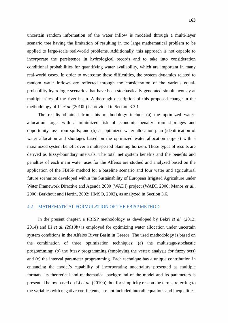
163

uncertain random information of the water inflow is modeled through a multi-layer

scenario tree having the limitation of resulting in too large mathematical problem to be

applied to large-scale real-world problems. Additionally, this approach is not capable to

incorporate the persistence in hydrological records and to take into consideration

conditional probabilities for quantifying water availability, which are important in many

real-world cases. In order to overcome these difficulties, the system dynamics related to

random water inflows are reflected through the consideration of the various equal-

probability hydrologic scenarios that have been stochastically generated simultaneously at

multiple sites of the river basin. A thorough description of this proposed change in the

methodology of Li et al. (2010b) is provided in Section 3.3.1.

The results obtained from this methodology include (a) the optimized water-

allocation target with a minimized risk of economic penalty from shortages and

opportunity loss from spills; and (b) an optimized water-allocation plan (identification of

water allocation and shortages based on the optimized water allocation targets) with a

maximized system benefit over a multi-period planning horizon. These types of results are

derived as fuzzy-boundary intervals. The total net system benefits and the benefits and

penalties of each main water uses for the Alfeios are studied and analyzed based on the

application of the FBISP method for a baseline scenario and four water and agricultural

future scenarios developed within the Sustainability of European Irrigated Agriculture under

Water Framework Directive and Agenda 2000 (WADI) project (WADI, 2000; Manos et al.,

2006; Berkhout and Hertin, 2002; HMSO, 2002), as analyzed in Section 3.6.

4.2 MATHEMATICAL FORMULATION OF THE FBISP METHOD

In the present chapter, a FBISP methodology as developed by Bekri et al. (2013;

2014) and Li et al. (2010b) is employed for optimizing water allocation under uncertain

system conditions in the Alfeios River Basin in Greece. The used methodology is based on

the combination of three optimization techniques: (a) the multistage-stochastic

programming; (b) the fuzzy programming (employing the vertex analysis for fuzzy sets)

and (c) the interval parameter programming. Each technique has a unique contribution in

enhancing the model’s capability of incorporating uncertainty presented as multiple

formats. Its theoretical and mathematical background of the model and its parameters is

presented below based on Li et al. (2010b), but for simplicity reason the terms, referring to

the variables with negative coefficients, are not included into all equations and inequalities,

164

since they are absent from the examined application to Alfeios River Basin. The complete

mathematical model including also these terms with negative coefficients can be found in

Li et al. (2010b).

In the FBISP model, assume that there is no intersection between the fuzzy sets at the two

bounds (e.g., let 561±7 = 2561%7,561&73 = 82561% , 561% 3, 9561& , 561& :;, where 561% 7 and 561&7 are fuzzy

lower- and upper-bounds of 561±7,561% and 561% are the lower- and upper-boundary of 561%7 ;

561& AE561& are the lower-and upper-boundary of 561&7 ). This is due to satisfy the definition

of an interval value that its lower-bound should not be larger than its upper-bound (Huang

et al., 1992). Secondly, interval numbers are used to express uncertainties without

distribution information. If the fuzzy sets of an interval’s lower- and upper- bounds

intersect, then the so-called “interval” is actually described by fuzzy membership

functions, such that the interval representation becomes unnecessary (Chen et al., 1998).

Thirdly, if the fuzzy sets of an interval’s lower- and upper-bound intersect, the interactive

algorithm for solving the interval-parameter programming problem cannot be used for

solving such a FBISP model.

Then, two solution methods are proposed for solving the FBISP model, which are

based on an optimistic and pessimistic approach of the uncertainties by the decision

makers, respectively. In the first solution methods (i.e., optimistic or risk-prone), a set of

submodels corresponding to &7 can be first formulated based on the interactive algorithm;

for each &7 submodel, take one end point from each of the fuzzy intervals (i.e., [?1&, ?1&],

[E1C% , E1C% ] and [561& , 561& ]); then, the obtained end points can be combined into an n-array,

leading to 2 combinations for n fuzzy sets (Dong and Shah, 1987; Nie et al., 2007).

Through solving 2 problems, a set of upper-bound objective-function values

(&, <&, … , <>& ) can be obtained. In detail, for each α-cut level, a set of &7 submodels can

be formulated as follows (assume that the right-hand sides and objective are both greater

than zero):

165

M&7 = l m9?1&, ?1&: +?1&n1&

D op

1− 1C l m9E1C% , E1C% : +E1C% nq

+1C% ors

Cp

1

(4.1)

subject to:

∑ 9uawxa% u S$IA yawxa% z , awxa% Signawxa% :xDx xxa& ≤[bwa& , bwa& ], ∀r, t (4.2)

1% S$IA1% 1&D+ 9u1C& u S$IA y1C& z , u1C& u S$IA y1C& z: +1C% q

≥ 91C% , 1C% : ∀, P = 1, 2, … . , L1 1&, +1C% ≥ 0

(4.3)

where 1& B = 1,2, … . , ) are upper-bounds of the first-stage decision variables (1±), and +1C% (P = 1, 2, … . , L1AE = 1, 2, … . , <) are lower-bounds of the recourse

decision variables B+1C± ). Through solving 2submodels, a set of values (&, <&, … , <>& ) can be obtained. Let /01& be the minimum value of the upper-bound (for the objective-function value) with

/01& = $AB&, <&, … , <>& ), and /01& be the maximum value of the upper-bound with

/01& = $AB&, <&, … , <>& ). Then, the optimized upper-bound interval for the objective

function value (under an α-cut level) can be identified as follows:

9/01& , /01& :! = '$AB&, <&, … , <>& ),B&, <&, … , <>& )(! (4.4)

Based on the solutions from the first set of submodels, submodels corresponding to %7 can be formulated as:

166

M%7 = l m9?1%, ?1%: +?′1%n1%

D op

1− 1C l m9E1C& , E1C& : +E′1C& nq

+1C& ors

Cp

1

(4.5)

subject to:

9uawxa& u Sign yawxa& z , uawxa& u Sign yawxa& z:xx xxa% ≤

[561% , 561% ],

∀, (4.6)

axa& Signaxa& xxa% xDx+ 9uaxab% u Sign yaxab% z, axab% Signaxab% : yxab& ≥ 9wab& , wab& :x<

x

, ∀i, t; k = 1, 2, … . , Ka 0 ≤ 1% ≤ 1/01& , ∀; = 1, 2, … , 1+1C& ≥ +1C/01% , ∀; = 1, 2, … , <, P = 1, 2, … , L1

(4.7)

where 1/01& ( = 1, 2, … , ), 1/01% ( = + 1, + 2,… , + A), +1C/01% ( =1, 2, … , <) and +1C/01& ( = < + 1, < + 2,… , < + A<), are solutions corresponding to

/01& . Through solving 2 deterministic problems, a set of values (%, <%, … , <% ) can be

obtained. The optimized lower-bound interval for the objective-function value (under an α-

cut level) can be identified as follows:

9/01% , /01% :! = '$AB%, <%, … , <>% ),B%, <%, … , <% )(!(4.8)

where /01% is the minimum value of the lower-bound (for the objective function

value) with /01% = $AB%, <%, … , <>% ); /01% is the maximum value of the lower-bound

with /01% = maxB%, <%, … , <% ). Then, through integrating the computational results of

167

the two sets of submodels, the solution for the objective function value (under an α-cut

level) can be obtained. Iteratively, the computational process can be repeated with the other

α-cut levels.

The above optimistic solution method identifies the solutions for the first-stage and

recourse decisions variables by first solving the best-case submodel (i.e., upper-bound objective

function value when the problem is to be maximized). This includes the upper-bound system

solution for total benefit, which is associated with more advantageous (more favorable)

conditions. In example, this is related to the upper-bound benefit coefficients, lower-bound cost

coefficients, upper-bound reservoir capacities, lower-bound reserved storage requirements, etc.

The resulting solution can provide intervals for the objective function value and decision

variables, and can be easily interpreted for generating decision alternatives.

However, this solution method may provide a wide-ranging objective function value

because significant (and costly) first-stage and recourse decisions are required under

unfavorable conditions (represented by worst-case parameter values) (Rosenberg, 2009).

Consequently, another solution method based on risk adverse is proposed for solving the

FBISP model to reduce the interval width of the objective-function value, in which the

worst-case submodel (i.e., corresponding to the lower-bound objective function) can be

first solved to identify a more appropriate set of first-stage and recourse decision variables.

In this case, the interval for the objective function value is narrower, but it may lead to

increased opportunity loss, being incapable of achieving the highest benefit under

advantageous conditions. Thus, we have:

M%7 = l m9?1%, ?1%: +?′1%n1%

D op

1− 1C l m9E1C& , E1C& : +E′1C& nq

+1C& ors

Cp

1

(4.9)

subject to:

∑ 9u61& u S$IA y61& z , u61& u S$IA y61& z:s 1% ≤'561% ,561% (,∀, (4.10)

∑ 1& S$IA1& 1% +D ∑ 9u1C% u S$IA y1C% z , 1C% S$IA1C%< (4.11)

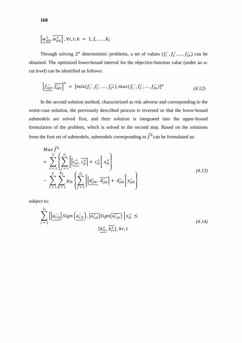
168

91C& , 1C& :,∀$, ; P = 1, 2, … . , L1Through solving 2 deterministic problems, a set of values (%, <%, … , <% ) can be

obtained. The optimized lower-bound interval for the objective-function value (under an α-

cut level) can be identified as follows:

9/01% , /01% :! = '$AB%, <%, … , <>% ),B%, <%, … , <% )(! (4.12)

In the second solution method, characterized as risk adverse and corresponding to the

worst-case solution, the previously described process is reversed so that the lower-bound

submodels are solved first, and their solution is integrated into the upper-bound

formulation of the problem, which is solved in the second step. Based on the solutions

from the first set of submodels, submodels corresponding to &7can be formulated as:

M&7 = l m9?1&, ?1&: +?1&n1&

D op

1− 1C l m9E1C% , E1C% : +E1C% nq

+1C% ors

Cp

1

(4.13)

subject to:

9u61% u S$IA y61% z , 61% S$IA61% :D 1& ≤

[561& , 561& ], ∀, (4.14)

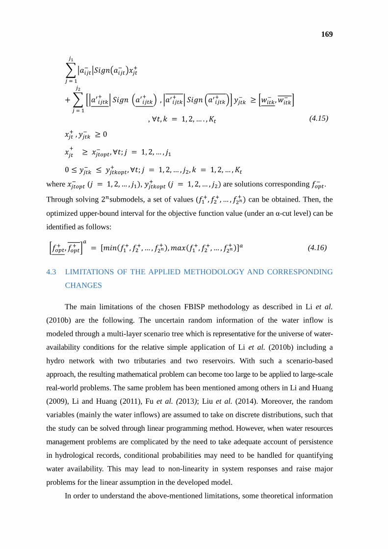
169

1% S$IA1% 1& D+ 9u1C& u S$IA y1C& z, u1C& u S$IA y1C& z: +1C% ≥ 91C% , 1C% :q

, ∀, P = 1, 2, … . , L1 1&, +1C% ≥ 0

1& ≥ 1/01% , ∀; = 1, 2, … ,

0 ≤ +1C% ≤ +1C/01& , ∀; = 1, 2, … , <, P = 1, 2, … , L1

(4.15)

where 1/01% ( = 1, 2, … , ), +1C/01& ( = 1, 2, … , <) are solutions corresponding /01% .

Through solving 2submodels, a set of values (&, <&, … , <>& ) can be obtained. Then, the

optimized upper-bound interval for the objective function value (under an α-cut level) can be

identified as follows:

9/01& , /01& :! = '$AB&, <&, … , <>& ),B&, <&, … , <>& )(! (4.16)

4.3 LIMITATIONS OF THE APPLIED METHODOLOGY AND CORRESPONDING

CHANGES

The main limitations of the chosen FBISP methodology as described in Li et al.

(2010b) are the following. The uncertain random information of the water inflow is

modeled through a multi-layer scenario tree which is representative for the universe of water-

availability conditions for the relative simple application of Li et al. (2010b) including a

hydro network with two tributaries and two reservoirs. With such a scenario-based

approach, the resulting mathematical problem can become too large to be applied to large-scale

real-world problems. The same problem has been mentioned among others in Li and Huang

(2009), Li and Huang (2011), Fu et al. (2013); Liu et al. (2014). Moreover, the random

variables (mainly the water inflows) are assumed to take on discrete distributions, such that

the study can be solved through linear programming method. However, when water resources

management problems are complicated by the need to take adequate account of persistence

in hydrological records, conditional probabilities may need to be handled for quantifying

water availability. This may lead to non-linearity in system responses and raise major

problems for the linear assumption in the developed model.

In order to understand the above-mentioned limitations, some theoretical information

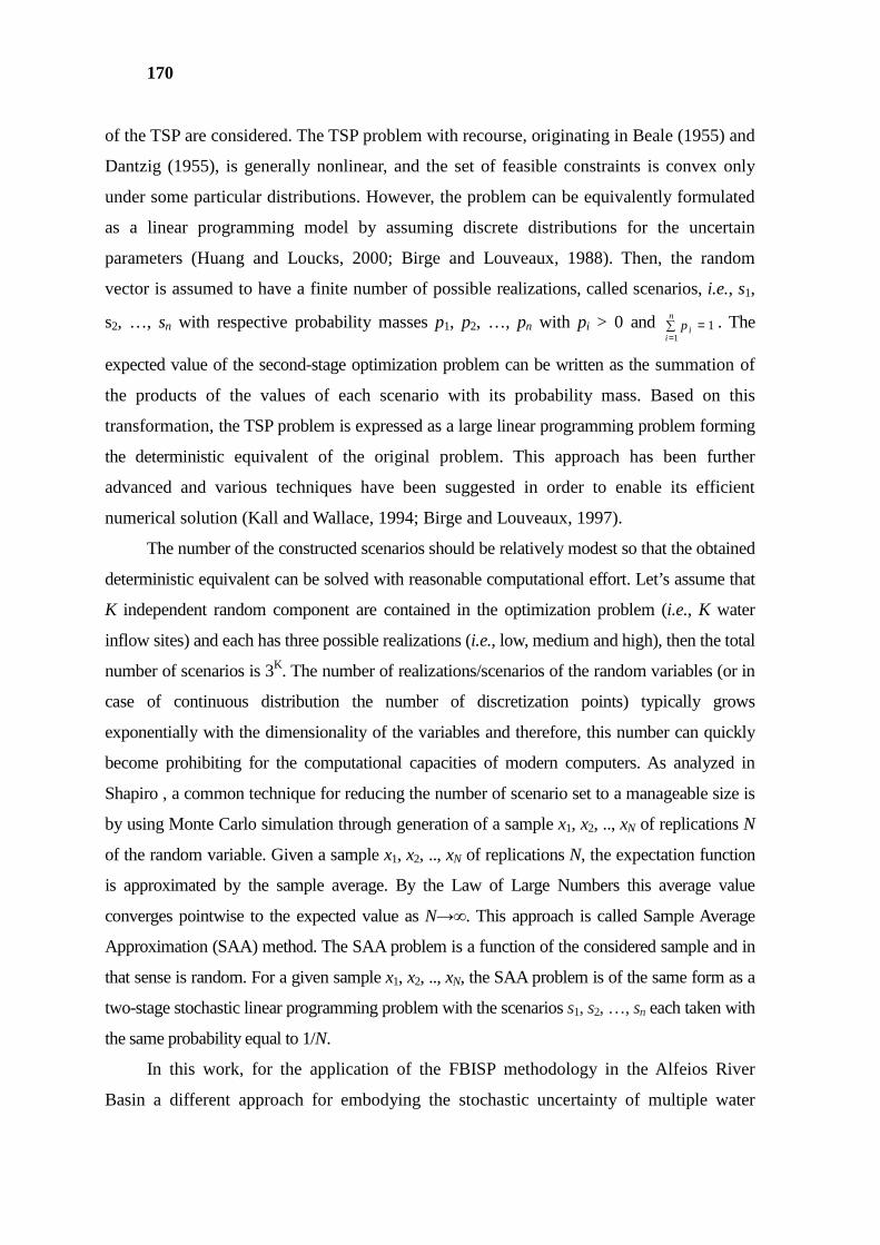
170

of the TSP are considered. The TSP problem with recourse, originating in Beale (1955) and

Dantzig (1955), is generally nonlinear, and the set of feasible constraints is convex only

under some particular distributions. However, the problem can be equivalently formulated

as a linear programming model by assuming discrete distributions for the uncertain

parameters (Huang and Loucks, 2000; Birge and Louveaux, 1988). Then, the random

vector is assumed to have a finite number of possible realizations, called scenarios, i.e., s1,

s2, …, sn with respective probability masses p1, p2, …, pn with pi > 0 and ∑ ==

n

iip

11 . The

expected value of the second-stage optimization problem can be written as the summation of

the products of the values of each scenario with its probability mass. Based on this

transformation, the TSP problem is expressed as a large linear programming problem forming

the deterministic equivalent of the original problem. This approach has been further

advanced and various techniques have been suggested in order to enable its efficient

numerical solution (Kall and Wallace, 1994; Birge and Louveaux, 1997).

The number of the constructed scenarios should be relatively modest so that the obtained

deterministic equivalent can be solved with reasonable computational effort. Let’s assume that

K independent random component are contained in the optimization problem (i.e., K water

inflow sites) and each has three possible realizations (i.e., low, medium and high), then the total

number of scenarios is 3K. The number of realizations/scenarios of the random variables (or in

case of continuous distribution the number of discretization points) typically grows

exponentially with the dimensionality of the variables and therefore, this number can quickly

become prohibiting for the computational capacities of modern computers. As analyzed in

Shapiro , a common technique for reducing the number of scenario set to a manageable size is

by using Monte Carlo simulation through generation of a sample x1, x2, .., xN of replications N

of the random variable. Given a sample x1, x2, .., xN of replications N, the expectation function

is approximated by the sample average. By the Law of Large Numbers this average value

converges pointwise to the expected value as N→∞. This approach is called Sample Average

Approximation (SAA) method. The SAA problem is a function of the considered sample and in

that sense is random. For a given sample x1, x2, .., xN, the SAA problem is of the same form as a

two-stage stochastic linear programming problem with the scenarios s1, s2, …, sn each taken with

the same probability equal to 1/N.

In this work, for the application of the FBISP methodology in the Alfeios River

Basin a different approach for embodying the stochastic uncertainty of multiple water

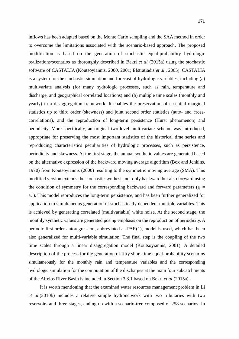
171

inflows has been adapted based on the Monte Carlo sampling and the SAA method in order

to overcome the limitations associated with the scenario-based approach. The proposed

modification is based on the generation of stochastic equal-probability hydrologic

realizations/scenarios as thoroughly described in Bekri et al (2015a) using the stochastic

software of CASTALIA (Koutsoyiannis, 2000, 2001; Efstratiadis et al., 2005). CASTALIA

is a system for the stochastic simulation and forecast of hydrologic variables, including (a)

multivariate analysis (for many hydrologic processes, such as rain, temperature and

discharge, and geographical correlated locations) and (b) multiple time scales (monthly and

yearly) in a disaggregation framework. It enables the preservation of essential marginal

statistics up to third order (skewness) and joint second order statistics (auto- and cross-

correlations), and the reproduction of long-term persistence (Hurst phenomenon) and

periodicity. More specifically, an original two-level multivariate scheme was introduced,

appropriate for preserving the most important statistics of the historical time series and

reproducing characteristics peculiarities of hydrologic processes, such as persistence,

periodicity and skewness. At the first stage, the annual synthetic values are generated based

on the alternative expression of the backward moving average algorithm (Box and Jenkins,

1970) from Koutsoyiannis (2000) resulting to the symmetric moving average (SMA). This

modified version extends the stochastic synthesis not only backward but also forward using

the condition of symmetry for the corresponding backward and forward parameters (aj =

a−j). This model reproduces the long-term persistence, and has been further generalized for

application to simultaneous generation of stochastically dependent multiple variables. This

is achieved by generating correlated (multivariable) white noise. At the second stage, the

monthly synthetic values are generated posing emphasis on the reproduction of periodicity. A

periodic first-order autoregression, abbreviated as PAR(1), model is used, which has been

also generalized for multi-variable simulation. The final step is the coupling of the two

time scales through a linear disaggregation model (Koutsoyiannis, 2001). A detailed

description of the process for the generation of fifty short-time equal-probability scenarios

simultaneously for the monthly rain and temperature variables and the corresponding

hydrologic simulation for the computation of the discharges at the main four subcatchments

of the Alfeios River Basin is included in Section 3.3.1 based on Bekri et al (2015a).

It is worth mentioning that the examined water resources management problem in Li

et al.(2010b) includes a relative simple hydronetwork with two tributaries with two

reservoirs and three stages, ending up with a scenario-tree composed of 258 scenarios. In

172

Alfeios River Basin, the simplified schematization of the river network, as presented in

Section 3.3, includes 5 streams and therefore, by considering one year with monthly time

step (12 stages), this results in a much more complex scenario-tree (i.e., taking into account

only 6 stages of the 12 stages (6 months): 2.8 × 1011 scenarios).

4.4 FORMULATION OF OPTIMIZATION PROBLEM FOR THE ALFEIOS RIVER

BASIN

4.4.1 BRIEF DESCRIPTION OF THE ALFEIOS RIVER BASIN FOR THE APPLICATION OF

FBISP

The Alfeios River Basin has been extensively described in the past (Bekri and

Yannopoulos, 2012; Manariotis and Yannopoulos, 2004; Podimata and Yannopoulos,

2013). This section describes briefly the information for the Alfeios required for the

application of the FBISP method, since the thorough analysis of the hydrosystem is

included in Session 3.3 based on Bekri et al. (2015a).

Beginning with the Ladhon river for the application of the FBISP method the upper-

and lower-bounds of the optimized hydropower production target ±T (in MWh) at Ladhon

are required. These bounds are approximated from the statistical analysis of the monthly

time series of hydropower production at Ladhon from 1985 to 2011. The ranges between

the mean value of the historical timeseries minus its standard deviation (lower-bound) and

its mean value plus its standard deviation (upper-bound) are considered as analyzed in

Section 3.4.

Proceeding to the Flokas irrigation region, for the application of the FBISP

methodology the upper- and lower-bounds of the water allocation targets for irrigation in m3

are required. The optimized water allocation target for irrigation (Table 2) is explored,

assuming that the irrigation demand can vary between the maximum demand of the present

crop pattern and the maximum demand given in the study of the small HPS at Flokas. Based

on this assumption, the lower-bound of the optimized water allocation target is set equal to the

maximum of all sets of irrigation water requirements for the fifty hydrologic scenarios as

computed by CROPWAT for the present irrigated area and crop pattern as analyzed in Section

3.5.

Concerning the small Flokas HPS, for the application of the FBISP method the

upper- and lower-bounds of the optimized hydropower production target ±T (in MWh) at

173

Flokas small HPS (Table 4.3) are required. These bounds are approximated also in this case,

from the statistical analysis of the monthly timeseries of hydropower production at Flokas

from 2011 to 2015. The ranges between the mean value of the historical timeseries minus its

standard deviation (lower-bound) and its mean value plus its standard deviation (upper-

bound) are taken into account as specified in Section 3.4.

Finally, a monthly water flow rate of 0.6 m3/s for the drinking water supply system

for the north and central part of the Region of Hleias is diverted from Erymanthos to the

water treatment plant and then to the neighboring communities extending up to the city of

Pyrgos. Due to the short operation period (starting in 2013), this water use is not

incorporated in the optimization process as a variable but as a steady and known water

abstraction demand.

The schematization of the Alfeios river network is depicted as shown in Figure 3.1,

including the main five water inflow locations, where historical timeseries (rain, temperature

and river discharge) are available and the main water users as described above.

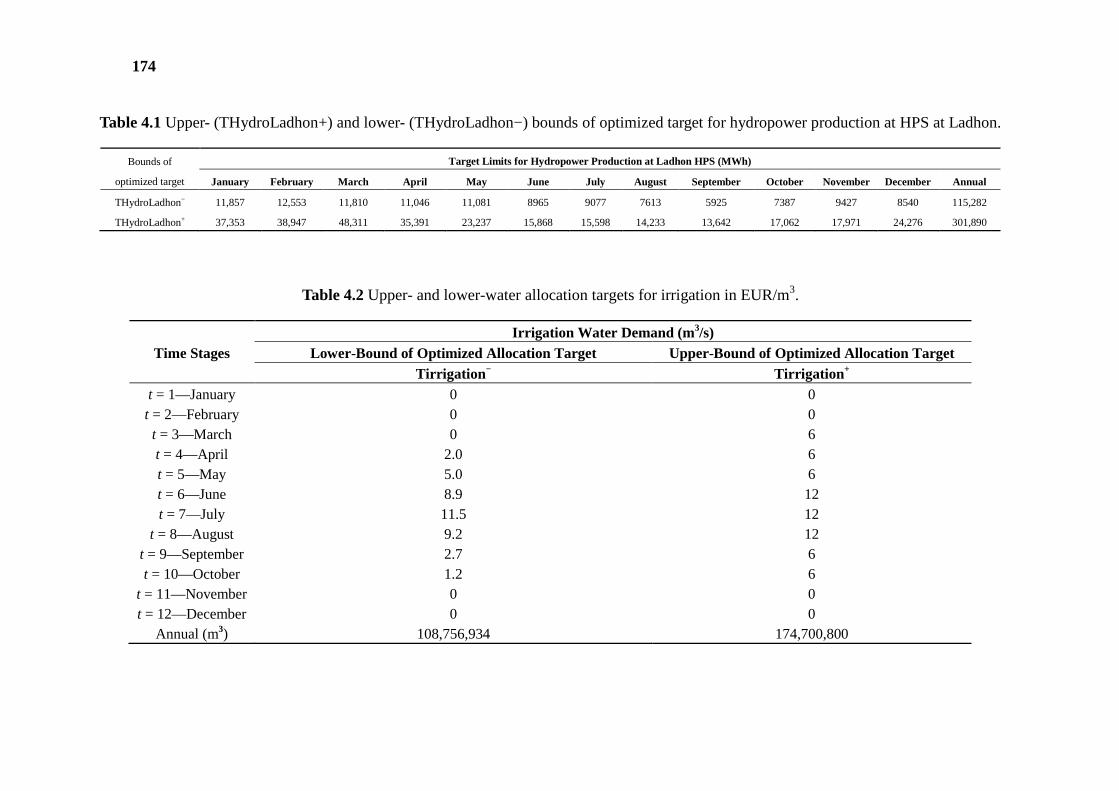
174

Table 4.1 Upper- (THydroLadhon+) and lower- (THydroLadhon−) bounds of optimized target for hydropower production at HPS at Ladhon.

Bounds of

optimized target

Target Limits for Hydropower Production at Ladhon H PS (MWh)

January February March April May June July August September October November December Annual

THydroLadhon− 11,857 12,553 11,810 11,046 11,081 8965 9077 7613 5925 7387 9427 8540 115,282

THydroLadhon+ 37,353 38,947 48,311 35,391 23,237 15,868 15,598 14,233 13,642 17,062 17,971 24,276 301,890

Table 4.2 Upper- and lower-water allocation targets for irrigation in EUR/m3.

Time Stages Irrigation Water Demand (m 3/s)

Lower-Bound of Optimized Allocation Target Upper-Bound of Optimized Allocation Target Tirrigation − Tirrigation +

t = 1—January 0 0 t = 2—February 0 0 t = 3—March 0 6 t = 4—April 2.0 6 t = 5—May 5.0 6 t = 6—June 8.9 12 t = 7—July 11.5 12

t = 8—August 9.2 12 t = 9—September 2.7 6 t = 10—October 1.2 6

t = 11—November 0 0 t = 12—December 0 0

Annual (m3) 108,756,934 174,700,800

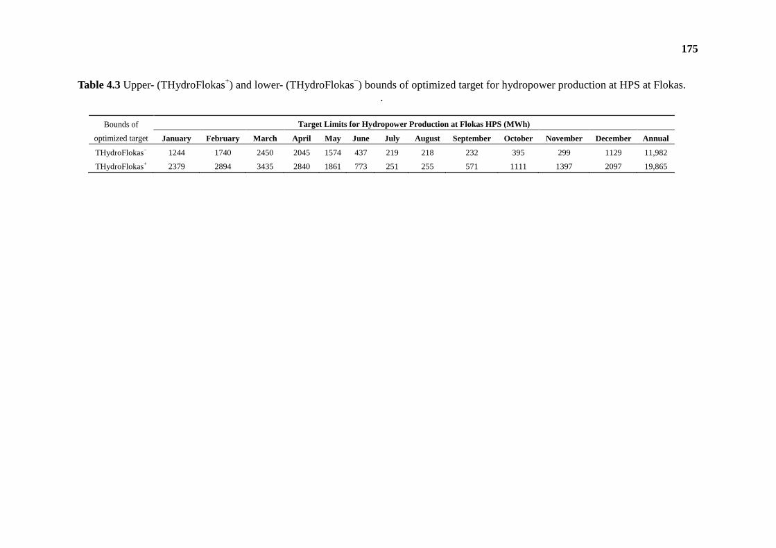
175

Table 4.3 Upper- (THydroFlokas+) and lower- (THydroFlokas−) bounds of optimized target for hydropower production at HPS at Flokas. .

Bounds of

optimized target

Target Limits for Hydropower Production at Flokas HPS (MWh)

January February March April May June July August September October November December Annual

THydroFlokas− 1244 1740 2450 2045 1574 437 219 218 232 395 299 1129 11,982

THydroFlokas+ 2379 2894 3435 2840 1861 773 251 255 571 1111 1397 2097 19,865

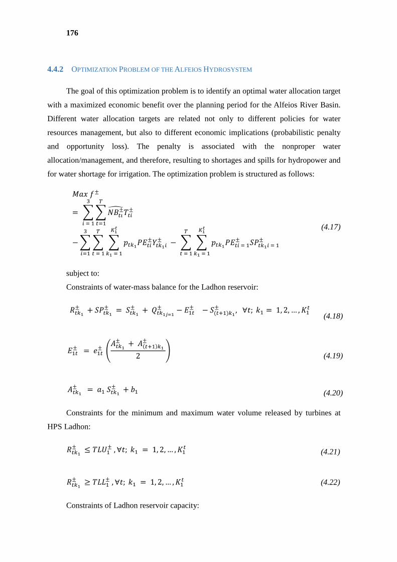
176

4.4.2 OPTIMIZATION PROBLEM OF THE ALFEIOS HYDROSYSTEM

The goal of this optimization problem is to identify an optimal water allocation target

with a maximized economic benefit over the planning period for the Alfeios River Basin.

Different water allocation targets are related not only to different policies for water

resources management, but also to different economic implications (probabilistic penalty

and opportunity loss). The penalty is associated with the nonproper water

allocation/management, and therefore, resulting to shortages and spills for hydropower and

for water shortage for irrigation. The optimization problem is structured as follows:

M± = 1V±W1±

p1

H

− 1CDKG1±1CD± − 1CDKG1± SK1CD± rD

CDp

1 rD

CDp

1H

(4.17)

subject to:

Constraints of water-mass balance for the Ladhon reservoir:

R1CD± + SK1CD± =S1CD± +Q1CDD± − G1 ± − SB1&)CD± ,∀; P = 1, 2, … , L1 (4.18)

G1± = F1± 41CD± +4B1&)CD±2

(4.19)

41CD± = S1CD± + 5 (4.20)

Constraints for the minimum and maximum water volume released by turbines at

HPS Ladhon:

R1CD± ≤ TX±, ∀; P = 1, 2, … , L1 (4.21)

R1CD± ≥ TT±, ∀; P = 1, 2, … , L1 (4.22)

Constraints of Ladhon reservoir capacity:

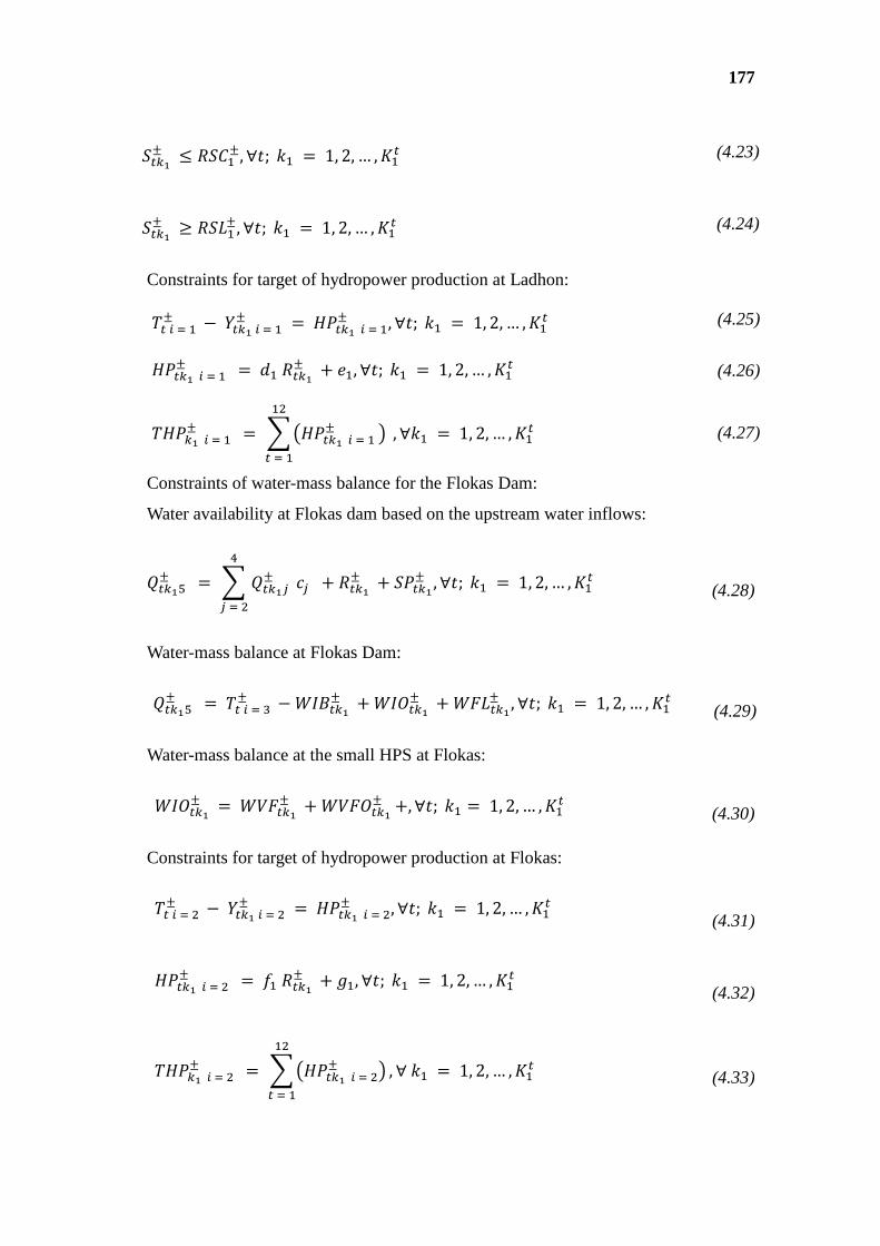
177

S1CD± ≤ RS±, ∀; P = 1, 2, … , L1 (4.23)

S1CD± ≥ RST±, ∀;P = 1, 2, … , L1 (4.24)

Constraints for target of hydropower production at Ladhon:

1± −1CD± = JK1CD± , ∀; P = 1, 2, … , L1 (4.25)

JK1CD± = ER1CD± + F, ∀; P = 1, 2, … , L1 (4.26)

JKCD± = JK1CD± <1 , ∀P = 1, 2, … , L1 (4.27)

Constraints of water-mass balance for the Flokas Dam:

Water availability at Flokas dam based on the upstream water inflows:

Q1CD± = Q1CD± ?< + R1CD± + SK1CD± , ∀; P = 1, 2, … , L1 (4.28)

Water-mass balance at Flokas Dam:

Q1CD± = 1H± − NZ1CD± + NZ[1CD± + NYT1CD± , ∀; P = 1, 2, … , L1 (4.29)

Water-mass balance at the small HPS at Flokas:

NZ[1CD± =N\Y1CD± + N\Y[1CD± +,∀;P = 1, 2, … , L1 (4.30)

Constraints for target of hydropower production at Flokas:

1<± −1CD<± = JK1CD<± , ∀; P = 1, 2, … , L1 (4.31)

JK1CD<± = R1CD± + I, ∀; P = 1, 2, … , L1 (4.32)

JKCD<± = JK1CD<± <1 , ∀P = 1, 2, … , L1 (4.33)

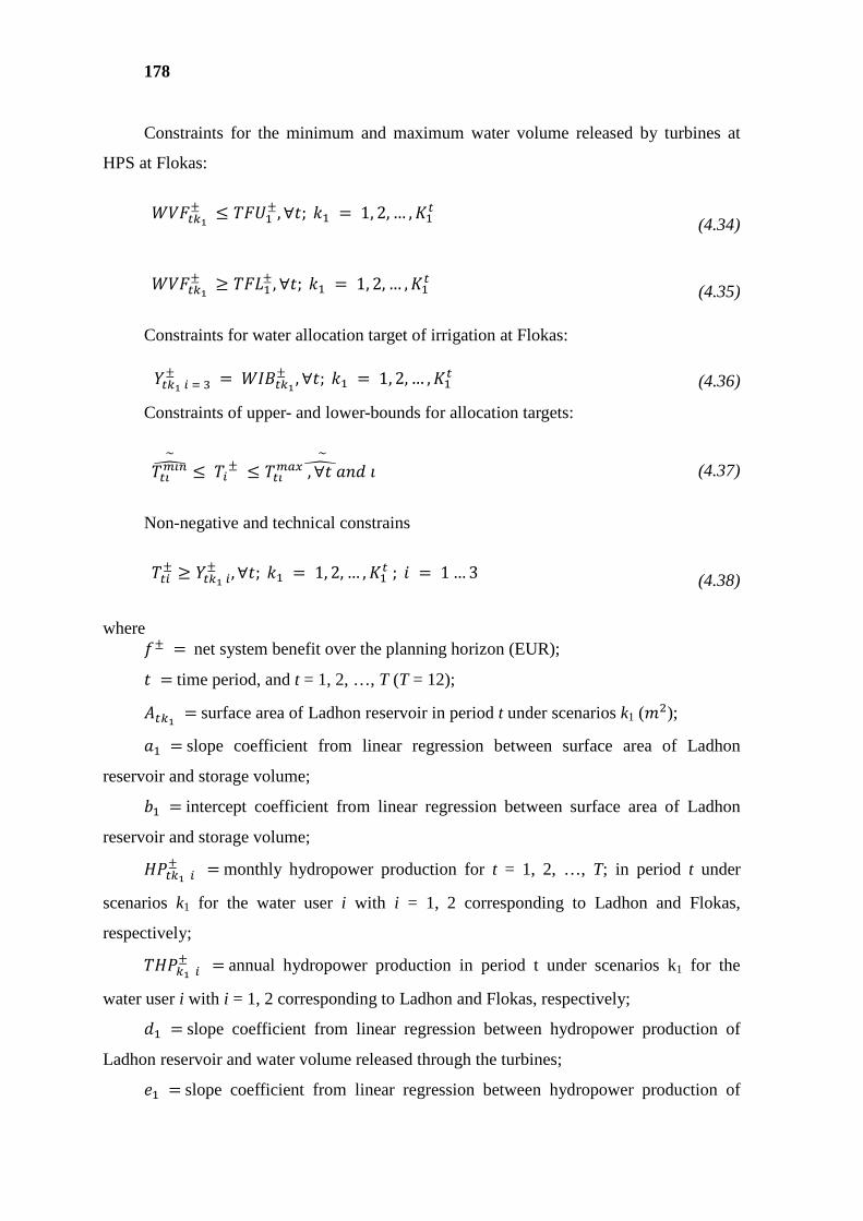
178

Constraints for the minimum and maximum water volume released by turbines at

HPS at Flokas:

N\Y1CD± ≤ YX±, ∀; P = 1, 2, … , L1 (4.34)

N\Y1CD± ≥ YT±, ∀; P = 1, 2, … , L1 (4.35)

Constraints for water allocation target of irrigation at Flokas:

1CDH± = NZ1CD± , ∀; P = 1, 2, … , L1 (4.36)

Constraints of upper- and lower-bounds for allocation targets:

1VVW~ ≤± ≤ 1V!", ∀AEW ~ (4.37)

Non-negative and technical constrains

1± ≥ 1CD± , ∀; P = 1, 2, … , L1; $ = 1…3 (4.38)

where ± =net system benefit over the planning horizon (EUR); =time period, and t = 1, 2, …, T (T = 12);

41CD =surface area of Ladhon reservoir in period t under scenarios k1 (<);

=slope coefficient from linear regression between surface area of Ladhon

reservoir and storage volume; 5 =intercept coefficient from linear regression between surface area of Ladhon

reservoir and storage volume;

JK1CD± =monthly hydropower production for t = 1, 2, …, T; in period t under

scenarios k1 for the water user i with i = 1, 2 corresponding to Ladhon and Flokas,

respectively;

JKCD± =annual hydropower production in period t under scenarios k1 for the

water user i with i = 1, 2 corresponding to Ladhon and Flokas, respectively; E =slope coefficient from linear regression between hydropower production of

Ladhon reservoir and water volume released through the turbines; F =slope coefficient from linear regression between hydropower production of

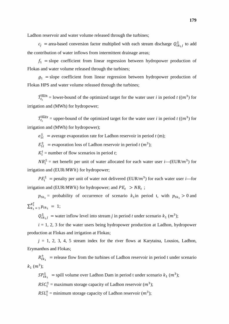
179

Ladhon reservoir and water volume released through the turbines;

? =area-based conversion factor multiplied with each stream discharge Q1CD± to add

the contribution of water inflows from intermittent drainage areas; =slope coefficient from linear regression between hydropower production of

Flokas and water volume released through the turbines; I =slope coefficient from linear regression between hydropower production of

Flokas HPS and water volume released through the turbines;

1UVW= lower-bound of the optimized target for the water user i in period t ((H) for

irrigation and (MWh) for hydropower;

1U!"W = upper-bound of the optimized target for the water user i in period t ((H) for

irrigation and (MWh) for hydropower);

F1± =average evaporation rate for Ladhon reservoir in period t (m);

G1± =evaporation loss of Ladhon reservoir in period t (H); L1 = number of flow scenarios in period t;

±= net benefit per unit of water allocated for each water user i—(EUR/H) for

irrigation and (EUR/MNℎ) for hydropower;

KG± =penalty per unit of water not delivered (EUR/H) for each water user i—for

irrigation and (EUR/MNℎ) for hydropower; and KG1 > 1 ; 1CD = probability of occurrence of scenario Pin period t, with 1CD > 0and

∑ 1CDrDCD = 1;

Q1CD± =water inflow level into stream j in period t under scenario P (H);

i = 1, 2, 3 for the water users being hydropower production at Ladhon, hydropower

production at Flokas and irrigation at Flokas;

j = 1, 2, 3, 4, 5 stream index for the river flows at Karytaina, Lousios, Ladhon,

Erymanthos and Flokas;

R1CD± =release flow from the turbines of Ladhon reservoir in period t under scenario

P (H);

SK1CD± =spill volume over Ladhon Dam in period t under scenario P (H);

RS±= maximum storage capacity of Ladhon reservoir (H);

RST±= minimum storage capacity of Ladhon reservoir (H);

180

TX± =maximum capacity of turbines at Ladhon HPS (H);

TT± =minimum capacity of turbines at Ladhon HPS (H);

YX± =maximum capacity of turbines at Flokas HPS (H);

YT± =minimum capacity of turbines at Flokas HPS (H);

S1CD± = storage level in Ladhon reservoir in period t under scenario P (H);

1 ± = water allocation target that is promised to the user i in period t (H);

1CD± =shortage level by which the water-allocation target is not met in period t under

scenarios P for the water user i, which is associated with probability of 1CD—(H) for

irrigation and MWh for hydropower;

NZ1CD± =irrigation shortage volume in period t under scenarios P (H);

NZ[1CD± =water volume left at Flokas after having allocated the irrigation water in

period t under scenarios P (H);

NYT1CD± =water volume flowing through the fish ladder at Flokas dam in period t

under scenarios P (H);

N\Y1CD± = water volume flowing through the turbines at Flokas HPS in period t

under scenarios P (H);

WVFOabD± =spill volume at Flokas dam in period t under scenarios P (H);

The steps of this process and the software programs used are presented schematically

in the form of a flow chart in Figure 4.1. CASTALIA model is applied for the simultaneous

stochastic generation of fifty equal-probability scenarios for the hydrologic variables of

rain and temperature at the four considered subcatchments (Karytaina, Lousios, Ladhon and

Erymanthos) having a time length of ten years (since the future WADI water and agriculture

scenarios are projected ten years after the baseline scenario) and monthly time step. The

stochastically simulated rain and temperature timeseries are introduced into the calibrated

simple lumped conceptual river basin model ZYGOS (Kozanis and Efstratiadis, 2006;

Kozanis et al., 2010) for the four subcatchments in order to compute the mean monthly

discharges for this ten years period. The uncertainty from the hydrologic model structure

and the parametrization is taken into account through the computation of the standard error

between the measured and the simulated water discharge timeseries. Based on this standard

error, upper-bound water inflows timeseries for all the hydrologic scenarios (which are

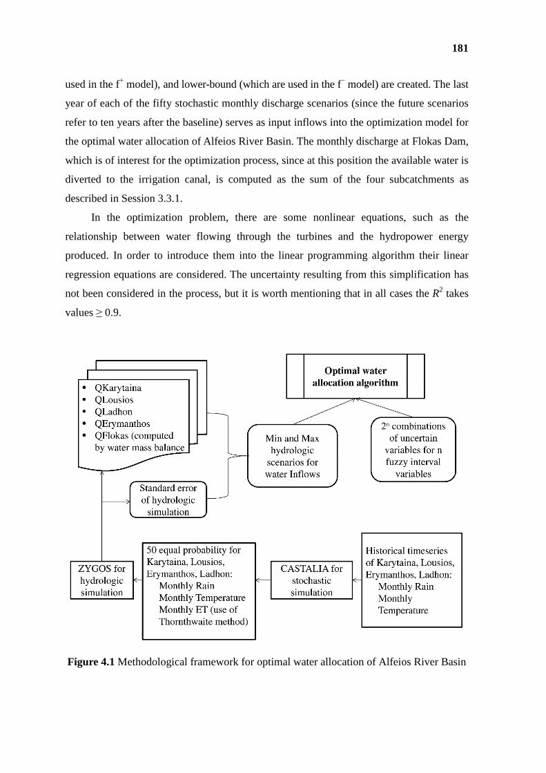
181

used in the f+ model), and lower-bound (which are used in the f− model) are created. The last

year of each of the fifty stochastic monthly discharge scenarios (since the future scenarios

refer to ten years after the baseline) serves as input inflows into the optimization model for

the optimal water allocation of Alfeios River Basin. The monthly discharge at Flokas Dam,

which is of interest for the optimization process, since at this position the available water is

diverted to the irrigation canal, is computed as the sum of the four subcatchments as

described in Session 3.3.1.

In the optimization problem, there are some nonlinear equations, such as the

relationship between water flowing through the turbines and the hydropower energy

produced. In order to introduce them into the linear programming algorithm their linear

regression equations are considered. The uncertainty resulting from this simplification has

not been considered in the process, but it is worth mentioning that in all cases the R2 takes

values ≥ 0.9.

Figure 4.1 Methodological framework for optimal water allocation of Alfeios River Basin

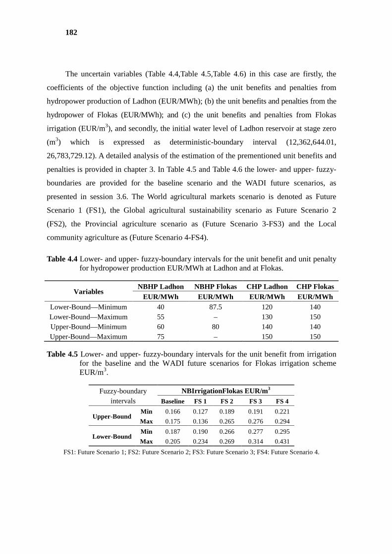
182

The uncertain variables (Table 4.4,Table 4.5,Table 4.6) in this case are firstly, the

coefficients of the objective function including (a) the unit benefits and penalties from

hydropower production of Ladhon (EUR/MWh); (b) the unit benefits and penalties from the

hydropower of Flokas (EUR/MWh); and (c) the unit benefits and penalties from Flokas

irrigation (EUR/m3), and secondly, the initial water level of Ladhon reservoir at stage zero

(m3) which is expressed as deterministic-boundary interval (12,362,644.01,

26,783,729.12). A detailed analysis of the estimation of the prementioned unit benefits and

penalties is provided in chapter 3. In Table 4.5 and Table 4.6 the lower- and upper- fuzzy-

boundaries are provided for the baseline scenario and the WADI future scenarios, as

presented in session 3.6. The World agricultural markets scenario is denoted as Future

Scenario 1 (FS1), the Global agricultural sustainability scenario as Future Scenario 2

(FS2), the Provincial agriculture scenario as (Future Scenario 3-FS3) and the Local

community agriculture as (Future Scenario 4-FS4).

Table 4.4 Lower- and upper- fuzzy-boundary intervals for the unit benefit and unit penalty for hydropower production EUR/MWh at Ladhon and at Flokas.

Variables NBHP Ladhon NBHP Flokas CHP Ladhon CHP Flokas

EUR/MWh EUR/MWh EUR/MWh EUR/MWh Lower-Bound—Minimum 40 87.5 120 140 Lower-Bound—Maximum 55 – 130 150 Upper-Bound—Minimum 60 80 140 140 Upper-Bound—Maximum 75 – 150 150

Table 4.5 Lower- and upper- fuzzy-boundary intervals for the unit benefit from irrigation for the baseline and the WADI future scenarios for Flokas irrigation scheme EUR/m3.

Fuzzy-boundary intervals

NBIrrigationFlokas EUR/m 3 Baseline FS 1 FS 2 FS 3 FS 4

Upper-Bound Min 0.166 0.127 0.189 0.191 0.221

Max 0.175 0.136 0.265 0.276 0.294

Lower-Bound Min 0.187 0.190 0.266 0.277 0.295

Max 0.205 0.234 0.269 0.314 0.431

FS1: Future Scenario 1; FS2: Future Scenario 2; FS3: Future Scenario 3; FS4: Future Scenario 4.

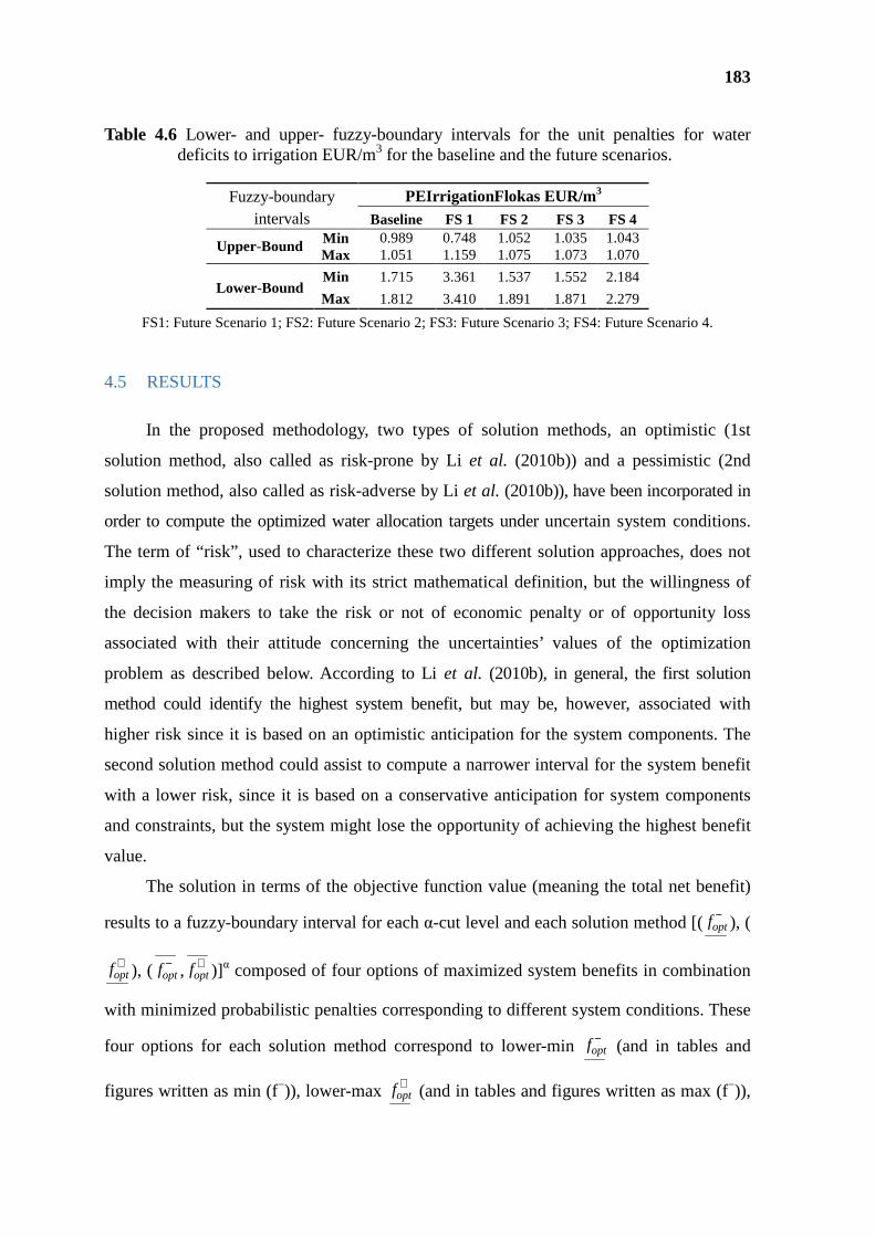
183

Table 4.6 Lower- and upper- fuzzy-boundary intervals for the unit penalties for water deficits to irrigation EUR/m3 for the baseline and the future scenarios.

Fuzzy-boundary intervals

PEIrrigationFlokas EUR/m 3 Baseline FS 1 FS 2 FS 3 FS 4

Upper-Bound Min 0.989 0.748 1.052 1.035 1.043 Max 1.051 1.159 1.075 1.073 1.070

Lower-Bound Min 1.715 3.361 1.537 1.552 2.184

Max 1.812 3.410 1.891 1.871 2.279

FS1: Future Scenario 1; FS2: Future Scenario 2; FS3: Future Scenario 3; FS4: Future Scenario 4.

4.5 RESULTS

In the proposed methodology, two types of solution methods, an optimistic (1st

solution method, also called as risk-prone by Li et al. (2010b)) and a pessimistic (2nd

solution method, also called as risk-adverse by Li et al. (2010b)), have been incorporated in

order to compute the optimized water allocation targets under uncertain system conditions.

The term of “risk”, used to characterize these two different solution approaches, does not

imply the measuring of risk with its strict mathematical definition, but the willingness of

the decision makers to take the risk or not of economic penalty or of opportunity loss

associated with their attitude concerning the uncertainties’ values of the optimization

problem as described below. According to Li et al. (2010b), in general, the first solution

method could identify the highest system benefit, but may be, however, associated with

higher risk since it is based on an optimistic anticipation for the system components. The

second solution method could assist to compute a narrower interval for the system benefit

with a lower risk, since it is based on a conservative anticipation for system components

and constraints, but the system might lose the opportunity of achieving the highest benefit

value.

The solution in terms of the objective function value (meaning the total net benefit)

results to a fuzzy-boundary interval for each α-cut level and each solution method [(−optf ), (

+optf ), ( −

optf , +optf )]α composed of four options of maximized system benefits in combination

with minimized probabilistic penalties corresponding to different system conditions. These

four options for each solution method correspond to lower-min −optf (and in tables and

figures written as min (f−)), lower-max +optf (and in tables and figures written as max (f−)),

184

upper-min −optf (and in tables and figures written as min (f+)), upper-max +

optf (and in tables

and figures written as max (f+)). These results (four prementioned options), however, do

not necessarily construct a set of stable intervals (Li et al., 2010b).

For the Alfeios River Basin considering five uncertain variables (as analyzed in

Section 3.2) with fuzzy-boundary intervals and two uncertain variables with deterministic-

boundary intervals (Table 4.4, Table 4.5,Table 4.6), 25 = 32 possible combinations of the

uncertain variable values/runs of the algorithm for each WADI future scenario (32 × 5 =

160 runs for all examined scenarios in total) has been undertaken based on the FBISP

algorithm as proposed by Li et al. (2010b).

For each examined case/run (1) the optimized water allocation target for each time

stage (the twelve months of the examined year), as well as for total annual (as the

summation of the values of the twelve time stages); (2) the probabilistic shortages and

allocations for each one of the fifty hydrologic scenarios and for each of the three water

users for each time stage (the twelve months of the examined year), as well as for the total

annual (as the summation of the values of the twelve time stages) and (3) the total benefits

and the benefits and penalties for each of the three water users are derived. The analysis of

these results is divided in two parts: (a) the analysis for the results of the baseline scenario,

enabling the understanding of the optimization technique used and (b) the comparison of

the results between the baseline and the future WADI water and agriculture scenarios in

order to assess the effect of the EU water and agricultural policy changes in the system

benefits and penalties on the baseline scenario.

4.5.1 RESULTS ANALYSIS FOR THE BASELINE SCENARIO

The total annual maximized net benefits of the Alfeios hydrosystem for the two

solution methods are presented in Table 4.7. The first solution method estimates a wider

range for the objective function value (meaning the total net benefits) equal to [(96,192,950,

102,180,847), (127,801,604, 135,950,230)] in EUR, but at the same time it embodies a

higher uncertainty or risk. The second solution process, on the other hand, results to a

narrower interval for the objective function value method [(104,523,859, 109,324,450),

(128,786,579, 134,978,247)], being related to a more conservative view of the uncertainties of

the hydrosystem and to the incapability to derive higher benefits under favorable

conditions. The interval solution can be easily interpreted for generating decision

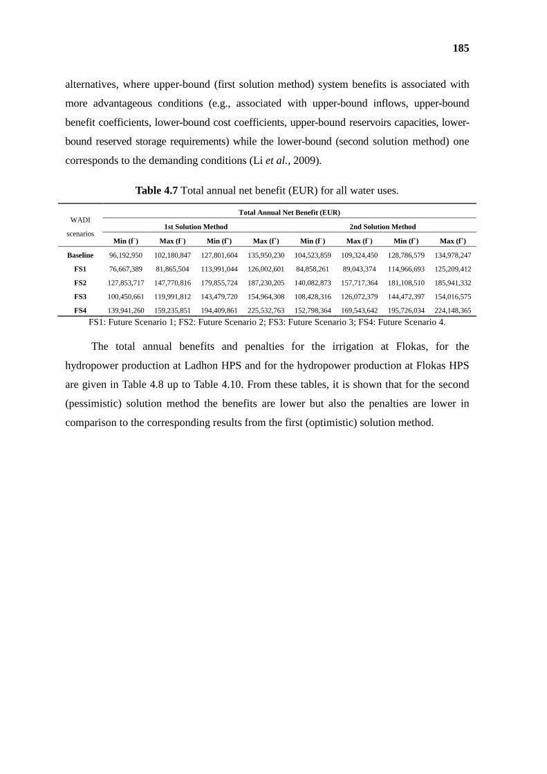
185

alternatives, where upper-bound (first solution method) system benefits is associated with

more advantageous conditions (e.g., associated with upper-bound inflows, upper-bound

benefit coefficients, lower-bound cost coefficients, upper-bound reservoirs capacities, lower-

bound reserved storage requirements) while the lower-bound (second solution method) one

corresponds to the demanding conditions (Li et al., 2009).

Table 4.7 Total annual net benefit (EUR) for all water uses.

WADI

scenarios

Total Annual Net Benefit (EUR)

1st Solution Method 2nd Solution Method

Min (f −) Max (f−) Min (f +) Max (f+) Min (f −) Max (f−) Min (f +) Max (f+)

Baseline 96,192,950 102,180,847 127,801,604 135,950,230 104,523,859 109,324,450 128,786,579 134,978,247

FS1 76,667,389 81,865,504 113,991,044 126,002,601 84,858,261 89,043,374 114,966,693 125,209,412

FS2 127,853,717 147,770,816 179,855,724 187,230,205 140,082,873 157,717,364 181,108,510 185,941,332

FS3 100,450,661 119,991,812 143,479,720 154,964,308 108,428,316 126,072,379 144,472,397 154,016,575

FS4 139,941,260 159,235,851 194,409,861 225,532,763 152,798,364 169,543,642 195,726,034 224,148,365

FS1: Future Scenario 1; FS2: Future Scenario 2; FS3: Future Scenario 3; FS4: Future Scenario 4.

The total annual benefits and penalties for the irrigation at Flokas, for the

hydropower production at Ladhon HPS and for the hydropower production at Flokas HPS

are given in Table 4.8 up to Table 4.10. From these tables, it is shown that for the second

(pessimistic) solution method the benefits are lower but also the penalties are lower in

comparison to the corresponding results from the first (optimistic) solution method.

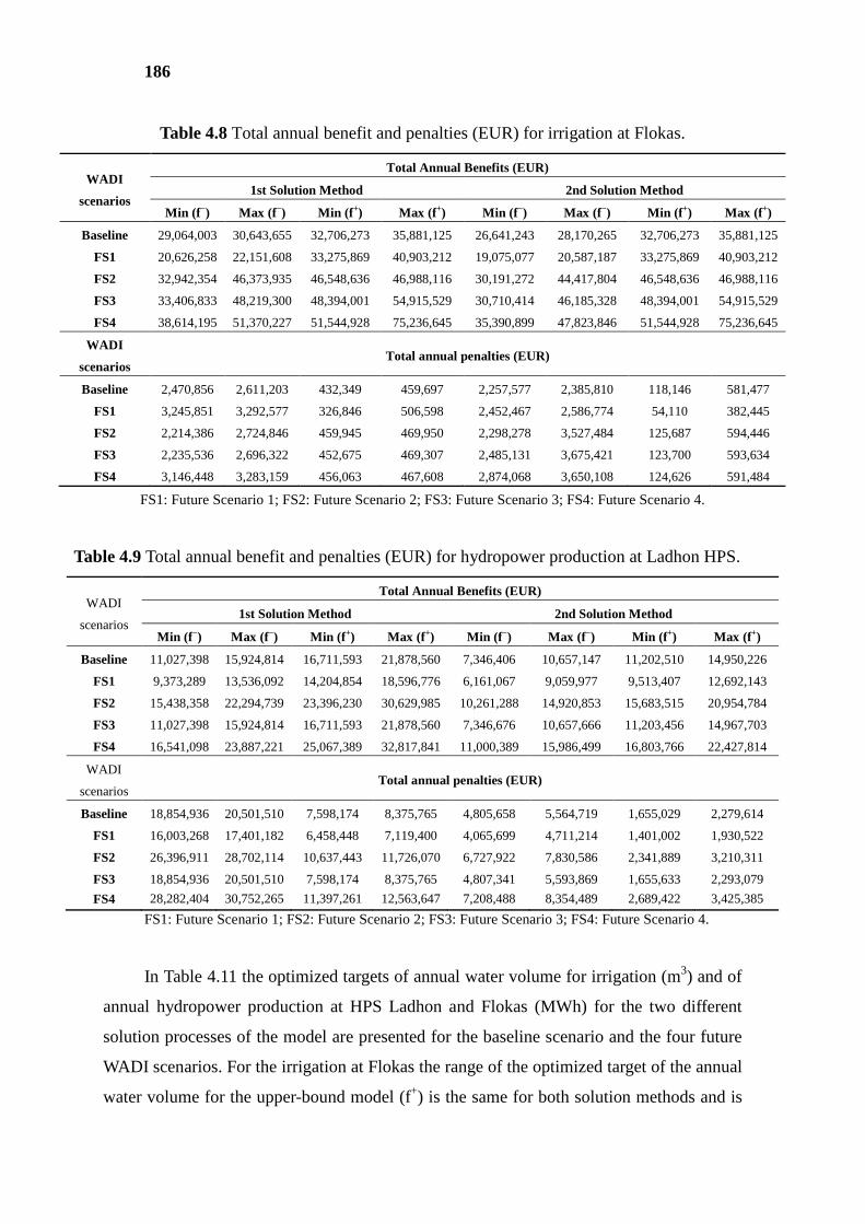
186

Table 4.8 Total annual benefit and penalties (EUR) for irrigation at Flokas.

WADI

scenarios

Total Annual Benefits (EUR)

1st Solution Method 2nd Solution Method

Min (f −) Max (f−) Min (f +) Max (f+) Min (f −) Max (f−) Min (f +) Max (f+)

Baseline 29,064,003 30,643,655 32,706,273 35,881,125 26,641,243 28,170,265 32,706,273 35,881,125

FS1 20,626,258 22,151,608 33,275,869 40,903,212 19,075,077 20,587,187 33,275,869 40,903,212

FS2 32,942,354 46,373,935 46,548,636 46,988,116 30,191,272 44,417,804 46,548,636 46,988,116

FS3 33,406,833 48,219,300 48,394,001 54,915,529 30,710,414 46,185,328 48,394,001 54,915,529

FS4 38,614,195 51,370,227 51,544,928 75,236,645 35,390,899 47,823,846 51,544,928 75,236,645

WADI

scenarios Total annual penalties (EUR)

Baseline 2,470,856 2,611,203 432,349 459,697 2,257,577 2,385,810 118,146 581,477

FS1 3,245,851 3,292,577 326,846 506,598 2,452,467 2,586,774 54,110 382,445

FS2 2,214,386 2,724,846 459,945 469,950 2,298,278 3,527,484 125,687 594,446

FS3 2,235,536 2,696,322 452,675 469,307 2,485,131 3,675,421 123,700 593,634

FS4 3,146,448 3,283,159 456,063 467,608 2,874,068 3,650,108 124,626 591,484

FS1: Future Scenario 1; FS2: Future Scenario 2; FS3: Future Scenario 3; FS4: Future Scenario 4.

Table 4.9 Total annual benefit and penalties (EUR) for hydropower production at Ladhon HPS.

WADI

scenarios

Total Annual Benefits (EUR)

1st Solution Method 2nd Solution Method

Min (f −) Max (f−) Min (f +) Max (f+) Min (f −) Max (f−) Min (f +) Max (f+)

Baseline 11,027,398 15,924,814 16,711,593 21,878,560 7,346,406 10,657,147 11,202,510 14,950,226

FS1 9,373,289 13,536,092 14,204,854 18,596,776 6,161,067 9,059,977 9,513,407 12,692,143

FS2 15,438,358 22,294,739 23,396,230 30,629,985 10,261,288 14,920,853 15,683,515 20,954,784

FS3 11,027,398 15,924,814 16,711,593 21,878,560 7,346,676 10,657,666 11,203,456 14,967,703

FS4 16,541,098 23,887,221 25,067,389 32,817,841 11,000,389 15,986,499 16,803,766 22,427,814

WADI

scenarios Total annual penalties (EUR)

Baseline 18,854,936 20,501,510 7,598,174 8,375,765 4,805,658 5,564,719 1,655,029 2,279,614

FS1 16,003,268 17,401,182 6,458,448 7,119,400 4,065,699 4,711,214 1,401,002 1,930,522

FS2 26,396,911 28,702,114 10,637,443 11,726,070 6,727,922 7,830,586 2,341,889 3,210,311

FS3 18,854,936 20,501,510 7,598,174 8,375,765 4,807,341 5,593,869 1,655,633 2,293,079

FS4 28,282,404 30,752,265 11,397,261 12,563,647 7,208,488 8,354,489 2,689,422 3,425,385

FS1: Future Scenario 1; FS2: Future Scenario 2; FS3: Future Scenario 3; FS4: Future Scenario 4.

In Table 4.11 the optimized targets of annual water volume for irrigation (m3) and of

annual hydropower production at HPS Ladhon and Flokas (MWh) for the two different

solution processes of the model are presented for the baseline scenario and the four future

WADI scenarios. For the irrigation at Flokas the range of the optimized target of the annual

water volume for the upper-bound model (f+) is the same for both solution methods and is

187

equal to its maximum possible value of 174,700,800 m3. For the lower-bound model (f−)

higher maximum allocation targets are computed by the first solution method

(160,079,569, 174,700,800) with much wider ranges between the minimum and the

maximum value (14,621,231 m3) compared to the ones from the second solution method

(160,574,718, 160,599,895) with corresponding range (25,177 m3). By comparing the

corresponding results of the FBISP method in this chapter with the ITSP as presented in

Bekri et al. (2015a), it is worth noticing that the monthly optimized water allocation target

values for irrigation at Flokas are equal to the maximum possible allocation for the upper-

and the lower-bound solution of the ITSP. This shows that the incorporation of the fuzzy

nature of the uncertainties in the FBISP results in lower optimized water allocation target

values for the lower-bound (second solution method) solution, reflecting a more analytic

and fine approximation of the effect of the uncertainties on the minimum and maximum

values of the boundaries of the results.

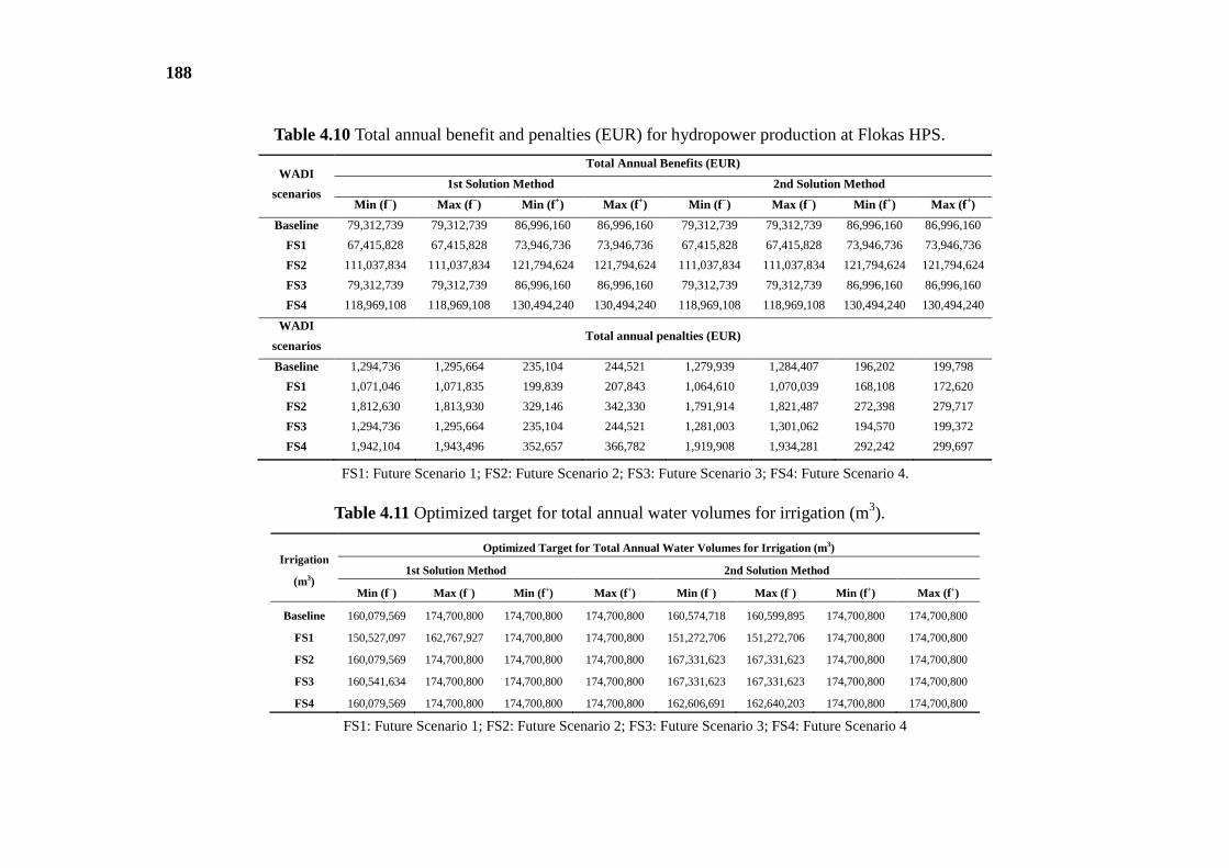
188

Table 4.10 Total annual benefit and penalties (EUR) for hydropower production at Flokas HPS.

WADI

scenarios

Total Annual Benefits (EUR)

1st Solution Method 2nd Solution Method

Min (f −) Max (f−) Min (f +) Max (f+) Min (f −) Max (f−) Min (f +) Max (f+)

Baseline 79,312,739 79,312,739 86,996,160 86,996,160 79,312,739 79,312,739 86,996,160 86,996,160

FS1 67,415,828 67,415,828 73,946,736 73,946,736 67,415,828 67,415,828 73,946,736 73,946,736

FS2 111,037,834 111,037,834 121,794,624 121,794,624 111,037,834 111,037,834 121,794,624 121,794,624

FS3 79,312,739 79,312,739 86,996,160 86,996,160 79,312,739 79,312,739 86,996,160 86,996,160

FS4 118,969,108 118,969,108 130,494,240 130,494,240 118,969,108 118,969,108 130,494,240 130,494,240

WADI

scenarios Total annual penalties (EUR)

Baseline 1,294,736 1,295,664 235,104 244,521 1,279,939 1,284,407 196,202 199,798

FS1 1,071,046 1,071,835 199,839 207,843 1,064,610 1,070,039 168,108 172,620

FS2 1,812,630 1,813,930 329,146 342,330 1,791,914 1,821,487 272,398 279,717

FS3 1,294,736 1,295,664 235,104 244,521 1,281,003 1,301,062 194,570 199,372

FS4 1,942,104 1,943,496 352,657 366,782 1,919,908 1,934,281 292,242 299,697

FS1: Future Scenario 1; FS2: Future Scenario 2; FS3: Future Scenario 3; FS4: Future Scenario 4.

Table 4.11 Optimized target for total annual water volumes for irrigation (m3).

Irrigation

(m3)

Optimized Target for Total Annual Water Volumes for Irrigation (m 3)

1st Solution Method 2nd Solution Method

Min (f −) Max (f−) Min (f +) Max (f+) Min (f −) Max (f−) Min (f +) Max (f+)

Baseline 160,079,569 174,700,800 174,700,800 174,700,800 160,574,718 160,599,895 174,700,800 174,700,800

FS1 150,527,097 162,767,927 174,700,800 174,700,800 151,272,706 151,272,706 174,700,800 174,700,800

FS2 160,079,569 174,700,800 174,700,800 174,700,800 167,331,623 167,331,623 174,700,800 174,700,800

FS3 160,541,634 174,700,800 174,700,800 174,700,800 167,331,623 167,331,623 174,700,800 174,700,800

FS4 160,079,569 174,700,800 174,700,800 174,700,800 162,606,691 162,640,203 174,700,800 174,700,800

FS1: Future Scenario 1; FS2: Future Scenario 2; FS3: Future Scenario 3; FS4: Future Scenario 4

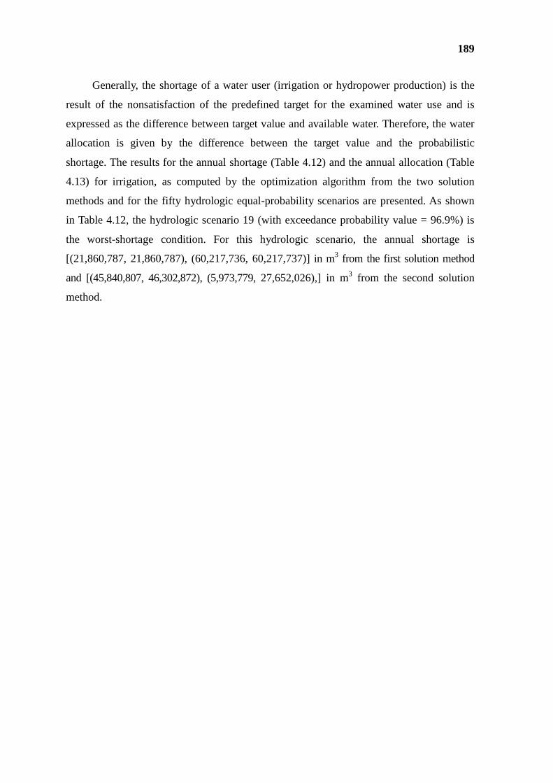
189

Generally, the shortage of a water user (irrigation or hydropower production) is the

result of the nonsatisfaction of the predefined target for the examined water use and is

expressed as the difference between target value and available water. Therefore, the water

allocation is given by the difference between the target value and the probabilistic

shortage. The results for the annual shortage (Table 4.12) and the annual allocation (Table

4.13) for irrigation, as computed by the optimization algorithm from the two solution

methods and for the fifty hydrologic equal-probability scenarios are presented. As shown

in Table 4.12, the hydrologic scenario 19 (with exceedance probability value = 96.9%) is

the worst-shortage condition. For this hydrologic scenario, the annual shortage is

[(21,860,787, 21,860,787), (60,217,736, 60,217,737)] in m3 from the first solution method

and [(45,840,807, 46,302,872), (5,973,779, 27,652,026),] in m3 from the second solution

method.

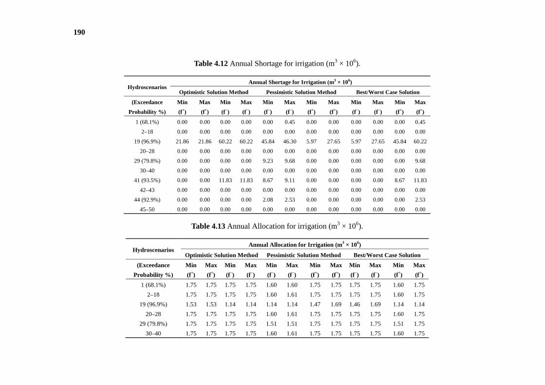
190

Table 4.12 Annual Shortage for irrigation (m3 × 106).

Hydroscenarios Annual Shortage for Irrigation (m 3 × 106)

Optimistic Solution Method Pessimistic Solution Method Best/Worst Case Solution

(Exceedance

Probability %)

Min

(f+)

Max

(f+)

Min

(f−)

Max

(f−)

Min

(f−)

Max

(f−)

Min

(f+)

Max

(f+)

Min

(f−)

Max

(f−)

Min

(f+)

Max

(f+)

1 (68.1%) 0.00 0.00 0.00 0.00 0.00 0.45 0.00 0.00 0.00 0.00 0.00 0.45

2–18 0.00 0.00 0.00 0.00 0.00 0.00 0.00 0.00 0.00 0.00 0.00 0.00

19 (96.9%) 21.86 21.86 60.22 60.22 45.84 46.30 5.97 27.65 5.97 27.65 45.84 60.22

20–28 0.00 0.00 0.00 0.00 0.00 0.00 0.00 0.00 0.00 0.00 0.00 0.00

29 (79.8%) 0.00 0.00 0.00 0.00 9.23 9.68 0.00 0.00 0.00 0.00 0.00 9.68

30–40 0.00 0.00 0.00 0.00 0.00 0.00 0.00 0.00 0.00 0.00 0.00 0.00

41 (93.5%) 0.00 0.00 11.83 11.83 8.67 9.11 0.00 0.00 0.00 0.00 8.67 11.83

42–43 0.00 0.00 0.00 0.00 0.00 0.00 0.00 0.00 0.00 0.00 0.00 0.00

44 (92.9%) 0.00 0.00 0.00 0.00 2.08 2.53 0.00 0.00 0.00 0.00 0.00 2.53

45–50 0.00 0.00 0.00 0.00 0.00 0.00 0.00 0.00 0.00 0.00 0.00 0.00

Table 4.13 Annual Allocation for irrigation (m3 × 106).

Hydroscenarios Annual Allocation for Irrigation (m 3 × 106)

Optimistic Solution Method Pessimistic Solution Method Best/Worst Case Solution

(Exceedance

Probability %)

Min

(f+)

Max

(f+)

Min

(f−)

Max

(f−)

Min

(f−)

Max

(f−)

Min

(f+)

Max

(f+)

Min

(f−)

Max

(f−)

Min

(f+)

Max

(f+)

1 (68.1%) 1.75 1.75 1.75 1.75 1.60 1.60 1.75 1.75 1.75 1.75 1.60 1.75

2–18 1.75 1.75 1.75 1.75 1.60 1.61 1.75 1.75 1.75 1.75 1.60 1.75

19 (96.9%) 1.53 1.53 1.14 1.14 1.14 1.14 1.47 1.69 1.46 1.69 1.14 1.14

20–28 1.75 1.75 1.75 1.75 1.60 1.61 1.75 1.75 1.75 1.75 1.60 1.75

29 (79.8%) 1.75 1.75 1.75 1.75 1.51 1.51 1.75 1.75 1.75 1.75 1.51 1.75

30–40 1.75 1.75 1.75 1.75 1.60 1.61 1.75 1.75 1.75 1.75 1.60 1.75

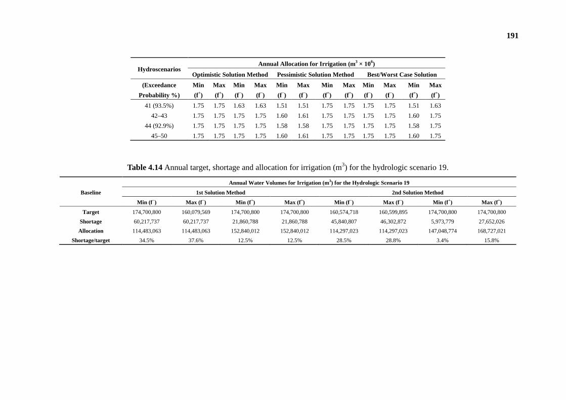
191

Hydroscenarios Annual Allocation for Irrigation (m 3 × 106)

Optimistic Solution Method Pessimistic Solution Method Best/Worst Case Solution

(Exceedance

Probability %)

Min

(f+)

Max

(f+)

Min

(f−)

Max

(f−)

Min

(f−)

Max

(f−)

Min

(f+)

Max

(f+)

Min

(f−)

Max

(f−)

Min

(f+)

Max

(f+)

41 (93.5%) 1.75 1.75 1.63 1.63 1.51 1.51 1.75 1.75 1.75 1.75 1.51 1.63

42–43 1.75 1.75 1.75 1.75 1.60 1.61 1.75 1.75 1.75 1.75 1.60 1.75

44 (92.9%) 1.75 1.75 1.75 1.75 1.58 1.58 1.75 1.75 1.75 1.75 1.58 1.75

45–50 1.75 1.75 1.75 1.75 1.60 1.61 1.75 1.75 1.75 1.75 1.60 1.75

Table 4.14 Annual target, shortage and allocation for irrigation (m3) for the hydrologic scenario 19.

Baseline

Annual Water Volumes for Irrigation (m 3) for the Hydrologic Scenario 19

1st Solution Method 2nd Solution Method

Min (f −) Max (f−) Min (f +) Max (f+) Min (f −) Max (f−) Min (f +) Max (f+)

Target 174,700,800 160,079,569 174,700,800 174,700,800 160,574,718 160,599,895 174,700,800 174,700,800

Shortage 60,217,737 60,217,737 21,860,788 21,860,788 45,840,807 46,302,872 5,973,779 27,652,026

Allocation 114,483,063 114,483,063 152,840,012 152,840,012 114,297,023 114,297,023 147,048,774 168,727,021

Shortage/target 34.5% 37.6% 12.5% 12.5% 28.5% 28.8% 3.4% 15.8%

192

In Table 4.14, presenting together the annual water allocation, shortage and

preregulated targets for this scenario, the shortage to target ratio (%) is also introduced.

From this ratio, it is indicated that the shortage is serious ranging from 12.5% to 37.6% of

the corresponding target for the first solution method and from 3.4% to 28.5% for the second

solution. In this case, the farmers should find an alternative water source such as pumping

water from groundwater. If the farmers do not have an alternative water source (such as

pumping water from groundwater or wastewater reuse), a yield reduction is highly

possible, which is introduced into the objective function as a penalty for irrigation. The

solutions of water shortage and allocation for the other hydrologic scenarios can be

accordingly interpreted.

From the Table 4.14, it is verified that for the first solution method the benefits and

the optimized targets are higher with wider ranges, but the penalties are also higher and

wider in comparison to the corresponding results from the second solution method, since

the two solution methods are associated with different risk attitudes of the decision makers

considering system uncertainties. They drive the results of the optimization algorithm to

different solutions in terms of target, shortage and allocation. The shortage intervals can be

low under favorable system conditions and high and critical under demanding conditions

as in the case of irrigation for the hydrologic scenario 19. Additionally, in Table 4.12 and

Table 4.13 the best/worst case results are provided in order to enable an evaluation of the

system capacity to fulfill the preregulated goals. These results, however, do not necessarily

construct a set of stable intervals (Li et al., 2010b).

In Table 4.16 the optimized annual target of the hydropower production at the small

hydropower station at Flokas Dam are provided. It is worth noticing that this optimized

annual target remains unchanged and equal to 19,828 MWh for all WADI scenarios as well

as for both solution methods, constituting a robust value. By comparing the corresponding

results of the FBISP method in this chapter with the ITSP as presented in Bekri et al.

(2015a) it is worth noticing that the optimized annual hydropower target at Flokas HPS are

the same for both optimization methodologies.

The corresponding monthly optimized targets of the hydropower production at

Flokas Dam in comparison to the maximum allowable ones are given in Table 4.16. These

optimized target values are the same for both solution methods. From this table it is

observed that for all months the optimized targets are equal to the maximum ones except of

May and June, for which the optimized target values are 1.8% and 0.5%, respectively,

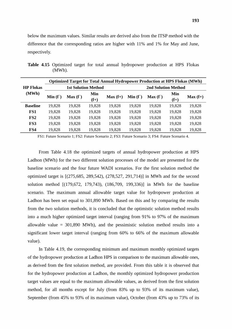
193

below the maximum values. Similar results are derived also from the ITSP method with the

difference that the corresponding ratios are higher with 11% and 1% for May and June,

respectively.

Table 4.15 Optimized target for total annual hydropower production at HPS Flokas (MWh).

HP Flokas (MWh)

Optimized Target for Total Annual Hydropower Production at HPS Flokas (MWh)

1st Solution Method 2nd Solution Method

Min (f −) Max (f−) Min (f+)

Max (f+) Min (f −) Max (f−) Min (f+)

Max (f+)

Baseline 19,828 19,828 19,828 19,828 19,828 19,828 19,828 19,828 FS1 19,828 19,828 19,828 19,828 19,828 19,828 19,828 19,828 FS2 19,828 19,828 19,828 19,828 19,828 19,828 19,828 19,828 FS3 19,828 19,828 19,828 19,828 19,828 19,828 19,828 19,828

FS4 19,828 19,828 19,828 19,828 19,828 19,828 19,828 19,828

FS1: Future Scenario 1; FS2: Future Scenario 2; FS3: Future Scenario 3; FS4: Future Scenario 4.

From Table 4.18 the optimized targets of annual hydropower production at HPS

Ladhon (MWh) for the two different solution processes of the model are presented for the

baseline scenario and the four future WADI scenarios. For the first solution method the

optimized target is [(275,685, 289,542), (278,527, 291,714)] in MWh and for the second

solution method [(179,672, 179,743), (186,709, 199,336)] in MWh for the baseline

scenario. The maximum annual allowable target value for hydropower production at

Ladhon has been set equal to 301,890 MWh. Based on this and by comparing the results

from the two solution methods, it is concluded that the optimistic solution method results

into a much higher optimized target interval (ranging from 91% to 97% of the maximum

allowable value = 301,890 MWh), and the pessimistic solution method results into a

significant lower target interval (ranging from 60% to 66% of the maximum allowable

value).

In Table 4.19, the corresponding minimum and maximum monthly optimized targets

of the hydropower production at Ladhon HPS in comparison to the maximum allowable ones,

as derived from the first solution method, are provided. From this table it is observed that

for the hydropower production at Ladhon, the monthly optimized hydropower production

target values are equal to the maximum allowable values, as derived from the first solution

method, for all months except for July (from 83% up to 93% of its maximum value),

September (from 45% to 93% of its maximum value), October (from 43% up to 73% of its

194

maximum value) and November (from 80% to 84% of its maximum value).

In Table 4.20 the corresponding minimum and maximum monthly optimized targets

of the hydropower production at Ladhon HPS in comparison to the maximum allowable

ones, as derived from the second solution method, are provided. From this table it is

observed that for the hydropower production at Ladhon, the monthly optimized hydropower

production target values deviate from the maximum allowable values for all months within a

range of 47% up to 94% of their maximum values. Therefore, it is obvious that when the

lower-bound water inflows (see the description for the incorporation of the uncertainty of

the rainfall-runoff model in Section 3.2) are used at the first step of the algorithm, which

corresponds to the process of the second solution (pessimistic) method, representing the

unfavorable (demanding) hydrologic conditions, the optimized targets for the monthly

hydropower production at Ladhon are significantly lower in comparison to the ones

resulting from the first solution method.

By comparing the corresponding results of the FBISP method in this chapter with the

ITSP as presented in Bekri et al. (2015a), it is worth noticing that from the ITSP method

the optimized monthly hydropower target at Ladhon HPS are equal to the maximum

allowable values as derived from the first solution method for all months except for July

(60% of its maximum value), September (67% of its maximum value), October (from 23%

of its maximum value) and November (from 58% of its maximum value). The four months

with the deviations from the maximum allowable values are the same as the ones derived by

the first solution method of the FBISP. The only difference is that the optimized targets from

the ITSP are lower. Also in this case, the FBISP method provides a more detailed overview

of the intervals for the optimized targets.

From the optimized targets of the three main users, as analyzed above, it can be

concluded that the highest priority for water allocation is set to irrigation, since it has the

highest unit benefit, but at the same time also the highest unit penalty. The next priorities

are given to hydropower production at Flokas and finally to the hydropower production at

Ladhon, which has the smallest unit benefit.

In Figure 4.2 and in Table 4.21, the interplay between the optimized total targets in

m3, which are derived from the addition of the optimum target water volumes allocated to

the three water users (hydropower production at Ladhon, hydropower production at Flokas

and irrigation at Flokas), and the system’s net benefits for these four options for both types

of solution methods is shown.

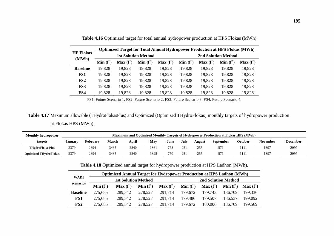
195

Table 4.16 Optimized target for total annual hydropower production at HPS Flokas (MWh).

HP Flokas (MWh)

Optimized Target for Total Annual Hydropower Production at HPS Flokas (MWh)

1st Solution Method 2nd Solution Method

Min (f −) Max (f−) Min (f +) Max (f+) Min (f −) Max (f−) Min (f +) Max (f+) Baseline 19,828 19,828 19,828 19,828 19,828 19,828 19,828 19,828

FS1 19,828 19,828 19,828 19,828 19,828 19,828 19,828 19,828 FS2 19,828 19,828 19,828 19,828 19,828 19,828 19,828 19,828 FS3 19,828 19,828 19,828 19,828 19,828 19,828 19,828 19,828

FS4 19,828 19,828 19,828 19,828 19,828 19,828 19,828 19,828

FS1: Future Scenario 1; FS2: Future Scenario 2; FS3: Future Scenario 3; FS4: Future Scenario 4.

Table 4.17 Maximum allowable (THydroFlokasPlus) and Optimized (Optimized THydroFlokas) monthly targets of hydropower production

at Flokas HPS (MWh).

Monthly hydropower

targets

Maximum and Optimized Monthly Targets of Hydropower Production at Flokas HPS (MWh)

January February March April May June July August September October November December

THydroFlokasPlus 2379 2894 3435 2840 1861 773 251 255 571 1111 1397 2097

Optimized THydroFlokas 2379 2894 3435 2840 1828 770 251 255 571 1111 1397 2097

Table 4.18 Optimized annual target for hydropower production at HPS Ladhon (MWh).

WADI

scenarios

Optimized Annual Target for Hydropower Production at HPS Ladhon (MWh) 1st Solution Method 2nd Solution Method

Min (f −) Max (f−) Min (f +) Max (f+) Min (f −) Max (f−) Min (f +) Max (f+) Baseline 275,685 289,542 278,527 291,714 179,672 179,743 186,709 199,336

FS1 275,685 289,542 278,527 291,714 179,486 179,507 186,537 199,092 FS2 275,685 289,542 278,527 291,714 179,672 180,006 186,709 199,569

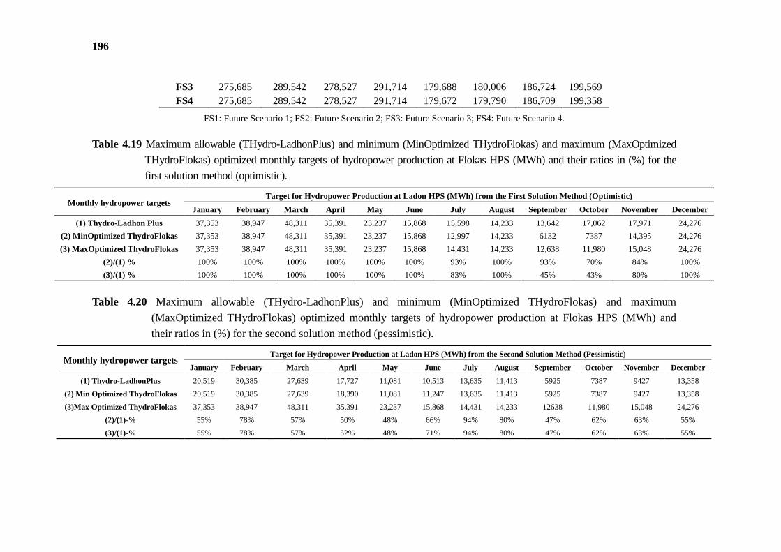
196

FS3 275,685 289,542 278,527 291,714 179,688 180,006 186,724 199,569 FS4 275,685 289,542 278,527 291,714 179,672 179,790 186,709 199,358

FS1: Future Scenario 1; FS2: Future Scenario 2; FS3: Future Scenario 3; FS4: Future Scenario 4.

Table 4.19 Maximum allowable (THydro-LadhonPlus) and minimum (MinOptimized THydroFlokas) and maximum (MaxOptimized

THydroFlokas) optimized monthly targets of hydropower production at Flokas HPS (MWh) and their ratios in (%) for the

first solution method (optimistic).

Monthly hydropower targets Target for Hydropower Production at Ladon HPS (MWh) from the First Solution Method (Optimistic)

January February March April May June July August September October November December

(1) Thydro-Ladhon Plus 37,353 38,947 48,311 35,391 23,237 15,868 15,598 14,233 13,642 17,062 17,971 24,276

(2) MinOptimized ThydroFlokas 37,353 38,947 48,311 35,391 23,237 15,868 12,997 14,233 6132 7387 14,395 24,276

(3) MaxOptimized ThydroFlokas 37,353 38,947 48,311 35,391 23,237 15,868 14,431 14,233 12,638 11,980 15,048 24,276

(2)/(1) % 100% 100% 100% 100% 100% 100% 93% 100% 93% 70% 84% 100%

(3)/(1) % 100% 100% 100% 100% 100% 100% 83% 100% 45% 43% 80% 100%

Table 4.20 Maximum allowable (THydro-LadhonPlus) and minimum (MinOptimized THydroFlokas) and maximum

(MaxOptimized THydroFlokas) optimized monthly targets of hydropower production at Flokas HPS (MWh) and

their ratios in (%) for the second solution method (pessimistic).

Monthly hydropower targets Target for Hydropower Production at Ladon HPS (MWh) from the Second Solution Method (Pessimistic)

January February March April May June July August September October November December

(1) Thydro-LadhonPlus 20,519 30,385 27,639 17,727 11,081 10,513 13,635 11,413 5925 7387 9427 13,358

(2) Min Optimized ThydroFlokas 20,519 30,385 27,639 18,390 11,081 11,247 13,635 11,413 5925 7387 9427 13,358

(3)Max Optimized ThydroFlokas 37,353 38,947 48,311 35,391 23,237 15,868 14,431 14,233 12638 11,980 15,048 24,276

(2)/(1)-% 55% 78% 57% 50% 48% 66% 94% 80% 47% 62% 63% 55%

(3)/(1)-% 55% 78% 57% 52% 48% 71% 94% 80% 47% 62% 63% 55%

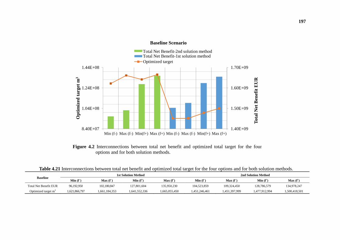
197

Table 4.21 Interconnections between total net benefit and optimized total target for the four options and for both solution methods.

Baseline 1st Solution Method 2nd Solution Method

Min (f −) Max (f−) Min (f +) Max (f+) Min (f −) Max (f−) Min (f +) Max (f+)

Total Net Benefit EUR 96,192,950 102,180,847 127,801,604 135,950,230 104,523,859 109,324,450 128,786,579 134,978,247

Optimized target m3 1,621,866,797 1,661,184,353 1,641,552,336 1,665,055,450 1,451,246,461 1,451,397,999 1,477,912,994 1,500,418,501

1.40E+09

1.50E+09

1.60E+09

1.70E+09

8.40E+07

1.04E+08

1.24E+08

1.44E+08

Min (f-) Max (f-) Min(f+) Max (f+) Min (f-) Max (f-) Min( f+) Max (f+)

Tota

l Net

Ben

efit

EU

R

Opt

imiz

ed ta

rget

m3

Baseline Scenario

Total Net Benefit-1st solution methodOptimized target

Total Net Benefit-2nd solution method

Figure 4.2 Interconnections between total net benefit and optimized total target for the four options and for both solution methods.

198

4.5.2 RESULTS ANALYSIS FOR THE BASELINE AND THE FOUR FUTURE SCENARIOS

The four WADI future scenarios represent four different possible water and

agricultural policy alternatives in comparison to the baseline scenario, which may have an

impact on the optimal water allocation. The differences between the future scenarios

include among others, changes of hydropower energy prices, water prices, selling prices of

the agricultural products, yield functions, subsidies, farmer income variable costs, labor, and

fertilizers. Since the uncertainties of water availability, water demand, benefits and costs

associated with probabilistic water allocations and shortages are incorporated in the

optimization algorithm, it is very interesting to investigate also the effect of the various

water and agricultural policies on the water allocation targets and on the corresponding

maximized system benefits.

The optimized total annual water allocation target, derived by the addition of the

water allocation targets of the three examined water uses, for all WADI scenarios is given

in Table 4.22. For comparison reasons the ratio of these targets for each future scenario to

the baseline target (%) is also shown. From these ratios (99.3% up to 100.5%) it is

concluded that the optimized total annual water allocation targets for the various alternative

water and agricultural policies compared to the baseline are only slightly affected. By

applying the ITSP method in Bekri et al.(2015a), the optimized total annual water

allocation targets are exactly the same for all four WADI future scenarios. Even though the

quantitative changes of these target values are relatively low, in the case of the application

of the FBISP method the consideration of the fuzzy nature for some of the uncertain

variables results in different water allocation targets revealing a more complicated structure

of the results.

The total annual maximized net benefits of the hydrosystem in EUR and their ratios of

the four future scenarios to the baseline are presented in Table 4.8 and Table 4.23,

respectively, for all scenarios and for the first (optimistic) and second (pessimistic) solution

method. It is obvious that the highest increase of these benefits is observed for the Local

Stewardship scenario (FS4) ranging for the first solution method from 45.5% up to 65.9%

and for the second solution method from 46.2% to 66.1%. The only decrease of the net

benefits compared to the benefits of the baseline scenario occurs for the World Market

scenario (FS1) for both upper-(f+) and lower-(f−) intervals of both solution methods up to

20%.

199

The statistical analysis of these optimized total annual net benefits from the various runs

(combinations of the uncertain variables values) is provided in Figure 4.4 for the baseline

and the four future scenarios through the use of box plots for Alfeios River Basin in

Western Greece. It is worth mentioning that for the Local Stewardship scenario (FS4) not

only the highest total net benefits are derived, but also the widest intervals ranges. On the

other hand, the baseline scenario has the narrowest upper- and lower-bound intervals.

Since the WADI scenarios focus mainly on the effects of the agricultural policy changes

on the irrigation sector, it is worth examining separately the changes between the scenarios

of the annual net benefits of water allocated to irrigation, which represent the agricultural

income. From Table 4.24 the highest reduction of the agricultural income (net benefit of

irrigation) compared to the baseline scenario is observed in the lower-bound (f−) interval

for both solution methods of the World Market scenario (FS1) (from 65.5% up to 69.80%

farmer income reduction compared to the baseline scenario). The corresponding upper-

bound intervals for this scenario drive to a small increase of agricultural income ranging

from 1.2% to 11.4% compared to the one for the baseline scenario. These results are

similar and compatible with the corresponding ones from the application of the ITSP

method in Bekri et al. (2015a). More precisely, the highest increase of the total system

benefits is also observed for the Local Stewardship scenario ranging from 52% to 59% and the

only decrease occurs for the World Market scenario (9%–24%). The above mentioned

reduction of the agricultural income can be explained by the fact that in the World Market

scenario the highest decrease of selling prices and a significant increase of the prices of

most of input variables for agriculture (pesticides, seeds, water price, etc.) in comparison to

the other scenarios is noticed. Moreover, for most of the crops cultivated at Flokas

Irrigation scheme, the presence of area subsidy plays a balancing role for the positive sign

(profit) of the agricultural income. In this scenario, no subsidies are provided to the

farmers. This fact in combination with the existence of mainly small agricultural units,

mainly family farms, renders this agricultural region and Greece in general into weak

competitor to bigger and stronger economically agricultural markets, such as U.S.A. or

Brazil. Through this analysis, the importance of a balancing area subsidy for economically

sensitive agricultural products for the Greek market is verified. The globalization and the

liberalization of the agricultural market in combination with the different orientation of the

new CAP reform 2014–2020 pose great challenges for the Greek farmers for

modernization and increased agricultural and technical expertise.

200

Finally, as already mentioned in the general analysis of the four future scenarios,

moving from Global Sustainability towards Local Stewardship the agricultural income and

the net benefits in general, increase (Figure 4.4). In Local Stewardship scenario, where the

focus is on strong local or regional governments with emphasis on social values, self-

reliance, self-sufficiency, and conservation of natural resources and the environment, the

highest agricultural income is derived and more specifically an increase of 33.5% to 111%

compared to the baseline scenario is noticed.

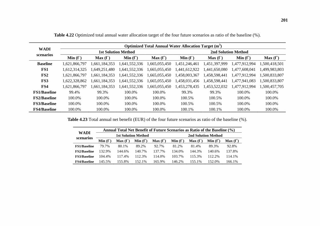
201

Table 4.22 Optimized total annual water allocation target of the four future scenarios as ratio of the baseline (%).

WADI scenarios

Optimized Total Annual Water Allocation Target (m3) 1st Solution Method 2nd Solution Method

Min (f −) Max (f−) Min (f +) Max (f+) Min (f −) Max (f−) Min (f +) Max (f+) Baseline 1,621,866,797 1,661,184,353 1,641,552,336 1,665,055,450 1,451,246,461 1,451,397,999 1,477,912,994 1,500,418,501

FS1 1,612,314,325 1,649,251,480 1,641,552,336 1,665,055,450 1,441,612,922 1,441,650,080 1,477,608,041 1,499,983,803 FS2 1,621,866,797 1,661,184,353 1,641,552,336 1,665,055,450 1,458,003,367 1,458,598,441 1,477,912,994 1,500,833,807 FS3 1,622,328,862 1,661,184,353 1,641,552,336 1,665,055,450 1,458,031,456 1,458,598,441 1,477,941,083 1,500,833,807 FS4 1,621,866,797 1,661,184,353 1,641,552,336 1,665,055,450 1,453,278,435 1,453,522,032 1,477,912,994 1,500,457,705

FS1/Baseline 99.4% 99.3% 100.0% 100.0% 99.3% 99.3% 100.0% 100.0% FS2/Baseline 100.0% 100.0% 100.0% 100.0% 100.5% 100.5% 100.0% 100.0% FS3/Baseline 100.0% 100.0% 100.0% 100.0% 100.5% 100.5% 100.0% 100.0% FS4/Baseline 100.0% 100.0% 100.0% 100.0% 100.1% 100.1% 100.0% 100.0%

Table 4.23 Total annual net benefit (EUR) of the four future scenarios as ratio of the baseline (%).

WADI scenarios

Annual Total Net Benefit of Future Scenarios as Ratio of the Baseline (%) 1st Solution Method 2nd Solution Method

Min (f −) Max (f−) Min (f +) Max (f+) Min (f −) Max (f−) Min (f +) Max (f+) FS1/Baseline 79.7% 80.1% 89.2% 92.7% 81.2% 81.4% 89.3% 92.8% FS2/Baseline 132.9% 144.6% 140.7% 137.7% 134.0% 144.3% 140.6% 137.8% FS3/Baseline 104.4% 117.4% 112.3% 114.0% 103.7% 115.3% 112.2% 114.1% FS4/Baseline 145.5% 155.8% 152.1% 165.9% 146.2% 155.1% 152.0% 166.1%

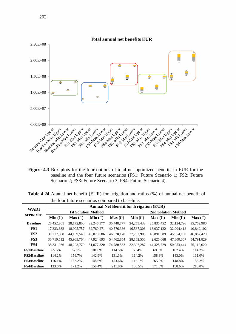
202

Table 4.24 Annual net benefit (EUR) for irrigation and ratios (%) of annual net benefit of

the four future scenarios compared to baseline.

WADI scenarios

Annual Net Benefit for Irrigation (EUR) 1st Solution Method 2nd Solution Method

Min (f −) Max (f−) Min (f +) Max (f+) Min (f −) Max (f−) Min (f +) Max (f+) Baseline 26,452,801 28,172,800 32,246,577 35,448,777 24,255,433 25,835,452 32,124,796 35,762,980

FS1 17,333,682 18,905,757 32,769,271 40,576,366 16,587,306 18,037,122 32,904,418 40,849,102

FS2 30,217,508 44,159,549 46,078,686 46,528,170 27,702,908 40,891,389 45,954,190 46,862,429

FS3 30,710,512 45,983,764 47,924,693 54,462,854 28,162,550 42,625,668 47,800,367 54,791,829

FS4 35,331,036 48,223,779 51,077,320 74,780,583 32,392,287 44,325,729 50,953,444 75,112,020

FS1/Baseline 65.5% 67.1% 101.6% 114.5% 68.4% 69.8% 102.4% 114.2%

FS2/Baseline 114.2% 156.7% 142.9% 131.3% 114.2% 158.3% 143.0% 131.0%

FS3/Baseline 116.1% 163.2% 148.6% 153.6% 116.1% 165.0% 148.8% 153.2%

FS4/Baseline 133.6% 171.2% 158.4% 211.0% 133.5% 171.6% 158.6% 210.0%

0.00E+00

5.00E+07

1.00E+08

1.50E+08

2.00E+08

2.50E+08Total annual net benefits EUR

Figure 4.3 Box plots for the four options of total net optimized benefits in EUR for the baseline and the four future scenarios (FS1: Future Scenario 1; FS2: Future Scenario 2; FS3: Future Scenario 3; FS4: Future Scenario 4).

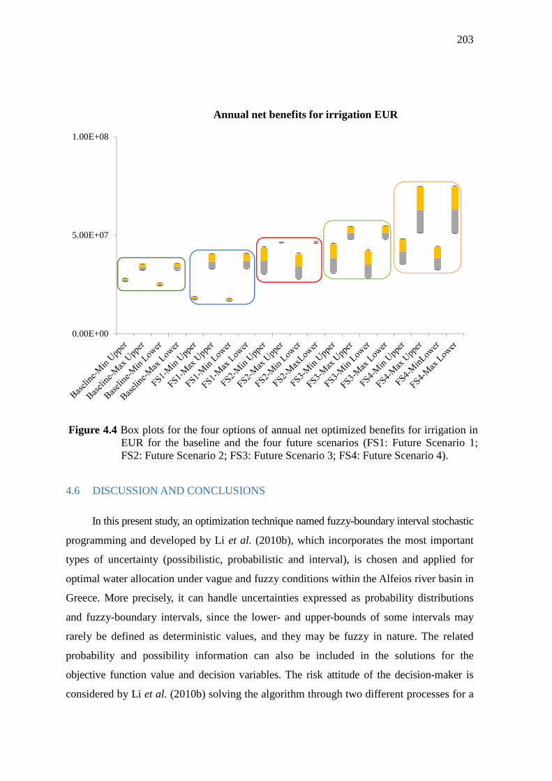
203

4.6 DISCUSSION AND CONCLUSIONS

In this present study, an optimization technique named fuzzy-boundary interval stochastic

programming and developed by Li et al. (2010b), which incorporates the most important

types of uncertainty (possibilistic, probabilistic and interval), is chosen and applied for

optimal water allocation under vague and fuzzy conditions within the Alfeios river basin in

Greece. More precisely, it can handle uncertainties expressed as probability distributions

and fuzzy-boundary intervals, since the lower- and upper-bounds of some intervals may

rarely be defined as deterministic values, and they may be fuzzy in nature. The related

probability and possibility information can also be included in the solutions for the

objective function value and decision variables. The risk attitude of the decision-maker is

considered by Li et al. (2010b) solving the algorithm through two different processes for a

0.00E+00

5.00E+07

1.00E+08

Annual net benefits for irrigation EUR

Figure 4.4 Box plots for the four options of annual net optimized benefits for irrigation in EUR for the baseline and the four future scenarios (FS1: Future Scenario 1; FS2: Future Scenario 2; FS3: Future Scenario 3; FS4: Future Scenario 4).

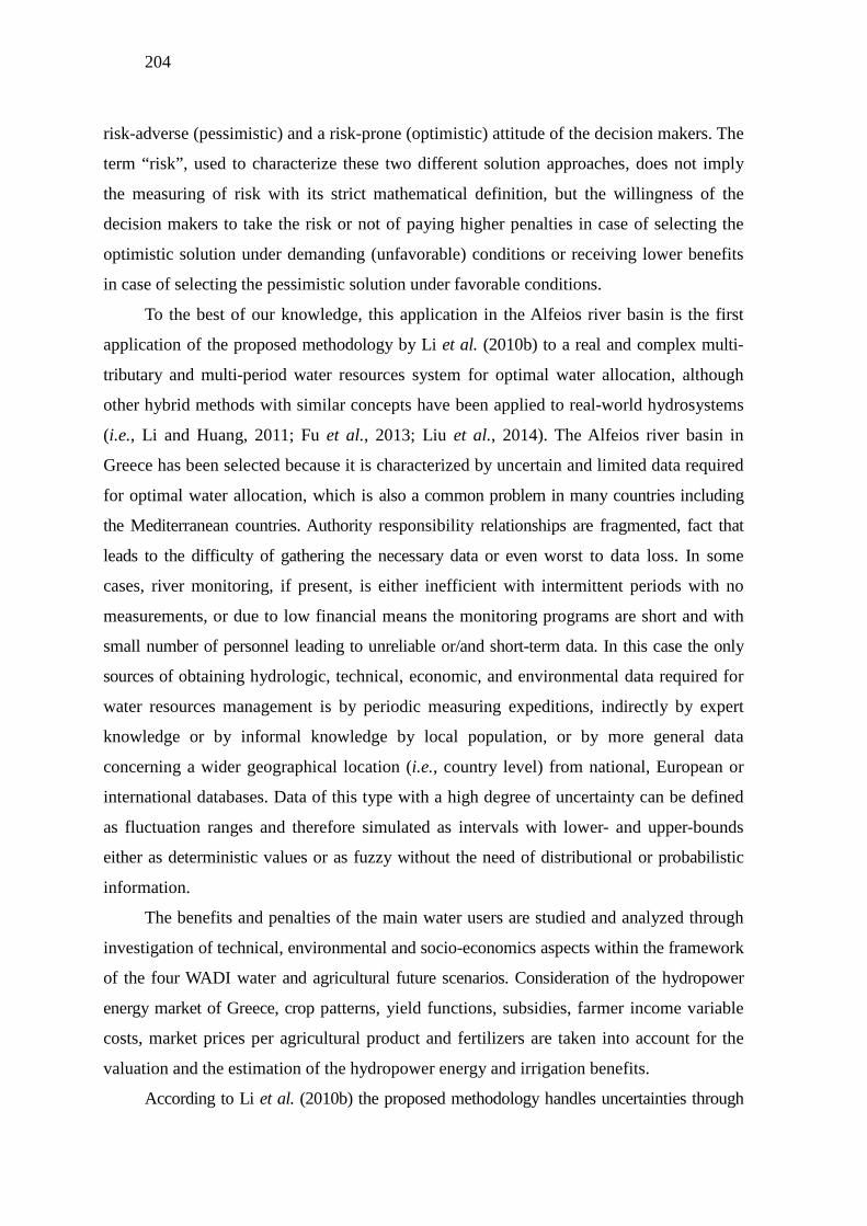
204

risk-adverse (pessimistic) and a risk-prone (optimistic) attitude of the decision makers. The

term “risk”, used to characterize these two different solution approaches, does not imply

the measuring of risk with its strict mathematical definition, but the willingness of the

decision makers to take the risk or not of paying higher penalties in case of selecting the

optimistic solution under demanding (unfavorable) conditions or receiving lower benefits

in case of selecting the pessimistic solution under favorable conditions.

To the best of our knowledge, this application in the Alfeios river basin is the first

application of the proposed methodology by Li et al. (2010b) to a real and complex multi-

tributary and multi-period water resources system for optimal water allocation, although

other hybrid methods with similar concepts have been applied to real-world hydrosystems

(i.e., Li and Huang, 2011; Fu et al., 2013; Liu et al., 2014). The Alfeios river basin in

Greece has been selected because it is characterized by uncertain and limited data required

for optimal water allocation, which is also a common problem in many countries including

the Mediterranean countries. Authority responsibility relationships are fragmented, fact that

leads to the difficulty of gathering the necessary data or even worst to data loss. In some

cases, river monitoring, if present, is either inefficient with intermittent periods with no

measurements, or due to low financial means the monitoring programs are short and with

small number of personnel leading to unreliable or/and short-term data. In this case the only

sources of obtaining hydrologic, technical, economic, and environmental data required for

water resources management is by periodic measuring expeditions, indirectly by expert

knowledge or by informal knowledge by local population, or by more general data

concerning a wider geographical location (i.e., country level) from national, European or

international databases. Data of this type with a high degree of uncertainty can be defined

as fluctuation ranges and therefore simulated as intervals with lower- and upper-bounds

either as deterministic values or as fuzzy without the need of distributional or probabilistic

information.

The benefits and penalties of the main water users are studied and analyzed through

investigation of technical, environmental and socio-economics aspects within the framework

of the four WADI water and agricultural future scenarios. Consideration of the hydropower

energy market of Greece, crop patterns, yield functions, subsidies, farmer income variable

costs, market prices per agricultural product and fertilizers are taken into account for the

valuation and the estimation of the hydropower energy and irrigation benefits.

According to Li et al. (2010b) the proposed methodology handles uncertainties through

205

constructing a set of scenarios (scenario-tree) that are representative for the universe of

water-availability conditions for two tributaries. With such a scenario-based approach, the

resulting mathematical programming model could become too large to be applied to large-

scale real-world problems. Moreover, the random variables (i.e., water inflows from two

tributaries) are assumed to take on discrete distributions and to be mutually independent, such

that the study problem can be solved through linear programming method. However,

conditional probabilities need to be handled for quantifying water availability, particularly

for a multi-stream and multi-reservoir system. This may lead to non-linearity in system

responses and raise a main challenge for identifying global optimal solution.

An alternative approach to these limitations of the FBISP methodology is proposed by

incorporating the water inflow uncertainty through the simultaneous generation of

stochastic equal-probability hydrologic scenarios for stochastically dependent multiple

variables at various locations of water inflows in the river basin. This is enabled by using

CASTALIA software for stochastic simulation and forecast of hydrologic variables,

combining not only multivariate analysis (for many hydrologic processes and geographical

correlated locations) as well as multiple time scales (monthly and yearly) in a

disaggregation framework. This software permits the preservation of essential marginal

statistics up to third order (skewness) and joint second order statistics (auto- and cross-

correlations), and the reproduction of long-term persistence (Hurst phenomenon) and

periodicity. In this application twelve time stages, one for each month of the examined year

have been used (whereas in Li et al. (2010b) only three stages have been considered) and

fifty equal-probability hydrologic scenarios (whereas in Li et al. (2010b) 258 scenarios

should be taken into account for only three stages). By increasing the number of the

generated equal-probability scenarios, the accuracy of the results also increases. But it is

worth mentioning that an increase of the time stages to more than 12 (i.e., in 24 stages for a

2 years analysis), would mean that 24 × 50 = 1200 probabilistic values for shortages and

allocations should be analyzed. This would make the analysis of the results very

complicated, setting also a matter of use of this methodology to a more complex time

horizon. From the analysis of the results, it is clear that due to the space limitations, the

monthly results cannot be presented in tabular form and analyzed as thoroughly.

Finally, in terms of the results from this methodology, the goal of this technique is

from one side to identify the optimized water-allocation target with a minimized risk of

economic penalty and opportunity loss, and from the other side to determine an optimized

206

water-allocation plan with a maximized system benefit over a multi-period planning

horizon. Fuzzy upper- and lower-bound intervals (expressing the effect of the embodied

uncertainties) for the optimal water allocation targets and the probabilistic water

allocations and shortages as well as the total benefits for the main water uses are identified.

The results show that variations in water-allocation targets could express different

strategies for water resources management and thus produce varied economic implications

under uncertainty.

The major results through the application of the FBISP method to optimal water

resources allocation in the Alfeios River Basin are the following:

(1) The monthly optimized water allocation target values are: (i) for irrigation for the

upper-bound model (f+) the same for both solution methods and equal to its maximum

possible value; for the lower-bound model (f−) are higher for the first solution method with

much wider ranges between the minimum and the maximum value compared to the ones

from the second solution method; (ii) for the hydropower production at Ladhon equal to

the maximum allowable values for all months except for July, September-November for

the first solution method; deviate from the maximum allowable values for all months for

the second solution method; and (iii) the maximum possible allocation for all months

except May and June for the hydropower production at Flokas. From the optimized targets

of the three main users, as analyzed above, it can be concluded that the highest priority for

water allocation is set to irrigation, since it has the highest unit benefit, but at the same

time also the highest unit penalty. The next priorities are given to hydropower production

at Flokas and finally to the hydropower production at Ladhon, which has the smallest unit

benefit.

(2) The optimized total annual water allocation targets for the various alternative water

and agricultural WADI policies compared to the baseline are only slightly affected, since

the main impact of these scenarios is on the net system benefits. Based on the comparison

of the total system benefits from the four future scenarios to the baseline, the highest

increase is observed for the Local Stewardship scenario and the only decrease for the

World Warket scenario.

(3) For irrigation, in most hydrologic scenarios, annual water shortages are zero,

since the water allocation is equal to the optimized water allocation target. There are only a

few hydrologic scenarios with nonzero shortages, for which, if the farmers do not have an

alternative water source, a yield reduction is highly possible. These shortages occur in

207

August and September, which can be justified by the low flow rate at Flokas Dam for these

two months in combination with the increased irrigation demand. On the other hand, the

hydropower production at Ladhon and Flokas in most hydrologic scenarios deviates from

the optimized target, therefore resulting in nonzero annual shortages for both hydropower

stations. For the hydropower production at Ladhon, the highest shortages take place from

January–April (with the highest in March), since in order to satisfy completely the most

important water use, that being irrigation (starting mainly from May), the water volume

flowing into the Ladhon Reservoir from December–April should be stored and not

released. A conflict between the two uses for this time period is observed. For the

hydropower production at Flokas, the highest shortages occur during the irrigation period

from June–October (with the highest in October), showing a conflict between the two uses.

The small HPS at Flokas is only set in operation after the satisfaction of irrigation demand,

driving toward water shortages for these months if the available water at Flokas Dam is not

adequate.

(4) By comparing the corresponding results of the FBISP method in this chapter with

the ITSP as presented in Bekri et al. (2015a), it is worth noticing that the results are

consistent and compatible but it can be concluded that the incorporation of the fuzzy nature

of the uncertainties in the FBISP results in a more analytic and fine approximation of the

effect of the uncertainties on the minimum and maximum values of the boundaries of the

results providing also a more complicated structure of the results.

208

209

5. EPILOGUE

5.1 SUMMARY AND SYNOPTIC RESULTS

5.1.1 CORRECTION TECHNIQUE FOR QUICK RIVER DISCHARGES

One of the key elements of river basin management is the water quantity and quality

monitoring programs. These programs are required to establish a coherent and

comprehensive overview of water status, to identify changes or trends in water quality and

quantity, and to assess remediation or preventive measures within each river basin district.

The necessity for developing and implementing integrated river basin management plans

has been introduced in Europe with the European Water Framework Directive 2000/60/EC

(WFD, 2000). According to the WFD, the river monitoring programs should determine

apart from the level of predefined pollutants, also their mass load. Discharge data are

essential for the estimation of loads of sediments or chemical pollutants of a river or stream

(NCSU, 2008). The mass load of a pollutant at a selected river cross-section is indirectly

estimated by the combination of parallel measurements of water discharge and pollutant

concentration and tts calculation results from their product.

For a holistic and complete picture of the whole river status, containing its

tributaries, quantitative and qualitative characteristics should be measured nearly in

parallel at suitably chosen cross-sections mirroring the state of the whole river. To achieve

this, from one side, fixed discharge measurement arrangements and from the other side,

automatic samplers of constant function for computing pollutant concentration should be

available. River discharge is usually estimated from water level recording at a properly

built cross-section by means of a discharge rating curve determined from a number of

discrete measurements by current meters and floats. The aforementioned thoroughly and

rightly systematized measuring scheme is not available in all river bodies world-wide. In

this case, mobile measurement equipment is employed. Determination of the geometric

properties of the cross-section in conjunction with the flow velocity, employing a current-

meter at specific depths, is the most common and reliable method. However, in many cases

the available time for the realization and completion of river flow rate and water quality

measurements at various cross-sections, incorporating the entire river and its tributaries, is

significantly shorter than the one needed for in-situ measurements and sampling. As a

210

consequence, quicker measurement techniques are needed to enable the previously

mentioned simultaneous measurements along the whole river during the daytime. In such

cases, where additionally low financial means are available for implementing monitoring

programs, quick methods of low cost and reliability, such as floats, release of air bubbles

and the pendulum (Yannopoulos, 1995; Yannopoulos et al., 2000; Yannopoulos et al.,

2008) could be employed for river discharge measurements.

The first part of the present PhD thesis contributed to the development of a

theoretical, mathematical and computational concept of an original correction technique

for river discharges measured with quick measurement methods of low cost and reliability,

in order to estimate more reliable values of river discharges and pollution loads in

ungauged rivers (Yannopoulos, 2009; Yannopoulos and Bekri, 2010; Bekri et al., 2012;

Bekri et al., 2013). For the application of the proposed methodology parallel measurements

of river flow rate and natural tracers should be available for representative cross-sections

of a river and its tributaries. Within this frame, the water volume conservation is combined

with pollutant/tracers mass balance synchronously in each single node of a river as well as

in all possible multiple-nodes combinations (considering balances every two successive

nodes, every three, etc.) covering the entire river.

Its basic concept is similar to data reconciliation, since they both aim at correcting

the raw measurements based on the principles of mass conservation without knowing the

precise values. Classical approaches for data validation rely on statistical approaches that

are based on the availability of an explicit characterization of the measurement errors

(knowledge of the precision of the measurements). The main difficulty in this approach is

that the processes are not always perfectly described and the measurement precision cannot

be precisely quantified. In many cases the user has only an experimental knowledge, which

even inaccurate can be used in the form of inequalities. The introduced methodology does

require any statistical assumption for the error distribution, since intervals in terms of error

bounds are used in order to express the allowable range of the corrected values of each

parameter based on their parameters’measured values and assumed measurement errors.

This concept of expressing the measurement error as interval is similar to the one

used in the so-called parameter set estimation from bounded error data (Milanese and

Belforte, 1982; Ragot and Maquin, 2005). In this case it is assumed that all types of errors

belong to a known set and that the measurement error is bounded. As analysed in these

scientific works, because of uncertainty and noise influence it is not feasible to calculate

211

the exact parameter values, but it seems reasonable to compute a domain in which the real

values of the system are contained.

An analogous approach as the one suggested in this PhD thesis, has been presented

by Mandel et al. (1998) in the domain of chemical engineering. In this paper, all variables

are expressed as confidence intervals resulting in upper and lower bounds. Moreover, a

minimum (upper) and maximum (lower) acceptable deviation of the water volume and

mass conservation balances are considered, completing the set of inequalities. Both

previously mentioned bounds are chosen as a function of empirical knowledge of the

process state and the probable variation domain of the variables. The formulated system of

inequalities is solved based on the Linear Matrix Inequality technique, which determines if

the system of all polynomial inequalities is feasible and computes a feasible solution.

In our methodology, similar error bounds constraints are considered, but these

inequalities are expressed additionally by replacing the variables with their equivalents

computed from the mass balances (water volume and pollutant mass load) written for each

single node and for all possible multiple-nodes combinations. In this way the optimized

values satisfy at the highest possible degree not only the single-node balances as in Mandel

et al. (1998) but all combinations of multiple-nodes balances. Moreover, a linear

optimization problem is solved for the assumed river discharge error combination, setting

as objective function the minimization of the sum of the absolute values of the residuals of

the water volume and tracer mass conservation equations of each single-node and of all

possible multiple-node combinations of the whole river plus the residuals of the

linearization of the nonlinear inequalities including the mass pollutant load, as analyzed

below. Such an objective function results in corrected river discharge and tracer

concentrations values building water volume and tracer mass balances as close as possible

to zero. It approaches more reliable and representative values compared to the initial

measurements. In this way all the residuals from the water balances and the mass

conservation of each single node and all possible node combinations are introduced into

the objective function. When a constraint considering their allowable values is violated,

there is a positive contribution to the objective function equal to the amount of violations

or the sum of infeasibilities.

In the introduced methodology, it is considered that the concentrations of m properly

selected pollutants have been estimated with sufficient accuracy, and therefore, resulting in

an adequately low and known error. It is notable that when pollutant or natural tracers are

212

measured very precisely, accuracy of discharge measurements becomes the most critical

component of the pollutant load computation and the largest source of error (NCSU, 2008).

Moreover, it is assumed that the measurement conditions refer to the mean hydraulic

conditions usually prevailing in the considered flow (Schmidt, 2002), being steady state

(no transient effects) and usual hydraulic controls (i.e. no varying backwater effects, no

change in channel roughness or the geometry of the controlling cross-section). Within this

framework and taking into account water compressibility, it is possible to express the mass

conservation for the water volume and the pollutant load for each one single-node and all

possible multiple-nodes combinations for the entire river.

In the proposed methodology for each node an unknown, not-directly measured

water quantity is taken into account. This unknown quantity is referred to as “latent”, since

it is impossible to directly measure it. The latent discharge of each node is assumed to

correspond to runoff of a catchment area, which is included between all considered

inflowing cross-sections and the outflowing cross-section around the node k. The exact

area for the latent quantity cannot be computed with certainty and only a rough

approximation given the various subcatchment areas and the in-between area can be made.

A model based on the water volume and pollutant mass conservation is developed and

incorporated into the methodology for approximation of the initial values of the latent

quantities (discharge and concentration).

Since the measurement error for the river discharge is not known, several

combinations of the river discharge measurement errors, including also the latent ones,

could be assumed based on the experience of the group that undertook the measurement

expeditions, in order to find a feasible domain of the solution space of the optimization

problem, if any. According to Ragot and Maquin (2004) by increasing the error bound, not

a single but various solutions are obtained from a bounded error optimization

methodology. This is due to the fact that increasing the error bound subject to the

considered constraints makes it possible for more than one error combination to satisfy the

whole set of constraints. In this work, the minimum possible errors for the river discharges,

which result in a feasible solution, have been selected by trial and error based on the

experience of the scientific team that undertook the measurements in combination with the

results from the qualitative analysis of the measurements for the detection of outliers.

Concerning the unknown estimation error of the latent discharge terms, for their

upper and lower bound, a wider “relaxed” value interval based on the results of the

213

qualitative analysis of the measurements is considered in order to avoid that these

unmeasured latent terms play a restricting and divergent role at the optimization of the

values of all measured cross-sections (Mandel et al., 1998; Ragot and Maquin, 2004).

The suggested optimization problem encompasses two types of constraints: from one

side, linear constraints based on the water volume conservation and from the other side,

nonlinear constraints based on tracer mass conservation. The latter constraints involve the

product of two variables, meaning river discharge and concentration, thus forming a

nonlinear bilinear system. In our methodology to overcome this nonlinear difficulty and to

convert the system into linear the solution proposed by Mandel et al. (1998) is adapted.

More precisely, an iterative solution is undertaken, which is based on the idea of

decoupling, using between two iterations the reciprocal contribution of these two balances.

Every nonlinear constraint is written twice: firstly, assuming that the values of river

discharges are known fixed and equal to their computation from the previous iteration and

that the only unknown variables are the tracer concentrations, and secondly, reversing the

known fixed variables and the unknown variables. In this way a linear optimization

problem is built. For the first iteration, initial values of river discharges and tracer

concentrations for all cross-sections, including the latent ones, are required. For all cross-

sections, their corresponding measurements are used (except of the measurements with

gross-errors), whereas for the latent unmeasured cross-sections, the resulting values from

the balances of the nodes are considered. This process involves a number of iterations,

until the convergence of the corrected flow rates and tracer concentrations toward constant

values between two successive steps is accomplished, or until a sufficiently small

difference of their values between two successive steps is reached.

Based on this linearization, a second term is added in the chosen objective function

including the minimization of the sum of the absolute values of the differences between the

mass balance residuals, when the mass balance is written assuming that the concentrations

are known and fixed and the river discharges are the unknown variables, and the mass

balance residuals, when the mass balance is written, assuming the concentrations are

unknown and the river discharges are known and fixed. Concerning the second term, since

the pollutant mass balance is expressed twice in order to keep the optimization problem in

the linear space, the solution of the optimization problem should verify that the difference

of the two expressions tends to zero.

The aforementioned methodology is applied to the Alfeios River Basin in

214

Peloponnisos, Greece, which has been described in detail in the past (Manariotis and

Yannopoulos, 2004; Bekri and Yannopoulos, 2012; Podimata and Yannopoulos, 2013). The

simultaneous discharge measurements using quick techniques and water sampling included

eleven cross-sections along the main river and its tributaries. For the application of the

suggested technique, four nodes of junctions were properly defined, in order to satisfy the

previously mentioned distance requirement, covering the entire river length and its

tributaries. From the six measuring expeditions, only four yielded sufficient and suitable

data for the application of the proposed methodology requirements for the whole-river

approach. The two expeditions were rejected since they were carried out under unstable

flow conditions due to sudden alterations of the operation of the Ladhon Hydroelectric

Power Station (HPS) during the measurement process, which violates the predefined

steady-state conditions for the application of the proposed methodology.

For each expedition, water conductivity, sulphate ions concentration (SO4-2) and

chloride ions concentration (Cl-) have been tested and selected as the most appropriate

tracers based on the requirements of the considered methodology (Ziabras and Tasias,

1999). The pollutant concentration is assumed to have a known and very small absolute

maximum relative error. It is taken equal to the value provided by the manufacturer of the

measuring equipment and only the tracers with suitably small error, which is assumed to be

less than 20%, are accepted.

A first qualitative evaluation of the discharge measurement is necessary before the

application of the introduced optimization process in order to identify if one or more

measurements include gross-errors. The reason for this is that data reconciliation can have

an unexpected effect if gross-errors are not eliminated (Mandel et al., 1998; Narasimhan

and Jordache, 2000). The presence of outliers in the methodologies based on bounded

errors and inequality balance equilibration, such as the one submitted here and the one

introduced by Ragot and Maquin (2004), drives to non-feasible solution for the set of

inequalities, because they are no longer compatible. In this methodology the initial

estimation of the latent discharge is derived from the water balance of each node using the

measurements of the river discharge. Based on the computed latent terms there are four

points to be checked for the identification of a probable cross-section with gross-error and

for the subsequent revision of tis measured value. These include (a) the assessment of the

magnitude of the latent discharge based on the comparison of the computed latent value

with a rough estimation of the maximum possible latent discharge value according to the

215

hydrologic characteristics of the river and its tributaries or to expert

understanding/knowledge of the examined hydrologic system, (b) the examination of the

sign of water balance of each node, from which the latent discharge is computed, since no

negative water or/and mass pollutant balances are acceptable, (c) the evaluation of the

magnitude of the computed latent concentration based on the mass pollutant balance of the

examined node, (The latent cross-section is situated within the catchment area and

therefore, the assumption is made that the latent concentration can vary between zero and

the maximum registered concentration of each pollutant plus the measurement error.), and

(d) the sign of the computed latent concentration based on the mass pollutant balance of

the examined node. Only positive concentration values are reasonable and accepted. If

negative values are derived, small changes of the measured concentration values within

their narrow ranges are undertaken in order to derive an initial solution with positive

concentrations. In the application of the proposed methodology in the Alfeios river,

electroconductivity has been measured with two measuring equipment. These two

measurements should not differ more than 15% from each other. For this reason before

applying the optimization process this check should be also done. In case of higher

deviations, the initial values of these concentrations should be properly adjusted within

their allowable value range based on their measurement error =10%.

In the proposed iterative optimization process, the lower and upper bounds of the

optimization variables (which are the right-hand sides of the constraints) are written based

on the measurements and their assumed measurements errors. In the left-hand side of the

constraints, where the optimization variables are included, revised values at the cross-

sections with gross-errors are used as initial values instead of their measurements at the

first step of the optimization process in order to ensure a feasible solution at the first step

of the algorithm. After the identification of the node(s) including cross-sections with gross-

errors, the identification of the “problematic” cross-sections should take place as well as

the computation/approximation of their revised values. In this methodology the following

process for these points is suggested. For each node an evaluation of the magnitude of the

river discharge measurement error of each cross-section should be made based on the

measuring knowledge of the team that undertook the measurements (i.e. based on the

geometric and morphological characteristics of the cross-section and the difficulties of

measuring associated with the reliability of the measurement).

In this way the categorisation of the measurement errors to small, medium and high

216

result for each cross-section of the node is enabled. The cross-sections with the assumed

highest measurements errors are supposed to be subject to revision. For these cross-

sections an upper and lower bound for the river discharge values for the month of the

measuring expedition should be identified. This can be done by using the statistical

analysis of historical timeseries, if available, or expert knowledge. The revised values are

assumed to lie within this estimated value range and equal to three values: the minimum,

mean (or the measured value if it lies within the computed range) and maximum value.

Based on this all possible combinations of the revised initial values of river discharges are

examined and assessed in terms of their feasibility according to the four prementioned

check points for the latent terms (magnitude and sign).

The proposed optimization algorithm was built using the advanced programming

language of LINGO optimization software (Schrage, 1997; Lindo Systems Inc., 1996). It

has been chosen, since it is a very efficient and robust tool for building and solving

mathematical optimization models. In order to increase the flexibility and the ease of the

proposed methodology, LINGO has been properly combined with Microsoft Excel 2010 in

order to import and export input and output data through OLE Automation Links. For the

introduced methodology it uses firstly a direct solver and then its linear solver for a

continuous linear optimization problem, which is based on the primal simplex.

Through the application of this optimization process, it is observed that at every step

the value of the objective function is reduced till it reaches the zero value. At this point if

we continue this process, it oscillates between two solutions about the optimum. It does not

converge to it probably as a result of the effect of the linearized constraints. In this case a

step bound for the corrected river discharges and for the corrected pollutant concentrations

should be applied which should be reduced properly, so that convergence to the optimal

solution is guaranteed (Edgar et al., 2001). This is achieved by adding upper-bound

constraints to the difference of the values of the variables between two successive steps of

the iterative process. The reduction of the step bounds is approximated by trial and error in

order to result into global optimum solutions.

The suggested methodology was successfully implemented in the Alfeios river in

Greece including tributaries, where only limited short-term quantitative and qualitative

measurement data are available. It enabled the estimation of: (a) corrected discharges,

pollutant and pollution loads for eight combinations of initial values as estimated from the

qualitative analysis of the river basin, (b) a best/worst case (Min/Max) interval and the

217

corresponding error of the computed/optimized river discharges pollutant and pollution

loads for the cross-sections of the main river and its tributaries, where tracer concentrations

were measured, and (c) the unknown latent parameters, including flow rate, pollutant

concentration and pollution loads of each river node.

Moreover, it provided satisfactory results with significantly lower errors for the

corrected discharges, and therefore, more reliable estimation of pollution loads. Based on

these results the methodology succeeded in restricting errors of the corrected mean

discharge values of all measured cross-sections. The determination of a hypothetical

unknown latent discharge and subsequently the correction of its estimation, even if it is

relatively inaccurate, are very important and useful, since the direct measurement of latent

discharge and generally of the assumed latent terms, is impossible. Besides, it is worth

underscoring that the combination of the single-node balances together with all possible

multiple-node combinations balances based on the previous findings, resulted in a

considerable reduction of the river discharge interval of the ensemble of cross-sections of

Alfeios river.

All resulting ranges for both variables, discharge and concentration, are in full

compliance with the qualitative analysis. For the cross-section 8 at Ladhon river, the value

of the registered water volume released by Ladhon HPS (=36.75m3/s) is included within

the range of the corrected river discharge (35.7, 38.25)m3/s, which is an important

verification point for the validity of the correction methodology.

Based on the corrected river discharges and concentrations for the eight

combinations of initial values of river discharges it can be concluded that generally, the

proposed methodology enables the computation of pollution loads with significantly lower

resulting error, revealing a very narrow value range for all measured cross-sections. For the

latent cross-sections, the relative errors for all pollutants are significantly high. A further

investigation of the pollutant loads and their statistical analysis based on the corrected river

discharges and concentrations are proposed for future work.

The direct confirmation of the corrected river discharges with simultaneous accurate

measurements is hampered by the lack of such precise measurements. Thus, the

consistency of the proposed methodology was compared with the results from the

nonlinear model and the following conclusions can be extracted: the value ranges of the

nonlinear model lie into similar but not exactly the same value region as the ranges of the

linear correction technique. The linear value range is enclosed within the nonlinear value

218

range, showing the consistency and the compatibility between the results of the two

methods. Generally, the nonlinear ranges are for most cross-sections wider.

Therefore, applying t-test statistics for the measured values and the results of the

corrected variables taken through either linear or nonlinear models, it is proven that both

population samples belong in similarly equivalent populations since the differences

between measurements and linear or nonlinear model results can be considered statistically

insignificant with a significance level 0.01. Therefore, the consistency of the resulting

solutions from the optimization process to the measurements is confirmed.

From a thorough literature review and to the best of our knowledge, the combination

of water volume and properly selected natural tracers mass conservation in a river network

with the use of bounded error data reconciliation, as in the introduced methodology, has

not been described in previous publications and applied to correct river discharge

measurements and to compute more reliable pollution loads, whereas similar data

reconciliation techniques are proposed in chemical and process engineering domain. In any

case, further investigation focused on direct comparison of methodology’s corrected river

discharges to accurately measured values would be a next task to be undertaken. Therefore,

the presented methodology could embody a valuable, efficient and necessary tool for the

implementation of monitoring programs of catchment pollution, in order to reasonably

increase and improve the reliability of the estimation of river discharge and pollution loads.

5.1.2 OPTIMAL WATER ALLOCATION UNDER UNCERTAIN SYSTEM CONDITIONS

Optimal water allocation of a river basin poses great challenges for engineers due to

various uncertainties associated with the hydrosystem, its parameters and its impact factors

as well as their interactions. These uncertainties are often associated with various

complexities in terms of information quality (Li et al., 2009). The random characteristics

of natural processes (i.e., precipitation and climate change) and stream conditions (i.e.,

stream inflow, water supply, storage capacity, and river-quality requirement), the errors in

estimated modeling parameters (i.e., benefit and cost parameters), and the vagueness of

system objectives and constraints are all possible sources of uncertainties. These

uncertainties may exist in both left- and right-hand sides of the constraints as well as

coefficients of the objective function. Some uncertainties may be expressed as random

variables. At the same time, some random events can only be quantified as discrete intervals

with fuzzy boundaries, leading to multiple uncertainties presented as different formats in the

219

system's components (Li et al., 2010b). Traditional optimization techniques can embody

various characteristics but only as deterministic values. In various real-world problems,

results generated by these traditional optimization techniques could be rendered highly

questionable if the modeling inputs could not be expressed with precision (Li et al., 2009;

Fan and Huang, 2012; Suo et al., 2013). For these reasons conventional deterministic

optimization approaches have given their place to stochastic (SP), fuzzy (FP) and interval-

parameter programming (IPP) approaches and their hybrid combinations in order to face

up these difficulties. Various methodologies have been developed and proposed (Suo et al.,

2013; Huang et al., 1992; Huang and Loucks, 2000; Maqsood et al., 2005; Li et al., 2006;

Nie et al., 2007; Yeomans, 2008; Li and Huang, 2009; Li and Huang, 2011; Yeomans,

2008; Li and Huang, 2009; Li and Huang, 2011; Fu et al., 2013; Liu et al., 2014; Miao et

al., 2014; Li et al., 2008) in order to embody in optimal water allocation uncertainties of

various influencing factors and hydrosystem characteristics.

Both hybrid methods are based on the concept that in real-world problems, some

uncertainties may indeed exist as ambiguous intervals, since planners and engineers

typically find it more difficult to specify distributions than to define fluctuation ranges. The

ITSP is a hybrid method of inexact optimization and two-stage stochastic programming

able to handle uncertainties, which cannot be expressed as probability density functions.

The FBISP incorporates the most important types of uncertainty (possibilistic, probabilistic

and interval) and is based on the combination of three optimization techniques: (a) the

multistage-stochastic programming; (b) the fuzzy programming (employing the vertex

analysis for fuzzy sets) and (c) the interval parameter programming. Each technique has a

unique contribution in enhancing the model’s capability of incorporating uncertainty

presented as multiple formats. Moreover, the risk attitude of the decision-maker is

considered in FBISP by solving the algorithm through two different processes for a risk-

adverse (pessimistic) and a risk-prone (optimistic) attitude of the decision makers. The

term “risk”, used to characterize these two different solution approaches, does not imply

the measuring of risk with its strict mathematical definition, but the willingness of the

decision makers to take the risk or not of paying higher penalties in case of selecting the

optimistic solution under demanding (unfavorable) conditions or receiving lower benefits

in case of selecting the pessimistic solution under favorable conditions.

The Alfeios river basin in Greece is chosen for the application of the two

methodologies, because it is characterized by uncertain and limited data, which can be

220

expressed easily as intervals, since the quality of the information is not good enough or not

sufficient to be presented as probability distributions. Authority responsibility relationships

are fragmented, fact that leads to the difficulty of gathering the necessary data or even

worst to data loss. In some cases, river monitoring, if present, is either inefficient with

intermittent periods with no measurements, or due to low financial means the monitoring

programs are short and with small number of personnel leading to unreliable or/and short-

term data. In this case the only sources of obtaining hydrologic, technical, economic, and

environmental data required for water resources management is by periodic measuring

expeditions, indirectly by expert knowledge or by informal knowledge by local population,

or by more general data concerning a wider geographical location (i.e., country level) from

national, European or international databases. Data of this type with a high degree of

uncertainty can be defined as fluctuation ranges and therefore simulated as intervals with

lower- and upper-bounds either as deterministic values or as fuzzy without the need of

distributional or probabilistic information. This is also a common problem met in other

Mediterranean countries, and therefore, the proposed decision support frame could be

applied to other catchments with limited and imprecise data.

The total net benefits and the benefits and penalties of the main water uses for

Alfeios (hydropower energy and irrigation) are studied and analyzed through investigation

of technical, environmental and socio-economics aspects within the framework of the four

WADI water and agricultural future scenarios. Consideration of the hydropower energy market

of Greece, crop patterns, yield functions, subsidies, farmer income variable costs, market

prices per agricultural product and fertilizers are taken into account for the valuation and

the estimation of the hydropower energy and irrigation benefits.

In terms of the results from this methodology, its goal is, from one side, to spot the

desired water allocation target with a minimized risk of economic penalty and opportunity

loss and, from the other side, to determine an optimized water allocation plan with a

maximized system benefit over a multi-period planning horizon. Deterministic or fuzzy

upper and lower bound intervals for the optimal water allocation targets and the

probabilistic water allocations and shortages, as well as for the total system benefits for the

main water uses are identified. The results acquired show that variations in water allocation

targets could express different strategies for water resources management and, thus,

produce varied economic implications under uncertainty.

The major results through the application of the ITSP and the FBISP methods to

221

optimal water resources allocation in the Alfeios River Basin are the following:

(1) The monthly optimized water allocation target values are compared to the

maximum possible value for all water uses in order to identify the tradeoffs and the

priorities of water allocation. From the optimized targets of the three main users, it can be

concluded that the highest priority for water allocation is set to irrigation, since it has the

highest unit benefit, but at the same time also the highest unit penalty. The next priorities

are given to hydropower production at Flokas and finally, to the hydropower production at

Ladhon.

(2) The optimized total annual water allocation targets for the various alternative water

and agricultural WADI policies compared to the baseline are only slightly affected, since

the main impact of these scenarios is on the net system benefits. Based on the comparison

of the total system benefits from the four future scenarios to the baseline, the highest

increase is observed for the Local Stewardship scenario and the only decrease for the

World Warket scenario.

(3) For irrigation, in most hydrologic scenarios, annual water shortages are zero,

since the water allocation is equal to the optimized water allocation target. There are only a

few hydrologic scenarios with nonzero shortages, for which, if the farmers do not have an

alternative water source, a yield reduction is highly possible. These shortages occur in

August and September, which can be justified by the low flow rate at Flokas Dam for these

two months in combination with the increased irrigation demand. On the other hand, the

hydropower production at Ladhon and Flokas in most hydrologic scenarios deviates from

the optimized target, therefore resulting in nonzero annual shortages for both hydropower

stations. For the hydropower production at Ladhon, the highest shortages take place from

January–April (with the highest in March), since in order to satisfy completely the most

important water use, that being irrigation (starting mainly from May), the water volume

flowing into the Ladhon Reservoir from December–April should be stored and not

released. A conflict between the two uses for this time period is observed. For the

hydropower production at Flokas, the highest shortages occur during the irrigation period

from June–October (with the highest in October), showing a conflict between the two uses.

The small HPS at Flokas is only set in operation after the satisfaction of irrigation demand,

driving toward water shortages for these months if the available water at Flokas Dam is not

adequate.

(4) By comparing the corresponding results of the FBISP method with the ITSP, it is

222

worth noticing that the results are consistent and compatible, but it can be concluded that

the incorporation of the fuzzy nature of the uncertainties in the FBISP results in a more

analytic and fine approximation of the effect of the uncertainties on the minimum and

maximum values of the boundaries of the results providing also a more complicated

structure of the results.

Finally, concerning the limitations according to Huang and Loucks (2000) and Li et al.

(2010b), the proposed methodologies handles uncertainties through constructing a set of

scenarios (scenario-tree) that are representative for the universe of water-availability

conditions for two tributaries. With such a scenario-based approach, the resulting

mathematical programming model could become too large to be applied to large-scale real-

world problems. Moreover, the random variables (i.e., water inflows from two tributaries)

are assumed to take on discrete distributions and to be mutually independent, such that the

study problem can be solved through linear programming method. However, conditional

probabilities need to be handled for quantifying water availability, particularly for a multi-

stream and multi-reservoir system. This may lead to non-linearity in system responses and

raise a main challenge for identifying global optimal solution.

An alternative approach to these limitations of the FBISP methodology is proposed by

incorporating the water inflow uncertainty through the simultaneous generation of

stochastic equal-probability hydrologic scenarios for stochastically dependent multiple

variables at various locations of water inflows in the river basin. This is enabled by using

CASTALIA software for stochastic simulation and forecast of hydrologic variables,

combining not only multivariate analysis (for many hydrologic processes and geographical

correlated locations) as well as multiple time scales (monthly and yearly) in a

disaggregation framework. This software permits the preservation of essential marginal

statistics up to third order (skewness) and joint second order statistics (auto- and cross-

correlations), and the reproduction of long-term persistence (Hurst phenomenon) and

periodicity.

5.2 ORIGINAL CONTRIBUTIONS OF THE PHD THESIS

The aim of this session is to present in a synoptic way the original contributions of

the present PhD Thesis (Table 5.1) as well as the total of publications and conferences

(Table 5.2) during the period of the PhD research.

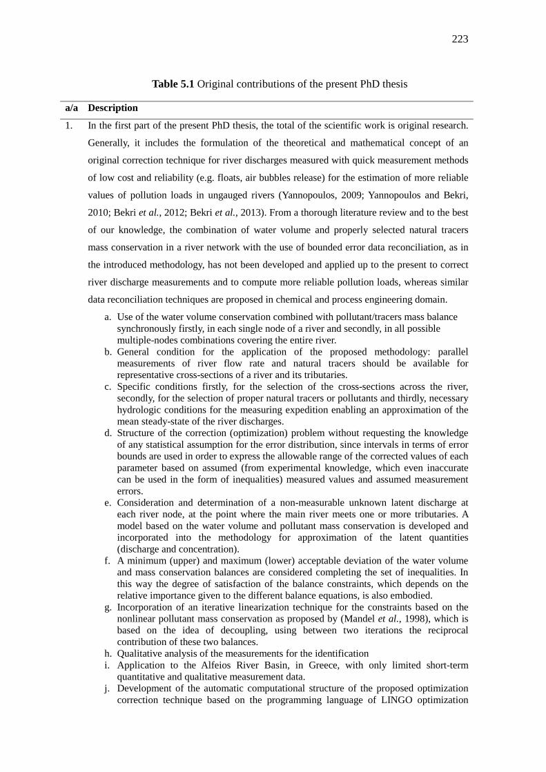
223

Table 5.1 Original contributions of the present PhD thesis

a/a Description

1. In the first part of the present PhD thesis, the total of the scientific work is original research.

Generally, it includes the formulation of the theoretical and mathematical concept of an

original correction technique for river discharges measured with quick measurement methods

of low cost and reliability (e.g. floats, air bubbles release) for the estimation of more reliable

values of pollution loads in ungauged rivers (Yannopoulos, 2009; Yannopoulos and Bekri,

2010; Bekri et al., 2012; Bekri et al., 2013). From a thorough literature review and to the best

of our knowledge, the combination of water volume and properly selected natural tracers

mass conservation in a river network with the use of bounded error data reconciliation, as in

the introduced methodology, has not been developed and applied up to the present to correct

river discharge measurements and to compute more reliable pollution loads, whereas similar

data reconciliation techniques are proposed in chemical and process engineering domain.

a. Use of the water volume conservation combined with pollutant/tracers mass balance synchronously firstly, in each single node of a river and secondly, in all possible multiple-nodes combinations covering the entire river.

b. General condition for the application of the proposed methodology: parallel measurements of river flow rate and natural tracers should be available for representative cross-sections of a river and its tributaries.

c. Specific conditions firstly, for the selection of the cross-sections across the river, secondly, for the selection of proper natural tracers or pollutants and thirdly, necessary hydrologic conditions for the measuring expedition enabling an approximation of the mean steady-state of the river discharges.

d. Structure of the correction (optimization) problem without requesting the knowledge of any statistical assumption for the error distribution, since intervals in terms of error bounds are used in order to express the allowable range of the corrected values of each parameter based on assumed (from experimental knowledge, which even inaccurate can be used in the form of inequalities) measured values and assumed measurement errors.

e. Consideration and determination of a non-measurable unknown latent discharge at each river node, at the point where the main river meets one or more tributaries. A model based on the water volume and pollutant mass conservation is developed and incorporated into the methodology for approximation of the latent quantities (discharge and concentration).

f. A minimum (upper) and maximum (lower) acceptable deviation of the water volume and mass conservation balances are considered completing the set of inequalities. In this way the degree of satisfaction of the balance constraints, which depends on the relative importance given to the different balance equations, is also embodied.

g. Incorporation of an iterative linearization technique for the constraints based on the nonlinear pollutant mass conservation as proposed by (Mandel et al., 1998), which is based on the idea of decoupling, using between two iterations the reciprocal contribution of these two balances.

h. Qualitative analysis of the measurements for the identification i. Application to the Alfeios River Basin, in Greece, with only limited short-term

quantitative and qualitative measurement data. j. Development of the automatic computational structure of the proposed optimization

correction technique based on the programming language of LINGO optimization

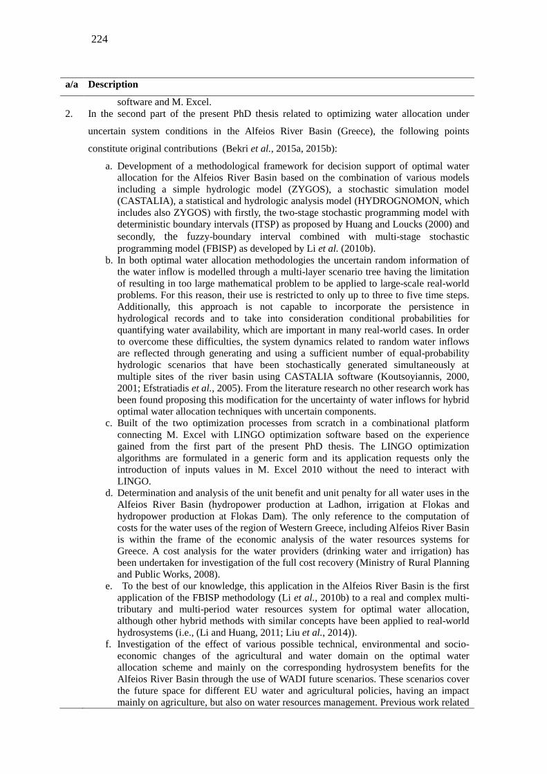
224

a/a Description

software and M. Excel. 2. In the second part of the present PhD thesis related to optimizing water allocation under

uncertain system conditions in the Alfeios River Basin (Greece), the following points

constitute original contributions (Bekri et al., 2015a, 2015b):

a. Development of a methodological framework for decision support of optimal water allocation for the Alfeios River Basin based on the combination of various models including a simple hydrologic model (ZYGOS), a stochastic simulation model (CASTALIA), a statistical and hydrologic analysis model (HYDROGNOMON, which includes also ZYGOS) with firstly, the two-stage stochastic programming model with deterministic boundary intervals (ITSP) as proposed by Huang and Loucks (2000) and secondly, the fuzzy-boundary interval combined with multi-stage stochastic programming model (FBISP) as developed by Li et al. (2010b).

b. In both optimal water allocation methodologies the uncertain random information of the water inflow is modelled through a multi-layer scenario tree having the limitation of resulting in too large mathematical problem to be applied to large-scale real-world problems. For this reason, their use is restricted to only up to three to five time steps. Additionally, this approach is not capable to incorporate the persistence in hydrological records and to take into consideration conditional probabilities for quantifying water availability, which are important in many real-world cases. In order to overcome these difficulties, the system dynamics related to random water inflows are reflected through generating and using a sufficient number of equal-probability hydrologic scenarios that have been stochastically generated simultaneously at multiple sites of the river basin using CASTALIA software (Koutsoyiannis, 2000, 2001; Efstratiadis et al., 2005). From the literature research no other research work has been found proposing this modification for the uncertainty of water inflows for hybrid optimal water allocation techniques with uncertain components.

c. Built of the two optimization processes from scratch in a combinational platform connecting M. Excel with LINGO optimization software based on the experience gained from the first part of the present PhD thesis. The LINGO optimization algorithms are formulated in a generic form and its application requests only the introduction of inputs values in M. Excel 2010 without the need to interact with LINGO.

d. Determination and analysis of the unit benefit and unit penalty for all water uses in the Alfeios River Basin (hydropower production at Ladhon, irrigation at Flokas and hydropower production at Flokas Dam). The only reference to the computation of costs for the water uses of the region of Western Greece, including Alfeios River Basin is within the frame of the economic analysis of the water resources systems for Greece. A cost analysis for the water providers (drinking water and irrigation) has been undertaken for investigation of the full cost recovery (Ministry of Rural Planning and Public Works, 2008).

e. To the best of our knowledge, this application in the Alfeios River Basin is the first application of the FBISP methodology (Li et al., 2010b) to a real and complex multi-tributary and multi-period water resources system for optimal water allocation, although other hybrid methods with similar concepts have been applied to real-world hydrosystems (i.e., (Li and Huang, 2011; Liu et al., 2014)).

f. Investigation of the effect of various possible technical, environmental and socio-economic changes of the agricultural and water domain on the optimal water allocation scheme and mainly on the corresponding hydrosystem benefits for the Alfeios River Basin through the use of WADI future scenarios. These scenarios cover the future space for different EU water and agricultural policies, having an impact mainly on agriculture, but also on water resources management. Previous work related

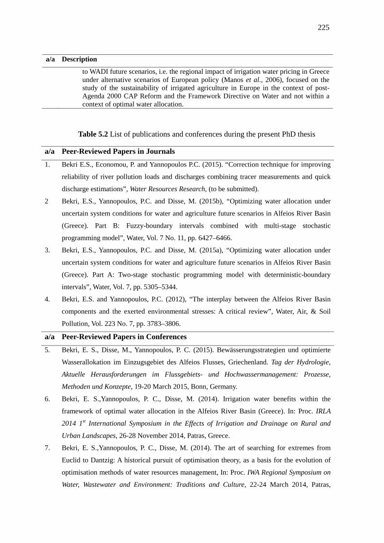
225

a/a Description

to WADI future scenarios, i.e. the regional impact of irrigation water pricing in Greece under alternative scenarios of European policy (Manos et al., 2006), focused on the study of the sustainability of irrigated agriculture in Europe in the context of post-Agenda 2000 CAP Reform and the Framework Directive on Water and not within a context of optimal water allocation.

Table 5.2 List of publications and conferences during the present PhD thesis

a/a Peer-Reviewed Papers in Journals

1. Bekri E.S., Economou, P. and Yannopoulos P.C. (2015). “Correction technique for improving

reliability of river pollution loads and discharges combining tracer measurements and quick

discharge estimations”, Water Resources Research, (to be submitted).

2 Bekri, E.S., Yannopoulos, P.C. and Disse, M. (2015b), “Optimizing water allocation under

uncertain system conditions for water and agriculture future scenarios in Alfeios River Basin

(Greece). Part B: Fuzzy-boundary intervals combined with multi-stage stochastic

programming model”, Water, Vol. 7 No. 11, pp. 6427–6466.

3. Bekri, E.S., Yannopoulos, P.C. and Disse, M. (2015a), “Optimizing water allocation under

uncertain system conditions for water and agriculture future scenarios in Alfeios River Basin

(Greece). Part A: Two-stage stochastic programming model with deterministic-boundary

intervals”, Water, Vol. 7, pp. 5305–5344.

4. Bekri, E.S. and Yannopoulos, P.C. (2012), “The interplay between the Alfeios River Basin

components and the exerted environmental stresses: A critical review”, Water, Air, & Soil

Pollution, Vol. 223 No. 7, pp. 3783–3806.

a/a Peer-Reviewed Papers in Conferences

5. Bekri, E. S., Disse, M., Yannopoulos, P. C. (2015). Bewässerungsstrategien und optimierte

Wasserallokation im Einzugsgebiet des Alfeios Flusses, Griechenland. Tag der Hydrologie,

Aktuelle Herausforderungen im Flussgebiets- und Hochwassermanagement: Prozesse,

Methoden und Konzepte, 19-20 March 2015, Bonn, Germany.

6. Bekri, E. S.,Yannopoulos, P. C., Disse, M. (2014). Irrigation water benefits within the

framework of optimal water allocation in the Alfeios River Basin (Greece). In: Proc. IRLA

2014 1st International Symposium in the Effects of Irrigation and Drainage on Rural and

Urban Landscapes, 26-28 November 2014, Patras, Greece.

7. Bekri, E. S.,Yannopoulos, P. C., Disse, M. (2014). The art of searching for extremes from

Euclid to Dantzig: A historical pursuit of optimisation theory, as a basis for the evolution of

optimisation methods of water resources management, In: Proc. IWA Regional Symposium on

Water, Wastewater and Environment: Traditions and Culture, 22-24 March 2014, Patras,

226

Greece.

8. Bekri, E. S., Yannopoulos, P. C., Disse, M. (2014). Investigation and Incorporation of Water

Inflow Uncertainties through Stochastic Modelling in a Combined Optimization Methodology

for Water Allocation in Alfeios River (Greece). EGU 2014, 27 April-02 Mai 2014, Vienna,

Austria. Available online at http://meetingorganizer.copernicus.org/EGU2014/EGU2014-

8657.pdf, checked on 2/20/2015.

9. Bekri, E. S.,Yannopoulos, P. C., Disse, M. (2013). A Combined Linear Optimisation

Methodology for Water Resources Allocation in an Alfeios River subBasin (Greece) under

Uncertain and Vague System Conditions. EGU 2013, 22-27 April 2013, Vienna, Austria.

Available online at http://meetingorganizer.copernicus.org/EGU2013/EGU2013-1753.pdf.

10. Podimata M., Bekri, E., Yannopoulos, P.C. (2012b). Proposing buffer zones and simple

technical solutions for safeguarding river water quality and public health. HS7.3/CL2.9/NP1.3

/ Climate, water and health, EGU 2012, 22-27 April. Vienna, Austria.

11. Bekri, E. S., Disse, M.,Yannopoulos, P. C. (2012a): Methodological framework for correction

of quick river discharge measurements using quality characteristics. In: Proc. 2nd Common

Conference on Integrated Water Resources Management for sustainable development. 11-13,

October 2012, Patras, Greece.

12. Bekri, E., Yannopoulos P.C. (2011). Decision Support Systems for sustainable development

of river basins. In: Proc. VI EWRA International Symposium on Water Engineering and

Management in a Changing Environment, European Water Resources Association, 29 June -

02 July 2011, Catania, Italy.

5.3 PROPOSALS FOR FUTURE WORK

For the first part of the present PhD thesis, including the development of a correction

technique for quick river discharges, the following points could be considered for future

work:

1. The confirmation of the proposed methodology based on a comparison with

accurate river discharge measurements is hampered by the lack of such data in

Alfeios River Basin. Further investigation focused on direct comparison of the

river discharges corrected by this methodology to accurately measured values is

needed.

2. Further investigation is proposed for developing a logical and automatic

conceptual process for reducing the step bounds so that convergence to the

optimal solution is guaranteed, avoiding the manual trial and error.

3. Application of the proposed methodology to other ungauged catchments will

227

further test the proposed methodology in order to identify possible modifications.

For the second part of the present PhD thesis, including the optimal water allocation

based on hybrid techniques, the following points could be considered for future work:

1. In this research work it is suggested to generate stochastically a sufficient number

of equal-probability scenarios instead of building a scenario-tree using a multiple

variables and multiple sites technique as the one incorporated into CASTALIA

software (Koutsoyiannis, 2000, 2001; Efstratiadis et al., 2005). In the application

of the methodology to the Alfeios River Basin a relatively low number of equal-

probability scenarios, equal to fifty, have been generated in order to enable a

deeper and easier analysis and understanding of the results. However, it is worth

mentioning that an increase of the number of the hydrologic scenarios generated

would increase the quality and the reliability of the statistical analysis of the

results, but it would make the analysis of the results even more complicated,

setting also the matter of the use of this methodology to a more complex time

horizon. In any case, it is proposed that a further application of this methodology

with various increasing numbers of equal probability scenarios is required in

order to evaluate its effect on the optimized water allocation targets and the

benefits and costs of the system.

2. An interesting addition in the unit benefit and penalties of all water uses of the

Alfeios River Basin would be the examination of nonzero environmental costs

for the various water uses. In example, an interesting topic for further research

would be the investigation of the environmental cost value in term of the

ecosystem status for various flow level at Ladhon river in relation to the water

releases from the HPS.

3. The addition of the drinking water supply in the optimization of the water

allocation is also needed, when sufficient data have been gathered, in order to

determine the tradeoffs of this critical water use with the others, and also to

identify an optimized water allocation target scheme in cases of extreme low

flow hydrologic scenarios.

4. Application of the proposed methodology to other river basins with more

conflicting water uses than the water uses in Alfeios river is needed.

228

REFERENCES

1. Abdollahzadeh, A., Luong, M., Maquin, D. and Ragot, J. (Eds.) (1996), Influence de la

précision des capteurs sur la précision de l'état d'un système. Application au choix de la

précision des capteurs: Simulation, Optimisation et Commande en Génie des procédés,

SIMO'96.

2. Abrishamchi, A., Marino, M.A. and Afshar, A. (1991), “Reservoir planning for

irrigation district”, Journal of Water Resources Planning and Management, Vol. 117,

pp. 74–85.

3. Agronews, “Agronews”, available at:

http://www.agronews.gr/files/1/PDF/agroktima_pdf/07-08_2010_agroktima.pdf.

4. Albuquerque, J.S. and Biegler, L.T. (1996), “Data reconciliation and gross error

detection for dynamic system”, AIChE Journal, Vol. 42 No. 10, pp. 2841–2856.

5. Alexopoulos, C.A. (2004), “Alfeios River”, available at:

http://arcadia.ceid.upatras.gr/arkadia/places/Alfeios.htm (accessed 10 September 2011).

6. Alexouli-Livaditi, A. (Ed.) (1990), Research of sediments and minerals at the

Kyparissiakos Gulf coasts.

7. Allan, J.D. and Reyeros de Castillo, Maria Magdalena (2007), Stream ecology,

Springer.

8. Androutsopoulou, A. (2010), “Ecological evaluation and environmental consequences

of construction works on the Alfeios river basin”, MSc Thesis, Sector of Biology of

Plants, Department of Biology, University of Patras, Greece, 2010.

9. APHA (1999), Standard Methods for the Examination of Water and Wastewater, 20th

edition.

10. Argiropoulos, P. (Ed.) (1960), The morphologic evolution of the rivers of the Greek

realm and the influence of the transported sediments on the relief of the country, Vol.

34.

11. Arkadhian Local Newspapers site (2011), “Monitoring network for Alfeios river

pollution”, available at: http://www.arcadiaportal.gr/news/diktuo-parakolouthisis-gia-ti-

rupansi-tou-alfeiou (accessed 20 February 2011).

12. Arnold, T. (2006), Crop growth module: Capturing crop yield response to water

deficit within MPMAS, In Mathematical Programming Multi-Agent System Modelling:

An Application to Water Resources Management, University of Hohenheim, Stuttgart,

229

Germany.

13. Arora, N. and Biegler, L.T., Redescending estimators for data reconciliation and

parameter estimation: Redescending estimators for data reconciliation and parameter

estimation.

14. Azaiez, M.N., Hariga, M. and Al-Harkan, I. (2005), “A Chance-Constrained Multi-

period Model for a Special Multi-reservoir System”, Computers & Operations

Research, Vol. 32, pp. 1337–1351.

15. Bakalis, N., Markantonatos, P., Gianatos, G., Zalahori, E., Robos N. and Panetsos, L.

(1995), Environmental impact assessment study for the relocation of the Alfeios River

bank in Arkadhia Province, Stages I, II, III., Athens, Greece.

16. Beale, E. (1955), “On minimizing a convex function subject to linear inequalities”,

Journal of the Royal Statistical Society: Series B, Vol. 17, pp. 173–184.

17. Bekri, E.S., Disse, M. and Yannopoulos, P.C. (Eds.) (2012), Methodological

framework for correction of quick river discharge measurements using quality

characteristics.

18. Bekri, E.S. and Yannopoulos, P.C. (2012), “The interplay between the Alfeios River

Basin components and the exerted environmental stresses: A critical review”, Water, Air,

& Soil Pollution, Vol. 223 No. 7, pp. 3783–3806.

19. Bekri, E.S., Yannopoulos, P.C. and Disse, M. (2013), “A Combined Linear

Optimisation Methodology for Water Resources Allocation in an Alfeios River subBasin

(Greece) under Uncertain and Vague System Conditions”, available at:

http://meetingorganizer.copernicus.org/EGU2013/EGU2013-1753.pdf (accessed 20

February 2015).

20. Bekri, E.S., Yannopoulos, P.C. and Disse, M. (2014), “Investigation and

Incorporation of Water Inflow Uncertainties through Stochastic Modelling in a

Combined Optimization Methodology for Water Allocation in Alfeios River (Greece).”,

available at: http://meetingorganizer.copernicus.org/EGU2014/EGU2014-8657.pdf

(accessed 20 February 2015).

21. Bekri, E.S., Yannopoulos, P.C. and Disse, M. (2015a), “Optimizing water allocation

under uncertain system conditions for water and agriculture future scenarios in Alfeios

river basin (Greece). Part A: Two-stage stochastic programming model with

deterministic-boundary intervals”, Water, Vol. 7 No. 10, pp. 5305–5344.

22. Bekri, E.S., Yannopoulos, P.C. and Disse, M. (2015b), “Optimizing water allocation

230

under uncertain system conditions for water and agriculture future scenarios in Alfeios

river basin (Greece). Part B: Fuzzy-boundary intervals combined with multi-stage

stochastic programming model”, Water, Vol. 7 No. 11, pp. 6427–6466.

23. Bender, M.J. and Simonovic, S.P. (2000), “A fuzzy compromise approach to water

resources planning under uncertainty”, Fuzzy Sets and Systems, Vol. 115, pp. 35–44.

24. Berkhout, F. and Hertin, J. (2002), “Foresight Futures Scenarios Developing and

Applying a Participative Strategic Planning Tool”, available at: http://www.greenleaf-

publishing.com/add_getquantity.kmod?productid=416 (accessed 20 February 2015).

25. Birge, J.R. (1985), “Decomposition and partitioning methods for multistage

stochastic linear programs”, Operations Research, Vol. 33, pp. 989–1007.

26. Birge, J.R. and Louveaux, F. (1997), Introduction to Stochastic Programming,

Springer, New York, NY, USA.

27. Birge, J.R. and Louveaux, F.V. (1988), “A Multicut Algorithm for Two-Stage

Stochastic Linear Programs”, European Journal of Operational Research, Vol. 34, pp.

384–392.

28. Box, G. and Jenkins, G.M. (1970), Time Series Analysis Forecasting and Control,

Holden-Day, San Francisco, CA, USA.

29. Budnick, F.S., McLeavey, D.M. and Mojena, R. (1988), Principles of Operations

Research for Management, Richard D. Irwin, Homewood, IL, USA.

30. Bunn, D.W. and Karakatsani, N.V. (2008), “Forecasting electricity prices. The impact

of fundamentals and time-varying coefficients”, International journal of forecasting,

Vol. 24 No. 4, pp. 764–785.

31. Carter, R.W. and Anderson, I.E. (1963), “Accuracy of current meter measurements”,

Journal of the Hydraulics Division, Vol. 89 No. 4, pp. 105–115.

32. Center of Environmental Education of Krestena (2010), “Alfeios: A journey in time

and space”, available at: http://kpekrestenon.viewschools.info/page12%20-%20f.htm

(accessed 5 July 2011).

33. Charnes, A. and Cooper, W.W. (1983), “Response to Decision problems under risk

and chance constrained programming: Dilemmas in the transitions”, Management

Science, Vol. 29, pp. 750–753.

34. Chatziapostolou, A. (2009), “Geological -soil parameters of the drained Mouria lake

(Ileia Region) as factors for the determination of criteria for the application of

rehabilitation and sustainable development of wetlands”, PhD Thesis, Sector of Applied

231

Geology &Geophysics, Department of Geology, University of Patras, Greece, 2009.

35. Chen, H.K., Hsu, W.K. and Chiang, W.L. (1998), “A comparison of vertex method

with JHE method”, Fuzzy Sets and Systems, Vol. 95, p. 201–214.

36. Christopoulos, G. (1998), “Late Holocene River Behaviour of the Lower Alfeios

Basin, Western Peloponnese, Greece”, PhD thesis, University of Leeds, UK, 1998.

37. Crowe, C.M. (1989), “Reconciliation of Process Flow Rates by Matrix Projection. II:

The Nonlinear Case”, AIChE Journal, Vol. 32, pp. 616–623.

38. Dafis, S., Papastergiadou, E., Georghiou, K., Babalonas, D., Georgiadis, T.,

Papageorgiou, M., Lazaridou, T. and Tsiaoussi, V. (1996), Directive 92/43/EEC. The

Greek ’Habitat’ Project NATURA 2000: An overview. Life Contract B4-3200/94/756,

Thessaloniki, Greece.

39. Dalezios, I., Ballassopoulos, O. and Sarletakos, D. (1977), Pollution of the Alfeios

River area. Confidential report of the working team for the protection of the

environment, Athens, Greece.

40. Dantzig, G. (1955), “Linear programming under uncertainty”, Management Science,

Vol. 1, pp. 197–206.

41. Delava, P., Maréchal, E., Vrielynck, B. and Kalitventzeff, B. (Eds.) (1999),

Modelling of a Crude Oil Distillation Unit in Term of Data Reconciliation with ASTM

or TBP Curves as Direct Input – Application Crude Oil Preheating Train,

Supplementary volume.

42. Di Baldassarre, G. and Montanari, A. (2009), “Uncertainty in river discharge

observations: a quantitative analysis”, Hydrology and earth system sciences, Vol. 13 No.

6.

43. Dickinson, W.T. (1967), Accuracy of discharge determinations, Hydrology Papers,

Ford Collins, CO.

44. Dong, W. and Shah, H.C. (1987), “Vertex method for computing functions of fuzzy

variables”, Fuzzy Sets and Systems, Vol. 24, pp. 65–78.

45. Doorenbos, J. and Kassam, A.H. (1979), Yield Response to Water, FAO Irrigation and

Drainage Paper (FAO), Vol. 33, Rome, Italy.

46. Dubois, D. and Prade, H. (1978), “Operations on fuzzy number”, International

Journal of Systems Science, Vol. 9, pp. 613–626.

47. Dupacova, J. (2002), “Application of stochastic programming: Achievements and

questions”, European Journal of Operational Research, Vol. 140, pp. 281–290.

232

48. Eaton, A.D., Clesceri, L.S. and Greenberg, A.E. (1995), Standard methods for the

examination of water and wastewater, 19th ed. / joint editorial board, Andrew D. Eaton,

Leonre S. Clesceri, Arnold E. Greenberg, American Public Health Association,

Washington, D.C.

49. Eaton, A.D., Clesceri, L.S., Rice, E.W. and Greenberg, A.E. (2005), Standard

Methods for the Examination of Water & Wastewater, 21st ed., USA.

50. ECEFA (2011), “Greece: Rebalancing growth amidst ongoing fiscal consolidation”,

available at: http://ec.europa.eu/economy_finance/eu/forecasts/2011_spring/el_en.pdf

(accessed 15 December 2011).

51. Economidis, P.S. and Banarescu, P.M. (1991), “The distribution and origins of

freshwater fishes in the Balkan Peninsula, especially in Greece”, Internationale Revue

der gesamten Hydrobiologia, Vol. 76, pp. 257–284.

52. Economou, A.N., Barbieri, R., Daoulas, C., Psarras, T., Stoumboudi, M., Bertahaas,

I., Giakoumi, S. and Patsias, A. (1999), Endangered freshwater fish of western Greece

and Peloponnese. Distribution, abundance, threats and recommended conservation

measures PENED. Technical Report, Greece.

53. Edgar, T.F., Himmelblau, D.M. and Lasdon, L.S. (2001), Optimization of chemical

processes, 2nd ed., McGraw Hill, New York.

54. Edirisinghe, N., Patterson, E.I. and Saadouli, N. (2000), “Capacity Planning Model

for a Multipurpose Water Reservoir with Target-Priority Operation”, Annals of

Operations Research, Vol. 100, pp. 273–303.

55. Efstratiadis, A., Koutsoyiannis, D. and Kozanis, S. (2005), Theoretical

documentation of the model of stochastic simulation of hydrologic parameters

CASTALIA, Athens, Greece.

56. Elhadi, N., Harrington, A., Hill, I., Lau, Y.L. and Krishnappan, B.G. (1984), “River

mixing - A state-of-the-art report”, Canadian Journal of Civil Engineering, Vol. 11 No.

3, pp. 585–609.

57. Etiope, G., Papatheodorou, G., Christodoulou, P.D., Ferentinos, G., Sokos, E. and

Favali, P. (2006), “Methane and hydrogen sulfide seepage in the northwest

Peloponnesus petroliferous basin (Greece): Origin and geohazard”, The American

Association of Petroleum Geologists Bulletin, Vol. 90 No. 5, pp. 701–713.

58. European Commission (2003), “NATURA 2000 data for GREECE”, available at:

http://ec.europa.eu/environment/nature/natura2000/db_gis/pdf/GRn2k_0802.pdf

233

(accessed 15 September 2011).

59. Eurostat European Commission (2008), “Agricultural Statistics: Main results 2006-

2007. Pocketbook. European Communities”, available at:

http://epp.eurostat.ec.europa.eu/cache/ITY_OFFPUB/KS-ED-08-001/EN/KS-ED-08-

001-EN.PDF (accessed 10 December 2011).

60. Fan, Y.R. and Huang, G.H. (2012), “A robust two-step method for solving interval

linear programming problems within an environmental management context”, Journal

of Environmental Informatics, Vol. 19, pp. 1–12.

61. Fogel, E. and Huang, Y.F. (1982), “On the value of information in system

identification-bounded noise case”, Automatica, Vol. 18 No. 2, pp. 229–238.

62. Freeze, R.A., Massmann, J., Smith, L., Sperling, J. and James, B. (1990),

“Hydrogeological decision analysis: 1. A framework”, Ground Water, Vol. 28, pp. 738–

766.

63. Fu, D.Z., Li, Y.P. and Huang, G.H. (2013), “A Factorial-based Dynamic Analysis

Method for Reservoir Operation Under Fuzzy-stochastic Uncertainties”, Water

Resources Management, Vol. 27, pp. 4591–4610.

64. Fukuda, M. and Kojima, M. (1999), Branch-an-cut algorithms for the bilinear matrix

inequality eigenvalue problem, Research reports on mathematical and computing

sciences, Vol. 351, Institute of Technology, Tokyo.

65. Gartner, J.W. and Ganju, N.K. (2007), “Correcting acoustic Doppler current profiler

discharge measurement bias from moving-bed conditions without global positioning

during the 2004 Glen Canyon Dam controlled flood on the Colorado River”, Limnology

and Oceanography: Methods, Vol. 5 No. 6, pp. 156–162.

66. Gawel, E. (2004), “Article 9 Water Framework Directive: Do we really need to

calculate environmental and resource costs?”, Journal for European Environmental and

Planning Law (JEEPL), Vol. 11 No. 3, pp. 249–271.

67. Geordiadis, T., Yannopoulos, P., Kaspiris, P., Tiniakos, L., Dimitrellos, G.,

Theocharopoulos, M. and Papandropoulos, D. (1998), “Investigation of environmental

parameters and conditions for the rehabilitation of the former Mouria Lake”, PhD,

University of Patras and Ilieaki A.E., Ileia Region, 1998.

68. Ghionis, G. and Poulos, S. (2005), “Greek case studies: Morphological evolution of

the R. Alfeios deltaic shoreline”, available at:

http://www.theseusproject.eu/wiki/Greek_case_studies:_Morphological_evolution_of_t

234

he_R.Alfeios_deltaic_shoreline (accessed 20 May 2011).

69. Gleick, P.H. (1998), “Water in crisis: Paths to sustainable water use”, Ecol. Appl.,

Vol. 8, pp. 571–579.

70. Goh, K.C., Safonov, M.G. and Papavassilopoulos, G.P. (1995), “Global optimization

for the biaffine matrix inequality problem”, Journal of Global Optimization, Vol. 7, pp.

365–380.

71. Greek Legislation (2001), “Dangerous substances Directive. Joint Ministerial

Decision 2/1.2.2001”, available at:

http://www3.aegean.gr/environment/eda/Envirohelp/greece/regulations/documents/WW

28.pdf (accessed 25 May 2011).

72. Guide to the Expression of Uncertainty in Measurement, International Organization

for Standardization (1993), Geneva.

73. Heliotis, F.D. (1988), “An inventory and review of the wetland resources of Greece”,

Wetlands, Vol. 8, pp. 15–31.

74. Hellenic Statistical Authority (HSA) (2002), “Real Population of Greece in regions,

municipalities, municipal departments and small residences (census results 2001)”,

available at: http://www.statistics.gr (accessed 25 February 2011).

75. HEMCO, “CORINE LAND COVER GREECE (CLCG)”, available at:

http://www.okxe.gr.

76. Herschy, R.W. (1971), The magnitude of errors at flow measurements stations: Water

Resources Board: Technical report, Berkshire, England.

77. Herschy, R.W. (1985), Streamflow measurement, Elsevier Applied Science, London.

78. Himmelblau, D.M. (1978), Fault detection and diagnosis in chemical and

petrochemical processes, Chemical engineering monographs, Vol. 8, Elsevier Scientific,

New York.

79. Himmelblau, D.M. (1985), “Material balance rectification via interval arithmetic.

The use of computers in chemical engineering”, Process Systems Engineering, Vol. 92,

pp. 121–133.

80. HMA (1997), River and lake water quality characteristics. Water sector of Western

Peloponnisos. Alfeios River water quality characteristics 1983– 97., Athens, Greece.

81. HMA (2001), Qualitative characteristics of water in Greek rivers and lakes, A & B,

Athens, Greece.

82. HMEPPPW (1997), Protection works of Flokas Dam of the Alfeios River, A & B,

235

Athens, Greece.

83. HMEPPPW (2008), Drawing of the middle-term program for the protection and

management of water resources of Greece. Technical Report, Athens, Greece.

84. HMSO (2002), Foresight Futures 2020 Revised Scenarios and Guidance,

Department of Trade and Industry, London, UK.

85. HNCMR (2001), Measurement of quantitative characteristics of surface waters:

2000-2001.

86. HREPPPW (2008), Application of Article 5 of the European WFD 2000/60/EC.

Report for the Water District (01)- Western Peloponnisos, Athens, Greece.

87. Huang, F.H. (1996), “IPWM: An interval parameter water quality management

model”, Engineering Optimization, Vol. 26, pp. 79–103.

88. Huang, G.H. (1998), “A hybrid inexact-stochastic water management model”,

European Journal of Operational Research, Vol. 107, pp. 137–158.

89. Huang, G.H., Baetz, B.W. and Patry, G.G. (1992), “A grey linear programming

approach for municipal solid waste management planning under uncertainty”, Civil

Engineering Systems, Vol. 9, pp. 319–335.

90. Huang, G.H. and Loucks, D.P. (2000), “An inexact two-stage stochastic

programming model for water resources management under uncertainty”, Civil

Engineering and Environmental Systems, Vol. 17, pp. 95–118.

91. Huang, Y., Li, Y.P., Chen, X. and Ma, Y.G. (2012), “Optimization of the irrigation

water resources for agricultural sustainability in Tarim River Basin, China”,

Agricultural water management, Vol. 107, pp. 74–85.

92. Huber, P.J. (1981), Robust statistics, Wiley, New York.

93. Iliopoulou-Georgoudaki, J., Kantzaris, V., Katharios, P., Kaspiris, P., Georgiadis, T.

and Montesantou, B. (2003), “An application of different bioindicators for assessing

water quality: a case study in the rivers Alfeios and Pineios (Peloponnisos, Greece)”,

Ecological Indicators, Vol. 2, pp. 345–360.

94. Imboden, D.M. and Wüest, A. (1995), Mixing mechanisms in lakes: in ‘Physics and

Chemistry of Lakes’, Springer Verlag.

95. Inuiguchi, M. and Ramik, J. (2000), “Possibilistic linear programming: A brief

review of fuzzy mathematical programming and a comparison with stochastic

programming in portofolio selection problem”, Fuzzy Sets and Systems, Vol. 111, pp. 3–

28.

236

96. ISO (1993), Guide to the Expression of Uncertainty in Measuremen, Geneva.

97. ISO 1100 (1981), Liquid Flow Measurement in Open Channels: Part 1:

Establishment and operation of a gauging station and Part 2: Determination of stage-

discharge relation, International Organization for Standardization (ISO), Geneva,

Switzerland.

98. ISO 748 (1979), Liquid Flow Measurement in Open Channels –velocity area

methods, International Organization for Standardization (ISO), Geneva, Switzerland.

99. ISO 772 (1988), Liquid Flow Measurement in Open Channels: Vocabulary and

Symbols, Third edition, International Organization for Standardization (ISO), Geneva,

Switzerland.

100. J. Environmental Management (2007), Environmental Management, Vol. 84 1-11.

101. Jairaj, P.G. and Vedula, S. (2000), “Multireservoir system optimization using fuzzy

mathematical programming”, Water Resources Management, Vol. 14, pp. 457–472.

102. Johnston, L.P.M. and Kramer, M.A. (1995), Maximum likelihood data rectification:

Steady‐state systems: Maximum likelihood data rectification: Steady‐state systems,

American Institute of Chemical Engineers, New York.

103. Kabouris, J. (2004), “Assessment of Secure RES penetration on Peloponnisos”,

available at: http://www.optires.info/pdf/report_peloponese_V3.pdf (accessed 10

October 2011).

104. Kall, P. and Wallace, S.W. (1994), Stochastic Programming, Wiley, Chichester, UK.

105. Kallinskis, A. (1957), The big reclamation works to develop the Alfeios river basin,

as well as the lakes of Agoulinitsa and Mouria: Summary Report, Athens, Greece.

106. Karapanos, I.S. (2009), “Hydrogeological-hydrochemical parameters of the drained

Mouria Lake (Ileia Region) as factors for the determination of criteria for the

application of rehabilitation and sustainable development of wetlands. .”, Phd Thesis,

Sector of Applied Geology &Geophysics, Department of Geology, University of Patras,

Greece, 2009.

107. Kim, K., Lee, J.S. and Oh, C.-W. (2002), “Inorganic chemicals in an effluent-

dominated stream as indicators for chemical reactions and streamflows”, Journal of

Hydrology, Vol. 264, pp. 147–156.

108. Kinori, B.Z. and Mevorach, J. (1984), Manual of Surface Drainage Engineering, Vol.

II: Stream Flow Engineering and Flood Protection, Elsevier Science, Amsterdam, The

Netherlands.

237

109. Koelling, C. (Ed.) (2004), SIMK-Calibration of streamflow - Gauging stations in

rivers and canals.

110. Kokoris, I. (2007), “Human effects on the riverine ecosystems of Alfeios River:

Perspectives for its integrated management”, Diploma thesis, Sector of Biology of

Plants, Department of Biology, University of Patras, Greece, 2007.

111. Konstantinou, I.K., Hella, D. and Albanis, T.A. (2006), “The status of pesticide

pollution in surface waters (rivers and lakes) of Greece. I. Review on occurrence and

levels”, Environmental Pollution, Vol. 141 No. 3, pp. 555–570.

112. Kontos, D. (2006), “Response from the Greek Government to the further

observations of MFHR on the merits. Collective Complaint No. 30/2005

Marangopoulos Foundation for Human Rights v. Greece, Case Document No. 6.

European Committee of Social Rights.”, available at:

http://www.coe.int/t/dghl/monitoring/socialcharter/complaints/CC30CaseDoc6_en.pdfp

(accessed 25 March 2011).

113. Koutsoyiannis, D. (2000), “A generalized mathematical framework for stochastic

simulation and forecast of hydrologic time series”, Water Resources Research, Vol. 36,

pp. 1519–1534.

114. Koutsoyiannis, D. (2001), “Coupling stochastic models of different time scales”,

Water Resources Research, Vol. 37, pp. 379–392.

115. Kozanis, S., Christoforides, A. and Efstratiadis, A. (2010), “Scientific Documentation

of Hydrognomon software (version 4). Development of Database and Software

Application in a Web Platform for the “National Database and Meterological

Information””.

116. Kozanis, S. and Efstratiadis, A. (Eds.) (2006), ZYGOS: A basin process simulation

model.

117. Kraft, J., Rapp, G.R., Gifford, J. and Aschenbrenner, S.E. (2005), “Coastal change

and archaeological settings in Ellis”, Hesperia, Vol. 74, pp. 1–39.

118. Kuehn, D.R. and Davidson, H. (1961), “Computer control. II. Mathematics of

control.”, Chemical Engineering Progress, Vol. 57, pp. 44–47.

119. Kuusisto, E. (1996), Hydrological measurements, in Water Quality Monitoring - A

Practical Guide to the Design and Implementation of Freshwater Quality Studies and

Monitoring Programmes, Chapter 12.

120. Langenstein, M., Jansky, J. and Laipple, B. (Eds.) (2004), Finding Megawatts in

238

nuclear power plants with process data validation.

121. Le Coz, J. (2012), A literature review of methods for estimating the uncertainty

associated with stage-discharge relations, WHO, Lyon, France.

122. Lee, C.S. and Chang, S.P. (2005), “Interactive fuzzy optimization for an economic

and environmental balance in a river system”, Water Research, Vol. 39, pp. 221–231.

123. Lekkas, T., Kolokythas, G., Nikolaou, A., Kostopoulou, M., Kotrikla, A., Gatidou,

G., Thomaidis, N.S., Golfinopoulos, S., Makri, C., Babos, D., Vagi, M., Stasinakis, A.,

Petsas, A. and Lekkas, D.F. (2004), “Evaluation of the pollution of the surface waters of

Greece from the priority compounds of List II, 76/464/EEC Directive, and other toxic

compounds”, Environmental International, Vol. 30, pp. 995–1007.

124. Li, W., Li, Y.P., Li, C.H. and Huang, G.H. (2010a), “An inexact two-stage water

management model for planning agricultural irrigation under uncertainty”, Agricultural

water management, Vol. 97, pp. 1905–1914.

125. Li, Y. and Huang, G.H. (2011), “Planning agricultural water resources system

associated with fuzzy and random features”, Journal of the American Water Resources

Association, Vol. 47, pp. 841–860.

126. Li, Y.P. and Huang, G.H. (2008), “Interval-parameter two-stage stochastic nonlinear

programming for water resources management under uncertainty”, Water Resources

Management, Vol. 22, pp. 681–698.

127. Li, Y.P. and Huang, G.H. (2009), “Fuzzy-stochastic-based violation analysis method

for planning water resources management systems with uncertain information”,

Information Sciences, Vol. 179, pp. 4261–4276.

128. Li, Y.P., Huang, G.H., Huang, Y.F. and Zhou, H.D. (2009), “A multistage fuzzy-

stochastic programming model for supporting sustainable water-resources allocation

and management”, Environmental Modelling & Software, Vol. 24, pp. 786–797.

129. Li, Y.P., Huang, G.H. and Nie, S.L. (2006), “An interval-parameter multi-stage

stochastic programming model for water resources management under uncertainty”,

Advances in Water Resources, Vol. 29, pp. 776–789.

130. Li, Y.P., Huang, G.H. and Nie, S.L. (2010b), “Planning water resources management

systems using a fuzzy-boundary interval-stochastic programming method”, Advances in

Water Resources, Vol. 33, pp. 1105–1117.

131. Li, Y.P., Huang, G.H., Yang, Z.F. and Nie, S.L. (2008), “Interval-fuzzy multistage

programming for water resources management under uncertainty”, Resources,

239

Conservation and Recycling, Vol. 52, pp. 800–812.

132. Lindo Systems Inc. (1996), LINDO User’s Manual, Chicago, Illinois.

133. Lindström, G., Johansson, B., Persson, M., Gardelin, M. and Bergström, S. (1997),

“Development and test of the distributed HBV-96 hydrological model”, Journal of

Hydrology, Vol. 201, pp. 272–288.

134. Liofagou, D. (2005), “The Cultivation of Potato in Naxos”, Bachelor Thesis,

Department of Crop Production, School of Agricultural and Food Technology, TEI of

Crete, Hrakleio, Greece, March 2005.

135. Liu, J., Li, Y.P., Huang, G.H. and Zeng, X.T. (2014), “A dual-interval fixed-mix

stochastic programming method for water resources management under uncertainty”,

Resources, Conservation and Recycling, Vol. 88, pp. 50–66.

136. Loucks, D.P. and Beek, E.v. (2005), Water resources systems planning and

management: An introduction to methods models and applications, Studies and reports

in hydrology, Unesco, Paris.

137. Loucks, D.P., Stedinger, J.R. and Haith, D.A. (1981), Water Resources Systems

Planning and Analysis, Prentice-Hall, Englewood Cliffs, NJ, USA.

138. Mah, R., Stanley, G.M. and Downing, D. (1976), “Reconciliation and rectification of

process flow and inventory data”, IEC Process Design Development, Vol. 15 No. 1, pp.

175–183.

139. Manariotis, I.D. and Yannopoulos, P.C. (Eds.) (2001), Environmental impact of

riverine activities on Alfeios River and measures toward sustainability, Xanthi, Greece.

140. Manariotis, I.D. and Yannopoulos, P.C. (2004), “Adverse effects on Alfeios River

Basin and an Integrated Management Framework Based on Sustainability”,

Environmental Management, Vol. 34 No. 2.

141. Mandel, D., Abdollahzadeh, A. and Maquin, D. (1998), “Data reconciliation by

inequality balance equilibration: a LMI approach”, International Journal of Mineral

Processing, Vol. 53, pp. 157–169.

142. Manos, B., Aschonitis, V., Papadopoulou, O. and Moulogianni, C. (2010), “Regional

report for the collected information: Sarigkiol basin, Western Macedonia, Greece.

Transnational Integrated Management of Water Resources in Agriculture for European

Water Emergency Control (EU WATER)”, available at: http://www.eu-

water.eu/images/Action_3.2_Regional_report_Qs_Greece.pdf (accessed 2 October

2011).

240

143. Manos, B., Bournaris, T., Kamruzzaman, M., Begum, A.A. and Papathanasiou, J.

(2006), “The regional impact of irrigation water pricing in Greece under alternative

scenarios of European policy: A multicriteria analysis”, Regional Studies, Vol. 40, pp.

1055–1068.

144. Maqsood, I., Huang, G.H. and Yeomans, J.S. (2005), “An interval-parameter fuzzy

two-stage stochastic program for water resources management under uncertainty”,

European Journal of Operational Research, Vol. 167, pp. 208–225.

145. Maquin, D., Bloch, G. and Ragot, J. (1991), “Data reconciliation for measurements”,

European Journal of Diagnosis and Safety in Automation, Vol. 1 No. 2, pp. 145–181.

146. Matloka, M. (1992), “Some generalization of inexact linear programming”,

Optimization, Vol. 23, pp. 1–6.

147. McMillan, H., Krueger, T. and Freer, J. (2012), “Benchmarking observational

uncertainties for hydrology”, Hydrological Processes, Vol. 26 No. 26, pp. 4078–4111.

148. MDDWPR (1996), A plan of project management of country water resources,

Athens, Greece.

149. Miao, D.Y., Huang, W.W., Li, Y.P. and Yang, Z.F. (2014), “Planning water resources

systems under uncertainty using an interval-fuzzy de novo programming method”,

Journal of Environmental Informatics, Vol. 24, pp. 11–23.

150. Milanese, M. and Belforte, G. (1982), “Estimation theory and uncertainty intervals

evaluation in presence of unknown but bounded errors: linear families of models”, IEEE

Transactions on Automatic Control, Vol. 27 No. 2, pp. 408–413.

151. Milanese, M., Norton, J., Piet-Lahanier, H. and Walter, E. (1996), Bounding

approaches to system identification, Springer US, New York.

152. Miller, R.W. (1983), Flow measurement engineering handbook, McGraw-Hill, New

York, London.

153. Ministry of Rural Planning and Public Works (2008), Application of the economic

aspects of Article 5 of the EU Water Framework Directive 2000/60/EU in Greece,

Athens, Greece, Economic University of Athens.

154. Müller, A. (1988), Discharge and velocity measurements: Proceedings of the Short

Course on Discharge and Velocity Measurements, Zurich … 1987 / edited by Andreas

Müller, Proceedings / International Association for Hydraulic Research, Vol. 2,

Balkema, Rotterdam.

155. Nakagawa, H., Ono, M., Oda, M. and Nishijim S. (2007), “Development of a

241

discharge measurement technique combined with measurement of mean flow velocity

and numerical simulation of cross-sectional velocity distribution; field verification in a

large river”, Journal of Hydroscience and Hydraulic Engineering, Vol. 25, pp. 77–88.

156. Narasimhan, S. and Jordache, C. (2000), Data Reconciliation & Gross Error

Detection: An Intelligent Use of Process Data, Gulf Publishing Company, Houston,

Texas.

157. Nash, J.E. and Sutcliffe, J.V. (1970), “River flow forecasting through conceptual

models, I, A discussion of principles”, Journal of Hydrology, Vol. 10, pp. 282–290.

158. National Statistical Sevice of Greece (2008), “Statistical Yearbook of Greece”

(accessed 5 September 2011).

159. NCSU (2008), Surface Water Flow Measurement for Water Quality: Monitoring

Projects, TechNotes 3, National Nonpoint Source Monitoring Program, U.S.EPA.,

U.S.A.

160. Nicholas, A.P., Woodward, J.C., Christopoulos, G. and Macklin, M.G. (1999),

Modelling and Monitoring River Response to Environmental Change: The Impact of

Dam Construction and Alluvial Gravel Extraction on Bank Erosion Rates in the Lower

Alfeios Basin, Greece, Fluid Processes and Environmental Change, John Wiley & Sons

Ltd, New York.

161. Nie, X.H., Huang, G.H., Li, Y.P. and Liu, L. (2007), “IFRP: A hybrid interval-

parameter fuzzy robust programming approach for municipal solid waste management

planning under uncertainty”, Journal of Environmental Management, Vol. 84, pp. 1–11.

162. Nikolakopoulos, K.G. (2002), “Use of remote sensing data and methods and

development of special digital image processing techniques for the geomorphologic and

geographic study of Alfeios River Basin”, PhD thesis, University of Athens, Greece,

2002.

163. Nikolakopoulos, K.G., Vaiopoulos, D.A. and Skianis, G.A. (2007), “Use of

multitemporal remote sensing data for mapping the Alfeios River network changes from

1977 to 2000”, Geocarto International, Vol. 22 No. 4, pp. 251–271.

164. NTUA (2011), “Filotis Database: Greek NATURA 2000 sites”, available at:

http://filotis.itia.ntua.gr/biotopes/c/GR2330004/ (accessed 20 October 2011).

165. Özyurt, D.B. and Pike, R.W. (2004), “Theory and practice of simultaneous data

reconciliation and gross error detection for chemical processes”, Computers and

Chemical Engineering, Vol. 28, pp. 381–402.

242

166. Papanousi, F. (2009), “Development of an environmental database for river basin

management”, MSc Thesis, Department of Civil Engineering, University of Patras,

Greece, 2009.

167. Pelletier, P.M. (1988), “Uncertainties in the determination of river discharge: A

literature review.”, Canadian Journal of Civil Engineering, Vol. 15, pp. 834–850.

168. Pereira, M. and Pinto, L. (1985), “Stochastic optimization of a multireservoir

hydroelectric system: A decomposition approach”, Water Resources Research, Vol. 6,

pp. 779–792.

169. Peters, N. (1994), Hydrologic processes, in Biogeochemistry of Small Catchments: A

Tool for Environmental Research: Scientific Committee on Problems of the Environment

(SCOPE) of the International Council of Scientific Unions (ICSU) and of the United

Nations Environment Programme (UNEP), Chapter 9, John Wiley & Sons Ltd, New-

York.

170. Podimata, M. (2009), “Establishment and Operation of a Central Watershed

Institution in Alfeios Basin aiming the Integrated Basin Management and the Rational

Decision Making concerning the Study Area”, MSc thesis, Department of Civil

Engineering, University of Patras, Greece, 2009.

171. Podimata, M. and Yannopoulos, P.C. (2013), “Evaluating challenges and priorities of

a trans-regional river basin in Greece by using a hybrid SWOT scheme and a

stakeholders’ competency overview”, International Journal of River Basin

Management, Vol. 11 No. 1, pp. 93–110.

172. Ragot, J., Boukhris, A. and Mandel, D. (Eds.) (1997), A propos de l’algèbre des

intervalles. Application à la validation de données, Rencontres Francophones sur la

Logique Floue et ses Applications.

173. Ragot, J. and Maquin, D. (Eds.) (2004), Data validation and diagnosis using interval

analysis.

174. Ramamurthi, Y. and Bequette, B.W. (Eds.) (1990), Data Reconciliation of Systems

with Unmeasured Variables using Nonlinear Programming Techniques.

175. Rantz, S.E. (1982), Measurement and Computation of Streamflow: Volume 1:

Measurement of Stage and Discharge, USGE Water-Supply Paper 2175, 01-01, U.S.

Government Printing Office, Washington D.C., U.S.A.

176. Rosenberg, D.E. (2009), “Shades of grey: A critical review of grey-number

optimization”, Engineering Optimization, Vol. 41, pp. 573–592.

243

177. Sauer, V.B. and Meyer, R.W. (1992), “Determination of error in individual discharge

measurements”.

178. Schmidt, C., Musolff, A., Trauth, N., Vieweg, M. and Fleckenstein, J.H. (2012),

“Transient analysis of fluctuations of electrical conductivity as tracer in the stream bed”,

Hydrology and earth system sciences, Vol. 16, pp. 3689–3697.

179. Schrage, L.E. (1997), Optimization modeling with LINDO, 5th ed., Duxbury Rress,

Pacific Grove, USA.

180. Shapiro, A., “Stochastic Programming by Monte Carlo Simulation Methods”,

available at: http://edoc.hu-berlin.de/series/speps/2000-3/PDF/3.pdf (accessed 6

October 2015).

181. Shrestha, R.R. and Simonovic, S.,P. (2010), “Fuzzy set theory based methodology for

the analysis of measurement uncertainties in river discharge and stage”, Canadian

Journal of Civil Engineering ., Vol. 37 No. 3, pp. 429–439.

182. Siavalas, G., Kalaitzis, S., Cornelissen, G., Chatziapostolou, A. and Christianis, K.

(2007), “Influence of Lignite Mining and Utilization on Organic Matter Budget in the

Alfeios River Plain, Peloponnese (South Greece).”, Energy & Fuels, Vol. 21.

183. Simpson, M.R. (2001), Discharge measurements using a broad-band acoustic

Doppler current profiler, U.S. Geological Survey open-file report, 01-01, U.S. Dept. of

the Interior U.S. Geological Survey; Information Services [distributor], Sacramento

Calif., Denver CO.

184. Skoulikidis, N.T., Amaxidis, Y., Bertahas, I., Laschou, S. and Gritzalis, K. (2006),

“Analysis of factors driving stream water composition and synthesis of management

tools - a case study on small/medium Greek catchments”, The Science of the Total

Environment, Vol. 362, pp. 205–241.

185. Skoulikidis, N.T., Economou, A.N., Critzalis, K.C. and Zogaris, S. (2009), Rivers of

Balkans, In: Rivers of Europe (pp. 421-466), 1st ed., Elsevier, Italy.

186. Smyrniotis, C. (1982), “Contribution à l’ étude des sources karstiques d’ Agios Floros

et Pidima (Taygète Septentrional-Grèce)”, Diplom Thesis, Université des Sciénces et

Techniques du Languedoc, 1982.

187. Soldatos, P., Lychnaras, V. and Asimakis, D. (2009), Cost Analysis and economic

evaluation of future crops in Europe, In 4F-Future Crops For Food, Feed, Fibre and

Fuel, FP7-KBBE-2007-1, Athens, Greece.

188. Stedinger, S. and Loucks, D.P. (1984), “Stochastic dynamic programming models for

244

reservoir operation optimatization”, Water Resources Research, Vol. 20, pp. 1499–1505.

189. Stefanakos, I.P. (Ed.) (2009), Small hydropower stations only or combined with bid

hydropower stations: Their role in the energy system of Greece.

190. Suo, M.Q., Li, Y.P., Huang, G.H., Deng, T.L. and Li, Y.F. (2013), “Electric power

system planning under uncertainty using inexact inventory nonlinear programming

method”, Journal of Environmental Informatics, Vol. 22, pp. 49–67.

191. Tjoa, I. and Biegler, I. (1991), “Simultaneous Strategies for Data Reconciliation and

Gross Error Detection of Non-linear Systems”, Comp. and Chem. Eng, Vol. 15, pp.

679–690.

192. Trekking Hellas, “Outdoor holidays in Greece”, available at: http://www.trekking.gr

(accessed 10 November 2015).

193. Turnipseed, D.P. and Sauer, V.B. (2010), Discharge measurements at gauging

stations, United States Geological Survey Techniques and Methods, Volume 3, Chapter

A8, Washington D.C., U.S.A.

194. U.S.E.P.A. (1986), Ambient Water Quality Criteria for Dissolved Oxygen. Criteria

and Standards Division.

195. U.S.E.P.A. (2003), Elements of a State Water Monitoring and Assessment Program

Assessment and Watershed Protection Division, Washington D.C., U.S.A.

196. USDA (2003), National Water Quality Handbook, Washington, DC, U.S.A.

197. Villiotis, E. (2008), “Mechanisation of the Crop Production of Potato, Onion and

Carrot in the Region of Thebes, Viotia, Greece”, Bachelor Thesis, Department of Plant

Sciences, School of Agricultural and Food Technology, TEI of Crete, Hrahleio, Greece,

June 2008.

198. Vossos, I., Kallitsis, T. and V. Xipolitidis. (1993), “Alfeios River pollution sources

and level”, Diploma Thesis, Department of Civil Engineering, University of Patras,

Greece, 1993.

199. WADI (2000), “Sustainability of European Irrigated Agriculture under Water

Framework Directive and Agenda 2000”, available at:

http://www.lu.lv/materiali/biblioteka/es/pilnieteksti/vide/Sustainability%20of%20Europ

ean%20Irrigated%20Agriculture%20under%20Water%20Framework%20Directive%20

and%20Agenda%202000.pdf (accessed 20 February 2015).

200. Wang, J.F., Cheng, G.D., Gao, Y.G., Long, A.H., Xu, Z.M., Li, X., Chen, H. and

Barke, T. (2008), “Optimal water resource allocation in arid and semi-arid areas”, Water

245

Resources Management, Vol. 22, pp. 239–258.

201. Watkins, D., McKinney, D.C., Lasdon, L.S., Nielsen, S.S. and Martin, Q.W. (2000),

“A scenario-based stochastic programming model for water supplies from the highland

lakes”, International Transactions in Operational Research, Vol. 7, pp. 211–230.

202. WFD (2000), “Water Framework Directive. Directive 2000/60/EC of the European

Parliament and of the Council of 23 October 2000 establishing a framework for

Community action in 12 the field of water policy”, Official Journal of the European

Communities. L327. 22.12.2000, Vol. 43, pp. 1–72.

203. White, W.R. (Ed.) (1988), Discharge measuring methods in open channels, in IAHR,

Rotterdam, Netherlands.

204. WHO (1980), Manual on Stream Gauging: Vol. I - Fieldwork and Vol. II -

Computation of Discharge, Operational Hydrology Report No. 13, WMO - No. 519,

World Meteorological Organization, Geneva, Switzerland.

205. Wilde, F.D. (2008), Guidelines for field-measured water-quality properties (ver. 2.0),

Investigations, USGS Techniques of Water-Resources, Book 9, Chap. A6, Section 6.0.

206. WMO (1980a), Manual on Stream Gauging: Vol. I - Fieldwork and Vol. II -

Computation of Discharge, Operational Hydrology: Report No. 13, WMO - No. 519,

Geneva, Switzerland.

207. WMO (1980b), “Manual on Stream Gauging: Vol. I - Fieldwork and Vol. II -

Computation of Discharge, Operational Hydrology Report No. 13”, World

Meteorological Organization (WNO), Vol. 519.

208. WWF Greece (2007), “Ecological evaluation of the disastrous fires of August 2007

in Peloponnesse”, available at:

http://www.wwf.gr/storage/additional/FIRE_report_Peloponnisos.pdf (accessed 10

April 2011).

209. WWF Water Security Series (2007), “Allocating scarce water. A primer on water

allocation, water Rights and water markets.”, available at:

http://www.wwf.org.uk/wwf_articles.cfm?unewsid=2844 (accessed 10 April 2015).

210. Yannopoulos, P., Mavrikos, G., Demetracopoulos, A. and Hatzitheodorou, C. (Eds.)

(2000), Velocity measurement in channels using a sphere.

211. Yannopoulos, P.C. (Ed.) (1995), Bubble size and movement in wide channel flows, in

Demokritus University of Thrace, Vol. II: Mechanics of Fluids and Thermal Sciences,

edited by, Xanthi, Greece.

246

212. Yannopoulos, P.C. (2008), Development of low cost methodologies for quickly

predicting and monitoring of river pollution: Final Report, Pythagoras II - Environment

Project, OPEVTΙΙ – ESF, Greece.

213. Yannopoulos, P.C. (Ed.) (2009), Correction of river discharge measurements using

natural tracers,

214. Yannopoulos, P.C. and Bekri, E.S. (Eds.) (2010), Correction of quick discharge

measurements in rivers using natural tracers, Vol. 2, Taylor and Francis Group,

London, U.K.

215. Yannopoulos, P.C., Demetracopoulos, A.C. and Hadjitheodorou, C. (2008), “Quick

method for open channel discharge measurements using air bubbles”, Journal of

Hydraulic Engineering, Vol. 134 No. 6.

216. Yannopoulos, P.C. and Manariotis, I. (Eds.) (2005), Consequences on

hydromorphology of Alfeios River from construction works and gravel extractions.

217. Yannopoulos, P.C., Manariotis, I.D., Ziogas, A.I. and Kaleris, V.K. (Eds.) (2007),

Methodology of river pollution assessment and preliminary results, Venice, Italy.

218. Yannopoulos, P.C. and Tsivoglou, I. (Eds.) (1992), Impact of riverine activities on

Alfeios River water quality.

219. Yannopoulous, P.C. (2008), Development of methodologies for quick prediction and

monitoring of river pollution. Final Report. Pyhtagoras II Program, Greece.

220. Yeomans, J.S. (2008), “Applications of simulation-optimization methods in

environmental policy planning under uncertainty”, Journal of Environmental

Informatics, Vol. 12, pp. 174–186.

221. Yorke, T.H. and Oberg, K.A. (2002), Measuring river velocity and discharge with

acoustic Doppler profilers: Measuring river velocity and discharge with acoustic

Doppler profilers.

222. Zeng, X.T., Li, Y.P., Huang, G.H. and Yu, L.Y. (2014a), “Inexact mathematical

modeling for identification of water trading policy under uncertainty”, Water, Vol. 6 No.

2, pp. 229–252.

223. Zeng, X.T., Li, Y.P., Huang, W., Chen, X. and Bao, A.M. (2014b), “Two-stage

credibility-constrained programming with Hurwicz criterion (TCP-CH) for planning

water resources management”, Engineering Applications of Artificial Intelligence, Vol.

35, pp. 164–175.

224. Ziabras, T. and Tasias, S. (1992), “River Discharge measurements through natural

247

tracers in Alfeios River”, Diplom, Environmental Engineering Laboratory, Civil

Engineering Department, University of Patras, Greece, 1992.

225. Zimmermann, H.J. (1995), Fuzzy Set Theory and Its Applications, 3rd ed., Kluwer

Academic Publishers, Dordrecht, The Netherlands.

226. Zissis, T. and Yannopoulos, P.C. (Eds.) (2011), Simulation of variable-density

groundwater flow and transport in the coastal aquifer of the Pyrgos area (Greece).

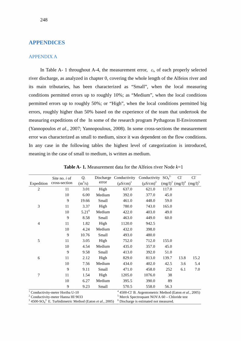
248

APPENDICES

APPENDIX A

In Table A- 1 throughout A-4, the measurement error, εi, of each properly selected

river discharge, as analyzed in chapter 0, covering the whole length of the Alfeios river and

its main tributaries, has been characterized as “Small”, when the local measuring

conditions permitted errors up to roughly 10%; as “Medium”, when the local conditions

permitted errors up to roughly 50%; or “High”, when the local conditions permitted big

errors, roughly higher than 50% based on the experience of the team that undertook the

measuring expeditions of the In some of the research program Pythagoras II-Environment

(Yannopoulos et al., 2007; Yannopoulous, 2008). In some cross-sections the measurement

error was characterized as small to medium, since it was dependent on the flow conditions.

In any case in the following tables the highest level of categorization is introduced,

meaning in the case of small to medium, is written as medium.

Table A- 1. Measurement data for the Alfeios river Node k=1

Site no. i of cross-section

Qi Discharge error

Conductivity Conductivity SO42- Cl- Cl-

Expedition (m3/s) (µS/cm)1 (µS/cm)2 (mg/l)3 (mg/l)4 (mg/l)5

2 11 3.01 High 637.0 621.0 117.0

10 6.00 Medium 392.0 377.0 45.0

9 19.66 Small 461.0 448.0 59.0

3 11 3.37 High 780.0 743.0 165.0

10 5.216 Medium 422.0 403.0 49.0

9 8.58 Small 463.0 449.0 60.0

4 11 1.82 High 1120.0 942.5

10 4.24 Medium 432.0 398.0

9 10.76 Small 493.0 480.0

5 11 3.05 High 752.0 712.0 155.0

10 4.54 Medium 435.0 357.0 45.0

9 9.58 Small 413.0 392.0 51.0

6 11 2.12 High 829.0 813.0 139.7 13.8 15.2

10 7.56 Medium 434.0 402.0 42.5 3.6 5.4

9 9.11 Small 471.0 458.0 252 6.1 7.0

7 11 1.54 High 1205.0 1076.0 38

10 6.27 Medium 395.5 390.0 89

9 9.23 Small 570.5 558.0 56.3 1 Conductivity-meter Horiba U-10 2 Conductivity-meter Hanna HI 9033 3 4500-SO4

2- E. Turbidimetric Method (Eaton et al., 2005)

4 4500-Cl- B. Argentometric Method (Eaton et al., 2005) 5 Merck Spectroquant NOVA 60 – Chloride test 6 Discharge is estimated not measured.

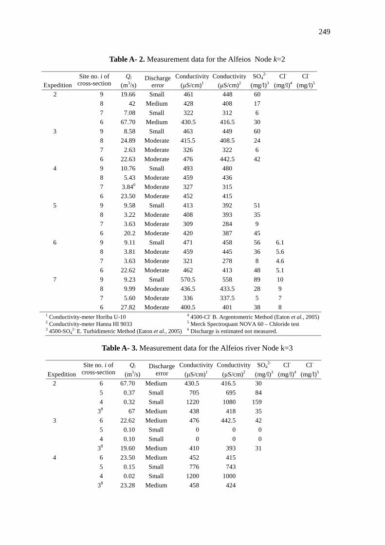
249

Table A- 2. Measurement data for the Alfeios Node k=2

Site no. i of cross-section

Qi Discharge error

Conductivity Conductivity SO42- Cl- Cl-

Expedition (m3/s) (µS/cm)1 (µS/cm)2 (mg/l)3 (mg/l)4 (mg/l)5

2 9 19.66 Small 461 448 60

8 42 Medium 428 408 17

7 7.08 Small 322 312 6

6 67.70 Medium 430.5 416.5 30

3 9 8.58 Small 463 449 60

8 24.89 Moderate 415.5 408.5 24

7 2.63 Moderate 326 322 6

6 22.63 Moderate 476 442.5 42

4 9 10.76 Small 493 480

8 5.43 Moderate 459 436

7 3.846 Moderate 327 315

6 23.50 Moderate 452 415

5 9 9.58 Small 413 392 51

8 3.22 Moderate 408 393 35

7 3.63 Moderate 309 284 9

6 20.2 Moderate 420 387 45

6 9 9.11 Small 471 458 56 6.1

8 3.81 Moderate 459 445 36 5.6

7 3.63 Moderate 321 278 8 4.6

6 22.62 Moderate 462 413 48 5.1

7 9 9.23 Small 570.5 558 89 10

8 9.99 Moderate 436.5 433.5 28 9

7 5.60 Moderate 336 337.5 5 7

6 27.82 Moderate 400.5 401 38 8 1 Conductivity-meter Horiba U-10 2 Conductivity-meter Hanna HI 9033 3 4500-SO4

2- E. Turbidimetric Method (Eaton et al., 2005)

4 4500-Cl- B. Argentometric Method (Eaton et al., 2005) 5 Merck Spectroquant NOVA 60 – Chloride test 6 Discharge is estimated not measured.

Table A- 3. Measurement data for the Alfeios river Node k=3

Site no. i of cross-section

Qi Discharge error

Conductivity Conductivity SO42- Cl- Cl-

Expedition (m3/s) (µS/cm)1 (µS/cm)2 (mg/l)3 (mg/l)4 (mg/l)5

2 6 67.70 Medium 430.5 416.5 30

5 0.37 Small 705 695 84

4 0.32 Small 1220 1080 159

38 67 Medium 438 418 35

3 6 22.62 Medium 476 442.5 42

5 0.10 Small 0 0 0

4 0.10 Small 0 0 0

38 19.60 Medium 410 393 31

4 6 23.50 Medium 452 415

5 0.15 Small 776 743

4 0.02 Small 1200 1000

38 23.28 Medium 458 424

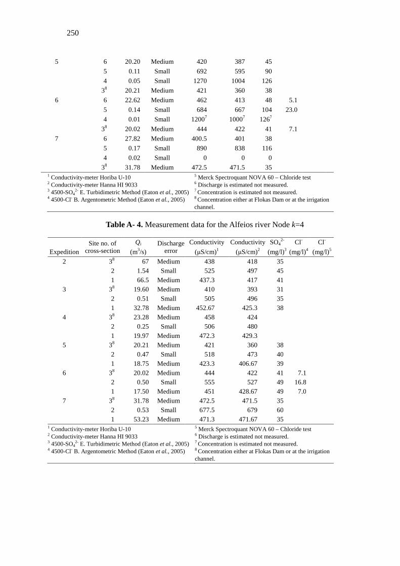
250

5 6 20.20 Medium 420 387 45

5 0.11 Small 692 595 90

4 0.05 Small 1270 1004 126

38 20.21 Medium 421 360 38

6 6 22.62 Medium 462 413 48 5.1

5 0.14 Small 684 667 104 23.0

4 0.01 Small 12007 10007 1267

38 20.02 Medium 444 422 41 7.1

7 6 27.82 Medium 400.5 401 38

5 0.17 Small 890 838 116

4 0.02 Small 0 0 0

38 31.78 Medium 472.5 471.5 35 1 Conductivity-meter Horiba U-10 2 Conductivity-meter Hanna HI 9033 3 4500-SO4

2- E. Turbidimetric Method (Eaton et al., 2005) 4 4500-Cl- B. Argentometric Method (Eaton et al., 2005)

5 Merck Spectroquant NOVA 60 – Chloride test 6 Discharge is estimated not measured. 7 Concentration is estimated not measured. 8 Concentration either at Flokas Dam or at the irrigation channel.

Table A- 4. Measurement data for the Alfeios river Node k=4

Site no. of cross-section

Qi Discharge error

Conductivity Conductivity SO42- Cl- Cl-

Expedition (m3/s) (µS/cm)1 (µS/cm)2 (mg/l)3 (mg/l)4 (mg/l)5

2 38 67 Medium 438 418 35 2 1.54 Small 525 497 45 1 66.5 Medium 437.3 417 41 3 38 19.60 Medium 410 393 31 2 0.51 Small 505 496 35 1 32.78 Medium 452.67 425.3 38 4 38 23.28 Medium 458 424 2 0.25 Small 506 480 1 19.97 Medium 472.3 429.3 5 38 20.21 Medium 421 360 38 2 0.47 Small 518 473 40 1 18.75 Medium 423.3 406.67 39 6 38 20.02 Medium 444 422 41 7.1 2 0.50 Small 555 527 49 16.8 1 17.50 Medium 451 428.67 49 7.0 7 38 31.78 Medium 472.5 471.5 35 2 0.53 Small 677.5 679 60 1 53.23 Medium 471.3 471.67 35

1 Conductivity-meter Horiba U-10 2 Conductivity-meter Hanna HI 9033 3 4500-SO4

2- E. Turbidimetric Method (Eaton et al., 2005) 4 4500-Cl- B. Argentometric Method (Eaton et al., 2005)

5 Merck Spectroquant NOVA 60 – Chloride test 6 Discharge is estimated not measured. 7 Concentration is estimated not measured. 8 Concentration either at Flokas Dam or at the irrigation channel.

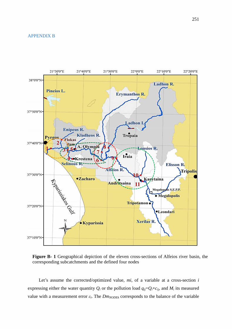
251

APPENDIX B

Let’s assume the corrected/optimized value, mi, of a variable at a cross-section i

expressing either the water quantity Qi or the pollution load qij=Qi×cij, and Mi its measured

value with a measurement error εi. The DmNODEk corresponds to the balance of the variable

Figure B- 1 Geographical depiction of the eleven cross-sections of Alfeios river basin, the corresponding subcatchments and the defined four nodes

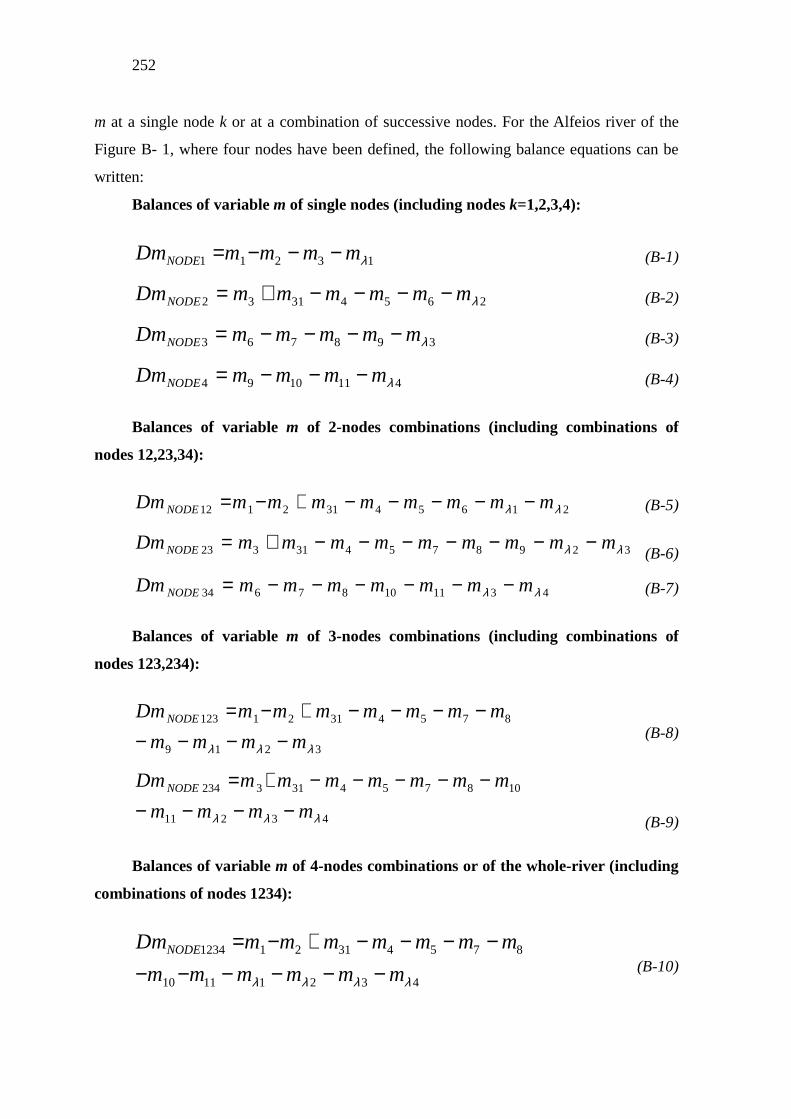
252

m at a single node k or at a combination of successive nodes. For the Alfeios river of the

Figure B- 1, where four nodes have been defined, the following balance equations can be

written:

Balances of variable m of single nodes (including nodes k=1,2,3,4):

13211 λmmmmDmNODE −−−= (B-1)

26543132 λmmmmmmDmNODE −−−−+= (B-2) 398763 λmmmmmDmNODE −−−−= (B-3)

4111094 λmmmmDmNODE −−−= (B-4) Balances of variable m of 2-nodes combinations (including combinations of

nodes 12,23,34):

21654312112 λλ mmmmmmmmDmNODE −−−−−+−= (B-5) 329875431323 λλ mmmmmmmmmDmNODE −−−−−−−+= (B-6)

43111087634 λλ mmmmmmmDmNODE −−−−−−= (B-7)

Balances of variable m of 3-nodes combinations (including combinations of

nodes 123,234):

3219

87543121123

λλλ mmmm

mmmmmmmDmNODE

−−−−−−−−+−= (B-8)

43211

108754313234

λλλ mmmm

mmmmmmmDmNODE

−−−−−−−−−+=

(B-9)

Balances of variable m of 4-nodes combinations or of the whole-river (including

combinations of nodes 1234):

43211110

875431211234

λλλλ mmmmmm

mmmmmmmDmNODE

−−−−−−−−−−+−= (B-10)

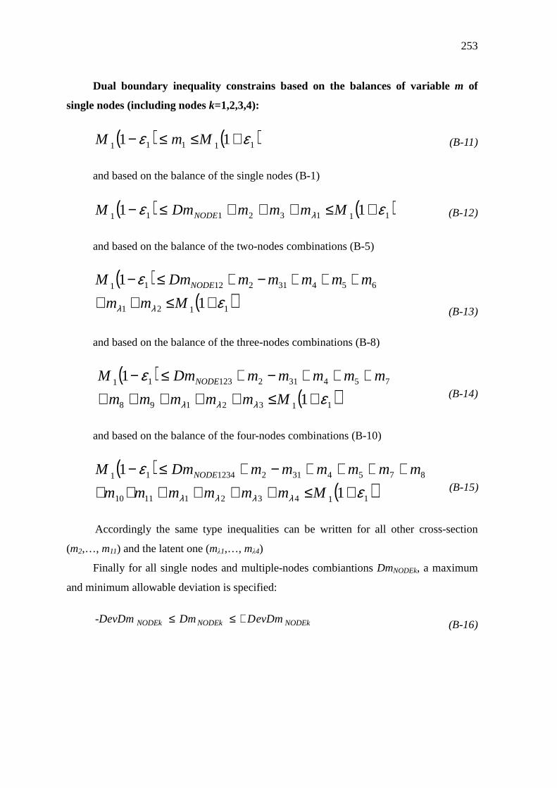
253

Dual boundary inequality constrains based on the balances of variable m of

single nodes (including nodes k=1,2,3,4):

( ) ( )11111 11 εε +≤≤− MmM (B-11)

and based on the balance of the single nodes (B-1)

( ) ( )11132111 11 εε λ +≤+++≤− MmmmDmM NODE (B-12)

and based on the balance of the two-nodes combinations (B-5)

( )( )1121

6543121211

1

1

εε

λλ +≤+++++−+≤−

Mmm

mmmmmDmM NODE

(B-13) and based on the balance of the three-nodes combinations (B-8)

( )( )1132198

75431212311

1

1

εε

λλλ +≤++++++++−+≤−

Mmmmmm

mmmmmDmM NODE (B-14) and based on the balance of the four-nodes combinations (B-10)

( )( )1143211110

8754312123411

1

1

εε

λλλλ +≤++++++++++−+≤−

Mmmmmmm

mmmmmmDmM NODE (B-15) Accordingly the same type inequalities can be written for all other cross-section

(m2,…, m11) and the latent one (mλ1,…, mλ4)

Finally for all single nodes and multiple-nodes combiantions DmNODEk, a maximum

and minimum allowable deviation is specified:

NODEkNODEkNODEk evDmDDm-DevDm +≤≤ (B-16)

254

APPENDIX C

It will be provided till the presentation of the PhD thesis.

255

APPENDIX D

D.1 INVESTIGATION OF THE ENVIRONMENTAL IMPACTS

D.1.1 HYDROGEOLOGICAL IMPACTS

The construction and operation of the enumerated in Table 1.4 infrastructure works,

in conjunction with continued gravel extraction, are linked to geomorphologic alterations,

which cause adverse environmental impacts and affect water resources, thereby causing

ecosystem deterioration (Dafis et al., 1996; HMEPPPW, 1997). Over the last decades, the

major human interference to the natural deltaic evolution of Alfeios River was the

construction of the Ladhon and Flokas dams. The former is a gravity-type of dam,

producing 750,000Volt of electric power, whilst the latter is an irrigation dam, that

establishes a fresh water steady flow of approximately 40m3/h, throughout the year

(Ghionis and Poulos, 2005). The Ladhon dam was set in operation in 1955 cutting off an

upstream area of some 900km2, which represents the 25% of the total drainage basin area.

The Flokas dam started its operation in 1967 and is situated almost 16km far from the

coastline, resulting in 97% retention of catchment water. Consequently, both dams have

drastically decreased the sediment fluxes, at least bed load and most of the suspended

sediment load.

Field observations, associated with area contour and photo maps from 1965 and 1996

respectively, have enabled the determination of the erosion evolution in the lower Alfeios

basin, estimated at ~11.5×106m3 (Manariotis and Yannopoulos, 2004). Based on this

methodology, a mean annual rate of river sediment transport is estimated to be ~31×104

m3/year. Additionally, 17.6×106m3 or even higher gravel quantities were cumulatively

extracted from the basin between 1967 and 1995 (Nicholas et al., 1999). The sediment

transport reaching Flokas dam from the upper part of Alfeios River and being there

retained is approximated at ~5×104m3/year (Dimitrakopoulos et al., 2010). From this

research work, it could be concluded that from the total 31×104m3/year natural sediment

transport assuming no human intervention (thus ignoring the inert material abstraction,

sediment retention from dam, etc.), 5×104m3/year (16%) corresponds to the sediments

volume retained from the dam and the rest 25×104m3/year (80%) to the sediment

abstraction, occurred in the past. From these computations of sediment transport, a surplus

of sediments at the river mouth is in absolute accordance with the delta formation.

256

After the construction of Flokas dam, mainly due to gravel extraction and sediment

retention, a continuous and intense retreat of the coastline is observed. According to

Ghionis et al. (Ghionis and Poulos, 2005), the Alfeios deltaic shore, and more particularly

its mouth area, has encountered extensive erosion over the last decades (coastline

retreat>1m annually) as a result of the effects of Flokas dam, which, in combination with

the intensive nearshore hydrodynamic regime with waves >3m in height and the strong

longshore currents, is associated with a potential longshore sediment transport of

>2×106m3. The side-effects of this phenomenon are evident in the reported destruction of

numerous illegal coastal residences from the wave erosion in a very short time (in only a

few months) (Kokoris, 2007). Based on the comparison of the land use coverage data from

CORINE for 1990 and 2000, the surface river area decreased by 730km2, or 7.2% in one

decade (Androutsopoulou, 2010). The affected river sections correspond to extensive

agricultural activities, where flood control dikes/embankments were built at various river

sections, whereas at others continuing sediment depositions for the extension of

agricultural holding areas around the river are observed. This effect is also strongly related

to the river water drop from extensive agricultural withdrawals, and to the river channel

degradation lowering the riverbed. Moreover, the combination of infrastructure works

(dams), which reduce drastically sediment transport downstream, and the uncontrolled

chronic sand and gravel extraction from cross-sections downstream of the dams has

contributed to lowering of the bed and narrowing of the width of the river. In the same

study, the surface river width alterations were analysed from topographic maps of the

Hellenic Army Geographical Department and digital maps of Hellenic Cadastre (1965-

1967 and 2007-2009 respectively). An average surface river width narrowing of 27m

(28%) was also verified in the medium and lower Alfeios in roughly 40 years, which is in

good agreement with the percentage of the decrease per decade of the river surface

calculated above using CORINE data.

Another implication associated with the Flokas dam is the degradation of the

ecological status and a shift of the riverine flora from the delta toward the dam (Dafis et

al., 1996) because of the limited enrichment of the Alfeios delta with descending debris

(Kallinskis, 1957). A tremendous monetary capital (107€ in 2000) was required (and is

expected to be requested also in the future due to the cyclical nature of the erosion

phenomenon) for restoration and stabilization of the foundation of the dam and to

corresponding bridges downstream the Flokas dam, arising from the extensive erosion

257

occurring at this area as a result of permanent sediment reduction. The extent of the

consequences is depicted by the height of the drop of the riverside level, estimated up to

5.1m at a distance of 2.4km far from the Flokas dam, and the water level drop of the river

up to 6.1m in relation to the groundlevel outside the dikes. Further measurements at the

region downstream of the Flokas dam (up to 0.8 km) reported a severe riverside drop (7m)

from 1965 till 1997. The water level decline of the riverbank in combination with the

overexploitation of groundwater at summertime drives to a remarkable fall of the

groundwater level, especially for regions far from the river. The relevant economical

contrecoups include beyond others the need of pumping equipment and the increase of

pumping cost. The groundwater level decline reached 8m or did even exceed 10m in

regions far from the rivercourse over the past 40 years (Yannopoulos and Manariotis,

2005). Through the application of the Principal Component Analysis (PCA) change

detention method and GIS techniques to the multitemporal and multisensor satellite data

from 1977 to 2000 (Nikolakopoulos et al., 2007), major and extensive riverbed

modifications were once more deduced between 1986 and 2000. In addition, the drainage

network and the riverbed of the last two years of the twentieth century (1999 and 2000)

have followed a straightening course and the number of meanders was reduced.

At last, the Alfeios River Basin has long served as the capital gravel source for the

nearby region. Till the mid of 1990s, gravel was primarily extracted in the lower Alfeios

basin, downstream Flokas dam. However, the need to reinforce the protection of the

archaeological site of Archaia Olympia, the extraction zone has been displaced upstream

the river reaches and to areas far away from the riverbank. Alexoulo-Livaditi (Alexouli-

Livaditi, 1990) emphasised the significant decrease in materials transferred by Alfeios

River, associating this with illegal gravel extraction at the lower Alfeios. The

corresponding zone of minimum bed incision migrates upstream and downstream over

time in response to variations in rates of gravel extraction (Nikolakopoulos, 2002).

(Christopoulos, 1998) verifies that eight excavation companies have been operating in the

Alfeios Riverbed extracting inert materials. According to Nicholas et al. (Nicholas et al.,

1999) in 1986, a high increase in the gravel extraction volume took place, resulting in a

rise from 200,000m3 in 1985 to more than 600,000m3 in 1986. The extraction volume

stabilized for the following three years at 600,000m3/year, while in 1990 a further increase

drove to an extracting volume of more than 900,000m3/year. Since then it continued at this

fixed rate until 2000. Officially, gravel extraction along Alfeios River has been stopped

258

since 2000, and no further measurements have been conducted.

D.1.2 AGRICULTURAL IMPACTS

The most significant human activity, influencing the Alfeios River Basin, is

agriculture, embracing crop production and livestock farming. Apart from the main river

segments, the principal land use of the deltaic areas is also agricultural. These rural

activities constitute non-point source river pollution, resulting in enrichment of water with

nitrates, nitrites, and phosphates, which in turn contribute to eutrophication phenomena.

The extensive and uncontrolled use of pesticides might cause toxicity problems on the

ecosystem and the area population. For the Alfeios watershed, the irrigated land is

estimated up to be 230.5 km². Moreover, the annual fertilizer use of the Alfeios section in

the Region of Ileia approached 30×106kg in 1993. Main nitrogen pressures are associated

with agricultural runoff and free livestock activities (57%), whereas significant point

sources result from confined livestock activities (31%) and urban wastewater (12%)

(HREPPPW, 2006). The primary phosphorus sources are livestock wastes (48%), and

secondarily agricultural runoff (27%). An approximate computation of the nutrient (N, P)

load of the Alfeios River, emanating from crop fertilisers, livestock farming, oil olive mills

and municipal wastewater, was carried out by Yannopoulos (2008). It was shown that the

most heavily charged subcatchments are Ladhon (with N- and P loads 20%), Enipeus (with

N- and P loads 16%) and Floka (with N- and P loads 14%), whereas the least charged

subcathment is Lousios (with N- and P loads 0,5%). This is explained by the number of

inhabitants and oil olive mills accumulated and polluting each tributary.

A second essential intervention in the natural morphology of the Alfeios River Basin

is the drainage of Agoulinitsa and Mouria lakes. The drainage of the Mouria lake was

completed at the end of 1960 in order to provide additional agricultural land areas

(Heliotis, 1988). Drainage channels and the installation of two pumping stations enabled

the pumping of water from the lake and its transfer to the Kyparissiakos Gulf, since the

region is situated below sea level. After the lake drainage, irrigation channels were

constructed, to satisfy the agricultural demand. Except for the land reclamation works

related to lake drainage, soil improvement with gypsum took place due to the high salt

concentration in soil in 1972 (Geordiadis et al., 1998).

Assessing potential benefits from the partial or total rehabilitation of Mouria lake

(Karapanos, 2009; Chatziapostolou, 2009), a lake was designed and constructed in a 0.5 ha

259

area in the eastern part of the former lake, filled with rainwater. The broad study area,

located in Pyrgos area in the subbasin of Enipeus River and in Staphylia basin, is

composed of several both unconfined and confined aquifers in different geological layers.

Some of the most important findings related to the Alfeios River Basin are mentioned

below.

In the Staphylia Basin along the Vounargo-Katakolo fault zone, the existence of

waters with specific characteristics, such as high sodium concentrations and methane

release, has been examined (Karapanos, 2009). High CO2 and Rn concentrations were

detected in groundwater, and are attributed to the presence of thermal waters near the

Vounargo fault zone. Moreover, high iron and manganese concentrations in water samples

from the confined aquifer is indicated as the main reason for their inappropriateness for

drinking water supply, due to the dominance of reducing conditions in an extensive part of

Pyrgos aquifer. Additionally, in a zone parallel to the sea shore, extending from the former

Mouria lake to Alfeios River, ion–exchange phenomena take place in the alluvial aquifer

because of seawater intrusion towards the land. Dedolomitization and pyrite oxidation

encounters in the aquifer, whereas high concentration of ammonia is attributed to

anthropogenic contamination. These outcomes have been supplementarily confirmed by

the factor analysis applied to the major and trace element contents. Regarding the chemical

composition of the drainage channels of the Mouria lake, the high element concentrations,

particularly in the coastal zone, are associated not only with seawater intrusion but also

with human pollution. The maximum values of major and trace elements revealed that

channel water is inappropriate for any use, as house and fabric waste are usually found in

those channels, enriching water with heavy metals. It is also remarkable that before the

Mouria lake drainage, the lateral leakage from the Alfeios River was 10% lower than the

present state, whilst the groundwater level was 2m higher, highlighting the severe impact

of the drainage channel on the region.

In accordance to (Chatziapostolou, 2009), the medium to high alkalinity and the high

electric conductivity, resulting from the combination of poor drainage and the evaporation

from the shallow brackish aquifer, drove in soil pathogenesis and unsuitability for

cultivation. The main activities in the drained Mouria lake, possibly leading to sediment

contamination, are the extensive use of fertilizers at the cultivated areas, as well as waste

dumping.

Zissis & Yannopoulos (Zissis and Yannopoulos, 2011) simulated the variable-density

260

groundwater flow under the existing hydrologic stresses of the Mouria Lake, and predicted

the long-term development of the aquifer under various rehabilitation and energy saving

scenarios. After the Mouria lake drainage, located in the low-lying area of the aquifer along

the coast, water table drawdown and groundwater quality deterioration related to enormous

annual electric power consumption are observed because of the pumped drainage of the

aquifer. The salt water intrusion at the coastline boundary, which was computed in this

investigation, is restricted to a distance of 200m, corresponding to the sand dunes zone.

The pumped drainage system removes considerable amount of water with a significant

energy consumption of approximately 670MWh per year. In case of lake restoration, the

transition zone is restricted underneath the area occupied by the lake, and it does not affect

the major area of the aquifer. The partial lake restoration was judged as equally effective as

the complete lake restoration with regard to the salt water intrusion.

D.1. 3 L IGNITE EXTRACTION AND POWER GENERATION IMPACTS

River geomorphological alterations have been observed at the Megalopolis region,

arising from the lignite extraction, required for the operation of the SEPP. Various

construction works have been executed at this river area, such as the embankment of

riverbank, extending at a length of 450m combined with levees to both riversides and its

diversion from the lignite extraction site. On top of that, the pumping water quantity from

the Megalopolis basin for the suppression of the karstic aquifer water level at this region

corresponds to 18×106m3/year (HREPPPW, 2008). According to Kokoris (Kokoris, 2007),

along the entire riverlength with constructed levees, the riverine flora is limited to a zone

of 5-25m at both riversides. The planned additional diversion of 7km of the Alfeios River

at the Megalopolis region for further lignite exploitation is expected to worsen the existing

geomorphological picture of the area (Yannopoulos and Manariotis, 2005). Local

population assumes that the operation of Megalopolis SEPP is responsible for observed

pollution episodes, leading to crops damage, unsuitable drinking water quality, and a great

ecological deterioration in riverine areas (Dalezios et al., 1977; Manariotis and

Yannopoulos, 2001).

The water quality deterioration in this region includes increased levels of turbidity

(black color of water and river banks) and, as mentioned before, direct municipal and

industrial wastewater discharges without appropriate treatment. The conductivity and the

SO2 concentrations in water are reported 1.6 and 2.0 higher compared to the nearby regions

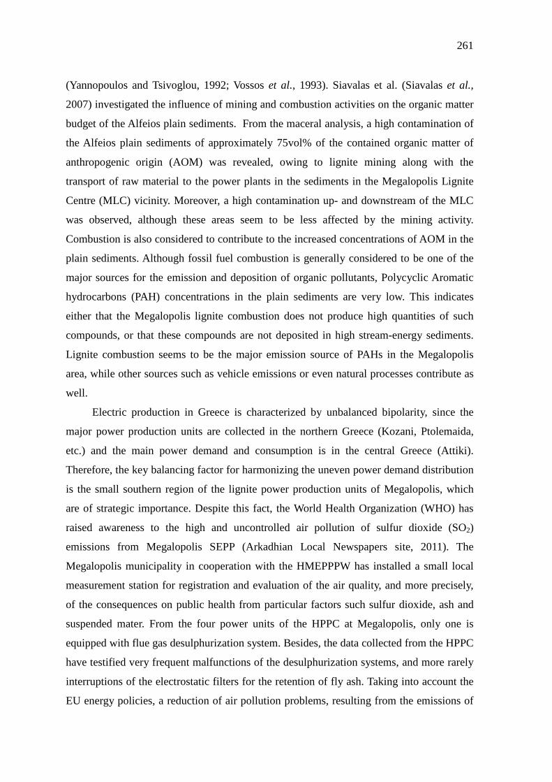
261

(Yannopoulos and Tsivoglou, 1992; Vossos et al., 1993). Siavalas et al. (Siavalas et al.,

2007) investigated the influence of mining and combustion activities on the organic matter

budget of the Alfeios plain sediments. From the maceral analysis, a high contamination of

the Alfeios plain sediments of approximately 75vol% of the contained organic matter of

anthropogenic origin (AOM) was revealed, owing to lignite mining along with the

transport of raw material to the power plants in the sediments in the Megalopolis Lignite

Centre (MLC) vicinity. Moreover, a high contamination up- and downstream of the MLC

was observed, although these areas seem to be less affected by the mining activity.

Combustion is also considered to contribute to the increased concentrations of AOM in the

plain sediments. Although fossil fuel combustion is generally considered to be one of the

major sources for the emission and deposition of organic pollutants, Polycyclic Aromatic

hydrocarbons (PAH) concentrations in the plain sediments are very low. This indicates

either that the Megalopolis lignite combustion does not produce high quantities of such

compounds, or that these compounds are not deposited in high stream-energy sediments.

Lignite combustion seems to be the major emission source of PAHs in the Megalopolis

area, while other sources such as vehicle emissions or even natural processes contribute as

well.

Electric production in Greece is characterized by unbalanced bipolarity, since the

major power production units are collected in the northern Greece (Kozani, Ptolemaida,

etc.) and the main power demand and consumption is in the central Greece (Attiki).

Therefore, the key balancing factor for harmonizing the uneven power demand distribution

is the small southern region of the lignite power production units of Megalopolis, which

are of strategic importance. Despite this fact, the World Health Organization (WHO) has

raised awareness to the high and uncontrolled air pollution of sulfur dioxide (SO2)

emissions from Megalopolis SEPP (Arkadhian Local Newspapers site, 2011). The

Megalopolis municipality in cooperation with the HMEPPPW has installed a small local

measurement station for registration and evaluation of the air quality, and more precisely,

of the consequences on public health from particular factors such sulfur dioxide, ash and

suspended mater. From the four power units of the HPPC at Megalopolis, only one is

equipped with flue gas desulphurization system. Besides, the data collected from the HPPC

have testified very frequent malfunctions of the desulphurization systems, and more rarely

interruptions of the electrostatic filters for the retention of fly ash. Taking into account the

EU energy policies, a reduction of air pollution problems, resulting from the emissions of

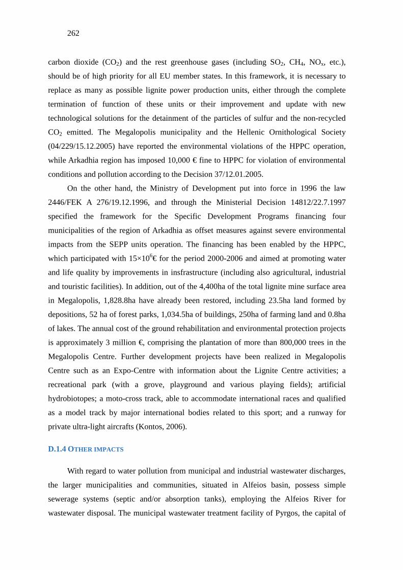
262

carbon dioxide (CO2) and the rest greenhouse gases (including SO2, CH4, NOx, etc.),

should be of high priority for all EU member states. In this framework, it is necessary to

replace as many as possible lignite power production units, either through the complete

termination of function of these units or their improvement and update with new

technological solutions for the detainment of the particles of sulfur and the non-recycled

CO2 emitted. The Megalopolis municipality and the Hellenic Ornithological Society

(04/229/15.12.2005) have reported the environmental violations of the HPPC operation,

while Arkadhia region has imposed 10,000 € fine to HPPC for violation of environmental

conditions and pollution according to the Decision 37/12.01.2005.

On the other hand, the Ministry of Development put into force in 1996 the law

2446/FEK A 276/19.12.1996, and through the Ministerial Decision 14812/22.7.1997

specified the framework for the Specific Development Programs financing four

municipalities of the region of Arkadhia as offset measures against severe environmental

impacts from the SEPP units operation. The financing has been enabled by the HPPC,

which participated with 15×106€ for the period 2000-2006 and aimed at promoting water

and life quality by improvements in insfrastructure (including also agricultural, industrial

and touristic facilities). In addition, out of the 4,400ha of the total lignite mine surface area

in Megalopolis, 1,828.8ha have already been restored, including 23.5ha land formed by

depositions, 52 ha of forest parks, 1,034.5ha of buildings, 250ha of farming land and 0.8ha

of lakes. The annual cost of the ground rehabilitation and environmental protection projects

is approximately 3 million €, comprising the plantation of more than 800,000 trees in the

Megalopolis Centre. Further development projects have been realized in Megalopolis

Centre such as an Expo-Centre with information about the Lignite Centre activities; a

recreational park (with a grove, playground and various playing fields); artificial

hydrobiotopes; a moto-cross track, able to accommodate international races and qualified

as a model track by major international bodies related to this sport; and a runway for

private ultra-light aircrafts (Kontos, 2006).

D.1.4 OTHER IMPACTS

With regard to water pollution from municipal and industrial wastewater discharges,

the larger municipalities and communities, situated in Alfeios basin, possess simple

sewerage systems (septic and/or absorption tanks), employing the Alfeios River for

wastewater disposal. The municipal wastewater treatment facility of Pyrgos, the capital of

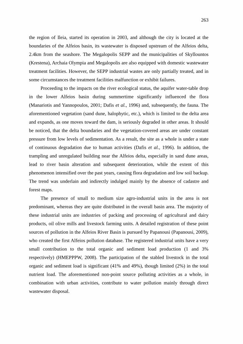
263

the region of Ileia, started its operation in 2003, and although the city is located at the

boundaries of the Alfeios basin, its wastewater is disposed upstream of the Alfeios delta,

2.4km from the seashore. The Megalopolis SEPP and the municipalities of Skyllountos

(Krestena), Archaia Olympia and Megalopolis are also equipped with domestic wastewater

treatment facilities. However, the SEPP industrial wastes are only partially treated, and in

some circumstances the treatment facilities malfunction or exhibit failures.

Proceeding to the impacts on the river ecological status, the aquifer water-table drop

in the lower Alfeios basin during summertime significantly influenced the flora

(Manariotis and Yannopoulos, 2001; Dafis et al., 1996) and, subsequently, the fauna. The

aforementioned vegetation (sand dune, halophytic, etc.), which is limited to the delta area

and expands, as one moves toward the dam, is seriously degraded in other areas. It should

be noticed, that the delta boundaries and the vegetation-covered areas are under constant

pressure from low levels of sedimentation. As a result, the site as a whole is under a state

of continuous degradation due to human activities (Dafis et al., 1996). In addition, the

trampling and unregulated building near the Alfeios delta, especially in sand dune areas,

lead to river basin alteration and subsequent deterioration, while the extent of this

phenomenon intensified over the past years, causing flora degradation and low soil backup.

The trend was underlain and indirectly indulged mainly by the absence of cadastre and

forest maps.

The presence of small to medium size agro-industrial units in the area is not

predominant, whereas they are quite distributed in the overall basin area. The majority of

these industrial units are industries of packing and processing of agricultural and dairy

products, oil olive mills and livestock farming units. A detailed registration of these point

sources of pollution in the Alfeios River Basin is pursued by Papanousi (Papanousi, 2009),

who created the first Alfeios pollution database. The registered industrial units have a very

small contribution to the total organic and sediment load production (1 and 3%

respectively) (HMEPPPW, 2008). The participation of the stabled livestock in the total

organic and sediment load is significant (41% and 49%), though limited (2%) in the total

nutrient load. The aforementioned non-point source polluting activities as a whole, in

combination with urban activities, contribute to water pollution mainly through direct

wastewater disposal.

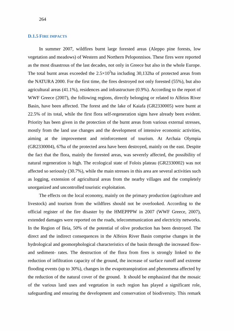
264

D.1.5 FIRE IMPACTS

In summer 2007, wildfires burnt large forested areas (Aleppo pine forests, low

vegetation and meadows) of Western and Northern Peloponnisos. These fires were reported

as the most disastrous of the last decades, not only in Greece but also in the whole Europe.

The total burnt areas exceeded the 2.5×105ha including 30,132ha of protected areas from

the NATURA 2000. For the first time, the fires destroyed not only forested (55%), but also

agricultural areas (41.1%), residences and infrastructure (0.9%). According to the report of

WWF Greece (2007), the following regions, directly belonging or related to Alfeios River

Basin, have been affected. The forest and the lake of Kaiafa (GR2330005) were burnt at

22.5% of its total, while the first flora self-regeneration signs have already been evident.

Priority has been given in the protection of the burnt areas from various external stresses,

mostly from the land use changes and the development of intensive economic activities,

aiming at the improvement and reinforcement of tourism. At Archaia Olympia

(GR2330004), 67ha of the protected area have been destroyed, mainly on the east. Despite

the fact that the flora, mainly the forested areas, was severely affected, the possibility of

natural regeneration is high. The ecological state of Folois plateau (GR2330002) was not

affected so seriously (30.7%), while the main stresses in this area are several activities such

as logging, extension of agricultural areas from the nearby villages and the completely

unorganized and uncontrolled touristic exploitation.

The effects on the local economy, mainly on the primary production (agriculture and

livestock) and tourism from the wildfires should not be overlooked. According to the

official register of the fire disaster by the HMEPPPW in 2007 (WWF Greece, 2007),

extended damages were reported on the roads, telecommunication and electricity networks.

In the Region of Ileia, 50% of the potential of olive production has been destroyed. The

direct and the indirect consequences in the Alfeios River Basin comprise changes in the

hydrological and geomorphological characteristics of the basin through the increased flow-

and sediment- rates. The destruction of the flora from fires is strongly linked to the

reduction of infiltration capacity of the ground, the increase of surface runoff and extreme

flooding events (up to 30%), changes in the evapotranspiration and phenomena affected by

the reduction of the natural cover of the ground. It should be emphasized that the mosaic

of the various land uses and vegetation in each region has played a significant role,

safeguarding and ensuring the development and conservation of biodiversity. This remark

265

should be kept in mind, when formulating a river basin management plan for the region.

Finally, in Table D- 1 an overview of numerous measures, which either individually or in

combination, should be considered, for mitigating the unfavourable effects of the

previously analysed environmental pressures, controlling their negative impacts and

preventing their reappearance for the Alfeios River Basin is provided.

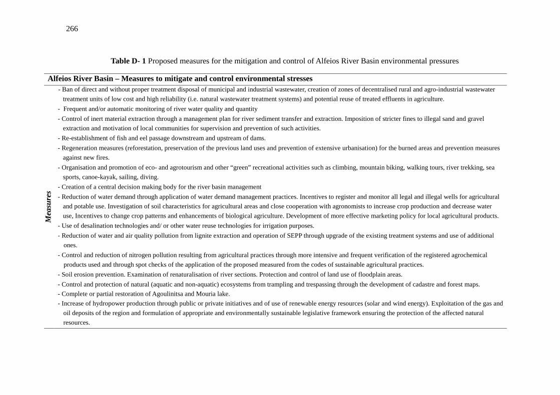
266

Table D- 1 Proposed measures for the mitigation and control of Alfeios River Basin environmental pressures

Alfeios River Basin – Measures to mitigate and control environmental stresses

Mea

sure

s

- Ban of direct and without proper treatment disposal of municipal and industrial wastewater, creation of zones of decentralised rural and agro-industrial wastewater

treatment units of low cost and high reliability (i.e. natural wastewater treatment systems) and potential reuse of treated effluents in agriculture.

- Frequent and/or automatic monitoring of river water quality and quantity

- Control of inert material extraction through a management plan for river sediment transfer and extraction. Imposition of stricter fines to illegal sand and gravel

extraction and motivation of local communities for supervision and prevention of such activities.

- Re-establishment of fish and eel passage downstream and upstream of dams.

- Regeneration measures (reforestation, preservation of the previous land uses and prevention of extensive urbanisation) for the burned areas and prevention measures

against new fires.

- Organisation and promotion of eco- and agrotourism and other “green” recreational activities such as climbing, mountain biking, walking tours, river trekking, sea

sports, canoe-kayak, sailing, diving.

- Creation of a central decision making body for the river basin management

- Reduction of water demand through application of water demand management practices. Incentives to register and monitor all legal and illegal wells for agricultural

and potable use. Investigation of soil characteristics for agricultural areas and close cooperation with agronomists to increase crop production and decrease water

use, Incentives to change crop patterns and enhancements of biological agriculture. Development of more effective marketing policy for local agricultural products.

- Use of desalination technologies and/ or other water reuse technologies for irrigation purposes.

- Reduction of water and air quality pollution from lignite extraction and operation of SEPP through upgrade of the existing treatment systems and use of additional

ones.

- Control and reduction of nitrogen pollution resulting from agricultural practices through more intensive and frequent verification of the registered agrochemical

products used and through spot checks of the application of the proposed measured from the codes of sustainable agricultural practices.

- Soil erosion prevention. Examination of renaturalisation of river sections. Protection and control of land use of floodplain areas.

- Control and protection of natural (aquatic and non-aquatic) ecosystems from trampling and trespassing through the development of cadastre and forest maps.

- Complete or partial restoration of Agoulinitsa and Mouria lake.

- Increase of hydropower production through public or private initiatives and of use of renewable energy resources (solar and wind energy). Exploitation of the gas and

oil deposits of the region and formulation of appropriate and environmentally sustainable legislative framework ensuring the protection of the affected natural

resources.