Embed Size (px)
Citation preview
University of Papua New Guinea
International Economics
Lecture 5: Trade Models II – The Specific Factors Model
The University of Papua New GuineaSlide 2
Lecture 5: Trade Models II – The Specific Factors Model Michael Cornish
Overview
• Introduction
• Setting up the Model
• Distributional effects of a change in price
• Adding trade to the Model
• Conclusions

The University of Papua New GuineaSlide 3
Lecture 5: Trade Models II – The Specific Factors Model Michael Cornish
Introduction
• The Ricardian Model proved the basics of
comparative advantage, but we need a more
complex model to understand the
distributional effects (effects on income
distribution)
• This is what the Specific Factors Model is for!

The University of Papua New GuineaSlide 4
Lecture 5: Trade Models II – The Specific Factors Model Michael Cornish
Capital goods0 1 2 3 4 5
5
10
15a
b
c
d
e
f
Co
nsum
er g
oods
Increasing (marginal)opportunity cost of capital goods
A bending-outwards PPF: increasing opportunity costs

The University of Papua New GuineaSlide 5
Lecture 5: Trade Models II – The Specific Factors Model Michael Cornish
Setting up the Model
Assumptions:
• Two products (just like in the Ricardian Model)
• But now we have three factors of production
– Can be any three, but convention is to use:
• L: Labour, the mobile, ‘non-specific’ factor
• K: Capital, a fixed and ‘specific’ factor
• T: Land, a fixed ‘specific’ factor
• All labour is employed
• We have perfectly competitive markets

The University of Papua New GuineaSlide 6
Lecture 5: Trade Models II – The Specific Factors Model Michael Cornish
Setting up the Model
• What is a ‘specific’ factor?
– A factor of production that is specific to a
particular product
– E.g. land for agriculture; or capital for
manufacturing

The University of Papua New GuineaSlide 7
Lecture 5: Trade Models II – The Specific Factors Model Michael Cornish
Setting up the Model
An example: cloth and food
• Our two products will be cloth and food
• Food requires land (T); cloth requires capital (K)
• Thus, our production functions are:
– QC = QC(K, LC)
– QF = QF(T, LF)
• Note, we assumed that all labour was employed,
thus: LC + LF = L
&

The University of Papua New GuineaSlide 8
Lecture 5: Trade Models II – The Specific Factors Model Michael Cornish
Graphing the production function
Note: The production
function for food has a similar shape!
The University of Papua New GuineaSlide 9
Lecture 5: Trade Models II – The Specific Factors Model Michael Cornish
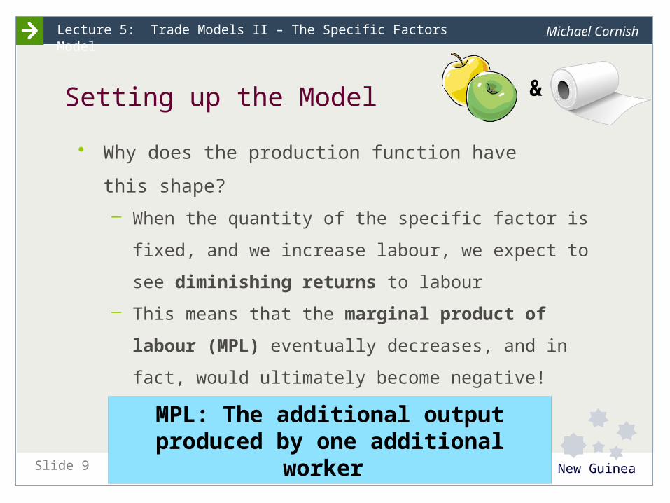
Setting up the Model
• Why does the production function have
this shape?
– When the quantity of the specific factor is fixed, and
we increase labour, we expect to see diminishing
returns to labour
– This means that the marginal product of labour
(MPL) eventually decreases, and in fact, would
ultimately become negative!
MPL: The additional output produced by one additional worker
&
The University of Papua New GuineaSlide 10
Lecture 5: Trade Models II – The Specific Factors Model Michael Cornish
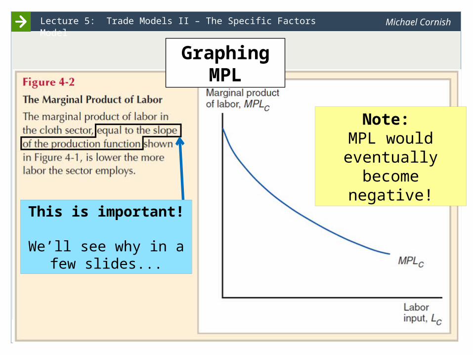
Graphing MPL
Note: MPL would eventually
become negative!
This is important! We’ll see why in a few
slides...
The University of Papua New GuineaSlide 11
Lecture 5: Trade Models II – The Specific Factors Model Michael Cornish

The University of Papua New GuineaSlide 12
Lecture 5: Trade Models II – The Specific Factors Model Michael Cornish
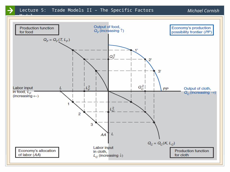
Setting up the Model
• Remember we saw that the MPL was equal to the
slope of production function?
• Using the graph from the previous page, we can
calculate that the slope of the PPF is:
– MPLF / MPLC
[Note: It is negative because of the negative slope]
&

The University of Papua New GuineaSlide 13
Lecture 5: Trade Models II – The Specific Factors Model Michael Cornish
Setting up the Model
• Now we know how much of each product
is produced, given how labour is allocated
• But how do we know how labour will be
allocated?
– For that, we need to know how high the wages
are in each of our two sectors…
&

The University of Papua New GuineaSlide 14
Lecture 5: Trade Models II – The Specific Factors Model Michael Cornish
Setting up the Model
• In the Ricardian Model, we assumed that
wages simply reflect the value of the work done
– It is the same for the Specific Factors Model!
• In the Ricardian Model, wages (per hour) were
determined by the price of the product divided by
how many hours it took to produce one unit
– Note: we fixed the quantity produced to one!
&

The University of Papua New GuineaSlide 15
Lecture 5: Trade Models II – The Specific Factors Model Michael Cornish
Setting up the Model
• In the specific factors model, we fix the
number of hours to one, and so it is the quantity
produced that changes
• Thus, if we set out MPL to reflect the value of
one additional (marginal) hour of labour:
w = MPL * P
E.g. wages in the food sector: wF = MPLF * PF
• Except, we assume labour can move freely –
thus wages should be identical in both sectors
&

The University of Papua New GuineaSlide 16
Lecture 5: Trade Models II – The Specific Factors Model Michael Cornish
Determining the equilibrium wage...
Note:The assumption is that the demand for labour in each sector is equal
to the value of the produce of labour
(P * MPL) [which is the willingness to pay a
certain level of wage]

The University of Papua New GuineaSlide 17
Lecture 5: Trade Models II – The Specific Factors Model Michael Cornish
Setting up the Model
• Looking at wages also helps us another way – it
tells us what the relative prices for our two
products should be
If: MPLC * PC = MPLF * PF = w
Then: – MPLF / MPLC = – PC / PF
• And since we know that – MPLF / MPLC is the slope
of our PPF…
&

The University of Papua New GuineaSlide 18
Lecture 5: Trade Models II – The Specific Factors Model Michael Cornish
Eureka!
In domestic equilibrium

The University of Papua New GuineaSlide 19
Lecture 5: Trade Models II – The Specific Factors Model Michael Cornish
Distributional effects of a change in price
• We’ve just established the relationship between
MPL, wages, prices, and the quantities produced
in autarky (an economy without trade)
• But before we add in the trade, let’s see what
happens if we change the domestic prices of
cloth and/or food…

The University of Papua New GuineaSlide 20
Lecture 5: Trade Models II – The Specific Factors Model Michael Cornish
A proportionally equal increase in both prices
It just increases the wage by the same proportion!
Therefore: • No change to
relative prices• No change to
the domestic PPF

The University of Papua New GuineaSlide 21
Lecture 5: Trade Models II – The Specific Factors Model Michael Cornish
An increase in one price only (e.g. cloth)
1. Labour shifts from the food sector into the cloth sector...

The University of Papua New GuineaSlide 22
Lecture 5: Trade Models II – The Specific Factors Model Michael Cornish
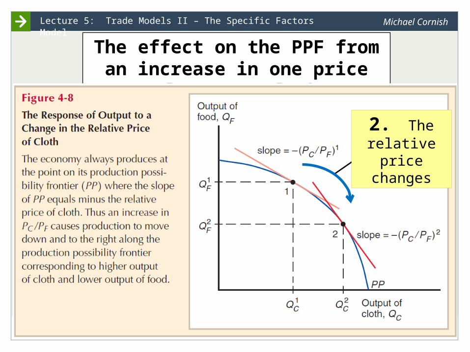
2. ...the relative price
changes
1. As labour shifts from the
food sector into the cloth
sector...
The University of Papua New GuineaSlide 23
Lecture 5: Trade Models II – The Specific Factors Model Michael Cornish
The effect on the PPF from an increase in one price only (e.g. cloth)
2. The relative price changes
The University of Papua New GuineaSlide 24
Lecture 5: Trade Models II – The Specific Factors Model Michael Cornish
Distributional effects of a change in price
• In our example, we saw that the absolute wage
increased by less than the increase in the price of
cloth (7% in our example)
– However, it still increased
• But the question is – are workers (L) better off??
The University of Papua New GuineaSlide 25
Lecture 5: Trade Models II – The Specific Factors Model Michael Cornish
Distributional effects of a change in price
• For this, we need to look at their real wage (w/p)
– That is, how much of the two different products
can they buy? Is it more or less than before?
• Their real wage in terms of cloth has fallen:
– w (less than 7%) < PC (7%) => w/PC
• Their real wage in terms of food has risen:
– w (less than 7%) > no Δ in PF => w/PF

The University of Papua New GuineaSlide 26
Lecture 5: Trade Models II – The Specific Factors Model Michael Cornish
Distributional effects of a change in price
• So the effect on workers (L) is ambiguous!
– It depends on what the relative preferences of
workers are for cloth and food...
• What about owners of capital (K) ?
– The price of their product has increased more
than the wage they pay workers
– So they are definitely better off!
The University of Papua New GuineaSlide 27
Lecture 5: Trade Models II – The Specific Factors Model Michael Cornish
Distributional effects of a change in price
• What about owners of land (T) ?
– The absolute price of their product has not
changed…
– …but the wages they must pay have increased
– So they are definitely worse off!
• And can show all of these distributional effects
diagrammatically!

The University of Papua New GuineaSlide 28
Lecture 5: Trade Models II – The Specific Factors Model Michael Cornish
Demand curve for Labour
Producer surplus
Consumer surplus
Distribution of income: consumer and producer surplus

The University of Papua New GuineaSlide 29
Lecture 5: Trade Models II – The Specific Factors Model Michael Cornish
Note: The effect on total wages paid [blue] is ambiguous:
(w/PC)1 * L1C => (w/PC)2 * L2
C
It depends!
[red]
Distribution of income: consumer and producer surplus
The University of Papua New GuineaSlide 30
Lecture 5: Trade Models II – The Specific Factors Model Michael Cornish
Adding trade to the Model
• Finally, let’s add the trade to our Model !
• Instead of considering two economies, we only look
at ‘Home’ and assume that they face a world price
• To do this, we again use general equilibrium analysis:
– Relative demand (RD) & relative supply (RS)
• Except we assume that producers are indifferent who
they supply to…
– So there is only the one RD with trade: RDWorld
The University of Papua New GuineaSlide 31
Lecture 5: Trade Models II – The Specific Factors Model Michael Cornish
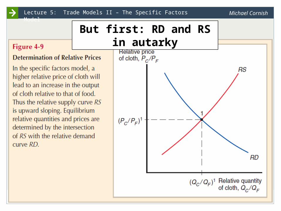
But first: RD and RS in autarky

The University of Papua New GuineaSlide 32
Lecture 5: Trade Models II – The Specific Factors Model Michael Cornish
...and now with tradeNote: In this example, the world relative price of cloth just happens to be higher
This is only an assumption!But it is true that there is
only one RDWorld

The University of Papua New GuineaSlide 33
Lecture 5: Trade Models II – The Specific Factors Model Michael Cornish
Opening up to trade leads to a changes in Home’s relative price!
We can then track the effects from this change in relative price just like we did
before (Slides 20 – 28)
Note: In all our examples we tracked an increase in the relative price of cloth
The University of Papua New GuineaSlide 34
Lecture 5: Trade Models II – The Specific Factors Model Michael Cornish
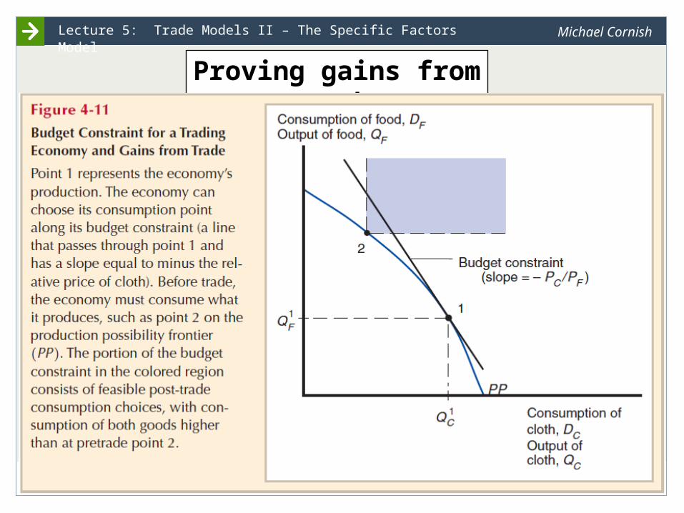
Proving gains from trade

The University of Papua New GuineaSlide 35
Lecture 5: Trade Models II – The Specific Factors Model Michael Cornish
Conclusions
• The Specific Factors Model is very useful in
determining the winners and losers from trade
• Trade benefits the factor that is specific to
the export market, but hurts the factor that
is specific to the import market
• The effects upon the non-specific factor are
ambiguous
• It gives us a some understanding of how resource
endowments – the stock of specific factors (i.e. K, T)
and non-specific factors (i.e. L) – affect trade

The University of Papua New GuineaSlide 36
Lecture 5: Trade Models II – The Specific Factors Model Michael Cornish
Conclusions
• However, it still doesn’t tell us exactly how
differences in resource endowments are a
cause of trade
• For that we need our next trade model:
The Heckscher-Ohlin Model
» So stay tuned!