Embed Size (px)
Citation preview
UNIVERSITY OF OKLAHOMA
GRADUATE COLLEGE
APPLICATION OF THE FORWARD SENSITIVITY METHOD TO
DATA ASSIMILATION OF THE LAGRANGIAN TRACER DYNAMICS
A DISSERTATION
SUBMITTED TO THE GRADUATE FACULTY
in partial fulfillment of the requirements for the
Degree of
DOCTOR OF PHILOSOPHY
By
RAFAL JABRZEMSKINorman, Oklahoma
2014

APPLICATION OF THE FORWARD SENSITIVITY METHOD TODATA ASSIMILATION OF THE LAGRANGIAN TRACER DYNAMICS
A DISSERTATION APPROVED FOR THESCHOOL OF COMPUTER SCIENCE
BY
Dr. S. Lakshmivarahan, Chair
Dr. Sudarshan Dhall
Dr. Sridhar Radhakrishnan
Dr. Krishnaiyan Thulasiraman
Dr. Ming Xue

c© Copyright by RAFAL JABRZEMSKI 2014All rights reserved.

DEDICATION
to
My parents
Kazimierz Jabrzemski and Eleonora Jabrzemska,
my wife Marzena Jabrzemski
and daughters Nina and Natalia Jabrzemski
For
Encouragement, belief and patience

Acknowledgements
I wish to express my enormous gratitude to my research advisor, Professor Laksh-
mivarahan, for teaching me a great deal of computational science, for his advice
and support, and for being an excellent mentor. I am very grateful for having
had the chance to work with him.
I greatly appreciate guidance and time given by the members of my committee
including Dr. Sridhar Radhakrishnan, Dr. Sudarshan Dhall, Dr. Krishnaiyan
Thulasiraman and Dr. Ming Xue.
I also wish to thank the Oklahoma Mesonet for supporting the work on my
dissertation.
iv

Table of Contents
1 Introduction 11.1 Motivation . . . . . . . . . . . . . . . . . . . . . . . . . . . . . . . 11.2 Previous work . . . . . . . . . . . . . . . . . . . . . . . . . . . . . 3
1.2.1 Assimilation of Lagrangian Data into a Numerical Model . 31.2.2 Assimilation of drifter observations for the reconstruction
of the Eulerian circulation field . . . . . . . . . . . . . . . 51.2.3 Assimilation of drifter observations in primitive equation
models of midlatitude ocean circulation . . . . . . . . . . . 101.2.4 A method for assimilation of Lagrangian data . . . . . . . 141.2.5 Using flow geometry for drifter deployment in Lagrangian
data assimilation . . . . . . . . . . . . . . . . . . . . . . . 191.2.6 A Bayesian approach to Lagrangian data assimilation . . . 22
1.3 Summary . . . . . . . . . . . . . . . . . . . . . . . . . . . . . . . 261.4 Organization of the Dissertation . . . . . . . . . . . . . . . . . . . 27
2 Shallow Water Model 282.1 Introduction . . . . . . . . . . . . . . . . . . . . . . . . . . . . . . 282.2 Large scale motion . . . . . . . . . . . . . . . . . . . . . . . . . . 282.3 Scalling assumptions . . . . . . . . . . . . . . . . . . . . . . . . . 322.4 Summary . . . . . . . . . . . . . . . . . . . . . . . . . . . . . . . 34
3 Linearized Shallow Water Model and Tracer Dynamics 353.1 Introduction . . . . . . . . . . . . . . . . . . . . . . . . . . . . . . 353.2 Model variables . . . . . . . . . . . . . . . . . . . . . . . . . . . . 353.3 Low-order model (LOM) . . . . . . . . . . . . . . . . . . . . . . . 36
3.3.1 Analytical solution for amplitudes . . . . . . . . . . . . . . 373.3.2 Eigenvalues and eigenvectors of A . . . . . . . . . . . . . . 38
3.4 Tracer dynamics . . . . . . . . . . . . . . . . . . . . . . . . . . . . 483.5 Analysis of Equilibria of Tracer dynamics . . . . . . . . . . . . . . 50
3.5.1 Case 1: Equilibria in geostrophic mode . . . . . . . . . . . 503.5.2 Case 2: Equilibria in inertial-gravity mode . . . . . . . . . 553.5.3 Case 3: Equilibria in general case . . . . . . . . . . . . . . 59
v

3.5.4 Conditions for the sign definiteness of ∆i(t) . . . . . . . . 643.6 Analysis of bifurcations . . . . . . . . . . . . . . . . . . . . . . . . 65
3.6.1 Case 1 . . . . . . . . . . . . . . . . . . . . . . . . . . . . . 673.6.2 Case 2 . . . . . . . . . . . . . . . . . . . . . . . . . . . . . 71
3.7 Tracer Dynamics in the Linearized Shallow Water Model . . . . . 723.8 Summary . . . . . . . . . . . . . . . . . . . . . . . . . . . . . . . 75
4 A Framework for Data Assimilation 814.1 Introduction . . . . . . . . . . . . . . . . . . . . . . . . . . . . . . 814.2 Model . . . . . . . . . . . . . . . . . . . . . . . . . . . . . . . . . 82
4.2.1 Observations . . . . . . . . . . . . . . . . . . . . . . . . . 834.2.2 Objective function . . . . . . . . . . . . . . . . . . . . . . 84
4.3 Data Assimilation using Forward Sensitivity Method (FSM) . . . 894.3.1 Multiple observations . . . . . . . . . . . . . . . . . . . . . 91
4.4 Summary . . . . . . . . . . . . . . . . . . . . . . . . . . . . . . . 92
5 Sensitivity 945.1 Introduction . . . . . . . . . . . . . . . . . . . . . . . . . . . . . . 945.2 Basic ideas . . . . . . . . . . . . . . . . . . . . . . . . . . . . . . . 955.3 Evolution of sensitivity of the shallow water model with respect to
initial conditions and parameters . . . . . . . . . . . . . . . . . . 965.3.1 Sensitivity to elements of
the control vector α . . . . . . . . . . . . . . . . . . . . . 985.3.2 Sensitivity to elements of
the initial conditions X(0) . . . . . . . . . . . . . . . . . . 995.4 Numerical experiments . . . . . . . . . . . . . . . . . . . . . . . . 100
5.4.1 Experiment 5.1 . . . . . . . . . . . . . . . . . . . . . . . . 1005.4.2 Experiment 5.2 . . . . . . . . . . . . . . . . . . . . . . . . 1075.4.3 Experiment 5.3 . . . . . . . . . . . . . . . . . . . . . . . . 114
5.5 Summary . . . . . . . . . . . . . . . . . . . . . . . . . . . . . . . 121
6 Numerical experiments in Data Assimilation 1226.1 Introduction . . . . . . . . . . . . . . . . . . . . . . . . . . . . . . 122
6.1.1 Root-mean-square error . . . . . . . . . . . . . . . . . . . 1236.1.2 Condition number of a matrix . . . . . . . . . . . . . . . . 1236.1.3 Methodology . . . . . . . . . . . . . . . . . . . . . . . . . 124
6.2 Data assimilation . . . . . . . . . . . . . . . . . . . . . . . . . . . 1256.2.1 Experiment 6.1 . . . . . . . . . . . . . . . . . . . . . . . . 1256.2.2 Experiment 6.2 . . . . . . . . . . . . . . . . . . . . . . . . 1376.2.3 Experiment 6.3 . . . . . . . . . . . . . . . . . . . . . . . . 181
6.3 Summary . . . . . . . . . . . . . . . . . . . . . . . . . . . . . . . 198
7 Conclusions 199
vi

A Reduction process 205
B Bounds on u1(t) in (2.14) 209
C Definition and properties of standard hyperbola 211
vii

List of Tables
5.1 Experiment 5.1: Base control vector α and initial conditions X(0) 1005.2 Experiment 5.2: Base control vector α and initial conditions X(0) 1075.3 Experiment 5.3: Base control vector α and initial conditions X(0) 114
6.1 Values of the observational error variance σ and σ2 used in dataassimilation experiments to create perturbed observations . . . . . 125
6.2 Experiment 6.1: Base control vector α and initial conditions X(0) 1266.3 Experiment 6.1: Perturbed control vector α and initial conditions
X(0) . . . . . . . . . . . . . . . . . . . . . . . . . . . . . . . . . . 1266.4 Experiment 6.1: Comparison of data assimilations for a set of
distributions and errors with 4 measurements . . . . . . . . . . . 1276.5 Experiment 6.2: Base control vector α and initial conditions X(0) 1376.6 Experiment 6.2: Perturbed control vector α and initial conditions
X(0) . . . . . . . . . . . . . . . . . . . . . . . . . . . . . . . . . . 1376.7 Experiment 6.2: Comparison of data assimilations for a set of
distributions and errors with 4 measurements . . . . . . . . . . . 1386.8 Experiment 6.2: Comparison of data assimilations for a set of
distributions and errors with 8 measurements . . . . . . . . . . . 1396.9 Experiment 6.2: Comparison of data assimilations for a set of
distributions and errors with 16 measurements . . . . . . . . . . . 1406.10 Experiment 6.2: Comparison of data assimilations for a set of
distributions and errors with 32 measurements . . . . . . . . . . . 1416.11 Experiment 6.2: Comparison of data assimilations for a set of
distributions and errors with 64 measurements . . . . . . . . . . . 1426.12 Experiment 6.2: Comparison of data assimilations for a set of
distributions and errors with 128 measurements . . . . . . . . . . 1436.13 Experiment 6.2: Comparison of data assimilations for a set of
distributions with different number of measurements and errorswith σ2 = 0.005 . . . . . . . . . . . . . . . . . . . . . . . . . . . . 174
6.14 Experiment 6.2: Comparison of data assimilations for a set ofdistributions with different number of measurements and errorswith σ2 = 0.075 . . . . . . . . . . . . . . . . . . . . . . . . . . . . 175
viii

6.15 Experiment 6.2: Comparison of data assimilations for a set ofdistributions with different number of measurements and errorswith σ2 = 0.01 . . . . . . . . . . . . . . . . . . . . . . . . . . . . . 176
6.16 Experiment 6.2: Comparison of data assimilations for a set ofdistributions with different number of measurements and errorswith σ2 = 0.0125 . . . . . . . . . . . . . . . . . . . . . . . . . . . 177
6.17 Experiment 6.2: Comparison of data assimilations for a set ofdistributions with different number of measurements and errorswith σ2 = 0.015 . . . . . . . . . . . . . . . . . . . . . . . . . . . . 178
6.18 Experiment 6.2: Comparison of data assimilations for a set ofdistributions with different number of measurements and errorswith σ2 = 0.0175 . . . . . . . . . . . . . . . . . . . . . . . . . . . 179
6.19 Experiment 6.2: Comparison of data assimilations for a set ofdistributions with different number of measurements and errorswith σ2 = 0.02 . . . . . . . . . . . . . . . . . . . . . . . . . . . . . 180
6.20 Experiment 6.3: Base control vector α and initial conditions X(0) 1816.21 Experiment 6.3: Perturbed control vector α and initial conditions
X(0) . . . . . . . . . . . . . . . . . . . . . . . . . . . . . . . . . . 1816.22 Experiment 6.3: Comparison of data assimilations for a set of
distributions and errors with 4 measurements, start (0,0) . . . . . 182
B.1 Distribution of the pairs(x∗, f(x∗)
). . . . . . . . . . . . . . . . . 210
ix

List of Figures
3.1 A display of equilibria of Type 1 - filled circles and Type 2 - unfilledcircles along with the velocity field around them. Filled circlesare saddle points and unfilled circles are centers. The field plotaround these equilibria corresponds to f(x, y) in (3.32) with u0 =1.0, u1(0) = v1(0) = h1(0) = 0 and time t = 0. . . . . . . . . . . . 52
3.2 A display of trajectories of the pure geostrophic dynamics . . . . 543.3 A display of equilibria of Type a - dashed line and Type b - solid
line, and the flow field around them. The plot of the time varyingvector field around these equilibria corresponding to g(x, α, t) in(3.33) at time t = 0 and for values of corresponding parametersu0 = 0, u1(0) = v1(0) = h1(0) = 1 and time t = 0. . . . . . . . . . 56
3.4 A display of trajectories of the pure inertial gravity modes . . . . 583.5 A display of equilibria of Type A (1/4, 1/4) and B (1/4, - 1/4)-
solid circles and Type C (-1/4, 1/4) and D (-1/4, -1/4) - emptycircles , and the flow field around them. A snapshot of the timevarying vector field given by (3.35) at time t = 0 where u0 = 1.0,u1(0) = 9.4248, v1(0) = λ and h1(0) = −1.5. . . . . . . . . . . . . 61
3.6 A display of trajectories in the combined mode . . . . . . . . . . . 633.7 Hyperbola corresponding to (14.9) C in the center at (2πu0, 0) for
u0 = 1 Let v1(0) = 1 and the semi axes AC = AC ′ = BC = 1.The asymptotes have slope ±1. . . . . . . . . . . . . . . . . . . . 69
3.8 Hyperbola corresponding to (14.11) C in the center at (−2πu0, 0)with u0 = 1 Let v1(0) = 1 and the semi axes CA = CA′ = CB =CB′ = 1. The asymptotes have slope ±1. . . . . . . . . . . . . . . 70
3.9 The combined system of hyperbolas from Figure 3.7 and 3.8. Re-gions corresponding to different signs of ∆1(t) and ∆2(t) are shown.Points on the hyperbola are the bifurcation points. . . . . . . . . 71
3.10 A snapshot of the time varying vector field given by (3.31) at timet = 0 and t = 0.5, where u0 = 1.0, u1(0) = 12.5664, v1(0) = λand h1(0) = −2.0. This corresponds to V (0) = 1, U(0) = 4π andH(0) = 0, which is a point in Region 1 in Figure 9. . . . . . . . . 76(a) Time t = 0.0 . . . . . . . . . . . . . . . . . . . . . . . . . . 76(b) Time t = 0.5 . . . . . . . . . . . . . . . . . . . . . . . . . . 76
x

3.11 A snapshot of the time varying vector field given by (3.31) t = 0and t = 0.5, where u0 = 1.0, u1(0) = 0.0, v1(0) = λ and h1(0) = 0.0This corresponds to V (0) = 1, U(0) = 0 and H(0) = 0, which is apoint in Region 2 in Figure 9. . . . . . . . . . . . . . . . . . . . . 77(a) Time t = 0.0 . . . . . . . . . . . . . . . . . . . . . . . . . . 77(b) Time t = 0.5 . . . . . . . . . . . . . . . . . . . . . . . . . . 77
3.12 A snapshot of the time varying vector field given by (3.31) A snap-shot of the time varying vector field given by (3.31) at time t = 0and t = 0.5, where u0 = 1.0, u1(0) = −12.5664, v1(0) = λ andh1(0) = 2.0. This corresponds to V (0) = 1, U(0) = −4π andH(0) = 0, which is a point in Region 3 in Figure 9. . . . . . . . . 78(a) Time t = 0.0 . . . . . . . . . . . . . . . . . . . . . . . . . . 78(b) Time t = 0.5 . . . . . . . . . . . . . . . . . . . . . . . . . . 78
3.13 A snapshot of the time varying vector field given by (3.31) A snap-shot of the time varying vector field given by (3.31) at time t = 0and t = 0.5, where u0 = 1.0, u1(0) = 7.2832, v1(0) = λ andh1(0) = −1.1592. This corresponds to V (0) = 1, U(0) = 2π+1 andH(0) = 0, which is a bifurcation point on the hyperbola separatingRegion 1 and 2 in Figure 9. . . . . . . . . . . . . . . . . . . . . . 79(a) Time t = 0.0 . . . . . . . . . . . . . . . . . . . . . . . . . . 79(b) Time t = 0.5 . . . . . . . . . . . . . . . . . . . . . . . . . . 79
3.14 A snapshot of the time varying vector field given by (3.31) Asnapshot of the time varying vector field given by (3.31) t = 0and t = 0.5, where u0 = 1.0, u1(0) = −7.2832, v1(0) = λ andh1(0) = 1.1592. This corresponds to V (0) = 1, U(0) = −2π − 1and H(0) = 0, which is a bifurcation point on the hyperbola sep-arating Region 2 and 3 in Figure 9. . . . . . . . . . . . . . . . . 80(a) Time t = 0.0 . . . . . . . . . . . . . . . . . . . . . . . . . . 80(b) Time t = 0.5 . . . . . . . . . . . . . . . . . . . . . . . . . . 80
5.1 Experiment 5.1: Sensitivity of x(t) w.r.t. x(0) . . . . . . . . . . . 1015.2 Experiment 5.1: Sensitivity of x(t) w.r.t. y(0) . . . . . . . . . . . 1015.3 Experiment 5.1: Sensitivity of y(t) w.r.t. x(0) . . . . . . . . . . . 1025.4 Experiment 5.1: Sensitivity of y(t) w.r.t. y(0) . . . . . . . . . . . 1025.5 Experiment 5.1: Sensitivity of x(t) w.r.t. u0 . . . . . . . . . . . . 1035.6 Experiment 5.1: Sensitivity of x(t) w.r.t. u1(0) . . . . . . . . . . 1035.7 Experiment 5.1: Sensitivity of x(t) w.r.t. v1(0) . . . . . . . . . . 1045.8 Experiment 5.1: Sensitivity of x(t) w.r.t. h1(0) . . . . . . . . . . 1045.9 Experiment 5.1: Sensitivity of y(t) w.r.t. u0 . . . . . . . . . . . . 1055.10 Experiment 5.1: Sensitivity of y(t) w.r.t. u1(0) . . . . . . . . . . . 1055.11 Experiment 5.1: Sensitivity of y(t) w.r.t. v1(0) . . . . . . . . . . 1065.12 Experiment 5.1: Sensitivity of y(t) w.r.t. h1(0) . . . . . . . . . . 106
xi

5.13 Experiment 5.2: Sensitivity of x(t) w.r.t. x(0) . . . . . . . . . . . 1075.14 Experiment 5.2: Sensitivity of x(t) w.r.t. y(0) . . . . . . . . . . . 1085.15 Experiment 5.2: Sensitivity of y(t) w.r.t. x(0) . . . . . . . . . . . 1085.16 Experiment 5.2: Sensitivity of y(t) w.r.t. y(0) . . . . . . . . . . . 1095.17 Experiment 5.2: Sensitivity of x(t) w.r.t. u0 . . . . . . . . . . . . 1105.18 Experiment 5.2: Sensitivity of x(t) w.r.t. u1(0) . . . . . . . . . . 1105.19 Experiment 5.2: Sensitivity of x(t) w.r.t. v1(0) . . . . . . . . . . 1115.20 Experiment 5.2: Sensitivity of x(t) w.r.t. h1(0) . . . . . . . . . . 1115.21 Experiment 5.2: Sensitivity of y(t) w.r.t. u0 . . . . . . . . . . . . 1125.22 Experiment 5.2: Sensitivity of y(t) w.r.t. u1(0) . . . . . . . . . . . 1125.23 Experiment 5.2: Sensitivity of y(t) w.r.t. v1(0) . . . . . . . . . . 1135.24 Experiment 5.2: Sensitivity of y(t) w.r.t. h1(0) . . . . . . . . . . 1135.25 Experiment 5.3: Sensitivity of x(t) w.r.t. x(0) . . . . . . . . . . . 1155.26 Experiment 5.3: Sensitivity of x(t) w.r.t. y(0) . . . . . . . . . . . 1155.27 Experiment 5.3: Sensitivity of y(t) w.r.t. x(0) . . . . . . . . . . . 1165.28 Experiment 5.3: Sensitivity of y(t) w.r.t. y(0) . . . . . . . . . . . 1165.29 Experiment 5.3: Sensitivity of x(t) w.r.t. u0 . . . . . . . . . . . . 1175.30 Experiment 5.3: Sensitivity of x(t) w.r.t. u1(0) . . . . . . . . . . 1175.31 Experiment 5.3: Sensitivity of x(t) w.r.t. v1(0) . . . . . . . . . . 1185.32 Experiment 5.3: Sensitivity of x(t) w.r.t. h1(0) . . . . . . . . . . 1185.33 Experiment 5.3: Sensitivity of y(t) w.r.t. u0 . . . . . . . . . . . . 1195.34 Experiment 5.3: Sensitivity of y(t) w.r.t. u1(0) . . . . . . . . . . . 1195.35 Experiment 5.3: Sensitivity of y(t) w.r.t. v1(0) . . . . . . . . . . 1205.36 Experiment 5.3: Sensitivity of y(t) w.r.t. h1(0) . . . . . . . . . . 120
6.1 Experiment 6.1: Trajectory with 4 measurements, START distri-bution . . . . . . . . . . . . . . . . . . . . . . . . . . . . . . . . . 126
6.2 Experiment 6.1: Cost function for three steps of data assimilation,START measurement distribution . . . . . . . . . . . . . . . . . 128
6.3 Experiment 6.1: Sensitivity functions, START measurement dis-tribution . . . . . . . . . . . . . . . . . . . . . . . . . . . . . . . . 129
6.4 Experiment 6.1: Trajectory with 4 measurements, MIDDLE dis-tribution . . . . . . . . . . . . . . . . . . . . . . . . . . . . . . . 130
6.5 Experiment 6.1: Cost function for three steps of data assimilation,MIDDLE measurement distribution . . . . . . . . . . . . . . . . 131
6.6 Experiment 6.1: Cost function for three steps of data assimilation 1326.7 Experiment 6.1: Trajectory with 4 measurements, FINISH distri-
bution . . . . . . . . . . . . . . . . . . . . . . . . . . . . . . . . . 1336.8 Experiment 6.1: Cost function for three steps of data assimilation,
FINISH measurement distribution . . . . . . . . . . . . . . . . . 1336.9 Experiment 6.1: Sensitivity functions, FINISH measurement dis-
tribution . . . . . . . . . . . . . . . . . . . . . . . . . . . . . . . . 134
xii

6.10 Experiment 6.1: Trajectory with 4 measurements, UNIFORM dis-tribution . . . . . . . . . . . . . . . . . . . . . . . . . . . . . . . 135
6.11 Experiment 6.1: Cost function for three steps of data assimilation,UNIFORM measurement distribution . . . . . . . . . . . . . . . 135
6.12 Experiment 6.1: Sensitivity functions, UNIFORM measurementdistribution . . . . . . . . . . . . . . . . . . . . . . . . . . . . . . 136
6.13 Experiment 6.2: Root-mean-square (RMSE) error of observationsas a function of number of experiments σ2 = 0.005, START mea-surement distribution. . . . . . . . . . . . . . . . . . . . . . . . . 144
6.14 Experiment 6.2: Condition number κ as a function of number ofexperiments σ2 = 0.005, START measurement distribution. . . . . 144
6.15 Experiment 6.2: Root-mean-square error of observations as a func-tion of number of experiments σ2 = 0.005, MIDDLE measurementdistribution. . . . . . . . . . . . . . . . . . . . . . . . . . . . . . . 145
6.16 Experiment 6.2: Condition number κ as a function of number ofexperiments σ2 = 0.005, MIDDLE measurement distribution. . . . 146
6.17 Experiment 6.2: Root-mean-square error of observations as a func-tion of number of experiments σ2 = 0.005, FINISH measurementdistribution. . . . . . . . . . . . . . . . . . . . . . . . . . . . . . . 147
6.18 Experiment 6.2: Condition number κ as a function of number ofexperiments σ2 = 0.005, FINISH measurement distribution. . . . . 148
6.19 Experiment 6.2: Root-mean-square error of observations as a func-tion of number of experiments σ2 = 0.005, UNIFORM measure-ment distribution. . . . . . . . . . . . . . . . . . . . . . . . . . . . 149
6.20 Experiment 6.2: Condition number κ as a function of number ofexperiments σ2 = 0.005, UNIFORM measurement distribution. . . 150
6.21 Experiment 6.2: Root-mean-square error of observations as a func-tion of number of experiments σ2 = 0.0075, START measurementdistribution. . . . . . . . . . . . . . . . . . . . . . . . . . . . . . . 151
6.22 Experiment 6.2: Condition number κ a function of number of ex-periments σ2 = 0.0075, START measurement distribution. . . . . 152
6.23 Experiment 6.2: Root-mean-square error of observations as a func-tion of number of experiments σ2 = 0.0075, MIDDLE measure-ment distribution. . . . . . . . . . . . . . . . . . . . . . . . . . . . 153
6.24 Experiment 6.2: Condition number κ as a function of number ofexperiments σ2 = 0.0075, MIDDLE measurement distribution. . . 154
6.25 Experiment 6.2: Root-mean-square error of observations as a func-tion of number of experiments σ2 = 0.0075, FINISH measurementdistribution. . . . . . . . . . . . . . . . . . . . . . . . . . . . . . . 155
6.26 Experiment 6.2: Condition number κ as a function of number ofexperiments σ2 = 0.0075, FINISH measurement distribution. . . . 156
xiii

6.27 Experiment 6.2: Root-mean-square error of observations as a func-tion of number of experiments σ2 = 0.0075, UNIFORM measure-ment distribution. . . . . . . . . . . . . . . . . . . . . . . . . . . . 157
6.28 Experiment 6.2: Condition number κ as a function of number ofexperiments σ2 = 0.0075, UNIFORM measurement distribution. . 158
6.29 Experiment 6.2: Root-mean-square error of observations as a func-tion of number of experiments σ2 = 0.01, START measurementdistribution. . . . . . . . . . . . . . . . . . . . . . . . . . . . . . . 159
6.30 Experiment 6.2: Condition number κ as a function of number ofexperiments σ2 = 0.01, START measurement distribution. . . . . 160
6.31 Experiment 6.2: Root-mean-square error of observations as a func-tion of number of experiments σ2 = 0.01, MIDDLE measurementdistribution. . . . . . . . . . . . . . . . . . . . . . . . . . . . . . . 161
6.32 Experiment 6.2: Condition number κ as a function of number ofexperiments σ2 = 0.01, MIDDLE measurement distribution. . . . 162
6.33 Experiment 6.2: Root-mean-square error of observations as a func-tion of number of experiments σ2 = 0.01, FINISH measurementdistribution. . . . . . . . . . . . . . . . . . . . . . . . . . . . . . . 163
6.34 Experiment 6.2: Condition number κ as a function of number ofexperiments σ2 = 0.01, FINISH measurement distribution. . . . . 164
6.35 Experiment 6.2: Root-mean-square error of observations as a func-tion of number of experiments σ2 = 0.01, UNIFORM measurementdistribution. . . . . . . . . . . . . . . . . . . . . . . . . . . . . . . 165
6.36 Experiment 6.2: Condition number κ as a function of number ofexperiments σ2 = 0.01, UNIFORM measurement distribution. . . 166
6.37 Experiment 6.2: Root-mean-square error of observations as a func-tion of number of experiments σ2 = 0.02, START measurementdistribution. . . . . . . . . . . . . . . . . . . . . . . . . . . . . . . 167
6.38 Experiment 6.2: Condition number κ as a function of number ofexperiments σ2 = 0.02, START measurement distribution. . . . . 168
6.39 Experiment 6.2: Root-mean-square error of observations as a func-tion of number of experiments σ2 = 0.02, MIDDLE measurementdistribution. . . . . . . . . . . . . . . . . . . . . . . . . . . . . . . 169
6.40 Experiment 6.2: Condition number κ as a function of number ofexperiments σ2 = 0.02, MIDDLE measurement distribution. . . . 170
6.41 Experiment 6.2: Root-mean-square error of observations as a func-tion of number of experiments σ2 = 0.02, FINISH measurementdistribution. . . . . . . . . . . . . . . . . . . . . . . . . . . . . . . 171
6.42 Experiment 6.2: Condition number κ as a function of number ofexperiments σ2 = 0.02, FINISH measurement distribution. . . . . 172
xiv
6.43 Experiment 6.2: Root-mean-square error of observations as a func-tion of number of experiments σ2 = 0.02, UNIFORM measurementdistribution. . . . . . . . . . . . . . . . . . . . . . . . . . . . . . . 173
6.44 Experiment 6.3: Track START σ2 = 0.005 . . . . . . . . . . . . . 1836.45 Experiment 6.3: Track MIDDLE σ2 = 0.005 . . . . . . . . . . . . 1836.46 Experiment 6.3: Track FINISH σ2 = 0.005 . . . . . . . . . . . . . 1846.47 Experiment 6.3: Track UNIFORM σ2 = 0.005 . . . . . . . . . . . 1846.48 Experiment 6.3: Track START σ2 = 0.0075 . . . . . . . . . . . . 1856.49 Experiment 6.3: Track MIDDLE σ2 = 0.0075 . . . . . . . . . . . 1856.50 Experiment 6.3: Track FINISH σ2 = 0.0075 . . . . . . . . . . . . 1866.51 Experiment 6.3: Track UNIFORM σ2 = 0.0075 . . . . . . . . . . 1866.52 Experiment 6.3: Track START σ2 = 0.01 . . . . . . . . . . . . . 1876.53 Experiment 6.3: Track MIDDLE σ2 = 0.01 . . . . . . . . . . . . 1876.54 Experiment 6.3: Track FINISH σ2 = 0.01 . . . . . . . . . . . . . 1886.55 Experiment 6.3: Track UNIFORM σ2 = 0.01 . . . . . . . . . . . 1886.56 Experiment 6.3: Track START σ2 = 0.0125 . . . . . . . . . . . . 1896.57 Experiment 6.3: Track MIDDLE σ2 = 0.0125 . . . . . . . . . . . 1896.58 Experiment 6.3: Track FINISH σ2 = 0.0125 . . . . . . . . . . . . 1906.59 Experiment 6.3: Track UNIFORM σ2 = 0.0125 . . . . . . . . . . 1906.60 Experiment 6.3: Track START σ2 = 0.015 . . . . . . . . . . . . . 1916.61 Experiment 6.3: Track MIDDLE σ2 = 0.015 . . . . . . . . . . . . 1916.62 Experiment 6.3: Track FINISH σ2 = 0.015 . . . . . . . . . . . . . 1926.63 Experiment 6.3: Track UNIFORM σ2 = 0.015 . . . . . . . . . . . 1936.64 Experiment 6.3: Track START σ2 = 0.0175 . . . . . . . . . . . . 1936.65 Experiment 6.3: Track MIDDLE σ2 = 0.0175 . . . . . . . . . . . 1946.66 Experiment 6.3: Track FINISH σ2 = 0.0175 . . . . . . . . . . . . 1956.67 Experiment 6.3: Track UNIFORM σ2 = 0.0175 . . . . . . . . . . 1956.68 Experiment 6.3: Track START σ2 = 0.02 . . . . . . . . . . . . . 1966.69 Experiment 6.3: Track MIDDLE σ2 = 0.02 . . . . . . . . . . . . 1966.70 Experiment 6.3: Track FINISH σ2 = 0.02 . . . . . . . . . . . . . 1976.71 Experiment 6.3: Track UNIFORM σ2 = 0.02 . . . . . . . . . . . 197
B.1 An illustration of the standard hyperbola . . . . . . . . . . . . . . 212
xv

Abstract
The analysis of the dynamics of a tracer/drifter/buoy floating on the free surface
of the water waves in the open ocean whose motion is described by the shallow
water model equations is of great interest in Lagrangian data assimilation. A
special case of the low/reduced order version of the linearized shallow water model
equations gives rise to a class of tracer dynamics given a system of two first order,
nonlinear, time varying systems of ordinary differential equations whose flow field
is the sum of a time invariant geostrophic mode that depends on a parameter
u0 ∈ R and a time varying inertial-gravity mode that depends on a set of three
parameters, α =(u1(0), v1(0), h1(0)
)T ∈ R3. In this thesis we provide a complete
characterization of the properties of the equilibria of the tracer dynamics along
with with bifurcation as the four parameters in α = (u0, α)T ∈ R4 are varied.
It is shown that the impact of the four parameters can be effectively captured
by to systems of intersecting hyperbolas in two dimensions. We then apply the
Forward Sensitivity Method (FSM) to assimilate data in the twin experiments
following the dynamics of the Lagrangian tracers in the shallow water model. In
these experiments, we assume that the error results from the incorrect estimation
of the control vector α =(u0, u1(0), v1(0), h1(0)
)T ∈ R4. We also analyze the
sensitivity of the model to changes in the elements of the control vector α in
order to improve placement of the observations. We have found that sensitivity,
together with the condition number of the matrix constructed with sensitivity
values, gives a good prognostications about success of the data assimilation.
xvi

Chapter 1
Introduction
1.1 Motivation
Dynamics started as a branch of physics in the seventeenth century to deal with
description of a change that can be observed for the systems that evolve in time.
Ever since, dynamical models are created and used to describe the evolution of
real systems. In order to use these dynamical models as a forecasting tool, we
must incorporate observations into dynamical system - a process that is known as
dynamical data assimilation. With the steady growth in the interest in ocean cir-
culation systems and their impact on climate change, there has been a predictable
growth in the number of tracer/drifter/buoy type ocean observing systems. There
is a rich and growing literature on the development and testing of data assimi-
lation technology to effectively utilize this new type of data sets. This class of
data assimilation has come to be known as Lagrangian data assimilation. In this
thesis, we consider problems concerning data assimilation in oceanography while
dealing with buoys in Lagrangian models that follow parcels as they move with
the flow.
1

Our goal in this research is twofold. First one is to analyze the shallow-
water model behavior following approach presented by Lorenz (1960) [13] that
he applied to the minimum hydrodynamic equations, and further expanded by
(Lakshmivarahan et al., 2006) [8] in a search of equilibrium points of the minimum
hydrodynamic equations model and to explore the bifurcation exhibited by the
tracer dynamics induced by the low/reduced order version of the shallow water
model obtained using the standard Galerkin type projection method. To this
end, instead of relying on numerical methods, we first solve the resulting low
order model which is a linear model equations in u, v and h given in Apte et
al., (2008) [1] in a closed form. Using this explicit solution, we then express the
flow field of the tracer dynamics as a sum of the two parts - a time invariant
nonlinear geostrophic mode, f(x, u0) depending on the geostrophic parameter u0
and a time varying nonlinear part known as the inertial gravity mode, g(x, α)
depending on three parameters α = (u1(0), v1(0), h1(0))T ∈ R3. It turns out that
the tracer dynamics controlled by the four parameters α = (u0, α) ∈ R4 exhibits
complex behavior.
Second goal is to explore the applicability of the new class of methods called
the forward sensitivity method (FSM) (Lakshmivarahan and Lewis 2010 [10])
for assimilating tracer data and test the impact of observations on assimilation
procedures as it was noticed by [Lakshmivarahan and Lewis (2011) [11]].
2

1.2 Previous work
1.2.1 Assimilation of Lagrangian Data into a Numerical
Model
In one of the earlier studies, Carter(1989) [2] examined the process of assimilating
data from a set of 39 neutrally buoyant floats that followed the Gulf stream, which
measured the location and depth collected three times a day, for 45 days. These
RAFOS floats were distributed at approximately ten day intervals during 1984
and 1985. Carter combined this data with the nonlinear shallow water model
that describes a single active layer as follows:
∂u
∂t+ u
∂u
∂x+ v
∂u
∂y− fv = −∂h
∂x, (1.1a)
∂v
∂t+ u
∂v
∂x+ v
∂v
∂y+ fu = −∂h
∂y, (1.1b)
∂h
∂t+ u
∂h
∂x+ v
∂h
∂y= −h
(∂u
∂x+∂v
∂y
), (1.1c)
where u and v denote the horizontal velocity components, h describes the geopo-
tential height of the active layer and f is the Coriolis parameter. We can notice
that this choice of model physics closely follows the components directly observed
by RAFOS floats. The assimilation of data was done using the well known ex-
tended Kalman filtering model (chapters 27 to 29, Lewis et al., 2006, [12]). This
technique allows for incorporation of the estimate of the field X at time t − 1
and observations Z at time t into the estimate X at time t. This is accomplished
with the use of the following equation
X(t|t) = X(t|t− 1) + K(t)[Z(t)−H(t)X(t|t− 1)
]. (1.2)
3

The matrix H describes transformation between the observations and the model
fields. The Kalman gain, K(t) is the key element of this equation that captures
the relative weights used to assimilate the observations into the current model
estimate. It is calculated by
K(t) = P(t|t− 1)HT (t)[H(t)P(t|t− 1)HT (t) + R
]−1
. (1.3)
The measurement noise covariance is given by matrix R. In case of measurements
with independent errors, R is a diagonal matrix. The analysis covariance matrix
updated each time the new measurements are available is given by
P(t|t) =[I−K(t)H(t)
]P(t|t− 1), (1.4)
where I is the identity matrix. The description of the evolution of the physical
field in time is captured in the system transition matrix Φ.
X(t|t− 1) = ΦX(t− 1|t− 1), (1.5)
Analogously, the forecast covariance matrix evolves in time
P(t|t− 1) = ΦP(t− 1|t− 1)ΦT + Q, (1.6)
where Q represents the covariance of the model errors. We have to note that Q
is usually not known accurately. Carter in his paper stresses the importance of
choosing a numerical method that would lend itself to Kalman filter application
(chapters 27 to 29, Lewis et al., 2006, [12]). The preferred numerical methods that
are used with the Kalman filter should not increase the size of the state vector
4

by using more than two fields for two time steps. Carter noticed that observation
influences only a very limited region and that they have a different impact on the
overall improvement to the forecast. He has also reported a difference whether
observations are taken and assimilated earlier or later during the model evolution.
It is also noted in the paper that one has to deal with the problem of inertia-
gravity waves that can be excited by the data insertion into the model. This has
to be taken under consideration during the design of the Kalman filter.
1.2.2 Assimilation of drifter observations for the recon-
struction of the Eulerian circulation field
Molcard et al., (2003) [14] using a quasi-geostrophic reduced gravity model equa-
tions in a twin experiment set up generated circulation related data and developed
an assimilation scheme that is based on the classical optimum interpolation (OI)
technique (chapter 19, Lewis et al., 2006 [12]) that follows the general Bayesian
theory. The quasi-geostrophic reduced gravity model is given by
∂q
∂t+ J (ψ, q) =
f0
HwE + ν∇4ψ − r∇2ψ, (1.7)
where the potential vorticity q is given by
q = ∇2ψ + βy − 1
R2d
ψ. (1.8)
The geostrophic stream function is denoted by ψ, f0 gives the Coriolis parameter
at a reference latitude, β is the meridional gradient of the Coriolis parameter, the
radius of deformation is Rd =√g′H/f0, where g′ is the reduced gravity, H is the
layer depth, wE is the Ekman velocity field proportional to the wind stress curl, ν
5

denotes the horizontal eddy viscosity, r is the interfacial friction coefficient. The
Jacobian operator is given by J (ψ, q) = ∂ψ∂x
∂q∂y− ∂q
∂x∂ψ∂y
.
In their paper, they treat the model and observations as equal contributors
and try to find their linear combination to represent the true field. Introducing
the derivative of the model-to-observation functional G defined as follows
G =∂H(ub)
∂ub, (1.9)
and variables: ua as the model velocity vector after assimilation, ub as the model
velocity vector before assimilation, y representing the vector of observations,
H(ub) as the functional that relates model state variables to the observations,
R0 as the observation error covariance matrix, and Rb is the covariance matrix of
the model uncertainty, they use the following equation to calculate the assimilated
vector field.
ua = ub + RbGT(GRbGT + R0
)−1 (y −H(ub)
)(1.10)
Superscript T indicates transposition. Equation (1.10) is optimal under several
conditions:
• The true vector u has the prior distribution that is Gaussian with mean ub
and covariance Rb.
• The observation vector y has also the Gaussian distribution with the mean
H(u) and covariance R0. It is assumed that the observation vector has error
characterized by R0 and that the is error depends on instrument resolution
and accuracy.
6

• It is assumed that the functional H(u) is linear, which may hold true only
locally. This condition is often not met in case of nonlinear problems. It
can be noted that there is an analogy between (1.10) and the extended
Kalman filter.
Their assimilation algorithm follows M Lagrangian particles released at the same
initial time t = 0 from different positions r01, r
,2 . . . , r
0M at the same plane. Motion
of these particles can be described as
drmdt
= u(t, rm), rm(0) = r0m, m = 1 . . .M,
vm(t) =drmdt
.
(1.11)
Here, u(t, r) represents the Eulerian velocity field, while vm(t) stands to rep-
resent the horizontal Lagrangian velocity of the m-th particle. Trajectories of
Lagrangian particles are measured at discrete times equal to n∆t, n = 1, . . . , N .
These observations are denoted as r0m(n). Their model counterparts are rep-
resented as rbm(n). In their paper, Molcard et al., (2003) [14] introduce finite
difference Lagrangian velocity, both for the observations and model
v0m(n) =
∆r0m
∆t=
r0m(n)− r0
m(n− 1)
∆t,
vbm(n) =∆rbm∆t
=rbm(n)− rbm(n− 1)
∆t.
(1.12)
There is an assumption made that the frequency of measurements is high enough
to capture the spatial gradients of the current. The zero-order assimilation for-
7

mulas used are as follows (from equation (5) Molcard et al. 2003):
uaij(n) = ubij(n) + α−1
M∑m=1
γijm
(u0m(n)− ubm(n)
),
vaij(n) = vbij(n) + α−1
M∑m=1
γijm
(v0m(n)− vbm(n)
).
(1.13)
Here, variables u, v with the single subscript (m) denote the Lagrangian velocity
component of the m-th drifter, while the velocity components u, v with subscripts
(ij) represent the Eulerian velocities at the corresponding grid point, and coeffi-
cient γ approximates the delta function from the derivative of the Gauss function
γijm = Eh
(xbm(n)− ih, ybm(n)− jh
), (1.14)
Eh (x, y) ≡ exp
(− x2
2h2− y2
2h2
), (1.15)
α = 1 +σ2o
σ2b
, where σ2o =
σ2r
∆t2, (1.16)
where σ2b is the modeling velocity mean square error and σ2
o denotes the error of
the Lagrangian velocity related to the error σ2r (the error of independent position
σ2o = σ2
r/∆t2). It is assumed that model and observed variables have errors that
are uncorrelated in space and time. It is worth noting that equation (1.13) takes
only two successive data points, that is only one time step ∆t; the particle path is
not represented, just two consecutive locations; authors indicated that the more
advanced algorithms that focus on complete path information are possible. In
this formulation, the position of the Lagrangian particle is converted into the
Lagrangian velocity v information along the particle trajectory that is averaged
over sampling time ∆t by using two endpoints of the particle path and converting
it into vb.
8

Using this methodology, Molcard et al., (2003) examined sensitivity to the
sampling period ∆t, since the sampling periods for Lagrangian tracers varies from
minutes to weeks. Experiments for ∆t = 2, 5 and 10 days were conducted. They
all showed trajectories improved by the process of data assimilation, with the error
being the smallest for ∆t = 2 days. For ∆t > 2 days, Molcard proposed repeating
the assimilation procedure in an iterative way, which gave improved results when
compared to only one assimilation run. Sensitivity to model forcing was also
investigated, since control runs and assimilation runs were subject to a difference
in a wind forcing. It was shown that this assimilation technique is effective even
in a presence of large errors in the wind forcing influencing the ocean circulation
model. In addition, numerical experiments were conducted to investigate the
sensitivity of the assimilation to the number of drifters that was varied (9, 16,
36, 49, 100, 144 and 196); it was noted that to a naked eye, difference is not
very noticeable for runs where the number of drifters is larger than 25 over the
area under their study. Lastly, sensitivity to the initial distribution of drifters was
addressed by Molcard et al., (2003). For this purpose, 25 drifters were distributed
over the domain. Their impact was higher when they were placed in the areas
with high average kinetic energy of the subdomain where they were released,
when averaged by the total kinetic energy of the full domain. But even then,
data assimilation experiments showed high sensitivity to their launch location.
Overall, the importance of the initial sampling location is high; a homogeneous
sampling is less efficient than a sampling that is aimed at the high energy regions
of the real ocean. This problem is even more complex in the real ocean, where
oftentimes, drifters are advected away from the energetic regions.
9

1.2.3 Assimilation of drifter observations in primitive
equation models of midlatitude ocean circulation
Ozgokmen et al., (2003) [15] examined the use of Kalman filter based method
to assimilate drifter observations into the Miami Isopycnic Coordinate Ocean
Model (MICOM). It is a comprehensive large-scale ocean model, that is an ide-
alized reduced-gravity layered primitive equation model. They describe an effort
to assimilate the Lagrangian data (the drifter position r) into ocean general cir-
culation model (OGCM) to correct the Eulerian surface velocity field u. This is
done at the time interval ∆t. In the so called ”Pseudo-Lagrangian” approach,
this is done by approximation of the Eulerian field by ∆r/∆t, assuming that the
sampling period is much smaller than the Lagrangian correlation timescale (order
of magnitude of time scale in which the flow forgets its past behavior). Problem
arises when the sampling time is not much smaller. In their work, Ozgokmen
et al., (2003) [15] build on the work of Molcard et al., (2003) [14], by extend-
ing the Lagrangian assimilation procedure to primitive equations and comparing
the Lagrangian and the Pseudo-Lagrangian assimilation techniques. The ocean
model used for their work is a comprehensive large-scale ocean model MICOM, in
its reduced-gravity version. The momentum and the layer-thickness conservation
equations are as follows:
∂u
∂t+ u · ∇u− fv = −g′h
x+
1
ρ
∂τx
∂z+νHh∇ · h∇u, (1.17a)
∂v
∂t+ u · ∇v + fu = −g′h
y+
1
ρ
∂τ y
∂z+νHh∇ · h∇v, (1.17b)
∂h
∂t+∇ · (uh) = 0. (1.17c)
Here, h is the thickness of a layer of a constant density, u = (u, v) is the layer-
10
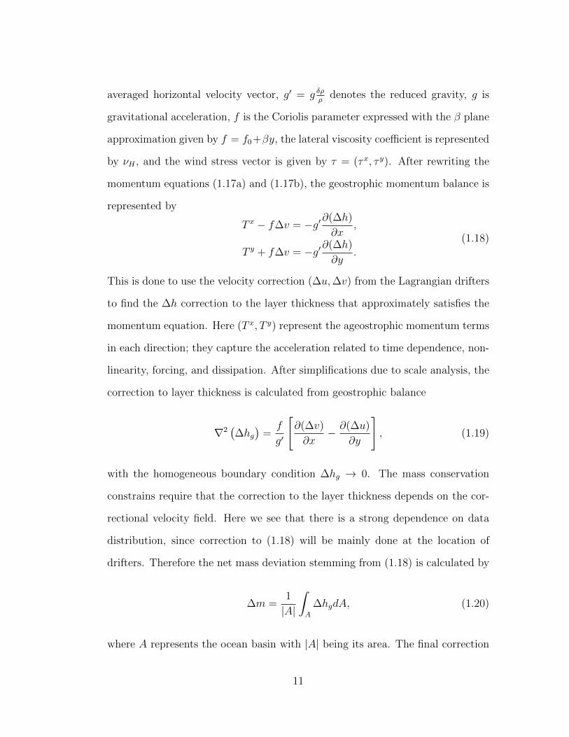
averaged horizontal velocity vector, g′ = g δρρ
denotes the reduced gravity, g is
gravitational acceleration, f is the Coriolis parameter expressed with the β plane
approximation given by f = f0+βy, the lateral viscosity coefficient is represented
by νH , and the wind stress vector is given by τ = (τx, τ y). After rewriting the
momentum equations (1.17a) and (1.17b), the geostrophic momentum balance is
represented by
T x − f∆v = −g′∂(∆h)
∂x,
T y + f∆v = −g′∂(∆h)
∂y.
(1.18)
This is done to use the velocity correction (∆u,∆v) from the Lagrangian drifters
to find the ∆h correction to the layer thickness that approximately satisfies the
momentum equation. Here (T x, T y) represent the ageostrophic momentum terms
in each direction; they capture the acceleration related to time dependence, non-
linearity, forcing, and dissipation. After simplifications due to scale analysis, the
correction to layer thickness is calculated from geostrophic balance
∇2(∆hg
)=f
g′
[∂(∆v)
∂x− ∂(∆u)
∂y
], (1.19)
with the homogeneous boundary condition ∆hg → 0. The mass conservation
constrains require that the correction to the layer thickness depends on the cor-
rectional velocity field. Here we see that there is a strong dependence on data
distribution, since correction to (1.18) will be mainly done at the location of
drifters. Therefore the net mass deviation stemming from (1.18) is calculated by
∆m =1
|A|
∫A
∆hgdA, (1.20)
where A represents the ocean basin with |A| being its area. The final correction
11

is given by ∆h = ∆hg −∆m. This leads to the equation for the assimilation of
the layer thickness as
ha(n) = hb(n) + ∆h. (1.21)
Here, the superscript a denotes assimilated data, and the superscript b denotes
the background (predicted) field.
Data assimilation part follows an array of M Lagrangian trajectories at times
n∆t = 1, 2, . . . N . Observations are indicated by r0m(n), while model values are
indicated by rbm(n) with m = 1, . . .M . We can express the Lagrangian velocity
calculated from observations and the model by the following finite differences:
v0m(n) =
∆r0m
∆t=
r0m(n)− r0
m(n− 1)
∆t,
vbm(n) =∆rbm∆t
=rbm(n)− rbm(n− 1)
∆t.
(1.22)
At the same time, the Eulerian velocity obtained from the grid is
uij = u(n∆t, i∆r, j∆r), (1.23)
where ∆r is the grid scale and n is the time index. The assimilation equations
for the velocity are given by:
uaij(n) = ubij(n) + β
M∑m=1
γijm
(v0m(n)− vbm(n)
), (1.24)
The velocity components u withs subscripts (ij) represent the Eulerian velocities
12

at the corresponding grid point, and the assimilation coefficients β and γ are
γijm = exp
−(xbm(n)− i∆r
)2
+(ybm(n)− j∆r
)2
2∆r2
,
β =σ2b
σ2b + σ2
o
, and σ2o =
σ2r
∆t2,
(1.25)
where σ2b is the modeling velocity mean square error and σ2
o denotes the error of
the Lagrangian velocity related to the error σ2r (the error of independent position
σ2o ∼ σ2
r/∆t2). It is assumed that model and observed variables have errors that
are uncorrelated in space and time, and that the velocity spatial gradients are
small in relation to (∆t)−1. And so, the optimal interpolation based Lagrangian
data assimilation is focused on calculating the velocity correction ∆u = (∆u,∆v)
field used in (1.24) given by
∆uij = βM∑m=1
γijm
(v0m(n)− vbm(n)
)(1.26)
and then by applying it as in input to the layer thickness field equation (1.18) to
(1.25); this is done following the multivariate dynamic balancing approach.
Ozgokmen et al., (2003) [15] have found that Pseudo-Lagrangian and La-
grangian assimilation gives similar results only for ∆t TL. For bigger ∆t val-
ues that are between (TL/5 ≤ ∆t ≤ TL/2), Lagrangian approach is better than
Pseudo-Lagrangian. When ∆t ≥ TL, neither of these methods can retrieve useful
Eulerian information, since Lagrangian predictability limits are surpassed. In
order to resolve this issue, Lagrangian assimilation has to be set in the primitive
equations. Twin experiments have shown that the simple dynamical balancing
technique developed in this paper, that corrects the model velocity field, and then
13

in term, corrects the layer thickness gives a positive result.
1.2.4 A method for assimilation of Lagrangian data
Kuznetsov et al. (2003) [7] examined the use of extended Kalman filter methodol-
ogy (EKF) to assimilate Lagrangian tracer data. Majority of models in oceanog-
raphy and meteorology use a fixed grid in space. To mesh Lagrangian data with
the Eulerian variables computed in a set grid, they have proposed to augment
the state space by inclusion of the tracer coordinates as an extra data, and then
to apply the EKF to this dynamics. This augmented state vector x = (xF ,xD)
consists of the Eulerian part xF (the state of the flow), and the Lagrangian part
xD (coordinates of the drifters). This approach, in which drifter information is a
part of the dynamical model, allows for tracking drifters along with their corre-
lation with the flow. Positions of ND particles are observed at the regular times
and assimilated into the model. And so, the state vector x(t) has a dimension
N . Its dimension is a product of the number of these variables and the number
of the discretization elements that include Fourier modes, gird points, etc. The
evolution of the state vector can by generalized as follows:
dxf
dt= M(xf , t), (1.27)
where xf corresponds to the forecasted state, whereas the true state is denoted as
xt, and M represents the dynamic operator. Since (1.27) is usually not a closed
system, to represent the subgrid-scale processes we can represent the dynamics
in a discrete form as a stochastic system
dxt = M(xt, t)dt+ ηt(t)dt. (1.28)
14

All of the unresolved processes are described by η as a zero-mean Gaussian white
noise. In a process of the sequential assimilation, the model is updated each time
the observation (xtj ≡ xt(tj)) is given at a given time tj. Observations yoj with
their uncorrelated zero-mean Gaussian errors εtj (with a covariance E[εtj(ε)tjT
]),
and their vector Hj of observation functions can be expressed in terms of
yoj = Hj[xtj] + εtj, (1.29)
The number of observations yoj , say Lj, can be different for each update time.
Data assimilation with the Kalman filter focuses on tracking the evolution of the
error covariance matrix defined as
Pf ≡ E[(xf − xt)(xf − xt)T ]. (1.30)
This is done with the tangent linear model (TLM) with the linearized dynamic
operator calculated at xf (t) by the following formula
M ≡ ∂M(xt, t)
∂x, (1.31)
and expressing the evolution of the error covariance matrix by
dPf
∂t= MPf + (MPf )T + Q(t), (1.32)
where Q(t) symbolizes our estimation for system noise covariance Qt(t). Data
assimilation proceeds by minimization of the mean-square error
trPaj = E[(xaj − xtj)
T (xaj − xtj)] (1.33)
15

at each update time tj, where xa represents the analysis state. We are using
the model error covariance matrix forecasted with the equation (1.32) to get the
first-order approximation of the optimal analysis state. The update combines the
predicted model state and the innovation vector with the size Lj
xaj = xfj + Kjdj,
dj ≡ yoj −Hj[xfj ],
Kj = PfjH
Tj
(HjP
fjH
Tj + Rj
)−1
,
Hj =∂Hj
∂x
(1.34)
where Hj is the linearized observation matrix, and our estimation of the covari-
ance matrix of the observation error is given by Rj. The Kalman gain matrix is
Kj, and the updated error covariance matrix is given by
Paj = (I−KjHj)P
fj . (1.35)
In their paper, Lagrangian tracers information (xD) is combined with the
model flow (xF ) into one model state vector x = (xF ,xD)T . The advection of
tracers is followed as
dxfFdt
= M(xfF , t), (1.36)
dxfDdt
= M(xfD,xfF , t). (1.37)
Equation (1.36) states the model in it original form stated in (1.27), and (1.37)
16
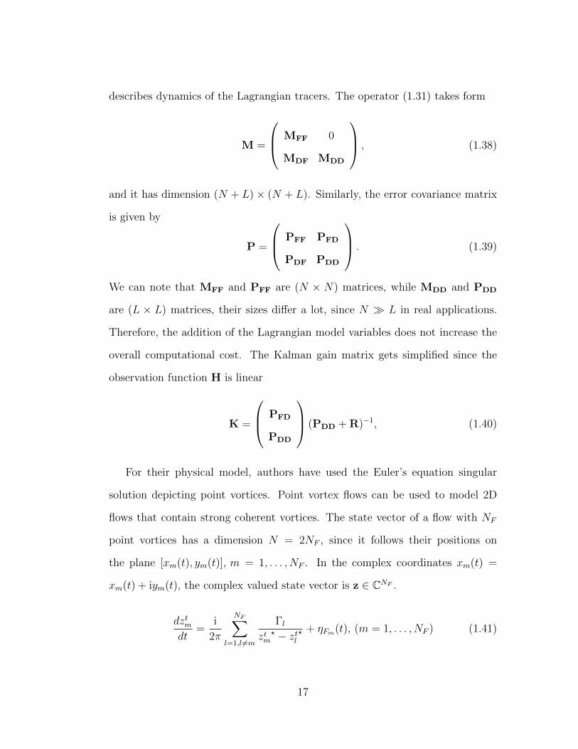
describes dynamics of the Lagrangian tracers. The operator (1.31) takes form
M =
MFF 0
MDF MDD
, (1.38)
and it has dimension (N + L)× (N + L). Similarly, the error covariance matrix
is given by
P =
PFF PFD
PDF PDD
. (1.39)
We can note that MFF and PFF are (N × N) matrices, while MDD and PDD
are (L × L) matrices, their sizes differ a lot, since N L in real applications.
Therefore, the addition of the Lagrangian model variables does not increase the
overall computational cost. The Kalman gain matrix gets simplified since the
observation function H is linear
K =
PFD
PDD
(PDD + R)−1, (1.40)
For their physical model, authors have used the Euler’s equation singular
solution depicting point vortices. Point vortex flows can be used to model 2D
flows that contain strong coherent vortices. The state vector of a flow with NF
point vortices has a dimension N = 2NF , since it follows their positions on
the plane [xm(t), ym(t)], m = 1, . . . , NF . In the complex coordinates xm(t) =
xm(t) + iym(t), the complex valued state vector is z ∈ CNF .
dztmdt
=i
2π
NF∑l=1,l 6=m
Γlztm
? − ztl? + ηFm(t), (m = 1, . . . , NF ) (1.41)
17

Here, Γl is circulation of vortex l, and the last term ηF = η(x)F + iη
(y)F captures
the unresolved processes.
E[η(x,y)F (t)η
(x,y)F (t′)] = σ2δ(t− t′)I,
E[η(x)F η
(y)F ] = 0.
(1.42)
Observations are provided by coordinates of the ND Lagrangian tracers. Here,
their coordinates are represented on the complex plane ζ ∈ CNF with their noise
as ηD = η(x)D + iη
(y)D with zero mean. The advection of ND tracers is described
by the following equation
dζtmdt
=i
2π
NF∑l=1
Γlζtm
? − ztl? + ηDm(t), (m = 1, . . . , ND) (1.43)
Analogously to the flow variables, the covariance of tracers position has
E[η(x,y)D (t)η
(x,y)D (t′)] = σ2δ(t− t′)I,
E[η(x)D η
(y)D ] = 0.
(1.44)
The state vector contains all the model equations with all corresponding dynam-
ical variables:
x =
z
ζ
,x ∈ CNF +ND (1.45)
The flow variables xF are corrected by the first N rows of K, which is propor-
tional to the correlation between the flow state and the drifter positions expressed
in PFD.
Numerical experiments focused on comparison of the model without data as-
similation process, and one with extra observations coming from different number
of tracers, and different sampling frequency. Influence of the launch position was
18

also investigated, in particular, relation of the initial position and separatrices of
the streamfunction in the corotating frame.The results point to dependency of
the assimilation on the scales of the motion and noise levels. Success in assimila-
tion is inversely proportional to how chaotic the system is, with biggest tracking
errors related to chaotic vortex initial condition.
1.2.5 Using flow geometry for drifter deployment in La-
grangian data assimilation
Salman et al., (2008) [18] recently explored the effectiveness of drifter deployment
strategies using a nonlinear reduced gravity shallow water model with external
wind forcing and combined it with the Ensemble nonlinear Kalman filter tech-
nology.
∂u
∂t= −u · ∇u+ fv − g′h
x+ F u +
1
h
(∂τxx∂x
+∂τxy∂y
), (1.46a)
∂v
∂t= −u · ∇v − fu− g′h
y+
1
h
(∂τyx∂x
+∂τyy∂y
), (1.46b)
∂h
∂t= −∂hu
∂x− ∂hv
∂y. (1.46c)
Here, h is the surface height, (u, v) is the fluid velocity vector, g′ is the reduced
gravity, F u is a horizontal wind-forcing acting in a zonal direction
F u =−τ0
ρH0(t)cos
(2πy
Ly
), (1.47)
and f is the Coriolis parameter expressed with the β plane approximation given
by f = f0 +βy, with β and f0 being constants, τ0 is the wind stress. To calculate
19

the average water depth H0 following equation
H0(t) =1
LxLy
∫ Lx
0
∫ Ly
0
h(x, y, t)dx dy (1.48)
is used. Lx and Ly are the dimensions of the zonal and the meridional directions.
The dissipation terms are given by the following equation
τij = µh
(∂ui∂xj
+∂uj∂xi− δij
∂uk∂xk
), (1.49)
where indices i and j take all possible permutations, while µ represents a constant
eddy viscosity of the flow. One of the ideas described in this paper is search for
Lagrangian coherent structures (LCS) in the numerically generated flow, since it
has become understood that they are responsible for the evolution of the motion of
material particles. This search is quite complicated because there is the non-linear
relation between the flow field and the Lagrangian drifter position. Successful
estimation of LCS aids placement of launch position for the Lagrangian drifters
and this improves data assimilation procedure. The assimilation of Lagrangian
data of ND drifters is conducted with the augmented state vector x = (xTF ,x
TD)T ,
where we have (NF×1) equations describing the flow vector XF, and the (2ND×1)
drifter state vector XD. For the ensemble forecast with NE members, following
equation is useddxfjdt
= mj(xj, t), j = 1, . . . , NE. (1.50)
Ensemble members are denoted by subscript j, forecast is denoted by superscript
f , and mj represents the evolution operator. The augmented system of equations
20

for ensemble members is used to define the covariance matrix as
Pf =1
NE − 1
NE∑j=1
(xfj − xf
)(xfj − xf
)T(1.51)
The mean of the state vector calculated for the ensemble x is calculated by
xf =1
NE
NE∑j=1
xfj . (1.52)
The analysis state of the system is defined as
xaj = xfj + Kdj, (1.53)
with Kalman gain matrix given by
K =
ρFD PFD
ρDD PDD
(ρDD PDD + R)−1 , (1.54)
while the innovation vector dj is represented by
dj = y0 −KxfD,j +˜εfj . (1.55)
The observations vector y0 holds spatial coordinates of the drifters in the zonal
and meridional coordinates. The matrix ρ holds distance-dependent correlation
function. The noise in the drifter positions is given by˜εfj and is based on the
gaussian distribution with a covariance matrix equal to R and
1
NE
NE∑j=1
˜εfj = 0. (1.56)
21

In equation (1.54) operator indicates the Schur product between two matrices.
Four different drifter locations were analyzed: a uniform drifter deployment
within the ocean basin, a saddle point launch strategy, a vortex launch strategy,
and a mixed combination of saddle and vortex centre launches. Nine drifters
were used for all these experiments. The mixed launch produced the highest con-
vergence for the velocity field whereas the uniform and saddle launches achieved
the minimal error in the height estimation. They have found that bifurcations
of coherent flow structures can lead to rapid dispersion of drifters placed within
such coherent vortices; forecasts made over longer time-scales can differ a great
deal from forecast over the shorter time.
1.2.6 A Bayesian approach to Lagrangian data assimila-
tion
Apte et al., (2008) [1] described a Bayesian perspective based approach to data
assimilation. Their motivation was to follow the issues related to the highly non-
linear characteristics of the Lagrangian data as it influences data assimilation.
This becomes a major problem when the time between the observations is large.
For their study, they have used an idealized ocean model given by the inviscid
linearized shallow water model given by equation (5) in [1]:
∂u
∂t= v − ∂h
∂x,
∂v
∂t= −u− ∂h
∂y,
∂h
∂t= −∂u
∂x− ∂v
∂y.
(1.57)
22

They took into the account first two modes of the Fourier modes for their nu-
merical modeling, with the first component describing the geostrophic mode and
the second one describing the inertia-gravity mode given by equation (6) in [1].
u(x, y, t) = −2πl sin(2πkx) cos(2πly)u0 + cos(2πmy)u1(t),
v(x, y, t) = +2πk cos(2πkx) sin(2πly)u0 + cos(2πmy)v1(t),
h(x, y, t) = sin(2πkx) sin(2πly)u0 + sin(2πmy)h1(t).
(1.58)
After combining (1.57) and (1.58) they have presented the following equations
for amplitudes (equation (7) in [1]):
u0 = 0,
u1 = v1,
v1 = −u1 − 2πmh1,
h1 = 2πmv1,
(1.59)
along with initial conditions [u0(0), u1(0), v1(0), h1(0)]; du0/dt ≡ u0 is following
standard notation, as is u1, v1 and h1.
Apte et al., (2008) described the use of Bayes theorem as applied to a data
assimilation problem with a deterministic dynamic model. The initial conditions
of the deterministic model with an n-dimensional state vector given by
dx
dt= f(x), x(0) = x0 ∼ ξ, (1.60)
are taken from a prior with probability density function pξ(x0). Noisy observa-
tions yk ∈ Rm represent the state of the system at a specific time tk. If we use
23

the solution operator for the dynamics Φ, state of the system can be expressed
as x(t) = Φ(x0, t). Therefore, observations yk can be written as
yk = h[x(tk)] + ηk = h[Φ(x0, tk)] + ηk, (1.61)
where operator h : Rn → Rm. This indicates that the observations can be treated
as the non-linear numerical functions of the initial conditons. For the set of noisy
observations at various times t1, . . . , tk, we can express the total observations
vector yT = (yT1 , . . . ,yTk ) as
y = H(x0) + η. (1.62)
We are using H(x0)T =(h[x(t1)]T , . . . ,h[(x(tm)]T
)and ηT = (ηT1 , . . . ,η
Tm). The
random vector η has a probability density function pη : RmK → R. Therefore,
the conditional probability of observations y related to the initial data x0 can be
described as:
p(y|x0) = pη[y −H(x0)]. (1.63)
If we have a prior distribution of initial conditions pζ along with a realization of
the observations y, using Bayes’ theorem, we can write a posterior probability
for the state vector
p(x0|y) =pη[y −H(x0)]pζ(x0)
p(y), (1.64)
where
p(y) =
∫pη[y −H(x0)]pζ(x0)dx0. (1.65)
It can be noticed that p(y) is only a function of observations and that p(y) has
a constant value for a particular realization of y which is independent of x0.
24

Apte et al., (2008) have noted several key features of the this approach to data
assimilation:
• The conditional distribution at time t = 0 of the state of the model in (1.64)
observed during time 0 to tk is the posterior of (1.64).
• To sample the posterior p(x0|y), there is a need for pη. This functional can
contain non-Gaussian errors than can be correlated.
• The problem was investigated under the twin experiments setup. Observa-
tions and posterior’s sampling are generated with the same model dynamics.
• True state of the model x(t)is never mentioned, since it is never known.
Equation (1.62) is different then from y = H(x(t)) + η, by the fact, that
H in not a function of the ’true’ state. Because of the random nature of
errors in the data, all that can be estimated is the probabilistic state of the
system, and we don’t know the best a priori estimate of the system.
• When we present the posterior distribution for the deterministic model, we
have a ’strong constrained formulation’ in mind. Oftentimes, a ’weak con-
strained formulation’ may be needed in the oceanographical applications.
Numerical experiments described by Apte et al., (2008) focus on a short trajec-
tories that stay in one cell, and on a trajectories that get close to the saddle
point and leave the cell. They have found that these instances have different
prior distributions. Examination of results showed that ensemble generated by
the model gives information about the variability of estimations due to different
initial conditions. The posterior distribution is impacted by the model dynamics
together with the assimilated observations. When compared to the Ensemble
nonlinear Kalman filter, Bayesian data assimilation works better in presence of
25

bigger interval between observations. It also performs well in presence of the cen-
ter point. Three different methods were used to sample the posterior: Langevin
stochastic differential equation (LSDE), Metropolis adjusted Langevin algorithm
(MALA) and Random walk Metropolis-Hastings (FWMH). For the Lagrangian
data assimilation, the Metropolis-Hastings methodology gives the best results.
1.3 Summary
Lagrangian data assimilation has a long history in meteorology and oceanography.
The above collected papers give a broad overview of different approaches taken
over the years by different authors. There are some underlying common threads in
all of them. First, data assimilation of the Lagrangian data is a very important
part of any modern model that uses data from sensors following the flow to
improve the Eulerian forecast. All of the described assimilation schemes are
sensitive to time period between measurements. Second, improvement in models
that deal with the shallow water models of a different level of complexity and
point vortex systems depends on the initial location of tracers which data is
used to improve forecast. This launch location has high significance when it
comes to being useful for data assimilation. Third, the number of the Lagrangian
tracers used for data assimilation has some importance, however, in some cases,
adding more sensors above a certain level does not increase the overall quality of
improvements to the data assimilation procedures.
26

1.4 Organization of the Dissertation
In chapter 2, we give an overview of the shallow water model, and scaling assump-
tion that we make in order to linearize it. In chapter 3, we present a low-order
model used to derive the explicit expressions for the tracer dynamics which is
a system of two first-order, coupled nonlinear, time varying ordinary differential
equations. A complete catalog of all of the equilibria and their character is also
presented. It is followed by examination of the bifurcation of the tracer dynamics
by succinctly summarizing the dependence on the four dimensional parameter set
using a simple two dimensional characterization. In chapter 4, we present a data
assimilation approach known as the Forward Sensitivity Method. It is followed
in chapter 5 by examination of the sensitivity of the shallow water model to
the initial conditions and model parameters, known as the control vector. Thor-
ough evaluation of the Data Assimilation experiments is included in chapter 6.
Concluding remarks are contained in chapter 7.
27

Chapter 2
Shallow Water Model
2.1 Introduction
In this chapter, we give a short description of atmospheric and oceanic motion
at a scale that is important to work done in this dissertation. We elaborate on
scaling assumptions taken in our work, as they are applied to linearized shallow
water model.
2.2 Large scale motion
For our study, we are using a model that can be used to describe a motion in the
earth’s ocean and atmosphere alike. The disparity between horizontal and vertical
scales is well known for a large-scale geophysical motions related to the fluid with
stable density. We think of the large-scale motion when it is influenced by the
earth’s rotation. There is a measure one can use to determine the significance
of rotation that is known as the Rossby number. To use it, we need to define
L to be a characteristic length scale, and U to be a horizontal velocity scale
28

characteristic of the motion. The angular velocity of the earth’ rotation Ω has
value of |ΩΩΩ| = 7.292× 10⁻⁵ rad/s. The non-dimensional parameter Ro is usually
used to denote Rossby number, and for a large-scale motion at the latitude Φ, it
can be expressed as
Ro =U
(2Ω sin Φ)L≤ 1.
It is worth indicating that only the component of earth’s rotation perpendicular
to the planetary surface is used in the estimation of the Rossby number. In the
atmosphere, vertical scale is of the order of ten kilometers while horizontal scale
is of the order of thousand kilometers. Similarly, the depth of the ocean almost
never is bigger than six kilometers, and the horizontal extent of major currents
systems is usually huge, that is much longer than six kilometers. Therefore, the
motion occurs within an relatively thin sheet of fluid, and given the large extent
of the horizontal scale of the motion the geometrical constraint produces fluid
trajectories which are very flat. Obviously, the motions described in such way
apply to cases in which stratification does not play a major role.
In meteorology and oceanography, there is a simple model called shallow water
model that describes a motion of this type. We can write a set of equations
following Daley (page 194, (1991)) [3] that states the shallow water model in
cartesian coordinates, where x is the eastward direction, and y is the northward
direction.
∂U
∂t+ U
∂U
∂x+ V
∂U
∂y− fV + g
∂H
∂x= 0, (2.1a)
∂V
∂t+ U
∂V
∂x+ V
∂V
∂y+ fU + g
∂H
∂y= 0, (2.1b)
∂H
∂t+ U
∂H
∂x+ V
∂H
∂y+H
(∂U
∂x+∂V
∂y
)= 0. (2.1c)
29
Here, U is the eastward wind component, V is the northward wind component, H
indicates the height of the free surface of the fluid, g is the gravitational constant
while f is the Coriolis parameter. Equations (2.1a) and (2.1b) constitute mo-
mentum equations for the eastward and northward components, while equations
(2.1c) represents the continuity equation. Our goal is to linearize the shallow
water model. Hence, we focus on analysis of the small-amplitude motions. To
this end, we introduce the following U = u + u, V = v + v and H = h + h into
the equations (2.1a)-(2.1c), where u, v and h indicate a base state, and u, v, and
h indicate perturbations. We also assume a constant Coriolis parameter f equal
f0; this is known as the mid-latitude f -plane assumption.
∂(u+ u)
∂t+ (u+ u)
∂(u+ u)
∂x+ (v + v)
∂(u+ u)
∂y
− f(v + v) + g∂(h+ h)
∂x= 0, (2.2a)
∂(v + v)
∂t+ (u+ u)
∂(v + v)
∂x+ (v + v)
∂(v + v)
∂y
+ f(u+ u) + g∂(h+ h)
∂y= 0, (2.2b)
∂(h+ h)
∂t+ (u+ u)
∂(h+ h)
∂x+ (v + v)
∂(h+ h)
∂y
+ (h+ h)
(∂(u+ u)
∂x+∂(v + v)
∂y
)= 0. (2.2c)
Now, we can think of a basic state in which fluid is at rest (u = v = 0) and has
a free surface with height h that is independent of the position and time:
∂u
∂t=∂v
∂t=∂h
∂t= 0,
∂h
∂x=∂h
∂y= 0.
30

∂u
∂t+ u
∂u
∂x+ v
∂u
∂y− fv + g
∂h
∂x= 0, (2.3a)
∂v
∂t+ u
∂v
∂x+ v
∂v
∂y+ fu+ g
∂h
∂y= 0, (2.3b)
∂h
∂t+ u
∂h
∂x+ v
∂h
∂y+ h
(∂u
∂x+∂v
∂y
)= 0. (2.3c)
Below we include a shallow water model as stated in Pedlosky([16] page 68.)
representing a deterministic dynamical framework appropriate for the motion
calculations of large space and time scales; motions of atmospheric and oceanic
relevance; this is the set of equations (2.3a)-(2.3a) in which we have dropped
the nonlinear terms u∂u∂x
, v ∂u∂y
, u ∂v∂x
, v ∂v∂y
, u∂h∂x
, v ∂h∂y
, because ∂u∂t u∂u
∂x, v ∂u
∂yand
similarly ∂v∂t u ∂v
∂x, v ∂v
∂y. We also can observe that h h.
∂u
∂t− fv = −g∂h
∂x, (2.4a)
∂v
∂t+ fu = −g∂h
∂y, (2.4b)
∂h
∂t+ h
(∂u
∂x+∂v
∂y
)= 0. (2.4c)
The velocity has horizontal components u and v, f denotes the Coriolis param-
eter, h indicates the height of the surface of the fluid above the reference level
h.
31

2.3 Scalling assumptions
Using non-dimensional variables h, u, v, t, x, y we can define
u = u0u, where u0 ∼ O(1 cm s−1) ∼ O(1× 10⁻² m s−1) ∼ O(0.036 km h−1),
v = u0v,
h = h0h, where h0 ∼ O(1× 10⁻¹ m),
t = t/f, where f ∼ O(1× 10⁻⁴ s−1),
x = Lx, where L ∼ O(1× 10⁶ m),
y = Ly.
(2.5)
We can now consider (2.4a)
∂u
∂t=∂u0u
∂t/f= (u0f)
∂u
∂t,
∂h
∂x=∂h0h
∂Lx=
(h0
L
)∂h
∂x,
(2.6)
and so, (2.4a) becomes
fu0∂u
∂t− fu0v = −gh0
L
∂h
∂x, (2.7)
and finally
∂u
∂t− v = − gh0
fLu0
∂h
∂x= N
∂h
∂x, where N =
gh0
fLu0
. (2.8)
Since g ∼ O(10 m s−2) and f is fixed at g ∼ 10−4,
N =1× 101 m s−2 × 1× 10−1 m
1× 10⁻⁴ s−1 × 1× 106 m× 1× 10−2 m s−1 = 1. (2.9)
32

And this gives us scaled equation (2.4a) as
∂u
∂t− v = −∂h
∂x. (2.10)
Similarly, now we can now consider (2.4b) and express its compnents as
∂v
∂t=∂u0v
∂t/f= (u0f)
∂v
∂t,
∂h
∂y=∂h0h
∂Ly=
(h0
L
)∂h
∂y,
(2.11)
and so, (2.4b) becomes
fu0∂v
∂t+ fu0u = −gh0
L
∂h
∂y, (2.12)
and finally, using N defined in (2.8)
∂v
∂t+ u = − gh0
fLu0
∂h
∂y,
∂v
∂t+ u = N
∂h
∂y.
(2.13)
And this gives us equation (2.4b) scaled as
∂v
∂t+ u = −∂h
∂y. (2.14)
Finally, we can consider parts of equation (2.4c)
∂h
∂t=∂h0h
∂t/f= (h0f)
∂h
∂t,
h
(∂u
∂x+∂v
∂y
)= h
(∂u0u
∂Lx+∂u0v
∂Ly
)=hu0
L
(∂u
∂x+∂v
∂y
),
(2.15)
33

We can combine the above to get
(fLh0
hu0
)∂h
∂t+
(∂u
∂x+∂v
∂y
)= M
∂h
∂t+
(∂u
∂x+∂v
∂y
)= 0,
where M =fLh0
hu0
.
(2.16)
Let us analyze M from the above equation using h ∼ O(1× 10³ m).
M =1× 10⁻⁴ s−1 × 1× 106 m× 1× 10−1 m
1× 103 m× 1× 10−2 m s−1 = 1. (2.17)
Finally this gives us (2.4c)
∂h
∂t+
(∂u
∂x+∂v
∂y
)= 0. (2.18)
And so, we can combine these three equations (2.10, 2.14 and 2.18) in their non-
dimensional form. After dropping the ˆ sign, we have the from as presented in
Apte et al., (2008) [1].∂u
∂t= v − ∂h
∂x,
∂v
∂t= −u− ∂h
∂y,
∂h
∂t= −∂u
∂x− ∂v
∂y.
(2.19)
2.4 Summary
We have introduced shallow water equation in their non-linear form. We have
demonstrated the assumptions that lead to linearized model. Thereafter, by
applying appropriate scale factors, we have derived a non dimensional form pre-
sented in equation (2.19); this will constitutes the basis for our analysis in the
subsequent chapters.
34
Chapter 3
Linearized Shallow Water Model
and Tracer Dynamics
3.1 Introduction
In this chapter, we introduce a solution to the low order linearized shallow water
model. We find a closed form solution for the time dependent amplitudes and
incorporate them into an analytical solution describing tracer dynamics. This is
followed by the analysis of the equilibria of tracer dynamics. For this purpose,
linearized shallow water model solutions are divided into geostrophic, inertial-
gravity and combine modes. Bifurcation analysis is given for each of these modes.
3.2 Model variables
The linear coupled system of three partial differential equations presented in
(2.19) establishes the basis of our work in this dissertation. Here (x, y)T ∈ R2
denote the two dimensional space coordinates and t ≥ 0 denote the time variable.
35

Let u(x, y, t)(v(x, y, t)) denote the east-west (north-south) components of the
velocity field at the spacial location (x, y)T and time t. Let h(x, y, t) denote the
height of the free surface of water measured above a pre-specified mean level.
Equation (2.19) shows the variation of the two components of the velocity field,
u(x, y, t) and v(x, y, t) with respect to the variation of the free surface height
measured from the mean level h(x, y, t).
3.3 Low-order model (LOM)
Lorenz (1960) [13] has shown that one can approximate the solution of a complex
model with the low-order model. This approach has been used with a great
success; a short list of a well know applications in the geophysical domain has
been listed by Laksmivarahan et al., (2006) [8]. Our analysis depends on the
low-order counter part of the infinite dimensional model in (2.19) obtained by
the application of the standard Galerkin type projection method. To this end,
we first express u, v and h in the standard two dimensional truncated Fourier
series consisting of only two terms given by (Apte et al. 2008) [1] in the equation
(6):
u(x, y, t) = −2πl sin(2πkx) cos(2πly)u0 + cos(2πmy)u1(t),
v(x, y, t) = +2πk cos(2πkx) sin(2πly)u0 + cos(2πmy)v1(t),
h(x, y, t) = sin(2πkx) sin(2πly)u0 + sin(2πmy)h1(t).
(3.1)
In each equation above, the first time independent term with constant amplitude
that is proportional to u0 is called the geostrophic mode and the second time de-
pendent terms with amplitudes u1(t), v1(t), h1(t) are called inertial-gravity modes.
In the following, we refer to u0 as the geostrophic parameter and u1(0), v1(0), h1(0)
as the inertial parameters. Without loss of generality we only consider the case
36
where n = m = l = 1 in ((3.1)). Following (Apte et al. 2008) [1] the equations
(7)), we combine equations (2.19) and (3.1) to find dynamic equations for the
amplitudes
u0 = 0,
u1 = v1,
v1 = −u1 − 2πmh1,
h1 = 2πmv1,
(3.2)
along with initial conditions [u0(0), u1(0), v1(0), h1(0)]; du0/dt ≡ u0 is following
standard notation, as is u1, v1 and h1. The process of reduction is shown in the
Appendix A.
3.3.1 Analytical solution for amplitudes
In order to find an analytical solution for amplitudes we rewrite equations (3.2)
in a matrix-vector form with a = 2πm.u1
v1
h1
=
0 1 0
−1 0 a
0 a 0
×u1
v1
h1
. (3.3)
This can be expressed succinctly as ξ = A ξ, with ξ(0) as initial conditions (I.C),
where
ξ =
u1
v1
h1
, and A =
0 1 0
−1 0 a
0 a 0
. (3.4)
Clearly A is a skew-symmetric matrix.
37

Property 3.3.1. Let E(t) = 1/2 ξT (t) ξ(t) denote the energy associated with
the state ξ(t). Then (3.3) conserves energy E(t), that is, E(t) = 0.
Proof. For,dE(t)
dt= ξT (t) A ξ(t)
= u1u1 + v1v1 + h1h1
= u1[v1] + v1[−u1 − ah1] + h1[av1]
= 0.
(3.5)
since A is a skew-symmetric matrix. Stated in other words, the solution ξ(t)
of the linear system (3.3) always lies on the surface of a sphere centered at the
origin with the radius given by
E(0)1/2 =[ξT (0) ξ(0)
]1/2
=[u2
1(0) + v21(0) + h2
1(0)]1/2
=[u2
1(t) + v21(t) + h2
1(t)]1/2
= E(t)1/2.
(3.6)
3.3.2 Eigenvalues and eigenvectors of A
Derivation of eigenvalues and eigenvectors of A
Let us look again at matrix A defined as
A =
0 1 0
−1 0 a
0 a 0
. (3.7)
38

We can proceed to set the characteristic polynomial
det(A− λI) = |A− λ I| =
∣∣∣∣∣∣∣∣∣∣∣−λ 1 0
−1 −λ a
0 a −λ
∣∣∣∣∣∣∣∣∣∣∣= 0. (3.8)
Expanding it, we get
−λ
∣∣∣∣∣∣∣−λ −a
a −λ
∣∣∣∣∣∣∣−∣∣∣∣∣∣∣−1 −a
0 −λ
∣∣∣∣∣∣∣ = −λ(λ2 − λ+ a2) = 0, (3.9)
where solutions are λ1 = 0 + i
√1 + a2
λ2 = 0− i√
1 + a2
λ3 = 0
. (3.10)
That is, the eigenvalues of a skew-symmetric matrix are purely imaginary or zero
as shown in equation (3.10). It can be verified that the eigenvectors V1,V2,V3
corresponding to λ1, λ2, λ3 are:
V = [V1,V2,V3] =
0 −1/λ a/λ
1 0 0
0 −a/λ −1/λ
. (3.11)
Now, for the first non-zero eigenvalue we have
AV1 = λ1V1,
A(x + iy) = iλ(x + iy).
(3.12)
39

Equating the real and imaginary parts we get
Ax = −λy
Ay = λx(3.13)
or
y = − 1λAx,
Ax2 = λ2x.
Analogously, for the second non-zero eigenvalue we have
AV2 = λ2V2,
A(x− iy) = iλ(x− iy).
(3.14)
Again, equating the real and imaginary parts we get
Ax = λy
Ay = λx
or
x = − 1λAy,
Ay2 = −λ2y.
We will use A2 in our calculations, so let us find it now as
A2 =
0 1 0
−1 0 a
0 a 0
0 1 0
−1 0 a
0 a 0
=
−1 0 −a
0 −(1 + a2) 0
−a 0 −a2
. (3.15)
It can be verified that A2 = AA = ATAT = (AA)T , therefore A2 is symmetric
(one for which AT = A) if A is skew-symmetric (one for which AT = −A). Now,
40

we continue on finding eigenvectors:
Ax2 = −λ2x, (3.16)
−1 0 −a
0 −(1 + a2) 0
−a 0 −a2
x1
x2
x3
= −(1 + a2)
x1
x2
x3
. (3.17)
After expanding, we arrive at
−x1 − ax3 = −(1 + a2)x1
−(1 + a2)x2 = −(1 + a2)x2
−ax1 − a2x3 = −(1 + a2)x3
.
Now, we can solve it after simplifying
x3 = ax1
x2 = x2
x3 = ax1
.
Since we can set x2 to an arbitrary value, let us choose x2 = 1, and then we
can set x1 = x3 = 0. This would give us the normalized first eigenvector V1 =
(0, 1, 0)T . For the second eigenvector, we can set x2 = 0, and x1 = −1. This
would give us x3 = −a, and after normalization we get get the second eigenvector
as V2 = −1/√
(1 + a2)(1, 0, a)T , and then we would find the third normalized
eigenvector as V3 = −1/√
(1 + a2)(1, 0,−a)T . It can be verified that the matrix
41
of eigenvectors of A
V = [V1, V2, V3] =
0 −1/λ a/λ
1 0 0
0 −a/λ −1/λ
(3.18)
is an orthogonal matrix, and so, VT = V−1.
Eigendecomposition of A
The Jordan canonical form of matrix A is as follows
A = VΛV−1 = VΛVT , (3.19)
where
Λ =
0 λ 0
−λ 0 0
0 0 0
,or
VTAV = Λ. (3.20)
We know that ξ = A ξ with ξ(0) as initial conditions. Then, following (chapter
31, Lewis et al., (2006) [12])
ξ(t) = eAt ξ(0)
= e(VΛVT )t ξ(0)
= [VeΛtVT ] ξ(0). (3.21)
42

The exponential of a matrix
For a moment, we have to shift our attention to finding an exponent of a matrix.
Following Hirsch et al., (2004) [4], we know the exponential function can be
expressed in a form of the infinite series
ex =∞∑k=0
xk
k!. (3.22)
Similarly for A, we can define its exponential as
exp A =∞∑k=0
Ak
k!. (3.23)
In our case, matrix Λ is as follows
Λ =
0 λ 0
−λ 0 0
0 0 0
= λ
0 1 0
−1 0 0
0 0 0
.
43

So, we can express its powers in the following manner
Λ0 =
1 0 0
0 1 0
0 0 1
,
Λ1 = λ
0 1 0
−1 0 0
0 0 0
,
Λ2 = −λ2
0 1 0
−1 0 0
0 0 0
0 1 0
−1 0 0
0 0 0
= −λ2
1 0 0
0 1 0
0 0 0
,
Λ3 = −λ3
1 0 0
0 1 0
0 0 0
0 1 0
−1 0 0
0 0 0
= −λ3
0 1 0
−1 0 0
0 0 0
,
Λ4 = −λ4
0 1 0
−1 0 0
0 0 0
0 1 0
−1 0 0
0 0 0
= λ4
1 0 0
0 1 0
0 0 0
,
Λ5 = λ5
1 0 0
0 1 0
0 0 0
0 1 0
−1 0 0
0 0 0
= λ5
0 1 0
−1 0 0
0 0 0
, · · ·
44

Therefore, to express exp(Λ) we can look at the few first elements
r(1, 1) = 1 + λ ∗ 0− λ2 ∗ 1− λ3 ∗ 0 + λ4 ∗ 1 + λ5 ∗ 0 + · · ·
= 1− λ2 + λ4 + · · ·
r(1, 2) = 0 + λ ∗ 1− λ2 ∗ 0− λ3 ∗ 1 + λ4 ∗ 0 + λ5 ∗ 1 + · · ·
= λ− λ3 + λ5 + · · ·
r(2, 1) = −λ ∗ 1 + λ2 ∗ 0 + λ3 ∗ 1− λ4 ∗ 0− λ5 ∗ 1 + · · ·
= −λ+ λ3 − λ5 − · · ·
r(2, 2) = 1 + λ ∗ 0− λ2 ∗ 1− λ3 ∗ 0 + λ4 ∗ 1 + λ5 ∗ 0 + · · ·
= 1− λ2 + λ4 + · · ·
Now, we can recall that cos function can be expressed in a form on an infinite
sum
cosλ =∞∑k=0
(−1)kλ2k
(2k)!.
Analogously, sin function can be expressed as
sinλ =∞∑k=0
(−1)kλ2k+1
(2k + 1)!.
45

Therefore, combining these we can express exp(Λ) as
eΛ =
∑∞
k=0(−1)k λ2k
(2k)!
∑∞k=0(−1)k λ2k+1
(2k+1)!0∑∞
k=0(−1)k λ2k+1
(2k+1)!
∑∞k=0(−1)k λ2k
(2k)!0
0 0 1
=
cosλ sinλ 0
− sinλ cosλ 0
0 0 1
.(3.24)
But we also know that
eΛt =
cos(λt) sin(λt) 0
− sin(λt) cos(λt) 0
0 0 1
=
c s 0
−s c 0
0 0 1
, where c = cos(λt), s = sin(λt).
(3.25)
Amplitudes
Combining all of the above terms, we get ξ(t) = e(VΛVT )t ξ(0) expanded as fol-
lows:u1(t)
v1(t)
h1(t)
=
0 −1/λ a/λ
1 0 0
0 −a/λ −1/λ
c s 0
−s c 0
0 0 1
0 −1/λ a/λ
1 0 0
0 −a/λ −1/λ
u1(0)
v1(0)
h1(0)
(3.26)
46

=
s/λ −c/λ a/λ
c s 0
as/λ −ac/λ 1
0 −1/λ a/λ
1 0 0
0 −a/λ −1/λ
u1(0)
v1(0)
h1(0)
=
c+a2
λ2sλ
ac−aλ2
−sλ
c −asλ
ac−aλ2
asλ
1+ca2
λ2
u1(0)
v1(0)
h1(0)
.
After we expand the above equation, we have an explicit expressions for the time
varying amplitudes u1(t), v1(t), andh1(t) as a function of time
u1(t) =c+ a2
λ2u1(0)+
s
λv1(0)+
ac− aλ2
h1(0),
v1(t) =−sλu1(0)+ c v1(0)+
−asλ
h1(0),
h1(t) =ac− aλ2
u1(0)+as
λv1(0)+
1 + ca2
λ2h1(0).
(3.27)
We can notice that for t = 0, we have c = cos(λt) = 1 and s = sin(λt) = 0. We
recall that a = 2πm, and λ =√
1 + a2 =√
1 + (2πm)2.
u1(0) =1 + a2
λ2u1(0) =
1 + a2
1 + a2u1(0) = u1(0),
v1(0) = v1(0),
h1(0) =1 + a2
λ2h1(0) =
1 + a2
1 + a2h1(0) = h1(0).
(3.28)
47

We can expand equations (3.27) to get full expressions for amplitudes
u1(t) =
(cos(t√
4π2m2 + 1)
+ 4m2 π2
)4π2m2 + 1
u1(0)
+sin(t√
4π2m2 + 1)
√4π2m2 + 1
v1(0)
+
2πm
(cos(t√
4 π2m2 + 1)− 1
)4 π2m2 + 1
h1(0),
v1(t) = −sin(t√
4 π2m2 + 1)
√4 π2m2 + 1
u1(0)
+ cos(t√
4π2m2 + 1)v1(0)
−2πm sin
(t√
4π2m2 + 1)
√4 π2m2 + 1
h1(0),
h1(t) =
2 πm
(cos(t√
4 π2m2 + 1)− 1
)4 π2m2 + 1
u1(0)
+2πm sin
(t√
4 π2m2 + 1)
√4 π2m2 + 1
v1(0)(4m2 π2 cos
(t√
4π2m2 + 1)
+ 1
)4π2m2 + 1
h1(0).
(3.29)
3.4 Tracer dynamics
We proceed with the analysis of the tracer dynamics after rearranging equations
(3.27). We can present a number of interesting features of the shallow water
48

model using the version of these equations in (3.30).
u1(t) =a
λ2
[au1(0)− h1(0)
]+
1
λ2
[u1(0) + ah1(0)
]c+
v1(0)
λs,
v1(t) = v1(0) c− 1
λ
[ah1(0) + u1(0)
]s,
h1(t) =1
λ2
[h1(0)− au1(0)
]+
a
λ2
[u1(0) + ah1(0)
]c+
av1(0)
λs.
(3.30)
Since the solution of equation (3.3) ξ(t) lies on a sphere, it is immediate that
u1(t), v1(t), and h1(t) are not linearly independent.
Let X(t) =(x(t), y(t)
)T ∈ R2 denote the position of the tracer particle float-
ing on the free surface of the water. The dynamics of motion of this tracer is
then given by
x = u(x, y, t),
y = v(x, y, t),(3.31)
where the right hand side of (3.31) is obtained by substituting (3.27) in (3.1) with
u0, a constant. For later reference, define the geostrophic velocity components
f1(x, y) = −2πu0 sin (2πx) cos (2πy) ,
f2(x, y) = 2πu0 cos (2πx) sin (2πy) ,(3.32)
and the inertial-gravity velocity components
g1(x, y, t) = u1(t) cos (2πmy) ,
g2(x, y, t) = v1(t) cos (2πmy) .(3.33)
Let f = (f1, f2)T ∈ R2 and g = (g1, g2)T ∈ R2. Then, (3.31) can be rewritten in
49

the vector form as
X(t) = f(x, u0) + g(x, α, t), (3.34)
where u1(t), v1(t), h1(t) are given in (3.27). We can also recall that α =(u1(0), v1(0), h1(0)
)∈ R3. Clearly, the first component f of the vector field de-
pends on the geostrophic parameter u0 and the second component g depends on
the inertial parameters α ∈ R3. One of our goals in this thesis is to characterize
and catalog the behavior of the solution of (3.34) as the geostrophic and inertial
parameters are varied. It turns out this class of nonlinear time varying dynamics
exhibits many interesting bifurcations as the four parameters (u0, α) are varied
in R4.
3.5 Analysis of Equilibria of Tracer dynamics
It is convenient to divide the analysis into three cases.
3.5.1 Case 1: Equilibria in geostrophic mode
By setting the inertial parameter α = 0, we obtain the tracer dynamics given by
the nonlinear autonomous system
X = f(X, u0) (3.35)
controlled by the geostrophic parameter u0. From (3.32), the Jacobian of the flow
field f(X, u0) is given by
Dx(f) = −4π2u0
cos(2πx) cos(2πy) − sin(2πx) sin(2πy)
sin(2πx) sin(2πy) − cos(2πx) cos(2πy)
. (3.36)
50

We consider two types of equilibria for (3.35)
Type 1 Equilibria:
From (3.35) and (3.32), it follows that f(X, u0) = 0 when sin(2πx) = 0 =
sin(2πy), that is, when
x = y = ±k2
for k = 0, 1, 2, . . . (3.37)
which is independent of u0. The Jacobian (3.36) at these equilibria becomes
Dx(f) = −4π2u0
1 0
0 −1
, (3.38)
whose eigenvalues are given by λ1 = 4π2u0 and λ2 = −4π2u0, with e1 = (1, 0)T
and e2 = (0, 1)T as their corresponding eigenvectors. Clearly, this family of equi-
libria corresponds to a saddle for all non-zero values of the geostrophic parameter
u0. In a small neighborhood around the equilibria in (3.37), the system (3.35) is
equivalent to a linear dynamics given by
η = Dx(f)η, (3.39)
with Dx(f) in (3.38) and η(t) =(η1(t), η2(t)
)T.
The solution of (3.39) is given by
η1(t) = η1(0)e(4π2u0)t and η2(t) = η2(0)e−(4π2u0)t. (3.40)
51

−1/2 −1/4 0 1/4 1/2
−1/2
−1/4
0
1/4
1/2
X
Y
Figure 3.1: A display of equilibria of Type 1 - filled circles and Type 2 - un-filled circles along with the velocity field around them. Filled cir-cles are saddle points and unfilled circles are centers. The fieldplot around these equilibria corresponds to f(x, y) in (3.32) withu0 = 1.0, u1(0) = v1(0) = h1(0) = 0 and time t = 0.
Type 2 Equilibria:
From (3.35) and (3.32), it again follows that f(X, u0) = 0 when cos(2πx) = 0 =
cos(2πy), that is, when
x = y = ±2k + 1
4for k = 0, 1, 2, . . . (3.41)
52

which is also independent of u0. The Jacobian (3.36) at these equilibria becomes
Dx(f) = −4π2u0
0 −1
1 0
, (3.42)
whose eigenvalues are purely imaginary and are given by λ1 = i4π2u0 and λ2 =
−i4π2u0, with any pair of unit, orthogonal vectors e1 = 1√a2+b2
(a, b)T and e2 =
1√a2+b2
(b,−a)T as corresponding eigenvectors, where a and b are arbitrary real
constants. This family of equilibria correspond to a center for all non-zero values
of the geostrophic parameter u0. In a small neighborhood around this equilibria,
equation (3.35) is equivalent to a linear dynamics
η = Dx(f)η, (3.43)
with Dx(f) in (3.42). The solution of (3.43) is then given by
η1(t)
η2(t)
=
cos(bt) sin(bt)
− sin(bt) cos(bt)
η1(0)
η2(0)
, where b = 4π2u0. (3.44)
It turns out that equation (3.35) with the field f(X, u0) given in (3.32) can
indeed be solved in closed form. It can be verified that (with a = 2π), (3.35) is
equivalent to
dy
dx= − tan (ay)
tan (ax). (3.45)
Expressing (3.45) as
dy
tan (ay)= − dx
tan (ax)(3.46)
53

−1/2 −1/4 0 1/4 1/2
−1/2
−1/4
0
1/4
1/2
x
y
Figure 3.2: A display of trajectories of the pure geostrophic mode in equa-tion (3.35) x = f(x, u0). The values of (x0, y0) = (0.209, 0.109),(x0, y0) = (−0.209, 0.109), (x0, y0) = (0.209,−0.109), (x0, y0) =(−0.209,−0.109) are indicated by *.
and integrating, the solution is given by
log(sin (ax) sin (ay)
)= c, (3.47)
where c is the constant of integration. If (x0, y0) is the initial position of the
tracer, from (3.47) the solution of (3.35) can be expressed as
sin (ax) sin (ay) = sin (ax0) sin (ay0) (3.48)
Figure 3.1 is an illustration of the relative disposition type 1 and type 2 equi-
libria along with the vector field around them when u0 = 1.0. Phase plots using
54

equation (3.48) for various choices of (x0, y0) are given in Figure 3.2.
3.5.2 Case 2: Equilibria in inertial-gravity mode
By setting the geostrophic parameter u0 to zero and ensuring that α is not equal
to zero, we obtain the second special case for the tracer dynamics given by the
nonlinear nonautonomous system
X = g(X, α, t), (3.49)
whose behavior is controlled by α ∈ R3. Referring to (3.33), the Jacobian of this
flow field is given by
Dx(g) = 2π
0 −u1(t) sin(2πy)
0 −v1(t) sin(2πy)
. (3.50)
From (3.33) it is immediate that g(x, α, t) = 0, when cos(2πy) = 0. Thus, the
equilibria for (3.49) are given by
x arbitrary, and y = ±2k + 1
4, for k = 0, 1, 2, . . . (3.51)
Again, it is convenient to consider two types of equilbria.
Type a: Equilibria in the upper half plane
This type of equilibria is given by
x arbitrary, and y =2k + 1
4, k = 0, 1, 2, . . . (3.52)
55

−1/2 −1/4 0 1/4 1/2
−1/2
−1/4
0
1/4
1/2
X
Y
Figure 3.3: A display of equilibria of Type a - dashed line and Type b - solidline, and the flow field around them. The plot of the time vary-ing vector field around these equilibria corresponding to g(x, α, t)in (3.33) at time t = 0 and for values of corresponding parametersu0 = 0, u1(0) = v1(0) = h1(0) = 1 and time t = 0.
The Jacobian (3.50) evaluated at these equilibria becomes
Dx(g) = 2π
0 −u1(t)
0 −v1(t)
, (3.53)
whose eigenvalues are given by λ1 = −2πv1(t) and λ2 = 0, where v1(t) depends
on α through (3.27). It can be verified that the eigenvector corresponding to λ1
56

is e1 =(u1(t)v1(t)
, 1)T
and that corresponding to λ2 is any arbitrary non-zero vector
in R2. Dynamics in (3.49) around the equilibrium (3.52) is equivalent to
η = Dx(g)η, (3.54)
with Dx(g) in (3.53). Clearly,
η2(t) = η2(0)e−2πΨ(t), (3.55a)
where Ψ(t) =
∫ t
0
v1(s)ds. (3.55b)
Hence,
η2(t) = −2πη2(0)
∫ t
0
u1(s)η2(s)ds. (3.56)
Type b: Equilibria in the lower half plane
This type of equilibria is given by
x arbitrary, and y = −2k + 1
4, for k = 0, 1, 2, . . . (3.57)
The Jacobian (3.50) evaluated at these equilibria becomes
Dx(g) = 2π
0 u1(t)
0 v1(t)
, (3.58)
whose eigenvalues are given by λ1 = 2πv1(t) and λ2 = 0, whose eigenvectors are
the same as in Type a. Again the nonlinear equation (3.49) is equivalent to
η = Dx(g)η (3.59)
57

−1/2 −1/4 0 1/4 1/2
−1/2
−1/4
0
1/4
1/2
x
y
Figure 3.4: A display of trajectories of the pure inertial gravity modes x =g(x, α, t) in (3.33). The starting points of various trajectories(x0, y0) = (0.209, 0.109), (x0, y0) = (−0.209, 0.109) ,(x0, y0) =(0.209,−0.109), (x0, y0) = (−0.209,−0.109) are shown by *.
around the equilibria in (3.57) with Dx(g) in (3.58). The solution of (3.59) is
given by
η2(t) = η2(0)e2πΨ(t)
η1(t) = 2πη1(0)
∫ t
0
u1(s)η2(s)ds(3.60)
Again it turns out that we can solve (3.49) from (3.33). The second equation in
(3.49) becomes
dy
cos ay= v1(t)dt, (3.61)
58

which on integrating becomes
1
aln
(tan
(π
4+ay
2
))= c+ Ψ(t), (3.62)
where Ψ(t) is given in (3.55b). If (x0, y0) is the initial position of the tracer, the
solution of (3.62) becomes
tan
(π
4+ay
2
)= e2πΨ(t) tan
(π
4+ayo2
), or (3.63a)
y(t) =2
a
arctan
(e2πΨ(t) tan
(π
4+ayo2
))− π
4
. (3.63b)
The first component of the solution of (3.49) is given by
x(t) = x(0) +
∫ t
0
u1(s) cos (2πy(s))ds. (3.64)
An illustration of the relative disposition of the equilibria and the field corre-
sponding to (3.49) are given in Figure 3.3. Figure 3.4 contains the phase plot(x(t), y(t)
)obtained from (3.63) and (3.64) for different initial points.
3.5.3 Case 3: Equilibria in general case
When u0 6= 0 and α 6= 0, we obtain the interesting general case where the
geostrophic and the inertial-gravity modes exert their own influence. Depending
on the relative strength of these component fields, we can obtain a variety of
behavior of the tracer dynamics
X = f(X, u0) + g(X, α, t). (3.65)
59

The Jacobian of this flow field is given by
Dx(f + g) = Dx(f) + Dx(g)
= 2π
−2πu0 cos(2πx) cos(2πy) 2πu0 sin(2πx) sin(2πy)− u1(t) sin(2πy)
−2πu0 sin(2πx) sin(2πy) 2πu0 cos(2πx) cos(2πy)− v1(t) sin(2πy)
= 2π
−PC(x, y) PS(x, y)− u1(t) sin(2πy)
−PS(x, y) PC(x, y)− v1(t) sin(2πy)
,(3.66)
where PS(x, y) = 2πu0 sin(2πx) sin(2πy), and PC(x, y) = 2πu0 cos(2πx) cos(2πy).
It can be verified that f(X, u0) + g(X, α) = 0 when
x = y = ±2k + 1
4, for k = 0, 1, 2, . . . (3.67)
To simplify the analysis we consider four types of equilibria.
Type A: Equilibria in the first quadrant
This type of equilibria is given by
x = y =2k + 1
4, for k = 0, 1, 2, . . .
In this case, the Jacobian (3.66) becomes
Dx(f + g) = 2π
0 2πu0 − u1(t)
−2πu0 −v1(t)
, (3.68)
60

whose eigenvalues are given by
λ1,2(t) =−v1(t)±
√∆1(t)
2, (3.69)
where
∆1(t) =(v1 (t)
)2 − 8πu0
(2πu0 − u1 (t)
). (3.70)
−1/2 −1/4 0 1/4 1/2
−1/2
−1/4
0
1/4
1/2
X
Y
Figure 3.5: A display of equilibria of Type A (1/4, 1/4) and B (1/4, - 1/4)-solid circles and Type C (-1/4, 1/4) and D (-1/4, -1/4) - emptycircles , and the flow field around them. A snapshot of the timevarying vector field given by (3.35) at time t = 0 where u0 = 1.0,u1(0) = 9.4248, v1(0) = λ and h1(0) = −1.5.
61

Type B: Equilibria in the fourth quadrant
This type of equilibria is given by
x = −y =2k + 1
4, for k = 0, 1, 2, . . .
In this case, the Jacobian (3.66) takes the form
Dx(f + g) = 2π
0 −2πu0 + u1(t)
2πu0 v1(t)
, (3.71)
whose eigenvalues are given by
λ1,2(t) =v1(t)±
√∆1(t)
2, (3.72)
where ∆1 is given in (3.70).
Type C: Equilibria in the second quadrant
x = −y = −2k + 1
4, for k = 0, 1, 2, . . . (3.73)
The Jacobian (3.66) becomes
Dx(f + g) = 2π
0 −2πu0 − u1(t)
2πu0 −v1(t)
, (3.74)
whose eigenvalues are given by
λ1,2(t) =−v1(t)±
√∆2(t)
2, (3.75)
62

where
∆2(t) =(v1 (t)
)2 − 8πu0
(2πu0 + u1 (t)
). (3.76)
−1/2 −1/4 0 1/4 1/2 3/4 1 5/4 3/2 7/4
−1/2
−1/4
0
1/4
1/2
x
Y
Figure 3.6: A display of trajectories of (3.35) are given where the startingpoints (x0, y0) = (0.209, 0.109), (x0, y0) = (−0.209, 0.109), (x0, y0) =(0.209,−0.109), (x0, y0) = (−0.209,−0.109) are indicated by *.
Type D: Equilibria in the third quadrant
x = y = −2k + 1
4, for k = 0, 1, 2, . . .
63

The Jacobian (3.66) at this equilibrium becomes
Dx(f + g) = 2π
0 2πu0 + u1(t)
2πu0 v1(t)
, (3.77)
whose eigenvalues are given by
λ1,2(t) =v1(t)±
√∆2(t)
2, (3.78)
where ∆2 is given in (3.76).
The character of the equilibria of Types A and B depends on the sign of
∆1(t) in (3.70) and that of the equilibria of Types C and D depends on the sign
of ∆2(t) in (3.76).
3.5.4 Conditions for the sign definiteness of ∆i(t)
From (3.70) and (3.76), since v21(t) ≥ 0, a necessary and sufficient condition for
∆i(t) > 0 for all t ≥ 0 is given by
∆1(t) ≥ 0 when u1(t) ≥ 2πu0 if u0 > 0, (3.79a)
u1(t) ≤ 2π|u0| if u0 < 0, (3.79b)
and
∆2(t) ≥ 0 when u1(t) ≤ −2πu0 if u0 > 0, (3.80a)
u1(t) ≥ 2π|u0| if u0 < 0. (3.80b)
64
Since u1(t) depends on α, for a given value of (u0, α), inequalities (3.79a) and
(3.80a) cannot hold simultaneously. Similarly, (3.79b) and (3.80b) cannot also
hold simultaneously. Thus, for a given (u0, α), if ∆1(t) ≥ 0 then ∆2(t) ≤ 0,
and vice versa. This is in term implies that if the eigenvalues of Type A and B
equilibria are real, then those of Type C and D are complex conjugates and vice
versa. To further understand the nature of the real eigenvalues, consider the case
when u0 > 0 and u1(t) ≥ 2πu0. For this choice,
∆1(t) = (v1(t))2 − 8πu0(2πu0 − u1(t))
= (v1(t))2 + 8πu0(u1(t)− 2πu0).
(3.81)
Hence√
∆1(t) > v1(t) and the two eigenvalues are such that
λ1(t) =−v1(t) +
√∆1(t)
2and λ2(t) =
−v1(t)−√
∆1(t)
2. (3.82)
This is, when u0 > 0 and u1(t) > 2πu0, the Type A and B equilibria are saddle
points while Type C and D are centers. Stated in other words, Type A and Type
B, and Types C and D have a mutually complementary character. A similar
argument carry over to the case when u0 < 0.
A display of these four types of equilibria along with the flow field around them
is given in Figure 3.5. Some sample solutions of (3.65) obtained numerically are
also given in Figure 3.6.
3.6 Analysis of bifurcations
In Section 3.5 we have cataloged the properties of the set of all equilibria of the
tracer dynamics in different regions of the four dimensional parameter space, R4
65

containing (u0, α) namely, u0 6= 0 and α = 0 in Case 1, u0 = 0 and α 6= 0 in
Case 2, u0 6= 0 and α 6= 0 in Case 3. In this section we examine the transition
between the equilibria as the parameters are varied continuously.
To this end we start by translating the conditions for the positive definiteness
of ∆i(t) in ((3.79a), (3.79b)) and ((3.80a), (3.80b)) directly in term of (u0, α)
using (3.27). Define a new set of parameters U,H and V through a linear trans-
formation suggested by the expressions for u1(t) in (3.30) as
U =a2
λ2u1(0)− a
λ2h1(0),
H =1
λ2u1(0) +
a
λ2h1(0),
(3.83)
V =1
λv1(0). (3.84)
Rewriting (3.83) in matrix form, it can be verified that
UH
=1
λ2
a2 −a
1 a
u1(0)
h1(0)
. (3.85)
The 2× 2 matrix in (3.85) is non-singular. Hence (3.83) and (3.84) define an in-
vertible linear transformation between(u1 (0) , v1 (0)), h1 (0)
)T ∈ R3 to (U, V,H) ∈
R3.
In terms of these new variables, u1(t) in (3.27) now becomes
u1(t) = U +H cos (λt) + V sin (λt). (3.86)
Now invoking the results from Appendix B, we obtain a uniform (in time) lower
66
and upper bound on u1(t) given by
U −√H2 + V 2 ≤ u1(t) ≤ U +
√H2 + V 2. (3.87)
Using these bounds, we now translate the conditions for sign definiteness of ∆i(t)
in (3.79) - (3.80) in terms of these new set of parameters. It can be verified that
∆1(t) ≥ 0 when U −√H2 + V 2 ≥ 2πu0 and U ≥ 2πu0 if u0 > 0,
(3.88a)
U +√H2 + V 2 ≤ −2π|u0| and U ≤ −2π|u0| if u0 < 0,
(3.88b)
and
∆2(t) ≥ 0 when U +√H2 + V 2 ≤ −2πu0 and U ≤ 2πu0 if u0 > 0,
(3.89a)
U −√H2 + V 2 ≥ 2π|u0| and U ≥ 2π|u0| if u0 < 0.
(3.89b)
Without the loss of generality, in the following we examine the bifurcation in the
new parameter space (U, V,H) ∈ R3 and u0 ∈ R. We consider two cases.
3.6.1 Case 1
To visualize these conditions graphically, consider first the condition for ∆1(t) ≥ 0
where u0 > 0, namely,
U −√H2 + V 2 ≥ 2πu0, and U ≥ 2πu0. (3.90)
67

Rewriting (3.90) as
(U − 2πu0)2
V 2− H2
V 2≥ 1 and U ≥ 2πu0, (3.91)
and referring to Appendix C, it turns out that (3.91) with the equality sign in-
deed represents the equation for a standard hyperbola in the U −H (two dimen-
sional) plane with the following key characteristics: the hyperbola is centered at
(2πu0, 0), its semi-major and semi-minor axes are equal and are given by V ; its ec-
centricity is e =√
2 and the slopes of its asymptotes are ±1. Since U ≥ 2πu0, we
only have to consider the right branch of hyperbola. Notice that the geostrophic
parameter u0 only affects the location of the center of the hyperbola and v1(0)
(through V) only affects the length of the semi-axes. It is interesting to note that
while the parameter space is really four dimensional, we can succinctly represent
the effects of all the parameters using the standard hyperbola in two dimensions.
Refer to Figure 3.7 for an illustration.
Now consider the case for ∆2(t) ≥ 0 when u0 > 0, namely
U +√H2 + V 2 ≤ −2πu0, and U ≤ −2πu0. (3.92)
Rewriting (3.92) as
(U + 2πu0)2
V 2− H2
V 2≤ 1, and U ≤ −2πu0, (3.93)
it can be verified that (3.93) with equality sign denotes a hyperbola which shares
all the characteristics of the one described above but centered (−2πu0, 0). Refer
to Figure 3.8 for an illustration. Again, in view of the constraint U ≤ 2πu0, we
only have to consider the left branch of hyperbola.
68

U
H C AA’
B
B’
Δ1 > 0
Δ1 < 0
2 π 3 π
−3
−2
−1
0
1
2
3
Figure 3.7: Hyperbola corresponding to (14.9) C in the center at (2πu0, 0) foru0 = 1 Let v1(0) = 1 and the semi axes AC = AC ′ = BC = 1. Theasymptotes have slope ±1.
69

U
H C AA’
B
B’
Δ2 > 0
Δ2 < 0
−3 π −2 π
−3
−2
−1
0
1
2
3
Figure 3.8: Hyperbola corresponding to (14.11) C in the center at (−2πu0, 0) withu0 = 1 Let v1(0) = 1 and the semi axes CA = CA′ = CB = CB′ = 1.The asymptotes have slope ±1.
70

U
H
Δ2 > 0 Δ
2 < 0
Δ1 > 0Δ
1 < 0
−4 π −3 π −2 π −π 0 π 2 π 3 π 4 π
−3
−2
−1
0
1
2
3
Region 3 Region 2 Region 1
Δ2 < 0
Δ1 < 0
Figure 3.9: The combined system of hyperbolas from Figure 3.7 and 3.8. Regionscorresponding to different signs of ∆1(t) and ∆2(t) are shown. Pointson the hyperbola are the bifurcation points.
The complete characterization of the four types of equilibria in Case 3 in
Section 4 is obtained by superimposing two systems of hyperbolas in Figures 3.7
and 3.8. This combined system along with the complete characteristic of various
regions are given in Figure 3.9.
When u0 → 0, the center of the hyperbolas move towards the origin of the
U−H plane. Similarly, when v1(0)→ 0, while the eccentricity e =√
2 the slopes
of the asymptotes remain constant at ±1, the lengths of the semi axes shrink to
zero.
3.6.2 Case 2
From (3.88), the condition for ∆1(t) ≥ 0, when u0 ≤ 0, becomes
(U + 2π |u0|)2
V 2− H2
V 2≤ 1, and U ≤ −2π|u0|. (3.94)
71
and from (3.89) the conditions for ∆2(t) ≥ 0, and u0 ≤ 0, becomes
(U − 2π |u0|)2
V 2− H2
V 2≥ 1, and U ≤ −2π|u0|. (3.95)
Equations (3.94)-(3.95) with equality sign again represent the system of hyper-
bolas whose properties are quite similar to the one for the case u0 > 0. For
completeness, we provide a snapshot of the field plot at time t = 0 and t = 0.5 for
values of parameters in Region 1, 2 and 3, in figures 3.10, 3.11 and 3.12 (in pages
76-80) respectively. Figure 3.13 gives the field plot at time t = 0 and t = 0.5
corresponding to a bifurcation point on the boundary between Regions 1 and
2. Similarly, figure 3.14 provides the field plot at time t = 0 and t = 0.5 for a
bifurcation point on the boundary between Regions 2 and 3.
3.7 Tracer Dynamics in the Linearized Shallow
Water Model
Now substituting (3.27) into (3.1), we get explicit expression for u(t), v(t), and,
h(t), which is the solution of (2.19). Given that we know u(t), v(t), and h(t) we
can now compute the solution of (3.31) setting
xi(t) = u(t),
yi(t) = v(t),
(3.96)
72
and integrating
xi(t) = xi(0) +
∫ t
0
u(τ)dτ,
yi(t) = yi(0) +
∫ t
0
v(τ)dτ.
(3.97)
Therefore, we can compute the position of the ith drifter using equations (3.27) -
(3.97).
System before substitution of amplitudes listed above
u(t) = −2πl sin(2πkx) cos(2πly)u0 + cos(2πmy)u1(t),
v(t) = +2πk cos(2πkx) sin(2πly)u0 + cos(2πmy)v1(t),
h(t) = sin(2πkx) sin(2πly)u0 + sin(2πmy)h1(t).
(3.98)
Summarizing all our efforts, we get explicit equations for tracer positions as
73

follows:
u(t) = −2 π l sin(2π k x) cos(2 π l y) u0
+ cos(2 πmy)
(
cos(t√
4 π2m2 + 1)
+ 4m2 π2
)4 π2m2 + 1
u1(0)
+sin(t√
4 π2m2 + 1)
√4 π2m2 + 1
v1(0)
+
2 πm
(cos(t√
4 π2m2 + 1)− 1
)4 π2m2 + 1
h1(0)
,
v(t) = 2 π k cos(2π k x) sin(2 π l y)u0
− cos(2πmy)
sin(t√
4 π2m2 + 1)
√4 π2m2 + 1
u1(0)
− cos(t√
4 π2m2 + 1)v1(0)
+2 πm sin
(t√
4 π2m2 + 1)
√4 π2m2 + 1
h1(0)
,
h(t) = sin(2 π k x) sin(2 π l y)u0
+ sin(2 πmy)
2 πm
(cos(t√
4 π2m2 + 1)− 1
)4 π2m2 + 1
u1(0)
+2πm sin
(t√
4π2m2 + 1)
√4 π2m2 + 1
v1(0)
+
(4m2 π2 cos
(t√
4 π2m2 + 1)
+ 1
)4π2m2 + 1
h1(0)
.
(3.99)
74
3.8 Summary
In this chapter we have presented a new analytical solution of the linear cou-
pled system of three PDE’s that describe amplitudes of the linear shallow water
model (LSWM). This, in term, allowed us to give a complete stability analy-
sis of the LSWM, after dividing model into three distinct modes (geostrophic,
inertial-gravity and combined). It can be noted that the geostrophic mode is
related to a cellular flow field with hyperbolic fixed points located at (x, y) =
(i/2k, j/2l), i, j ∈ Z. This flow is prevented from mixing by separatrices. In-
troduction of the time-dependent inertial-gravity modes brings mixing. We were
able to find equilibria points of SWM at hand, for each of the three cases. The bi-
furcation analysis was done; the four dimensional parameter space was converted
into two dimensional space with the system of hyperbolas indicating bifurcations.
In addition, we have expressed tracer dynamics in a closed form with the use of
the above mentioned analytical expressions for amplitudes. These findings were
presented by Jabrzemski and Lakshmivarahan (2013) at [5]. These analytical
expressions for tracer dynamics are going to be used for data assimilation and
sensitivity analysis in the subsequent chapters.
75

−1/2 −1/4 0 1/4 1/2
−1/2
−1/4
0
1/4
1/2
X
Y
(a) Time t = 0.0
−1/2 −1/4 0 1/4 1/2
−1/2
−1/4
0
1/4
1/2
X
Y
(b) Time t = 0.5
Figure 3.10: A snapshot of the time varying vector field given by (3.31) at timet = 0 and t = 0.5, where u0 = 1.0, u1(0) = 12.5664, v1(0) = λand h1(0) = −2.0. This corresponds to V (0) = 1, U(0) = 4π andH(0) = 0, which is a point in Region 1 in Figure 9.
76

−1/2 −1/4 0 1/4 1/2
−1/2
−1/4
0
1/4
1/2
X
Y
(a) Time t = 0.0
−1/2 −1/4 0 1/4 1/2
−1/2
−1/4
0
1/4
1/2
X
Y
(b) Time t = 0.5
Figure 3.11: A snapshot of the time varying vector field given by (3.31) t = 0and t = 0.5, where u0 = 1.0, u1(0) = 0.0, v1(0) = λ and h1(0) = 0.0This corresponds to V (0) = 1, U(0) = 0 and H(0) = 0, which is apoint in Region 2 in Figure 9.
77

−1/2 −1/4 0 1/4 1/2
−1/2
−1/4
0
1/4
1/2
X
Y
(a) Time t = 0.0
−1/2 −1/4 0 1/4 1/2
−1/2
−1/4
0
1/4
1/2
X
Y
(b) Time t = 0.5
Figure 3.12: A snapshot of the time varying vector field given by (3.31) A snap-shot of the time varying vector field given by (3.31) at time t = 0and t = 0.5, where u0 = 1.0, u1(0) = −12.5664, v1(0) = λ andh1(0) = 2.0. This corresponds to V (0) = 1, U(0) = −4π andH(0) = 0, which is a point in Region 3 in Figure 9.
78

−1/2 −1/4 0 1/4 1/2
−1/2
−1/4
0
1/4
1/2
X
Y
(a) Time t = 0.0
−1/2 −1/4 0 1/4 1/2
−1/2
−1/4
0
1/4
1/2
X
Y
(b) Time t = 0.5
Figure 3.13: A snapshot of the time varying vector field given by (3.31) A snap-shot of the time varying vector field given by (3.31) at time t = 0and t = 0.5, where u0 = 1.0, u1(0) = 7.2832, v1(0) = λ andh1(0) = −1.1592. This corresponds to V (0) = 1, U(0) = 2π + 1and H(0) = 0, which is a bifurcation point on the hyperbola sepa-rating Region 1 and 2 in Figure 9.
79

−1/2 −1/4 0 1/4 1/2
−1/2
−1/4
0
1/4
1/2
X
Y
(a) Time t = 0.0
−1/2 −1/4 0 1/4 1/2
−1/2
−1/4
0
1/4
1/2
X
Y
(b) Time t = 0.5
Figure 3.14: A snapshot of the time varying vector field given by (3.31) Asnapshot of the time varying vector field given by (3.31) t = 0and t = 0.5, where u0 = 1.0, u1(0) = −7.2832, v1(0) = λ andh1(0) = 1.1592. This corresponds to V (0) = 1, U(0) = −2π− 1 andH(0) = 0, which is a bifurcation point on the hyperbola separatingRegion 2 and 3 in Figure 9.
80

Chapter 4
A Framework for Data
Assimilation
4.1 Introduction
We are going to follow the approach known as a forward sensitivity method (FSM)
to data assimilation as its value was demonstrated by Laksmivarahan and Lewis
in [10]. The have demonstrated the utility of FSM to improve correspondence
of model results and observations, and pointed out that sensitivity of the model
to elements of control vector provides insight into model dynamics. They have
also demonstrated that there is a dual relationship to equations stemming from
4D-Var/adjoint equations using a simplified air-sea interaction model in Laksh-
mivarahan (2010) [9] and [10].
81

4.2 Model
In our dissertation we are going to focus on horizontal components of tracer
positions. Therefore, our model can be categorized as a deterministic dynamical
system, where x(t) and y(t) describe its state, as shown in equations (4.1). Here,
t ≥ 0 denotes the time, and α belongs to the parameter space R4. We state this
system of ordinary differential equations again for completeness
u = x = F1(x, y,α),
v = y = F2(x, y,α),
(4.1)
We can define
X =
xy
, X =
xy
, and
F =
F1
F2
,
(4.2)
where X ∈ R2, F ∈ R2, and X(0) ∈ R2 gives initial conditions. We assume that
that the solution X(t) exists and is unique. The time derivatives of x(t) and y(t)
are indicated respectively by x and y. The equation (4.1) becomes
X = F(X(k),α
). (4.3)
Discretizing the above equation using an Euler scheme (k indicates the time step),
we get:
X(k + 1)−X(k)
∆t= F
(X(k),α
),
82

or
X(k + 1) = X(k) + F(X(k),α
)∆t. (4.4)
More generally, this can be stated as
X(k + 1) = M(X(k),α), where M(X(k),α) = X(k) + F(X(k),α
)∆t. (4.5)
So, our physical model is given by the above equation, where
M : R2 × R4 → R2, (4.6)
M(X(k),α) =
M1(X(k),α)
M2(X(k),α)
. (4.7)
4.2.1 Observations
If it is assumed that we have a set of N observations of the position of the tracer
z(k) = h(X(k),α) + ν(k),where h : R2 × R4 and ν(k) ∈ N(0, σ2) (4.8)
The mapping h(·) can be called the observation operator, or the forward operator.
We assume that ν(t) is a white Gaussian noise.
83

4.2.2 Objective function
We define our objective function as
J(X(0),α) =1
2σ2
N∑k=1
[z(k)− h(X(k),α)]2 =1
2σ2
N∑k=1
Jk(X(0),α), where
X(0) =
x(0)
y(0)
is the initial position of the tracers,
α = (u0, u1(0), v1(0), h1(0))T , andσ2 is the variance of observations.
(4.9)
Our goal is to estimate X(0) and/or α based on the set of N observations (4.8)
to minimize (4.9) w.r.t X(0) and α, where X(k) are constrained by the model
dynamics. Therefore, we have a constrained optimization problem with equality
constraints.
Fact 1
Given h(X,α), if X is perturbed by δX and α by δα, then
h(X + δX,α+ δα) ≈ h(X,α) + DX(h)δX + Dα(h)δα, where
DX(h) =
[∂h
∂x,∂h
∂y
]and
Dα(h) =
[∂h
∂u0
,∂h
∂u1(0),
∂h
∂v1(0),
∂h
∂h1(0)
].
(4.10)
Here DX(h) ∈ R1×2 indicates the Jacobian of the forward operator h(·) with
respect to X, and Dα(h) ∈ R1×4 represents the Jacobian of the forward operator
h(·) with respect to α. Therefore, from (4.10), the variation in h denoted by δh
84

is given by
δh = h(X + δX,α+ δα)− h(X,α) = DX(h) δX + Dα(h) δα. (4.11)
Fact 2
Let as define
Jk(X(0),α) =1
2σ2[z(k)− h(X(k),α)]2. (4.12)
Then we can express its first variation as
δJk =−1
σ2[z(k)− h(X(k),α)]δh, (4.13)
and further, using equation (4.11), we get
δJk =−1
σ2
[z(k)− h(X(k),α)
] [DX(h)δX
∣∣∣∣X=X(k)
+ Dα(h)δα
∣∣∣∣X=X(k)
]. (4.14)
If we define a vector of forecast errors
e(k) = z(k)− h(X(k),α), (4.15)
then we can express variation (4.14) as
δJk =−e(k)
σ2
[DX(h)δX(k) + Dα(h)δα
]. (4.16)
Fact 3
We can relate δX(k) to δX(0) and δα using a simple model, that we depict below:
85

(X(0),α) //
(X(k))
(X(0) + δX(0),α+ δα) // (Y (k) = X(k) + δX(k))
(4.17)
Clearly δX(k) is the first variation in X(k) resulting from a first variation δX(0)
in X(0) and from δα in α. From first principles:
δX(k) =
[∂X(k)
∂X(0)
]δX(0) +
[∂X(k)
∂α
]δα, (4.18)
with the forward sensitivity of the solution at time k w.r.t X(0) is given by the
Jacobian [∂X(k)
∂X(0)
]= DX(0)[X(k)],
and the forward sensitivity of the solution at time k w.r.t α is represented by the
Jacobian [∂X(k)
∂α)
]= Dα[X(k)].
86

Fact 4
Consider the first variation of J in equation (4.9) from Fact 2.
δJ =−1
σ2
N∑k=1
e(k)δh from Fact 2
=−1
σ2
N∑k=1
e(k)[DX(h)δX(k) + Dα(h)δα
]from Fact 1
=−1
σ2
N∑k=1
e(k)
DX(h)
[∂X(k)
∂X(0)
]δX(0) +
[∂X(k)
∂α
]δα
+ Dα(h)δα
=−1
σ2
N∑k=1
e(k)
[∂X(k)
∂X(0)
]DX(h)δX(0) +
−1
σ2
N∑k=1
e(k)
[∂X(k)
∂α
]DX(h)δα
+−1
σ2
N∑k=1
e(k)Dα(h)δα.
(4.19)
Let < a,b > denote the inner product. We can apply it as follows:
δJ =−1
σ2
N∑k=1
⟨[∂X(k)
∂X(0)
]DT
X(h)e(k), δX(0)
⟩
− 1
σ2
N∑k=1
⟨[∂X(k)
∂α
]DT
X(h)e(k), δα
⟩
− 1
σ2
N∑k=1
⟨DTα(h)e(k), δα
⟩=
⟨−1
σ2
N∑k=1
[∂X(k)
∂X(0)
]DT
X(h)e(k), δX(0)
⟩
−
⟨1
σ2
N∑k=1
[∂X(k)
∂α
]DT
X(h)e(k), δα
⟩
−
⟨1
σ2
N∑k=1
DTα(h)e(k), δα
⟩.
(4.20)
87

Using first principles, we can express it as
δJ =⟨∇X(0)J, δX(0)
⟩+ 〈∇αJ, δα〉 . (4.21)
Comparing the like terms on the r.h.s of (4.19) and (4.20), we can get
∇X(0)J =−1
σ2
N∑k=1
[∂X(k)
∂X(0)
]TDTX(h) e(k), (4.22)
∇αJ =−1
σ2
N∑k=1
[∂X(k)
∂α
]TDTX(h) e(k)
− 1
σ2
N∑k=1
DTα(h)
∣∣∣∣∣∣X=X(k)
e(k).
(4.23)
Fact 5
Left hand side of (4.22) is called the adjoint sensitivity, if it is expressed as the
sum of the products of the forward sensitivity[∂X(k)∂X(0)
]TDT
X(h) and the forecast
errors e(k). Thus, ∇X(0)J will be non-zero at time k only if both[∂X(k)∂X(0)
]TDT
X(h)
and e(k) are non-zero. If one of them is small, their contribution will be small.
Similarly, the same can be noted for the other gradient ∇αJ . Therefore, it is of
interest to examine the evolution of[∂X(k)∂X(0)
]and
[∂X(k)∂α
]with time k.
Fact 6
Consider equation (4.5)
X(k + 1) = M(X(k),α).
88

We can differentiate both sides with respect to X(0) and get
[∂X(k + 1)
∂X(0)
]= DX(k)(M)
[∂X(k)
∂X(0)
]with I.C.
∂X(0)
∂X(0)= I. (4.24)
Solution of (4.24) gives the forward sensitivity ∂X(k)∂X(0)
for all k. We can note that
∂X(k)∂X(0)
∈ R2×2. Analogously, we can differentiate it with respect to α and obtain
[∂X(k + 1)
∂α
]= DX(k)(M)
[∂X(k)
∂α
]+ Dα(M)
= DX(k)(M)
[∂X(k)
∂α
]+
[∂Mi(k)
∂αj
]with I.C.
∂X(0)
∂α≡ 0.
(4.25)
Solution of (4.25) gives the forward sensitivity with respect to α for all k. Note
that ∂X(k)∂α∈ R2×4.
4.3 Data Assimilation using Forward Sensitiv-
ity Method (FSM)
Let X(k) be the solution at time k starting with [X(0),α], such that forecast
error can be represented as
e(k) = z(k)− h(X(k),α
)6= 0, (4.26)
where h(X(k),α
)Tis the forward operator with X(k) =
(x(k), y(k)
)Tand
α =(u0, u1(0), v1(0), h1(0)
). Our goal is to find a correction
(δX(0), δα
)such
that the new solution Y(k) = X(k)+δX(k) at time k will annihilate the forecast
89
error e(k).
z(k)− h(Y(k),α+ δα
)= 0,
z(k)− h(X(k) + δX(k),α+ δα
)= 0,
z(k)− h(X(k),α
)︸ ︷︷ ︸e(k)
−[DX(k)(h)δX(k) + Dα(h)δα
]= 0.
(4.27)
This gives as expression for the forecast error as
e(k) = DX(h)δX(k) + Dα(h)δα. (4.28)
But from Fact 3 (equation (4.18)) we get
δX(k) =
[∂X(k)
∂X(0)
]δX(0) +
[∂X(k)
∂α
]δα.
When we substitute equation (4.18) in equation (4.28) we express the forecast
error as
e(k) = DX(k)(h)
[∂X(k)
∂X(0)
]δX(0) +
[∂X(k)
∂α
]δα
+ Dα(h)δα
= DX(k)(h)
[∂X(k)
∂X(0)
]δX(0) + DX(k)(h)
[∂X(k)
∂α
]δα+ Dα(h)δα
=
DX(k)(h)
[∂X(k)
∂X(0)
]︸ ︷︷ ︸
H1
, (DX(k)(h)
[∂X(k)
∂α
]+ Dα(h))︸ ︷︷ ︸
H2
δX(0)
δα
.(4.29)
Let H1 = DX(k)(h)
∣∣∣∣∣∣1×2
[∂X(k)∂X(0)
]∣∣∣∣∣∣2×2
be a row vector of size two. We can compute
∂X(k)∂X(0)
using equation (4.24), and ∂X(k)∂α
using equation (4.25).
90

Let H2 = DX(k)(h)
∣∣∣∣∣∣1×2
[∂X(k)∂α
]∣∣∣∣∣∣2×4
+ Dα(h))
∣∣∣∣∣∣1×4
be a row vector of size four.
We can compute ∂X(k)∂α
using equation (4.25).
Let
ζ =
∂X(0)
. . . .
∂α
2
. .4
∈ R6,
[H1(k),H2(k)
]∂X(0)
. . . .
∂α
= e(k), or
H(k)ζ = e(k)
(4.30)
with[H1(k),H2(k)
]is a row vector of size 1×6. Equation (4.30) is a linear least
squares problem (chapter 5, Lewis et at. (2006) [12]).
4.3.1 Multiple observations
Let there be N observations of the position of the tracer as it floats in the flow.
Then we have one equation like (4.30) for each time, and we can combine them
to get
H(1)
H(2)
. . . .
H(N)
ζ =
e(1)
e(2)
. . . .
e(N)
, or
Hζ = e,
(4.31)
91

where
H(1)
H(2)
. . . .
H(N)
∈ RN×6, and
e(1)
e(2)
. . . .
e(N)
∈ RN . (4.32)
If N > 6, the there are more equations than the number of unknowns, and
the system is over-determined. If we apply the method of normal equations, then
the solution is given by:
ζ =(HTH
)−1
HTe. (4.33)
The equation giving the optimal solution can be expressed as
(HTH
)ζ = HTe. (4.34)
This can also be solved by QR decomposition or using SVD. They are described
in [12] in chapters 5 and 9. Thus, FSM based method gives the correction ζ. We
can improve the estimate by iteratively repeating the above procedure numerous
times.
4.4 Summary
We have provided a general description of the methodology that we are going
to use for our data assimilation experiments. As indicated by Lakshmivarahan
and Lewis (2010) [10], FSM allows for correction of the control vector and initial
conditions given the governing equations of the physical model. We will use
it as a diagnostic tool to better understand measurement placement within a
time domain, and compare sensitivity following different starting points for our
92

experiments. We will start off with the investigation of the evolution of the
sensitivity functions derived for the linearized shallow water model that is the
focus of this dissertation. In addition, the FSM methodology outlined in the
chatter will server as a tool for data assimilation that will follow.
93

Chapter 5
Sensitivity
5.1 Introduction
In this chapter we will provide the most fundamental definition of sensitivity to
bring it together with FSM and apply ideas from FSM to find sensitivity of the
linearized shallow water model to initial conditions and the control vector. We
will derive analytical formulas for sensitivity, since we have a closed form solution
for trajectories. Using these closed form expressions, we will conduct a series of
numerical experiments to investigate sensitivity of the linearized shallow water
model, and illustrate how placement of measurements influences our ability to
improve model error.
The dependence of the model prediction on initial conditions and parameters
has always been a part of the sensitivity analysis. A comprehensive overview
of sensitivity analysis used for chemical models has been given by Rabitz et
al. (1983) [17]. Rabitz has indicated that sensitivity analysis gives a measure
of model error propagation, and a great insight into fine physical structure of
the model. Obviously, there are some simple calculations that can be applied
94

repeatedly to gain a very general idea about this structure, but sensitivity anal-
ysis conducted with well-defined sensitivity gradients answers a wide variety of
questions concerning mutual relation of all of the dependent and independent
variables in the model.
5.2 Basic ideas
We can start by presenting a fundamental measure of sensitivity following (Ap-
pendix E, Lewis et al. (2006) [12]). For a scalar valued function F of a scalar
variable x, we indicate ∆F (x) as a change stemming from a change ∆x in x,
that is, ∆F (x) = F (x + ∆x) − F (x). As a next step, we introduce a relative
change in F (x) as ∆F (x)F (x)
, and relative change in x as ∆xx
. And finally we can
formulate a measure of sensitivity of the dependent variable F to changes in the
independent variable x, and apply the standard finite difference approximation
to the derivative of F (x) w.r.t x
SF (x) =
∆F (x)F (x)
∆xx
=∆F (x)
F (x)
x
∆x≈ dF (x)
dx
(x
F (x)
). (5.1)
Clearly, SF (x) as a measure of sensitivity is related to the first derivative of F
w.r.t x. Along these lines, we can relate the gradient of the dependent variable
F to the measure of the first-order sensitivity.
95
5.3 Evolution of sensitivity of the shallow water
model with respect to initial conditions and
parameters
Let us present equations that reflect the sensitivity of the linearized shallow
water model to the control vector and initial conditions. These equations listed
below are used in our DA experiments using FSM and are derived from equations
(3.99) that were presented in the closed form. We are only focusing on (x, y)
components.
Let us bring equation (4.5) again; this and (3.99) gives a starting point for
sensitivity analysis of the linearized shallow water model.
X(k + 1) = M(X(k), α
), where M
(X(k), α
)= X(k) + F
(X(k), α
)∆t.
Our physical model describes x(t) and y(t); it was mentioned in (4.6),
M : R2 × R4 → R2,
M(X(k), α) =
M1(X(k),α)
M2(X(k),α)
.
96
M1
(X(k), α
)= x(t+ 1)
= x(t) +[−2 π l sin
(2 π k x(t)
)cos(2 π l y(t)
)u0
+ cos(2πmy(t)
)(
cos(t√
4π2m2 + 1)
+ 4m2 π2
)4 π2m2 + 1
u1(0)
+sin(t√
4 π2m2 + 1)
√4 π2m2 + 1
v1(0)
+
2πm
(cos(t√
4π2m2 + 1)− 1
)4π2m2 + 1
h1(0)
∆t,
(5.2)
M2
(X(k), α
)= y(t+ 1)
= y(t) +[2π k cos
(2 π k x(t)
)sin(2π l y(t)
)u0
− cos(2πmy(t)
) sin(t√
4π2m2 + 1)
√4π2m2 + 1
u1(0)
− cos(t√
4 π2m2 + 1)v1(0)
+2 πm sin
(t√
4π2m2 + 1)
√4π2m2 + 1
h1(0)
∆t.
(5.3)
We have given general equations to find sensitivity in (4.10); here we provide
Jacobians of the solution X(t) that will be used to trace sensitivity of the shallow
water model:
Dα(M) =
[∂M
∂u0
,∂M
∂u1(0),∂M
∂v1(0),∂M
∂h1(0)
], and
DX(M) =
[∂M
∂x,∂M
∂y
].
(5.4)
97

5.3.1 Sensitivity to elements of
the control vector α
Dα(M)(1,1) = −2 π l cos(2π l y) sin(2 π k x) , (5.5)
Dα(M)(1,2) =
cos(2πmy)
(cos(t√
4 π2m2 + 1)
+ 4m2 π2
)4π2m2 + 1
, (5.6)
Dα(M)(1,3) =sin(t√
4π2m2 + 1)
cos(2πmy)√
4π2m2 + 1, (5.7)
Dα(M)(1,4) =
2 πm cos(2πmy)
(cos(t√
4π2m2 + 1)− 1
)4π2m2 + 1
, (5.8)
Dα(M)(2,1) = 2π k cos(2π k x) sin(2 π l y) , (5.9)
Dα(M)(2,2) = −sin(t√
4 π2m2 + 1)
cos(2πmy)√
4 π2m2 + 1, (5.10)
Dα(M)(2,3) = cos(t√
4π2m2 + 1)
cos(2πmy) , (5.11)
Dα(M)(2,4) = −2πm sin
(t√
4π2m2 + 1)
cos(2πmy)√
4 π2m2 + 1, (5.12)
Dα(M)(3,1) = sin(2π k x) sin(2 π l y) , (5.13)
Dα(M)(3,2) =
2 πm sin(2πmy)
(cos(t√
4 π2m2 + 1)− 1
)4 π2m2 + 1
, (5.14)
Dα(M)(3,3) =2 πm sin
(t√
4 π2m2 + 1)
sin(2πmy)√
4 π2m2 + 1, (5.15)
Dα(M)(3,4) =
sin(2πmy)
(4m2 π2 cos
(t√
4π2m2 + 1)
+ 1
)4π2m2 + 1
. (5.16)
98

5.3.2 Sensitivity to elements of
the initial conditions X(0)
DX(0)(M)(1,1) = −4 k l π2 u0 cos(2π k x) cos(2 π l y) , (5.17)
DX(0)(M)(1,2) = 4 l2 π2 u0 sin(2π k x) sin(2 π l y) (5.18)
− 2πm sin(2πmy)
v1(0) sin(t√
4π2m2 + 1)
√4π2m2 + 1
+
u1(0)
(cos(t√
4 π2m2 + 1)
+ 4m2 π2
)4 π2m2 + 1
+
2πmh1(0)
(cos(t√
4π2m2 + 1)− 1
)4 π2m2 + 1
,
DX(0)(M)(2,1) = −4 k2 π2 u0 sin(2π k x) sin(2 π l y) , (5.19)
DX(0)(M)(2,2) = +4 k l π2 u0 cos(2π k x) cos(2 π l y) (5.20)
+ 2 πm sin(2πmy)
u1(0) sin(t√
4 π2m2 + 1)
√4 π2m2 + 1
− v1(0) cos(t√
4 π2m2 + 1)
+2πm sin
(t√
4π2m2 + 1)
√4 π2m2 + 1
h1(0)
,
DX(0)(M)(3,1) = 2π k u0 cos(2π k x) sin(2 π l y) , (5.21)
99

DX(0)(M)(3,2) = 2π l u0 sin(2π k x) cos(2π l y) (5.22)
+ 2 πm cos(2πmy)
h1(0)
(4m2 π2 cos
(t√
4π2m2 + 1)
+ 1
)4 π2m2 + 1
+2πmv1(0) sin
(t√
4 π2m2 + 1)
√4π2m2 + 1
+
2 πmu1(0)
(cos(t√
4 π2m2 + 1)− 1
)4π2m2 + 1
.
5.4 Numerical experiments
5.4.1 Experiment 5.1
In this experiment, we are running a combined mode, with control vector and
initial conditions given in Table 5.1. The goal of this experiment is to show and
analyze the sensitivity of the model to the initial conditions and elements of the
control vector.
Table 5.1: Experiment 5.1: Base control vector α and initial conditions X(0)
u0 u1(0) v1(0) h1(0) x0 y0 t time step
1.000 0.000 0.500 0.000 0.209 0.109 0.5 2.5e-05
100

0 0.1 0.2 0.3 0.4 0.5−0.6
−0.4
−0.2
0
0.2
0.4
0.6
0.8
1
Time [h]
∂x/
∂x
0
Figure 5.1: Experiment 5.1: Sensitivity of x(t) w.r.t. x(0)
0 0.1 0.2 0.3 0.4 0.5−6
−4
−2
0
2
4
6
8
Time [h]
∂x/
∂y
0
Figure 5.2: Experiment 5.1: Sensitivity of x(t) w.r.t. y(0)
101

0 0.1 0.2 0.3 0.4 0.5−0.8
−0.6
−0.4
−0.2
0
0.2
0.4
0.6
Time [h]
∂y/
∂x
0
Figure 5.3: Experiment 5.1: Sensitivity of y(t) w.r.t. x(0)
0 0.1 0.2 0.3 0.4 0.5−4
−2
0
2
4
6
Time [h]
∂y/
∂y
0
Figure 5.4: Experiment 5.1: Sensitivity of y(t) w.r.t. y(0)
102

0 0.1 0.2 0.3 0.4 0.5−2
−1
0
1
2
3
Time [h]
∂x/
∂u0
Figure 5.5: Experiment 5.1: Sensitivity of x(t) w.r.t. u0
0 0.1 0.2 0.3 0.4 0.5−0.3
−0.2
−0.1
0
0.1
0.2
Time [h]
∂x/
∂u1
Figure 5.6: Experiment 5.1: Sensitivity of x(t) w.r.t. u1(0)
We can make several general comments about the sensitivity functions for this
particular experiment. When it comes to initial conditions, x depends initially on
x0 as seen in Figure 5.1, but not on y0 as depicted in Figure 5.2. However, by the
103

0 0.1 0.2 0.3 0.4 0.5−0.2
−0.1
0
0.1
0.2
0.3
Time [h]
∂x/
∂v1
Figure 5.7: Experiment 5.1: Sensitivity of x(t) w.r.t. v1(0)
0 0.1 0.2 0.3 0.4 0.5−0.4
−0.3
−0.2
−0.1
0
0.1
0.2
0.3
Time [h]
∂x/
∂h0
Figure 5.8: Experiment 5.1: Sensitivity of x(t) w.r.t. h1(0)
end of our simulation, x depends much more on y0 than on x0. This dependence
is similar in the middle part of the run, when it initially decreases, then increase
and decreases again before reaching high values at the end of the run. We have a
104
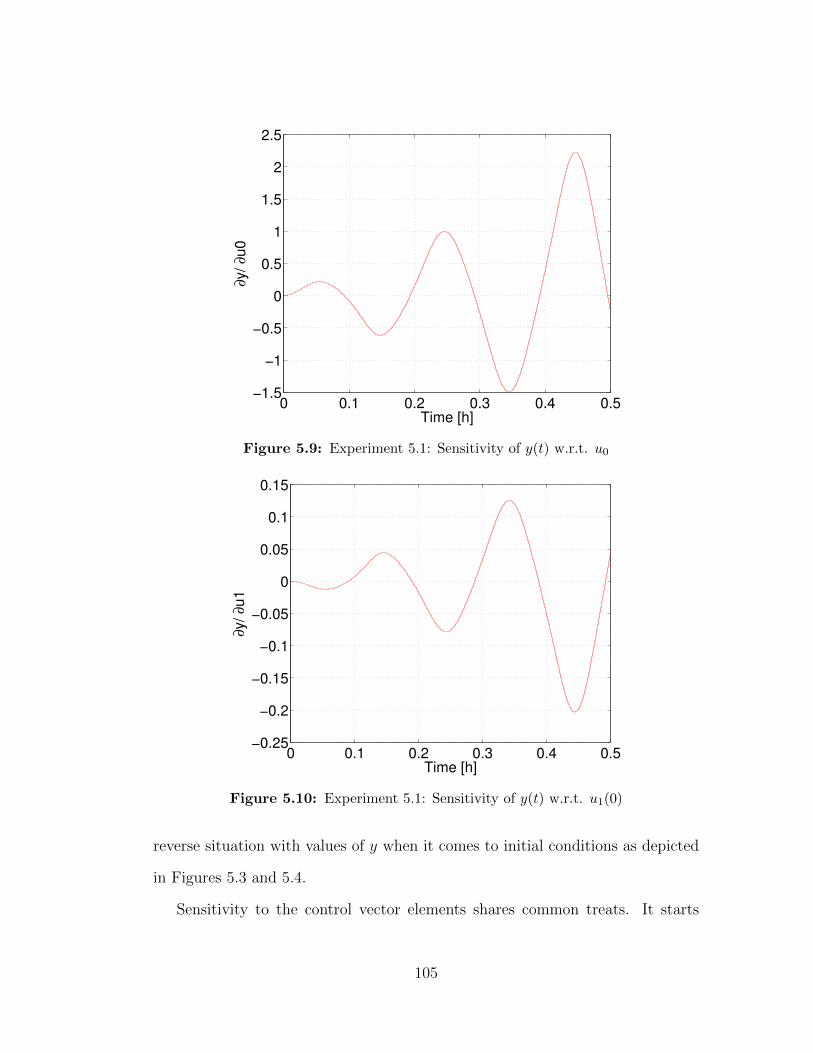
0 0.1 0.2 0.3 0.4 0.5−1.5
−1
−0.5
0
0.5
1
1.5
2
2.5
Time [h]
∂y/
∂u0
Figure 5.9: Experiment 5.1: Sensitivity of y(t) w.r.t. u0
0 0.1 0.2 0.3 0.4 0.5−0.25
−0.2
−0.15
−0.1
−0.05
0
0.05
0.1
0.15
Time [h]
∂y/
∂u1
Figure 5.10: Experiment 5.1: Sensitivity of y(t) w.r.t. u1(0)
reverse situation with values of y when it comes to initial conditions as depicted
in Figures 5.3 and 5.4.
Sensitivity to the control vector elements shares common treats. It starts
105

0 0.1 0.2 0.3 0.4 0.5−0.15
−0.1
−0.05
0
0.05
0.1
0.15
0.2
Time [h]
∂y/
∂v1
Figure 5.11: Experiment 5.1: Sensitivity of y(t) w.r.t. v1(0)
0 0.1 0.2 0.3 0.4 0.5−0.3
−0.2
−0.1
0
0.1
0.2
Time [h]
∂y/
∂h0
Figure 5.12: Experiment 5.1: Sensitivity of y(t) w.r.t. h1(0)
from nearly zero, and after several zero crossings goes to a maximum value at
the end of the simulation at time 0.5. We can see that at the end of the run,
sensitivity of x to u0 seen in Figure 5.5 is much bigger than to u1(0) as depicted
106

in Figure 5.6, and they are reverse in sign. There is not much initial sensitivity of
x to h1(0), but it intensifies by the end of the run. Similar pattern of sensitivity
characterizes y.
5.4.2 Experiment 5.2
In this experiment, we are running a combined mode, with control vector and
initial conditions given in Table 5.2. We have kept u0, u1(0) , v1(0) and h1(0)
identical to Experiment 5.1, but we have changed the initial conditions x0 , y0.
Table 5.2: Experiment 5.2: Base control vector α and initial conditions X(0)
u0 u1(0) v1(0) h1(0) x0 y0 t time step
1.000 0.000 0.500 0.000 0.0 0.0 0.5 2.5e-05
0 0.1 0.2 0.3 0.4 0.50
2
4
6
8
10
12
Time [h]
∂x/
∂x
0
Figure 5.13: Experiment 5.2: Sensitivity of x(t) w.r.t. x(0)
107

0 0.1 0.2 0.3 0.4 0.5−20
−15
−10
−5
0
Time [h]
∂x/
∂y
0
Figure 5.14: Experiment 5.2: Sensitivity of x(t) w.r.t. y(0)
0 0.1 0.2 0.3 0.4 0.5−10
0
10
20
30
40
Time [h]
∂y/
∂x
0
Figure 5.15: Experiment 5.2: Sensitivity of y(t) w.r.t. x(0)
108

0 0.1 0.2 0.3 0.4 0.5−60
−50
−40
−30
−20
−10
0
10
20
Time [h]
∂y/
∂y
0
Figure 5.16: Experiment 5.2: Sensitivity of y(t) w.r.t. y(0)
109
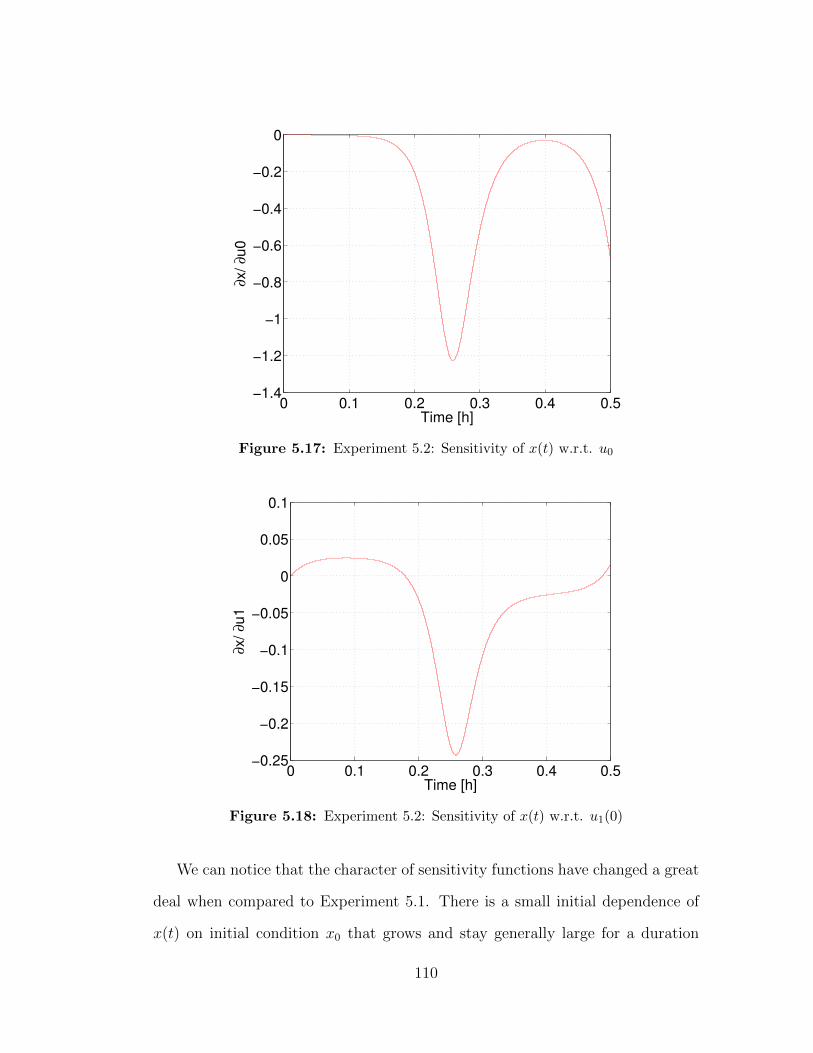
0 0.1 0.2 0.3 0.4 0.5−1.4
−1.2
−1
−0.8
−0.6
−0.4
−0.2
0
Time [h]
∂x/
∂u0
Figure 5.17: Experiment 5.2: Sensitivity of x(t) w.r.t. u0
0 0.1 0.2 0.3 0.4 0.5−0.25
−0.2
−0.15
−0.1
−0.05
0
0.05
0.1
Time [h]
∂x/
∂u1
Figure 5.18: Experiment 5.2: Sensitivity of x(t) w.r.t. u1(0)
We can notice that the character of sensitivity functions have changed a great
deal when compared to Experiment 5.1. There is a small initial dependence of
x(t) on initial condition x0 that grows and stay generally large for a duration
110

0 0.1 0.2 0.3 0.4 0.5−0.7
−0.6
−0.5
−0.4
−0.3
−0.2
−0.1
0
0.1
Time [h]
∂x/
∂v1
Figure 5.19: Experiment 5.2: Sensitivity of x(t) w.r.t. v1(0)
0 0.1 0.2 0.3 0.4 0.5−0.5
0
0.5
1
1.5
2
Time [h]
∂x/
∂h0
Figure 5.20: Experiment 5.2: Sensitivity of x(t) w.r.t. h1(0)
of the experiment, as seen in Figure 5.13. By looking at Figure 5.14, we can
state that this is not the case for dependence of x(t) on y0 that starts from zero
and grows, but is much smaller than dependence on x0. We can notice that
111
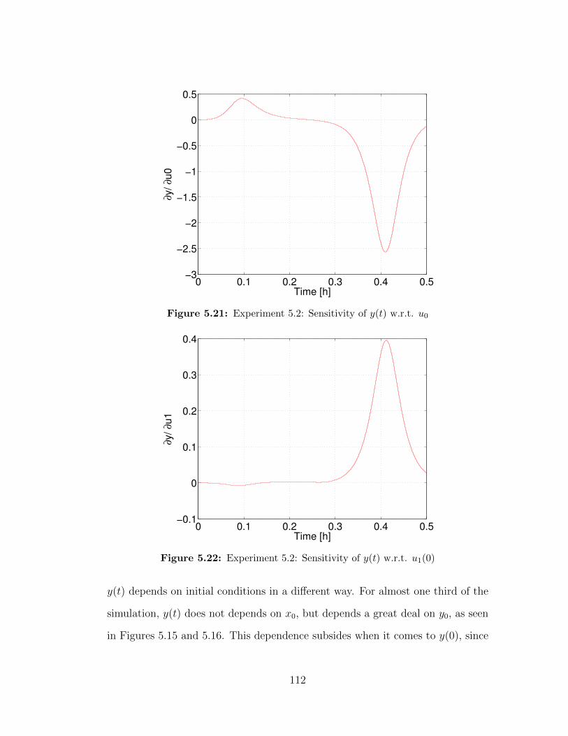
0 0.1 0.2 0.3 0.4 0.5−3
−2.5
−2
−1.5
−1
−0.5
0
0.5
Time [h]
∂y/
∂u0
Figure 5.21: Experiment 5.2: Sensitivity of y(t) w.r.t. u0
0 0.1 0.2 0.3 0.4 0.5−0.1
0
0.1
0.2
0.3
0.4
Time [h]
∂y/
∂u1
Figure 5.22: Experiment 5.2: Sensitivity of y(t) w.r.t. u1(0)
y(t) depends on initial conditions in a different way. For almost one third of the
simulation, y(t) does not depends on x0, but depends a great deal on y0, as seen
in Figures 5.15 and 5.16. This dependence subsides when it comes to y(0), since
112

0 0.1 0.2 0.3 0.4 0.5−2
−1.5
−1
−0.5
0
0.5
Time [h]
∂y/
∂v1
Figure 5.23: Experiment 5.2: Sensitivity of y(t) w.r.t. v1(0)
0 0.1 0.2 0.3 0.4 0.5−2
0
2
4
6
8
10
Time [h]
∂y/
∂h0
Figure 5.24: Experiment 5.2: Sensitivity of y(t) w.r.t. h1(0)
it falls to nearly zero levels after one fifth of the simulation time.
We can notice in Figures 5.17 and 5.18 that u(t) does not depend initially on
u0 or u1(0). This dependence grows with the simulation time, and is inversely
113

dependndent on u0, and directly dependent on u1(t). We can also notice that for
this simulation, x(t) is sensitive more to u1(0) than to v1(0).
Judging from Figure 5.22, y(t) is sensitive to u1(0) more than to v1(0) that is
depicted in Figure 5.23.
5.4.3 Experiment 5.3
In this experiment, we are running a combined mode, with control vector and
initial conditions given in Table 5.3. While the control vector α is the same as
the two previous experiments, initial conditions are moved to the point (0.1, 0.1).
Table 5.3: Experiment 5.3: Base control vector α and initial conditions X(0)
u0 u1(0) v1(0) h1(0) x0 y0 t time step
1.000 0.000 0.500 0.000 0.1 0.1 0.5 2.5e-05
114
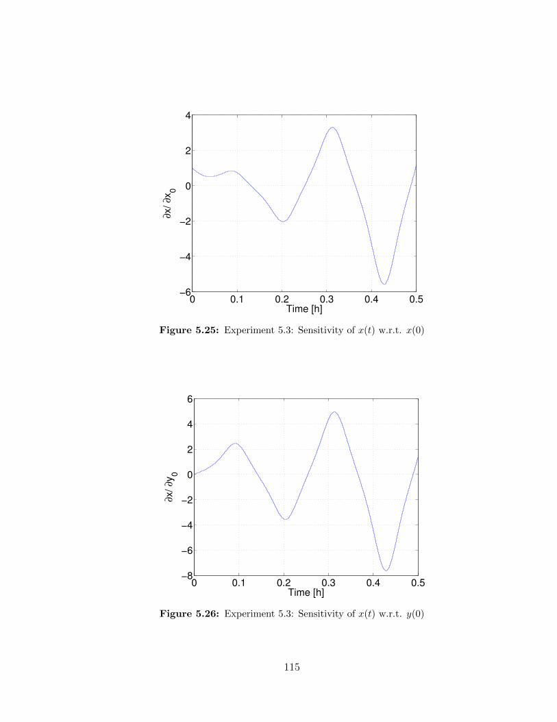
0 0.1 0.2 0.3 0.4 0.5−6
−4
−2
0
2
4
Time [h]
∂x/
∂x
0
Figure 5.25: Experiment 5.3: Sensitivity of x(t) w.r.t. x(0)
0 0.1 0.2 0.3 0.4 0.5−8
−6
−4
−2
0
2
4
6
Time [h]
∂x/
∂y
0
Figure 5.26: Experiment 5.3: Sensitivity of x(t) w.r.t. y(0)
115

0 0.1 0.2 0.3 0.4 0.5−5
0
5
10
Time [h]
∂y/
∂x
0
Figure 5.27: Experiment 5.3: Sensitivity of y(t) w.r.t. x(0)
0 0.1 0.2 0.3 0.4 0.5−10
−5
0
5
10
15
Time [h]
∂y/
∂y
0
Figure 5.28: Experiment 5.3: Sensitivity of y(t) w.r.t. y(0)
116

0 0.1 0.2 0.3 0.4 0.5−3
−2
−1
0
1
2
Time [h]
∂x/
∂u0
Figure 5.29: Experiment 5.3: Sensitivity of x(t) w.r.t. u0
0 0.1 0.2 0.3 0.4 0.5−0.2
−0.1
0
0.1
0.2
0.3
0.4
0.5
Time [h]
∂x/
∂u1
Figure 5.30: Experiment 5.3: Sensitivity of x(t) w.r.t. u1(0)
We can notice in Figure 5.25 that x(t) sensitivity starts around one, then
goes through a zero crossing point at time 0.13 to reach value −2, then it grows
to about 3.5 to have a zero crossing again at time 0.36 do drop to −5.5. While
117

0 0.1 0.2 0.3 0.4 0.5−0.5
−0.4
−0.3
−0.2
−0.1
0
0.1
0.2
0.3
Time [h]
∂x/
∂v1
Figure 5.31: Experiment 5.3: Sensitivity of x(t) w.r.t. v1(0)
0 0.1 0.2 0.3 0.4 0.5−0.4
−0.2
0
0.2
0.4
0.6
0.8
1
Time [h]
∂x/
∂h0
Figure 5.32: Experiment 5.3: Sensitivity of x(t) w.r.t. h1(0)
behavior is similar to this in Figure 5.1, values of sensitivity are bigger than in the
Experiment 5.1. Sensitivity of x(t) w.r.t. y0 start from zero, but it reaches values
bigger than in the Experiment 5.1 as well. We can see in Figure 5.27 that y(t) is
118

0 0.1 0.2 0.3 0.4 0.5−3
−2
−1
0
1
2
3
4
Time [h]
∂y/
∂u0
Figure 5.33: Experiment 5.3: Sensitivity of y(t) w.r.t. u0
0 0.1 0.2 0.3 0.4 0.5−0.6
−0.4
−0.2
0
0.2
0.4
Time [h]
∂y/
∂u1
Figure 5.34: Experiment 5.3: Sensitivity of y(t) w.r.t. u1(0)
initially not sensitive to value of x(0), but it reaches value in the order of 7.5 by
the end of the simulation. Its graph has three zeros crossings, and behaves quite
differently than the one from Figure 5.3 in Experiment 5.1. When we compare
119

0 0.1 0.2 0.3 0.4 0.5−0.4
−0.2
0
0.2
0.4
0.6
Time [h]
∂y/
∂v1
Figure 5.35: Experiment 5.3: Sensitivity of y(t) w.r.t. v1(0)
0 0.1 0.2 0.3 0.4 0.5−1.5
−1
−0.5
0
0.5
Time [h]
∂y/
∂h0
Figure 5.36: Experiment 5.3: Sensitivity of y(t) w.r.t. h1(0)
sensitivity y(t) from Figure 5.28 with the one from the Experiment 5.1 Figure
5.4, we can notice than they have similar shape but y(t) sensitivity values in the
Experiment 5.3 are almost twice as big.
120

5.5 Summary
In this chapter, we have analyzed model sensitivity, that is the dependence of the
linearized shallow water model on initial conditions and parameters. We have
shown that the shallow water model can exhibit different behavior that depends
on the initial conditions and the control vector. This gives us a great insight into
the fine structure of the tracer dynamics. By analyzing sensitivity plots, we can
answer in the quantitative way, which parameters control tracer position for a
given prediction to a bigger degree. We can also see in included plots that for the
linearized shallow water model, there is no identical dependence on parameters
and initial conditions; they have to be analyzed case by case. This determination
of parametric sensitivity is very important for the successful data assimilation.
This is studied in the next chapter.
121

Chapter 6
Numerical experiments in Data
Assimilation
6.1 Introduction
In the previous chapter, we have conducted numerical experiments in which we
have analyzed sensitivity of tracer dynamics to the initial conditions X(0) and
elements of the control vector α. Our findings would suggest that there is a
reason for different influence of measurements taken with in a temporal domain.
In this chapter, we demonstrate the effectiveness of the forward sensitivity
method (FSM) by conducting a series of numerical experiments conducting DA.
We differ the number of observations, their temporal distribution and the obser-
vational error variance. We need to bring some definitions we can use to compare
different data assimilation experiments.
122

6.1.1 Root-mean-square error
We use the root-mean-square (RMSE) error to estimate the goodness of our data
assimilation scheme, that is, to evaluate a difference between the values that
are observed and values that are estimated by the model. It represents a very
valuable measure of forecast errors and it allows for comparison between forecast
and different number of observations and their placement. Predicted values yt at
n different times are compared with the observed values
RMSE =
√∑nt=1(yt − yt)2
n(6.1)
6.1.2 Condition number of a matrix
Let us bring up a definition of the condition number of a matrix, usually indicated
as κ, from (page 667, Lewis et al. (2006)) [12]. For matrix A ∈ Rm×m, where
A−1 is the inverse of A,
κ(A) = ‖A‖‖A−1‖. (6.2)
The condition number of a matrix describes how the sensitivity of the solution
of a system of linear equations depends on error in the data. It can be said that
matrices with small condition number are well conditioned; singular matrices
have infinite condition numbers. We will use a spectral condition number defined
on (page 668, Lewis et al. (2006))
κ2(A) = ‖A‖2‖A−1‖2 =maxi |λi|mini |λi|
. (6.3)
123

6.1.3 Methodology
The observations that are used for data assimilation experiments are created using
”Base” trajectory by adding the noise with the observational error variance σ of
different magnitudes given in Table 6.1. In every experiment, control vectors
used for ”Base” trajectory are shown alongside the perturbed control vectors
that we try to improve. We start each numerical experiment with the incorrect
control vector. The forward sensitivity method uses sensitivity functions that
use that erroneous solution. We use FSM to assimilate a different number of
observations, and since we have four elements of the control vector, for number of
observations bigger than four, we have an overdetermined system. Our numerical
experiments use observations from four different temporal ranges described as:
START, MIDDLE, FINISH, UNIFORM. They are described in the next section.
We keep track of the condition number, the ratio of the largest to the smallest
of HTH, since the inverse of HTH influences the optimal adjustments to the
control vector. We have to look at the observation spacing in some temporal
ranges. We can infer some characteristic of the measurement distribution and
compare condition numbers.
We use the iterative process correcting elements of the control vector. After
first iteration, we apply the correction and repeat the process, that is, we make
another forecast using the corrected control vector. We have shown results of
the firs three steps of the iteration. Clearly, FSM improves forecast at each step;
we track improvements by following RMS error between observations and the
forecast.
124

Table 6.1: Values of the observational error variance σ and σ2 used in data as-similation experiments to create perturbed observations
σ σ2
1 0.0707 0.00502 0.0866 0.00753 0.1000 0.01004 0.1118 0.01255 0.1225 0.01506 0.1323 0.01757 0.1414 0.0200
6.2 Data assimilation
Each of our data assimilation experiments consist of four separate data assim-
ilations that deal with different distribution of measurements called: START,
MIDDLE, FINISH and UNIFORM. They differ by placing measurements as fol-
lows: START puts all measurements in the first third of the temporal domain,
MIDDLE puts all measurements in the second third or the temporal domain,
FINISH puts all measurements in the last third of the temporal domain, and
finally UNIFORM distributes measurements over the entire period of modeling.
6.2.1 Experiment 6.1
Experiment base configuration is shown in Table 6.2. These values are used to
create observations in a twin-experiment by adding a random noise with different
σ2 values shown in Table 6.1. Then, control vector α values are modified as shown
in 6.3. Then, four separate experiments are conducted with different distribution
of measurements. We can see a trajectory of the Lagrangian tracer, and data
assimilation.
125

Table 6.2: Experiment 6.1: Base control vector α and initial conditions X(0)
u0 u1(0) v1(0) h1(0) x0 y0 t time step
1.000 0.000 0.500 0.000 0.209 0.109 0.5 2.5e-05
Table 6.3: Experiment 6.1: Perturbed control vector α and initial conditionsX(0)
u0 u1(0) v1(0) h1(0) x0 y0 t time step
0.986523 -0.001833 0.546079 0.136232 0.209 0.109 0.5 2.5e-05
0.1 0.2 0.3 0.4 0.50.1
0.2
0.3
0.4
0.5
X
Y
Base
First
Third
Observation
Figure 6.1: Experiment 6.1: Trajectory with 4 measurements, START distribu-tion
In table 6.4, we can see a summary of similar experiments described so far
with 4 measurements. They differ by increasing value of σ2, by which we perturb
observations in the twin-experiment. We can see in all experiments except one,
126

Table 6.4: Experiment 6.1: Comparison of data assimilations for a set of distri-butions and errors with 4 measurements
Distribution of σ2 RMS Error κmeasurements of observations
Iteration Iteration1st 3rd 1st 3rd
0.005 0.0190 0.0056 1.7e+04 1.7e+040.007 0.0579 0.0138 2.5e+04 1.8e+040.010 0.0565 0.0162 2.4e+04 2.0e+04
START 0.013 0.0361 0.0122 1.7e+04 1.8e+040.015 0.0418 0.0129 1.7e+04 1.8e+040.018 0.0211 0.0095 1.9e+04 1.7e+040.020 0.0479 0.0288 2.0e+04 3.0e+040.005 0.0395 0.0073 3.5e+04 3.1e+040.007 0.1411 0.0511 5.7e+04 3.0e+040.010 0.1428 0.0600 5.8e+04 3.2e+04
MIDDLE 0.013 0.0675 0.0188 3.8e+04 3.1e+040.015 0.1059 0.0468 3.5e+04 3.2e+040.018 0.0609 0.0177 3.6e+04 3.0e+040.020 0.0429 0.0171 3.3e+04 3.4e+040.005 0.0574 0.0145 1.1e+05 1.4e+050.007 0.2377 0.1652 1.5e+05 1.1e+050.010 0.2335 0.1798 1.5e+05 1.3e+05
FINISH 0.013 0.1174 0.0609 9.2e+04 1.2e+050.015 0.1774 0.1651 8.1e+04 1.0e+050.018 0.1185 0.0568 9.5e+04 1.3e+050.020 0.1067 0.1812 1.1e+05 1.2e+050.005 0.0319 0.0071 2.2e+05 1.3e+050.007 0.1400 0.0592 4.8e+04 8.4e+040.010 0.1260 0.0613 5.2e+04 1.4e+05
UNIFORM 0.013 0.0773 0.1497 2.5e+05 5.1e+040.015 0.1153 0.5134 1.0e+06 6.0e+040.018 0.0628 0.0269 3.9e+04 9.7e+040.020 0.0513 0.0209 4.6e+04 1.7e+05
consecutive iterations improve match between the model and observations. In a
run with a uniform distribution, and σ2 set to 0.0125, RMS error increase and
127

1 2 30.005
0.01
0.015
0.02
Iteration
J
Figure 6.2: Experiment 6.1: Cost function for three steps of data assimilation,START measurement distribution
condition number κ is about three times bigger than in most other experiments.
128

0 0.1 0.2 0.3 0.4 0.5−2
−1
0
1
2
3
Time [h]
Figure 6.3: Experiment 6.1: Sensitivity functions, START measurement distri-bution, measurements times indicated along the sensitivity plot by*
129

0.1 0.2 0.3 0.4 0.50.1
0.2
0.3
0.4
0.5
X
Y
Base
First
Third
Observation
Figure 6.4: Experiment 6.1: Trajectory with 4 measurements, MIDDLE distri-bution
130

1 2 30
0.005
0.01
0.015
0.02
0.025
0.03
0.035
0.04
Iteration
J
Figure 6.5: Experiment 6.1: Cost function for three steps of data assimilation,MIDDLE measurement distribution
131
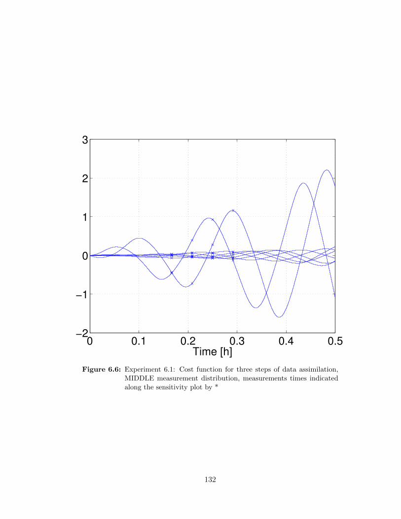
0 0.1 0.2 0.3 0.4 0.5−2
−1
0
1
2
3
Time [h]
Figure 6.6: Experiment 6.1: Cost function for three steps of data assimilation,MIDDLE measurement distribution, measurements times indicatedalong the sensitivity plot by *
132
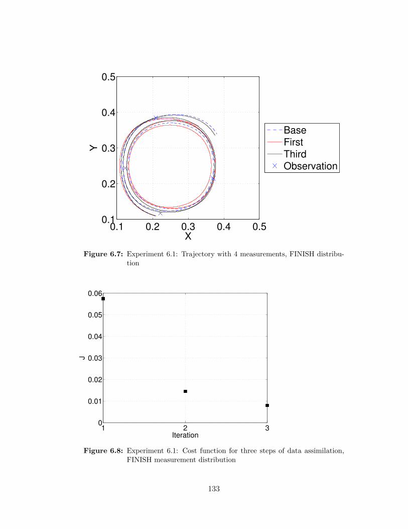
0.1 0.2 0.3 0.4 0.50.1
0.2
0.3
0.4
0.5
X
Y
Base
First
Third
Observation
Figure 6.7: Experiment 6.1: Trajectory with 4 measurements, FINISH distribu-tion
1 2 30
0.01
0.02
0.03
0.04
0.05
0.06
Iteration
J
Figure 6.8: Experiment 6.1: Cost function for three steps of data assimilation,FINISH measurement distribution
133

0 0.1 0.2 0.3 0.4 0.5−2
−1
0
1
2
3
Time [h]
Figure 6.9: Experiment 6.1: Sensitivity functions, FINISH measurement distri-bution, measurements times indicated along the sensitivity plot by*
134

0.1 0.2 0.3 0.4 0.50.1
0.2
0.3
0.4
0.5
X
Y
Base
First
Third
Observation
Figure 6.10: Experiment 6.1: Trajectory with 4 measurements, UNIFORM dis-tribution
1 2 30
0.01
0.02
0.03
0.04
0.05
0.06
Iteration
J
Figure 6.11: Experiment 6.1: Cost function for three steps of data assimilation,UNIFORM measurement distribution
135

0 0.1 0.2 0.3 0.4 0.5−2
−1
0
1
2
3
Time [h]
Figure 6.12: Experiment 6.1: Sensitivity functions, UNIFORM measurement dis-tribution, measurements times indicated along the sensitivity plotby *
136

6.2.2 Experiment 6.2
In this experiment, we are going to continue with the way it was organized in
Experiment 6.1, and we are going to investigate whether the increased number of
measurements within the set period always lead to better correction of the control
vector α. We are going to use 4, 8, 16, 32, 64 and 128 measurements within
periods described in the Experiment 6.1. Base control vector and perturbed
control vector are like the one described in the Experiment 6.1.
Table 6.5: Experiment 6.2: Base control vector α and initial conditions X(0)
u0 u1(0) v1(0) h1(0) x0 y0 t time step
1.000 0.000 0.500 0.000 0.209 0.109 0.5 2.5e-05
Table 6.6: Experiment 6.2: Perturbed control vector α and initial conditionsX(0)
u0 u1(0) v1(0) h1(0) x0 y0 t time step
0.986523 -0.001833 0.546079 0.136232 0.209 0.109 0.5 2.5e-05
137
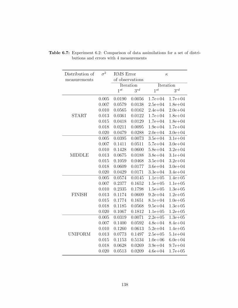
Table 6.7: Experiment 6.2: Comparison of data assimilations for a set of distri-butions and errors with 4 measurements
Distribution of σ2 RMS Error κmeasurements of observations
Iteration Iteration1st 3rd 1st 3rd
0.005 0.0190 0.0056 1.7e+04 1.7e+040.007 0.0579 0.0138 2.5e+04 1.8e+040.010 0.0565 0.0162 2.4e+04 2.0e+04
START 0.013 0.0361 0.0122 1.7e+04 1.8e+040.015 0.0418 0.0129 1.7e+04 1.8e+040.018 0.0211 0.0095 1.9e+04 1.7e+040.020 0.0479 0.0288 2.0e+04 3.0e+040.005 0.0395 0.0073 3.5e+04 3.1e+040.007 0.1411 0.0511 5.7e+04 3.0e+040.010 0.1428 0.0600 5.8e+04 3.2e+04
MIDDLE 0.013 0.0675 0.0188 3.8e+04 3.1e+040.015 0.1059 0.0468 3.5e+04 3.2e+040.018 0.0609 0.0177 3.6e+04 3.0e+040.020 0.0429 0.0171 3.3e+04 3.4e+040.005 0.0574 0.0145 1.1e+05 1.4e+050.007 0.2377 0.1652 1.5e+05 1.1e+050.010 0.2335 0.1798 1.5e+05 1.3e+05
FINISH 0.013 0.1174 0.0609 9.2e+04 1.2e+050.015 0.1774 0.1651 8.1e+04 1.0e+050.018 0.1185 0.0568 9.5e+04 1.3e+050.020 0.1067 0.1812 1.1e+05 1.2e+050.005 0.0319 0.0071 2.2e+05 1.3e+050.007 0.1400 0.0592 4.8e+04 8.4e+040.010 0.1260 0.0613 5.2e+04 1.4e+05
UNIFORM 0.013 0.0773 0.1497 2.5e+05 5.1e+040.015 0.1153 0.5134 1.0e+06 6.0e+040.018 0.0628 0.0269 3.9e+04 9.7e+040.020 0.0513 0.0209 4.6e+04 1.7e+05
138

Table 6.8: Experiment 6.2: Comparison of data assimilations for a set of distri-butions and errors with 8 measurements
Distribution of σ2 RMS Error κmeasurements of observations
Iteration Iteration1st 3rd 1st 3rd
0.005 0.0621 0.0184 1.2e+04 1.4e+040.007 0.0182 0.0085 1.6e+04 1.4e+040.010 0.0190 0.0131 1.4e+04 1.6e+04
START 0.013 0.0309 0.0141 1.8e+04 1.5e+040.015 0.0874 0.0375 2.7e+04 1.4e+040.018 0.0339 0.0220 1.9e+04 1.5e+040.020 0.0456 0.0266 1.8e+04 1.4e+040.005 0.1538 0.0984 2.8e+04 3.2e+040.007 0.0502 0.0167 4.1e+04 3.5e+040.010 0.0156 0.0139 3.5e+04 3.6e+04
MIDDLE 0.013 0.0872 0.0358 4.5e+04 3.6e+040.015 0.1810 0.0865 6.6e+04 2.8e+040.018 0.0927 0.0475 4.9e+04 3.3e+040.020 0.0830 0.0402 4.3e+04 3.7e+040.005 0.2532 0.1322 7.9e+04 6.9e+040.007 0.0900 0.0312 1.1e+05 1.2e+050.010 0.0261 0.0213 1.2e+05 1.2e+05
FINISH 0.013 0.1243 0.0636 1.1e+05 1.4e+050.015 0.2422 0.1288 1.7e+05 1.2e+050.018 0.1412 0.0913 1.1e+05 1.5e+050.020 0.1350 0.0658 1.1e+05 1.3e+050.005 0.1642 0.1307 2.9e+04 1.6e+040.007 0.0546 0.0173 4.7e+04 3.3e+040.010 0.0080 0.0069 3.8e+04 3.9e+04
UNIFORM 0.013 0.0807 0.0274 5.1e+04 3.4e+040.015 0.1776 0.0880 5.2e+04 8.6e+030.018 0.0946 0.0429 5.6e+04 3.4e+040.020 0.0977 0.0407 4.8e+04 2.7e+04
139
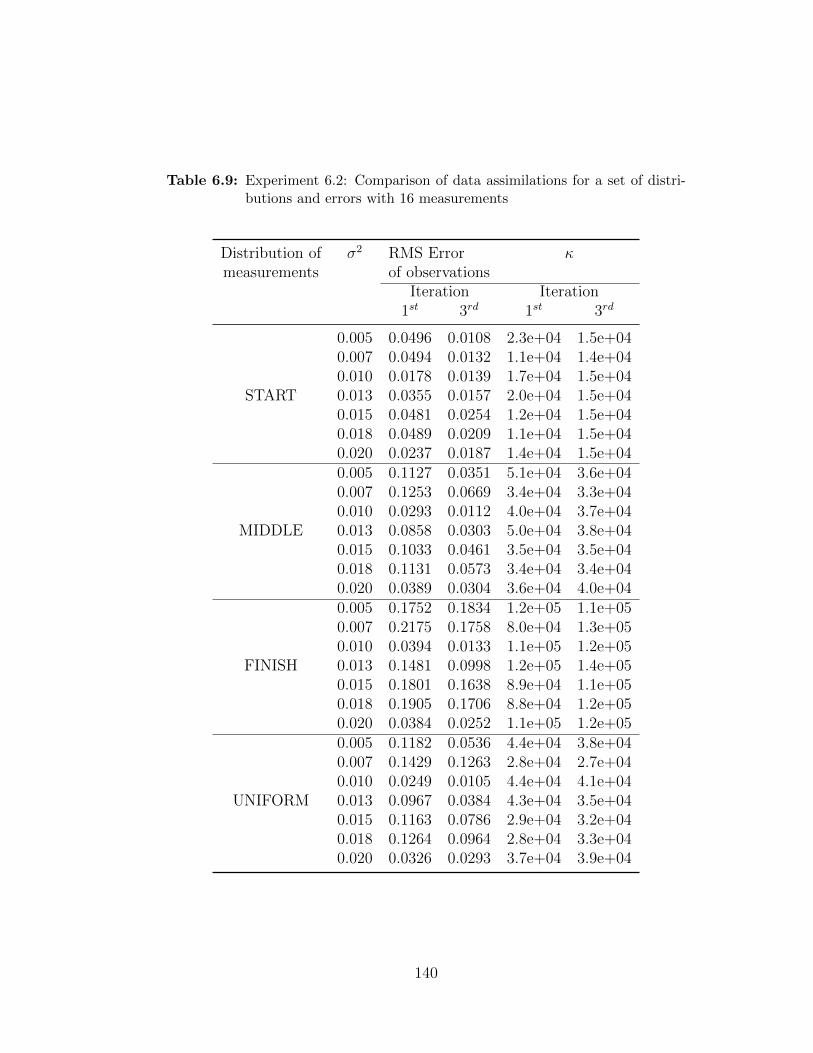
Table 6.9: Experiment 6.2: Comparison of data assimilations for a set of distri-butions and errors with 16 measurements
Distribution of σ2 RMS Error κmeasurements of observations
Iteration Iteration1st 3rd 1st 3rd
0.005 0.0496 0.0108 2.3e+04 1.5e+040.007 0.0494 0.0132 1.1e+04 1.4e+040.010 0.0178 0.0139 1.7e+04 1.5e+04
START 0.013 0.0355 0.0157 2.0e+04 1.5e+040.015 0.0481 0.0254 1.2e+04 1.5e+040.018 0.0489 0.0209 1.1e+04 1.5e+040.020 0.0237 0.0187 1.4e+04 1.5e+040.005 0.1127 0.0351 5.1e+04 3.6e+040.007 0.1253 0.0669 3.4e+04 3.3e+040.010 0.0293 0.0112 4.0e+04 3.7e+04
MIDDLE 0.013 0.0858 0.0303 5.0e+04 3.8e+040.015 0.1033 0.0461 3.5e+04 3.5e+040.018 0.1131 0.0573 3.4e+04 3.4e+040.020 0.0389 0.0304 3.6e+04 4.0e+040.005 0.1752 0.1834 1.2e+05 1.1e+050.007 0.2175 0.1758 8.0e+04 1.3e+050.010 0.0394 0.0133 1.1e+05 1.2e+05
FINISH 0.013 0.1481 0.0998 1.2e+05 1.4e+050.015 0.1801 0.1638 8.9e+04 1.1e+050.018 0.1905 0.1706 8.8e+04 1.2e+050.020 0.0384 0.0252 1.1e+05 1.2e+050.005 0.1182 0.0536 4.4e+04 3.8e+040.007 0.1429 0.1263 2.8e+04 2.7e+040.010 0.0249 0.0105 4.4e+04 4.1e+04
UNIFORM 0.013 0.0967 0.0384 4.3e+04 3.5e+040.015 0.1163 0.0786 2.9e+04 3.2e+040.018 0.1264 0.0964 2.8e+04 3.3e+040.020 0.0326 0.0293 3.7e+04 3.9e+04
140
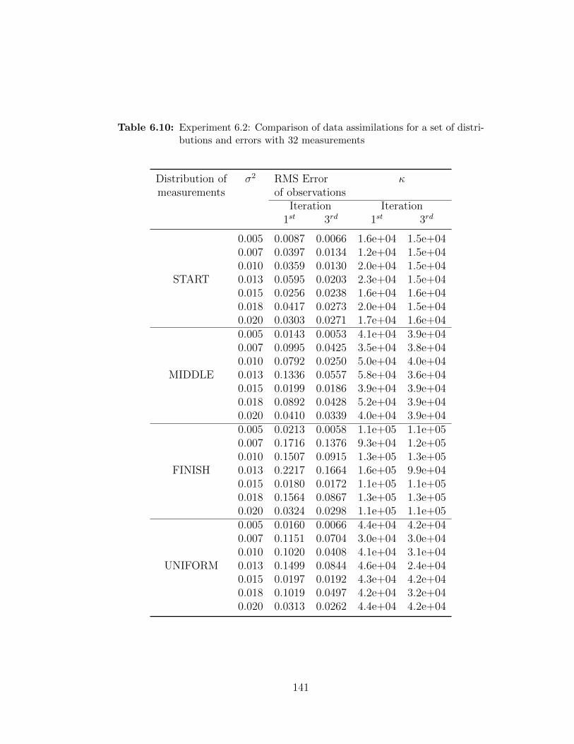
Table 6.10: Experiment 6.2: Comparison of data assimilations for a set of distri-butions and errors with 32 measurements
Distribution of σ2 RMS Error κmeasurements of observations
Iteration Iteration1st 3rd 1st 3rd
0.005 0.0087 0.0066 1.6e+04 1.5e+040.007 0.0397 0.0134 1.2e+04 1.5e+040.010 0.0359 0.0130 2.0e+04 1.5e+04
START 0.013 0.0595 0.0203 2.3e+04 1.5e+040.015 0.0256 0.0238 1.6e+04 1.6e+040.018 0.0417 0.0273 2.0e+04 1.5e+040.020 0.0303 0.0271 1.7e+04 1.6e+040.005 0.0143 0.0053 4.1e+04 3.9e+040.007 0.0995 0.0425 3.5e+04 3.8e+040.010 0.0792 0.0250 5.0e+04 4.0e+04
MIDDLE 0.013 0.1336 0.0557 5.8e+04 3.6e+040.015 0.0199 0.0186 3.9e+04 3.9e+040.018 0.0892 0.0428 5.2e+04 3.9e+040.020 0.0410 0.0339 4.0e+04 3.9e+040.005 0.0213 0.0058 1.1e+05 1.1e+050.007 0.1716 0.1376 9.3e+04 1.2e+050.010 0.1507 0.0915 1.3e+05 1.3e+05
FINISH 0.013 0.2217 0.1664 1.6e+05 9.9e+040.015 0.0180 0.0172 1.1e+05 1.1e+050.018 0.1564 0.0867 1.3e+05 1.3e+050.020 0.0324 0.0298 1.1e+05 1.1e+050.005 0.0160 0.0066 4.4e+04 4.2e+040.007 0.1151 0.0704 3.0e+04 3.0e+040.010 0.1020 0.0408 4.1e+04 3.1e+04
UNIFORM 0.013 0.1499 0.0844 4.6e+04 2.4e+040.015 0.0197 0.0192 4.3e+04 4.2e+040.018 0.1019 0.0497 4.2e+04 3.2e+040.020 0.0313 0.0262 4.4e+04 4.2e+04
141

Table 6.11: Experiment 6.2: Comparison of data assimilations for a set of distri-butions and errors with 64 measurements
Distribution of σ2 RMS Error κmeasurements of observations
Iteration Iteration1st 3rd 1st 3rd
0.005 0.0542 0.0161 2.2e+04 1.5e+040.007 0.0145 0.0110 1.5e+04 1.6e+040.010 0.0800 0.0300 1.0e+04 1.4e+04
START 0.013 0.0709 0.0265 1.1e+04 1.5e+040.015 0.0239 0.0198 1.4e+04 1.5e+040.018 0.0303 0.0251 1.8e+04 1.5e+040.020 0.0282 0.0258 1.7e+04 1.6e+040.005 0.1354 0.0650 6.4e+04 3.6e+040.007 0.0183 0.0114 3.9e+04 3.9e+040.010 0.1866 0.1402 2.7e+04 3.1e+04
MIDDLE 0.013 0.1592 0.1037 3.0e+04 3.0e+040.015 0.0380 0.0209 3.6e+04 4.0e+040.018 0.0495 0.0265 4.6e+04 3.9e+040.020 0.0442 0.0249 4.5e+04 3.9e+040.005 0.2312 0.1393 1.7e+05 1.2e+050.007 0.0220 0.0115 1.2e+05 1.1e+050.010 0.2840 0.1718 8.2e+04 5.6e+05
FINISH 0.013 0.2506 0.1277 7.9e+04 9.5e+040.015 0.0520 0.0190 1.2e+05 1.1e+050.018 0.0794 0.0313 1.1e+05 1.2e+050.020 0.0830 0.0398 1.1e+05 1.2e+050.005 0.1555 0.0801 5.3e+04 1.4e+040.007 0.0190 0.0105 4.4e+04 4.2e+040.010 0.2010 0.1273 3.3e+04 5.4e+04
UNIFORM 0.013 0.1757 0.1409 2.7e+04 2.2e+040.015 0.0416 0.0197 3.9e+04 3.9e+040.018 0.0573 0.0264 4.3e+04 3.8e+040.020 0.0509 0.0274 3.9e+04 4.0e+04
142

Table 6.12: Experiment 6.2: Comparison of data assimilations for a set of distri-butions and errors with 128 measurements
Distribution of σ2 RMS Error κmeasurements of observations
Iteration Iteration1st 3rd 1st 3rd
0.005 0.0530 0.0141 1.1e+04 1.5e+040.007 0.0368 0.0119 1.2e+04 1.5e+040.010 0.0441 0.0169 1.2e+04 1.5e+04
START 0.013 0.0227 0.0182 1.5e+04 1.6e+040.015 0.0349 0.0185 1.2e+04 1.6e+040.018 0.0469 0.0268 1.2e+04 1.6e+040.020 0.0807 0.0379 2.3e+04 1.5e+040.005 0.1235 0.0631 3.4e+04 3.5e+040.007 0.0971 0.0397 3.6e+04 3.7e+040.010 0.0981 0.0429 3.4e+04 3.9e+04
MIDDLE 0.013 0.0306 0.0210 4.1e+04 3.9e+040.015 0.0748 0.0311 3.5e+04 4.1e+040.018 0.0952 0.0441 3.5e+04 3.9e+040.020 0.1770 0.0844 6.7e+04 3.4e+040.005 0.2040 0.1753 8.7e+04 9.9e+040.007 0.1871 0.1869 8.6e+04 9.8e+040.010 0.1527 0.1052 1.0e+05 1.3e+05
FINISH 0.013 0.0327 0.0355 1.1e+05 1.1e+050.015 0.1251 0.0664 1.1e+05 1.3e+050.018 0.1643 0.1274 9.9e+04 1.3e+050.020 0.2742 0.1449 1.7e+05 7.9e+040.005 0.1406 0.1152 2.8e+04 2.5e+040.007 0.1230 0.0923 3.2e+04 3.7e+040.010 0.1088 0.0577 3.0e+04 2.9e+04
UNIFORM 0.013 0.0280 0.0226 3.9e+04 4.4e+040.015 0.0862 0.0363 3.5e+04 3.6e+040.018 0.1153 0.0670 3.2e+04 3.1e+040.020 0.1919 0.1158 6.1e+04 2.1e+04
143

4 8 16 32 64 1280
0.01
0.02
0.03
0.04
0.05
0.06
0.07
Numer of measurments
RM
SE
1st iteration
3rd iteration
Figure 6.13: Experiment 6.2: Root-mean-square (RMSE) error of observationsas a function of number of experiments σ2 = 0.005, START mea-surement distribution.
4 8 16 32 64 1281
1.2
1.4
1.6
1.8
2
2.2
2.4x 10
4
Numer of measurments
Conditio
n n
um
ber
κ
1st iteration
3rd iteration
Figure 6.14: Experiment 6.2: Condition number κ as a function of number ofexperiments σ2 = 0.005, START measurement distribution.
144

4 8 16 32 64 1280
0.02
0.04
0.06
0.08
0.1
0.12
0.14
0.16
Numer of measurments
RM
SE
1st iteration
3rd iteration
Figure 6.15: Experiment 6.2: Root-mean-square error of observations as a func-tion of number of experiments σ2 = 0.005, MIDDLE measurementdistribution.
145

4 8 16 32 64 1282.5
3
3.5
4
4.5
5
5.5
6
6.5x 10
4
Numer of measurments
Conditio
n n
um
ber
κ
1st iteration
3rd iteration
Figure 6.16: Experiment 6.2: Condition number κ as a function of number ofexperiments σ2 = 0.005, MIDDLE measurement distribution.
146

4 8 16 32 64 1280
0.05
0.1
0.15
0.2
0.25
0.3
0.35
Numer of measurments
RM
SE
1st iteration
3rd iteration
Figure 6.17: Experiment 6.2: Root-mean-square error of observations as a func-tion of number of experiments σ2 = 0.005, FINISH measurementdistribution.
147

4 8 16 32 64 1280.6
0.8
1
1.2
1.4
1.6
1.8x 10
5
Numer of measurments
Conditio
n n
um
ber
κ
1st iteration
3rd iteration
Figure 6.18: Experiment 6.2: Condition number κ as a function of number ofexperiments σ2 = 0.005, FINISH measurement distribution.
148

4 8 16 32 64 1280
0.05
0.1
0.15
0.2
Numer of measurments
RM
SE
1st iteration
3rd iteration
Figure 6.19: Experiment 6.2: Root-mean-square error of observations as a func-tion of number of experiments σ2 = 0.005, UNIFORM measurementdistribution.
149

4 8 16 32 64 1280
0.5
1
1.5
2
2.5x 10
5
Numer of measurments
Conditio
n n
um
ber
κ
1st iteration
3rd iteration
Figure 6.20: Experiment 6.2: Condition number κ as a function of number ofexperiments σ2 = 0.005, UNIFORM measurement distribution.
150

4 8 16 32 64 1280
0.01
0.02
0.03
0.04
0.05
0.06
Numer of measurments
RM
SE
1st iteration
3rd iteration
Figure 6.21: Experiment 6.2: Root-mean-square error of observations as a func-tion of number of experiments σ2 = 0.0075, START measurementdistribution.
151

4 8 16 32 64 1281
1.5
2
2.5x 10
4
Numer of measurments
Conditio
n n
um
ber
κ
1st iteration
3rd iteration
Figure 6.22: Experiment 6.2: Condition number κ a function of number of ex-periments σ2 = 0.0075, START measurement distribution.
152

4 8 16 32 64 1280
0.02
0.04
0.06
0.08
0.1
0.12
0.14
0.16
Numer of measurments
RM
SE
1st iteration
3rd iteration
Figure 6.23: Experiment 6.2: Root-mean-square error of observations as a func-tion of number of experiments σ2 = 0.0075, MIDDLE measurementdistribution.
153

4 8 16 32 64 1283
3.5
4
4.5
5
5.5
6x 10
4
Numer of measurments
Conditio
n n
um
ber
κ
1st iteration
3rd iteration
Figure 6.24: Experiment 6.2: Condition number κ as a function of number ofexperiments σ2 = 0.0075, MIDDLE measurement distribution.
154
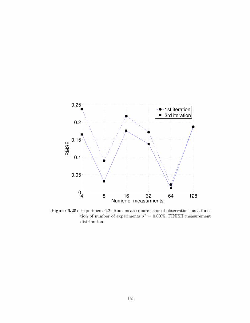
4 8 16 32 64 1280
0.05
0.1
0.15
0.2
0.25
Numer of measurments
RM
SE
1st iteration
3rd iteration
Figure 6.25: Experiment 6.2: Root-mean-square error of observations as a func-tion of number of experiments σ2 = 0.0075, FINISH measurementdistribution.
155

4 8 16 32 64 1280.8
0.9
1
1.1
1.2
1.3
1.4
1.5
1.6x 10
5
Numer of measurments
Conditio
n n
um
ber
κ
1st iteration
3rd iteration
Figure 6.26: Experiment 6.2: Condition number κ as a function of number ofexperiments σ2 = 0.0075, FINISH measurement distribution.
156

4 8 16 32 64 1280
0.02
0.04
0.06
0.08
0.1
0.12
0.14
0.16
Numer of measurments
RM
SE
1st iteration
3rd iteration
Figure 6.27: Experiment 6.2: Root-mean-square error of observations as a func-tion of number of experiments σ2 = 0.0075, UNIFORM measure-ment distribution.
157

4 8 16 32 64 1282
3
4
5
6
7
8
9x 10
4
Numer of measurments
Co
nd
itio
n n
um
be
r κ
1st iteration
3rd iteration
Figure 6.28: Experiment 6.2: Condition number κ as a function of number ofexperiments σ2 = 0.0075, UNIFORM measurement distribution.
158

4 8 16 32 64 1280.01
0.02
0.03
0.04
0.05
0.06
0.07
0.08
Numer of measurments
RM
SE
1st iteration
3rd iteration
Figure 6.29: Experiment 6.2: Root-mean-square error of observations as a func-tion of number of experiments σ2 = 0.01, START measurementdistribution.
159
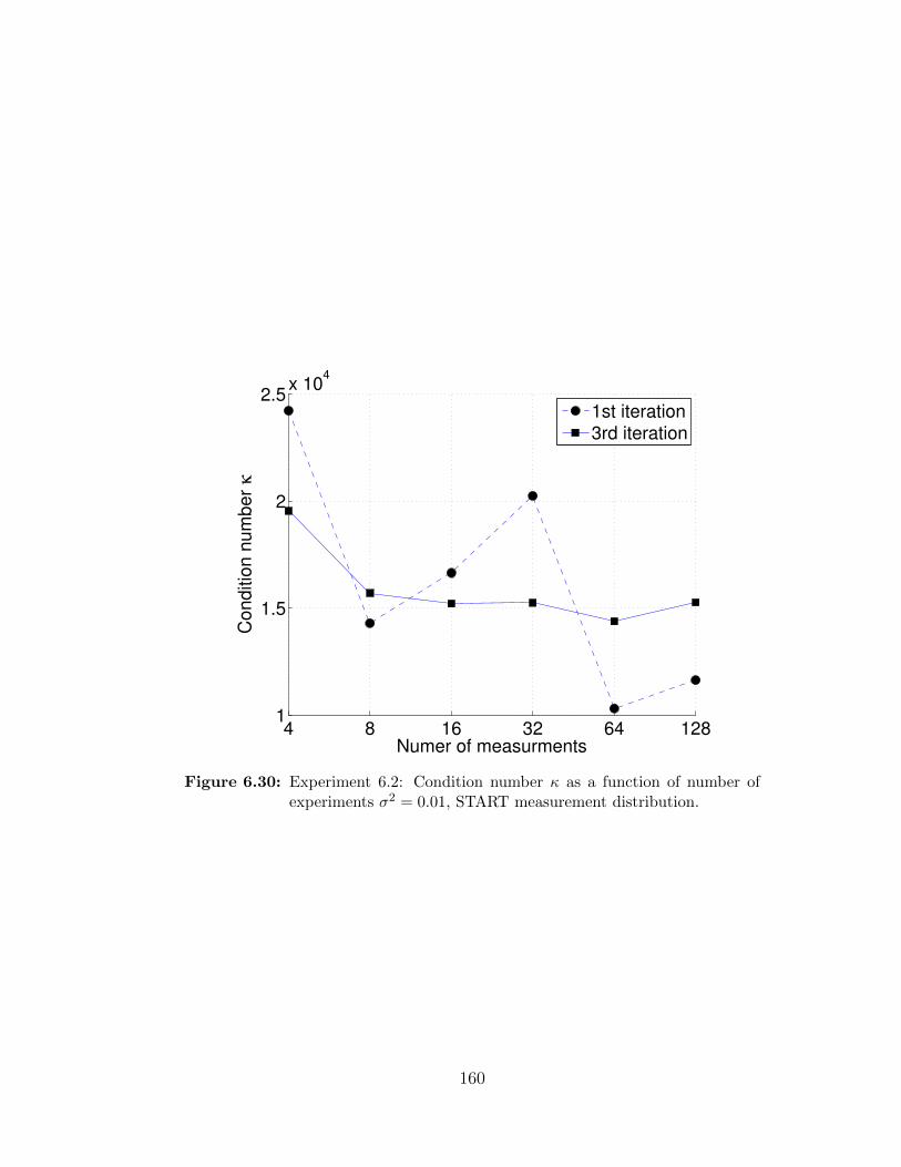
4 8 16 32 64 1281
1.5
2
2.5x 10
4
Numer of measurments
Conditio
n n
um
ber
κ
1st iteration
3rd iteration
Figure 6.30: Experiment 6.2: Condition number κ as a function of number ofexperiments σ2 = 0.01, START measurement distribution.
160

4 8 16 32 64 1280
0.05
0.1
0.15
0.2
Numer of measurments
RM
SE
1st iteration
3rd iteration
Figure 6.31: Experiment 6.2: Root-mean-square error of observations as a func-tion of number of experiments σ2 = 0.01, MIDDLE measurementdistribution.
161

4 8 16 32 64 1282.5
3
3.5
4
4.5
5
5.5
6x 10
4
Numer of measurments
Conditio
n n
um
ber
κ
1st iteration
3rd iteration
Figure 6.32: Experiment 6.2: Condition number κ as a function of number ofexperiments σ2 = 0.01, MIDDLE measurement distribution.
162

4 8 16 32 64 1280
0.05
0.1
0.15
0.2
0.25
0.3
0.35
Numer of measurments
RM
SE
1st iteration
3rd iteration
Figure 6.33: Experiment 6.2: Root-mean-square error of observations as a func-tion of number of experiments σ2 = 0.01, FINISH measurementdistribution.
163

4 8 16 32 64 1280
1
2
3
4
5
6x 10
5
Numer of measurments
Co
nd
itio
n n
um
be
r κ
1st iteration
3rd iteration
Figure 6.34: Experiment 6.2: Condition number κ as a function of number ofexperiments σ2 = 0.01, FINISH measurement distribution.
164

4 8 16 32 64 1280
0.05
0.1
0.15
0.2
0.25
Numer of measurments
RM
SE
1st iteration
3rd iteration
Figure 6.35: Experiment 6.2: Root-mean-square error of observations as a func-tion of number of experiments σ2 = 0.01, UNIFORM measurementdistribution.
165

4 8 16 32 64 1282
4
6
8
10
12
14x 10
4
Numer of measurments
Co
nd
itio
n n
um
be
r κ
1st iteration
3rd iteration
Figure 6.36: Experiment 6.2: Condition number κ as a function of number ofexperiments σ2 = 0.01, UNIFORM measurement distribution.
166

4 8 16 32 64 1280.01
0.02
0.03
0.04
0.05
0.06
0.07
0.08
0.09
Numer of measurments
RM
SE
1st iteration
3rd iteration
Figure 6.37: Experiment 6.2: Root-mean-square error of observations as a func-tion of number of experiments σ2 = 0.02, START measurementdistribution.
167

4 8 16 32 64 1281
1.5
2
2.5
3x 10
4
Numer of measurments
Conditio
n n
um
ber
κ
1st iteration
3rd iteration
Figure 6.38: Experiment 6.2: Condition number κ as a function of number ofexperiments σ2 = 0.02, START measurement distribution.
168

4 8 16 32 64 1280
0.05
0.1
0.15
0.2
Numer of measurments
RM
SE
1st iteration
3rd iteration
Figure 6.39: Experiment 6.2: Root-mean-square error of observations as a func-tion of number of experiments σ2 = 0.02, MIDDLE measurementdistribution.
169

4 8 16 32 64 1283
3.5
4
4.5
5
5.5
6
6.5
7x 10
4
Numer of measurments
Conditio
n n
um
ber
κ
1st iteration
3rd iteration
Figure 6.40: Experiment 6.2: Condition number κ as a function of number ofexperiments σ2 = 0.02, MIDDLE measurement distribution.
170

4 8 16 32 64 1280
0.05
0.1
0.15
0.2
0.25
0.3
0.35
Numer of measurments
RM
SE
1st iteration
3rd iteration
Figure 6.41: Experiment 6.2: Root-mean-square error of observations as a func-tion of number of experiments σ2 = 0.02, FINISH measurementdistribution.
171

4 8 16 32 64 1280.6
0.8
1
1.2
1.4
1.6
1.8x 10
5
Numer of measurments
Conditio
n n
um
ber
κ
1st iteration
3rd iteration
Figure 6.42: Experiment 6.2: Condition number κ as a function of number ofexperiments σ2 = 0.02, FINISH measurement distribution.
172

4 8 16 32 64 1280
0.05
0.1
0.15
0.2
Numer of measurments
RM
SE
1st iteration
3rd iteration
Figure 6.43: Experiment 6.2: Root-mean-square error of observations as a func-tion of number of experiments σ2 = 0.02, UNIFORM measurementdistribution.
173

Table 6.13: Experiment 6.2: Comparison of data assimilations for a set of dis-tributions with different number of measurements and errors withσ2 = 0.005
Distribution of Number of RMS Error κmeasurements measurements of observations
Iteration Iteration1st 3rd 1st 3rd
4 0.0190 0.0056 1.7e+04 1.7e+048 0.0621 0.0184 1.2e+04 1.4e+04
START 16 0.0496 0.0108 2.3e+04 1.5e+0432 0.0087 0.0066 1.6e+04 1.5e+0464 0.0542 0.0161 2.2e+04 1.5e+04128 0.0530 0.0141 1.1e+04 1.5e+044 0.0395 0.0073 3.5e+04 3.1e+048 0.1538 0.0984 2.8e+04 3.2e+04
MIDDLE 16 0.1127 0.0351 5.1e+04 3.6e+0432 0.0143 0.0053 4.1e+04 3.9e+0464 0.1354 0.0650 6.4e+04 3.6e+04128 0.1235 0.0631 3.4e+04 3.5e+044 0.0574 0.0145 1.1e+05 1.4e+058 0.2532 0.1322 7.9e+04 6.9e+04
FINISH 16 0.1752 0.1834 1.2e+05 1.1e+0532 0.0213 0.0058 1.1e+05 1.1e+0564 0.2312 0.1393 1.7e+05 1.2e+05128 0.2040 0.1753 8.7e+04 9.9e+044 0.0319 0.0071 2.2e+05 1.3e+058 0.1642 0.1307 2.9e+04 1.6e+04
UNIFORM 16 0.1182 0.0536 4.4e+04 3.8e+0432 0.0160 0.0066 4.4e+04 4.2e+0464 0.1555 0.0801 5.3e+04 1.4e+04128 0.1406 0.1152 2.8e+04 2.5e+04
174

Table 6.14: Experiment 6.2: Comparison of data assimilations for a set of dis-tributions with different number of measurements and errors withσ2 = 0.075
Distribution of Number of RMS Error κmeasurements measurements of observations
Iteration Iteration1st 3rd 1st 3rd
4 0.0579 0.0138 2.5e+04 1.8e+048 0.0182 0.0085 1.6e+04 1.4e+04
START 16 0.0494 0.0132 1.1e+04 1.4e+0432 0.0397 0.0134 1.2e+04 1.5e+0464 0.0145 0.0110 1.5e+04 1.6e+04128 0.0368 0.0119 1.2e+04 1.5e+044 0.1411 0.0511 5.7e+04 3.0e+048 0.0502 0.0167 4.1e+04 3.5e+04
MIDDLE 16 0.1253 0.0669 3.4e+04 3.3e+0432 0.0995 0.0425 3.5e+04 3.8e+0464 0.0183 0.0114 3.9e+04 3.9e+04128 0.0971 0.0397 3.6e+04 3.7e+044 0.2377 0.1652 1.5e+05 1.1e+058 0.0900 0.0312 1.1e+05 1.2e+05
FINISH 16 0.2175 0.1758 8.0e+04 1.3e+0532 0.1716 0.1376 9.3e+04 1.2e+0564 0.0220 0.0115 1.2e+05 1.1e+05128 0.1871 0.1869 8.6e+04 9.8e+044 0.1400 0.0592 4.8e+04 8.4e+048 0.0546 0.0173 4.7e+04 3.3e+04
UNIFORM 16 0.1429 0.1263 2.8e+04 2.7e+0432 0.1151 0.0704 3.0e+04 3.0e+0464 0.0190 0.0105 4.4e+04 4.2e+04128 0.1230 0.0923 3.2e+04 3.7e+04
175

Table 6.15: Experiment 6.2: Comparison of data assimilations for a set of dis-tributions with different number of measurements and errors withσ2 = 0.01
Distribution of Number of RMS Error κmeasurements measurements of observations
Iteration Iteration1st 3rd 1st 3rd
4 0.0565 0.0162 2.4e+04 2.0e+048 0.0190 0.0131 1.4e+04 1.6e+04
START 16 0.0178 0.0139 1.7e+04 1.5e+0432 0.0359 0.0130 2.0e+04 1.5e+0464 0.0800 0.0300 1.0e+04 1.4e+04128 0.0441 0.0169 1.2e+04 1.5e+044 0.1428 0.0600 5.8e+04 3.2e+048 0.0156 0.0139 3.5e+04 3.6e+04
MIDDLE 16 0.0293 0.0112 4.0e+04 3.7e+0432 0.0792 0.0250 5.0e+04 4.0e+0464 0.1866 0.1402 2.7e+04 3.1e+04128 0.0981 0.0429 3.4e+04 3.9e+044 0.2335 0.1798 1.5e+05 1.3e+058 0.0261 0.0213 1.2e+05 1.2e+05
FINISH 16 0.0394 0.0133 1.1e+05 1.2e+0532 0.1507 0.0915 1.3e+05 1.3e+0564 0.2840 0.1718 8.2e+04 5.6e+05128 0.1527 0.1052 1.0e+05 1.3e+054 0.1260 0.0613 5.2e+04 1.4e+058 0.0080 0.0069 3.8e+04 3.9e+04
UNIFORM 16 0.0249 0.0105 4.4e+04 4.1e+0432 0.1020 0.0408 4.1e+04 3.1e+0464 0.2010 0.1273 3.3e+04 5.4e+04128 0.1088 0.0577 3.0e+04 2.9e+04
176

Table 6.16: Experiment 6.2: Comparison of data assimilations for a set of dis-tributions with different number of measurements and errors withσ2 = 0.0125
Distribution of Number of RMS Error κmeasurements measurements of observations
Iteration Iteration1st 3rd 1st 3rd
4 0.0361 0.0122 1.7e+04 1.8e+048 0.0309 0.0141 1.8e+04 1.5e+04
START 16 0.0355 0.0157 2.0e+04 1.5e+0432 0.0595 0.0203 2.3e+04 1.5e+0464 0.0709 0.0265 1.1e+04 1.5e+04128 0.0227 0.0182 1.5e+04 1.6e+044 0.0675 0.0188 3.8e+04 3.1e+048 0.0872 0.0358 4.5e+04 3.6e+04
MIDDLE 16 0.0858 0.0303 5.0e+04 3.8e+0432 0.1336 0.0557 5.8e+04 3.6e+0464 0.1592 0.1037 3.0e+04 3.0e+04128 0.0306 0.0210 4.1e+04 3.9e+044 0.1174 0.0609 9.2e+04 1.2e+058 0.1243 0.0636 1.1e+05 1.4e+05
FINISH 16 0.1481 0.0998 1.2e+05 1.4e+0532 0.2217 0.1664 1.6e+05 9.9e+0464 0.2506 0.1277 7.9e+04 9.5e+04128 0.0327 0.0355 1.1e+05 1.1e+054 0.0773 0.1497 2.5e+05 5.1e+048 0.0807 0.0274 5.1e+04 3.4e+04
UNIFORM 16 0.0967 0.0384 4.3e+04 3.5e+0432 0.1499 0.0844 4.6e+04 2.4e+0464 0.1757 0.1409 2.7e+04 2.2e+04128 0.0280 0.0226 3.9e+04 4.4e+04
177

Table 6.17: Experiment 6.2: Comparison of data assimilations for a set of dis-tributions with different number of measurements and errors withσ2 = 0.015
Distribution of Number of RMS Error κmeasurements measurements of observations
Iteration Iteration1st 3rd 1st 3rd
4 0.0418 0.0129 1.7e+04 1.8e+048 0.0874 0.0375 2.7e+04 1.4e+04
START 16 0.0481 0.0254 1.2e+04 1.5e+0432 0.0256 0.0238 1.6e+04 1.6e+0464 0.0239 0.0198 1.4e+04 1.5e+04128 0.0349 0.0185 1.2e+04 1.6e+044 0.1059 0.0468 3.5e+04 3.2e+048 0.1810 0.0865 6.6e+04 2.8e+04
MIDDLE 16 0.1033 0.0461 3.5e+04 3.5e+0432 0.0199 0.0186 3.9e+04 3.9e+0464 0.0380 0.0209 3.6e+04 4.0e+04128 0.0748 0.0311 3.5e+04 4.1e+044 0.1774 0.1651 8.1e+04 1.0e+058 0.2422 0.1288 1.7e+05 1.2e+05
FINISH 16 0.1801 0.1638 8.9e+04 1.1e+0532 0.0180 0.0172 1.1e+05 1.1e+0564 0.0520 0.0190 1.2e+05 1.1e+05128 0.1251 0.0664 1.1e+05 1.3e+054 0.1153 0.5134 1.0e+06 6.0e+048 0.1776 0.0880 5.2e+04 8.6e+03
UNIFORM 16 0.1163 0.0786 2.9e+04 3.2e+0432 0.0197 0.0192 4.3e+04 4.2e+0464 0.0416 0.0197 3.9e+04 3.9e+04128 0.0862 0.0363 3.5e+04 3.6e+04
178

Table 6.18: Experiment 6.2: Comparison of data assimilations for a set of dis-tributions with different number of measurements and errors withσ2 = 0.0175
Distribution of Number of RMS Error κmeasurements measurements of observations
Iteration Iteration1st 3rd 1st 3rd
4 0.0211 0.0095 1.9e+04 1.7e+048 0.0339 0.0220 1.9e+04 1.5e+04
START 16 0.0489 0.0209 1.1e+04 1.5e+0432 0.0417 0.0273 2.0e+04 1.5e+0464 0.0303 0.0251 1.8e+04 1.5e+04128 0.0469 0.0268 1.2e+04 1.6e+044 0.0609 0.0177 3.6e+04 3.0e+048 0.0927 0.0475 4.9e+04 3.3e+04
MIDDLE 16 0.1131 0.0573 3.4e+04 3.4e+0432 0.0892 0.0428 5.2e+04 3.9e+0464 0.0495 0.0265 4.6e+04 3.9e+04128 0.0952 0.0441 3.5e+04 3.9e+044 0.1185 0.0568 9.5e+04 1.3e+058 0.1412 0.0913 1.1e+05 1.5e+05
FINISH 16 0.1905 0.1706 8.8e+04 1.2e+0532 0.1564 0.0867 1.3e+05 1.3e+0564 0.0794 0.0313 1.1e+05 1.2e+05128 0.1643 0.1274 9.9e+04 1.3e+054 0.0628 0.0269 3.9e+04 9.7e+048 0.0946 0.0429 5.6e+04 3.4e+04
UNIFORM 16 0.1264 0.0964 2.8e+04 3.3e+0432 0.1019 0.0497 4.2e+04 3.2e+0464 0.0573 0.0264 4.3e+04 3.8e+04128 0.1153 0.0670 3.2e+04 3.1e+04
179

Table 6.19: Experiment 6.2: Comparison of data assimilations for a set of dis-tributions with different number of measurements and errors withσ2 = 0.02
Distribution of Number of RMS Error κmeasurements measurements of observations
Iteration Iteration1st 3rd 1st 3rd
4 0.0479 0.0288 2.0e+04 3.0e+048 0.0456 0.0266 1.8e+04 1.4e+04
START 16 0.0237 0.0187 1.4e+04 1.5e+0432 0.0303 0.0271 1.7e+04 1.6e+0464 0.0282 0.0258 1.7e+04 1.6e+04128 0.0807 0.0379 2.3e+04 1.5e+044 0.0429 0.0171 3.3e+04 3.4e+048 0.0830 0.0402 4.3e+04 3.7e+04
MIDDLE 16 0.0389 0.0304 3.6e+04 4.0e+0432 0.0410 0.0339 4.0e+04 3.9e+0464 0.0442 0.0249 4.5e+04 3.9e+04128 0.1770 0.0844 6.7e+04 3.4e+044 0.1067 0.1812 1.1e+05 1.2e+058 0.1350 0.0658 1.1e+05 1.3e+05
FINISH 16 0.0384 0.0252 1.1e+05 1.2e+0532 0.0324 0.0298 1.1e+05 1.1e+0564 0.0830 0.0398 1.1e+05 1.2e+05128 0.2742 0.1449 1.7e+05 7.9e+044 0.0513 0.0209 4.6e+04 1.7e+058 0.0977 0.0407 4.8e+04 2.7e+04
UNIFORM 16 0.0326 0.0293 3.7e+04 3.9e+0432 0.0313 0.0262 4.4e+04 4.2e+0464 0.0509 0.0274 3.9e+04 4.0e+04128 0.1919 0.1158 6.1e+04 2.1e+04
180

6.2.3 Experiment 6.3
In a setup similar to Experiment 5.2, we are going to conduct data assimilation
experiments.
Table 6.20: Experiment 6.3: Base control vector α and initial conditions X(0)
u0 u1(0) v1(0) h1(0) x0 y0 t time step
1.000 0.000 0.500 0.000 0.0 0.0 0.5 2.5e-05
Table 6.21: Experiment 6.3: Perturbed control vector α and initial conditionsX(0)
u0 u1(0) v1(0) h1(0) x0 y0 t time step
1.129419 0.170145 0.549086 -0.040774 0.000 0.000 0.5 2.5e-05
181
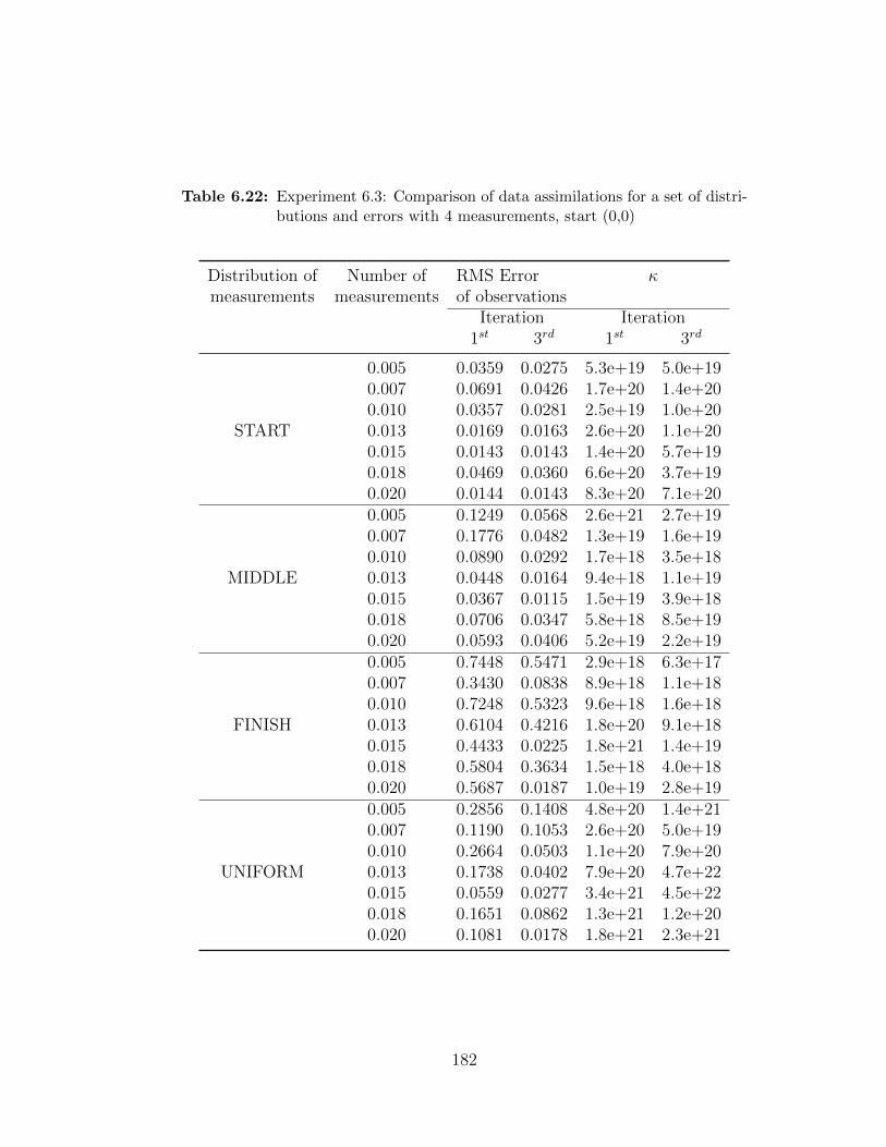
Table 6.22: Experiment 6.3: Comparison of data assimilations for a set of distri-butions and errors with 4 measurements, start (0,0)
Distribution of Number of RMS Error κmeasurements measurements of observations
Iteration Iteration1st 3rd 1st 3rd
0.005 0.0359 0.0275 5.3e+19 5.0e+190.007 0.0691 0.0426 1.7e+20 1.4e+200.010 0.0357 0.0281 2.5e+19 1.0e+20
START 0.013 0.0169 0.0163 2.6e+20 1.1e+200.015 0.0143 0.0143 1.4e+20 5.7e+190.018 0.0469 0.0360 6.6e+20 3.7e+190.020 0.0144 0.0143 8.3e+20 7.1e+200.005 0.1249 0.0568 2.6e+21 2.7e+190.007 0.1776 0.0482 1.3e+19 1.6e+190.010 0.0890 0.0292 1.7e+18 3.5e+18
MIDDLE 0.013 0.0448 0.0164 9.4e+18 1.1e+190.015 0.0367 0.0115 1.5e+19 3.9e+180.018 0.0706 0.0347 5.8e+18 8.5e+190.020 0.0593 0.0406 5.2e+19 2.2e+190.005 0.7448 0.5471 2.9e+18 6.3e+170.007 0.3430 0.0838 8.9e+18 1.1e+180.010 0.7248 0.5323 9.6e+18 1.6e+18
FINISH 0.013 0.6104 0.4216 1.8e+20 9.1e+180.015 0.4433 0.0225 1.8e+21 1.4e+190.018 0.5804 0.3634 1.5e+18 4.0e+180.020 0.5687 0.0187 1.0e+19 2.8e+190.005 0.2856 0.1408 4.8e+20 1.4e+210.007 0.1190 0.1053 2.6e+20 5.0e+190.010 0.2664 0.0503 1.1e+20 7.9e+20
UNIFORM 0.013 0.1738 0.0402 7.9e+20 4.7e+220.015 0.0559 0.0277 3.4e+21 4.5e+220.018 0.1651 0.0862 1.3e+21 1.2e+200.020 0.1081 0.0178 1.8e+21 2.3e+21
182

−0.6 −0.4 −0.2 0 0.2−0.5
0
0.5
1
X
Y
Base
First
Third
Observation
Figure 6.44: Experiment 6.3: Track START σ2 = 0.005
−0.6 −0.4 −0.2 0 0.2−0.5
0
0.5
1
X
Y
Base
First
Third
Observation
Figure 6.45: Experiment 6.3: Track MIDDLE σ2 = 0.005
183
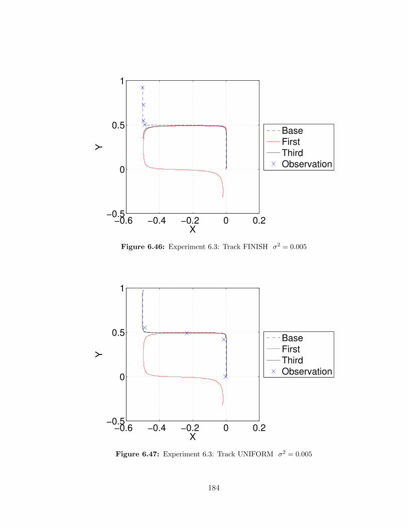
−0.6 −0.4 −0.2 0 0.2−0.5
0
0.5
1
X
Y
Base
First
Third
Observation
Figure 6.46: Experiment 6.3: Track FINISH σ2 = 0.005
−0.6 −0.4 −0.2 0 0.2−0.5
0
0.5
1
X
Y
Base
First
Third
Observation
Figure 6.47: Experiment 6.3: Track UNIFORM σ2 = 0.005
184

−0.6 −0.4 −0.2 0 0.2−0.2
0
0.2
0.4
0.6
0.8
1
X
Y
Base
First
Third
Observation
Figure 6.48: Experiment 6.3: Track START σ2 = 0.0075
−0.6 −0.4 −0.2 0 0.2−0.5
0
0.5
1
X
Y
Base
First
Third
Observation
Figure 6.49: Experiment 6.3: Track MIDDLE σ2 = 0.0075
185

−0.6 −0.4 −0.2 0 0.20
0.2
0.4
0.6
0.8
1
X
Y
Base
First
Third
Observation
Figure 6.50: Experiment 6.3: Track FINISH σ2 = 0.0075
−0.6 −0.4 −0.2 0 0.2−0.5
0
0.5
1
X
Y
Base
First
Third
Observation
Figure 6.51: Experiment 6.3: Track UNIFORM σ2 = 0.0075
186

−0.6 −0.4 −0.2 0 0.2−0.5
0
0.5
1
X
Y
Base
First
Third
Observation
Figure 6.52: Experiment 6.3: Track START σ2 = 0.01
−0.6 −0.4 −0.2 0 0.2−0.5
0
0.5
1
X
Y
Base
First
Third
Observation
Figure 6.53: Experiment 6.3: Track MIDDLE σ2 = 0.01
187

−0.6 −0.4 −0.2 0 0.2−0.5
0
0.5
1
X
Y
Base
First
Third
Observation
Figure 6.54: Experiment 6.3: Track FINISH σ2 = 0.01
−0.6 −0.4 −0.2 0 0.2−0.5
0
0.5
1
X
Y
Base
First
Third
Observation
Figure 6.55: Experiment 6.3: Track UNIFORM σ2 = 0.01
188

−0.6 −0.4 −0.2 0 0.2−0.5
0
0.5
1
X
Y
Base
First
Third
Observation
Figure 6.56: Experiment 6.3: Track START σ2 = 0.0125
−0.6 −0.4 −0.2 0 0.2−0.5
0
0.5
1
X
Y
Base
First
Third
Observation
Figure 6.57: Experiment 6.3: Track MIDDLE σ2 = 0.0125
189
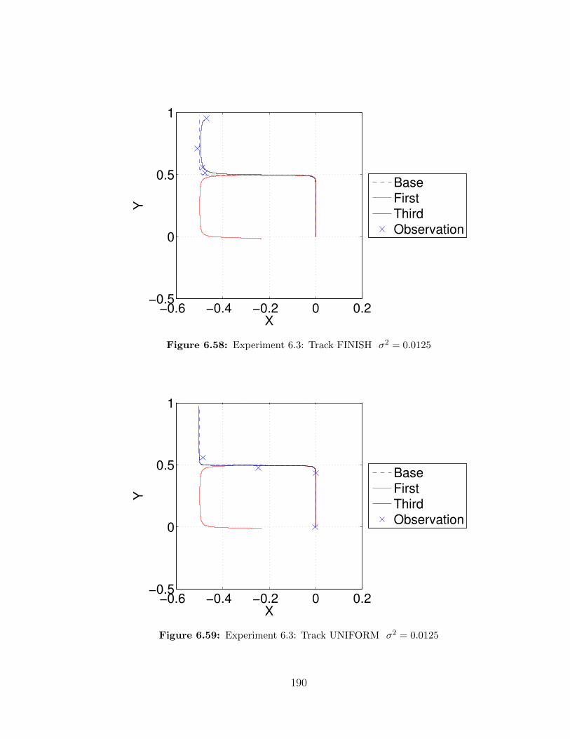
−0.6 −0.4 −0.2 0 0.2−0.5
0
0.5
1
X
Y
Base
First
Third
Observation
Figure 6.58: Experiment 6.3: Track FINISH σ2 = 0.0125
−0.6 −0.4 −0.2 0 0.2−0.5
0
0.5
1
X
Y
Base
First
Third
Observation
Figure 6.59: Experiment 6.3: Track UNIFORM σ2 = 0.0125
190

−0.6 −0.4 −0.2 0 0.20
0.2
0.4
0.6
0.8
1
X
Y
Base
First
Third
Observation
Figure 6.60: Experiment 6.3: Track START σ2 = 0.015
−0.6 −0.4 −0.2 0 0.2−0.5
0
0.5
1
X
Y
Base
First
Third
Observation
Figure 6.61: Experiment 6.3: Track MIDDLE σ2 = 0.015
191
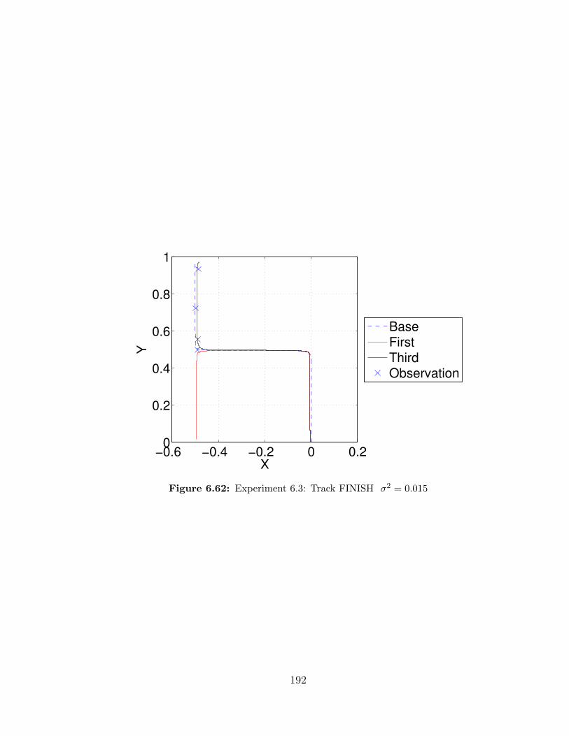
−0.6 −0.4 −0.2 0 0.20
0.2
0.4
0.6
0.8
1
X
Y
Base
First
Third
Observation
Figure 6.62: Experiment 6.3: Track FINISH σ2 = 0.015
192

−0.6 −0.4 −0.2 0 0.2−0.5
0
0.5
1
X
Y
Base
First
Third
Observation
Figure 6.63: Experiment 6.3: Track UNIFORM σ2 = 0.015
−0.6 −0.4 −0.2 0 0.2−0.5
0
0.5
1
X
Y
Base
First
Third
Observation
Figure 6.64: Experiment 6.3: Track START σ2 = 0.0175
193

−0.6 −0.4 −0.2 0 0.2−0.5
0
0.5
1
X
Y
Base
First
Third
Observation
Figure 6.65: Experiment 6.3: Track MIDDLE σ2 = 0.0175
194

−0.6 −0.4 −0.2 0 0.2−0.5
0
0.5
1
X
Y
Base
First
Third
Observation
Figure 6.66: Experiment 6.3: Track FINISH σ2 = 0.0175
−0.6 −0.4 −0.2 0 0.2−0.5
0
0.5
1
X
Y
Base
First
Third
Observation
Figure 6.67: Experiment 6.3: Track UNIFORM σ2 = 0.0175
195
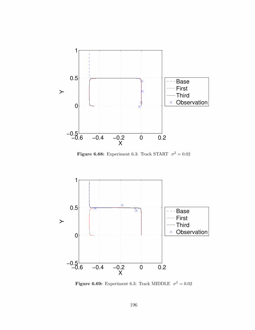
−0.6 −0.4 −0.2 0 0.2−0.5
0
0.5
1
X
Y
Base
First
Third
Observation
Figure 6.68: Experiment 6.3: Track START σ2 = 0.02
−0.6 −0.4 −0.2 0 0.2−0.5
0
0.5
1
X
Y
Base
First
Third
Observation
Figure 6.69: Experiment 6.3: Track MIDDLE σ2 = 0.02
196

−0.6 −0.4 −0.2 0 0.2−0.5
0
0.5
1
X
Y
Base
First
Third
Observation
Figure 6.70: Experiment 6.3: Track FINISH σ2 = 0.02
−0.6 −0.4 −0.2 0 0.2−0.5
0
0.5
1
X
Y
Base
First
Third
Observation
Figure 6.71: Experiment 6.3: Track UNIFORM σ2 = 0.02
197

6.3 Summary
Experiments 6.1 and 6.2 using (4, 8, 16, 32, 64 and 128) measurements dis-
tributed in four distinct patterns: START, MIDDLE, FINISH and UNIFORM
prove effectiveness of the forward sensitivity method applied to data assimilation
of the linear shallow water model tracers. In almost all cases, after third iteration
improving match between observations and model prediction, root-square mean
error is reduced. Method proves effective in a presence of wide selection of the
observational error variance used to generate observations. Visual inspection of
the forecast error shows its close relation to model sensitivity and distribution of
observations (START, MIDDLE, FINISH and UNIFORM). In cases where obser-
vations are taken in a period when sensitivity is higher, overall forecast error is
smaller when compared to cases when sensitivity is lower. For cases when trajec-
tories are well within the cell, condition number κ is in order of 104 to 105. It is
noted that increasing the number of observations does not necessarily reduce the
root-square mean error by much; this fact depends however on the observational
error variance σ.
Experiments are indicating that even when the condition number κ is of order
of 1020, there can be an improvement made to the control vector, if the location
of measurements is in the time period when the model has high sensitivity to the
control vector, as shown in Experiment 6.3.
Results illustrating the model sensitivity to initial conditions are the elements
of the control vector together with the data assimilation experiments described
by Jabrzemski and Lakshmivarahan (2014) [6] were presented at the American
Meteorological Society Annual Meeting.
198

Chapter 7
Conclusions
Our work in this dissertation is centered on the linearized shallow water model
used by other researchers to evaluate Lagrangian data assimilation. It is divided
into two major parts.
First one, focuses on finding the closed form solution to the linearized shallow
water model. This in turn, allows us to provide a complete characterization of the
properties of equilibria of the tracer dynamics given by a system of two first order
nonlinear time varying ordinary differential equations. This dynamics is derived
from a low order or reduced order spectral model obtained using Galerkin type
projection of the linearized shallow water equations, while the tracer dynamics
is controlled by four parameters, we provide a succinct characterization of the
bifurcation using a system of hyperbolas in two dimensions. The shallow water
model is thoroughly analyzed after looking separately at the geostrophic mode,
the inertia-gravity mode, and both of them combined. We find that most ap-
plications of the shallow water model in meteorology and oceanography use the
model within region 2, and we don’t have to be concerned with the bifurcations
in the control space.
199

Second part focuses on application of the forward sensitivity method to a
problem that is historically done in meteorology and oceanography with the use
of 4D-Var method. Several experiments investigated sensitivity of the LSWM to
initial conditions and control vector elements. They gave a good illustration of the
fact that the sensitivity has to be considered on the case by case basis. Therefore,
model sensitivity gives a great insight into the model dynamics and its relation
to the forecasting error. In this respect, FSM provides information about how
each element of the control vector influences the solution; it shows the relation
of the magnitudes of sensitivity together with their temporal distribution. This
in turn helps to guide the placement of observations, or determines the impact
of the observations on the forecast improvement.
Number of numerical experiments conducted with the use of FSM to assim-
ilate data explains possible difficulties with the judicious placement of the ob-
servations by highlighting the fine physical structure of the model; there is a big
value in using the closed form solution derived in the first part of this dissertation
in accomplishing this second goal. Influence of the temporal distribution of the
observations can be explained by evaluation of the sensitivity functions that are
also derived in the closed form. There is a definite relation between a distribution
of the observations and forecast error. Data assimilation of observations taken in
the temporal domain related to the high sensitivity has smaller error forecast and
better match of forecasted and measured tracer positions. It is worth noting that
increasing the number of observations does not always lead to the improvement of
the forecast error as a difference between the observations and predicted values.
Future work with the use of FSM and LSWM should focus on analyzing
possible improvement to the initial condition estimation subject to the initial
incorrect tracer position. Next, the forward sensitivity method can be used to
200

improve the initial conditions and the elements of the control vector, when both
of them are incorrect. We have investigated only the measurements related to the
horizontal position of a tracer, data assimilation of the height measurements can
also be of interest. Data assimilation experiments can investigate FSM usefulness
in analyzing data assimilation in the model while the small changes in the control
vector can lead to bifurcations of the model.
201

Bibliography
[1] Apte, A., Jones, C. K., and Stuart, A. A bayesian approach to
lagrangian data assimilation. Tellus A 60, 2 (2008), 336–347.
[2] Carter, E. F. Assimilation of lagrangian data into a numerical model.
Dynamics of atmospheres and oceans 13, 3 (1989), 335–348.
[3] Daley, R. Atmospheric data analysis. Cambridge university press, 1991.
[4] Hirsch, M. W., Smale, S., and Devaney, R. L. Differential equations,
dynamical systems and an introduction to chaos, vol. 60. Access Online via
Elsevier, 2004.
[5] Jabrzemski, R., and Lakshmivarahan, S. Lagrangian data assimila-
tion: Part I analysis of bifurcations in tracer dynamics. In Proc. 17th Confer-
ence on Integrated Observing and Assimilation Systems for the Atmosphere,
Oceans, and Land Surface (IOAS-AOLS) (2013), American Meteorological
Society.
[6] Jabrzemski, R., and Lakshmivarahan, S. Lagrangian data assimi-
lation: Part II data assimilation with the forward sensitivity method. In
Proc. 18th Conference on Integrated Observing and Assimilation Systems for
202

the Atmosphere, Oceans, and Land Surface (IOAS-AOLS) (2014), American
Meteorological Society.
[7] Kuznetsov, L., Ide, K., and Jones, C. A method for assimilation of
lagrangian data. Monthly Weather Review 131, 10 (2003), 2247–2260.
[8] Lakshmivarahan, S., Baldwin, M. E., and Zheng, T. Further analy-
sis of lorenz’s maximum simplification equations. Journal of the atmospheric
sciences 63, 11 (2006), 2673–2699.
[9] Lakshmivarahan, S., and Lewis, J. Forecast bias correction using for-
ward sensitivity analysis: A framework. Tech. rep., School of Computer
Science, University of Oklahoma, 2009.
[10] Lakshmivarahan, S., and Lewis, J. Forward sensitivity approach to
dynamic data assimilation. Advances in Meteorology 2010 (2010).
[11] Lakshmivarahan, S., and Lewis, J. M. Impact of observations on
adjoint sensitivity. Septermber 2011.
[12] Lewis, J. M., Lakshmivarahan, S., and Dhall, S. Dynamic data
assimilation: a least squares approach, vol. 13. Cambridge University Press,
2006.
[13] Lorenz, E. N. Maximum simplification of the dynamic equations. Tellus
12, 3 (1960), 243–254.
[14] Molcard, A., Piterbarg, L. I., Griffa, A., Ozgokmen, T. M., and
Mariano, A. J. Assimilation of drifter observations for the reconstruction
of the eulerian circulation field. Journal of geophysical research 108, C3
(2003), 3056.
203

[15] Ozgokmen, T. M., Molcard, A., Chin, T. M., Piterbarg, L. I.,
and Griffa, A. Assimilation of drifter observations in primitive equation
models of midlatitude ocean circulation. Journal of geophysical research 108,
C7 (2003), 3238.
[16] Pedlosky, J. Geophysical fluid dynamics. New York and Berlin, Springer-
Verlag, 1982. 636 p. 1 (1982).
[17] Rabitz, H., Kramer, M., and Dacol, D. Sensitivity analysis in chem-
ical kinetics. Annual review of physical chemistry 34, 1 (1983), 419–461.
[18] Salman, H., Ide, K., and Jones, C. K. Using flow geometry for drifter
deployment in lagrangian data assimilation. Tellus A 60, 2 (2008), 321–335.
204

Appendix A
Reduction process
We start with the linearized shallow water model equations (2.19):
∂u
∂t= v − ∂h
∂x, (A.1)
∂v
∂t= −u− ∂h
∂y, (A.2)
∂h
∂t= −∂u
∂x− ∂v
∂y. (A.3)
We express u, v and h in the standard two dimensional truncated Fourier series
consisting of only two terms given (3.1)
u(x, y, t) = −2πl sin(2πkx) cos(2πly)u0 + cos(2πmy)u1(t),
v(x, y, t) = +2πk cos(2πkx) sin(2πly)u0 + cos(2πmy)v1(t),
h(x, y, t) = sin(2πkx) sin(2πly)u0 + sin(2πmy)h1(t).
(A.4)
205
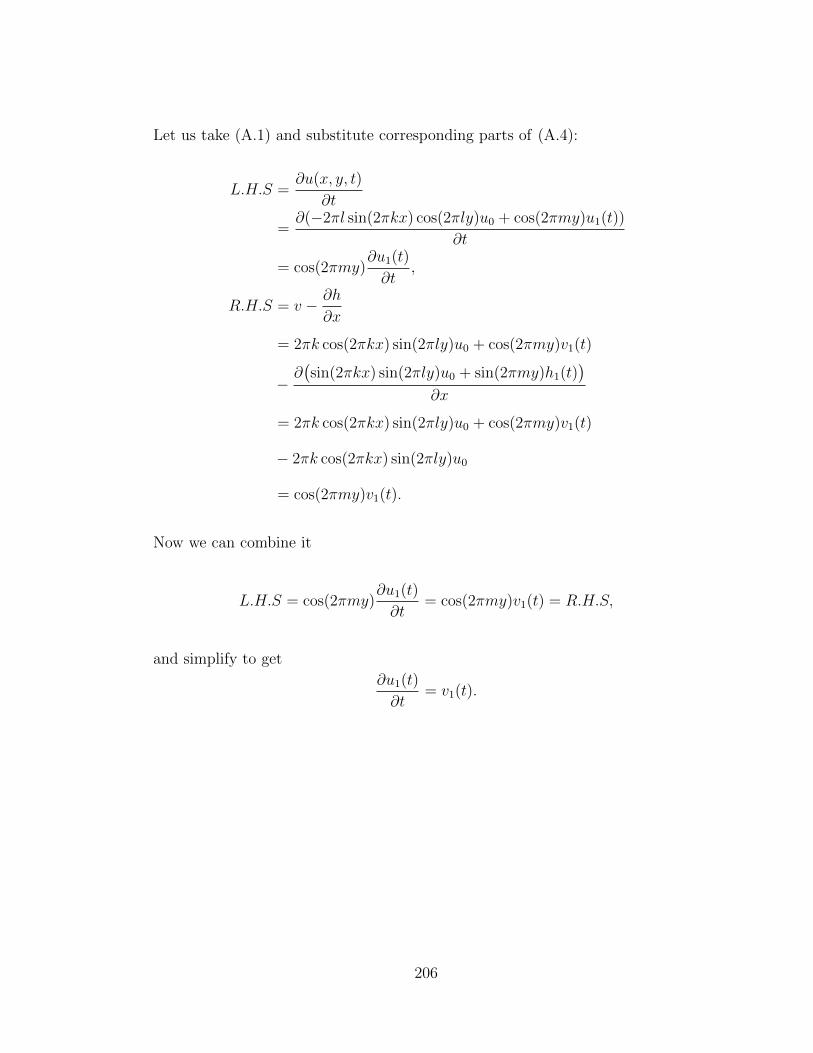
Let us take (A.1) and substitute corresponding parts of (A.4):
L.H.S =∂u(x, y, t)
∂t
=∂(−2πl sin(2πkx) cos(2πly)u0 + cos(2πmy)u1(t))
∂t
= cos(2πmy)∂u1(t)
∂t,
R.H.S = v − ∂h
∂x
= 2πk cos(2πkx) sin(2πly)u0 + cos(2πmy)v1(t)
−∂(sin(2πkx) sin(2πly)u0 + sin(2πmy)h1(t)
)∂x
= 2πk cos(2πkx) sin(2πly)u0 + cos(2πmy)v1(t)
− 2πk cos(2πkx) sin(2πly)u0
= cos(2πmy)v1(t).
Now we can combine it
L.H.S = cos(2πmy)∂u1(t)
∂t= cos(2πmy)v1(t) = R.H.S,
and simplify to get
∂u1(t)
∂t= v1(t).
206

Similarly, we can look at (A.2) and substitute corresponding parts of (A.4):
L.H.S =∂v(x, y, t)
∂t
=∂(2πk cos(2πkx) sin(2πly)u0 + cos(2πmy)v1(t)
)∂t
= cos(2πmy)∂v1(t)
∂t,
R.H.S = −u− ∂h
∂y
= 2πl sin(2πkx) cos(2πly)u0 − cos(2πmy)u1(t)
−∂(sin(2πkx) sin(2πly)u0 + sin(2πmy)h1(t)
)∂y
= 2πl sin(2πkx) cos(2πly)u0 − cos(2πmy)u1(t)
− 2πl sin(2πkx) cos(2πly)u0
− 2πm cos(2πmy)h1(t)
= − cos(2πmy)u1(t)− 2πm cos(2πmy)h1(t).
Now we can combine it
L.H.S = cos(2πmy)∂v1(t)
∂t= − cos(2πmy)u1(t)− 2πm cos(2πmy)h1(t) = R.H.S,
and simplify to get
∂v1(t)
∂t= −u1(t)− 2πmh1(t).
207

Finally, we can look at (A.3) and substitute corresponding parts of (A.4):
L.H.S =∂h(x, y, t)
∂t=∂(sin(2πkx) sin(2πly)u0 + sin(2πmy)h1(t)
)∂t
= sin(2πmy)∂h1(t)
∂t,
R.H.S = −∂u∂x− ∂v
∂y= −
∂(−2πl sin(2πkx) cos(2πly)u0 + cos(2πmy)u1(t)
)∂x
−∂(2πk cos(2πkx) sin(2πly)u0 + cos(2πmy)v1(t)
)∂y
= 2πl2πk cos(2πkx) cos(2πly)u0+
− 2πk2πl cos(2πkx) cos(2πly)u0 + 2πm sin(2πmy)v1(t)
= 2πm sin(2πmy)v1(t).
Now we can combine it
L.H.S = sin(2πmy)∂h1(t)
∂t= 2πm sin(2πmy)v1(t) = R.H.S,
and simplify to get
∂h1(t)
∂t= 2πmv1(t).
Using the fact that u0 is constant, we can get the equations describing amplitudes
as follows
u0 = 0,
u1 = v1,
v1 = −u1 − 2πmh1,
h1 = 2πmv1,
which is exactly the set of equations presented in (3.2).
208

Appendix B
Bounds on u1(t) in (2.14)
Let A and B be two real numbers with at least one of them non-zero. For
0 ≤ x ≤ 2π, consider the function
f(x) = A cosx+B sinx. (B.1)
The behavior of f(x) in the interval [0, 2π] is given in the following
Property B.0.1.
(a) f(x) attains its extremum values at x∗ where tanx∗ = B/A
(b) The distribution of(x∗, f(x∗)
)pair for various values and signs of A and B
are given in Table A.
(c) If f(x∗) is a maximum / minimum, then f(x∗+π) is a minimum / maximum.
(d) For all x ∈ [0, 2π],
−√A2 +B2 = fmin ≤ f(x) ≤ fmax =
√A2 +B2. (B.2)
209

Proof. Setting the derivative of f(x) to zero, the claim (a) follows. Hence
cosx∗ =A√
A2 +B2and sinx∗ =
B√A2 +B2
. (B.3)
Consider the case when A > 0 and B > 0 and A > B. For this choice of A
and B, it can be verified that 0 ≤ x∗ ≤ π/4. Further, it is easy to verify that the
second derivative of f(x) is negative at x∗ and positive at (x∗ + π). Hence f(x∗)
is a maximum and f(x∗+π) is a minimum from which one of the entries in Table
A and claim (c) follows. Considering these and (A.3) with (A.1), the claim (d)
immediately follows
Table B.1: Distribution of the pairs(x∗, f(x∗)
)Ratio A B x∗ belongs to f(x) =|A| > |B| + + [0, π/4] fmaxor - - [0, π/4] fmin0 ≤ |B|
|A| ≤ 1 - + [−π/4, 0] fmin+ - [−π/4, 0] fmax
|A| < |B| + + [π/4, π/2] fmaxor - - [π/4, π/2] fmin|B||A| ≥ 1 - + [−π/2,−π/4] fmax
+ - [−π/2,−π/4] fmin
210

Appendix C
Definition and properties of
standard hyperbola
Equation for a standard hyperbola with center at x0, y0) is given by (Spigel
(1968))
(x− x0)2
a2− (y − y0)2
b2= 1 (C.1)
where a and b are called the length of the semi major and semi minor axes
respectively. The graph of the hyperbola in (C.1) is given in Figure B1.
C is the center of the hyperbola whose coordinates are (x0, y0) with respect
to the origin 0. AA′ = 2a is the major axis, and BB′ = 2b is the minor axis. F
and F ′ are called the foci and CF = CF ′ =√a2 + b2. The eccentricity e of this
hyperbola is given by e =√a2+b2
a> 1. The slope of the asymptote HG′ is (b/a)
and the of the asymptote H ′G is −(b/a). The hatched region indicate where
(x− x0)2
a2− (y − y0)2
b2> 1.
211

Figure B.1: An illustration of the standard hyperbola given by (C.1).AA′ = 2a, BB′ = 2b, c is the center, F and F ′ are foci.
CF = CF ′ =√a2 + b2. The eccentricity c =
√a2+b2
a > 1.
212