Entropic-graphs: Applications

Alfred O. Hero

Dept. EECS, Dept Biomed. Eng., Dept. Statistics

University of Michigan - Ann Arbor

hero@eecs.umich.edu

http://www.eecs.umich.edu/˜hero

Collaborators: Huzefa Heemuchwala, Jose Costa, Bing Ma, Olivier

Michel

� Image registration

� Multivariate outlier rejection

� Divergence estimation

1

Image Registration

(a) ImageX0 (b) ImageXi

Figure 1: A multidate 3D breast-registration example

2

Range of UL breast Image Types

Figure 2: Three ultrasound breast scans. From top to bottom are: case 151,

case 142 and case 162.

3

MI Registration of Gray Levels (Viola&Wells:ICCV95)� X: aN�N UL image (lexicographically ordered)

� X(k): image gray level at pixel locationk

� X0 andX1: primary and secondary images to be registered

Hypothesis: f(X0(k);Xi(k)gN2

k=1 are i.i.d. r.v.’s with j.p.d.f

f0;i(x0;x1); x0;x1 2 f0;1; : : : ;255g

Mutual Information (MI) criterion : T = argmaxTiMI

whereMI is an estimate of

MI( f0;i) =Z Z

f0;i(x0;x1) ln f0;i(x0;x1)=( f0(x0) fi(x1))dx1dx0: (1)

4

(a) ImageIR (b) ImageIT

Figure 3: Single Pixel Coincidences (Left and right: reference imageIR at

0o and rotated imageIT at 8o)

5

Single-Pixel Scatterplot(ZRj ;Z

Tj )

pj=1

50 100 150 200 250

50

100

150

200

250

50 100 150 200 250

50

100

150

200

250

50 100 150 200 250

50

100

150

200

250

50 100 150 200 250

50

100

150

200

250

Figure 4:Grey level scatterplots. 1st Col: target=reference slice. 2nd Col: target = reference+1 slice.

6

α-MI Registration of Coincident Features� X: aN�N UL image (lexicographically ordered)

� Z = Z(X): a general image feature vector in aP-dimensional feature

space

Let fZ0(k)gKk=1 andfZi(k)gK

k=1 be features extracted fromX0 andXi at K

identical spatial locations

α-MI coincident-feature criterion

T = argmaxTiMIα

whereMIα is an estimate of

MIα( f0;i) =

1α�1

log

Z Z

f α0;i(z0;z1) f 1�α

0 (z0) f 1�αi (z1)dz1dz0: (2)

7

Why α-MI?

Special cases:

� α-MI vs. Shannon MI

limα!1

MIα( f0;i) =Z Z

f0;i ln f0;i=( f0 fi)dz1dz0:

� α-MI vs. Hellinger Mutual Affinity

MI 12

( f0;i) = � ln�Z Z p

f0;i f0 fi dz0dz1

�2

� α-MI vs. Batthacharyya-Hellinger information

Z Z �p

f0;i �p

f0 fi

�2dz0dz1 = 2

�1�expf�MI 1

2

( f0;i)g�

8

α-MI and Decision Theoretic Error Exponents

H0 : Z0(k);Zi(k) independent

H1 : Z0(k);Zi(k) o:w:

Bayes probability of error

Pe(n) = β(n)P(H1)+α(n)P(H0)

Chernoff bound

liminfn!∞

1n

logPe(n) =� supα2[0;1]

f(1�α)MIα( f0;i)g :9

−5 −4 −3 −2 −1 0 1 2 3 4 5−0.3

−0.25

−0.2

−0.15

−0.1

−0.05

0

0.05

ANGLE OF ROTATION (deg) −−−−−−>

α−D

IVE

RG

EN

CE

(αM

I) −

−−

−−

−>

α−DIVERGENCE v/s α CURVES FOR α ∈ [0,1] FOR SINGLE PIXEL INTENSITY

α =0 α =0.1α =0.2α =0.3α =0.4α =0.5α =0.6α =0.7α =0.8α =0.9

α=0.1

α=0.9

α=0

0 0.1 0.2 0.3 0.4 0.5 0.6 0.7 0.8 0.90

0.005

0.01

0.015

0.02

0.025

α −−−−−−>

curv

atur

e of

α−

MI −

−−

−−

−>

CURVATURE OF: α−MI v/s α CURVE FOR SINGLE PIXEL INTENSITY

Figure 5: Left: α-Divergence as function of angle. Right: Resolution ofα-

Divergence as function of alpha

10

Higher Level Features

Disadvantages of single-pixel features:

� Only depends on histogram of single pixel pairs

� Insensitive to spatial reording of pixels in each image

� Difficult to select out grey level anomalies (shadows, speckle)

� Spatial discriminants fall outside of single pixel domain

� Alternative : Aggregate spatial features

11

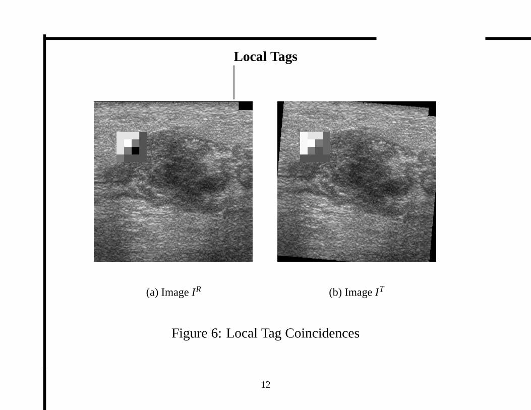
Local Tags

(a) ImageIR (b) ImageIT

Figure 6: Local Tag Coincidences

12

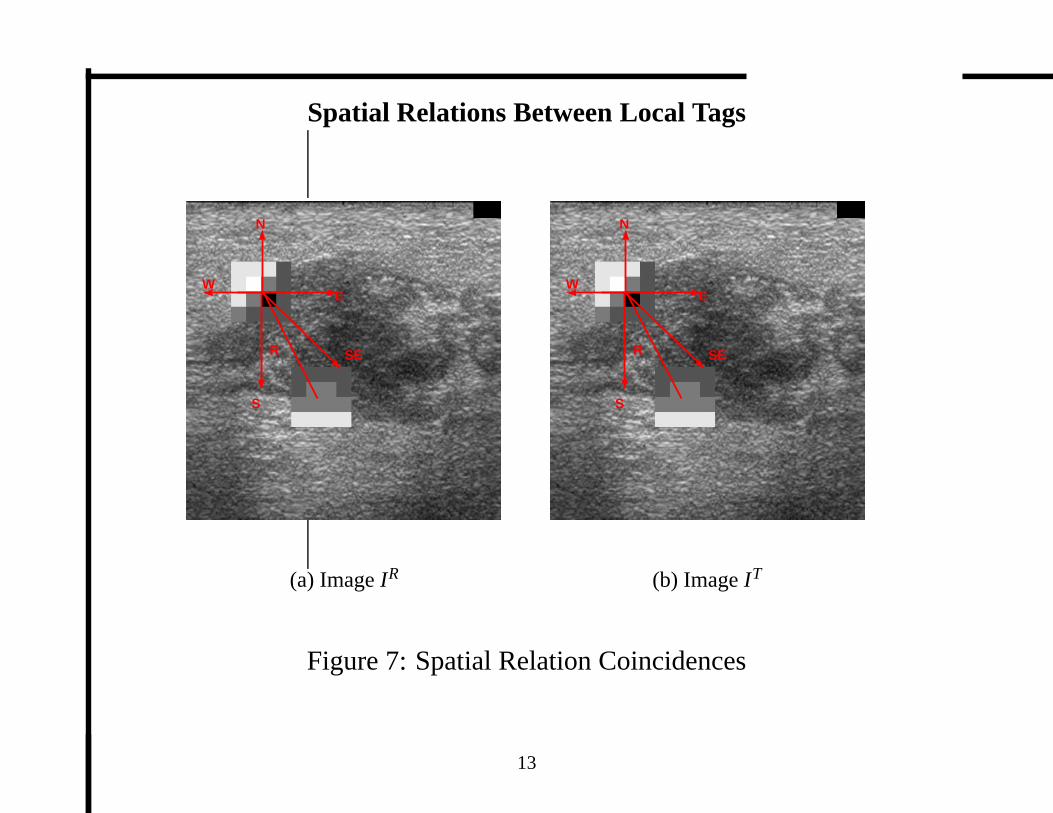
Spatial Relations Between Local Tags

N

E

SE

S

W

R

(a) ImageIR

N

E

SE

S

W

R

(b) ImageIT

Figure 7: Spatial Relation Coincidences

13

Feature Coincidence Tree of Local Tags

Root Node

Depth 1

Depth 2

Not examined further

Figure 8:Part of feature tree data structure.

Terminal nodes (Depth 16)

Figure 9:Leaves of feature tree data structure.

14

Forests of Randomized Feature TreesRANDOMIZED TREES

Figure 10:Forest of randomized trees

Registration criterion:

T = argmaxTi

# trees

∑t=1

MIα(t)

15

US Registration Comparisons

151 142 162

pixel 0:6=0:9 0:6=0:3 0:6=0:3

tag 0:5=3:6 0:5=3:8 0:4=1:4

spatial-tag 0:99=14:6 0:99=8:4 0:6=8:3

Table 1: Numerator =optimal values ofα and Denominator = maximum

resolution of mutualα-information for registering various images (Cases

151, 142, 162) using various features (pixel, tag, spatial-tag, ICA).

16

ICA Features

Decomposition ofM�M tag imagesY(k) acquired atk= 1; : : : ;K spatial

locations

Y(k) =

P

∑p=1

akpSp

� fSkg

Pk=1: statistically independent components

� akp: projection coefficients of tagY(k) onto componentSp

� fSkg

Pk=1 andP: selected via MLE and MDL

� Feature vector for coincidence processing:

Z(k) = [ak1; : : : ;akP]T

17

ICA feature basis for US breast images

Figure 11:Estimated ICA basis set for ultrasound breast image database

18

Feature-based Indexing: Challenges� How to best select discriminating features?

– Require training database of images to learn feature set

– Apply cross-validation...

– ...bagging, boosting, or randomized selection?

� How to computeα-MI for multi-dimensional features?

– Tag space is of high cardinality:25616� 1032

– ICA projection-coefficient space is multi-dimensional continuum

– Soln 1: partition feature space and count coincidences...

– Soln 2: apply density estimation and ...

– ... plug into theα-MI

– Soln 3: estimateα-MI directly

19

Methods of Entropy/Divergence Estimation� Z = (ZR;ZT): a statistic (feature pair)

� fZig: n i.i.d. realizations fromf (Z)

Objective: Estimate

Hα( f ) =1

1�αln

Z

f α(x)dx

1. Parametric density estimation methods

2. Non-parametric density estimation “plug-in” methods

3. Non-parametric minimal-graph estimation methods

20

Minimal Graphs: Minimal Spanning Tree (MST)

0 0.2 0.4 0.6 0.8 10

0.2

0.4

0.6

0.8

1

z1

z 2

128 random samples

0 0.2 0.4 0.6 0.8 10

0.2

0.4

0.6

0.8

1

z1

z 2

MST

0 0.2 0.4 0.6 0.8 10

0.2

0.4

0.6

0.8

1

z1

z 2

128 random samples

0 0.2 0.4 0.6 0.8 10

0.2

0.4

0.6

0.8

1

z1

z 2

MST

Figure 12:

21

Asymptotics of estimators ofHα( f )

DefineBσ;qp , the Besov space of`p(IRd) functions with smoothness given

by parametersσ andq.

Proposition 1 Let p> d� 2 andα = (d� γ)=d 2 [1=2;(d�1)=d]

supf α2B1;1

p

E1=κ

�����Z bf α(x)dx�Z

f α(x)dx

����κ

�� O

�

n�1=(2+d)�

while,

supf α2B1;1

p

E1=κ

�����Lγ(X1; : : : ;Xn)

nα �βLγ;dZ

f α(x)dx

����κ

��O

�

n

�

αλ(p)

1+αλ(p)

1d

�

whereλ(p) = d+1�d=p.

Note: minimal-graph estimator converges faster for allα� 1=2

22

Extension: divergence estimation� g(x): a reference density on IRd

� Assumef � g, i.e. for allx such thatg(x) = 0 we havef (x) = 0.

� Make measure transformationdx! g(x)dxon [0;1]d. Then forYn =

transformed data

limn!∞

L(Yn)=nα = βLγ;d exp((α�1)Dα( fkg)) ; (a:s:)

23

Proof

1. Make transformation of variablesx= [x1; : : : ;xd]T ! y= [y1; : : : ;yd]T

y1 = G(x1) (3)

y2 = G(x2jx1)

......

yd = G(xdjxd�1; : : : ;x1)

whereG(xkjxk�1; : : : ;x1) =R xk

�∞ g(xkjxk�1; : : : ;x1)dxk

2. Induced densityh(y), of the vectory, takes the form:

h(y) =

f (G�1(y1); : : : ;G�1(ydjyd�1; : : : ;y1))

g(G�1(y1); : : : ;G�1(ydjyd�1; : : : ;y1))

(4)

whereG�1 is inverse CDF andxk = G�1(ykjxk�1; : : : ;x1).

24

3. Then we know

Hα(Yn)!

11�α

ln

Z

hα(y)dy (a:s:)

4. By Jacobian formula:dy=���dy

dx

���dx= g(x)dx and

11�α

ln

Zhα(y)dy=

11�α

ln

Z �

f (x)

g(x)�α

g(x)dx= D( fkg)

25

0 0.2 0.4 0.6 0.8 10

0.2

0.4

0.6

0.8

1Original data

z1

z 2

0 0.2 0.4 0.6 0.8 1

0

0.2

0.4

0.6

0.8

1

exact inverse transform

z1

z 2

0 0.2 0.4 0.6 0.8 10

0.2

0.4

0.6

0.8

1tranfd data

z1

z 2

0 0.2 0.4 0.6 0.8 10

0.2

0.4

0.6

0.8

1tranfd data, 2D cdf estd

z1

z 2

Figure 13:Top Left: i.i.d. sample from triangular distribution, Top Right: exact

transformation, Bottom: after application of exact and empirical transformations.

26

Application: α-MI estimation

Objective: To estimate

MIα(X;Y) =

1α�1

ln

Z

f α(X;Y)( f (X) f (Y))1�αdXdY:

Assume thatf (X;Y) is such thatf α(X;Y) is in the the Besov space

B1p;1(R

2), p> 2 andα = 1=2.

Density plug in method: rms convergence rate

MSE12 (MI)�O(n�1=4)

Measure transformation method: rms convergence rate

MSE12 (MI)�O(n�αλ(p)=(1+αλ(p))1=d)!p!∞ O(n�3=10)

27

Alternative depedency measure:α-Jensen difference

1. Extract features from reference and transformed target images:

Xm = fXig

mi=1 and Yn = fYig

ni=1

2. Construct following MST function onXm andYn

∆L= lnLγ(Xm[Yn)=(n+m)α�m

n+mlnLγ(Xm)=mα�

nn+m

lnLγ(Yn)=nα

3. Minimize∆Lγ over transformations producingYn.

(1�α)�1∆L ! Hα (ε fx+(1� ε) fy)� εHα ( fx)� (1� ε)Hα ( fy)

whereε = mm+n

28

Example

0

200

400

0

100

200

3000

10

20

30

40

X

misaligned points

Y

Inte

nsity

(a)

0

200

400

0

100

200

3000

10

20

30

40

X

MST demonstration

Y

Inte

nsity

(b)

Figure 14: MST demonstration for misaligned images

29

0

200

400

0

100

200

3000

20

40

60

X

Aligned points

Y

Inte

nsity

(a)

0

200

400

0

100

200

3000

20

40

60

X

MST demonstration

Y

inte

nsity

(b)

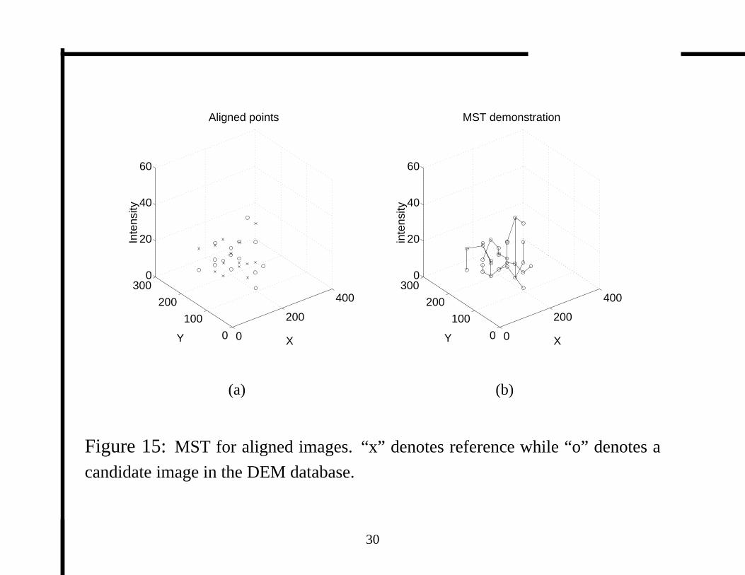
Figure 15:MST for aligned images. “x” denotes reference while “o” denotes a

candidate image in the DEM database.

30

254256

258260

262264

266 10

15

20

25

30

5500

6000

6500

7000

7500

8000

8500

9000

yrot

xrot

MS

T L

engt

h

MST Length versus Registration Angle

Figure 16:Scatter plot of MST length for a selection of relative rotation angles

between reference DEM image and target radar image.

31

Experimental results for US Image Registration

−8 −6 −4 −2 0 2 4 6 80

0.1

0.2

0.3

0.4

0.5

0.6

0.7

0.8

0.9

1

Relative rotation between images (degrees)

Nor

mal

ized

MS

T L

engt

h, M

I

MST Length, alphaMI profiles. Single Pixel domain, vol. 142

MI (alpha=0.5)MST Length

(a)

−8 −6 −4 −2 0 2 4 6 80

0.1

0.2

0.3

0.4

0.5

0.6

0.7

0.8

0.9

1

Relative rotation between images (degrees)

MS

T L

en.,

alph

aJen

sen(

4 bi

ns/d

imen

sion

)

MST & alphaJensen profile for 8D ICA feature vector, vol. 142

Jensen (alpha=0.5)MST Length

(b)

−8 −6 −4 −2 0 2 4 6 80

0.1

0.2

0.3

0.4

0.5

0.6

0.7

0.8

0.9

1

MS

T L

engt

h

Relative rotation between images (degrees)

Norm. MST Length profile for 64D ICA feature vector, vol. 142

(c)

Figure 17:Objective function profiles for histogram (L,M) and MST (L,M,R) es-

timators ofα-Jensen difference vs histogram plug-in estimator (α= 1=2): Single-

pixel (L), 8D ICA (M), 64D ICA (R).

32

Quantitative Performance Comparisons

0 5 10 15 20 250

5

10

15

Standard Deviation of Noise

Pos

ition

of P

eak

Effect of Additive Noise on peak of objective function

alphaJensen Diff MST on 8D−ICAalphaMI on single pixels w/ HitogramsalphaJensen on 8D−ICA using HistogramsalphaJensen on single pixels w/ MST

Figure 18: Quantitative registration MSE comparisons.

33

Computational Acceleration of MST

0 0.2 0.4 0.6 0.8 10

0.1

0.2

0.3

0.4

0.5

0.6

0.7

0.8

0.9

1

z0

z1

Selection of nearest neighbors for MST using disc

r=0.15

Figure 19:Acceleration of Kruskal’s MST algorithm from n2 logn to nlogn.

34

0 50000 1000000

50

100

150

200

Number of points, N

Exe

cutio

n tim

e in

sec

onds

Linearization of Kruskals MST Algorithm for N 2 edges

Standard Kruskal Algorithm O(N 2)Intermediate: Disc imposed, no rank orderingModified algorithm: Disc imposed, rank ordered

Figure 20:Comparison of Kruskal’s MST to our nlogn MST algorithm.

35

Outlier Sensitivity of minimal n-point graphs

Assumef is a mixture density of the form

f = (1� ε) f1+ ε fo; (5)

where

� fo is a known (uniform) outlier density

� f1 is an unknown target density

� ε 2 [0;1] is unknown mixture parameter

36

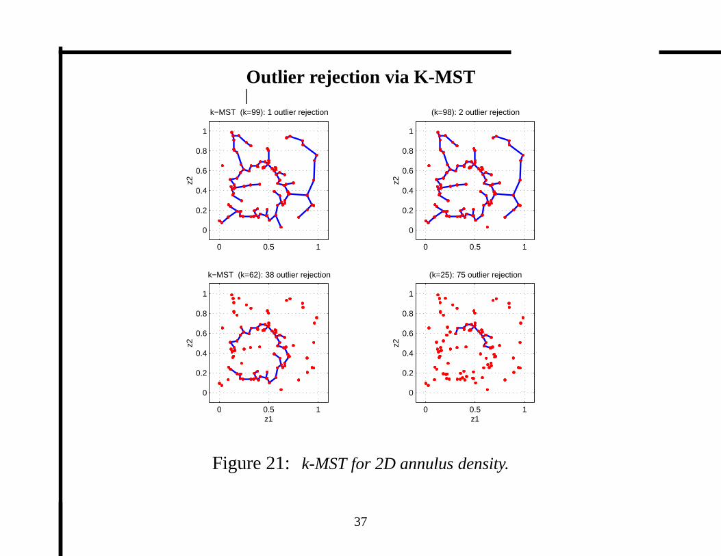
Outlier rejection via K-MST

0 0.5 1

0

0.2

0.4

0.6

0.8

1

z2

k−MST (k=99): 1 outlier rejection

0 0.5 1

0

0.2

0.4

0.6

0.8

1

z2

(k=98): 2 outlier rejection

0 0.5 1

0

0.2

0.4

0.6

0.8

1

z1

z2

k−MST (k=62): 38 outlier rejection

0 0.5 1

0

0.2

0.4

0.6

0.8

1

(k=25): 75 outlier rejection

z1

z2

Figure 21: k-MST for 2D annulus density.

37

k-MST Stopping Rule

0 20 40 60 80 1000

20

40

60

80

100

k

k−M

ST

leng

thk−MST length as function of k

0 20 40 60 80 1000

5

10

15

20

25

30

k

crite

rion(

k)

selection criterion

Figure 22:Left: k-MST curve for 2D annulus density with addition of uniform “outliers” has a knee in the vicinity of n� k = 35. This

knee can be detected using residual analysis from a linear regression line fitted to the left-most part of the curve. Right: error residual of linear

regression line.

38

Greedy partioning approximation to K-MST

0 0.2 0.4 0.6 0.8 10

0.1

0.2

0.3

0.4

0.5

0.6

0.7

0.8

0.9

1

Figure 23:A sample of75 points from the mixture density f(x) = 0:25f1(x)+0:75fo(x) where fo is a uniform density over[0;1]2 and

f1 is a bivariate Gaussian density with mean(1=2;1=2) and diagonal covariancediag(0:01). A smallest subset Bmk is the union of the two cross

hatched cells shown for the case of m= 5 and k= 17.

39

Extended BHH Theorem for Greedy K-MST

Fix ρ 2 [0;1] and assume that thek-minimal graph istightly coverable. If

k= bρnc, asn! ∞ we have (Hero&Michel:IT99)

Lγ(X �

n;k)=(bρnc)α ! βLγ;d minA:P(A)�ρ

Z

f α(xjx2 A)dx (a:s:)

or, alternatively, with

Hα( f jx2 A) =1

1�αln

Zf α(xjx2 A)dx

Lγ(X �

n;k)=(bρnc)α ! βLγ;d exp

�(1�α) min

A:P(A)�ρHα( f jx2 A)

�(a:s:)

40

0 10 20 30 40 500

0.1

Density of X

x

f(x)

0 10 20 30 40 500

0.1

x

max

(f(x

)−f(

x)

Water filled density

0 10 20 30 40 500

0.1

0.2Asymptotic density of X seen by k−MST

x

f(x|

A)

Figure 24:Waterpouring contruction of minimum entropy density.

41

k-MST Influence Function for Gaussian Feature Density

−20

0

20

−20

0

20−100

0

100

200

300

MST for planar Gaussian

IC(x

,F,L

)

−20

0

20

−20

0

20−40

−20

0

20

40

60

k−MST for planar Gaussian

IC(x

,F,L

)

Figure 25:MST and k-MST influence curves for Gaussian density on the plane.

42

Application: testing distributions

Non-parametric density classification problem:decide between

H0 : f (x) = f0(x)

H1 : f (x) 6= f0(x)

Step 1: Perform uniformizing transformation onXn (underH0)

Step 2: Construct MST on transformed variablesYn

Classification rule:

Dα( fk f0)

def

= Lγ(Yn)=nαH1

><

H0

η

43

Application: Robust density estimation

Estimatef1(x) given sample from mixture

f (x) = (1� ε) f1(x)+ ε f0(x)

� f0(x)= known contaminating density

Step 1: Perform transformation onXn to uniformize f0 component

Step 2: Constructk-MST on transformed variablesYn

Lγ(Y �

n;k)=(bρnc)α ! βLγ;d minA:P(A)�ρ

ZA

�f (x)

f0(x)�α

f0(x)dx

Robust Density Estimator:kernel estimator applied toXi1; : : : ;Xibρnc

44

Classification Example

To test:

H0 : f (x) = triangular

H1 : f (x) 6= triangular

Ground Truth:

� f (x) = (1� ε) f1(x)+ ε f0(x): mixture density

� f1(x) is uniform density on[0;1]2

� f0(x) is triangular density on[0;1]2

Test statistic:Dα( fk f0)

H1

><

H0

η

45

ROC curves

0 0.2 0.4 0.6 0.8 10

0.2

0.4

0.6

0.8

1

N=256, ε=0.9, h=(green,unif), g=(red,triang)

0 0.2 0.4 0.6 0.8 10

0.2

0.4

0.6

0.8

1

ROC, α div. test, N=256, ε=.1,.3,.5,.7,.9 ; f=h(H0)

PFA

PD

Figure 26: Left: A sample from triangle-uniform mixture density withε = 0:9 in the transformed domainYn. Right: ROC curves of

thresholded K-MST. Curves are increasing inε over the rangeε 2 f0:1;0:3;0:5;0:7;0:9g

46

Outlier rejection example

0 0.2 0.4 0.6 0.8 10

0.2

0.4

0.6

0.8

1

N=256, ε =0.9, h=(green,unif), g=(red,triang)

Clustering in transformed data domain0 0.2 0.4 0.6 0.8 1

0

0.2

0.4

0.6

0.8

1

N=256, ε =0.9, h=(green,unif), g=(red,triang)

Clustering in original data domain

Figure 27:Left: the k-MST implemented on the transformed scatterplotYn with k= 230. Right: same k-MST displayed in the original

data domain.

47

Conclusions

1. α-divergence can be justified via decision theory

2. Applicable to feature-based image registration

3. Non-parametric estimation is possible even for very high dimensions

via MST

4. MST outperforms plug-in estimation when latter is feasible

5. Robustified MST can be defined via optimal pruning of MST: k-MST

6. Divergence can be estimated by preprocessing with measure

tranformation

48