UNIVERSITY Of HAWAI'I UBHARYEconomic Perspectives on the Siting of a Municipal Solid Waste Facility

A DISSERTATION SUBMITTED TO THE GRADUATE DIVISION OF THEUNIVERSITY OF HAWAI'I IN PARTIAL FULFILLMENT OF THE

REQUIREMENTS FOR THE DEGREE OF

DOCTOR OF PHILOSOPHY

IN

ECONOMICS

DECEMBER 2003

ByHyuncheol Kim

Dissertation Committee:

Eric lksoon Im, ChairpersonEdward Shultz

Chennat GopalakrishnanJames Moncur

Yeong-Her Yeh

ACKNOWLEDGMENTS

Completing a dissertation is a monumental task which demands an unwavering

dedication and personal and professional supports from many a willing persons. Over the

entire course of this dissertation, I have been deeply indebted to many individuals without

whom this dissertation could not have been completed. First and foremost, I would like to

express my deep gratitude to my advisor, Professor Eric Iksoon 1m. He steered me to stay

on right track all the way through by providing valuable comments, suggestions, critiques,

and insights - from setting a theoretical framework to working out mathematical

problems to specifying the empirical model. His continuous press for higher standards

was a driving force behind the steady progress in virtually every respect of this

dissertation. I also would like to thank my committee members: Professors Edward

Shultz, Chennat Gopalakrishnan, James Moncur, and Yeong-Her Yeh for their helpful

comments. Professor Gopalakrishnan deserves my special recognition for his constant

encouragement and challenging questions.

I am very grateful to my colleagues, Tomoko, Kimberly, Kijun, Sunghee,

Jaecheon, and Edward (Eundak) for sharing their interest in my dissertation topic and

their valuable feedbacks. I am especially grateful to my friends Nao and Sunil. Nao has

been a rock that I could lean on whenever I needed help. I deeply appreciate his time

shared with me sorlng out some technical and editorial errors. Sunil, my best friend,

helped revive my spirits up whenever I hit the bottom. May we always cherish the

beautiful things in Anna Bananas and strive for the never-ending quest for knowledge

and friendship.

III

Finally, I wish to express my gratitude to my whole family for all their sacrifice

and moral support all these years: my parents (Suntaik Kim and Dukyung Kim), my

brothers (Heecheol, Mincheol, and Sincheol), my wife Eunkyoung, and our dear son

Taehyung Joshua. To all of them I dedicate this dissertation.

IV

ABSTRACT

LULU (Locally Unwanted Land Use) and NIMBY (Never In My Back Yard) are

often cited as two major hurdles to overcome for successful siting of a noxious facility.

Among various types of waste in Korea, food waste has been posing a serious problem

for its high rate of moisture and salt component (MOE 200 I). This has necessitated siting

of large scale composting facilities around the country. Although there has been an

increasing number of studies on NIMBY towards siting of noxious facilities, one can

hardly find a study on NIMBY attitudes toward a composting facility from an economic

perspective. To analyze NIMBY attitude of residents in Cheju City, Korea toward hosting

a composting facility, we base our theoretical analysis on the expected utility theory and

subsequently use a MNLM (muitinomiallogit model) for empirical analysis.

This study consists of four major parts: theoretical analysis, data management,

MNLM estimations, and interpretation. A theoretical model is constructed by maximizing

expected utility: first, a two-choice model, then extending it to a three-choice model to

incorporate residents' uncertain attitudes toward a composting facility, providing a

theoretical basis for using MNLM model. Our empirical results show with statistical

significance that the higher the income, the stronger the NIMBY attitude towards siting a

composting facility. Further, it shows that the negative effect of economic benefits on

NIMBY attitude is (marginally) stronger than the positive effect of environmental

concern, which contrast with what is usually observed in US where the effect of

environmental concern dominates over that of economic benefits. Socio-demographic

v

variables included to have the economic variables controlled for are mostly insignificant.

Further, from our empirical results is deduced that the residents gave uncertain responses

are tilted towards accepting the composting facility.

VI

TABLE OF CONTENTS

Acknowledgments 1\1

Abstract V

List of Tables XI

List of Figures XV

CHAPTER I: INTRODUCTION

I .I Background

I .2 Purpose of the study 2

1.3 Outline of the Study 3

CHAPTER II. ECLECTICS ON WASTE AND THE CASE OF KOREA

2. I Overview

2.2 Economics of Waste Disposal and Disposal Modes

2.3 NIMBY Syndrome

2.4 Some Eclectics on Waste in Korea

2.4.1 Waste in Korea

2.4.2 Food Waste and NIMBY in Korea

CHAPTER III. LITERATURE REVIEW

3. I Testing Expected Utility Theory

VII

4

4

8

IO

IO

12

17

3.2 Siting Studies in Korca

3.3 Empirical Findings

3.3.1 Distance

3.3.2 Participation

3.3.3 Environmental impact and Economic opportunity

3.3.4 Trust

3.3.5 Knowledge

3.3.6 Compensation and Information Source

3.3.7 Socio-economic variables

3.4 Summary of Literaturc Review

20

22

22

23

24

24

25

26

27

29

CHAPTER IV. THEORETICAL MODEL FOR SITING OF THE COMPOSTING

FACILITY

4.1 Overview

4.1 Two - choice Model

4.2 Three - choice Model

CHAPTER V. SURVEY AND DATA MANAGEMENT

5.1 Variable Selection

5.2 Survey and Data

5.2.1 Sampling and Survey Procedure

5.2.2 Survey Data and Bias Problcm

5.2.3 Survey Content

VIII

30

30

39

51

55

55

57

58

5.3 Measurement Variables and Factor Analysis

53.1 Measurement Variables

5.3.2 Factor Analysis

CHAPTER VI. MULTINOMIAL LOGIT ESTIMATION

6.1 Overview

6.2 Empirical Model

6.3 Estimation Results

6.4 Nonnalizing Logit Coefficients

6.4.1 Positive Wealth Attribute Variables

6.4.2 Negative Wealth Attribute variables

6.4.3 Socio-demographic Variables

6.5 Discussion on the Level of Risk Orientation

6.6 Hypothesis Test

6.7 Policy Implication

CHAPTER VII. CONCLUSION

7.1 Summary of the Study

7.2 Summary of Empirical Findings and

Policy Implication

7.3 Contributions and Future Research Suggestion

IX

61

61

64

70

71

76

79

81

86

88

89

93

101

106

107

109

APPENDIX

APPENDIX A: PROOF OF SECOND ORDER CONDITIONS

AI. Two-choice Model

All. Three-choice Model

APPENDIX B: SURVEY QUESTIONNAIRE (IN ENGLISH)

APPENDIX C: SURVEY QUESTIONNAIRE (IN KOREAN)

APPENDIX D: STATISTICAL SUMMARY

DI. Survey Questions

DII. Explanatory variables

DII-I List of explanatory variables

DII-2 Statistical Summary of Explanatory Variables

APPENDIX E: LIST OF SIGNIFICANT COEFFICIENTS

APPENDIX F: COMPOSTING FACILITIES IN KOREA (MAP)

REFERENCES

x

IlJ

I II

lJ4

117

124

130

130

147

147

148

149

154

156

UST OF TABLES

Table 2.1: The Required Time Period for Decomposition of Wastes

Table 2.2: Trend of Food Waste Output in Korea

Table 2.3: Trend of Food Waste Output in the US

Table 2.4: The Compostng Facilities in Korea

Table 3.1: Previous Estimation Results ofSocio-economic Variables

Table 4.1: Impacts on Wealth Attributes on Odds

Table 5.1 : Sample Distribution

Table 5.2: Binary Codes for Measurement Variable JPWM

Table 5.3: Frequency Distribution of IPWM

Table 5.4: Summary Statistics of IPWM

Table 5.5: Codes for Measurement Variable TRUST

Table 5.6: Frequency Distribution of TRUST

Table 5.7: Summary Statistics of TRUST

Table 5.8: Factor Loadings

Table 5.9: Rotated Factor Loadings

Table 5.10: Scoring Coefficients

Table 5.11: Summary Statistics ofENV and ECO

Table 6.1: Expected Signs of Coefficients (Yes Base Estimation)

Table 6.2: Summary of the Yes Base Estimation

Table 6.3: Summary of the No Base Estimation

Table 6.4: Resident's Risk Orientation

Table 6.5: Wald Test

XI

10

13

13

14

28

50

56

61

62

62

62

63

67

65

66

68

69

75

77

91

92

94

Table 6.6: LR Test 94

Table 6.7: Wald Test and LR Test for Independent Variables as a Whole 97

Table 6.8: Identification of the Level of Risk Orientation Factor 98

Table 6.9: Test Result of Resident's Risk Orientation 100

Table DI.1: Question J 130

Table D1.2: Question 2 130

Table D1.3: Question 3 130

Table DI.4: Question 4 131

Table D1.5: Question 5 J31

Table DI.6: Question 6 131

Table DI.7: Question 7 132

Table Dl.8: Question 8 132

Table Dl.9: Question 9 132

Table DI.! 0: Question 10 133

Table DI.1I: Question 11 133

Table DI.12: Question ]2 133

Table DI.13: Question 13 134

Table DI.14: Question 14 134

Table DI.15: Question ]5 134

Table DI.16: Question 16 135

Table DI.17: Question J7 135

Table DI.! 8: Question 18 135

Table DI.l9: Question 19 136

XII

Table 01.20: Question 20 136

Table 01.21: Question 21 136

Table 01.22: Question 22 137

Table 01.23: Question 23 137

Table Dl.24: Question 24 137

Table 01.25: Question 25 138

Table 01.26: Question 26 138

Table 01.27: Question 27 138

Table 01.28: Question 28 139

Table 01.29: Question 29 139

Table 01.30: Question 30 139

Table 01.31: Question 31 140

Table 01.32: Question 32 140

Table 01.33: Question 33 140

Table 01.34: Question 34 141

Table 01.35: Question 35 141

Table 01.36: Question 36 141

Table 01.37: Question 37 142

Table 01.38: Question 38 142

Table 01.39: Question 39 142

Table DIAO: Question 40 143

Table 0I.41: Question 41 143

Table 01.42: Question 42 143

XIII

Table 01.43: Question 43

Table 01.44: Question 44

Table 01.45: Question 45

Table 01.46: Question 46

Table 01.47: Question 47

Table 01.48: Question 48

Table 01.49: Question 49

Table 01.50: Question 50

Table 01.51: Question 51

Table 01.52: Question 52

Table 011: Statistical Summary of Explanatory Variables

Table E.l: IPWM

Table E.2: PPDSP

Table E.3: TRUST

Table E.4: KNOW

Table E.5: ACCESS

Table E.6: COMP

Table E.7: RELCOM

Table E.8: ECO

Table E.9: DIST

Table E.l0: ENV

Table E.II: INCOME

Table E.12: NHMBR

XIV

144

144

144

145

145

145

146

146

146

147

148

149

149

150

150

150

151

151

151

152

152

152

153

LIST OF FIGURES

Figure 5.1: The Eigenvalues

Figure 6.1 : Positive Wealth Attribute Variables

Figure 6.2: Negative Wealth Attribute Variables

Figure 6.3: Socio-demographic Variables

Appendix F: Composting Facilities in Korea

xv

64

84

87

88

154

CHAPTER I

INTRODUCTION

1.1 Background

Human activity generates waste in one fonn or another. Virtually no economic

activity without a negative externality in the fonn of waste exists. Therefore, as an

economy grows, the waste disposal poses an enonnous challenge whieh defies an easy

solution. Waste can be either simply dumped or disposed of through different modes of

disposal. Each mode, however, necessitates or requires so-called noxious facilities that can

be harmful to the local communities and their environments. Whatever mode is chosen for

waste disposal, it adversely affects the community in one way or another. For example,

landfilling with waste not only take away pieces of land from their alternative uses but also

may contaminate water sources through leachate. Dioxin, a chemical residue of waste

incineration, is a lethal component of air pollution. Composting, though considered to be

safe compared to other disposal modes, is likely to spill out foul smell, cause heavy traffic,

and lower the property value in the vieinity of the facility. These negative effects result in

the tendeney for people to oppose the construction of noxious facilities. Popular phrases

such as "LULU (Locally Unwanted Land Use)" and "NIMBY (Never In My Backyard)"

reflect the community resistance to having noxious facilities in the neighboring area.

In Korea, the disposal of food waste which contains a high degree of saturation and

salt, and landfilling with or incinerating food waste causes an environmental problem

(MOE 1999). For a number of years, the issue of food waste disposal in Korea has been a

major issue which concerns the public as well as local and central governments. So far the

1

most widely used mode of waste disposal is through large - scale composting facilities

(MOE 2000). Composting facility does have some advantages: it recycles food waste into

compost, and is relatively safer as compared with other waste disposal modes.

Nonetheless, due to the NIMBY attitude, communities are reluctant to host a composting

facility regardless of its advantage over other modes.

A great deal of research has bccn conducted on the siting problems associated with

waste disposal facilities. These studies are mostly in disciplines such as political science,

sociology, and psychology rather than economics. A few studies from economic

perspective exist but none of them is with a theoretical rigor. Furthermore, the focus of

those has been rarely on composting facilities.

This study analyzes NIMBY attitude towards siting of the composting facilities

from an economic perspective. The target area selected is Cheju City, Korea. Compared to

other places in Korea, Cheju is one of the most popular tourist destinations in Korea where

natural and environmental resources have greater economic values than elsewhere in

Korea, hence the opportunity costs of siting a waste disposal facility is expected to be

significantly higher than elsewhere in Korea.

1.2 Purpose of the Study

NIMBY has been traditionally described as the behavior of people driven by

collective self-interest (O'Hare 1977). Though a significant number of NIMBY related

studies exist, they are mostly from non-economic perspectives. From an economic

perspective, NIMBY can be viewed as a rational behavior based on economic principles. In

the same vein, this research attempts to identify the major determinants ofNIMBY attitude

2

when a noxious facility is built around a residential area.

In view oflack of theoretical rigor in the previous NIMBY related studies, the first

objective of this study is to provide a theoretical framework prior to empirical analysis. The

second objective is to estimate the effects of various variables on NIMBY attitude toward

the hosting a large - scale composting facility using a survey data and multinomial logit

model. The final objective is to analyze the estimation results to draw policy implications.

1.3 Outline of the Study

Reviewed in Chapter II are various waste disposal modes, NIMBY syndrome, and

some eclectics on waste in Korea. Chapter III reviews existing literature on the expected

utility theory, and also provides empirical findings in previous siting studies. The

theoretical foundation for empirical analysis is laid out in Chapter IV. Chapter V provides a

brief background description ofthe survey data collection and management. In Chapter VI

we analyze estimated multinomial logit models: general interpretation of estimation

results, discussion of new findings, and the hypothesis test results. Finally, Chapter VII

concludes this study by providing a brief summary, policy implications, and suggestions

for future research.

3

CHAPTER II

ECLECTICS ON WASTE DISPOSAL AND THE CASE OF KOREA

2.1 Overview

As stated in the introduction, this research explores a local resident's attitude

towards the siting of a noxious facility. The object facility in our study is a large - scale

composting facility planned for Cheju City, Korea. Since there are several other waste

disposal modes other than composting, the next section provides a brief overview of

waste disposal modes. The general nature of NIMBY phenomenon is elaborated in

Section 2.3. While many countries are common in having to deal with the waste disposal

problem, the degree of urgency varies from country to country. Since the target area for

this study is in Korea, an overview of Korea with regard to waste disposal is also

provided in Section 2.4.

2.2 Economics of Waste Disposal and Disposal Modes

Production and consumption of goods generate solid waste, which in turn entails

environmental issues. Collection of solid waste generated from economic activity can be

through either legal (paying a fixed fee or user fee) or illegal channel. The legal channel

creates demand for WDS (waste disposal services), while the illegal channel is simply

through illegal dumping in an area. The collected waste can be separated by type into

reeyclables and non-reeyclables. The recyclable waste is transfonned through the MRF

(Material Reeycling Facility) in the case of non-organic waste and turned into compost in

a composting facility in the case of organic waste (food or yard waste). As for the non-

4

recyc1ables, the waste can be dumped into the designated landfill area or burned in an

incinerating facility. Since waste is an output of economic acti vity, its continuous outflow

creates negative externalities to the environment.

The potential contributions that can be made by economists in this field are quite

extensive, encompassing subjects ranging from waste generation to disposal. Most of

studies on waste so far have focused on waste collection rather than disposal, and

examines the effectiveness of user fee as opposed to fixed fee to pay for WDS. A

common argument in these studies is that the user fee is more effective in reducing waste

generated at the firm and household levels than the fixed fee (Jenkins 1993), but the

argument is valid only if there is no illegal dumping as a result of imposing a user fee.

However, Fullerton and Kinnaman (1996) find significant evidence of illegal dumping

under the user fee system, which calls for economic studies on waste disposal.

Tammemagi (1999) sets policy priorities in the order of source reduction, reuse and

recycling (3Rs) I. This hierarchical approach suggests that if policies aimed at source

reduction and reuse are not effective through a user fee due to the increased illegal

dumping, then recycling assumes an important role in waste management. However, US

statistics shows that waste disposal through recycling accounts for no more than 50% of

the total waste output (EPA 1996), leaving more than half of the total disposal through

other modes of waste disposal such as composting2•

The m~jor modes of waste disposal may be listed as incinerating, landfil1ing,

recycling, and composting. Incineration is a mode which requires large-scale burning

I Some authors use the term "4Rs" to include incineration.2 There arc many of studies on recycling, but not on composting in economics.

5

furnaces that could generate and maintain heat of high tempcratures. ] Since the

incinerator generates energy in the proccss of burning thc waste, it is callcd a 'waste­

energy facility'.

In the past, incinerating facilities in Korea incurred high operating costs, and werc

blamed for a great deal of environmental deterioration (MOE 2001). Technological

improvement has made the incineration process safer and more efficient, thus generating

more cnergy and substantially reducing the hazardous residue from incineration as well

as saving landfill space. Incineration facility, however, requires high fixed cost compared

with other modes of waste disposal facilities. The technology for controlling the side

effects of incinerators has bcen improved, but a large fixed cost of the facility poses a

challenge in adopting new technologies, which in turn slows down the application of new

technology. In particular, the dioxin emission remains a serious problem.

Landfilling, another mode of waste disposal, requires large waste collecting areas,

specifically designed large depressions in the ground lined with a protective material

(Carless 1992). While modern landfills are operated safely, still several environmcntal

problems such as water contamination, air pollution, and methane gas emission could

emerge as a consequence of continuous use of unsafe equipment (Tammemagi 1999). A

study on 43 landfill areas in Korea shows that the average levels of 3,743mglL in BOD

(Biological Oxygen Demand) and 5,023 mg/L in COD (Chemical Oxygen Demand) in

groundwater around urban areas are higher than those (BOD: 278mglL, COD: 488mg/L)

in rural areas due to poor handling of leachate (MOE, 1999).

There are other problems associated with the use of the landfills such as

decreasing landfill space available and the rising cost of landfilling. Several states in US

3por more detailed features of incinerators, see Tammemagi (1999)

6

are running out of pennitted landfill areas, and in a matter of few years, according to

previous studies, US will be hard pressed for landfill space (Tammemagi 1999). The

rising costs of landfilling will be an added issue. Waste tipping and transportation costs in

certain landfill areas have been increasing rather rapidly. This problem has become more

serious in urban than rural areas due to shortage of available landfill space (Tammemagi

1999). Careless (1992) argues that tipping fees in New Jersey have been increasing

continuously since the early eighties and concludes that the high tipping cost will force

states to look for cheaper places, which results in substantial higher transportation costs

for waste disposal.

The increasing costs of waste tipping and transportation makes recycling more

attractive. Recycling is defined as the colJection and separation of materials from MSW

(Municipal Solid Waste) and the processing of these materials to produce marketable

products (Tammemagi 1999). Two factors (i.e., the ever increasing solid waste and rising

waste disposal costs) make recycling the best available alternative option in dealing with

the waste problem. Statistics show that in Korea the recycling rate had been increasing

since the introduction of user-fee system4 introduced in early 90's, indicating that the

system works. But there are some doubts about its effectiveness. When residents dispose

of waste, they are required to separate waste into different types. However, there is no

information on the final recycled products, their purchases by consumers, and their

distributions. Hence, in view of the definition of recycling, the recycling rate as reported

by MOE (2001) appears to be higher than the actual rate.

4 Under this system residents are required to separate the waste into recyc1ables and non-recyclable, usingstandardized bags distributed by the government.

7

Finally, composting is a special recycling in which organic waste is biologically

converted into a product that could be beneficial to land and friendly to environment

(Tammemagi 1999). Once waste is collected and transferred to a composting facility, the

waste is separated by types: inorganic waste (which is sent to a landfill or an incinerating

facility) and organic waste such as food and yard waste (Miller and Golden 1992). The

organic waste is processed into compost under special conditions. Through the natural

process, the organic waste is changed into a soil-like substance. .The recycled product,

compost, is marketable after a certain curing period. Several environmental problems

could arise during the composting process. A rather serious one is unpleasant odor which

spills out from flawed composting facilities or flawed process. Nevertheless, the

composting has long been familiar to Koreans. In the past, Koreans made compost for

agricultural use by fermenting organic waste such as leaves, stems, and excretion from

farm animals. Given the fact that food waste in Korea is substantial in quantity and toxic

in nature causing an environmental concern, in addition to the traditional demand for

compost, Koreans well appreciate the necd oflarge - scale cornposting facilities.

2.3 NIMBY Syndrome

Waste disposal may cause serious health and environmental problems. Naturally,

when a noxious facility is planned to be build, it is not uncommon to meet a vehement

resistance from the residents near those facilities. This is known as LULU. The

explanation for this phenomenon is that there are negative externalities in the vicinity of

the noxious facility and unfair geographical distribution of costs of and benefits from the

faculty. There are several approaches to explaining the LULU phenomenon. The most

8

popular and extensively used approach is NIMBY, a ternlinology first used by O'Hare

(1977) to describe individuals' opposition against having to reside around an unpopular

facility.

While some views NIMBY as an irrational response from those residing close to

the noxious facility (for example Rej]Jy 1987'), there are others who view NIMBY as a

rational and justifiable response on the premise that local residents understand the

community matters better than the experts who are directly or indirectly associated with

the siting plan. Thus, the concerns of local residents with regard to the risks to the

environment and the community's well being are rational from economic perspective.

Fiorino (1989) argues that local residents are the best judges of their own community

matters. Without resistance from local residents, the allocation of the facility siting may

not attain efficiency (Laws and Susskind 199 J).

In developing or newly developed countries like Korea, a deep-rooted distrust has

been built toward government and public officials in charge of siting unpopular facilities.

Many environmentalists and local residents alike have argued that the government should

listen to the residents and must compensate for their losses. Some people in developing

countries assert that NIMBY should not be viewed solely as irrational.

NIMBY has been studied rather extensively cross-different disciplines. Most of

these studies have been focused on siting facilities for toxic or hazardous waste disposal,

including landfills and incineration facilities. However, very few studies are on

composting facilities. If organic waste such as food or yard waste is substantial and its

disposal through landfilling or incineration is costly, then the siting a composting facility

5 "Almost everyone seems to agree on the need for waste disposal facilities. Yet almost no one seems towant one of them anywhere near his or her residence."

9

may be the economic alternative. Nevertheless, no disposal facility is completely free of

negative externalities, thus some degree of NIMBY opposition is unavoidable regardless

of waste disposal mode.

2.4 Some Eclectics on Waste in Korea

Each type of waste has a different time period required for decomposition as

reported in Table 2.1. For example, waste such as leather shoes takes decades to

decompose, whereas waste such as paper takes a relatively short time period.

Tahle 2.1: The Required Time Period for Decomposition of Waste

Kinds of WasteRequired Time for

Types of WasteRequired Time for Waste to

Waste to Decompose Decompose

Paper 2-5 months Orange Peel 6 monthsMilk Carton 5 years Cigarette Filter 10 - 12 yearsPlastic 10 - 20 vears Plastic bowl 50 - 80 yearsCloth' 30 - 40 years Leather Shoes 25 - 40 years

Source: MOE (2000). 'Made from Nylon

2.4.1 Waste in Korea6

In general, the types and quantities of solid waste generated depend on the

industrial structure, GDP, recycling cost, and lifestyles of the residents. In many a

developing country, industrialization has led to massive rural-to-urban migration. A

considerable number of countries experienced rapid urbanization since World War II. In

urban areas, unlike rural areas, the limited land supply has created a daunting challenge

of waste management. Korea followed a similar path: a rapid industrialization

6 Ministry of Environment (MOE) (2000), Environmental Statistics Year Book. Seoul.

10

accompanied by a dramatic increase in urban population during the 1960' s. Most of the

solid waste in Korea was produced in large cities such as Seoul, Pusan and Daegu7 This

can be attributed to growing consumption of non-reusable products by growing urban

population. The increase in demand for non-reusable products not only accelerates

depletion of the resources but also creates the problem of waste disposal. 8

The annual growth rate of solid waste from the industrial sector has also been

outpacing the growth of Korean economy. The growth rate of solid waste from the

industrial sector had been hovering over 10% in the late 1980's, which contrasts with

over 20% ofhazardous waste during the same period, creating an added problem of waste

toxicity. During 1960's, around 80% of solid waste in Korea was accounted for by

briquette - ash while food waste accounted for a relatively small proportion. In the past

the mixture of briquette - ash with good aeration and food waste turned into a good

compost, and when used for landfilling, the landfills were converted back into fertile

farmland after a certain period of time for decomposition of food waste.

Since the 1970's, however, there has been an increase in organic solid waste such

as yard or food waste. There has also been a substantial increase in the use of goods that

produce toxic waste such as batteries, light bulbs, and household appliances.

Concomitantly, new types of waste such as plastics, glass, textiles, and aluminum came

into the picture.

7 However, other regions in Korea are not free of waste problem. Though relatively less serious, for therest of Korea the waste problem is expected to be increasingly more serious into the future.

Il Current increasing demand for fast food has led to a concomitant increase jn demand for non-reusableproducts.

11

2.4.2 Food Waste and NIMBY in Korea

Economic conditions vary from country to country, and so does the urgency of the

waste disposal problem. Initially, food waste problem in Korea was virtually nonexistent.

As Korea economy grew at a rapid pace, the waste management issue became

increasingly urgent. More and more residents were involved in public debates and

hearings about landfilling and incineration between 1980-1993. During 1994-1995 the

user fee system was introduced. Since 1996, the food waste disposal has bcen emerging

rapidly as an urgent issue. Prior to that, food waste was simply incinerated or landfilled

with other types of waste. Food waste in Korea contains high moisture contents which

decay rather quickly, hence the process of its collection, transportation, and disposal is

much more costly and complex than those for other types ofwaste.

These problems forced the Seoul municipal government to stop using food waste

for landfilling in and around the city. The similar action was taken for the incinerating

facilities in the capital (OWM I994c). Currently, the generally held public view on the

issue is that each producer offood waste should be responsible for its disposal. It is also a

public consensus that food waste should be treated as a toxic and hazardous waste. The

total output of food waste in 1998, for instance, is 11,798 ton/day which representing

26% of the total solid waste output of the year.

As Table 2.2 shows, the output of food waste has been steadily decreasing from

26,311 tons/day in 1991 to 11,798 ton/day in 1998. Comparing the rates of change of FW

(Food Waste) and MSW, one can notice similar patterns of change over the period in the

table with one exception of 1996: MSW increased by 4.5% whereas FW decreased by

3.6%.

12

Table 2.2: Trend of Food Waste Output iu Korea (unit: ton per day)

Total Amount Amount of Ratio of Food Growth Rate Growth Rate

Yearof Municipal Food Waste Waste To afMSW of Food WasteSolid Waste (B) TotalMSW (%) (%)

(A) (BIA)

1991 92,246 26,311 0.28 9.9 14.4

1992 75,096 21,807 0.29 ~ 18.6 - 17.1

1993 62,940 19,764 0031 - 16.2 - 9.41994 58,118 18,055 0.31 ~ 7.7 - 8.61995 47,774 15,075 0.32 ~ 17.8 - 16.51996 49,925 14,532 0.29 4.5 ~ 3.61997 47,895 13,063 0.27 - 4.1 ~ lO.11998 44,583 11,798 0.26 -6.9 - 9.7

Source: MOE (1999).

The annual output of food waste in US for 1991/98 period is shown in Table 2.3.

Comparison of Tables 2.2 and 2.3 shows that the average annual ratio of food waste to

total MSW in Korea is approximately three times as high as in US. The annual growth

rate of food waste in Korea in comparison with US appears to indicate an effective food

waste management in Korea in light of the fact that the growth rate of food waste in

Korea has been negative from the year 1992 to 1998 while that of food waste in USA

mostly has been positive.

Table 2.3: Trend of Food Waste Output in the US (unit: tou per day)

Output ofOutput of Ratio of Food Growth Rate Growth Rate

MunicipalYear

Solid WasteFood Waste Waste to Total ofMSW of Food Waste

(A)(B) MSW (BIA) (%) (%)

1991 204,550 20,910 0.10 - 0032 0.531992 208,930 21,000 0.10 2.14 0.431993 211,820 20,910 0.10 1.38 ~ 0.431994 214,170 21,500 0.10 l.ll 2.821995 211,460 21,800 0.10 ~ 1.27 1.401996 209,660 21,900 010 -0.85 0.461997 218,180 22,730 0.10 406 3.791998 223,360 24,910 0.11 2.37 9.60

Source. EPA (2000)

13

In Korea, the cost of food waste disposal through composting is higher than

through landfilling and lower than through incineration: landfilling with food waste cost

24,879-26,384 won/ton as opposed to 75,711-86,339 won/ton for incineration in ]996.

Based on these costs, the estimated cost of recycling food waste would be 30,000 to

60,000 won/ton (MOE, 2001). However, the composting cost would be much lower if

one takes into account the environmental costs associated with land filling/incineration

and the opportunity cost of landfills. It would be even lower if one considers the revenue

generated from sales of the compost.

Table 2.4: The Composting Facilities in Korea

City and The Number of Composting The Number ofPlauned

Province Existing Facilities Size* Planned Facilities CompostingSize

Seoul 15 290 I 30Pusan 10 210 I 120Taegu 0 0 I 20Inchon 0 0 0 0Kwangju 2 46 0 0Taejon I 10 I 10Ulsan 0 0 1 60Kyunggi 14 423 3 300

Kangwon 2 30 1 10

Chungbuk 0 0 0 0

Chungnam 4 28 1 30

Chonbuk 0 0 I 20

Chonnam 2 27 1 30Kyungbuk I 4 I 20

Kyungnam 3 70 0 0Cheju 0 0 I 19Total 54 1138 14 669

Source. MOE (1999), *. Unit (ton per day)

14

To deal with the problem of food waste disposal, large-scale composting facilities

have been constructed throughout Korea. As of 1999 in Korea, a total of 54 public

composting facilities were in operation. Detailed infom1ation on the number and the sizes

of respective composting facilities are summarized in Table 2.4. Table 2.4 shows that

Seoul, the capital city of Korea, has the largest number of composting facilities. Fourteen

more composting facilities are planned for construction across Korea in the near future.

Currently, there are regions still without composting facilities including Cheju

Island. However, as Table 2.4 shows, one is slated for construction in Cheju. Hence, an

ex ante analysis of NIMBY attitudes of Cheju residents towards the composting facility

will be not only timely but also give insights to the policy makers in Cheju and elsewhere

in Korea.

The NIMBY syndrome is a common phenomenon observed in many a developed

economy (Rabe 1991; Malone 1991). It is quite strong even among developing and newly

developed economies. In the case of Korea, the incidences of NIMBY syndrome has

increased considerably in number. The most notable one in Korea was in connection with

the Anmyon Island (Moon 1994). Since the mid-eighties, the degree of NIMBY attitude

in Korea has grown in terms of scale and intensity. A number of noxious facilities

planned could not survive the NIMBY syndrome, which includes a low-level radioactive

waste repository (Kim et al. 1994) as well as 34 large regional landfills throughout the

country (Park 1992). Several studies show that the NIMBY attitudes in Korea are

expected to be even stronger in the future. This may be attributed to two major factors:

first, more decentralized Korean political system; second, the residents in Korea

15

increasingly more concerned with environment quality rather than higher income. 9

Taking these factors into account, the NIMBY attitude is expected to be a major hurdle to

overcome for successful siting of a noxious facility. Therefore, it may well be a valuable

source of reference for policy makers to identify the major determinants of NIMBY

syndrome, which is the intended purpose of this study.

'Central Daily News [Choong Ang lIbo]. March 28, 1996.

16

CHAPTER III

LITERATURE REVIEW

3.1 Testing Expected Utility Theory

Since Alfred Marshall laid out the foundation for modem economic theory, one

of the greatest achievements in economics is in incorporating uncertainty into economic

analysis. Pioneered by Neumann and Morgenstern (1947), the expected utility (ED)

theory is built on four axioms that are assumed to rule consumer behavior: continuity,

complete ordering, independence, and unequal probability. The key premise of ED theory

is that each individual maximizes the expected utility in the context of uncertainty.

There are two main challenges to ED theory by Baumol (1951). One relates to the

consistency of EU theory within the general economic theory of consumer preferences,

the other to measurability of utility. Friedman and Savage (1952) address these two issues.

By making several postulates about expected utility, they draw the conclusion that utility

is consistent with the usual preference system and can be measured within EU theory

framework. However, their theoretical argument prompts a fundamental question: Can

ED theory predict or describe actual behavior under uncertain state? The answer to the

question is in the empirical test for its validity.

There are empirical studies that test for EU model's applicability in predicting an

economic agent's rational response under uncertain conditions (e.g., Rapoport and

Wallstem 1972; Becker and McClintock 1967; Edwards 1961). A comprehensive critical

review of the applicability of EU theory is given in Schoemaker (1982) who himself

made a significant contribution to both theory and practice in this regard. He states "It has

17

been used prescriptively in management SClCnce (especially decision analysis),

predictively in finance and economics, descriptively by psychologists, and has played a

central role in theories of measurable utility," but in the end he argues that ED theory is

fragile in its applicability. However, there are a number of empirical studies which

counter Schoemaker's argument. For example, Gould (1969) shows that ED hypothesis

cannot be ruled out as a description of behavior for a consumer's purchase of auto

insurance.

There are several studies based on EO theory usmg either of two different

approaches. One is the hedonic pricing approach (Brookshire et al. 1985) and the other is

the risk perception approach (Halstead et al. 1999; Kunreuther and Easterling 1990).

Brookshire et al. (1985), using the data on property values, in the context of two states of

event earthquake and no earthquake, they derive the "hedonic price gradient for safety"

for two areas; Los Angeles and San Francisco. Their study shows that people tend to pay

less for houses located in an earthquake-prone area, ceteris paribus. Paying more for

safer houses is a form of "self-insurance". Their empirical results show that price gradient

is consistent with their theoretical expectation, hence extending an empirical support for

ED theory. Based on the data on land and housing prices, Brookshire et al. also show

how the value of economic goods are affected by expected environmental damage.

Though the same rationale can be applied to siting of a hazardous waste facility, their

study falls short of analyzing the local residents' detailed NIMBY attitudes towards the

facility. The determinants of NIMBY behavior can also be found in residents' attitudes

as well as the environmental impacts in the area of hosting a noxious facility.

18

The risk perception approach primarily uses survey data gathered from residents.

The major focus ofthis approach is on identifying the effects on NIMBY attitude of such

variables as the proximity to a facility and the residents' socio - economic idiosyncrasies.

Siting studies using the risk perception approach are found in Kunreuther and Easterling

(1990), and Halstead et al. (1999).

With their model built on the EU, Kunreuther and Easterling (1990) explain

several relevant factors which include compensation and the level of public trust. They

specified a two-period additive utility is a function of WTA (willingness to accept

amount). In their model, the compensation is a return to the local residents for hosting a

nuclear waste repository near the community. The model predicts a positive relationship

between acceptance of the hazardous waste facility and the level of compensation. In the

empirical part of their analysis, they use two sets of telephone survey data in early 1987;

one is a national data (1,201 U.S. households), and the other is a Nevada data (1,001

households). In specifying their logit model, they add an attitude variable (trust) to see

how personal attitude affects an individual's siting decision. The main conclusion of the

study is twofold. First, local residents do not respond to any level of compensation under

the situation without adequate environmental safeguards. Second, the residents' attitudes

are important in mitigating risk perception.

Kunreuther and Easterling (1990) find an empirical evidence on relationships

between risk perception and a set of independent variables including attitude variables.

Their theoretical analysis, however, is not based on maximizing expected utility though it

is relevant. Moreover, in their theoretical analysis "trust" is the only attitude variable

considered.

19

Using the same theory of expected utility as Brookshire et al. (/985), Halstead et

al. (/999) examines the local resident's behavior towards the siting of a composting

facility. The two states of event in the theoretical model are assumed: one in which the

composting facility is built and operated without any negative externalities and the other

in which an environmental externality occurs. Following Kline et al. (J 993), this study

uses subjective (perceived) probability rather than the actual probability. Of the nine

regressors used in estimating a logit model, eight of them show the statistical significance

at 5% or less.

The contribution made by Halstead et al. (1999) includes discussion of NIMBY

determinants based on economic theory and also consideration of uncertainty by

including "Maybe" choice as a choice for dependent variable in their empirical model. In

the case of Brookshire et al. (/985) the theoretical derivation of the FOCs (First Order

Conditions) is consistent with their empirical model. However, in Halstead et al. (/999),

the linkage is not clear. They assume two states (hazardous and safe) in their theoretical

model whereas the dependent variable has three choices in their empirical model. Though

they explicitly assume uncertainty, they do not derive any implication of the uncertainty

in their model.

3.2 Siting Studies in Korea10

There have been several siting studies in Korea based on two approaches: hedonic

pricing approach and risk perception one. Based on the hedonic pricing are studies by

Cho (J 998), Cheong (1995), 1m and Chun (1993), and Yi (1996). Cho (1998) investigates

the impact of a noxious facility on land price of the surrounding area. The area covered

10 To our knowledge, there are no siting studies in Korea that adopt Ell theory.

20

by the research is within three kilometers from the incineration facility located in

Mokdong, Seoul, Korea. He finds that the noxious facility affects land price negatively at

I % significance level. Cheong (\ 995) finds that the effect of the incineration facility on

the property value in the same area is not as influential as in Cho. 1m and Chun (1993),

and Yi (1996) find that air pollution has a significant negative impact on housing prices.

Overall, the results of these studies, with the exception of Cheong (1995), show that the

environmental factors have significant negative effects on the property value in the host

area; thus extending empirical evidences in support of the residents' NIMBY attitudes.

Based on the risk perception approach, Lee and An (\ 999) treat NIMBY as a

function of the socio-psychological characteristics of residents. For instance, if a resident

has a strong altruistic view, his attitude is likely to be more permissive of the facility.

They estimated a binomial logit model to capture NIMBY attitude with a purpose of

making a policy proposal to effectively mitigate the residents' NIMBY attitudes towards

the siting large - scale incinerating facilities. Their analysis based on the survey data in

Chungju City, Korea shows that the socio-demographic variables are important

determinants of NIMBY attitudes as well as the residents' degree of trust in mass media

and knowledge of the noxious facility. They emphasize the importance of residents'

participation in decision making process and information dissemination which promotes

the public knowledge with regard to the safety ofthe facilities.

As discussed in Chapter Two, a solution to food waste disposal in Korea may be

to use composting facilities. Nearly all of the siting studies in Korea, however, focus on

other waste disposal modes such as landfilling and incineration which are more

21

hazardous than composting facilities. Most of these studies either implicitly or explicitly

assume away uncertainty.

3.3 Empirical Findings

In this section, we review the determinants of NIMBY phenomenon in the siting

noxious facilities found in previous empirical studies. Except for a few, the studies on

NIMBY attitudes are based on risk perception approach. Since our study is basically a risk

perception approach based on expected utility theory, we review empirical evidence in

studies based on risk perception approach.

3.3.1 Distance

One of the key determinants of NIMBY is the proximity of a residence from a

noxious facility. Many studies show a significant correlation between the proximity and a

local resident's attitude with regard to the siting a noxious facility (Halstead et al. 1999;

Lober 1993; Furseth and Johnson 1988): the closer to the facility, thc greater the costs to

the resident. NIMBY attitude is triggered when the costs outweigh the benefits from the

facility. Therefore, the probability ofresidents' accepting a noxious facility depends upon

the distance to the proposed facility. Kraft and Clay (1991) find that the effects of

distance may be caused by a "shadow effect" from the past experience with a similar

hazardous facility. A similar conclusion is made by Mushkatel et al. (1993) who argue

that there is a positive relationship between the shadow effect and the resident's

perceived risk concerning a new proposed facility, particularly regarding nuclear and

radioactive waste facilities.

22

3.3.2 Participation

Participation in waste management is considered an important attitude variable in

the siting study. One form of participation is an individual's waste management activity

in one's daily life (Halstead et al. 1999). Halstead et al. (1999) combine seven variables

on the local resident's waste management activity to create the measurement variable,

"WIM (Waste Involvement Measure)". In calculating WIM, they use survey questions on

household trash handling or recycling activity. The estimation result on WIM shows that

a local resident's active involvement in waste management plays a significant role in

determining one's siting decision.

Another form of participation is the public involvement in the decision making

process. In many developing countries, studies show that the opportunities of

participating in the decision making process (public policy) available to the local

residents are very limited (Yun 1997). The limited participation in tum limits the

information available to the residents and their knowledge. In natural resource

management, public participation is crucial for its success (BJahna and Yonts 1990)

though conflicts of interests are inevitable. Heberlin (1976) suggests that offering each

group equal opportunity to be heard and participate in the decision making process would

decrease the potential conflict. A signi ficant number of studies find that the limited public

participation diminishes the chance of success of hosting a facility (Bogdonoff 1995;

Matheny and Williams 1988; Davis 1986).

23

3.3.3 Environmental Impact and Economic Opportunity

A noxious facility almost certainly causes some damage on the environment. The

degree and kind of damage depend on the type of the facility. The environmental

problems include air pollution from incinerating facilities (e.g., dioxin), contamination of

water sources from landfilling, and odor from composting facilities. A number of

previous studies provide empirical evidence that residents' environmental concern has a

negative effect on their attitudes toward a noxious facility (e.g., Lober 1994).

Counterbalancing the negative effect are the economic benefits from the facilities

such as jobs created, lower property taxes, and local economic growth (Bacot et al. 1993).

Which effect is relatively stronger than or dominates the other depends on the various

factors specific to the region. Halstead et al (1999) find that in the case of three New

England cities (Keene, Rochester, and New Hampshire) the residents' environmental

concern overrides their economic benefits expected from a large-scale composting

facility in their neighboring area. That is, the income effect on their demand for safer

environment overrides the substitution effect ofeconomic benefits for safer environment.

3.3.4 Trust

The distrust of waste management agencies or institutions is also considered to

be important factors in the siting studies. Lack of trust of government appears to be a

strong source of persistent resistance to siting of a facility (Morell and Magorian 1982).

This may be due to the fact that residents tend to take their distrust of the government as

identical with its inability to safeguard the residents against the negative environmental

impact from a noxious facility.

24

Rising public distrust has made a solution to the siting problem even more

difficult and complicated, especially for extremely hazardous facilities such as a nuclear

repository. A negative relationship between the level of trust of local residents and the

level of their potential risk perception is found in many studies where public's trust in the

government is a key factor in siting decision (Desvousges et al. 1993; Mushkatel et al.

1993). Kunreuther et al. (1993) find that the resident's level of trust is a significant

detel1l1inant of NIMBY attitude and is something for which the monetary compensation

is not an easy solution.

3.3.5 KnOWledge

Knowledge on the part of residents also plays an important role in siting of a

noxious facility. 11 Lack of knowledge on the facility's potential benefits and risk may

cause a great deal of anxiety among the residents, therefore more likely to show a

negative response to the proposed siting plan. Knowledge with every respect to the

proposed facility may have a significant bearing on the residents' propensity to respond

to a proposed or planned a noxious facility (Dunlap et al. 1993; Matheny and Williams

1985). Kraft and Clay (1991) argue that residents' resistance to siting a nuclear power

station near their residential area is largely due to their lack of knowledge.

However, the effect of knowledge on residents' NIMBY attitudes could be either

way. For instance, even if actual risk is quite low, more in-depth knowledge on a

hazardous facility could raise, instead oflower, concerns about potential risk (Brody and

II O'Hare et a1. (1983) cite three important aspects of knowledge. First, knowledge varies by both thequantity and quality. Second, knnwledge can be both subjective and objective. Third, the value ofknowledge varies from person to person depending on individual interests.

25

Fleishman 1993; Rosa and Freundenberg 1993). This reaction may stems from the local

residents' higher level concern about higher technology application such as nuclear

power generation than with traditional one.

Kunreuther et al. (1993) argues that, though it is unclear whether in-depth

knowledge raises or lowers the public's level of concern, enhanced knowledge of noxious

facilities overall increases the probability of the final decision in favor of a planned

facility. Even if the waste disposal facility is operated with an extreme safety precautions,

a lack of knowledge on the part of residents are likely to trigger residents' over-action

against a proposed facility (Kraft and Clary 1991).

3.3.6 Compensation and Information Source

Kunreuther and Easterling (1990) suggest that "compensation in the form of a

rebate is unlikely to have positive effects on siting a facility unless the risk is perceived to

be sufficiently low to an individual and to others, including future generations", which

reverses the common belief that a positive reaction to a facility siting is a positive linear

function of the monetary compensation offered. Rather, they argue that a more significant

determinant of the residents' acceptance of the siting proposal is the level of trust in the

siting institution.

According to Peele and Ellis (1987), a threshold level of safety for residents in a

host area should be made prior to a compensation offer. The key observation in the past

empirical findings with regard to the compensation may be summarized as follows:

without adequate environmental safety measures, the compensation offered does not alter

the residents' NIMBY position. That is, the compensation offer is conditionally effective.

26

In addition to "compensation," the availability of infonnation sources on waste

management is also critical. Slovic (1987) argues that the residents in the host area may

be overly concerned with the noxious facility's negative externalities in the absence of

the information sources or the channels on the facility. In short, a limited information

availability has a greater chance ofleading to a groundless negative rumor on the facility

planned. Hence, the more infonnation dissemination and the resulting higher

transparency may mitigate local residents' fear towards the siting of a noxious facility.

3.3.7 Socio-economic Variables12

Empirical findings with regard to the effects of socio-economic variables on

NIMBY attitude fail to show any stylized fact. Mushkatel et al. (l993) conclude in their

research that the efIects of various socio-economic characteristics are not consistent in

tenns of statistical significance and direction. That is, the effects of socio-economic

variables are specific to regional idiosyncrasies. Table 3.1 briefly summarizes the

findings in the previous studies wher.e socio-economic variables include gender, the

number of children, age, education, and income.

12 Socio-economic variables are also referred to as socio-demographic variables (Halstead et al. J999).

27

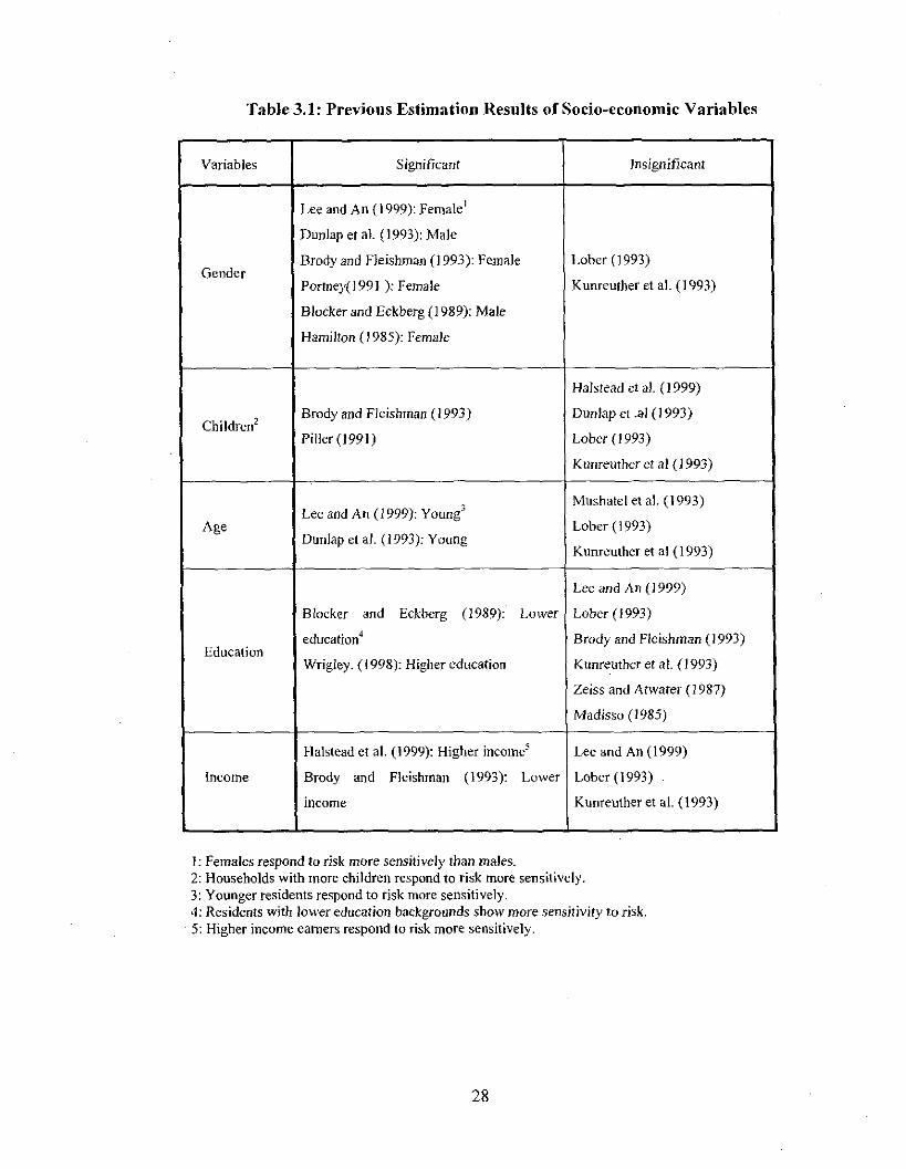
Table 3.1: Previous Estimation Results of Socio-ecouomic Variables

Variables Significant ]nsignificant

Lee and An (1999): Female'

Dunlap el at (1993): Male

GenderBrody and Fleishman (1993): Female Lober (J 993)

Portney(J991 ): Female Kunreulher et al. (1993)

Blocker and Eckberg (1989): Male

Hamilton (J 985): Female

Halstead et al. (1999)

Children'Brody and Fleishman (1993) Dunlap et .al (1993)

Piller (1991) Lober (1993)

Kunreuther et al (1993)

Lee and An (1999): Young'Mushatel et at (1993)

Age Lober (1993)Dunlap et al. (1993): Young

Kunreuther et al (1993)

Lee and An (1999)

Blocker and Eckberg (1989): Lower Lober (1993)

education4 Brody and Fleishman (1993)Education

Wrigley. (1998): Higher education Kunreuther et al. (1993)

Zeiss and Atwater (1987)

Madisso (1985)

Halstead et aJ. (1999): Higher income' Lee and An (1999)

Income Brody and Fleishman (1993): Lower Lober (1993)

income Kunreuther et aJ. (1993)

1: Females respond to risk more sensitively than males.2: Households with more children respond to risk more sensitively.3: Younger residents respond to risk more sensitively.4: Residents with lower education backgrounds show more sensitivity to risk.5: Higher income earners respond to risk more sensitively.

28

3.4 Summary of Literature Review

Economic analysis of NIMBY may be characterized as based on the expected utility

theory. Under expected utility theory, there are two major approaches: the hedonic price

approach and the risk perception approach. The hedonic price approach is the one where

NIMBY attitude is explained indirectly by way of measuring the impacts on property

values of a noxious facility in the host area. However, a major limitation of this approach

is that attitudes on the part of residents are completely ignored. On the other hand, risk

perception model incorporates both residents' attitudes and the environmental impact of a

sited facility but without a clear theoretical basis.

The regression analyses show that attitude and other variables have significant

bearings on the siting decision of local residents. However, there is no clear linkage

between theory and empirical analysis in the study of NIMBY, leaving a gap for further

analysis. Our study is intended to fill the existing gap by developing a theoretical

justification for subsequent empirical analysis.

29

CHAPTER IV

THEORETICAL MODEL FOR SITING OF THE COMPOSTING FACILITY

4.1 Overview

In this Chapter, we derive a theoretical model describing the representative

resident's attitude towards the siting of a large - scale composting facility in the vicinity

of his residential area. 13 Section 4.2 presents a two-choice model as a theoretical basis in

general for using the simple logit model in siting studies. In section 4.3, we extend the

two-choice model to three-choice one which provides the theoretical basis for our

empirical model (i.e., MNLM).

4.2 Two-choice Model

As stated earlier, our approach for developing a theoretical model is based on the

expected utility theory. 14 The siting of a MSW composting facility generates both

expected wealth equivalent and expected costs. 'S Wealth equivalent (w) may be specified

as a function of a vector of positive wealth attributes (a), which is continuous and twice

differentiable.

w=w(a)

where

(I)

13 To our 10low]edge, there is no siting study that provides a rigorous theoretical basis for empiricalapplication of the logit model.I For example, see Brookshire et al. (1985).IS Hereafter, "expected" will be omitted for convenience.

30

Subscript a, denotes derivative of the subscripted function with respect to a,. The vector

of major positive wealth attributes contains compensation, the local residents' positive

attitudes (such as active waste management behavior and trust in the siting institutions),

and economic benefits from hosting the facility.lo The wealth equivalent to be generated

by the siting of the MSW composting facility can be considered as an increasing function

of each positive wealth attribute. For example, for a resident with a strong tendency to

dispose of yard and food waste regardless of the existence of the composting facility, the

composting facility sited close to his property would save him a great deal of effort and

time. Therefore, the closer to his residence is the facility, the greater is his expected

wealth equivalent. The proximity of the facility to his residence would also generate other

wealth effects through economic benefits offered by siting authorities (local or central

government) to the residents in host area.

The costs (h)17 associated with the MSW composting facility also may be stated

as a function of both positive and negative wealth attributes, and assumed to be

continuous and twice differentiable with respect to each argument.

h=h(a,s)

where

(2)

16 For example, enhanced school quality and economic opportunity such as new jobs, lower property taxes,and economic growth (Halstead et aJ. 1999)"Brookshire et aJ. (1985) used consumer's house payment as the hedonic price function under the twostates of event; earthquake or no earthquake state. In the context of the siting of a composting facility, thehedonic price is considered as the purchasing price of various estates and real estate. Since the role of thehedonic price is the cost to the buyers ofestates, for convenience the hedonic price function will be referredto as cost function.

31

Sh1 = [.1 1 .1, ... .1/)'.

Subscript sf dcnotes derivative of the subscribed function with respect to .Ii' The cost is an

increasing function with respect to each positive wealth attribute. A resident with an

active waste management trait may have a higher reservation price for a property closer

to the composting facility. 1& Note that s as an argument in the cost function is a vector of

negative wealth attributes in terms of monetary loss as a self-insurance. It also includes

the indirect monetary costs the representative resident perceives in connection with the

existing negative environmental impact. A greater monetary loss would incur if the

property were within the perimeters subject to significant environmental impact, thus

reducing the market value of the property (- I < h, < 0).19 The cost function is assumedJ

to be convex in both attributes.2o

18 The positive attitude variables are nonnaJJy referred to simply as ·'attitude variables" in siting studies.According to Sears et al. (1980), there is a close linkage between one's attitude and pursuit of wealth.Henc~ attitude variables positively affect the wealth equivalent as well as the cost functions. As stated inthe literature review in Section 3.2, attitude variables include such variables as trust in institutions, publicparticipation in the decision making process, general knowledge on facilities and the available informationsources on the noxious facilities. While previous siting studies attach importance to the attitude variables,none of studies treats them from an economic perspective.19 The marginal cost of safety ( - 1 < h < 0) implies that 'one additional dollar spent on safety more than, j

offsets the cost' (Brookshire et al. 1985). More specifically, if a resident spends one dollar for safety of hisestate, the price of the estate increases by more than a dollar.20 The Hessian for the cost function is,

H ~ fhh",a, hha"'j J. By the assumptions of haa. > 0, ha,. = h, a < 0, h" > 0, and. II IJ "JI 'PJ

SjO; ofjS)

h h - h .. 2 > 0 in Equation (2) the Hessian is positive definite, which implies the cost function isow; 5j-lj a,s,

convex.

32

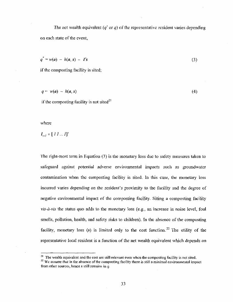
The net wealth equivalent (q' or q) of the representative resident varies depending

on each state of the event,

q' = wen) - hen, s) - l's

if the composting facility is sited;

q = wen) - hen, s)

if the composting facility is not sited2J

where

[<xl = [ 1 1 '" 1]'

(3)

(4)

The right-most term in Equation (3) is the monetary loss due to safety measures taken to

safeguard against potential adverse environmental impacts such as groundwater

contamination when the composting facility is sited. In this case, the monetary loss

incurred varies depending on the resident's proximity to the facility and the degree of

negative environmental impact of the composting facility. Siting a composting facility

vis-a-vis the status quo adds to the monetary loss (e.g., an increase in noise level, foul

smells, pollution, health, and safety risks to children). In the absence of the composting

facility, monetary loss (s) is limited only to the cost function. 22 The utility of the

representative local resident is a function of the net wealth equivalent which depends on

21 The wealth equivalent and the cost arc still relevant even when the composting facility is not sited.22 We assume that in the absence of the composting facility there is still a minimal environmental impactfrom other sources, hence s still remains in q.

33

whether the composting facility is sited or not. Utility functions in both cases may be

expressed as:

U(q') =U[w(a) - h(a,s) -I's]

if the composting facility is sited

U(q) = U[w(a) - h(a,s)]

ifthe composting facility is not sited

where

U . > 0; U .• < 0; U q > 0; U qq < O.q qq

(5)

(6)

Functions subscripted with q* and q denote their derivatives with respect to q* and q,

respectively. Each utility function is assumed to be concave in the net wealth equivalent.

The subjective probabilities that the local resident accepts or rejects siting the composting

facility are denoted by p and (1 - p), respectively. The representative local resident's

expected utility?3 may be written as

EU(q) =p U(q*) + (1- p) U(q) (7)

23 The siting of a large-scale waste facility is an important public issue of social optimal allocation. For itsunique nature of non-rivalry and non-excludability, however, public goods do not have markets whichdetermine their prices. CVM(Contingent Valuation Method) is a practical approach to valuing the publicgoods. In CVM, the value of a public good is measured based on the compensatiou value orpublic's "willingness to accept or pay". Unlike CVM, our approach is based on expected utility where theprobability is endogenously determined by positive and negative wealth attributes. Therefore, the"compensation" variable in CVM 1S only a component in the vector of wealth attributes in our model.

34

Equating to zero the partial derivatives with respect to G; and s I yields Equations (8) and

(9) as the FOC.24

(1- p)h, U.___'-,-J _q_

p(l+h,) U qJ

where

i = 1, 2, ... , n; j =1, 2, ... , I.

(8)

(9)

Equation (8) states that at the optimum the marginal (net wealth) benefit and the marginal

cost of the i-th wealth attribute are balanced (w = h ). Equation (9) shows that at theOf of

optimum the ratio of marginal utilities in two states (of siting and no siting) equals the

ratio of marginal costs weighted by the corresponding probabilities. It also describes the

willingness to bear a higher cost for a greater safety.

The final objective of this section is to analyze the effects of positive and negative

wealth attributes (ui and SJ) on the subjective probability of the representative local

resident's attitude toward siting of the composting facility in terms of Yes (accepting) or

No (rejecting). To show the relationship between these attributes and the resident's

24 Fonnal proof of second order condition is available in the appendix A

35

subjective probability, first we rearrange Equation (9) for the ratio of the probabilities or

odds (r).

where

r = --.!!..­I-p

(10)

Under the optimal condition (w = h.), taking partial derivatives of Equation (10) withOr ill

respect to both positive (a,) and negative (s) wealth attributes yields Equations (11) and

(12).

>0 (11)

Iy = ------,- A < 0

'/ U.(l+h)'q S}

where

(12)

36

Equations (11) and (12) indicate that the positive wealth attribute increases the

probability that the resident accepts the facility, while the negative wealth attribute

decreases the probability. By Equations (II) and (12), we find that thc odds r is a

positive function of the vector of positive wealth attributes (a) and the negative function

of the vector of negative wealth attributes (s). In short, r can be expressed as the

function of a and s as:25

r = f (a, s)

where

fa; > 0; f'J < O.

(13)

Equation (13) is a two-choice theoretical model which renders itself as a sound

theoretical basis for applications of a binomial logit model. It also explains NIMBY

attitude as an outcome of rational behavior on the part ofresidents.

There are two principal reasons for Equation (J 3) being a sound theoretical basis

for empirical application of the simple logit model. First, the subjective probability in our

theoretical model is endogenously determined. Previous siting studies have modeled the

resident's subjective probability as the main indicator of risk perception; such a

probability is given exogenously (Kunreuther and Easterling 1990; Halstead et al. 1999).

Second, our model is a theoretical counterpart of the simple logit model. Since the

25 \\toen y is redefined as its reciprocal, then the signs of r .and r ~ are reversed.(1, . j

37

dependent variable in the logit model is the log of odds ratio, this model's endogenously

determined odds ratio can be recast as a simple logit model:

In r =In~ = x<t> + I:1- P

where

X'xk =[ x, x2 ••• X k ]; <t> kd =[9, 92'" 9, ]'; I: = residual vector.

(14)

Suppose x, and x) are proxies for a, and sJ respectively. That is, x,= x,(a,) and xj=

xJ(s .. ), for which (x,)a> 0 and (x), > O. Differentiating Equation (14) with respect to

, I ) . j

a, ' and rearranging for ¢, ,

[I I J= --- > 09, r (x,)" Yo,

(15)

Noting that the positivity of 9, is due to r > 0, (x,)a > 0, and y, > 0, and ¢,measures, ,

the impact of a, on the Yes odds (ra ).,

Similarly,

38

II I ]- --- <0if>; - Y (x)'J Y.'J

(16)

Noting the negativity of if>; due to Y > 0 and (Xl)') > 0, and Y.'J < O. Therefore, the

two-choice model lends itself as a theoretical justification for applying the simple logit

model.

4.3 Three-choice Model

Equation (13) is derived under the assumptions of two states of event, therefore

unsuitable as a theoretical basis for MNLM applied in our empirical analysis, where

survey respondents have three choices to questions: Yes, No, and Maybe.26 Therefore, in

this section we extend the two-choice model to a three-choice one under the same

assumptions as the previous section27

Suppose that respondents have three choices with regard to siting the composting

facility: PI for choice Yes, P, for choice No, and p, for choice Maybe which reflects

respondents' reservation on whether the facility should or should not be sited. The

expected utility function in the context of these three choices is:

(17)

2. See question 40 in Appendix B. Detailed explanation is given in Chapter 5.27 Assumptions on the wealth equivalent, cost, and utility functions remain the same as the previous section,unless otherwise stated.

39

where

q, = w(a) - h(a, s) - l's

q, = w(a) - h(a, s)

if the composting facility is sited;

if the composting facility is not sited;

qJ = A[w(a) - h (a, s) -I's] + (1- A)[w(a) - h(a,s)]

=[w(a) - h(a,s) - ;U's]

o<A < 1

if the siting of a composting facility is uncertain;

risk orientation factor;

The value of resident's risk orientation factor ( A ) is assumed to range from 0 to

I. If A is close to I, the resident tends towards in favor of siting of the composting. If A

is close to 0, the resident tends towards against the composting facility. Therefore, if A is

between 0 and I, this represents an intermediate case between the two choices; accepting

the composting facility and rejecting the composting facility. As in the previous two -

choice case, FOes are obtained by taking partial derivatives of Equation (17) with respect

to OJ and Sf respectively.

- P, U q, (I +h'i) - p, U" h" - P3 U" (1- A+ hi!) = 0

40

(18)

(19)

The value of marginal cost of safety h'J in Equation (19) is between -1 and O. The

greater absolute value of the marginal cost of safety implies that one dollar spent on the

safety measure has a smaller positive impact on the property value.

To investigate the effect of positive and negative wealth attributes on the

representative local resident's siting decision, we divide through Equation (J 9) by PI =

(1- P, - P3 ).

where

Y_ P, . Y = P3

21 - , }](1- p, - P3) (1- P, - P3)

(20)

By taking partial 'derivatives ofEquation (20) with respect to G" holding YJI constant,

we have,

Rearranging Equation (21) for (y21) Q; ,

41

(21 )

h- _'ia, (U U U )

U h. " + r 21 'I, + r 31 'I)112 .Ij

< 0 (22)

Partially differentiating Equation (20) with respect to S J' holding r31 constant,

- U (1 + h )' + U h + (r ) U h + r (-U h 2 + U h )111, Sj ql Sjs} 21 5j q1 Sj 21 q2q2 Sj 1f2 J/ j

+ rJJ[-U'MJ U + h'l)' + Uq)h'J'l] = 0

Rewriting Equation (23) for (r 21 )"l

'

(r21).,,= U Ih

[U'I,q,(I+h'j)'-U'I,h'J'i +r,,(Uq,q,h'j' -Uq,h'J')qz Sj

(23)

(24)

By taking partial derivatives of Equation (20) with respect to a" holding r 21

constant,

Rearranging Equation (25) for (r31)a.'

42

(25)

where

(26)

The absolute value of the marginal cost of safety (I h,1 ) could be lower or higher than')

that of the risk orientation factor ( Jc ), determining the sign of (r31)", .

Now, partially differentiating Equation (20) with respect to S J ' holding r 21

constant,

- V.,q, (I + h'J)' + V q,h'h + r 21 (-V"", h'J 2 +V q, h')ll)

+(r) V (Jc+h )+r [-V (Jc+h ')'+V h ]= 0]J .fj q3 Sj 3J fJ3q; 5j il3 $jsJ

Rewriting Equation (27) for (r3j), ,, )

where

43

(27)

(28)

(Y 3 ,) < 0, in + h > °(A > Ihi); (Y3I). > 0, in + h, <°(A < Ih,I)·5j Sj SjJ} ',I .I

Equations (22) and (24) show that the odds of No to Yes is a decreasing function of the

positive wealth attributes and an increasing function of the negative wealth attributes28

Equations (26) and (28) show that the signs of partial derivatives of Maybe odds depend

on the sign of the difference between>' and h, . . When the value of the risk orientationJ

factor is greater (smaller) than the absolute value of the marginal safety cost, the signs of

partial derivatives of Maybe odds are the same as those of the partial derivatives of Yes

(No) odds.

The odds ratios Ym , (= Pm , m = 2,3) in Equation (20) change into Ym2P,

m = 1, 3) if Equation (19) is divided by Pz as shown in Equation (29).

(= Pm ,P2

y 12 U" (I+h,)+Uq h,. +Y32Uq (A +h,)1 J 2) 3 j

where

o (29)

28 Having three choices available to respondents is exactly the case in our survey form (see Appendix B). Inour empirical model (MNLM) in Chapter VI, the dependent variables are the log of odds whichcorresponds to the odds functions in three·choice model. The direction of change in the odds ratio is the

same as that of log of odds ratio: when the odds ratio of No to Yes cboice (Y" = P2IP,) increases

(decreases), the log of odds ratio (In(P,IP,)) also increases (decreases). Hence, for consistency in both

theoretical and empirical analyses, we use the same tenninology " odds of rn to b choice ,. for both rmb

and In(PmIP,,) (m = 1,2,3, b = 1,2,3, and m oF b). Further, by "Yes odds (ratio)" we refer to y'o = In(P/P,,),

b = 2 or 3), and by "No odds (ratio) " to y", ~ In(P,iP,,), b = lor 3, and by "Maybe odds (ratio)" to Y3b =

In(P,iP,,), b = I or 2.

44

P, PJYI2 = , Yr =

(1- p, - PJ) " (1- P, - P3)

Taking partial derivatives of Equation (29) with respect to a, ands} respectively, holding

Y32 constant,

(YI2),jV,, (1 +h) + Yd-V q''I, (1 +h)' +V'I,h'J ).f)

-V h '+V h 2+ y [-V (h +:\.)'+V h )=0q2g2 Sj q2 oS j 32 q~l/J .'OJ qJ SjS j

Rewriting Equation (30) for (YI2)a, and Equation (31) for(y,,).,),

hs _o .

(y) - J' (yU+U+yU»O" ai - - U (I + h) "" 42 32 4J

" s

(30)

(31 )

(32)

45

Equations (32) and (33) have the same implication as Equations (22) and (24). The partial

derivatives of two odds (Y'2' Y21) show that they are symmetric as expected: forexample,

(y"la, > °and (Y21)a, < 0. The positive sign of (Y" la, indicates that the odds of Yes to

No choice increases as a positive wealth attribute increases. Which, in turn, implies that

the odds of No to Yes choice decrease as a positive wealth attribute increases. The same

implication also holds for (Y" )'J and (y 21 )'J .

Now, holding y" constant, partially differentiating (29) with respect to a,and Sj'

and rearranging for (Y3,)"" (Y")"J' the following equations are obtained:

hs ,0

)' (yU+U+yU)U (Jc + h) "q, " "q,

qJ s)

(34)

where

(Y"la, >O,ifJc +h'i >O(Jc > Ih,); (Y32)a, <O,ifJc +h'i <O(Jc < Ih,).

I [ 2 , .= U I+h -U h +U h -U h(Y")'I U fA +h ) (Y/,{ q'<J( 'I) q"J'j} qHz'J qZ'f'f

q3 '(I s)

where

46

(35)

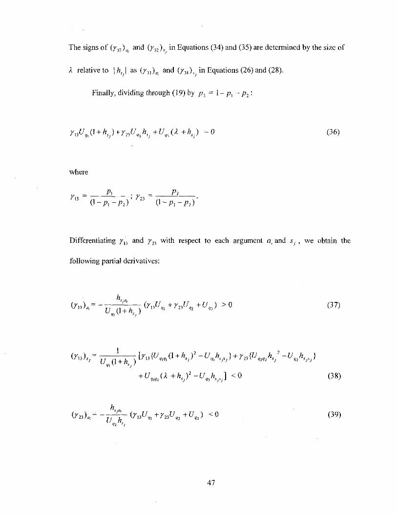
The signs of (Y")a and (Y"L in Equations (34) and (35) are determined by the size ofI '.I

A relativeto 1\1 as (Y")a; and (Y3J)'j in Equations (26) and (28).

Finally, dividing through (19) by Pl = 1- P, - P, :

where

P, . Y = P,r13 = , 23(J - P, - p,) (1- P, - p,)

(36)

Differentiating YI3 and Y23 with respect to each argument a, and s), we obtain the

following partial derivatives:

hs -a(Y) - ]' (yU+yU+U»O

13 aj - - U (1 + h.) 13 'II 23 n '13q! '\j

(37)

h(Y23)a; = - U 'j~ (y 13Uq, +Y23Uq, +Uq,) < 0

iJ2 Sj

47

(39)

(40)

The sign for each of (Y,,) a , (Y,,), ' (y 21 ) a ' and (y 21), in Equations (22), (24), (32),I .)} )

and (33) indicates the direction of the relationship between a non-base choice and a

wealth attribute. The signs of partial derivatives of the Yes and No odds are invariant with

respect to the base choice as Equations (37) through (40) show.

Our three-choice model can be expressed as Equation (41), summmg up the

previous 12 equations: (22), (24), (26), (28), (32) through (35), and (37) through (40).

where

P1mb = --'!'.-, (m= 1,2, 3; b= 1, 2, 3; m,. b);Pb

Umb)a, > 0 and (fmb)"J < 0, if the non - base ehoiee is Yes (m = 1);

Umb) a < 0 and (fmb) , > 0, if the non - base choice is No (m = 2);, J

(41 )

Umb)a, > 0 and (fmb)'J < 0, if the non - base choice is Maybe (m = 3) and A > 1\1;

Umb)a, < 0 and (fmb)"J > 0, if the non - base choice is Maybe (m = 3) and A < 'h,)-

48

The signs of partial derivatives of each odds are summarized in Table 4.1. The

signs in Table 4.1 imply that a resident's response on the siting is contingent upon wealth

attributes (positive or negative) and the magnitude of the risk orientation factor relative to

that of the marginal safety cost. The signs of partial derivative of Yes and No odds

(r" ,rl3 ,r2l , and r 23) depend upon whether the wealth attribute is positive or negative.

More specifically, residents have more tendency to vote against (for) the noxious facility

when their positive wealth attributes are lower (greater), which is exactly the opposite for

negative wealth attributes.

With respect to the sIgns of Maybe odds' partial derivatives, if one's risk

orientation factor is relatively high (X > Ih'jl), then the signs of (r31)0, and (r32)o, (or,

(r31 )'i and (r32) 'j) are the same as those ofthe Yes odds' partial derivatives: (r" )0, and

(rJ3 t, (or, (r")'jand (rl3),)- When the risk orientation factor is relatively small (X <

Ih'jl ), then the signs of (r 31 )a, and (r 32)", (or, (r 31 )"1 and (r 32 )'1 ) are the same as those

of the No odds' partial derivatives: (r2Jla, and (r23)o, (or, (r21)'1 and (rn).,)' Therefore,

the risk orientation factor can be identified simply by referring to the signs of Maybe

odds' partial derivatives. That is, if the signs of both (r31)", and (r,,) a, are negative,

then the signs are the same as those of No odds' partial derivatives «r21 )" and (r23),,),

which indicates that the risk orientation factor is less than that of the absolute value of the

marginal safety cost, thus implying a relatively weak orientation towards the siting. The

opposite (a stronger orientation towards Yes) will be the case if the sign of both (r31 )a,

and (r,,), are positive. Our model with the risk orientation factor incorporated has a. ,

49

greater applicability to empirical analysis of the siting problem associated with any other

unpopular facilities where the local resident's level ofrisk perception matters.

In short, the three-choice model has identified the impacts of wealth attributes on

the residents' responses to the planned siting of an obnoxious facility, and also the

relevance of the risk orientation factor latent in Maybe choice. Compared to the two-

choice model, the three-choice model's implications are more amenable to reality with

more detailed information regarding Maybe choice incorporated into the model.

Table 4.1: Impacts of Wealth Attributes on Odds

Yes odds Sign

(Y"),,, (Yl3\ +

(y,,) 'j , (y" \ -

No odds Sign

(Y2I)", (y"),, -

(Y21)'i' (Y")'J +

Maybe odds Sign Sign Condition

irA. > liz,)+

(Y3I )" ' (y" t,- if it < Ih,1

)

- if it > liz,)(r3l),j' (Y")"J

if it < Ih,}1+

50

CHAPTER V

SURVEY AND DATA MANAGEMENT

5.1 Variable Selection

In specifying the logit model, we have chosen mostly the variables employed in

previous siting studies. As mentioned in the previous chapter, there are a number of

explanatory variables that have been previously used. The three-choice model indicates

that the subjective probability of rejecting (accepting) the facility is a decreasing

(increasing) function of positive wealth attributes and an increasing (decreasing) function

of negative wealth attributes. The variables chosen, therefore, may be classified into two

categories: positive wealth attribute variables and negative wealth attribute variables.

Five variables (IPWM, PPDSP, TRUST, KNOW, ACCESS) of the positive

attribute variables employed may be called 'the positive attitude variables'. Past studies

show that a local resident's active participation in waste management leads to a fairly

high probability of accepting the facility (Halstead et a1. 1999). Involvement in the

decision making process regarding the siting plan is also an important factor (Bogdonoff

1995; Blahna and Yonts 1990). IPWM (individual's participation in waste management)

and PPDSP (public participation in decision making for siting plan) are meant to capture

the permissiveness. IPWM is intended to measure how the residents remain active in

managing waste disposal and their attitudes towards recycling. By PPDSP we measure

the extent of the residents' participation in the decision making process. TRUSTmeasures

the individual's perceived dependability of various waste management related

institutions; such as the central and local government, universities, etc. Hence, the higher

the residents' trust of the institutions considerably, their responses would reveal a higher

51

probability of accepting the unpopular facility (Kunreuther et a\. 1993; Desvousges et a\.

1993).

Several studies also argue that the general knowledge of a noxious facility may

reduce risk perception induced by such a facility. Residents with correct knowledge of

the environmental impacts of facilities tend to reveal a lower probability of rejecting the

noxious facility as opposed to residents who do not have knowledge (Dunlap et a\. 1993;

Kraft and the Clay 1991; Rosa and Freundenberg 1993). The level of general knowledge

is measured by KNOW.

COMP (monetary compensation) and RELCOM (relative monetary

compensation) are selected as the compensation variables. As stated in previous studies,

monetary compensation is found to be effective in encouraging local residents to accept

the noxious facility; assuming sufficient environmental safeguards are strictly enforced

(Bacot et al. 1993; Kunreuther and Easterling 1990; Peele and Ellis 1987). In managing a

composting facility, it is unlikely that any hazardous incident will occur with normal

efforts to protect the environment in place. In our analysis, we anticipate that a resident

demanding a high monetary compensation has a stronger NIMBY attitude, hence a

monetary compensation will have a positive effect on the residents' attitudes toward a

composting facility siting. In addition, we have RELCOM which is obtained through

dividing COMP by the individual's income. Hence, the amount of compensation chosen

by each respondent is expected to vary according as his or her income level. 29

A resident's siting decision also depends on the number of information sources

one has access to on a facility (GAO 1996; Slovic 1987). By ACCESS (the availability of

information sources on waste management) we measure the information sources available

29 The issue related to data bias is discussed in Section 5.2.3.

52

to the public. Variable ACCESS is used to investigate whether the availability of

information sources matters in Korea as observed elsewhere in previous studies. ECO

measures the economic opportunity that local residents in a host area can anticipate from

hosting a composting facility. Examples include lower property tax, lower waste disposal

cost and an increase in employment. ECO is generated through factor analysis to

represent the multiple aspects of a community's local economic situation that may vary

by the hosting of a noxious facility.

We have three negative wealth attribute variables: DIST (proximity), ENV

(environmental impact), and INCOME (monthly disposable income). 30 There is

significant amount of evidence of a positive relationship between a resident's proximity

to a noxious facility and a resident's negative attitude towards siting decision. Thus, we

have chosen proximity as one of the negative wealth attribute variables for our empirical

analysis. The positive effect of an economic opportunity available to a local economy is

weighed against the environmental impact of hosting a noxious facility (Halstead et al.

1999; Cho 1998; Wirth and Heinz 1991). Like ECO, ENV is generated through factor

analysis to measure the various degrees of environmental impact that stems from hosting

the composting facility.

Previous empirical evidence does not support an lmambiguous prediction of the

resident's income level's effect on siting attitude. However, compared to other countries,

the price of real estate in Korea has been unstable and extremely high relative to other

assets. Consequently, many Koreans earning high incomes are likely to allocate a

30 Often in the SIting literature 'socia-economic variable' and 'socio-demographic variable' are usedinterchangeably. However, since technically INCOME is classified as one of the negative wealth attributevariables, we will refer to the previous socio-economic variables as socio-demographic variables if incomeis excluded. Otherwise, the variables will be referred to as socio-economic variables for convenience.

53

significant portion of their wealth to real estate or land. The presence of a noxious facility

would, therefore, make high income residents have a keener risk perception relative to

low income residents. Thus, we expect a positive relationship between the residents'

negative siting decision and their income level.

Socio-demographic variables are included In many siting studies along with

attitude variables, because they are considered very much relevant in explaining the

siting decision of residents in local context. Though the socio-demographic variables are

not explicitly mentioned in our theoretical discussion in Chapter IV, they are included in

our empirical model to see how they are important in the local resident's siting decision

in Korea. The socio-demographic variables used in our empirical model are CHILD

(number of children in household), EDU (level of education), GENDER (a resident's

gender), AGE (a resident's age), NHMBR (household size), YRSTAY (number of years a

resident has lived in their home), and HSFORM (a resident's house type).

In anticipating the result of our empirical estimation, we leave the effects of two

socio-demographic variables (CHILP EDU) to a siting decision as unknown due to

contrasting results from previous studies. Following Lee and An (1999), we expect that

women and young people are more likely to perceive high risk, and therefore more

sensitive to the siting of a composting facility. In addition to CHILP NHMBR is added to

reflect the long tradition of respecting the elderly in the Korean culture. If residents have

more family members, including elders, they are likely to respond more negatively to the

composting facility than otherwise.

There are two additional socio-demographic variables; YRSTAY and HSFORM.

For YRSTAY we expect that as people live longer in one place they will display a more

54

rigid attitude towards a facility siting. A longer period of residence may be a good

indicator of a weaker incentive to move to another place, causing residents to feel more

sensitive to environmental impacts than otherwise.

HSFORM may also be related to a resident's siting decision. Apartment

complexes in Korea are usually located in the central area of a city. The composting

facility is considered to have a greater impact on the average market value of apartment

units rather than houses. Hence, residents living in apartment units may feel more

susceptible to a composting facility sited in their neighborhood.

5.2 Survey and Data

5.2.1 Sampling and Survey Procedure

We chose Cheju City, Korea as target area for our survey for the reason that

Cheju Province is one of the most attractive tourist destinations in Korea for its cleaner

environment and mild temperature, therefore the opportunity cost of the composting

facility would be much higher than the rest of Korea. Further, we are unaware of any

previous study with respect to siting a noxious facility in Cheju Province. Our ex-ante

study will provide insights for future plans to site noxious facilities in Cheju Province and

other parts ofKorea.

The population ofCheju City is 279,087, and the number of households is 90,562

as of December 2000 (Cheju City Hall 2001). Cheju City is composed of 19 dongs. To

minimize the sampling bias, the random sampling was used. Table 5.1 shows the

distribution of the total sample sIze III proportion to the population distribution.

Following the sample distribution, we used the telephone directory to randomly select

55

2,500 respondents. A total of 2,500 survey forms were distributed randomly to the

respondents. Of the 2,500 forms, 650 were classified as 'incomplete' and excluded from

our analysis. The remaining 1,850 forms only were used, which is approximately 2.04 %

of the total households in Cheju City.

Table 5.1: Sample Distribution

Number of

DongHouseholds B~(A/90,562)X

C D E~D/I,850in each 100Dong~A

II do II dong 1,775 2.0 49 31 1.7II do I dong 12,289 13.6 339 256 13.9I do II dong 2,76\ 3.0 76 59 3.2I do I dong . 12,791 14. I 353 302 16.3Samdo II dong 4,871 5.4 134 11\ 6.0Samdo \ dong 3,763 4.2 104 92 5.0Yongdam II dong 3,417 3.8 94 73 4.0Yongdam \ dong 5,943 6.6 164 98 5.3Gunip dong 4,128 4.6 114 71 3.8Hoabuk dong 6,222 6.9 172 III 6.0Sam Yang dong 2,541 2.8 70 41 2.2Bongaedon o 885 1.0 24 12 0.7Ara dong 3,920 4.3 108 63 3.4Ora dong 1,723 1.9 48 39 2.1Yeon dong II ,391 12.6 314 233 12.6Nohyung dong 7,480 8.3 206 \58 8.6Oido dong 2,708 3.0 75 62 3.31ho dong 1,301 1.4 36 24 1.3Do du dong 653 0.7 18 12 0.7

Total 90,562 100.0 2,500 1,850 100.0

Source: CheJu CIty hall, 2001

B: The percentage of the number of households in each dong out of the total number of households inCheju City

C: The total number of distributed survey formsD: The total number of available survey forms taken from CE: The percentage of the number offinally used survey forms out of 1,850

The survey forms were divided into 5 groups based on the distance between

respondent's home and the hypothetically proposed composting facility, i.e., 100 m, 300

56

m, 700 m, I km, and 3 km. The survey was conducted by individual visits to 2,500

households asking the residents to fill out the questionnaires. The whole data collection

process took approximately eight months. 31

5.2.2 Survey Data and Bias Problems

The survey data is usually susceptible to biases in conducting CVM. The bias

problem in sun'ey data relates to the primary goal of CVM: measuring one's WTP

(willingness to pay) (Dixon et aJ. 1986). However, our study's main objective is not to

produce any specific numerical value but to find the relationship between the local

resident's siting decision and the various factors (independent variables) based on

economic principles. Therefore, there is a low probability of our data being affected by

the same type of biases found in CVM. Since we opted to usc surveys for collecting data,

however, we endeavored to minimize the biases by implementing our survey based on a

planned and conducted survey questionnaire (Dixon et al. 1986) as explained below.

Information Bias Problem

The information bias can be caused by misleading survey questions or insufficient

infonnation presented in questionnaires (Dixon et al. 1986). To avoid this type of biases,

the survey contents should be as clear and objective as possible. Many telephone or mail

survey involves a great deal of miscommunication between interviewers and interviewees,

consequently leading to information bias (Kwak and Chun 1995). In order to minimize

the problem, we conducted personal interviews instead of relying on telephone or mail

31 From May 200 I to December 200 I.

57

survey. Surveyors were given a specific guideline on how to explain survey questions

with a maximum clarity.

Instrument Bias Problem

The instrument bias emerges from tbe choice of inappropriate payment means

(Dixion et al. 1986). Generally, instrument bias occurs when the willingness to pay vary

depending on the different payment vehicles in CVM (i.e., tax or entrance fee).

Instrument bias also occurs from choosing 0 (no money), which indicates strong support

by the respondent towards hosting the facility. Following Douglas (1989), we used tax as

a proxy variable for the monetary compensation COMPo We designed the options for

question 43 corresponding to COMP to vary between 3,000 and 50,00032 to alleviate this

bias. Having taken this precaution, an instrument bias is unlikely to occur in our study.

Inappropriate Measure Bias Problem

Inappropriate measure bias is associated with respondents having different

income levels. To avoid this bias, we divided COMP by each respondent's income level

so that the level of compensation can be differentiated among different income groups.

5.2.3 Survey Content

We reviewed several previous survey forms for format as well as content to create

our survey questionnaire. While drafting the survey questionnaire, we found that most

previous studies were on the siting of hazardous waste facilities, and that there were only

a few studies related to the siting of composting facilities. This is the primary reason why

32 This approximately corresponds to US$ 2.50 - 45.00.

58

we relied on Halstead et al. (1999).33 Through interviews with waste management

personnel in Korea, we were able to omit non-relevant questions from their survey. In

addition, waste management personnel in Korea provided valuable insights resulting in

some additional questions. We referred to the survey fornls conducted by Kunreuther and

Easterling (1990), and Douglas (1989) to add questions on compensation and socio-

economic variables. Since our study involves Korea, we also referred to several survey

fornls implemented in Korea to reflect the germane feature of Korea. Prior to the survey

implementation, an experimental survey was conducted for a selected number of

residents with a purpose of improving initial draft.

The final version of our survey questionnaire consists of 52 questions. Question

40 relates to the dependent variable, asking the respondent to select one of three choices,

i.e., Yes, No or Maybe. The survey has three major sections. The first section is

concerning solid waste management practices and attitudes, which consists of 14

questions. Questions 1 through 6 measure the resident's willingness to be involved in

waste management, which are used for IPWM. Questions 7 to 14 are used to gauge the

level of trust (TRUST) that residents place in institutions (e.g., local government,

environmental groups). The second section begins with the sentence "What if a

composting facility is built around your residence?" There are questions about how local

residents perceive negative environmental effects and what kind of economic opportunity

they expect from the composting facility (questions 15 to 28). Based on these survey

questions, we implement factor analysis to generate two new variables: ENV and ECO.

33 In formulating survey questionnaire, they also referred to several previous works such as Lober (1993),Portney (1991) and Hamilton (1985).

59

Question 41 is intended to measure the resident's general knowledge of the

composting facility compared to that ofother waste disposal facilities. In this question we

try to measure whether residents have a general knowledge of a composting facility's

safety relative to other waste disposal methods (KNOW). Respondents have five options

to choose from "very low" to "very high".

Question 42 is designed to capture the degree of public participation (PPDSP).

Question 42 asks how residents feel about their involvement in the decision making

process in relation to their previous experiences. As in the question 41, this question also

provides five options; 1 (not at all) to 5 (yes). Question 43 relates to compensation in

return for hosting a facility (COMP). The respondents are asked to choose from among 9

options. Question 44 is to find the number of information sources regarding waste

management (ACCESS).

The third section of the survey consists of eight questions: questions 45 through

52. These questions are intended to find the information on the socio-economic traits of

the residents; the number of children in respondent's home (CHILD), a respondent's

education level (EDU), a respondent's gender (GENDER), a respondent's age (AGE), a

respondent's household size (NHMBRl4, the number of years at the current residence

(YRSTAy), a resident's house type (HSFORM), and a household's average monthly

disposable income (lNCOME).35

'.j NHMBR is calculated through [1+ 'number ofchildren in one's household'+ 'number of adults in one'shousehold'].35 As stated in section 5. L INCOME is used as a negative wealth attribute variable. Since Section III in thesurvey questionnaire includes income, we refer to this set of questions as socio~economic questions.

60

5.3 Measurement Variables and Factor Analysis

5.3.1 Measurement Variables36

There are two measurement variables; JPWM and TRUST. IPWM is measured as a

composite of responses to questions 1 through 6 in our survey. These questions have

binary options coded "0" or "1". For example, question 1 is to see whether the respondent

is actively involved in waste management. The yes option indicates that the respondent

has a high tendency to recycle whereas the no option indicates the opposite. Yes and no

options are coded "1" or "0" respectively. Unlike questions I and 2, there are four

options to answer questions 3 to 6: 1 (never), 2 (sometimes), 3 (very often), and 4

(always). These questions are to measure how much effort a respondent exerts to reduce

the waste output in daily life. Among 4 options, "0" codes the choice of 1 or 2. Similarly,

"1" codes the option of 3 or 4. The binary measurements for IPWM are summarized in

Table 5.2. The summation of the binary codes for question I through 6 generates the

measurement variable IPWM. The range of IPWM is from "0" through "6". Tables 5.3

and 5.4 respectively present the frequency distribution and summary statistics ofJPWM.

Table 5.2: Binary Codes for Measurement Variable IPWM

Question number Response I Code I Response2 Code 21. Recycle Yes 1 No 02. Compost Yes I No 03. Less package lor 2 0 3 or4 14. Using reusables 1 or 2 0 3 or4 15. Borrow/rent lor 2 0 3 or 4 16. Sellfdonate lor 2 0 3 or4 1

3~easurement variable herein js defined as a variable generated by combining more than one variable insurvey data.

61

Table 5.3: Frequency Distribution of IPWM

IPWM Frequency Percentage Cumulative Percentage

0 87 4.74 4.74

1 416 22.65 27.38

2 404 21.99 49.37

3 300 16.33 65.70

4 242 13.1 7 78.88

5 281 15.30 94.18

6 107 5.82 JOO.OO

Total 1,837 100.00 100.00

Table 5.4: Summary Statistics of IPWM

Variable Obs Mean Std. Dev Min Max

IPWM 1,837 2.80 1.67 0 6

Table 5.5: Codes for Measurement Variable TRUST

QuestionResponse 1 Code J Response2 Code 2 Response3 Code 3

Number

7 lor2 0 3 ) 4 2

8 ) or 2 0 3 1 4 2

9 lor2 0 3 1 4 2

10 1 or 2 0 3 1 4 2

II 1 or2 0 3 1 4 2

12 1 or 2 0 3 1 4 2

13 lor2 0 3 1 4 2

14 1 or 2 0 3 1 4 2

62

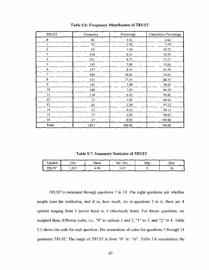
Table 5.6: Frequency Distribution of TRUST

TRUST Frequency Percentage Cumulative Percentage

0 85 4.63 4.63

1 47 2.56 7.19

2 65 3.54 10.72

3 114 6.21 16.93

4 151 8.22 25.15

5 145 7.89 33.04

6 157 8.55 41.59

7 184 10.Q2 51.61

8 315 17.15 68.75

9 145 7.89 76.65

10 146 7.95 84.59

11 118 6.42 91.02

12 72 3.92 94.94

13 42 2.29 97.22

14 17 0.93 98.15

15 17 0.93 99.07

16 17 0.93 100.00

Total 1,837 100.00 100.00

Table 5.7: Summary Statisties of TRUST

Variable Obs Mean Std. Dev. Min Max

TRUST 1,837 699 3.47 0 16

TRUST is measured through questions 7 to 14. The eight questions ask whether

people trust the institution, and if so, how much. As in questions 3 to 6, there are 4

options ranging from I (never trust) to 4 (absolutely trust). For theses questions, we

assigned three different codes, i.e., "0" to options 1 and 2, "I" to 3, and "2" to 4. Table

5.5 shows the code for each question. The summation of codes for questions 7 through 14

generates TRUST. The range of TRUST is from "0" to "16". Table 5.6 summarizes the

63

frequency of the measurement range (0 - 16) of TRUST. Table 5.7 presents the summary

statistics of TRUST.

5.3.2 Factor Analysis

The purpose of the factor analysis is to first extract out unobserved orthogonal

factors latent in observable data. These factors then are added to other regressors in

estimation. The procedure for the factor analysis is as follows: 1) Extract factors, 2)

Rotate the extracted factors, and 3) Generate factor scores for each factor (Kachigan

1991).

4

3

Figure 5.1: The Eigenvalues

64

Questions 15 through 28 relate to environmental and economic impacts on the

community. Presence of the composting facility incurs both wealth equivalence and costs,

neither of which can be fully captured by one or two questions. By asking as many

questions as needed, we attempt to capture the information which reveals the

respondents' attitudes towards the hypothetically proposed facility. The factor analysis

converted 14 questions into two factors; negative environmental externality and

economic opportunity respectively.J7 Each variable's eigenvalue can be checked. Figure

5. I shows that two eigenvalues exceed 1, which is the usual threshold value as significant.

Table 5.8: Factor Loadings

Question Number Factor Loading I Factor Loading 2

IS 0.32 0.47

16 0.57 -0.27

17 0.36 0.43

18 0.48 - 0.41

19 0.39 0.36

20 0.50 - 0.39

21 0.40 0.32

22 0.59 - 0.33

23 0.36 0.47

24 0.50 - 0.28

25 0.41 0.48

26 0.51 - 0.27

27 0.36 0.51

28 0.54 -0.22

37 Here each question is referred to as a variable. Variables ECO and ENVare composite variablesgenerated from the 14 variables

65

Table 5.8 reports "factor loadings" which are obtained through extracting factors.

By comparing two factor values for each variable, we can tell which variable is more of

which factor. For instance, for question 15 "stimulate economic growth", the factor

loading values are 0.32 for factor I and 0.47 for factor 2. This implies that question 15 is

more related to the second factor since the value of the second factor (0.47) is greater

than that of the first factor (0.32).

Table 5.9: Rotated Factor Loadings

Question Number Rotated Factor Loading I Rotated Factor Loading 2

15 - 0,004 0.57

16 0.6J 0.10

17 0.04 0.56

18 0.62 - 0.06

19 0.12 0.52

20 0,63 - 0.03

21 0.14 0.49

22 0,67 0.D7

23 0.03 0.60

24 0,57 0.05

25 0.06 0.62

26 0.57 0.D7

27 0.005 0.62

28 0.56 0.13

For question 28 "increase noise pollution," the relationship is reversed with the

value of factor loading I (0.54) being greater than that of factor loading 2 (-0.22). By

comparing the values of factor loadings for each variable,38 one can judge whether the

38 In factor analysis, each question is treated as a variable. Ibe resulting factors, composed ofquestions,become independent variables (Kachigan 1991).

66

question IS more of the adverse environmental impact or economlC opportunities

according as factor I value is greater or less than factor 2 value.

Next, we rotated the factor loadings by using varimax. The results are reported in

Table 5.9. Table 5.9 indicates that differences between rotated factor loadings become

more conspicuous. The rotated factor loadings for question 15, for example, give less

weight to the first factor and more weight to the second factor. Next, to generate the

composite variables, factor loadings are converted into scoring coefficients, following the

formula:

s = A' b (C'Cr'

where

sh J = A matrix of scoring coefficients;

A hk = The correlation matrix of variables (k is a number of variables);

(I)

bhJ

= Unrolated factor loading matrix (j is a number of factors);

CPi = Varimax rotated factor loading matrix.

In our study, k = 14 andj = 2. The scoring coefficients are reported in Table 5.1 O.

67

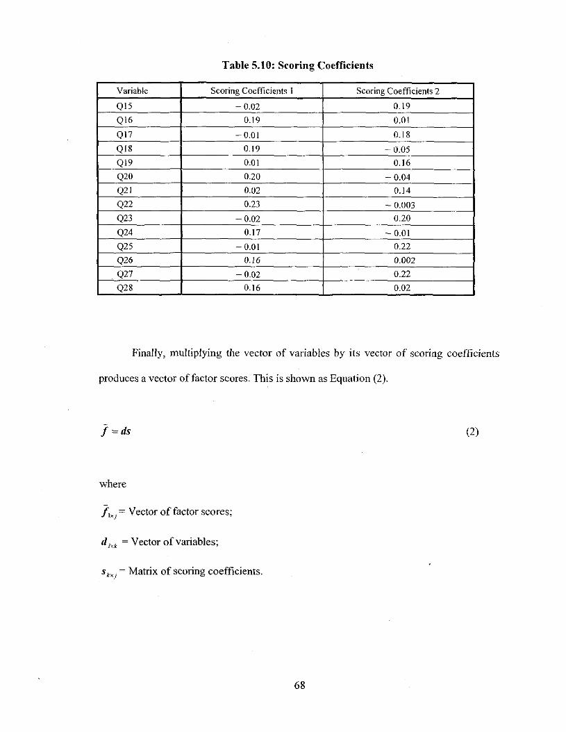
Table 5.10: Scoring Coefficients

Variable Scoring Coefficients 1 Scoring Coefficients 2

Ql5 - 0.02 0.19

QI6 0.19 0.01

Q17 - 0.01 0.18

Ql8 0.19 - 0.05

QI9 0.01 0.16

Q20 0.20 -0.04

Q21 0.02 0.14

Q22 0.23 - 0.003

Q23 ~0.D2 0.20

Q24 0.17 - 0.01

Q25 - 0.01 0.22

Q26 0.16 0.002

Q27 -0.02 0.22

Q28 0.16 0.02

Finally, multiplying the vector of variables by its vector of scoring coefficients

produces a vector offactor scores. This is shown as Equation (2).

f =ds

where

f,,)= Vector of factor scores;

d M = Vector of variables;

S h) = Matrix of scoring coefficients.

68

(2)

The vector of factor scores, which are the two composite variables ENV and ECG, are

used as independent variables. Table 5.11 reports the summary statistics of these two

variables.

Table 5.11: Summary Statistics of ENV and ECO

Variable No. ofobs Mean Std. Dev. Min Max

ENV 1,809 0.004 0.89 - 2.81 1.93

ECO 1,809 0.008 0.87 - 3.02 1.84

69

CHAPTER VI

MULTINOMIAL LOGIT ESTIMATION

6.1 Overview

Our empirical model is specified in accordance with the implications of our

theoretical model. Our three-choice model sheds two key theoretical implications. The

first one is that the positive and negative wealth attributes affect a resident's siting

decision accordingly. The second one is that the level ofrisk orientation can be identified

by the signs of partial derivative ofMaybe odds ratios.

One of our empirical focal 'points is whether or not our empirical finding on the

relationships between a resident's siting decision and the wealth attributes are consistent

with what is implied by our theoretical model and what is observed in the previous siting

studies. Previous studies suggest that specific regional factors (socio-demographic

variables) are relevant to a resident's attitude toward the siting. Though socio­

demographic variables are not dealt with explicitly in our theoretical model, these

variables are also included in our empirical model to avoid possible estimation biases

without them. Second focal point is to identify risk orientation level indirectly through

the signs ofestimated coefficients.

The chapter is organized as follows. Section 6.2 discusses and specifies the

empirical counterpart of our theoretical model in Chapter IV, The section also presents

the expected signs ofcoefficients. Section 63 presents the results of Yes base estimation.

The analytical interpretation is provided in Section 6.4. Section 6.5 discusses the level of

risk orientation as implied by the estimated coefficients. Section 6.6 carry out the

70

significance test for Yes base estimation39 and for risk orientation. Section 6.7 examines

the policy implication of our empirical findings.

6.2 Empirical Model

We established theoretically In Chapter IV that the logit model is indeed the

empirical counterpart of our theoretical model: Equation (4]) in Chapter IV. Specifically,

we use the MNLM following Luce and Suppes (1965)40 for our analysis. Due to the

paucity of published data suitable for our study, we obtained the data we need through a

carefully designed survey. In our survey form, the respondents had three choices (Yes, No,

or Maybe) for their answer to each of the questions with regard to hosting the composting

facility. These choices are related to the dependent variable in our empirical model.

Maybe choice reflects the uncertainty of respondent's perception regarding the impact of

the composting facility on the local community (Halstead et al. 1999). With the Maybe

choice available to the respondents, the Yes and No choices are expected to be less likely

biased.

For our empirical model specification, first, we take the natural logarithm of

Equation (41) and use proxies x, for positive wealth attributes (aj) and x j for negative

. wealth attributes ( sJ ):

39 Unlike the simple logit model, MNLM involves multiple choices which are normalized by a particularchoice. For convenience, we refer to the nonnalizing choice as base choice.

40 They found that a logit model is matched well with expected utility theory under the normalityassumption, i.e., disturbance term is iid (independently and identically distributed).

7]

where

m ~ Choice m;

b ~ Base choice;

Pm ~ Probability of choice m;

Pb = Probability of choice b;

In( ~: ) =Odds of m to b choice;4!

(I)

x"' = [Xl X, X 3 ... Xk ]: Vector of independent variables as proxies for a, and s,;

do = Intercept tenn;rOmb

II>mb 'hi =[91 9, 93 '" 9k]: Vector oflogit coefficients;

k = Number of independent variables;

k] = Number of positive wealth attribute variables.

In addition to the wealth attributes as regressors of the logit model in Equation (I),

we include socia-demographic variables, which are important as well. Even if our

primary focus is on estimating the effects of the wealth attributes on the resident's

attitudes toward the siting, exclusion of relevant variables may well bias the estimated

41 As stated in footnote 28 in Chapter IV, we use the tenn "odds of m to b choice" for In(Pt/Pm) as analternative to using "logarithm of the odds ofm to b choice".

72

effects of wealth attributes. To avoid the bias problem, it is necessary to include the

socio-demographic variables in the model. With the socio-demographic variables

included, the logit model specified for our empirical analysis contains a total of eighteen

variables: eight for positive wealth attributes, three for negative wealth attributes, and

seven for socio-demographic variables.

In(ymb) =In( ~: J

=¢o + ¢I IPWM + ¢, PPDSP + ¢J TRUST + ¢, KNOW +¢, ACESSml:> mh mh mb mb mh

+ ¢6 COMP + ¢7 RELCOM + ¢, ECO + ¢9 DIST + ¢IO ENVmb mh mb mb mb

+ ¢II INCOME + ¢12 CHILD + ¢13 EDU + ¢14 GENDER + ¢15 AGEmb mb mb mb mb

+ ¢16 NHMBR + ¢17 YRSTAY + ¢18 HSFORM + £:mb mh mh

where

PWA# = Positive Wealth Attribute Variables:

IPWM= Individual's participation in waste management (PWAI);

PPDSP = Public participation in decision making for siting plan (PWA2);

(2)

TRUST = Individual's trust in the institution related to waste management (PWA3);

KNOW = General knowledge of the large - scale composting facility's environmental

impact (PWA4);

ACCESS = Number of information sources on waste management (PWA5);

COMP = Amount of monetary compensation in terms of a tax (PWA6);

73

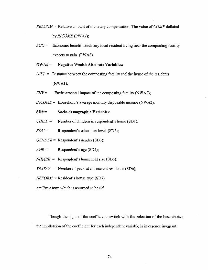
RELCOM = Relative amount of monetary compensation. The value of COMP deflated

by INCOME (PWA7);

ECO = Economic benefit which any local resident living near the composting facility

expects to gain (PWA8).

NWA# = Negative Wealth Attribute Variables:

DIST = Distance between the composting facility and the home ofthe residents

(NWAl);

ENV = Environmental impact ofthe composting facility (NWA2);

INCOME = Household's average monthly disposable income (NWA3).

SD#=

CHILD =

EDU=

Socio-demographic Variables:

Number of children in respondent's home (SDl);

Respondent's education level (SD2);

GENDER = Respondent's gender (SD3);

AGE = Respondent's age (SD4);

NHMBR = Respondent's household size (SD5);

YRSTAY = Number of years at the current residence (SD6);

HSFORM =Resident's house type (SD7).

Ei = Error term which is assumed to be iid.

Though the signs of the coefficients switch with the selection of the base choice,

the implication of the coefficient for each independent variable is in essence invariant.

74

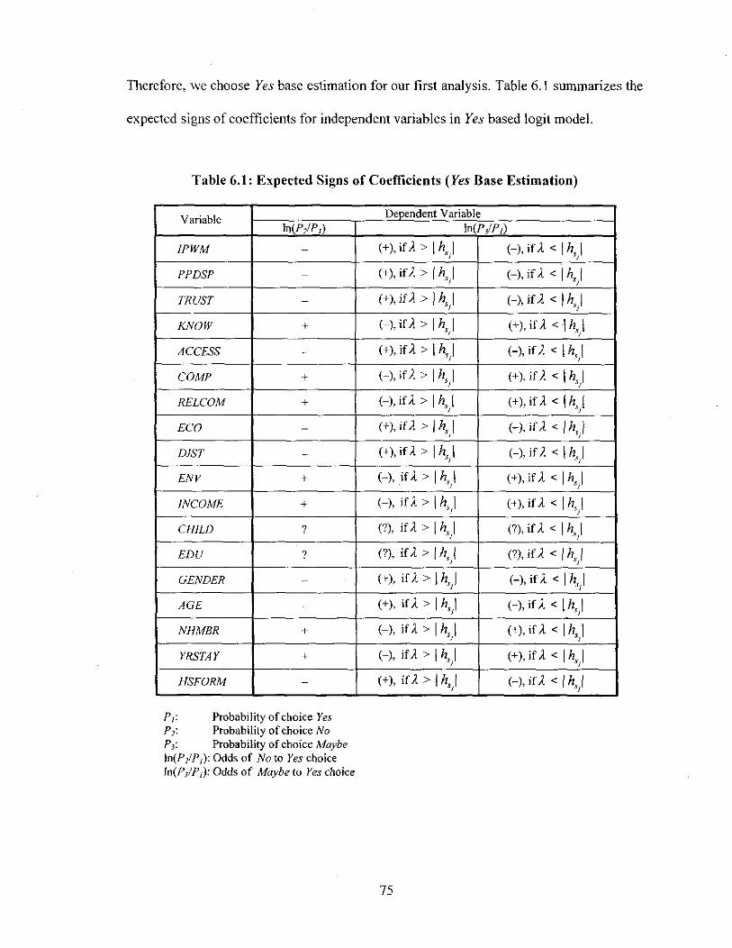
Therefore, we choose Yes base estimation for our first analysis. Table 6.1 summarizes the

expected signs of coefficients for independent variables in Yes based logit model.

Table 6.1: Expected Signs of Coefficients (Yes Base Estimation)

Variable Dependent VariableIn(P,/P/) In(P,/P/)

IPWM - (+),ifA>lhl (-), itA < Ih,1'I /

PPDSP - (+), ifA > Ih,1 (-), ifA < Ih,1/ " /

TRUST - (+), jrA > Ih,1 (-),itA<lh,1I "f

KNOW + (-), irA > Ih I (+), itA <I h, I'i /

ACCESS - (+),irA > Ih,1 (-), iLt < Ih,1) " /

CaMP + (-), irA > Ih I (+), ifA < Ih, I,) " )

RELCOM + (-),irA > Ih I (+), itA < Ih, ISj " )

ECO - (+),ifA>/h,1 (-), ifA < Ih, II /

DIST -" (+), irA > Ih I (-), if A < Ih,1,) " I

ENV + (-), ifA > Ih, I (+), ifA < Ih,1/ /

INCOME + (-), ifA > Ih,l (+),ifA<lh,1f "f

CHILD 7 (7), ifA > Ih,1 (7), irA < Ih, I"I "j

EDU 7 (7), irA > Ih I (7), if). < Ih,1$) /

GENDER - (+), irA> Ih,1 (-), if). < Ih,1/ /

AGE - (+), irA > Ih I (-), if A < Ih,1.~ j

"/

NHMBR + (-), if A > Ih, I (+), ifA < Ih, I/ " j

YRSTAY + H, ifA > I h,1 (+), if A < Ih,1I I

HSFORM - (+), if). > Ih, I (-),if).<lh,1/ /

PI: Probability ofchoice YesPl : Probability ofchoice NoP l : Probability of choice MaybeIn(P,IP/): Odds of No to Yes choiceIn(P,!PJ): Odds of Maybe to Yes choice

75

The expected signs are based on the theoretical expectation in our model as well as

previous empirical evidence. For PWA variables, signs of coefficients are expected to be

negative for the odds of No to Yes choice In(?,!?/) as a dependent variable. However, three

PWA variables (KNOW, COM?, RELCOMj have positive signs since they are scaled in

the reverse of the usual order. NWA variables are expected to be positive in their signs.

Of the three NWA variables (DIST, ENV, INCOME), only DIST is expected to be

negative in sign for the same reason as in the case of KNOW, COM?, and RELCOM.

Of SD variables, the coefficients for CHILD and EDU are sign indefinite. A) For

other SD variables, the expected signs were based on either what is observed in previous

studies in Korea (GENDER and AGE) or on specific rationales (NHMBR, YRSTAY, and

HSFORM).42

6.3 Estimation Results

Using the survey data, we estimated our MNLM as specified Section 6.3. For our

analysis we used the Yes base estimation. The results are summarized in Table 6.2. Two

dependent variables for the Yes base estimation are the odds of No to Yes choice In(?2!?I)

and Maybe to Yes choice In(?3!?I)' The estimated McFadden's pseudo R2 is 0.3076,

which is within the usual range of estimated fits for cross-sectional data. The slope

coefficients in the logit model measure the changes of the odds of No or Maybe to Yes

choice for one unit change in the independent variables.

42 The elaborate discussion on these variables is given in Section 5.1.

76

Table 6.2: Summary of the Yes Base Estimation (n = 1531)

Independent VariableIn(P/P,) In(P/P,)

(Expected Sign for In (P/P,))

lPWM (-) ~0.171 - 0.202

(0.003) (0.000)

PPDSP(-)~ 0.733 - 0.325

(0.000) (0.000)

TRUST(-)~ 0.055 0.006

(0.050) (0.809)

KNOW(+)0.49 0.291

(0.000) (0.000)

ACCESSH- 0.343 ~ 0.154

(0.000) (0.004)

COMP(+)0.160 .- 0.018

(0.027) (0.817)

RELCOM(+)0.411 0.199

(0.006) 10.193)

ECO (-)- 0.887 - 0.596

(0.000) (0.000)

DfST(-)- 0.0009 - 0.00014

(0.000) (0.077)

ENV (+)0.790 0.199

(0.000) (0.030)

lNCOME(+)0.451 0.151

(0.000) (0.014)

CHILD (?)-0.140 0.067

(0.186) (0.498)

EDU ('1)- 0.013 0013

(0.820) (0.806)

GENDER(-)- 0.278 - 0.654

(0.102) (0.000)

AGE (-)0.00] - 0.0002

(0.885) (0.9811

NHMBR (+)0.252 0.052

(0.001) (0.445)

YRSTAY (+)0.0004 0.005

(0.948) (0.418)

HSFORM(-)1).1)67 - 1),1)75

(0.477) (1).397)

Constant- 0.977 - 0.091

(0.182) (0.892)

PI: Probability of choice Yes

P,: Probability of choice NoP,: Probability ofchoice Maybe

Absolute p - values are in parenthesesDependent variable: In(P/P,)); [niP/Pi).Pseudo R2

: 0.3076

77

In Table 6.2, a positive coefficient indicates that the percentage change in probability of

choice No or choice Maybe is higher than that of choice Yes by the amount of the

coefficient for one unit increase in the independent variable. The effect is exactly the

opposite if the coefficient's sign is negative. For instance, - 0.055 as the estimated

coefficient for independent variable TRUST in the model for In(P;lP/) implies that the

percentage change in probability ofchoice No is lower than that ofchoice Yes by as much

as 0.055 for one unit increase in TRUST. Coefficients for 12 variables out of 18 are

significant at less than or equal to the 5% significance level for In(P;lP/) whereas 9

variables are significant for In(P3Ip/).43 These results are mostly consistent with those

observed in the previous siting studies. 44 The signs of estimated coefficients in In(P2IP/)

are all consistent with the expected ones, except for four variables (CHILD, EDU, AGE,

HSFORM).

These empirical results are consistent with the theoretically expected in our three-

choice model: the subjective probability of accepting (rejecting) the facility is an

increasing (decreasing) function of PWA variables (IPWM, PPDSP, TRUST, KNOW,

ACCESS, COMP, RELCOM, ECO), and a decreasing (increasing) function of NWA

variables (DIST, ENV, INCOME).

Out of four variables (CHILD, EDU, AGE, HSFORM), the signs of CHILD and

EDU are found to be negative. This implies that as the resident's concern with the

negative impact on children's health (CHILD) and the resident's level of education

(EDU) are higher, the probability of choice No is lower. However, the results are not

statistically significant. Negative signs of the other two variables (A GE, HSFORM)

43 The coefficient ofDlSTfor 1n(P/P/) is significant at the 10 % level.44 The previous empirical findings are summarized in Chapter III.

78

indicate that if the resident is young (AGE) or lives in an apartment complex (HSFORM),

the resident tends to reject the composting facility. The impact of these two variables on

the siting decision, however, is not statistically significant either. Overall, we find that the

logit model specified well describes the data in terms of pseudo R2, statistical

significance of estimated coefficients, and the expected signs4S

6.4 Normalizing Logit Coefficients

To facilitate an easier comparison of estimated impacts of regressors, we

normalize the estimated logit coefficients ('h ) by following the procedure. First, wemh

take anti-log of the estimated MNLM in (2). That is:

Pm '......\r mb =- =exp ( X '" mlYPb

Then we can rewrite Equation (3),

exp ( x'et> mol =exp ( ¢o + ¢I XI + ... + 9\ X k )mb rob mh

=exp (rPo ) exp (rPl XI ) ... exp (rPk X,)~ m6 mb

where

(3)

(4)

45 The coefficient's sign and its statistical significance in In(P3 IP j ) model are discussed in Section 6.5 inrelation to the level of risk orientation.

79

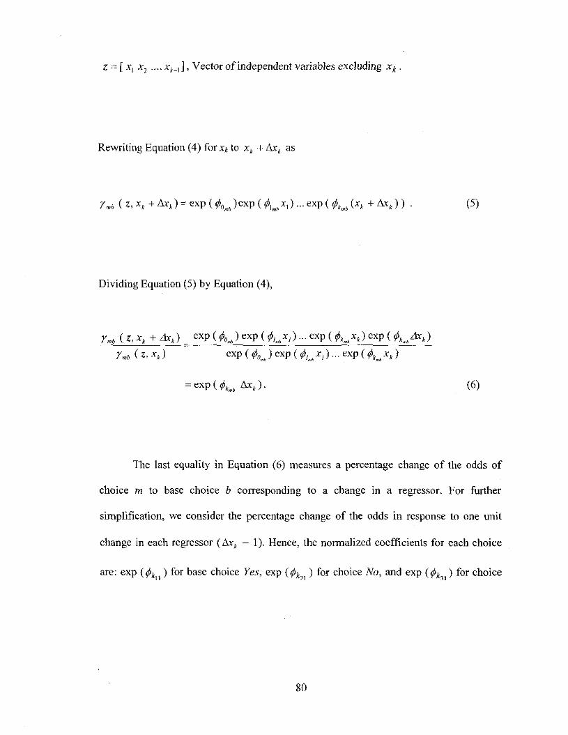
z ~ [Xl X, .... X'_l J, Vector of independent variables excluding Xk'

Rewriting Equation (4) for Xk to X, + L1x, as

Dividing Equation (5) by Equation (4),

~ exp ( ¢, L1xk ) •mb

(5)

(6)

The last equality in Equation (6) measures a percentage change of the odds of

choice m to base choice b corresponding to a change in a regressor. For further

simplification, we consider the percentage change of the odds in response to one unit

change in each regressor (&k = 1). Hence, the normalized coefficients for each choice

are: exp (¢k ) for base choice Yes, exp (¢k ) for choice No, and exp (¢k ) for choice11 21 31

80

Maybe. Note that normalized coefficients for base choice (Yes) is exp( IA ) = 146 1f a"

normalized coefficient is less than I, the corresponding variable has a negative

coefficient in the logit model. If it is greater than one, the corresponding variable has a

positive coefficient. The magnitude of impact of each independent variable becomes

greater as the value of the normalized coefficient departs father from unity.

The next three subsections discuss the impacts of three groups of variables in

terms of normalized coefficients.

6.4.1 Positive Wealth Attribute Variables

Figure 6.1 shows normalized coeftlcients for eight PWA variables (lP/flAJ,

PPDSP, TRUST, KNOW, ACCESS, COMP, RELCOAJ, ECO). Each bar in Figure 6.1

represents the corresponding choice; Yes (base choice), No, and Maybe. The height of

each bar indicates the value of the normalized coefficient. For instance. the values of the

three bars of JPWM are exp (¢k ) = 0.843 for choice No, exp (¢k ) = I for base choice21 II

Yes, and exp (¢'3' ) = 0.817 for choice Maybe. The values in parentheses are statistical

46 By the characteristic of MNLM, logit coefficient ¢, equals ¢, - ¢, (Long 1997; Long and Freesemb m b

exp (x,¢, )200 t). Probability Pq (q is choice m or b) in MNLM can be expressed as Pq~ J q, where j ~ I,

L:exp(x,¢, )j=J }

"., J choices. By taking the ratio of Pm to Ph, we get:

Pm exp (x,¢, ) / exp (x,¢, )= .J m J '. =exp (x, (¢'m - ¢'h)) =exp (x'¢'m')· Therefore, if

Ph L:exp (xd,) L:exp (xk¢, )J~l ) j=1 J

non-base choice m is the same as the base choice b, then ¢'m' =!/J,,, =!/J", = ¢k, -!/J" ~ 0 and

exp (!/J'm') = exp (!/J,,,) =exp (¢,") ~ J.

8J

significance levels; I % level (***), 5 % level (**), and 10 % level (*). In the section, we

mainly discuss the independent variable's effect on choice No, i.e., the odds of No to Yes

by the nonnalized coefficient. The reason for selecting choice No is that there is no

previous empirical analysis of choice Maybe that can be compared with our estimation

results.47

Five out of eight PWA variables are positive attitude variables (IPWM, PPDSP,

TRUST, KNOW, ACCESS) in our empirical model. IPWM measures the resident's degree

of involvement in waste management activity. IPWM in Figure 6.1 shows that the values

of nonnalized coefficients corresponding to choices No and Maybe are 0.843 and 0.817

respectively. This implies that the probabilities of selecting choice No and Maybe are less

than that of selecting choice Yes. Both nonnalized coefficients of IPWM are statistical1y

significant at the I % level. The value of the nonnalized coefficient for IPWM indicates

that as the residents become more involved in waste management activities such as

recycling, the resident shows a less negative response. This result is consistent with the

previous empirical evidence that a local resident's waste management activity is

positively related to one's positive siting attitude (Halstead et at. 1999).

PPDSP measures public participation in decision making for the siting plan. The

estimated nommlized coefficients of PPDSP corresponding to choices No and Maybe are

0.480 and 0.723 respectively. Both coefficients are statistical1y significant at the I %

level. The normalized coefficient for choice No indicates that the odds of No to Yes

choice are almost half (0.480) for the local residents believing that the siting institutions

have sufficiently considered a local resident's economic loss in a hosting area. The

47 The discussion on choice Maybe (or Maybe odds) is done separately in the section 6.5 in regards to therisk orientation factor.

82

normalized coefficients for choice No of PPDSP imply that as the siting institutions

convince the residents in a hosting area, the resident shows a less negative response. This

result supports the previous empirical evidence that the source of strong NIMBY lies in

the siting institution's improper consideration of the local resident's opinion (Bogdonoff

1995).

TRUST measures the resident's degree of trust in the institutions in charge of

waste management. According to previous studies, TRUST is also found to be an

important factor affecting a resident's siting behavior (Kunreuther and Easterling 1990).

TRUST in Figure 6.1 shows that the effect of the resident's level oftmst in institutions is

statistically significant at the 5 % level for choice No while the effect of TRUST for

choice Maybe is insignificant. Compared to the other PWA variables. the normalized

coefficients of TRUST are not much different from that of base choice Yes (~l). The

normalized coefficient for choice No is found to be close to I (0.946) implying that the

probability of selecting choice No is very close to that of selecting choice Yes. Hcnce, our

result moderately supports the previous empirical results.

KNOW measures the extent to which the residents can distinguish the differences

in adverse environmental effects among the various waste disposal facilities. Showing

statistical significance at the 1 % level for the two choices No and Maybe, the values of

the two normalized coefficients of this variable are found to be 1.632 for choice No and

1.338 for choice Maybe. The normalized coefficient for choice No implies that the odds

of No to Yes choice is slightly more than one and a half for residents who do not know

common facts on waste disposal methods. This indicates that the lack of common

knowledge on waste disposal methods tends to cause the residents to respond negatively.

83

This also implies that a resident's knowledge of the noxious facility's hazardousness has

a significant impact on siting decisions.

2.5ONo

Y""I"'''I,oM3ybe

***1%=--.:;r- : **5%t ::: * 10%

C\J If?;- c:io r-

-

r-

f'•'-~*' ....y •*' .. ~: ,,-

'- It)0_ Q:);::r- o'

o r--

r-

-

=--~'-

"-.... .-Q) ... --c:i .:..

r- 0Q:)"<:to

-0.5

1.0

1.5 - .-..'-

I,

0.0

Figure 6.1: Positive Wealth Attribute Variables

ACCESS measures the information sources available to residents. Compared to

the effects of the other positive attitude variables, its impact appears to be intermediate:

stronger than IPWM and TRUST yet weaker than PPDSP and KNOW. The normalized

coefficient for ACCESS (0.710) in No choice model is far less than that of base choice;"''--.-

(=1), as compared to those for IPWM (0.843 in NO choice model) and TRUST (0.946 in

No choice model). The impact of ACCESS is weaker than PPDSP and KNOW as its

84

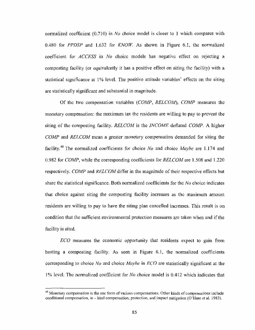
normalized coefficient (0.710) in No choice model is closer to I which compares with

0.480 for PPDSP and 1.632 for KNOW. As shown in Figure 6.1, the normalized

coefficient for ACCESS in No choice models has negative effect on rejecting a

composting facility (or equivalently it has a positive effect on siting the facility) with a

statistical significance at I % level. The positivc attitude variables' effects on the siting

are statistically significant and substantial in magnitude.

Of the two compensation variables (COMP, RELCOM), COMP measures the

monetary compensation: the maximum tax the residents are willing to pay to prevent the

siting of the composting facility. RELCOM is the INCOME deflated COMPo A higher

COMP and RELCOM mean a greater monetary compensation demanded for siting the

facility.48 The normalized coefficients for choice No and choice Maybe are 1.174 and

0.982 for COMP, while the corresponding coefficients for RELCOM are 1.508 and 1.220

respectively. COMP and RELCOM differ in the magnitude of their respective effects but

share the statistical significance. Both normalized coefficients for the No choice indicates

that choice against siting the composting facility increases as the maximum amount

residents are willing to pay to have the siting plan cancelled increases. This result is on

condition that the sufficient environmental protection measures are taken when and if the

facility is sited.

ECO measures the economIC opportunity that residents expect to gam from

hosting a composting facility. As seen m Figure 6.1, the normalized coefficients

corresponding to choice No and choice Maybe in ECO are statistically significant at the

1% level. The normalized coefficient for No choice model is 0.412 which indicates that

48 Monetary compensation is the one form of various compensations. Other kinds of compensations includeconditional compensation, in - kind compensation, protection, and }mpact mitigation (O'Hare et al. 1983).

85

the probability that a resident is against the siting is less than the probability he is for.

Hence, our estimation result from ECO is consistent with the previous empirical studies

(Halstead et al. 1999, for example) which shows that the probability of rejecting the

facility declines as a resident expects more economic benefits from the composting

facility.

6.4.2 Negative Wealth Attribute Variables

The effects of NWA variables on the resident's siting decision are presented in

Figure 6.2. DIST measures the hypothetical distance from a resident's home to the

composting facility. As seen in Figure 6.2, the normalized coefficients for DIST in No

and Maybe choice models are very close to 1. Figure 6.2 also shows their statistical

significance at 1% and 10% level respectively. This implies that a local resident's attitude

against siting a composing facility weakens as his residence is farther away from the

composting facility, demonstrating NIMBY attitude. This finding is consistent with a

number of siting studies (Halstead et al. 1999; Lober 1993; Furseth and Johnson 1988).

ENV measures the degree of concern that the residents have about the

environmental impact of the composting facility. Both ENV and ECO are generated

through factor analysis. The normalized coefficients for ENV (2.203) and ECO (00412) in

No choice model shows that the probability of choosing No as opposed to Yes is

positively affected by the residents' environmental concern whereas it is negatively

affected by the economic benefits. In other words, the environmental concern has a

negative impact on residents' willingness to accept the facility whereas the economic

benefits have a positive effect.

86

The estimated impacts of ECO and ENV on NIMBY attitude in our study are in a

clear contrast with those of Halstead et al. (1999). In a US study by Halstead et al. (1999),

the estimated coefficients for ENV and ECO are found to be 2.0803 and - 0.6078

respectively as opposed to ENV (0.789) and ECO (-0.887) in out study. This clearly

indicates that for residents in Cheju City environmental concern has almost as strong an

impact as economic benefits on making their siting decision, whereas the environmental

concern in Halstead et al. (1999) dominates over the economic benefits from the facility.

Figure 6.2: Negative Wealth Attribute Variables

Figure 6.2 also shows that the normalized coefficient for INCOME in No choice

model is 1.570, which means that the greater a resident's income, the higher the

probability of rejecting (as opposed to accepting). In contrast to Lee and An (1999), the

87

coefficients of INCOME in our estimation results are statistically significant at 1% level

or less. This extends supporting evidence that the NIMBY attitudes are stronger and

prevalent amongst high income earners than lower ones as previously found (Hankyeoreh

Daily News May 5 2002).

6.4.3 Socio-demographic Variables

Figure 6.3 shows the effects of SD variables on the resident's siting decision. The

main feature of Figure 6.3 is that many of SD variables are insignificant. Of the seven

variables (CHILD, EDU, GENDER, AGE, NHMBR, YRSTAY, HSFORM), the coefficients

of six variables (CHILD, EDU, GENDER, AGE, YRSTAY, HSFORM) are insignificant for

choice No.

***1%** 5%* 10%

[0 t-.b

Yes(base)

OM3ybe__ ---.J

-~.

!~......

"-~

o I..: 8 g<::> ... 0 OJ r- 0 0 2i{.... "- . .. o' -' ,.: ..: ...:~ ..... . - o'r- ;;-r- r: r- r- - ~ ... r- -

r-o'

~r-

r-o' .~

"II:!;

111 "-~

<::> ~...:~ o'

res ..... ~r- r--

2.5II)-cQ)

2.0~Q)0

1.5(J

'tJQ)

.~ 1.0'EIV'tJc 0.5.5II)c

:::;)0.0

Figure 6.3: Socio-demographic Variables

88

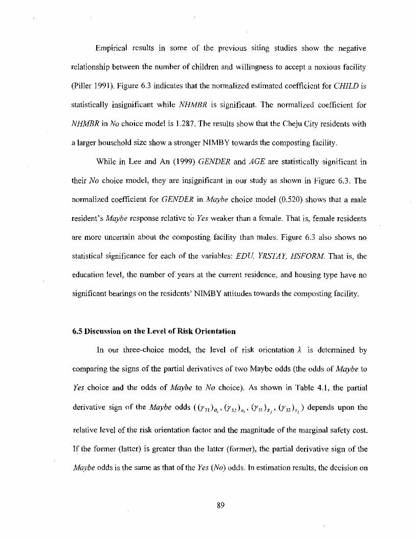
Empirical results in some of the prevIOus siting studies show the negative

relationship between the number of children and willingness to accept a noxious facility

(Piller 199 J). Figure 6.3 indicates that the normalized estimated coefficient for CHILD is

statistically insignificant while NHMBR is significant. The normalized coefficient for

NHMBR in No choice model is 1.287. The results show that the Cheju City residents with

a larger household size show a stronger NIMBY towards the composting facility.

While in Lee and An (1999) GENDER and AGE are statistically significant in

their No choice model, they are insignificant in our study as shown in Figure 6.3. The

normalized coefficient for GENDER in Maybe choice model (0.520) shows that a male

resident's Maybe response relative to Yes weaker than a female. That is, female residents

are more uncertain about the composting facility than males. Figure 6.3 also shows no

statistical significance for each of the variables: EDU, YRSTAY, HSFORM. That is, the

education level, the number of years at the current residence, and housing type have no

significant bearings on the residents' NIMBY attitudes towards the composting facility.

6.5 Discussion on the Level of Risk Orientation

In our three-choice model, the level of risk orientation A is determined by

comparing the signs of the partial derivatives of two Maybe odds (the odds of Maybe to

Yes choice and the odds of Maybe to No choice). As shown in Table 4.1, the partial

derivative sign of the Maybe odds «r31) a ' (r32)a' (r31)s., (r32),.) depends upon theI I J J

relative level of the risk orientation factor and the magnitude of the marginal safety cost.

If the former (latter) is greater than the latter (former), the partial derivative sign of the

Maybe odds is the same as that of the Yes (No) odds. In estimation results, the decision on

89

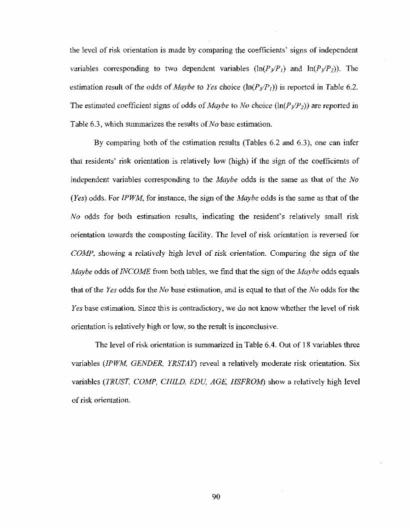
the level of risk orientation is made by comparing the coefficients' signs of independent

variables corresponding to two dependent variables (In(P/P I ) and In(P!P2». The

estimation result of the odds of Maybe to Yes choice (In(PyTI ») is reported in Table 6.2.

The estimated coefficient signs of odds of Maybe to No choice (In(P/P;)) are reported in

Table 6.3, which summarizes the results ofNo base estimation.

By comparing both of the estimation results (Tables 6.2 and 6.3), one can infer

that residents' risk orientation is relatively low (high) if the sign of the coefficients of

independent variables corresponding to the Maybe odds is the same as that of the No

(Yes) odds. For IPWM, for instance, the sign of the Maybe odds is the same as that of the

No odds for both estimation results, indicating the resident's relatively small risk

orientation towards the composting facility. The level of risk orientation is reversed for

COMP, showing a relatively high level of risk orientation. Comparing the sign of the

Maybe odds of INCOME from both tables, we find that the sign of the Maybe odds equals

that of the Yes odds for the No base estimation, and is equal to that of the No odds for the

Yes base estimation. Since this is contradictory, we do not know whether the level of risk

orientation is relatively high or low, so the result is inconclusive.

The level of risk orientation is summarized in Table 6.4. Out of 18 variables three

variables (IPWM, GENDER, YRSTAy) reveal a relatively moderate risk orientation. Six

variables (TRUST, COMP, CHILD, EDU, AGE, HSFROM) show a relatively high level

of risk orientation.

90

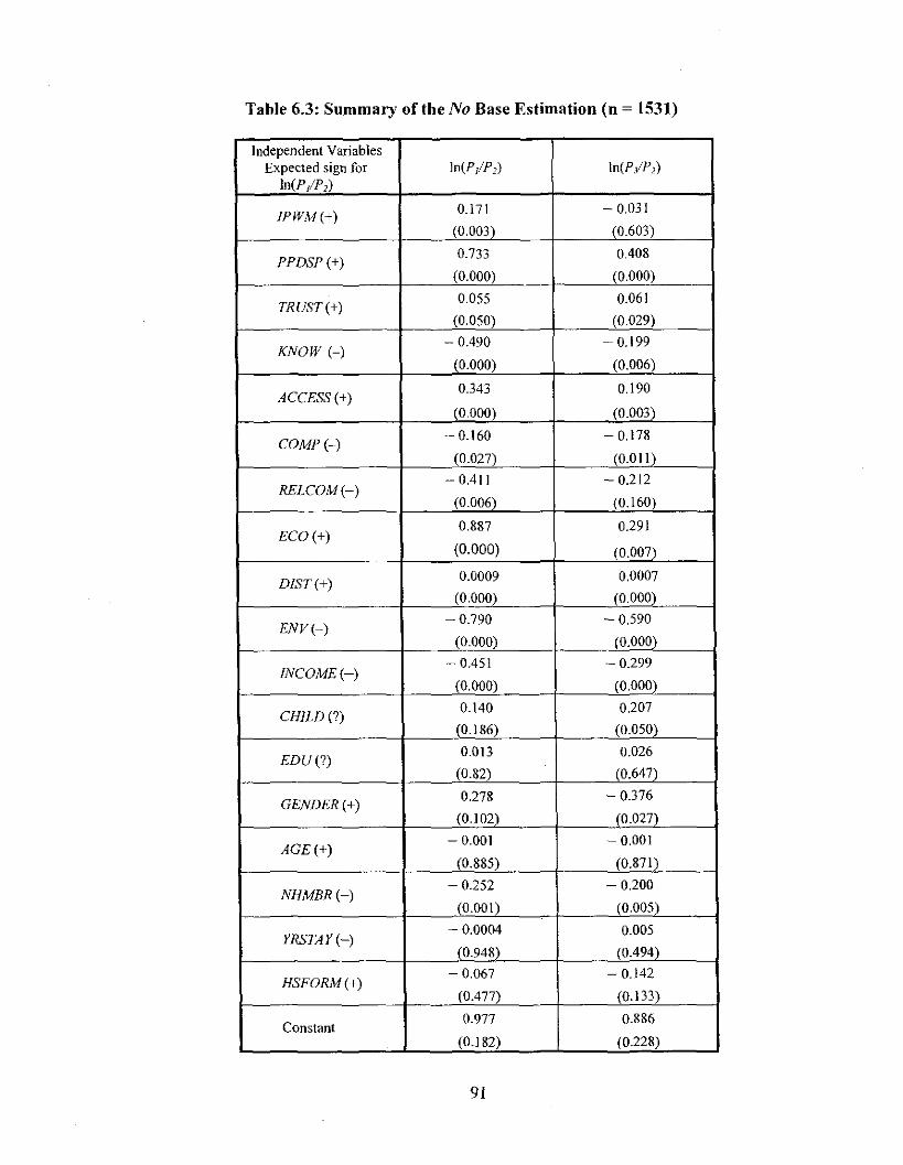
Table 6.3: Summary of the No Base Estimation (n = 153])

Independent VariablesExpected sign for In(P/P,) In(P/P,)

In(P/P,)

IPWM(+) 0.171 - 0.031

(0.003) (0.603)

PPDSP(+)0.733 0.408

(0.000) (0.000)

TRUST(+)0.055 0.061

(0.050) (0.029)

KNOW (-)- 0.490 - 0.199

(0.000) (0.006)

ACCESS(+)0.343 0.190

(0.0001 (0.003)

COMPH- 0.160 - 0.178

(0.027) (0.011 )

RELCOM(-)- 0.4 II - 0.212

(0.006) (0.160)

ECO(+)0.887 0.291

(0.000) (0.007)

DIST(+) 0.0009 0.0007

(0.000) (0.000)

ENVH- 0.790 - 0.590

(0.000) (0.000)

INCOME(-)- 0.451 - 0.299

(0.000) (0.000)

CHILD (?)0.140 0.207

(0.186) (0.050)

EDU(?)0.013 0.026

(0.82) (0.647)

GENDER(+)0.278 - 0.376

(0.102) (0.027)

AGE (+)- 0.001 - 0.001

(0.885) (0.871)

NHMBR(-)- 0.252 - 0.200

(0.001) (0.005)

YRSTAY(-)- 0.0004 0.005

(0.948) (0.4941

HSFORM(+)- 0.067 -0.142

(0.477) (0.133)

Constant0.977 0.886

(0.182) (0.228)

91

Table 6.4: Resident's Risk Orientation

Sign oflndependent Variable in the Sign oflndependent Variable in theIndependent Yes Base EstimatiDn No Base Estimation Orientation

VariablesIn(p!p,) In(pJiPJ) f. VS. I IIs.1 In(p,lp,) In(p;lp,) f. vs. I hsl of Maybe

J }

fPWM - - ;.. < I iI,.1 + - ;.. < 1iI,.1 No} 'J

PPDSP - - f. < Ih,.1 + + f. > I h,.1 Inconclusive} }

TRUST - + f. > I ils .1 + + f. > I iI,.1 Yes} }

KNOW + + f. < I h,.1 - - f. > I h\".1 InconclusiveJ '}

ACCESS - - f. < 1iI,.1 + + f. > I iI,.1 InconclusiveJ J

COMP + - f. > 1h,.1 - - f. > 1iI,.1 Yes} 'J

RELCOM + + f. < I iI,.1 - - f. > 1ils·1 Inconclusive} }

ECO - - f. < I hs .1 + + f. > I iI,l Inconclusive} }

DfST - - f. < 1",.1 + + f. > I lIs.1 InconclusiveJ }

ENV + + f. < 1h,.1 - - f. > Iii, .1 Inconclusive} '}

INCOME + + f. < 1iI,.1 - - f. > 1h, I Inconclusive'} J

CHILD - + f. > !h 1 + + f. > I h,.1 YesI Sj '}

EDU - + f. > Iii .1 + + f. > 1hs·1 YessJ J

GENDER - - f. < 1iI .1 + - f. < I h, I No.,}}

AGE + - f. > I h,.1 - - f. > 1h .1 Yes} .,}

NHMBR + + f. < I h, .1 - - f. > I hs.1 InconclusiveJ }

YRSTAY + + f. < 1iI,.1 - + f. < I h,.. 1 NoJ 'J

HSFORM + - f. > I h,.1 - - f. > 1ils.1 Yes} }

Nine variables (PPDSP, KNOW, RELCOM, ACCESS, DIST, ECO, ENV, INCOME,

NHMBR) are found to be the inconclusive for the level of risk orientation toward the

composting facility. The inferences on the risk orientation as listed in the last column in

92

table are based on the test statistics calculated under the null hypotheses discussed in the

following section.

6.6 Hypothesis Test

We have carried out significance tests on our empirical results. The statistical

significance of each coefficient of our empirical result is reported in tables 6.2 and 6.3.

Although p-value· indicates the statistical significance of each estimated coefficient, it

does not test whether a pair of coefficients for each regressor is simultaneously

significant. Hence, we also carry out the significance test for each pair of coefficients.

Then we carry out a simultaneous significance test for the estimated coefficients as a

whole. Finally, we discuss the statistical significance of the level of risk orientation.

Since there are three choices in our model, each independent variable has two

coefficients. Hence we need to test whether both coefficients are simultaneously different

from "0" with a statistical significance. The null hypothesis can be stated as:

H·nI _nI =0o· 'rk Ny - ¥"k.MY

where,

¢k = Coefficient for k-th regressor (k=1,2,3, ... ,18);

"NY", "MY" = No choice,Maybe choice with Yes choice as base.

93

(7)

Table 6.5: Wald Testdf 2

Variable X' p - value

iPWM 16.069 0.000PPDSP 108.518 0.000TRUST 5.541 0.063KNOW 46.983 0.000ACCESS 31.131 0.000COMP 8.056 0.018RELCOM 7.534 0.023ECO 62.651 0.000DIST 67.824 0.000ENV 60.931 0.000INCOME 53.065 0.000CHILD 3.897 0.142EDU 0.211 0.900GENDER 17.009 0.000AGE 0.031 0.985NHMBR 13.026 0.001YRSTAY 0.778 0.678HSFORM 2.281 0.320

Table 6.6: LR Testdf 2

Variable X' p-va1ueIPWM 16.168 0.000PPDSP 121.848 0.000TRUST 5.558 0.062KNOW 49.056 0.000ACCESS 33.228 0.000COMP 8.202 0.017RELCOM 7.794 0.020ECO 69.496 0.000DiST 81.827 0.000ENV 66.165 0.000INCOME 56.69J 0.000CHILD 3.915 0.141EDU 0.211 0.900GENDER 17.277 0.000AGE 0.031 0.985NHMBR 13.206 0.001YRSTAY 0.773 0.679HSFORM 2.308 0.3J5

94

The Wald test statistic is,

where

(8)

cI>' =,f,k,2xl ('f'k Ny

¢'MV)': Vector of the maximum likelihood estimates for variable xk;

viir(cI>~)w= Estimated covariance matrix.

The number oftotal choices (= 3) minus I is the degrees of freedom. The null hypothesis

in this test is "no effect of the independent variable on the resident's decision towards the

hosting the facility". The null hypothesis stated above is tested for each of 18 regressors.

The test results are reported in both Tables 6.5 (Wald test) and 6.6 (LR test), and both

results are very close, although the p-values for both Wald and LR tests are different.49

Out of 18 variables, 13 variables show a statistical significance at 10 % level or less.

The null hypothesis for simultaneous significance test for entire coefficients is:

49 LR test statistic is, LRk ~ lIn L(MF) - 21n L(MR) - X' (2)

whereL(MF) ~ The value of the likelihood function evaluated at the maximum likelihood estimates for the full

(unconstrained) model;L(MR) ~ The value of the likelihood function evaluated at the maximum likelihood estimates for the

restricted (constrained) model.

Both of Wald and LR tests follow X 2 distribution whose total restrictions are the number of variablesmultiplied by J-I (J is the total number of choices).

95

do _do =0\PIS NY - \PISMy

The test statistics used for testing the null hypothesis in (9) are:

, '] , 2W = cI>'var(cI> r cI> - X (36)

where

(9)

(10)

for variables X, ,... ,X,,;

var( <i> ) 36x36 = The estimated covariance matrix.

(II)

Since there are 18 variables and 3 choices, the degrees of freedom are equal to 36 for

both tests. The test statistics as reported in Table 6.7 reject the null at I % significance

level.

96

Table 6.7: Wald Test and LR Test for Independent Variables as a Whole

Accept y' df p-value

Wald 466.818 36 0.000LR 983.768 36 0.000

The final· section in this Chapter relates to testing for the risk orientation latent in

Maybe responses. Based on the empirical results reported in Table 6.8, we can draw a

conclusion with regard to the residents' risk orientation (A ) in our three-choice model

theoretically analyzed in Chapter 4. The analysis therein suggests that if the resident's net

wealth equivalent function (or utility function) becomes closer to the case of the

composting facility not sited, the level of risk orientation factor A becomes closer to "0".

This means that as A approaches to "0" the estimated coefficients in the Yes based

MNLMs (In(PjP]) and In(P!P]) as reported in Table 6.2 converge to each other with

their differences vanishing. Hence, the non-zero difference between In(P]/P]) and

In(?!P]) implies the existence of a certain level of risk orientation as presented in Table

6.8. In Table 6.8, in(P2/P]) and In(P!P]) are the dependent variables for the Yes base

estimations: i.e., the odds ofNo to Yes choice and the odds ofMaybe to Yes choice.

In(P]/P]), in the fourth column in Table 6.8, is the difference between the two

dependent variables corresponding to two (log of) odds, which are shown in Equation

(/2).

97

I P2-lnP3 = n(-)P3

(12)

Table 6.8: Identification of the Level of Risk Orientation Factor

Independent Variables In(P/P j ) In(PJP j ) In(P/P,)

IPWM - 0.171 - 0.202 0.031(0.003) (0.000)

PPDSP - 0.733 - 0325~ 0.408

(0.000) (0.000)

TRUST - 0.055 0.006 - 0.061(0.050) (0.809)

KNOW 0.49 0.291 0.199(0.000) (0.000)

ACCESS - 0.343 - 0.J54 - 0.190(0.000) (0.004)

COMP 0.160 - 0.018 0.178(0.027) (0.817)

RELCOM 0.41 J 0.199 0.212(0.006) (0.193)

ECO - 0.887 - 0.596 - 0.291(0.000) (0.000)

DlST- 0.0009 - 0.00014 - 0.0007(0.000) (0.077)

ENV 0.790 0.199 0.590(0.000) (0.030)

INCOME 0.451 0.151 0.299(0.000) (0.014)

CHILD -0.140 0.067 - 0.207(0. J86) (0.498)

EDU -0.013 0.013 - 0.026(0.820) (0.806)

GENDER - 0.278 - 0.654 0.376(0.102) (0.000)

AGE 0.001 - 0.0002 0.001(0.885) (0.981)

NHMBR 0.252 0.052 0.200(0.001) (0.445)

YRSTAY 0.0004 0.005 - 0.005(0.948) (0.418)

HSFORM 0.067 - 0.Q75 0.142(0.477) (0.397)

Constant - 0.977 - 0.091 -0.886(0.182) (0.892)

98

As seen in Equation (12), the numerical values in the fourth column indicate the

difference between the coefficients of the two independent variables corresponding to

In(P2/P t ) and In(P;!Pt ). For example, the coefficients of IPWM corresponding to

In(P2/PJ) and In(PJ/PJ) are - 0.171 and ~ 0.202. Subtracting the coefficient of JPWM in

In(P;!PJ) from that of IPWM in In(P2/PJ) produces 0.031. Column 4 in Table 6.8 lists the

differences between columns 2 and 3 which are identical with the estimated coefficients

for MNLM with In(P2/P3) as dependent variable.

As previously discussed, in three-choice model the non-zero coefficients of the

fourth column imply the existence of a level of risk orientation. However, these non-zero

coefficients need to be subject to the statistical significance test. To test the significance

of a coefficient, z-test is used to confirm whether uncertain residents in Cheju City have a

significant level of risk orientation toward siting of a composting facility. The null

hypothesis for this test is,

Ho: rPk = 0NM(13)

The null hypothesis (13) states that k-th regressor in MNLM (xd does not have an

impact on odds ofNo to Maybe. The test statistic used in this test is,

(14)

99

where

17k The estimated standard deviation for variable xk in No/Ma!ybe model.NM

Table 6.9 summarizes the test results of the level of risk orientation. The Table

shows the statistical significance of the risk orientations inferred from pairwise

comparisons of signs for estimated coefficients as reported in Table 6.4.

Table 6.9: Test Result of Resident's Risk Orientation

Variable Izl p·value Orientation of Maybe

IPWM 0.52 0.603 NoPPDSP 5.91 0.000 JnconclusiveTRUST 2.19 0.029 resKNOW 2.75 0.006 InconclusiveACCESS 2.96 0.003 InconclusiveCOMP 2.54 . 0.011 YesRELCOM 1.41 0.160 InconclusiveECO 2.70 0.007 InconclusiveDIST 6.98 0.000 InconclusiveENV 5.87 0.000 InconclusiveINCOME 4.90 0.000 InconclusiveCHILD 1.96 0.050 YesEDU 0.46 0.647 YesGENDER 2.22 0.027 NoAGE 0.16 0.871 YesNHMBR 2.78 0.005 JnconclusiveYRSTAY 0.68 0.494 NoHSFORM 1.50 0.133 res

*: slgmficant at or less than 5% level

In Table 6.4 three variables (IPWM, GENDER, YRSTA Y) out of 18 regressors show a

relatively weak risk orientation. Among the three variables. only GENDER is statistically

significant. Six variables show a higher risk orientation, out of which three (TRUST,

100

COMP, CHILD) show a statistical significance and the remaining three (EDU, AGE,

HSFORJi..f) are insignificant. Nine variables (KNOW, ACCESS, DIST, ECO ENV,

INCOME, PPDSP, NHMBR, RELCOJi,.f) show the inconclusiveness with regard to the

risk orientation of Maybe responsiveness, and all but RELCOM show statistical

insignificance.

Among the four variables which are a statistically significant risk orientation, the

higher risk orientation cases outnumber the lower cases. Therefore we may conclude that

uncertain respondents in Cheju City are more oriented towards accepting the facility.

6.7 Policy Implication

In this section we examine the policy implications of our empirical findings. The

estimated impacts of PWA and NWA variables in Yes base model may be relevant to the

policy fonnulation. In mid 1990's in Korea a user fee system was instituted for municipal

solid waste disposal where the residents are required to separate the waste by type,

recycle, and pack the waste with bags provided by the municipal government. This policy

has been reported as effectively motivating residents in waste management (MOE 2000).

The estimated coefficients for IPWM are consistent with the report. In many instances, a

strong NIMBY attitude is an outcome of improper procedures followed on the part of the

central or local government (Bogdonoff 1995). Hence, the local residents' opinions

should be accommodated through a public hearing or debate (Hankyeore Daily News

May 20, 2001). The estimated impact of PPDSP suggests that the awareness on the part

of residents that their opinions are reflected could soften their NIMBY attitudes towards

sting a composting facility.

101

It appears that the residents have different degrees of trust (TRUST) in the

institutions related to waste management. Our survey shows that the local residents have

different degrees of trust for different institutions in the order of: environmental

organizations, local public officials, civil organizations, local recycling/solid waste

managers, universities, central government, mass media, and private businesses.

Therefore, it appears to be desirable that officials from highly trusted institutions be

included in the policy making body. Our estimation results indicate that the residents'

knowledge of the hazardousness of waste facilities is an important factor in the siting

decision. Out of 1,850 observations, 12.11 % of respondents believe that a composting

facility would result in more serious environmental damage than other facilities. A

substantial number of residents of the 12.11 % do not want the composting facility to be

sited near their residences. This implies that the more misinformed, the more misguided

views the residents may have on siting a noxious facility. Transfer of knowledge on the

environmental impacts can be achieved through various educational programs or

campaign initiated by local governments or educational institutions. In addition, the

estimated impact of ACCESS suggests that a wide spectrum of information on waste

management may contribute to a substantial mitigation of NIMBY attitudes. That is,

provision of as many information sources as possible may work.

In our survey, the siting of a hypothetical composting facility is on condition that

a minimum environmental safety measures are in place. The estimated coefficients for

COMP and RELCOM show that the NIMBY attitude bears a positive relationship with

the amount of monetary compensation and the NIMBY attitude holds on condition that

the resident's risk perception is sufficiently low (Kunreuther and Easterling 1990).

102

Further, this implies that the use of pure monetary compensation as a policy instrument

may be effective only when neeessary environmental safety measures are in place.

The result of ECO implies that the local or the central government ean motivate

the local residents to host the composting facility by either offering lower taxes or

employing local people to operate the facility. These policies will be highly effective

when the resident's expectation of the economic benefit increases. The results of ECO

and ENV indicate that people in Korea, as opposed to people in the USA, do not perceive

a high environmental threat. This is due to the fact that Koreans are more familiar with

the environmental safety of the composting facilities. Rather, Koreans are more

concerned about the availability of economic opportunity that arises from hosting the

facility.

As with several previous empirical studies (Kraft and Clay 1991; Lindel and Earle

1983), our result of DIST also shows a high level of significance. The difference in

proximity to a noxious facility incurs different cost burdens to local residents while

benefits are evenly distributed. The significance of DIST reflects the imbalance of benefit

and cost distribution by siting the noxious facility. Hence, close proximity to the facility

motivates the residents to reveal the NIMBY attitude. Aecordingly, to mitigate the

NIMBY attitudes, the effective policy may require offering differentiated compensation

that varies by each resident's level of proximity to the facility. However, one

shortcoming is that our estimation result of DIST does not provide any information on the

critical distance where the residents may feel safe. One way to find the critical distance is

to use the response elasticity analysis, where we find that the value of elasticity becomes

almost constant beyond a certain distance.

103

The level of income (INCOME) is found to be significant. Hence, the high income

earner in Cheju City is likely to oppose any noxious facility in their neighborhood. This

result contradicts Brody and Fleishman (1993) and supports Halstead et al. (1999). One

of the most serious problems of siting noxious facilities in Korea is the strong opposition

from the high income earners as opposed to lower income households (Hankyoreh Daily

News January 15, 2002). High income residents in Korea own lopsidedly more properties

relative to low income residents. This fact combined with high land value due to scarcity

of land in Korea makes high income residents quite sensitive to the adverse

environmental impact of the sited facility near their properties. The statistical significance

of INCOME in our study indicates that policy makers may need to persuade high income

residents in Korea of the importance of the facility in terms of economic benefits for all

residents. Overall, the results of Yes base estimation suggest that relevant policy should

consider 'the perception of need' for a facility rather than concentrating solely on

compensation and risk alleviation as policy instruments.

As shown in the previous section, the results of the SD variables from Yes base

estimation convey specific regional information for different countries or regions. The

resident's education level (EDU)'s insignificant effect on one's siting decision may

indicate that although environmental concerns are sounded throughout the Korean

educational system, post-education endeavors are less focused on the natural environment.

In regards to the significance of NHMBR, there are two possible explanations. The first

explanation may be found in centuries-old Confucian Culture in Korea. As a consequence,

the respondents show a greater concern for their elderly and children than in other

cultures. The second explanation is that a resident living with a greater number of family

104

members may have a greater sensitivity to any kind of nUisances including the

environmental one. The impacts of GENDER and AGE as estimated in our study are

different from those of Lee and An (1999). This implies that socio-demographic variables

may have a significantly different set of impacts depending on the region-specific factors,

which suggests that policy makers may have to assign a different set of weights to the

same set of socio - demographic variables in formulating their policies related to siting

the noxious facilities.

We compared estimated coefficients for Yes and No choice models and carried out

the significance test for each pair of coefficients to draw a conclusion with regard to the

level of risk orientation latent in Maybe responses. Three variables: TRUST, COMP, and

CHILD show a more risk orientation with a statistical significance. Only GENDER

variable showed a statistically significant less risk orientation. The risk orientation based

on estimated coefficients for other variables are mostly inconelusive with a statistical

significance. Therefore, on balance, we may conclude that Maybe responses tend towards

Yes responses with regard to hosting the composting facility, which may be received as a

favorable sign by the policy makers who may have to sway the residents' attitudes into

accepting the composting facility planned.

lOS

CHAPTER VII

CONCLUSION

7.1 Summary of the Study

Expected utility theory was applied to derive a theoretical basis for our empirical

model employed to analyze the residents' attitudes in Cheju City, Korea towards siting of

a large - scale composting facility. As a preliminary step, we worked out a two-choice

model by optimizing expected utility which provides a theoretical basis for applying the

two-choice logit model. Then, we extended it to a three-choice model to address the

nature of uncertain responses of the residents towards siting a composting facility.

Out of the 2,500 survey forms collected, only 1,850 completed ones were entered

as the database we analyzed. Responses to several questions were transformed to

generate two measurement variables: one is intended to measure the individual resident's

degree of participation in waste management, and the other to measure the resident's

degree of trust of waste management institutions. We also generated additional two

variables .through a factor analysis of fourteen variables: one as a measure of

envirorunental impact, and the other of economic opportunity. A total of eighteen

regressors were used for regression. As a reference for assessment of our estimation

results, we produced a list of expected signs for estimated coefficients based on our

theoretical analysis, findings in previous empirical studies, and observed facts in Korea

except two variables: the number of children in a household and the respondent's level of

education. Yes base estimation produced the results, which are largely consistent with the

expected signs and robust in terms of statistical significance of estimated coefficients.

Comparison of estimated coefficients for both Yes and No base MNLMs indicates that

106

there is a high level of risk orientation latent In Maybe responses to the proposed

composting facility.

7.2 Summary of Empirical Findings and Policy Implications

As in the previous siting studies, all of the five positive attitude variables have

significant impact on the resident's siting decision. Local residents' active participation in

both waste management and decision making process, access to information on waste

management, public trust of the waste management institutions, and knowledge on

environmental impact on the eomposting faculty have a significant positive impact on

siting of a compost facility. The public trust, though statistically significant, has a notably

small impact relative to the rest of the positive attitude variables on the residents'

permissive attitudes on siting the facility.

Both absolute and relative monetary compensations are found to have positive

impact on the residents' siting decision on condition that appropriate environmental

protection measures are taken. This indicates that a policy of monetary compensation

without being accompanied by environmental safety measures will be ineffective.

Expected economic benefits from the facility also have a favorable impact on the siting

decision. Therefore, to successfully induce the residents to accept siting of the

composting facility, government may need to consider providing the economic benefits to

the residents in hosting area.

Variables of environmental impact, proximity to the facility, and resident's

income all have significant negative impacts on the siting, revealing the typical NIMBY

attitudes as seen elsewhere. Somewhat interestingly, the positive economic benefits ofthe

107

facility appear to slightly override the negative environmental impact, which contrasts

with a US study by Halstead et al (1999) where the negative impact of environmental

concern is more than three times the positive impact of the economic benefits on the

siting decision in terms of the estimated coefficients in the logit model. This reveals that

the income effect on demand for safer environment is much weaker in Korea than in US,

which may be a useful piece of information to policy makers.

Socio-demographic variables may be summarized as mostly statistically

insignificant. As in Lee and An (1999), the effect of resident's education level is

statistically insignificant. Unlike Lee and An (1999), the resident's age and gender have

no statistically significant bearing on the probability of accepting the composting facility.

It is interesting to note, though, that females show a significantly stronger reservation

than males to respond either way to siting an obnoxious facility. Only statistically

significant socio-demographic variable is the size of household, and it did show a

negative impact as expected. Overall, it appears to be the case for Cheju City that socio­

demographic variables are insignificant. This observation appears to indicate a weak

inter-regional consistency with regard to impact of the socio-demographic variables,

which implies that policy makers may have to take into consideration their region­

specific socio-demographic factors instead of simply emulating the policies successful

elsewhere.

We made pairwise sign comparisons of corresponding estimated coefficients from

Yes and No based MNLMs estimated for Maybe responses to identify the risk orientation

level for Maybe responses. The level of risk orientation based on the pairwise sign

comparisons for the variables: public participation in decision making, resident's general

108

knowledge, a number of infonnation sources, proximity, economIc benefit,

environmental impact, level of income, public participation, and household sIze are

inconclusive. However, the pairwise comparisons for trust, monetary compensation,

number of children, and resident's gender showed a relatively high or low risk orientation

with a statistical significance. Only gender variable shows a low risk orientation level

while three others show a high risk orientation. The implication is that Maybe responses

in our study tend towards Yes responses rather than toward No, which may prove to be

useful information for policy makers.

7.3 Contributions and Future Research Suggestion

The theoretical contribution of this study is in having provided a theoretical basis

for empirical application of the logit model, establisbing a clearer linkage between the

theory and empirical model. In our study, unlike others, the probability is endogenously

detennined. Further, we incorporate a third choice, without which there may be serious

biases in estimating probabilities.

At empirical level, the contribution of this study may be described as having

provided an ex-ante analysis of the attitudes of Cheju City residents towards a

composting facility which may prove to be very useful as a reference for policy makers

not only in Cheju City but also in other regions in Korea which are potential candidates

for siting a noxious facility, particularly in view of the fact that most existing siting

studies in Korea have focused solely on more hazardous waste disposals such as land

filling or incineration.

109

Our study opens a venue for further research in the future. At theory level, it is

possible to generalize our model by incorporating any number of choices though its

practical value may diminish as the number increases. At empirical level, since Maybe

choice in the logit model is relevant to virtually all circumstances, it may prove to be

fruitful to repeat our approach in siting studies in general. In addition, our study is an ex­

ante rather than ex-post analysis. If and when the facility is actually sited, our ex-ante

study may prove to be a valuable reference for any ex-post impact analysis of the facility.

110

APPENDIX A: PROOF OF SECOND ORDER CONDITIONS

AI. Two-choice Model

Max EU(q)~pU(q*)+(I-p)U(q)

where

•q = w(a) - hen, s) - l's;

q ~ wen) - hen, s).

It,! = [ 11 ... 1]'; i = 1,2, ... , n; j = 1,2, ..., I.

aEU-- = pU .(w -h )+(I-p)U (w -h) ~Oaa- If 0, OJ q OJ OJ,

aEU-- = -pU .(I+h )-(l-p)U h =08 q Sj 'i Jj

sJ

a'EU--C2~ = [p U • + (1- p) Uq](Waa - haa ) < 0~ If I I I IU ai

a'EU a'EU--(~ )=-ha , [pU. +(I-p)Uq]>Oaas asa ' ) q

I J } j

III

(AI-I)

(AI-2)

(AI-3)

(AI-4)

(AI-5)

0' EU 2 ,--,o-=[pU .. (l+h,) +(l-p)Uqqh, ]-[pU. +(l-p)Uq]h" <0as. qq) } if JJ

}

The Hessian for the objective function is,

(AI-6)

o'EU o'EU--oQ;

,OQ;OS j

H= (AI-7)o'EU o'EU

--OSjOQ; OS}

2

By Equation (AI-4), the sign of the first order leading principal minor is,

o'EU(HJi= -- <0

O 'Q,

The second order leading principal minor is,

IH2

1 = &'E~ &'E~ _ (a' EU )'aQ, as) aa,as}

RHS ofEquation (AI-9) is

112

(AI-8)

(AI-9)

[{p U,' + (1- p) Uq}(Waia, - haia)][{p U,',. + (1 +h,y + (1- p) Uqqh,/}

-{pU,. +(1-p)Uq }h'J,)-hil"j'[pU,. +(I-p)Uq]'

Equation (AI -9)' can be expressed as Equation (AlO)

where

R ~ p U • + (1- p) > 0;q

T= pU .• (1+h,)' +(1- p)Uq"h, 2 <0;q q 'j ".1

(AI - 9)'

(AI-IO)

Negative sign of [Waiaih,J"J - (hiliil,h'h - hili') 2)] holds by the assumptions of convex cost

function. The positive sign of Equation (AI - 9)' indicates the positive second order

leading principal minor (iH21 > 0). Since the two leading principal minors duly alternate

in sign, IHIi being negative, the two-choice model satisfies the second order condition

under the given assumptions.

113

All. Three-choice Model

Max EU(q) = P, U(qj) + Po U(q2) + P3 U(q,)

where

q, = w(a) - h(a, s) - l's;

q2 = w(a) - h(a, s);

q, =I\[w(a) - h (a, s) -l's] + (1-1\) [w(a) - h(a,s)]

=[w(a) - h(a,s) -I\l's];

I", = [ J J ... 1]'; i = I, 2, ... , n; j = I, 2, ... , 1.

8EU~ = P, U", (WOi - ho) + P, Uq, (wa, - ha) + P3 U,,, (WOi - hOi) =0

,

8EU--=-p U (I+h )-p U h -pU (I\+h )=0as. I ql .Ii 2 q2 Sj 3 q~ Sj,

82EU (_ 8'EU) _ h (U U U )

-8-- --8-- - - ai'; P, ,,+ P2 ,,+ P3 " >0aisj sjai

114

(All-I)

(AII-2)

(AII-3)

(AII-4)

(AII-5)

a'EU2

as)P, U 'lJ'I1 (1 + h'j )' + P, U'I2'12 h'i ' + P3 UqJqJ (A + h'J )'

-h'jJj( P, Uq, + p, Uq2 + PJ UqJ ) < 0 (AII-6)

The Hessian for the objective function is,

a'EU a'EU--aa,

,aa,as]

H= (AII-7)a'EU a'EU

--as,aa, aSj

,

By Equation (AlIA), the sign of the first order leading principal minor is,

a'EUIHd~ --, <0

aa,

The second order leading principal minor is,

a' EU a' EU ( a' EU J'IH21=-----oa,' as;' oa,os;

115

(AII-8)

(All-9)

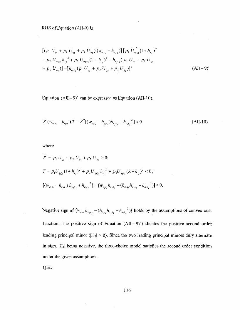
RHS of Equation (AlI-9) is

[(p V +p, V +p V )(w ~h »)[p V· (I+h )'- J Cf\ L 12 J q3 a,a, 0roi 1 q(q, sf

+ p, V'l,,,h,/ + P3 V q,Q3(). +h,)' -h,J'J(p, V'll + P, V 'l '

+ Pc V q)) -fha,,! (PI V'll + P, V 'l ' + P3 V qJ )]'

Equation (All- 9)' can be expressed as Equation (All-I 0).

where

T = P,Vq,q,O +h'i)' + P,Vq,q,h,,' + P3Vq,q,(;[+h,,)' <0;

(All- 9)'

(All-l 0)

Negative sign of [wa,a,h'h -(ha,a,h'j') -hai,/)] holds by the assumptions of convex cost

function. The positive sign of Equation (All- 9)' indicates the positive second order

leading principal minor (IH21 > 0). Since the two leading principal minors duly alternate

in sign, IHd being negative, the three-choice model satisfies the second order condition

under the given assumptions.

QED

116

APPENDIX B: SURVEY QUESTIONNAIRE (IN ENGLISH)

Dear Sir or Madame:

This survey is designed to collect residents' opinion on large ~ scale composting facility in Cheju~

Province~ South Korea. Around 2,500 copies of this questionnaire are be,iug distributed. Your

participation in this survey is on the voluntary basis only, and your candid and as precise as possible

responses to the questionnaire will contribute to making right decisions with respect to establishing the

waste disposal system in this area.

There is no definite right or wrong answer. Your thoughtful and honest response is important and will

be greatly appreciated. The survey results will be used for the research purpose only. Accordingly,

your privacy will be completely protected. If you have any questions or suggestions, please feel free to

contact me at (808) 956-7561, (064) 746-2302 or the Committee on Human Studies «808) 956-5007).

Thank you for your cooperation.

Hyuncheol Kim

Ph.D Candidate

Department of Economics

University of Hawaii at Manoa

117

[Questiounaire]

Part - waste disposal and attitude

I. Do you recycle part of your waste generated from your household?

Yes ( )/No( )

2. Do you compost part of your waste generated from your household?

Yes ( )/No( )

(Question 3-6) Please check one corresponding to how much effort you are making to

lessen the generation ofwaste in your daily life.

Never SometimesVery

Alwaysoften

3. Purchase goods with less packaging.I 2 3 4

,(Ex: Buy 1 big bottle instead of 2 smaller ones)4. Purchase recyclable products.

I 2 3 4I (Ex: Use coffee mug in the office instead ofvaDer CUDS)5. Borrow or share items.

1 2 3 4(Ex: share a lawnmower with neighbors or friends)6. Sell or donate unused items to neighbors instead of

I 2 3 4throwing them away.

(Question 7-14) How much do you trust the following organizations to make decision

about the waste management?

Never Trust Trust Absoluteltrust a little a lot trust

7. Community organizations I 2 3 4

8. Local recycling and waste administrator 1 2 3 4

9. Local public officials 1 2 3 4

10. Private businesses I 2 3 4

11. Environmental organizations 1 2 3 4

12. Universities I 2 3 4

13. Central govemment I 2 3 4

14. Mass media (newspaper and broadcast media) I 2 3 4

118

Part - If a new composting facility were built around your residence.

The following scenario is a hypothetical situation on the large - scale composting facility.

Please read carefully prior to answering the questions 15 - 44.

[Suppose that public institution of your community has suggested building a large- scale

composting facility in the neighborhood of your local residential area. The facility will be

housed inside a building and produce compost by processing organic wastes (leaves,

paper, diaper, food, etc.) of your and neighboring communities. Other wastes will be

disposed at other places. Eight-meters-tall trees will be planted around the facility and the

facility will be located 100m away from your house.]

(Question 15-28) Please read each question and answer on how it would affect yourcommunilv.

Never To some To muchAbsolutely

de~ree degree

15. Promote economic growth. 1 2 3 4

16. Pose serious risks to your children. 1 2 3 4

17. Create new job opportunities. 1 2 3 4

18. Generate bad odor. 1 2 3 4

19. Safety measures will decrease the risk. 1 2 3 4

20. Contaminate ground water. 1 2 3 4

21. Lower property tax. 1 2 3 4

22. Risk your neighbors' health and safety. 1 2 3 4

23. Lower the cost ofwaste disposal. 1 2 3 4

24. Lower the property value. 1 2 3 4

25. Provide a safe way for waste disposal. 1 2 3 4

26. Create a negative image on the community. 1 2 3 4

27. Will help improve the quality of the soil. 1 2 3 4

28. Increase the noise and pollution. 1 2 3 4

119

(Question 29-34) Under the hypothetical situation above on the composting facility,

please read each question and answer on the importance of each issue can be.

Don't NotImportant

Veryknow imoortant imnortant

29. The supervising and governing power of thefacility should be placed in the hands ofhoth 0 1 2 3community and facilitv owner.

30. The waste should be sorted out into organic and0 I 2 3

inorganic types before reaching the facility.31. The responsibility for the facility should be specified

0 1 2 3as a document before it is built.

32. In the event of accident or problems, your community0 I 2 3

should have the right to close the facility.33. Markets for the compost should be guaranteed in

0 1 2 3documents before the facility is constructed.

34. More benefits should be given to your communityhosting the facility than others using the facility. (e.g., 0 1 2 3free waste disposal, lower taxes, etc)

35. Which issue do you think is the most important among questions 29-34?

(1) Question 29 (Monitoring the facility)

(2) Question 30 (Sorting the waste by the type)

(3) Question 31 (The environmental responsibilities for the facility)

(4) Question 32 (Closing off the facility in the event of accident)

(5) Question 33 (Securing the market for the compost)

(6) Question 34 (More benefits to the facility hosting community)

36. In admitting the facility, what fonus of benefits do you think should be given to yourlocal community? Please select only 3 ( ) ( ) ( )

(1) Free waste disposal

(2) The grants for the building, parking lots, scholarship, etc.

(3) Reduce tax or guarantee property value for the landlords near the facility

(4) Hiring the local residents and purchasing the product from the facility

(5) Securing the fund for unexpected accidents or financial difficulties

120

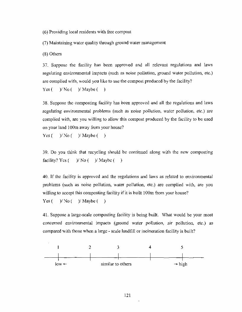
(6) Providing local residents with free compost

(7) Maintaining water quality through ground water management

(8) Others

37. Suppose the facility has been approved and all relevant regulations and laws

regulating environmental impacts (such as noise pollution, ground water pollution, etc.)

are complied with, would you like to use the compost produced by the facility?

Yes ( )/ No ( )! Maybe ( )

38. Suppose the composting facility has been approved and all the regulations and laws

regulating environmental problems (such as noise pollution, water pollution, etc.) are

complied with, are you willing to allow this compost produced by the facility to be used

on your land 100m away from your house?

Yes ( )! No ( )! Maybe ( )

39. Do you think that recycling should be continued along with the new composting

facility? Yes ( )! No ( )/ Maybe ( )

40. If the facility is approved and the regulations and laws as related to environmental

problems (such as noise pollution, water pollution, etc.) are complied with, are you

willing to accept this composting facility if it is built 100m from your house?

Yes ( )/ No ( )/ Maybe ( )

41. Suppose a large-scale composting facility is being built. What would be your most

concerned environmental impacts (ground water pollution, air pollution, etc.) as

compared with those when a large - scale landfill or incineration facility is built?

1

Jow~

2 3

similar to others

121

4 5

..... high

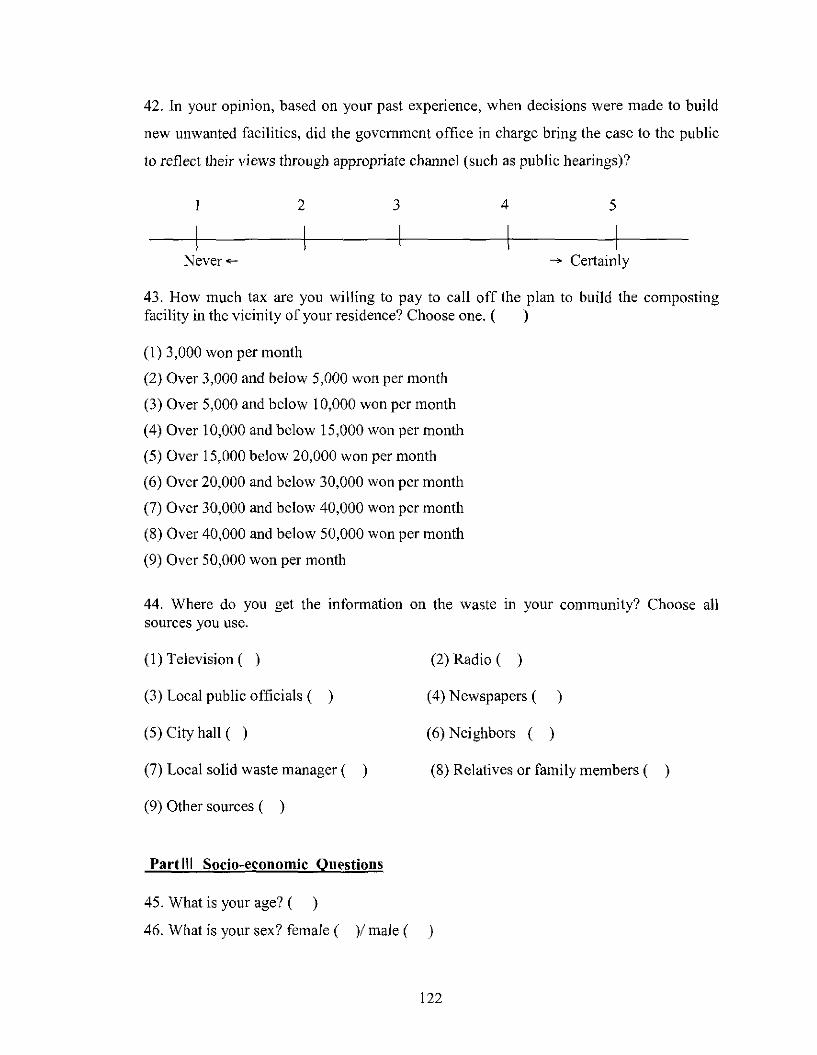
42. In your opinion, based on your past experience, when decisions were made to build

new unwanted facilities, did the government office in charge bring the case to the public

to reflect their views through appropriate channel (such as public hearings)?

Never <-

2 3 4 5

~ Certainly

43. How much tax are you willing to pay to call off the plan to build the compostingfacility in the vicinity of your residence? Choose one. ( )

(I) 3,000 won per month

(2) Over 3,000 and below 5,000 won per month

(3) Over 5,000 and below 10,000 won per month

(4) Over 10,000 and below 15,000 won per month

(5) Over 15,000 below 20,000 won per month

(6) Over 20,000 and below 30,000 won per month

(7) Over 30,000 and below 40,000 won per month

(8) Over 40,000 and below 50,000 won per month

(9) Over 50,000 won per month

44. Where do you get the information on the waste in your community? Choose allsources you use.

(I) Television ( )

(3) Local public officials ( )

(5) City hall ( )

(7) Local solid waste manager ( )

(9) Other sources ( )

Part III Socio-economic Questions

(2) Radio ( )

(4) Newspapers ( )

(6) Neighbors ( )

(8) Relatives or family members ( )

45. What is your age? ( )

46. What is your sex? female ( )/ male ( )

122

47. How many children under 18 are in your household? ( )

48. How many are older than 18 in your household? ( )

49. What is the level of your formal education? ( )

(I) Elementary school graduate or below

(2) Junior high school graduate

(3) Senior high school dropout

(4) Senior high school graduate

(5) Two year - college graduate

(6) University student

(7) University graduate

(8) Graduate work or above

50. Approximately how long have you been living in your current residence? ( ) years

.51. What is the type of your current housing?

(I) an independent house (2) a tenement house (3) an apartment

52. Approximately how much is your monthly household income (monthly disposable

income in 10,000 won)? ( )

(I) Less than 100 (2) 100 -149 (3) 150 - 199 (4) 200 - 249

(5) 250 - 299

(9) Over 500

(6) 300 - 349 (7) 350 - 399 (8) 400 - 499

Closing: Thank you for your time and cooperation.

123

APPENDIX C: SURVEY QUESTIONNAIRE (IN KOREAN)

~ '-2l <5HJ Y7J}?

01 1J. -if- 2. fill-?- s:. /-J, 10M ~+'~ 011 "'i'!~ -?- 'i'l aj 10i~ 91 917,1 ~ ~ i}] <5} 71 ~ ~

aj1Oi~91 7]-W3:J'{j {!-aj~ olif-Oi1J1.-]eJ-.aj1OliE-91 917,12. ;:Z1~A}§j2j .0'-101]71

51 C1 7ij {"j 011 '2!- s:.%0] -11 7;J ~ y t:j-. 01 1J. -if- 01]~ 1l '8- 01 '\.l ~ 7;J 01 o}1.-] E-~

aj~i~ol A~z.j-<5]-Al~ ::::It:l1~ t:l1'8-i>ij -?-Al'i'! ~*+. ~;:Z1<5}711 A~z.j-<5}{l ~

~Z1<5]-711 3:JOi -?-1J A1.2.. -i']<5}91 g1f cJl%2. ';171 i":- 'ti-=r-~ ~i>H'i'l- A]-%-11

7;J olJil, ~t:l1lJl~ol !t.AJ~1.-]r+. 'i'l-'21' ~-if-0l ~~ J..l 011 ~ fill A]--¥-~ (808)956­

7561 0] L} 7} f2j (064)746-2302. office of Human study (808) 956-5007 ~ -if-2j

<5}J..171 lJ]-'if1.-] eJ-.

~A~ 1.-] t:j-.

124

1. 7'-IOf;:: 7'-lof9.1 GiOiIAl Lfg ""ClIJI9.1 '&J~~ XH~~ (1'!''2.I4'-Ji) Of~L1JJf?

Ojl ( 1/ OfLl2 ( )

2.7'-101;:: 7'-lo!9.1 ""ClDI9.1 '&J~~ "-ItJl~Hcomposting)ol~L1JJf?

011 ( )/ OfLl2 ( )

• (?i!~ 3-6) Cf~ .'I'JI~ Af~OfOj ""ClIJI~ ~Ol;:: ':c~~ )§jOfLf of:;} Jjl CJ AI;j13 Of OJ ;;;;~ AI2

{! ?;~ 7}.g- *01 ~,7}

~h~1-I:l- %1:f %1:f %t:,

3. ""-~Ol ~ 8 Xil~~ -T'gjE!Cf.1 2 3 4

(Ojl: 2 JH 2j <S,f::: '2!3 01 CJ 1 JH 9.1 C' '2!3 Xii~ =[l gj)

4. XHAf~ Jf~e! Xil~~ =[lgje!Cf.J 2 3 4

(011: Af!?~OiIAl JH2J9.1 3iIIlH~ Af§2!Cf.)5.~!:f- ~h~ ~2:!~~ ~2.IJ1L~ ~J)jl ~.g0C~.

1 2 3 4(Ojl: ';§I.'E7IJjI~ OI~OILi ~-T'£f €tOI ~Cf)

6. 2J .ll.;:: ~2!;;;;~ 1::H2UI f'J":;} OI:::;;;;OiIJiI ~JiLf JI!¥e!Cf. 1 2 3 4

• (?i!@ 7-14)7'-101;:: ""ClIJI ~2.iOiI Ole ~tJI~ 9.IAf~2i~ 01;::[11 2lOJAl OI2H2j

71~~ ~ )§j Of2Jg CJ £1 of~ LI JJf?

~&l"1'Z!

\\t°l -'t!:zl -.51

0:~{l5!]

{l51~ ,""I "II'1l

7. AI2J8x41 1 2 3 4

8 XH ~§ ~ illI71~ ~2.1 AI 1 2 3 4

9. AI.~ ~~~ 1 2 3 4

10. Af 71 gj ('&J \:!f JH 2J JI gj ""- g) J 2 3 4

11. ~~~~ 8;41 1 2 3 4

12. 01 ~ 1 2 3 4

13.2:l¥ 1 2 3 4

14. ~E Jl~ 1 2 3 4

125

[:;>IOf~ XI Q1AI:2.1 ~~JI~OI XIQ1A1:2.1 ilIIJI~ MClIJI ~ltJl:2.1 Algj~ C!gjof::llXI

~eJ~OIIJjI C!~~ Of~;;;;LlCI. 01 AI~g C!~ LHOII ~()jAlDi :;>IOf~1 XI21AI:2.121

~\:!'IXI21A1:2.1~ g.JI MClIJI (LI~~, ~Ol, JIJ:PI, ~6!~ ~)~ x-jclolDi

tJl j'i(!~1 tJl) ~ ~ 0~ 3:! gj LI CI. ~ ~~l MCli JI ~::: CI~ 8::toOil Al J:,cl gj 3:! gj LI C[. ~

Algj ~i'10I1~ 8m ~I LlEi!~OI ]'2jgj 3:!OID:l :;>lolJI AI~ 8::to~'¥El 100m ~OW

~ 011 i'l J:I 01 Jjl gj 3:! gj LI CI.]

• (~~ 15-28) 7'-IOf~1 J:I21 AI:2.I011 ()j~)jl 'E!§~ DI~ XI 011 CHoH 012H .'I'JI~.'I'.:Ll

~olDi "?~AI.2.

~ii:l~ Q};'} Y~.:L if§ 6}"'T'-~

:I '?t q. -~-~q Ct sJcf-

15. ~All~ 2j8~ ~~1§t 3:!OICI. I 2 3 4

16. 7'-Iol~1 XIL~OIIJjI ~2.(e! i'lgj~ :EcH'1§t 3:!OICi. I 2 3 4

17. AH~@ "'i gj JI2.1 ~ All~1§t 3:! 01 CI. I 2 3 4

18. EJjAHJI ~2{~ 3:!OICi. I 2 3 4

19. 2! C'I], AI [H@OI! i'l gj 01 at ~ 3:! 01 CI. I 2 3 4

20. J:lol*~ .2.~AI§1 3:!OICf. 1 2 3 4

21 . J:121 AI 2.1 011 '5!'::: XII~ 01 '¥JlI gj 3:! 01 CI. I 2 3 4

22. 01:;::~1 C!~ill 2!C'I~ oH~ 3:!OICI. I 2 3 4

23. MClIJI Alcl tJl§~ ~::toAI§1 3:!OICi. 1 2 3 4

24. Algj2!2 ::tog.~~1 JIAI~ ~()jO:§! 3:!OICi. I 2 3 4

25. MClIJI ;:,cIOlI CHEf 2!~Ef \1t<gj~ All~~ 3:!OIC[. 1 2 3 4

26. J:I21 AI:2.I011 ~J:I 2i::: OIDIJ:I~ ~ 3:!OICi. I 2 3 4

27. OJ.g V::ll 2! C'I el ~~ JW.Q ill ~ .'I' '§i 3:! 0ICf. 1 2 3 4

28. ::to ~~oH ~ ~ ][AI ~ 3:! 01 CI. I 2 3 4

126

• (@i~ 29-34) 7'-lof9.1 ;;>\:!'!0I1 AH£~ ~ltJl£f AI~ ~~0I1 CHE!: ~I!:OI JI2f~ 2f~OIIAl

Cf g Af~ ~ 011 CH oH ~ OfLI 3 RoICf.:i2 ~ 2,'01 AI ~ XI xii 3 olOj ;;>~ AI2

£.@.t::} 1!.~ TJlg o~:r

-"t .fL 'j-1J" 'FJl'i}

29. AI~bfAI ~ ~Xil~ XI 9"1 Af 2.1 2f AI{g~';::;XfJf iiH 00 1 2 3

2 Cf.30. lli':/IJI ~ .:J AI~~OiI ~0i2JI BOil ';::;JI~llf

0tJl';::;JI~ ~@i£ =[1;'O"£IOiO~ 2Cf.

1 2 3

31. Algj~OiI CHef ;:fq. ~gj~XH~ 2jgj 01C!0i1 ~Al£0 1 2 3

2JJI£lOjO~ 2Cf.32. ~AiIJI ~~~~ AIOiI. 7'-lol!:01 XI 9"1 Af£1Jf .:J Algj~

0 1 2 3~Ji~ *" £iOjO~ 2Cf.

33. ~08 tJlli9.1 ±:.f£~ AI~ 2:1~ OIBOiI ~Al£ .'1:'80 1 2 3

£IOjO~ e:>Cf.34. 7'-1 of!:Ol AI Q1 Af 2.1 ~ .:J Algj ~ Af~ol~ [IE AI Q1 Af 2.1

.'1:'Cf [l Bt~ 0I1~~ WOfOr e:> [f . (011 : fFh£ lli':/IJI 0 1 2 3J;l 2.1. [l 3:' ~ Ail ~ ~.)

(1) @i~ 29 (Algj~OiI CHe:> 8AI ~ ~Ail)(2) @i~ 30 (lli':/IJI!:OI ;'0"2.1)(3) @i~ 31 (Algj~9.1 &?3~ 9.lfi2) (4) @i~ 32 (~Ail~~AI Algj~IT/IJI)

(5) @i~ 33 (tJlfi9.1 ~£ ~'I') (6) @i~ 34 (AI~~~ ';::;;(:12 AI 9"1 Oil 0I11O!i 3)

36. .:J Algj~ WOf~OIJI ~loH 7'-IOfJJlIAl 'i!d"Of~~el"2 *"011 ~ Jm ~R2 3 JfAIe!"xJI30lOj '?~AI5'.. ( ) ( ) ( )

(3) '2J2 ~AI ~';::;AI~OII)j1 AilE '2Jof ±~ ~.;::;~ JfJ;1 'I'8(4) .:J AI 9"1 Af\5"~ +{:<:I ~ 0 £ .:i2 §Of:J} .:J XI Q1 OIIAl ~& £1 ~ Xii~ ~ =[1gJ oH O~ gr.(5) Af:J} ±~ XH2j~'2J ~Xjl ~~AI@ CHtJI2 AfE~'I'

(6) .:J XIQ1 '?'2J~()U fi2fi£ ~ltJl£f OH3(7) ~ Xi e:> XI of*" :t':!:2.1 £ '2J:C! e:> *"@i ~ ~.'1:'

(8) JIEI

37. 9-121 g ~ AI ~ 01 OJ JfJI £I:J} .:J AI ~ ~ 01 2j ¥JI 2j e:> 5'.:= THil ~

\1:j ~ (~g~oH. Alof*" 5'. gJ ~ 011 :t':!:e:> nXil ~) ~ el"~ e:>Cft'! 7'1 of ~ 'jli of!:Ol ~.;::;~

9-1011 .:J g~ 8 tJl fi ~ Af~ofAI:;(lI~ LI »f?011 ( )/ OfLl5'. ( )/ Of Of .:J~3:iOI[f. (

127

38. 'i'15'.f g~ AI~OI ojJf]f £I:J} ~~]f ~El 2.~ TrAjl ~ \;;i%j(~~~oH.xlof*

2gJ ~0I1 Ef"El TrAjl~)~ ~~ ElW::! 7'-lof~ ;;JOIIA-j 100m ~~ '§!OW @0I1 01 Cllfi]fAfgs:.I~~ OJ'''fofAI~~LIJJf?

()il( )/OfLI2( )/OfOf.:J§!3:!OICf.(

39. AH~gOI AH~~ ~ClI£f AI~llf [-j~(}j Jjl~~o~ OI~(}jXiOf ElCf:J}~2.tofGJLIJJf?

()il ( )/ OfU2 ( )/ Of Of .:J§!3:!OICf. (

40. XI'2iAf£1 ilII]l~ ~ClI£f AI~OI OJ]f]f s:.1:J} ~~]f ~El 2~ THI ~ \;;i%j(~~~oH. XIOf* 2f?J~0I1 2fEl TrAil;:;) ~ ~~ oW! OIAI~OI 7'-101]1 AfAI~ :£OII'!d100m '§!(}j~ :£011 ~):18W~ .:J AI~~~ 'i1!Of ~OIAm~LIJJf?()il ( )/ OlLI2 ( )/ OIDI .::J§!3:!OICf. ( )

41. I]Tr2 ~IClI£1 AI~~ 2i~ElCI:J} ]f~~ [lL OH~OIU ~2.tAI~llf I:JlliloHA-j ~IClI£f

AI~OI §~0I1 J)I~ 'l'-lgj2! (Xlof* 2f?J. ClDI2f?J ;:;) ~ ~OfU 8Cf:J} ~2{

ofGJ U JJf?

2 3 4 5

42. 2"eJ (~~XI ~2!Xf)!::'.1 'E!§0I1 9.I]j~ ITH 2I:Ej~~OI g2AI~~ =;2!XIQ101I ¥;):I~

ITH oH ~XI Q1 "?eJ ~9.1 OloH ~ ~JI '1'-1 El ~ \;;i El ~ ):f( ()il: Af~OII I] El ~~ 2.1)~ ~oH omXI Q1 "? eJ ~ 9.1 !::'.I =22 ~ * ~ ~ [I:J} ~ 2.t of GJ LI ))f?

2 3 4 5

43. 7'-1 of] f Af ~ XI Q1 "? t'! 011 I] rt 2. .u. Cli ] I ~II:J I£f AI~ ~):I Jjl ~ ~ '}I i: .'f ~X1XIAI§! *~ ~Cfi:::! §(A115)~ '§jOfJJfXI XI~ ~ * ~~XI9.? [f~ ~]I g olU~

{:<j~ofCJ:I ~GJAI2. ( )

(1) ~ 3~~ DI~ (2) ~ 3~~ - 5~~ DI~

(4) ~ 1~~ - 1~5~~ DI~

(6) ~ 2~~ - 3~~ DI~

128

(3) ~ 5~~ - 1~~ DI~

(5) ~ 1~5~~ - 2~~ DI~

(7) ~ 3~~ - 4~~ DI~

(8) ~ 4e!"@ - 5e!"~ 01 e!"

44. '1'-lof~ XI~Af£.1 LH MClIJI01I am 215'.:::: amId gj::L! V~LIW? oH'S'Afg-01I 2SF.HAloIAIS?.

(1) ~ Cli tJ I~ ( )(4)t!§( )(7) MClIJI ~:1: ggAf((9) .:J S:I~ w= *~ (

(2) cf[lS?(5) AI ~

))

))

(3) XI~ ~-'?-~( )(6) 01;: ~::' .lll~ ~(

(8) elXI ~g Jf~(

))

45.7'101:::: LfOIJI (}j~)jl £1 GiL/JJf? e!"( )@i

46. '1'-1 of~ ~ l!1::'? am ( )/ 'e3Af (

47. '1'-IOf2.\ Jf2l011 e!" 18 All OIN2.j XfLoj *:::: ~ ~OIGiLIJJf? ( )~

48. -1'1 0[2.[ ~ 01[ g- J)j[ J1 ~o[:::: '2j '2J::' ~ 2l 01 Gi LI JJf? ( )2l

49. '1'-1 Of 2.1 2t~::' [f ~ ~ OJ [I 011 om £1 Gi LI W? (

(1) ;:;~ Olaf (2) ~~ (3) ::L!~2t.lll ~~I (4) ::L!~2t.lll ~gj

(5) lO!§CH ~gj (6) CH2t.lll XH2t (7) CH2tliI ~gj (9) CH2t~ DIY

50. '1'-1 of:::: ~ 'CI ~ '2J E!AH XI ~ 011 @i::L! )11 G! L/ JJf? ( ) to!

(2) 9j "" A: E"L...: t::::IT-. (3) OIIlfE

52. 7'lof2.1 Jf~2.1 ~ 3 *~~ := '§jOf~LIJJf? (

(1) 100 e!"~ Ole!"(4) 200-249 e!"§(7) 350-399 e!" §

(2) 100-149 e!"~

(5) 250-299 e!"~

(8)400-499 e!"@

(3) 150-199 e!"~

(6) 300-349 e!"~

(9) 500 e!"~OIY

© gj§XI~ ~~ofAILCf 7'1e! AI2J- LH~JilAl ?J-AfgrLI[f. 7'INJf ~~ oft!~§LH~:= MCiIJI J:l cl Oil CHE! t"!-T'0i1 Of"? jf~of)jl Af~£I(}j @!3;!~L/[f.

?J- AfgrL/ [I. ©

129

APPENDIX D: STATISTICAL SUMMARY

DI. Survey Qucstious

Question 1. Do you recycle part of your waste generated from your household?

Table DI.I: Question I

Response Frequency Percent Cumulative PercentYes 1,646 88.97 88.97No 203 10.97 99.95No answer I 0.05 100.00Total 1,850 100.00

Question 2. Do you compost part of your waste generated from your household?

Table DI.2: Question 2

Response Frequency Percent Cumulative PercentYes 427 23.08 23.08No 1,421 76.81 99.89No answer 2 0.11 100.00Total 1,850 100.00

Question 3. Purchase goods with less packaging.

Table DI.3: Question 3

Response Frequency Percent Cumulative PercentNever 216 11.68 11.68Sometimes 873 47.19 58.86VerY often 527 28.49 87.35Always 232 12.54 99.89No answer 2 0.11 100.00Total 1,850 100.00

130

Question 4. Purchase recyclable products.

Table 01.4: Question 4

Response Frequency Percent Cumulative PercentNever 239 12.92 12.92Sometimes 717 38.76 51.68VerY often 566 30.59 82.27Always 323 17.46 99.73No answer 5 0.27 100.00Total 1,850 100.00

Question 5. Borrow or share items.

Table 01.5: Question 5

Response Frequency Percent Cumulative PercentNever 275 14.86 14.86Sometimes 741 40.05 54.92VerY often 571 30.86 85.78Always 256 13.84 99.62No answer 7 0.38 100.00Total 1,850 100.00

Question 6. Sell or donate unused items to neighbors instead of throwing them away.

Table 01.6: Question 6

ResDonse Freauencv Percent Cumulative PercentNever 422 22.81 22.81Sometimes 808 43.68 66.49Very often 413 22.32 88.81Alwavs 201 10.86 99.68No answer 6 0.32 100.00Total 1,850 100.00

131

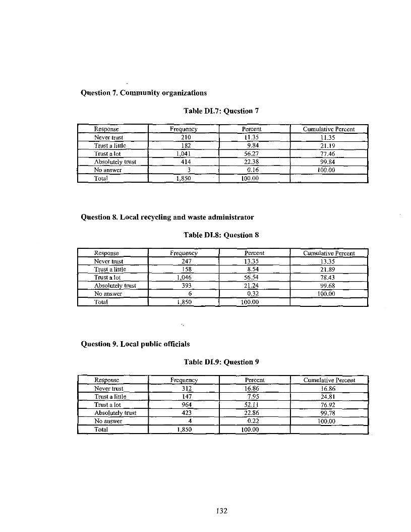
Question 7. Community organizations

Table DI.7: Question 7

Resoonse Freauencv Percent Cumulative Percent

Never trust 210 11.35 11.35Trust a little 182 9.84 21.19Trust a lot 1,041 56.27 77.46Absolutely trust 414 22.38 99.84No answer 3 0.16 10000Total 1,850 100.00

Question 8. Local recycling and waste administrator

Table DI.8: Question 8

Response Frequency Percent CUllluJative PercentNever trust 247 13.35 13.35Trust a little 158 8.54 21.89Trust a lot 1,046 56.54 78.43Absolutely trust 393 21.24 99.68No answer 6 0.32 100.00Total 1,850 100.00

Question 9. Local public officials

Tablc DI.9: Question 9

Response Frequency Percent Cumulative Percent

Never trust 312 16.86 16.86Trust a little 147 7.95 24.81Trust a lot 964 52.II 76.92Absolutely trust 423 22.86 99.78No answer 4 0.22 100.00Total 1,850 100.00

132

Question 10. Private businesses

Table DI.10: Question 10

Response Frequency Percent Cumulative PercentNever trust 672 36.32 36.32Trust a little 280 15.14 51.46Trust a lot 785 42.43 93.89i\bsolutely trust 107 5.78 99.68No answer 6 0.32 10000Total 1,850 100.00

Question 11. Environmental organizations

Table DI.11: Question 11

ResDonse Freauency Percent Cumulative PercentNever trust 166 8.97 8.97Trust a lillie 127 6.86 15.84Trust a lot 896 48.43 64.27i\bsolutely trust 658 35.57 99.84No answer 3 0.16 100.00Total 1,850 100.00

Question 12. Universities

Table D1.12: Question 12

Response Freauency Percent Cumulative PercentNever trust 405 21.89 21.89Trust a little 254 13.73 35.62Trust a lot 926 50.05 85.68i\bsolutely trust 260 14.05 99.73No answer 5 0.27 100.00Total 1,850 100.00

133

Question 13. Central government

Table 01.13: Question 13

Response Frequency Percent Cumulative PercentNever trust 474 25.62 25.62Trust a little 200 10.81 36.43Trust a lot 956 51.68 88.11Absolutely trust 215 11.62 99.73No answer 5 0.27 100.00

Total 1,850 100.00

Question 14. Mass media (newspaper and broadcast media)

Table 01.14: Question 14

ReSDonse Freouencv Percent Cumulative PercentNever trust 462 24.97 24.97Trust a little 227 12.27 37.24Trust a lot 967 52.27 89.51Absolutely trust 189 10.22 99.73No answer 5 0.27 100.00Total 1,850 100.00

Question 15. Promote economic growth.

Table 01.15: Question 15

Response Frequency Percent Cumulative PercentNever 184 9.95 9.95To some degree 442 23.89 33.84To much degree 865 46.76 80.59Absolutely 336 18.16 98.76No answer 23 1.24 100.00Total 1,850 100.00

134

Question 16. Pose serious risks to your children.

Table 01.16: Question 16

Response Frequency Percent Cumulative PercentNever 156 8.43 8.43To some degree 726 39.24 47.68To much degree 727 39.30 86.97Absolutely 218 11.78 98.76No answer 23 1.24 100.00Total 1,850 100.00

Question 17. Create new job opportunities.

Table 01.17: Question 17

Response Frequency Percent Cumulative PercentNever 144 7.78 7.78To some degree 341 18.43 26.22To much degree 983 53.14 79.35Absolutely 360 19.46 98.81No answer 22 1.19 100.00Total 1,850 100.00

Question 18. Generate bad odor.

Table 01.18: Question 18

Response Frequency Percent Cumulative PercentNever 67 3.62 3.62To some de~ree 244 13.19 16.81To much degree 918 49.62 66.43Absolutelv 598 32.32 98.76No answer 23 1.24 100.00

Total 1,850 100.00

135

Question 19. Safety measures will decrease the risk.

Table DI.19: Question 19

Response Frequency Percent Curnulati ve Percent

Never 224 12.11 12.11To some degree 449 24.27 36.38To much degree 895 48.38 84.76Absolutely 259 14.00 98.76No answer 23 1.24 100.00Total 1,850 100.00

Question 20. Contaminate ground water.

Table DI.20: Question 20

Response Frequency Percent Cumulative PercentNever 123 6.65 6.65To some degree 318 17.19 23.84To much degree 892 48.22 72.05Absolutely 494 26.70 98.76No answer 23 1.24 100.00Total 1,850 100.00

Question 21. Lower property tax.

Table DI.21: Question 21

Response Frequency Percent Cumulative PercentNever 203 10.97 10.97To some degree 459 24.81 35.78To much degree 818 44.22 80.00Absolutely 347 18.76 98.76No answer 23 1.24 100.00Total 1,850 100.00

136

Question 22. Risk your neighbors' health and safety.

Table DI.22: Question 22

Response Frequency Percent Cumulative PercentNever 167 9.03 9.03To some degree 531 28.70 37.73To much deuree 898 48.54 86.27Absolutely 231 12.49 98.76No answer 23 1.24 100.00Total 1,850 100.00

Question 23. Lower the cost of waste disposal.

Table DI.23: Question 23

Response FreQuency Percent ClUllulative PercentNever 104 5.62 5.62To some dcgree 265 14.32 19.95To much de~ree 857 46.32 66.27Absolutely 604 32.65 98.92No answer 20 1.08 100.00Total 1,850 100.00

Question 24. Lower the property value.

Table DI.24: Question 24

Response Frequency Percent Cumulative PercentNever 106 5.73 5.73To some degree 243 13.14 18.86To much de~ree 912 49.30 68.16Absolutely 566 30.59 98.76No answer 23 1.24 100.00Total 1,850 100.00

137

Question 25. Provide a safe way for waste disposal.

Table DI.25: Question 25

ReSoonse Freauencv Percent Cumulative PercentNever 151 8.16 8.16To some dCfTfCe 233 12.59 20.76To much degree 950 51.35 72.11Absolutely 495 26.76 98.86No answer 21 1.14 100.00Total 1,850 100.00

Qnestion 26. Create a negative image on the community.

Table DI.26: Question 26

Resnonse Freauencv Percent Cumulative PercentNever lIS 6.22 6.22To some de.ree 506 27.35 33.57To much dCPTce 847 45.78 79.35Absolutelv 361 19.51 98.86No answer 21 1.14 100.00Total 1,850 100.00

Question 27. Will help improve the quality of the soil.

Table DI.27: Question 27

Resnonse Frenuencv Percent Cumulative PercentNever 161 8.70 8.70To some degree 348 18.81 27.51To much depree 888 48.00 75.51Absolutelv 432 23.35 98.86No answer 21 1.14 100.00Total 1,850 100.00

138

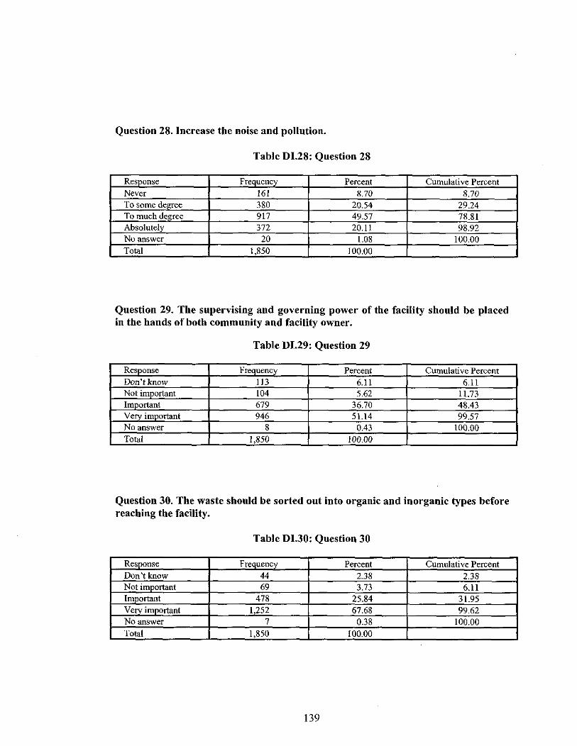
Question 28. Increase the noise and pollution.

Table 01.28: Question 28

Resnonse Frenuencv Percent Cumulative PercentNever 161 8.70 8.70To some dearee 380 20.54 29.24To much de~ree 917 49.57 78.81Absolutely 372 20.11 98.92No answer 20 1.08 100.00Total 1,850 100.00

Question 29. The supervising and governing power of the facility should be placedin the hands of both community and facility owner.

Table 01.29: Question 29

Resnonse Frenuencv Percent Cumulative PercentDon't know 113 6.11 6.11Not imnortant 104 5.62 11.73lmoortant 679 36.70 48.43Ve'::';iwortant 946 51.14 99.57No answer 8 0.43 100.00Total 1,850 100.00

Question 30. The waste should be sorted out into organic and inorganic types beforereaching the facility.

Table 01.30: Question 30

Resnonse Freouencv Percent Cumulative PercentDon't know 44 2.38 2.38Not irrmortant 69 3.73 6.11Imnortant 478 25.84 31.95Ve;;; imnortant 1,252 67.68 99.62No answer 7 0.38 100.00Total 1,850 100.00

139

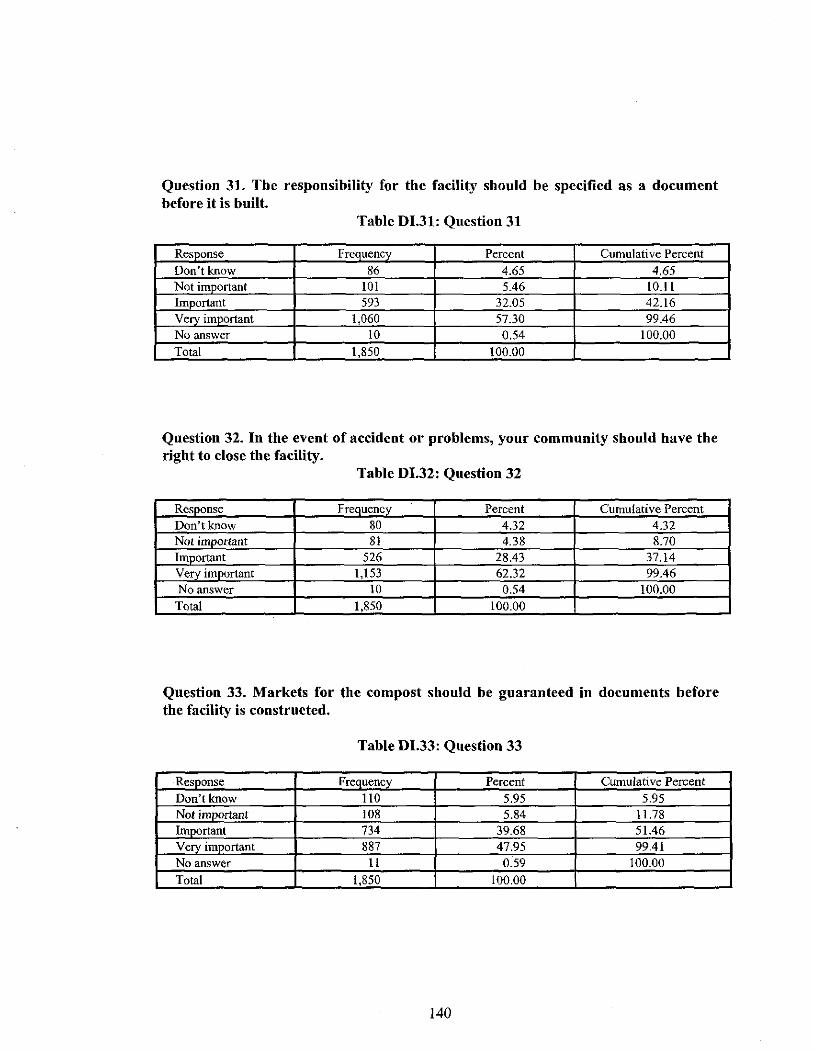
Question 31. The responsibility for the facility should be specified as a documentbefore it is built.

Table 01.31: Question 31

Response Frequency Percent Cumulative PercentDon't know 86 4.65 4.65Not imnonant 101 5.46 10.11Important 593 32.05 42.16Very imnortant 1,060 57.30 99.46No answer 10 0.54 100.00Total 1,850 100.00

Question 32. In the event of aecident or problems, your eommunity should have theright to close the facility.

Table 01.32: Question 32

ReSDonse Frequency Percent Cumulati.ve PercentDon't know 80 4.32 4.32Not imootlant 81 4.38 8.70Important 526 28.43 37.14Very important 1,153 62.32 99.46No answer 10 0.54 100.00Total 1,850 100.00

Question 33. Markets for the compost should be guaranteed in documents beforethe facility is construeted.

Table 01.33: Question 33

Response Frequency Percent Cumulative PercentDon't know 110 5.95 5.95Not impotlant 108 5.84 11.78Imnortant 734 39.68 51.46Very important 887 47.95 99.41No answer II 0.59 100.00Total 1,850 100.00

140

Question 34. More benefits should be given to your community hosting the facilitythan others using the facility. (e.g., free waste disposal, lower taxes, etc)

Table DI.34: Question 34

Response Freauencv Percent Cumulative Percent

Don't know 68 3.17 3.68Not important 107 15.78 9.46Important 634 314.27 43.73Very important 1,030 5I5.68 991.41No answer 11 10.59 100.00Total 1,850 100.00

Question 35. Which issue do you think is the most important among questions 29­34?

Table DI.35: Question 35

Response Frequencv Percent Cumulative Percent

Ouestion 29 392 21.19 21.19Question 30 405 21.89 43.08Question 31 464 25.08 68.16Question 32 328 17.73 85.89Question 33 28 1.51 87.41Question 34 205 11.08 98.49No answer 28 1.51 100.00

Total 1,850 100.00

Question 36. In admitting the facility, what forms of benefits do you think should begiven to your local community? Please select only 3. ( ) ( ) ( )

Table DI.36: Question 36

Response Frequencv Percent Cumulative PercentFree disposal 727 13.35 13.35Grant 415 7.62 20.97Reduce tax 891 16.36 37.32Local benefit 742 13.62 50.95Fund 824 15.13 66.07Free composting 339 6.22 72.30Good Environment 1,438 26.40 98.70Others 71 1.30 100.00Total 5,447 100.00

141

Question 37. Suppose the facility has been approved and all relevant regulations andlaws regulating environmental impacts (such as noise pollution, ground waterpollution, etc.) are complied with, would you like to use the compost produced bythe facility?

Table DI.37: Question 37

Response Frequency Percent Cumulative Percent

Yes 1,089 58.86 58.86No 206 11.14 70.00Maybe 540 29.19 99.19No answer 15 0.81 100.00Total 1,850 100.00

Question 38. Suppose the composting facility has been approved and all theregulations and laws regulating environmental problems (such as noise pollution,water pollution, etc.) are complied with, are you willing to allow this compostproduced by the facility to be used on your land 100m away from your house?

Table DI.38: Question 38

ReSDonse Freauency Percent Cumulative Percent

Yes 1,032 55.78 55.78No 385 20.81 76.59Maybe 417 22.54 99.14No answer 16 0.86 .100.00

Total 1,850 100.00

Question 39. Do you think that recycling should be continued along with the newcomposting facility?

Table DI.39: Question 39

Response Frequency Percent Cumulative Percent

Yes 1,562 84.43 84.43No 93 5.03 89.46Maybe 162 8.76 98.22No answer 33 1.78 100.00

Total 1,850 100.00

142

,

Question 40. If the facility is approved and the regulations and laws as related toenvironmental problems (such as noise pollution, water pollution, etc.) are compliedwith, are you willing to accept this composting facility if it is built 100m from yourhouse?

Table DI.40: Question 40

Reseonsc Freauency Percent Cumulative PercentYes 854 46.16 46.16No 571 30.86 77.03Mav-be 398 21.51 98.54No answer 27 1.46 100.00Total 1,850 100.00

Question 41. Suppose a large-scale composting facility is being built. What wouldbe your most concerned environmental impacts (ground water pollution, airpollution, etc.) as compared with those when a large - scale landfill or incinerationfaeility is built?

Table DI.41: Question 41

Resnonse Frenuency Percent Cumulative PercentjiloWl 322 17.41 17.412 421 22.76 40.1631similar to others) 552 29.84 70.004 287 15.51 85.5151hi;,hj 224 12.11 97.62

No answer 44 2.38 100.00Total 1,850 100.00

Question 42. In your opinion, based On your past experience, when decisions weremade to build new unwanted facilities, did the government office in charge bring thecase to the public to reflect their views through appropriate channel (such as publichearings)?

Table DI.42: Question 42

Resnonse Freauency Percent Cumulative Percentltneyeil 280 15.14 15.142 370 20.00 35.143 517 27.95 63.084 421 22.76 85.845IcertainM 241 13.03 98.86

No answer 21 1.14 100.00Total 1,850 100.00

143

Question 43. How much tax are you willing to pay to call off the plan to build thecomposting facility in the vicinity of your residence? Choose one.

Table DI.43: Question 43

ReS%nse Frenuencv Percent Cwnulative Percent

\3,000 * 674 36.43 36.43\3,000 - \5,000 409 22.11 58.54

\5,000 -\10,000 285 15.41 73.95\10,000 - \15 000 131 7.08 . 81.03\15,000 - \20,000 78 4.22 85.24

\20.000 - \30,000 65 3.51 88.76\30,000 - \40 000 47 2.54 91.30\40 000 - \50 000 25 1.35 92.65Over \50.000 35 1.89 94.54No answer 101 5.46 100.00Total 1,850 100.00

'" Utut: won

Question 44. Where do you get the information on the waste in your community?Choose all sources you use.

Table DI.44: Question 44

Resnonse Freauencv Percent Cwnulative PercentTelevision 1,456 27.58 27.58Radio 563 10.66 38.24*LPO 551 10.44 48.68Ncwsoaoer 1,205 22.82 71.50City Hall 458 8.67 80.17NeiM>bors 259 4.91 85.08**LSWM 289 5.47 90.55Relatives 258 4.89 95.44Other sources 241 4.56 100.00Total 5,280 100.00

*Local public offiCIals, **Local sohd waste manager

Question 45. What is your age?

Table DI.45: Question 45

Resnonse Freauency Percent Cumulative Percent20s 590 31.9 3\.930s 658 35.6 67.540s 384 20.8 88.350s 94 5.1 93.4Over 60s 37 2.0 95.4No answer 87 4.7 100.00

Total 1,850 100.00

144

Question 46. What is your sex?

Table DI.46: Question 46

Response Frequency Percent Cumulative PercentFemale 875 47.30 47.30Male 944 51.03 98.32No answer 31 1.68 100.00Total 1,850 100.00

Question 47. How many children under 18 are staying in your household?

Table DI.47: Question 47

Response Frequency Percent Cumulative Percent0 601 32.49 32.49I 337 18.22 50.702 579 31.30 82.003 166 8.97 90.974 26 1.41 92.385 9 0.49 92.866 2 0.11 92.977 4 0.22 93.19

No answer 126 6.81 100.00Total 1,850 100.00

Question 48. How many are older than 18 in your household?

Table DI.48: Question 48

Response Frequency Percent Cumulative PercentI 308 16.65 16.652 649 35.08 51.733 383 20.70 72.434 307 16.59 89.035 121 6.54 95.576 2 0.11 95.687 2 O.ll 95.78

No answer 78 4.22 100.00Total 1,850 100.00

145

Question 49. What is the level of your formal education?

Table DI.49: Question 49

Response Frequency Percent Cumulative PercentElementary II 0.59 0.59Junior high 38 2.05 2.65Dropout of senior high 66 3.57 6.22Senior high 537 29.03 35.24Two year - college 405 21.89 57.14University student 85 4.59 61.73University graduate 615 33.24 94.97Beyond post graduate 43 2.32 97.30No answer 50 2.70 100.00Total 1,850 100.00

Question 50. Approximately how long have you been living in your currentresidence?

Table DI.50: Question 50

Response Frequency Percent Cumulative PercentBelow 5 l'ears 509 27.5 27.55 - 10 years 343 18.5 46.011-15years 138 7.5 53.516 - 20 years 176 9.5 63.021 - 25 years'. 169 9.1 72.126 -30 years 199 10.8 82.931 - 35 years 97 5.2 88.1Over 36 years lSI 8.2 96.3No answer 68 3.7 100.00Total 1,850 100.00

Question 51. What is the type of your current housing?

Table DI.51: Question 51

Response FreQuencv Percent Cumulative PercentIndependent house 934 50.49 50.49Tenement house 472 25.51 76.00Apartment 395 21.35 97.35No answer 49 2.65 100.00Total 1,850 100.00

146

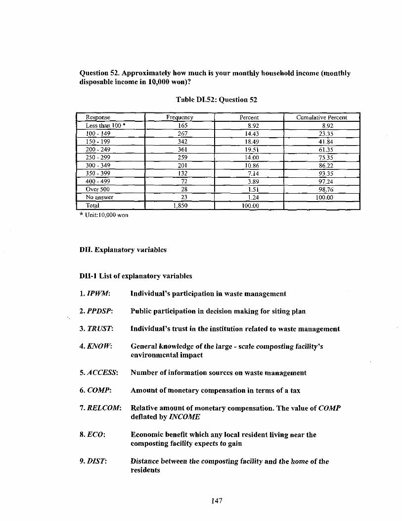
Question 52. Approximately how much is your monthly household income (monthlydisposable income in 10,000 won)?

Table DI.52: Question 52

Resnonse Freouencv Percent Cumulative PercentLess than 100 • 165 8.92 892100 - 149 267 14.43 23.35150 - 199 342 18.49 41.84200 - 249 361 19.51 61.35250 - 299 259 14.00 75.35300 - 349 201 10.86 86.22350 - 399 132 7.14 93.35400 - 499 72 3.89 97.24Over 500 28 1.51 98.76No answer 23 1.24 100.00Total 1,850 100.00

* Unit: 10,000 won

DII. Explanatory variables

DII-l List of explanatory variables

1. IPWM: Individual's participation in waste management

2. PPDSP: Pnblic participation in decision making for siting plan

3. TRUST: Individual's trust in the institution related to waste management

4. KNOW: General knowledge of the large - scale composting facility'senvironmental impact

5. ACCESS: Number ofinformation sources on waste management

6. COMP: Amount of monetary compensation in terms of a tax

7. RELCOM: Relative amount of monetary compensation. The value of COMPdeflated by INCOME

8. ECO: Economic benefit which any local resident living near thecomposting facility expects to gain

9. DIST: Distance between the eomposting facility and the home of theresidents

147

10.ENV: Environmental impact of the composting facility

11.INCOAfE: Household's average monthly disposable income

12. CHILD:

l3.EDU:

Number of children in respondent's home

Respondent's education level

14. GENDER: Gender of respondent

15. AGE: Age of respondent

16. NHMBR: Respondent's household size

17. YRSTAY: Number of years at the current residence

18. HSFORM: Respondent's house type

Dll-2 Statistical Summary of Explanatory Variables

Table DII.l: Statistical Summary of Explanatory Variables

Variable Obs· Mean Std. Dev.** Min MaxIPWM 1.837 2.797 1.667 0 6PPDSP 1,829 2.985 1.254 I 5TRUST 1,837 6.987 3.470 0 16KNOW 1,806 2.817 1.252 1 5ACCESS 1,813 2.866 1.609 I 9COMP 1,749 2.570 1.920 I 9RELCOM 1,739 0.840 0.971 I 8ECO 1,809 0.008 0.874 -3.023 1.842DIST 1850 1.020.865 1,052.498 100.000 3,000.000ENV 1,809 0.004 0.891 -2.810 1.930INCOME 1,827 4.062 1.957 I 9CHILD 1,724 1.266 1.154 0 7EDU 1,800 5.343 1.498 1 8GENDER 1,819 0.520 0.500 0 IAGE 1802 34.173 10.100 19 79NHMBR 1,695 4.805 1.613 I 12YRSTAY 1,782 16.333 13.004 I 73HSFORM 1,801 1.743 0.894 1 4* number ofobservatIOn, ** standard deViatIOn

148

APPENDIX E: LIST OF SIGNIFICANT COEFFICIENTS

NOTE

sd: standard deviation, b: coefficients.

1. IPWM

Table E.1: IPWMsd~1667

Odds of Base choiceVS, Non~base choice

b P> Izi exp(b) exp(b x sd)zBase Non~base

choice choiceNo Maybe 0.031 0.521 0,603 1.031 1.053No Yes -0.171 - 2.926 0.003 0.843 0,752Maybe No - 0.031 - 0.521 0.603 0.970 0.950Mavbe Yes -0.202 - 3.752 0.000 0,817 0.714Yes No 0.171 2.926 0.003 1.187 1.330Yes Maybe 0.202 3.752 0.000 1.224 1.401

2.PPDSP

Table E.2: PPDSPsd - I 266-

Odds of Base choicevs. Non-base choice

b P>jzl exp(b) exp(b x sd)zBase Non-basechoice choiceNo Maybe - 0.408 - 5.914 0.000 0,665 0.597No Yes - 0.733 - 10.417 0,000 0.481 0,395Maybe No 0.408 5,914 0.000 1.503 1.676Mavbe Yes - 0.325 - 5,074 0,000 0.722 0.663Yes No 0.733 10.417 0.000 2.081 2.529Yes Maybe 0.325 5.074 0,000 1.384 1.509

149

3. TRUST

Table E.3: TRUSTsd - 3458-

Odds of Base choicevs. Non-base choice

b P> Izi exp(b) exp(b x sd)zBase Non-basechoice choiceNo Maybe - 0.061 - 2.188 0.029 0.941 0.811No res -0.055 - 1.960 0.050 0.947 0.828Maybe No 0.061 2.188 0.029 1.063 1.234Maybe res 0.006 0.241 0.809 1.006 1.022Yes No 0.055 1.960 0.050 1.056 1.208res Maybe - 0.006 -0.241 0.809 0.994 0.979

4. KNOW

Table E.4: KNOWsd - 1 262-

Odds of Base choicevs. Non-base choice

b P> Izi exp(b) exp(b x sd)zBase Non-basechoice choiceNo Maybe 0.199 2.753 0.006 1.220 1.286No res 0.491 6.734 0.000 1.633 1.857Mavbe No -0.199 - 2.753 0.006 0.819 0.778Maybe res 0.291 4.306 0.000 1.338 1.444res No - 0.49 [ - 6.734 0.000 0.612 0.539res Mavbe - 0.291 -4.306 0.000 0.747 0.692

5. ACCESS

Table E.5: ACCESSsd ~ 1 590

Odds of Base choicevs. Non-base choice

b P> Izi exp(b) exp(b x sd)zBase Non-basechoice choiceNo Maybe - 0.190 - 2.961 0.003 0.827 0.740No Yes -0.343 - 5.5\7 0.000 0.709 0.579Maybe No 0.190 2.96\ 0,003 1.209 1.352Mavbe res - 0.154 - 2.912 0.004 0.858 0.783Yes No 0.343 5.517 0.000 1.410 1.726Yes Maybe 0.154 2.9\2 0.004 Ll66 1.277

150

6.COMP

Table E.6: COMPsd - 1 898-

Odds of Base choicevs. Non-base choice

b p> Izi exp(b) exp(b x sd)zBase Non-basechoice choiceNo Mavbe 0.178 2,536 0,011 1.l95 1.402No Yes 0.160 2.213 0.027 1.174 1.356Maybe No -0.178 - 2.536 0.011 0.837 0.713Mavbe Yes - 0.018 - 0.231 0.817 0.982 0.967Yes No - 0.160 - 2.213 0.027 0.852 0.738Yes Maybe 0.018 0.231 0,817 1.018 1.034

7.RELCOM

Table E.7: RELCOMsd - 967-

Odds ofRasc choicevs. Non-base choice

b P> Izl exp(b) exp(b x sd)zBase Non-basechoice choice

No Maybe 0,212 10405 0.160 1.236 1.227No Yes 0.411 2.743 0.006 1.509 1.488Maybe No - 0.212 - 10405 0.160 0.809 0.815Mavbe Yes 0.200 1.302 0,193 1.221 1.213Yes No -00411 - 2.743 0.006 0.663 0.672Yes Maybe - 0.200 - 1.302 0.193 0.819 0.825

8.ECO

Table E.8: ECOsd - 877-

Odds ofBase choicevs. Non-base choice

b P> Izl exp(b) exp(b x sd)zBase Non-basechoice choice

No Mavbe - 0.291 -2.698 0.007 0.748 0.775No Yes -0.887 -7.685 0.000 00412 0.460Maybe No 0.291 2.698 0.007 1.338 1.290Maybe Yes - 0.596 - 5.657 0.000 0.551 0.593Yes No 0.887 7.685 0.000 20428 2.176Yes Maybe 0.596 5.657 0.000 1.815 1.687

151

9.DIST

Table E.9: DISTsd - 988 792-

Odds of Base choicevs. Non-base choice

b P> Izi exp(b) exp(b x sd)zBase Non-basechoice choiceNo Mavbe -0.00074 -6.979 0.000 0.999 0.480No Yes -0.00089 - 8.051 0.000 0.999 0.417Mavbe No 0.00074 6,979 0,000 1.001 2.082Maybe Yes -0,00014 -1.769 0.077 1.000 0.867Yes No 0.00089 8.051 0.000 1.001 20401Yes Mavbe 0.00014 1.769 0.077 1.000 1.153

lO.ENV

Table E.IO: ENVsd - 880-

Odds of Base choicevs. Non-base choice

b P> Izi exp(b) exp(b x sd)zBase Non-basechoice choiceNo Mavbe 0.590 5,867 0.000 1.804 1.681No Yes 0,790 7.625 0.000 2.203 2.004Maybe No -0.590 - 5.867 0.000 0,554 0.595Mavbe Yes 0.200 2.170 0.030 1.221 1.192Yes No - 0.790 -7,625 0.000 0.454 0.499Yes Mavbe -0,200 -2.170 0.030 0.819 0.839

11. INCOME

Table E.ll: INCOMEsd - I 942-

Odds of Base choicevs. Non-base choice

b P> Izi exp(b) exp(b x sd)zBase Non-basechoice choiceNo Mavbe 0.299 4.904 0.000 1.349 1.788No Yes 00451 7.131 0.000 1.569 2.399Mavbe No -0,299 -4.904 0,000 0.742 0.559Ma"be Yes 0.152 2.459 0.014 1.164 1.342Yes No - 0.451 -7.131 0.000 0.637 00417Yes Mavbe - 0.152 - 2.459 0.014 0.859 0.745

152

12.NHMBR

Table E.12: NHMBRsd - 1 618-

Odds of Base choicevs. Non-base choice

b P>lzl exp(b) exp(b x sd)zBase Non-basechoice choiceNo Mavbe 0.200 2.782 0.005 1.222 1.382No Yes 0.252 3.459 0.001 1.287 1.504Maybe No - 0.200 - 2.782 0.005 0.819 0.724Mavbe Yes 0.052 0.764 0.445 1.054 1.088Yes No - 0.252 - 3.459 0.001 0.777 0.665Yes Maybe -0.052 -0.764 0.445 0.949 0.919

153

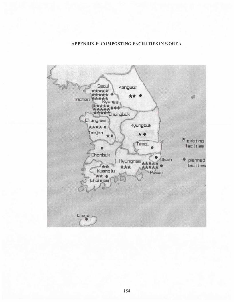
APPENDIX F: COMPOSTING FACILITIES IN KOREA

154

* ~. infat::;ili ie

pl n dfiJdlitl

PukchE!Ju-gun

SClgwipc city

namJE!jU-gUn{1

155

REFERENCES

Bacot, H., T. Bowen, and M.R. Fitzgerald. 1993. "Managing the Solid Waste Crisis:

Exploring the Link Between Citizen Attitudes, Policy Incentives, and Siting

Landfills," Policy Studies Journal. 22(2): 229-244.

Baumol, W. J. 1951. "The Neumarm-Morgenstem Utility Index - an Ordinalist View,"

Journal ofPolitical Economy. LIX (February): 61-66.

Becker, Selwyn W. and Charles G. McClintock. 1967. " Value: Behavioral Decision

Theory," Analytical Review ofPsychology. 18: 239-268.

Blahna, D. J. and S. Yonts. 1990. Preservation or Use? Confronting Public Issues in

Forest PIarming and Decision ~ making. New York: Greenwood Press.

Blocker, T. J. and D. L. Eckberg. 1989. "Environmental Issues as Women's Issues:

General Concerns and Local Hazards," Social Science Quarterly. 70(3): 586­

593.

Bogdonoff, S. 1995. Consensus Building to Write Environmentally Responsive Rules for

Maine's New Transportation Policy. Westport, Cormecticut: Quorum Books.

Brody, J. G. and J. K. Fleishman. 1993. Sources of Public Concern About Nuclear Waste

Disposal in Texas Agricultural Communities. Durham, North Carolina: Duke

University Press.

Brookshire, D.S., M.A. Thayer, J. Tschirhart and W.D. Schulze. 1985. "A Test of the

Expected Utility Model: Its Variants, Purposes, Evidence, and Limitations,"

Journal ofPolitical Economy. 95(21): 369-389.

156

Carless, J. 1992. Taking Ont the Trash: A No - Nonsense Guide to Recycling.

Washington. D.C: Island Press.

Central Daily News [Choong Ang nbo]. March 28, 1996.

Cheju City HaiL 2001. Statistical Report. South Korea, Cheju: Office ofSolid Waste

Cheong, Y. 1995. The analysis of the effects of locally unwanted facilities - a case study

of incineration facility in Yangchon-gu, SeouL Seoul: Sung Kyun Kwan

University Public Administration.

Cho, M. 1998. The Analysis of the Effect of Incineration Facility on the Land Price of

PeIipheral Area. Thesis of Masters Degree. Seoul: Seoul National University.

Davis, C. E. 1986. "Public Involvement in Hazardous Waste Siting Decisions," Policy.

XIX (2): 296-304.

Desvousges, W., H. Kunreuther, P.R. Siovic. and E. A. Rosa. 1993. Perceived Risk and

Attitudes Toward Nuclear Wastes: National and Nevada Perspectives. Duke

University Press: Durham, North Carolina: Duke University Press

Dixon, A J., L. F. Scura., A. R. Carpenter and B. P. Sherman. 1986. Economic Analysis

of Envirolunental Impacts. London: Eastern Publication Ltd.

Douglas, M. V. 1989. External Costs to the Carter Community from Siting a Municipal

Landfill in East Knox County, Tennessee: A Contingent Valuation Analysis. Ph.D.

Dissertation. Knoxville, Tennessee: The University of Tennessee

Dunlap, R. R, R A. Rosa, R. K. Baxter, and R. C. MitchelL 1993. Local Attitudes

Toward Siting a High-Level Nuclear Waste Repository at Hanford, Washington.

Durham, North Carolina: Duke University Press.

157

Edwards, Ward. 1961. "Behavioral Decision Theory," Analytical Review ofPsychology.

12: 473-498.

Environmental Protection Agency (EPA). 1996. Standards of Perfonnance for New

Stationary Sources, and Guidelines for Control of Existing Sources, Municipal

Solid Waste Landfills. Washington, D.C.: Federal Register 61.

Environmental Protection Agency (EPA). 2000. Decision-Makers' Guide to Solid Waste

Management Problems. Washington, D.C.: Office of Solid Waste.

Fiorino, D. J. 1989. " Environmental Risk and Democratic Process: A Critical Review,"

Columbia Journal ofEnvironmental Law. 14: 501- 547.

Friedman, M. and L.J. Savage. 1952. " The Expected Utility Hypothesis and the

Measurement of Utility," The Journal ofPolitical Economy. LX (6): 463-474.

Fullerton, D., T. C. Kinnaman. 1996." Household Response to Pricing Garbage by the

Bag," American Economic Review. 86 (4): 210-285:971-984.

Furuseth, O.J. and M.S. Johnson. 1988. "Neighborhood Attitudes Towards a Sanitary

Landfill: A North Carolina Study," Applied Geography. 8: 135- I45.

GAO. 1996. " Chemical Accident Safety: EPA's responsibilities for preparedness,

response, and prevention. Washington, D.C.: United States General Accounting

Office: 28-31.

Gould, J. P. 1969. "The Expected Utility Hypothesis and the Selection of Optimal

Deductible for a Given Insurance Policy," Journal ofBusiness. 42(2): 143-151.

Halstead, J.M., J. L. Whitcomb., and L.C. Hamilton. 1999. " Economic Insights into the

Siting Problem: An Application of the Expected Utility Model," Agricultural and

Resource Economics Review. April: 65 - 75.

158

Hamilton, L.c. 1985. "Concerns About Toxic Wastes: Three Demographic Predictors,"

Sociological Perspectives. 28(4): 463-486.

Hankyeoreh Sihnmoon [Hankyeoreh Dalily News]. May 20, 2001, Janumy 8, January 15,

May 5, May 9,2002.

Heberlein, T. 1976. " Some observations on Alternative Mechanisms for Public

Involvement: The hearing, Public Opinion Poll, the workshop, and the Quasi­

experiment," Natural Resource Journal. 16(1): 197 - 212.

1m, Y. and Y. Chun.1993. " Benefit estimate of air quality improvement using hedonic

pricing model," Journal ofResource Economics. 3: 81-106

Jenkins, R.R. 1993. The Economics of Solid Waste Reduction. The Impact of User Fees.

Aldershot, Hampshire: Edward Elgar Publishing Limited.

Kachigan, S.K. 1991 Multivariate Statistical Analysis: A Conceptual Introduction. New

York: Radius Press.

Kim, .I., H. Chun, and D. Kang 1994 "A study on the Interest Conflict between Regions

Or Groups and Its Reconciliation in the Construction of the Public Facilities,"

Journal ofLocal Government Studies. 6: 60 - 86.

Kline, E., N. Cirillo, and J. Sugannan. 1993. Promising Techniques: Hazardous Waste

Siting Process. Medford, Massachusetts: Tufts University Center for

Environmental Management.

Kraft, M.E. and B.B. Clary. 1991. " Citizen Participation and the NIMBY Syndrome:

Public Response to Radioactive Waste Disposal," Western Political Quarterly.

44: 299-328.

159

Kunreuther, H., and D. Easterling. 1990. "Are Risk-benefit Tradeoffs Possible in Siting

Hazardous Facilities?" AEA Papers and proceedings. American Economic Review.

80(2): 252-256.

Kunreuther, H., K. Fitzgerald. and T. Aarts. 1993. "Siting Noxious Facilities: A Test of

the Facility Siting Credo," Risk Analysis. 13(3): 301-18.

Kwak, S., and Y. Chun. 1995. Economic Value of Environrnent. Seoul: Hakhyunsa.

Laws, D. and 1. Susskind. 1991. " Changing Perspectives on the Facility Siting Process,"

Maine Policy Review. December: 29-44.

Lee, C. and H. An. 1999. "Political suggestions for recovering NIMBY: focusing on

citing unwanted facilities and residents' opposition," Journal of Korean Policy

Sciences. 3(3): 99,127.

Lindell, M. and T.C. Earle. 1983."How Close is Close Enough: Public Perceptions of the

Risks ofindustrial Facilities," Risk Analysis. 3(4): 245-53.

Lober, D. J. 1993. "Beyond Self-Interest. A Model of Public Attitudes Toward Waste

Facility Siting," Journal of Environmental Planning and Management. 36(3):

345-363.

Lober, D. J. and D. P. Green. 1994. " NIMBY or NIABY: a Logit Model ofOpposition to

Solid -waste - disposal Facility siting," Journal of Environmental Management.

40: 33-50.

Long, J. Scott.l997 Regression Models For Categorical and Limited Dependent

Variables. Thousand Oaks, London: SAGE Publications.

Long, J. and .J. Freese. 2001 Regression Models For Categorical Dependent Variables

Using Stata. College Station, Texas: A Stata Press Publication.

160

Luce, D.R. and P.Supess. 1965. Preference, Utility, and Subjective Probability. In

Handbook of Mathematical Psychology. New York: Wiley and Sons.

Madisso, U. 1985. A Synthesis of Social and Psychological Effects of Exposure to

Hazardous Substances, Burlington, Ontario: Water Planning and Management

Branch.

Malone, C.R., 1991. "High-Level Nuclear Waste Disposal: A Perspective on Technology

and Democracy," Growth and Change.22 (2): 69 -74.

Matheny, A. R. and B. A. Williams. 1985. " Knowledge vs. NIMBY: Assessing Florida's

Strategy for Siting Hazardous Waste Disposal Facilities," Policy Studies Journal.

14 (I): 70-80.

Matheny, A.R., and B.A. Williams. 1988. Rethinking Participation: Assessing Florida's

Strategy for Siting Hazardous Waste Disposal Facilities. Westport, Connecticut:

Greenwood press.

Miller, P. A. and P. A. Golden. 1992. Earth For Sale: Policy Issues in MSW Composting.

New York: New York Legislative Committee.

Ministry of Environment (MOE). 1999. National Waste Generation and Disposal. Seoul.

Ministry of Environment (MOE). 2000 and 2001. Environmental Statistic Year Book.

Seoul.

Moon, J. 1994. Planning Against the Leviathan: State Planning and the Prospects for

Social Movements in South Korea, Focusing on Environmental Movements. Ph.

D. Dissertation. California: University of Southern California.

Morrell, D. and C. Magorian. 1982. Siting Hazardous Waste Facilities. Cambridge,

Massachusetts: Ballinger Press.

161

Mushkatel, A.H., J.M. Nigg and K.D. Pijawaka. 1993. Nevada Urban Residents'

Attitudes Toward a Nuclear Waste Repository. In Public Reactions to Nuclear

Waste. Durham, North Carolina: Duke University Press.

Neuman, J.V. and O. Morgenstern, 1947. Theory of Games and Economic Behavior.

Second edition. Princeton: Princeton University Press.

O'Hare, M., L.Bacow. and D. Sanderson. 1983. Facility Siting and Public Opposition.

New York: Van Nostrand Reinhold.

O'Hare, M. 1977. " Not on My Block You Don't: Facility Siting and the Strategic

Importance of Compensation," Public Policy. 25: 407-458.

OWM (Office of Waste Management). 1994a, 1994b, and 1994c. Cleaning Work '94.

Seoul: Seoul City Government.

Park, C. 1992. "Landfill Sites and a Fair Compensation," Journal of Korean Planners

Association. 28(4): 52 - 77.

Peele, E. and R. Ellis. 1987. "Beyond the 'Not-In-My-Backyard' Impasse," Forum for

Applied Research and Public Policy. Applied Research and Public policy.

September: 68-77.

Piller, C. 1991. The Fall Safe Society: Community Defiance and the End of American

Technological Optimism. Oakland, California: Basic Books.

Popper, F. J. 1981." Siting LULUs," Planning. April: 12 - 15.

Rabe, B.G., 1991 April. " Beyond the NIMBY Syndrome, Hazardous Waste Facility

Siting: The Albertan Breakthrough and Prospects for Cooperation in Canada and

the United States," An International Journal ofPolicy and Administration. April:

184 - 206.

162

Rapoport, Amnon and Thomas S. Wallsten. 1972. "Individual Decision Behavior,"

Analytical Review ofPsychology. 23: 131-175.

Reilly, W. K. 1987. "Lets Circle Table, Not Wagons," Waste Age. September: 35-38.

Rosa, E. A. and W. R. Freudenburg. 1993. The Historical Development of Public

Reactions to Nuclear Power: Implications for Nuclear Waste Policy. In Public

Reactions to Nuclear Waste. Durham, North Carolina: Duke University Press.

Schoemaker,PJ. 1982. "The Expected Utility Model: Its Variants, Purposes, Evidence,

and Limitations," Journal ofEconomic Literature. 20: 529-563.

Sears, D.O., R.R. Lau, T.R. Tyler and H. M. Jr. Allen. 1980. "Self interest versus

symbolic politics in policy attitudes and presidential voting," American Political

Science Review. 74: 670-684.

Seoul Metropolitan Government. 1994. Seoul Statistical Year Book. Seoul.

Slovic, P. 1987. "Perception of risk," Science. 236. 280-285.

Tammemagi, H. 1999 The waste crisis: Landfills, incinerators, and the search for a

sustainable future. Oxford: Oxford University Press.

Wirth, T.E. and J. Heinz. 1991. Project 88-Round II. Incentives for Action: Designing

Market Based Environmental Strategies. Washington. D.C.: U.S. Congress.

Wrigley, K. N. 1998 Conceptualizing" Not In My Backyard" (NIMBY): Structural

Factors Affecting Hazardous Waste Facility Siting. Ph.D. Dissertation. Logan,

Utah: Utah State University.

Yi, K. 1996. A study on the housing market in Seoul and the benefit of air quality

improvement: an application of hedonic price model considering identification.

MA Thesis. Seoul: Seoul National University.

163

Yun, Y. 1997. "The Impacts of Locally Unwanted Facilities on Housing Price; An

Intenupted Time Series Analysis of Sanggye-dong Incinerator," Journal of

Korean Policy Sciences. 6 (I): 52-67.

Zeiss, C. and J. Atwater. 1987. " Waste Facilities in Residential Communities: Impacts

and Acceptance," Journal of Urban Planning and Development. I 13 (I): 19-34.

164