University of Groningen

The Quadratic Matrix Inequality in Singular H∞ Control with State FeedbackStoorvogel, A.A.; Trentelman, H.L.

Published in:SIAM Journal on Control and Optimization

IMPORTANT NOTE: You are advised to consult the publisher's version (publisher's PDF) if you wish to cite fromit. Please check the document version below.

Document VersionPublisher's PDF, also known as Version of record

Publication date:1990

Link to publication in University of Groningen/UMCG research database

Citation for published version (APA):Stoorvogel, A. A., & Trentelman, H. L. (1990). The Quadratic Matrix Inequality in Singular H Control withState Feedback. SIAM Journal on Control and Optimization, 28(5), 1190-1208.

CopyrightOther than for strictly personal use, it is not permitted to download or to forward/distribute the text or part of it without the consent of theauthor(s) and/or copyright holder(s), unless the work is under an open content license (like Creative Commons).

Take-down policyIf you believe that this document breaches copyright please contact us providing details, and we will remove access to the work immediatelyand investigate your claim.

Downloaded from the University of Groningen/UMCG research database (Pure): http://www.rug.nl/research/portal. For technical reasons thenumber of authors shown on this cover page is limited to 10 maximum.

Download date: 08-04-2020

SIAM J. CONTROL AND OPTIMIZATIONVol. 28, No. 5, pp. 1190-1208, September 1990

(C) 1990 Society for Industrial and Applied Mathematics

009

THE QUADRATIC MATRIX INEQUALITY IN SINGULAR Hoo CONTROLWITH STATE FEEDBACK*

A. A. STOORVOGEL" AND H. L. TRENTELMANt

Abstract. In this paper the standard Ho control problem using state feedback is considered. Given alinear, time-invariant, finite-dimensional system, this problem consists of finding a static state feedback suchthat the resulting closed-loop transfer matrix has H norm smaller than some a priori given upper bound.In addition it is required that the closed-loop system is internally stable. Conditions for the existence of asuitable state feedback are formulated in terms of a quadratic matrix inequality, reminiscent of the dissipationinequality of singular linear quadratic optimal control. Where the direct feedthrough matrix of the controlinput is injective, the results presented here specialize to known results in terms of solvability of a certainindefinite algebraic Riccati equation.

Key words. H control, state feedback, quadratic matrix inequality, strong controllability, almostdisturbance decoupling

AMS(MOS) subject classifications. 93C05, 93C35, 93C45, 93C60, 93B27, 49B99

1. Introduction. In a series of recent papers [1], [2], [5], [8], [10], [15], [18], [23]the by now well-known H optimal control problem was studied in a perspective ofclassical linear quadratic optimal control theory. In these papers it is shown that theexistence of feedback controllers that result in a closed-loop transfer matrix with Hnorm less than a given upper bound is equivalent to the existence of solutions ofcertain algebraic Riccati equations. Typically, these algebraic Riccati equations are ofthe type we encounter in the context of linear quadratic differential games.

The first contributions to this new approach in H optimal control theory werereported in [8], [10], and [23]. These papers deal with the special case where thecontrollers to be designed are restricted to being state feedback control laws. In latercontributions [2], [5], [18] these results were extended to the more general case ofdynamic measurement feedback.

If we take a close look at the type of conditions for the existence of suitablecontrollers that are derived in the above references, we see there is a fundamentaldistinction between two cases. This distinction is tied up with the question of whetheror not the direct feedthrough matrix of the control input is injective. In 10] and [23],no assumptions are imposed on the direct feedthrough matrix. The conditions for theexistence of a suitable state feedback control law are formulated in terms of a familyof algebraic Riccati equations, parameterized by a positive real parameter e. It is shownthat there exists an internally stabilizing state feedback control law such that theclosed-loop transfer matrix has H norm less than an a priori given upper bound ifand only if there exists a parameter value e for which the corresponding Riccatiequation has a certain solution. In our opinion, a more satisfactory type of conditionis obtained in [2], [5], and 18]. In these papers it is assumed that the direct feedthroughmatrix of the control input is injective. It is then shown that a suitable state feedbackcontrol law exists if and only if one particular algebraic Riccati equation has a solutionwith certain properties.

The purpose of the present paper is to reexamine the H problem with statefeedback as studied in [2] and [18], without making the assumption that the above-mentioned direct feedthrough matrix is injective. Our aim is to find conditions for the

* Received by the editors March 6, 1989; accepted for publication (in revised form) November 7, 1989.f Department of Mathematics and Computing Science, Eindhoven University of Technology, P.O. Box

513, 5600 MB Eindhoven, the Netherlands.

1190

SINGULAR H CONTROL 1191

existence of suitable state feedback control laws that are of a different type from theone derived in [8], [10], and [23]. Instead our conditions will be of the type proposedin [2] and [18]. Stated differently: we will show how it is possible "to get rid of theparameter e" in the conditions for the existence of suitable state feedback controllaws. Rather than in terms of a particular algebraic Riccati equation, our conditionswill be in terms of a certain "quadratic matrix inequality," reminiscent ofthe dissipationinequality appearing in singular linear quadratic optimal control [4], [13], [19]. It willturn out that the results from [2] and 18] on the special case that the direct feedthroughmatrix is injective can be re-obtained from our results.

The outline of this paper is as follows. In 2 we introduce the problem to bestudied and give a statement of our main result. In 3 we recall some important notionsthat will be used in this paper. In 4 we give a description of a decomposition of theinput space, the state space and the output space. This decomposition will be instru-mental in the proof of our main result. Sections 5 and 6 are devoted to a proof of ourmain result. Finally, the paper closes with a brief discussion on our results in 7.

2. Problem formulation and main results. We consider the finite-dimensional,linear, time-invariant system

(2.1) Ax + Bu + Ew, z Cx + Du,

where x E" is the state, u E is the control input, w E is an unknown disturbance,and z EP is the output to be controlled. A, B, C, D, and E are real matrices ofappropriate dimensions. In this paper we are primarily interested in state feedback. IfF is a real m x n matrix, then the closed-loop transfer matrix resulting from the statefeedback control law u Fx is equal to

OF(S) C + DF)(Is- A- BF)-IE.

The influence of the disturbance w on the output z is measured by the H norm ofthis transfer matrix:

Oll:- sup p[GF(kO)].

Here, p[M] denotes the largest singular value of the complex matrix M. The problemthat we will study in this paper is the following" given a positive real number 7, findF " such that

Gv [] < y and o-(A + BF) C-.

Here, r(M) denotes the set of eigenvalues of the matrix M and

C-:= {s C[Re s <0}.

A central role in our study of the above problem is played by what we will callthe quadratic matrix inequality. For any real number y > 0 and matrix P E"" wedefine a matrix F(P) e E("+"("+" by

(2.2) Fv(P):=(PA+ATP+y-2PEETP+CTC PB+CTD]BTp+DTC DTD ]"

Clearly, if P is symmetric, then F(P) is symmetric as well. If F(P)>-O, then we willsay that P is a solution to the quadratic matrix inequality at 3’.

In addition to (2.2), for any 3’ > 0 and P eN we define a n x (n + m) polynomialmatrix L(P, s) by

(2.3) Lv(P, s):= (sI, A- y-EETp -B).

1192 A. A. STOORVOGEL AND H. L. TRENTELMAN

We note that Lv(P, s) is the controllability pencil associated with the system

2=(A+),-2EETp)x+Bu.

The transfer matrix of the system E given by the equations

(2.4) Ax + Bu, y Cx + Du

is equal to the real rational pm matrix G(s)= C(Is-A)-IB+D. The normal rankof a real rational matrix is defined as its rank as a matrix with entries in the field ofreal rational functions, The normal rank of the transfer matrix G is denoted bynormrank G.

In the formulation of our main result we need the concept of invariant zero ofthe system E (A, B, C, D). For this definition we refer to 3 (see also [11]). Finally,let CO := {s C iRe s 0} and let C+ := {s C IRe s > 0}. The following is the main resultof this paper.

TrtEOgEM 2.1. Consider the system (2.1). Assume that (A, B, C, D) has no invariantzeros in C. Let , > O. Then the following two statements are equivalent:

(i) There exists FRmn such that iIGll< , and o-(A+ BF)c C-.(ii) There exists a real symmetric solution P >= 0 to the quadratic matrix inequality

at / such that

rank F(P) normrank G

and

(2.6) rank(L(P’s))F(P)n +normrank Gfor all sCUC+.

In other words, the existence of a suitable state feedback control law is equivalentto the existence of a particular positive semidefinite solution of the quadratic matrixinequality at ,. This solution should be such that two rank conditions are satisfied.

Before embarking on a proof of this theorem we would like to point out how theresults from [2] and [18] for the special case that D is injective can be obtained fromour theorem as a special case. First note that in this case we have

normrank G m.

Define

R,(P) := PA+ ATp + "),-2pEE Tp + CCT (PB + CTD)(DTD)-I(BTp+ DTC).

Furthermore, define a real (n + m) (n + m) matrix by

S(P) := ( I0 -(PB + CTD)(DTD)-1)I.,

Then clearly we have

S(P)F,(P)S(P) T/|Rv(P)

0\

SINGULAR H(R) CONTROL 1193

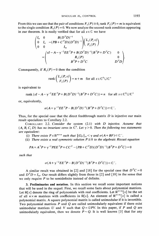
From this we can see that the pair of conditions F(P) >- 0, rank Fv(P) rn is equivalentto the single condition R(P) 0. We now analyze the second rank condition appearingin our theorem, it is easily verified that for all s C we have

I. -(PB + CTD)(DTD)-’ Lv(

0 Im J Fv(P) /

sI-A-T-2EETp+ B(DTD)-(BTp+ DTc)R(P)

BrP+DrC

Consequently, if R(P)=0 then the condition

rank (L(P, s)F(P) ]=n+m for allsCLJC+

is equivalent to

rank(sI-A-y-2EETp+B(DTD)-I(BTp+DTC))=n for all sCLJC+

or, equivalently,

cr(A + y-2EE Tp_ B(DTD)-I(BTp + DTc)) C-.

Thus, for the special case that the direct feedthrough matrix D is injective our mainresult specializes to Corollary 2.2.

COROLLARY 2.2. Consider the system (2.1) with D injective. Assume that(A, B, C, D) has no invariant zeros in C. Let y > O. Then the following two statements

are equivalent:(i) There exists F6 such that ]]GFI]o< )’ and o’(A+BF)cC-.(ii) There exists a real symmetric solution P >-0 to the algebraic Riccati equation

PA + ATp + y-2pEE Tp + CC T (PB + CTD)(DTD)-I(BTp + DTc) 0

such that

cr(A + T-2EETp B(DTD)-’(BTp + DTc)) C-.

A similar result was obtained in [2] and [18] for the special case that DTc =0

and DTD Ira. Our result differs slightly from those in [2] and [18] in the sense thatwe only require P to be semidefinite instead of definite.

3. Preliminaries and notation. In this section we recall some important notionsthat will be used in the sequel. First, we recall some facts about polynomial matrices.Let [s] denote the ring of polynomials with real coefficients. Let "’[s] be the setof all n x rn matrices with coefficients in [s]. An element of ""[s] is called a

polynomial matrix. A square polynomial matrix is called unimodular if it is invertible.Two polynomial matrices P and Q are called unimodularly equivalent if there existunimodular matrices U and V such that Q UPV. In this paper, if P and Q are

unimodularly equivalent, then we denote P---Q. It is well known [3] that for any

1194 A.A. STOORVOGEL AND H. L. TRENTELMAN

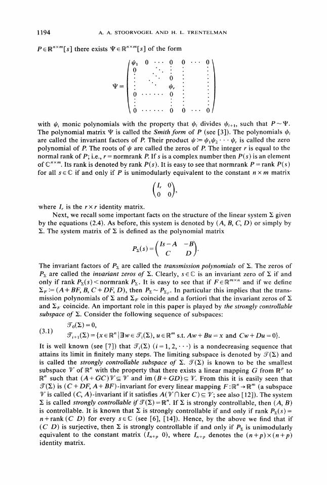
P "’[s] there exists Enxm[s] of the form

0....0 o... o

= q.0

6 60...0with ’i monic polynomials with the property that q,i divides q,+, such that P-q.

The polynomial matrix is called the Smith form of P (see [3]). The polynomials @are called the invariant factors of P. Their product , := ’1’2" ’r is called the zeropolynomial of P. The roots of @ are called the zeros of P. The integer r is equal to thenormal rank of P; i.e., r normrank P. If s is a complex number then P(s) is an elementof CEm. Its rank is denoted by rank P(s). It is easy to see that normrank P rank P(s)for all s C if and only if P is unimodularly equivalent to the constant n x m matrix

where L is the r x r identity matrix.Next, we recall some impoant facts on the structure of the linear system given

by the equations (2.4). As before, this system is denoted by (A, B, C, D) or simply byN. The system matrix of is defined as the polynomial matrix

P(s)=(Is-AC -2)"The invariant factors of P are called the transmission polynomials of . The zeros ofPx are called the invariant zeros of E. Clearly, s C is an invariant zero of if andonly if rank Px(s)< normrank Px. It is easy to see that if F" and if we defineEv := (A + BF, B, C + DF, D), then PxPx.. In paicular this implies that the trans-mission polynomials of E and Ev coincide and a fortiori that the invariant zeros of Eand Ev coincide. An impoant role in this paper is played by the strongly controllablesubspace of E. Consider the following sequence of subspaces:

o() =0,(3.1) W+(E)={x"[3wW(E),u s.t. Aw+Bu=x and Cw+Du=O}.It is well known (see [7]) that W(Z) (i 1, 2,-..) is a nondecreasing sequence thatattains its limit in finitely many steps. The limiting subspace is denoted by W(E) andis called the strongly controllable subspace of . W(E) is known to be the smallestsubspace of " with the propey that there exists a linear mapping G from P to

" such that (A+GC) and im(B+GD) . From this it is easily seen thatW(E) is (C + DF, A + BF)-invariant for every linear mapping F:" (a subspace

is called (C, A)-invariant if it satisfies A( ker C) ; see also 12]). The systemis called strongly controllable if W(Z)=". If Z is strongly controllable, then (A, B)

is controllable. It is known that is strongly controllable if and only if rank Px(s)n+rank(C D) for every sC (see [6], [14]). Hence, by the above we find that if(C D) is surjective, then E is strongly controllable if and only if P is unimodularlyequivalent to the constant matrix (I,+p 0), where I,+p denotes the (n +p) x (n +p)identity matrix.

SINGULAR H(R) CONTROL 1195

We conclude this section by introducing some notation. We will denote N+ := [0,2(+) denotes the space of real-valued measurable functions from N+ to such that

I+ Ilxll dt <00. For a given positive integer r we denote by ;(+) the space ofr-vectors with components in 2(N+). The notation is used for the Euclidean normon Nr; 112 denotes the usual norm on w;(N+); i.e., Ilx[12 := (In+ Ilxll 2 dt) 1/2.

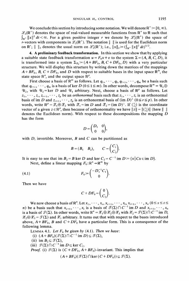
4. A preliminary feedback transformation. In this section we show that by applyinga suitable state feedback transformation u Fox + v to the system E (A, B, C, D), itis transformed into a system EVo := (A + BFo, B, C + DFo, D) with a very particularstructure. We will display this structure by writing down the matrices of the mappingsA + BFo, B, C + DFo, and D with respect to suitable bases in the input space N", thestate space ", and the output space Np.

First choose a basis of N as follows. Let q,. ., ql, ql+," ", q,, be a basis suchthat q+l, ", qm is a basis ofker D (0=< 1 -<_ m). In other words, decompose N9/2, with 2=ker D and 0- arbitrary. Next, choose a basis of Np as follows. Letz, , zr, Zr+," ", Zp be an orthonormal basis such that z,. , zr is an orthonormalbasis ofim D and Zr+,’’’, Zp is an orthonormal basis of (ira D) +/- (0-< r<-p). In otherwords, write NP LrLr2 with Lr=im D and Lr2= (im D)+/-. If (Zz) is the coordinatevector of a given z [P, then because of orthonormality we have IIz[I z2)l[ (heredenotes the Euclidean norm). With respect to these decompositions the mapping Dhas the form

0

with D invertible. Moreover, B and C can be partitioned as

B=(B, B2) C=(C)C2It is easy to see that im B2 B ker D and ker C2 C- im D := {x Cx im D}.

Next, define a linear mapping Fo" N" Nm by

(-D-(a Ca)(4.1) Fo :=0

Then we have

(0)C+DFo=C2

We now choose a basis of ". LetXl,’’’,Xs, Xs+l,’’’,xt, xt+l,’’’,xn (0 <= s <= <--

n) be a basis such that Xs+,’",xt is a basis of -(;)(’1C- im D and xs+,’", x,is a basis of -(E). In other words, write " @2@3 with 2 -(E) f-I C- im D,f2@3 T(;) and arbitrary. It turns out that with respect to the bases introducedabove, A + BFo, B and C + DFo have a particular form. This is a consequence of thefollowing lemma.

LEMMA 4.1. Let Fo be given by (4.1). Then we have:(i) (A + BFo)((E) f3 C- im D) 8-(;),(ii) im B2 c__ 8-(Y),(iii) -(E) (’1C-’ im D c_ ker Cz.Proof (i) 8(E) is (C + DFo, A + BFo)-invariant. This implies that

(A + BFo)( -(E) 71 ker C + DFo))_-(E).

1196 A.A. STOORVOGEL AND H. L. TRENTELMAN

Since ker (C + DFo) ker C2 C -1 im D, the result follows.(ii) Let -i(E) be the sequence defined by (3.1). Then l(E)= B ker D=im B2.

Since ffi(E) is nondecreasing this proves our claim.(iii) This follows immediately from the fact that C-1 im D ker C2.By applying this lemma we find that the matrices of A+ BFo, B, C + DFo, and D

with respect to the given bases have the following form"

{a o A13t {BllA+BFo=IA21 A22 Aa3

\A31 A32 A33 \B31(4.2)

C21 0 C23 0

B22B32/

:).If we apply the feedback transformation u Fox + v to the system E (A, B, C, D),then the resulting system EFo is given by

(4.3) : (A + BFo)x + Bv, z (C + DFo)x + Dr.

With respect to the given decomposition, let () be the coordinate vector of a givenvem. Likewise, we use the notation (x(, xr, x)T and thel). Then equations ofthe system EFo can be arranged in such a way that they have the following form:

(4.4) 2=AllX+(Bll A3) (tl),X3

(2) (A22 A23\l(x:z)+(B:zz] (B21A21](v1)(4.5)3 -’-\A32 A33] x3 B32//v2-{ B31 A3] Xl’

(4.6) (Zl) (0) (D1 0)(Vl)Z2 C21 0 C23 x

As already suggested by the way that we have arranged these equations, the systemEFo can be considered as the interconnection of two subsystems. This is depicted asfollows:

Here,

(4.7) X:= A,a, (Bll A13),C21 0 C23

is the system given by (4.4) and (4.6). It has input space 1 ;T3, state space 1, andoutput space P. Zo is the system given by (4.5). It has input space r,T and statespace @3. The interconnection is made via xl and x3, as depicted above. Notethat and XFo have the same output equation. However, in ZFo the variable x3 is

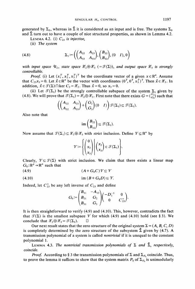
SINGULAR H CONTROL 1197

generated by Eo, whereas in : it is considered as an input and is flee. The systems Eoand turn out to have a couple of nice structural properties, as shown in Lemma 4.2.

LEMMA 4.2. (i) C23 is injective,(ii) The system

((A22 A23] (B2] (0 ’),0)(4.8) E;1 :=\A32 A33], B32],

with input space all:, state space @3 (=if(E;)), and output space g3 is stronglycontrollable.

Proof (i) Let (Xlr, xf, x3r) r be the coordinate vector of a given x R". Assumethat C23x3 0. Let E" be the vector with coordinates (O r, O r, x3r) r. Then Y 3. Inaddition, -(E;) f-I ker C2 2. Thus Y 0, so x3 0.

(ii) Let -(E1) be the strongly controllable subspace of the system E; given byG(4.8). We will prove that -(E) 3. First note that there exists G (3) such that

[Aaa A:3+ (0 I)\A3: A33] G3

Also note that

c -(1).imB32/_

Now assume that -(E1)C___ 2(3 with strict inclusion. Define W_R" by

it0tX2

X3

Clearly,

___-(E) with strict inclusion. We claim that there exists a linear map

Go:p ...> n such that

(4.9) (A + GoC)_

(4.10) im (B + GoD)

Indeed, let C+23 be any left inverse of C23 and define

-A13\Go := /B G 0

\B31 63 /]o)

It is then straightforward to verify (4.9) and (4.10). This, however, contradicts the factthat -(E) is the smallest subspace 7/" for which (4.9) and (4.10) hold (see 3). Weconclude that @3 (E1). ["]

Our next result states that the zero structure of the original system E; (A, B, C, D)is completely determined by the zero structure of the subsystem ; given by (4.7). Atransmission polynomial of a system is called nontrivial if it is unequal to the constantpolynomial 1.

LEMMA 4.3. The nontrivial transmission polynomials of , and , respectively,coincide.

Proof According to 3 the transmission polynomials of E; and EFo coincide. Thus,to prove the lemma it suffices to show that the system matrix Po of EF is unimodularly

1198 A.A. STOORVOGEL AND H. L. TRENTELMAN

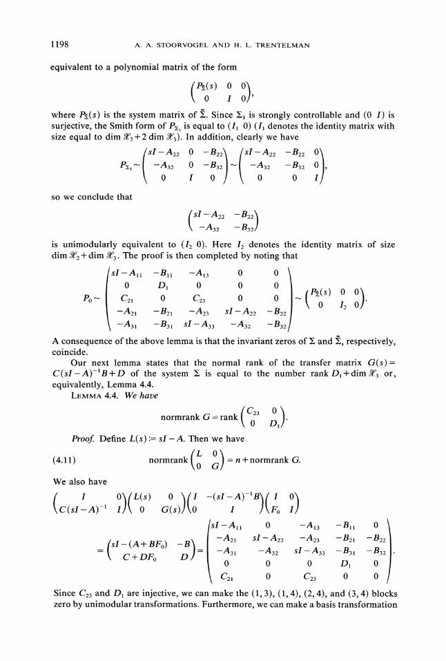
equivalent to a polynomial matrix of the form

where P(s) is the system matrix of . Since E1 is strongly controllable and (0 I) issurjective, the Smith form of Px, is equal to (11 0) (I1 denotes the identity matrix withsize equal to dim 2+ 2 dim 3). In addition, clearly we have

P.t -A32 0

0 / 32 0A32 -B32

0

so we conclude that

sI A2_ B)_2-A3:z

is unimodularly equivalent to (I2 0). Here I2 denotes the identity matrix of sizedim 2+ dim 3. The proof is then completed by noting that

SI-oAll-Bll -A13 0 0

D1 0 0 0

P0" / C21 0 C23 0 0 (P S 120 0 )-A21 -B21 -A23 sI-A22 -B22

\ -A31 -B31 sI A33 -A32 -B32A consequence of the above lemma is that the invariant zeros of E and E, respectively,coincide.

Our next lemma states that the normal rank of the transfer matrix G(s)=C(sI-A)-IB+D of the system is equal to the number rank Dl/dim3 or,equivalently, Lemma 4.4.

LEMMA 4.4. We have

normrank G rank (C23 0).0 D1Proof. Define L(s):= sI-A. Then we have

(4.11) nrmrank( L0 )=n+normrankG.We also have

I G0(s)) (0(C(sl-a)-’ OI)(L(So I -(sI-a)-B) I(FosI All 0 -A13 -nil 0

B22_(sI-(A+BFo) -BD) //-!21 sI A22 -A23 -B21

C + DFo 31 -A32 sI- A33 -B31 -B3:0 0 D, 00 /\ C21 0 C23 0

Since C23 and D1 are injective, we can make the (1, 3), (1, 4), (2, 4), and (3, 4) blockszero by unimodular transformations. Furthermore, we can make a basis transformation

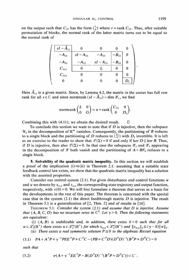
SINGULAR Hoo CONTROL 1199

on the output such that C23 has the form () where r=rank C23 Thus, after suitablepermutation of blocks, the normal rank of the latter matrix turns out to be equal tothe normal rank of

-A21

-A31C211C2120

0 0 0

-A32 s../...A..3.3......B.3.2.0 Ir 0

0 0 0

0 0 0

0

Here All is a given matrix Since, by Lemma 4.2, the matrix in the center has full rowrank for all s e C and since normrank (s!-/11) dim 1, we find

0 Gn + rank

Combining this with (4.11), we obtain the desired result. UTo conclude this section we want to note that if D is injective, then the subspace

2 in the decomposition of Em vanishes. Consequently, the partitioning of B reducesto a single block and the partitioning of D reduces to (,) with D1 invertible. It is leftas an exercise to the reader to show that if(E)= 0 if and only if ker D c__ ker B. Thus,if D is injective, then also -(E)= 0. In that case the subspaces f2 and 3 appearingin the decomposition of T both vanish and the partitioning of A+ BFo reduces to a

single block.

5. Solvability of the quadratic matrix inequality. In this section we will establisha proof of the implication (i)=:>(ii) in Theorem 2.1: assuming that a suitable statefeedback control law exists, we show that the quadratic matrix inequality has a solutionwith the asserted properties.

Consider our control system (2.1). For given disturbance and control functions wand u we denote by Xw, and Zw, the corresponding state trajectory and output function,respectively, with x(0)= 0. We will first formulate a theorem that serves as a basis forthe developments in the rest of this paper. The theorem is concerned with the specialcase that in the system (2.1) the direct feedthrough matrix D is injective. The resultin Theorem 5.1 is a generalization of [2, Thm. 2] and of results in [18].

THEOREM 5.1. Consider the system (2.1) and assume that D is injective. Assumethat (A, B, C, D) has no invariant zeros in C. Let y > O. Then the following statementsare equivalent:

(i) (A, B) is stabilizable and, in addition, there exists 6>0 such that for allw (+) there exists u ’(+) for which Xw,, (R+) and Ilzw,.ll=_-< )llwll=.

(ii) There exists a real symmetric solution P >-0 to the algebraic Riccati equation

(5.1) PA + AT"P + y-2pEET"P + CT"C -(PB + CrD)(DT"D)-I(B’P + DT"C) O

such that

o’(A + y-2EE Tp_ B(DTD)-,(BTp + DTc)) C-

1200 A. A. STOORVOGEL AND H. L. TRENTELMAN

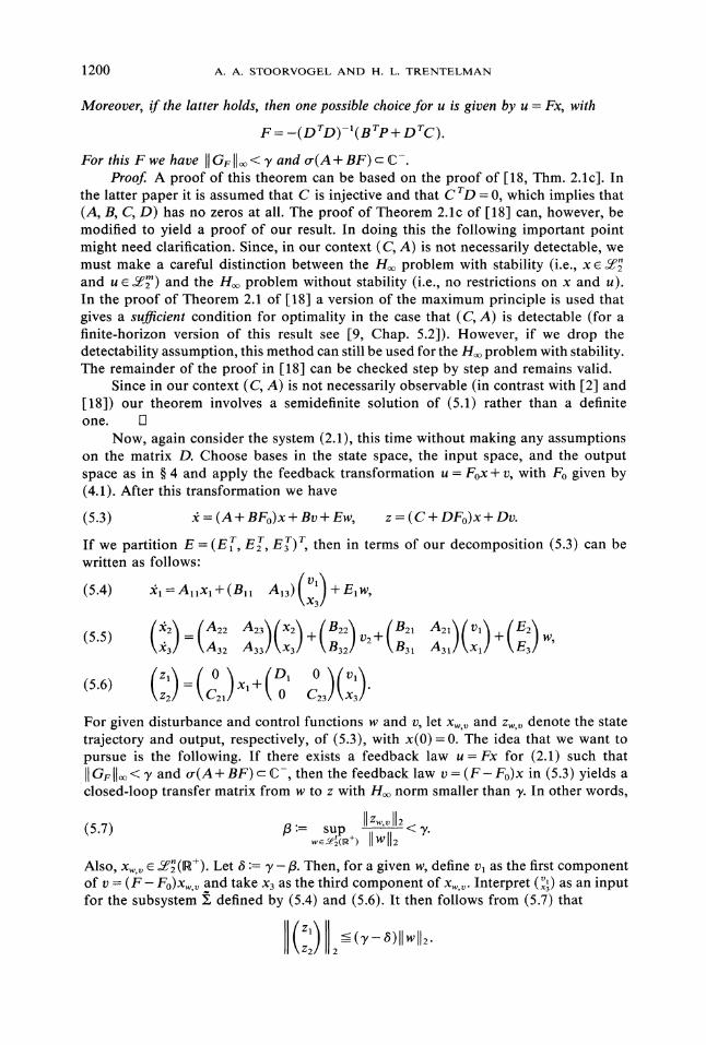
Moreover, if the latter holds, then one possible choice for u is given by u Fx, with

F= -(DT"D)-I(BrP + DrC).For this F we have Iloo < and r(A+ BF)c C-.

Proof. A proof of this theorem can be based on the proof of [18, Thm. 2.1c]. Inthe latter paper it is assumed that C is injective and that C rD 0, which implies that(A, B, C, D) has no zeros at all. The proof of Theorem 2.1c of [18] can, however, bemodified to yield a proof of our result. In doing this the following important pointmight need clarification. Since, in our context (C, A) is not necessarily detectable, wemust make a careful distinction between theand u ’) and the H problem without stability (i.e., no restrictions on x and u).In the proof of Theorem 2.1 of [18] a version of the maximum principle is used thatgives a sufficient condition for optimality in the case that (C, A) is detectable (for afinite-horizon version of this result see [9, Chap. 5.2]). However, if we drop thedetectability assumption, this method can still be used for the Hoo problem with stability.The remainder of the proof in [18] can be checked step by step and remains valid.

Since in our context (C, A) is not necessarily observable (in contrast with [2] and[18]) our theorem involves a semidefinite solution of (5.1) rather than a definiteone.

Now, again consider the system (2.1), this time without making any assumptionson the matrix D. Choose bases in the state space, the input space, and the outputspace as in 4 and apply the feedback transformation u Fox + v, with Fo given by(4.1). After this transformation we have

(5.3) 2 (A + BFo)x + Bv + Ew, z (C + DFo)x + Dv.

If we partition E (Er, E, E)r, then in terms of our decomposition (5.3) can bewritten as follows:

(5.4) 21=allX1+(B11 al3)(Vl] +ElW,\IX3

(:2) (A29-A:z3)(x2)(B22 (B21 A21)(Vl)+ V2 + + w,(5,5)23 \A32 A33] X3 B32,] B31 A31] Xl E3

Xl -lt-Z2 C21 0 C23 x

For given disturbance and control functions w and v, let Xw. and Zw. denote the statetrajectory and output, respectively, of (5.3), with x(0)=0. The idea that we want topursue is the following. If there exists a feedback law u Fx for (2.1) such thatIlG ll < and r(A+BF)cC-, then the feedback law v=(F-Fo)x in (5.3) yields aclosed-loop transfer matrix from w to z with Hoo norm smaller than 3’. In other words,

(5.7) /3 := sup < y.w’+) Ilwll2

Also, Xw,, (R+). Let 6 := 3’-/3. Then, for a given w, define vl as the first componentof v (F- Fo)xw. and take x3 as the third component of Xw,. Interpret () as an inputfor the subsystem defined by (5.4) and (5.6). It then follows from (5.7) that

(-)llwl12.2

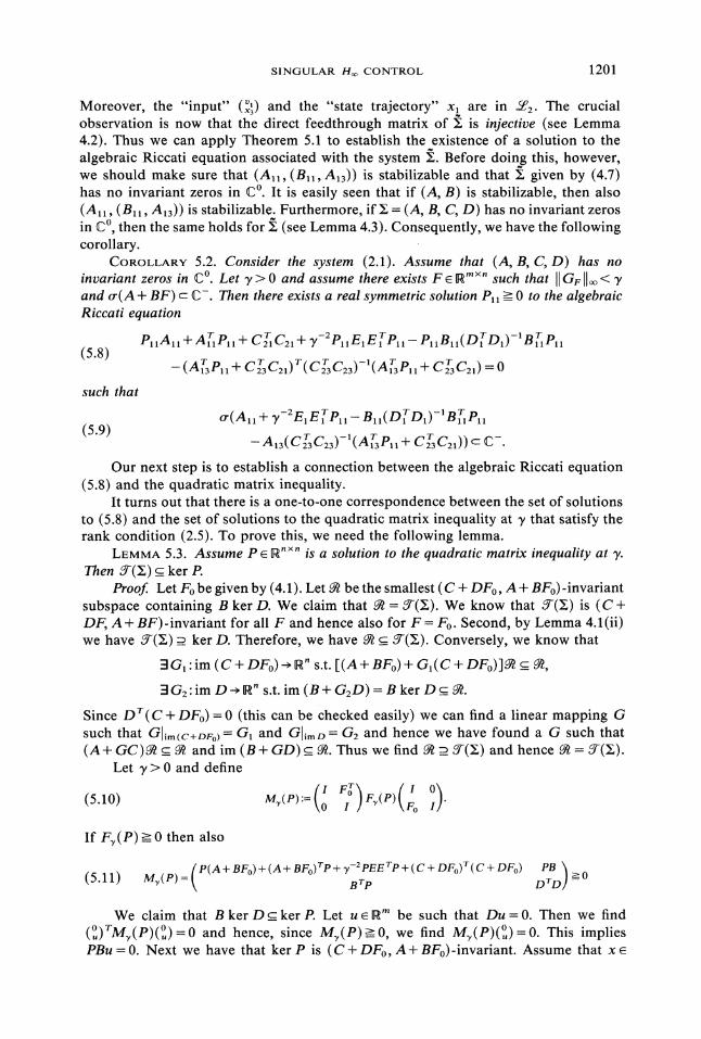
SINGULAR /-/ CONTROL 1201

Moreover, the "input" () and the "state trajectory" Xl. are in 2. The crucialobservation is now that the direct feedthrough matrix of E is injective (see Lemma4.2). Thus we can apply Theorem 5.1 to establish the existence of a solution to thealgebraic Riccati equation associated with the system E. Before doing this, however,we should make sure that (All, (Bll, A13)) is stabilizable and that ; given by (4.7)has no invariant zeros in C. It is easily seen that if (A, B) is stabilizable, then also(AI, (Bll, A3)) is stabilizable. Furthermore, ire (A, B, C, D) has no invariant zerosin C, then the same holds for (see Lemma 4.3). Consequently, we have the followingcorollary.

COROLLARY 5.2. Consider the system (2.1). Assume that (A, B, C, D) has noinvariant zeros in C. Let / > 0 and assume there exists F Rmn such that GFI] < 7and tr(A + BF) c C- Then there exists a real symmetric solution Pll ->-- 0 to the algebraicRiccati equation

(5.8)P,,All + AP,I +CC21 + T-2pllE1ET1P,1- PllBll(DD1)-IBP,1

(A3P, + c2Tc=,) T(C3C23)-l(Ap, + CC2,) 0

such that

(5.9)r(A,, + 7-E,ET p,,- B,,(DD,)-’BP,,

-A,3(cT3c3)-’(API, + C3C,)) C-

Our next step is to establish a connection between the algebraic Riccati equation(5.8) and the quadratic matrix inequality.

It turns out that there is a one-to-one correspondence between the set of solutionsto (5.8) and the set of solutions to the quadratic matrix inequality at y that satisfy therank condition (2.5). To prove this, we need the following lemma.

LEMMA 5.3. Assume P R is a solution to the quadratic matrix inequality atThen if(E) __. ker P.

Proofi Let Fo be given by (4.1). Let be the smallest (C + DFo, A + BFo)-invariantsubspace containing B ker D. We claim that (E). We know that 5r(E) is (C +DF, A / BF)-invariant for all F and hence also for F Fo. Second, by Lemma 4.1(ii)we have ’(E)_ ker D. Therefore, we have

_f(). Conversely, we know that

3G, im (C + DFo)R" s.t. [(A+ BFo)+ GI(C / DFo)]_ ,

3G2 im D --> " s.t. im (B + G2D) B ker D__ .

Since Dr(C + DFo)= 0 (this can be checked easily) we can find a linear mapping Gsuch that Glim(C+DFo)= G1 and G]imD G2 and hence we have found a G such that(A+GC) and im (B+GD) . Thus we find

_ff-(Z) and hence if(Z).

Let 3’ > 0 and define

If Fr(P) _>- 0 then also

(5.11) Mv(p)=(p(A+ BFo)+(A+ BFo)7rp+ y-ZPEETp+(C + DFo)T(C + DTDPB )>-0_We claim that B kerD ker P. Let u rn be such that Du =0. Then we find

()7Mr(P)(,)=0 and hence, since Mv(P)>=O, we find Mr(P)(,)=0. This impliesPBu =0. Next we have that ker P is (C + DFo, A+ BFo)-invariant. Assume that x

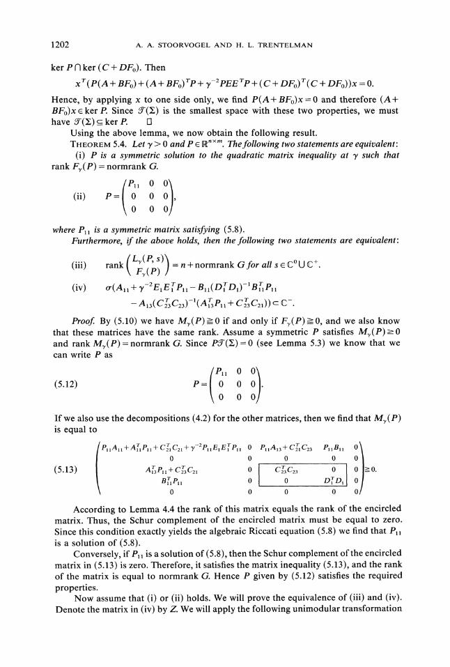
1202 A.A. STOORVOGEL AND H. L. TRENTELMAN

ker P f-) ker C + DFo). Then

xT(p(A + BFo)+ (A + BFo)Tp + y--PEE Tp +(C + DFo)T(C + DFo))X O.

Hence, by applying x to one side only, we find P(A+ BFo)x =0 and therefore (A+BFo)x ker P. Since ff() is the smallest space with these two properties, we musthave ()_ ker P. 1-1

Using the above lemma, we now obtain the following result.THEOREM 5.4. Let ), > 0 and P n,,. Thefollowing two statements are equivalent:

(i) P is a symmetric solution to the quadratic matrix inequality at y such thatrank Fr(P) normrank G.

(ii) P 0

0

where Pl is a symmetric matrix satisfying (5.8).Furthermore, if the above holds, then the following two statements are equivalent:

(iii) rankF(P)

n+normrank Gfor all seCuc/.

-A13(C T23 C23) -1(APll + C3C9_1))c C-.

Proof By (5.10) we have M(P)>=O if and only if F(P)->0, and we also knowthat these matrices have the same rank., Assume a symmetric P satisfies Mr(P)>_Oand rank Mr(P) =normrank G. Since Pff(E) =0 (see Lemma 5.3) we know that wecan write P as

(5.12) P= 0 00 0

If we also use the decompositions (4.2) for the other matrices, then we find that Mr(P)is equal to

(5.13)

T T --2 EET1P 0PllAll + AllPll + C2C21+’Y P0 0

T T 0AP+CC13 11 23 21

BP 0

0 0

PllA13+CflC23 PB0 0

cc o0 DTD0 0

According to Lemma 4.4 the rank of this matrix equals the rank of the encircledmatrix. Thus, the Schur complement of the encircled matrix must be equal to zero.Since this condition exactly yields the algebraic Riccati equation (5.8) we find that Pllis a solution of (5.8).

Conversely, if Pll is a solution of (5.8), then the Schur complement ofthe encircledmatrix in (5.13) is zero. Therefore, it satisfies the matrix inequality (5.13), and the rankof the matrix is equal to normrank G. Hence P given by (5.12) satisfies the requiredproperties.

Now assume that (i) or (ii) holds. We will prove the equivalence of (iii) and (iv).Denote the matrix in (iv) by Z. We will apply the following unimodular transformation

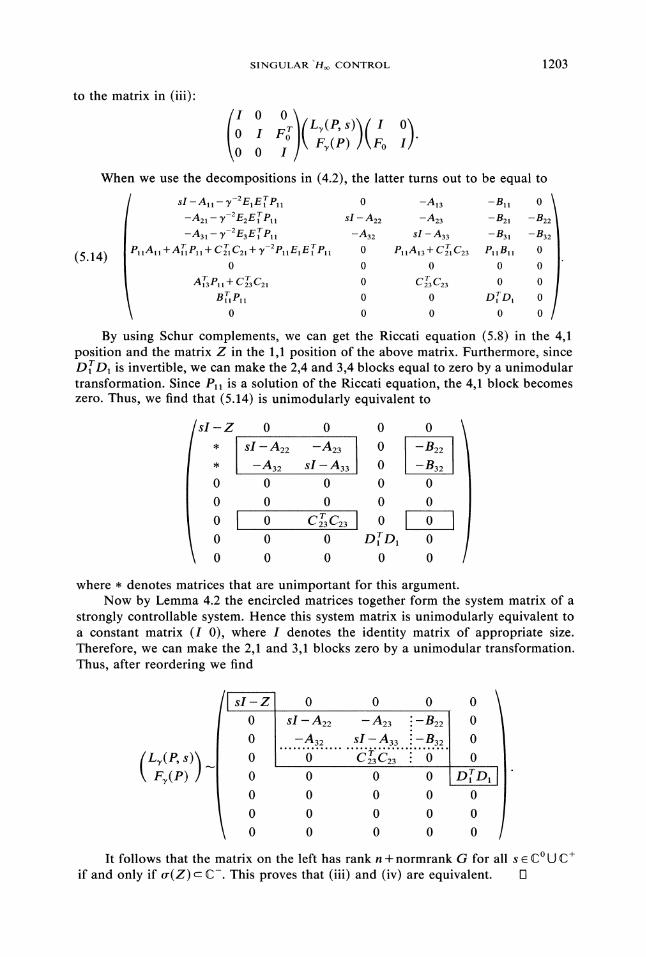
SINGULAR "H, CONTROL 1203

to the matrix in (iii)"

When we use the decompositions in (4.2), the latter turns out to be equal to

(5.14)

sI A y-EE(PI 0 -A13 -B 0

-A21 /-2E2ETPll sI A22 -A23 -B21 -B22-A31 "y-EE3EPll -A32 sI A33 -B31 -B32

PllAII+ATllPll+CflCEI+y-2pllE1EPI1 0 PI1AI3+CflC23 PllBll 0

0 0 0 0 0

AaP + c2T3c21 0 Cf3C23 0 0

B "(P 0 0 D D 0

0 0 0 0 0

By using Schur complements, we can get the Riccati equation (5.8) in the 4,1position and the matrix Z in the 1,1 position of the above matrix. Furthermore, since

DrlD1 is invertible, we can make the 2,4 and 3,4 blocks equal to zero by a unimodulartransformation. Since Pll is a solution of the Riccati equation, the 4,1 block becomeszero. Thus, we find that (5.14) is unimodularly equivalent to

sI-Z,,0

0

0

0

0

0 0

sI-A22 -A23-A32 si-A330 0

0 0

Cf3C230 0

0 0

10 1,-B32,0 0

0 0

DD, 0

0 0

where denotes matrices that are unimportant for this argument.Now by Lemma 4.2 the encircled matrices together form the system matrix of a

strongly controllable system. Hence this system matrix is unimodularly equivalent toa constant matrix (I 0), where I denotes the identity matrix of appropriate size.Therefore, we can make the 2,1 and 3,1 blocks zero by a unimodular transformation.Thus, after reordering we find

sI-Z0

0

0

0

0

0

0

0 0 0sI A22 A23 "-B22-A32 sI-A33 "-B32

6"0 0 0

0 0 0

0 0 0

0 0 0

o0

0

0

DIDll0

0

o

It follows that the matrix on the left has rank n + normrank G for all s C C+

if and only if or(Z)c C-. This proves that (iii) and (iv) are equivalent. D

1204 A. A. STOORVO3EL AND H. L. TRENTELMAN

A proof of the implication (i)(ii) in Theorem 2.1 is now obtained immediatelyby combining Corollary 5.2 and Theorem 5.4.

6. Existence of state feedback control laws. In this section we give a proof of theimplication (ii)(i) in Theorem 2.1. We first explain the idea of the proof,,Again, weconsider our control system (5.3) as the interconnection of the subsystem 5: given by(5.4), (5.6) and the subsystem Eo given by (5.5). Suppose that the quadratic matrixinequality has a positive-semidefinite solution at 2, such that the rank conditions (2.5)and (2.6) hold. Then according to Theorem 5.4, the algebraic Riccati equation associatedwith the subsystem has a positive-semidefinite solution Pll such that (iv) of Theorem5.4 holds. Thus by applying Theorem 5.1 to the subsystem , we find that the "feedbacklaw"

(6.1)

(6.2)

vl -(DD,)-’BP,Xl,

x3 -(CC3)-’(AP, + C3C21)x1,

yields a closed-loop transfer matrix for with H norm smaller than y. Now we willdo the following" construct a state feedback law for the original system (5.3) in sucha way that in the subsystem the equality (6.2) holds approximately. The closed-looptransfer matrix of the original system will then be approximately equal to that of thesubsystem and will therefore also have H norm smaller than y.

In our proof an important role will be played by a result in the context of theproblem of almost disturbance decoupling as studied in [19] and [22]. We will firstrecall this result here. For the moment assume that we have the following system"

(6.3) Ax + Bu + Ew, z Cx.

For this system, the almost disturbance decoupling problem with pole placement(ADDPPP) is formulated as follows. For all e > 0 and for all M , find Fmxnsuch that IIGllo< e and cr(A+BF)c {sClRe s<M}. It is shown in [19] and [22]that conditions for the existence of such F can be stated in terms of the stronglycontrollable subspace -(E) associated with the system E (A, B, C, 0). (In fact, in

[19] and [22] this subspace is denoted by (ker C).) The exact result is as follows.LEMMA 6.1. Consider the system (6.3). Let (E) denote the strongly controllable

subspace associated with E=(A, B, C, 0). Then the following two statements areequivalent:

(i) For all e > 0 and for all M there exists F mn such that GF I1 < e and

or(A+ BF) c {s CIRe s < M}.(ii) im E c -(E) and (A, B) is controllable.As an immediate consequence of the above we obtain the following fact. If(A, B, C, 0) is strongly controllable, then for all e > 0 and for all M there exists

F mn such that IIG < and cr(A + BF) c {s C [Re s < M}. Thus, in particular,if Z (A, B, C, 0) is strongly controllable, then for all e > 0 there exists F E"" suchthat ]1GF < e and cr(A + BF) C-.

We now formulate and prove the converse of Corollary 5.2.TqEOREM 6.2. Consider the system (2.1). Assume that (A, B, C, D) has no invariant

zeros in C. Let y > O. Assume there exists a real symmetric solution Pa >-- 0 to the algebraicRiccati equation (5.8) such that (5.9) holds. Then there exists Fe such that

IIGII< and cr(A+ BF) C-.

SINGULAR Ho CONTROL 1205

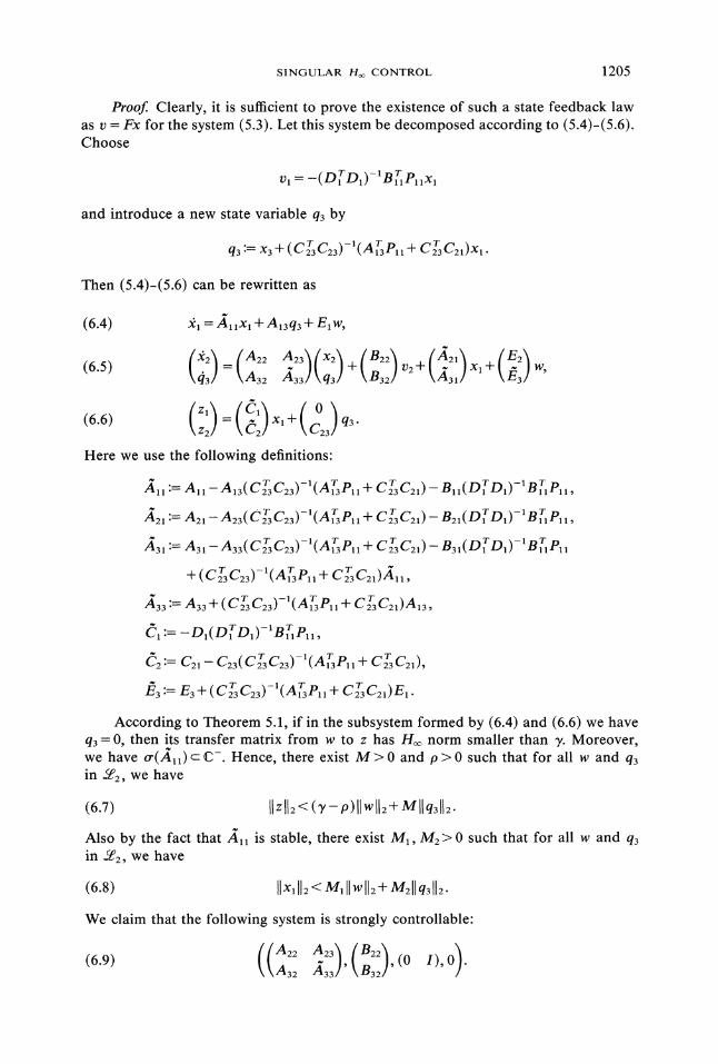
Proof Clearly, it is sufficient to prove the existence of such a state feedback lawas v Fx for the system (5.3). Let this system be decomposed according to (5.4)-(5.6).Choose

, -(D D,)-’B P,,Xl

and introduce a new state variable q by

q := x +(CC)-’(AP,, + CC,)x,.

Then (5.4)-(.6) an be rewritten as

(6.4)

C3) q3"

Here we use the following definitions"

:= A-Aa(CgCa)-’(Ae + CgC) B(DD)-BIPI,

:= A-A(CgC)-I(APll + CC)-B(DD)-BP,

31 := n31- Aa3(CgCa)-(AP + cCl)-B3(DD)-’BP

:=A+ CC2)-’(AP,, + CC,)A,,, := -D,(DD,)-’BP,,,:= C, C(CC)-’(AP,, + CC,),

:= E + CC)-’(AP,, + CC,)E,

According to Theorem 5.1, if in the subsystem formed by (6.4) and (6.6) we haveq 0, then its transfer matrix from w to z has H norm smaller than . Moreover,we have (A) C- Hence, there exist M > 0 and p > 0 such that for all w and qin , we have

Also by the fact that A is stable, there exist M, M> 0 such that for all w and qin , we have

(6.8) IIx, ll=We claim that the following system is strongly controllable:

(6.9)A3 A33] B3

1206 A. A. STOORVOGEL AND H. L. TRENTELMAN

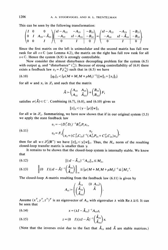
This can be seen by the following transformation:

/i A33 --/33 -A3 sI A33 "...3.2 ..’..3.2... sI- A33" .3.2

Since the first matrix on the left is unimodular and the second matrix has full rowrank for all s C (see Lemma 4.2), the matrix on the right has full row rank for alls C. Hence the system (6.9) is strongly controllable.

Now consider the almost disturbance decoupling problem for the system (6.5)with output q3 and "disturbance" (xd). Because of strong controllability of (6.9) thereexists a feedback law v2 F(’2o3) such that in (6.5) we have

(6.10)

for all w and xl in 2 and such that the matrix

(A22 A.23)(Bz2)A :=A3: A33]

-Fn3:z

satisfies r()c C-. Combining (6.7), (6.8), and (6.10) gives us

for all w in 2. Summarizing, we have now shown that if in our original system (5.3)we apply the state feedback law

V -(D(D1)-aBPXl,(6.11) ( x )2 F

X3 + CC23)-l(APll + CC21)xthen for all w(+) we have [[z[[ < yllw[[. Thus, the H norm of the resultingclosed-loop transfer matrix is smaller than y.

It remains to be shown that the closed-loop system is internally stable. We knowthat

(6.12) [[(sI-)-A3][ M2,

(6.13)A31]

The closed-loop A-matrix resulting from the feedback law (6.11) is given by

Assume (x y zr)r is an eigenvector of A with eigenvalue I with Re i 0. It canbe seen that

(6.14) x

kA3x.

(Note that the inverses exist due to the fact that and are stable matrices.)

SINGULAR Hoo CONTROL 1207

Combining (6.12) and (6.14) we find Ilxll M211zll, and combining (6.13) and (6.15)yields Ilzll2<-1/2Mllxll2. Hence x= z=0. This, however, would imply that (y 0)is an unstable eigenvector of . Since r()c C-, this yields a contradiction. Thisproves that the closed-loop system is internally stable. [3

A proof of the implication (ii)(i) in Theorem 2.1 is now obtained by combiningTheorems 5.4 and 6.2.

Remark 6.3. In the regular case (i.e., D injective) it is quite easy to give an explicitexpression for a suitable state feedback law. Indeed, if P->_0 is a solution to thealgebraic Riccati equation (5.1) such that (5.2) holds, then the feedback law u--(D’D)-I(B’P+D’C)x achieves internal stability and [[GF[[o< y. In the singularcase (i.e., D not injective) a state feedback law is given by u Fox + v. Here, Fo isgiven by (4.1) and v=(Vrl, vr2) " is given by (6.11). The matrix Pll is obtained bysolving the quadratic matrix inequality or, equivalently, by solving the reduced orderRiccati equation (5.8). The matrix F1 is a "state feedback" for the strongly controllableauxiliary system (6.5). This state feedback achieves almost disturbance decouplingbetween the "disturbance" (xr, wr) r and the "output" q3. The required accuracy ofdecoupling is expressed by (6.10). A conceptual algorithm to construct such F1 canbe based on the proof of [19, Thm. 3.36].

7. Discussion and conclusions. In this paper we have shown that if in theproblem with state feedback no assumptions are made on the direct feedthrough matrixof the control input, then the central role of the algebraic Riccati equation is takenover by a quadratic matrix inequality. We note that a similar phenomenon is knownto occur in the linear quadratic regulator problem: if the weighting matrix of the controlinput is singular, then the optimal cost is given in terms of a (linear) matrix inequalityrather than in terms of an algebraic Riccati equation (see [21]). However, while in thesingular LQ problem optimal inputs in general are distributions, in the H contextalso in the singular case suitable state feedback laws can befound. It is well known thatin the LQ problem a special role is played by solutions of the linear matrix inequalitythat minimize the rank of the dissipation matrix (see [4], [13]). It turns out that alsoin our context the relevant solutions to the quadratic matrix inequality are rankminimizing. Indeed, it follows from the proof of Theorem 5.4 that for all symmetricmatrices P we have rank F(P)>-normrank G. Thus, (2.5) can be interpreted as sayingthat P minimizes the rank of Fv(P). On the other hand, once we know that rank Fv(P)normrank G, then obviously for all s C we have

rank(L(P’s)F(P) ]--< n + normrank G.

Thus, (ii) of Theorem 2.1 can, loosely speaking, be reformulated as follows. Thereexists a solution P_->0 to F(P)>-O that minimizes rank Fv(P) and maximizesrank (Lv(P, s) , Fv(P)7") 7" for all s Ct_J C+.

As can be expected, the quadratic matrix inequality and the rank conditions (2.5)and (2.6) turn out to play an important role in the context of singular linear quadraticdifferential games. This connection is elaborated in [16].

Needless to say, several questions remain unanswered in this paper. The mostobvious topic is the extension of the theory of this paper to the case of dynamicmeasurement feedback, i.e., the singular counterpart of the problem studied in [2],[5], and [18]. In [17] it is shown that the existence of suitable dynamic compensatorsrequire solvability of a pair of quadratic matrix inequalities.

Finally, in [20] the ideas of the present paper are used to tackle the finite horizon"H" control problem by measurement feedback, i.e., the problem of finding a dynamic

1208 A.A. STOORVOGEL AND H. L. TRENTELMAN

compensator such that the L2[t0, tl]-induced norm (instead of the L2(N+)-inducednorm) of the closed-loop operator is smaller than an a priori given upper bound. In[20] conditions for the existence of such a compensator are formulated in terms ofquadratic differential inequalities (the extensions of Riccati differential equations).

REFERENCES

[1 J. A. BALL AND N. COHEN, Sensitivity minimization in the H norm: parametrization of all suboptimalsolutions, Internat. J. Control, 46 (1987), pp. 785-816.

[2] J.C. DOYLE, K. GLOVER, P. P. KHARGONEKAR, AND B. m. FRANCIS, State space solutions to standardH and Hoo control problems, IEEE Trans. Automat. Control, 34 (1989), pp. 831-847.

[3] F. R. GANTMACHFR, The Theory of Matrices, Chelsea, New York, 1959.[4] T. GEERTS, All optimal controls for the singular linear-quadratic problem without stability; a new

interpretation of the optimal cost, Linear Algebra Appl., 122 (1989), pp. 65-104.[5] K. GLOVER AND J. C. DOYLE, State space formulae for all stabilizing controllers that satisfy an Hm

norm bound and relations to risk sensitivity, Systems Control Lett., 11 (1988), pp. 167-172.[6] M. L. J. HAUTUS, Strong detectability and observers, Linear Algebra Appl., 50 (1983), pp. 353-368.[7] M. L. J. HAUTUS AND L. M. SILVERMAN, System structure and singular control, Linear Algebra Appl.,

50 (1983), pp. 369-402.[8] P. P. ,KHARGONEKAR, I. R. PETERSEN, AND M. A. ROTEA, Ho optimal control with state feedback,

IEEE Trans. Automat. Control, 33 (1988), pp. 786-788.[9] E. B. LEE AND L. MARKUS, Foundations of Optimal Control Theory, John Wiley, New York, 1967.

[10] I. R. PETERSEN, Disturbance attenuation and H optimization: a design method based on the algebraicRiccati equation, IEEE Trans. Automat. Control, 32 (1987), pp. 427-429.

[11] H. H. ROSENBROCK, The zeros of a system, Internat. J. Control, 18 (1973), pp. 297-299.[12] J. M. SCHUMACHER, Dynamic Feedback in Finite and Infinite Dimensional Linear Systems, Mathe-

matical Centre Tracts, Vol. 143, Amsterdam, 1981.[13] , The role of the dissipation matrix in singular optimal control, System Control Lett., 2 (1983),

pp. 262-266.[14], On the structure of strongly controllable systems, Internat. J. Control, 38 (1983), pp. 525-545.[15] A. A. STOORVOGEL, H control with state feedback, Proceedings MTNS-89, Amsterdam, 1990,

16] ., The singular zero-sum differential game with stability using H control theory, Math. ControlSign. Systems, to appear.

17] , The singularH control problem with dynamic measurementfeedback, SIAM J. Control Optim.,to appear.

[18] G. TADMOR, H in the time domain: the standard four blocks problem, Math. Control Sign. Systems,to appear.

[19] H. L. TRENTELMAN, Almost Invariant Subspaces and High Gain Feedback, CWI Tracts, Vol. 29,Amsterdam, 1986.

[20] H. L. TRENTELMAN AND A. A. STOORVOGEL, Completion of the squares in the finite horizon Hcontrol problem by measurement feedback, preprint, October 1989.

[21] J. C. WILLEMS, Least squares stationary optimal control and the algebraic Riccati equation, IEEE Trans.Automat. Control, 16 (1971), pp. 621-634.

[22] ., Almost invariant subspaces: an approach to high gainfeedback designPart 1: almost controlledinvariant subspaces, IEEE Trans. Automat. Control, 26 (1981), pp. 235-252.

[23] K. ZHOU AND P. P. KHARGONEKAR, An algebraic Riccati equation approach to H optimization,Systems Control Lett., 11 (1988), pp. 85-91.