University of Groningen Interregional migration in ... · is the increasing importance of Sumatera (Mebidangro and Rest of Sumatera) as a receiver as well as a sender of migrants

University of Groningen

Interregional migration in IndonesiaWajdi, Nashrul

IMPORTANT NOTE: You are advised to consult the publisher's version (publisher's PDF) if you wish to cite fromit. Please check the document version below.

Document VersionPublisher's PDF, also known as Version of record

Publication date:2017

Link to publication in University of Groningen/UMCG research database

Citation for published version (APA):Wajdi, N. (2017). Interregional migration in Indonesia: Macro, micro, and agent-based modellingapproaches. [Groningen]: University of Groningen.

CopyrightOther than for strictly personal use, it is not permitted to download or to forward/distribute the text or part of it without the consent of theauthor(s) and/or copyright holder(s), unless the work is under an open content license (like Creative Commons).

Take-down policyIf you believe that this document breaches copyright please contact us providing details, and we will remove access to the work immediatelyand investigate your claim.

Downloaded from the University of Groningen/UMCG research database (Pure): http://www.rug.nl/research/portal. For technical reasons thenumber of authors shown on this cover page is limited to 10 maximum.

Download date: 27-04-2019

https://www.rug.nl/research/portal/en/publications/interregional-migration-in-indonesia(daa8a115-c4fe-4f64-b82b-d54f9c4c72c2).html

Interregional Migration in Indonesia: An Agent-based

Modelling Approach

5

2017_N_Wajdi_Dissertation.indb 1112017_N_Wajdi_Dissertation.indb 111 31-8-2017 10:03:2431-8-2017 10:03:24

112

Chapter 5

Interregional migration in Indonesia: an agent-based modelling approach*

Abstract - To simulate the future migration patterns of the population of Indonesia, we build an agent-based model (ABM) of interregional migration in Indonesia based on combined information from our previous analyses (Chapters 2, 3, and 4). The agents represent individuals who live in a geographic area, respond to the push factors at the origins, are self-selected by individual characteristics, and choose their migration destination based on the attractiveness of the destination. We include three scenarios that vary in terms of the sensitivity of migrants to population density. We demonstrate that the model predicts not only migration rates, but also the dynamics of structural changes in the spatial migration patterns. It has been projected that up to 2035, processes of urbanisation, suburbanisation, and metropolitan to non-metropolitan migration will characterise the interregional migration system in Indonesia. Our fi ndings also emphasise the growing metropolitan-to-non-metropolitan movements in Indonesia, whereby the metropolitan areas are sending migrants to all destinations, while non-metropolitan areas are receiving migrants from all points of origin. One common pattern that emerges from all of these scenarios is the increasing importance of Sumatera (Mebidangro and Rest of Sumatera) as a receiver as well as a sender of migrants. This fi nding suggests that a transition to a new migration pattern is occurring: i.e., from a monocentric (Java-centric only) to a dual-centric (Java-centric and Sumatera-centric) pattern. Another observation we can make based on these diff erent scenarios is that the lower the population’s tolerance for population density is (i.e., stronger negative agglomeration eff ects), the faster the suburbanisation process is in the metropolitan areas of Jakarta, Bandung Raya, and Mebidangro.

Keywords: Migration, agent-based modelling, Indonesia

* This chapter is co-authored with Leo van Wissen. A preliminary version of this chapter was presented at Dutch Demography Day 2016, Utrecht, The Netherlands. The latest version of this chapter was presented at the 6th Indonesian Regional Science Association (IRSA) International Institute annual conference on 17-18 July 2017 in Manado, North Sulawesi, Indonesia.


An Agent-based Modelling Approach

5

113

5.1. Introduction In the previous chapters of this thesis (Chapters 2, 3, and 4), we described and

sought to explain the dynamics of interregional migration in Indonesia from 2000 to 2010 using diff erent modelling approaches. The fi ndings presented in Chapter 2, which are based on Long’s population redistribution phases framework (1985), indicate that in addition to over-urbanisation, suburbanisation—i.e., people moving from densely populated areas to suburban or low-density regions (e.g., migration from Jakarta to Bodetabek)—is occurring. In Chapter 3, we apply the gravity modelling approach. The results suggest that migration in Indonesia follows Long’s population redistribution phases: i.e., during the early stages of development, the concentration of population is positively related to economic development. In Chapter 4, we apply a micro approach to migration. The fi ndings show that migration varies with age and with life course characteristics, and that diff erent characteristics are associated with diff erent migration outcomes. Thus, it appears that interregional migration in Indonesia is not a linear process, but is instead characterised by diff erent phases that are triggered by changing circumstances, and the reactions of migrants to these circumstances.

However, the studies presented in this thesis have some drawbacks, as do other empirical models of interregional migration in Indonesia (see, for example, Darmawan & Chotib, 2007; and Van Lottum & Marks, 2012). First, these models are unable to incorporate the interactions between individuals or individuals’ responses to contextual changes. Second, these models fail to capture the interrelated and dynamic nature of migration, because they do not take into account the tendency for migration decisions and related variables to be continuously updated over time (Hassani-Mahmooei, 2012; Wu et al., 2010). Third, these models are unable to capture the non-linearity of migration systems in Indonesia. Projecting the future pattern using these models is just as likely to result in a linear pattern as using the simple extrapolation model. Furthermore, the previous studies presented in this thesis were limited to covering developments that occurred between 2000 and 2010, and used separate analyses based on either a micro or a macro approach. To address the limitations of this previous research, we pose two questions. First, how are inter-regional migration patterns in Indonesia likely to develop, and what are the likely consequences of these developments for the regional population dynamics based on recent historical trends in inter-regional migration? Second, how are these patterns likely to diff er based on varying thresholds of population density?

According to Long (1985), there is a relationship between the migration behaviour of individuals and both population redistribution and geographical


114

Chapter 5

settlement patterns. For example, population redistribution from area i to area j would involve the sum of all individual migration decisions from area i to area j. The result of this micro-to-macro transformation should be an integrated model that not only explains all of these individual fl ows, but is also useful to researchers in all of the major disciplines that study population movement and settlement patterns (Long, 1985). However, Long (1985) warned that developing this type of model could be very diffi cult. Fortunately, recent advances in modelling techniques make building such a model more feasible. One of the techniques that could be applied in this context is agent-based modelling and simulation (ABMS). ABMS can, for example, be used to assess the eff ects of agents’ interactions with other agents (micro level) and with their environment, and to examine how these interactions aff ect the whole system (macro level). The changes at the macro level will further infl uence the decisions of individuals (feedback mechanism). This approach is also known as the bottom-up approach (Railsback & Grim, 2011).

ABMS is a computational model of a system. A system in ABMS is modelled as the aggregation of autonomous decision-making entities called agents. These unique and autonomous agents interact with each other and with their environment, assess their situations, and make decisions using a set of rules. ABMS has been previously used to simulate migration responses to diff erent environment stimuli. For example, Cai and Oppenheimer (2013), Hassani-Mahmooei and Paris (2012), Kniveton et al. (2012), Smith (2014), and Ziervogel et al. (2005) studied migration responses to climate change using ABMS. Applying the push-and-pull factors framework, while also taking into account moving costs and job search costs as determinants of migration, Heiland (2003) demonstrated that ABMS could replicate the state-level migration pattern from East to West Germany in the period of 1989 to 1998.

According to Bonabeau (2002, p. 7280), ABMS has three key benefi ts relative to other modelling techniques: (1) it captures emergent phenomena, (2) it provides a natural environment for the study of certain systems, and (3) it is fl exible. These advantages of ABMS are relevant to the aim of our study, and particularly the ability of ABMS to capture emergent phenomena.

An emergent phenomenon is the collective behaviour of a particular group: i.e., it is a certain pattern that emerges in a larger entity of a system as a result of the interactions in a smaller entity of the system (Bonabeau, 2002; Epstein & Axtel, 1996). As an example, consider a simple economic system that consists of two types of agents: sellers and buyers. Both sellers and buyers interact at the micro level: buyers make the purchase, and sellers make the sales. Both buyers and sellers have their autonomous goals and are involved in a larger economic system; thus, both



5

115

types of agents are aff ected by the developments in this larger economic system, such as global decreases, global increases, or crashes. In this case, the emergent phenomena are the aggregate economic quantities that result from these interactions; e.g., prices (Bonabeau et al., 1995). Another example is Schelling’s dynamic models of segregation (Schelling, 1971). Schelling (1971) explained how the emergent phenomenon of the spatial segregation between black and white people is the result of individual behaviour. That is, an individual has a certain tolerance threshold for living in an area that belongs to his/her ethnic group. If the racial composition of the area exceeds the individual’s tolerance threshold, he/she moves to another area. In this chapter, ABMS is used to model the migration behaviour of individual agents. These individual agents migrate and try to settle in a particular area, resulting in an (emerging) pattern of in- and out-migration fl ows at the macro scale (for more detailed explanations on emergent phenomena, see Bonabeau, 2002, p. 7280; and Castle & Crooks, 2006, pp. 12-16).

For the decision-making modelling in ABMS related to migration, Klabunde and Willekens (2016) distinguished six type of ABMS, ranging from minimalist models, to models that rely on direct observations or purely empirical observational rules without referring to a specifi c theory, to models that utilise behavioural theories. The minimalist models make no or minimal use of decision theory; their main purpose is to demonstrate that simple behavioural rules for individual interaction could result in complex macro-level patterns. We consider our model to be an empirical observational rules model, because we built our model based on empirical observational rules from our previous studies (Chapters 2, 3, and 4), even though not all of the parameters from the previous chapters are included in the model.

The aim of the model is to reproduce interregional migration fl ows in Indonesia. After validating this pattern, we explore simple scenarios to produce projections of interregional migration. We then compare our simulations results with the offi cial projection results.

5.2. Model description and the scenariosAn ABMS is constructed to simulate the migration fl ows in Indonesia for

the period of 2000-2010, and to simulate the future pattern of migration fl ows in Indonesia. The development of this model was inspired by the cellular automata (CA) models (see, for example, Barredo et al., 2003; Santé et al., 2010; and Semboloni, 1997) and by Schelling’s dynamic models of segregation (Schelling, 1971). These ABMS show that a simple individual rule can lead to a complex pattern of macro behaviour. Furthermore, small changes in those rules can have huge eff ects on


116

Chapter 5

macro behaviour (see, for example, Bonabeau, 2002 p.7280, Chan et al., 2010 for the emergent patterns from Conway’s games-of-life model and the boids model). The main emergent patterns expected from this model are the set of origin-destination migration fl ows that result from individual preferences and individuals’ interactions with other individuals, as well as individuals’ interactions with their surroundings.

Figure 5.1. shows the parts of our ABMS. The macro part of the model is represented by Region. Region is a geographical unit that stores the macro variables, including city type, area count, population density, population size, population growth, GDP, the attraction force, the share of agricultural workers, and migrant stock. The macro variables of Region are updated over Time. There are three exogenous macro variables: namely, natural population growth, GDP, and the share of agricultural workers. The values of these exogenous macro variables are based on observed and projected data, such data as from BPS-Statistics Indonesia. The other macro variables—namely, population size (including the migration component) and population density—are endogenous. During the simulation, the values of Regions’ macro variables are updated, which will aff ect the migration decisions of the individual agents, and the values of Region’s endogenous macro variables are the result of the individual agents’ decisions (feedback mechanism).

FIGURE 5.1. Diagram for the agent-based model for interregional migration in Indonesia (see the text for an explanation)



5

117

Since we assume that individual Agents are autonomous and are capable of making decisions based on certain rules (Klabunde & Willekens, 2016), we designed for the micro part of our analysis a “mental model”—to use the term coined by Svart (1976)—intended to refl ect how individual agents make their migration decisions. We attempt to model this decision-making process by building a simple model that incorporates the factors that have been studied in Chapters 2, 3, and 4. We assume that Agents take into account the fi ve main external factors we identifi ed for Regions: (1) population density in the origin and in the destination, (2) population size in the origin and in the destination, (3) the socioeconomic conditions in the origin and in the destination, (4) the size of the social network that provides the individual-level interactions, and (5) the distance between regions. As the density, the population size, and the size of the migration network are updated in every period in response to the agent’s decisions, it is likely that the agent’s decision outcomes are changing accordingly. The patterns that emerge from the model are the main origin-destination Regions of the Agents, and which result in the in- and out-migration fl ows.

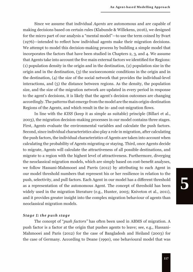
In line with the KISS (keep it as simple as suitable) principle (Billari et al., 2003), the migration decision-making processes in our model contains three stages. First, Agents evaluate the environmental variables and calculate the push factors. Second, since individual characteristics also play a role in migration, after calculating the push factors, the individual characteristics of Agents are taken into account when calculating the probability of Agents migrating or staying. Third, once Agents decide to migrate, Agents will calculate the attractiveness of all possible destinations, and migrate to a region with the highest level of attractiveness. Furthermore, diverging the neoclassical migration models, which are simply based on cost-benefi t analyses, we follow Hassani-Mahmooei and Parris (2012) by attributing to each Agent in our model threshold numbers that represent his or her resilience in relation to the push, selectivity, and pull factors. Each Agent in our model has a diff erent threshold as a representation of the autonomous Agent. The concept of threshold has been widely used in the migration literature (e.g., Hunter, 2005; Kniveton et al., 2011), and it provides greater insight into the complex migration behaviour of agents than neoclassical migration models.

Stage 1: the push stageThe concept of “push factors” has often been used in ABMS of migration. A

push factor is a factor at the origin that pushes agents to leave; see, e.g., Hassani-Mahmooei and Paris (2012) for the case of Bangladesh and Heiland (2003) for the case of Germany. According to Deane (1990), one behavioural model that was


118

Chapter 5

developed through the application of economic push-pull models is the stress-threshold model proposed by Wolpert (1966). Wolpert (1966) argued that migration is an adjustment process that results from “stress” caused by the environment. However, an individual’s responses to stress due to environmental conditions may vary considerably (Brown & Moore, 1970). In identifying the relevant push factors in our context, we consider two concepts: namely, population density and population size. It should be noted that in the gravity models of interregional migration in Indonesia (Chapter 3), the share of agricultural workers at the origin and per capita GDP at the origin were also utilised in the model. However, as these two variables were found to have no statistically signifi cant eff ects on migration fl ows from origin to destination, they are not included in the push stage.

We employ population density as one of the push factors because, for the case of Indonesia, Alatas (1993) has argued that the decline in the urban population in Java appears to have been caused by high population density and the scarcity of land and housing. Furthermore, according to Long (1985), one important phase of population redistribution is suburbanisation, whereby people start to move to less dense regions. The analysis in Chapter 2 showed that during the 1995-2010 period, Jakarta had out-fl ows to Bodetabek, Rest of Sumatera, Kalimantan, Sulawesi, and Rest of Indonesia that were larger than the corresponding in-fl ows. This type of movement can be regarded as the suburbanisation phase of population redistribution (for a more detailed explanation of the population redistribution phases, please refer to Chapter 2). Long (1985) argued that this movement might be due to strong preferences for low-density locations as a result of experiences with counterproductive social interactions in congested metropolitan areas.

Zhang and Jager (2011) have argued that some people prefer to live in a congested-noisy region, whereas others prefer to live in spacious-tranquil areas. Thus, the tolerance for density diff ers among individuals. From a macro perspective, the diff erences in preferences regarding population density may result in a diff erent levels of city agglomeration. The World Bank (2012) used the modifi ed Agglomeration Index to defi ne metropolitan regions based on three factors: the size of an urban centre, population density, and the distance of a district to the urban centre. In the original Agglomeration Index developed by Uchida and Nelson (2010), the threshold for high population density was 150 persons per square kilometre. However, given the relatively high population density of Java (more than 150 persons per square kilometre), the use of this threshold would lead us to conclude that almost the entire island of Java is essentially one very large urban zone (World Bank, 2012). Therefore, the World Bank modifi ed this threshold to 700 persons per square kilometre for



5

119

Java, and to 200 persons per square kilometre for the rest of Indonesia. Based on the modifi ed Agglomeration Index, the World Bank identifi ed 44 metropolitan regions. A decrease in the population density threshold suggests that Agents have become more sensitive to the negative eff ects of density, and thus fi nd high-density areas less attractive. Consequently, Agents start to choose other, less densely populated metropolitan areas, and the number of metropolitan areas increases. As cities tend to grow over time, a lower threshold means that the negative externalities of a metropolitan area’s density occurred at an earlier point in time. In contrast, if the threshold for population density increases, we can assume that people are less concerned about the negative externalities of high density, and are willing to tolerate living in higher density agglomerations. This type of development leads to spatial patterns with only a few large metropolitan areas, and the negative externalities of agglomeration tend to be pushed back in time.

Figure 5.2. shows the empirical relationship between population density and the out-migration rate after controlling for population size. This empirical relationship is derived from a linear regression model that models population density, population size, and out-migration (see Table 5.1. for the parameters). The results show that there is a positive relationship between population density and the out-migration rate; that is, rates of out-migration are higher in more densely populated regions.

0

20

40

60

80

100

120

140

0 2000 4000 6000 8000 10000 12000 14000 16000

Ou

t-m

igra

tion

rat

e

Population density per square km

Provinces out-migration rate

Linear estimation of out-migration rate

13 regions out-migration rate

FIGURE 5.2. Population density and the out-migration rate in Indonesia, 1980-2010


120

Chapter 5

TABLE 5.1. Linear regression results for out-migration rate, 1980-2010

Variables Coef. Std. Err. t P>t

Constant 22.1060 1.0927 20.23 0.0000Population density 0.0058 0.0003 15.17 0.0000Population size -0.1983 0.0931 -2.13 0.0350

Source: Authors’ statistical calculation. The data for the regression were derived from https://www.bps.go.id/linkTabelStatis/view/id/1273

Based on the parameters shown in Table 5.1., ceteris paribus --the population size is assumed to be fi xed at means (6.7769) to allow us to analyse the infl uence of population density, and, therefore, the constant term is 22.1060 + (-0.1983 * 6.7769) = 20.7620-- with the maximum value of population density is 18,341, the equation for out-migration rate is as follows:

The out-migration equation is transformed into the probability density function as follows:

Substituting c for out-migration equation will result in:

with the cumulative density function as follows:

The probability [F(densix)] of Agent x originated from region i aff ected by a certain density (p) is then compared with a random number between zero and one (r) assigned to Agent x. If the threshold random number r assigned to Agent x exceeds the probability p, Agent x proceeds to stage 2, the selectivity stage.

(5.1.)

(5.2.)

(5.3.)

(5.4.)



5

121

Stage 2: the selectivity stageMigration is a selective process. The selectivity of migration has been

demonstrated in both the internal and the international migration literature (De Jong & Gardner, 1981; Greenwood, 1975; Massey, 1988; Rebhun & Goldstein, 2009). To account for migrant selectivity, we use the individual characteristics we examined in Chapter 4.

The fi ndings regarding the relationship between individual characteristics and migration presented in Chapter 4 show that diff erent individual characteristics are associated with diff erent migration outcomes. The general pattern of the age-migration profi le indicates that among the population studied, migration propensity reached its peak at ages 15-29, and then declined up to retirement age, or ages 55-69. Females were particularly likely to move to more developed areas compared to their previous place of residence, and males were particularly likely to move to less developed areas compared to their previous place of residence. The probability of migration increased with the level of education. Divorced people were more likely to move to non-metro areas than married people, whereas widowed people were more likely to move to another metro area within commuting distance or to a non-metro area. Those who had dependent children under age fi ve (including those whose children were born shortly after a potential move) were more likely to migrate than those who had no young dependent children.

The parameters for the selectivity stage in our ABMS are derived from Chapter 4 (listed in Tables 4.2-4.4 in Chapter 4, pp. 105-109). Nine types of migration were examined in Chapter 4. Three multinomial logit models were utilised to analyse the relationship between individual characteristics and migration: namely, a model for migration from Jakarta, a model for migration from metropolitan areas, and a model for migration from non-metropolitan areas. The multinomial logistic regression model used in Chapter 4 estimated the eff ects of the individual variables on the probability of migrating to a certain area. The independent variables used as predictors of migrating to a particular destination included age, gender, educational attainment, labour market participation status, marital status, and the presence of children under age fi ve in the household.

Three multinomial logistic regression models were utilised in Chapter 4. With each migration destination j = 1, 2, and 3 against the reference category zero (stay), the log odds of migrating depend on the values of the k explanatory variables, and can be formulated as follows:

(5.5.)


122

Chapter 5

where k is the number of explanatory variables with and β are the parameters. From the estimated parameters, the probability of response in category j can be calculated as follows:

where π(j) is the probability of choosing area j over the reference category stay, and L(j)=log(π(j)/π(0)), or the log odds of a response in area j rather than the reference category stay.

The probability [π(j)] of agent x to move (p) is then compared with a random number between zero and one (r) assigned to agent x. If the threshold random number r assigned to agent x exceeds the probability p, agent x proceeds to stage 3, the pull stage.

Stage 3: the pull stageThe third stage in our model is the pull stage. Migration is a form of

welfare-maximising behaviour of individuals, families, or household groups; and people migrate from less advantaged areas (in terms of economic opportunities and amenities) to more advantaged areas (Long 1985). The better the economic opportunities and the amenities are in an area, the more attractive that area is for migrants (Chapters 2 and 3). Thus, Agents migrate to the region with the strongest pull forces.

FIGURE 5.3. Population density and in-migration rates in Indonesia, 1980-2010

(5.6.)



5

123

The pull forces in our model is a function of six factors: namely, population density, population size, the share of agricultural workers, per capita GDP, distance, and migrant stock. The empirical relationship between population density and in-migration in Indonesia for the years 1980 to 2010 is shown in Figure 5.3. which reveals a quadratic pattern. This pattern refl ects the agglomeration eff ects of a city that attracts migrants. At a certain point, due to congestion, the city become less attractive, which results in less in-migration to this city.

The other factors that may be considered by Agents in choosing a destination are the share of agricultural workers, per capita GDP, and distance to the potential destination. For Indonesia, we found that the share of agricultural workers generally had insignifi cant eff ects on migration at both the origin and the destination (Chapter 3). However, since migration of labour out of agriculture is a feature of economic development and modernisation that has been observed in developed as well as in developing countries (Rozelle et al., 1999); and since people may be tempted to move to more industrialised areas not just for economic, but for cultural and social reasons (Adams, 1969); we assume that Agents are less likely to move to agricultural regions. The higher the share of agricultural workers in a region is, the less attractive that region is.

One important factor in the attractiveness of a region is the expected earnings of an individual, usually measured by income per capita (Beine et al., 2014; Fan, 2005). There are two perspectives on the eff ects of income on migration. First, the micro viewpoint argues that migration occurs because a migrant foresees income benefi ts from moving (Greenwood, 1975). Second, the macro perspective argues that migration fl ows from low-income to high-income regions; i.e., that the income elasticity is positive at the destination. One indicator that can be used to measure the income prospects of potential migrants from all origins is GDP per capita at the destination (Beine et al., 2014). For Indonesia, we found that the coeffi cients for per capita GDP at the destination had positive signs related to in-migration (Chapter 3). We therefore we assume that the higher the GDP in a region is, the more attractive that region is.

In the migration literature, the distance between regions has been used as a representation of the physical costs of migration, as well as of the information loss between the origin and the destination (Greenwood, 1975; Nelson, 1959). The fi ndings presented in Chapter 3 show that for interregional migration in Indonesia, distance is negatively related to migration. We therefore assume that the longer the distance is between the origin and the destination, the less attractive the destination is.


124

Chapter 5

Agents retrieve the macro information regarding the possible destinations from the Agents’ networks; i.e., the Agents’ family and friends who live in other places. Existing research has shown that destination areas with relatively large numbers of migrants tend to be more attractive to potential migrants, as such contexts provide newly arrived migrants with the opportunity to enter existing social networks or to create new networks with people from the same place of origin (Anjos & Campos, 2010). In our model, we use migrant stock—that is, the accumulated number of previous in-migrants to the destination who migrated from the origin—as a representation of the network. The study in Chapter 3 shows a strong and statistically signifi cant positive eff ect of migrant stock on interregional migration in Indonesia. We therefore assume that the bigger the migrant stock from the place of origin who are already living at the potential destination is, the more attractive the destination is.

Accounting for non-linearity in the pattern of in-migration, and taking into account the other factors discussed earlier in this section, the pull factors of region j are modelled as follows:

pullijx=b1*densj - b2*densj2 - b3*popsizej - b4*agrij + b5*gdpj - b6*dij + b7*Sij

The pull forces of region j for agent x who reside in region i is a weighted function of population density (densj), population size (popsizej), share of agricultural workers (agrij), per capita gdp (gdpj), distance (dij), and migrant stock (Sij—the number of migrants from i who reside in j), where all b coeffi cients are non-negative, and b1+b2+b3+b4+b5+b6+b7 = 1. To create bs, each agent fi rst produces seven random numbers between zero and 99 (ri), and then bi = ri/∑ri . A weighted function is used to express diff erent individuals’ preferences regarding each factor. Once an agent evaluates all of the pull values for all possible regions using the set of random generated coeffi cients, this agent will choose the highest value of pull, and move to the region with the highest pull value.

The scenariosAccording to Relethford (1986), migration is density-dependent; that is,

migration is aff ected by population size. The population density factor can be either a push or a pull factor in the migration decision-making process, and is crucial for understanding how the population redistribution pattern evolves. The urbanisation phases are driven by changing preferences for urban, suburban, or rural living; and these changing preferences are at least partially dependent on urbanisation (dis)

(5.7.)



5

125

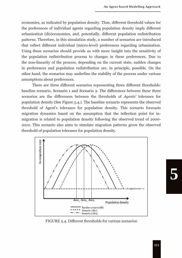
economies, as indicated by population density. Thus, diff erent threshold values for the preferences of individual agents regarding population density imply diff erent urbanisation (dis)economies, and, potentially, diff erent population redistribution patterns. Therefore, in this simulation study, a number of scenarios are introduced that refl ect diff erent individual (micro-level) preferences regarding urbanisation. Using these scenarios should provide us with more insight into the sensitivity of the population redistribution process to changes in these preferences. Due to the non-linearity of the process, depending on the current state, sudden changes in preferences and population redistribution are, in principle, possible. On the other hand, the scenarios may underline the stability of the process under various assumptions about preferences.

There are three diff erent scenarios representing three diff erent thresholds: baseline scenario, Scenario 1 and Scenario 2. The diff erences between these three scenarios are the diff erences between the thresholds of Agents’ tolerance for population density (See Figure 5.4.). The baseline scenario represents the observed threshold of Agent’s tolerance for population density. This scenario forecasts migration dynamics based on the assumption that the infl ection point for in-migration is related to population density following the observed trend of 2000-2010. This scenario also aims to simulate migration patterns given the observed threshold of population tolerance for population density.

FIGURE 5.4. Diff erent thresholds for various scenarios


126

Chapter 5

Scenario 1 represents a 10 percent increasing threshold of acceptable density compared to the baseline scenario. From a macro perspective, this increasing threshold will result in lower agglomeration eff ects; that is, the infl ection point for in-migration moves to the right. In contrast, Scenario 2 represents a 10 percent decreasing threshold of acceptable density compared to the baseline scenario. The decreasing threshold will result in a faster negative eff ect of agglomeration on in-migration; that is, the infl ection point for in-migration moves to the left. From a micro perspective, the increasing threshold (Sc1) represents a decreased tolerance for population density. On the other hand, the decreasing threshold (Sc2) accounts for an increased tolerance for population density.

5.3. Implementation and resultsWe implemented the model in NetLogo 5.3 (Wilensky, 1999). Since the model

requires a high level of computing performance, we ran the model at the University of Groningen’s High-Performance Computing cluster, called the Peregrine HPC cluster (http://www.rug.nl/society-business/centre-for-information-technology/research/services/hpc/facilities/peregrine-hpc-cluster). After validating the model, we analysed the simulation results using four methods. First, to gain a better understanding of the general pattern and the migration fl ow trends, we visualised the total in- and out-migration fl ows using circular plots, as in Sander et al. (2014). Second, we examined the spatial structure of migration destinations using a method employed in Chapter 2; namely, a saturated multinomial logit model that includes the interaction of origin-destination variables. Third, we measured the spatial focusing—i.e., the inequality that exists in the relative volumes of a set of origin-destination-specifi c migration fl ows—using the Gini index of migration. Fourth, we compared the simulation results with the offi cial projection results produced by Statistics Indonesia.

Model setting and calibrationFor the initialisation (at the year 2000), we drew a sample from the Indonesian

Census 2000 (PC2000). We added more agents for each year to account for natural population growth, in line with the offi cial regional population projection of BPS-Statistics Indonesia (BPS-Statistics Indonesia, 2013). Each agent was assigned characteristics from our sample data. Before starting the Time tick, Agents were placed at their origins.



5

127

For the Regions, following Wajdi et al. (2015), we built 13 geographic areas representing Indonesia (see Table 1.1. in Chapter 1, pp.14-15). Table 5.2. shows the number of agents used for the initialisation. One agent in our model represents 10,000 individuals in the regional population. We used only the population aged 15+ to represent the autonomous migration decision-makers.

TABLE 5.2. Initialisation for population, initial vs. real data

RegionPopulation Distribution (%)

PC2000 Initial PC2000 Initial

Jakarta 6,397,035 640 4.57 4.57

Bodetabek 8,819,336 882 6.30 6.30

Bandung Raya 4,501,907 450 3.22 3.22

Rest of West Java and Banten (RoWJB) 16,966,411 1,697 12.13 12.13

Kedungsepur 3,897,058 390 2.79 2.79

Rest of Central Java and Yogyakarta (RoCJY) 20,637,363 2,064 14.75 14.75

Gerbangkertosusila 6,110,711 611 4.37 4.37

Rest of East Java (RoEJ) 19,885,567 1,989 14.21 14.22

Mebidangro 2,563,835 256 1.83 1.83

Rest of Sumatera (RoS) 23,560,835 2,356 16.84 16.84

Kalimantan 7,414,927 741 5.30 5.30

Sulawesi 9,734,356 973 6.96 6.95

Rest of Indonesia 9,417,358 942 6.73 6.73

Total 139,906,699 13,991 100.00 100.00

Source: Authors’ calculation

Results for the baseline model, simulation period 2000-2010We ran the simulation 100 times and validated the results using Population

Census 2010 data. Figure 5.5. shows the simulated (x-axis) and the observed (y-axis) out-migration rate for each region where each point is a fl ow to another region. The corresponding R-square indicates the goodness of fi t of our simulation results. Our model predicts out-migration (Figure 5.5.) quite well for most areas, with the exceptions being Kalimantan (R-sq= 0.5810), Rest of West Java and Banten (R-


128

Chapter 5

sq=0.6129), Rest of Central Java and Yogyakarta (R-sq=0.6596), and Mebidangro (R-sq=0.6807). For in-migration (Figure 5.6.), our model predicts the in-migration rate very well (R-square ranging from 0.8152 to 0.9946). It is likely that the prediction of the in-migration rate is more accurate than the prediction of the out-migration rate because of omitted variable bias due to the exclusion of non-signifi cant variables for the out-migration stage (i.e., the push stage).

R² = 0.9286

0

20

40

60

0 20 40 60Out

-mig

ratio

n ra

te ((

sim

ulat

ed)

Out-migration rate (observed)

1. Jakarta

R² = 0.9751

0

10

20

30

0 10 20 30Out

-mig

ratio

n ra

te ((

sim

ulat

ed)


2. Bodetabek

R² = 0.7894

0

2

4

6

0 2 4 6Out

-mig

ratio

n ra

te ((

sim

ulat

ed)


3. Bandung Raya

R² = 0.6129

0

10

20

30

0 10 20 30Out

-mig

ratio

n ra

te ((

sim

ulat

ed)


4. RoWJB

R² = 0.9462

0

2

4

6

0 2 4 6Out

-mig

ratio

n ra

te ((

sim

ulat

ed)


5. Kedungsepur

R² = 0.6596

0

10

20

30

40

0 10 20 30 40Out

-mig

ratio

n ra

te ((

sim

ulat

ed)


6. RoCJYR² = 0.8642

0

2

4

6

0 2 4 6Out

-mig

ratio

n ra

te ((

sim

ulat

ed)


7. Gerbangkertosusila

R² = 0.9299

0

10

20

30

40

0 10 20 30 40Out

-mig

ratio

n ra

te ((

sim

ulat

ed)


8. RoEJ

R² = 0.6807

0

2

4

6

8

0 2 4 6 8Out

-mig

ratio

n ra

te ((

sim

ulat

ed)


9. Mebidangro

R² = 0.9916

0

10

20

30

40

0 10 20 30 40Out

-mig

ratio

n ra

te ((

sim

ulat

ed)


10. RoS

R² = 0.5810

0

1

2

3

4

0 1 2 3 4Out

-mig

ratio

n ra

te ((

sim

ulat

ed)


11. Kalimantan

R² = 0.9779

0

2

4

6

8

10

0 2 4 6 8 10Out

-mig

ratio

n ra

te ((

sim

ulat

ed)


12. Sulawesi

R² = 0.7211

0

2

4

6

0 2 4 6Out

-mig

ratio

n ra

te ((

sim

ulat

ed)


13. Rest of Indonesia

R² = 0.9665

0

50

100

150

0 50 100 150Out

-mig

ratio

n ra

te (s

imul

ated

)


Indonesia FIGURE 5.5. Observed out-migration rate vs simulated out-migration rate for each region in Indonesia in 2010



5

129

R² = 0.9946

0

20

40

60

80

100

120

140

0 20 40 60 80 100 120 140

In-m

igra

tion

rate

(sim

ulat

ed)

In-migration rate (observed)

1. Jakarta

R² = 0.9701

0

20

40

60

80

100

120

140

0 20 40 60 80 100 120 140

In-m

igra

tion

rate

(sim

ulat

ed)


2. Bodetabek

R² = 0.8556

0

20

40

60

0 20 40 60

In-m

igra

tion

rate

(sim

ulat

ed)


3. Bandung Raya

R² = 0.9924

0

5

10

15

20

25

0 5 10 15 20 25

In-m

igra

tion

rate

(sim

ulat

ed)


4. RoWJB

R² = 0.9808

0

20

40

60

0 20 40 60

In-m

igra

tion

rate

(sim

ulat

ed)


5. Kedungsepur

R² = 0.9806

0

10

20

30

0 10 20 30

In-m

igra

tion

rate

(sim

ulat

ed)


6. RoCJY

R² = 0.9764

0

20

40

60

0 20 40 60

In-m

igra

tion

rate

(sim

ulat

ed)



R² = 0.9935

0

5

10

15

20

0 5 10 15 20

In-m

igra

tion

rate

(sim

ulat

ed)


8. RoEJ

R² = 0.9154

0

20

40

60

80

0 20 40 60 80

In-m

igra

tion

rate

(sim

ulat

ed)


9. Mebidangro

R² = 0.9877

0

10

20

30

0 10 20 30

In-m

igra

tion

rate

(sim

ulat

ed)


10. RoS

R² = 0.9839

0

20

40

60

0 20 40 60

In-m

igra

tion

rate

(sim

ulat

ed)


11. Kalimantan

R² = 0.9679

0

5

10

15

20

0 5 10 15 20

In-m

igra

tion

rate

(sim

ulat

ed)


12. Sulawesi

R² = 0.9531

0

10

20

30

0 10 20 30

In-m

igra

tion

rate

(sim

ulat

ed)



R² = 0.8152

0

30

60

90

120

150

180

0 30 60 90 120 150 180

In-m

igra

tion

rate

(sim

ulat

ed)


Indonesia FIGURE 5.6. Observed in-migration rate vs simulated in-migration rate for each region in Indonesia in 2010

Figure 5.7. presents the circular plots showing the pattern of in-migration and out-migration fl ows from both the observed data and the simulated data. For the total out-migration and in-migration fl ows for each region, our model predicts the fl ows quite well (as can also be seen in Figures 5.5. and 5.6.). However, for region specifi c out- and in-migration pairs, there are some notable diff erences between the observed and simulated fl ows.

Based on Figure 5.7., the model predicts the out-migration fl ows of seven regions (Jakarta, Bodetabek, Kedungsepur, Gerbangkertosusila, Mebidangro, Kalimantan, and Sulawesi) as observed fl ows, but the other six regions (Bandung Raya, Rest of West Java and Banten, Rest of Central Java and Yogyakarta, Rest of


130

Chapter 5

East Java, Rest of Sumatera, and Rest of Indonesia) have slightly diff erent patterns. Although there are some deviations between the observed and the simulated fl ows (the out- and the in- migration fl ows), the directions of the out- and the in-migration fl ows in the simulated data are generally similar to those of the observed data. However, the order of the fl ows diff ers.

FIGURE 5.7. Observed migration fl ows (left), simulated migration fl ows (right)

In the observed out-migration fl ows, the main out-fl ow from Bandung is directed to Rest of West Java and Banten. In the simulated out-migration fl ows, the main out-fl ow from Bandung is directed not only to Rest of West Java and Banten, but also to Rest of Sumatera. Another example can be seen by looking at the out-fl ows from Rest of West Java and Banten. The observed out-fl ows are mainly directed to Bodetabek, Jakarta, Bandung Raya, and Rest of Sumatera. But in the simulation, the order of the out-fl ows from Rest of West Java and Banten is a little diff erent: the four biggest outfl ows are directed to Bodetabek, Jakarta, Rest of Sumatera, and Rest of Central Java and Yogyakarta. An example of diff erences in the ordering of in-migration fl ows can be seen by looking at the in-fl ows for Jakarta. In the observed in-fl ows, the main sources are Rest of Central Java and Yogyakarta, Rest of West Java and Banten, Bodetabek and Rest of Sumatera; but in the simulated in-fl ows, the main sources are Rest of Central Java and Yogyakarta, Bodetabek, Rest of West Java and Banten, Rest of Sumatera, and Rest of East Java.

The simulated fl ows show the modelled fl ows based on the rules. Therefore, the diff erences between the observed and the simulated fl ows indicate that certain factors/rules have not been taken into account. For example, the out-migration fl ows



5

131

from Rest of Sumatera are directed to Mebidangro, Bodetabek, Jakarta and Rest of Central Java, and Yogyakarta; but in the simulated out-fl ows, the main destinations are Mebidangro, Bodetabek, and Jakarta. This means that in the “modelled” world, a migrant from Rest of Sumatera would have only three main destinations; while in the “real” world, a migrant from Rest of Sumatera would have four main destinations.

Simulation results and analyses, simulation period 2010-2035Out-migration rate, in-migration rate, and net migration rate

Although strictly speaking a rate can never be negative, it is common practice to use a negative number for a net migration rate that indicates that out-migration is greater than in-migration. Figures 5.8.1 to 5.8.13 display the simulated out-migration, in-migration, and net migration rates for the 2000-2035 period in three diff erent scenarios. These fi gures show that the out-migration and the in-migration rates are increasing in all regions; a fi nding that is in line with the idea that population mobility is increasing over time (Zelinsky, 1971). However, the projection shows that some of the patterns in the out- and the in-migration fl ows are changing, as can be seen in Figures 5.10.1 – 5.10.3.

60 80

100 120 140 160 180 200

2000 2010 2015 2020 2025 2030 2035Year

Out-migration rate

Baseline Scenario 1 Scenario 2

60 80

100 120 140 160 180 200

2000 2010 2015 2020 2025 2030 2035Year

In-migration rate


(50)

(40)

(30)

(20)

(10)

-

2000 2010 2015 2020 2025 2030 2035Year

Net-migration rate


FIGURE 5.8.1. Simulated out-migration rate (left), in-migration rate (middle), and net migration rate (right) for Jakarta

20

40

60

80

100

120

2000 2010 2015 2020 2025 2030 2035Year

Out-migration rate


20

40

60

80

100

120

2000 2010 2015 2020 2025 2030 2035Year

In-migration rate


-

20

40

60

80

100

120

2000 2010 2015 2020 2025 2030 2035Year

Net-migration rate


FIGURE 5.8.2. Simulated out-migration rate (left), in-migration rate (middle), and net migration rate (right) for Bodetabek


132

Chapter 5

20 30 40 50 60 70 80 90

100

2000 2010 2015 2020 2025 2030 2035Year

Out-migration rate


20 30 40 50 60 70 80 90

100

2000 2010 2015 2020 2025 2030 2035Year

In-migration rate


(40)

(30)

(20)

(10)

-

10

20

30

2000 2010 2015 2020 2025 2030 2035

Year

Net-migration rate


FIGURE 5.8.3. Simulated out-migration rate (left), in-migration rate (middle), and net migration rate (right) for Bandung Raya

10

20

30

40

50

60

2000 2010 2015 2020 2025 2030 2035Year

Out-migration rate


10

20

30

40

50

60

2000 2010 2015 2020 2025 2030 2035Year

In-migration rate


(30)

(25)

(20)

(15)

(10)

(5)

-2000 2010 2015 2020 2025 2030 2035

Year

Net-migration rate


FIGURE 5.8.4. Simulated out-migration rate (left), in-migration rate (middle), and net migration rate (right) for Rest of West Java and Banten

35

45

55

65

75

85

95

2000 2010 2015 2020 2025 2030 2035Year

Out-migration rate


35

45

55

65

75

85

95

2000 2010 2015 2020 2025 2030 2035Year

In-migration rate


(10) (5) - 5

10 15 20 25 30

2000 2010 2015 2020 2025 2030 2035

Year

Net-migration rate


FIGURE 5.8.5. Simulated out-migration rate (left), in-migration rate (middle), and net migration rate (right) for Kedungsepur

10

20

30

40

50

60

2000 2010 2015 2020 2025 2030 2035Year

Out-migration rate


10

20

30

40

50

60

2000 2010 2015 2020 2025 2030 2035Year

In-migration rate


(25)

(20)

(15)

(10)

(5)

-2000 2010 2015 2020 2025 2030 2035

Year

Net-migration rate


FIGURE 5.8.6. Simulated out-migration rate (left), in-migration rate (middle), and net migration rate (right) for Rest of Central Java and Yogyakarta



5

133

20

40

60

80

100

120

2000 2010 2015 2020 2025 2030 2035Year

Out-migration rate


20

40

60

80

100

120

2000 2010 2015 2020 2025 2030 2035Year

In-migration rate


- 10 20 30 40 50 60 70

2000 2010 2015 2020 2025 2030 2035Year

Net-migration rate


FIGURE 5.8.7. Simulated out-migration rate (left), in-migration rate (middle), and net migration rate (right) for Gerbangkertosusila

5 10 15 20 25 30 35 40

2000 2010 2015 2020 2025 2030 2035Year

Out-migration rate


5 10 15 20 25 30 35 40

2000 2010 2015 2020 2025 2030 2035Year

In-migration rate


(20)

(15)

(10)

(5)

-2000 2010 2015 2020 2025 2030 2035

Year

Net-migration rate


FIGURE 5.8.8. Simulated out-migration rate (left), in-migration rate (middle), and net migration rate (right) for Rest of East Java

25

75

125

175

225

2000 2010 2015 2020 2025 2030 2035Year

Out-migration rate


25

75

125

175

225

2000 2010 2015 2020 2025 2030 2035Year

In-migration rate


(200)

(150)

(100)

(50)

-2000 2010 2015 2020 2025 2030 2035

Year

Net-migration rate


FIGURE 5.8.9. Simulated out-migration rate (left), in-migration rate (middle), and net migration rate (right) for Mebidangro

10

15

20

25

30

35

2000 2010 2015 2020 2025 2030 2035Year

Out-migration rate


10

15

20

25

30

35

2000 2010 2015 2020 2025 2030 2035Year

In-migration rate


-

5

10

15

20

2000 2010 2015 2020 2025 2030 2035Year

Net-migration rate


FIGURE 5.8.10. Simulated out-migration rate (left), in-migration rate (middle), and net migration rate (right) for Rest of Sumatera


134

Chapter 5

5 15 25 35 45 55 65 75

2000 2010 2015 2020 2025 2030 2035Year

Out-migration rate


5 15 25 35 45 55 65 75

2000 2010 2015 2020 2025 2030 2035Year

In-migration rate


-

10

20

30

40

50

2000 2010 2015 2020 2025 2030 2035Year

Net-migration rate


FIGURE 5.8.11. Simulated out-migration rate (left), in-migration rate (middle), and net migration rate (right) for Kalimantan

10

15

20

25

30

2000 2010 2015 2020 2025 2030 2035Year

Out-migration rate


10

15

20

25

30

2000 2010 2015 2020 2025 2030 2035Year

In-migration rate


-

2

4

6

8

10

12

2000 2010 2015 2020 2025 2030 2035Year

Net-migration rate


FIGURE 5.8.12. Simulated out-migration rate (left), in-migration rate (middle), and net migration rate (right) for Sulawesi

10

15

20

25

30

35

40

2000 2010 2015 2020 2025 2030 2035Year

Out-migration rate


10

15

20

25

30

35

40

2000 2010 2015 2020 2025 2030 2035Year

In-migration rate


(16) (14) (12) (10)

(8) (6) (4) (2) -

2000 2010 2015 2020 2025 2030 2035

Year

Net-migration rate


FIGURE 5.8.13. Simulated out-migration rate (left), in-migration rate (middle), and net migration rate (right) for Rest of Indonesia

Three patterns emerge from Figures 5.8.1.-5.8.13. First, there is a group of regions with consistently negative net migration rates (the out-migration rate is larger than the in-migration rate), and for which net migration becomes increasingly negative. Moreover, for these regions the net migration rate in Scenario 1 is more negative than in the baseline scenario, and the net rate in the baseline scenario is more negative than in Scenario 2. This pattern can be found in Jakarta, Bandung Raya, Rest of West Java, and Banten and Mebidangro. If the populations in these regions become more sensitive to population density as an attractiveness factor, the process of suburbanisation away from these areas will develop faster.



5

135

In the second group of regions, the positive net migration rate (the out-migration rate is lower than the in-migration rate) shows a fl at trend (Bodetabek, Rest of Sumatera and Kalimantan) or an increasingly positive trend (Kedungsepur, Gerbangkertosusila and Sulawesi). The positive net migration rate for Sc1 is higher than in the BS; and the BS rate is, in turn, higher than the Sc2 rate. These regions will profi t from a decreasing tolerance for population density: net migration will increase. Therefore, a decreasing tolerance for population density implies a more rapid process of urbanisation for these regions.

FIGURE 5.9. Map of Indonesia (above) and map of Java (below) showing areas with diff erent groups based on the observed patterns of net migration rate

The third group of regions consists of those areas with a negative net migration rate (the out-migration rate is higher than the in-migration rate) that has an increasing trend. Moreover, for these regions, the negative net migration rate for Scenario 1 is greater than the baseline scenario rate; and the negative baseline scenario rate is, in turn, higher than the Scenario 2 rate. This pattern can be found for Rest of Central Java and Yogyakarta and Rest of East Java. This pattern also indicates that if the tolerance for density decreases, migration for Rest of Central Java and Yogyakarta and also Rest of East Java becomes more positive. Moreover, these fi ndings suggest


136

Chapter 5

that Rest of Central Java and Yogyakarta, a region surrounding Kedungsepur, gain more population as results of migration which strongly suggest the phase of sub-urbanisation for Kedungsepur, as also the case of migration between Jakarta and Bodetabek.

The results from the diff erent scenarios shown in this sub-section suggest that a decreasing tolerance for population density is associated with a faster process of suburbanisation for Jakarta, Bandung Raya, and Mebidangro. Bodetabek (the area surrounding Jakarta) and Rest of Sumatera (the area surrounding Mebidangro) will experience more in-migration from the origin metropolitan regions. For the other metropolitan areas (Kedungsepur and Gerbangkertosusila), the eff ect of a decreasing tolerance for population density is faster urbanisation.

Origin-destination pairs of fl owsFigure 5.8. is able to show the general pattern of in- and out-migration in the

interregional migration system in Indonesia, but it is unable to show the pattern of the origin (out-) and the destination (in-) pairs for a specifi c region. Therefore, Figure 5.10. is created to explore the pattern of the origin-destination pairs of fl ows. One common pattern that emerges from all of the scenarios is the increasing importance of Sumatera (Mebidangro and Rest of Sumatera) as a receiver as well as a sender of migrants. As we can see in Figure 5.10., over time, Rest of Sumatera receives migrants not only from Mebidangro (a metropolitan area in Sumatera) but from almost every region in Java. Furthermore, the migration pattern between Mebidangro and Rest of Sumatera is relatively similar to the migration pattern between metropolitan and non-metropolitan areas in Java (e.g., between Jakarta and Bodetabek, between Kedungsepur and Rest of Central Java and Yogyakarta, and between Gerbangkertosusila and Rest of East Java). These fi ndings suggest that a transition to a new migration pattern is occurring: i.e., from a monocentric (Java-centric only) to a dual-centric (Java-centric and Sumatera-centric) pattern. The emergence of the Sumatera-centric pattern is in line with the fact that Sumatera has an economic centre (Batam) that is close to and connected with Singapore. Our projections are also consistent with the fi ndings of Wajdi (2010), who showed that the population shifted from Java to Sumatera during the 1930-2005 period.



5

137

FIG

UR

E 5

.10.

1. T

he s

imul

ated

out

-mig

rati

on r

ate

from

201

0-20

35 fo

r th

e ba

selin

e sc

enar

io B

S


138

Chapter 5

FIG

UR

E 5

.10.

2. T

he s

imul

ated

out

-mig

rati

on r

ate

from

201

0-20

35 fo

r sc

enar

io 1

Sc1



5

139

FIG

UR

E 5

.10.

3. T

he s

imul

ated

out

-mig

rati

on r

ate

from

201

0-20

35 fo

r sc

enar

io 2

Sc2


140

Chapter 5

Another common pattern that emerged from the simulation is that the out-migration fl ows from some metropolitan areas are consistently directed to the surrounding non-metro areas. evidence of this de-concentration process can be seen in the suburbanisation and metropolitan-to-non-metropolitan migration fl ows. For example, the main out-migration fl ows from Jakarta are consistently directed to Bodetabek (the area surrounding Jakarta). Other examples are the out-fl ows from Bandung Raya that are directed to Rest of West Java and Banten, and the out-fl ows from Kedungsepur that are directed to Rest of Central Java and Yogyakarta.

Migration structure (the logit model for distribution component)To explore the pattern of migration in Indonesia further, we apply a saturated

multinomial logit to analyse the projection results. It aims to examine the origin-destination distribution of migration representing the spatial structure of migration destinations. This methodology was also used in Chapter 2 to analyse migration fl ows.

The logit model in Chapter 2 is a saturated multinomial logit model that describes the distribution component; that is, the i to j linkages. The dependent variables in this model are the areas of destination, while the independent variables are the areas of origin and time. The logit model for the distribution component for analysing the spatial structure of migration destinations with the time variable included to produce the period-specifi c distribution can be specifi ed as:

where vj|i is the intercept for destination j, denoting the odds of choosing destination region j relative to reference destination region k given the origin region i, and is the period eff ect for the origin-destination pair (i,j), while S denotes the number of migrants (Rogers et al. 2001).

The multiplicative regression coeffi cients for this model are shown in Appendices 5.1. – 5.18. For the comparison, the intercept-only model for each region and for each scenario are plotted as shown in Figure 5.11. These intercepts are interpreted as the odds that a migrant who leaves i during 2030-2035 selects region j as the destination rather than the reference region k. A coeffi cient above one means that migrant from i prefers region j to reference destination k. For example, the fi gure of Jakarta shows the odds that a migrant who leaves Jakarta during 2030-2035 selects region j as the destination rather than the reference region k (Rest of Indonesia).

(5.8.)



5

141

The data in Figure 5.11. for Jakarta suggest that the migration pattern for Jakarta in the coming 25 years is dominated by metropolitan-to-non-metropolitan migration. For the 2005-2010 period (shown in the graph as +), there are six intercepts for migration from Jakarta with values of less than 1.0: that is, migration to Kedungsepur, Gerbangkertosusila, Rest of East Java, Mebidangro, Kalimantan, and Sulawesi. These results indicate that those regions are the least favoured destinations for migrants leaving Jakarta in the 2005-2010 period. For the baseline scenario BS, it is projected that Kedungsepur and Sulawesi are the least desirable destinations for migrants leaving Jakarta in the 2030-2035 period. The fi ndings also indicate that the number of preferred destinations for migrants from Jakarta is

0.005.00

10.0015.0020.0025.0030.0035.0040.00

1 2 3 4 5 6 7 8 9 10 11 12 13

Coe

ffic

ient

Destination

1. Jakarta

Baseline

Scenario 1

Scenario 2

2005-2010

0.00

0.50

1.00

1.50

2.00

2.50

3.00

1 2 3 4 5 6 7 8 9 10 11 12 13

Coe

ffic

ient

Destination

2. Bodetabek

Baseline

Scenario 1

Scenario 2

2005-2010

0.00

0.50

1.00

1.50

2.00

2.50

3.00

3.50

1 2 3 4 5 6 7 8 9 10 11 12 13

Coe

ffic

ient

Destination

3. Bandung Raya

Baseline

Scenario 1

Scenario 2

2005-2010

0.000.200.400.600.801.001.201.401.601.80

1 2 3 4 5 6 7 8 9 10 11 12 13

Coe

ffic

ient

Destination

4. Rest of West Java and Banten

Baseline

Scenario 1

Scenario 2

2005-2010

0.00

0.50

1.00

1.50

2.00

2.50

1 2 3 4 5 6 7 8 9 10 11 12 13C

oeff

icie

nt

Destination

5. Kedungsepur

Baseline

Scenario 1

Scenario 2

2005-2010

0.00

0.20

0.40

0.60

0.80

1.00

1.20

1.40

1 2 3 4 5 6 7 8 9 10 11 12 13

Coe

ffic

ient

Destination

6. Rest of Central Java and Yogyakarta

Baseline

Scenario 1

Scenario 2

2005-2010

0.00

1.00

2.00

3.00

4.00

5.00

1 2 3 4 5 6 7 8 9 10 11 12 13

Coe

ffic

ient

Destination


Baseline

Scenario 1

Scenario 2

2005-2010

0.00

1.00

2.00

3.00

4.00

5.00

6.00

1 2 3 4 5 6 7 8 9 10 11 12 13

Coe

ffic

ient

Destination

8. Rest of East Java

Baseline

Scenario 1

Scenario 2

2005-2010

0.002.004.006.008.00

10.0012.0014.0016.00

1 2 3 4 5 6 7 8 9 10 11 12 13

Coe

ffic

ient

Destination

9. Mebidangro

Baseline

Scenario 1

Scenario 2

2005-2010

0.00

0.50

1.00

1.50

2.00

2.50

1 2 3 4 5 6 7 8 9 10 11 12 13

Coe

ffic

ient

Destination

10. Rest of Sumatera

Baseline

Scenario 1

Scenario 2

2005-2010

0.00

0.50

1.00

1.50

2.00

2.50

3.00

1 2 3 4 5 6 7 8 9 10 11 12 13

Coe

ffic

ient

Destination

11. Kalimantan

Baseline

Scenario 1

Scenario 2

2005-2010

0.001.002.003.004.005.006.007.008.009.00

1 2 3 4 5 6 7 8 9 10 11 12 13

Coe

ffic

ient

Destination

12. Sulawesi

Baseline

Scenario 1

Scenario 2

2005-2010

0.000.501.001.502.002.503.003.504.004.505.00

1 2 3 4 5 6 7 8 9 10 11 12 13

Coe

ffic

ient

Destination


Baseline

Scenario 1

Scenario 2

2005-2010

Note: the straight dash line indicates the value of 1. Point plotted above this line means that migrant from i prefer region j compares to the reference destination k.

FIGURE 5.11. The intercepts (νj|i) of saturated multinomial logit of regions in Indonesia by Destination ([O][D]), 2025-2030


142

Chapter 5

increasing. In the 2005-2010 period, the preferred destinations for migrants from Jakarta are Bodetabek, Sumatera other than Mebidangro, Central Java other than Kedungsepur, Rest of West Java and Banten, and Bandung Raya; in the 2030-2035 period, the preferred destinations for migrants from Jakarta are all regions except Kedungsepur and Sulawesi.

It has been projected that there will be a change in the preferred migration destinations of migrants from Bodetabek, Bandung Raya, Kedungsepur, and Gerbangkertosusila. The recent rise in metropolitan-to-non-metropolitan movements suggests that migrants from these regions are increasingly developing a preference for non-metropolitan regions. Meanwhile, the preference for metropolitan areas in Java is being replaced by an increasing preference for non-metropolitan areas. For Bodetabek, Figure 5.11. shows that the preference for Bandung Raya, Kedungsepur, Mebidangro, Sulawesi and Rest of Indonesia remains unchanged between 2005-2035; that is, migrants from Bodetabek prefer migrating to Jakarta to migrating to these regions. Over the same period, the preference for Rest of West Java and Banten, Rest of Central Java and Yogyakarta, Rest of Sumatera and Kalimantan changes. That is, migrants from Bodetabek would rather move to Rest of West Java and Banten, Rest of Central Java and Yogyakarta, Rest of Sumatera, and Kalimantan than to Jakarta.

There are strong indications that a suburbanisation phase is occurring in Jakarta, Bandung Raya, Kedungsepur, Gerbangkertosusila, and Mebidangro. For example, Bodetabek (an area surrounding Jakarta) remains the most favoured destination for migrants from Jakarta; while Rest of West Java and Banten (the area surrounding Bandung Raya) continues to be the main destination for migrants from Bandung Raya. Other regions that are projected to undergo a suburbanisation phase include Kedungsepur, Gerbangkertosusila, and Mebidangro. Moreover, the fi nding that some migrant groups expressed a preference to move to metro areas rather than to non-metro areas indicates that urbanisation phases are also occurring. For example, in Rest of West Java and Banten and in Rest of East Java and Rest of Sumatera, migrants show a preference for migrating to nearby metropolitan areas.

Diff erences in the threshold of population density have diff erent eff ects on the preferences expressed in a region. For example, for the 2030-2035 period, it is projected that for migration from Jakarta, there is one intercept with values less than 1.0: migration to Kedungsepur (for Scenario 1); and three intercepts with values less than 1.0: migration to Kedungsepur, Mebidangro, and Sulawesi (Scenario 2). In the case of Bodetabek, if the tolerance for population density increases, the preference for non-metropolitan areas is even higher because the reference category



5

143

(Jakarta) is too dense for migrants from Bodetabek. In the case of Bandung Raya, if the tolerance for population density decreases, migrants from Bandung Raya are more likely to choose non-metropolitan areas outside Java; but if the tolerance for population density increases, migrants from Bandung Raya are more likely to choose non-metropolitan areas inside Java.

As the preceding discussion shows, three ongoing types of migration are projected to occur in Indonesia up to 2035: urbanisation, suburbanisation, and metropolitan to non-metropolitan migration. There are also some indications that levels of suburbanisation and of metropolitan to non-metropolitan migration will be particularly high. For Kedungsepur and Gerbangkertosusila, there are strong indications that levels of suburbanisation will be high: following the pattern of migration from Jakarta to Bodetabek, migration to the surrounding areas of these metropolitan areas is likely to be strong. The processes of suburbanisation in Kedungsepur and Gerbangkertosusilo are faster when the people living in these areas have a lower tolerance for population density.

Spatial focusing of migrationThe concept of spatial focusing in a migration system was fi rst introduced

by Plane and Mulligan (1997). According to Plane and Mulligan (1997, p.251), spatial focusing can be defi ned as follows: “The inequality that exists in the relative volumes of a set of origin-destination-specifi c migration fl ows. A high degree of spatial focusing means that most in-migrants are moving selectively to only a few destinations while most out-migrants are leaving only a few origins. A low degree of spatial focusing means that migrants are moving among all possible origins and destinations in relatively equal numbers”.

According to Plane and Mulligan (1997), the spatial concentration index can be used to provide an indication of the structural changes in the geographic patterns of fl ow in a migration system. This measure gives a summary of the diff erences in the concentration of out-migration and in-migration fl ows in migration systems in Indonesia; that is, the spatial structure of in- and out-migration in Indonesia.

Figure 5.12. shows the projected migration distribution from 2010 to 2035. Unlike in the pattern observed for 2005-2010, we can see for this period that the Gini indices in the out-migration rows (Figure 5.12. left) are greater than the Gini indices in the in-migration columns (Figure 5.12. middle); it is thus projected that in the 2010-2035 period, the Gini indices in the out-migration rows (Figure 5.12. left) will be lower than the Gini indices in the in-migration columns (Figure 5.12. middle). This implies that in-migration is more spatially concentrated than out-migration.


144

Chapter 5

In other words, the destinations for in-migration are more concentrated in some regions, while the origins for out-migration are more diverse. However, Figure 5.12. (right) indicates that in general, interregional migration fl ows in Indonesia are becoming less spatially focused over time; that is, migrants are increasingly moving among all possible origins and destinations. The more tolerance people have for population density, the faster the out- and in-migration distribution becomes more equal.

0.0300

0.0320

0.0340

0.0360

0.0380

0.0400

0.0420

0.0440

2005 2010 2015 2020 2025 2030 20350.0300

0.0320

0.0340

0.0360

0.0380

0.0400

0.0420

0.0440

2005 2010 2015 2020 2025 2030 2035

BaselineScenario 1Scenario 2

0.5000

0.5200

0.5400

0.5600

0.5800

0.6000

0.6200

0.6400

0.6600

2005 2010 2015 2020 2025 2030 2035

FIGURE 5.12. The raw coeffi cients for the out-migration component fl ow index (left), the raw coeffi cients for the in-migration component fl ows index (middle),

and the raw coeffi cients for the total fl ow index (right) for the 2010–2035

The Gini indices in Figure 5.12. do not reveal the regional concentration of in- and out-migration for each specifi c region; the Gini fi eld indices for each region are shown in Appendices 5.22. – 5.24. Following Plane and Mulligan (1997), and for ease of interpretation, these indices are presented in standardised z-scores (Appendices 5.25. – 5.27.). The fi gure shown in Appendices 5.28.1. – 5.28.13. is divided into quadrants through which a line at a 45-degree angle is drawn. This line is used to distinguish outward redistributors from inward redistributors. Regions plotted above this line are called outward redistributors because these regions have larger in-migration than out-migration fi eld indices, which indicates that the origins of in-migration to these regions are relatively concentrated, while out-migration from these regions is relatively dispersed among destinations. Regions plotted below this line are called inward redistributors because in-migration to these regions is relatively uniform across all origins, whereas out-migration from these regions is more highly focused on selective destinations (Plane & Mulligan, 1997; Roseman & McHugh, 1982).



5

145

Furthermore, following Plane and Mulligan (1997), a small box in the centre of each graph is plotted. The regions plotted outside of this box are the regions with index values (Gini indices in z-score standardised indices) greater than one standard deviation above or below the mean. Based on the values of the in- and the out- migration indices, four types of regions can be created (see Table 5.3.). Each type has two sub-types: namely, outward redistributor and inward redistributor.

TABLE 5.3. Typology of the focus of interregional in- and out-migration fi elds based on the in- and out- migration indices

Types CharacteristicsA. Regions with focused fi elds in- and out- indices are positive with mini-

mum one indices values above 11. Outward redistributors in- indices > out- indices2. Inward redistributors in- indices < out- indices

B. Regions with broad fi elds in- and out- indices are negative with mini-mum one indices values below 1

3. Outward redistributors in- indices > out- indices4. Inward redistributors in- indices < out- indices

C. Pure redistributor regions Mixed sign5. Pure outward redistributors in- indices is positive and above 1; out- indices

is negative6. Pure inward redistributors in- indices is negative; out- indices is positive

and above 1

D. Ordinary redistributor regions The values of in- and out- indices are between -1 to +1

7. Ordinary outward redistributors

in- indices > out- indices

8. Ordinary inward redistributors

in- indices < out- indices

Source: Authors’ elaboration

The fi rst type is that of regions with focused fi elds. Regions of this type have spatially focused destinations for out-migration, and have spatially focused sources of in-migration. In-migration to these regions is from some specifi c regions, and out-migration from these regions is to some specifi c destinations. There are three


146

Chapter 5

regions in Indonesia of this type: Rest of West Java and Banten, Kedungsepur, and Mebidangro.

The second type is that of regions with broad fi elds. Regions of this type have broad destinations for out-migration and have broad sources of in-migration; that is, in-migration to these regions is from across regions, and out-migration from these regions is to various destinations. There are three regions of this type: Rest of Central Java and Yogyakarta, Rest of Sumatera, and Rest of Indonesia. The third type is that of pure redistributor regions. Bodetabek and Gerbangkertosusilo have a moderately broad destination fi eld for out-migrants but a strongly focused in-migration fi eld, and are thus considered pure outward redistributors of the population. In contrast, Sulawesi has a strongly focused destination fi eld for out-migrants but a moderately broad in-migration fi eld, and is thus considered a pure inward redistributor of the population. The fourth type is that of ordinary redistributor regions. Jakarta, Bandung Raya, Rest of East Java, and Kalimantan are regions of this type. These regions have a moderately broad destination fi eld for out-migrants and a moderately broad in-migration fi eld.

FIGURE 5.13. Map of Indonesia (above) and map of Java (below) showing regions based on the typology in the migration system in 2010



5

147

This typology (Figure 5.13.) provides an indication of the levels of de-concentration of the population that are occurring in some regions. The regions classifi ed as outward redistributors are Bodetabek, Kedungsepur, Gerbangkertosusila, Rest of Sumatera, and Rest of Indonesia. These regions send migrants to diverse areas of the country, while the sources of their in-migrants are relatively concentrated in a few regions. Two metropolitan areas, Bodetabek and Gerbangkertosusila, are classifi ed as pure outward redistributor regions. These two regions each have a strongly focused source of in-migration; that is, their surrounding area (Jakarta for Bodetabek and Rest of East Java for Gerbangkertosusila).

There are indications of population concentration in some regions. The regions classifi ed as inward redistributors are Jakarta, Bandung Raya, Rest of West Java and Banten, Rest of Central Java and Yogyakarta, Rest of East Java, Mebidangro, Kalimantan, and Sulawesi. These areas attract migrants from diverse areas of the nation, whereas the destinations of their out-migrants are relatively concentrated in some areas. The result of these trends is a higher concentration of population in these regions.

FIGURE 5.14. Map of Indonesia (above) and map of Java (below) showing regions based on the typology in the migration system in 2035


148

Chapter 5

In all of the scenarios, it is projected that in 2035 (Figure 5.14), all of the metropolitan areas (except Mebidangro) will be classifi ed as outward redistributors regions, and all of the non-metropolitan areas and Mebidangro (a metropolitan area in Sumatera) will be classifi ed as inward redistributor regions. These fi ndings indicate that in addition to the non-metropolitan areas in Java and the non-metropolitan areas outside Java, Sumatera (Mebidangro and Rest of Sumatera) is becoming a main destination for migration. Thus, these results strongly suggest that there is a growing metropolitan-to-non-metropolitan movement in Indonesia, whereby the metropolitan areas are sending migrants across all destinations, while non-metropolitan areas are receiving migrants from all origins.

Comparison with the offi cial projection resultsA comparison of the offi cial population growth projection for the 2010-2035

period (BPS-Statistics Indonesia 2013) and the population growth projection for this period from the baseline scenario of the simulation are shown in Figure 5.15. The fi gure shows that there are structural diff erences between the results of the offi cial projection and the results of our simulation.

If population density is taken into account in the population projection, Jakarta, Bandung Raya, and Mebidangro become less attractive than the results of the offi cial projection indicate; while certain other metropolitan regions (Kedungsepur and Gerbangkertosusilo) become much more attractive. For example, the baseline scenario from our model estimates that population growth in Jakarta will be 14.50 percent lower than the level estimated in the offi cial population projection. That is, our projection foresees a per annum growth rate of 0.87 percent, compared to a 1.02 percent growth rate in the offi cial projection. This diff erence represents approximately 327,000 (3.47 percent) of the people living in Jakarta. Bodetabek (the area surrounding Jakarta), on the other hand, is more attractive. That is, the population growth of Bodetabek from the baseline scenario is projected to be 10.67 percent higher that the population growth estimated in the offi cial projection. A similar pattern can also be found for Mebidangro and Rest of Sumatera. This pattern shows that a phase of suburbanisation is occurring whereby people are moving from the core regions to the areas surrounding the core regions. Moreover, the lower the tolerance for population density, the faster the process of suburbanisation from Jakarta and Mebidangro is occurring; and, consequently, the faster the populations of Bodetabek and Rest of Sumatera are growing.

In contrast to the patterns observed for Jakarta-Bodetabek and Mebidangro-Rest of Sumatera, when the simulation projection is compared with the offi cial



5

149

population projection, Kedungsepur and Gerbangkertosusilo (two metropolitan areas in Central Java and East Java) are found to be more attractive, while their surrounding areas are found to be less attractive. These fi ndings indicate that over-urbanisation is occurring in Kedungsepur and Gerbangkertosusila. The projected population growth rates from the baseline scenario for Kedungsepur and Gerbangkertosusila are 8.29 percent higher and 31.98 percent higher, respectively, than in the offi cial projection. Moreover, a decreasing tolerance for population density implies a faster process of urbanisation in Kedungsepur and Gerbangkertosusila.

FIGURE 5.15. Map of Indonesia (above) with a map of Java (below) showing the percentage diff erences of population growth between the offi cial population projection and the baseline scenario of the simulation in the 2010-2035 period

For the regions outside of Java and Sumatera, the comparison between the baseline scenario and the offi cial projection show a faster rate of population growth, ranging from 1.17 percent faster for Rest of Indonesia to 11.69 percent faster for Kalimantan. These fi ndings refl ect the increasing preference for low-density non-metropolitan areas. These results also suggest that when population density is taken into account, Kalimantan is the most attractive region outside of Java and Sumatera.

The fi ndings discussed in this sub-section show that there are structural diff erences between the results of the simulation and the offi cial population projection. The use of simulation, which takes into account individual behaviours and non-linearity in migration processes, provides us with additional insights


150

Chapter 5

relative to the information contained in the offi cial projection. The comparison shows that suburbanisation is occurring in the three metropolitan regions of Jakarta, Bandung Raya, and Mebidangro; and that urbanisation is occurring in Bodetabek, Kedungsepur, and Gerbangkertosusilo. It also shows that Kalimantan is the most attractive region outside of Java and Sumatera.

5.4. Conclusion In this chapter, we built an agent-based model to replicate the interregional

migration phenomena in Indonesia. Our aim was to project the future dynamics of interregional migration in Indonesia based on combined information collected from previous studies presented in Chapters 2, 3, and 4. Compared to the conventional projection method, the use of ABMS allows us to account not only for macro factors, but for micro factors; that is, for the interactions at the micro level that emerge in a pattern of origin-destination migration fl ows. We built in a micro-macro link model based on urban population density that refl ects the positive and negative externalities of urban agglomeration eff ects. We have demonstrated that the model describes the observed migration fl ows in the 2000-2010 period quite well, and can therefore be used to predict migration rates and detailed origin and destination pairs of fl ows over time. Thus, in addition to the traditional projection method, an agent-based model approach can be used as an alternative method for predicting migration fl ows, including for Indonesia.

The simulations show that up to 2035, the dynamics of migration lead to urbanisation and de-concentration processes; i.e., to suburbanisation and metropolitan to non-metropolitan migration. The lower the tolerance for population density is, the faster the process of suburbanisation is for Jakarta, Bandung Raya, and Mebidangro. This suggests that there is an increasing need for low-density areas as migration destinations. The corresponding regions for Jakarta (Bodetabek) and Mebidangro (Rest of Sumatera) will continue to experience more in-migration, especially from Jakarta and Mebidangro. In contrast, Kedungsepur and Gerbangkertosusila both profi t from the negative externalities in the largest metropolitan areas: the lower the tolerance for population density is, the faster the process of urbanisation is for these two metropolitan areas.

Compared to the offi cial population projection, the inclusion of population density in an ABMS shows that the growth of the largest metropolitan regions will be much slower, and that levels of redistribution to other areas will be much higher. While Jakarta, Bandung Raya, and Mebidangro are projected to shrink; Bodetabek, Kedungsepur, and Gerbangkertosusilo are projected to grow. Moreover, when population density is taken into account in modelling migration, non-metropolitan



5

151

areas outside Java are projected to grow, while non-metropolitan areas in Java are projected to decline.

The projected pattern for 2035—in which all of the metropolitan areas (except Mebidangro) are classifi ed as outward redistributors regions, and all of the non-metropolitan areas and Mebidangro (a metropolitan area in Sumatera) are classifi ed as inward redistributor regions—indicates that Sumatera (Mebidangro and Rest of Sumatera) is becoming the other main destination for migration other than Java. These fi ndings strongly suggest that metropolitan-to-non-metropolitan movement is growing in Indonesia, with the metropolitan areas sending migrants to all destinations; while non-metropolitan areas are receiving migrants from all origins.

5.5. Discussion and possible model extensions This chapter has presented an analysis of an agent-based model for

interregional migration fl ows in Indonesia. One main fi nding from this research is that Sumatera is increasing in importance, and is becoming the next main destination for migration. The fact that Sumatera can be easily accessed from Java also supports our fi nding that patterns of migration are shifting in Indonesia.

The model predicts a structural shift in the spatial population structure of Indonesia; e.g., that Sumatera will be the next Java (in terms of attracting migration) in the next 20 years. The structural shift in the population structure needs to go hand-in-hand with additional infrastructure structural changes, such as the construction of toll roads, which could have an accelerating eff ect on the speed of the population restructuring process. Currently, the government of Indonesia is accelerating the development of Trans-Sumatera (a 2818-km toll road that connects Lampung in the eastern part of Sumatera to Aceh in the western part of Sumatera), which is scheduled to be fi nished in 2018. This toll road will improve access to almost all regions in Sumatera, and will lower the physical cost of migration from Java to Sumatera.

Compared to the traditional projection method, one main advantage of the use of an ABMS is that the ABMS allows us to “inject” new data into the model. In this model, we have the fl exibility to inject individual data as well as observed macro data. Having the fl exibility to inject new information will give researchers new opportunities to explore various scenarios. For example, in this chapter, we only consider the change in the population tolerance for population density. The model could be extended by generating new scenarios; e.g., a change in the economic structure.

There are several points that we identifi ed in our model that could be improved. First, the agent’s decision-making processes in our model are simplifi ed and are limited to behavioural rules derived from the previous empirical chapters.


152

Chapter 5

This process should be modeled in more detailed and realistic ways in order to generate a more precise picture of the macro pattern of migration. The migration decision-making process involves not only individuals, but the household in which each individual lives. We lack the empirical basis to study this multilevel household-individual decision-making process in our model.

Migration decisions are also life course decisions. The framework proposed by Mulder and Hooimeijer (1999) could be used as a basis for building an agent-based model for migration from a life course perspective. Their concept of opportunities and constraints in the macro context (i.e., that opportunities drive migration while constraints hinder it), and their concept of resources and restrictions at the micro level (i.e., the individual’s resources will enhance migration while restrictions will hinder migration) are important for understanding migration processes (Mulder & Hooimeijer, 1999; see also Kley & Mulder, 2010). Building an agent-based model employing this framework would make the modelling of decision-making processes more realistic, as it would take into account the important events in Agent’s life course.

Second, the population growth in our model is exogenous; that is, it uses the projected natural rate of population growth and treats each tick (years) as a set of random samples. Modelling the population growth as complete demographic processes (i.e., fertility, mortality, and migration) could give us a more realistic picture of population dynamics. Another exogenous variable is GDP, even though GDP is highly related to the population growth. Third, for the random coeffi cients in the micro-level model, we assume that all of the factors are equally strong because we lack suffi cient information about the strength of each factor on the attractiveness of a region. Therefore, an assessment is needed of the diff erent weights for the diff erent factors subject to the diff erent preferences of individual agents regarding each factor. Furthermore, although we introduce the decreasing factor for distance to account for the declining eff ect of spatial friction, other spatial friction indicators, such as travel time, could be used to make the simulation more realistic. Fourth, we implemented our model in NetLogo, which limits the number of agents. Our model used 13,991 individual agents, and 13 Regions. The limited number of observations may cause a relatively larger error, as the variation of agent’s characteristics is limited.



5

153

5.6. References

Anas, A. (1983). Discrete choice theory, information theory and the multinomial logit and gravity models. Transportation Research Part B: Methodological, 17(1), 13-23. doi:http://dx.doi.org/10.1016/0191-2615(83)90023-1

Anjos, C., & Campos, P. (2010). The role of social networks in the projection of international migration fl ows: An agent-based approach. Work Session on Demographic Projections, 305.

Barredo, J.I., Kasanko, M., McCormick, N., & Lavalle, C. (2003). Modelling dynamic spatial processes: Simulation of urban future scenarios through cellular automata. Landscape and Urban Planning, 64(3), 145-160. doi:http://dx.doi.org/10.1016/S0169-2046(02)00218-9

Bartlett, J.E., Kotrlik, J.W., & and Higgins, C.C. (2001). Organizational research: Determining appropriate sample size in survey research appropriate sample size in survey research. Information Technology, Learning, and Performance Journal, 19(1), 43-50.

Ben-Akiva, M., & Bierlaire, M. (1999). Discrete choice methods and their applications to short term travel decisions. Handbook of transportation science (pp. 5-33) Springer.

Bierlaire, M. (2003). BIOGEME: A free package for the estimation of discrete choice models. Swiss Transport Research Conference, (TRANSP-OR-CONF-2006-048)

Billari, F.C., Ongaro, F., & Prskawetz, A. (2003). Introduction: Agent-Based Computational Demography. In Billari, F.C., & Prskawetz, A.(Eds) Agent-Based Computational Demography. Using Simulation to Improve Our Understanding of Demographic Behaviour, pp. 1-17. Berlin: Springer-Verlag.

Bonabeau, E. (2002). Agent-based modeling: Methods and techniques for simulating human systems. Proceedings of the National Academy of Sciences of the United States of America, 99 Suppl 3, 7280-7287. doi:10.1073/pnas.082080899

Bonabeau, E., Dessalles, J.L., & Grumbach, A. (1995). Characterizing emergent phenomena (1): A critical review. Revue internationale de systémique, 9(3), 327-346.

BPS-Statistics Indonesia. (2013). Proyeksi Penduduk Indonesia (Indonesia Population Projection) 2010-2035. BPS: Jakarta.

Cai, R., & Oppenheimer, M. (2013). An agent-based model of climate-induced agricultural labor migration. Annual Meeting of the Agricultural & Applied Economics Association, Washington DC. August 4-6, 2013,

Castle, C.J., & Crooks, A.T. (2006). Principles and concepts of agent-based modelling for developing geospatial simulations (Working paper series. Paper 110 - Sep 06 ed.). London: University College London, Centre for Advanced Spatial Analysis.

Chan, W.K.V., Son, Y., & Macal, C.M. (2010). Agent-based simulation tutorial-simulation of emergent behavior and diff erences between agent-based simulation and discrete-event simulation. Proceedings of the 2010 Winter Simulation Conference<br />B. Johansson, S. Jain, J. Montoya-Torres, J. Hugan, and E. Yucesan, Eds. 135-150.

Darmawan, B., & Chotib. (2007). Estimated migration patterns among provinces in Indonesia based on the index of economic attraction. Parallel Session IIIC : Poverty, Population & Health, Jakarta.

De Groot, C., Mulder, C.H., Das, M., & Manting, D. (2011). Live events and the gap between intention to move and actual mobility. Environment and Planning A, 43, 48-66.

Dean, J.S., Gumerman, G.J., Epstein, J.M., Axtell, R.L., Swedlund, A.C., Parker, M.T., & McCarroll, S. (2000). Understanding anasazi culture change through agent-based modeling. Dynamics in Human and Primate Societies: Agent-Based Modeling of Social and Spatial Processes, 179-205.

Epstein, J.M., & Axtell, R. (1996). Growing artifi cial societies: Social science from the bottom up. Washington, D.C: Brookings Institution Press.

Epstein, J.M. (1999). Agent-based computational models and generative social science. Complexity, 4(5), 41-60.

García-Díaz, C., & Moreno-Monroy, A.I. (2012). Social infl uence, agent heterogeneity and the emergence of the urban informal sector. Physica A: Statistical Mechanics and its Applications, 391(4), 1563-1574.

Greenwood, M.J. (1975). Research on internal migration in the United States: a survey. Journal of Economic Literature, 397-433.


154

Chapter 5

Grimm, V., Berger, U., Bastiansen, F., Eliassen, S., Ginot, V., Giske, J., . . . DeAngelis, D. L. (2006). A standard protocol for describing individual-based and agent-based models. Ecological Modelling, 198(1–2), 115-126. doi:http://dx.doi.org/10.1016/j.ecolmodel.2006.04.023

Hassani-Mahmooei, B., & Parris, B.W. (2012). Climate change and internal migration patterns in Bangladesh: An agent-based model. Environment and Development Economics, 17(06), 763-780.

Heiland, F. (2003). The collapse of the berlin wall: Simulating state-level east to west german migration patterns. In Billari, F., & Prskawetz, A. (Eds.) Agent-based computational demography, pp. 73-96. Heidelberg: Physica-Verlag HD.

Klabunde, A., & Willekens, F. (2016). Decision-making in agent-based models of migration: State of the art and challenges. European Journal of Population, 1-25.

Kley, S.A., & Mulder, C.H. (2010). Considering, planning, and realizing migration in early adulthood. The infl uence of life-course events and perceived opportunities on leaving the city in Germany. Journal of Housing and the Built Environment, 25(1), 73-94.

Kniveton, D., Smith, C., & Wood, S. (2011). Agent-based model simulations of future changes in migration fl ows for burkina faso. Global Environmental Change, 21, S34-S40.

Long, J.F. (1985). Migration and the phases of population redistribution. Journal of Development Economics, 17(1–2), 29-42. doi:http://dx.doi.org/10.1016/0304-3878(85)90018-5

Macy, M.W., & Willer, R. (2002). From factors to actors: Computational sociology and agent-based modeling. Annual Review of Sociology, 28, 143-166.

Mulder, C.H., & Hooimeijer, P. (1999). Residential relocations in the life course. In Van Wissen LJG and Dykstra PA(eds) Population issues: An interdisciplinary focus. New York: Plenum, pp. 159-186.

Nelson, P. (1959). Migration, real income and information. Journal of Regional Science, 1(2), 43-74.

Railsback, S.F., & Grimm, V. (2011). Agent-based and individual-based modeling: A practical introduction. Princeton University Press.

Relethford, J.H. (1986). Density-dependent migration and human population structure in historical Massachusetts. American journal of physical anthropology, 69(3), 377-388.

Reynolds, C.W. (1987). Flocks, herds and schools: A distributed behavioral model. ACM SIGGRAPH Computer Graphics, , 21(4) 25-34.

Rogers, A., Willekens, F., & Raymer, A.J. (2001). Modeling interregional migration fl ows: continuity and change. Mathematical population studies, 9(3-4), 231-263.

Santé, I., García, A.M., Miranda, D., & Crecente, R. (2010). Cellular automata models for the simulation of real-world urban processes: A review and analysis. Landscape and Urban Planning, 96(2), 108-122. doi:http://dx.doi.org/10.1016/j.landurbplan.2010.03.001

Schelling, T.C. (1971). Dynamic models of segregation. Journal of Mathematical Sociology, 1(2), 143-186.

Semboloni, F. (1997). An urban and regional model based on cellular automata. Environment and Planning B: Planning and Design, 24(4), 589-612. doi:10.1068/b240589

Smith, C.D. (2014). Modelling migration futures: Development and testing of the rainfalls agent-based migration Model–Tanzania. Climate and Development, 6(1), 77-91.

Wainer, G. (2015). Using discrete-event cell-based multimodels for the simulation of evacuation processes. In L. Yilmaz (Ed.), Concepts and methodologies for modeling and simulation, simulation foundations, methods and applications (pp. 175-196) Springer. doi:10.1007/978-3-319-15096-3_8

Wajdi, N., van Wissen, L.J., & Mulder, C.H. (2015). Interregional migration fl ows in Indonesia. Sojourn: Journal of Social Issues in Southeast Asia, 30(2), 371-422.

Wilson, A.G. (1967). A statistical theory of spatial distribution models. Transportation Research, 1(3), 253-269.

Wu, J., Mohamed, R., & Wang, Z. (2011). Agent-based simulation of the spatial evolution of the historical population in china. Journal of Historical Geography, 37(1), 12-21. doi:http://dx.doi.org/10.1016/j.jhg.2010.03.006

Zhang, Q., & Jager, W. (2011). Agent-based modeling of population dynamics in municipalities: Migration in the derbyshire & nottinghamshire cases in the UK. Report for the EU Prima Project, WP3.University of Groningen, Center for Social Complexity Studies.



5

155

Ziervogel, G., Bithell, M., Washington, R., & Downing, T. (2005). Agent-based social simulation: A method for assessing the impact of seasonal climate forecast applications among smallholder farmers. Agricultural Systems, 83(1), 1-26.


[This page is intentionally left blank]


Documents

University of Groningen Interregional migration in ... · is the increasing importance of Sumatera (Mebidangro and Rest of Sumatera) as a receiver as well as a sender of migrants