Embed Size (px)
Citation preview

University of Groningen
Inference of Gaussian graphical models and ordinary differential equationsVujacic, Ivan
IMPORTANT NOTE: You are advised to consult the publisher's version (publisher's PDF) if you wish to cite fromit. Please check the document version below.
Document VersionPublisher's PDF, also known as Version of record
Publication date:2014
Link to publication in University of Groningen/UMCG research database
Citation for published version (APA):Vujacic, I. (2014). Inference of Gaussian graphical models and ordinary differential equations [S.l.]: s.n.
CopyrightOther than for strictly personal use, it is not permitted to download or to forward/distribute the text or part of it without the consent of theauthor(s) and/or copyright holder(s), unless the work is under an open content license (like Creative Commons).
Take-down policyIf you believe that this document breaches copyright please contact us providing details, and we will remove access to the work immediatelyand investigate your claim.
Downloaded from the University of Groningen/UMCG research database (Pure): http://www.rug.nl/research/portal. For technical reasons thenumber of authors shown on this cover page is limited to 10 maximum.
Download date: 22-09-2018
Inference of Gaussian graphical models and ordinary differential equations
PhD Thesis
to obtain the degree of PhD at theUniversity of Groningenon the authority of the
Rector Magnificus Prof. E. Sterkenand in accordance with
the decision by the College of Deans.
This thesis will be defended in public on
1 July 2014 at 11:00 hours
by
Ivan Vujačić
born on 6 March 1983in Podgorica, Montenegro

SupervisorProf. E.C. Wit
Assessment committeeProf. M. GirolamiProf. C. KlaassenProf. E.R. van den Heuvel

To my parents
Nikola and Vjera


Acknowledgements
First of all, I would like to thank my supervisor Professor Ernst Wit for his help andguidance.
I am grateful to Marija Kovačević for her encouragement and help while applyingfor the JoinEU-SEE scholarship, which I received for my PhD position. I thank theJoinEU-SEE project for granting me the scholarship and Ernst for providing the restof the funding.
This thesis is richer as a result of collaborations with Antonino Abbruzzo, ItaiDattner and Javier Gonzaléz.
I thank the professors from the assessment committee Mark Girolami, Chris Klaassenand Edwin van den Heuvel for reading my thesis. Also, I thank my office mate Ab-dolreza Mohammadi for reading the first three chapters.
My thanks go to Maurits Silvis for translating the summary into Dutch. Again,thanks to Ernst for improving the translation.
I am grateful to everyone who helped me somehow during this work.Finally, special thanks go to my family: my father Nikola, my mother Vjera, my
brother Andrej and my sisters Tijana and Marija for supporting me throughout theyears of work on this thesis. Also thanks to Tijana’s family: my brother-in-law Novak,my nephew Uroš and my niece Simona.
Ivan Vujačić, May 2014


”Bachatu, Bachatu...”
Antony Santos,El Mayimbe


Contents
Contents vii
List of Figures xi
List of Tables xiii
Notation xv
Symbols xxii
Chapter 1: Introduction 11.1 Motivation . . . . . . . . . . . . . . . . . . . . . . . . . . . . . . . . . . 11.2 Estimating Gaussian graphical models . . . . . . . . . . . . . . . . . . 2
1.2.1 Introduction . . . . . . . . . . . . . . . . . . . . . . . . . . . . . 21.2.2 References . . . . . . . . . . . . . . . . . . . . . . . . . . . . . . 3
1.3 Estimating parameters in ordinary differential equations . . . . . . . . 51.3.1 Introduction . . . . . . . . . . . . . . . . . . . . . . . . . . . . . 51.3.2 References . . . . . . . . . . . . . . . . . . . . . . . . . . . . . . 8
1.4 Our work and contribution . . . . . . . . . . . . . . . . . . . . . . . . . 81.5 Outline of the thesis . . . . . . . . . . . . . . . . . . . . . . . . . . . . 10
Chapter 2: Model selection in Gaussian graphical models 112.1 Undirected graphical models . . . . . . . . . . . . . . . . . . . . . . . . 122.2 Gaussian graphical models . . . . . . . . . . . . . . . . . . . . . . . . . 142.3 Kullback-Leibler information . . . . . . . . . . . . . . . . . . . . . . . . 152.4 Penalized likelihood estimation in Gaussian graphical model . . . . . . 18
2.4.1 Estimation . . . . . . . . . . . . . . . . . . . . . . . . . . . . . . 182.4.2 Model selection . . . . . . . . . . . . . . . . . . . . . . . . . . . 20
viii Contents
2.4.3 Measuring the goodness of a model . . . . . . . . . . . . . . . . 222.5 Summary . . . . . . . . . . . . . . . . . . . . . . . . . . . . . . . . . . 23
Chapter 3: Estimating the KL loss in Gaussian graphical models 253.1 Prediction VS graph structure . . . . . . . . . . . . . . . . . . . . . . . 263.2 The GIC and the KLCV as estimators of the KL loss . . . . . . . . . . 273.3 Derivation of the GIC and the KLCV . . . . . . . . . . . . . . . . . . . 28
3.3.1 Derivation of the GIC for the maximum likelihood estimator . . 283.3.2 Derivation of the KLCV for the maximum likelihood estimator . 303.3.3 Extension of the GIC and the KLCV for the maximum penalized
likelihood estimator . . . . . . . . . . . . . . . . . . . . . . . . . 313.4 Implementation . . . . . . . . . . . . . . . . . . . . . . . . . . . . . . . 333.5 Simulation study . . . . . . . . . . . . . . . . . . . . . . . . . . . . . . 343.6 Using the KLCV and the GIC for graph estimation . . . . . . . . . . . 353.7 Summary . . . . . . . . . . . . . . . . . . . . . . . . . . . . . . . . . . 38
Appendices3.A Proof of Theorem 3.1 . . . . . . . . . . . . . . . . . . . . . . . . . . . . 383.B Matrix differential calculus . . . . . . . . . . . . . . . . . . . . . . . . . 433.C Calculation of the derivatives . . . . . . . . . . . . . . . . . . . . . . . 453.D Derivation of the expression for Q . . . . . . . . . . . . . . . . . . . . 453.E Proof of Lemma 3.1 . . . . . . . . . . . . . . . . . . . . . . . . . . . . . 463.F Calculation of the algorithmic complexity . . . . . . . . . . . . . . . . . 46
Chapter 4: Time course window estimator for ordinary differential equa-tions linear in the parameters 494.1 Introduction . . . . . . . . . . . . . . . . . . . . . . . . . . . . . . . . . 504.2 Time-course window estimator . . . . . . . . . . . . . . . . . . . . . . . 514.3 Simulation examples . . . . . . . . . . . . . . . . . . . . . . . . . . . . 55
4.3.1 Empirical validation of√n-consistency . . . . . . . . . . . . . . 56
4.3.2 Comparing different error distributions . . . . . . . . . . . . . . 574.3.3 Window-based estimator as initial estimate . . . . . . . . . . . . 60
4.4 Computational complexity . . . . . . . . . . . . . . . . . . . . . . . . . 614.5 Real data example . . . . . . . . . . . . . . . . . . . . . . . . . . . . . 624.6 Discussion . . . . . . . . . . . . . . . . . . . . . . . . . . . . . . . . . . 634.7 Summary . . . . . . . . . . . . . . . . . . . . . . . . . . . . . . . . . . 65
Contents ix
Appendices4.A Proof of Theorem 1 . . . . . . . . . . . . . . . . . . . . . . . . . . . . . 654.B Auxiliary results . . . . . . . . . . . . . . . . . . . . . . . . . . . . . . . 694.C Calculation of the algorithmic complexity . . . . . . . . . . . . . . . . . 704.D Calculation of the integrals . . . . . . . . . . . . . . . . . . . . . . . . . 72
Chapter 5: RKHS approach to estimating parameters in ordinary dif-ferential equations 775.1 Preliminaries . . . . . . . . . . . . . . . . . . . . . . . . . . . . . . . . 77
5.1.1 Reproducing kernel Hilbert spaces . . . . . . . . . . . . . . . . 775.1.2 Green’s function and reproducing kernel Hilbert spaces . . . . . 80
5.2 Explicit ODEs . . . . . . . . . . . . . . . . . . . . . . . . . . . . . . . . 825.3 RKHS based penalized log-likelihood . . . . . . . . . . . . . . . . . . . 845.4 Approximate ODEs inference . . . . . . . . . . . . . . . . . . . . . . . 86
5.4.1 Model selection . . . . . . . . . . . . . . . . . . . . . . . . . . . 875.5 Examples using synthetically generated data . . . . . . . . . . . . . . . 88
5.5.1 Explicit ODEs versus regularization approach . . . . . . . . . . 885.5.2 Comparison with the MLE . . . . . . . . . . . . . . . . . . . . . 895.5.3 Influence of the sample size on the estimation . . . . . . . . . . 905.5.4 Comparison with generalized profiling procedure . . . . . . . . . 94
5.6 Real example: Reconstruction of Transcription Factor activities in Strep-tomyces coelicolor . . . . . . . . . . . . . . . . . . . . . . . . . . . . . . 94
5.7 Summary . . . . . . . . . . . . . . . . . . . . . . . . . . . . . . . . . . 96
Appendices5.A Proof of Proposition 1 . . . . . . . . . . . . . . . . . . . . . . . . . . . 975.B Derivation of the AIC for the maximum penalized likelihood estimator 98
Chapter 6: Inferring latent gene regulatory network kinetics 1016.1 System and methods . . . . . . . . . . . . . . . . . . . . . . . . . . . . 102
6.1.1 Modelling transcriptional GRN with ODE models . . . . . . . . 1026.1.2 GRN with one TF: single input motif . . . . . . . . . . . . . . . 1036.1.3 Noise model . . . . . . . . . . . . . . . . . . . . . . . . . . . . . 1046.1.4 Penalized log-likelihood of a GRN with one TF . . . . . . . . . 1046.1.5 Parameter estimation . . . . . . . . . . . . . . . . . . . . . . . . 1066.1.6 Model selection . . . . . . . . . . . . . . . . . . . . . . . . . . . 106
x Contents
6.1.7 Confidence intervals . . . . . . . . . . . . . . . . . . . . . . . . 1066.2 Algorithm . . . . . . . . . . . . . . . . . . . . . . . . . . . . . . . . . . 107
6.2.1 Augmented data formulation . . . . . . . . . . . . . . . . . . . . 1076.2.2 E-step . . . . . . . . . . . . . . . . . . . . . . . . . . . . . . . . 1086.2.3 M-step . . . . . . . . . . . . . . . . . . . . . . . . . . . . . . . . 1086.2.4 EM algorithm . . . . . . . . . . . . . . . . . . . . . . . . . . . . 109
6.3 SOS repair system in Escherichia coli . . . . . . . . . . . . . . . . . . . 1096.3.1 The data set and the goal . . . . . . . . . . . . . . . . . . . . . 1106.3.2 Estimation process . . . . . . . . . . . . . . . . . . . . . . . . . 1106.3.3 Reconstruction of the LexA activity . . . . . . . . . . . . . . . . 1116.3.4 Inferred kinetics profiles . . . . . . . . . . . . . . . . . . . . . . 1126.3.5 Estimated kinetic parameters and interpretation . . . . . . . . . 112
6.4 Summary . . . . . . . . . . . . . . . . . . . . . . . . . . . . . . . . . . 113
Appendices6.A Notation . . . . . . . . . . . . . . . . . . . . . . . . . . . . . . . . . . . 1136.B Proof of the expectation step of the EM algorithm . . . . . . . . . . . . 1156.C Proof of the maximization step of the EM algorithm . . . . . . . . . . . 116
Conclusion 117
Summary 119
Samenvatting 121
References 123
List of Figures
3.1 Hub graphs with p = 40 and p = 100 nodes used in the simulation study. 35
3.2 Simulations results for hub graph with p = 100 nodes. Average perfor-mance in terms of F1 score of different estimators for different samplesize n is shown. The results are based on 100 simulated data sets. . . . 39
4.1 The Lotka-Volterra system. The solid lines correspond to the states x1
and x2 as given by the model (4.11) with θ1 = 0.1, θ2 = 0.9, θ3 = 0.9,θ4 = 0.5. The bold step functions correspond to the window smoothersof x1 and x2. The data, represented by the circles in the figure, consistof 100 equidistant observations on the interval [0, 49.9]. . . . . . . . . . 58
4.2 FhNdata. The data are represented by the circles. The curves areobtained by solving the FitzHugh-Nagumo system for the parameter(a1, b1, c1)⊤ = (0.017,−0.007, 0.160)⊤ (dashed lines) and (a2, b2, c2)⊤ =(0.318,−0.140, 3.003)⊤ (solid lines) and initial condition (ξ1, ξ2)⊤ =(0.051, 0.569)⊤. . . . . . . . . . . . . . . . . . . . . . . . . . . . . . . . 61
4.3 England Wales measles data. Upper panel: The solid line is the solutionS(·) based on the parameter estimate β and the dashed line is theestimated S(·). Lower panel: The data are given by the circles, thesolid line is the solution based on the parameter estimate β and thestepwise solid line is the window estimator. . . . . . . . . . . . . . . . . 64
5.1 The results obtained for the differential equation x′(t) = θx(t). . . . . . 89
5.2 The results obtained for the Lotka-Volterra equations. . . . . . . . . . 89
5.3 Solution of the FHN model and generated data points in one run of theexperiment (n = 100). . . . . . . . . . . . . . . . . . . . . . . . . . . . 91

xii List of Figures
5.4 95% confidence intervals for the parameters a, b, c and σ2 of the FHNequations for different sample sizes. Horizontal grey lines represent thetrue values of the parameters. The results are obtained using 50 runsof the experiment. . . . . . . . . . . . . . . . . . . . . . . . . . . . . . 92
5.5 Box-plots for the absolute errors |ai − a|, |bi − b| and |ci − c| in theestimation of the parameters of the FHN equations. The results areobtained using the generalized profiling and the maximum penalizedlikelihood approach (MPLE-rkhs) proposed in this work for n = 50. . . 93
5.6 Reconstructed genes profiles and master activator cdaR. . . . . . . . . 95
6.1 Single Input Motif (SIM) of a gene regulatory network with one tran-scription factor. . . . . . . . . . . . . . . . . . . . . . . . . . . . . . . . 102
6.2 Reconstruction of the activity of the master repressor LexA scaled be-tween 0 and 1. The smoothed LexA profile is obtained using a cubicspline. Time is given in minutes. . . . . . . . . . . . . . . . . . . . . . 111
6.3 Data and reconstructed profiles of two genes which represent the twoexpression patterns found in the database. Raw data are representedby empty points. Dense points represent the values of the estimatedprofiles in the 6 observed and 20 hidden points of each gene. . . . . . . 112

List of Tables
1.1 List of methods for choosing the regularization parameter in Gaussiangraphical models. . . . . . . . . . . . . . . . . . . . . . . . . . . . . . . 4
1.2 List of general methods for solving the inverse problem of ODEs startingfrom the seminal paper Ramsay et al. (2007). . . . . . . . . . . . . . . 7
3.1 Simulation results for hub graph with p = 40 nodes. Performancein terms of Kullback-Leibler loss of different estimators for differentsample size n is shown. The results are based on 100 simulated datasets. Standard errors are shown in brackets. The best result is boldfacedand the second best is underlined. . . . . . . . . . . . . . . . . . . . . . 36
3.2 Simulation results for hub graph with p = 40 nodes. Performance interms of Kullback-Leibler loss of different estimators for different samplesize n is showed. The results are based on 100 simulated data sets.Standard errors are shown in brackets. The best result is boldfaced andthe second best is underlined. . . . . . . . . . . . . . . . . . . . . . . . 37
4.1 The empirical mean and standard deviation (in parentheses) of thewindow estimator of the parameters of the HIV dynamics model withGaussian error. Results are based on 500 simulations. . . . . . . . . . 55
4.2 Empirical mean and standard deviation (in parentheses) of window es-timator of parameters and initial values of Lotka-Volterra system withGaussian and Laplace error. The results are based on 500 simulations. . 59
xiv List of Tables
4.3 Fitz-Hugh Nagumo system. The data are obtained from the R pack-age CollocInfer and comprise 41 equally spaced observations on theinterval [0, 20]. The window estimator does not require an initial guess(first row) and as such it can be used as initial guess for the general-ized profiling method (second row). Estimates obtained by the gener-alized profiling method with initial guesses 10i−1u, i = 1, . . . , 5, whereu = (1, 1, 1)⊤, are shown in other rows. The best results are boldfaced.Comparison in terms of running time is only between the two best,boldfaced estimates. . . . . . . . . . . . . . . . . . . . . . . . . . . . . 62
5.1 Mean square error for the inferred parameters in the Lotka-Volterramodel. Standard deviations shown in parenthesis. The true value ofthe parameters are fixed to θ1 = 0.2, β1 = 0.35 θ2 = 0.7, β2 = 0.40.The best result for each comparison is boldfaced. . . . . . . . . . . . . 91
5.2 Average, maximum and minimum errors for the estimation of the pa-rameters of the FHN system achieved by the generalized profiling andthe maximum penalized likelihood approach (MPLE-RKHS) proposedin this work. Two different sample sizes (50, 300) are used for the com-parison. The best result for each comparison is boldfaced. . . . . . . . 94
6.1 Parameter estimates and confidence intervals for the 14 genes of theEcoli-SOS system. Above, genes recN and umuC whose expressiondoes not decline after minute 20. Below, the 12 remaining genes of thedatabase which decline after minute 20 sorted by the ratio rk. 95 %confidence intervals are calculated using a parametric bootstrap. . . . . 114

Notation
In order to distinguish between one-dimensional and multidimensional objects we useboldface symbols. Scalars are not boldfaced while vectors and matrices are. To differ-entiate between vectors and matrices we use italic symbols. A vector is denoted by anitalic boldface symbol whereas a matrix is denoted by an upright boldface one. Herefollows a more detailed list of math fonts and conventions used in this thesis.
• Scalar variables are denoted by lower case italics or Greek symbols (e.g. t, λ ).• Functionals and scalar functions are denoted by lower- or upper case italics or
lower case Greek symbols (e.g. δx, l, L, ψ ).• Vectors are denoted by bold italics or bold Greek (e.g. y, Y , µ ).• Vector functions are denoted by bold italics or bold Greek (e.g. f).• Matrices are denoted by bold upper case Roman or bold upper case Greek (e.g.
A, Θ).• Matrix functions are denoted by bold upper- or lower case Roman (e.g. F, g).• Operators are denoted by upper case Roman (e.g. P, G).• The derivative is upright sans serif D, differential is lower case Roman d and the
symbol ∂ is used for partial differential.• Symbol ε is used for stochastic noise and ϵ for positive real number.• Sub/superscripts that are variables are in italics or Greek, while those that are
labels are Roman (e.g. yk, lλ, BICKLCV ).• Brackets are arranged in the order [()].


Symbols
Roman Symbols
(X)ij (i, j)th entry of the matrix X = (xij), i.e. (X)ij = xij
A B Schur (Hadamard) product of two matrices: (A B)ij = (A)ij(B)ij
A ⊗ B Kronecker product of two matrices
A⊤ the transpose of a matrix A
Dn matrix of a difference operator
df degrees of freedom
df(λ) degrees of freedom of the MPLE estimator Θλ of the precision ma-trix; it is equal to the number of nonzero elements in the upperdiagonal of Θλ
Eq expectation with respect to a distribution q
G Green’s matrix, discrete analogue of Green’s function
Ip identity matrix of order p
Iλ indicator matrix whose entry is 1 if the corresponding entry in theprecision matrix Θλ is nonzero, and zero if the corresponding entryin the precision matrix is zero
K K def= (k(xi, xj))i,j is kernel (or Gram) matrix; xi, xj ∈ X, where kis a kernel on X
Kp commutation matrix Kp of dimension p2 × p2; it has the property:KpvecA = vecA⊤ for any p× p matrix A
xviii Symbols
⟨f, g⟩H inner product in Hilbert space H
D data set
G graph (V,E)
Mp the matrix defined as Mp = (Ip2 + Kp)/2
Nd(y;µ,Θ−1) density function of variable y of a Gaussian distribution with meanµ and precision matrix Θ
Np(µ,Θ−1) p-dimensional Gaussian distribution with mean vector µ and preci-sion matrix Θ
∥x∥A norm induced by a symmetric positive definite matrix A, ∥x∥A =x⊤Ax
∥f∥H norm in Hilbert space H
Op zero matrix of order p
0d d-dimensional zero vector
R the set of real numbers
S empirical covariance matrix, S = ∑nk=1 yky
⊤k /n
S(−k) in GACV, this is the sample covariance matrix based on the datawith the kth observation excluded
S(k) in cross-validation, this is the sample covariance matrix based onthe kth partition of the data
Sk empirical covariance matrix of kth observation, Sk = yky⊤k
Sλ,k influence matrix for gene k
Df,Df ,DF the derivative of scalar, vector and matrix function, respectively
t vector (t1, . . . , tn)⊤ of time points
diag(d1, . . . , dn) diagonal matrix with the diagonal equal to the vector (d1, . . . , dn)⊤
tr(A) trace of (square) matrix A
Symbols xix
vec the vectorization operator which transforms a matrix into a columnvector obtained by stacking the columns of the matrix on top of oneanother
x(t) vector (x1(t), . . . , xd(t))⊤, where x = (x1, . . . , xd)⊤
YA random vector (Yi)i∈A, where A ⊂ 1, 2, ..., p
E the set of edges of a graph G = (V,E)
G Green’s function
k kernel function
L, Ln loss functions
l(θ|DS) the log-likelihood function based on a part of the data DS ⊂ D; Dis the entire data set
l(θ) the log-likelihood function based on the entire data D, i.e. l(θ) =l(θ|D)
L2 space of square Lebesgue integrable functions
lk(θ) the log-likelihood function based on the kth observation yk, i.e.lk(θ) = l(θ|yk)
Lλ regularized (penalized) loss function
lλ penalized log-likelihood function
O(·) big O; for vector valued functions f and g defined on a subset of R,we write f(x) = O(g(x)) as x → ∞ if there exists a positive realnumber M and a real number x0 such that
∥∥f(x)∥∥ ≤ M
∥∥g(x)∥∥ for
all x ≥ x0
Op(·) stochastic big O; for a random vector Yn and positive deterministicsequence an → 0 we write Yn = Op(an) if a−1
n Yn is bounded inprobability
x(t) vector (x(t1), . . . , x(tn))⊤, where x : [0, T ] → R
X Y |Z X is conditionally independent of Y given Z
xx Symbols
H Hilbert space or Reproducing Kernel Hilbert Space
Hpre inner product space spanned by finite linear combinations of func-tions k(·, xi), where xi ∈ X and k is a kernel on X
cl(i) the closure of i for a node i
nei(i) the set of neighbours of a node i
V the set of nodes of a graph G = (V,E)
Greek Symbols
χ2d the chi-squared distribution with d degrees of freedom
δx depending on context, either Dirac’s functional or Dirac’s function
λ regularization (penalization) parameter
Ω the sample space or a regularization functional
Φ feature map
Θ precision matrix
Θλ maximum penalized likelihood estimator of the precision matrixwith regularization parameter λ
I the indicator function
Other Symbols
def= is equal by definition to
CdaR a particular transcription factor in Streptomyces coelicolor bacterium
LexA a particular transcriptional factor (repressor) in Escherichia coli bac-terium
p53 tumour repressor transcription factor
SCO3235 a particular gene in Streptomyces coelicolor bacterium
SOS response response to DNA damage

Symbols xxi
Acronyms / Abbreviations
F1 score defined as F1 = 2TP/(2TP + FN + FP)
AIC Akaike information criterion
BIC Bayesian information criterion
CV cross-validation
EBIC extended Bayesian information criterion
EM expectation maximization
FHN FitzHugh-Nagumo
FN false negatives
FP false positives
GACV generalized approximate cross-validation
GGM Gaussian graphical model
GIC generalized information criterion
GRN gene regulatory network
KL Kullback-Leibler information
KLCV Kullback-Leibler cross-validation
LOOCV leave-one-out cross-validation
MLE maximum likelihood estimator
MM Michaelis Menten
MPLE maximum penalized likelihood estimator
MRF Markov random field
mRNA messenger Ribonucleic acid
ODE ordinary differential equation

xxii Symbols
RKHS reproducing kernel Hilbert space
SIM single input motif
StARS stability approach to regularization selection
TF transcription factor
TN true negatives
TP true positives
Chapter 1
Introduction
1.1 Motivation
On a cellular level various biological processes are continually taking place. Theyinvolve the interaction of different molecules and this interaction exhibits various kindsof dynamics. The key words here are interaction and dynamics. These can be modelledusing the mathematical notions of graph and ordinary differential equation. The topicof this thesis is the statistical treatment of these mathematical concepts.
Graphs or networks are used to model interactions; an example is gene regulatorynetworks (GRNs), which are complex systems made up of genes, proteins and othermolecules. It is of great interest to biologists to discover the structure of the graphthat represents a particular GRN. The problem is that there are thousands of genesand data are sparse; i.e. we are dealing with huge networks but with few data toprovide us with information about them. Fortunately, like the data, GRNs are alsosparse in the sense that only a few elements interact with each other. The sparsityassumption can be incorporated into statistical methods. One statistical approach thatincorporates sparsity into the classical statistical methodology is penalized Gaussiangraphical models (GGMs). This is the first topic to be treated in this thesis. To bemore specific, we treat the topic of model selection, i.e. how to select an appropriateGGM.
Once the graph structure of a GRN is found, it is of interest to understand thedynamics of this network. The dynamics are usually modelled by ordinary differentialequations (ODEs). The equations used for modelling, generally, contain parametersthat are unknown, since they depend on the network. These parameters can only beestimated from the data. This is the second topic that we treat in this thesis. More
2 Introduction
specifically, the main problem here is computational since using classical statisticalmethodology requires repeated solving of ODEs. In this thesis, however, we presentestimation methods that do not require using numerical solvers.
1.2 Estimating Gaussian graphical models
1.2.1 Introduction
A graphical model is composed of nodes that represent random variables and edges thatrepresent conditional dependencies between variables. The Gaussian graphical model(GGM) is a graphical model in which the nodes are jointly normally distributed. InGGMs conditional dependencies are summarized in the inverse covariance matrix,called the precision matrix. Non-zero elements in the precision matrix correspond toconditionally dependent variables. Therefore the main goal in GGM is to estimate theprecision matrix.
The maximum likelihood estimator (MLE): The saturated modelMaximum likelihood estimation is a general method for estimating the parameters
of the statistical model by maximizing the log-likelihood of the data. In the case ofa GGM with p nodes and a data set D = y1, . . . ,yn of p-dimensional observations,the scaled log-likelihood up to an additive constant is equal to
2nl(Θ) = log |Θ| − tr(ΘS), (1.1)
where Θ is the p × p precision matrix and S = ∑nk=1 yky
⊤k /n is the p × p empirical
covariance matrix. The maximizer of (1.1), which almost surely exists when n > p,is called the maximum likelihood estimator (MLE) and has the form Θ = S−1. Thegraph that corresponds to the MLE is the full graph. This is because the maximumlikelihood estimator of any entry of the precision matrix, as a continuous randomvariable, takes a zero value with probability zero. This model does not assume anyconditional independence relations between variables and is called the saturated model.
The maximum likelihood estimator under a given graphical modelSince the MLE does not yield any zeros in the precision matrix, sparsity can
be achieved by setting some of the elements of the precision matrix to zero whileestimating the rest with the maximum likelihood method (Dempster, 1972). Thismeans that we assume certain conditional independence relations, i.e. a certain graph
1.2 Estimating Gaussian graphical models 3
structure. Since there are many possible graphs, we deal with the problem of modelselection: i.e. from the family of estimated precision matrices, how do we choosethe precision matrix with ”the right” pattern of zeros? This approach is problematicsince parameter estimation and model selection are done separately, which leads toinstability of the estimator (Breiman, 1996). Furthermore, when p > n there is thefundamental problem of the existence of MLE (Lauritzen, 1996, p.148) and when p islarge there are computational problems.
Maximum penalized likelihood estimation (MPLE)Setting zeros in the precision matrix can be done automatically by penalizing the
coefficients of the precision matrix (Yuan and Lin, 2007). This idea was first usedin regression (Tibshirani, 1996). This is achieved by maximizing the penalized log-likelihood function c.f. (1.1)
lλ(Θ) = log |Θ| − tr(ΘS) −p∑
i=1
p∑j=1
pλij(|θij|), (1.2)
where λ = (λ11, . . . , λpp)⊤ are the regularization parameters (tuning or penalizationparameters) and typically λ11 = . . . = λpp = λ. The penalty function is chosen in away that enforces sparsity in the estimator of the precision matrix. This approachhas the advantage that estimation and model selection are done simultaneously. Itcan be used when n ≤ p, because the maximizer of (1.2) exists for a particular choiceof penalty. An important issue is determining the amount of penalization, which iscontrolled by λ. We treat this problem in Chapter 3 after a more in depth review ofGGMs in Chapter 2. The list of existing methods is given in Table 1.1.
1.2.2 References
Dempster (1972), Lauritzen (1996), Edwards (2000), Rue and Held (2005), Mein-shausen and Bühlmann (2006), Yuan and Lin (2007), Rothman et al. (2008), Fried-man et al. (2008), Banerjee et al. (2008), Whittaker (2009), Fried and Vogel (2010),Lam and Fan (2009), Fan et al. (2009), Liu et al. (2010), Foygel and Drton (2010),Menéndez et al. (2010), Bühlmann and Van De Geer (2011), Schmidt (2010), Raviku-mar et al. (2011), Cai et al. (2011), Lian (2011), Gao et al. (2012), Fitch (2012), Chen(2012), Liu et al. (2012), Fellinghauer et al. (2013), Voorman et al. (2013).

Aut
hors
Met
hod
Type
Goa
lT
heor
etic
alpr
oper
ties
Rpa
ckag
e
Aka
ike
(197
3)A
ICcl
osed
-form
crite
rion
pred
ictio
nno
tes
tabl
ished
N.A
.
Ston
e(1
974)
K-C
Vco
mpu
tatio
nal
pred
ictio
nno
tes
tabl
ished
huge
Yuan
and
Lin
(200
7)BI
Ccl
osed
-form
crite
rion
grap
hid
entifi
catio
ngr
aph
sele
ctio
nco
nsist
ent
with
huge
SCA
Dan
dA
dapt
ive
LASS
Ope
nalti
esn
→∞
;pfix
ed
Foyg
elan
dD
rton
(201
0)EB
ICcl
osed
-form
crite
rion
grap
hid
entifi
catio
ngr
aph
sele
ctio
nco
nsist
ent
with
huge
SCA
Dpe
nalty
n→
∞;p
→∞
Liu
etal
.(20
10)
StA
RS
com
puta
tiona
lgr
aph
iden
tifica
tion
huge
part
ially
spar
siste
nt;
n→
∞;p
→∞
Lian
(201
1)G
AC
Vcl
osed
-form
crite
rion
pred
ictio
nno
tes
tabl
ished
N.A
.
Tabl
e1.
1Li
stof
met
hods
for
choo
sing
the
regu
lariz
atio
npa
ram
eter
inG
auss
ian
grap
hica
lmod
els.
1.3 Estimating parameters in ordinary differential equations 5
1.3 Estimating parameters in ordinary differentialequations
1.3.1 Introduction
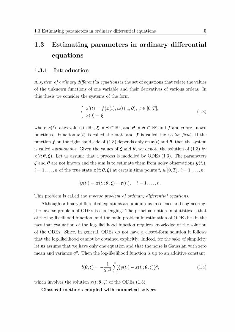
A system of ordinary differential equations is the set of equations that relate the valuesof the unknown functions of one variable and their derivatives of various orders. Inthis thesis we consider the systems of the form
x′(t) = f(x(t),u(t), t;θ), t ∈ [0, T ],x(0) = ξ,
(1.3)
where x(t) takes values in Rd, ξ in Ξ ⊂ Rd, and θ in Θ ⊂ Rp and f and u are knownfunctions. Function x(t) is called the state and f is called the vector field. If thefunction f on the right hand side of (1.3) depends only on x(t) and θ, then the systemis called autonomous. Given the values of ξ and θ, we denote the solution of (1.3) byx(t;θ, ξ). Let us assume that a process is modelled by ODEs (1.3). The parametersξ and θ are not known and the aim is to estimate them from noisy observations y(ti),i = 1, . . . , n of the true state x(t;θ, ξ) at certain time points ti ∈ [0, T ], i = 1, . . . , n:
y(ti) = x(ti;θ, ξ) + ε(ti), i = 1, . . . , n.
This problem is called the inverse problem of ordinary differential equations.Although ordinary differential equations are ubiquitous in science and engineering,
the inverse problem of ODEs is challenging. The principal notion in statistics is thatof the log-likelihood function, and the main problem in estimation of ODEs lies in thefact that evaluation of the log-likelihood function requires knowledge of the solutionof the ODEs. Since, in general, ODEs do not have a closed-form solution it followsthat the log-likelihood cannot be obtained explicitly. Indeed, for the sake of simplicitylet us assume that we have only one equation and that the noise is Gaussian with zeromean and variance σ2. Then the log-likelihood function is up to an additive constant
l(θ, ξ) = − 12σ2
n∑i=1
y(ti) − x(ti;θ, ξ)2, (1.4)
which involves the solution x(t;θ, ξ) of the ODEs (1.3).Classical methods coupled with numerical solvers
6 Introduction
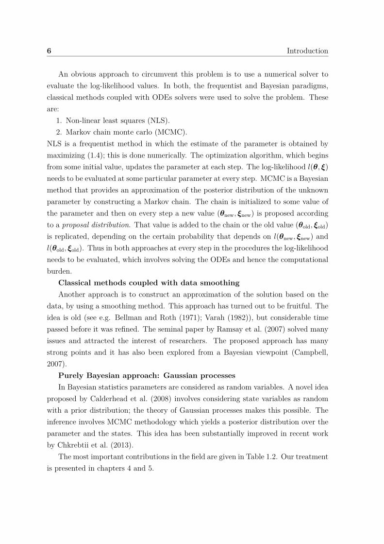
An obvious approach to circumvent this problem is to use a numerical solver toevaluate the log-likelihood values. In both, the frequentist and Bayesian paradigms,classical methods coupled with ODEs solvers were used to solve the problem. Theseare:
1. Non-linear least squares (NLS).2. Markov chain monte carlo (MCMC).
NLS is a frequentist method in which the estimate of the parameter is obtained bymaximizing (1.4); this is done numerically. The optimization algorithm, which beginsfrom some initial value, updates the parameter at each step. The log-likelihood l(θ, ξ)needs to be evaluated at some particular parameter at every step. MCMC is a Bayesianmethod that provides an approximation of the posterior distribution of the unknownparameter by constructing a Markov chain. The chain is initialized to some value ofthe parameter and then on every step a new value (θnew, ξnew) is proposed accordingto a proposal distribution. That value is added to the chain or the old value (θold, ξold)is replicated, depending on the certain probability that depends on l(θnew, ξnew) andl(θold, ξold). Thus in both approaches at every step in the procedures the log-likelihoodneeds to be evaluated, which involves solving the ODEs and hence the computationalburden.
Classical methods coupled with data smoothingAnother approach is to construct an approximation of the solution based on the
data, by using a smoothing method. This approach has turned out to be fruitful. Theidea is old (see e.g. Bellman and Roth (1971); Varah (1982)), but considerable timepassed before it was refined. The seminal paper by Ramsay et al. (2007) solved manyissues and attracted the interest of researchers. The proposed approach has manystrong points and it has also been explored from a Bayesian viewpoint (Campbell,2007).
Purely Bayesian approach: Gaussian processesIn Bayesian statistics parameters are considered as random variables. A novel idea
proposed by Calderhead et al. (2008) involves considering state variables as randomwith a prior distribution; the theory of Gaussian processes makes this possible. Theinference involves MCMC methodology which yields a posterior distribution over theparameter and the states. This idea has been substantially improved in recent workby Chkrebtii et al. (2013).
The most important contributions in the field are given in Table 1.2. Our treatmentis presented in chapters 4 and 5.

Aut
hors
Type
ofm
etho
dEr
ror
Do
allt
hest
ates
The
oret
ical
prop
ertie
sR
pack
age
need
tobe
obse
rved
?
Ram
say
etal
.(20
07)
frequ
entis
tno
ton
lyG
auss
ian
No
√n
-con
siste
ntC
ollo
cInf
eras
ympt
otic
ally
norm
alas
ympt
otic
ally
effici
ent
Brun
el(2
008)
frequ
entis
tno
ton
lyG
auss
ian
Yes
N.A
.√n
-con
siste
ntas
ympt
otic
ally
norm
al
Cal
derh
ead
etal
.(20
08)
Baye
sian
Gau
ssia
nN
oN
.A.
N.A
.
Lian
gan
dW
u(2
008)
frequ
entis
tno
ton
lyG
auss
ian
Yes
stro
ngly
cons
isten
tN
.A.
Che
nan
dW
u(2
008b
)fre
quen
tist
not
only
Gau
ssia
nN
oop
timal
conv
erge
nce
N.A
.ra
tebu
ton
lyfo
ra
linea
rm
odel
Gug
ushv
ilian
dK
laas
sen
(201
2)fre
quen
tist
not
only
Gau
ssia
nYe
s√n
-con
siste
ntN
.A.
Chk
rebt
iiet
al.(
2013
)Ba
yesia
nG
auss
ian
No
prob
abili
stic
solu
tion
N.A
.of
the
stat
eis
cons
isten
tinL
1no
rm
Dat
tner
and
Kla
asse
n(2
013)
frequ
entis
tno
ton
lyG
auss
ian
Yes
N.A
.√n
-con
siste
nt
Hal
land
Ma
(201
4)fre
quen
tist
not
only
Gau
ssia
nYe
sN
.A.
√n
-con
siste
ntas
ympt
otic
ally
norm
alTa
ble
1.2
List
ofge
nera
lmet
hods
for
solv
ing
the
inve
rse
prob
lem
ofO
DEs
star
ting
from
the
sem
inal
pape
rR
amsa
yet
al.
(200
7).
8 Introduction
1.3.2 References
Bellman and Roth (1971), Hemker (1972), Bard (1974), Varah (1982), Voit and Sav-ageau (1982), Bock (1983), Biegler et al. (1986), Vajda et al. (1986), Bates and Watts(1988), Wild and Seber (1989), Tjoa and Biegler (1991), Ogunnaike and Ray (1994),Gelman et al. (1996), Stortelder (1996), Ramsay (1996), Jost and Ellner (2000), Pas-cual and Ellner (2000), Ellner et al. (2002), Putter et al. (2002), Li et al. (2002),Madár et al. (2003), Li et al. (2005), Ramsay and B.W. (2006), Barenco et al. (2006),Lawrence et al. (2006), Lalam and Klaassen (2006), Huang et al. (2006), Huang andWu (2006), Poyton et al. (2006), Ramsay et al. (2007), Cao and Ramsay (2007), Hookerand Biegler (2007), Campbell (2007), Khanin et al. (2007), Rogers et al. (2007), Don-net and Samson (2007), Hooker (2007), Brunel (2008), Calderhead et al. (2008), Liangand Wu (2008), Chen and Wu (2008b), Varziri et al. (2008), Cao et al. (2008), Girolami(2008), Miao et al. (2008), Chen and Wu (2008a), Cao and Zhao (2008), Steinke andSchölkopf (2008), Hooker (2009), Äijö and Lähdesmäki (2009), Secrier et al. (2009),Qi and Zhao (2010), Lillacci and Khammash (2010), Lu et al. (2011), Lawrence et al.(2011), Gugushvili and Klaassen (2012), Chkrebtii et al. (2013), Dattner and Klaassen(2013), González et al. (2013), González et al. (2014), Hall and Ma (2014).
1.4 Our work and contribution
In this section we outline the contributions made by this thesis. The results presentedare based on the following articles and manuscripts: Vujačić et al. (2014a), Abbruzzoet al. (2014), Vujačić et al. (2014b), González et al. (2014) and González et al. (2013).
1. Estimating Kullback-Leibler information in Gaussian graphical mod-elsMotivation. A special feature of the Gaussian graphical model is that theestimation of its parameters, i.e. the precision matrix, can have two goals. Oneis prediction accuracy, which is usually measured in terms of Kullback-Leiblerdistance. The other is graph identification.Results. The scaled log-likelihood is a biased KL estimator and estimating thebias yields an improved estimator of KL. We propose two criteria, both hav-ing the same structure: the sum of the log-likelihood term and an estimatedbias term. The first criterion, which we call Kullback-Leibler cross-validation(KLCV), is an approximation of leave-one-out cross-validation. The second cri-
1.4 Our work and contribution 9
terion is based on the generalized information criterion (GIC), which is a gener-alization of the AIC for a wider class of models. This is the content of Chapter3, which is based on Vujačić et al. (2014a) and Abbruzzo et al. (2014).
2. Estimating graph structure in Gaussian graphical modelsMotivation. In gene regulatory networks we are usually interested in relation-ships between different elements. It is of interest to infer these relationships asrepresented by a graph. In a Gaussian graphical model framework this meansthat we are more interested in the graph induced by the precision matrix thanin the precision matrix itself.Results. The only existing closed-form model selection consistent criteria areBIC and EBIC. They use degrees of freedom that are unstable when the samplesize is small. We use the derived criteria KLCV and GIC to define alternativedegrees of freedom for Gaussian graphical models. These alternative definitionscan be used with BIC or EBIC when the sample size is small. We do not advocatetheir usage for larger sample sizes. We discuss this in Chapter 3.
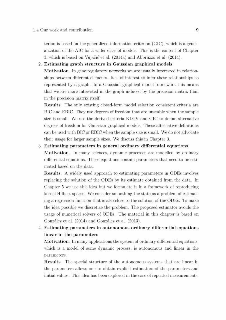
3. Estimating parameters in general ordinary differential equationsMotivation. In many sciences, dynamic processes are modelled by ordinarydifferential equations. These equations contain parameters that need to be esti-mated based on the data.Results. A widely used approach to estimating parameters in ODEs involvesreplacing the solution of the ODEs by its estimate obtained from the data. InChapter 5 we use this idea but we formulate it in a framework of reproducingkernel Hilbert spaces. We consider smoothing the state as a problem of estimat-ing a regression function that is also close to the solution of the ODEs. To makethe idea possible we discretize the problem. The proposed estimator avoids theusage of numerical solvers of ODEs. The material in this chapter is based onGonzález et al. (2014) and González et al. (2013).
4. Estimating parameters in autonomous ordinary differential equationslinear in the parametersMotivation. In many applications the system of ordinary differential equations,which is a model of some dynamic process, is autonomous and linear in theparameters.Results. The special structure of the autonomous systems that are linear inthe parameters allows one to obtain explicit estimators of the parameters andinitial values. This idea has been explored in the case of repeated measurements.
10 Introduction
For time course data we introduce a window estimator that yields√n-consistent
estimators of the parameters. The explicit form of the estimators are also avail-able in this case. Because of this, no optimization is needed and estimation iscomputationally fast. Due to its computational efficiency, the estimator can becombined with more efficient procedures. This is the topic of Chapter 4, whichis based on Vujačić et al. (2014b).
5. Inferring latent gene regulatory network kineticsMotivation. Transcription factors (TFs) are proteins that activate or repressgenes. Regulatory networks consist of genes and TFs and their dynamics canbe modelled by ODEs. It is of interest to infer the activity profile of TFs thatare unobserved, and to estimate the kinetic parameters of the ODEs using levelexpression measurements of the genes regulated by the TFs.Results. We model the regulatory network in Escherichia coli. By using thetheory developed in Chapter 5, we reconstruct the unobserved LexA transcrip-tion factor and estimate the kinetic parameters of the ODEs. We also use anEM algorithm to improve the precision of the derivative approximation. This isthe topic of Chapter 6, which is based on González et al. (2013).
1.5 Outline of the thesis
The remainder of this thesis is divided into five chapters. Chapter 2 includes back-ground material for Chapter 3; more specifically, in Chapter 2 we give an overviewof Gaussian graphical models and penalized maximum likelihood estimation as wellas model selection for these models. In Chapter 3 we describe two new estimates ofKullback-Leibler information for Gaussian graphical models and we show how theycan also be used for graph estimation. Chapter 4 deals with the estimation of param-eters of autonomous differential equations linear in the parameters. In Chapter 5 wedescribe a method for estimating parameters of general differential equations whichuses the theory of reproducing kernel Hilbert (RKHS) spaces. In Chapter 6 we applythe methodology developed in Chapter 5 to infer gene regulatory kinetics in the caseof the SOS repair system in Escherichia coli.
Chapter 2
Model selection in Gaussiangraphical models
A graphical model is a statistical model that uses a graph to represent conditionaldependencies between random variables. Having a graphical representation of the de-pendencies enables one to have better understanding of the relations between randomvariables. To undertake a formal definition of a graphical model we first introducea notion of conditional independence. Our exposition is based mainly on Lauritzen(1996). Other useful references are Whittaker (2009), Rue and Held (2005), Edwards(2000) and Fried and Vogel (2010). Hereafter we focus on continuous random vectors,although the theory is more general (Lauritzen, 1996). Therefore, throughout thischapter we consider the Lebesgue measure on the product space.
Definition 2.1. Let X, Y, Z be real random variables with a joint distribution P
that has a continuous density f with respect to the product measure. We say thatthe random variable X is conditionally independent of Y given Z under P , and writeX ⊥⊥ Y |Z[P ], if
fXY |Z(x, y|z) = fX|Z(x|z)fY |Z(y|z),
for all z with fZ(z) > 0. If Z is trivial we say that X is independent of Y , and writeX Y [P ].
The simpler notation X Y |Z and X Y is usually used. Consider a randomvector Y = (Y1, . . . , Yp)⊤ : Ω → Rp, where Ω is the sample space. We are interestedin relations of the type
YA YB|YC ,
12 Graphical models
where YA stands for (Yi)i∈A and A,B,C are subsets of the set V = 1, 2, ..., p. Theaim is to have a graph that describes the probability distribution of the vector Y . Inthis thesis, a graph is a pair G = (V,E), where V = 1, 2, ..., p is a finite set whoseelements are called nodes or vertices and E is a subset of unordered pairs of distinctvalues from V , whose elements are called edges or lines. Thus our graphs are finite –have a finite set of nodes, undirected – the edges are undirected and simple – there areno multiple edges and no edges that connect a node to itself (loops).
In order to bring together random vector Y and graph G we assign to every randomvariable Yi a node i ∈ V and to any unordered pair Yi, Yj of random variables anedge i, j ∈ E. In this context, instead of YA YB|YC we write
A B|C.
2.1 Undirected graphical models
From the definition of conditional independence it follows that the condition A B|C,can only be satisfied when the sets A,B,C are disjoint. Depending on the nature ofthe sets A,B,C we have the following so-called Markov properties. A probabilitymeasure P on Rp is said to obey:
(P) the pairwise Markov property, relative to G, if for any pair (i, j) of non-adjacentnodes
i j|V \ i, j .
(L) the local Markov property, relative to G, if for node i ∈ V
i V \ cl(i)|ne(i),
where ne(i) = j ∈ V : i, j ∈ E is the set of neighbours of a node i and cl(i) =ne(i) ∪ i is the closure of the set i.
(G) the global Markov property, relative to G if, for any triple (A,B,C) of disjointsubsets of V such that C separates A from B in G
A B|C.
The subset C is said to separate A from B if all paths in G from any a ∈ A toany b ∈ B intersect C. A path in G is a sequence of distinct nodes such that two
2.1 Undirected graphical models 13
consecutive nodes form an edge in G.The properties implicitly describe the distribution P ; they do not define the form
of the density of P , in case it exists. The next property does exactly that.(F) A probability measure P on Rp is said to factorize according to G, if for all
cliques c ⊂ V there exist non-negative functions ψc that depend on y = (y1, ..., yp)through yc = (yi)i∈c only, such that the density f of P has the form
f(y) =∏c∈C
ψc(yc),
where C is a set of cliques. A clique is a maximal subset of nodes (with respect to ⊆)that has the property that each two nodes in the subset are joined by a line.
For any undirected graph G and any probability distribution on Rp it holds that(F ) ⇒ (G) ⇒ (L) ⇒ (P ). More can be said for the distributions that have continuouspositive density; that is the content of the following theorem.
Theorem 2.1 (Hammersley and Clifford). A probability distribution with positiveand continuous density function with respect to the product measure satisfies the pair-wise Markov property with respect to an undirected graph G if and only if it factorizesaccording to G.
The theorem implies that in the case of a probability distribution with positiveand continuous density with respect to a product measure it holds that:
(F ) ⇔ (G) ⇔ (L) ⇔ (P ).
Finally, we give the definition of an undirected graphical model (Wainwright andJordan, 2008).
Definition 2.2. An undirected graphical model - also known as a Markov random field(MRF) – associated with graph G is a family of probability distributions that factorizesaccording to G.
The definition assumes the strongest F property, although some authors assumethe weakest, pairwise Markov property (Whittaker, 2009).
Definition 2.3. An undirected graphical model associated with graph G is a family ofprobability distributions that satisfies the pairwise conditional independence restrictionsinherent in G.
14 Graphical models
In the case of probability distributions that have positive and continuous den-sity, the case considered in this thesis, theorem 2.1 implies that both definitions areequivalent.
2.2 Gaussian graphical models
If in the definition of the graphical model we restrict the family of distributions to beGaussian we obtain a Gaussian graphical model (GGM). In the case of a GGM theconditional dependencies can be read off from the inverse covariance matrix which iscalled the precision matrix or concentration matrix.
The density of the normal distribution with mean µ and precision matrix Θ = (θij)has the form
f(y) = (2π)−p/2|Θ|1/2 exp−(y − µ)⊤Θ(y − µ)/2
.
The following result is of fundamental importance.
Proposition 2.1. For a Gaussian graphical model it holds
i j|V \ i, j ⇐⇒ θij = 0.
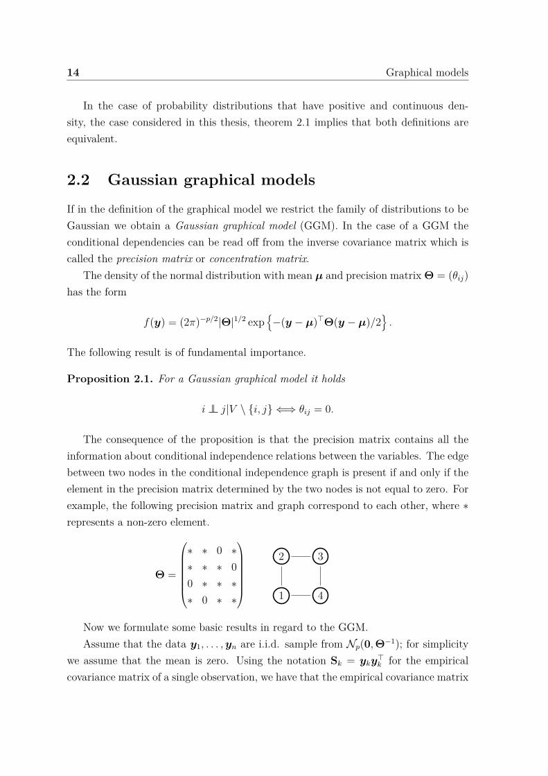
The consequence of the proposition is that the precision matrix contains all theinformation about conditional independence relations between the variables. The edgebetween two nodes in the conditional independence graph is present if and only if theelement in the precision matrix determined by the two nodes is not equal to zero. Forexample, the following precision matrix and graph correspond to each other, where ∗represents a non-zero element.
Θ =
∗ ∗ 0 ∗∗ ∗ ∗ 00 ∗ ∗ ∗∗ 0 ∗ ∗
1
2 3
4
Now we formulate some basic results in regard to the GGM.Assume that the data y1, . . . ,yn are i.i.d. sample from Np(0,Θ−1); for simplicity
we assume that the mean is zero. Using the notation Sk = yky⊤k for the empirical
covariance matrix of a single observation, we have that the empirical covariance matrix
2.3 Kullback-Leibler information 15
is given as S = ∑nk=1 Sk/n. The log-likelihood of one observation yk is up to an additive
constantlk(Θ) = 1
2log |Θ| − tr(ΘSk)
,
and the log-likelihood of the data is
l(Θ) =n∑
k=1lk(Θ) = n
2 log |Θ| − tr(ΘS). (2.1)
For the result that follows we introduce some notation. The commutation matrix Kp
is defined as a matrix that has the property KpvecA = vecA⊤ for any p × p matrixA. Here, vec is the vectorization operator which transforms a matrix into a columnvector obtained by stacking the columns of the matrix on top of one another. DefineMp = (Ip2 + Kp)/2, where Ip2 is identity matrix of order p2.
Proposition 2.2. If n > p the maximum likelihood estimator (MLE) almost surelyexists and is given by Θ = S−1. Furthermore, Θ is a strongly consistent estimator ofthe true precision matrix Θ0 and
√n(Θ − Θ0) → Np2
(0, 2Mp(Θ0 ⊗ Θ0)
), n → ∞.
For details see Fried and Vogel (2010).
2.3 Kullback-Leibler information
In this section we review the Kullback-Leibler information which is used as a crite-rion for evaluating statistical models. Assume that the data D = y1, . . . ,yn arei.i.d. sample generated from some p-dimensional distribution q that we refer to asthe true distribution. Let Θ ⊂ Rp and consider a parametric family of distributionsp(y|θ);θ ∈ Θ that we use to approximate the true distribution.
The goodness of the model p(y) can be assessed in terms of its closeness to the truedistribution q(y). Akaike (1973) proposed to measure this closeness by using Kullback-Leibler information [or Kullback-Leibler divergence, Kullback and Leibler (1951), here-inafter abbreviated as “KL”]:
KL(q; p) = Eq
log q(Y )
p(Y )
=∫Rp
logq(y)p(y)
q(y)dy.
16 Graphical models
Here, Y stands for the random variable distributed according to p(y). The basicproperties of KL are given in the following proposition (Konishi and Kitagawa, 2008).
Proposition 2.3 (Properties of KL.). The KL has the following properties:1. KL(q; p) ≥ 0,2. KL(q; p) = 0 ⇔ q(y) = p(y).
KL is not a metric on the space of probability distributions since it is not symmetricand does not satisfy the triangle inequality. KL is, up to a constant, equal to the minusexpected log-likelihood since
KL(q; p) = Eq
log q(Y )
p(Y )
= Eqlog q(Y ) − Eqlog p(Y ) = C − Eqlog p(Y ),
where C = Eqlog q(Y ) does not depend on p. Assume that p is chosen from aparametric family of distributions, i.e. p(·) = p(·|θ), where θ is an estimator ofθ. Denote by l(θ|DS) the log-likelihood function based on the data set DS ⊂ Dand let lk(θ) = l(θ|yk) and l(θ) = l(θ|D) denote the log-likelihood based on thekth observation and the entire data set, respectively. Estimating Eqlog p(y|θ) byreplacing the density q(y) by its empirical counterpart we obtain that
KL(q(·); p(·|θ)) = − 1n
n∑k=1
log p(yk|θ) = − 1n
n∑k=1
lk(θ) = − 1nl(θ).
Thus the scaled log-likelihood is an estimator of KL. However, it is a biased esti-mator since the data have been used twice – once to obtain the estimator θ and onceto obtain the empirical density of the true distribution. We list some of the estimatorsof KL that reduce this bias.
Akaike’s Information Criterion (AIC) Akaike’s Information Criterion, intro-duced by Akaike (1973), is an estimator of KL in the case of the models estimatedby maximum likelihood. It reduces the bias by adding the penalty to the likelihood,where the penalty is given in terms of the number of the parameters of the model.AIC has the form:
AIC = −2l(θ) + 2df,
where df = dim(Θ). Similarly, in case of penalized maximum likelihood estimatorswe can define the AIC selector (Zhang et al., 2010), which is a special case of Nishii’sgeneralized information criterion (GIC) (Nishii, 1984). The AIC selector has the form:
2.3 Kullback-Leibler information 17
AIC = −2l(θλ) + 2df(λ), (2.2)
where θλ is the penalized maximum likelihood estimator and df(λ) is the degrees offreedom of the corresponding model. We refer to these criteria simply as AIC.
Generalized Information Criterion (GIC) Generalized Information Criterion,introduced by (Konishi and Kitagawa, 1996), is an estimator of KL which is applicableto a wide class of models and not only for models estimated by maximum likelihood.This is different from the GIC proposed by (Nishii, 1984). Here we present the GICfor M estimators. An M -estimator is defined as a solution of the system of equations
n∑k=1ψ(yk,θ) = 0d,
where ψ is a column vector of dimension d and 0d is the zero vector of the samedimension. The GIC for an M -estimator (Konishi and Kitagawa, 2008) is given by:
GIC = −2l(θ) + 2tr(R−1Q), (2.3)
where R and Q are square matrices of order p given by
R = − 1n
n∑k=1
Dψ(yk, θ)⊤,
Q = 1n
n∑k=1ψ(yk, θ)Dlk(θ).
Here, Dψ(yk, θ) and Dlk(θ) are Jacobian matrices of corresponding functions at θ.We use the definition of the derivative given in Magnus and Neudecker (2007) (see ap-pendix 3.B on matrix calculus). The maximum likelihood estimator is an M -estimator,corresponding to ψ(yk,θ) = vecDlk(θ).
Cross-validation (CV) Cross-validation (Stone, 1974) is an estimator of KL thatinvolves reusing the data. We split the data D into K, roughly equal-sized parts, thatwe denote by D1, . . . ,DK . For the kth part of the data Dk, we estimate the parameterθ by using the data from the other K − 1 parts. Denote this estimator by θ−(k).Then we calculate the minus log-likelihood based on Dk at the estimate θ−(k); thisis an estimator of KL. This procedure is repeated for k = 1, 2, . . . , K and then the
18 Graphical models
estimators are averaged. In other words, the cross-validation estimator of KL is
CV = − 1K
K∑k=1
l(θ−(k)|Dk). (2.4)
Usual choices of K are 5 or 10. When K = N we obtain leave-one-out cross-validation(LOOCV)
LOOCV = − 1n
n∑k=1
l(θ−(k)|yk) = − 1n
n∑k=1
lk(θ−(k)). (2.5)
We finish the section by presenting the KL between two normal distributions andwriting the explicit form of the bias.
KL for normal models. Let q(y) = Nd(y; 0,Θ−1q ) and p(y) = Nd(y; 0,Θ−1
p ) bethe multivariate normal densities. Then (Penny, 2001):
KL(q; p) = 12− log |Θ−1
q Θp| + tr(Θ−1q Θp) − d. (2.6)
Having in mind expression for the log-likelihood in Gaussian models (see 2.1) and thatit is a biased estimator of KL we can write
KL(q; p) = − 1nl(Θp) + bias, (2.7)
where bias = trΘp(Θ−1q − S)/2.
2.4 Penalized likelihood estimation in Gaussian Graph-ical Models
2.4.1 Estimation
Suppose we have n i.i.d. multivariate observations y1, . . . ,yn from distribution Np(0,Θ−1).When n > p the precision matrix Θ can be estimated by maximizing the scaled log-likelihood function (see 2.1)
2nl(Θ) = log |Θ| − tr(ΘS),
over positive definitive matrices Θ. The global maximizer, called the maximum likeli-hood estimator, almost surely exists and is given by Θ = S−1 (Proposition 2.2). Whenn ≤ p a maximum likelihood estimator does not exist. Moreover, in the case when
2.4 Penalized likelihood estimation in Gaussian graphical model 19
n > p and the true precision matrix is known to be sparse, the MLE has a non-desirableproperty: with probability one all elements of the precision matrix are nonzero. Asparse estimator can be obtained by maximizing the penalized log-likelihood:
Θλ = argmaxΘ log |Θ| − tr(ΘS) −p∑
i=1
p∑j=1
pλij(|θij|), (2.8)
where the maximization is over positive definitive matrices Θ. Here, pλijis a sparsity
inducing penalty function, θij is the (i, j)th entry of matrix Θ and λij > 0 is the corre-sponding regularization parameter. We refer to λ = (λ11, . . . , λpp) as a regularizationparameter and typically λ11 = . . . = λpp = λ.
The LASSO penalty uses the L1 penalty function pλ(|θ|) = λ|θ|. Friedman et al.(2008) propose the graphical lasso algorithm for the optimization in (2.8) in the caseof the LASSO penalty. The algorithm uses a coordinate descent procedure and isextremely fast. However, it is known that the LASSO penalty produces substantialbiased estimates in a regression setting (Fan and Li, 2001). To address this issueLam and Fan (2009) have studied the theoretical properties of sparse precision matrixestimation via a general penalty function satisfying the properties in Fan and Li (2001).This general penalty function includes LASSO and also SCAD and adaptive LASSOpenalties, originally introduced in a linear regression setting (Fan and Li, 2001; Zou,2006). They also show that the LASSO penalty produces bias in the case of sparseprecision matrix estimation. The SCAD penalty has a derivative of the form
p′λ,a(|θ|) = λI(|θ| ≤ λ) + (aλ− |θ|)+
a− 1 I(|θ| > λ),
where a is a constant usually set to 3.7 (Fan and Li, 2001). Another penalty, calledthe adaptive LASSO, which is proposed in Zou (2006), uses the L1 penalty functionpλ(|θ|) = λ|θ| and
λij = λ/|θij|γ,
where γ > 0 is a constant and θij is any consistent estimator of θij. The constant γ isusually chosen to be 0.5. Implementing the optimization with the SCAD and adaptiveLASSO penalties can be done efficiently by using the graphical lasso algorithm (Fanet al., 2009).
These penalties are important because under certain conditions the estimated pre-cision matrix tends to the true one when sample size tends to infinity. Also, theestimator has the sparsistency property, which means that when sample size tends to
20 Graphical models
infinity all the parameters that are zero are actually estimated as zero with probabilitytending to one (Lam and Fan, 2009). Also Fan et al. (2009) show that using the SCADpenalty in a GGM setting produces estimators that are not just sparsistent but also√n-consistent, asymptotically normal, and have the oracle property. They also prove
that oracle property holds for the adaptive LASSO penalty. Oracle property of theestimator means that the estimator performs as if the correct submodel is known inadvance. More specifically, when there are zeros in the true precision matrix, they areestimated as zero with probability tending to one, and the nonzero components areestimated as if the correct submodel is known.
We refer to a Gaussian graphical model estimated by penalized maximum likelihoodas a penalized Gaussian graphical model.
2.4.2 Model selection
Model selection in penalized graphical models is essentially a matter of choosing theregularization parameter. It has been shown that certain asymptotic rates of λ resultin consistent or sparsistent estimators (Ravikumar et al., 2011; Lam and Fan, 2009).However, for finite n and p the choices are less clear. In this section we review existingmethods for selection of λ.
In what follows, we use the notion of degrees of freedom in Gaussian graphicalmodels, defined as (Yuan and Lin, 2007):
df(λ) =∑
1≤i<j≤p
I(θij,λ = 0),
where θij,λ is (i, j)th entry of the estimated precision matrix Θλ and I is the indicatorfunction.
1. Bayesian Information Criterion (BIC) (Yuan and Lin, 2007; Schmidt, 2010;Menéndez et al., 2010; Lian, 2011; Gao et al., 2012) has the form
BIC(λ) = −2l(Θλ) + log ndf(λ).
Roughly speaking, the criterion provides an approximation of the natural log-arithm of the posterior probability of the model defined by Θλ scaled with -2.Approximation is based on the assumption that when n tends to infinity p isfixed.
2. Extended Bayesian Information Criterion (EBIC) (Foygel and Drton,
2.4 Penalized likelihood estimation in Gaussian graphical model 21
2010; Gao et al., 2012) is an extension of BIC and is introduced to deal withcases when also p tends to infinity together with n. It has the form
EBIC(λ) = −2l(Θλ) + (log n+ 4γ log p)df(λ),
where γ ∈ [0, 1] is the parameter that penalizes the number of models, whichincreases when p increases. In case of γ = 0 the classical BIC is obtained.Typical values for γ are 1/2 and 1.
3. Aikaike’s Information Criterion (AIC) (Menéndez et al., 2010; Liu et al.,2010; Lian, 2011) has the form c.f. (2.2)
AIC(λ) = −2l(Θλ) + 2df(λ).
4. Cross-validation (CV) (Rothman et al., 2008; Fan et al., 2009; Schmidt, 2010;Ravikumar et al., 2011; Fitch, 2012) has the form c.f. (2.4)
CV(λ) = − 1n
K∑k=1
nk
[log |Θ(−k)
λ | − tr
S(k)Θ(−k)λ
],
where nk is the sample size of the kth partition, Θ(−k)λ is the estimator of the
precision matrix, with λ as regularization parameter, based on the data withkth partition excluded and S(k) is the empirical covariance matrix based on thekth partition of the data. The formula presented here differs from the one given,for example, in (Fan et al., 2009; Lian, 2011) in that we have the term −1/n infront of the sum. This term is usually omitted for the sake of simplicity.
5. Generalized Approximate Cross Validation (GACV) (Lian, 2011) is in-troduced as an approximation of leave-one-out cross validation (LOOCV) andhas the form
GACV(λ) = −2l(Θλ) + 2n∑
k=1vec(Θ−1
λ − Sk)⊤vecΘλ(S(−k) − S)Θλ,
where S(−k) is the empirical covariance matrix based on the data with kth obser-vation excluded. The formula presented here differs from the one given in Lian(2011) in that we have scaled it with −2. We introduce this scaling to make theconnection with KL.For any criterion mentioned above, denoted by CRITERION, the best regular-
22 Graphical models
ization parameter is chosen as
λ∗ = argminλCRITERION(λ).
6. Stability Approach to Regularization Selection (StARS) (Liu et al.,2010) is based on the idea of subsampling. First, define Λ = 1/λ so that smallΛ corresponds to a more sparse graph. Let Gn = Λ1, . . . ,ΛK be a grid ofregularization parameters. Let b = b(n) be such that 1 < b(n) < n. We draw N
random subsamples D1, . . . ,DN from y1, . . . ,yn each of size b. The estimationof a graph for each Λ ∈ Gn yields N estimated edge matrices Eb
1(Λ), . . . , EbN(Λ).
Let ψΛ(·) denote the graph estimation algorithm with the regularization param-eter Λ and for any subsample Dj let ψΛ
st(·) be equal to one if the estimationalgorithm puts an edge s, t, and otherwise let it be equal to zero. Define theparameters θb
st(Λ) = P (ψΛst(Y1, . . . ,Yb) = 1) and ξb
st(Λ) = 2θbst(Λ)1 − θb
st(Λ)and its estimators θb
st(Λ) = 1N
∑Nj=1 ψ
Λst(Dj) and ξb
st(Λ) = 2θbst(Λ)1 − θb
st(Λ),respectively. Then ξb
st(Λ) is the variance of the Bernoulli indicator of the edges, t as well as the fraction of times each pair of graphs disagree on the pres-ence of the edge. For Λ ∈ Gn, the quantity ξb
st(Λ) measures instability of theedge across subsamples, with 0 ≤ ξb
st(Λ) ≤ 1/2. Total instability is defined byaveraging over all edges Db(Λ) = Σs<tξ
bst/(
p2
). Let Db(Λ) = sup0≤t≤Λ Db(t), then
the StARS approach chooses Λ by defining
Λs = supΛ : Db(Λ) ≤ β
for specified cut point value β, usually taken to be equal to 0.05.
2.4.3 Measuring the goodness of a model
The goodness of the estimated precision matrix can be evaluated in terms of: (i) graphaccuracy, i.e. how close its corresponding graph is to the true graph or (ii) predictionaccuracy. BIC, EBIC and StARS are designed for the former and CV, GACV andAIC for the latter.To measure graph accuracy we use F1 measure
F1 = 2TP2TP + FN + FP ,
2.4 Penalized likelihood estimation in Gaussian graphical model 23
where True and False Positives (TP/FP) refer to the estimated edges that are cor-rect/incorrect; True and False Negatives (TN/FN) are defined in a similar way (Baldiet al., 2000; Powers, 2011). The F1 score measures the quality of a binary classifier bytaking into account both true positives and negatives and takes values in the interval[0, 1]. The larger the value of this measure, the better the classifier. The predictionaccuracy is measured by KL-information.
Depending on whether we are interested in graph identification or prediction weshould use different methods for choosing the regularization parameter (see Section3.1).If the aim is graph estimation then the criteria BIC, EBIC and StARS are appropriate.Most of them are graph selection consistent, which means that when the sample sizegoes to infinity they identify the true graph. The BIC is shown to be consistent for pe-nalized graphical models with adaptive LASSO and SCAD penalties for fixed p (Lian,2011; Gao et al., 2012). Numerical results suggest that the BIC is not consistent withthe LASSO penalty (Foygel and Drton, 2010; Gao et al., 2012). When also p tendsto infinity EBIC is shown to be consistent for the graphical LASSO, though only fordecomposable graphical models (Foygel and Drton, 2010). The disadvantage of EBICis that it includes an additional parameter γ that needs to be tuned. Gao et al. (2012)set γ to one and show that in this case the EBIC is consistent with the SCAD penalty.StARS has the property of partial sparsistency which means that when the samplesize goes to infinity all the true edges are included in the selected model (Liu et al.,2010).On the other hand, Cross-validation (CV), Generalized Approximate Cross Validation(GACV) and AIC are methods for evaluating prediction accuracy. Cross-validationand AIC are both estimators of Kullback-Leibler (KL) loss (Yanagihara et al., 2006),which under some assumptions are asymptotically equivalent (Stone, 1977). General-ized Approximate Cross Validation is also an estimator of KL loss since it is derivedas an approximation to leave-one-out cross-validation (Lian, 2011). The advantage ofAIC and GACV is that they are less computationally expensive than CV. In the nextchapter we propose two new estimators of Kullback-Leibler loss. We also show howthey can be used for graph estimation.

24 Graphical models
2.5 Summary
In this chapter we have reviewed undirected graphical models which are widely usedto model conditional independence relationships. We focused on a special class, Gaus-sian graphical models (GGMs), for which the pattern of zeros in the precision matrixdetermines the conditional independence relationships. When the number of variablesis large as compared to the sample size, we have introduced the penalized likelihoodestimation of GGMs. The Kullback-Leibler (KL) information was introduced as a cri-terion to evaluate statistical models. Various estimators of KL, such as the Akaike’sInformation Criterion (AIC), Cross Validation (CV) and Generalized ApproximateCross Validation (GACV) for Gaussian graphical models were presented. These cri-teria yield an estimator of a precision matrix which has good predictive power. Forgraph estimation we presented the Bayesian Information Criterion (BIC), ExtendedBayesian Information Criterion (EBIC) and Stability Approach to Regularization Se-lection (StARS).
Chapter 3
Estimating the KL loss in Gaussiangraphical models
In this chapter, we propose two estimators of the Kullback-Leibler loss in Gaussiangraphical models. One approach uses the Generalized Information Criterion (GIC)and the other, which we call Kullback Leibler cross-validation (KLCV), is based onderiving a closed form approximation of leave-one-out cross validation. We first derivethe formulae for the maximum likelihood estimator (MLE) for both GIC and KLCV.For the maximum penalized likelihood estimator (MPLE) we use a unifying frameworkwhich allows us to modify the formulae derived for the MLE so as to incorporate theassumption of sparsity. As pointed out in the previous chapter, in GGM a distinctionshould be made between estimating the KL and estimating the graph. Consequently,we treat the graph estimation problem separately. We explore the use of the pro-posed criteria in the graph estimation problem by combining it with consistent graphselection criteria such as BIC and EBIC.
The remainder of this chapter is divided into seven sections. In Section 3.1 weclarify the aim of different model selection methods. In Section 3.2 we introduce twonew estimators of KL loss for which the derivation is given in Section 3.3. Section3.4 deals with the computational aspect of the proposed methods, while Section 3.5shows their performance on simulated data. Finally, the use of the proposed criteriafor graph estimation is explored in Section 3.6. The last section contains the summary.All proofs and auxiliary results are given in the Appendix.
26 Entropy loss in GGMs
3.1 Prediction VS graph structure
Let Θ be a precision matrix that corresponds to the true non-complete graph G andlet Θϵ be the matrix obtained by adding ϵ > 0 to every entry of matrix Θ. The matrixΘϵ is positive definite since it is a sum of one positive definite matrix and one positivesemi-definite matrix. Indeed, Θϵ = Θ+xϵx
⊤ϵ , where xϵ = (
√ϵ, . . . ,
√ϵ)⊤ is a vector of
dimension p. Hence, Θϵ belongs to the class of precision matrices and it corresponds toa graph Gϵ. The Kullback-Leibler divergence of N (0,Θ−1
ϵ ) from N (0,Θ−1), denotedby KL(Θ; Θϵ), is equal to
KL(Θ; Θϵ) = 12tr(Θ−1Θϵ) − log |Θ−1Θϵ| − p
(see 2.6). Since ϵ → 0 implies Θϵ → Θ, by continuity of the log-determinant and traceit follows that
limϵ↓0
KL(Θ; Θϵ) = 0.
However, for every 0 < ϵ < mini,j |θij| the matrix Θϵ is a matrix without zero entriesand consequently the graph Gϵ is the full graph. Thus, even though a matrix canbe close to the precision matrix of the true distribution with respect to KL loss, thecorresponding graph can be completely different from the true one.
Since K-CV, AIC and GACV are estimators of KL, their use is appropriate forobtaining a model with good predictive power. On the other hand, the previousexample indicates that they should not be used for graph identification. The followingtheorem confirms this claim in the case of the AIC when p is fixed as n → ∞. Toformulate the theorem we introduce some notation and assumptions. Each precisionmatrix induces a set of labels corresponding to its nonzero entries. The full modelα = (i, j) : i, j = 1, . . . , p; i < j is the set of labels of all entries in the upperdiagonal of the corresponding precision matrix; it corresponds to precision matriceswithout nonzero elements. A candidate model is a set α ⊂ α that consists of labels ofnonzero elements of the corresponding precision matrix. We denote by A the collectionof all candidate models and assume that there is a unique true model α0 in A. LetΩ− = λ : αλ ⊃ α0, Ω0 = λ : αλ = α0 and Ω+ = λ : αλ ⊃ α0 and αλ = α0denote the sets of regularization parameters that induce, respectively, underfitted,true, and overfitted model. We assume technical conditions as in Zhang et al. (2010),from which the proof is adapted. These conditions are satisfied by SCAD and L1
penalties.
3.2 The GIC and the KLCV as estimators of the KL loss 27
Theorem 3.1. Assume that p is fixed as n → ∞ and denote the optimal tuningparameter selected by minimizing AIC(λ) by λAIC. Then the penalized likelihood esti-mator defined in 2.8 cannot correctly identify all the zero elements in the true precisionmatrix. That is,
P (λAIC ∈ Ω−) → 0 and P (λAIC ∈ Ω+) → π,
where π is a nonzero probability.
The proof of the theorem is given in the Appendix 3.A. We conjecture that thetheorem also holds in the case when p → ∞ as n → ∞. Moreover, we hypothesizethat GACV and K-CV, where K is fixed as n → ∞ are not graph selection consistent.
For graph identification, BIC, EBIC and StARS are appropriate because of theirgraph selection consistency. Consequently, we treat these two problems separately.We devote the next section to two new estimators of KL and in Section 3.6 we showhow they can be used to improve the performance of E(BIC).
3.2 The GIC and the KLCV as estimators of theKL loss
In this section, we propose two new estimators of the KL in GGMs. Let Θλ be themaximum penalized likelihood estimator defined by (2.8). The Kullback-Leibler di-vergence of the model N (0, Θ−1
λ ) from the true distribution N (0,Θ−10 ) can be written
up to an additive constant as (see 2.7)
KL(Θ0; Θλ) = − 1nl(Θλ) + bias,
where l(Θ) = nlog |Θ| − tr(ΘS)/2 and bias = trΘλ(Θ−10 − S)/2. By estimating
the bias term we obtain an estimate of the KL. The first estimator we propose, theso-called Generalized Information Criterion (GIC), has the form
GIC(λ) = −2l(Θλ) + 2dfGIC,
28 Entropy loss in GGMs
where
dfGIC = 12n
n∑k=1
vec(Sk Iλ)⊤vecΘλ(Sk Iλ)Θλ − 12vec(S Iλ)⊤vecΘλ(S Iλ)Θλ,
(3.1)where Iλ is the indicator matrix, whose entry is 1 if the corresponding entry in theprecision matrix Θλ is nonzero and zero if the corresponding entry in the precisionmatrix is zero. Here is the Schur or Hadamard product of matrices. In fact, GIC isan estimator of KL scaled by 2n, which means that the estimator of the bias providedby GIC is dfGIC/n. We keep the scale in order to be consistent with the originaldefinition of GIC (see 2.3).
Another estimator which we propose, referred to as the Kullback-Leibler cross-validation (KLCV), has the form
KLCV(λ) = − 1nl(Θλ) + biasKLCV, (3.2)
where
biasKLCV = 12n(n− 1)
n∑k=1
vec(Θ−1λ − Sk) Iλ⊤vec[Θλ(S − Sk) IλΘλ]. (3.3)
To obtain the model N (0, Θλ∗), which is good in terms of prediction, we pick λ∗ thatminimizes GIC(λ) or KLCV(λ) over λ > 0.
3.3 Derivation of the GIC and the KLCV
In this section we derive the GIC and the KLCV, in two steps. First, we derivethe criteria for the maximum likelihood estimator. In the second step we use thederived formula and the assumption of sparsity to propose a formula for the maximumpenalized likelihood estimator. The obtained formula is an extension of that for MLE,since both formulae are equivalent in the case of the maximum likelihood estimator.
3.3.1 Derivation of the GIC for the maximum likelihood es-timator
The log-likelihood of one observation yk for a Gaussian model Np(0,Θ−1) is, up toan additive constant, lk(Θ) = 1
2log |Θ| − tr(ΘSk)
, where Sk = yky
⊤k . The maxi-
3.3 Derivation of the GIC and the KLCV 29
mum likelihood estimator Θ is an M-estimator defined as a solution of the system ofequations
n∑k=1ψ(yk,Θ) = 0p2 , (3.4)
where ψ(yk,Θ) = vecDlk(Θ) and 0p2 is the p2-dimensional zero vector. Consequently,the GIC for Θ (see 2.3) is given by:
GIC = −2l(Θ) + 2tr(R−1Q),
where R and Q are square matrices of order p2
R = − 1n
n∑k=1
Dψ(yk, Θ)⊤, (3.5)
Q = 1n
n∑k=1ψ(yk, Θ)Dlk(Θ). (3.6)
We are interested in deriving the term tr(R−1Q). Using matrix differential calculus(see Appendix 3.B) we obtain
ψ(yk,Θ) = vecDlk(Θ) = 12vec(Θ−1 − Sk),
Dψ(yk; Θ)⊤ = −12Θ−1 ⊗ Θ−1. (3.7)
Using (3.4), (3.6) and equality Θ−1 = S (see Appendix 3.D for details) yields
Q = 14n
n∑k=1
vecSkvecS⊤k − 1
4vecSvecS⊤.
Expression for R−1 we obtain from (3.5) and (3.7)
R−1 = 2Θ ⊗ Θ.
Finally, formulas tr(AB) = tr(BA) and tr(x⊤Ax) = x⊤Ax imply that
tr(R−1Q) = 12n
n∑k=1
vecS⊤k (Θ ⊗ Θ)vecSk − 1
2vecS⊤(Θ ⊗ Θ)vecS.
This formula is equivalent to (3.1) without the Schur product. This is shown in theSection 3.3.3.
30 Entropy loss in GGMs
3.3.2 Derivation of the KLCV for the maximum likelihoodestimator
We follow the idea of Xiang and Wahba (1996), i.e. we introduce an approximationfor LOOCV via several first order Taylor expansions. Lian (2011) uses this idea toderive the GACV for the MPLE in GGM, where in deriving the formula, the partialderivatives corresponding to the zero elements of the precision matrix are ignored.Here, unlike in Lian (2011), we apply the idea only for the MLE and therefore weavoid all technical difficulties entailed in ignoring the derivatives. We deal with theMPLE separately in the next section.
Consider the following function of two variables
f(S,Θ) = 2nl(Θ) = log |Θ| − tr(SΘ).
With this notation we have the identity
n∑k=1
f(Sk,Θ) = nf(S,Θ). (3.8)
Let Θ(−k) be the MLE estimator of the precision matrix defined based on the dataexcluding the kth data point. The leave-one-out cross validation score (see 2.5 ) isdefined by
LOOCV = − 1n
n∑k=1
lk(Θ(−k)) = − 12n
n∑k=1
f(Sk, Θ(−k))
= − 12n
n∑k=1
f(Sk, Θ(−k)) − f(Sk, Θ) + f(Sk, Θ)
(3.8)= −12f(S, Θ) − 1
2n
n∑k=1
f(Sk, Θ(−k)) − f(Sk, Θ)
≈ − 1nl(Θ) − 1
2n
n∑k=1
df(Sk, Θ)dΘ
⊤
vec(Θ(−k) − Θ).
Using matrix differential calculus (see Appendix 3.B) we deduce that df(Sk, Θ)/dΘ =vec(Θ−1 −Sk)⊤. The term vec(Θ(−k) − Θ) is obtained via the Taylor expansion of the
vector valued function(
df(S(−k),Θ(−k))dΘ
)⊤around (S, Θ). We expand the transposed
3.3 Derivation of the GIC and the KLCV 31
term because we consider vectors as columns.
0p2 =df(S(−k), Θ(−k))
dΘ
⊤
≈
df(S, Θ)dΘ
⊤
+ d2f(S, Θ)dΘ2 vec(Θ(−k) − Θ)
+ d2f(S, Θ)dΘdS
vec(S(−k) − S).
From here it follows that
vec(Θ(−k) − Θ) ≈ −
d2f(S, Θ)dΘ2
−1d2f(S, Θ)
dΘdSvec(S(−k) − S).
We have df(S, Θ)/dΘ = vec(Θ−1−S)⊤, so d2f(S, Θ)/dΘdS = −Ip2 , d2f(S, Θ)/dΘ2 =−Θ−1 ⊗ Θ−1 and consequently
vec(Θ(−k) − Θ) ≈ −(Θ ⊗ Θ)vec(S(−k) − S).
Therefore, the approximation of LOOCV, denoted by KLCV, has the form
KLCV = − 1nl(Θ) + 1
2n
n∑k=1
vec(Θ−1 − Sk)⊤(Θ ⊗ Θ)vec(S(−k) − S).
After simplifying the term in the sum we finally obtain
KLCV = − 1nl(Θ) + 1
2n(n− 1)
n∑k=1
vec(Θ−1 − Sk)⊤(Θ ⊗ Θ)vec(S − Sk).
This formula is equivalent to (3.2) without the Schur product. This is shown in thenext section.
3.3.3 Extension of the GIC and the KLCV for the maximumpenalized likelihood estimator
Before proposing the formulae for the penalized case we formulate two auxiliary results.
Lemma 3.1. Let A and Θ be symmetric matrices of order p. Then the followingidentity holds
(Θ ⊗ Θ)vecA = Mp(Θ ⊗ Θ)vecA. (3.9)
32 Entropy loss in GGMs
Lemma 3.2. Let A be a symmetric matrix of order p and x,y any vectors of dimen-sion p. Then the value of the bilinear form
B(x,y) = x⊤Ay,
when ith row (respectively column) of the matrix A is set to zero is the same as thevalue of B(x,y) when ith entry of the vector x (respectively y) is set to zero.
The proof of Lemma 3.1 is given in the Appendix 3.E; Lemma 3.2 is obtained bystraightforward calculation. The penalty terms added to the log-likelihood in the GICand the KLCV can be written in terms of the expression
T (A,B) = (vecA)⊤(Θ ⊗ Θ)vecB, (3.10)
where A and B are symmetric matrices of order p. Indeed,
biasKLCV = 12n(n− 1)
n∑k=1
T (Θ−1 − Sk,S − Sk), (3.11)
dfGIC = 12n
n∑k=1
T (Sk,Sk) − 12T (S,S). (3.12)
According to Lemma 3.1 it follows that
T (A,B) = (vecA)⊤Mp(Θ ⊗ Θ)vecB.
The fact that 2Mp(Θ ⊗ Θ) is an estimator of the asymptotic covariance matrix of Θ(Proposition 2.2) suggests an asymptotic argument for treating the case of a penalizedestimator. Essentially, we only need to define the term T (A,B) for the MPLE.To obtain the formula for the MPLE we assume standard conditions, as in Lam and Fan(2009), that guarantee a sparsistent MPLE. These conditions imply that λ → 0 whenn → ∞, so we use formula (3.10), derived for the MLE, as an approximation in thepenalized case. By sparsistency it follows that with probability one the zero coefficientsare estimated as zero when n tends to infinity. This implies that, asymptotically, thecovariances between the zero elements and the nonzero elements in the estimatedprecision matrix are equal to zero. Thus, to obtain the term Tλ(A,B) for the MPLEwe not only plug the expression Θλ into the formula for the term T (A,B), but we alsoset the elements of the matrix Mp(Θλ ⊗ Θλ) that correspond to covariances betweenthe zero and nonzero elements of the precision matrix to zero. According to Lemma
3.3 Derivation of the GIC and the KLCV 33
3.2 this is equivalent to setting the corresponding entries of vectors vecA and vecB tozero, i.e.
Tλ(A,B) def= vec(A Iλ)⊤Mp(Θλ ⊗ Θλ)vec(B Iλ)= vec(A Iλ)⊤(Θλ ⊗ Θλ)vec(B Iλ), (3.13)
where the second equality follows from Lemma 3.1. The obtained formula involves ma-trices of order p2, which entails high cost in terms of memory usage and floating-pointoperations. For this reason, we rewrite the formula in a way that it is computationallyfeasible. Following Lian (2011) we apply identity vec(ABC) = (C⊤ ⊗ A)vecB to(3.13) and obtain
Tλ(A,B) = vec(A Iλ)⊤vecΘλ(B Iλ)Θλ. (3.14)
For details on the implementation of this formula, see the next section. Finally, itfollows that bias and degrees of freedom terms for the GIC and the KLCV in the caseof the MPLE are obtained by substituting T with Tλ in expressions (3.11) and (3.12),i.e
biasKLCV(λ) = 1n(n− 1)
n∑k=1
Tλ(Θ−1λ − Sk,S − Sk),
dfGIC(λ) = 12n
n∑k=1
Tλ(Sk,Sk) − 12T (S,S),
which are formulae presented in (3.3) and (3.1).
To conclude this section, we show that the derived formulae for the MPLE areextensions of the corresponding formulae for the MLE, meaning that applying theMPLE formulae to the maximum likelihood estimator yields the same result as thecorresponding MLE formulae. To this aim, let Θ be the maximum likelihood estimatorof the precision matrix, which is the MPLE for λ = 0, i.e. Θ = Θλ, for λ = 0. Sincewith probability one all the elements of Θ are nonzero it follows that Iλ is the matrixwith all entries equal to one. This implies that in the formula (3.13) we have AIλ = Aand B Iλ = B, which in turn implies Tλ(A,B) = T (A,B).
34 Entropy loss in GGMs
3.4 Implementation
In this section, we give more details as to why formula (3.14) is computationally muchmore efficient than (3.13). Also, we show how to implement (3.14) efficiently. First, thecomputational complexity of (3.14) is O(p3) while for (3.13) it is O(p4) (see Appendix3.F for details). Furthermore, (3.13) requires storing matrices of order p2, which is p4
elements per matrix. Even for moderate p, allocation of that amount of memory ona standard desktop computer is not possible. On the other hand, the formula (3.14)is written in terms of vectors of dimension p2, which implies storing of p2 elementsper vector. To further simplify, we demonstrate that we can avoid the usage of thetranspose and vectorization operators. For any matrices X = (xij) and Y = (yij) itholds that (vecX)⊤vecY = ∑
i,j xijyij so it follows that (vecX)⊤vecY is just the sumof the elements of the matrix X Y, i.e. (vecX)⊤vecY = ∑
i,j(X Y)ij. Applying thisto (3.14) we obtain
Tλ(A,B) =∑i,j
(A Iλ Θλ(B Iλ)Θλ)ij.
In the statistical programming language R, expression ∑i,j(X Y)ij can be efficientlyimplemented as sum(X*Y). This can be used in expressions (3.1) and (3.3).
3.5 Simulation study
In this section, we test the performance of the proposed formulas in terms of Kullback-Leibler loss. We do this in the case of the LASSO penalty for two sparse hub graphs.The graphs have p = 40 nodes and 38 edges and p = 100 nodes and 95 edges. Thesparsity values of these graphs are 0.049 and 0.019 respectively. The graphs are shownin Figure 3.1. We omit the results for other type of graphs having the same combi-nations of n and p. These methods were tested for a band graph, a random graph, acluster graph and a scale-free graph. Our estimators exhibits similar performance inall these cases. All the simulations are done on a grid of two hundred regularizationparameters.
We compare the following estimators: the KL oracle estimator, the proposed KLCVestimator, and the AIC and the GACV estimators. The KL oracle estimator is thatΘλ in the LASSO solution path that minimizes the KL loss if we know the truematrix. Under each model we have generated 100 simulated data sets with different
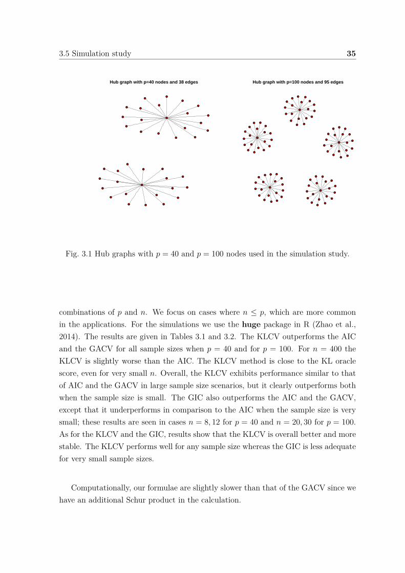
3.5 Simulation study 35
Hub graph with p=40 nodes and 38 edges
Hub graph with p=100 nodes and 95 edges
Fig. 3.1 Hub graphs with p = 40 and p = 100 nodes used in the simulation study.
combinations of p and n. We focus on cases where n ≤ p, which are more commonin the applications. For the simulations we use the huge package in R (Zhao et al.,2014). The results are given in Tables 3.1 and 3.2. The KLCV outperforms the AICand the GACV for all sample sizes when p = 40 and for p = 100. For n = 400 theKLCV is slightly worse than the AIC. The KLCV method is close to the KL oraclescore, even for very small n. Overall, the KLCV exhibits performance similar to thatof AIC and the GACV in large sample size scenarios, but it clearly outperforms bothwhen the sample size is small. The GIC also outperforms the AIC and the GACV,except that it underperforms in comparison to the AIC when the sample size is verysmall; these results are seen in cases n = 8, 12 for p = 40 and n = 20, 30 for p = 100.As for the KLCV and the GIC, results show that the KLCV is overall better and morestable. The KLCV performs well for any sample size whereas the GIC is less adequatefor very small sample sizes.
Computationally, our formulae are slightly slower than that of the GACV since wehave an additional Schur product in the calculation.
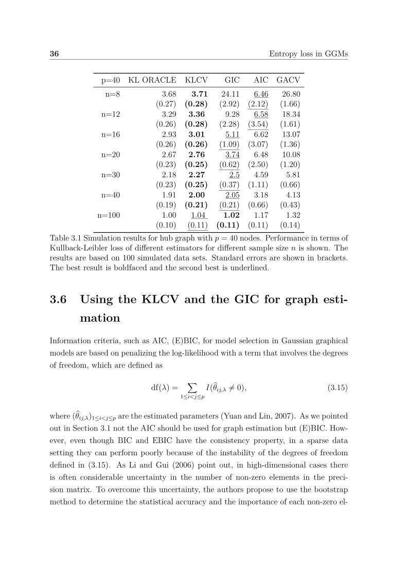
36 Entropy loss in GGMs
p=40 KL ORACLE KLCV GIC AIC GACVn=8 3.68 3.71 24.11 6.46 26.80
(0.27) (0.28) (2.92) (2.12) (1.66)n=12 3.29 3.36 9.28 6.58 18.34
(0.26) (0.28) (2.28) (3.54) (1.61)n=16 2.93 3.01 5.11 6.62 13.07
(0.26) (0.26) (1.09) (3.07) (1.36)n=20 2.67 2.76 3.74 6.48 10.08
(0.23) (0.25) (0.62) (2.50) (1.20)n=30 2.18 2.27 2.5 4.59 5.81
(0.23) (0.25) (0.37) (1.11) (0.66)n=40 1.91 2.00 2.05 3.18 4.13
(0.19) (0.21) (0.21) (0.66) (0.43)n=100 1.00 1.04 1.02 1.17 1.32
(0.10) (0.11) (0.11) (0.11) (0.14)Table 3.1 Simulation results for hub graph with p = 40 nodes. Performance in terms ofKullback-Leibler loss of different estimators for different sample size n is shown. Theresults are based on 100 simulated data sets. Standard errors are shown in brackets.The best result is boldfaced and the second best is underlined.
3.6 Using the KLCV and the GIC for graph esti-mation
Information criteria, such as AIC, (E)BIC, for model selection in Gaussian graphicalmodels are based on penalizing the log-likelihood with a term that involves the degreesof freedom, which are defined as
df(λ) =∑
1≤i<j≤p
I(θij,λ = 0), (3.15)
where (θij,λ)1≤i<j≤p are the estimated parameters (Yuan and Lin, 2007). As we pointedout in Section 3.1 not the AIC should be used for graph estimation but (E)BIC. How-ever, even though BIC and EBIC have the consistency property, in a sparse datasetting they can perform poorly because of the instability of the degrees of freedomdefined in (3.15). As Li and Gui (2006) point out, in high-dimensional cases thereis often considerable uncertainty in the number of non-zero elements in the preci-sion matrix. To overcome this uncertainty, the authors propose to use the bootstrapmethod to determine the statistical accuracy and the importance of each non-zero el-
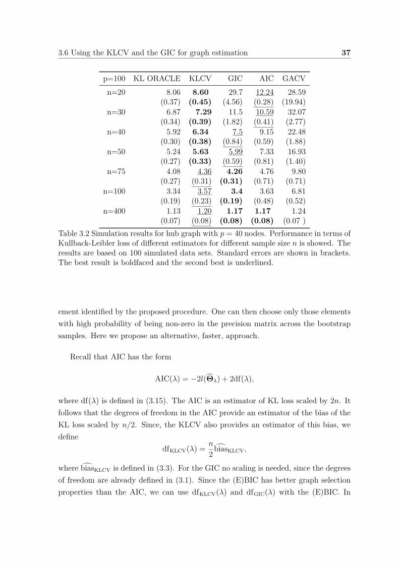
3.6 Using the KLCV and the GIC for graph estimation 37
p=100 KL ORACLE KLCV GIC AIC GACVn=20 8.06 8.60 29.7 12.24 28.59
(0.37) (0.45) (4.56) (0.28) (19.94)n=30 6.87 7.29 11.5 10.59 32.07
(0.34) (0.39) (1.82) (0.41) (2.77)n=40 5.92 6.34 7.5 9.15 22.48
(0.30) (0.38) (0.84) (0.59) (1.88)n=50 5.24 5.63 5.99 7.33 16.93
(0.27) (0.33) (0.59) (0.81) (1.40)n=75 4.08 4.36 4.26 4.76 9.80
(0.27) (0.31) (0.31) (0.71) (0.71)n=100 3.34 3.57 3.4 3.63 6.81
(0.19) (0.23) (0.19) (0.48) (0.52)n=400 1.13 1.20 1.17 1.17 1.24
(0.07) (0.08) (0.08) (0.08) (0.07 )Table 3.2 Simulation results for hub graph with p = 40 nodes. Performance in terms ofKullback-Leibler loss of different estimators for different sample size n is showed. Theresults are based on 100 simulated data sets. Standard errors are shown in brackets.The best result is boldfaced and the second best is underlined.
ement identified by the proposed procedure. One can then choose only those elementswith high probability of being non-zero in the precision matrix across the bootstrapsamples. Here we propose an alternative, faster, approach.
Recall that AIC has the form
AIC(λ) = −2l(Θλ) + 2df(λ),
where df(λ) is defined in (3.15). The AIC is an estimator of KL loss scaled by 2n. Itfollows that the degrees of freedom in the AIC provide an estimator of the bias of theKL loss scaled by n/2. Since, the KLCV also provides an estimator of this bias, wedefine
dfKLCV(λ) = n
2 biasKLCV,
where biasKLCV is defined in (3.3). For the GIC no scaling is needed, since the degreesof freedom are already defined in (3.1). Since the (E)BIC has better graph selectionproperties than the AIC, we can use dfKLCV(λ) and dfGIC(λ) with the (E)BIC. In
38 Entropy loss in GGMs
other words, we define
BICKLCV(λ) = −2l(Θλ) + log ndfKLCV(λ),BICGIC(λ) = −2l(Θλ) + log ndfGIC(λ).
We can also do the same for EBIC. We compare the BICGIC(λ) and BICKLCV(λ) toBIC and StARS in terms of the F1 score. The largest possible value of the F1 scoreis given by the F1 oracle and is evaluated by using the true matrix. We have donesimulations for the graph with p = 100 nodes from the previous section and a gridof two hundred regularization parameters. Average results over 100 simulations aregiven in Figure 3.2. The results suggest that BICGIC(λ) and BICKLCV(λ) can improveBIC for small sample sizes and can be competitive with the computationally muchmore involved StARS. In the case of the adaptive LASSO penalty the improvement isevident. Theoretical properties of BICKLCV(λ) and BICGIC(λ) are unclear, due to thecomplicated form of the bias terms. In any case, we propose the method only whenthe sample size is small since for larger n the degrees of freedom defined in 3.15 aremore stable, which can be also seen from the performance of AIC in Tables 3.1 and3.2.
3.7 Summary
In this chapter, we have discussed model selection in Gaussian graphical models. Weargued that minimizing KL divergence performs well in obtaining a model with goodpredicting power, but poorly in retrieving the graph structure. For obtaining a modelwith a good predictive power we have proposed two new, closed-form estimators of theKullback-Leibler loss. After an extensive literature review, we have found that theseestimators are the best closed-form estimators available for selecting a predictivelyaccurate model in sparse data settings for sparse Gaussian graphical models. We havedemonstrated that the estimators can be implemented relatively efficiently. We haveconcluded the chapter by illustrating that the proposed estimators of KL can be usefulfor the graph selection problem when the sample size is small.

3.7 Summary 39
20 40 60 80 100
0.0
0.2
0.4
0.6
0.8
1.0
Average F1 score for the hub graph with p=100 nodes
n
F1
scor
e
F1 ORACLEBIC_KLCVSTARSBICBIC_GIC
(a) GLASSO
20 40 60 80 100
0.0
0.2
0.4
0.6
0.8
1.0
Average F1 score for the hub graph with p=100 nodes
n
F1
scor
e
F1 ORACLEBIC_KLCVSTARSBICBIC_GIC
(b) SCAD
20 40 60 80 100
0.0
0.2
0.4
0.6
0.8
1.0
Average F1 score for the hub graph with p=100 nodes
n
F1
scor
e
F1 ORACLEBIC_KLCVSTARSBICBIC_GIC
(c) ADAPTIVE GLASSO
Fig. 3.2 Simulations results for hub graph with p = 100 nodes. Average performancein terms of F1 score of different estimators for different sample size n is shown. Theresults are based on 100 simulated data sets.
40 Entropy loss in GGMs
3.A Proof of Theorem 3.1
The proof follows the line of reasoning in the proof of Theorem 1 given in (Zhanget al., 2010). First we list the necessary notation:
- α = (i, j) : i, j = 1, . . . , p; i < j is the full model (labels of all entries in theupper diagonal of the precision matrix ).
- α ⊂ α is the candidate model which is defined by the set of labels of nonzeroentries of the precision matrix α.
- A is the collection of all candidate models.- Θ∗
α is the nonpenalized MLE computed via the model α.- Θλ is the MPLE that corresponds to tuning parameter λ.- αλ is the model associated with Θλ.- dα is the size of the model α, i.e. the number of nonzero elements in the upper
diagonal of the precision matrix Θ∗α.
- dfλ is the size of the model αλ, i.e. the number of nonzero elements in the upperdiagonal of the precision matrix Θλ.
- Ω− = λ : αλ ⊃ α0 is the set of λs that induce an underfitted model.- Ω0 = λ : αλ = α0 is the set of λs that induce the true model.- Ω+ = λ : αλ ⊃ α0 and αλ = α0 is the set of λs that induce an overfitted
model.- l(Θ) = n
2 log |Θ| − tr(ΘS) is the log-likelihood.- D(λ) = −2l(Θλ) is the deviance evaluated in the MPLE Θλ.- D∗(α) = −2l(Θ∗
α) is the deviance evaluated in the MLE Θ∗α that corresponds to
model α.- AIC(λ) = D(λ)/n+ 2dfλ/n is the AIC for the MPLE Θλ.- AIC∗(α) = D∗(α)/n + 2dα/n is the AIC for the MLE Θ∗
α that corresponds tomodel α.
There are two results needed to prove the statement of the theorem; these are givenin lemmas 3.3 and 3.4. Then, application of the apparatus of (Zhang et al., 2010)to our framework yields lemmas 3.5 and 3.6 from which follows the statement of thetheorem.
Lemma 3.3. For any candidate model α ∈ A, there exists cα such that
D∗(α)n
= cα + oP (1).
3.A Proof of Theorem 3.1 41
In addition, for any underfitted model α ⊃ α0, it holds
cα > cα0 ,
where Θ∗α0 is the precision matrix of the true model α0.
Proof. From the definition of D∗(α) it follows that
D∗(α)n
= tr(Θ∗αS) − log |Θ∗
α|.
Fix any candidate model α ∈ A. Since Θ∗α is the MLE under the model α the limit
limn→∞ Θ∗α exists in probability; we denote it by Θα. By consistency of the estimator
S (MLE under the full model) it follows that S P−→ Θ−1α0 , where Θα0 is the true precision
matrix. According to the continuous mapping theorem it follows that in probabilityit holds that
limn→∞
D∗(α)n
= tr(ΘαΘ−1α0 ) − log |Θα| := cα, (3.16)
which establishes the existence of cα. Let α ⊃ α0 be any underfitted model. Accordingto (3.16)
cα − cα0 = tr(ΘαΘ−1α0 ) − log |Θα| − tr(Θα0Θ−1
α0 ) + log |Θα0|
= tr(ΘαΘ−1α0 ) − log |ΘαΘ−1
α0 | − p
= 2KL(Θα0 ; Θα) > 0,
where we have used the formula for KL (2.6), the proposition 2.3 and the fact thatthe densities Np(y; 0,Θ−1
α ) are not equal Np(y; 0,Θ−1α0 ).
Lemma 3.4. Let α0 denote the true model and α the full model. With the notationof the previous lemma we have cα0 = cα.
Proof. Let Θα0 be the true precision matrix. According to (3.16)
cα = tr(ΘαΘ−1α0 ) − log |Θα|,
where Θα = limn→∞ Θ∗α, in probability. It follows that
cα0 = tr(Θα0Θ−1α0 ) − log |Θα0| = p− log |Θα0|.
From Θ∗α = S it follows that Θα = Θα0 , because S is a consistent estimator.
42 Entropy loss in GGMs
Finally we obtain
cα = tr(ΘαΘ−1α0 ) − log |Θα| = tr(Θα0Θ−1
α0 ) − log |Θα0| = p− log |Θα0 | = cα0 .
Lemma 3.5. Pinfλ∈Ω− AIC(λ) > AIC∗(α)
→ 1, as n → ∞.
Proof. For a given λ > 0, the nonpenalized MLE Θ∗αλ
maximizes log-likelihood func-tion under the model αλ. Therefore, l(Θ∗
αλ) ≥ l(Θλ) which is equivalent to
D(λ) ≥ D∗(αλ).
According to previous inequality and definition of the AIC(λ) it follows that
AIC(λ) = D(λ)n
+ 2dfλ
n>D∗(αλ)n
+ 2dfλ
n>D∗(αλ)n
,
since 2dfλ/n > 0. Hence
AIC(λ) − AIC∗(α) > D∗(αλ)n
− D∗(α)n
− 2dα
n, for every λ > 0. (3.17)
Consequently, the last inequality also holds for any λ ∈ Ω− = λ : αλ ⊃ α0, whichimplies
P
inf
λ∈Ω−AIC(λ) − AIC∗(α) > 0
≥ P
inf
αλ ⊃α0
D∗(αλ)n
− D∗(α)n
− 2dα
n> 0
.
(3.18)Since the subset of all underfitted models contains the subset of underfitted modelsobtained by the MPLE, i.e. αλ : αλ ⊃ α0 ⊂ α : α ⊃ α0 it follows that
P
inf
αλ ⊃α0
D∗(αλ)n
− D∗(α)n
− 2dα
n> 0
≥ P
inf
α ⊃α0
D∗(α)n
− D∗(α)n
− 2dα
n> 0
.
(3.19)Because p is fixed and it holds that 0 ≤ 2dα
n≤ 2p2
nwe obtain that 2dα
n= oP (1). Lemma
3.3 implies that D∗(α)/n−D∗(α)/n− 2dα/n = cα − cα + oP (1), whence it follows that
P
inf
α ⊃α0
D∗(α)n
− D∗(α)n
− 2dα
n> 0
= P
inf
α ⊃α0cα − cα + oP (1) > 0
. (3.20)
3.B Matrix differential calculus 43
Since there are a finite number of underfitted models, infimum is equal to minimumso
P
inf
α ⊃α0cα − cα + oP (1) > 0
= P
minα ⊃α0
cα − cα + oP (1) > 0. (3.21)
According to Lemma 3.4 cα = cα0 . From this equality, the sequence of inequalities(3.18), (3.19), (3.20), (3.21) and Lemma 3.3, i.e. cα > cα0 , it follows that
P
inf
λ∈Ω−AIC(λ) > AIC∗(α)
→ 1 as n → ∞.
Lemma 3.6. lim infn→∞ Pinfλ∈Ω0 AIC(λ) > AIC∗(α)
≥ π > 0.
Proof. Let λ ∈ Ω0 be arbitrary. Applying (3.17) to αλ = α0 and taking infimum overλ ∈ Ω0 yields
infλ∈Ω0
AIC(λ) − AIC∗(α) >D∗(α0)n
− D∗(α)n
− 2dα
n
= 1n
D∗(α0) −D∗(α
− 2dα
n. (3.22)
According to (Lauritzen, 1996, p.142)
D∗(α0) −D∗(α) = −2l(Θ∗α0) − l(Θ∗
α) d−→ χ2dα−dα0
, (3.23)
where χ2d denotes the chi-squared distribution with d degrees of freedom. Finally (3.22)
and (3.23) imply
P
inf
λ∈Ω0AIC(λ) > AIC∗(α)
≥ P
− 2n
l(Θ∗α0) − l(Θ∗
α) − 2dα
n> 0
= P
−2l(Θ∗
α0) − l(Θ∗α) > 2dα
→ Pχ2
dα−dα0> 2dα = π,
where 0 < π < 1.
3.B Matrix differential calculus
If F is a differentiable m × p matrix function of an n × q matrix X of variables thenthe natural question is how to define the Jacobian matrix of F. The literature gives

44 Entropy loss in GGMs
different definitions, since it is possible to construct the matrix containing the mnpqpartial derivatives of F in many ways. In this thesis we opt for the definition proposedin Magnus and Neudecker (1985), where the authors point out the following issueswith other definitions of the derivative.
1. The definition does not give the Jacobian matrix, it just displays the partialderivatives.
2. The determinant of the matrix that contains partial derivatives has no interpre-tation.
3. The definition is such that the chain rule does not exist.The authors show that the only natural and viable generalization of the notion of aJacobian matrix of a vector function to a Jacobian matrix of a matrix function is theone that we present here.
Definition 3.1. Let ϕ be a scalar function of an n × 1 vector x = (x1, . . . , xn)⊤, fbe an m× 1 vector function of x and F be a differentiable m× p real matrix functionof an n × q matrix of real variables X = (xij). Then the derivative of ϕ at x is then× 1 vector
Dϕ(x) =(∂ϕ(x)∂x1
, . . . ,∂ϕ(x)∂xn
)= ∂ϕ(x)
∂x⊤ ,
the derivative (or Jacobian matrix) of f at x is the m× n matrix
Df(x) =
∂f1(x)
∂x1. . . ∂f1(x)
∂xn,
... ...∂fm(x)
∂x1. . . ∂fm(x)
∂xn
= ∂f(x)∂x⊤ ,
and the derivative (or Jacobian matrix) of F at X is the mp× nq matrix
DF(X) = ∂vecF(X)∂(vecX)⊤ .
We also use the following notation for the matrix derivatives of scalar function ϕ
of two matrix arguments X = (xij) and Y = (yij)
dϕ(X,Y)dX
def= DXϕ(X,Y) = ∂ϕ(X,Y)∂(vecX)⊤ ,
dϕ(X,Y)dXdY
def= DXDYϕ(X,Y)
⊤ ,
3.C Calculation of the derivatives 45
where DX and DY stress that the derivatives are with respect to X and Y, respectively.The transpose sign of a row vector DYϕ(X,Y) in the second formula is necessary since,in this framework, the calculus is developed for column vector valued functions.
Regarding the previous comment, in matrix calculus attention should be paid tothe dimension of the matrix. Taking the derivative of the matrix is not the same astaking the derivative of the transpose matrix. Indeed, for the matrix X the derivativeof the transpose function F(X) = X⊤ is not an identity matrix, but it is given byDF(X) = Kp. For more on this subject see Magnus and Neudecker (2007), on whichour discussion is based on and which also contains the following results that we use.
Lemma 3.7. Let X be a square matrix of order p, A be a constant matrix of orderp and Ip2 and Op2 the identity and the zero matrix of order p2, respectively. Thefollowing identities hold:
D|X| = |X|vec(X−1)⊤⊤, (3.24)Dtr(AX) = (vecA⊤)⊤, (3.25)Dvec(X) = Ip2 , (3.26)
DX−1 = −(X⊤)−1 ⊗ X−1, (3.27)DA = Op2 . (3.28)
As a final remark, we note that a good reference on an alternative approach tomatrix derivatives, which is frequently used, is given in (Turkington, 2005). Anotheruseful reference is Harville (2008).
3.C Calculation of the derivatives
Recall that lk(Θ) = 12log |Θ| − tr(ΘSk)
and f(S,Θ) = log |Θ| − tr(SΘ). Through-
out the section we use the fact that the matrices Θ and Sk are symmetric.The chain rule and formulas (3.24) and (3.25) imply
Dlk(Θ) = 12vec(Θ−1 − Sk)⊤,
df(S,Θ)dΘ
= vec(Θ−1 − S)⊤.
46 Entropy loss in GGMs
Since ψ(yk,Θ) = vecDlk(Θ) it follows that
ψ(yk,Θ) = 12vec(Θ−1 − Sk).
The formulas (3.26), (3.27) and (3.28), and equality (A ⊗ B)⊤ = A⊤ ⊗ B⊤ yield
Dψ(yk; Θ)⊤ = −12Θ−1 ⊗ Θ−1,
d2f(S,Θ)dΘ2 = −Θ−1 ⊗ Θ−1.
Finally, d2f(S,Θ)/dΘdS = −Ip2 follows from (3.26) and (3.28).
3.D Derivation of the expression for Q
We have thatn∑
k=1ψ(yk, Θ) = 1
2
n∑k=1
vec(Θ−1 − Sk
)= 0p2 .
Applying the last equality and Θ−1 = S we obtain
Q = 14n
n∑k=1
vec(Θ−1 − Sk
)vec(Θ−1 − Sk)⊤
= 14n
n∑
k=1vec
(Θ−1 − Sk
) vec(Θ−1)⊤ + 14n
n∑k=1
vec(Θ−1 − Sk
)vec(Sk)⊤
= 14n
n∑k=1
vec(Θ−1 − Sk
)vec(Sk)⊤
= 14n
n∑k=1
(vecS − vecSk)vec(Sk)⊤
= 14nvecS
n∑k=1
vec(Sk)⊤ − 14n
n∑k=1
vecSkvec(Sk)⊤
= 14vecSvec(S)⊤ − 1
4n
n∑k=1
vecSkvec(Sk)⊤.
3.E Proof of Lemma 3.1
Substituting Mp = (Ip2 + Kp)/2 in the equality (3.9) we obtain that it is equivalentto
(Θ ⊗ Θ)vecA = Kp(Θ ⊗ Θ)vec(A).
3.F Calculation of the algorithmic complexity 47
To show this, we use identities vec(ABC) = (C⊤ ⊗ A)vecB, KpvecA = vecA⊤ andsymmetry of A and Θ
KpΘ ⊗ ΘvecA = Kpvec(ΘAΘ) = vec(ΘAΘ)⊤ = vec(ΘAΘ) = Θ ⊗ ΘvecA.
2
3.F Calculation of the algorithmic complexity
Throughout this section we use Lemma 4.5 from Section 4.C. We also use the resultwhich follows from the definition of the Kronecker product.
Lemma 3.8. If Θ is a matrix of dimension p×p then the computational cost of Θ⊗Θis O(p4) flops.
The matrices that appear in the calculations have the following dimensions:• Θλ,A,B, Iλ are of dimension p× p.• Θλ ⊗ Θλ is of dimension p2 × p2.• vec(A Iλ)⊤ is of dimension 1 × p2.• vec(B Iλ) and vecΘλ(B Iλ)Θλ are of dimension p2 × 1.We do not take into account vectorization and transpose operator since they are
connected with memory allocation and also because in 3.4 we show that these can beavoided.
The cost for the term vec(A Iλ)⊤(Θλ ⊗ Θλ)vec(B Iλ)We have that:• Θλ 7→ Θλ ⊗ Θλ costs p4 flops.• (A, Iλ) 7→ vec(A Iλ) costs p2 flops.• (B, Iλ) 7→ vec(B Iλ) costs p2 flops.• (Θλ ⊗ Θλ, vec(B Iλ)) 7→ (Θλ ⊗ Θλ)vec(B Iλ) costs O(p4) flops.• (vec(A Iλ)⊤, (Θλ ⊗ Θλ)vec(B Iλ)) 7→ vec(A Iλ)⊤(Θλ ⊗ Θλ)vec(B Iλ) costsp2 flops.
Thus, the total computational cost is O(2p4 + 3p2), which is equal to O(p4) flops.The cost for the term vec(A Iλ)⊤vecΘλ(B Iλ)ΘλIt has already been shown that calculation of vec(A Iλ) and vec(B Iλ) costs a
total of 2p2 flops. Furthermore, it holds:• (B Iλ, Θλ) 7→ (B Iλ)Θλ costs p3 flops.

48 Entropy loss in GGMs
• (Θλ, (B Iλ)Θλ) 7→ Θλ(B Iλ)Θλ costs p3 flops.• (vec(AIλ)⊤, vecΘλ(BIλ)Θλ) 7→ vec(AIλ)⊤vecΘλ(BIλ)Θλ costs O(p2)
flops.Thus, the total computational cost is O(2p3 + 3p2), which is equal to O(p3) flops.

Chapter 4
Time course window estimator forordinary differential equationslinear in the parameters
The subject of this chapter is the estimation of parameters in autonomous systemsof ordinary differential equations. We consider systems that have a special structure,those for which the vector field is linear in the parameters. The structure of thesesystems allows construction of an estimator that has an explicit form. By using thisestimator we not only avoid the usage of numerical ODEs solvers but optimizationmethods as well. As a result the estimator that we present is extremely fast. This isvery important, since in Bayesian and likelihood approaches for estimating parametersof ODEs, the speed and convergence of the procedure may crucially depend on goodinitial values of the parameters, which this method can provide. Moreover, we provethat the proposed estimator is
√n-consistent. The estimator does not require an
initial guess for the parameters and is computationally fast, and therefore can serveas a good initial estimate for more efficient estimators. We illustrate our results insimulation studies .
The remainder of this chapter is divided into six sections. The problem is intro-duced in Section 4.1. In Section 4.2 we define the time course window estimator andpresent the formulae for the estimators of the parameters. In Section 4.3 we showresults for different examples. Section 4.4 deals with the computational speed andcomplexity of the estimation procedure. In Section 4.5 we illustrate our method on areal data set. We conclude with a discussion in section 4.6. The last section containsthe summary. All proofs and auxiliary results are given in the Appendix.
50 Window estimator
4.1 Introduction
Consider the system of differential equations of the form
x′(t) = f(x(t);θ), t ∈ [0, T ],x(0) = ξ,
(4.1)
where x(t) takes values in Rd, ξ in Ξ ⊂ Rd, and θ in Θ ⊂ Rp. From (4.1) we obtainthe system of integral equations
x(t) = ξ +∫ t
0f(x(s);θ) ds, t ∈ [0, T ]. (4.2)
Given the values of ξ and θ, we denote the solution of (4.1)-(4.2) by x(t;θ, ξ). In manypractical applications, the values of ξ and θ are unknown and need to be estimatedfrom the data, which consist of noisy observations of x(t;θ, ξ) at certain time pointsin [0, T ]. We denote the observations by
y(ti) = x(ti;θ, ξ) + ε(ti), i = 1, . . . , n, (4.3)
where for simplicity ti = iT/n, i = 1, . . . , n and ε(ti), are the d-dimensional columnvectors of measurement errors at time ti. We focus on the special class of nonlinearsystems that are linear in the parameter θ
f(x(t);θ) = g(x(t))θ, (4.4)
where the measurable function g : Rd → Rd×p maps the d-dimensional column vectorx into a d×p matrix. In this chapter, we consider estimators of the parameters θ andξ that are obtained by minimizing
Ln(ξ,θ) =∫ T
0
∥∥∥∥xn(t) − ξ −∫ t
0g(xn(s)) dsθ
∥∥∥∥2dt, (4.5)
with respect to ξ and θ, where xn(t), t ∈ [0, T ], is a particular estimator of x(t;θ, ξ).Here, ∥ · ∥ denotes the Euclidean norm ∥z∥ = ∑d
j=1 z2j 1/2. Minimization of (4.5)
results in an explicit form for the estimators θn and ξn, which is not the case withclassical approaches, such as non-linear least squares (NLS) or maximum likelihoodestimator (MLE). Indeed, NLS and MLE require the solution of the system of differ-ential equations, which generally does not have a closed form. This remains true even
4.2 Time-course window estimator 51
when the dependence on the model parameters is linear.In case of repeated measures, using a step function estimator for xn(t) yields a
very simple and computationally fast estimator. The estimators of the parameters are√n-consistent if, roughly speaking, the number of time points is of order
√n and for
most time points the number of replicates is of the same order (Dattner and Klaassen,2013). In case of time course data without repeated measurements, as introducedabove, the aforementioned consistency result does not hold unless some smoothing isapplied. In this chapter we examine this case. We show that by defining a suitablestep-function estimator of the solution of the system x, we obtain explicit estimators ofthe parameters that are
√n-consistent. This parametric convergence rate is obtained
by using only weak assumptions on the measurement error.The idea of smoothing as a way to avoid numerical integration of the system of
differential equations has been used before and is referred to as the collocation esti-mation method; for example, there are two-step methods (Bellman and Roth, 1971;Varah, 1982; Brunel, 2008; Liang and Wu, 2008; Fang et al., 2011; Gugushvili andKlaassen, 2012; Gugushvili and Spreij, 2012; Dattner and Klaassen, 2013) and gener-alized profiling methods (Ramsay et al., 2007; Qi and Zhao, 2010; Hooker et al., 2011;Xun et al., 2013). Also, other regularization based approaches, which make use ofproperties of differential operators, have been proposed to avoid numerical integrationof the system of differential equations (Steinke and Schölkopf, 2008). In most cases,the main computational bottleneck lies in the optimization of a non-linear objectivefunction. Indeed, standard problems connected with optimization also appear here.For example, a poor initial guess may lead to considerably slower convergence to theglobal optimum or even to some local optimum. For systems that are linear in theparameters this optimization can be avoided, since the estimator can be obtainedexplicitly (Himmelblau et al., 1967; Dattner and Klaassen, 2013). Moreover, follow-ing Khanin et al. (2006, 2007) further simplifications can be obtained by assumingpiecewise constant solutions of the differential equations.
4.2 Time-course window estimator
Let t1, . . . , tn be equidistant time points of the observations. We divide the interval[0, T ] into I = ⌊
√n⌋ subintervals of the length ∆ = T/I so that in every interval we
have at least ⌊√n⌋ and at most ⌊
√n⌋ + 2 time points, i.e. I, I+ 1 or I+ 2 points. Let
Si = [ai−1, ai) be the ith subinterval i = 1, . . . , I−1 and SI = [aI−1, aI ]. The boundary
52 Window estimator
points of the subintervals are ai = i∆, i = 0, . . . , I and endpoints of [0, T ] are a0 = 0and aI = T . For t ∈ [0, T ], let S(t) denote the subinterval to which t belongs. In otherwords, if t ∈ Si then S(t) = Si. The window estimator of x is defined as
xn(t) = 1|S(t)|
∑tj∈S(t)
y(tj), t ∈ S(t). (4.6)
This estimator is a stepwise function that estimates x(t) in each interval as the meanof the observations that belong to that interval. On each interval Si, the windowestimator xn takes a constant value that we denote by xn(Si). In other words it holds
xn(t) = xn(Si), t ∈ Si. (4.7)
We estimate G(t) =∫ t
0 g(x(s))ds via a plug-in approach
Gn(t) =∫ t
0g(xn(s))ds.
This is just a finite sum as it is the integral of a piecewise constant function. Indeed,since xn(·) is piecewise constant therefore g(xn(·)) is as well. This gives
Gn(t) =i−1∑
m=1g(xn(Sm))∆ + g(xn(Si))(t− ai−1), t ∈ Si.
Throughout the chapter, we adhere to the convention that the sums of the form∑i−1m=1 fm are equal to zero for i = 1. Minimizing the criterion function (4.5) with
respect to ξ and θ yields explicit formulae for the estimators of the parameters. Indeed,the objective function Ln can be written as
Ln(ω) = ω⊤∫ T
0F(t)⊤F(t)dtω − 2ω⊤
∫ T
0F(t)⊤xn(t)dt+
∫ T
0∥xn(t)∥2dt,
where ω = (ξ;θ)⊤ and F(t) = (T Id; Gn(t)). Thus, Ln is quadratic in ω and itsminimizer is
ω =( ∫ T
0F(t)⊤F(t)dt
)−1 ∫ T
0F(t)⊤xn(t)dt =
T Id An
A⊤n Bn
−1 ∫ T0 xn(t)dt∫ T
0 Gn(t)⊤xn(t)dt
,
4.2 Time-course window estimator 53
where
An =∫ T
0Gn(t)dt,
Bn =∫ T
0Gn(t)⊤Gn(t)dt.
By using the matrix block inversion (Bernstein, 2009, Chapter 2) we obtain
ξn =(T Id − AnB−1
n A⊤n
)−1 ∫ T0
Id − AnB−1
n Gn(t)⊤xn(t)dt,
θn = B−1n
∫ T0 Gn(t)⊤xn(t) − ξndt.
(4.8)
Plugging (4.7) into (4.8) we obtain
ξn =(T Id − AnB−1
n A⊤n
)−1T∑I
i=1 xn(Si)/I − AnB−1n
∑Ii=1 An(i)⊤xn(Si)
,
θn = B−1n
∑Ii=1 An(i)⊤xn(Si) − A⊤
n ξn
,
where An(i) =∫
SiGn(t)dt. The integrals An, Bn, An(i) have explicit forms in terms
of Gn(ai) and g(xn(Si)):
An = T Gn(T ) − ∆2
2
I∑i=1
(2i− 1)g(xn(Si)),
An(i) = tGn(t)|aiai−1
− 12(2i− 1)∆2g(xn(Si)), (4.9)
and
Bn = Gn(T )⊤An − 12
I∑i=1
g(xn(Si))⊤t2Gn(t)∣∣∣∣ai
ai−1
+ ∆3
6
I∑i=1
(3i2 − 1)g(xn(Si))⊤g(xn(Si))
+ ∆3
2
I−1∑i=1
(2i− 1)R⊤i g(xn(Si)), (4.10)
where Ri = ∑Im=i+1 g(xn(Sm)). See appendix 4.D for the derivations of these formulas.
Next, we formulate the√n-consistency of ξn and θn in the following theorem. A
prerequisite for consistent estimation is the identifiability of the parameters. There areseveral concepts of identifiability. Here we are concerned with structural identifiability,a property that depends on the structure of the model and is not affected by the
54 Window estimator
experimental set-up. This means that knowledge of the solution x(t), t ∈ [0, T ]yields the unique values of the parameters ξ and θ. For ξ = x(0) this is true, whileidentifiability for θ means that θ′ = θ ⇒ x(·;θ′, ξ) = x(·;θ, ξ); see Dattner andKlaassen (2013) for a necessary and sufficient condition for identifiability in the caseof systems linear in the parameters.
Theorem 4.1. Let an ODE model be defined by (4.1), (4.2) and (4.4) with the twicecontinuously differentiable map g : Rd → Rd × Rp. Let ξ ∈ Ξ and θ ∈ Θ andlet x(·) = x(·;θ, ξ) exist and be bounded on [0, T ]. Assume that θ is identifiable.Let the observations be given by (4.3) with ti = iT/n, i = 1, ..., n. Assume thatεk(ti), k = 1, . . . , d, i = 1, . . . , n, are i.i.d. random variables with zero expectationand finite variance σ2. Let xn(·) be given by (4.6) and let θn, ξn be defined as in (4.8).Then
(θn − θ, ξn − ξ) = Op(n−1/2), n → ∞,
holds.
Below we sketch the proof of this theorem. The full proof is deferred to theappendix. The main idea is that if xn(·) is a consistent estimator of x(·) in thesup norm, then the estimators θn and ξn are also consistent. If, in fact, the estimatorxn(·) satisfies some stronger conditions, then it even implies
√n-consistency of θn and
ξn.The proof can be divided into two parts. In the first part we analyze the behaviour
of the expected value of the window estimator and in the second we analyze its vari-ance. In order to obtain the consistency of xn we first need to show that the sup normof xn is bounded in probability, i.e.
∥xn∥∞ = Op(1),
and that the expected value of xn converges to x(·) in the sup norm. If g(·) is bounded,then this condition is not needed. However, to obtain
√n-consistency, convergence
needs to be at least at√n rate, i.e.
∥Exn − x∥∞ = O(cn),
where cn = n−1/2. The previous two equalities can be proven by using the boundednessof the parameter space, the linearity of the system in the parameters and Chebyshev’s
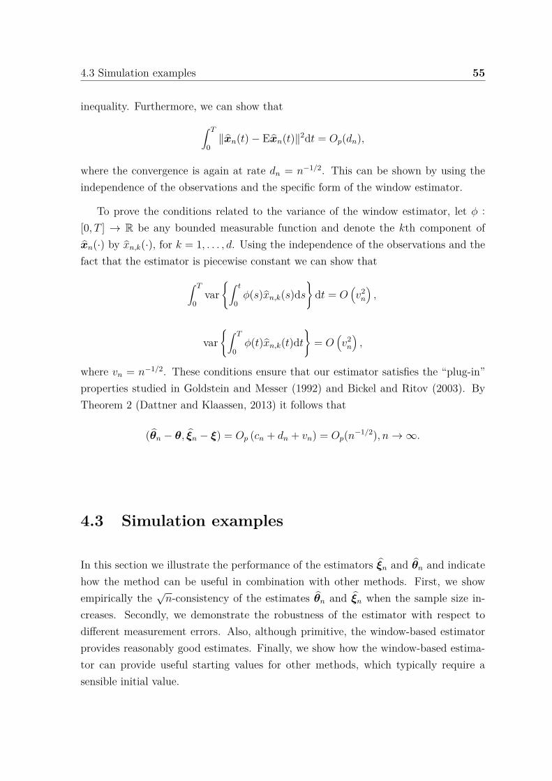
4.3 Simulation examples 55
inequality. Furthermore, we can show that∫ T
0∥xn(t) − Exn(t)∥2dt = Op(dn),
where the convergence is again at rate dn = n−1/2. This can be shown by using theindependence of the observations and the specific form of the window estimator.
To prove the conditions related to the variance of the window estimator, let ϕ :[0, T ] → R be any bounded measurable function and denote the kth component ofxn(·) by xn,k(·), for k = 1, . . . , d. Using the independence of the observations and thefact that the estimator is piecewise constant we can show that
∫ T
0var
∫ t
0ϕ(s)xn,k(s)ds
dt = O
(v2
n
),
var∫ T
0ϕ(t)xn,k(t)dt
= O
(v2
n
),
where vn = n−1/2. These conditions ensure that our estimator satisfies the “plug-in”properties studied in Goldstein and Messer (1992) and Bickel and Ritov (2003). ByTheorem 2 (Dattner and Klaassen, 2013) it follows that
(θn − θ, ξn − ξ) = Op (cn + dn + vn) = Op(n−1/2), n → ∞.
4.3 Simulation examples
In this section we illustrate the performance of the estimators ξn and θn and indicatehow the method can be useful in combination with other methods. First, we showempirically the
√n-consistency of the estimates θn and ξn when the sample size in-
creases. Secondly, we demonstrate the robustness of the estimator with respect todifferent measurement errors. Also, although primitive, the window-based estimatorprovides reasonably good estimates. Finally, we show how the window-based estima-tor can provide useful starting values for other methods, which typically require asensible initial value.
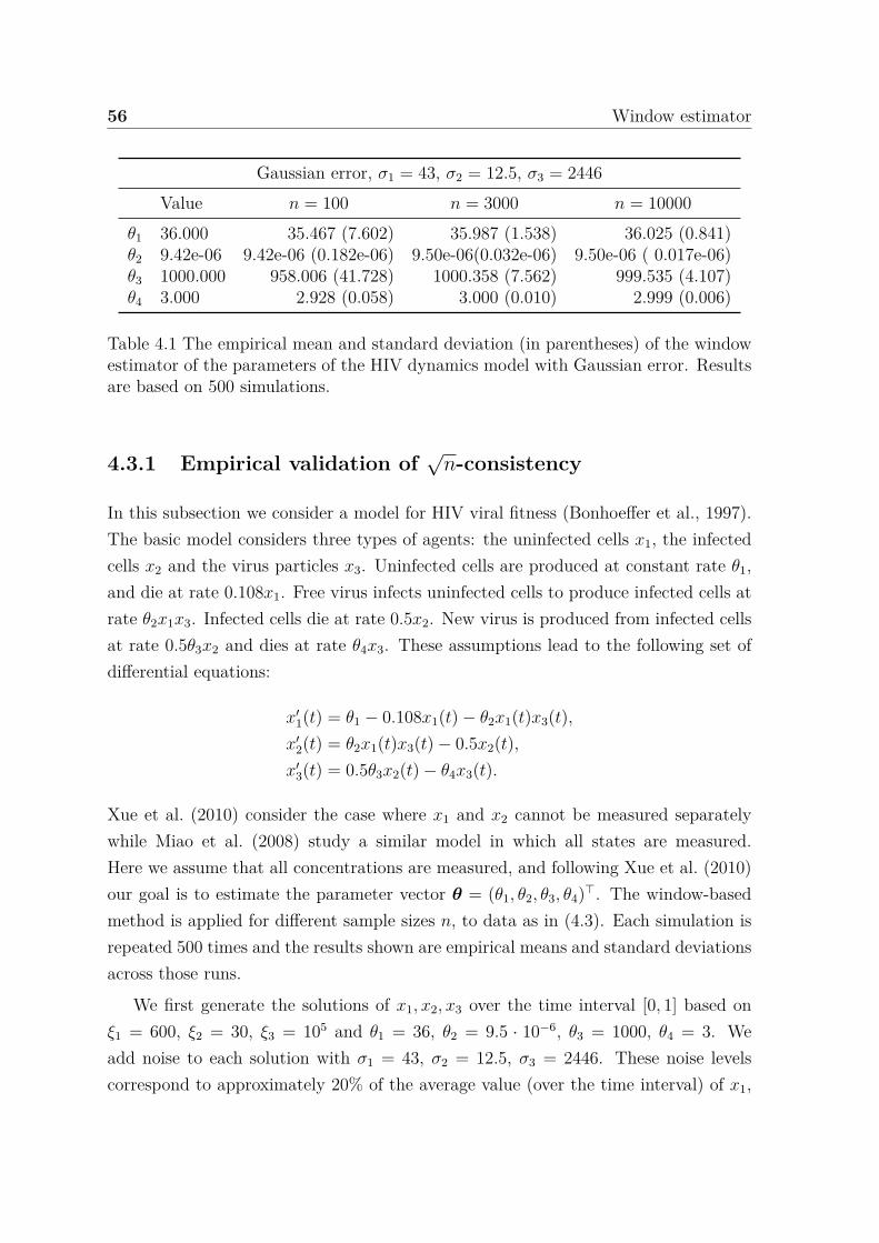
56 Window estimator
Gaussian error, σ1 = 43, σ2 = 12.5, σ3 = 2446Value n = 100 n = 3000 n = 10000
θ1 36.000 35.467 (7.602) 35.987 (1.538) 36.025 (0.841)θ2 9.42e-06 9.42e-06 (0.182e-06) 9.50e-06(0.032e-06) 9.50e-06 ( 0.017e-06)θ3 1000.000 958.006 (41.728) 1000.358 (7.562) 999.535 (4.107)θ4 3.000 2.928 (0.058) 3.000 (0.010) 2.999 (0.006)
Table 4.1 The empirical mean and standard deviation (in parentheses) of the windowestimator of the parameters of the HIV dynamics model with Gaussian error. Resultsare based on 500 simulations.
4.3.1 Empirical validation of√n-consistency
In this subsection we consider a model for HIV viral fitness (Bonhoeffer et al., 1997).The basic model considers three types of agents: the uninfected cells x1, the infectedcells x2 and the virus particles x3. Uninfected cells are produced at constant rate θ1,and die at rate 0.108x1. Free virus infects uninfected cells to produce infected cells atrate θ2x1x3. Infected cells die at rate 0.5x2. New virus is produced from infected cellsat rate 0.5θ3x2 and dies at rate θ4x3. These assumptions lead to the following set ofdifferential equations:
x′1(t) = θ1 − 0.108x1(t) − θ2x1(t)x3(t),x′
2(t) = θ2x1(t)x3(t) − 0.5x2(t),x′
3(t) = 0.5θ3x2(t) − θ4x3(t).
Xue et al. (2010) consider the case where x1 and x2 cannot be measured separatelywhile Miao et al. (2008) study a similar model in which all states are measured.Here we assume that all concentrations are measured, and following Xue et al. (2010)our goal is to estimate the parameter vector θ = (θ1, θ2, θ3, θ4)⊤. The window-basedmethod is applied for different sample sizes n, to data as in (4.3). Each simulation isrepeated 500 times and the results shown are empirical means and standard deviationsacross those runs.
We first generate the solutions of x1, x2, x3 over the time interval [0, 1] based onξ1 = 600, ξ2 = 30, ξ3 = 105 and θ1 = 36, θ2 = 9.5 · 10−6, θ3 = 1000, θ4 = 3. Weadd noise to each solution with σ1 = 43, σ2 = 12.5, σ3 = 2446. These noise levelscorrespond to approximately 20% of the average value (over the time interval) of x1,
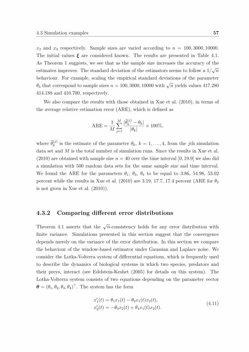
4.3 Simulation examples 57
x2 and x3 respectively. Sample sizes are varied according to n = 100, 3000, 10000.The initial values ξ are considered known. The results are presented in Table 4.1.As Theorem 1 suggests, we see that as the sample size increases the accuracy of theestimates improves. The standard deviation of the estimators seems to follow a 1/
√n
behaviour. For example, scaling the empirical standard deviations of the parameterθ3 that correspond to sample sizes n = 100, 3000, 10000 with
√n yields values 417.280
414.188 and 410.700, respectively.
We also compare the results with those obtained in Xue et al. (2010), in terms ofthe average relative estimation error (ARE), which is defined as
ARE = 1M
M∑j=1
|θ(j)k − θk|
|θk|× 100%,
where θ(j)k is the estimate of the parameter θk, k = 1, . . . , 4, from the jth simulation
data set and M is the total number of simulation runs. Since the results in Xue et al.(2010) are obtained with sample size n = 40 over the time interval [0, 19.9] we also dida simulation with 500 random data sets for the same sample size and time interval.We found the ARE for the parameters θ1, θ3, θ4 to be equal to 3.86, 54.98, 53.02percent while the results in Xue et al. (2010) are 3.19, 17.7, 17.4 percent (ARE for θ2
is not given in Xue et al. (2010)).
4.3.2 Comparing different error distributions
Theorem 4.1 asserts that the√n-consistency holds for any error distribution with
finite variance. Simulations presented in this section suggest that the convergencedepends merely on the variance of the error distribution. In this section we comparethe behaviour of the window-based estimator under Gaussian and Laplace noise. Weconsider the Lotka-Volterra system of differential equations, which is frequently usedto describe the dynamics of biological systems in which two species, predators andtheir preys, interact (see Edelstein-Keshet (2005) for details on this system). TheLotka-Volterra system consists of two equations depending on the parameter vectorθ = (θ1, θ2, θ3, θ4)⊤. The system has the form
x′1(t) = θ1x1(t) − θ2x1(t)x2(t),x′
2(t) = −θ3x2(t) + θ4x1(t)x2(t).(4.11)
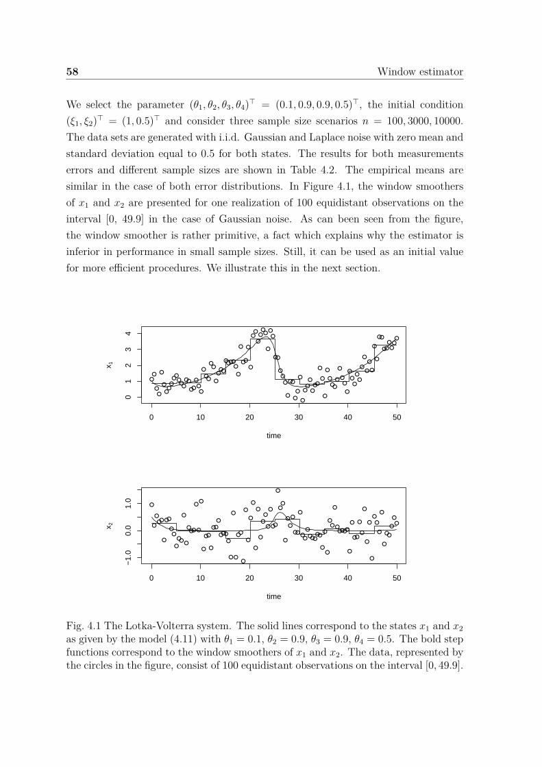
58 Window estimator
We select the parameter (θ1, θ2, θ3, θ4)⊤ = (0.1, 0.9, 0.9, 0.5)⊤, the initial condition(ξ1, ξ2)⊤ = (1, 0.5)⊤ and consider three sample size scenarios n = 100, 3000, 10000.The data sets are generated with i.i.d. Gaussian and Laplace noise with zero mean andstandard deviation equal to 0.5 for both states. The results for both measurementserrors and different sample sizes are shown in Table 4.2. The empirical means aresimilar in the case of both error distributions. In Figure 4.1, the window smoothersof x1 and x2 are presented for one realization of 100 equidistant observations on theinterval [0, 49.9] in the case of Gaussian noise. As can been seen from the figure,the window smoother is rather primitive, a fact which explains why the estimator isinferior in performance in small sample sizes. Still, it can be used as an initial valuefor more efficient procedures. We illustrate this in the next section.
0 10 20 30 40 50
01
23
4
time
x 1
0 10 20 30 40 50
−1.
00.
01.
0
time
x 2
Fig. 4.1 The Lotka-Volterra system. The solid lines correspond to the states x1 and x2as given by the model (4.11) with θ1 = 0.1, θ2 = 0.9, θ3 = 0.9, θ4 = 0.5. The bold stepfunctions correspond to the window smoothers of x1 and x2. The data, represented bythe circles in the figure, consist of 100 equidistant observations on the interval [0, 49.9].
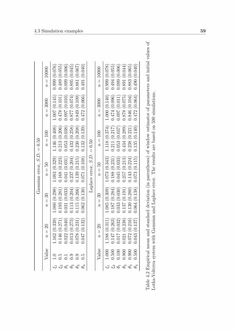
4.3 Simulation examples 59G
auss
ian
erro
r,S.D.=
0.50
Valu
en
=20
n=
30n
=50
n=
100
n=
3000
n=
1000
0ξ 1
1.0
1.16
2(0
.339
)1.
080
(0.2
98)
1.08
3(0
.329
)1.
146
(0.4
08)
1.00
7(0
.145
)0.
999
(0.0
76)
ξ 20.
50.
146
(0.2
71)
0.19
3(0
.281
)0.
168
(0.2
23)
0.21
3(0
.206
)0.
478
(0.1
01)
0.48
9(0
.055
)θ 1
0.1
0.02
2(0
.040
)0.
031
(0.0
33)
0.04
1(0
.031
)0.
053
(0.0
38)
0.09
7(0
.010
)0.
099
(0.0
06)
θ 20.
90.
013
(0.2
73)
0.11
3(0
.204
)0.
237
(0.2
04)
0.43
2(0
.258
)0.
877
(0.0
74)
0.89
5(0
.045
)θ 3
0.9
0.07
8(0
.231
)0.
115
(0.2
66)
0.13
9(0
.215
)0.
230
(0.2
08)
0.84
9(0
.109
)0.
881
(0.0
67)
θ 40.
50.
047
(0.1
32)
0.06
2(0
.130
)0.
071
(0.1
08)
0.13
2(0
.139
)0.
472
(0.0
66)
0.49
1(0
.040
)La
plac
eer
ror,S.D.=
0.50
Valu
en
=20
n=
30n
=50
n=
100
n=
3000
n=
1000
0ξ 1
1.00
01.
188
(0.3
11)
1.08
5(0
.309
)1.
073
(0.3
43)
1.11
8(0
.374
)1.
000
(0.1
40)
0.99
9(0
.078
)ξ 2
0.50
00.
147
(0.2
63)
0.18
7(0
.284
)0.
188
(0.2
31)
0.21
1(0
.217
)0.
474
(0.0
96)
0.49
4(0
.055
)θ 1
0.10
00.
017
(0.0
32)
0.03
3(0
.030
)0.
045
(0.0
33)
0.05
3(0
.037
)0.
097
(0.0
11)
0.09
9(0
.006
)θ 2
0.90
00.
021
(0.2
38)
0.13
7(0
.191
)0.
257
(0.2
13)
0.43
4(0
.289
)0.
878
(0.0
75)
0.89
1(0
.044
)θ 3
0.90
00.
072
(0.2
16)
0.13
0(0
.280
)0.
143
(0.2
24)
0.23
8(0
.221
)0.
846
(0.1
04)
0.88
3(0
.065
)θ 4
0.50
00.
043
(0.1
37)
0.06
4(0
.138
)0.
073
(0.1
15)
0.13
5(0
.140
)0.
472
(0.0
64)
0.49
0(0
.040
)
Tabl
e4.
2Em
piric
alm
ean
and
stan
dard
devi
atio
n(in
pare
nthe
ses)
ofw
indo
wes
timat
orof
para
met
ers
and
initi
alva
lues
ofLo
tka-
Volte
rra
syst
emw
ithG
auss
ian
and
Lapl
ace
erro
r.T
here
sults
are
base
don
500
simul
atio
ns.
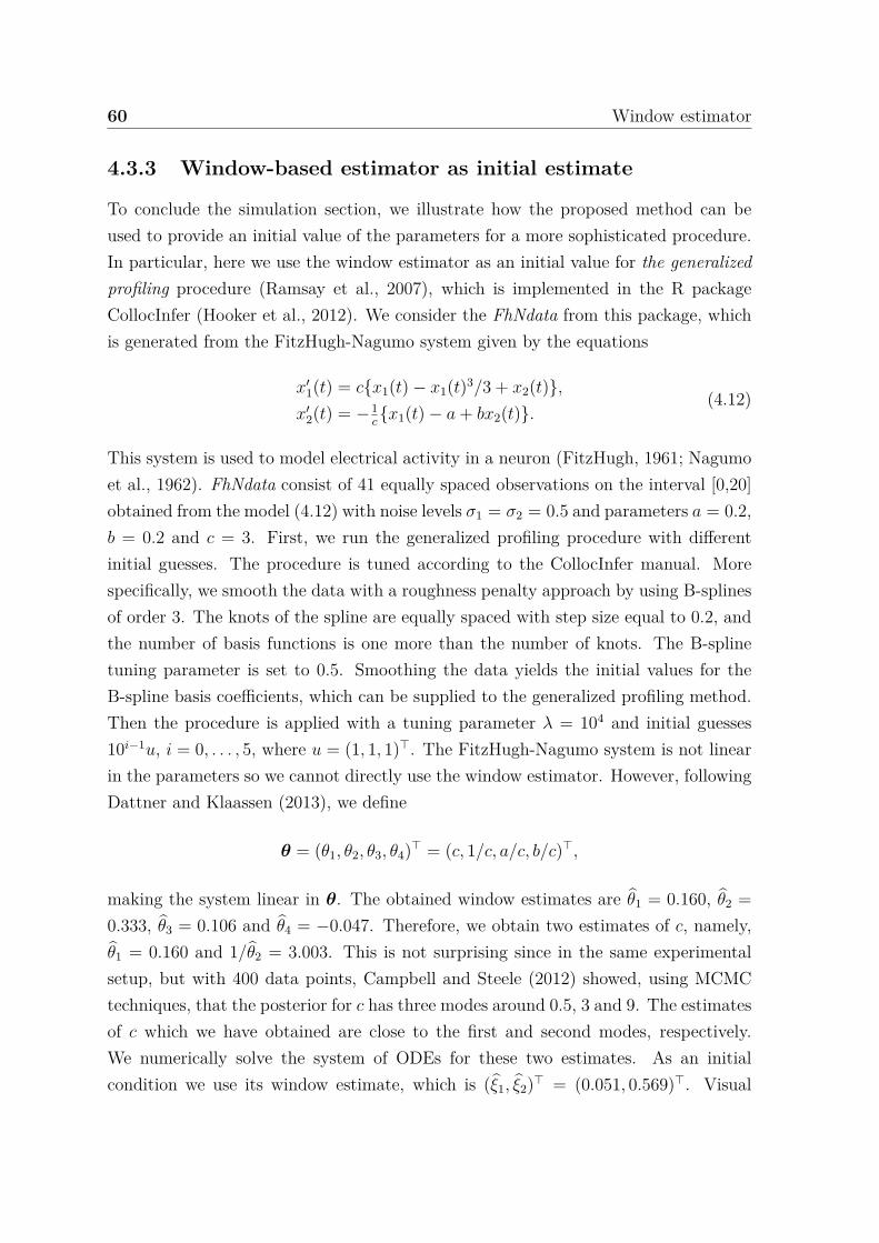
60 Window estimator
4.3.3 Window-based estimator as initial estimate
To conclude the simulation section, we illustrate how the proposed method can beused to provide an initial value of the parameters for a more sophisticated procedure.In particular, here we use the window estimator as an initial value for the generalizedprofiling procedure (Ramsay et al., 2007), which is implemented in the R packageCollocInfer (Hooker et al., 2012). We consider the FhNdata from this package, whichis generated from the FitzHugh-Nagumo system given by the equations
x′1(t) = cx1(t) − x1(t)3/3 + x2(t),x′
2(t) = −1cx1(t) − a+ bx2(t).
(4.12)
This system is used to model electrical activity in a neuron (FitzHugh, 1961; Nagumoet al., 1962). FhNdata consist of 41 equally spaced observations on the interval [0,20]obtained from the model (4.12) with noise levels σ1 = σ2 = 0.5 and parameters a = 0.2,b = 0.2 and c = 3. First, we run the generalized profiling procedure with differentinitial guesses. The procedure is tuned according to the CollocInfer manual. Morespecifically, we smooth the data with a roughness penalty approach by using B-splinesof order 3. The knots of the spline are equally spaced with step size equal to 0.2, andthe number of basis functions is one more than the number of knots. The B-splinetuning parameter is set to 0.5. Smoothing the data yields the initial values for theB-spline basis coefficients, which can be supplied to the generalized profiling method.Then the procedure is applied with a tuning parameter λ = 104 and initial guesses10i−1u, i = 0, . . . , 5, where u = (1, 1, 1)⊤. The FitzHugh-Nagumo system is not linearin the parameters so we cannot directly use the window estimator. However, followingDattner and Klaassen (2013), we define
θ = (θ1, θ2, θ3, θ4)⊤ = (c, 1/c, a/c, b/c)⊤,
making the system linear in θ. The obtained window estimates are θ1 = 0.160, θ2 =0.333, θ3 = 0.106 and θ4 = −0.047. Therefore, we obtain two estimates of c, namely,θ1 = 0.160 and 1/θ2 = 3.003. This is not surprising since in the same experimentalsetup, but with 400 data points, Campbell and Steele (2012) showed, using MCMCtechniques, that the posterior for c has three modes around 0.5, 3 and 9. The estimatesof c which we have obtained are close to the first and second modes, respectively.We numerically solve the system of ODEs for these two estimates. As an initialcondition we use its window estimate, which is (ξ1, ξ2)⊤ = (0.051, 0.569)⊤. Visual
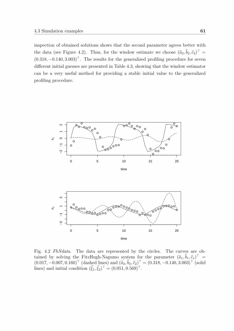
4.3 Simulation examples 61
inspection of obtained solutions shows that the second parameter agrees better withthe data (see Figure 4.2). Thus, for the window estimate we choose (a2, b2, c2)⊤ =(0.318,−0.140, 3.003)⊤. The results for the generalized profiling procedure for sevendifferent initial guesses are presented in Table 4.3, showing that the window estimatorcan be a very useful method for providing a stable initial value to the generalizedprofiling procedure.
0 5 10 15 20
−2
−1
01
2
time
x 1
0 5 10 15 20
−3
−1
13
time
x 2
Fig. 4.2 FhNdata. The data are represented by the circles. The curves are ob-tained by solving the FitzHugh-Nagumo system for the parameter (a1, b1, c1)⊤ =(0.017,−0.007, 0.160)⊤ (dashed lines) and (a2, b2, c2)⊤ = (0.318,−0.140, 3.003)⊤ (solidlines) and initial condition (ξ1, ξ2)⊤ = (0.051, 0.569)⊤.
62 Window estimator
Estimation of parameters in Fitz-Hugh Nagumo systemMethod Initial value a = 0.2 b = 0.2 c = 3 Relative error Time(secs)Window NO 0.318 -0.140 3.003 2.291 0.011
Generalizedprofiling
Window 0.237 0.144 3.050 0.483 25.4660.1u 0.239 0.009 0.069 2.130 8.6871u 0.144 0.567 3.461 2.266 55.72510u 1.797 3.082 3.295 22.493 123.914100u 1.829 3.142 3.251 22.935 151.2031000u 0.237 0.144 3.050 0.483 380.79810000u 6e+99 6e+99 1e+56 6e+100 681.449
Table 4.3 Fitz-Hugh Nagumo system. The data are obtained from the R packageCollocInfer and comprise 41 equally spaced observations on the interval [0, 20]. Thewindow estimator does not require an initial guess (first row) and as such it can be usedas initial guess for the generalized profiling method (second row). Estimates obtainedby the generalized profiling method with initial guesses 10i−1u, i = 1, . . . , 5, whereu = (1, 1, 1)⊤, are shown in other rows. The best results are boldfaced. Comparisonin terms of running time is only between the two best, boldfaced estimates.
4.4 Computational complexity
Computing the window smoother costs O(n) flops. The main bottleneck in computingthe proposed estimator is the inversion of the matrices Bn and In − AnB−1
n A⊤n , which
are of order p and d, respectively. The algorithmic complexity of the window estimatoris
O(p3 + d3 +√ndp2)
flops; thus cubic in p and d, and square root in n. The derivation is given in theappendix.
4.5 Real data example
In this section we apply our method to infectious disease data from England and Walestaken from the web page http://ms.mcmaster.ca/∼bolker/measdata.html (consultedon 13/4/2014). The data contain weekly case reports of measles in England and Walesfrom 1948 to 1963. Modelling dynamics of measles over time has been much studied(e.g Finkenstädt and Grenfell (2000); Earn et al. (2000); Stone et al. (2007); Olinky
4.6 Discussion 63
et al. (2008); He et al. (2010); Hooker et al. (2011)). Here, our goal is just to showthe applicability of our method. We consider the SIR model for the epidemic processwithout a seasonality component (see, e.g.,Huppert et al. (2012)),
S ′(t) = −βS(t)I(t),I ′(t) = βS(t)I(t) − γI(t),
(4.13)
where S stands for the number of susceptible individuals and I stands for the infectiouscompartment. An individual is transferred into infectious compartment I at rateβ and, when recovered, leaves I at rate γ. For measles modelling, an individualexperiences one recovery in about 5 days, so we set γ = 1.4. The SIR model consideredhere is the Lotka-Volterra system studied in the previous section, where now twoparameters are constrained to be equal and one of the parameters is set to zero.However, in this case we only have observations from state I(·), while the proposedmethod can be applied only if all the states are observed. Although handling ofunobserved states will be part of our future work, this particular case is not difficultto handle by using the proposed method. Indeed, from (4.13) it follows that S(t) =−I(t) + I(0) − γ
∫ t0 I(s)ds+ S(0), which means that S can be obtained from I(·) and
S(0). Here we assume that I(0) is known, which is common practice in the literature oninfectious disease. Hence the statistical problem is reduced to estimating β and S(0).In this case, we need to optimize with respect to S(0); we started the optimizationwith an initial guess for S(0) generated from a uniform distribution over [0, 1 × 10⁷].As measles is a childhood disease, we let time start in September when school begins.The results are shown in Figure 4.3. In the upper panel, the estimated S(·) (dashedline) and the solution based on the parameter estimate for β (solid line) are plotted.In the lower panel the observations are displayed with circles while the solution basedon the window-based estimate for β is plotted with a solid smooth line; the windowestimator itself is given by the stepwise solid line. The β estimate is 3.30 × 10⁻⁷ whilethe S(0) estimate is 4.59 × 10⁶; these estimates are similar to those obtained in Fineand Clarkson (1982).
4.6 Discussion
The window estimator is similar to those proposed by Brunel (2008) and Gugushviliand Klaassen (2012). The main difference is that by considering the system of inte-gral equations (4.2) we avoid the estimation of x′(·). This is important because the
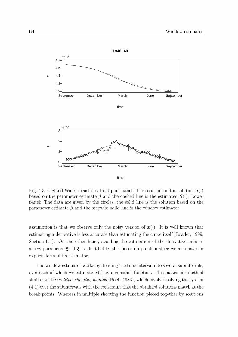
64 Window estimator
1948−49
time
S
3.9
4.1
4.3
4.5
4.7x10⁶
September December March June September
time
I
0
1
2
3x10⁴
September December March June September
Fig. 4.3 England Wales measles data. Upper panel: The solid line is the solution S(·)based on the parameter estimate β and the dashed line is the estimated S(·). Lowerpanel: The data are given by the circles, the solid line is the solution based on theparameter estimate β and the stepwise solid line is the window estimator.
assumption is that we observe only the noisy version of x(·). It is well known thatestimating a derivative is less accurate than estimating the curve itself (Loader, 1999,Section 6.1). On the other hand, avoiding the estimation of the derivative inducesa new parameter ξ. If ξ is identifiable, this poses no problem since we also have anexplicit form of its estimator.
The window estimator works by dividing the time interval into several subintervals,over each of which we estimate x(·) by a constant function. This makes our methodsimilar to the multiple shooting method (Bock, 1983), which involves solving the system(4.1) over the subintervals with the constraint that the obtained solutions match at thebreak points. Whereas in multiple shooting the function pieced together by solutions
4.7 Summary 65
obtained over each subinterval is continuous, the window smoother is not. Also, inmultiple shooting the interval is divided to improve the convergence and numericalstability of the ODEs solver, but here the window smoothing is introduced as a meansto obtain fast but
√n-consistent estimates of the underlying parameters — we are not
directly interested in the solution of the ODEs. In order to improve the estimationaccuracy, other non-parametric curve estimators could be used. For example, Dattnerand Klaassen (2013) use a local polynomial type of estimator. The trade-off is thatusing more complicated estimators usually involves choosing tuning parameters. Also,the algorithmic complexity would be affected due to the calculation of integrals andrepeated integrals in Gn(t), An and Bn.
4.7 Summary
In this chapter, we have presented an extension of a method for parameter estimationin systems of ODEs that are linear in their parameters when the data contain noreplicates. Our method is completely automatic; it requires no tuning whatsoever.It is computationally inexpensive and also does not need any initial values of theparameters. This is very appealing, since in Bayesian and likelihood-based methodsa good initial estimate is essential. Thus, the method can be used as a fast way toobtain an initial value for the MCMC in the case of Bayesian methods or an initialguess for optimization in the case of likelihood-based methods.
4.A Proof of Theorem 1
Denote the number of time points in subinterval Si by Ii. The length of each subin-terval S(t) is T/I. We have that ∑I
i=1 Ii = n and ⌊√n⌋ ≤ Ii ≤ ⌊
√n⌋ + 2, which
implies
I∑i=1
1Ii
= O(1), (4.14)
I∑i=1
1I3
i
= O( 1n
). (4.15)
With the following notation
ε(ti) = (ε1(ti), . . . , εd(ti))⊤,
66 Window estimator
ε(ti) = y(ti) − x(ti),
we have
Eεk(ti) = 0, k = 1, . . . , d, i = 1, . . . , n,
Exn(t) = 1|S(t)|
∑tj∈S(t)
x(tj), t ∈ S(t),
xn(t) − Exn(t) = 1|S(t)|
∑tj∈S(t)
ε(tj), (4.16)
E
1|S(t)|
∑tj∈S(t)
εk(tj)
= 0, k = 1, . . . , d,
Eεk(ti)εk(tj) = 0, i = j, (4.17)
and for any t ∈ [0, T ] we have
var
1|S(t)|
∑tj∈S(t)
εk(tj)
= 1|S(t)|2 var
∑tj∈S(t)
εk(tj)
= σ2
|S(t)| .
We use these results throughout the proof. The proof is based on verifying the followingconditions as stated in Theorem 2 in (Dattner and Klaassen, 2013).
1. ∥Exn − x∥2∞ = O( 1
n)
For nonnegative numbers a1, . . . , am it holds that( m∑
k=1ak
)2≤ m
m∑k=1
a2k. (4.18)
The inequality is the consequence of the inequality between arithmetic and quadraticmean. Applying the triangle inequality and (4.18) yields
∥Exn − x∥2∞ = max
1≤i≤Isupt∈Si
∥ 1Ii
∑tj∈Si
x(tj) − x(t)∥2
= max1≤i≤I
supt∈Si
∥ 1Ii
∑tj∈Si
x(tj) − x(t)∥2
≤ max1≤i≤I
supt∈Si
1I2
i
( ∑tj∈Si
∥∫ tj
tx′(s)ds∥
)2
(4.18)≤ max
1≤i≤Isupt∈Si
I
I2i
∑tj∈Si
∥∫ tj
tg(x(s))θds∥2
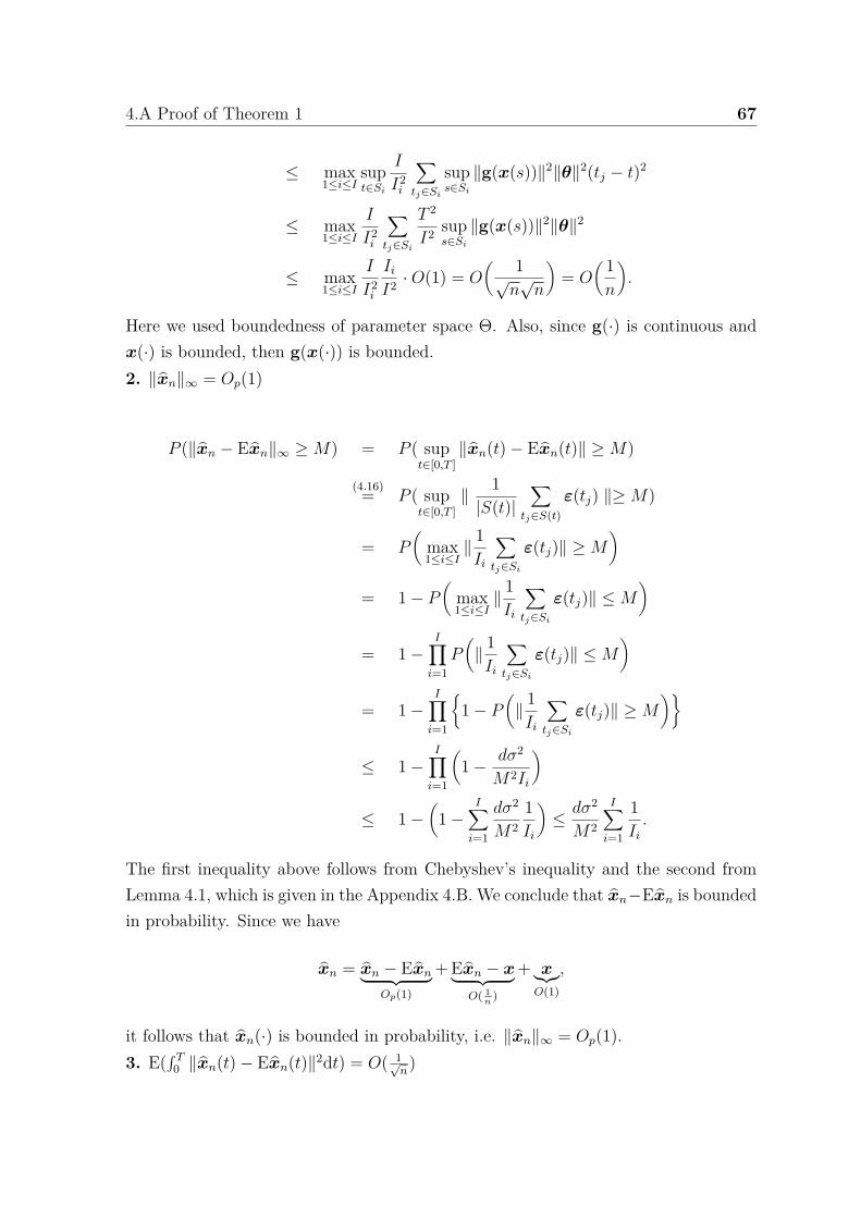
4.A Proof of Theorem 1 67
≤ max1≤i≤I
supt∈Si
I
I2i
∑tj∈Si
sups∈Si
∥g(x(s))∥2∥θ∥2(tj − t)2
≤ max1≤i≤I
I
I2i
∑tj∈Si
T 2
I2 sups∈Si
∥g(x(s))∥2∥θ∥2
≤ max1≤i≤I
I
I2i
Ii
I2 ·O(1) = O( 1√
n√n
)= O
( 1n
).
Here we used boundedness of parameter space Θ. Also, since g(·) is continuous andx(·) is bounded, then g(x(·)) is bounded.2. ∥xn∥∞ = Op(1)
P (∥xn − Exn∥∞ ≥ M) = P ( supt∈[0,T ]
∥xn(t) − Exn(t)∥ ≥ M)
(4.16)= P ( supt∈[0,T ]
∥ 1|S(t)|
∑tj∈S(t)
ε(tj) ∥≥ M)
= P(
max1≤i≤I
∥ 1Ii
∑tj∈Si
ε(tj)∥ ≥ M)
= 1 − P(
max1≤i≤I
∥ 1Ii
∑tj∈Si
ε(tj)∥ ≤ M)
= 1 −I∏
i=1P(
∥ 1Ii
∑tj∈Si
ε(tj)∥ ≤ M)
= 1 −I∏
i=1
1 − P
(∥ 1Ii
∑tj∈Si
ε(tj)∥ ≥ M)
≤ 1 −I∏
i=1
(1 − dσ2
M2Ii
)
≤ 1 −(
1 −I∑
i=1
dσ2
M21Ii
)≤ dσ2
M2
I∑i=1
1Ii
.
The first inequality above follows from Chebyshev’s inequality and the second fromLemma 4.1, which is given in the Appendix 4.B. We conclude that xn−Exn is boundedin probability. Since we have
xn = xn − Exn︸ ︷︷ ︸Op(1)
+ Exn − x︸ ︷︷ ︸O( 1
n)
+ x︸︷︷︸O(1)
,
it follows that xn(·) is bounded in probability, i.e. ∥xn∥∞ = Op(1).3. E(
∫ T0 ∥xn(t) − Exn(t)∥2dt) = O( 1√
n)
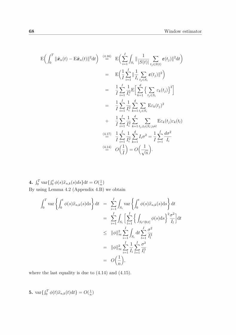
68 Window estimator
E( ∫ T
0∥xn(t) − Exn(t)∥2dt
)(4.16)= E
( I∑i=1
∫Si
∥ 1|S(t)|
∑tj∈S(t)
ε(tj)∥2dt)
= E(1I
I∑i=1
∥ 1Ii
∑tj∈Si
ε(tj)∥2)
= 1I
I∑i=1
1I2
i
E[ d∑
k=1
∑tj∈Si
εk(tj)2]
= 1I
I∑i=1
1I2
i
d∑k=1
∑tj∈Si
Eεk(tj)2
+ 1I
I∑i=1
1I2
i
d∑k=1
∑tj ,tl∈Si:j =l
Eεk(tj)εk(tl)
(4.17)= 1I
I∑i=1
1I2
i
d∑k=1
Iiσ2 = 1
I
I∑i=1
dσ2
Ii
(4.14)= O(1I
)= O
( 1√n
).
4.∫ T
0 var∫ t
0 ϕ(s)xn,k(s)dsdt = O( 1n)
By using Lemma 4.2 (Appendix 4.B) we obtain
∫ T
0var
∫ t
0ϕ(s)xn,k(s)ds
dt =
I∑i=1
∫Si
var∫ t
0ϕ(s)xn,k(s)ds
dt
=I∑
i=1
∫Si
[ I∑l=1
∫Sl∩[0,t]
ϕ(s)ds2σ2
Il
]dt
≤ ∥ϕ∥2∞
I∑i=1
∫Si
dtI∑
l=1
σ2
I3l
= ∥ϕ∥2∞
I∑i=1
1Ii
I∑l=1
σ2
I3l
= O( 1n
),
where the last equality is due to (4.14) and (4.15).
5. var∫ T
0 ϕ(t)xn,k(t)dt = O( 1n)
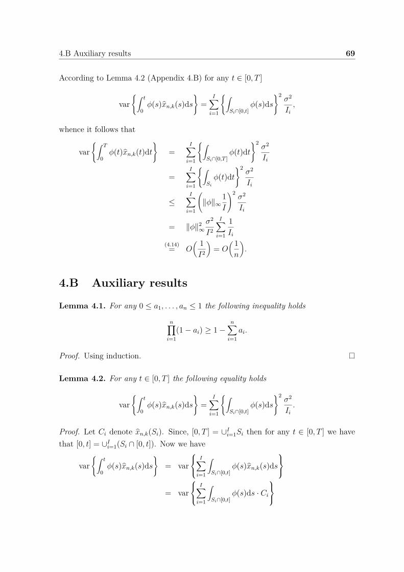
4.B Auxiliary results 69
According to Lemma 4.2 (Appendix 4.B) for any t ∈ [0, T ]
var∫ t
0ϕ(s)xn,k(s)ds
=
I∑i=1
∫Si∩[0,t]
ϕ(s)ds2
σ2
Ii
,
whence it follows that
var∫ T
0ϕ(t)xn,k(t)dt
=
I∑i=1
∫Si∩[0,T ]
ϕ(t)dt2
σ2
Ii
=I∑
i=1
∫Si
ϕ(t)dt2
σ2
Ii
≤I∑
i=1
(∥ϕ∥∞
1I
)2σ2
Ii
= ∥ϕ∥2∞σ2
I2
I∑i=1
1Ii
(4.14)= O( 1I2
)= O
( 1n
).
4.B Auxiliary results
Lemma 4.1. For any 0 ≤ a1, . . . , an ≤ 1 the following inequality holds
n∏i=1
(1 − ai) ≥ 1 −n∑
i=1ai.
Proof. Using induction.
Lemma 4.2. For any t ∈ [0, T ] the following equality holds
var∫ t
0ϕ(s)xn,k(s)ds
=
I∑i=1
∫Si∩[0,t]
ϕ(s)ds2
σ2
Ii
.
Proof. Let Ci denote xn,k(Si). Since, [0, T ] = ∪Ii=1Si then for any t ∈ [0, T ] we have
that [0, t] = ∪Ii=1(Si ∩ [0, t]). Now we have
var∫ t
0ϕ(s)xn,k(s)ds
= var
I∑
i=1
∫Si∩[0,t]
ϕ(s)xn,k(s)ds
= var
I∑i=1
∫Si∩[0,t]
ϕ(s)ds · Ci
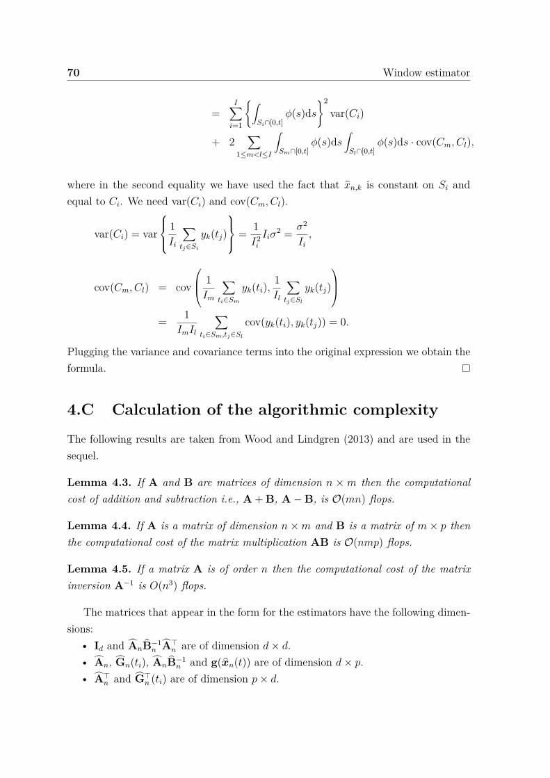
70 Window estimator
=I∑
i=1
∫Si∩[0,t]
ϕ(s)ds2
var(Ci)
+ 2∑
1≤m<l≤I
∫Sm∩[0,t]
ϕ(s)ds∫
Sl∩[0,t]ϕ(s)ds · cov(Cm, Cl),
where in the second equality we have used the fact that xn,k is constant on Si andequal to Ci. We need var(Ci) and cov(Cm, Cl).
var(Ci) = var
1Ii
∑tj∈Si
yk(tj)
= 1I2
i
Iiσ2 = σ2
Ii
,
cov(Cm, Cl) = cov
1Im
∑ti∈Sm
yk(ti),1Il
∑tj∈Sl
yk(tj)
= 1
ImIl
∑ti∈Sm,tj∈Sl
cov(yk(ti), yk(tj)) = 0.
Plugging the variance and covariance terms into the original expression we obtain theformula.
4.C Calculation of the algorithmic complexity
The following results are taken from Wood and Lindgren (2013) and are used in thesequel.
Lemma 4.3. If A and B are matrices of dimension n × m then the computationalcost of addition and subtraction i.e., A + B, A − B, is O(mn) flops.
Lemma 4.4. If A is a matrix of dimension n×m and B is a matrix of m× p thenthe computational cost of the matrix multiplication AB is O(nmp) flops.
Lemma 4.5. If a matrix A is of order n then the computational cost of the matrixinversion A−1 is O(n3) flops.
The matrices that appear in the form for the estimators have the following dimen-sions:
• Id and AnB−1n A⊤
n are of dimension d× d.• An, Gn(ti), AnB−1
n and g(xn(t)) are of dimension d× p.• A⊤
n and G⊤n (ti) are of dimension p× d.
4.C Calculation of the algorithmic complexity 71
• Bn is of dimension p× p.• xn(ti), y(ti) and ξn are of dimension d× 1.
1. The cost for xn(Si) and Gn(ai)We calculate xn(Si), for i = 1, . . . , I. The cost for xn(Si) is O((I − 1)d) so the
total cost is O(I(I − 1)d) = O(I2d) = O(nd). The calculation of Gn(ai) involves thecalculation of g(xn(Si)) and since the construction of matrix g depends on the form ofthe ODEs we assume that every entry of the matrix is obtained by at most a constantnumber of flops C that does not depend on n, p and d. Then the cost of obtainingmatrix g(xn(Si)), for any i = 1, . . . , I, is O(Cdp) = O(dp) flops . The estimator Gn(t)can be calculated recursively by
Gn(a1) = g(xn(S1))a1,
Gn(ai) = Gn(ai−1) + g(xn(Si))∆, i = 2, . . . , I. (4.19)
Since the cost for computing g(xn(Si)), for i = 1, . . . , I is O(dp) flops, from (4.19)it follows that Gn(ai), i = 1, . . . , I can be computed in O(dp) flops and thereforesumming across i = 1, . . . , I we obtain that the total cost is O(Idp) = O(
√ndp) flops.
2. The cost for An, An(i) and Bn
Since the cost for computing g(xn(Si)) and Gn(ai), for each i is O(dp) flops, from(4.9) it follows that the cost for An(i) is O(dp) flops. The equality An = ∑n
i=1 An(i)implies that the total cost for computing An and An(i), i = 1, . . . , n is O(Idp) flops.For the cost of Bn we analyze each term in (4.10).
• (Gn(T )⊤, An) 7→ Gn(T )⊤An costs O(p2d) flops.
•(
g(xn(Si))⊤, t2Gn(t)∣∣∣∣ai
ai−1
)7→ g(xn(Si))⊤t2Gn(t)
∣∣∣∣ai
ai−1
costs O(p2d) flops.
• (R⊤i ,g(xn(Si))(2i− 1)) 7→ R⊤
i g(xn(Si))(2i− 1) costs O(p2d) flops.• (g(xn(Si))⊤,g(xn(Si))(3i2 − 1)) 7→ g(xn(Si))⊤g(xn(Si))(3i2 − 1) costs O(p2d)
flops.Each term above has complexity O(p2d) and summing over i we get that the costfor Bn is O(Ip2d). Finally, the total cost for An, An(i), i = 1, . . . , I, and Bn isO(Idp) +O(Ip2d) = O(Ip2d), which is equal to O(
√np2d) flops.
3. The cost for ξn
The term(T Id − AnB−1
n A⊤n
)−1
• Bn 7→ B−1n costs O(p3) flops.
• (An, B−1n ) 7→ AnB−1
n costs O(p2d) flops.• (AnB−1
n , A⊤n ) 7→ AnB−1
n A⊤n costs O(d2p) flops.
72 Window estimator
• (Id, AnB−1n A⊤
n ) 7→ T Id − AnB−1n A⊤
n costs O(d2) flops.• Id − AnB−1
n A⊤n 7→ (Id − AnB−1
n A⊤n )−1 costs O(d3) flops.
Thus, the computational cost of(Id − AnB−1
n A⊤n
)−1is O(p3 + p2d + d2p + d2 + d3)
which is equal to O(p3 + d3) flops.The term T
∑Ii=1 xn(Si)/I − AnB−1
n
∑Ii=1 An(i)⊤xn(Si)
• xn(Si) 7→ T∑I
i=1 xn(Si)/I costs O(Id) flops.• (An(i)⊤, xn(Si)) 7→ ∑I
i=1 An(i)⊤xn(Si) costs O(Ipd) flops.• (AnB−1
n ,∑I
i=1 An(i)⊤xn(Si)) 7→ AnB−1n
∑Ii=1 An(i)⊤xn(Si) costs O(dp) flops.
In total, the cost for T ∑Ii=1 xn(Si)/I−AnB−1
n
∑Ii=1 An(i)⊤xn(Si) isO(Idp) = O(
√ndp)
flops. Finally we have the following:•(Id − AnB−1
n A⊤n
)−1costs O(p3 + d3) flops.
• T∑I
i=1 xn(Si)/I − AnB−1n
∑Ii=1 An(i)⊤xn(Si) costs O(
√ndp) flops.
• Multiplication of two aforementioned terms costs O(d2) flops.In total, calculation of ξn costs O(p3 + d3 +
√ndp+ d2), which is equal to O(p3 + d3 +
√ndp) flops.
4. The cost for θn
The term ∑Ii=1 An(i)⊤xn(Si) − A⊤
n ξn
• (An(i)⊤, xn(Si)) 7→ ∑Ii=1 An(i)⊤xn(Si) costs O(Ipd) flops.
• (A⊤n , ξn) 7→ A⊤
n ξn costs O(pd) flops.• Addition of two aforementioned terms costs O(p) flops.
In total, the cost for calculating ∑Ii=1 An(i)⊤xn(Si) − A⊤
n ξn is O(Ipd) = O(√npd)
flops. The multiplication of B−1n with the last mentioned term costs O(p2) flops so the
total cost for θn is O(p2 +√npd) flops.
Hence, the computational complexity of the procedure is O(√ndp+
√ndp2 + p3 +
d3 +√ndp+ p2 +
√npd) flops which is equal to O(p3 + d3 +
√ndp2) flops.
4.D Calculation of the integrals
Let us first recall that Si = [ai−1, ai], for i = 1, . . . , I − 1 and SI = [aI−1, T ]. Thelength of each subinterval Si is ∆ = T/I and the boundary points of the subintervalsare ai = i∆, for i = 0, . . . , I. To shorten notation, we let G1(t) stand for an arbitraryentry of the matrix Gn(t). Similarly, let g1(xn(t)) denote the entry of the matrixg(xn(t)) that corresponds to G1(t), i.e G1(t) =
∫ t0 g1(xn(s))ds. Let Ci = g1(xn(Si)),
4.D Calculation of the integrals 73
for i = 1, . . . , I. Using integration by parts yields∫Si
G1(t)dt =∫ ai
ai−1G1(t)dt = tG1(t)|ai
ai−1−∫ ai
ai−1tg1(xn(t))dt
= tG1(t)|aiai−1
− g1(Ci)(a2i − a2
i−1)/2
= tG1(t)|aiai−1
− 12(2i− 1)∆2g1(Ci), (4.20)
where we have used the identity a2i − a2
i−1 = (2i − 1)∆2. In the same manner, weobtain that for t ∈ Si it holds that∫ t
0G1(s)ds = sG1(s)|t0 −
∫ t
0sg1(xn(s))ds
= tG1(t) −i−1∑
m=1
∫ am
am−1sg1(xn(s))ds−
∫ t
ai−1sg1(xn(s))ds
= tG1(t) −i−1∑
m=1
g1(Cm)2 (a2
m − a2m−1) − 1
2g1(Ci)(t2 − a2i−1)
= tG1(t) − ∆2
2
i−1∑m=1
(2m− 1)g1(Cm) − 12g1(Ci)(t2 − a2
i−1),
(4.21)
Recall the convention that ∑i−1m=1(2m − 1)g1(Cm) is equal to zero for i = 1. Setting
t = T in (4.21) we obtain
∫ T
0G1(t)dt = TG1(T ) − ∆2
2
I∑m=1
(2m− 1)g1(Cm). (4.22)
Applying (4.20) and (4.22) to every entry of the matrices∫
SiGn(t)dt and
∫ T0 Gn(t)dt,
respectively, we conclude that
An(i) =∫
Si
Gn(t)dt = tGn(t)|aiai−1
− 12(2i− 1)∆2g(xn(Si)),
An =∫ T
0Gn(t)dt = T Gn(T ) − ∆2
2
I∑i=1
(2i− 1)g(xn(Si)).
To obtain Bn, we need integrals of the form∫ T
0 G1(t)G2(t)dt where, to simplifynotation, entries of the matrix Gn(t) are denoted by G1(t) and G2(t). Similarlyg1(xn(t)) and g2(xn(t)) denote the corresponding entries of the matrix g(xn(t)), i.e
74 Window estimator
Gi(t) =∫ t
0 gi(xn(s))ds, i = 1, 2. Integration by parts yields
∫ T
0G1(t)G2(t)dt = G1(s)
∫ t
0G2(s)ds
∣∣∣∣∣T
0−∫ T
0
g1(xn(s))
∫ t
0G2(s)ds
dt
= G1(T )∫ T
0G2(t)dt−
I∑i=1
g1(Ci)∫ ai
ai−1
∫ t
0G2(s)ds
dt.
According to (4.21), for any t ∈ Si
∫ t
0G2(s)ds = tG2(t) − ∆2
2
i−1∑m=1
(2m− 1)g2(Cm) − g2(Ci)2 (t2 − a2
i−1)
and hence∫ ai
ai−1
∫ t
0G2(s)ds
dt =
∫ ai
ai−1tG2(t)dt− ∆3
2
i−1∑m=1
(2m− 1)g2(Cm)
− g2(Ci)2
13(a3
i − a3i−1) − a2
i−1(ai − ai−1).
Again using integration by parts, we obtain∫ ai
ai−1tG2(t)dt = 1
2t2G2(t)
∣∣∣∣ai
ai−1
− 12
∫ ai
ai−1t2g2(xn(t))dt
= 12t
2G2(t)∣∣∣∣ai
ai−1
− 12g2(Ci)
13(a3
i − a3i−1).
Since ai = i∆, for i = 0, . . . I it follows that
a3i − a3
i−1 = (3i2 − 3i+ 1)∆3,
13(a3
i − a3i−1) − a2
i−1(ai − ai−1) = ∆3(3i− 2)/3.
Also, the following identity holds
I∑i=1
g1(Ci)i−1∑
m=1(2m− 1)g2(Cm) =
I−1∑i=1
(2i− 1)Rig2(Ci),
where Ri = ∑Im=i+1 g1(Cm). By using previous identities, we finally obtain
∫ T
0G1(t)G2(t)dt = G1(T )
∫ T
0G2(s)ds− 1
2
I∑i=1
g1(Ci)t2G2(t)∣∣∣∣ai
ai−1
4.D Calculation of the integrals 75
+ ∆3
6
I∑i=1
(3i2 − 1)g1(Ci)g2(Ci)
+ ∆3
2
I−1∑i=1
(2i− 1)Rig2(Ci).
Since (r, k)th entry, Gn(t)[r, k], of the matrix∫ T
0 Gn(t)⊤Gn(t)dt is the sum of expres-sions
∫ T0 Gn(t)[l, r]Gn(t)[l, k]dt that are of the form above we obtain that
Bn =∫ T
0Gn(t)⊤Gn(t)dt = Gn(T )⊤
∫ T
0Gn(t)dt
− 12
I∑i=1
g(xn(Si))⊤t2Gn(t)∣∣∣∣ai
ai−1
+ ∆3
6
I∑i=1
(3i2 − 1)g⊤(xn(Si))g(xn(Si))
+ ∆3
2
I−1∑i=1
(2i− 1)R⊤i g(xn(Si)),
where Ri = ∑Im=i+1 g(xn(Sm)).

Chapter 5
RKHS approach to estimatingparameters in ordinary differentialequations
In this chapter, we discuss the problem of estimating parameters in ODEs which havea general form. In our approach we combine the frequentist set-up, such as in Ramsayet al. (2007), with the kernel approach of Steinke and Schölkopf (2008). In this waywe define the estimation problem explicitly as a maximum likelihood problem, wherethe differential equation is interpreted as a constraint. By introducing a reproducingkernel Hilbert space (RKHS), we transform the constrained maximization probleminto an unconstrained one. We detail this idea in Section 5.3 after a review of RKHSand Green’s functions given in Section 5.1, and the classical MLE approach reviewedin Section 5.2. In Section 5.4 we focus on the implementation of our methodology.Sections 5.5 and 5.6 illustrate the behaviour of the technique in simulated and realdata scenarios, respectively. The last section contains the summary and the appendixcontains proofs.
5.1 Preliminaries
5.1.1 Reproducing kernel Hilbert spaces
In this section we give an introduction to the theory of reproducing kernel Hilbertspaces. Our exposition is based on Steinwart and Christmann (2008). We restrictourselves to real Hilbert spaces although the theory holds for complex Hilbert spaces
78 RKHS
as well.
Definition 5.1. Let X be a nonempty set. A function k : X × X → R is called akernel on X if it is symmetric and positive definite, i.e. for all n ∈ N , α1, . . . , αn ∈ Rand all x1, . . . , xn we have
n∑i=1
n∑j=1
αiαjk(xi, xj) ≥ 0. (5.1)
Condition (5.1) is equivalent to the positive definiteness of the kernel matrix (orGram matrix)
K = (k(xi, xj))i,j. (5.2)
Kernels are intimately connected to Hilbert spaces since it can be shown that k is akernel on X if and only if there exists a Hilbert space H called a feature space and amap Φ : X → H called a feature map such that for all x, x′ ∈ X we have
k(x, x′) = ⟨Φ(x),Φ(x′)⟩H,
where ⟨·, ·⟩H is an inner product on H. For a kernel neither the feature map nor thefeature space are uniquely determined. Although not unique, it can be shown that thefeature space H has to be a Hilbert function space over X, i.e., a Hilbert space thatconsists of functions mapping X into R. Related to this, we can consider an oppositesituation: for a given Hilbert function space H over X does there exist a kernel k thatcan reproduce the functions of the space H? In this regard, we have the followingdefinition.
Definition 5.2. Let X be a nonempty set and H be a Hilbert function space over X.A function k : X ×X → R is called a reproducing kernel of H if we have k(·, x) ∈ Hfor all x ∈ X and the reproducing property
f(x) = ⟨f, k(·, x)⟩
holds for all f ∈ H and all x ∈ X.
In definition 5.2 it is not assumed that k is a kernel, since it can be shown thatevery reproducing kernel is a kernel in the sense of definition 5.1 with the feature map
Φ(x) = k(·, x), x ∈ X.
5.1 Preliminaries 79
Furthermore, it can be shown that every Hilbert function space with a reproducingkernel is a reproducing kernel Hilbert space in the sense of the following definition.
Definition 5.3. Let X be a nonempty set. A Hilbert function space H over X is areproducing kernel Hilbert space (RKHS) over X if for all x ∈ X the Dirac functionalδx : H → R defined by
δx(f) = f(x), f ∈ H,
is continuous.
There is a one-to-one relation between kernels and RKHSs; that is the content ofthe following theorem.
Theorem 5.1. 1. (Every RKHS has a unique reproducing kernel) Let H be an RKHSover X. Then k : X ×X → R defined by
k(x, x′) = ⟨δx, δx′⟩, x ∈ X,
is the only reproducing kernel of H.2. (Every kernel has a unique RKHS) Let X be a nonempty set and k be a kernel
on X. Then the metric completion H of the set
Hpre =
n∑i=1
αik(·, xi) : n ∈ N,α1, . . . , αn ∈ R, x1, . . . , xn ∈ X
is the only RKHS for which k is a reproducing kernel. Also, for f = ∑ni=1 αik(·, xi) ∈
Hpre we have
∥f∥2H =
n∑i=1
n∑j=1
αiαjk(xi, xj) = α⊤Kα,
where K is the kernel matrix defined in (5.2) and α = (α1, . . . , αn)⊤.
Consider the problem of estimating a function f : X → R from the data D =(x1, y1), . . . , (xn, yn) |xi ∈ X , yi ∈ R. We focus here on the quadratic loss butthe problem could be formulated for an arbitrary loss function (Smola et al., 2002).Minimizing the functional
L(f) = an∑
i=1yi − f(xi)2,
where a is some positive constant, is an ill-posed problem (Chen and Haykin, 2002)unless we restrict the class of functions f . One approach is to restrict the class of
80 RKHS
functions f to a compact set of an RKHS over X. This can be done by regularizingthe empirical loss L with a strictly monotone function of ∥f∥2
H. In our work, weconsider the regularized (penalized) loss
Lλ(f) = an∑
i=1yi − f(xi)2 + λ
2 ∥f∥2H. (5.3)
The existence of the minimizer of the penalized loss and its representation in termsof kernels is guaranteed by the representer theorem in the case of an arbitrary lossfunction and a penalty which is a strictly monotonic function of the RKHS norm(Smola et al., 2002). In the case of the penalized loss (5.3) the solution is also unique.
Theorem 5.2 (Representer theorem). Let a and λ be positive constants and let Hbe an RKHS over X associated to a kernel k. Then for all x1, . . . , xn ∈ X and ally1, . . . , yn ∈ R the minimizer f ∈ H of the functional
Lλ(f) = an∑
i=1yi − f(xi)2 + λ
2 ∥f∥2H
is unique and admits a representation of the form
f(x) =n∑
i=1αik(xi, x),
where vector α = (α1, . . . , αn)⊤ is given by
α =(λ
2aIn + K)−1
y
and y = (y1, . . . , yn)⊤.
As a consequence of this theorem we have that f = (f(x1), . . . , f(xn))⊤ = Kα.
5.1.2 Green’s function and reproducing kernel Hilbert spaces
In this section we cover the concept of Green’s function and its relation to RKHS. Inour exposition we define Green’s function as a function of two variables, though it canbe defined as a distribution, i.e. generalized function. The terminology varies (Griffel,1985; Nikol’skij, 1992; Kelley and Peterson, 2010; Folland, 1992; Duffy, 2001; Stakgoldand Holst, 1979; Barton, 1989; Roach, 1982; Fasshauer, 2012), but roughly speaking,
5.1 Preliminaries 81
the main idea is that Green’s function is the kernel of the integral operator, which isthe inverse of a linear differential operator.
Definition 5.4. Let P = dm/dtm + ∑m−1k=1 θkdk/dtk be a linear differential operator,
where θ1, . . . , θm−1 ∈ R. Any function G(t, s) satisfying
PtG(t, s) = δ(t− s), (5.4)
where δ is the Dirac delta function, is called a fundamental solution or Green’s functionof the operator P.
The subscript t in P is to stress that the differentiation is with respect to the vari-able t. The Dirac δ function is defined as a ”function” such that
∫+∞−∞ δ(t− s)f(s)ds =
f(t) and
δ(t) = +∞ if t = 0
0 if t = 0.
As we use the delta function for notational simplicity, equality (5.4) should not beunderstood in a distributional sense (Folland, 1992) but as follows:
• G(t, s) belongs to the class Cm−2[a, b] and its (m− 1)st and mth derivative existand are continuous for t = s.
• PtG(t, s) = 0, for t = s.• (m− 1)st derivative has a unit jump for t = s.
Green’s function is important because it is used to solve linear differential equations.If we have the differential equation
Pg(t) = f(t), t ∈ [0, T ],
and certain conditions the solution g needs to satisfy, like boundary conditions, initialvalue conditions or more generally distributed conditions, then the solution can bewritten as
g(t) = (P−1f)(t) =∫ T
0G(t, s)f(s)ds.
Besides (5.4), G also needs to satisfy the conditions that arise from those conditionsimposed on the solution g. In other words, the inverse operator P−1 of the differentialoperator P is an integral operator with the kernel G. For more details see Nikol’skij(1992).
In this thesis we use only differential operators of first order, which we discretize.In other words, we use a difference operator and consequently we are interested in its
82 RKHS
Green’s function. Thus, we consider a Hilbert space of functions over a finite set X =x1, . . . , xn, i.e. H = f : f : X → R. Here the situation is much simpler, becauseevery function f ∈ H is fully described by the vector f = (f(x1), . . . , f(xn))⊤ ∈ Rn,linear operators P : H → H are isomorphic to matrices and any function G : X×X →R uniquely determines a linear operator G : H → H through its matrix G, where(G)ij = G(xi, xj). Also, for every invertible operator on a finite dimensional space wehave the form of the matrix of its inverse. The role of the delta function is taken bythe Kronecker delta. For more details see Steinke and Schölkopf (2008). Hence, thedefinition (5.4) for the difference operator with a matrix P translates into
(PG)(t, s) = δ(t, s),
where δ(t, s) is the Kronecker delta. In other words, G is the inverse matrix of thematrix P of a difference operator, i.e. G = P−1.
In the following theorem we connect Green’s function with RKHS.
Theorem 5.3. Let P be the standard matrix of an invertible linear operator on Rn.Define an inner product on H with
⟨f ,f ′⟩H = ⟨Pf ,Pf ′⟩Rn ,
where ⟨·, ·⟩Rn is the standard Euclidean inner product in Rn. Then H is an RKHSover X that admits as a reproducing kernel Green’s function of P⊤P, i.e. the functionG : X ×X → R determined by the Green’s matrix
G = (P⊤P)−1.
Proof. Green’s function G : X × X → R determined by the matrix G = (P⊤P)−1 isthe reproducing kernel of H since for any function f ∈ H we have
⟨f,G(·, x)⟩H = ⟨f ,G(·, x)⟩H = ⟨Pf ,PG(·, x)⟩Rn = ⟨f ,P⊤PG(·, x)⟩Rn
= ⟨f , δ(·, x)⟩ = f(x),
where G(·, x) is the column of G. Every linear functional on a finite dimensional vectorspace is continuous, and so is the Dirac’s. Therefore, H is an RKHS determined bythe kernel G.
5.2 Explicit ODEs 83
5.2 Explicit ODEs
We consider dynamical systems with d interacting elements evolving in some closedtime interval [0, T ]. We denote by xk : [0, T ] → IR for k = 1, . . . , d, the functionsdescribing the evolution of the elements of the system and by uk : [0, T ] → IR fork = 1, . . . ,m, the action of m external forces. In compact notation, we denote byx(t) = (x1(t), . . . , xd(t))⊤, u(t) = (u1(t), . . . , um(t))⊤ the vectors of state variablesand external forces respectively. We assume that each state variable xk satisfies
Pθkxk(t) = fk(x(t),u(t),β), k = 1, . . . , d, t ∈ [0, T ],
where Pθk= d/dt + θkI is the linear differential operator associated with the kth
equation of the system. Here, fk is a known function depending on t through x(t) andu(t), and β is a vector of parameters. We use notation I for the identity operator.For differential operators of a higher order see González et al. (2014).
In the sequel, we refer to the whole set of the parameters of the system by θ,β,where θ = (θ1, . . . , θd)⊤. Typically, a noisy sample of x is observed at a grid of timepoints t = (t1, . . . , tn)⊤. Let yk indicate the available data for state k and let xk(t)indicate the vector of values corresponding to the evaluated kth state at time pointst, i.e.
yk = yk(t) = (yk(t1), . . . , yk(tn))⊤, (5.5)xk = xk(t) = (xk(t1), . . . , xk(tn))⊤, (5.6)fk = (fk(x(t1),u(t1),β), . . . , fk(x(tn),u(tn),β))⊤. (5.7)
We consider a model with additive noise
yk(t) = xk(t) + εk(t),
where ϵk represents a noise process for the kth state. We assume that εk(t) is anindependent multivariate zero-mean Gaussian noise with variance σ2
k for each kthstate. Let y(t) and x(t) denote the matrices that comprise all the rows yk, xk, fork = 1, . . . , d, respectively. Then the log-likelihood of the model given y(t) is
l(θ,β,x(t)|y(t)) = −d∑
k=1
12σ2
k
∥yk − xk∥2 where Pθkxk(t) = fk(x(t),u(t),β). (5.8)
84 RKHS
Here, x depends on θ,β although for the sake of simplicity it is not explicitly spec-ified. Since ODEs generally do not have a closed-form solution, evaluating the log-likelihood at a specific value of the parameters θ,β requires solving numerically thesystem for those parameters. Thus, the numerical maximization of the log-likelihoodfunction involves repeatedly solving the system for every new iteration in the opti-mization algorithm. This approach is thus computationally costly, especially for largesystems.
5.3 RKHS based penalized log-likelihood
In this section, our goal is to reformulate (5.8) in terms of a penalized loss so as toobtain a computationally tractable solution that does not require an explicit solution ofthe system of ODEs. To this aim, we discretize the system and consider the differenceequation
Pθkxk = fk,
where xk and fk are defined in (5.6) and (5.7) and Pθkis the operator defined by
Pθk= Dn + θkIn. (5.9)
Here, In is the identity matrix of order n and Dn ∈ IRn×n is the first order differencematrix
Dn = ∆−1
−1 1−1 0 1
. . .−1 0 1
−1 1
, (5.10)
where ∆ = diag(t2 − t1, 2(t3 − t1), . . . , 2(tn−1 − tn−2), tn − tn−1). The difference in finiteapproximations used for t1 and tn is due to the fact that they are boundary points.We aim to define a penalized loss function
lλ(θ,β,x(t)|y(t)) = −d∑
k=1
12σ2
k
∥yk − xk∥2 − λ
2
d∑k=1
Ω(xk), (5.11)
where Ω defines a norm of xk in an RKHS.First consider the homogeneous system, i.e. fk = 0n. In this case, according to
5.3 RKHS based penalized log-likelihood 85
theorem 5.3 defining the penalty as Ω(xk) = ∥Pθkxk∥2 implies that
Ω(xk) = ∥xk∥2Hθk
,
where Hθkis the RKHS defined by the kernel matrix
Kθk= (P⊤
θkPθk
)−1. (5.12)
Consequently, according to the representer theorem 5.2 the penalized loss has theminimizer xk of the form
xk = Kθkαk,
where αk = (Kθk+ λσ2
kIn)−1yk.
In general, the interest in inferring parameters of ODEs is for nonhomogeneoussystems. In the same spirit as above, one might consider
Ω(xk) = ∥Pθkxk − fk∥2, (5.13)
as a penalty. However, (5.13) cannot be used directly as a penalty for two reasons.Expression (5.13) cannot be reformulated as a norm of xk in an RKHS; when xk = 0n
then ∥Pθkxk − fk∥2 is not necessarily zero. Also, in this case the equations of the
system are not independent. In a general setting, each xk is affected by x1, . . . ,xn.
To circumvent the previous problem we consider that each fk is a function of βthat depends on t through u(t) and some fixed surrogate of x, denoted by x⋆(t),independent of θ and β. This step represents a linearization of the system and makesthe equations independent of each other. In subsection 4 we elaborate on the definitionof an appropriate x⋆(t).
In order to find an RKHS representation of the system in a general case, as before,we assume that Pθk
is invertible for each k . Denote by
f ⋆k = (fk(x⋆(t1),u(t1),β), . . . , fk(x⋆(tn),u(tn),β))⊤, (5.14)xk = xk − P−1
θkf ⋆
k .
Since Pθkis a linear operator we obtain that for all k = 1, . . . , d
∥Pθkxk − f ⋆
k ∥2 = ∥Pθkxk∥2,
86 RKHS
which according to theorem 5.3 is a norm of xk in an RKHS defined by the kernel(5.12). Hence, we write
Ω(xk) = ∥Pθkxk∥2 = ∥xk∥2
Hθk.
In practice, noise samples are obtained for xk and not for xk. Therefore, the inferenceproblem on xk requires the following transformation of the original data
yk = yk − P−1θkf ⋆
k .
It is straightforward to check that yk ∼ N (xk(t), σ2kIn) and therefore the variance of
the ykj’s is the same as the variance of the ykj’s.
5.4 Approximate ODEs inference
The goal of this section is to provide computational details to infer the set of param-eters θ,β by using the approximate ODEs representation described in Section 5.3.As detailed there, a definition of each x⋆
k, a surrogate of xk is required. In this thesis,we express each x⋆
k in terms of a spline basis expansion,
x⋆k =
q∑i=1
ckiϕi(t), (5.15)
where q is the number of basis functions ϕi and cki, i = 1, . . . , 1 are coefficients ofthe expansion. The number of basis functions should be large enough to capture thevariation in the solutions of the system of ODEs .
Definition 5.5. Let yk, xk, Pθk, f ⋆
k and x⋆k be defined by (5.5), (5.6), (5.9), (5.14)
and (5.15) for k = 1, . . . , d. We define the approximated penalized pseudo log-likelihoodof the ODEs model associated to (5.11) as
lλ(θ,β|y(t),x⋆(t)) = −d∑
k=1
12σ2
k
∥yk − xk∥2 − λ
2
d∑k=1
∥Pθkxk − f ⋆
k ∥2,
where λ > 0 and x⋆(t) = (x⋆1(t), . . . , x⋆
d(t))⊤.
Since for all k = 1, . . . , d it holds
∥yk − xk∥2 = ∥yk − P−1θkf ⋆
k − (xk − P−1θkf ⋆
k )∥2 = ∥yk − xk∥2,
5.4 Approximate ODEs inference 87
it follows that we can rewrite lλ(θ,β|y(t),x⋆(t)) as follows
lλ(θ,β|y(t),x⋆(t)) = −d∑
k=1
12σ2
k
∥yk − xk∥2 − λ
2
d∑k=1
∥Pθkxk∥2. (5.16)
This form allows us to use the representer theorem according to which the minimizerof (5.16) is given by xk = Kθk
αk, where αk = (Kθk+ λσ2
kIn)−1yk. It follows that
x = Sλ,kyk, (5.17)
whereSλ,k = Kθk
(Kθk+ λσ2
kIn)−1yk. (5.18)
Hence, the minimizer written in terms of xk is given by
xk = Kθkαk + P−1
θkf ⋆
k .
Next, we show how to compute lλ in practice.
Proposition 5.1. Assume that P−1θk
exists. Then it holds
θ, β = argmaxθ,β
lλ(θ,β|y(t),x⋆(t)) = argmaxθ,β
gλ(θ,β|y(t),x⋆(t)),
where
gλ(θ,β|y(t),x⋆(t)) = −d∑
k=1
12σ2
k
y⊤k
In − (In + σ2
kλK−1θk
)−1yk. (5.19)
Optimization of (5.19) with a conjugate gradient method produces estimates of θ,β.If the set of parameters of the system is separable by equations, independent opti-mization for those can be done, thus helping to avoid local maxima and speed up theprocedure. Finally, estimates for each xk are available by means of
xk = Kθkαk + P−1
θkfk(u(t),x⋆(t), β),
where αk = (Kθk
+ λσ2kIn)−1yk.
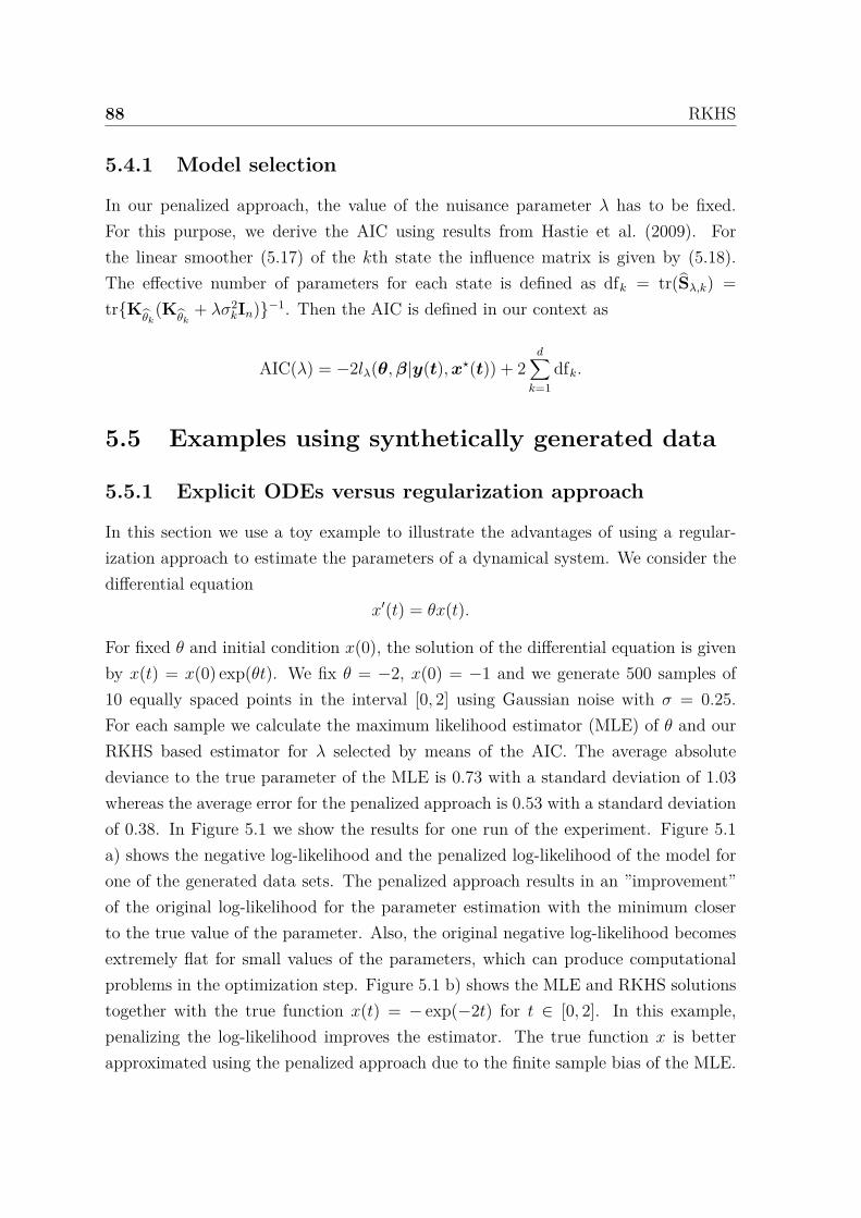
88 RKHS
5.4.1 Model selection
In our penalized approach, the value of the nuisance parameter λ has to be fixed.For this purpose, we derive the AIC using results from Hastie et al. (2009). Forthe linear smoother (5.17) of the kth state the influence matrix is given by (5.18).The effective number of parameters for each state is defined as dfk = tr(Sλ,k) =trK
θk(K
θk+ λσ2
kIn)−1. Then the AIC is defined in our context as
AIC(λ) = −2lλ(θ,β|y(t),x⋆(t)) + 2d∑
k=1dfk.
5.5 Examples using synthetically generated data
5.5.1 Explicit ODEs versus regularization approach
In this section we use a toy example to illustrate the advantages of using a regular-ization approach to estimate the parameters of a dynamical system. We consider thedifferential equation
x′(t) = θx(t).
For fixed θ and initial condition x(0), the solution of the differential equation is givenby x(t) = x(0) exp(θt). We fix θ = −2, x(0) = −1 and we generate 500 samples of10 equally spaced points in the interval [0, 2] using Gaussian noise with σ = 0.25.For each sample we calculate the maximum likelihood estimator (MLE) of θ and ourRKHS based estimator for λ selected by means of the AIC. The average absolutedeviance to the true parameter of the MLE is 0.73 with a standard deviation of 1.03whereas the average error for the penalized approach is 0.53 with a standard deviationof 0.38. In Figure 5.1 we show the results for one run of the experiment. Figure 5.1a) shows the negative log-likelihood and the penalized log-likelihood of the model forone of the generated data sets. The penalized approach results in an ”improvement”of the original log-likelihood for the parameter estimation with the minimum closerto the true value of the parameter. Also, the original negative log-likelihood becomesextremely flat for small values of the parameters, which can produce computationalproblems in the optimization step. Figure 5.1 b) shows the MLE and RKHS solutionstogether with the true function x(t) = − exp(−2t) for t ∈ [0, 2]. In this example,penalizing the log-likelihood improves the estimator. The true function x is betterapproximated using the penalized approach due to the finite sample bias of the MLE.
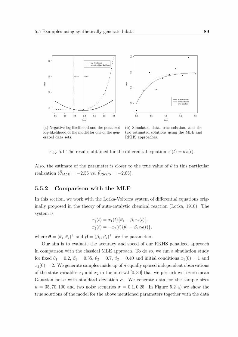
5.5 Examples using synthetically generated data 89
−3.5 −3.0 −2.5 −2.0 −1.5 −1.0 −0.5
510
1520
Theta
Val
ue
log−likelihoodpenalized log−likelihood
−2.05−2.55
(a) Negative log-likelihood and the penalizedlog-likelihood of the model for one of the gen-erated data sets.
0.0 0.5 1.0 1.5 2.0
−1.0
−0.5
0.0
0.5
Time
Val
ue
true solutionrkhs solutionmle solution
(b) Simulated data, true solution, and thetwo estimated solutions using the MLE andRKHS approaches.
Fig. 5.1 The results obtained for the differential equation x′(t) = θx(t).
Also, the estimate of the parameter is closer to the true value of θ in this particularrealization (θMLE = −2.55 vs. θRKHS = −2.05).
5.5.2 Comparison with the MLE
In this section, we work with the Lotka-Volterra system of differential equations orig-inally proposed in the theory of auto-catalytic chemical reaction (Lotka, 1910). Thesystem is
x′1(t) = x1(t)θ1 − β1x2(t),x′
2(t) = −x2(t)θ1 − β2x2(t),
where θ = (θ1, θ2)⊤ and β = (β1, β2)⊤ are the parameters.Our aim is to evaluate the accuracy and speed of our RKHS penalized approach
in comparison with the classical MLE approach. To do so, we run a simulation studyfor fixed θ1 = 0.2, β1 = 0.35, θ2 = 0.7, β2 = 0.40 and initial conditions x1(0) = 1 andx2(0) = 2. We generate samples made up of n equally spaced independent observationsof the state variables x1 and x2 in the interval [0, 30] that we perturb with zero meanGaussian noise with standard deviation σ. We generate data for the sample sizesn = 35, 70, 100 and two noise scenarios σ = 0.1, 0.25. In Figure 5.2 a) we show thetrue solutions of the model for the above mentioned parameters together with the data
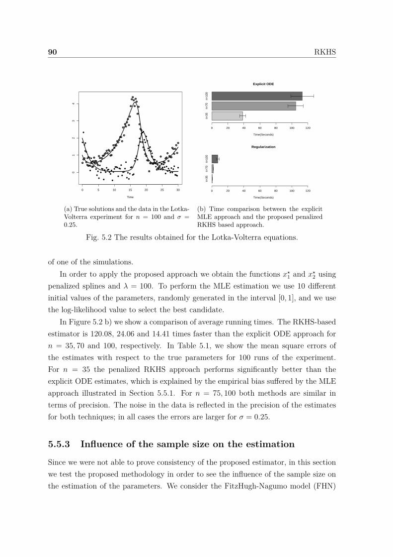
90 RKHS
0 5 10 15 20 25 30
01
23
4
Time
(a) True solutions and the data in the Lotka-Volterra experiment for n = 100 and σ =0.25.
n=35
n=70
n=10
0
Explicit ODE
Time(Seconds)
0 20 40 60 80 100 120
n=35
n=70
n=10
0
Regularization
Time(Seconds)
0 20 40 60 80 100 120
(b) Time comparison between the explicitMLE approach and the proposed penalizedRKHS based approach.
Fig. 5.2 The results obtained for the Lotka-Volterra equations.
of one of the simulations.In order to apply the proposed approach we obtain the functions x⋆
1 and x⋆2 using
penalized splines and λ = 100. To perform the MLE estimation we use 10 differentinitial values of the parameters, randomly generated in the interval [0, 1], and we usethe log-likelihood value to select the best candidate.
In Figure 5.2 b) we show a comparison of average running times. The RKHS-basedestimator is 120.08, 24.06 and 14.41 times faster than the explicit ODE approach forn = 35, 70 and 100, respectively. In Table 5.1, we show the mean square errors ofthe estimates with respect to the true parameters for 100 runs of the experiment.For n = 35 the penalized RKHS approach performs significantly better than theexplicit ODE estimates, which is explained by the empirical bias suffered by the MLEapproach illustrated in Section 5.5.1. For n = 75, 100 both methods are similar interms of precision. The noise in the data is reflected in the precision of the estimatesfor both techniques; in all cases the errors are larger for σ = 0.25.
5.5.3 Influence of the sample size on the estimation
Since we were not able to prove consistency of the proposed estimator, in this sectionwe test the proposed methodology in order to see the influence of the sample size onthe estimation of the parameters. We consider the FitzHugh-Nagumo model (FHN)
5.5 Examples using synthetically generated data 91
Lotka-Volterra ODE modelσ n Method |θ1 − θ1| |β1 − β1| |θ2 − θ2| |β2 − β2|
0.1
35 RKHS 0.0002 (0.0003) 0.0007 (0.0007) 0.0031 (0.0036) 0.0014 (0.0014)MLE 0.0016 (0.0088) 0.0063 (0.0425) 0.0422 (0.1809) 0.0227 (0.1064)
70 RKHS 0.0001 (0.0001) 0.0002 (0.0002) 0.0009 (0.0011) 0.0003 (0.0004)MLE 0.0000 (0.0001) 0.0001 (0.0006) 0.0017 (0.0034) 0.0005 (0.0010)
100 RKHS 0.0001 (0.0001) 0.0001 (0.0002) 0.0005 (0.0006) 0.0002 (0.0002)MLE 0.0000 (0.0001) 0.0002 (0.0010) 0.0013 (0.0023) 0.0004 (0.0008)
0.25
35 RKHS 0.0010 (0.0013) 0.0017 (0.0024) 0.0111 (0.0205) 0.0038 (0.0059)MLE 0.0029 (0.0180) 0.0081 (0.0392) 0.0173 (0.0487) 0.0078 (0.0359)
70 RKHS 0.0004 (0.0006) 0.0008 (0.0009) 0.0042 (0.0047) 0.0015 (0.0019)MLE 0.0007 (0.0025) 0.0030 (0.0115) 0.0151 (0.0474) 0.0062 (0.0301)
100 RKHS 0.0003 (0.0004) 0.0005 (0.0006) 0.0034 (0.0043) 0.0011 (0.0016)MLE 0.0008 (0.0032) 0.0028 (0.0116) 0.0174 (0.0603) 0.0083 (0.0387)
Table 5.1 Mean square error for the inferred parameters in the Lotka-Volterra model.Standard deviations shown in parenthesis. The true value of the parameters are fixedto θ1 = 0.2, β1 = 0.35 θ2 = 0.7, β2 = 0.40. The best result for each comparison isboldfaced.
(FitzHugh, 1955) which is described by the equations
x′1(t) = cx1(t) − x1(t)3
3 + x2(t),x′
2(t) = 1cx1(t) − a+ bx2(t),
(5.20)
where a, b and c are the parameters of the system and x1 and x2 are the state variables.
In our experiment, we fix the parameters a, b = 0.2 and c = 3 and initial conditionsx1,0 = −1 and x2,0 = −1. We generate samples D = (yki, ti) ∈ IR × [0, 20]n
i=1 fori = 1, 2 made up of independent noisy observations of the state variables x1 and x2
at n fixed (and equally spaced) time points t1, . . . , tn in the interval [0, 20]. We usea normal scheme yki ∼ N (xk(ti), σ2), where the variance σ2 is assumed equal for x1
and x2 with a value of 0.1. Within this framework, we estimate the parameters of theFHN model for sample sizes n ranging between 30 and 200. In Figure 5.3, we showthe true functions x1 and x2 and the data generated for n = 100.
In order to apply the proposed methodology we need to make the system homo-geneous as detailed in Section 5.3. Since x1 is non-linearly included in (5.20) we fitspline functions to the data. Then we replace x1 and x2 by their spline estimates x⋆
1
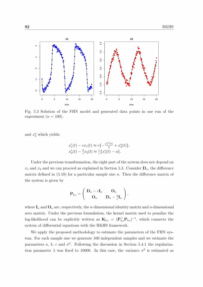
92 RKHS
0 5 10 15 20
−2
−1
01
2
x1
time
0 5 10 15 20−
1.5
−1.
0−
0.5
0.0
0.5
1.0
1.5
x2
time
x[, 2
]
Fig. 5.3 Solution of the FHN model and generated data points in one run of theexperiment (n = 100).
and x⋆2 which yields:
x′1(t) − cx1(t) ≈ c−x⋆
13(t)3 + x⋆
2(t),x′
2(t) − bcx2(t) ≈ 1
cx⋆
1(t) − a.
Under the previous transformation, the right part of the system does not depend onx1 and x2 and we can proceed as explained in Section 5.3. Consider Dn, the differencematrix defined in (5.10) for a particular sample size n. Then the difference matrix ofthe system is given by
Pb,c = Dn − cIn On
On Dn − bcIn
,where In and On are, respectively, the n-dimensional identity matrix and n-dimensionalzero matrix. Under the previous formulation, the kernel matrix used to penalize thelog-likelihood can be explicitly written as Kb,c = (P⊤
b,cPb,c)−1, which connects thesystem of differential equations with the RKHS framework.
We apply the proposed methodology to estimate the parameters of the FHN sys-tem. For each sample size we generate 100 independent samples and we estimate theparameters a, b, c and σ2. Following the discussion in Section 5.4.1 the regulariza-tion parameter λ was fixed to 10000. In this case, the variance σ2 is estimated as
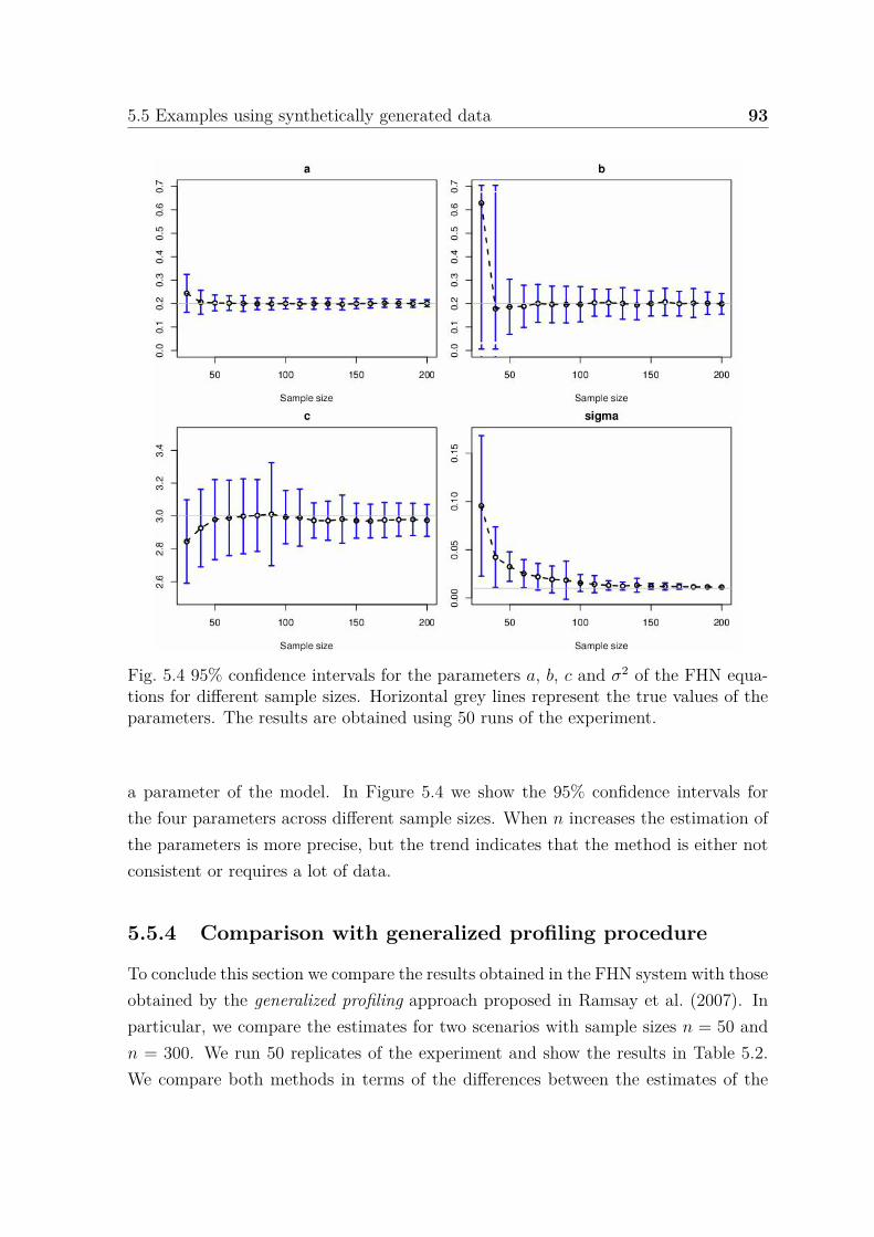
5.5 Examples using synthetically generated data 93
Fig. 5.4 95% confidence intervals for the parameters a, b, c and σ2 of the FHN equa-tions for different sample sizes. Horizontal grey lines represent the true values of theparameters. The results are obtained using 50 runs of the experiment.
a parameter of the model. In Figure 5.4 we show the 95% confidence intervals forthe four parameters across different sample sizes. When n increases the estimation ofthe parameters is more precise, but the trend indicates that the method is either notconsistent or requires a lot of data.
5.5.4 Comparison with generalized profiling procedure
To conclude this section we compare the results obtained in the FHN system with thoseobtained by the generalized profiling approach proposed in Ramsay et al. (2007). Inparticular, we compare the estimates for two scenarios with sample sizes n = 50 andn = 300. We run 50 replicates of the experiment and show the results in Table 5.2.We compare both methods in terms of the differences between the estimates of the
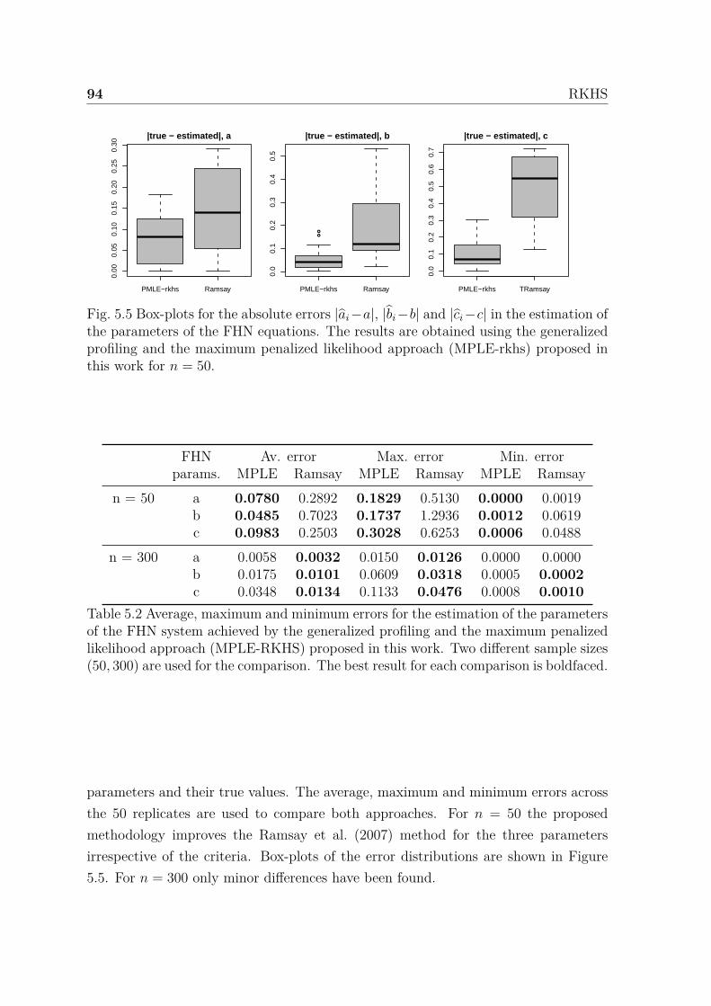
94 RKHS
PMLE−rkhs Ramsay
0.00
0.05
0.10
0.15
0.20
0.25
0.30
|true − estimated|, a
PMLE−rkhs Ramsay
0.0
0.1
0.2
0.3
0.4
0.5
|true − estimated|, b
|true
−es
timat
ed|
PMLE−rkhs TRamsay
0.0
0.1
0.2
0.3
0.4
0.5
0.6
0.7
|true − estimated|, c
|true
−es
timat
ed|
Fig. 5.5 Box-plots for the absolute errors |ai −a|, |bi −b| and |ci −c| in the estimation ofthe parameters of the FHN equations. The results are obtained using the generalizedprofiling and the maximum penalized likelihood approach (MPLE-rkhs) proposed inthis work for n = 50.
FHN Av. error Max. error Min. errorparams. MPLE Ramsay MPLE Ramsay MPLE Ramsay
n = 50 a 0.0780 0.2892 0.1829 0.5130 0.0000 0.0019b 0.0485 0.7023 0.1737 1.2936 0.0012 0.0619c 0.0983 0.2503 0.3028 0.6253 0.0006 0.0488
n = 300 a 0.0058 0.0032 0.0150 0.0126 0.0000 0.0000b 0.0175 0.0101 0.0609 0.0318 0.0005 0.0002c 0.0348 0.0134 0.1133 0.0476 0.0008 0.0010
Table 5.2 Average, maximum and minimum errors for the estimation of the parametersof the FHN system achieved by the generalized profiling and the maximum penalizedlikelihood approach (MPLE-RKHS) proposed in this work. Two different sample sizes(50, 300) are used for the comparison. The best result for each comparison is boldfaced.
parameters and their true values. The average, maximum and minimum errors acrossthe 50 replicates are used to compare both approaches. For n = 50 the proposedmethodology improves the Ramsay et al. (2007) method for the three parametersirrespective of the criteria. Box-plots of the error distributions are shown in Figure5.5. For n = 300 only minor differences have been found.
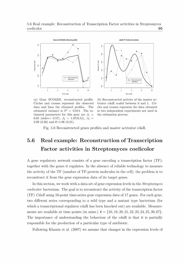
5.6 Real example: Reconstruction of Transcription Factor activities in Streptomycescoelicolor 95
2 4 6 8 10
−1.
0−
0.5
0.0
0.5
1.0
Gene SCO3235 inferred profile
Time order
Exp
ress
ion
leve
l
ReconstructedObserved
(a) Gene SCO3235, reconstructed profile.Circles and crosses represent the observeddata and lines the obtained profiles. Theestimated variance is σ2 = 0.014. The es-timated parameters for this gene are β1 =0.65 (stdev= 0.57), β2 = 1.07(0.51), β3 =2.09 (0.26) and θ=1.06 (0.21).
2 4 6 8 10
0.0
0.2
0.4
0.6
0.8
1.0
cdaR TF inferred activity
Time order
Rel
ativ
e T
F le
vel
ReconstructedValildation
(b) Reconstructed activity of the master ac-tivator cdaR scaled between 0 and 1. Cir-cles and crosses represent the data obtainedin two independent experiments not used inthe estimation process.
Fig. 5.6 Reconstructed genes profiles and master activator cdaR.
5.6 Real example: Reconstruction of TranscriptionFactor activities in Streptomyces coelicolor
A gene regulatory network consists of a gene encoding a transcription factor (TF);together with the genes it regulates. In the absence of reliable technology to measurethe activity of the TF (number of TF-protein molecules in the cell), the problem is toreconstruct it from the gene expression data of its target genes.
In this section, we work with a data set of gene expression levels in the Streptomycescoelicolor bacterium. The goal is to reconstruct the activity of the transcription factor(TF) CdaR using 10-point time-series gene expression data of 17 genes. For each gene,two different series corresponding to a wild type and a mutant type bacterium (forwhich a transcriptional regulator cdaR has been knocked out) are available. Measure-ments are available at time points (in mins.) t = 16, 18, 20, 21, 22, 23, 24, 25, 39, 67.The importance of understanding the behaviour of the cdaR is that it is partiallyresponsible for the production of a particular type of antibiotic.
Following Khanin et al. (2007) we assume that changes in the expression levels of
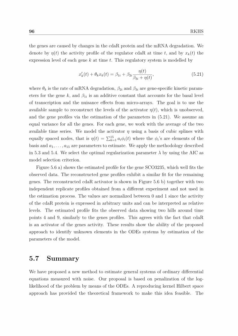
96 RKHS
the genes are caused by changes in the cdaR protein and the mRNA degradation. Wedenote by η(t) the activity profile of the regulator cdaR at time t, and by xk(t) theexpression level of each gene k at time t. This regulatory system is modelled by
x′k(t) + θkxk(t) = β1i + β2i
η(t)β3i + η(t) , (5.21)
where θk is the rate of mRNA degradation, β2i and β3i are gene-specific kinetic param-eters for the gene k, and β1i is an additive constant that accounts for the basal levelof transcription and the nuisance effects from micro-arrays. The goal is to use theavailable sample to reconstruct the levels of the activator η(t), which is unobserved,and the gene profiles via the estimation of the parameters in (5.21). We assume anequal variance for all the genes. For each gene, we work with the average of the twoavailable time series. We model the activator η using a basis of cubic splines withequally spaced nodes, that is η(t) = ∑15
k=1 aiϕi(t) where the ϕi’s are elements of thebasis and a1, . . . , a15 are parameters to estimate. We apply the methodology describedin 5.3 and 5.4. We select the optimal regularization parameter λ by using the AIC asmodel selection criterion.
Figure 5.6 a) shows the estimated profile for the gene SCO3235, which well fits theobserved data. The reconstructed gene profiles exhibit a similar fit for the remaininggenes. The reconstructed cdaR activator is shown in Figure 5.6 b) together with twoindependent replicate profiles obtained from a different experiment and not used inthe estimation process. The values are normalized between 0 and 1 since the activityof the cdaR protein is expressed in arbitrary units and can be interpreted as relativelevels. The estimated profile fits the observed data showing two hills around timepoints 4 and 9, similarly to the genes profiles. This agrees with the fact that cdaRis an activator of the genes activity. These results show the ability of the proposedapproach to identify unknown elements in the ODEs systems by estimation of theparameters of the model.
5.7 Summary
We have proposed a new method to estimate general systems of ordinary differentialequations measured with noise. Our proposal is based on penalization of the log-likelihood of the problem by means of the ODEs. A reproducing kernel Hilbert spaceapproach has provided the theoretical framework to make this idea feasible. The
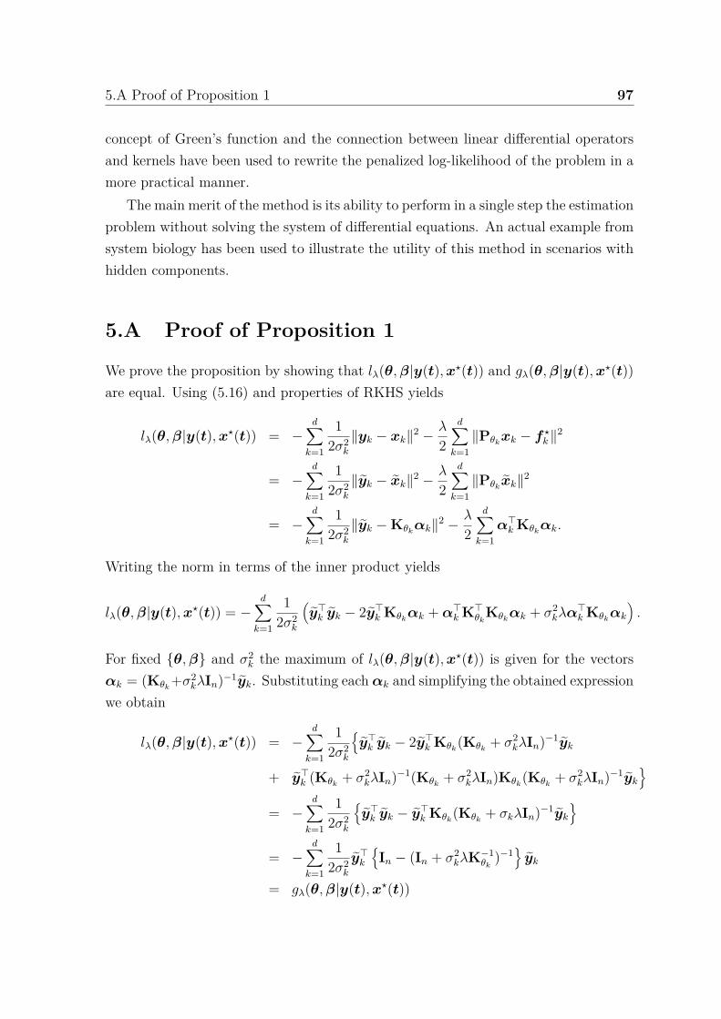
5.A Proof of Proposition 1 97
concept of Green’s function and the connection between linear differential operatorsand kernels have been used to rewrite the penalized log-likelihood of the problem in amore practical manner.
The main merit of the method is its ability to perform in a single step the estimationproblem without solving the system of differential equations. An actual example fromsystem biology has been used to illustrate the utility of this method in scenarios withhidden components.
5.A Proof of Proposition 1
We prove the proposition by showing that lλ(θ,β|y(t),x⋆(t)) and gλ(θ,β|y(t),x⋆(t))are equal. Using (5.16) and properties of RKHS yields
lλ(θ,β|y(t),x⋆(t)) = −d∑
k=1
12σ2
k
∥yk − xk∥2 − λ
2
d∑k=1
∥Pθkxk − f ⋆
k ∥2
= −d∑
k=1
12σ2
k
∥yk − xk∥2 − λ
2
d∑k=1
∥Pθkxk∥2
= −d∑
k=1
12σ2
k
∥yk − Kθkαk∥2 − λ
2
d∑k=1α⊤
k Kθkαk.
Writing the norm in terms of the inner product yields
lλ(θ,β|y(t),x⋆(t)) = −d∑
k=1
12σ2
k
(y⊤
k yk − 2y⊤k Kθk
αk +α⊤k K⊤
θkKθk
αk + σ2kλα
⊤k Kθk
αk
).
For fixed θ,β and σ2k the maximum of lλ(θ,β|y(t),x⋆(t)) is given for the vectors
αk = (Kθk+σ2
kλIn)−1yk. Substituting eachαk and simplifying the obtained expressionwe obtain
lλ(θ,β|y(t),x⋆(t)) = −d∑
k=1
12σ2
k
y⊤
k yk − 2y⊤k Kθk
(Kθk+ σ2
kλIn)−1yk
+ y⊤k (Kθk
+ σ2kλIn)−1(Kθk
+ σ2kλIn)Kθk
(Kθk+ σ2
kλIn)−1yk
= −
d∑k=1
12σ2
k
y⊤
k yk − y⊤k Kθk
(Kθk+ σkλIn)−1yk
= −d∑
k=1
12σ2
k
y⊤k
In − (In + σ2
kλK−1θk
)−1yk
= gλ(θ,β|y(t),x⋆(t))
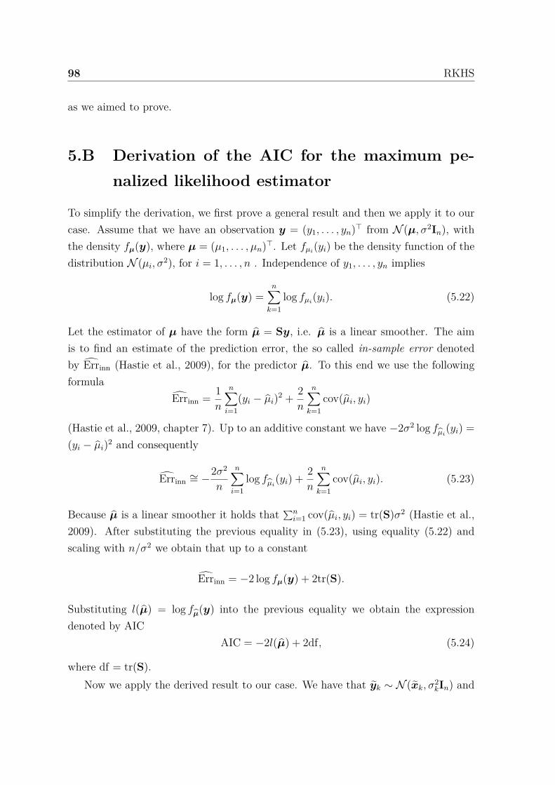
98 RKHS
as we aimed to prove.
5.B Derivation of the AIC for the maximum pe-nalized likelihood estimator
To simplify the derivation, we first prove a general result and then we apply it to ourcase. Assume that we have an observation y = (y1, . . . , yn)⊤ from N (µ, σ2In), withthe density fµ(y), where µ = (µ1, . . . , µn)⊤. Let fµi
(yi) be the density function of thedistribution N (µi, σ
2), for i = 1, . . . , n . Independence of y1, . . . , yn implies
log fµ(y) =n∑
k=1log fµi
(yi). (5.22)
Let the estimator of µ have the form µ = Sy, i.e. µ is a linear smoother. The aimis to find an estimate of the prediction error, the so called in-sample error denotedby Errinn (Hastie et al., 2009), for the predictor µ. To this end we use the followingformula
Errinn = 1n
n∑i=1
(yi − µi)2 + 2n
n∑k=1
cov(µi, yi)
(Hastie et al., 2009, chapter 7). Up to an additive constant we have −2σ2 log fµi(yi) =
(yi − µi)2 and consequently
Errinn ∼= −2σ2
n
n∑i=1
log fµi(yi) + 2
n
n∑k=1
cov(µi, yi). (5.23)
Because µ is a linear smoother it holds that ∑ni=1 cov(µi, yi) = tr(S)σ2 (Hastie et al.,
2009). After substituting the previous equality in (5.23), using equality (5.22) andscaling with n/σ2 we obtain that up to a constant
Errinn = −2 log fµ(y) + 2tr(S).
Substituting l(µ) = log fµ(y) into the previous equality we obtain the expressiondenoted by AIC
AIC = −2l(µ) + 2df, (5.24)
where df = tr(S).Now we apply the derived result to our case. We have that yk ∼ N (xk, σ
2kIn) and
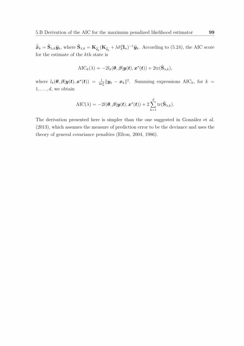
5.B Derivation of the AIC for the maximum penalized likelihood estimator 99
xk = Sλ,kyk, where Sλ,k = Kθk
(Kθk
+ λσ2kIn)−1yk. According to (5.24), the AIC score
for the estimate of the kth state is
AICk(λ) = −2lk(θ,β|y(t),x⋆(t)) + 2tr(Sλ,k),
where lk(θ,β|y(t),x⋆(t)) = 12σ2
k∥yk − xk∥2. Summing expressions AICk, for k =
1, . . . , d, we obtain
AIC(λ) = −2l(θ,β|y(t),x⋆(t)) + 2d∑
k=1tr(Sλ,k).
The derivation presented here is simpler than the one suggested in González et al.(2013), which assumes the measure of prediction error to be the deviance and uses thetheory of general covariance penalties (Efron, 2004, 1986).


Chapter 6
Inferring latent gene regulatorynetwork kinetics
Regulatory networks consist of gene encoding transcription factors (TFs) and the genesthey activate or repress. Various types of systems of ordinary differential equationshave been proposed to model these networks, ranging from linear to Michaelis-Mentenapproaches. In practice, a serious drawback to estimating these models is that the TFsare generally unobserved because of a lack of high-throughput techniques to measurethe abundance of proteins in the cell. The challenge is to infer their activity profiletogether with the kinetic parameters of the ODEs using level expression measurementsof the genes they regulate. In this chapter we show how the framework presented inthe previous chapter can be used to infer the kinetic parameters of regulatory networkswith one or more TFs using time course gene expression data. Our approach is alsoable to predict the activity levels of the TF. We illustrate this using the example ofan SOS repair system in Escherichia coli. The reconstructed TF exhibits a behavioursimilar to experimentally measured profiles and the genetic expression data are fittedwell.
The remainder of this chapter is divided into four sections. In Section 6.1, weintroduce a model for observed gene data expression with one transcription factor.In Section 6.2, we detail the estimation procedure, which for this specific exampleis complemented by an EM algorithm. In Section 6.3, our statistical framework isapplied to 6 time-course gene expression data in the SOS system in Escherichia coliwith one TF. We show some results regarding the reconstruction of the TF and thefit of the model to the data. The last section contains the summary and the appendixcontains proofs.
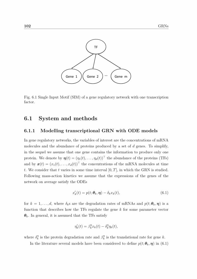
102 GRNs
Gene 1 … Gene 2 Gene m
TF
Fig. 6.1 Single Input Motif (SIM) of a gene regulatory network with one transcriptionfactor.
6.1 System and methods
6.1.1 Modelling transcriptional GRN with ODE models
In gene regulatory networks, the variables of interest are the concentrations of mRNAmolecules and the abundance of proteins produced by a set of d genes. To simplify,in the sequel we assume that one gene contains the information to produce only oneprotein. We denote by η(t) = (η1(t), . . . , ηd(t))⊤ the abundance of the proteins (TFs)and by x(t) = (x1(t), . . . , xd(t))⊤ the concentrations of the mRNA molecules at timet. We consider that t varies in some time interval [0, T ], in which the GRN is studied.Following mass-action kinetics we assume that the expressions of the genes of thenetwork on average satisfy the ODEs
x′k(t) = p(t;θk,η) − δkxk(t), (6.1)
for k = 1, . . . , d, where δks are the degradation rates of mRNAs and p(t;θk,η) is afunction that describes how the TFs regulate the gene k for some parameter vectorθk. In general, it is assumed that the TFs satisfy
η′k(t) = βη
kxk(t) − δηkηk(t),
where δηk is the protein degradation rate and βη
k is the translational rate for gene k.In the literature several models have been considered to define p(t;θk,η) in (6.1)
6.1 System and methods 103
ranging from linear approaches (Chen et al., 1999) to non-parametric methods (Äijöand Lähdesmäki, 2009). In practice, experimental work suggests that the response ofthe mRNA abundance to the concentration of a TF follows a Hill curve (De Jong,2002). This response can be well described by the Michaelis-Menten (MM) formula-tion. In case of activation of gene k by the transcription factor s, the transcriptionfunction is assumed to satisfy
p+(t;θk, ηs) = βkηs(t)
γk + ηs(t)+ φk,
for θk = (φk, βk, γk)⊤. Similarly, in cases of repression, the response can be modelledby
p−(t;θk, ηs) = βk1
γk + ηs(t)+ φk. (6.2)
If a gene is regulated by several TFs, a product of type-p+ and type-p− functions canbe used to model the regulatory component of expression (6.1). The only non-standardpart in this model is the presence of φk, which is added to detect possible non-specificactivation.
6.1.2 GRN with one TF: single input motif
In expression (6.1) several genes encoding TFs are involved in the model. Nevertheless,these types of regulatory networks are difficult to identify given the actual lack ofreliable methods for measuring TF activities. For this reason, networks involving onlyone TF and the genes it regulates as in Figure 6.1 are the most studied in the literatureand are the primary focus of our following analysis.
These one-to-many patterns of interaction between one TF and several genes arecalled single input motifs (SIM), a term first introduced in Milo et al. (2002). Withina SIM, the expression of gene k depends on the decay constant δk and on the tran-scription function p(t;θk, η) where η is the unique transcription factor of the network.
The profile η is unobserved and has to be reconstructed from the expression of thegenes. In this work we assume that η is a function which can be written in terms ofa basis of spline functions defined in [0, T ]. That is,
η(t) =m∑
j=1µjϕj(t), (6.3)
where µj ∈ IR and ϕ1, . . . , ϕm is a truncated-power basis set.
104 GRNs
Although the transcription factor η is common to all target genes in the network,the kinetic parameters of each gene are expected to be target-dependent. That is,
xk(t) = xk(t; δk,θk,µ),
where µ = (µ1, . . . , µm)⊤ is the vector of weights of the TF in the spline representation(6.3). Biologically, it is reasonable to assume that the gene-specific parameters θk andδk are the same across different biological conditions. However, this is not the casewith the initial amount of gene expression xk(0) since the gene transcription can beaffected by an uncontrolled number of external conditions.
6.1.3 Noise model
Let yki denote the measured expression of gene k at a time-point ti. We assumethat the observed gene expression measurements of the target genes are conditionallyindependent given the transcription factor activity, and that each target gene k isnormally distributed with location parameter xk(t) and scale parameter σ2
k(t). Thatis, we assume that
yki ∼ N (xk(ti), σ2k(ti)). (6.4)
In our context, the log-likelihood contribution of a single observation is, up to anadditive constant, given by
l(xk(ti), σ2ki|yki) = −1
2
yki − xk(ti)
σki
2
− 12 log(σ2
ki).
Let Dk = (yki, ti) ∈ IR× [0, T ]ni=1 denote the set of gene expression measurements
of gene k across the time points t1, . . . , tn. Then the contribution of each gene k tothe log-likelihood of the network is
lk(δk,θk,Σk,µ|Dk) =n∑
i=1l(xk(ti), σ2
ki|yki),
for Σk = diag(σ2k1, . . . , σ
2kn) and where it is assumed that each function xk satisfies
(6.1).
6.1 System and methods 105
6.1.4 Penalized log-likelihood of a GRN with one TF
The system of differential equations (6.1) describes the dynamics of the gene regulatorysystem in interval [0, T ]. However, in practical scenarios, we have access to only a finitenumber of measurements of the gene expression levels. Following the approach fromthe previous chapter we approximate the rate of gene expression by the first orderdifference.
Let t = (t1, . . . , tn)⊤ denote the vector whose elements represent the time points inwhich gene expression measurements are available and define xk(t) = (xk(t1), . . . , xk(tn))⊤
and p(t;θk, η) = (p(t1;θk, η), . . . , p(tn;θk, η))⊤. Then one can rewrite the discrete ver-sion of dynamics of the gene k in (6.1) as
Dnxk(t) = p(t;θk, η) − δkxk(t),
where the matrix Dn is the difference operator defined in (5.10).
Let In be the identity matrix and denote by Pδk= Dn+δkIn the difference operator
associated with gene k. To define penalized loss, we assume that Pδkis invertible and
introduce
xk(t) = xk(t) − P−1δkp(t;θk,µ), (6.5)
yk = yk − P−1δkp(t;θk,µ), (6.6)
∥xk(t)∥2Kδk
= α⊤k Kδk
αk,
where Kδk= (P⊤
δkPδk
)−1 and αk is the vector in IRn characterizing xk(t).
Denote by Dk the transformed set of expression measurements associated with thegene k. Using the framework from the previous chapter, for a GRN where a single TFη regulates all genes in the network the penalized log-likelihood can be written as
lλ(∆,Θ,Σ,µ|D) =d∑
k=1lk(δk,θk,Σk,µ|Dk) − λ
2
d∑k=1
∥xk(t)∥2Kδk
,
where D = D1, . . . , Dd represents the whole sample available for the network; Θrepresents the set of kinetic parameters θk, ∆ = δ1, . . . , δd, Σ stands for all scaleparameters of the normal distribution, and µ is the set of weights corresponding tothe representation of the TF activity in a spline basis.
In the RKHS framework, the (transformed) expression level of each gene k and its
106 GRNs
influence matrix are
xk(t) = Kδkαk = Sλ,kyk, (6.7)
Sλ,k = Kδk(Kδk
+ λΣk)−1. (6.8)
Estimates of the gene expression profiles x1, . . . , xd can be recovered using (6.5) and(6.7).
6.1.5 Parameter estimation
Denote by A = α1, . . . ,αd the set of parameters characterizing the gene profiles x.Then the maximum penalized log-likelihood estimators of ∆,Θ,Σ,µ and A are givenby
(∆λ, Θλ, Σλ, µλ, Aλ) = arg max∆,Θ,Σ,µ,A
lλ(∆,Θ,Σ,µ, A|D). (6.9)
6.1.6 Model selection
For selecting λ we use the AIC, which we have derived in the previous chapter. For thelinear smoother (6.7) the influence matrix for gene k is given by (6.8). The effectivenumber of parameters is defined as dfk = tr(Sλ,k). Then the AIC is defined in ourcontext as
AICk(λ) = −2lk(δk, θk, Σk, µ|Dk) + 2dfk.
Extending the criterion to all genes of the network, we can select the optimal λ as
λopt = arg minλ
d∑k=1
AICk(λ).
In the literature, λ and Σk are normally not allowed to change simultaneously. Asdetailed in Rasmussen (2006), λ is sometimes fixed to 1/2 or to 1/n if the varianceparameters are allowed to vary. In this work the variance parameters are estimatedoff-line and the matrices Σk are fixed in the estimation process. Then the parameter λis obtained using the above mentioned AIC or other sensible model selection criteria.
6.1.7 Confidence intervals
In maximum likelihood estimation approaches the most standard way of obtaining thevariance of a parameter estimate θ is by means of the negative Hessian evaluated at
6.2 Algorithm 107
θ. In our context, however, the parameter estimates of the gene regulatory networkare obtained by a penalized likelihood approach and the aforementioned approach isnot directly applicable.
To circumvent this issue we propose a parametric bootstrap (Efron, 1979) to obtainconfidence intervals in our setting. To this aim and by virtue of (6.4) we consider thefitted model N (xk(ti), σk
2(ti)), where the hat-expressions are estimated values. Thenfrom this model we generate B bootstrap data sets for which we use the proposedmethod to obtain new estimates of the parameters. The quantiles of the empiricaldistribution of the bootstrap estimates are then used to estimate the confidence inter-vals.
6.2 Algorithm
In this section we detail the steps to obtain the estimators ∆λ, Θλ, Σλ and µλ in(6.9). Also, estimators for the gene profiles xk are provided. To this aim, we proposean augmented formulation of the problem in order to provide a way to deal with thecommon lack of observations in real applications. Since the derivative approximationis better for smaller discretization steps, increasing the number of data points resultsin a better derivative approximation. To use this idea we propose an EM algorithmto accommodate hidden observations.
6.2.1 Augmented data formulation
Denote by DOk = (yO
ki, tOi ) ∈ IR × [0, T ]n
i=1 the set of expression measurements of thegene k across the observed time points tO1 , . . . , tOn . Consider a refinement of hiddenobservations, all different from those in DO
k , given by DH = (yHki , t
Hki) ∈ IR× [0, T ]r
i=1.Denote by
tO = (tO1 , . . . , tOn )⊤, tH = (tH1 , . . . , tHr )⊤,
yOk = (yO
k1, . . . , yOkn)⊤, yH
k = (yHk1, . . . , y
Hkr)⊤,
the vectors of times and data of both samples for gene k. Define t to be the vectorresulting from the ordered concatenation of tO and tH , and let yk be the concatenationof the vectors yO
k and yHk ordered according to the ordering in t. Then the log-
108 GRNs
likelihood for the augmented data formulation is
lλ(·|DO, DH) = −12
d∑k=1
(yk − Kδkαk)⊤Σ−1
k (yk − Kδkαk)
− 12
d∑k=1
n+r∑i=1
log(σ2ki) − λ
d∑k=1α⊤
k Kδkαk, (6.10)
where yk is the vector of transformed data defined in (6.6), Kδk= (P⊤
δkPδk
)−1, andαk ∈ IRn+r.
6.2.2 E-step
In the expectation (E) step, we need to calculate the expectation of lλ(·|DO, DH) interms of the hidden observations. For simplicity of notation, define
Qλ(∆,Θ,Σ,µ, A) = EyH
lλ(·|DO, DH)|DO,∆∗,Θ∗,Σ∗,µ∗, A∗
.
Consider the matrix CH ∈ IRr×(n+r) defined by
(CH)ij = 1 if tHi
= tj
0 otherwise.
Then it can be proven that
Qλ(∆,Θ,Σ,µ, A) = lλ(·|DO, DH∗) − 12
d∑k=1
r∑i=1
(σ∗ki)2,
for DH∗ = DH∗1 , . . . , DH∗
d , where the augmented vector y∗k of observations associated
with each gene k is given by the ordered concatenation of the vectors yOk and CHKδ∗
kα∗
k
according to the ordering in t. See appendix for details.
6.2.3 M-step
In the maximization (M) step, we maximize the augmented log-likelihood over theparameters of interest. Assume that some values for ∆∗,Θ∗,Σ∗,µ∗ and A∗ are givenand consider the augmented vectors of observations y∗
k. Then in this step we searchfor the values of the parameters such that
(∆, Θ, Σ, µ, A) = arg max∆,Θ,Σ,µ
Qλ(∆,Θ,Σ,µ, A).
6.3 SOS repair system in Escherichia coli 109
In practice, the problem can be split into two different maximization problems. Pa-rameters ∆,Θ,Σ and µ can be calculated independently of A by taking
(∆, Θ, Σ, µ) = arg max∆,Θ,Σ,µ
−12
d∑k=1
(y∗k)⊤Σ−1
k (I − Sλ,k)y∗k
− 12
d∑k=1
n+r∑i=1
log(σ2ki) − 1
2
d∑k=1
r∑i=1
(σ∗ki)2, (6.11)
where Sλ,k is the influence matrix associated with each gene defined in (6.8). Regardingthe set of parameters A, made up of the vectors α1, . . . .αd, it can be shown usingstandard methods of differential calculus that they can be calculated by
αk = (Kδk
+ λΣk)−1y∗k. (6.12)
See appendix for details.
6.2.4 EM algorithm
In order to apply the EM algorithm we need to consider some initial values of theparameters. If no other information about the system is provided, a reasonable wayto proceed is to smooth each yO
k with some standard smoothing technique. In thisway for each individual gene we obtain a reasonable initial set of hidden observationsyH
k . Then we can define yk as the ordered concatenation of the vectors yOk and yH
k
according to the ordering in t. Assuming some values for ∆∗,Θ∗,Σ∗ and µ∗ we cannow calculate each α∗
k = (Kδ∗k
+ λΣ∗k)−1yk to obtain reasonable initial value for A∗.
The steps of the EM algorithm are detailed next.1. Start: Consider some initial values ∆∗,Θ∗,Σ∗,µ∗ and A∗.2. E-step: Compute each Kδ∗
kand obtain y∗
k.3. M-step: Obtain (∆, Θ, Σ, µ) as in (6.11) using a conjugate gradient algorithm
and each αk using (6.12). Go to step 2.4. End: Upon convergence, take (∆λ, Θλ, Σλ, µλ) = (∆, Θ, Σ, µ) and αλ,k = αk
for k = 1 . . . , d.
6.3 SOS repair system in Escherichia coli
Changes in the expression levels of genes in Escherichia coli as a result of DNA damage(SOS response) have been extensively studied in the last few years. However their
110 GRNs
behaviour has not been completely understood (Khanin et al., 2006). The SOS systemincludes more than 30 genes controlled by a (transcriptional repressor) protein calledLexA. Under normal conditions the levels of LexA are high and the expression of thegene is repressed. With DNA damage the LexA protein is inactivated, causing theup-regulation of genes suppressed by the LexA under normal conditions. The aim ofthis analysis is twofold: first, to reconstruct the activity level of the repressor LexAby using the expression profiles of its target genes, and second, to identify the systemand to order the genes of the SOS system in terms of the speed with which they arerepressed by the LexA protein. To this aim we use the proposed penalized likelihoodapproach.
6.3.1 The data set and the goal
The data set used for this experiment is made up of 14 expression genes (dinF, dinI,lexA, recA, recN, ruvA, ruvB, sbmC, sulA, umuC, umuD, uvrB, yegG and ijW) of theEscherichia coli SOS system. These 14 genes are targets of the master repressor LexAand their expression is studied under UV exposure (40 J/m2) in both wild-type cellsand lexA1 mutants. (Khanin et al., 2006). The abundance of the mRNA moleculesassociated with the genes was measured at six time points: 0, 5, 10, 20, 40 and 60minutes. Raw data are normalized as detailed in (Khanin et al., 2006). The masterrepressor is unobserved. Following expression (6.3) we assume that its activity canbe described by a cubic spline function with d = 5 basis functions. In this examplewe assume a Michaelis-Menten formulation (see 6.2). The goal of this experiment isto use this gene expression sample to reconstruct the activity of the repressor η(t)and to estimate the kinetic parameters in (6.1). In addition, the gene profiles will beinferred by means of (6.5) and (6.7). The parameters to be estimated are the kineticparameters of the 14 genes together with the TF weights and the vectors α1, . . . ,α14
characterizing the gene profiles.
6.3.2 Estimation process
Only six data points are available per gene. This lack of observations could causeinstabilities in the estimation process which we deal with as follows. First, the varianceparameters are assumed to be constant for the data within the same gene. We estimateσ2
1, . . . , σ214 off-line by fitting smoothing splines to the data and estimating the residual
variance in each case. The TF factor is assumed to be normalized between zero and
6.3 SOS repair system in Escherichia coli 111
one, which robustifies the estimation of the parameters of the system. In practice thisis not a problem since the repression or activation of the LexA protein is expressed inarbitrary units, which can be interpreted as relative levels.
Reconstruction of the TF and estimation of the gene-specific kinetic parameters aredone in two steps. In both, maximization of the penalized log-likelihood is achieved bymeans of the conjugate gradient method. First we estimate the TF profile. To do sowe estimate the system without intermediate points. The penalization parameter λ iscalculated by using the AIC as detailed in Section 6.1.6. We consider the estimates ofthe weights of the spline basis µ1, . . . , µ5 and we reconstruct the TF profile. We observethat the values of the φi are zero for most of the genes. Given the lack of data, in orderto gain more precision in the estimation of the remaining kinetic parameters we assumeall the φi to be zero and we re-estimate each gene independently considering the TFprofile obtained above to be fixed. A different penalization term is now recalculatedfor each gene using the AIC. Four intermediate points are considered in order toimprove the estimation. Confidence intervals for the parameters were obtained usinga parametric bootstrap as detailed in Section 6.1.7.
6.3.3 Reconstruction of the LexA activity
The reconstructed LexA repressor is shown in Figure 6.2. The smoothed LexA profile,obtained using a cubic spline, is shown. The crucial aspect of the obtained profile isthat it agrees with the behaviour of experimentally observed profiles in Ronen et al.(2002) and Sassanfar and Roberts (1990). It has been observed that after irradiationthe amount of LexA decreases, and after a recovery phase it increases again. This isthe behaviour shown in Figure 6.2 where the level of the LexA decreases to zero withinthe first 20 minutes to completely recover by 60 minutes.
6.3.4 Inferred kinetics profiles
The reconstructed gene profiles show a good fit with the data in the 14 cases. In Figure6.3 we show the data and the estimated profiles for the genes dinI and recN. These twogenes were selected because they exhibit different types of profiles. Gene dinI showsa fast increase in regulation up until min 20-30, and later descends gradually. Thiscoincides with the time point in which the master repressor starts to recover. On theother hand gene recN is stable in time after minute 20. The introduced intermediatepoints help to recover a smooth version of the gene profiles.
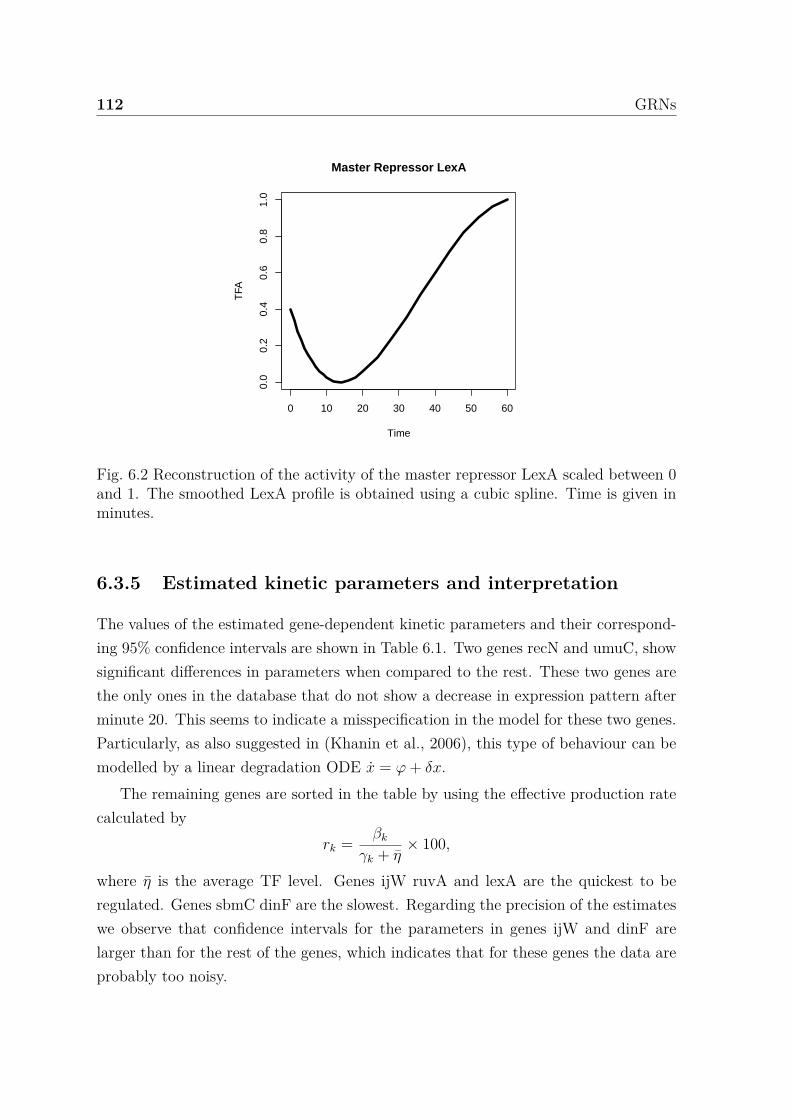
112 GRNs
0 10 20 30 40 50 60
0.0
0.2
0.4
0.6
0.8
1.0
Master Repressor LexA
Time
TFA
Fig. 6.2 Reconstruction of the activity of the master repressor LexA scaled between 0and 1. The smoothed LexA profile is obtained using a cubic spline. Time is given inminutes.
6.3.5 Estimated kinetic parameters and interpretation
The values of the estimated gene-dependent kinetic parameters and their correspond-ing 95% confidence intervals are shown in Table 6.1. Two genes recN and umuC, showsignificant differences in parameters when compared to the rest. These two genes arethe only ones in the database that do not show a decrease in expression pattern afterminute 20. This seems to indicate a misspecification in the model for these two genes.Particularly, as also suggested in (Khanin et al., 2006), this type of behaviour can bemodelled by a linear degradation ODE x = φ+ δx.
The remaining genes are sorted in the table by using the effective production ratecalculated by
rk = βk
γk + η× 100,
where η is the average TF level. Genes ijW ruvA and lexA are the quickest to beregulated. Genes sbmC dinF are the slowest. Regarding the precision of the estimateswe observe that confidence intervals for the parameters in genes ijW and dinF arelarger than for the rest of the genes, which indicates that for these genes the data areprobably too noisy.
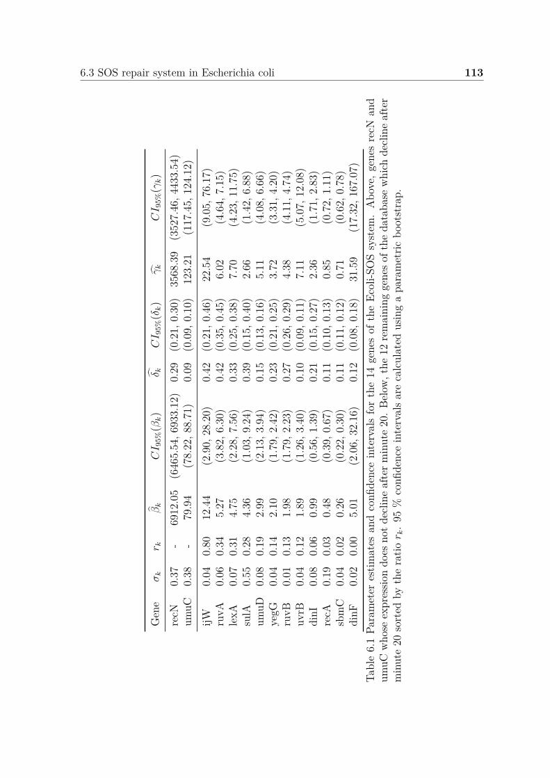
6.3 SOS repair system in Escherichia coli 113
Gen
eσ
kr k
βk
CI 9
5%(β
k)
δ kCI 9
5%(δ
k)
γk
CI 9
5%(γ
k)
recN
0.37
-69
12.0
5(6
465.
54,6
933.
12)
0.29
(0.2
1,0.
30)
3568
.39
(352
7.46
,443
3.54
)um
uC0.
38-
79.9
4(7
8.22
,88.
71)
0.09
(0.0
9,0.
10)
123.
21(1
17.4
5,12
4.12
)ijW
0.04
0.80
12.4
4(2
.90,
28.2
0)0.
42(0
.21,
0.46
)22
.54
(9.0
5,76
.17)
ruvA
0.06
0.34
5.27
(3.8
2,6.
30)
0.42
(0.3
5,0.
45)
6.02
(4.6
4,7.
15)
lexA
0.07
0.31
4.75
(2.2
8,7.
56)
0.33
(0.2
5,0.
38)
7.70
(4.2
3,11
.75)
sulA
0.55
0.28
4.36
(1.0
3,9.
24)
0.39
(0.1
5,0.
40)
2.66
(1.4
2,6.
88)
umuD
0.08
0.19
2.99
(2.1
3,3.
94)
0.15
(0.1
3,0.
16)
5.11
(4.0
8,6.
66)
yegG
0.04
0.14
2.10
(1.7
9,2.
42)
0.23
(0.2
1,0.
25)
3.72
(3.3
1,4.
20)
ruvB
0.01
0.13
1.98
(1.7
9,2.
23)
0.27
(0.2
6,0.
29)
4.38
(4.1
1,4.
74)
uvrB
0.04
0.12
1.89
(1.2
6,3.
40)
0.10
(0.0
9,0.
11)
7.11
(5.0
7,12
.08)
dinI
0.08
0.06
0.99
(0.5
6,1.
39)
0.21
(0.1
5,0.
27)
2.36
(1.7
1,2.
83)
recA
0.19
0.03
0.48
(0.3
9,0.
67)
0.11
(0.1
0,0.
13)
0.85
(0.7
2,1.
11)
sbm
C0.
040.
020.
26(0
.22,
0.30
)0.
11(0
.11,
0.12
)0.
71(0
.62,
0.78
)di
nF0.
020.
005.
01(2
.06,
32.1
6)0.
12(0
.08,
0.18
)31
.59
(17.
32,1
67.0
7)Ta
ble
6.1
Para
met
eres
timat
esan
dco
nfide
nce
inte
rval
sfo
rth
e14
gene
sof
the
Ecol
i-SO
Ssy
stem
.A
bove
,gen
esre
cNan
dum
uCw
hose
expr
essio
ndo
esno
tdec
line
afte
rmin
ute
20.B
elow
,the
12re
mai
ning
gene
soft
heda
taba
sew
hich
decl
ine
afte
rm
inut
e20
sort
edby
the
ratio
r k.
95%
confi
denc
ein
terv
als
are
calc
ulat
edus
ing
apa
ram
etric
boot
stra
p.
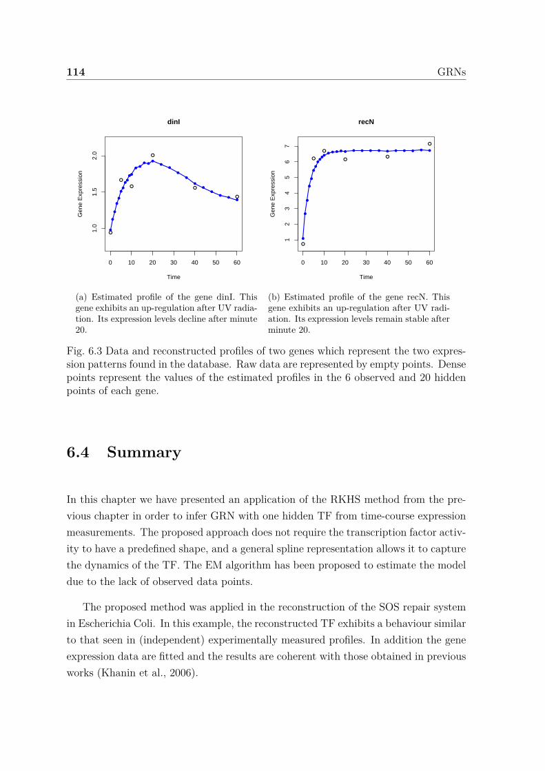
114 GRNs
0 10 20 30 40 50 60
1.0
1.5
2.0
dinI
Time
Gen
e E
xpre
ssio
n
(a) Estimated profile of the gene dinI. Thisgene exhibits an up-regulation after UV radia-tion. Its expression levels decline after minute20.
0 10 20 30 40 50 60
12
34
56
7
recN
TimeG
ene
Exp
ress
ion
(b) Estimated profile of the gene recN. Thisgene exhibits an up-regulation after UV radi-ation. Its expression levels remain stable afterminute 20.
Fig. 6.3 Data and reconstructed profiles of two genes which represent the two expres-sion patterns found in the database. Raw data are represented by empty points. Densepoints represent the values of the estimated profiles in the 6 observed and 20 hiddenpoints of each gene.
6.4 Summary
In this chapter we have presented an application of the RKHS method from the pre-vious chapter in order to infer GRN with one hidden TF from time-course expressionmeasurements. The proposed approach does not require the transcription factor activ-ity to have a predefined shape, and a general spline representation allows it to capturethe dynamics of the TF. The EM algorithm has been proposed to estimate the modeldue to the lack of observed data points.
The proposed method was applied in the reconstruction of the SOS repair systemin Escherichia Coli. In this example, the reconstructed TF exhibits a behaviour similarto that seen in (independent) experimentally measured profiles. In addition the geneexpression data are fitted and the results are coherent with those obtained in previousworks (Khanin et al., 2006).
6.A Notation 115
6.A Notation
For the proofs below we introduce some notation. We define a matrix CO ∈ IRn×(n+r)
such that
(CO)ij = 1 if tOi
= tj
0 otherwise,
vectors Φk = (δk,θk,Σk,µ,αk), Φ∗k = (δ∗
k,θ∗k,Σ∗
k,µ∗,α∗
k) and functions
lλ,k(Φk) = lk(Φk|Dk) − λ
2α⊤k Kδk
αk
= −12(yk − Kδk
αk)⊤Σ−1k (yk − Kδk
αk)
− 12
n+r∑i=1
log(σ2ki) − λ
2α⊤k Kδk
αk,
k = 1, . . . , d. With this notation we can write the penalized log-likelihood as
lλ(∆,Θ,Σ,µ) =d∑
k=1lλ,k(Φk).
6.B Proof of the expectation step of the EM algo-rithm
Proof. For every k = 1, . . . , d we calculate EyHk
(lλ,k|DO
k ,Φ∗k
). Denote with ΣH,k and
ΣO,k diagonal matrices whose diagonals are vectors of variances of observed and hiddenobservations of the kth equation respectively. Splitting the log-likelihood into twoparts corresponding to the hidden and the observed observations we obtain that
EyHk
(lλ,k|DO
k ,Φ∗k
)= −1
2
n+r∑i=1
log σ2ki − λ
2α⊤k Kδk
αk − 12∥yO
k − COKδkαk∥2
(Σ∗O,k
)−1
− 12EyH
k
(∥yH
k − CHKδkαk∥2
(Σ∗H,k
)−1|DOk , δ
∗k,Σ∗
k,α∗k
),
where ∥x∥2A = x⊤Ax. In the previous expression we have that
EyHk
(∥yH
k − CHKδkαk∥2
Σk|DO
k ,Φ∗k
)= EyH
k
(yH
k )⊤(Σ∗H,k)−1yH
k |DOk , δ
∗k,Σ∗
k,α∗k
− 2EyH
k
(yH
k )⊤(Σ∗H,k)−1CHKδk
αk|DOk , δ
∗k,Σ∗
k,α∗k
+ α⊤
k KδkC⊤
H(Σ∗H,k)−1CHKδk
αk.
116 GRNs
By using the properties of the expectation and the variance and by factorizing termswe obtain that
EyHk
(∥yH
k − CHKδkαk∥2
Σk|DO
k ,Φ∗k
)= ∥CHKδ∗
kα∗
k − CHKδkαk∥2
(Σ∗H,k
)−1 +r∑
i=1(σ∗
ki)2.
Substituting the last expression into the expected log-likelihood we obtain that
EyHk
(lλ,k|DO
k ,Φ∗k
)= −1
2
n+r∑i=1
log σ2ki − λ
2α⊤k Kδk
αk − 12∥yO
k − COKδkαk∥2
(Σ∗O,k
)−1
− 12
∥CHKδ∗kα∗
k − CHKδkαk∥2
(Σ∗H,k
)−1 +r∑
i=1(σ∗
ki)2
.Define y∗
k = (yOk ,CHKδ∗
kα∗
k)⊤. Grouping the terms we obtain that
EyHk
(lλ,k(yO
k ,yHk |Φk)|DO
k ,Φ∗k
)= −1
2
n+r∑i=1
log σ2ki − 1
2∥y∗k − Kδk
αk∥2Σ−1
k
− λ
2α⊤k Kδk
αk − 12
r∑i=1
(σ∗ki)2.
The proof is completed by summing over k’s and taking into account (6.10).
6.C Proof of the maximization step of the EM al-gorithm
Proof. Denote by y∗k = (yO
k ,CHKδ∗kα∗
k)⊤. Then for fixed δk and Σk the maximum ofEyH
k
(lλ,k|DO
k , δ∗k,Σ∗
k,α∗k
)is given for the vector αk = (Kδk
+λΣk)−1y∗k. By substitut-
ing αk into the expression and simplifying we obtain that
EyHk
(lλ,k|DO
k ,Φ∗k
)= −1
2
n+r∑i=1
log σ2ki − 1
2
r∑i=1
(σ∗ki)2 − 1
2(y∗k)⊤Σ−1
k (I − Sλ,k)y∗k,
where Sλ,k = Kδk(Kδk
+ λΣ2k)−1. By taking sum over k’s we obtain
(∆, Θ, Σ, µ) = arg max∆,Θ,Σ,µ
−12
d∑k=1
(y∗k)⊤Σ−1
k (I − Sλ,k)y∗k
− 12
d∑k=1
n+r∑i=1
log(σ2ki) − 1
2
m∑k=1
r∑i=1
(σ∗ki)2,
as we aimed to prove.
Conclusion
In Chapter 1, we have displayed Table 1.1 and Table 1.2. The former lists existingmethods for choosing the regularization parameter in Gaussian graphical models; thelatter contains those for estimating parameters in ordinary differential equations. Theresults presented in this thesis complement both tables.
We have complemented Table 1.1 with two new methods, the generalized infor-mation criterion and the Kullback-Leibler cross-validation. These methods improvethe Akaike’s information criterion and generalized approximate cross-validation. Thepurpose of Table 1.1 is not only to give a summary of the methods and show ourcontribution, but more importantly, to make a clear distinction between differentmethods. This distinction with respect to prediction and model selection does notseem to be stressed enough in the literature. For example, usage of cross-validation(CV) for model selection is not uncommon (Wang and Pillai, 2013; Gao et al., 2012)even though it was pointed out that this method is not appropriate for that purpose(Liu et al., 2010; Lian, 2011). However, to our best knowledge, so far it has not beenactually proved that cross-validation is not model selection consistent. Therefore, asa step in that direction, we have proved that this claim is true for the Akaike’s infor-mation criterion (AIC). Since AIC and CV share similar asymptotic properties (Shao,1997; Yang, 2005) in the regression setting, it is plausible that the same holds forGaussian graphical models. Moreover, we expect the same result to hold for othermethods whose aim is prediction. Thus we conclude and conjecture the following:
• AIC, K-CV, GACV, GIC and KLCV are appropriate for prediction but not formodel selection.
• BIC, EBIC, StARS are appropriate for model selection.Another important issue is the generality of the methods. Although the methods wepropose have advantages, they rely on the assumption of Gaussianity. In regard tothis, computational methods K-CV and StARS are expected to be the most robustwith respect to the departure from Gaussianity.
118 GRNs
As for Table 1.2, we have both proposed a new method and extended an existingone. The one that we propose, the RKHS approach, can deal with systems of differen-tial equations of a general form. The method is relatively simple to use and producesestimates of the parameters in one step. It has been tested on real and simulated dataand it exhibits reasonable performance. However, the drawback is that it relies on theassumption of Gaussianity and its asymptotic properties are unclear. It seems likelythat the method is not asymptotically consistent, due to the various approximationswe employ.
On the other hand, although the second method, the window-based estimator,can be applied only to autonomous systems of differential equations linear in theparameters, it does provide an asymptotically consistent estimator. Although werestrict the class of systems we consider, many applied problems are defined by thesystems that belong to this class. The window-based estimator has an explicit form, itis computationally fast and it does not require strong assumptions on the distributionof the data.
Finally, both methods discussed can be applied only if all states of the systemare observed. Estimation of the parameters in the partially observed systems has notbeen covered in this thesis. In the literature two ways are used to deal with partiallyobserved systems. One way is to use a Bayesian approach which relies on Gaussianprocesses (Chkrebtii et al., 2013). The other involves writing the unobserved states asa linear combination of certain basis functions and optimizing with respect to both theparameters of the system and the coefficients of the basis expansion (Ramsay et al.,2007). In the case of the window estimator both approaches can be used; this will bethe topic of our further research.
Summary
In this thesis we treat the problem of inference of two types of models: Gaussiangraphical models and ordinary differential equation models.
After presenting the background material in Chapter 2, we address the problem ofestimating the precision matrix in Gaussian graphical models. Every precision matrixcorresponds to a certain conditional independence graph. The main idea which wewe stress is that one can obtain an estimate of a precision matrix that yields a goodmodel in terms of prediction but whose corresponding conditional independence graphis poor. We prove that Akaike’s information criterion is not model selection consistentin a fixed p setting. We propose two criteria that yield predictively accurate modelsand we show how these criteria can be used to obtain models with a good conditionalindependence graph; this is the content of Chapter 3.
In Chapter 4, we extend to the time course data the existing method for estimat-ing autonomous systems of differential equations linear in the parameters, developedfor repeated measurements. The linearity of the system in parameters allows oneto explicitly obtain the estimators of the parameters without solving the differentialequation. This is of great importance since no optimization is needed. The methoddoes not require any initial values and is extremely fast. Furthermore, the obtainedestimator is asymptotically consistent.
In Chapter 5, we develop a method for estimating parameters in general systemsof differential equations. We dicretize the system of differential equations and usethe reproducing kernel Hilbert space to define an approximation of the log-likelihoodand its corresponding regularizer. By optimizing the obtained approximated penalizedlog-likelihood we estimate the parameters without solving the differential equation.
Finally, in the last chapter we apply the method developed in Chapter 5 to inferenceof gene regulatory kinetics. One ingredient present here and not in Chapter 5 is theuse of the EM algorithm which we employed to deal with the lack of observations.


Samenvatting
In dit proefschrift bestuderen we het probleem van inferentie voor twee typen statis-tische modellen, te weten Gaussische grafische modellen, en modellen die op gewonedifferentiaalvergelijkingen zijn gebaseerd.
Na een beschrijving van de achtergrond in hoofdstuk 2, bekijken we in hoofdstuk3 het probleem van het schatten van de concentratiematrix van Gaussische grafischemodellen. Elke concentratiematrix correspondeert met een bepaalde voorwaardelijkeonafhankelijkheidsgraaf. We benadrukken het feit dat het mogelijk is om een be-nadering van de concentratiematrix te verkrijgen die een model met een goede voor-spellende waarde oplevert, maar waarvan de voorwaardelijke onafhankelijkheidsgraaferg onnauwkeurig is. We bewijzen bovendien dat Akaikes informatiecriterium voorconstante p niet leidt tot consistente modelselectie. Er worden twee nieuwe crite-ria voorgesteld die leiden tot modellen die nauwkeurige voorspellingen opleveren enwe laten ook zien hoe deze criteria gebruikt kunnen worden om modellen met goedevoorwaardelijke onafhankelijkheidsgrafen te verkrijgen.
In hoofdstuk 4 breiden we de bestaande methode voor het schatten van autonomestelsels differentiaalvergelijkingen met lineaire parameters uit naar het geval waariner herhaalde metingen in de tijd worden uitgevoerd. Doordat de parameters van hetstelsel lineair zijn, is het mogelijk om een expliciete uitdrukking te vinden voor deschatters van de parameters, zonder dat het stelsel differentiaalvergelijkingen opgelosthoeft te worden. Dit is van groot belang, omdat hiervoor geen optimalisatieprocesnodig is. De zo gevonden methode heeft geen beginvoorwaarden nodig en is zeerefficient. Bovendien is de verkregen schatter asymptotisch consistent.
In hoofdstuk 5 ontwikkelen we een methode voor het schatten van parameters vanalgemene stelsels differentiaalvergelijkingen. We discretizeren het stelsel en gebruikeneen Hilbertruimte met reproducerende kern om een benadering van de waarschijnli-jkheidsfunctie en de bijbehorende regularisator te definiëren. Door het optimaliserenvan de verkregen benadering van de waarschijnlijkheidsfunctie waarbij een boeteterminbegrepen is, schatten we de parameters van het stelsel differentiaalvergelijkingen,

122 GRNs
zonder dit stelsel op te hoeven lossen.In het laatste hoofdstuk passen we de in hoofdstuk 5 ontwikkelde methode toe op
inferentie van de reactiekinetiek van genregulatienetwerken. Een nieuw onderdeel indit hoofdstuk is het gebruik van het EM-algoritme, toegepast om om te gaan met eenbeperkte aantal waarnemingen in de tijd .
References
Abbruzzo, A., Vujačić, I., Wit, E., and Mineo, A. M. (2014). Generalized informa-tion criterion for model selection in penalized graphical models. arXiv preprintarXiv:1403.1249.
Äijö, T. and Lähdesmäki, H. (2009). Learning gene regulatory networks from geneexpression measurements using non-parametric molecular kinetics. Bioinformatics,25(22):2937–2944.
Akaike, H. (1973). Information theory and an extension of the maximum likelihoodprinciple. In Second international symposium on information theory, pages 267–281.Akademinai Kiado.
Baldi, P., Brunak, S., Chauvin, Y., Andersen, C. A., and Nielsen, H. (2000). Assessingthe accuracy of prediction algorithms for classification: an overview. Bioinformatics,16(5):412–424.
Banerjee, O., El Ghaoui, L., and d’Aspremont, A. (2008). Model selection throughsparse maximum likelihood estimation for multivariate gaussian or binary data. TheJournal of Machine Learning Research, 9:485–516.
Bard, Y. (1974). Nonlinear parameter estimation. Academic Press New York.
Barenco, M., Tomescu, D., Brewer, D., Callard, R., Stark, J., and Hubank, M. (2006).Ranked prediction of p53 targets using hidden variable dynamic modeling. Genomebiology, 7(3):R25.
Barton, G. (1989). Elements of Green’s functions and propagation: potentials, diffu-sion, and waves. Oxford University Press.
Bates, D. M. and Watts, D. G. (1988). Nonlinear regression: iterative estimation andlinear approximations. Wiley.
Bellman, R. and Roth, R. S. (1971). The use of splines with unknown end points inthe identification of systems. Journal of Mathematical Analysis and Applications,34(1):26–33.
Bernstein, D. S. (2009). Matrix mathematics: theory, facts, and formulas. PrincetonUniversity Press.
Bickel, P. J. and Ritov, Y. (2003). Nonparametric estimators which can be ”plugged-in”. The Annals of Statistics, 31(4):1033–1053.

124 References
Biegler, L., Damiano, J., and Blau, G. (1986). Nonlinear parameter estimation: a casestudy comparison. AIChE Journal, 32(1):29–45.
Bock, H. G. (1983). Recent advances in parameter identification techniques for O.D.E.Springer.
Bonhoeffer, S., May, R. M., Shaw, G. M., and Nowak, M. A. (1997). Virus dynamicsand drug therapy. Proceedings of the National Academy of Sciences, 94(13):6971–6976.
Breiman, L. (1996). Heuristics of instability and stabilization in model selection. TheAnnals of Statistics, 24(6):2350–2383.
Brunel, N. J. B. (2008). Parameter estimation of ode’s via nonparametric estimators.Electronic Journal of Statistics, 2:1242–1267.
Bühlmann, P. and Van De Geer, S. (2011). Statistics for high-dimensional data:methods, theory and applications. Springer.
Cai, T., Liu, W., and Luo, X. (2011). A constrained l1 minimization approach tosparse precision matrix estimation. Journal of the American Statistical Association,106(494):594–607.
Calderhead, B., Girolami, M., and Lawrence, N. (2008). Accelerating bayesian in-ference over nonlinear differential equations with gaussian processes. Advances inNeural Information Processing, 21:217–224.
Campbell, D. and Steele, R. J. (2012). Smooth functional tempering for nonlineardifferential equation models. Statistics and Computing, 22(2):429–443.
Campbell, D. A. (2007). Bayesian collocation tempering and generalized profiling forestimation of parameters from differential equation models. PhD thesis, McGillUniversity, Montreal, Quebec.
Cao, J., Fussmann, G. F., and Ramsay, J. O. (2008). Estimating a predator-preydynamical model with the parameter cascades method. Biometrics, 64(3):959–967.
Cao, J. and Ramsay, J. O. (2007). Parameter cascades and profiling in functional dataanalysis. Computational Statistics, 22(3):335–351.
Cao, J. and Zhao, H. (2008). Estimating dynamic models for gene regulation networks.Bioinformatics, 24(14):1619–1624.
Chen, J. and Wu, H. (2008a). Efficient local estimation for time-varying coefficientsin deterministic dynamic models with applications to hiv-1 dynamics. Journal ofthe American Statistical Association, 103(481):369–384.
Chen, J. and Wu, H. (2008b). Estimation of time-varying parameters in deterministicdynamic models. Statistica Sinica, 18(3):987–1006.
Chen, T., He, H. L., Church, G. M., et al. (1999). Modeling gene expression withdifferential equations. In Pacific symposium on biocomputing, volume 4, pages 29–40.
References 125
Chen, X. (2012). Lasso-type sparse regression and high-dimensional Gaussian graphicalmodels. PhD thesis, The University of British Columbia, Vancouver, Canada.
Chen, Z. and Haykin, S. (2002). On different facets of regularization theory. NeuralComputation, 14(12):2791–2846.
Chkrebtii, O., Campbell, D. A., Girolami, M. A., and Calderhead, B. (2013).Bayesian uncertainty quantification for differential equations. arXiv preprintarXiv:1306.2365.
Dattner, I. and Klaassen, C. A. (2013). Estimation in systems of ordinary differentialequations linear in the parameters. arXiv preprint arXiv:1305.4126.
De Jong, H. (2002). Modeling and simulation of genetic regulatory systems: a litera-ture review. Journal of computational biology, 9(1):67–103.
Dempster, A. P. (1972). Covariance selection. Biometrics, 28(1):157–175.
Donnet, S. and Samson, A. (2007). Estimation of parameters in incomplete datamodels defined by dynamical systems. Journal of Statistical Planning and Inference,137(9):2815–2831.
Duffy, D. (2001). Green’s functions with applications. CRC Press.
Earn, D. J., Rohani, P., Bolker, B. M., and Grenfell, B. T. (2000). A simple modelfor complex dynamical transitions in epidemics. Science, 287(5453):667–670.
Edelstein-Keshet, L. (2005). Mathematical models in biology, volume 46. Siam.
Edwards, D. (2000). Introduction to graphical modelling. Springer.
Efron, B. (1979). Bootstrap methods: another look at the jackknife. The Annals ofStatistics, 7(1):1–26.
Efron, B. (1986). How biased is the apparent error rate of a prediction rule? Journalof the American Statistical Association, 81(394):461–470.
Efron, B. (2004). The estimation of prediction error: Covariance penalties and cross-validation. Journal of the American Statistical Association, 99(467):619–642.
Ellner, S. P., Seifu, Y., and Smith, R. H. (2002). Fitting population dynamic modelsto time-series data by gradient matching. Ecology, 83(8):2256–2270.
Fan, J., Feng, Y., and Wu, Y. (2009). Network exploration via the adaptive lasso andscad penalties. The Annals of Applied Statistics, 3(2):521–541.
Fan, J. and Li, R. (2001). Variable selection via nonconcave penalized likelihood andits oracle properties. Journal of the American Statistical Association, 96(456):1348–1360.
Fang, Y., Wu, H., and Zhu, L.-X. (2011). A two-stage estimation method for randomcoefficient differential equation models with application to longitudinal hiv dynamicdata. Statistica Sinica, 21(3):1145–1170.
126 References
Fasshauer, G. E. (2012). Green’s functions: Taking another look at kernel approx-imation, radial basis functions, and splines. In Approximation Theory XIII: SanAntonio 2010, pages 37–63. Springer.
Fellinghauer, B., Bühlmann, P., Ryffel, M., Von Rhein, M., and Reinhardt, J. D.(2013). Stable graphical model estimation with random forests for discrete, contin-uous, and mixed variables. Computational Statistics & Data Analysis, 64:132–152.
Fine, P. E. and Clarkson, J. A. (1982). Measles in england and wales—i: an analysis offactors underlying seasonal patterns. International journal of epidemiology, 11(1):5–14.
Finkenstädt, B. F. and Grenfell, B. T. (2000). Time series modelling of childhooddiseases: a dynamical systems approach. Journal of the Royal Statistical Society:Series C (Applied Statistics), 49(2):187–205.
Fitch, A. M. (2012). Computationally tractable fitting of graphical models: the cost andbenefits of decomposable Bayesian and penalized likelihood approaches. PhD thesis,Massey University, Albany, New Zealand.
FitzHugh, R. (1955). Mathematical models of threshold phenomena in the nervemembrane. The bulletin of mathematical biophysics, 17(4):257–278.
FitzHugh, R. (1961). Impulses and physiological states in theoretical models of nervemembrane. Biophysical journal, 1(6):445–466.
Folland, G. B. (1992). Fourier analysis and its applications. Wadsworth &Brooks/Cole.
Foygel, R. and Drton, M. (2010). Extended bayesian information criteria for gaussiangraphical models. Advances in Neural Information Processing Systems, 23:604–612.
Fried, R. and Vogel, D. (2010). On robust gaussian graphical modelling. In RecentDevelopments in Applied Probability and Statistics. Berlin, Heidelberg: Springer.
Friedman, J., Hastie, T., and Tibshirani, R. (2008). Sparse inverse covariance estima-tion with the graphical lasso. Biostatistics, 9(3):432–441.
Gao, X., Pu, D. Q., Wu, Y., and Xu, H. (2012). Tuning parameter selection for penal-ized likelihood estimation of gaussian graphical model. Statistica Sinica, 22(3):1123.
Gelman, A., Bois, F., and Jiang, J. (1996). Physiological pharmacokinetic analy-sis using population modeling and informative prior distributions. Journal of theAmerican Statistical Association, 91(436):1400–1412.
Girolami, M. (2008). Bayesian inference for differential equations. Theoretical Com-puter Science, 408(1):4–16.
Goldstein, L. and Messer, K. (1992). Optimal plug-in estimators for nonparametricfunctional estimation. The Annals of Statistics, 20(3):1306–1328.
González, J., Vujačić, I., and Wit, E. (2013). Inferring latent gene regulatory networkkinetics. Statistical applications in genetics and molecular biology, 12(1):109–127.
References 127
González, J., Vujačić, I., and Wit, E. (2014). Reproducing kernel hilbert space basedestimation of systems of ordinary differential equations. Pattern Recognition Letters,45:26–32.
Griffel, D. H. (1985). Applied functional analysis. Ellis Horwood Limited.
Gugushvili, S. and Klaassen, C. A. J. (2012).√n-consistent parameter estimation
for systems of ordinary differential equations: bypassing numerical integration viasmoothing. Bernoulli, 18(3):1061–1098.
Gugushvili, S. and Spreij, P. (2012). Parametric inference for stochastic differentialequations: a smooth and match approach. Latin American Journal of Probabilityand Mathematical Statistics, 9(2):609–635.
Hall, P. and Ma, Y. (2014). Quick and easy one-step parameter estimation in differ-ential equations. To be published in Journal of the Royal Statistical Society: SeriesB (Statistical Methodology).
Harville, D. A. (2008). Matrix algebra from a statistician’s perspective. Springer, 2edition.
Hastie, T., Tibshirani, R., and Friedman, J. J. H. (2009). The elements of statisticallearning. Springer New York, 2 edition.
He, D., Ionides, E. L., and King, A. A. (2010). Plug-and-play inference for diseasedynamics: measles in large and small populations as a case study. Journal of theRoyal Society Interface, 7(43):271–283.
Hemker, P. (1972). Numerical methods for differential equations in system simulationand in parameter estimation. Analysis and Simulation of biochemical systems, pages59–80.
Himmelblau, D., Jones, C., and Bischoff, K. (1967). Determination of rate constantsfor complex kinetics models. Industrial & Engineering Chemistry Fundamentals,6(4):539–543.
Hooker, G. (2007). Theorems and calculations for smoothing-based profiled estimationof differential equations. Technical report, Technical Report BU-1671-M, Dept. Bio.Stat. and Comp. Bio., Cornell University.
Hooker, G. (2009). Forcing function diagnostics for nonlinear dynamics. Biometrics,65(3):928–936.
Hooker, G. and Biegler, L. (2007). Ipopt and neural dynamics: Tips, tricks and diag-nostics. Technical report, Department of Biological Statistics and ComputationalBiology, Cornell University.
Hooker, G., Ellner, S. P., Roditi, L. D. V., and Earn, D. J. (2011). Parameterizingstate–space models for infectious disease dynamics by generalized profiling: measlesin ontario. Journal of The Royal Society Interface, 8(60):961–974.
128 References
Hooker, G., Xiao, L., and Ramsay, J. (2012). Collocinfer: collocation inference fordynamic systems. R package version 0.1.7.
Huang, Y., Liu, D., and Wu, H. (2006). Hierarchical bayesian methods for estimationof parameters in a longitudinal hiv dynamic system. Biometrics, 62(2):413–423.
Huang, Y. and Wu, H. (2006). A bayesian approach for estimating antiviral efficacyin hiv dynamic models. Journal of Applied Statistics, 33(2):155–174.
Huppert, A., Barnea, O., Katriel, G., Yaari, R., Roll, U., and Stone, L. (2012). Mod-eling and statistical analysis of the spatio-temporal patterns of seasonal influenzain israel. PloS one, 7(10):e45107.
Jost, C. and Ellner, S. P. (2000). Testing for predator dependence in predator-preydynamics: a non-parametric approach. Proceedings of the Royal Society of London.Series B: Biological Sciences, 267(1453):1611–1620.
Kelley, W. G. and Peterson, A. C. (2010). The Theory of Differential Equations:Classical and Qualitative. Springer, 2 edition.
Khanin, R., Vinciotti, V., Mersinias, V., Smith, C., and Wit, E. (2007). Statisti-cal reconstruction of transcription factor activity using michaelis–menten kinetics.Biometrics, 63(3):816–823.
Khanin, R., Vinciotti, V., and Wit, E. (2006). Reconstructing repressor protein levelsfrom expression of gene targets in escherichia coli. Proceedings of the NationalAcademy of Sciences, 103(49):18592–18596.
Konishi, S. and Kitagawa, G. (1996). Generalised information criteria in model selec-tion. Biometrika, 83(4):875–890.
Konishi, S. and Kitagawa, G. (2008). Information criteria and statistical modeling.Springer.
Kullback, S. and Leibler, R. A. (1951). On information and sufficiency. The Annalsof Mathematical Statistics, 22(1):79–86.
Lalam, N. and Klaassen, C. A. (2006). Pseudo maximum likelihood estimation fordifferential equations. Eurandom.
Lam, C. and Fan, J. (2009). Sparsistency and rates of convergence in large covariancematrix estimation. The Annals of Statistics, 37(6B):4254–4278.
Lauritzen, S. L. (1996). Graphical models. Oxford University Press.
Lawrence, N., Rattray, M., Honkela, A., and Titsias, M. (2011). Gaussian processinference for differential equation models of transcriptional regulation. HandBookof Statistical Systems Biology, pages 376–394.
Lawrence, N. D., Sanguinetti, G., and Rattray, M. (2006). Modelling transcriptionalregulation using gaussian processes. Advances in Neural Information Processing,19:785–792.
References 129
Li, H. and Gui, J. (2006). Gradient directed regularization for sparse gaussian con-centration graphs, with applications to inference of genetic networks. Biostatistics,7(2):302–317.
Li, L., Brown, M. B., Lee, K.-H., and Gupta, S. (2002). Estimation and inference fora spline-enhanced population pharmacokinetic model. Biometrics, 58(3):601–611.
Li, Z., Osborne, M. R., and Prvan, T. (2005). Parameter estimation of ordinarydifferential equations. IMA Journal of Numerical Analysis, 25(2):264–285.
Lian, H. (2011). Shrinkage tuning parameter selection in precision matrices estimation.Journal of Statistical Planning and Inference, 141(8):2839–2848.
Liang, H. and Wu, H. (2008). Parameter estimation for differential equation mod-els using a framework of measurement error in regression models. Journal of theAmerican Statistical Association, 103(484):1570–1583.
Lillacci, G. and Khammash, M. (2010). Parameter estimation and model selection incomputational biology. PLoS computational biology, 6(3):e1000696.
Liu, H., Han, F., Yuan, M., Lafferty, J., and Wasserman, L. (2012). High-dimensional semiparametric gaussian copula graphical models. The Annals of Statis-tics, 40(4):2293–2326.
Liu, H., Roeder, K., and Wasserman, L. (2010). Stability approach to regulariza-tion selection (stars) for high dimensional graphical models. Advances in NeuralInformation Processing Systems, 23:1432–1440.
Loader, C. (1999). Local Regression and Likelihood. Springer.
Lotka, A. J. (1910). Contribution to the theory of periodic reactions. The Journal ofPhysical Chemistry, 14(3):271–274.
Lu, T., Liang, H., Li, H., and Wu, H. (2011). High-dimensional odes coupled withmixed-effects modeling techniques for dynamic gene regulatory network identifica-tion. Journal of the American Statistical Association, 106(496).
Madár, J., Abonyi, J., Roubos, H., and Szeifert, F. (2003). Incorporating prior knowl-edge in a cubic spline approximation-application to the identification of reactionkinetic models. Industrial & engineering chemistry research, 42(17):4043–4049.
Magnus, J. R. and Neudecker, H. (1985). Matrix differential calculus with applicationsto simple, hadamard, and kronecker products. Journal of Mathematical Psychology,29(4):474–492.
Magnus, J. R. and Neudecker, H. (2007). Matrix differential calculus with applicationsin statistics and econometrics. Wiley & Sons, third edition.
Meinshausen, N. and Bühlmann, P. (2006). High-dimensional graphs and variableselection with the lasso. The Annals of Statistics, 34(3):1436–1462.
130 References
Menéndez, P., Kourmpetis, Y. A., ter Braak, C. J., and van Eeuwijk, F. A. (2010).Gene regulatory networks from multifactorial perturbations using graphical lasso:application to the dream4 challenge. PloS one, 5(12):e14147.
Miao, H., Dykes, C., Demeter, L. M., Cavenaugh, J., Park, S. Y., Perelson, A. S.,and Wu, H. (2008). Modeling and estimation of kinetic parameters and replicativefitness of hiv-1 from flow-cytometry-based growth competition experiments. Bulletinof mathematical biology, 70(6):1749–1771.
Milo, R., Shen-Orr, S., Itzkovitz, S., Kashtan, N., Chklovskii, D., and Alon, U.(2002). Network motifs: simple building blocks of complex networks. Science,298(5594):824–827.
Nagumo, J., Arimoto, S., and Yoshizawa, S. (1962). An active pulse transmission linesimulating nerve axon. Proceedings of the IRE, 50(10):2061–2070.
Nikol’skij, N. K. (1992). Functional analysis I: linear functional analysis, volume 19.Springer.
Nishii, R. (1984). Asymptotic properties of criteria for selection of variables in multipleregression. The Annals of Statistics, 12(2):758–765.
Ogunnaike, B. A. and Ray, W. H. (1994). Process dynamics, modeling, and control.Oxford University Press.
Olinky, R., Huppert, A., and Stone, L. (2008). Seasonal dynamics and thresholdsgoverning recurrent epidemics. Journal of mathematical biology, 56(6):827–839.
Pascual, M. and Ellner, S. P. (2000). Linking ecological patterns to environmentalforcing via nonlinear time series models. Ecology, 81(10):2767–2780.
Penny, W. D. (2001). Kullback-liebler divergences of normal, gamma, dirichlet andwishart densities. Technical report, Wellcome Department of Cognitive Neurology.
Powers, D. (2011). Evaluation: From precision, recall and f-measure to roc., in-formedness, markedness & correlation. Journal of Machine Learning Technologies,2(1):37–63.
Poyton, A., Varziri, M. S., McAuley, K. B., McLellan, P., and Ramsay, J. O. (2006).Parameter estimation in continuous-time dynamic models using principal differentialanalysis. Computers & chemical engineering, 30(4):698–708.
Putter, H., Heisterkamp, S., Lange, J., and De Wolf, F. (2002). A bayesian approach toparameter estimation in hiv dynamical models. Statistics in medicine, 21(15):2199–2214.
Qi, X. and Zhao, H. (2010). Asymptotic efficiency and finite-sample properties ofthe generalized profiling estimation of parameters in ordinary differential equations.The Annals of Statistics, 38(1):435–481.
Ramsay, J. and B.W., S. (2006). Functional data analysis. Springer, 2 edition.
References 131
Ramsay, J. O. (1996). Principal differential analysis: Data reduction by differen-tial operators. Journal of the Royal Statistical Society. Series B (Methodological),58(3):495–508.
Ramsay, J. O., Hooker, G., Campbell, D., and Cao, J. (2007). Parameter estimationfor differential equations: a generalized smoothing approach. Journal of the RoyalStatistical Society: Series B (Statistical Methodology), 69(5):741–796.
Rasmussen, C. E. (2006). Gaussian processes for machine learning. The MIT Press.
Ravikumar, P., Wainwright, M. J., Raskutti, G., and Yu, B. (2011). High-dimensionalcovariance estimation by minimizing l1-penalized log-determinant divergence. Elec-tronic Journal of Statistics, 5:935–980.
Roach, G. F. (1982). Green’s functions. Cambridge University Press, 2 edition.
Rogers, S., Khanin, R., and Girolami, M. (2007). Bayesian model-based inference oftranscription factor activity. BMC bioinformatics, 8(Suppl 2):S2.
Ronen, M., Rosenberg, R., Shraiman, B. I., and Alon, U. (2002). Assigning numbers tothe arrows: parameterizing a gene regulation network by using accurate expressionkinetics. Proceedings of the national academy of sciences, 99(16):10555–10560.
Rothman, A. J., Bickel, P. J., Levina, E., and Zhu, J. (2008). Sparse permutationinvariant covariance estimation. Electronic Journal of Statistics, 2:494–515.
Rue, H. and Held, L. (2005). Gaussian Markov random fields: theory and applications.CRC Press.
Sassanfar, M. and Roberts, J. W. (1990). Nature of the sos-inducing signal in Es-cherichia coli: The involvement of dna replication. Journal of molecular biology,212(1):79–96.
Schmidt, M. (2010). Graphical model structure learning with l1-regularization. PhDthesis, The University of British Columbia, Vancouver, Canada.
Secrier, M., Toni, T., and Stumpf, M. P. (2009). The abc of reverse engineeringbiological signalling systems. Molecular Biosystems, 5(12):1925–1935.
Shao, J. (1997). An asymptotic theory for linear model selection. Statistica Sinica,7(2):221–242.
Smola, A. J. et al. (2002). Learning with Kernels: Support Vector Machines, Regular-ization, Optimization and Beyond. MIT press.
Stakgold, I. and Holst, M. J. (1979). Green’s functions and boundary value problems.John Wiley & Sons.
Steinke, F. and Schölkopf, B. (2008). Kernels, regularization and differential equations.Pattern Recognition, 41(11):3271–3286.
Steinwart, I. and Christmann, A. (2008). Support vector machines. Springer.
132 References
Stone, L., Olinky, R., and Huppert, A. (2007). Seasonal dynamics of recurrent epi-demics. Nature, 446(7135):533–536.
Stone, M. (1974). Cross-validatory choice and assessment of statistical predictions.Journal of the Royal Statistical Society. Series B (Methodological), 36(2):111–147.
Stone, M. (1977). An asymptotic equivalence of choice of model by cross-validation andakaike’s criterion. Journal of the Royal Statistical Society. Series B (Methodological),39(1):44–47.
Stortelder, W. J. (1996). Parameter estimation in dynamic systems. Mathematics andComputers in Simulation, 42(2):135–142.
Tibshirani, R. (1996). Regression shrinkage and selection via the lasso. Journal of theRoyal Statistical Society. Series B (Methodological), 58(1):267–288.
Tjoa, I. B. and Biegler, L. T. (1991). Simultaneous solution and optimization strategiesfor parameter estimation of differential-algebraic equation systems. Industrial &Engineering Chemistry Research, 30(2):376–385.
Turkington, D. A. (2005). Matrix calculus and zero-one matrices: Statistical andeconometric applications. Cambridge University Press.
Vajda, S., Valko, P., and Yermakova, A. (1986). A direct-indirect procedure for esti-mation of kinetic parameters. Computers & chemical engineering, 10(1):49–58.
Varah, J. (1982). A spline least squares method for numerical parameter estimationin differential equations. SIAM Journal on Scientific and Statistical Computing,3(1):28–46.
Varziri, M., Poyton, A., McAuley, K., McLellan, P., and Ramsay, J. (2008). Select-ing optimal weighting factors in ipda for parameter estimation in continuous-timedynamic models. Computers & Chemical Engineering, 32(12):3011–3022.
Voit, E. O. and Savageau, M. A. (1982). Power-low approach to modeling biologicalsystems: Ii. application to ethanol production. Journal of fermentation technology,60(3):229–232.
Voorman, A., Shojaie, A., and Witten, D. (2013). Graph estimation with joint additivemodels. Biometrika, page ast053.
Vujačić, I., Abbruzzo, A., and Wit, E. (2014a). A computationally fast alterna-tive to cross-validation in penalized gaussian graphical models. arXiv preprintarXiv:1309.6216.
Vujačić, I., Dattner, I., González, J., , and Wit, E. (2014b). Time-course windowestimator for ordinary differential equations linear in the parameters. manuscriptunder revision in Statistics and Computing.
Wainwright, M. J. and Jordan, M. I. (2008). Graphical models, exponential families,and variational inference. Foundations and Trends® in Machine Learning, 1(1-2):1–305.
References 133
Wang, H. and Pillai, N. S. (2013). On a class of shrinkage priors for covariance matrixestimation. Journal of Computational and Graphical Statistics, 22(3):689–707.
Whittaker, J. (2009). Graphical models in applied multivariate statistics. Wiley Pub-lishing.
Wild, G. and Seber, C. (1989). Nonlinear Regression. Wiley.
Wood, N. S. and Lindgren, F. (2013). Apts statistical computing. Notes.
Xiang, D. and Wahba, G. (1996). A generalized approximate cross validation forsmoothing splines with non-gaussian data. Statistica Sinica, 6:675–692.
Xue, H., Miao, H., and Wu, H. (2010). Sieve estimation of constant and time-varyingcoefficients in nonlinear ordinary differential equation models by considering bothnumerical error and measurement error. The Annals of Statistics, 38(4):2351–2387.
Xun, X., Cao, J., Mallick, B., Maity, A., and Carroll, R. J. (2013). Parameter esti-mation of partial differential equation models. Journal of the American StatisticalAssociation, 108(503):1009–1020.
Yanagihara, H., Tonda, T., and Matsumoto, C. (2006). Bias correction of cross-validation criterion based on kullback–leibler information under a general condition.Journal of multivariate analysis, 97(9):1965–1975.
Yang, Y. (2005). Can the strengths of aic and bic be shared? a conflict between modelindentification and regression estimation. Biometrika, 92(4):937–950.
Yuan, M. and Lin, Y. (2007). Model selection and estimation in the gaussian graphicalmodel. Biometrika, 94(1):19–35.
Zhang, Y., Li, R., and Tsai, C.-L. (2010). Regularization parameter selections viageneralized information criterion. Journal of the American Statistical Association,105(489):312–323.
Zhao, T., Liu, H., Roeder, K., Lafferty, J., and Wasserman, L. (2014). huge: High-dimensional Undirected Graph Estimation. R package version 1.2.6.
Zou, H. (2006). The adaptive lasso and its oracle properties. Journal of the Americanstatistical association, 101(476):1418–1429.


Curriculum vitae
Ivan Vujačić was born on March 6, 1983 in Podgorica, Montenegro. He graduatedfrom the University of Montenegro, Podgorica, Montenegro, with diploma in Theoret-ical Mathematics in 2007. During the last year of his studies he taught mathematicsat the Electrical Engineering High school Vaso Aligrudić, Podgorica. He receivedthe Master of Science degree (MSc) in Mathematics in 2009. From 2007 to 2010 hetaught at the Faculty of Mathematics and Natural Sciences, University of Montenegro.In 2010 he began his PhD project in statistics at the Johann Bernoulli Institute forMathematics and Computer Science at the University of Groningen, The Netherlands.During his PhD he worked on inference of Gaussian graphical models and ordinarydifferential equations. The results of his research are described in this thesis.


Inference of Gaussian Graphical models andordinary differential equations
Ivan Vujačić[email protected]
Please email me comments and corrections.
ISBN 978-90-367-7098-9 (printed version)ISBN 978-90-367-7097-2 (electronic version)
Colophon
This thesis was completed using the PhD/MPhil thesis LATEX template, by KrishnaKumar, University of Cambridge.Proofreader: JoAnn van Seventer ([email protected])Printed by: Grafimedia ([email protected])