UNIVERSITY OF CRETE

DEPARTMENT OF PHYSICS

Experimental Energy Resolution of a Paracentric

Hemispherical Deflector Analyzer for Different Entry Positions and Bias

Gennarakis Giannis

Supervisor: Prof. Theo J. M. Zouros, Univ. of Crete

Heraklion, 2015

May 2015

Dissertation

Experimental Energy Resolution of a

Paracentric Hemispherical Deflector Analyzer

for Different Entry Positions and Bias

Gennarakis Giannis

Supervisor:

Prof. Theo J. M. Zouros, Univ. of Crete

Abstract

Results from the simulation of a biased paracentric hemispherical deflector analyzer

(HDA) with injection lens are presented. The finite differences electron optics software

SIMION was used to perform Monte Carlo type trajectory simulations in an effort to

investigate the focusing effects of the HDA entry and exit fringing fields which are used

to improve energy resolution - a novel feature of this type of analyzer. Comparisons

to recent experimental results are also presented. Biased paracentric HDAs represent

a novel class of HDAs, which use the lensing action of the strong fringing fields at the

HDA entry, to restore the first order focus characteristics of ideal HDAs in a controlled

way. The improvement in energy resolution and transmission without the use of any

additional fringing field correction electrodes is of particular interest to modern

analyzers using position sensitive detectors.

SUBJECT AREA: Electron spectroscopy, Ion-Atom collisions, Atomic Physics

KEYWORDS: Hemispherical Analyser, SIMION, Electron Spectroscopy, Electrostatic lens

Acknowledgments

Being involved in scientific research for the first time of my life, I would specially like to thank Prof. Zouros for giving me this ability, and making this small but worthwhile journey smooth, through his patience with new students, clear scientific thought and all the things that taught me on how to do the research and think. Also, for the spirit of teamwork that he promoted to all the members of the research and his unlimited time to keep the project going. Furthermore, I would like to thank Prof. Genoveva Martinez Lopez for her comments and advice on various matters concerning the simulation method and results, as well as Dr. Omer Sise for giving us his lights on how to exploit the old data and overtake obstacles during the experimental process and results. Last but not least, the creator of software SIMION, Mr. David Manura for all the debugging and coding tips that kept us moving forward till the end. Special acknowledgment to the funding source This research has been co-financed by the European Union (European Social Fund ESF) and Greek national funds through the Operational Program "Education and Lifelong Learning" of the National Strategic Reference Framework (NSRF) Research Funding Program: THALES. Investing in knowledge society through the European Social Fund, grant number MIS 377289).

Nomenclature Symbol Units Description

𝐷𝛾 (𝑚𝑚) γ-independent dispersion length

𝐸𝑠0 (𝑒𝑉) Nominal electron gun energy

𝑅0 = �̅� (𝑚𝑚) HDA mean radius

𝑅𝐵 = 𝛥𝛦𝐵/𝛦 ( − ) HDA Base Energy Resolution

𝑅𝜋 (𝑚𝑚) Radius of exit of the beam

𝑉0 (𝑉) Nominal voltage 𝑉(𝑅0)

𝑉1 (𝑉) Nominal voltage 𝑉(𝑅1) on 𝑅1

𝑉2 (𝑉) Nominal voltage 𝑉(𝑅2) on 𝑅2

𝑉𝑝 (𝑉) Nominal voltage on the HDA front plate

𝛦0 (𝑒𝑉) Nominal electron HDA pass energy

𝐹 ( − ) Pre-retardation ratio – 𝐸𝑠0/𝐸0

𝑀 ( − ) HDA linear magnification

𝑇 (𝑒𝑉) Initial kinetic energy of the particle

𝑉(𝑟) (𝑉) HDA potential, 𝑉(𝑟) = −𝑘/𝑟 + 𝑐 + 𝑉𝑝

𝑊 Undecelerated tuning energy

𝑤 (𝑒𝑉) Energy of the central trajectory or tuning energy (after deceleration)

𝛥𝛦𝐵 = 𝐹𝐵𝑀 (𝑒𝑉) Base energy resolution; full width of the energy transmission function.

𝛥𝛦𝑃 (𝑒𝑉) Individual particle energy relative to the pass energy of the analyzer.

𝛥𝑅 = 𝑅2 − 𝑅1 (𝑚𝑚) Distance between the hemisphere plates

𝛥𝑅𝜋 (𝑚𝑚) Exit beam width along the energy dispersion direction

𝛥𝛦 = 𝐹𝑊𝐻𝑀 (𝑒𝑉) Full width at half of the maximum height of the energy transmission function.

𝛼 (deg) Angle of particle prior to entering the HDA

𝛾 ( − ) Control Parameter to set 𝑉0

𝜉 ( − ) HDA parameter 𝜉 = 𝑅𝜋/𝑅0

𝜌 = 𝛥𝑅/�̅� ( − ) Interradial separation

𝜏 = 𝑡/𝑤 ( − ) Reduced pass energy

Contents Introduction ............................................................................................................................... 7

Historical Review ................................................................................................................... 7

Electron Spectroscopy ........................................................................................................... 8

Photoelectron Spectroscopy (PES) .................................................................................... 8

Auger Spectroscopy ........................................................................................................... 8

Zero Degree Auger Projectile Spectroscopy ...................................................................... 9

Electrostatic Analysers .......................................................................................................... 9

Theory ...................................................................................................................................... 10

Motion of a charged particle in an ideal 1/r potential ........................................................ 11

Derivation of a charged particle trajectory ......................................................................... 13

Focusing Conditions of the Ideal HDA ................................................................................. 14

Spectrograph basic equation ............................................................................................... 15

Analyzer Voltages ................................................................................................................ 15

Ion Optics Simulation Software SIMION.............................................................................. 17

References ............................................................................................................................... 18

Appendix A (Works Cited) ....................................................................................................... 19

Appendix B (Research Papers Published) ................................................................................ 20

Introduction

Electron energy analyzers which are a vital component of electron spectrometers have

become important tools in many branches of collision physics. In order to resolve higher

electronic states and vibrational states in these experiments, some sort of electron energy

analyzer is required to provide an incident beam of sufficiently narrow energy spread and to

determine the energy of the scattered or ejected electrons. The most common arrangement

is to use a hemispherical deflector analyzer.

Historical Review

The history of electron spectroscopy goes back more than 100 years when first H. Hertz

reported in 1887 [1] about the matter-light interaction famously known as “the photoelectric

effect” which was later described extensively by A. Einstein in 1905 [2]. Two years after

Einstein's publication, in 1907 P. D. Innes experimented with a Röntgen tube, Helmholtz coils,

a magnetic field hemisphere (an electron momentum analyzer), and photographic plates to

record broad bands of emitted electrons as a function of velocity, in effect recording the first

X-Ray Photoelectron Spectroscopy (XPS) spectrum [3]. The “scattering experiment”, initiated

in 1911 by Rutherford in his famous experiment of bombarding thin gold films with α-particles

[4], provided valuable information both on the structure and on the interaction potential of

the partners involved. The fundamental aspects of atomic collision theory were already

formulated by Mott and Massey in their monumental work first published in 1933 [5].

However, interest remained focused solely on nuclear physics for the next 30 years.

It wasn’t until the early 1960’s when the tandem Van de Graff ion accelerators, popular in

nuclear physics by the time, were implemented in atomic physics, primarily due to the fact

that projectile-ions can excite atomic states inaccessible by photon and electron impact.

Shortly, the use of light ions, available in most of the charge states and in a wide band of

collision energies, became a unique tool in atomic physics studies. At the same time, the

increasing interest in the investigation of the Auger and auto-ionization effects made the use

of electrostatic spectrometers wide spread.

Today, tandem Van de Graaff accelerators, Linear Accelerators, Electron Cyclotron Resonance

(ECR) ion sources, Electron Beam Ion Sources (EBIS) and Storage Rings, can provide atomic

ions from hydrogen to uranium in all charge states and in energies varying from a few eV/u to

hundreds of MeV/u, depending on the atomic species, the charge state and the source in use.

A large variety of energy dispersive spectrometers like the parallel plate analyser, the

cylindrical plate analyser, the toroidal analyser, the hemispherical analyser and spherical plate

analyser are also extremely popular, indicating the continuous interest in the physics of ion-

atom collisions, as also the wide development of different experimental techniques, as for

example the most modern COLd Target Recoil Ion Momentum Spectroscopy (COLTRIMS)

experiments.

Electron Spectroscopy

The term electron spectroscopy refers to methods where the sample is ionized and the

emitted electrons are observed. The most common type is photoelectron spectroscopy, in

particular X-ray photoelectron spectroscopy (XPS) but also the UV photoelectron

spectroscopy (UPS) is widely used.

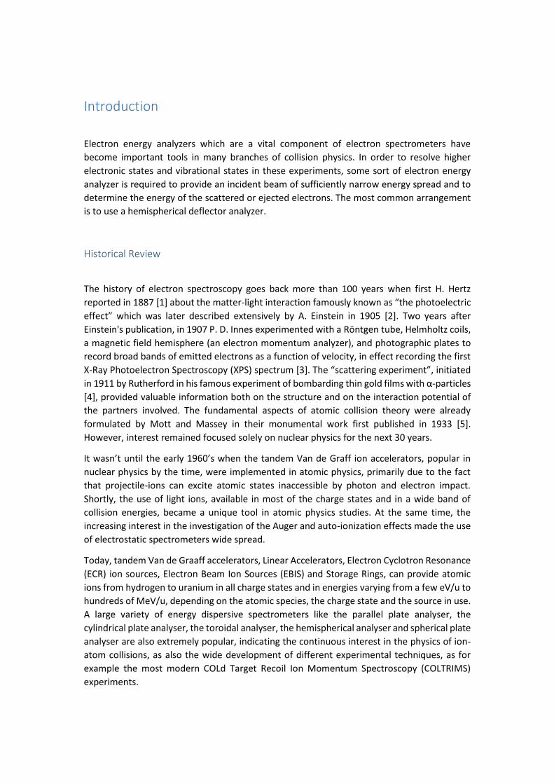
Photoelectron Spectroscopy (PES)

Photoelectron spectroscopy (PES) is a method where

the molecule is ionized by irradiating it with such

photons that an electron is released. When using

moderate photon energies in the far ultraviolet

region, only the weakly bound valence electrons can

be released while a harder rays in the X-ray region will

also release electrons from the innermost core

orbitals.

When UV light is used the method is called UV photoelectron spectroscopy (UPS) and when X-

rays are used it is called X-ray photoelectron spectroscopy (XPS or ESCA (Electron Spectroscopy

for Chemical Analysis). The principle of these methods are shown schematically in Fig. 1.

Auger Spectroscopy

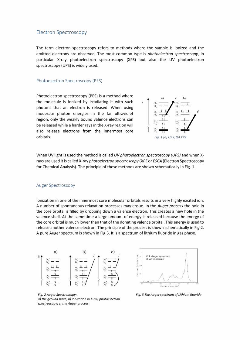
Ionization in one of the innermost core molecular orbitals results in a very highly excited ion. A number of spontaneous relaxation processes may ensue. In the Auger process the hole in the core orbital is filled by dropping down a valence electron. This creates a new hole in the valence shell. At the same time a large amount of energy is released because the energy of the core orbital is much lower than that of the donating valence orbital. This energy is used to release another valence electron. The principle of the process is shown schematically in Fig.2. A pure Auger spectrum is shown in Fig.3. It is a spectrum of lithium fluoride in gas phase.

Fig. 1 (a) UPS; (b) XPS

Fig. 2 Auger Spectroscopy: a) the ground state; b) ionization in X-ray photoelectron spectroscopy; c) the Auger process

Fig. 3 The Auger spectrum of Lithium fluoride

The Auger process is customarily described by indicating in which shell the original ionization occurred and where the final two holes reside in the electronic structure of the doubly ionised molecule. In LiF the initial X-ray ionisation extracted an electron from the K shell. Afterwards the hole was filled by an electron from the L shell and finally one further electron was ejected from the L shell.

Zero Degree Auger Projectile Spectroscopy

Projectile ions are mostly moving at relatively high velocities. Consequently, the Auger lines

from projectile ions suffer considerable kinematic effects. A very popular method to improve

the intrinsic analyser resolution, is to perform electron deceleration prior to their analysis in

the spectrometer. However, the tremendous decrease of the electron transmission, present

in all spectrographs utilizing slits, sets a practical limit on the applied deceleration and

therefore to the achieved energy resolution. To improve the energy resolution the projectile

Auger electrons are detected at 0o or 180o with respect to the beam direction, as in this way

substantial reduction of the kinematic broadening can be achieved. The technique of

detecting Auger electrons emitted from ions at 0o with respect to the beam direction, is

known as Zero-degree Auger Projectile Spectroscopy (ZAPS) and has received considerable

attention the past two decades. The potential advantage of this technique is that it is the only

efficient method which can provide state-selective cross section information about collision

mechanisms.

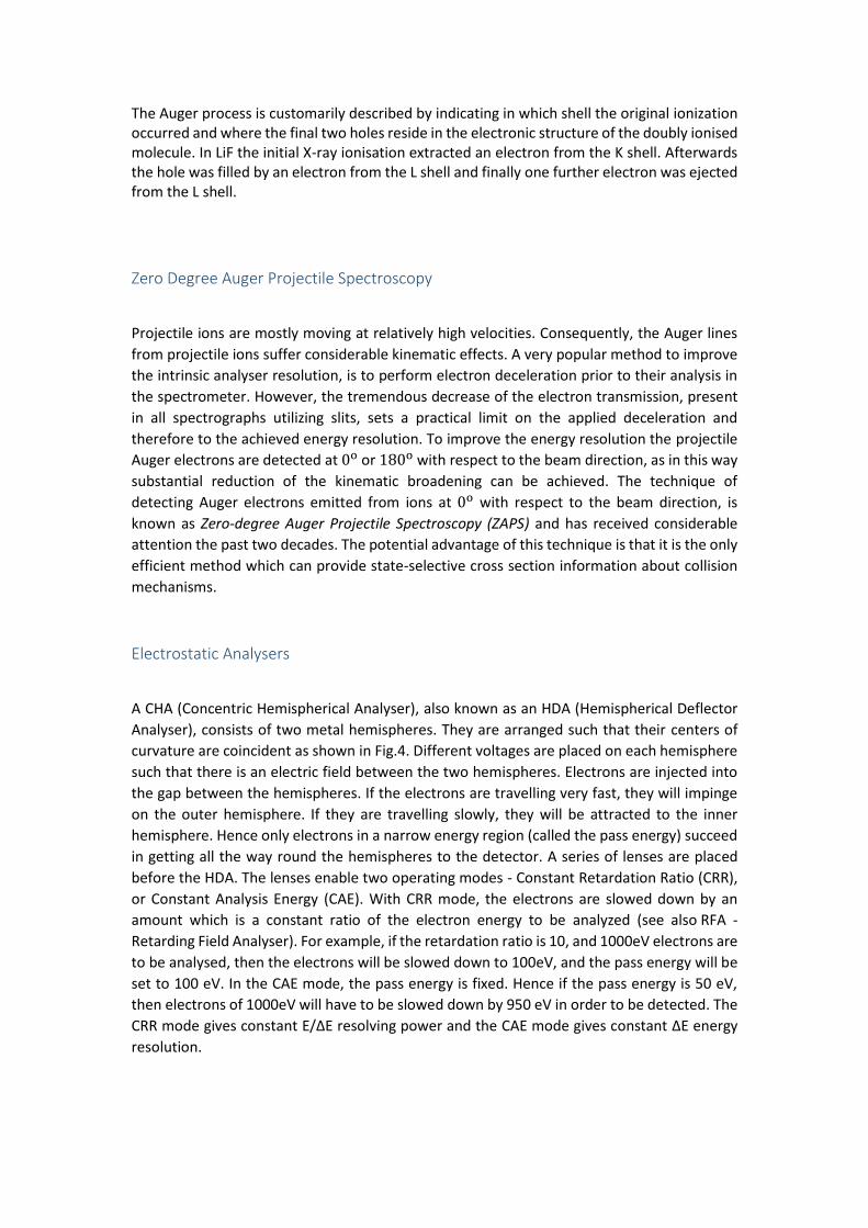
Electrostatic Analysers

A CHA (Concentric Hemispherical Analyser), also known as an HDA (Hemispherical Deflector

Analyser), consists of two metal hemispheres. They are arranged such that their centers of

curvature are coincident as shown in Fig.4. Different voltages are placed on each hemisphere

such that there is an electric field between the two hemispheres. Electrons are injected into

the gap between the hemispheres. If the electrons are travelling very fast, they will impinge

on the outer hemisphere. If they are travelling slowly, they will be attracted to the inner

hemisphere. Hence only electrons in a narrow energy region (called the pass energy) succeed

in getting all the way round the hemispheres to the detector. A series of lenses are placed

before the HDA. The lenses enable two operating modes - Constant Retardation Ratio (CRR),

or Constant Analysis Energy (CAE). With CRR mode, the electrons are slowed down by an

amount which is a constant ratio of the electron energy to be analyzed (see also RFA -

Retarding Field Analyser). For example, if the retardation ratio is 10, and 1000eV electrons are

to be analysed, then the electrons will be slowed down to 100eV, and the pass energy will be

set to 100 eV. In the CAE mode, the pass energy is fixed. Hence if the pass energy is 50 eV,

then electrons of 1000eV will have to be slowed down by 950 eV in order to be detected. The

CRR mode gives constant E/ΔE resolving power and the CAE mode gives constant ΔE energy

resolution.

Fig. 4 Schematic of an HDA (or CHA) comprised of two concentric metal hemispheres with different voltages

Theory

First Hughes and Rojansky [6] mentioned in their paper the possibility of energy analyzing

charged particles using electrostatic fields instead of magnetic fields. It was already well

known by that time (1929) that electrons entering with small angles in a cylindrical

spectrograph with magnetic fields, describe a circle whose radius depends on the velocity of

the electrons and the strength of the magnetic fields and that good refocusing happened at

𝜑 = 180𝜊 from the plane containing the entrance slit. For electrostatic fields they found that

positions 180𝑜 and 90𝑜 (of the plane of the receiving slit) where not suitable for good

refocusing and instead suggested good re-focusing and good resolution to be found at a

characteristic angle of 𝛷 = 127𝜊 17′.

A few years later Purcell [7] considered the refocusing properties of charged particles in an

ideal (no fringing fields) spherical condenser and studied the possibility of deflecting and

focusing a slightly diverging beam of charged particles in a cylindrical condenser. He described

this device as an energy-analyser where the trajectory of a nonrelativistic particle in any given

electrostatic field depends only on its initial position and direction and the ratio of its charge

to its initial kinetic energy. These types of analysers were previously incorporated successfully

as mass spectrographs. Ever since, the hemispherical version of the condenser became very

popular in electron spectroscopy – due to its advantageous focusing properties and rugged

construction – and many hemispherical spectrometers were studied and utilized in

experiments.

In 1967 Kuyatt and Simpson developed [8] an electron monochromator design based on a

hemispherical analyser. They examined the slit width and electron energy at a given resolution

for obtaining maximum current. They concluded on the choice of equal size round apertures

for the entrance and exit of the beam instead of slits with dimensions satisfying the equation

𝛼2 = 𝑤/2�̅� (where 𝑎 is the pencil angle, 𝑤 the aperture diameter and �̅� the mean analyser

radius) which became a standard criterion for HDA designs. Paolini and Theodoridis, and

Kennedy et. al. reported on the transmission properties of spherical plate electrostatic

analysers. Roy and Carette, included the hemispherical spectrometer in their method of

calculating the energy distribution of electrons selected electrostatically. Heddle reported on

the comparison of the étendue (the product of the entrance area and solid angle) of electron

spectrometers including spherical plate analysers. Polaschegg reported on the features of the

spherical analysers with and without pre-retardation. He also reported on the study of the

energy resolution and the intensity behavior of the spherical analysers as a function of the

entrance parameters. Imhof et. al. studied the energy resolution and transit time spread in

the hemispherical analysers involved in coincidence experiments. Kevan also reported on

design criteria for high-resolution angle-resolving HDAs. Hadjarab and Erskine reported on the

image properties of the HDA used with a position sensitive detector (PSD), replacing in this

way the commonly used exit slit with a large area detector. A double-stage spectrograph

consisting of two HDAs has been reported by Mann and Linder, as well as Baraldi and Dhanak.

Page and Read investigated the energy non-linearity of HDA when used with a multi-detector

anode or PSD.

In the previous references, the HDA was studied as if the electrostatic field was ideal, i.e.

fringing field effects, primarily present at the HDA entry and exit, were not taken into account.

However, for HDAs used with large PSDs, fringing field effects become important, resulting in

departures from the spectrograph properties predicted for ideal fields theoretically.

All studies to date, have basically treated the specific case of a hemispherical spectrometer

constructed with the entry and exit apertures placed at the mean radius of the analyser

opening (i.e. for radii 𝑅1 and 𝑅2 the entry 𝑅0 is placed at the position 𝑅0 = �̅� =𝑅1+𝑅2

2. In all

these cases the potential value 𝑉0 for the circular equipotential line is set to be zero, while the

orbit followed by the particles inside the HDA is circular. Analysers whose exit due to geometry

limitations could not be placed at �̅� have recently been reported in the literature [9].

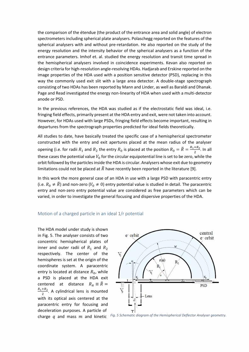
In this work the more general case of an HDA in use with a large PSD with paracentric entry

(i.e. 𝑅0 ≠ �̅�) and non-zero (𝑉0 ≠ 0) entry potential value is studied in detail. The paracentric

entry and non-zero entry potential value are considered as free parameters which can be

varied, in order to investigate the general focusing and dispersive properties of the HDA.

Motion of a charged particle in an ideal 1/r potential

The HDA model under study is shown

in Fig. 5. The analyser consists of two

concentric hemispherical plates of

inner and outer radii of 𝑅1 and 𝑅2

respectively. The center of the

hemispheres is set at the origin of the

coordinate system. A paracentric

entry is located at distance 𝑅0, while

a PSD is placed at the HDA exit

centered at distance 𝑅𝜋 ≡ �̅� =𝑅1+𝑅2

2. A cylindrical lens is mounted

with its optical axis centered at the

paracentric entry for focusing and

deceleration purposes. A particle of

charge 𝑞 and mass 𝑚 and kinetic Fig. 5 Schematic diagram of the Hemispherical Deflector Analyser geometry.

energy 𝑇 is ejected at zero potential far from the spectrograph. Prior to entering the analyser

it passes through a deceleration/focusing stage (e.g. lens system) which can take its kinetic

energy to 𝑡 such that:

𝑡 = 𝑇 − 𝑞𝑉𝑝

by applying a potential 𝑉𝑝 on the last electrode of the deceleration stage. When deceleration

is not required, 𝑉𝑝 is set to zero (𝑉𝑝 = 0). However, when deceleration is used 𝑉𝑝 is the voltage

upon which all analyser potentials are referenced to.

The particle enters the HDA at a point 𝑟0 (in the vicinity of 𝑅0) with kinetic energy 𝑡 and polar

angle 𝛼. Actually, since the particle is ejected in three-dimensional space, it enters the

analyser at an azimuthal angle 𝛽 too. However, 𝛽 just rotates the motion plane around the

axis defined by the entrance point 𝑟0 and the center of the analyser. This is the reason why it

is not included in the figure which shows the motion in the orbit plane only. The particle

follows a trajectory specified by 𝑟(𝜃) and exits at 𝑟𝜋 after being deflected through an angle

𝛥𝜃 = 𝜋.

The analyser potential 𝑉(𝑟) is ideally given by 𝑉(𝑟) = �̃�(𝑟) + 𝑉𝑝 where the symbol �̃�(𝑟) is

used as a shorthand for the frequently appearing quantity:

�̃�(𝑟) = −𝑘

𝑟+ 𝑐

The symbols 𝑉1 ≡ 𝑉(𝑅1), 𝑉2 ≡ 𝑉(𝑅2) and the corresponding �̃�1, �̃�2 are reserved for the inner

and outer hemispheres, respectively. Also, the symbol 𝑉0 ≡ 𝑉(𝑅0) and the corresponding �̃�0

is reserved for the value of the potential at the entry 𝑅0. Finally the quantities 𝛥𝑉 ≡ 𝑉2 −

𝑉1 = �̃�2 − �̃�1 and 𝛥𝑅 ≡ 𝑅2 − 𝑅1 are defined.

When the analyser is “tuned” to the energy 𝑤, an electron with kinetic energy 𝑡 = 𝑤 can be

made to follow a particular reference trajectory known as the central trajectory, in which case

the particle is also referred to as the central ray and 𝑤 as the tuning energy.

For analyzing systems with deceleration, as in the present system, one may define an

“undecelerated tuning energy” W:

𝑊 ≡ 𝑤 + 𝑞 𝑉𝑝

and the deceleration ratio 𝐹:

𝐹 ≡𝑊

𝑤

so that a central ray with kinetic energy 𝑊 far from the spectrometer (at “infinity”) undergoing

deceleration with factor 𝐹 will have the energy 𝑤 just prior to entering the hemispherical

analyser. The “reduced” pass energy 𝜏 is also defined as:

𝜏 ≡𝑡

𝑤= 𝐹 (

𝑇

𝑊− 1) + 1

which may also be expressed in terms of the undecelerated quantities, 𝑇, 𝑊 and the

deceleration factor 𝐹. Finally, the independent parameter 𝛾 by which the potential set on the

analyser is controlled:

𝑞 (𝑉0 − 𝑉𝑝) = 𝑞 �̃�0 ≡ (1 − 𝛾) 𝑤

and the parameter 𝜉 , characterizing the ‘asymmetry’ of the HDA:

𝜉 ≡𝑅𝜋

𝑅0

The parameter γ is known as the entry bias parameter. A conventional HDA is seen to have

𝜉 = 1 and 𝛾 = 1.

Derivation of a charged particle trajectory

The motion of a charged particle of mass 𝑚 and charge 𝑞 in a central potential 𝑉(𝑟) is always

motion in a plane. The problem is equivalent to the “two body” problem, the general solution

of which can be found in most undergraduate textbooks of classical mechanics.

The solution of the orbital motion will be derived in brief steps taking the fixed center of force

which corresponds to the potential as the origin of the coordinate system.

Expressed in plane polar coordinates the Lagrangian is:

ℒ =1

2𝑚(𝑟2̇ + 𝑟2𝜃2)̇ − 𝑞𝑉(𝑟)

The Euler-Lagrange equations of motion are:

𝑑

𝑑𝑡(

𝜕ℒ

𝜕�̇�) −

𝜕ℒ

𝜕𝜃= 0 ⇒

𝑑

𝑑𝑡(𝑚𝑟2�̇�) = 0

𝑑

𝑑𝑡(

𝜕ℒ

𝜕�̇�) −

𝜕ℒ

𝜕𝑟= 0 ⇒ 𝑚�̈� − 𝑚𝑟𝜃2̇ = −𝑞

𝜕𝑉(𝑟)

𝜕𝑟

Integrating the equations of motion the first integrals of motion are obtained:

⇒ 𝑚𝑟2�̇� = 𝑐𝑜𝑛𝑠𝑡. = 𝐿

⇒1

2𝑚𝑟2̇ +

1

2

𝐿2

𝑚𝑟2+ 𝑞𝑉(𝑟) = 𝐸

𝐿 is the magnitude of the angular momentum of the system while 𝐸 is the total energy. Two

more integrations are needed to solve the equations of motion, since there are two variables,

𝑟 and 𝜃. After two more integrations the above equations give

𝜃 = ∫𝑑𝑟

𝑟2√2𝑚𝐸𝐿2 −

2𝑚𝑞𝑉(𝑟)𝐿2 −

1𝑟2

+ 𝜃𝜀

𝑟

𝑟0

where 𝑟0 and 𝜃𝜀 are defined by the initial conditions. This is the most general solution of the

equation of motion. Replacing the general central potential 𝑉(𝑟) with the electrostatic

potential of a spherical capacitor, the final solution of the particle orbit inside a spherical

analyser is obtained

𝑟(𝜃) =

𝐿2

𝑚𝑞𝑘

1 + √1 + (2𝐸′𝐿2

𝑚𝑞𝑘2) cos(𝜃 − 𝜃𝜀)

=𝑝

1 + 𝜀 cos(𝜃 − 𝜃𝜀)

The above equation is the general solution of a conic section with one focus at the origin and

latus rectum 𝑝 and eccentricity ε given by the equations:

𝑝 =𝐿2

𝑚𝑞𝑘

𝜀 = √1 +2𝛦′𝐿2

𝑚𝑞𝑘2

𝐸′ is a quantity with dimensions of energy which defines the nature of the orbit by defining

the magnitude of 𝜀 and is defined as

1

2𝑚𝑟2̇ +

1

2

𝐿2

𝑚𝑟2− 𝑞

𝑘

𝑟= 𝐸 − 𝑞𝑐 − 𝑞𝑉𝑝 ≡ 𝐸′

In the case of the elliptical orbit –which is the case of a charged particle orbit inside the

spherical analyser- the equation of the article orbit is reduced to

𝑟(𝜃) =𝑎(1 − 𝜀2)

1 + 𝜀 cos(𝜃 − 𝜃𝜀)

where 𝑎 is the semi-major axis given by:

𝑎 = −𝑞𝑘

2𝐸′

Focusing Conditions of the Ideal HDA

The focusing conditions of the ideal hemispherical analyser are directly obtained by expanding the elliptical orbit equation to second order in 𝑎 around 𝑎 = 0.

𝑟0

𝑟𝜃=

𝑞𝑘 + (2𝑡𝑟0 − 𝑞𝑘)𝑐𝑜𝑠𝜃

2𝑡𝑟0− (𝑠𝑖𝑛𝜃)𝛼 +

𝑞𝑘(1 − 𝑐𝑜𝑠𝜃)

2𝑡𝑟0𝑎2

The first order term in 𝑎 is readily seen to be zero for 𝜃 = 𝜋 and thus the hemispherical deflector analyser (HDA) is said to focus to first order for a deflection angle of 180°. Particles that enter the HDA with the same radius 𝑟 = 𝑟0 and the same energy but different angles 𝑎, after a deflection of 180o, will all lie on radii 𝑟𝜋 = 𝑟(𝜃 = 𝜋, 𝛼), which will only differ to second order in 𝛼. The most important feature of the HDA is its all order focusing at 𝜃 = 𝜋 for the azimuthal angle 𝛽.

Spectrograph basic equation

Since the HDA focusing properties can be studied only from the ray trace on the exit plane, an expression which gives the position of the particle at the image (exit), as a function of its position and direction at the object (entrance) and its pass energy 𝜏 can be derived:

r𝜋 = −𝑟0 +𝑅0(1 + 𝜉)

1 +𝜉𝛾

(1 − 𝜏 cos2 𝑎∗)

This kind of equation is known as the basic equation of the spectrograph. The equation can also be written (in terms of potential constants 𝑘 and 𝑐) in the form

𝑟𝜋 = −𝑟0 +𝑞𝑘

𝑞𝑐 − 𝑡 cos2 𝑎∗

or may be rearranged into the usual form:

𝑟𝜋 − 𝑅𝜋

𝑅𝜋= −

(𝑟0 − 𝑅0)

𝜉𝑅0− (1 +

1

𝜉)

1

1 +𝜉𝛾 sin2 𝑎∗ − (𝜏 − 1)

𝜉𝛾

(1 − sin2 𝑎∗)

The first of the three equations shows that the range of the electron trajectory inside the analyser (i.e. the sum 𝑟𝜋 + 𝑟0) is a universal function of the "reduced" pass-energy 𝜏 and the incident angle 𝛼. This, universal scaling with 𝜏 is particularly useful during the energy calibration of the spectrometer since different energies 𝑇 and deceleration factors 𝐹 must all fall on one universal curve dependent on 𝜏, avoiding the tedious task of calibrating the spectrometer for all combinations of 𝐹, 𝑇 and 𝑊 used.

Analyzer Voltages

The voltage scheme 𝑉1 and 𝑉2 applied on the inner and outer spherical shells of the analyser, respectively, is actually a function of the tuning energy of the spectrometer. The determination of the voltages is based on the concept of "central" ray, in a straightforward way. The entry and exit points are specified. For these points, a central or reference ray with 𝑎 = 0 and pass energy 𝑡, set to the analyser tuning energy 𝑤, i.e. 𝑡 = 𝑤, is decided. These conditions are adequate to define the proper potential applied on the analyser. In this study, the central ray is defined such that a charged particle enters at 𝑟 =𝑅0 (𝑖. 𝑒. 𝑟0 = 𝑅0) and exits after a deflection by 180𝑜 at 𝑟 = �̅� ≡ (𝑅1 + 𝑅2)/2. Applying voltages 𝑉1 and 𝑉2 on the inner and outer spherical shells of the analyser, respectively, the expressions for 𝑘 and 𝑐 are obtained:

𝑐 =𝑅2𝑉2−𝑅1𝑉1

𝛥𝑅− 𝑉𝑝 =

𝑅2�̃�2−𝑅1�̃�1

𝛥𝑅

𝑘 =𝛥𝑉

𝛥𝑅𝑅1𝑅2 =

𝛥�̃�

𝛥𝑅𝑅1𝑅2

Substituting 𝑘 and 𝑐 from the expressions above into the spectrograph basic equation, the central ray case reduces to:

𝑅𝜋 = −𝑅0 −𝑞𝛥𝑉𝑅1𝑅2

𝑞�̃�1𝑅1 − 𝑞�̃�2 + 𝑤𝛥𝑅

Furthermore, for a pre-specified entrance potential 𝑉0, after substitution of 𝑘 and 𝑐 in terms of 𝑉1 and 𝑉2, 𝑉0 is written in terms of 𝑉1 and 𝑉2:

𝑉0 =(𝑅2 − 𝑅0)𝑅1𝑉1 + (𝑅0 − 𝑅1)𝑅2𝑉2

𝛥𝑅 𝑅0

And

�̃�0 =(𝑅2 − 𝑅0)𝑅1�̃�1 + (𝑅0 − 𝑅1)𝑅2�̃�2

𝛥𝑅 𝑅0+ 𝑉𝑝

Finally, solving for 𝑉1 and 𝑉2 the voltage equations are obtained:

𝑞𝑉𝑖 = 𝑞𝑉𝑝 + 𝑤 + [𝑞(𝑉0 − 𝑉𝑝) − 𝑤]𝑅0(𝑅𝜋+𝑅0−𝑅𝑖)

𝑅𝜋𝑅𝑖 𝑖 = 1,2

Or expressed in terms of the �̃� potentials:

𝑞�̃�𝑖 = 𝑤 + (𝑞�̃�0 − 𝑤)𝑅0(𝑅𝜋+𝑅0−𝑅𝑖)

𝑅𝜋𝑅𝑖 𝑖 = 1,2

Which uniquely determine 𝑉1 and 𝑉2 in terms of potentials 𝑉0, 𝑉𝑝, the tuning energy 𝑤 and

the “central ray” positions of the entrance 𝑅0 and the exit 𝑅𝜋, respectively. This is the most general formula for the voltages from which all specific cases can be derived. The potential energy difference 𝑞𝛥𝑉 is:

𝑞𝛥𝑉 = (𝛾

𝜉)

(1+𝜉)

𝜉

𝑅𝜋𝛥𝑅

𝑅1𝑅2𝑤

From which a spectrometer constant 𝑓 can be defined to be:

𝑓 ≡ 𝑞𝛥𝑉

𝑤=

1

2(

𝛾

𝜉)

(1 + 𝜉)

𝜉

𝑅𝜋

�̅�𝑓0

Where 𝑓0 is just the spectrometer constant of the conventional hemispherical analyser, i.e. 𝑅0 = �̅� = 𝑅𝜋 with 𝑉0 = 𝑉𝑝 (𝛾 = 1):

𝑓0 =𝛥𝑅

𝑅2𝑅12�̅�

The constant of the analyser 𝑓 is actually a number which determines the gradient voltage value applied on the plates, for tuning the spectrometer at a given energy 𝑡 = 𝑤. This number was introduced in the past for convenience, since in most spectrometers it uniquely defines the voltages set on the analyser as a function of 𝑤. However, in the paracentric HDA case, 𝑓 does not determine the voltage values 𝑉1 and 𝑉2 uniquely, since the information on 𝑉0 (or γ) value is also needed. Therefore 𝑓 is only a qualitative number describing the actual potential gradient between the hemispheres. For further details on the theory behind the HDA and how these equations derive analytically the reader is referenced to the following citations [10] [11] [12].

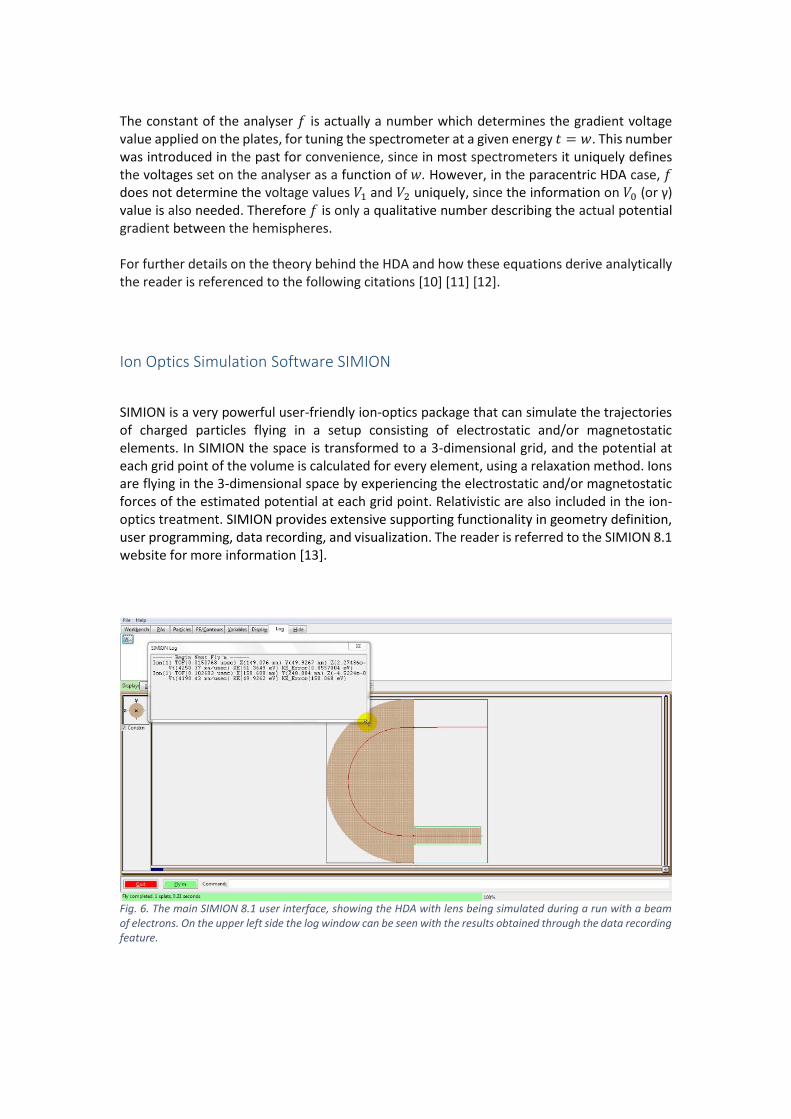
Ion Optics Simulation Software SIMION

SIMION is a very powerful user-friendly ion-optics package that can simulate the trajectories of charged particles flying in a setup consisting of electrostatic and/or magnetostatic elements. In SIMION the space is transformed to a 3-dimensional grid, and the potential at each grid point of the volume is calculated for every element, using a relaxation method. Ions are flying in the 3-dimensional space by experiencing the electrostatic and/or magnetostatic forces of the estimated potential at each grid point. Relativistic are also included in the ion-optics treatment. SIMION provides extensive supporting functionality in geometry definition, user programming, data recording, and visualization. The reader is referred to the SIMION 8.1 website for more information [13].

Fig. 6. The main SIMION 8.1 user interface, showing the HDA with lens being simulated during a run with a beam of electrons. On the upper left side the log window can be seen with the results obtained through the data recording feature.

References

[1] H. Hertz, "Ueber den Einfluss des ultravioletten Lichtes auf die electrische Entladung,"

vol. 267, no. 8, p. 983–1000, 1987.

[2] A. Einstein, "Über einen die Erzeugung und Verwandlung des Lichtes betreffenden

heuristischen Gesichtspunkt (On a Heuristic Point of View about the Creation and

Conversion of Light)," Annalen der Physik, vol. 17, no. 6, p. 132–148, 1905.

[3] P. D. Innes, "On the Velocity of the Cathode Particles Emitted by Various Metals under

the Influence of Rontgen Rays, and Its Bearing on the Theory of Atomic Disintegration,"

The Royal Society, vol. 79, no. 532, 1907.

[4] E. Rutherford, "The Scattering of α and β rays by Matter and the Structure of the

Atom," Philosophical Magazine, vol. 21, no. 6, pp. 669-688, 1911.

[5] N. F. Mott and H. W. Massey, The theory of atomic collisions, Oxford: Oxford University

Press, 1933.

[6] A. L. Hughes and V. Rojansky, "On the analysis of electrostatic velocities by electrostatic

means," vol. 34, 1929.

[7] E. M. Purcell, "The focusing of charged particles by a spherical condenser," vol. 54,

1938.

[8] C. E. Kuyatt and J. A. Simpson, "Electron Monochromator Design," vol. 38, no. 1, 1967.

[9] V. D. B. a. M. I. Yavor, Rev. Sci. lustrum., no. 71, p. 1651, 2000.

[10] E. P. Benis, "A novel high-efficiency paracentric hemispherical spectrograph for zero-

degree auger projectile spectroscopy," Heraklion, 2001.

[11] E. P. B. a. T. J. M. Zouros, "The hemispherical deflector analyser revisited: II. Electron-

optical properties," J. Electron Spectrosc. Relat. Phenom., vol. 163, no. 1-3, pp. 28-39,

2008.

[12] T. J. M. Z. a. E. P. Benis, J. Electron Spectrosc. Relat. Phenom, vol. 142, no. 125, pp. 221-

248, 2005.

[13] "The field and particle trajectory simulator - Industry standard charged particle optics

software SIMION," [Online]. Available: www.simion.com.

Appendix A (Works Cited)

Articles in International Journals

Experimental energy resolution of a paracentric hemispherical deflector analyzer for

different entry positions and bias, M. Dogan, M. Ulu, G. G. Gennarakis, T.J.M.

Zouros, Review of Scientific Instruments 84 (2013) 043105

Posters Presentations for International Conferences/Meetings

M. Dogan, M. Ulu, G. G. Gennarakis, T.J.M. Zouros, ICPEAC 2013, July 24-30, 2013, Lanzhou, China Poster Contribution

Posters Presentations for Local Conferences/Meetings

G. G. Gennarakis, T. J. M. Zouros, M. Dogan, M. Ulu, 22nd Hellenic Nuclear Physics Symposium, May 31-June 1, 2013, Athens, Greece Poster Contribution 2

Abstracts for Local Conference/Meetings

G. G. Gennarakis, T. J. M. Zouros, M. Dogan, M. Ulu, HNPS2013: May 31-June 1,2013, Athens, Greece

Articles in Local Proceedings

Experimental energy resolution of a paracentric hemispherical deflector analyzer for different entry positions and bias simulated in SIMION, G.G. Gennarakis, T.J.M. Zouros, 22nd Hellenic Nuclear Physics Symposium, May 31-June 1, 2013, Athens, Greece, Proceedings.

Appendix B (Research Papers Published)

Experimental energy resolution of a paracentric hemispherical deflector analyzer for

different entry positions and bias

M. Dogan, M. Ulu, G. G. Gennarakis, and T. J. M. Zouros

Citation: Review of Scientific Instruments 84, 043105 (2013); doi: 10.1063/1.4798592

View online: http://dx.doi.org/10.1063/1.4798592

View Table of Contents: http://scitation.aip.org/content/aip/journal/rsi/84/4?ver=pdfcov

Published by the AIP Publishing

This article is copyrighted as indicated in the article. Reuse of AIP content is subject to the terms at: http://scitationnew.aip.org/termsconditions. Downloaded to IP:

147.52.159.18 On: Fri, 17 Jan 2014 11:07:46

REVIEW OF SCIENTIFIC INSTRUMENTS 84, 043105 (2013)

Experimental energy resolution of a paracentric hemispherical deflector

analyzer for different entry positions and bias

M. Dogan,1,a) M. Ulu,1 G. G. Gennarakis,2 and T. J. M. Zouros2

1eCOL Laboratory, Department of Physics, Science and Arts Faculty, Afyon Kocatepe University, 03200 Afyonkarahisar, Turkey

2Atomic Collisions and Electron Spectroscopy Laboratory, Department of Physics, University of Crete,

P.O. Box 2208, 71003 Heraklion, Crete, Greece

(Received 6 March 2013; accepted 14 March 2013; published online 10 April 2013)

A specially designed hemispherical deflector analyzer (HDA) with 5-element input lens having a

movable entry position R0 suitable for electron energy analysis in atomic collisions was constructed

and tested. The energy resolution of the HDA was experimentally determined for three different

entry positions R0 = 84, 100, 112 mm as a function of the nominal entry potential V(R0) under

pre-retardation conditions. The resolution for the (conventional) entry at the mean radius R0 = 100 mm was found to be a factor of 1.6-2 times worse than the resolution for the two (paracentric) po-

sitions R0 = 84 and 112 mm at particular values of V(R0). These results provide the first experi- mental verification and a proof of principle of the utility of such a paracentric HDA, while demon-

strating its advantages over the conventional HDA: greater dispersion with reduced angular aberra-

tions resulting in better energy resolution without the use of any additional fringing field correction

electrodes. Supporting simulations of the entire lens plus HDA spectrometer are also provided and

mostly found to be within 20%–30% of experimental values. The paracentric HDA is expected to

provide a lower cost and/or more compact alternative to the conventional HDA particularly useful

in modern applications utilizing a position sensitive detector. © 2013 American Institute of Physics.

[http://dx.doi.org/10.1063/1.4798592] typically also equipped with an input lens this would require,

in addition, special hardware allowing for the precise reposi-

tioning of the entire electron source, lens and entry aperture

assembly at the various entry radii to be tested, clearly re-

quiring a special arrangement. In this paper we report on first

experimental results using such a variable entry HDA, specif-

ically designed for testing the biased paracentric HDA con-

cept experimentally and the energy resolution improvements

claimed by simulation.

The design considerations outlined in our previous sim-

ulation work were realized experimentally here and the new

biased paracentric HDA configuration for atomic collisions

was constructed and tested. The present analyzer uses a wide-

I. INTRODUCTION

The hemispherical deflector analyzer (HDA) is one of

the most widely used electrostatic energy selectors in low

energy atomic collision physics (for a recent review see Ref.

1 and the references therein). However, the first-order fo-

cusing characteristics of a HDA are impaired due to the fring-

ing fields created at the electrode entry boundaries. In the con-

ventional HDA, fringing fields generally produce an image

with larger angular aberrations at the dispersion plane from

that predicted for the ideal (no fringing fields) HDA leading

to a substantial deterioration in its energy resolution.1 Partial

recovery of the high resolution attributes of the ideal HDA can

be attained by incorporating additional electrodes in various

fringing field correction schemes.2 Over the last decade, it has

been shown in simulation2–5 that this drawback can also be

readily overcome without using any type of additional fring-

ing field corrector electrodes in an arrangement that has come

to be known as the “biased paracentric” HDA.5 This HDA

utilizes a biased optical axis (i.e., the central ray trajectory is

not at 0 potential as in a conventional HDA) and an optimized

entry position R0 offset from the center position (at the mean

5

gap inter-electrode distance /')R ≡ R2 − R1 = 50 mm and

a mean radius R̄ = 100 mm. It incorporates a standard input lens, which in this case is mounted on a rail to allow for the

repositioning of the entry at any value R0 between the inner

hemisphere at radius R1 = 75 mm and the outer hemisphere

at R2 = 125 mm. The apparatus is shown in Fig. 1. Here, we report on energy resolution measurements for two paracentric

entry positions R0 = 84 mm and R0 = 112 mm, on either side of the mean radius, respectively, in comparison to the conven-

radius R̄ = (R1 + R2)/2) used in conventional HDAs.5 Pre-

vious simulations have shown2–5 that the biased paracentric HDA can in principle restore near ideal field conditions. To

date, however, these expectations have not been tested exper-

imentally since they require a direct comparison of conven-

tional and paracentric entries in the same analyzer necessitat-

ing a HDA with a variable entry radius R0. Since HDAs are

tional (central) entry at R0 = R̄ = 100 mm. These specific R0 5 entry positions were predicted from our previous simulation

work to correspond to positions of optimal energy resolu-

tion for the right entry bias.

We note that our reported experimental measurements

are performed on a combined ESCA-type spectrometer (com-

prised of a HDA with input lens) under pre-retardation condi-

tions, typical in high resolution electron spectroscopy applica-

tions. This necessitated the use of new additional simulations

2, 4

a)Author to whom correspondence should be addressed. Electronic mail: mdogan@aku.edu.tr

0034-6748/2013/84(4)/043105/8/$30.00 84, 043105-1 © 2013 American Institute of Physics

This article is copyrighted as indicated in the article. Reuse of AIP content is subject to the terms at: http://scitationnew.aip.org/termsconditions. Downloaded to IP:

147.52.159.18 On: Fri, 17 Jan 2014 11:07:46

043105-2 Dogan et al. Rev. Sci. Instrum. 84, 043105 (2013)

where the central ray is in general part of an ellipse, while in

the conventional HDA it is part of a circle.1

An electron entering a HDA (tuned to pass a central ray

of energy E0), in the vicinity of the entry at r0 = R0 ± /')r0/2

with a pass energy E ± /')E/2 and small input half-angle α,

will exit the HDA (after 180◦ deflection) at the radius rπ = Rπ

± /')rπ /2. Under these conditions, the exit beam width along the energy dispersion direction, /')rπ , is given to 2nd order in

α by10

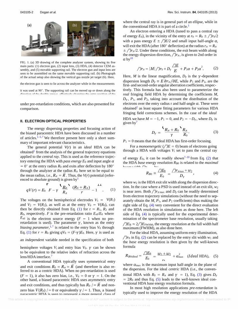
FIG. 1. (a) 3D drawing of the complete analyzer system, showing its five

main parts: (1) electron gun, (2) input lens, (3) HDA, (4) detector CEM as-

sembly, and (5) movable supporting rail. The electron gun and input lens are

seen to be assembled on the same movable supporting rail. (b) Photograph

of the actual setup also showing the vertical gas nozzle jet target (6). Here,

the electron gun is seen to lie across the analyzer while in the measurements

it was used at 90◦. The supporting rail can be moved up or down along the

direction of the double arrows, effectively changing the entry position of the

analyzer R0.

/')E 2 /')rπ = |M| /')r0 + Dγ + P1α + P2α . (2)

E

Here, M is the linear magnification, Dγ is the γ -dependent

dispersion length Dγ ≡ E ∂rπ /∂E, while P1 and P2, are the first- and second-order angular aberration coefficients, respec-

tively. This formula has also been used to parameterize the

real fringing field HDA by determining the coefficients M,

Dγ , P1, and P2, taking into account the distribution of the

electrons over the entry radius r and half-angle α. These were

obtained2 as least square fitting parameters for various HDA

fringing field corrections schemes. In the case of the ideal

under pre-retardation conditions, which are also presented for

comparison.

HDA we have M = −1, P1 = 0, and P2 = −Dγ , where Dγ is given by7

II. ELECTRON OPTICAL PROPERTIES

The energy dispersing properties and focusing action of

the biased paracentric HDA have been discussed in a number

of articles.1–5, 7 We therefore present here only a short sum-

mary of important relevant characteristics.

The general potential V(r) in an ideal HDA can be

obtained1 from the analysis of the general trajectory equations

applied to the central ray. This is used as the reference trajec-

tory entering the HDA with pass energy E0 and input angle α

= 0◦ at the entry radius R0 and exits after deflection by 180◦

through the analyzer at the radius Rπ here set to be equal to

( Rπ + R0

\ Rπ

(3) Dγ = . γ R 0

P1 = 0 means that the ideal HDA has first-order focusing.

For a monoenergetic (/')E = 0) beam of electrons going through a HDA with voltages Vi set to pass the central ray

of energy E0, it can be readily shown7–10 from Eq. (2) that

the HDA base energy resolution RB0 is related to the maximal

beam width /')rπ max by /')EB

E

/')rπ max + w2 RB0 ≡ , (4)

the mean radius, i.e., Rπ = R̄ . Thus, the V(r) potential (refer- enced to absolute ground) is given by1

r

= D 0 γ

where w2 is the HDA exit slit width along the dispersion direc-

tion. In the case where a PSD is used instead of an exit slit, w2

is near zero. Both /')rπ max and Dγ can be readily determined

from electron trajectory simulations (without the need to sep-

arately obtain the M, P1, and P2 coefficients) thus making the

right side of Eq. (4) very convenient for the direct evaluation

of the HDA resolution in simulations as done here. The left

side of Eq. (4) is typically used for the experimental deter-

mination of the spectrometer base resolution, usually taking

/')EB ≈ 2/')EFWHM, the energy resolution at the full width half maximum (FWHM), as also done here.

For the ideal HDA, assuming uniform entry illumination,

/')r0 in Eq. (2) can be replaced by the entry slit width w1 and

the base energy resolution is then given by the well-known

formula

( R0

\ (R0 + Rπ )

11

qV (r) = E0 F − γ − 1 . (1) R r π

The voltages on the hemispherical electrodes V1 = V(R1)

and V2 = V(R2), as well as at the entry V0 = V(R0), can then be directly obtained from Eq. (1) for r = R1, R2 and

R0, respectively. F is the pre-retardation ratio Es0/E0 where Es0 is the electron source energy (F = 1 when no pre- retardation is used). The parameter γ , known as the entry

biasing parameter,1, 7 is related to the entry bias V0 through

Eq. (1) for r = R0 giving qV0 = (F-γ )E0. Here, γ is used as

an independent variable needed in the specification of both

hemisphere voltages Vi and entry bias V0. γ can be shown

to be equivalent to the relative index of refraction across the

lens/HDA interface.7

A conventional HDA typically uses symmetrical entry

and exit conditions R0 = Rπ = R̄ (and therefore is also re- ferred to as a centric HDA). When no pre-retardation is used

(F = 1), it also has zero bias, i.e., V0 = 0 or γ = 1. On the other hand, a biased paracentric HDA uses asymmetric entry

and exit conditions, and thus typically has R0 /= R̄ and non-

zero bias V (R0) /= 0 or equivalently γ /= 1. Thus, a biased paracentric HDA is seen to represent a more general class of

HDAs in which the conventional HDA is just a special case,

/')EB

E0

w1 + w2

Dγ

2 RB0ideal = + α (Ideal HDA), (5) = max

where αmax is the maximum input half-angle in the plane of

the dispersion. For the ideal centric HDA (i.e., the conven-

tional HDA with R0 = Rπ and γ = 1), Eq. (3) gives Dγ

= 2R0 and thus Eq. (5) leads to the well-known ideal con- ventional HDA base energy resolution formula.

In most high resolution applications pre-retardation is

typically used to improve the energy resolution of the HDA

This article is copyrighted as indicated in the article. Reuse of AIP content is subject to the terms at: http://scitationnew.aip.org/termsconditions. Downloaded to IP:

147.52.159.18 On: Fri, 17 Jan 2014 11:07:46

043105-3 Dogan et al. Rev. Sci. Instrum. 84, 043105 (2013)

by decelerating the electron beam prior to HDA (lens) entry. This is accomplished by negatively biasing the last input lens

element at the potential V5a = −(Es0-E0) (the same potential

used on the base plate of the HDA). In this case the overall base resolution of the HDA is improved by the pre-retardation

factor F and simply given by

III. EXPERIMENTAL SETUP

The spectrometer setup13 used to test our analyzer is

based on the crossed-beams principle and basically consists

of a high intensity electron gun, a gas beam target, and the

HDA. A near-monoenergetic beam of electrons produced by

an e-gun was focused onto the target beam and collected in a

Faraday cup, while the scattered electrons were detected as a

function of their kinetic energy and the angle through which

they were scattered.

A 3D drawing and photograph of the complete analyzer

system is shown in Fig. 1(a) and Fig. 1(b), respectively. A

mounting plate supported the input lens, hemispheres, and

detector. The input lens was mounted on a rail, electrically

isolated from the shielding electrode. A screw was used to

position the lens system, which could be moved up and down

along the dispersion direction thus allowing the entry distance

R0 to be effectively varied. The electron gun was also mounted

on the same rail and therefore both e-gun and lens remained

aligned on the lens axis as they were both moved up or down

together.

A circular (2 mm diameter) lens entrance aperture was

used and positioned 50 mm from the scattering center. The

analyzer entrance and exit apertures were also circular with

a 2 mm diameter. The electron gun could be rotated relative

to the analyzer about the axis of the gas jet target. All an-

alyzer parts were made from dural. All surfaces exposed to

electrons were covered with soot and all aperture plates were

made from molybdenum. The vacuum chamber was pumped

by a 500 l/s turbomolecular pump. The background pressure

/')EB 1 (

/')EB

\

(Overall base resolution). RBs0 = = F

E E s0 0

(6)

Here Es0 is the original central trajectory electron source en-

ergy prior to retardation.

In the case of pre-retardation the value of αmax, the size

of the lens image /')r0 and F are all linked via the Helmholtz-

Lagrange law and an optimal solution exists given by11

\2/3 ( /')EB 3 dpds w2

RBs0 opt imal = = 22/3

+ FD 2lF D E s0 γ γ

(Optimal overall ideal base resolution), (7)

where dp is the diameter of the pupil (lens entry aperture),

ds is the source diameter (height of object), and l is the dis-

tance between source and entry pupil. The optimal resolution

RBs0 optimal should be best seen as the absolute resolution limit

of an ideal HDA using an input lens for focusing and pre-

retardation and in practice is rarely, if ever, attained. In ad-

dition, the actual resolution will also be modified12 by the

distance h between HDA exit plane and the detection or exit

slit plane. When a PSD is used, h is typically 12–15 mm and

can therefore additionally contribute to the resolution. In our

present slit setup, h ≈ 5 mm and its effect was found to be small and therefore has not been included. In Table I, we list

the values of the important parameters.

in the vacuum chamber was better than 8 × 10 8 mbar. The −

chamber was magnetically shielded by both μ-metal, which

lined the inner wall, and an external Helmholtz coil system.

The magnetic fields across the electron beam directions were

consequently reduced to a few mG.

A 140 mm long five-element cylindrical electrostatic in- lens13–15 put transported the scattered electrons to the ana-

lyzer. The electrons were then energy analyzed by the hemi-

spherical deflector and detected by a single channel electron

multiplier (CEM). The electronic circuits (voltage supply and

signal processing) needed for the operation of the analyzer is

shown in Fig. 2. All the potentials for the input lens and the

deflector electrodes, namely V1a–5a, V1, and V2, could be inde-

pendently tuned by a set of potentiometers with low ripple HV

power supplies. The signal from the CEM was amplified by

a fast amplifier (Philips Scientific 777) and discriminated by

a constant fraction discriminator (Philips Scientific 705). By

scanning the deceleration voltage (V5a) and HDA voltages Vi,

the scattered electron profile was transmitted through the ana-

lyzer while the pass energy E0 = Es0 − e|V5a| remained fixed.

The voltage ramp applied to V5a was generated by an Ortec MCS-PCI card and the transmitted beam profile stored in the computer and displayed. The ramp voltage sequence was re- peated until a pre-determined statistical accuracy of the signal was obtained. The electron gun was placed at two different

positions. In the first position, used to study transmission as a

function of γ , the analyzer was located directly across from

the electron gun (00) with the CEM used as a Faraday cup. In

these tests the value of γ was varied while the electron current

TABLE I. List of most important geometric parameters used in both exper-

imental setup and theoretical modeling (SIMION simulations and ideal field

theoretical calculations).

Parameter Values Explanation

R0

R1

R2

w1

w2

h

s

g

d

dp

l

ds

Es0

E0

F

αmax

84, 100, 112 mm

75 mm

125 mm

2 mm

2 mm

5 mm

140 mm

2.5 mm

20 mm

2 mm

50 mm

2 mm

200 eV

50 eV

4

HDA entry radius

HDA inner radius

HDA outer radius

HDA diameter of entry aperture

HDA diameter of exit aperture

Gap between HDA plane and exit slit plane

Length of 5-element cylindrical lens

Lens inter-electrode gap

Lens internal diameter

Diameter of pupil (lens entry aperture)

Distance between target and lens

Source diameter

Nominal electron gun energy

Nominal electron HDA pass energy

Pre-retardation ratio – Es0/E0

Maximal HDA input half-angle (F = 4)

This article is copyrighted as indicated in the article. Reuse of AIP content is subject to the terms at: http://scitationnew.aip.org/termsconditions. Downloaded to IP:

147.52.159.18 On: Fri, 17 Jan 2014 11:07:46

043105-4 Dogan et al. Rev. Sci. Instrum. 84, 043105 (2013)

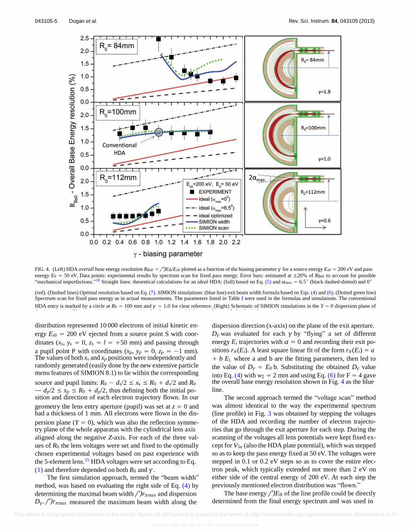
FIG. 3. Electron kinetic energy spectra showing the elastic scattering peak

from 200 eV electrons incident on a Helium target for R0 = 84 mm (left), R0

= 100 mm (middle), and R0 = 112 mm (right). The spectrometer was set to

pass electrons with a kinetic energy of E0 = 50 eV corresponding to 0 energy loss. The y-axis represents normalized counts.

ters. A base energy width of /')Es0 = 0.6 eV was associated with the gun as determined experimentally. The base energy

resolution of the analyzer /')EB = /')Eanal was then extracted after deconvolution of the gun resolution, using the relation

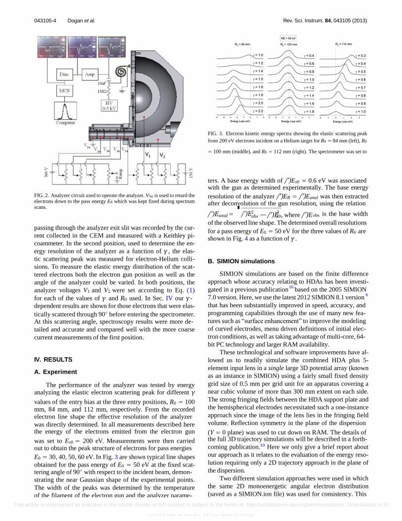
FIG. 2. Analyzer circuit used to operate the analyzer. V5a is used to retard the electrons down to the pass energy E0 which was kept fixed during spectrum scans. I

/')E2

2 — /')E , where /')E is the base width /')Eanal = obs obs s0

of the observed line shape. The determined overall resolutions passing through the analyzer exit slit was recorded by the cur-

rent collected in the CEM and measured with a Keithley pi-

coammeter. In the second position, used to determine the en-

ergy resolution of the analyzer as a function of γ , the elas-

tic scattering peak was measured for electron-Helium colli-

sions. To measure the elastic energy distribution of the scat-

tered electrons both the electron gun position as well as the

angle of the analyzer could be varied. In both positions, the

analyzer voltages V1 and V2 were set according to Eq. (1)

for each of the values of γ and R0 used. In Sec. IV our γ - dependent results are shown for those electrons that were elas-

tically scattered through 90◦ before entering the spectrometer. At this scattering angle, spectroscopy results were more de-

tailed and accurate and compared well with the more coarse

current measurements of the first position.

for a pass energy of E0 = 50 eV for the three values of R0 are shown in Fig. 4 as a function of γ .

B. SIMION simulations

SIMION simulations are based on the finite difference

approach whose accuracy relating to HDAs has been investi-

gated in a previous publication based on the 2005 SIMION

7.0 version. Here, we use the latest 2012 SIMION 8.1 version

that has been substantially improved in speed, accuracy, and

programming capabilities through the use of many new fea-

tures such as “surface enhancement” to improve the modeling

of curved electrodes, menu driven definitions of initial elec-

tron conditions, as well as taking advantage of multi-core, 64-

bit PC technology and larger RAM availability.

These technological and software improvements have al-

lowed us to readily simulate the combined HDA plus 5-

element input lens in a single large 3D potential array (known

as an instance in SIMION) using a fairly small fixed density

grid size of 0.5 mm per grid unit for an apparatus covering a

near cubic volume of more than 300 mm extent on each side.

The strong fringing fields between the HDA support plate and

the hemispherical electrodes necessitated such a one-instance

approach since the image of the lens lies in the fringing field

volume. Reflection symmetry in the plane of the dispersion

(Y = 0 plane) was used to cut down on RAM. The details of the full 3D trajectory simulations will be described in a forth-

coming publication.19 Here we only give a brief report about

our approach as it relates to the evaluation of the energy reso-

lution requiring only a 2D trajectory approach in the plane of

the dispersion.

Two different simulation approaches were used in which

the same 2D monoenergetic angular electron distribution

(saved as a SIMION.ion file) was used for consistency. This

16

6

IV. RESULTS

A. Experiment

The performance of the analyzer was tested by energy analyzing the elastic electron scattering peak for different γ

values of the entry bias at the three entry positions, R0 = 100 mm, 84 mm, and 112 mm, respectively. From the recorded electron line shape the effective resolution of the analyzer

was directly determined. In all measurements described here the energy of the electrons emitted from the electron gun

was set to Es0 = 200 eV. Measurements were then carried out to obtain the peak structure of electrons for pass energies

E0 = 30, 40, 50, 60 eV. In Fig. 3 are shown typical line shapes

obtained for the pass energy of E0 = 50 eV at the fixed scat- tering angle of 90◦ with respect to the incident beam, demon-

strating the near Gaussian shape of the experimental points.

The width of the peaks was determined by the temperature

of the filament of the electron gun and the analyzer parame-

This article is copyrighted as indicated in the article. Reuse of AIP content is subject to the terms at: http://scitationnew.aip.org/termsconditions. Downloaded to IP:

147.52.159.18 On: Fri, 17 Jan 2014 11:07:46

043105-5 Dogan et al. Rev. Sci. Instrum. 84, 043105 (2013)

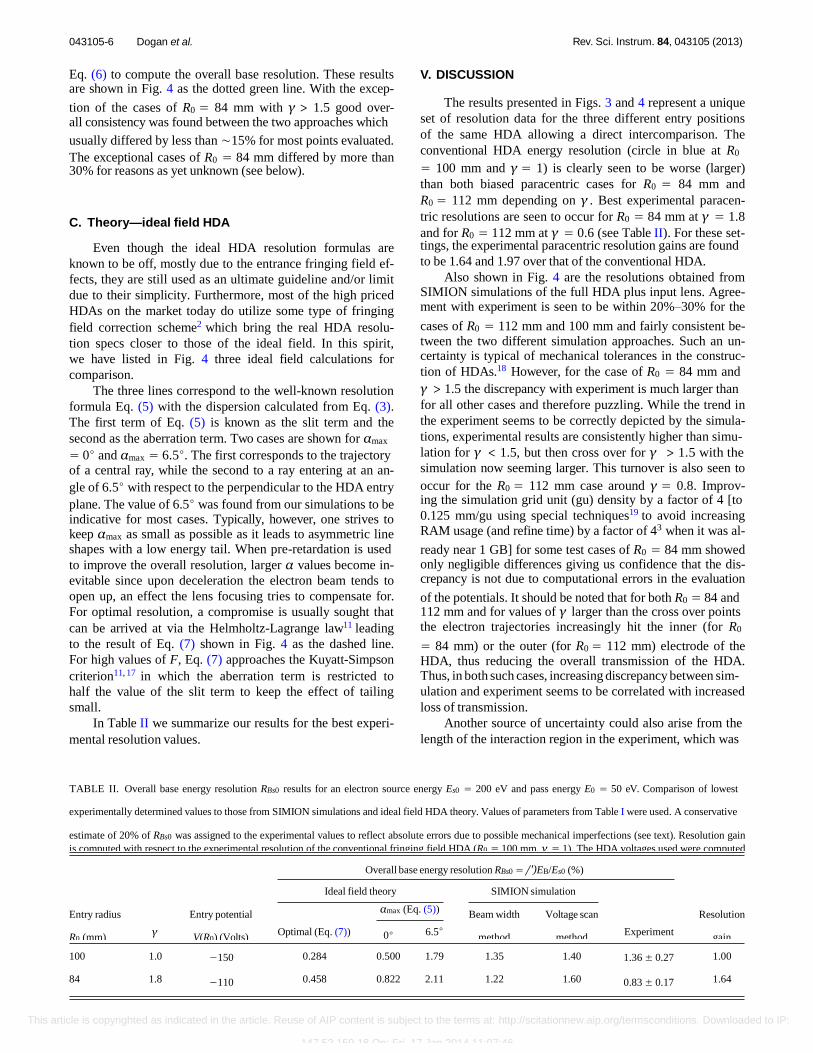
FIG. 4. (Left) HDA overall base energy resolution RBs0 = /')EB/Es0 plotted as a function of the biasing parameter γ for a source energy Es0 = 200 eV and pass

energy E0 = 50 eV. Data points: experimental results by spectrum scan for fixed pass energy. Error bars: estimated at ±20% of RBs0 to account for possible

“mechanical imperfections.”18 Straight lines: theoretical calculations for an ideal HDA: (full) based on Eq. (5) and αmax = 6.5◦ (black dashed-dotted) and 0◦

(red). (Dashed lines) Optimal resolution based on Eq. (7). SIMION simulations: (blue line) exit beam width formula based on Eqs. (4) and (6). (Dotted green line) Spectrum scan for fixed pass energy as in actual measurements. The parameters listed in Table I were used in the formulas and simulations. The conventional

HDA entry is marked by a circle at R0 = 100 mm and γ = 1.0 for clear reference. (Right) Schematic of SIMION simulations in the Y = 0 dispersion plane of the spectrometer. Electron trajectories are shown in red and equipotentials in green for specified values of γ .

distribution represented 10 000 electrons of initial kinetic en-

ergy Es0 = 200 eV ejected from a source point S with coor-

dinates (xs, ys = 0, zs = l = +50 mm) and passing through

a pupil point P with coordinates (xp, yp = 0, zp = −1 mm). The values of both xs and xp positions were independently and

randomly generated (easily done by the new extensive particle menu features of SIMION 8.1) to lie within the corresponding

source and pupil limits: R0 − ds/2 ≤ xs ≤ R0 + ds/2 and R0

— dp/2 ≤ xp ≤ R0 + dp/2, thus defining both the initial po- sition and direction of each electron trajectory flown. In our

geometry the lens entry aperture (pupil) was set at z = 0 and had a thickness of 1 mm. All electrons were flown in the dis-

persion plane (Y = 0), which was also the reflection symme- try plane of the whole apparatus with the cylindrical lens axis

aligned along the negative Z-axis. For each of the three val-

ues of R0 the lens voltages were set and fixed to the optimally

chosen experimental voltages based on past experience with

the 5-element lens.15 HDA voltages were set according to Eq.

(1) and therefore depended on both R0 and γ . The first simulation approach, termed the “beam width”

method, was based on evaluating the right side of Eq. (4) by

determining the maximal beam width /')rπ max and dispersion

dispersion direction (x-axis) on the plane of the exit aperture.

Dγ was evaluated for each γ by “flying” a set of different

energy Ei trajectories with α = 0 and recording their exit po-

sitions rπ (Ei). A least square linear fit of the form rπ (Ei) = a

+ b Ei, where a and b are the fitting parameters, then led to

the value of Dγ = E0 b. Substituting the obtained Dγ value

into Eq. (4) with w2 = 2 mm and using Eq. (6) for F = 4 gave the overall base energy resolution shown in Fig. 4 as the blue

line.

The second approach termed the “voltage scan” method

was almost identical to the way the experimental spectrum

(line profile) in Fig. 3 was obtained by stepping the voltages

of the HDA and recording the number of electron trajecto-

ries that go through the exit aperture for each step. During the

scanning of the voltages all lens potentials were kept fixed ex-

cept for V5a (also the HDA plate potential), which was stepped

so as to keep the pass energy fixed at 50 eV. The voltages were

stepped in 0.1 or 0.2 eV steps so as to cover the entire elec-

tron peak, which typically extended not more than 2 eV on

either side of the central energy of 200 eV. At each step the

previously mentioned electron distribution was “flown.”

The base energy /')EB of the line profile could be directly

determined from the final energy spectrum and was used in Dγ . /')rπ max measured the maximum beam width along the

This article is copyrighted as indicated in the article. Reuse of AIP content is subject to the terms at: http://scitationnew.aip.org/termsconditions. Downloaded to IP:

147.52.159.18 On: Fri, 17 Jan 2014 11:07:46

043105-6 Dogan et al. Rev. Sci. Instrum. 84, 043105 (2013)

Eq. (6) to compute the overall base resolution. These results are shown in Fig. 4 as the dotted green line. With the excep-

tion of the cases of R0 = 84 mm with γ > 1.5 good over- all consistency was found between the two approaches which

usually differed by less than ∼15% for most points evaluated.

The exceptional cases of R0 = 84 mm differed by more than 30% for reasons as yet unknown (see below).

V. DISCUSSION

The results presented in Figs. 3 and 4 represent a unique

set of resolution data for the three different entry positions

of the same HDA allowing a direct intercomparison. The

conventional HDA energy resolution (circle in blue at R0

= 100 mm and γ = 1) is clearly seen to be worse (larger)

than both biased paracentric cases for R0 = 84 mm and

R0 = 112 mm depending on γ . Best experimental paracen-

tric resolutions are seen to occur for R0 = 84 mm at γ = 1.8

and for R0 = 112 mm at γ = 0.6 (see Table II). For these set- tings, the experimental paracentric resolution gains are found

to be 1.64 and 1.97 over that of the conventional HDA.

Also shown in Fig. 4 are the resolutions obtained from SIMION simulations of the full HDA plus input lens. Agree- ment with experiment is seen to be within 20%–30% for the

cases of R0 = 112 mm and 100 mm and fairly consistent be- tween the two different simulation approaches. Such an un- certainty is typical of mechanical tolerances in the construc-

tion of HDAs.18 However, for the case of R0 = 84 mm and

C. Theory—ideal field HDA

Even though the ideal HDA resolution formulas are

known to be off, mostly due to the entrance fringing field ef-

fects, they are still used as an ultimate guideline and/or limit

due to their simplicity. Furthermore, most of the high priced

HDAs on the market today do utilize some type of fringing

field correction scheme2 which bring the real HDA resolu-

tion specs closer to those of the ideal field. In this spirit,

we have listed in Fig. 4 three ideal field calculations for

comparison.

The three lines correspond to the well-known resolution

formula Eq. (5) with the dispersion calculated from Eq. (3).

The first term of Eq. (5) is known as the slit term and the

second as the aberration term. Two cases are shown for αmax

= 0◦ and αmax = 6.5◦. The first corresponds to the trajectory of a central ray, while the second to a ray entering at an an-

gle of 6.5◦ with respect to the perpendicular to the HDA entry

plane. The value of 6.5◦ was found from our simulations to be indicative for most cases. Typically, however, one strives to keep αmax as small as possible as it leads to asymmetric line shapes with a low energy tail. When pre-retardation is used

to improve the overall resolution, larger α values become in-

evitable since upon deceleration the electron beam tends to

open up, an effect the lens focusing tries to compensate for.

For optimal resolution, a compromise is usually sought that

can be arrived at via the Helmholtz-Lagrange law11 leading

to the result of Eq. (7) shown in Fig. 4 as the dashed line.

For high values of F, Eq. (7) approaches the Kuyatt-Simpson

criterion11, 17 in which the aberration term is restricted to

half the value of the slit term to keep the effect of tailing

small.

In Table II we summarize our results for the best experi-

mental resolution values.

γ > 1.5 the discrepancy with experiment is much larger than

for all other cases and therefore puzzling. While the trend in

the experiment seems to be correctly depicted by the simula-

tions, experimental results are consistently higher than simu-

lation for γ < 1.5, but then cross over for γ > 1.5 with the

simulation now seeming larger. This turnover is also seen to

occur for the R0 = 112 mm case around γ = 0.8. Improv- ing the simulation grid unit (gu) density by a factor of 4 [to

0.125 mm/gu using special techniques19 to avoid increasing

RAM usage (and refine time) by a factor of 43 when it was al-

ready near 1 GB] for some test cases of R0 = 84 mm showed only negligible differences giving us confidence that the dis- crepancy is not due to computational errors in the evaluation

of the potentials. It should be noted that for both R0 = 84 and 112 mm and for values of γ larger than the cross over points the electron trajectories increasingly hit the inner (for R0

= 84 mm) or the outer (for R0 = 112 mm) electrode of the HDA, thus reducing the overall transmission of the HDA. Thus, in both such cases, increasing discrepancy between sim-

ulation and experiment seems to be correlated with increased

loss of transmission.

Another source of uncertainty could also arise from the

length of the interaction region in the experiment, which was

TABLE II. Overall base energy resolution RBs0 results for an electron source energy Es0 = 200 eV and pass energy E0 = 50 eV. Comparison of lowest

experimentally determined values to those from SIMION simulations and ideal field HDA theory. Values of parameters from Table I were used. A conservative

estimate of 20% of RBs0 was assigned to the experimental values to reflect absolute errors due to possible mechanical imperfections (see text). Resolution gain

is computed with respect to the experimental resolution of the conventional fringing field HDA (R0 = 100 mm, γ = 1). The HDA voltages used were computed

from Eq. (1). Lens voltages used were fixed at V1a = 0, V2a = 114.0 V, V3a = −104.7 V, V4a = 144.0 V. Overall base energy resolution RBs0 = /')EB/Es0 (%)

Ideal field theory SIMION simulation

αmax (Eq. (5)) Entry radius

R0 (mm)

Entry potential

V(R0) (Volts)

Beam width

method

Voltage scan

method

Resolution

gain γ Optimal (Eq. (7)) 0◦ 6.5◦ Experiment

100

84

112

1.0

1.8

0.60

−150

−110

−170

0.284

0.458

0.184

0.500

0.822

0.314

1.79

2.11

1.60

1.35

1.22

0.47

1.40

1.60

0.50

1.36 ± 0.27

0.83 ± 0.17

0.69 ± 0.14

1.00

1.64

1.97

This article is copyrighted as indicated in the article. Reuse of AIP content is subject to the terms at: http://scitationnew.aip.org/termsconditions. Downloaded to IP:

147.52.159.18 On: Fri, 17 Jan 2014 11:07:46

043105-7 Dogan et al. Rev. Sci. Instrum. 84, 043105 (2013)

estimated to be between 1–2 mm, which is imaged by the lens onto the entry of the HDA. In all simulations a line source

of ds = 2 mm length along the X-direction (dispersion direc- tion) was used giving the best agreement with experimental results. In the past, when only the HDA (without the lens)

was simulated, our source always lay within the entry slit of

the HDA and results depended sensitively on its extent. Large

resolution gains of up to 34 were reported4 for a point source

and 4.2 for a 1 mm source, respectively. Here, it is the size of

the image of the original object at the collision region as con-

trolled by the lens magnification that lies within the entry slit.

While the lens voltages were set according to best working ex-

perience with this lens, a full search for the optimal voltages

giving the best resolution was not performed. Such a search

can be readily carried out in simulation and could yield still

further improvements in the ultimate experimental resolution

gains of the paracentric HDAs.

and lowers the overall cost of construction and HV power

supplies. Improvement in energy resolution also means that

paracentric HDAs of smaller size and therefore weight could

replace larger conventional HDAs of equal resolution, partic-

ularly attractive to outer space instrumentation applications

where both size and weight are invaluable. Finally, not having

to introduce cumbersome additional correction electrodes that

could partly block transmission, especially when used with a

position sensitive detector, is clearly a big advantage.

ACKNOWLEDGMENTS

This work was supported on the Turkish side by the

Scientific and Technological Research Council of Turkey

(TUBITAK), through Grant Nos. 106T722 and 109T738. On

the Greek side this research has been cofinanced by the Eu-

ropean Union (European Social Fund—ESF) and Greek na-

tional funds through the Operational Program “Education

and Lifelong Learning” of the National Strategic Reference

Framework (NSRF)—Research Funding Program: THALES.

Investing in knowledge society through the European So-

cial Fund (Grant No. MIS 377289). We are also grateful to

the Turkish Patent Institute for funding this work (Registra-

tion No: 2009 08700). The authors thank Dr. Omer Sise for

his contribution to the initial stages of this investigation and

Ahmet Deniz for his help with the technical drawings of the

variable entry analyzer. Theo Zouros would also like to thank

David Manura of SIS for critically reading the manuscript,

as well as for his help with various SIMION 8.1 issues and

Lua programming and Professor Kai Rossnagel of the Uni-

versity of Kiel for useful conversations. Finally, we thank

Professor Genoveva Martínez López for critically reading the

manuscript.

VI. SUMMARY AND CONCLUSION

In this paper we present, for the first time, direct exper-

imental evidence showing the energy resolution of a biased

paracentric HDA to be at least a factor of 1.7–2 times bet-

ter than the resolution of a conventional HDA, in support of

predictions based on previous simulation work. This experi-

mental finding is also in agreement with new simulations pre-

sented here which for the first time treat the more realistic case

of a HDA with input lens under pre-retardation conditions.

The biased paracentric HDA differs from a conventional

HDA in two important ways: (a) the HDA entry distance

R0 is paracentric, i.e., either larger or smaller than the mean

HDA radius used in a conventional HDA and (b) the two

hemispherical electrode voltages are set so that the entry po-

tential V(R0) of the HDA is non-zero (biased), as opposed

to conventional HDA usage in which this bias is typically

zero. For very particular values of R0 and V(R0), empirically

found through simulations, we have shown2 in the past that

substantial improvements in energy resolution can be made,

practically restoring first-order focusing conditions without

the use of any additional fringing field correction electrodes,

as typically done for conventional HDAs.

The above experimental validation was accomplished by a specially designed HDA with a five-element input lens for

which the entry position radius R0 (i.e., the position of the HDA entry aperture) could be readily moved and placed at

any position between R1 = 75 mm and R2 = 125 mm, the

two radii of the HDA. Thus, we experimentally determined

the overall base energy resolution of this HDA for entries R0

= 84, 100, 112 mm presenting results for the case of pre-

retardation factor of F = 4 for various values of the bias V(R0) allowing for their direct inter-comparison on the same setup.

The measured improvement in energy resolution is par-

ticularly remarkable as it is conveniently attained without the

use of any type of additional fringing field correction elec-

trodes, but simply by taking advantage of the strong intrin-

sic lensing properties of the existing HDA fringing fields as

determined and optimized by the particular paracentric entry

position and bias control. Clearly, the use of fewer electrodes

in the paracentric design reduces its operational complexity

1T. J. M. Zouros and E. P. Benis, J. Electron Spectrosc. Relat. Phenom. 125,

221–248 (2002); “Erratum,” 142, 175 (2005).

2O. Sise, T. J. M. Zouros, M. Ulu, and M. Dogan, Meas. Sci. Technol. 18,

1853–1858 (2007).

3E. P. Benis and T. J. M. Zouros, Nucl. Instrum. Methods Phys. Res. A 440,

462–465 (2000).

4T. J. M. Zouros, O. Sise, M. Ulu, and M. Dogan, Meas. Sci. Technol. 17,

N81–N86 (2006).

5O. Sise, G. Martinez, T. J. M. Zouros, M. Ulu, and M. Dogan, J. Electron Spectrosc. Relat. Phenom. 177, 42–51 (2010); predictions of optimal para-

centric conditions were found to lie at R0 = 85 mm, γ = 1.435, and R0

= 115 mm, γ = 0.672 for a HDA with R1 = 75 mm and R2 = 125

mm. Here the constructed HDA has the same electrode radii, but the

entry positions could only be approximately set at R0 = 84 mm and 112 mm.

6SIMION version 8.1.1.29, 12/29/2012, Scientific Instrument Services, Inc.,

Ringoes, NJ, see http://www.simion.com.

7E. P. Benis and T. J. M. Zouros, J. Electron Spectrosc. Relat. Phenom. 163,

28–39 (2008). In this reference as well as in Ref. 1, two angles α are de-

fined: α*, the input half-angle prior to refraction by the lens/HDA interface

and α the half-angle after refraction. The two are related by α = α∗/√

γ

via Snell’s law and/or the Helmholtz-Lagrange theorem.8–11 Here, to avoid

cumbersome notation, we just use the symbol α for what in Refs. 1 and 7

was symbolized by α*.

8Volker Schmidt, Electron Spectrometry of Atoms Using Synchrotron Radi-

ation (Cambridge University Press, 1997) (see Eq. (4.7a)).

9M. Yavor, “Optics of Charged Particle Analyzers: Chapter 6. Electrostatic

energy analyzers,” in Advances in Imaging and Electron Physics (Aca-

demic, 2009), Vol. 157, pp. 213–258.

10E. H. A. Granneman and M. J. Van der Wiel, “Transport, dispersion and

This article is copyrighted as indicated in the article. Reuse of AIP content is subject to the terms at: http://scitationnew.aip.org/termsconditions. Downloaded to IP:

147.52.159.18 On: Fri, 17 Jan 2014 11:07:46

043105-8 Dogan et al. Rev. Sci. Instrum. 84, 043105 (2013)

15M. Dogan and A. Crowe, J. Phys. B 35, 2773–2781 (2002).

16T. J. M. Zouros, Omer Sise, F. M. Spiegelhalder, and David J. Manura, Int.

J. Mass Spectrom. 261, 115–133 (2007).

17C. E. Kuyatt and J. A. Simpson, Rev. Sci. Instrum. 38, 103–111 (1967).

18B. Wannberg, Nucl. Instrum. Methods Phys. Res. A 239, 269–272 (1985). 19G. G. Gennarakis et al., “Energy resolution of a paracentric hemispheri-

cal deflector analyzer for different entry positions and bias: Detailed Mea-

surements and 3D Simulation,” J. Electr. Spectr. Rel. Phenom. (to be pub-

lished).

Radiation, edited by E. E. Koch (North Holland, Amsterdam, 1983), Vol.

1A, Chap. 6, pp. 367–456.

11T. J. M. Zouros and E. P. Benis, Appl. Phys. Lett. 86, 094105 (2005).

12T. J. M. Zouros, E. P. Benis, and I. Chatzakis, Nucl. Instrum. Methods Phys.

Res. B 235, 535–539 (2005).

13M. Dogan, M. Ulu, and O. Sise, J. Electron Spectrosc. Relat. Phenom. 161,

58–62 (2007).

14M. Dogan, A. Crowe, K. Bartschat, and P. J. Marchalant, J. Phys. B 31,

1611–1624 (1998).

This article is copyrighted as indicated in the article. Reuse of AIP content is subject to the terms at: http://scitationnew.aip.org/termsconditions. Downloaded to IP:

147.52.159.18 On: Fri, 17 Jan 2014 11:07:46