Embed Size (px)
Citation preview

UNIVERSITY OF CINCINNATI
_____________ , 20 _____
I,______________________________________________,hereby submit this as part of the requirements for thedegree of:
________________________________________________
in:
________________________________________________
It is entitled:
________________________________________________
________________________________________________
________________________________________________
________________________________________________
Approved by:________________________________________________________________________________________________________________________

Obstacle Avoidance using Laser Scanner for Bearcat III
A thesis submitted to the
Division of Graduate studies and Research
of the University of Cincinnati
in partial fulfillment of the
requirements for the degree of
Master of Science
in the Department of Mechanical, Industrial and Nuclear Engineering
of the College of Engineering
2001
by
Mayank Saxena
B.E (Mechanical Engineering)
M.R.E.C., Jaipur
Rajasthan University, India, 1999.
Thesis Advisor and Committee Chair: Dr. Ernest L. Hall

Abstract
One of the major challenges in designing intelligent vehicles capable of
autonomous travel on highways is reliable obstacle detection. Obstacle avoidance is one
of the key problems in computer vision and mobile robotics. There has been a great
amount of research devoted to the obstacle detection problem for mobile robot platforms
and intelligent vehicles. Any mobile robot that must reliably operate in an unknown or
dynamic environment must be able to perform obstacle detection. As road following
systems have become more capable, more attention has been focused on obstacle
detection problem, much of it driven by programs such as the Automated Highway
System or PROMETHEUS which seek to revolutionize automobile transportation,
providing consumers with a combination of “smart” cars and smart roads. Laser scanners
have been used for many years for obstacle detection and are found to be the most
reliable and provide accurate results. They operate by sweeping a laser beam across a
scene and at each angle, measuring the range and returned intensity.
The Center for Robotics Research at the University of Cincinnati has built an unmanned,
autonomous guided vehicle (AGV), named Bearcat III for the International Ground Robotics Competition
conducted each year by the Association for Unmanned Vehicle Systems (AUVS). We were using ultrasonic
transducers last year on Bearcat II to detect and avoid unexpected obstacles, which did not provide us with
accurate data. This year there is an enhancement in obstacle avoidance system using a laser scanner. The
vehicle senses its location and orientation using the integrated vision system and a high-performance laser
scanner is used for obstacle detection system of Bearcat III. It provides fast single- line laser scans and is
used to map the location and size of possible obstacles. With these inputs the fuzzy logic controls the
steering speed and steering decisions of the robot on an obstacle course 10 feet wide bounded by
white/yellow/dashed lines.

The goal of this research was to implement a laser scanner on the U.C. robot Bearcat III to detect
and avoid obstacles in its environment. I performed obstacle detection experiments both indoors and
outdoors. Each experiment consisted of 180° field of view of the laser scanner with a 0.5° resolution. The
scans were made using a scan-oriented approach rather than a pixel oriented approach because of the faster
refresh rate and with the laser scanner giving us a clear field of view of the coordinates of every point along
x and y-axis, obstacles were detected and avoided accurately.

Acknowledgements
I would like to thank my advisor Dr. Ernest Hall without whose guidance and
support this thesis would not have been possible. His suggestions and feedback had
greatly helped me in my thesis. He helped and encouraged me from all perspectives to
complete this work.
I would like to thank Dr. Richard L. Shell and Dr. Ronald L. Huston for agreeing
to chair the committee. I would also like to thank them for their suggestions and positive
feedbacks.
I would like to thank the Robotics Team members for all the help and support
they had given me during my graduate period of study at the University Of Cincinnati. I
would like to thank all my friends and well-wishers who had helped me from time to
time.
Last but not the least, I would like to thank my family for their encouragement
and support in all my endeavors. I owe all my success to them.
1
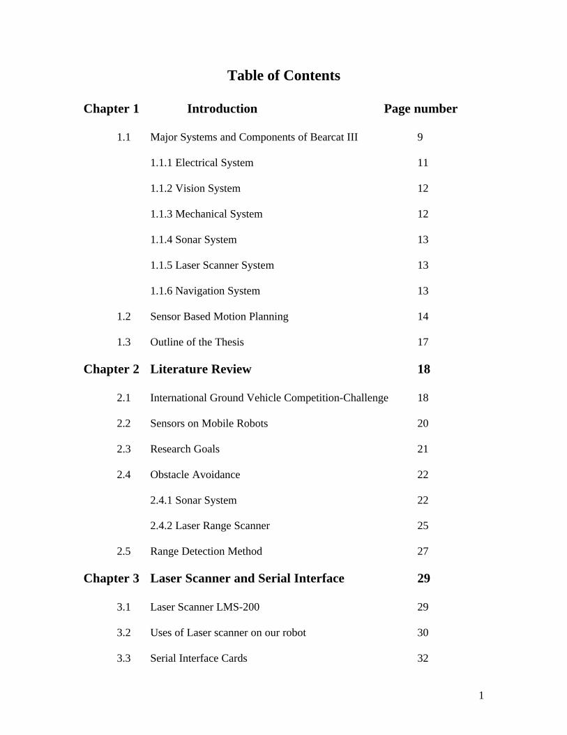
Table of Contents
Chapter 1 Introduction Page number
1.1 Major Systems and Components of Bearcat III 9
1.1.1 Electrical System 11
1.1.2 Vision System 12
1.1.3 Mechanical System 12
1.1.4 Sonar System 13
1.1.5 Laser Scanner System 13
1.1.6 Navigation System 13
1.2 Sensor Based Motion Planning 14
1.3 Outline of the Thesis 17
Chapter 2 Literature Review 18
2.1 International Ground Vehicle Competition-Challenge 18
2.2 Sensors on Mobile Robots 20
2.3 Research Goals 21
2.4 Obstacle Avoidance 22
2.4.1 Sonar System 22
2.4.2 Laser Range Scanner 25
2.5 Range Detection Method 27
Chapter 3 Laser Scanner and Serial Interface 29
3.1 Laser Scanner LMS-200 29
3.2 Uses of Laser scanner on our robot 30
3.3 Serial Interface Cards 32

2
3.3.1 RS-232 34
3.3.2 RS-422 35
3.3.3 RS-485 35
3.4 Using the Laser Scanner 36
Chapter 4 Experimental Design 38
4.1 Theory of Laser Scanner LMS-200 38
4.2 Performance of the Laser Scanner 42
4.3 Algorithm used for obstacle avoidance 46
Chapter 5 Experimental Results 55
5.1 Obstacle Detection and Range Estimation Results 55
5.1.1 Indoor Experiments 55
5.1.2 Outdoor Testing 61
5.2 Programming the laser scanner in MS-DOS 63
5.2.1 Accessing MS DOS operating system facilities 63
5.2.2 Using the RS-422 serial port via MS-DOS 65
Chapter 6 Conclusion and Future Work 67
3
List of Figures
Chapter 1 Page Number
1.1 Schematic diagram of Bearcat III design 10
1.2 Testing Bearcat III in Campus green 11
1.3 Relationship between various sub-tasks of Navigation 14
1.4 Path Planning with complete information 15
1.5 Path Planning with incomplete information 16
Chapter 2
2.1 Obstacle course for Bearcat III 19
2.2 Bearcat III and its associated sensors 21
2.3 Undetected large object due to reflection 24
2.4 Range errors due to angle between object and sonar 25
2.5 Field of view of the Laser Scanner 28
Chapter 3
3.1 Monitored fields and corresponding switching outputs 30
3.2 LMS in stand-alone operation 31
Chapter 4
4.1 Step-by-step procedures for using the laser scanner 41
4.2 Converting Fields 42
4.3 Request measured values 43
4.4 Logging communications 44

4
4.5 All measured values shown on the screen 46
4.6 Obstacle on the right of the robot with clearance 47
4.7 Obstacle on the right of the robot with no clearance 49
4.8 Obstacle avoidance by turning an angle α 50
4.9 Obstacle on the left of the robot with clearance 51
4.10 Obstacle in the center of the track 53
4.11 Triangle showing the angles robot will turn 54
Chapter 5
5.1 Picture of the corridor 56
5.2 Screen Shot of the corridor 57
5.3 View of the laser scanner in real world 57
5.4 Screen shot with two chairs in the Field of View 58
5.5 Obstacle in the path of the robot 59
5.6 Screen shot of the obstacle 59
5.7 Monitor’s view 60
5.8 Close view of the monitor 61
5.9 Outdoor testing of the robot 62
5.10 Screen shot of the laser scanner 62
5.11 Measured values on the screen 63
5
Chapter 1. Introduction
The present day requirement for ever-increasing reliability is now more important
than ever before and continues to grow constantly. Advances are continually being made
in engineering. This means that the detection, location and analysis of faults play a vital
role. The need to have efficiency and safety in the design and development of Automated
Guided Vehicle (AGV) leads to the development of diagnostic strategies that could cover
the major potential faults of the AGV. Following several decades of intense research in
automated vehicle guidance, we are now witnessing market introduction of driver
assistance functions into standard passenger cars. Most of these functions are based on
inertial sensors, i.e. sensors measuring the status of the vehicle itself.
A hi-tech product like a robot needs a sophisticated system for analyzing the
failures, storing the related information in an integrated repository and retrieving the
same via standard user-friendly interface. The Center for Robotics Research at University
of Cincinnati has been developing Robot for the past 13 years. The Bearcat robot of UC
Robotics team has undergone two major versions till now. The latest version called
Bearcat III is an Autonomous Guided Vehicle. Fault diagnosis system provides a
systematic review of the components, assemblies and subsystems of a product to identify
single point failures and the causes and effects of such failures. It identifies and tabulates
the potential modes by which equipment or a system might fail and the consequences
such a failure would have on the equipment or system being studied.
The main focus of this thesis is on the sensor concept developed for the
autonomous system of our Bearcat III robot using a laser scanner and on the realization

6
thereof. Reliable detection and tracking of obstacles is a crucial issue for automated
vehicle guidance functions. The main task of the sensors is twofold, namely lane
recognition and obstacle detection and tracking. The lane recognition is done by the two
cameras attached to the ISCAN tracker of the Bearcat III robot while the obstacle
detection and tracking is done using the laser scanner or ultrasonic transducers. The
sensors use fairly simple temporal differencing techniques to find objects since it is
monitoring a constant area. Sensor placement is more flexible depending on the particular
sensor it could be placed very close to the ground or far above it to avoid occlusions,
whichever works best for the particular sensor. The information provided by the sensors
enables the control unit to keep the vehicle on the track and to avoid collision with the
obstacles.
1.1 Major systems and components of Bearcat III
According to the functionality Bearcat III has been categorized into the following
major units [1] as -
a. Electrical System
b. Vision System
c. Mechanical System
d. Sonar system
e. Laser scanner system
f. Navigation system
The system description of Bearcat III by grouping the components into major units is
given in the following paragraphs. For efficient operation of the robot not only should the
individual subsystems work satisfactorily but they also should work in tandem.
7
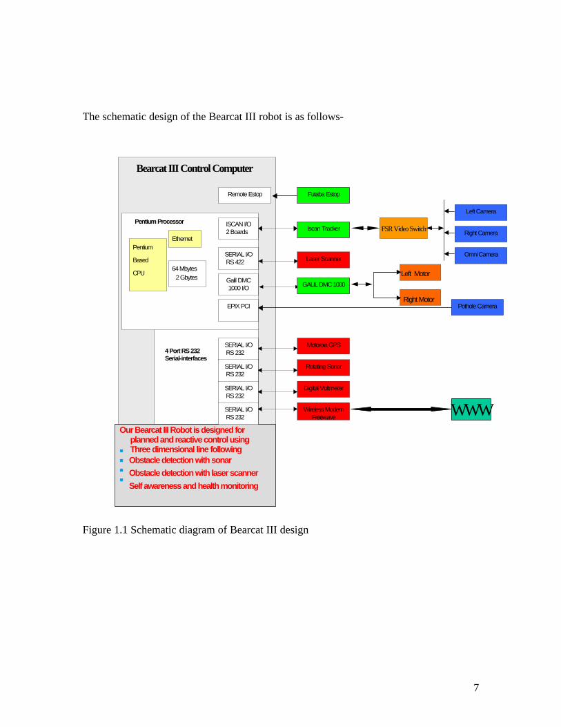
The schematic design of the Bearcat III robot is as follows-
Pentium Processor
Pentium
Based
CPU 64 Mbytes
2 Gbytes
Ethernet
4 Port RS 232Serial-interfaces
Bearcat III Control Computer
Left Motor
Right Motor
Assembled In Phase I Usingn
n Planet’s ATV Control Processorn UC’s PerceptorProcessor Architecturen Draper’s Vehicle Control Unit
Our Bearcat III Robot is designed forplanned and reactive control using
n Three dimensional line followingn Obstacle detection with sonarn Obstacle detection with laser scannern
Self awareness and health monitoring
Futaba Estop
FSR Video SwitchIscan Tracker
Laser Scanner
GALIL DMC 1000
Motorola GPS
Rotating Sonar
Digital Voltmeter
Wireless Modem Freewave
WWW
Left Camera
Right Camera
Omni Camera
Pothole Camera
Remote Estop
SERIAL I/ORS 422
ISCAN I/O2 Boards
Galil DMC 1000 I/O
EPIX PCI
SERIAL I/ORS 232
SERIAL I/ORS 232
SERIAL I/ORS 232
SERIAL I/ORS 232
Figure 1.1 Schematic diagram of Bearcat III design

8
Figure 1.2 Testing Bearcat III in Campus green 1.1.1 Electrical System
The electrical system of Bearcat III consists of a DC power system and an AC
power system. Both these systems derive power from three 12-volt DC 130 amp hour
deep cycle batteries connected in series. A 36-volt DC 600-watt power inverter provides
60 Hz pure sine wave output at 115 volts. The inverter supplies AC electrical power for
all AC systems including the main computer, cameras, and auxiliary regulated DC power
supplies. The heart of the power system being the solenoid acts as a switch, which can be
controlled to cut off the power during emergency.
9
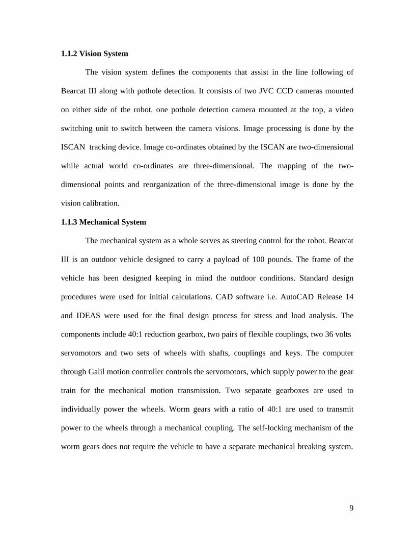
1.1.2 Vision System
The vision system defines the components that assist in the line following of
Bearcat III along with pothole detection. It consists of two JVC CCD cameras mounted
on either side of the robot, one pothole detection camera mounted at the top, a video
switching unit to switch between the camera visions. Image processing is done by the
ISCAN tracking device. Image co-ordinates obtained by the ISCAN are two-dimensional
while actual world co-ordinates are three-dimensional. The mapping of the two-
dimensional points and reorganization of the three-dimensional image is done by the
vision calibration.
1.1.3 Mechanical System
The mechanical system as a whole serves as steering control for the robot. Bearcat
III is an outdoor vehicle designed to carry a payload of 100 pounds. The frame of the
vehicle has been designed keeping in mind the outdoor conditions. Standard design
procedures were used for initial calculations. CAD software i.e. AutoCAD Release 14
and IDEAS were used for the final design process for stress and load analysis. The
components include 40:1 reduction gearbox, two pairs of flexible couplings, two 36 volts
servomotors and two sets of wheels with shafts, couplings and keys. The computer
through Galil motion controller controls the servomotors, which supply power to the gear
train for the mechanical motion transmission. Two separate gearboxes are used to
individually power the wheels. Worm gears with a ratio of 40:1 are used to transmit
power to the wheels through a mechanical coupling. The self-locking mechanism of the
worm gears does not require the vehicle to have a separate mechanical breaking system.

10
Power is transmitted to the front wheels. The rear wheel is a castor wheel and this gives
the Bearcat a zero turning radius.
1.1.4 Sonar System
Apart from the vision system for line tracking the sonar system is used for
obstacle avoidance. It is powered by a 12 Volts DC, 0.5 Amps power unit. The two main
components of the ultrasonic ranging system are the transducers and the drive electronics.
The rotating sonar mounted in front of the robot senses the position and size of obstacles
and the measured values are used to navigate the robot around them.
1.1.5 Laser Scanner System
This year the Laser scanner LMS-200 has been the greatest enhancement in the
obstacle avoidance system on our Bearcat for sensing obstacles in the path. LMS 200 is a
non-contact measurement system that scans its surroundings two dimensionally. LMS
works by measuring the time of flight of laser light pulses. The pulsed laser beam is
deflected by an internal rotating mirror so that a fan shaped scan is made of the
surrounding area. The shape of the object is determined by the sequence of impulses
received. Scanner’s measurement data can be individually processed in real time with
external evaluation software. Standard solutions are also available for object
measurement. The unit communicates with the central computer using a RS422 Serial
interface card. The central controller houses the logic for the obstacle avoidance and the
interface between the line following and the motion control program.
1.1.6 Navigation System
Global navigation is the ability to determine one’s position in absolute or map-
referenced terms and to move to a desired destination point. This year we are using a new
Motorola GPS to navigate from one point to the other. The GPS tracks the NAVSTAR
11
GPS constellation of satellites. The satellite signals received by an active antenna are
tracked with 12 parallel channels of L1. C/A code is then down converted to an IF
frequency and digitally processed to obtain a full navigation solution of position,
velocity, time and heading. The solution is then sent over the serial link via the 10-pin
connector.
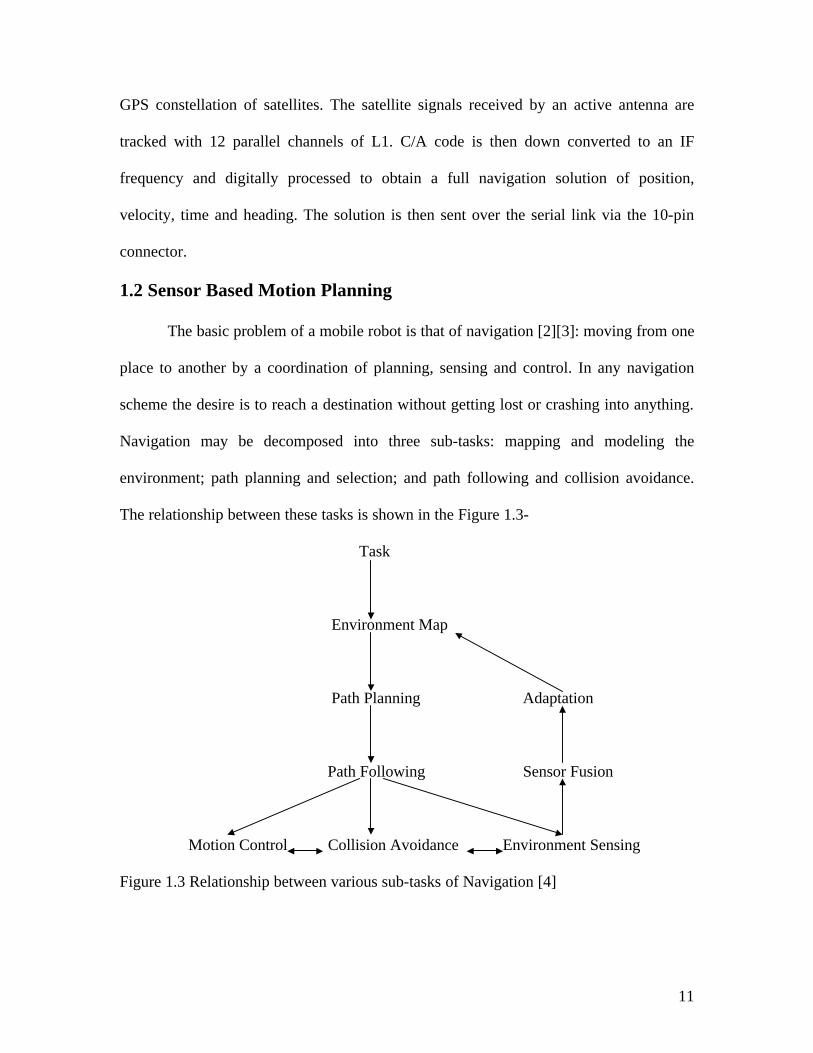
1.2 Sensor Based Motion Planning
The basic problem of a mobile robot is that of navigation [2][3]: moving from one
place to another by a coordination of planning, sensing and control. In any navigation
scheme the desire is to reach a destination without getting lost or crashing into anything.
Navigation may be decomposed into three sub-tasks: mapping and modeling the
environment; path planning and selection; and path following and collision avoidance.
The relationship between these tasks is shown in the Figure 1.3-
Task
Environment Map
Path Planning Adaptation
Path Following Sensor Fusion
Motion Control Collision Avoidance Environment Sensing
Figure 1.3 Relationship between various sub-tasks of Navigation [4]
12
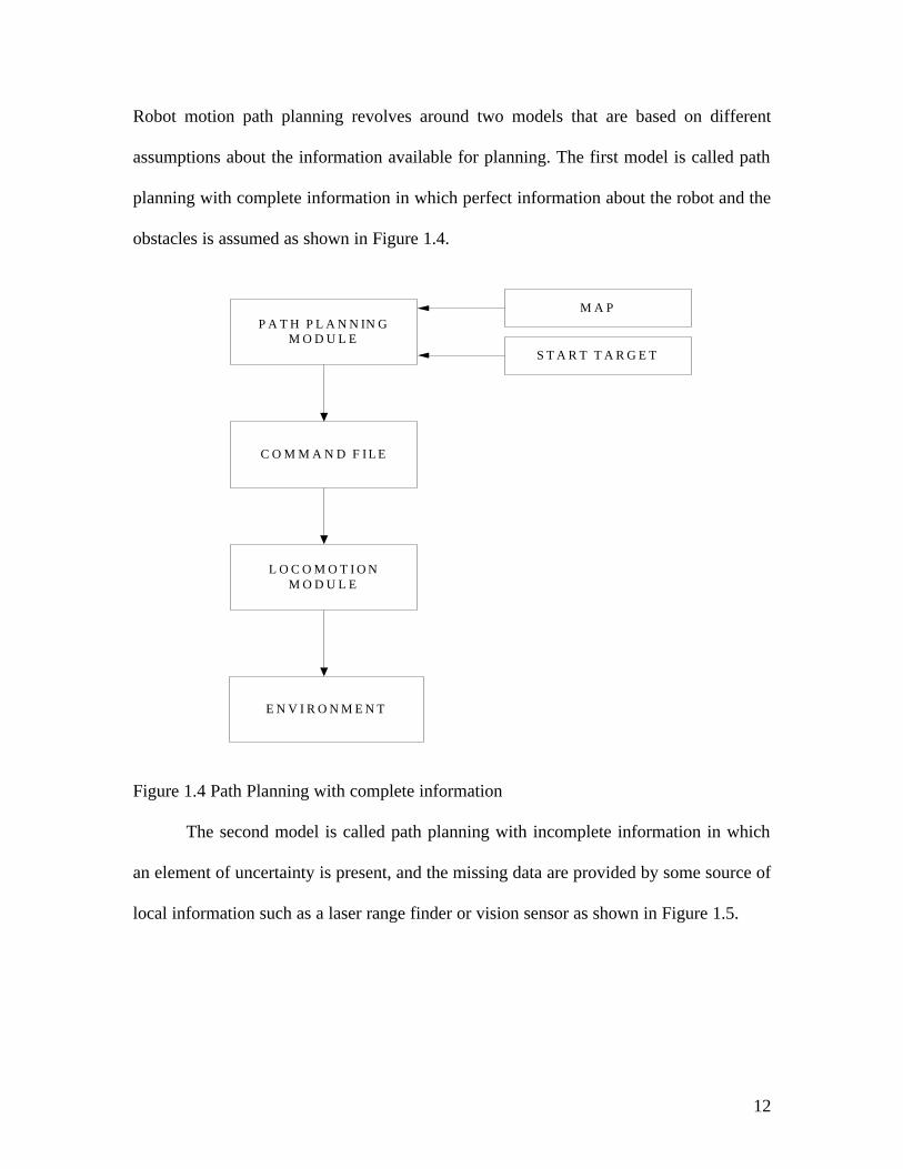
Robot motion path planning revolves around two models that are based on different
assumptions about the information available for planning. The first model is called path
planning with complete information in which perfect information about the robot and the
obstacles is assumed as shown in Figure 1.4.
P A T H P L A N N IN GM O D U L E
C O M M A N D F I L E
L O C O M O T I O NM O D U L E
E N V I R O N M E N T
M A P
S T A R T T A R G E T
Figure 1.4 Path Planning with complete information
The second model is called path planning with incomplete information in which
an element of uncertainty is present, and the missing data are provided by some source of
local information such as a laser range finder or vision sensor as shown in Figure 1.5.

13
REACTIVE PLANNINGMODULE
COMMAND FILE
LOCOMOTIONMODULE
ENVIRONMENT
SENSOR
START TARGET
Figure 1.5 Path Planning with incomplete information
During the navigation of our robot on an obstacle course, which is 10 ft. wide, there
exists the danger that it collides with a dynamic or unmodelled obstacle. The robot under
this model transforms the operation of motion planning into a continuous dynamic
process from sensor feedback. Two methods have been implemented in order to prevent
the robots from running into such obstacles. Previously ultrasonic transducers were used
and this year we are using laser scanners to detect the obstacles around the robot.

14
Under this approach, sensing becomes an active process; the robot decides at each step of
its path what sensory information [9][10] is required for generating its next step. The
laser range sensor provides the robot with coordinates of those points of obstacle
boundaries that lie within a limited radius of vision around the robot. In our laser range
sensor the radius of vision is 8m or above. So, if there is an obstacle present in this range,
our robot changes its path according to the data it receives from the scanner.
1.3 Outline of the Thesis
The research work is organized into five chapters. Chapter 1 presents the
introduction to the topic. Chapter 2 discusses the existing literature on the topic of
obstacle avoidance. Chapter 3 describes the software and hardware for the laser scanner
and how it is interfaced. Chapter 4 presents theory and performance of the laser scanner
with the help of flowcharts. Chapter 5 gives the experimental results and finally Chapter
6 concludes the thesis with some recommendations and areas of improvement for the
future.

15
Chapter 2
Literature Review 2.1 International Ground Vehicle Competition –Challenge
A hi-tech product like a robot needs a sophisticated system for analyzing the
failures, storing the related information in an integrated repository and retrieving the
same via standard user-friendly interface. The Center for Robotics Research at University
of Cincinnati has been developing robots for the past 13 years. The Bearcat robot of UC
Robotics team [5][6] has undergone three major versions till now. The latest version
called Bearcat III is an Autonomous Guided Vehicle. The Cincinnati Center for Robotics
Research at the University of Cincinnati has been a participant in the AUVS (Association
for Unmanned Vehicle Systems) competition for the last 8 years. The University of
Cincinnati has so far used two versions of their AGV’s (Automated Guided Vehicles).
Bearcat I was the first robot weighing approximately 600 lbs., and it was 4 feet wide and
6 feet long. In the 1997 competition, the track was 10 feet wide. This meant that the space
left for maneuvering was 3 feet on either side of the robot. The increasing difficult
competition rules made it necessary to build a new AGV. This resulted in the creation of
the Bearcat II robot. In 1998 the UC Robot Team developed a new design for a mobile
robot. The most outstanding feature of the design was that the entire structure was
designed, built and assembled by the student team within the UC lab. Most of the
components were ordered from different vendors with the bulk of the body structure
coming from the 80/20 extruded aluminum components, which were made to order.
The International ground vehicle competition is held each year by the AUVS. The
competition is such that a fully autonomous ground robotic vehicle must negotiate around

16
an outdoor obstacle course under a prescribed time while staying within the 5 mph speed
limit, and avoiding the obstacles on the track. Unmanned, autonomous vehicles must
compete based on their ability to perceive the course environment and avoid obstacles. A
remote human operator cannot control them during competition. All computational
power, sensing and control equipment must be carried on board the vehicle. The course is
out on grass, pavement, simulated pavement, or any combination, over an area of
approximately 60 to 80 yards long, by 40 to 60 yards wide. The path of robot travel is
marked by solid white lines (which can be dashed at certain regions). Sometimes the lines
may get obscure or change color from white to green. The road direction may change but
the width of the road is always approximately 10 feet.
Figure 2.1 Obstacle course for Bearcat III
The obstacles are positioned on the track in such a way that they block the path of
the robot. It is expected that there is always enough clearance that the robot can pass

17
these obstacles without touching them or knocking them down. These obstacles may vary
from 5 gallon buckets; construction barrels (aligned at an angle to the track) or it can be a
sand trap and also a ramp (inclined at 10 percent or about 8 degrees). In short, the robot
must be able to follow the changing track while avoiding obstacles at the same time. In
order for this to happen, the robot must be designed in such a way that it can sense and
deal with the issue of uncertainty and incomplete information about the environment in a
reasonably short duration of time.
2.2 Sensors on Mobile Robots
Robots require a wide range of sensors to obtain information about the world
around them. There are many different sensors used to detect the position, velocity, and
range to an object in the robots workspace. One of the most common range finding
methods uses ultrasonic transducers. Vision systems are also used to greatly improve the
robot’s versatility, speed, and accuracy for its complex tasks.
Ultrasonic transducers, or sonar, are frequently used for many automated guided
vehicles (AGV) as a primary means to detect obstacles and avoid them, operating within
appropriate boundaries. W.S. H. Munro, S. Pomeroy, M. Rafiq, H.R. Williams, M.D.
Wybrow and C. Wykes [7] developed a vehicle guidance system using ultrasonic sensing.
The ultrasonic unit is based on electrostatic transducers and comprises a separate linear
array and curved divergent transmitter, which gives it an effective field of view of 60°
and a range of more than 5 meters. Vision systems provide information that is difficult or
impossible to obtain in other ways. They give a clearer idea about the position of the
object, the size of the object, and the kind of object. The Laser range scanner can produce
both a two-dimensional reflectance and a three-dimensional range image. Bearcat III at

18
University of Cincinnati produces a two-dimensional floor map by integrating knowledge
obtained from several range images acquired as the robot moves around in its attempt to
find a path to the goal position. Using a scanning laser range finder, Moring et al. [8]
were able to construct a three-dimensional range image of the robot’s world.
2.3 Research Goals
The goal of this research was to implement a laser scanner on the U.C. robot
Bearcat III to detect and avoid obstacles in its environment. Ultrasonic transducers were
used last year on the Bearcat III to detect and avoid unexpected obstacles. This year there
was an enhancement for obstacle avoidance using a laser scanner. A vision system
including a camera and a laser range finder are used on the Bearcat III to aid in object
identification. The data from this system is used to build a graphical world model.
Figure 2.2 Bearcat III and its associated sensors.
19
2.4 Obstacle Avoidance
2.4.1 Sonar System
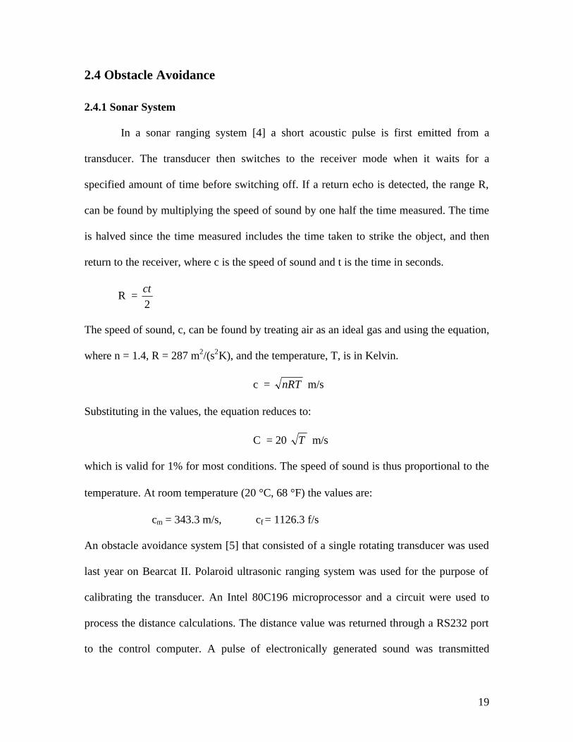
In a sonar ranging system [4] a short acoustic pulse is first emitted from a
transducer. The transducer then switches to the receiver mode when it waits for a
specified amount of time before switching off. If a return echo is detected, the range R,
can be found by multiplying the speed of sound by one half the time measured. The time
is halved since the time measured includes the time taken to strike the object, and then
return to the receiver, where c is the speed of sound and t is the time in seconds.
R = 2ct
The speed of sound, c, can be found by treating air as an ideal gas and using the equation,
where n = 1.4, R = 287 m2/(s2K), and the temperature, T, is in Kelvin.
c = nRT m/s
Substituting in the values, the equation reduces to:
C = 20 T m/s
which is valid for 1% for most conditions. The speed of sound is thus proportional to the
temperature. At room temperature (20 °C, 68 °F) the values are:
cm = 343.3 m/s, cf = 1126.3 f/s
An obstacle avoidance system [5] that consisted of a single rotating transducer was used
last year on Bearcat II. Polaroid ultrasonic ranging system was used for the purpose of
calibrating the transducer. An Intel 80C196 microprocessor and a circuit were used to
process the distance calculations. The distance value was returned through a RS232 port
to the control computer. A pulse of electronically generated sound was transmitted

20
toward the target and the resulting echo was detected. The system converted the elapsed
time into a distance value. The digital electronics generated the ultrasonic frequency and
all the digital functions were generated by the Intel microprocessor. Operating parameters
such as transmit frequency; pulse width, blanking time and the amplifier gain were
controlled by software supplied by Polaroid. The drive system for the transducer
consisted of a DC motor and its control circuitry. With this arrangement the transducer
was made to sweep and angle depending on the horizon (range between which we need
detection). The loop was closed by an encoder feedback from an encoder. The drive
hardware comprised of two interconnected modules, the Galil ICB930 and the 4-axis
ICM 1100. The ICM 1100 communicated with the main motion control board the DMC
1030 through an RS232 interface. The required sweep was achieved by programming the
Galil. Adjusting the Polaroid system parameters and synchronizing them with the motion
of the motor maintained distance values at known angles with respect to the centroid of
the robot.
Common to all sonar ranging systems is the problem of sonar reflection. With
light waves, our eye can see objects because the incident light energy is scattered by most
objects, which means that some energy will reach our eye, despite the angle of the object
to us or to the light source. This scattering occurs because the roughness of an object’s
surface is large compared to the wavelength of light (0.550 nm). Only with very smooth
surfaces (such as a mirror) does the reflectivity become highly directional for light rays.
Ultrasonic energy has wavelengths much larger (0.25 in) in comparison. Hence,
ultrasonic waves find almost all large flat surfaces reflective in nature. The amount of
energy returned is strongly dependent on the incident angle of sound energy. The Figure

21
2.3 shows a case where a large object is not detected because the energy is reflected away
from the receiver.
SONAR
LargeObstacle
Reflectance Energy
Relectance Energy
Figure 2.3 Undetected large object due to reflection.
Although the basic range formula is accurate, there are several factors when
considering the accuracy of the result. Since the speed of sound relies on the temperature,
a 10° temperature difference may cause the range to be in error by 1%. Geometry also
affects range. When the object is at an angle to the receiver, the range computed will be
to the closest point on the object, not the range from the centerline of the beam.

22
SONAR
LargeObstacle
Range Calculated
Actual Range
Figure 2.4 Range errors due to angle between object and sonar. 2.4.2 Laser Range Scanner
The human brain has a tremendous computational power dedicated to the
processing and integration of sensory input. The computers generated graphic displays
since the early 1970s that have made the job of interpreting a vast amount of data
considerably less difficult. It is much easier to see changes in data if it is displayed in
graphical terms. Flight-test engineers for the U.S. Air Force view graphical distributions
of the collected data from the prototype aircraft to evaluate the performance of the
aircraft.

23
Programming third-generation robot systems is very difficult because of the need
to program sensor feedback data. A visualization of the sensor view [7] of a scene,
especially the view of the laser scanner, helps human programmers to develop the
software and verify action plan of a robot. A laser range scanner operates on a similar
principle to conventional radar. Electromagnetic energy is beamed into the space to be
observed and reflections are detected as return signals from the scene. The scene is
scanned with a tightly focused beam of amplitude-modulated [4], infrared laser light (835
nm). As the laser beam passes over the surface of objects in the scene, some light is
scattered back to a detector that measures both the brightness and the phase of the return
signal. The brightness measurements are assembled into a conventional 2-D intensity
image. The phase shift between returning and outgoing signals are used to produce a 3-D
range image.
The Laser scanner has the advantage that it gives us a detailed description of the
field of view. We can get a maximum scan angle of 180° with a resolution of 0.250, 0.50,
10. Now with this resolution and scan angle we get a clear profile of the path in front of
our robot. We even get data such as at every angle scanned what is the position of the
point of reflection of laser beam from any object in the field of view with it’s coordinates.
Giving these values in the algorithm we are using for tracking our robot we can avoid
obstacles easily. There were many disadvantages of using sonar for obstacle avoidance
like reflection from objects other than obstacles, i.e. grass. There was no scan profile
given by the sonar and it just scanned at certain angles giving the reflection from certain
points but not all. All these disadvantages were overcome using a laser scanner as it gave
us a wide field of view containing every detail.

24
2.5 Range Detection Method Used
This section discusses the basic nature of relationships between the robot and the
obstacle. Before the system makes any decision, it is important that we know the
distance, width and shape of the obstacle. Depending upon these factors, the robot has to
make a decision as to whether it will go straight, turn left or turn right. Also it has to
decide upon the amount of turn depending on the nearness of the target to it. The optimal
angle of sweep per reading should be obtained in such a way that it does not slow down
the overall system performance. The laser scanner gives us a field of view showing the
complete 1800 sweep made by the laser beam. The laser beam starts from the right and
goes to left.
So at every angle, depending on the resolution set, we can get the distance and
position of the objects along the robot’s path. With these values we know exactly at what
angle is an obstacle present and what is it’s size. This simplifies the problem we had
earlier in our algorithm where we could not get the exact position and size of the
obstacle.

25
θ2
θ1
Figure 2.5 Field of View of Laser Scanner
Visible
Not visible
Ljne Track
Laser Scanner
Field of View

26
Chapter3
Laser Scanner and Serial Interface 3.1 Laser Scanner LMS-200
A laser scanner works by measuring the time of flight [11] of laser light pulses. It
is a non-contact measurement device that scans its surroundings two dimensionally. The
pulsed laser beam is deflected by an internal rotating mirror so that a fan shaped scan is
made of the surrounding area and the shape of the object is determined by the sequence
of impulses received. The scanner provides a distance value every 0.25°, 0.5° or 1° per
individual impulse, depending on angular resolution of the scanner.
The real time measurement data scanned by the device is given out in binary
format via the RS-232/422 serial interface, which is available for further evaluation.
There are many advantages of using laser scanners for obstacle avoidance. Some of the
advantages are-
a. High measurement resolution (10mm).
b. Contact-free measurement.
c. Target objects require no reflectors or markings.
d. Target objects require no special reflective properties.
e. High scanning frequency (up to 75Hz).
f. Transfer of measurement data in real time.
In addition the scanners contour measurement data can be evaluated to determine the
relative positions and sizes of objects. LMS 200 with 10mm resolution offer
programmable monitored zones with corresponding switching outputs in stand-alone

27
operation, i.e. without external evaluation. The functions and options required can be
configured within the scanner itself.
A B Monitored Fields A, B, C C Figure 3.1. Monitored fields and corresponding switching outputs
The range of the scanner depends on reflectivity of target object and the
transmission strength of the scanner. So it has a minimum range for cardboard materials
having a reflectivity of 10% and a maximum range for aluminum materials having a
reflectivity of 130%.
3.2 Uses of Laser scanner on our robot Laser scanner measurement data can be used for object measurement and
determining position. The measurement data corresponds to the surrounding contour
scanned by the device and is given out in binary format via RS232/RS 422 interface. As
the individual values are given out in sequence (beginning with the value 1), particular
angular positions can be allocated on the basis of the values’ positions in the data string.
Here, the system is responsible for automatically reporting that an area is free. This
Switching outputs A, B, C
Data interface (measured values)

28
means that an infringement of a field, e.g. by an object or machine part, leads to a
switching signal at an output.
The scanner can operate in pixel oriented or scan oriented mode. Pixel-oriented
evaluation is used for suppressing raindrops and snowflakes or other particles, and thus
makes the system less sensitive to environment factors. This involves saving the
measured values from each individual spot in each scan, and a sequence counter being
started for each spot. This kind of evaluation should be included in the corresponding
evaluation software when external data processing is undertaken. Object blanking can be
used for suppressing an object that is not to be detected, e.g. a steel cable, that is located
within the monitored field.
The Laser scanner on our robot communicates with the host computer and the
host computer communicates with the laser scanner using a serial interface. Any of the
common interfaces either RS 422/232 could be used. The transfer rate varies from 9.6
kbaud to 500 kbaud which can be set using telegrams. The data is transferred in binary
format where a byte of data consists of 1 start bit, 8 data bits, a parity bit with even parity
or without parity and 1 stop bit.
Figure 3.2 LMS in stand - alone operation
Sensor LMS
RS 232 / 422
COM

29
3.3 Serial Interface Cards
A serial port, or interface [12] can be used for serial communication in which only
one bit is transmitted at a time. All IBM PC and compatible computers are typically
equipped with two serial ports and one parallel port. Although these two types of ports
are used for communicating with external devices, they work in different ways. A parallel
port sends and receives data eight bits at a time over eight separate wires. This allows
data to be transferred very quickly; however, the cable required is more bulky because of
the number of individual wires it must contain. Parallel ports are typically used to
connect a PC to a printer and are rarely used for much else. A serial port sends and
receives data in a stream one bit at a time over one wire. While it takes eight times as
long to transfer each byte of data this way, only a few wires are required.
The 2-port RS- 232/422/485 PCI host adapter is a two-channel PCI-bus serial I/O
adapter for PC’s. It has two very versatile asynchronous serial ports. They are field
selectable as RS-232 ports or RS-422/485 ports. Any serial port has two data lines, TD
(Transmit Data) and RD (Receive Data). RS-422 devices running in full-duplex mode
will have two pairs of data lines: TD+, TD-, RD+ and RD-. In this mode, they can send
and receive data at the same time. In half-duplex mode (RS-232), TD and RD are shared
on a single pair of lines: TD+, TD-, RD+ and RD-. A device configured for half-duplex
operation cannot transmit and receive data at the same time.
The IC133-R2 adapter for Bearcat III uses a 16550 UART. This chip features
programmable baud rates, data format, interrupt control and a 16-byte input and output
FIFO. We can replace the 16550 with a 16950 UART for even better performance.
Pronounced u-art, and short for universal asynchronous receiver-transmitter, the UART
30
is a computer component that handles asynchronous serial communication. Every
computer contains a UART [13] to manage the serial ports and all internal modems have
their own UART. As modems have become increasingly fast, the UART has come under
greater scrutiny as the cause of transmission bottlenecks. For fast data transmission
devices it is to be made sure that the computer's UART can handle their maximum
transmission rate.
The newer 16550 UART contains a 16-byte buffer, enabling it to support higher
transmission rates than the older 8250 UART. The original UART chip shipped with the
IBM personal computer was the 8250. This chip was limited to 9600 bps maximum rate.
It was replaced with the 16450, which had the same architecture as the 8250 but has a
higher maximum bps specification. Both of the chips only have a one byte FIFO/buffer.
The 16550 has a 16-byte FIFO, 16650 has a 32-byte FIFO, 16750 has a 64-byte FIFO and
the 16950 has a 128-byte FIFO. When operating under DOS at speeds below 9600 bps
the 16450 should provide satisfactory performance. When operating under any Windows
or other multitasking operating system, a 16450 will be limited to about 1200 or 2400
bps. Any of today’s high-speed devices require more than a 16450 UART can offer even
when running under DOS. A 16 byte FIFO may not sound like much, but it allows up to
16 characters to be received before the computer has to service the interrupt. This
increases the maximum bps rate the computer can process reliably from 9600 to 153,000
bps if it has a 1 millisecond interrupt dead time. A 32 byte FIFO increases the maximum
rate to over 300,000 bps. A second benefit to having a FIFO is that the computer only has
to service about 8 to 12% as many interrupts, allowing more CPU time for updating the
screen, or doing other chores. Thus the computer's responses will improve as well. Our

31
laser scanner has a high data transmission rate of over 500 kbaud. The computer we were
using had a 16550 UART, which is sufficient for our laser scanner.
3.3.1 RS-232
The IBM PC computer defined the RS-232 [14] port on a 9-pin D-subminiature
connector, and subsequently the EIA/TIA approved this implementation as the EIA/TIA-
574 standard. RS-232 is capable of operating at data rates up to 20 kbps at distances less
than 50ft. The absolute maximum data rate may vary due to line conditions and cable
lengths. We can configure both the ports of the Bearcat III adapter as RS-232 (suitable
for communication with modems, printers and plotters) for standard serial COM-port
requirements. In both RS-232 and RS-422 modes, the card works seamlessly with the
standard operating-system serial driver.
Pinout of connector set to RS-232
Abbreviation Name Pin # Mode
TD Transmit Data Pin # 3 Output
RTS Request to Send Pin # 7 Output
DTR Data Term Ready Pin # 4 Output
GND Ground Pin # 5
RD Receive Data Pin # 2 Input
DCD Data Carrier Detector Pin # 1 Input
DSR Data Set Ready Pin # 6 Input
CTS Clear to Send Pin # 8 Input
RI Ring Indicator Pin # 9 Input
32
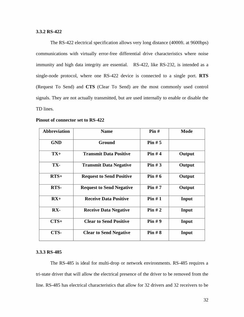
3.3.2 RS-422
The RS-422 electrical specification allows very long distance (4000ft. at 9600bps)
communications with virtually error-free differential drive characteristics where noise
immunity and high data integrity are essential. RS-422, like RS-232, is intended as a
single-node protocol, where one RS-422 device is connected to a single port. RTS
(Request To Send) and CTS (Clear To Send) are the most commonly used control
signals. They are not actually transmitted, but are used internally to enable or disable the
TD lines.
Pinout of connector set to RS-422
Abbreviation Name Pin # Mode
GND Ground Pin # 5
TX+ Transmit Data Positive Pin # 4 Output
TX- Transmit Data Negative Pin # 3 Output
RTS+ Request to Send Positive Pin # 6 Output
RTS- Request to Send Negative Pin # 7 Output
RX+ Receive Data Positive Pin # 1 Input
RX- Receive Data Negative Pin # 2 Input
CTS+ Clear to Send Positive Pin # 9 Input
CTS- Clear to Send Negative Pin # 8 Input
3.3.3 RS-485
The RS-485 is ideal for multi-drop or network environments. RS-485 requires a
tri-state driver that will allow the electrical presence of the driver to be removed from the
line. RS-485 has electrical characteristics that allow for 32 drivers and 32 receivers to be

33
connected to one line. RS-485 can be cabled in two-wire or four-wire mode and it does
not define a connector pinout, a physical connector, or a set of modem control signals.
RS-485 always runs in half-duplex programming mode. They handle the low-level RS-
485 driver maintenance automatically, so communications driver replacements are not
necessary. To the host operating system, the cards appear to be standard RS-232 COM
ports requiring no special drivers or additional software. Initial development can be
targeted for RS-232, debugged, tested, and then implemented as RS- 485.
Pinout of connector set to RS-485
Abbreviation Name Pin # Mode
GND Ground Pin # 5
TX+ Transmit Data Positive Pin # 4 Output
TX- Transmit Data Negative Pin # 3 Output
RTS+ Request to Send Positive Pin # 6 Output
RTS- Request to Send Negative Pin # 7 Output
RX+ Receive Data Positive Pin # 1 Input
RX- Receive Data Negative Pin # 2 Input
CTS+ Clear to Send Positive Pin # 9 Input
CTS- Clear to Send Negative Pin # 8 Input
3.4 Using the Laser Scanner
We are using a RS-422 serial interface card with our scanner as it has a higher
baud rate for faster communication. After we set the interface card to have it in RS-422
mode we make the changes in the BIOS of our system. There are some changes done in

34
BIOS to have the port addresses and IRQ’s assigned to the ports. After changing the IRQ
and the addresses to standard values we select proper cord connecting the LMS to the
computer making sure the right port is selected in the interface menu in LMS. If a wrong
port is selected in LMS menu and the Com3 or 4 exists then we see a message sensor
cannot be closed. The sensors that exist can be seen at the status bar when the interface
assistant is used and the LMS makes connection. The laser scanner is then ready to be
used for obstacle detection after we have the COM ports working and a connection is
made between the scanner and the host computer.
35
Chapter 4 Experimental Design
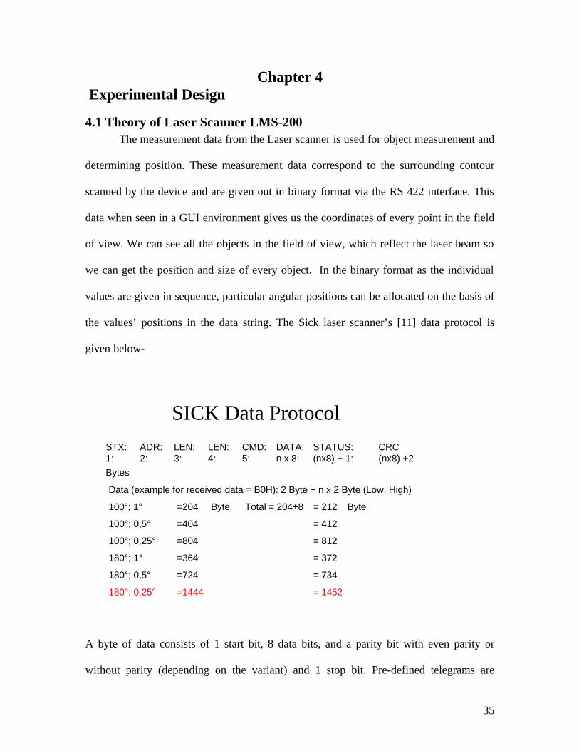
4.1 Theory of Laser Scanner LMS-200 The measurement data from the Laser scanner is used for object measurement and
determining position. These measurement data correspond to the surrounding contour
scanned by the device and are given out in binary format via the RS 422 interface. This
data when seen in a GUI environment gives us the coordinates of every point in the field
of view. We can see all the objects in the field of view, which reflect the laser beam so
we can get the position and size of every object. In the binary format as the individual
values are given in sequence, particular angular positions can be allocated on the basis of
the values’ positions in the data string. The Sick laser scanner’s [11] data protocol is
given below-
STX: ADR: LEN: LEN: CMD: DATA: STATUS: CRC
Bytes1: 2: 3: 4: 5: n x 8: (nx8) + 1: (nx8) +2
Data (example for received data = B0H): 2 Byte + n x 2 Byte (Low, High)
100°; 1° =204 Byte Total = 204+8 = 212 Byte
100°; 0,5° =404 = 412
100°; 0,25° =804 = 812
180°; 1° =364 = 372
180°; 0,5° =724 = 734
180°; 0,25° =1444 = 1452
SICK Data Protocol
A byte of data consists of 1 start bit, 8 data bits, and a parity bit with even parity or
without parity (depending on the variant) and 1 stop bit. Pre-defined telegrams are

36
available for communication with the host computer via the serial interface of the LMS.
Telegrams are hexadecimal codes, which change the response of either the computer or
the Laser scanner when transferring data. Data is transferred in binary format. Transfer is
initiated by STX (02h).
________________________________________________________________________
STX ADR LENL LENH CMD LMS No. MODE CRCL CRCH ________________________________________________________________________ 0x02 0x00 0x03 0x00 0x30 0x00 0x01 0x71 0x38 where,
0x02 is the start character for initiation of transmission
0x00 is the LMS address, which is the BROADCAST address
0x0003 is the length = 3, i.e. three data bytes follow
0x30 is the command for request for measured values
0x00 is the LMS number 0, i.e. the LMS currently active sends the measured values
0x01 is the mode for all 361 measured values of the current scan
0x3871 is the CRC 16 checksum.
We give 02h/00h/02h/00h/20h/24h/34h/08h/ command to change the operating mode of
LMS to send all measured values of the scans continuously. For this command we get the
following response from LMS: 06h/02h/80h/03h/00h/A0h/00h/10h/16h/0Ah/
The scanner now sends the complete measured value in a continuous stream of data. The
corresponding evaluation software, which is a C-code, is capable of synchronizing itself
to the start of the telegram.
Command: B0h
Number of measured value 361: (LOWBYTE) 69h (HIGHBYTE) 41h

37
Measured values in mm: ADh/01h/9Bh/01h/...
Status byte for LMS Type 6: 10h
CRC16: E3h/1Bh/
When we give the telegram number B0 to the LMS we get a continuous stream of data.
For every two bytes of data, which are useful to us, we have the following format:
The number of measured values transmitted (2 Bytes) is laid down in bits 0 to 13.
Bit 15 and bit 14 code for the unit of the measured values:
0 0 Unit = 1 cm
0 1 Unit = 1 mm (default setting)
1 0 Unit = 10 cm
Bit 13 0 - complete scan (Standard)
1 – partial scan
Bit 12 Bit 11 coding of number of partial scan:
0 0 measured values belong to partial scan X.00
0 1-measured values belong to partial scan X.25
1 0 measured values belong to partial scan X.50
1 1 measured values belong to partial scan X.75
The LMS software is divided into three sections (paths):
1. For laying down monitored fields and configuring field evaluation,
2. For the configuration of an LMS for measurement tasks (configuring measured
values, measurement dimensions, etc.),
3. For displaying the LMS scanning line (control, tests or demonstrations).
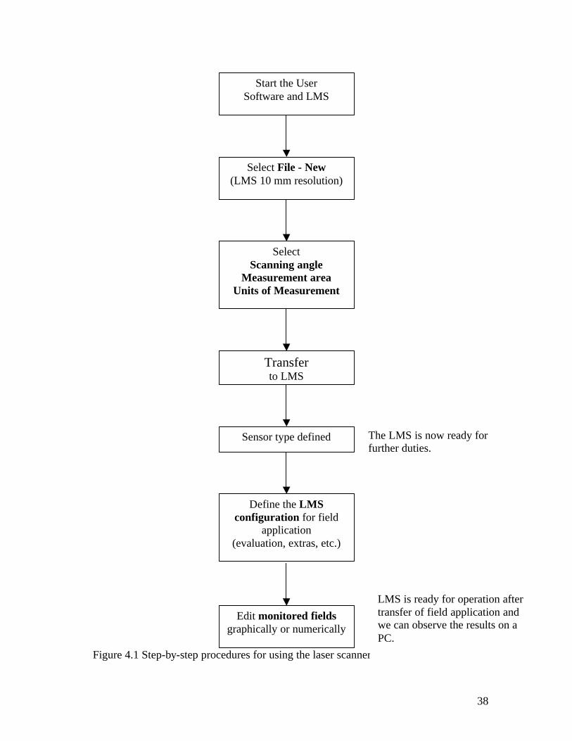
38
The LMS is now ready for further duties.
Figure 4.1 Step-by-step procedures for using the laser scanner
Start the User Software and LMS
Select File - New (LMS 10 mm resolution)
Select Scanning angle
Measurement area Units of Measurement
Transfer to LMS
Sensor type defined
Define the LMS configuration for field
application (evaluation, extras, etc.)
Edit monitored fields graphically or numerically
LMS is ready for operation after transfer of field application and we can observe the results on a PC.

39
4.2 Performance of the Laser scanner
The various functions that can be used with the laser scanner are given below.
Converting fields
The laser scanner displays data either in a rectangular grid or in a radial grid. We have
an option to show the field of view in a rectangular or a segmented grid, which can be
changed using the converter function. As shown in the page view we can even set the
size of the grid, change the units etc. After the settings have been made we have to
transfer the configuration to the LMS.
Figure 4.2 Converting Fields
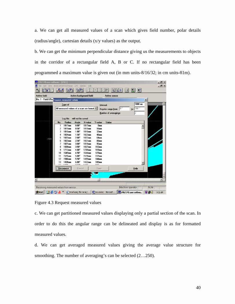
Request measured values
The user software displays or saves the distance measurement values of the LMS in a
variety of ways. There are several individual options that can be selected:
40
a. We can get all measured values of a scan which gives field number, polar details
(radius/angle), cartesian details (x/y values) as the output.
b. We can get the minimum perpendicular distance giving us the measurements to objects
in the corridor of a rectangular field A, B or C. If no rectangular field has been
programmed a maximum value is given out (in mm units-8/16/32; in cm units-81m).
Figure 4.3 Request measured values c. We can get partitioned measured values displaying only a partial section of the scan. In
order to do this the angular range can be delineated and display is as for formatted
measured values.
d. We can get averaged measured values giving the average value structure for
smoothing. The number of averaging’s can be selected (2…250).
41
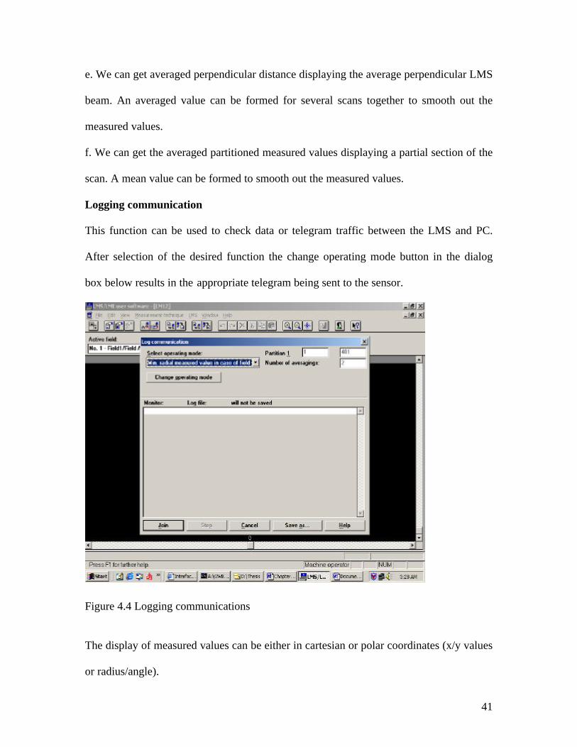
e. We can get averaged perpendicular distance displaying the average perpendicular LMS
beam. An averaged value can be formed for several scans together to smooth out the
measured values.
f. We can get the averaged partitioned measured values displaying a partial section of the
scan. A mean value can be formed to smooth out the measured values.
Logging communication
This function can be used to check data or telegram traffic between the LMS and PC.
After selection of the desired function the change operating mode button in the dialog
box below results in the appropriate telegram being sent to the sensor.
Figure 4.4 Logging communications
The display of measured values can be either in cartesian or polar coordinates (x/y values
or radius/angle).

42
We can select the operating mode to be any one of the following -
a. Minimum radial measured value on field infringement:
The sensor only supplies measured values after a field infringement.
b. All measured values continuously:
The sensor provides a constant supply of measured values.
c. Minimum measured values continuously:
The sensor provides a constant supply of the shortest measured distances (per field
segment).
d. Continuous perpendicular distance:
The sensor only provides the smallest perpendicular distance to the object in the corridor
or the field’s transient direction.
e. Continuous averaged measured values:
Output of all measured values. An average value of the individual measured values can
be formed to smooth out the values.
f. Continuous partition of measured values:
Constant output of all the measured values within the defined field section.
g. Continuous partition of measured values and field values:
As above, but with additional output of the distance to the outer field limit. i.e.
information is provided on the radial distance to the LMS for a measurement beam that
leaves the particular field (separate for fields A, B, C).
h. Continuous averaged partition of measured values:
Constant output of all measured values of a partial section with average value
information for smoothing.

43
i. All measured values direct continuously:
Constant output of all raw measurement values.
Figure 4.5 All measured values shown on the screen
j. Continuous measured values and reflectivity:
Output of all measured values and their corresponding reflectivity values.
Option: formation of a max. of any five partial sections.
4.3 Algorithm used for obstacle avoidance
Offset distance compensation check by the Fuzzy Logic

44
y
x
ab
w
d
X
Figure 4.6 Obstacle on the right of the robot with clearance

45
Case 1: Obstacle to the right [15] (a < 90° and b < 90°)
1.Check if robot can maintain same path and avoid obstacle without offsetting the
centroid of the robot from the center of the track.
2.If X =d*Cos (b) and X > ½ w it can continue on straight path without offsetting robot
centroid.
3.When X = d*Cos (b) and X< = ½ w
Calculate angle α that the robot has to turn such that Xnew = ( ½ w + safety factor)
where safety factor = 0.5 ft.
4.Robot starts turning left and continues turning left till d*Cos (b - α) = Xnew and α is
the angle robot has turned from its original position.
5.The robot now starts to turn right to maintain its centroid along a path parallel to the
centerline of the track and offset by a distance of Xnew-Xold.
6.Thus the hugging distance (the distance of the robot from the centroid of the line
followed) is calculated as the previous hugging distance ± the offset.
46
y
x
a
b
w
d
X
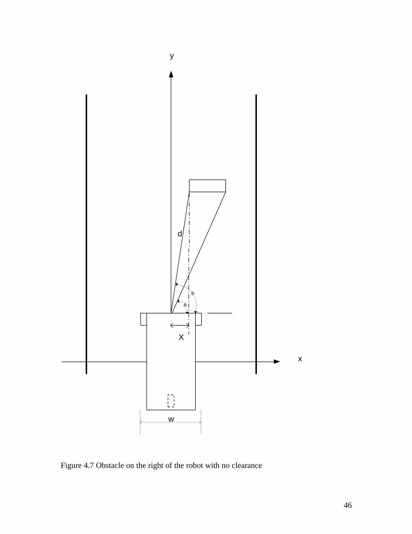
Figure 4.7 Obstacle on the right of the robot with no clearance

47
α
y
x
a
b
w
d
x
Figure 4.8 Obstacle avoidance by turning an angle α

48
y
x
a
b
w
d
Figure 4.9 Obstacle on left of the robot with clearance

49
Case 2: Obstacle to the left (a>90° and b>90°)
1.Check if robot can maintain same path and avoid obstacle without offsetting the
centroid of the robot from the center of the track.
2.If X=d*Cos (b) and X > ½ w
It can continue on straight path without offsetting robot centroid.
3.When X = d*Cos (b) and X< = ½ w
Calculate angle that the robot has to turn such that Xnew = ( ½ w + safety factor) where
safety factor = 0.5 ft.
4.Robot starts turning right and continues turning right till d*Cos (b - α) = Xnew and α is
the angle robot has turned from its original position.
5.The robot now starts to turn left to maintain its centroid along a path parallel to the
centerline of the track and offset by a distance of Xnew-Xold.
6.Thus the hugging distance (the distance of the robot from the centroid of the line
followed) is calculated as the previous hugging distance ± the offset.

50
y
x
a
w
b
Figure 4.10 Obstacle in the center of the track
51
b β
β β β β β β β
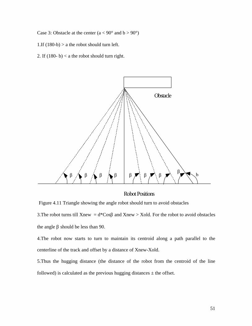
Case 3: Obstacle at the center (a < 90° and b > 90°)
1.If (180-b) > a the robot should turn left.
2. If (180- b) < a the robot should turn right.
Obstacle
Robot Positions
Figure 4.11 Triangle showing the angle robot should turn to avoid obstacles
3.The robot turns till Xnew = d*Cosβ and Xnew > Xold. For the robot to avoid obstacles
the angle β should be less than 90.
4.The robot now starts to turn to maintain its centroid along a path parallel to the
centerline of the track and offset by a distance of Xnew-Xold.
5.Thus the hugging distance (the distance of the robot from the centroid of the line
followed) is calculated as the previous hugging distances ± the offset.
52
Chapter 5
Experimental Results
This chapter provides the obstacle detection, and range estimation results using the laser
scanner attached to the Bearcat III.
5.1 Obstacle Detection and Range Estimation Results
I performed obstacle detection experiments both indoors and outdoors. Each experiment
consisted of 180° field of view of the laser scanner with a 0.5° resolution. The scans were
made using a scan-oriented approach rather than a pixel oriented approach because of the
slow refresh rate. The refresh rate makes the computer very slow if it is changed to over a
certain value. The laser scanner gives us a clear field of view with the coordinates of
every point along x and y-axis. Even with accurate laser scanner view there are some
spurious detections in the individual scans with reasonable frequency.
5.1.1 Indoor Experiments
I performed a series of experimental runs in the corridor at the 5th floor of Rhodes hall in
front of the Center For Robotics Research lab at University of Cincinnati. In each case,
the laser lookahead distance was between 7m to 8m. This could be changed to a value
greater than that. The hallway had a few obstacles present but they were not right in front
of Bearcat III. In each experiment, I placed one obstacle in front of the robot and I could
see the changes in the field of view with the changes in the coordinates measured at
certain angles. Detecting the placed obstacle was the primary objective. The obstacles
tested included different people standing at different positions, Chairs, and wooden
blocks. At least two experiments were performed with every object and every object
could be detected at a minimum of 8 meters. Since the reflectance by any object does not
53
really matter every object looks the same. Its size depends on the distance from the
scanner and the laser rays, which cannot pass through the object, are reflected back with a
data.
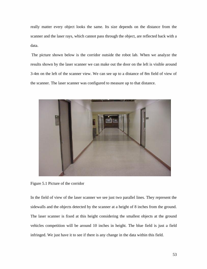
The picture shown below is the corridor outside the robot lab. When we analyze the
results shown by the laser scanner we can make out the door on the left is visible around
3-4m on the left of the scanner view. We can see up to a distance of 8m field of view of
the scanner. The laser scanner was configured to measure up to that distance.
Figure 5.1 Picture of the corridor In the field of view of the laser scanner we see just two parallel lines. They represent the
sidewalls and the objects detected by the scanner at a height of 8 inches from the ground.
The laser scanner is fixed at this height considering the smallest objects at the ground
vehicles competition will be around 10 inches in height. The blue field is just a field
infringed. We just have it to see if there is any change in the data within this field.

54
Figure 5.2 Screen shot of the corridor The picture below gives the view at the height of the scanner. There are two chairs placed
within the distance of 8m. The second chair is farther than the first one.
Figure 5.3 View of the laser scanner in real world

55
We see two spikes in the field of view. One is larger than the other one as one chair is
closer to the scanner. Now the scanner just sees the two legs of the two chairs as it has a
two dimensional field of view.
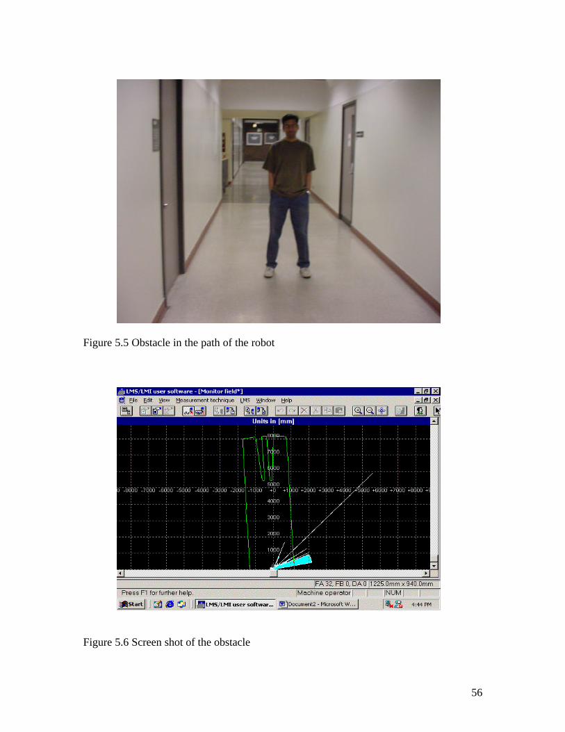
Figure 5.4 Screen shot with two chairs in the Field of View Below is the picture shown of one of my friends who has his legs spread wide to see the
difference in the field of view. When we see him in the field of view we see two legs
separately as two objects. At the height of the laser scanner they will be seen as two
separate objects. The two curves show that the obstacle is at a distance of around 5m
from the robot. The shape of the curves shows how accurately the laser scanner gives us
data.
56
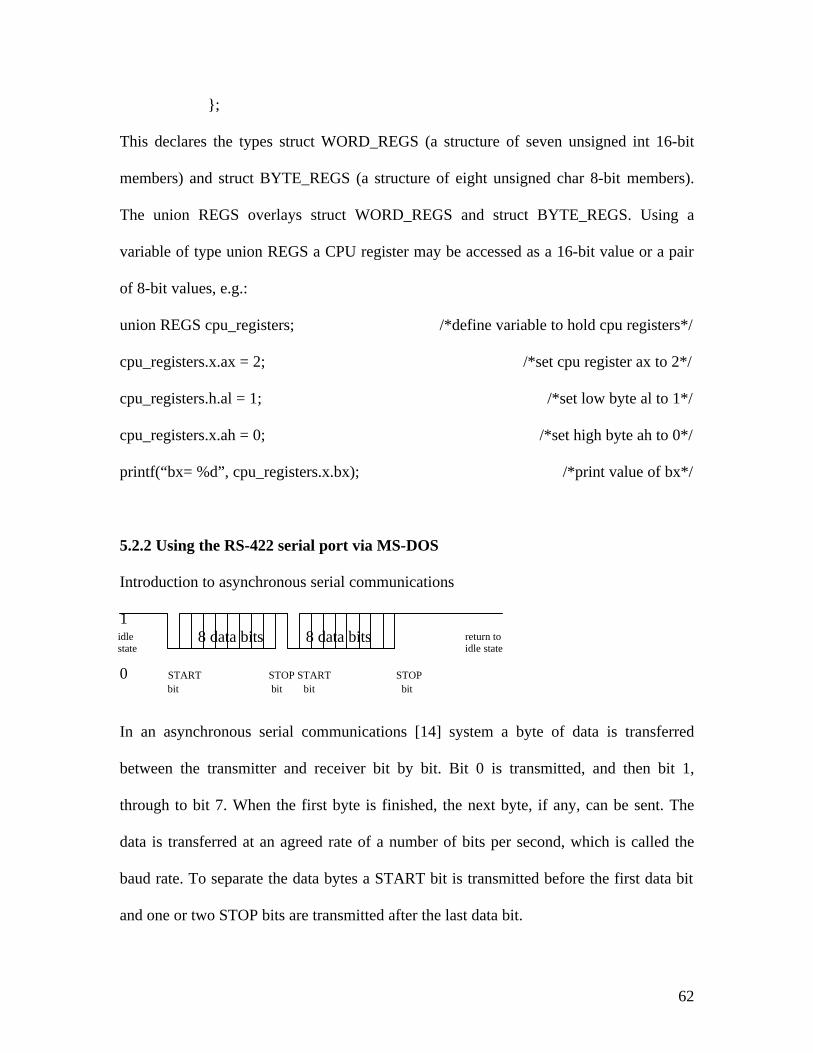
Figure 5.5 Obstacle in the path of the robot
Figure 5.6 Screen shot of the obstacle

57
The pictures below show the computer screen with the real time data measured by the
scanner. This gives us the detailed view in front of the robot in real time. It refreshes at a
fast rate, which can be changed accordingly.
Figure 5.7 Monitor’s view

58
Figure 5.8 Close view of the monitor
5.1.2 Outdoor Testing
Outdoor experiments were all performed at the loading dock of the University of
Cincinnati. The results were similar to the indoor experiments except that the field of
view was increased but the objects were seen similar to the indoor objects. In each
outdoor experiment the actual field view was reduced by the shades kept on the sides of
the scanner. The actual field of view is 180° but with the shades to protect the indoor
scanner from direct sunlight the field of view was reduced. The picture below shows me
standing in front of the robot. There is a little heap on my left side, which is visible in the
laser scanner’s view also. The results of the laser scanner are shown below where this
picture shows the real world in front of the robot.

59
Figure 5.9 Outdoor testing of robot
Figure 5.10 Screen shot of the laser scanner

60
Figure 5.11 Measured values on the screen The Request Measured Values screen shown above gives the detail about the x and y-
coordinates of every 0.5° with the radial distance from the scanner. Thus the position of
the obstacle with the size in two dimensions of all obstacles in front of the scanner can be
known. These values can be used in our algorithm to avoid obstacles and follow line
track.
5.2 Programming the laser scanner in MS-DOS
The laser scanner sends data in binary format. The data is sent serially through the RS-
422 port. This data is read from the registers and a program is written to analyze the data
stored in a file, which is read byte by byte.
5.2.1 Accessing MS DOS operating system facilities The MS-DOS operating system [17], used on IBM PC compatible microcomputers, is
accessed via the INT instruction. It is possible to write an assembly language function,

61
which loads relevant values into the processor registers, executes INT and then returns
register values to the calling function. The majority of C compilers, which run under MS-
DOS, provide such a function, e.g. both Turbo C and Borland C have the function int86.
When int86 is called, information is passed to MS-DOS via the 16-bit processor registers
[16], ax, bx, cx, dx, si, and di or their byte equivalents (the 16-bit register ax can be
addressed as two 8-bit registers ah (the high byte) and al (the low byte)). Under Turbo C
and Borland C the function prototype of int86 is declared in header file <dos.h> as
follows:
int int86 (int int_number, union REGS*in_registers, union REGS*out_registers);
where,
int_number is the interrupt number to invoke the required MS-DOS function,
in_registers are the values to be passed to MS-DOS via processor registers, and
out_registers are the values of the processor registers as returned by MS-DOS.
The declaration of union REGS is of the form:
/* Intel 8086 family word registers (16-bit), cflag is the carry flag*/
struct WORD_REGS {unsigned int ax, bx, cx, dx, si, di, cflag; };
/* Intel 8086 family byte registers (8-bit) */
struct BYTE_REGS {unsigned char al, ah, bh, cl, dl, dh; };
/* Intel 8086 general purpose registers: union overlays word and byte registers*/
union REGS {
struct WORD_REGS x; /*word registers*/
struct BYTE_REGS h; /*byte registers*/
62
};
This declares the types struct WORD_REGS (a structure of seven unsigned int 16-bit
members) and struct BYTE_REGS (a structure of eight unsigned char 8-bit members).
The union REGS overlays struct WORD_REGS and struct BYTE_REGS. Using a
variable of type union REGS a CPU register may be accessed as a 16-bit value or a pair
of 8-bit values, e.g.:
union REGS cpu_registers; /*define variable to hold cpu registers*/
cpu_registers.x.ax = 2; /*set cpu register ax to 2*/
cpu_registers.h.al = 1; /*set low byte al to 1*/
cpu_registers.x.ah = 0; /*set high byte ah to 0*/
printf(“bx= %d”, cpu_registers.x.bx); /*print value of bx*/
5.2.2 Using the RS-422 serial port via MS-DOS
Introduction to asynchronous serial communications
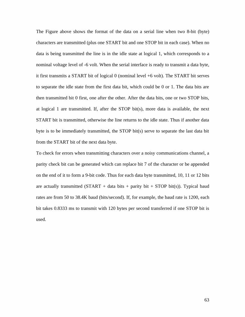
1 8 data bits 8 data bits 0 0 START STOP START STOP bit bit bit bit
In an asynchronous serial communications [14] system a byte of data is transferred
between the transmitter and receiver bit by bit. Bit 0 is transmitted, and then bit 1,
through to bit 7. When the first byte is finished, the next byte, if any, can be sent. The
data is transferred at an agreed rate of a number of bits per second, which is called the
baud rate. To separate the data bytes a START bit is transmitted before the first data bit
and one or two STOP bits are transmitted after the last data bit.
idle state
return to idle state
63
The Figure above shows the format of the data on a serial line when two 8-bit (byte)
characters are transmitted (plus one START bit and one STOP bit in each case). When no
data is being transmitted the line is in the idle state at logical 1, which corresponds to a
nominal voltage level of -6 volt. When the serial interface is ready to transmit a data byte,
it first transmits a START bit of logical 0 (nominal level +6 volt). The START bit serves
to separate the idle state from the first data bit, which could be 0 or 1. The data bits are
then transmitted bit 0 first, one after the other. After the data bits, one or two STOP bits,
at logical 1 are transmitted. If, after the STOP bit(s), more data is available, the next
START bit is transmitted, otherwise the line returns to the idle state. Thus if another data
byte is to be immediately transmitted, the STOP bit(s) serve to separate the last data bit
from the START bit of the next data byte.
To check for errors when transmitting characters over a noisy communications channel, a
parity check bit can be generated which can replace bit 7 of the character or be appended
on the end of it to form a 9-bit code. Thus for each data byte transmitted, 10, 11 or 12 bits
are actually transmitted (START + data bits + parity bit + STOP bit(s)). Typical baud
rates are from 50 to 38.4K baud (bits/second). If, for example, the baud rate is 1200, each
bit takes 0.8333 ms to transmit with 120 bytes per second transferred if one STOP bit is
used.

64
Chapter 6 Conclusion Obstacle detection and avoidance is a challenging problem especially on highways where
fast highway travel speeds force long lookahead distances and fast data processing.
Currently, there are no systems proven capable of reliable highway obstacle detection.
My thesis presents a theory and implementation of a novel laser-based obstacle detection
system. This system is capable of detecting and tracking a large variety of objects at long
distances. The principle behind this system is the same as the sonar, “Time of Flight”
(TOF) approach but it overcomes the drawbacks of using sonar for this purpose. The
laser scanner does not detect the external noise from the surrounding environment as
detected by the sonar. Hence it proves to be a better system than the one previously used
on Bearcat II. Segmentation of potential obstacles is very fast and requires minimal
processing.
Future Work
Scanner Mechanism Modifications
The original purpose and use of the laser scanner was for automated guided
vehicles running at slow speeds <5mph. For this purpose, the scanner provides excellent
range information with 180° scan angle and a slower frame rate, which was acceptable.
But these are poor design parameters for highway obstacle detection.
A more revolutionary sensor might use a strobe of a specific optical frequency
[18] and a nearby CCD with a matching optical band filter. This should provide entire
images similar to that produced by a scanning laser, but at a much faster CCD camera
rates. By eliminating optical frequency besides that of strobe, most ambient light should

65
be eliminated allowing the same intensity-based approaches to be used for obstacle
detection. With 2-D image data at each frame, obstacle tracking and segmentation may
become easier and more reliable since texture-based methods can be used. Range
estimation should also benefit from the increased amount of data.
Software Improvements
We have a DOS operating system on Bearcat III. This system posed many
problems in installing the laser scanner, as we were not able to install the RS-422 card
initially because of OS limitations. We also found it difficult to integrate the laser scanner
with our robot. In future, we could think about having both Linux OS and programming
all the code using Matlab, as it is easier to program in Matlab than most of the present
high-level languages.
Applications of the current system
This robot avoids obstacles and follows a line track. So, this robot could be used at places
where humans cannot go. This could be used with the army and the robot could go in a
minefield where it would be very dangerous for the human beings.
This robot could also be used for making tar-roads. If we have a vision system that gives
us a two-dimensional view of the potholes and the laser scanner gives us a depth of the
potholes this machine could be used to fill potholes. So there are many applications we
could think of this robot.
66
References
[1] http://reeses.mie.uc.edu/IGRC2001/DesignReport/DesignReport2001.doc.
[2] L.H. Matthies, A. Kelly, T. Litwin, G. Tharp, “Obstacle detection for Unmanned
Ground Vehicles,” Proceedings of the Intelligent Vehicles ’95 Symposium 1995.
[3] S. Singh, P.Keler, “Obstacle Detection for High Speed Autonomous Navigation,”.
[4] David Novick, “ Interactive Simulation of an Ultrasonic Transducer and Laser Range
Scanner”, Masters Thesis, University of Florida, 1993.
[5] Ramesh Thyagarajan, “A Motion Control Algorithm for Steering an AGV in an
Outdoor Environment”, Masters Thesis, 2000.
[6] Vishnuvardhanaraj Selvaraj, “Failure Mode Analysis of an Autonomous Guided
Robot using JDBC”, Masters Thesis, 2000.
[7] Munro, W.S.H., Pomeroy, S., Rafiq, M., Williams, H.R., Wybrow, M.D., and Wykes,
C., "Ultrasonic Vehicle Guidance Transducer," Ultrasonics, 28, pp. 350-354, 1990.
[8] Moring, I., Heikkinen, T., Myllyla, R., "Acquisition of Three-Dimensional Image
Data by a Scanning Laser Range Finder," Optical Engineering, pp. 897-902, 8, 28(1989).
[9] C. Stiller, J. Hipp, C. Rossig, A. Ewald, “Multi-Sensor Obstacle Detection and
Tracking,” Image vision Computing 18, pp. 389-396, September 2000.
[10] R.D. Schraft, B. Graf, A. Traub, D. John, “A Mobile Robot Platform for Assistance
and Entertainment,” Fraunhofer Institute Manufacturing Engineering and Automation
(IPA), Nobelstrasse 12, 70569 Stuttgart, Germany.
[11] http://www.Sickoptic.com
[12] http://www.Blackbox.com
[13] http://www.taltech.com/introserial.htm

67
[14] http://webopedia.internet.com/TERM/s/serial_port.html
[15] Sampath Kanakaraju, Sathish Shanmugasundaram, Ramesh Thyagarajan and
Ernest L. Hall, “Steering of an Automated Vehicle in an Unstructured Environment”
Proceedings of SPIE, Intelligent Robotics and Computer Vision, V 3837-18, Boston,
Nov. 1999.
[16] B. Bramer, S. Bramer, “C for Engineers,”1997.
[17] Ray Duncan, “Advanced MS DOS Programing,”2nd edition, 1994.
[18] J. Hancock, M. Herbert, C. Thorpe, “Laser Intensity-Based Obstacle Detection,”
Proceedings of the IEEE Conference on Intelligent Robots and Systems, 1998.