University of Chicago — Physics 575

Accelerator Physics and Technology of Linear Colliders

Winter 2002

J. Rosenzweig

UCLA Dept. of Physics and Astronomy

CHAPTER 4 — PARTICLE SOURCES

Lecture 1

4.0. Introduction

These sets of lectures will be organized using a historical logic, where we first

discuss more standard approaches — schemes which have an existing experimenental

track record — to obtaining electrons and positrons for linear colliders. We then move

on to more advanced approaches, which present both physics and technological

challenges to the linear collider effort. In addition, as future linear collider construction

seems likely to be closely linked the development of x-ray free-electron lasers (XFELs),

we also discuss very high quality electron sources associated with XFEL injection. The

techniques used in XFEL sources (the rf photoinjector) in turn have direct implications

for electron production in linear colliders.

We will begin by tracing back the demands of the linear collider physics goals,

and overall luminosity they imply, to the electron and positron sources. We compare

these demands to those of the XFEL electron injectors, and note that they imply different

technical solutions at this time. An eventual merging of these technologies will be

discussed in at the end of these lectures.

During these lectures, we will try to point out the most interesting accelerator

physics aspects of the linear collider/XFEL source problem. We will also emphasize the

current challenges in pushing the state-of-the-art in these systems.

4.1. Demands of the Linear Collider on Particle Sources

The requirements of the eventual application of the particles to obtain luminosity

in a linear collider drive many of the demands on particle sources. The luminosity, which

is a direct measure of the collider's capability to produce adequate particle physics event

rates (excluding beam-beam collective effects), is given by

=N e +N e − f c

4 x y

=N e + N e− fc

4 x*

y* ⋅ x,n y ,n

. (4.1)

If we examine the parameters evident in Eq. 4.1 one at a time, we may draw conclusions

about the source performance. Clearly, the energy mec2 and the final focus beta-

functions, x* and y

* , are dependent only on the final state of the beam as dictated by

acceleration and beam optics. The collision rate f c as well as the electron and positron

populations, Ne − and Ne + , at the collision point, however, must clearly be equaled or

exceeded by their values at injection. In the absence of phase space cooling, the

normalized emittances at the collision point, x ,n and y ,n , will be equal to or greater than

(due to phase space dilution) than their values at injection.

None of the parameters for injection are particularly difficult to attain, with the

exception of the normalized rms emittances, x ,n and y ,n , which for a recent NLC design

are given by 3 mm-mrad and 0.02 mm-mrad, respectively. The vertical emittance is well

beyond that presently achieved from electron sources (not to mention the much higher

emittance positron sources).

Fortunately, the present paradigm for the linear collider, whose layout in shown in

Fig. 4.1, includes powerful damping rings, which use synchrotron radiation to quickly

diminish (by many orders of magnitude in normalized emittances) the 6D phase space

volume of the electron and positron beams between the sources and the main linac. Thus

the demand on the transverse emittances from the source are not at all extreme, and are

dependent on damping ring performance.

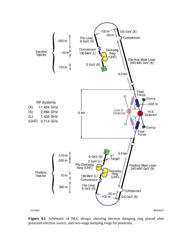
Figure 4.1. Schematic of NLC design, showing electron damping ring placed afterpolarized electron source, and two-stage damping rings for positrons.

The two relevant (and related) parameters from the damping ring that place limits

on the maximum allowable transverse emittance are the machine repetition rate

f rep = fc / Nb ( Nb is the number of bunches in a train accelerated per machine cycle) and

the phase space acceptance of the ring A . In order to avoid either physical (from

mechanical boundaries) or dynamical (from field nonlinearities) collimation upon

injection into the damping ring, the normalized emittance of the source beams must

satisfy n < DRA in x and y. Here DRmec2 is the injection energy of the damping ring.

The repetition rate, in the simplest scenario where particles are used on the same cycle as

they are created, sets the maximum time allowed for damping Td = f rep−1 . If more than one

damping ring is used, as in the NLC positron source shown in Fig. 4.1, or the damping

ring has the capability of containing many pulse trains, then the number of repetition

periods used for damping may be increased proportionately. For very large initial

emittances, the time needed for damping to the small final values demanded for collisions

expands, and thus the size and cost of the damping ring must increase accordingly. Thus

the motivation for small emittances out of the initial source is to mitigate the demands on

the damping ring.

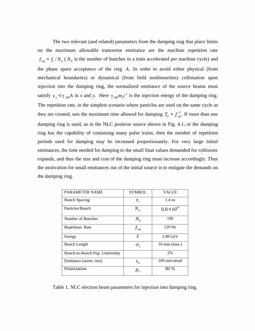
PARAMETER NAME SYMBOL VALUE

Bunch Spacings

1.4 ns

Particles/Bunch N e− 0.8 ×1010

Number of Bunches Nb190

Repetition Rate f rep120 Hz

Energy E 1.98 GeV

Bunch Lengthz

10 mm (max.)

Bunch-to-Bunch Pop. Uniformity 2%

Emittance (norm. rms)n

100 mm-mrad

Polarization pe −80 %

Table 1. NLC electron beam parameters for injection into damping ring.

The parameters describing the electron beam which may be injected into the NLC

damping ring are given in Table 1. Note that stability of the bunch population within the

bunch train is specified, as this parameter affects the beam loading throughout the

system. If the charge stability is not controlled, the collider performance will degrade

dramatically.

Note also that the electron polarization is included in Table 1 as well. Knowledge

of the initial polarization state of one or both colliding species is a crucial tool for the

particle experimenter in lepton colliders. Polarized electrons have been employed at the

SLC collider to great advantage.

The bunch length needed at the focus of a linear collider is constrained to by the

“hour-glass” (depth of focus) effect, by z < x,y* . As the vertical beta-function is smaller

than one mm in typical designs (see Chapter 3), the damping ring (and bunch

compressor) systems must be used to damp the longitudinal phase space and shorten the

bunch from its value at the particle source, to well sub-mm.

4.2. Electron Sources for XFEL

The XFEL is a device which amplifies spontaneous undulator radiation (self-

amplified spontaneous emission, or SASE) from an ultra-relativistic electron beam. The

near-axis radiation wavelength is given by

r = u

2 2 1+ au2[ ] (4.2)

where u is the undulator periodicity, and au = 2 eBu,rms u mec2 is the normalized rms

vector potential of the undulator. Equation 4.2 can be understood physically as the

relativistic Thomson backscattering of the virtual photons associated with the undulator

field. Thus a 10-15 GeV beam ( ≅ 2 − 3×104 ), a several cm period undulator may

produce Angstrom wavelength light. Furthermore, this light is coherent, and produced in

sub-ps levels — roughly the same time structure as the electron beam.

The XFEL based on use of a very high brightness electron beams, where the

brightness is defined as

Be =2I

x,n y,n

. (4.2)

The exponential gain-length of the XFEL is proportional to Be

1/3 , and so the brightness is

a measure of the quality of the gain medium. A high current (>3 kA) and low normalized

emittance (<1 mm-mrad) beam is demanded of current XFEL designs, in order to create

an XFEL which reaches saturation after approximately 100 m(!). An additional constraint

on the emittance in these devices arises from phase space matching, which is stated as

n ≤ r

4= u

81+ au

2[ ] . (4.3)

This constraint essentially requires that both the electron and photon beam envelopes

behave in similar ways; it also arises from consideration of whether all the radiated

photons from individual electrons are emitted inside the coherent angle of the system. It

can be seen that as increases, Eq. 4.3 becomes progressively harder to satisfy. It is in

fact weakly violated, by a factor of ~ 2, in present Angstrom-class XFEL designs.

There is now a strong movement worldwide (e.g. LCLS at SLAC, TESLA-FEL at

DESY) to create such Angstrom-class systems. The TESLA-FEL design has now been

explicitly bundled with the proposed TESLA superconducting linear collider, to produce

a laboratory where high energy physics is performed alongside materials and biological

sciences. The XFEL is a very new type of x-ray light source—its peak photon brightness

is larger than present sources by many orders of magnitude, and its time structures are

shorter by at least 100.

The electron source demands important new scientific tool must thus be examined

in the context of linear collider design. As can be seen in Fig. 4.2, the TESLA design

does in fact incorporate three electron sources, two (polarized, unpolarized) for the

collider, and one for XFEL. As the charge per bunch is nearly the same in each case, and

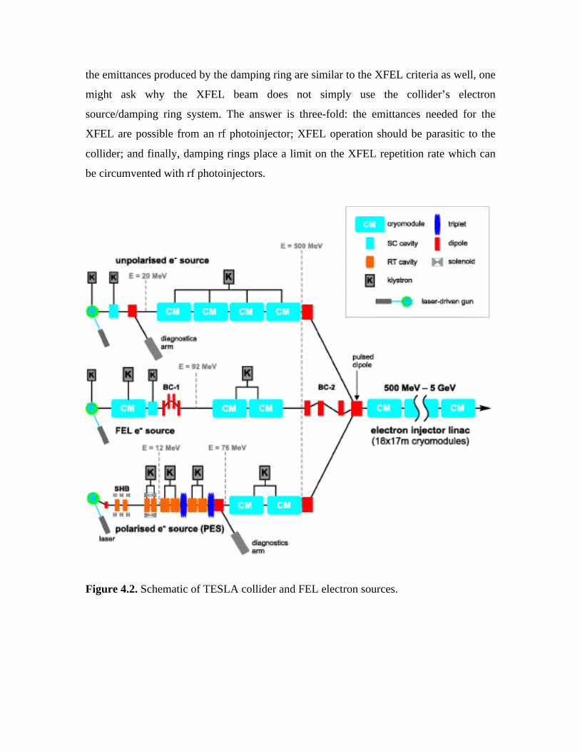
the emittances produced by the damping ring are similar to the XFEL criteria as well, one

might ask why the XFEL beam does not simply use the collider’s electron

source/damping ring system. The answer is three-fold: the emittances needed for the

XFEL are possible from an rf photoinjector; XFEL operation should be parasitic to the

collider; and finally, damping rings place a limit on the XFEL repetition rate which can

be circumvented with rf photoinjectors.

Figure 4.2. Schematic of TESLA collider and FEL electron sources.

4.3. Polarized Electron Sources

Electrons are notoriously easy to produce experimentally. The most common

processes which are used to allow electron emission from solid surfaces are: thermionic,

field, and photoelectric emission. In every system, aspects of the thermal state of the

solide, and surface field applied to it are important to some degree. In klystrons, for

example, the cathode is heated, and then pulsed with a high voltage. The cathode

temperature is high enough that the emitted current is never thermionically limited, but is

in fact limited by the cancellation of the applied field due to space-charge effects (see

Exercise 4.1).

Gating of a hot cathode using applied voltage has two shortcomings when one

thinks of linear collider electron sources. The first is time-structure; it is very difficult to

produce the sub-ns (ps level for XFELs!) high voltage pulses. The second is that it is not

possible to obtain polarized electrons from a thermionic source. Both of these problems

are circumvented by use of photo-emission. As the photoelectric effect in metals is quite

prompt, 100 fs lasers (e.g. Ti:Sapphire) may be used to gate cathodes at this ultra-fast

time scale. This is especially important in the creation of XFEL-quality beams. To

preserve such short pulses at relevant charges (~ nC), one must apply enormous (~100

MV/m) electric fields at the cathode, to overcome space charge-induced debunching.

This is possible in rf cavities, and the placement of a photocathode inside of an rf cavity

forms an rf photocathode gun, or rf photoinjector. This device is the enabling technology

for high brightness electron beams used in XFELs.

The photoemission process in metals is initiated by illuminating the metallic

surface by a photon of energy h greater than the work function of the metal, W. As the

electron leaves the surface of the metal with the excess energy ∆E = h − W in energ-

etically allowed direction, an inherent normalized emittance is imparted at the cathode,

x,n cathode=

1

2

∆E

m ec2 x. (4.4)

For Cu, a common metallic cathode material, the value of ∆E = h − W is in the range of

0.15-0.25 eV.

In semiconductors, such as those needed for production of polarized electrons, the

microscopic physics of the photoemission process look a bit different than the familiar

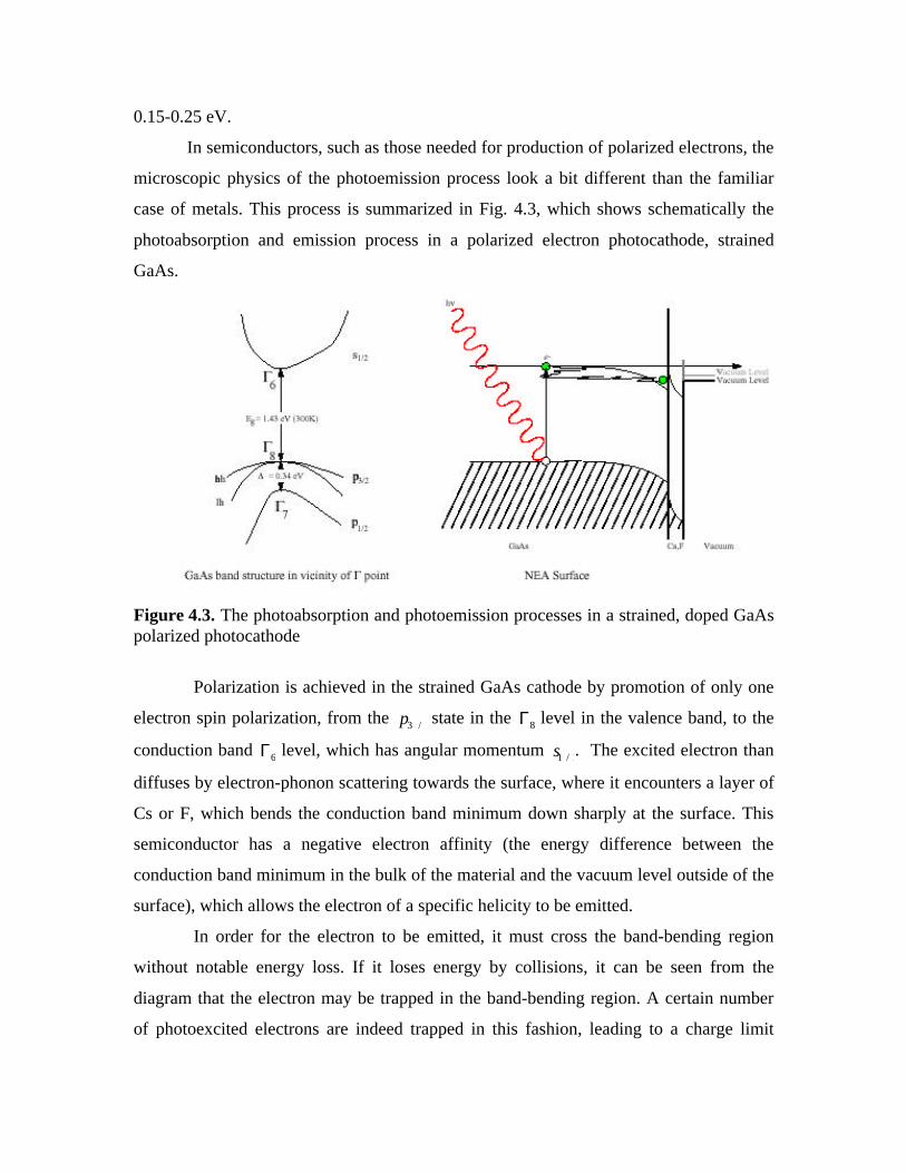
case of metals. This process is summarized in Fig. 4.3, which shows schematically the

photoabsorption and emission process in a polarized electron photocathode, strained

GaAs.

Figure 4.3. The photoabsorption and photoemission processes in a strained, doped GaAspolarized photocathode

Polarization is achieved in the strained GaAs cathode by promotion of only one

electron spin polarization, from the p3 / 2 state in the Γ8 level in the valence band, to the

conduction band Γ6 level, which has angular momentum s1 / 2. The excited electron than

diffuses by electron-phonon scattering towards the surface, where it encounters a layer of

Cs or F, which bends the conduction band minimum down sharply at the surface. This

semiconductor has a negative electron affinity (the energy difference between the

conduction band minimum in the bulk of the material and the vacuum level outside of the

surface), which allows the electron of a specific helicity to be emitted.

In order for the electron to be emitted, it must cross the band-bending region

without notable energy loss. If it loses energy by collisions, it can be seen from the

diagram that the electron may be trapped in the band-bending region. A certain number

of photoexcited electrons are indeed trapped in this fashion, leading to a charge limit

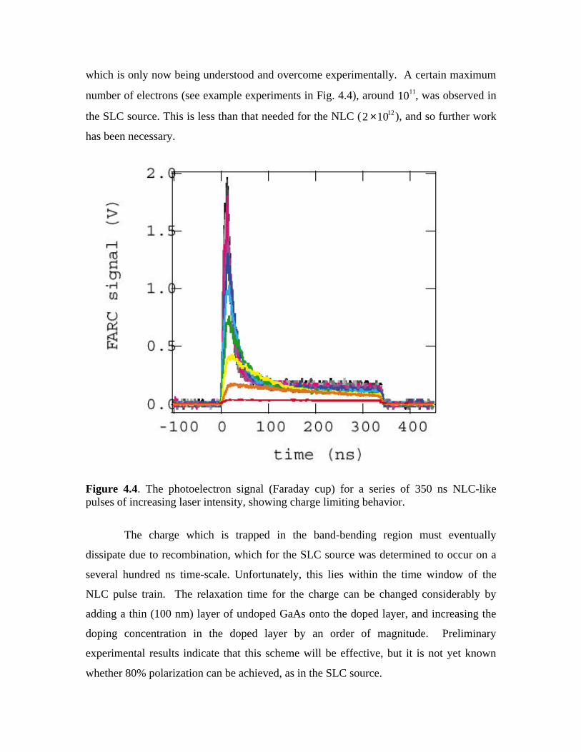
which is only now being understood and overcome experimentally. A certain maximum

number of electrons (see example experiments in Fig. 4.4), around 1011, was observed in

the SLC source. This is less than that needed for the NLC (2 ×1012), and so further work

has been necessary.

Figure 4.4. The photoelectron signal (Faraday cup) for a series of 350 ns NLC-likepulses of increasing laser intensity, showing charge limiting behavior.

The charge which is trapped in the band-bending region must eventually

dissipate due to recombination, which for the SLC source was determined to occur on a

several hundred ns time-scale. Unfortunately, this lies within the time window of the

NLC pulse train. The relaxation time for the charge can be changed considerably by

adding a thin (100 nm) layer of undoped GaAs onto the doped layer, and increasing the

doping concentration in the doped layer by an order of magnitude. Preliminary

experimental results indicate that this scheme will be effective, but it is not yet known

whether 80% polarization can be achieved, as in the SLC source.

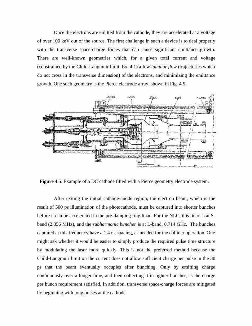
Once the electrons are emitted from the cathode, they are accelerated at a voltage

of over 100 keV out of the source. The first challenge in such a device is to deal properly

with the transverse space-charge forces that can cause significant emittance growth.

There are well-known geometries which, for a given total current and voltage

(constrained by the Child-Langmuir limit, Ex. 4.1) allow laminar flow (trajectories which

do not cross in the transverse dimension) of the electrons, and minimizing the emittance

growth. One such geometry is the Pierce electrode array, shown in Fig. 4.5.

Figure 4.5. Example of a DC cathode fitted with a Pierce geometry electrode system.

After exiting the initial cathode-anode region, the electron beam, which is the

result of 500 ps illumination of the photocathode, must be captured into shorter bunches

before it can be accelerated in the pre-damping ring linac. For the NLC, this linac is at S-

band (2.856 MHz), and the subharmonic buncher is at L-band, 0.714 GHz. The bunches

captured at this frequency have a 1.4 ns spacing, as needed for the collider operation. One

might ask whether it would be easier to simply produce the required pulse time structure

by modulating the laser more quickly. This is not the preferred method because the

Child-Langmuir limit on the current does not allow sufficient charge per pulse in the 30

ps that the beam eventually occupies after bunching. Only by emitting charge

continuously over a longer time, and then collecting it in tighter bunches, is the charge

per bunch requirement satisfied. In addition, transverse space-charge forces are mitigated

by beginning with long pulses at the cathode.

Even without the need for short pulse lengths, the laser needed for driving the

photocathode is technically quite challenging, as a long total pulse-train is involved.

Since the quantum efficiency of the polarized cathode is near 0.1%, at an approximate

illumination wavelength of 800 nm (1 eV photons), 2 ×1012 electrons requires a 265 ns

laser pulse with with 800 microJoules of energy.

4.4. Positron Sources

Unlike electrons, it is quite difficult to find make positrons. Laboratory sources

of positrons are all based fundamentally on the pair-creation processes in high fields,

such as occur near nuclei. The successful SLC source consisted of a tungsten-rhenium

target (WRe), which was irradiated with a multi-GeV, multi-nC electron beam. This

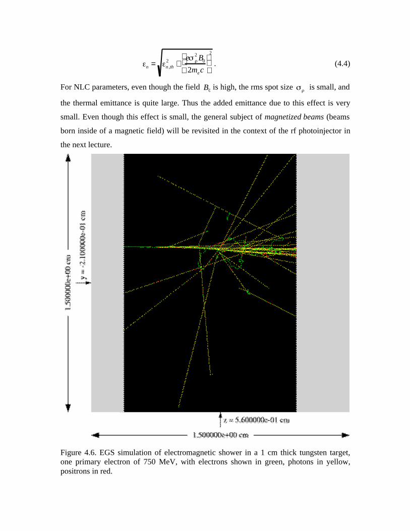
primary produces an electromagnetic shower of electrons, photons and positrons, as

illustrated by Fig. 4.6, which shows the results of an EGS simulation of a shower

resulting from a single 750 MeV electron incident on the tungsten target. Note that there

are three positrons exiting the 1 cm thick target, and also that their trajectories have

significant angles with respect to the original beam axis. Furthermore, there is a very

large spread in the energy spectrum of the positrons produced, as can be seen from Fig.

4.7, which shows the longitudinal phase space of the positrons produced from the NLC

target as designed, which uses 6.2 GeV primary electrons. The positron collection

system is designed to operate at near 250 MeV. The collection system consists of a

strong applied solenoid field, which is 1.2 T at the target, rising quickly over 5 mm to 5.8

T in a flux concentrator, and then lowering adiabatically to 0.5 T over 15 cm.

Because the positrons are created in a solenoidal field B0, Busch’s theorem (see

Exercise 4.2) tells us that each positron is “born” with an inherent component of the

momentum in the azimuthal direction,

p =e B0

2. (4.4)

This angular momentum component translates into an inherent contribution to the

emittance after exiting the solenoidal region, which adds in squares with the thermal

emittance n,th ,

n = n ,th2 +

e 2 B0

2mec

2

. (4.4)

For NLC parameters, even though the field B0 is high, the rms spot size is small, and

the thermal emittance is quite large. Thus the added emittance due to this effect is very

small. Even though this effect is small, the general subject of magnetized beams (beams

born inside of a magnetic field) will be revisited in the context of the rf photoinjector in

the next lecture.

Figure 4.6. EGS simulation of electromagnetic shower in a 1 cm thick tungsten target,one primary electron of 750 MeV, with electrons shown in green, photons in yellow,positrons in red.

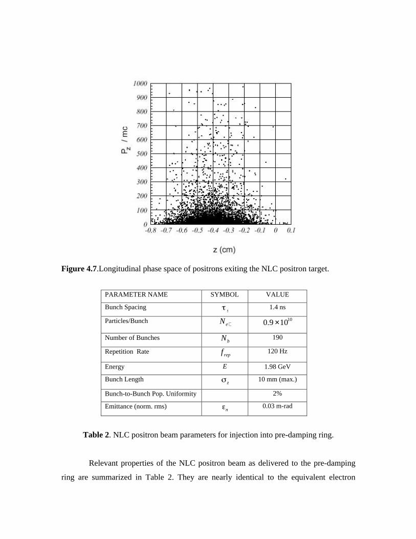
Figure 4.7.Longitudinal phase space of positrons exiting the NLC positron target.

PARAMETER NAME SYMBOL VALUE

Bunch Spacings

1.4 ns

Particles/Bunch N e + 0.9 ×1010

Number of Bunches Nb190

Repetition Rate f rep120 Hz

Energy E 1.98 GeV

Bunch Lengthz

10 mm (max.)

Bunch-to-Bunch Pop. Uniformity 2%

Emittance (norm. rms)n

0.03 m-rad

Table 2. NLC positron beam parameters for injection into pre-damping ring.

Relevant properties of the NLC positron beam as delivered to the pre-damping

ring are summarized in Table 2. They are nearly identical to the equivalent electron

parameters, except for a small excess of charge (to account for expected losses), and a

large difference in emittances. This reflects the fact that the high-Z target produces a very

hot positron distribution.

The spread in angles emanating from the target is handled by the particular

magnetic field profile of the flux concentrator assembly. There are two ways of looking

at the effect of this device. It can be shown that the equation of motion for transverse

offset in the Larmor frame (rotating with half the local cyclotron frequency

L = c /2 = eB/ me ) has an associated betatron wavenumber k = kL = L /v = eB/2 p ,

where p is the momentum. For a field peaking at 5.8 T, such as in the flux concentrator,

the phase advance of a 250 MeV positron is thus nearly unity, indicating that significant

focusing takes place. Another way of looking at this system is to note that the “magnetic

moment” (or the more descriptively, the action, which is the product of the transverse

momentum and the radius of curvature of the orbit p⊥R = p⊥2 /eB) associated with the

transverse motion of the particle is an adiabatic invariant. Thus when B is lowered

slowly, p⊥2 is lowered proportionately, and the initially strongly diverging beam is made

much more parallel. This better-behaved beam can then be sent into a linac section with

further solenoid focusing, and accelerated up to damping ring energy. The key to this

adiabatic matching section is that the beam is made parallel, in a way which is insensitive

to initial conditions and, more importantly, energy errors. Thus a larger bandwidth of

initial energies can be collected into the acceptance of the solenoid/linac system.

The most pressing problem with the present approach to positron sourcery for the

NLC is that the target is highly stressed by the thermal shock of the electromagnetic

shower, and fatigued by the extremely high radiation dose it absorbs over time. After 5

years of use, the SLC target finally failed as a result of these problems. As NLC positron

demands are much in excess of the SLC, this presents a problem in extrapolating the SLC

design. While there are proposals use to liquid metal targets to evade thermal shock

limits, the most conservative way to approach this problem is to multiplex several targets,

with primary electron beams and collected positron beams separated and recombined

using deflection mode rf cavities. This scheme is illustrated in Fig. 4.8, which shows a 4

target system where 3 are in use and the 4th can be serviced while the others are running.

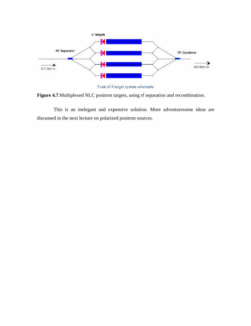
Figure 4.7.Multiplexed NLC positron targets, using rf separation and recombination.

This is an inelegant and expensive solution. More adventuresome ideas are

discussed in the next lecture on polarized positron sources.

Lecture 2

4.6. Polarized Positron Sources

The production of polarized positrons can be approached in a similar way as

polarized electrons are obtained, through use of circularly polarized photons, which can

pair-produce in relatively low-Z targets to give positrons of definite polarization. The

photons needed for positron production are much more energetic(!), however. In practice,

one needs 20-60 MeV photons, requiring 150-250 GeV electrons propagating through a

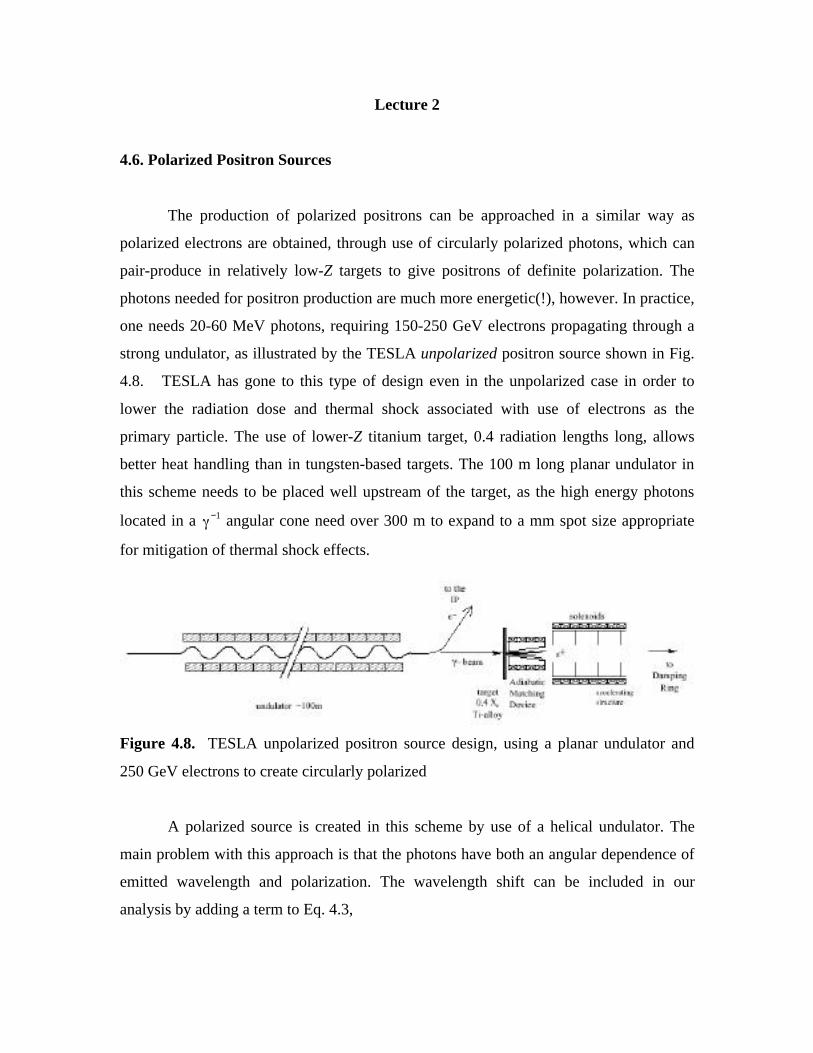
strong undulator, as illustrated by the TESLA unpolarized positron source shown in Fig.

4.8. TESLA has gone to this type of design even in the unpolarized case in order to

lower the radiation dose and thermal shock associated with use of electrons as the

primary particle. The use of lower-Z titanium target, 0.4 radiation lengths long, allows

better heat handling than in tungsten-based targets. The 100 m long planar undulator in

this scheme needs to be placed well upstream of the target, as the high energy photons

located in a −1 angular cone need over 300 m to expand to a mm spot size appropriate

for mitigation of thermal shock effects.

Figure 4.8. TESLA unpolarized positron source design, using a planar undulator and

250 GeV electrons to create circularly polarized

A polarized source is created in this scheme by use of a helical undulator. The

main problem with this approach is that the photons have both an angular dependence of

emitted wavelength and polarization. The wavelength shift can be included in our

analysis by adding a term to Eq. 4.3,

r = u

2 2 1+ au2 + ( )2[ ] . (4.5)

Thus the energy of the photons decreases off-axis (relativistic Doppler effect). In addi-

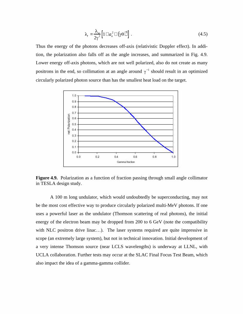
tion, the polarization also falls off as the angle increases, and summarized in Fig. 4.9.

Lower energy off-axis photons, which are not well polarized, also do not create as many

positrons in the end, so collimation at an angle around −1 should result in an optimized

circularly polarized photon source than has the smallest heat load on the target.

Figure 4.9. Polarization as a function of fraction passing through small angle collimatorin TESLA design study.

A 100 m long undulator, which would undoubtedly be superconducting, may not

be the most cost effective way to produce circularly polarized multi-MeV photons. If one

uses a powerful laser as the undulator (Thomson scattering of real photons), the initial

energy of the electron beam may be dropped from 200 to 6 GeV (note the compatibility

with NLC positron drive linac…). The laser systems required are quite impressive in

scope (an extremely large system), but not in technical innovation. Initial development of

a very intense Thomson source (near LCLS wavelengths) is underway at LLNL, with

UCLA collaboration. Further tests may occur at the SLAC Final Focus Test Beam, which

also impact the idea of a gamma-gamma collider.

4.5. High Brightness RF Photoinjectors

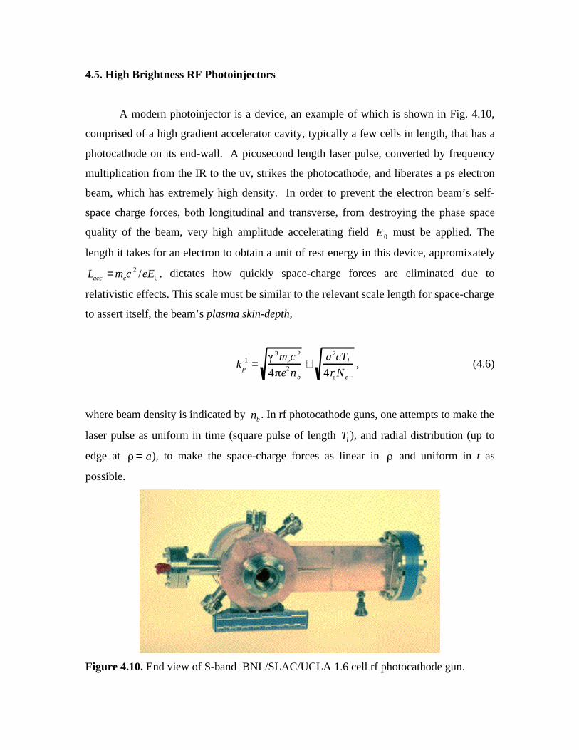
A modern photoinjector is a device, an example of which is shown in Fig. 4.10,

comprised of a high gradient accelerator cavity, typically a few cells in length, that has a

photocathode on its end-wall. A picosecond length laser pulse, converted by frequency

multiplication from the IR to the uv, strikes the photocathode, and liberates a ps electron

beam, which has extremely high density. In order to prevent the electron beam’s self-

space charge forces, both longitudinal and transverse, from destroying the phase space

quality of the beam, very high amplitude accelerating field E0 must be applied. The

length it takes for an electron to obtain a unit of rest energy in this device, appromixately

Lacc = mec2 /eE0 , dictates how quickly space-charge forces are eliminated due to

relativistic effects. This scale must be similar to the relevant scale length for space-charge

to assert itself, the beam’s plasma skin-depth,

kp−1 =

3mec2

4 e2nb

≅a2cTl

4reN e −

, (4.6)

where beam density is indicated by nb . In rf photocathode guns, one attempts to make the

laser pulse as uniform in time (square pulse of length Tl ), and radial distribution (up to

edge at = a), to make the space-charge forces as linear in and uniform in t as

possible.

Figure 4.10. End view of S-band BNL/SLAC/UCLA 1.6 cell rf photocathode gun.

If one takes the highest brightness rf photocathode gun design presently known,

the LCLS photoinjector, where N e− = 6.2 ×109 (1 nC), a=1 mm, and Tl =10 psec, the

plasma skin depth as approximated in Eq. 4.5 is 6.5 mm. The average field in this device

at injection (35 degrees from the zero crossing) is as E0=80 MV/m, which gives

Lacc = 6.3 mm, in good agreement.

Figure 4.11. Major features, and constant flux contours (parallel to electric field lines) inthe 1.6 cell gun of Figure 4.10. This device is a standing wave cavity, run in the π-mode.

The dynamics of the electron beam in the rf gun are quite rich, as they arise from

both enormous applied and self-fields. The applied fields are violently accelerating, and

also give rise to longitudinal focusing (enhanced bunching); they are also alternating

focusing and defocusing. The self-fields are of course defocusing and debunching. Thus

we may expect the system to be one where the motion occurs near an equilibrium.

In addition to the previously mentioned constraint on the accelerating field, it

should be noted that E0 should be large enough that an electron can become relativistic

in one-half of a spatial period rf , and thus captured by the forward accelerating wave.

This implies that the parameter (introduced by K.J. Kim)

= krf Lacc( )− 1= rfeE 0 /2 m ec

2 (4.6)

Photocathode

Photoelectronbeam

Beam exithole

must be greater than approximately unity. Note that in the LCLS photoinjector example,

= 4.5, and the beam is easily captured. Other types of photoinjectors, where the gun is

lengthened, to effectively attach a post-acceleration linac directly onto the initial

(capture) cells tend to be run at much lower values of . The moderate compression of

electron beam pulse length that one obtains in the gun is a decreasing function of , as

one must launch the beam well ahead of the rf crest for it to slip into the correct, maximal

acceleration phase after the beam is relativistic.

The transverse dynamics in this system are controlled by the very large transverse

rf forces (especially the unbalanced electric kick upon exiting the gun, cf. Fig. 4.11), and

the focusing solenoid. For small (e.g. TESLA-FEL gun), the focusing solenoid is

optimally placed over the gun, while for large , the solenoid is placed after the high

gradient gun, as shown in Fig. 4.12. For a high gradient system the plasma frequency is

lower, kp−1 ∝ 3 / 2, and focusing need not be applied as urgently, allowing the solenoid to

be moved downstream.

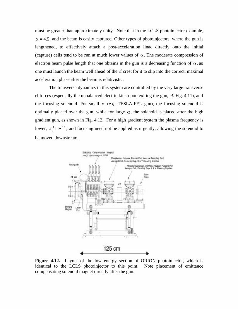
Figure 4.12. Layout of the low energy section of ORION photoinjector, which isidentical to the LCLS photoinjector to this point. Note placement of emittancecompensating solenoid magnet directly after the gun.

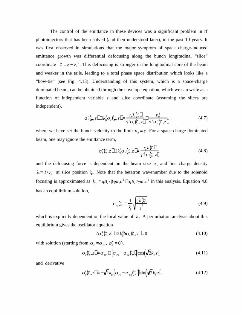
The control of the emittance in these devices was a significant problem in rf

photoinjectors that has been solved (and then understood later), in the past 10 years. It

was first observed in simulations that the major symptom of space charge-induced

emittance growth was differential defocusing along the bunch longitudinal “slice”

coordinate = z − vbt . This defocusing is stronger in the longitudinal core of the beam

and weaker in the tails, leading to a total phase space distribution which looks like a

“bow-tie” (see Fig. 4.13). Understanding of this system, which is a space-charge

dominated beam, can be obtained through the envelope equation, which we can write as a

function of independent variable z and slice coordinate (assuming the slices are

independent),

′ ′ r ,z( ) + k2

r ,z( ) =re ( )3

r ,z( )+ th

2

2r3 ,z( )

, (4.7)

where we have set the bunch velocity to the limit vb = c . For a space charge-dominated

beam, one may ignore the emittance term,

′ ′ r ,z( ) + k2

r ,z( ) =re ( )3

r ,z( )(4.8)

and the defocusing force is dependent on the beam size r and line charge density

= I /vb at slice position . Note that the betatron wavenumber due to the solenoid

focusing is approximated as k = qBz / m0c2 ≅ qBz / m0c

2 in this analysis. Equation 4.8

has an equilibrium solution,

eq( ) =1

k

re ( )3 (4.9)

which is explicitly dependent on the local value of . A perturbation analysis about this

equilibrium gives the oscillator equation

′ ′ r ,z( ) + 2k2

r ,z( ) = 0 (4.10)

with solution (starting from r = r0 , ′ r = 0),

r ,z( ) = r0 + r0 − eq( )[ ]cos 2k z( ) (4.11)

and derivative

′ r ,z( ) = − 2k r 0 − eq( )[ ]sin 2k z( ). (4.12)

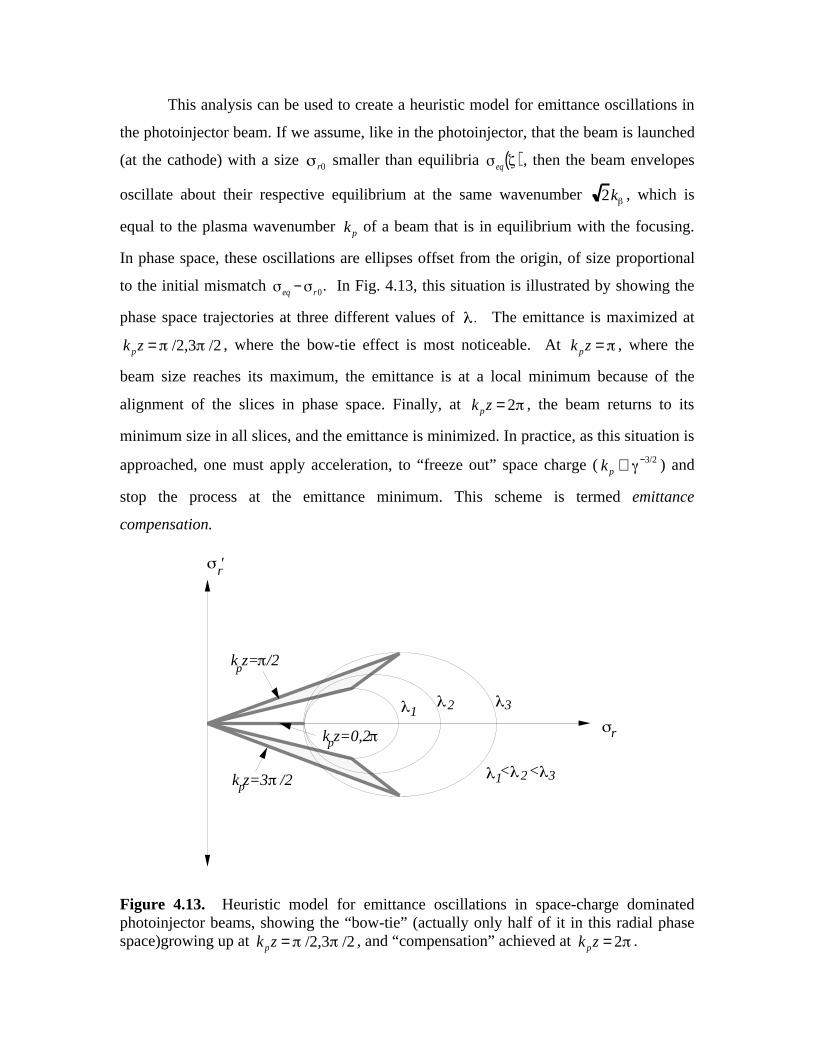
This analysis can be used to create a heuristic model for emittance oscillations in

the photoinjector beam. If we assume, like in the photoinjector, that the beam is launched

(at the cathode) with a size r0 smaller than equilibria eq( ), then the beam envelopes

oscillate about their respective equilibrium at the same wavenumber 2k , which is

equal to the plasma wavenumber kp of a beam that is in equilibrium with the focusing.

In phase space, these oscillations are ellipses offset from the origin, of size proportional

to the initial mismatch eq − r 0. In Fig. 4.13, this situation is illustrated by showing the

phase space trajectories at three different values of . The emittance is maximized at

kpz = /2,3 /2 , where the bow-tie effect is most noticeable. At kpz = , where the

beam size reaches its maximum, the emittance is at a local minimum because of the

alignment of the slices in phase space. Finally, at kpz = 2 , the beam returns to its

minimum size in all slices, and the emittance is minimized. In practice, as this situation is

approached, one must apply acceleration, to “freeze out” space charge ( kp ∝ −3/2 ) and

stop the process at the emittance minimum. This scheme is termed emittance

compensation.

r

r'

k z=3 /2p

k z=0,2 p

1

2

3

1< <

2

3

k z= /2p

Figure 4.13. Heuristic model for emittance oscillations in space-charge dominatedphotoinjector beams, showing the “bow-tie” (actually only half of it in this radial phasespace)growing up at kpz = /2,3 /2 , and “compensation” achieved at kpz = 2 .

0.0

1.0

2.0

3.0

0 50 100 150 200 250 300 350 400

rms beam size (uniform beam)

rms emittance (uniform beam)

σz (

mm

), ε ν(m

m-m

rad)

z (cm)

PWT linacs

Focusing solenoidHigh gradient RF photocathode gun

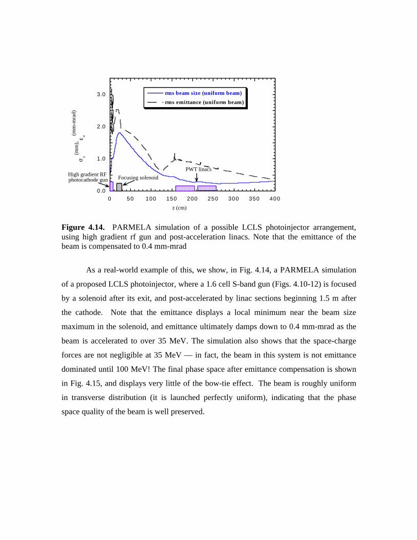
Figure 4.14. PARMELA simulation of a possible LCLS photoinjector arrangement,using high gradient rf gun and post-acceleration linacs. Note that the emittance of thebeam is compensated to 0.4 mm-mrad

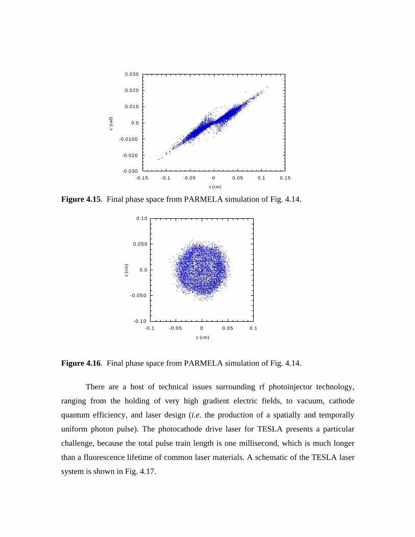
As a real-world example of this, we show, in Fig. 4.14, a PARMELA simulation

of a proposed LCLS photoinjector, where a 1.6 cell S-band gun (Figs. 4.10-12) is focused

by a solenoid after its exit, and post-accelerated by linac sections beginning 1.5 m after

the cathode. Note that the emittance displays a local minimum near the beam size

maximum in the solenoid, and emittance ultimately damps down to 0.4 mm-mrad as the

beam is accelerated to over 35 MeV. The simulation also shows that the space-charge

forces are not negligible at 35 MeV — in fact, the beam in this system is not emittance

dominated until 100 MeV! The final phase space after emittance compensation is shown

in Fig. 4.15, and displays very little of the bow-tie effect. The beam is roughly uniform

in transverse distribution (it is launched perfectly uniform), indicating that the phase

space quality of the beam is well preserved.

-0.030

-0.020

-0.0100

0.0

0.010

0.020

0.030

-0.15 -0.1 -0.05 0 0.05 0.1 0.15

x' (

rad)

x (cm)

Figure 4.15. Final phase space from PARMELA simulation of Fig. 4.14.

-0.10

-0.050

0.0

0.050

0.10

-0.1 -0.05 0 0.05 0.1

x (c

m)

y (cm)

Figure 4.16. Final phase space from PARMELA simulation of Fig. 4.14.

There are a host of technical issues surrounding rf photoinjector technology,

ranging from the holding of very high gradient electric fields, to vacuum, cathode

quantum efficiency, and laser design (i.e. the production of a spatially and temporally

uniform photon pulse). The photocathode drive laser for TESLA presents a particular

challenge, because the total pulse train length is one millisecond, which is much longer

than a fluorescence lifetime of common laser materials. A schematic of the TESLA laser

system is shown in Fig. 4.17.

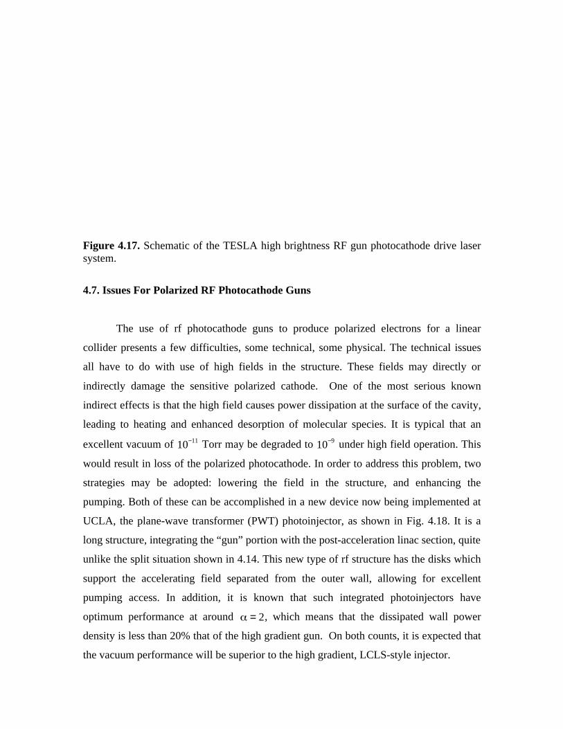
Figure 4.17. Schematic of the TESLA high brightness RF gun photocathode drive lasersystem.

4.7. Issues For Polarized RF Photocathode Guns

The use of rf photocathode guns to produce polarized electrons for a linear

collider presents a few difficulties, some technical, some physical. The technical issues

all have to do with use of high fields in the structure. These fields may directly or

indirectly damage the sensitive polarized cathode. One of the most serious known

indirect effects is that the high field causes power dissipation at the surface of the cavity,

leading to heating and enhanced desorption of molecular species. It is typical that an

excellent vacuum of 10−11 Torr may be degraded to 10−9 under high field operation. This

would result in loss of the polarized photocathode. In order to address this problem, two

strategies may be adopted: lowering the field in the structure, and enhancing the

pumping. Both of these can be accomplished in a new device now being implemented at

UCLA, the plane-wave transformer (PWT) photoinjector, as shown in Fig. 4.18. It is a

long structure, integrating the “gun” portion with the post-acceleration linac section, quite

unlike the split situation shown in 4.14. This new type of rf structure has the disks which

support the accelerating field separated from the outer wall, allowing for excellent

pumping access. In addition, it is known that such integrated photoinjectors have

optimum performance at around = 2, which means that the dissipated wall power

density is less than 20% that of the high gradient gun. On both counts, it is expected that

the vacuum performance will be superior to the high gradient, LCLS-style injector.

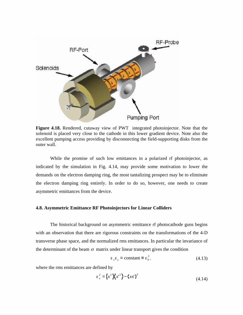
Figure 4.18. Rendered, cutaway view of PWT integrated photoinjector. Note that thesolenoid is placed very close to the cathode in this lower gradient device. Note also theexcellent pumping access providing by disconnecting the field-supporting disks from theouter wall.

While the promise of such low emittances in a polarized rf photoinjector, as

indicated by the simulation in Fig. 4.14, may provide some motivation to lower the

demands on the electron damping ring, the most tantalizing prospect may be to eliminate

the electron damping ring entirely. In order to do so, however, one needs to create

asymmetric emittances from the device.

4.8. Asymmetric Emittance RF Photoinjectors for Linear Colliders

The historical background on asymmetric emittance rf photocathode guns begins

with an observation that there are rigorous constraints on the transformations of the 4-D

transverse phase space, and the normalized rms emittances. In particular the invariance of

the determinant of the beam matrix under linear transport gives the condition

x y = constant ≡ 02. (4.13)

where the rms emittances are defined by

x2 = x2 x'2 − xx'

2

(4.14)

y2 = y2 y' 2 − yy'

2.

If we take the product of the emittances to be the square of the final state shown in Fig.

4.14, 0,n2 = 0.4 ×10−6 m - r a d( )2

, then we may imagine that there is some transformation

which lowers the vertical emittance by a factor of 10, while lowering x by the same

amount, to preserve Eq. 4.13. The simplest device that may cause such phase plane

coupling is a skew quadrupole, one which is rotated at 45 degrees with respect to the

standard orientation about the beam axis. Such a beam, which would have 6 ×109

electrons, and x,y (n ) = 4,0.04 mm-mrad, is quite close to the NLC design parameters as

given!

There are, however, also other invariants associated with higher moments of the

distribution function. Of particular interest is a second order moment, which considering

only transverse phase space is

22 = x

2 + y2 + 2 xy x' y' − 2 xy' x ' y . (4.15)

This invariant moment is a constant of the motion even if the x and y phase

space planes become coupled. Note that if one introduces an infinitesimal coupling to a

previously uncoupled system, it must be by applying a skew quadrupole kick, which only

changes the last term in the above equation. In that case, it is easy to show that a kick of

this form causes this additional term to be positive, xy' x' y > 0. Thus the rms

emittances must grow if one couples the phase space planes, in order to preserve the

invariance of 2 .

Because of this, if one begins with uncoupled phase space planes, one must

always completely uncouple the phase space planes in order to obtain a minimum sum of

squares of the emittances. Now we have a second constraint on the emittances, derived

from the second order invariant,

22 = constant = x

2 + y2.

If we now apply both constraints on the emittances, we can derive a condition for

the final state emittances in terms of the initial emittances x and y , as follows. We

have

22 = x 0

2 + y02

and 02 = x 0 y 0 .

Solving this system for the final emittances, we have

x, y2 = 2

2 ± 24 −4 0

4

2 = x 02 or y 0

2 .

The final emittances, under this uncoupled condition, can take on only the value of either

of the initial emittances. The condition of leaving the emittances unchanged is obtained

by any total transformation which contains a rotation of n , and exchange of the two

emittances by any transformation containing a rotation of (n + 12 ) (n integer).

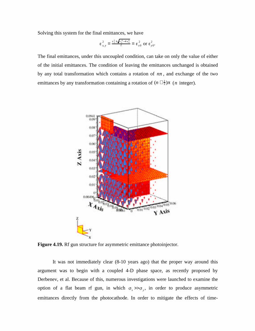
Figure 4.19. Rf gun structure for asymmetric emittance photoinjector.

It was not immediately clear (8-10 years ago) that the proper way around this

argument was to begin with a coupled 4-D phase space, as recently proposed by

Derbenev, et al. Because of this, numerous investigations were launched to examine the

option of a flat beam rf gun, in which x >> y , in order to produce asymmetric

emittances directly from the photocathode. In order to mitigate the effects of time-

dependent rf focusing on the horizontal emittance, a novel H-shaped structure was

designed, as shown in Fig. 4.19. This device needed emittance compensation, which is

quite different with an asymmetric rather than a symmetric beam. Because of the need to

avoid x-y coupling, solenoids may not be used, rather quad triplets must be implemented.

They are too length, however, to provide emittance compensation correctly.

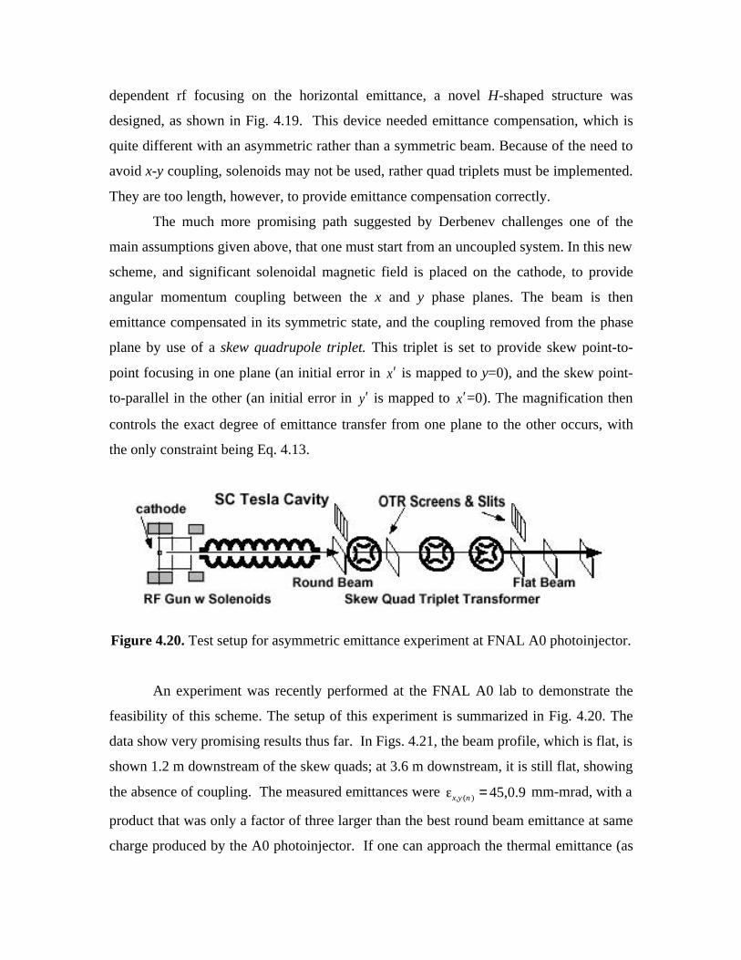
The much more promising path suggested by Derbenev challenges one of the

main assumptions given above, that one must start from an uncoupled system. In this new

scheme, and significant solenoidal magnetic field is placed on the cathode, to provide

angular momentum coupling between the x and y phase planes. The beam is then

emittance compensated in its symmetric state, and the coupling removed from the phase

plane by use of a skew quadrupole triplet. This triplet is set to provide skew point-to-

point focusing in one plane (an initial error in ′ x is mapped to y=0), and the skew point-

to-parallel in the other (an initial error in ′ y is mapped to ′ x =0). The magnification then

controls the exact degree of emittance transfer from one plane to the other occurs, with

the only constraint being Eq. 4.13.

Figure 4.20. Test setup for asymmetric emittance experiment at FNAL A0 photoinjector.

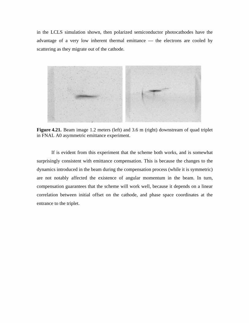
An experiment was recently performed at the FNAL A0 lab to demonstrate the

feasibility of this scheme. The setup of this experiment is summarized in Fig. 4.20. The

data show very promising results thus far. In Figs. 4.21, the beam profile, which is flat, is

shown 1.2 m downstream of the skew quads; at 3.6 m downstream, it is still flat, showing

the absence of coupling. The measured emittances were x,y (n ) = 45,0.9 mm-mrad, with a

product that was only a factor of three larger than the best round beam emittance at same

charge produced by the A0 photoinjector. If one can approach the thermal emittance (as

in the LCLS simulation shown, then polarized semiconductor photocathodes have the

advantage of a very low inherent thermal emittance — the electrons are cooled by

scattering as they migrate out of the cathode.

Figure 4.21. Beam image 1.2 meters (left) and 3.6 m (right) downstream of quad tripletin FNAL A0 asymmetric emittance experiment.

If is evident from this experiment that the scheme both works, and is somewhat

surprisingly consistent with emittance compensation. This is because the changes to the

dynamics introduced in the beam during the compensation process (while it is symmetric)

are not notably affected the existence of angular momentum in the beam. In turn,

compensation guarantees that the scheme will work well, because it depends on a linear

correlation between initial offset on the cathode, and phase space coordinates at the

entrance to the triplet.