University of Cape Town - COnnecting REpositoriesUniversity of Cape Town A Learning-based ... The evolution of communication standards promotes the development and use of several spectrum-sharing

Univers

ity of

Cap

e Tow

n

A Learning-based Scheme to Optimise a Cognitive Handoff

Kurai Luke Gombiro

This thesis is submitted in fulfilment of the academic requirements for the degree

of a

Master of Science (in Engineering) in Electrical Engineering

from the Department of Electrical Engineering in the

Faculty of Engineering and the Built Environment

at the

2015

The copyright of this thesis vests in the author. No quotation from it or information derived from it is to be published without full acknowledgement of the source. The thesis is to be used for private study or non-commercial research purposes only.

Published by the University of Cape Town (UCT) in terms of the non-exclusive license granted to UCT by the author.

Univers

ity of

Cap

e Tow

n

As the candidate’s supervisor, I have approved this dissertation for submission.

Name: Mr. Neco Ventura

Signed: ______________________

Date: ________________________

Declaration The presentation of this dissertation for examination is for the degree of a Master of Science (in

Engineering) in Electrical Engineering. Acknowledgment of all sources used, quoted, or

abstracted from, is in the references section of the document.

This work is not up for submission to any other university for any other degree or examination

and the University can reproduce this thesis for the purpose of research.

To both my grandfathers, for all the sacrifice and more.

(R.I.P Isaac Muguza Gombiro)

v

Synopsis The evolution of communication standards promotes the development and use of several spectrum-

sharing strategies. From the noted results, machine-learning techniques have paved a direction for

radio protocols to achieve better levels of performance. With their definition, efficient learning

practices and the use of effective spectrum sharing methods necessitate the development of better

channel selection schemes. In this work, a radios’ learning capability enables the manipulation of a

spectrum-sharing concept. This involves the radio obeying certain rules in a spectrum sharing

facility, which defines a decentralised form of coexistence (sharing) between the radios occupying

that specific radio space. Amongst other benefits, the sharing promotes the node’s independence in

the radio space, between the cohabitating radios for the essence of efficient spectrum sharing.

The learning dimension is realised by the use of a Stochastic Estimator Learning Automata

(SELA) algorithm. It allows a radio node to roam independently, while achieving the goal of

learning to control spectrum use over time. This is by selecting an effective action that defines the

radio’s channel choice, leading to the long-term benefit of learning the radio usage patterns. A key

condition for spectrum sharing requires that a ‘borrowed’ channel be handed-over to the owner, in

any network for the sake of fair sharing practices. The sharing practices promote the evolution of

spectrum use by making use of a device called a Cognitive Radio (CR). The CR, as a device that is

set to redefine the sharing landscape, creates a paradigm that will revolutionise the concept of

machine learning in the communications world. For the CR to have a good level of functionality,

the learning rate and evolution should be dynamic. This is because, the results from its interactions

with other users enhances its capability of coexistence and further promotes the progression of the

spectrum-sharing concept. The algorithm in use, the SELA, allows the scheme to exercise these

four steps for showing its key functionality. For the learning’s relevance, the steps are:

- An observation of the common activity forms in the radio environment, as a case of efficient

data mining

- The perception of the data acquired to have the learning take place, while achieving a level

of understanding of the radio environment for better decision-making options.

- The use of reasoning during the decision processes, for the scheme to manage the selection

of a channel during any service segment.

This allows any defined decision space to minimise a possibility of a channel handoff.

vi

- The use of an outcome from the environment to reinforce and evolve the learning cause,

for any future sharing purposes the scheme will go through.

From the scheme’s modelling in MATLAB, we have a view of the network activity levels and a

variation of the scheme’s channel selection trend. These results reveal the scheme’s performance

when evaluated in an emulated environment, to signify the CR capability as a secondary user of

any random network within its vicinity. From the performance analysis, we have the

management of a ‘created’ decision space leading to the service completion during that selection

segment. This nominated decision space is ‘conditioned to’ reduce any constraints found during

sensing stage, which can hinder the scheme’s capability to manipulate the network data to its

advantage.

Overall, this capability to manipulate network data delivers a network state that will

achieve better control of the service process. The scheme executes the service stage with an

active goal of managing the process of a Cognitive Handoff when it has to occur, which is to

release a requested channel for an active primary user. The service operation comes through the

following:

1. The estimation of a selection threshold from a hypothesis (discovered radio) space, which

is set out to limit the number of competing users during a service process

2. The development of a predictive state while creating a decision space provides a criterion

for a network’s rejection during a handoff, should it not match to desired utilisation levels.

This is from the independence found during a previous selection process and when

used as a reference, creates a set of avoidable ambiguous cases for the CR during

service

3. In turn, the management of the decision process allows the node to define a learning rate

and reveals how the found independence promotes spectrum-sharing practices that reduce

the high levels of underutilisation.

The state in a network, in the form of activity patterns, allows for the future provisioning of a

channel’s selection as a means of preparing for any possible handoff. This is by using a

benchmark defined by the previous action choice to define the level of service expectation during

that segment. The decision space estimation and the results from the scheme’s deduction during

problem formulation, leads to basing its current selection needs from the history outcome and

vii

evolves the selection scheme over time. As the cycle continues, the scheme realises optimality

in performance from learning the other users’ activity, leading to the management of a cognitive

handoff process.

viii

Acknowledgements I would like to thank many people for making this journey possible, with the first being the Lord

for granting me so many opportunities in life and bringing me this far.

Neco Ventura for all the assistance and guidance throughout the duration of study

My parents; words can never express how grateful I am for the level of sacrifice.

To my siblings and the greater family for the unconditional love and support

All my friends, for being the family I chose to have.

Bernard Muanda, Tinashe Chizema, Keegan Naidoo, Mamello Mongoatu and Colleen Goko,

for being there at the right time.

Nicholas Katanekwa, Ronnie Mugisha, Eric Mukiza, and Joyce Mwangama for leading the

way

Mary Hilton, for making me feel right at home

Carol Koonin, catch-up sessions will never be the same

Ayodele Periola for taking the time to render some valuable input in this work.

Everyone in the CRG family for the priceless moments in the lab.

The Electrical Engineering dept. particularly Janine, Karin, Marlene, Nicole and Rachmat, for

making life so much easier for us.

To everyone else for being there for me regardless, a huge thank you for having my back!

ix

Table of Contents

DECLARATION ....................................................................................................................................................... III

SYNOPSIS ................................................................................................................................................................. V

ACKNOWLEDGEMENTS ................................................................................................................................... VIII

TABLE OF CONTENTS .......................................................................................................................................... IX

LIST OF FIGURES ............................................................................................................................................... XIII

LIST OF TABLES ................................................................................................................................................. XIV

GLOSSARY .............................................................................................................................................................. XV

RESEARCH OVERVIEW ............................................................................................................ 1-1 CHAPTER 1

INTRODUCTION .................................................................................................................................................. 1-2

MOTIVATION FOR RESEARCH ....................................................................................................................................... 1-7 1.1

Research statement .......................................................................................................................................... 1-8 1.1.1

Problem identification ..................................................................................................................................... 1-9 1.1.2

Research questions ............................................................................................................................................ 1-9 1.1.3

ACHIEVABLE OUTCOMES ........................................................................................................................................... 1-10 1.2

SCOPE AND LIMITATIONS .......................................................................................................................................... 1-12 1.3

THESIS OUTLINE ......................................................................................................................................................... 1-13 1.4

OVERVIEW: THE COGNITIVE RADIO ................................................................................ 2-15 CHAPTER 2

INTRODUCTION ............................................................................................................................................... 2-16

THE COGNITIVE RADIO .............................................................................................................................................. 2-16 2.1

Motivation for the cognitive radio .......................................................................................................... 2-16 2.1.1

THE COGNITIVE CYCLE (HOW A COGNITIVE RADIO WORKS) ............................................................................... 2-18 2.2

Spectrum sharing schemes ......................................................................................................................... 2-18 2.2.1

SERVICE PROVISIONING IN AN OVERLAY ................................................................................................................. 2-24 2.3

Pro-activeness as an attribute .................................................................................................................. 2-25 2.3.1

The role of the radio environment .......................................................................................................... 2-26 2.3.2

Spectrum fragmentation and active synchronisation ................................................................... 2-26 2.3.3

Learning for service related moments .................................................................................................. 2-27 2.3.4

Spectrum Mobility and channel selection ............................................................................................ 2-28 2.3.5

TRAFFIC PATTERNS IN AN OVERLAY ........................................................................................................................ 2-29 2.4

The ON-OFF model ......................................................................................................................................... 2-29 2.4.1

x

The Hidden Markov Model (HMM) ......................................................................................................... 2-30 2.4.2

The M/G/1 priority queuing model ........................................................................................................ 2-31 2.4.3

SPECTRUM MOBILITY: A CASE OF SPECTRUM HANDOFF ....................................................................................... 2-32 2.5

Analytics for learning from the case under study ............................................................................ 2-33 2.5.1

BACKGROUND IN LITERATURE .................................................................................................................................. 2-35 2.6

Forms of channel selection ......................................................................................................................... 2-35 2.6.1

CHAPTER DISCUSSION ................................................................................................................................................ 2-42 2.7

LEARNING FOR THE MANAGEMENT OF A COGNITIVE HANDOFF ........................... 3-43 CHAPTER 3

INTRODUCTION ............................................................................................................................................... 3-44

PROVISION FOR LEARNING ........................................................................................................................................ 3-44 3.1

Forms of learning ........................................................................................................................................... 3-44 3.1.1

AN OBJECTIVE-BASED VIEW OF THE ENVIRONMENT ............................................................................................. 3-46 3.2

Operational conflict from coexistence ................................................................................................... 3-46 3.2.1

Node capability ................................................................................................................................................ 3-48 3.2.2

Computation levels to deal with the realised effects ...................................................................... 3-49 3.2.3

KEY DESIGN CONSIDERATIONS ................................................................................................................................. 3-51 3.3

Adaption to domain differences ............................................................................................................... 3-52 3.3.1

Policies for service (handoff) management ........................................................................................ 3-53 3.3.2

Robustness to instantaneous conditions .............................................................................................. 3-54 3.3.3

Pro-activeness for handoff cases .............................................................................................................. 3-56 3.3.4

FUNCTIONING CONTROL TASKS ................................................................................................................................ 3-57 3.4

Cognition though bias .................................................................................................................................. 3-58 3.4.1

Service oriented learning for decision moments .............................................................................. 3-59 3.4.2

Management of the learning process .................................................................................................... 3-59 3.4.3

AUTOMATED LEARNING METHOD: THE LEARNING AUTOMATA ALGORITHM .................................................. 3-60 3.5

STRUCTURE OF THE PROPOSED ALGORITHM .......................................................................................................... 3-63 3.6

The S-model Learning Automata based selection scheme ........................................................... 3-63 3.6.1

Reasoning during a reactive decision .................................................................................................... 3-68 3.6.2

Key metrics for spectrum decisions ........................................................................................................ 3-70 3.6.3

CHAPTER DISCUSSION ................................................................................................................................................ 3-70 3.7

MANAGEMENT OF THE SELECTION PROCESS AND OF A COGNITIVE HANDOFF 4-72 CHAPTER 4

PRELIMINARIES OF THE PROPOSED SELECTION SCHEME ..................................................................................... 4-73 4.1

The channel composition (Sensing phase) .......................................................................................... 4-73 4.1.1

Criteria for Context selection .................................................................................................................... 4-74 4.1.2

Conditions for channel selection between users ............................................................................... 4-76 4.1.3

xi

TRAINING FOR FEATURE IDENTIFICATION .............................................................................................................. 4-77 4.2

Using bias from the HMM ............................................................................................................................ 4-78 4.2.1

Feature estimation and selection (reasoning based) ..................................................................... 4-81 4.2.2

Observed effects from the Hidden Markov Model ............................................................................ 4-82 4.2.3

The realisation of the expectation vs maximisation ....................................................................... 4-84 4.2.4

SPECTRUM DECISION (EVIDENCE OF A SELECTED CHANNEL) .............................................................................. 4-86 4.3

Domain selection and differences observed ........................................................................................ 4-87 4.3.1

Control during domain selection ............................................................................................................. 4-88 4.3.2

Learning for domain selection moments ............................................................................................. 4-90 4.3.3

THE HANDOFF MOMENT (EXECUTING HANDOFF) ................................................................................................. 4-91 4.4

Variables for handoff execution ............................................................................................................... 4-91 4.4.1

The objective satisfaction stage ............................................................................................................... 4-92 4.4.2

CHAPTER SUMMARY ................................................................................................................................................... 4-97 4.5

EFFECTIVENESS OF A LEARNING SCHEME FOR MANAGING HANDOFF ................ 5-98 CHAPTER 5

FRAMEWORK DEFINITION ......................................................................................................................................... 5-99 5.1

Deliverables from the framework ........................................................................................................... 5-99 5.1.1

IMPLEMENTATION PROCEDURE .............................................................................................................................5-101 5.2

Exploration stage (effective sensing capability for metric definition) ................................. 5-101 5.2.1

The use of bias for training ...................................................................................................................... 5-103 5.2.2

The learning stage (exploitation and reasoning capability) .................................................... 5-105 5.2.3

EVALUATION OF THE SCHEME ................................................................................................................................5-106 5.3

The relevance of efficient exploring (a case of data mining) .................................................... 5-106 5.3.1

The essence of training .............................................................................................................................. 5-109 5.3.2

The definition of exploitation (the learning based selection process) .................................. 5-113 5.3.3

The effect of prediction on learning ..................................................................................................... 5-122 5.3.4

Significance of a good decision ............................................................................................................... 5-123 5.3.5

CHAPTER SUMMARY .................................................................................................................................................5-125 5.4

CONCLUSION .........................................................................................................................6-127 CHAPTER 6

SUMMARY ..................................................................................................................................................................6-128 6.1

RECOMMENDATIONS ................................................................................................................................................6-131 6.2

BIBLIOGRAPHY ................................................................................................................................................. 133

ANNEXE A: THE REALISATION OF LEARNING BASED ON CONTROL FROM THE SCHEME ......... 140

ANNEXE B: TABULATED RESULTS OF THE SCHEMES PERFORMANCE ............................................ 141

APPENDIX A: THE VARIABLE STOCHASTIC LEARNING AUTOMATA (VSLA) ALGORITHM ........ 150

xii

APPENDIX B: THE BAUM-WELCH ALGORITHM ..................................................................................... 153

APPENDIX C: ACCOMPANYING CD-ROM .................................................................................................... 156

xiii

List of Figures

Figure 1-1: An analysis of Spectrum usage patterns, as outlined by the FCC on a traffic per site (base station)

basis, to evaluate the utilisation levels of spectrum [1] ................................................................. 1-4

Figure 1-2: A comparative representation of the spectrum sharing methods .................................................... 1-5

Figure 1-3: A diagrammatic representation of the Underlay model [2] ............................................................. 1-5

Figure 1-4: A 2 Dimensional view of the Overlay model for spectrum sharing purposes [3]. ............................. 1-6

Figure 2-1: Environmental stimuli as perceived by the CR [6] .......................................................................... 2-17

Figure 2-2: The cognition capability projected into a cycle of operation to exhibit cognition [9]. ..................... 2-18

Figure 2-3: The Power Spectral Densities (PSD) differentiating the sharing schemes. ....................................... 2-20

Figure 2-4: A relationship of the link maintenance and evaluation phases of handoff [17]. .............................. 2-24

Figure 3-1: The Stochastic Learning Automata concept, showing a relationship with the stimuli...................... 3-62

Figure 4-1: The schemes outlay, defining the main, and sub processes of the schemes progression ................. 4-75

Figure 4-2: HMM modelling of the state patterns in the network [67]. ............................................................ 4-80

Figure 4-3: The state characterization for the perceived prediction strategy.................................................... 4-88

Figure 4-4: A flowchart showing the execution of handoff in an overlay network. ........................................... 4-96

Figure 5-1: Channel values from the use of network A .................................................................................. 5-107

Figure 5-2: Channel values from the use of network B .................................................................................. 5-108

Figure 5-3: Channel values from the use network C ...................................................................................... 5-108

Figure 5-4: The comparison of network activity in view of a node’s random channel selections..................... 5-109

Figure 5-5: Channel selections based on the training scheme for network A .................................................. 5-110

Figure 5-6: Channel selection based on the training scheme for network B ................................................... 5-111

Figure 5-7: Channel selection based on the training scheme for network C ................................................... 5-112

Figure 5-8: The comparison of network activity during service provisioning from a HMM ............................. 5-113

Figure 5-9: A comparison of the deduced hypothesis values for network A ................................................... 5-114

Figure 5-10: A comparison of the deduced hypothesis values for network B ................................................. 5-115

Figure 5-11: A comparison of the deduced hypothesis values for network C .................................................. 5-115

Figure 5-12: The comparison of network activity when making use of the learning scheme ........................... 5-116

Figure 5-13: Channel selection in Network A, during a service phase ............................................................. 5-117

Figure 5-14: Channel selection in Network B, during a service phase ............................................................. 5-118

Figure 5-15: Channel selection in Network C, during a service phase ............................................................. 5-119

Figure 5-16: The blocking probability values for network selection during service ......................................... 5-120

Figure 5-17: The variation of idleness to show context desirability. ............................................................... 5-120

Figure 5-18: A comparison of handoff control during the training and learning segments .............................. 5-122

xiv

List of Tables

Table 2-1: A comparative description of the Underlay, Interweave, and Overlay CR techniques [10] ............... 2-20

Table B- 1: Activity patterns for the first network ............................................................................................ 141

Table B-2: Activity patterns for the second networks ....................................................................................... 142

Table B-3: Activity patterns for the third network ............................................................................................ 142

Table B-4: Activity in network one during service provisioning from the HMM ................................................. 143

Table B-5: Activity in network two during service provisioning from the HMM ................................................ 144

Table B-6: Activity in network three during service provisioning from the HMM .............................................. 145

Table B-7: Activity in network one during learning ........................................................................................... 146

Table B- 8: Activity in network two during learning the exploitation stage ....................................................... 147

Table B-9: Activity in network three during learning the exploitation stage ...................................................... 148

Table B- 10: Assessment of an exaggerated level of bias during the exploitation stage ..................................... 149

xv

Glossary

1. The Automation process is when a channel in any sub system, (a segment in an

environment or a network) is rewarded by the scheme for producing a positive outcome

from the decision given as input into the nominated environment.

2. Belief is the state that a context, considered a network, is in during that decision segment.

This allows the scheme to identify the current form of activity in the partitioned

network, for the development of the channel selection policy for that epoch (instance).

3. Cognition is a feature that enhances any Radio to make use of the Dynamic Spectrum

Access (DSA) concept

4. A Cognitive Radio is a communication device that enhances the use of the DSA concept

by making use of optimal parameters during a service session

5. Dynamic Spectrum Access (DSA) is a unified spectrum usage concept, which allows

radios to make use of the spectrum as a pool of radio resources. This is by giving

preference to the owners of the spectrum band and having other radio users on a secondary

user basis, make use of the relative bands within conditional operating capabilities.

6. Environment is a state space that has all the radio related stimuli defining the other radios

activity for the CR to make use of the cognitive cycle.

7. Handoff is the releasing of a current channel occupied by a SU to a specific PU, which is

taking the channel for use in its own network.

In certain cases, it can be the releasing a channel and waiting for the resumption of

service to continue with service, as a form of non-switching handoff.

8. Hidden channels/states are channels that are not visible during a sensing segment. These

obstruct the CR operation by reducing the channels in the state (network) space that is

desirable to the CR during a specific channel selection segment.

9. Learning is a process that any CR scheme utilizes to increase the level of optimality the

cognitive node can achieve when roaming in any environment

10. Management in this work is taken as the execution of the decision process, leading to how

the selection policies will complete any form of mobility that will come with each current

service phase

11. Network Activity Factor (NAF) is a relation to the NVF and this allows the scheme to

xvi

derive the hypothesis space for its problem formulations.

This defines a context or network space that the CR will find to be active and opt to

select it because of the level of activity during that selection segment.

12. Network Value Function (NVF) is a value attached to a network for the definition of a

reliability level as a hypothesis. This allows the scheme to maximize the belief of the

network and prepare for a decision moment, based on the derivation of this value.

13. A node/s defines the CR/s as a radio unit during the any stage of the scheme’s execution.

14. Optimize defines how the scheme will try to minimize the number of mobility counts

during each service session. This is to achieve a service count with as little handover as

possible

15. Policy is a defined service objective that will deal with any active effects found within the

environment. The definition of a policy assists the learning algorithm to create a decision

space that will have the scheme maximize the cognitive features in that environment.

16. Redundant data is found when certain parameter values are revealed as content that does

not change when a sensing segment occurs. These occur when the network state does not

change resulting in the node making use of the same values or space state.

17. The scheme’s level of Robustness will have it less susceptible to resulting effects of the

instantaneous conditions when the state has a change in its current observation pattern

18. Self-reliance is a mode that has the CR roaming without the assistance of a central

controller when making decisions.

This enhances its survival chances in a non-cooperative decentralized network.

19. State is a term used interchangeably depending on its relevance; it defines a network

segment as selected by the scheme or a channel either in an ON or OFF state during the

training run.

20. Step size is a measure of the number of runs the learning scheme would have gone through.

This increases the level of competence expected from the learning scheme as a means

to show the level of operational experience the algorithm has in any environment.

21. A use-case scenario is an abstraction of the environment state during that segment. This

defines a case that the scheme will use from the resulting belief adoption.

22. The value Iteration Process (VIP) is the derivation of a context or network’s worth during

a channel selection segment. This derives the effective parameters for selection with which

xvii

when manipulated; formulates the decision space for the node to begin the objective

formulation for that current selection segment.

Research overview Chapter 1

Research overview: Spectrum Mobility

& the Dynamic Spectrum Access (DSA) concept

1-2

Research overview

Introduction

Traditional radio systems produce traffic patterns that are dynamic, and the variance promotes

the evolution of management strategies to formulate better radio usage practices. Because of the

systems’ evolution, the number of connected devices keeps rising due to the adoption of the

Software as a Service (SaaS) paradigm. This shift in the forms of service delivery engages

consumers to access services while on the go, for the sake of convenience. The convenience

however comes at a cost for the operators to provision for network resources and more so,

fuelling costs of doing so. The modifications to the network infrastructure done after such a turn

translate into a high demand for spectrum, for the operator to continue with desired service

provisions. The spectrum allocation process as controlled by regulators reveals a level of

underutilisation as seen through recent studies of spectrum use, exaggerating the demand of

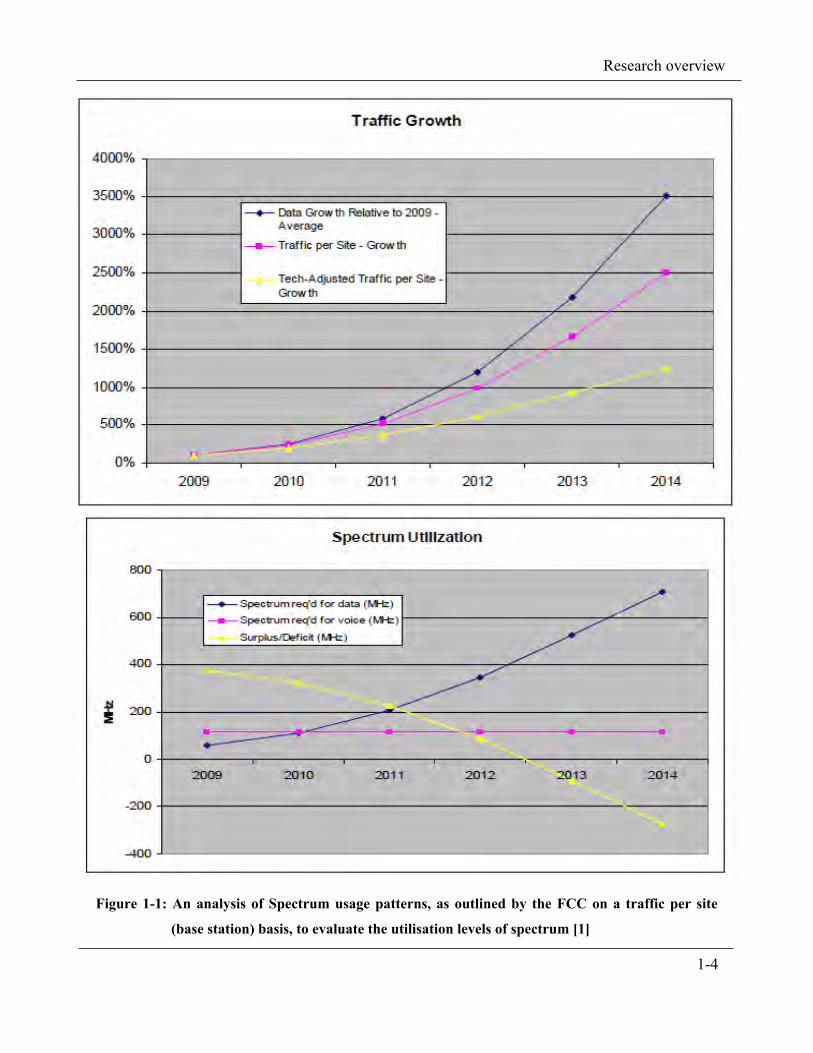
spectrum on a per user basis. The data shown in figure 1-1 gives an outline of the traffic

observed per site (as a percentage value). This is on a year on year basis, giving the range of

usage patterns exhibited on the network as conducted by the FCC. The second diagram at the

bottom shows the underutilisation trend for radio usage traffic and the observed surplus/deficit

shows the change in traffic patterns [1].

Research efforts to promote better forms of spectrum usage, are trending toward the use

of systems that use radio resources in a more effective manner. This is by developing strategies

for the radio systems’ operational capability to share resources while cooperatively accessing

service from a network. The realised coordination should not affect the capabilities of the other

users within that same band. Such a coordination of networking devices, called the Dynamic

Spectrum Access (DSA) is a type of architecture that makes use of a family of technologies

called the Cognitive Radio (CR). The CR is capable of modifying their operating parameters

into a form that will allow the usage of a particular range of frequencies, in a radio band that the

particular cognitive node will be occupying. As the CR’s adoption tries to bridge the divide

between the old and new forms of spectrum usage, it outlines the need for effective methods to

use the open spectrum bands. The old spectrum-sharing concept, ‘a command and control’

model classifies how the incumbent, (the holder of the license) is going to operate. Essentially in

such a case, if a radio is outside its specified band of usage, it cannot get service unless if the

service providers have a sharing agreement. This is typically during National Roaming, which

1-3

Research overview

allows a smaller operator to use the larger operator’s network for service continuity as shown in

figure 1-2.

1-4

Research overview

Figure 1-1: An analysis of Spectrum usage patterns, as outlined by the FCC on a traffic per site

(base station) basis, to evaluate the utilisation levels of spectrum [1]

1-5

Research overview

Spectrum Sharing

National roaming

Dynamic Spectrum Access

Mobile virtual Operator (MVO)

Roaming Agreement

PU - Owner of band

SU - Leasee

With consent to the sharing of spectrum by a contract

(can involve monetary value)

Without consent but this is confined to regulatory

standards when utilised

Classical - command and control method

Unbound spectrum sharing method

Figure 1-2: A comparative representation of the spectrum sharing methods

The CR’s capability in any network is realised through a coexistence model that it has to adapt to

when making decisions. This defines how the radio is to manage the interference levels towards

the owners of the licenced bands, called the Primary Users (PU). There are two defined models:

the underlay and overlay designs that divide how the number of communicating devices in a

network should transmit their signals, while sharing any spectrum bands. Of the two designs, the

underlay model has the CR, also known as the Secondary User (SU) sharing spectrum with

various PU. It does this by regulating its power to a level lower than that of a PU receiver’s

sensitivity, so as not to interfere with the on-going transmission. The DSA paradigm involves a

cycle used by the CR to suit the parameters suitable for that particular band. This cycle, dubbed

the Cognitive cycle, has the radio making a 4-stage pattern of operational adaptation, between

the spectrum sharing, decision and handoff moment, leading to the mobility stage in the PU

Figure 1-3: A diagrammatic representation of the Underlay model [2]

1-6

Research overview

network.

Figure 1-4: A 2 Dimensional view of the Overlay model for spectrum sharing purposes [3].

The overlay model, as shown in the figure 1-4, is when an SU occupies a channel from any

spectrum band in a ‘hop fashion.’ This is in-between the spectrum bands called ‘spectrum holes’

or ‘white spaces’. The utilisation of the white spaces is if and only if (iff) they are not being

used by a PU in that particular band. When the radio is initialising a communication session, a

decision made by the node has the radio occupying a channel if deemed suitable for use at that

moment. The channel in use, if requested for by a PU, forces the SU to vacate the channel in

question to select another vacant channel, identified through a recent search done by the radio.

This moment constitutes as the handoff phase and the continuation of the current transmission by

the SU is on another channel. This channel’s selection can be in the same or in a different band

found to be acceptable for use, during that stage by the radio.

The CR’s transition from one band to another forms part of the cognitive cycle and

characterises the spectrum mobility phase. This type of mobility, called spectrum handoff, is

more apparent in the overlay model. This comes from the radio’s ability to control parameters

used during operation as defined below, by making use of the following steps:

1. a searching phase (defined by the sensing of idle spectrum bands in the overlaid networks)

2. a spectrum decision segment, where there is the selection of a good channel in a band

3. a spectrum handoff process, which is when the CR is forced to move to another channel

having been caused by the (possibly) multiple disturbance from the primary user

1-7

Research overview

4. a mobility phase, which is the proper execution of spectrum handoff to another spectrum

band [4]

Motivation for research 1.1

Research efforts in the CR area show a great deal of detail being required during the

design stage of a Cognitive node’s protocols. As each stage of the cognitive cycle has its own

demands, the most affected are those that involve change during spectrum use. The effects

realised by the node are at times in an ambiguous form as the roaming in different environments

progresses and this is due to the CR interaction with various PU and random patterns they exhibit

in each environment. As a result, the recognition of a CR performance comes from its successful

completion of the characterisation process (recognition of an environment’s actual state),

together with the observed effects of the PU within that segment of the radio environment. As

the CR development is centred on its ability to develop operating strategies through learning, the

level and capability of adaption should as well, evolve with time. These operational patterns

define a basis of coexistence and this is in relation to the node’s interpretation of these other

users’ activity levels.

For a seamless mobility phase, the management of any ‘possible’ effects observed from

PU is for the node to prepare for any forms of unpredictable traffic levels, in any network band

that the radio will select. The conditions in each environment tend to vary and at times, an

exaggeration can or tends to occur. This comes from how well the cognitive node is receiving

the information from the surrounding based on the level of activity in the network. A distinction

observed in some related work shows how the CR node subtly neglects some factors

‘considered’ relevant during a channel selection segment for the execution of handoff. This

predominantly, makes the node resort to the use of a greedy form of selection as the need to

contend for the best channel increases with each selection instance. In certain scenarios, the CR

node neglects some of the pertinent factors during the mobility phase, as a means to avoid a lot

of channel switching and this usually results in the handoff process failing. From such a

standpoint, the maximisation of a handoff opportunity to a new channel is not effective as there

is a poor characterisation process of the current activity levels in the occupied spectrum band.

Taking the characterisation process as a basic requirement for the CR’s channel selection

1-8

Research overview

process, this defines how the node will make use of this operation as a basis for learning. To this

effect, the channel selection process (particularly when in a handoff scenario) will not only be

lacking the long-term capability to progress (the management of handoff), but realises a different

level of computational complexity due to the differences found in the spectrum bands.

A channel, if realised as a basic spectrum unit in terms of spectral use, makes it easier for

the decision process to be maximised. Channels used in a quantified state such as a threshold

value are limited to that condition of use, mostly expressed by the signal strength. In such a

case, the node cannot negotiate for a different outcome if needed, especially during an instance

when the threshold levels do not tally to the level of expectation. This is a very controlling

condition, during the selection of a channel for the node’s execution of service or spectrum

handoff; where there is no time to balance the outcome from the sensing phase vs. expectation

(understanding) of the environment. From such an experience, the difficulty (found in the CR

context) comes in balancing the requirements needed at that point to change to a different

channel. This usually, is in contrast to the requirements that the radio can control to reduce

further delay, as the need to process the transfer of data is imminent. As a result, the

computational complexity increases as the value of data points (in the form of the different

channels structures) vary per band. From such a realisation, the selection process is prolonged

further invalidating the learning process.

The determination of the level of any network’s activity, together with the random

elements in the different environment segments usually causes the CR to reconfigure further than

it needs to. Therefore, the creation of an operating metric for the CR to use a state (network) is

ideally to make the process more selection process more dynamic. This comes as an added

advantage, especially during a spectrum handoff segment when the radio has reduced ‘time

privileges’ in which to make a decision, based on the available information. The realisation of

any varied effects during channel selection shows a need for the selection scheme to be resilient

to any conditions identified i.e. the contention or misidentification of the channel opportunities

[5].

Research statement 1.1.1

The CR’s architecture outlines how imperative it is to have a defined spectrum decision-

1-9

Research overview

making strategy and further enhances the required level of performance in the DSA scheme. It is

apparent from the non-deterministic behaviour (randomness) of the environment that the CR can

adopt ways that lower or reduce the effects of spectrum underutilisation. This is more so during

the selection of any bands and it should be in a manner that enhances its own service levels for

the realisation of an effective DSA process. With this form of operation, any policy for the CR

should have a proactive element to deal with the mobility process, for effective sharing purposes.

Problem identification 1.1.2

A number of schemes identified in literature keep the learning aspect during a CR’s

channel selection process. The learning element then becomes a key performance

optimiser and often, a limitation during the definition of a learning process can occur. This is in

relation to the management of a cognitive handoff and to validate this cause, the flow of the

selection process should allow for some independence and raise the need for adaption to these

differences. The independence realised by the node through learning can maintain a

consideration of a n y r a n d o m f a c t o r s a n d include them as possible conditions during the

selection process. The cognitive radios operation should not be privy to these factors, as the

learning and levels of optimality come from the use of the different environments. The

subsequent stages after each selection process should evolve the decision-making approach,

allowing the progression of learning cause and for effective handoff management. This in turn,

defines an updated strategy each time the radio is disturbed and this enhances the execution of

handoff in a different environment [5].

Research questions 1.1.3

From the various efforts in related work, a number of issues observed when

implementing any form of a learning based selection process, tend to vary. When optimised for,

these issues can lead to the definition of better operational levels for the CR. The issues come

with differing weight levels and lead to the inquiry of how the selection of a channel should

work for the CR. The points below define how we are going to model the selection process:

- What key processes can enhance the verification of a channel‘s availability e.g.

1-10

Research overview

environment activity, the verification of hidden states etc.?

- How can certain elements lead to the optimisation of channel selection process e.g. the

rate of disturbance during transmission, poor input of important data structures etc.?

- What criteria can best define the selection process to allow for better service outcomes?

- How can some of the options available to the radio (possible actions), enable the radio to

make its own conditions of operation or something related to thereof?

- How some parameters can be adapted for use during the management of handoff process?

- To define a spectrum usage method that evolves with the scheme’s operating curve.

Achievable Outcomes 1.2

The premise behind this dissertation is the use of a radio’s cognitive attribute,

particularly the learning element, to enhance the decision-making capability needed during

spectrum sharing. This is by enhancing the management process that the node utilises to

make decisions such that, there is an efficient utilisation of spectrum. To achieve this, below

are defined objectives and their sub goals from a detailed study of the DSA concept. From the

review process, we have the hand over facilitation in the learning scheme for the decision-making

to be a better-managed process. The following points summarise the flow of the learning

scheme’s development process, in the three stages that separate them:

1. An extensive literature review will outline the elements of the spectrum sharing process.

a. This is going to assist in defining a framework for implementing the case under

study, which is of managing the decision processes to avoid a lot of spectrum

handoff.

b. It will provide a criterion for comparison of the current handoff approaches with the

learning based schemes, as well as how they deviate from the learning concept.

c. Overall, the review should reveal a method for the node to reveal a self-management

element, which enhances the roaming capability in a decentralised architecture.

2. From the spectrum sharing definition, the next step involves the use of defined traffic

structures, generating random forms of traffic. The traffic patterns define an underlying

channel state model to bias the forms of state observations as seen by the CR. This is a

1-11

Research overview

minimum requirement for the node to learn any patterns exhibited by PU and how the SU

will put them to use when in any PU network with any defined sharing model.

a. The observed patterns will facilitate the recognition of all possible PU identifiers.

These come as features that allow the CR to maintain their association with its own

spectrum use. This is with the PU and other SU that may be in the network as well.

b. The visible patterns should allow the node to learn the distinctions between any

features during the evaluation of any state (network) model. This will allow the

node to use the features as cases, when it has to reason for a decision during the

selection of a channel, either for service provisioning or during a handoff moment.

c. This stage counts as a form of training, to have the cognitive node initialise the

recognition of the choices (actions) that it can use when it wants to make a decision.

This will define the selection process as an extract from the learning scheme and

then benchmark how any future selection segments, will have an optimised criteria

to base on. This method of context (network bands) selections will enable a

guaranteed level of performance from the radio, as a proactive approach to deal with

any handoff cases.

3. To engage the scheme’s three main attributes fully i.e. the learning, control, and adaption;

this stage involves an analysis of the decision management process. This is during the

state (network) identification segments, leading to the selection of a channel during a

handoff moment. This will represent the (learning and) management process, based on:

a. How the node utilises its network (state) characterisation method to manipulate the

network resources based on available environmental data semantics. This is through

a load balancing based approach (a cooperative scheme), in a decentralised network

to gauge on the capability of the CR to be self-sufficient when making decisions.

b. The use of a learning-based scheme for the selection of a channel and this is for the

cognitive node to reduce the need to engage in multiple handoff counts, during the

roaming cases in the various environments.

c. Overall, the differences between the designed framework and the random

management process will outline if the scheme is performing at an optimal level of

1-12

Research overview

operation. This will allow for the derivation of any concluding remarks for any

future work that can be done or corrected thereof.

The use of a learning approach for modelling of a decision process, allows for the redirecting of

its current parameter estimations to the next epoch, which is after the CR has been pre-empted

from the active channel. This is for service continuity with a better management technique of

any effects from that point forward. For the node to base any future decision-making on the

history patterns, the multiple forms of disturbances allow for recognition of the usage patterns

from the previous choices made during decision-making. The above objectives are some of the

scenarios used during the operation of the proposed scheme, as used by a CR in a PU network

and for us to show proof of concept. The definition of this work in summary is through the

following points:

1. To make use of a management technique that aims to reduce the occurrence of handoff

effectively, regardless of the nature of the traffic in the environment

2. To investigate the level of resilience the scheme has in an emulated environment, through

a reasoning based-learning approach, as a means to satisfy the channel selection process.

Scope and limitations 1.3

This work focuses on the selection of a channel for a CR and the extension of the state’s

(network) activity to a segment where the ‘same parameters’ can manage a cognitive handoff.

When extending this operational dimension to any form of learning in the environment, the node

uses the current service level as a basis of adaptation from one epoch to another. From this view,

the learning element defines how the node at any point will decipher the effective parameters for

managing the handoff process. This complements any decision it makes in that environment to

account for the benchmarking of the service progression through the different networks i.e.

details from the previous selection segment to the next channel in use. From such a basis, the

definition of the scope of this work is around the following focal points:

- The node is set to be roaming in an overlay architecture. This is with a decentralised type

of approach that will have all the decisions made sorely by the node, for it to access

service.

- The decisions made by the node, are sorely to show its capability (independence) without

1-13

Research overview

the facilitation of a central controller and not abiding to the structure of an ad-hoc

network.

- The access is in the uplink part of service because the controller of the network that the

node has selected to make use of, caters for the downlink part of the transmission.

- The use of a learning method is through a reinforcement learning based approach and this

is to enhance the reasoning capability, which is the biggest factor being made use to effect

the mobility during the handoff moments.

- The proof of concept is through the emulation of the cognitive capability for the node to

derive an effective decision-making scheme and parameter usage capability.

For the node to execute handoff and allow for better mobility management, there are a few

assumptions made for the effecting of such a scheme for the cognitive radio. These are:

1. That an appropriate sensing mechanism is used, which will allow for the compensation of

the transmission loss, should this occur.

2. That there will be updated channel values, together with an activity profile in the network

to have the channel definitions relate to the required Quality of Service (QoS) levels.

This is when the node has to make a channel switch and the profiling can then award

us with the use of the various triggers. These triggers can be in the form of various

parameters, which should allow the cognitive handoff to be an optimised operation at

any instance, as there are no device specific parameters.

Thesis outline 1.4

The body of this thesis is in six parts, and the presentation is as follows:

Chapter 2 presents a background on related work in spectrum sharing methods. It outlines the

importance of some key variables that affect the node during any operational phase. With this,

an analysis to assess how some of the selection methods perform follows subsequently, outlining

how they can fit to the criteria of selection that we are trying to propose for spectrum mobility.

Chapter 3 presents the variables considered relevant for the development of the decision making

scheme, the CR node will adopt. These are set as the key functional requirements for a cognitive

node to share spectrum with other users on a management basis. It also presents the definition of

the learning strategy to show the importance of the network characterization for the spectrum

1-14

Research overview

decision process. This will lead to the presentation of the learning scheme for the channel

selection process, when a node has to perform handoff and its automation strategy.

Chapter 4 expands on the background that the third chapter gives for the learning method and

presents the structure of the evaluation method. This includes a background into the choice of

the coexistence framework and further outlines the factors considered, while developing the

operational structure of the selection scheme.

Chapter 5 is an analogy of the work regarding the deliverables of the scheme. This is going to

define how it should fair out when it has to make decision during a channel selection process.

The expected results are required to show the proof of concept, relative to how learning is an

effective optimiser of the decision making process.

Chapter 6 presents a set of concluding remarks, expressing the issues that came out from the

evaluation of the scheme as presented in the first chapter.

Overview: The Cognitive Chapter 2

Radio

Overview: The Cognitive Radio

& the Channel Selection Process

2-16


Introduction

In the previous chapter, we have an overview of the spectrum-sharing concept while looking into

the role of the CR in the DSA scheme. This is predominantly for the management of any factors

that govern the channel selection process for a CR node, from a spectrum decision point of view.

This chapter presents a definition of the CR standard; discusses the relevance of the cognition

element together with how the channel selection process has an effect on the operation of a CR.

Subsequently, an analysis of related work follows together with a discussion of the detailed

features in their work. This is to say, for the credibility of our work, the analysis of their

nominated strategies will include the merits and de-merits of their solutions during the handoff

process.

The Cognitive Radio 2.1

The design of a cognitive radio, in comparison with the structure of most communication

devices, makes it imperative that the sharing concept offers spectrum resources effectively. The

introduction of the CR in this chapter elaborates on the CR related features and defines the forms

of coexistence with other users in any PU network. For the purpose of this work, the

presentation of the CR framework is in an overlay architecture to show the need for handoff

control.

Motivation for the cognitive radio 2.1.1

The spectrum bands in the radio environment consist of various forms of channel activity.

If we regard each channel as a basic unit of spectrum, the provisioning of service is because the

channel is in use during that epoch irrespective of the user. As such, the CR redefines spectrum

usage patterns and allows for a more relaxed use of the underutilised spectrum bands owned by

the licensed users. Apart from rules from the licensing scheme, there is need for a CR to show:

- a reliable performance level during communication; this is to say that it should be able to

manage and control all forms of service provisioning

- a provision for an efficient and effective method of using of any spectrum bands

- gain various forms of capacity usage mechanisms of the radio environment, such as how to

2-17


adapt to an environment when needed due to resource availability

- the need for a unified system of rules allowing the radio to roam in unknown boundaries

The consideration of spectrum as a lacking resource during the provisioning of a radio service is

because of the command and control based regulatory methods. When coupled together with

the aforementioned conditions, the Federal Communications Commission (FCC) of the USA

gave a definition for the CR standard. This definition presents the CR as ‘A device that is

capable of changing its transmitters parameters, based on its interactions with the

environment in which it operates in’ [7]. A lot of research into the definition of

spectrum use and service provisioning has produced results leaning towards the evolution of the

DSA concept. The premise behind most research efforts optimises the application of the CR

standard to the usage patterns observed from the sharing method in any PU network. With this

in mind, several regulatory bodies have endorsed a unified spectrum sharing policy for the

wireless radio systems.

From the research conducted, the learning element brings out effective methods to enhance

the performance of the CR. This allows the manipulation of its hardware to attain the highest

level of performance, based on the stimuli coming from the radio environment. Figure 2-1

shows a representation of how the environmental effects have an impact on the CR

decision-making process, basing them on the provision of actions and decisions for its

cognitive behaviour. The occupation of spectrum holes in-between the PU periods of

Figure 2-1: Environmental stimuli as perceived by the CR [6]

2-18


operation shows the level of access gained by the SU for spectrum use. This is an attribute

showing the radios dependency on learning, while adapting to any activity patterns (defined as

data sets) such that it can optimise its performance in return. The enhancements on the data sets

is a regressive process as the PU patterns change over time, creating a trend of operation for the

CR, through adaptation [8].

Figure 2-2: The cognition capability projected into a cycle of operation to exhibit cognition [9].

The Cognitive cycle (how a cognitive radio works) 2.2

The cognitive cycle as a basis for the CR operational behaviour, allows the radio to make

use of the Dynamic Spectrum Access (DSA) concept in any environment. This is because the

four defined phases of operation within its cycle are put to use to define the node’s level of

potential when it needs to provision for service. The phases in the cycle are complementary and

bound by the form of sensing employed for detecting suitable bands for the radio to make use of

imminently. Figure 2-2 shows the old and new outlines of the cognitive cycle, with its four main

phases of operation. These define the key elements that exhibit how it will behave during any

associative segment and make use of an action defining the CR’s option.

Spectrum sharing schemes 2.2.1

Sharing in a cognitive network is specific to a model, which defines how the network

occupied by the SU is set up. It has a centralised or decentralised approach, which is set on a

2-19


cooperative or a non-cooperative scheme. The schemes come with different rules defined

according to the model in use for spectrum sharing. The centralised approach has a spectrum

broker, which governs how the radios access service on the network and the decentralised model

is when the cognitive users can assign routing patterns themselves. The decentralisation

approach creates a need for the cooperation of all users involved, where they will assist each

other during channel selection or the non-cooperative scheme that has each node acting

independently [10].

2.2.1.1 Spectrum sharing models The models defined in this section explicitly outline how the CR associate themselves

with the sharing of any network. These are the Underlay, Interweave, and Overlay schemes, and

the SU makes use of them based on an abstraction of the other radios power spectral densities

(PSD). This is a factor defining how the radio will behave in each model as shown by figure 2-3.

The Underlay model is when both PU and SU share the same spectrum band and have their

power densities within the same noise floor. The SU has to operate within an acceptable level

of noise during its own transmission and not towards the PU. This is strictly for coexistence

purposes and the level of power that the SU uses should be below the PU sensitivity margin.

The management of any interference caused is by keeping a more deterministic mode of

operation, mostly utilised in the Ultra-Wide Band spectrum access scheme [10].

The Interweave model is an opportunistic method, where the termination of service that the

SU is getting in the PU network can occur randomly. This is from the point when the PU

arrives and the SU has to vacate the nominated channel immediately, by having its current

transmission either forcefully terminated or relocated to another band. With this model, a

very accurate sensing method is imperative as it assists in the definition of the occupancy

patterns observed by the SU. This is for the desired spectrum bands at that point as the

unpredictable traffic levels tend to force service terminations [10]. Another issue is of the SU

having to know the dimensions of the network for it to change to, each time a displacement

occurs and this where it differs from the overlay model as shown in table 2-1.

2-20


Figure 2-3: The Power Spectral Densities (PSD) differentiating the sharing schemes.

Table 2-1: A comparative description of the Underlay, Interweave, and Overlay CR techniques [10]

Underlay Overlay Interweave

SU transmitter has knowledge

of the PU sensitivity margins.

SU can transmit

simultaneously with PU user

as long as interference caused

is below an acceptable limit.

SU transmit power is capped

below the transmit power used

by the PU

SU have a knowledge of the channel state

information in the environment and any possible

detail relating to the PU channel usage patterns.

SU simultaneously transmit with the PU and the

control of the interference is by relaying part of

the PU messages.

SU can define their spectrum choices based on

how capable it is to make use of the related

spectrum band.

SU have knowledge of the spectrum

holes regardless of the owner of the PU

SU can transmit at the same time as the

PU but this is limited to cases where

there could be a false alarm in

detecting spectrum holes.

The SU capability is restricted to the

sensing or detection power of the PU

open spectrum spaces.

The Overlay model is utilised when the SU has most of the decision-making processes left to

itself, based on the statistics obtained from the PU activity. A suitable sensing mechanism

allows the node to define or model its own activity patterns, based on the results obtained

from the PU network usage patterns. The SU will then execute any handoff cases in a ‘hop’

fashion while cooperating with the PU to allow for the compensation of any interference it

may cause. With this advantage, the SU can make use of this information to define its own

predictive spectrum availability models, which in turn assist in the development of

parameters that are able to optimise the channel handoff process [10].

2-21


2.2.1.2 Spectrum sensing (detection of the spectrum opportunities) Several methods identified in related work are utilised for the sensing of spectrum

opportunities that the SU can make use of, when requesting for service from a PU network in the

form of channel choices. In most cases, the SU makes use of a hypothesis to verify the presence

of a PU and the results obtained differ per method employed, as each outcome is different due to

the sensing parameters used [11]. The four common methods in literature are as follows:

The Energy detection method makes use of the power levels in the detected signals, for

the verification of a PU presence on the channel under assessment. The confirmation of a

positive result is by using a defined threshold to verify the channel’s availability. It has a poor

accuracy level as it is difficult to gauge the level with which the node can consider optimal,

while testing the hypothesis for the presence of the PU. It is heavily dependent on variables like

bandwidth, the sampling rate, amount of noise in the signal and the power spectral densities, to

define what level of energy it can make use of, during the PU detection process [11].

The Matched filter detection method uses the received signal level to define the PU

patterns. Some of the PU usage patterns consist of a symbol duration corresponding to the

power of the CR’s signal. The next stage of the detection process takes the pilot signal that

resembles the strongest primary user and goes through a sampling process against a pre-

determined binary hypothesis. The major drawback with this method is of having an assumption

in place, to have the SU and PU in a strict synchronisation pattern. This can render some of the

results unreliable because the pattern in use enables the CR to make use of the binary hypothesis

for validating the presence of a PU [12].

In the Cyclostationary feature detection method, the node observes the received signal

levels and makes use of the periodicities found within the signal to its advantage. From this

deduction, the node will perform a Fast Fourier Transform (FFT) on the auto correlation function

associated with the signal to produce an estimate of the spectral correlation functions. From the

FFT, the correlation function together with the central, spectral and the cyclic frequency values

of the received signal lead to the deduction of the spectral correlation functions. The utilisation

of these functions is for the CR to use the unique frequencies that show the presence of the PU

signal, based on the differences in the peaks of the frequency values obtained [13].

2-22


This method is robust to the effects of random noise and interference but is more complex to

implement and ultimately results in the CR taking up more time to detect the PU signals.

Although this method is widely accepted as a suitable sensing method in most cases, it has a

huge disadvantage of the degrading cyclostationary signatures and these effects are due to the

multipath fading of the detected signal [14].

The Wavelet based detection method takes a wideband spectrum sensing approach, where

a PU can be occupying several frequency bands. These bands could be relatively close to each

other or can be in a consecutive format. If there is a variation in the corresponding sub bands

near the consecutive ones, the power spectral densities of these bands start to show changes used

to detect the received signal strength (RSS). With the RSS values obtained, the SU deduces the

continuous wavelet transformation of the PSD by making use of an appropriate wavelet

smoothing function. From the deduction made, the SU makes use of the waves local maxima by

taking their first order derivative and uses the wavelets obtained from the sharp variations as an

indication of the PU free bands. There is however, an element of the PU not occupying the sub

bands in a contiguous manner, which results in a more complex detection scenario. This

eventually forces the radio to try to decipher the PU occupied channels in a more difficult

manner [15].

2.2.1.3 Spectrum decision (for a channel in a spectrum band)

When the determination of the unoccupied bands is complete, the next stage is to

characterise the channel availabilities and usage levels to those of the SU’s expectation. This is

an important stage as the effectiveness of the selection process is from this stage’s outcome such

that there is optimal usage of the spectrum hole identified. A common stance by the CR is to

have a verification process of the channel’s power level in comparison to that of the desired

quality of service (QoS) requirements, which will govern how further the radio has to

reconfigure. When the node makes a channel selection, the level of optimisation obtained comes

from the parameter estimations during the QoS provisioning of a channel. After the parameter

verification, the channel taken for use should have a ‘guarantee’ as set by the QoS level, to let

the service completion time be within the channel’s estimate [16]. When service initiation is on

a new channel, the node can base any future decisions on the feedback it receives from the

network, alerting it if there is need to have updated parameters from using that band.

2-23


2.2.1.4 Spectrum mobility (a case of spectrum handoff)

The spectrum handoff phase is primarily the default trigger of the mobility phase in the

cognitive cycle. The handoff trigger, being the pre-emption of a SU from a channel engages the

node into a channel selection mode for that particular period. This continues until a decision is

realised, as an action made by the node to complete the mobility phase. The segment is prone to

many channel- switching effects like delay, service drops, and unavailability of channels during

the handshaking process for the SU to complete the service. It eventually leads to the failure of

the current transmission, further prolonging the handoff and could have the whole service

process repeated. Based on the feedback from the environment, the node needs to make constant

updates to its data set as the value of the information changes. This promotes a varied use of the

RSS levels to make the best spectrum decision as a means of solidifying the channel selection

process.

2-24


The CR coexistence with other PU and SU in the environment is a case outlining a possibility of

the hidden node problem (which is of the CR not being able to detect any other node within its

vicinity). This is preventable if the node initiates an evaluation phase of any unexpected

variables, leading to a link maintenance segment in which the SU will try to avoid another

handoff count of the selected channel [17]. The final stage can be the resumption of the sensing

activity and looking for other channels to migrate to, should a channel collision occur again. In

alternate cases, the radio will continue sensing during service for the other spectrum holes and

provisioning for the occurrence of a channel handoff in the future [18]. Figure 2-4 shows a

cycle, outlining the occurrence of a cognitive handoff in the overlay network, in both a proactive

and reactive manner.

Service provisioning in an overlay 2.3

During service delivery, there are a set of conditions governing any radios decision-

making process. These come in variations based on the node density within the system and the

traffic conditions revealing the availability of bands in comparison with ease of sensing, etc.

Amongst other conditions, some of these variables induce constraints on the node’s performance,

while it is trying to migrate to the next channel after a disturbance. Some factors during certain

cases can be realised as an exaggerated case of environment activity because of the node density.

This further outlines a difference in operational patterns observed, in comparison to those

Figure 2-4: A relationship of the link maintenance and evaluation phases of handoff [17].

2-25


expected when the CR is roaming in different environments.

Other issues include but are not limited to, the traffic asymmetry because of the

heterogeneity of the networks as well as the diverse service offering in any of the networks. This

therefore, creates a need for the selection method to validate the traffic mode for the service in-

session and this should not gravely affect the node’s capabilities to deduce the multiple

variations that the CR should be accustomed to [19].

Pro-activeness as an attribute 2.3.1

A general occurrence of handoff in a classic sense is usually associated with a degrading

channel’s signal. This comes from the desired level of QoS in relation to the received signal

strength or a hysteresis margin, as a form of measurement of the channel’s strength. A

comparison of the signal strength between the neighbouring base stations as done by the node

shows a variance that gives the hysteresis margin, amongst other factors [20]. With this, it

differs with that of a cognitive radio because there is a multi-user spectrum domain that has

many users, variables, and conditions to deal with during execution. If the spectrum handoff

occurs because of the spectrum- pooling concept (which is of viewing the entire radio spectrum

as a pool), the node has to take advantage of the coexistence of itself (the CR) with other nodes

in a multi-user environment.

When assessing some of the dynamics found in any network, the proactive nature from

the cognition element is a good way to validate how the form of learning in use is effective.

During the various roaming instances, the node makes use of several conclusive actions, evolved

in account of the learning’s progression during CR the various service sessions. These definitive

actions come as the CR decisions and are suggestive of a performance level (a benchmark)

allowing the CR to take note of the differences in the environment composition. This eventually

becomes a comparative advantage over the all the networks’ conditions. As an aid to the

proactive approach, the adaption from the observations made from the previous usage patterns,

(when used as a form of reference) leads to the transmission behaviour being characterised

before it happens. As the operational level of the SU is also defined by how much the PU and

other SU characteristics have disruptive effects, there may be some other ‘extremities’ that are

caused by the spectrum-pooling concept [21]. These define how resilient the node needs to be as

2-26


it is progressing through any network usage and moreover gaining knowledge of how best to

avoid some of the extreme conditions, visible in any overlay networks.

The role of the radio environment 2.3.2The channel characterisation process in a cognitive radio network is subject to the many

variables that come from the environment in question. Because of the multiple switching

activity that occurs in this domain, the need for a dynamic method is imperative with each

selection stage. This in turn promotes the relevance of a management profile or policy, for the

selection process to cater for an unexpected differences observed in the environment activity. In

addition, there is the definition of a channel satisfaction level to deal with any, if not all possible

factors that can (possibly) hinder the use of that channel. This is one limitation observed as

many random uncertainties come along with the use of that channel within the confines of the

environment. As such, because of these uncertainties, the radio needs to define its own

(satisfactory) level of selection. This is while the CR is negotiating for a channel with a central

controller [21], while in an active radio space.

Spectrum fragmentation and active synchronisation 2.3.3

Spectrum fragmentation is a factor or a condition that can be realised in the environment.

This leads to the derivation of various white space sizes, found at any point during the searching

of spectrum bands. Such a variation in band sizes is a good example of how the randomness in

the environment causes the erratic conditions the CR endures when making a decision to have a

channel selected. The type of sharing approach (centralised or decentralised) adopted by the

node, can enhance the use of independent channel bargaining strategies when negotiating for

service because of how it can manipulate the ‘spectrum hole’ sizes. The variation in the

spectrum size estimations creates a problem with the stability of any selection scheme the node

will use. This is when the objectives need to be characterised effectively during each selection

based on the identified spectrum patterns. A channel selection process is only complete when an

objective defined and characterised for, can manage the fragmentations effects during channel

selection [22].

The synchronisation phase for the CR is the guarantee of an active channel selection,

after a handoff trigger or service initiation. This condition complements the performance of the

2-27


selection process further enhancing the reduction of the handshaking time after it selects a

channel. This process defines the stability of the evaluation phase during the resumption of

service and ultimately, determines the success of the channel selection. The success level in a

network that has a lot of fragmentation as a condition is when there is guarantee of channel

identification, despite the circumstances. The affirmation of channel’s utilisation is when the

spectrum broker (the central controller in a network) complements the service session. This

raises the importance of the synchronisation process in that, if it not executed in a timeous

manner, it will not only affect the scheduling but also prolong any handoff process. This can

cause or will force disconnections when the process fails, thus requiring the provisioning of new

QoS levels as the computations done for the next phase of the transmission cycle, have to cater

for the difference observed [23].

Learning for service related moments 2.3.4

The element of a radio learning usage patterns stems from how best to control the

capability of the SU coexisting with the PU over time. If the channel selection mechanism is of

a rigid or stationary approach of execution, the feedback process as a bargaining method is not

enough to enhance the definition of more strategies. This eventually forces the radio to have a

substandard form of performance, when it is in a dynamic radio environment. In related work,

learning theories in the CR domain have shown to have good results during channel selection

and this evolves to the maximisation of the radio’s performance level. The levels attained can

allow the radio to maintain the learning concept as well as achieving desired results, based on a

set of conditions that define the learning strategy during the nominated service interval.

The strategy put to use can be in a single or multiuser CR domain but some methods in

literature do not model with a generic form of traffic, to cater for the usage methods. As learning

can constitute for a twenty percent increase in throughput, this comes from the creation of well-

objected scenarios. From this, the handoff is dependent on how the node behaves as traffic

increases in the network. When there is an increase in traffic, we have the node needing better

negotiation levels when in a circumstance like that of handoff, requiring the extension of the

learning concept to the prioritisation of traffic [24]. From this view, a number of traffic

prioritization enablers like the multi-dimensional channel capacity are useful during the learning

2-28


stage, making the channel selection process a less computational task from the common

identifiers. Taking this basis from traffic engineering, we can enable the optimisation process to

allow the channel selection from the future traffic estimations. These estimations predefine the

actioning of a reactive handoff moment and reduce any complications that arise due to various

forms of adaption needed during handoff [25].

Spectrum Mobility and channel selection 2.3.5

In literature, the presentation of any models that can deal with the CR handoff in an

overlay, come in many variations. Each of the developed models forms a mobility scheme for

the CRs that assist the node during coexistence. Most of the models defined are from a queuing

theory background, using Markov principles, whether discrete or continuous [26], [27], [28],

[29], [30]. They all distinguish their modelling techniques by referring to a particular trade-off,

which makes most of them fall under the some form of holistic method of dealing with the

handoff scenario. The goal from most of the work in this area is to have the handoff performed

based on:

1. traffic forms that have a service distribution for the radio to adapt to, with the arrival rate,

λ of the traffic having a general distribution and the service time, µ having an exponential

distribution (considered to be of a Poisson distribution)

2. multiple operating environments (contexts / domains) found within a radio environment

meaning that in each context, there are various operating channels in the system’s model

3. a delay of some sort being experienced when channel handoff is in effect, because of

issues like contention, handshaking etc. that can occur as a result of the other users in the

network

When we make use of these three conditions, the definition of the channel selection strategy has

to be either in a single or multiuser environment. Most of the schemes identified do not

provision for the selection of a channel during handoff and limit this process to the general

admission of the radio’s traffic in the network of interest. If there is an adoption of a proactive

form of a channel selection as an operational basis, the prioritisation of the results from an

accuracy perspective leads to a number of advantages. These make the decision-making process

a less computational task, especially during handoff. This process is by enhancing the CR

attributes that make the handoff a smoother operation, such as the control of the predictions for

2-29


the channel selection process [31].

Traffic patterns in an overlay 2.4

During certain handoff cases, the sensing process is often in an abstracted form to have

the prediction of the state changes in the overlay network done. This allows the forecasting

(predictive) model to deliver during a reactive handoff scenario, based on how dynamic the

traffic patterns are in the environment. The node can at times, deduce the channel usage

statistics and model its own usage patterns based on received occupancy levels. These models

can be as defined in literature, in the form of Markov Chains (MC) or used as Markov Renewal

models to maximise of the channel selection opportunities. In this section, we are going to

discuss three traffic models evolved from the understanding of a channel’s identity, when the

cognitive node is characterising the selection of variables during handoff moments, while in a

spectrum mobility phase.

The ON-OFF model 2.4.1

In this model, we have a channel viewed in two forms, the ON state depicting occupation

by a CR or PU, and the SU cannot make use of the channel during such an instance. This is also

the simplest model in which when the sensing process finds a channel, the node will take it for

use in its OFF state. The behaviour of the PU, which is the primary cause for CR to change

channels from the current one, shows the predictive provisioning of a handoff occurrence as one

technique that can solidify the mechanisms used to facilitate for easier channel utilisation. A

common cause during a handoff case is that, when the channel goes back to the PU the node can

suffer from high levels of contention from the other users. This is because of a single queue

system, within the channel’s structure that reduces the chances of the CR getting a channel

easily.

The channel evaluation criteria, during a decision process have to derive the probability

of a channel being in an OFF state. This leads to the deduction of how best to manage handoff,

based on a threshold that comes from the probability of this prediction. This is to say, if the node

is in a proactive state of selection and goes into a reactive handoff scenario; the conditional

factor is the immediate availability of the nominated channel. This reduces the need for any

2-30


further negotiation for any channel, leading to the selection of the desired channel. The ON and

OFF model can be developed using the periodic or the alternative exponential approach, which

are outlined in [32].

The Hidden Markov Model (HMM) 2.4.2

The HMM in literature has gained credibility for its capability to model systems based on

various environment structures and related systems that can be associated with channel

occupancy. To define a HMM; it is a process that allows the occupation of states (in our case,

network states) to be viewed as probability-based state machines and the occupation patterns of

the PU are represented by a set of states, revealing their true and underlying activity patterns

to the CR.

Mathematically, the definition of an HMM is as follows;

There is a set X of N possible states that are available in the set:

X = (x1, x2, x3… xN), (2.1)

Another set Y that has M emissions produced by the states:

Y = (y1, y2, y3 … yM). (2.2)

The probability of emissions comes from the value of P (Y|λ), which is the value that shows the

resulting state’s outcome in the form of symbols, during that observation period. For the HMM

to be operational, there are a few conditional probabilities in the set P that govern these changes

observed in the states and these are defined in a matrix format by;

P = (pij) nxn, i,j ϵ X, (2.3)

The value of p, is obtained as

𝑝𝑖𝑗 = 𝑃(𝑥𝑎 = 𝑗|𝑥𝑎−1 = 𝑖), 2 ≤ 𝑎 ≤ 𝜏, (2.4)

In equation (2.4), 𝜏 is the length of an observation period. The matrix that represents the

emissions that occur at any given time, is given by E, as a M x N matrix, showing the output that is

received from a state ya, given that the state ya is a true state. The value of E, given by:

E = (eij) mxn, i, j ϵY

2-31


(2.5)

In addition, the probability of an emission during an instant a, is:

𝑒𝑖𝑎 = 𝑃(𝑦𝑎 = 𝑗|𝑥𝑎 = 𝑖), 2 ≤ 𝑎 ≤ 𝜏 (2.6)

From the equations (2.4) and (2.6), the prediction realised, is to define the occurrence of a

channel sequence using the HMM model. The value of λ of the HMM denoted the parameters,

which are defined by the tuple (P, E, π), with which, the value of π, is the initial state distribution

of the system [33].

The M/G/1 priority queuing model 2.4.3

The concept of pre-emption, allows a channel to have a level system within its operational

structure. In this representation, the awarding of a priority level is within the channel’s operating

bounds i.e. a two level queue system to cater to different forms of traffic.

In this model, the channel in usual cases has the PU being of a priority that is higher than

that of the SU, depending on the number of queues the channel can accommodate. This can have

the SU having the option of waiting in a lower priority queue of that respective channel or at the

back of another channel’s queue especially in a handoff case. This allows the radio to have more

choices, as opposed to the option of always switching from channel to channel when in a handoff

situation, as seen in the ON and OFF model. This type of a traffic model is best in the case

where the node is prone to multiple transmission failures and if the SU has limited traffic

privileges in each instance, or if it is handling highly sensitive traffic [34].

2.4.3.1 Conditions for channel usage

In summary, all three models define forms in which the channel’s adoption can apply to a

cognitive node. These forms of channel adoption present cases that the SU can make use of to

understand the traffic patterns exhibited when in a PU network. With these, the node can better

manage handoff scenarios and cater to all forms of traffic however prioritized, based on the

random service interruptions occurring. Analysing the handoff models in literature, the channel

state (modelling usage of a CR channel) is of paramount importance but because of its relation to

the traffic patterns of the PU, the basis for the derivation of the state model is as follows:

- The cognitive node has to ascertain if the channel is idle before a certain frame length or

2-32


period to avoid many channel switchovers or the possibility of pre-emption.

- The channel will remain idle, in the case of prediction until the n – 1th frame, during the

same epoch to guarantee success of the prediction.

- That there is no inherent interference experienced by the PU at the expense of the SU and

that the absorption of a session by a state (channel) is imminent based on these conditions.

For the CR to maximize the result from the characterization process during a channel’s selection,

the derivation of the various joint models is from using Markov models together with machine

learning techniques. These can yield better results for the prediction of the traffic patterns and

state changes, better yet, guaranteeing the goal of learning for better channel selection processes

during handoff. A common model is based on the use of the HMM scheme but can be outlined

as a Partially Observable Markov Decision Process (POMDP). It presents the evolution of a

channel together with the decision processes as higher order Markov channel representations

[35].

Spectrum mobility: a case of spectrum handoff 2.5

The use of spectrum handoff in the cognitive radio standard is to enhance the efficient

use of spectrum, through the acquisition of knowledge from the desired environment. This

promotes for better sharing practices and allows the PU to have ‘uninterrupted’ forms of service

provision. This is even when the CR is disturbed by a multiple number of users and conditions,

through the process of network data acquisition. Although handoff is the leaving one band to

another, the process may have the SU staying on that channel until the PU finishes its service

session. This comes as a non-switching handoff, or a pre-emptive resume priority type of

handoff.

For the sake of our work, we make use of the cases presented in [36] and [37], to outline

some of the requirements needed as parameters to show proof of concept. Both cases present a

number of handoff models, which show how the proactive and reactive switching counts can

occur [36], as well as the provisioning for the handoff proactively [37]. This is based on a

priority type scheme in [36] and an enhancement of a HMM for traffic modelling [37]. The

value of the work is immense in that, it defines the value of the choices that the node has to make

when making a decision during pre-emption. However, both cases propose the following with

2-33


limitations in some of their methods, creating a basis for the development of the selection

scheme in this work.

1. There is a well-put analysis of how a choice can be made, for the CR to use a certain type

of handoff based on the nominal activity parameters it has (either for a random, non-

random (provisioned for) handoff scheme). However, it does not show how the pre-

empted node has priority from the evidence an environment gives during the handoff’s

execution [36].

2. The CR is allowed to determine what handoff mode to use, while preparing for a handoff

moment, whether proactive or reactive, but fails to account for an action needed in the

case of redundant network data values [36], [37].

3. The proposed method has a queuing background, which adds the advantage of the non-

switching handoff choice for the node during handoff [36].

4. In [36], they do not define the possibility of a predictive approach that can come as an

extension of a proactive scheme, as a means to reduce the computational complexity

during handoff [36].

5. Both cases make an assumption that the CR will have or make use of the same traffic

models in the various environments it will roam in, which is very different in reality [36],

[37].

6. In [36], [37], they do not define the CR as an independent decision maker, which leaves

the node to be always under the control of a central controller. This is a very prohibitive

move when a node gets into an environment with a decentralised sharing scheme.

7. As the CR relies on the element of priority only, it is a limiting condition when there is a

segment the handoff fails and the waiting time for a channel is not as expected [36], [37].

The handoff process, in light of the observations from these two cases, presents how the node

will change from one channel to another. In both cases, the handoff definition can be how a

node is willing to participate in the migration process, for the transfer of a session from the one

channel to another. For this work, the addition of learning is for a better decision-making

capability, for the execution of a cognitive handoff process especially in a decentralised scheme

with other users.

Analytics for learning from the case under study 2.5.1

2-34


The handoff processes presented in both cases has the consideration of the following

elements during the decision-making stage. This promotes a use of these choices for the

completion of the ongoing service, when a node is pre-empted from a channel by another user.

The focus in this work is to optimise both the non-random (proactive) and random (reactive)

handoff schemes and this is by use of a criteria that is based on how the node will learn the

channel patterns. Firstly, we look at the default channel form, to initialise transmission for a

service session. From this, the following apply when a node is disturbed:

- The definition of an activity level in the different networks; from the sensing stage, these

are used to gauge the node density in the environment that the node is in, when disturbed.

How many PU and SU are in the same band for the CR to estimate a handoff delay?

- The type of the switch, is it going to be in the same band or a different band or channel?

- What is the resulting effect from the waiting period, while the PU uses the channel?

- How will the CR define the processing of a decision, during the reactive handoff moment?

This includes how the segments involved; contribute to the facilitation of the

process.

The definition of handoff, as the transfer of a spectrum opportunity from a user that has low

priority to that which has high priority, being the owner of the band, causes a CR’s operational

dependency toward the incumbent. As such, from how a handoff session progresses, we deduce

the following as parameters for use with the learning cause:

- The arrival rates λp and λs for the PU and SU (an indication of the increase in node

density)

- The service rates per channel, µp and µs for both the primary and secondary users

- ρ as the network utilization level for the CR to estimate the possibility of more

disturbances.

Basing the resulting scheme’s operation on these metrics, the cognitive node has to have a

provision for handoff based on certain mechanisms that it is going to derive through learning.

The use of learning as a means to enhance the spectrum decision process is for the node to

reduce the reliance on the classic methods of facilitating the handoff process, as given in [36].

The use of the classic methods, to define the choice of the reactive handoff process is one of the

delimiters, together with the anticipation that the node will have service provisioned after a mean

2-35


waiting time. This promotes the need for optimality in the decision-making capability of a CR,

so that it can have better negotiation strategies during the channel selection moments. A form of

flexibility can be realised in the operation of the CR, in the different environments, through the

exploitation of reasoning as a learning based deliverable for the SU.

Background in literature 2.6

Cognition in the communications domain is still receiving a lot of attention and from the

reviewed literature, the modelling of a node’s mobility is through several strategies. The

decision made by the node is primarily for a reactive stance during a handoff moment. These

approaches can be for the traffic admitted in a connection or slot based manner. The slot

connection method is more time centric and the connection-based scheme is a tally of each

connection made by the node when it had provisioning for service. The SU, when using the

connection type of channel admission, goes through a more complex operational process as there

is an element of vulnerability in the connection-based scheme. This is due to a lack of flexibility

as seen in the slot-based method [38]. For the reactive scheme, the CR obtains a target channel

in an on-demand manner, through a complimentary sweep of the spectrum to gauge and can at

times, collect information of any prospective backup channels that maybe available. The

proactive scheme is characterised by provisioning for a future handoff occurrence, based on a

long-term collection of the data when the PU activity is high. The development of a heuristic

model is imperative as we are dealing with the various modes of traffic that are not just centric to

one type of band. The radio has more freedom to exercise the decision-making processes when

it is a connection-based mode but it is vulnerable to the effects of ongoing PU activity at any

point in time [39].

Forms of channel selection 2.6.1

Several approaches in literature show a trend of having the identified problems (related to

handoff), avoiding a number of issues during the channel selection stage. Their classification

can be either in a load or a non-load balancing scheme, which make use of a threshold or

probabilistic background to select the required channels. The non-load balancing aspect of

selection is heavily dependent on the use of conditions like traffic load, channel idle

probabilities, and the waiting time for the node to occupy it, etc. While some of the methods ‘are

2-36


optimal,’ the other issues like channel contention arise, making the process a lot more

computationally tedious and makes the radio more susceptible to delay and a number of failed

transmissions, during service.

In this work, the presentation of the related work in literature is with the following

weighing criteria and differentiation; it considers the relevance of the scheme to the objective of

the study, as well as how the proposed solution manages the spectrum handoff phase.

1. The first section (2.6.1.1), outlines the probabilistic measurement of a channel’s strength,

for the node to gauge how worthy a channel’s use is to the service it has to provision for.

2. The second section (2.6.1.2) provides a hierarchical presentation of the related channel

selection strategies that have a relation to the learning aspect. The definition of these

methods is based on their level of weakness (in the beginning) and the progression of their

presentation, is with an increase in relevance to the learning cause for channel selection.

This also includes the level of complexity, the balance of conditions vs. the execution of

handoff, with the use of the learning approach and what is lacking thereof.

2.6.1.1 The probability based approach to channel selection The probability-based selection methods can be categorised into two types; a learning

based and the packet wise probability approach, when representing a channel during the

selection process. These methods define how the probabilities define the detected channels and

can present a form for the CR strategies to use them when sharing spectrum opportunities [40].

The packet wise probability based approach uses a channel’s busy probability value and

capacity when making a selection. There are several approaches of the scheme’s development in

literature and the most distinct definition is in [41], where a p-persistent protocol defines a

probability scale by making use of the Carrier Sense Multiple Access-Media Access Control

(CSMA-MAC), in a decentralised manner. In certain environments, the scheme achieves a Nash

equilibrium level when the number of the cognitive users can approach an infinity level. As an

extension, the work of [42] incorporates the possibility of having sensing errors mostly due to

false alarms and missed detection probabilities in the selection process. In addition, they have

the selection scheme maximising the throughput of the SU in a two-channel system but fails at

trying to maintain the latency levels as the biggest constraint, based on the PU activity.

2-37


The authors in [43], further extend the probability selection method presented in [42] to a

multiple user environment, with the difference being the characterisation of the transmission in a

slot-by-slot manner. The resulting problem tends to be an exaggerated case of channel switching

behaviour, when the nodes assumes that other SU have saturated the network in question. Based

on this condition, there is a visible contradiction from the SU traffic model and the PU network

definition, which comes as a Bernoulli process with exponential distribution times. This

difference in traffic models, has the SU experiencing a lot of contention due to the assumed

saturation and not rely on the PU behavioural patterns, as it should during the use of normal

operating methods.

2.6.1.2 Learning related channel selection strategies

This section gives highlights of the related work on channel selection; the authors have

adopted an automated selection strategy or the use of a games approach, with which, they

use a variation of learning based on the interaction of the CR with the environment. To ensure

use of the learning feature, the decision-making is over a number of iterations and the node has

to deduce the resulting parameters, for the selection of an ideal channel given any sensing

outcome.

The soft or hard decision fusion method is an adaptation given in [44] but not in many

variations as identified in literature, for channel selection. It is however, linked to the sensing

segment; leading to the scheduling of the transmission in progress as the channel selection stage.

This method makes use of a set of rules, governed by a fusion centre and all the decisions in

relation to the channel selection are limited to what those rules can deliver i.e. a hypothesis

system for instance. This creates a level of difficulty for the CR during the roaming sessions in

different environments, as the channel selection process in a cognitive radio system is more

erratic. Ultimately, when the radio does roam in a different environment, the survival levels are

slim to none and this comes from the fusion centre’s failure to facilitate the rules of operation

that it is accustomed to, during normal strategy execution for the ongoing channel selection

process.

The authors in [45] present a selection scheme’s outline, which makes use of a prediction-

based method. It uses of a time-series model that allowing the radio to have a decision made from a

regressive point of view. The work fails to point out that if or when relatable forms of data are not

2-38


available, the process can very expensive to construct resulting in the node not having a strategy for

such a scenario. This ultimately makes the prediction process more complex because of the heavy

dependence on past data to create a probability scale that will deal with the current situation for the

radio. The other drawback identified is that the prediction scheme is not extendable to a handoff

scenario and particularly, a reactive one because of the ever-changing conditions in an environment.

This causes limitations, with which an exaggeration occurs during cases where the identified

parameters are different to those predicted from the time series model.

Grey modelling is a channel selection technique used in [46] and [47], which relies on a key

assumption that all the data used for processing is discrete and of an exponential variation, or can be

changed or manipulated into an exponential pattern. It makes use of the positive values from the

manipulation and does not allow for any usage of the negative values. Another setback is that the

model suffers heavily from short disconnections of the system under study and does not manage to

capture the true patterns for use as a long-term channel selection method. The model operates best

when a merger is realised between the Grey relational analysis and the Grey prediction theory to

define the channel selection criteria. A huge setback from the resulting merger is in the reactive

handoff segment, where its dependency on the received signal strength forces it not to consider other

factors that can enhance the channel selection process.

The most popular approach is the Greedy-channel selection model, which is an optimisation

technique modelling the channel selection per user but it causes issues related with channel

contention. This is because the radio claims all the resources assigned to it, to keep its operational

levels optimal during service. Its use is in a scenario with a number of assumptions that will define

the decisions made to counter some of the realised obstacles that the radio might encounter when

completing the service session. The algorithm works with a combination of permutations during

operation and the one condition for the algorithm in its simplest form, is to have at most three

channel selections from the permutation it is to make use. From the three possibilities, the busy

periods of the channels used by the PU can increase abruptly, causing the radio to stay on its selected

channel because of the risk of not being able to secure another channel for it to complete the current

service session [48].

In [49], they make use of a fuzzy based selection scheme, which is a great candidate for a

reactive handoff process but it fails to satisfy the long-term principle for the CR to gain from

2-39


learning. The scheme in [50] has the fuzzy based system making use of a logic processor together

with the input and output segments of the radio. The system works by having a set of input data

identified by the radio and feeds the data set into a fuzzifier, which then sends the data into an

inference engine. The engine will process the received data to produce a set of instructions that are

then defuzzified to get an output adopted by the radio. The algorithm performs relatively well but

lacks the need to be dependent on certain metrics, while creating an instruction set from the input

values used to make a decision, during the selection of a channel for a handoff phase.

In [51], they make use of a Graph colouring scheme by tuning identified variables into a set

of vertices with edges and weights and the affirmation of selection is by the amount of weight

assigned to the vertices. Most work in this area classifies it as a Non-deterministic Polynomial time

(NP) hard problem in the assigning of the weights, as it searches for the optimal probabilities that fit

to the weights in question. The probabilities assigned to the weights are conditional, which denies

the node the possibility of using reinforcement learning as a move to increase optimality. There are

several causes in the scheme’s poor performance, resulting from several limitations apart from its

rigidity in operation. The CR’s need to operate in a dynamic environment to create utility functions

is the biggest case and this causes a number of conditions and difficulties experienced during the

manipulation of its operation. This effectively shows how the node will have difficulties in making

an instantaneous decision, as the progression of weight assignment will not be able to cater for a

reactive handoff phase, as well as the definition of the working probabilities of the edges in the graph

definition scheme.

Another technique useful for channel mapping is by using a Neural network and these

operate by providing a ‘black box’ type approach to define the input and output parameter operation,

while the node in question is in translation between environments. Its type of approach is useful

during the selection of the optimal parameters needed during the channel selection but requires a lot

of them to present an output that models network’s desired performance level, if the data available is

sufficient for it to make a decision [52]. This particular point shows how the scheme fails at the

characterisation stages, as it needs to have decision variables that can allow the radio to characterise

the channels easily, without any limitation. From such an assessment, the creation of several

possibilities for a successful reactive handoff reduces with every missing variable.

Another area adapted to channel selection is the use of Genetic algorithms. The learning phase

2-40


is realised after conducting several simulations to achieve a successful population from the results, until

it reaches the stop criteria [53]. They are adapted from the concept of evolution and the modelling

defines how the channel selection should occur over time. The algorithm makes its decisions based on a

set of probabilistic rules and relies on the chromosomes realised to account for the required differences

in the modelling of a channel’s selection. Each chromosome has a decision-making capability encoded

into it and if there exists a different variable, the scheme adds it to decision set for the chromosomes to

use. The decision can create a mutation or a crossover based on the assumption that it will be able to

satisfy the selection process at that point in time. The strategy is similar to that of Learning Automata

but the outlined difference is from the effects it can endure during execution because of imperfect

feedback from the environment. This results in the imperfect pairing of the chromosomes, leading to a

direct impact on the performance of the strategy during channel selection and further prolonging the

learning process [54].

When making use of Game theories, the approaches in related work define the process having

each player in the secondary user network participating in the definition of the selection. Each player

decides on the best strategy to maximise its utility function, being the channel selection probability as it

converges to the Nash equilibrium. In [55], Chronopoulos et al. make use of a load balancing approach

that makes use of an incentive to make each user wants to unilaterally change its channel selection

probability. The algorithm makes use of a best reply system that computes the channel selection

probability and the duration of the transmission, basing the process on the load balancing function as the

only outcome optimised.

The extension of this concept in [56] uses a utility function that considers the channel’s

bandwidth and idle periods as a performance enhancer during the selection process. From this, the

authors identified that for the procedure to have more optimal levels during operation, the node has to

perform spectrum decision several times to identify the scenario when PU randomly activate or

deactivate each segment they are involved with during the channel selection. Although the Nash

equilibrium is not an optimal solution from this viewpoint, the need to have the players balance out their

utility functions in a load-balancing context is the cause of this limitation. Over time, the scheme has

the capability to be a suitable candidate for channel selection but the number of considerations that need

to be employed for it to have positive outcomes, outweigh the benefits for a reactive selection strategy.

This is especially in a delay sensitive context like that of the work in [55].

2-41


The authors in [57] make use of an Experience-based learning approach and maximise on

the estimation of a history-based account of a channel’s selection. Following the results from the

estimation process, the scheme makes use of a weighted scale to deduce the required probability

level to base the selection on. This promotes a dynamic form of prediction, leading to the selection

and updating of the channel, based on how the ongoing session is progressing (considered an online

rewarding system). This achieves better levels of communication and reduces the outage

probability of a communication link because of a two-stage update system. The online state before

the selection requires a computation of a new weight component that the cognitive node will makes

use of, furthering the need to have the probability estimated. If no channel matches the estimated

probability value, it takes the result as a blocking state and the node has to wait for a new weighing

cycle to make a channel selection. This causes the node to lose the current session, as there is no

‘defined’ form of flexibility in the system.

The Learning Automata based selection is presented in [58], [59], and allows the radio to

manage the channels selection over time by making use of an automated learning function. The

selection comes from the exploring of uncertainties realised in unknown traffic patterns, as they

converge to a certain limit while in use as a basis for the channel selection. The scheme then

rewards a channel / action, based on the completion of service provisioning during that moment.

This type of optimisation is beneficial when the node’s capabilities evolve to make the scheme

expedient at a faster rate, at the same time not being statistically optimal. The manipulation of this

feature allows for the incorporation of learning more (active) cases for the scheme’s decision-

making processes. The major drawback is that the tuning of parameters should balance out before

the initiation of the system, so that the reward-penalty system will not limit the radio to a few

scenarios. This can cause the learning process to converge when it is not getting optimal results the

selection of channels.

In summary, the implementation of the selection process should be within the bounds of a

probabilistic type of measure, for the channel identity and allow the use of a reasoning based

learning strategy to manage the facilitation of the handoff segment. This is in comparison to the

learning methods from the relevant efforts in related work, regarding the structure of their selection

schemes. The platform created for the development of an algorithm of a heuristic nature, defines

the selection scheme in a position where it can cater for the handoff phase while managing the

2-42


selection process effectively. This comes in the subsequent chapters and the presentation is to show

proof of concept.

Chapter discussion 2.7

In this chapter, we have the presentation of the schemes in related work for the selection

of a channel. This is for both the handoff scenario and the general scheduling segments for a

cognitive radio node. The presentation of their work is with emphasis on the strategies employed

for the selection segment, especially how it extends to the management of any handoff cases.

The efforts realised in related work address a capability of the learning element to show a level

of competency or how it lacks thereof. For most of the schemes outlined, the build-up of a

successful selection process is from the mechanisms that have a provision for learning. This also

includes how the environment effects can prolong the learning process and induce the handoff

causes. Some go further to extend the issue of a form of bias in the system, as it comes from the

other radio nodes’ activity in each specific network that the radio will be trying to use.

It is evident from the literature used that the schemes identified, portray a dependency on

a key condition (whichever it may be), to signify how the selection of a channel works. These

conditions usually resort to a greedy type approach due to the lack of some flexibility in their

execution methods. As a result, the learning may not achieve the required level of optimality

desired by the cognitive node because of the relational modelling of the schemes to be of a

holistic nature. The next chapter presents some of the key attributes (for the proposed scheme)

that can enhance the learning process during channel selection, in a handoff scenario for a

cognitive node, which is the basis of this work.

Learning for the Chapter 3

management of a Cognitive

Handoff

Learning for the management of a Cognitive Handoff

3-44


Introduction

The previous chapter gives an overview of the various learning-based channel selection strategies.

These associate an extension of the channel selection process with how the methods provision for

the spectrum mobility process in literature. The highlight of the chapter is a presentation of some

key functions considered beneficial during the selection of a channel. This is when a node has to

prepare for handoff and the outline of how the decision process is an extract from the cognitive

cycle.

With these functions in place, we discuss the value of the CR related phenomena utilised

during the decision-making processes. Their nomination in this work is with reference to the

environment activity as shown in figure 2.1. These effects facilitate the use of cognition during the

decision-making and outline how the node can benefit from the phenomena during a handoff phase.

The features are instrumental for the learning purpose, as the node goes from one band to another

while developing strategies to control handoff. These strategies stem from the knowledge bases

collated from the data acquired while the CR is roaming in any environment during a service.

Provision for learning 3.1

When several CR behavioural elements conform to a certain type of operation, they define the

implementation of a learning-based approach of performing various service tasks. As the node has to

gain optimal levels of performance, the type of learning method has to be well characterised to ensure

positive results. In addition, for the node to have a reduced switching count during handoff, it has to

satisfy a selection level based on the criteria in use during the delivery of a service session. The

amount of knowledge it can retain for the learning process comes from the use of a well-structured

scheme that provisions for an effective feedback process. In this section, we discuss the characteristics

of different forms of learning. These define the learning purpose for optimisation of service through

the realisation of a joint model, with specific optimisation criteria.

Forms of learning 3.1.1

Any type of learning in its simplest form is in a supervised format. The supervisory

element has a set of training data that corresponds to some form of input and when the learning is

active, the decisions fall towards a certain amount of known outputs. This is more of a ‘student –

3-45


teacher’ approach in which, the outcome produced is as how the radio has been instructed. If the

objective were to be different to the node’s expectation, in any case, it has to make a significant

amount of computation, based on the instruction set that it follows to realize a decision.

Another form of learning is one that is unsupervised, where the inputs are identifiable to

the radio, but the resulting output links are unknown. It makes use of a clustering method for

grouping certain inputs known to have common characteristics. These inputs together, assist the

node in identifying the unknown outputs or to create a new cluster if or when needed. The only

drawback with this type of learning is of not having any obvious forms of output, as it has to

learn how each new cluster behaves. From this result, the node then matches each new outcome

to the mean of a recognised cluster, nearest to the mean of the outcome in question.

Lastly, we have Reinforcement learning, where an agent has to take action within that

moment to cater for a decision as and when made by the node. The selection of an action is such

that the outcome is of a long-term reward to the agent, despite the immediate goal to facilitate the

objective. The scheme defines a policy based on a sequence of events and these assist the node

in assigning positive outcomes for better rewards in the environment. This is for the node to

recognise the capability of the actions during any decision-making moment. The only difference

with the other forms of learning is that the reinforcement strategy has no knowledge of the inputs

and the outputs that result from the decision process. The radio bases its level of performance on

a rewarding strategy to define how it will make the necessary changes to its selection methods.

The reinforcement-learning scheme comes in different forms and some do not have a

model to base the learning on, for example Q learning. These schemes are better suited for

systems that do not exhibit a lot of change, which occurs during its learning phases in the

environment under study. This is however a conflict because this work seeks to extend the

concept of learning to the CR handoff phase, which is a highly dynamic event. Another issue is

of optimality, in which the convergence process resorts to a selection policy, defining the

operating method of the scheme as the final state, before it reaches the stop criteria. As a result,

this shows how some of them are undesirable for the purpose of this work, depending on how the

learning is applied.

For the learning cause to have considerable weight, the radio has to evolve the results for

it to learn how to deal with any new data structures or sample cases. This is because of the

3-46


number of unknown disturbances that can happen while it is in translation [60]. Ultimately, the

rate of learning determines the cases’ sampling rate and the node’s ability to define better strategies

for the learning method in use. The subsequent sections in this chapter outline the variables used by

the scheme to make use of a learning-based approach as a means to manage the handoff process.

An objective-based view of the environment 3.2

For the node to have a good objective creation basis (used for the selection of a good

channel even during handoff), it needs to have a good view of the environment’s activity

patterns. The rendered view of the other users’ activity in the environment is a starting point for

the development of any contingencies for a cognitive handoff, which can come as a proactive

decision. The following subsections are a definition of how the CR will allow for coexistence

within its operational capability. This creates a form of cautiousness when controlling its

intentions, through a level of computation it can use. Ultimately, this shows how the CR is

maintaining a learning approach based on the level of bias coming from the others users’ activity

in the network. This is when the node is trying to manage a cognitive handoff because of the

effects observed from the other users.

Operational conflict from coexistence 3.2.1

In any multi-user environment, any outcome from the other users’ behaviour dictates on

how the node will exhibit its operational capability. The form of cohabitation adopted is an

indicator of the amount of control needed from the node, in such a state. As this work will

employ a node-by-node approach, the sharing scheme is oriented towards a decentralized form

and more so, dominated by the behaviour of the other nodes. This work takes two behavioural

effects and recognises them as the extremes that the node will consider in expressing itself, in a

coexistence scheme. The first is an ‘egocentric’ approach to sharing as compared to one that is

more of a ‘benevolent’ cohabitation nature. For fairness to come into context, there needs to be a

balance outlining how the radio is to operate from its own objective with an outlook from the

environment. The objective satisfaction segment should have the CR in a more conscious to

altruistic manner. This is to achieve fairness whilst allowing a level of participation that benefits

the CR own objective, which is to select a good channel and preventing multiple handoff counts

[61].

3-47


During operation, the scheme will have a utility vector U (0) in use for collating the

candidate channels after a sensing segment, as evaluated by the radio. The set Ui, has a group of

channels with the lowest probability value pi as the least good found during the instant i, given

by:

U (0) = [U1, U2 …, UN] (3.1)

From this set, the belief taken by the node in a decentralised approach (with an uncontrolled

form of activity in the band) is as defined from such a segment. This is important as it motivates

the modification of the selection process, for the CR to gauge the level of control needed or to be

established. However, if an element of ignorance (by the cognitive node) is pronounced, the

node needs to revaluate the parameter selection process based on the state of the belief in the

environment. This leads to a different form of belief that the channel vector it has, should

synergise with the current environmental patterns. The agent’s behaviour during the sharing

cases can have operational differences by having the learning moments classified under or

towards regretful outcomes. The cause of regretful outcomes is of viewing the environment

passively such that the data received from the environment, heavily affects the level of

computation needed for the node to satisfy the decision moment.

The use of the behavioural traits below is from the adoption of a load balancing form of

sharing, based on the node’s understanding of the environment. This is where the node

maximises the decision-making based on the conditions that it is facing, as well as the

parameters available (a maximisation of resources available). An egocentric characteristic is

visible when the node makes a decision based on this property:

ui+1 (pi+1) ≥ u i (pi) (3.2)

The value of pi, is used iff the node believes that the value of pi is a value strictly above the

threshold that all the other users in the system will use during that epoch. A benevolent

approach however, is one that allows for the recognition of the cognitive node’s objective (being

of selecting a good channel). In this case, the CR is optimising the nominated parameters to

achieve the long-term goal, which is of learning to pick up the good channels with the main

operative being a fair user. The ‘benevolent’ approach has the scheme reducing its selection

threshold or channel utilisation value to one that is below the utility vector’s probability in that

3-48


state as follows:

𝑢𝑖+1(𝑝𝑖+1) ≤ 𝑢𝑖 (𝑝𝑖) (3.3)

This condition is satisfied iff the probability of a channel selected, is above a value that avoids

the loss of the channel during service provision.

Node capability 3.2.2

For the node to show its capability at a basic level, (for the sake of coexistence) the

accurate deduction of the environment’s form is when it has a view of the instantaneous

conditions. The instantaneous conditions are any attributes found in the environment that may

affect the node during a handoff segment or service operation. Their accurate deduction reveals

how well the node has understood the environment that it will be adopting, when making the

selection of a spectrum band. This is a definitive stage, where it gets to outline a means of

maximising its performance i.e. showing control as an example. The amount of control it can

have over its decisions is realised when it can execute the right to own or secure a channel or

time slot, based on the current objective function. The form of control projected by a node

during such an instance allows the definition of a strategy, where if the radio can control all the

effects during the objective it is satisfying; then it can manage to have control of these same

objectives over the whole network.

The CR during some instances may have to adjust to a needed level of computation for it

to make a decision that will not affect other nodes in the multi-user environment. This is

regarded as limiting the amount of control it can make use of, to execute an objective.

To clarify this form of functionality, we define the nodes operation in a network A and in

that network, there are levels of functionality defined as A = (a1, a2, a3… an). From network A,

the CR is capable of executing a number of b cognitive features [61]. Partial control is realised

when the node’s performance to define functionality in the network falls below the acceptable

level, as follows:

𝑏𝑛

𝑎𝑛< 1 (3.4)

Full control is when the capability to define functionality is as follows:

3-49


𝑏𝑛

𝑎𝑛= 1 (3.5)

3.2.2.1 Maximisation of the node’s capability based on network status A validation process conducted during or after the mapping of any bands / networks from

the perceived data defining the environment, leads to a reasoning segment for the node to make a

decision. The following questions lead to an estimation of the quantities involved during the

reasoning process for a decision, during a CR’s handoff process:

1. What is the best possible way of extracting the information needed any environment,

while the scheme aims to reduce the passiveness done by the node during network

mapping?

These are elements from the activity in the environment defining how the node

can view the desirable features and manipulate them as data found in that

network.

2. What effect/s can be expected from the environment to define a global variable/s as the

ideal parameter for optimisation, with which when used can be taken as a reference for

reviewing a network’s desirability level?

3. Is there some evidence to allow for a case-by-case analysis of the differences in each

defined network? What do these cases present as a default method for any feature’s

estimation from each environment?

4. How do the characteristics and the levels of complexity in any of the developed sub-

systems (the networks) control or affect the scheme’s learning evolution?

5. What size or the level of organisation in the system (number of users occupying the

network) can the scheme learn to adapt from, for the sake of coexistence purposes?

6. What deduction comes from the criticality of the managed system (operation of the

network) and how does the active number of nodes in the network balance it?

Computation levels to deal with the realised effects 3.2.3

To effect the cognition element, there has to be a form of sacrifice in performance

experienced due to the amount of computation needed for the radio to exercise its potential.

Apart from the obvious decision, which is to select a channel, the learning aspect has to allow the

node’s use of its capability to control parameters. Due to incomplete characterisation at times

(because of the passiveness of the node towards the environment), the determined features may

3-50


be a huge cost to the node. The cost can be realised through the several ambiguous cases that the

radio has to deal with computationally. To define the cost of a feature, we take this as a factor

used to evaluate the level of control needed for each context in the environment. This brings out

the level of computation that a node has to induce in any system, as the environment’s ambiguity

and node densities come as variables used to prepare for any handoff counts. From the deduced

elements in an environment, the pre-partitioning of the environment is for assessing the

contexts. This verifies the reliability of the sensing segment and evaluates how each network

will be a good choice to have service on. When evaluating the options, the variables in each of

the created contexts will allow the node to consider the following:

- How to create a suitable output state space for the selection of parameter values that will

allow for the provisioning of individual actions, considered viable in such an

environment?

- Take a reservation approach of channel use (as a proactive strategy) with some flexibility

to account for the shortage of resource availability during a selection stage.

- How the scheme will use the information from the environment to account for the hidden

terminal problem in each context? This is from the missing channel information and it

helps in defining a contingency when the node anticipates a possibility of the problem.

- How to carry out an assessment during the partitioning of the spectrum data, as this is the

first stage the CR will go through while trying to perceive the network details?

This stage can also provide the parameters deemed suitable for use, as given by

the network patterns for learning or the decision needed during channel selection.

The use of the pre-partitioning stage is for the transition of the detected parameters, from the

state space created into a weighing stage. This allows the node to assess the available

parameters and converting them to attributes for use by scheme, based on the consideration of

the following points:

1. What type of state space or feature set deduced at this point is extendable to the selection

stage of a channel from that desired network as a decision space?

2. Are the current network cases fit for use as reference points for the selection of a

channel?

3. How will the estimation of a cost (an error estimate) for the obtained features in the

3-51


desired networks account for the exploitation of any resources in the same network?

4. If the objective definition for the selected network defines the performance, capability or

competence needed during a handoff segment.

5. How the learning of multiple or related conditions reduces the sampling burden required

for a good generalization of the mapped environments. This allows the deduction of:

the cost from the number of anticipated handoff moments per service task

the binding cost of changing to another network from the partitioned environment

the benefit that is realised from the previous use of or the selection of an action

6. To gauge the bias that affects the scheme based on the differences in each network and

taking it as evidence to reduce the computation each time the CR has to make a decision.

The amount of computation required from this stage has to yield a decision, with the value of the

probability having a level defined by the following property:

p (i+1|j+1) ≥ p (i|j) (3.6)

Where p (i|j), is the probability used for the selection process at that instance to move from a state

(band) at instance i, to a state at instance j, and is taken as the minimum value p (i+1|j+1) can have,

for a state change at a instance i+1. This is a pre-set variable for a decision when in a handoff

scenario due any possible instantaneous conditions and is managed by the learning scheme. As

such, the pre-set variable should allow the scheme to make decisions above the initial probability

threshold p (i|j) for that particular network n, should the network conditions allow for a less

computationally invasive operation during that selection moment. The value of p is as derived

by the objective function, as a default channel value from its selection by the learning scheme

[61].

Key design considerations 3.3

The increasing data sets (varying in size) extracted from the environment make it

imperative for the node to have better managed decision-making processes. This is paramount to

attain a level of success for each channel to be selected and more so, the accuracy of the

predictive usage estimations from the activity patterns. These are essential for the reduction of

the handoff counts, while it is roaming in the different environments. The use of learning in this

work can enhance the CR’s capability of adaption in the various bands, for it to learn from the

effects observed when it is in translation. In addition, the selection of a band i.e. for the channel

3-52


used during a service session is bound to the probability value obtained from the environment, as

outlined by the sensing process. To facilitate the operation of the scheme, the value of learning

is going to be realised by allowing the node to have:

1. An exploration capability, to go through the various bands that are visible to it and this is

also in relation to realising the differences that come with each band occupied.

2. The reasoning capability is for the realisation of the decision process. This is to achieve

a balance of the expectation from a desired band vs. the realisation that the metrics

deduced from the band may equate to a good or a poor level of service.

3. The use of the outcome from the reasoning stage is for a decision made or realised to

allow for the exploitation of the realised band in its discovered form. The exploitation is

when the node is using the available resources in an effective manner, maximising the

goal of effecting the handoff successfully or minimising it, depending on the level of

optimality desired.

Adaption to domain differences 3.3.1

The biggest issue found in any radio landscape, is having a lot of varied activity, which

creates many identifiers (data metrics) in need of classification for the radio to learn from them.

This creates a complex situation with big data, with which, the node will have to observe,

perceive, and learn for its own benefit. The large amounts of data necessitates for the CR to:

1. Define an effective method of classifying the activity in the environment (this reduces the

reliance on continuous sensing, as there can be many instantaneous conditions, which go

undetected during the sensing stage).

2. Extract certain data structures that will create knowledge bases, gained from each adopted

band, and how the knowledge obtained will enhance the learning process to achieve the

goal of effectively managing handoff.

As the erratic nature of stochastic models shows that it is difficult to have any service predictions

done, the node will make use of a defined global variable, to gauge the desirability of a network.

This will come from the information gained through the observations, leading to the perception

of the network data for the node to use:

1. A suitable band is distinguished by having the most unoccupied channels, m, from the

3-53


other bands, which will allow the node to confirm the following:

The arrival rates λ, service rates, µ, of the other nodes and the network’s utilisation

level, ρ, of the network selected.

The channel variation in quantity of busy to idle levels, allow for the evaluation of

the network to show the possibility of the hidden terminal condition.

2. Take a network usage level, to outline how it will proactively provision for a handoff

scenario, from the data delivered and extracted from the desired band. From this, it will

try to estimate features that it will use for the decision process through:

The use of the underlying PU activity data, so that the node can gauge the possibility

of a disturbance occurring and disrupting it from the ongoing service

The estimation of the service provision based on the value of the current band’s data

semantics, which will lead to the definition of an action for the execution of the

channel selection process before or during handoff.

The above process, defines a case-based approach for deducing a network’s level of competency,

solidifying the selection of that band. This will show how well the node is adapting to the effects

exhibited by the other nodes and create a basis for reasoning when it has to handle a handoff

decision. At times, there is an absence of the descriptive variables and this hinders the capability

of the proposed selection strategy. As such, the scheme’s implementation should adapt in

relation to the rate of change of the data sets, further supporting any nominal service functions

for the CR.

Policies for service (handoff) management 3.3.2

A node defining how well it is learning, while in translation, will outline how a strategy it

finds optimal in each scenario and how they should vary per band. This is the definition of

maximisation of its actions, where a strategy defined, is simply a basis to make the best of what

is available in any environment. The creation of a policy is thus a mandatory process as it

identifies the overall handoff objective and can control issues related to;

- The reliance on a greedy type approach due to lack of parameters at that instance by

creating a use-network-case scenario.

- Taking the first state or a visible channel, as a form of belief, which forces it back to use

3-54


greedy strategies, if the network does not meet the current service level expected.

A belief is a network condition that it finds value in abstracting from i.e. taking the

state of the network as the optimal state to continue with the selection.

- Defining a form of operational flexibility by creating an estimate for each network, which

acts as a value based factor, used by the node to show its capability of being a fair user.

- A heavily tailed mean value of the network (biased towards the busy state of a network,

derived from the probability value defining the network activity).

- The network desirability as a means for performance measurement (the network activity

value as a factor) is for the satisfaction of a short-term goal, which is to maintain the

estimation of a channel identity within reasonable bounds of the policy’s execution.

This is such that when a handoff moment is prolonged, it can trace the outcome

easily for the management of any future handoff moments.

The policy creation process comes from the interpretation of the parameters that are visible from

the environment, which may be unidentifiable at times due to sensing inconsistencies. In such

cases, a meta-generalization strategy is an effective method that can reduce the processing time

for the node to make a decision. Undoubtedly, a conflict at times arises due to the lack of

parameters but if the CR generalizes well, after consuming data sufficiently whilst learning, it

obtains a hypothesis with a high probability that it will do well when handling handoff. The

hypothesis can perform well on future cases of the same task and with this statement, it shows

that the expectation and maximisation concept is a key feature to manipulate and exploit learnt

data, during handoff.

Robustness to instantaneous conditions 3.3.3

Essentially, the node is to adapt to the varying effects of service and this has to induce a

level of robustness in its strategy formulations. This comes from the instantaneous conditions

found within the different bands, necessitating a lot of change to the desired scope of the

environment. Due to the level of variation in environment contexts, the scheme will adopt a

multi-teacher based system. This basis comes from how the node is teaching itself to understand

the environment patterns, and then separate the networks to become individual teachers in their

own regard. From such an understanding, we regard the other contexts that are different from

3-55


the one occupied, to be of a varied nature.

The knowledge base derived from the perception stage, defines the quantity of data useful

in the creation of contingencies, for the management and control of any handoff effects. From

such a performance requirement, we take robustness as a form of resilience that can help the

node effectively characterise for a policy (objectives) before or during handoff. This allows for

flexibility in the learning scheme, for the scheme to adapt to any system changes that come

because of the unexpected environment changes. From such a stance, self-reliance as a CR

feature is a key requirement as this work is making use of a decentralised approach of spectrum

sharing. This should allow the node to have a better position of preventing any service failures,

from any effects that come from the instantaneous conditions brought on by the activity in the

same network.

To define the moments where robustness is a key requirement, the node will use the

following conditions as a means to assess the level of resilience that it can achieve. This is to

show how the node will tolerate or profit from the unanticipated changes induced by the

instantaneous conditions in the system. The definition of the key elements is going to be

through:

1. The level of complexity found in the network; what are some of the characteristics of the

sub-systems (the individual networks or multi teachers) that will hinder the performance?

These will translate into a tolerance level the scheme considers enough for it to

control or manage the selection scheme’s evolution during service provision

2. From the parameters available, what are the missing global variables during an operational

segment, which will not guarantee some persistence of the scheme’s performance?

The efficient clustering, in this case is a means of eliminating the weak contexts

realised and allow their sizes to define how effective they are, for a decision.

Because of the multi agent attribute and the need to have a multi teacher concept, the design

should be able to help the node adapt to the load balancing approach, by making use of the

exploitive nature of decision-making. The clustering process will reveal the competency of the

available features with which, their persistence under unforeseen perturbations from the other

users will show the much needed level of robustness, to continue with its service in the network

3-56


[62].

Pro-activeness for handoff cases 3.3.4

The use of flexibility as a means of gaining advantage during certain handoff scenarios,

gives a varied level of service acceptance as well as the recommendation for better handoff

service levels, based on resilience. The sensing delay experienced during handoff is an

indication that the node should have a contingency for the instantaneous conditions as most of

the information discovered, accounts for the redundant data values (the same network data).

This is primarily a means to allow for some adaption from the trend observed from the history of

channel evidence, together with the performance evaluation from its decision-making capability.

As such, the pro-activeness of the scheme should cater for the following, when there is limited

activity information:

- What network conditions can come about from the variation of the nodes at that moment?

- Does the information acquired guarantee the effective handling of the instantaneous

conditions during the selection of a channel in the next epoch or after epoch?

- What actions can provisionally come from the analysis of the redundant data structures,

based on the history of activity, to assist in predictive modelling of the handoff segment?

These questions allow for the identification of several possibilities that make the radio relate to

the ongoing conditions during execution of the handoff (from the history and clusters developed

through learning). The conditions produce effects that overall, affect the reactive handoff

because of the longevity of processing or during the decision-making. The amount of time units

consumed by the sensing phase when needing to perform a reactive handoff, together with the

instantaneous conditions, makes it imperative that there is a provision of the proactive handling

of the handoff case. The provisioning for the proactive approach results in the determination of

contingencies, leading to the balance of the robustness and adaption to the context that has been

realised.

When setting the decision space for the node to base its selection on, it can proactively

realise a high chance of a successful service count based on the level of robustness attained by

the node. The outcome from the provisioning process primarily has the node, selecting a

decision space as the base strategy for the selection of active channels in that environment. This

3-57


is a feature that reveals the mean channel value from the decision space, as a means to aid in

quicker decision-making moments and continues with the handoff facilitation or if the node

should make an instantaneous decision. From this, the CR will or can manage the handoff case

showing the relevance of pro-activeness in selection of states due to adopting such a strategy.

3.3.4.1 Transition from pro-activeness to a reactive decision The key principle is to outline how the radio will take the information from the

observation stage, translating to the perception of the learnt data patterns for a proactively set

reasoning and decision stage for handoff. From the data extracted during sensing, the node will

account for the possibility of any disturbances and for their management during the handoff

moment from the policy definition in place. If such an approach is utilised in reference to the

required level of robustness, the node can look at:

1. How the data semantics will aid in the proactive modelling, further allow for the definition

of a use-case profile.

This case will go through the reasoning process for the realisation of a decision for

the selection during that epoch.

2. How much of the network data fits in the decision space of the defined case and whether

the data allows the CR to maintain the pro-activeness realised?

The management of a reactive decision is from the action selection process

enhanced by the number of actions found in the same range as the decision space.

A balance of the two variables, the service policy vs. the case-based handoff objective uses the

definition of a state space for the node to choose parameters for use in each network. This

becomes a hypothesis space and is useful for the node to fulfil the learning element during the

selection process. Its outcome in the subsequent sections acts as a guide that defines how the

selection process will use the suitable global variables in the decision space. The hypothesis

space can have the scheme formulate a strategy that will allow the node to have an estimate of

the state activity predicted for the next epoch. This is such that there is a relatable level of

expectation from the required handoff outcome. The strategies allow for manipulation of the

same or different activity patterns used in other contexts, as a network-wide approach from a

history-based feature.

Functioning control tasks 3.4

3-58


One of the considerations in this work is to assess the impact of the state activity identified

and balancing the elements of cognition the scheme will opt to use. These define how the

scheme has strength towards to the purpose of effecting handoff effectively or not, based on the

account of learning. The following subsections detail the three key variables adopted as part of

the scheme’s functions in this work.

Cognition though bias 3.4.1

Cognition has no basic metric of use as function but when used in application, the

benefits realised are immensely profound. When directed towards a universally accepted

definition, which makes the radio conform to the learning approach as an optimisation technique,

the effects show a level of performance management regardless of criteria used. From this

realisation, the level of cognition developed becomes the biggest attribute for its performance

output. As such, the use of bias in this work is to effect how the handoff should be priority to the

node, by having the CR learn to identify the cases that have multiple disturbances. In addition,

the scheme will allow other options to be considered when a node is affected each time it is

roaming in a PU environment.

Rather than adopting a statistically defined approach (where the scheme converges to

probability maxima) during the selection scheme’s evolution, the node can have options. As

seen in literature, the greedy approach is the dominant selection method on the decision tree. In

account of evolving the learning element, the automation of the decision process will build its

own its adaptation strategies.

These use a composition of reusable and adaptive service policies, which are set to

address different and possibly conflicting goals during each handoff case. This definition, when

extended to certain dynamics (prioritizing the use of bias, how parameter estimation works, the

rewarding of a satisfactory service delivery etc.), allows the CR to define its learning through

these qualities. This is during any instance it is disturbed to achieve better levels of performance

ratings, particularly in a reactive handoff [63]. The decision made by the learning scheme has to

maintain a relatively high level of certainty (proof that service completion is within the estimated

period). This will guarantee a level of throughput based on the dynamic changes that the

environment offers. This certainty is to avoid, for example, errors made during previous

3-59


selections that when identified again will not affect the selection criteria of a future action. The

learning approach is thus in an asynchronous manner, for the change in each scenario to be

adapted to. This is as defined by the events from each operating environment further fulfilling

the multi-teacher concept.

Service oriented learning for decision moments 3.4.2

There is no ideal way for a cognitive node to prepare for how conditions change during

each service session in a cognitive domain. These force some control on the scheme to outline a

suitable response within that epoch to acquire a channel, based on resource availability. When

an action-objective balance is established, the next step is to have the learning adapt to a

converged form of ‘understanding’ (relate the developed policy with the traffic patterns to the

benefit of the selection process). The node can manipulate the policy to adapt to changes as it

makes changes to suit the different channel characteristics based on the level of service

provisioning. This is by making sure that the policy created for each recognised form of belief

(considered a state of operation from the network in use) is not the only one used for handoff

optimality.

For a proactive handoff, this means that the radio should be able to handle any

modification to the objective while coordinated with any changes that come from the

environment. By outlining a scale with different degrees of freedom (based on the handoff

expectation), the node can cater for the adaption. The channels selected are therefore, because of

the channel vector that is being defined by use a proactive form of characterisation. This form of

characterisation will then define how the node can translate the results of this service phase into

successful counts. This will benefit the learning cause by defining update parameters that suit

the achieved performance level and furthers the learning process for the benefit of handoff.

Management of the learning process 3.4.3

The extension of a learning based selection approach to a handoff scenario is for the radio

to have a negotiating level that avoids long segments of synchronisation after selecting a

channel. This concept is by using a case-based reasoning approach during the selection process,

where management of the observed effects is a result of the derived use-case scenario. The

scheme should then weighs the objective from the desired outcome of the entire transmission

3-60


process so that the channel selected, will achieve service completion. This explicitly makes this

type of a selection process lean towards the idea of an always-changing case, because the

dissatisfaction from a current handoff objective (used to select the channel in use) can cause a

switch to a different channel. As the learning is asynchronous, the adaption to each scenario

caters for the learning segment, as each reward given to a channel is independent. The particular

form of variation found in the traffic-induced conditions is a result of the multi-teacher concept

defined in 3.3.3.

The multi-teacher concept classifies the notable differences during each selection

instance the radio is going through, to help the radio decipher how to best objectify for the

possible handoff cases. This is another form of adaption in that the channels in view, will weigh

in on the learning or at least allow relevance to a selection criteria based on the effect of

reasoning defined for their selection. An optimisation of the CR’s performance with such a

stance, allows for a prediction-based decision approach for a reactive handoff segment. This

form of management (through the use of reasoning) during the selection process signifies how

the node will cater to the variation of objectives during channel selection, effectively outlining

better strategies for future handoff cases.

Automated learning method: the Learning Automata Algorithm 3.5

Several forms of learning can have their usage patterns made to be adaptive and with all

forms of optimisation, some machine learning methods have resulting enhancements that

outweigh the advantages observed in others. Going back to the basis of this work, a form of

learning called Stochastic Estimator Learning Automata (SELA) has proven to be a suitable

candidate for the proposed scheme. This is from the presentation learning and its definition in an

environment that is heavily characterised by an occurrence of a multitude of random events.

These events give the node its ability, as an added advantage of leaving room for modification to

its operational patterns, based on the unknown effects from the occupied environment. The

algorithm’s operation is through an estimation of other users’ behavioural effects within the

same environment (activities observed) vs. its objectives (selecting good channels or controlling

handoff effects) as the resulting optimisation criterion. This form of operation is realised when

the radio can improve its performance through its decisions, based on a set of action choices that

all have some optimal level of performance during execution.

3-61


Initially, the actions used by the learning scheme, are all valued by a threshold level over a

learning space as expected by the node. They evolve into different values based on their

effectiveness, as the node interacts with the environment per objective. The conditions that

trigger the selection of an action at any time are entirely random and the resulting choice is from

a probability distribution, kept over the action set, defining a response from the node. At each

instance, the choice made by the node as a probability-based parameter, is a basis for the

decision that the node is going to make. The environment then responds with a reinforced signal,

used to update the action set and this cycle continues to maximise the action set, based on the

rewarded (successfully completed choices) actions made by the node in the environment in

question [64].

Figure 3-1 below, shows a view of the LA algorithm in operation. It has three different

types of modelling, the P, Q, and S models; depending on the degrees of extension to the number

of responses, the environment can give. The operating environment is described by a quintuple

of elements E ≡ {𝜶, 𝜷, 𝒄, 𝑿, 𝑷} , where, 𝛂 ≡ {𝜶𝟏, … . , 𝜶𝒎} is the set of actions; 𝛃 ≡

{𝜷𝟏, … . 𝜷𝒎} is the value deduced from the environment, 𝒄 ≡ {𝒄𝟏, 𝒄𝟐, 𝒄𝟑, … . 𝒄𝒎} is the penalty

value that is used as a discounting factor for a poorly performing action. The definition of these

values is over a set of vectors defining a segment (context) in the environment or an input state

space; X and these elements define the operation of the radio. Mathematically, the environment

is defined by the tuple E with elements characterised by the probabilities from the following sets:

P = {(αi, ci) | αi ∈ α; c ∈ ci}. Based on the responses that are coming from the environment, the

values of P are defined over time and expected to reward the action set of α. This is iff there is a

successful outcome from the reinforced value, from the environment 𝛽, or a penalty to discount

the set of c from the probability 𝐜𝒊.

The automation, given as the following state transition quadruple {X, α, β, c} and this is

in the environment context Xm during a segment m. The probabilities defined in P are such that

𝜃𝑚 x 𝛼𝑚 → 𝜃𝑚+1 where 𝜃𝑚+1 is a state that is altered by the chosen action 𝛼 m to give that

output, which falls under the context Xm+1 in the environment tuple E.

3-62


Environment

Automata

βm xm αm

Figure 3-1: The Stochastic Learning Automata concept, showing a relationship with the stimuli.

The selection of an action 𝛼𝑚, is under the ‘pretence’ of a defined objective at that stage for the

input space X and 𝛽𝑚 being the reinforcement value used to produce the state of automation

recorded, depending on it being a reward or a penalty. The use of ‘pretence’ in this sentence is

to clarify how there can be constraints that deter the node from completing the objective, as its

full definition, is never be pronounced because of the absence of certain parameters.

3.5.1.1 The basis for learning for a handoff phase

To aid in the development of the proposed scheme, this sub section is an introduction of

the preliminaries of the learning scheme, such that there is a clear definition of the elements

required from it. This form of modelling involves a technique called inductive bias [65], which

will make the radio recognise certain instances, as features that it should be aware of as certain

emissions and observations. The type of bias involved, is the minimum features bias, which

uses the analogy that a node can delete a feature from an active selection set, during the selection

process unless there is good evidence allowing for its translation to the next stage of the selection

process. An indication of how the node will handle the handoff stage, together with the

individual actions selected should be enough to account for the state selected, in relation to the

identified features. This is a guide to the estimation of a probability value defining the

occurrence of handoff, based on the bias feature.

The speed of learning is controllable by selecting appropriate actions for the channels

needed, based on the feedback from the environment. To avoid the greedy selection approach,

we have the learning scheme adopting the control of the selection process, based on the available

3-63


features found in the state space X, during that instant. These define the probability that can used

in comparison to the actions that are available for selection. The cause of the greedy selection

approach would be the use of highly valued actions, to satisfy the current channel selection while

ignoring the node’s expectation during each selection scenario. Although the use of automated

forms of learning is application dependent, the node will make use of the responses defined by

the bias, for the benefit of better parameter definitions / estimations. This allows for the

modification of the state space (during parameter estimation), based on the reinforced conditions

that are set by the learning algorithm. The ability of SELA to be a modelled learning strategy

that maintains its own action set to account for the history-based input is a quality that makes it a

good candidate to deal with unknown objectives in an environment for future interactions. This

is a performance enhancer in that the node will make an action choice based on the reliability of

the action choice.

Structure of the proposed algorithm 3.6

The learning element during channel selection allows for many calculated provisions,

presented as estimations for use as decision metrics, for the appropriate value to represent the

objective function. The estimation ultimately becomes an indication of the action for that epoch,

when selecting a channel. The Learning Automata (LA) concept can accommodate a feature-

selection approach, based on its ability to be variable, by using the learning by association

element. This is when the node associates or includes the state of the environment when

formulating the learning scenario during the channel selection process from that required

context. In associative learning, the state parameters are visible in the environment context and

in the non-associative mode; the node makes a choice that is optimal for that environment. In

this work, we make use of the non-associative learning automata, defined in the next section as a

build-up on the band selection strategy. In relation to the use of the S-model LA, is because it

derives an ‘estimator,’ which is a defined value using the reasoned data from the environment

and leads to the node effecting the learning stage of the selection process, also known as the

rewarding process.

The S-model Learning Automata based selection scheme 3.6.1

The adoption of the S-Model algorithm is from the structure of the Variable Stochastic

3-64


Learning Automata (VSLA) and mostly put to use in instances where a discrete methodology

(which is in the use of a single context in our case) works better, for good results [66].

For this work, the adaption we are to make use of for the rewarding scheme is the Learning In-

Action (LARI). This adaptation of LA to the proposed scheme’s evolution is with the structure of

the VSLA scheme and the description of its structure is in appendix A. For the Learning

Automata to be operational, it has to have a defined environment, where the problem

formulation is for the satisfaction of a current objective and the automation process leading to

the rewarding of the successful action.

The steps below provide a descriptive process flow during the learning’s execution for the sake

of managing the occurrence of a cognitive handoff. The outline starts with:

1. The channel composition identified during the sensing stage leads to the data extraction

phase, where the creation of an input space Xn, is a probability distribution defining the

activity in the environment.

a. From the data in Xn, we get a tally of the number of channels available in their OFF

state and the node has to cluster them into their respective networks, based on

similar channel characteristics.

i. From the mapping of features available in X, the node will have a view of a

number of probability estimates for the determination of:

The level of activity per network

The reliability estimate for use during the decision process

The creation of a possible decision space for the selection of an action

The estimate of disturbances that can occur in the network

The quantity of the features that differentiate the networks

b. From the mapping of Xn, there is the verification of the channels viability from the

probability estimations that match the level of activity in the environment.

i. This assesses the weight from the network-based activity, on the node’s

parameter estimation process

ii. To assess if there is a possibility of the hidden node problem from the

recognition of any silent states in the input state space.

Silent states are channels that have a high probability of having a

3-65


different status, while the node is in operation. They lead to a busier

network, promoting the chances of the node being pre-emption from the

increased activity in the network.

2. The assessment of the network-based features is for the decision process by using the

individual vector information identified by the CR. This is during the clustering of the

networks activity patterns for the selection of the probable network. For the node to have

an optimal service level, it will consider the most satisfactory idle network conditions to

continue with the current service. From this, we have the definition of an output space,

Yn, for the desired network to present all the data, from the value of:

i. ρ, the network utilisation value, which defines how busy it is at that epoch

ii. the arrival rates, λ of other nodes on that same network showing the impact of

the silent states on the current service provisioning

iii. the service rate, μ for the nodes on the network reveals the instantaneous

conditions per epoch and how the node can allow for a predictive approach

3. The problem formulation stage is where the node manipulates the network data, for it to

realise the parameter choices extendable to the selection of an action for service.

a. The parameters should allow the node to derive a handoff policy for the selection of

a channel when pre-empted. This is through the following sub processes:

i. The utility vector of the desired network, which is a collation of the idle

channels found in an OFF state in the desired network

U (A, B, C), where U (i) = {c1, c2 … cn} (3.6)

ii. The derivation of a probability value, as a parameter P (u), based on the

number of idle channels m in the state partition, where P (u) = 1

𝑚. This is also

an initialisation probability and the node relates this value to λ, the traffic

arrival rates, to deal with the hidden node problem and the effects from silent

states.

iii. The number of occupied channels gives an impression of how ρ will affect the

survival level of the node in the network, based on how busy the network is.

The busy state of the network, gives a probability value, the

hypothesis ℎ ∈ ℋ, as the hypothesis space. This value gives the node a

3-66


selection threshold, as an indication of how the other nodes are affecting

the rate of service on the network, as defined in (3.2). As such, the

selection of a channel is from the conditions surrounding this hypothesis

value and should be within the range defined by the hypothesis space.

This value h, becomes a metric defining the network value function (NVF)

when handoff occurs and the node has to make a reactive channel

selection.

A hypothesis space ℋ, is a definition of the extremum points for a

state space in which, the node will use the feature mappings from X

and take them for decision processes i.e. the channel selection

process.

b. It produces the estimation of l = ℎ − 𝑝(𝑢), which is a loss estimate, used to

define the probability of disturbances occurring when the node uses that network.

i. The estimate leads to the derivation of a decision space, considered based on

(3.4) that the node is capable of using some cognitive functionality in that

network segment. This reveals how the objective creation process takes into

account, the possibility of any disturbances and will have its service completed.

4. The objective realisation and execution: The randomness of the environment may cause

some fluctuations, causing the realisation of more constraints. The constraints may

include disturbances that can affect the node and may have it displaced from the active

channel.

a. The derivation of a parameter optimisation vector Q is from the distribution of ℋ,

the hypothesis space for a policy definition. The vector defining Q, consists of the

features found in the network at that moment and made use of, based on the CR

related phenomena from step 2 and 3, that apply to that selection segment.

i. Q in its the compact form, can be represented in the following form:

Minimise: Q (i) = {Q 1(x), Q 2(x) … Q N (x)} (3.7)

Subject to x ∈ Ql

Where Q (i), is the vector used at an instance i, for the facilitation of a

decision based on the features and parameters from the network available.

Ql is a region considered feasible in the hypothesis space for the node to

3-67


make any good decisions. The derivation of variables in this region is

from the basis of the number of adjustable parameters identified for the

possible satisfaction of any handoff conditions.

ii. The parameter optimisation is a process done for the provision of a handoff

management process, to try to have the node complete the rendered service

despite any associated disturbances from the activity in the network.

b. The objective optimisation can be represented in the following form:

Maximise P {Qs ≤ Q (i)} (3.8)

Subject to s ∈ Ql

From (3.8) we observe that the value of Q that the node adopts for a decision

should allow for a service experience enough to cater for the handoff possibility

and the required channel switch, based on (3.5).

c. The estimated reward used to select an action, is calculated based on the following

constants:

i. The number of times the action has been selected, w(r)

ii. The number of times the selected action has been rewarded, z(r)

iii. The value of dr (i) = 𝑧(𝑟)

𝑤(𝑟) which is the deterministic estimate of the reward

value for the action r, used during instance i.

This is for the actions that have a probability value, which qualifies to be

in the range of the decision space Ql.

d. After the estimation process, we have an arrangement of the actions in comparison

with the defined extremum points from Ql. This brings out the selection of an action

from the action set, according to its degree of favourableness in the decision space.

e. From the rearranging, we have the action with the highest reward estimate in

relation to the degree of favourableness considered by the cognitive node.

i. The reward of the action selected, is based on the resolution parameter M,

where M = 1

𝜎, and σ is the step size

f. An action selected from the action set A, is based on (3.8) from Q (i), of all the

compared actions and is applied to the environment as the spectrum decision i.e. it is

going to represent the desired channel.

g. The network occupied, will respond to the action input and an assessment of the

3-68


service output from the decision (channel in this case), is according to a tally of the

handoff counts and the service completion in the hypothesis space, H.

h. The randomness in the environment may cause some fluctuations, causing the

realisation of some constraints. The constraints include any disturbances that affect

the node and may have it displaced from the active channel to select another one.

Such a turn of events is the cause of the key condition under study, handing a

channel over to the PU. If the conditions permit, the scheme will select another

channel.

5. The automation: After a successful service session, a reinforcement value β is given by

the environment and the rewarding of an action is by use of the resolution parameter

(point 4.e.i), as the best compromise or solution that simultaneously satisfies the multi-

criteria of the learning process.

a. As we are using the reward in-action reinforcement method, the value of pi (n) for

the selected action αr(i), after a successful outcome becomes pi (n+1), given by:

pi (n+1) = pi (n) - 1

𝑀, for all i ≠ j (3.9)

From the entire selection process, steps one and two are important in that they lead to step three,

where there is the completion of the value iteration process (VIP). The network’s VIP should

manage to complete the desired objective (selecting a good channel in this case) within the same

period based on the deduced conditions.

If the node selects an action, its choice is made from the guarantee of the service related bounds

being close to those of the mean of the channel activity in a state, as given in section 3.4.2. This

can redefine the range of extremum (boundary) points that are usable for any objective function,

when the handoff is still ongoing, as a means to deal with the reactive handoff moment from the

service provisioned.

Reasoning during a reactive decision 3.6.2

The need for the learning process to have a reasoning-based approach is for the selection

process to manage the instantaneous information when displaced from a channel. This enhances

the selection of a state, while reducing the element of passiveness towards the comprehension of

the environment activity during the estimating of the NVF, the network value function. The

3-69


passiveness as an issue is a cause for the increase of some computational complexity, further

necessitating the reasoning stance. In relation to the value obtained from the learning basis, this

forms a set of cases and tasks, based on the features available. These are set to assist in

improving performance of the selection process that the node will go through, by reasoning to

estimate how well they fit into a decision-making process for that particular handoff count.

3.6.2.1 Proposed reasoning strategy for a reactive handoff The amount of steps the scheme will make use of, is ultimately, the efficiency realised

from the definition of a reasoning stance within the execution of the handoff policy. As the node

has to balance options available during the handoff segment with its expectation of a service

completion, this creates a constraint of having a reduced decision space, during the handoff

process. From the decision space, a revalued policy becomes an action, during execution of the

handoff, based on:

1. A view of the channel composition and node density to get a mean channel value count,

and then deduce the extremum points to estimate the handoff window.

2. The node will use a mathematical expectation E = h, based on the probability value of the

hypothesis h, or the NVF as the node anticipates this value to be a minimum value that

can satisfy all its expectations, despite the disturbance that occurred.

3. From this deduction, the node will take the action used previously and scale it as a

minimum value for the selection of the current action choice. This is based on the

condition of the following attributes:

a. The network data semantics; these are deduced during that epoch as features that can

account for the handoff validation as the data may have been changed or altered.

b. Instantaneous conditions that can occur based on the value or size of the decision

space. From this, the node estimates the elements that come from them (a channel

transmission’s capacity, coverage of the action selected for service satisfaction, the

near-far condition (hidden terminal condition), level of gravity on ρ, from the

pattern variation in the different networks and change in activity frequency).

c. The obscurity of the actual conditions i.e. the risk mitigation through experience

from the missing variables

4. The node will try to maintain this selection criterion, for maximisation of the decision

made, (the action selected) from the reasoning based on the current instantaneous

3-70


conditions.

a. This comes from the maximisation variable Pr from (3.8), for the selection of an

action.

b. If there is a successful outcome, the node will move into a synchronization mode to

evaluate the epoch related issues and for the automation based on (3.9). This phase

should allow for service absorption if no other disturbance occurs.

The translation of the handoff segment processing into a new objective is through the reasoning

process, as a basis for getting an effective result during the same cycle. This is such that if there

is need for reconsideration, the node will need to have a mild to vivid contrast of how to achieve

a better objective scenario, in the band under scrutiny. This is throughout the process of

spectrum mobility for any of the discovered bands and the conversion of the information gained

by the node into knowledge bases, for learning purposes using the derived reward values. The

estimation of the reward function, allows the scaling of actions not to be limited to the fixed or

default values that the node has before handoff.

Key metrics for spectrum decisions 3.6.3

The following metrics are useful for the assessment of the scheme, when in a simulation-

based environment for the evaluation purposes. They may be useful in an abstracted form or

taken as they are to show proof of concept.

The hypothesis value h is going to give the network value function as a reliability factor.

The probability p (u) is a network’s blocking probability estimate

The action probability is the value used by the node during that instance for the definition

of a selected channel

The channel arrival rates for service estimation based on the idle channels identified

Chapter discussion 3.7

This chapter presents various elements that define how the scheme will optimise the

decision-making during a channel selection process. The majority of the elements are an abstract

of a type of CR phenomena that promote the use of learning-based operational methods. These

3-71


include the capability to observe and understand data, the reasoning, and control during

computation and the definition of intent when it has to select a channel.

The proposed scheme should manage a balance between the effecting of handoff

procedures vs. the SU learning on a long-term basis. Based on the environment’s conditions, the

data observed from the PU becomes the input data when the node needs to make a decision

during service or when it has to perform deal with a handoff case. This is with emphasis on how

the node maintains the knowledge gained from each service scenario in the PU environment with

each decision process, to show how it going to optimise the learning of how to effectively

manage handoff.

The feedback process is the biggest guarantor of the scheme, as it is going to cater for the

management of a reactive handoff segment, particularly based on a proactive approach. To

facilitate for this, there is a standard of performance expected when the node progresses through

various channel usage patterns. This usage standard comes from how it is going to define the

proactive element of the selection process, by assessing how each required value of the action is

capable of executing the objective in contrast to any previous level of performance.

When an action completes a service objective successfully, it receives an outcome as a

response from the environment and the learning algorithm then prompts for the update of the

action used during that session. This segment is to complement the action as a short-term

benefit, while maintaining the long-term benefit of learning from the objective function as a

means to reduce the effects of handoff.

From the impression projected in annexe A, the decision-making property of the cognitive

node should be able to manage all the conditions that can come within any context as the

learning evolves. The impartial environment realisations affect the determination of any

network’s status should one of these features be not considered or made use of. This is because

the sub-processes of the scheme are complementary for the realisation of the full potential of the

learning scheme, for a better decision-making process. Adjustments made to the individual

elements of the learning scheme concerning the handoff phase, are in the proposed scheme’s

background, which is the basis of the next chapter.

Management of the Chapter 4

selection process and of a

Cognitive Handoff

Management of the selection process and of a Cognitive handoff

4-73

Management of the selection process and of a Cognitive Handoff

Introduction

In this chapter, we have a background into the decision process for the spectrum mobility stage,

when taken in light of the CR’s point of view. This comes from the learning definition and how

to conduct handoff from a control and management perspective, as outlined in the previously.

This chapter also elaborates on the integration of the elements outlined in chapter three, during

the decision-making process, when a node is in an active service phase. Subsequently, the

sections outline the preliminaries defining the node’s exploration phase, for the presentation of a

descriptive analysis of the sharing conditions. From the conditions for coexistence, we define

the essence of training the node, for the algorithm to understand the features defining the primary

user environment and to get a good step size for the best results. The traffic definition and

modelling used for evaluation, is for the scheme to provide results for proof of concept purposes.

This will come with some assumptions that outline the relevance of certain omissions, during

development of the scheme.

Preliminaries of the proposed Selection scheme 4.1

For the proposed scheme’s full functionality, we need to establish how the three elements

set as a basis in this work, come together to form a joint model. These elements are the

capability of prediction, the learning, and most importantly, the training of the node. When the

node is roaming in any PU environment, it does not only observe traffic from the PU but from

other SU as well. The channel patterns are not always visible to the node, as they may be

hidden, unavailable or in use and thus creating a case where there can be a true form of channel

activity vs. that of an underlying one, from the other users. For a success level to be of

guarantee, the node needs to be able to distinguish the types of channels awarded to it, as

detailed in the following subsections.

The channel composition (Sensing phase) 4.1.1

Initially, the node will employ a sensing operation and an assumption made, is that the

node is capable of providing sensing results, which are near-to-perfect in terms of accuracy, to

account for the overlooked channels in existence. From this, the channel characterisation is

associated with the conditions outlined by the traffic model, in section 2.4.3.1. The information

4-74


will have the environments data vector made available to the node during the selection instance.

Criteria for Context selection 4.1.2

To prevent a lot of channel switching, the state realisation and selection is going to be

through the learning scheme as defined in the previous chapter. When the selection process is

ongoing, the node has to assess the visible features as emissions at that point, from the input

space X, defining the environment based on the following conditions:

- The node will take each visible network with a fifty percent outlook of utilisation to

account for the hidden node condition when looking at the highest number of idle

channels.

- The consideration of the utilisation factors is in relation to the average probabilities for the

networks (the network activity factors). These should lean towards the distribution

patterns as follows:

The first choice is a probability that is based on idle channels, Pi

The next available choice is based on the activity factors of 𝑃𝑏→𝑖 and 𝑃𝑖→𝑏 . Their

selection’s condition is in terms of how likely the node is susceptible to more

disturbances from the high values of 𝑃𝑏→𝑖 → 𝑃𝑖→𝑏 . The values of 𝑃𝑏→𝑖 → 𝑃𝑖→𝑏 are

probability values defining the network as a silent state, with channels that switch

and update during service.

- If the state has a value leaning toward a high value of 𝑃𝑏, a busy state, then it can take the

observed network’s vector iff there is no other state available.

- There is a high likelihood that the same network with idle channels is a favourite for many

nodes; therefore, the need to balance out conditions relied on for channel selection dictates

on the ability to control effects from such a context.

The synchronization of parameters with the decision made is the next phase of the selection.

From this, the node will try to achieve the end-to-end service delivery within that same epoch.

When it attains the desired level of throughput, the node should maintain that level of service,

unless if a new state is assumed for utilization. From this, the action selected will be rewarded

iff the network absorbs the service on that channel, using the online rewarding system as defined

in the previous chapter. Figure 4-1, gives an outline of the scheme’s progression through the

4-75


stages of network realisation (during the sensing stages), to the channel selection, as a means of

showing the exploitation capability, during handoff. The different sections and their

interconnections, outline the relevance of the stages, presenting the necessity of learning through

the node’s translation.

Figure 4-1: The schemes outlay, defining the main, and sub processes of the schemes progression

This is a stage where the node identifies the environment under examination. It estimates the variables from the activity of the other users, through prolonged channel realisations and usage.

This is for the node’s training, for the deduction of relevant features as outlined by the bias in the system. This defines a multi-functional dependency for the adoption of a belief in any environment.

This stage is for the exploitation of the available resources in comparison to the level of expectation from the adopted belief by the node during the service provision.

Context definition

Utility space (State Value decoding)

Handoff parameter estimations

State observations

Emission probabilitiesTransition probabilities

Prediction values

Handoff trigger (disturbance from a PU)

Policy definition

Action selection

Service abosrption

Handoff parameters

Channel selection

Objective extremum

Environment Awareness /

Exploration stage

Training for feature

Estimation

Exploitation stageand theHandoff

Facilitation

Utility vector (For the creation of the Hypothesis boundary)

Traffic pattern model from the HMM (the training)

Synchronisation phase for both the handoff and

services stages

4-76


This represents the handoff stage as it occurs as it occurs while node is already in session, during the delivering of a service. The sub processes eventually lead to the exploitation and decision-making.

This represents an overall decision made per stage the node is involved in, defining the choice as either a channel, the network or the hypothesis space with its boundary values. These stages are important for the verification of the parameters in translation to a variable for the next stage of the selection cycle or of the scheme’s operation, i.e. from the exploration → reference from the training features → the exploitation of the available resources.

Conditions for channel selection between users 4.1.3

To have the load-balancing approach satisfied when a CR is coexisting with the other users

in the network; we are going to have the following rules defining the selection of the channel as

the node is roaming in any network. First off, the goal is to keep a reference of a channel’s

selection during a reactive handoff case having the highest priority. This adds an advantage in a

multi-dimensional network as the node will have multiple disturbances because of the single

channel model. The coexistence of both the PU and SU in any network will have both types of

radios trying to initiate transmission during certain segments. During such an instance, if any

other undetected PU or SU are occupying a channel requested by the node due to sensing

inconsistencies, the node will not be disturbing the transmission of both the primary and

secondary users but will leave the said channel to go and select another channel. If the desired

channel for selection is idle and there is no identified contention with a SU, the node can then

start or resume with transmission, whatever the case may be. The guidelines below are for the

node to adhere to, as it is going through a channel selection phase:

- If the node selects a channel for transmission, the radio will maintain the same

transmission parameters during handoff unless if it has to re-compute parameters for a

different band.

- Should there be a conflict between the CR and another SU, the awarding of priority is

toward the node experiencing handoff and not the one initiating communication.

- The channel has the following order for service representation, on a priority scale:

handoff → service initiation → new arrivals (when the channel is in the ON state).

For the emphasis of fairness in the network adopted, this will apply to the SUs only.

The primary users are to follow the load-balancing scheme used by the central

4-77


controller of the PU network.

When the selection is ongoing during a handoff phase, the node will make the decision in

reference to the identification of the observation and its resulting effect i.e. the impact of the

disturbance considering the current state of the occupied network. This can come within the

synchronisation stage, from the initial selection and can at times, be a recurring condition (a

number of disturbances). In such cases, the node will conduct the channel selection process

based on:

- Maintaining an always-changing case during handoff, to avoid the need to have to be

predominantly in a queue because of the single channel system. If the network allows for

an always-staying case, then the node can try to retain the channel to facilitate for the

provision of service through a good utilisation factor.

- While in operation, the node will not allow another SU to interrupt it during service but

can still be pre-empted by a PU from a channel in use.

- The CR will make use of the action applicable during that selection moment, as selected by

the learning concept.

Should the node be disturbed again from this point onward, it will take the next available context

defined to have a better channel composition (the network value function to deduce probability

of activity). This new context is utilised when found to be within a usable state (sensed and

accumulated state data) and updating the service provision to suit the requirements of the current

service provision.

Training for feature identification 4.2

The essence of training the CR is to guarantee an evolution of the scheme, for it to

acknowledge the existence of identifiable features from any environment. This is for the

reduction of the level of complexity that can accumulate because of the amount of data defined

in the input space defining an environment. Most of the time, the PU traffic is in an

unpredictable form as viewed by the CR and for this reason, the node needs a model that can

account for this condition for the learning to take considerable effect. This analogy defines a

case where, if the node ‘knew’ the likely state sequence, we can have a more realistic count of

states such that the handoff occurrence is not heavily biased or poorly estimated. From such an

4-78


understanding, the scheme ultimately maximizes the short-term goal during that moment of

interpreting the unknown state effects causing the disturbances. It will however, maintain the

objective of having to fulfil the long-term progression of the learning scheme, which is to pick

up the good channels.

The hypothesis space is a part of the pre-processing stage, where the output space defines

the evidence for a scheme to make confident decisions. This is key, as some of the variables

taken for consideration may be unavailable to the scheme during the selection stage. For the

modelling of the traffic patterns, we adopt the use of a Markov model. While the use of a

Markov model is a good representation of a stochastic process, it does not assist in the definition

of the predictive patterns that define the activity patterns of the other users in any system. From

this limitation, the provision for a predictive outcome is therefore, a result from the outline of

existing channel activity in the discovered network. The state activity, defines patterns that are

an analytical representation of what can happen in an environment, as can be expected by the

cognitive node. For this reason, we make use of the HMM, as it allows the node to have a

preview of the unpredictable PU patterns, for the node to learn how to manage the stochastic

effects of the environment will form the various forms of state activity for coexistence purposes.

A second cause for training is for the verification of parameters that will define better

methods for the estimation of the state occupation patterns. This formulates learning rates based

on an objective view of the disturbances observed. For the selections to have and maintain a

high level of control and accuracy, based on these disturbances, the scheme will comprehend the

training from the HMM patterns to align the prediction estimates into a form that it can make use

of. To verify the performance of the scheme, the node’s training is as detailed in this section and

the verification process is by an emulated random environment, detailed in a subsequent chapter.

Using bias from the HMM 4.2.1

Initially, there are observable states within the environment, as governed by the Markov

modelling process that is representing the forms of PU activity. The observable sequences have

a probabilistic dependence on the underlying state characterisations as given by the Hidden

Markov Model (HMM). Due to the characterisation of the model from inception, (realising

context/network awareness), the node will value each state on a probability scale, to cater for a

pure chance situation of network states. This is based on the values produced by the Baum-

4-79


Welch (BW) Algorithm, that will provide the evolution of the HMM states. From the deduction

of the probabilities, we can have the modelling of the HMM produced states and parameters,

maximise the probability of observing the next state sequence, O, given by P= (O|λ). The

training of the node commences when the BW produces a set of parameters to get the re-

estimated values for λ, which represents the initial distribution, π, transition probabilities, P and

emission probabilities E, for the next set of states. These re-estimated values for the state

distribution patterns will refine the prediction of any future state sequence i.e. the likelihood of a

sequence of states occurring for a duration T.

When the BW is operational, we have the state sequence produced by a forward variable,

αt. The forward variable is the probability of observing a partial observation sequence, O, that

terminates at time t, as the next probable sequence that is seen by the cognitive node.

The observable states that are in view are as presented in equation (4.1) for a number of steps, N:

𝛼𝑡(𝑖) = 𝑃(𝑜1, 𝑜2, … . 𝑜𝑡, 𝑞𝑡 = 𝑆𝑖|𝜆), for 1 ≤ i ≤N (4.1)

Equation (4.1) forms a recursive relationship, given by the Forward algorithm of the BW, seen

as:

𝛼𝑡+1(𝑗) = 𝑒𝑗(𝑜𝑡+1)𝛾𝑡 , 1 ≤ 𝑗 ≤ 𝑁, 1 ≤ 𝑡 ≤ 𝑇 − 1, (4.2)

The value of 𝛼𝑡(𝑖) is used as a means of lowering the complexity that is associated with the

value of P (O|λ) and this is from the estimation of the observation sequence O as it is progressing

toward terminating in a state i, at time t.

The equation (4.3) is the expression of the forward algorithm, defining the value of 𝛼𝑡+1 as:

𝛼𝑡+1(𝑗) = 𝑒𝑗(𝑜𝑡+1)𝛾𝑡 , 1 ≤ 𝑗 ≤ 𝑁, 1 ≤ 𝑡 ≤ 𝑇 − 1, (4.3)

Where the value of γt is,

𝛾𝑡 = ∑ 𝛼𝑡𝑁𝑖=1 (𝑖)𝑝𝑖𝑗 , 1 ≤ 𝑗 ≤ 𝑁, 1 ≤ 𝑡 ≤ 𝑇 − 1.

(4.4)

When training is in full swing the of αt (i), defined by the initial distribution π, can be expressed

as follows,

α1 (i) = πi ei (o1), 1 ≤ i ≤ N (4.5)

4-80


As we can get to the value of αT (i), 1 ≤ i ≤ N, the probability of getting the emission space Y

(given the model parameters in λ) is

𝑃(𝑌|𝜆) = ∑ 𝛼𝑇(𝑖)𝑁𝑖=1 (4.6)

Each time the model calculates a sequence of states, the node has to estimate the best position it

has based on the learning criteria. This will allow the evolution of learning process for the

handoff moments as they occur, since the emissions are available instantaneously for the node to

gauge how best it can handle the possibility of any possible or future handoff counts.

The crossover of a decision from one stage to another, is with the recognition of the state

emissions representing the channels that the other nodes are occupying. To present the concept

of the PU activity from the description given by the HMM, the modelling of this section is based

on an adaptation given by the authors of [67], where they used the HMM for a sensing based

scheme as seen in figure 4-2.

yi = 0

xi = 0 xi = 1

Hidden States

Observed states

e0 (0) e1 (1)

e1 (0) e0 (1)

a01

a10

a11a00

Figure 4-2: HMM modelling of the state patterns in the network [67].

4.2.1.1 HMM elements for the learning scheme Following the definition of the HMM in section 2.5.2, we have states X and Y showing the

true and hidden state activity. Since the HMM is responsible for the training as well as the

introduction of the prediction for the CR’s expectation, we have to nominate the parameters of P,

Y and π for the HMM and this is where the bias start to apply, based on how we presume the

states to behave. From this, the radio will collect a set of observations of state activity observed

4-81


within a period to a maximum of N observations, based on the observed environment activity.

This will allow for the training of the node to predict the most likely sequence of state

occupations, from these observed results. The elements defined below for the HMM are:

P = an N x N matrix of transition probabilities with the function pij = P (xj|xi), to input space

Xt+1

Y = an M x N matrix of observation probabilities where ej = P (ot|xj), where e, is the observed

emitted symbol during instance t and ei ∈ Y, from a channel and this creates the output space,

Y.

π = initial state distribution of the HMM, to express how the HMM will start in state i.

There are choices made by the node to deal with any emitted symbol from any network or state.

These are from the set A, which has the possible actions used to define a decision made by the

node, based on the Learning Automata algorithm. Subsequently this set calls for the use of R, a

rewarding system that defines the selected action’s response to the system. This rewards a

channel as conditioned by the learning scheme and the rewarding factor is from the accurate

estimation of a decision space that minimises prohibitive conditions for the scheme to complete

service. The collection of parameters in the set (P, Y, A, R, and π) shows the effect of the action

system on the HMM, to reveal proof of the existence of a POMDP element of the joint model.

The MDP part of the POMDP is the channel selection stage as delivered and developed by the

LA algorithm and the Hidden Markov Modelling is thus responsible for the interpretation of the

predictive outcome of state selection.

Feature estimation and selection (reasoning based) 4.2.2

For effective results from the training segment, there has to be a good analysis of the

environment information available or in use. With the PU occupancy defined as a Markov chain,

there are certain rules that apply when a Markov Model is in use, as given below:

1. The limited horizon assumption, that the previous state will be the only outcome to

effect the observation in the current state.

𝑃(𝑎𝑡|𝑎𝑡−1, 𝑎𝑡−2, 𝑎𝑡−3 … , 𝑎1) = 𝑃(𝑎𝑡|𝑎𝑡−1) (4.7)

2. The stationarity process of a Markov chain, which is of the state not changing before the

4-82


CR can deduce how the state emissions being projected by the HMM.

𝑃 = (𝑎𝑡|𝑎𝑡−1) = 𝑃 (𝑎2|𝑎1)

(4.8)

Based on these two conditions, the features available at this point are from the series of PU

representations and the parameters that are in view are from the following:

- The transition probability used by the model for state changes

When the values in view give an impression of the network being idle or busy or

having silent states, the node can carry the decision to the next epoch; iff the rate of

change of activity is still within an idle to busy frame.

- The states will produce a context, with which, the respective emission probabilities and

their evaluation is for the management of the service function. This leads to a

comparison with the variation of the available actions, as a means to initialise their

selection as an objective or required channel value.

- The benchmarking of the ongoing processes is for the verification of the performance in

comparison with the parameters estimated initially or as the training evolves for the

learning to evolve based on the rewarded action values.

- The basic features can be in use as beliefs from the outcome of the state’s emissions and

if the parameters that the node uses are leaning towards the predicted state activity.

- The initial parameters used for the construction of the HMM, are they are sufficient to

introduce the node’s disturbance patterns to allow for an accurate training and an

effective prediction process, for the next selection period.

Observed effects from the Hidden Markov Model 4.2.3

The channel distribution patterns in the network under assessment are analogous to the

features defined from the learning of the PU activity. This is because of the need to outline how

certain effects come from the variations of node density and states changes over time. To

determine a view of the possible effects from the transition of states, a quadrant with four

properties, classifying the possible forms of state activity anticipated when a node is in a random

environment, is defined. The result is the partitioning of each possibility into various effects that

occur as defined below:

4-83


[𝑎𝑏⋯

⋮ 𝑞− ⋯

𝑖 ⋮ 𝑏]

(4.9)

Where the values in the quadrant are representing states with the following effects:

ab = a state having channel activity that does not have a huge effect on the ongoing service

absorption by the channel in use, meaning they have long idle times.

q = a state having a lot of channel activity, which shows a high possibility of disturbance.

i = a state that do not change considerably and the CR may wait and resume service on the

same channel or another one within the same state.

b = a states found in a busy or blocking form, preventing the node to use any other channel.

The definition of these elements, defines the induced features that can been seen as the node is

under training. This is with the intuition that some of the state observations, in relation to the

emissions, are self-correlated. The self-correlation element means that a trend in a current

observation tends to affect the same or a different observation related to the relevant observation

or symbol during the same epoch or the next, based on the stationarity condition in section 4.2.2.

4.2.3.1 The transition probabilities

The transition probabilities facilitate the amount of change possible in a state, to outline

how the CR can relate to the state conditions for the next channel occupation. This gives a

preview of the probabilities that the HMM will use to model changes from any state i to j.

The value of P causes a change with the following three attributes i, b, u, as follows:

- u is any silent channel activity, the ones that are considered to have evolved during service

- i is when a state is effecting an element of having more idle emissions

- b is when the state is effecting a predominantly busy outcome

This is how certain emissions are realised, when the node has to satisfy an objective concerning

the execution of that handoff phase.

4-84


4.2.3.2 The emission probabilities

The varied elements observed in any state are from the emission probability values in the

matrix. This shows how the differences found in certain states, will help the node to estimate the

level of service a node can accept from these channels. To justify why certain channel symbols

are projected, the three questions below help to validate their relevance.

- If a state is fully or partially observable, what is the effect resulting from its availability?

- If a state is busy, what can we deduce from the variation of the channels for future

decisions?

- If there is a lot of silent state activity, what can happen when the node is disturbed and

wants to assume the occupation of a channel in the same state?

From these questions, the visible symbols should be of a dynamic variance, to determine the cost

of the state activity as indicated in chapter three. The node density can make the context

accountable for any effects experienced by the node, such that the definition of the objective is

around the bounds of the scheme’s operation as an independent decision maker. The translation

of the emissions from one state to another reveals the relevance of the utilisation factor, ρ, of the

network, showing how the channel states are an additive factor to the number of disturbances.

These disturbances are to occur from how the other nodes influence the state of activity patterns

and the severity of their occurrence is as gauged from the value of ρ, as seen from the channel

states in a multi-state environment.

4.2.3.3 Initial state distribution The variation of channels in the first state is from the value of this probability. This is

distributed as found in the vector π, and it defines the state probabilities that the HMM will

produce as the first state. In our case, we also assume that the states can be equi-probable,

meaning that they each have a likelihood of occurring as the first observed state, as given below:

𝜋 = (𝑝0−𝑢, 𝑝0−𝑖 , 𝑝0−𝑏) (4.10)

This is going to form the state changes for all three possibilities of network activity and the node

should not anticipate that a state activity is available initially, as it can be biased towards being

idle (𝑝0−𝑖,), busy (𝑝0−𝑏) or having a lot of silent activity (𝑝0−𝑢).

The realisation of the expectation vs maximisation 4.2.4

4-85


As we start by generating a set of states to define the occupancy of the PU, the CR has to

primarily rely on the initial state values coded for the HMM. This will lead to the initialisation

of the actions, for their selection as the learning progresses. Ideally, the best way to learn is

through the number of times that a parameter (symbol) is visible in the training set. This will

align the learning to distinguish the effectiveness of certain actions as directed by the emissions

through a tally of their selection.

To facilitate this from the training, the parameters produced are such that the probability,

P = (O|λ), is maximised and can be used to deduce the predicted values of the observation

sequence at a state t+1, after they have been estimated. This is when a node has to reason for a

decision, based on the value of the true state vs. the predicted estimate. The derivation of the

parameters P, Y and π, is by use of two procedural steps as detailed in section 4.2.1 i.e. the

procedure from the BW algorithm. Its full description is in Appendix B, at the end of this

document.

4.2.4.1 Prediction for future state emissions The features identified during the training segment, should allow the node to be able to

create better objective functions for the execution of the handoff segment. This is also

synonymous with the frequency of alteration in the band’s traffic patterns that are going to be

used by the node i.e. the bands or contexts in this case, of interest. This however, is mostly

beneficial in an always-staying case, where the node has the freedom to be in that particular band

of interest by reverting to the back of another channels queue.

From the training of the CR, the results should give a better visual of the dynamics in each of the

contexts. For the node to acquire a sufficient level of evidence, the use of the favourable features

is because of the node’s control from the executed cases. For CR to have more control during

each objective’s definition, we continue with the assumption that the node takes a state with at

least an outlook of fifty percent of occupancy, from the other users at any given time. When

the prediction is done, we have the observed state presenting an observation sequence with the

maximum likelihood of observing of a balance between P (O=1|λ) and P (O=0|λ). The value of

P (O=1|λ), is a state emitted with a higher likelihood of states having a busier outcome and P

(O=0|λ), being a state emitted with a higher likelihood of idle channels for a set of generated

states. To outline the effectiveness of the prediction, an extension is utilised by taking the

4-86


interpretation of the results in comparison to the realised results. This is to say that if the

outcome is:

P (O=1|λ) ≥ P (O=0|λ), the node adopts O t+1, as a busy state

P (O=0|λ) ≥ P (O=1|λ), the node adopts O t+1, as a state in idle mode

Basing on the outlook of the fifty percent network activity defined, the outcome is analysed as

follows; the balance between the idle and busy states from the sequence predicted, aids in

defining the extremum points used for each handoff stage. This promotes a better confidence

level upon the realisation of the true activity in a state; iff the objective does not match the

required definition of the observed state. The prediction however realised, is conditional to the

following rules:

1. P is the result of an activity estimation and if there is a huge variation of the parameters

from those used initially, the node needs to select an action to cater for the deviation.

2. The node will not be calculating a likely state path (how the emissions will differ) as it

will use an observation sequence only. This contradicts with the operational capability of

the learning scheme to define its own progression and hence, creates an operational

imbalance.

The utilisation of the values of P P (O|λ) is in relation to the joint modelling of the scheme. This

will have the verification of the prediction of the state activity done by the learning scheme as it

is going through the problem formulation stage. The values of probability are in a position to

define the impact of both channel emissions as a complete state observation probability i.e. the

values of the two key network states (idle and busy) represented. The value of P becomes an

addition to the belief for the current objective created for any of the handoff phases from the

instance when the node takes P, for consideration as the predictive status.

Spectrum decision (evidence of a selected channel) 4.3

For a decision to be realised as made by the cognitive node, there is need for some form

of evidence that it bases its choice on, for that decision to be valid. The need for the CR to have

some guarantee as a form of surety that the disturbances will be minimal means the decision has

to show how effective it is. This calls for the deduction of what an ‘effective’ decision is and

how it defines the action selection process. A confidence level derived from the loss estimation

4-87


value, during the policy definition, is the starting point, further creating boundaries that show

relativity of evidence to a channel’s strength. For clarity, we are going to call this an estimated

objective for a handoff’s action selection. This is from the analogy that if a policy made is not

for a particular case, then it has no basis to make a decision within that context, unless the node

is sure that there is guaranteed successful service delivery. This analogy is from the use of the

inductive bias as noted in the previous chapter and this is to aid in the development of an

effective policy during a handoff count.

The channels utilized during the roaming of various environments primarily present the

evidence needed to make any form of analysis and henceforth, an informed decision for the

current selection. This comes from the outline of the LA algorithm and to solidify the selection

of the action during that stage, the prediction probability is utilised as the surety value. From

such a derivation, other factors or features available like the rate of service and coexistence

effects that can enhance performance, will allow the node to recognize the contexts and have

them better managed. This approach (to make a decision) allows for the reduction of the

elements that can extend the synchronization process subsequently and affect the handling of the

reactive handoff moment. The sections below show how the attributes used in this work are

going to quantify the realization of a decision made.

Domain selection and differences observed 4.3.1

Characterization, in the case of a cognitive handoff, is a basic form of presentation (of a

network) that will allow for identification of a state’s activity pattern. For the node to manage

the differences in the network clusters discovered, it needs to set a benchmark for the level of

consistency that should come with the use of each network. To validate this form of

benchmarking, there are three parameters considered for the characterisation process:

- What features apart from the global variables (ρ, λ and μ), are available for the node to

utilise?

- How is the node maximising each decision moment during a selection segment and is it

making use of the realised parameters on account of any future disturbances occurring?

- How many (possible) constants (e.g. the hypothesis), are affected by the decision-making

process when selecting a context and will it affect a good outcome for handoff?

4-88


This promotes for their identification, further outlining their relevance during the

problem formulation stage in any particular domain by the LA algorithm.

- An estimation of the required service level for the handoff count should lead to a decision

made as a means of satisfying the objective in question.

This reveals how effective the exploration stage (sensing) for any of the networks is

for the node to use the channels identified vs. the level of exploitation the node is

capable of, as defined by the prediction process.

Given all the considerations above, the level of accuracy realised during the domain estimations

should guarantee better reactive handoff processing times, while reducing the need for prolonged

sensing as an added advantage to the CR. Figure 4-3 shows the establishment of a predictive

outlook on the decision-making, for the future states as the scheme progresses through its

operational process. To have a better level of confidence and reduce the reliance of the pre-

processed values of a prediction process, the decision is strictly under the management of the

learning process. The use of the rewarding system should be able to define and establish a better

level of control of each environment-induced effect, within a targeted level of performance.

Channel decisions

Context creation based on clustering

Action modelling

Network Value iteration Predictive estimations

State characterisation

Initialization loopOptimization loopLearning for

decisions Network

usage Evidence to make a decision Training for feature estimation

Figure 4-3: The state characterization for the perceived prediction strategy.

Control during domain selection 4.3.2

The element of the environment being volatile, bring various forms of disturbance and puts

a lot more pressure on the value iteration process (determination of the network activity

function), leading to an incorrectly developed belief of the network or system’s state. The

4-89


belief of a system is the state of affairs in a context, defined by the output space that the node

will use to make decisions, after the exploration stage. In such a system where the state

emissions are unpredictable to the cognitive node, the level of control is a significant element

defining the nodes capability to make better decisions when needed. To make an affirmation that

has considerable weight when negotiating for a channel, the node needs to exercise a balance of

its external vs internal factors i.e. resource availability vs. the need for completing the service

provision. As a requirement for the protection of the node’s objective during the service

provision, the decisions have to work in line with the requirements of the ecosystem (the

environment) that it exercises control over. From this outlook, the deduction of the dependent

and independent variables available allows the scheme to ascertain how much computation it

can induce into the network in question.

- The dependent variables for instance, are those that need further validation for the node to

make a decision based on that outcome. An example is during service calls; the

availability of more idle channels in the next epoch is determined by the level of utilisation

ρ.

This outlines how the observations made in relation to the actions appear in an

apparent manner to the node. The determination of a network’s worth, from the

realised belief, will deduce how the selection scheme is heavily dependent on them.

After the value iteration process, the computation vs. complexity assessment per attribute

outlines the needed level of control, based on need (desired channel values). It is from such a

stage, during the selection process does the node gauge if the levels of prediction are producing

consistent results, as a means to reduce the inconsistencies found in the results. The following

relation is a representation of the spectrum decision process for the node to realise an optimal

level of control.

OPERATIONAL TREND →

BEHAVIOURAL ANALYSIS →

BELIEF OF THE SYSTEM = REALISATION OF

CONTROL

4-90


This assessment aids in the realisation of a more accurate belief adoption capability over time,

based on the policies deemed suitable at that juncture. This scenario is going to be in effect

when there is amongst other conditions, the comparison of the rate of action change to the rate of

the policy creation. This leads to how the determination of the belief states has fewer disruptions

with the realisation of the best actions per policy.

Learning for domain selection moments 4.3.3

The amount of influence the level of control has on the learning ability to select states is

related to the level and rate of adaption to the changes noted i.e. the rewarding scheme. The

classification of policies for a better belief, ultimately defines the need to have a slower or faster

learning rate and this is dependent on the amount of correct actions chosen per observation. At

this stage, during the progression of the node in the different contexts, it is likely that the radio

would have managed to formulate the desired levels of prediction needed to select a domain and

achieve a successful handoff operation.

As an advantage, the evolution of the loss estimate during the control of the decision-

making is a means to plan for the minimisation of the error levels, should incorrect context

identification occur. This should be within the bounds of the objective’s manipulation of the

data in that context such that, it realistically, minimises the number of context verifications as it

selects the next channel during handoff. The minimising of the switching counts between

channels is a key condition for satisfying an objective during handoff and the same objective

bounds are verified by the outcome of the second disturbance, should it occur. In summary, if

there is no notable difference in the rate of change of states when selected, the following lines of

equality define the relationship for the learning criterion between the domain mapping and the

handoff decision:

Learning + Training = Expectation vs Maximisation

Training + Performance = Tracking vs Optimisation

The analogy that comes with these two statements is from the outlook that; when the node learns

initially or as it trains itself to learn, there are varied levels of expectation that will lead to better

forms of maximisation of the handoff function. From such a realisation, the node can therefore

allow the performance of the selection process to define how best to learn, leading to

4-91


optimisation of the long-term goal of controlling handoff.

The handoff moment (executing handoff) 4.4

When disturbed during service, the node is in an active handoff mode to select the

variables for use within the related epoch. The scheme’s design is to handle each handoff

moment for each particular service instance in three stages and they are as follows:

- The first stage is for the objective formulated to execute the handoff

- The second stage is where, if there is a subsequent disturbance, there is validation of the

cause of the prior failure to have a different objective for the second phase formulated.

- The third stage handles any subsequent state effects that produce more disturbances. In

such a case then it should have the handoff to a different state if there is an updated utility

vector.

These stages together, should manage to effect the service to an absorption phase but if not, the

node goes into a validation state and evaluates the model to configure it for effective handling of

the future handoff moments.

Variables for handoff execution 4.4.1

The use of learning as a base strategy is a means to reduce the issues with large data sets

during service. If we maintain a facilitation of cognitive behaviour (the learning) during each

handoff moment, this promotes the management of handoff in many overlay networks. At times,

the data definitions becoming sparse, resulting in a greater need for the control of the data

acquisition process. This is imperative to reduce the longevity often experienced from the

computation process. For the data acquired by the node to have a direct relation to the metrics,

the management process needs to be effective when handling the handoff process. The outline

below refers to the relevance of the variables listed and these define their use during the

management of handoff from the convenience of the learning scheme.

1. The hypothesis definition ℋ, reduces the stochastic space, to give an estimate as the

hypothesis space for the problem formulation. This is obtained from the value of 𝑌, the

output vector of the network

2. The hypothesis value h; is the mean derived from the level of utilisation in a network and

4-92


is a key parameter for the execution of the current handoff policy. This value is going to

define a number of distributions, taken as state spaces, for the management of choices

made by the node during the reasoning process. The variables come in the form of:

a. The value of Ph is the probability defining an estimated number of disturbances that can or

may occur.

b. These disturbances are or should be within the range of l (the lost estimate), for them to

have a low error count on the range of H and this is synonymous with how the training

stage tries to provide for a more effective feature detection process.

c. The definition of Q provides the range of possible actions based on the values of Ph and l

and h, from the procedure outlined in section 3.6.1.

i. The use of the hypothesis value h, eliminates the need to re-compute estimates for

the execution of any subsequent disturbances during the same policy execution.

The consideration of each variable per each stage of assessment is in the following chapter, as a

means to outline the relevance of the management capability of the handoff stage. This will

reveal how the use of a learning-based approach defines a better performance level for the CR

during handoff cases. As the estimates on the data sets promote the definition of the possible

reward values, this reveals how the actions are fit for use during the handoff stage. This is

because the reduction of active variables and the use of the estimation process benefits the

management of the reactive handoff process but may not provide a good range of actions for the

completion of the selection process.

The objective satisfaction stage 4.4.2

From the parameter deduction and variable estimations, the node needs to do the

following, while in an active handoff mode, for the satisfaction of the ongoing handoff process:

1. Make a comparison of the available channels to the possible action choices, for it to gauge

the probability of effective service completion (control management)

2. Look at the remaining transmission probability (estimation of remaining time vs. channel

worth)

3. Select an action for service completion, complemented by the reasoning process outlined

in section 3.6.2.

4. Moves into a synchronization mode to complete the service process and evaluate the

4-93


epoch related issues.

The four parameters used above, will determine the effectiveness of the created objective

function (policy) and if the action receives a rewarding response by ensuring the absorption of

the service.

4.4.2.1 The channel-action definition

The definition of state observations comes in three categories, a defined in three activity

options of either having the network at a silent, idle or a busy level of utilisation. This

subsection details the evaluation of the actions available for section, based on the composition of

the observed channels and the usable variables during that handoff instance. When validating

the occurrence of a disturbance, together with the channel emissions realised during the handoff

instance, the node has to identify how much of an impact the disturbance has on the remaining

amount of service. If the channel failure is attributed to the hidden node condition, then the

scheme would have been poorly estimated the network conditions, further affecting the decisions

that can be made by the node. The action selected by the node for the fulfilment of the objective

during the handoff execution, should reveal a level of effectiveness towards the execution of

bounds that control the possibility of any more disturbance.

The reason of considering a state space (network) that has a variation of more idle

channels is due to the evidence from the network activity in comparison with the threshold (that

it managed to acquire from the sensing) it needs. If subsequent effects force the node to migrate

to a different channel, the node can move to another channel within the same band if the NVF is

moderately low. This is when the node is trying to select a channel; the adoption of this

consideration is from the definition of the network probability values as follows:

𝐴𝑐𝑡𝑖𝑜𝑛 𝑠𝑢𝑏𝑠𝑒𝑡 𝐴(𝑛) = {𝑃0→𝑖 𝑃ℎ(𝑖)

= action reshufle stage

= min prob for action selection (4.11)

The action subset defined within the bounds of Q is derivative of the action that is available for

selection at that instance, n. The mean in use in relation to the hypothesis-based value Ph, is a

basis for estimation of the action needed for the related channel value. The value selected has to

be within the bounds of the objective and strictly above this mean value delivered by the output

space. If the mean is within the bounds of 𝑃0→𝑖 i.e. lower than the value of Ph, then the actions

4-94


are, in comparison to the objective’s minimum estimation, reshuffled to have the rated in

accordance to the objective. From an active reshuffle, the desired action has to be the highest

ranked action to satisfy the handoff segment. This is in the case where:

1. The node is in a subsequent disturbance phase and needs a channel to complete

transmission of the ongoing service session.

This is a case having the selection process derived from the remaining service

probability, after the node has been pre-empted. The value of the channel can be

within the range of probability below the defined hypothesis, while the node was

selecting the channel used for initialising the transmission segment.

2. The node has a service requirement that does not need a highly ranked action.

In this case, we have the node requiring a channel that does not relate to a channel

offering longevity in service time. This will have the selection process identifying

the action that suits the channel needed during that selection instant.

3. That the action desired should be below the value of the mean but with the range of the

loss estimate.

In this instance, we have the network having a very low value defining Ph, which

makes the selection fall within the bounds of 𝑃0→𝑖 .

Upon assessment, the satisfaction of any subsequent stages will allow the node to reward the

selection of the action utilised during that handoff stage. If there are subsequent disturbances or

effects noted from this stage onward, the derivation of a policy is in accordance with the

following:

- The tally of the switching occurrence, how many disturbances has the node gone through.

- The number of actions in the system, are they still within a usable ranges?

- The range of the objective function, if it is within an estimated duration of the channel

transfer mechanism needed for service completion.

As the notable emissions vary per every segment of handoff, a huge contributing factor to the

weighting of the new context’s selection is the probability of any preceding state’s action. To

facilitate for any difficulty that comes with redundant data, there is need for the node to

constantly lookout for the variables that are efficient within each state change. This is where, if

there is anything prompting change to network activity, the radio should follow an evaluation of

4-95


the context selected to keep the operation levels optimal. If not, it would render the session’s

outcome with a regret because of the instantaneous conditions adding weight to the service

provision. Within such a segment, the training results are imperative as they enhance the feature

optimisation and the node needs to use more data semantics for the value iteration. This will

gauge the need vs. the relevance of the estimations, to create a better policy for the handoff

criterion. Figure 4-4 shows a flowchart giving an outline of the handoff process as it goes

through each service process.

4-96


Figure 4-4: A flowchart showing the execution of handoff in an overlay network.

State selection model during radio operationSe

rvic

e H

and

over

sta

geH

ando

ver

dec

isio

n s

tage

Sy

nchr

oniz

atio

n st

age

The handoff segment

Disturbance from a PU?Asynchronous learning mode for parameters update and training

Utility vector (state values) satisfied?

Handoff mode – creation of an objective function when

triggered

Select a state with a favorable mean value of node density

Validation of channel properties with the

desired metric

Is state absorbing?

Synchronization of objective function for a proactive selection

for next handoff phase

Update probabilities to reward the selected action

No

Yes

Yes

No

No

Yes

Service Completion

Start service initiation

4-97


Chapter summary 4.5

This chapter defines the structure of the schemes background processes. The definition

of these processes is with the emphasis of how the underlying channel state emissions, contribute

to the realised network effects. It also puts forward, the measures associated with the evaluation

of the handoff segment and its capability to use the two suggested models for the optimization of

a cognitive handoff.

The implementation of the procedure is primarily based on how the two structures (the

HMM and the SELA), will have control over the schemes performance. Firstly, this is by having

the Baum Welch algorithm train the node using an underlying HMM in the POMDP model for

the training phase. Subsequently, the reinforcement learning is because of the Learning

Automata algorithm and it achieves better levels of control of the learning rate as well as the

handoff capability of the model.

From the presented outline, the basis for the proof of concept and the verification of the

metrics used for the initialising the learning stage, will determine the robustness of the selection

scheme in an event related scenario. This leads to the next chapter where we present the

simulation criteria and the facilitation for the learning approach. The structure of the scheme

defined, is to outline how the selection process obtains results, based on the learning criteria and

this is a means used to evaluate the proposed framework.

Effectiveness of a learning Chapter 5

scheme for managing handoff

Effectiveness of a learning scheme for managing handoff

5-99


Introduction

As a basic outline of the scheme’s sub processes, the sub sections in chapter 4 give some

background to the selection approach, for the benefit of the handoff process. Each available

variable during a selection segment gives premise to the derivation of an operational level for the

CR, when facilitating for a channel switch over. For the proposed framework to show an

effective rate of learning, this chapter details the implementation procedure used to show proof

of concept.

The starting point is how the node makes a discovery of the channel activity in the environment

and this is for the definition of the possible networks for selection. This leads to the derivation

of PU channel usage levels, for each period the node is in translation. Involved in the simulation

process is the verification of a level of efficiency that the scheme can reach, by subjecting it to

scenarios that extend some of the node’s cognitive capabilities to any environment considered

for coexistence. This is for the scheme to have a good step size, as the operational levels to

produce optimal results come from how much it learns to manage a cognitive handoff.

Framework definition 5.1

An ideal framework for evaluation purposes has to have definitive structures for the

extraction of information. This should allow the scheme to project a level of operation that is in

line with the requirements of how it should be performing, based on the design philosophy.

Overall, the key condition defining performance comes from how it will exhibit the capabilities

of prediction, learning, and training, outlining the effectiveness of the scheme. This is by

accounting for the prediction process from recognition of the training phase, the realisation of

nominal parameters for state estimations and the learning scheme’s level of performance from

the node’s point of view.

Deliverables from the framework 5.1.1

The simulation environment should satisfy the following:

- a management capability of the emulated handoff activities, so that the results can allow

for tracing of the individual stages of its execution

- an analogous approach to event modelling so that the node can identify the parameters

5-100


needed for use during every test case

- the definition of a proactive stance from the capabilities of a cognitive node, to define the

effectiveness of the proactive-ness in a reactive handoff scenario

- allowing for the variation of channel thresholds, for the representation of the stochastic

nature of a radio environment which leading to the definition of an always-changing

channel scene

5.1.1.1 Framework requirements To fulfil the objectives in question, the evaluation framework should be able to satisfy the

following conditions during the operation of the scheme:

1. The existence of a heterogeneous (overlay) architecture to define the spectrum-pooling

concept as a model, which promotes a load balancing approach in response to the

network’s needs as a form of priority within the structure of the sharing conditions.

2. The secondary users can be pre-empted from the current channel they are occupying when

a PU arrives at any point.

3. The provision of a suitable channel definition (in a format that allows for characterization)

from the observed states as required by the objectives.

4. The service scheduling should be within the requirements of the node while requesting

channel aaccess.

5. To allow for the derivation of the optimal performance parameters that will be agnostic of

the equipment it is running on

6. Most importantly, to ensure that it meets the learning scheme’s design objectives.

5.1.1.2 Limitations of the framework

A software based simulation with a high mathematical capability has been adopted

because of the nature of the scheme and this is to rate the level of computation needed per

service phase. This form of the simulating promotes the verification of the scheme’s scalability

and leads to a direct estimation of performance results, based on the defined parameters. The

scheme’s performance from the verification of these values is strictly in an event driven scenario.

The major disadvantage from such a verification process is that the scheme becomes theoretical

and does not define how unbiased the trend becomes. This comes from the parameters observed

for the scheme’s evaluation. Hardware based testing can be done but due to cost based

5-101


limitations, it would be best to later adapt to such a platform when a precise scheme has been

developed.

Implementation procedure 5.2

For the scheme to provide a detailed account of its capability and performance, the

simulation is in three stages and this is synonymous with the adopted design. These stages

define the relevance of the proposed solution in the overlay approach, where a node is set to

roam primarily in a mode that allows it to use its own decision-making facilities (a decentralised

approach). If the scheme’s modelling is effective and aligns the results towards the reliance of a

learning approach, this shows how learning is a good basis for managing a cognitive handoff.

The optimisation of a channel selection process through the decision management is an angle

taken for the satisfaction of the handoff process. All the stages have the results deduced from the

use of a discrete event simulator, MATLAB, and its use is comes from the satisfaction of the

conditions specified in section 5.1, to guarantee the accuracy of the modelling stage.

The general operation of each defined overlay is as follows: a random channel generator

runs to provide a set of sixty channels, with each set consisting of the idle, busy, or silent state

emissions. The generation of these states during each run is for every sensing segment and can

have the channel visibility in an ON or OFF mode. The silent states represent channels that the

scheme overlooks, as they are either hidden, unavailable or can be due to sensing

inconsistencies, so that the node understands the stochastic nature of the radio environment. The

definition of the three stages is in the structure of the implementation procedure, with emphasis

to the relevance of the element under results.

Exploration stage (effective sensing capability for metric definition) 5.2.1

This is the initial stage where the node is in an overlay, to gauge the level of network

activity as a starting point. The aim of this process is for the node to have an overview of the

environment, while obtaining a benefit of exploring efficiently for the deduction of several cases,

as benchmarks, for use during the subsequent stages of service provision e.g. any determination

of a channel’s characteristics. The goal from this stage is to deduce how the node can:

1. Reduce the dependence on sensing by teaching itself patterns for prediction purposes

2. Allow the realisation of bad environments, which outline restrictive operational metrics so

5-102


that the node can be resilient to some of those effects when provisioning for service.

3. Provide a form of confidence during the generalisation of the state data so that it can learn

how to deal with redundant data structures.

4. Have a meta-generalisation capability that can assist in the reduction of the over fitting of

data being observed.

This is such that, during the creation of state spaces, the node does not resort to a

case of passiveness towards the mapping of the environment for the definition of

metrics.

5. Assess the environment such that, the form of network activity allows for an easier

distinction of any features as they are defined by the use of the HMM, during training.

This leads to the creation of a comparison platform, allowing us to deduce if the

node can comprehend the differences in the environment activity patterns.

5.2.1.1 The data mining process (learning the value of context variations) As the node has to determine how contextualisation works, this comes from a rendered

view of the environment, as defined, during the first stage of the simulation. The data gathered is

to deduce the following during each run:

- The probability based activity patterns that the node will take note of during this segment,

are a definition of the level of correlation needed for the benefit of the learning scheme.

The probabilities can be an abstraction from another metric or from a current formulation of

the network e.g. a direct measurement. When deduced, the CR takes the probability values

as:

1. Distinct network values as it partitions the environment from the channels in view

2. Mean values of the number of idle channels verified to be available for selection

3. The threshold value as given by the network, based on the network’s utilisation

factor, as a metric taken for activity representation, when found to be in a desirable

state.

4. The minimum threshold for transmission that the network gives when the node

selects a channel from the network it is abstracting the information.

5. Overall, the arrival rate of other nodes on the network, as a means to assess the level

5-103


of busyness in the network during the next is during that instant.

During the progression of the data mining stage, the node should be able to deal with some

conditions that come from each network selection process. The active state space when extended

to relatable network cases, can define a means to assess the CR’s capability to reuse network

data in any future segments.

The use of bias for training 5.2.2

While the node is going through the data mining stage, the determination of network

usage levels is going to define how the node has captured enough of the environment’s patterns.

This is useful during the meta-generalisation process of network data for reactive segments.

Before the node is given free reign over its choices, this stage outlines how the learning of the

features related to handoff occurs for any decision moments. The data obtained during the

exploration stage, together with the recognition of the bias will have the node in a better position

to identify how the defined policies will assist in the management of the decision-making

process.

5.2.2.1 The features estimation From all the data gathered, we take the network identity data from the exploration stage

and import it to an HMM generator in MATLAB. This is so that the probabilities in use for

effecting the training allow for verification of actual stochastic network activity perceived to be

affecting the node. The process has the training realised as follows:

1. MATLAB will define an HMM with a sequence of hundred states by making use of the

built-in function hmmgenerate. This data evolves from the initial state distribution of the

HMM, λ, which is estimated from the data mining trends.

a. The data sets produced, come as (3x3) matrices, representing various spectrum

spaces.

i. The data in the matrices will define the values of the idle, busy and silent states

ii. The variation of the visible sets, is for the definition of direct channel structures

given by the exploratory stage (data mining), with specific band definitions

(clustered channel characteristics) to have a view of the overlay

iii. The network structures from the collation of the bands is based on the other

5-104


users data to give a network use-case scenario

b. The state space in view has the following data deduced after the generation process:

i. An output state space where the network partition has the output space, Y(i)

ii. The NVF as a mean measure of the idleness in network activity

iii. The level of service as a utilisation probability value ρ, in each network

iv. The hypothesis ℋ, given by the lowest and highest channel values observed.

2. After the state generation stage, the matrices produced go to the next stage, which is the

actual feature deduction. The deduced HMM data is used as follows:

a. MATLAB provides the probability values of the state spaces and emitted channel

values. These values are used for the derive:

i. The emitted state values that are going to define the reliability of the channels,

lead to the selection stage in the decision space from their probability levels.

ii. A belief of the system (network in view), for the characterisation of the

environment as a means to prevent the possibility of handoff

iii. The estimation of a hypothesis value, for the deduction of a resilience level that

becomes useful in contributing to a satisfactory action selection

iv. The estimation of a loss function from the differences noted in the probability

estimates during the computation of a decision space

v. The deduction of the actions that apply to the same or related network data

b. When the HMM decodes the network output, the node will receive training on how

to characterise the form future activity in the adopted state, as a form of prediction.

The training commences when we use the hmmdecode command to produce

posterior probabilities for the observed states, by having the HMM re-compute

elements of λ, for each matrix. This will create new output state spaces that will

have the node have:

i. Each new matrix produced, allows for a comparative definition of state

changes, where the node can translate this into a handoff prevention measure

ii. The deduced values showing how the bias being induced in the system is

providing enough cause for learning the differences in channel estimates

iii. To gauge how the node is responding to the values in the matrices and if the

acceptance of the belief is assisting in the derivation of better action estimates

5-105


iv. The node comprehending the state data accurately for predictive decisions

v. If there is a huge difference noted, the deviation should allow for the deduction

of the error margin so that the node can have better loss estimation capabilities.

3. From the prediction feature, we introduce the handoff facilitation by allowing the system

to deliver a pre-emptive operation, for the purpose of handoff. After a trial run of making

the node understand how prediction works, we define the handoff stage in two steps:

a. The action initialisation process; this is imperative as at this point, the learning

scheme has not been used highlighting how the node needs to be aware of its

selection choices before it understands the handoff concept during service

provisioning.

i. The action set, has each action valued at 0.35, 0.45, 0.55, 0.65 and 0.75.

ii. The conditions for the selection of an action as stated in section 4.4.2.1.

iii. Allow for action reshuffling if some of the actions keep falling out of the

selection boundary i.e. the probability value of the network is high and the

action value is not sufficient for the action to initialise.

iv. Ensure that all channels are within the usable probabilities as defined by ℋ.

b. The next stage is to induce handoff effects in the system so that the node can be pre-

empted and facilitate the handoff stage. This will define the performance metrics

needed to show the effectiveness of the learning scheme, as at this stage the node

has not realised the benefit of the learning scheme. To effect this, we make use of:

i. An increased rate of state change such that the known state activity is altered

and induces the occurrence of a forced channel dismissal

ii. The realisation of the difference in state change to initiate the decision process

iii. The selection of an action for the facilitation of the handoff and if it does not

satisfy the created policy, the node should take note of the activity in the state.

iv. The session conclusion is by allowing for service absorption without the

constant need to migrate between channels in the process.

This stage concludes the training and leads to the actual assessment of the learning scheme.

The learning stage (exploitation and reasoning capability) 5.2.3

5-106


To show the effectiveness of the scheme, no parameters are going to be set for the node.

It is going to make its selection choices based on the value of the state activity and the use of the

reasoning based learning approach to control or manage the handoff process. The use of such a

stance, allows the node to:

- Be self-reliant in its decision making as a protective measure during handoff counts

- Control adverse effects without the need for assurance from a central controller

- Define operation strategies that enhance the learning cause, whether it is during handoff or

not a handoff segment.

- Outline the cases that show the exploitation of network data and how it can balance the

cases for better state identification strategies

Evaluation of the scheme 5.3

For us to gauge the effectiveness of the design philosophy, we are going to separate the

sections as they are presented in this dissertation. This gives a view of this section having

enough weight in contributing to the learning cause. The two reasons below, define this analogy:

1. The joint modelling of the bias based operation, together with the reinforcement learning

has each attribute producing strengths at different times of the schemes operation.

This shows how the reasoning enhances the resulting choice by binding the selected

parameters when one element of the scheme proposed becomes redundant.

2. The implementation of the handoff sessions in the evaluation stage is without the use of

the use of bias as a means for the node to learn independently, based on the training

process.

This is by using the exploration and training stages, where we are outlining the

deduction of all the relevant features for self-management purposes.

In summary, the correlation to the training process has each section assessed individually. This

is for us to gauge how each attribute in each selection stage allows the node to identify the key

features that are necessary for the learning cause to be realised. It is also important to note that

the epochs on each figure represent the instance a channel’s selection from that particular

network.

The relevance of efficient exploring (a case of data mining) 5.3.1

5-107


In this section, the node has to realise how spectrum occupancy works when participating

in any sharing scheme. The definition of a node’s level of operational capability is such that we

can assess the value of its random network usage patterns to those of the learning based selection

stages. In this stage, the node is in view of the environment and has to present an efficient

characterisation of the network activity for its own benefit, based on a random selection process.

The data in figure 5-1 reveals a comparison of the selected channels using the network

A’s activity levels. This comes from the opposing values during each selection epoch, as the

network provided values that corresponded to the level of node density at a time. The difference

noted during epoch 4-6 shows that the random estimations have some influence (as a form of

bias) because of the service levels in the network. This then has the node receiving channel

values related to the network’s utilisation probability, based on the priority levels awarded to the

existing users available in the network i.e. the channel value reduces because of the load

balancing process.

Figure 5-1: Channel values from the use of network A

The second network, as represented by figure 5-2, presents a good case of random state of

activity. The estimation of traffic patterns in the network comes from the networks level of

activity and the channel selection in each epoch is because of what the network could deliver. In

addition, the network balanced the channel values for the node as it progressed through its

selection moments (epochs) to reduce the service imbalance that comes with each domain. It

0

0.1

0.2

0.3

0.4

0.5

0.6

0.7

0.8

0.9

1 2 3 4 5 6 7 8 9 10

Pro

bab

ility

val

ue

Epoch number

channel value

Activity factor

5-108


also works in the favour of the node in that, the expectation of a good channel is not always a

guarantee, when it needs to have service provisioned, as the service levels can change despite the

level of use in the network.

Figure 5-2: Channel values from the use of network B

Figure 5-3: Channel values from the use network C

Network three however, shows a very askew method of service provisioning. This is a

conditional form of limitation based on the trail of channel offerings, despite the lowering of

values of the activity patterns as it moved in the network. This is also a good case of

unpredictable network activity as when the history aspect of decision-making comes into

0

0.1

0.2

0.3

0.4

0.5

0.6

0.7

0.8

1 2 3 4 5 6 7 8 9 10

Pro

bab

ility

val

ue

Epoch number

channel value

Activity factor

0

0.1

0.2

0.3

0.4

0.5

0.6

0.7

0.8

1 2 3 4 5 6 7 8 9 10

Pro

bab

ility

val

ue

Epoch number

channel value

Activity factor

5-109


consideration; the node will have cases as an example of how unreliable the network can be. To

cement this view, the network shows that the next epoch shown could have had a low value of

activity deduced but still provides a poor channel value. This would either delay the node in

fulfilling the service provision or reveal a huge error value in the prediction of the possibility of

disturbance in the next epoch.

Figure 5-4: The comparison of network activity in view of a node’s random channel selections

Overall, the deduction from the data mining stage is that the scheme captured the activity

patterns and this evolved to the selection of a state as shown in figure 5-4. It did come with

different forms of limitations but these effects are a necessity for the derivation of relevant

features that differentiate the learning based selection from the random forms of selection. In

conclusion, the following traits from the exploration of the environment observed during the

simulation run:

- There is an environment partitioning within each selection segment and as the usage levels

are varying, this results in the node assessing its intention vs. what the network delivered.

- The scheme received channel usage levels between a moderate to a high range of values,

outlining a form of a greedy approach during certain epochs.

- The node gives each network weight and the weighing outcome may not correspond to the

usage outcome, showing the relevance of resilience to the state effects experienced.

Based on expectation, network B has a better reliability outlook due to a stable operational trend.

The essence of training 5.3.2

0

0.1

0.2

0.3

0.4

0.5

0.6

0.7

0.8

0.9

1 2 3 4 5 6 7 8 9 10

Pro

bab

ility

val

ue

Epoch number

Network A

Network B

Network C

5-110


The results from this section, allow for the determination of how successful the training

is, using the biasing method. Again, this form of biasing is a means to make the scheme aware

of the varying nature of the instantaneous conditions. This promotes a level of reasoning that

should happen during each epoch when a node has to select a channel. To assess the selection’s

outline during training, the HMM values are being assessed based on probability estimates given

to the scheme as the network’s utilisation level estimates.

Figure 5-5: Channel selections based on the training scheme for network A

Figure 5-5 shows the channel values used as by the HMM, for the node to select a channel in

network one. As this stage is also responsible for the action initialisation, the action estimates

used were made available based on the learning algorithm’s ability to comprehend the state

activity. To initialise the use of the LA algorithm, the node had to have a state model to relate to,

as it was only receiving probability values of state activity, the NAF, to base the selection on.

This was the first feature identified by the node for the recognition of state patterns. The trend in

the figure also shows how the selection was within the needs of the node as a means to relate to

the sharing scheme’s conditions, as it maintains a load balancing approach. This trend controls

the development of a high expectation during selection as it has limited information. From such

a selection limitation, the high expectation becomes a basis for the reasoning method with which

the scheme will try to maximise the option of losing service vs. the selection of a high channel

value.

In figure 5-6, the selection was rather distributed and mostly along the use of how the node

0

0.1

0.2

0.3

0.4

0.5

0.6

0.7

1 2 3 4 5 6 7 8 9 10

Pro

bab

ility

val

ue

Epoch number

Channel

activity factor

5-111


was anticipating the distribution to be oriented. To start off, we observe the selection of a

channel in each epoch with a moderate level and as the value within the network activity

dropped, the selection trend followed suit. To justify the selection of the relatively high actions,

we consider how the HMM evolved the network activity patterns of the exploration stage. As

the random activity developed, the decoding of usage levels follows a zigzag pattern, outlining a

dependence on the information found in the decision state space, when it needs service. This

shows how efficient network characterisation provides a decision space estimation, allowing the

scheme to make any defined action choice during the selection phase regardless of the limiting

conditions.

Figure 5-6: Channel selection based on the training scheme for network B

0

0.1

0.2

0.3

0.4

0.5

0.6

0.7

1 2 3 4 5 6 7 8 9 10

Pro

bab

ility

val

ue

Epoch value

Channel

activity factor

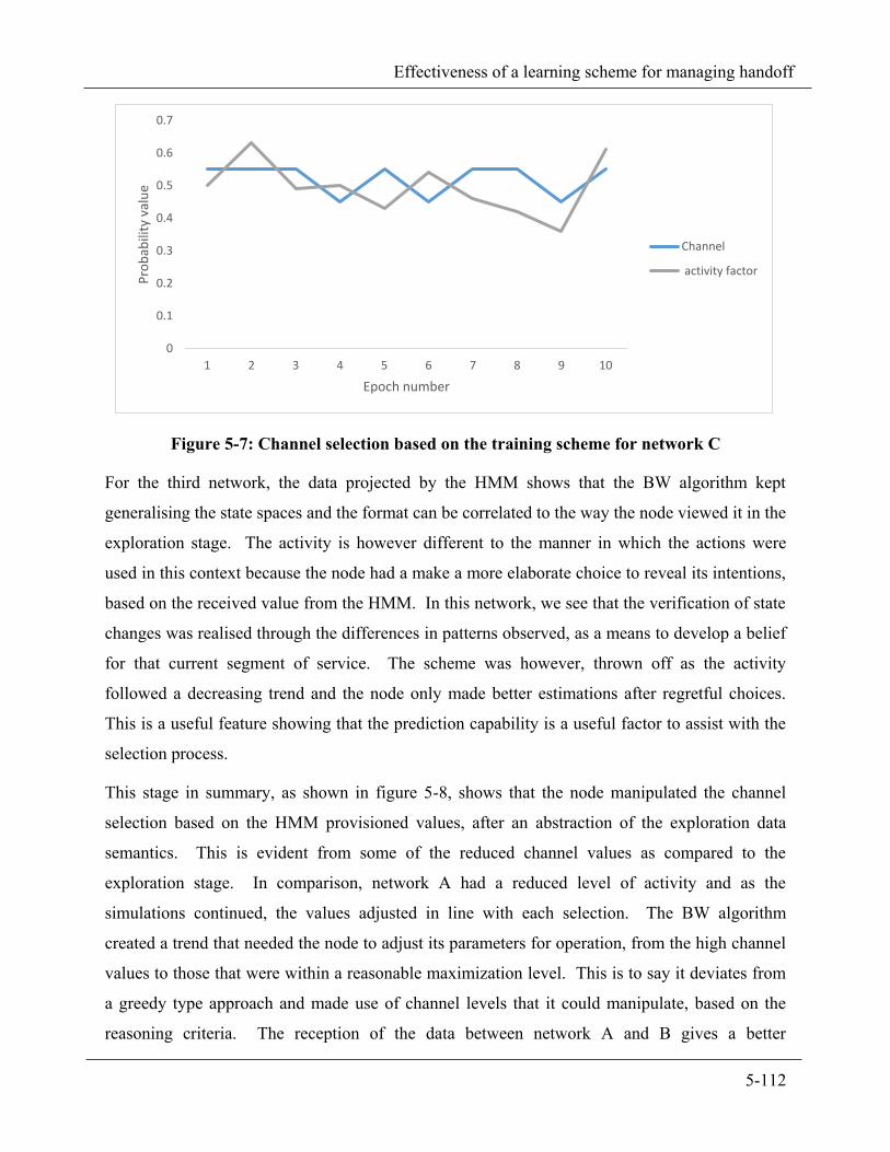
5-112


Figure 5-7: Channel selection based on the training scheme for network C

For the third network, the data projected by the HMM shows that the BW algorithm kept

generalising the state spaces and the format can be correlated to the way the node viewed it in the

exploration stage. The activity is however different to the manner in which the actions were

used in this context because the node had a make a more elaborate choice to reveal its intentions,

based on the received value from the HMM. In this network, we see that the verification of state

changes was realised through the differences in patterns observed, as a means to develop a belief

for that current segment of service. The scheme was however, thrown off as the activity

followed a decreasing trend and the node only made better estimations after regretful choices.

This is a useful feature showing that the prediction capability is a useful factor to assist with the

selection process.

This stage in summary, as shown in figure 5-8, shows that the node manipulated the channel

selection based on the HMM provisioned values, after an abstraction of the exploration data

semantics. This is evident from some of the reduced channel values as compared to the

exploration stage. In comparison, network A had a reduced level of activity and as the

simulations continued, the values adjusted in line with each selection. The BW algorithm

created a trend that needed the node to adjust its parameters for operation, from the high channel

values to those that were within a reasonable maximization level. This is to say it deviates from

a greedy type approach and made use of channel levels that it could manipulate, based on the

reasoning criteria. The reception of the data between network A and B gives a better

0

0.1

0.2

0.3

0.4

0.5

0.6

0.7

1 2 3 4 5 6 7 8 9 10

Pro

bab

ility

val

ue

Epoch number

Channel

activity factor

5-113


approximation of how the HMM translated data from the exploration stage and further defines

the features of a stochastic environment.

Figure 5-8: The comparison of network activity during service provisioning from a HMM

The definition of exploitation (the learning based selection process) 5.3.3

As the scheme is running in a self-sufficient mode, which is the first requirement of the

sharing model adopted in this work. It has to show a selection trend that relates to the conditions

of the sharing scheme and how the partitioning is provisioning for the required service. A key

condition that was set out for each network is that the node always has a view of each network

with at least a fifty percent usage level. This limits it to a few channels available in the network

as a means to enhance the management capability of the service provisioning with limited

resources. The outline of the figures is a comparison of the activity in the networks from the

training and the exploitation stages. Hypothesis T represents the training, and the exploitation

stage values are as given by the Hypothesis L to show the results from the learning scheme.

From the trend visible in figure 5-9, the node manages to capture the low traffic activity

of the network from the activity factors. The evidence from the little to moderate network

activity in the state shows that the node did not have to resort to the highest action values for the

selection of a channel, as the deduced activity allowed for flexible channel selections. This is

also guaranteeing the availability of a channel when the node is pre-empted from the current

occupation, as the network has an average to little rate of utilisation. Although low traffic values

0.00

0.10

0.20

0.30

0.40

0.50

0.60

0.70

1 2 3 4 5 6 7 8 9 10

Pro

bab

ility

val

ue

Epoch number

Network A

Network B

Network C

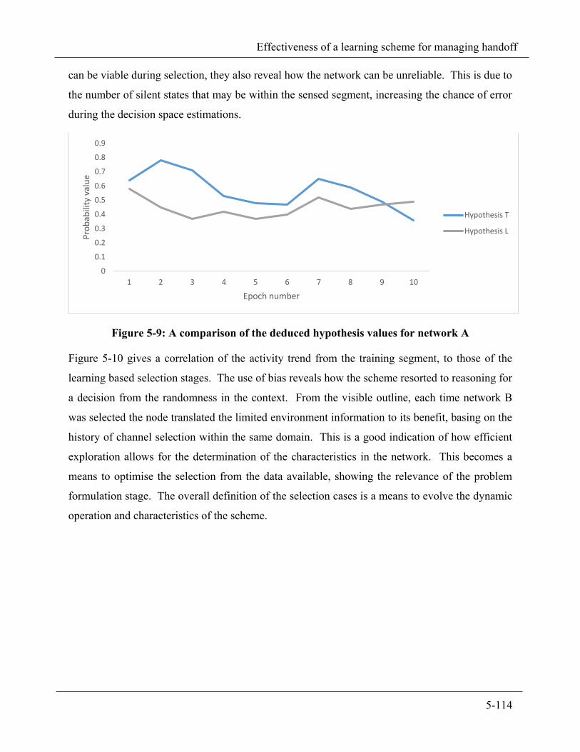
5-114


can be viable during selection, they also reveal how the network can be unreliable. This is due to

the number of silent states that may be within the sensed segment, increasing the chance of error

during the decision space estimations.

Figure 5-9: A comparison of the deduced hypothesis values for network A

Figure 5-10 gives a correlation of the activity trend from the training segment, to those of the

learning based selection stages. The use of bias reveals how the scheme resorted to reasoning for

a decision from the randomness in the context. From the visible outline, each time network B

was selected the node translated the limited environment information to its benefit, basing on the

history of channel selection within the same domain. This is a good indication of how efficient

exploration allows for the determination of the characteristics in the network. This becomes a

means to optimise the selection from the data available, showing the relevance of the problem

formulation stage. The overall definition of the selection cases is a means to evolve the dynamic

operation and characteristics of the scheme.

0

0.1

0.2

0.3

0.4

0.5

0.6

0.7

0.8

0.9

1 2 3 4 5 6 7 8 9 10

Pro

bab

ility

val

ue

Epoch number

Hypothesis T

Hypothesis L

5-115


Figure 5-10: A comparison of the deduced hypothesis values for network B

Figure 5-11: A comparison of the deduced hypothesis values for network C

Network C shows a different view of the exploitation concept. In comparison with the

comprehension of the data from the training stage, there is evidence of a neutral approach in this

network to allow for the selection of the hypothesis value. This is also in line with the history

patterns of selection but the scheme based its decisions on the values the network provided

during that stage of selection. Ideally, the training in all cases is supposed to be a means to trace

how the features incorporated in the learning, enhance the selection or making of decisions. This

allows for verification of past decisions made as time progresses for the node because the

0

0.1

0.2

0.3

0.4

0.5

0.6

0.7

1 2 3 4 5 6 7 8 9 10

Pro

bab

ility

val

ue

Epoch number

Hypothesis T

Hypothesis L

0

0.1

0.2

0.3

0.4

0.5

0.6

0.7

1 2 3 4 5 6 7 8 9 10

Pro

bab

ility

val

ue

Epoch value

Hypothesis T

Hypothesis L

5-116


comparison with the history patterns from both networks. Another issue is how the scheme is

closely dependent on the value of the activity within the network during each epoch to base its

decisions on. As such, this limits the decisions to the threshold obtained but if any other

conditions apply in the decision space, the value of an action opted for solidifies the selection of

a channel.

To affirm the trend in network C, the learning model is showing an operational bias as the

selection of a network comes from the features found in the state activity. Overall, the

hypothesis selection stage is an effective one in comparison with some of the cases during

training. The node dealt with the conditions that came with little the data from the selection of a

state, in account of the evidence laid out for a spectrum decision phase. It maps the domain

based on its capability to provide service absorption in a directed manner, from the value of the

hypothesis margin. This is outline is defined by the data in figure 5-12, from the performance

levels in all three networks.

Figure 5-12: The comparison of network activity when making use of the learning scheme

The HMM is the biggest differentiator in the levels of activity and it created a platform for the

scheme to become aware of the constraints in any network. This makes the scheme more robust

to the environment’s effects and this is a key feature from the design. As this was in a

decentralized sharing scheme, the node had to show that it could negotiate for a better service,

when given a good selection criterion. The relevance of the learning element is in the section

below.

0

0.1

0.2

0.3

0.4

0.5

0.6

0.7

1 2 3 4 5 6 7 8 9 10

Pro

bab

ility

val

ue

Epoch number

Network A

Network B

Network C

5-117


5.3.3.1 Management capability from reasoning This section is the determinant of how the scheme performed from the outline of the

design philosophy, which is to manage the effects from traffic conditions while it is trying to

access service from a network. The goal is to extend the decision space estimation to a point

where there is a reduction of the switching counts associated with the handoff phase. To track

the segments effectively, we will observe the attributes that contribute to a good management

level of service from any network. This will be from the sequence of events; from receiving

network data and translating it into the desired parameters that it needs for a selection case

during any epoch.

5.3.3.1.1 Channels selected during translation In this section, the selection is in line with the management of choices when a node has

the hypothesis value estimated. The value has to be in relation to the estimate of the presumed

activity that may occur in the next epoch within the same network as defined in section 4.3.2. To

allow for the explicit definition of performance, the evaluation relies on the derivation of an

action and the performance we observe when the limitation of handoff counts occur during

service.

Figure 5-13: Channel selection in Network A, during a service phase

The action selection in network A is synonymous with pattern changes and their relation to the

next selection epoch. This shows how an element of prediction came into account as each

0

0.1

0.2

0.3

0.4

0.5

0.6

0.7

1 2 3 4 5 6 7 8 9 10

Pro

bab

ility

val

ue

Epoch value

hypothesis

action

5-118


subsequent selection epoch is accounted for, when the node is reasoning for a selection segment.

This trend further promotes the use of the predictive capability when the objective made a

selection choice. The scheme only lowered its selection value after realising the evidence of

reduced evidence in state activity that will not affect it in the next epoch as an adaption

capability.

Figure 5-14: Channel selection in Network B, during a service phase

In network B, the selection is proving to be dependent on the values deduced during the selection

instant. This is a classic case where it has to reason for the selection of a channel, based on the

gravity of the number of instantaneous conditions that were available during the decision making

process. The prediction capability is however, often validated as seen by the trend in figure 5-

14, when it expects the activity to change, it then may drop in value, having the node use the

same hypothesis bounds or selecting an action within the same or a lower range.

0

0.1

0.2

0.3

0.4

0.5

0.6

0.7

1 2 3 4 5 6 7 8 9 10

Pro

bab

ility

val

ue

Epoch value

hypothesis

action

5-119


Figure 5-15: Channel selection in Network C, during a service phase

The data from the usage patterns of network C, shows that the prediction capability is again, a

useful feature for the management of a network. This is based on the Markovian principle

(section 4.3.2), that the node is basing its decisions on, as a means to control a lot of parameter

change during handoff. The usage values also reveal that the history element may give a

misleading impression, making the node continue with a high selection trend. The conditions

around channel usage, eventually force it to change its selection strategy when it deviates from

the policy in use as seen during the third and eight selection epochs.

5.3.3.1.2 Robustness from the contingencies The level of precision in the scheme comes from the amount of robustness the node could

achieve in the network. This is a good case of how the use of expectation and maximisation

when making decisions, allows the node to realise how the evolution of the learning is

progressing. This is due to the action usage and characterisation of the network activity during

channel selection. There are cases where the node needs to have better assessment techniques

and this is by use of the idleness of the channel values available and the blocking probabilities of

a context realised.

0

0.1

0.2

0.3

0.4

0.5

0.6

0.7

1 2 3 4 5 6 7 8 9 10

Pro

bab

ility

val

ue

Epoch nummber

hypothesis

action

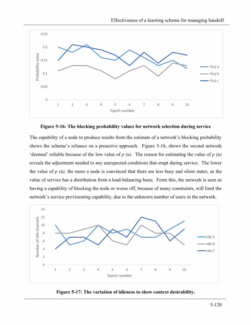
5-120


Figure 5-16: The blocking probability values for network selection during service

The capability of a node to produce results from the estimate of a network’s blocking probability

shows the scheme’s reliance on a proactive approach. Figure 5-16, shows the second network

‘deemed’ reliable because of the low value of p (u). The reason for estimating the value of p (u)

reveals the adjustment needed to any unexpected conditions that erupt during service. The lower

the value of p (u), the more a node is convinced that there are less busy and silent states, as the

value of service has a distribution from a load-balancing basis. From this, the network is seen as

having a capability of blocking the node or worse off, because of many constraints, will limit the

network’s service provisioning capability, due to the unknown number of users in the network.

Figure 5-17: The variation of idleness to show context desirability.

0

0.05

0.1

0.15

0.2

0.25

1 2 3 4 5 6 7 8 9 10

Pro

bab

ility

val

ue

Epoch number

P(u) a

P(u) b

P(u) c

0

2

4

6

8

10

12

14

1 2 3 4 5 6 7 8 9 10

Nu

mb

er o

f id

le c

han

nel

s

Epoch number

idle A

idle B

idle C

5-121


The benefit from making use of the state of idleness in a network is from the value of the

network’s stationarity approach. This may be a contradiction as the other users desiring the

same network for the next epoch arrive, thus misleading the node when it accept use of the

network. As a strategy, it will allow for the prevention of the under valuing and over estimation

of certain parameters, which ultimately can reduce the model to converge to a maxima a lot

sooner than it should be. This deduction is shown by a view of the randomness as exhibit by

figure 5-17. This enhances the robustness from the missing features that the scheme expects, to

allow for the verification of all the variables that are missing during that estimation segment.

This way the node will better prepare for the selection of a network under the notion of risk

mitigation, as a means to show a form of robustness from the missing information needed for

better parameter estimation.

To sum up the capability of the scheme, the graph below shows an impression of handoff

control based on the management capability as used during the learning stage. This allowed the

node to be pre-empted by a PU and still facilitate a channel switch to effect service completion,

based on the limited network data during certain instances. The system did perform well despite

a few lags and oversights during selection. This shows that the node had received sufficient

training and allowed for expansion of the data into its own planning as shown by the results. The

structure of the two models performance wise needed extensive training to get a good step size

for the assessment purposes. This is imperative as the LA operates better after at least 200

hundred iterations and gives better reward estimates, bettering the schemes performance for

handoff.

5-122


Figure 5-18: A comparison of handoff control during the training and learning segments

The effect of prediction on learning 5.3.4

When the node goes through the training stage for the actions to initialize, there is a huge

contrast of any activity patterns with those of stationary context (network) distributions. This is

during the exploration stage and it comes in comparison to those that come with a biased state

occupancy. The scheme reveals the need to take more than a dynamic approach to capture the

handoff occurrence from the parameters selection as well as the declaration of the independent

and non-independent variables. This affirms a form of benchmarking of that particular state’s

activities with which when used, defines better strategies for the objective from the performance

results.

As such, a learning approach is only capable of capturing the independent behaviour of

the channels when there is the use of a stationary approach to view the activity in the

environment. An analysis of the stationary distributions from the two cases, the HMM

provisioning, and the stationary context distributions (exploration) reveals the notable

differences in state usage patterns. The use of reasoning for the understanding of such patterns

by the LA is such that, when the contexts are abstracted from the environment, it enables for

their independent management. Such an element from the node, will allow for a better form of

the capturing of the network activity, due to the outline of the contexts as well as the occupation

0 1 2 3 4 5 6 7

Network A

Network B

Network C

6

4

5

1

2

2

Training Learning

5-123


density within the environment system. From this realisation, an adoption of a good epoch

optimization (predictive) approach each time is because of the node scrutinizing each network’s

activity value. This comes within the outlines of each selection and learning epoch, for an

effective decision made to be a means of showing the effectiveness of the prediction made.

Significance of a good decision 5.3.5

From the simulation process, we realised that a number of complications can occur

because of trying for a direct modelling of the handoff process with the learning and training

(HMM) schemes. This cause promotes the model definition to be as presented in this chapter

and this result gives a less complex situation for the scheme to deal with, during the capturing of

each service segment. Several authors of related work dwell on assumptions to define the

existence of certain cases that come with their proposed systems. From this stance, we look at

how the decisions made during the translation of the node, emphasise the relevance of the

scheme’s background and not resorting to the use of a number of assumptions.

This allows us to relate the dependency of the algorithm on other metrics, (which can be

considered trivial) and how their correlation can effect a better decision-making process from the

learning scheme.

1. The continuous environment (classification of the different networks)

Due to focusing on a single action for the handoff segment, the network observation is to have

some form of discrete relation. This allows the node to recognise the handoff segment and its

management when the node captures the network structure correctly. This is to say; if the

discretisation of the environment into a state space shows the estimated activity with a finite set

of channels, the patterns over time will account for any differences in the observed mix of

parameters.

2. The balancing of parameters from both subsystems i.e. the HMM and the LA

To outline this point, we need to map certain conditions with the prescribed changes and have

their validation confirmed with the node’s capability to comprehend to them. These cases are in

a hierarchical manner, from the least to the most concerning, and can be possibly mitigated

through;

When the node has been pre-empted, its capability to deal with the traffic scaling issue

5-124


comes from the values that only effect a change during that moment (from the output space

deduced). The re-estimation of the new operating parameters is structured in a manner that

does not to affect the generalisation process, so as not to get the required set of

probabilities for the handoff, learning and more so, affecting the precision of parameter

detection process during a different epoch for another channel selection.

The concern with multiple observations from each of the observed states is controllable by

having the bias account for them. The existence of the multi-teacher approach in this work

necessitates the development of a better policy for the node, during decision-making. As

the biasing system lead to the training of the node for the recognition of the various

scenarios, this showed a possibility of multiple conditions during each observation case.

The scheme is set up to cater for a single state (network) observation initially and the

reason for this is to have the node define the exploration process based on the channels

states relevant at that time. For the problem formulation stage of the LA to take advantage

of the environment structures during each sensing process, the definition of the finite

segments allows for better optimisation strategies. From such a stance, the LA can capture

each attribute of the network easily, for ease of interpretation of the activity for better

learning moments i.e. the estimation reward for the action that is applicable in the decision

space.

Accounting for the initial parameters for the BW is imperative for the node to learn from

the differences in the changes, in relation to the observed data during exploration. This is

through the re-estimation of the elements of λ, from the HMM and the steps taken during

the simulation process. The cause of such an outcome is the convergence of the BW

algorithm, toward a different direction and this defines a trend of more distributed

posterior probabilities. As the deviation noted throughout the entire simulation run reveals

the accuracy of the training stage, the exploration phase still had to be efficient to account

for how the node will comprehend its usage parameters for its own benefit.

To enhance the level of robustness during the HMM service provisioning stage, the BW

makes the use of the forward and backward algorithms, as a means to mismatch the

schemes expectation of the state activity, as the training progresses. This condition shows

the node that the prediction element will not be consistent at times and as such, allow it to

be less reliant on the outcome from the prediction by reasoning for better decisions.

5-125


3. Level of sufficiency needed for the bias system to have effect in any environment

For this effect to come into consideration, we have to look at the use of an ergodic HMM from

an implementation basis, due to its optimality as a system. As the HMM model used in this work

realises the value of a fully connected model, this is effective when the system is evolving the

data mining values to the posterior probabilities. From this, the training of the node is thus to

engage the node fully from the beginning of the state transitions (network changes), to the point

where it can be self-sufficient as an independent decision maker. This will work with the LA

because the non-stationarity of the effects realised in each context will not gravely affect the

node when it has to make its own decisions using the learning-based scheme. The validation of

this point is in the exploitation stage, where the node has to make spectrum decisions, with the

bias induced as a form of reference to assist with the reasoning method instructed, and the

learning case.

4. Adaption to the changes and different levels in model performance

For the node to benefit from the use of both schemes, we have the definition of their properties in

line with the evolution process of a learning algorithm. This allows the scheme to develop each

attribute and benchmark the level of performance for the benefit of the decision process. The

overall benefit is from the knowledge bases created during the adaption process that is occurring

with the evolution of the scheme.

Chapter summary 5.4

This chapter outlines the relevance of a good management scheme when a cognitive node

is going through a service encounter that leads to a handoff process. During the handoff

moment, the node evolves the service objective as an assessment basis for the next selection

epoch in each scenario. The selection of an action is in relation to the outcome observed from

the interpretation of the network data. This process further allows the node to trace the model in

an individual capacity and observe where it fails, during service provisioning or handoff

facilitation.

The tracing of the service stage reveals how the reliance of a particular belief led to the

scheme not being able to make a decision when in such a scenario. From the results observed,

the learning plays a great role in the deduction of a suitable response to the environment activity.

5-126


This is imperative, as the node will have to deal with the current level of activity in the system

regardless of the sensing result. The next chapter gives a concluding assessment of the work

done in this thesis, as well as an extension of the work for the benefit of other avenues of

research.

Conclusion Chapter 6

Conclusion

6-128

Conclusion

Introduction

The highlight of this work shows the importance of managing handoff from a nodal perspective.

With the background of the work based on the selection of a channel during handoff, this thesis

discusses the development of better decision-making criteria, in a sharing based architecture for

CR. The type of sharing involves having effects from both primary and other secondary user

activities and these define how the node will make any parametric deductions, leading to the

provision for service and more so, account for the handoff cases. A channel, when used by a

potential incoming secondary user into that network, observes it as a basic unit of network

activity that will allow for the derivation of an operational state space. This is a best-case

scenario development for the node to make any decision from the network’s point of view, in

comparison with its own desire to have service.

Summary 6.1

The network definitions came as an overlay and this is to have the node deduce how best to

behave in any shared network with a decentralised scheme. From there, we have the node

roaming through the networks and gathering data for its own benefit, which is a credible method

adopted by the CR for learning purposes. Based on such a learning scenario, the form of

decision-making adopted for the different encounters caters for most of the PU concerns as well

as the cognitive node in meeting its own intensions i.e. the handoff management. The scheme’s

outline is with a regard of the level of activity in the environment, as a means to deduce any

nominal state parameters. The results from the deduction process lead to a cause for learning

what the environment can offer during the channel selection segment and evolve the decision-

making scheme for any future selection of any spectrum bands.

Initially, the node had to learn to define the channel behaviour ‘realistically’ in its favour,

such that it can be adapted to model scenarios for mobility management and more so, the

decision processes during spectrum handoff. From such a stance, the node will perform an

exploration activity as a means to collect data and have a dynamic view of the activity patterns in

the environment. The exploration phase is where the node has to observe and understand how

the differences in the activity patterns will condition its operating forms when in an overlay.

This leads to an outcome where the learning of the usage patterns exhibited in the network will

6-129

Conclusion

occur.

From the challenges identified in literature, the selection of bias as a means to enhance the

capturing of the PU activity promotes the use of training for feature estimations. For the scheme

to manage the balance between the CR’s current intention vs. the need to progress in any

environment, the training subjects the node to various extremes of disruptive encounters. These

came as varying conditions during the selection epochs, enhancing the node’s resilience in any

multi-dimensional sharing scheme. Ultimately, the scheme promoted the global variables

identified during the exploration stage and created learning objectives to manage the spectrum

mobility process.

The key attribute of the scheme is its capability to track the service phase of an SU, from

the point of pre-emption to a point where it has to continue with the service provision. This can

be in the same state or a different one and in either one; the scheme makes use of two global

variables, the arrival rates of other nodes on the same network and its current level of utilisation.

The two variables, translate into metrics within that network’s parameter set with which, the

channel handoff count’s reduction comes from their use as realised by the learning automata

algorithm. In summary, the following give an account of the scheme’s performance and allows a

portrayal of the learning benefit through:

1. An exploitation of the spectrum opportunities; this defines the selection of a network

based on the variables that are available at a time. With this, the advantage of self-

awareness becomes more pronounced as the node is operates in a self-sufficient mode.

This mode is when it has to make any decision based on the effects from the visible traffic

patterns and what it can comprehend from them without the help of a central controller.

a. The findings also show the CR’s capability to partition the networks as the sensing

progresses, further outlining how the use of network data is from the estimation of

suitable variables that assist in the management of the handoff process.

b. The use of the load balancing approach promotes the selection of a channel within a

CR’s transmission needs. This forges a scenario where the node takes advantage of

the network data and the result of this manipulation comes with the reduction of the

sensing cycles when in a handoff count.

c. The network selection basis comes from the prescribed activity in the desired state

6-130

Conclusion

space. This has the node bettering its negotiation levels when nominating

operational policies, based on the density of the nodes during the selection moment.

2. The use of training is a means to enhance the recognition of instantaneous conditions that

come because of unpredicted traffic effects and patterns. When the HMM provided a

probability value for the network, it came with limitations each time the node needed to

make a decision. This is because when the value changes, the node has less room to make

an effective decision and considers that segment to have an amount of instantaneous

conditions. From this form of interaction:

a. The node took the probability space for the actions and initialised them based on the

distribution space Q. The state space of Q elaborates on effective choices during the

management of the handoff process as a means to maximise its cognitive ability.

b. From the number of limitations observed, the prediction process becomes an

advantage when the HMM values change and this is in comparison to the posterior

probability values. This stage enhances the cognitive nodes robustness to the ever-

changing conditions and this promotes a better handoff policymaking system.

c. The handoff count, in addition to the conditions in the network subjected the node to

varying operational levels. These levels allow the training to have weight because

of the changes in the network and this is in comparison to those observed during the

data mining (exploration) stage.

3. The exploration capability of the scheme comes as a means of revealing the benefit of the

CR’s learning process. This defines how the reasoning and learning aspects of the scheme

maintain the need to provision for handoff because of the network usage patterns during

the translation period. The structure of scheme is around the node’s probabilistic

dependence on the network values, showing if the selection of the network will suffice as

a form of activity characterisation. From the network outlook, we have:

a. The definition of a dynamic approach with which, a node can estimate the value of a

session loss or any possible handover delays, allowing for the creation of a

contingency relating to a better service estimations, during a channel’s selection.

b. The CR makes use of the current service objective in relation to the learning’s

progression within the network as a means of cooperating with other users during

the channel selection.

6-131

Conclusion

i. This is visible from the node’s attempt to balance the mean state activity with

the channel value in use, based on the action selected by the learning scheme.

c. The satisfaction of an objective during a service segment leads to the backtracking

of the node’s performance for the satisfaction of the reward estimate. This is in

recognition of an updated belief from the observed patterns translating into a policy

definition, based on the decision space. The result is primarily from the scheme’s

adaption capability, showing the node’s progression from the data mining, through

its training phase and eventually leads to the learning stage.

d. The scalability of performance comes from the number of allowed permutations at a

given time because of adopting the reasoning process. This was enhanced from how

the node only had a probability value from the HMM to base all its decisions on.

The eradication of the greediness during the channel selection process forces the CR

to have reference points in the network, which promote its chances of a successful

service count.

Overall, the definition of a state proliferation approach when selecting parameters achieves a

better use of the reasoning criteria during the learning and decision-making moments. If the

enhancement of the cognition element is fully utilised, the node can realise each channel’s

benefit when put to use and in return, maximise the selection process when it is pre-empted by a

primary user. As multi-user environments show a level of complexity when being adapted to,

the use of an objective enhances the control of the learning approach when deducing the best

operational parameters. This allows the node to have a more dynamic view of the decision space

when utilising the varying channel composition.

Recommendations 6.2

Some realisations came during the conceptualisation of this scheme and this is in light of how the

node was performing. As notable distinctions came with each segment of the evaluation stage,

the optimised variables revealed some limitations that can enhance other areas of research, as a

continuation of this work. These are:

1. For the handoff execution, the node relies on the channel selection strategy and the

decision making process, as a phase, is very important as noted in this work. For it to be

limited to the general admission of service is a hindering condition in the progression of a

6-132

Conclusion

CR’s performance. As such, there should be the development of handoff priority

schemes, especially when it has to deduce if it should take the service resumption option

or if it has to repeat the transmission. As an attribute, the service criticality define the

type of approach that can be opted for, further allowing the node to better handle

redundant data structures.

2. The extension of the channel usage patterns to have some form of energy related

methods caters for the control of power, along with other metrics that outline the level of

power consumed. This area will reveal the benefit of the cognition towards the concept

of green computing, when planning for resource management.

3. The issue with channel contentions causes exaggerated levels of delay as the other users

force the node to wait for a continuance of the service. This id mostly prevalent in a

decentralised form of sharing, where the channel provisioning and selection is very

competitive because of the node density in the same band as the cognitive node. The

evidence from the environment’s outlay leans towards the development of efficient

sharing methods that enhances the nodes capability when roaming in a decentralised

architecture. This assists in the management of the computation associated with the

service segment and more beneficial in the cases that lack any provisioning of the

instantaneous conditions.

4. The use of smart systems is gaining a lot of recognition especially with ‘big data’ being

the key buzzword being thrown around in their research and development domains. The

manipulation of data has to have each scheme evolve toward better forms of data usage

and interpretation and in turn, assists with better data mining capabilities.

133

Bibliography

[1] Federal Communications Commission, “Report of the Spectrum Policy Task Force,” ET

Docket No. 02-135, Nov. 2002.

[2] R. Qiu et al. “A Unified Multi-Functional Dynamic Spectrum Access Framework: Tutorial,

Theory and Multi-GHz Wideband Test-bed.” Sensors journal, pp. 6530-6603, 2009.

[3] E. Hossain, D. Niyato, Z. Han, “Dynamic Spectrum Access and Management in Cognitive

Radio Networks.” [Online], Cambridge: Cambridge University Press 2009.

[4] I. Akyildiz, W. Lee, M. Vuran and S. Mohanty, "Next Generation/Dynamic Spectrum

Access/Cognitive Radio Wireless Networks: A Survey," Computer Networks, Vol. 50, pp.

2127-2159, 2006.

[5] I. Christian, S. Moh, I. Chung and L. Jinyi, “Spectrum mobility in Cognitive Radio Networks,”

Communications magazine, IEEE, Vol 50, Issue 6, pp. 114-121, 2012.



[7] Federal Communications Commission, Report of the Spectrum Policy Task Force, ET Docket

No. 02-135, November 2002.

[8] V. Kolar, A. Gerco, T. Milcher, M Petrova, P. Mähönen, “Capacity Estimation and Adaptation

in Cognitive Radio Networks: Demonstrating Software Defined Radios in Action,” 15th Annual

International Conference on Mobile Computing and Networking, MOBICOM, 2009.



[10] A. Goldsmith, S. Jafar, I. Maric and S. Srinivasa, “Breaking Spectrum Grid- lock with

Cognitive Radios: An Information Theoretic Perspective” Proceedings of the IEEE, vol.97,

no.5, pp.894-914, May 2009.

[11] H. Kim and K. Shin, “In-Band Spectrum Sensing in IEEE 802.22 WRANS for Incumbent

Protection,” IEEE Transactions on Mobile Computing, vol. 9, no. 12, pp. 1766 –1779,

December 2010.

[12] K. Letaief, W. Zhang, "Cooperative Communications for Cognitive Radio Networks,"

Proceedings of the IEEE, vol.97, no.5, pp.878-893, May 2009.

[13] P. Sutton, J. Lotze, K. Nolan and L. Doyle, “Cyclostationary Signature Detection In Multipath

http://ieeexplore.ieee.org/search/searchresult.jsp?searchWithin=p_Authors:.QT.Christian,%20I..QT.&searchWithin=p_Author_Ids:38246379900&newsearch=true

http://ieeexplore.ieee.org/search/searchresult.jsp?searchWithin=p_Authors:.QT.Moh,%20S..QT.&searchWithin=p_Author_Ids:37313720900&newsearch=true

http://ieeexplore.ieee.org/search/searchresult.jsp?searchWithin=p_Authors:.QT.Ilyong%20Chung.QT.&searchWithin=p_Author_Ids:37275921700&newsearch=true

http://ieeexplore.ieee.org/search/searchresult.jsp?searchWithin=p_Authors:.QT.Jinyi%20Lee.QT.&searchWithin=p_Author_Ids:37406253900&newsearch=true

134

Rayleigh Fading Environments,” in Proceedings of the 2nd International Conference on

Cognitive Radio Oriented Wireless Networks and Communications 2007 (CrownCom ’07), pp.

408 –413, Aug. 2007.

[14] R. Mahapatra and M. Krusheel, "Cyclostationary Detection for Cognitive Radio With Multiple

Receivers," Wireless Communication Systems, ISWCS '08, IEEE International Symposium on,

pp.493-497, 21-24 Oct. 2008.

[15] Z. Tian and G Giannakis, "A Wavelet Approach to Wideband Spectrum Sensing for Cognitive

Radios," Cognitive Radio Oriented Wireless Networks and Communications, 1st International

Conference on, pp.1-5, 8-10 June 2006.

[16] M. Masonta, M. Mzyece, N. Ntlatlapa, "Spectrum Decision in Cognitive Radio Networks: A

Survey," Communications Surveys & Tutorials, IEEE, Vol.15, no.3, pp.1088-1107, Third

Quarter 2013.

[17] I. Christian, S. Moh, I. Chung and L. Jinyi, “Spectrum Mobility In Cognitive Radio Networks,”




[19] I. Christian, S. Moh, I. Chung and L. Jinyi, “Spectrum Mobility In Cognitive Radio Networks,”


[20] A. Singhrova and N. Prakash, “Adaptive Vertical Handoff Decision Algorithm for Wireless

Heterogeneous Networks” 11th IEEE Intl. Conf. on High Performance Computing and

Communications, 2009, pp. 476-481, 2009.

[21] L. Won-Yeol and I. Akyildiz, “Spectrum-Aware Mobility Management in Cognitive Radio

Cellular Networks,” Mobile Computing, IEEE Transactions on, Vol. 11, Issue 4, pp. 529-542,

April 2012.

[22] Y. Lu, H. Cao, X. Mu and S. Yang, “Adaptive Spectrum Access Strategies in the Context of

Spectrum Fragmentation in Cognitive Radio Networks,” Concurrency Computation: Practical

Experience, Vol. 25, pp 1101–1112, 2013.

[23] S. Bayhan and F. Alagoz, “Distributed Channel Selection In Crahns: A Non-Selfish Scheme

For Mitigating Spectrum Fragmentation,” Ad Hoc Networks, Volume 10, Issue 5, Pages 737-

870, July 2012.

[24] E. Hossain, D. Niyato and Z. Han, “Dynamic Spectrum Access and Management in Cognitive









135


[25] R. Jugens and F. Klugl, “Programming agent behaviour by learning in simulated models,”

Applied Artificial Intelligence, Vol. 26, Issue no. 4, 2012.

[26] M. Zhang, S. Jiang, G. Wei, and H. Wang, “Performance Analysis of the Cognitive Radio

Network With a Call Level Queue for Secondary Users,” in Proc. of the 5th Int‟l Con on

Wireless Communications, Networking and Mobile Computing (WiCom‟09), pp. 1 –4, Sep.

2009.

[27] X. Li, Q. Zhao, X. Guan, and L. Tong, “Optimal Cognitive Access of Markovian Channels

under Tight Collision Constraints,” IEEE Journal on Selected Areas in Communications, Vol.

29, No. 4, pp. 746-759, Apr. 2011.

[28] L. C. Wang and A. Chen, “On the Performance of Spectrum Handoff for Link Maintenance in

Cognitive Radio,” Proc. IEEE Int‟l Symposium on Wireless Pervasive Computing (ISWPC),

May 2008.

[29] B. Wang, Z. Ji, K.J. Ray Liu, and T.C. Clancy, “Primary-Prioritized Markov Approach for

Dynamic Spectrum Allocation,” IEEE Transactions on Wireless Communications, Vol. 8, No.

4, pp. 1854-1865, Apr. 2009.

[30] H.-P. Shiang and M. Van der Schaar, “Queuing-Based Dynamic Channel Selection for

Heterogeneous Multimedia Applications over Cognitive Radio Networks,” IEEE Trans.

Multimedia, Vol. 10, No. 5, pp. 896-909, Aug. 2008.

[31] S. Bayhan and F. Alagoz, “Distributed channel selection in CRAHNs: A non-selfish scheme for

mitigating spectrum fragmentation,” Ad Hoc Networks, Volume 10, Issue 5, Pages 737-870,

July 2012.

[32] L. Yang, L. Cao and H Zheng, “Proactive Channel Access in Dynamic Spectrum Networks,”

Physical Communication, Vol. 1, Issue 2, Pages 103–111, June 2008.

[33] C. Ghosh, C. Cordeiro, D. Agrawal, M. Rao, "Markov Chain Existence And Hidden Markov

Models In Spectrum Sensing," Pervasive Computing and Communications, PerCom, IEEE

International Conference on, pp.1-6, 9-13 March 2009.

[34] A. Azarfar, J. Frigon and B. Sanso, "Analysis Of Cognitive Radio Networks Based On A

Queueing Model With Server Interruptions," Communications (ICC), 2012 IEEE International

Conference on, pp.1703, 1708, 10-15 June 2012.

[35] M. Rui-Ting, Y, Hsu and K Feng, "A POMDP-Based Spectrum Handoff Protocol for Partially

http://www.tandfonline.com/toc/uaai20/26/4

http://www.sciencedirect.com/science/journal/18744907

http://www.sciencedirect.com/science/journal/18744907/1/2

136

Observable Cognitive Radio Networks," Wireless Communications and Networking

Conference, 2009, WCNC 2009, IEEE, pp.1-6, 5-8 April 2009.

[36] S. Zahed, I. Awan and A Cullen, “Analytical Modelling for Spectrum Handoff Decision in

Cognitive Handoff Networks,” Simulation Modelling and Practice, Vol. 38, pp. 98-114,

November 2013.

[37] C. Pham, N. H. Tran, C. T. Do, S Moon and C. S. Hong “Spectrum Handoff Model Based on

Hidden Markov Model in Cognitive Radio Networks,” IEEE International Conference on

International Networking, ICOIN, pp. 406-411, 10-12 November 2014.

[38] L. C. Wang, C. W. Wang and J. C. Chang, "Modelling and Analysis for Spectrum Handoffs in

Cognitive Radio Networks," Mobile Computing, IEEE Transactions on, Vol.11, no.9, pp.1499-

1513, Sept. 2012.

[39] F. A. Gonzalez-Horta et al, “A Cognitive Handoff: Holistic Vision, Reference Framework,

Model-Driven Methodology and Taxonomy of Scenarios,” Int. Journal on Adv. in Networks

and Services, Vol. 4, Issue 3&4, pp. 324-342, 2011.

[40] L. C. Wang, C. W. Wang and J. C. Chang, "Modelling and Analysis for Spectrum Handoffs in

Cognitive Radio Networks," Mobile Computing, IEEE Transactions on, Vol.11, no.9, pp.1499-

1513, Sept. 2012.

[41] A. Banaei and C. Georghiades, "Throughput Analysis of a Randomized Sensing Scheme in

Cell-Based Ad-Hoc Cognitive Networks," Communications, ICC '09, IEEE International

Conference on, pp.1-6, 14-18 June 2009.

[42] J. Gambini, O. Simeone, U. Spagnolini, Y. Bar-Ness and Y. Kim, "Cognitive Radio with

Secondary Packet-By-Packet Vertical Handover," Communications, ICC '08. IEEE

International Conference on, pp.1050-1054, 19-23 May 2008.

[43] C. Lee, J. Lin, Y. Hsu and K. Feng, "Design and Analysis of Optimal Channel-Hopping

Sequence for Cognitive Radio Networks," Wireless Communications and Networking

Conference (WCNC), IEEE , pp.1-6, 18-21 April 2010.

[44] D. Teguig, B. Scheers and V. Le Nir, "Data Fusion Schemes for Cooperative Spectrum Sensing

in Cognitive Radio Networks," Communications and Information Systems Conference (MCC),

Military, vol., no., pp.1-7, 8-9 Oct. 2012.

[45] S. Barnes and B. Maharaj, “Prediction Based Channel Allocation Performance for Cognitive

Radio,” AEU - Int‟l Journal of Electronics and Comm., Vol. 68, Issue 4, pp. 336-345, April

137

2014.

[46] A. Amana, M. Price and R. Tamvichai, “Grey Systems Theory Applications to Wireless

Communications” Analog Integrated Circuits and Signal Processing, Volume 69, Issue 2-3, pp

259-269, December 2011.

[47] M. T. Quach, D. Ouattara, F. Krief, H. Khalife and M. A. Chalouf, "Overlap Regions and Grey

Model-Based Approach for Interference Avoidance In Cognitive Radio Networks," Ubiquitous

and Future Networks (ICUFN), 2013 Fifth International Conference on, pp.642,647, 2-5 July

2013.

[48] L. C. Wang, C. W. Wang, J. C. Chang, "Modelling and Analysis for Spectrum Handoffs in

Cognitive Radio Networks," Mobile Computing, IEEE Transactions on, vol.11, no.9,

pp.1499,1513, Sept. 2012.

[49] Y. Yao, S. Ngoga, D. Erman and A. Popescu, "Competition-based Channel Selection for

Cognitive Radio Networks," Wireless Communications and Networking Conference (WCNC),

IEEE, pp.1432-1437, 1-4 April 2012.

[50] L Giupponi and A. I. Perez-Neira, “Fuzzy Based Spectrum Handoff in Cognitive Radio

Networks,”Cognitive Radio Oriented Wireless Networks and Communications, CrownCom

2008. 3rd International Conference on pp 1-6 May 2008.

[51] J. Wu, Ying Dai and Yanchao Zhao, “Effective Channel Assignments in Cognitive Radio

Networks,” Computer Communications, Volume 36, Issue 4, Pages 411-420, 15 February

2013.

[52] K. Tsagkaris, A. Katidiotis and P. Demestichas, “Neural Network-Based Learning Schemes for

Cognitive Radio Systems,’ Computer Communications, Volume 31, Issue 14, Pages 3394-

3404, 5 September 2008.

[53] K. Singh, G. Singh and P. Vibhakar, “Spectrum Management for Cognitive Radio Based on

Genetics Algorithm,” Computer Science - Neural and Evolutionary Computing, 24 Jan 2011.

[54] S. Aslam and K. Geun Lee, “Channel Selection and Parameter Adaption Scheme Based on

Genetic Algorithm for CR Ad Hoc Networks,” EURASIP Journal on Wireless Communications

and Networking, November 2012.

[55] T. Chronopoulos, M. Musku, S. Penmatsa and D. Popescu, "Spectrum Load Balancing for

Medium Access in Cognitive Radio Systems," Communications Letters, IEEE , Vol.12, no.5,

pp.353-355, May 2008.

http://link.springer.com/journal/10470

http://link.springer.com/journal/10470/69/2/page/1

http://ieeexplore.ieee.org/xpl/mostRecentIssue.jsp?punumber=6153583



















138

[56] I. Malanchini, M. Cesana and N. Gatti, "On Spectrum Selection Games in Cognitive Radio

Networks," Global Telecommunications Conference, GLOBECOM, IEEE, pp.1-7, Nov. 30-

Dec 2009.

[57] Y. Sun and J. Qian, “EWA Selection Strategy with Channel Handoff Scheme in Cognitive

Radio.” Sensors and Transducers Journal, Vol. 173, Issue 6, pp. 68-74, June 2014.

[58] H. Li, G. Zhu, L. Jian, Z. Liang and D. Wang, "Stochastic Spectrum Access Based on Learning

Automata in Cognitive Radio Network," Intelligent Computing and Intelligent Systems, ICIS,

IEEE International Conference on, vol.3, pp.294-298, 2009.

[59] S. Misra, S. Chatterjee, and M. Guizani, “Stochastic Learning Automata-Based Channel

Selection in Cognitive Radio/Dynamic Spectrum Access For Wimax Networks,” Int. J.

Communications Systems, 2014.



[61] Capt. R. Thomas, “Cognitive Radios,” a PhD. Thesis, Virginia Polytechnic Institute and State

University, 2007.

[62] M. Rui-Ting, Y. Hsu and K Feng, "A POMDP-Based Spectrum Handoff Protocol for Partially

Observable Cognitive Radio Networks," Wireless Communications and Networking

Conference, WCNC 2009, IEEE, pp.1-6, 5-8 April 2009.

[63] A. Urken, A. Nimz and T. Schuck, “Designing Evolvable Systems in a Framework Of Robust,

Resilient and Sustainable Engineering Analysis,” Advanced Engineering Informatics, Volume

26, Issue 3, Pages 553-562, August 2012.

[64] S. Misra, P. V. Krishna and V. Saritha, “An Efficient Approach for Distributed Channel

Allocation with Learning Automata-based Reservation in Cellular Networks,” Society for

Modelling and Simulation International (SCS), 8 October 2012.

[65] J. Baxter, “A Model of Inductive Bias Learning,” Journal of Artificial Intelligence Research,

Volume 3, November 1999.

[66] C. Ghosh, C. Cordeiro, D. Agrawal and M. Rao, "Markov Chain Existence And Hidden

Markov Models In Spectrum Sensing," Pervasive Computing and Communications, Per.Com,

IEEE International Conference on, pp.1-6, 9-13 March 2009.

[67] J. Torkestani and M. Meybodi, “A Learning Automata-based Channel Assignment Algorithm

for Clustered Wireless AdHoc Networks,” Journal of Network and Systems Management,





http://www.sensorsportal.com/HTML/DIGEST/june_2014/Vol_173/P_2150.pdf

http://www.sensorsportal.com/HTML/DIGEST/june_2014/Vol_173/P_2150.pdf



























139

Springer, 2010.



14

0

Ann

exe A

: The

rea

lisat

ion

of le

arni

ng b

ased

on

cont

rol f

rom

the

sche

me

Util

ity

vect

or

defin

ition

Stat

e oc

cupa

ncy

pred

icti

on

Obj

ecti

ve f

unct

ion

defin

iton

Serv

ice

stat

e an

d ab

sorp

tion

Stat

e bo

unds

ch

arac

teri

zati

on

HM

M t

rain

ing

Han

doff

par

amet

er

estim

atio

n

Act

ion

mod

ellin

g

Envi

ronm

ent

cont

exts

def

init

ion

HM

M d

ecod

ing

Pred

ictio

n in

terp

reta

tion

Lear

ning

reso

luti

on

stag

e

Act

ive

sche

me

oper

atio

n

(met

rics

for

futu

re

sele

ctio

n)

Off

line

para

met

er t

raci

ng

(Res

olut

ion

of p

rior

met

rics

)Le

arni

ng p

aram

eter

es

tim

atio

n

Cha

nnel

sel

ecti

on

sche

me

Stat

e se

quen

cees

tim

atio

n

Ove

rall

lear

ning

pro

cess

Overall balance of control

Dom

ain

m

appi

ng

Proa

ctiv

e st

ate

mod

ellin

g

Figu

re A

- 1: A

bal

ance

of l

earn

ing

vs. c

ontr

ol fo

r th

e pr

opos

ed se

lect

ion

sche

me

141

Annexe B: Tabulated results of the schemes performance

This section gives all the collated values that outline the quantitative values of the node’s activity

in the overlay networks. These values give a descriptive analysis of the action values and their

worth when selected, the value from rewarding process, the collated values of probability when

the node is roaming in the different contexts and the number of handoff moments experienced in

each regard.

Table B- 1: Activity patterns for the first network

Data mining values Network 1 Channel composition

Run count channel value P(u) Activity factor idle busy silent 1 0.49 0.2 0.64 10 6 4 2 0.36 0.18 0.78 3 9 8 3 0.35 0.23 0.71 6 5 9 4 0.68 0.13 0.48 10 6 4 5 0.42 0.15 0.38 8 10 2 6 0.51 0.25 0.47 9 8 3 7 0.36 0.23 0.65 5 9 6 8 0.51 0.15 0.59 7 10 3 9 0.55 0.15 0.49 9 7 4 10 0.64 0.12 0.36 11 6 3

Mean 0.49 0.17 0.55 7.8 7.6 4.6 SD 0.12 0.03 0.14 2.53 1.84 2.32

142

Table B-2: Activity patterns for the second networks


Run count channel value P(u) Activity factor idle busy silent 1 0.39 0.1 0.52 4 11 5 2 0.65 0.13 0.36 8 10 2 3 0.72 0.13 0.54 6 9 5 4 0.53 0.08 0.40 10 7 3 5 0.35 0.08 0.53 8 5 7 6 0.62 0.11 0.42 9 8 4 7 0.55 0.13 0.58 10 5 5 8 0.68 0.09 0.33 6 7 7 9 0.48 0.14 0.55 8 8 4

10 0.35 0.13 0.65 2 13 5

Mean 0.53 0.12 0.49 7 8 5 SD 0.14 0.02 0.10 3 3 2

Table B-3: Activity patterns for the third network


Run count channel value P(u) Activity factor idle busy silent 1 0.32 0.15 0.65 4 8 8 2 0.44 0.21 0.54 11 2 7 3 0.37 0.20 0.53 11 6 3 4 0.29 0.19 0.50 5 10 5 5 0.23 0.17 0.35 9 8 3 6 0.44 0.13 0.52 7 11 2 7 0.32 0.18 0.52 12 7 1 8 0.61 0.14 0.39 10 8 2 9 0.39 0.18 0.46 6 10 4

10 0.79 0.17 0.43 9 9 2

Mean 0.42 0.17 0.49 8 8 4 SD 0.17 0.03 0.09 3 3 2

14

3

Tab

le B

-4: A

ctiv

ity in

net

wor

k on

e du

ring

serv

ice

prov

isio

ning

from

the

HM

M

Run

co

unt

Act

ion

num

ber

Cha

nnel

ca

paci

ty

Act

ion

upda

te

valu

e H

ando

ff

Yes

/No?

Con

tinge

ncy

valu

e fo

r ha

ndof

f ac

tion

Han

doff

N

etw

ork

activ

ity fa

ctor

Initi

al

netw

ork

stat

us

Cou

nts

Serv

ice

stat

us

1 5

0.55

2.

30E-

03

yes

0.20

1

busy

stat

e 0.

62

busy

2

3 0.

55

1.40

E-03

no

0

0 0

0.50

bu

sy

3 4

0.55

1.

70E-

03

yes

0.18

1

busy

stat

e 0.

53

idle

4

3 0.

55

1.20

E-03

no

0

0 0

0.43

id

le

5 4

0.55

1.

90E-

03

yes

0.11

1

busy

stat

e 0.

59

idle

6

2 0.

65

8.99

E-04

ye

s 0.

22

1 0

0.40

id

le

7 3

0.55

1.

30E-

03

no

0 0

0 0.

49

busy

8

2 0.

65

8.94

E-04

ye

s 0.

18

1 0

0.38

id

le

9 3

0.55

1.

23E-

03

no

0 0

0 0.

42

idle

10

4

0.55

1.

80E-

03

yes

0.15

1

busy

stat

e 0.

54

busy

M

ean

0.57

0.

05

0.40

0.

49

SD

0.04

0.

07

0.52

0.

08

14

4

Tab

le B

-5: A

ctiv

ity in

net

wor

k tw

o du

ring

serv

ice

prov

isio

ning

from

the

HM

M

Run

co

unt

Act

ion

num

ber

Cha

nnel

ca

paci

ty

Act

ion

Upd

ate

valu

e H

ando

ff

Yes

/No?

Con

tinge

ncy

valu

e fo

r ha

ndof

f ac

tion

Han

doff

N

etw

ork

activ

ity fa

ctor

Initi

al

netw

ork

stat

us

Cou

nt

Serv

ice

stat

us

1

4 0.

7 7.

93E-

04

no

0 0

0 0.

35

desi

rabl

e 2

2 0.

65

8.16

E-04

ye

s 0

0 0

0.38

id

le

3 4

0.55

1.

80E-

03

no

0.11

1

idle

0.

35

desi

rabl

e 4

3 0.

65

1.10

E-03

no

0

0 0

0.42

id

le

5 4

0.65

1.

20E-

03

yes

0.25

1

idle

0.

44

idle

6

3 0.

55

1.20

E-03

no

0

0 0

0.44

id

le

7 5

0.65

8.

23E-

04

no

0 0

0 0.

37

idle

8

4 0.

55

1.60

E-03

ye

s 0.

17

1 bu

sy

0.50

id

le

9 2

0.65

8.

98E-

04

no

0 0

0 0.

40

idle

10

3

0.65

7.

97E-

04

yes

0.15

1

idle

0.

35

desi

rabl

e

M

ean

0.63

0.

07

0.20

0.40

SD

0.05

0.

09

0.40

0.

05

14

5

Tab

le B

-6: A

ctiv

ity in

net

wor

k th

ree

duri

ng se

rvic

e pr

ovis

ioni

ng fr

om th

e H

MM

Run

co

unt

Act

ion

Cha

nnel

A

ctio

n U

pdat

e H

ando

ff

Con

tinge

ncy

Han

doff

N

etw

ork

activ

ity fa

ctor

Initi

al

netw

ork

stat

us

num

ber

capa

city

va

lue

Yes

/No?

va

lue

for

hand

off

actio

n C

ount

Se

rvic

e st

atus

1

4 0.

55

1.6

0E-

03

ye

s 0.

11

1 bu

sy st

ate

0.5

idle

2

5 0.

55

2.4

0E-

03

ye

s 0.

2 1

busy

0.

63

idle

3

3 0.

55

1.3

0E-

03

no

0

0 0

0.49

bu

sy

4 4

0.55

1

.60

E-0

3

yes

0.16

1

busy

stat

e 0.

5 id

le

5 3

0.55

1

.20

E-0

3

no

0 0

0 0.

43

idle

6

4 0.

55

1.7

0E-

03

ye

s 0.

19

1 bu

sy st

ate

0.54

id

le

7 3

0.55

1

.30

E-0

3

no

0 0

0 0.

46

idle

8

3 0.

55

1.2

0E-

03

no

0

0 0

0.42

id

le

9 2

0.65

8

.19

E-0

5

no

0 0

0 0.

36

idle

10

5

0.55

2

.30

E-0

3

yes

0.21

1

busy

stat

e 0.

61

idle

M

ean

0.56

0.

5 0.

07

0.

5

SD

0.03

0.

53

0.08

0.

08

14

6

Tab

le B

-7: A

ctiv

ity in

net

wor

k on

e du

ring

lear

ning

Run

C

ount

A

ctio

n fo

r ch

anne

l val

ue

Act

ion

num

ber

Act

ion

upda

te

valu

e

Han

doff

Y

es/N

o?

Con

tinge

ncy

valu

e fo

r ha

ndof

f ac

tion

Han

doff

N

etw

ork

activ

ity fa

ctor

Initi

al

netw

ork

stat

us

Cou

nt

Serv

ice

stat

us

Net

wor

k 1

1 0.

55

4 1.

90E-

03

yes

0.11

1

busy

0.

58

idle

2

0.55

3

1.20

E-03

no

0

0 0

0.45

bu

sy

3 0.

65

2 8.

42E-

04

no

0 0

0 0.

37

idle

4

0.65

3

0.00

12

no

0 0

0 0.

42

idle

5

0.55

2

8.30

E-04

no

0

0 0

0.37

id

le

6 0.

65

2 8.

95E-

04

no

0 0

0 0.

40

idle

7

0.55

4

1.80

E-03

no

0

0 0

0.57

id

le

8 0.

65

3 0.

0012

no

0

0 0

0.44

id

le

9 0.

55

3 1.

30E-

03

no

0 0

0 0.

47

busy

10

0.

55

3 1.

30E-

03

no

0 0

0 0.

49

busy

M

ean

0.59

1.25

E-03

0.

46

SD

5.

13E-

02

3.66

E-04

7.

31E-

02

14

7

Tab

le B

- 8: A

ctiv

ity in

net

wor

k tw

o du

ring

lear

ning

the

expl

oita

tion

stag

e

Run

C

ount

Act

ion

for

chan

nel

valu

e

Act

ion

num

ber

Act

ion

upda

te

valu

e

Han

doff

Y

es/N

o?

Con

tinge

ncy

valu

e fo

r ha

ndof

f act

ion

Han

doff

N

etw

ork

activ

ity

fact

or

Initi

al n

etw

ork

stat

us

Cou

nt

Serv

ice

stat

us

Net

wor

k 2

1 0.

55

4 0.

0017

1

0.1

1 bu

sy

0.44

id

le

2 0.

55

4 0.

0018

0

0 0

0 0.

56

idle

3

0.65

2

8.28

E-04

0

0 0

0 0.

37

idle

4

0.55

3

0.00

12

0 0

0 0

0.45

bu

sy

5 0.

65

4 0.

0017

0

0 0

0 0.

53

idle

6

0.55

3

1.30

E-03

0

0 0

0 0.

47

busy

7

0.65

2

8.95

E-04

0

0 0

0 0.

40

idle

8

0.55

4

1.70

E-03

1

0.1

1 bu

sy

0.53

id

le

9 0.

55

3 0.

0013

0

0 0

0 0.

48

busy

10

0.

55

4 1.

80E-

03

0 0

0 0

0.57

id

le

M

ean

0.59

1.36

E-03

0.

48

SD

5.

16E-

02

3.49

E-04

6.

79E-

02

14

8

Tab

le B

-9: A

ctiv

ity in

net

wor

k th

ree

duri

ng le

arni

ng th

e ex

ploi

tatio

n st

age

Run

co

unt

Act

ion

for

chan

nel

valu

e

Act

ion

num

ber

Act

ion

upda

te

valu

e

Han

doff

C

ontin

genc

y H

ando

ff

Act

ivity

fa

ctor

In

itial

net

wor

k st

atus

Y

es/N

o?

valu

e fo

r ha

ndof

f ac

tion

Cou

nt

Net

wor

k st

ate

Net

wor

k 3

1 0.

65

4 7.

79E-

04

no

0 0

0 0.

35

desi

rabl

e 2

0.55

3

0.00

13

no

0 0

0 0.

47

busy

3

0.65

3

0.00

12

no

0 0

0 0.

43

idle

4

0.55

3

0.00

14

no

0 0

0 0.

50

busy

5

0.55

4

0.00

17

yes

0.13

1

busy

0.

52

idle

6

0.55

4

0.00

11

yes

0.18

1

busy

0.

52

idle

7

0.55

5

0.00

13

no

0 0

0 0.

47

busy

8

0.65

2

8.90

E-04

no

0

0 0

0.40

id

le

9 0.

55

2 8.

92E-

04

no

0 0

0 0.

40

idle

10

0.

65

3 0.

0012

no

0

0 0

0.44

id

le

M

ean

0.61

1.24

E-03

0.

45

SD

6.

99E-

02

3.19

E-04

5.

77E-

0.2

149

Tab

le B

- 10:

Ass

essm

ent o

f an

exag

gera

ted

leve

l of b

ias d

urin

g th

e ex

ploi

tatio

n st

age

Tra

cing

of b

ias f

or th

e po

ster

ior

prob

abili

ties

Run

C

hann

el

Act

ion

Upd

ate

Han

doff

C

ontin

genc

y H

ando

ff

Act

ivity

fact

or

Initi

al n

etw

ork

stat

us

Cou

nt

valu

e nu

mbe

r va

lue

Yes

/No?

C

ount

N

etw

ork

stat

e

1 0.

35

5 4.

33E-

02

1 0.

4 1

busy

0.

58

cong

este

d 2

0.35

5

6.23

E-02

1

0.4

1 co

nges

ted

0.83

co

nges

ted

3 0.

35

5 6.

34E-

02

1 0.

4 1

cong

este

d 0.

85

cong

este

d 4

0.35

5

0.07

02

1 0.

4 1

cong

este

d 0.

94

cong

este

d 5

0.35

5

0.07

02

1 0.

4 1

cong

este

d 0.

95

cong

este

d 6

0.35

5

0.07

02

1 0.

4 1

cong

este

d 0.

95

cong

este

d 7

0.35

5

0.07

02

1 0.

4 1

cong

este

d 0.

95

cong

este

d 8

0.35

5

0.07

02

1 0.

4 1

cong

este

d 0.

96

cong

este

d 9

0.35

5

0.07

02

1 0.

4 1

cong

este

d 0.

96

cong

este

d 10

0.

35

5 0.

0702

1

0.4

1 co

nges

ted

0.35

co

nges

ted

Mea

n 0.

35

6.60

E-02

0.

4 0.

83

SD

5.85

E-17

8.

56E-

03

5.85

E-17

0.

2

150

Appendix A: The Variable Stochastic Learning Automata

(VSLA) Algorithm

To give some background into the Learning Automata concept, this section describes the

algorithm’s autonomy from a variable operational point of view. The variation in the model’s

operation has a number of actions that have an indirect association with the known outputs when

used by the automation process. The key attribute of this scheme has a definition of the actions

in line with the progression of the learning curve based on the number of iterations.

The main reason for its consideration in this work is for the node to balance out the

conditions from the exploration phase and make use of the results during the exploitation basis.

This will have the scheme exhibit the benefits of learning at the intended rate and allow the

benefit to be maximised when needed to. The analogy comes from how some reinforcement

learning models are subject to several conditions in their rewarding system, leading to the need

for a balance to be realised between the two (the exploration and the exploitation phase), which

is difficult to satisfy. The definition of the variable action set allows for the independent usage

of the actions, which enhances the use of the exploration vs the exploitation concept. This

allows the node to have objectives that maintain the long-term goal of learning from their own

evaluations and a short-term rewarding option for the actions that bring good results during that

epoch.

The probability values obtained in each selection instance encountered, define how the

change is applicable to an action subset (the individual actions selected) or for the set of actions

as a whole, A (n). The feedback as a reinforcement factor for the learning to evolve comes from

the current interaction with the environment and its use is for a rewarding or penalising the

actions that do not produce satisfactory results. For this work, the rewarding in-action mode

facilitates an online method of revaluing the actions as a short-term form of recognition of the

scheme’s performance. This allows a probability definition between the ranges of 0-1, used by

the environment as the feedback that comes for that action choice.

To define how the schemes modelling in line with the objective of the study, we have a set

of five finite actions 𝛼 = {𝛼1𝛼2𝛼3, … , 𝛼𝑛}. Each defined action belongs to an action subset

defined by A = (A1, A2, A3 … A5), 𝐴(𝑘) ⊆ 𝛼𝑘 that can be selected by the LA at a certain instance k.

151

The selection of a particular action is subject to an external factor, the pre-emption from a

channel by a PU and initiating the handoff management segment. This disturbance during

service will have the objective formulation defining the use of a probability distribution:

𝑸(𝒌) = 𝑸𝟏𝒌, 𝑸𝟐

𝒌, … . 𝑸𝒎𝒌 , as a decision state space, where the scheme will make use of any

of the applicable action subsets. This distribution is from the condition:

𝐐𝒊𝒌 = 𝒑𝒓𝒐𝒃[𝐴(𝑘) = 𝑨𝒊 |𝑨𝒊 ∈ 𝑨, 𝟏 ≤ 𝒊 ≤ 𝟐𝒏 − 𝟏], (A.1)

However, an extension of 𝐐𝒊𝒌 can define the probability of selecting an action 𝛼𝑖 as

𝒑�̂�(𝒌) = 𝒑𝒓𝒐𝒃 [ 𝜶𝒌 = 𝜶𝒊|𝑨(𝒌), 𝛼𝑚 ∈ 𝑨(𝒌)] (A.2)

Subject to the condition, that 𝛼𝑖 ∈ 𝐴(𝑘) and that 𝐴(𝑘)has a history count for the system to select

the action 𝛼i. In this case 𝒑�̂�(𝒌) is the scaled probability defined as:

�̂�(𝒌) =𝒑𝒊

𝒌

𝑲𝒌, (A.3)

Where 𝑲(𝒌) = ∑ 𝒑𝒊𝒌

𝜶𝒊∈𝑨(𝒌) is the sum of all the probabilities in the action set 𝐴(𝑘), at an

instance k and 𝑝𝑖(𝑘)

= 𝑝𝑟𝑜𝑏𝑎𝑏𝑖𝑙𝑖𝑡𝑦 [𝛼(𝑘) = 𝛼𝑖]. This is a step taken before the selection of an

action from the subset of the action set.

The updating of the sub sets probability is as follows; if 𝐴(𝑘) is the action subset selected

with all its history count at instance m, the probability of that action set is scaled using the

equation (A.4).

𝑝𝑖(𝑘 + 1) = 𝑝�̂�(𝑘 + 1) ∙ 𝐾(𝑘) ∀ 𝛼𝑖 ∈ 𝐴(𝑘) (A.4)

In summary, the LA selects a desired action based on the probability from �̂�(𝑘) (A.2) and

pending the response from the environment, the probability update value is from the scaled

probability of the selected action. This is only if there is evidence of using that particular action,

prior to this epoch based on (A.1). After this stage, the probability vector of all actions in the

selected subset are re-scaled, to give this new probability state but is dependent on the scaling

value for the scheme [67].

152

153

Appendix B: The Baum-Welch Algorithm


This section is a full description of the Baum-Welch algorithm, as an extension to the summary

in section 4.2.1. It provides a systematic analysis of how the values of �̂�𝑖𝑗 and �̂�𝑗𝑘 evolve from

their initial values, as they are decoded from the data supplied to the HMM. The initial

parameters are such that the probability P = (O|λ), is maximised and can be used to deduce the

values used as a form of prediction of an observation sequence at a state t, after P = (O|λ) been

re-estimated.

The derivation of the parameters A, B and π, from the set of λ, is by use of two procedural

steps i.e. the forward and backward algorithms. The starting point is from the sequence

𝛼𝑡(𝑖), given as:

𝛼𝑡(𝑖) = 𝑃(𝑜1, 𝑜2, … . 𝑜𝑡, 𝑞𝑡 = 𝑆𝑖|𝜆), for 1 ≤ i ≤ N (B.1)

Where the value of 𝛼𝑡(𝑖) is used as a means of lowering the complexity that is associated

with the value of P (O|λ). This is from an estimation of the sequence O, when it terminates in a

state i, at time t. The value of 𝛼𝑡+1 , forms a recursive relationship known as the forward

variable, expressed by (B.2) through N time steps and an observation period T as:

𝛼𝑡+1(𝑗) = 𝑒𝑗(𝑜𝑡+1)𝛾𝑡 , 1 ≤ 𝑗 ≤ 𝑁, 1 ≤ 𝑡 ≤ 𝑇 − 1, (B.2)

Where the value of γt is as expressed by (B.3):

𝛾𝑡 = ∑ 𝛼𝑡𝑁𝑖=1 (𝑖)𝑝𝑖𝑗 , 1 ≤ 𝑗 ≤ 𝑁, 1 ≤ 𝑡 ≤ 𝑇 − 1.

(B.3)

When the training instance commences, the value of αt (i), with the initial distribution π, can be

expressed as follows,

α1 (i) = πi ei (o1), 1 ≤ i ≤ N (B.4)

As we can get to the value of αT (i), 1 ≤ i ≤ N, the probability of getting the emission state space

Y (given the model parameters in λ) is

𝑃(𝑌|𝜆) = ∑ 𝛼𝑇(𝑖)𝑁𝑖=1 (B.5)

For the backward algorithm, we can derive the outlook of a partial observation sequence, O,

when it is in a state i, and recognised during the time, t +1 to the end of the observation period T.

154


In the terms of the state observation sequence,

𝛽𝑡(𝑖) = 𝑃(𝑂𝑡+1, 𝑂𝑡+2, … . 𝑂𝑇 , 𝑞𝑡 = 𝑆𝑖|𝜆), for 1≤ i ≤N (B.6)

For the derivation of βt, we have the procedure of finding α coming with the elements of P and E

involved in the computation process. As this is the backward variable, the value of β is as

follows:

𝛽𝑡(𝑖) = 𝑒𝑗(𝑜𝑡+1)𝜑𝑡+1, 1 ≤ 𝑗 ≤ 𝑁, 1 ≤ 𝑡 ≤ 𝑇 − 1,

(B.7)

Where 𝜑𝑡+1 in (B.8) is with the initial values of β given as βT (i), 1≤i≤N:

𝜑𝑡+1 = ∑ 𝛽𝑡+1𝑁𝑗=1 (𝑗)𝑝𝑖𝑗 , 1 ≤ 𝑗 ≤ 𝑁, 1 ≤ 𝑡 ≤ 𝑇 − 1. (B.8)

From the two definitions of the forward and backward algorithms, the next step is to refine the

estimation of the probabilities of both being in a particular state, γ and that of the transition of

states from one state to another, ξ.

𝛾𝑡(𝑖) = 𝑃(𝑞𝑡 = 𝑥𝑖|𝑂, 𝜆),

(B.9)

In terms of the forward and the backward variables, γt, expressed as:

𝛾𝑡(𝑖) = 𝛼𝑡(𝑖)𝛽𝑡(𝑖)

𝑃(𝑂|𝜆) (B.10)

Because these estimates can be of a varying degree, a new parameter is realized to control the

transition of the state progressions from time yi at time t, to yj at time t+1 but this is dependent on

the visibility of the sequence of O.

𝜉𝑡(𝑖, 𝑗) = 𝑃(𝑞𝑡 = 𝑦𝑖 , 𝑞𝑡+1 = 𝑦𝑗|𝑂, 𝜆)

(B.11)

Expressing the above equation in terms of the backward and forward variables, gives the

following equation:

𝜉𝑡(𝑖, 𝑗) =𝑒𝑗(𝑜𝑡+1)𝛼𝑡(𝑖)𝛽𝑡+1(𝑗)𝑝𝑖𝑗

𝑃(𝑂|𝜆) (B.12)

This new estimation allows for the derivation of the accurate values used for the

probabilities of pij and that of ei (o t+1). The expected number of transitions from yi can be given

155


by ∑ 𝛾𝑡𝑇−1𝑡=1 (𝑖) the expected number of transitions from yi to yj are given as ∑ 𝜉𝑡

𝑇−1𝑡=1 (𝑖, 𝑗) and this

allows improved estimates to be calculated. From this, the improved estimate is 𝜋�̂� = 𝛾𝑖(𝑖), and

the improved transition probability is based on

�̂�𝑖𝑗 =∑ 𝜉𝑡

𝑇−1𝑡=1 (𝑖,𝑗)

∑ 𝛾𝑡𝑇−1𝑡=1 (𝑖)

(B.13)

For the transition probabilities:

�̂�𝑗𝑘 =∑ 𝛾𝑡

𝑇𝑡=1,𝑜𝑡=𝑥𝑘

(𝑗)

∑ 𝛾𝑡𝑇𝑡=1 (𝑗)

(A.7)

Which is the ratio between the frequency of emitting a particular symbol xk and the

frequency that there is emission on any other symbol [66]. To render the training valid in this

work, a comparison with the exploration stage’s results should give a form of variance when the

learning is taking effect. This will show the extent in which the channel values obtained from

the data mining stage, when made analogous to those of the learning algorithm should reveal the

effectiveness of training process. This is also, to allow for the testing of the precision of the

prediction stage of the HMM when the node is translating the features from the use of the HMM

for its own benefit through learning.

156

Appendix C: Accompanying CD-ROM

Appendix C: Accompanying CD-ROM

The CD-ROM attached together with this documentation has the following folders, with the

related information:

Research Literature contains papers used for the basis of this work and what was

referenced in the thesis

Publications contains authored manuscripts of work submitted to conferences in relation

to the work in this thesis.

Software contains files used for the analysis of the concept

Thesis contains a PDF copy of this report’s manuscript

Results contains a spreadsheet with the collated results used for proof of concept

purposes.

Documents

University of Cape Town - COnnecting REpositoriesUniversity of Cape Town A Learning-based ... The evolution of communication standards promotes the development and use of several spectrum-sharing