Embed Size (px)
Citation preview

UNIVERSITY OF CALIFORNIA, SAN DIEGO
Liquid Types
A dissertation submitted in partial satisfaction of therequirements for the degree
Doctor of Philosophy
in
Computer Science
by
Patrick Rondon
Committee in charge:
Professor Ranjit Jhala, ChairProfessor Samuel R. BussProfessor Sorin LernerProfessor Jens PalsbergProfessor Geo↵rey Voelker
2012

CopyrightPatrick Rondon, 2012
All rights reserved.
The dissertation of Patrick Rondon is approved, and it isacceptable in quality and form for publication on micro-film and electronically:
Chair
University of California, San Diego
2012
iii

DEDICATION
For Mom, Dad, and Claudia.
iv

EPIGRAPH
Given the pace of technology, I propose we leave math to the machines and go play outside.
— Calvin
v

TABLE OF CONTENTS
Signature Page . . . . . . . . . . . . . . . . . . . . . . . . . . . . . . . . . . . . . . . . . . . . iii
Dedication . . . . . . . . . . . . . . . . . . . . . . . . . . . . . . . . . . . . . . . . . . . . . . iv
Epigraph . . . . . . . . . . . . . . . . . . . . . . . . . . . . . . . . . . . . . . . . . . . . . . . v
Table of Contents . . . . . . . . . . . . . . . . . . . . . . . . . . . . . . . . . . . . . . . . . . vi
List of Figures . . . . . . . . . . . . . . . . . . . . . . . . . . . . . . . . . . . . . . . . . . . . viii
List of Tables . . . . . . . . . . . . . . . . . . . . . . . . . . . . . . . . . . . . . . . . . . . . . ix
Acknowledgements . . . . . . . . . . . . . . . . . . . . . . . . . . . . . . . . . . . . . . . . . x
Vita . . . . . . . . . . . . . . . . . . . . . . . . . . . . . . . . . . . . . . . . . . . . . . . . . . xii
Abstract of the Dissertation . . . . . . . . . . . . . . . . . . . . . . . . . . . . . . . . . . . . xiii
Chapter 1 Introduction . . . . . . . . . . . . . . . . . . . . . . . . . . . . . . . . . . . . . 11.1 Toward Automated Program Verification . . . . . . . . . . . . . . . . . 21.2 Quantified Reasoning with Refinement Types . . . . . . . . . . . . . . 51.3 Liquid Types: A Method for Refinement Type Inference . . . . . . . . . 71.4 Other Approaches to Refinement Type Inference . . . . . . . . . . . . . 81.5 Low-Level Liquid Types . . . . . . . . . . . . . . . . . . . . . . . . . . . 81.6 Related Approaches to Verifying Low-Level Programs . . . . . . . . . 111.7 Contributions . . . . . . . . . . . . . . . . . . . . . . . . . . . . . . . . . 14
Chapter 2 Liquid Types . . . . . . . . . . . . . . . . . . . . . . . . . . . . . . . . . . . . . 152.1 Overview . . . . . . . . . . . . . . . . . . . . . . . . . . . . . . . . . . . 15
2.1.1 Refinement Types and Qualifiers . . . . . . . . . . . . . . . . . . 152.1.2 Liquid Type Inference by Example . . . . . . . . . . . . . . . . . 16
2.2 The lL Language and Type System . . . . . . . . . . . . . . . . . . . . . 222.2.1 Elements of lL . . . . . . . . . . . . . . . . . . . . . . . . . . . . 222.2.2 Liquid Type Checking Rules . . . . . . . . . . . . . . . . . . . . 252.2.3 Features of the Liquid Type System . . . . . . . . . . . . . . . . 27
2.3 Liquid Type Inference . . . . . . . . . . . . . . . . . . . . . . . . . . . . 292.3.1 ML Types and Templates . . . . . . . . . . . . . . . . . . . . . . 302.3.2 Constraint Generation . . . . . . . . . . . . . . . . . . . . . . . . 312.3.3 Constraint Solving . . . . . . . . . . . . . . . . . . . . . . . . . . 342.3.4 Features of Liquid Type Inference . . . . . . . . . . . . . . . . . 37
2.4 Implementation and Evaluation . . . . . . . . . . . . . . . . . . . . . . 382.4.1 DSOLVE: Liquid Types for OCaml . . . . . . . . . . . . . . . . . 382.4.2 Benchmark Results . . . . . . . . . . . . . . . . . . . . . . . . . . 39
Chapter 3 Low-Level Liquid Types . . . . . . . . . . . . . . . . . . . . . . . . . . . . . . 433.1 Overview . . . . . . . . . . . . . . . . . . . . . . . . . . . . . . . . . . . 45
3.1.1 Physical and Refinement Types and Heaps . . . . . . . . . . . . 453.1.2 Low-Level Liquid Types By Example . . . . . . . . . . . . . . . 46
3.2 The NANOC Language and Type System . . . . . . . . . . . . . . . . . 533.2.1 Syntax . . . . . . . . . . . . . . . . . . . . . . . . . . . . . . . . . 533.2.2 Types . . . . . . . . . . . . . . . . . . . . . . . . . . . . . . . . . . 55
vi

3.2.3 Typing Rules . . . . . . . . . . . . . . . . . . . . . . . . . . . . . 583.3 Data Structure Verification with Final Fields . . . . . . . . . . . . . . . 69
3.3.1 Final Fields Example: Memory Allocation . . . . . . . . . . . . 703.3.2 Linked Structure Invariants . . . . . . . . . . . . . . . . . . . . . 723.3.3 Formal Changes to the NANOC Type System . . . . . . . . . . . 75
3.4 Type Inference . . . . . . . . . . . . . . . . . . . . . . . . . . . . . . . . . 793.4.1 Physical Type Inference . . . . . . . . . . . . . . . . . . . . . . . 803.4.2 Fold and Unfold Inference . . . . . . . . . . . . . . . . . . . . . 803.4.3 Final Field Inference . . . . . . . . . . . . . . . . . . . . . . . . . 813.4.4 Refinement Inference . . . . . . . . . . . . . . . . . . . . . . . . 81
3.5 Implementation and Evaluation . . . . . . . . . . . . . . . . . . . . . . 823.5.1 CSOLVE: Liquid Types for C . . . . . . . . . . . . . . . . . . . . 823.5.2 Memory Safety Benchmarks . . . . . . . . . . . . . . . . . . . . 833.5.3 Data Structure Benchmarks . . . . . . . . . . . . . . . . . . . . . 87
Chapter 4 Conclusions and Future Work . . . . . . . . . . . . . . . . . . . . . . . . . . . 894.1 Polymorphism . . . . . . . . . . . . . . . . . . . . . . . . . . . . . . . . 894.2 Flow-Sensitive Invariants . . . . . . . . . . . . . . . . . . . . . . . . . . 904.3 Liquid Types for Dynamic Languages . . . . . . . . . . . . . . . . . . . 91
Bibliography . . . . . . . . . . . . . . . . . . . . . . . . . . . . . . . . . . . . . . . . . . . . . 92
Appendix A Correctness of Liquid Type Inference . . . . . . . . . . . . . . . . . . . . . . . 99
Appendix B Dynamic Semantics of NANOC . . . . . . . . . . . . . . . . . . . . . . . . . . 118
Appendix C Soundness of NANOC Type Checking . . . . . . . . . . . . . . . . . . . . . . 123
vii
LIST OF FIGURES
Figure 2.1: Example OCaml Program . . . . . . . . . . . . . . . . . . . . . . . . . . . . . . 17Figure 2.2: Syntax of lL expressions and types . . . . . . . . . . . . . . . . . . . . . . . . 23Figure 2.3: Rules for Liquid Type Well-Formedness . . . . . . . . . . . . . . . . . . . . . . 25Figure 2.4: Rules for Liquid Type Checking . . . . . . . . . . . . . . . . . . . . . . . . . . 26Figure 2.5: Constraint Generation from lL Programs . . . . . . . . . . . . . . . . . . . . . 31Figure 2.6: Liquid Type Inference Algorithm . . . . . . . . . . . . . . . . . . . . . . . . . . 32
Figure 3.1: Example: make string . . . . . . . . . . . . . . . . . . . . . . . . . . . . . . . . 47Figure 3.2: Example: new string . . . . . . . . . . . . . . . . . . . . . . . . . . . . . . . . 48Figure 3.3: Example: new strings . . . . . . . . . . . . . . . . . . . . . . . . . . . . . . . . 49Figure 3.4: Syntax of NANOC programs . . . . . . . . . . . . . . . . . . . . . . . . . . . . 54Figure 3.5: Syntax of NANOC types . . . . . . . . . . . . . . . . . . . . . . . . . . . . . . . 56Figure 3.6: Well-formedness rules for NANOC . . . . . . . . . . . . . . . . . . . . . . . . . 59Figure 3.7: Subtyping rules for NANOC . . . . . . . . . . . . . . . . . . . . . . . . . . . . 61Figure 3.8: Subindex relation . . . . . . . . . . . . . . . . . . . . . . . . . . . . . . . . . . . 62Figure 3.9: Typing rules for pure NANOC expressions . . . . . . . . . . . . . . . . . . . . 63Figure 3.10: Index arithmetic operators . . . . . . . . . . . . . . . . . . . . . . . . . . . . . 64Figure 3.11: Typing rules for standard NANOC expressions . . . . . . . . . . . . . . . . . . 65Figure 3.12: Typing rules for NANOC heap reads and writes . . . . . . . . . . . . . . . . . 66Figure 3.13: Non-standard typing rules for NANOC expressions . . . . . . . . . . . . . . . 67Figure 3.14: Program Typing . . . . . . . . . . . . . . . . . . . . . . . . . . . . . . . . . . . 69Figure 3.15: Final fields example: memory management . . . . . . . . . . . . . . . . . . . 71Figure 3.16: Additions to NANOC types to support final fields . . . . . . . . . . . . . . . . 76Figure 3.17: Determining well-formedness of refinement predicates . . . . . . . . . . . . . 76Figure 3.18: Rules for well-formedness of NANOC types with final fields . . . . . . . . . . 77Figure 3.19: Rules for type checking NANOC expressions with final fields . . . . . . . . . 78
Figure B.1: Small-step semantics of pure NANOC expressions . . . . . . . . . . . . . . . . 119Figure B.2: Small-step semantics of effectful NANOC expressions . . . . . . . . . . . . . . 121Figure B.3: Small-step semantics of NANOC programs . . . . . . . . . . . . . . . . . . . . 122
Figure C.1: Updated reference values and semantics for NANOC . . . . . . . . . . . . . . 128Figure C.2: Updated typing rules for NANOC expressions . . . . . . . . . . . . . . . . . . 133
viii

LIST OF TABLES
Table 2.1: Liquid Types Benchmark Results . . . . . . . . . . . . . . . . . . . . . . . . . . 40
Table 3.1: Low-Level Liquid Types Benchmark Results . . . . . . . . . . . . . . . . . . . 85
ix

ACKNOWLEDGEMENTS
I owe a huge thanks to my advisor, Ranjit Jhala, for all the generous and patient guidance
and support as well as the insight, inspiration, good humor, and, of course, food and coffee he’s
provided over the years.
Thanks to my committee members Sorin Lerner, Sam Buss, Geoff Voelker and Jens
Palsberg for showing a keen interest in the work and firming up my efforts with their questions
and insights.
I feel very fortunate to have spent the last few years with the incredibly talented and
driven UCSD programming languages group. Thanks to all of you for hearing out my half-baked
ideas, reading my half-written drafts, and sitting through my half-cocked talks; the other halves
were always so much better for your input. Particular thanks are due to Sorin Lerner, who was
always ready to dole out advice or lend an ear as needed.
I’ve been especially lucky to have Ming Kawaguchi, Ravi Chugh, and Alexander Bakst
as collaborators and friends. Trying to keep up with them has always pushed me to go further
and faster. Among non-collaborators, I owe particular thanks to Ross Tate and Zach Tatlock, who
have been great friends and good or bad influences as appropriate (or inappropriate).
I’m lucky to have made a large number of friends at UCSD who have changed my life
for the better in countless ways. I won’t attempt an exhaustive list, for fear of missing someone
or running out of pages; you know who you are. Thanks for everything!
I’m grateful for the lifelong support and encouragement of my “generalized parents”:
thanks, Mom, Dad, Uncle Ronnie, Tom, and Norah, for keeping me going. Thanks to Joseph,
Vanessa, Aprille, Frank, Ryan, and Evan; if I turned out OK, it’s largely because I grew up in
such good company.
Finally, much of the credit for the actual completion of this work belongs to my wife and
constant coffee shop companion, Claudia, who made the bad days bearable and the good days
outstanding.
Published Works Adapted in This Dissertation
Chapter 2 contains material adapted from the following publications:
Patrick Rondon, Ming Kawaguchi, Ranjit Jhala. “Liquid Types”, Proceedings of the 2008
ACM SIGPLAN conference on Programming Language Design and Implementation (PLDI), pages
159–169, 2008.
Ming Kawaguchi, Patrick Rondon, Ranjit Jhala. “DSolve: Safety Verification via Liquid
Types”, Proceedings of Computer Aided Verification 2010 (CAV), pages 123–126, 2010.
The dissertation author was principal investigator on both publications.
Chapter 3 contains material adapted from the following publications:
x
Patrick Rondon, Ming Kawaguchi, Ranjit Jhala. “Low-Level Liquid Types”, Proceedings of
the 2010 ACM SIGPLAN-SIGACT Symposium on Principles of Programming Languages (POPL),
pages 131–144, 2010.
Patrick Rondon, Alexander Bakst, Ming Kawaguchi, Ranjit Jhala. “CSolve: Verifying C
with Liquid Types”, Proceedings of Computer Aided Verification 2012 (CAV), pages 744–750,
2012.
The dissertation author was principal investigator on both publications.
xi

VITA
2006 B. S. in Computer Science, Pennsylvania State University
2009 M. S. in Computer Science, University of California, San Diego
2012 Ph. D. in Computer Science, University of California, San Diego
PUBLICATIONS
Patrick Rondon, Ming Kawaguchi, Ranjit Jhala, “Liquid Types”, Programming Language Designand Implementation, 2008.
Ming Kawaguchi, Patrick Rondon, Ranjit Jhala, “Type-Based Data Structure Verification”, Pro-gramming Language Design and Implementation, 2009.
Patrick Rondon, Ming Kawaguchi, Ranjit Jhala, “Low-Level Liquid Types”, Principles of Program-ming Languages, 2010.
Ming Kawaguchi, Patrick Rondon, Ranjit Jhala, “DSolve: Verification via Liquid Types”, Computer-Aided Verification, 2010.
Ravi Chugh, Patrick Rondon, Ranjit Jhala, “Nested Refinements: A Logic for Duck Typing”,Principles of Programming Languages, 2012.
Ming Kawaguchi, Patrick Rondon, Alexander Bakst, Ranjit Jhala, “Deterministic Parallelism withLiquid Effects”, Programming Language Design and Implementation, 2012.
Patrick Rondon, Alexander Bakst, Ming Kawaguchi, Ranjit Jhala, “CSolve: Low-Level ProgramVerification via Liquid Types”, Computer-Aided Verification, 2012.
xii

ABSTRACT OF THE DISSERTATION
Liquid Types
by
Patrick Rondon
Doctor of Philosophy in Computer Science
University of California, San Diego, 2012
Professor Ranjit Jhala, Chair
Because of our increasing dependence on software in every aspect of our lives, it is
crucial that our software systems are reliable, safe, and correct — they must not crash, must be
safe from attack, and must consistently compute the results we expect from them. As testing
is insufficient to show the absence of errors and manual code review is tedious, costly, and
error-prone, the only clear path to efficiently and reliably ensuring software quality is to develop
automatic verification tools which require as little intervention from the programmer as possible.
In this dissertation, we present Liquid Types, an automated approach to software ver-
ification based on inferring and checking expressive refinement types, data types which are
augmented with logical predicates, which can be used to express and verify sophisticated pro-
gram invariants. We show how Liquid Types divides the task of program verification between
type-based and logic-based reasoning to infer precise invariants of unboundedly-large data
structures. Further, we show how the Liquid Types technique is suited both to high-level, pure
functional languages and low-level, imperative languages with mutable state, allowing for the
verification of programmings running the full range from applications to systems programs.
xiii

The Liquid Types technique has been implemented in type checkers for both the OCaml
and C languages and applied to a number of challenging programs taken from the literature and
from the wild. We highlight experimental results that show that the refinement type inference
performed by Liquid Types can be used to verify crucial safety properties of real-world programs
without imposing an undue verification-related overhead on the programmer.
xiv

Chapter 1
Introduction
In spite of advances in language design, development environments, run-time support,
software engineering practices, and verification technology, the task of writing correct, reliable
software remains tremendously difficult: it is still distressingly common for newly-developed
programs to be susceptible to crashes, misbehaviors, and security vulnerabilities.
What makes writing reliable programs difficult, in spite of our decades of experience
in the craft, is that it is both exacting and abstract. Programming is exacting in the sense that
every detail of a program matters in determining how it will execute. Even the tiniest error — for
example, reading one too many characters from an untrusted source into a buffer — can have
catastrophic consequences — for example, complete takeover of a user’s computer. Reasoning
about all possible sources of errors requires programmers to be infallible experts on the semantics
of their languages, libraries, and run-time environments.
Yet many factors influencing the behavior of a program are unknown until run-time. For
example, we do not know until run time how threads will be scheduled or what inputs the user
will provide. Programs that manipulate unboundedly-large data structures like linked lists also
have infinite state spaces, making it impossible to reason about every concrete program state.
(Of course, even a finite state space is typically far too large to admit case-by-case analysis, even
using automated techniques.) Thus, programming is not just exacting, but also abstract, in that
the programmer must use not concrete program states, but rather sets of possible program states,
in reasoning about their programs.
In order to write correct and reliable programs, then, programmers are expected to have
a flawless understanding of the semantics of their programming environments and complete
omniscience with respect to the kinds of inputs their programs will receive and environments in
which they will run. In order to safely maintain, extend, and update their programs, programmers
must be able to carry out this reasoning not only flawlessly, but do so repeatedly and quickly.
It is highly unrealistic to expect that fallible human programmers can reliably carry out such
1

2
detailed reasoning once, much less repeatedly and at a pace consistent with our demand for new
and updated software, as people are incredibly ill-suited to such detailed reasoning.
The inescapable conclusion is that, if we wish to establish that our programs are correct
and reliable, and we wish to ensure that they remain so as we upgrade and extend them, we
must do so by automated means. Any tool for ensuring program quality must satisfy several
criteria. First, it must be low-overhead: the cost of using the tool, in terms of programmer time
invested in interacting with and understanding the tool, must be low, so that there is a net benefit
to its use as compared with by-hand reasoning. Second, it must be precise: the tool should not
give too many false positives, signaling to the programmer that their code is incorrect when in
fact there is no error, again so that the overhead of sorting the wheat from the chaff does not
negate the benefits of using the tool. Third, the tool should be expressive: the tool should be
able to express and check a wide variety of program properties. In particular, to verify realistic
programs, the tool must be able to reason precisely about the contents of unboundedly-large data
structures like lists, arrays, and hash tables, which are ubiquitous in real-world programs.
1.1 Toward Automated Program Verification
Our criteria point us toward precise automated program verification tools which analyze
programs and determine, with a limited amount of user intervention, whether they satisfy the
desired criteria. Broadly, such tools work by automatically exploring the space of reachable
program states and ensuring that any program state where a desired invariant is broken — for
example, where an array index is out of bounds — is unreachable, thus verifying the absence
of the error. Specific approaches to exploring the state space vary, but generally fall into the
categories of model checking [16] and abstract interpretation [24]. (We consider type checking as
a special case of abstract interpretation, and defer further discussion of type checking until
later.) In model checking, the program’s state space is explored systematically, beginning with
the initial state and following all possible execution paths until all reachable states have been
discovered or an error state is reached. This naıve approach to model checking is only applicable
to programs that have finite state spaces; if the program manipulates unboundedly-large data
structures like linked lists and trees, the set of possible program states will be infinite, and
the state space exploration may not terminate. Thus, to effectively model check infinite-state
programs, one generates an abstraction of the state space that breaks the infinite state space into
subsets represented by a finite number of abstract representatives. One can then model check a
corresponding finite-state abstract program which simulates the original program but operates
on abstract, rather than concrete, states. The abstract interpretation approach is similar, but
differs in the details: we take as our abstract state space a complete lattice whose elements are
the abstract states. The concrete program statements are mapped to corresponding, monotone
abstract transformers over the abstract state space. The program is executed with respect

3
to this abstract domain by evaluating the composition of the program’s constituent abstract
transformers to a fixed point; this is analogous to executing the abstract program in the model
checking approach until all reachable states are discovered. Given a finite-height lattice, then, it’s
possible to use abstract interpretation to compute program invariants in a finite amount of time.
In both approaches, after interpreting the program over the abstract state space, we check that no
undesirable abstract states can be reached.
We note that the model checking and abstract interpretation approaches are more alike
than they are different, and their central concerns are the same. First, we wish to construct an
abstract domain which is precise in the following two senses: first, it is expressive enough to
prove interesting program invariants, and second, it avoids using the same abstract state to
represent both undesirable concrete program states and legitimate, valid program states which
cause no trouble at runtime; doing so could result in a high number of “false alarms” where safe
programs are erroneously reported as unsafe. Second, the operations on the abstract domain that
we require to perform the analysis must be efficiently implementable, so that the analysis has
reasonable performance. In particular, we must be able to efficiently decide inclusion between
two abstract program states, in order to determine whether a given abstract program state
includes an undesirable state, and, in the case of abstract interpretation, we must be able to
efficiently compute a an abstract overapproximation of two abstract program states.
We thus note that an abstract domain is an enhanced logic of abstract program states:
concrete and abstract program states are related by a modeling relation which determines which
concrete states belong to a given abstract state; an entailment relation tells us when a model
of one abstract state is also a model of another; and (most of) the operations on abstract states
correspond to a proof theory in the logic of program states. Intuitively, it would seem that a
natural choice for a logic of program states is first-order logic, augmented with theories suitable
for program verification; indeed, the earliest work in manual program verification, based on
Floyd-Hoare logic [39, 48, 29], represented program states using formulas of first-order logic.
Representing program states with first-order logic comes with a considerable advantage: the
availability of fast Satisfiability Modulo Theories (SMT) solvers for first-order logical formulas,
which incorporate fast reasoning about such quantifier-free theories as arrays, integer linear
arithmetic, and uninterpreted functions, makes it possible to automatically and efficiently reason
about sophisticated quantifier-free first-order order facts about program states. Tools built on
SMT technology automatically benefit from advances in the area, which incorporates SAT solving,
theory-specific reasoning, and combination procedures for reasoning about facts which combine
elements from several theories.
Unfortunately, unrestricted first-order logic suffers two problems that make it a poor
choice for representing abstract states in an automated program verifier. First, unrestricted first-
order logic is simultaneously not expressive enough to verify realistic programs with unbounded
data structures and too expressive to be efficiently decidable. Second, first-order logic by itself

4
does not provide any sort of abstraction; the ability to precisely express arbitrary program states
means that the set of abstract program states expressible in first-order logic simply subsumes the
set of concrete program states. We review approaches to expressiveness and state abstraction in
turn, then describe approaches to balancing abstraction and expressiveness.
A number of approaches have been developed to create logics which have better decid-
ability or expressiveness properties than first-order logic. Logics which include transitive closure
or reachability predicates have been developed for coping with linked data structures; a principal
concern in the design of such logics is imposing sufficient restrictions on the allowed formulas
so that validity remains decidable, ensuring that programmers do not need to provide explicit
proofs, or providing semi-decision procedures which are sufficient for practical use. Examples
of logics of this type include the Pointer Assertion Logic Engine [66] and the reachability logics
of Chatterjee et al. [13] and Lahiri and Qadeer [59]. A related system is McPeak and Necula’s
logic based on local equality axioms [63], which provides a decision procedure for shape (rather
than data) properties that constrain a fixed-size region around heap nodes. On the other hand, a
number of higher-order logics have been developed for reasoning about programs, and corre-
sponding verifiers have been developed. Example of systems of this type include NuPRL [21]
and Coq [8], which support the development and verification of higher-order, pure functional
programs; a number of systems have extended or incorporated these logics to accommodate
writing and verifying imperative programs, among them Ynot, based on Hoare Type Theory [67],
Bedrock [14], and Jahob [87]. Logical validity checking in such systems is undecidable, so that
such systems approach automatic validity checking on a “best-effort” basis: both built-in and
user-provided tactics are used to attempt to discharge proof obligations, with the user ultimately
responsible for manually proving any obligations which the tactics are unable to discharge. As
with first-order logic, we note that the logics discussed above do not inherently provide any sort
of finite program state abstraction; these logics may satisfy our precision and expressiveness
requirements, but do not themselves help with automating the verification process.
On the other hand, a number of abstract domains have been developed for automatic
program analysis, based both on specialized state representations and on full first-order logic.
These include a number of abstract domains specialized to properties of integer values, among
them intervals [22], octagons [65], and polyhedra [25]. A number of abstract domains have also
been developed for inferring shape, rather than data, properties of linked data structures. Much
work in this area has focused on three-valued logic analysis [62] or separation logic [74, 49] (for
example, [30, 86]); in the case of separation logic, the abstract domains are typically tailored to
the particular data structures being analyzed, e.g., singly- or doubly-linked lists. In the same
vein, a number of abstract domains have been developed for analyzing data-sensitive properties
of specific data structures, among them arrays [42, 23] and singly-linked lists [10]. Such abstract
domains tend to be efficient and expressive within their application domains, but these gains
come at the cost of generality, trading expressiveness for efficiency.
5
The predicate abstraction domain [43] retains the full expressiveness of first-order logic
and most of the automation of more specialized abstract domains. Elements of the predicate
abstraction domain are Boolean combinations of user-provided first-order predicates. Thus, the
domain is finite, but, in the limit, the expressiveness of the domain is the same as first-order logic,
as the user may provide arbitrary predicates. Automation is still quite high because the user needs
only to provide a set of relatively small predicates from which sophisticated program invariants
can be constructed; further, sets of such predicates sufficient for performing verification can be
often be guessed based on the syntax of the program and types of its identifiers, as in the Houdini
annotation assistant [36]. Predicate abstraction forms the foundation of a number of successful
automated program verification tools, among them SLAM [5], BLAST [47], MAGIC [12], and
ESC/Java [37].
However, in spite of its advantages, predicate abstraction over first-order logic formulas
suffers the same expressiveness and decidability limitations as first-order logic, and introduces
new limitations of its own: in addition to the problems of deciding the validity of first-order
formulas and the need for additional logical primitives to express invariants over linked struc-
tures, the user needs to explicitly provide any quantified facts in full as input predicates —
predicate abstraction alone will not insert quantifiers where appropriate: for example, given a
predicate stating that a value is nonzero, predicate abstraction-based techniques cannot infer that
all elements of an array are nonzero without the user explicitly providing the entire quantified
fact. Indexed predicate abstraction [37, 58] solves the latter problem by allowing the user to write
predicates over both program variables and index variables, which will be quantified over when
constructing predicates describing program states. A more sophisticated approach proposed by
Srivastava and Gulwani [77] takes from the user both a set of predicates and a set of templates
which contain variables ranging over conjunctions of the predicates; the user specifies the Boolean
structure of the inferred invariants, including any desired quantifiers, as part of the template.
Unfortunately, such approaches still leave the user with the burden of either deciding which
variables within a given predicate should be quantified or deciding on the quantified structure of
the invariants that should be inferred, and do not address the problems of automatically deciding
the validity of universally-quantified facts.
1.2 Quantified Reasoning with Refinement Types
We now turn to a more restrictive abstract domain which supports efficient reasoning
with quantified facts about unbounded data structures: types. In a type system, simple (non-
compound) program values are classified according to their types, for example, int for integer
values and bool for Boolean values. Complex data values, like lists of values of a particular type
of value, are described with type constructors, which are simply functions from types to types:
for example, the type constructor list can be applied to the type int to yield the type int list,

6
the type of a list whose elements are all integers; note that this type compactly represents a
universally-quantified fact about the elements of a list, that all of its elements are integers.
The syntaxes of both programs and types guide reasoning about such universally-quantified
facts: an int list is only constructed by creating a new empty list or by applying the cons
data constructor to a pair of an int value and an int list value; similarly, deconstructing an
int list value into its components must always yield either an empty list or a pair of an int
and an int list; and two program values have the same type only when all the components of
their types are the same. Thus, types efficiently guide us in reasoning about quantified facts: in
particular, they provide efficient syntax-directed methods for generalizing facts about individual
data items to facts about entire data structures, for instantiating facts about data structures into
facts about individual elements, and for deciding inclusion between abstract program states.
However, simple types like int list are not sufficiently expressive for the majority of
program verification tasks. For example, such type systems are unable to express important
program invariants like the fact that an integer value is nonzero or within the bounds of some
array. To address this shortcoming, prior work has developed a number of refinement type
systems [41, 27, 71], which enhance conventional types with formulas that allow for precise
reasoning about data values. A refinement type is formed by combining a conventional type,
like int or bool, with a logical predicate that further restricts the values that belong to the type.
For example, the refinement type
{n : int | n 6= 0}
combines the base type int with the predicate n 6= 0. The special value variable, n, is used to
indicate the value which is described by this type; the refinement predicate n 6= 0 specifies that
all values that have this type must be nonzero, so that the refinement type above specifies the
set of nonzero integer values. Quantified reasoning with refinement types proceeds similarly
to ordinary data types. The strategies for generalizing and instantiating universally-quantified
data structure facts remain the same. To show that one quantified fact, expressed as a refinement
type, implies another, we simply check pairwise implication between the components of the
type. For example, we determine that the property of being a list of positive integers implies
the property of being a list of list of nonzero integers, we simply check that the type of lists of
positive integers,
{n : int | n > 0} list,
is included in the type of lists of nonzero integers,
{n : int | n 6= 0} list,
by verifying that n > 0 implies n 6= 0. Thus, refinement type checking reduces checking implica-
tions between universally-quantified facts about data structures, expressed as refinement types,
to checking implications between quantifier-free formulas; such checks are easily discharged by
off-the-shelf SMT solvers.

7
Refinement types have been shown to be broadly applicable and highly expressive
program verification tools. Xi and Pfenning [83, 84] show that refinement types can be used
to show the absence of array bounds violations in a number of higher-order ML programs.
Dunfield [32] shows that refinement types can be used to verify the correctness of data structure
implementations; he shows, for example, that an implementation of red-black tree operations
maintains the required color invariant. Bengtson et al. [7] use refinement types to show the
correctness of cryptographic protocol implementations. In each of the above, the verification
was done by manually annotating each function in the program with refinement types, with
annotation burdens of upwards of 10% of the total lines of source code. To make verification
with refinement types practical, we will have to lower this burden considerably.
1.3 Liquid Types: A Method for Refinement Type Inference
Our key insight is that we can combine the quantified reasoning machinery of refine-
ment type checking with the invariant inference machinery of predicate abstraction to yield an
algorithm for refinement type inference, which will allow us to significantly lower the annotation
burden associated with refinement type-based verification. We define a class of refinement types,
called liquid types, whose refinement predicates are restricted to be conjunctions of instances of
user-provided predicate templates. We then perform refinement type inference in three phases.
First, we infer conventional data types like int and bool for each program expression. We then
assign each inferred type a refinement predicate variable representing an unknown refinement
predicate, and use the structure of the program and its inferred types to generate a set of logical
constraints on the refinement predicate variables. We apply a fixed point procedure to solve for
the refinement predicate variables as conjunctions of instances of the user-provided predicate
templates such that, if a solution is found, replacing each refinement predicate variable with its
solution yields a refinement typing for the program.
The resulting abstract domain neatly divides the invariant inference task between type-
based and logic-based reasoning. Facts about values of base type are expressed by simple,
quantifier-free formulas. These facts about individual data items are lifted to quantified facts over
entire data structures by the type constructors used to form the types of unbounded collections,
shifting the burden of quantified reasoning to the type system. The type system, in turn, uses
straightforward, syntax-guided rules to reduce quantified reasoning to a set of quantifier-free
implication checks which can be easily discharged by existing SMT solvers. The combination of
type inference, predicate abstraction, and fast SMT solving leads to an automated approach to
program verification which is precise, automatic, and scalable.
8
1.4 Other Approaches to Refinement Type Inference
Liquid types is not the first or only approach to refinement type inference for higher-
order, functional programs. Knowles and Flanagan [53] present a type reconstruction algorithm
for generalized refinement types, in which the refinement predicates are allowed to be arbitrary
terms of the language being type checked. The authors use the power of generalized refinement
type systems as leverage in solving a generalized type reconstruction problem: they present an
algorithm which assigns types to program expressions in a way that preserves typability, in a
manner roughly analogous to computing strongest postconditions and which takes advantage
of the presence of fixed point combinators in the refinement type language to express loop
invariants in the refinement type system.
The algorithm of Knowles and Flanagan only annotates expressions with types such
that the original program is typable if and only if annotated program is typable. However, their
algorithm does not — and cannot — decide if a program is typable, which is the essential step in
using a type system to perform static program verification. Instead, type checking is deferred to
a hybrid type checker [35, 44], which copes with the undecidability of type checking by deferring
checks which are not statically decidable to runtime.
An alternative approach to verifying higher-order functional programs is to reduce such
programs to higher-order recursion schemes and perform model checking on the result, as in
[56]. Originally, such approaches were limited to verifying Boolean programs; recent work by
Kobayashi et al. [57] has extended the reach of this approach to infinite-state programs by using
predicate abstraction to generate an abstract Boolean program from a given infinite-state program.
In the approach of Kobayashi et al., Counterexample-Guided Abstraction Refinement (CEGAR)
is used to attempt to automatically discover a set of predicates sufficient to verify the program
being analyzed. Terauchi [79] presents a similar approach to refinement type inference based on
CEGAR. As is generally true for CEGAR-based approaches, the type inference methods outlined
by Kobayashi et al. and Terauchi are incomplete: the CEGAR process may loop indefinitely,
endlessly generating counterexamples but never finding an invariant strong enough to prove
safety. In contrast, we provide an algorithm for deciding whether a program is typable using
more restrictive liquid types over a particular set of predicate templates. Thus, we trade off the
(typically quite small) cost of manually specifying a set of predicates over which to perform
inference for the benefit of a sound and complete (relative to the provided predicates) inference
system.
1.5 Low-Level Liquid Types
The first part of this dissertation presents liquid types as a suitable abstract domain for
verifying the safety and correctness of programs written in a high-level, pure functional language.
9
The second part of the dissertation shows that the benefits of liquid types for performing
quantified reasoning about unboundedly-large data structures can be extended to the setting
of low-level languages which incorporate mutable state, unrestricted aliasing, and unrestricted
casting and pointer arithmetic. To do so, we combine the basic liquid types technique with a
number of other techniques, each aimed at solving a particular part of the problem of verifying
low-level programs. We show that the resulting system, which we call low-level liquid types, is
capable of inferring precise invariants and showing the memory safety of a variety of programs
taken both from the wild and from the literature.
A principal concern in verifying programs with mutable state is coping with temporary
invariant violation: when the fields of a data structure are updated separately, invariants that
relate the values of the fields may be broken at intermediate points where not all fields have been
updated yet. A seemingly straightforward solution is to simply use strong updates: as each field
is updated, the type system updates the type of the field to precisely track the new value it was
assigned. When the invariant is reestablished, it will be directly reflected in the type of the data
structure, as the types of its fields precisely reflect the values they were assigned.
However, accommodating strong updates in a type system is complicated by two factors:
unrestricted aliasing and unboundedly-large data structures. Unrestricted aliasing means that
updating the type of a field is a non-trivial task: we must update the type of the field not only
for the pointer that is being accessed directly, but also for any of its potential aliases, which
may not even be in scope at the point where the update is performed, and thus not in the type
environment, making their types inaccessible for the type system to update. The presence of
unbounded collections makes strong updates difficult, as a single type must be used to describe
multiple elements.
To allow strong updates in spite of aliasing, we adopt ideas from the alias types system
of Walker and Morrisett [80], which adds a layer of indirection to the type system to allow
strong updates to simultaneously update the type of all of a pointer’s aliases. In the alias types
discipline, the type of a pointer does not explicitly mention the type of its referent, but instead
names a location in an abstract heap where the type of the referent is stored. Strong updates are
then performed on the types of abstract heap locations, rather than on the types of the pointers
themselves. Thus, by adding this layer of indirection, it becomes safe to perform strong updates
in spite of unrestricted aliasing, since all aliases of a pointer will share the same location name
and thus indirectly reference the same structure type.
As a side effect of adopting the alias types discipline, our type system automatically
separates the heap into disjoint regions in the style of separation logic. Thus, our type system
inherits some of the local reasoning capabilities of separation logic: updates to pointers affect
only a restricted, statically-determined part of the heap’s type, and our handling of function calls
follows a frame rule-like discipline to allow us to preserve the types of heap locations present in
the caller which are not accessed in the callee.

10
Adapting alias types to our setting solves our problems with reconciling aliasing with
strong update, but still does not make strong update safe in the presence of unbounded collections.
On the one hand, we wish to use strong updates to infer precise invariants in spite of temporary
invariant violations. On the other hand, the presence of unbounded collections means that
we must represent unbounded numbers of run-time objects using a bounded number of static
types — in essence, by representing all elements of a collection with a single type. It would be
unsound to strongly update the type of all elements of a collection when only a single element
has been modified, but this does not make the need for strong updates any less necessary. To
allow safe strong updates in the presence of unbounded collections, we adopt a local non-aliasing
discipline, which we intuitively describe via a version control analogy. We begin in a state where
all elements of the collection satisfy the same invariant, expressed as a type. At any point where
we need to modify an element of the collection, we conceptually check out that element from
the collection, giving it a type which is specific to that single element and which may thus be
strongly updated safely. After the element has been updated and its invariant reestablished, as
witnessed by the element’s type, it may be checked in to the collection, restoring the property
that all elements of the collection satisfy the same invariant. To preserve this property, we do
not allow two elements from the same collection to be checked out simultaneously. Our local
non-aliasing technique borrows from work on restrict [40, 3], adopt and focus [34], and thawing
and freezing [2].
A further complication in type checking low-level programs written in C-like languages
is the lack of an existing static type discipline: in C, types exist only to guide the compiler in
mapping C’s operations to machine operations, and arbitrary casts are permitted, so that the C
type information need not accurately describe the actual data values manipulated by the program
and is thus useless in building a refinement type system. In order to provide a solid foundation
for building a refinement type system suitable for low-level programs, we begin by developing
a physical type system which can accurately reflect the contents of memory. Our physical type
system expresses the types of pointers as pairs of an abstract location and an offset into that
location, expressed as the product of an interval, giving upper and lower bounds to the offset,
and a congruence class, giving the “period” of the offset (e.g., the integers mod 4 for a pointer
which may point to elements within an array of 4-byte integers); this representation allows us to
precisely track the targets of pointers in spite of pointer arithmetic. Similarly, our heap locations
are expressed as blocks composed of bindings to fixed and periodic offsets. Our structures for
physical types and processes for performing physical type inference are thus similar to those
adapted by [81, 64].
Finally, not all invariants we wish to express can be captured as refinement types which
relate fields of the same structure; properties of linked data structures, like sortedness, require
that we relate the values of fields within two linked structures. However, in the presence of
uncontrolled mutation, refinement types that contain references between two structures are

11
unsound. To allow our system to express such relationships, we allow fields of a data structure
to become final, i.e., immutable. We allow refinement predicates to contain pointer dereferences
as long as they only refer to final fields, allowing a sound form of dereference in refinement
types. One can then express invariants like sortedness by giving a refinement type that says, in
effect, that the value of the data field in any linked list node is less than the value of the data
field in the node pointed to by its next field. Our notion of final fields is inspired by Leino
et al.’s frozen fields [61] and the handling of object properties in Nystrom et al.’s system of
constrained types [70]; a key difference is that we infer which fields are final in our system and
automatically infer properties over final fields, while the other systems mentioned require users
to both manually annotate which fields are final and manually specify the invariants they expect
to hold.
The combination of liquid types with the above techniques results in an effective au-
tomated technique for inferring precise invariants of low-level programs that manipulate un-
bounded data structures.
1.6 Related Approaches to Verifying Low-Level Programs
We have already placed liquid types in the general context of existing program analysis
techniques. However, there are a few techniques which are especially closely related to low-level
liquid types; we draw explicit comparisons to them below.
Gulwani et al. [45] give a method for constructing abstract domains of quantified facts
from existing abstract domains which capture unquantified facts. In order to guide their analysis
in discovering quantified facts, the user is required to provide indexed predicate-style templates:
the analysis infers quantified facts that are instances of the user-provided templates, and the
variables the user wishes to be universally quantified must be explicitly annotated. Thus, the
user is ultimately responsible for guiding the analysis in inferring quantified facts. By contrast,
our system allows the user to provide predicate templates which the system may apply equally
well to either local variables or heap-allocated data; quantification is performed automatically,
without the user’s guidance.
The Boolean heaps abstract domain of Podelski and Wies [72] also addresses the problem
of applying predicate abstraction to infer quantified invariants of heap-allocated data. In their
approach, heap objects are abstracted as their evaluation under a set of a user-provided predicates;
a Boolean heap is a set of such evaluations, and their abstract domain is taken to be a set of
such heaps. Thus, the size of the abstract state may be doubly-exponential in the number of
predicates provided. Further, because there is no notion of heap separation built in to their
system, computing the abstract post state of a command in their system potentially involves
analyzing the state of all abstract objects on the heap. Finally, facts about linked data structures
must be expressed in their system using transitive closure or similar mechanisms. By contrast,

12
our low-level type system first divides the heap objects according to their may-alias sets; the
states of the objects in each set are then abstracted by liquid types, which are essentially the
objects’ evaluations under the user-provided predicates. Abstract post states are computed by
isolating a single element, performing strong updates, and performing a subtyping test. Finally,
we rely on the type structure to express quantification over linked data structures rather than
using transitive closure or reachability. Our system thus sacrifices some degree of expressiveness
for increased scalability: our goal is whole-program refinement type inference, while the Boolean
heaps approach has largely been applied to local shape inference, e.g., inferring loop invariants in
functions which have already been annotated with pre- and post-conditions. A further difference
between our approaches is that our low-level liquid types also ensure memory safety with respect
to a basic, unrefined type system, preventing certain errors like partial reads and writes of data
structure fields.
Both CCured [20] and Deputy [19] implement enhanced type systems for existing C
programs with the aim of ensuring memory safety. The CCured system annotates pointers with
kinds indicating whether they are used to reference a single item (“Safe” pointers), a sequence
of items as in an array (“Seq” pointers), or are subject to arbitrary pointer arithmetic (“Wild”
pointers). CCured then inserts run-time bounds checks for Seq and Wild pointers to ensure
the safety of memory accesses in the presence of arbitrary pointer arithmetic. For unannotated
programs, a whole-program pointer kind inference algorithm annotates each program with its
kind, attempting to find as many Safe pointers as possible. The Deputy system implements a
refinement type checker for the C programming language. In Deputy, a flow- and path-insensitive
type system is used to insert dynamic safety checks into the program. The system then performs
a static analysis to attempt to optimize away as many checks as possible, reducing the run-
time penalty imposed for type safety. Both CCured and Deputy are hybrid type systems which
insert dynamic type checks when a type obligation cannot be proven statically. In contrast to
these hybrid type systems, we aim for full static verification, and do not insert dynamic checks.
However, our system could easily be extended to handle the insertion of dynamic contract checks
where type inference is unable to prove that a term has a particular required type. Similarly, our
system could be used to discharge the assertions placed by a system like Deputy.
An alternate approach of Condit et al., implemented in the Havoc system [17], similarly
combines logic- and type-based approaches to program verification, but comes at the problem
from a complementary direction: rather than embedding logic into types, as in a refinement type
system, their system begins with a Hoare-style verifier, then embeds type assertions into the
logic. Type safety is proved by explicitly asserting and verifying a type safety predicate relating
the contents of memory and their corresponding types at each step of evaluation. Combining
type assertions with other properties makes their system highly expressive, at the cost of placing
additional burdens on the underlying theorem prover. While the authors provide a decision
procedure for discharging type assertions, they do not address the problems of invariant inference

13
and reasoning with general quantified invariants.
The aforementioned projects focus on bringing the benefits of static checking to C
programs. However, in recent years, a number of new languages and accompanying type
systems have been created to address the problem of safe low-level programming.
The Cyclone project of Jim et al. [51] aims to develop a type- and memory-safe C-like
language with region-based memory management, polymorphic types, existential types, and
without pointer arithmetic. Types are explicitly specified by the user. The Cyclone language
ensures memory and type safety for valid programs, but does not include a refinement type
system capable of verifying more general properties. Additionally, programs written in C must
be ported to Cyclone — for example, to remove pointer arithmetic to use regions in place of
manual memory management.
Similarly, the BitC project of Shapiro et al. [76] attempts to bring strong static type
checking and inference for (non-refinement) types to a low-level language suitable for operating
system development. The goal of BitC is essentially to build a low-level derivative of ML which
can be used to write systems software, that is, one which allows the programmer to determine
the representations of data types and which features a type system that thoroughly integrates
polymorphism with mutable state. In contrast to BitC, our system aims at proving more general
properties of data structures in existing C programs, but does not (yet) incorporate features like
type polymorphism and effect types.
The ATS project of Xi et al. [88] combines type checking and theorem proving techniques
to create a language suitable for systems programming. The techniques supported by the system
enable the verification of a wide range of properties — for example, linear types can be used
to verify correct resource and API usage. Strong updates and pointer arithmetic are handled
through stateful views, in which proof terms witness the types of memory contents at particular
addresses; proof terms are consumed and produced during set and get operations, in an approach
based on linear logic. The stateful views approach is more general than ours: for example, it is
possible in ATS to change the type of all elements in a data structure after an update, while our
system only allows strong updates on single data structure elements to ensure data structure
invariants hold for the entire execution of the program, in spite of temporary invariant violations.
The generality of ATS comes at the cost of increased programmer annotation burden: even simple
programs using stateful views require the programmer to explicitly manipulate proof terms to
show that heap accesses are within bounds and that the data accessed have the expected types.
In comparison to all of the above projects, low-level liquid types is the only system
to combine a refinement type system expressive enough to statically verify memory safety in
existing C programs while also supporting type inference.

14
1.7 Contributions
This dissertation makes the following contributions:
• We present liquid types, an approach to automated program verification based on refinement
type inference. We show how liquid types combines type checking with predicate abstrac-
tion to automatically infer precise, universally-quantified invariants about unboundedly-
large data structures like lists, arrays, and trees, and permits simple reasoning about
higher-order functions.
• We develop the basic liquid types technique in the context of a higher-order, pure functional
language.
• We present low-level liquid types, which adapts liquid types to the setting of low-level
programs with mutable state, pointer arithmetic, and unrestricted aliasing.
• We show, through a series of benchmarks taken from the literature and from the wild, that
the liquid types approach to program verification can be used to show a variety of safety
and correctness properties of realistic programs, both functional and imperative, while
imposing an extremely low annotation burden on the programmer — under 3% of the total
number of the program source lines are composed of input predicate templates used in
refinement type inference.
In the following chapters, we show that liquid refinement type inference allows pro-
grammers to verify data-sensitive safety properties of real-world programs written in high-level,
functional languages, as well as in low-level imperative languages, at the cost of an extremely
small annotation burden on the programmer. We first develop the liquid types technique in the
context of a high-level, functional language which is a subset of ML. Next, we adapt the liquid
types technique to the setting of a low-level, C-like language with pointer arithmetic and mutable
state. Throughout, we show, through a series of benchmarks taken both from the literature and
the wild, that liquid types enables the verification of a crucial safety properties in real-world
programs while imposing an annotation burden of at most 3% of the program size. Finally, we
suggest a number of directions for future work in extending the reach of the liquid type inference
technique and the expressiveness of refinement types in general.

Chapter 2
Liquid Types
In this chapter, we develop the liquid type inference technique in the setting of an
ML-like, higher-order, functional language.
2.1 Overview
To start, we show how the liquid types algorithm works through a series of examples
that demonstrate how liquid types enables precise data- and control flow-sensitive reasoning to
prove the safety of array-manipulating benchmarks which take advantage of language features
like recursion, higher-order functions, and polymorphism.
2.1.1 Refinement Types and Qualifiers
We begin our overview of the liquid types algorithm for refinement type inference by
describing refinement types, logical qualifiers, and liquid types.
Refinement Types Following [4, 35], our system allows base refinement types of the form
{n : t | f},
where n is a special value variable not appearing in the program, t is a base type, and f is a logical
predicate constraining the value variable called the refinement predicate. Intuitively, the refinement
predicate specifies the set of values v of the base type t such that the predicate f[n 7! v] is valid.
For example, {n : int | 0 < n} specifies the set of positive integers, and {n : int | n n}specifies the set of integers whose value is less than or equal to the value of the program variable
n. We use the base refinement types to build up dependent function types, written x : t1 ! t2
(following [4, 35]). Here, t1 is the domain type of the function, and the formal parameter x may
appear in the refinements of the range type t2.
15
16
Logical Qualifiers and Liquid Types A logical qualifier is a logical predicate over the program
variables, the special value variable n which is distinct from the program variables, and the
special placeholder variable ? that can be instantiated with program variables.
For the rest of this subsection, let us assume that Q is the set of logical qualifiers
{0 n, ? n, n < ?, n < len ?}.
In section 2.4 we describe a simple set of qualifiers for array bounds checking. We say that a
qualifier q matches the qualifier q0 if replacing some subset of the free variables in q with ? yields
q0. For example, the qualifier x n matches the qualifier ? n. We write Q? for the set of all
qualifiers not containing ? that match some qualifier in Q. For example, when Q is as defined as
above, Q? includes the qualifiers
{0 n, x n, y n, k n, n < n, n < len a}.
We write t as an abbreviation for {n : t | true}. Additionally, when the base type t is
clear from the context, we abbreviate {n : t | f} as {f}. For example,
x : int ! y : int ! {x n ^ y n}
denotes the type of a (curried) function that takes two integer arguments x and y and returns an
integer no less than x and y.
2.1.2 Liquid Type Inference by Example
Given a program and a set of qualifiers Q, our liquid type inference algorithm proceeds
in three steps:
Step 1: Hindley-Milner Type Inference First, our algorithm invokes Hindley-Milner [26] to
infer types for each subexpression and the necessary type generalization and instantiation
annotations. Next, our algorithm uses the computed ML types to assign to each subexpression a
template, a dependent type with the same structure as the inferred ML type, but which has liquid
type variables k representing the unknown type refinements.
Step 2: Liquid Constraint Generation Second, we use the syntax-directed liquid typing rules to
generate a system of constraints that capture the subtyping relationships between the templates
that must be met for a liquid type derivation to exist.
Step 3: Liquid Constraint Solving Third, our algorithm uses the subtyping rules to split
the complex template constraints into simple constraints over the liquid type variables. Our
algorithm then solves these simple constraints using a fixpoint computation inspired by predicate
abstraction [1, 43] to find, for each k, the strongest conjunction of qualifiers from Q? that satisfies
17
let max x y =
if x > y then x else y
let rec sum k =
if k < 0 then 0 else
let s = sum (k-1) in
s + k
let foldn n b f =
let rec loop i c =
if i < n then loop (i+1) (f i c) else c in
loop 0 b
let arraymax a =
let am l m = max (sub a l) m in
foldn (len a) 0 am
Figure 2.1: Example OCaml Program
all the constraints. Note that, for the final step, we need only consider the finite subset of Q?
whose free variables belong to the program.
In the following, through a series of examples, we show how our type inference algorithm
incorporates features essential for inferring precise dependent types — namely path sensitivity,
recursion, higher-order functions, and polymorphism — and thus can statically prove the safety
of array accesses.
Example 1: Path Sensitivity
Consider the max function, shown in Figure 2.1, as an OCaml program. We will show
how our algorithm infers that max returns a value no less than both its arguments.
Step 1 HM infers that max has the type x : int ! y : int ! int. Using this type, we create
a template for the liquid type of max, x : {kx
} ! y : {ky
} ! {k1}, where kx
, ky
, k1 are liquid
type variables representing the unknown refinements for the formals x and y and the body of max,
respectively.
Step 2 As the body is an if expression, our algorithm generates the following two constraints
that stipulate that, under the appropriate branch condition, the then and else expressions,
respectively x and y, have types that are subtypes of the entire body’s type:
x : {kx
}; y : {ky
}; x > y ` {n = x} <: {k1} (1.1)
x : {kx
}; y : {ky
};¬(x > y) ` {n = y} <: {k1} (1.2)

18
Constraint 1.1 stipulates that when x and y have the types {kx
} and {ky
}, respectively,
and x > y, the type of the expression x, namely the set of all values equal to x, must be a subtype
of the body’s type, {k1}. Similarly, constraint 1.2 stipulates that when x and y have the types
{kx
} and {ky
}, respectively, and ¬(x > y), the type of the expression y, namely the set of all
values equal to y, must be a subtype of the body’s type, {k1}.
Step 3 Since the program is “open”, i.e., there are no calls to max, we assign kx
and ky
the
predicate true, meaning that any integer arguments can be passed, and use a theorem prover
to find the strongest conjunction of qualifiers in Q? that satisfies the subtyping constraints. The
theorem prover deduces that when x > y (respectively, ¬(x > y)) if n = x (respectively, n = y)
then x n and y n. Hence, our algorithm infers that x n ^ y n is the strongest solution for
k1 that satisfies the two constraints. By substituting the solution for k1 into the template for max,
our algorithm infers
max : x : int ! y : int ! {n : int | x n ^ y n}.
Example 2: Recursion
Next, we show how our algorithm infers that the recursive function sum from Figure 2.1
always returns a non-negative value greater than or equal to its argument k.
Step 1 HM infers that sum has the type k : int ! int. Using this type, we create a template for
the liquid type of sum, k : {kk
} ! {k2}, where kk
and k2 represent the unknown refinements
for the formal k and body, respectively. Due to the let rec, we use the created template as the
type of sum when generating constraints for the body of sum.
Step 2 Again, as the body is an if expression, we generate constraints that stipulate that, under
the appropriate branch conditions, the “then” and “else” expressions have subtypes of the body
type {k2}. For the “then” branch, we get a constraint:
sum : . . . ; k : {kk
}; k < 0 ` {n = 0} <: {k2} (2.1)
The else branch is a let expression. First, considering the expression that is locally bound, we
generate a constraint
sum : . . . ; k : {kk
};¬(k < 0) ` {n = k� 1} <: {kk
} (2.2)
19
from the call to sum that forces the actual passed in at the callsite to be a subtype of the formal of
sum. The locally bound variable s gets assigned the template corresponding to the output of the
application, {k2[k 7! k� 1]}, i.e., the output template of sum with the formal replaced with the
actual argument, and we get the next constraint that ensures the “else” expression is a subtype of
the body’s type, {k2}:
¬(k < 0); s : {k2[k 7! k� 1]} ` {n = s+ k} <: {k2}. (2.3)
Step 3 Here, as sum is called, we try to find the strongest conjunction of qualifiers for kk
and k2 that satisfies the constraints. To satisfy constraint 2.2, kk
can only be assigned true
(the empty conjunction), as when ¬(k < 0), the value of k� 1 can be negative, zero, or pos-
itive. On the other hand, k2 is assigned 0 n ^ k n, the strongest conjunction of qualifiers
in Q? that satisfies constraint 2.1 and constraint 2.3. Constraint 2.1 is trivially satisfied as the
theorem prover deduces that when k < 0, if n = 0 then 0 n and k n. When k2 is as-
signed the above conjunction, the binding for s in the environment for constraint 2.3 becomes
s : {0 n ^ k� 1 n}. Thus, constraint 2.3 is satisfied, as the theorem prover deduces that
when ¬(k < 0) and (0 n ^ k� 1 n)[n 7! s], if n = s+ k then 0 n and k n. The sub-
stitution simplifies to 0 s^ k� 1 s, which effectively asserts to the solver the knowledge
about the type of s, and crucially allows the solver to use the fact that s is non-negative when
determining the type of s+ k, and hence the output of sum. Thus, recursion enters the picture,
as the solution for the output of the recursive call, which is bound to the type of s, is used in
conjunction with the branch information to prove that the output expression is non-negative.
Plugging the solutions for kk
and k2 into the template, our system infers
sum : k : int ! {n : int | 0 n ^ k n}.
Example 3: Higher-Order Functions
Next, consider a program comprising only the higher-order accumulator foldn shown
in Figure 2.1. We show how our algorithm infers that f is only called with arguments between 0
and n.
Step 1 HM infers that foldn has the polymorphic type
La.n : int ! b : a ! f : (int ! a ! a) ! a.
From this ML type, we create the new template
La.n : {kn
} ! b : a ! f : ({k3} ! a ! a) ! a
for foldn, where kn
and k3 represent the unknown refinements for the formal n and the first
parameter for the accumulation function f passed into foldn. This is a polymorphic template, as the

20
occurrences of a are preserved. This will allow us to instantiate a with an appropriate dependent
type at places where foldn is called. HM infers that the type of loop is i : int ! c : a ! a,
from which we generate a template i : ki
! c : a ! a for loop, which we will use when
analyzing the body of loop.
Step 2 First, we generate constraints inside the body of loop. As HM infers that the type of the
body is a, we omit the trivial subtyping constraints on the “then” and “else” expressions. Instead,
the two interesting constraints are:
. . . ; i : {ki
}; i < n ` {n = i+ 1} <: {ki
} (3.1)
which stipulates that the actual passed into the recursive call to loop is a subtype of the expected
formal, and
. . . ; i : {ki
}; i < n ` {n = i} <: {k3} (3.2)
which forces the actual i to be a subtype of the first parameter of the higher-order function f, in
the environment containing the critical branch condition. Finally, the application loop 0 yields
. . . ` {n = 0} <: {ki
} (3.3)
forcing the type of the actual, 0, to be a subtype of the type of the formal, i.
Step 3 Here, as foldn is not called, we assign kn
the predicate true and try to find the strongest
conjunction of qualifiers in Q? for ki
and k3. We can assign to ki
the predicate 0 n, which
trivially satisfies constraint 3.3, and also satisfies constraint 3.1 as when (0 n)[n 7! i], if
n = i+ 1 then 0 n. That is, the theorem prover can deduce that if i is non-negative, then so is
i+ 1. To k3 we can assign the conjunction 0 n ^ n < n which satisfies constraint 3.2 as when
(0 n)[n 7! i] and i < n, if n = i then 0 n and n < n. By plugging the solutions for k3 and kn
into the template our algorithm infers
foldn : La.n : int ! b : a ! f : ({0 n ^ n < n} ! a ! a) ! a.
Example 4: Polymorphism and Array Bounds Checking Consider the function amax that calls
foldn with a helper that calls max to compute the max of the elements of an array and 0. Suppose
there is a base type array representing arrays of integers. Arrays are accessed via a primitive
function
sub : a : array ! j : {n : int | 0 n ^ n < len a} ! int,
where the primitive function len returns the number of elements in the array. The sub function
takes an array and an index that is between zero and the number of elements, and returns the
integer at that index in the array. We show how our algorithm combines predicate abstraction,

21
function subtyping, and polymorphism to prove that (a) the array a is safely accessed at indices
between 0 and len a, and (b) amax returns a non-negative integer.
Step 1 HM infers that (1) amax has the type a : array ! int, (2) am has the type l : int !m : int ! int, and (3) foldn called in the body is a polymorphic instance where the type
variable a has been instantiated with int. Consequently, our algorithm creates the following
templates: (1) a : array ! {k4} for amax, where k4 represents the unknown refinement for the
output of amax, (2) l : kl
! m : km
! {k5} for am, where kl
, km
, and k5 represent the unknown
refinements for the parameters and output type of am respectively, and (3) {k6} for the type
that a is instantiated with, and so the template for the instance of foldn inside amax is the type
computed in the previous example with {k6} substituted for a, namely,
n : int ! b : {k6} ! f : ({0 n ^ n < n} ! {k6} ! {k6}) ! {k6}.
Step 2 First, for the application sub a l, our algorithm generates
l : {kl
}; m : {km
} ` {n = l} <: {0 n ^ n < len a}, (4.1)
which states that the argument passed into sub must be within the array bounds. For the
application max (sub a l) m, using the type inferred for max in Example 1, we get
l : {kl
}; m : {km
} ` {sub a l n ^ m n} <: {k5}, (4.2)
which constrains the output of max (with the actuals (sub a l) and m substituted for the parameters
x and y, respectively), to be a subtype of the output type {k5} of am. The call foldn (len a) 0
generates
. . . ` {n = 0} <: {k6}, (4.3)
which forces the actual passed in for b to be a subtype of {k6}, the type of the formal b in this
polymorphic instance. Similarly, the call foldn (len a) 0 am generates a constraint
. . . ` l : {kl
} ! m : {km
} ! {k5} <: {0 n ^ n < len a} ! {k6} ! {k6}, (4.4)
forcing the type of the actual am to be a subtype of the formal f inferred in Example 1, with the
curried argument len a substituted for the formal n of foldn, and
. . . ` {k6} <: {k4}, (4.5)
forcing the output of the foldn application to be a subtype of the body of amax. Upon simplifica-
tion using the standard rule for subtyping function types, constraint 4.4 reduces to
. . . ` {0 n ^ n < len a} <: {kl
} (4.6)
. . . ` {k6} <: {km
} (4.7)
. . . ` {k5} <: {k6} (4.8)
22
Step 3 The strongest conjunction of qualifiers from Q? that we can assign to km
, k4, k5 and k6 is
the predicate 0 n. In essence, our algorithm infers that we can “instantiate” the type variable a
with the dependent type {n : int | 0 n}. This is sound because the base value 0 passed in is
non-negative, so that constraint 4.3 is satisfied, and the accumulation function passed in (am), is
such that if its second argument (m of type {km
}) is non-negative then the output (of type {k5})
is non-negative, so that constraint 4.2 is satisfied. Plugging the solution into the template, our
algorithm infers
amax : array ! {n : int | 0 n}.
The strongest conjunction over Q? we can assign to kl
is 0 n ^ n < len a, which trivially
satisfies constraint 4.6. Moreover, with this assignment, we have satisfied the “bounds check”
constraint 4.1, i.e., we have inferred an assignment of dependent types to all the program
expressions that proves that all array accesses occur within bounds.
This concludes our broad overview of the liquid types refinement type inference tech-
nique. In section 2.2, we outline the basic ML-like language, lL, on which we build the liquid
types algorithm, and give its refinement typing rules. We give the details of the constraint-
based liquid types algorithm in section 2.3, and prove its correctness in Appendix A. We report
benchmark results in section 2.4.
2.2 The lL Language and Type System
We first present the syntax and static semantics of our core language lL, a variant of the
l-calculus with ML-style polymorphism extended with liquid types. We begin by describing the
elements of lL, including expressions, types, and environments (Section 2.2.1). Next, we present
the type judgments and derivation rules and state a soundness theorem which relates the static
type system with the operational semantics (Section 2.2.2). We conclude by describing how the
design of our type system enables automatic refinement type inference (Section 2.2.3).
2.2.1 Elements of lL
The syntax of values, expressions, and types for lL is summarized in Figure 2.2. lL
values include variables and special constants which include integers, arithmetic operators
and other primitive operations described below. lL expressions include values, l-abstractions,
and function applications. In addition, lL includes as expressions the common constructs
if-then-else and let, which the liquid type inference algorithm exploits to generate precise
types.
Types and Schemas We use t to denote base types such as bool or int. lL has a system of
refined base types, dependent function types, and ML-style polymorphism via type variables

23
v ::= Values
x variable
| c constant
e ::= Expressions
v value
| lx.e abstraction
| v1 v2 application
| if v then e1 else e2 if-then-else
| let x = e1 in e2 let binding
| La.e type abstraction
| e[t] type instantiation
Q ::= Liquid Refinements
true true
| q logical qualifier in Q?
| Q1 ^ Q2 conjunction of qualifiers
t ::= Base Types
int base type of integers
| bool base type of Booleans
| a type variable
F(R) ::= Type Skeletons
{n : t | R} base
| x : F(R) ! F(R) function
S(R) ::= Type Schema Skeletons
F(R) monotype
| La.S(R) polytype
t, s ::= F(·), S(·) Types, Schemas
t, s ::= F(f), F(f) Refinement Types, Schemas
t, s ::= F(Q), S(Q) Liquid Types, Schemas
Figure 2.2: Syntax of lL expressions and types

24
that are universally quantified at the outermost level to yield polymorphic type schemas. We
write t and s for ML types and schemas, t and s for refinement types and schemas, and t and s
for liquid types and schemas. Our refinement predicates f are drawn from EUFA, the decidable
logic of equality, uninterpreted functions, and linear arithmetic [69].
Environments and Well-formedness A type environment G is a sequence of type bindings x : s and
guard predicates f. The former are standard; the latter capture constraints about the if-then-else
branches under which an expression is evaluated, which is required to make the system path
sensitive (Section 2.2.3). A type is considered well-formed with respect to an environment if all the
free variables appearing in the refinement predicates of the type are bound in the environment.
An environment is considered well-formed if, in each type binding, the type is well-formed with
respect to the preceding (prefix) environment.
Shapes The shape of the refinement type t, denoted by Shape(t), is the ML type obtained by
erasing all refinement predicates. We lift Shape to type schemas s in the natural way. We lift
Shape to type environments by applying it to each type binding and eliminating the guard
predicates.
Constants As in [71, 35], the basic units of computation are the constants c built into lL,
each of which has a dependent type ConstType(c) that precisely captures the semantics of the
constants. These include basic constants, corresponding to integers and Boolean values, and
primitive functions, which encode various operations. The set of constants of lL includes:
true : {n : bool | n}false : {n : bool | ¬n}
, : x : bool ! y : bool ! {n : bool | n , (x , y)}3 : {n : int | n = 3}= : x : int ! y : int ! {n : bool | n , x = y}+ : x : int ! y : int ! {n : int | n = x+ y}
fix : La.(a ! a) ! a
len : a : array ! {n : int | 0 n ^ n = len a}sub : a : array ! i : {n : int | 0 n ^ n < len a} ! int
It may seem that the types of some constants are defined in terms of themselves — for
example, in the return type of +. This is simply an artifact of using the same symbol, +, to
represent both addition in the logic we use to express refinement predicates and as a name for
the ML function which performs addition; the entities referenced by the symbol are completely
distinct.
For clarity, we will use infix notation for constants like +. To simplify the exposition,
we assume there is a special base type that encodes integer arrays in lL. The length of an array
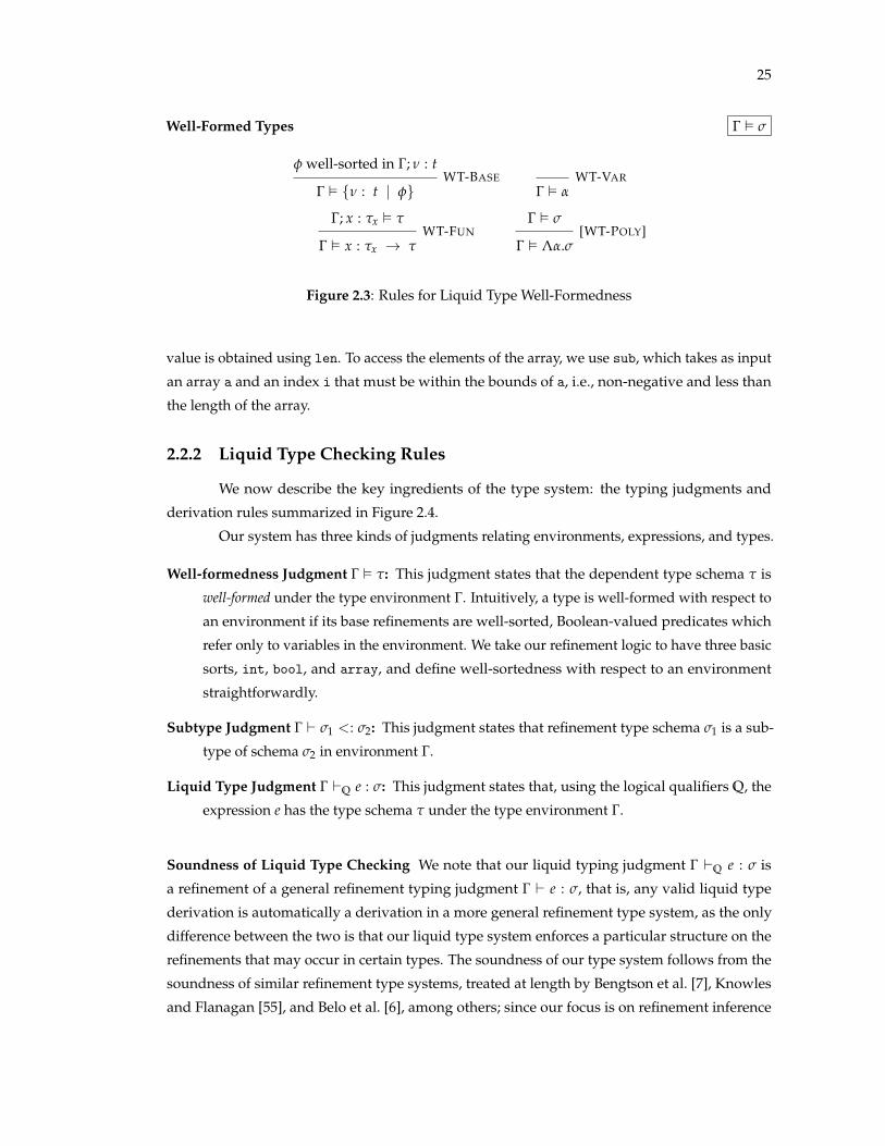
25
Well-Formed Types G ✏ s
f well-sorted in G; n : t
G ✏ {n : t | f}WT-BASE
G ✏ aWT-VAR
G; x : tx ✏ t
G ✏ x : tx ! tWT-FUN
G ✏ s
G ✏ La.s[WT-POLY]
Figure 2.3: Rules for Liquid Type Well-Formedness
value is obtained using len. To access the elements of the array, we use sub, which takes as input
an array a and an index i that must be within the bounds of a, i.e., non-negative and less than
the length of the array.
2.2.2 Liquid Type Checking Rules
We now describe the key ingredients of the type system: the typing judgments and
derivation rules summarized in Figure 2.4.
Our system has three kinds of judgments relating environments, expressions, and types.
Well-formedness Judgment G ✏ t: This judgment states that the dependent type schema t is
well-formed under the type environment G. Intuitively, a type is well-formed with respect to
an environment if its base refinements are well-sorted, Boolean-valued predicates which
refer only to variables in the environment. We take our refinement logic to have three basic
sorts, int, bool, and array, and define well-sortedness with respect to an environment
straightforwardly.
Subtype Judgment G ` s1 <: s2: This judgment states that refinement type schema s1 is a sub-
type of schema s2 in environment G.
Liquid Type Judgment G `Q e : s: This judgment states that, using the logical qualifiers Q, the
expression e has the type schema t under the type environment G.
Soundness of Liquid Type Checking We note that our liquid typing judgment G `Q e : s is
a refinement of a general refinement typing judgment G ` e : s, that is, any valid liquid type
derivation is automatically a derivation in a more general refinement type system, as the only
difference between the two is that our liquid type system enforces a particular structure on the
refinements that may occur in certain types. The soundness of our type system follows from the
soundness of similar refinement type systems, treated at length by Bengtson et al. [7], Knowles
and Flanagan [55], and Belo et al. [6], among others; since our focus is on refinement inference

26
Liquid Type Checking G `Q e : s
G `Q e : s1 G ` s1 <: s2 G ✏ s2
G `Q e : s2LT-SUB
G(x) = {n : t | f}
G `Q x : {n : t | n = x}LT-VAR
G(x) not a base type
G `Q x : G(x)LT-VAR
G `Q c : ConstType(c)LT-CONST
G; x : tx `Q e : t G ✏ x : tx ! t
G `Q lx.e : x : tx ! tLT-FUN
G `Q v1 : x : tx ! t G `Q v2 : tx
G `Q v1 v2 : t[x 7! v2]LT-APP
G `Q v : bool G; v `Q e1 : s G;¬v `Q e2 : s G ✏ s
G `Q if v then e1 else e2 : sLT-IF
G `Q e : s a not free in G
G `Q La.e : La.sLT-GEN
G `Q e : La.s G ✏ t Shape(t) = t
G `Q e[t] : s[a 7! t]LT-INST
Subtyping G ` s1 <: s2
G ✏ f1 ) f2
G ` {n : t | f1} <: {n : t | f2}<:-BASE
G ` t0x <: tx G; x : t0
x ` t <: t0
G ` x : tx ! t <: x : t0x ! t0
<:-FUN
G ` a <: a<:-VAR
G ` s1 <: s2
G ` La.s1 <: La.s2<:-POLY
Figure 2.4: Rules for Liquid Type Checking
rather than the underlying refinement type system, we simply assume the soundness of the
underlying refinement type system. We formalize this assumption as follows:
27
Assumption 1. (Overapproximation of Liquid Type Judgment) If G `Q e : s then G ` e : s.
Let ,! describe the single evaluation step relation for lL expressions and ,!⇤ describe
the reflexive, transitive closure of ,!. We formalize our assumption of a sound underlying
refinement type system as follows:
Assumption 2. (Refinement Type Soundness) If G ` e : s, then either e ,!⇤v for some value v or the
evaluation of e does not terminate.
The preceding two assumptions combine to give the safety of the liquid types system:
Theorem 1. (Liquid Type Safety) If ∆ `Q e : s, then either e ,!⇤v for some value v or the evaluation of
e does not terminate.
We conclude that if an expression is well-typed in our type system then we are guaran-
teed that evaluation does not get “stuck”, i.e., at run-time, every primitive operation receives
valid inputs. Thus, if a program type checks we are guaranteed that every call to sub gets an
index that is within the array’s bounds. Arbitrary safety properties (e.g., divide-by-zero errors)
can be expressed by using suitable types for the appropriate primitive constant (e.g., requiring
the second argument of (/) to be non-zero or requiring the argument to the assert function to
evaluate to true).
2.2.3 Features of the Liquid Type System
Next, we describe some of the features unique to the design of the liquid type system
and how they contribute to automatic type inference and verification.
1. Value and Path Sensitivity Our type system is both value and path sensitive: its reasoning
incorporates both the values of variables, as determined through the refinement type bindings in
the environment, and information about the branches under which an expression is evaluated,
determined by the guard predicates in the environment. Both value and path sensitivity are
crucial to proving properties like the safety of array accesses within a program. For example,
our type system uses the branch information in the sum example of section 2.1 to infer that the
occurrence of k inside the else expression is non-negative, since the else expression is evaluated
only when k � 0. Further, our system uses the fact that s is non-negative, expressed as the
refinement type {n : int | n � 0} bound to s, to determine that the expression s + k returns a
non-negative value.
Note that value and path sensitivity are especially important in performing static array
bounds checking, as programmers often compare an array index to some some other variable that
is known to be smaller than the array length (e.g., in amax from section 2.1), and only perform the
array access under the appropriate guard; verifying the safety of array accesses in this situation
28
requires knowing not only what values variables may take on, captured in their refinement types,
but also which branch conditions are in effect.
Checking that a value has an expected type — for example, that an array index is within
bounds — is done by performing a subtyping check, while type inference is performed by
generating subtyping constraints. Thus, the crucial place where value and path information must
be accounted for in our reasoning is in subtyping. By the rules in Figure 2.4, all subtyping checks
are reduced to subtyping checks over base (i.e., non-function) refinement types; these subtyping
checks are further reduced to checking logical implications between refinement predicates, given
the value and path assumptions in the environment. Thus, in order to use the information from
the environment in implication checks, we must embed the type environment into the logic. We
write
[[G]] ⌘^{f | f 2 G} ^
^{f[n 7! x] | x : {n : t | f} 2 G}
as the embedding for the environment into our refinement logic. Notice that we use the guard
predicates and base type bindings in the environment to strengthen the antecedent of the
implication. However, we substitute all occurrences of the value variable n in the refinements
from G with the actual variable being refined, thereby asserting in the antecedent that the program
variable satisfies the base refinement predicate. Thus, in the embedded formula, all occurrences
of n refer to the two types that are being checked for subtyping. For example, for the then
expression in max from section 2.1, the subtyping relation: x : int; y : int; x > y ` {n = x} <:
{x n ^ y n} holds as the following implication is valid in EUFA: (true ^ true ^ x > y) ^(n = x) ) x n ^ y n.
2. Recursion via Polymorphism To handle polymorphism, our type system incorporates type
generalization and instantiation annotations, which are over ML type variables a and monomor-
phic ML types t, respectively, and thus can be reconstructed via a standard type inference
algorithm. The rule LT-INST allows a type schema to be instantiated with an arbitrary liquid type
t of the same shape as t, the monomorphic ML type used for instantiation. We use polymorphism
to encode recursion via the polymorphic type given to fix. That is, let rec bindings are syntac-
tic sugar: let rec f = e in e’ is internally converted to let f = fix (fun f -> e) in e’.
The expression type checks if there is an appropriate liquid type that can be instantiated for the a
in the polymorphic type of fix; this liquid type corresponds to the type of the recursive function
f.
3. The Liquid Type Restriction The most critical difference between the rules for liquid type
checking and other refinement type systems is that our rules stipulate that certain kinds of
expressions have liquid types. In essence, these expressions are the key points where appropriate
refinement types must be inferred. By forcing the types to be liquid, we bound the space of
possible solutions, thus making inference efficiently decidable.

29
LT-INST For polymorphic instantiation, also the mechanism for handling recursion, the liquid
type restriction enables efficient inference by making the set of candidate refinement types finite.
LT-FUN For l-abstractions, we impose the restriction that the input and output be liquid to
ensure the types remain small, thereby making algorithmic checking and inference efficient. This
is analogous to procedure “summarization” for first-order programs.
LT-IF For conditional expressions we impose the liquid restriction and implicitly force the then
and else expressions to be subtypes of a fresh liquid type, instead of an explicit “join” operator
as in dataflow analysis. We do so as the expression may have a function type and, with a join
operator, input type contravariance would introduce disjunctions into the refinement type which
would have unpleasant algorithmic consequences.
LT-LET For let expressions, we impose the liquid restriction as a means of eliminating the locally
bound variable from the refinement type of the whole expression (as the local variable goes
out of scope). The antecedent G ✏ t requires that the liquid type be well-formed in the outer
environment, which, together with the condition, enforced via alpha-renaming, that each variable
is bound only once in the environment, is essential for ensuring the soundness of our system
(Appendix A). An alternative would be to existentially quantify the bound variable in the let
expression’s type, in the style of Knowles and Flanagan [54]; we eschew this option for simplicity.
4. Placeholder Variables and a-Renaming We use the placeholder variables ? in our refinement
predicates instead of “hard-coded” program variables to make our type system robust to a-
renaming. If Q is {x < n}, then ∆ `Q lx.x + 1 : x : int ! {x < n} a valid judgment, but
∆ `Q ly.y + 1 : y : int ! {y < n} is not, as y < n is not in Q?. If instead Q is {? < n}, then
Q? includes {x < n, y < n} and so both of the above are valid judgments. In general, our type
system is robust to renaming in the following sense: if G `Q e1 : s1 and e1 is a-equivalent to e2
and the free variables of Q are bound1 in G, then for some s2 that is a-equivalent to s1, we have
G `Q e2 : s2.
2.3 Liquid Type Inference
We now turn to the heart of our system: the algorithm Liquid, shown in Figure 2.6,
that takes as input a type environment G, an expression e, and a finite set of logical qualifiers
Q and determines whether e is well-typed over Q, i.e., whether there exists some s such that
G `Q e : s. Our algorithm proceeds in three steps. First, we observe that the dependent type for
any expression must be a refinement of its ML type, and so we invoke Hindley-Milner (HM) to
infer the types of subexpressions, and use the ML types to generate templates representing the1Recall that variables are bound at most once in any environment
30
unknown refinement types for the subexpressions (Section 2.3.1). Second, we use the syntax-
directed liquid typing rules from Figure 2.4 to build a system of constraints that capture the
subtyping relationships between the templates that must hold for a liquid type derivation to exist
(Section 2.3.2). Third, we use Q to solve the constraints using a technique inspired by predicate
abstraction (Section 2.3.3).
2.3.1 ML Types and Templates
Our type inference algorithm is based on the observation that the liquid type derivations
are refinements of the ML type derivations, and hence the refinement types for all subexpressions
are refinements of their ML types.
ML Type Inference Oracle Let HM be an ML type inference oracle, which takes an ML type
environment G and an expression e and returns the ML type schema s if and only if, using
the classical ML type derivation rules [26], there exists a derivation G ` e : s. The liquid type
derivation rules are refinements of the ML type derivation rules. That is, if G `Q e : s then
HM(Shape(G), e) = Shape(s). Moreover, we assume that the ML type derivation oracle has
“inserted” suitable type generalization (La.e) and instantiation (e[t]) annotations. Thus, the
problem of refinement type inference reduces to inferring appropriate refinements of the ML
types.
Templates Let K be a set of liquid type variables k, used to represent unknown type refinement
predicates. A template T is a refinement type schema described via the grammar shown below,
where some of the refinement predicates are replaced with liquid type variables with pending
substitutions. A template environment is a map G from variables to templates.
q ::= e | [x 7! v]; q (Pending Substitutions)
T ::= S(f [ qk) (Templates)
Variables with Pending Substitutions A sequence of pending substitutions q is defined using the
grammar above. To understand the need for q, consider rule LT-APP from Figure 2.4, which
specifies that the type of a function application is obtained by substituting all occurrences of
the formal argument x in the output type of v1 with the actual expression v2 passed in at the
application. When generating the constraints, the output type of v1 is unknown and is represented
by a template containing liquid type variables. Suppose that the type of v1 is x : t ! {n : t | k},
where k is a liquid type variable. In this case, we will assign the application v1 v2 the type
{n : t | k[x 7! v2]}, where k[x 7! v2] is a variable with a pending substitution [53]. Note that
substitution can be “pushed inside” type constructors, e.g., q({k1} ! {k2}) is the same as
{qk1} ! {qk2} and so it suffices to apply the pending substitutions only to the root of the
template.
31
ConsGen(G, e) = match e with
| x ! if HM(Shape(G), e) = t then ({n : t | n = x}, ∆) else (G(x), ∆)
| c ! (ConstType(c), ∆)
| v1 v2 !let (x : Tx ! T, C1) = ConsGen(G, v1)
let (T0x, C2) = ConsGen(G, v2)
(T[x 7! v2], C1 [ C2 [ {G ` T0x <: Tx})
| lx.e !let x : Tx ! T = Fresh(HM(Shape(G), lx.e))
let (T0, C) = ConsGen(G; x : Tx, e)
(x : Tx ! T, C [ {G ✏ x : Tx ! T} [ {G; x : Tx ` T0 <: T})| if v then e2 else e3 !
let T = Fresh(HM(Shape(G), e))
let ( , C1) = ConsGen(G, v)
let (T2, C2) = ConsGen(G; v, e2)
let (T3, C3) = ConsGen(G;¬v, e3)
(T, C1 [ C2 [ C3 [ {G ✏ T}[{G; v ` T2 <: T} [ {G;¬v ` T3 <: T})
| let x = e1 in e2 !let T = Fresh(HM(Shape(G), e))
let (T1, C1) = ConsGen(G, e1)
let (T2, C2) = ConsGen(G; x : T1, e2)
(T, C1 [ C2 [ {G ✏ T} [ {G; x : T1 ` T2 <: T})| La.e !
let (T, C) = ConsGen(G, e)
(La.T, C)
| e[t] !let T = Fresh(t)
let (La.T0, C) = ConsGen(G, e)
(T0[a 7! T], C [ {G ✏ T})
Figure 2.5: Constraint Generation from lL Programs
2.3.2 Constraint Generation
We now describe how our algorithm generates constraints over templates by traversing
the expression in the syntax-directed manner of a type checker, generating fresh templates
32
Refine(C, A) = match C with
| G ✏ {n : t | qk} ! A[k 7! {q | q 2 A(k) and qq well-sorted in Shape(G); n : t}]| G ` {n : t | p} <: {n : t | qk} ! A[k 7! {q | q 2 A(k) and A(G) ✏ A(p) ) qq}]| ! ?
Solve(C, A) =
if exists C 2 C such that A(C) is not valid then Solve(C, Refine(C, A)) else A
Liquid(G, e, Q) =
let (T, C) = ConsGen(G, e)
let A = Solve(Split(C), lk. QInst(G, e, Q))
A(T)
Figure 2.6: Liquid Type Inference Algorithm
for unknown types, constraints that capture the relationships between the types of various
subexpressions, and well-formedness requirements. The generated constraints are such that they
have a solution if and only if the expression has a valid liquid type derivation. Our inference
algorithm uses two kinds of constraints over templates.
Well-formedness Constraints Constraints of the form G ✏ T, where G is template environment,
and T is a template, ensure that the types inferred for each subexpression are over program
variables that are in scope at that subexpression.
Subtyping Constraints Constraints of the form G ` T1 <: T2 where G is a template environment
and T1 and T2 are two templates of the same shape, ensure that the types inferred for each
subexpression can be combined using appropriate subsumption relationships to yield a valid
type derivation.
Our constraint generation algorithm, ConsGen, shown in Figure 2.5, takes as input a
template environment G and an expression e that we wish to infer the type of and returns as output
a pair of a type template T, which corresponds to the unknown type of e, and a set of constraints
C. Intuitively, ConsGen mirrors the type derivation rules and generates constraints C which
capture exactly the relationships that must hold between the templates of the subexpressions in
order for e to have a valid type derivation over Q. To understand how ConsGen works, notice
that the expressions of lL can be split into two classes: those whose types are constructible from
the environment and the types of subexpressions, and those whose types are not.
Expressions with Constructible Types The first class of expressions are variables, constants,
function applications and polymorphic generalizations, whose types can be immediately con-
33
structed from the types of subexpressions or the environment. For such expressions, ConsGen
recursively computes templates and constraints for the subexpressions and appropriately com-
bines them to form the template and constraints for the expression.
As an example, consider ConsGen(G, v1 v2). First, ConsGen is called recursively to
obtain the templates and constraints for the subexpressions v1 and v2. If a valid ML type
derivation exists, then v1 must be a function type with some formal x. The returned template is
the result of pushing the pending substitution of x with the actual argument v2 into the “leaves”
of the template corresponding to the return type of v1. The returned constraints are the union of
the constraints for the subexpressions and a subtyping constraint ensuring that the type of the
argument v2 is a subtype of the argument type of v1.
Expressions with Liquid Types The second class are expressions whose types cannot be derived
as above, as the subsumption rule is required to perform some kind of “over-approximation” of
their concrete semantics. These include l-abstractions, if-then-else expressions, let-bindings, and
polymorphic instantiations (which includes recursive functions). We use two observations to
infer the types of these expressions. First, the shape of the refinement type is the same as the ML
type of the expression. Second, from the liquid type restriction, we know that the refinement
predicates for these expressions are conjunctions of logical qualifiers from Q? (see rules LT-LET,
LT-FUN, LT-IF, and LT-INST of Figure 2.4). Thus, to infer the types of these expressions, we
invoke HM to determine the ML type of the expression, use Fresh to generate a template with
the same shape as the ML type but with fresh liquid type variables representing the unknown
refinements, and generate subtyping constraints which are satisfied if and only if there is an
assignment to the predicate variables in the type template that makes the expression well-typed.
As an example, consider ConsGen(G, if v then e1 else e2). First, a fresh template is
generated using the ML type of the expression. Next, ConsGen recursively generates templates
and constraints for the then and else subexpressions. Note that, for the then subexpression, the
environment is extended with v, while, for the else subexpression, the environment is extended
with ¬v, as in the type derivation rule LT-IF from Figure 2.4. The fresh template is returned as
the template for the whole expression. The constraints returned are the union of those for the
subexpressions, a well-formedness constraint for the whole expression’s template, and subtyping
constraints forcing the templates for the then and else subexpressions to be subtypes of the
whole expression’s template.
Example Constraints The well-formedness constraint ∆ ✏ x : {kx
} ! y : {ky
} ! k1 is
generated for the fresh template for max from Figure 2.1. The constraint ensures that the inferred
type for max only contains program variables that are in scope at the point where max is bound.
The if expression that is the body of max is an expression with liquid type. For this expression, a

34
fresh template k10 is generated, and the subtyping constraints
x : {kx
}; y : {ky
}; x > y ` {n = x} <: {k10}
x : {kx
}; y : {ky
};¬(x > y) ` {n = y} <: {k10}
x : {kx
}; y : {ky
} ` {k10} <: {k1}
are generated, capturing the relationships between the then and the if expression, the else
and the if expression, and the if and the output expression, respectively. (Constraints 1.1 and
1.2 are the above constraints, simplified for exposition.) The recursive application sum (k-1)
from Figure 2.1 is an expression with a constructible type. For this expression the subtyping
constraint 2.2 is generated, forcing the actual to be a subtype of the formal. The output of the
application, i.e., the output type k2 of sum, with the pending substitution of the formal k with the
actual (k� 1) is shown bound to s in constraint 2.3.
2.3.3 Constraint Solving
Next, we describe our two-step algorithm for solving the constraints, i.e., assigning liquid
refinement predicates to all variables k such that all constraints are satisfied. In the first step, the
algorithm uses the well-formedness and subtyping rules to split the complex constraints, which
may contain function types, into simple constraints over refinement predicate variables with
pending substitutions. In the second step, the algorithm computes a solution to the simplified
constraints by beginning with a trivial assignment, in which each refinement predicate variable
is assigned the conjunction of all logical qualifiers, and iteratively weakening the solution until it
find the least fixpoint solution for all the simplified constraints or determines that the constraints
have no solution. In the following, we formalize the notion of a solution and then describe the
two-step algorithm that computes solutions.
Satisfying Liquid Assignments A Liquid Assignment over Q is a map A from refinement predi-
cate variables k to sets of qualifiers from Q?. Assignments can be lifted to maps from templates
T to refinement type schemas A(T) and template environments G to environments A(G), by
substituting each refinement predicate variable k withV
A(k) and then applying the pending
substitutions. The Liquid Assignment A satisfies a constraint C if A(C) is valid. That is, A satisfies
a well-formedness constraint G ✏ T if A(G) ✏ A(T), and a subtyping constraint G ` T1 <: T2 if
A(G) ` A(T1) <: A(T2). Liquid Assignment A is a solution for a set of constraints C if it satisfies
every constraint in C.
Step 1: Splitting into Simple Constraints. First, the algorithm calls Split, which uses the rules
for well-formedness and subtyping (Figure 2.4) to convert all the constraints over complex types
(e.g., function types) into simple constraints over base types. An assignment is a solution for C if
and only if it is a solution for Split(C).
35
Example: Splitting The well-formedness constraint ∆ ✏ x : {kx
} ! y : {ky
} ! {k1} splits
into the three simple constraints: ∆ ✏ {kx
}, x : {kx
} ✏ {ky
} and x : {kx
}; y : {ky
} ✏ {k1}, which
ensure that: the parameter x must have a refinement over only constants and the value variable
n, as the first constraint’s environment is empty; the parameter y must have a refinement over
only x and n; and the output type’s refinement can refer to both parameters x, y and the value
variable. The function subtyping constraint generated by the call foldn (len a) 0 am (constraint
4.4) splits into the simple subtyping constraints 4.6, 4.7, and 4.8. Notice how substitution and
contravariance combine to cause the flow of the bounds information into input parameter {kl
}(constraint 4.6) thus allowing the system to statically check the array access.
Step 2: Iterative Weakening Due to the well-formedness constraints, any solution over Q must
map the liquid type variables to sets of qualifiers whose free variables are either the value
variable n or the variables in the input environment G, written Vars(G), or the variables in the
input expression e, written Vars(e). That is, any solution maps the liquid variables to a set of
qualifiers contained in QInst(G, e, Q) which is defined as
{q | q 2 Q? and FV(q) ✓ {n} [ Vars(G) [ Vars(e)}
where Vars(G) and Vars(e) are the set of variables in G and e, respectively. Notice that if Q is
finite, then QInst(G, e, Q) is also finite, as the placeholder variables can only be instantiated with
the finitely many variables from G and e. Thus, to solve the constraints, we call the procedure
Solve, shown in Figure 2.6, with the split constraints and a trivial initial assignment that maps
each liquid type variable to QInst(G, e, Q).
Solve repeatedly picks a constraint that is not satisfied by the current assignment and calls
Refine to remove the qualifiers that prevent the constraint from being satisfied. For unsatisfied
constraints of the form G ✏ {n : t | qk}, Refine removes from the assignment for k all the
qualifiers q such that qq (the result of applying the pending substitutions q to q) would not
be well-sorted in the environment Shape(G); n : t. For unsatisfied constraints of the form
G ` {n : t | p} <: {n : t | qk}, where p is either a refinement predicate or a refinement
predicate variable with pending substitutions, Refine removes from the assignment for k all
the logical qualifiers q such that the implication [[A(G)]] ^ A(p) ) qq is not valid in EUFA. For
unsatisfied constraints of the form G ` {n : t | p} <: {n : t | f}, Refine, and therefore Solve,
returns ?, indicating that the constraints have no solution, as there is no way to weaken p to
satisfy the constraint.
Correctness of Solve For two assignments A and A0, we say that A A0 if, for all k, the set
of logical qualifiers A(k) contains the set of logical qualifiers A0(k). We can prove that if a set
of constraints has a solution over Q then it has a unique minimum solution with respect to .
Intuitively, we invoke Solve with the least possible assignment that maps each liquid variable
to all the possible qualifiers. Solve then uses Refine to iteratively weaken the assignment until

36
the unique minimum solution is found. The correctness of Solve follows from the following
invariant about the iterative weakening: if A? is the minimum solution for the constraints,
then in each iteration, the current assignment A satisfies A A?. Thus, if Solve returns a
solution, then it must be the minimum solution for C over Q. If at some point a constraint
G ` {n : t | p} <: {n : t | f} is unsatisfied, subsequent weakening cannot make it satisfied.
Thus, if Solve returns ?, then C has no solution over Q.
By combining the steps of constraint generation, splitting and solving, we obtain our
dependent type inference algorithm, Liquid, shown in Figure 2.6. The algorithm takes as input
an environment G, an expression e and a finite set of logical qualifiers Q, and determines whether
there exists a valid liquid type derivation over Q for e in the environment G. The correctness
properties of Liquid are stated in the theorem below, whose proof is in Appendix A. From
Theorems 1 and 2, we conclude that, if Liquid(∆, e, Q) = s, then every primitive operation
invoked during the evaluation of e succeeds.
Theorem 2. Liquid Type Inference
1. Liquid(G, e, Q) terminates,
2. If Liquid(G, e, Q) = s then G `Q e : s, and,
3. If Liquid(G, e, Q) = ? then there is no s such that G `Q e : s.
Running Time Most of the time taken by Liquid is spent in Solve, which asymptotically domi-
nates the time taken to generate constraints. Solve returns the same output regardless of the order
in which the constraints are processed; for efficiency, we implement Solve in two phases. First,
Solve makes a (linear) pass that solves the well-formedness constraints, thus rapidly pruning
away irrelevant qualifiers. Second, Solve uses a standard worklist-based algorithm that solves
the subtyping constraints. The time taken in the first phase is asymptotically dominated by
the time taken in the second. Let Q be the maximum number of qualifiers that any refinement
predicate variable is mapped to after the first well-formedness pass, V be the number of variables
in the program e that have a base type, and D be the size of the ML type derivation for e in
the environment G. A constraint is sent to Refine only when the antecedent of its implication
changes, i.e., at most V ⇥ Q times. There are at most O(D) constraints and so Refine is called
at most O(D ⇥ V ⇥ Q) times. Each call to Refine makes at most Q calls to the theorem prover.
Thus, in all the running time of Liquid is O(D ⇥ V ⇥ Q2) assuming each theorem prover call
takes unit time. Of course, D can be exponential in the program size (but tends to be linear in
practice), and the size of each theorem prover query is O(V ⇥ Q). Though validity checking in
EUFA is NP-Hard, several solvers for this theory exist which are very efficient for the simple
queries that arise in our context [28, 33].
37
2.3.4 Features of Liquid Type Inference
We now discuss some features of the inference algorithm.
1. Type Variables and Polymorphism There are two kinds of type variables used during
inference: ML type variables a obtained from the ML types returned by HM, and refinement
predicate variables k introduced during liquid constraint generation to stand for unknown
liquid refinement predicates. Our system is monomorphic in the refinement predicate variables.
Polymorphism only enters via the ML type variables as fresh liquid type variables are created at
each point where an ML type variable a is instantiated with a monomorphic ML type.
2. Whole Program Analysis and Non-General Types Due to the above, the types we ob-
tain for function inputs are the strongest liquid supertype of all the arguments passed into
the function. This is in contrast with ML type inference, which infers the most general type
of the function independent of how the function is used. For example, consider the func-
tion neg defined as fun x -> (-x), and suppose that Q = {0 n, 0 � n}. In a program
comprising only the above function, i.e., where the function is never passed arguments, our
algorithm infers neg : {0 n ^ 0 � n} ! {0 n ^ 0 � n} which is useless but sound. If
neg is only called with (provably) non-negative arguments, the algorithm infers the type
neg : {0 n} ! {0 � n}, while if neg is only called with (provably) non-positive arguments,
the algorithm infers the type neg : {0 � n} ! {0 n}. If neg is called with arbitrary argu-
ments, the algorithm infers neg : int ! int and not a more general intersection of function
types. We found this design choice greatly simplified the inference procedure by avoiding
expensive “case splits” on all possible inputs [41] while still allowing us to prove the safety
of challenging benchmarks. Moreover, we can represent the intersection type in our system
as: x : int ! {(0 x ) 0 � n) ^ (0 � x ) 0 n)}, and so, if needed, we can recover the
precision of intersection types by using qualifiers containing implications.
3. A-Normalization Recall the sum example from section 2.1. Our system as described would
fail to infer that the output type of
let rec sum k = if k < 0 then 0 else (s + sum (k-1))
was non-negative, as it cannot use the fact that sum (k-1) is non-negative when inferring the
type of the else expression. This is solved by A-Normalizing[38] the program so that intermediate
subexpressions are bound to temporary variables, thus allowing us to use information about
types of intermediate expressions, as in the original sum implementation.
38
2.4 Implementation and Evaluation
To validate the utility of the liquid types refinement type inference technique as applied
to high-level, functional programming languages, we have built DSOLVE, which infers liquid
types for OCaml programs. While refinement types can be used to statically prove a variety
of properties, as shown by Kawaguchi et al. [52], Bengtson et al. [7], and Dunfield [31], among
others, in our evaluation we focus on the canonical problem of proving the safety of array
accesses. We use a diverse set of challenging benchmarks that were previously annotated in
the DML project [83] to demonstrate that DSOLVE, together with a simple set of array bounds
checking qualifiers, can prove safety completely automatically for many programs. For the few
programs where these bounds checking qualifiers are insufficient, the programmer typically
only needs to specify one or two extra qualifiers. Even in these rare cases, the refinement types
DSOLVE infers using only the bounds checking qualifiers help the programmer to rapidly identify
the relevant extra qualifiers. We show that, over all the benchmarks, DSOLVE reduces the manual
annotation required to prove safety from 17%, by number of lines, to under 1%. Finally, we
describe a case study where DSOLVE was able to pinpoint an error in an open source OCaml bit
vector library implementation, in a function that contained an explicit, but insufficient, safety
check.
2.4.1 DSOLVE: Liquid Types for OCaml
We begin with a description of our implementation of liquid type inference in the tool
DSOLVE, which infers liquid types for OCaml programs.
Architecture DSOLVE is built on top of OCaml: DSOLVE uses the OCaml parser and type
inference engine to implement the oracle HM, and uses OCaml’s facilities for outputting type
annotations that can be viewed by the user using an external tool. Type inference in DSOLVE is
divided into the following three phases: First, the OCaml compiler’s parser and type checker
are used to translate the input program to a typed AST; this phase also parses the module’s
refinement type specification. Second, the typed AST is traversed to generate a set of subtyping
constraints over templates that represent the potentially-unknown refinement types of the
program expressions. Third, the constraints are solved using predicate abstraction over a finite
set of predicates generated from user-provided logical qualifiers. This pass uses the Z3 SMT
solver [28] to discharge logical implications corresponding to the subtyping constraints. If the
constraints can be satisfied, the program is deemed safe. Otherwise, DSOLVE reports a type error
and the lines in the original source program that yielded the unsatisfiable constraints.
DSOLVE is conservative: if an error is reported, it may be because the program is unsafe,
or because the set of qualifiers provided was insufficient, or because the invariants needed to
prove safety cannot be expressed within our refinement type system.

39
Input DSOLVE takes as input a source (.ml) file containing an OCaml program, an interface
(.mlq) file containing a refinement type specification for the interface functions of the .ml file, and
a qualifier (.hquals) file containing a set of logical qualifiers. DSOLVE combines the qualifiers
from the .hquals file with some scraped from the specification .mlq file and a standard qualifier
library to obtain the set of logical qualifiers used to infer liquid types.
Output DSOLVE produces as output a refinement type for each program expression in a standard
OCaml type annotation (.annot) file. The user can view the inferred refinement types using
standard tools like Emacs, Vim, and Caml2HTML. If all the constraints are satisfied, the program
is reported as safe. Otherwise, DSOLVE outputs warnings indicating the potentially unsafe
expressions in the program.
Modular Checking DSOLVE verifies one module at a time. If a module depends on another
module, it can be checked against that module’s .mlq file; the other module’s source code is not
required.
Abstract Modules It is possible to create a .mlq file which defines types, axioms (background
predicates), and uninterpreted functions, without a corresponding .ml file. Such “abstract
modules” allow the user to extend DSOLVE with reasoning about mathematical structures which
do not appear directly in the program. For example, an abstract module Set.mlq might contain
a type which represents a polymorphic set collection, along with an appropriate refined interface
and axioms which build a set theory. This set theory can be used in another module’s type
refinements; for example, it may be used in a sorting module to verify that the sets of elements in
the input and output lists of a sorting function are equal.
2.4.2 Benchmark Results
To show the real-world applicability of the liquid types approach, we applied DSolve
to a number of benchmarks from the DML project [82] (ported to OCaml) that were previously
annotated with dependent types with the goal of statically proving the safety of array accesses
[83]. The benchmarks are listed in the first column of Table 2.1. The second column indicates the
size of the benchmark (ignoring comments and whitespace). The benchmarks include OCaml
implementations of the Simplex algorithm for linear programming (simplex), the fast Fourier
transform (fft), Gaussian elimination (gauss), matrix multiplication (matmult), binary search
in a sorted array (bsearch), computing the dot product of two vectors (dotprod), insertion
sort (isort), the n-queens problem (queen), the Towers of Hanoi problem (tower), a fast byte
copy routine (bcopy), and heap sort (heapsort). The above include all DML array benchmarks
except quicksort, whose invariants remain unclear to us. In addition, we ran DSOLVE on a
simplified Quicksort routine from OCaml’s Sort module (qsort-o), a version ported from the

40
Table 2.1: Experimental Results: LOC is the number of lines of program text (withoutannotation) after removing whitespace and comments from the code. DML is the number oflines of manual annotation required in the DML versions of the benchmarks. DSOLVE is the
amount of manual annotation required by DSOLVE, i.e., number of lines of qualifiers not in QBC.Time is the time taken by DSOLVE to infer refinement types.
Program LOC DML (LOC) DSOLVE (LOC) Time (s)dotprod 7 3 (30%) 0% 0.31bcopy 8 3 (27%) 0% 0.15bsearch 24 3 (11%) 0% 0.46queen 30 7 (19%) 0% 0.70isort 33 12 (27%) 0% 0.88tower 36 8 (18%) 1 (2%) 3.33matmult 43 10 (19%) 0% 1.79heapsort 84 11 (12%) 0% 0.53fft 107 13 (11%) 1 (1%) 9.13simplex 118 33 (22%) 0% 7.73gauss 142 22 (13%) 1 (1%) 3.17TOTAL 633 125 (17%) 3(1%)qsort-o 62 0 (0%) 1.89qsort-d 112 5 (5%) 18.28bitv 426 65 (15%) 63.11
DML benchmark (qsort-d) where one optimization is removed, and BITV, an open source bit
vector library (bitv).
Array Bounds Checking Qualifiers To automate static array bounds checking with DSOLVE,
we observe that the safety of array accesses typically depends on the relative ordering of integer
expressions. Thus, to statically prove the safety of array accesses, we use the mechanically-
generated set of array bounds checking qualifiers QBC defined as
QBC , {n ./ X | ./2 {<,,=, 6=,>,�} ^ X 2 {0, ?, len ?}}.
Next, we show experimental results demonstrating that liquid type inference over QBC suffices
to prove the safety of most array accesses. Even when DSOLVE needs extra qualifiers, the types
inferred using QBC help the programmer quickly identify the relevant extra qualifiers.
Array Bounds Checking Results As shown in column DSOLVE of Table 2.1, DSOLVE needs no
manual annotations for most programs; that is, the qualifiers QBC suffice to automatically prove
the safety of all array accesses. For some of the examples, e.g., tower, we do need to provide extra
qualifiers. However, even in this case, the annotation burden is typically just a few qualifiers. For
example, in tower, we require a qualifier which is analogous to n = n� h1� h2, which describes
the height of the “third” tower, capturing the invariant that the height is the total number of rings
n minus the rings in the first two towers. Similarly, in bitv, one qualifier states the key invariant
41
relating a bit vector’s length to the length the underlying data structure used to store the bit
vector, an array of integers. The time for inference is robust to the number of qualifiers, as most
qualifiers are pruned away by the well-formedness constraints. In our prototype implementation,
the time taken for inference is reasonable even for non-trivial benchmarks like simplex, fft and
gauss.
Case Study: Bit Vectors We applied DSOLVE to verify the open source BITV bit vector library
(version 0.6). A bit vector in BITV consists of a record with two fields: length, the number of
bits stored, and bits, the actual data, stored within an array of integers. If b is the number of bits
stored per array element, length and bits are related by
(len bits� 1) · b < length (len bits) · b.
The executed code, and hence refinement types, are different for 32- and 64-bit machines. Thus,
to verify the code using our conjunctive types, we fixed the word size to 32 bits. We were able to
verify the array safety of 58 of BITV’s 65 bit vector creation, manipulation, and iteration functions,
which contain a total of 30 array access operations.
There are three kinds of manual annotation needed for verification: extra qualifiers (14
lines), trusted assumptions (8 lines), and interface specifications (43 lines). The trusted assumptions
(which are akin to dynamic checks) are needed due to current limitations of our system. These
include the conservative way in which modular arithmetic is embedded into EUFA, the lack of
refinements for type variables and recursive datatypes, and the conservative handling of control
flow. The interface specifications are needed because BITV is a library, i.e., an open program.
Thus, for verification, we need to specify that the API functions are called with valid input
vectors that satisfy invariants like the one described above. The interface specifications, by far
the largest category of annotations, are unavoidable. The extra qualifiers and expressiveness
limitations are directions for future work.
DSOLVE was able to locate a serious bounds checking error in BITV. The error occurs in
BITV’s blit function, which copies c bits from v1, starting at bit offset1, to v2, starting at bit
offset2. This function first checks that the arguments passed are safe, and then calls a fast but
unsafe internal function, unsafe blit:
let blit v1 offset1 v2 offset2 c =
if c < 0 || offset1 < 0 || offset1 + c > v1.length
offset2 < 0 || offset2 + c > v2.length
then invalid_arg "Bitv.blit";
unsafe_blit v1.bits offset1 v2.bits offset2 c
unsafe blit immediately accesses the bit at offset1 in v1, regardless of the value of c. When
the parameters are such that: offset1 = v1.length and v1.length mod b = 0 and c = 0,

42
unsafe blit attempts to access the bit at index v1.length, which must be located in
v1.bits[v1.length / b];
but this is
v1.bits[len v1.bits],
which is out of bounds and can cause a crash, as we verified with a simple input. The problem
is that blit does not verify that the starting offset is within the bounds of the bit vectors.
This is fixed by adding the test offset1 >= v1.length (and offset2 >= v2.length for similar
reasons). DSOLVE successfully type checks the corrected version.
Acknowledgements
This chapter contains material adapted from the following publications:
Patrick Rondon, Ming Kawaguchi, Ranjit Jhala. “Liquid Types”, Proceedings of the 2008
ACM SIGPLAN conference on Programming Language Design and Implementation (PLDI), pages
159–169, 2008.
Ming Kawaguchi, Patrick Rondon, Ranjit Jhala. “DSolve: Safety Verification via Liquid
Types”, Proceedings of Computer Aided Verification 2010 (CAV), pages 123–126, 2010.
Chapter 3
Low-Level Liquid Types
Static verification is a crucial last line of defense at the lowest levels of the software stack,
as at those levels we cannot fall back on dynamic mechanisms to protect against bugs, crashes, or
malicious attacks. Recent years have seen significant progress on automatic static verification
tools for systems software. These tools employ abstract interpretation [9, 50] or software model
checking [5, 46, 12, 85] to infer path-sensitive invariants over program variables like status
flags and counters and thereby verify control-sensitive safety properties. Unfortunately, these
approaches have been proven insufficient for verifying data-sensitive properties of values stored
in lists, trees, etc., as this requires the precise inference of invariants of data values stored within
unbounded collections of heap-allocated cells.
In the previous chapter, we introduced liquid types, a refinement type system for OCaml
that marries the ability of OCaml types to infer coarse invariants of data structures (and higher-
order functions) with the ability of predicate abstraction and SMT solvers to infer path-sensitive
invariants of individual variables. We demonstrated that this symbiotic combination enables
the highly automated verification of complex data-sensitive properties of high-level, functional
programs. Unfortunately, the very nature of low-level, imperative code, typically written in C,
makes the translation of the liquid types program verification strategy to the setting of systems
software verification extremely challenging.
Lack of Types First, due to the presence of casts and pointer arithmetic, low-level systems code
is essentially untyped: C’s type system is designed only to allow the compiler to determine the
number of bytes that should be read or written by each instruction, and hence, unlike the type
systems of higher-level languages, C’s types provide no invariants about data values.
Mutation Second, mutation makes the very notion of type refinement problematic. The key
idea in refinement types is to adorn the basic underlying types with refinement predicates over
program variables. For example, in an OCaml program, the refinement type {n : int | x < n}
43
44
describes an integer that is greater than the program variable x. However, this type is meaningless
if the value of x can change over time.
Unbounded Collections Third, even if we could meaningfully track mutation, we cannot always
uniquely identify the object being mutated. In particular, the presence of unbounded collections
means that we must represent many elements of a collection by a single type. This makes it
impossible to strongly update the type of an element in the collection, creating a major loss of
precision in the presence of the temporary invariant violations common in low-level programs.
In this chapter, we develop low-level liquid types, a static refinement type system for C that
enables the precise verification and inference of data-sensitive properties of low-level software.
Low-level liquid types tackles the above challenges via a three-tiered design.
First, low-level liquid types is founded on a new physical type system that classifies
values and heaps. A value is either a datum of a given size, e.g., a 4-byte integer or a 1-byte
character, or a reference corresponding to a pair of a heap location and an offset within the location.
Intuitively, an offset corresponds to a field (respectively, cell) of the structure (respectively, array)
resident at the location. A heap is a map from locations to a sequence of offset-value bindings
that define the contents of the given location. By precisely tracking arithmetic on offsets, physical
types provide coarse invariants about the basic shapes of data values.
Second, each physical type is refined with a predicate that captures precise properties
of the values defined by the type. Low-level liquid types makes a clear separation between
immutable state, which is tracked using a traditional type environment, and mutable state, which
is tracked in a flow-sensitive heap. We ensure soundness by restricting the refinements to pure
predicates that refer only to immutable values. Of course, in C all entities are mutable. We
recover precision for stack-allocated variables by first carrying out an SSA renaming, which
creates different (immutable) versions of each variable at different program points.
Third, we recover precision for heap-allocated locations by using the physical type
information to strongly update the types of the heap’s contents on writes through pointers. Since
such strong updates are unsound when several physical heap locations are represented by a
single type, low-level liquid types distinguishes between abstract locations which summarize
a collection of physical memory locations and concrete locations which describe exactly one
physical memory location. Low-level liquid types enables strong updates by enforcing the
requirement that all pointer reads and writes are to concrete locations, and by employing two
mechanisms to account for aliasing, which we explain via a version control metaphor. The
unfold operation “checks out” a concrete reference to a particular location from the set described
by an abstract location, obtaining a pointer to a single run-time location whose type may be
strongly updated soundly. The dual to the unfold operation, fold, “commits” the changes made
to the particular location back into the abstract location after ensuring that the particular location
satisfies the invariants of the abstract location. Together, the automatically-inserted fold and

45
unfold annotations ensure that the invariants for an abstract location soundly apply to all the
elements that correspond to that location, while simultaneously allowing strong updates. This
is crucial, as strong updates are essential for both establishing invariants in spite of field-at-a-
time, incremental object initialization and reasoning in spite of the temporary violations of the
invariants that are ubiquitous in low-level code.
To demonstrate the utility of low-level liquid types, we have implemented our type
system in CSOLVE, a prototype static verifier for C. CSOLVE takes as input a C program and a set
of logical predicate templates and returns as output the inferred refinement types of functions,
local variables, and heap contents, along with a report of any type errors that occurred. Through a
set of challenging case studies, we show how the combination of types and predicate abstraction
enables the precise, path-sensitive verification and inference of control-sensitive properties
of individual variables and data-sensitive properties of aggregate structures manipulated in
low-level programs.
3.1 Overview
We begin with a high-level overview of low-level liquid types, and then, via a sequence
of examples, we illustrate how they enable the precise static verification and inference of program
invariants in the presence of challenging low-level programming constructs, including pointer
arithmetic, memory allocation, temporary invariant violations, aliasing, and unbounded data
structures.
3.1.1 Physical and Refinement Types and Heaps
We begin our overview of the low-level liquid types system by explaining the physical
base types that our system uses to represent data in low-level programs. We then explain how
these types are combined into heap types that represent the contents of the mutable run-time
store. Finally, we explain how refinement and liquid types and heaps are formed.
Physical Types Our system is based on a physical type system for C where every program
variable is either a basic data value of some size, e.g., a 4-byte integer, denoted by int, or a reference
comprising a location and an index within the location, denoted by ref(`, i), where ` is the location
and i the index within the location. For the purposes of this section, an index is either a natural
number n, which is a singleton offset used to model pointers to specific fields of a structure, or of
the form n+m, which is a sequence of offsets {n + km}•k=0 used to model pointers into an array
of items, each of size m, that starts at offset n. Thus, ref(`, 4) is a (possibly null) pointer that
refers to a location ` at (field) offset 4, while ref(`, 0+4) is a (possibly null) pointer that refers to a
location within an array of 4-byte integers.

46
Heaps To ensure the soundness of types in the presence of mutation, our representation of the
program state is partitioned into an environment, which is a standard sequence of type bindings
for immutable variables, and a heap, which is a mapping from locations ` to a set of index-type
pairs that describe the contents of the location, called a block. For example, the heap
`1 7! 0 : int, 4 : int
`2 7! 0+1 : char
has two locations. The first, `1, contains a structure with two integer fields, one at offset 0 and
one at offset 4. The second, `2, contains an array of one-byte characters (denoted char).
Refinement Types and Heaps In low-level liquid types, as in the liquid types system of the
previous chapter, program invariants are captured via refinement types, denoted by {n : t | f},
where t is the physical type being refined, n is a special value variable that denotes the value being
described, and f is the refinement predicate, a logical predicate containing the value variable. A
refinement heap is a heap where each location is mapped to a sequence of offset-refinement-type
pairs. For example, `1 7! 0 : {n : int | 0 n} is a heap with a location `1 which contains a
non-negative integer at offset 0.
Liquid Types The definitions of logical qualifiers and liquid types were given in section 2.1; we
review them here for convenience. A logical qualifier is a Boolean-valued expression over the
program variables, the value variable n, and a placeholder variable ?. We say that a qualifier q
matches the qualifier q0 if replacing some subset of the free variables in q with ? yields q0. For
example, the qualifier n x + y matches the qualifier n ?+ ?. We write Q? for the set of all
qualifiers not containing ? that match some qualifier in Q. In the rest of this section, let Q be the
set
{0 n, n = ?+ ?, n = BBegin(n), BBegin(n) = BBegin(?), BEnd(n) = BBegin(n) + ?}.
The terms BBegin(·) and BEnd(·) are uninterpreted function applications denoting the start and
end addresses of memory blocks; we will explain these shortly. A liquid type over Q (abbreviated
to just liquid type) is a refinement type where the refinement predicates are conjunctions of
qualifiers from Q?. Our system enables inference by requiring that the certain entities, e.g.,
loop-modified variables, functions, and blocks in aggregate structures, have liquid types.
3.1.2 Low-Level Liquid Types By Example
In the following, we give a high-level, example-driven overview of how low-level liquid
types is used to infer properties of low-level programs that manipulate stack-allocated scalar
data, in-heap array data, and unbounded heap data structures.

47
char *make_string (int n) {
char *res;
char *str;
1: if (n < 0) return NULL;
2: res = (char *) malloc (n * sizeof (char ));
3: str = res;
4: for (int i = 0; i < n; i++) {
5: *str++ = ’\0’;
}
6: return res;
}
Figure 3.1: Example: make string
Local Invariants
We begin by showing how our system uses local refinement types for individual program
variables to verify the safety of the pointer dereferences in the make string function shown in
Figure 3.1. The function takes an integer parameter n, allocates a new block of memory of size n,
iterates over the block using str to initialize it, and returns a reference, res, to the start of the
block.
Physical Types First, we describe the physical types computed for each variable. The function
calls malloc to create a new heap location `1 and returns a pointer to the location with offset 0.
Thus, res gets the physical type ref(`1, 0). str is initialized with res, but is updated inside the
loop with an increment of 1. Hence, res gets assigned the physical type ref(`1, 0+1). The loop
index i gets the physical type int.
Pointer Allocation and Arithmetic To specify when it is safe to dereference a pointer, we refine
the output type of malloc so that it contains information about the size of the allocated block. In
particular, in our system malloc returns a value of type
{n : ref(`, 0) | BLen(n, n)}
where n is the size argument passed to malloc and BLen is the following block length predicate:
BLen(n, n) , BBegin(n) = n ^ BEnd(n) = n +p n
The refinement states that the return value is equal to the start of the allocated region in which it
points, denoted BBegin(n), and that the end of the allocated region, denoted BEnd(n), is n bytes
from the beginning; the operator +p represents pointer arithmetic in our refinement logic. We
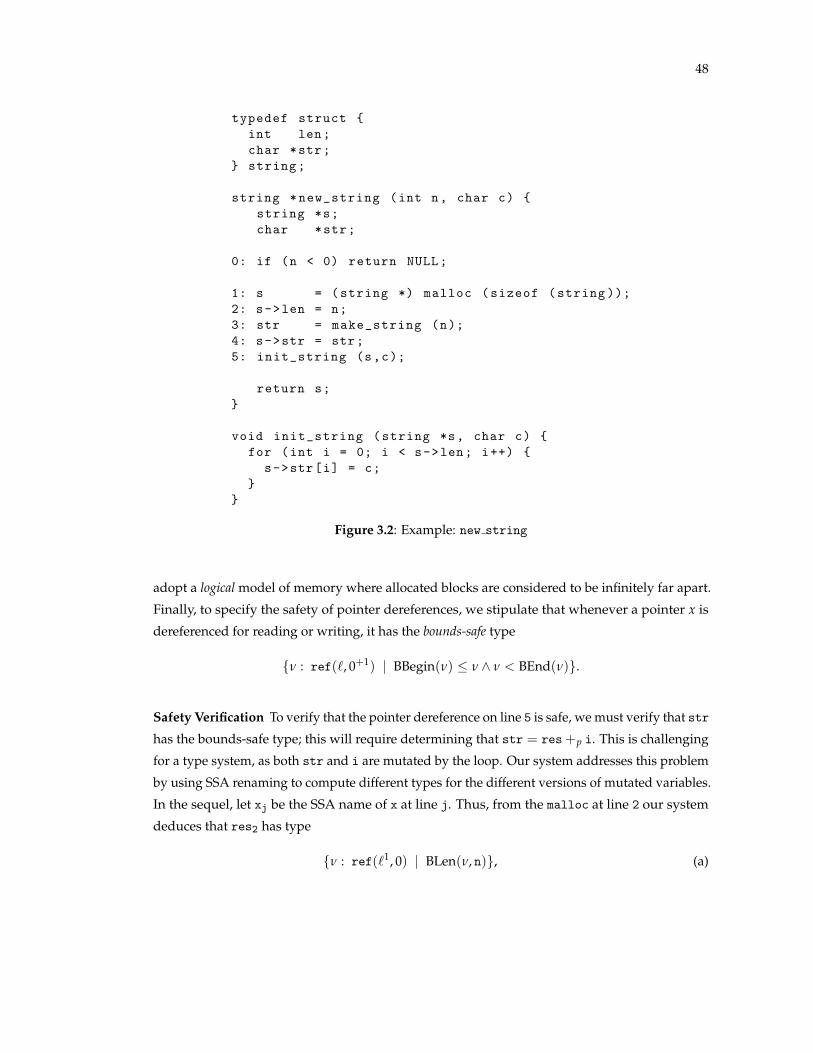
48
typedef struct {
int len;
char *str;
} string;
string *new_string (int n, char c) {
string *s;
char *str;
0: if (n < 0) return NULL;
1: s = (string *) malloc (sizeof (string ));
2: s->len = n;
3: str = make_string (n);
4: s->str = str;
5: init_string (s,c);
return s;
}
void init_string (string *s, char c) {
for (int i = 0; i < s->len; i++) {
s->str[i] = c;
}
}
Figure 3.2: Example: new string
adopt a logical model of memory where allocated blocks are considered to be infinitely far apart.
Finally, to specify the safety of pointer dereferences, we stipulate that whenever a pointer x is
dereferenced for reading or writing, it has the bounds-safe type
{n : ref(`, 0+1) | BBegin(n) n ^ n < BEnd(n)}.
Safety Verification To verify that the pointer dereference on line 5 is safe, we must verify that str
has the bounds-safe type; this will require determining that str = res+p i. This is challenging
for a type system, as both str and i are mutated by the loop. Our system addresses this problem
by using SSA renaming to compute different types for the different versions of mutated variables.
In the sequel, let xj
be the SSA name of x at line j. Thus, from the malloc at line 2 our system
deduces that res2
has type
{n : ref(`1, 0) | BLen(n, n)}, (a)

49
typedef struct _slist {
struct _slist *next;
string *s;
} slist;
slist *new_strings (int n) {
string *s;
slist *sl, *t;
1: sl = NULL;
2: for (int i = 1; i < n; i++) {
3: s = (string *) malloc (sizeof (string ));
4: s->len = i;
5: s->str = make_string (i);
6: t = (slist *) malloc (sizeof (slist ));
7: t->s = s
8: t->next = sl;
9: sl = t;
}
return sl;
}
Figure 3.3: Example: new strings
i.e., that res is a pointer to the start of a new location `1 whose size is n bytes. This same type is
assigned to str3
. Next, our system uses liquid type inference over the qualifiers Q to infer that,
at line 5, i5
and str5
have the respective types
{n : int | 0 n < n}
{n : ref(`1, 0+1) | n = res2
+p i5}.
Notice that these types are loop invariants. They hold the first time around the loop as initially i
is 0 and str is equal to res. The types are inductive invariants, as each loop iteration increments
i and res. Thus, our system uses liquid type inference to combine the above facts with (a) and
deduce that at line 5
BBegin(str5
) str5
^ str5
< BEnd(str5
),
i.e., that str5
has the bounds-safe type and hence the pointer dereferences at line 5 of make string
are safe.
Function Types Finally, note that make string returns the pointer res (i.e., res2
) on line 6. Thus,
using the type from (a) and the fact that the location `1 was freshly generated via malloc, our

50
system concludes that make string has the type:
8`1.(n : int)/∆ ! {n : ref(`1, 0) | BLen(n, n)}/`1 7! 0+1 : char (b)
That is, the function takes an integer n and an empty heap (that is, the function does not touch
any pre-existing heap contents) and returns a pointer to the start of a new char array of size n.
Heap-block Invariants
Next, we show how our system uses refinements to verify safety properties of blocks of
data residing in the heap. Consider the new string function shown in Figure 3.2. This function
takes a parameter, n, and produces a string structure representing a string of length n. The
string structure has two fields: len, the length of the string, and str, a pointer to the contents
of the string. The programmer intends that the fields obey the following two invariants:
(I1) the len field is non-negative, and
(I2) the str field points to a char array of size len.
Note that these invariants do not hold at all points during the lifetime of the structure; instead,
the programmer establishes them on lines 1-4, and then calls the procedure init string to fill
in the string with the supplied character c.
Next, we show how our system precisely tracks updates to the structure, tolerating the
early stages in which the invariant does not hold, in order to verify the safety of the pointer
dereferences within init string.
First, the malloc in line 1 creates a new location on the heap, `2, and gives s the type
ref(`2, 0), stating that it points into this location at offset 0. Initially, this location contains an
8-byte block (the size of the string structure), and so at line 2 the heap is
`2 7! uninitialized 8-byte block .
In line 2, we assign n to the len field of s, which creates a new binding in the heap for `2 at the
offset corresponding to the field len, namely 0, since len is the first element of the structure.
Thus, at line 3 the heap is
`2 7! 0 : {n : int | n = n}, uninitialized 4-byte block.
Next, in line 3, the call to make string creates a new location and assigns to str a pointer to the
new location, with the type shown in (b) (and (a)). Thus, at line 4 the heap contains two locations
`1 7! 0+1 : char
`2 7! 0 : {n : int | n = n}, uninitialized 4-byte block.

51
In line 4, the value of str is assigned to s->str, which creates a binding at the corresponding
offset in `2, namely 4, as the first field, len, was an int which is 4 bytes long. Thus, at line 5 the
heap is
`1 7! 0+1 : char
`2 7! 0 : {n : int | n = n}, 4 : {n : ref(`1, 0) | n = str}.
Finally, at line 5 we have the call to init string. At the callsite, our system uses the qualifiers in
Q, and the type of str to infer that the previously shown heap binding for `2 is subsumed by
`2 7! 0 : {n : int | n = n}, 4 : {n : ref(`1, 0) | BLen(n, n)}.
As the value at offset 0 equals n, the above block is subsumed by
`2 7! 0 : {n : int | n = n}, 4 : {n : ref(`1, 0) | BLen(n, @0)},
where n is replaced by @0, a name that denotes the value within the same block at offset 0. Finally,
our system uses the test at line 0 to deduce that n is non-negative at the callsite, so init string
is called with the heap h defined as
h , `2 7! 0 : {n : int | 0 n}, 4 : {n : ref(`1, 0) | BLen(n, @0)},
`1 7! 0+1 : char.
Note that, as the len field of a string structure is located at offset 0 and its str field is located
at offset 4, the bindings for `2 capture exactly the structure invariants I1, I2 intended by the
programmer. Moreover, even though the invariants don’t hold everywhere, our system is able to
use strong updates to establish them at function call boundaries. Thus, our system infers that the
function init string has the type
8`1, `2.(s : ref(`2, 0))/h ! void/h,
and, via reasoning analogous to that for make string, our system verifies the safety of array
accesses in init string.
Data Structure Invariants
In new string, s pointed to exactly one heap location, `1, throughout the execution
of the function. Thus, we could soundly perform strong updates to the block describing the
contents of `1; this allowed us to determine that the strings built by new string satisfied the
desired invariants. Unfortunately, we cannot soundly use strong updates when dealing with
collections of locations.

52
Consider the function new strings shown in Figure 3.3. This function takes an integer
parameter, n, and creates a list of strings of lengths from 1 to n, all of which satisfy the invariants
I1, I2. This is accomplished by looping from 1 to n, allocating memory for a new string and
assigning the pointer to this memory to s (line 3), initializing it as in new string (lines 4,5), and
inserting s into a list of strings (lines 6,7,8).
Note that s points to many different concrete locations over the course of executing the
function; this is in contrast to the previous functions, in which pointers only pointed to a single
concrete location while the function was executed. We formalize this distinction by saying that s
points to an abstract location⇠` . That is, in our system, s has the physical type ref(
⇠` , 0), which
states that it refers to the offset 0 within one of many possible locations.
Observe that it is not sound to perform strong updates to an abstract location’s type. To
see why, suppose that we had strongly updated⇠` as we did when analyzing new string. Then
we would assign⇠` a block type as follows:
⇠` 7! 0 : {n : int | n = i}, . . .
The problem with this type is that every string has a different length, and the above type only
ascribes a single length, i, to all strings. Thus, while we need strong updates to establish the
desired invariants for each string, we clearly cannot soundly perform strong updates on the
types of abstract locations.
We solve this problem with the following crucial observation. Suppose that the code
uses a pointer s to access a collection of locations⇠` . As long as we do not modify s or use other
pointers to⇠` , only one particular concrete location from the set represented by
⇠` can be modified
at a time. Thus, when a pointer to⇠` is first used, we can unfold the abstract location into a fresh
concrete location, `j, which inherits⇠` ’s invariant. As long as
⇠` is only accessed by a pointer to `j,
we can soundly perform strong updates on `j’s type. However, as soon as another pointer to⇠` is
used, the possibility of aliasing means we can no longer rely on `j’s type to be accurate. Thus,
before we access an abstract location via another pointer of type⇠` , we fold the concrete location `j
back into the collection by verifying that `j satisfies⇠` ’s invariants and removing it from the heap.
The other pointer then gets its own unfolded copy of the location, and can strongly update it,
until it gets folded back into the collection, and so on. Our system automatically places folds and
unfolds in the code in a manner that ensures that: (1) every heap access occurs via a reference
to a concrete location, and (2) every abstract location has at most one corresponding concrete
location unfolded in the heap at any point in time. In this way, our system can soundly establish
invariants about unbounded data structures in spite of temporary invariant violation even in the
presence of aliasing.
We now illustrate the above mechanism using the code in Figure 3.3. We will say that,
within the body of the loop, s points to some concrete location, `j, which is an instance of⇠` . We
will use strong updates, as in the previous examples, to verify that `j has the desired invariants,

53
i.e., that
`j 7! 0 : {n : int | 0 n}, 4 : {n : ref(`2, 0) | BLen(n, @0)}.
Finally, at the end of the loop — i.e., before we access another pointer into⇠` in the next iteration
— we fold the concrete location `j into the collection by ensuring that it satisfies⇠` ’s invariants,
i.e, by stipulating that at the end of of the loop, the block `j is a subtype of the block⇠` . In this
manner, our system performs strong updates locally and infers using Q that at the end of the
new strings, the heap is of the form
⇠` 7! 0 : ref(
⇠` , 0), 4 : ref(
⇠`1, 0)
⇠`1 7! 0 : {n : int | 0 n}, 4 : {n : ref(
⇠`2, 0) | BLen(n, @0)}
⇠`2 7! 0+1 : char.
Thus, our system infers that the function returns a list (⇠`) of pointers to string structures (`1)
each of which satisfy invariants I1 and I2.
This concludes our overview of low-level liquid types. Next we formalize our core
language and static type system (section 3.2). We then describe our experimental evaluation via
a set of challenging case studies (section 3.5). The operational semantics of our core language
appears in Appendix B, while a proof that our type system is sound with respect to the semantics
is given in Appendix C.
3.2 The NANOC Language and Type System
In this section, we present the syntax and types of NANOC, a simple C-like language
with integers and pointers, then present its type checking judgments.
3.2.1 Syntax
The syntax of NANOC is shown in Figure 3.4. We give an overview of the language’s
features below.
Values The set of NANOC values includes variables and integer constants. Integer constants
have the form n|w|, where w is the size, in bytes, of the value and n is the numerical integer value.
When it does not cause ambiguity, we will sometimes write 0 for the constant 0|W|, where W is
the length in bytes of a machine word. (Throughout this dissertation, we often assume a machine
word is 4 bytes long for illustrative purposes; this does not reflect a limitation of our system.)
Pure Expressions We distinguish the pure expressions of NANOC, which do not access the heap,
from its potentially impure expressions. The pure expressions of NANOC, denoted by a, include

54
v ::= Values
x variable
| n|w| integer
a ::= Pure Expressions
v value
| v1 � v2 arithmetic operation
| v1 +p v2 pointer arithmetic
| v1 ./ v2 relation
e ::= Expressions
a pure expression
| ⇤nv heap read of n bytes
| ⇤v1 := v2 heap write
| if v then e1 else e2 if-then-else
| f (v)[` f 7! `] function call
| malloc(v) memory allocation
| let x = e1 in e2 let binding
| letu x = unfold v in e location unfold
| fold ` location fold
F ::= f (xi) { e } Function Declarations
P ::= F e Programs
Figure 3.4: Syntax of NANOC programs
values, integer and pointer arithmetic expressions, and integer and pointer comparisons. We use
the symbol � to stand for the arithmetic operators +, ⇤, and /, and the symbol +p to denote the
binary operation that adds an integer offset to a pointer value. We use the symbol ./ to stand for
the Boolean-valued binary relations <, , =, 6=, �, and >. NANOC uses the C convention that
nonzero values represent truth and all other values represent falsehood.
Expressions The impure expressions of NANOC, denoted by e, include the pure expressions,
as well as if-then-else expressions, let bindings, reads from and writes to memory, memory
allocation, location folding and unfolding, and function calls. Note that all bindings are to
immutable variables — all mutation is factored into the heap. Next, we examine location
55
unfolding and folding and function calls in more detail.
Location Fold and Unfold Our goal is to verify invariants of in-memory data structures. These
invariants are represented as types associated with abstract heap locations, each of which may
represent several concrete (actual, run-time) heap locations. Verifying properties of the data at
these abstract locations in the presence of temporary invariant violation would seem to require
performing strong updates on the types of abstract locations. Unfortunately, this would be
unsound, since a single abstract location can represent several concrete locations.
However, at run-time a reference will only point to a single concrete location at a time.
Thus, operations on abstract locations through a single reference will only affect a single concrete
location. Intuitively, if we can get access to this concrete location, we can soundly perform strong
updates on it.
Our intuition follows a version control metaphor. Before using a pointer, we can “check
out a copy” of its abstract location, giving a concrete location for the pointer which has the same
type as the abstract location — a “working copy”. As long as the abstract location is accessed
only through this pointer to the working copy, it will be sound to perform strong updates on the
type of the new concrete location. Finally, if it becomes necessary to use another pointer to the
same abstract location, we “check in” the concrete location by checking that it satisfies the same
invariant as the corresponding abstract location. The concrete location is then discarded so that
no further modification can be made to the working copy.
The “check out” operation is implemented via the letu x = unfold v in e construct,
where v is a reference to abstract location⇠` . The expression creates a new concrete location
corresponding to⇠` ; a reference to this new location is bound to x in e. The “check in” operation
is implemented via the fold ` expression, which verifies that the concrete location corresponding
to⇠` satisfies the same invariant as
⇠` . These procedures and the distinction between abstract
and concrete locations are discussed in more detail in the context of their static typing rules in
section 3.2.
Function Calls The expression f (x)[` f 7! `] calls function f with parameters x, and instantiates
the quantified locations ` f in f ’s type with the locations `. We discuss function calls in more
detail in section 3.2.
Programs A NANOC program, denoted by P, is a sequence of function definitions followed
by an expression. The program is evaluated by evaluating the expression using the provided
function definitions.
3.2.2 Types
The syntax of NANOC types is shown in Figure 3.5. NANOC has a system of refined
base types, t, dependent heaps, h, and dependent function schemas, s.
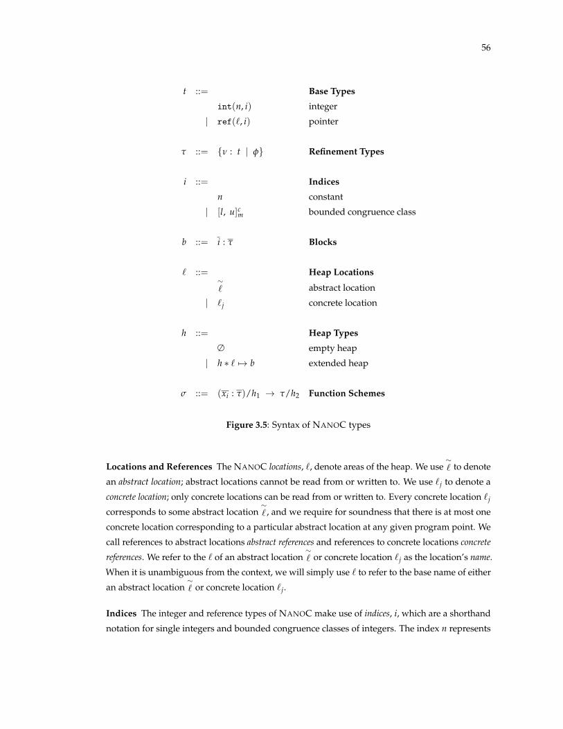
56
t ::= Base Types
int(n, i) integer
| ref(`, i) pointer
t ::= {n : t | f} Refinement Types
i ::= Indices
n constant
| [l, u]cm bounded congruence class
b ::= i : t Blocks
` ::= Heap Locations⇠` abstract location
| `j concrete location
h ::= Heap Types
∆ empty heap
| h ⇤ ` 7! b extended heap
s ::= (xi : t)/h1 ! t/h2 Function Schemes
Figure 3.5: Syntax of NANOC types
Locations and References The NANOC locations, `, denote areas of the heap. We use⇠` to denote
an abstract location; abstract locations cannot be read from or written to. We use `j to denote a
concrete location; only concrete locations can be read from or written to. Every concrete location `j
corresponds to some abstract location⇠` , and we require for soundness that there is at most one
concrete location corresponding to a particular abstract location at any given program point. We
call references to abstract locations abstract references and references to concrete locations concrete
references. We refer to the ` of an abstract location⇠` or concrete location `j as the location’s name.
When it is unambiguous from the context, we will simply use ` to refer to the base name of either
an abstract location⇠` or concrete location `j.
Indices The integer and reference types of NANOC make use of indices, i, which are a shorthand
notation for single integers and bounded congruence classes of integers. The index n represents
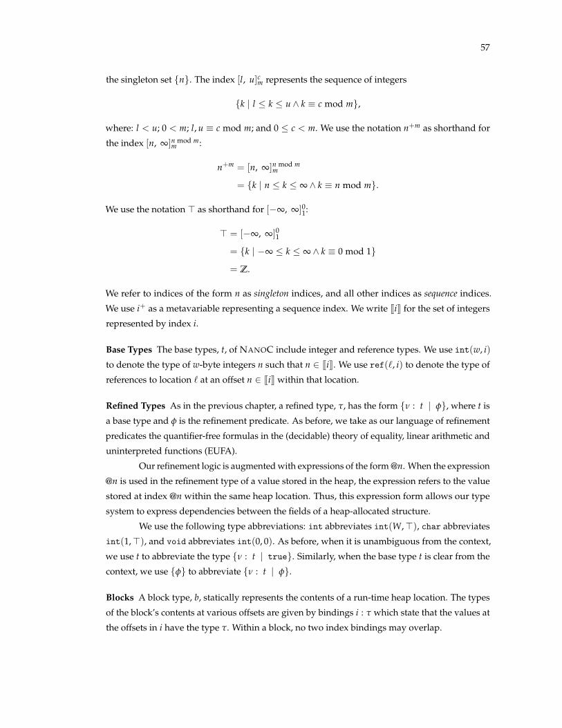
57
the singleton set {n}. The index [l, u]cm represents the sequence of integers
{k | l k u ^ k ⌘ c mod m},
where: l < u; 0 < m; l, u ⌘ c mod m; and 0 c < m. We use the notation n+m as shorthand for
the index [n, •]n mod mm :
n+m = [n, •]n mod mm
= {k | n k • ^ k ⌘ n mod m}.
We use the notation > as shorthand for [�•, •]01:
> = [�•, •]01
= {k | �• k • ^ k ⌘ 0 mod 1}
= Z.
We refer to indices of the form n as singleton indices, and all other indices as sequence indices.
We use i+ as a metavariable representing a sequence index. We write [[i]] for the set of integers
represented by index i.
Base Types The base types, t, of NANOC include integer and reference types. We use int(w, i)
to denote the type of w-byte integers n such that n 2 [[i]]. We use ref(`, i) to denote the type of
references to location ` at an offset n 2 [[i]] within that location.
Refined Types As in the previous chapter, a refined type, t, has the form {n : t | f}, where t is
a base type and f is the refinement predicate. As before, we take as our language of refinement
predicates the quantifier-free formulas in the (decidable) theory of equality, linear arithmetic and
uninterpreted functions (EUFA).
Our refinement logic is augmented with expressions of the form @n. When the expression
@n is used in the refinement type of a value stored in the heap, the expression refers to the value
stored at index @n within the same heap location. Thus, this expression form allows our type
system to express dependencies between the fields of a heap-allocated structure.
We use the following type abbreviations: int abbreviates int(W,>), char abbreviates
int(1,>), and void abbreviates int(0, 0). As before, when it is unambiguous from the context,
we use t to abbreviate the type {n : t | true}. Similarly, when the base type t is clear from the
context, we use {f} to abbreviate {n : t | f}.
Blocks A block type, b, statically represents the contents of a run-time heap location. The types
of the block’s contents at various offsets are given by bindings i : t which state that the values at
the offsets in i have the type t. Within a block, no two index bindings may overlap.
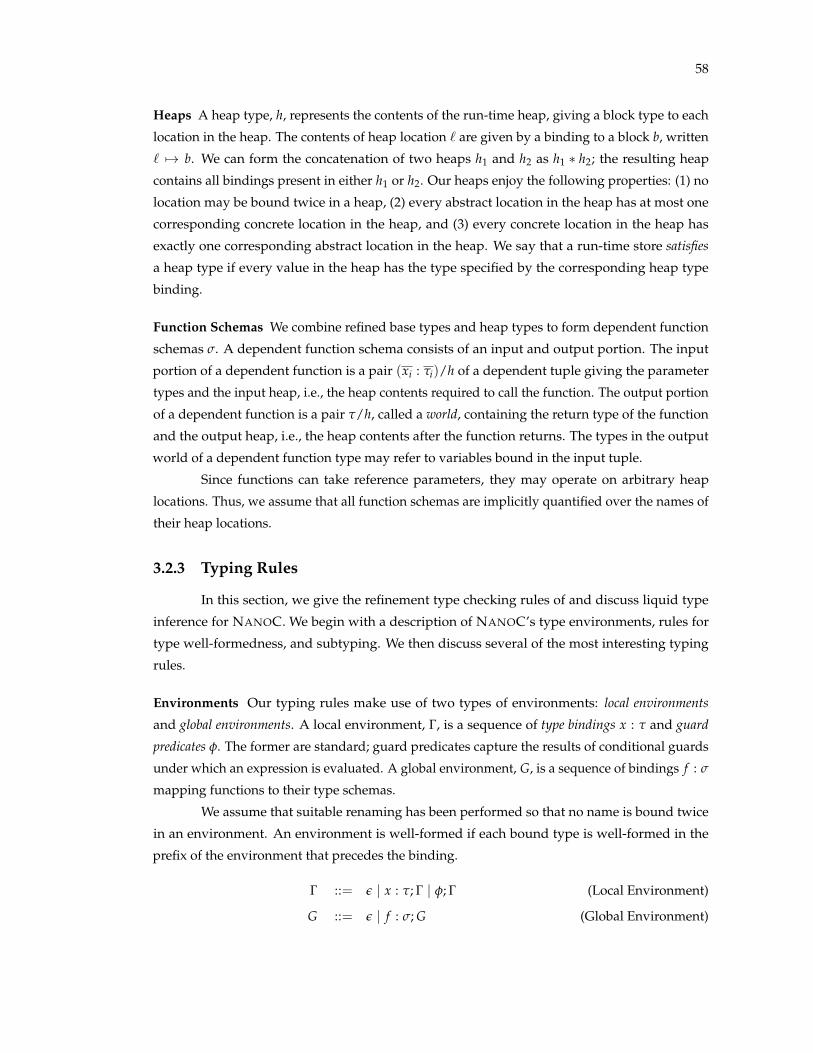
58
Heaps A heap type, h, represents the contents of the run-time heap, giving a block type to each
location in the heap. The contents of heap location ` are given by a binding to a block b, written
` 7! b. We can form the concatenation of two heaps h1 and h2 as h1 ⇤ h2; the resulting heap
contains all bindings present in either h1 or h2. Our heaps enjoy the following properties: (1) no
location may be bound twice in a heap, (2) every abstract location in the heap has at most one
corresponding concrete location in the heap, and (3) every concrete location in the heap has
exactly one corresponding abstract location in the heap. We say that a run-time store satisfies
a heap type if every value in the heap has the type specified by the corresponding heap type
binding.
Function Schemas We combine refined base types and heap types to form dependent function
schemas s. A dependent function schema consists of an input and output portion. The input
portion of a dependent function is a pair (xi : ti)/h of a dependent tuple giving the parameter
types and the input heap, i.e., the heap contents required to call the function. The output portion
of a dependent function is a pair t/h, called a world, containing the return type of the function
and the output heap, i.e., the heap contents after the function returns. The types in the output
world of a dependent function type may refer to variables bound in the input tuple.
Since functions can take reference parameters, they may operate on arbitrary heap
locations. Thus, we assume that all function schemas are implicitly quantified over the names of
their heap locations.
3.2.3 Typing Rules
In this section, we give the refinement type checking rules of and discuss liquid type
inference for NANOC. We begin with a description of NANOC’s type environments, rules for
type well-formedness, and subtyping. We then discuss several of the most interesting typing
rules.
Environments Our typing rules make use of two types of environments: local environments
and global environments. A local environment, G, is a sequence of type bindings x : t and guard
predicates f. The former are standard; guard predicates capture the results of conditional guards
under which an expression is evaluated. A global environment, G, is a sequence of bindings f : s
mapping functions to their type schemas.
We assume that suitable renaming has been performed so that no name is bound twice
in an environment. An environment is well-formed if each bound type is well-formed in the
prefix of the environment that precedes the binding.
G ::= e | x : t; G | f; G (Local Environment)
G ::= e | f : s; G (Global Environment)

59
Type Well-Formedness G ✏ t
f well-sorted in G; n : t
G ✏ {n : t | f}WF-TYPE
Dependent Block Well-Formedness G ✏@ b
DisjointOffsets(n : t, b)
x /2 G, FV(tj) G ✏ t G, x : t ✏@ b[@n 7! x]
G ✏@ n : t, bWF-DBLOCK-SINGLE
G ✏ i+j : tj
G ✏@ i+j : tjWF-DBLOCK-SEQUENCE
Non-Dependent Block Well-Formedness G ✏ b
DisjointOffsets(ij : tj) 8j.G ✏ tj
G ✏ ij : tjWF-NDBLOCK
Heap Type Well-Formedness G ✏ h
G ✏ ∆WF-HEMPTY
G ✏ h0⇠` /2 dom(h0) G ✏@ b
G ✏ h0 ⇤⇠` 7! b
WF-HABSTRACT
G ✏ h0 G ✏ b⇠`2 dom(h0) `k /2 dom(h0)
G ✏ h0 ⇤ `j 7! bWF-HCONCRETE
G ✏ t G ✏ h
G ✏ t/hWF-WORLD
Function Schema Well-Formedness ✏ s
G = xi : ti G ✏ ti G ✏ h1 G ✏ t/h2 ti, h1, t, h2 abstract
✏ (xi : ti)/h1 ! t/h2WF-FUNSCHEME
Figure 3.6: Well-formedness rules for NANOC

60
Well-Formedness Judgments The judgments of Figure 3.6 ensure that types, heaps, worlds, and
function type schemas are well-formed in local environments G and heaps h. A type is well-formed
in a local environment G if its refinement predicate f is a well-sorted Boolean formula in G.
A block is well-formed if no two index bindings overlap and each type is well-formed
with respect to the local environment and preceding indices. We distinguish between concrete
blocks, bound to concrete heap locations, which must have refinements over immutable variables
bound in the environment, and abstract blocks, bound to abstract heap locations, which have
refinements which may additionally use offset names (e.g., @0) to refer to values at other offsets
within the block. We disallow offset names in the refinements for concrete blocks for two reasons.
First, they are unnecessary, as we can use names bound in the environment to precisely describe
a particular location. Second, they are problematic, as the values at the offsets can be changed by
strong updates, thus invalidating the refinements.
To ensure that no block bindings overlap, the block well-formedness rules make use
of an auxiliary function, DisjointOffsets, which determines whether all the bindings in a block
refer to disjoint offsets within the block. Before we can define DisjointOffsets, we must first
define a function, OffsetsOf, which returns the block offsets occupied by a particular binding.
Formally, the function OffsetsOf(i, t) yields the set of sets of offsets occupied by a value of type
t located at offsets k 2 [[i]], where each set represents the offsets occupied by the contiguous
bytes of a value starting at some offset k. For example, OffsetsOf(0, int(4, 0)) produces the
set {{0, 1, 2, 3}}, i.e., the set of offsets occupied by a 4-byte integer located at offset 0. As
another example, OffsetsOf(0+4, int(4, 0)) produces the set {{0, 1, 2, 3}, {4, 5, 6, 7}, . . .}. Finally,
the function DisjointOffsets is defined as:
DisjointOffsets(ij : tj) = 8S, T 2]
jOffsetsOf(ij, tj). S \ T = ∆,
where ] is the multiset union operator — we must use multiset rather than traditional union
because, if two bindings were to map to the same set of indices, the traditional union would keep
only a single copy of that set of indices, and DisjointOffsets would thus not be able to detect the
overlap.
A heap is well-formed if each block is well-formed, no location is bound twice, each
abstract location has at most one corresponding concrete location, and each concrete location
has a corresponding abstract location. Note that we check the well-formedness of blocks bound
to abstract and concrete locations using separate well-formedness rules; only blocks bound to
abstract locations are allowed to contain types with dependent field references.
A function schema is well-formed if all parameters are well-formed with respect to
the previous parameters and the input heap, the input heap is well-formed with respect to the
parameters, and the output world is also well-formed with respect to the parameters.
Subtyping Judgments The subtyping judgments of NANOC are shown in Figure 3.7. The rules

61
Base Subtyping G ` t1 <: t2
i1⇠✓ i2 G ✏ f1 ) f2
G ` {n : int(w, i1) | f1} <: {n : int(w, i2) | f2}<:-INT
i1⇠✓ i2 G ✏ f1 ) f2
G ` {n : ref(`, i1) | f1} <: {n : ref(`, i2) | f2}<:-REF
G ` {n : ref(`j, i) | f} <: {n : ref(⇠` , i) | f}
<:-ABSTRACT
G ` {n : int(W, 0) | n = 0} <: {n : ref(`, i) | n = 0}<:-NULL
G ` t1 <: t2 G ` t2 <: t3
G ` t1 <: t3<:-TRANS
Block Subtyping G ` b1 <: b2
G ` t1 <: t2 x /2 G G; x : t1 ` b1[@n 7! x] <: b2[@n 7! x]
G ` n : t1, b1 <: n : t2, b2<:-SINGLE
G ` t1 <: t2 G ` b1 <: b2
G ` i+ : t1, b1 <: i+ : t2, b2<:-SEQUENCE
Heap Subtyping G ` h1 <: h2
G ` ∆ <: ∆<:-EMPTY-HEAP
G ` b1 <: b2 G ` h1 <: h2
G ` h1 ⇤ ` 7! b1 <: h2 ⇤ ` 7! b2<:-HEAP
World Subtyping G ` t1/h1 <: t2/h2
G ` t1 <: t2 G ` h1 <: h2
G ` t1/h1 <: t2/h2<:-WORLD
Figure 3.7: Subtyping rules for NANOC
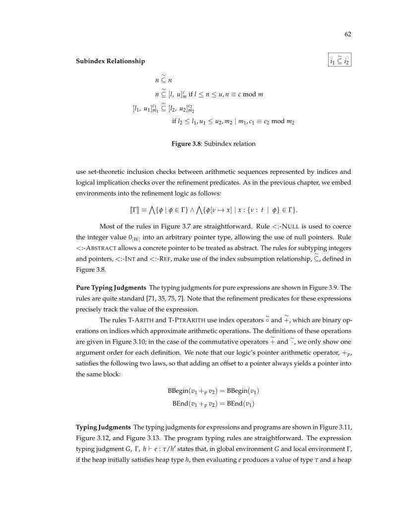
62
Subindex Relationship i1⇠✓ i2
n⇠✓ n
n⇠✓ [l, u]cm if l n u, n ⌘ c mod m
[l1, u1]c1m1
⇠✓ [l2, u2]
c2m2
if l2 l1, u1 u2, m2 | m1, c1 ⌘ c2 mod m2
Figure 3.8: Subindex relation
use set-theoretic inclusion checks between arithmetic sequences represented by indices and
logical implication checks over the refinement predicates. As in the previous chapter, we embed
environments into the refinement logic as follows:
[[G]] ⌘^{f | f 2 G} ^
^{f[n 7! x] | x : {n : t | f} 2 G}.
Most of the rules in Figure 3.7 are straightforward. Rule <:-NULL is used to coerce
the integer value 0|W| into an arbitrary pointer type, allowing the use of null pointers. Rule
<:-ABSTRACT allows a concrete pointer to be treated as abstract. The rules for subtyping integers
and pointers, <:-INT and <:-REF, make use of the index subsumption relationship,⇠✓, defined in
Figure 3.8.
Pure Typing Judgments The typing judgments for pure expressions are shown in Figure 3.9. The
rules are quite standard [71, 35, 75, 7]. Note that the refinement predicates for these expressions
precisely track the value of the expression.
The rules T-ARITH and T-PTRARITH use index operators⇠� and
⇠+, which are binary op-
erations on indices which approximate arithmetic operations. The definitions of these operations
are given in Figure 3.10; in the case of the commutative operators⇠+ and
⇠· , we only show one
argument order for each definition. We note that our logic’s pointer arithmetic operator, +p,
satisfies the following two laws, so that adding an offset to a pointer always yields a pointer into
the same block:
BBegin(v1 +p v2) = BBegin(v1)
BEnd(v1 +p v2) = BEnd(v1)
Typing Judgments The typing judgments for expressions and programs are shown in Figure 3.11,
Figure 3.12, and Figure 3.13. The program typing rules are straightforward. The expression
typing judgment G, G, h ` e : t/h0 states that, in global environment G and local environment G,
if the heap initially satisfies heap type h, then evaluating e produces a value of type t and a heap

63
Pure Typing Rules G ` a : t
G(x) = {n : t | f}
G ` x : {n : t | n = x}T-VAR
G ` n|w| : {n : int(w, n) | n = n|w|}T-INT
G ` a1 : int(n, i1) G ` a2 : int(n, i2)
G ` a1 � a2 : {n : int(n, i1⇠� i2) | n = a1 � a2}
T-ARITH
G ` a1 : ref(`, i1) G ` a2 : int(W, i2)
G ` a1 +p a2 : {n : ref(`, i1⇠+ i2) | n = a1 +p a2}
T-PTRARITH
G ` a1 : t G ` a2 : t
G ` a1 ./ a2 : {n : int(W, [0, 1]01) | if a1 ./ a2 then n = 1|W| else n = 0|W|}T-RELATION
G ` a : t1 G ` t1 <: t2 G ✏ t2
G ` a : t2T-PURESUB
Figure 3.9: Typing rules for pure NANOC expressions
satisfying h0. The majority of the rules are straightforward; the most interesting rules are those
that deal with memory access.
Type Checking Memory Operations
Below, we discuss the rules for memory allocation, heap operations, function calls, and
location unfolding. The key idea that enables our system to verify and infer invariants about
in-memory data structures in the presence of temporary invariant violation is our distinction
between concrete locations and abstract locations. Thus, to better understand the rules for memory
operations, we begin with a more thorough description of abstract and concrete locations.
Concrete Locations Concrete locations are names that refer to exactly one physical memory
location. For example, a single item in a linked list has one physical location and thus can be
identified with a concrete location. The block bound to a concrete location describes the current
state of the contents of exactly one physical location.
Abstract Locations Abstract locations are names that refer to zero or more concrete locations. For
example, all items in a linked list may share the same abstract location, although each item is at a
different concrete location. The block bound to an abstract location is an invariant that applies to
all elements which share that abstract location.
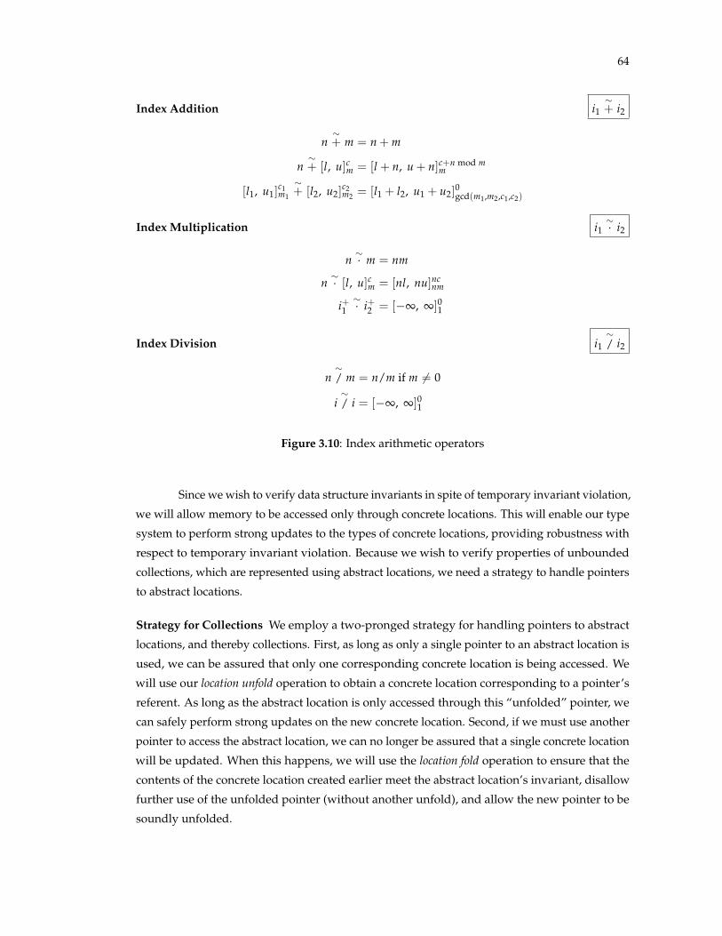
64
Index Addition i1⇠+ i2
n⇠+ m = n + m
n⇠+ [l, u]cm = [l + n, u + n]c+n mod m
m
[l1, u1]c1m1
⇠+ [l2, u2]
c2m2 = [l1 + l2, u1 + u2]
0gcd(m1,m2,c1,c2)
Index Multiplication i1⇠· i2
n⇠· m = nm
n⇠· [l, u]cm = [nl, nu]nc
nm
i+1⇠· i+2 = [�•, •]01
Index Division i1⇠/ i2
n⇠/ m = n/m if m 6= 0
i⇠/ i = [�•, •]01
Figure 3.10: Index arithmetic operators
Since we wish to verify data structure invariants in spite of temporary invariant violation,
we will allow memory to be accessed only through concrete locations. This will enable our type
system to perform strong updates to the types of concrete locations, providing robustness with
respect to temporary invariant violation. Because we wish to verify properties of unbounded
collections, which are represented using abstract locations, we need a strategy to handle pointers
to abstract locations.
Strategy for Collections We employ a two-pronged strategy for handling pointers to abstract
locations, and thereby collections. First, as long as only a single pointer to an abstract location is
used, we can be assured that only one corresponding concrete location is being accessed. We
will use our location unfold operation to obtain a concrete location corresponding to a pointer’s
referent. As long as the abstract location is only accessed through this “unfolded” pointer, we
can safely perform strong updates on the new concrete location. Second, if we must use another
pointer to access the abstract location, we can no longer be assured that a single concrete location
will be updated. When this happens, we will use the location fold operation to ensure that the
contents of the concrete location created earlier meet the abstract location’s invariant, disallow
further use of the unfolded pointer (without another unfold), and allow the new pointer to be
soundly unfolded.
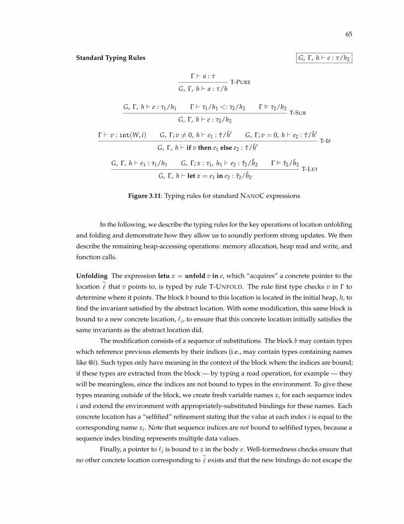
65
Standard Typing Rules G, G, h ` e : t/h2
G ` a : t
G, G, h ` a : t/hT-PURE
G, G, h ` e : t1/h1 G ` t1/h1 <: t2/h2 G ✏ t2/h2
G, G, h ` e : t2/h2T-SUB
G ` v : int(W, i) G, G; v 6= 0, h ` e1 : t/h0 G, G; v = 0, h ` e2 : t/h0
G, G, h ` if v then e1 else e2 : t/h0T-IF
G, G, h ` e1 : t1/h1 G, G; x : t1, h1 ` e2 : t2/h2 G ✏ t2/h2
G, G, h ` let x = e1 in e2 : t2/h2T-LET
Figure 3.11: Typing rules for standard NANOC expressions
In the following, we describe the typing rules for the key operations of location unfolding
and folding and demonstrate how they allow us to soundly perform strong updates. We then
describe the remaining heap-accessing operations: memory allocation, heap read and write, and
function calls.
Unfolding The expression letu x = unfold v in e, which “acquires” a concrete pointer to the
location⇠` that v points to, is typed by rule T-UNFOLD. The rule first type checks v in G to
determine where it points. The block b bound to this location is located in the initial heap, h, to
find the invariant satisfied by the abstract location. With some modification, this same block is
bound to a new concrete location, `j, to ensure that this concrete location initially satisfies the
same invariants as the abstract location did.
The modification consists of a sequence of substitutions. The block b may contain types
which reference previous elements by their indices (i.e., may contain types containing names
like @i). Such types only have meaning in the context of the block where the indices are bound;
if these types are extracted from the block — by typing a read operation, for example — they
will be meaningless, since the indices are not bound to types in the environment. To give these
types meaning outside of the block, we create fresh variable names xi for each sequence index
i and extend the environment with appropriately-substituted bindings for these names. Each
concrete location has a “selfified” refinement stating that the value at each index i is equal to the
corresponding name xi. Note that sequence indices are not bound to selfified types, because a
sequence index binding represents multiple data values.
Finally, a pointer to `j is bound to x in the body e. Well-formedness checks ensure that
no other concrete location corresponding to⇠` exists and that the new bindings do not escape the
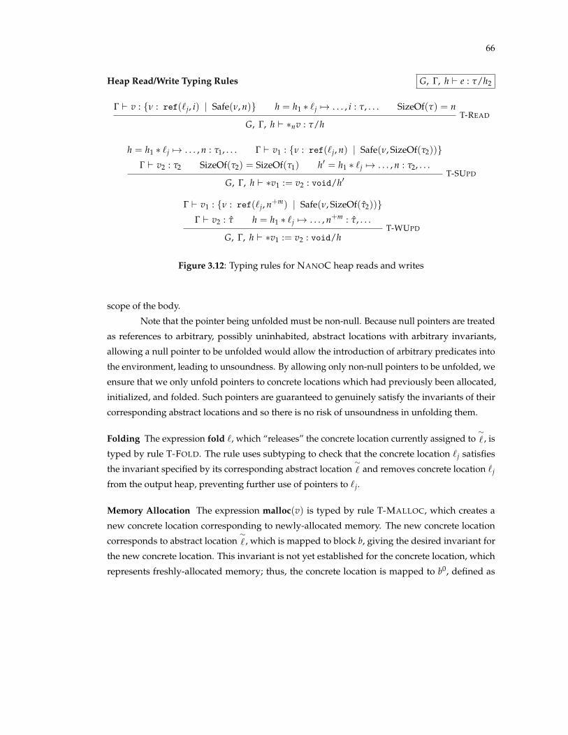
66
Heap Read/Write Typing Rules G, G, h ` e : t/h2
G ` v : {n : ref(`j, i) | Safe(n, n)} h = h1 ⇤ `j 7! . . . , i : t, . . . SizeOf(t) = n
G, G, h ` ⇤nv : t/hT-READ
h = h1 ⇤ `j 7! . . . , n : t1, . . . G ` v1 : {n : ref(`j, n) | Safe(n, SizeOf(t2))}G ` v2 : t2 SizeOf(t2) = SizeOf(t1) h0 = h1 ⇤ `j 7! . . . , n : t2, . . .
G, G, h ` ⇤v1 := v2 : void/h0T-SUPD
G ` v1 : {n : ref(`j, n+m) | Safe(n, SizeOf(t2))}G ` v2 : t h = h1 ⇤ `j 7! . . . , n+m : t, . . .
G, G, h ` ⇤v1 := v2 : void/hT-WUPD
Figure 3.12: Typing rules for NANOC heap reads and writes
scope of the body.
Note that the pointer being unfolded must be non-null. Because null pointers are treated
as references to arbitrary, possibly uninhabited, abstract locations with arbitrary invariants,
allowing a null pointer to be unfolded would allow the introduction of arbitrary predicates into
the environment, leading to unsoundness. By allowing only non-null pointers to be unfolded, we
ensure that we only unfold pointers to concrete locations which had previously been allocated,
initialized, and folded. Such pointers are guaranteed to genuinely satisfy the invariants of their
corresponding abstract locations and so there is no risk of unsoundness in unfolding them.
Folding The expression fold `, which “releases” the concrete location currently assigned to⇠` , is
typed by rule T-FOLD. The rule uses subtyping to check that the concrete location `j satisfies
the invariant specified by its corresponding abstract location⇠` and removes concrete location `j
from the output heap, preventing further use of pointers to `j.
Memory Allocation The expression malloc(v) is typed by rule T-MALLOC, which creates a
new concrete location corresponding to newly-allocated memory. The new concrete location
corresponds to abstract location⇠` , which is mapped to block b, giving the desired invariant for
the new concrete location. This invariant is not yet established for the concrete location, which
represents freshly-allocated memory; thus, the concrete location is mapped to b0, defined as
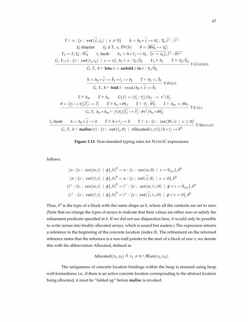
67
G ` v : {n : ref(⇠` , iy) | n 6= 0} h = h0 ⇤
⇠` 7! nk : tk, i+ : t+
xk disjoint xk /2 G, e, FV(h) q = [@nk 7! xk]
G1 = G; xk : qtk `j fresh h1 = h ⇤ `j 7! nk : {n = xk}, i+ : qt+
G, G1; x : {n : ref(`j, iy) | n = v}, h1 ` e : t2/h2 G1 ✏ h1 G ✏ t2/h2
G, G, h ` letu x = unfold v in e : t2/h2T-UNFOLD
h = h0 ⇤⇠` 7! b1 ⇤ `j 7! b2 G ` b2 <: b1
G, G, h ` fold ` : void/h0 ⇤⇠` 7! b1
T-FOLD
G ✏ hm G ✏ hu G( f ) = (xj : tj)/h f ! t0/h0fq = [xj 7! vj][` f 7! `] G ✏ hu ⇤ qh f G ` vj : qtj G ` hm <: qh f
G, G, hu ⇤ hm ` f (vj)[` f 7! `] : qt0/hu ⇤ qh0fT-CALL
`j fresh h = h0 ⇤⇠` 7! b G ✏ h ⇤ `j 7! b G ` v : {n : int(W, i) | n � 0}
G, G, h ` malloc(v) : {n : ref(`j, 0) | Allocated(n, v)}/h ⇤ `j 7! b0T-MALLOC
Figure 3.13: Non-standard typing rules for NANOC expressions
follows:
(n : {n : int(w, i) | f}, b)0 = n : {n : int(w, 0) | n = 0|w|}, b0
(n : {n : ref(`, i) | f}, b)0 = n : {n : ref(⇠` , 0) | n = 0}, b0
(i+ : {n : int(w, i) | f}, b)0= i+ : {n : int(w, i t 0) | f _ n = 0|w|}, b0
(i+ : {n : ref(`, i) | f}, b)0= i+ : {n : ref(
⇠` , i t 0) | f _ n = 0}, b0
Thus, b0 is the type of a block with the same shape as b, where all the contents are set to zero.
(Note that we change the types of arrays to indicate that their values are either zero or satisfy the
refinement predicate specified in b. If we did not use disjunction here, it would only be possible
to write zeroes into freshly-allocated arrays, which is sound but useless.) The expression returns
a reference to the beginning of the concrete location (index 0). The refinement on the returned
reference states that the reference is a non-null pointer to the start of a block of size v; we denote
this with the abbreviation Allocated, defined as
Allocated(v1, v2) , v1 6= 0 ^ BLen(v1, v2).
The uniqueness of concrete location bindings within the heap is ensured using heap
well-formedness; i.e., if there is an active concrete location corresponding to the abstract location
being allocated, it must be “folded up” before malloc is invoked.
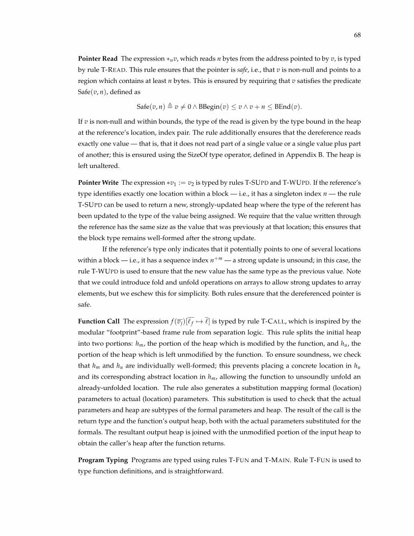
68
Pointer Read The expression ⇤nv, which reads n bytes from the address pointed to by v, is typed
by rule T-READ. This rule ensures that the pointer is safe, i.e., that v is non-null and points to a
region which contains at least n bytes. This is ensured by requiring that v satisfies the predicate
Safe(v, n), defined as
Safe(v, n) , v 6= 0 ^ BBegin(v) v ^ v + n BEnd(v).
If v is non-null and within bounds, the type of the read is given by the type bound in the heap
at the reference’s location, index pair. The rule additionally ensures that the dereference reads
exactly one value — that is, that it does not read part of a single value or a single value plus part
of another; this is ensured using the SizeOf type operator, defined in Appendix B. The heap is
left unaltered.
Pointer Write The expression ⇤v1 := v2 is typed by rules T-SUPD and T-WUPD. If the reference’s
type identifies exactly one location within a block — i.e., it has a singleton index n — the rule
T-SUPD can be used to return a new, strongly-updated heap where the type of the referent has
been updated to the type of the value being assigned. We require that the value written through
the reference has the same size as the value that was previously at that location; this ensures that
the block type remains well-formed after the strong update.
If the reference’s type only indicates that it potentially points to one of several locations
within a block — i.e., it has a sequence index n+m — a strong update is unsound; in this case, the
rule T-WUPD is used to ensure that the new value has the same type as the previous value. Note
that we could introduce fold and unfold operations on arrays to allow strong updates to array
elements, but we eschew this for simplicity. Both rules ensure that the dereferenced pointer is
safe.
Function Call The expression f (vj)[` f 7! `] is typed by rule T-CALL, which is inspired by the
modular “footprint”-based frame rule from separation logic. This rule splits the initial heap
into two portions: hm, the portion of the heap which is modified by the function, and hu, the
portion of the heap which is left unmodified by the function. To ensure soundness, we check
that hm and hu are individually well-formed; this prevents placing a concrete location in hu
and its corresponding abstract location in hm, allowing the function to unsoundly unfold an
already-unfolded location. The rule also generates a substitution mapping formal (location)
parameters to actual (location) parameters. This substitution is used to check that the actual
parameters and heap are subtypes of the formal parameters and heap. The result of the call is the
return type and the function’s output heap, both with the actual parameters substituted for the
formals. The resultant output heap is joined with the unmodified portion of the input heap to
obtain the caller’s heap after the function returns.
Program Typing Programs are typed using rules T-FUN and T-MAIN. Rule T-FUN is used to
type function definitions, and is straightforward.

69
Program Typing G ` P : t/h
✏ s
s = (xj : tj)/h ! t0/h0 G; f : s, e, xj : tj, h ` e : t0/h0 G; f : s ` P : tp/hp
G ` f (xj) { e } P : tp/hp[T-FUN]
h abstract G, ∆, h ` e : t/h0
G ` e : t/h0T-MAIN
Figure 3.14: Program Typing
Rule T-MAIN, which type checks the expression that makes up the “main” function of
the program, ensures the initial heap contains only abstract locations: since at the beginning
of execution no locations have been allocated and no invariants established, the initial heap
cannot contain concrete locations. It may, however, contain abstract locations, since they need
not describe the contents of any concrete locations.
3.3 Data Structure Verification with Final Fields
While the system presented so far is adept at specifying, verifying, and inferring invari-
ants that express relationships between local variables or between two fields of one structure,
it cannot express invariants which relate fields in one structure to fields in another, different
structure, and thus cannot express or verify properties of linked, mutable data structures.
To understand why, consider expressing the following invariant as a type:
p->size = p->next->size
We might consider a naıve approach which would give p a type which says that it is a reference
to a location ` of type
` 7! size : int, next : {n : ref(`, 0) | n->size = size},
which says that the value obtained by dereferencing the next pointer to obtain its size field
yields a value equal to the size field of the current structure, p. However, giving p such a type
would be unsound if the value of its size field can change as the program executes. Nonetheless,
if we are to verify the safety and correctness of realistic programs, we must be able to reason
about inter-link invariants like this one.
In this section, we augment our type system to express and verify such precise inter-link
invariants of mutable linked data structures. To do so, we wish to retain the expressive power af-
forded by allowing dereferences inside type refinements while avoiding the unsoundness usually

70
associated with them. Our key observation is that the problem with allowing references inside
refinement predicates is uncontrolled mutation: in our example, at any point in the program, the
size field of either structure may change, invalidating the refinement and causing unsoundness.
If, however, we can be sure that the size field is immutable after the current program point, it is
completely safe to allow dereferences that access size within refinements. We call such fields
final, and our type system soundly allows refinement predicates to contain dereferences to such
final fields.
This extension considerably increases the expressiveness of our type system. For exam-
ple, our system is able to use flow- and path-sensitive reasoning, along with the refinements
expressible using final fields, to determine automatically that library code which destructively
updates lists in order to add or remove elements maintains the lists’ sortedness invariants.
3.3.1 Final Fields Example: Memory Allocation
We now illustrate by example how the addition of final fields to our system enables the
verification and inference of invariants of mutable linked data structures.
Figure 3.15 shows an implementation of a malloc-like memory manager whose free list
is divided into allocation “pools” of type pool which consist of an allocation size and the free list
for that size, which is a linked list of region structures, each of which consists of an 8-byte header
containing the region’s size and link to the next free region, followed by an array of characters
containing the allocated memory itself. The pools themselves are linked together in a list in
increasing order of allocation size.
Link Invariants We begin by verifying that each pointer produced by new region points to the
mem field of an allocated location which contains exactly as many bytes as specified by the region
header, plus space for the header itself. Ideally, we would give the return value the type
{n : ref(`, 8) | n = BBegin(n) + 8 ^ BEnd(n) = n + ⇤BBegin(n)}.
Note the term ⇤BBegin(n) dereferences the pointer to access its size field. Thus, this type states
that the return value is a pointer to the mem field (eighth byte) of its location and that the end of
the block comes size bytes beyond the referenced location. Unfortunately, it is not generally
sound to use dereferences in types; if the size field of the returned structure is mutated at any
point, the refinement may be invalidated, and the type system will be unsound.
Final Fields On the other hand, a straightforward analysis of the program shows that, after its
initialization on line 6, the size field of the returned structure is never mutated. We say that such
a field is final, and note that it is sound for refinements to dereference such fields so long as they
remain final. In refinement predicates, we syntactically distinguish dereferences to final fields
from dereferences to potentially mutable fields by writing references to final fields as !v.
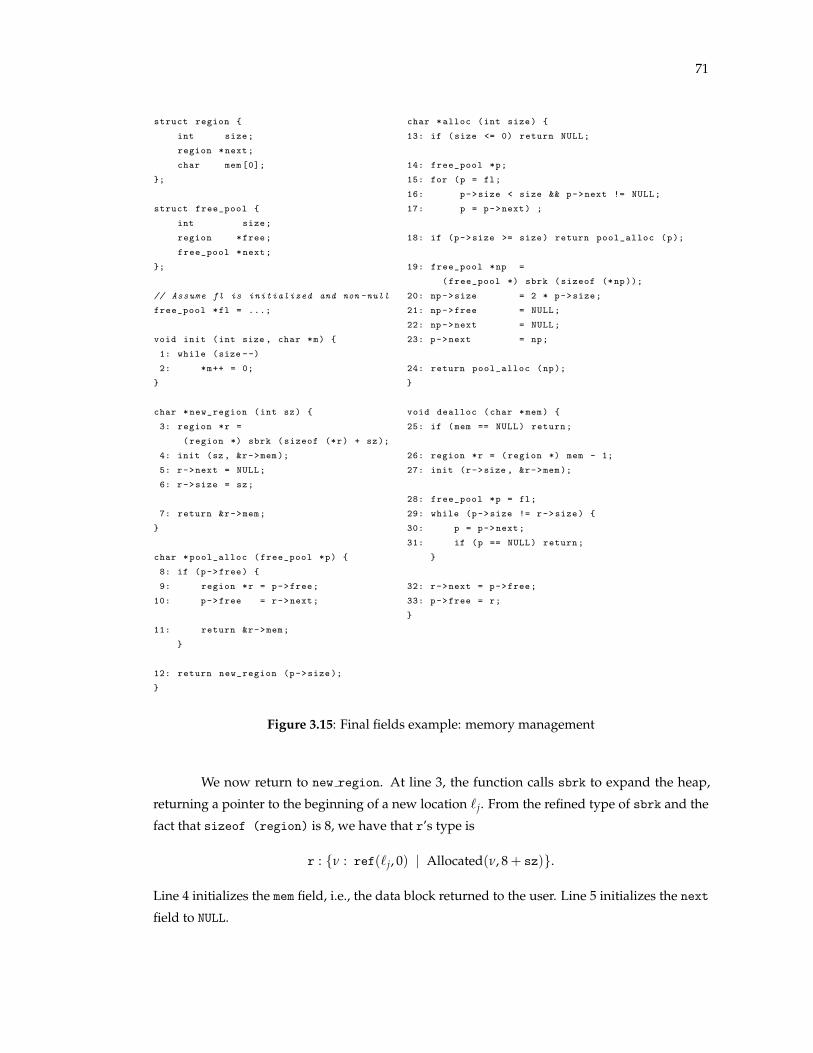
71
struct region {
int size;
region *next;
char mem [0];
};
struct free_pool {
int size;
region *free;
free_pool *next;
};
// Assume fl is initialized and non -null
free_pool *fl = ...;
void init (int size , char *m) {
1: while (size --)
2: *m++ = 0;
}
char *new_region (int sz) {
3: region *r =
(region *) sbrk (sizeof (*r) + sz);
4: init (sz, &r->mem);
5: r->next = NULL;
6: r->size = sz;
7: return &r->mem;
}
char *pool_alloc (free_pool *p) {
8: if (p->free) {
9: region *r = p->free;
10: p->free = r->next;
11: return &r->mem;
}
12: return new_region (p->size);
}
char *alloc (int size) {
13: if (size <= 0) return NULL;
14: free_pool *p;
15: for (p = fl;
16: p->size < size && p->next != NULL;
17: p = p->next) ;
18: if (p->size >= size) return pool_alloc (p);
19: free_pool *np =
(free_pool *) sbrk (sizeof (*np));
20: np->size = 2 * p->size;
21: np->free = NULL;
22: np->next = NULL;
23: p->next = np;
24: return pool_alloc (np);
}
void dealloc (char *mem) {
25: if (mem == NULL) return;
26: region *r = (region *) mem - 1;
27: init (r->size , &r->mem);
28: free_pool *p = fl;
29: while (p->size != r->size) {
30: p = p->next;
31: if (p == NULL) return;
}
32: r->next = p->free;
33: p->free = r;
}
Figure 3.15: Final fields example: memory management
We now return to new region. At line 3, the function calls sbrk to expand the heap,
returning a pointer to the beginning of a new location `j. From the refined type of sbrk and the
fact that sizeof (region) is 8, we have that r’s type is
r : {n : ref(`j, 0) | Allocated(n, 8 + sz)}.
Line 4 initializes the mem field, i.e., the data block returned to the user. Line 5 initializes the next
field to NULL.

72
Line 6 initializes the size field to the requested size, sz. This is the final assignment
made to the size field for the lifetime of this structure; thus, after this point, the size field is
final. Our analysis will soundly introduce the assumption
!r = sz
into the environment when type checking the remainder of the function, reflecting the immutable
value of r’s size field.
We compute the type of the returned pointer as
&r->mem : {n : ref(`j, 8) | n = r+p 8}.
Together, this type, the assumption !r = sz, and the type of r allow our system to deduce that
BEnd(&r->mem) = &r->mem + ! BBegin(&r->mem).
By subsumption, then, we are able to give the return value of new region the type
{n : ref(⇠` , 8) | n 6= 0 ^ n = BBegin(n) + 8 ^ BEnd(n) = n+! BBegin(n)}
which soundly dereferences the final field size to express the invariant that the returned pointer
references an allocated block of memory that is as long as the region header plus the number
of bytes specified in the size field of the header. Our system is able to verify all the invariants
shown so far using the qualifier set Q2 defined as
Q2 = {n 6= 0, n > 0, n � 0,
BEnd(n) = n +p ?,
n 6= 0 ) n � BBegin(n),
n 6= 0 ) n = BBegin(n) + 8,
n 6= 0 ) BEnd(n) = n + ! BBegin(n)}.
3.3.2 Linked Structure Invariants
At least as important as the invariants that hold for each region and pool of the allocator
of Figure 3.15 are the invariants that hold between these objects. For example:
1. The list of pools must be sorted in ascending order by size to avoid allocating new regions
when a sufficiently large free region is already available.
2. The elements of the free list of a pool must have a size field that agrees with the size field
of the pool.
3. All regions within the free list of a pool must have the same value for size.

73
These invariants are challenging because they are not properties of single elements within the
pool and free list structures, but rather relationships between them. Nevertheless, we can take
advantage of the fact that certain fields are final to express, verify, and infer these invariants.
Sorted Free List We begin by showing how our system verifies that the list of pools is sorted in
increasing order of their size fields. This amounts to showing that the linked list insertion in
alloc maintains the order of the free list fl.
Block Invariants We first note that the heap has the following type at entry to alloc:⇠`1 7! 0 : final {n : int | n > 0},
4 : ref(⇠`1, 0),
8+1 : char⇠`2 7! 0 : final int,
4 : ref(⇠`1, 0),
8 : {n : ref(⇠`2, 0) | n 6= 0 ) @0 < !n}
Here,⇠`1 represents the collection of region structures, while
⇠`2 represents the collection of pool
structures. The qualifier “final” attached to a field’s type indicates that the field is final, i.e., it will
not be mutated after the current program point. The type {n : ref(⇠`2, 0) | n 6= 0 ) @0 < !n}
indicates that the next field of each pool is either null or points to a pool structure with a strictly
greater size — in other words, that the list of pools is sorted by size.
We demonstrate how our system verifies that this type is maintained through execution
of the alloc function. If the test on line 13 passes, the function returns immediately without
touching the heap. Otherwise, the loop of lines 14–17 iterates over the free list fl until either
a pool of regions of sufficient size is found or we reach the last pool without finding any that
contains large enough regions. Line 18 checks whether the loop exited because a large enough
pool was found; if so, the function exits. Otherwise, a new pool is allocated and appended to the
free list in lines 19–23.
Verifying Insertion At line 18, p is unfolded to a concrete location `2p
:
`2p
7! 0 : {n : final int | n = x1},
4 : {n : ref(⇠`1, 0) | n = x2},
8 : {n : ref(⇠`2, 0) | n = x3}
The fresh variables x1, x2, x3 are created to represent the initial values of p’s fields and bound in
the environment; their types are not important, except to note that we know that x1 is positive.

74
At line 19, np is assigned the result of an sbrk call which allocates new memory; the
effect of this call is to create a concrete location pair, `2np
, on the heap and bind np to a pointer to
`2np
:
`2np
7! 0 : int,
4 : ref(⇠`1, 0),
8 : ref(⇠`2, 0)
The type of `3np
contains no refinements, reflecting the fact that nothing is known about the
uninitialized data at that location. Note that we have unfolded both p and np, which share the
same abstract location; this is sound, as the freshly-allocated pointer np cannot possibly alias
with any existing pointers.
At line 20, the assignment to np->size changes the type of np’s size field:
`2np
7! 0 : final {n : int | n = 2 ⇤ x1},
4 : ref(⇠`1, 0),
8 : ref(⇠`2, 0)
Recall that x1 is the fresh variable corresponding to p->size. The size field is marked final to
indicate that it is no longer mutated after this assignment, and our system soundly adds the
guard
!np = 2 ⇤ x1
to the environment.
Lines 21 and 22 alter the remaining fields:
`2np
7! 0 : final {n : int | n = 2 ⇤ x1},
4 : {n : ref(⇠`1, 0) | n = 0},
8 : {n : ref(⇠`2, 0) | n = 0}
Finally, we update the type of p->next to reflect the assignment of np:
`2p
7! 0 : final {n : int | n = x1},
4 : {n : ref(⇠`1, 0) | n = x2},
8 : {n : ref(⇠`2, 0) | n = np}

75
By subtyping and the guard !np = 2 ⇤ x1, we have
`2p
7! 0 : final {n : int | n = x1},
4 : {n : ref(⇠`1, 0) | n = x2},
8 : {n : ref(⇠`2, 0) | x1 < !n}
This type is subsumed by the type of⇠`2, and so we have successfully verified that appending a
new pool to the end of the memory pool list preserved the sortedness of the list.
Our system is able to verify all the invariants shown so far using the qualifier set Q3,
defined as
Q3 = Q2 [ {n 6= 0 ) ? < !n}.
Size Agreement The remaining invariants, that the elements of the free list for each pool have
size fields that match the size field of the pool itself and that each region in a free list has the
same value for its size fields, are proved similarly. Thus, using the qualifier set
Q4 = Q3 [ {n 6= 0 ) !n = ?},
our system is able to prove all the invariants of this section by inferring that the heap has the
following type:
⇠`1 7! 0 : final int,
4 : {n : ref(⇠`1, 0) | @0 = !n},
8+1 : char⇠`2 7! 0 : final int,
4 : {n : ref(⇠`1, 0) | @0 = !n},
8 : {n : ref(⇠`2, 0) | n 6= 0 ) @0 < !n}
3.3.3 Formal Changes to the NANOC Type System
In this section, we describe the changes to the NANOC type system that are needed to
accommodate final fields.
Dereference Expressions in Refinement Predicates We augment our language of refinement
predicates with the expression form !v, which represents the value obtained by dereferencing the
pointer v. To ensure that our type system is sound, our well-formedness rules only allow such
dereferences to appear in refinement predicates when v is a pointer to a final field. Formally, this

76
u ::= Field Qualifiers
| e mutable field (no qualifier)
| final final field
b ::= Blocks
| i : u t block
Figure 3.16: Additions to NANOC types to support final fields
Refinement Dereference Well-Formedness G, h ✏! v
h = h0 ⇤ ` 7! . . . , i : final t, . . . G ` v : ref(`, i)
G, h ✏! vWF-DEREF
Predicate Well-Formedness G, h ✏ f
f well-sorted in G, h !v 2 f ) G, h ✏! v
G, h ✏ fWF-PRED
Figure 3.17: Determining well-formedness of refinement predicates
obligation is shown with the judgment G, h ✏! v of Figure 3.17, which states that it is acceptable to
dereference v under environment G and heap h exactly when G and h indicate that v is a pointer
to a final field within h.
Field Qualifiers A field qualifier u is used to indicate whether a field within a heap-allocated
structure may be modified. If a field has no qualifier, it may be modified; a field with the modifier
final cannot be modified.
Block Types We modify the form of blocks so that each field consists of a triple of its index,
which gives its location within the block, its field qualifier, which determines whether the field
may be mutated, and its type. The syntaxes of field qualifiers and block types augmented with
field qualifiers are shown in Figure 3.16.
Type Well-Formedness The updated type well-formedness rules of NANOC are given in Fig-
ure 3.18. The changes are largely straightforward: because the well-formedness of refinement
predicates now depends on the field qualifiers contained in the heap, it is necessary to thread
heaps through the well-formedness rules.

77
Type Well-Formedness G, h ✏ t
G, h ✏ f
G, h ✏ {n : t | f}WF-TYPE
Dependent Block Well-Formedness G, h ✏@ b
DisjointOffsets(n : t, b)
x /2 G, FV(tj) G, h ✏ t G, x : t, h ✏@ ij : tj[@n 7! x]
G, h ✏@ n : t, ij : tjWF-DBLOCK-SINGLE
G, h ✏ i+j : tj
G, h ✏@ i+j : tjWF-DBLOCK-SEQUENCE
Non-Dependent Block Well-Formedness G, h ✏ b
DisjointOffsets(ij : tj) 8j.G, h ✏ tj
G, h ✏ ij : tjWF-NDBLOCK
Heap Type Well-Formedness G, h1 ✏ h2
G, h ✏ ∆WF-HEMPTY
G, h ✏ h0⇠` /2 dom(h0) G, h ✏@ b
G, h ✏ h0 ⇤⇠` 7! b
WF-HABSTRACT
G, h ✏ h0 G, h ✏ b⇠`2 dom(h0) `k /2 dom(h0)
G, h ✏ h0 ⇤ `j 7! bWF-HCONCRETE
World Well-Formedness G ✏ t/h
G, h ✏ t G, h ✏ h
G ✏ t/hWF-WORLD
Function Schema Well-Formedness ✏ s
G = xi : ti G, h1 ✏ ti G ✏ h1 G ✏ t/h2 ti, h1, t, h2 abstract
✏ (xi : ti)/h1 ! t/h2WF-FUNSCHEME
Figure 3.18: Rules for well-formedness of NANOC types with final fields
Type Checking The changed and updated type checking rules for NANOC with final fields
are shown in Figure 3.19. The rules T-READ-MUTABLE and T-READ-FINAL are straightforward
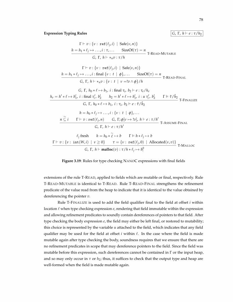
78
Expression Typing Rules G, G, h ` e : t/h2
G ` v : {n : ref(`j, i) | Safe(n, n)}h = h1 ⇤ `j 7! . . . , i : t, . . . SizeOf(t) = n
G, G, h ` ⇤nv : t/hT-READ-MUTABLE
G ` v : {n : ref(`j, i) | Safe(n, n)}h = h1 ⇤ `j 7! . . . , i : final {n : t | f}, . . . SizeOf(t) = n
G, G, h ` ⇤nv : {n : t | n =!v ^ f}/hT-READ-FINAL
G, G, h0 ⇤ ` 7! b1, i : final ti, b2 ` e : te/he
he = h0 ⇤ ` 7! b01, i : final t0i , b02 h2 = h0 ⇤ ` 7! b01, i : u t0
i , b02 G ✏ t/h2
G, G, h0 ⇤ ` 7! b1, i : ti, b2 ` e : t/h2T-FINALIZE
h = h0 ⇤ `j 7! . . . , i : {n : t | f}, . . .
n⇠✓ i G ` v : ref(`j, n) G, G; f[n 7! !v], h ` e : t/h0
G, G, h ` e : t/h0T-ASSUME-FINAL
`j fresh h = h0 ⇤⇠` 7! b G ✏ h ⇤ `j 7! b
G ` v : {n : int(W, i) | n � 0} t = {n : ref(`j, 0) | Allocated(n, v)}
G, G, h ` malloc(v) : t/h ⇤ `j 7! b0!
T-MALLOC
Figure 3.19: Rules for type checking NANOC expressions with final fields
extensions of the rule T-READ, applied to fields which are mutable or final, respectively. Rule
T-READ-MUTABLE is identical to T-READ. Rule T-READ-FINAL strengthens the refinement
predicate of the value read from the heap to indicate that it is identical to the value obtained by
dereferencing the pointer v.
Rule T-FINALIZE is used to add the field qualifier final to the field at offset i within
location ` when type checking expression e, rendering that field immutable within the expression
and allowing refinement predicates to soundly contain dereferences of pointers to that field. After
type checking the body expression e, the field may either be left final, or restored to mutability;
this choice is represented by the variable u attached to the field, which indicates that any field
qualifier may be used for the field at offset i within `. In the case where the field is made
mutable again after type checking the body, soundness requires that we ensure that there are
no refinement predicates in scope that may dereference pointers to the field. Since the field was
mutable before this expression, such dereferences cannot be contained in G or the input heap,
and so may only occur in t or h2; thus, it suffices to check that the output type and heap are
well-formed when the field is made mutable again.
79
For simplicity of implementation, we generally use T-FINALIZE to finalize a field for the
remainder of a function; that is, we do not make a field mutable again after it has been finalized.
The sole exception is when a function whose heap indicates a field is mutable calls a function
which does not mutate that field, and so whose function type assigns the final qualifier to that
field. In this case, we wrap the call using T-FINALIZE to make the field immutable solely for the
duration of the call, restoring the field to mutability as soon as the callee returns.
Rule T-ASSUME-FINAL is used to introduce assertions about the values obtained by
dereferencing pointers into the environment when type checking an expression. Note that the
assertion added to the environment is over a value v which points to a concrete location in the
heap, guaranteeing that it refers to a single (non-null) run-time location.
Rule T-MALLOC changes in two significant ways. First, the block returned is b0! , defined
as
(n : u {n : int(w, i) | f}, b)0! = n : {n : int(w, 0) | n = 0|w|}, b0
!
(n : u {n : ref(`, i) | f}, b)0! = n : {n : ref(
⇠` , 0) | n = 0}, b0
!
(i+ : u {n : int(w, i) | f}, b)0! = i+ : {n : int(w, i t 0) | f _ n = 0|w|}, b0
!
(i+ : u {n : ref(`, i) | f}, b)0! = i+ : {n : ref(
⇠` , i t 0) | f _ n = 0}, b0
!
The key difference from b0 is that all field qualifiers are removed from the fields, meaning
that every field in the newly-allocated location is mutable. This does not cause any problems
with soundness, as the location is newly-allocated; to be unsound, there would have to be an
existing pointer whose refinement type contains a dereference targeting one of the fields in the
newly-allocated region, which is impossible.
Second, we omit the well-formedness requirement, which allows us to have an existing
pointer and any number of freshly-allocated pointers all unfolded simultaneously. This is sound,
as it is impossible for a freshly-allocated pointer to alias with any existing pointer. (While this
change is independent of the changes related to final fields, we have deferred it to this point
because it complicates the theory and we do not prove it sound.)
Soundness While we believe the rules presented to be sound, we do not make any formal claims
of their soundness. In particular, the soundness proof of Appendix C does not consider the rules
presented in this section.
3.4 Type Inference
Next, we give a brief overview of type inference in NANOC. Type inference occurs in
three phases. The first infers physical types for each function in the program. The second inserts
location fold and unfold operations where necessary. The third and final step infers refinement
types using liquid type inference.

80
3.4.1 Physical Type Inference
In the previous chapter, we based our type inference technique on the rich type informa-
tion provided by ML’s type system. Because C programs are essentially untyped, we first use a
basic type inference pass to assign rich physical types to local variables and expressions and to
discover the types of the heap’s contents.
We first use the declared C types of all functions in the program to generate a correspond-
ing physical type schema for each function. This process is largely automatic and rarely requires
annotations to be added. The generated function schemas are then used to infer physical types
for local variables and the heap. This process occurs in two phases: First, our algorithm infers
physical types for local variables, assuming that the types of values stored in the heap conform
to the declared types of the pointers used to access the values. Physical type inference for local
variables works by first assigning each local variable a physical type with an index variable
representing its as-yet-unknown index. The algorithm then traverses the body of the function in
a syntax-directed manner and emits subtyping constraints capturing the flow of data within the
function. The algorithm then uses a fixpoint algorithm to solve the constraints over the index
domain to find an assignment of index variables to indices so that the function is typable given
the assumptions made about the heap.
After the types of local variables have been inferred, the function’s (abstract) heap type
is inferred by traversing the function and incrementally building the heap type as heap read and
write instructions are encountered. This phase also performs a field-sensitive may alias analysis
to determine which locations exist in the heap and to assign location names to values of reference
type.
The type assumptions made in the first phase are checked in an assume-guarantee
fashion by emitting appropriate deferred type checks that are enforced by the refinement type
system.
3.4.2 Fold and Unfold Inference
After physical type inference, our system automatically inserts location fold and unfold
expressions in order to ensure that every dereference is on a concrete pointer and that only
one concrete location is unfolded at a time, as required by our typing rules. The appropriate
spots to insert folds and unfolds are determined by a forward dataflow analysis that works as
follows: At the beginning of the function, all heap locations are in a folded state, i.e., there are no
concrete locations in the heap. The algorithm traverses each block in the control flow graph in
order, inserting an unfold before any access to a pointer which has not already been unfolded,
and inserting any necessary folds if another pointer which may alias the one being unfolded is
already unfolded. The analysis tracks which pointers are currently unfolded at the exit of each
block; if two different unfolded pointers to the same abstract location can reach the entry of a

81
block — for example, if two different pointers are unfolded along the then and else branches of
an if statement — the pointers are folded at the exits of their respective blocks. The algorithm
iterates until it reaches a fixed point.
3.4.3 Final Field Inference
Type inference with final fields has two components. First, we must determine which
fields within the heap are final at each program point. Second, we must determine where to use
the non-syntax-directed rules T-FINALIZE and T-ASSUME-FINAL.
Determining Final Fields Per Program Point We use an interprocedural dataflow analysis to
discover, at each program point, which fields in the heap are final, i.e., will not be mutated from
that program point on. The intraprocedural component is a straightforward backwards dataflow
analysis. The analysis begins with all fields final at the exits of the function, then traverses the
control flow graph backwards from the function exits. At each program statement, the analysis
computes the set of final fields at the start of the statement from the set of final fields at the exit of
the statement by removing any fields which were assigned in the current statement; which fields
are assigned within the statement is determined using the inferred physical type information. At
each control flow join point, the set of final fields at a control flow graph node is taken to be the
intersection of the final fields at the entry to each of its successors.
The interprocedural analysis simply computes per-function final fields information and
runs the intraprocedural analysis. The process is iterated to a fixed point.
Inferring uses of T-FINALIZE and T-ASSUME-FINAL Next, we use the inferred final fields
information to determine where the non-syntax directed rules T-FINALIZE and T-ASSUME-FINAL
may be used. Rule T-FINALIZE is invoked in two places. First, whenever a field is written and its
value remains final for the remainder of the function body, T-FINALIZE is used to mark that field
as final. Second, whenever a call is made from a function where a field is mutable to a function
whose input heap marks the field as final, T-FINALIZE is used to wrap the call, allowing the
function to be called in spite of the fact that the field is not final in the caller.
Uses of T-ASSUME-FINAL also appear in two places. First, whenever a field is written
and finalized with T-FINALIZE, T-ASSUME-FINAL is used to record the relationship between the
pointer that was written through and the value that was just written. Second, T-ASSUME-FINAL
is used after invocations of T-UNFOLD to assert the relationship between the unfolded pointer
and the values of those of its final fields which occur at singleton offsets.
3.4.4 Refinement Inference
Finally, we use liquid type inference, as described in the previous chapter, to infer
refinement types thus automatically discover data structure invariants. As before, we observe

82
that our type checking rules encode an algorithm for type inference and so we perform type
inference by attempting to produce a type derivation. At various points in the derivation, we
encounter types, heaps, and function schemas which cannot be synthesized directly from the
form of the expression and the current environment, but instead must be inferred. We insist
that such types, blocks, heaps, and schemas be liquid, denoted t (respectively, b, h, s), i.e.,
their refinements must be liquid refinements consisting of a conjunction of logical qualifiers, as
described in the previous chapter. Whenever we encounter a type which must be inferred, we
create a new template type, which is the physical type inferred earlier where a fresh variable is
used to represent the as-yet-unknown liquid refinement. As in the previous chapter, we generate
subtyping constraints over the template types using the subtyping premises in our type rules; the
subtyping rules are used to reduce these constraints to simple implication constraints between
refinement predicates and unknown refinement variables. These constraints are solved to yield a
liquid refinement for each refinement variable; replacing each variable with its solution yields a
refinement typing for the program.
3.5 Implementation and Evaluation
We implemented our type system in CSOLVE, a prototype static verifier for C programs.
In this section, we describe the architecture of CSOLVE and the results of applying CSOLVE to a
variety of challenging benchmarks.
3.5.1 CSOLVE: Liquid Types for C
Below, we briefly describe the architecture and usage of CSOLVE. CSOLVE takes as input
a C source file and a set of logical qualifiers, which CSOLVE uses to perform liquid type inference.
CSOLVE then outputs the inferred liquid types of functions, local variables, and heap locations
and reports any refinement type errors that occur.
Architecture Type inference in CSOLVE is split into four phases. In the first phase, the input
C program is read by CIL [68], which generates an AST. This AST is then simplified in various
ways, the most significant of which is that the code is transformed to SSA so that local variables
are never mutated. The second phase generates physical types for each declared function and
global variable and checks that the program code respects these types. The third phase walks
the CIL AST and assigns each expression and variable in the program a refinement type with a
distinct refinement predicate variable representing its as-yet-unknown refinement predicate, as
well as generating subtyping constraints over these refinement types such that solving for the
refinement variables within the constraints yields a valid typing for the program, in the same
style as the ConsGen function of section 2.3. The fourth phase attempts to solve the subtyping

83
constraints using a fixpoint procedure based on predicate abstraction, using the Z3 SMT solver
[28] to discharge the logical validity queries that arise in constraint solving.
Input CSOLVE takes as input a C source code file and a file specifying the set of logical qualifiers
to use in refinement inference. Qualifiers are also read from a standard library of qualifiers
that have proven to be useful on a large variety of programs, further easing the programmer’s
annotation burden.
Output If the program is type-safe, CSOLVE outputs “Safe”. Otherwise, the program may be
type-unsafe, according to either the physical type system or the refinement type system. In either
case, for each error, CSOLVE prints the name of the file and line number where the error occurs,
as well as a description of the error. In the case where the error is in refinement type inference,
CSOLVE prints the subtyping constraints which cannot be solved. Whether the program type
checks or not, CSOLVE produces a mapping of program identifiers to their inferred types, which
can be viewed using the tag browsing facilities provided by common editors, e.g., Vim and
Emacs.
Compatibility With C Infrastructure Thanks to the infrastructure provided by CIL, CSOLVE is
able to work as a drop-in replacement for GCC. Hence, to check a multi-file program one need
only construct or slightly modify a makefile which builds the program from source.
Modular Type Checking If the user specifies a type for a function with the extern keyword,
CSOLVE will use the provided type when checking the current source file, allowing the user to
omit the body of the external function. This allows for modular type checking and, by abstracting
away the details of other source files, it permits the user to work around cases where a function
may be too complex for CSOLVE to type check.
3.5.2 Memory Safety Benchmarks
We applied CSOLVE to several challenging benchmarks, drawn from [11], [60], [73], and
the example of section 3.1, which illustrate common low-level coding idioms. The results are
shown in Table 3.1. In each case, CSOLVE was able to precisely reason about complex invariants
of in-heap data structures and memory access patterns to statically verify memory safety by
proving the absence of null pointer dereferences and array bounds violations. (In the case of ft,
we show only array bounds safety; see chapter 4.) We explain several of the benchmarks below.
String Lists Using CSOLVE, we verified the safety of a program implementing a C idiom for
linked list manipulation which is particularly common in operating system code [18] and which
requires precise reasoning about pointer arithmetic. Recall the example of section 3.1, which
contained functions for creating and initializing strings and for creating lists of strings. We
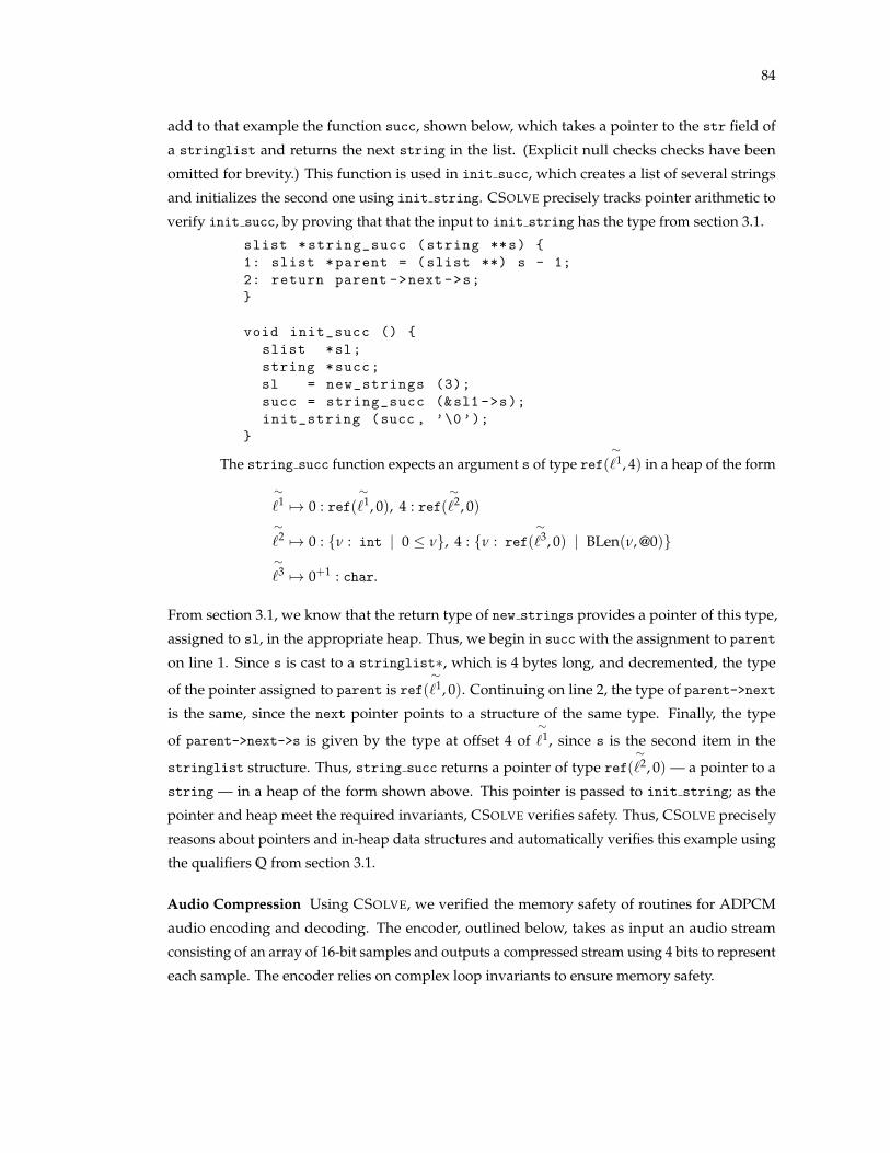
84
add to that example the function succ, shown below, which takes a pointer to the str field of
a stringlist and returns the next string in the list. (Explicit null checks checks have been
omitted for brevity.) This function is used in init succ, which creates a list of several strings
and initializes the second one using init string. CSOLVE precisely tracks pointer arithmetic to
verify init succ, by proving that that the input to init string has the type from section 3.1.slist *string_succ (string **s) {
1: slist *parent = (slist **) s - 1;
2: return parent ->next ->s;
}
void init_succ () {
slist *sl;
string *succ;
sl = new_strings (3);
succ = string_succ (&sl1 ->s);
init_string (succ , ’\0’);
}
The string succ function expects an argument s of type ref(⇠`1, 4) in a heap of the form
⇠`1 7! 0 : ref(
⇠`1, 0), 4 : ref(
⇠`2, 0)
⇠`2 7! 0 : {n : int | 0 n}, 4 : {n : ref(
⇠`3, 0) | BLen(n, @0)}
⇠`3 7! 0+1 : char.
From section 3.1, we know that the return type of new strings provides a pointer of this type,
assigned to sl, in the appropriate heap. Thus, we begin in succ with the assignment to parent
on line 1. Since s is cast to a stringlist⇤, which is 4 bytes long, and decremented, the type
of the pointer assigned to parent is ref(⇠`1, 0). Continuing on line 2, the type of parent->next
is the same, since the next pointer points to a structure of the same type. Finally, the type
of parent->next->s is given by the type at offset 4 of⇠`1, since s is the second item in the
stringlist structure. Thus, string succ returns a pointer of type ref(⇠`2, 0) — a pointer to a
string — in a heap of the form shown above. This pointer is passed to init string; as the
pointer and heap meet the required invariants, CSOLVE verifies safety. Thus, CSOLVE precisely
reasons about pointers and in-heap data structures and automatically verifies this example using
the qualifiers Q from section 3.1.
Audio Compression Using CSOLVE, we verified the memory safety of routines for ADPCM
audio encoding and decoding. The encoder, outlined below, takes as input an audio stream
consisting of an array of 16-bit samples and outputs a compressed stream using 4 bits to represent
each sample. The encoder relies on complex loop invariants to ensure memory safety.

85
Table 3.1: Results. Lines is the number of source lines without comments. Qualifiers is thenumber of manually-provided logical qualifiers used. Assumes is the number of manual
assumptions inserted. Time (s) is the time in seconds CSOLVE requires to verify safety.
Program Lines Qualifiers Assumes Time (s)
stringlist 72 1 0 2strcpy 77 3 0 4adpcm 198 13 0 42pmap 250 3 0 34mst 309 1 0 16power 620 7 2 111ft 652 2 6 310ks 742 9 7 721
Total 2,920 39 15 1,240
void encoder (int nsamp , short *inz , char *outz) {
short *in = inz;
char *out = outz;
int bufferempty = 1;
char buffer;
for (int len = nsamp; 0 < len; len --) {
// Read an input sample
... *in++ ...;
if (! bufferempty) {
// Write to buffer elided
*out++ = buffer;
} else {
// Write to buffer elided
}
bufferempty = !bufferempty;
}
if (! bufferempty) *out++ = buffer;
}
The encoder takes three parameters: nsamp, the total number of samples in the input;
inz, a pointer to the start of the input buffer, an array of 16-bit short values; and outz, a pointer
to the output buffer, an array of 8-bit char values. The number of elements in the input buffer is
twice the number of elements in the output buffer. The pointer in, initially set to inz, is used
to read data from the input buffer; the pointer out, initially set to outz, is used to write data
to the output buffer. The for loop iterates through each element of the input buffer. At each
iteration, the loop reads 16 bits (a single short value) from the input buffer and advances in.
Each iteration also computes a new 4-bit value for the output; however, since out is a char
pointer, the encoder must write 8 bits at a time. Thus, the encoder buffers output into a local
char value and only writes to out every other iteration. The flag bufferempty indicates whether
to write to and advance out. The final if writes to the output in case there is a value in the buffer
which has not been written, i.e., if there are an odd number of samples in the input.

86
CSOLVE verifies the safety of dereferences of in and out, by inferring that in and out
have the respective types
{n = inz+ nsamp� len}
{2 ⇤ (n � outz) = nsamp� len� (1 � bufferempty)}
which encode the crucial loop-invariants that relate the values of the respective pointers with the
number of iterations and the flag. By inferring similar invariants CSOLVE verifies the decoding
routine.
Virtual Memory Using CSOLVE, we verified the array safety of pmap, a 317-line program
implementing a virtual memory subsystem of the JOS OS kernel [11] that comprises functions
for allocating and freeing virtual address spaces, allocating and freeing a physical page backing a
virtual page, and mapping two virtual pages onto the same physical page.
To ensure the safety of array accesses in pmap we must precisely reason about the values
contained in the collection of environment structures that represents virtual address spaces. Each
environment includes a mapping from virtual pages to physical pages, envpgdir, represented as
an array of fixed length. Each index of envpgdir is mapped to either the physical page allocated
to the virtual page or -1 if no physical page has been allocated. Environments are joined together
in doubly-linked fashion to form a list of virtual address spaces.
The physical address space is described by the array pages, which contains N page
entries. Operations like allocating and freeing physical pages use entries from an envpgdir field
to index into pages. Thus, to prove array safety, we must verify that the items in every envpgdir
in every environment are valid indices into pages. Formally, we must verify that every pointer to
an environment points to a heap location⇠` whose description is
⇠` 7! 0 : ref(
⇠` , 0), 4 : ref(
⇠` , 0), 8+4 : {n : int | n < N}
where the pointers at offsets 0 and 4 are pointers to the next and previous environments, re-
spectively, and the integers at indices in 8+4 are the entries in envpgdir. Note that we cannot
prove that every entry in envpgdir is non-negative, as -1 is used to indicate an unused virtual
page. However, every item in envpgdir is verified to be non-negative before use as an index into
pages.
Using CSOLVE, we were able to verify that the above heap typing holds and thus
determine that every array access in pmap is within bounds. This is challenging because the
majority of array accesses are indirect, using an entry in an envpgdir field to index into an array
of physical page data. This requires precise reasoning about the values of all elements contained
in an in-heap data structure. Further, array offsets are frequently checked for validity in a
different function from the one in which they are used to access an array, requiring flow-sensitive
reasoning about values across function boundaries. Nevertheless, CSOLVE is able to verify the
safety of all array accesses in pmap.

87
3.5.3 Data Structure Benchmarks
Using CSOLVE, we verified several functions for manipulating sorted singly- and doubly-
linked lists in glib [78], a widely-used open source library. We specialize the list implementations,
which use void pointers to implement a sort of polymorphism, to instead operate only on integers;
we leave the issue of polymorphism to future work.
Singly-Linked Sorted Lists The glib library contains functions for manipulating sorted singly-
linked lists by inserting elements, removing an element identified either by a pointer to the
element or by its contents, and finding the n-th element of the list. We added a function
for checking the invariant that the list is sorted and a driver which exercises the library by
constructing and manipulating a sorted list using all of the above functions; together, the program
totals 182 physical (non-comment, non-blank) lines. CSOLVE is able to infer the sortedness
invariant and verify memory safety using 3 user-provided qualifiers in 6 seconds.
Doubly-Linked Sorted Lists The glib library also contains functions for manipulating sorted
doubly-linked lists; these include analogues of the mentioned functions for manipulating singly-
linked lists, as well as a function for retrieving the n-th previous element from a list element. As
before, we add a driver function which exercises the library; the total size of the program is 138
physical lines. Verifying the sorted insertion function required modifying two lines and inserting
a single trusted annotation. With this small modification, CSOLVE is able to infer sortedness
invariant and verify memory safety using 4 user-provided qualifiers in 9 seconds.
We briefly explain the nature of the annotation. The sorted list insertion function uses a
loop to iterate through the list in order using a pointer p until it reaches the node after which
the new element should be inserted. The loop has the invariant p->prev->data data, where
data is the new value to be inserted. As the prev field of p is modified by the function after the
loop, this loop invariant is not expressible as a refinement that explicitly dereferences p->prev.
Instead, we explicitly assume the loop invariant where it is used.
Memory Manager We applied CSOLVE to the memory manager example of Section 3.3.1, along
with a driver function which exercises the allocator and checks the invariants of the free list and
allocated regions, altogether 84 physical lines of code. CSOLVE verified the memory safety of
all field accesses (which are simply memory dereferences) within the program and statically
guarantees that all asserts used to check invariants will pass. We used the qualifiers Q4 of
Section 3.3.1, 4 of which are in CSOLVE’s standard library, along with one additional qualifier
required for proving memory safety. Thus, with 6 user-provided qualifiers, CSOLVE was able to
infer the invariants of the example and verify its safety in 9 seconds.
88
Acknowledgements
This chapter contains material adapted from the following publications:
Patrick Rondon, Ming Kawaguchi, Ranjit Jhala. “Low-Level Liquid Types”, Proceedings of
the 2010 ACM SIGPLAN-SIGACT Symposium on Principles of Programming Languages (POPL),
pages 131–144, 2010.
Patrick Rondon, Alexander Bakst, Ming Kawaguchi, Ranjit Jhala. “CSolve: Verifying C
with Liquid Types”, Proceedings of Computer Aided Verification 2012 (CAV), pages 744–750,
2012.

Chapter 4
Conclusions and Future Work
In this dissertation, we have shown that the liquid types refinement type inference
technique allows for the highly-automated verification of safety properties in programs written in
both high-level, pure functional languages and low-level imperative languages. We implemented
the liquid types technique in two tools, DSOLVE and CSOLVE, which perform refinement type
inference for OCaml and C programs, respectively, and showed, through a number of benchmarks
taken both from the literature and from the wild, that liquid types enables the verification of
safety and correctness properties of real-world programs while imposing a very small annotation
burden. We see a number of directions for future work to both increase the expressiveness of our
type systems and bring liquid type inference into new domains.
4.1 Polymorphism
Presently, our low-level type system lacks several forms of polymorphism which would
be useful in verifying real-world programs.
Void Pointer Polymorphism Our current low-level type system has no support for any form of
type or heap polymorphism. Nonetheless, it is common for C programmers to write functions
which are polymorphic in their arguments or in the contents of their heaps; in particular, large
libraries like glib make use of polymorphism to implement generic data structures and algo-
rithms. Since the C type system does not include any form of polymorphism, polymorphism is
simulated by using pointers to the void type and inserting casts as appropriate. Scaling to large
C programs which take advantage of the generic data structures and algorithms will require
accommodating this style of polymorphism.
Structural Subtyping Some C programs take advantage of structural subtyping: a function
expects a pointer to a data structure and is called with pointers to “subtypes” of that structure
89

90
which may contain additional fields that are not accessed by the function. Because the callee may
modify some fields of the structure, it is not sound to keep the refinements on the untouched
fields as they were before the call, since they may depend on the modified fields. On the other
hand, eliminating these refinements could lead to unnecessary losses in precision when fields
are read but not written. Future versions of our low-level type system should accommodate the
combination of mutability, dependent refinements, and structural subtyping.
4.2 Flow-Sensitive Invariants
Our low-level type system allows flow-sensitive strong updates to the type of a single
member of an in-memory data structure. However, the type of the whole data structure is flow-
invariant: each individual element must reestablish the data structure’s type before the next
member of the structure is accessed.
For example, suppose that a list contains cells each of which has a data field with the
value 0, and suppose that an loop iterates over the list and sets each data field to 1. Our system
can only verify that at all points in time, each cell has the value 0 or 1. In particular, our system
cannot determine that before the loop, the data fields have the value 0, while after the loop the
data fields have the value 1. An important area of future work will be to capture and infer such
flow-sensitive invariants; more example target invariants follow.
Modeling Deallocation Currently, NANOC does not model deallocation: we assume that a
location, once allocated, is allocated for the duration of program execution. This assumption is
rarely justified in real-world low-level programs, which manually free memory when they are
no longer using it, so that our analysis does not guarantee the absence of use-after-free or double
free errors. Thus, a verifier which hopes to make strong guarantees about the absence of such
errors will need to track whether each region of memory is currently allocated.
Array Initialization Our low-level type system allows strong updates to the type of a single
elements within a data structure, but only allows weak updates to the type of all elements of the
data structure. In a similar vein, it only allows weak updates to the type of an array’s contents.
Suppose that we have an array of pointers which is allocated using malloc. Initially, all pointers
within the array are null. The array is then initialized so that all pointers are non-null. At present,
our type system can only determine that, after initialization, all pointers within the array may be
null — but it cannot verify that they must be non-null. Handling such array initializations will be
an important direction for future work.

91
4.3 Liquid Types for Dynamic Languages
The work of Chugh et al. [15] demonstrates how a refinement type system can be used to
verify the type safety of sophisticated higher-order dynamic language programs which operate
on dictionaries with dynamically-determined keys. While their work gives an algorithm for type
checking such programs, they do not give an inference algorithm. An exciting area of future
work would adapt the refinement type inference techniques shown here to the setting of dynamic
languages like Javascript and Python.

Bibliography
[1] Tilak Agerwala and Jayadev Misra. Assertion graphs for verifying and synthesizing pro-grams. Technical Report 83, University of Texas, Austin, 1978.
[2] Amal Ahmed, Matthew Fluet, and Greg Morrisett. L3: A linear language with locations.Fundam. Inf., 77(4):397–449, December 2007.
[3] Alex Aiken, Jeffrey S. Foster, John Kodumal, and Tachio Terauchi. Checking and inferringlocal non-aliasing. In Proceedings of the ACM SIGPLAN 2003 conference on Programminglanguage design and implementation, PLDI ’03, pages 129–140, New York, NY, USA, 2003.ACM.
[4] Lennart Augustsson. Cayenne — a language with dependent types. In Proceedings of the thirdACM SIGPLAN international conference on Functional programming, ICFP ’98, pages 239–250,New York, NY, USA, 1998. ACM.
[5] Thomas Ball and Sriram K. Rajamani. The slam project: debugging system software viastatic analysis. In Proceedings of the 29th ACM SIGPLAN-SIGACT symposium on Principles ofprogramming languages, POPL ’02, pages 1–3, New York, NY, USA, 2002. ACM.
[6] Joao Filipe Belo, Michael Greenberg, Atsushi Igarashi, and Benjamin C. Pierce. Polymorphiccontracts. In Proceedings of the 20th European conference on Programming languages and systems:part of the joint European conferences on theory and practice of software, ESOP’11/ETAPS’11,pages 18–37, Berlin, Heidelberg, 2011. Springer-Verlag.
[7] Jesper Bengtson, Karthikeyan Bhargavan, Cedric Fournet, Andrew D. Gordon, and SergioMaffeis. Refinement types for secure implementations. In Proceedings of the 2008 21st IEEEComputer Security Foundations Symposium, CSF ’08, pages 17–32, Washington, DC, USA, 2008.IEEE Computer Society.
[8] Yves Bertot and Pierre Casteran. Interactive theorem proving and program development.coq’art: The calculus of inductive constructions, 2004.
[9] Bruno Blanchet, Patrick Cousot, Radhia Cousot, Jerome Feret, Laurent Mauborgne, AntoineMine, David Monniaux, and Xavier Rival. A static analyzer for large safety-critical software.In Proceedings of the ACM SIGPLAN 2003 conference on Programming language design andimplementation, PLDI ’03, pages 196–207, New York, NY, USA, 2003. ACM.
[10] Ahmed Bouajjani, Cezara Dragoi, Constantin Enea, and Mihaela Sighireanu. Abstractdomains for automated reasoning about list-manipulating programs with infinite data. InProceedings of the 13th international conference on Verification, Model Checking, and AbstractInterpretation, VMCAI’12, pages 1–22, Berlin, Heidelberg, 2012. Springer-Verlag.
92

93
[11] Josh Cates, Frans Kaashoek, and Emil Sit. The JOS operating system. http://pdos.csail.mit.edu/.
[12] Sagar Chaki, Edmund M. Clarke, Alex Groce, Somesh Jha, and Helmut Veith. Modularverification of software components in c. IEEE Trans. Software Eng., 30(6):388–402, 2004.
[13] Shaunak Chatterjee, Shuvendu K. Lahiri, Shaz Qadeer, and Zvonimir Rakamaric. A reach-ability predicate for analyzing low-level software. In Proceedings of the 13th internationalconference on Tools and algorithms for the construction and analysis of systems, TACAS’07, pages19–33, Berlin, Heidelberg, 2007. Springer-Verlag.
[14] Adam Chlipala. Mostly-automated verification of low-level programs in computationalseparation logic. In Proceedings of the 32nd ACM SIGPLAN conference on Programming languagedesign and implementation, PLDI ’11, pages 234–245, New York, NY, USA, 2011. ACM.
[15] Ravi Chugh, Patrick M. Rondon, and Ranjit Jhala. Nested refinements: a logic for ducktyping. In Proceedings of the 39th annual ACM SIGPLAN-SIGACT symposium on Principles ofprogramming languages, POPL ’12, pages 231–244, New York, NY, USA, 2012. ACM.
[16] Edmund M. Clarke and E. Allen Emerson. Design and synthesis of synchronization skeletonsusing branching-time temporal logic. In Logic of Programs, Workshop, pages 52–71, London,UK, UK, 1982. Springer-Verlag.
[17] Jeremy Condit, Brian Hackett, Shuvendu K. Lahiri, and Shaz Qadeer. Unifying type checkingand property checking for low-level code. In Proceedings of the 36th annual ACM SIGPLAN-SIGACT symposium on Principles of programming languages, POPL ’09, pages 302–314, NewYork, NY, USA, 2009. ACM.
[18] Jeremy Condit, Brian Hackett, Shuvendu K. Lahiri, and Shaz Qadeer. Unifying type checkingand property checking for low-level code. In Proceedings of the 36th annual ACM SIGPLAN-SIGACT symposium on Principles of programming languages, POPL ’09, pages 302–314, NewYork, NY, USA, 2009. ACM.
[19] Jeremy Condit, Matthew Harren, Zachary Anderson, David Gay, and George C. Necula.Dependent types for low-level programming. In Proceedings of the 16th European conferenceon Programming, ESOP’07, pages 520–535, Berlin, Heidelberg, 2007. Springer-Verlag.
[20] Jeremy Condit, Matthew Harren, Scott McPeak, George C. Necula, and Westley Weimer.CCured in the real world. In Proceedings of the ACM SIGPLAN 2003 conference on Programminglanguage design and implementation, PLDI ’03, pages 232–244, New York, NY, USA, 2003. ACM.
[21] R.L. Constable. Implementing Mathematics with the Nuprl Proof Development System. Prentice-Hall, 1986.
[22] P. Cousot and R. Cousot. Static determination of dynamic properties of programs. InProceedings of the Second International Symposium on Programming, pages 106–130. Dunod,Paris, France, 1976.
[23] P. Cousot, R. Cousot, and F. Logozzo. A parametric segmentation functor for fully automaticand scalable array content analysis. In Conference Record of the 38th Annual ACM SIGPLAN-SIGACT Symposium on Principles of Programming Languages, pages 105–118, Austin, Texas,January 26-28 2011. ACM Press, New York.
[24] Patrick Cousot and Radhia Cousot. Abstract interpretation: a unified lattice model for staticanalysis of programs by construction or approximation of fixpoints. In Proceedings of the 4thACM SIGACT-SIGPLAN symposium on Principles of programming languages, POPL ’77, pages238–252, New York, NY, USA, 1977. ACM.

94
[25] Patrick Cousot and Nicolas Halbwachs. Automatic discovery of linear restraints amongvariables of a program. In Proceedings of the 5th ACM SIGACT-SIGPLAN symposium onPrinciples of programming languages, POPL ’78, pages 84–96, New York, NY, USA, 1978. ACM.
[26] Luis Damas and Robin Milner. Principal type-schemes for functional programs. In Pro-ceedings of the 9th ACM SIGPLAN-SIGACT symposium on Principles of programming languages,POPL ’82, pages 207–212, New York, NY, USA, 1982. ACM.
[27] Rowan Davies. Practical Refinement-Type Checking. PhD thesis, Carnegie Mellon University,Pittsburgh, PA, USA, 2005.
[28] Leonardo De Moura and Nikolaj Bjørner. Z3: an efficient smt solver. In Proceedings ofthe Theory and practice of software, 14th international conference on Tools and algorithms for theconstruction and analysis of systems, TACAS’08/ETAPS’08, pages 337–340, Berlin, Heidelberg,2008. Springer-Verlag.
[29] Edsger W. Dijkstra. Guarded commands, nondeterminacy and formal derivation of pro-grams. Commun. ACM, 18(8):453–457, August 1975.
[30] Dino Distefano, Peter W. O’Hearn, and Hongseok Yang. A local shape analysis based onseparation logic. In Proceedings of the 12th international conference on Tools and Algorithms forthe Construction and Analysis of Systems, TACAS’06, pages 287–302, Berlin, Heidelberg, 2006.Springer-Verlag.
[31] J. Dunfield. A Unified System of Type Refinements. PhD thesis, Carnegie Mellon University,Pittsburgh, PA, USA, 2007.
[32] Joshua Dunfield. Refined typechecking with stardust. In Proceedings of the 2007 workshopon Programming languages meets program verification, PLPV ’07, pages 21–32, New York, NY,USA, 2007. ACM.
[33] B. Dutertre and L. De Moura. Yices SMT solver. http://yices.csl.sri.com/.
[34] Manuel Fahndrich and Robert DeLine. Adoption and focus: practical linear types for imper-ative programming. In Proceedings of the ACM SIGPLAN 2002 Conference on Programminglanguage design and implementation, PLDI ’02, pages 13–24, New York, NY, USA, 2002. ACM.
[35] Cormac Flanagan. Hybrid type checking. In Conference record of the 33rd ACM SIGPLAN-SIGACT symposium on Principles of programming languages, POPL ’06, pages 245–256, NewYork, NY, USA, 2006. ACM.
[36] Cormac Flanagan, Rajeev Joshi, and K. Rustan M. Leino. Annotation inference for modularcheckers. Inf. Process. Lett., 77(2-4):97–108, February 2001.
[37] Cormac Flanagan and Shaz Qadeer. Predicate abstraction for software verification. InProceedings of the 29th ACM SIGPLAN-SIGACT symposium on Principles of programminglanguages, POPL ’02, pages 191–202, New York, NY, USA, 2002. ACM.
[38] Cormac Flanagan, Amr Sabry, Bruce F. Duba, and Matthias Felleisen. The essence ofcompiling with continuations. In Proceedings of the ACM SIGPLAN 1993 conference onProgramming language design and implementation, PLDI ’93, pages 237–247, New York, NY,USA, 1993. ACM.
[39] R.W. Floyd. Assigning meanings to programs. In Mathematical Aspects of Computer Science,pages 19–32. American Mathematical Society, 1967.

95
[40] Jeffrey S. Foster, Tachio Terauchi, and Alex Aiken. Flow-sensitive type qualifiers. In Proceed-ings of the ACM SIGPLAN 2002 Conference on Programming language design and implementation,PLDI ’02, pages 1–12, New York, NY, USA, 2002. ACM.
[41] Tim Freeman and Frank Pfenning. Refinement types for ml. In Proceedings of the ACMSIGPLAN 1991 conference on Programming language design and implementation, PLDI ’91, pages268–277, New York, NY, USA, 1991. ACM.
[42] Denis Gopan, Thomas Reps, and Mooly Sagiv. A framework for numeric analysis of arrayoperations. In Proceedings of the 32nd ACM SIGPLAN-SIGACT symposium on Principles ofprogramming languages, POPL ’05, pages 338–350, New York, NY, USA, 2005. ACM.
[43] Susanne Graf and Hassen Saıdi. Construction of abstract state graphs with pvs. In Proceedingsof the 9th International Conference on Computer Aided Verification, CAV ’97, pages 72–83.Springer-Verlag, London, UK, UK, 1997.
[44] Jessica Gronski, Kenneth Knowles, Aaron Tomb, Stephen N. Freund, and Cormac Flanagan.Sage: Hybrid checking for flexible specifications. In Scheme and Functional ProgrammingWorkshop, pages 93–104, 2006.
[45] Sumit Gulwani, Bill McCloskey, and Ashish Tiwari. Lifting abstract interpreters to quantifiedlogical domains. In Proceedings of the 35th annual ACM SIGPLAN-SIGACT symposium onPrinciples of programming languages, POPL ’08, pages 235–246, New York, NY, USA, 2008.ACM.
[46] Thomas A. Henzinger, Ranjit Jhala, Rupak Majumdar, and Kenneth L. McMillan. Abstrac-tions from proofs. In Proceedings of the 31st ACM SIGPLAN-SIGACT symposium on Principlesof programming languages, POPL ’04, pages 232–244, New York, NY, USA, 2004. ACM.
[47] Thomas A. Henzinger, Ranjit Jhala, Rupak Majumdar, and Gregoire Sutre. Software verifica-tion with BLAST. In Proceedings of the 10th international conference on Model checking software,SPIN’03, pages 235–239, Berlin, Heidelberg, 2003. Springer-Verlag.
[48] C. A. R. Hoare. An axiomatic basis for computer programming. Commun. ACM, 12(10):576–580, October 1969.
[49] Samin S. Ishtiaq and Peter W. O’Hearn. Bi as an assertion language for mutable datastructures. In POPL, pages 14–26, 2001.
[50] Himanshu Jain, Franjo Ivancic, Aarti Gupta, Ilya Shlyakhter, and Chao Wang. Usingstatically computed invariants inside the predicate abstraction and refinement loop. InProceedings of the 18th international conference on Computer Aided Verification, CAV’06, pages137–151, Berlin, Heidelberg, 2006. Springer-Verlag.
[51] Trevor Jim, J. Greg Morrisett, Dan Grossman, Michael W. Hicks, James Cheney, and YanlingWang. Cyclone: A safe dialect of c. In Proceedings of the General Track of the annual conferenceon USENIX Annual Technical Conference, ATEC ’02, pages 275–288, Berkeley, CA, USA, 2002.USENIX Association.
[52] Ming Kawaguchi, Patrick Rondon, and Ranjit Jhala. Type-based data structure verification.In Proceedings of the 2009 ACM SIGPLAN conference on Programming language design andimplementation, PLDI ’09, pages 304–315, New York, NY, USA, 2009. ACM.
[53] Kenneth Knowles and Cormac Flanagan. Type reconstruction for general refinement types.In Proceedings of the 16th European conference on Programming, ESOP’07, pages 505–519, Berlin,Heidelberg, 2007. Springer-Verlag.
96
[54] Kenneth Knowles and Cormac Flanagan. Compositional reasoning and decidable checkingfor dependent contract types. In Proceedings of the 3rd workshop on Programming languagesmeets program verification, PLPV ’09, pages 27–38, New York, NY, USA, 2008. ACM.
[55] Kenneth Knowles and Cormac Flanagan. Hybrid type checking. ACM Trans. Program. Lang.Syst., 32(2):6:1–6:34, February 2010.
[56] Naoki Kobayashi. Types and higher-order recursion schemes for verification of higher-orderprograms. In Proceedings of the 36th annual ACM SIGPLAN-SIGACT symposium on Principlesof programming languages, POPL ’09, pages 416–428, New York, NY, USA, 2009. ACM.
[57] Naoki Kobayashi, Ryosuke Sato, and Hiroshi Unno. Predicate abstraction and CEGARfor higher-order model checking. In Proceedings of the 32nd ACM SIGPLAN conference onProgramming language design and implementation, PLDI ’11, pages 222–233, New York, NY,USA, 2011. ACM.
[58] Shuvendu K. Lahiri and Randal E. Bryant. Predicate abstraction with indexed predicates.volume 9, New York, NY, USA, December 2007. ACM.
[59] Shuvendu K. Lahiri and Shaz Qadeer. Verifying properties of well-founded linked lists. InConference record of the 33rd ACM SIGPLAN-SIGACT symposium on Principles of programminglanguages, POPL ’06, pages 115–126, New York, NY, USA, 2006. ACM.
[60] Chunho Lee, M. Potkonjak, and W.H. Mangione-Smith. Mediabench: a tool for evaluatingand synthesizing multimedia and communications systems. Microarchitecture, IEEE/ACMInternational Symposium on, 0:330, 1997.
[61] K. Rustan Leino, Peter Muller, and Angela Wallenburg. Flexible immutability with frozenobjects. In Proceedings of the 2nd international conference on Verified Software: Theories, Tools,Experiments, VSTTE ’08, pages 192–208, Berlin, Heidelberg, 2008. Springer-Verlag.
[62] Tal Lev-Ami and Shmuel Sagiv. TVLA: A system for implementing static analyses. InProceedings of the 7th International Symposium on Static Analysis, SAS ’00, pages 280–301.Springer-Verlag, London, UK, UK, 2000.
[63] Scott McPeak and George C. Necula. Data structure specifications via local equality axioms.In Proceedings of the 17th international conference on Computer Aided Verification, CAV’05, pages476–490, Berlin, Heidelberg, 2005. Springer-Verlag.
[64] Antoine Mine. Field-sensitive value analysis of embedded C programs with union typesand pointer arithmetics. In Proceedings of the 2006 ACM SIGPLAN/SIGBED conference onLanguage, compilers, and tool support for embedded systems, LCTES ’06, pages 54–63, New York,NY, USA, 2006. ACM.
[65] Antoine Mine. The octagon abstract domain. Higher Order Symbol. Comput., 19(1):31–100,March 2006.
[66] Anders Møller and Michael I. Schwartzbach. The pointer assertion logic engine. In Proceed-ings of the ACM SIGPLAN 2001 conference on Programming language design and implementation,PLDI ’01, pages 221–231, New York, NY, USA, 2001. ACM.
[67] Aleksandar Nanevski, Greg Morrisett, Avraham Shinnar, Paul Govereau, and Lars Birkedal.Ynot: dependent types for imperative programs. In Proceedings of the 13th ACM SIGPLANinternational conference on Functional programming, ICFP ’08, pages 229–240, New York, NY,USA, 2008. ACM.
97
[68] G. C. Necula, S. McPeak, S. P. Rahul, and W. Weimer. CIL: Intermediate language and toolsfor analysis and transformation of C programs. In CC 02: Compiler Construction, LectureNotes in Computer Science 2304, pages 213–228. Springer, 2002.
[69] G. Nelson. Techniques for program verification. Technical Report CSL81-10, Xerox PaloAlto Research Center, 1981.
[70] Nathaniel Nystrom, Vijay Saraswat, Jens Palsberg, and Christian Grothoff. Constrainedtypes for object-oriented languages. In Proceedings of the 23rd ACM SIGPLAN conference onObject-oriented programming systems languages and applications, OOPSLA ’08, pages 457–474,New York, NY, USA, 2008. ACM.
[71] Xinming Ou, Gang Tan, Yitzhak Mandelbaum, and David Walker. Dynamic typing withdependent types. In IFIP TCS, pages 437–450, 2004.
[72] Andreas Podelski and Thomas Wies. Boolean heaps. In Proceedings of the 12th internationalconference on Static Analysis, SAS’05, pages 268–283, Berlin, Heidelberg, 2005. Springer-Verlag.
[73] The GNU Project. GNU Coreutils. http://www.gnu.org/software/coreutils/.
[74] John C. Reynolds. Separation logic: A logic for shared mutable data structures. In Proceedingsof the 17th Annual IEEE Symposium on Logic in Computer Science, LICS ’02, pages 55–74,Washington, DC, USA, 2002. IEEE Computer Society.
[75] Patrick M. Rondon, Ming Kawaguci, and Ranjit Jhala. Liquid types. In Proceedings of the2008 ACM SIGPLAN conference on Programming language design and implementation, PLDI ’08,pages 159–169, New York, NY, USA, 2008. ACM.
[76] Swaroop Sridhar, Jonathan S. Shapiro, and Scott F. Smith. Sound and complete typeinference for a systems programming language. In Proceedings of the 6th Asian Symposium onProgramming Languages and Systems, APLAS ’08, pages 290–306, Berlin, Heidelberg, 2008.Springer-Verlag.
[77] Saurabh Srivastava and Sumit Gulwani. Program verification using templates over predicateabstraction. In Proceedings of the 2009 ACM SIGPLAN conference on Programming languagedesign and implementation, PLDI ’09, pages 223–234, New York, NY, USA, 2009. ACM.
[78] The GTK+ Team. glib. http://www.gtk.org/.
[79] Tachio Terauchi. Dependent types from counterexamples. In Proceedings of the 37th annualACM SIGPLAN-SIGACT symposium on Principles of programming languages, POPL ’10, pages119–130, New York, NY, USA, 2010. ACM.
[80] David Walker and J. Gregory Morrisett. Alias types for recursive data structures. In Selectedpapers from the Third International Workshop on Types in Compilation, TIC ’00, pages 177–206,London, UK, UK, 2001. Springer-Verlag.
[81] Robert P. Wilson and Monica S. Lam. Efficient context-sensitive pointer analysis for cprograms. In Proceedings of the ACM SIGPLAN 1995 conference on Programming languagedesign and implementation, PLDI ’95, pages 1–12, New York, NY, USA, 1995. ACM.
[82] H. Xi. DML code examples. http://www.cs.bu.edu/fac/hwxi/DML/.
[83] Hongwei Xi and Frank Pfenning. Eliminating array bound checking through dependenttypes. In Proceedings of the ACM SIGPLAN 1998 conference on Programming language designand implementation, PLDI ’98, pages 249–257, New York, NY, USA, 1998. ACM.
98
[84] Hongwei Xi and Frank Pfenning. Dependent types in practical programming. In Proceedingsof the 26th ACM SIGPLAN-SIGACT symposium on Principles of programming languages, POPL’99, pages 214–227, New York, NY, USA, 1999. ACM.
[85] Yichen Xie and Alex Aiken. Scalable error detection using boolean satisfiability. In Proceed-ings of the 32nd ACM SIGPLAN-SIGACT symposium on Principles of programming languages,POPL ’05, pages 351–363, New York, NY, USA, 2005. ACM.
[86] Hongseok Yang, Oukseh Lee, Josh Berdine, Cristiano Calcagno, Byron Cook, Dino Diste-fano, and Peter O’Hearn. Scalable shape analysis for systems code. In Proceedings of the20th international conference on Computer Aided Verification, CAV ’08, pages 385–398, Berlin,Heidelberg, 2008. Springer-Verlag.
[87] Karen Zee, Viktor Kuncak, and Martin Rinard. Full functional verification of linked datastructures. In Proceedings of the 2008 ACM SIGPLAN conference on Programming languagedesign and implementation, PLDI ’08, pages 349–361, New York, NY, USA, 2008. ACM.
[88] Dengping Zhu and Hongwei Xi. Safe programming with pointers through stateful views.In Proceedings of the 7th international conference on Practical Aspects of Declarative Languages,PADL’05, pages 83–97, Berlin, Heidelberg, 2005. Springer-Verlag.
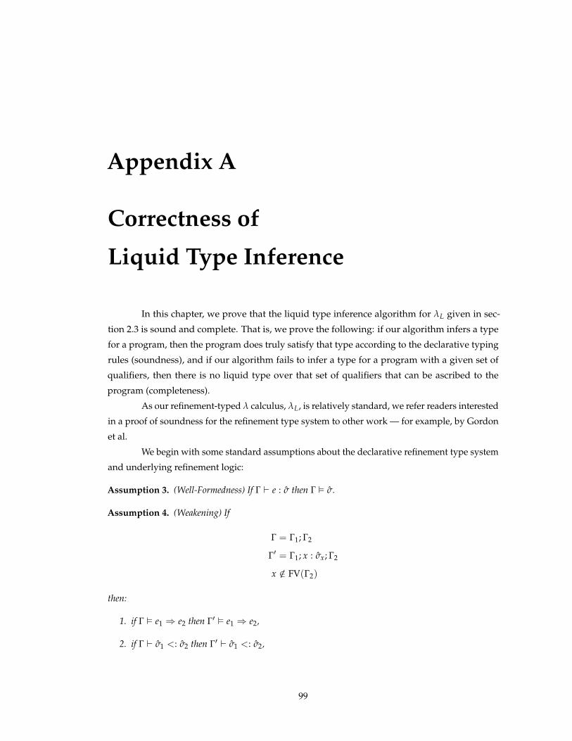
Appendix A
Correctness of
Liquid Type Inference
In this chapter, we prove that the liquid type inference algorithm for lL given in sec-
tion 2.3 is sound and complete. That is, we prove the following: if our algorithm infers a type
for a program, then the program does truly satisfy that type according to the declarative typing
rules (soundness), and if our algorithm fails to infer a type for a program with a given set of
qualifiers, then there is no liquid type over that set of qualifiers that can be ascribed to the
program (completeness).
As our refinement-typed l calculus, lL, is relatively standard, we refer readers interested
in a proof of soundness for the refinement type system to other work — for example, by Gordon
et al.
We begin with some standard assumptions about the declarative refinement type system
and underlying refinement logic:
Assumption 3. (Well-Formedness) If G ` e : s then G ✏ s.
Assumption 4. (Weakening) If
G = G1; G2
G0 = G1; x : sx; G2
x /2 FV(G2)
then:
1. if G ✏ e1 ) e2 then G0 ✏ e1 ) e2,
2. if G ` s1 <: s2 then G0 ` s1 <: s2,
99

100
3. if G ✏ s then G0 ✏ s,
4. if G `Q e : s then G0 `Q e : s.
Assumption 5. (Guard Weakening) If
G = G1; G2
G0 = G1; f; G2
then,
1. if G ✏ e1 ) e2 then G0 ✏ e1 ) e2,
2. if G ` s1 <: s2 then G0 ` s1 <: s2,
3. if G ✏ s then G0 ✏ s,
4. if G `Q e : s then G0 `Q e : s.
Assumption 6. (Subtyping Reflexive Transitive)
1. if G ✏ s then G ` s <: s,
2. if G ✏ e1 ) e2 and G ✏ e2 ) e3 then G ✏ e1 ) e3,
3. if G ` s1 <: s2 and G ` s2 <: s3 then G ` s1 <: s3.
Theorem 3. (Soundness of Decidable Checking) If G `Q e : s then G ` e : s.
Proof. By induction on the structure of the derivation of G `Q e : s. The key observations are that
each liquid type (schema) is also a dependent type schema and that each liquid type deriviation
rule [LT-*] has a matching refinement type derivation rule.
Lemma 1. (Fresh) For each type schema s and assignment A over Q, A(Fresh(s)) is a liquid type over
Q.
Proof. By induction on the structure of s
Lemma 2. (Shape) For every liquid type assignment A:
1. Shape(T) = Shape(AT),
2. Shape(G) = Shape(AG).
Proof. (1) follows by induction on the structure of T. (2) follows from (1).
Lemma 3. (Derivation Projection) If G `Q e : s then Shape(G) ` e : Shape(s).
Proof. Induction on the derivation of G `Q e : s, and observing that each derivation rule for `Q
is a refinement of a matching rule for `.
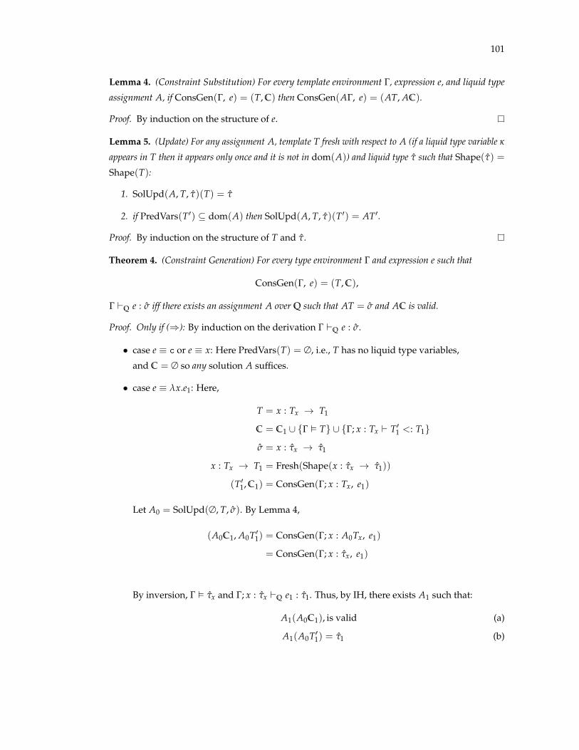
101
Lemma 4. (Constraint Substitution) For every template environment G, expression e, and liquid type
assignment A, if ConsGen(G, e) = (T, C) then ConsGen(AG, e) = (AT, AC).
Proof. By induction on the structure of e.
Lemma 5. (Update) For any assignment A, template T fresh with respect to A (if a liquid type variable k
appears in T then it appears only once and it is not in dom(A)) and liquid type t such that Shape(t) =
Shape(T):
1. SolUpd(A, T, t)(T) = t
2. if PredVars(T0) ✓ dom(A) then SolUpd(A, T, t)(T0) = AT0.
Proof. By induction on the structure of T and t.
Theorem 4. (Constraint Generation) For every type environment G and expression e such that
ConsGen(G, e) = (T, C),
G `Q e : s iff there exists an assignment A over Q such that AT = s and AC is valid.
Proof. Only if ()): By induction on the derivation G `Q e : s.
• case e ⌘ c or e ⌘ x: Here PredVars(T) = ∆, i.e., T has no liquid type variables,
and C = ∆ so any solution A suffices.
• case e ⌘ lx.e1: Here,
T = x : Tx ! T1
C = C1 [ {G ✏ T} [ {G; x : Tx ` T01 <: T1}
s = x : tx ! t1
x : Tx ! T1 = Fresh(Shape(x : tx ! t1))
(T01, C1) = ConsGen(G; x : Tx, e1)
Let A0 = SolUpd(∆, T, s). By Lemma 4,
(A0C1, A0T01) = ConsGen(G; x : A0Tx, e1)
= ConsGen(G; x : tx, e1)
By inversion, G ✏ tx and G; x : tx `Q e1 : t1. Thus, by IH, there exists A1 such that:
A1(A0C1), is valid (a)
A1(A0T01) = t1 (b)
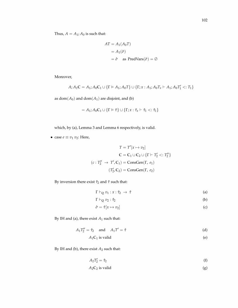
102
Thus, A = A1; A0 is such that:
AT = A1(A0T)
= A1(s)
= s as PredVars(s) = ∆
Moreover,
A; A1C = A1; A0C1 [ {G ✏ A1; A0T} [ {G; x : A1; A0Tx ` A1; A0T01 <: T1}
as dom(A0) and dom(A1) are disjoint, and (b)
= A1; A0C1 [ {G ✏ t} [ {G; x : tx ` t1 <: t1}
which, by (a), Lemma 3 and Lemma 6 respectively, is valid.
• case e ⌘ v1 v2: Here,
T = T0[x 7! v2]
C = C1 [ C2 [ {G ` T02 <: T00
2 }
(c : T002 ! T0, C1) = ConsGen(G, e1)
(T02, C2) = ConsGen(G, e2)
By inversion there exist t2 and t such that:
G `Q v1 : x : t2 ! t (a)
G `Q v2 : t2 (b)
s = t[x 7! v2] (c)
By IH and (a), there exist A1 such that:
A1T002 = t2 and A1T0 = t (d)
A1C1 is valid (e)
By IH and (b), there exist A2 such that:
A2T02 = t2 (f)
A2C2 is valid (g)

103
Moreover,
dom(A1) = PredVars(x : T002 ! T0) [ PredVars(C1)
dom(A2) = PredVars(T02) [ PredVars(C2)
are disjoint (h)
as they result from generating constraints on different subexpressions and PredVars(G) = ∆.
Consider A = A1; A2.
AT = A1; A2T0[x 7! v2]
which, due to delayed substitutions
= A1; A2T0[x 7! v2]
which, because of disjoint domains (g)
= A1T0[x 7! v2]
which, due to (d)
= t[x 7! v2]
= s
Moreover,
AC =A1; A2C1 [ A1; A2C2 [ {G ` A1; A2T02 <: A1; A2T00
2 }
which, due to disjoint domains (g)
=A1C1 [ A2C2 [ {G ` A2T02 <: A1T00
2 }
which, due to (f) and (d)
=A1C1 [ A2C2 [ {G ` t2 <: t2}
which, by (e),(g) and Lemma 6 is valid.

104
• case e ⌘ if v then e2 else e3: Here,
T = Fresh(Shape(s)) (by Lemma 3)
C = C1 [ C2 [ C3 [ {G ✏ T}
[ {G; v ` T02 <: T}
[ {G;¬e1 ` T03 <: T}
(·, C1) = ConsGen(G, v)
(T02, C2) = ConsGen(G; v, e2)
(T03, C3) = ConsGen(G;¬v, e3)
where PredVars(C1),PredVars(C2),PredVars(C3) are disjoint. By inversion, and applying
the IH, there exist solutions A1, A2, A3 such that:
A1C1, A2C2, A3C3 are valid (a)
A2T02 = A3T0
3 = s (b)
G ✏ s (c)
Consider A = SolUpd(A1; A2; A3, T, s), By Lemma 5,
AT = s
AC = A1C1 [ A2C2 [ A3C3 [ {G ✏ s}
[ {G; v ` A2T02 <: s}
[ {G;¬v ` A3T03 <: s}
by (b) and (c)
= A1C1 [ A2C2 [ A3C3 [ {G ✏ s}
[ {G; v ` s <: s}
[ {G;¬v ` s <: s}
which, by (a), inversion and Lemma 6 is valid.
• case e ⌘ let x = e1 in e2: Here,
T = Fresh(Shape(s)) (by Lemma 3)
C = C1 [ C2 [ {G ✏ T} [ {G; x : T01 ` T0
2 <: T} (a0)
(T01, C1) = ConsGen(G, e1)
(T02, C2) = ConsGen(G; x : T0
1, e2) (a1)

105
By inversion there exists s1 such that:
G `Q e1 : s1 (a)
G; x : s1 `Q e2 : s (b)
G ✏ s (c)
By (a) and IH there exists A1 such that:
A1C1 is valid (d)
A1T01 = s1 (e)
By Lemma 4 and (a1),
(A1T02, A1C2) = ConsGen(G; x : A1T0
1, expr2)
= ConsGen(G; x : s01, e2) by (e)
By (b) and IH, there exists A2 such that:
dom(A2) = PredVars(C2) which is disjoint from dom(A1) (f)
A2(A1C2) is valid (g)
A2(A1T02) = s (h)
Consider A = SolUpd(A2; A1, T, s). By Lemma 5,
AT = s
By (a0), (f), and (i):
AC = A1C1 [ A2(A1C2) [ {G ✏ AT} [ {G; x : A1T01 ` A2(A1T0
2) <: AT}
by (i), (e), (h)
= A1C1 [ A2(A1C2) [ {G ✏ s} [ {G; x : s1 ` s <: s}
which, by (d), (g), (c), and Lemma 6 is valid.
• case e ⌘ La.e1: Here,
(T, C) = (La.T01, C1)
(T01, C1) = ConsGen(G, e1)

106
By inversion, exists s1 such that G `Q e1 : s1. Thus, by IH, exists a A1 such that:
A1C1 is valid (a)
A1T01 = s1 (b)
Consider A = A1.
AT = A1T
= A1(La.T01)
= La.A1T01
which, by (b),
= La.s1
= s
Finally,
AC =A1C1 which, by (a), is valid.
• case e ⌘ e1[t]: Here,
T = T01[a 7! Ta]
C = C1 [ {G ✏ Ta})
(T01, C1) = ConsGen(G, e1)
Ta = Fresh(t)
By inversion, there exists t, s1 such that:
G ✏t (a)
Shape(t) =t (b)
G `Q e1 : La.s1 (c)
By IH, there exists A1 such that:
A1C1 is valid (d)
A1T01 = La.s1 (e)
Consider A = SolUpd(A1, Ta, t):
AT = A(T01[a 7! Ta])
= AT01[a 7! ATa]

107
by Lemma 5
= A1T01[a 7! t]
= La.s1[a 7! t]
= s
If ((): By induction on the structure of e.
• case e ⌘ c or e ⌘ x Trivial as C = ∆ and T such that PredVars(T) = ∆ and G `Q e : T.
• case e ⌘ lx.e1: Here
T = x : Tx ! T1
C = C1 [ {G ✏ T} [ {G; x : Tx ` T01 <: T1}
s = x : tx ! t1
x : Tx ! T1 = Fresh(Shape(x : tx ! t1))
(T01, C1) = ConsGen(G; x : Tx, e1)
As AC is valid,
AC1 is valid (a)
G ✏ x : ATx ! AT1 (b)
G; x : ATx ` AT01 <: AT1 (c)
By Lemma 4,
(AT01, AC1) = ConsGen(G; x : ATx, e1)
By (a) and the IH,
G; x : ATx `Q e1 : AT01 (d)
By (d),(b),(c) and rule LT-SUB,
G; x : ATx `Q e1 : AT1 (e)
By Lemma 1, and rule LT-FUN,
G `Q lx.e1 : x : ATx ! AT1
implies G `Q lx.e1 : A(x : Tx ! T1)
implies G `Q lx.e1 : AT
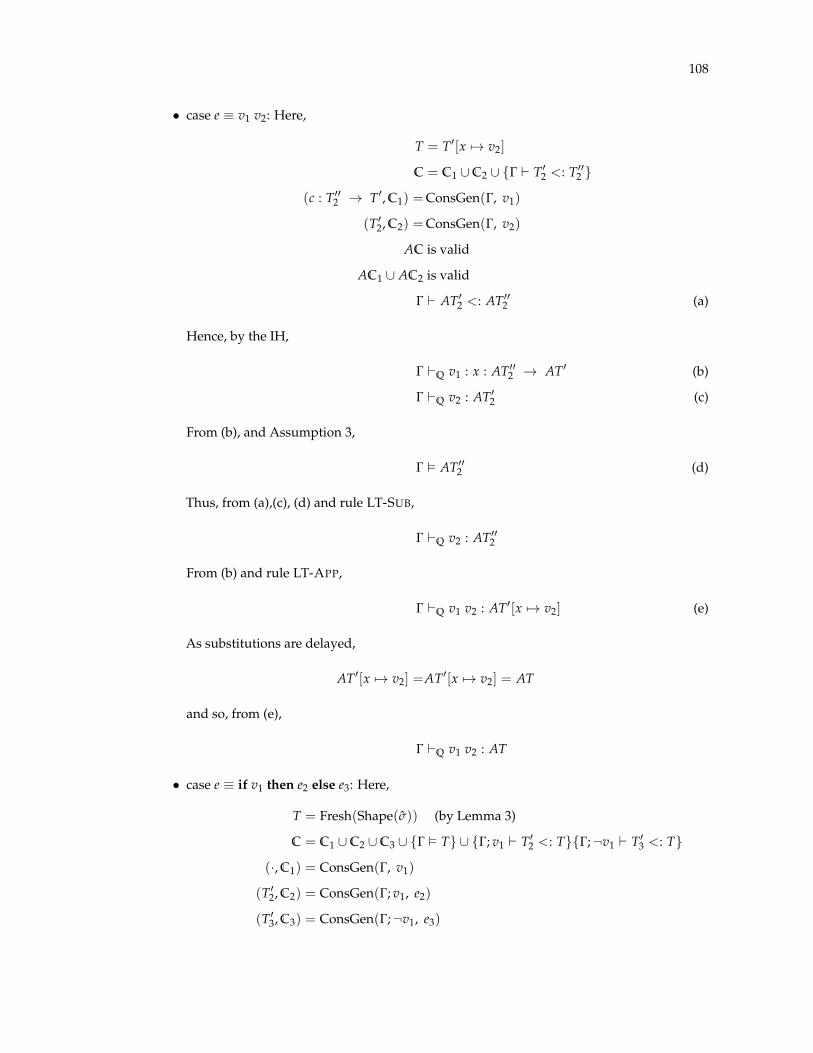
108
• case e ⌘ v1 v2: Here,
T = T0[x 7! v2]
C = C1 [ C2 [ {G ` T02 <: T00
2 }
(c : T002 ! T0, C1) =ConsGen(G, v1)
(T02, C2) =ConsGen(G, v2)
AC is valid
AC1 [ AC2 is valid
G ` AT02 <: AT00
2 (a)
Hence, by the IH,
G `Q v1 : x : AT002 ! AT0 (b)
G `Q v2 : AT02 (c)
From (b), and Assumption 3,
G ✏ AT002 (d)
Thus, from (a),(c), (d) and rule LT-SUB,
G `Q v2 : AT002
From (b) and rule LT-APP,
G `Q v1 v2 : AT0[x 7! v2] (e)
As substitutions are delayed,
AT0[x 7! v2] =AT0[x 7! v2] = AT
and so, from (e),
G `Q v1 v2 : AT
• case e ⌘ if v1 then e2 else e3: Here,
T = Fresh(Shape(s)) (by Lemma 3)
C = C1 [ C2 [ C3 [ {G ✏ T} [ {G; v1 ` T02 <: T}{G;¬v1 ` T0
3 <: T}
(·, C1) = ConsGen(G, v1)
(T02, C2) = ConsGen(G; v1, e2)
(T03, C3) = ConsGen(G;¬v1, e3)

109
As AC is valid,
AC1, AC2, AC3 are valid (a)
G ✏ AT (b)
G; v1 ` AT02 <: AT (ct)
G;¬v1 ` AT03 <: AT (cf)
By (a) and IH,
G; v1 `Q e2 : AT02
G;¬v1 `Q e3 : AT03
By (b), (ct), (cf), Lemma 5,
G; v1 `Q e2 : AT
G;¬v1 `Q e3 : AT
By (a), Lemma 1 and rule LT-IF,
G `Q if v1 then e2 else e3 : AT
• case e ⌘ let x = e1 in e2: Here,
T = Fresh(Shape(s)) (by Lemma 3)
C = C1 [ C2 [ {G ✏ T} [ {G; x : T01 ` T0
2 <: T}
(T01, C1) = ConsGen(G, e1)
(T02, C2) = ConsGen(G; x : T0
1, e2)
As AC is valid
AC1, AC2 are valid (a)
G ✏ AT (b)
G; x : AT01 ` AT0
2 <: T (c)
By (a) and IH,
G `Q e1 : AT01 (d1)
G; x : AT01 `Q e2 : AT0
2 (d2)
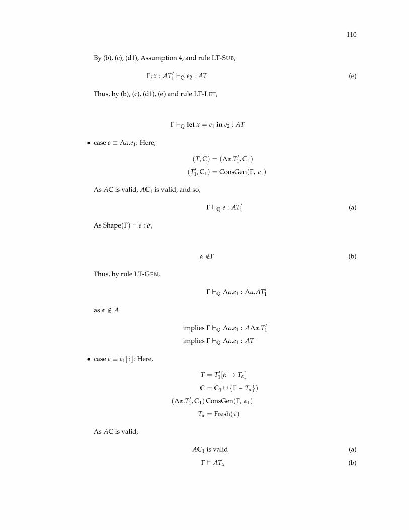
110
By (b), (c), (d1), Assumption 4, and rule LT-SUB,
G; x : AT01 `Q e2 : AT (e)
Thus, by (b), (c), (d1), (e) and rule LT-LET,
G `Q let x = e1 in e2 : AT
• case e ⌘ La.e1: Here,
(T, C) = (La.T01, C1)
(T01, C1) = ConsGen(G, e1)
As AC is valid, AC1 is valid, and so,
G `Q e : AT01 (a)
As Shape(G) ` e : s,
a /2G (b)
Thus, by rule LT-GEN,
G `Q La.e1 : La.AT01
as a /2 A
implies G `Q La.e1 : ALa.T01
implies G `Q La.e1 : AT
• case e ⌘ e1[t]: Here,
T = T01[a 7! Ta]
C = C1 [ {G ✏ Ta})
(La.T01, C1)ConsGen(G, e1)
Ta = Fresh(t)
As AC is valid,
AC1 is valid (a)
G ✏ ATa (b)
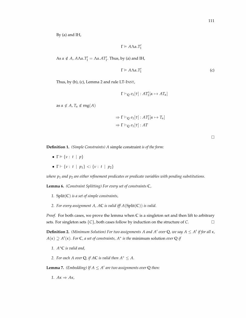
111
By (a) and IH,
G ✏ ALa.T01
As a /2 A, ALa.T01 = La.AT0
1. Thus, by (a) and IH,
G ✏ ALa.T01 (c)
Thus, by (b), (c), Lemma 2 and rule LT-INST,
G `Q e1[t] : AT01[a 7! ATa]
as a 62 A, Ta /2 rng(A)
) G `Q e1[t] : AT01[a 7! Ta]
) G `Q e1[t] : AT
Definition 1. (Simple Constraints) A simple constraint is of the form:
• G ✏ {n : t | p}
• G ` {n : t | p1} <: {n : t | p2}
where p1 and p2 are either refinement predicates or predicate variables with pending substitutions.
Lemma 6. (Constraint Splitting) For every set of constraints C,
1. Split(C) is a set of simple constraints,
2. For every assignment A, AC is valid iff A(Split(C)) is valid.
Proof. For both cases, we prove the lemma when C is a singleton set and then lift to arbitrary
sets. For singleton sets {C}, both cases follow by induction on the structure of C.
Definition 2. (Minimum Solution) For two assignments A and A0 over Q, we say A A0 if for all k,
A(k) ◆ A0(k). For C, a set of constraints, A⇤ is the minimum solution over Q if
1. A⇤C is valid and,
2. For each A over Q, if AC is valid then A⇤ A.
Lemma 7. (Embedding) If A A0 are two assignments over Q then:
1. Ak ) Ak,
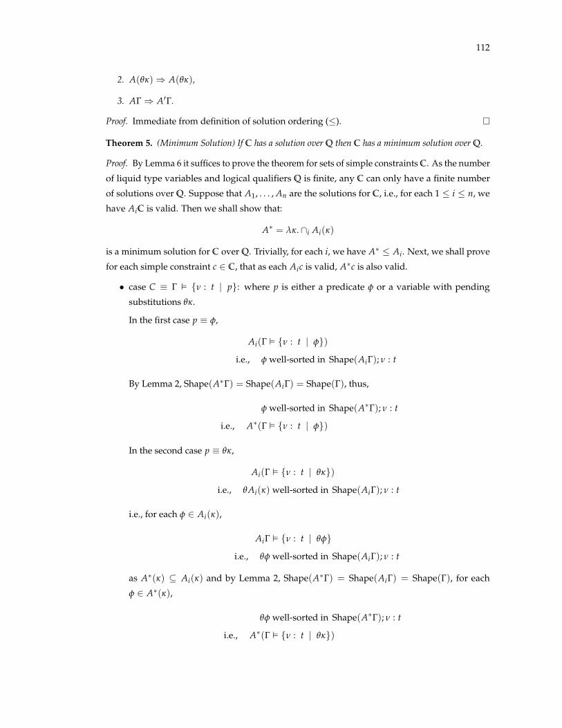
112
2. A(qk) ) A(qk),
3. AG ) A0G.
Proof. Immediate from definition of solution ordering ().
Theorem 5. (Minimum Solution) If C has a solution over Q then C has a minimum solution over Q.
Proof. By Lemma 6 it suffices to prove the theorem for sets of simple constraints C. As the number
of liquid type variables and logical qualifiers Q is finite, any C can only have a finite number
of solutions over Q. Suppose that A1, . . . , An are the solutions for C, i.e., for each 1 i n, we
have AiC is valid. Then we shall show that:
A⇤ = lk. \i Ai(k)
is a minimum solution for C over Q. Trivially, for each i, we have A⇤ Ai. Next, we shall prove
for each simple constraint c 2 C, that as each Aic is valid, A⇤c is also valid.
• case C ⌘ G ✏ {n : t | p}: where p is either a predicate f or a variable with pending
substitutions qk.
In the first case p ⌘ f,
Ai(G ✏ {n : t | f})
i.e., f well-sorted in Shape(AiG); n : t
By Lemma 2, Shape(A⇤G) = Shape(AiG) = Shape(G), thus,
f well-sorted in Shape(A⇤G); n : t
i.e., A⇤(G ✏ {n : t | f})
In the second case p ⌘ qk,
Ai(G ✏ {n : t | qk})
i.e., qAi(k) well-sorted in Shape(AiG); n : t
i.e., for each f 2 Ai(k),
AiG ✏ {n : t | qf}
i.e., qf well-sorted in Shape(AiG); n : t
as A⇤(k) ✓ Ai(k) and by Lemma 2, Shape(A⇤G) = Shape(AiG) = Shape(G), for each
f 2 A⇤(k),
qf well-sorted in Shape(A⇤G); n : t
i.e., A⇤(G ✏ {n : t | qk})

113
• case C ⌘ G ` {n : t | p1} <: {n : t | p2}: where each of p1 and p2 is either a refinement
predicate or a predicate variable with pending substitution.
For each i, Ai(G ` {n : t | p1} <: {n : t | p2})
i.e., AiG ✏ Ai p1 ) Ai p2
by the properties of implication,
^i AiG ✏ ^i Ai p1 ) ^i Ai p2
as [[A⇤G]] = [[^i AiG]] and [[A⇤p1]] = [[^i Ai p1]] and [[A⇤p2]] = [[^i Ai p2]], we have:
A⇤G ✏ A⇤p1 ) A⇤p2
i.e., A⇤(G ` {n : t | p1} <: {n : t | p2})
Lemma 8. (Refinement) If A0 = Refine(A, C) then:
1. A A0,
2. if AC is not valid, then A 6= A0,
3. if A00C is valid and A A00 then A0 A00.
Proof. 1. From the definition of Refine, we have:
A0 ⌘ SolUpd(A, kc, A(k) \ Q0)
for some kc and Q0. We shall show that for any k, we have A0(k) ✓ A(k).
Consider k 6= kc. Here A0(k) = A(k) ✓ A(k).
Consider k = kc. Here A0(k) = A(k) \ Q0 ✓ A(k).
2. We split cases on the type of constraint used for refinement, and in each case, show that if
A0 = A then Ac must be valid.
• case C ⌘ G ✏ {n : t | p}: where p is a refinement predicate or a predicate variable
with pending substitutions. From the definition of Refine, we have:
A0p well-sorted in Shape(AG); n : bool
If A = A0 then,
Ap well-sorted in Shape(AG); n : bool
i.e., AC is valid.

114
• case C ⌘ G ✏ p ) qkc: From the definition of Refine, we have:
AG ✏ Ap ) qA0(kc)
If A = A0 then,
AG ✏ Ap ) qA(kc)
i.e., AC is valid.
3. We split cases on the type of constraint used for refinement.
• case C ⌘ G ✏ {n : t | p}: where p is an expression or a refinement predicate variable
with pending substitutions. We have,
A00C is valid (a)
8k.A00(k) ✓ A(k) (b)
as A A00. From the definition of Refine, we have:
A0 ⌘ SolUpd(A, kc, A(k) \ Q0) (c)
Q0 ⌘{f | f 2 Q, f well-sorted in Shape(G); n : t} (d)
for some kc. We shall show that for any k, we have A00(k) ✓ A0(k).
Consider k 6= kc. From (b)
A00(k) ✓A(k) = A0(k)
Consider k = kc. Now (a) implies that
for each f 2 A00(kc), f 2 Q, andf well-sorted in Shape(G); n : t
i.e., for each f 2 A00(kc), f 2 Q0
From (b),
A00(kc) ✓A(kc) \ Q0 = A0(kc)

115
• case C ⌘ G ✏ p ) qkc: We have,
A00C is valid (a)
8k.A00(k) ✓ A(k) (b)
as A A00. From the definition of Refine, we have:
A0 ⌘ SolUpd(A, kc, A(k) \ Q0) (c)
Q0 ⌘{f | f 2 Q and AG ✏ Ap ) qf} (d)
We shall show that for any k, we have A00(k) ✓ A0(k).
Consider k 6= kc. From (b)
A00(k) ✓A(k) = A0(k)
Consider k = kc. Now (a) implies that
for each f 2 A00(kc), f 2 Q, andA00G ✏ A00p ) qf
As A A00, from Lemma 7 we have
[[AG]] )[[A00G]]
[[Ap]] )[[A00p]]
i.e., [[AG]] ^ [[Ap]] )[[A00G]] ^ [[A00p]] )
and so,
for each f 2 A00(kc), f 2 Q, andA00G ✏ A00p ) qe
i.e., for each f 2 A00(kc), f 2 Q0
i.e., A00(kc) ✓Q0
From (b),
A00(kc) ✓A(kc) \ Q0 = A0(kc)
Theorem 6. (Constraint Solving) For every set of constraints C and qualifiers Q,
1. Solve(C, lk.Q) terminates,

116
2. if Solve(C, lk.Q) returns A then A is the minimum solution for C over Q,
3. if Solve(C, lk.Q) returns ? then C has no solution over Q.
Proof. 1. To prove that Solve terminates, we associate a well-founded measure with solutions
and show that in each iteration of the refinement loop, the potential of the solution A
strictly decreases. Let,
MA ⌘ ÂkkA(k)k
where kA(k)k is the cardinality of A(k). Consider any loop iteration. From the definition
of Solve, we know that the constraint C chosen for refinement is such that AC is not valid.
Let A0 be the refined solution returned by calling Solve(A, C). By Lemma 8,
A A0
A 6=A0
Thus, by the definition of , we have MA0 < MA, i.e., the potential of the solution strictly
decreases in the iteration. As the potential is non-negative, Refine must terminate.
2. Assume that Solve returns a solution A. Then AC is valid (as otherwise the loop would
finish), and so by Theorem 5, C has a minimum solution A⇤ over Q. To prove that the re-
turned solution is the same as A⇤, we show by induction over n that after n iterations of the
loop in Solve, the solution A A⇤. In the base case, A has the initial assignment mapping
each liquid type variable to Q and thus A is less than every solution over Q, including A⇤.
Let us assume the induction hypothesis, that after n iterations, A A⇤. The value of A
after n + 1 iterations is Refine(A, C) where A is the solution after n iterations. As A⇤C is
valid (A⇤ is the minimum solution for C over Q, and A A⇤ (by the induction hypothesis),
from Lemma 8, we deduce that Refine(A, C) A⇤, and so after n + 1 iterations, A A⇤.
Thus, if A is the solution returned by Solve, then A A⇤. As A⇤ is the minimum solution
over Q, and A is a valid solution, A = A⇤.
3. Suppose that Solve fails,but that there is a valid solution for C over Q. Then, there exists a
minimum solution A⇤ over Q, and by the reasoning above, at each iteration, A A⇤. By
the definition of Refine, the outcome ? only happens when A and the constraint C are such
that C ⌘ G ✏ p ) f, where p is either a predicate or a predicate variable with pending
substitutions, and:
AG ✏ Ap 6) f

117
Now, as A A⇤, by Lemma 7, we have
[[AG]] ) [[A⇤G]]
[[Ap]] ) [[A⇤p]]
and therefore,
A⇤G ✏ A⇤p 6) f
i.e., A⇤C is not valid, which is a contradiction, and so there is no valid solution for C over
Q.
Proof. (of Theorem 2) Immediate corollary of Theorems 4 and 6.

Appendix B
Dynamic Semantics of NANOC
In this chapter, we give a standard small-step, call-by value semantics for our core
low-level language, NANOC.
B.1 Reference Values
The program syntax of section 3.2 is meant to describe source-level programs. However,
as a program executes, it produces values of reference type, which are not accounted for in our
syntax of values. Thus, we add reference values to the syntax of values:
v ::= Values
| . . .
| ref(r, n) constant pointer
A reference value ref(r, n) represents a pointer to run-time location r at offset n from the start of
the location r. We assume locations r are drawn from a countable, totally-ordered set of run-time
heap locations, RLoc.
B.2 Semantics
For clarity, we assume that the global environment G is threaded through the evaluation
rules, and thus omit the global environment from the rules. The rules for evaluating programs
use a mapping D from function names to their body expressions.
Definition 3 (Run-Time Block). A run-time block c is a partial function from natural number offsets
to values:
c : N * v.
118

119
n|w| � m|w| ,! (n � m)|w| E-ARITH
ref(r, n) +p m|W| ,! ref(r, n + m) E-PTR-PLUS
0|W| +p m|W| ,! 0|W| E-NULL-PLUS
v1 ./ v2 ,! 1|W| if Comparable(v1, v2), v1 ./ v2 E-REL-TRUE
v1 ./ v2 ,! 0|W| if Comparable(v1, v2),¬(v1 ./ v2) E-REL-FALSE
Figure B.1: Small-step semantics of pure NANOC expressions
Definition 4 (Run-Time Store). A run-time store s is a map from run-time location names r to run-time
blocks c:
s : r * c.
Definition 5 (Comparable Values). Values v1, v2 are comparable, written Comparable(v1, v2), if
and only if one of the following holds:
• v1 = n1|w|, v2 = n2|w|
• v1 = ref(r1, n1), v2 = ref(r2, n2)
• v1 = 0|W|, v2 = ref(r, n)
• v1 = ref(r, n), v2 = 0|W|
Definition 6 (Value Comparisons). We define the behavior of the comparison operators as follows:
• w|n| ./ w|m| iff n ./ m
• W|0| < ref(r, n) for all r, n
• ref(r1, n) ./ ref(r2, m) iff (r1, n) ./ (r2, m) lexicographically
• All relations between comparable values (as defined by Definition 5) that are not explicitly specified
satisfy the appropriate laws (e.g., = is always an equivalence relation on comparable values).
Relations between non-comparable values are left unspecified.
Definition 7 (Type Sizes). We obtain the size of a type t, written SizeOf(t), as
SizeOf(int(w, i)) = w
SizeOf(ref(`, i)) = W
SizeOf({n : t | f}) = SizeOf(t).

120
Definition 8 (Value Sizes). We define the size of a value, written SizeOf(v), as
SizeOf(n|w|) = w
SizeOf(ref(r, n)) = W
Definition 9 (Fitting Data Into Blocks). We define a predicate, Fits, which determines when a value of
size m fits in a run-time block c when stored at offset n:
Fits(n, m, c) = {n . . . n + m � 1} ✓ dom(c)
Definition 10 (Block Value Updates). We define a function, Write, which computes the block resulting
from updating the block c to contain the value v at offset n:
Write(c, n, v) = c[n 7! v][(n + 1 . . . SizeOf(v)� 1) 7! 0|1|]

121
E-PURE
a ,! a0
a/s ,! a0/s
E-SEQ
e1/s ,! e01/s0 e1 not a value
let x = e1 in e2/s ,! let x = e01 in e2/s0
E-LET
let x = v in e/s ,! e[x 7! v]/s
E-IF-TRUE
n 6= 0
if n|W| then e1 else e2/s ,! e1/s
E-IF-FALSE
if 0|W| then e1 else e2/s ,! e2/s
E-READ
v = s(r)(n) SizeOf(v) = m Fits(n, m, s(r))
⇤mref(r, n)/s ,! v/s
E-WRITE
Fits(n, SizeOf(v), s(r))
⇤ref(r, n) := v/s ,! 0|0|/s[r 7! Write(s(r), n, v)]
E-CALL
G( f ) = f (x) { e }
f (v)[` f 7! `]/s ,! e[` f 7! `][x 7! v]/s
E-MALLOC
n � 0 r /2 dom(s)
malloc(n|W|)/s ,! ref(r, 0)/s[r 7! ([0, n) 7! 0|0|)]
E-UNFOLD
letu x = unfold ref(r, n) in e/s ,! e[x 7! ref(r, n)]/s
E-FOLD
fold `/s ,! 0|0|/s
Figure B.2: Small-step semantics of effectful NANOC expressions

122
E-FUN
P/s ,!D[f 7!e] e0/s
f (xj) { e } P/s ,!D e0/s0
E-PROGRAM
e/s ,!D e0/s0
e/s ,!D e0/s0
Figure B.3: Small-step semantics of NANOC programs

Appendix C
Soundness of
NANOC Type Checking
In this chapter, we give a proof of type soundness for the NANOC language and associ-
ated refinement type system. We begin with an overview of our approach to proving soundness,
paying special attention to those aspects of the proof which are unconventional.
C.1 Proof Overview
At a high level, the proof follows the standard format: we prove the usual progress and
preservation lemmas, thus ensuring that every well-typed, closed expression either evaluates to
a value or does not terminate. However, the presence of a mutable heap, along with the unfold
and fold expressions which facilitate strong updates to the types of heap locations, requires us to
add extra machinery to relate the run-time store arising from evaluating an expression to the
static heap type used to type the expression.
The key element of the soundness proof is the heap modeling relation, s ✏m h (Defini-
tion 23), read “run-time store s models the heap h, where m is a correspondence between run-time
store locations r and concrete location names `j”. Intuitively, this relation says that the contents
of each block in the run-time store s satisfy a type given by a block type in the heap type h. Which
block type that is is specified by the location map m (Definition 18), which maps concrete location
names to their corresponding run-time location names. (Recall that our concrete locations are
meant to correspond to exactly one run-time location.) If a run-time location has a corresponding
concrete location `j in the heap type h — that is, the location is currently unfolded — the run-time
block corresponding to that location must satisfy the block type bound to `j in the heap type h.
Otherwise, the location is not unfolded, and the run-time block corresponding to that location
123

124
must have the type specified by the corresponding abstract location in h. The key to showing
type preservation is demonstrating that this heap modeling relation is preserved through location
unfolds and folds (T-UNFOLD and T-FOLD), heap reads and writes (T-READ, T-SUPD, T-WUPD),
and memory allocations (T-MALLOC).
In addition to establishing a correspondence between run-time stores and heap types,
location maps m are used to assign types to pointer-valued constants, which do not appear in
user code but arise as a result of evaluation: they are created by calls to malloc and pointer
arithmetic operations. Thus, we add the current location map m as an additional parameter of
the typing judgment in our updated, proof-oriented typing rules, shown in Figure C.2. A pointer
value that points to run-time location r can be typed as a reference to any concrete location `j
such that the location map m maps `j to r. As evaluation proceeds and new concrete locations
are either allocated with malloc or unfolded with unfold, we introduce new mappings into the
location map m. In order to prove preservation, we require that m grows monotonically, i.e.,
mappings from concrete location names to run-time location names are only ever added after a
step of evaluation; this ensures that every pointer value can be given the same type both before
and after a step of evaluation.
The type checking rules of Section 3.2.3 require that certain concrete location names
used in derivations are “fresh”; to put our proof on firm footing, we must specify exactly
what it means for a location name to be fresh. It is important that concrete location names
assigned to freshly-allocated or unfolded locations are fresh so that every concrete location name
corresponds to exactly one run-time location throughout the course of evaluation, which is the
crucial requirement for our strong update reasoning to be sound. This restriction is reflected in
the proof by our requirement that the location map m is a function, and thus a concrete location
name can only be assigned a single run-time location at a given point in evaluation, and that,
after a step of evaluation, the location map with which we type the result must include m, so that,
in the course of evaluating a program, a single concrete location name is never assigned to two
different run-time locations.
We can satisfy these requirements if, when we require a fresh concrete location name,
we choose a name which is not in the domain of the current location map, m; this ensures that,
after a step of evaluation, we can grow the location map, instead of having to replace a binding
for an existing location name. However, this restriction alone is not sufficient. Suppose we run
expressions e1 and e2 in sequence, and our current location map is m. Suppose that we evaluate e1
to e01, and evaluating e1 unfolds a new concrete location `j. In order to type the resulting sequence
expression e01; e2, we must expand our location map m to include a binding for `j. However, we
know only that e2 was typable in m, which did not include a binding for `j; if we do not make
any further restrictions, it may be the case that our initial type derivation for e2 used the “fresh”
location `j, so that if we add `j to the location map, that location is no longer fresh and so e2 is
not typable in the expanded location map.

125
To resolve this problem, we update our typing rules to ensure that two expressions which
are evaluated in sequence must use disjoint sets of location names (Figure C.2). We parameterize
the typing relation by a countably infinite set of concrete location names, I. Our rule for sequence
expressions, T-LET, enforces the restriction that sequenced expressions e1 and e2 use disjoint
concrete location names by typing e1 with name set I1 and e2 with name set I2, where I1 \ I2 = ∆.
Our preservation lemma ensures that, after a step of evaluation, any concrete locations which
must be added to the location map in order to type the resulting expression are be included in
the name set used to type the original expression, so that the situation described in the preceding
paragraph cannot arise: if a concrete location is unfolded in e1, it cannot have been used in the
type derivation of e2, since the expressions must have been typed with disjoint sets of location
names.
Our proof rests on a complement of substitution lemmas concerning well-formedness,
subtyping, and typing. We use standard value substitution lemmas to eliminate free variables
from environments; these lemmas are used in the proofs of preservation for let, unfold, and
function call expressions. Because our function types are polymorphic in the names of the
heap locations over which they operate, proving preservation in the T-CALL case requires us
to prove a series of location name substitution lemmas. Note that we cannot prove that heap
well-formedness is preserved by arbitrary location name substitutions: if a substitution maps
two location names to a single location name, then a well-formed heap may become ill-formed,
as it may now contain two bindings for the same location. Instead, we show that location name
substitutions preserve heap well-formedness if they are injective on the location names bound in
the heap, i.e., they do not map two distinct location names to the same name. Finally, because
the sets of fresh names used to type check a function and the sets of fresh names available in
the calling context of a function may differ, we must use substitution to prove type preservation
after a function call in two steps. First, we prove that, since both sets of concrete location
names involved are countably infinite, we may consistently substitute location names in the type
derivation of the callee to obtain a substituted version of the function’s type which uses the set
of fresh names available in the calling context. Second, we use the fact that function types may
not contain concrete locations to eliminate the concrete name substitutions, thus showing type
preservation after a function call.
Our type preservation lemma (Lemma 94) incorporates all of the above concerns. We
assume a closed, well-typed expression e, which is typable using location map m and a well-
formed initial heap h, and suppose that s is a run-time store that models h using location map
m. We show that if we take a step of evaluation, yielding expression e0 and store s0, then there
is a heap hs and location map m0 such that the s0 models hs under m0, hs is well-formed, and m0
includes m, such that e0 is typable in then empty environment and heap hs under location map
m0. We further stipulate that any newly-bound concrete location names added to m0 must have
come from the set of location names initially used to type e, which, as we have explained above,
126
is useful in proving preservation in the T-LET case.
To make the proof of preservation for certain rules easier, we make a (results-preserving)
simplification to the dynamic semantics of NANOC (Section C.2.1): we assume that every
run-time block contains a binding for all offsets, rather than some finite region determined
by the number of bytes that were requested in a call to malloc. This change means that the
dynamic semantics can no longer perform bounds checking by checking the domains of run-time
blocks; instead, our syntax of constant pointer values uses fat pointers, which carry their bounds
information as part of the pointer, and our revised evaluation rules for memory access expressions
(Figure C.1) check these bounds at each access. These changes permit three simplifications in
the proof and associated definitions. First, we note that an allocated location may not be large
enough to hold all the items specified in its block type — for example, a block type may specify a
type for the value at offset 10, yet the program may allocate only 8 bytes to a location which has
this type. This would complicate the block modeling relation (Definition 22), which determines
when a run-time block satisfies a block type; because the field types within a block type may
depend on the values defined at non-sequence offsets within the same block, the block modeling
relationship is much simpler if we can assume that these values are always defined. Second,
the proof of preservation for the T-UNFOLD rule crucially relies on being able to substitute in
concrete values for each of the fresh variables introduced to represent the values at non-sequence
offsets within the unfolded block; the theory is again much simpler if we can always assume
that such values exist. Finally, using fat pointers allows us to give a simple, straightforward
definition of the block boundary functions BBegin and BEnd (Assumption 14), which can now
be defined as functions on pointer values, without any reference to heap types or stores. We
prove that these simplifications do not alter the behavior of programs in any significant way
(Lemma 13): terminating expressions yield exactly the same values in either semantics, modulo
the difference between fat and thin pointers, and the resulting stores contain the same values,
modulo the contents of the out-of-bounds portions of the run-time store.
The progress lemma (Lemma 96) is more standard: We show that, if an expression e is
typable with initial heap h and location map m, and if s models h under m, then the expresion
is either a value or may take a step of evaluation. The refinement validity lemma (Lemma 27)
guarantees that, whenever a pointer is dereferenced, it is non-null and within bounds. Heap
modeling guarantees that the location that the pointer refers to actually exists in the run-time
store.
Together, the above lemmas imply that closed, well-typed expressions cannot get stuck,
but must evaluate to a value or loop forever (Theorem 7). That no well-typed, closed expression
can get stuck has three important consequences in our system. First, all memory accesses are to
non-null pointers that are within an allocated region of memory. Second, all primitive operators
(arithmetic, pointer arithmetic, and relations) are provided with valid operands. Finally, the
physical type system ensures that there are never any partial field reads or writes or “overlaps”

127
between fields in the heap: every read or write to the heap accesses an entire contiguous field,
and the fields at each offset within a block are disjoint.
C.2 Changes to the Base Language
To begin, we make several small alterations to NANOC to make the soundness proof
easier, and show that these changes do not affect program execution in any significant way.
C.2.1 Dynamic Semantics
In the dynamic semantics of NANOC given in Appendix B, each allocated run-time block
has the domain [0, n), where n is the number of bytes allocated to the block by a call to malloc.
This accurately reflects the fact that a program may not access a run-time block with an out-of-
bounds index. Further, reference values are of the form ref(r, n), for some run-time location r
and offset into the location n. This accurately reflects the conventional run-time representation of
“thin” pointers that do not carry bounds information.
For the purposes of the soundness proof, however, we make two simplifying changes to
the semantics of programs and run-time pointer representation. First, we assume that run-time
block has the domain Z, i.e., each block is defined at every possible offset. This simplifies the
block modeling relation, which establishes a correspondence between run-time stores and heap
types, as well as the cases for T-UNFOLD and T-MALLOC within the preservation lemma, which
may freely assume that every run-time block is defined at every possible offset. Second, we
change the representation of run-time reference values so that each reference contains the length
of the run-time block where it points. This has two effects. First, it simplifies the definitions of
the BBegin and BEnd predicates, which can now be defined on reference values directly, without
reference to a particular run-time store. Second, it allows us to perform bounds checks in the
simplified semantics by using the bounds information contained within the reference itself;
this will allow us to show that the simplified and original semantics permit exactly the same
evaluations, proving that our simplifications are sound.
We formalize these simplifications in two steps. First, we update the evaluation relation
,! to operate on reference values which carry their bounds; note that, while the updated
,! propagates these bounds, it does not use them to enforce memory safety, and they may
safely be erased. We then create a new evaluation relation, , whose evaluation rules for
heap reads, writes, and allocations incorporate our assumption that every run-time block is
infinitely large and use the bounds information contained in reference values to enforce bounds
safety. The updated rules and values are shown in in Figure C.1. The remaining rules for the
evaluation relation are unchanged from ,!, modulo the substitution of for ,!. We give a
bisimulation establishing that expressions have the same behavior under both ,! and , modulo

128
v ::= Values
x variable
| n|w| integer
| bref(r, n, z) constant pointer with bound
bref(r, n, z) +p m|W| ,! bref(r, n + m, z) PE-PTR-PLUS
PE-READ
0 n n + m � 1 < z v = s(r)(n)
⇤mbref(r, n, z)/s ,! v/s
PE-WRITE
0 n n + SizeOf(v)� 1 < z
⇤bref(r, n, z) := v/s ,! 0|0|/s[r 7! Write(s(r), n, v)]
PE-MALLOC
z > 0 r /2 dom(s)
malloc(z|W|)/s ,! bref(r, 0, z)/s[r 7! (Z 7! 0|0|)]
Figure C.1: Updated reference values and semantics for NANOC
the (inaccessible) contents of the out-of-bounds portions of the run-time store. (We note, without
proof, that bounds information does not figure in to evaluation in the original semantics, and
may be safely erased once safety has been established.)
Definition 11 (Store Similarity). Stores s1 and s2 are similar, written s1 ⇠ s2, if
1. dom(s1) = dom(s2)
2. 8r 2 dom(s1), n 2 dom(s1(r)). s1(r)(n) = s2(r)(n).
Definition 12 (Reference-Store Consistency). We say a reference value v = bref(r, n, z) is consistent
with store s, written s ✏ v, if dom(s(r)) = [0, z).
We say pure and impure expressions a and e are consistent with store s, written s ✏ a and s ✏ e,
respectively, if every value v contained in the expression is consistent with s.
Lemma 9 (Store-Consistent Substitution). For any store s and reference value v,
1. If s ✏ a and s ✏ v, then s ✏ a[x 7! v].
2. If s ✏ e and s ✏ v, then s ✏ e[x 7! v].

129
Proof. Each case proceeds by straightforward induction on the structure of the expression.
Lemma 10 (Store Consistency Preservation). For all stores s, pure expressions a, and impure expres-
sions e,
1. If s ✏ a and a ,! a0 then s ✏ a0.
2. If s ✏ e and e/s ,! e0/s0 then s0 ✏ e0.
Proof. The first case proceeds by cases on the evaluation rule used.
The second case proceeds by straightforward induction on the derivation of e/s ,! e0/s0,
using the first case and Lemma 9. Additionally, the T-CALL case uses the assumption that source
programs do not contain reference constants, and hence that s ✏ e f trivially holds for every
function body e f .
Lemma 11 (Offsets Fit If And Only If In Reference Bounds).
If v = bref(r, n, z)
and s ✏ v (11.1)
then Fits(n, m, s(r)),
if and only if 0 n
and n + m � 1 < z.
Proof. By Fact 11.1 and Definition 12,
dom(s(r)) = [0, z).
Both directions follow immediately from Definition 9.
Lemma 12 (Consistent Update Preserves Store Similarity). If s1 ⇠ s2, then
s1[r 7! Write(s1(r), n, v)] ⇠ s2[r 7! Write(s2(r), n, v)].
Proof. The proof is straightforward from Definition 11.
Lemma 13 (Bisimulation Between Proof and Ordinary Semantics).
If s1 ⇠ s2, (13.1)
and s1 ✏ e, (13.2)
then e/s1 ,! e0/s01
if and only if e/s1 e0/s02,
with s01 ⇠ s02.

130
Proof. Both directions proceed by straightforward induction on the derivation of the hypoth-
esized evaluation step, splitting cases on the final rule used. We show the forward direction
first.
Case e/s1 ,! e0/s01The only interesting cases are E-READ, E-WRITE, and E-MALLOC.
Case E-READ
By the form of the rule,
e ⌘ ⇤mbref(r, n, z) (13.3)
v = s1(r)(n) (13.4)
Fits(n, m, s1(r)) (13.5)
e0 ⌘ v (13.6)
s01 = s1 (13.7)
By Fact 13.2 and Definition 12,
dom(s(r)) = [0, z) (13.8)
By Fact 13.2, Fact 13.5, and Lemma 11,
0 n (13.9)
n + m � 1 < z (13.10)
By Fact 13.1, Fact 13.4, and Definition 11,
s2(r)(n) = v (13.11)
By Fact 13.3, Fact 13.9, Fact 13.10, Fact 13.11, and PE-READ,
e/s e0/s02
with
s02 = s2
so that, by Fact 13.7 and Fact 13.1,
s01 ⇠ s02

131
as required.
Case E-WRITE
By the form of the rule,
e ⌘ ⇤bref(r, n, z) := v (13.12)
Fits(n, SizeOf(v), s(r)) (13.13)
e0 ⌘ 0|0| (13.14)
s01 = s1[r 7! Write(s1(r), n, v)] (13.15)
By Fact 13.2, Fact 13.13, and Lemma 11,
0 n (13.16)
n + SizeOf(v)� 1 < z (13.17)
By Fact 13.16, Fact 13.17, and PE-WRITE,
e/s2 e0/s02
where
s02 = s2[r 7! Write(s2(r), n, v)] (13.18)
By Fact 13.14, Fact 13.18, and Lemma 12,
s01 ⇠ s02
as required.
Case E-MALLOC
By the form of the rule,
e ⌘ malloc(n|W|) (13.19)
n > 0 (13.20)
r /2 dom(s1) (13.21)
e0 ⌘ bref(r, 0, n) (13.22)
s01 = s1[r 7! ([0, n) 7! 0|0|)] (13.23)
By Fact 13.1, Fact 13.21, and Definition 11,
r /2 dom(s2) (13.24)

132
By Fact 13.19, Fact 13.20, Fact 13.24, and E-MALLOC,
e/s2 e0/s02
where
s02 = s2[r 7! ([0, n) 7! 0|0|)] (13.25)
By Fact 13.1, Fact 13.23, Fact 13.25, and Definition 11,
s01 ⇠ s02
as required.
Case e/s2 e0/s02This direction is nearly identical to the other, but uses the reverse direction of Lemma 11.
Lemma 14 (Similar Executions). For any expression e such that ∆ ✏ e,
e/∆ ,!⇤ e0/s1
if and only if e/∆ ⇤ e0/s2
with s1 ⇠ s2.
Proof. The proof proceeds by straightforward induction on the hypothesized derivation, using
Lemma 10 and Lemma 13.
C.2.2 Static Semantics
The typing rules of section 3.2 are sufficient to type check source-level programs. How-
ever, to prove the standard progress and preservation lemmas, we must enhance the language’s
typing judgments to account for reference-valued constants that appear in the course of evalua-
tion as the result of allocating memory. We update the rules of Section 3.2.3 in two ways. First,
to formalize the notion of what it means for a name to be “fresh”, we thread a countable set of
fresh names, I, through the rules. Note that each variable I is meant to represent an infinite set
of names. Second, we add another parameter to the typing judgment, m, which is described in
section C.5; its purpose is to allow us to assign types to constant reference values bref(r, n, z). We
show the new and non-trivially-updated rules in Figure C.2; all rules not shown are the same as
in Section 3.2.3, except that m and I have been threaded through the derivation.
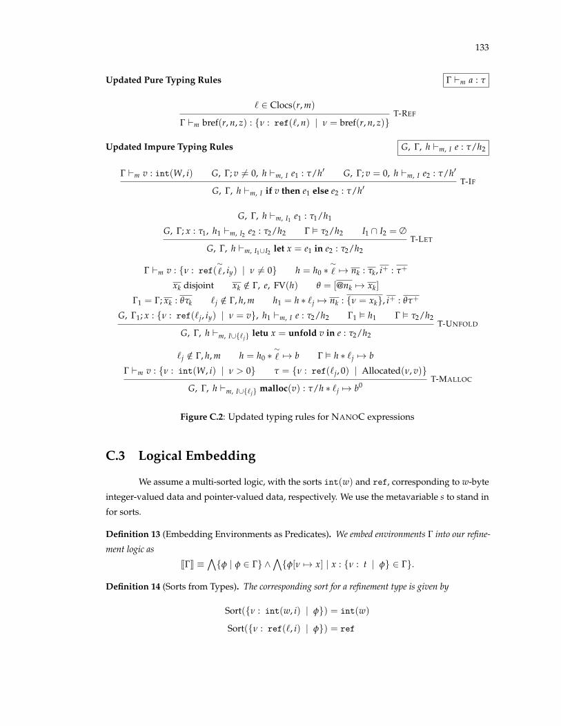
133
Updated Pure Typing Rules G `m a : t
` 2 Clocs(r, m)
G `m bref(r, n, z) : {n : ref(`, n) | n = bref(r, n, z)}T-REF
Updated Impure Typing Rules G, G, h `m, I e : t/h2
G `m v : int(W, i) G, G; v 6= 0, h `m, I e1 : t/h0 G, G; v = 0, h `m, I e2 : t/h0
G, G, h `m, I if v then e1 else e2 : t/h0T-IF
G, G, h `m, I1 e1 : t1/h1
G, G; x : t1, h1 `m, I2 e2 : t2/h2 G ✏ t2/h2 I1 \ I2 = ∆
G, G, h `m, I1[I2 let x = e1 in e2 : t2/h2T-LET
G `m v : {n : ref(⇠` , iy) | n 6= 0} h = h0 ⇤
⇠` 7! nk : tk, i+ : t+
xk disjoint xk /2 G, e, FV(h) q = [@nk 7! xk]
G1 = G; xk : qtk `j /2 G, h, m h1 = h ⇤ `j 7! nk : {n = xk}, i+ : qt+
G, G1; x : {n : ref(`j, iy) | n = v}, h1 `m, I e : t2/h2 G1 ✏ h1 G ✏ t2/h2
G, G, h `m, I[{`j} letu x = unfold v in e : t2/h2T-UNFOLD
`j /2 G, h, m h = h0 ⇤⇠` 7! b G ✏ h ⇤ `j 7! b
G `m v : {n : int(W, i) | n > 0} t = {n : ref(`j, 0) | Allocated(n, v)}
G, G, h `m, I[{`j} malloc(v) : t/h ⇤ `j 7! b0T-MALLOC
Figure C.2: Updated typing rules for NANOC expressions
C.3 Logical Embedding
We assume a multi-sorted logic, with the sorts int(w) and ref, corresponding to w-byte
integer-valued data and pointer-valued data, respectively. We use the metavariable s to stand in
for sorts.
Definition 13 (Embedding Environments as Predicates). We embed environments G into our refine-
ment logic as
[[G]] ⌘^{f | f 2 G} ^
^{f[n 7! x] | x : {n : t | f} 2 G}.
Definition 14 (Sorts from Types). The corresponding sort for a refinement type is given by
Sort({n : int(w, i) | f}) = int(w)
Sort({n : ref(`, i) | f}) = ref
134
Definition 15 (Sort Environments from Type Environments). We create a sort environment from a
type environment using the operation SortEnv:
SortEnv(∆) = ∆
SortEnv(x : t; G) = x : Sort(t); SortEnv(G)
SortEnv(a; G) = SortEnv(G)
Definition 16 (Well-Sorted Refinement Predicates). We say that f well-sorted in G if f is a well-
sorted predicate in the refinement logic under the sort environment SortEnv(G). A well-sorted predicate
may not contain any offset expressions @n.
C.4 Concrete Name Sets
In this section, we give lemmas and definitions concerning the substitution of concrete
location names.
Assumption 7 (Disjoint Concrete Location Numberings). We assume that, for any concrete location
set I, if `j, `0k 2 I, then j 6= k. In particular, this means that, for any location name substitution r,
r(`j) 6= r(`0k).
Definition 17 (Concrete Name Substitution). A concrete name substitution w is a injective function
on concrete location names,
w : CLoc ! CLoc,
where CLoc is the set of all concrete location names. We require that concrete name substitutions preserve
location names, i.e., that w(`j) = `k for some k.
Lemma 15 (Concrete Name Substitution: Well-Formedness). For any concrete name substitution w,
1. If G ✏ t, then wG ✏ wt.
2. If G ✏ b, then wG ✏ wb.
3. If G ✏@ b, then wG ✏@ wb.
4. If G ✏ h, then wG ✏ wh.
5. If G ✏ t/h, then wG ✏ wt/wh.
Proof. The first case proceeds by cases on the rule used to prove G ✏ t, while the next three cases
proceed by straightforward induction on the hypothesized derivation, splitting cases on the final
rule used. The final case is immediate from the previous cases.
Lemma 16 (Concrete Name Substitution: Subtyping). For any concrete name substitution w,

135
1. If G ` t1 <: t2, then wG ` wt1 <: wt2.
2. If G ` b1 <: b2, then wG ` wb1 <: wb2.
3. If G ` h1 <: h2, then wG ` wh1 <: wh2.
4. If G ` t1/h1 <: t2/h2, then wG ` wt1/wh1 <: wt2/wh2.
Proof. Each proof proceeds by induction on the structure of the hypothesized derivation, splitting
cases on the final rule used and using the previous cases of the lemma.
Lemma 17 (Concrete Name Substitution: Pure Typing).
If G `m a : t
then wG `wm a : wt
Proof. The proof proceeds by straightforward induction on the derivation of G `m a : t, splitting
cases on the final rule used, and using Lemma 15 and Lemma 16.
Lemma 18 (Concrete Name Substitution: Typing).
If G, G, h `m, I e : t/h
then G, wG, wh `wm, wI e : wt/wh
Proof. The proof proceeds by straightforward induction on the derivation of
G, G, h `m, I e : t/h,
splitting cases on the final rule used and using Lemma 15, Lemma 16, and Lemma 17. We also
use the fact that w is injective to guarantee that concrete name sets which were distinct in the
original derivation remain so in the updated derivation.
Lemma 19 (Concrete Name Set Weakening).
If G, G, h `m, I1 e : t/h0
and I1 ✓ I2,
then G, G, h `m, I2 e : t/h0
Proof. The proof proceeds by straightforward induction on the derivation of
G, G, h `m, I1 e : t/h0,
splitting cases on the final rule used.
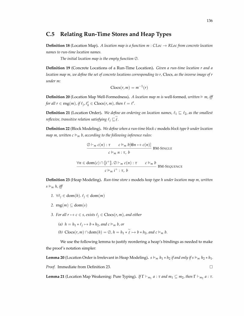
136
C.5 Relating Run-Time Stores and Heap Types
Definition 18 (Location Map). A location map is a function m : CLoc ! RLoc from concrete location
names to run-time location names.
The initial location map is the empty function ∆.
Definition 19 (Concrete Locations of a Run-Time Location). Given a run-time location r and a
location map m, we define the set of concrete locations corresponding to r, Clocs, as the inverse image of r
under m:
Clocs(r, m) = m�1(r)
Definition 20 (Location Map Well-Formedness). A location map m is well-formed, written ✏ m, iff
for all r 2 rng(m), if `j, `0k 2 Clocs(r, m), then ` = `0.
Definition 21 (Location Order). We define an ordering on location names, `1 v `2, as the smallest
reflexive, transitive relation satisfying `j v⇠` .
Definition 22 (Block Modeling). We define when a run-time block c models block type b under location
map m, written c ✏m b, according to the following inference rules:
∆ `m c(n) : t c ✏m b[@n 7! c(n)]
c ✏m n : t, bBM-SINGLE
8n 2 dom(c) \ [[i+]]. ∆ `m c(n) : t c ✏m b
c ✏m i+ : t, bBM-SEQUENCE
Definition 23 (Heap Modeling). Run-time store s models heap type h under location map m, written
s ✏m h, iff
1. 8`j 2 dom(h). `j 2 dom(m)
2. rng(m) ✓ dom(s)
3. For all r 7! c 2 s, exists `j 2 Clocs(r, m), and either
(a) h = h1 ⇤ `j 7! b ⇤ h2, and c ✏m b, or
(b) Clocs(r, m) \ dom(h) = ∆, h = h1 ⇤⇠` 7! b ⇤ h2, and c ✏m b.
We use the following lemma to justify reordering a heap’s bindings as needed to make
the proof’s notation simpler:
Lemma 20 (Location Order is Irrelevant in Heap Modeling). s ✏m h1 ⇤ h2 if and only if s ✏m h2 ⇤ h1.
Proof. Immediate from Definition 23.
Lemma 21 (Location Map Weakening: Pure Typing). If G `m1 a : t and m1 ✓ m2, then G `m2 a : t.

137
Proof. The proof proceeds by induction on the derivation of G `m1 a : t, splitting cases on the
final rule used.
The only interesting case is T-REF. By the form of the rule,
a ⌘ bref(r, n, z)
t = {n : ref(`, n) | n = bref(r, n, z)}
` 2 Clocs(r, m1) (21.1)
Since m1 ✓ m2,
Clocs(r, m1) ✓ Clocs(r, m2) (21.2)
So by Fact 21.1, Fact 21.2, and T-REF,
G `m2 bref(r, n, l) : {n : ref(`, n) | n = bref(r, n, z)}
as required.
Lemma 22 (Location Map Weakening).
If G, G, h `m1, I e : t/h0,
m1 ✓ m2,
and dom(m2 \ m1) \ I = ∆,
then G, G, h `m2, I e : t/h0.
Proof. The proof proceeds by induction on the derivation of G, G, h `m1, I e : t/h0, splitting
cases on the final rule used. The requirement that dom(m2 \ m1) \ I = ∆ is used in the cases
for T-UNFOLD and T-MALLOC to ensure that we can use the same concrete locations in both
derivations.
Lemma 23 (Abstract Types and Location Map Weakening).
If G, G, h `∆, I e : t/h0 (23.1)
and G, h, t, h0 abstract, (23.2)
then G, G, h `m, I e : t/h0.
Proof. Let w be such that
I \ dom(m) = wI. (23.3)
We know such a substitution exists because I is countable. By Fact 23.1 and Lemma 18,
G, wG, wh `∆, wI e : wt/wh.

138
By Fact 23.2, this is equivalent to
G, G, h `∆, wI e : t/h. (23.4)
By Fact 23.3, Fact 23.4, and Lemma 22,
G, G, h `m, wI e : t/h. (23.5)
By Fact 23.3,
wI ✓ I. (23.6)
By Fact 23.5, Fact 23.6, and Lemma 19,
G, G, h `m, I e : t/h,
as required.
Lemma 24 (Location Map Weakening Preserves Block Modeling).
If c ✏m1 b
and m1 ✓ m2
then c ✏m2 b.
Proof. Straightforward induction on the derivation of c ✏m1 b, using Lemma 21.
Lemma 25 (Typable References). If G `m bref(r, n, z) : t, then r 2 rng(m).
Proof. The proof proceeds by straightforward induction on the derivation of G `m bref(r, n, z) : t.
The only interesting case is T-REF, where the conclusion follows immediately from the premise
that there exists some ` 2 Clocs(r, m) and Definition 19.
C.6 Index Properties
Proposition 1 (Reflexivity and Transitivity of⇠✓). The operator
⇠✓ is reflexive and transitive.
Proof. Immediate from the definition of⇠✓.
Proposition 2 (Singleton Subindexing is Inclusion). n 2 [[i]] if and only if n⇠✓ i.
Proof. Immediate from the definition of⇠✓.
Proposition 3 (Soundness of Abstract Arithmetic). If n1⇠✓ i1 and n2
⇠✓ i2, and n1 � n2 is defined,
then n1 � n2⇠✓ i1
⇠� i2.
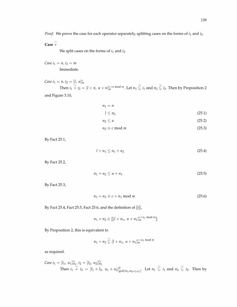
139
Proof. We prove the case for each operator separately, splitting cases on the forms of i1 and i2.
Case⇠+
We split cases on the forms of i1 and i2.
Case i1 = n, i2 = m
Immediate.
Case i1 = n, i2 = [l, u]cmThen i1
⇠+ i2 = [l + n, u + n]c+n mod m
m . Let n1⇠✓ i1 and n2
⇠✓ i2. Then by Proposition 2
and Figure 3.10,
n1 = n
l n2 (25.1)
n2 u (25.2)
n2 ⌘ c mod m (25.3)
By Fact 25.1,
l + n1 n1 + n2 (25.4)
By Fact 25.2,
n1 + n2 u + n1 (25.5)
By Fact 25.3,
n1 + n2 ⌘ c + n1 mod m (25.6)
By Fact 25.4, Fact 25.5, Fact 25.6, and the definition of [[i]],
n1 + n2 2 [[[l + n1, u + n1]c+n1 mod mm ]]
By Proposition 2, this is equivalent to
n1 + n2⇠✓ [l + n1, u + n1]
c+n1 mod mm
as required.
Case i1 = [l1, u1]c1m1 , i2 = [l2, u2]
c2m2
Then i1⇠+ i2 = [l1 + l2, u1 + u2]0gcd(m1,m2,c1,c2)
. Let n1⇠✓ i1 and n2
⇠✓ i2. Then by
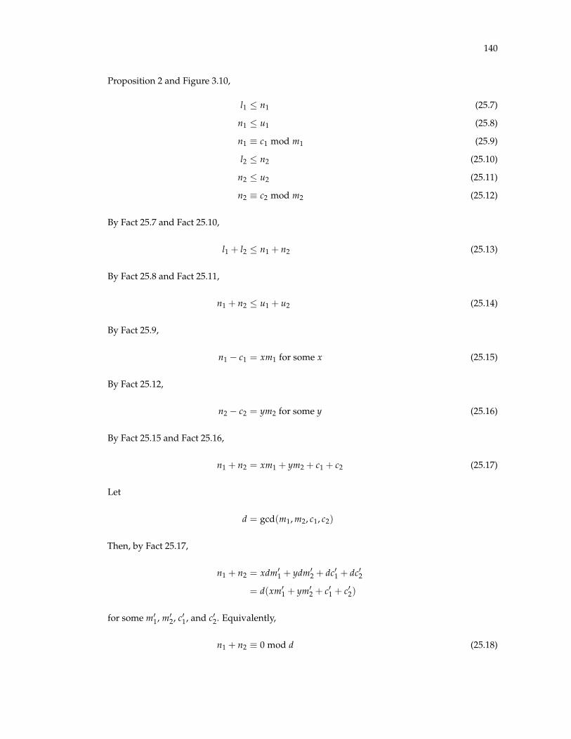
140
Proposition 2 and Figure 3.10,
l1 n1 (25.7)
n1 u1 (25.8)
n1 ⌘ c1 mod m1 (25.9)
l2 n2 (25.10)
n2 u2 (25.11)
n2 ⌘ c2 mod m2 (25.12)
By Fact 25.7 and Fact 25.10,
l1 + l2 n1 + n2 (25.13)
By Fact 25.8 and Fact 25.11,
n1 + n2 u1 + u2 (25.14)
By Fact 25.9,
n1 � c1 = xm1 for some x (25.15)
By Fact 25.12,
n2 � c2 = ym2 for some y (25.16)
By Fact 25.15 and Fact 25.16,
n1 + n2 = xm1 + ym2 + c1 + c2 (25.17)
Let
d = gcd(m1, m2, c1, c2)
Then, by Fact 25.17,
n1 + n2 = xdm01 + ydm0
2 + dc01 + dc02
= d(xm01 + ym0
2 + c01 + c02)
for some m01, m0
2, c01, and c02. Equivalently,
n1 + n2 ⌘ 0 mod d (25.18)

141
By Fact 25.13, Fact 25.14, Fact 25.18, and the definition of [[i]],
n1 + n2 2 [[[l1 + l2, u1 + u2]0gcd(m1,m2,c1,c2)
]]
By Proposition 2, this is equivalent to
n1 + n2⇠✓ [l1 + l2, u1 + u2]
0gcd(m1,m2,c1,c2)
as required.
Case⇠·
We split cases on the forms of i1 and i2.
Case i1 = n, i2 = m
Immediate.
Case i1 = n, i2 = [l, u]cmThen i1
⇠· i2 = [nl, nu]ncnm. Let n1
⇠✓ i1 and n2
⇠✓ i2. Then by Proposition 2 and
Figure 3.10,
n1 = n
l n2 (25.19)
n2 u (25.20)
n2 ⌘ c mod m (25.21)
By Fact 25.19,
n1l n1n2 (25.22)
By Fact 25.20,
n1n2 n1u2 (25.23)
By Fact 25.21,
n2 � c = xm for some x
Then
n1(n2 � c) = n1n2 � n1c
= n1xm
= x(n1m)

142
Equivalently,
n1n2 ⌘ n1c mod n1m (25.24)
By Fact 25.22, Fact 25.23, Fact 25.24, and the definition of [[i]],
n1n2 2 [[[n1l, n1u]n1cn1m]]
By Proposition 2, this is equivalent to
n1n2⇠✓ [n1l, n1u]n1c
n1m
as required.
Case i1 = [l1, u1]c1m1 , i2 = [l2, u2]
c2m2
Immediate.
Case⇠/
Immediate.
C.7 Logical Assumptions
We assume a many-sorted refinement logic that subsumes quantifier-free first-order logic
with equality and theories of integer and pointer arithmetic. We detail our assumptions with
respect to well-sortedness and the theories of integer and pointer arithmetic below.
Assumption 8 (Well-Sorted Logical Substitution). If f is well-sorted in sort environment G and x
and t have the same sort in G, then f[x 7! t] is well-sorted in G.
Assumption 9 (Free Variables in Well-Sorted Predicates). If f well-sorted in G, then FV(f) ✓dom(G).
Assumption 10 (Values’ Logical Sorts). For every value v, if ∆ `m v : t, then v has sort Sort(t).
In particular, zero-valued integers 0|w| can take on both int(w) and ref sorts.
Assumption 11 (Weakening Well-Sortedness).
If f well-sorted in G1; G2
and dom(G1; G2) \ dom(G) = ∆,
then f well-sorted in G1; G; G2.
Assumption 12 (Strengthening Well-Sortedness). If f well-sorted in G; x : s and x /2 FV(f), then
f well-sorted in G.

143
Assumption 13 (Theories of Arithmetic). The refinement logic includes a complete theory of arithmetic
for each integer width. That is, for all w, n1, n2, and operations �,
n1|w| � n2|w| = (n1 � n2)|w|
is valid.
We also assume a theory of pointer arithmetic such that the following two are valid:
bref(r, n1, z) +p n2|W| = bref(r, n1 + n2, z)
0|W| +p n2|W| = 0|W|
For all values v1, v2 of the same sort, we assume that:
1. v1 ./ v2 is valid iff v1 ./ v2.
2. v1 ./ v2 is valid iff ¬(v1 ./ v2)
Assumption 14 (Block Boundary Functions). We define the BBegin and BEnd functions as follows:
BBegin(bref(r, n, z)) = bref(r, 0, z)
BEnd(bref(r, n, z)) = bref(r, z, z)
BBegin(0|W|) = 0|W|
BEnd(0|W|) = 0|W|
C.8 Relating Logic and Typing
Lemma 26 (Subtyping Implication). If ∆ ` {n : t1 | f1} <: {n : t2 | f2}, then ∆ ✏ f1 ) f2.
Proof. The proof proceeds by straightforward induction on the derivation of ∆ ` {n : t1 | f1} <:
{n : t2 | f2}, splitting cases on the final rule used.
Lemma 27 (Refinement Validity). For any value v, if ∆ `m v : {n : t | f}, then f[n 7! v] is valid.
Proof. The proof proceeds by straightforward induction on the derivation of ∆ `m v : {n : t | f},
splitting cases on the final rule used and using Lemma 26 in the T-PURESUB case.
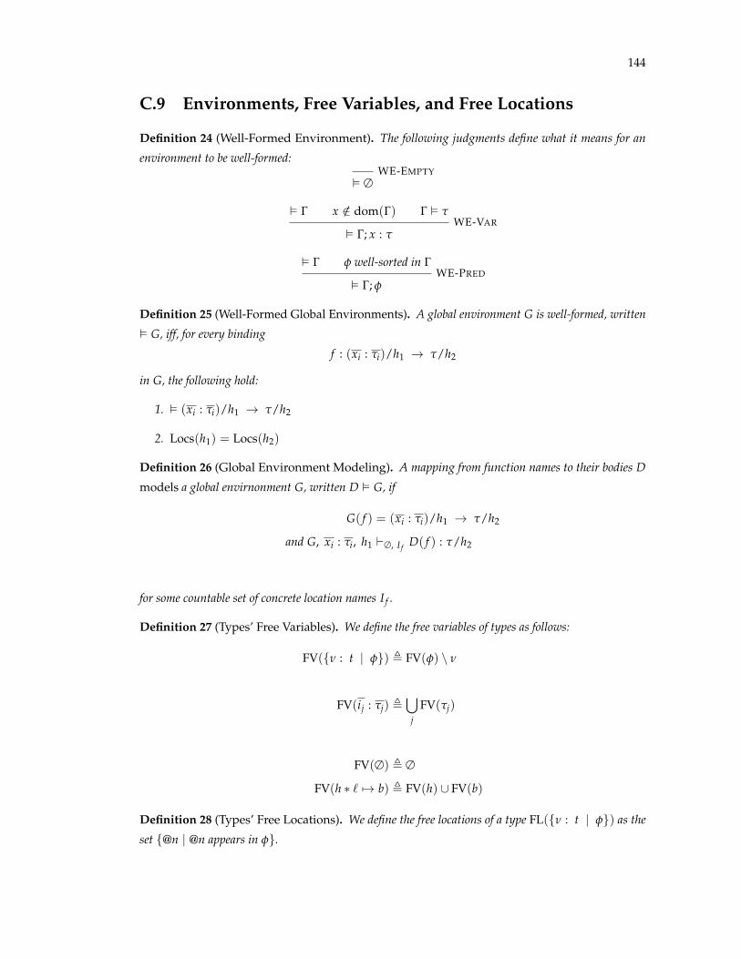
144
C.9 Environments, Free Variables, and Free Locations
Definition 24 (Well-Formed Environment). The following judgments define what it means for an
environment to be well-formed:
✏ ∆WE-EMPTY
✏ G x /2 dom(G) G ✏ t
✏ G; x : tWE-VAR
✏ G f well-sorted in G
✏ G; fWE-PRED
Definition 25 (Well-Formed Global Environments). A global environment G is well-formed, written
✏ G, iff, for every binding
f : (xi : ti)/h1 ! t/h2
in G, the following hold:
1. ✏ (xi : ti)/h1 ! t/h2
2. Locs(h1) = Locs(h2)
Definition 26 (Global Environment Modeling). A mapping from function names to their bodies D
models a global envirnonment G, written D ✏ G, if
G( f ) = (xi : ti)/h1 ! t/h2
and G, xi : ti, h1 `∆, I f D( f ) : t/h2
for some countable set of concrete location names I f .
Definition 27 (Types’ Free Variables). We define the free variables of types as follows:
FV({n : t | f}) , FV(f) \ n
FV(ij : tj) ,[
jFV(tj)
FV(∆) , ∆
FV(h ⇤ ` 7! b) , FV(h) [ FV(b)
Definition 28 (Types’ Free Locations). We define the free locations of a type FL({n : t | f}) as the
set {@n | @n appears in f}.
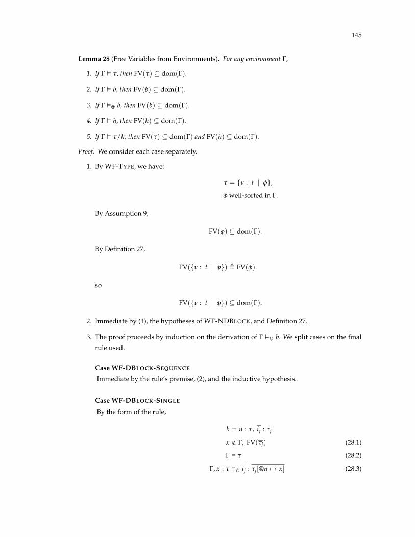
145
Lemma 28 (Free Variables from Environments). For any environment G,
1. If G ✏ t, then FV(t) ✓ dom(G).
2. If G ✏ b, then FV(b) ✓ dom(G).
3. If G ✏@ b, then FV(b) ✓ dom(G).
4. If G ✏ h, then FV(h) ✓ dom(G).
5. If G ✏ t/h, then FV(t) ✓ dom(G) and FV(h) ✓ dom(G).
Proof. We consider each case separately.
1. By WF-TYPE, we have:
t = {n : t | f},
f well-sorted in G.
By Assumption 9,
FV(f) ✓ dom(G).
By Definition 27,
FV({n : t | f}) , FV(f).
so
FV({n : t | f}) ✓ dom(G).
2. Immediate by (1), the hypotheses of WF-NDBLOCK, and Definition 27.
3. The proof proceeds by induction on the derivation of G ✏@ b. We split cases on the final
rule used.
Case WF-DBLOCK-SEQUENCE
Immediate by the rule’s premise, (2), and the inductive hypothesis.
Case WF-DBLOCK-SINGLE
By the form of the rule,
b = n : t, ij : tj
x /2 G, FV(tj) (28.1)
G ✏ t (28.2)
G, x : t ✏@ ij : tj[@n 7! x] (28.3)
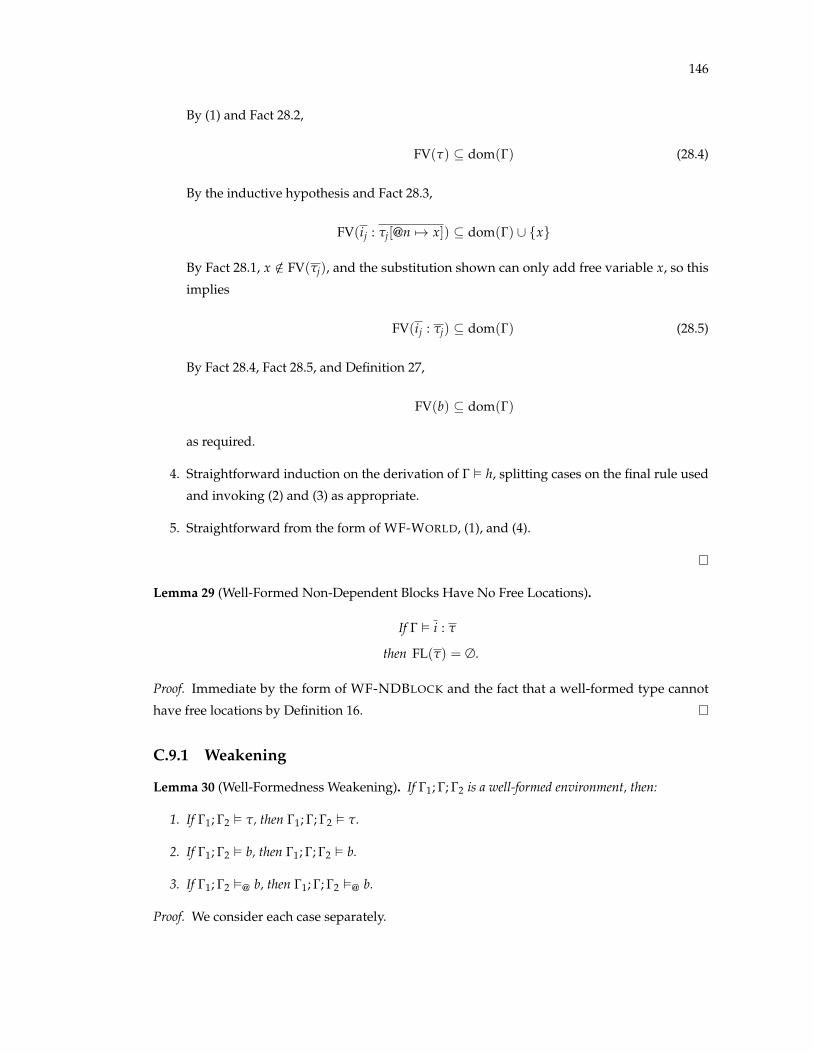
146
By (1) and Fact 28.2,
FV(t) ✓ dom(G) (28.4)
By the inductive hypothesis and Fact 28.3,
FV(ij : tj[@n 7! x]) ✓ dom(G) [ {x}
By Fact 28.1, x /2 FV(tj), and the substitution shown can only add free variable x, so this
implies
FV(ij : tj) ✓ dom(G) (28.5)
By Fact 28.4, Fact 28.5, and Definition 27,
FV(b) ✓ dom(G)
as required.
4. Straightforward induction on the derivation of G ✏ h, splitting cases on the final rule used
and invoking (2) and (3) as appropriate.
5. Straightforward from the form of WF-WORLD, (1), and (4).
Lemma 29 (Well-Formed Non-Dependent Blocks Have No Free Locations).
If G ✏ i : t
then FL(t) = ∆.
Proof. Immediate by the form of WF-NDBLOCK and the fact that a well-formed type cannot
have free locations by Definition 16.
C.9.1 Weakening
Lemma 30 (Well-Formedness Weakening). If G1; G; G2 is a well-formed environment, then:
1. If G1; G2 ✏ t, then G1; G; G2 ✏ t.
2. If G1; G2 ✏ b, then G1; G; G2 ✏ b.
3. If G1; G2 ✏@ b, then G1; G; G2 ✏@ b.
Proof. We consider each case separately.
147
1. The only rule that applies is WF-TYPE, from which we have
t = {n : t | f}
f well-sorted in G1; G2
By the assumption that G1; G; G2 is well-formed, dom(G1; G2)\ dom(G) = ∆, so by Assump-
tion 11,
f well-sorted in G1; G; G2
By WF-TYPE,
G1; G; G2 ✏ t
as required.
2. Follows immediately using (1).
3. The proof proceeds by straightforward induction on the derivation of G ✏@ b, using (1) and
(2).
Lemma 31 (Subtyping Weakening). If G ` t1 <: t2, then G; G0 ` t1 <: t2.
Proof. The proof proceeds by induction on the derivaton of G ` t1 <: t2. We split cases on the
final rule used.
Case <:-INT
By the form of the rule, we have
i1⇠✓ i2 (31.1)
G ✏ f1 ) f2 (31.2)
By logical monotonicity,
G; G0 ✏ f1 ) f2 (31.3)
By <:-INT, Fact 31.1, and Fact 31.3,
G; G0 ` t1 <: t2 (31.4)
as required.

148
Case <:-REF
Similar to the case for <:-INT.
Case <:-ABSTRACT, <:-NULL
Immediate.
Case <:-TRANS
Immediate by the inductive hypothesis and a use of <:-TRANS.
Lemma 32 (Pure Type Weakening).
If G; G0 is a well-formed environment (32.1)
and G `m a : t
then G; G0 `m a : t.
Proof. By induction on the derivation of G `m a : t. We split cases on the final rule used.
Case T-VAR
By the form of the rule, we have
a ⌘ x
G(x) = {n : t | f}
t = {n : t | n = x}
Since G; G0 is well-formed, dom(G) \ dom(G0) = ∆. So
(G; G0)(x) = t
By T-VAR, then,
G; G0 `m x : {n : t | n = x}
Case T-INT, T-REF
Immediate.
Case T-ARITH
By the form of the rule,
a ⌘ a1 � a2
t = {n : int(n, i1⇠� i2) | n = a1 � a2}
G `m a1 : int(n, i1) (32.2)
G `m a2 : int(n, i2) (32.3)

149
By Fact 32.2, Fact 32.3, and the inductive hypothesis,
G; G0 `m a1 : int(n, i1) (32.4)
G; G0 `m a2 : int(n, i2) (32.5)
By Fact 32.4, Fact 32.5, and T-ARITH,
G; G0 `m a1 � a2 : {n : int(n, i1⇠� i2) | n = a1 � a2}
Case T-PTRARITH, T-RELATION
Similar to the case for T-ARITH.
Case T-PURESUB
By the form of the rule,
G `m a : t1 (32.6)
G ` t1 <: t (32.7)
G ✏ t (32.8)
By Fact 32.6 and the inductive hypothesis,
G; G0 `m a : t1
By Fact 32.7 and Lemma 31,
G; G0 ` t1 <: t
By Fact 32.8, Fact 32.1, and Lemma 30,
G; G0 ✏ t
By the above and T-PURESUB,
G; G0 `m a : t
C.10 Subtyping
Lemma 33 (Narrowing To Base Subtyping). If G ` {n : t1 | f1} <: {n : t2 | f2} then G `{n : t1 | f1} <: {n : t2 | f1}
150
Proof. Straightforward induction on the derivation of G ` {n : t1 | f1} <: {n : t2 | f2}.
Lemma 34 (Subtyping Inversion). If G ` t1 <: t2 then one of the following holds:
1.
t1 = {n : int(w, i1) | f1}
t2 = {n : int(w, i2) | f2}
i1⇠✓ i2
G ✏ f1 ) f2
2.
t1 = {n : ref(`1, i1) | f1}
t2 = {n : ref(`2, i2) | f2}
`1 v `2
i1⇠✓ i2
G ✏ f1 ) f2
3.
t1 = {n : int(W, 0) | f1}
t2 = {n : ref(⇠` , i2) | f2}
G ✏ f1 ) n = 0
G ✏ n = 0 ) f2
Proof. The proof proceeds by induction on the derivation of G ` t1 <: t2. We split cases on the
final rule used.
Case <:-INT
By the form of the rule, case (1) is immediately satisfied.
Case <:-REF
By the form of the rule, case (2) is immediately satisfied.
Case <:-ABSTRACT
By the form of the rule, case (2) is immediately satisfied.

151
Case <:-NULL
By the form of the rule, case (3) is immediately satisfied.
Case <:-TRANS
By the form of the rule,
G ` t1 <: t3 (34.1)
G ` t3 <: t2 (34.2)
By the inductive hypothesis and Fact 34.2, there are three cases to consider, corresponding to the
three cases of the lemma.
Case (1)
Then
t3 = {n : int(w, i3) | f3} (34.3)
t2 = {n : int(w, i2) | f2} (34.4)
i3⇠✓ i2 (34.5)
G ✏ f3 ) f2 (34.6)
By Fact 34.3, Fact 34.1, and the inductive hypothesis,
t1 = {n : int(w, i1) | f1} (34.7)
i1⇠✓ i3 (34.8)
G ✏ f1 ) f3 (34.9)
By Fact 34.5, Fact 34.8, and Proposition 1,
i1⇠✓ i2 (34.10)
By Fact 34.6, Fact 34.9, and the transitivity of implication,
G ✏ f1 ) f2 (34.11)
By Fact 34.4, Fact 34.7, Fact 34.10, and Fact 34.11, case (1) is satisfied.
Case (2)
Then

152
t3 = {n : ref(`3, i3) | f3} (34.12)
t2 = {n : ref(`2, i2) | f2} (34.13)
`3 v `2 (34.14)
i3⇠✓ i2 (34.15)
G ✏ f3 ) f2 (34.16)
By Fact 34.12 and the inductive hypothesis, there are two more cases to consider.
First, consider the case where
t1 = {n : ref(`1, i1) | f1} (34.17)
`1 v `3 (34.18)
i1⇠✓ i3 (34.19)
G ✏ f1 ) f3 (34.20)
By Fact 34.14, Fact 34.18, and Definition 21,
`1 v `2 (34.21)
By Fact 34.15, Fact 34.19, and Proposition 1,
i1⇠✓ i2 (34.22)
By Fact 34.16, Fact 34.20, and the transitivity of implication,
G ✏ f1 ) f2 (34.23)
By Fact 34.13, Fact 34.17, Fact 34.21, Fact 34.22, and Fact 34.23, case (2) of the lemma is satisfied.
Next, consider the case where
t1 = {n : int(W, 0) | f1} (34.24)
`3 =⇠` (34.25)
G ✏ f1 ) n = 0 (34.26)
G ✏ n = 0 ) f3 (34.27)
By Fact 34.25 and Definition 21,
`2 =⇠` (34.28)
By Fact 34.16, Fact 34.27, and the transitivity of implication,
G ✏ n = 0 ) f2 (34.29)

153
By Fact 34.24, Fact 34.26, Fact 34.28, and Fact 34.29, case (3) of the lemma is satisfied.
Case (3)
Then
t3 = {n : int(W, 0) | f3} (34.30)
t2 = {n : ref(⇠` , i2) | f2} (34.31)
G ✏ f3 ) n = 0 (34.32)
G ✏ n = 0 ) f2 (34.33)
By Fact 34.1, Fact 34.30, and the inductive hypothesis,
t1 = {n : int(W, 0) | f1} (34.34)
G ✏ f1 ) f3 (34.35)
By Fact 34.32, Fact 34.35, and the transitivity of implication,
G ✏ f1 ) n = 0 (34.36)
By Fact 34.31, Fact 34.34, Fact 34.33, and Fact 34.36, case (3) of the lemma is satisfied.
Lemma 35 (Subtyping is Transitive). For any environment G,
1. If G ` t1 <: t2 and G ` t2 <: t3, then G ` t1 <: t3.
2. If G ` b1 <: b2 and G ` b2 <: b3, then G ` b1 <: b3.
3. If G ` h1 <: h2 and G ` h2 <: h3, then G ` h1 <: h3.
Proof. We consider each case separately.
1. Follows immediately from the assumptions and an application of <:-TRANS.
2. By induction on the derivation of G ` b1 <: b2, using (2).
3. By induction on the derivation of G ` h1 <: h2, using (3).
Lemma 36 (Subtyping is Reflexive). For any environment G,
1. G ` t <: t
2. G ` b <: b
3. G ` h <: h
154
Proof. We consider each case separately.
1. Straightforward by cases on the form of t, using Proposition 1.
2. Straightforward induction on the derivation of G ` b <: b, using (1).
3. Straightforward induction on the derivation of G ` h <: h, using (2).
Lemma 37 (Related Heaps Share Bound Locations). If G ` h1 <: h2, then h1 and h2 have the same
set of bound locations.
Proof. The proof proceeds by straightforward induction on the derivation of G ` h1 <: h2.
Lemma 38 (Partial Heap Subtyping).
If G ` h1 <: h2
then G ` h ⇤ h1 <: h ⇤ h2
Proof. The proof proceeds by straightforward induction on the derivation of G ` h1 <: h2, using
Lemma 36.
C.11 Well-Formedness
Lemma 39 (Pure Values Have Well-Formed Types).
If G `m v : t
then G ✏ t.
Proof. Straightforward induction on the derivation of G `m v : t.
Lemma 40 (Base Subtyping Preserves Well-Formedness). If G ✏ {n : t1 | f} and G ` {n : t1 | f} <:
{n : t2 | f} then G ✏ {n : t2 | f}.
Proof. Straightforward induction on the derivation of G ` {n : t1 | f} <: {n : t2 | f}.
Lemma 41 (Refinement Irrelevance in Well-Formedness). For any G, t, f, f0,
1. If G; {n : t | f} ✏ t, then G; {n : t | f0} ✏ t.
2. If G; {n : t | f} ✏ b, then G; {n : t | f0} ✏ b.
3. If G; {n : t | f} ✏@ b, then G; {n : t | f0} ✏@ b.
Proof. Straightforward induction on the derivation of the assumed well-formedness fact, using
Definition 14 and Definition 15.

155
Lemma 42 (Fresh Self Type Well-Formedness).
If G ✏ {n : t | f}
and x /2 G,
then G; x : {n : t | f} ✏ {n : t | n = x}.
Proof. Immediate by cases on the rule used to derive G ✏ {n : t | f} and Definition 15.
Lemma 43 (Well-Formedness Preserved By Same-Sorted Substitutions). If x, y 2 dom(G), and x
and y have the same sort in SortEnv(G), then:
1. If G ✏ f, then G ✏ f[x 7! y].
2. If G ✏ b, then G ✏ b[x 7! y].
3. If G ✏@ b, then G ✏@ b[x 7! y].
Proof. We consider each case separately.
1. Follows immediately by Assumption 8.
2. Follows immediately by (1).
3. Straightforward induction on the derivation of G ✏@ b, using (1) and (2).
Lemma 44 (Well-Formedness Strenghtening). For any G,
1. If G; x : tx ✏ t and x /2 FV(t), then G ✏ t.
2. If G; x : tx ✏ b and x /2 FV(b), then G ✏ b.
3. If G; x : tx ✏@ b and x /2 FV(b), then G ✏@ b.
Proof. The proof of (1) is by cases on the rule used to derive G; x : t ✏ t, using Assumption 12.
The proof of (2) is immediate from (1).
The proof of (3) is a straightforward induction on the derivation of G; x : t ✏@ b, using
(1) and (2).
Lemma 45 (Eliminating Free Locations From Abstract Blocks).
If G ✏@ n : {n : t | f}, ij : tj,
x /2 G, FV(tj),
and q = [@n 7! x],
then G; x : {n : t | f} ✏@ n : {n : t | n = x}, ij : qtj
and @n /2 FL(qtj).

156
Proof. We split cases on the final rule used to show G ✏@ n : {n : t | f}, ij : tj.
Case WF-DBLOCK-SEQUENCE
Impossible.
Case WF-DBLOCK-SINGLE
By the form of the rule,
DisjointOffsets(n : {n : t | f}, ij : tj) (45.1)
y /2 G, FV(tj) (45.2)
G ✏ {n : t | f} (45.3)
G, y : {n : t | f} ✏@ ij : tj[@n 7! y] (45.4)
By Fact 45.3 and Lemma 42,
G; x : {n : t | f} ✏ {n : t | n = x} (45.5)
Assume, without loss of generality, that x 6= y, so that
G; x : {n : t | f};y : {n : t | f} (45.6)
is well-formed. By Fact 45.4, Fact 45.6, and Lemma 30,
G; x : {n : t | f}; y : {n : t | f} ✏@ ij : tj[@n 7! y]
By Lemma 41, we have
G; x : {n : t | f}; y : {n : t | n = x} ✏@ ij : tj[@n 7! y]
By Lemma 43,
G; x : {n : t | f}; y : {n : t | n = x} ✏@ ij : tj[@n 7! y][y 7! x]
Equivalently,
G; x : {n : t | f}; y : {n : t | n = x} ✏@ ij : qtj
Note that @n /2 FL(qtj), as required, and so
G; x : {n : t | f}; y : {n : t | n = x} ✏@ ij : qtj[@n 7! y] (45.7)
By Fact 45.1, Fact 45.2, x 6= y, Fact 45.5, Fact 45.7, and WF-DBLOCK-SINGLE,
G; x : {n : t | f} ✏@ n : {n : t | n = x}, ij : qtj
as required.

157
Lemma 46 (Dependent Blocks Without Free Locations). If G ✏@ b and FL(b) = ∆, then G ✏ b.
Proof. The proof proceeds by induction on the derivation of G ✏@ b. We split cases on the final
rule used.
Case WF-DBLOCK-SEQUENCE
The desired conclusion follows immediately.
Case WF-DBLOCK-SINGLE
By the form of the rule,
b = n : t, ij : tj
DisjointOffsets(n : t, ij : tj) (46.1)
x /2 G, FV(tj) (46.2)
G ✏ t (46.3)
G, x : t ✏@ ij : tj[@n 7! x] (46.4)
Since FL(b) = ∆, Fact 46.4 gives
G, x : t ✏@ ij : tj
By Fact 46.2 and Lemma 44,
G ✏@ ij : tj (46.5)
By the inductive hypothesis,
G ✏ ij : tj
The only rule by which this can be derived is WF-NDBLOCK, by which we have
8j.G ✏ tj (46.6)
By Fact 46.1, Fact 46.3, Fact 46.6, and WF-NDBLOCK,
G ✏ n : t, ij : tj
as required.
Lemma 47 (One Binding per Location in Well-Formed Heaps). If G ✏ h, then any location is bound
at most once in h.
Proof. The proof proceeds by straightforward induction on the derivation of G ✏ h.

158
Lemma 48 (Partial Heap Subtyping Preserves Well-Formedness).
If G ✏ h1 ⇤ h2,
G ✏ h3,
and G ` h2 <: h3,
then G ✏ h1 ⇤ h3
Proof. The proof proceeds by straightforward induction on the derivation of G ✏ h3.
Lemma 49 (Unfolded Block Well-Formedness).
If G ✏@ nk : {n : tk | fk}, i+m : tm,
q = [@nk 7! xk],
xk disjoint,
and xk /2 G, FV(nk : {n : tk | fk}, i+m : tm),
then G; xk : {n : tk | qfk} ✏ nk : {n : tk | n = xk}, i+m : qtm.
Proof. By repeated application of Lemma 45, ending with an application of Lemma 46.
C.12 Values
Lemma 50 (Value Self-Typing).
If G `m v : {n : t | f}
then G `m v : {n : t | n = v}.
Proof. By induction on the derivation of G `m v : {n : t | f}. We split cases on the final rule
used.
Case T-VAR, T-INT, T-REF
Immediate.
Case T-ARITH, T-PTRARITH, T-RELATION
Impossible, since these rules do not apply to values.
Case T-PURESUB
By the form of the rule,
G `m v : {n : t1 | f1} (50.1)
G ` {n : t1 | f1} <: {n : t | f} (50.2)

159
By the inductive hypothesis and Fact 50.1,
G `m v : {n : t1 | n = v} (50.3)
By Fact 50.3 and Lemma 39,
G ✏ {n : t1 | n = v} (50.4)
By Fact 50.2 and Lemma 33,
G ` {n : t1 | n = v} <: {n : t | n = v} (50.5)
By Fact 50.4, Fact 50.5, and Lemma 40,
G ✏ {n : t | n = v} (50.6)
By Fact 50.3, Fact 50.5, Fact 50.6, and T-PURESUB,
G `m v : {n : t | n = v}
as required.
C.13 Substitutions
Definition 29 (Substitution Combination). Let q1 = [xj 7! vj]. Define the combination q2[q1] as
q2[q1] = [xj 7! q2vj].
Lemma 51 (Substitution Composition, Combination, and Free Variables). Let q1, q2 be substitu-
tions.
1. If FV(f) ✓ dom(q1), then q2(q1f) = q2[q1]f.
2. If FV(t) ✓ dom(q1), then q2(q1t) = q2[q1]t.
3. If FV(b) ✓ dom(q1), then q2(q1b) = q2[q1]b.
4. If FV(h) ✓ dom(q1), then q2(q1h) = q2[q1]h.
Proof. We prove only the first case, for refinement predicates, from which the other cases follow
easily.
Let x be a variable in FV(f). Since FV(f) ✓ dom(q1), q1(x) = v for some v. So
q2(q1(x)) = q2(v). But this is the same as q2[q1](x).

160
Definition 30 (Well-Formed Substitutions). A substitution q from variables to values is well-formed
in environment G with respect to location map m, written G ✏m q, according to the following rules:
∆ ✏m ∆WFSUBST-EMPTY
∆ `m v : t G[x 7! v] ✏m q
x : t; G ✏m [x 7! v]qWFSUBST-VAR
∆ ✏ true ) f G ✏m q
f; G ✏m qWFSUBST-PRED
Lemma 52 (Substitution Domains). If G ✏m q, then dom(q) = dom(G).
Proof. The proof proceeds by straightforward induction on the derivation of G ✏m q.
Lemma 53 (Value Substitution: Well-Formedness). If G ✏m q, then
1. If f well-sorted in G; G0, then qf well-sorted in qG0.
2. If G; G0 ✏ t, then qG0 ✏ qt.
3. If G; G0 ✏ b, then qG0 ✏ qb.
4. If G; G0 ✏@ b, then qG0 ✏@ qb.
5. If G; G0 ✏ h, then qG0 ✏ qh.
6. If G; G0 ✏ t/h, then qG0 ✏ qt/qh.
Proof. We consider each case separately.
1. We proceed by induction on the derivation of G ✏m q, splitting cases on the final rule used.
Case WFSUBST-EMPTY
Then q = · and G = ∆, so by assumption we have f well-sorted in ∆; G0. Since q is empty,
this is equivalent to qf well-sorted in qG0.
Case WFSUBST-PRED
By the form of WFSUBST-PRED, we have
G = a; G00,
G00 ✏m q. (53.1)
Note that, by Definition 15, SortEnv(a; G00) = SortEnv(G00), so
f well-sorted in G; G0 ) f well-sorted in G00; G0.

161
By the inductive hypothesis and Fact 53.1, then, we have
qf well-sorted in qG0.
Case WFSUBST-VAR
By the form of WFSUBST-VAR, we have
G = x : t; G00,
q = [x 7! v]q0
∆ `m v : t (53.2)
G00[x 7! v] ✏m q0. (53.3)
By assumption, we have
f well-sorted in x : t; G00; G0. (53.4)
By Assumption 10 and Fact 53.2, v has sort Sort(t). By Assumption 8 and Fact 53.4, and
using the fact that SortEnv(G) = SortEnv(qG) for all G, q,
f[x 7! v] well-sorted in x : t; G00[x 7! v]; G0[x 7! v].
Since x /2 FV(f[x 7! v]), by Assumption 12 and the above,
f[x 7! v] well-sorted in G00[x 7! v]; G0[x 7! v].
By the above, the inductive hypothesis, and Fact 53.3,
q0(f[x 7! v]) well-sorted in q0(G0[x 7! v]).
That is,
qf well-sorted in qG0.
as required.
2. The proof is straightforward by cases on the rule used to derive G; G0 ✏ f and (1).
3. The proof follows immediately from the premises of WF-NDBLOCK, which is the only rule
that may be used to show G; G0 ✏ b, and (2).
4. The proof proceeds by straightforward induction on the derivation of G; G0 ✏@ b, splitting
cases on the final rule used and using (2).

162
5. The proof proceeds by straightforward induction on the derivation of G; G0 ✏ h, splitting
cases on the final rule used and using (3) and (4).
6. Follows immediately from (2) and (5).
Lemma 54 (Value Substitution: Implication). If G1 ✏m q and G1; G2 ✏ f1 ) f2, then qG2 ✏ qf1 )qf2.
Proof. The proof proceeds by induction on the derivation of G1 ✏m q. We split cases on the final
rule used.
Case WFSUBST-EMPTY
Immediate.
Case WFSUBST-VAR
By the form of WFSUBST-VAR, we have
G1 = x : {n : t | fx}; G0
q = [x 7! v]q0
∆ `m v : {n : t | fx} (54.1)
G0[x 7! v] ✏m q0 (54.2)
By assumption and Definition 13, we have
fx[n 7! x] ^ [[G0]] ^ [[G2]] ^ f1 ) f2.
This is equivalent to
fx[n 7! x] ) ([[G0]] ^ [[G2]] ^ f1 ) f2).
The above is universally closed, so we may replace x by v to obtain
fx[n 7! v] ) ([[G0]] ^ [[G2]] ^ f1 ) f2)[x 7! v].
By Lemma 27 and Fact 54.1,
true ) fx[n 7! v].
So
([[G0]] ^ [[G2]] ^ f1 ) f2)[x 7! v].
By pushing substitutions inward, this is
[[G0[x 7! v]]] ^ [[G2[x 7! v]]] ^ f1[x 7! v] ) f2[x 7! v].

163
Which, by Definition 13, is equivalent to
G0[x 7! v]; G2[x 7! v] ✏ f1[x 7! v] ) f2[x 7! v].
By the inductive hypothesis and Fact 54.2,
q0G2[x 7! v] ✏ q0f1[x 7! v] ) q0f2[x 7! v].
Equivalently,
qG2 ✏ qf1 ) qf2.
Case WFSUBST-PRED
By the form of WFSUBST-PRED, we have
G1 = f; G0
∆ ✏ true ) f (54.3)
G0 ✏m q (54.4)
By assumption and Definition 13,
f ^ [[G0]] ^ [[G2]] ^ f1 ) f2.
This is equivalent to
f ) ([[G0]] ^ [[G2]] ^ f1 ) f2).
Which, by Fact 54.3, becomes
[[G0]] ^ [[G2]] ^ f1 ) f2.
Which, by Definition 13, is equivalent to
G0; G2 ✏ f1 ) f2.
By the inductive hypothesis and Fact 54.4
qG2 ✏ qf1 ) qf2.
Lemma 55 (Value Substitution: Subtyping). If G ✏m q, then
1. If G; G0 ` t1 <: t2, then qG0 ` qt1 <: qt2.
2. If G; G0 ` b1 <: b2, then qG0 ` qb1 <: qb2.
3. If G; G0 ` h1 <: h2, then qG0 ` qh1 <: qh2.

164
4. If G; G0 ` t1/h1 <: t2/h2, then qG0 ` qt1/qh1 <: qt2/qh2.
Proof. We consider each case separately.
1. The proof proceeds by induction on the derivation of G; G0 ` t1 <: t2. We split cases on the
final rule used.
Case <:-INT
By the form of the rule, we have
t1 = {n : int(n, i1) | f1}
t2 = {n : int(n, i2) | f2}
i1⇠✓ i2 (55.1)
G; G0 ✏ f1 ) f2 (55.2)
By Fact 55.2 and Lemma 54,
qG0 ✏ qf1 ) qf2 (55.3)
By Fact 55.1, Fact 55.3, and <:-INT,
qG0 ` qt1 <: qt2
Case <:-REF
Similar to <:-INT.
Case <:-ABSTRACT, <:-NULL
Immediate.
Case <:-TRANS
Follows immediately from the inductive hypothesis and another application of <:-TRANS.
2. The proof proceeds by induction on the derivation of G; G0 ` b1 <: b2. We split cases on the
final rule used.
Case <:-SEQUENCE
By the form of the rule, we have

165
b1 = i+ : t1, b01
b2 = i+ : t2, b02
G; G0 ` t1 <: t2 (55.4)
G; G0 ` b01 <: b02 (55.5)
By Fact 55.4 and (1),
qG0 ` qt1 <: qt2 (55.6)
By Fact 55.5 and the inductive hypothesis,
qG0 ` qb01 <: qb02 (55.7)
By Fact 55.6, Fact 55.7, and <:-SEQUENCE,
qG0 ` i+ : qt1, qb01 <: i+ : qt2, qb02
as required.
Case <:-SINGLE
By the form of the rule,
b1 = i+ : t1, b01
b2 = i+ : t2, b02
G; G0 ` t1 <: t2 (55.8)
x /2 G; G0 (55.9)
G; G0; x : t1 ` b1[@n 7! x] <: b2[@n 7! x] (55.10)
By Fact 55.8 and (1),
qG0 ` qt1 <: qt2 (55.11)
By Fact 55.10 and the inductive hypothesis,
qG0; x : qt1 ` q(b1[@n 7! x]) <: q(b2[@n 7! x])
Since x /2 G, x /2 dom(q) by Lemma 52, so
qG0; x : qt1 ` qb1[@n 7! x] <: qb2[@n 7! x] (55.12)
By Fact 55.11, Fact 55.12, Fact 55.9, and <:-SINGLE,
qG0 ` i+ : qt1, qb01 <: i+ : qt2, qb02
as required.

166
3. The proof proceeds by induction on the derivation of G; G0 ` h1 <: h2. We split cases on the
final rule used.
Case <:-EMPTY-HEAP
Immediate.
Case <:-HEAP
By the form of the rule,
h1 = h01 ⇤ ` 7! b1
h2 = h02 ⇤ ` 7! b2
G; G0 ` b1 <: b2 (55.13)
G; G0 ` h01 <: h02 (55.14)
By Fact 55.13 and (2),
qG0 ` qb1 <: qb2 (55.15)
By Fact 55.14 and the inductive hypothesis,
qG0 ` qh01 <: qh02 (55.16)
By Fact 55.15, Fact 55.16, and <:-HEAP,
qG0 ` qh1 <: qh2
4. The only rule that applies is <:-WORLD. By the form of the rule:
G; G0 ` t1 <: t2 (55.17)
G; G0 ` h1 <: h2 (55.18)
By Fact 55.17 and (1),
qG0 ` qt1 <: qt2 (55.19)
By Fact 55.18 and (3),
qG0 ` qh1 <: qh2 (55.20)
By Fact 55.19, Fact 55.20, and <:-WORLD,
qG0 ` qt1/qh1 <: qt2/qh2
167
Lemma 56 (Variable Substitution).
If G ✏m q
and G(x) = {n : t | f},
then ∆ `m qx : {n : t | n = qx}.
Proof. The proof proceeds by induction on the derivation of G ✏m q. We split cases on the final
rule used.
Case WFSUBST-EMPTY
Impossible.
Case WFSUBST-VAR
By the form of the rule, we have
G = y : t; G0
q = [y 7! v]q0
∆ `m v : t (56.1)
G0[y 7! v] ✏m q0 (56.2)
We split cases on whether x = y.
Case x = y
Then qx = qy = v. By Fact 56.1 and Lemma 50,
∆ `m qx : {n : t | n = qx}
as required.
Case x 6= y
Then x 2 dom(G0), so that
G0(x) = {n : t | f}
from which we have
(G0[y 7! v])(x) = {n : t | f[y 7! v]}
By the above, Fact 56.2, and the inductive hypothesis,
∆ `m qx : {n : t | n = qx}

168
as required.
Case WFSUBST-PRED
By the form of the rule,
G = f; G0
G0 ✏m q (56.3)
Then x 2 dom(G0), so that
G0(x) = {n : t | f} (56.4)
(56.5)
By Fact 56.3, Fact 56.5, and the inductive hypothesis,
∆ `m qx : {n : t | n = qx}
as required.
Lemma 57 (Pure Typing Value Substitution). If G ✏m q and G; G0 `m a : t, then qG0 `m qa : qt.
Proof. The proof proceeds by induction on the derivation of G; G0 `m a : t. We split cases on the
final rule used.
Case T-VAR
Then
a ⌘ x
t = {n : t | n = x}
By the form of the rule,
(G; G0)(x) = {n : t | f}. (57.1)
We split cases on whether x 2 dom(G).
Case x 2 dom(G)
By Lemma 56,
∆ `m qx : {n : t | n = qx}
By Lemma 32,
qG0 `m qx : {n : t | n = qx}

169
as required.
Case x /2 dom(G)
Then x 2 dom(G0). By Fact 57.1,
G0(x) = {n : t | f}
from which we have
(qG0)(x) = {n : t | qf}
By T-VAR,
qG0 `m x : {n : t | n = x}
Since x /2 dom(G), x /2 dom(q) by Lemma 52, so this is equivalent to
qG0 `m qx : {n : t | n = qx}
as required.
Case T-INT, T-REF
Immediate.
Case T-ARITH
By the form of the rule,
a ⌘ v1 � v2
t = {n : int(n, i1⇠� i2) | n = v1 � v2}
G; G0 `m v1 : int(n, i1) (57.2)
G; G0 `m v2 : int(n, i2) (57.3)
By the inductive hypothesis and Fact 57.2,
qG0 `m qv1 : int(n, i1) (57.4)
By the inductive hypothesis and Fact 57.3,
qG0 `m qv2 : int(n, i2) (57.5)
By Fact 57.4, Fact 57.5, and T-ARITH,
qG0 `m qv1 � qv2 : {n : int(n, i1⇠� i2) | n = qv1 � qv2}

170
as required.
Case T-PTRARITH, T-RELATION
Similar to T-ARITH.
Case T-PURESUB
By the form of the rule, we have
G; G0 `m a : t1 (57.6)
G; G0 ` t1 <: t (57.7)
G; G0 ✏ t (57.8)
By the inductive hypothesis and Fact 57.6,
qG0 `m qa : qt1 (57.9)
By Lemma 55 and Fact 57.7,
qG0 ` qt1 <: qt (57.10)
By Lemma 53 and Fact 57.8,
qG0 ✏ qt (57.11)
By Fact 57.9, Fact 57.10, Fact 57.11, and T-PURESUB,
qG0 `m qa : qt
as required.
Lemma 58 (Value Substitution).
G ✏m q,
G, G; G0, h `m, I e : t/h0,
and ✏ G,
then G, qG0, qh `m, I qe : qt/qh0.
Proof. By induction on the derivation of G, G; G0, h `m, I e : t/h0. We split cases on the final rule
used.
Case T-PURE
By the form of the rule,

171
h = h0
G; G0 `m e : t
By Lemma 57,
qG0 `m qe : qt
By T-PURE,
G, qG0, qh `m, I qe : qt/qh
as required.
Case T-SUB
By the form of the rule,
G, G; G0, h `m, I e : t1/h1 (58.1)
G; G0 ` t1/h1 <: t/h0 (58.2)
G; G0 ✏ t/h0 (58.3)
By the inductive hypothesis and Fact 58.1,
G, qG0, qh `m, I qe : qt1/qh1 (58.4)
By Lemma 55 and Fact 58.2,
qG0 ` qt1/qh1 <: qt/qh0 (58.5)
By Lemma 53 and Fact 58.3,
qG0 ✏ qt/qh0 (58.6)
By Fact 58.4, Fact 58.5, Fact 58.6, and T-SUB,
G, qG0, qh `m, I qe : qt/qh0
as required.
Case T-IF
By the form of the rule,

172
e ⌘ if v then e1 else e2
G; G0 `m v : int(W, i) (58.7)
G, G; G0; v 6= 0, h `m, I e1 : t/h0 (58.8)
G, G; G0; v = 0, h `m, I e2 : t/h0 (58.9)
By Lemma 57 and Fact 58.7,
qG0 `m qv : int(W, i) (58.10)
By the inductive hypothesis and Fact 58.8,
G, qG0; qv 6= 0, qh `m, I qe1 : qt/qh0 (58.11)
By the inductive hypothesis and Fact 58.9,
G, qG0; qv = 0, qh `m, I qe2 : qt/qh0 (58.12)
By Fact 58.10, Fact 58.11, Fact 58.12, and T-IF,
G, qG0, qh `m, I if qv then qe1 else qe2 : qt/qh0
as required.
Case T-LET
By the form of the rule,
e ⌘ let x = e1 in e2
I = I1 [ I2
I1 \ I2 = ∆
G, G; G0, h `m, I1 e1 : t1/h1 (58.13)
G, G; G0; x : t1, h1 `m, I2 e2 : t/h0 (58.14)
G; G0 ✏ t/h0 (58.15)
By the inductive hypothesis and Fact 58.13,
G, qG0, qh `m, I1 qe1 : qt1/qh1 (58.16)
By the inductive hypothesis and Fact 58.14,
G, qG0; x : qt1, qh1 `m, I2 qe2 : qt/qh0 (58.17)

173
By Lemma 53 and Fact 58.15,
qG0 ✏ qt/qh0 (58.18)
By Fact 58.16, Fact 58.17, Fact 58.18, and T-LET,
G, qG0, qh `m, I let x = qe1 in qe2 : qt/qh0
as required.
Case T-READ
By the form of the rule,
e ⌘ ⇤nv
h0 = h
G; G0 `m v : {n : ref(`j, i) | Safe(n, n)} (58.19)
h = h1 ⇤ `j 7! . . . , i : t, . . . (58.20)
SizeOf(t) = n (58.21)
By Lemma 57 and Fact 58.19,
qG0 `m qv : {n : ref(`j, i) | Safe(qn, n)} (58.22)
By Fact 58.20,
qh = qh1 ⇤ `j 7! . . . , i : qt, . . . (58.23)
By Fact 58.21 and Definition 7,
SizeOf(qt) = n (58.24)
By Fact 58.22, Fact 58.23, Fact 58.24, and T-READ,
G, qG0, qh `m, I ⇤nqv : qt/qh
as required.
Case T-SUPD
By the form of the rule,
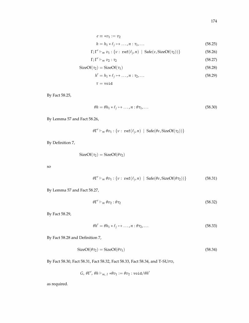
174
e ⌘ ⇤v1 := v2
h = h1 ⇤ `j 7! . . . , n : t1, . . . (58.25)
G; G0 `m v1 : {n : ref(`j, n) | Safe(n, SizeOf(t2))} (58.26)
G; G0 `m v2 : t2 (58.27)
SizeOf(t2) = SizeOf(t1) (58.28)
h0 = h1 ⇤ `j 7! . . . , n : t2, . . . (58.29)
t = void
By Fact 58.25,
qh = qh1 ⇤ `j 7! . . . , n : qt1, . . . (58.30)
By Lemma 57 and Fact 58.26,
qG0 `m qv1 : {n : ref(`j, n) | Safe(qn, SizeOf(t2))}
By Definition 7,
SizeOf(t2) = SizeOf(qt2)
so
qG0 `m qv1 : {n : ref(`j, n) | Safe(qn, SizeOf(qt2))} (58.31)
By Lemma 57 and Fact 58.27,
qG0 `m qv2 : qt2 (58.32)
By Fact 58.29,
qh0 = qh1 ⇤ `j 7! . . . , n : qt2, . . . (58.33)
By Fact 58.28 and Definition 7,
SizeOf(qt2) = SizeOf(qt1) (58.34)
By Fact 58.30, Fact 58.31, Fact 58.32, Fact 58.33, Fact 58.34, and T-SUPD,
G, qG0, qh `m, I ⇤qv1 := qv2 : void/qh0
as required.
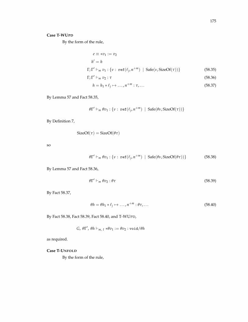
175
Case T-WUPD
By the form of the rule,
e ⌘ ⇤v1 := v2
h0 = h
G; G0 `m v1 : {n : ref(`j, n+m) | Safe(n, SizeOf(t))} (58.35)
G; G0 `m v2 : t (58.36)
h = h1 ⇤ `j 7! . . . , n+m : t, . . . (58.37)
By Lemma 57 and Fact 58.35,
qG0 `m qv1 : {n : ref(`j, n+m) | Safe(qn, SizeOf(t))}
By Definition 7,
SizeOf(t) = SizeOf(qt)
so
qG0 `m qv1 : {n : ref(`j, n+m) | Safe(qn, SizeOf(qt))} (58.38)
By Lemma 57 and Fact 58.36,
qG0 `m qv2 : qt (58.39)
By Fact 58.37,
qh = qh1 ⇤ `j 7! . . . , n+m : qt, . . . (58.40)
By Fact 58.38, Fact 58.39, Fact 58.40, and T-WUPD,
G, qG0, qh `m, I ⇤qv1 := qv2 : void/qh
as required.
Case T-UNFOLD
By the form of the rule,
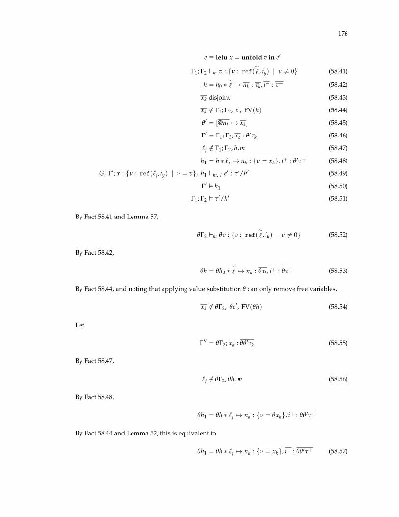
176
e ⌘ letu x = unfold v in e0
G1; G2 `m v : {n : ref(⇠` , iy) | n 6= 0} (58.41)
h = h0 ⇤⇠` 7! nk : tk, i+ : t+ (58.42)
xk disjoint (58.43)
xk /2 G1; G2, e0, FV(h) (58.44)
q0 = [@nk 7! xk] (58.45)
G0 = G1; G2; xk : q0tk (58.46)
`j /2 G1; G2, h, m (58.47)
h1 = h ⇤ `j 7! nk : {n = xk}, i+ : q0t+ (58.48)
G, G0; x : {n : ref(`j, iy) | n = v}, h1 `m, I e0 : t0/h0 (58.49)
G0 ✏ h1 (58.50)
G1; G2 ✏ t0/h0 (58.51)
By Fact 58.41 and Lemma 57,
qG2 `m qv : {n : ref(⇠` , iy) | n 6= 0} (58.52)
By Fact 58.42,
qh = qh0 ⇤⇠` 7! nk : qtk, i+ : qt+ (58.53)
By Fact 58.44, and noting that applying value substitution q can only remove free variables,
xk /2 qG2, qe0, FV(qh) (58.54)
Let
G00 = qG2; xk : qq0tk (58.55)
By Fact 58.47,
`j /2 qG2, qh, m (58.56)
By Fact 58.48,
qh1 = qh ⇤ `j 7! nk : {n = qxk}, i+ : qq0t+
By Fact 58.44 and Lemma 52, this is equivalent to
qh1 = qh ⇤ `j 7! nk : {n = xk}, i+ : qq0t+ (58.57)
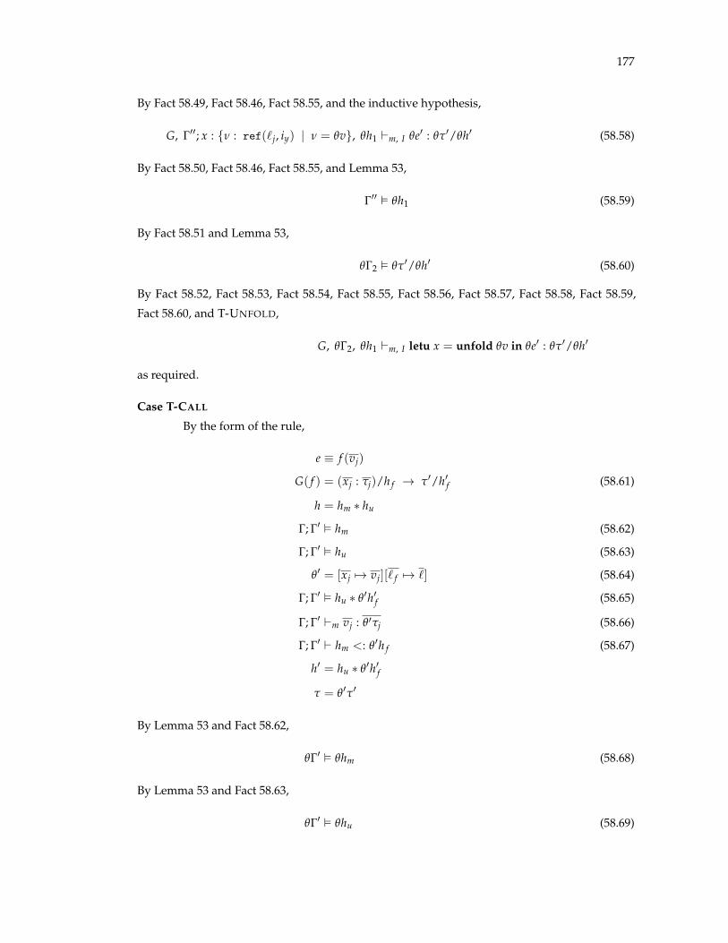
177
By Fact 58.49, Fact 58.46, Fact 58.55, and the inductive hypothesis,
G, G00; x : {n : ref(`j, iy) | n = qv}, qh1 `m, I qe0 : qt0/qh0 (58.58)
By Fact 58.50, Fact 58.46, Fact 58.55, and Lemma 53,
G00 ✏ qh1 (58.59)
By Fact 58.51 and Lemma 53,
qG2 ✏ qt0/qh0 (58.60)
By Fact 58.52, Fact 58.53, Fact 58.54, Fact 58.55, Fact 58.56, Fact 58.57, Fact 58.58, Fact 58.59,
Fact 58.60, and T-UNFOLD,
G, qG2, qh1 `m, I letu x = unfold qv in qe0 : qt0/qh0
as required.
Case T-CALL
By the form of the rule,
e ⌘ f (vj)
G( f ) = (xj : tj)/h f ! t0/h0f (58.61)
h = hm ⇤ hu
G; G0 ✏ hm (58.62)
G; G0 ✏ hu (58.63)
q0 = [xj 7! vj][` f 7! `] (58.64)
G; G0 ✏ hu ⇤ q0h0f (58.65)
G; G0 `m vj : q0tj (58.66)
G; G0 ` hm <: q0h f (58.67)
h0 = hu ⇤ q0h0f
t = q0t0
By Lemma 53 and Fact 58.62,
qG0 ✏ qhm (58.68)
By Lemma 53 and Fact 58.63,
qG0 ✏ qhu (58.69)

178
Using Fact 58.64, define
q2 = [xj 7! qvj][` f 7! `]
= q[q0] (58.70)
By the assumption that ✏ G and Definition 25,
✏ (xj : tj)/h f ! t0/h0f (58.71)
By the form of WF-FUNSCHEME and Fact 58.71,
G f = xj : tj (58.72)
G f ✏ tj
G f ✏ h f
G f ✏ t0/h0f
By the preceding, Fact 58.72, and Lemma 28,
FV(tj) ✓ {xj} (58.73)
FV(h f ) ✓ {xj} (58.74)
FV(t0) ✓ {xj} (58.75)
FV(h0f ) ✓ {xj} (58.76)
By Lemma 53 and Fact 58.65,
qG0 ✏ qhu ⇤ q(q0h0f ) (58.77)
By Fact 58.74, Fact 58.77, and Lemma 51,
qG0 ✏ qhu ⇤ q2h0f (58.78)
By Lemma 57 and Fact 58.66,
qG0 `m qvj : q(q0tj) (58.79)
By Fact 58.73, Fact 58.79, and Lemma 51,
qG0 `m qvj : q2tj (58.80)
By Lemma 55 and Fact 58.67,
qG0 ` qhm <: q(q0h f ) (58.81)

179
By Fact 58.74, Fact 58.81, and Lemma 51,
qG0 ` qhm <: q2h f (58.82)
By Fact 58.68, Fact 58.69, Fact 58.61, Fact 58.70, Fact 58.78, Fact 58.80, Fact 58.82, and T-CALL,
G, qG0, qh `m, I f (qvj) : q2t0/qhu ⇤ q2h0f
By Fact 58.70, Fact 58.75, Fact 58.76, and Lemma 51, this is equivalent to
G, qG0, qh `m, I f (qvj) : q(q0t0)/qhu ⇤ q(q0h0f )
as required.
Case T-MALLOC
By the form of the rule
e ⌘ malloc(v)
`j /2 G; G0, h, m (58.83)
h = h0 ⇤⇠` 7! b (58.84)
h0 = h ⇤ `j 7! b0 (58.85)
G; G0 ✏ h ⇤ `j 7! b (58.86)
G; G0 `m v : {n : int(W, i) | n � 0} (58.87)
t = {n : ref(`j, 0) | Allocated(n, v)} (58.88)
By Fact 58.83,
`j /2 qG0, qh, m (58.89)
By Fact 58.84,
qh = qh0 ⇤⇠` 7! qb (58.90)
By Fact 58.85,
qh0 = qh ⇤ `j 7! (qb)0
As b0 contains no free variables, we have
qh0 = qh ⇤ `j 7! qb0 (58.91)

180
By Fact 58.86 and Lemma 53,
qG0 ✏ qh ⇤ `j 7! qb (58.92)
By Fact 58.87 and Lemma 57,
qG0 `m qv : {n : int(W, i) | qn � 0} (58.93)
By Fact 58.88,
qt = {n : ref(`j, 0) | Allocated(n, qv)} (58.94)
By Fact 58.89, Fact 58.90, Fact 58.91, Fact 58.92, Fact 58.93, Fact 58.94, and T-MALLOC,
G, qG0, qh `m, I malloc(v) : qt/qh0
as required.
C.14 Location Name Sets
Definition 31 (Location Name Sets). The set of location names bound in a heap h, Locs(h), is defined
as
{` |⇠`2 dom(h)} [ {` | `j 2 dom(h)}.
Lemma 59 (Same Location Names in Related Heaps). If G ` h1 <: h2, then Locs(h1) = Locs(h2).
Proof. Straightforward induction on the derivation of G ` h1 <: h2, using Definition 31.
Lemma 60 (Same Location Names In Input and Output Heaps).
If G, G, h `m, I e : t/h0
and ✏ G (60.1)
then Locs(h) = Locs(h0).
Proof. The proof proceeds by induction on the derivation of G, G, h `m, I e : t/h0, splitting cases
on the final rule used. The only interesting case is T-CALL.
Case T-CALL
By the form of the rule,

181
h = hu ⇤ hm
G ` hm <: qh f (60.2)
G( f ) = (xj : tj)/h f ! t0/h0f (60.3)
h0 = hu ⇤ qh0f (60.4)
By Fact 60.2 and Lemma 59,
Locs(hm) = Locs(qh f ) (60.5)
By Fact 60.3, Fact 60.1, and Definition 25,
Locs(h f ) = Locs(h0f ) (60.6)
By Fact 60.5 and Fact 60.6,
Locs(qh0f ) = Locs(hm)
from which it follows by Definition 31 that
Locs(hu ⇤ hm) = Locs(hu ⇤ qh0f )
as required.
C.15 Location Name Substitution
Definition 32. A location name substitution is a function r : LocName ! LocName, where
LocName is the set of location names (i.e., names ` from which we form abstract location names⇠` and
concrete location names `j).
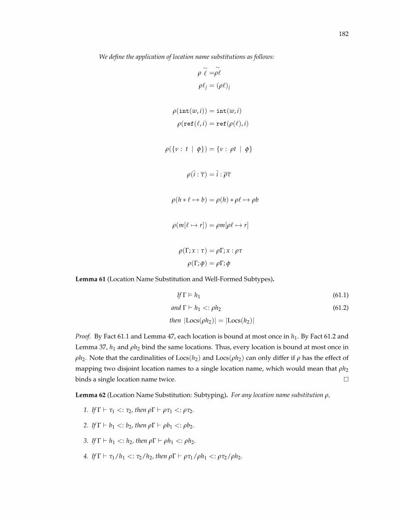
182
We define the application of location name substitutions as follows:
r⇠` =
⇠r`
r`j = (r`)j
r(int(w, i)) = int(w, i)
r(ref(`, i) = ref(r(`), i)
r({n : t | f}) = {n : rt | f}
r(i : t) = i : rt
r(h ⇤ ` 7! b) = r(h) ⇤ r` 7! rb
r(m[` 7! r]) = rm[r` 7! r]
r(G; x : t) = rG; x : rt
r(G; f) = rG; f
Lemma 61 (Location Name Substitution and Well-Formed Subtypes).
If G ✏ h1 (61.1)
and G ` h1 <: rh2 (61.2)
then |Locs(rh2)| = |Locs(h2)|
Proof. By Fact 61.1 and Lemma 47, each location is bound at most once in h1. By Fact 61.2 and
Lemma 37, h1 and rh2 bind the same locations. Thus, every location is bound at most once in
rh2. Note that the cardinalities of Locs(h2) and Locs(rh2) can only differ if r has the effect of
mapping two disjoint location names to a single location name, which would mean that rh2
binds a single location name twice.
Lemma 62 (Location Name Substitution: Subtyping). For any location name substitution r,
1. If G ` t1 <: t2, then rG ` rt1 <: rt2.
2. If G ` b1 <: b2, then rG ` rb1 <: rb2.
3. If G ` h1 <: h2, then rG ` rh1 <: rh2.
4. If G ` t1/h1 <: t2/h2, then rG ` rt1/rh1 <: rt2/rh2.
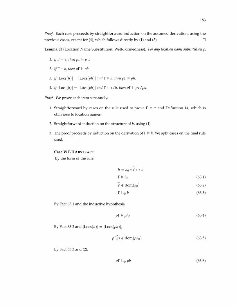
183
Proof. Each case proceeds by straightforward induction on the assumed derivation, using the
previous cases, except for (4), which follows directly by (1) and (3).
Lemma 63 (Location Name Substitution: Well-Formedness). For any location name substitution r,
1. If G ✏ t, then rG ✏ rt.
2. If G ✏ b, then rG ✏ rb.
3. If |Locs(h)| = |Locs(rh)| and G ✏ h, then rG ✏ rh.
4. If |Locs(h)| = |Locs(rh)| and G ✏ t/h, then rG ✏ rt/rh.
Proof. We prove each item separately.
1. Straightforward by cases on the rule used to prove G ✏ t and Definition 14, which is
oblivious to location names.
2. Straightforward induction on the structure of b, using (1).
3. The proof proceeds by induction on the derivation of G ✏ h. We split cases on the final rule
used.
Case WF-HABSTRACT
By the form of the rule,
h = h0 ⇤⇠` 7! b
G ✏ h0 (63.1)⇠` /2 dom(h0) (63.2)
G ✏@ b (63.3)
By Fact 63.1 and the inductive hypothesis,
rG ✏ rh0 (63.4)
By Fact 63.2 and |Locs(h)| = |Locs(rh)|,
r(⇠`) /2 dom(rh0) (63.5)
By Fact 63.3 and (2),
rG ✏@ rb (63.6)

184
By Fact 63.4, Fact 63.5, Fact 63.6, and WF-HABSTRACT,
rG ✏ h0 ⇤ r⇠` 7! rb
as required.
Case WF-HCONCRETE
By the form of the rule,
h = h0 ⇤ `j 7! b
G ✏ h0 (63.7)
G ✏ b (63.8)⇠` 2 dom(h0) (63.9)
`k /2 dom(h0) (63.10)
By Fact 63.7 and the inductive hypothesis,
rG ✏ rh0 (63.11)
By Fact 63.8 and (2),
rG ✏ rb (63.12)
By Fact 63.9,
r(⇠`) 2 dom(rh0) (63.13)
By Fact 63.10 and |Locs(h)| = |Locs(rh)|,
r(`k) /2 dom(rh0) (63.14)
By Fact 63.11, Fact 63.12, Fact 63.13, Fact 63.14, and WF-HCONCRETE,
rG ✏ rh0 ⇤ r(`j) 7! rb
4. Follows immediately from (1) and (3).
Lemma 64 (Location Name Substitution: Pure Typing).
If G `m a : t
then rG `rm a : rt.

185
Proof. The proof proceeds by induction on the derivation of G `m a : t. We split cases on the
final rule used.
Case T-VAR
By the form of the rule,
a ⌘ x
G(x) = {n : t | f}
t = {n : t | n = x}
By Definition 32,
(rG)(x) = {n : rt | f}
By T-VAR,
rG `rm x : {n : rt | n = x}
as required.
Case T-INT
Immediate.
Case T-REF
By the form of the rule,
a ⌘ bref(r, n, z)
` 2 Clocs(r, m) (64.1)
t = {n : ref(`, n) | n = bref(r, n, z)}
By Definition 18, Definition 32, and Fact 64.1,
r` 2 Clocs(r, rm) (64.2)
By Fact 64.2 and T-REF,
r(G) `rm bref(r, n, z) : {n : ref(r`, n) | n = bref(r, n, z)}
as required.
Case T-ARITH, T-PTRARITH, T-RELATION
Immediate from the form of the rule, the inductive hypothesis, and another application
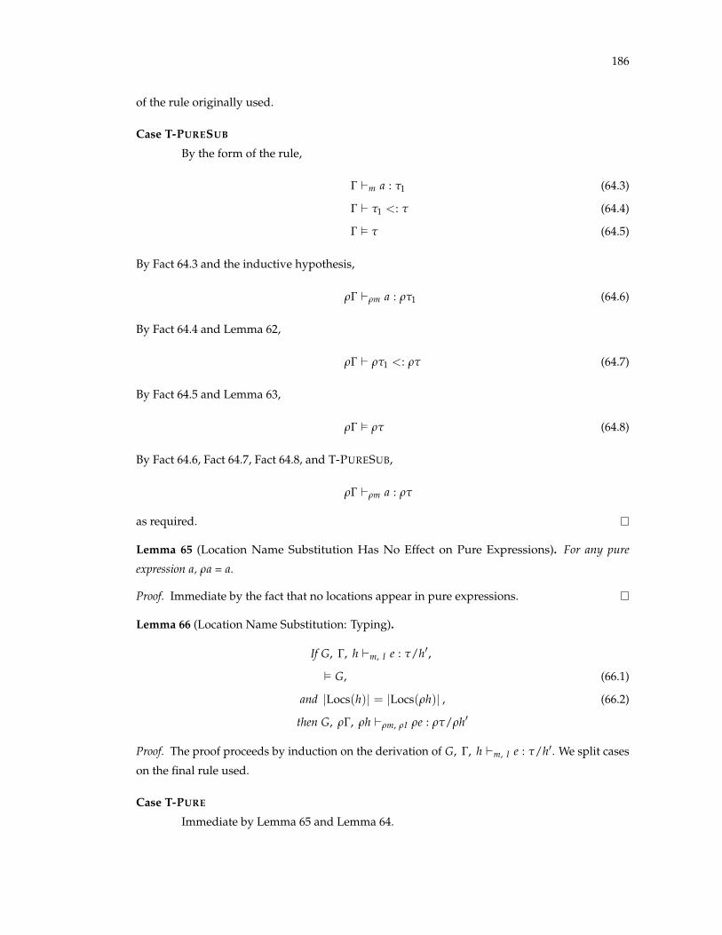
186
of the rule originally used.
Case T-PURESUB
By the form of the rule,
G `m a : t1 (64.3)
G ` t1 <: t (64.4)
G ✏ t (64.5)
By Fact 64.3 and the inductive hypothesis,
rG `rm a : rt1 (64.6)
By Fact 64.4 and Lemma 62,
rG ` rt1 <: rt (64.7)
By Fact 64.5 and Lemma 63,
rG ✏ rt (64.8)
By Fact 64.6, Fact 64.7, Fact 64.8, and T-PURESUB,
rG `rm a : rt
as required.
Lemma 65 (Location Name Substitution Has No Effect on Pure Expressions). For any pure
expression a, ra = a.
Proof. Immediate by the fact that no locations appear in pure expressions.
Lemma 66 (Location Name Substitution: Typing).
If G, G, h `m, I e : t/h0,
✏ G, (66.1)
and |Locs(h)| = |Locs(rh)| , (66.2)
then G, rG, rh `rm, rI re : rt/rh0
Proof. The proof proceeds by induction on the derivation of G, G, h `m, I e : t/h0. We split cases
on the final rule used.
Case T-PURE
Immediate by Lemma 65 and Lemma 64.
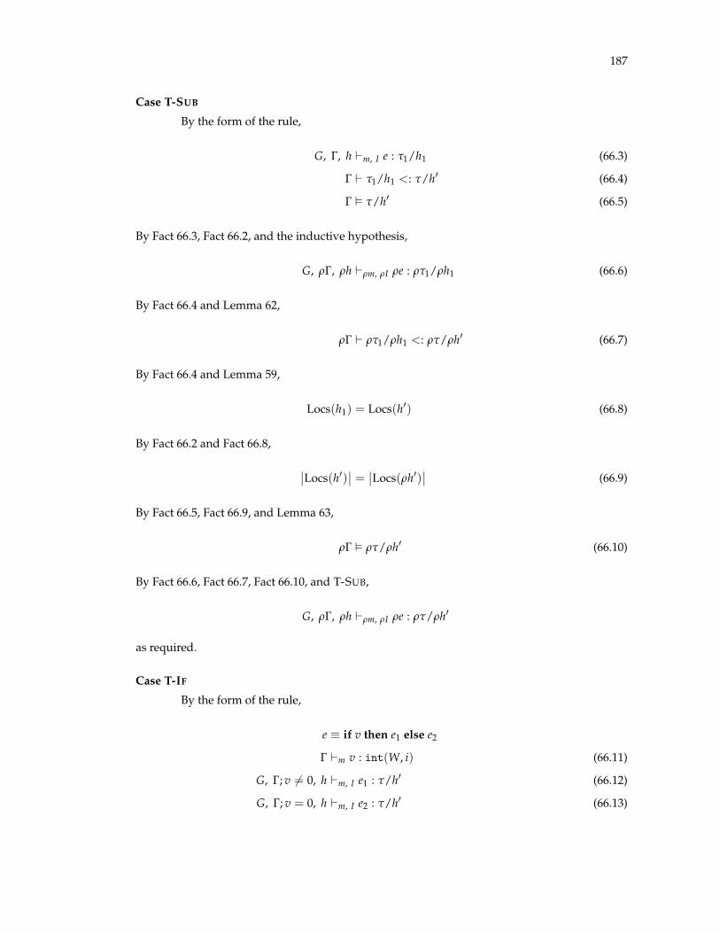
187
Case T-SUB
By the form of the rule,
G, G, h `m, I e : t1/h1 (66.3)
G ` t1/h1 <: t/h0 (66.4)
G ✏ t/h0 (66.5)
By Fact 66.3, Fact 66.2, and the inductive hypothesis,
G, rG, rh `rm, rI re : rt1/rh1 (66.6)
By Fact 66.4 and Lemma 62,
rG ` rt1/rh1 <: rt/rh0 (66.7)
By Fact 66.4 and Lemma 59,
Locs(h1) = Locs(h0) (66.8)
By Fact 66.2 and Fact 66.8,
��Locs(h0)�� =
��Locs(rh0)�� (66.9)
By Fact 66.5, Fact 66.9, and Lemma 63,
rG ✏ rt/rh0 (66.10)
By Fact 66.6, Fact 66.7, Fact 66.10, and T-SUB,
G, rG, rh `rm, rI re : rt/rh0
as required.
Case T-IF
By the form of the rule,
e ⌘ if v then e1 else e2
G `m v : int(W, i) (66.11)
G, G; v 6= 0, h `m, I e1 : t/h0 (66.12)
G, G; v = 0, h `m, I e2 : t/h0 (66.13)
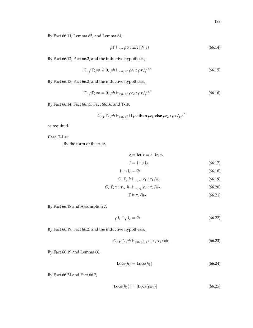
188
By Fact 66.11, Lemma 65, and Lemma 64,
rG `rm rv : int(W, i) (66.14)
By Fact 66.12, Fact 66.2, and the inductive hypothesis,
G, rG; rv 6= 0, rh `rm, rI re1 : rt/rh0 (66.15)
By Fact 66.13, Fact 66.2, and the inductive hypothesis,
G, rG; rv = 0, rh `rm, rI re2 : rt/rh0 (66.16)
By Fact 66.14, Fact 66.15, Fact 66.16, and T-IF,
G, rG, rh `rm, rI if rv then re1 else re2 : rt/rh0
as required.
Case T-LET
By the form of the rule,
e ⌘ let x = e1 in e2
I = I1 [ I2 (66.17)
I1 \ I2 = ∆ (66.18)
G, G, h `m, I1 e1 : t1/h1 (66.19)
G, G; x : t1, h1 `m, I2 e2 : t2/h2 (66.20)
G ✏ t2/h2 (66.21)
By Fact 66.18 and Assumption 7,
rI1 \ rI2 = ∆ (66.22)
By Fact 66.19, Fact 66.2, and the inductive hypothesis,
G, rG, rh `rm, rI1 re1 : rt1/rh1 (66.23)
By Fact 66.19 and Lemma 60,
Locs(h) = Locs(h1) (66.24)
By Fact 66.24 and Fact 66.2,
|Locs(h1)| = |Locs(rh1)| (66.25)

189
By Fact 66.20, Fact 66.25, and the inductive hypothesis,
G, rG; x : rt1, rh1 `rm, rI2 re2 : rt2/rh2 (66.26)
By Fact 66.19 and Lemma 60,
Locs(h2) = Locs(h1)
By the above and Fact 66.24,
Locs(h2) = Locs(h) (66.27)
By Fact 66.27, and Fact 66.2,
|Locs(h2)| = |Locs(rh2)| (66.28)
By Fact 66.21, Fact 66.28, and Lemma 63,
rG ✏ rt2/rh2 (66.29)
By Fact 66.17, Fact 66.22, Fact 66.23, Fact 66.26, Fact 66.29, and T-LET,
G, rG, rh `rm, rI re : rt2/rh2
as required.
Case T-READ
By the form of the rule,
e ⌘ ⇤nv
G `m v : {n : ref(`j, i) | Safe(n, n)} (66.30)
h = h1 ⇤ `j 7! . . . , i : t, . . . (66.31)
h0 = h
SizeOf(t) = n (66.32)
By Fact 66.30, Lemma 65, and Lemma 64,
rG `rm rv : {n : ref(r(`j), i) | Safe(n, n)} (66.33)
By Fact 66.31 and Definition 32,
rh = rh1 ⇤ r(`j) 7! . . . , i : rt, . . . (66.34)

190
By Fact 66.32 and Definition 7,
SizeOf(rt) = n (66.35)
By Fact 66.33, Fact 66.34, Fact 66.35, and T-READ,
G, rG, rh `rm, rI ⇤nrv : rt/rh0
as required.
Case T-SUPD
By the form of the rule,
e ⌘ ⇤v1 := v2
h = h1 ⇤ `j 7! . . . , n : t1, . . . (66.36)
G `m v1 : {n : ref(`j, n) | Safe(n, SizeOf(t2))} (66.37)
G `m v2 : t2 (66.38)
SizeOf(t2) = SizeOf(t1) (66.39)
h0 = h1 ⇤ `j 7! . . . , n : t2, . . . (66.40)
By Fact 66.36 and Definition 32,
rh = rh1 ⇤ r(`j) 7! . . . , n : rt1, . . . (66.41)
By Fact 66.37, Lemma 65, and Lemma 64,
rG `rm rv1 : {n : ref(r(`j), n) | Safe(n, SizeOf(t2))}
By Definition 7,
SizeOf(t2) = SizeOf(rt2)
so
rG `rm rv1 : {n : ref(r(`j), n) | Safe(n, SizeOf(rt2))}
(66.42)
By Fact 66.38, Lemma 65, and Lemma 64,
rG `rm rv2 : rt2 (66.43)

191
By Fact 66.40 and Definition 32,
rh0 = rh1 ⇤ r(`j) 7! . . . , n : rt2, . . . (66.44)
By Fact 66.39 and Definition 7,
SizeOf(rt2) = SizeOf(rt1) (66.45)
By Fact 66.41, Fact 66.42, Fact 66.43, Fact 66.44, and T-SUPD,
G, rG, rh `rm, rI ⇤rv1 := rv2 : void/rh0
as required.
Case T-WUPD
By the form of the rule,
e ⌘ ⇤v1 := v2
G `m v1 : {n : ref(`j, n+m) | Safe(n, SizeOf(t))} (66.46)
G `m v2 : t (66.47)
h = h1 ⇤ `j 7! . . . , n+m : t, . . . (66.48)
h0 = h
By Fact 66.46, Lemma 65, and Lemma 64,
rG `rm rv1 : {n : ref(r(`j), n+m) | Safe(n, SizeOf(t))}
By Definition 7,
SizeOf(t) = SizeOf(rt)
so
rG `rm rv1 : {n : ref(r(`j), n+m) | Safe(n, SizeOf(rt))} (66.49)
By Fact 66.47, Lemma 65, and Lemma 64,
rG `rm rv2 : rt (66.50)
By Fact 66.48 and Definition 32,
rh = rh1 ⇤ r(`j) 7! . . . , n+m : rt, . . . (66.51)

192
By Fact 66.49, Fact 66.50, Fact 66.51, T-WUPD,
G, rG, rh `rm, rI ⇤rv1 := rv2 : void/rh
as required.
Case T-UNFOLD
By the form of the rule,
e ⌘ letu x = unfold v in e0
I = I1 [ {`j} (66.52)
h0 = h2
G `m v : {n : ref(⇠` , iy) | n 6= 0} (66.53)
h = h0 ⇤⇠` 7! nk : tk, i+ : t+ (66.54)
xk disjoint (66.55)
xk /2 G, e, FV(h) (66.56)
q = [@nk 7! xk] (66.57)
G1 = G; xk : qtk (66.58)
`j /2 G, h, m (66.59)
h1 = h ⇤ `j 7! nk : {n = xk}, i+ : qt+ (66.60)
G, G1; x : {n : ref(`j, iy) | n = v}, h1 `m, I e : t2/h2 (66.61)
G1 ✏ h1 (66.62)
G ✏ t2/h2 (66.63)
By Fact 66.52 and Assumption 7,
rI = rI1 [ {r(`j)} (66.64)
By Fact 66.53, Lemma 65, and Lemma 64,
rG `rm rv : {n : ref(r⇠` , iy) | n 6= 0} (66.65)
By Fact 66.54 and Definition 32,
rh = rh0 ⇤ r⇠` 7! nk : rtk, i+ : rt+ (66.66)
By Fact 66.56, Fact 66.66, and Definition 32,
xk /2 rG, re, FV(rh) (66.67)

193
By Fact 66.58 and Definition 32,
rG1 = rG; xk : rqtk (66.68)
By Fact 66.59 and Definition 32,
r(`j) /2 rG, rh, rm (66.69)
By Fact 66.60 and Definition 32,
rh1 = rh ⇤ r(`j) 7! nk : r({n = xk}), i+ : rqt+
(66.70)
By Fact 66.2, Fact 66.70, and Definition 31,
|Locs(h1)| = |Locs(rh1)| (66.71)
By Fact 66.71, Fact 66.61, and the inductive hypothesis,
G, rG1; x : {n : ref(r(`j), iy) | n = v}, rh1 `rm, rI1 re0 : rt2/rh2 (66.72)
By Fact 66.62, Fact 66.71, and Lemma 63,
rG1 ✏ rh1 (66.73)
By Fact 66.1, Fact 66.72, and Lemma 60,
Locs(h1) = Locs(h2)
so
|Locs(h2)| = |Locs(rh2)| (66.74)
By Fact 66.74, Fact 66.63, and Lemma 63,
rG ✏ rt2/rh2 (66.75)
By Fact 66.64, Fact 66.65, Fact 66.66, Fact 66.55, Fact 66.67, Fact 66.57, Fact 66.68, Fact 66.69,
Fact 66.70, Fact 66.72, Fact 66.73, Fact 66.75, and T-UNFOLD,
G, rG, rh `rm, rI letu x = unfold rv in re0 : rt2/rh2
as required.

194
Case T-FOLD
By the form of the rule,
e ⌘ fold `
h = h0 ⇤⇠` 7! b1 ⇤ `j 7! b2 (66.76)
h0 = h0 ⇤⇠` 7! b1 (66.77)
G ` b2 <: b1 (66.78)
By Fact 66.76 and Definition 32,
rh = rh0 ⇤ r⇠` 7! rb1 ⇤ r(`j) 7! rb2 (66.79)
By Fact 66.78 and Lemma 62,
rG ` rb2 <: rb1 (66.80)
By Fact 66.77 and Definition 32,
rh = rh0 ⇤ r⇠` 7! rb1 (66.81)
By Fact 66.79, Fact 66.80, Fact 66.81, and T-FOLD,
G, rG, rh `rm, rI fold r` : void/rh0
as required.
Case T-CALL
By the form of the rule,
e ⌘ f (vj)[` f 7! `]
h = hu ⇤ hm
h0 = hu ⇤ qh0f
t = t0
G ✏ hm (66.82)
G ✏ hu (66.83)
G( f ) = (xj : tj)/h f ! t0/h0f (66.84)
q = [xj 7! vj][` f 7! `] (66.85)
G ✏ hu ⇤ qh0f (66.86)
G `m vj : qtj (66.87)
G ` hm <: qh f (66.88)

195
By Fact 66.82, Fact 66.2, and Lemma 63,
rG ✏ rhm (66.89)
By Fact 66.83, Fact 66.2, and Lemma 63,
rG ✏ rhu (66.90)
By Fact 66.88 and Lemma 59,
Locs(hm) = Locs(qh f ) (66.91)
By Fact 66.84, Definition 25, and Fact 66.1,
Locs(h0f ) = Locs(h f ) (66.92)
By Fact 66.91 and Fact 66.92,
Locs(qh0f ) = Locs(hm) (66.93)
By Fact 66.93 and Fact 66.2,
���Locs(hu ⇤ qh0f )��� =
���Locs(rhu ⇤ rqh0f )��� (66.94)
By Fact 66.86, Fact 66.94, and Lemma 63,
rG ✏ rhu ⇤ rqh0f (66.95)
By Fact 66.87, Lemma 65, and Lemma 64,
rG `rm rvj : rqtj (66.96)
By Fact 66.88 and Lemma 64,
rG ` rhm <: rqh f (66.97)
By Fact 66.89, Fact 66.90, Fact 66.84, Fact 66.95, Fact 66.96, Fact 66.97, and T-CALL,
G, rG, rh `rm, rI f (rvj) : rt0/rh0
as required.
Case T-MALLOC
By the form of the rule,
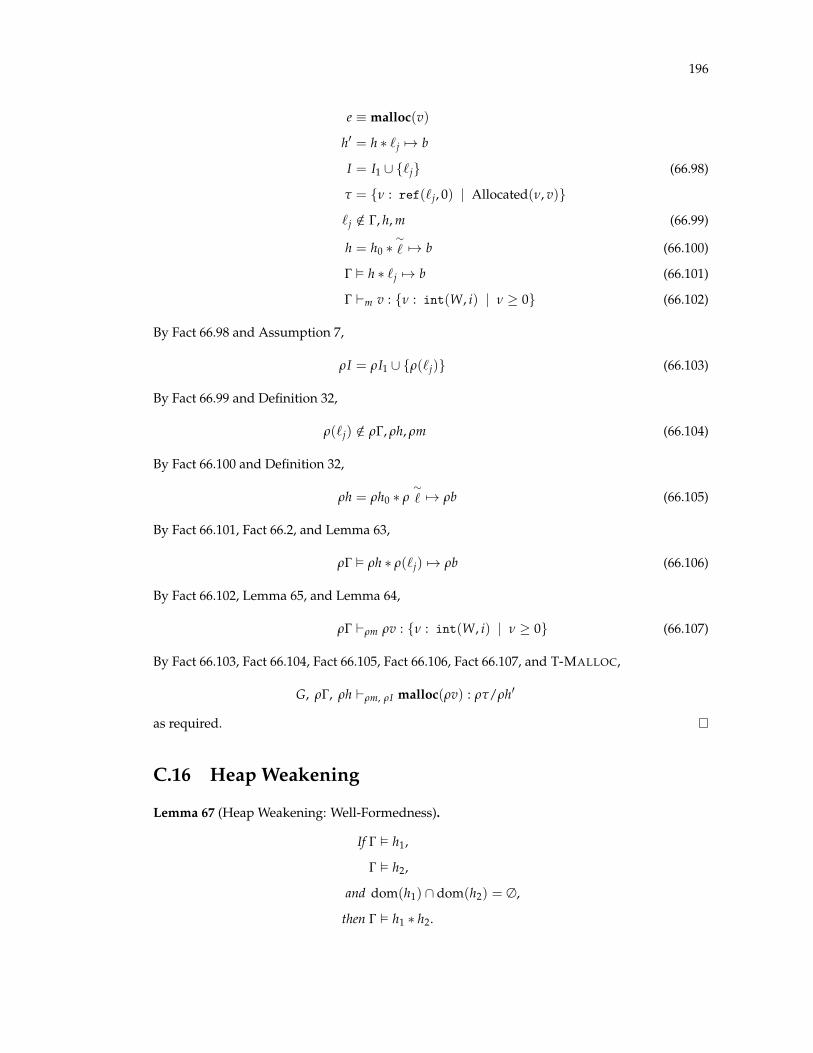
196
e ⌘ malloc(v)
h0 = h ⇤ `j 7! b
I = I1 [ {`j} (66.98)
t = {n : ref(`j, 0) | Allocated(n, v)}
`j /2 G, h, m (66.99)
h = h0 ⇤⇠` 7! b (66.100)
G ✏ h ⇤ `j 7! b (66.101)
G `m v : {n : int(W, i) | n � 0} (66.102)
By Fact 66.98 and Assumption 7,
rI = rI1 [ {r(`j)} (66.103)
By Fact 66.99 and Definition 32,
r(`j) /2 rG, rh, rm (66.104)
By Fact 66.100 and Definition 32,
rh = rh0 ⇤ r⇠` 7! rb (66.105)
By Fact 66.101, Fact 66.2, and Lemma 63,
rG ✏ rh ⇤ r(`j) 7! rb (66.106)
By Fact 66.102, Lemma 65, and Lemma 64,
rG `rm rv : {n : int(W, i) | n � 0} (66.107)
By Fact 66.103, Fact 66.104, Fact 66.105, Fact 66.106, Fact 66.107, and T-MALLOC,
G, rG, rh `rm, rI malloc(rv) : rt/rh0
as required.
C.16 Heap Weakening
Lemma 67 (Heap Weakening: Well-Formedness).
If G ✏ h1,
G ✏ h2,
and dom(h1) \ dom(h2) = ∆,
then G ✏ h1 ⇤ h2.

197
Proof. The proof proceeds by straightforward induction on the derivation of G ✏ h2.
Lemma 68 (Heap Weakening: Subtyping).
If G ` h1 <: h2
then G ` h ⇤ h1 <: h ⇤ h2.
Proof. The proof proceeds by straightforward induction on the derivation of G ` h1 <: h2, using
Lemma 36.
Lemma 69 (Heap Weakening: Typing).
If G, G, h `m, I e : t/h0,
G ✏ h,
G ✏ h2,
dom(h1) \ dom(heap2) = ∆,
and Clocs(h2) \ I = ∆,
then G, G, h2 ⇤ h `m, I e : t/h2 ⇤ h0.
Proof. The proof proceeds by straightforward induction on the derivation of G, G, h `m, I e : t/h0,
using Lemma 67 and Lemma 68.
C.17 Canonical Forms
Lemma 70 (Subtyping Preserves Sizes). If G ` t1 <: t2, then SizeOf(t1) = SizeOf(t2).
Proof. The proof proceeds by straightforward induction on the derivation of G ` t1 <: t2.
Lemma 71 (Value Sizes). If ∆ `m v : t, then SizeOf(v) = SizeOf(t).
Proof. The proof proceeds by straightforward induction on the derivation of ∆ `m v : t, using
Lemma 70.
Lemma 72 (Canonical Forms). For any value v:
1. If ∆ `m v : int(w, i), then v = n|w| for some n 2 [[i]].
2. If ∆ `m v : ref(`, i), then either v = 0|W| or v = bref(r, n, z) for some n 2 [[i]] and there exists
`j v ` such that `j 2 Clocs(r, m).
Proof. The proofs proceed by induction on the given typing derivation, splitting cases on the
final rule used.

198
1. The proof proceeds by induction on the derivation of ∆ `m v : int(w, i). We split cases on
the final rule used.
Case T-INT
Immediate.
Case T-VAR, T-REF, T-ARITH, T-PTRARITH, T-RELATION
Impossible.
Case T-PURESUB
By the form of the rule,
∆ `m v : t (72.1)
∆ ` t <: int(w, i) (72.2)
By Fact 72.2 and Lemma 34,
t = int(w, i1) (72.3)
By the Fact 72.1, Fact 72.3, and the inductive hypothesis,
v = n|w|
n 2 [[i1]]
for some n. By Fact 72.2 and Lemma 34,
i1⇠✓ i
By Proposition 1,
n⇠✓ i
By Proposition 2,
n 2 [[i]]
as required.
2. The proof proceeds by induction on the derivation of ∆ `m v : ref(`, i). We split cases on
the final rule used.
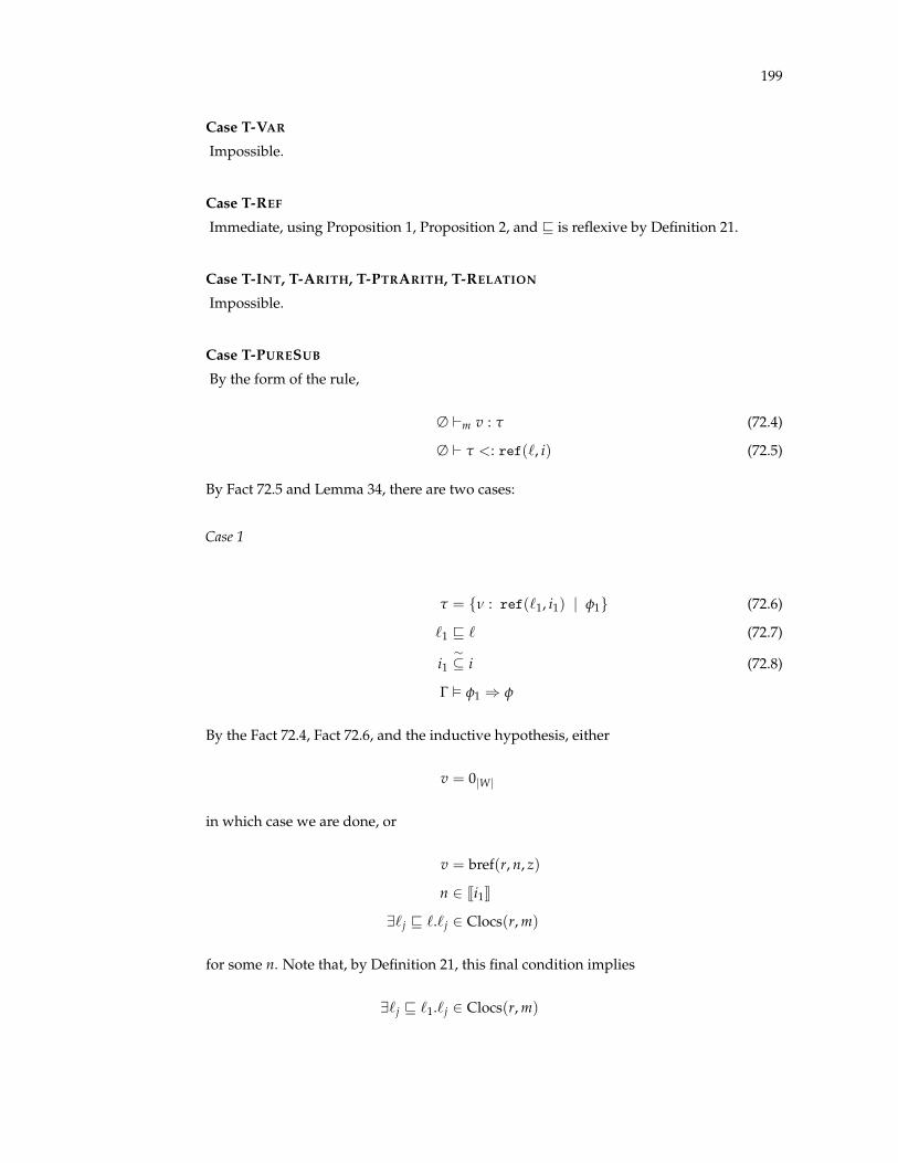
199
Case T-VAR
Impossible.
Case T-REF
Immediate, using Proposition 1, Proposition 2, and v is reflexive by Definition 21.
Case T-INT, T-ARITH, T-PTRARITH, T-RELATION
Impossible.
Case T-PURESUB
By the form of the rule,
∆ `m v : t (72.4)
∆ ` t <: ref(`, i) (72.5)
By Fact 72.5 and Lemma 34, there are two cases:
Case 1
t = {n : ref(`1, i1) | f1} (72.6)
`1 v ` (72.7)
i1⇠✓ i (72.8)
G ✏ f1 ) f
By the Fact 72.4, Fact 72.6, and the inductive hypothesis, either
v = 0|W|
in which case we are done, or
v = bref(r, n, z)
n 2 [[i1]]
9`j v `.`j 2 Clocs(r, m)
for some n. Note that, by Definition 21, this final condition implies
9`j v `1.`j 2 Clocs(r, m)

200
By Fact 72.8 and Proposition 1,
n⇠✓ i
By Proposition 2,
n 2 [[i]]
as required.
Case 2
t = {n : int(W, 0) | f1} (72.9)
By Fact 72.4, (1), and Fact 72.9,
v = 0|W|
as required.
C.18 Unfolding, Folding, Heap Modeling, Well-Formedness
This section presents the key lemmas that relate the location unfold and fold operations
to our concepts of heap modeling and well-formedness.
Lemma 73 (Modeling of Freshly-Allocated Locations). For any block b such that ∆ ✏ b,
Z 7! 0|1| ✏m b0.
Proof. We assume that the run-time block Z 7! 0|1| can be treated as the run-time block containing
the bindings
{n 7! 0|SizeOf(t)| | n 2 [[i]], i : t 2 b0} [ {n 7! 0|1| | n /2 dom(b0)}.
This assumption is justified by the facts that the run-time blocks have the same physical repre-
sentation in memory and that all bindings in the block are disjoint.
The remainder of the proof proceeds by straightforward induction on the structure of b,
using BM-SINGLE, BM-SEQUENCE, and the definition of b0.

201
Lemma 74 (Fresh Concrete Location Preserves Heap Modeling).
If s ✏m h, (74.1)
c ✏m b, (74.2)
`j /2 dom(m) (74.3)
m0 = m[`j 7! r], (74.4)
h0 = h ⇤ `j 7! b (74.5)
s0 = s[r 7! c] (74.6)
then s0 ✏m0 h0.
Proof. By Fact 74.1 and Definition 23,
8`0k 2 dom(h). `0k 2 dom(m) (74.7)
rng(m) ✓ dom(s) (74.8)
And, for all r0 7! c0 2 s, either
exists `0k 2 Clocs(r0, m),
h = h0 ⇤ `0k 7! b0,
c0 ✏m b0,
or
Clocs(r0, m) \ dom(h) = ∆,
h = h0 ⇤⇠`07! b0,
c0 ✏m b0
By Fact 74.3 and Fact 74.4,
m ✓ m0 (74.9)
By Fact 74.4, Fact 74.5, Fact 74.7, and Fact 74.9,
8`0k 2 dom(h0). `0k 2 dom(m0) (74.10)
By Fact 74.4, Fact 74.8, and Fact 74.6,
rng(m0) ✓ dom(s0) (74.11)
By Fact 74.10 and Fact 74.11, we have satisifed the first two conditions of Definition 23. To show
the final condition, we choose an arbitrary r0 7! c0 2 s0 and split cases on whether r0 = r.

202
Case r0 6= r
We again split cases, this time on how the location was modeled according to Fact 74.1
and Definition 23.
Case exists `0k 2 Clocs(r0, m), h = h0 ⇤ `0k 7! b0, c0 ✏m b0
Then by Fact 74.9 and Definition 19,
`0k 2 Clocs(r0, m0)
By Fact 74.5,
h0 = h00 ⇤ `0k 7! b0
And, by Fact 74.9 and Lemma 24,
c0 ✏m0 b0
Thus, part (3a) of Definition 23 remains satisfied.
Case exists `0k 2 Clocs(r0, m), Clocs(r0, m) \ dom(h) = ∆, h = h0 ⇤⇠`07! b0, c0 ✏m b0
Then by Fact 74.9 and Definition 19,
`0k 2 Clocs(r0, m0)
Note that
Clocs(r0, m) \ dom(h) = ∆
implies, by, r0 6= r, Fact 74.4, Fact 74.3, Definition 19, that
Clocs(r0, m0) \ dom(h0) = ∆
By Fact 74.5,
h0 = h00 ⇤⇠`07! b0
Finally, by Fact 74.9 and Lemma 24,
c0 ✏m0 b0
Thus, part (3b) of Definition 23 remains satisfied.
Case r0 = r
Then

203
c0 = c
By Fact 74.4 and Definition 19,
`j 2 Clocs(r, m0)
By Fact 74.5,
h0 = h ⇤ `j 7! b
By Fact 74.2 and Lemma 24,
c ✏m0 b
Thus, part (3a) of Definition 23 is satisfied.
Lemma 75 (Unfolding Preserves Block Modeling).
If c ✏m nk : {n : tk | fk}, i+j : tj
then c ✏m nk : {n : tk | n = c(nk)}, i+j : qtj
where q = [@nk 7! c(nk)]
Proof. The proof proceeds by induction on the derivation of c ✏m nk : {n : tk | fk}, i+j : tj. We
split cases on the final rule used.
Case BM-SEQUENCE
Trivial, as the substitution is empty.
Case BM-SINGLE
By the form of the rule,
nk : {n : tk | fk} = n : {n : tn | fn}, nm : {n : tm | fm}
∆ `m c(n) : {n : tn | fn} (75.1)
c ✏m nm : {n : tm | fm[@n 7! c(n)]}, i+j : tj[@n 7! c(n)] (75.2)
By the inductive hypothesis and Fact 75.2,
c ✏m nm : {n : tm | n = c(nm)}, i+j : q0(tj[@n 7! c(n)])
where q0 = [nm 7! c(nm)]
Equivalently,
c ✏m nm : {n : tm | n = c(nm)}, i+j : qtj
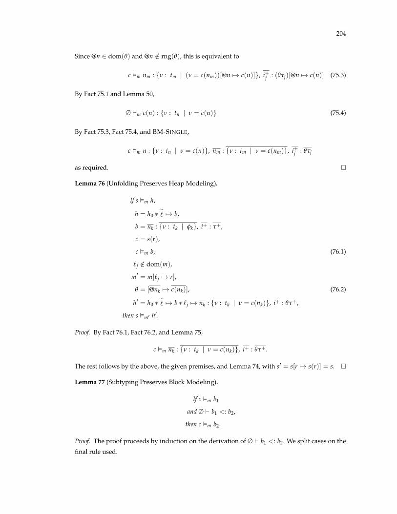
204
Since @n 2 dom(q) and @n /2 rng(q), this is equivalent to
c ✏m nm : {n : tm | (n = c(nm))[@n 7! c(n)]}, i+j : (qtj)[@n 7! c(n)] (75.3)
By Fact 75.1 and Lemma 50,
∆ `m c(n) : {n : tn | n = c(n)} (75.4)
By Fact 75.3, Fact 75.4, and BM-SINGLE,
c ✏m n : {n : tn | n = c(n)}, nm : {n : tm | n = c(nm)}, i+j : qtj
as required.
Lemma 76 (Unfolding Preserves Heap Modeling).
If s ✏m h,
h = h0 ⇤⇠` 7! b,
b = nk : {n : tk | fk}, i+ : t+,
c = s(r),
c ✏m b, (76.1)
`j /2 dom(m),
m0 = m[`j 7! r],
q = [@nk 7! c(nk)], (76.2)
h0 = h0 ⇤⇠` 7! b ⇤ `j 7! nk : {n : tk | n = c(nk)}, i+ : qt+,
then s ✏m0 h0.
Proof. By Fact 76.1, Fact 76.2, and Lemma 75,
c ✏m nk : {n : tk | n = c(nk)}, i+ : qt+.
The rest follows by the above, the given premises, and Lemma 74, with s0 = s[r 7! s(r)] = s.
Lemma 77 (Subtyping Preserves Block Modeling).
If c ✏m b1
and ∆ ` b1 <: b2,
then c ✏m b2.
Proof. The proof proceeds by induction on the derivation of ∆ ` b1 <: b2. We split cases on the
final rule used.
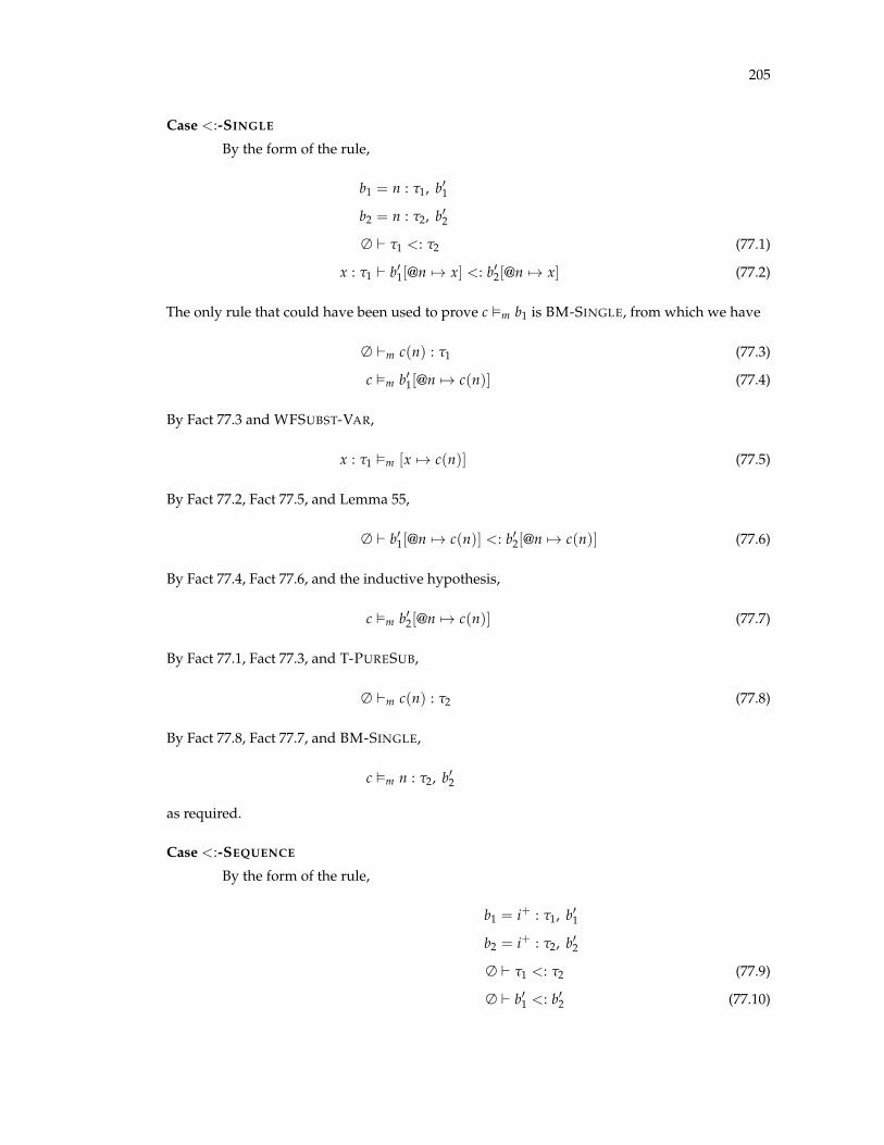
205
Case <:-SINGLE
By the form of the rule,
b1 = n : t1, b01
b2 = n : t2, b02
∆ ` t1 <: t2 (77.1)
x : t1 ` b01[@n 7! x] <: b02[@n 7! x] (77.2)
The only rule that could have been used to prove c ✏m b1 is BM-SINGLE, from which we have
∆ `m c(n) : t1 (77.3)
c ✏m b01[@n 7! c(n)] (77.4)
By Fact 77.3 and WFSUBST-VAR,
x : t1 ✏m [x 7! c(n)] (77.5)
By Fact 77.2, Fact 77.5, and Lemma 55,
∆ ` b01[@n 7! c(n)] <: b02[@n 7! c(n)] (77.6)
By Fact 77.4, Fact 77.6, and the inductive hypothesis,
c ✏m b02[@n 7! c(n)] (77.7)
By Fact 77.1, Fact 77.3, and T-PURESUB,
∆ `m c(n) : t2 (77.8)
By Fact 77.8, Fact 77.7, and BM-SINGLE,
c ✏m n : t2, b02
as required.
Case <:-SEQUENCE
By the form of the rule,
b1 = i+ : t1, b01
b2 = i+ : t2, b02
∆ ` t1 <: t2 (77.9)
∆ ` b01 <: b02 (77.10)

206
The only rule that could have been used to prove c ✏m b1 is BM-SEQUENCE, from which we have
8n 2 dom(c) \ [[i+]]. ∆ `m c(n) : t1 (77.11)
c ✏m b01 (77.12)
By Fact 77.9, Fact 77.11, and T-PURESUB,
8n 2 dom(c) \ [[i+]]. ∆ `m c(n) : t2 (77.13)
By Fact 77.10, Fact 77.12, and the inductive hypothesis,
c ✏m b02 (77.14)
By Fact 77.13, Fact 77.14, and BM-SEQUENCE,
c ✏m i+ : t2, b02
as required.
Lemma 78 (Subtyping Preserves Heap Modeling).
If s ✏m h1
and ∆ ` h1 <: h2
then s ✏m h2.
Proof. The proof follows straightforwardly by induction on the derivation of ∆ ` h1 <: h2, using
s ✏m h1, Definition 23, and Lemma 77.
Lemma 79 (Well-Formed Substitutions from Block Contents).
If c ✏m nk : tk, i+ : t+,
xk disjoint,
and q = [xk 7! c(nk)],
then xk : qtk ✏. q
Proof. The proof proceeds by induction on the derivation of c ✏m nk : tk, i+ : t+, using
WFSUBST-VAR.
Lemma 80 (One Location Name Mapped Per Run-Time Location).
If ∆ `m bref(r, n, z) : {n : ref(⇠` , i) | f}, (80.1)
✏ m, (80.2)
and `0j 2 Clocs(r, m), (80.3)
then `0 = `.

207
Proof. By Fact 80.1 and Lemma 72, there exists
`00k 2 Clocs(r, m) (80.4)
`00k v⇠` (80.5)
By Fact 80.5 and Definition 21,
`00 = ` (80.6)
By Fact 80.3, Fact 80.4, Fact 80.2, and Definition 20,
`00 = `0 (80.7)
By Fact 80.6 and Fact 80.7,
`0 = `
as required.
Lemma 81 (Folding Preserves Heap Modeling).
If s ✏m h1, (81.1)
h1 = h2 ⇤ `j 7! b1,
h2 = h0 ⇤⇠` 7! b2,
∆ ` b1 <: b2, (81.2)
∆ ✏ h1, (81.3)
and ✏ m, (81.4)
then s ✏m h2.
Proof. We note that, by assumption, parts (1) and (2) of Definition 23 are satisfied. It only remains
to show that part (3) is satisfied.
Let r 7! c 2 s. By Fact 81.1 and part (3) of Definition 23, there are two cases:
Case exists `0k 2 Clocs(r, m), h1 = h00 ⇤ `0k 7! b, and c ✏m b
Then there are two cases:
Case `0 6= `
Then h2 = h000 ⇤ `0k 7! b for some h000 . By assumption, `0k 2 Clocs(r, m) and c ✏m b. Thus,
part (3a) of Definition 23 is satisfied.
Case `0 = `
The only rule which could have been used to prove Fact 81.3 is WF-HCONCRETE. By

208
the form of the rule,
`q /2 dom(h2) (81.5)
for any q, so we have `k = `j and b = b1. By assumption, Fact 81.2, and Lemma 77,
c ✏m b2 (81.6)
By Fact 81.4 and Definition 20,
if `00z 2 Clocs(r, m) then `00 = `
So by Fact 81.5,
Clocs(r, m) \ dom(h2) = ∆ (81.7)
So by the definition of h2, Fact 81.6, and Fact 81.7, part (3b) of Definition 23 is satisfied.
Case exists `0k 2 Clocs(r, m), Clocs(r, m) \ dom(h1) = ∆, h1 = h00 ⇤⇠`07! b, and c ✏m b
Note that
dom(h2) ( dom(h1)
Note also that h2 contains all the same abstract location bindings as h1, so
h2 = h000 ⇤⇠`07! b
And by assumption we have
c ✏m b
Thus, part (3b) of Definition 23 is satisfied.
Lemma 82 (Just-Unfolded Location Models Corresponding Abstract Location).
If ∆ ✏ h ⇤ `k 7! b2, (82.1)
h = h0 ⇤⇠` 7! b,
`j 2 Clocs(r, m), (82.2)
✏ m, (82.3)
s ✏m h, (82.4)
and s(r) = c,
then c ✏m b.
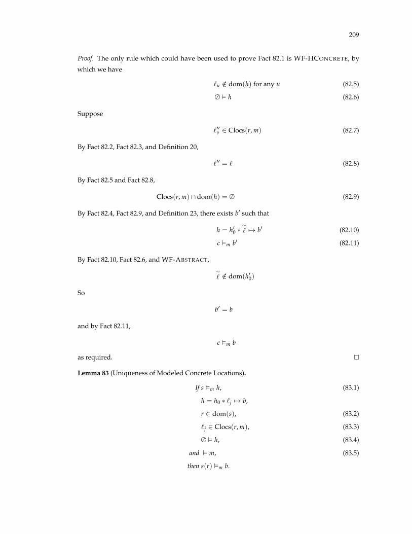
209
Proof. The only rule which could have been used to prove Fact 82.1 is WF-HCONCRETE, by
which we have
`u /2 dom(h) for any u (82.5)
∆ ✏ h (82.6)
Suppose
`00v 2 Clocs(r, m) (82.7)
By Fact 82.2, Fact 82.3, and Definition 20,
`00 = ` (82.8)
By Fact 82.5 and Fact 82.8,
Clocs(r, m) \ dom(h) = ∆ (82.9)
By Fact 82.4, Fact 82.9, and Definition 23, there exists b0 such that
h = h00 ⇤⇠` 7! b0 (82.10)
c ✏m b0 (82.11)
By Fact 82.10, Fact 82.6, and WF-ABSTRACT,
⇠` /2 dom(h00)
So
b0 = b
and by Fact 82.11,
c ✏m b
as required.
Lemma 83 (Uniqueness of Modeled Concrete Locations).
If s ✏m h, (83.1)
h = h0 ⇤ `j 7! b,
r 2 dom(s), (83.2)
`j 2 Clocs(r, m), (83.3)
∆ ✏ h, (83.4)
and ✏ m, (83.5)
then s(r) ✏m b.
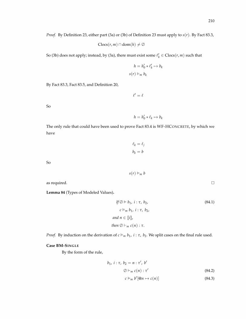
210
Proof. By Definition 23, either part (3a) or (3b) of Definition 23 must apply to s(r). By Fact 83.3,
Clocs(r, m) \ dom(h) 6= ∆
So (3b) does not apply; instead, by (3a), there must exist some `0k 2 Clocs(r, m) such that
h = h00 ⇤ `0k 7! bk
s(r) ✏m bk
By Fact 83.3, Fact 83.5, and Definition 20,
`0 = `
So
h = h00 ⇤ `k 7! bk
The only rule that could have been used to prove Fact 83.4 is WF-HCONCRETE, by which we
have
`k = `j
bk = b
So
s(r) ✏m b
as required.
Lemma 84 (Types of Modeled Values).
If ∆ ✏ b1, i : t, b2, (84.1)
c ✏m b1, i : t, b2,
and n 2 [[i]],
then ∆ `m c(n) : t.
Proof. By induction on the derivation of c ✏m b1, i : t, b2. We split cases on the final rule used.
Case BM-SINGLE
By the form of the rule,
b1, i : t, b2 = n : t0, b0
∆ `m c(n) : t0 (84.2)
c ✏m b0[@n 7! c(n)] (84.3)
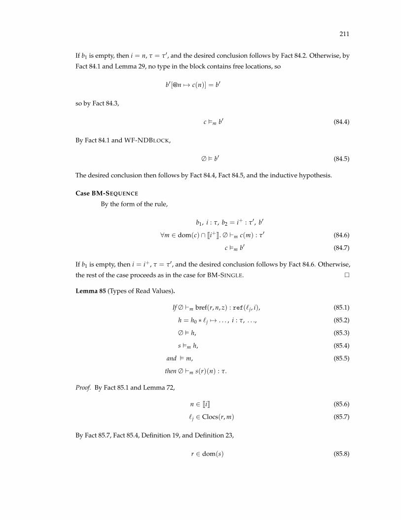
211
If b1 is empty, then i = n, t = t0, and the desired conclusion follows by Fact 84.2. Otherwise, by
Fact 84.1 and Lemma 29, no type in the block contains free locations, so
b0[@n 7! c(n)] = b0
so by Fact 84.3,
c ✏m b0 (84.4)
By Fact 84.1 and WF-NDBLOCK,
∆ ✏ b0 (84.5)
The desired conclusion then follows by Fact 84.4, Fact 84.5, and the inductive hypothesis.
Case BM-SEQUENCE
By the form of the rule,
b1, i : t, b2 = i+ : t0, b0
8m 2 dom(c) \ [[i+]]. ∆ `m c(m) : t0 (84.6)
c ✏m b0 (84.7)
If b1 is empty, then i = i+, t = t0, and the desired conclusion follows by Fact 84.6. Otherwise,
the rest of the case proceeds as in the case for BM-SINGLE.
Lemma 85 (Types of Read Values).
If ∆ `m bref(r, n, z) : ref(`j, i), (85.1)
h = h0 ⇤ `j 7! . . . , i : t, . . ., (85.2)
∆ ✏ h, (85.3)
s ✏m h, (85.4)
and ✏ m, (85.5)
then ∆ `m s(r)(n) : t.
Proof. By Fact 85.1 and Lemma 72,
n 2 [[i]] (85.6)
`j 2 Clocs(r, m) (85.7)
By Fact 85.7, Fact 85.4, Definition 19, and Definition 23,
r 2 dom(s) (85.8)
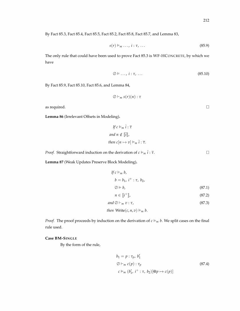
212
By Fact 85.3, Fact 85.4, Fact 85.5, Fact 85.2, Fact 85.8, Fact 85.7, and Lemma 83,
s(r) ✏m . . . , i : t, . . . (85.9)
The only rule that could have been used to prove Fact 85.3 is WF-HCONCRETE, by which we
have
∆ ✏ . . . , i : t, . . . (85.10)
By Fact 85.9, Fact 85.10, Fact 85.6, and Lemma 84,
∆ `m s(r)(n) : t
as required.
Lemma 86 (Irrelevant Offsets in Modeling).
If c ✏m i : t
and n /2 [[i]],
then c[n 7! v] ✏m i : t.
Proof. Straightforward induction on the derivation of c ✏m i : t.
Lemma 87 (Weak Updates Preserve Block Modeling).
If c ✏m b,
b = b1, i+ : t, b2,
∆ ✏ b, (87.1)
n 2 [[i+]], (87.2)
and ∆ `m v : t, (87.3)
then Write(c, n, v) ✏m b.
Proof. The proof proceeds by induction on the derivation of c ✏m b. We split cases on the final
rule used.
Case BM-SINGLE
By the form of the rule,
b1 = p : tp, b01
∆ `m c(p) : tp (87.4)
c ✏m (b01, i+ : t, b2)[@p 7! c(p)]
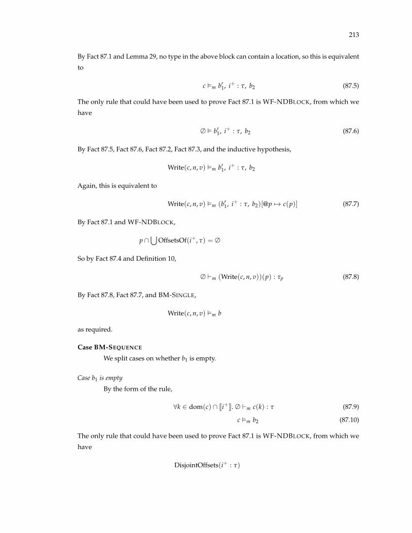
213
By Fact 87.1 and Lemma 29, no type in the above block can contain a location, so this is equivalent
to
c ✏m b01, i+ : t, b2 (87.5)
The only rule that could have been used to prove Fact 87.1 is WF-NDBLOCK, from which we
have
∆ ✏ b01, i+ : t, b2 (87.6)
By Fact 87.5, Fact 87.6, Fact 87.2, Fact 87.3, and the inductive hypothesis,
Write(c, n, v) ✏m b01, i+ : t, b2
Again, this is equivalent to
Write(c, n, v) ✏m (b01, i+ : t, b2)[@p 7! c(p)] (87.7)
By Fact 87.1 and WF-NDBLOCK,
p \[
OffsetsOf(i+, t) = ∆
So by Fact 87.4 and Definition 10,
∆ `m (Write(c, n, v))(p) : tp (87.8)
By Fact 87.8, Fact 87.7, and BM-SINGLE,
Write(c, n, v) ✏m b
as required.
Case BM-SEQUENCE
We split cases on whether b1 is empty.
Case b1 is empty
By the form of the rule,
8k 2 dom(c) \ [[i+]]. ∆ `m c(k) : t (87.9)
c ✏m b2 (87.10)
The only rule that could have been used to prove Fact 87.1 is WF-NDBLOCK, from which we
have
DisjointOffsets(i+ : t)

214
That is, for any p, q 2 [[i+]] such that p 6= q,
([
OffsetsOf(p, t)) \ ([
OffsetsOf(q, t)) = ∆ (87.11)
By Fact 87.3, Fact 87.2, Fact 87.9, Fact 87.11, and Definition 10,
8k 2 dom(Write(c, n, v)) \ [[i+]]. ∆ `m (Write(c, n, v))(k) : t (87.12)
By Fact 87.1 and WF-NDBLOCK, all OffsetsOf(i+, t) are disjoint from all OffsetsOf(b2). Thus,
by Fact 87.10 and Lemma 86,
Write(c, n, v) ✏m b2 (87.13)
By Fact 87.12, Fact 87.13, and BM-SEQUENCE,
Write(c, n, v) ✏m i+ : t, b2
as required.
Case b1 = i+1 : t1, b01By the form of the rule,
8k 2 dom(c) \ [[i+1 ]]. ∆ `m c(k) : t1 (87.14)
c ✏m b01, i+ : t, b2 (87.15)
By Fact 87.1 and WF-NDBLOCK,
∆ ✏ b01, i+ : t, b2 (87.16)
([
OffsetsOf(i+1 , t1)) \ ([
OffsetsOf(i+, t)) = ∆ (87.17)
By Fact 87.15, Fact 87.16, Fact 87.2, Fact 87.3, and the inductive hypothesis,
Write(c, n, v) ✏m b01, i+ : t, b2 (87.18)
By Fact 87.14 Fact 87.17, and Definition 10,
8k 2 dom(Write(c, n, v)) \ [[i+1 ]]. ∆ `m c(k) : t1 (87.19)
By Fact 87.18 and Fact 87.19 and BM-SEQUENCE,
Write(c, n, v) ✏m i+1 : t1, b01, i+ : t, b2
as required.

215
Lemma 88 (Non-Dependent Partial Block Well-Formedness). G ✏ b1, b2 iff G ✏ b1 and G ✏ b2.
Proof. Immediate by the form of WF-NDBLOCK.
Lemma 89 (Strong Update Preserves Block Modeling).
If b = b1, n : t1, b2,
c ✏m b, (89.1)
∆ ✏ b, (89.2)
∆ `m v : t2, (89.3)
SizeOf(t2) = SizeOf(t1), (89.4)
and ∆ ✏ t2, (89.5)
then Write(c, n, v) ✏m b1, n : t2, b2.
Proof. First, we note that the only rule that could have been used to prove Fact 89.2 is WF-
NDBLOCK. By the form of the rule,
b = ij : tj
DisjointOffsets(ij : tj) (89.6)
8j.∆ ✏ tj (89.7)
Also, by Definition 7, Fact 89.3, Fact 89.4, and Lemma 71,
SizeOf(v) = SizeOf(t1)
so that
[n, n + SizeOf(v)) = OffsetsOf(n, t1) (89.8)
The rest of the proof proceeds by induction on the derivation of c ✏m b1, n : t1, b2. We
split cases on the final rule used.
Case BM-SINGLE
By the form of the rule, we have
b = k : t, b01
∆ `m c(k) : t (89.9)
c ✏m b2[@k 7! c(k)] (89.10)
By Fact 89.7, the types of b2 cannot contain locations, so Fact 89.10 is equivalent to
c ✏m b2 (89.11)

216
We further split cases on whether b1 is empty.
Case b1 is empty
Then k = n and b01 = b2. By Fact 89.6 and Fact 89.8,
[n, n + SizeOf(v)) \ OffsetsOf(b2) = ∆ (89.12)
By Fact 89.12, Definition 10, and Lemma 86,
Write(c, n, v) ✏m b2
Since b2 cannot contain offsets, this is equivalent to
Write(c, n, v) ✏m b2[@n 7! v] (89.13)
By Fact 89.3, Fact 89.13, and BM-SINGLE,
Write(c, n, v) ✏m n : t2, b2 (89.14)
as required.
Case b1 = k : t, b01By Fact 89.6,
n 6= k
Then by Fact 89.9,
∆ `m (Write(c, n, v))(k) : t (89.15)
By Fact 89.2 and Lemma 88,
∆ ✏ b01, n : t1, b2
By Fact 89.7, this is equivalent to
∆ ✏ (b01, n : t1, b2)[@k 7! c(k)] (89.16)
The only rule which could have been used to prove Fact 89.1 is BM-SINGLE, from which we have
c ✏m (b01, n : t1, b2)[@k 7! c(k)] (89.17)
By Fact 89.17, Fact 89.16, Fact 89.3, Fact 89.5, Fact 89.4, and the inductive hypothesis,
Write(c, n, v) ✏m b01, n : t2, b2

217
By Fact 89.7, this is equivalent to
Write(c, n, v) ✏m (b01, n : t2, b2)[@k 7! c[n 7! v](k)] (89.18)
By Fact 89.15, Fact 89.18, and BM-SINGLE,
Write(c, n, v) ✏m b1, n : t2, b2
as required.
Case BM-SEQUENCE
By the form of the rule, we have
b1 = i+ : t, b01
8k 2 dom(c) \ [[i+]]. ∆ `m c(k) : t (89.19)
c ✏m b01, n : t1, b2 (89.20)
By Fact 89.6 and Fact 89.8,
[n, n + SizeOf(v)) \ [[i+]] = ∆ (89.21)
By Fact 89.21, Fact 89.19, and Definition 10,
8k 2 dom(Write(c, n, v)) \ [[i+]]. ∆ `m (Write(c, n, v))(k) : t (89.22)
By Fact 89.2 and Lemma 88,
∆ ✏ b01, n : t2, b2 (89.23)
By Fact 89.20, Fact 89.23, Fact 89.3, Fact 89.5, Fact 89.4, and the inductive hypothesis,
Write(c, n, v) ✏m b01, n : t2, b2 (89.24)
By Fact 89.22, Fact 89.24, and BM-SEQUENCE,
Write(c, n, v) ✏m b1, n : t2, b2
as required.
Lemma 90 (Strong Update Preserves Block Well-Formedness).
If ∆ ✏ b1, n : t1, b2,
∆ ✏ t2,
and SizeOf(t1) = SizeOf(t2),
then ∆ ✏ b1, n : t2, b2

218
Proof. Immediate from the form of WF-NDBLOCK and the given assumptions.
Lemma 91 (Consistent Block Updating).
If ∆ ✏ h, (91.1)
s ✏m h, (91.2)
h = h0 ⇤ `j 7! b1,
`j 2 Clocs(r, m), (91.3)
c ✏m b2, (91.4)
s2 = s[r 7! c],
and h2 = h0 ⇤ `j 7! b2, (91.5)
then s2 ✏m h2.
Proof. By Definition 23, we must show
1. 8`j 2 dom(h). `j 2 dom(m)
2. rng(m) ✓ dom(s2)
3. For all r0 2 dom(s2), either
(a) exists `0k 2 Clocs(r0, m), h = h00 ⇤ `0k 7! b, and s2(r0) ✏m b, or
(b) Clocs(r0, m) \ dom(h) = ∆, h = h00 ⇤⇠` 7! b, and s2(r0) ✏m b
Note (1) and (2) follow immediately from the assumptions.
We choose an arbitrary r0 2 dom(s0) and show that one of the conditions of (3) is satisfied.
We split cases on whether r0 = r.
Case r0 = r
Then
s2(r0) = c
And, by Fact 91.3,
`j 2 Clocs(r0, m)
Note also that, by Fact 91.5,
h2 = h0 ⇤ `j 7! b2
while, by Fact 91.4,
c ✏m b2
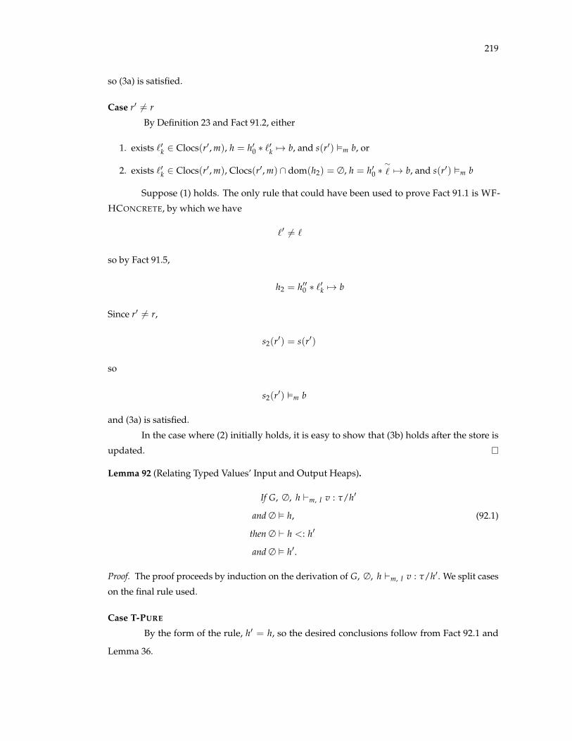
219
so (3a) is satisfied.
Case r0 6= r
By Definition 23 and Fact 91.2, either
1. exists `0k 2 Clocs(r0, m), h = h00 ⇤ `0k 7! b, and s(r0) ✏m b, or
2. exists `0k 2 Clocs(r0, m), Clocs(r0, m) \ dom(h2) = ∆, h = h00 ⇤⇠` 7! b, and s(r0) ✏m b
Suppose (1) holds. The only rule that could have been used to prove Fact 91.1 is WF-
HCONCRETE, by which we have
`0 6= `
so by Fact 91.5,
h2 = h000 ⇤ `0k 7! b
Since r0 6= r,
s2(r0) = s(r0)
so
s2(r0) ✏m b
and (3a) is satisfied.
In the case where (2) initially holds, it is easy to show that (3b) holds after the store is
updated.
Lemma 92 (Relating Typed Values’ Input and Output Heaps).
If G, ∆, h `m, I v : t/h0
and ∆ ✏ h, (92.1)
then ∆ ` h <: h0
and ∆ ✏ h0.
Proof. The proof proceeds by induction on the derivation of G, ∆, h `m, I v : t/h0. We split cases
on the final rule used.
Case T-PURE
By the form of the rule, h0 = h, so the desired conclusions follow from Fact 92.1 and
Lemma 36.

220
Case T-SUB
By the form of the rule,
G, ∆, h `m, I v : t1/h1 (92.2)
∆ ` t1/h1 <: t/h0 (92.3)
∆ ✏ t/h0 (92.4)
By the inductive hypothesis and Fact 92.2,
∆ ` h <: h1 (92.5)
Fact 92.3 can only be proved by <:-WORLD, from which we have
∆ ` h1 <: h0 (92.6)
By Fact 92.5, Fact 92.6, and Lemma 35,
∆ ` h <: h0
The only rule that can be used to prove Fact 92.4 is WF-WORLD, from which we have
G ✏ h0
as required.
Case T-IF, T-LET, T-READ, T-SUPD, T-WUPD, T-UNFOLD, T-FOLD, T-CALL, T-MALLOC
Impossible, as the expression considered in each case is not a value.
C.19 Preservation
Lemma 93 (Pure Expression Preservation). If ∆ `m a : t and a ,! a0, then ∆ `m a0 : t.
Proof. The proof proceeds by induction on the derivation of ∆ `m a : t. We split cases on the
final rule used.
Case T-VAR
Impossible.
Case T-INT, T-REF
Since a is a value, there is no a0 such that a ,! a0.

221
Case T-ARITH
By the form of the rule,
a ⌘ v1 � v2
∆ `m v1 : int(w, i1) (93.1)
∆ `m v2 : int(w, i2) (93.2)
t = {n : int(w, i1⇠� i2) | n = v1 � v2} (93.3)
By Fact 93.1 and Lemma 72,
v1 = n1|w|
n1⇠✓ i1 (93.4)
By Fact 93.2 and Lemma 72,
v2 = n2|w|
n2⇠✓ i2 (93.5)
The only evaluation rule that applies is E-ARITH, from which we have
a0 ⌘ (n1 � n2)|w|
By T-INT,
∆ `m (n1 � n2)|w| : {n : int(w, n1 � n2) | n = (n1 � n2)|w|} (93.6)
By Fact 93.4, Fact 93.5, and Proposition 3,
n1 � n2⇠✓ i1
⇠� i2 (93.7)
By Assumption 13,
∆ ✏ n = (n1 � n2)|w| ) n = n1|w| � n2|w| (93.8)
By Fact 93.8, Fact 93.7, and <:-INT,
∆ ` {n : int(w, n1 � n2) | n = (n1 � n2)|w|} <: {n : int(w, i1⇠� i2) | n = n1|w| � n2|w|}
(93.9)
By Fact 93.6, Fact 93.9, and T-PURESUB,
∆ `m (n1 � n2)|w| : {n : int(w, i1⇠� i2) | n = n1|w| � n2|w|}

222
as required.
Case T-PTRARITH
By the form of the rule,
a ⌘ v1 +p v2
∆ `m v1 : ref(`, i1) (93.10)
∆ `m v2 : int(w, i2) (93.11)
t = {n : ref(`, i1⇠+ i2) | n = v1 +p v2} (93.12)
By Fact 93.10 and Lemma 72,
v = 0|W|
or
v = bref(r, n, z)
n 2 [[i1]]
9`j v `.`j 2 Clocs(r, m)
We now split cases.
Case v = 0|W|
Then the evaluation rule which applied must have been E-NULL-PLUS. Then
a0 ⌘ 0|W|
v2 = m|W|
` =⇠`
By <:-NULL,
∆ ` {n : int(W, 0) | n = 0|W|} <: {n : ref(⇠` , i1
⇠� i2) | n = 0|W|}
By Assumption 13,
∆ ✏ n = 0|W| ) n = 0|W| +p m|W|
By the above and <:-REF,
∆ ` {n : ref(⇠` , i1
⇠� i2) | n = 0|W|} <: {n : ref(⇠` , i1
⇠� i2) | n = 0|W| +p m|W|}
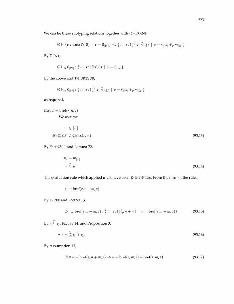
223
We can tie these subtyping relations together with <:-TRANS:
∆ ` {n : int(W, 0) | n = 0|W|} <: {n : ref(⇠` , i1
⇠� i2) | n = 0|W| +p m|W|}
By T-INT,
∆ `m 0|W| : {n : int(W, 0) | n = 0|W|}
By the above and T-PURESUB,
∆ `m 0|W| : {n : ref(⇠` , i1
⇠� i2) | n = 0|W| +p m|W|}
as required.
Case v = bref(r, n, z)
We assume
n 2 [[i1]]
9`j v `.`j 2 Clocs(r, m) (93.13)
By Fact 93.11 and Lemma 72,
v2 = m|w|
m⇠✓ i2 (93.14)
The evaluation rule which applied must have been E-INT-PLUS. From the form of the rule,
a0 ⌘ bref(r, n + m, z)
By T-REF and Fact 93.13,
∆ `m bref(r, n + m, z) : {n : ref(`j, n + m) | n = bref(r, n + m, z)} (93.15)
By n⇠✓ i1, Fact 93.14, and Proposition 3,
n + m⇠✓ i1
⇠+ i2 (93.16)
By Assumption 13,
∆ ✏ n = bref(r, n + m, z) ) n = bref(r, m, z) + bref(r, m, z) (93.17)
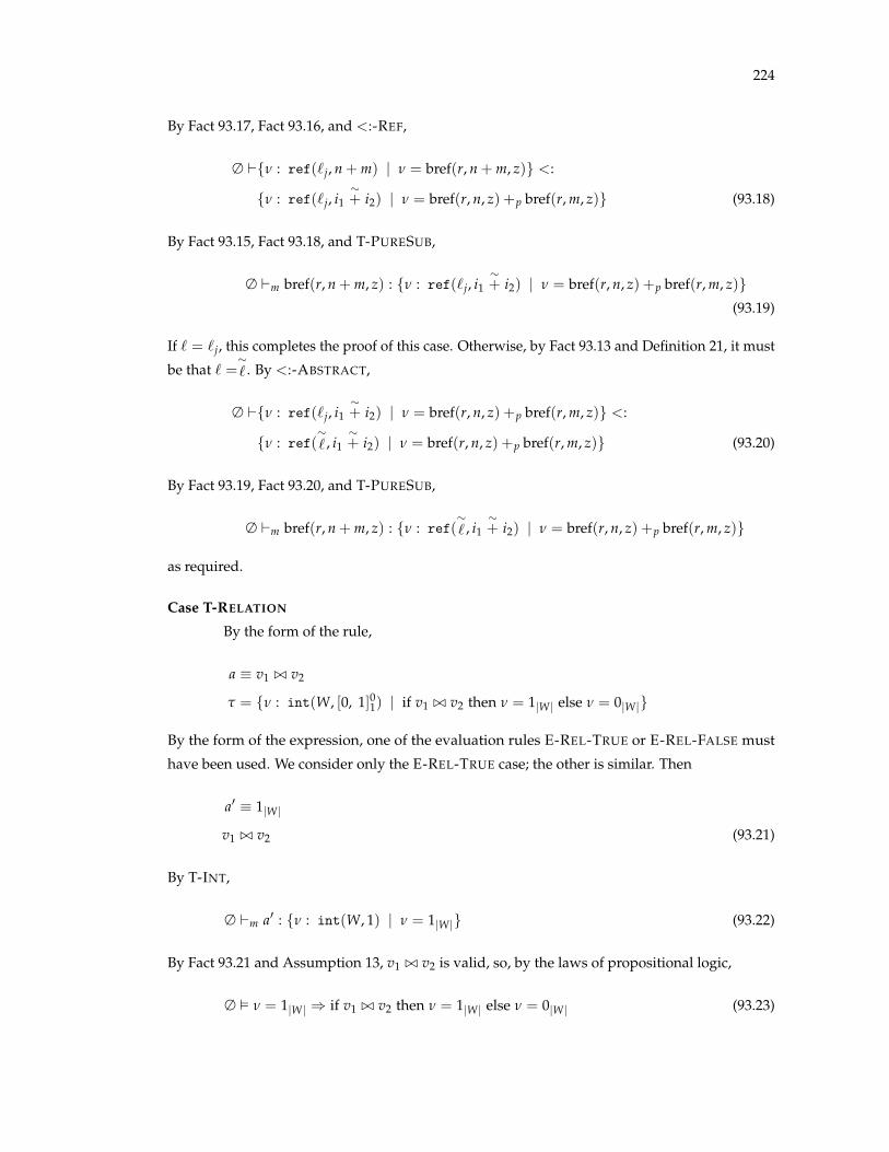
224
By Fact 93.17, Fact 93.16, and <:-REF,
∆ `{n : ref(`j, n + m) | n = bref(r, n + m, z)} <:
{n : ref(`j, i1⇠+ i2) | n = bref(r, n, z) +p bref(r, m, z)} (93.18)
By Fact 93.15, Fact 93.18, and T-PURESUB,
∆ `m bref(r, n + m, z) : {n : ref(`j, i1⇠+ i2) | n = bref(r, n, z) +p bref(r, m, z)}
(93.19)
If ` = `j, this completes the proof of this case. Otherwise, by Fact 93.13 and Definition 21, it must
be that ` =⇠` . By <:-ABSTRACT,
∆ `{n : ref(`j, i1⇠+ i2) | n = bref(r, n, z) +p bref(r, m, z)} <:
{n : ref(⇠` , i1
⇠+ i2) | n = bref(r, n, z) +p bref(r, m, z)} (93.20)
By Fact 93.19, Fact 93.20, and T-PURESUB,
∆ `m bref(r, n + m, z) : {n : ref(⇠` , i1
⇠+ i2) | n = bref(r, n, z) +p bref(r, m, z)}
as required.
Case T-RELATION
By the form of the rule,
a ⌘ v1 ./ v2
t = {n : int(W, [0, 1]01) | if v1 ./ v2 then n = 1|W| else n = 0|W|}
By the form of the expression, one of the evaluation rules E-REL-TRUE or E-REL-FALSE must
have been used. We consider only the E-REL-TRUE case; the other is similar. Then
a0 ⌘ 1|W|
v1 ./ v2 (93.21)
By T-INT,
∆ `m a0 : {n : int(W, 1) | n = 1|W|} (93.22)
By Fact 93.21 and Assumption 13, v1 ./ v2 is valid, so, by the laws of propositional logic,
∆ ✏ n = 1|W| ) if v1 ./ v2 then n = 1|W| else n = 0|W| (93.23)

225
By Proposition 2,
1⇠✓ [0, 1]01 (93.24)
By Fact 93.23, Fact 93.24, and <:-INT,
∆ ` {n : int(W, 1) | n = 1|W|}
<: {n : int(W, [0, 1]01) | if v1 ./ v2 then n = 1|W| else n = 0|W|} (93.25)
By Fact 93.22, Fact 93.25, and T-PURESUB,
∆ `m a0 : {n : int(W, [0, 1]01) | if v1 ./ v2 then n = 1|W| else n = 0|W|} (93.26)
as required.
Case T-PURESUB
By the form of the rule,
∆ `m a : t1 (93.27)
∆ ` t1 <: t (93.28)
∆ ✏ t (93.29)
By the inductive hypothesis and Fact 93.27,
∆ `m a0 : t1 (93.30)
By Fact 93.28, Fact 93.29, Fact 93.30, and T-PURESUB,
∆ `m a0 : t
as required.

226
Lemma 94 (Type Preservation).
If G, ∆, h `m, I e : t/h0,
∆ ✏ h, (94.1)
s ✏m h, (94.2)
✏ m, (94.3)
✏ G, (94.4)
D ✏ G, (94.5)
and e/s ,! e0/s0,
then there exist hs, m0 such that
G, ∆, hs `m0 , I e0 : t/h0,
∆ ✏ hs,
s0 ✏m0 hs,
✏ m0,
m ✓ m0,
and dom(m0 \ m) ✓ I.
Proof. The proof proceeds by induction on the derivation of G, ∆, h `m, I e : t/h0. We split cases
on the final rule used. Unless noted otherwise, we let m0 = m and hs = h.
Case T-PURE
Immediate from Lemma 93.
Case T-SUB
By the form of the rule,
G, ∆, h `m, I e : t1/h1 (94.6)
∆ ` t1/h1 <: t/h (94.7)
∆ ✏ t/h (94.8)
By the initial assumptions, Fact 94.6, and the inductive hypothesis, there exist hs and m0 such that
G, ∆, hs `m0 , I e0 : t1/h1 (94.9)
∆ ✏ hs
s0 ✏m0 hs
✏ m0
m ✓ m0
dom(m0 \ m) ✓ I

227
Most obligations follow immediately. By Fact 94.9, Fact 94.7, Fact 94.8, and T-SUB,
G, ∆, hs `m0 , I e0 : t/h,
as required.
Case T-IF
By the form of the rule,
e ⌘ if v then e1 else e2
G, v 6= 0, h `m, I1 e1 : t/h0 (94.10)
G, v = 0, h `m, I2 e2 : t/h0 (94.11)
The only evaluation rules that could have applied are E-IF-TRUE and E-IF-FALSE. We show only
the E-IF-TRUE case; the case for E-IF-FALSE is similar.
By the form of E-IF-TRUE, we have
v = 1|W|
e0 ⌘ e1
s0 = s
By Assumption 13,
1|W| 6= 0
is valid, so, by WFSUBST-PRED,
v 6= 0 ✏m ·
By the above, Fact 94.10, and Lemma 58, then,
G, ∆, h `m, I e1 : t/h0
as required.
Case T-LET
By the form of the rule,
e ⌘ let x = e1 in e2
I = I1 [ I2 (94.12)
I1 \ I2 = ∆ (94.13)
G, ∆, h `m, I1 e1 : t1/h1 (94.14)
G, x : t1, h1 `m, I2 e2 : t/h0 (94.15)
∆ ✏ t/h0 (94.16)

228
We split cases on whether e1 is a value.
Case e1 is not a value
Then the only evaluation rule that applies is E-SEQ, so that we have:
e1/s ,! e01/s0
e0 ⌘ let x = e01 in e2
By the inductive hypothesis and Fact 94.14,
G, ∆, hs `m0 , I1 e01 : t1/h1 (94.17)
for some hs and m0 such that
∆ ✏ hs
s0 ✏m0 hs
m ✓ m0
✏ m0
dom(m0 \ m) ✓ I1. (94.18)
Most obligations follow immediately. By Fact 94.13, Fact 94.15, Fact 94.18, and Lemma 22,
G, x : t1, h1 `m0 , I2 e2 : t/h0 (94.19)
By Fact 94.12, Fact 94.17, Fact 94.19, Fact 94.16, and T-LET,
G, ∆, hs `m0 , I let x = e01 in e2 : t/h
as required.
Case e1 ⌘ v for some value v
The only evaluation rule that applies is E-LET. From the form of the rule, we have:
e0 ⌘ e2[x 7! v]
s0 = s
The only rule that could have been used to prove Fact 94.14 is T-PURE, from which we have
∆ ` v : t1
By WF-VAR, then,
∆ ✏m [x 7! v] (94.20)

229
By Fact 94.20, Fact 94.15, and Lemma 58,
G, ∆, h1[x 7! v] `m, I2 e2[x 7! v] : t[x 7! v]/h0[x 7! v]
By Fact 94.16 and Lemma 28,
FV(t) = ∆
FV(h0) = ∆
So the above is equivalent to
G, ∆, h1[x 7! v] `m, I2 e2[x 7! v] : t/h0 (94.21)
By Fact 94.14 and Lemma 92,
∆ ` h <: h1 (94.22)
∆ ✏ h1 (94.23)
By Fact 94.23 and Lemma 28,
FV(h1) = ∆ (94.24)
so
h1[x 7! v] = h1 (94.25)
so we have
G, ∆, h1 `m, I2 e2[x 7! v] : t/h0 (94.26)
By Fact 94.12 and Lemma 19,
G, ∆, h1 `m, I e2[x 7! v] : t/h0
which settles type preservation. By Fact 94.22, Fact 94.2, and Lemma 78,
s ✏m h1
Thus, we let
hs = h1,
which satisfies the heap well-formedness and modeling requirements.

230
Case T-READ
By the form of the rule,
e ⌘ ⇤nv
h = h1 ⇤ `j 7! . . . , i : t, . . . (94.27)
h0 = h
∆ `m v : {n : ref(`j, i) | Safe(n, n)} (94.28)
The only evaluation rule that applies is E-READ, from which we have
v = bref(r, n, z)
e0 ⌘ s(r)(n)
s0 = s
for some r, n, and z. By Fact 94.28, Fact 94.27, Fact 94.1, Fact 94.2, and Fact 94.3,
∆ `m s(r)(n) : t
By the above and T-PURE,
G, ∆, h `m, s(r)(n) : t/h
as required.
Case T-SUPD
By the form of the rule,
e ⌘ ⇤v1 := v2
t = void
∆ `m v1 : {n : ref(`j, n) | Safe(n, SizeOf(t2))} (94.29)
∆ `m v2 : t2 (94.30)
SizeOf(t2) = SizeOf(t1) (94.31)
h = h1 ⇤ `j 7! b1, n : t1, b2 (94.32)
h0 = h1 ⇤ `j 7! b1, n : t2, b2

231
The only evaluation rule that applies is E-WRITE, from which we have
v1 = bref(r, k, z)
e0 ⌘ 0|0|
r 2 dom(s) (94.33)
s(r) = c
s0 = s[r 7! Write(c, k, v2)]
for some r, k, and z. By Fact 94.29 and Lemma 72,
k = n
`j 2 Clocs(r, m) (94.34)
By Fact 94.30 and Lemma 39,
∆ ✏ t2 (94.35)
By Fact 94.1, Fact 94.2, Fact 94.3, Fact 94.32, Fact 94.33, Fact 94.34, and Lemma 83,
c ✏m b1, n : t1, b2 (94.36)
The only rule that could have been used to prove Fact 94.1 is WF-HCONCRETE, by which we
have
∆ ✏ b1, n : t1, b2 (94.37)
∆ ✏ h1 (94.38)
By Fact 94.36, Fact 94.37, Fact 94.30, Fact 94.35, Fact 94.31, and Lemma 89,
Write(c, n, v2) ✏m b1, n : t2, b2 (94.39)
We let
hs = h0 (94.40)
By Fact 94.1, Fact 94.2, Fact 94.34, Fact 94.39, Fact 94.40, and Lemma 91,
s0 ✏m hs
as required. By Fact 94.37, Fact 94.35, Fact 94.31, and Lemma 90,
∆ ✏ b1, n : t2, b2 (94.41)

232
By Fact 94.38, Fact 94.41, Fact 94.40, and WF-HCONCRETE,
∆ ✏ hs
as required. By T-INT, <:-INT, T-PURESUB, and T-PURE,
G, ∆, hs `I, m 0|0| : void/hs
as required.
Case T-WUPD
By the form of the rule,
e ⌘ ⇤v1 := v2
t = void
∆ `m v1 : {n : ref(`j, n+k) | Safe(n, SizeOf(t))} (94.42)
∆ `m v2 : t (94.43)
h = h1 ⇤ `j 7! . . . , n+k : t, . . . (94.44)
h0 = h
The only evaluation rule that applies is E-WRITE, from which we have
v1 = bref(r, q, z)
e0 ⌘ 0|0|
s0 = s[r 7! Write(s(r), q, v2)]
r 2 dom(s) (94.45)
for some r, q, z. By Fact 94.42 and Lemma 72,
q 2 [[n+k]] (94.46)
`j 2 Clocs(r, m) (94.47)
By Fact 94.1, Fact 94.2, Fact 94.3, Fact 94.44, Fact 94.45, Fact 94.47, and Lemma 83,
s(r) ✏m . . . , n+k : t, . . . (94.48)
The only rule that could have been used to prove Fact 94.1 is WF-HCONCRETE, by which we
have
∆ ✏ . . . , i : t, . . . (94.49)

233
By Fact 94.48, Fact 94.49, Fact 94.46, Fact 94.43, and Lemma 87,
Write(s(r), q, v2) ✏m . . . , i : t, . . . (94.50)
We let
hs = h (94.51)
By Fact 94.1, Fact 94.2, Fact 94.47, Fact 94.50, Fact 94.51, and Lemma 91,
s0 ✏m hs
as required. By Fact 94.1 and Fact 94.51,
∆ ✏ hs
as required. Finally, by T-INT, <:-INT, T-PURESUB, and T-PURE,
G, ∆, hs `I, m 0|0| : void/hs
as required.
Case T-UNFOLD
By the form of the rule,
e ⌘ letu x = unfold v in e
I = I1 [ {`j} (94.52)
∆ `m v : {n : ref(⇠` , iy) | n 6= 0} (94.53)
h = h0 ⇤⇠` 7! nk : tk, i+ : t+ (94.54)
xk disjoint (94.55)
xk /2 e, FV(h) (94.56)
q = [@nk 7! xk] (94.57)
G1 = xk : qtk (94.58)
`j /2 h, m (94.59)
h1 = h ⇤ `j 7! nk : {n = xk}, i+ : qt+ (94.60)
G, G1; x : {n : ref(`j, iy) | n = v}, h1 `m, I1 e : t2/h2 (94.61)
G1 ✏ h1 (94.62)
∆ ✏ t2/h2 (94.63)
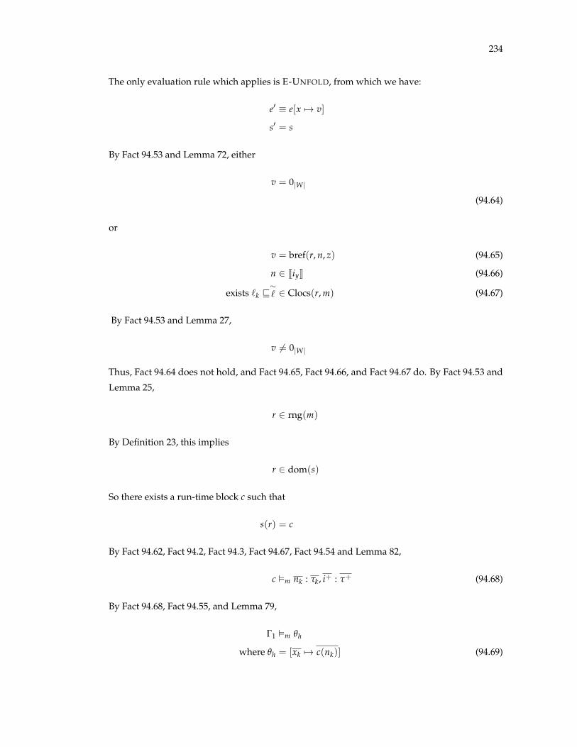
234
The only evaluation rule which applies is E-UNFOLD, from which we have:
e0 ⌘ e[x 7! v]
s0 = s
By Fact 94.53 and Lemma 72, either
v = 0|W|
(94.64)
or
v = bref(r, n, z) (94.65)
n 2 [[iy]] (94.66)
exists `k v⇠` 2 Clocs(r, m) (94.67)
By Fact 94.53 and Lemma 27,
v 6= 0|W|
Thus, Fact 94.64 does not hold, and Fact 94.65, Fact 94.66, and Fact 94.67 do. By Fact 94.53 and
Lemma 25,
r 2 rng(m)
By Definition 23, this implies
r 2 dom(s)
So there exists a run-time block c such that
s(r) = c
By Fact 94.62, Fact 94.2, Fact 94.3, Fact 94.67, Fact 94.54 and Lemma 82,
c ✏m nk : tk, i+ : t+ (94.68)
By Fact 94.68, Fact 94.55, and Lemma 79,
G1 ✏m qh
where qh = [xk 7! c(nk)] (94.69)

235
By Fact 94.69, Fact 94.61, and Lemma 58,
G, x : {n : ref(`j, iy) | n = v}, qhh1 `m, I1 qhe : qht2/qhh2
By Fact 94.56, this is equivalent to
G, x : {n : ref(`j, iy) | n = v}, qhh1 `m, I1 e : qht2/qhh2 (94.70)
By Fact 94.63 and Lemma 28,
FV(t2/h2) = ∆ (94.71)
By Fact 94.70 and Fact 94.71,
G, x : {n : ref(`j, iy) | n = v}, qhh1 `m, I1 e : t2/h2 (94.72)
We now show location map inclusion, then conclude type preservation. We let
m0 = m[`j 7! r] (94.73)
Note that, by Fact 94.52,
dom(m0 \ m) ✓ I
as required. By Fact 94.73 and Fact 94.59,
m ✓ m0 (94.74)
which settles location map inclusion. By Fact 94.74, Fact 94.72, Fact 94.52, and Lemma 22,
G, x : {n : ref(`j, iy) | n = v}, qhh1 `m0 , I1 e : t2/h2 (94.75)
By Fact 94.73, Fact 94.66, Proposition 2, Definition 19, T-REF, and <:-REF,
∆ `m0 bref(r, n, z) : {n : ref(`j, iy) | n = bref(r, n, z)}(94.76)
Define qx by
qx = [x 7! bref(r, n, z)]
By Fact 94.76 and WFSUBST-VAR,
x : {n : ref(`j, iy) | n = bref(r, n, z)} ✏m0 qx (94.77)

236
By Fact 94.75, Fact 94.77, and Lemma 58,
G, ∆, qxqhh1 `m0 , I1 qxe : qxt2/qxh2
By Fact 94.71, this implies
G, ∆, qxqhh1 `m0 , I1 qxe : t2/h2
We assume that
x /2 FV(h1)
So we have
G, ∆, qhh1 `m0 , I1 qxe : t2/h2 (94.78)
By Fact 94.78, Fact 94.52, and Lemma 19,
G, ∆, qhh1 `m0 , I qxe : t2/h2
which settles type preservation. We now show that the new input heap
hs = qhh1
= qhh ⇤ `j 7! nk : {n = qhxk}, i+ : qhqt+
is well-formed. By Fact 94.56,
hs = h ⇤ `j 7! nk : {n = qhxk}, i+ : qhqt+ (94.79)
By WF-HCONCRETE, we must show
∆ ✏ h (94.80)⇠` 2 dom(h) (94.81)
`k /2 dom(h) (94.82)
∆ ✏ nk : {n = qhxk}, i+ : qhqt+ (94.83)
Note that Fact 94.80 was assumed, while Fact 94.81 follows from Fact 94.54. The only rule that
could be used to prove Fact 94.62 is WF-HCONCRETE, from which we have
`k /2 dom(h) for any k
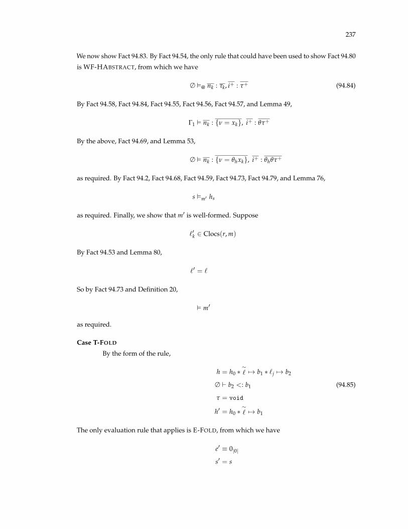
237
We now show Fact 94.83. By Fact 94.54, the only rule that could have been used to show Fact 94.80
is WF-HABSTRACT, from which we have
∆ ✏@ nk : tk, i+ : t+ (94.84)
By Fact 94.58, Fact 94.84, Fact 94.55, Fact 94.56, Fact 94.57, and Lemma 49,
G1 ✏ nk : {n = xk}, i+ : qt+
By the above, Fact 94.69, and Lemma 53,
∆ ✏ nk : {n = qhxk}, i+ : qhqt+
as required. By Fact 94.2, Fact 94.68, Fact 94.59, Fact 94.73, Fact 94.79, and Lemma 76,
s ✏m0 hs
as required. Finally, we show that m0 is well-formed. Suppose
`0k 2 Clocs(r, m)
By Fact 94.53 and Lemma 80,
`0 = `
So by Fact 94.73 and Definition 20,
✏ m0
as required.
Case T-FOLD
By the form of the rule,
h = h0 ⇤⇠` 7! b1 ⇤ `j 7! b2
∆ ` b2 <: b1 (94.85)
t = void
h0 = h0 ⇤⇠` 7! b1
The only evaluation rule that applies is E-FOLD, from which we have
e0 ⌘ 0|0|
s0 = s

238
We define the output heap hs as
hs = h0
= h0 ⇤⇠` 7! b1
By Fact 94.1, Fact 94.2, Fact 94.3, Fact 94.85, and Lemma 81,
s ✏m hs
The only rule that could have been used to show Fact 94.1 is WF-HCONCRETE, from which we
have
∆ ✏ hs
By T-INT, T-PURESUB, and T-PURE,
G, ∆, hs `m, 0|0| : void/h0
Thus, all the obligations are satisfied.
Case T-CALL
By the form of the rule
e ⌘ f (vj)[` f 7! `]
h = hu ⇤ hm (94.86)
∆ ✏ hm (94.87)
∆ ✏ hu (94.88)
G( f ) = (xj : tj)/h f ! t0/h0f (94.89)
q = [xj 7! vj] (94.90)
r = [` f 7! `] (94.91)
∆ ✏ hu ⇤ qrh f (94.92)
∆ `m vj : qrtj (94.93)
∆ ` hm <: qrh f (94.94)
t = qrt0
h = hu ⇤ qrh0f
By Fact 94.5 and Definition 26,
D( f ) = e f (94.95)

239
The only evaluation rule which applies is E-CALL, from which we have
e0 ⌘ qre f (94.96)
s0 = s (94.97)
By Fact 94.87, Fact 94.94, and Lemma 61,
���Locs(rh f )��� =
���Locs(h f )��� (94.98)
By Fact 94.89, Fact 94.5, Fact 94.95, and Definition 26,
G, xj : tj, h f `∆, I f e f : t0/h0f (94.99)
By Fact 94.99, Fact 94.98, Fact 94.4, and Lemma 66,
G, xj : rtj, rh f `∆, rI f re f : rt0/rh0f (94.100)
By Fact 94.93 and repeated applications of WFSUBST-VAR,
xj : qrtj ✏m q (94.101)
By Fact 94.101, Fact 94.99, Fact 94.4, and Lemma 58,
G, ∆, qrh f `∆, rI f qre f : qrt0/qrh0f (94.102)
Since I and I f are both countable, there exists a substitution w such that
wrI f = I
By Fact 94.107, and Lemma 18,
G, ∆, wrqh f `∆, I qre f : wqrt0/wqrh0f (94.103)
By Fact 94.4 and Definition 25,
✏ (xj : tj)/h f ! t0/h0f (94.104)
The only rule that could be used to prove Fact 94.104 is WF-FUNSCHEME, from which we have
tj, h f , t0, h0f abstract (94.105)
xj : tj ✏ h f (94.106)
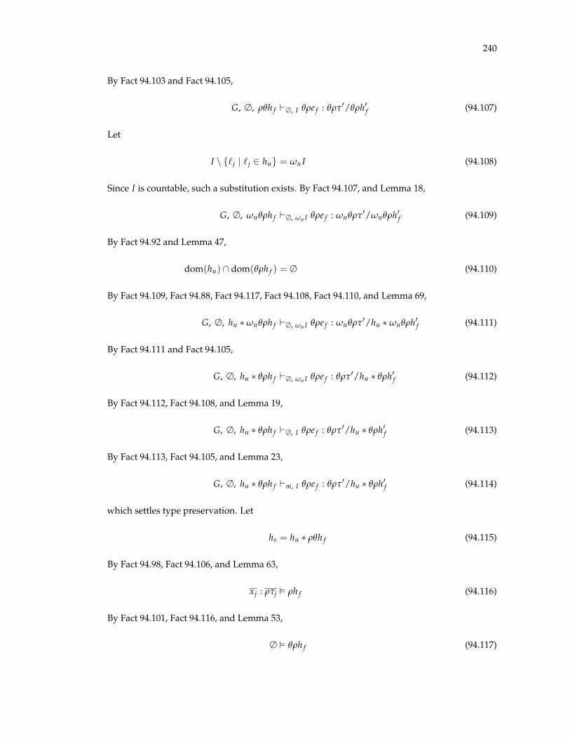
240
By Fact 94.103 and Fact 94.105,
G, ∆, rqh f `∆, I qre f : qrt0/qrh0f (94.107)
Let
I \ {`j | `j 2 hu} = wu I (94.108)
Since I is countable, such a substitution exists. By Fact 94.107, and Lemma 18,
G, ∆, wuqrh f `∆, wu I qre f : wuqrt0/wuqrh0f (94.109)
By Fact 94.92 and Lemma 47,
dom(hu) \ dom(qrh f ) = ∆ (94.110)
By Fact 94.109, Fact 94.88, Fact 94.117, Fact 94.108, Fact 94.110, and Lemma 69,
G, ∆, hu ⇤ wuqrh f `∆, wu I qre f : wuqrt0/hu ⇤ wuqrh0f (94.111)
By Fact 94.111 and Fact 94.105,
G, ∆, hu ⇤ qrh f `∆, wu I qre f : qrt0/hu ⇤ qrh0f (94.112)
By Fact 94.112, Fact 94.108, and Lemma 19,
G, ∆, hu ⇤ qrh f `∆, I qre f : qrt0/hu ⇤ qrh0f (94.113)
By Fact 94.113, Fact 94.105, and Lemma 23,
G, ∆, hu ⇤ qrh f `m, I qre f : qrt0/hu ⇤ qrh0f (94.114)
which settles type preservation. Let
hs = hu ⇤ rqh f (94.115)
By Fact 94.98, Fact 94.106, and Lemma 63,
xj : rtj ✏ rh f (94.116)
By Fact 94.101, Fact 94.116, and Lemma 53,
∆ ✏ qrh f (94.117)
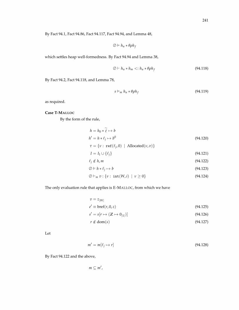
241
By Fact 94.1, Fact 94.86, Fact 94.117, Fact 94.94, and Lemma 48,
∆ ✏ hu ⇤ qrh f
which settles heap well-formedness. By Fact 94.94 and Lemma 38,
∆ ` hu ⇤ hm <: hu ⇤ qrh f (94.118)
By Fact 94.2, Fact 94.118, and Lemma 78,
s ✏m hu ⇤ qrh f (94.119)
as required.
Case T-MALLOC
By the form of the rule,
h = h0 ⇤⇠` 7! b
h0 = h ⇤ `j 7! b0 (94.120)
t = {n : ref(`j, 0) | Allocated(n, v)}
I = I1 [ {`j} (94.121)
`j /2 h, m (94.122)
∆ ✏ h ⇤ `j 7! b (94.123)
∆ `m v : {n : int(W, i) | n � 0} (94.124)
The only evaluation rule that applies is E-MALLOC, from which we have
v = z|W|
e0 ⌘ bref(r, 0, z) (94.125)
s0 = s[r 7! (Z 7! 0|1|)] (94.126)
r /2 dom(s) (94.127)
Let
m0 = m[`j 7! r] (94.128)
By Fact 94.122 and the above,
m ✓ m0,
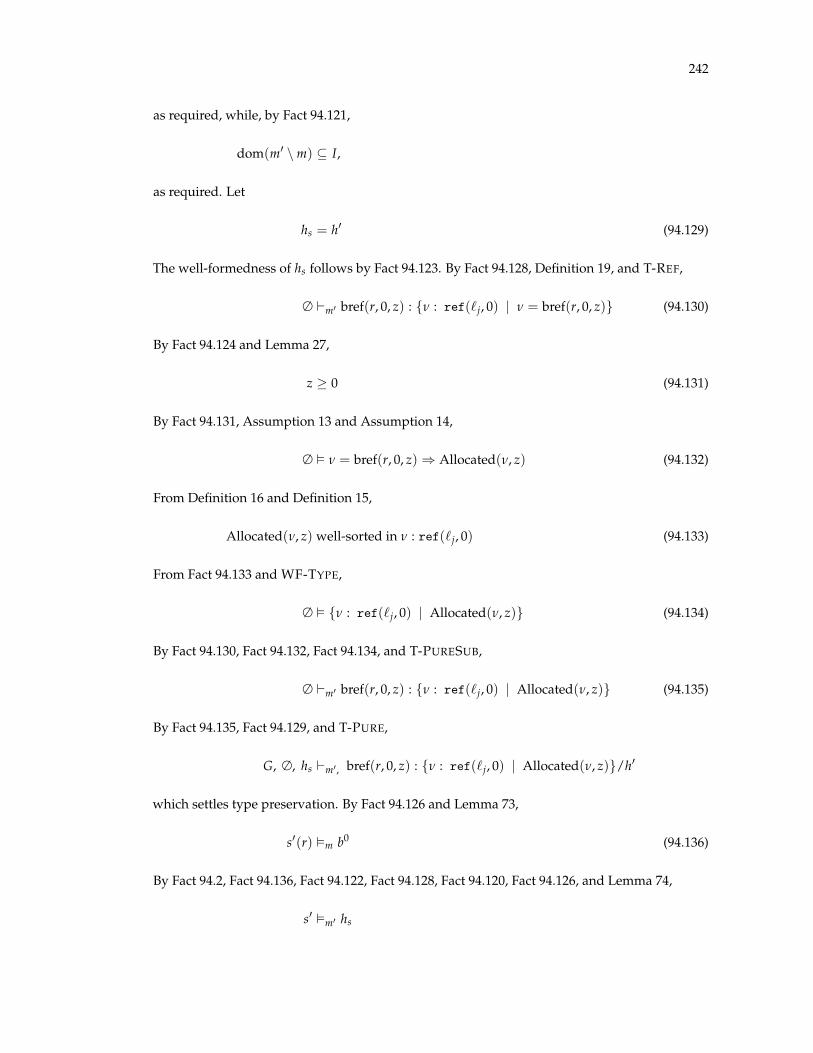
242
as required, while, by Fact 94.121,
dom(m0 \ m) ✓ I,
as required. Let
hs = h0 (94.129)
The well-formedness of hs follows by Fact 94.123. By Fact 94.128, Definition 19, and T-REF,
∆ `m0 bref(r, 0, z) : {n : ref(`j, 0) | n = bref(r, 0, z)} (94.130)
By Fact 94.124 and Lemma 27,
z � 0 (94.131)
By Fact 94.131, Assumption 13 and Assumption 14,
∆ ✏ n = bref(r, 0, z) ) Allocated(n, z) (94.132)
From Definition 16 and Definition 15,
Allocated(n, z) well-sorted in n : ref(`j, 0) (94.133)
From Fact 94.133 and WF-TYPE,
∆ ✏ {n : ref(`j, 0) | Allocated(n, z)} (94.134)
By Fact 94.130, Fact 94.132, Fact 94.134, and T-PURESUB,
∆ `m0 bref(r, 0, z) : {n : ref(`j, 0) | Allocated(n, z)} (94.135)
By Fact 94.135, Fact 94.129, and T-PURE,
G, ∆, hs `m0 , bref(r, 0, z) : {n : ref(`j, 0) | Allocated(n, z)}/h0
which settles type preservation. By Fact 94.126 and Lemma 73,
s0(r) ✏m b0 (94.136)
By Fact 94.2, Fact 94.136, Fact 94.122, Fact 94.128, Fact 94.120, Fact 94.126, and Lemma 74,
s0 ✏m0 hs

243
By Fact 94.2 and Definition 23,
rng(m) ✓ dom(s) (94.137)
By Fact 94.127 and Fact 94.137,
r /2 rng(m) (94.138)
By Fact 94.138, Fact 94.128, and Definition 20,
✏ m0
as required.
C.20 Progress
Lemma 95 (Pure Expression Progress). If ∆ `m a : t and a is not a value, then there exists a0 such
that a ,! a0.
Proof. The proof proceeds by induction on the derivation of ∆ `m a : t. We split cases on the
final rule used.
Case T-VAR
Impossible.
Case T-INT, T-REF
Impossible, as a is a value.
Case T-ARITH
By the form of the rule,
a ⌘ v1 � v2
∆ `m v1 : int(w, i1) (95.1)
∆ `m v2 : int(w, i2) (95.2)
By Lemma 72 and Fact 95.1,
v1 = n1|w| (95.3)
for some n1. By Lemma 72 and Fact 95.2,
v2 = n2|w| (95.4)

244
for some n2. Rule E-ARITH applies:
n1|w| � n2|w| ,! (n1 � n2)|w|
as required.
Case T-PTRARITH
By the form of the rule,
a ⌘ v1 +p v2
∆ `m v1 : ref(`, i1) (95.5)
∆ `m v2 : int(W, i2) (95.6)
By Lemma 72 and Fact 95.6,
v2 = n2|W| (95.7)
for some n2. By Lemma 72 and Fact 95.5, either
v1 = 0|W| (95.8)
or
v1 = bref(r, n1, z1) (95.9)
for some n1 and z1. In the former case, by Fact 95.7, Fact 95.8, and E-NULL-PLUS, we have
v1 +p v2 ,! 0|W|
In the latter case, by Fact 95.7 and Fact 95.9, and E-PTR-PLUS, we have
v1 +p v2 ,! bref(r, n1 + n2, z1)
as required.
Case T-RELATION
By the form of the rule,
a ⌘ v1 ./ v2
∆ `m v1 : t1 (95.10)
∆ `m v2 : t2 (95.11)

245
By Lemma 72, Fact 95.10, and Fact 95.11, there are four cases:
v1 = n1|w|,
v2 = n2|w|
v1 = bref(r, n1, z1),
v2 = 0|W|
v1 = 0|W|,
v2 = bref(r, n2, z2)
v1 = bref(r, n1, z1),
v2 = bref(r, n2, z2)
In each of the above cases, it follows from Definition 5 that
Comparable(v1, v2) (95.12)
Then either rule E-REL-TRUE or E-REL-FALSE applies, i.e.,
v1 ./ v2 ,! 1|W|
or
v1 ./ v2 ,! 0|W|
as required.
Case T-PURESUB
Follows immediately from the inductive hypothesis.
Lemma 96 (Progress).
If G, ∆, h `m, I e : t/h0,
s ✏m h, (96.1)
∆ ✏ h, (96.2)
✏ m, (96.3)
and D ✏ G (96.4)
then e is a value or there exists e0/s0 such that e/s ,! e0/s0.
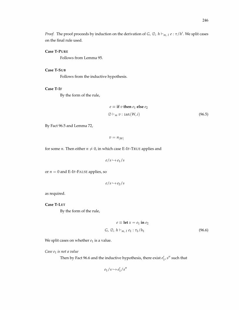
246
Proof. The proof proceeds by induction on the derivation of G, ∆, h `m, I e : t/h0. We split cases
on the final rule used.
Case T-PURE
Follows from Lemma 95.
Case T-SUB
Follows from the inductive hypothesis.
Case T-IF
By the form of the rule,
e ⌘ if v then e1 else e2
∆ `m v : int(W, i) (96.5)
By Fact 96.5 and Lemma 72,
v = n|W|
for some n. Then either n 6= 0, in which case E-IF-TRUE applies and
e/s ,! e1/s
or n = 0 and E-IF-FALSE applies, so
e/s ,! e2/s
as required.
Case T-LET
By the form of the rule,
e ⌘ let x = e1 in e2
G, ∆, h `m, I e1 : t1/h1 (96.6)
We split cases on whether e1 is a value.
Case e1 is not a value
Then by Fact 96.6 and the inductive hypothesis, there exist e01, s00 such that
e1/s ,! e01/s00

247
Thus, rule E-SEQ applies, so that
e/s ,! let x = e01 in e2/s00
as required.
Case e1 = v for some v
Then E-LET applies, and we have
e/s ,! e2[x 7! v]/s
as required.
Case T-READ
By the form of the rule,
e ⌘ ⇤nv
∆ `m v : {n : ref(`j, i) | Safe(n, n)} (96.7)
h = h1 ⇤ `j 7! . . . , i : t, . . . (96.8)
SizeOf(t) = n (96.9)
where
Safe(n, n) , n 6= 0|W| ^ BBegin(n) n ^ n + n < BEnd(n) (96.10)
By Fact 96.7 and Lemma 72, either
v = 0|W| (96.11)
or
v = bref(r, p, z) (96.12)
p 2 [[i]] (96.13)
`j 2 Clocs(r, m) (96.14)
By Fact 96.7, Fact 96.10, and Lemma 27,
v 6= 0|W| (96.15)
BBegin(v) v (96.16)
v + n < BEnd(v) (96.17)

248
By Fact 96.15, Fact 96.11 cannot hold, so Fact 96.12, Fact 96.13, and Fact 96.14 must hold. By
Fact 96.16, Fact 96.17, and Assumption 14,
bref(r, 0, l) bref(r, p, z)
bref(r, p + n, z) < bref(r, z, z)
Equivalently,
0 p (96.18)
p + n < z (96.19)
By Fact 96.14, Fact 96.1, and Definition 23,
r 2 dom(s) (96.20)
By Fact 96.18 and the assumption that run-time blocks bind all offsets,
p 2 dom(s(r)) (96.21)
By Fact 96.7, Fact 96.8, Fact 96.2, Fact 96.1, Fact 96.3,
∆ `m s(r)(p) : t (96.22)
By Fact 96.22 and Lemma 71,
SizeOf(s(r)(p)) = n (96.23)
By Fact 96.12, Fact 96.18, Fact 96.19, Fact 96.20, Fact 96.20, Fact 96.21, and Fact 96.23, E-READ
applies, so that
⇤nv/s ,! s(r)(p)/s
as required.
Case T-SUPD, T-WUPD
Similar to T-READ.
Case T-UNFOLD
By the form of the rule,
e ⌘ letu x = unfold v in e

249
Rule E-UNFOLD applies, so that
letu x = unfold v in e/s ,! e[x 7! v]/s
as required.
Case T-FOLD
By the form of the rule,
e ⌘ fold `
Rule E-FOLD applies, so that
e/s ,! 0|0|/s
as required.
Case T-CALL
By the form of the rule,
e ⌘ f (vj)
G( f ) = (xj : tj)/h f ! t0/h0f
By Fact 96.4 and Definition 26,
D( f ) = e f
for some e f . By E-CALL,
f (v)/s ,! e f [xj 7! vj]/s
as required.
Case T-MALLOC
By the form of the rule,
e ⌘ malloc(v)
∆ ` v : {n : int(W, i) | n � 0} (96.24)
By Lemma 72,
v = n|W| (96.25)
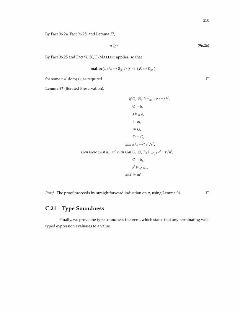
250
By Fact 96.24, Fact 96.25, and Lemma 27,
n � 0 (96.26)
By Fact 96.25 and Fact 96.26, E-MALLOC applies, so that
malloc(v)/s ,! 0|1|/s[r 7! (Z 7! 0|0|)]
for some r /2 dom(s), as required.
Lemma 97 (Iterated Preservation).
If G, ∆, h `m, I e : t/h0,
∆ ✏ h,
s ✏m h,
✏ m,
✏ G,
D ✏ G,
and e/s ,!n e0/s0,
then there exist hs, m0 such that G, ∆, hs `m0 , I e0 : t/h0,
∆ ✏ hs,
s0 ✏m0 hs,
and ✏ m0.
Proof. The proof proceeds by straightforward induction on n, using Lemma 94.
C.21 Type Soundness
Finally, we prove the type soundness theorem, which states that any terminating well-
typed expression evaluates to a value.
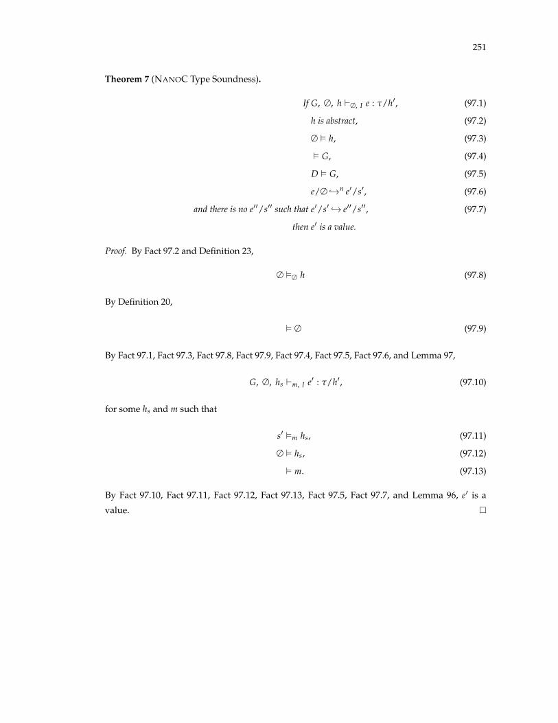
251
Theorem 7 (NANOC Type Soundness).
If G, ∆, h `∆, I e : t/h0, (97.1)
h is abstract, (97.2)
∆ ✏ h, (97.3)
✏ G, (97.4)
D ✏ G, (97.5)
e/∆ ,!n e0/s0, (97.6)
and there is no e00/s00 such that e0/s0 ,! e00/s00, (97.7)
then e0 is a value.
Proof. By Fact 97.2 and Definition 23,
∆ ✏∆ h (97.8)
By Definition 20,
✏ ∆ (97.9)
By Fact 97.1, Fact 97.3, Fact 97.8, Fact 97.9, Fact 97.4, Fact 97.5, Fact 97.6, and Lemma 97,
G, ∆, hs `m, I e0 : t/h0, (97.10)
for some hs and m such that
s0 ✏m hs, (97.11)
∆ ✏ hs, (97.12)
✏ m. (97.13)
By Fact 97.10, Fact 97.11, Fact 97.12, Fact 97.13, Fact 97.5, Fact 97.7, and Lemma 96, e0 is a
value.


![Buss Comm1[1]](https://img.pdfslide.us/doc/110x75/577ce35a1a28abf1038be5ce/buss-comm11.jpg)