Embed Size (px)
Citation preview

UNIVERSITY OF CALGARY
H∞ Model Predictive Control -
Theory and Application
by
Antal Soós
A THESIS
SUBMITTED TO THE FACULTY OF GRADUATE STUDIES
IN PARTIAL FULFILMENT OF THE REQUIREMENTS FOR THE
DEGREE OF DOCTOR OF PHILOSOPHY
DEPARTMENT OF ELECTRICAL AND COMPUTER
ENGINEERING
CALGARY, ALBERTA
April, 2005
© Antal Soós 2005
UNIVERSITY OF CALGARY
FACULTY OF GRADUATE STUDIES
The undersigned certify that they have read, and recommend to the Faculty of Graduate
Studies for acceptance, a thesis entitled “H∞ Model Predictive Control - Theory and
Application” submitted by Antal Soos in partial fulfillment of the requirements for the
degree of Doctor of Philosophy.
________________________________________________Supervisor, Dr. Om P. MalikDepartment of Electrical and Computer Engineering
________________________________________________Dr. Ed NowickiDepartment of Electrical and Computer Engineering
________________________________________________Dr. David WestwickDepartment of Electrical and Computer Engineering
________________________________________________Dr. Qiao SunDepartment of Mechanical and Manufacturing Engineering
________________________________________________External Reader, Dr. Tongwen ChenDepartment of Electrical and Computer EngineeringUniversity of Alberta
Date: 2005 04 15 Calgary,
ii

Abstract
Future industrial systems will require control systems to be more reliable, autonomous,
robust, and yet efficient. The emphasis of this thesis is to introduce a robust control algo-
rithm definition that addresses the needs of future industrial environments. The proposed
controller is based on an adaptive concept with a two-step approach. In step one, the sys-
tem model is identified in a closed-loop by a robust technique. In step two, the obtained
system model from step one is used to formulate a robust controller.
The system identification is the central part of the controller design since the controller
can only be as good as the model that is used to design it. In order to improve the perfor-
mance and robustness of the system identification, this thesis proposes expert system
supervised multiple system identifications. The role of the expert system is to periodically
evaluate the estimated models and to propose one for the controller design.
The robust controller is formulated by the H∞ (sub)optimal design procedure using the
proposed system model. The idea behind this controller design technique is to combine an
on-line identification algorithm with a control design method that yields a time-varying
controller which follows the changing plant.
The effectiveness of the proposed robust controller in an industrial environment is
demonstrated by simulation and experimental tests. The proposed robust controller as a
power system stabilizer has been tested by simulations on a power system model and in
the experimental environment using the micro-synchronous generator at the University of
Calgary.
iii

Acknowledgements
I would like to take this opportunity to thank all those people who have helped me
along the path to the completion of this research thesis.
I am deeply grateful to my supervisor, Dr. O. P. Malik, for his guidance and encourage-
ment. His enthusiasm and insightful criticism has been inspiring and motivating through-
out this study. Dr. Malik has been a wonderful mentor and he was the one who directed my
attention to the concept of a multiple model system identification. This idea has deter-
mined the direction of my research and added another dimension to the final product.
Some colleagues and friends have been particularly kind in their willingness to impart
ideas and information relevant to my research. I would like to acknowledge
Dr. Ramakrishna Gokaraju for his help in decoding the cryptic language of power engi-
neers. Mr. Zsigmond Poda supported me with his ideas stemming from his in depth
knowledge and expertise in the electrical design of embedded controllers. I am also
indebted to Mr. Howard R. Patton, a family friend, who has devoted hours of meticulous
reading to the editing of my drafts.
Research of this kind could not have been completed without the assistance provided
by the technical support team at Texas Instruments Inc. Their prompt replies to my inquir-
ies and professionalism helped me through the process of transferring developed software
to the experimental environment.
Finally, my deepest thanks goes to my family for their understanding and patience.
They have tolerated many late nights and lost weekends. I would not have completed this
thesis without them.
iv

Table of Contents
Abstract .................................................................................................................iii
Acknowledgements ...............................................................................................iv
Table of Contents ...................................................................................................v
List of Tables .......................................................................................................xiv
List of Figures ......................................................................................................xv
Operators and Notational Conventions ............................................................xxi
General notation practices .................................................... xxi
Abbreviations and acronyms .............................................. xxiii
Symbols used in text .......................................................... xxvi
1 Introduction............................................................................................................1
1.1 Control .........................................................................................................1
1.1.1 Modern Control................................................................................2
1.1.2 System Identification .......................................................................4
1.1.3 Model Predictive Control.................................................................7
1.2 Application of the Proposed Approach........................................................8
1.2.1 The Power System ...........................................................................9
1.2.2 Nature of Power System Oscillations ............................................10
v

1.2.3 Power System Stability Modelling ...............................................11
1.2.4 Steady-State Stability ....................................................................12
1.2.5 Dynamic Stability .........................................................................13
1.2.6 Synchronizing Oscillations ...........................................................14
1.2.7 Damping Controls.........................................................................15
1.3 Thesis Objective ........................................................................................18
1.4 Contribution of the Thesis and Novelty.....................................................19
1.5 Outline of the Contents ..............................................................................22
Part - I ..................................................... System Identification 24
2 Introduction to System Identification ...............................................................25
2.1 Control Oriented System Identification.....................................................26
2.2 System Identification by Multiple Models ................................................29
2.3 Model Set Definition .................................................................................30
2.4 Practical Stability .......................................................................................34
2.5 Theory for Model Selection.......................................................................39
2.6 Implementation of Model Selection ..........................................................43
2.6.1 Prediction Error Calculation ..........................................................43
2.6.2 Parametric Error Estimation ..........................................................45
Approximation by the mean square error ...............................45
Approximation by the prediction error ...................................47
2.6.3 Decision Process Formulation .......................................................48
2.7 Linear System Model.................................................................................50
vi
3 Parameter Estimation Strategies ........................................................................53
3.1 H2 Approach to System Identification.......................................................56
3.2 H∞ Approach to System Identification ......................................................59
3.2.1 Least Mean Squares (LMS) Algorithms.......................................60
3.3 Worst-Case Estimation...............................................................................63
3.4 Kalman Filter Based System Identification ...............................................67
3.5 Array Algorithms for System Identification..............................................71
3.5.1 QR-RLS Algorithm........................................................................73
3.5.2 IQR-RLS Algorithm ......................................................................73
3.5.3 QR-LMS Algorithm.......................................................................74
Part - II ............................................................. Robust Control 78
4 Preliminary to Robust Control ...........................................................................79
4.1 Uncertainty in Plant Model........................................................................80
4.2 Linear Fractional Transformation ..............................................................81
4.3 Small Gain Theorem..................................................................................83
4.4 All Stabilizing Controllers .........................................................................86
5 Fundamentals of Game Theory ..........................................................................89
5.1 Discrete-Time Dynamic Game ..................................................................89
5.2 Zero-Sum Dynamic Games .......................................................................93
5.2.1 Optimal Solution for Discrete-Time Dynamic Game....................95
5.3 Certainty Equivalence Principle ................................................................99
vii

5.4 Finite-Horizon Discrete-Time Linear System..........................................104
6 Measurement Feedback H∞ Controller ........................................................... 111
6.1 Standard H∞ Control Problem .................................................................111
6.2 Finite Horizon Suboptimal H∞ Controller ...............................................114
6.2.1 Preliminary Assumptions for the Control ....................................115
Controllability condition ......................................................115
Observability condition ........................................................115
Injective condition for G ......................................................115
Surjective condition for E ....................................................116
Surjective condition for [A D] ..............................................116
Injective condition for [AT HT]T ..........................................117
6.2.2 Selection of γ................................................................................117
6.2.3 The H∞ Algorithm .......................................................................120
6.2.4 Step-by-Step Implementation ......................................................126
6.2.5 The Riccati Recursion..................................................................128
6.3 Implementation Example.........................................................................130
6.3.1 First Tryout ..................................................................................135
6.3.2 Second Tryout ..............................................................................143
7 Model Predictive Control ..................................................................................152
7.1 Requirements for Stability .......................................................................156
7.2 Robust MPC for Non-Linear Systems .....................................................159
7.3 Essentials of the Recursive Implementation............................................162
viii

Part - IIISimulation Studies .....................................................165
8 Single-Machine Infinite-Bus System ................................................................166
8.1 Introduction..............................................................................................167
8.2 Multimodel System Identification ...........................................................169
8.2.1 System Model ..............................................................................169
The implemented algorithms ................................................170
Generator’s operating point ..................................................171
8.2.2 Moving Average Calculation .......................................................172
8.2.3 Quadratic Moving Average Calculation ......................................173
8.2.4 Maximum Residual Amplitude....................................................174
8.2.5 Parameter Vector’s Mean Square Error Estimation ....................175
8.2.6 Reminiscence Function................................................................178
8.3 Control Test Results.................................................................................183
8.3.1 Weight Selection for H∞ MPC.....................................................183
8.3.2 CPSS Parameter Tuning ..............................................................184
8.3.3 Full Load Test ..............................................................................185
8.3.4 Light Load Test ............................................................................189
8.3.5 Leading Power Factor Test ..........................................................191
8.3.6 Transient Stability Test ................................................................193
8.4 Summary..................................................................................................194
9 Multi-Machine Power System...........................................................................196
9.1 Introduction..............................................................................................196
ix

9.2 Five-Machine Power Model ....................................................................197
9.3 Simulation Studies for H∞ MPC..............................................................200
9.3.1 PSS on One Generator .................................................................201
9.3.2 PSS on Three Generators .............................................................202
9.3.3 Mixed System with CPSS and H∞ MPC .....................................203
9.3.4 Three Phase to Ground Fault Test................................................205
9.3.5 New Operating Condition Test ....................................................206
9.4 Summary..................................................................................................207
Part - IV ................................................... Experimental Tests 208
10 Real-Time Test Environment ............................................................................209
10.1 Power System Model ...............................................................................210
10.1.1 Turbine Model ............................................................................211
10.1.2 Generator Model ..........................................................................212
10.1.3 Transmission Line Model ............................................................213
10.2 Embedded Controller ...............................................................................214
10.2.1 Analog Interface Card..................................................................215
10.2.2 Enhancement of A/D Conversion ................................................218
10.2.3 Digital Interface Card ..................................................................220
10.2.4 Embedded Software....................................................................222
10.3 Power System Stabilizer Implementation................................................225
10.3.1 Excitation System ........................................................................226
10.3.2 Conventional Power System Stabilizer (CPSS)...........................230
x

11 Real-Time Tests ..................................................................................................232
11.1 System Identification of the Power System Model .................................232
11.1.1 Comparison of System Identifications.........................................233
RLS algorithm ......................................................................234
LMS algorithm .....................................................................235
WCE algorithm ....................................................................236
Kalman Filter ........................................................................237
IQR algorithm ......................................................................237
FQR algorithm .....................................................................238
QRL algorithm .....................................................................239
11.1.2 Selection by the Expert System ...................................................240
11.1.3 The Proposed PRO Model ...........................................................241
11.1.4 Using the PRO Model for Controller Calculation .......................242
11.1.5 Conclusion for the System Identification ....................................243
11.2 Voltage Reference Step Change...............................................................243
11.2.1 Experiment 1................................................................................244
11.2.2 Experiment 2................................................................................246
11.2.3 Experiment 3................................................................................247
11.3 Input Torque Step Change ......................................................................249
11.3.1 Experiment 4................................................................................249
11.3.2 Experiment 5................................................................................252
11.3.3 Experiment 6................................................................................253
11.4 Three-Phase to Ground Fault Test ...........................................................255
xi

11.4.1 Experiment 7................................................................................255
11.4.2 Experiment 8................................................................................258
11.4.3 Experiment 9................................................................................259
11.5 Summary..................................................................................................260
11.5.1 Experiment 10..............................................................................261
12 Conclusions and Recommendation ..................................................................263
12.1 Conclusions..............................................................................................263
12.2 Recommendation for Future Research ....................................................266
13 References...........................................................................................................270
Appendix A -Single-Machine Power System .............................................294
A.1 Generator Model ......................................................................................294
A.2 IEEE ST1A AVR and Exciter .................................................................297
A.3 IEEE PSS1A Conventional PSS ..............................................................299
A.4 Governor Transfer Function ....................................................................301
Appendix B - Multi-Machine Power System Model ..................................302
B.1 Generator Model ......................................................................................302
B.2 Operating Conditions and Loads for Operating Point #1 ........................304
B.3 Operating Conditions and Loads for Operating Point #2 .......................305
Appendix C -QR Factorization ...................................................................306
Appendix D -The Lyapunov Equation........................................................308
xii

Lyapunov theory ...................................................................310
Second norm of the observations theorem ...........................310
l2 space definition ................................................................311
Appendix E -Discrete-Time System Theory...............................................312
E.1 Stability of Discrete-Time Systems .........................................................312
Stability theorem ..................................................................312
E.2 Stabilizability of Discrete-Time Systems ................................................313
Stabilizability theorem .........................................................313
E.3 Controllability of Discrete-Time Systems ...............................................313
Controllability theorem ........................................................313
E.4 Observability of Discrete-Time Systems.................................................314
Observability theorem ..........................................................315
E.5 Detectability of Discrete-Time Systems ..................................................316
Detectability theorem ...........................................................316
Appendix F -Test for Positive Definiteness................................................317
Appendix G -ARMA Model Stability Test.................................................318
Index ...................................................................................................................319
xiii

xiv
List of Tables
Table 8-1 Disturbance sequence for the system identification tests ........................171
Table 10-1 Characteristic components of the A2D2A card .......................................215
Table 10-2 AVR parameters used in experimental tests............................................230
Table 10-3 CPSS parameters used in experimental tests ...........................................231
Table 11-1 Parameters in system identifications........................................................234
Table A-1 Generator parameters used in simulation................................................ 297
Table A-2 AVR and exciter parameters used in simulation ..................................... 299
Table A-3 CPSS parameters used in simulation ...................................................... 300
Table A-4 Governor parameters used in simulation ................................................ 301
Table B-1 Generator parameters .............................................................................. 302
Table B-2 AVR and simplified ST1A exciter parameters........................................ 303
Table B-3 Governor parameters............................................................................... 303
Table B-4 Transmission line parameters.................................................................. 304
Table B-5 Power flow parameters ........................................................................... 304
Table B-6 Load parameters...................................................................................... 305
Table B-7 Power flow parameters for 2nd operating point ...................................... 305
Table B-8 Load parameters for 2nd operating point................................................. 305

List of Figures
Figure 1-1 Parameter adaptive controller - model predictive controller...................... 7
Figure 2-1 Observation of an unknown system ......................................................... 26
Figure 2-2 Closed-loop system identification............................................................ 27
Figure 2-3 Control relevant frequency range............................................................. 28
Figure 2-4 Multiple model system identification....................................................... 29
Figure 2-5 Model uncertainty set estimation ............................................................. 32
Figure 2-6 Definition of finite time stability.............................................................. 38
Figure 2-7 Decision points on the timeline................................................................ 42
Figure 2-8 System identification................................................................................ 44
Figure 3-1 Feasible parameter set for the WCE......................................................... 65
Figure 4-1 Plant modelling ........................................................................................ 80
Figure 4-2 Plant model with uncertainty ................................................................... 82
Figure 4-3 Small gain theorem model ....................................................................... 83
Figure 4-4 Controller Q parametrization .................................................................. 87
Figure 5-1 Two-player control system model ............................................................ 93
Figure 5-2 Performance index for the game ............................................................ 101
xv

Figure 6-1 Measurement feedback control system TK ............................................ 112
Figure 6-2 Infimum search ....................................................................................... 118
Figure 6-3 Search algorithm for γ............................................................................. 120
Figure 6-4 ACC benchmark problem ....................................................................... 130
Figure 6-5 Open loop system response with nominal parameters............................ 132
Figure 6-6 Additive and multiplicative perturbations ............................................. 134
Figure 6-7 First tryout: Test Group I ....................................................................... 138
Figure 6-8 First tryout: Test Group II ...................................................................... 139
Figure 6-9 First tryout: Test Group III...................................................................... 141
Figure 6-10 First tryout: Test Group IV .................................................................... 142
Figure 6-11 Second tryout: Test Group I ................................................................... 145
Figure 6-12 Second tryout: Test Group II.................................................................. 147
Figure 6-13 Second tryout: Test Group III ................................................................ 148
Figure 6-14 Second tryout: Test Group IV................................................................ 150
Figure 7-1 Model predictive control strategy - pointwise ........................................ 153
Figure 7-2 Model predictive control strategy - intervalwise .................................... 154
Figure 7-3 MPC as a multi-tasking function ............................................................ 155
Figure 7-4 Practical stability..................................................................................... 158
Figure 8-1 System model used in the simulation studies ......................................... 168
Figure 8-2 Moving average of the residuals ............................................................. 173
Figure 8-3 Quadratic moving residuals .................................................................... 174
Figure 8-4 Maximum residual amplitude ................................................................. 175
xvi

Figure 8-5 Forbenius norm of the identified parameter variance ............................. 177
Figure 8-6 Performance index for all algorithms ..................................................... 179
Figure 8-7 System model selection index................................................................. 180
Figure 8-8 Identified ai parameters........................................................................... 181
Figure 8-9 Identified bi parameters .......................................................................... 181
Figure 8-10 System model prediction error for the PRO model ................................ 182
Figure 8-11 Mechanical power reference step change of +/- 0.05 pu ....................... 185
Figure 8-12 Electrical power change for mechanical torque change ......................... 186
Figure 8-13 Control action for an average disturbance .............................................. 186
Figure 8-14 Terminal voltage during three phase to ground fault .............................. 187
Figure 8-15 Control action for a large disturbance..................................................... 188
Figure 8-16 Terminal voltage for exciter reference changes ...................................... 188
Figure 8-17 Control action for small disturbances ..................................................... 189
Figure 8-18 Response to a +/- 0.15 pu step change of torque in light load test ......... 190
Figure 8-19 Voltage reference step changes in light load test .................................... 191
Figure 8-20 Response to a +/- 0.15 pu step change of torque in lead load test .......... 192
Figure 8-21 Voltage reference step changes in a lead load test .................................. 193
Figure 8-22 Bus three phase to ground fault test in overload condition..................... 194
Figure 9-1 Network topology for a five-machine power system.............................. 198
Figure 9-2 Multi-mode oscillations in a multi-machine power system.................... 199
Figure 9-3 System response with PSS installed on G3 ............................................ 202
xvii

Figure 9-4 System response with PSS installed on G1, G2 and G3......................... 203
Figure 9-5 System response with a mixed CPSS and MPC installed....................... 204
Figure 9-6 System response to three phase to ground fault test ............................... 205
Figure 9-7 Three phase to ground fault test in a new operating condition ............... 206
Figure 10-1 PSS development environment ............................................................... 209
Figure 10-2 Laboratory power system configuration ................................................. 210
Figure 10-3 DC motor as a turbine model .................................................................. 211
Figure 10-4 Micro-synchronous generator model ...................................................... 212
Figure 10-5 π section .................................................................................................. 213
Figure 10-6 Embedded controller............................................................................... 214
Figure 10-7 A2D2A signal diagram ........................................................................... 216
Figure 10-8 A2D2A conversion and access timing diagram...................................... 217
Figure 10-9 Data flow between A2D2A and the DSK1............................................. 218
Figure 10-10 Digital interface signal diagram.............................................................. 221
Figure 10-11 Rotational speed deviation estimation .................................................... 222
Figure 10-12 DSK-1 program allocation and execution .............................................. 223
Figure 10-13 DSK-2 program allocation and execution .............................................. 224
Figure 10-14 Tests on power system model ................................................................. 225
Figure 10-15 Excitation system with AVR and PSS ................................................... 226
Figure 11-1 Residual comparison between RLS and PRO........................................ 235
Figure 11-2 Residual comparison between LMS and PRO....................................... 236
Figure 11-3 Residual comparison between WCE and PRO ...................................... 236
xviii

Figure 11-4 Residual Comparison between KF and PRO......................................... 237
Figure 11-5 Residual comparison between IQR and PRO ........................................ 238
Figure 11-6 Residual comparison between FQR and PRO ....................................... 239
Figure 11-7 Residual comparison between QRL and PRO....................................... 239
Figure 11-8 Source selection for the PRO.................................................................. 240
Figure 11-9 The autoregressive parameters of the PRO model.................................. 241
Figure 11-10 The moving average parameters of the PRO model ............................... 241
Figure 11-11 The infimum of the H∞ controller........................................................... 242
Figure 11-12 Terminal voltage change in Experiment 1 .............................................. 244
Figure 11-13 Speed deviation in Experiment 1 ............................................................ 245
Figure 11-14 Control signal in Experiment 1 ............................................................... 245
Figure 11-15 Speed deviation in Experiment 2 ............................................................ 246
Figure 11-16 Control action in Experiment 2............................................................... 247
Figure 11-17 Speed deviation in Experiment 3 ............................................................ 248
Figure 11-18 Control action in Experiment 3............................................................... 248
Figure 11-19 Electric power in Experiment 4 ............................................................. 249
Figure 11-20 Speed deviation in Experiment 4 ............................................................ 250
Figure 11-21 Control action in Experiment 4............................................................... 251
Figure 11-22 System identification during Experiment 4 ............................................ 251
Figure 11-23 Speed deviation in Experiment 5 ............................................................ 252
Figure 11-24 Control action in Experiment 5............................................................... 253
Figure 11-25 Speed deviation in Experiment 6 ............................................................ 254
xix

Figure 11-26 Control action in Experiment 6............................................................... 254
Figure 11-27 Terminal voltage change during Experiment 7....................................... 256
Figure 11-28 Speed deviation in Experiment 7 ............................................................ 256
Figure 11-29 Control action in Experiment 7............................................................... 257
Figure 11-30 System identification in Experiment 7.................................................... 257
Figure 11-31 Speed deviation in Experiment 8 ............................................................ 258
Figure 11-32 Control action in Experiment 8............................................................... 259
Figure 11-33 Speed deviation in Experiment 9 ............................................................ 259
Figure 11-34 Control action in Experiment 9............................................................... 260
Figure 11-35 Speed deviation in Experiment 10 .......................................................... 262
Figure 11-36 Control action in Experiment 10............................................................. 262
Figure A-1 Mathematical model for the power system............................................. 294
Figure A-2 AVR and exciter model........................................................................... 298
Figure A-3 IEEE standard power system stabilizer .................................................. 300
Figure A-4 Governor in a power system ................................................................... 301
xx

Operators and Notational Conventions
General notation practices.
in general, subscript refers to the time
subscript refers to the present time
superscript refers to the element
sequence with sampling
complex number,
function of argument x
p-norm, p = 1, 2 and ∞
rank(A) rank of matrix A
Riccati recursion
mse() mean square error
inf infimum operator is the greatest lower bound. It is lower than the value under
consideration, example: ;
i i t iT=
n n t nT=
k k
° Ts n 0 1 …N, ,=
1 j0,–( ) j 1–=
f x( )
° p
Ric ( )
inf 1 1 2⁄ 1 3⁄ …, , , 0=
inf 0 1 1 2⁄ 1 3⁄ …, , , , 0=
xxi

sup supremum operator is the least upper bound
min minimum operator, example: ;
max maximum operator,
Kronecker’s delta operator ( )
transpose of matrix
inverse of matrix
integer numbers
optimizes the least squares of the error
H_infinity norm, optimizes the maximum energy gain from the error
pth norm in linear space
space of square sumable vector sequence over the nonnegative integers
computation complexity of an algorithm
eigenvalues of A, the m roots of the characteristic polynomial,
spectral radius, the maximal modulus of the eigenvalues,
min 1 1 2⁄ 1 3⁄ …, , , ∅=
min 0 1 1 2⁄ 1 3⁄ …, , , , 0=
δn j, δn j, 0 if j n≠=
AT A
A 1– A
ℵ
H2
H∞
l p
l 2
O d2( )
p λ( )
p λ( ) det λI A–( )=
ρ A( )
ρ A( )max
1 i m≤ ≤λi=
xxii

for , means that is a symmetric and positive definite,
backward shift operator
real numbers, real matrix dimension pxq (p rows, q columns)
complex numbers
for all
Abbreviations and acronyms.
A/D Analog to Digital converter
A2D2A analog interface card: A/D and D/A converter
AC Alternating Current
ACC American Control Conference
APSS Adaptive PSS
AR Auto Regressive model
ARMA Auto Regressive Moving Average model
ARMAX Auto Regressive Moving Average model with an eXogenous signal
AVR Automatic Voltage Regulator
CPSS Conventional Power System Stabilizer
D/A Digital to Analog converter
DARE Discrete-time Algebraic Riccati Equation
DC Direct Current, constant part of a signal
P 0> P ℜ∈ p p× P p λ( ) 0>
q 1–
ℜp q×
ℑ ℜ iℜ,( )
∀
xxiii

DSK DSP Starter Kits
DSP Digital Signal Processor
EWMA Exponentially Weighted Moving Average
FIR Finite Impulse Response
FQR Recursive Fast QR RLS algorithm
Gi Generator number i
GPC Generalized Predictive Control
KF Kalman Filter
KFA modified version of the Kalman Filter
IEEE Institute of Electrical and Electronics Engineers
IQR-RLS Inverse QR estimation algorithm
IQR Inverse QR RLS algorithm
Li electrical Load number i
LED Light Emitting Diode
LFT Fractional Transformation
LMS Least Mean Squares algorithm
LQ Linear Quadratic controller
LQG Linear Quadratic Gaussian controller
LQGR Linear Quadratic Gaussian Regulator
LQR Linear Quadratic Regulator
LS Least Squares
xxiv

LTI Linear Time Invariant process
MA Moving Average mode
MIMO Multiple-Input/Multiple-Output
MPC Model Predictive Controller
NoC No Controller
PID Proportional Integral Derivative controller
PLD Programable Logic Device
PRO Proposed model by the expert system
PSS Power System Stabilizer
QL algorithm produces a lower triangular matrix where the Left of the matrix is
non zero
QR-LMS QR based LMS algorithm
QR algorithm produces an upper triangular matrix where the Right of the matrix
is non zero
QR-RLS conventional QR estimation algorithm
RHC Receding-Horizon Control
RLS Recursive Least Squares algorithm
SISO Single-Input/Single-Output
TCR Time Constant Regulator
USA United States of America
WCE Worst-Case Estimation algorithm
un 0=
Q
Q
xxv

ZOH Zero-Order-Hold
Symbols used in text.
This list contains symbols that have some global use. Some of the symbols may have
another local meaning.
state transition matrix
intermediate matrix for the optimization algorithm
intermediate matrix for the optimization algorithm
input gain matrix
measurement matrix
weighting matrix in controller optimization
damping coefficient (representing the mechanical as well as the electrical
damping effect) for the power system
weighting matrix in controller optimization
infinite-bus voltage
control signal gain matrix of the state estimator for the controller
state transition matrix of the state estimator for the controller
system output gain matrix of the state estimator for the controller
An
A H∞
A H∞
Bn
Cn
D H∞
Di
E H∞
E0
Fu H∞
Fx H∞
Fy H∞
xxvi

weighting matrix in controller optimization
transfer function of the unknown physical system
continuous time system observed in intervals
discrete transfer function for system dynamics
weighting matrix in controller optimization
discrete error model
information space of the player
state-measurement (-observation) equation,
entropy integral of
cost function
cost function for two-player zero-sum game
upper value of the cost function for two-player zero-sum game
lower value of the cost function for two-player zero-sum game
optimal solution for the game
RLS algorithm gain
players’ set, , used to distinguish between the actors in
the game
G H∞
G t( )
GTst( ) Ts
G θ Ts,( )
H H∞
H θ Ts,( )
Hnk
hnk yn
k hnk xn( )=
Id TK γ,( ) TK~ ejω( ) TK∗ e j– ω( )=
Ji
J u ω x, ,( )
J
J
J∗
KRLS n,
K K 1 … k … K, , , , =
xxvii
controller gain matrix for the controller
intermediate matrix for the optimization algorithm
cost functional of player
space in which the signal is square sumable and the sum is finite
average of the signal’s absolute value in linear space
maximum value from the linear space
linear space of a signal observed at N data point
information state
performance index for the th estimation algorithm
reminiscence, , of the adaptive algorithm
constant (DC) model order: 0 or 1
autoregressive (AR) model order
moving average (MA) model order
estimated system model
data sequence size
stages of the game, , where is the maximum possible
number of moves by a player
Kx H∞
L H∞
Lk
L2
l 1
l ∞
l RN( )
L xn( )
Lk θnk φn,( ) k
LΣk R xn( ) k-th
md
ma
mb
M θ( )
N
N N 0 … n … N, , , , = N
xxviii

zero vector
zero matrix
player
pu per unit a normalized value used in power engineering
solution matrix of the algebraic Riccati equation for the controller
intermediate matrix for the optimization algorithm
intermediate matrix for the optimization algorithm
solution matrix of the algebraic Riccati equation for the state estimation
RLS estimated error covariance of the system parameter vector
electrical power
turbine mechanical power applied to rotor
intermediate matrix for the optimization algorithm
process-noise matrix at the KF
free parameters at admissible controllers to form the set of all stabilizing con-
trollers
intermediate matrix for the optimization algorithm
reference signal for system operation
reminiscence function
o
O
Pk
PC
Pn 1+F H∞
PnC H∞
PF
PRLS n,
Pe
PMi
Q H∞
Qn
Q∞
Q H∞
rn
R xn( )
xxix

estimated error variance of the predicted system output
covariance matrices for measurement-noise at the KF
intermediate matrix for the optimization algorithm
intermediate matrix for the optimization algorithm
true system
desired system output at the KF
impulse moment of the rotor
plant with the closed-loop control system, transfer function from
strategy for identification
sampling interval
system state estimation function
discrete time control variable
control set of player at stage
saddle-point solution or noncooperative equilibrium
value function of the game
generator’s terminal voltage
discrete Lyapunov function for model stability analysis
RRLS n,
Rn
R H∞
S H∞
S
sn Rq∈
Tωi
TK ωn zn→
Ti
Ts
T un 1– yn 1– xn, ,( )
un
Unk Pk n
u∗ ω∗,( )
Vn xn( )
Vt
Vn θn vn,( )
xxx

residual sequence at the system identification
additive disturbance acting on the output of the system
intermediate matrix for the optimization algorithm
, weighting factors
space where the disturbance trajectory lies
intermediate matrix for the optimization algorithm
intermediate matrix for the optimization algorithm
state set (space) of the game
terminal constraint set
initialization matrix of the algebraic Riccati equation for the controller
initialization matrix of the algebraic Riccati equation for the state estimation
state variable vector in discrete time
discrete time measurement variable, system output
observation set
space where the measurements trajectory lies
measurement, measurement equation,
observed discrete data sequence
νn
vnx
V H∞
Wθ Wv
W
W H∞
W H∞
X
Xf
XC
XF
xn
yn
Ynk
Y
ynk yn
k hnk xn( )=
ZN
xxxi

discrete time regulated signal
intermediate matrix for the optimization algorithm
intermediate matrix for the optimization algorithm
intermediate matrix for the optimization algorithm
phase angle lead (load angle)
small positive constant/magnitude bounds at WCE
closed-loop norm bound of the controller
infimum, the lower limit on the minimum achievable norm for
strategy set (space) of the player
intermediate matrix for the optimization algorithm
inverse of the innovation variance matrix for the controller
solution of the Lyapunov equation, matrix
solution of the Lyapunov equation, matrix
model uncertainty
information structure of the game.
“true system” parameters
linear model parameters
zn
∆F H∞
∆C H∞
∆S H∞
δi
δ
γ H∞
γ∗ γ
Γnk
Γn 1+C H∞
ΓnF H∞
ΠF
ΠC
∆ ∆ G θ T,( ) GT t( )–=
ηnk
θ0
θn θn a1…amab1…bmb
c1…cmc,,[ ]T=
xxxii

rotation matrix in QR decomposition
model uncertainty set
bound on the variable
observation vector for the linear model
positive weighting coefficients
intermediate matrix for the optimization algorithm
intermediate matrix for the optimization algorithm
forgetting factor in estimation algorithm,
learning rate, adaptation constant at the LMS algorithm
learning rate, adaptation constant at the LMS algorithm
positive weighting sequence at WCE
feedback controller
measurement vector
correlation matrix at QR algorithm
generator’s rotational speed deviation
inputs to the model which interpret the effects of the model uncertainty
ΘR
Θ
θ∇MAX θ∇
φn
φn [ yn 1– …,– yn ma– u, n 1– …un mb– ,vn 1– …vn mc– ]T,,–=
κ2 κ, ∞ κσ, κ, Σ
Λn 1+C H∞
ΛnF H∞
λ 0 λ« R 1≤
µLMS
µLMS
ρn
ΣK T( ) ΣK : un K yn⋅=
φn
Φn
∆ω
ωn
xxxiii

1
1 Introduction
Many industrial systems exhibit unsatisfactory natural behavior. These systems are
characterized by inadequate or unstable performance. In order to compensate for the
unsatisfactory natural behavior and to provide the desired stability and performance, a
controller shall be implemented. It is expected that the controller will enhance the effi-
ciency and operation of the system by improving setpoint tracking and disturbance attenu-
ation. In this chapter a brief outline of the design process for a robust control system is
provided.
1.1 Control
In the past, many control tasks have been successfully addressed by the classical con-
trol theory, where the controller is implemented using simple analog technology. Charac-
terized by a certain amount of trial-and-error analysis, this approach to control has
matched well the technology of that period. Classical design algorithms, such as lead-lag
compensation, were not clearly formalized as design problems to be solved, but rather as
tools of practice largely dependent on trial and error processes[1]. With advances in tech-
nology and industrial systems, the demand for more adequate controllers has increased.
The benefits of implementing more advanced control systems in industry are manyfold.

2
These benefits include improved product quality, reduced energy consumption, minimiza-
tion of waste material, and increased system stability.
1.1.1 Modern Control
The first success with adaptive control theory, which addressed the above listed expec-
tations, emerged in 1960s, when Kalman1 published his ground breaking papers [2] and
[3] on linear quadratic feedback control (LQR). The novelty in LQR is the introduction of
the state-space representation of the plant as a general linear system and the use of the Ric-
cati2 differential equation as an algorithm for computing the state feedback gain of the
optimal controller with a quadratic performance criterion [4-6].
The first practical implementation of LQR was in the guidance and maneuvering of
space vehicles. As it turned out, the new optimal control theory was well suited to many of
the control problems that arose from the space program [7]. However, the early success of
the LQR was unable to translate into a widespread industrial implementation mainly
because of the preliminary assumption that the disturbances affecting the plant can be
modelled as stationary stochastic signals with known characteristics. The other weakness
of the LQR is that it does not contain a mechanism to include plant model uncertainty in
the design. These issues are common in industrial environments. Therefore, a need for a
control algorithm which would be less sensitive to plant modelling errors and the lack of
statistical information on the disturbances became evident.
1. Rudolf Emil Kalman, 1930-, Hungarian born mathematical system theorist2. Jacopo Riccati, 1667-1754, Mathematician in Venetian Republic

3
A solution to the above problems was proposed in 1981, when Zames1 published his
pioneering paper [8] on control, which initiated the development of robust control
theory. The fundamental idea of the control theory is that the disturbances effecting the
plant can be modelled as deterministic square integrable signals, where only an upper
bound on the signal power is assumed to be known. The controller is selected in such a
way that it minimizes the disturbance energy gain on the plant output. In other words, the
control theory addresses the issue of worst-case controller design. The designed con-
troller is robust with respect to model uncertainty and deals with unknown disturbances.
Since the publication of [8], control theory has been extensively studied and many
different techniques have been used to develop the control algorithm [9-18]. Among
the various time-domain approaches to this class of worst-case design problems, the one
that uses the framework of dynamic (differential) game theory seems to be the most natu-
ral [19]. In the game theoretical framework, the control problem can be regarded as a
game where nature (the opponent) has access to the unknown exogenous input and the
designer has a choice for the controller. The objective in selecting the controller is to
obtain a design that minimizes a given performance index under the worst possible distur-
bances or parameter variations in the plant model. At the same time, nature (the opponent)
has the objective to maximize the same performance index by controlling the exogenous
input by selecting the worst possible disturbances. In the literature, this is described as the
1. George Zames, 1934-1997, Polish born control theorist, McGill University
H∞
H∞
H∞
H∞
H∞
H∞

4
two player zero-sum game between nature - the maximizing player, and controller - the
minimizing player.
The resulting controller has a state feedback structure where the gains are calcu-
lated by two recursive Riccati equations. One, a backward Riccati recursion, is used to cal-
culate the controller gains. The other, a forward Riccati recursion, is used to calculate the
gain for the state estimator.
The control design obtained under these guidelines is an controller that is less sen-
sitive to plant model parameter variations and more robust to disturbances than in the case
of LQR control. Thus the controller regulates the plant against the worst possible distur-
bances. However, the resulting controller may be overly conservative [20]. Finally, it is
worth noting that the control includes LQR control as a limiting case. More precisely,
as the specified closed-loop norm bound (normally denoted by ) tends to infinity, the
central solution of the control problem converges to the corresponding LQR control
[1].
1.1.2 System Identification
In order to implement the controller, it is required to obtain a linear model of the
plant to be controlled. Since the early 1980s, it has been gradually recognized that the real
challenge of the control engineering is the modelling of the plant to be controlled [1].
Originally, the plant model is derived by formulating the physical laws that describe the
physical process of the plant. In this approach, to successfully obtain the plant model it
H∞
H∞
H∞
γ
H∞
H∞

5
requires not only a thorough understanding of the plant’s physical process but also the
knowledge of it’s parameters. Outside of the research laboratories and space exploration,
most plants are too complicated for this type of modelling. In addition, formulating the
appropriate physical laws can be time consuming, which makes the method economically
not feasible.
These constrains are resolved in the system identification approach, where the model is
constructed by fitting a parameter model to the observed data. The system identification
method is characterized by the fact that the resulting model does not have any physical
interpretation, and it describes only the relationship between the observed input(s) and
output(s) of the plant.
The process of system identification can be also seen as a search for the solution of an
overdetermined system of equations. The overdetermined system is characterized by a sig-
nificantly higher number of equations than variables. In system identification the observed
input-output data corresponds to the equations, while the model parameters stand for the
variables. An exact solution for the overdetermined system does not exist, only an approx-
imate one. The approximate solution is based on a criterion for solution search. In the lit-
erature there are numerous criteria to fit the model parameters to the observed data. The
selected criterion defines the identification method.
Generally, the criterion for solution search is based on minimizing a particular norm of
the error between the output from the estimated model and the observations. There are
three dominant norms in the literature. The first norm criterion is when the criterion is
selected to minimize the average absolute value of the difference between the model and
the observations. The second norm criterion is applied when the parameters for the model

6
are selected in a way to minimize the average squares of the difference between the model
and the observations. The third or infinity norm criterion is implemented when the goal is
to minimize the single largest difference between the model and the observations. These
three types of identification methods are the basis for the different types of algorithms. In
the research literature, a countless number of implementation methods can be found for
identification algorithms.
It is impossible to define the best identification method due to the fact that for the dif-
ferent implementations the criterion for the “best” changes with the particular require-
ments. A system identification that uses many different models simultaneously dismisses
the task of evaluating the best identification method for a particular implementation.
Instead, an expert system is designed which, in real-time, selects the best identification
method from a pool of methods running in parallel. This real-time multi model system
identification is possible due to the advances in computation power.
The controller design that is able to improve the performance of a controlled system by
means of system identification and robust control, begins by recognizing the link and
interaction between modelling and control [21]. The robust control-oriented identification
procedure is a closed-loop identification, where the controller provides relevant informa-
tion on the dynamics of the plant to feedback control. An interactive scheme for modelling
and redesigning of the feedback controllers is described in the following.

7
1.1.3 Model Predictive Control
If the controller is designed using a system model obtained by system identification, it
can be described as parameter-adaptive control. In this approach, the system parameters
are estimated in real-time and used for the controller on-line parametrization, as shown in
Figure 1-1.
Due to the fact that the model with estimated parameters only describes the past obser-
vations of the plant’s input and output, and it only predicts the future behavior, this type of
controller is called model predictive controller (MPC). The term MPC does not designate
a specific control strategy but rather an ample range of control methods, which make
explicit use of a model of the process to obtain the control signal by minimizing the objec-
tive function [22]. In other words, the MPC is an optimal control-based strategy that uses a
plant model to predict the effects of an input sequence on the evolving state of the plant
[23]. In general, the control action of the MPC is calculated by minimizing an objective
Plant
System IdentificationController Parameter Calculation
Controller
State Estimation
r u y
estimated system parameters
controller parameters
Figure 1-1 Parameter adaptive controller - model predictive controller
&

8
function over a given horizon, producing an optimal open-loop control sequence. The first
control in that sequence is applied to the plant until another plant measurement becomes
available. At the next sampling instant, a new optimal control problem is formulated and
solved based on the new measurements [24]. The objective function is defined in terms of
both present and predicted system variables and is evaluated using an explicit model to
predict future process outputs [25].
Overall, the MPC can be summarized as an explicit use of a model for controller for-
mulation, where the controller is calculated by minimizing an objective function. The
resulting controller has a receding strategy characterized by the displacement of the hori-
zon towards the future as new updates from the system become available.
The research in this thesis describes the MPC implementation, where the system
model is obtained in real-time by system identification processes, and it is used to deter-
mine the discrete-time (sub)optimal controller, also in real-time. Each time when an
updated system model is available, an optimal control problem with an control objec-
tive is solved. The resulting controller is utilized until a new update on the system
model becomes available, thereby providing an update to the controller.
1.2 Application of the Proposed Approach
A method for designing an MPC output feedback controller for complex nonlinear
systems is proposed in this thesis. Using this methodology, a power system stabilizer is
H∞
H∞
H∞
H∞
H∞
H∞

9
implemented. Through the implementation process, the MPC is examined to deter-
mine how well it handles model uncertainty, disturbances and measurement noise. The
results are compared to that of a conventional power system stabilizer (CPSS) on the same
benchmark power system model realized in software and on a scaled physical model.
1.2.1 The Power System
Electrical energy has become a major form of energy for end use consumption in
today's society. To make electric energy generation and transmission more economic and
reliable, the trend in electric power production is towards an interconnected network of
transmission lines linking generators and loads into large integrated systems. The power
station sites are selected close to a source of energy, such as large coal mines and water
power sources. Consequently, power transmission lines and networks have to meet the fol-
lowing requirements [26]:
• connect distant power stations in secure parallel operation
• transmit electrical power to large load centers over large distances
• ensure satisfactory parallel operation with other interconnected power systems.
For proper operation, this large integrated system requires a stable operating condition.
Stability in power systems is generally regarded as the ability of the generating units to
maintain synchronous operation [26].
H∞

10
1.2.2 Nature of Power System Oscillations
Smaller power systems have hundreds of kilometers of transmission lines; while the
largest (the eastern USA/Canadian interconnected system) has thousands of kilometers of
transmission lines. Most electric power systems are AC with a frequency that is almost
uniform over the whole network. This is achieved by using synchronous AC generators. In
small systems, there may be only tens of generators; in large systems there are
thousands [27]. System frequency is held within tight limits by governing the speed of the
generator prime movers, and system voltages are maintained by generator excitation sys-
tem control.
Interconnected AC generators produce torques that depend on the relative angular dis-
placement of their rotors. These torques act to keep the generators in synchronism (syn-
chronizing torques). Thus, if the angular difference between generators increases, an
electrical torque is produced that tries to reduce the angular displacement. It is as though
the generators were connected by torsional springs, and, just as in mass-spring systems,
the moment of inertia of the rotors and the synchronizing torques cause the angular dis-
placement of the generators to oscillate following a system disturbance. The angular dis-
placements should settle to values that maintain the required power flows through the
transmission network and supply the system load [27].
If the disturbance is large, for example a prolonged three-phase fault on the transmis-
sion system, the nonlinear nature of the synchronizing torque may not be able to return the
generator angles to a steady state. Some or all generators then lose synchronism and the
system exhibits transient instability. On the other hand, if the disturbance is small, the syn-

11
chronizing torques keep the generators nominally in synchronism, but the generators’ rel-
ative angles oscillate. In a correctly designed and operated system, these oscillations
decay: the system is then called small-signal stable. In an overstressed system, small dis-
turbances may result in oscillations that increase in amplitude exponentially: the system is
then said to be small-signal unstable [28].
Unstable power system oscillations have occurred all over the word in the last 30
years. They appear first when a power system is pressed to supply increasing load. As
transmission lines are loaded more and more, the generators need to rely more heavily on
their excitation systems to maintain synchronism, and at some point, without supplemen-
tary control, the synchronizing oscillations become unstable. Also, during the last 30
years, many power systems have been interconnected in order to enable the exchange of
power. This allows operating cost to be kept at a minimum.
The interconnecting ties between neighboring power systems, although they may not
be overloaded, are often relatively weak when compared to the connections within each
system. The synchronizing torques are lower across these weak ties; and this, coupled
with the high aggregate inertia of each of the systems being interconnected, leads to low
frequency inter-area oscillations. Many of the early instances of oscillatory instability
occurred at low frequencies when these interconnections were made [27].
1.2.3 Power System Stability Modelling
Stability calculation methods have always lagged behind interconnected power system
size, so there has been a continuous striving for suitable simplifications. A kind of

12
“instinctive simplification” was to divide the theoretically unique problem of stability into
two parts: steady-state and transient stability, for which analysis methods have been devel-
oped independently over many years. In the American literature, the steady-state stability
and dynamic stability concept pair is in use. The analytical approach to a synchronous
machine’s fundamental behavior is best modeled by Park's1 reference frame [29], see
Appendix A and B. In order to obtain some appreciation of power system oscillations, it is
important to include a discussion of stability analysis. However, this is not the main pur-
pose of this study.
1.2.4 Steady-State Stability
Steady-state stability analysis is the study of a power system and its generators in
strictly steady state conditions. It is also an attempt to determine the maximum possible
generator load that can be transmitted without loss of synchronism of any one generator.
The maximum power is called the steady-state stability limit.
For an n-machine power system the active power fed in by the ith generator is defined
by the equation
(1.1)
1. R.H. Park, Electrical Engineer, General Electric Company
PEiUpi
2
Zii---------- αiisin Upi
UpjZij-------- δi δj– αij–( )sin
j 1=j i≠
n
∑+=
13
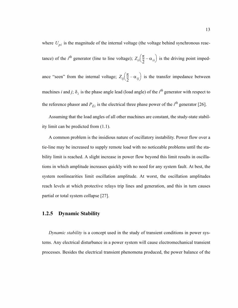
where is the magnitude of the internal voltage (the voltage behind synchronous reac-
tance) of the ith generator (line to line voltage); is the driving point imped-
ance “seen” from the internal voltage; is the transfer impedance between
machines i and j; is the phase angle lead (load angle) of the ith generator with respect to
the reference phasor and is the electrical three phase power of the ith generator [26].
Assuming that the load angles of all other machines are constant, the study-state stabil-
ity limit can be predicted from (1.1).
A common problem is the insidious nature of oscillatory instability. Power flow over a
tie-line may be increased to supply remote load with no noticeable problems until the sta-
bility limit is reached. A slight increase in power flow beyond this limit results in oscilla-
tions in which amplitude increases quickly with no need for any system fault. At best, the
system nonlinearities limit oscillation amplitude. At worst, the oscillation amplitudes
reach levels at which protective relays trip lines and generation, and this in turn causes
partial or total system collapse [27].
1.2.5 Dynamic Stability
Dynamic stability is a concept used in the study of transient conditions in power sys-
tems. Any electrical disturbance in a power system will cause electromechanical transient
processes. Besides the electrical transient phenomena produced, the power balance of the
Upi
Ziiπ2--- αii–
Zijπ2--- αij–
δi
PEi

14
generating units is always disturbed, and thereby mechanical oscillations of machine
rotors follow the disturbance.
To describe the transient phenomena, the well-known swing equation of the synchro-
nous generators, derived from the torque equation for synchronous machine, is used
(1.2)
where is “the impulse moment” of the rotor of the generating unit, is the damp-
ing coefficient (representing the mechanical as well as the electrical damping effect), is
the phase angle (load angle), is the turbine power applied to rotor and is the
electrical power output from the stator [26].
1.2.6 Synchronizing Oscillations
Two types of synchronizing oscillations are common in all interconnected AC power
systems. The first is associated with a single generator (or a plant of identical generators)
acting against the system. The second is more complex and involves generators in one
area of the power system oscillating against other generators in other areas of the power
system. Local or plant modes of oscillations have natural frequencies of about 1 to 2 Hz.
Inter-area modes of oscillation have lower natural frequencies on the order of 0.1 to 0.7
Hz. In small systems, inter-area oscillations generally have higher natural frequencies than
those of large systems [27].
Tω i,t2
2
d
d δi PM i, Kd i, tdd δi PE i,––=
Tω i, Kd i,
δi
PM i, PE i,

15
The total number of modes of synchronizing oscillations is equal to one less than the
number of interconnected generators. In a system having thousands of generators, there
are thousands of modes of oscillation. All of these modes of oscillation must decay fol-
lowing a system disturbance. If any one mode increases in amplitude, the system's opera-
tors would have to take action to prevent either local or system-wide collapse.
Power systems must be designed to be stable under as wide a range of system loads
and operating conditions as possible. Generally, if the operation of the system is con-
strained, those constraints should be due to the thermal operating limits of the transmis-
sion system or loss of synchronism (transient instability) and not due to oscillatory
instability.
To determine the nature of system oscillations, analysis of the following system char-
acteristics is required:
• Frequency and damping of the system’s synchronizing oscillation
• Pattern of generators that take part in each mode of oscillations.
Generators that are able to have a controlling effect on the oscillations must be identi-
fied, and tools must be provided to allow for efficient and robust design of oscillation
damping controls [27].
1.2.7 Damping Controls
Power system stabilizers are the most cost-effective tools for power system oscillation
damping controls. Essentially, they use the power amplification capability of the genera-
tors to generate a damping torque in phase with the speed change. This is achieved by

16
injecting a stabilizing signal into the excitation system voltage reference summing junc-
tion as presented in Figure A-2 in Appendix A.2. The stabilizing signal is most often the
change in generator rotor speed, phase advanced to counteract the phase lag between the
exciter voltage reference and generator electrical torque [27].
Historically, in the late sixties, the need for such devices was demonstrated by some
cases of sustained power swings in the western part of the USA. Subsequent analysis has
shown that these swings were due to poor damping characteristics caused by modern volt-
age regulators of conventional structure, but with comparatively high gain from the stabil-
ity point of view. To compensate for the unwanted effect of these voltage regulators,
additional signals were introduced in the feedback loop of voltage regulators. The addi-
tional signals were mostly speed deviation, AC bus frequency, or accelerating power. The
devices set up to provide these signals through properly chosen transfer functions have
been called “power system stabilizers” [26].
The basic objective of a power system stabilizer is to modulate the generator’s excita-
tion in such a way as to provide additional damping to the electromechanical oscillations
of generating units; thereby improving the steady-state stability of the whole power sys-
tem. To do this the power system stabilizer has to produce a component of electrical
torque in the synchronous machine that is in phase with the speed variation of rotors.
Designing a power system stabilizer is a challenging task because of the highly non-
linear dynamics and strong performance requirements of the power system under the wide
variations in plant parameters. The present industrial control realization is dominated by
the conventional PSS (CPSS) type of control, described in Appendix A.3. The dominance
of CPSS can be explained by the simpleness of the lead-lag compensator implementation

17
and maintenance, using trial and error. However, when a CPSS is used to control a highly
nonlinear process, the controller must be tuned very conservatively in order to provide sta-
ble behavior over the entire range of operating conditions. Conservative controller tuning
can result in serious degradation of control system performance.
There have been problems in the past with power system stabilizers causing steam tur-
bine shaft torsional modes to become unstable, but this risk has been eliminated in many
modern power system stabilizer designs. However, there are still many problems with
installed power system stabilizers that have been introduced by ineffective commissioning
and tuning of the devices. Generally, in systems with both local and inter-area modes,
power system stabilizer parameters are determined through off-line analysis, and tuned
further during commissioning. The validity of the model used in the off-line studies
should be checked on commissioning. Setting power system stabilizers to typical values is
particularly dangerous for systems in which inter-area modes are of concern. It is very
easy for the stabilizer to have a destabilizing effect at low frequencies that cannot be
observed during on-line commissioning tests. Further, it is easy for controller settings to
be inadvertently changed due to nonlinear changes in generators’ and in transmission-
lines’ operating conditions. The models based on original manufacturers’ information may
not be accurate in few years [27]. This problem can be resolved by implementing an
MPC where the nonlinear changes in generators’ and in transmission-lines’ operating con-
ditions is tracked by system identification and the controller is adjusted accordingly.
H∞

18
1.3 Thesis Objective
In this research thesis a new control algorithm with a systematic design procedure is
proposed. This procedure consists of a robust system identification and an suboptimal
control law. The resulting controller is an MPC algorithm. A detailed implementation
process is provided for the MPC, using the finite horizon (sub)optimal control
algorithm derived from the game theory. The controller is calculated using two recur-
sive Riccati equations, one for the controller and one for the state estimator. The conver-
gence of these Riccati recursions is dependent upon the initial values given for the
recursions. Strict specifications for the convergence conditions are provided using
Lyapunov1 equations.
The objective of this study is to present a systematic methodology for building an
MPC algorithm, which is ready for application. The difficulty with the implementation of
MPC is that it requires a sophisticated background in mathematics.
The purpose of this research project is to translate a complex mathematical theory of
control into a format that is easy to comprehend, and to identify how MPC can be suc-
cessfully applied in industrial designs. In the test environment, the MPC is applied as
a power system stabilizer. The role of the applied control algorithm is to solve the power
system stabilizer design problem in the face of nonlinear plant and exogenous distur-
bances.
1. Alexander Mikhailovich Lyapunov, 1857-1918, Russian mathematician
H∞
H∞
H∞ H∞
H∞
H∞
H∞
H∞
H∞

19
By employing digital signal processing techniques more complex control algorithms,
such as the MPC, can be used in a variety of control devices. It is hoped that this
research will make a contribution to the development and application of robust control
implementation.
1.4 Contribution of the Thesis and Novelty
The motivation for this research arose from recent developments in robust control and
control-oriented identification. The main contribution of this thesis is the development of
a robust control-oriented modelling procedure for an unknown plant subsequently fol-
lowed by a robust control design. The model is obtained by a control-oriented system
identification procedure. Although, this model will always be a simplified representation
of the unknown plant, the subsequent robust control is designed to account for the pres-
ence of the modelling error.
The system identification procedure developed in this thesis addresses the problem of
robust identification by using multiple system identification techniques simultaneously
and by selecting the best model through an expert system. The best model is the one which
most likely describes the plant until the expert system’s next decision. In this way, a reli-
able model for a robust controller design is obtained.
In order to achieve the goal of this thesis, the following research areas have been
merged:
• Control relevant system identification of models in closed-loop.
H∞

20
• Expert system design for model selection from the identified set of models.
• Robust control design using model based approach.
Within the above mentioned areas existing results on system identification and robust
controller design techniques have been employed. However, in order to define a robust
control procedure, the following were developed:
• A new expert system, which selects the model that most likely describes the plant in the
future.
• An expert system reminiscence, which is modelled using an exponentially weighted
moving average (EWMA) function.
• A definition of system identification stability, by extending the Lyapunov stability cri-
terion with the practical stability criterion.
• An expert system decision using the Bellman’s1 Principle of Optimality.
• The limits on the initial values for the backward and forward Riccati recursions, to be
used in the (sub)optimal controller optimization algorithm.
• A definition of MPC stability by extending the Lyapunov stability criterion with the
practical stability criterion.
• A new algorithmic description for the implementation of the (sub)optimal control-
ler.
The contribution of this research is that it provides a proof through simulation and
experimental studies that an expert system supervising multiple system identification
leads to a robust system identification, which can be used for robust control in the form of
1. Richard Bellman, 1910-1984, American applied mathematician
H∞
H∞

21
an MPC. The new multi-model MPC has successfully been implemented as a
power system stabilizer. The application of the robust multi-model identification in com-
bination with an control design procedure led to a controller with a guaranteed robust
performance.
As a consequence of the development of the new multi-model MPC, the following
by-products emerged:
• A matrix positivity test algorithm;
• An ARMA model stability test algorithm;
• A median based algorithm to estimate the frequency deviation of the power system.
Also, it has been proven that using the present DSP technology, it is possible to simul-
taneously calculate seven different types of system identification algorithms, namely, the
RLS, LMS, Kalman Filter, three QR based algorithms and the worst-case identification
algorithm along with the (sub)optimal controller, within 33 ms sampling time. The
optimization algorithm for the (sub)optimal controller weight’s calculation and
the model selection expert system, however, run once every second.
In order to achieve a real time implementation of the proposed algorithm, an embed-
ded system has been developed. This embedded system was built from two DSP boards
and from an analog card and a digital interface card.
The thesis is written with the intention to allow an easy usage and implementation of a
MPC algorithm following the steps defined in this research.
H∞ H∞
H∞
H∞
H∞
H∞ H∞
H∞

22
1.5 Outline of the Contents
This thesis is divided into four parts and 12 chapters. The first two parts contain the
theoretical background, while the last two parts present the results from the simulations
and experiments. For ease of reference, a brief summary for each of the chapters is pro-
vided below.
• Part I - “System Identification” This part is divided into Chapters 2 and 3. Chapter 2
describes the underlying theoretical framework used for system identification. In Chap-
ter 3, the idea of a multi-model system identification is introduced in order to imple-
ment a robust system identification. A variety of system identification techniques are
reviewed, which are used as building blocks for a multi model system identification. In
multi model system identification various system identification techniques are imple-
mented in parallel, from which the best is selected periodically in real-time. The selec-
tion process for the best system parameter is investigated and an expert system for this
parameter selection is described.
• Part II - “Robust Control” - This part consists of Chapters 4 - 7. Chapter 4 provides a
brief overview of the robust control theory. Chapter 5 gives a general description of two
player game theory. The game theory is used as the basic theoretical framework for the
control algorithm derivation. In Chapter 6, the algorithmic definition for the dis-
crete time control algorithm is presented. And finally, in Chapter 7, theory for the
MPC is reviewed, where the system identification and the controller calcula-
tion are integrated within the MPC theory.
H∞
H∞
H∞ H∞

23
• Part III - “Simulation Studies” - In this part, the simulation studies are described,
where the MPC is used as a power system stabilizer. The simulation was conducted
on a UNIX system based power system model, which was developed at the University
of Calgary. Part III is divided into two Chapters: first, the “Single-Machine Infinite-Bus
System” simulations are presented followed by the “Multi-Machine Power System”
simulations, in Chapters 8 and 9, respectively.
• Part IV - “Experimental Tests” - In addition to the theoretical investigations and
simulation studies, the behavior of the MPC power system stabilizer is tested in
real-time, on a physical model of a power system. Chapter 10 describes the test envi-
ronment in a format of a power system model located in the Power Research Labora-
tory at the University of Calgary. This power system model, also called a micro
machine power system, consists of a scaled synchronous generator and transmission
line model. Chapter 11 presents the results of the experiments collected from the micro-
machine power system.
H∞
H∞

24
Part - I System Identification
The focus of this thesis is directed to the derivation of dynamic models (system identifi-
cation) to be used for model based (robust) control designs. The aim is to extend previous
research in closed-loop identification in robust control. This research is an experimenta-
tion with the supervisory (model switching) control, in an effort to ensure good adaptation
transients in the presence of large parameter variations.
A robust multi model based system identification is described. The discrete time vary-
ing model of the system is constructed by using the observed input/output data. The pro-
posed technique applies an expert system, which periodically selects a set of system
parameters from those estimated by different adaptive algorithms. Selection is based on
the Principle of Optimality in decision making by analyzing the models’ stability. Adaptive
algorithms with the and norms of index performance and with a “Worst-Case
Estimation” strategy calculate concurrently the discrete models of the system. To improve
computational efficiency and numerical stability of the previously mentioned algorithms,
the QR decomposition approach is employed. The obtained model is a fundamental and an
essential element in the construction of an optimal controller, which has superior adapta-
tion to the system parameter changes.
H2 H∞

25
2 Introduction to System Identification
In order to characterize the relevant systematic dynamic relations of the system to be
controlled, most modern control synthesis methods require some kind of mathematical
model. In general, there are two approaches to the system model construction: white-box
and black-box models [30].
The construction of the white-box or physical modelling of the system requires
detailed knowledge of the physical laws governing the behavior of the system. In this
model, all parameters and variables can be interpreted in terms of physical entities.
In the black-box or experimental approach, a model is constructed from the measured
input and output data using no physical insight whatsoever, and the model parameters are
simply knobs that can be adjusted to optimize the model fit. This modelling approach,
which characterizes any systematic dynamic relations that are present in the system, is
based on experimental data observation and is also called system identification. Despite
the simplistic nature of many black-box models, they are very efficient for modelling
dynamic systems and require less engineering time to construct than white-box models
[31].
The generic problem formulation for system identification using the black-box model
can be described as an observation of the unknown system, , based on the collected
discrete data points, , that consist of the applied input signal, ,
and the observation of the (possibly) disturbed output signal, , as presented in Figure
G t( )
N ZN un yn ,[ ]= un
yn

26
2-1 [21]. The additive disturbance, , acting on the output of the system is used to
model the effects on the observation of that cannot be described by the input ,
applied to the system [32].
The black-box model approach provides satisfactory results in system identification
through its ability to construct models which describe the map from the input to the output
of the system, and to use this map in the design of a feedback controller.
2.1 Control Oriented System Identification
Many systems have to operate under feedback control for safety or productivity rea-
sons [33]. Under feedback control, the input and output of the system
can only be observed in the so called closed-loop condition. Further, in order to track the
system parameter changes during the time of regular system operation, the system identifi-
cation should be performed continuously. This practice of persistent system identification
under feedback control must overcome the correlation between the system input and out-
put. As presented in Figure 2-2, the system output is correlated to the system input due to
vnx
yn un
GTst( ) ynun
vnx
Figure 2-1 Observation of an unknown system
ZN un yn ,[ ]=
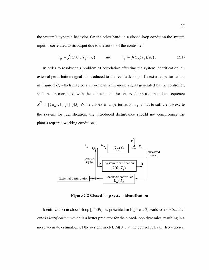
27
the system’s dynamic behavior. On the other hand, in a closed-loop condition the system
input is correlated to its output due to the action of the controller
. (2.1)
In order to resolve this problem of correlation affecting the system identification, an
external perturbation signal is introduced to the feedback loop. The external perturbation,
in Figure 2-2, which may be a zero-mean white-noise signal generated by the controller,
shall be un-correlated with the elements of the observed input-output data sequence
[43]. While this external perturbation signal has to sufficiently excite
the system for identification, the introduced disturbance should not compromise the
plant’s required working conditions.
Identification in closed-loop [34-39], as presented in Figure 2-2, leads to a control ori-
ented identification, which is a better predictor for the closed-loop dynamics, resulting in a
more accurate estimation of the system model, , at the control relevant frequencies.
yn f G θ0 Ts,( ) u, n( )= and un f ΣK Ts( ) yn,( )=
ZN un yn ,[ ]=
GTst( ) yn
un
vnx
Figure 2-2 Closed-loop system identification
Feedback controller
System identification θ
observed signal
control signal
External perturbation
rn
ΣK Ts( )
G θ Ts,( )
M θ( )

28
The control relevant frequency range typically corresponds to the frequencies in the
neighborhood of the cross-over frequency, on the Bode1 plot, of the controlled system
[40]. In other words, the objective of the system identification in the closed-loop is to
achieve better prediction for the closed-loop dynamics via estimation of the system model
on the critical frequencies in the region where the Nyquist2 plot is closest to the critical
point [41], shown in Figure 2-3.
It was found [42] that the models identified in closed-loop are particularly suitable for
model-based robust control design because the controller can have a linearizing effect on a
nonlinear plant’s dynamic behavior at a relevant working point, enabling accurate linear
modelling.
1. Hendrik Wade Bode, 1905-1982, Madison, Wisconsin, Electrical Engineer at Bell lab.2. Harry Nyquist, 1889-1976, Nilsby, Sweden, Electrical Engineer at Bell lab.
1 j0,–( )
-1
ηω=ωs
ω=ωp
ω=ωg
ωp ωg ω
ω
Mag
nitu
dePh
ase
ω
Figure 2-3 Control relevant frequency range
Mg 20 a( )log–=Mf φ=
φ
Mf
Mg
a
Mf 2 η2---
asin≥ GT jω( )ΣK
jω( )
GT jω( )ΣK
jω( )

29
2.2 System Identification by Multiple Models
In this thesis, the black-box model based system identification is enhanced by the ideas
described in [41] and [44], which suggest a multi model based system identification.
According to the literature [41-45], the multiple model based system identification has an
advantage when the system’s working point changes abruptly due to system error or exter-
nal disturbances.
The approach proposed here implies that instead of using one adaptive algorithm and
several fixed models suggested in earlier studies [41-45], the model of the plant should be
estimated with different system identification techniques. The use of diversified parameter
estimation techniques will guarantee better estimated parameter accuracy and stability.
GTst( )
ynun
vnx
Figure 2-4 Multiple model system identification
Feedback controller
System identification #1 θ1
observed signalcontrol
signal
Exte
rnal
per
turb
atio
n
rn
ΣK Ts( )
System identification #2 θ2
System identification #r θr Expe
rt sy
stem
θn
30
This diversification of parameter estimation is made possible by techniques such as ,
, Kalman Filter, Worst-Case Estimation, etc. These techniques are concurrently per-
forming the system identification. The selection process evaluates the resulting models
and the one, which may show the best performance in the future, is selected as a represen-
tation of the process. An elegant solution to perform this selection process is to develop an
expert system.
Implementation of the approach suggested in this research requires large processing
power for calculations in real time. Recent developments in Digital Signal Processing
(DSP) devices, by various manufacturers, provide the necessary processing power for cal-
culating algorithms in industrial environments.
The rest of this chapter is dedicated to establishing a theoretical background for an
expert system, which selects the best system identification technique. Special attention is
given to model stability which can be obtained using multi model system identification. In
the following sections, system identification is defined on an abstract level.
2.3 Model Set Definition
In this research, system identification is based on the assumption that the observed
input-output data sequence, of length , is generated by the “true
system” [46]
(2.2)
H2
H∞
ZN un yn ,[ ]= N
S
S : yn G θ0 Ts,( )un H θ0 Ts,( )νn+=

31
where is the sampling time and is the transfer function, which represents the
dynamics of the system. The second part of the equation is the additive noise model,
sometimes called residual, which accounts for both external perturbing forces and unmod-
elled system dynamics. According to the Wold decomposition theorem [47], the additive
noise model can be interpreted as a component that is constituted from the deterministic
part, , and the white-noise sequence, . The deterministic part, ,
models the systematic (predictable) information which is observed on the system output
sequence and cannot be correlated to the system input sequence, .
The so called true system parameters, , where , are unknown but can be
determined through estimation. The estimation procedures are developed by the strive to
minimize the norm of the error between the output of the model and the measurements.
Different norms render different optimum solutions, with different deficiencies in the esti-
mation process. In order to address the presence of deficiency in the modelling process,
the system is not modelled by a single model. Instead, the system is assumed to lie in a set
of models that is built up from a nominal model along with an allowable model perturba-
tion [21]. These estimated coefficients are denoted by , where and it dif-
ferentiates between the various estimated parameter vectors.
The estimation can be described as a procedure where the model structure, , defined
with the assumed system in (2.2), is parametrized by the coefficient vector, , forming
a set of models, , and it is for the estimation procedure to select that member in the set
that appears to be the most suitable for the purpose in question [30]. In this way, the esti-
Ts G θ0 Ts,( )
H θ0 Ts,( ) vn H θ0 Ts,( )
yn un
θ0 θ0 R∈d
θk k 1 2… r,,=
M
S θk
M∗

32
mated parameter vector, , selects a particular model, , from the model set ,
presented in Figure 2-5.
Determining the model structure, , involves the following steps: first, the type of the
model has to be selected (e.g., nonlinear, linear, black-box, white-box, etc.); second, the
size of the model needs to be determined (e.g., state-space model order, degrees of the
polynomials in the model, etc.); and third, the model parametrization has to be completed
in order to find a suitable model structure. There is a freedom in choosing a nominal
model, , upon the assumption that the system will supposedly be described
through the input/output observations with the given bound on the modelling error. How-
ever, both the nominal model, , and the bound on the modelling error will determine the
structure of the model uncertainty set, , and its suitability for the design of a robust con-
troller [30].
In many situations, an identified model can only be an approximation of the exact
plant dynamics, due to the fact that the model set is restricted to models of limited order
[42]. The requirement for the estimation procedure is that the estimate should belong to
θk M θk( ) M∗
M
M S M S∋( )
M
Θ
ZN un yn ,[ ]=
Θ
θ0θ1 θ2
θrestimation
Figure 2-5 Model uncertainty set estimation
M∗ M θ1 θ2 … θr, , , =
d dimensional space N dimensional spaceN d»
33
the parameter vector uncertainty set, , or in other words, to the feasible parameter set
where . The model uncertainty set is an estimated set of models that is used to rep-
resent the unavoidable incomplete knowledge of the unknown dynamic system to be con-
trolled [21]. From the system identification’s point of view, a model uncertainty set, ,
consists of all models that are either validated or cannot be invalidated by the available
data [21].
The source of uncertainty in the model originates from the so called parametric and
nonparametric uncertainties. Parametric uncertainty refers to the possible error in the
model parameters. Nonparametric uncertainty refers to the model error originating from
unmodelled dynamics.
Any parameter vector that belongs to this uncertainty set, , with the selected model
structure, defines a particular model, , for the system. Using mathematical nota-
tions [30]
. (2.3)
The estimated parameter vector, , belongs to the uncertainty set, , if it satisfies the
bounds, , made by the requirements toward the estimation. In a formal way
(2.4)
where the function describes the quantification of the selected requirements,
is the index of last observation, and is the length of the observed data,
Θ
Θ R∈ d
Θ
Θ
M θk( )
M : Θ θk M θk( )→∋
θk Θ
γ
θk Θ∈ θk : Vn i– θn i–k vn i–,( ) γ≤
i 1=
N
∩=
Vn θn vn,( ) n
N
34
. A rational choice for a model uncertainty set, , would be to collect
all models that are not invalidated by the data and the prior information on the system,
using (2.4) [48]. The selected model is not invalidated if it can account for all the previ-
ously observed input-output behavior within the tolerance limits. In section 2.4 validation
of the model is considered through the concept of stability.
2.4 Practical Stability
In the instance of permanent closed-loop identification, the practical interest is on the
behavior of the model over a fixed interval of time. The objective is to provide an accurate
model which will describe the dynamic behavior of the system.
In the case of a “practical” system, it is quite certain that perturbations, captured as part
of additive noise, will come up not only because of the initial conditions but also due to
exterior actions. Will the selected model exhibit a response to possible disturbances within
certain expected bounds? It appears reasonable to formulate such a question within a sta-
bility framework, i.e., a model is “stable” if it operates within the pre-specified bounds
and is “unstable” if it does not. However, it is evident that the classical theory of stability
requires strong modifications in order to be relevant toward the solution of such a stability
question [49]. In the literature this problem is described as practical stability [50] or as
finite time stability [49]. In this research, the idea of finite time stability is used as an inspi-
ration for the model validation.
ZN un yn ,[ ]= Θ

35
The main objective in any system identification is to minimize the prediction error and
the parametric error under external disturbances.
• The prediction error, , for the model is the difference between the
plant output and the output predicted by the model and it is used to characterize
the error in modelling.
• The parametric error, , is the difference between the “true system
parameters” and the estimated ones by the model and it is the error in the esti-
mated parameters.
The objective function, which includes the prediction error as well as the parametric error,
can be defined as
(2.5)
where, and are freely selectable time varying weighting factors,
and . The term under the summation can be expressed as a function
of and
. (2.6)
This discrete function, , satisfies all the requirements of the Lyapunov function
[50] in the discrete domain. Specifically, it is non-negative
(2.7)
vnk yn yn
k–= k-th
k-th
ωnk θn
k θn0–( )=
k-th
Jn min
k θn
k θn0–( )
TWθ θnk θn
0–( ) vnkWvvn
k+n 1=
N
∑=
Wθ 0≥ Wv 0≥
Wθ Rd d×∈ Wv R1∈
θnk vn
k
Vn θnk vn,( ) θn
k θn0–( )
TWθ θnk θn
0–( ) vnkWvvn
k+=
Vn θnk vn
k,( )
Vn θnk vn
k,( ) 0≥ θnk vn
k ,( )∀

36
and it vanishes only at the origin , and as or
. The time difference is defined as
(2.8)
where, is the discrete-time step.
According to the Lyapunov stability theorem, a system is asymptotically stable if the
time difference of its Lyapunov function is non-positive . The Lyapunov
asymptotic stability requirement is satisfied if and as . This sta-
bility definition is developed for an ideal system, which is not necessarily valid for real
systems. The stability theory for “practical” systems, which is concerned with a physical
system and environment, requires some modifications. It is quite certain that in a physical
environment perturbations will occur not only as initial conditions, which is a base of the
conventional Lyapunov stability theory, but also due to exterior forces. It is important to
make it obvious that the system identification under the influence of perturbing forces is
moving away from the optimal estimation, which will manifest in the increase of the
Lyapunov function, , and its positive time derivative . Con-
trary to the conventional stability theory, where the positive time derivative of the
Lyapunov function immediately qualifies the system as unstable, in a practical stability
environment the assumption is that the system can be regarded as stable even when it is
losing its stability, if , as depicted in Figure 2-6.
Vn θn0 0,( ) 0= Vn θn
k vnk,( ) ∞→ θn
k ∞→
vnk ∞→
∆Vn θnk vn
k,( )Vn θn
k vnk,( ) Vn 1– θn 1–
k vn 1–k,( )–[ ]
Ts----------------------------------------------------------------------------------=
Ts
∇Vn θnk vn
k,( ) 0≤
θnk θn
0→ vnk 0→ n ∞→
Vn θnk vn
k,( ) ∇Vn θnk vn
k,( ) 0>
Vn θnk vn
k,( ) γ<

37
For the finite time environment, the quality measurements of stability should also be
redefined. Since the word “asymptotic” has little meaning in the finite time contexts, the
word “contractive” is used instead [49]. Using the idea of practical stability the question
is, will a given system’s response to the exogenous perturbing forces, observed through its
Lyapunov function over a fixed interval of time , be contained within certain
specified bounds. A system is stable if it operates within pre-specified bounds and it is
unstable if it does not [49].
A minimum requirement for a stable system identification is that the estimated param-
eters belong to the uncertainty set, , as presented in Figure 2-5. This uncertainty
set, , can have an equivalent definition through a Lyapunov function, by introduc-
ing the corresponding bound, . The system identification will be contrac-
tively stable, if under the perturbing forces the estimated parameters are close to the true
system parameters, , or an equivalent definition through the Lyapunov function,
by introducing the corresponding bound, . And further, an intermediate
stability region, called quasicontractive stability region, , can be intro-
duced. Stability in finite time environment is illustrated with four trajectories of the
function, illustrated in Figure 2-6, where the trajectory of the Lyapunov func-
tion is observed for the time interval .
Td N Ts⋅=
θnk Θ∈
θnk Θ∈
Vn θnk vn
k,( ) γ≤
θnk θ0≈
Vn θnk vn
k,( ) α≤
α V≤ n θnk vn
k,( ) β≤
Vn θnk vn
k,( )
t Tn … Tn N+, , =

38
It is also important to point out that the perturbing forces should not be limited with
any theoretically convenient limits, as it is suggested in most theoretical research, but
instead they should be anticipated of any magnitude that is possible in the particular phys-
ical system. Under the assumption that the perturbing forces are not limited by convenient
limits, the conventional stability analysis presented in numerous publications can not be
implemented.
The stability of the model in this research is evaluated in real time. The argument in
support of this method is that many investigations of stability that take account only of the
model with linear approximations and introduce “proof by assumption,” should not be
taken too seriously [50-51]. This statement is very well sided with multiple model based
identification, where the stability of the system identification is re-examined, based on
observed information, in every time period. If the model is found to be unstable or
another method shows better performance, the used source of system parameter estimation
shall be disqualified. A more stable source for the model as a source of the identified
α βγ
1 - Unstable
3 - Quasicontractively stable2 - Stable
4 - Contractively stable
12
4
Trajectories of Vn θnk vn
k,( )Vn θnk vn
k,( )
Figure 2-6 Definition of finite time stability
3
for Td time period
Td

39
parameters shall be selected from the competing system identification techniques. Evalu-
ating the quality of the identified system model is not possible with the single system iden-
tification technique.
Based on the a priori information, the model selection process assumes a hypothesis
that the selected model parameters will have the best ability to describe the dynamic
behavior of the real system. The selected model parameters are valid for the following
time period, during which the model is reevaluated using the observed data from the plant.
This process ensures that the system identification is stable based on the experimental
information about the system, instead of the theoretical analysis, which will be defined in
detail in the following sections.
2.5 Theory for Model Selection
In the multiple model estimation procedure, the implemented algorithms calculate
the model parameters for the selected model structure . Although each algorithm results
in an optimally estimated parameter vector, , these vectors differ from each other
because of the different optimization criteria used to develop the particular algorithms.
These estimated parameter vectors assemble the model set, , at time , with
particular system models
. (2.9)
Td
r
M
θnk
M∗ t nTs= r
M∗ θn1 θn
2…θnr, =

40
The task for the model selection is to select one parameter set, which will have the best
chance to be the stable one in a sense of functions in the next
intervals, where is the number of collected discrete data points, .
Practically, the model selection process assumes the hypothesis that the selected model
will meet the performance specifications in the next time periods based on the past
observations. The ultimate objective of this selection process is to choose a model from
the model set, , and use that model to construct a model-based robust controller that
best controls the plant.
In the literature [52], the previously described method of model validation which uses
experimental data, is known as model unfalsification. Model unfalsification is based on
the concept that the observed input-output data cannot be used to demonstrate the model’s
inability to provide the desired level of system model accuracy. In other words, the model
selection process selects the best model from the model uncertainty sets. The optimal solu-
tion is to choose the model with the largest a posteriori probability. Specifically, the exper-
imental data does not and can not guarantee that the model will meet the desired
performance specifications in the future. At this point it should be clarified that the param-
eters for the uncertainty model set are estimated with different algorithms, each with guar-
anteed stability obtained in the process of particular algorithm development ( , ,
etc.). In the model selection process, instead of making the decision on theoretical bases,
the unfalsification process should be used to validate the model. When the model is unfal-
sified (selected), it means that no evidence is available that contradicts the model stability
[53].
Vn θnk vn
k,( ) Td N Ts⋅=( )
N ZN un yn ,[ ]=
Td
M∗
H2 H∞

41
Consequently, the optimal decision algorithm can be developed by reflecting on Bell-
man’s principle of optimality, which states that “An optimal policy has the property that
no matter what the previous decisions have been, the remaining decisions must constitute
an optimal policy with regards to the state resulting from those previous decisions.” [54].
According to Bellman, the optimal cost from time ( ) equals to
(2.10)
where the optimal decision at time is the that achieves this minimum. Equation
(2.10) is the functional equation of dynamic programming, where represents
the optimal cost from time to the terminal time, and is the selected per-
formance index.
In general implementation, the optimal control strategies must be determined by work-
ing backwards from the final stage. However, the solution of this equation for the model
selection is simplified due to the fact that every decision point is independent from the
previous and the following ones. Further, every decision that is made at time is only
valid for time period, as presented in Figure 2-7, where the arrows represent the con-
currently calculating algorithms for the parameter vectors, and the solid-line-arrows repre-
sent the algorithms with selected parameters.
n t nTs=
Jn* θn( )
min
θnk M∈
Ln θn φn,( )
Jn 1+* θn 1+( )+=
n θnk
Jn 1+* θn 1+( )
n 1+ Ln θn φn,( )
n
Td

42
Taking into account the simplifications mentioned above, the solution of equation (2.10)
results in the optimization equation
(2.11)
where is the performance index defined for model validation and selection.
The performance index can be selected in many different ways as described in [55].
The goal is to predict the future behavior of the system dynamics, in the sense of model
stability represented by function , using past observations. To accomplish this
goal, the performance index should be determined based on stability measure-
ment function .
In order to better predict the system dynamics, the performance index requires further
enhancements, using more observation data from the past. This idea is inspired by the way
the human recollection or reminiscence works, using the memory of the past events and
θnsn-1 n+1n
θn 1–sθn 2–
sθn 1+
s
Td Td
Figure 2-7 Decision points on the timeline
N Ts⋅=
Θ
Θ … θn 1–s θn
s θn 1+s …, , , , ∋
Jn* θn( )
min
θnk M∈
Lk θnk φn,( )( )= θn
s→
Lk θnk φn,( )
Vn θn vn,( )
Lk θnk φn,( )
Vn θnk vn
k,( )
43
experiences. Selection of the performance index, which entails the residuals and the mean
square error of the estimated parameter vector, for model selection is detailed below.
2.6 Implementation of Model Selection
As stated above, the general theoretical background for model selection requires fur-
ther specifications for practical implementation in a real time recursive environment. In
the following this bridge between theory and practical implementation is given for the per-
formance index (2.11) using the earlier definition of (2.6) and the theory which underpins
it. First, the utilization of the prediction error is analyzed in a practical real time environ-
ment. This is followed by the analysis of the parametric error in a real time environment.
And finally, the possible implementation of a reminiscence function as part of the perfor-
mance index (2.11) is provided.
2.6.1 Prediction Error Calculation
The main performance index parameter is the residual , the difference between the
predicted and observed system output, which represents part of the output that cannot
be predicted by the model, from past data
(2.12)
vnk
yn
vnk yn yn
k θnk( )–=

44
where is the predicted system with the particular model , as represented
in Figure 2-8. The is the backward shift operator which introduces a sample delay in
the observation sequence.
An important characteristic of a signal is its size. Norm functions are one way to deter-
mine the size of a signal. Collection of the residuals between two decisions constitutes a
linear space of signals . The norms used to characterize this linear space are the
norms. The three commonly used norms are:
the norm, which measures the sum of absolute values
; (2.13)
the norm, which measures the energy of the signal sequence
ynk θn
k( ) G θnk Ts,( )
q 1–
q 1–
GT t( )
G θnk Ts,( )
vnk
yn
yn 1–
un
yn θnk( )
vnx
Figure 2-8 System identification
1r
l RN( ) l p
l p
l 1
l 1 : e 1 en i–
i 1=
N
∑=
l 2
45
; and (2.14)
the norm, which measures the maximum value attained by the sequence
. (2.15)
Both the and norms are measuring similar properties of the signal,
, but because the norm calculation is simpler, using it along with the
norm of the residuals is proposed for the model selection.
With the implementation of the above two norms, the selection is reduced to the esti-
mators, which on the average yield the true parameter values. Hopefully, the estimators
obtained in this way will produce values close to the true values most of the time [56].
2.6.2 Parametric Error Estimation
Due to the unknown true system parameters, , the direct calculation of the paramet-
ric error, , as defined in (2.6) is not possible. Two alternative methods are
presented below for evaluating the parametric error in system identification.
Approximation by the mean square error . One possible solution is to approximate the
parametric error by the mean square error of the estimated parameter vector. This
l 2 : e 2 en i–2
i 1=
N
∑=
l ∞
l ∞ : e ∞max1 i N≤ ≤
en i–=
l 1 l 2
l 2 l 1≤ N l 2≤ l 2 l ∞
θn0
ωnk θn
k θn0–( )=

46
approach is warranted if the goal is to find the estimator that exhibits the least variability
in the parameter vector.
The mean square error (mse) of the estimated parameter vector can be used as the
measure of variations in the estimated parameter vector
. (2.16)
Due to the fact that the system’s true parameter vector is unknown, the mean square
error calculation cannot be directly implemented. However, by introducing some approxi-
mations, a lower bound on the variations of the estimated parameter vector can be
obtained. The mean square error on the interval can be approximated as
. (2.17)
The true parameter vector can be expressed as
(2.18)
where is the bias in the averaged estimated parameter vector . If (2.18) is sub-
stituted in (2.17), it is found that
(2.19)
ωnk( )2 m≈ se θn
k( ) E θnk θn
0–( )T
θnk θn
0–( )⋅[ ]=
θn0
Td N Ts⋅=
mse θnk( ) 1
N---- θn
k θn0–( )
Tθn
k θn0–( )⋅
i n N–=
n
∑=
θn0 θn
k ∇k;+= θnk 1
N---- θi
k
i n N–=
n
∑=
∇k k-th θnk
mse θnk( ) σ
θnk
2 ∇k( )2
+=

47
the mean square error in the estimated parameter vector is expressed through the cal-
culated variance of the same
. (2.20)
The introduced error is equivalent to the square of the bias. It is expected however, that all
the implemented algorithms are unbiased, or in other words, the estimation is contractive
with the bias error approaching zero as the estimators process more input-output informa-
tion from the system.
Approximation by the prediction error . The assumption in this approach is that the
model is linear, as defined in section 2.7. The derivation of approximation starts with the
original formulations of the parametric error from (2.6)
(2.21)
where is a freely selectable, time varying weighting factor, . Without
loosing any generality, the weighting factor can be selected as a function of the measured
system input and output
(2.22)
where is the measurement vector as defined in (2.32). If (2.22) is substituted in (2.21)
the resulting equation is
(2.23)
k-th
σθn
k2 1
N---- θi
k θnk–( )
Tθi
k θnk–( )⋅
i n N–=
n
∑=
θnk θn
0–( )TWθ θnk θn
0–( )
Wθ 0≥ Wθ Rd d×∈
Wθ φnφnT=
φn
θnk θn
0–( )TWθ θnk θn
0–( ) θnk θn
0–( )T= φnφnT θn
k θn0–( )

48
and by further manipulation it leads to
(2.24)
where , , , and are the pre-
dicted and the measured system outputs. Further, the difference calculated is the predic-
tion error (2.12) in the model
. (2.25)
In conclusion,
(2.26)
the parametric error, , in the performance index calculation as defined in
(2.6) can be approximated by the prediction error square as shown in (2.14) by selecting a
particular weighting factor which is the function of the measurement variables.
2.6.3 Decision Process Formulation
Formulation of the decision process for the expert system began with the analysis of
the Lyapunov Stability theorem. As a next step, this theorem was combined with Bell-
man’s principle of optimality, which led to the performance index (2.11). Fur-
ther, by extending this expression by the analysis of residuals and the mean square error
from above, a new performance index has been derived for the adaptive algorithm
(2.27)
θnk θn
0–( )TWθ θnk θn
0–( ) θnkTφn θn
0Tφn–( )= φnTθn
k φnTθn
0–( )
ynk θn
k( )T
θnkT
φn= ynT θn
0Tφn= yn
k θnk( ) φn
Tθnk= yn θn
0Tφn=
θnk θn
0–( )TWθ θn
k θn0–( ) vn
kT= vnk
ωnk( )2 vn
kT≈ vn
k
ωnk θn
k θn0–( )=
Lk θ φ,( )
k-th
Lnk θn
k φn,( ) κ2 enk
2 κ∞ enk
∞ κσσθn
k2 κΣLΣ
k+ + +=
49
where , and are positive weighting coefficients. If the parametric error in
(2.27) is approximated through the prediction error, the term is to be zero.
In order to have more control over the behavior of the performance index, a new term
is included. The stands for the reminiscence, , of the adaptive
algorithm from the past
. (2.28)
In the decision process the function of the reminiscence is based on the general obser-
vation that the model with a continuous good performance has the most chance to perform
well in the next decision interval. The reminiscence function can be selected as
(2.29)
where is the independent variable of the function , is the number of the deci-
sion intervals included in reminiscence calculation, which corresponds to
time interval, and is the reminiscent weighting factor. If the reminiscent
weighting factor is selected as , it has a uniform weighting on the data in the deci-
sion process. Accordingly, if it is selected as , the recent performance of the estima-
tion algorithm has more influence on the decision-making.
κ2 , κ∞ , κσ κΣ
κσσθn
k2
κΣLΣk LΣ
k R xn( ) k-th
LΣk R en
k2 en
k∞ σ
θnk
2, , =
R xn( ) 1NR------ xn i– λR
i–⋅
i 0=
NR
∑⋅=
xn R xn( ) NR
t Td NR⋅=
0 λ« R 1≤
λR 1=
λR 1<

50
• The model, which shall best represent the system for the next interval, is the model
with the smallest performance index .
It is possible that during the adaptation period large perturbing forces may disturb the
process resulting in disturbed estimated parameters. For this reason the last selected
parameter vector, like a fixed model, will compete in every decision interval.
2.7 Linear System Model
In general situations, as in most technical systems, the relationship between the input
sequence and the output sequence is nonlinear, which requires a nonlinear transfer func-
tion (2.2) for the model structure . System identification of general nonlinear structures
is quite demanding in the estimation mathematical procedures as well as in the observed
data quality and quantity. The well practiced solution for this problem is the linearization
of the nonlinear system around a certain trajectory, using the fact that the controller in
closed-loop system identification can linearize the nonlinear system behavior on a rele-
vant operating point. This trajectory will be a time varying function of the nonlinear sys-
tem’s operating point, with a linear model using a time varying parameter
vector .
The model-structure for the linear system model is
. (2.30)
Td
Lnk θ φ,( )
M
G θn0 Ts,( )
θn0
M
G θ0 Ts,( )un H θ0 Ts,( )νn+ φnTθn vn+=

51
The time-varying parameter vector is defined as
(2.31)
where are the dimensions of the appropriate parameters, which are
selected as zero if the corresponding parameter is not included in the model. The measure-
ment vector is defined as
. (2.32)
The model formed by the product of is the so called ARMAX model,
(2.33)
consisting not only from the autoregressive (AR), , and moving average
(MA), , but also from the noise model (X), . The term represented
by the , is the fourth component of the model, which is used to determine the
constant (DC) part of the observed signal, . If the observed signals contain a DC
value the adaptation process will not work. This problem can be resolved by including in
the model the term, , which allows the DC value to be estimated with . Other-
wise, if the observed signal does not contain a DC value, the term can
be excluded from the system identification.
θn dmda, 1…ama
b1…bmbc1…cmc
,,[ ]T=
md ma mband mc, ,
φn [1mdyn 1– …,–, yn ma– u, n 1– …un mb– ,,–=
vn 1– …vn mc– ]T,
φnTθn
yn θn( ) φnTθn=
a1…ama[ ]T
b1…bmb[ ]T c1…cmc
[ ]T
1mddmd
⋅
yn
1md1= dmd
ZN un yn ,[ ]=

52
In order to estimate the parameters of the linearized system model, which represents
the actual nonlinear system at the time of system identification, persistent system identifi-
cation is the only possible solution. However, this results in the problem of system identi-
fication in the closed-loop. In the closed-loop identification the output is being fed back to
the input by the controller, where the system input is correlated with the system output,
which can confuse the identification algorithm. The research literature on closed-loop
identification is very extensive, for example see [21,30,40,52], suggesting that in the
closed-loop environment, the prediction error method is one of the best approaches to be
applied [31]. The literature on the algorithms using the prediction error method is exten-
sive. In the next chapter some of these techniques are described that use the prediction
error method for the system parameter estimation.

53
3 Parameter Estimation Strategies
There are many means available to provide an estimate for using the observation of
an input-output data sequence, . The strategy for identification, ,
can be defined as
(3.1)
where represents the selected strategy for identification. In mathematical terms
(3.2)
the strategy of identification defines the way in which the information in is used to
estimate the parameter vector . This can be interpreted as a problem of an overdeter-
mined system [57], where there are more equations than unknowns,
(3.3)
the data matrix, , and the observation vector, , are given
as
(3.4)
where the measurement vectors are defined as
θn0
N ZN un yn ,[ ]= Ti
θ Ti un yn ,( )=
Ti
Ti : ZN θ Θ∈→
ZN
θ0
An θn⋅ Yn=
An ℜN ma mb mc+ +( )×∈ Yn ℜN∈
An
φn
φn 1+
…φn N+
= and Yn
yn
yn 1+
…yn N+
=
54
, (3.5)
and the parameter vector, to be calculated, is
(3.6)
where are the dimensions of the appropriate measurements and param-
eters, which are selected as zero if the corresponding parameter is not included in the
model.
Usually an overdetermined system has no exact solution , rather the
solution can be found by selecting a strategy
, (3.7)
which minimizes the norm of the prediction error. Selection of different norms renders
different solution strategies . For example if it is the “Worst-Case Estimation”
algorithm, if it is the “Least Squares” algorithm, if it is the “Least Mean
Squares” algorithm.
• The use of a norm criterion is appropriate when it is suspected that a small por-
tion of the data being analyzed is unreliable (i.e., contains data outliers). The
norm criterion has the capability of effectively ignoring a few bad data points while
emphasizing the majority of data points which more properly reflects the true nature of
the data [58].
φn [1mdyn 1– …,– yn ma– u, n 1– …un mb– ,vn 1– …vn mc– ],,–=
θn dmda, 1…ama
b1…bmbc1…cmc
,,[ ]T=
md ma mband mc, ,
θ ℜ ma mb mc+ +( )∈
Ti
Ti :minθn
An θn⋅ Yn–p
p
Ti p 1=
p 2= p ∞=
p 1=
p 1=

55
• The use of a norm criterion makes no assumption other than that the measure-
ment errors, of the data being analyzed, have a normal distribution about the mean (i.e.,
broadband measurement noise) [59].
• The use of a norm criterion is appropriate when it is desired to find an approxi-
mate solutions to an inconsistent1 system of linear equations in which the largest
error magnitude is to be minimized [58].
Many different parameter estimation techniques, which differ in the necessary a priori
information, convergence speed, required calculation power, variances in estimated
parameters, and robustness to external disturbances are described in the literature. Differ-
ent situations make all techniques equally attractive. In order to select the right approach
in every particular implementation, it would require the execution of countless tests with
all available algorithms. To eliminate the long procedure of selection or the compromise
between the techniques, an intelligent supervisor is proposed in section 2.5 “Theory for
Model Selection” which in real-time continuously performs the evaluation of the imple-
mented algorithms, and selects the identified parameters from the concurrently running
algorithms. This approach not only simplifies the required research prior to the implemen-
tation, but also increases the robustness of the parameter identification without compro-
mising the parameter identification convergence, speed, and robustness. This research
focuses only on a few algorithms that were selected with the aim to achieve good perfor-
mance, in terms of applicability, stability, accuracy, etc.
1. If there exists at least one choice for the vector which satisfies the linear relation-
ship, , then the system of equations is said to be consistent [58].
p 2=
p ∞=
Ti
θn
Yn An θn⋅=

56
In the following sections, different parameter estimation algorithms, that are used in
this research, are discussed.
3.1 H2 Approach to System Identification
The so-called ‘least squares’ or technique is obtained if the strategy for the esti-
mation fits the model parameters to the observed data by minimizing the quadratic
norm, , of the prediction error. The estimation strategy based on the observation of an
point input-output data sequence can be presented as [30]
. (3.8)
The underlying assumption of the least squares technique is a priori knowledge of the
statistical properties of the external perturbing forces. More specifically, it is the require-
ment towards the external disturbing forces to be stochastic, with Gaussian1 distribution,
in nature with known statistical properties [30].
There are a variety of choices for the estimation of system parameters under the
criterion, yet the most widely used estimation algorithm is the Recursive Least Squares
(RLS) algorithm, with a a forgetting factor . This forgetting factor is a parameter for
1. Karl Friedrich Gauss, 1777-1855, German mathematician
H2 Ti
θn
H2
N ZN
Ti : θnarg
θi
min
yk φkTθk–( )
2
k 1=
N
∑
=
θn H2
λ
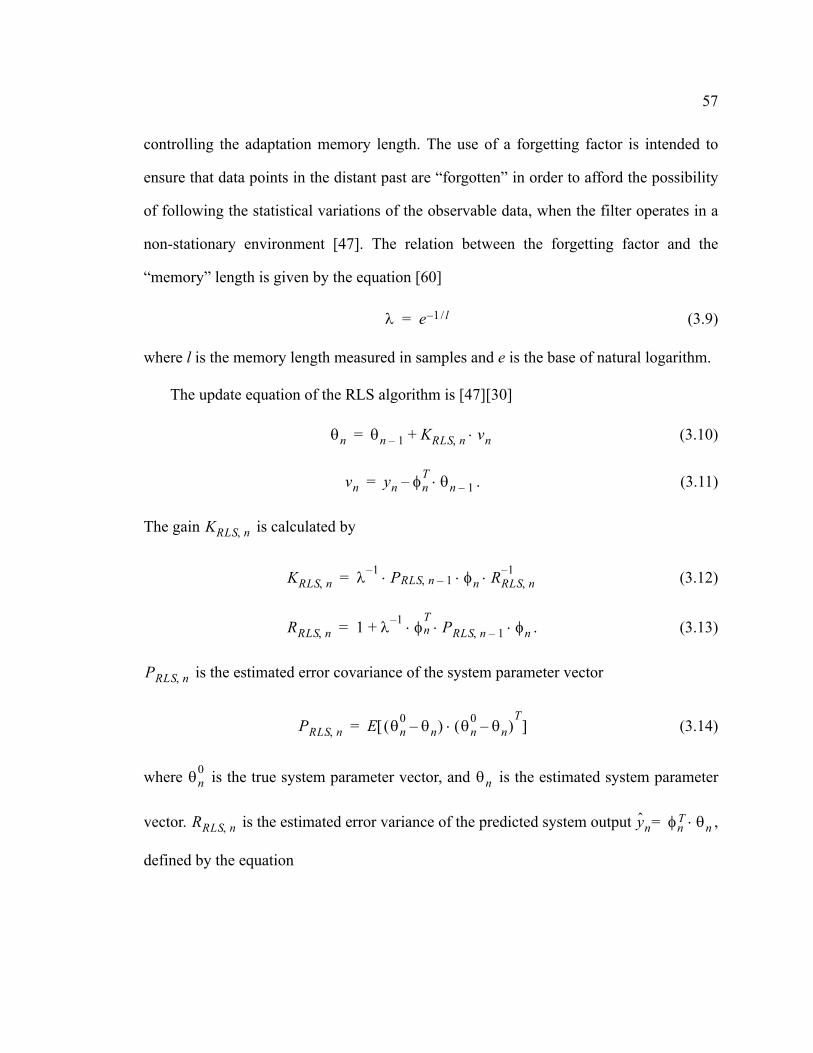
57
controlling the adaptation memory length. The use of a forgetting factor is intended to
ensure that data points in the distant past are “forgotten” in order to afford the possibility
of following the statistical variations of the observable data, when the filter operates in a
non-stationary environment [47]. The relation between the forgetting factor and the
“memory” length is given by the equation [60]
(3.9)
where l is the memory length measured in samples and e is the base of natural logarithm.
The update equation of the RLS algorithm is [47][30]
(3.10)
. (3.11)
The gain is calculated by
(3.12)
. (3.13)
is the estimated error covariance of the system parameter vector
(3.14)
where is the true system parameter vector, and is the estimated system parameter
vector. is the estimated error variance of the predicted system output ,
defined by the equation
λ e 1 l/–=
θn θn 1– KRLS n, vn⋅+=
vn yn φnT θn 1–⋅–=
KRLS n,
KRLS n, λ 1– P⋅ RLS n, 1– φn RRLS n,1–⋅ ⋅=
RRLS n, 1 λ 1– φ⋅ nT
PRLS n, 1– φn⋅ ⋅+=
PRLS n,
PRLS n, E θn0 θn–( ) θn
0 θn–( )T
⋅[ ]=
θn0 θn
RRLS n, yn φ= nT θn⋅

58
(3.15)
where the estimated error covariance of the system parameter vector , satisfies the
Riccati recursion
. (3.16)
The algorithm is initialized by setting , where is a small positive con-
stant and the parameter vector is set to .
As described earlier, if the external disturbing forces satisfy the stochastic assump-
tions, the -optimal estimators minimize the expected estimation error energy and yield
to a maximum-likelihood estimate from the parameter vector . In practical applications,
the assumption about stochastic disturbances cannot be always guaranteed. Therefore, the
performance of the estimator in such an environment is undetermined or even un-robust
where small deterministic disturbances can lead to large estimation error. The problem of
robust estimation is a critical requirement in system identification. In the following sec-
tion, an -optimal estimation algorithm will be used to address this question. In the -
optimal framework, in order to achieve better robustness, the estimators minimize the
maximum energy gain from the disturbances to the estimation error.
RRLS n, E yn yn–( )2[ ]=
PRLS n,
PRLS n, λ 1– PRLS n 1–,⋅ λ 1– PRLS n, 1–⋅ φn RRLS n,1– φ⋅ n
TPRLS n, 1–⋅ ⋅ ⋅–=
λ 1– PRLS n 1–,⋅ λ 1– KRLS n,⋅ φnT PRLS n, 1–⋅ ⋅–=
PRLS 0, δ 1– I⋅= δ
θ0 0=
H2
θn
H∞ H∞

59
3.2 H∞ Approach to System Identification
The approach that has been developed to address the estimation in the presence of
deterministic disturbances is the so-called estimation theory. The estimation tech-
nique is obtained if the strategy for the estimation fits the model parameters to the
observed data by minimizing (or in the suboptimal case, bounds) the maximum energy
gain from the external disturbing forces, which are unknown, but nonrandom
. (3.17)
The goal in developing the estimation algorithm is to minimize the worst-case
energy gain. The resulting estimators will be robust with respect to disturbances and less
sensitive to parameter variations, since no statistical assumptions are being made about the
disturbances. Or in other words, the -optimal estimator guarantees the smallest estima-
tion error energy over all possible disturbances of fixed energy. However, the resulting
estimators may be over conservative.
Due to the minmax nature of the -optimal estimator, which means that the estima-
tor minimizes the maximum energy of the disturbances, it can be treated as a game theo-
retical control problem with two players. Consequently, the nature (opponent) has access
to the unknown disturbance sequences and chooses them to maximize the error energy
gain in estimation. Concurrently, on the other side is the -optimal estimator, which
H∞ H∞
Ti θn
Ti : θnarg
θi
supνn
yk φkTθk–( )
k 0=
N
∑
=
H∞
H∞
H∞
H∞

60
should be designed in such a way as to minimize this estimation error energy gain. Since
the worst-case disturbance is a deterministic sequence, the -optimal estimator does not
require any statistical assumptions on the disturbance signal [20].
The over conservative behavior of the estimators often leads to slower conver-
gence in the parameter estimation compared to the estimation technique. In contrast to
, the optimal system parameter estimation offers faster system parameter estima-
tion but with a less robust behavior in the case of external disturbances, especially if the
disturbances violate the assumption that the external disturbance distribution is Gaussian.
Despite the slower convergence of the estimators, one of them is the least mean
squares algorithm, which is widely used as an estimation technique. This algorithm has
low computational requirements with excellent stability.
3.2.1 Least Mean Squares (LMS) Algorithms
Most of the estimation algorithms, such as the least squares, maximum likelihood esti-
mation, require a priori knowledge of the statistical properties of the external disturbances.
However, most of the applications (outside the research simulations) have none or very
limited a priori information about these external disturbances. The introduction of the
LMS adaptive filter by Widrow1 and Hoff2 in 1960 came as a significant development for
a broad range of engineering applications, since the LMS algorithm does not require a pri-
1. Bernard Widrow 1929- , Stanford University, California2. Marcian (Ted) Hoff 1937- , Rochester NY, Inventor of the microprocessor at Intel
H∞
H∞
H2
H∞ H2
H∞
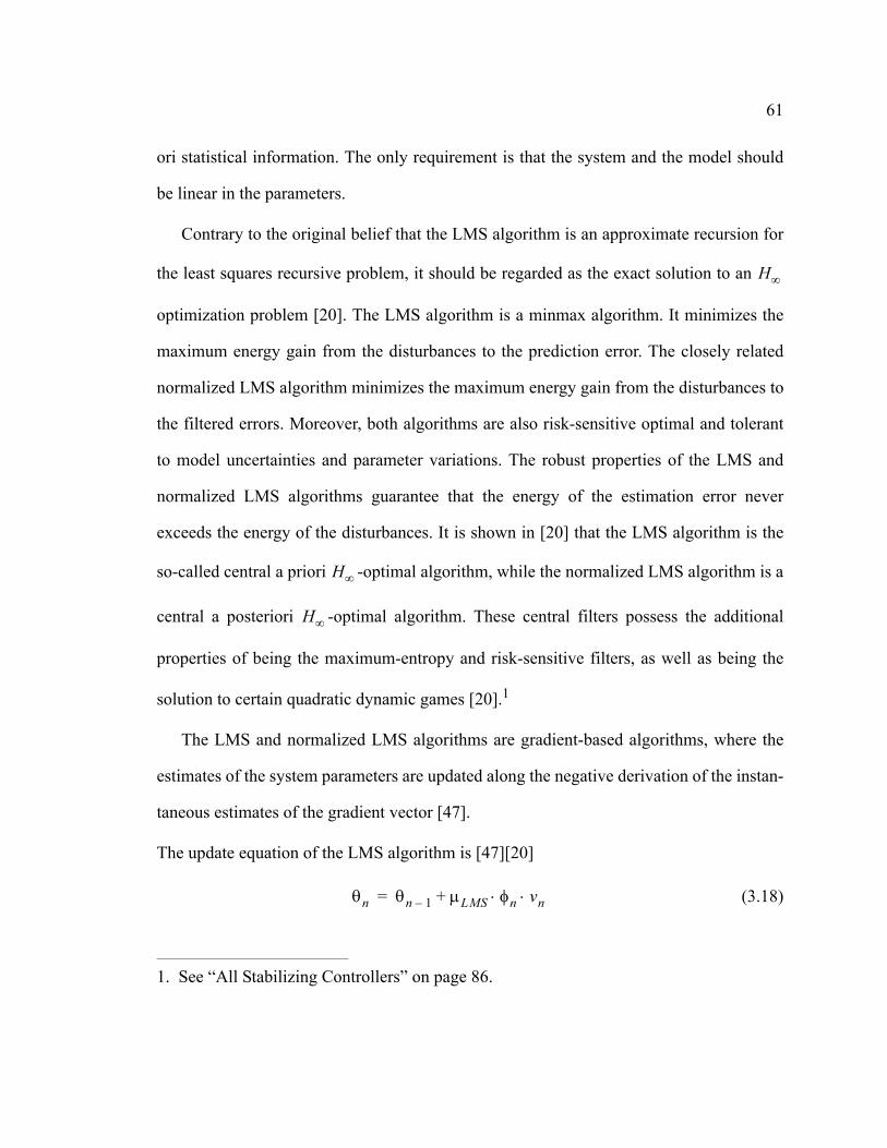
61
ori statistical information. The only requirement is that the system and the model should
be linear in the parameters.
Contrary to the original belief that the LMS algorithm is an approximate recursion for
the least squares recursive problem, it should be regarded as the exact solution to an
optimization problem [20]. The LMS algorithm is a minmax algorithm. It minimizes the
maximum energy gain from the disturbances to the prediction error. The closely related
normalized LMS algorithm minimizes the maximum energy gain from the disturbances to
the filtered errors. Moreover, both algorithms are also risk-sensitive optimal and tolerant
to model uncertainties and parameter variations. The robust properties of the LMS and
normalized LMS algorithms guarantee that the energy of the estimation error never
exceeds the energy of the disturbances. It is shown in [20] that the LMS algorithm is the
so-called central a priori -optimal algorithm, while the normalized LMS algorithm is a
central a posteriori -optimal algorithm. These central filters possess the additional
properties of being the maximum-entropy and risk-sensitive filters, as well as being the
solution to certain quadratic dynamic games [20].1
The LMS and normalized LMS algorithms are gradient-based algorithms, where the
estimates of the system parameters are updated along the negative derivation of the instan-
taneous estimates of the gradient vector [47].
The update equation of the LMS algorithm is [47][20]
(3.18)
1. See “All Stabilizing Controllers” on page 86.
H∞
H∞
H∞
θn θn 1– µLMS φn vn⋅ ⋅+=

62
. (3.19)
The learning rate is selected according to
(3.20)
where the infinity norm calculates the maximum possible input power represented in the
observed data. The presented bounds on the learning rate guarantees optimality. If
is selected accordingly to (3.20), then the LMS algorithm ensures that the energy of
the predicted error will never exceed the energy of the disturbances. On the other hand, if
(3.20) is not followed, the optimality is no longer warranted, since it is a well-known
fact that the LMS algorithm behaves poorly if the chosen learning rate is too large [20].
The update equation of the normalized LMS algorithm is [61]
(3.21)
. (3.22)
The normalized LMS algorithm converges in the mean square of prediction error, if
the adaptation constant satisfies [20] the following requirement
. (3.23)
When a small value is assigned to , the adaptation is slow, which is equivalent to the
LMS algorithm having a long “memory”. Correspondingly, the excess mean-squared error
after the adaptation is small. On the other hand, when is large, the adaptation is rel-
vn yn φnT θn 1–⋅–=
0 µLMS1
φnT φ⋅ n ∞
------------------------< <
H∞
µLMS
H∞
θn θn 1–µLMS
1 µLMS+( ) φnT φn⋅ ⋅
----------------------------------------------- φn vn⋅ ⋅+=
vn yn φnT θn 1–⋅–=
µLMS
0 µLMS 1< <
µLMS
µLMS
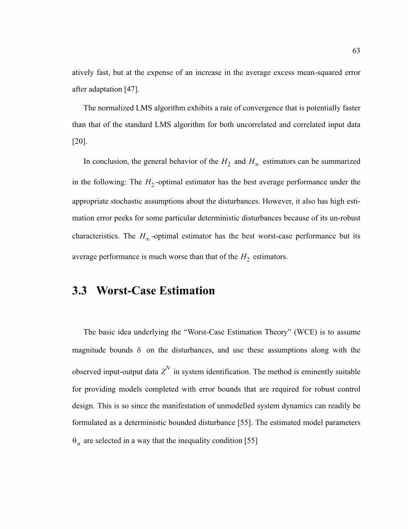
63
atively fast, but at the expense of an increase in the average excess mean-squared error
after adaptation [47].
The normalized LMS algorithm exhibits a rate of convergence that is potentially faster
than that of the standard LMS algorithm for both uncorrelated and correlated input data
[20].
In conclusion, the general behavior of the and estimators can be summarized
in the following: The -optimal estimator has the best average performance under the
appropriate stochastic assumptions about the disturbances. However, it also has high esti-
mation error peeks for some particular deterministic disturbances because of its un-robust
characteristics. The -optimal estimator has the best worst-case performance but its
average performance is much worse than that of the estimators.
3.3 Worst-Case Estimation
The basic idea underlying the “Worst-Case Estimation Theory” (WCE) is to assume
magnitude bounds on the disturbances, and use these assumptions along with the
observed input-output data in system identification. The method is eminently suitable
for providing models completed with error bounds that are required for robust control
design. This is so since the manifestation of unmodelled system dynamics can readily be
formulated as a deterministic bounded disturbance [55]. The estimated model parameters
are selected in a way that the inequality condition [55]
H2 H∞
H2
H∞
H2
δ
ZN
θn

64
(3.24)
must apply for every sample observed in an point data record. In mathematical terms,
this strategy can be formulated as
(3.25)
where the goal is to select a parameter vector , which will satisfy the inequality for all
the observed data. The recursive solution to this strategy was first presented in [62]. The
drawback of this approach is that in most cases the bound is not known a priory, but
only as an approximate . If the approximate bound is significantly larger than
it is necessary, it will have degenerating effects on the estimated parameters. Next, using
the approach published in [55], the theoretical background of the WCE theory will be pre-
sented.
The selected criterion in the WCE is that the residual of the model should be smaller
than , which defines the limits for the parameter vector , presented in
. (3.26)
The limits can be visualized as a pair of straight lines in parameter space that are orthogo-
nal to . The calculation (3.25) then becomes the region bounded by the intersection of
simple straight lines so that the parameter vector is in the convex polytope in the
yn φnTθn– δ≤
N
Ti : θnarg
θi yn φn
Tθn– δ≤
k 1=
N
∩
=
θn
δ
δ δ> δ δ»
δ θn
yn φnT θ⋅– δ θ→± φn
T( )1–
y⋅ n δ φnT( )⋅
1– ±= =
φn
θn d

65
dimensional parameter space, where is the dimension of . This is illustrated in Figure
3-1 where the feasible parameter set is within the dimensional parameter space.
Direct implementation of this parameter estimation method, using linear programming
with 2N constraints, is feasible but it is characterized with computationally intensive algo-
rithms. An enhanced version of the WCE algorithm can be obtained if the absolute value
calculation is replaced with a square, in which case the straight line bound region is
replaced with an ellipsoidal overbounding region. For any choice of the positive weighting
sequence the equation (3.25), satisfies the following inequality
. (3.27)
With an appropriate selection of the weighting sequence the estimation of
can be optimized. A recursive solution for this was proposed in [62]. It was suggested that
at each iteration the ellipsoid overbounding approximation should be made tight by mini-
d θn0
Θ d
Θ
y3 φ3T θ3⋅– δ±=
y2 φ2T θ2⋅– δ±=
y1 φ1T θ1⋅– δ±=
1
2d
Figure 3-1 Feasible parameter set for the WCE
ρn
ρn
δn2
----- yn φnTθn–( )
2ρn
n 0=
N 1–
∑≤
n 0=
N 1–
∑ ρn 0>;
ρn θn
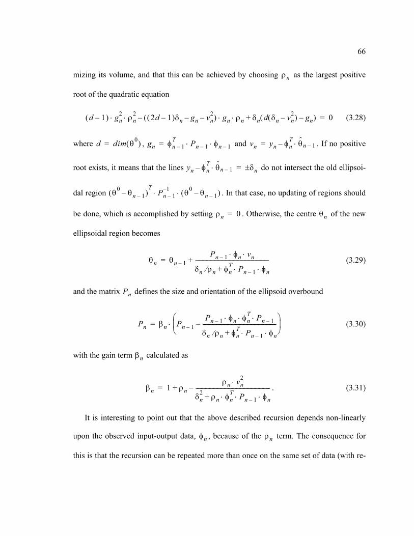
66
mizing its volume, and that this can be achieved by choosing as the largest positive
root of the quadratic equation
(3.28)
where , and . If no positive
root exists, it means that the lines do not intersect the old ellipsoi-
dal region . In that case, no updating of regions should
be done, which is accomplished by setting . Otherwise, the centre of the new
ellipsoidal region becomes
(3.29)
and the matrix defines the size and orientation of the ellipsoid overbound
(3.30)
with the gain term calculated as
. (3.31)
It is interesting to point out that the above described recursion depends non-linearly
upon the observed input-output data, , because of the term. The consequence for
this is that the recursion can be repeated more than once on the same set of data (with re-
ρn
d 1–( ) gn2 ρn
2 2d 1–( )δn gn– vn2–( ) g⋅ n ρn δn d δn vn
2–( ) gn–( )+⋅–⋅ ⋅ 0=
d dim θ0( )= gn φn 1–T Pn 1– φn 1–⋅ ⋅= vn yn φn
T θn 1–⋅–=
yn φnT θn 1–⋅– δn±=
θ0 θn 1––( )T
Pn 1–1– θ0 θn 1––( )⋅ ⋅
ρn 0= θn
θn θn 1–Pn 1– φn vn⋅ ⋅
δn ρn⁄ φnT Pn 1– φn⋅ ⋅+
------------------------------------------------------+=
Pn
Pn βn Pn 1–Pn 1– φn φn
T Pn 1–⋅ ⋅ ⋅
δn ρn⁄ φnT Pn 1– φn⋅ ⋅+
------------------------------------------------------–
⋅=
βn
βn 1 ρnρn vn
2⋅
δn2 ρn φn
T Pn 1– φn⋅ ⋅ ⋅+-------------------------------------------------------–+=
φn ρn
67
initialization from the previous recursion) with the goal to find the smallest pos-
sible ellipsoidal bound on the feasible parameter set .
By selecting for the recursion for the worst-case parameter estimation is pre-
cisely that of the Kalman Filter estimation algorithm where the sequence of residuals,
, is a white Gaussian noise with variance [55].
3.4 Kalman Filter Based System Identification
The Kalman Filter with its different derivatives is perhaps the most widely known
algorithm for recursively estimating dynamic state vectors that evolve according to the
difference equations known as state-space model [20] [63-64]
(3.32)
where is the d dimensional state-space variable , is the control input
, is the exogenous input which may be interpreted as a process-noise or driv-
ing disturbance , is the desired system output , is the measured out-
put , is an additive disturbance which can be regarded as a measurement noise
. The corresponding system matrices, possibly time varying, have the following
P0 Pn=
Θ
βn 1=
vn δn2 ρn⁄
xn
xn 1+ An xn Bn un Gn wn⋅+⋅+⋅=
yn Cn xn Dn un vn+⋅+⋅=
sn Ln xn Mn un⋅+⋅=
xn xn Rd∈ un
un Rm∈ wn
wn Rr∈ sn sn Rq∈ yn
yn Rp∈ vn
vn Rp∈

68
dimensions: , , , , , ,
and .
The Kalman Filter derivation is based on the least squares estimation strategy with
assumptions about certain quantities that define the stochastic identification environment
[65]. These values are presumed to be known. They include the covariance matrices for
measurement-noise , and the process-noise , assuming that the mean values are zero
or known constants. The covariance matrices are given by the statistical expectation oper-
ation
(3.33)
where is the initial state disturbance, is the process-noise and is the measure-
ment noise, and is the delta operator ( ). The degree to which this
information is correct is critical for the estimation performance and stability. Normally,
this information is not readily available. The correct values can be estimated separately or
by using the trial and error method. In mathematical terms, the Kalman Filer can be
described as a minimum mean-square error optimization
. (3.34)
An Rd d×∈ Bn Rd m×∈ Gn Rd r×∈ Cn Rp ×∈ Dn Rp m×∈ Ln Rq n×∈
Mn Rq m×∈
Rn Qn
Ex0
wn
vn
x0 wj vj
Π0 0 00 Qnδn j, 00 0 Rnδn j,
=
x0 wn vn
δn j, δn j, 0 if j n≠=
Ti : θnarg
θi
min
yk φkTθk–( )
2Rn Qn,
k 0=
N
∑
=

69
The solution to this problem is given by the Kalman Filter recursion [20]. In general
form the desired system output is presented as
(3.35)
where satisfies the filtered form of the Kalman Filter recursion
(3.36)
(3.37)
(3.38)
and satisfies the Riccati recursion
. (3.39)
When Kalman Filter is used for system parameter estimation, the recursive equation is
in the state-space form. The system model can easily be rewritten in the
state-space form by selecting
, and, . (3.40)
In this way equation (3.32) becomes
(3.41)
sn Lnxn=
xn
xn xn- KKF n, yn Cn xn
-⋅–( )⋅+=
xn- An xn 1–⋅ Bnun 1–+=
KKF n, PKF n, 1– CnT RKF n,
1–⋅ ⋅= RKF n, Rn Cn PKF n, 1– CnT⋅ ⋅+=
PKF n,
PKF n, An PKF n, 1– AnT Gn Qn Gn
T⋅ ⋅
An PKF n, 1– CnT RKF n,
1– Cn PKF n, 1– AnT⋅ ⋅ ⋅ ⋅ ⋅ ⋅–
+⋅ ⋅=
yn φnT θn⋅ vn+=
An I Bn, 0 Gn, I Cn, φn Dn, 0 Ln, I Mn, 0= = = = = = = xn θn≡
xn 1+ An x⋅ n Gn w⋅ n xn wn+=+=
yn Cn xn vn+⋅=
sn Ln xn⋅=

70
where is the system parameter vector to be determined, is the system noise the
residual between two estimations, is the regression vector containing the
observed data, is the measurement noise which corrupts the observed system output,
and is the desired system output.
It is interesting to point out that the desired system output for the selected is
the estimated system parameter . On the other hand, if for would be selected
the desired output will be the filtered (uncorrupted) output of the system.
By applying the introduced transformations (3.41) the Kalman Filter based system
parameter estimation can be expressed in the following form
(3.42)
(3.43)
where the Kalman gain is calculated by
(3.44)
and satisfies the Riccati recursion,
. (3.45)
In the above equations, is the estimated error covariance of the system parameter
vector
(3.46)
xn θn= wn
Cn φn=
vn
sn
sn Ln I=
θn Ln φn=
θn θn- KKF n, yn φn θn
-⋅–( )⋅+=
θn- θn 1–=
KKF n,
KKF n, PKF n, 1– φn RKF n,1–⋅ ⋅= RKF n, Rn φn
T PKF n, 1– φn⋅ ⋅+=
PKF n,
PKF n, PKF n, 1– Qn PKF n, 1– φn RKF n,1– φk
T PKF n, 1–⋅ ⋅ ⋅ ⋅–+=
PKF n,
PKF n, E θn0 θn–( ) θn
0 θn–( )T
⋅[ ]=

71
where is the true system parameter vector and is the estimated system parameter
vector. The estimated error variance of the predicted system output is calcu-
lated by the recursion for , and it is defined as
. (3.47)
In the Kalman Filter equations the covariance matrices for measurement-noise , and
the process-noise represent a priori knowledge of the external disturbing forces. At the
same time, these parameters can be used to control the estimation process by the Kalman
Filter, such as the speed of the estimation versus variance in the estimated parameters. The
correlation matrices, and can be defined using a parameter for each, to be placed
along the matrix diagonals. This will ensure that these matrices are symmetric. The filter
algorithm obtained in this way is also known as the random-walk Kalman Filter. These
values can be estimated using the residuals in the system output and the variances between
two estimated system parameters
(3.48)
. (3.49)
3.5 Array Algorithms for System Identification
Since the first array form of the Kalman Filter was developed in the 1960s, an inten-
sive research in this field has taken place resulting in various solutions for the array algo-
θn0 θn
yn φ= n θn⋅
RKF n,
RKF n, E yn yn–( )2[ ]=
Rn
Qn
Rn Qn
Rn E yn yn–( )2[ ]∼
Qn E θn θn 1––( )2[ ]∼

72
rithms. Basically, the least square array algorithms for adaptive filtering can be divided
into two big families: the transversal adaptive filtering algorithms; and for the order-
recursive lattice adaptive filtering algorithms. Both are characterized with an order of
magnitude reduction in computation effort, compared to the RLS algorithm. The main
characteristics of these algorithms are the reduced need in numerical range for the calcula-
tion (well-conditioned) and the use of orthogonal transformations, which typically leads to
more stable algorithms.
In compact form, array algorithms can be described via rotation operations on a pre-
array of numbers, which have to be triangularized in order to yield a post-array of num-
bers. The desired quantities can be read out from the post-array. In schematic way, this can
be presented as [66]
(3.50)
where is any rotation matrix that triangularizes the pre-array. The different realization
of the triangularization [57] and its algorithmic realization lead to a number of “different”
algorithms.
In this research two least squares or transversal filtering algorithms are selected for
implementation: the conventional QR algorithm (QR-RLS) and the Inverse QR algorithm
(IQR-RLS) algorithm. The LMS algorithm also has a QR based realization (QR-LMS)
[66] which is also included.
x x x xx x x xx x x xx x x x
ΘR⋅
x 0 0 0x x 0 0x x x 0x x x x
=
ΘR
H2
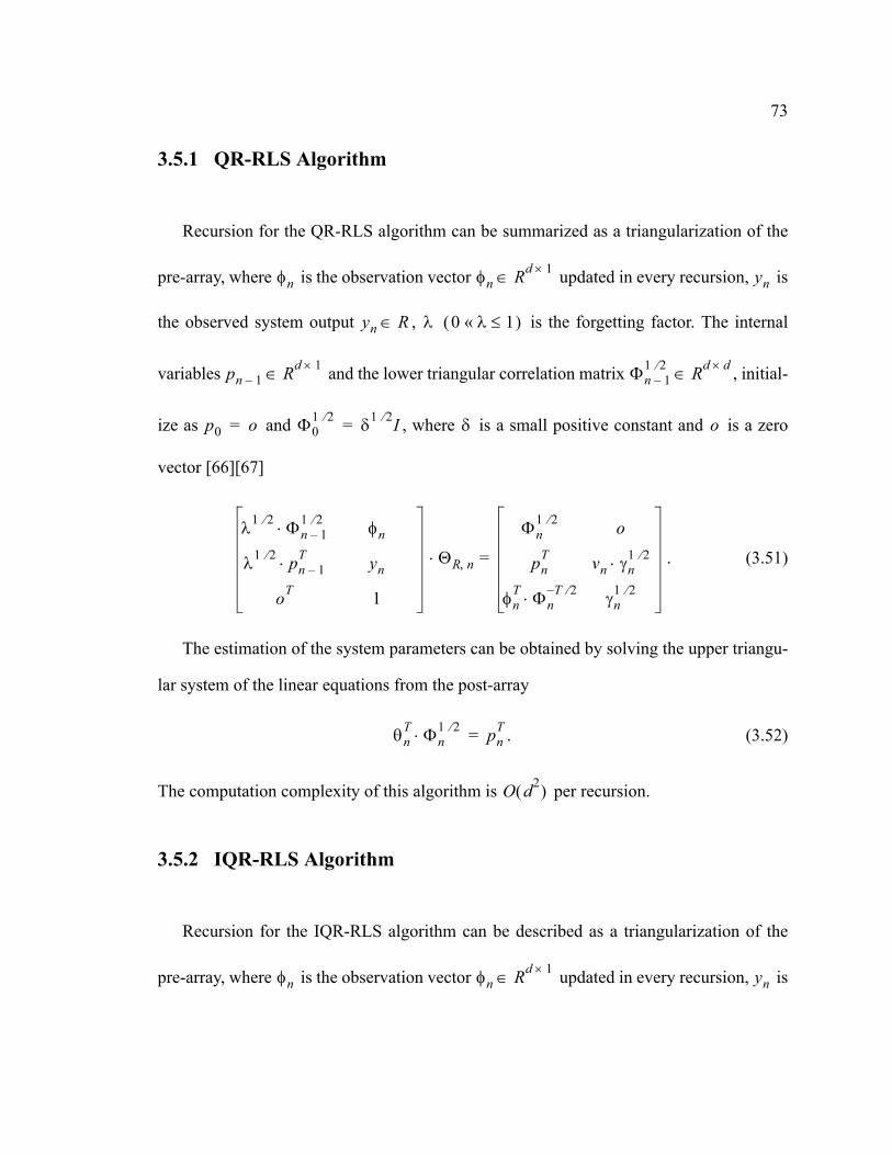
73
3.5.1 QR-RLS Algorithm
Recursion for the QR-RLS algorithm can be summarized as a triangularization of the
pre-array, where is the observation vector updated in every recursion, is
the observed system output , is the forgetting factor. The internal
variables and the lower triangular correlation matrix , initial-
ize as and , where is a small positive constant and is a zero
vector [66][67]
. (3.51)
The estimation of the system parameters can be obtained by solving the upper triangu-
lar system of the linear equations from the post-array
. (3.52)
The computation complexity of this algorithm is per recursion.
3.5.2 IQR-RLS Algorithm
Recursion for the IQR-RLS algorithm can be described as a triangularization of the
pre-array, where is the observation vector updated in every recursion, is
φn φn Rd 1×∈ yn
yn R∈ λ 0 λ 1≤«( )
pn 1– Rd 1×∈ Φn 1–1 2⁄ Rd d×∈
p0 o= Φ01 2⁄ δ1 2⁄ I= δ o
λ1 2⁄ Φn 1–1 2⁄⋅ φn
λ1 2⁄ pn 1–T⋅ yn
oT 1
ΘR n,
Φn1 2⁄ o
pnT vn γn
1 2⁄⋅
φnT Φn
T– 2⁄⋅ γn1 2⁄
=⋅
θnT Φn
1 2⁄⋅ pnT=
O d2( )
φn φn Rd 1×∈ yn
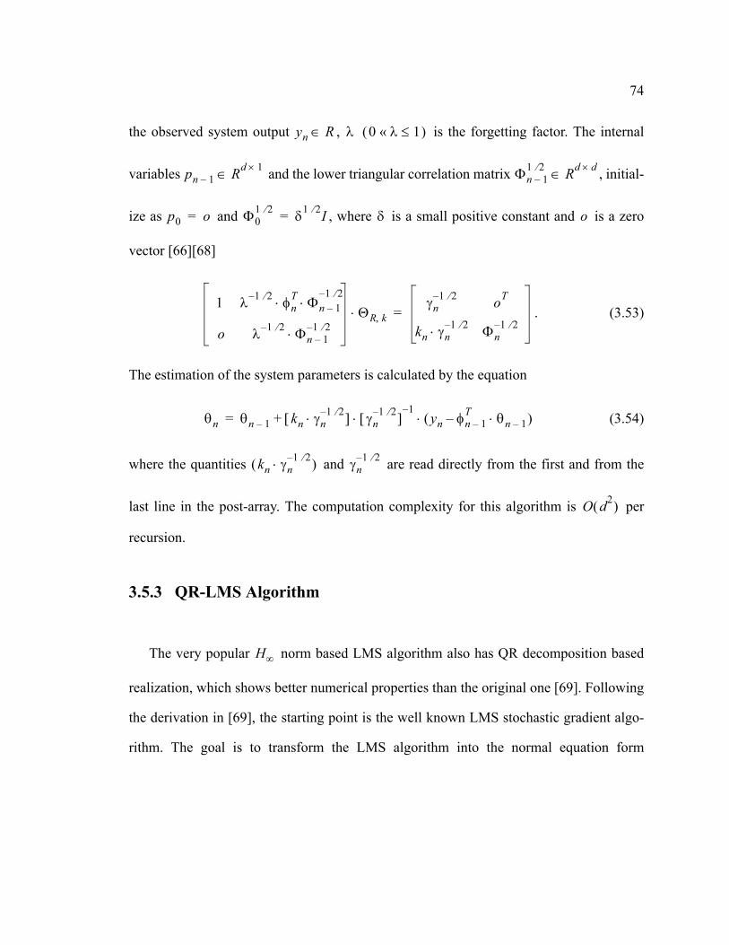
74
the observed system output , is the forgetting factor. The internal
variables and the lower triangular correlation matrix , initial-
ize as and , where is a small positive constant and is a zero
vector [66][68]
. (3.53)
The estimation of the system parameters is calculated by the equation
(3.54)
where the quantities and are read directly from the first and from the
last line in the post-array. The computation complexity for this algorithm is per
recursion.
3.5.3 QR-LMS Algorithm
The very popular norm based LMS algorithm also has QR decomposition based
realization, which shows better numerical properties than the original one [69]. Following
the derivation in [69], the starting point is the well known LMS stochastic gradient algo-
rithm. The goal is to transform the LMS algorithm into the normal equation form
yn R∈ λ 0 λ 1≤«( )
pn 1– Rd 1×∈ Φn 1–1 2⁄ Rd d×∈
p0 o= Φ01 2⁄ δ1 2⁄ I= δ o
1 λ 1– 2⁄ φnT Φ⋅ n 1–
1– 2⁄⋅
o λ 1– 2⁄ Φn 1–1– 2⁄⋅
ΘR k,⋅γn
1 2⁄– oT
kn γn1 2⁄–⋅ Φn
1– 2⁄=
θn θn 1– kn γn1 2⁄–⋅[ ] γn
1 2⁄–[ ]1–
yn φn 1–T θn 1–⋅–( )⋅ ⋅+=
kn γn1 2⁄–⋅( ) γn
1 2⁄–
O d2( )
H∞

75
, which is the base for the QR algorithm development. A different derivation
can be found in [20]. The equations for the LMS algorithm are
(3.55)
(3.56)
where is the step size parameter, which satisfies the norm requirement
(3.57)
is the weighting factor for the step size. Inserting (3.56) and (3.57) into (3.55)
(3.58)
and expanding this equation with
(3.59)
and by using the identity
(3.60)
the equation can be further rearranged as
(3.61)
θn R 1– b=
θn θn 1– µ φn vn⋅ ⋅+=
vn yn φnT θn 1–⋅–=
µ H∞
µ 1a2 φn
T φn⋅+---------------------------=
a 0>
θn θn 1–φn yn φn
T θn 1–⋅–( )⋅
a2 φnT φn⋅+
------------------------------------------------+=
a 2– yn φn φnT φn⋅ ⋅ ⋅ ⋅( )±
θn θn 1–yn φn⋅ φn φ⋅ n
T θn 1– a 2– yn φn φnT φn a 2– yn φn φn
T φn⋅ ⋅ ⋅ ⋅–⋅ ⋅ ⋅ ⋅+⋅–
a2 φnT φn⋅+
------------------------------------------------------------------------------------------------------------------------------------------------------------------+=
yn φ⋅ n a 2– yn φn φnT φn⋅ ⋅ ⋅ ⋅+ a 2– yn φn⋅ ⋅( ) a2 φn
T φn⋅+( )⋅=
θn θn 1–φn φ⋅ n
T θn 1–⋅
a2 φnT φn⋅+
--------------------------------– a 2– yn φn⋅ ⋅a 2– yn φn φn
T φn⋅ ⋅ ⋅ ⋅
a2 φnT φn⋅+
------------------------------------------------–+=

76
(3.62)
. (3.63)
Using the matrix inversion lemma [47]
(3.64)
(3.65)
the equation can be transformed into
. (3.66)
Further rearrangement results in
. (3.67)
This representation of the conventional LMS equation has the well known normal
equation form of the estimation process. The array algorithm form can be
acquired when the matrix inverse calculation is performed using the QR decomposition
θn Iφn φ⋅ n
T
a2 φnT φn⋅+
---------------------------–
θn 1–⋅ Iφn φn
T⋅
a2 φnT φn⋅+
---------------------------–
a 2– y⋅ n φn⋅ ⋅+=
θn a 2– Iφn φ⋅ n
T
a2 φnT φn⋅+
---------------------------–
a2 θ⋅ n 1– yn φn⋅+( )⋅=
A B 1– C D 1– CT⋅ ⋅+=
A 1– B B C D CT B C⋅ ⋅+( )1–
CT B⋅ ⋅ ⋅ ⋅–=
B 1– a2 I⋅= D I= C φ=
a 2– I a 2– I φ⋅ n φ⋅ nT
a 2– I⋅
a2 φnT φn⋅+( ) a 2– I⋅
-----------------------------------------------– a2 I⋅ φn φ⋅ nT+( )
1–=
θn a2 I⋅ φn φ⋅ nT+( )
1–a2 θ⋅ n 1– yn φn⋅+( )⋅=
aI φnaI
φnT⋅
1–
aI φnaθn 1–
yn
⋅
⋅=
θn R 1– b⋅=

77
algorithm. The above described solution has improved numerical properties but it requires
more calculations compared to the conventional LMS algorithm.

78
Part - II Robust Control
Robust control theory has emerged in response to the need to design controllers for
complex dynamic systems, where the classical control system design techniques, with their
trial and error approach, are unsatisfactory. The development of robust control theory has
arrived from the realization that the model representing the plant has some level of uncer-
tainty. The uncertainty arises in the mathematical models that are only approximate repre-
sentations of the real plant and it’s exogenous signals. Most controllers implemented in
industrial environments, where the real issue is the difficulty of modelling the plant to be
controlled, belong to this category. Historically, one can think of the problem of robust
stabilization as having its origin in the conjectures of Aizerman [70] and Kalman [71], i.e.
long before the word ‘robustness’ itself come into vogue [72]. In the early 1980s, with
considerable mathematical basis, Zames [8] defined the fundamentals of robust control
with the original formulation of the control theory. In the following decade, the time
domain formulation evolved [73], built on the game theory, which resulted in a Riccati
equations based solution. Since the early 1990s the discrete-time solution has been
defined in research papers [74-77] and published in a number of books [78-85].
In this Part, a brief introduction to control theory is provided in the context of the
noncooperative dynamic game theory. The practical aspects and a numerical implementa-
tion of the control design will also be demonstrated.
H∞
H∞

79
4 Preliminary to Robust Control
Robust control is a term used to define a control system design where, beside the
requirements for stability, a desire to minimize the preliminary assumptions about the
plant and the disturbances effecting it are also present. The robust control investigated in
this research is the “worst-case design”. In this approach, the preliminary assumption is
that the disturbances affecting the plant have the worst possible effect from the control
point of view, however these effects are limited by their intensity. Further research encom-
passing these ideas resulted in the development of the (sub)optimal control algorithm.
The implementation of this algorithm is also investigated.
Some underlying theories that are essential to understand and to successfully imple-
ment (sub)optimal control in discrete time are introduced in this thesis. First, the plant
model used for the control system design is examined. It is reflected upon the fact that, in
most of the realistic applications, the exact plant model is unknown. This lack of knowl-
edge brings uncertainty to the design. To address and characterize this uncertainty by the
control system, the small gain theorem is introduced. Finally, some properties of the
(sub)optimal control are described.
H∞
H∞
H∞

80
4.1 Uncertainty in Plant Model
For the control system design a discrete-time mathematical model, , of the
plant is required. The purpose of this model, , is to map the control inputs to the
outputs. Due to the fact that only the finite time and disturbed observations from the plant
are available, it is unlikely that even the most complex mathematical model can represent
the true physical plant. On the other hand, it is usually advantageous for the implementa-
tion if the mathematical representation is a simpler one, concentrating only on the behav-
ior that is relevant for control. To be practical, a design technique must account for the
inevitable inadequacy of models. A good model should be simple enough to facilitate the
design, yet complex enough to give the engineer confidence that designs based on the
model will work on the true plant [83].
Figure 4-1 illustrates the modelling of a physical plant, , with a discrete plant
model, . The difference between the observed plant, , and the representa-
G θ Ts,( )
G θ Ts,( )
Figure 4-1 Plant modelling
G θ Ts,( ) ∆⊕GT t( )un yn
u t( ) y t( )
Physical Plant Discrete Plant Modelmodelling
GTst( )
G θ Ts,( ) GTst( )

81
tion of the model, , is the model uncertainty, , [83]. To achieve a high level of
performance in the design of the control system, this model uncertainty must be taken into
account.
The model uncertainty arises from the fact that the plant model, , is only an
approximation of the true model, , where is an unknown but bounded,
random variable. If the bound on the variable can be estimated in some way as
, the uncertain model would be defined by the model and the bound
. Uncertainty models inherently describe both a nominal model and a
bound on the model accuracy [86]. In other words, an uncertainty model is simply a
description of a set of possible models for an unknown plant.
4.2 Linear Fractional Transformation
A widely accepted approach to the representation of uncertainty, , is the so called
Linear Fractional Transformation (LFT) uncertainty model [7][80], as shown in Figure 4-
2. The LFT model enables the known part to be separated from the unknown
part of the plant model.
G θ Ts,( ) ∆
G θ Ts,( )
G θ θ∇+ Ts,( ) θ∇
θ∇
θ± ∇MAX
G θ θ∇MAX+ Ts,( )
∆
G θ Ts,( )
∆

82
The plant model, , is extended with a new set of inputs , which interpret
the effects of the model uncertainty to the behavior of the model. The signal , as a time
function belongs to the space (square sumable), and can be considered as the process-
noise, which is generated by the model uncertainty system . Furthermore, interprets
all the possible exogenous disturbances acting on the plant. The set of control signals is
used to influence the dynamic behavior of the plant. This control action, based on the
present and past observations of the system outputs , is calculated by the controller .
The additional output quantity , the controlled output of , is a performance
measure, depending on the particular problem at hand [84]. The goal of the controller
is to stabilize the plant under the acts of exogenous disturbances.
Figure 4-2 Plant model with uncertainty
G θ Ts,( )
∆
znynun
ωn
Plant Model
G θ Ts,( ) ωn
ωn
l2
∆ ∆
un
yn ΣK
zn G θ Ts,( )
ΣK

83
4.3 Small Gain Theorem
The plant stability affected by the uncertainty in the model, as depicted in Figure 4-2,
can be assessed using the small gain theorem [7][80]. This is shown in more detail in Fig-
ure 5-3. The small gain theorem is based on the fact that a plant modeled by the closed-
loop of and , will be stable if the closed-loop gain is less
than one.
This theorem can be more precisely interpreted using the four blocks technique. The
LFT plant model, , in Figure 4-3, has two inputs and two outputs. Therefore, it
can be partitioned into a four block transfer matrix form, where the output is a function
of both inputs and . The control signal, , is calculated by the controller
: (4.1)
from the model’s other output, . In mathematical terms, this can be expressed as
zn ωn zn 1+→ → G θ Ts,( ) ∆
Figure 4-3 Small gain theorem model
∆
znωn
TK
ΣK
G θ Ts,( )un yn
G θ Ts,( )
zn
ωn un un
ΣK un K yn⋅=
yn

84
(4.2)
where , , , and the transfer matrices have the appropriate
dimensions. The transfer function from : can be obtained as
(4.3)
where the transfer function, , represents the plant with the closed-loop control system.
As mentioned earlier, if is a time function in space, and if the transfer function
has a finite gain, then the output will also belong to space. The small gain theo-
rem requires the worst-case closed-loop gain to be less than one, or
. (4.4)
Moreover, it is required that the uncertainty, , be small in the sense that
. (4.5)
Then, for the plant stability it is required that the maximum transfer gain from to
be less than
. (4.6)
Equation (4.6) is interpreted as a necessary condition to implement a robust control, if
the model uncertainty is bounded by the equation (4.5). Consequently, an internally stabi-
zn G11 ωn G12 un⋅+⋅=
yn G21 ωn G22 un⋅+⋅=
un K yn⋅=
where G11 G12
G21 G22
G θ Ts,( )=
ωn Rm∈ un Rl∈ zn Rq∈ yn Rp∈
ωn zn→ zn TK ωn⋅=
TK G11 G12 I K G22⋅–( )1–
⋅+= K G21⋅ ⋅
TK
ωn l2
TK zn l2
∆ ∞ TK ∞ 1<⋅
∆
∆ ∞1γ---<
ωn zn
γ
TK ∞ γ<

85
lizable controller can be formulated based on the knowledge that the uncertainty is
bounded by , such that the transfer function is , if it exists. From equation
(4.6), is seen as an attenuation factor, which is a function of the controller . The
lower limit on the minimum achievable value for is represented with and is called
infimum. This can be regarded as the fundamental idea for the (sub)optimal control
design.
The norm of the transfer function from : is defined as the
maximum energy gain from the disturbances on the regulated signal [75] [76]
. (4.7)
In other words, the norm is defined as a norm on transfer matrices, when trans-
lated to the time domain, the norm is nothing else than the -induced norm (from the
input time-function to the output time-function for initial state zero) [87]. The goal in
(sub)optimal control design is to minimize the worst-case energy gain, and the claim is
that the resulting controllers will be robust with respect to disturbance variations,
since no statistical assumptions are being made about the disturbances [20].
ΣK
1 γ⁄ TK ∞ γ<
γ ΣK
γ γ∗
H∞
H∞ ωn zn→ zn TK ωn⋅=
ωn zn
TK ∞
supω l2 ω 0≠,∈
=z 2ω 2
-----------
H∞
H∞ l2
H∞
ΣK

86
4.4 All Stabilizing Controllers
The robust stabilizing controller , which satisfies equation (4.6) for the
(sub)optimal control system design, is not unique. By definition, this controller needs to
achieve robust stability not only for the nominal plant , but also for all plants in a
suitably large neighborhood of the nominal plant . In general, there are infi-
nite number of controllers that can robustly stabilize or maintain stability of an uncertainty
model , described by and . The controller, which internally stabilizes the
plant, is called admissible. An admissible controller is called optimal controller if
it was obtained such that is minimized. The closed-form solution to the optimal
control problem is available only for some special cases, and a simpler problem
results if one relaxes the minimization condition and settles for a suboptimal solution [20].
An admissible controller is called suboptimal controller if for a given there
are any controllers such that . In control terminology, the set of suboptimal
controllers, which can robustly stabilize an uncertainty model, is called the all stabi-
lizing controller [79-80]. This set of all admissible controllers, which satisfies ,
equals the set of all transfer-matrices that can be represented using LFT with a
free parameter as , shown in Figure 4-4. The selection of the parameter
matrix only needs to satisfy the norm .
ΣK H∞
G θ T,( )
G θ θ∇+ T,( )
Σ G θ T,( ) ∆
H∞ ΣK
TK ∞
H∞
H∞ ΣK γ 0>
TK ∞ γ< H∞
H∞
TK ∞ γ<
yn un→
Q∞ ΣK Q∞( )
Q∞ Q∞ ∞ γ<

87
With (at the “center” of the set ) the so called central controller is
selected [80]. This central controller has the alternative interpretation as the controller
which minimizes the entropy integral [78] defined as [88]
(4.8)
where . Considering that the central controller minimizes the
entropy integral [7] of the closed-loop control system transfer function , it reveals some
new properties for the (sub)optimal central controller.
First, it can be observed that the entropy integral is finite if, and only if
, which implies . Thus, the integral is finite if and
only if is an achievable bound in the (sub)optimal control problem [20].
Second, it is shown in [83] that
. (4.9)
ΣK
Q∞
yn un
Figure 4-4 Controller Q parametrization
Q∞ 0= Q∞ ∞ γ<
Id TK γ,( ) γ2
2π------– ln det I γ 2– TK
~ ejω( ) TK ejω( )⋅ ⋅–[ ] dω⋅π–
π
∫⋅=
TK~ ejω( ) TK∗ e j– ω( )=
TK
H∞
γ2 I⋅ TK~ ejω( ) TK ejω( )⋅> γ TK ∞>
γ H∞
Id TK γ,( )γ ∞→lim TK 2
2=

88
Therefore, the entropy is in fact a performance index, measuring the trade-off
between the optimality and the optimality [83]. It should be
remembered at this point that if the controller is designed according to the principles of the
(sub)optimal control, it is designed to minimize the effects of the peak value of the
disturbances affecting the plant, consequently yields to a higher level of robustness. On
the other hand, the classical or Linear Quadratic Gaussian Regulator (LQGR) is
designed to minimize the effects of the average value from the disturbances affecting the
plant. The controller is not concerned with the peaks of the disturbances as long as
they are acting only for a short time. Consequently it yields to a lower level of robustness.
Therefore, it is hoped that by minimizing the entropy function, one can obtain a good
trade-off between the norm for robustness and the norm for performance [89].
The properties learned from the entropy function analysis motivate the selection of the
central controller for implementation. In recent years, numerous time-domain approaches
have emerged to implement the control design theory. Among the various approaches
to the worst-case design problems, the one that uses the framework of dynamic (differen-
tial) game theory seems to be the most natural [19]. In the following chapter, the basics of
the game theory relevant to the robust control are discussed.
Id TK γ,( )
H∞ γ TK ∞→ H2 γ ∞→
H∞
H2
H2
H∞ H2
H∞

89
5 Fundamentals of Game Theory
The game theory was established by the pioneering work of von Neumann1 in his book
Theory of Games and Economics Behavior, published in 1944. The game theory is the
mathematical formulation of the conflict situation where one or more individuals, the
players, have to make decisions and each possible decision leads to a different outcome of
the results, which are valued differently by the players. In the following a general intro-
duction is provided on the discrete-time dynamic game theory and its special class, the
zero-sum dynamic game. More detailed description can be found in [19] [85].
5.1 Discrete-Time Dynamic Game
If the players can only make moves every time period, and if the game’s length is
defined as , then the game is called discrete-time game of specified fixed
duration or finite-horizon control. Using the system theory terminology, the basic ele-
ments of a game can be specified by the following definition.
Definition: A -person discrete-time deterministic dynamic game of specified fixed
duration involves [85]:
1. John von Neumann, 1903-1957, Hungarian born mathematician
Ts
Td Ts N⋅=
K
Td N Ts⋅=

90
1. An index set called the players’ set, used to distinguish between
the actors in the game.
2. An index set denotes the stages of the game, where is the
maximum possible number of moves a player is allowed to make in the game, used as a
time measurement.
3. An infinite set with some topological structure, called the state set (space) of the
game, to which the state of the game belongs for all , during the
dynamical modelling of the games.
4. An infinite set with some topological structures, defined for each and ,
which is called the action (control) set of player at stage . Its elements are the per-
missible actions of player at stage . In other words, defines the limits of the
control action.
5. A function , defined for each , so that
(5.1)
for some , which is called the initial state of the game. This difference equation
is called the state equation of the dynamic game, describing the evolution of the under-
lying decision process.
6. A set with some topological structure, defined for each and , and
called the observation set of kth player at stage , to which the observation
of player belongs at stage .
K 1 … k … K, , , , =
N 0 … n … N, , , , = N
X
xn( ) n N N 1+ ∪∈
Unk n N∈ k K∈
Pk n
unk Pk n Un
k
fn : X Un1× … Un
K×× X→ n N∈
xn 1+ fn xn un1 … un
K,,,( ) n N∈,=
x1 X∈
Ynk n N∈ k K∈
Pk n N∈ ynk
Pk n N∈

91
7. A function , defined for each and , so that
(5.2)
which is the state-measurement (-observation) equation of player concerning the
value of .
8. A finite set defined for each and as a subset of
, which deter-
mines the information gained and recalled by the player at the stage of the game.
Specification of for all characterizes the information structure (pattern) of
player , and the collection (over ) of these information structures is the infor-
mation structure of the game.
9. A set defined for each and as an appropriate subset of
, compatible
with . is called the information space of the player at the stage , induced by
his information .
10. A prespecified class of mappings which are the permissible strat-
egies of player at stage . The aggregate mapping is a strat-
egy for the player in the game, and the class of all such mappings so that
, , is the strategy set (space) of the player .
hn : X Ynk→ n N∈ k K∈
ynk hn
k xn( ) n N k K∈,∈,=
Pk
xn
ηnk n N∈ k K∈
y11 … yn
1, , … y1K … yn
K, , u11 … un 1–
1, , … u1K … un 1–
K, , , , , , ,
Pk n
ηnk n N∈
Pk k K∈
Hnk n N∈ k K∈
Y11 … Yn
1, , … Y1K … Yn
K, , U11 … Un 1–
1, , … U1K … Un 1–
K, , , , , , ,
ηnk Hn
k Pk n
ηnk
Γnk γn
k : Hnk Un
k→
Pk n γk γ1k γ2
k … γNk, , , =
Pk Γk γk
γnk Γn
k∈ n N∈ Pk

92
11. A functional
defined for each , and called the cost functional of player in the game of fixed
duration.
As a conclusion, for a player discrete-time dynamic game, for the kth player with
strategy set and with decision (action) vector , the
player’s actions are completely determined by the relations
(5.3)
where the set describes the strategies for the players ,
and is the information available to the player . The optimal strategy set, marked by
star, , called the Nash equilibria, can be calculated using one of the
standard techniques of optimal control, like the minimum principle for open-loop systems
or dynamic programming for feedback systems. In game theory, the Nash equilibrium is
the synonym for the optimal solution. When the Nash equilibrium is achieved, one player
cannot improve his outcome of the game by altering his decision unilaterally. The Nash
equilibrium solution has the nice property to guarantee for each player a given optimal
value for the objective functional [90].
Lk : X U11 …× U1
K××( ) X U21 …× U2
K××( )× … X UK1 …× UK
K××( ) ℜ→××
k K∈ Pk
K Pk
Γk k K∈; uk U k K∈;∈
uk γk ηk( )= k K∈
γk Γk k K∈;∈ Pk ; k K∈
ηk Pk
γk∗ Γk k K∈;∈

93
5.2 Zero-Sum Dynamic Games
A particularly important component in game theory is the conflict situation between
two players, where one player’s gain incurs a loss to the other player. Due to the conflict-
ing interests of the two players, this game does not allow any cooperation between them.
In mathematical terms, the two-player game can be evaluated through its cost functions
. If represents the decision variable for the player with cost function , the sum of
the cost functions of the two players [85]
(5.4)
will always be zero (or a constant value), hence the name two-player zero-sum game.
The control system setup, presented in Figure 5-1, can be regarded as a two-player
zero-sum game. In this game, nature is the maximizing player or the opponent. This
player has access to the disturbance signal , which is modulated in a way to maximize
Ji ui i Ji
J1 u1 u2,( ) J2 u1 u2,( ) 0≡+
Figure 5-1 Two-player control system model
G θ T,( )
∆
zn
ynun
ωn
ΣK
∆
ωn

94
the regulated signal . On the other hand, the controller is the minimizing player that
is modulating the control signal with a goal to minimize the regulated signal .
Let be the cost function for this two-player zero-sum game, which is mini-
mized by , from the possible set of values , and maximized by , from the possible
set , and is the state-variable of the dynamic system. The game will have an upper
value if the cost function is first maximized by selecting the optimal value and after
it is minimized by [85]
. (5.5)
The game will have a lower value if the cost function is first minimized by selecting
the optimal value and after it is maximized by
. (5.6)
The optimal solution for the game will have a value between the upper value and
lower value of the game [85]
(5.7)
where the inequality is called the Nash inequality. Furthermore, if an optimal solution
exists for the game such that
(5.8)
zn ΣK
un zn
J u ω x, ,( )
u U ω
W x
J ω∗
u
J J u ω∗ x, ,( )inf
u U∈
supω W∈
J u ω x, ,( )= =
J
u∗ ω
J J u∗ ω x, ,( )sup
ω W∈
infu U∈
J u ω x, ,( )= =
J∗ J
J
J u∗ ω x, ,( ) J∗ J u∗ ω∗ x, ,( )≡ J u ω∗ x, ,( )≤ ≤ ω∀ W∈ u∀ U∈,
J∗
J u∗ ω x, ,( ) J u∗ ω∗ x, ,( ) J u ω∗ x, ,( )= =

95
then the Nash equilibria solution pair is called a saddle-point solution or nonco-
operative equilibrium, and is called the game’s value function.
The saddle-point solution has the nice property to guarantee to each player a given
optimal value for the objective function. For example if is a saddle-point solu-
tion, the choice of ensures to player 1 that the value of the objective function is at
most equal to . The same holds for the player 2 if it chooses . Optimal-
ity arises from the fact that it is not possible for a player to improve this value if the other
player adopts his saddle-point strategy. For this reason is called the value of
the game [90].
5.2.1 Optimal Solution for Discrete-Time Dynamic Game
The discrete-time dynamic process, characterized by its system’s state process ,
can be modelled by its state and output equations, which in general can be nonlinear,
(5.9)
. (5.10)
If denotes the system’s performance criterion, or objective function, for the
time interval , the two-player zero-sum game is defined by the finite-horizon N-
stage cost, [19]
u∗ ω∗,( )
J∗
u∗ ω∗,( )
u u∗=
J u∗ ω∗,( ) ω ω∗=
J u∗ ω∗ x, ,( )
xn
xn 1+ fn xn un ωn, ,( )= n 1 N,[ ]∈
yn hn xn ωn,( )= n 2 N,[ ]∈
J u ω,( )
N Ts⋅
96
(5.11)
where is the initial cost, is the final cost and is the cost
at the time . The game is to be minimized by the control policy and
maximized by the opponent’s policy , both from their respective sets of
possible values, and . The controller’s problem is to find a
minimax strategy , more precisely, the strategy that guarantees the best per-
formance, measured by the objective function, in the worst possible situation. The proper
strategy minimizes the maximum expected objective function, where the maximum is
obtained by the opponent’s best policy over all possible strategies . To
determine its policy the controller can access the current as well as the entire
past values of the state [19]
(5.12)
where are the control policies in time.
The control policy, if it exists, can be determined using the Dynamic Programming
method. The dynamic programming theory is based on Bellman’s principle of optimality,
where the solution is obtained in retrograde time. The counterpart of this in two-player
zero-sum dynamic games is a recursive equation that involves (again in retrograde time)
the saddle-point solution of the static games, known as the Isaacs1 equation. Such an
J u ω x, ,( ) p x0( ) q+ xN( ) gn xn 1+ un ωn xn, , ,( )
n 1=
N 1–
∑+=
p x0( ) q xN( ) gn xn 1+ un ωn xn, , ,( )
t n Ts⋅= µ un =
ν x0 ω, n =
un U Rr⊂∈ ωn W Rl⊂∈
µ∗ un∗ =
ν∗ x0 ω, n∗ = ν
µ un =
un µn x 1 …n,[ ]( )=
µ1 µ2 …µn, ,

97
equation provides a sufficient condition for the existence of a saddle-point for a dynamic
game.
To utilize the Isaacs equation, the value function of the game is defined as the saddle-
point solution of the cost function (5.11), if it exists,[19]
. (5.13)
Equation (5.13), written as a backward recursion, led to a familiar solution in dynamic
programming, called the Isaacs equation
. (5.14)
(5.14) is the Isaacs equation, being the discrete-time version of a similar equation
obtained by Isaacs as a solutions for a continuos-time two-player zero-sum dynamic game,
which is known as the Hamilton-Jacobi-Isaacs equation [19][85].
1. Rufus Philiph Isaac, 1914 - , USA mathematician
Vn xn( )min
u U ∈max
ω W∈ q xN( ) gk xk 1+ uk ωk xk, , ,( )
k n=
N
∑+
=
maxω W ∈
mixu U∈
q xN( ) gk xk 1+ uk ωk xk, , ,( )
k n=
N
∑+
=
Vn xn( )min
u U ∈max
ω W∈ gn xn 1+ un ωn xn, , ,( ) Vn 1+ xn 1+( )+[ ]=
maxω W ∈
mixu U∈
gn xn 1+ un ωn xn, , ,( ) Vn 1+ xn 1+( )+[ ]=
gn xn 1+ un∗ ωn∗ xn, , ,( ) Vn 1+ xn 1+ ∗( )+=
VN 1+ xN 1+( ) 0≡

98
By utilizing this backward recursion, the control policies for the minimizing player
and for the maximizing player are calculated from the cur-
rent value of the state . This is known as the feedback policy. If the equivalence in
(5.14) exists, it is a saddle-point of the game and the corresponding performance index,
the value of the game, is given by .
The control policies assume that the minimizing player has full knowl-
edge of the state-variables , called the full-information control. This situation rarely
occurs. In most cases the minimizing player can access only the measurement sequence
up to the current time from the plant output as
defined in (5.10). This type of control is the measurement-feedback control.
A similar problem is solved by the Linear Quadratic Gaussian Regulator (LQGR)
design using the separation principle. In LQGR the control is separated into an observer
and a linear feedback structure for the control . The observer estimates the
state-variables using the Kalman Filter. The main difference between the LQGR and
the minimax design is that in the latter no separation principle applies. In minimax design,
the observer and the controller are linked [82]. Nevertheless, the solution to the
controller synthesis problem may be obtained by solving the full-informa-
tion control problem and finding a minimax estimator for the full-information control [7].
The two processes are not separated but rather coupled in a way that the state estimation
filter design depends on the solution for control, but not vice versa [20]. The theory that
un∗ µ∗ xn( )= ωn∗ ν∗ xn( )=
xn
V1 x1( )
un∗ µ∗ xn( )=
xn
y1 … yn 1–, , t nTs= yn hn xn ωn,( )=
un K xn⋅=
xn
un∗ µ∗ xn( )=
99
upholds the state estimation filter design for the minimax controller is called the certainty
equivalence principle, which is the topic of the following section.
5.3 Certainty Equivalence Principle
As shown above, the players using the current value of the state are evaluating the
game with the value function , and calculating their optimizing feedback controls
, . The difficulty with this full state feedback control strat-
egy is that in most cases neither player has access to the exact value of the state vector
[91]. Due to the lack of access to the state-variables, the players can not evaluate their
optimal saddle-point strategies, which brings uncertainty into the game. To resolve this
problem, a risk-sensitive state estimator that may be fed into the full state feedback control
is introduced in the form of the certainty equivalence principle [19][91][92].
Assume that an optimal control policy is required to choose a control
to minimize the cost function . In the case of perfect information where the sys-
tem states are known, the optimal control policy is chosen
such that for all . However, if is only
known through the observations of the plant output , and the solution of the optimal
control policy is not known, it is not totally without merit to use the control
law [19]
xn
Vn xn( )
un∗ µ∗ xn( )= ωn∗ ν∗ xn( )=
xn
µ∗ un U Rr⊂∈
J u ω x, ,( )
xn X Rm⊂∈ un∗ µ∗ xn( )=
J u∗ x( ) ω x, ,( ) J u ω x, ,( )≤ un n, 1 2…N,= xn
y xn( )
un∗ µ∗ y( )=

100
(5.15)
where
(5.16)
under the condition that there is a function , which is an estimator for the
system states , constructed on the observed sequences and
. This idea, called certainty equivalence principle, states that an optimal
controller can be obtained by inserting an estimate (if one exists) into the corresponding
optimal state feedback law [92].
The measurement-feedback control problem can be solved via a two-step procedure.
In the first step, a full-information control problem is solved assuming that the states of the
system are known. The second step entails the estimation of the unknown unmeasurable
system states, using the observed system output measurements.
In the selection of the system state estimation function , using the
game theoretic approach, the goal is to anticipate the “worst possible disturbances” gener-
ated by nature, the maximizing player. Accordingly, the aim is to estimate the “worst pos-
sible current state” compatible with the available information. If this state estimate is
used by the minimizing player, the worst possible action of the maximizing player will be
minimized.
un∗ µ= y( ) µ∗ xn( )=
xn T un 1– yn 1– xn, ,( )⇐
T un 1– yn 1–,( )
xn u1 … un 1–, ,
y1 … yn 1–, ,
T un 1– yn 1– xn, ,( )
xn
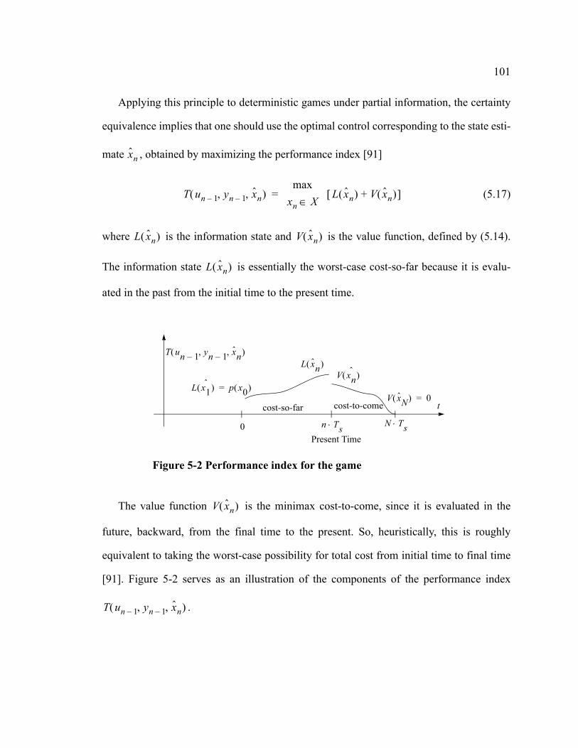
101
Applying this principle to deterministic games under partial information, the certainty
equivalence implies that one should use the optimal control corresponding to the state esti-
mate , obtained by maximizing the performance index [91]
(5.17)
where is the information state and is the value function, defined by (5.14).
The information state is essentially the worst-case cost-so-far because it is evalu-
ated in the past from the initial time to the present time.
The value function is the minimax cost-to-come, since it is evaluated in the
future, backward, from the final time to the present. So, heuristically, this is roughly
equivalent to taking the worst-case possibility for total cost from initial time to final time
[91]. Figure 5-2 serves as an illustration of the components of the performance index
.
xn
T un 1– yn 1– xn, ,( ) max
xn X∈ L xn( ) V xn( )+[ ]=
L xn( ) V xn( )
L xn( )
Figure 5-2 Performance index for the game
n Ts⋅
t
N Ts⋅0
V xnˆ( )
L x1ˆ( ) p x0( )=
L xn( )
V xN( ) 0=
T un 1– yn 1– xn, ,( )
Present Time
cost-so-far cost-to-come
V xn( )
T un 1– yn 1– xn, ,( )

102
To anticipate the worst possible influence of the maximizing player, the general form
of information state as a worst past cost, can be defined as a function of
and [19]
(5.18)
where, is the cost on the initial state and is the cost on the state
at time . Since only partial information is available from the state, the initial
state is also unknown. This problem can be handled by considering as part of the
disturbance, controlled by the maximizing player, included within the initial cost term
.
Furthermore, represents the set of all possible disturbances consistent
with the observations from and such that the equations
(5.9) and (5.10) are satisfied. Thus, and the past values of should agree with the
past control and measurements but future could be the worst possible, if it belongs to
the action (control) set of the maximizing player and it is chosen according to ,
leading to a least cost-to-go [19].
Using a simple recursion, the information state can be written in a forward
dynamic programming equation form
L xn( )
u1 … un 1–, , y1 … yn 1–, ,
L xn( )sup
x0 ω, k 1–( ) Ωn 1–∈ p x0( ) gk xk 1+ yk uk ωk, , ,( )
k 1=
n 1–
∑+=
p x0( ) gk xk 1+ yk uk ωk, , ,( )
t k Ts⋅=
x0 x0
p x0( )
Ωn 1– x0 ω,( )
u1 … un 1–, , y1 … yn 1–, ,
x0 ωn 1–
ωn
ν∗ xn( )
V xn( )
L xn( )
103
(5.19)
where the recursion is initialized by . If the recursion satisfies the saddle-
point solution requirements, which is formulated below, it can be regarded as the general
definition for the state estimator.
The state estimator, obtained as an upper limit of the recursion (5.19), is only the nec-
essary condition for the existence of one. Defined by the certainty equivalence principle in
(5.17), the sufficient condition for the worst-case state estimator is the existence of the
saddle-point solution for the equation (5.17). This sufficient condition is formulated next.
If the value function in the performance index (5.17) is replaced by the one
based on the Isaacs equation, as defined in (5.14), equation (5.17) can be rewritten as [19]
. (5.20)
If there is a solution to the two-players game, is required to be a
saddle-point solution
L xn( )sup
ωn 1– W∈ gn xn yn 1– u, n 1– ωn 1–, ,( ) L xn 1–( )+[ ]=
L x1( ) p x0( )=
V xn( )
T un 1– yn 1– xn, ,( )max
xn X∈
minun U ∈
maxωn W∈
gn xn un 1– ωn 1– xn 1–, , ,( )
Vn 1+ xn 1+( ) L xn 1–( )+ +
[
]
=
T un 1– yn 1– xn, ,( )
T un 1– yn 1– xn, ,( )max
xn X∈
min un U ∈
maxωn W∈
gn xn un 1– ωn 1– xn 1–, , ,( )
Vn 1+ xn 1+( ) L xn 1–( )+ +
[
]
=
104
. (5.21)
If the saddle-point solution exists then it yields to a uniquely defined ,
which is a minimax controller [19].
The intuition behind introducing this controller, using the certainty equivalence princi-
ple, can be interpreted in the following way. At time , knowing the observations
and the control up to time , one should antici-
pate the “worst disturbance” compatible with the available information and in accor-
dance with the performance index (5.17). Then estimate the corresponding “worst
possible current state” , by (5.19), and use it as if it were indeed the actual current state
for the control. This is indeed a worst-case certainty-equivalence principle, but it is not a
separation principle since the worst-case state estimate depends on the performance index
(5.17) to be minimized [19].
5.4 Finite-Horizon Discrete-Time Linear System
The previously developed general discrete-time control theory can be adapted to the
situation where the system is considered to be finite-horizon discrete-time linear, and the
performance index for the control function is quadratic. In this setup, it is required that the
signals belong to the space, see Appendix D. The plant model , a discrete-time
minun U ∈
max
xn X∈
maxωn W∈
gn xn un 1– ωn 1– xn 1–, , ,( )
Vn 1+ xn 1+( ) L xn 1–( )+ +
[
]
=
un∗ µ∗ y( )=
t n Ts⋅=
y1 … yn 1–, , u1 … un 1–, , t n 1–( ) Ts⋅=
ωn
xn
l2 0 N,[ ], Σ

105
linear state space equation, is defined by the difference state equation and by the two out-
put equations
(5.22)
where represents the state variable, is the disturbance (control input of
the maximizing player), is the control input (control input of the minimizing
player), is the measurement output, is the controlled output, and
are (possible time-variables) matrices with appropriate dimensions.
The design of the worst-case control system , using the (sub)optimal control
system design process, is based on the requirements stipulated by the inequality (4.6).
Using the relations of (4.7) and by relaxing the inequality of (4.6), the main requirement
for the (sub)optimal control is formulated as
(5.23)
for some prespecified positive real number . This can be regarded as the main idea for
the worst-case controller cost function definition. In the performance index definition, the
norm operator can be substituted with the sum of squares. Further, equation (5.23) can be
extended with the cost on the initial and final states. It is assumed that the initial state is
not known for the minimizing player and that it is part of the disturbance, controlled by the
maximizing player. The cost on the final state expresses the desire for the system
Σ :
xn 1+ A xn B un⋅ D+ ωn⋅+⋅=
yn C xn⋅ E ωn⋅+=
zn H xn⋅ G un⋅+=
xn ℜm∈ ωn ℜl∈
un ℜr∈
yn ℜq∈ zn ℜq∈
A B D C E H G, , , , , ,
ΣK H∞
H∞
z l2 0 N 1–,[ ]2 γ2 ω l2 0 N 1–,[ ]
2 0≤⋅– for all ω l2∈
γ
x0
xN
106
behavior at the end of the control horizon. Taking all these premises into consideration, a
control system for the plant can be designed, if a saddle-point solution exists for the asso-
ciated soft-constrained linear quadratic game with the objective function [19][20]
(5.24)
for some where , and . In this game, the minimizing player controls
, calculating its strategy based on the observations of the measurement output. It is
expected that the resulting admissible controller is strictly causal output feedback of the
form . The maximizing player controls the disturbances either as
a state dependent or in an open-loop fashion [93].
The design of the measurement feedback (sub)optimal controller consists of three
steps. In the first step a controller is designed assuming a full state feedback. The solution
for the game is obtained if the game has as a saddle-point solution (5.5)-(5.8)
. (5.25)
Then, the value function is defined as
(5.26)
and the associated Isaacs equation is
Jγ u ω,( ) xNT XC xN zn
T zn⋅ γ2 ωnT ωn
⋅ ⋅–
γ2 x0T⋅ XF x0⋅ ⋅–
n 1=
N 1–
∑+⋅ ⋅=
γ 0≥ XC 0≥ XF 0≥
un
un µ un 1– yn 1–,( )= ωn
H∞
Jγ u∗ ω∗,( )
Jγ u∗ ω∗,( ) min
u U∈
maxω W∈
Jγ u ω,( ) max
ω W∈
minu U∈
Jγ u ω,( )= =
Vn xn( ) min
u U∈
maxω W∈
xNT XC xN zn
T zn⋅ γ2 ωnT ωn
⋅ ⋅–
k n=
N 1–
∑+⋅ ⋅
=

107
(5.27)
with the initializing condition . For the linear-quadratic game the suitable
value function , which for the given saddle-point policy uniquely solves the Isaacs
equation (5.14), is defined as [19]
(5.28)
where the matrix needs to be determined.
Using the equations (5.27) and (5.28)
(5.29)
and substituting and from (5.22), leads to the following equation
. (5.30)
The solution of the above equation defines the optimal feedback control policy, where
, if it exists, is attained as a solution of the well known backward Riccati recursion
from dynamic programming.
Vn xn( ) min
u U∈
maxω W∈
znT zn⋅ γ2 ωn
T ωn
⋅ ⋅–
Vn 1+ xn 1+( )
+
=
V0 x0( ) 0=
Vn xn( )
Vn xn( ) xnT Pn
C xn⋅ ⋅=
PnC
xnT Pn
C xn⋅ ⋅ minu U∈
max
ω W∈
znT zn⋅ γ2 ωn
T ωn
⋅ ⋅–
xn 1+T Pn 1+
C xn 1+⋅ ⋅
+
=
xn 1+ zn
xnT Pn
C xn⋅ ⋅ minu U∈
max
ω W∈
H xn⋅ G un⋅+( )T H xn⋅ G un⋅+( ) + ⋅
γ2– ω⋅ kT ωk +⋅
=
+ A xn B un⋅ D+ ωn⋅+⋅( )T Pn 1+C A xn B un⋅ D+ ωn⋅+⋅( )
⋅ ⋅
PnC
108
The second step entails the design of the worst-case state estimator, using the certainty
equivalence principle. The state estimate , which is obtained by maximizing the perfor-
mance index (5.17), repeated hereafter for convenience
(5.31)
where is defined by (5.27) and the information state is calculated by
(5.32)
where is the set of all possible disturbances, consistent with the
observations of and . The information state can be
written in a forward dynamic programming equation form
(5.33)
where the recursion is initialized by .
For the linear-quadratic game the suitable information state , which for the
given saddle-point policy uniquely solves the Isaacs equation (5.33), is defined as [19]
(5.34)
where the vector , the matrix and the scalar are coefficients to be determined.
xn
T un 1– yn 1– xn, ,( ) max
xn X∈ L xn( ) V xn( )+[ ]=
Vn xn( ) Ln xn( )
Ln xn( ) sup
ωk Ωn 1–∈= zn
T zn⋅ γ2 ωnT ωn
⋅ ⋅–
γ2 x0T⋅ XF x0⋅ ⋅–
k 1=
n 1–
∑
Ωn 1– x0 ωk 1 n 1–,[ ],,
uk 1 n 1–,[ ], yk 1 n 1–,[ ], Ln xn( )
L xn( )sup
ωn 1– Ωn 1–∈ zn 1–
T zn 1–⋅ γ2 ωn 1–T ωn 1–
⋅ ⋅–
L xn 1–( )
+=
L x0( ) γ2 x0T⋅ XF x0⋅ ⋅–=
Ln xn( )
L xn( ) γ xn xn–[ ]T⋅ PnF xn xn–[ ]⋅ ⋅– φn+=
xn PnF φn

109
Substituting (5.34) in (5.33)
(5.35)
takes the form of the information state equation, the solution of which defines the worst-
case state estimation policy. In this equation , if it exists, is attained as a solution of the
well known forward Riccati recursion from dynamic programming.
The final step in the design of the measurement feedback (sub)optimal controller
is to test the coupling condition between the control and the state estimator. The condition
outlined by the solution of equation (5.31) leads to the so called coupling condition
(5.36)
which expresses the coupling requirements towards the solution of the control in step one
and towards the solution of the state estimator in step two.
In summary, the resulting game-theoretic saddle-point solution for robust control can
be interpreted as follows: having worked out the worst possible case noise/perturbation
that nature could impose given the objective, it is still practicable to design an optimal
controller for achieving stability and disturbance attenuation. The full-information
controller accomplishes this task. Once completed, an optimal estimator of actual noise
γ xn xn–[ ]T⋅ PnF xn xn–[ ]⋅ ⋅– φn =+
supωn 1– Ωn 1–∈
zn 1–
T zn 1–⋅ γ2 ωn 1–T ωn 1–⋅ ⋅–
+
γ xn 1– xn 1––[ ]T⋅ Pn 1–F xn 1– xn 1––[ ]⋅ ⋅– φn 1–
+
PnF
H∞
γ2 I⋅ PnF Pn
C⋅–( ) 0>
H∞

110
and perturbation can also be designed quite independently. This is the estimator for
the accompanying full-information controller. However, due to a coupling between the
control and estimation problems, the filter cannot be designed independently of the control
objective and depends on the relevant control law. Of necessity, the relevant Riccati equa-
tions must also have feasible solutions [94].
The main ideas for a worst-case control system design using the two-player zero sum
game as a theoretical background to define the (sub)optimal control algorithm are
described in this chapter. The detailed solution and implementation of a two-player zero-
sum linear-quadratic game is presented in the following chapter.
H∞
H∞

111
6 Measurement Feedback H∞ Controller
Robust control problems are often used to solve the minimax type two-player zero-
sum dynamic games. For the linear systems with quadratic cost criteria and with the
assumption that all the state variables are known, the controller is obtained with the aid of
a Riccati equation. In the partially observed case, when only the plant outputs are observ-
able, the certainty equivalence principle certifies the use of the observed states instead of
the measured one. The observer calculates the states of the system from the observation of
the past plant output. This observer is obtained with the aid of a second Riccati equation.
This chapter describes the practical implementation of the linear discrete-time mea-
surement feedback (sub)optimal control algorithm. As a theoretical base for this algo-
rithm, the game theoretical approach, as defined in the previous chapter (Section 5.4), is
used [95-100].
6.1 Standard H∞ Control Problem
The widely accepted, so called standard control system, representation for the
control system can be obtained using the ideas introduced in Figure 4-2. The standard con-
trol system, as presented in Figure 6-1, is obtained by expanding the linear state space
plant model with input and output.
H∞
H∞
ωn zn
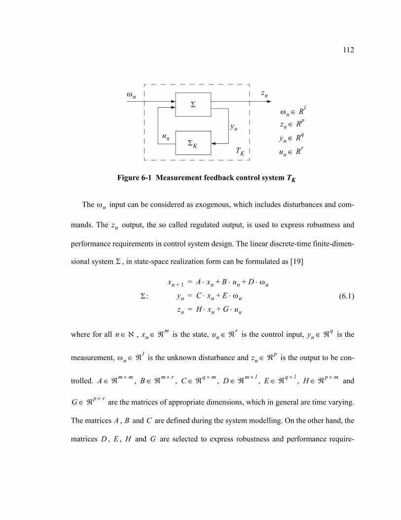
112
The input can be considered as exogenous, which includes disturbances and com-
mands. The output, the so called regulated output, is used to express robustness and
performance requirements in control system design. The linear discrete-time finite-dimen-
sional system , in state-space realization form can be formulated as [19]
(6.1)
where for all , is the state, is the control input, is the
measurement, is the unknown disturbance and is the output to be con-
trolled. , , , , , and
are the matrices of appropriate dimensions, which in general are time varying.
The matrices , and are defined during the system modelling. On the other hand, the
matrices , , and are selected to express robustness and performance require-
Σ
ΣK
ynun
ωn
Figure 6-1 Measurement feedback control system TK
zn
ωn Rl∈
zn Rp∈
yn Rq∈
un Rr∈TK
ωn
zn
Σ
Σ:
xn 1+ A xn B un⋅ D+ ωn⋅+⋅=
yn C xn⋅ E ωn⋅+=
zn H xn⋅ G un⋅+=
n ℵ∈ xn ℜm∈ un ℜr∈ yn ℜq∈
ωn ℜl∈ zn ℜp∈
A ℜm m×∈ B ℜm r×∈ C ℜq m×∈ D ℜm l×∈ E ℜq l×∈ H ℜp m×∈
G ℜp r×∈
A B C
D E H G

113
ments for the control system. This selection is mostly done by iteratively solving and
implementing a number of control problems, until the desired performance is
achieved [101]. The goal during the selection of the weights is to minimize the effect of
the disturbances on the controlled output by finding a dynamic feedback law which
calculates the appropriate control input . The resulting control system design leads
to a dynamic feedback law in state-pace form [19]
(6.2)
where , , and are matrices with appropriate dimensions, calculated from
by the design algorithm. This dynamic feedback operator minimizes the -
induced operator norm of , that internally stabilizes the plant.
The state-space formulation of the closed-loop system , with state-variables
is
. (6.3)
This closed-loop system is internally stabilized by the controller . The closed-
loop system is internally stable if, with and for all initial states , the state con-
verges to zero as [78]. The system (6.3) is internally stable if the
H∞
ωn zn
un H∞
ΣK:xn 1+ Fx xn Fu un⋅ F+ y yn⋅+⋅=
un Kx xn⋅=
Fx Fu Fy Kx Σ
H∞ ΣK l2
ω z→
TK xn xn,
TK:
xn 1+
xn 1+
A B Kx⋅Fy C⋅ Fu Kx Fx+⋅
xn
xn
DFy E⋅
ωn⋅+⋅=
zn H G Kx⋅xn
xn
⋅=
TK ΣK
ω 0= x0
zn 0→ n ∞→ 2m 2m×

114
closed-loop system-matrix (6.4) is asymptotically stable. See “Stability of Discrete-Time
Systems” on page 312.
. (6.4)
6.2 Finite Horizon Suboptimal H∞ Controller
For the plant model , defined by equation (6.1), the central controller (6.2) can
be found if the associated soft-constrained linear-quadratic game with objective function,
as introduced in (5.24) has a feedback saddle-point solution for some pre-selected [19]
. (6.5)
The concept of , as a measure for the control system robustness is defined in Chapter
4, and the selection of its value is clarified in Section 6.2.2. Where is a scalar that deter-
mines the respective contributions of the original quadratic cost, in (6.1), and distur-
bance energy to the cost function [20]. Further, is the weighting matrix for the
final state, see (6.20) and the comments thereafter. The weighting matrix for the initial
state is , see (6.24) and the comments thereafter. Finally, , and are weight-
A A B Kx⋅Fy C⋅ Fu Kx Fx+⋅
=
Σ ΣK
γ
Jγ u ω,( ) =
xNT XC xN xn
T unT Q S
ST R
xn
un
γ2 ωT ω⋅ ⋅–⋅ ⋅
γ2 x0T⋅ XF x0⋅ ⋅–
n 1=
N 1–
∑+⋅ ⋅
γ
γ
zn
XC 0≥
XF 0≥ Q R S

115
ing matrices for the states, for the control and for the combined states and control, respec-
tively, defined by (6.14).
6.2.1 Preliminary Assumptions for the Control
For the existence of the linear discrete-time measurement feedback (sub)optimal
control algorithm, (6.2), it is expected that the following necessary requirements are
satisfied.
Controllability condition. The existence of the stabilizing controller requires that the
unstable modes have to be reachable by the control signal , or equivalently the pair
in (6.1) needs to be controllable over . See “Controllability of
Discrete-Time Systems” on page 313.
Observability condition. The controller is required to have access to all the information
concerning the unstable modes, the pair needs to be detectable over
. See “Observability of Discrete-Time Systems” on page 314.
Injective condition for G. The matrix is required to have full column rank in order that
all control signals in (6.1) be penalized, or equivalently matrix needs to be injective
(one to one)
H∞
ΣK
un
A B, n[ N ) n∀ 0 N,( )∈, ,
A C,
0[ n ) n∀ 0( N ],∈, ,
G
un G

116
. (6.6)
Surjective condition for E. The matrix in (6.1) is required to have full row rank in
order to characterize the measurement noise. Therefore, for each output signal some
disturbance shall be defined, and modelled as direct feed-through from the disturbance
signal in (6.1). Noise-free measurements can not exist as they would be infinitely reli-
able. In other words, the matrix needs to be surjective (onto)
. (6.7)
The assumptions for the injective and surjective conditions require the dimensions of
the controlled output to be at least that of the control input or ,
while the dimension of the unknown disturbance to be at least that of the mea-
surement , or . Since no measurement is error free and no control action is
costless, these are reasonable assumptions [7].
Surjective condition for [A D]. The matrix in (6.1) is required to have full row
rank
. (6.8)
if G ℜp r× and cG rank G( )=∈ then cG r⇔
E
yn
ωn
E
if E ℜq l× and rE rank E( )=∈ then rE q⇔
zn ℜp∈ un ℜr∈ p r≥
ωn ℜl∈
yn ℜq∈ l q≥
A D
rank A D m=

117
This requirement is equivalent to the statement that for a sequence , the map
be surjective (onto) for all , which is equivalent to the require-
ment that the system (6.1) is reachable by .
Injective condition for [AT HT]T. The matrix in (6.1) is required to have full
column rank
. (6.9)
This requirement is equivalent to the statement that for a sequence and ,
the map be injective (one to one) for all , which is equivalent to
the requirement that the system (6.1) is observable by .
6.2.2 Selection of γ
The theoretical background for interpreting as an upper bound for the uncer-
tainties of the control system model is detailed in Chapter 4. In this section a practical
selection of this parameter is presented. From the lower side this is bounded by the
infimum , the norm of the transfer function : . Unfortunately, there is no
analytical expression which would calculate the value . On the other hand, the upper
side of the is soft bounded by the vanishing robustness in the controller’s performance.
un
x0 ω 0 n,[ ],( ) xn 1+→ n
ω
AT HTT
rank AH
m=
un ωn
x0 z 0 n,[ ] xn 1+,( )→ n
z
γ 1 γ⁄( )
γ γ
γ0 H∞ TK ω z→
γ0
γ

118
From the technical point of view, it is essential that a sufficiently large be chosen in
order to obtain an admissible controller but to achieve the highest performance in the
robustness of the control loop, must be close to the infimum
The above discussion can be summarized by the definition of and
, as presented in Figure 6-2.
The following two statements are equivalent:
• If belongs to , the (sub)optimal control system design leads to an admissible
control system, and if belongs to the controller in not admissible.
• The controller is admissible if the positivity tests (6.23), (6.27) and (6.30) or (6.31),
given as an integral part of the algorithm are satisfied. If any of the three positivity
tests fails the controller is not admissible.
These statements then lead to the conclusion that in order to obtain the minimally
achievable norm , it is required to interactively check the positivity tests for differ-
ent values of by a search algorithm.
γ
γ γ0
0 γ0ΓF ΓP
γ
Decreasing Robustness
Test fails Tests pass
Figure 6-2 Infimum search
All the PositivityThe Positivity
γPγF
Admissible controllers
ΓF : γ 0 : γ0[ ]∈
ΓP : γ γ( 0 : ∞ ]∈
γ ΓP H∞
γ ΓF
H∞
H∞ γ0
γ

119
The proposed algorithm, as presented in Figure 6-3, starts by selecting any positive
number for and initializing the temporary variables and , which are the
containers for the if it fails or passes the positivity tests, respectively, see Figure 6-2.
During the search, if for the selected value of , the control optimization algorithm
passes all three positivity tests then and otherwise and .
The search algorithm consists of two phases. The first phase lasts until a is found
by the binomial search
. (6.10)
The first phase yields to a lower limit and upper limit on the infimum . The
second phase is the bisectional search for to obtain a close to optimal solution
. (6.11)
This iterative procedure continues until the magnitude of the difference between the
smallest and the largest is small [102]
(6.12)
where the tolerance is selected according to the required accuracy for the opti-
mal solution of the infimum .
According to the literature [78] using approximately 10% larger than the infimum
for the control system design, leads to a proper solution
γ γF 0= γP 0=
γ
γ H∞
γ ΓP∈ γP γ= γ ΓF∈ γF γ=
γ ΓP∈
γ 2 γ⋅=
γF γP γ0
γ0
γ γP γF+( ) 2⁄=
γP γF
if γP γF–
γP---------------- γTOL<
then γ0 γP=
γTOL 0>
γ0
γ
γ0 H∞

120
. (6.13)
Otherwise, numerical difficulties will be encountered. The required matrix inverse calcu-
lation , which appears in almost all formulations for the control,
is the reason for the numerical difficulties near the infimum [101]. The closer the itera-
tion gets to the infimum , the more the matrix inverse
approaches singularity.
6.2.3 The H∞ Algorithm
The necessary and sufficient condition for the existence of an admissible controller
involves the existence of two positive definite matrices, which are formed from the stabi-
γ 1.1 γ0⋅=
γ2 I⋅ m PnF Pn
C⋅–( )1–
H∞
γ0
γ γ→ 0 sup ρ PnF Pn
C⋅( )=
γP γF–γP
---------------- γTOL<
γ 0>
Figure 6-3 Search algorithm for γ
γF γP 0= =
pass
γ 2 γ⋅=γP γ=γF γ=
γ γP γF+( ) 2⁄=Positivity testsfail
fail
pass
γF γ=
γ γP γF+( ) 2⁄=
Positivity tests
yesno
γP γ=
γ 1.1 γ0⋅=γ0 γP=

121
lizing solutions of two Riccati recursions. Moreover, the coupling condition between the
solutions of these two Riccati recursions must be satisfied.
The algorithm becomes more readable by the introduction of the notation
(6.14)
where represents the weight on the state variable , is the weight for the control sig-
nal and is the weight on the cross terms between the state and the control signal .
Furthermore,
(6.15)
where represents the measure of system noise intensity and is the measure of mea-
surement noise intensity [19].
The following notations are introduced for further simplification of the formulas
(6.16)
(6.17)
(6.18)
. (6.19)
The control policy of a soft-constrained linear-quadratic dynamic game is obtained by
the dynamic programming approach. The solution of the dynamic programming is a back-
Q SST R
HT
GTH G⋅=
Q x R
u S x u⋅
W LLT V
DE DT ET⋅=
W V
A A B R 1– ST⋅ ⋅–=
Q Q S R 1– ST⋅ ⋅–=
A A L V 1– C⋅ ⋅–=
W W L V 1– LT⋅ ⋅–=

122
ward recursion based discrete-time generalized Riccati equation, which calculates the pos-
itive definite matrices
(6.20)
where the intermediate variables and are defined in the following, and the
initialization of the Riccati recursion is selected such that is a positive definite,
(See “The Riccati Recursion” on page 128.)
(6.21)
where the term in the quadratic form, an indefinite matrix in the Riccati recursion,
is defined as
. (6.22)
The unique feedback saddle-point solution exists if the solvability test for the Riccati
recursion, in the form of positivity condition, is satisfied such that
. (6.23)
The positivity condition actually implies the nonsingularity of inversion and also a
positive definite matrix calculation in (6.20) in the next recursion. If this condition is
not met, then the game does not admit a saddle-point solution and the algorithm must be
aborted and tested again with an increased .
PN 1+C P, N
C … P1C,,
PnC AT Pn 1+
C A AT Pn 1+C Λn 1+
C Pn 1+C A Q+⋅ ⋅ ⋅ ⋅–⋅ ⋅= PN 1+
C XC=
Λn 1+C Γn 1+
C
XC 0≥
Λn 1+C B D Γn 1+
C BT
DT⋅ ⋅=
Γn 1+C
Γn 1+C
R BT Pn 1+C B⋅ ⋅+ BT Pn 1+
C D⋅ ⋅
DT Pn 1+C B⋅ ⋅ γ2– Il DT Pn 1+
C D⋅ ⋅+⋅
1–
=
γ2 Il DT Pn 1+C D 0>⋅ ⋅–⋅
Γn 1+C
PnC
γ

123
The worst-case state estimator for a soft-constrained linear-quadratic dynamic game is
obtained by the dynamic programming approach. The solution of the dynamic program-
ming is a forward recursion based on a discrete-time generalized Riccati equation, which
calculates the positive definite matrices such that
(6.24)
where the intermediate variables and are defined below and the initialization for
the Riccati recursion is selected such that is a positive definite (See “The Riccati
Recursion” on page 128.)
(6.25)
where the term in the quadratic form, an indefinite matrix in the Riccati recursion, is
the inverse of the innovation variance defined as
. (6.26)
The algorithm admits a unique feedback saddle-point solution if the solvability test for
the Riccati recursion, in the form of positivity condition
(6.27)
is satisfied.
P1F P2
F … PNF,,,
Pn 1+F A Pn
F AT A PnF Λn
F PnF AT W+⋅ ⋅ ⋅ ⋅–⋅ ⋅= P0
F XF=
ΛnF Γn
F
XF 0≥
ΛnF CT HT Γn
F CH
⋅ ⋅=
ΓnF
ΓnF
V C PnF CT⋅ ⋅+ C Pn
F HT⋅ ⋅
H PnF CT⋅ ⋅ γ2– Ip H Pn
F HT⋅ ⋅+⋅
1–
=
γ2 Ip H PnF HT 0>⋅ ⋅–⋅
124
This condition actually implies the nonsingularity of the inversion and a positive
definite matrix calculation in (6.24) in the next recursion. It can be shown that the
existence of is related to the question of how well the state can be estimated on the
basis of the observations of . For instance, if it will be shown that [78].
If this condition is not satisfied, the game does not admit a saddle-point solution and the
algorithm must be aborted and tested again with increased .
By introducing the following two intermediate variables
(6.28)
and
(6.29)
the coupling condition can be expressed in its usual simple form.
It is required that the coupling condition, expressed in the form of the positivity test, is sat-
isfied by either
(6.30)
or
. (6.31)
It is a kind of test whether state estimation and the state feedback combined in some
way yield the desired result: an internally stabilizing feedback which makes the norm
ΓnF
Pn 1+F
ΓnF xn
y y x= ΓnF 0=
γ
PnC AT Pn
C( )1–
γ 2– W⋅–( )1–
A Q+⋅ ⋅=
Pn 1+F A Pn
F( )1–
γ 2– Q⋅–( )1–
AT W+⋅ ⋅=
γ2 Im PnF Pn
C 0>⋅–⋅
γ2 Im PnF Pn
C 0>⋅–⋅
H∞

125
less than [78]. If the coupling condition is not satisfied, the selected is too small.
Therefore, the algorithm must be aborted and tested again using an increased .
If all the positivity tests, (6.23), (6.27), and (6.30) or (6.31), are satisfied then the
(sub)optimal state-feedback controller can be written as
(6.32)
where the state-feedback gain for the robust (sub)optimal controller is defined as
(6.33)
(6.34)
. (6.35)
The robust state estimator can be written in the form
(6.36)
where the matrices , , and are defined as
(6.37)
(6.38)
(6.39)
and the intermediate matrix is calculated as
. (6.40)
γ γ
γ
ΣK
µ∗ xn( ) : un Kx xn⋅=
H∞
Kx R 1– BT ∆C A ST+⋅ ⋅( ) ∆S⋅ ⋅–=
∆C PnC( ) 1– B R 1– BT⋅ ⋅ γ 2– W⋅–+( )
1–=
∆S Im γ 2– PnF Pn
C⋅ ⋅–( )1–
=
xn 1+ Fx xn Fu un⋅ F+ y yn⋅+⋅=
Fx Fu Fy
Fx A γ 2– A ∆F Q⋅ ⋅ ⋅ A ∆F CT L+⋅ ⋅( ) V 1– C⋅ ⋅–+=
Fu B γ 2– A ∆F S⋅ ⋅ ⋅+=
Fy A ∆F CT L+⋅ ⋅( ) V 1–⋅=
∆F
∆F PnF( ) 1– CT V 1– C γ 2– Q⋅–⋅ ⋅+( )
1–=

126
The (sub)optimal controller, obtained by the equations (6.32) and (6.36), ensures
an attenuation level of for the worst-case external disturbances, as explained in
Chapter 4.
6.2.4 Step-by-Step Implementation
With the integration of sections 6.2.1, 6.2.2 and 6.2.3, the step-by-step implementation
of the (sub)optimal control algorithm is described. The efficient implementation of
the controller requires the proper integration of the search for the infimum . The com-
plete (sub)optimal algorithm with the infimum search can be defined in the following:
1. The process starts with the selection of an initial value . Go to step 2.
2. The infimum search with and is initialized. The equations from (6.14)
through (6.19) are calculated. Go to step 4.
3. Defined by the inequality (6.23), the solvability test is performed. If the positive defi-
niteness is satisfied go to step 4. If the solvability condition is not satisfied, the selected
is too small. In this situation, go to step 10.
4. The backward Riccati recursion for the control is calculated using the equations (6.20)
through (6.22). Go to step 5.
5. The solvability test, defined by the inequality (6.27), is performed. If the positive defi-
niteness is satisfied go to step 6, else go to step 10.
6. The forward Riccati recursion for the state estimation is calculated using equations
(6.24) to (6.26). Continue with step 7.
H∞
γ
H∞
γ0
H∞
γ 0>
γF 0= γP 0=
γ

127
7. In preparation for testing the coupling condition, some intermediate matrices, defined
by equations (6.28) and (6.29), are calculated. Go to step 8.
8. The coupling condition is evaluated using either (6.30) or (6.31) inequality. If the test is
successful, becomes the upper limit in the search . Go to step 9. If the test is
unsuccessful go to step 10.
9. A valid , which satisfies all the positivity tests, is confirmed. At this step, a deci-
sion is made whether the search for the infimum should be terminated or not. If the
inequality test is satisfied , where is the selected tolerance, continue
with step 11. Otherwise and return to step 4.
10. The iteration for the selected is unsuccessful ; therefore, the lower limit on
should be modified to . Furthermore, if then else
. Go to step 4.
11. An infimum , within a desired accuracy, is obtained. For a stable solution, it is
suggested in [78] that should be used for control calculations. Go to
step 12.
12. With the defined , the equations from (6.20) to (6.31) are recalculated. All the tests
are expected to pass. Go to step 13.
13. To obtain the controller defined by equation (6.32), equations (6.33) to (6.35) are cal-
culated for the control gain. Continue with step 14.
14. The state-space estimator, defined by equation (6.36), requires that the matrices are
calculated using equations (6.37) to (6.40). Continue with step 15.
γ γP γ=
γ ΓP∈
γ0
ε γP γF–( )> γP⁄ ε
γ γP γF+( ) 2⁄=
γ γ ΓF∈ γ
γF γ= γP 0≠ γ γP γF+( ) 2⁄=
γ 2 γ⋅=
γ0 γP=
γ 1.1 γ0⋅=
γ

128
15. The measurement feedback (sub)optimal control algorithm, defined by equations
(6.32) and (6.36), is ready for real time implementation.
The algorithm, calculated through the above 15 steps, defines a central (sub)opti-
mal measurement feedback controller such that the closed-loop system mapping
has an induced norm less than , where is calculated in step 11.
6.2.5 The Riccati Recursion
The control system design for the time-invariant discrete-time plant with linear-qua-
dratic objective function, typically results in the well studied Discrete-time Algebraic Ric-
cati Equation (DARE). On the other hand, the control system design for the time-varying
discrete-time plant with linear-quadratic objective function, uses the Riccati equation in its
recursive form.
If the discrete-time plant is time-invariant the controller can be calculated either by the
DARE or by the Riccati equation in its recursive form. It is a reasonable expectation that
the control system design obtained using both these methods will result in an equivalent
design. As shown in [20] and [7], the recursive Riccati equations (6.20) and (6.24) con-
verge to the desired solution, equivalent to the solution of DARE, depending on the value
chosen for ( and ). The initial value is required to be positive semidefinite
and . The convergence will not be guaranteed if the initialization matrices are too
large.
H∞
H∞
ω z→
γ γ
XC XF XC 0≥
XF 0≥

129
In case of the Riccati recursion for controller calculation in equation (6.20), if the ini-
tial matrix is selected such that
(6.41)
where is the solution of the Lyapunov equation
(6.42)
and where is defined by (6.16) and is defined by (6.17), the Riccati recursion
sequence will converge to the unique stabilizing solution of an equiva-
lent DARE, if it exists. Consequently, the sequence is also bounded by
, otherwise the initial condition will be violated.
In case of the Riccati recursion for state-space estimation in equation (6.24), if the ini-
tial matrix is selected such that
(6.43)
where is the solution of the Lyapunov equation
(6.44)
and where is defined by (6.18) and is defined by (6.19), the Riccati recursion
sequence will converge to the unique stabilizing solution of an equivalent
DARE, if it exists. Consequently, the sequence is also bounded by
, otherwise the initial condition will be violated.
XC
0 XC ΠC≤ ≤
ΠC
ΠC AT ΠC A Q+⋅ ⋅=
A Q
PN 1+C P, N
C … P1C,,
PN 1+C P, N
C … P1C,,
0 PnC ΠC≤ ≤
XF
0 XF ΠF≤ ≤
ΠF
ΠF A ΠF AT W+⋅ ⋅=
A W
P1F P, 2
F … PNF,,
P1F P, 2
F … PNF,,
0 PnF ΠF≤ ≤

130
6.3 Implementation Example
To illustrate the implementation of the measurement feedback (sub)optimal con-
trol algorithm, an example is selected involving the mass spring system. Originally pro-
posed in [103], known as the ACC benchmark problem from the American Control
Conference, this example is widely used in the control literature [103-105].
The plant consists of two masses and , connected with the spring of stiffness ,
and the plant damping is expressed by . The challenge for the control design is originat-
ing from the very large phase lags in the control system due to the non collocated actuator/
sensor set-up. The sensor senses the position of the mass while the actuator acts
on the mass . The state-space representation of the plant model in continuos time is
given by the equations
H∞
Figure 6-4 ACC benchmark problem
m1 m2κ
x2 y=x1
uw
disturbancecontrol
m1 m2 κ
ζ
y m2 u
m1

131
(6.45)
where are the states of the system: is the position of the mass , is the
position of the mass , is the speed of the mass , is the speed of
the mass , is the control input, and is the plant output.
The design requirement is to find a controller that stabilizes the system with an uncer-
tain spring constant , varying between 0.5 and 2, with the nominal value set to 1. Both
masses are selected to be equivalent . The plant damping is set for
. However, even if , i.e., the plant is undamped, simulation studies show
that the control system performance is not significantly affected by this value.
The open loop plant response for an initial disturbance in the state is pre-
sented in Figure 6-5. This disturbance is used to test and demonstrate the behavior of the
control system. The discrete time representation, , of the continuous time system, ,
from (6.45), is obtained by substituting the nominal parameter values and using the matlab
function c2d with the sampling time of and the zero-order-hold (ZOH) option
P:
x· 1
x· 2
x· 3
x· 4
0 0 1 00 0 0 1
κ– m1⁄ κ m1⁄ ζ– m1⁄ ζ m1⁄
κ m2⁄ κ– m2⁄ ζ m2⁄ ζ– m2⁄
x1
x2
x3
x4
00
1 m1⁄
0
u⋅+⋅=
y x2=
x1 … x4, , x1 m1 x2
m2 x3 tddx1= m1 x4 td
dx2=
m2 u y
κ
m1 m2 1= =
ζ 0.01= ζ 0=
x1 t, 0= 1=
Pd P
TS 0.05s=
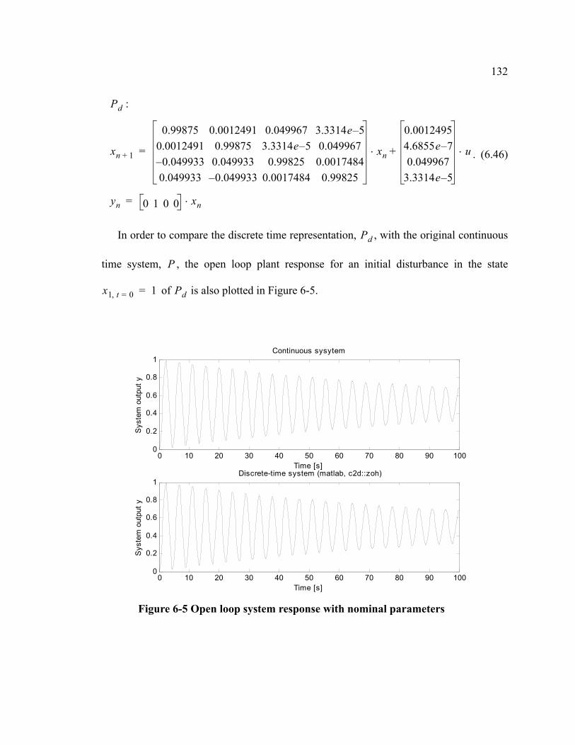
132
. (6.46)
In order to compare the discrete time representation, , with the original continuous
time system, , the open loop plant response for an initial disturbance in the state
of is also plotted in Figure 6-5.
Pd :
xn 1+
0.99875 0.0012491 0.049967 3.3314e 5–0.0012491 0.99875 3.3314e 5– 0.049967
0.049933– 0.049933 0.99825 0.00174840.049933 0.049933– 0.0017484 0.99825
xn
0.00124954.6855e 7–0.049967
3.3314e 5–
u⋅+⋅=
yn 0 1 0 0 xn⋅=
Pd
P
x1 t, 0= 1= Pd
0 10 20 30 40 50 60 70 80 90 1000
0.2
0.4
0.6
0.8
1Continuous sysytem
Time [s]
Sys
tem
out
put y
0 10 20 30 40 50 60 70 80 90 1000
0.2
0.4
0.6
0.8
1 Discrete-time system (matlab, c2d::zoh)
Time [s]
Sys
tem
out
put y
Figure 6-5 Open loop system response with nominal parameters

133
To formulate the robustness and performance requirements for the standard con-
trol algorithm in the form of (6.1), it is required to choose the appropriate matrices
, , and . For the selection of these matrices,
in the case of single-input/single-output (SISO) system design, graphical tools, like the
Bode and Nyquist diagrams, can be used. For multiple-input/multiple-output (MIMO)
systems the selection of these matrices is not straightforward [78]. One possible solution
for MIMO system design would be the implementation of the trial and error approach.
In this research, the trial and error approach is applied to select the proper weighting
matrices by observing the plant behavior through its output . In the following, this pro-
cedure is illustrated.
Through the selection of matrices and , the weights for the per-
formance index are determined. The dimensions and are defined by the plant model.
The dimension , which can be selected freely, defines the size of the controlled output
vector. One good choice for the initial guess, is to select that . In this
case,
, (6.47)
then the controlled output contains all the state and control variables
H∞
D ℜq m×∈ E ℜq l×∈ H ℜp m×∈ G ℜp r×∈
yn
H ℜp m×∈ G ℜp r×∈
m r
p
z ℜp∈ p m r+=
H
1 0 0 0 00 1 0 0 00 0 1 0 00 0 0 1 00 0 0 0 0
= G
00001
=

134
. (6.48)
The selection of and is more complex because through these
matrices the model uncertainty and the effects of the exogenous disturbances for the con-
trol system are modelled.
For better understanding of the functions of the and matrices, Figure 6-6 shows
the modelling of the disturbances as additive perturbations and multiplicative perturba-
tions. Matrix is used to interpret the model perturbations effecting the states of the plant
model, and matrix is used to interpret the disturbances equivalent to the measurement
noise.
zn
x1 n,
x2 n,
x3 n,
x4 n,
un
=
D ℜq m×∈ E ℜq l×∈
D E
D
E
Figure 6-6 Additive and multiplicative perturbations
G θ T,( )
∆n
ynun G θ T,( )
∆n
un yn
xn 1+ A xn B u⋅+⋅=
yn C xn ∆n u⋅+⋅=
xn 1+ A xn B u B ∆n⋅+⋅+⋅=
yn C xn ∆n u⋅+⋅=

135
The and dimensions for the matrices and are defined in
the plant model. The dimension shall be selected according to the requirement to ade-
quately represent the perturbations effecting the plant model.
Testing of the control system design with the dimension , always resulted in an
unstable controller. Therefore it is concluded that the dimension of can not be selected
freely, as its lower value is limited. In the first and second trial, as presented below,
and were selected respectively, resulting in a stable control system.
6.3.1 First Tryout
In the first tryout, it is expected that the disturbances on the masses and have
the same accelerating force as the control signal. This is the reason for selecting the values
for the matrix similarly to the matrix , in the first tryout
. (6.49)
Substituting the nominal parameter values and by using the matlab function c2d with
and with the zero-order-hold (ZOH) options, the discrete time matrix is
defined as
m l D ℜq m×∈ E ℜq l×∈
q
q 1=
q
q 2=
q 4=
m1 m2
D B
D
0 00 00 1 m1⁄
1 m2⁄ 0
=
TS 0.05s=

136
. (6.50)
During the first trial matrix remains unchanged. Only the values in , and
matrices are manipulated. In the following the results from several tests are presented,
which illustrate the effects of the selection of matrices , and on the resulting con-
trol performance, through the control signal and the plant response.
Overall, thirteen test results are recorded, named as Test a through Test m. Since pre-
senting all these tests in one graph would not result in any meaningful information, the
visualization of tests is divided in four groups, named Test Group I through Test Group IV.
Every graph consists of two parts. The upper part is the performance index obtained as a
square sum of the plant output, over the time period of from the disturbance. The
lower part represents the control energy attained as a square sum of the control signal,
over the same period of time. In each test the controller is calculated when the nomi-
nal spring stiffness is substituted into the plant model. Once the controller is
obtained, the spring stiffness in the plant model is varied from 0.2 up to 4 by 0.1 steps, and
for all steps the control performance was recorded and visually presented.
Test a:
D
4.6855e 7– 0.00124950.0012495 4.6855e 7–3.3314e 5– 0.0499670.049967 3.3314e 5–
=
D E H G
E H G
100s
H∞
κ 1=
H
1 0 0 0 00 1 0 0 00 0 1 0 00 0 0 1 00 0 0 0 0
= G
00001
= E 1 1=

137
Test b:
Test c:
Test d: .
In Test Group I, Figure 6-7 compares the plants’ performance indexes and the control
energy as a function of spring stiffness, obtained from Tests a, b, c, and d. It is apparent
that in this test group the controller in Test a is stable only for the nominal plant, while its
best performance is demonstrated in Test d.
H
1 0 0 0 00 1 0 0 00 0 1 0 00 0 0 1 00 0 0 0 0
= G
00001
= E 0.1 1 1⋅=
H
1 0 0 0 00 1 0 0 00 0 1 0 00 0 0 1 00 0 0 0 0
= G
00001
= E 0.01 1 1⋅=
H
1 0 0 0 00 1 0 0 00 0 1 0 00 0 0 1 00 0 0 0 0
= G
00001
= E 0.003 1 1⋅=

138
Test e:
Test f:
0 0 . 5 1 1 . 5 2 2 . 5 3 3 . 5 4
1 0 0
1 0 5
1 0 1 0
S p r in g s t i ffn e s k
Per
form
ance
Inde
x
abcd
0 0 . 5 1 1 . 5 2 2 . 5 3 3 . 5 4
1 0 2
1 0 4
S p r in g s t i ffn e s k
Con
trol E
nerg
y
Figure 6-7 First tryout: Test Group I
H
10 0 0 0 00 10 0 0 00 0 1 0 00 0 0 1 00 0 0 0 0
= G
00001
= E 0.003 1 1⋅=
H
100 0 0 0 00 100 0 0 00 0 1 0 00 0 0 1 00 0 0 0 0
= G
00001
= E 0.003 1 1⋅=

139
Test g: .
In Test Group II, Figure 6-8 compares the plants’ performance indexes and the control
energy as a function of spring stiffness, obtained from Tests e, f, and g. To facilitate the
comparison between the tests, Test d from Test Group I is also included. This test group
shows significant improvement in performance, when dealing with lower values of spring
stiffness. At the same time, the controller’s performance deteriorates for higher values of
spring stiffness. However, if it is taken into account that the control design solely requires
H
300 0 0 0 00 300 0 0 00 0 1 0 00 0 0 1 00 0 0 0 0
= G
00001
= E 0.003 1 1⋅=
0 0 . 5 1 1 . 5 2 2 . 5 3 3 . 5 4
1 0 0
1 0 5
1 0 1 0
S p r i n g s t i ffn e s k
Per
form
ance
Inde
x
defg
0 0 . 5 1 1 . 5 2 2 . 5 3 3 . 5 41 0 1
1 0 2
1 0 3
1 0 4
1 0 5
S p r in g s t i ffn e s k
Con
trol E
nerg
y
Figure 6-8 First tryout: Test Group II

140
a stabilizing controller for spring stiffness between 0.5 and 2, all controllers belonging into
this test group are admissible. It can be noted that the controller in Test g has the best per-
formance.
Test h:
Test i:
Test j: .
For Test Group III, Figure 6-9 compares the plants’ performance indexes and the con-
trol energy as a function of spring stiffness, obtained from Tests h, i, and j. To facilitate the
comparison between the tests, Test g from Test Group II is also included. Compared to the
performance of the controller in Test g, an overall performance degradation can be
observed. At the same time, the control energy consumption is reduced. The controller
designed in Test h, satisfies all the control design requirements.
H
300 0 0 0 00 300 0 0 00 0 1 0 00 0 0 1 00 0 0 0 0
= G
00005
= E 0.003 1 1⋅=
H
300 0 0 0 00 300 0 0 00 0 1 0 00 0 0 1 00 0 0 0 0
= G
000050
= E 0.003 1 1⋅=
H
300 0 0 0 00 300 0 0 00 0 1 0 00 0 0 1 00 0 0 0 0
= G
0000
300
= E 0.003 1 1⋅=

141
Test k:
Test l:
0 0 . 5 1 1 . 5 2 2 . 5 3 3 . 5 4
1 0 0
1 0 5
1 0 1 0
S p r i n g s t i f fn e s k
Per
form
ance
Inde
x
ghij
0 0 . 5 1 1 . 5 2 2 . 5 3 3 . 5 41 0 1
1 0 2
1 0 3
1 0 4
1 0 5
S p r i n g s t i f fn e s k
Con
trol E
nerg
y
Figure 6-9 First tryout: Test Group III
H
300 0 0 0 00 300 0 0 00 0 1 0 00 0 0 1 00 0 0 0 0
= G
0000
0.8
= E 0.003 1 1⋅=
H
300 0 0 0 00 300 0 0 00 0 1 0 00 0 0 1 00 0 0 0 0
= G
0000
0.6
= E 0.003 1 1⋅=

142
Test m: .
For Test Group IV, Figure 6-10 compares the plants’ performance indexes and the con-
trol energy as a function of spring stiffness, obtained from Tests k, l, and m. To facilitate
the comparison between the tests, Test g from Test Group II is included. Compared to the
performance of the controller in Test g, the performance of the controllers and the control
energy consumption are similar to each other. Although there are performance variations
for higher values of spring stiffness, these performances are beyond the control design
requirements.
H
300 0 0 0 00 300 0 0 00 0 1 0 00 0 0 1 00 0 0 0 0
= G
0000
0.5
= E 0.003 1 1⋅=
0 0 . 5 1 1 . 5 2 2 . 5 3 3 . 5 4
1 0 0
1 0 5
1 0 1 0
S p r i n g s t i f fn e s k
Per
form
ance
Inde
x
0 0 . 5 1 1 . 5 2 2 . 5 3 3 . 5 41 0 1
1 0 2
1 0 3
1 0 4
1 0 5
S p r i n g s t i f fn e s k
Con
trol E
nerg
y
gklm
Figure 6-10 First tryout: Test Group IV

143
From the engineering design perspective, where a compromise must be made between
the control energy and controller performance, the design specified in Test h shall be
selected for control implementation. For the resulting controller , the matrices for
the real-time control (6.2) are
. (6.51)
6.3.2 Second Tryout
In the second tryout the effects of a more complex disturbance model are tested. In this
model the length of four has been selected for the external disturbances vector . The
appropriate noise model is defined as
. (6.52)
By substituting the nominal parameter values and using the matlab function c2d with
and the zero-order-hold (ZOH) option, the discrete time matrix is
γ 330=
Fx
1.0585 31.501– 0.049967 3.3368e 5–0.0018572 0.91708– 3.3314e 5– 0.049967
0.039576– 5.6301 0.99825 0.00174840.05471 10.048– 0.0017484 0.99825
= Fu
0.00124954.6855e 7–0.049967
3.3314e 5–
=
Fy
31.5031.91585.5804–
9.9985
= Kx 108.25– 36.187– 15.103– 192.47–=
ω
D
0 0 1 00 0 0 10 1 m1⁄ 1 m1⁄ 1 m1⁄
1 m2⁄ 0 1– m2⁄ 1 m2⁄
=
TS 0.05s=

144
. (6.53)
During the trial, matrix remains unchanged. Only the values in , and matri-
ces are manipulated. The description of the tests is equivalent to that presented in the first
tryout, not repeated here. The test results are presented in the following
Test a:
Test b:
Test c:
D
4.6855e 7– 0.0012495 0.0012491 0.001250.0012495 4.6855e 7– 0.0012491 0.001253.3314e 5– 0.049967 0.049933 0.050.049967 3.3314e 5– 0.049933 0.05
=
D E H G
H
1 0 0 0 00 1 0 0 00 0 1 0 00 0 0 1 00 0 0 0 0
= G
00001
= E 1 1 1 1=
H
1 0 0 0 00 1 0 0 00 0 1 0 00 0 0 1 00 0 0 0 0
= G
00001
= E 0.1 1 1 1 1⋅=
H
1 0 0 0 00 1 0 0 00 0 1 0 00 0 0 1 00 0 0 0 0
= G
00001
= E 0.01 1 1 1 1⋅=
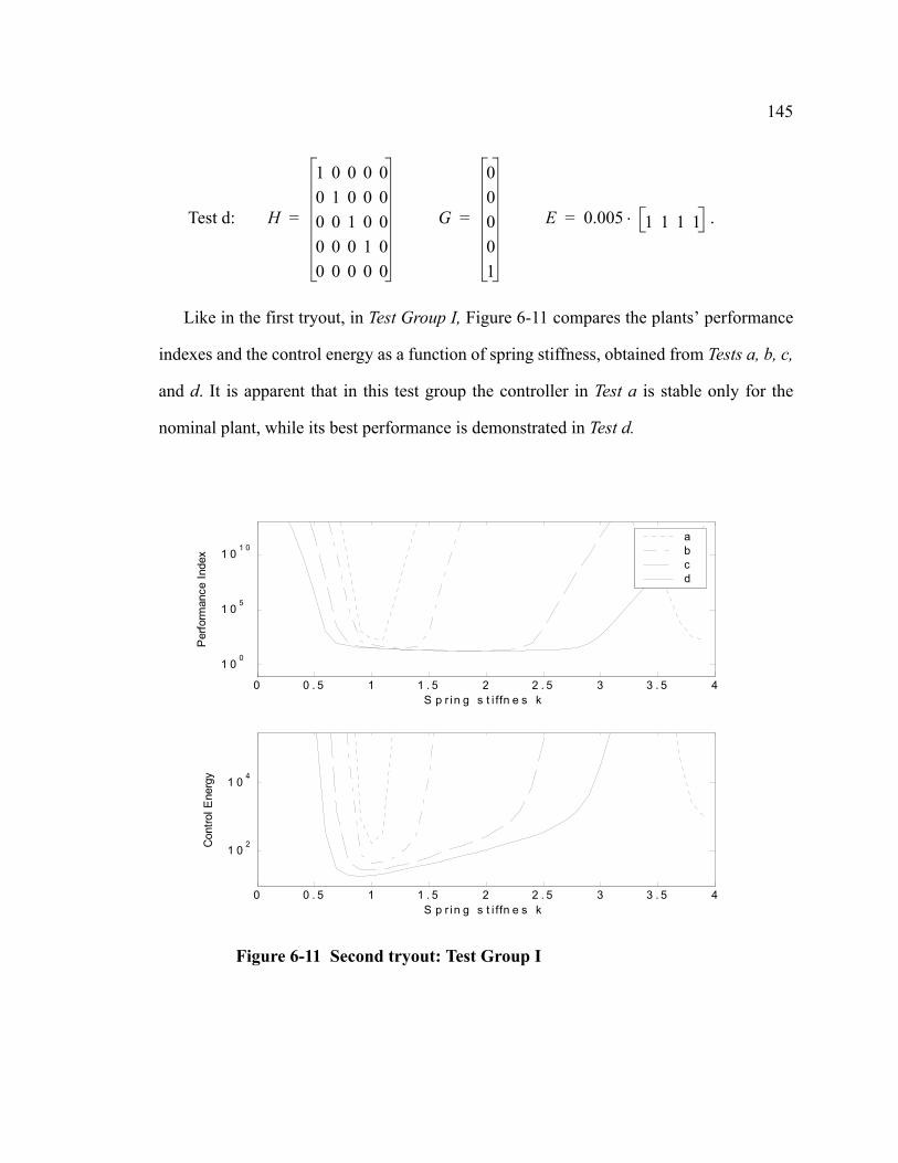
145
Test d: .
Like in the first tryout, in Test Group I, Figure 6-11 compares the plants’ performance
indexes and the control energy as a function of spring stiffness, obtained from Tests a, b, c,
and d. It is apparent that in this test group the controller in Test a is stable only for the
nominal plant, while its best performance is demonstrated in Test d.
H
1 0 0 0 00 1 0 0 00 0 1 0 00 0 0 1 00 0 0 0 0
= G
00001
= E 0.005 1 1 1 1⋅=
0 0 . 5 1 1 . 5 2 2 . 5 3 3 . 5 4
1 0 0
1 0 5
1 0 1 0
S p r in g s t i ffn e s k
Per
form
ance
Inde
x
abcd
0 0 . 5 1 1 . 5 2 2 . 5 3 3 . 5 4
1 0 2
1 0 4
S p r in g s t i ffn e s k
Con
trol E
nerg
y
Figure 6-11 Second tryout: Test Group I

146
Test e:
Test f:
Test g: .
In Test Group II, Figure 6-12 compares the plants’ performance indexes and the con-
trol energy as a function of spring stiffness, obtained from Tests e, f, and g. To facilitate the
comparison between the tests, Test d from Test Group I is also included. This test group
shows some improvement in performance, when dealing with lower values of spring stiff-
ness. As in the first tryout, the controller in Tests f and g has the best performance.
H
10 0 0 0 00 10 0 0 00 0 1 0 00 0 0 1 00 0 0 0 0
= G
00001
= E 0.005 1 1 1 1⋅=
H
100 0 0 0 00 100 0 0 00 0 1 0 00 0 0 1 00 0 0 0 0
= G
00001
= E 0.005 1 1 1 1⋅=
H
140 0 0 0 00 140 0 0 00 0 1 0 00 0 0 1 00 0 0 0 0
= G
00001
= E 0.005 1 1 1 1⋅=

147
Test h:
Test i:
0 0 . 5 1 1 . 5 2 2 . 5 3 3 . 5 4
1 0 0
1 0 5
1 0 1 0
S p r in g s t i ffn e s k
Per
form
ance
Inde
x
0 0 . 5 1 1 . 5 2 2 . 5 3 3 . 5 41 0 1
1 0 2
1 0 3
1 0 4
1 0 5
S p r in g s t i ffn e s k
Con
trol E
nerg
y
defg
Figure 6-12 Second tryout: Test Group II
H
140 0 0 0 00 140 0 0 00 0 1 0 00 0 0 1 00 0 0 0 0
= G
000010
= E 0.005 1 1 1 1⋅=
H
140 0 0 0 00 140 0 0 00 0 1 0 00 0 0 1 00 0 0 0 0
= G
0000
100
= E 0.005 1 1 1 1⋅=
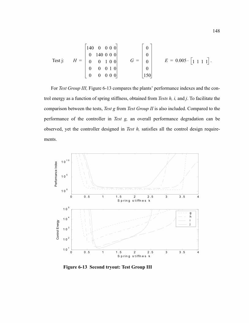
148
Test j: .
For Test Group III, Figure 6-13 compares the plants’ performance indexes and the con-
trol energy as a function of spring stiffness, obtained from Tests h, i, and j. To facilitate the
comparison between the tests, Test g from Test Group II is also included. Compared to the
performance of the controller in Test g, an overall performance degradation can be
observed, yet the controller designed in Test h, satisfies all the control design require-
ments.
H
140 0 0 0 00 140 0 0 00 0 1 0 00 0 0 1 00 0 0 0 0
= G
0000
150
= E 0.005 1 1 1 1⋅=
0 0 . 5 1 1 . 5 2 2 . 5 3 3 . 5 4
1 0 0
1 0 5
1 0 1 0
S p r i n g s t i f fn e s k
Per
form
ance
Inde
x
0 0 . 5 1 1 . 5 2 2 . 5 3 3 . 5 41 0 1
1 0 2
1 0 3
1 0 4
1 0 5
S p r i n g s t i f fn e s k
Con
trol E
nerg
y
ghij
Figure 6-13 Second tryout: Test Group III

149
Test k:
Test l:
Test m: .
In Test Group IV, Figure 6-14 compares the plants’ performance indexes and the con-
trol energy as a function of spring stiffness, obtained from Tests k, l, and m. To facilitate
the comparison between the tests, Test g from Test Group II is included. Compared to the
performance of the controller in Test g, the performance of the controllers and the control
energy consumption are similar to each other. Although there are performance variations
for higher values of spring stiffness, these performances are beyond the control design
requirements.
H
140 0 0 0 00 140 0 0 00 0 1 0 00 0 0 1 00 0 0 0 0
= G
0000
0.9
= E 0.005 1 1 1 1⋅=
H
140 0 0 0 00 140 0 0 00 0 1 0 00 0 0 1 00 0 0 0 0
= G
0000
0.8
= E 0.005 1 1 1 1⋅=
H
140 0 0 0 00 140 0 0 00 0 1 0 00 0 0 1 00 0 0 0 0
= G
0000
0.7
= E 0.005 1 1 1 1⋅=

150
From the engineering design perspective, where a compromise must be made between
control energy and controller performance, the design specified in Test h shall be selected
for control implementation. For the resulting controller , the same as in the first
tryout, the matrices for the real-time control (6.2), are
. (6.54)
0 0 . 5 1 1 . 5 2 2 . 5 3 3 . 5 4
1 0 0
1 0 5
1 0 1 0
S p r i n g s t i f f n e s k
Per
form
ance
Inde
x
0 0 . 5 1 1 . 5 2 2 . 5 3 3 . 5 41 0 1
1 0 2
1 0 3
1 0 4
1 0 5
S p r i n g s t i f f n e s k
Con
trol E
nerg
y
gklm
Figure 6-14 Second tryout: Test Group IV
γ 374=
Fx
1.029 14.02– 0.049967 3.335e 5–0.001714 1.0221– 3.3312e 5– 0.0499670.045472– 8.3879 0.99825 0.0017483
0.054438 11.907– 0.0017485 0.99825
= Fu
0.00124954.6855e 7–0.049967
3.3314e 5–
=
Fy
14.0222.02098.3382–
11.857
= Kx 33.423– 3.9344– 8.8928– 35.36–=

151
The resulting controller performance is very similar to that of the first tryout, even
though the noise model in the second tryout is much more complicated. It can be con-
cluded that the noise model, the dimension of the external disturbance vector , requires
a specific minimum dimension. Therefore, in this example, no admissible controller can
be obtained for the dimension of one. If the necessary dimension of the external distur-
bances vector is used, an admissible controller is obtained. Any further increase of the
noise model does not significantly improve the controller’s behavior. Either way, the con-
troller’s dimension is determined by the dimension of the plant model.
ω
ω

152
7 Model Predictive Control
The control system design, defined in the previous chapters, assumes the knowledge,
with some accuracy, of the plant model for a time invariant system, or the plant model as a
function of time for a time varying system. This assumption is rarely valid outside theoret-
ical control research, especially in the design of controllers for industrial systems. In most
cases, from observations of the plant’s response to the input, it can be assumed that the
system model is known up to the present time; however, the model validity is uncertain in
the future. Theoretically, it is possible to construct models which describe the plant’s
future behavior but this would require a design effort which, in most industrial environ-
ments, is not economically feasible.
The so called model predictive control (MPC) is one of the few suitable methods,
which can be used to resolve the controller design without the enormous task of identify-
ing the exact (very accurate non-linear) plant model. This method describes the plant not
only in the past but also in the near future and it can be used to control the changing plant.
Model predictive control (MPC), receding-horizon control (RHC), moving-horizon
control [106], and generalized predictive control (GPC) are names in the literature used as
synonyms to describe the same form of control. In this type of control, the current control
action is determined by solving an on-line optimal control problem for every time interval
[107-110].

153
When using MPC, the optimal control problem is required to have a finite horizon. The
resulting control law is a feedback control, usually calculated using state models, where
the control is dependent on the plant’s state [106].
The optimal control problem, when calculated at each sampling time, is referred to as
the pointwise strategy, which is presented in Figure 7-1. The terminal point in this control
is of fixed-length, ( is the sampling interval), where the finite cost horizon con-
tinuously recedes at each time instant [111]. The implementation of the pointwise strategy
requires processing power which is capable of calculating the optimal strategy in real
time. This calculation must be performed in less time than the sampling interval .
In most industrial control systems, the processing power presently available is not suf-
ficient for the implementation of the (sub)optimal control algorithm. In ten to fifteen
years, there will probably be computers on the market with sufficient processing power to
allow the implementation of the pointwise strategy. Until then, the so called intervalwise
strategy should be used for implementation.
un∗ xn
N Ts⋅ Ts
Ts
Figure 7-1 Model predictive control strategy - pointwise
Tn Tn 1+Tn 1–
xn
un
xn 1–
xn 1+
un 1–
uncertainty
Tn N+Tn 1+ Tn 2+Tn
N T⋅
t t
H∞

154
In the intervalwise strategy, the terminal point is kept fixed for the finite cost
horizon and after an interval of , the terminal point moves by and the strat-
egy is fixed for the next period, as presented in Figure 7-2.
The intervalwise receding-horizon technique, at each time , solves an opti-
mization problem based on a cost function evaluated on the interval , for
some fixed . The resulting controller is implemented on a shorter interval, say
. Then, at time the optimization is performed again, with the
cost function applied to the interval . For the selection of
the interval , it is required that this interval be smaller than the selected finite hori-
zon interval for the control policy and that this interval be longer than the required
time for all the calculations, as illustrated in Figure 7-3. The controller calculations entail
the following:
1. system parameter estimation ,
N Ts⋅
Nc Ts⋅ Nc Ts⋅
Nc Ts⋅
Figure 7-2 Model predictive control strategy - intervalwise
Tn N+Tn 1+ Tn Nc+Tn
N Ts⋅
tTn 2 Nc⋅+ Tn Nc N+ +
Nc Ts⋅
N Ts⋅
Nc Ts⋅
t Nc= Ts⋅
t t N Ts⋅+,[ ]
N Ts⋅
t t Nc Ts⋅+,[ ] t Nc Ts⋅+
t Nc Ts⋅+ t N Nc+( ) Ts⋅+,[ ]
Nc Ts⋅
Nc N<
tce

155
2. model selection ,
3. control policy calculation ,
4. smoothing update of the state space observer ,
5. real time feedback control calculation .
In this technique, the calculations for the system parameter estimation and the real
time feedback control are performed in real time. Therefore, the minimum require-
ments for the interval can be defined as
. (7.1)
If the requirements for the MPC implementation, beside the granted stability, also
include the induced norm bound from disturbances to states, the implementation of a
robust control algorithm, usually in the form of (sub)optimal control, is needed. The
tcm
tcp
tcs
tcr
tce
tcr
Nc Ts⋅
tce tcm tcp tcs tcr+ + + + Nc Ts⋅<
andtce tcr Ts<+
System parameter estimation
Model selection
Control policy calculation
Smoothing update
Real time feedback calculation
Figure 7-3 MPC as a multi-tasking function
tce
tcm
tcp
tcs
tcr
tcm
tcp
tcs
tcr
Nc Ts⋅
l2
H∞

156
time domain game theoretic technique allows the solution of finite horizon problems with
non-zero initial conditions and therefore supports the MPC formulation [112]. The con-
structed MPC system is affected by external disturbances, which raises the question of the
MPC’s stability under these perturbations. In the following, the requirements of the
MPC’s stability are defined for real-time stability analysis.
7.1 Requirements for Stability
The feedback controller, resulting from the application of the MPC strategy, is a stabi-
lizing controller as long as the design parameters satisfy the MPC stability conditions
below [106] [107].
The terminal constraint set is a subset of which contains the neighborhood of the
origin. The task of the MPC is to steer the state of the plant into in a finite time which
is less than the selected control horizon time . In other words, it is required that
for every initial state which is automatically satisfied for a controllable
system, if is chosen sufficiently large. The terminal constraint set is selected to be
the maximal admissible output set for the system . It is required that the
admissible MPC sequence , obtained by solving the optimal control
problem, steers every initial state of the plant into the terminal constraint set
in finite time . Further, it is expected that the admissible control
sequence satisfies the control constraint when the plant state belongs
Xf X
Xf
t N= Ts⋅
xn N+ Xf∈ xn X∈
N Xf
xn 1+ fn xn un,( )=
un … un N+, , U∈
xn X∈
xn N+ Xf∈ t N= Ts⋅
un N 1+ + …, U∈

157
to the terminal constraint set . Furthermore, it is required that if the state of the
plant belongs to the terminal constraint set the future admissible control
sequence acts in a way so that the plant state stays in the terminal
constraint set which concurs that is positively invariant1 under
the admissible MPC sequence.
The stability of the MPC technique can be established by using the Lyapunov stability
criterion, which requires that the Lyapunov function defined on the MPC strategy be non-
positive. As suggested in [107], the value function, defined by (5.13), is widely
accepted as a Lyapunov function in MPC. Now, if one deals with a “practical” system that
is arising out of physics or technology, it is quite certain that perturbations will come up
not only because of initial conditions other than but also, and above all, due to the
action of exterior and adventitious actions, for example fairly brusque impulses [50]. As a
consequence, the strict Lyapunov stability theory cannot be expected to validate the stabil-
ity of MPC, rather the practical stability should be used. Following the same logic as
defined in the section “Practical Stability” on page 34 and by using the definition intro-
duced for the continuous systems in [50], the stability requirements for MPC can be
defined as below.
1. A set X is called positively invariant if . It is called invariant if . For a dynamic system, a subset of the state space is said invariant if the state is in the set at some time, then it is in the set in the past and in the future. A subset of the state space is said to be positively invariant if it contains the system state at some time, then it will stay in it at the future time [108].
xn N+ Xf∈
xn N+ Xf∈
un N 1+ + …, U∈
xn N 1+ + …, Xf∈ Xf
φ X( ) X⊂ φ X( ) X=
Vn xn( )
x0 0=

158
Theorem Let be a Lyapunov function for the MPC system, a scalar function
which for all has discrete difference and with the property that as
. Let denote the discrete time derivative of the Lyapunov function. If
for all outside for all in , and all and if
for all in and all in , then the system possesses a strong
practical stability. Moreover, it is required that the state of the system outside be for a
finite time or less. The definition of in practical stability could then be limited by
requiring that if in and in then if
implies that the plant state for the stable system outside will remain for the time or
less.
In the determination of the practical stability the boundedness of the disturbances
defined by , as introduced in (4.5) during the development of the (sub)opti-
mal controller, is a necessary condition. For better understanding, this stability definition
is illustrated as a trajectory of the Lyapunov function, in Figure 7-4. In this figure the
Vn xn( )
xn Vn xn( ) ∞→
xn ∞→ ∇Vn xn( )
∇Vn xn( ) ε 0<–≤ xn Xf ωn W n n 1 …,+,
Vn xn( ) Vn xn( )≤ xn Xf xn Xe
Xf
Te ε
Vn xn( ) v1≤ Xf Vn xn( ) v2≥ Xe ε v2 v1–( )= Te⁄
Xf Te
ωn W∈ γ H∞
1 - Unstable2 - Strong Practical Stability
1
2
Trajectory of Vn xn( )V x( ) :
Figure 7-4 Practical stability
X XfXe
t1
t2
t2 t1 Te≤–( )
Xf Xe∩ ∅=Xf Xe X⊂∪
Xe γ∴ from (4.6) equation

159
region characterized by the set, corresponds to the uncertainty space defined by the
(4.6) equation limit which is calculated as the norm of the control system.
The sufficient stability requirements for an MPC can be summarized as in [107] and
extended by the practical stability from [50]:
1. ,
2. ,
3. ( is positively invariant under
),
4. .
The stability theory introduced in this section is not limited by any assumption of the
system linearity. On the other hand, the control algorithm defined in Chapter 6, is limited
to linear systems. In the following, the implementation of this linear control algorithm
by the MPC technique for non-linear systems is investigated.
7.2 Robust MPC for Non-Linear Systems
Although the theory for non-linear control is well developed, there have been very
few practical applications due to the lack of efficient numerical methods for solving these
problems. To solve the non-linear state-feedback control problem, the solution of the
Hamilton-Jacobi-Isaacs equation (inequality) needs to be attained [87] [113]. Since this
Xe γ
H∞
Xf X Xf closed 0 Xf (state constraint satisfied in Xf )∈,,⊂
un µ xn( )=( ) U xn Xf control constraint satisfied in Xf( )∈∀,∈
xn 1+ fn xn un ωn, ,( )=( ) Xf xn Xf ωn W∈∀,∈∀,∈ Xf
un µ xn( )=
∇Vn xn ωn,( ) ε xn Xe ωn W∈∀ is a local Lyapunov function( ), ,∈∀,≤
H∞
H∞
H∞

160
equation is a first order partial differential equation, solving it in real-time with the current
theoretical framework is an impossible computational task.
Studies show that beside its advantages, the implementation of a non-linear controller
has some disadvantages. In general, the region of attraction of the non-linear controller is
larger than that of the linear controller. However, one should be cautioned to the fact that
due to the higher-order polynomial terms, the non-linear controller may exhibit a
more dramatic onset of instability than the linear controller [114].
The alternative implementation for the non-linear control is to use MPC for con-
trolling non-linear plants through their linearized models. The theoretical proof that a non-
linear plant can be replaced by its linearized model to achieve local stability and robust-
ness is given in [115], where it is shown that a non-linear system will be internally stable
with a certain level of disturbance attenuation if its linearized form is stabilizable with the
same level of disturbance attenuation. The linearization process of the general non-linear
plant model can be summarized as follows. The general non-linear plant model introduced
by the equations (5.9) and (5.10), is repeated here
(7.2)
(7.3)
with the assumption of and . This equation can be rewritten
in the equivalent matrix function form
(7.4)
H∞
H∞
H∞
xn 1+ fn xn un ωn, ,( ) ,= x0 0=
yn hn xn ωn,( )=
0 f0 0 0 0, ,( )= 0 h0 0 0,( )=
xn 1+ A xn( ) xn⋅ B xn( ) un⋅ D xn( ) ωn ,⋅+ += x0 0=
161
(7.5)
where and are continuous matrix functions. To obtain
the standard control system formulation, the regulated output equation should be included
. (7.6)
The linearization process is performed by the linear estimation process in a way that
the non-linear equations (7.4) and (7.5) are replaced by the linearized ones. In MPC, this
linearization is a process performed by system identification
(7.7)
where represents the selected strategy for identification, described in “Parameter Esti-
mation Strategies” page 53. The matrices and , as well as the and , are design
parameters selected during the control system design. The plant model , in discrete-time
linear state space equation form is defined by the difference state equation and by the two
output equations as introduced in (5.22) and repeated here
. (7.8)
It is shown in [116] and [115] that a non-linear control problem is locally solved
by the linear control law, synthesized in (7.8) by the linearization of (7.4) through
(7.6) or equivalently (7.2) and (7.3).
yn C xn( ) xn⋅ E xn( ) ωn⋅+=
A xn( ) B xn( ) D xn( ) C xn( ) E xn( )
zn H xn( ) xn⋅ G xn( ) un⋅+=
Ti : A xn( ) B xn( ) C xn( ), , n 0=NC A B C, , →
Ti
D E H G
Σ
Σ :
xn 1+ A xn B un⋅ D+ ωn⋅+⋅=
yn C xn⋅ E ωn⋅+=
zn H xn⋅ G un⋅+=
H∞
H∞

162
7.3 Essentials of the Recursive Implementation
The purpose of this section is to define the implementation of an output feedback
MPC, determined by the objective function (6.5). However, in the MPC environment,
some assumptions that led to the formulation of (6.5), are no longer valid. For example,
the term describes the assumption that at the initial time the state of the
plant is not known and it is handled as a disturbance under the control of maximizing
player. With MPC, the estimation of the state is a continuous process and the estima-
tion of the plant state is available up to the present time , see
Figure 7-1. To include this knowledge of the states, the objective function is modified in a
way that the optimization does not start in the present, but rather in the past. The modified
objective function (6.5) is [19]
. (7.9)
The objective function results in the backward and forward sequence of the Riccati
equation solutions
. (7.10)
γ2 x0T⋅ XF x0⋅ ⋅–
xn
… xn 2– xn 1–,, t n Ts⋅=
Jγ u ω,( ) xNT XC xN
xkT uk
T Q SST R
xk
uk
γ2 ωkT ωk⋅ ⋅–⋅ ⋅
γ2 xn N0–T⋅ XF xn N0–⋅ ⋅–
k n N0–=
N 1–
∑
+⋅ ⋅=
Jγ u ω,( ) →XC P= n N+
C … Pn NC+C … Pn
C … Pn N0–C, , , , , ,
XF P= n N0–F … Pn
F … Pn NC+F … Pn N+
F, , , , , ,

163
As a consequence of MPC, the resulting dynamic feedback control is only used for the
time period . If the lengths of the sequences and are
selected sufficiently large, it is expected that the recursive Riccati equation asymptotically
converges to the solution of the Algebraic Riccati equations and , due to the fact
that in every optimization period of the MPC, the model is not time varying
(7.11)
. (7.12)
The sequences of the Riccati recursions and , on
the interval , which are converging to the solution of the Algebraic
Riccati equations and respectively, can be replaced by and in the dynamic
control action calculation
. (7.13)
Furthermore, there can only be a limited change in the plant model between two opti-
mizations because these optimizations occur within short intervals. If this is taken into
account, instead of initializing with the final and initial constrains, the Riccati
recursion can be initialized with the results of the previous optimizations and .
n Ts⋅ n Nc+( ) Ts⋅,[ ] N NC– N0
PC PF
Pn k+C
XC
converges to PC
k N=k N 1– NC, =
PC k NC N– 0, =
=
Pn k+F
XF
converges to PF
k N– 0=
k N– 0 1+ 0, =
PF k 0 N, =
=
Pn NC+C … Pn
C, , PnF … Pn NC+
F, ,
n Ts⋅ n Nc+( ) Ts⋅,[ ]
PC PF PC PF
Pn NC+C … Pn
C, , PC ⇔
PnF … Pn NC+
F, , PF ⇔
XC XF
PC PF

164
Moreover, due to the fact that the optimization is performed on a constant plant model, the
forward or backward optimization is meaningless and the backward optimization can be
replaced with a forward recursion to calculate the algebraic Riccati solution. The Riccati
recursion is initialized with the solution from the previous recursion and
for the controller calculation
(7.14)
and for the state observer calculation
. (7.15)
In every control period, the new dynamic control parameters have to be re-initialized,
similarly as presented in [117]. At the start of the control period the collected observations
from the plant input and the corresponding response
are used for the re-initialization. The estimator for the dynamic feed-
back defined in (6.2) is re-tuned by the observations
. (7.16)
It is required that the selected is large enough for the recursion in the equation
(7.16) to converge to the state of the plant at the start of the present control sequence.
Ric ( ) PC' PF'
PC PkC Ric Pk 1–
C( )= = until PkC Pk 1–
C 0≈– P0C PC'=
PF PkF Ric Pk 1–
F( )= = until PkF Pk 1–
F 0≈– P0F PF'=
un N0– … un 1–, ,
yn N0– … yn 1–, ,
k N0 … 0, ,–=
xn k 1+ + Fx xn k+ Fu un k+⋅ F+ y yn k+⋅+⋅= xn NC– 0=
N0
xn

165
Part - III Simulation Studies
Part I of this thesis has defined the theoretical background for system identification,
while in Part II an overview of the control system implementation is provided. In Part III
the validity of the theory is examined through simulation studies.
Simulation techniques are very useful in the planning and design of modern power sys-
tems. They allow researchers to conduct inexpensive and reliable experiments involving
various variables, scenarios, and techniques. The advantage of simulation studies lies in
their ability to invoke unexpected and unforeseen circumstances and to simulate situations
before they happen in the real physical plant. Development of new numerical computation
techniques and fast computers has made it possible to simulate large power systems com-
prised of thousands of generators.
In this Part, the objective is to test the correctness and effectiveness of the proposed
control algorithm as a power system stabilizer. This is considered as a challenging task
due to the non-linear nature of the power system. At this stage, the testing is conducted on
the simulated plant model, before it is performed on a physical system.

166
8 Single-Machine Infinite-Bus System
Electrical energy has become a major form of energy for end use consumption in
today's society. To make electric power generation and transmission more economic and
reliable, the power station sites are selected close to a source of energy, such as large coal
mines and water power sources. This has resulted in an interconnected network of trans-
mission lines, linking generators and loads into a large integrated system. In such a sys-
tem, the power transmission lines and networks have to meet the following requirements:
1. ensure parallel operation of the thousands of distant power stations connected together
2. transmit electrical power to large load centers over large distances
3. ensure satisfactory parallel operation with other interconnected power systems.
For proper operation, this large integrated system requires a stable operating condition.
Stability in power systems is generally regarded as the ability of generating units to main-
tain synchronous operation [26].
A power system is a sophisticated combination of multiple electrical and mechanical
components. In general, these elements are highly non-linear. Also, power system opera-
tion is characterized by a wide range of operating conditions, random load changes and
various unpredictable disturbances, which make it an ideal test bench for the proposed
supervised system parameter identification [118-119]. The power system simulation pack-
age used in this research was developed at the University of Calgary in the early 1990s,
and used in numerous simulation studies. A description of this package can be found in
[120].

167
To understand the dynamic behavior of an electric power system and to design a con-
troller to improve its stability, it is necessary to first become familiar with the basic com-
ponents of the system and to understand the simplest connection between its elements.
The single-machine infinite-bus system, as shown in Figure 8-1, is the simplest form of a
power system [121].
8.1 Introduction
The power system stabilizer (PSS) is used to modulate the generator’s excitation in
such a way as to provide additional damping to the electromechanical oscillations of the
generating unit, thereby improving the steady-state stability of the power system. To meet
this expectation, the PSS has to produce a component of electrical torque in the synchro-
nous machine that is in phase with the speed variation of rotors. Studies have shown that
the use of supplementary control signal in the excitation system and/or governor system of
the generating unit can provide extra damping for the system and thus, improve the unit’s
dynamic performance [122].
The PSS, first proposed in the 1950’s, is based on a simplified model of the power sys-
tem, linearized at some operating point, to damp the low frequency oscillations of the
power system. The most widely used PSS, known as the Conventional PSS (CPSS), is a
fixed parameter lead-lag type control device that has made a great contribution in enhanc-
ing power system dynamic stability [123]. See Appendix A.3.

168
The complexity of power systems is increasing continuously. At the same time secur-
ing uninterrupted electricity supply for the customers is increasing in importance. This
increasing demand for quality electricity in a fundamentally unstable environment led to
research in using modern control techniques to improve stability. Since the power system
configuration keeps changing, either due to switching actions in the short term or system
enhancements in the long term, it would be more suitable to use adaptive control tech-
niques that can track the operating conditions and changes in the system. An Adaptive
PSS (APSS) can adjust its parameters on-line according to the environment in which it
operates and can provide good damping over a wide range of operating conditions [124-
125]. In the following, the implementation of model predictive control (MPC), introduced
in Parts I and II, as a PSS is examined.
Figure 8-1 System model used in the simulation studies
PSS
VtExciterand AVR
∆ω
δ
ωref
ω Vt Transmission Lines
ShortCircuits
Test
GeneratorTurbine
Governor
Ener
gy S
ourc
e
ωωref
Infin
ite-B
us
E0
Tm

169
8.2 Multimodel System Identification
A simulation study was conducted using the MPC as an adaptive power system
stabilizer. The tests were performed on a UNIX based power system model. The results
are presented next.
8.2.1 System Model
In the proposed MPC, the system model is identified by a fifth order discrete time
model of the form
(8.1)
where and are polynomials in the backward shift operator and are
defined as
(8.2)
(8.3)
and variables , and are the system output, system input and the model prediction
error, respectively.
The control response is computed based on the identified model parameters. The cor-
rectness of the identification method determines the preciseness of the identified model,
which tries to reflect the true system. There are several methods which can be used to
H∞
H∞
A q 1–( ) yn⋅ B q 1–( ) un⋅ vn+=
A q 1–( ) B q 1–( ) q 1–
A q 1–( ) 1 a1 q 1– a2 q 2–⋅ a3 q 3–⋅ a4 z 4–⋅ a5 q 5–⋅+ + + +⋅+=
B q 1–( ) b1 q 1– b2 q 2–⋅ b3 q 3–⋅ b4 z 4–⋅ b5 q 5–⋅+ + + +⋅=
yn un vn

170
obtain an estimate for the model parameters. For example, the RLS, LMS and Kalman Fil-
tering methods are well known and in widespread use.
To enhance the system identification and to omit the difficult task of choosing one par-
ticular parameter estimation method, the idea introduced in Part I is implemented. Instead
of one algorithm to estimate the system parameters, two or more algorithms should be
used, which compete with each other, and an expert system does the selection between
them.
The implemented algorithms. In this study eight algorithms, developed according to the
definitions in Part I, are implemented:
1. PRO - the Proposed model. In this algorithm the parameters are kept fixed which are
the estimated parameters, selected at the last decision. These parameters are
used by the controller to calculate the control action.
2. RLS - the well known Recursive Least Squares algorithm from Section 3.1.
3. LMS - the Least Mean Squares algorithm from Section 3.2.
4. WCE - the Worst-Case Estimation algorithm, based on the linear programming
method, from Section 3.3.
5. KF - the famous Kalman Filter based system identification from Section 3.4.
6. FQR - a mathematically more stable Recursive Fast QR RLS algorithm from
Section 3.5.
7. IQR - another version of a mathematically more stable Inverse QR RLS algorithm
from Section 3.5
H∞

171
8. KFA - a modified version of the Kalman Filter algorithm from Section 3.4.
When the power system is under transient conditions, such as configuration changes or
operating condition changes, the identifier is required to track such changes quickly. This
can be achieved with a short decision period, , where for and for a
sampling interval the time between two decisions is . This is
illustrated in Figure 2-7 and Figure 7-2. An odd number for is randomly
selected to avoid coincidences with the disturbances during simulations.
The expert system for the selection process calculates the moving average, the qua-
dratic moving average, and the difference between the maximum and minimum error of
the residuals. In the following this process is presented for an array of perturbations.
Generator’s operating point. In order to investigate the system identification stability
and reliability, the generator of the single-machine infinite-bus system is operated under a
full load condition and . A sequence of different perturbations
is applied to the infinite-bus system as presented in Table 8-1. This sequence of distur-
bances is selected to simulate a worst-case situation.
Table 8-1 Disturbance sequence for the system identification tests
T_occur [s] Intensity Disturbance type256 0.06 pu Mechanical power reference step change276 -0.03 pu Mechanical power reference step change285 -0.03 pu Mechanical power reference step change381 0.1 s Bus three phase to ground fault411 -0.1 s Exciter voltage reference step change
Td N Ts⋅= N 183=
Ts 0.025s= Td 4.575s=
N 183=
P 0.97pu= pf 0.97lag=

172
8.2.2 Moving Average Calculation
The moving average, , is calculated for every decision period, , as a
sum of residuals for all eight algorithms
. (8.4)
Simulation results are presented in Figure 8-2 as absolute values of the residuals from
the eight algorithms. In this figure, the consistently good performance of the PRO algo-
rithm is shown by the dark line. It is also interesting to point out that the KFA model
behavior, presented by the dotted line of the highest magnitude, is not stable. This instabil-
ity is detected by the expert system and it is discounted from the PRO model.
435 0.07 pu Exciter voltage reference step change450 0.03 pu Exciter voltage reference step change561 -0.18 pu Exciter voltage reference step change571 0.09 pu Exciter voltage reference step change587 0.09 pu Exciter voltage reference step change621 0.1 s Exciter voltage reference step change681 0.1 s Exciter voltage reference step change711 0.05 pu Mechanical power reference step change720 -0.05 pu Mechanical power reference step change801 0.1 s Bus three phase to ground fault851 0.1 s Bus three phase to ground fault935 -0.05 pu Exciter voltage reference step change975 0.05 pu Exciter voltage reference step change
Table 8-1 Disturbance sequence for the system identification tests
T_occur [s] Intensity Disturbance type
vmoak Td N Ts⋅=
vmoak 1
N---- vi
k
i n N–=
n
∑⋅= where vik φi
Tθik yi–= k 1 2… 8,,=

173
8.2.3 Quadratic Moving Average Calculation
The quadratic moving average, , is calculated for every decision period,
, as a sum of square of residuals for all eight algorithms
. (8.5)
The results from the simulation, in Figure 8-3, clearly show that the residuals of PRO
algorithm have very low values of quadratic moving average. This further indicates that
the selection of the expert system results in a proper system model.
1e-08
1e-06
0.0001
0.01
1
100
10000
1e+06
0 200 400 600 800 1000
KFARLSLMSWCE
KF
FQRIQRPRO
Time [s]
[Mag
nitu
de]
KFA
vmoa
Figure 8-2 Moving average of the residuals
vqmak
Td N Ts⋅=
vqmak 1
N---- vn
k( )2
i n=
n N+
∑⋅= where vnk φn
Tθnk yn–= k 1 2… 8,,=

174
8.2.4 Maximum Residual Amplitude
The maximum residual amplitude, , is calculated for every decision period,
, as a difference between the maximum and minimum (negative) residuals for
all eight algorithms
. (8.6)
The maximum residual is the largest prediction error which occurs in the decision
interval, and the minimum residual is the smallest (negative) prediction error. The differ-
0.0001
0.01
1
100
10000
1e+06
1e+08
1e+10
1e+12
0 200 400 600 800 1000
KFARLSLMSWCE
KF
FQRIQRPRO
Time [s]
KFA
[Mag
nitu
de]
vqma
Figure 8-3 Quadratic moving residuals
vmerk
Td N Ts⋅=
vmerk max
i n n N+, ∈
vi
k
min
i n n N+, ∈
vi
k
–= k 1 2… 8,,=

175
ence of these two values will always be a positive number, which is in some sense propor-
tional to the norm of the system identification. From Figure 8-4 it can be observed
that the selected PRO algorithm’s maximum residual amplitude is among the lowest one
during the simulation.
8.2.5 Parameter Vector’s Mean Square Error Estimation
Estimating the mean square error, (mse) , of the estimated parameter vector, ,
in accordance with the theory introduced in section 2.6.2, is described below
H∞
0.01
0.1
1
10
100
1000
10000
100000
1e+06
1e+07
0 200 400 600 800 1000
KFARLSLMSWCE
KF
FQRIQRPRO
Time [s]
KFA
[Mag
nitu
de]
vmer
Figure 8-4 Maximum residual amplitude
vmsek θn
k

176
(8.7)
(8.8)
. (8.9)
The obtained parameter variances, , are matrix (vector) values which cannot be
easily compared to each other in the decision process. To overcome this difficulty, a norm
of the variance vector is calculated. One of the most frequently used matrix norm in
numerical linear algebra is the Frobenius1 norm [57]
. (8.10)
This norm is implemented to evaluate the quality of the identified system parameters.
For comparison, this norm is presented in Figure 8-5. The curve with the highest magni-
tude belongs to the AKF algorithm because during this simulation, the AKF algorithm is
not a reliable identification method.
The two curves below the PRO line belong to the WCE and LMS algorithms and sug-
gest slower adaptation and less variance in the identified parameters.
1. George Frobenius, 1849-1917, Berlin, Germany, Mathematician
θmoak θi
k
i n=
n N+
∑= for k 1 2… 8,,=
θqmak θi
k( )2
i n=
n N+
∑= for k 1 2… 8,,=
θvark 1
N---- θqma
k θmoak( )
2–( )⋅= for k 1 2… 8,,=
θvark
θvark
F θvark i j,( )
j 1=
col
∑i 1=
row
∑= for k 1 2… 8,,=

177
The analysis of the simulation results shown in Figure 8-2 to Figure 8-5 led to the con-
clusion that the expert system decision should be satisfactory if only and values
are used in the decision process. In addition, it is not necessary to implement the mean
square error, (mse) , of the estimated parameter vector, , in the decision process
because the analysis of the residuals well represents the quality of the identified model.
This simplification significantly reduces the necessary calculations.
1
100
10000
1e+06
1e+08
1e+10
1e+12
1e+14
1e+16
0 200 400 600 800 1000
KFARLSLMSWCE
KF
FQRIQRPRO
Time [s]
[Mag
nitu
de]
KFA
LMS
WCE
vmse
Figure 8-5 Forbenius norm of the identified parameter variance
vqmak vmer
k
vmsek θn
k

178
8.2.6 Reminiscence Function
The suggested reminiscence function, introduced in Section 2.6.3, can be effectively
implemented using the exponentially weighted moving average (EWMA) function, which
is calculated for every decision period, ,
(8.11)
where is the last calculated performance index at time , is the
reminiscence factor, and are the calculated values from (8.5) and (8.6) respec-
tively. The reminiscence factor shall be selected from the interval . If the
decision will be based on the latest residual analysis only and the decision will ignore any
past experience. If the decision is more reliant on the past behavior of the residu-
als. In this research was selected as a compromise solution, since it results in
a less frequent switching between the parameters. However, it allows the selection of new
parameters when the system changes.
In Figure 8-6 the comparison of the performance index (8.11) is presented. As
expected, the selected model represented by the PRO algorithm has one of the best perfor-
mance indices.
Td N Ts⋅=
Jnk λ= Jn N–
k 1 λ–( ) vqmak vmer
k⋅ ⋅+⋅ for k 1 2… 8,,=
Jn N–k t n N–( ) Ts⋅= λ
vqmak vmer
k
0 λ 1<≤ λ 0=
λ 1→
λ 0.3333=

179
The expert system based on the calculated performance index selects the system
parameters from one of the eight identification algorithms, for the next
period. The selected parameters are loaded into the PRO model and are used by the control
algorithm in that same period. To illustrate this selection process Figure 8-7 is presented,
where the “y” coordinate indicates from which algorithm the parameters are selected. For
example, at the start, t=0, the PRO algorithm is selected, which at that time contains zero
elements. The first selected identified parameters belong to the 7th algorithm (IQR), which
is selected few times in a row. After that, the expert system selects the same parameters for
a while, which are identified by IQR, and so on. It is interesting to mention that in this par-
ticular simulation the Kalman Filter (KF) algorithm is never selected. However, in some
1e-05
1
100000
1e+10
1e+15
1e+20
0 200 400 600 800 1000
KFARLSLMSWCE
KF
FQRIQRPRO
Time [s]
[Mag
nitu
de]
KFAJn
Figure 8-6 Performance index for all algorithms
Td N Ts⋅=

180
other simulations, it is favored. Finally, due to unreliable operation, the AKF algorithm is
never selected.
Figure 8-8 and Figure 8-9 show the typical curves of the identified parameters as a
function of time for the 5th order linear system model
. (8.12)
2
4
6
8
0 200 400 600 800 1000
2
4
6
8
SEL
1 1
3
5
7 7
5
3
Time [s]
PRO
RLS
WCE
LMS
KF
FQR
IQR
KFA
Figure 8-7 System model selection index
yn [ yn 1– …,– yn 5– u, n 1– …un 5– ]
a1
…a5
b1
…b5
⋅,–=

181
-3
-2
-1
0
1
2
3
0 200 400 800 1000
a1a2a3a4a5
Time [s]
[Val
ues]
a5
a4
600
a3
a2
a1
AR
Coe
ffic
ient
s
Figure 8-8 Identified ai parameters
-20
-15
-10
-5
0
5
10
15
20
25
0 200 400 600 800 1000
b1b2b3b4b5
Time [s]
[Val
ues]
b1
b2
b4
b3
b5
MA
Coe
ffic
ient
s
Figure 8-9 Identified bi parameters

182
The squared residuals for the identified and selected model, presented in Figure 8-10,
demonstrate steady quality. The spikes above the 0.01 level stem from the inability of the
model to predict the external perturbations that are introduced during the simulation to test
the MPC stability. It is evident that the model is keeping its stability under these perturba-
tions.
1e-14
1e-12
1e-10
1e-08
1e-06
0.0001
0.01
1
100
10000
0 200 400 600 800 1000
PRO
Time [s]
[Mag
nitu
de]
( yn-yn )2
Figure 8-10 System model prediction error for the PRO model

183
8.3 Control Test Results
A number of tests have been performed to investigate the effect of the proposed
Model Predictive Controller ( MPC) on the power system stability. The results are
compared with those of the Conventional Power System Stabilizer (CPSS) and No Con-
troller (NoC). The CPSS is a two stage lead-lag type controller that is part of the simula-
tion package, see Appendix A.3. The MPC is an algorithm based digital controller
with the sampling time of . A block diagram of the study system is shown in
Figure 8-1.
8.3.1 Weight Selection for H∞ MPC
As explained in section 7.2, the MPC adaptively selects its own system model for
the control calculation. The control performance, however, is also determined by the
selection of weight matrices. In the case of linear (sub)optimal controller, the system
performance depends on the weighting matrices , , and from (6.1). In the
design, during the selection of weight matrices, a trade-off must be made to achieve stabil-
ity and satisfactory control action.
It was found in the simulation studies that the control system of less than 5th order does
not provide adequate stabilizing response. When tested, the control system of 9th order
offered an excellent performance. However, as a compromise the minimum control sys-
H∞
H∞
H∞
TS 0.025s=
H∞
H∞
D E H G
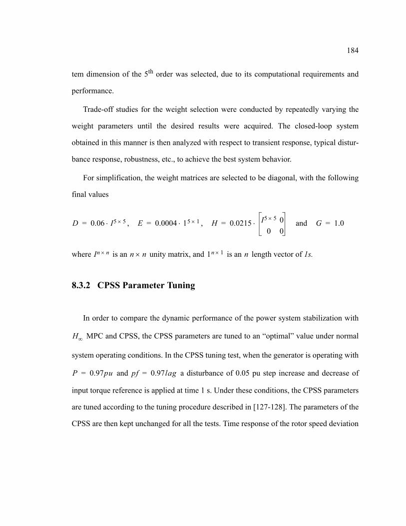
184
tem dimension of the 5th order was selected, due to its computational requirements and
performance.
Trade-off studies for the weight selection were conducted by repeatedly varying the
weight parameters until the desired results were acquired. The closed-loop system
obtained in this manner is then analyzed with respect to transient response, typical distur-
bance response, robustness, etc., to achieve the best system behavior.
For simplification, the weight matrices are selected to be diagonal, with the following
final values
, , and
where is an unity matrix, and is an length vector of 1s.
8.3.2 CPSS Parameter Tuning
In order to compare the dynamic performance of the power system stabilization with
MPC and CPSS, the CPSS parameters are tuned to an “optimal” value under normal
system operating conditions. In the CPSS tuning test, when the generator is operating with
and a disturbance of 0.05 pu step increase and decrease of
input torque reference is applied at time 1 s. Under these conditions, the CPSS parameters
are tuned according to the tuning procedure described in [127-128]. The parameters of the
CPSS are then kept unchanged for all the tests. Time response of the rotor speed deviation
D 0.06 I5 5×⋅= E 0.0004 15 1×⋅= H 0.0215 I5 5× 00 0
⋅= G 1.0=
In n× n n× 1n 1× n
H∞
P 0.97pu= pf 0.97lag=

185
with MPC, CPSS and an open system response is shown in Figure 8-11. The selected
CPSS parameters are presented in Appendix A.3.
8.3.3 Full Load Test
The system state is observed by the controller through the generator’s rotational speed
deviation, , as illustrated in Figure 8-1. To demonstrate the control action three charac-
teristic examples are shown in Figures 8-13 through 8-17. In these tests, the generator of
the single-machine infinite-bus system is operating under a full load condition
and .
In the first test, a step increase and decrease in input mechanical torque
is applied at 1 s and 5 s respectively. These changes in the system can be best observed
through the generator’s electrical power, presented in Figure 8-12.
H∞
-0.3
-0.2
-0.1
0
0.1
0.2 0.3
0 1 2 3 5
NoCCPSSMPC
-0.3
-0.2
-0.1
0
0.1
0.2 0.3
0 1 2 3 4 5
Figure 8-11 Mechanical power reference step change of +/- 0.05 pu
Time [s]
[Hz]∆ω
∆ω
P 0.97pu= pf 0.97lag=
∆P 0.15pu=

186
This test is intended to demonstrate the control action of the MPC for an “aver-
age” disturbance. The measured rotational speed deviation, , of the generator with the
controller’s response is shown in Figure 8-13. It can be observed from this figure that the
0.85
0.9
0.95
1
1.05
1.1
1.15
1.2 1.25
0 1 2 3 4 5 6 7 8
NoCCPSSMPCPe
[pu]
Time [s]
Figure 8-12 Electrical power change for mechanical torque change
H∞
∆ω
-0.6-0.4-0.2
0 0.2 0.4 0.6
NoCCPSSMPC
-0.1
-0.05
0
0.05
0.1
0 1 2 3 4 5 6 7 8
CPSSMPC
Time [s]
Con
trol S
igna
l [pu
]
[Hz]∆ω
Figure 8-13 Control action for an average disturbance

187
control action of the MPC is faster than that of the CPSS, which results in a lower
peak of .
To demonstrate the control action for a large disturbance, a three phase to ground fault
test of 100 ms length on generator bus has been performed. This test is best characterized
by the change in generator’s terminal voltage, Vt, as presented in Figure 8-14.
The controller’s response to the three phase to ground fault is shown in Figure 8-15.
The control action of the MPC is fast and strong. However, it is constrained by the
0.1 pu control signal limits. As expected from an control, the MPC significantly
reduces the peak of the generator’s rotational speed deviation after the fault, and it helps
the system return to its operating point quickly.
H∞
∆ω
0
0.2
0.4
0.6
0.8
1
1.2 1.4
0 1 2 3 4 5 6 7 8
NoCCPSSMPC
Vt
[pu]
Time [s]
Figure 8-14 Terminal voltage during three phase to ground fault
H∞
H∞ H∞

188
To demonstrate the control action for small disturbances, a sequence of exciter voltage
reference step change tests have been performed. Figure 8-16 shows the changes in the
terminal voltage of the generator, Vt, when the exciter voltage reference is changed by
pu, pu and pu steps, at 0.5 s, 2.8 s and 5 s respectively.
-8
-6
-4
-2
0
2
4 6 NoC
CPSSMPC
-0.1
-0.05
0
0.05
0.1
0 1 2 3 4 5 6 7 8
CPSSMPC
Time [s]
Con
trol S
igna
l [pu
][Hz]∆ω
Figure 8-15 Control action for a large disturbance
1.03
1.04
1.05
1.06
1.07
1.08
1.09 1.1
0 1 2 3 4 5 6 7 8
NoCCPSSMPC
Vt
[pu]
Time [s]
Figure 8-16 Terminal voltage for exciter reference changes
0.015– 0.015– 0.03

189
Figure 8-17 shows the generator’s rotational speed deviation and control action for the
exciter voltage reference step change. This test further demonstrates the effectiveness of
the MPC controller, which significantly reduces the peak of the generator’s rotational
speed deviation. Contrary to this, the initial response of the CPSS to these smaller distur-
bances is confused.
8.3.4 Light Load Test
With the generator in a single-machine infinite-bus power system operating under light
load condition, and , a 0.15 pu step increase and decrease in
input mechanical torque is applied at 1 s and 5 s. The generator’s rotational speed devia-
tion, , for this test is shown in Figure 8-18. The test results verify that both control
-0.5-0.4-0.3-0.2-0.1
0 0.1 0.2 0.3 NoC
CPSSMPC
-0.04
-0.02
0
0.02
0.04
0 1 2 3 4 5 6 7 8
CPSSMPC
Time [s]
Con
trol S
igna
l [pu
]
[Hz]∆ω
Figure 8-17 Control action for small disturbances
H∞
P 0.5pu= pf 0.87lag=
∆ω

190
algorithms perform very well. The difference in performance goes in favor of the
MPC with smaller amplitudes in post-disturbance oscillations. However, the over-conser-
vative behavior of the controller can be observed in Figure 8-18, where the effects of
disturbances with highest magnitudes are reduced, while the small oscillations are left
uncontrolled.
Further, under the same load conditions, and , a sequence
of exciter voltage reference step changes of -0.015 pu, -0.015 pu and 0.03 pu is applied at
0.5 s, 2.8 s and 5 s respectively. The measured rotational speed deviation, , of the gen-
erator with the controller’s response is shown in Figure 8-19.
The CPSS parameters are selected as such to have the best performance under the load
conditions when the generating unit is operated with and .
H∞
H∞
-0.8-0.6-0.4-0.2
0 0.2 0.4 0.6 0.8 NoC
CPSSMPC
-0.1
-0.05
0
0.05
0.1
0 1 2 3 4 5 6 7 8
CPSSMPC
Time [s]
Con
trol S
igna
l [pu
]
[Hz]∆ω
Figure 8-18 Response to a +/- 0.15 pu step change of torque in light load test
P 0.5pu= pf 0.87lag=
∆ω
P 0.97pu= pf 0.97lag=

191
Under light load conditions, the stabilization effect of the CPSS cannot match the perfor-
mance of MPC which performs an adaptation for the changed load conditions.
8.3.5 Leading Power Factor Test
In some situations it is required that the generator supplies a reactive load. For exam-
ple, to absorb a capacitive load it may be necessary that the generator operate with a lead-
ing power factor. In this situation the stability margin of the generator is reduced.
Therefore, it is vital to demonstrate that the controller is able to guarantee stable operation
of the generator under the leading power factor conditions.
When the generator is operating in a single-machine infinite-bus system under leading
power factor condition, and , a 0.15 pu step increase and
H∞
-0.25-0.2
-0.15-0.1
-0.05 0
0.05 0.1
0.15 NoCCPSSMPC
-0.04
-0.02
0
0.02
0.04
0 1 2 3 4 5 6 7 8
CPSSMPC
Time [s]
Con
trol S
igna
l [pu
]
[Hz]∆ω
Figure 8-19 Voltage reference step changes in light load test
P 0.5pu= pf 0.9lead=

192
decrease in input mechanical torque is applied at 1 s and 5 s, respectively. The generator’s
rotational speed deviation with the control action for this test is shown in Figure 8-20.
Under the same load conditions, , and termi-
nal voltage, -0.015 pu, -0.015 pu and 0.03 pu step change in reference voltage is applied at
0.5 s, 2.8 s and 5 s respectively. The generating unit’s rotational speed deviation with con-
trol action, is shown in Figure 8-21.
The results presented in Figure 8-20 and Figure 8-21 demonstrate that the oscillations
are damped out by the MPC with more success than with the CPSS, and that the
MPC can operate under leading power factor operating conditions.
-0.8-0.6-0.4-0.2
0 0.2 0.4 0.6 0.8 NoC
CPSSMPC
-0.1
-0.05
0
0.05
0.1
0 1 2 3 4 5 6 7 8
CPSSMPC
Time [s]
Con
trol S
igna
l [pu
]
[Hz]∆ω
Figure 8-20 Response to a +/- 0.15 pu step change of torque in lead load test
P 0.5pu= pf 0.9lead= Vt 0.94pu=
H∞ H∞

193
8.3.6 Transient Stability Test
Transient stability studies are aimed at determining if the system will remain in syn-
chronism following major disturbances such as transmission system fault, sudden load
changes, loss of generating units, or line switching [126]. For this test, the generating unit
is operated under overload conditions, with and . Figure 8-22
illustrates the response of the power system to a three phase to ground fault test at the gen-
erator bus that is applied at 1 s and is cleared after 100 ms.
-0.5-0.4-0.3-0.2-0.1
0 0.1 0.2 0.3 NoC
CPSSMPC
-0.04
-0.02
0
0.02
0.04
0 1 2 3 4 5 6 7 8
CPSSMPC
Time [s]
Con
trol S
igna
l [pu
][Hz]∆ω
Figure 8-21 Voltage reference step changes in a lead load test
P 1.1pu= pf 0.95lag=

194
Test results demonstrate the superior behavior of the MPC. This controller mini-
mizes the peak of the generator’s rotational speed deviation after the fault and helps the
system return to its normal operating condition faster than the CPSS.
8.4 Summary
A qualitative analysis of the MPC as power system stabilizer in a single-machine
infinite-bus system is presented in Figures 8-13 through 8-22, and compared to the widely
used CPSS. Simulation results verify that the MPC has very good damping character-
istics for disturbances under different operating conditions of the generating unit. For
example, the machine settles to the new operating condition with a much smaller over-
-6-4-2 0 2 4 6
NoCCPSSMPC
-0.1
-0.05
0 0.05
0.1
0 1 2 3 4 5 6 7 8
CPSSMPC
Con
trol S
igna
l [pu
][Hz]∆ω
Time[s]
Figure 8-22 Bus three phase to ground fault test in overload condition
H∞
H∞
H∞

195
shoot and oscillation amplitude than with the CPSS, therefore, improving the dynamic sta-
bility properties of the generator in the power system.
The robustness of the controller, with respect to modelling errors and disturbance
variations, stems from the fact that the maximum gain is minimized over all possible dis-
turbances. Since no assumption is made about the disturbances during the definition of the
control, and all the conceivable disturbances have to be accommodated, the con-
trol may be over conservative [20]. This over conservative behavior can be observed in
Figure 8-13, Figure 8-18 and Figure 8-20, where the effects of disturbances with highest
magnitudes are reduced while the small oscillations are left uncontrolled. This explains
the effort of some researchers, whose aim is to develop a control algorithm which mini-
mizes the mixed norm of the objective function.
H∞
H∞ H∞
H∞ H2⁄

196
9 Multi-Machine Power System
In the previous chapter, the results of the simulation studies demonstrated the
MPC controller properties as a power system stabilizer in a single-machine infinite-bus
power system environment. In this chapter the performance of the MPC controller is
examined in a more complex test environment. Specifically, the implementation of the
MPC in a multi-machine power system is investigated. The power system simulation
package, used in this research, is identical to that used in a single-machine infinite-bus
power system simulation.
9.1 Introduction
Power system dynamics, with its transient response to a large disturbance, are charac-
terized by multi-mode oscillation phenomena, with frequencies typically in the range of
0.1 to 2.0 Hz. Multi-mode oscillations emerge in multi-machine power systems, in which
the interconnected generating units have quite different inertia and they are weakly con-
nected by transmission lines. These oscillations are generally analyzed in three main oscil-
lation modes; local, inter-area and inter-machine modes. Depending upon their location in
the system, some generators participate in only one oscillation mode, while others partici-
pate in more than one mode [123].
H∞
H∞
H∞

197
Depending upon the origin of the oscillations, the multi-mode oscillations can be
divided into three groups [120][129]:
• Local Mode is characterized by the oscillation frequencies in the range of 0.8 to 2 Hz.
These oscillations are caused by the rotational speed deviation of a single generator
connected to the infinite-bus, formed by the combined equivalent rotational speed of
the interconnected power system.
• Inter-Machine Mode of oscillation is characterized by frequencies in the range of 0.3 to
1 Hz. This type of oscillation originates when the generators in a closely coupled group
swing relative to each other. The PSS has no control over this type of oscillation.
• Inter-Area Mode of oscillation is characterized by frequency in the range of 0.1 to 0.7
Hz. These type of oscillations originate from a coherent group of generators in one area
swinging relative to a number of other coherent groups of generators in other areas.
These multi-mode oscillations can be modelled by a five-machine power system.
9.2 Five-Machine Power Model
The interconnection scheme of a multi-machine power system model is shown in Fig-
ure 9-1. This model consists of five generator units. Generators , and have
much larger capacities than and . The generators in this simulation are modelled
with fifth-order non-linear differential equations, as given in Appendix B.1. All five gen-
erators are equipped with governors, exciters and automatic voltage regulators (AVR). The
G1 G2 G4
G3 G5

198
parameters for the generators, AVRs, transmission lines and load operating conditions are
given in Appendix B.
In the selected model, generators , and form one area, while generators
and form a second area. These two areas are linked through a tie line, which is con-
necting busses #6 and #7. Normally, each area serves its own load and it is almost fully
loaded with a small load flow over the tie line [120].
Generator is connected to bus #6 through a double transmission line, which
enables different fault tests on the second line. In Figure 9-1 a square indicates the second
line, where the fault test takes place.
When the system is disturbed, multi-mode oscillations arise because of the different
size generators and network configurations. The rotational speed difference between
G3 G2 G5 G1
G4
Figure 9-1 Network topology for a five-machine power system
G3
G2
G5
G1
G4
L3L 1
L 2
bus #1bus #7bus #6bus #3
bus #2
bus #5
bus #8
bus #4
tie line
G3
G3
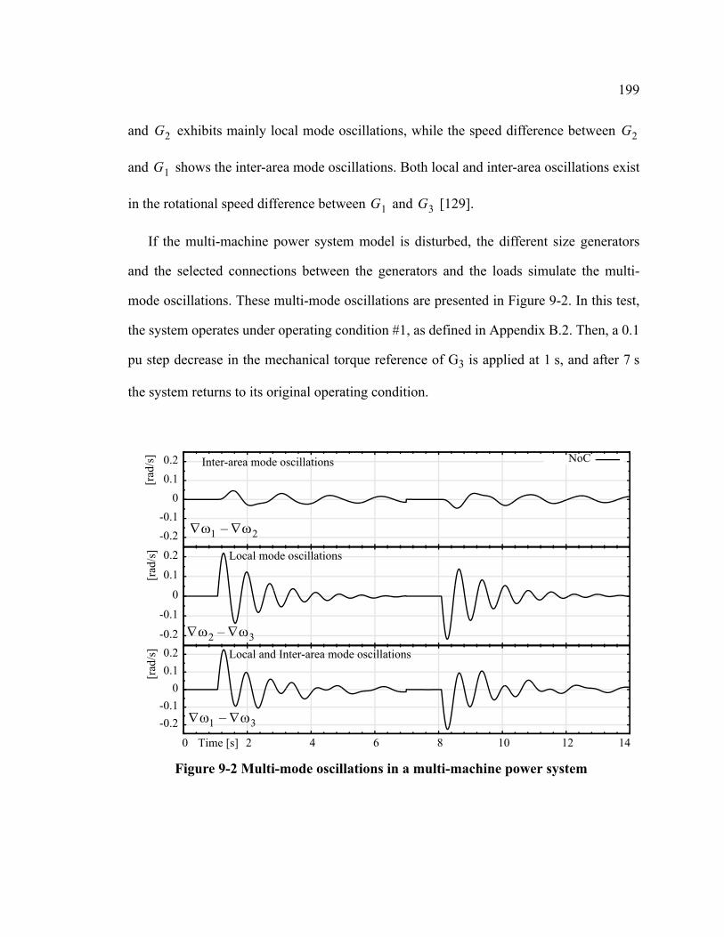
199
and exhibits mainly local mode oscillations, while the speed difference between
and shows the inter-area mode oscillations. Both local and inter-area oscillations exist
in the rotational speed difference between and [129].
If the multi-machine power system model is disturbed, the different size generators
and the selected connections between the generators and the loads simulate the multi-
mode oscillations. These multi-mode oscillations are presented in Figure 9-2. In this test,
the system operates under operating condition #1, as defined in Appendix B.2. Then, a 0.1
pu step decrease in the mechanical torque reference of G3 is applied at 1 s, and after 7 s
the system returns to its original operating condition.
G2 G2
G1
G1 G3
-0.2-0.1
0 0.1 0.2 NoC
-0.2
-0.1
0
0.1
0.2
-0.2-0.1
0 0.1 0.2
0 2 4 6 8 10 12 14Time [s]
Inter-area mode oscillations
Local mode oscillations
Local and Inter-area mode oscillations
∇ω1 ∇ω3–
∇ω2 ∇ω3–
∇ω1 ∇ω2–
[rad
/s]
[rad
/s]
[rad
/s]
Figure 9-2 Multi-mode oscillations in a multi-machine power system

200
It can be observed from Figure 9-2 that the local mode oscillations arise from the
speed difference between G2 and G3 at a frequency of about 1.3 Hz. The inter-area mode
oscillations can be observed as a speed difference between G1 and G3 at a frequency of
about 0.65 Hz, originating from the large difference of the generators’ power used in the
simulation model.
9.3 Simulation Studies for H∞ MPC
The MPC implemented in this test is the same one used in the single machine sim-
ulation with sample time. The speed deviation, , used for the system
state observation, contains a DC offset value since there is no infinite-bus in the system. A
high-pass filter is implemented to remove the DC value before the speed deviation signal
is used by the control system.
The high-pass filter introduces changes in the dynamics of the speed deviation, ,
and it requires compensation by changing the weights in the control
, , and where is an
unity matrix and is an length vector of 1s and is an length vector of 0s.
The weights are kept constant during the simulation.
H∞
TS 0.025s= ∆ω
∆ω
H∞
D 0.01 I5⋅= E 0.001 15⋅= H 0.2 I5
0⋅= G o5
1= In
n n× 1n n on n

201
9.3.1 PSS on One Generator
During this test, in the multi-machine power system only one PSS is installed on the
G3 generator. When the system operates under operating condition #1, as defined in
Appendix B.2, a 0.1 pu step decrease in the mechanical torque reference of G3 occurs at
1 s and after 4 s the system returns to its original operating condition. The system response
is shown in Figure 9-3. The MPC installed on G3 effectively damps the local mode
oscillations, which arise as a rotational speed difference between the generators G2 and
G3, . However, as expected, it has little influence on the inter-area mode oscil-
lations, which arise as a rotational speed difference between the generators G1 and G3,
. This is because the rated power of G3 is much less than G1 and G2; and G3
does not have enough power to control the inter-area mode oscillations [129].
For comparison, in a separate test, a CPSS, see Appendix A.3, with the following
parameter set [130][120][129]
G3: (9.1)
performs almost similar to the MPC. Figure 9-3 presents both these test results and it
also includes a response with no controller involved.
H∞
∇ω2 ∇ω3–
∇ω1 ∇ω3–
Ks 1.0= T1 T3 0.3= = T2 T4 0.1= = T5 0.4=
H∞

202
9.3.2 PSS on Three Generators
In order to damp both local and inter-area mode oscillations, it is required that the PSS
is installed on two additional generators G1 and G2, beside the already installed one on G3.
The MPC is identical an all three units, while the CPSS requires different new param-
eters due to the difference in generator size [130]
G1: (9.2)
G2: . (9.3)
-0.2-0.1
0 0.1 0.2 NoC
CPSSMPC
-0.2
-0.1
0
0.1
0.2
-0.2-0.1
0 0.1 0.2
0 1 2 3 4 5 6 7 8Time [s]
Inter-area mode oscillations
Local mode oscillations
Local and Inter-area mode oscillations
[rad
/s]
[rad
/s]
∇ω1 ∇ω3–
∇ω2 ∇ω3–
∇ω1 ∇ω2–
[rad
/s]
Figure 9-3 System response with PSS installed on G3
H∞
Ks 0.4= T1 T3 0.1= = T2 T4 0.08= = T5 0.3=
Ks 0.5= T1 T3 0.1= = T2 T4 0.08= = T5 0.3=
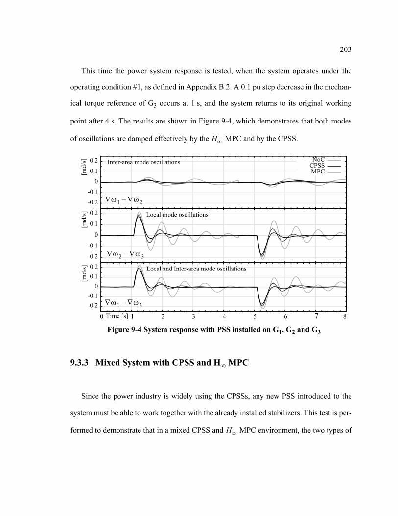
203
This time the power system response is tested, when the system operates under the
operating condition #1, as defined in Appendix B.2. A 0.1 pu step decrease in the mechan-
ical torque reference of G3 occurs at 1 s, and the system returns to its original working
point after 4 s. The results are shown in Figure 9-4, which demonstrates that both modes
of oscillations are damped effectively by the MPC and by the CPSS.
9.3.3 Mixed System with CPSS and H∞ MPC
Since the power industry is widely using the CPSSs, any new PSS introduced to the
system must be able to work together with the already installed stabilizers. This test is per-
formed to demonstrate that in a mixed CPSS and MPC environment, the two types of
H∞
-0.2-0.1
0 0.1 0.2 NoC
CPSSMPC
-0.2
-0.1
0
0.1
0.2
-0.2-0.1
0 0.1 0.2
0 1 2 3 4 5 6 7 8Time [s]
Inter-area mode oscillations
Local mode oscillations
Local and Inter-area mode oscillations
[rad
/s]
[rad
/s]
∇ω1 ∇ω3–
∇ω2 ∇ω3–
∇ω1 ∇ω2–
[rad
/s]
Figure 9-4 System response with PSS installed on G1, G2 and G3
H∞

204
PSSs can work co-operatively. In the multi-machine power system simulation, the
MPC is installed on G1 and G3, while the CPSSs are installed on G2, G4 and G5. The
parameters for CPSS on G4 and G5 generators are selected as [130]
G4: (9.4)
G5: . (9.5)
When the system operates under the operating condition #1, as defined in
Appendix B.2., the power system response is tested for a 0.1 pu step decrease in the
mechanical torque reference of G3, which occurs at 1 s. After 4 s the system returns to its
original working point. The results in Figure 9-5 confirm that the two types of PSSs can
work co-operatively.
H∞
Ks 0.5= T1 T3 0.1= = T2 T4 0.08= = T5 0.3=
Ks 1.0= T1 T3 0.3= = T2 T4 0.1= = T5 0.4=
-0.2-0.1
0 0.1 0.2 NoC
MPC & CPSS
-0.2
-0.1
0
0.1
0.2
-0.2-0.1
0 0.1 0.2
0 1 2 3 4 5 6 7 8Time [s]
Inter-area mode oscillations
Local mode oscillations
Local and Inter-area mode oscillations
[rad
/s]
[rad
/s]
∇ω1 ∇ω3–
∇ω2 ∇ω3–
∇ω1 ∇ω2–
[rad
/s]
Figure 9-5 System response with a mixed CPSS and MPC installed
205
9.3.4 Three Phase to Ground Fault Test
With the power system operating under operating condition #1, as defined in
Appendix B.2, a three phase to ground fault is applied at the middle of the transmission
line between buses #3 and #6 at 1 s. The fault is cleared 100 ms later, when the faulty line
is removed. Figure 9-6 shows the system response with no PSS, with the proposed
MPC, and with the CPSSs installed on G1, G2 and G3. The results show that the MPC
minimizes the deviation of the generator’s rotational speed after the fault.
H∞
H∞
-1-0.5
0 0.5
1NoC
CPSSMPC
-1-0.5
0 0.5
1
-1-0.5
0 0.5
1
0 1 2 3 4 5 6 7 8Time [s]
Inter-area mode oscillations
Local mode oscillations
Local and Inter-area mode oscillations
[rad
/s]
[rad
/s]
∇ω1 ∇ω3–
∇ω2 ∇ω3–
∇ω1 ∇ω2–
[rad
/s]
Figure 9-6 System response to three phase to ground fault test

206
9.3.5 New Operating Condition Test
The dynamic behavior of the power system changes with load and system operating
conditions. To test the robustness of the proposed MPC under other operating condi-
tions, the operating point of the power system is changed to a new point as indicated in
Appendix B.3.
A three phase to ground fault is applied at the middle of the transmission line between
buses #3 and #6 at 1 s, and cleared 100 ms later when the faulted line is removed. Figure
9-7 shows the system response with no PSS, with the proposed MPC and with the
H∞
-0.6-0.3
0 0.3 0.6 NoC
CPSSMPC
-0.6-0.3
0 0.3 0.6
-0.6-0.3
0 0.3 0.6
0 1 2 3 4 5 6 7 8Time [s]
Inter-area mode oscillations
Local mode oscillations
Local and Inter-area mode oscillations
[rad
/s]
[rad
/s]
∇ω1 ∇ω3–
∇ω2 ∇ω3–
∇ω1 ∇ω2–
[rad
/s]
Figure 9-7 Three phase to ground fault test in a new operating condition
H∞

207
CPSSs installed on G1, G2 and G3. Again, it is shown that the oscillations in the system
with MPC are more reduced than with CPSS.
9.4 Summary
In this Chapter, the effectiveness of an MPC as a power system stabilizer is inves-
tigated in a multi-machine environment. The speed deviation of the generating unit is used
as a signal to observe the generator’s state. This signal contains a DC component, which
has been successfully removed by a high-pass filter. During the simulation all of the off
line selectable parameters of the MPC are kept constant. The system changes are
tracked by the online adaptation processes.
The simulation results indicate that the proposed MPC not only performs well in
damping multi-mode oscillations in the system but it also exhibits good adaptation and
stable operation in all tested environments. It can be concluded that the proposed
MPC can produce satisfactory performance as a PSS both in single-machine and multi-
machine power system environments. The performance of the proposed MPC on a
physical system is studied in the next part.
H∞
H∞
H∞
H∞
H∞
H∞

208
Part - IV Experimental Tests
An excellent way to gain an intuitive feel for control system design and performance is
to conduct computer simulations. Conceptually, there is a short step from simulation to
actual implementation, since the subroutines that are used on today’s digital signal pro-
cessors are very similar to those used for simulation facilitated by digital computers.
However, a numerical system model can only approximate the dynamics of a system. There
is always some unexpected dynamic behavior inherent in a system that is not accounted
for by any given mathematical model. Consequently, it is necessary to do some laboratory
and/or field tests to further assess the evidence from the computer simulation before the
installation of the proposed control algorithm on an actual system occurs. This is espe-
cially true for a power system, in which the resulting damage could be very extensive. For
this kind of system the solution is to build a scaled physical model of the target system,
which is capable of emulating the behavior of the actual plant in the laboratory environ-
ment.
A real-time digital control system and the physical power system model for implemen-
tation and testing of the MPC are described in this part. H∞

209
10 Real-Time Test Environment
The next step in the progression of this thesis entails testing the proposed control strat-
egy on a plant. In practice, new instrumentation and control schemes are tested on scaled
physical models, that can simulate the behavior of the plant in the laboratory environment.
Earlier studies have shown that most phenomena encountered in large power systems can
be qualitatively duplicated with the small machines [131].
Implementation of the MPC power system stabilizer with a real-time digital con-
trol system applied on a laboratory power system is described in this chapter. The pro-
posed power system stabilizer setup is shown in Figure 10-1.
The real-time test environment consists of two parts; physical model of a power sys-
tem model and an embedded controller. The power system is modelled by a micro-syn-
chronous generator connected to an infinite-bus through a transmission line. The
H∞
Figure 10-1 PSS development environment
ef
A
BC
Micro-Synchronous Generator
Digital Signal Processing
Vtω
USB & Parallel
Infin
ite-B
us
Analog Signals
4
Man-Machine InterfaceConnections
Embedded Controller for
E0 ω0,
rt jxt+

210
excitation of the micro-synchronous generator is controlled by the embedded controller
using digital signal processing techniques. In order to observe the control system behavior
in real time, a four-channel oscilloscope is utilized. The program for the embedded control
system is developed on a personal computer. The personal computer is also used to control
the program execution and the data collection.
In the following the functionality and characteristics of the elements of this power sys-
tem model and the embedded controller are described.
10.1 Power System Model
The physical model of the power system to be simulated is available in the Power Sys-
tem Research Laboratory at the University of Calgary. It consists of a 3-phase 3kVA
micro-synchronous generator connected to an infinite busbar through a double circuit
transmission line simulator. An overall schematic diagram of this physical model is given
in Figure 10-2. The major units of this model are: the turbine model, the generator model,
the transmission line model, and the automatic voltage regulator.
M G
Figure 10-2 Laboratory power system configuration
Generator FieldControl 3-Phase Fault Tests
AC Generator
DC Motor
Exciter
Transmission Line Model
Power StepChange Test
Timing
ωVt
EF
InfiniteBusbar

211
10.1.1 Turbine Model
The mechanical energy source, in practice usually a turbine, is modelled by a 5.5 kW
(7.5 h.p.) separately excited DC motor, made by Madsley’s Ltd. in 1968. The technical
parameters of this DC motor are: 220 V, 30 A, 1800 RPM, 7.5 h.p. (5592.75 W), excitation
40/20/10 V. The connection diagram with the measurement points is represented in Figure
10-3.
The active electrical power, , of the micro-synchronous generator, shown in Figure
10-4, can be set by varying the field current of the DC motor by the resistances and
. A large power step disturbance or input torque step, can be produced by using the
switch . The corresponding power step is adjusted by the resistor .
Figure 10-3 DC motor as a turbine model
Vf
Va
Ia
If
R1
R2
R3 S3
Shunt Winding
Rotor
Ia - Control
MechanicalStep Input Test
SeriesWinding
InterpoleWinding
If - Control
A
V
V
A
DC
DC
Pe
R1
R2
S3 R3

212
10.1.2 Generator Model
A generator is modelled by a three phase 3 kVA, 220 V micro-synchronous generator,
made by Madsley’s Ltd. The technical parameters of this alternator are: 220/127 V, 7.9 A,
3 kW, 3 phase, 60 Hz with a power factor of 0.8 lag. The measurable parameters for the
micro-synchronous generator are shown in Figure 10-4.
The field winding resistance of these synchronous machines, on per unit basis, is much
higher than that of the large machines to be simulated. This results in a comparatively low
field transient time constant s, where the transient time constant of the mod-
ern large machines is in the neighborhood of 5 s, thus adversely affecting the performance
of the machine under transient conditions. An electrical device called the Time Constant
Ic
Il
Vt
Figure 10-4 Micro-synchronous generator model
φQePe φ( )cos
C
A
B
A
V
V
A
Field Winding
Control Signal from the AVR
Exciter
& TCRW R
Micro-Synchronous Generator Terminal
Tran
smis
sion
Lin
e
EF
Tdo 0.765=

213
Regulator (TCR) has been designed to reduce the effective field resistance and thereby
alter to the order of that required for the simulation of large machines. With the time
constant regulator, the effective field time constant of the micro-synchronous generator
can be increased up to 10 s [132].
The voltage reference step disturbance can be simulated using this generator model, to
conduct a dynamic performance study and evaluate the performance of the proposed
power system stabilizer. The generator’s terminal voltage, , can be stepped up or down
by changing the voltage reference setting of the AVR.
10.1.3 Transmission Line Model
The main objective of the transmission line is the power flow through an AC line,
which is a function of the phase angle, the line end voltages, and the line-impedance [133].
The transmission line is modelled by a lumped element transmission line. The physical
model consists of six π sections as presented in Figure 10-5, and gives a frequency
response that is close to the actual transmission line response up to 500 Hz [134]. This
Tdo
Vt
Figure 10-5 π section
L 1.65mH…1.85mH=
C1 8.03µF= C2 8.03µF=
RL 0.1Ω=with

214
model simulates the performance of a 300 km long, 500 kV, double circuit transmission
line connected to a constant voltage bus (infinite busbar), as shown in Figure 10-1.
Large disturbances such as various single phase to ground, phase to phase and three
phase to ground faults can be simulated using relays controlled by short circuit simulation
logic, presented in Figure 10-1.
10.2 Embedded Controller
Real-time implementation of the proposed MPC algorithm requires an embedded
controller with higher computation power. Therefore, a powerful Digital Signal Processor
(DSP) that existed at the time of the design was selected for building the controller. The
DSPs developed by the Texas Instruments Incorporated were identified as most suitable.
The embedded control system consists of four cards: two computation cards and two
interface cards, as shown in Figure 10-6. The four cards are mounted on a plexiglas panel.
Two DSP Starter Kits (DSK), developed by Texas Instruments, are utilized for the compu-
H∞
A2D2ATMS320C6711TMS320C6713
Analog Interface Input: 8 × ±10V 14 bit A/DOutput: 4 × ±5V 16 bit D/A
225 MHz DSP16 MByte Memory
150 MHz DSP8MByte Memory
40 MHz Serial Connection
16 BitParallel
Connection
Figure 10-6 Embedded controller
DSK-1DSK-2
AVRData AcquisitionControl Algorithm
Man-Machine Interface
Digital Interface

215
tation. These DSK cards are the TMDS320006711 and TMDSDSK6713, containing high
performance floating point DSPs TMS320C6711 and TMS320C6713, respectively. The
technical description of the DSKs is provided in [135] and [136]. For software develop-
ment additional technical literature [137 - 146] has been consulted.
The analog and digital interface cards were designed to satisfy the requirements of this
research. The embedded system connection is presented in Figure 10-6. Their detailed
description is provided in the following.
10.2.1 Analog Interface Card
In order to facilitate communication between the embedded controller and the environ-
ment, an analog interface card, named A2D2A, was developed. This card contains eight
analog to digital (A/D) converter channels and four digital to analog (D/A) converter
channels. For easy interfacing, the card uses common BNC coaxial connectors. The com-
ponents that characterize the A2D2A are listed in Table 10-1, while its logical structure is
presented in Figure 10-7.
Table 10-1 Characteristic components of the A2D2A card
Description Part Number Quantity ManufacturerA/D converter AD7865AS-1 2 Analog DevicesD/A converter DAC7644E-ND 1 Burr-BrownVoltage Reference LT1461DHS8-2.5 2 Linear TechnologyOperational Amplifier OPA2277UA 9 Burr-BrownBuffer BUF634U 4 Burr-BrownSwitching power supply LT1533CS 3 Linear Technology3.3V & 5V interface SN74LVC4245APWR 3 Texas InstrumentsControl logic EMP7032AE 1 Altera Corporation

216
In order to simplify the card’s usage, the A2D2A is equipped with its own voltage con-
verters for -12, -5, 5, and 12 V, which are required for functioning of devices.
The A2D2A board’s conversion and access timing diagram is presented in Figure 10-
8. Conversion is controlled by the Timer 0 output of the DSP, which generates the TOUT0
periodic pulses. The TTOUT0 period is controlled by the appropriate Timer 0 initialization,
where the minimum period shall be selected for no less than 12 µs.
5V
-12V
5V
12V5V
7V
-12V
-5V
7V 5V
12V -12V -5V 5V
+2.500V Ref -2.500V Ref
A/D - 1
A/D - 2
D/A
PLD
3.3/5V
BUSY2
BUSY1
WR#RD#
CONVST#
FRSDATA1CS_ADC1#
FRSDATA2CS_ADC2#
LOA
DD
AC
S#
CS_
DA
C#
R/W
#
A0
A2
A1
A3
D0
D1
RES
ET
DAT
A B
US
D0
: D15
AD
RES
S B
US
EA2:
EA
5
E_IN
T4TO
UT0
AWE#
CE2
#
AR
E#
RES
ET
AO
E#
EA2:
5
ED0:
153.3V
3.3V 5V
Memory and Peripheral Connectors of the DSP
CH2
A/D CH3
A/D CH4
A/D CH5
A/D CH7
A/D CH8
CH6
A/D CH1D/A CH1
D/A CH2
D/A CH3
D/A CH4
Figure 10-7 A2D2A signal diagram
CONTROL

217
As presented in Figure 10-9, the TOUT0 pulse initiates the A/D conversion and it also
starts a direct memory access (DMA) that updates the D/A converter registers. These pro-
cesses occur simultaneously. The fourth D/A register will update within 1.2 µs from the
start pulse. The A/D converter is designed to sample the eight channels concurrently to
within a few nano seconds, thereby preserving the relative phase information between the
input signals. At the end of A/D conversion, the E_INT4 interrupt signal initiates a second
DMA access to the A2D2A board, in order to read the eight A/D registers. When the data
transfer is complete, the DSP receives the INT8 interrupt, which signals that the converted
data are ready for processing. In this design, the maximum conversion frequency can be
selected up to 83 kHz.
In this research, the A/D and D/A converters are utilized to convert specifically at the
frequency of 50.0 kHz, which corresponds to 20 µs TTOUT0 period. The DSP collects from
all the eight channels sixteen samples of consecutive A/D conversion data and after calcu-
Figure 10-8 A2D2A conversion and access timing diagram
4 x D/A WRITE
8 x A/D READ
TOUT0
EDMA CH1
EDMA CH4
A/D BUSY
INT8
0 1.2 µs 11.2 µs
E_INT4
Time
TTOUT0

218
lating the average of the A/D conversions, it makes the data available every 0.32 ms to the
rest of the processes.
10.2.2 Enhancement of A/D Conversion
In general, the data from the A/D conversion contains some error due to the effects
of the conversion process and the necessary signal conditioning prior to it. Usually this
error can be modelled by an additive random signal , superposed on the measured sig-
nal [147]
. (10.1)
The accuracy of the A/D conversion improves if the signal to noise ratio is increased in the
measurement. This is attained if multiple A/D conversions are performed and an average
is calculated
A/D
A/D
D/A
EDMA CH4
EDMA CH1
TIMER 0
Filter
0
127
tra->x
ad_buffer
0
0
7
3
TOUT0CONVST#
BUSY1 E_INT4
ad_buffer
EDMA READY
0
3rec->x
Fix/Float
HWI IN8
Figure 10-9 Data flow between A2D2A and the DSK1
A/D Buffer
D/A BufferDSK1A2D2A
0
3
0
3
0
3
1/16Σx
yn
ξn
yn0
yn yn0 ξn+=

219
. (10.2)
For this procedure to be legitimate, the changes in the measured signal must be negligible
on the length of the sampling interval. Thus, and
(10.3)
where is the average of the measured signal. The increase in the signal to noise ratio by
the averaging process depends on the distribution of this random signal . In a technical
environment, this signal is usually a normally distributed random signal (white Gaussian
noise) with zero mean. In the worst case scenario, this signal can be a uniformly distrib-
uted random signal. It is important to stress that if the mean of the random signal is
other than zero, the averaging process will not improve the measurements; rather, it will
emphasize the bias of the nonzero mean.
• When the random signal is normally distributed with zero mean and
variance , then the noise reduction in the A/D conversion data, obtained by averag-
ing, is [148]
where . (10.4)
yn1N---- yn i–
i 0=
N
∑⋅=
N yn0 yn 1–
0 … yn N–0≅ ≅
yn yn0 1
N---- ξn i–
i 1=
N
∑⋅+=
yn0
ξn
ξn
ξn N 0 σ2,( )∼
σ2
ξn1N---- ξn i–
i 1=
N
∑⋅= ξn N 0 1N----σ2,
∼

220
Even though the averaged signal is also normally distributed with a zero mean, there is
a reduction in the noise variance, which corresponds to a reduction of the
standard deviation of the random signal. Consequently, the calculated average of 16
converted samples will improve the measurement accuracy by reducing four times the
Gaussian noise in the measured data. In this way, the measurement accuracy improves
by an extra two least significant valid bits.
• When the random signal is uniformly distributed in the interval
, the corresponding variance is [149]. It is well known that
the distribution of the sum of uniformly distributed random signals rapidly
approaches normal distribution, as increases [150]. Accordingly,
where . (10.5)
The variance of the sum is linearly increasing by the number of summing elements.
This means that if the random signal is uniformly distributed, the signal
accuracy cannot be improved by the averaging process. Fortunately, very few technical
systems have uniformly distributed contaminating signals.
10.2.3 Digital Interface Card
The digital interface card is used to connect the pulses, generated by the generator’s
rotation, to an interrupt line on the DSP. The full rotation of the generator produces four
pulses. The rotational speed of the generator is 1800 revolution per minute, which corre-
1 N⁄ 1 N⁄
ξn U ω– ω,( )∼
ω– ξn ω≤ ≤ σ2 ω2 3⁄=
N
N
ξn1N---- ξn i–
i 1=
N
∑⋅= ξn N 0 1N---- Nσ2( ),
∼
ξn U ω– ω,( )∼

221
sponds to 30 Hz of rotation. If the pulses were to interrupt the DSP at 120 Hz frequency,
the DSP would overload. In order to avoid this overload, the pulses are divided by four on
the digital interface card. Also, to alleviate accidents from high voltage sparks which can
harm the DSP, the digital interface card has an optocoupler signal isolation built in it, as
presented in Figure 10-10. The function of the LED on the digital interface card is to alert
if the signal connection has been severed. During operation, a uniform blinking light sig-
nals normal conditions.
The synchronous generator, as part of the power system, is observed through its rota-
tional speed deviation, , as presented in Figure 10-11. The rotational speed, or more
precisely, the rotational speed deviation of the synchronous generator is observed by mea-
suring the time length of one full rotation. In order to measure the oscillations in the rota-
tional speed, the DSP must calculate the difference between the measured rotational time
and the moving median of the last 25 rotational times. Using the median as a reference
rotational time assures that the rotational speed deviation does not contain an unwanted
offset from zero.
1/4
1/16
3.3V
Figure 10-10 Digital interface signal diagram
DSP INT 3.9 kΩ4.6 kΩ
SFH628SN74MC161 LED
∆ω

222
10.2.4 Embedded Software
The embedded software is divided between the two DSKs in such a way that the
Exciter-AVR function with the analog interface handling is allocated to the DSK-1, while
the control algorithm, containing the MPC or CPSS, with the digital interface han-
dling is allocated to the DSK-2. Between the two DSKs a serial link is established which
continuously exchanges two blocks of data. Each block contains 16 data. The real-time
control application is primarily interrupt driven, with a basic structure shown in Figures
10-12 and 10-13 for DSK-1 and DSK-2 respectively.
The primary function of the software on DSK-1 board is to handle the analog data
communications and the AVR. The timing of the software execution is driven by two peri-
odic interrupts of 20 µs and 0.32 ms. Every 20 µs the software reads the data registers of
the A/D converters and updates the D/A data registers on the A2D2A board. From the A/
D readings of all eight analog input channels, the software collects 16 samples during a
0.32 ms long interval. The A/D Data Filter calculates the average of these 16 A/D samples
1/4~8.33ms ~33.33msTR
TR4TR
Median
DSK-2
Rotational SpeedDeviation
Measured
Figure 10-11 Rotational speed deviation estimation
in 17.7 ns Increments
∇ω
H∞

223
that are used in subsequent signal processing. This way the Gaussian noise in the mea-
sured data is reduced four times.
The primary control loop for the generator’s voltage stability is the AVR, which also
executes with 0.320 ms sampling time. The equations for AVR are provided in Section
10.3.1.
A synchronous serial connection line is used for communication between DSK-1 and
DSK-2 boards. Every 4 µs the block of the 16 data is exchanged between the two DSKs.
DSK-2 contains a higher level of calculations. Its execution period is much longer than
that of DSK-1. The execution cycle of the primary real-time application is 33.33 ms,
which includes the control action calculations or the CPSS and the system identifica-
tions by different techniques. The secondary applications, which include the expert system
for Proposed (PRO) model selection, are executed at 1 s interval.
If a new PRO model is selected, a new set of weights are calculated for the real time
controller using the optimization algorithm in a background calculation, as
defined in sections 6.2.2 through 6.2.4.
The real-time control application program is interrupt driven. To measure the period of
a rotation, it uses the external interrupt from the generator’s rotation, as presented in Fig-
A/D
D/A
Analog Interface HandlingA/D Data Collection
A/D Data Filtering DSK-1 to DSK-2 Communication
AVR Compensation
TExecution Period = 20 µs TExecution Period = 0.32 ms
Figure 10-12 DSK-1 program allocation and execution
A/D
D/A
A/D
D/A
DSK-2
H∞
H∞ H∞

224
ure 10-11. Due to this particular interrupt driven structure, the control action can be imme-
diately calculated when the measurements from the rotational speed deviation are
available. Consequently, the delay is minimized between sampling and control. The calcu-
lation of the system identification algorithms takes place in the same real time loop of
33.33 ms.
In this research, seven different system identification techniques are concurrently cal-
culating the system model. Every second a new interrupt is generated which invokes the
expert system in order to make a decision for the PRO model. The expert system has eight
possible choices, either it can keep the PRO model or it can replace it with one of the
seven possible models resulting from the seven system identification techniques.
If a new model is proposed for PRO, the optimization algorithm starts to execute
in the background. The reason for this background action is that this part of the algorithm
requires a longer than the 33.33 ms interval for the calculations. When the new parameters
are available, the old weights in the controller are replaced.
H∞
H∞
DSK to DSK Communication
H∞ Controller or CPSSDigital Interface Handling
7 x System Identification
Model Evaluation/Selection for PRO
H∞ Controller Optimization
Figure 10-13 DSK-2 program allocation and execution
TExecution Period = 33.33 ms TExecution Period= 1s
TExecution Period= If New PRO Model Found
PROH∞ Controller
Models
DSK-1
DigitalInterface

225
10.3 Power System Stabilizer Implementation
As described above, the real-time control environment of a power system stabilizer is
based on an embedded controller. The embedded controller is a state of the art computa-
tion unit containing two floating point digital signal processors with the required inter-
faces. The implementation and the test environment are illustrated in Figure 10-14.
V
Figure 10-14 Tests on power system model
UPSS
EF
PSS AVR
Vref +Vref
-VrefStep Test Vref
Embedded Controller
ω V Short-Circuits
Step Test Mechanical Power
Test
Infin
ite-B
us
Transmission Line Model
DC
MotorGenerator
Exciter

226
10.3.1 Excitation System
The main purpose of the excitation system is to feed the field winding of the synchro-
nous machine with direct current so that the main flux in the rotor is generated. Further,
the terminal voltage of the synchronous machine is controlled by the excitation system,
which also performs a number of protection and control tasks [151].
The terminal voltage, , and rotation speed, , of a synchronous generator are two
important quantities on which the operation of the power system depends. Special means
are necessary to control them if the best operating conditions are to be obtained. As shown
in Figure 10-15, terminal voltage, , and rotation speed, , can be used to control the
synchronous generator’s magnetic field.
According to the North American Electric Reliability Council (NERC) requirement
definitions as it is stipulated in the NERC Planning Standards, all synchronous generators
connected to the interconnected transmission systems shall be operated with their excita-
tion system in the automatic voltage control mode [152]. The terminal voltage of a gener-
Vt ω
Vt ω
Median
Filter
VREF
AVR
PSS
Vt
ω
EF
Figure 10-15 Excitation system with AVR and PSS
A
B
C
∇ωVt
ω

227
ator operating by itself can be wholly controlled by an Automatic Voltage Regulator
(AVR) actuated by voltage feedback. When the generator is connected to a large power
system (infinite busbar), its voltage and rotation speed are largely determined by the volt-
age and frequency of the system. The main effect of the automatic voltage regulator is to
control the reactive power, , of the generator [153].
Automatic voltage regulators (AVRs) shall be continuously acting solid state analog or
digital. Tuning should be in accordance with the NERC Planning Standard Guide IIC G8
cited below [152]
• Generator voltage regulators, to the extent practical, should be tuned for fast response
to step changes in terminal voltage or voltage reference. It is preferable to run the step
change in voltage tests with the generator not connected to the system so as to eliminate
the system effects on the generator voltage. Terminal voltage overshoot should gener-
ally not exceed 10% for an open circuit step change in a voltage test.
The AVR and exciter used in the experimental studies is a discrete version of the ana-
log AVR defined in the IEEE Standard P421.5/D15, Type ST1A, shown in Figure A-2.
The input signal for the controller is the voltage error, , from the compensation
equipment. The stabilizing feedback, , is subtracted and the signal from the PSS,
, is added. Both these signals vanish in steady state. The controller is mainly
described by the dominating time constant, , and the amplification, . The limits rep-
resent saturation effects or limitations of the control signal. The time constants, , ,
, and are used to model internal time constants in the controller. These are often
Qe
VI
VF
UPSS
TA KA
TC TC1
TB TB1

228
small and can then usually be neglected [151]. The output signal, , from the AVR con-
trols the exciter.
In the IEEE Standard the transfer function of the AVR is defined in the complex
domain from which, in practical applications the best discrete transformation can be
obtained using the bilinear z-transformation [154]
. (10.6)
The to filter numerically can be approximated by the discrete transfer func-
tion
. (10.7)
The lead-lag part numerical approximation using the bilinear z-transformation is
(10.8)
EF
s 2Ts----- 1 z 1––
1 z 1–+----------------⋅=
VC1 VC
VCVK------ 1
1 2Ts----- 1 z 1––
1 z 1–+----------------⋅
TR+------------------------------------------------
TsTs 2TR+---------------------
TsTs 2TR+--------------------- z 1–⋅+
1Ts 2TR–Ts 2TR+--------------------- z 1–⋅+
-------------------------------------------------------------= =
1 sTC+( ) 1 sTC1+( )1 sTB+( ) 1 sTB1+( )
-------------------------------------------------
1 2Ts----- 1 z 1––
1 z 1–+----------------⋅
TC+ 1 2
Ts----- 1 z 1––
1 z 1–+----------------⋅
TC1+
1 2Ts----- 1 z 1––
1 z 1–+----------------⋅
TB+ 1 2
Ts----- 1 z 1––
1 z 1–+----------------⋅
TB1+
---------------------------------------------------------------------------------------------------------------
→
N0 N1 z 1–⋅ N2 z 2–⋅+ +1 D1 z 1–⋅ D2 z 2–⋅+ +-------------------------------------------------------=

229
where , ,
, , and
.
The output filter is approximated as
(10.9)
and, finally, the derivative feedback filter is approximated as
. (10.10)
Using the discretization defined in (10.7) through (10.10), the rest of the implementa-
tion of the digital AVR on the DSP follows the IEEE standard depicted in Figure A-2. The
N0
1 2TS----- TC TC1+( )
4TCTC1
TS( )2-------------------+ +
12 TB TB1+( )
TS-----------------------------
4TBTB1
TS( )2------------------+ +
--------------------------------------------------------------------= N1
2 8TCTC1
TS( )2----------------–
12 TB TB1+( )
TS-----------------------------
4TBTB1
TS( )2------------------+ +
----------------------------------------------------------------=
N2
1 2TS----- TC TC1+( )
4TCTC1
TS( )2-------------------+–
12 TB TB1+( )
TS-----------------------------
4TBTB1
TS( )2------------------+ +
--------------------------------------------------------------------= D1
2 8TBTB1
TS( )2---------------–
12 TB TB1+( )
TS-----------------------------
4TBTB1
TS( )2------------------+ +
----------------------------------------------------------------=
D2
1 2TS----- TB TB1+( )
4TBTB1
TS( )2------------------+–
12 TB TB1+( )
TS-----------------------------
4TBTB1
TS( )2------------------+ +
-------------------------------------------------------------------=
KA1 sTA+------------------
KA
1 2Ts----- 1 z 1––
1 z 1–+----------------⋅
TA+------------------------------------------------→
KA1 2TA Ts⁄+----------------------------
KA1 2TA Ts⁄+---------------------------- z 1–⋅+
11 2TA Ts⁄–1 2TA Ts⁄+---------------------------- z 1–⋅+
---------------------------------------------------------------------------=
sKF1 sTF+------------------
2Ts----- 1 z 1––
1 z 1–+----------------⋅
KF
1 2Ts----- 1 z 1––
1 z 1–+----------------⋅
TF+------------------------------------------------→
2KF Ts⁄1 2TF Ts⁄+----------------------------
2KF Ts⁄1 2TF Ts⁄+---------------------------- z 1–⋅–
11 2TF Ts⁄–1 2TF Ts⁄+---------------------------- z 1–⋅+
---------------------------------------------------------------------------=
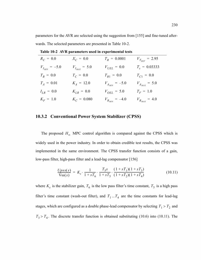
230
parameters for the AVR are selected using the suggestion from [155] and fine-tuned after-
wards. The selected parameters are presented in Table 10-2.
10.3.2 Conventional Power System Stabilizer (CPSS)
The proposed MPC control algorithm is compared against the CPSS which is
widely used in the power industry. In order to obtain credible test results, the CPSS was
implemented in the same environment. The CPSS transfer function consists of a gain,
low-pass filter, high-pass filter and a lead-lag compensator [156]
(10.11)
where is the stabilizer gain, is the low pass filter’s time constant, is a high pass
filter’s time constant (wash-out filter), and ... are the time constants for lead-lag
stages, which are configured as a double phase-lead compensator by selecting and
. The discrete transfer function is obtained substituting (10.6) into (10.11). The
Table 10-2 AVR parameters used in experimental tests
RC 0.0= XC 0.0= TR 0.0001= VTREF2.95=
VIMIN5.0–= VIMAX
5.0= VUEL 0.0= Ts 0.03333=
TB 0.0= TC 0.0= TB1 0.0= TC1 0.0=
TA 0.01= KA 12.0= VAMIN5.0–= VAMAX
5.0=
ILR 0.0= KLR 0.0= VOEL 5.0= TF 1.0=
KF 1.0= KC 0.080= VRMIN4.0–= VRMAX
4.0=
H∞
Upss s( )ω s( )∇
-------------------- Ks1
1 sT6+-----------------
T5s1 sT5+-----------------
1 sT1+( ) 1 sT3+( )1 sT2+( ) 1 sT4+( )
---------------------------------------------⋅⋅ ⋅=
Ks T6 T5
T1 T4
T1 T2>
T3 T4>

231
discrete transfer function with simple variable changes is analogous to (10.7), (10.8) and
(10.10).
The CPSS parameters are tuned using the tuning procedure described in [128] and
[156-160]. The parameters for the CPSS algorithm are presented in Table 10-3. These
parameters are the result of the fine tuning of the CPSS parameters suggested in [156],
when the generator is operating at and with a . This operating
point is selected because it is assumed to be the highest operating point of the power sys-
tem model which is able to withstand without permanent failure disturbances caused by
the CPSS misbehavior during tuning. If a much lower operating point were selected the
generator’s rotational speed deviation would be negligible with no control response from
the CPSS.
The objective of the fine tuning of the CPSS parameters is to minimize the duration of
the oscillations in generator’s rotational speed deviation. For the tuning, a 0.15 pu
mechanical torque step change is used as an external disturbance. During the tuning pro-
cess the generator’s rotational speed deviation is observed on an oscilloscope.
The parameters of the CPSS are then kept unchanged for all the experimental tests.
Table 10-3 CPSS parameters used in experimental tests
P 0.8pu= pf 0.95lag=
T1 0.25= T2 0.005= T3 0.5=
T4 0.06= T5 0.1= T6 1.6=
KS 0.2–= Ts 0.03333=

232
11 Real-Time Tests
Result of experimental studies with the proposed MPC as a power system stabi-
lizer are presented in this chapter. Performance of the proposed MPC has been inves-
tigated on a physical model of a single machine infinite bus power system described in
Chapter 10, under different operating conditions and disturbances. For comparison, a digi-
tal version of the conventional power system stabilizer (CPSS) has been also implemented
in the same environment and tested under the same conditions, see section 10.3.2.
All experimental data were collected through a human-machine interface and were
saved on a disk for further analysis. The results of the data analysis are presented in this
chapter. On the figures, the time axis has been adjusted so that the disturbances occur
coincidentally, ensuring a consistent visual presentation.
11.1 System Identification of the Power System Model
To evaluate the proposed multiple model system identification in a stationary environ-
ment, the micro-synchronous generator was operated at power with a power-
factor . During this experiment, data is collected over a 20 minute time
interval, while the system is undisturbed.
To model the power system, a fifth order ARMA model was selected. The system out-
put with the ARMA model, , is predicted using
H∞
H∞
P 0.9 p.u.=
pf 0.93 lag=
yn

233
(11.1)
where and are the measured system input and output, respectively. The and
parameters are the result of the system identification process. They are presented in
Figures 11-9 and 11-10. The powers of residuals, used to compare different techniques, are
calculated as the difference between the predicted and measured system outputs
. (11.2)
In Figures 11-1 through 11-6, the powers of residuals from the different system identi-
fication techniques are compared with that of the PRO model. This PRO model is pro-
posed by the expert system. Values for the powers of residuals are averaged in these
figures. These are obtained using the “smooth bezier”, a built in function of the Gnuplot
4.0, plotting program.
11.1.1 Comparison of System Identifications
In this research the proposed approach to system identification is to implement multi-
ple techniques with different behaviors concurrently, while an expert system selects the
best model periodically. All system identification techniques used are parametrized in
their unique ways to evoke different identification behaviors. The used parameters for the
algorithms in this experiment are presented in Table 11-1. As a result, system identifica-
tions are characterized by different adaptation speeds and accuracy. The goal is to utilize
this in various transient situations of a plant.
yn biun i– aiyn i–
i 1=
5
∑–i 1=
5
∑=
un i– yn i– ai
bi
vn2 yn yn–( )2=
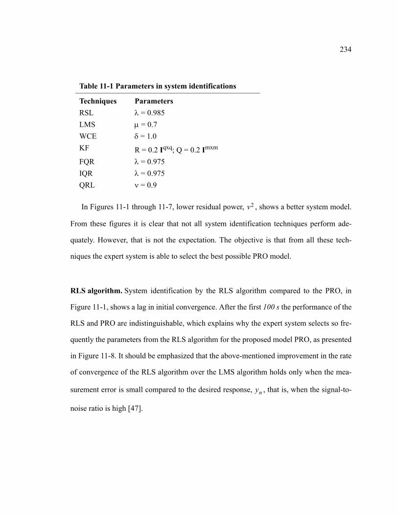
234
In Figures 11-1 through 11-7, lower residual power, , shows a better system model.
From these figures it is clear that not all system identification techniques perform ade-
quately. However, that is not the expectation. The objective is that from all these tech-
niques the expert system is able to select the best possible PRO model.
RLS algorithm. System identification by the RLS algorithm compared to the PRO, in
Figure 11-1, shows a lag in initial convergence. After the first 100 s the performance of the
RLS and PRO are indistinguishable, which explains why the expert system selects so fre-
quently the parameters from the RLS algorithm for the proposed model PRO, as presented
in Figure 11-8. It should be emphasized that the above-mentioned improvement in the rate
of convergence of the RLS algorithm over the LMS algorithm holds only when the mea-
surement error is small compared to the desired response, , that is, when the signal-to-
noise ratio is high [47].
Table 11-1 Parameters in system identifications
Techniques ParametersRSL λ = 0.985LMS µ = 0.7WCE δ = 1.0KF R = 0.2 Iqxq; Q = 0.2 Imxm
FQR λ = 0.975IQR λ = 0.975QRL ν = 0.9
v2
yn

235
LMS algorithm. Convergence of the system identification using the LMS algorithm, in
Figure 11-2, is the slowest from all the techniques. This result concurs with that from the-
ory and parametrization. On the other hand, after the 300s convergence period the perfor-
mance of the LMS and PRO models are close, which explains why the LMS model is
selected by the expert system.
It is interesting to point out that in the very same environment, if the ARMAX form is
selected for the power system model,
, (11.3)
the LMS system identification with the same parameter does not converge at all.
1e-008
1e-007
1e-006
1e-005
0.0001
0 200 400 600 800 1000 1200 1400Time [s]
RLSPRO
[Hz2]
v2
Figure 11-1 Residual comparison between RLS and PRO
yn d biun i– aiyn i–
i 1=
5
∑– civn i–
i 1=
2 or ( 3…5 )
∑+i 1=
5
∑+=

236
WCE algorithm. An example of a non converging system identification is the WCE,
shown in Figure 11-3. If the traditional single system identification technique were imple-
mented using the WCE, a disaster in the control loop would result. However, in the multi-
1e-008
1e-007
1e-006
1e-005
0.0001
0.001
0.01
0.11
0 200 400 600 800 1000 1200 1400Time [s]
LMSPRO
[Hz2]
v2
Figure 11-2 Residual comparison between LMS and PRO
1e-008
1e-006
0.0001
0.01
1
100
10000
1e+006
0 200 400 600 800 1000 1200 1400Time [s]
WCEPRO
[Hz2]v2
Figure 11-3 Residual comparison between WCE and PRO

237
model approach the expert system simply avoids selecting the parameters from the WCE,
which eliminates any harm from the poorly behaving algorithm. The five distinguishable
regions in the WCE algorithm’s chart originate from the five consecutive experiments,
which are necessary to collect the 20 minute long measurement sequence.
Kalman Filter. As presented in Figure 11-4, the performance of the system identification
using the KF shows a slower convergence with a unsatisfactory initial behavior, repre-
sented by a huge error in initial prediction. However, after the convergence of the KF, as
expected the resulting system identification is excellent.
IQR algorithm. The initial error of the IQR algorithm is almost as high as that of the KF.
Compared to other algorithms, it is followed by the fastest initial convergence, as illus-
trated in Figure 11-5. Due to this fast convergence the expert system favors the model sup-
plied by the IQR. On the other hand, when the system identification becomes stationary,
1e-008
1e-006
0.0001
0.01
1
100
10000
0 200 400 600 800 1000 1200 1400Time [s]
KFPRO
[Hz2]v2
Figure 11-4 Residual Comparison between KF and PRO

238
the IQR algorithm as it is parametrized, experiences higher volatility in its prediction.
Consequently, the expert system prefers other model sources over IQR.
FQR algorithm. The FQR algorithm is characterized by a smaller initial prediction error
and a very fast convergence, which explains the initial favoritism by the expert system.
After the initial period, as seen in Figure 11-6, the residual power of the FQR model is
slightly higher than that of the PRO model, which leads to a less favored status of the
FQR.
This higher convergence speed can be attributed to a smaller forgetting factor, where
both IQR and FQR use while the RLS uses . The consequence of
this can be observed on the corresponding figures for these algorithms. After the conver-
gence is achieved the algorithm with a smaller forgetting factor or shorter memory demon-
strates more volatility in system identification.
1e-008
1e-006
0.0001
0.01
1
100
10000
0 200 400 600 800 1000 1200 1400Time [s]
IQRPRO
[Hz2]v2
Figure 11-5 Residual comparison between IQR and PRO
λ 0.975= λ 0.985=

239
QRL algorithm. The QR version of the LMS algorithm, QRL, has a much faster conver-
gence than the LMS as seen from comparing Figure 11-7 and Figure 11-2. Naturally, fast
convergence leads to system identification with a higher variation in estimated parameters
1e-008
1e-007
1e-006
1e-005
0.0001
0.001
0.01
0.1
0 200 400 600 800 1000 1200 1400Time [s]
FQRPRO[Hz2]
v2
Figure 11-6 Residual comparison between FQR and PRO
1e-008
1e-006
0.0001
0.01
1
100
10000
0 200 400 600 800 1000 1200 1400Time [s]
QRLPRO
[Hz2]
v2
Figure 11-7 Residual comparison between QRL and PRO
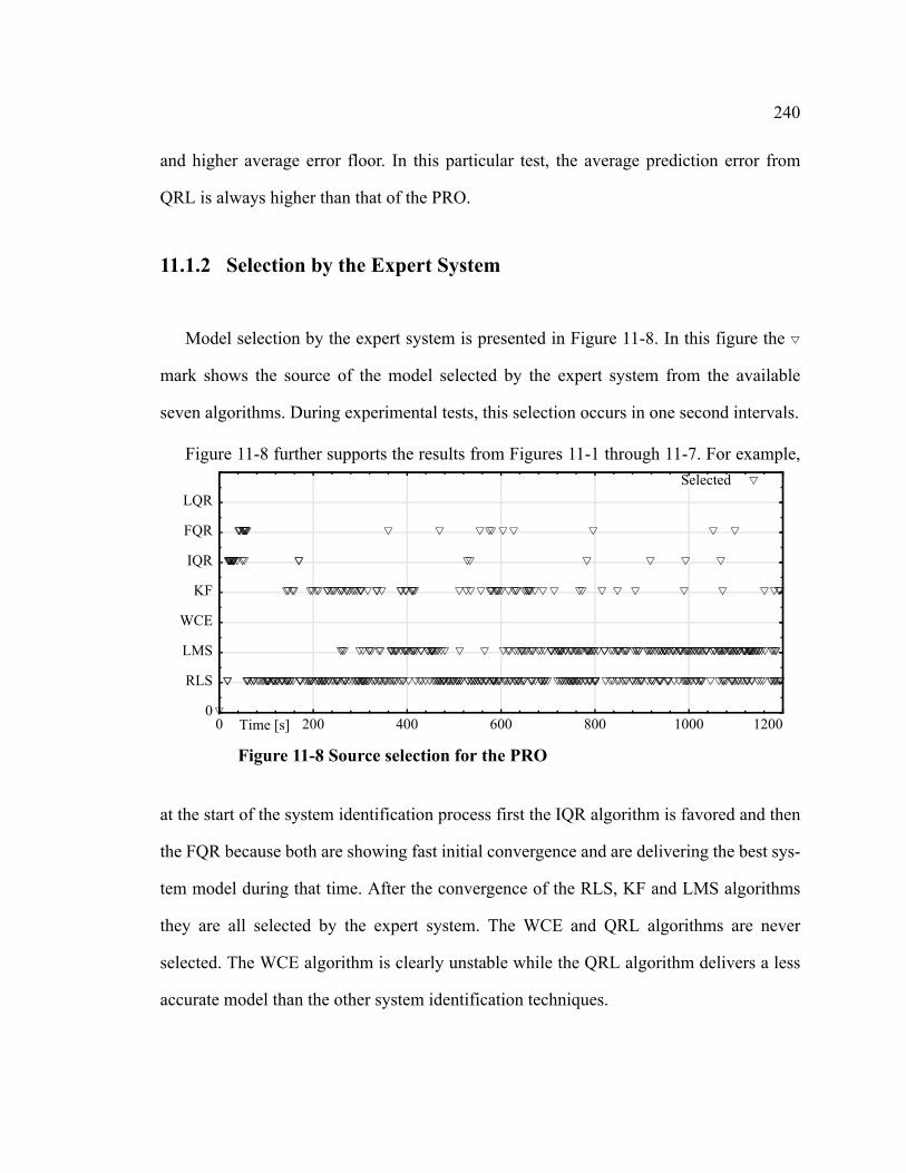
240
and higher average error floor. In this particular test, the average prediction error from
QRL is always higher than that of the PRO.
11.1.2 Selection by the Expert System
Model selection by the expert system is presented in Figure 11-8. In this figure the
mark shows the source of the model selected by the expert system from the available
seven algorithms. During experimental tests, this selection occurs in one second intervals.
Figure 11-8 further supports the results from Figures 11-1 through 11-7. For example,
at the start of the system identification process first the IQR algorithm is favored and then
the FQR because both are showing fast initial convergence and are delivering the best sys-
tem model during that time. After the convergence of the RLS, KF and LMS algorithms
they are all selected by the expert system. The WCE and QRL algorithms are never
selected. The WCE algorithm is clearly unstable while the QRL algorithm delivers a less
accurate model than the other system identification techniques.
0
RLS
LMS
WCE
KF
IQR
FQR
LQR
0 200 400 600 800 1000 1200Time [s]
Selected
Figure 11-8 Source selection for the PRO

241
11.1.3 The Proposed PRO Model
The resulting parameters for the PRO model, selected by the expert system, are pre-
sented in Figures 11-9 and 11-10 for the Autoregressive and Moving average parts of the
model respectively. The AR parameters demonstrate a stable behavior despite the fact
that they are composed from different system identification techniques. The MA parame-
-1.5
-1
-0.5
0
0.5
1
1.5
0 200 400 600 800 1000 1200
Para
met
ers
Time [s]
a1a2a3
a4a5
a1
a2
a5
a4a3
Figure 11-9 The autoregressive parameters of the PRO model
-0.6
-0.4
-0.2
0
0.2
0.4
0.6
0 200 400 600 800 1000 1200
Para
met
er
Time [s]
b1b2b3
b4b5
b1
b2
b3b4
b5
Figure 11-10 The moving average parameters of the PRO model

242
ters show higher variations, therefore, they can not be observed in their original forms.
Thus, they are presented as filtered parameters in Figure 11-10 using the “smooth bezier”,
a built in function of the Gnuplot.
11.1.4 Using the PRO Model for Controller Calculation
As the above test results demonstrate, the PRO model is the best representation for the
plant to be controlled. Therefore, the PRO model is used in the optimization algo-
rithm. The resulting MPC, see sections 6.2.2 through 6.2.4, can be considered as a
best performing robust controller given the limited a priori knowledge of the plant. The
MPC is characterized by the achieved infimum, , presented in Figure 11-11.
.
H∞
H∞
H∞ γ
0
1
2
3
4
5
6
7
0 200 400 600 800 1000 1200
H∞
Nor
m
Time [s]
γ
Figure 11-11 The infimum of the H∞ controller

243
11.1.5 Conclusion for the System Identification
As a result of the above analysis, the properties of an expert system supervised system
identification have been established in a stationary environment. It has also been proved
the PRO model is not worse than the models obtained by any single model system identi-
fication process. Consequently, the expert system fulfills its tasks.
It is expected that in real implementation, the system will operate in a stationary envi-
ronment most of the time. However, the control system shall always be ready for occa-
sional perturbations in the system. During the non stationary state of the system, the
controller’s role is to preserve the system’s stability and to steer the process back into its
stationary state. As the experiments show, if in a non stationary environment different
external disturbances are applied on the power system, the different algorithms behave
differently. These tests are presented in sections 11.2 through 11.4 The effects of external
disturbances are analyzed through voltage reference change, mechanical input torque
change and fault on the transmission line using the possible perturbing methods, as shown
in Figure 10-14.
11.2 Voltage Reference Step Change
The voltage reference step change is examined at three different working points of the
generator, as described in Experiments 1 through 3.

244
11.2.1 Experiment 1
In Experiment 1, the micro-synchronous generator is operated at power = 0.9 p.u.
and power-factor = 0.93 lag. A 2% step increase in the reference voltage is applied at
1 s and removed at 5 s, as presented in Figure 11-12. As a consequence of this perturba-
tion, the generator’s power-factor changes to = 0.91 lag during the 1 s through 5 s
interval.
The micro-synchronous generator’s rotational speed deviations, , with the pro-
posed MPC power system stabilizer, the conventional power system stabilizer (CPSS)
and with no controller (NoC) for the 2% step increase in the reference voltage is shown in
Figure 11-13. The amplitude of the oscillations is significantly reduced by the MPC.
Pe
φcos
φcos
2.86
2.88
2.9
2.92
2.94
2.96
2.98
3
0 1 2 3 4 5 6 7 8Time [s]
NoCCPSSMPC
Vt
[100V]
Figure 11-12 Terminal voltage change in Experiment 1
∆ω
H∞
H∞

245
The control actions of the MPC and CPSS are compared in Figure 11-14. The
fluctuation in the control action of the MPC is due to the random signal associated
with the system identification algorithm. As described in theory, the system identification
requires a random signal for input-output decoupling. The selected signal has a Normal
Distribution and it is less than 5% of the control signal. This corresponds to a control
-0.04
-0.03
-0.02
-0.01
0
0.01
0.02
0.03
0.04
0 1 2 3 4 5 6 7 8Time [s]
NoCCPSSMPC
[Hz]∆ω
Figure 11-13 Speed deviation in Experiment 1
H∞
-0.25-0.2
-0.15-0.1
-0.050
0.050.1
0.150.2
0.25
0 1 2 3 4 5 6 7 8Time [s]
CPSSMPC
Con
trol S
igna
l [p.
u.]
Figure 11-14 Control signal in Experiment 1
H∞
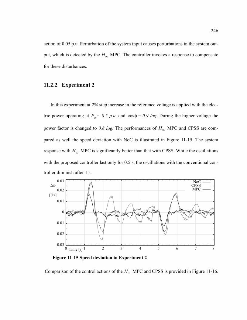
246
action of 0.05 p.u. Perturbation of the system input causes perturbations in the system out-
put, which is detected by the MPC. The controller invokes a response to compensate
for these disturbances.
11.2.2 Experiment 2
In this experiment at 2% step increase in the reference voltage is applied with the elec-
tric power operating at = 0.5 p.u. and = 0.9 lag. During the higher voltage the
power factor is changed to 0.8 lag. The performances of MPC and CPSS are com-
pared as well the speed deviation with NoC is illustrated in Figure 11-15. The system
response with MPC is significantly better than that with CPSS. While the oscillations
with the proposed controller last only for 0.5 s, the oscillations with the conventional con-
troller diminish after 1 s.
Comparison of the control actions of the MPC and CPSS is provided in Figure 11-16.
H∞
Pe φcos
H∞
H∞
-0.03
-0.02
-0.01
0
0.01
0.02
0.03
0 1 2 3 4 5 6 7 8Time [s]
NoCCPSSMPC
[Hz]
∆ω
Figure 11-15 Speed deviation in Experiment 2
H∞

247
11.2.3 Experiment 3
The voltage reference step change of 2% is also tested with a leading power factor
when the generator operates with the electric power = 0.5 p.u. and power-factor =
0.9 lead. During this experiment the power-factor changes to = 0.8 lead. The micro-
synchronous generator’s rotational speed deviation, , with the MPC, CPSS and
NoC is demonstrated in Figure 11-17. Compared to the amplitude of oscillations with
CPSS, the amplitude of the oscillations with MPC is reduced almost to half.
-0.3
-0.2
-0.1
0
0.1
0.2
0.3
0 1 2 3 4 5 6 7 8Time [s]
CPSSMPC
Con
trol S
igna
l [p.
u.]
Figure 11-16 Control action in Experiment 2
Pe φcos
φcos
∆ω H∞
H∞

248
The control actions of the MPC and CPSS are compared in Figure 11-18.
The above presented test results verify that both control algorithms perform well at all
operating points for this type of disturbance. The difference in performance goes in favor
of MPC, which has smaller amplitudes in post-disturbance oscillations.
-0.04
-0.03
-0.02
-0.01
0
0.01
0.02
0.030.04
0 1 2 3 4 5 6 7 8Time [s]
NoCCPSSMPC
[Hz]∆ω
Figure 11-17 Speed deviation in Experiment 3
H∞
-0.4
-0.3
-0.2
-0.1
0
0.1
0.2
0.30.4
0 1 2 3 4 5 6 7 8Time [s]
CPSSMPC
Con
trol S
igna
l [p.
u.]
Figure 11-18 Control action in Experiment 3
H∞

249
11.3 Input Torque Step Change
The input torque step change disturbance is examined at three different working points
of the generator, as described in Experiments 4 through 6.
11.3.1 Experiment 4
In this experiment the micro-synchronous generator is operated at power = 0.9 p.u.
and power-factor = 0.93 lag. A 18% step decrease in the input torque is applied at 1
s and removed at 5 s. During this time the system operating point changes to a power of
=0.725 p.u. and power-factor = 0.91 lag. This step change in the electric power of
the micro-synchronous generator with the MPC, CPSS and NoC is shown in Figure
11-20.
Pe
φcos
Pe φcos
H∞
0.6
0.65
0.7
0.75
0.8
0.85
0.9
0.95
11.05
0 1 2 3 4 5 6 7 8Time [s]
NoCCPSSMPC
Elec
tric
Pow
er [p
.u.]
Figure 11-19 Electric power in Experiment 4

250
The micro-synchronous generator’s rotational speed deviation, , with the
MPC, CPSS and NoC is shown in Figure 11-20. In this experimental situation the
MPC provides better reduction in the amplitude of the oscillations but the CPSS shows
faster settling time of the response after the second disturbance. This can be explained as a
result of controller action, whose primary objective is to reduce the effects of larger
disturbances and ignore the smaller ones.
The investigation of control actions with MPC and CPSS is presented in Figure
11-21.
∆ω
H∞ H∞
H∞
-0.15
-0.1
-0.05
0
0.05
0.1
0.15
0 1 2 3 4 5 6 7 8Time [s]
NoCCPSSMPC
[Hz]∆ω
Figure 11-20 Speed deviation in Experiment 4
H∞
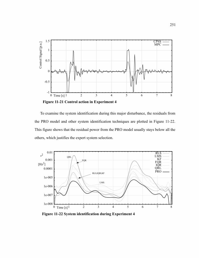
251
To examine the system identification during this major disturbance, the residuals from
the PRO model and other system identification techniques are plotted in Figure 11-22.
This figure shows that the residual power from the PRO model usually stays below all the
others, which justifies the expert system selection.
-1
-0.5
0
0.5
1
1.5
0 1 2 3 4 5 6 7 8Time [s]
CPSSMPC
Con
trol S
igna
l [p.
u.]
Figure 11-21 Control action in Experiment 4
1e-008
1e-007
1e-006
1e-005
0.0001
0.001
0.01
0 1 2 3 4 5 6 7 8Time [s]
RLSLMS
KFFQRIQR
QRLPRORLS,IQR,KF
LMS
QRLFQR
[Hz2]
v2
Figure 11-22 System identification during Experiment 4

252
11.3.2 Experiment 5
The input torque step change experiment is performed with power = 0.5 p.u. and
= 0.9 lag. When a 0.1 p.u. step change is introduced during the time interval of 1 s
through 5 s, the operating point changes to = 0.4 p.u. and = 0.8 lag. System
responses with the MPC, CPSS and NoC are illustrated in Figure 11-23. While the
oscillations for both controllers last for 2 s and 2.5 s, the amplitude of the oscillations are
much faster reduced with MPC and that brings the system closer to its stable state.
The control signals for MPC and CPSS are shown in Figure 11-24.
Pe
φcos
Pe φcos
H∞
H∞
-0.08
-0.06
-0.04
-0.02
0
0.02
0.04
0.060.08
0 1 2 3 4 5 6 7 8Time [s]
NoCCPSSMPC
[Hz]∆ω
Figure 11-23 Speed deviation in Experiment 5
H∞

253
11.3.3 Experiment 6
A 0.1 p.u. step decrease in the input torque is also tested with a leading power factor.
During this experiment, the generator’s electric power = 0.5 p.u. with = 0.9 lead,
changes to = 0.4 p.u. with = 0.93 lead. Speed deviations with MPC, CPSS
and NoC are presented in Figure 11-25. At the above indicated operating point the system
response with the MPC shows superior performance compared to that of the CPSS.
The oscillations with the MPC last for 0.5 s while the oscillations with the CPSS last
for 1 s. At the same time the maximum amplitude of oscillations is also reduced with the
MPC.
-1.5
-1
-0.5
0
0.5
1
0 1 2 3 4 5 6 7 8Time [s]
CPSSMPC
Con
trol S
igna
l [p.
u.]
Figure 11-24 Control action in Experiment 5
Pe φcos
Pe φcos H∞
H∞
H∞
H∞

254
The control actions of MPC and CPSS are examined in Figure 11-26.
-0.08
-0.06
-0.04
-0.02
0
0.02
0.04
0.06
0.08
0 1 2 3 4 5 6 7 8Time [s]
NoCCPSSMPC
[Hz]∆ω
Figure 11-25 Speed deviation in Experiment 6
H∞
-0.8
-0.6
-0.4
-0.2
0
0.2
0.4
0.60.8
0 1 2 3 4 5 6 7 8Time [s]
CPSSMPC
Con
trol S
igna
l [p.
u.]
Figure 11-26 Control action in Experiment 6

255
11.4 Three-Phase to Ground Fault Test
The three-phase to ground fault is examined at three different working points of the
generator, as described in Experiments 7 through 9.
11.4.1 Experiment 7
To investigate the performance of the MPC under transient conditions caused by
transmission line fault, a three phase to ground fault test has been conducted. In Experi-
ment 7, the micro-synchronous generator is operated at power = 0.9 p.u. with power
factor = 0.93 lag. Under this operating condition, with both lines in operation, a
three phase to ground fault is applied in the middle of one transmission line at 1 s The
faulty transmission line is opened by relay action at both ends 100 ms later. The first
unsuccessful closure attempt is made after 600 ms, and the line is re-opened again after
100 ms due to a permanent fault. During the fault state the micro-synchronous generator is
operated at power = 0.9 p.u. with = 0.85 lag. The second successful closure
attempt is applied at 8 s and the system returns to its initial operating condition. This test is
best characterized by a change in the generator’s terminal voltage, . Prior to the fault the
energy is transported through two transmission lines. Following the fault the same energy
must be transported through only one transmission line, which explains the terminal volt-
age increase during the fault, as shown in Figure 11-27.
H∞
Pe
φcos
Pe φcos
Vt

256
Under the above transient conditions, system responses with the MPC and CPSS
are compared in Figure 11-28. It can be observed that the MPC outperforms the CPSS
with smaller overshoot and faster settling time in both cases, at 1 s and 5 s
.
2.75
2.8
2.85
2.9
2.95
3
0 1 2 3 4 5 6 7 8Time [s]
NoCCPSSMPC
Vt[100V]
Figure 11-27 Terminal voltage change during Experiment 7
H∞
H∞
-0.15
-0.1
-0.05
0
0.05
0.1
0.15
0 1 2 3 4 5 6 7 8Time [s]
NoCCPSSMPC
[Hz]∆ω
Figure 11-28 Speed deviation in Experiment 7

257
Control actions of MPC and CPSS under transient conditions are also investi-
gated. Figure 11-29 outlines the test results.
To examine the system identification during this power line fault, the residuals from
the PRO model along with other system identification techniques are plotted in Figure 11-
30. This graph shows that the residual from the PRO model usually stays below all the
others, by which the expert system selection is justified. The first and last 0.5 s on the Fig-
H∞
-1-0.8-0.6-0.4-0.2
00.20.40.60.8
1
0 1 2 3 4 5 6 7 8Time [s]
CPSSMPC
Con
trol S
igna
l [p.
u.]
Figure 11-29 Control action in Experiment 7
1e-008
1e-007
1e-006
1e-005
0.0001
0.001
0 1 2 3 4 5 6 7 8Time [s]
RLSLMS
KFWCEFQRIQRPRO
LMS
FQR
KF
IQR
WCE
RLS[Hz2]
v2
Figure 11-30 System identification in Experiment 7

258
ure 11-30 is a distorted representation of the measurements which is caused by the
smoothing function “smooth bezier”.
11.4.2 Experiment 8
Responses to a three phase to ground fault disturbance are compared in Experiment 8,
where the micro synchronous generator’s power is = 0.5 p.u. with = 0.9 lag. As
seen in Figure 11-31, during the fault the micro-synchronous generator is operating at a
power of = 0.5 p.u. with a power factor = 0.8 lag. Although the well tuned CPSS
reduces the oscillations, the MPC exhibits excellent damping properties.
The control actions of MPC and CPSS are examined in Figure 11-32.
Pe φcos
Pe φcos
H∞
-0.1
-0.08
-0.06
-0.04
-0.02
0
0.02
0.04
0.060.08
0 1 2 3 4 5 6 7 8Time [s]
NoCCPSSMPC
[Hz]∆ω
Figure 11-31 Speed deviation in Experiment 8
H∞

259
11.4.3 Experiment 9
Performance in response to another three phase fault is presented in Figure 11-33. The
micro synchronous generator’s operating power is = 0.5 p.u. with a power factor
-1-0.8
-0.6-0.4-0.2
00.20.40.60.8
1
0 1 2 3 4 5 6 7 8Time [s]
CPSSMPC
Con
trol S
igna
l [p.
u.]
Figure 11-32 Control action in Experiment 8
-0.08
-0.06
-0.04
-0.02
0
0.02
0.04
0.06
0.080.1
0 1 2 3 4 5 6 7 8Time [s]
NoCCPSSMPC
[Hz]∆ω
Figure 11-33 Speed deviation in Experiment 9
Pe

260
= 0.9 lead. During the fault, the micro-synchronous generator operates at a power
= 0.5 p.u. with a power factor = 0.8 lead. It is obvious that the MPC provides
an effective way to improve the generator’s stability under these operating conditions,
where a very fast control action brings the amplitude of the oscillations down.
In Figure 11-34 the control signals for MPC and CPSS are compared.
11.5 Summary
In a real-time digital control environment, described in Chapter 10, an MPC
power system stabilizer, discussed in Section I and II, has been implemented and tested on
a physical model of a power system. The experimental results obtained with the MPC
are compared with that of a digitized conventional power system stabilizer CPSS,
described in section 10.3.2. The test results, presented on graphs, have proved that both
φcos
Pe φcos H∞
H∞
-1-0.8-0.6-0.4-0.2
00.20.40.60.8
1
0 1 2 3 4 5 6 7 8Time [s]
CPSSMPC
Con
trol S
igna
l [p.
u.]
Figure 11-34 Control action in Experiment 9
H∞
H∞

261
the CPSS and the proposed MPC are very effective in improving the dynamic perfor-
mance of the model power system. Furthermore, both control methods keep their abilities
for any operating point of the system. Yet, a clear difference in the performance of these
two control methods can be observed. This difference originates in the derivation of these
methods. The CPSS is based on a conventional controller design using proportional-inte-
gral compensator with lead-lag elements, which are fine-tuned around one operating
point. The MPC is designed using optimization techniques with the objective to
reduce the effects of disturbances with highest magnitude. The test results clearly show
that the system outputs with larger deviations are much more reduced with the MPC
than with the CPSS.
This difference in reducing effects of disturbances with highest magnitude originates
from the weaker control action of the CPSS. Figures that illustrate control actions from the
above experiments clearly attest to this argument. To verify that with a higher CPSS gain
, see Table 10-3, the weakness in the performance of the CPSS can be
improved, one last experiment was conducted.
11.5.1 Experiment 10
In Experiment 10, the generator’s operating power is Pe = 0.5 p.u. with cosφ=0.93 lag.
At time 1 s, a 0.12 p.u. step decrease in torque reference is applied to the system. The
operating power of the generator returns to its original value at time 5 s. As Figure 11-36
illustrates, when the CPSS gain is the control action of the CPSS is improved.
H∞
H∞
H∞
KS 0.4–=
KS 0.4–=

262
However, the resulting system stability is compromised by longer lasting oscillations, as
shown in Figure 11-35. Overall, performance of the CPSS deteriorates when the operating
conditions deviate from the design point. These experiments also prove that the MPC
is able to adapt itself to new operating conditions and it can produce consistently good
performance in accordance with the optimization criterion. These experimental results are
consistent with the theoretical and simulation results and demonstrate that the proposed
MPC stabilizer outperforms the CPSS.
-0.08
-0.06
-0.04
-0.02
0
0.02
0.04
0.06
0.080.1
0 1 2 3 4 5 6 7 8Time [s]
NoCCPSSMPC
[Hz]∆ω
Figure 11-35 Speed deviation in Experiment 10
-1.5
-1
-0.5
0
0.5
1
1.5
0 1 2 3 4 5 6 7 8Time [s]
CPSSMPC
Con
trol S
igna
l [p.
u.]
Figure 11-36 Control action in Experiment 10
H∞
H∞

263
12 Conclusions and Recommendation
12.1 Conclusions
One can reasonably expect that future industrial systems will become more complex.
Consequently, improved performance requirements will be established for industrial con-
trollers. Therefore, conventional three-term-controllers may not be able to resolve the
need for higher accuracy and robustness in these industrial environments. The next gener-
ation of controllers will be expected to handle the working point changes of a nonlinear
plant and they should perform well under system disturbances. It is also expected that the
control systems of the future will require minimal studies prior to their implementation.
A controller that could handle the above requirements is an adaptive controller with
the control action that is optimal for both system identifications and implementation of the
control. The focal point of this thesis is to develop a controller that will meet the above
expectations. The controller design is based on the estimation of the current plant model
and the information obtained from the estimate is used to redesign the controller. This the-
sis proposes a two step adaptive solution for a robust control in the form of an MPC
algorithm, where considerable attention is directed towards the reduction of prior studies.
In step one, the MPC algorithm performs a robust system identification using a
general method for estimating discrete unknown parameters associated with robust control
uncertainty models. The key element of this robust system identification is an expert sys-
H∞
H∞

264
tem, which supervises multiple concurrently performing system identification techniques
and periodically selects from the estimated parameters to define the optimal system
model. This concept requires that the concurrently performing system identification tech-
niques have distinct estimation properties. The difference in behavior is accomplished
either by using different algorithms, such as the RLS, LMS, WKE, KF, FQR, IQR, and
QRL or by parametrizing one algorithm with , , and parameters.
The different behavior of system identification techniques is used with the assumption
that they will behave differently under different perturbations and thereby, at least one will
provide a chance for the expert system to select a proper model. In order to obtain a sys-
tem model which is relevant to the plant control, the system identification is performed in
a closed-loop. As test results show, with this approach the robustness of system identifica-
tion is significantly improved.
In step two, the MPC algorithm uses the proposed system model from step one to
solve the corresponding robust control problem by the (sub)optimization technique. A
detailed implementation procedure for this control algorithm, which is obtained by the
game theory approach, is provided in this thesis. The controller is formulated using
the solutions of two recursive Riccati equations, one for the controller and one for the state
estimator. The acquired design technique is one of the most advanced methods avail-
able today for designing robust controllers. One big advantage of this technique is that it
allows the designer to tackle the most general form of control architecture, while explicitly
considering such factors as uncertainties, disturbances, actuator/sensor noises, and perfor-
mance measures. This is accomplished through four weighting matrices. In the proposed
λMIN λMED λMAX
H∞
H∞
H∞
H∞

265
design the selection of weighting matrices is simplified by a coefficient that multiplies a
unity matrix. The weighting matrices with the system model define the infimum, , of the
controller. If the value of is smaller, the controller is more robust with a conserva-
tive control action. However, if increases, the control action approaches to that of LQR.
It is a design trade-off to select those weighting matrices that deliver a desired control
action.
During the simulation study and in the experimental tests, the MPC was applied as
a power system stabilizer and tested under various conditions. For comparison, a digitized
conventional power system stabilizer, CPSS, has also been implemented and tested under
the same conditions. The MPC has proven to be wide ranging in action and appropri-
ate for steady-state, dynamic and transient operating conditions. It has provided good
post-fault recovery for the tested disturbances, such as the reference voltage step change,
input torque step change and three phase to ground fault. These results are consistent with
the expectations, demonstrating the correctness and superiority of the proposed MPC
over the CPSS results.
The simulation and experimental results have also confirmed that the introduced
expert system increased the effectiveness and robustness of the real-time system identifi-
cation techniques.
The implementation of concurrently running algorithms has been greatly simplified by
the C++ object oriented programming language. This programing language not only sim-
plifies the multiple usage of a function like the system identification technique but it also
enables the development of common library functions which can be used in different algo-
γ
H∞ γ
γ
H∞
H∞
H∞

266
rithms ensuring that all the algorithms use the same functions while the parameters in each
algorithm are defined in a unique way.
The outcome of this thesis is a systematic, ready for application methodology for
building an MPC algorithm. This has been accomplished by translating the complex
mathematical theory of control into a format that is easy to comprehend. This research
also contributes to a thorough understanding of the application of MPC to industrial
system control problems and it demonstrates how the MPC can be successfully
applied in an industrial design.
12.2 Recommendation for Future Research
The idea behind developing MPC was to introduce a controller which requires a
minimum of preliminary research and tuning for a particular implementation. Several
important findings have emerged as a result of this research. However, there are still
opportunities for further improvements and development. In the following paragraphs a
few feasible and required improvements are proposed.
• Preliminary controller - During the initial phase of the MPC implementation, the
controller is not defined for a period of time. Taking into account that during this phase
some systems may be inherently unstable, the need for an integrated preliminary simple
controller is necessary. Starting with an initial feedback controller, an iterative scheme
of modelling and designing the MPC will provide information on the dynamics of the
plant relevant to feedback system identification and the consequent robust control.
H∞
H∞
H∞
H∞
H∞

267
• Model order selection - Estimating the appropriate model order of a dynamic system
from the observed input-output data is an important procedure in adaptive control. Nei-
ther having a more complex model nor having an overly simplified one has advantages.
The literature on model order selection is plentiful [164-176]. The most popular ones
are the Akaike’s Information Criterion (ACI) [164] and the Minimum Description
Length (MDL) criterion [165]. Including a model order selection function into the
expert system increases the autonomy of system identification.
• Sampling interval selection - Selection of the proper sampling interval, Ts, is crucial
to the process of system identification because the quality of the estimated model
depends upon it. The upper limit of the sampling interval is determined by the Nyquist
interval, TNq. Oversampling must be avoided in order to maintain good accuracy in sys-
tem identification. System identification using the ARMA model was found to be very
sensitive to the selection of the sampling interval [170]. The expert system would be
enhanced by a sampling interval selection functional.
• Feedback loop delay calculation - System response to control action can have a sig-
nificant delay relative to the sampling interval. This delay originates from the system
inertia in response to a control action. If this delay is significant it should be included in
the system identification. During the experimental tests it was found that if an extra
delay of one sample is included in the control signal for the system identification, the
controller’s performance improves. This delay estimation should be included as an
expert system function in the future.

268
• Robust system identification - The concurrently occurring system identifications
should consist of at least three different system identification techniques, where the
techniques perform concurrently a few different versions of parametrization. For exam-
ple, the RLS, FQR and IQR algorithms should be parametrized with , , and
parameters and similarly the LMS algorithms with , , and .
This way the number of concurrently performing algorithms would increase by three
times, ensuring fast, medium and slow system identifications. Similarly, the parametri-
zation of the KF with weighting matrices and , would result in four to nine com-
binations for the KF implementation. Thereby the robustness of system identification
would improve for all situations.
• Weight matrix selection - The design is one of the most advanced techniques
available today for a robust controller. However, one big drawback of this technique is
the experience and skill needed to design the shape of the weighting functions on sensi-
tivity and closed-loop transfer functions to achieve the desired goal [177]. The practical
issue of the design of weighting matrices lacks a systematic approach. In this thesis
each weighting matrix has been simplified by a coefficient that multiplies the unity
matrix. During tests, it was found that the ratio between these coefficients determines
the infimum for the controller. Further research should be conducted to determine
the possibility of a systematic algorithm for tuning these coefficients. If the weights
selection were performed by an online expert system, the proposed MPC could
play an important role in industrial control.
λMIN λMED
λMAX µMIN µMED µMAX
Qn Rn
H∞
H∞
H∞

269
In conclusion, a novel robust adaptive control design procedure has been introduced in
this thesis, which integrates an robust controller with a robust parameter estimation.
This integration resulted in an MPC algorithm, which has been formulated in a way to
achieve a systematic, ready for application methodology for building an MPC con-
troller. The controller design has been simplified by translating the complex mathematical
theory of control into a procedure that is easy to follow and implement. The developed
theory contributes to a thorough understanding of the application of MPC to industrial
system control problems.
The effectiveness of the proposed procedure as a power system stabilizer has been
demonstrated through simulation studies and by experimental tests. The successful imple-
mentation of the controller demonstrates how the MPC can be effectively applied in
an industrial design. The approach described is quite general and is, therefore, applicable
to systems other than those studied in the context of this thesis.
H∞
H∞
H∞
H∞
H∞
270
13 References
[1] Kimura, H., “Chain-Scattering Approach to Control”, Birkhauser, Boston, 1997.
[2] Kalman, R. E., “Contribution to the theory of optimal control”, Boletin de la
Sociedad Matemetica Mexicana, Vol. 5, 1960, pp. 102-119.
[3] Kalman, R. E., “A new approach to linear filtering and prediction problems”, Trans-
actions of the ASME, Journal of Basic Engineering, Vol. 82D, March, 1960, pp. 35-
45.
[4] Athans, M., and Falb, P. L., “Optimal Control - An Introduction to the Theory and its
Applications”, McGraw-Hill Book Company, New York, 1966.
[5] Athans, M., “The role and use of the stochastic linear-quadratic-gaussian problem in
control system design”, IEEE Transactions on Automatic Control, Vol. 16, No. 6,
December, 1971, pp. 529-551.
[6] Chen, T., “A simple derivation of the -optimal sampled-data controllers”, North-
Holland, System & Control Letters, Vol. 20, 1993, pp. 49-56.
[7] Green, M., and Limebeer, D. J. N., “Linear Robust Control”, Prentice-Hall, Engle-
wood Cliffs, New Jersey, 1995.
H∞
H2

271
[8] Zames, G., “Feedback and optimal sensitivity: Model reference transformations, mul-
tiplicative seminorms, and approximate inverses”, IEEE Transactions on Automatic
Control, Vol. 26, No. 2, April, 1981, pp. 301-320.
[9] Francis, B. A., and Zames, G., “On -optimal sensitivity theory for SISO feedback
systems”, IEEE Transactions on Automatic Control, Vol. 29, No. 1, January, 1984,
pp. 9-16.
[10] Ball, J. A., and Cohen, N., “Sensitivity minimization in an norm: Parametriza-
tion of all suboptimal solutions”, International Journal of Control, Vol. 46, No. 3,
September, 1987, pp. 785-816.
[11] Kimura, H., “Directional interpolation approach to - Optimization and robust
stabilization”, IEEE Transactions on Automatic Control, Vol. 32, No. 12, December,
1987, pp. 1085-1093.
[12] Doyle, J. C., Glover, K., Khargonekar, P. P., and Francis, B. A., “State-space solu-
tions to standard and control problems”, IEEE Transactions on Automatic
Control, Vol. 34, No. 8, August, 1989, pp. 831-847.
[13] Green, M., Klover K., Limbeer, D. J. N., and Doyle, J. C., “A J-spectral factoriza-
tion approach to control”, SIAM Journal on Control and Optimization, Vol. 28,
1990, pp. 1350-1371.
H∞
H∞
H∞
H∞ H∞
H∞

272
[14] Stoorvogel, A. A., and Trentelman, H. L., “Quadratic matrix inequality in singular
control with state feedback”, SIAM Journal on Control and Optimization, Vol.
28, No. 5, September, 1990, pp. 1190-1208.
[15] Tadmor, G., “Worst case design in time domain: The maximum principle and the
standard problem”, Mathematics of Control, Signals, and Systems, Vol. 3, No.
4, 1990, pp. 301-324.
[16] Gahinet, P., and Apkarian, P., “Linear matrix inequality approach to control”,
International Journal of Robust and Nonlinear Control, Vol. 4, No. 4, July-August,
1994, pp. 421-448.
[17] Dragan, V., Halanay, A., and Ionescue, V., “Infinite horizon disturbance attenuation
for discrete-time systems: A Popov-Yakubovich approach”, Integral Equations and
Operator Theory, Vol. 19, 1994, pp. 153-215.
[18] Feintuch, A., “Robust Control Theory in Hilbert Space”, Springer-Verlag, New
York, 1998.
[19] Basar, T., and Bernhard P., “ - Optimal Control and Related Minimax Design
Problems - A Dynamic Game Approach”, Second Edition, Birkhauser, Boston,
1995.
[20] Hassibi, B., Sayed, A. H., and Kailath, T., “Indefinite-Quadratic Estimation and
Control”, SIAM Applied and Numerical Mathematics, Philadelphia, 1999.
H∞
H∞
H∞
H∞

273
[21] de Callafon, R. A., “Feedback Oriented Identification for Enhanced and Robust
Control”, PhD thesis, Delft University of Technology, Delft, The Netherlands, 1998.
[22] Camacho, E. F., and Bordons, C., “Model Predictive Control”, Second Edition,
Springer-Verlag London Ltd., London, 2004.
[23] Rao, C. V., Wright, S. J., and Rawlings, J. B., “Application of interior-point methods
to model predictive control”, Journal of Optimization Theory and Applications, Vol.
99, No. 3, December, 1998, pp. 723-757.
[24] Camponogara, E., Jia, D., Krogh, B. H., and Talukdar, S., “Distributed model pre-
dictive control”, IEEE Control Systems Magazine, Vol. 22, No. 1, February, 2002,
pp. 44-52.
[25] Henson, M. A., and Seborg, D. E., “Nonlinear Process Control”, Prentice Hall,
Upper Saddle River, New Jersey, 1997.
[26] Rácz, L. Z., and Bókay, B., “Power System Stability”, Akadémiai Kiadó, Budapest,
1988.
[27] Rogers, G., “Demystifying power system oscillations”, IEEE Computer Applica-
tions in Power, Vol. 9, No. 3, July, 1996, pp. 30-35.
[28] Pavella, M., and Murthy, P. G., “Transient Stability of Power Systems: Theory and
Practice”, John Wiley & Sons, New York, 1994.
[29] Park, R. H., “Two-reaction theory of synchronous machines - Generalized methods
of analysis: Part I ”, AIEE Transactions, Vol. 48, July, 1929, pp. 716–727.
274
[30] Ljung, L., “System Identification: Theory for the User”, Prentice Hall - Information
and System Science Series, Upper Saddle River, New Jersey, 1999.
[31] Forssell, U., “Closed-loop Identification – Methods, Theory, and Applications”,
PhD Thesis, Linkoping University, Linkoping, Sweden, 1999.
[32] Söderström, T., and Stoica, P., “System Identification”, Prentice Hall, New York,
1989.
[33] Söderström, T., “Comments on ‘Identification of closed-loop systems via least-
squares method’”, International Journal of Adaptive Control and Signal Processing,
Vol. 13, No. 1, February, 1999, pp. 37-41.
[34] Forssell, U., and Ljung, L., “Closed-loop Identification Revisited”, Automatica, Vol.
35, No. 7, July, 1999, pp. 1215-1241.
[35] Wang, L. Y., and Yin, G. G., “Persistent identification of systems with unmodeled
dynamics and exogenous disturbances”, IEEE Transactions on Automatic Control,
Vol. 45, No. 7, July, 2000, pp. 1264-1256.
[36] Zhang, Y., and Feng, C., “Identification of closed-loop systems via least-squares
method”, International Journal of Adaptive Control and Signal Processing, Vol. 12,
No.1, February, 1998, pp. 29-39.
[37] Johnson, C. R. Jr., “On the interaction of adaptive filtering, identification, and con-
trol”, IEEE Signal Processing Magazine, Vol. 12, No. 2, March, 1995, pp. 22-37.

275
[38] Zhou, T., “Unfalsified plant model parametrization from closed-loop experimental
data”, Automatica, Vol. 33, No. 5, May, 1997, pp. 805-820.
[39] Landau, I. D., “Identification in closed loop: a powerful design tool (better design
models, simpler controllers)”, Control Engineering Practice, Vol. 9, No. 1, January,
2001, pp. 51-65.
[40] Hakvoort, R. G., “System Identification for Robust Process Control: Nominal Mod-
els and Error Bounds“, PhD Thesis, Delft University of Technology, Delft, The
Netherlands, 1994.
[41] Landau, I. D., “From robust control to adaptive control”, Control Engineering Prac-
tice, Vol. 7, No. 9, September, 1999, pp. 1113-1124.
[42] Van den Hof, P., “Closed-loop issues in system identification”, Annual Reviews in
Control, Vol. 22, 1998, pp. 173-186.
[43] Isermann, R., “Digital Control Systems: Stochastic Control, Multivariable Control,
Adaptive Control, Applications”, Second Edition, Springer-Verlage, Berlin, Heidel-
berg, 1991.
[44] Narendra, K., and Cheng Xiang, “Adaptive Control of Discrete-Time Systems
Using Multiple Models”, IEEE Transactions on Automatic Control, Vol. 45. No. 9,
September, 2000, pp. 1669-1686.
[45] Autenrieth, T., and Rogers, E., “Performance enhancement for a class of multiple
model adaptive control schemes”, International Journal of Adaptive Control and
Signal Processing, Vol. 13, No. 2, March, 1999, pp. 105-127.

276
[46] Goodwin, G. C., Gevers, M., and Ninness, B., “Quantifying the error in estimated
transfer functions with application to model order selection”, IEEE Transactions on
Automatic Control, Vol. 37, No. 7, July, 1992, pp. 913-928.
[47] Haykin, S., “Adaptive Filter Theory”, Third Edition, Prentice Hall, Upper Saddle
River, New Jersey, 1996.
[48] Van den Hof, P., “Closed-loop issues in system identification”, Annual Reviews in
Control, No. 22, 1998, pp. 173-186.
[49] Weiss, L., and Infante, E. F., “Finite time stability under perturbing forces and on
product spaces”, Differential Equations and Dynamical Systems, Proceedings of an
International Symposium, Puerto Rico, Edited by Hale, J. K., and La Salle, J. P.,
Academic Press, New York, 1967, pp. 341-350.
[50] La Salle, J. P., and Lefschetz, S., “Stability by Liapunov’s Direct Method - With
Applications”, Academic Press, New York, 1961.
[51] Safonov, M. G., “Focus on the knowable”, in “Control Using Logic-Based Switch-
ing”, Editor: Morse, A. S., Springer Verlag, Berlin, 1996, pp. 224-233.
[52] Kosut, R. L., “Uncertainty Model Unfalsification: A System Identification Paradigm
Compatible with Robust Control Design”, Proceedings of the 34th IEEE Conference
on Decision and Control (Cat. No.95CH35803), Vol. 4, 1995, pp. 3492-3497.
[53] Wodoley, B. R., How, J. P., and Kosut, R. L., “Direct unfalsified controller design -
solution via convex optimization”, Proceedings of the 1999 American Control Con-
ference (Cat. No.99CH36251), Vol. 5, 1999, pp. 3302-3306.

277
[54] Lewis, F. L., and Syrmos, V. L., “Optimal Control”, Second Edition, John Wiley &
Sons, New York, 1995.
[55] Ninness, B., and Goodwin, G., “Estimation of Model Quality”, System Identifica-
tion (SYSID 1994), A Postprint Volume from the IFAC Symposium, Vol. 1, 1995,
pp. 25-44.
[56] Kay, S. M., “Fundamentals of Statistical Signal Processing, Volume 2: Detection
Theory”, Prentice Hall - Signal Processing Series, New Jersey, 1998.
[57] Golub, G. H., and Van Loan, C. F., “Matrix Computations”, Johns Hopkins Univer-
sity Press, Baltimore, 1996.
[58] Cadzow, J. A., “Minimum , and norm approximate solutions to an overde-
termined system of linear equations”, Digital Signal Processing, Vol. 12, No. 4,
October, 2002, pp. 524-560.
[59] Jacklin, S. A., “Comparison of five system identification algorithms for rotorcraft
higher harmonic control”, NASA Center for Aerospace Information, NASA/TP-
1998-207687, Springfiled, VA, May, 1998.
[60] Åström, K. J., and Wittenmark, B., “Adaptive Control”, Second Edition, Addison-
Wesley Publishing Company, Massachusetts, 1995.
[61] Widrow, B., and Walach, E., “Adaptive Inverse Control”, Prentice Hall, Upper Sad-
dle River, New Jersey, 1996.
l1 l2 l∞

278
[62] Fogel, E., and Huang, Y. F., “On the value of information in system identification-
bounded noise case”, Automatica, Vol. 18, No. 2, March, 1982, pp. 229-238.
[63] Grewal, M. S., and Andrews, A. P., “Kalman Filtering: Theory and Practice”, Pren-
tice Hall, Englewood Cliffs, New Jersey, 1993.
[64] Srinath, M. D., Rajasekaran, P. K., and Viswanathan, R., “Introduction to Statistical
Signal Processing with Applications”, Prentice Hall, Englewood Cliffs, New Jersey,
1996.
[65] Chen, G., “Approximate Kalman Filtering”, Word Scientific Publishing Co., River
Edge, New Jersey, 1993.
[66] Sayed, A. H., and Kailath, T., “A state-space approach to adaptive RLS filtering”,
IEEE Signal Processing Magazine, Vol. 11, No. 3, July, 1994, pp. 18-60.
[67] Zheng-She Liu, “QR methods of O(N) complexity in adaptive parameter estima-
tion”, IEEE Transactions on Signal Processing, Vol. 43, No. 3, March, 1995, pp.
720-729.
[68] Alexander S. T., and Ghirnikar A. L., “A method for recursive least squares filtering
based upon an inverse QR decomposition”, IEEE Transactions on Signal Processing,
Vol. 41, No. 1, January, 1993, pp. 20-30.
[69] Zheng-She Liu, and Jian Li, “A QR-based least mean square algorithm for adaptive
parameter estimation”, IEEE Transaction on Circuits and Systems II: Analog and
Digital Signal Processing, Vol. 45, No. 3, March, 1998, pp. 321-329.

279
[70] Aizerman, M., “On a problem concerning stability in the large dynamical systems”,
Uspekhi Matematicheskiks Nauk, No. 4, 1949, pp. 187-188.
[71] Kalman, R. E., “Physical and mathematical mechanisms of instability in nonlinear
automatic control systems”, Transactions of the ASME, Vol. 79, 1957, pp. 533-566.
[72] Vidyasagar, M., “Beyond -design: robustness, disturbance rejection and Aizer-
man-Kalman type conjectures in general signal spaces”, International Journal of
Robust and Nonlinear Control, Vol. 10, No. 11-12, September-October, 2000, pp.
961-982.
[73] Doyle, J. C., Glover, K., Khargonekar, P. P., and Francis, B. A., “State-space solu-
tions to standard and control problems”, IEEE Transactions on Automatic
Control, Vol. 34, No. 8, August, 1989, pp. 831-847.
[74] Iglesias, P. A., and Glover, K., “State space approach to discrete-time control”,
International Journal of Control, Vol. 54, No. 5, November, 1991, pp. 1031-1073.
[75] Stoorvogel, A. A., “The discrete time control problem with measurement feed-
back”, SIAM Journal on Control and Optimization, Vol. 30, No. 1, January, 1992,
pp. 182-202.
[76] Stoorvogel, A. A., Saberi, A., and Chen, B. M., “The discrete-time control prob-
lem with measurement feedback”, International Journal of Robust and Nonlinear
Control, Vol. 4, No. 4, July-August, 1994, pp. 457-479.
H∞
H2 H∞
H∞
H∞
H∞

280
[77] Ionescu, V., and Weiss, M., “Two-Riccati formulae for the discrete-time -con-
trol problem”, International Journal of Control, Vol. 57, No. 1, January, 1993, pp.
141-195.
[78] Stoorvogel, A. A., “The Control Problem: A State Space Approach”, Prentice
Hall, New York, 1992.
[79] Chen, T., and Francis, B., “Optimal Sampled-Data Control Systems”, Springer-Ver-
lag London Ltd., London, 1995.
[80] Zhou, K., Doyle, J. C., and Glover, K., “Robust and Optimal Control”, Prentice
Hall, Upper Saddle River, New Jersey, 1996.
[81] Chen, B. M., “ Control and Its Applications”, Springer-Verlag London Ltd.,
London, 1998.
[82] Tay, T., Mareels, I., and Moor, J. B., “High Performance Control”, Birkhäuser, Bos-
ton, 1998.
[83] Zhou, K., and Doyle, J. C., “Essentials of Robust Control”, Prentice Hall, Upper
Saddle River, New Jersey, 1998.
[84] Helton, J. W., and James, M. R., “Extending Control to Nonlinear Systems -
Control of Nonlinear Systems to Achieve Performance Objective”, SIAM, Philadel-
phia, 1999.
H∞
H∞
H∞
H∞

281
[85] Basar, T., and Olsder, G. J., “Dynamic Noncooperative Game Theory”, Second Edi-
tion, SIAM, Philadelphia, 1999.
[86] Rangan, S., “Validation, Identification and Control of Robust Control Uncertainty
Models”, PhD Thesis, Electrical Engineering and Computer Sciences, University of
California at Berkeley, Berkeley, 1997.
[87] van der Schaft, A. J., “L_2-gain analysis of nonlinear systems and nonlinear state-
feedback H_inf control”, IEEE Transactions on Automatic Control, Vol. 37, No. 6,
June, 1992, pp. 770-784.
[88] Iglesias, P. A., “An entropy formula for time-varying discrete-time control system”,
SIAM Journal of Control and Optimization, Vol. 34, No. 5, September, 1996, pp.
1691-1706.
[89] Trentelman, H. L., Stoorvogel, A. A., and Hautus, M., “Control Theory for Linear
Systems”, Springer-Verlag London Ltd., London, 2001.
[90] Amato, F., Mattei, M., and Pironti, A., “Guaranteeing cost strategies for linear qua-
dratic differential games under uncertain dynamics”, Automatica, Vol. 38, No. 3,
March, 2002, pp. 507-515.
[91] McEneaney, M. W., and Fitzpatrick, B., “Control for UAV operations under imper-
fect information”, The American Institute of Aeronautics and Astronautics Inc.,
AIAA-2002-3418, 2002.

282
[92] James, M. R., “On the certainty equivalence principle and the optimal control of par-
tially observed dynamic games”, IEEE Transactions on Automatic Control, Vol. 39,
No. 11, November, 1994, pp. 2321-2324.
[93] Basar, T., “A dynamic games approach to controller design: disturbance rejection in
discrete-time”, IEEE Transactions on Automatic Control, Vol. 36, No. 8, August,
1991, pp. 936-952.
[94] Juniper, J., “Macroeconomic stability and control in an uncertain word”, University
of South Australia, Web: business2.unisa.edu.au, CoBAR Working Paper Series,
2000-06, Australia, Adelaide, 2000.
[95] Magni, L., Nijmeijer, H., van der Schaft, A. J., “A receding-horizon approach to the
nonlinear H_inf control problem”, Automatica, Vol. 37, No. 3, March, 2001, pp.
429-435.
[96] Lee, L-H., Goodwin, G., and Kolodziej, W., “Interconnections between continuous
and discrete games with applications to ”, Proceedings of the 29th IEEE Confer-
ence on Decision and Control (Cat. No.90CH2917-3), Vol. 4, 1990, pp. 2425-2430.
[97] James, M. R., Baras, J. S., and Elliott, R. J., “Risk-sensitive control and dynamic
games for partially observed discrete-time nonlinear systems”, IEEE Transactions
on Automatic Control, Vol. 39, No. 4, April, 1994, pp. 780-792.
[98] Van De Water, H., and Willems, J. C., “The certainty equivalence property in sto-
chastic control theory”, IEEE Transactions on Automatic Control, Vol. 26, No. 5,
October, 1981, pp. 1080-1087.
H∞

283
[99] Gonzalez-Trejo, J. I., Hernandez-Lerma, O., and Hoyos-Reyes, L. F., “Minimax
control of discrete-time stochastic systems”, SIAM Journal on Control and Optimi-
zation, Vol. 41, No. 5, 2002, pp. 1626-1659.
[100] Brozenec, T. F., Tsao, T. C., and Safonov, M. G., “Controller validation”, Interna-
tional Journal of Adaptive Control and Signal Processing, Vol. 15, No. 5, August,
2001, pp. 431-444.
[101] Stoorvogel, A. A., “Numerical problems in robust and optimal control”,
NICONET report, 1999-13, Belgium, 1999.
[102] Balas, J. G., Doyle, C. J., Glover, K., Packard, A., and Smith, R., “µ-Analysis and
Synthesis Toolbox for Use with MATLAB”, User’s Guide Version 3, The MatWorks
Inc., 1998.
[103] Tchernychev, A., and Sideris, A., “Robust discrete-time control design with time-
varying parametric uncertainties”, International Journal of Robust and Nonlinear
Control, No. 9, No. 4, April, 1999, pp. 199-213.
[104] Wie, B., and Bernstein, D. S., “A benchmark problem for robust control design”,
Proceedings of the 1990 American Control Conference (IEEE Cat. No.90CH2896-
9), Vol. 1, 1990, pp. 961-962.
[105] Matlab, “Robust Control Toolbox User’s Guide”, The MatWorks Inc., 2001.
H∞

284
[106] Fontes, F. A. C. C., “A general framework to design stabilizing nonlinear model
predictive controllers”, Systems & Control Letters, Vol. 42, No. 2, February, 2001,
pp. 127-143.
[107] Mayne, D. Q., Rawlings, J. B., Rao, C. V., and Scokaert, P. O. M., “Constrained
model predictive control: stability and optimality”, Automatica, Vol. 36, No. 6, June,
2000, pp. 789-814.
[108] Blanchini, F., “Set invariance in control”, Automatica, Vol. 35, No. 11, November,
1999, pp. 1747-1767.
[109] De Schutter, B., and van den Boom, T., “Model predictive control for max-plus-lin-
ear discrete event systems”, Automatica, Vol. 37, No. 7, July, 2001, pp. 1049-1056.
[110] Camacho, E. F., and Bordons, C., “Model Predictive Control in the Process Indus-
try”, Springer-Verlag, London, 1995.
[111] Ki Baek Kim, Jae-Won Lee, and Wook Hyun Kwon, “Intervalwise receding hori-
zon H_inf-tracking control for discrete linear periodic systems”, IEEE Transactions
on Automatic Control, Vol. 45, No. 4, April, 2000, pp. 747-752.
[112] Lall, S., and Glover, K., “Robust performance and adaptation using receding hori-
zon H_inf control of time varying systems”, Proceeding of the 1995 American Con-
trol Conference (IEEE Cat. No.95CH35736), Vol. 3, 1995, pp. 2384-2388.
[113] Beard, R. W., and McLain, T. W., “Successive Galerkin approximation algorithms
for nonlinear optimal and robust control”, International Journal of Control, Vol. 71,
No. 5, November, 1998, pp. 717-743.

285
[114] Tsiotras, P., Corless, M., and Rotea, M. A., “An L_2 disturbance attenuation solu-
tion to the nonlinear benchmark problem”, International Journal of Robust and Non-
linear Control, Vol. 8, No. 4-5, April, 1998, pp. 311-330.
[115] Lin, W., and Xie, L. “A link between H_inf control of a discrete-time nonlinear
system and its linearization”, International Journal of Control, Vol. 69, No. 2, Janu-
ary, 1998, pp. 301-314.
[116] Magni, L., De Nicolao, G., Scattolini, R., and Allgower, F., “Robust model predic-
tive control for nonlinear discrete-time systems”, International Journal of Robust
and Nonlinear Control, Vol. 13, No. 3-4, March-April, 2003, pp. 229-246.
[117] Rao, C. V., Rawlings, J. B., and Lee, J. H., “Constrained linear state estimation - a
moving horizon approach”, Automatica, Vol. 37, No. 10, October, 2001, pp. 1619-
1628.
[118] Chen, G. P., Malik, O. P., and Hope, G. S., “Generalized discrete control system
design method with control limit consideration”, IEE Proceedings - Control Theory
Applications, Vol. 141, No.1, January, 1994, pp. 39-47.
[119] Chen, G. P., and Malik, O. P., “Tracking constrained adaptive power system stabi-
lizer”, IEE Proceedings - Generation, Transmission and Distribution, Vol. 142, No.
2, March, 1995, pp. 149-156.
[120] Gokaraju, R., “Beyond Gain-Type Scheduling Controllers: New Tools of Identifi-
cation and Control for Adaptive PSS”, PhD Thesis, University of Calgary, Calgary,
2000.
286
[121] Mortlock, J. R., and Davies, H. M. W., “Power System Analysis”, Chapman and
Hall, London, England, 1952.
[122] deMello, F. P., and Laskowski, T. F., “Concept of power system dynamic stability”,
IEEE Transactions on Power Apparatus and Systems, Vol. PAS-94, No. 3, May-
June, 1975, pp. 827-883.
[123] Larsen, E. V. and Swann, D. A., “Applying power system stabilizer: Parts 1-3”,
IEEE Transactions on Power Apparatus and Systems, Vol. PAS-100, No. 6, June,
1981, pp. 3017-3046.
[124] Ghosh, A., Ledwich, G., Malik, O. P., and Hope, G. S., “Power system stabilizer
based on adaptive control techniques”, IEEE Transactions on Power Apparatus and
Systems, Vol. PAS-103, No. 8, August, 1984, pp. 1983-1989.
[125] Cheng, S. J., Malik, O. P., and Hope, G. S., “Damping of multi-modal oscillations
in power systems using a dual-rate adaptive stabilizer”, IEEE Transactions on Power
Systems, Vol. 3, No. 1, February, 1988, pp. 101-108.
[126] Stevenson, W. D. Jr., “Elements of Power System Analysis”, McGraw-Hill, New
York, 1982.
[127] Yu, Y. N., "Electric Power System Dynamics", Academic Press, New York, 1983.
[128] Girgis, G., “WECC Power System Stabilizer Tuning Guidelines”, Western Electric-
ity Coordination Council, Salt Lake City, UT, Web www.wecc.biz, May, 2002.
287
[129] Hariri, A., “An Adaptive Fuzzy Logic Power System Stabilizer”, PhD Thesis, Uni-
versity of Calgary, Calgary, 1996.
[130] Chen, S., “Power System Uncertainty Analysis And Robust Stabilizer Design”,
PhD Dissertation, University of Calgary, Calgary, 1995.
[131] Summers, C. M., “The Faraday electrical machines laboratory”, Proceedings of the
IEEE, Vol. 64, No. 11, November, 1976, pp. 1556-1582.
[132] Huber, D. W., Hope, G. S., and Malik, O.P., “Synchronous machine field time con-
stant regulator”, Manual in the Department of Electrical Engineering, The Univer-
sity of Calgary, Calgary,
[133] Hingorani, N. G., “Power electronics in electric utilities: role of power electronics
in future power systems”, Proceedings of the IEEE, Vol. 76, No. 4, April, 1988, pp.
481-482.
[134] Gilany, M., “A Microprocessor Based Relay for Parallel Transmission Line”, A
Thesis, University of Calgary, Calgary, 1992.
[135] Spectrum Digital Incorporated, “TMS320C6713 DSK Technical Reference”, Liter-
ature Number: 506735-0001, Stafford, Texas, 2004.
[136] Texas Instruments Incorporated, “TMS320C6711 DSK Help”, Provided in soft
form with the TMDS320006711 kit on CD, Dallas, Texas, 2000.

288
[137] Texas Instruments Incorporated, “Code Composer Studio Getting Started Guide”,
Literature Number: SPRU509, Dallas, Texas, 2001.
[138] Texas Instruments Incorporated, “TMS320 DSP/BIOS User's Guide, SPRU423,
Dallas, Texas, 2002.
[139] Texas Instruments Incorporated, “TMS320C6000 Assembly Language Tools
User's Guide, SPRU186, Dallas, Texas, 2002.
[140] Texas Instruments Incorporated, “TMS320C6000 DSP/BIOS Application Pro-
gramming Interface (API) Reference Guide”, Literature Number: SPRU403, Dallas,
Texas, 2002.
[141] Texas Instruments Incorporated, “TMS320C6000 Optimizing Compiler User's
Guide”, Literature Number: SPRU187, Dallas, Texas, 2002.
[142] Texas Instruments Incorporated, “TMS320C6000 Programmer's Guide”, Literature
Number: SPRU198, Dallas, Texas, 2002.
[143] Texas Instruments Incorporated, “TMS320C6000 Chip Support Library API Refer-
ence Guide”, Literature Number: SPRU401, Dallas, Texas, 2003.
[144] Texas Instruments Incorporated, “TMS320C6000 DSK Board Support Library API
User's Guide”, Literature Number: SPRU432, Dallas, Texas, 2001.
[145] Texas Instruments Incorporated, “TMS320C6000 CPU and Instruction Set Refer-
ence Guide”, Literature Number: SPRU189, Dallas, Texas, 2000.
289
[146] Texas Instruments Incorporated, “TMS320C6000 Peripherals Reference Guide”,
Literature Number: SPRU190, Dallas, Texas, 2001.
[147] Kay, S. M., “Fundamentals of Statistical Signal Processing, Volume 1: Estimation
Theory”, Prentice Hall - Signal Processing Series, New Jersey, 1993.
[148] Papoulis, A., and Pillai, S. U., “Probability, Random Variables, and Stochastic Pro-
cesses”, Fourth Edition, McGraw Hill, New York, 2002.
[149] Cramér, H., “Mathematical Methods of Statistics”, Princeton University Press,
Princeton, New Jersey, 1958.
[150] Mitra, S. K., “On the probability distribution of the sum of uniformly distributed
random variables”, SIAM Journal on Applied Mathematics, Vol. 20, No. 2, March,
1971, pp. 195-198.
[151] Andersson, G., “Dynamics and Control of Electric Power Systems”, Lectures -
Swiss Federal Institute of Technology Zurich - Power Systems Laboratory, Zurich
March, 2003.
[152] The Generation Interconnection Development Team, “Technical Requirements for
the Interconnection of Generation Resources”, U.S. Department of Energy Bonnev-
ille Power Administration Transmission Business Line, Vancouver, Washington,
April, 1999.
[153] Adkins, B., and Harley, R. G., “The General Theory of Alternating Current
Machines: Application to Practical Problems”, Chapman and Hall, London,
England, 1975.

290
[154] Phillips, C. L., and Troy Nagle H. Jr., “Digital Control System Analysis and
Design”, Third Edition, Prentice Hall, Englewood Cliffs, New Jersey, 1995.
[155] Andersson, G., “Dynamics and Control of Electric Power Systems”, EEH - Power
Systems Laboratory, Swiss Federal Institute of Technology, Zurich, March, 2003.
[156] Larsen, E. V., and Swann, D. A., “Applying power system stabilizers: Parts 1-3”,
IEEE Transactions on Power Apparatus and Systems, Vol. PAS-100, No. 6, June,
1981, pp. 3017-3046.
[157] Cai, L.J. and Erlich, I., “Simultaneous coordinated tuning of PSS and FACTS con-
troller for damping power system oscillations in multimachine systems”, 2003 IEEE
Bologna Power Tech (IEEE Cat. No.03EX719), Vol. 2, 2003.
[158] Hiskens, I. A., “Systematic tuning of nonlinear power system controllers”, Pro-
ceedings of the 2002 IEEE International Conference on Control Applications (Cat.
No.02CH37330), Vol. 1, No. 1, 2002, pp. 19-24.
[159] Long Term Forecasts & Assessments Department, “Connection Assessment &
Approval Process”, Independent Electricity Market Operator,
Web: www.theIMO.com, CAA ID 2002-069, Toronto, February 14, 2003.
[160] Mithulananthan, N., Cañizares, C. A., and Reeve, J., “Tuning, performance and
interactions of PSS and FACTS Controllers”, 2002 IEEE Power Engineering Society
Summer Meeting (Cat. No.02CH37376), Vol. 2, No. 2, 2002, pp. 981-987.
[161] Rafee, N., “Optimal Multirate Discretization of Analog Controllers: Theory and
Application”, PhD Thesis, University of Calgary, Calgary, 1997.

291
[162] IEEE Excitation System Model Working Group, “Excitation System Models for
Power System Stability Studies”, Draft 15 for ANSI/IEEE Standard P421.5/D15,
1990.
[163] Eitzmann, M., “Excitation System Tuning and Testing for Increased Power System
Stability”, GE Energy BROC10605, 2004.
[164] Akaike, H., “A new look at the statistical model identification”, IEEE Transactions
on Automatic Control, Vol. 19, No. 6, December, 1974, pp. 716-723.
[165] Rissanen, J., “Modelling by shortest data description”, Automatica, Vol. 14, No. 5,
September, 1978, pp. 465-471.
[166] Rohrs, C. E., Valavani, L., Athans, M., and Stein, G., “Robustness of continuos-
time adaptive control algorithms in the presence of unmodeled dynamics”, IEEE
Transactions on Automatic Control, Vol. 30, No. 9, September, 1985, pp. 881-889.
[167] Liang, G., Wilkes, D. M., and Cadzow, J. A., “ARMA model order estimation
based on the eigenvalues of the covariance matrix”, IEEE Transactions on Signal
Processing, Vol. 41, No. 10, October, 1993, pp. 3003-3009.
[168] Kay, S., “Conditional model order estimation”, IEEE Transactions on Signal Pro-
cessing, Vol. 49, No. 9, September, 2001, pp. 1910-1917.
[169] Djuric, P. M., “Asymptotic MAP criteria for model selection”, IEEE Transactions
on Signal Processing, Vol. 46, No. 10, October, 1998, pp. 2726-2735.

292
[170] Smail, M., Thomas, M., and Lakis, A., “ARMA models for modal analysis: effect
of model orders and sampling frequency”, Mechanical Systems and Signal Process-
ing, Vol. 13, No. 6, November, 1999, pp. 925-941.
[171] Smail, M., Thomas, M., and Lakis, A., “Assessment of optimal ARMA model
orders for modal analysis”, Mechanical Systems and Signal Processing, Vol. 13, No.
5, September, 1999, pp. 803-819.
[172] Guyon, X., and Yao, J., “On the underfitting and overfitting sets of models chosen
by order selection criteria”, Journal of Multivariante Analysis, Vol. 70, 1999, pp.
221-249.
[173] Goodwin, G. C., Gevers, M., and Ninness, B., “Quantifying the error in estimated
transfer functions with application to model order selection”, IEEE Transactions on
Automatic Control, Vol. 37, No. 7, July, 1992, pp. 913-928.
[174] Moddemeijer, R., and Spaanenberg, B., “Selection of sufficient stochastic data-
models applied to modelling”, IEEE ProRISC99, 1999.
[175] Pan, J., and Levine, W. S., “Theoretical and experimental study of order estima-
tion”, University of Maryland - System Research Centre, Technical Research
Report, Maryland, 1992.
[176] Stoica, P., and Jansson, M., “Transfer function approach to MIMO system identifi-
cation”, Proceedings of the IEEE Conference on Decision and Control, Vol. 3,1999,
pp. 2400-2405.

293
[177] Kruck, K., and Kelkar, A. G., “Development of robust control strategies for aero-
space systems - robust control of elastic systems with applications to spacecraft and
terrestrial structures”, Iowa State University, Final Report for Iowa Space Grant
Consortium, “Seed” Grant - PY13, December, 2002.

294
Appendix A - Single-Machine Power System
The structural diagram of the single-machine infinite-bus power system model is
shown in Figure 8-1. Each interconnected block is described by linear/nonlinear differen-
tial equations. The signal to be controlled is the power angle, denoted by . The PSS has
access to the rotor speed, , or to the generator electric power, , and produces an
auxiliary control signal, , applied to the automatic voltage regulator (AVR).
A.1 Generator Model
The block diagram of a generator’s mathematical model is shown in Figure A-1, where
the external signals and are the driving mechanical torque and infinite-bus voltage
respectively.
δ
ω t( ) Pe t( )
Upss t( )
Tm E0
Gen
erat
or m
odel
ωδ
λdλfλkdλqλkq
(A.8
)
idifikdiqikq
(A.1
3)
it
AVR
Governorg
(A.1
) - (A
.7)
(A.14) Vt
(A.16)(A.15)
(A.17)
edeq
Te
E0
edeqTe
Tm
ef
idifikdiqikq
Figure A-1 Mathematical model for the power system
PSS
UPSS
Pe
ω
Vt
ω Pe⁄
itif
itωδ
if
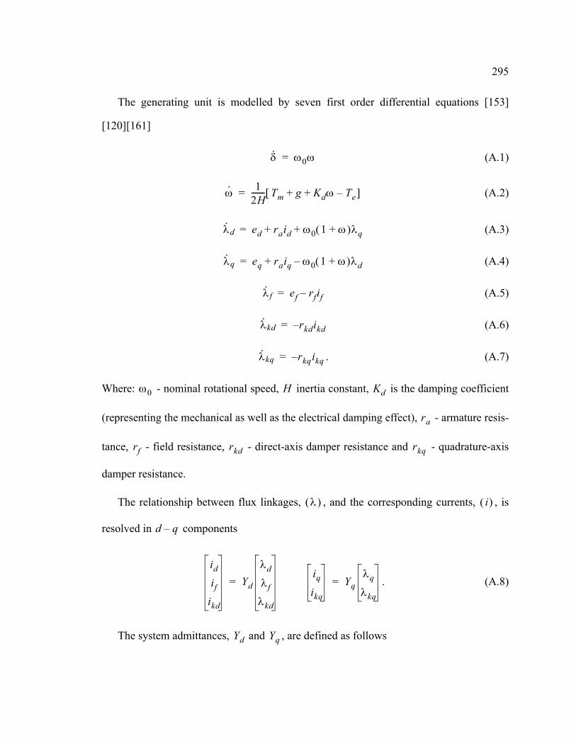
295
The generating unit is modelled by seven first order differential equations [153]
[120][161]
(A.1)
(A.2)
(A.3)
(A.4)
(A.5)
(A.6)
. (A.7)
Where: - nominal rotational speed, inertia constant, is the damping coefficient
(representing the mechanical as well as the electrical damping effect), - armature resis-
tance, - field resistance, - direct-axis damper resistance and - quadrature-axis
damper resistance.
The relationship between flux linkages, , and the corresponding currents, , is
resolved in components
. (A.8)
The system admittances, and , are defined as follows
δ· ω0ω=
ω· 12H------- Tm g Kdω Te–+ +[ ]=
λ· d ed raid ω0 1 ω+( )λq+ +=
λ· q eq raiq ω0 1 ω+( )λd–+=
λ· f ef rfif–=
λ· kd rkdikd–=
λ· kq rkqikq–=
ω0 H Kd
ra
rf rkd rkq
λ( ) i( )
d q–
id
if
ikd
Yd
λd
λf
λkd
=iq
ikq
Yqλq
λkq
=
Yd Yq

296
(A.9)
(A.10)
(A.11)
. (A.12)
Where: - field leakage reactance, - direct-axis magnetizing reactance, -
quadrature-axis magnetizing reactance, - leakage reactance, - direct-
axis synchronous reactance, - quadrature-axis synchronous reactance,
direct-axis damper leakage reactance and quadrature-axis damper leakage reactance.
The terminal current, , is calculated from its direct and quadrature components,
and , and from the power angle, ,
. (A.13)
For the single-machine infinite-bus system the terminal voltage, , is computed as
(A.14)
where and are the transmission-line resistance and reactance, and is the infinite-
bus voltage.
Zd xmd2 xd xf xkd 2xmd–+ +( ) xdxfxkd–=
Zq xmd2 xqxkq–=
Yd1Zd-----
xfxkd xmd2– xmd– xkd xmd–( ) xmd– xf xmd–( )
xmd xkd xmd–( ) x– dxkd xmd2+ xmd xd xmd–( )
xmd xf xmd–( ) xmd xd xmd–( ) x– fxd xmd2+
=
Yq1Zq----- xkq xmq–
xmq xq–=
xf xmd xmq
xa xd xmd xa+=
xq xmq xa+= xkd
xkq
it id
iq δ
it id δsin iq δcos+( ) j iq δsin id δcos+( )+=
Vt
Vt E0 rt jxt+( )it+=
rt xt E0

297
The transmission network with an equivalent impedance of , which connects
the generator to an infinite-bus of voltage , is given by the equations
(A.15)
. (A.16)
The electrical components of the machine torque, , are expressed as
. (A.17)
Parameter values for these equations are listed in Table A-1.
All resistances/reactances are expressed in PER UNIT.
A.2 IEEE ST1A AVR and Exciter
The AVR and exciter models used in the system are from the IEEE Standard P421.5/
D15, Type ST1A, shown in Figure A-2 [162].
Table A-1 Generator parameters used in simulation
re jxe–
E0
ed E0 δ( ) reid xeiq–+sin=
eq E0 δ( ) reiq xeid+ +cos=
Te
Pe edid eqiq+= Te Pe raid2 raiq
2+ +=
H 4.0= Kd 0.0027–= ra 0.007= rf 0.00089=
rkd 0.023= rkq 0.023= re 0.05= xe 0.6=
xd 1.24= xf 1.33= xkd 1.15= xmd 1.126=
xq 0.743= xkq 0.652= xmq 0.626=
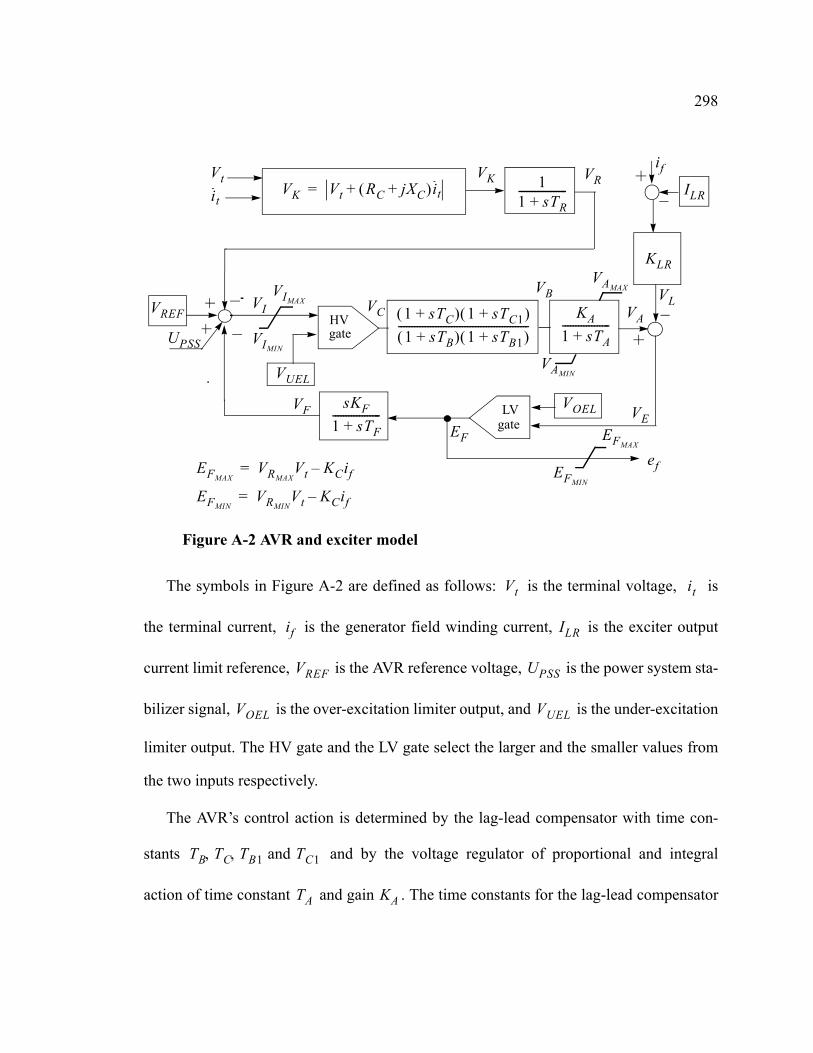
298
The symbols in Figure A-2 are defined as follows: is the terminal voltage, is
the terminal current, is the generator field winding current, is the exciter output
current limit reference, is the AVR reference voltage, is the power system sta-
bilizer signal, is the over-excitation limiter output, and is the under-excitation
limiter output. The HV gate and the LV gate select the larger and the smaller values from
the two inputs respectively.
The AVR’s control action is determined by the lag-lead compensator with time con-
stants and by the voltage regulator of proportional and integral
action of time constant and gain . The time constants for the lag-lead compensator
Figure A-2 AVR and exciter model
VK Vt RC jXC+( )it+=Vtit
VK 11 sTR+------------------
HVgate
1 sTC+( ) 1 sTC1+( )1 sTB+( ) 1 sTB1+( )
-------------------------------------------------KA
1 sTA+------------------
VAMAX
VAMIN
LVgate
VREF
UPSS
VIMAX
VIMIN
VUEL
KLR
sKF1 sTF+------------------
if
ILR
EFMAX
EFMINEFMAX
VRMAXVt KCif–=
EFMINVRMIN
Vt KCif–=
VR
VOEL
ef
VLVA
VF
VCVI
VB
VEEF
Vt it
if ILR
VREF UPSS
VOEL VUEL
TB TC TB1 and TC1, ,
TA KA

299
should be selected such that for lead, and for lag type compen-
sations. The local control loop is closed by the proportional-derivative action block with
of gain and time constant respectively.
Excitation systems with high gain and fast response times greatly aid transient stability
(synchronizing torque) but at the same time tend to reduce small signal stability (damping
torque) [163]. Consequently, for increased system stability an additional control loop is
required, which is the so called power system stabilizer.
All resistances/reactances/voltages are expressed in PER UNIT. The time constants are
shown in seconds.
A.3 IEEE PSS1A Conventional PSS
The objective of the PSS is to increase the damping of generator’s rotor angle swings,
which can occur in a broad range of frequencies in the power system [163]. The PSS pro-
vides a supplemental control signal that improves dynamic stability by increasing damp-
Table A-2 AVR and exciter parameters used in simulation
TC TB> TC1 TB1<
KF and TF
RC 0.0= XC 0.0= TR 0.040= KA 190.0=
KC 0.080= KF 0.05= TA 0.01= TB 10.0=
TC 1.0= TB1 0.0= TC1 0.0= TF 1.0=
VIMIN999–= VIMAX
999= VAMIN999–= VAMAX
999=
VRMIN6.7–= VRMAX
7.8= KLR 0.0= ILR 0.0=

300
ing of power swing oscillations. The conventional power system stabilizer is a PSS1A
type controller, from IEEE Standard P421.5/D15, shown in Figure A-3.
PSS acts through the AVR excitation system, where it introduces a component of addi-
tional damping torque proportional to speed change.
The transfer function of the PSS1A consists of a low-pass input filter with time
constant, presented in the first block. The second block is a high-pass filter, a derivative
type regulator block, with time constant and stabilizer gain. These two blocks can
be considered as a proportional-integral-differential controller. In the third block, a second
order torsional filter with and parameters is presented. Lastly, a lead-lag compen-
sator with time constants of , , and is shown in the fourth block. The lead-lag
blocks provide the appropriate phase-lead characteristics to compensate the phase lag
between the exciter input and the generator’s electrical torque. The time constants for the
lead-lag compensator should be selected such that for lead and
for lag type compensations.
Table A-3 CPSS parameters used in simulation
ω
ω0
11 sT6+----------------- 1
1 A1s A2s2+ +-----------------------------------
VSTMAX
VSTMIN
UPSS
Figure A-3 IEEE standard power system stabilizer
KsT5s
1 sT5+-----------------
1 sT1+( ) 1 sT3+( )1 sT2+( ) 1 sT4+( )
---------------------------------------------
T6
T5 Ks
A1 A2
T1 T2 T3 T4
T1 T2> T3 T4<
T1 0.10= T2 0.01= T3 0.12= T4 0.02=

301
All voltages are expressed in PER UNIT and the time constants are shown in seconds.
A.4 Governor Transfer Function
If a generator is embedded in a large interconnected system, it can with a very good
approximation be modelled as connected to an infnite-bus, as presented in Figure A-4. In
steady state the frequency is given by the one of the infnite-bus, . The governor con-
trols only the power of the generator, not the frequency.
The governor used in the system for simulation has a transfer function
. (A.18)
Parameter values for the equations are listed in Table A-4.
Table A-4 Governor parameters used in simulation
Table A-3 CPSS parameters used in simulation
T5 1.65= T6 0.005= A1 0.0= A2 0.0=
VSTMIN0.1–= VSTMAX
0.1= KS 0.11=
ω0
Governorω0
P0 Pm Pere xe+ E0
ω0
ω P,
g
Figure A-4 Governor in a power system
g s( ) agbg
1 sTg+-----------------+ ω s( )=
ag 0.00133–= bg 0.17–= Tg 0.25=

302
Appendix B - Multi-Machine Power System Model
The generating unit is modeled by five first order differential equations [130], [120].
These equations are presented below. The different transfer functions, which are also ele-
ments of the power system, are described with the single-machine infinite-bus model in
Appendix A.
B.1 Generator Model
(B.1)
(B.2)
(B.3)
(B.4)
. (B.5)
The structural diagram of the five machine power system is given in Figure 9-1, for
which the parameters are defined below [120][129].
Table B-1 Generator parameters
0.1026 0.1026 1.0260 0.1026 1.0260
0.0658 0.06580 0.658 0.0658 0.6580
0.0339 0.0339 0.3390 0.0339 0.3390
δ· ω0ω=
ω· 12H------- Tm g Kdω Te–+ +( )=
Td0'e·q' ef xd xd'–( )id– eq'–=
Td0''e·q'' eq' xd' xd''–( )id– eq''–[ ] Td0''e·q'+=
Tq0''e·d'' xq xq''–( )iq ed''–=
G1 G2 G3 G4 G5
xd
xq
xd'

303
All resistances and reactances are expressed in PER UNIT and the time constants are
shown in seconds.
All resistances and reactances are expressed in PER UNIT and the time constants are
shown in seconds.
0.0269 0.0269 0.2690 0.0269 0.2690
0.0335 0.0335 0.3350 0.0335 0.3350
5.6700 5.6700 5.6700 5.6700 5.6700
0.6140 0.6140 0.6140 0.6140 0.6140
0.7230 0.7230 0.7230 0.7230 0.7230
80.000 80.000 10.000 80.000 10.000
Table B-2 AVR and simplified ST1A exciter parameters
0.0400 0.0400 0.0400 0.0400 0.0400
190.00 190.00 190.00 190.00 190.00
0.0800 0.0800 0.0800 0.0800 0.0800
10.000 10.000 10.000 10.000 10.000
1.0000 1.0000 1.0000 1.0000 1.0000
Table B-3 Governor parameters
0.2500 0.2500 0.2500 0.2500 0.2500
-0.00015 -0.00015 -0.00133 -0.00015 -0.00133
-0.01500 -0.01500 -0.17000 -0.01500 -0.17000
Table B-1 Generator parameters
G1 G2 G3 G4 G5
xd''
xq''
Td0'
Td0''
Tq0''
H
G1 G2 G3 G4 G5
Tr
Ka
Kc
Tb
Tc
G1 G2 G3 G4 G5
Tg
ag
bg

304
All resistances and reactances are expressed in PER UNIT and the time constants are
shown in seconds.
All resistances and reactances are shown in PER UNIT.
B.2 Operating Conditions and Loads for Operating Point #1
All electrical power and voltages are expressed in PER UNIT and the power angles are
in rad.
Table B-4 Transmission line parameters
Bus #1 -- 7 0.00435 0.01067 0.015362 -- 6 0.00213 0.00468 0.004043 -- 6 0.01002 0.03122 0.032043 -- 6 0.01002 0.03122 0.032044 -- 8 0.00524 0.01184 0.017655 -- 6 0.00711 0.02331 0.027326 -- 7 0.04032 0.12785 0.158587 -- 8 0.01724 0.04153 0.06014
Table B-5 Power flow parameters
5.1076 8.5835 0.8055 8.5670 0.8501
6.8019 4.3836 0.4353 4.6686 0.2264
1.0750 1.0500 1.0250 1.0750 1.0250
0.0000 0.3167 0.2975 0.1174 0.3051
Rt Xt Bt 2⁄
G1 G2 G3 G4 G5
P
Q
V
δ

305
All resistances and reactances are shown in PER UNIT.
B.3 Operating Conditions and Loads for Operating Point #2
All electrical power and voltages are shown in PER UNIT and the rotor angles are in
rad.
All resistances and reactances are shown in PER UNIT.
Table B-6 Load parameters
7.5 - j5.0 8.5 - j5.0 7.0 - j4.5
Table B-7 Power flow parameters for 2nd operating point
3.1558 3.8835 0.4055 4.0670 0.4501
2.9260 1.4638 0.4331 2.1905 0.2574
1.0500 1.0300 1.0250 1.0500 1.0250
0.0000 0.1051 0.0943 0.0361 0.0907
Table B-8 Load parameters for 2nd operating point
3.755 - j2.5 4.25 - j2.5 3.5 - j2.25
L1 L2 L3
G1 G2 G3 G4 G5
P
Q
V
δ
L1 L2 L3

306
Appendix C - QR Factorization
The QR factorization of an m-by-n matrix is given by [47][57]
(C.1)
where is orthogonal, that is and is upper triangular.
One implementation of the QR factorization is to solve the linear equation
(C.2)
for , where and are known. After QR factorization of the
matrix and using the orthogonal property of matrix,
(C.3)
the equation can be solved by back-substitution.
The standard algorithms for QR factorization involve successive Householder reflec-
tion or Givens rotation.
An appropriate Householder matrix applied to a given matrix can zero all elements in a
column of a matrix situated below a chosen element. Thus, the first Householder matrix,
, can be selected to zero all elements in the first column of matrix , below the first
element. Similarly, matrix zeros all elements in the second column below the second
element, and so on, up to . Consequently,
. (C.4)
A
A Q R⋅=
Q ℜm m×∈ Q QT⋅ I= R ℜm n×∈
Φ x⋅ b=
x ℜn 1×∈ Φ ℜn n×∈ b ℜn 1×∈
Φ Q R⋅→ Q
R x⋅ QT b⋅=
H1 A
H2
Hn 1–
R Hn 1– … H2 H⋅ ⋅ 1 A⋅⋅=

307
Since the Householder matrices are orthogonal
. (C.5)
The algorithm for the Givens rotation is very similar, except that it only introduces one
zero at a time, so it requires rotations
. (C.6)
The nomenclature QR is originating from the fact that for an upper triangular matrix
the right of the matrix is non zero. In a same way the QL algorithm will produce a
lower triangular matrix where the left of the matrix is non zero.
Q Hn 1– … H2 H⋅ ⋅ 1⋅( ) 1– Hn 1– … H2 H⋅ ⋅ 1⋅= =
t n 1–( )2 2⁄=
Q G1 G2 … Gt⋅ ⋅ ⋅=
Q
L

308
Appendix D - The Lyapunov Equation
Let the plant dynamic be defined with the state and output equations [54]
(D.1)
(D.2)
where , , and the associated matrices have the appropriate
dimensions. If the plant is uncontrolled, , the general quadratic per-
formance index of the form
(D.3)
will be reduced to
. (D.4)
In order to determine the behavior of the plant in uncontrolled environment, the cost
should be evaluated in the interval . This evaluation can be done
using backward recursion. The value of the cost in the final time interval is defined as
. (D.5)
Now, let and the cost can be expressed as
xn 1+ An xn Bn un⋅+⋅=
yn Cn xn⋅=
xn ℜm∈ un ℜr∈ yn ℜq∈
un 0 n 0 N,( )∈∀,=
J xNT PN xN xn
T unT
Qn Sn
SnT Rn
xn
un
⋅ ⋅
n 1=
N 1–
∑+⋅ ⋅=
J xNT PN xN xn
T Qn xn⋅ ⋅
n 1=
N 1–
∑+⋅ ⋅=
Jn 0 … n … N, , , ,
JN xNT PN xN⋅ ⋅=
n N 1–=

309
. (D.6)
Using the plant dynamics (D.1) for the uncontrolled plant , the cost
can be written as
. (D.7)
The content in the brackets can be defined as a backward recursion for a new variable ,
. (D.8)
With the backward recursion variable , the cost (D.6) is
(D.9)
which has the same form as the cost for the final state (D.5). According to the recursion
(D.9), all costs can be calculated. The backward recursion for this intermediate variable
is
. (D.10)
This is the Lyapunov recursive equation, which calculates the performance index kernel
sequence . The Lyapunov recursive equation can be solved off-line, using only the sys-
tem state transformation matrix . The performance index kernel sequence, , can be
used to calculate the cost for the uncontrolled plant for any initial state .
If the weighting matrix (positive definite), then will be positive definite as
well ( ).
JN 1– xNT PN xN xN 1–
T QN 1– xN 1–⋅ ⋅+⋅ ⋅=
xN AN 1– xN 1–⋅=
JN 1– xN 1–T AN 1–
T PN AN 1– QN 1–+⋅ ⋅( ) xN 1–⋅ ⋅=
Pn
PN 1– AN 1–T PN AN 1– QN 1–+⋅ ⋅=
Pn
JN 1– xN 1–T PN 1– xN 1–⋅ ⋅=
Pn
Pn AnT Pn 1+ An Qn+⋅ ⋅= n N 1– … n … 0, ,,, =
Pn
An Pn
xn
Qn 0> Pn
Pn 0>

310
Lyapunov theory. If the plant is internally stable and the selected , then the
Lyapunov equation has a positive definite solution, .
In the time invariant case the recursion can be written as
(D.11)
as , (D.11) converges to steady state value
(D.12)
and as , it become the algebraic Lyapunov equation
. (D.13)
Second norm of the observations theorem. [7] Consider the signal generated by the
system (D.1) and (D.2) with in which every entry of and is
bounded and for all . Then, the second norm of the observations , on
the interval , can be calculated as
(D.14)
where is obtained by the backward Lyapunov recursion
. (D.15)
Q 0>
P 0>
An A=
Pn AT( )N n– PN AN n–⋅ ⋅= AT( )
N k– 1– Q AN k– 1–⋅ ⋅
k n=
N 1–
∑+
N n–( ) ∞→
P∞ AT( )k Q Ak⋅ ⋅
k 0=
∞
∑=
P Pn Pn 1+= =
P AT P A Q+⋅ ⋅=
un 0 n 0 N,( )∈∀,= An Cn
yn l2 0 N,[ ]∈ x0 yn
0 N,[ ]
y 2 0 N,[ ],2 x0
T P0 x0⋅ ⋅=
P0 n N N 1 … 0, ,–,=
Pn AnT Pn 1+ An Cn
T Cn⋅+⋅ ⋅= PN 1+ 0=

311
l2 space definition. The function belongs to the space if it has observable outputs
where each sequence of observations is in , defined by
. (D.16)
The second norm is calculated by
. (D.17)
For the function to have the properties defined above, the shorthand is
often used.
fn l2 m
ℜm
l2 0 N,[ ] f : fn 0 for n 0 N,[ ] fn 2 0 N,[ ], ∞<,∉= =
fn 2 0 N,[ ], fnT f⋅ n
n 0=
N
∑
1 2/
=
fn fn l2 0 N,[ ]∈

312
Appendix E - Discrete-Time System Theory
E.1 Stability of Discrete-Time Systems
The discrete-time system [7]
(E.1)
(E.2)
is stable if is in l2 space, whenever the input sequence is
in l2 space.
Stability theorem. The following conditions are equivalent
1. The closed-loop system, without external effects,
(E.3)
is internally stable if, from any finite initial state, it will converge to zero final state as
.
2. If , all eigenvalues of have magnitudes less than 1.
3. For any positive symmetric matrix there exists a unique positive definite symmetric
matrix , which is the solution of the following algebraic Lyapunov equation
. (E.4)
xn 1+ f n xn un, ,( )=
yn h n xn,( )=
yn n 0 N,[ ]∈;
un n 0 N,[ ]∈;
xn 1+ A xn⋅=
n ∞→
ρ A( ) 1< A
Q
P
P AT P A Q+⋅ ⋅=

313
E.2 Stabilizability of Discrete-Time Systems
A system is stabilizable if, and only if, every unstable mode is controllable.
Stabilizability theorem. The following statements are equivalent [80]
1. (A, B) is stabilizable.
2. The matrix has full row rank for all .
3. There exists a matrix F, such that is stable.
E.3 Controllability of Discrete-Time Systems
The discrete-time system
(E.5)
is controllable/reachable if, for any initial state , there exists a finite control sequence
that will transfer the state to , where is any selectable finite
state.
Controllability theorem. The following statements are equivalent [80]
1. The linear time invariant system of mth order
A λ I⋅– B λ 1≥
A B F⋅+
xn 1+ f n xn un, ,( )=
x0
un n 0 N,[ ]∈; x0 xN xN
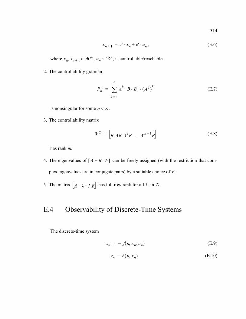
314
, (E.6)
where , , is controllable/reachable.
2. The controllability gramian
(E.7)
is nonsingular for some .
3. The controllability matrix
(E.8)
has rank m.
4. The eigenvalues of can be freely assigned (with the restriction that com-
plex eigenvalues are in conjugate pairs) by a suitable choice of .
5. The matrix has full row rank for all in .
E.4 Observability of Discrete-Time Systems
The discrete-time system
(E.9)
(E.10)
xn 1+ A xn B un⋅+⋅=
xn xn 1+, ℜm∈ un ℜr∈
PnC Ak B BT AT( )k⋅ ⋅ ⋅
k 0=
n
∑=
n ∞<
WCB AB A2B … Am 1– B=
A B F⋅+[ ]
F
A λ I⋅– B λ ℑ
xn 1+ f n xn un, ,( )=
yn h n xn,( )=

315
is observable if for any initial state there exist a finite number of observations of the
output sequence and the knowledge of the input sequence
is such that the initial state can be determined.
Observability theorem. The following statements are equivalent [80]
1. The linear time invariant system of mth order
(E.11)
(E.12)
where , , and is observable.
2. The observability gramian
(E.13)
is nonsingular for some .
3. The observability matrix
(E.14)
has rank m.
4. The eigenvalues of can be freely assigned (with the restriction that com-
plex eigenvalues are in conjugate pairs) by a suitable choice of .
x0
yn n 0 N,[ ]∈;
un n 0 N,[ ]∈; x0
xn 1+ A xn B un⋅+⋅=
yn C xn⋅=
xn xn 1+, ℜm∈ un ℜr∈ yn ℜq∈
PnO AT( )
k CT C A( )k⋅ ⋅ ⋅
k 0=
n
∑=
n ∞<
WO
CCA…
CAm 1–
=
A L C⋅+[ ]
L

316
5. The matrix has full column rank for all in
E.5 Detectability of Discrete-Time Systems
A system is detectable if, and only if, every unstable mode is observable.
Detectability theorem. The following statements are equivalent [80]
1. (C,A) is detectable.
2. The matrix has full column rank for all .
3. There exists a matrix L, such that is stable.
A λ I⋅–C
λ ℑ
A λ I⋅–C
λ 1≥
A L C⋅+

317
Appendix F - Test for Positive Definiteness
The positive definite test is an essential part of the algorithm. A matrix
is positive definite if for all nonzero . The algorithm
presented here is a compromised solution between the required computational power and
memory. The positive definite test is based on the property of a positive definite matrix
which, when factorized as , the diagonal matrix
has positive diagonal elements, where is a unit lower triangu-
lar and is a unit upper triangular [57].
H∞
A ℜm m×∈ xT A x 0>⋅ ⋅ x ℜm∈
A 0> A L D MT⋅ ⋅=
D diag d1 d2 … dk,,,( )= L
M∗
x is an [m x m] Matrix
ptest(Matrix x) % return ptest = TRUE if 'x' is a Positive definite matrix (ptest=FALSE otherwise) flim = 1e-9; m=x->rows; for(j=1; j<=m; j++) for(i=1; i<=j; i++) sum1=0; for(k=1; k<i; k++) sum1 += x[i][k] * x[k][j]; x[i][j] = x[i][j] - sum1; if(x[j][j] < flim) return FALSE, j=m; else for(i=j+1; i<=m; i++) sum2 = 0; for(k=1; k<j; k++) sum2 += x[i][k] * x[k][j]; x[i][j] = (x[i][j] - sum2)/x[j][j]; return TRUE;

318
Appendix G - ARMA Model Stability Test
The Schur-Cohn stability test is the backward Levinson recursion, when used to deter-
mine filter stability. All of the reflection coefficients of an AR process must be less than
one in magnitude for the filter to be stable. This can easily be tested by the algorithm pre-
sented below [47].
θ <=> [DC, a1, a2, a3,...am_a, b1,...] if m_s = 1 where: φ = [1,-yn-1,...-yn-m_a,un-1,...un-m_b,vn-1,...vn-m_c]
θ <=> [ a1, a2, a3,...am_a, b1,...] if m_s = 0 where: φ = [-yn-1,...-yn-m_a,un-1,...un-m_b,vn-1,...vn-m_c]
Backward Levinson (step-down) recursion:
stable (Vector θ) % return Stable=TRUE if 'θ' is a stable ARMA model (Stable=FALSE otherwise) f = θ[m_s+1]; for(i=1;i < m_a;i++) Vb[i] = Va[i] = (θ[m_s+i+1] / f) end f = Va[m_a-1]; // Γ(1) if( abs(f) > 1 ) Stable=FALSE, return; for(j=m_a-1;j>=2;j--) for(i=1;i<=j;i++) Va[i] = Va[i] - (f * Vb[j-i]); f = 1 - (f * f ); for(i=1;i<=j-1;i++) Va[i] = Vb[i] = Va[i]/f ; f = Va[j-1]; // Γ(i) if( abs(f) > 1) return FALSE ; return TRUE ; // system model is stable all |Γ(i)| < 1

319
Index
AA2D2A 215ACC benchmark problem 130adaptation constant 62adaptive PSS 168additive disturbance 26additive perturbations 134admissible controller 120analog interface card 215array algorithm 71attenuation factor 85automatic voltage regulator 197AVR 197, 227, 229AVR parameters 230
Bbackward recursion 98Bellman 96binomial search 119bisectional search 119
Ccentral controller 87certainty equivalence principle 99, 100,
103closed-loop system 113
closed-loop transfer function 84condition
controllability 115injective 115, 117observability 115surjective 116
controlclassical 1lead-lag 1linear quadratic 2measurement feedback 111model predictive 7model-based 28parameter-adaptive 7relevant frequency 28robust 3, 19, 78worst-case 3
control action 82control signal 82control system 113controlled output 82controller
admissible 86all stabilizing 86central 87, 114embedded 210linearization process 160non-linear 160step-by-step implementation 126suboptimal H_inf 86trade-off 88
control-oriented identification 6Conventional PSS 167coupling condition 121, 124CPSS 222, 230CPSS parameters 184
DDARE 128DC motor 211decision period 171

320
detectable 115digital interface card 220DSK 214DSP 21, 30, 214dynamic feedback 113dynamic programming 92, 96dynamic stability 13
Eelectric power production 9embedded controller 214embedded software 222entropy integral 87estimation 31estimation strategies 53estimation techniques 55EWMA 178excitation system 226Exciter-AVR 222expert system 19, 170exponentially weighted moving average
178
Ffinite time stability 34forgetting factor 56forward dynamic programming 102four blocks technique 83FQR 170Frobenius norm 176full-information control 98
Ggame
control set 90discrete-time 89
information state 101, 102information structure 91lower value 94minimax 111objective function 95observation equation 91observation set 90optimal solution 94performance index 101players’ set 90soft-constrained linear-quadratic 114space 90stages 90state equation 90state set 90two-player 93upper value 94value function 95, 97, 101zero-sum 89, 93, 111
game theory 3, 89generalized predictive control 152generator model 212gradient-based algorithm 61
HHamilton-Jacobi-Isaacs equation 97
Iidentification
control-oriented 19multi-model 21multiple techniques 19robust 20strategy 53
identified parameters 180Implementation Example 130induced norm 85industrial systems 152infimum 85infimum search 117

321
infimum search algorithm 118innovation variance 123intelligent supervisor 55inter-area mode oscillation 197, 200inter-area oscillations 11interface card 214inter-machine mode oscillation 197internally stabilized 113interrupt driven structure 224intervalwise strategy 153IQR 170IQR-RLS 72IQR-RLS algorithm 73Isaacs equation 96, 103
KKalman 2Kalman Filter 67Kalman Filter algorithm 70Kalman Filter recursion 69KF 170KFA 171
Llaboratory power system 209learning rate 62least mean squares 54least squares 54, 56, 60LFT 81, 83Linear Fractional Transformation 81linearization process 161LMS 60, 170LMS algorithm 61local mode oscillation 197, 200, 201LQGR 88, 98Lyapunov 18
Lyapunov equation 129Lyapunov function 35Lyapunov stability 157Lyapunov stability theorem 36
Mmass spring system 130matlab 131matrices of appropriate dimensions 112maximizing player 93maximum residual amplitude 174maximum-likelihood estimate 58mean square error 175measurement-feedback control 98, 100measurement-noise 68memory length 57micro-synchronous generator 212minimax strategy 96minimizing player 94minimum principle 92model
black-box 25, 26invalidated 33mathematical 25, 80nonparametric uncertainty 33order 183parametric uncertainty 33relevant for the control 28, 80selection 55uncertainty set 33white-box 25
model predictive control 152model structure 31, 32model uncertainty 81moving average 172moving-horizon control 152MPC 152, 222MPC objective function 162multi model 6

322
multi-machine power system 196multiplicative perturbations 134
NNash equilibria 92Nash inequality 94NoC 183noncooperative equilibrium 95norm
l_infinity 55l1 54l2 55
norm criterion 5normalized LMS algorithm 62numerical difficulties near the infimum 120
Oon-line optimal control problem 152opponent 93orthogonal transformation 72overdetermined system 5, 53
Pparameter set 33parameter variances 176parametric error 35performance measure 82perturbations 134physical model 209, 210plant modelling 4player
cost functional 92information space 91permissible strategies 91
pointwise strategy 153positively invariant 157
positivity condition 122positivity test 118, 124, 125power system 10
dynamic stability 13inter-area oscillations 14local mode oscillations 14multi-machine 197multi-mode oscillations 196stabilizer 15, 16, 17, 18, 167steady-state stability 12
power system operation 166power system oscillations 11power system simulation package 166practical stability 34, 157prediction error 35principle of optimality 96PRO 170PRO model 179process-noise 68, 82
QQR-LMS 72QR-LMS algorithm 74QR-RLS 72QR-RLS algorithm 73quadratic moving average 173
Rrandom-walk Kalman Filter 71rank 115reactive power 227real-time control 222real-time digital control system 209receding-horizon control 152Recursive Least Squares 56reminiscence function 178Riccati 2, 18

323
Riccati equation 111, 128, 163Riccati recursion 121, 129Riccati recursion initialization 128RLS 56, 170RLS algorithm 57robust state estimator 125robustness measure 114rotation operation 72rotational speed deviation 221
Ssaddle-point solution 95, 103selection process 179separation principle 98set of models 31simulation studies 165small gain theorem 79, 83, 84stability
contractive 37experimental 39proof by assumption 38quasicontractive 37
stability of the MPC 157standard control system 111state-feedback controller 125state-space model 67, 112steady-state stability 12system identification 5, 25
control oriented 27diversification 30multi model based 29objective 35objective function 35problem of correlation 27
TTCR 213terminal constraint 156
terminal constraint set 156time constant regulator 212transient instability 10transmission line 213true system 30true system parameters 31turbine model 211
Vvalue 95von Neumann 89
WWCE 170WCE algorithm 65weighting matrices 112, 114, 183Wold decomposition theorem 31worst-case design 79, 88worst-case estimation 54, 63worst-case state estimator 103
ZZames 3, 78