Embed Size (px)
Citation preview

University of Birmingham
Assessing blending of non-newtonian fluids instatic mixers by planar laser- induced fluorescenceand electrical resistance tomographyForte, Giuseppe; Albano, Andrea; Simmons, Mark; Stitt, E. Hugh; Brunazzi, Elisabetta ;Alberini, FedericoDOI:10.1002/ceat.201800728
License:Other (please specify with Rights Statement)
Document VersionPeer reviewed version
Citation for published version (Harvard):Forte, G, Albano, A, Simmons, M, Stitt, EH, Brunazzi, E & Alberini, F 2019, 'Assessing blending of non-newtonian fluids in static mixers by planar laser- induced fluorescence and electrical resistance tomography',Chemical Engineering & Technology, vol. 42, no. 8, pp. 1602-1610. https://doi.org/10.1002/ceat.201800728
Link to publication on Research at Birmingham portal
Publisher Rights Statement:Checked for eligibility: 28/06/2019
This is the peer reviewed version of the following article: Forte, G. , Albano, A. , Simmons, M. J., Stitt, H. E., Brunazzi, E. and Alberini, F.(2019), Assessing Blending of NonNewtonian Fluids in Static Mixers by Planar LaserInduced Fluorescence and Electrical ResistanceTomography. Chem. Eng. Technol.. doi:10.1002/ceat.201800728., which has been published in final form at:https://doi.org/10.1002/ceat.201800728. This article may be used for non-commercial purposes in accordance with Wiley Terms andConditions for Use of Self-Archived Versions.
General rightsUnless a licence is specified above, all rights (including copyright and moral rights) in this document are retained by the authors and/or thecopyright holders. The express permission of the copyright holder must be obtained for any use of this material other than for purposespermitted by law.
•Users may freely distribute the URL that is used to identify this publication.•Users may download and/or print one copy of the publication from the University of Birmingham research portal for the purpose of privatestudy or non-commercial research.•User may use extracts from the document in line with the concept of ‘fair dealing’ under the Copyright, Designs and Patents Act 1988 (?)•Users may not further distribute the material nor use it for the purposes of commercial gain.
Where a licence is displayed above, please note the terms and conditions of the licence govern your use of this document.
When citing, please reference the published version.
Take down policyWhile the University of Birmingham exercises care and attention in making items available there are rare occasions when an item has beenuploaded in error or has been deemed to be commercially or otherwise sensitive.
If you believe that this is the case for this document, please contact [email protected] providing details and we will remove access tothe work immediately and investigate.
Download date: 29. Nov. 2021

Assessing blending of non-Newtonian fluids in static
mixers by Planar Laser Induced Fluorescence and
Electrical Resistance Tomography
G. Forte1,2, A. Albano1,3, M.J.H. Simmons1, E.H. Stitt2, E. Brunazzi3, F. Alberini1*
1 School of Chemical Engineering, University of Birmingham, Edgbaston, B152TT, Birmingham, UK.
2 Johnson Matthey Technology Centre, TS23 4LB, Billingham, UK.
3 Department of Civil and Industrial Engineering, University of Pisa, I-56126, Pisa, Italy.
*Corresponding author: [email protected]
Abstract: PLIF and ERT have been used simultaneously to monitor the mixing
performance of 6 elements KM static mixer for the blending of non-Newtonian
fluids of dissimilar rheologies in the laminar regime. The areal distribution method
was used to obtain quantitative information from the ERT tomograms and the PLIF
images. Comparison of the ERT and PLIF results demonstrates the ability of ERT
to detect mixing performance in cases of poor mixing within the resolution of the
measurement, though the accuracy decreases as the condition of perfect mixing is
approached. ERT thus has the potential to detect poor mixing within the confines of
its resolution limit and the required conductivity contrast, providing potential rapid
at-line measurement for industrial practitioners.
Keywords: Mixing, Non-Newtonian, ERT, PLIF, Static mixer
Introduction
Non-Newtonian fluids are widespread in industrial processes, for example in the manufacture
of home and personal care products, foods and chemicals. Amongst other unit operations,
mixing and blending of complex fluids remains a significant process challenge (Connelly and
Kokini, 2007; Prakash et al., 1999). Although this operation is often executed in stirred tanks,
the industry-driven benefits of moving towards continuous processing suggests a solution
involving static mixers. Such devices consist of metallic inserts installed within pipes and
applications also include chemical reactions and heat transfer (Paul et al., 2004). Static
mixers promote chaotic advection within the flow (Alvarez et al., 1998; Hobbs and Muzzio,
1997; Saatdjian et al., 2012; Wunsch and Bohme, 2000) which contributes significantly to

mixing in the laminar regime, considering the difficulty to reach turbulence for non-
Newtonian fluids without excessive amount of power input (Aref, 1984; Le Guer and El
Omari, 2012). The flow deformation given by the mixing elements causes the formation of
striations and as a result the interfacial surface area is increased, improving the diffusion rate
at low Reynolds number (Hobbs and Muzzio, 1997).
Many literature studies have been made of the flow in motionless mixers, employing optical
methods as Planar Laser Induced Fluorescence (PLIF) (Alberini et al., 2014a; Arratia and
Muzzio, 2004; Ramsay et al., 2016, Faes and Glasmacher, 2008), Particle Image Velocimetry
(PIV) (Pianko-Oprych et al., 2009; Stobiac et al., 2014; Szalai et al., 2004) or decolorization
measurement techniques (Chandra and Kale, 1992; Li et al., 1997). The application of the
reported methods requires both the fluid and the pipelines to be transparent, therefore they are
not implementable for opaque fluids. An alternative non-invasive technique applicable for
opaque media, Positron Emission Particle Tracking (PEPT), employs the Lagrangian tracking
of the 3-D position of a positron emitting tracer particle within the fluid to reconstruct its
velocity flow field over time (Edwards et al., 2009) and has been applied both for studies on
stirred vessels (Barigou, 2004) and static mixers (Rafiee et al., 2011) for Newtonian and non-
Newtonian fluids. Alternatively, to measure the concentration distribution, PET (Positron
Emission Tracking) can be used where the position and concentration of a radiotracer is
monitored in time (Bell, 2015).
Amongst the many geometries commercially available, Kenics® KM static mixers
(Chemineer, USA) are commonly used for academic investigations due to their simple
geometry (Avalosse and Crochet, 1997; Rahmani et al., 2005; Rauline et al., 2000; Regner et
al., 2006; Wageningen et al., 2004). Some works describe numerical simulations of the
mixing performance of non-Newtonian fluids in SMX® (Sulzer) geometry (Peryt-Stawiarska,
2014; Wunsch and Bohme, 2000). However, apart from these few studies, the research focus
by means of numerical simulation has remained on blending of non-Newtonian fluids in
stirred vessels, with the use of different approaches such as Computational Fluid Dynamics
including Direct Numerical Simulation (DNS) of the Navier-Stokes equations (Zalc et al.,
2002).
The industry driver for continuous processing, is concomitant with the requirement for
appropriate Process Analytical Technology (PAT) to enable real-time product quality
assurance and control (Uendey et al., 2010). In the context of this paper, the development of
in situ measurement techniques represents a critical step towards this. Furthermore,
traditional approaches to the development of new formulated liquid products are laboratory
scale oriented with little or even no attention given to formulation “manufacturability”. This

frequently results in not only longer and costlier time to scale up but also increased
production costs.
A number of measurement techniques have been applied for monitoring fluid characteristics
in inline flows. Nuclear Magnetic Resonance (NMR) (Blythe et al., 2017) and ultrasonics
(Pfund et al., 2006) were applied to estimate rheological parameters of non-Newtonian fluids
(aqueous solutions of Carbopol 940 and Carbopol EZ-1 respectively) in pipelines in real time,
while micro-PIV was applied in determining the velocity profile of both non-Newtonian and
Newtonian fluids in laminar regime (Fu et al., 2016).
Electrical Resistance Tomography (ERT), amongst other techniques, offers the advantages of
being non-invasive, low-cost, robust and with a high temporal resolution; it is thus an
interesting candidate technique in this context for measurement of the phase distribution
within liquid continuous mixtures (Pakzad et al., 2008; Wang et al., 1999). Jegatheeswaran et
al. (2018) uses ERT to validate CFD simulations of the blending of two non-Newtonian fluids
flowing in SMX static mixers. The same technique has been used for measuring velocity
profiles of shampoo in pipelines (Ren et al., 2017) and to evaluate mixing of industrial pulp in
static mixers (Yenjaichon et al., 2011). Recent applications of ERT in pipe flows have
demonstrated potential for in-line rheometry measurements (ERR) (Machin et al., 2018).
In this paper, we describe the use of ERT to determine the distribution of two non-Newtonian
fluids of dissimilar rheology at the outlet of a Kenics KM static mixer in the laminar regime.
The measurements are made at the mixer outlet using a two plane circular array. The ERT
measurements are compared with measurements of the mixing distribution collected
simultaneously using Planar Laser Induced Fluorescence (PLIF) a proven method in this
application. Both ERT and PLIF data are compared quantitatively using the areal distribution
method developed by Alberini et al. (Alberini et al., 2014b).
Material and Methods
Aqueous solutions of carboxymethylcellulose (CMC) and Carbopol 940 were chosen as the
model of non-Newtonian fluids, whose flow rheology can be well represented by the power
law and Herschel Bulkley constitutive laws respectively. Flow curves were obtained and
fitted to the constitutive models using a rheometer (TA Instruments, model: Discovery HR-1)
equipped with a 40 mm 4° cone and plate geometry and associated software: the data are
shown in Tab. 1.
Fig. 1 shows the rig schematic. The flow to the mixer was delivered by an Albany rotary gear
pump controlled using an inverter control WEG (model CF208). The secondary flow, doped
with fluorescent dye (Rhodamine 6G) with a concentration of 0.04 mg l-1 (concentration was

selected within the linear range of greyscale versus dye concentration), was introduced using
a Cole-Parmer Micropump (GB-P35). The injection pipe (with internal diameter of 7.6 mm)
was placed in the centre of the main pipe as close as possible to the static mixer. The
experiments, reported in Tab. 2, were conducted at isokinetic condition between main flow
(MF) and secondary flow (SF): the two fluids were fed at the same superficial velocity, uS,
hence the ratio between the two volumetric flows was equal to the ratio between main and
injection pipe sections (MF/SF≈10). The Kenics KM mixer unit had an internal diameter of
25.4 mm (1”) and length of 220 mm (L/D= 9) and was equipped with 6 mixing elements.
Tab. 1: Fluid rheology parameters.
Fluids Mass composition Behaviour τ0 [Pa] K [Pa/sn] n [−]
PL 0.5% w/w sodium Carboxymethyl Cellulose
99.5% w/w water Power Law 0.49 0.59
HB1 0.1% w/w Carbopol 99.9% w/w water
Herschel-Bulkley 0.85 0.40 0.58
HB2 0.2% Carbopol 99.8% w/w water
Herschel-Bulkley 10.27 7.45 0.38
The mixing unit is followed by a planar circular ERT sensor consisting of 16 electrodes. The
ERT sensor was connected to a V5R data acquisition system (Industrial Tomography Systems
plc, UK) that controlled electrical excitation and measurement collection. The ERT plane
was located 100 mm after the mixer outlet, while the PLIF measurement plane was located at
200 mm from the end of the mixing zone; the two measurement planes were separated by 100
mm.
The terminal part of the pipeline was equipped with a Tee piece designed with a glass window
inserted at its end corner through which PLIF measurements are made (the capture procedure
may be found in Alberini et al. (2014b).

Fig. 1: Schematic of the experimental rig (adapted from Alberini et al. (2014b)) .
A range of superficial velocities, uS, was investigated to identify the accuracy of ERT
measurements once the contrast, in term of conductivity, between the injected (secondary)
and the main flow is decreased. The list of experiment and flow conditions is shown in Tab. 2.
Within the range of investigated velocities, the values of Re, calculated using same
methodology used by Alberini et al. (2014a), were in the range 25-220 which suggest the
system was always running in laminar regime (Re << 2000). The inlet absolute difference in
conductivity (no addition of salt), ∆c= |cMF − c
SF |, between the main flow (MF) and the
secondary flow (SF) is also reported in Tab. 2, since it is the principal parameter which affects
the ERT measurement.
Tab. 2: List of experiment and flow conditions.
Experiment MF SF ∆c
(mS cm-1)
uS (m s-1)
I HB1 PL 0.871 0.20 | 0.27 | 0.34 | 0.40 | 0.47
II HB2 PL 0.686 0.20 | 0.27 | 0.34 | 0.40 | 0.47
III HB1 HB2 0.112 0.20 | 0.27 | 0.34 | 0.40 | 0.47
Calibration and Post Processing
The ERT system was calibrated prior to the experiment, which consists of taking a baseline
reference frame. For each experiment, the reference was captured with continuous phase at
each flow rate after reaching a steady flow condition. The V5R automatically sets the
conductivity of the reference measurements equal to unity, thus the changes occurring after
the injection are relative and not absolute. The V5R system employs a sample frequency of
125 Hz: for each run a sample of 1000 frames was analysed. The data obtained were
processed using the Toolsuite V7.4 software (ITS Ltd.) in order to reconstruct conductivity
tomograms. Since ERT is a soft-field technique, the reconstruction problem is not trivial and
several algorithms have been developed to generate conductivity tomograms from the raw
data, both iterative and non-iterative (Yang and Peng, 2003). Commonly, in the latter
category, the Linear Back Projection (LBP) method or one of its variants is used (Noser,
Tikhonov reconstruction algorithms) (Wei et al., 2015). In this work the modified standard
back projection (MSBP) algorithm implemented in the V5r software was used. Furthermore,

for simplicity, only the tomograms obtained in the second plane are used for comparison with
PLIF.
The areal method (Alberini et al., 2014b) requires an initial calibration step to be applied in
evaluating mixing performance. In this step, the values of and are identified for all
the mixtures, as the value of conductivity and greyscale respectively reached at the condition
of perfect mixing. Since ERT and PLIF have a different basis of measurement, two
dimensionless parameters, and , are introduced to allow comparison of the measured
mixing performance between them. A dimensionless relative conductivity can be defined
for each pixel as:
/ (1)
Where is the relative conductivity of the i-th pixel of the tomogram, is the relative
conductivity achieved at perfect mixing and is the reference conductivity of the pixel
before the injection, equal to 1 in condition of single phase. Analogously, a dimensionless
greyscale is defined:
/ (2)
Where is the grey scale value of the i-th pixel of the PLIF image, is the grey scale
value reached at perfect mixing found in the calibration step, and is the reference status of
the pixel before the injection. The grey scale values of “pure” (100% secondary flow fluids)
fluids have been measured resulting in 92 and 250 for PL and HB2 respectively at fixed
Rhodamine 6G concentration of 0.04 mg l-1.
In the calibration procedure, both greyscale values and conductivity of the mixtures are
measured at different volume fraction xSF values of the secondary flow in the main flow in the
interval of interest. Pre-fully-mixed solutions with volume fractions xSF of the secondary flow
between 0.02 and 0.10 (which is the maximum volume ratio obtained in the system), were fed
to the system and ERT and PLIF measurements were captured simultaneously. It was noticed
that the effect of flow velocity on both measurements (in case of fully premixed solutions) is
negligible. The results of the calibration for the relative conductivity and the greyscale
values, to obtain and , are reported for the three mixtures in Tab.3.

Tab. 3: Relative conductivity, Cinf, and greyscale, Ginf, values of the mixture of primary and secondary
fluids at different volume fraction of secondary fluids for each pair of fluids employed in the different
experiments: I(PL in HB1), II (PL in HB2), and III (HB2 in HB1)
Experiment I Experiment II Experiment III
xpl in HB1 Cinf xpl in HB2 Cinf xhb2 in HB1 Cinf
0.02 1.08 0.02 1.06 0.02 0.99
0.04 1.12 0.04 1.10 0.04 0.98
0.06 1.18 0.06 1.13 0.06 0.97
0.08 1.27 0.08 1.15 0.08 0.96
0.1 1.35 0.1 1.18 0.1 0.95
xpl in HB1 Ginf xpl in HB2 Ginf xhb2 in HB1 Ginf
0.02 120 0.02 247 0.02 247
0.04 119 0.04 243 0.04 245
0.06 119 0.06 240 0.06 242
0.08 118 0.08 237 0.08 239
0.1 118 0.1 234 0.1 237
Results
The two imaging techniques employed have a substantial difference in spatial resolution:
whilst PLIF is able to capture high resolution pictures (2048×2048 pixels), ERT yields
relatively low resolution tomograms (20×20 pixels) which cannot be expected to resolve
striations of fluid that are often present when mixing complex rheology fluids. The first step
of the conducted study consists in evaluating the effect of downscaling PLIF images from full
resolution to a reduced resolution, of the same order of magnitude of ERT tomograms (32×32
pixels). The applied downsizing algorithm allows a reduction scaled by powers of 2, therefore
from the starting resolution of 211×211 pixels, a resolution of 25×25 pixels is obtained,
reasonably close to the ERT tomogram resolution, to draw significant comparison.
Subsequently, full size PLIF images and ERT tomograms are directly compared on evaluating
achieved mixing performance.
PLIF image analysis by varying resolution
Downscaled PLIF (32×32) images are obtained using the Lanczos kernel downsizing method
(Komzsik, 2003) and compared to original full size PLIF images. The objective is to gather

whether
of infor
in Fig. 2
Full size
image
Downscale
image
Fig. 2. Fu
In Fig.
the mai
increase
becomin
observe
improve
Althoug
images,
of view
method,
pictures
r at low reso
rmation in d
2, as a funct
uS = 0.2
(a
ed
(f
ull size (a-e)
2, the thick
in flow. Th
ed with the
ng less inte
ed in Fig. 2f
ements in te
gh it is poss
this transfo
w of mixing
, it is poss
s and the do
olution it is
downscaling
tion of flow
20 m s-1
(a)
(f)
and downsca
k white stria
he images s
e dark reg
ense in Fig
f progressiv
erms of mix
sible to appr
formation do
g performan
sible to com
ownscaled im
possible to
g PLIF ima
w rate.
uS = 0.27 m s
(b)
(g)
aled (f-l) PLI
ations repre
show a sub
gions observ
. 2d and 2e
vely disappe
xing perform
reciate by e
oes not tran
nce detectio
mpare the m
mages in Fi
o characteriz
ages. An ex
s-1 uS =
IF images at
esent the un
bstantial inc
rvable in F
e. In an an
ear as uS inmance.
eye how the
nslate in sig
on capabilit
mixing perf
g. 3.
ze mixing p
xample of th
0.34 m s-1
(c)
(h)
t different sup
nmixed seco
crease in ho
Fig. 2a red
alogous wa
ncreases in F
e downscali
gnificant los
y. In fact,
formance d
performance
he resulting
uS = 0.40 m
(d)
(i)
perficial velo
ondary flow
omogeneity
ducing and
ay, the whit
Fig. 2l wher
ng decrease
ss of inform
by applying
detected by
e and assess
g images ar
m s-1 uS =
locities for ex
w and the da
as the flow
the white
te and blac
ere the imag
es the quali
mation from
g the areal
the full re
s the loss
re shown
= 0.47 m s-1
(e)
(l)
xperiment I
ark areas
w rate is
regions
ck pixels
ge shows
ty of the
m a point
fraction
esolution

(a)
(b)
(c)
Fig. 3. Areal fraction performance for full resolution images (a) and downscaled images (b); (c) cumulative
distributions of areal intensity
In Fig. 3a and 3b, the area fraction histograms are shown for selected superficial velocities.
The mixing performance trends are similar for the two set of data (high resolution in Fig. 3a

and low resolution in Fig. 3b). This suggests that the resolution can affect the overall results
but not drastically as it could be expected (see Fig. 3c for the comparison).
The loss of information in this transformation is not significant particularly at high superficial
velocity, where the mixing behaviour of the system is equally depicted by the 32×32 and the
2048×2048 images. This analysis demonstrates how in case of optical methods, although
higher resolution guarantees a higher level of insight and information at meso and micro
scale, it is still possible to gather information on general mixing performance with low
resolution images. In the following sections, PLIF is used to evaluate the capability of ERT
to describe mixing performance in the pipeline; as in this work, PLIF is used as a validation
for ERT, full resolution PLIF images are used for comparison.
ERT-PLIF comparison
Experiment I
Fluids HB1 and PL have similar rheological parameters in terms of consistency index (K)
0.40 and 0.49 and power index (n) 0.58 and 0.59 respectively. The main difference is the
presence of a yield stress in HB1. For this set of experiments, different superficial velocities
(uS) were used as given in Tab. 2 and samples of raw PLIF images and ERT tomograms
obtained are shown in Fig. 4.

PLIF imag
ERT imag
Fig. 4. Fu
It shoul
images
location
mixer e
the ERT
unmixed
colour i
areal di
measure
uS = 0.2
ge
(a
ge
(f
ull size PLIF
d be noted t
since the
n in the PLIF
elements wh
T is inferio
d state. In
increases as
stribution a
ements for a
20 m s-1
(a)
(f)
IF (a-e) and
that there is
high condu
F images. T
hich slowly
or to the PL
n both sets
s the superf
analysis toge
all values of
uS = 0.27 m s
(b)
(g)
d ERT (f-l) im
s a differenc
uctivity zon
This is thou
dissipates a
LIF, yet th
of images,
ficial veloci
ether with t
f uS in Fig.
s-1 uS =
mages at dif
I
ce in orienta
nes in som
ught due to r
after the mi
he contrast
, it is possi
ity is increa
the cumulat
5.
0.34 m s-1
(c)
(h)
ifferent supe
ation betwe
me cases do
residual rot
ixer outlet.
in the imag
ible to appr
ased and be
tive plot is s
uS = 0.40 m
(d)
(i)
erficial velo
en the tomo
o not corres
ational flow
As expecte
ge is suffic
reciate how
etter blendin
shown for b
m s-1 uS =
ocities for ex
ogram and t
spond to th
w following
ed, the resol
cient to ide
w the unifo
ng is achiev
both PLIF a
0.47 m s-1
(e)
(l)
xperiment
the PLIF
he same
g the KM
lution of
entify an
rmity in
ved. The
and ERT

(a)
(b)
(c)
Fig. 5. Discrete areal intensity distribution from PLIF (a) and ERT (b) for all values of uS and
cumulative distributions of areal intensity comparison (c) for experiment I
As expected, the results do not overlap perfectly due to the different principle and resolution
between the two techniques and ERT performs poorly as the mixing improves beyond the

resolutio
for the
similar.
mixing
two mix
Experim
With th
Carbopo
the cons
II (PL),
l respec
properti
indeed o
6.
PLIF image
ERT image
Fig. 6.
Both fro
in mixin
that at u
Despite
quantita
on of the m
first four
This is tak
performanc
xing fluids,
ment II
he objectiv
ol 940 was
sistency ind
are higher.
ctively. F
ies would b
observed - t
uS = 0.20
(a)
(f)
. Full size PL
om ERT tom
ng performa
uS between 0
the ERT to
ative agreem
measuremen
investigated
ken to extre
ce, probably
which is a c
ve to invest
used in the
dex (KHB2/K
A few exa
rom previo
be expected
the increase
0 m s-1 u
LIF (a-e) and
mograms an
ance at high
0.27 m s-1 (
omograms i
ment shown
nt and the s
d values of
emes at hig
y also due t
consequenc
tigate wors
e main flow
KHB1~20) va
amples of P
ous finding
to cause a
e of yield st
uS = 0.27 m s-1
(b)
(g)
d ERT (f-l) im
nd PLIF im
her speed; p
(Fig. 6b) an
in Fig. 6 are
in the cumu
striations be
f uS, the ob
gher speeds,
to the low c
ce of the rec
se mixing
w (fluid HB2
alues of the
PLIF and ER
gs (Alberini
drastic red
tress entails
1 uS = 0.
(
(
mages at diff
mages it is di
particularly
nd 0.47 m s-
e qualitativ
ulative distr
ecome too t
bserved tre
, where ERT
contrast bet
constructive
performanc
2). As a con
secondary
RT images a
i et al., 20
duction in m
s the format
.34 m s-1
(c)
(h)
fferent superf
ifficult to q
y looking at -1 (Fig 6e) t
ely well rep
ribution plo
thin to be d
end of mixi
T tomogram
tween the c
algorithm.
ce, a highe
nsequence,
fluid, empl
are showed
014b), incr
mixing perfo
tion of lump
uS = 0.40 m
(d)
(i)
ficial velociti
ualitatively
PLIF imag
the blending
presenting t
ot (Fig. 7) is
detected. H
ing perform
ms overestim
conductivitie
er concentr
the yield st
loyed in exp
in Fig. 6a-e
reasing the
ormance an
ps as shown
s-1 uS =
ies for exper
y observe ev
ges it can be
g does not i
the PLIF im
s worse.
However,
mance is
mate the
es of the
ration of
tress and
periment
e and 6f-
viscous
nd this is
n in Fig.
= 0.47 m s-1
(e)
(l)
iment II
volutions
e argued
improve.
mage, the

Fig. 7. Cumulative distributions of areal intensity for experiment II
Although, in this case, the ERT is shown to significantly over predict the mixing performance
in absolute terms. However, it correctly does not predict an improvement in mixing
performance as the superficial velocity is increased. As observed for PLIF, particularly in the
high mixing performance categories (90-100 and 80-90%) the system does not record any
significant difference between the runs, as shown by the coinciding last three points of the
cumulative areal fraction (Fig. 7), meaning that in this case the increase in speed does not
significantly improve mixing. This suggests that ERT may be used as a relative measure
more than as absolute measurement.
Experiment III
In this experiment, the difference in conductivity was set to a lower value to further challenge
the ERT technique. Moreover, at the same time, the level of achieved final mixing is reduced
using fluids HB1 and HB2 as the main and secondary flows respectively. In Fig. 8 both
instantaneous PLIF images and a ERT tomograms are shown for comparison at different
superficial velocities.
PLIF imag
ERT imag
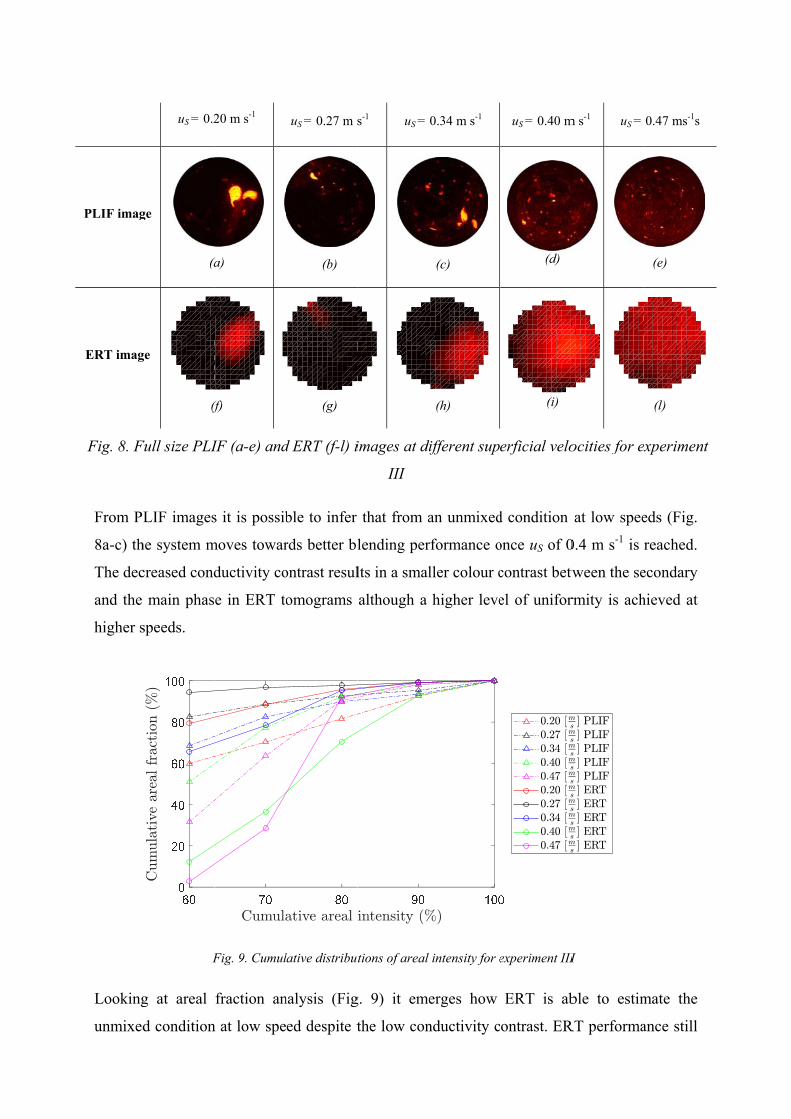
Fig. 8. F
From P
8a-c) th
The dec
and the
higher s
Looking
unmixed
uS = 0.2
ge
(a
ge
(f
Full size PLI
LIF images
he system m
creased cond
main phas
speeds.
F
g at areal
d condition
20 m s-1
(a)
(f)
IF (a-e) and
s it is possib
moves towar
ductivity co
e in ERT to
Fig. 9. Cumul
fraction an
n at low spe
uS = 0.27 m s
(b)
(g)
d ERT (f-l) i
ble to infer
rds better bl
ontrast resul
omograms
lative distribut
nalysis (Fig
ed despite t
s-1 uS =
images at di
III
that from a
lending per
lts in a smal
although a
tions of areal
g. 9) it eme
the low con
0.34 m s-1
(c)
(h)
ifferent sup
an unmixed
rformance o
ller colour c
higher leve
intensity for e
erges how
nductivity c
uS = 0.40 m
(d)
(i)
erficial velo
d condition
once uS of 0
contrast betw
el of unifor
experiment III
ERT is ab
ontrast. ER
m s-1 uS =
ocities for e
at low spee
0.4 m s-1 is
tween the se
rmity is ach
I
ble to estim
RT performa
0.47 ms-1s
(e)
(l)
experiment
eds (Fig.
reached.
econdary
hieved at
mate the
ance still

follows observed trends for PLIF, highlighting the same inflection at mixing performance at
the speed of 0.27 m s-1, compared to higher and lower superficial velocities. Although, an
overestimation is still observed at high speed, particularly for the category of 70-80% mixing,
while in this case ERT does not overestimate the highest mixing condition (80-90% and 90-
100%) commonly the targeted condition in mixing processes.
Increasing the speed (above 0.27 m s-1), and as a consequence the number of lumps of
unmixed injected material, the divergence between PLIF and ERT data increases consistently.
This is an issue which is partly due to the reconstruction algorithm and partly to the
measurement resolution. In fact, the first approximates a non-linear problem with a linear
hypothesis, instead the low resolution characterising the technique limits the size of lumps
that can be detected. Clearly, from the tomograms at low speed (at 0.20 m s-1 , 0.27 m s-1 and
0.34 m s-1), the lumps, or the agglomerations of lumps, can be detected while at higher speed
ERT fails in detecting them. In the present study, an additional obstacle is represented by the
use of small conductivity contrast between the employed phases, which however does not
seem to affect significantly the measurement in condition of poor mixing.
Conclusions
In this work, the ability of ERT to assess the mixing performance of non-Newtonian fluids in
static mixer has been investigated. The same methodology, developed in previous works
(Alberini et al., 2014b, 2014a) is used for both PLIF images and ERT tomograms. Three
experiments using different fluids with different initial contrast in conductivity have been
employed. PLIF has been used to validate the data obtained in terms of qualitative and
quantitative analysis. With the proposed method, ERT can be used as a relative measurement
(measuring how much the mixing improved relative to the other runs at different superficial
velocities) but not as an absolute one, as it could be expected, due to its limitations such as
resolution and reconstructive algorithm smoothing. However, the relative trends show high
level of agreement with PLIF results in particular to identify conditions of poor mixing
(generally for all experimental runs below 0.34 m s-1). This is not the case once the level of
mixing increases (generally for all experimental runs above 0.34 m s-1). The tested conditions
were inherently challenging for the ERT, considering the employed small conductivity
contrast (down to 0.1 mS cm-1), however the lowest observed performance were (commonly
to all experiments) obtained when the dimension of the striations/lumps is below the
measurement resolution, regardless of the conductivity difference between the mixed phases.
References

Alberini, F., Simmons, M.J.H., Ingram, A., Stitt, E.H., 2014a. Use of an Areal Distribution of
Mixing Intensity to Describe Blending of Non-Newtonian Fluids in a Kenics KM Static
Mixer Using PLIF. Aiche J. 60, 332–342. https://doi.org/10.1002/aic.14237
Alberini, F., Simmons, M.J.H., Ingram, A., Stitt, E.H., 2014b. Assessment of different
methods of analysis to characterise the mixing of shear-thinning fluids in a Kenics KM static
mixer using PLIF. Chem. Eng. Sci. 112, 152–169. https://doi.org/10.1016/j.ces.2014.03.022
Alvarez, M.M., Muzzio, F.J., Cerbelli, S., Adrover, A., Giona, M., 1998. Self-similar
spatiotemporal structure of intermaterial boundaries in chaotic flows. Phys. Rev. Lett. 81,
3395–3398. https://doi.org/10.1103/PhysRevLett.81.3395
Aref, H., 1984. Stirring by Chaotic Advection. J. Fluid Mech. 143, 1–21.
https://doi.org/10.1017/S0022112084001233
Arratia, P.E., Muzzio, F.J., 2004. Planar Laser-Induced Fluorescence Method for Analysis of
Mixing in Laminar Flows. Ind. Eng. Chem. Res. 43, 6557–6568.
https://doi.org/10.1021/ie049838b
Avalosse, T., Crochet, M.J., 1997. Finite-element simulation of mixing: 2. Three-dimensional
flow through a kenics mixer. AIChE J. 43, 588–597. https://doi.org/10.1002/aic.690430304
Barigou, M., 2004. Particle Tracking in Opaque Mixing Systems: An Overview of the
Capabilities of PET and PEPT. Chem. Eng. Res. Des., In Honour of Professor Alvin W.
Nienow 82, 1258–1267. https://doi.org/10.1205/cerd.82.9.1258.44160
Bell, S.D., 2015. The Development of Radioactive Gas Imaging for the Study of Chemical
Flow Processes. PhD Thesis, University of Birmingham, Birmingham.
Blythe, T.W., Sederman, A.J., Stitt, E.H., York, A.P.E., Gladden, L.F., 2017. PFG NMR and
Bayesian analysis to characterise non-Newtonian fluids. J. Magn. Reson. 274, 103–114.
https://doi.org/10.1016/j.jmr.2016.11.003
Chandra, K.G., Kale, D.D., 1992. Pressure-drop for laminar-flow of viscoelastic fluids in
static mixers. Chem. Eng. Sci. 47, 2097–2100.
Connelly, R.K., Kokini, J.L., 2007. Examination of the mixing ability of single and twin
screw mixers using 2D finite element method simulation with particle tracking. J. Food Eng.
79, 956–969. https://doi.org/10.1016/j.jfoodeng.2006.03.017
Edwards, I., Axon, S.A., Barigou, M., Stitt, E.H., 2009. Combined Use of PEPT and ERT in
the Study of Aluminum Hydroxide Precipitation. Ind. Eng. Chem. Res. 48, 1019–1028.
https://doi.org/10.1021/ie8010353

Faes, M., Glasmacher, B., 2008. Measurements of micro- and macromixing in liquid mixtures
of reacting components using two-colour laser induced fluorescence. Chem. Eng. Sci., Model-
Based Experimental Analysis 63, 4649–4655. https://doi.org/10.1016/j.ces.2007.10.036
Fu, T., Carrier, O., Funfschilling, D., Ma, Y., Li, H.Z., 2016. Newtonian and Non-Newtonian
Flows in Microchannels: Inline Rheological Characterization. Chem. Eng. Technol. 39, 987–
992. https://doi.org/10.1002/ceat.201500620
Hobbs, D.M., Muzzio, F.J., 1997. The Kenics static mixer: a three-dimensional chaotic flow.
Chem. Eng. J. 67, 153–166. https://doi.org/10.1016/S1385-8947(97)00013-2
Jegatheeswaran, S., Ein-Mozaffari, F., Wu, J., 2018. Process intensification in a chaotic SMX
static mixer to achieve an energy-efficient mixing operation of non-newtonian fluids. Chem.
Eng. Process. 124, 1–10. https://doi.org/10.1016/j.cep.2017.11.018
Komzsik, L., 2003. The Lanczos Method: Evolution and Application. SIAM.
Le Guer, Y., El Omari, K., 2012. Chaotic Advection for Thermal Mixing, in: vanderGiessen,
E., Aref, H. (Eds.), Advances in Applied Mechanics, Vol 45. Elsevier Academic Press Inc,
San Diego, pp. 189–237.
Li, H.Z., Fasol, C., Choplin, L., 1997. Pressure Drop of Newtonian and Non-Newtonian
Fluids Across a Sulzer SMX Static Mixer. Chem. Eng. Res. Des., Fluid Flow 75, 792–796.
https://doi.org/10.1205/026387697524461
Machin, T.D., Wei, H.-Y., Greenwood, R.W., Simmons, M.J.H., 2018. In-pipe rheology and
mixing characterisation using electrical resistance sensing. Chem. Eng. Sci. 187, 327–341.
https://doi.org/10.1016/j.ces.2018.05.017
Pakzad, L., Ein-Mozaffari, F., Chan, P., 2008. Using electrical resistance tomography and
computational fluid dynamics modeling to study the formation of cavern in the mixing of
pseudoplastic fluids possessing yield stress. Chem. Eng. Sci. 63, 2508–2522.
https://doi.org/10.1016/j.ces.2008.02.009
Paul, E.L., Atiemo-Obeng, V.A., Kresta, S.M., 2004. Handbook of Industrial Mixing: Science
and Practice. John Wiley & Sons.
Peryt-Stawiarska, S., 2014. The CFD analysis of non-Newtonian fluid flow through a SMX
static mixer. Przemysl Chem. 93, 196–198.
Pfund, D.M., Greenwood, M.S., Bamberger, J.A., Pappas, R.A., 2006. Inline ultrasonic
rheometry by pulsed Doppler. Ultrasonics 44, E477–E482.
https://doi.org/10.1016/j.ultras.2006.05.027

Pianko-Oprych, P., Nienow, A.W., Barigou, M., 2009. Positron emission particle tracking
(PEPT) compared to particle image velocimetry (PIV) for studying the flow generated by a
pitched-blade turbine in single phase and multi-phase systems. Chem. Eng. Sci. 64, 4955–
4968. https://doi.org/10.1016/j.ces.2009.08.003
Prakash, S., Karwe, M.V., Kokini, J.L., 1999. Measurement of velocity distribution in the
Brabender Farinograph as a model mixer, using Laser-Doppler Anemometry. J. Food Process
Eng. 22, 435–454. https://doi.org/10.1111/j.1745-4530.1999.tb00498.x
Rafiee, M., Bakalisa, S., Fryer, P.J., Ingram, A., 2011. Study of laminar mixing in kenics
static mixer by using Positron Emission Particle Tracking (PEPT). Procedia Food Sci., 11th
International Congress on Engineering and Food (ICEF11) 1, 678–684.
https://doi.org/10.1016/j.profoo.2011.09.102
Rahmani, R.K., Keith, T.G., Ayasoufi, A., 2005. Numerical Simulation and Mixing Study of
Pseudoplastic Fluids in an Industrial Helical Static Mixer. J. Fluids Eng. 128, 467–480.
https://doi.org/10.1115/1.2174058
Ramsay, J., Simmons, M.J.H., Ingram, A., Stitt, E.H., 2016. Mixing performance of
viscoelastic fluids in a Kenics KM in-line static mixer. Chem. Eng. Res. Des., 10th European
Congress of Chemical Engineering 115, 310–324. https://doi.org/10.1016/j.cherd.2016.07.020
Rauline, D., Le Blévec, J.-M., Bousquet, J., Tanguy, P.A., 2000. A Comparative Assessment
of the Performance of the Kenics and SMX Static Mixers. Chem. Eng. Res. Des., Fluid
Mixing 78, 389–396. https://doi.org/10.1205/026387600527284
Regner, M., Östergren, K., Trägårdh, C., 2006. Effects of geometry and flow rate on
secondary flow and the mixing process in static mixers—a numerical study. Chem. Eng. Sci.
61, 6133–6141. https://doi.org/10.1016/j.ces.2006.05.044
Ren, Z., Kowalski, A., Rodgers, T.L., 2017. Measuring inline velocity profile of shampoo by
electrical resistance tomography (ERT). Flow Meas. Instrum. 58, 31–37.
https://doi.org/10.1016/j.flowmeasinst.2017.09.013
Saatdjian, E., Rodrigo, A.J.S., Mota, J.P.B., 2012. On chaotic advection in a static mixer.
Chem. Eng. J. 187, 289–298. https://doi.org/10.1016/j.cej.2012.01.122
Stobiac, V., Fradette, L., Tanguy, P.A., Bertrand, F., 2014. Pumping characterisation of the
maxblend impeller for Newtonian and strongly non-Newtonian fluids. Can. J. Chem. Eng. 92,
729–741. https://doi.org/10.1002/cjce.21906

Szalai, E.S., Arratia, P., Johnson, K., Muzzio, F.J., 2004. Mixing analysis in a tank stirred
with Ekato Intermig® impellers. Chem. Eng. Sci. 59, 3793–3805.
https://doi.org/10.1016/j.ces.2003.12.033
Uendey, C., Ertunc, S., Mistretta, T., Looze, B., 2010. Applied advanced process analytics in
biopharmaceutical manufacturing: Challenges and prospects in real-time monitoring and
control. J. Process Control 20, 1009–1018. https://doi.org/10.1016/j.jprocont.2010.05.008
Wageningen, W.F.C. van, Kandhai, D., Mudde, R.F., Akker, H.E.A. van den, 2004. Dynamic
flow in a Kenics static mixer: An assessment of various CFD methods. AIChE J. 50, 1684–
1696. https://doi.org/10.1002/aic.10178
Wang, M., Dickin, F.J., Mann, R., 1999. Electrical Resistance Tomographic Systems for
Industrial Applications. Chem. Eng. Commun. 175, 49–70.
https://doi.org/10.1080/00986449908912139
Wei, K., Qiu, C., Soleimani, M., Primrose, K., 2015. ITS Reconstruction Tool-Suite: An
inverse algorithm package for industrial process tomography. Flow Meas. Instrum., Special
issue on Tomography Measurement & Modeling of Multiphase Flows 46, 292–302.
https://doi.org/10.1016/j.flowmeasinst.2015.08.001
Wunsch, O., Bohme, G., 2000. Numerical simulation of 3d viscous fluid flow and convective
mixing in a static mixer. Arch. Appl. Mech. 70, 91–102.
https://doi.org/10.1007/s004199900042
Yang, W.Q., Peng, L., 2003. Image reconstruction algorithms for electrical capacitance
tomography. Meas. Sci. Technol. 14, R1. https://doi.org/10.1088/0957-0233/14/1/201
Yenjaichon, W., Pageau, G., Bhole, M., Bennington, C.P.J., Grace, J.R., 2011. Assessment of
Mixing Quality for an Industrial Pulp Mixer Using Electrical Resistance Tomography. Can. J.
Chem. Eng. 89, 996–1004. https://doi.org/10.1002/cjce.20502
Zalc, J.M., Szalai, E.S., Alvarez, M.M., Muzzio, F.J., 2002. Using CFD to understand chaotic
mixing in laminar stirred tanks. AIChE J. 48, 2124–2134.
https://doi.org/10.1002/aic.690481004