Embed Size (px)
Citation preview

University of Alberta
Library Release Form
Name of Author: Japan Trivedi
Title of Thesis: Dynamics of Enhanced Oil Recovery and Sequestration during CO2
Injection in Fractured Reservoirs
Degree: Doctor of Philosophy
Year this Degree Granted: 2008
Permission is hereby granted to the University of Alberta Library to reproduce single copiesof this thesis and to lend or sell such copies for private, scholarly or scientific researchpurposes only.
The author reserves all other publication and other rights in association with the copyrightin the thesis, and except as hereinbefore provided, neither the thesis nor any substantialportion thereof may be printed or otherwise reproduced in any material form whateverwithout the author’s prior written permission.
. . . . . . . . . . . . . . . . . . .Japan TrivediNREF 7-116University of AlbertaEdmonton, ABCanada, T6G 2G6
Date: . . . . . . . . .

University of Alberta
Dynamics of Enhanced Oil Recovery and Sequestration during CO2
Injection in Fractured Reservoirs
by
Japan Trivedi
A thesis submitted to the Faculty of Graduate Studies and Research in partial fulfillmentof the requirements for the degree of Doctor of Philosophy.
in
Petroleum Engineering
Department of Civil and Environmental Engineering
Edmonton, AlbertaFall 2008

University of Alberta
Faculty of Graduate Studies and Research
The undersigned certify that they have read, and recommend to the Faculty of Gradu-ate Studies and Research for acceptance, a thesis entitled Dynamics of Enhanced OilRecovery and Sequestration during CO2 Injection in Fractured Reservoirs sub-mitted by Japan Trivedi in partial fulfillment of the requirements for the degree of Doctorof Philosophy in Petroleum Engineering.
. . . . . . . . . . . . . . . . . . .Tayfun Babadagli (Supervisor)
. . . . . . . . . . . . . . . . . . .Mingzhe Dong (External Examiner)
. . . . . . . . . . . . . . . . . . .Ergun Kuru (Chair and Examiner)
. . . . . . . . . . . . . . . . . . .Jozef Szymanski (Committee Member)
. . . . . . . . . . . . . . . . . . .Ahmed Bouferguene (Committee Member)
Date: . . . . . . . . .
My work is dedicated to
“Lord Shree Swaminarayan” and H.D.H “Pramukh Swami Maharaj”
For their blessings and inspiration
My parents and brother
For their love and support
Friends - Without who it wouldn’t be so easy

Acknowledgements
I am deeply indebted to my supervisor Dr. Tayfun Babadagli for his technical directions,
motivation and moral support throughout this research. With the oil recovery enhancement,
my technical, visional, goal directional and intrapersonal enhancement was also achieved
through improvisation constantly pumped by Dr. Babadagli. I am thankful to Dr. Ergun
Kuru, Dr. Minzhe Dong, Dr. Ahmed Bouferguene and Dr. Jozef Szymanski for serving as
members on the examination committee. I am also thankful to Apache Canada Ltd. for
providing field and well data, and permission to use them in this research. Assistance in
obtaining the Midale field cores by Apache from the Saskatchewan Geological Survey is also
appreciable. I, finally, would like to extend my gratitude to Mr. Rob Lavoie (CalPetra) for
his invaluable assistance during data collection, trip to the Midale field and for sharing his
experience on the operations done in the field over the last three decades.
This research was funded by NSERC (Strategic Grant No: G121990070) and Apache
Canada Ltd. Partial funding was also obtained from an NSERC Grant (No: G121210595)
and FSIDA (University of Alberta, Fund for Support of International Development
Activities) Grant (#04-14O). The funds for the equipment used in the experiments were
obtained from the Canadian Foundation for Innovation (CFI, Project #7566) and the
University of Alberta. All these supports are greatly appreciated. I am also thankful for
various scholarships from the FGSR (University of Alberta) and GSA (University of Alberta)
to present my research at various conferences.
I would also like to thank Schlumberger (ECLIPSE), Computer Modeling Group
(CMG) and COMSOL for their software supports.
This work could not have been completed without the help and support from a
number of people; thanks to Nathan Buzik and Sean Watt for providing their technical
expertise in preparing core-holder design and experimental set-ups; members of the
EOGRRC group at the University of Alberta for stimulating discussions and knowledge
exchange during group meetings.
Finally, I am greatly thankful to all invisible forces acting towards my dreams, desire
and destiny.

Abstract
With urgent need of greenhouse gas sequestration and booming oil prices, underground
oil/gas reservoirs seem the only value added choice for CO2 storage. A great portion of
current CO2 injection projects in the world is in naturally fractured reservoir. It is our aim to
show that the matrix part of these reservoirs could be used as a permanent CO2 storage unit
while recovering oil from it.
This dissertation presents a different approach to the problem following a multi-
stage research work. Initially, a series of laboratory experiments were performed at ambient
conditions using artificially fractured (single) sandstone rocks to mimic fully miscible CO2
injection. Different injection rates were tested and the efficiency of the process was analyzed
in terms of maximized oil recovery. Next, CO2 injection experiments at different miscible
conditions were conducted to analyze the dominant transport mechanisms and to quantify
enhanced oil recovery (EOR) / storage potential. CO2 diffusion and other effective oil
recovery mechanisms were studied during continuous injection at different rates into the
fracture. After the continuous injection of CO2, a soaking period was allowed following a
blowdown period to produce the oil recovered by back-diffusion. The CO2 storage and
EOR capacity during the blowdown period were analyzed. Using dimensionless analysis and
matrix-fracture diffusion groups, a critical number for optimal recovery/sequestration was
obtained.
The pressure decay behavior during the shutdown was analyzed in conjunction with
the gas chromatograph analysis of the produced oil sample collected during blowdown after
the quasi-equilibrium reached during pressure decay. This gave insights into the governing

mechanism of extraction/condensation and miscibility for recovering lighter to heavier
hydrocarbons during pressure depletion from fractured reservoirs.
The importance of miscible recovery from fractured reservoirs in current petroleum
industry makes its comprehensive understanding, characterization, and quantitative
prediction very critical. Therefore, as a final step, a universal procedure of inspectional
analysis followed by a numerical sensitivity was performed for the scaling of fractured
porous media. A new dimensionless group introduced by combining the effects of major
governing groups will improve the understanding of pore scale mechanisms also it can be
further used for the improvement of fractured reservoir models and upscaling laboratory
results.

TABLE OF CONTENTS
1 Introduction ............................................................................................................ 1
1.1 Overview...............................................................................................................................1
1.2 Literature Review.................................................................................................................6
1.2.1 Critical Injection Rate ...........................................................................................6
1.2.2 First-Contact Miscible or Immiscible Matrix-Fracture Interaction
Experiments ...........................................................................................................8
1.2.3 Effect of Flow on Diffusion/Dispersion in Fractured Porous Media ........10
1.2.4 Scaling and Dimensionless Analysis .................................................................12
1.2.5 Multi-Contact Miscible CO2 Injection into Fractures - Experimental Study
................................................................................................................................14
1.3 Problem Statement ............................................................................................................15
1.4 Methodology ......................................................................................................................16
1.5 Outline.................................................................................................................................18
2 Efficiency of Diffusion Controlled Miscible Displacement in Fractured Porous
Media............................................................................................................................20
2.1 Introduction .......................................................................................................................20
2.2 Experimental Method .......................................................................................................22
2.2.1 Porous Media .......................................................................................................22
2.2.2 Fluids .....................................................................................................................23
2.2.3 Test Conditions....................................................................................................23
2.2.4 Core Preparation and Test Procedure ..............................................................23
2.2.5 Measurement Technique ....................................................................................24
2.2.6 Effect of Water Saturation .................................................................................25
2.2.7 Effect of Aging ....................................................................................................25
2.2.8 Effect of Viscosity Ratio/Density.....................................................................25
2.2.9 Effect of Gravity..................................................................................................26
2.3 Results and Analysis ..........................................................................................................26
2.4 Efficiency Analysis ............................................................................................................28

2.5 Conclusions ........................................................................................................................29
3 Experimental and Numerical Modeling of the Mass Transfer between Rock
Matrix and Fracture .....................................................................................................40
3.1 Introduction .......................................................................................................................40
3.2 Experimental Study ...........................................................................................................43
3.2.1 Procedure..............................................................................................................44
3.3 Experimental Observations .............................................................................................48
3.4 Modeling of Fracture-Matrix Transfer Process.............................................................53
3.4.1 Analogy between Monolith Catalysts (Reactor) and Matrix-Fracture
Systems..................................................................................................................54
3.4.2 Mathematical Model Formulation.....................................................................56
3.4.3 Dispersion and Diffusion...................................................................................60
3.5 Mass Transfer Rate Constant and Effective Diffusion into Porous Matrix .............63
3.6 Conclusions ........................................................................................................................68
4 Efficiency Analysis of Greenhouse Gas Sequestration during Miscible CO2
Injection in Fractured Oil Reservoirs ..........................................................................70
4.1 Introduction .......................................................................................................................70
4.2 Background.........................................................................................................................71
4.3 Dimensionless Parameters and the Effectiveness Factor for Matrix-Fracture
Interaction by Diffusion during Injection of a Miscible Phase...............................................72
4.4 Effective Parameters and Efficiency Correlations........................................................76
4.5 Summary and Discussion .................................................................................................78
5 Scaling Miscible Displacement in Fractured Porous Media Using Dimensionless
Groups ..........................................................................................................................84
5.1 Background on Scaling Process.......................................................................................84
5.2 Dimensional Analysis (DA) .............................................................................................84
5.2.1 Inspectional Analysis (IA) ..................................................................................84
5.3 Derivation of the Dimensionless Groups for Flow in Fractured Porous Medium.....
..............................................................................................................................................86
5.4 New Dimensionless Number ..........................................................................................90
5.4.1 Similarity and Comparison with the Immiscible Process ..............................91
5.5 Validation of Proposed Group........................................................................................92

5.5.1 Experiments .........................................................................................................92
5.6 Physical Significant of the Proposed Group and Analysis ..........................................95
5.7 Concluding Remarks .........................................................................................................97
6 Experimental Investigations on the Flow Dynamics and Abandonment Pressure
for CO2 Sequestration and Incremental Oil Recovery in Fractured Reservoirs: The
Midale field Case.........................................................................................................101
6.1 Introduction .................................................................................................................... 101
6.2 Experimental Components ........................................................................................... 103
6.2.1 Diffusion Cell (Core Holder).......................................................................... 103
6.2.2 Injection Set-up................................................................................................. 103
6.2.3 Production System............................................................................................ 104
6.2.4 Data Acquisition System (DAQ).................................................................... 104
6.2.5 Core Properties and Core Preparation .......................................................... 105
6.3 Experimental Procedure................................................................................................ 105
6.3.1 Continuous CO2 Diffusion for Oil Recovery............................................... 106
6.3.2 Blow Down ....................................................................................................... 107
6.4 Effect of Rate – Existence of Critical Rate................................................................. 107
6.5 Sequestration – Time and Economical Aspects......................................................... 109
6.6 Effect of Miscibility – Sequestration and EOR ......................................................... 109
6.7 Rock Type – Sandstone and Limestone...................................................................... 110
6.8 Blow Down – Sequestration and EOR....................................................................... 110
6.9 Critical Observations...................................................................................................... 111
6.10 Cap Rock Sealing ............................................................................................................ 112
6.11 Conclusions and Remarks ............................................................................................. 113
7 Experimental Analysis of CO2 Sequestration Efficiency during Oil Recovery in
Naturally Fractured Reservoirs.................................................................................. 120
7.1 Overview.......................................................................................................................... 120
7.2 Introduction .................................................................................................................... 120
7.2.1 Importance/Role of Diffusivity in Miscible and Immiscible Matrix-
Fracture Transfer Process ............................................................................... 121
7.3 Experimental Components ........................................................................................... 122
7.3.1 Core Properties and Core Preparation .......................................................... 122

7.3.2 Diffusion Cell (Core Holder).......................................................................... 122
7.3.3 Injection Set-up................................................................................................. 123
7.3.4 Production System............................................................................................ 123
7.3.5 Data Acquisition System (DAQ).................................................................... 123
7.4 Experimental Procedure................................................................................................ 124
7.4.1 Continuous CO2 Diffusion for Oil Recovery............................................... 125
7.4.2 Blow Down ....................................................................................................... 125
7.5 Experimental Results and Discussion ......................................................................... 126
7.6 Matrix-Fracture Diffusion Simulation......................................................................... 129
7.7 Correlation for CO2 Sequestration and Oil Production ........................................... 131
7.8 Conclusions ..................................................................................................................... 133
8 Analysis of Observations on the Mechanics of Miscible Gravity Drainage in
Fractured Systems...................................................................................................... 145
8.1 Problem Statement ......................................................................................................... 145
8.2 Mechanisms: Miscible Gravity Drainage in NFRs .................................................... 146
8.3 Soaking: Improving Extraction Mechanism............................................................... 147
8.4 Effect of Diffusion/Dispersion and Injection Rate.................................................. 148
9 Contributions and recommendations ................................................................. 150
9.1 Contributions and Conclusions .................................................................................... 150
9.1.1 First Contact Miscible Experiments .............................................................. 150
9.1.2 Scaling of Matrix-Fracture Miscible Process and Critical Rate Definition151
9.1.3 Simulation of Matrix-Fracture Process.......................................................... 152
9.1.4 Multi-Contact CO2 Experiments.................................................................... 153
9.2 Recommendations for Future Research...................................................................... 155
10 Nomenclature...................................................................................................... 157
11 Appendix ............................................................................................................. 164
12 Bibliography........................................................................................................ 172

LIST OF FIGURES
Figure 2.1: Core-holder design. ........................................................................................................30
Figure 2.2: Core samples cut for fracture creation and the core-holder used. ..........................30
Figure 2.3: Experimental set-up. ......................................................................................................31
Figure 2.4: Calibration chart for refractometer for mineral oil-heptane mixture. ....................33
Figure 2.5: Cumulative production with solvent injected (PV) for Berea sandstone horizontal
orientation. ..........................................................................................................................................33
Figure 2.6: Cumulative production with solvent injected (PV) for Berea sandstone vertical
orientation. ..........................................................................................................................................34
Figure 2.7: Cumulative production with solvent injected (PV) for aged Berea sandstone
horizontal orientation. .......................................................................................................................34
Figure 2.8: Cumulative production with solvent injected (PV) for Indiana limestone
horizontal orientation. .......................................................................................................................35
Figure 2.9: Cumulative production with solvent injected (PV) comparing aged and unaged
Berea sandstone horizontal orientation. .........................................................................................35
Figure 2.10: Cumulative production with time for water imbibed cores. ..................................36
Figure 2.11: Cumulative production with time for Berea sandstone horizontal orientation. .36
Figure 2.12: Cumulative production with time for aged Berea sandstone horizontal
orientation. ..........................................................................................................................................37
Figure 2.13: Cumulative production with time for Berea sandstone vertical orientation........37
Figure 2.14: Cumulative production at different flow rate and time axis for Berea sandstone
horizontal orientation. .......................................................................................................................38

Figure 2.15: Cumulative production at different flow rate and time axis for Indiana limestone
horizontal orientation. .......................................................................................................................38
Figure 2.16: Cumulative production at different flow rate and time axis for aged Berea
sandstone horizontal orientation. ....................................................................................................39
Figure 3.1(a): Core cutting and fracture preparation.....................................................................45
Figure 3.1(b): Core holder design. ...................................................................................................45
Figure 3.2: Experimental set-up. ......................................................................................................46
Figure 3.3: Solute recoveries during solvent diffusion for different oil types. ..........................48
Figure 3.4: Solute recoveries during solvent diffusion for horizontal and vertical cases.........50
Figure 3.5: Solute recoveries during solvent diffusion comparing Berea sandstone and
Indiana limestone cores.....................................................................................................................51
Figure 3.6: Comparison of the solute recoveries during solvent diffusion for the aged and
non-aged samples. ..............................................................................................................................52
Figure 3.7: Solute recoveries during solvent diffusion from high viscosity mineral oil aged
and non-aged core samples...............................................................................................................52
Figure 3.8: Solute recoveries during solvent diffusion comparing 3” and 6” longer samples.
...............................................................................................................................................................53
Figure 3.9: Diffusion and flux behavior in monoliths. .................................................................55
Figure 3.10: Diffusion and flux in matrix-fracture system. ..........................................................56
Figure 3.11(a): Geometrical representation of matrix-fracture system used in this study (not
to scale). ...............................................................................................................................................57
Figure 3.11(b): Simulation match with the experimental results of solute (mineral oil)
concentration (C2) change for two different rates on aged Berea sandstone cores..................60
Figure 3.12: Mass transfer rate constant with velocity..................................................................64
Figure 3.13: Comparison of the Kv (s-1) values obtained through the numerical simulation and
the ones obtained from Equation (3.17).........................................................................................65
Figure 3.14: Comparison of DeM values used for the simulation matches with the ones
obtained from Equation (3.18).........................................................................................................67
Figure 3.15: Concentration-time curves for matrix-fracture transfer at low and high rates. ..67
Figure 4.1(a): Core cutting/fracture preparation and core holder assembly .............................79
Figure 4.1(b): Core holder design ....................................................................................................80
Figure 4.2(a): Recovery of solute (oil) with injection of miscible solvent (heptane) ................80
Figure 4.2(b): Simulation match (solid lines) with experimental results (symbols) ..................81
Figure 4.3: Power-law relationship between (TSP/TSI) and effectiveness factor (ηG). BHA:
Berea sandstone-horizontal-mineral oil-aged, IH: Indiana limestone-horizontal- mineral oil,
BHS: Berea sandstone-horizontal-mineral oil, BHK: Berea sandstone-horizontal-kerosene,
HO: Heavy (mineral) oil, HOA: Heavy (mineral) oil-aged. .........................................................82
Figure 4.4: Power-law relation of (TSS/TSI) with effectiveness factor (NG) [Legend as given
in Figure 4.3]. ......................................................................................................................................82
Figure 4.5: Comparison of (TSP/TSI) experimental value and the one obtained from
Equation (4.7) [% error showing 10, 20 & 30 % error in predicted values]..............................83
Figure 4.6: Comparison of (TSS/TSI) experimental value and the one obtained from
Equation (4.8) [% error showing 10, 20 & 30 % error in predicted values]..............................83
Figure 5.1 Geometrical representation of matrix-fracture system used in this study. .............97
Figure 5.2: Experimental set-up .......................................................................................................98
Figure 5.3: Normalized oil production with respect to amount of solvent injected as a
function of the gravity number (Ng). ..............................................................................................98
Figure 5.4: Normalized oil production with respect to amount of solvent injected as a
function of the Peclet number (Pe). .................................................................................................99

Figure 5.5: Normalized oil production with respect to amount of solvent injected as a
function of (Peclet Number/Gravity Number).............................................................................99
Figure 5.6: Normalized oil production with respect to amount of solvent injected as a
function of Matrix-Fracture Diffusion Group (NM-FD). ............................................................ 100
Figure 5.7: Normalized oil production with respect to amount of solvent injected as a
function of Fracture Diffusion Index (FDI). .............................................................................. 100
Figure 6.1: Experimental set-up (A schematic is presented in chapter 7, Figure 7.2)........... 115
Figure 6.2: Core cutting, cleaning and fracture preparation...................................................... 115
Figure 6.3: Oil production for different rates and pressures. ................................................... 116
Figure 6.4: CO2 produced per amount of CO2 injected for different rates and pressures. .. 117
Figure 6.5: CO2 stored per amount of CO2 injected for different rates and pressures......... 117
Figure 6.6: CO2 stored with time for different rates and pressures. ........................................ 118
Figure 6.7: Core pressure change against time for four different cases. ................................ 118
Figure 6.8: Cap rock sealing capacity test. ................................................................................... 119
Figure 7.1: Core Preparation.......................................................................................................... 136
Figure 7.2: Experimental Setup (Photo of the set-up is shown in Figure 6.1). ...................... 136
Figure 7.3: Oil recovery with the pressure blowdown for Berea sandstone........................... 137
Figure 7.4: Oil recovery with the pressure blowdown for Midale carbonate. ........................ 137
Figure 7.5: CO2 production with the pressure blowdown for Berea sandstone. ................... 138
Figure 7.6: CO2 production with the pressure blowdown for Midale carbonate. ................. 139
Figure 7.7: CO2 storage with the pressure blowdown for Berea sandstone. .......................... 140
Figure 7.8: CO2 storage with the pressure blowdown for Midale carbonate. ........................ 141
Figure 7.9: Normalized recovery factor with the CO2 PV injected for Berea sandstone. .... 142

Figure 7.10: Normalized recovery factor with the CO2 PV injected for Midale carbonate. 142
Figure 7.11: Pressure decay and attainment of quasi-equilibrium behavior. .......................... 143
Figure 7.12: Hydrocarbon recovery distribution for the Case-8 at different stages of the
production life. ................................................................................................................................ 143
Figure 7.13: (TOP/TSI) with matrix-fracture diffusion group (NM-FD). ................................ 144

LIST OF TABLES
Table 1.1 Miscible (major) CO2 projects in the USA......................................................................3
Table 1.2 Miscible (major) CO2 projects in Canada........................................................................4
Table 1.3 Imiscible (major) CO2 projects world-wide ....................................................................4
Table 2.1: Properties of displacing and displaced fluids. ..............................................................31
Table 2.2: Detailed outline of experiments conducted. ................................................................32
Table 3.1: Properties of solute and solvent used in the study. ....................................................46
Table 3.2: Details of experiments performed.................................................................................47
Table 4.1. Time-scales and dimensionless number associated with our physics similar to that
of monolith (Bhattacharya et al. 2004)............................................................................................79
Table 5.1: Dependent and independent variables, symbols and their dimensions. ..................88
Table 5.2: Dimensionless groups derived using the Inspectorial Analysis. ...............................90
Table 5.3: Experiments performed..................................................................................................94
Table 5.4: Properties of solvent and solute used in experiments ................................................94
Table 6.1: Core and fluid properties and experimental details ................................................ 114
Table 7.1: Experiments details ...................................................................................................... 134
Table 7.2: Hyperbolic behavior for oil recovery during production life ................................. 134
Table 7.3: Dimensionless numbers and TOP/TSI predicted values using NM-FD. ................ 135
Table 10.1: The unique dimensionless group from the above equations (marked as bold
letters)................................................................................................................................................ 167
1
1 INTRODUCTION
1.1 Overview
Fossil fuels are likely to remain a major primary source of world’s energy supply in today’s
industrialized world because of their inherent advantages such as availability, competitive
cost, ease of transportation and storage, and well-advanced technology over other energy
sources. Hence, the generation and emission of greenhouse gases, more specifically CO2 and
flue gas are likely to continue. The concentrations of CO2 in the atmosphere have increased
by 31% since 1750. Of the total CO2 emissions in the United States in 2002, approximately
98% resulted from the combustion of fossil fuels (coal, petroleum, and natural gas).
Industrial processes, including gas flaring and cement production, accounted for the other
2%. Fossil fuel combustion for electricity generation is the largest contributor to CO2
emissions in the United States followed by fossil fuel combustion for transportation. In
2002, electricity generation accounted for 39% of CO2 emissions in the United States while
transportation accounted for about 32%. By weight, CO2 is the most emitted greenhouse
gas. In 2002, sources in the United States emitted 5,796 million metric tons of CO2
compared to 27 million metric tons of methane and 1.1 million metric tons of nitrous
oxides. The amount of anthropogenic CO2 emitted to the atmosphere has risen from the
preindustrial levels of 280 parts per million (ppm) to the present levels of over 365 ppm. It
is estimated that ~6 gigatons of carbon enters the environment annually as a result of global
energy-related CO2 emission, North America being responsible for ~0%–25% of this total.
Because of the reasons outlined above, the sequestration of CO2 turned out to be a
critical issue in the last decade. There are several different ways to sequester CO2. They can
be classified as follows:
• CO2 reactions with naturally or artificially formed alkine compounds, like silicate,
oxide and hydroxide to store CO2 in form of solid hydroxide to store CO2 in form of solid
carbonates.
• Storage of CO2 in form of bicarbonate in solution by reaction of solid carbonate
dissolution in the presence of water and CO2.

2
• Deep-ocean injection, subterranean injection of captured CO2 for biomass formation
and accumulation.
• Stratigraphic and structural trapping in depleted oil and gas reservoirs.
• Adsorption trapping in uneconomic coal beds.
• Mineral immobilization
• Solubility trapping in reservoir oil and gas and formation water.
The mechanisms to sequester CO2 geologically are: 1) stratigraphic and structural trapping
in depleted oil and gas reservoirs, 2) solubility trapping in reservoir oil and formation water,
3) adsorption trapping in uneconomic coal beds, 4) cavern trapping in salt structures, and 5)
mineral immobilization.
Recognition of the importance of CO2 emissions has stimulated research toward mitigation
of CO2 effects as mandated under the Kyoto Protocol of the United Nations Framework
Convention on Climate Change. The sequestration of CO2 and/or flue gas is not cheap;
however, the injection of those gases into oil or gas reservoirs to enhance production may
offset some of the associated costs. Hydrocarbon miscible processes have received
extensive field appraisal since 1950’s, especially in the USA and Canada. CO2 solvent
flooding is one of the most successful EOR methods in the USA and worldwide.
A large proportion of the world’s proven oil has been found in reservoir rocks that are
naturally fractured. Due to poor sweep efficiency, waterflooding in such reservoirs may not
be applicable if the matrix is not water-wet, very tight and heterogeneous, and oil viscosity is
high. Use of vast and successful experience of miscible especially CO2 flooding from
homogeneous (un-fractured) reservoirs to fractured reservoir could benefit the tertiary
recovery prospects and at the same time those reservoirs could be targeted for sequestration.

3
Table 1.1 Miscible (major) CO2 projects in the USA
Pay zone (Basin)
Major fields Formation Porosity, %
Permeability md
Area, acres
Slaughter 20,328
Vacuum 5,984
Seminole Unit 16,679
Wasson (Denver, Willard, ODC)
43,648
Hanford 1,460
San Andres (Tex/N.M)
Yates (Immiscible)
Dolo/LS 9-15 1.3-123
26,000
Silurian-Niagaran (Mich)
Dover LS/Dolo 7-8 5-10 4,525
SACROC 49,900 Canyon Reef (Tx)
Cogdell
LS 4-5 19
2,204
Devonian (Tx) N.Cross-Devonian Unit S.Cross Devonian Unit Mid Cross Devonian Unit North Dollarhide Dollarhide Devonian
- 18-22 4-5 4,525
Little Creek 6,200
West Mallalieu 8,240
McComb 12,600
Smithdale 4,100
Lower Tuscaloosa (Miss.)
Brookhaven
S 23-26 60-90
10,800
Ismay Desert Creek (Utah)
Greater Aneth Area LS 14 5 13,400
Canyon Salt Creek LS 20 12 12,000
Sims (Ok) Sho-Vel-Tum S 16 30 1,100
Delaware, Ramsey (Tx)
Twofreds East Ford El Mar
S 19-20 30-32 4,392 1,953 6,000
Abo (Tx) T-Star (Slaughter Consolidated)
Dolo 7 2 1,000
Grayburg (Tx) North Cowden Demo Dolo 10 2-5 200
Clearfork (Tx) Antosh Irish Dolo 7-11 5 2,853
Springer (Ok) Northeast Purdy Bradley Unit
S 13-14 44-50 4,100
Tensleep (Wyo) Lost Soldier Wertz
S 9-10 20-30 1,345 1,400
Weber SS Rangerly Weber sand S 12 10 18,000
Morrow Postle S 16 30 11,000

4
Table 1.2 Miscible (major) CO2 projects in Canada
Pay zone (Basin)
Major fields Formation Porosity, % Permeability md
Area, acres
Midale Weyburn Unit LS/Dolo 15 10 9,900
Marly & Vuggy Midale Dolo/LS 16.3 75 30,483
Jofrre 13 500 6,625 Viking Cardium
Pembina
S
16 20 80
Beaverhill Lake Swan Hills LS 8.5 50-60 -
Nisku Enchant Dolo 10-17 10-50 -
Table 1.3 Imiscible (major) CO2 projects world-wide
Pay zone (Basin)
Major fields Formation Porosity, % Permeability md
Area, acres Start Date
Garzan (Turkey)
Bati Raman LS 18 58 12,890 3/86
Area 2102 6/76
Area 2121 1/74
Area 2124 1/86
Forest Sands (Trinidad)
EOR 34-Cyclic
S 29-32 150-300 -
84
LS – Limestone
S – Sandstone
Dolo - Dolomite
During the injection of fluids that are miscible with oil for enhanced oil recovery, oil
recovery and transport of the injectant are controlled by fracture and matrix properties in
naturally fractured reservoirs (NFR). For such systems, the transfer between matrix and
fracture due to diffusion constitutes the major part of oil recovery. While injecting
secondary or tertiary recovery materials that are miscible with matrix oil, i.e., hydrocarbon
solvents, alcohols, CO2, N2 etc., because of the large permeability contrast between the
matrix and the fracture; fracture network creates the path for the injected solvent to bypass
and leave the oil in the matrix untouched. Significant amount of oil can be recovered from
the unswept bypassed parts of the reservoir by maximizing the subsequent crossflow or

5
mass transfer between fracture and porous matrix. Likewise, when the greenhouse gases
(CO2, pure or in the form of flue gas) are injected into NFRs, the matrix part could be a
proper storage environment and the transfer of the injected gas to the matrix needs to be
well understood for the determination of process efficiency. The same process is
encountered in the transportation of contaminants and waste material in NFRs.
Understanding the effects of the different parameters on the dynamics of such processes is
essential in modeling such processes. In fact, the description of matrix fracture interaction
for dual-porosity dual-permeability models developed for NFRs is still a challenge.
Different solvent injection processes such as carbon dioxide, nitrogen, flue gas, natural gas,
or other hydrocarbon gases (methane, ethane, propane, and butane) have one of the most
important things in common; they all dissolve into the oil phase eventually causing mixing of
oil and injected gas depending on the pressure applied. The efficiency of the mixing or
dissolving here is always measured or characterized by mutual diffusion coefficient of
solvent into the oil phase. Solute transport in fractures, however, is controlled not only by
diffusion but also advective processes. The fracture dispersion coefficient and effective
matrix diffusion coefficient are the most important parameters controlling the matrix
diffusion. In the fractured porous media, the matrix diffusion is of primary importance in
several problems such as geological disposal of nuclear waste, contaminant transport during
ground water contamination, enhanced oil recovery and greenhouse gas sequestration.
During CO2 injection into naturally fractured oil reservoirs for enhanced oil recovery, a great
portion of oil is recovered by matrix-fracture interaction. Diffusive mass transfer between
matrix and fracture controls this process if CO2 is miscible with matrix oil. The oil expelled
from matrix is replaced by CO2 and the matrix could be potentially a good storage medium
for long term. Detailed analysis is needed for the co-optimization of the oil recovery and
CO2 storage, i.e., maximizing the oil recovery while maximizing the amount of CO2 stored.
During CO2 injection into fractured systems there still exist several unanswered questions.
How the injection scheme is optimized? What is the optimal injection rate that delays the
breakthrough time, and reduces the recycling cost keeping the process still efficient by
producing oil at an economic rate? What range of reservoir pressure should be maintained
for the best result (immiscible, miscible or near miscible process)? Which of the
mechanisms of oil; swelling, gravity drainage or diffusion governs the production mechanism

6
during miscible recovery? What should be done when oil cut drops significantly during
continuous CO2 injection and most of the injected CO2 needs to be recycled? How does the
different hydrocarbon components’ recovery get affected? Is sequestration goal a byproduct
of oil production or hampers incremental recovery? These fundamental questions can only
be answered by thorough experimental analyses.
1.2 Literature Review
1.2.1 Critical Injection Rate
Macroscopic/microscopic heterogeneities are the major reasons of unequal displacement
rates between oil in place and solvent injected. Heterogeneities cause poor areal sweep
efficiencies and early breakthroughs hampering oil recoveries. When a gas is injected to
displace oil, the mobility ratio between the injected gas and displaced oil is typically highly
unfavorable owing to low viscosity of gas that results in gravity segregation. In 1952, Hill
defined a critical velocity above which viscous instability due to lower gravity compared to
viscous forces can occur. Dumore (1964) modified the equation suggested by Hill (1952)
with mixing of solvent and oil behind the front taken into consideration. Slobod and
Howlett (1964) derived a critical rate for frontal stability in gravity drainage given by:
)*( gk
qo
ooc ρ
µ∆
∆= ......................................................................................................................(1.1)
Gravity drainage rate for immiscible process in homogeneous porous media defined by
Barkve and Firoozabadi (1992) is
)/*( )( LPgk
q TH
C
o
ooc −∆= ρ
µ.....................................................................................................(1.2)
For miscible processes:
)*( gk
qo
ooc ρ
µ∆= ........................................................................................................................(1.3)

7
where
oµ = Oil viscosity
ok = Single phase oil permeability
ρ∆ = Density difference between injected/displaced fluids
)(TH
CP = Threshold capillary pressure
G = gravitational acceleration
L = Height
Tiffin and Kremesec (1986) noted recovery improvements for gravity-assisted vertical core
displacement over horizontal displacement. They performed first contact as well as multi-
contact miscible experiments. Their results indicated that the mass transfer strongly affects
frontal stability and the efficiency increases at lower cross flow and mixing conditions.
Recovery mechanism of matrix-fracture systems has been studied at laboratory scale since
1970’s. Thompson and Mungan (1969) compared displacement velocity to critical velocity
(VC) and showed its effect on recovery efficiency. Slobod and Howlett (1964) and
Thompson and Mungan (1969) showed that the critical velocity defines the fingering
behavior in displacement of more viscous and denser fluid in a miscible process.
Babadagli and Ershaghi (1993) proposed a fracture capillary number (Nf,Ca) as the ratio of
viscous to capillary forces for immiscible displacement in fractured systems. The fracture
capillary number is a ratio of viscous forces active in fracture to the capillary forces active in
matrix. Stubos and Poulou (1999) introduced a modified diffusive capillary number as the
ratio of diffusion to the capillary gradient driven rate. Their work mainly focused on drying
of porous media with existence of two phases. Later, Babadagli (2002) showed a
relationship between capillary imbibition recovery and matrix/fracture properties while there
is a constant rate flow in the fracture using a scaling group where he included the length of
the matrix. This group was derived based on the Handy’s equation (Handy, 1960).

8
1.2.2 First-Contact Miscible or Immiscible Matrix-Fracture Interaction
Experiments
Mahmoud (2006) and Wood et al. (2006) showed that the presence of vertical fracture
improved the oil recovery through immiscible gas assisted gravity drainage (GAGD)
compared to the unfractured counterpart. They observed that gas will try to stay on the top
and expand laterally and if the gravity force loses its dominance to viscous forces, then the
adverse effect of fractures can be observed.
Saidi (1987) studied the diffusion/stripping process in fractured media. He emphasized the
compositional effects between gas in the fracture and oil in the matrix on recovery
enhancement. Using the results of single matrix block analytical studies and multicomponent
laboratory experiments Da Silva and Belery (1989) confirmed the importance of molecular
diffusion in NFRs and concluded that it may override the other hydrocarbon displacement
mechanisms. Morel et al. (1990) performed nitrogen diffusion experiments with horizontal
chalk cores and studied the effect of initial gas saturation. They found that the recovery
process is not purely dependent on diffusion mechanism. Hu et al. (1991) showed the
importance of diffusion calculation as well as capillary pressure curve correction on the IFT
change due to compositional change. Part (1993) studied the formation of drying patterns
assuming only capillary forces and neglecting viscous effects. It was the first attempt to
theoretically characterize drying patterns in porous media as well.
The effect of displacement rates and pressure on the recovery performance was investigated
by Zakirov et al. (1991) in miscible displacement through fractured reservoirs. Firoozabadi
and Markeset (1994) showed that the capillary pressure contrast between matrix and fracture
could be the major driving force. Further, they studied the effect of matrix/fracture
configuration and fracture aperture on first contact miscible efficiency. If the capillary
contrast (capillary pressure) of the fractured and layered reservoirs are reduced or eliminated,
gravity drainage performance can be improved (Dindoruk and Firoozabadi, 1997; Correa
and Firoozabadi, 1996). Burger et al. (1996) and Burger and Mohanty (1997) found that
capillary driven crossflow does not contribute significantly to mass transfer in near-miscible
hydrocarbon floods.

9
The presence of water affects the pore-scale distribution of hydrocarbon phases (Pandey and
Orr al., 1990, Mohanty and Salter, 1982). Connectivity and tortuosity of the pore structure
influences the effective diffusivity and the relative permeability of each hydrocarbon phase.
Hence, the mass transfer and bypassing are affected. LeRomancer et al. (1994) examined the
effect of water saturation (<30%) on mass transfer in the matrix blocks of a fractured
reservoir. As the water saturation increases, the liquid-hydrocarbon-phase area available for
diffusion and the gas/liquid interfacial area decrease resulting in a reduction in mass transfer.
At high water saturations, islands of oil will be isolated by water, effectively reducing mass
transfer further. They also concluded that water saturation has no effect during nitrogen
injection because of a strong capillary crossflow. Whylie and Mohanty (1997) further
investigated the effects of water saturation on mass transfer from bypassed region and
bypassing during miscible/near-miscible gas injection. They used 1-D model and calculated
effective diffusion coefficient.
The orientation of the bypassed region with respect to gravity and enrichment of the
solvents affect the mass-transfer rate. The mass-transfer was least for the vertically up
orientation (against gravity), intermediate for the vertically down, and highest for the
horizontal orientation for the experiments (Burger et al., 1996). Burger et al. (1996) also
concluded in his analysis that in vertical orientation gravity does not induce the flow of oil to
the outlet face; therefore, the recovery is primarily due to the diffusion. The oil-phase
diffusivity is the controlling parameter in vertical mass transfer experiments.
Comings and Sherwood (1934) modeled the process considering moisture moment by
capillary in drying granular materials. But determining mass transfer coefficients during flow
in fracture is more complex process due to the involvement of injection rate effect and
fracture properties. In most of the available commercial simulators, the mass transfer is
assumed to proceed by diffusion within single phase. Recent studies from Jamshidnezhad et
al. (2004) considered mass transfer between the same phases in the fracture and porous
medium. They concluded that the displacement rates are of great importance for miscible
process in NFRs.
Matrix fracture interaction in fractured rocks for different types of fluids was investigated
computationally (Zakirov et al., 1991; Jensen et al., 1992) and experimentally (Li et al., 2000;

10
Le Romancer et al., 1994) in different studies. Analytical and numerical solutions for the
diffusion process in the fracture and transport to the matrix are also available (Hu et al.,
1991; Lenormand, 1998; LaBolle et al., 2000; Jamshidnezhad et al., 2004; Ghorayeb and
Firoozabadi, 2000).
Experimental methods to measure diffusivity could be direct or indirect. The direct method
is the one which requires the compositional analysis of the diffusing species while the
indirect method changes one of the parameters affected by diffusion and the diffusivity is
measured such as volume change, pressure variation or solute volatilization. As reported in
the literature, direct methods are time consuming and expensive (Sigmund, 1976; Upreti and
Mehrotra, 2002). Recently, studies (Upreti and Mehrotra, 2002; Riazi, 1996; Tharanivasan et
al., 2004; Zhang et al., 2000; Sheikha et al., 2005) were reported on indirect method which
measures change in pressure due to gas diffusion into liquid.
1.2.3 Effect of Flow on Diffusion/Dispersion in Fractured Porous Media
During the flow through porous media, the additional mixing caused by uneven flow or
concentration gradient is called dispersion. It results from the different paths and speeds and
the consequent range of transit times available to tracer particles convected across a
permeable medium. Dispersive mixing is a resultant of molecular diffusion and mechanical
dispersion. Perkins and Johnston (1963) provided an analysis of the dispersion phenomena
and correlations for two types of dispersion; (1) longitudinal direction, and (2) transverse to
the direction of gross fluid movement. Both, having different magnitude, have to be
considered separately. Dispersive mixing plays important role in determining how much
solvent will dissolve/mix with solute to promote miscibility. Molecular diffusion will cause
mixing along the interface. The net result will be a mixed zone growing at a more rapid rate
than would be obtained from diffusion alone. Diffusion is a special case of dispersion and a
result of concentration gradient, with or without the presence of the velocity field (Bear,
1988; Sahimi et al., 1982).
Gillham and Cherry (1982) defined the hydrodynamic dispersion coefficient as the sum of
coefficient of mechanical dispersion (Dmech) and the effective diffusion coefficient in porous

11
media (Deff). The hydrodynamic dispersion coefficient is also referred as dispersion-diffusion
coefficient (DL).
effmechL DDD += ........................................................................................................................(1.4)
The mechanical dispersion is proportional to the average linearized pore-water velocity (V)
and the dispersivity (α) (Bear, 1979; Freeze and Cherry, 1979). The effective diffusion
coefficient is related to diffusion coefficient in free solution and tortuosity.
Taylor (1953) showed that in case of substantial diffusion perpendicular to the average fluid
velocity, the dispersion coefficient in the tube would be proportional to the square of the
average fluid velocity. Later, Horne and Rodriguez (1983) concluded that in the diffusion
dominated system, the dispersion coefficient in the single, straight, parallel plate fracture will
be proportional to the square of the fluid velocity. Keller et al. (1999) showed that dispersion
coefficient and velocity has linear relationship, where DL α V. Bear (1979) suggested that
the relation between dispersion coefficient and the average fluid velocity would be DL = α *
Vn. The range of the n value is limited to 1.0 ≤ n ≤ 2.0.
From the findings of Ippolite et al. (1984) and Roux et al. (1998), it is known that the
dispersion coefficient in the variable aperture fracture is the sum of molecular diffusion,
Taylor dispersion and microscopic dispersion.
The Peclet number, Pe, for the flow in fracture is defined as;
mD
bVPe
*= ....................................................................................................................................(1.5)
where V is average fluid velocity in the fracture, b is the fracture aperture and Dm is the
molecular diffusion coefficient.
Dronfield and Silliman (1993) conducted transport experiments in sand-roughened analog
fracture and observed the following relationship: DL α Pe1.4. He also suggested that the
power term to be 2 for parallel plate fracture and 1.3 to 1.4 for rough fractures. Detwiler et
al. (2000) studied the effect of Pe on DL using experiments and numerical results. His
observations were in accordance with those of earlier studies by Ippolite et al. (1984) and

12
Roux et al. (1998). Molecular diffusion dominates within the regime of Pe<<1. The Taylor
dispersion and microscopic dispersion are related to Pe. The Taylor dispersion is
proportional to Pe2 while the microscopic dispersion is proportional to Pe. Detwiller et al.
(2000) obtained the following quadratic relationship from the result of Roux et al. (1998) in
the form of a first-order approximation of the total non-dimensional longitudinal dispersion
coefficient:
ταα ++= )()( 2 PePeD
DmacroTaylor
m
L .........................................................................................(1.6)
They further indicated that for typical Pe ranges,τ (tortuosity for fracture) can be neglected.
The Taylor dispersion coefficient defined for parallel plate fracture is: (Taylor 1953; Aris
1956; Fischer et al. 1979)
m
TaylorLD
bVD
22
,210
1= ..................................................................................................................(1.7)
The mechanism of gas injection into a fractured porous media is governed by convection,
dispersion and diffusion. Most mixing (dispersion) is mainly caused by adjacent rock block
(rock matrix), the variations in velocity due to fracture roughness, mixing at fracture
intersections, and the variations in velocity due to differing scales of fracturing variations in
velocity caused by variable fracture density. The recovery in fractured reservoirs also
requires the determination of transfer parameters between fracture and matrix, called
transfer functions. Theoretical and empirical transfer functions for immiscible interaction
are abundant in literature and an extensive of the review of those functions were provided
previously (Babadagli and Zeidani, 2004; Civan and Rasmussen, 2005). More efforts are
needed, however, to derive transfer functions capturing the physics of the miscible
interaction.
1.2.4 Scaling and Dimensionless Analysis
The dimensionless analysis (DA) determines the minimum number and form of scaling
groups based on the primary dimensions of any physical system (Fox and McDonald, 1998).

13
The dimensionless groups will not predict the physical behavior of the system only but these
groups can also be joined together to be easily interpreted physically. The experimental
validation for the final form of physically meaningful dimensionless group was also
recommended (Fox and McDonald, 1998). The DA method does not require that the
process being modeled be expressed by equations rather it is based on the knowledge of the
pertinent variables affecting the process. Dimensionless numbers obtained through the
inspectional analysis (IA) are generally considered to be more useful (Craig et al., 1957;
Shook et al., 1992). Two succinct and apparently different methods for obtaining
dimensionless numbers can be found in the general fluid flow literature. General fluid
dynamics literature (Johnson, 1998; Fox and McDonald, 1998) suggests the use of DA,
whereas petroleum related literature relies more on the IA (Shook et al., 1992).
Dimensionless numbers obtained through the IA are generally considered to be more useful
(Craig et al., 1957; Shook et al., 1992).
Scaling of miscible and immiscible processes using inspectorial analysis has led to better
understanding of the process based on the dimensionless groups associated. In previous
attempts, different studies derived dimensionless groups to represent the efficiency of the
immiscible or miscible EOR processes. Mostly all of them were for homogeneous systems
and only a few focused on heterogeneous reservoirs. Gharbi et al. (1998) and Gharbi (2002)
used the IP to investigate the miscible displacement in homogeneous porous media.
Grattoni et al. (2001) defined a new dimensionless group combining the effects of gravity;
viscous and capillary forces which showed a linear relationship with the total recovery. For
the application of the dimensionless groups, Kulkarni and Rao (2006a) presented the effect
of major dimensionless groups on the final recovery based on various miscible and
immiscible gas assisted gravity drainage field and laboratory experimental data. Wood et al.
(2006) derived dimensionless groups for tertiary enhanced oil recovery (EOR) using CO2
flooding in waterflooded reservoirs and presented a screening model for EOR and storage in
Gulf Coast reservoirs.

14
1.2.5 Multi-Contact Miscible CO2 Injection into Fractures - Experimental
Study
A very limited number of experimental work have been reported in the context of oil
recovery from naturally fractured reservoir using carbon dioxide as a solvent, and of these,
sequestration related ones are even less. With the success of miscible flooding in different
ongoing projects, researchers and industry have come together to focus on sequestration as
well recently. Studies performed in these contexts are summarized below:
Karimaie et al. (2007) performed experiments for secondary and tertiary injection of CO2
and N2 in a fractured carbonate rock. In their work, 2 mm gap between core cylinder and
core was used as a fracture while the core acted as a matrix. They used binary mixture of C1-
C7 at 170 bar and 85 0C as solute. Gas was injected at 5 cc/min into the fracture to drain the
oil (in secondary injection) or water (in tertiary injection) and then reduced to 1 cc/min.
Within 10 hrs of secondary CO2 injection, 75% of oil was recovered while it took 400 hrs
(~17days) to recover 15% of oil using secondary N2.
Darvish et al. (2006a; 2006b) used 96.6 mm long and 46 mm in diameter (4 mD, 44%) chalk
cores. After saturating the core with live oil at 300 bar and 130 oC, CO2 was injected at 5.6
cc/min to displace the oil from the fracture and then the rate was reduced to 1 cc/min.
Chakravarthy et al. (2006) used WAG and polymer gels to delay the breakthrough during
CO2 injection into fractured cores. They studied immiscible condition and used Berea cores
(D = 2.5 cm (1 inch); L = 10 cm (3.9 inches)). They injected CO2 continuously at 0.03
cc/min and 0.1 cc/min and compared core flooding experiments with continuous CO2
injection, viscosified water injection followed by CO2, and gel injection into fractured Berea
sandstone.
Muralidharan et al. (2004) conducted experimental and simulation studies to investigate the
effect of different stress conditions (overburden pressure) on fracture/matrix permeability
and fracture width. They concluded that during constant injection average fracture
permeability decreased about 91% and the average mean fracture aperture decreased about
71% while increasing overburden pressure from 500 psi to 1500 psi.

15
Torabi and Asghari (2007) studied CO2 huff-and-puff performance on two Berea sandstone
cores (k = 100 md and 1000 md; L = 30.48 cm; D = 5.08 cm). CO2 was injected into 0.5 cm
annular space between the core and core holder acting as a fracture. In their experiments,
they injected CO2 at six different pressure steps of constant pressure into saturated core. It
followed by production at atmospheric pressure for 24 hours and removing CO2/flash fluid
from the top. Each step was continued until production ceases. No consideration was taken
for sequestration. They observed drastic increase in the recovery factor from immiscible to
near miscible/miscible conditions.
Asghari and Torabi (2007) performed gravity drainage experiments in sandstone core
samples with fracture at the annular space and concluded that miscibility can increase the
production substantially. One of their findings was that the recovery may decrease far above
the miscibility. Injection and production was not at controlled rate, hence sudden increase or
decrease in pressure may affect the results when comparing and also sequestration cannot be
accomplished.
1.3 Problem Statement
It is obvious that underground oil/gas reservoirs are the only value added choice for CO2
sequestration as the oil/gas recovered would offset the cost of the process. Most of the
fractured reservoirs are suitable for CO2 flooding, either miscible or immiscible. Continuous
injection into a fractured medium may lead to early breakthrough and recovery of by-passed
oil in the matrix is a major problem. Sequestering CO2 into these by-passed matrix blocks is
an added challenge. The physics of the matrix-fracture interaction process during CO2
injection is still not known to great extent.
Injection rates play an important role in the recovery processes being more critical in the
presence of fractures. Hence, a definition of critical rate for optimization with solvent and
solute properties, matrix and fracture properties, pressure conditions as well as gravity effect
consideration is a big challenge. Complexities are involved in understanding of the
qualitative nature of the physics behind the matrix-fracture interaction process and
quantitative representation of the controlling transfer parameters.

16
Moreover, comprehensive understanding of the pore scale mechanism is necessary so that
these processes can be included in the development of models for miscible process in
fractured medium and upscaling laboratory results. Studies on scaling the flow through
fracture in oil saturated fractured reservoirs for a miscible displacement of oil by a solvent
are limited. A model based on universal dimensionless groups that quickly predicts the
efficiency of the recovery as well as sequestration is required.
Limited number of studies focused on the numerical modeling with enough experimental
support. Very limited number of experimental work has been reported in the context of oil
recovery from naturally fractured reservoir using carbon dioxide as a miscible solvent, and of
these, sequestration related ones are even less. During continuous injection when the oil cut
drops very low and still matrix possesses a large amount of bypassed oil, what could be done
for incremental recovery has not been studied in depth. Lack of understanding of governing
mechanisms may lead to excessive pressure depletion for oil recovery and this eventually
causes severe damage to sequestration goals. Mechanistic knowledge of other methods of
recovery such as huff-and-puff and soaking-and-depletion after continuous injection as well
as the knowledge of optimal abandonment pressure for recovery and sequestration during
depletion is completely unknown for fractured reservoirs.
Recently, pressure decay method has been used to quantify the diffusion between two fluid
phases. However, the existence of this pressure decay in porous media (especially in
fractured porous media) during CO2 injection and its implication to recovery has not been
studied to date. Also, the mechanisms of matrix diffusion, oil swelling, and extraction during
miscible and immiscible processes need more focus to identify the operational criteria which
help these mechanisms to affect positively towards recovery enhancement as well as CO2
storage.
1.4 Methodology
Co-optimization of EOR and greenhouse gas sequestration is to manipulate the reservoir
conditions and associated factors/parameters that will lead to the best outcome of the
process. For this purpose, experimental analyses are needed initially.

17
The experimental study was performed in two phases:
a) First contact miscible experiments using heptane as solvent and mineral oil as solute,
b) Multi-contact miscible/immiscible experiments using CO2 as solvent while n-decane
and crude oil as solute.
With capillary drive and pressure drive not affecting the recovery due to first contact
miscibility and gravity forces minimized as the orientation of the cores was horizontal, the
influence of diffusion/displacement drive - only mechanism governing the process - was
tested for recovery from naturally fractured reservoirs. The main focus was to study the
dominance of the phase diffusion into matrix through fracture over viscous flow in the
matrix-fracture system. The process efficiency in terms of the time required for the recovery
as well as the amount of solvent injected was also investigated. This work mainly focuses on
generalizing the effects of flow rate, matrix, fracture and fluid properties, to obtain a
diffusion driven matrix-fracture transfer function and to propose a critical injection rate for
an efficient miscible displacement.
The results of the continuous injection experiments were used to obtain process parameters
governing the convection-diffusion equation by matching simulation results of matrix-
fracture governing equations. For the co-optimization of the oil recovery and CO2 storage
efficiency analysis using a global effectiveness factor was defined based on experimental
observations on artificially fractured core samples and finite element modeling results.
Using the Inspectional Analysis, a method based on the set of differential equations that
governs the process of interest with the initial and boundary conditions into dimensionless
forms, a set of dimensionless groups were derived. Based on the dimensionless groups
derived, a new dimensionless group was proposed for better defining the effectiveness of the
process. The new dimensionless group combined varying strength of all forces acting as
different dimensionless groups during the process. Validation of the applicability and
physical significance was done through the results of laboratory experiment of first contact
as well as multi-contact experiments.

18
In the second phase, experiments were performed on fractured Berea sandstone and Midale
carbonate cores obtained from a good quality matrix part of the field for continuous
injection of CO2. Effects of flow dynamics on sequestration and recovery were studied at
different pressure ranges of miscible, immiscible and near miscible regions. At the end of
the production life, system was shut down for enough time to allow the CO2 and oil
diffusion/back diffusion to occur. Then the pressure into the system was released to
different pressure steps and kept shut (soaking period) for longer period of time at all the
reduced steps of pressure. With the continuous data logging system pressure, CO2
production rates and oil production weight as well as chromatography analysis of the liquid
produced if required were collected for quantitative analysis. The storage capacity of the
rock with change in pressure and the amount of oil recovered during blow down period
were studied for critical understanding of abandonment pressure during the project life to
achieve the goal of sequestration and recovery optimization.
The pressure decay behavior during the shutdown (soaking) was analyzed in conjunction
with the gas chromatograph analysis of produced oil sample collected at initial stage (stock
tank oil used for saturation of the core), during continuous injection, during the first
blowdown followed by quasi-equilibrium during first shutdown (soaking) and during the last
cycle of blowdown after the quasi-equilibrium reached during pressure decay. This practice
gave an insight into the governing mechanism of extraction/condensation driven by
diffusion and miscibility for recovering lighter to heavier hydrocarbons during pressure
depletion from fractured reservoirs.
In summary, first contact and multi-contact diffusion experiments in oil saturated porous
media were performed for better physical understanding of miscible/immiscible matrix-
fracture diffusion interaction. For evaluating the performance of enhanced oil recovery and
CO2 sequestration, a dimensionless analysis yielding a new matrix-fracture diffusion transfer
group was performed.
1.5 Outline
Chapter-2 of this dissertation is focused on first contact miscible experiments to understand
the flow dynamics. Chapter-3 and Chapter-4 are based on numerical simulation to obtain

19
parameters that affects the miscible displacement process and defining the efficiency process
using empirical correlations. In Chapter-5, dimensionless groups based on Inspectional
Analysis of the matrix-fracture transfer equations are derived and a new group (matrix-
fracture diffusion group) is proposed for critical rate definition and efficiency analysis.
In Chapter-6, CO2 injection experiments on the artificially fractured Berea sandstone and
carbonate cores from the Midale reservoir at miscible, near miscible and immiscible
conditions are explained with detailed analysis. Chapter-7 focuses on in-depth
understanding of the role of diffusion in CO2 sequestration and EOR mechanisms during
the project life. Also, in this chapter results from all miscible vertical gravity drainage (first
contact or multi-contact) are used to obtain a critical value of matrix-fracture interaction
group proposed earlier in Chapter-5. The mechanistic insight of the governing mechanism
of miscible gravity drainage flow in fractured NFRs is described in Chapter-8. Each Chapter
(from Chapter-2 to Chapter-7) is a paper published in journals or presented at conferences.
They all have individual literature survey at the beginning and concluding remarks at the end
of the chapter. As each chapter used different terminology and different symbols sometimes
to define the same parameter, the terms and symbols are defined in Nomenclature separately
for each chapter at the end of the thesis. Chapter-8 and Chapter-9 are general analyses and
conclusions/contributions with recommendation for future research, respectively.

20 A version of this chapter has been published Trivedi J. and Babadagli T., 2008. Transport in Porous Media. 71(3): 379.
2 EFFICIENCY OF DIFFUSION CONTROLLED MISCIBLE DISPLACEMENT
IN FRACTURED POROUS MEDIA
2.1 Introduction
A large proportion of the world’s proven oil reserves have been found in naturally fractured
reservoirs (NFRs). During the injection of fluids that are miscible with oil for enhanced oil
recovery, the transport of the injectant and the oil recovery are controlled by fracture and
matrix properties in this type of reservoirs. For such systems, the transfer between matrix
and fracture due to diffusion is a significant oil recovery mechanism. Similar processes can
be encountered during the sequestration of greenhouse gases, and the transport of
contaminants in subsurface reservoirs. Understanding the effects of different parameters on
the dynamics of the transfer due to diffusion is essential in modeling such processes. In fact,
the description of matrix fracture interaction for dual-porosity dual-permeability models
developed for NFRs is still a challenge.
Oil recovery mechanism of matrix-fracture systems has been studied at laboratory scale since
1970’s. Thompson and Mungan (1969) compared displacement velocity to critical velocity
(VC) and showed its effect on recovery efficiency. Using the results of single matrix block
analytical studies and multicomponent laboratory experiments Da Silva and Belery (1989)
confirmed the importance of molecular diffusion in NFRs and concluded that it may
override the other hydrocarbon displacement mechanisms. Firoozabadi and Markeset (1994)
showed the effect of matrix/fracture configuration and fracture aperture on first contact
miscible efficiency. Matrix fracture interaction in fractured rocks for different types of fluids
was investigated computationally (Zakirov et al., 1991; Jensen et al., 1992) and
experimentally (Li et al., 2000; Le Romancer et al., 1994) in different studies. Saidi (1987)
studied the diffusion/stripping process in fractured media. Morel et al. (1990) performed
diffusion experiments with chalk and studied the effect of initial gas saturation. Analytical
and numerical solutions for the diffusion process in the fracture and transport to the matrix

21 A version of this chapter has been published Trivedi J. and Babadagli T., 2008. Transport in Porous Media. 71(3): 379.
are also available (Hu et al., 1991; Lenormand, 1998; Labolle et al., 2000; Jamshidnezhad et
al., 2004; Ghorayeb and Firoozabadi, 2000).
More recently, static experiments were reported on the diffusion process from fracture to
matrix (Babadagli et al., 2005; Rangel-German and Kovscek, 2000; Hatiboglu and Babadagli,
2006). There are also experimental methods for calculating diffusion coefficients between
two fluid systems (Yang and Gu, 2003; Civan and Rasmussen, 2002; Raizi, 1996; Stubos and
Poulou, 1999). But within the porous media transfer by diffusion depends on the conditions
at the boundaries and fracture geometry as well as flow conditions. The mechanism of gas
injection into a fractured porous media is governed by convection, dispersion and diffusion.
Most mixing (dispersion) is mainly caused by adjacent rock block (rock matrix), variations in
velocity due to fracture roughness, mixing at fracture intersections, variations in velocity due
to differing scales of fracturing variations in velocity due to variable fracture density.
Recovery in fractured reservoirs requires the determination of transfer parameters between
fracture and matrix, called transfer functions. The theoretical derivations of such transfer
functions are available in literature (Babadagli and Zeidani, 2004; Civan and Rasmussen,
2005).
In general four factors contribute to crossflow/mass transfer between matrix-fracture:
• Pressure drive
• Gravity drive
• Dispersion/diffusion drive
• Capillary drive
When the bypassed fluid and displacement fluids are first contact miscible (FCM), there is
no capillary crossflow. When the fluids are multicontact miscible (MCM) or immiscible,
there can be some capillary-driven crossflow. Burger et al. (Burger et al., 1996; Burger and
Mohanty, 1997) found that capillary driven crossflow does not contribute significantly to
mass transfer in near-miscible hydrocarbon floods. The other three has to be focused for
understanding of crossflow/mass transfer between fracture and surrounding matrix block
during miscible displacements. The current work was done at room temperature and
pressure conditions; hence the pressure drive was also out of focus.

22 A version of this chapter has been published Trivedi J. and Babadagli T., 2008. Transport in Porous Media. 71(3): 379.
Our work mainly focuses on studying the effects of flow rate, matrix, fracture and fluid
properties during the recovery of oil mainly under the influence of dispersion/diffusion
drive.
2.2 Experimental Method
Series of experiments were conducted with solvent injection into fractured cores. The
detailed experimental outline has been given in Tables 2.1 and 2.2. Parameters investigated
in this study are as follows:
• Flow rate (injection rate) in the fracture,
• Gravity effect,
• Water saturation in the matrix,
• Rock type,
• Effect of aging (wettability),
• Effect of viscosity ratio.
2.2.1 Porous Media
Different samples representing two characteristic sedimentary rocks were used to study the
effect of the rock type: (1) Berea sandstone (average permeability = 500 md and average
porosity = 20% and (2) Indiana limestone (average permeability =15 md and average
porosity = 11%). For porosity measurement, core samples were weighted and placed in a
desiccator filled with oil. The desiccator was connected to a vacuum pump. The core was
saturated under constant vacuum for 48-72 hours. The weight of the core after saturation
was measured and the porosity of the matrix was calculated from the difference between the
weight of the saturated and unsaturated core. The porosity of Berea sandstone cores ranges
from 19 to 21 % and that of Indiana limestone cores is between 10 to 12 %. The
permeability of the Berea sandstone and Indiana limestone cores were calculated using the
data obtained from constant rate water injection experiments and the Darcy equation.
Experiments were conducted on a few samples from the same block and the average values
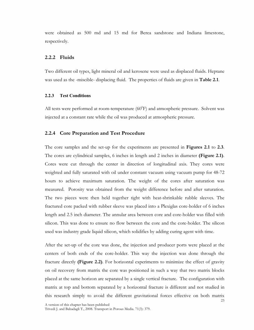
23 A version of this chapter has been published Trivedi J. and Babadagli T., 2008. Transport in Porous Media. 71(3): 379.
were obtained as 500 md and 15 md for Berea sandstone and Indiana limestone,
respectively.
2.2.2 Fluids
Two different oil types, light mineral oil and kerosene were used as displaced fluids. Heptane
was used as the -miscible- displacing fluid. The properties of fluids are given in Table 2.1.
2.2.3 Test Conditions
All tests were performed at room-temperature (600F) and atmospheric pressure. Solvent was
injected at a constant rate while the oil was produced at atmospheric pressure.
2.2.4 Core Preparation and Test Procedure
The core samples and the set-up for the experiments are presented in Figures 2.1 to 2.3.
The cores are cylindrical samples, 6 inches in length and 2 inches in diameter (Figure 2.1).
Cores were cut through the center in direction of longitudinal axis. They cores were
weighted and fully saturated with oil under constant vacuum using vacuum pump for 48-72
hours to achieve maximum saturation. The weight of the cores after saturation was
measured. Porosity was obtained from the weight difference before and after saturation.
The two pieces were then held together tight with heat-shrinkable rubble sleeves. The
fractured core packed with rubber sleeve was placed into a Plexiglas core-holder of 6 inches
length and 2.5 inch diameter. The annular area between core and core-holder was filled with
silicon. This was done to ensure no flow between the core and the core-holder. The silicon
used was industry grade liquid silicon, which solidifies by adding curing agent with time.
After the set-up of the core was done, the injection and producer ports were placed at the
centers of both ends of the core-holder. This way the injection was done through the
fracture directly (Figure 2.2). For horizontal experiments to minimize the effect of gravity
on oil recovery from matrix the core was positioned in such a way that two matrix blocks
placed at the same horizon are separated by a single vertical fracture. The configuration with
matrix at top and bottom separated by a horizontal fracture is different and not studied in
this research simply to avoid the different gravitational forces effective on both matrix

24 A version of this chapter has been published Trivedi J. and Babadagli T., 2008. Transport in Porous Media. 71(3): 379.
blocks. Therefore, the position of the fracture is vertical but the whole core system was
placed and the injection was in horizontal direction.
The same core preparation method was used in all experiments. Note that each core was
used only once to avoid the property change due to cleaning procedure. The cores are
assumed to have similar properties as they were plugged out from the same block. The list
of the experiments conducted in this study is given in Table 2.2.
Heptane was continuously injected through the fracture at a constant rate. The flow rate and
the cumulative volume injected were monitored using ISCO-500 D pumps. The effluent was
collected over time to time and analyzed with a refractometer (Figure 2.3).
The permeability contrast between matrix and fracture was kept as high as possible to ensure
that the viscous flow dominates only in the fracture and the matrix oil is recovered only by
diffusion. No overburden was applied on the cores and the average value of fracture
permeability on the cores was measured as around 8-10 Darcies. This value yields enough
contrast between matrix and fracture permeabilities for viscous flow to be effective only in
the fractures.
2.2.5 Measurement Technique
Because of the small density difference between oil and solvent used here, the need of a
different technique which does not depend on density for determining the composition of
the produced liquid raised. Measurement of refractive index (RI) was used to determine the
relative proportions of the mixture from the production end. The ratio of the speed of light
in air to the speed of light in another media is called “refractive index” (RI). A bench-type
Refractometer supplied by Fisher Scientific was used. The minimum reading of scale
indicates down to 4 places of decimal of the RI values. The accuracy is +/- 0.0002 refractive
units. Proper care was taken to conduct all the readings at same temperature to avoid any
effect of temperature change on the final reading. The RI values for the pure compounds
were measured and a calibration curve was generated with the known percentage of oil
mixed with heptane. This curve is presented in Figure 2.4. Using this curve composition of
the produced liquid was determined.
25 A version of this chapter has been published Trivedi J. and Babadagli T., 2008. Transport in Porous Media. 71(3): 379.
2.2.6 Effect of Water Saturation
Most of the reservoirs at present state are water flooded. Sometimes the percentage of water
present is higher than the oil. Considering this fact we decided to create similar situation.
Two (100%) oil-saturated Berea sandstone cores, packed in heat-shrinkable Teflon sleeve,
were prepared similar way as mentioned earlier in other experiments. These cores were
exposed to water by spontaneous imbibition using imbibition tubes. The recovery was
monitored against time. When oil production through imbibition reached plateau, the cores
were taken out and placed into Plexiglas core-holder as discussed above, similar to the other
experiments for solvent injection. Note that this is a secondary -miscible- recovery after a
primary waterflooding. The solvent injection rates applied for these water imbibed cores
were 3 ml/hr and 6 ml/hr.
2.2.7 Effect of Aging
Aging the rock with oil over a period of time may change the wettability of the rock type and
may cause considerable effect on oil recovery process. Though there is no water in the cores,
aging over longer period of time changes the affinity as well as the contact angle of oil to the
rock. To study this effect, four Berea sandstone cores were aged in mineral oil over one
month. The experimental results as well as the imbibition tests reported in other papers
(Babadagli and Ershaghi, 1993; Babadagli, 2000) indicated that the longer contact time
altered the wettability of the rock to mineral oil. Although the polar components are not as
high as in crude oils, the mineral oil we used showed change in the affinity to oil after aging.
Solvent was injected into these aged samples at the flow rates of 3, 4.5, 6 and 9 ml/hr.
2.2.8 Effect of Viscosity Ratio/Density
In order to analyze the effects of viscosity and density of the non-wetting phase, we
conducted some experiments with kerosene as a non-wetting phase. Cores were saturated
with kerosene under vacuum and prepared in a similar way as other experiments.

26 A version of this chapter has been published Trivedi J. and Babadagli T., 2008. Transport in Porous Media. 71(3): 379.
2.2.9 Effect of Gravity
Gravity also contributes to recovery, mostly when the fracture orientation is vertical. In our
work, we studied the recovery from three samples with vertical orientation of fracture. After
preparing the cores following the same procedure, we mounted them vertically and injected
solvent at three different rates of 1, 3 and 6 ml/hr from the top of the sample downward to
the bottom. For these experiments, we used only mineral oil as the displaced phase.
2.3 Results and Analysis
The recovery curves for the above mentioned experiments are presented in Figures 2.5 to
2.8 as pore volume injected vs. pore volume recovered. Here, recovery of mineral oil was
used as y-axis. In a sense, this is the solvent concentration in the system. We used heptane
as solvent to mimic miscible CO2 displacement in fractured oil reservoirs. As our
preliminary target was oil recovery, we preferred this type of representation in y-axis rather
than solvent concentration.
With capillary drive and pressure drive not affecting the recovery and gravity forces
minimized as the orientation of the cores was horizontal, the only mechanism governing the
process could be diffusion/displacement drive. The diffusion dominant process yields
slower recovery of oil with a delayed solvent breakthrough when the solvent injection rate
was low, but it results in higher ultimate recovery for the horizontal mineral oil-Berea
sandstone cases (Figure 2.5). When comparing the recovery trends for a lower (BSH-3)
and a higher (BSH-6) rate, BSH-6 shows faster initial recovery compared to BSH-3. But
after certain period of time, the BSH-3 case overpasses the production as an evidence of
diffusion controlling mechanism. It is also evident that during the initial phase of the
recovery, the displacement was driven by diffusion between fracture and matrix for lower
rates rather than viscous flow in fracture. Hence, 3ml/hr flow rate overrides the recovery of
6 ml/hr flow rate. Performance of kerosene was also included in this plot. The recovery
rate and ultimate recovery for the kerosene case is remarkably lower than those of mineral
oil cases for the same injection rate. The effect of viscosity and oil type on this process
needs more detailed study and this part of research is on-going

27 A version of this chapter has been published Trivedi J. and Babadagli T., 2008. Transport in Porous Media. 71(3): 379.
The recovery rate behavior for the cases of solvent injection with vertical orientation of
Berea sandstone cores is very similar to that of the horizontal case. But the ultimate
recoveries for all vertical orientated cores turned out to be the same despite different solvent
injection rates (Figure 2.6), unlike the horizontal orientation. The gravity drainage
mechanism might have played a role in the oil recovery process. Similar to the horizontal
Berea sandstone cases, the recovery curve at lower solvent injection rate overpasses the one
at higher solvent injection rate after a certain period of time for the cores with vertical
orientation, i.e., BSV-1, BSV-3 and BSV-6. Initial difference in the recoveries is not much
compared to the difference between the two equivalent horizontal cases (BSH-3 and BSH-
6). Still at a certain point, the recovery of BSV-1 curve overpasses the recovery curves of
higher solvent injection rate cases (BSV-3 and BSV-6). The location of this crossover point
occurs almost at the same time as noticed during horizontal experiments.
In the case of limestone, the recovery trends with 3 ml/hr and 6 ml/hr injection rates are
almost similar to the Berea sandstone cases (Figure 2.8). But the ultimate recoveries are
very low almost half to that of the Berea sandstones.
With the aged samples of Berea sandstone cores, the recovery is lower than the same cores
without aging (Figure 2.9). For the cases of BSH-3A and BSH-6A, aging has a negative
effect on miscible displacement efficiency compared to cases BSH-3 and BSH-6 (Figure
2.7). It is notable that slowest solvent injection rate (3 ml/hr) yielded the highest ultimate
recovery. Similar recovery trends and ultimate recoveries were obtained from all other four
rates.
The recovery curves for the previously depleted matrix cases by water imbibition are shown
in Figure 2.10. The BSH-3W case showed higher ultimate recovery than BSH-6W. The
ultimate recovery after solvent injection into previously water flooded cores were only 55%,
much lower than the one without water flooded (95%). Proving that solvent has diffuses
easily into oil phase rather than water. It shows that starting the process by solvent injection
(diffusion) results in higher ultimate recovery than injecting solvent into already
waterflooded cases.

28 A version of this chapter has been published Trivedi J. and Babadagli T., 2008. Transport in Porous Media. 71(3): 379.
It is clear that the injection rate is a critical parameter as well as the matrix and fluid
properties on the process. Higher injection rates resulted in earlier breakthrough and less
residing time in order for the matrix fracture interaction due to diffusion to take place. This
was more significant for some cases and it even affected the ultimate recovery from the
matrix. Therefore, it is essential to define a critical rate as a function of matrix and fluid
properties. This can be done in two different ways depending on what type of efficiency is
considered. For example, if the critical parameter in the efficiency of the process is the
amount of oil produced per amount of solvent injected, one can define a critical rate
(Babadagli and Ershaghi, 1993). If the critical parameter is the time to complete the process
rather than the amount of injected fluid, then one can define an optimal injection rate as
suggested by a previous study for water imbibition transfer between matrix and fracture
(Babadagli, 2000).
2.4 Efficiency Analysis
In many enhanced oil recovery processes including miscible processes, the amount of
solvent injected per oil recovery is the critical parameter. However, oil recovery rate, i.e.,
process time required to reach the ultimate recovery could also be important because the
time value of money might offset the cost of extra injected solvent. Therefore, the time to
reach the ultimate recovery could be equally important parameter with the amount of solvent
injected in certain circumstances, especially when the oil prices are high. Hence, the
efficiency of the process was analyzed with respect to the diffusion time as well. For this
exercise, the amount of oil produced was plotted against time instead of total amount of
solvent injected. The plots are given in Figures 2.10 to 2.13. Using those plots, the amount
of total oil produced (PV) was plotted against the flow rate at different times. Figures 2.14
to 2.16 show the optimal rate for maximum oil recovery at different diffusion time scale.
The optimal rate was observed to be around 6 ml/hr for the sandstone and limestone
horizontal experiments without aging (Figures 2.14 and 2.15). At the end of the process
after 40-50 hrs, the slower rate (3 ml/hr) overpasses the production obtained from the 6
ml/hr case. This indicates the dominance of the diffusional flow (matrix-fracture
interaction) compared to the viscous flow (in fracture). One can conclude from these results
that, for faster and higher ultimate recovery, the process should be operated at 6 ml/hr at
29 A version of this chapter has been published Trivedi J. and Babadagli T., 2008. Transport in Porous Media. 71(3): 379.
the start and should be switched to 3 ml/hr. Figure 2.16 suggests that there is no optimal
rate for the aged sample as they all followed a similar recovery trend as given in Figure 2.12
regardless the rate. Interestingly enough, the ultimate recoveries of aged samples vary
significantly compared to that obtained from unaged samples.
2.5 Conclusions
Dominance of the phase diffusion into matrix through fracture over viscous flow in the
fracture was shown in this study. Though the higher solvent injection rate yields high
production rate of oil in the initial period of the project life, considering the long run, the
low rate solvent injection strategy is the best with most of the production contribution from
matrix through the diffusion process. Solvent injected at lower rate has more time to diffuse
into matrix in transverse direction before it breaks through, hence results into higher
ultimate recovery than that of higher rate solvent injection strategy.
With some water existing in the rock from previous waterflooding, one can still obtain oil
recovery from matrix by the diffusion process. Note that the ultimate recovery obtained
from the waterflooding followed by the solvent diffusion process would be much lower than
the cases with solvent diffusion only.
The efficiency of the process was investigated using two different parameters. When the
amount of oil produced per time is the critical efficiency parameter, a rate of 6 ml/hr was
found to be the optimal rate for almost all the cases except less water-wet samples. This
approach for efficiency analysis is useful for enhanced oil recovery applications.
In this study, we have not varied two critical parameters; the size of the matrix (length or
width) and oil type (mainly for viscosity variation). Further attempts were made in
subsequent studies where the process has been theoretically modeled using the experimental
observations and considering those parameters (Trivedi and Babadagli, 2007a-b). Also, this
study focused on first contact miscibility. The multi-contact miscible diffusion at reservoir
temperature and pressure is more complex. This case requires more effort and could be
critical especially in the CO2 injection for EOR and sequestration.

30 A version of this chapter has been published Trivedi J. and Babadagli T., 2008. Transport in Porous Media. 71(3): 379.
Figure 2.1: Core-holder design.
Figure 2.2: Core samples cut for fracture creation and the core-holder used.
Teflon heat-shrinkable tub
Matrix
Matrix Fracture
Silicon
Silicon
Plaxy glass core-holder
End caps Core holder

31 A version of this chapter has been published Trivedi J. and Babadagli T., 2008. Transport in Porous Media. 71(3): 379.
Figure 2.3: Experimental set-up. Table 2.1: Properties of displacing and displaced fluids.
Displacing Fluid Displaced Fluid Properties
Heptane Mineral Oil Kerosene
Density (g/cc) 0.69 0.83 0.81
Viscosity (cp) 0.410 33.5 2.1
Refraction Index 1.3891 1.469 1.475
Heptane
Source
ISCO
Pum
Injection
Line
Core
Holder
Production Line
Refractometer
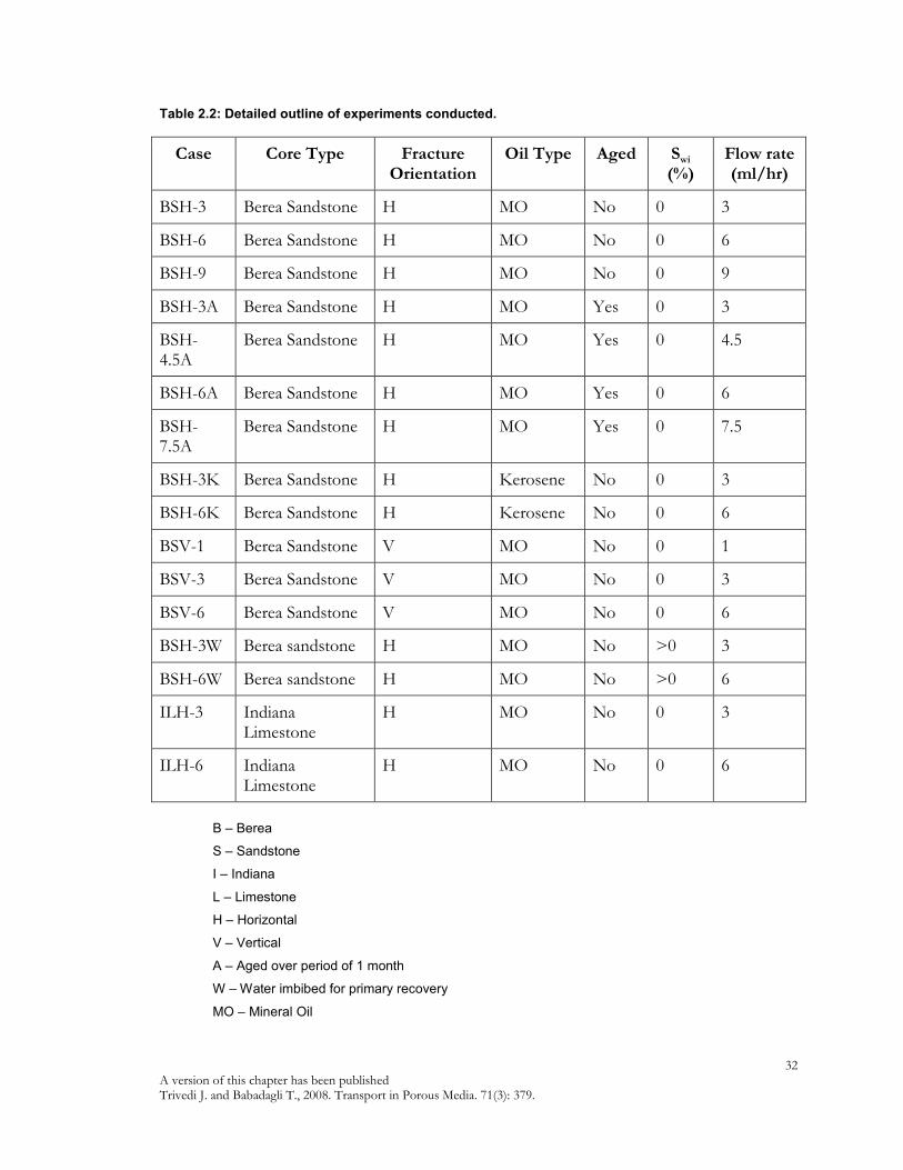
32 A version of this chapter has been published Trivedi J. and Babadagli T., 2008. Transport in Porous Media. 71(3): 379.
Table 2.2: Detailed outline of experiments conducted.
Case Core Type Fracture Orientation
Oil Type Aged Swi (%)
Flow rate (ml/hr)
BSH-3 Berea Sandstone H MO No 0 3
BSH-6 Berea Sandstone H MO No 0 6
BSH-9 Berea Sandstone H MO No 0 9
BSH-3A Berea Sandstone H MO Yes 0 3
BSH-4.5A
Berea Sandstone H MO Yes 0 4.5
BSH-6A Berea Sandstone H MO Yes 0 6
BSH-7.5A
Berea Sandstone H MO Yes 0 7.5
BSH-3K Berea Sandstone H Kerosene No 0 3
BSH-6K Berea Sandstone H Kerosene No 0 6
BSV-1 Berea Sandstone V MO No 0 1
BSV-3 Berea Sandstone V MO No 0 3
BSV-6 Berea Sandstone V MO No 0 6
BSH-3W Berea sandstone H MO No >0 3
BSH-6W Berea sandstone H MO No >0 6
ILH-3 Indiana Limestone
H MO No 0 3
ILH-6 Indiana Limestone
H MO No 0 6
B – Berea
S – Sandstone
I – Indiana
L – Limestone
H – Horizontal
V – Vertical
A – Aged over period of 1 month
W – Water imbibed for primary recovery
MO – Mineral Oil
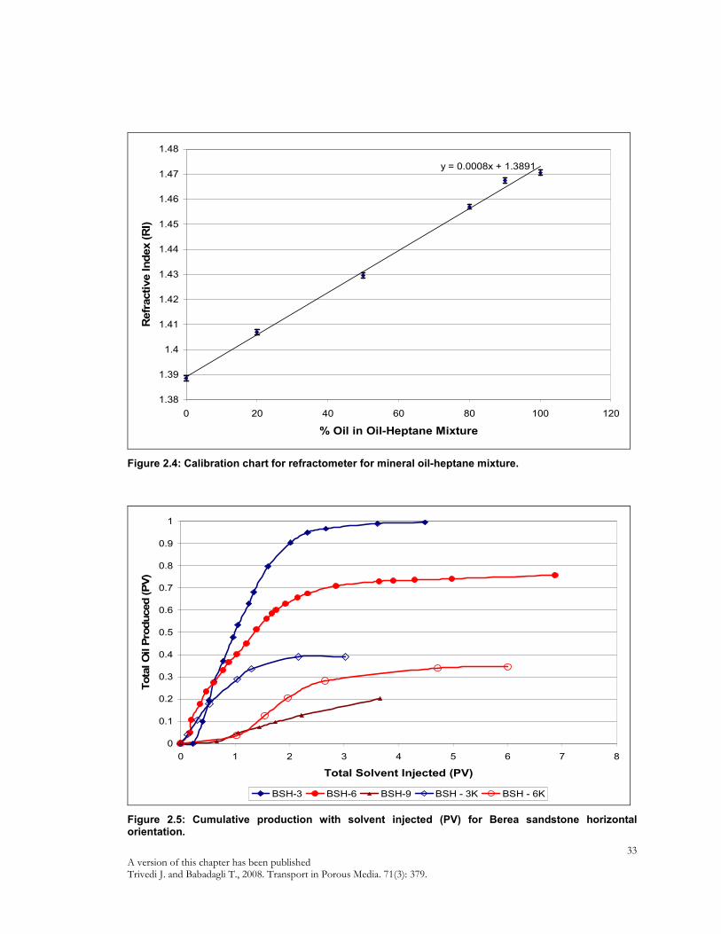
33 A version of this chapter has been published Trivedi J. and Babadagli T., 2008. Transport in Porous Media. 71(3): 379.
y = 0.0008x + 1.3891
1.38
1.39
1.4
1.41
1.42
1.43
1.44
1.45
1.46
1.47
1.48
0 20 40 60 80 100 120
% Oil in Oil-Heptane Mixture
Refr
acti
ve Ind
ex (
RI)
Figure 2.4: Calibration chart for refractometer for mineral oil-heptane mixture.
0
0.1
0.2
0.3
0.4
0.5
0.6
0.7
0.8
0.9
1
0 1 2 3 4 5 6 7 8
Total Solvent Injected (PV)
Tota
l O
il P
roduced (P
V)
BSH-3 BSH-6 BSH-9 BSH - 3K BSH - 6K
Figure 2.5: Cumulative production with solvent injected (PV) for Berea sandstone horizontal orientation.

34 A version of this chapter has been published Trivedi J. and Babadagli T., 2008. Transport in Porous Media. 71(3): 379.
0
0.1
0.2
0.3
0.4
0.5
0.6
0.7
0.8
0.9
1
0 0.5 1 1.5 2 2.5 3 3.5 4 4.5
Total Solvent Injected (PV)
Tota
l O
il P
roduced (P
V)
BSV-1 BSV-3 BSV-6
Figure 2.6: Cumulative production with solvent injected (PV) for Berea sandstone vertical orientation.
0
0.1
0.2
0.3
0.4
0.5
0.6
0.7
0.8
0.9
1
0 1 2 3 4 5 6 7
Total Solvent Injected (PV)
To
tal O
il P
rod
uced
(P
V)
BSH - 3A BSH - 4.5A BSH - 6A BSH -7.5A BSH-9A
Figure 2.7: Cumulative production with solvent injected (PV) for aged Berea sandstone horizontal orientation.

35 A version of this chapter has been published Trivedi J. and Babadagli T., 2008. Transport in Porous Media. 71(3): 379.
0
0.05
0.1
0.15
0.2
0.25
0.3
0.35
0.4
0.45
0.5
0 1 2 3 4 5 6 7 8 9 10
Total Solvent Injected (PV)
To
tal O
il P
rod
ucte
d (
PV
)
3 ml/hr 6 ml/hr 9 ml/hr
Figure 2.8: Cumulative production with solvent injected (PV) for Indiana limestone horizontal orientation.
0
0.1
0.2
0.3
0.4
0.5
0.6
0.7
0.8
0.9
1
0 1 2 3 4 5 6 7 8
Total Solvent Injected (PV)
Tota
l O
il P
roduced (P
V)
BSH-3 BSH-6 BHA-3 BHA-6
Figure 2.9: Cumulative production with solvent injected (PV) comparing aged and unaged Berea sandstone horizontal orientation.
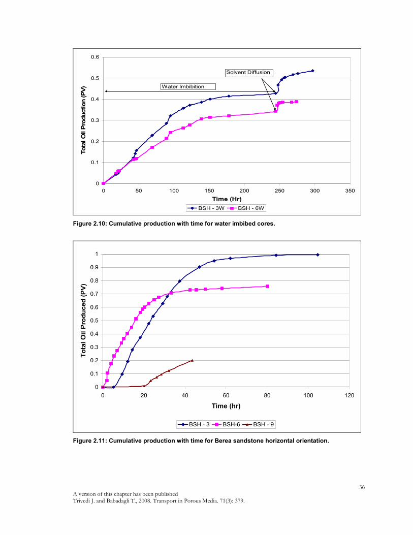
36 A version of this chapter has been published Trivedi J. and Babadagli T., 2008. Transport in Porous Media. 71(3): 379.
0
0.1
0.2
0.3
0.4
0.5
0.6
0 50 100 150 200 250 300 350
Time (Hr)
Tota
l O
il P
roduction (P
V)
BSH - 3W BSH - 6W
Solvent Diffusion
Water Imbibition
Figure 2.10: Cumulative production with time for water imbibed cores.
0
0.1
0.2
0.3
0.4
0.5
0.6
0.7
0.8
0.9
1
0 20 40 60 80 100 120
Time (hr)
To
tal O
il P
rod
uced
(P
V)
BSH - 3 BSH-6 BSH - 9
Figure 2.11: Cumulative production with time for Berea sandstone horizontal orientation.
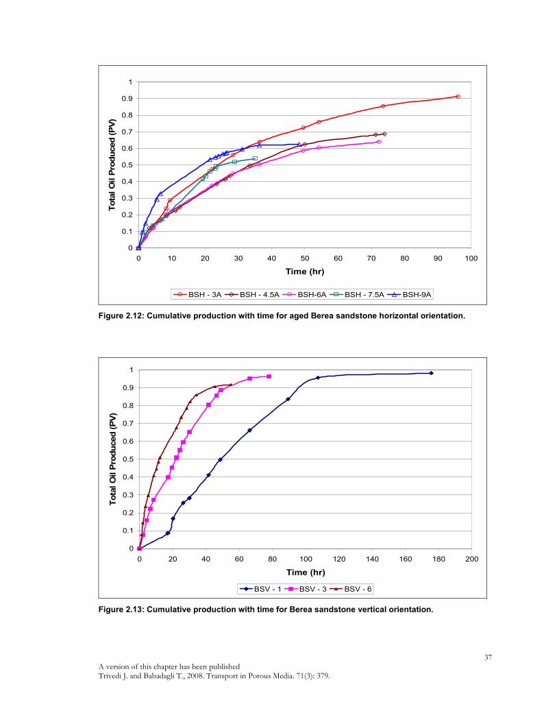
37 A version of this chapter has been published Trivedi J. and Babadagli T., 2008. Transport in Porous Media. 71(3): 379.
0
0.1
0.2
0.3
0.4
0.5
0.6
0.7
0.8
0.9
1
0 10 20 30 40 50 60 70 80 90 100
Time (hr)
Tota
l O
il P
roduced (P
V)
BSH - 3A BSH - 4.5A BSH-6A BSH - 7.5A BSH-9A
Figure 2.12: Cumulative production with time for aged Berea sandstone horizontal orientation.
0
0.1
0.2
0.3
0.4
0.5
0.6
0.7
0.8
0.9
1
0 20 40 60 80 100 120 140 160 180 200
Time (hr)
Tota
l O
il P
rodu
ced (
PV
)
BSV - 1 BSV - 3 BSV - 6
Figure 2.13: Cumulative production with time for Berea sandstone vertical orientation.

38 A version of this chapter has been published Trivedi J. and Babadagli T., 2008. Transport in Porous Media. 71(3): 379.
Horizontal Berea Sandstone
0
0.1
0.2
0.3
0.4
0.5
0.6
0.7
0.8
0.9
1
2 3 4 5 6 7 8 9 10
Flow rate (ml/hr)
To
tal O
il P
rod
ucte
d (
PV
)
20 hrs 30 hrs 40 hrs 80 hrs
Figure 2.14: Cumulative production at different flow rate and time axis for Berea sandstone horizontal orientation.
Horizontal Indiana Limestone
0
0.05
0.1
0.15
0.2
0.25
0.3
0.35
0.4
0.45
0.5
2 3 4 5 6 7 8 9 10
Flow Rate (ml/hr)
Tota
l O
il P
roduced (P
V)
10 hrs 20 hrs 25 hrs 50 hrs 70 hrs
Figure 2.15: Cumulative production at different flow rate and time axis for Indiana limestone horizontal orientation.
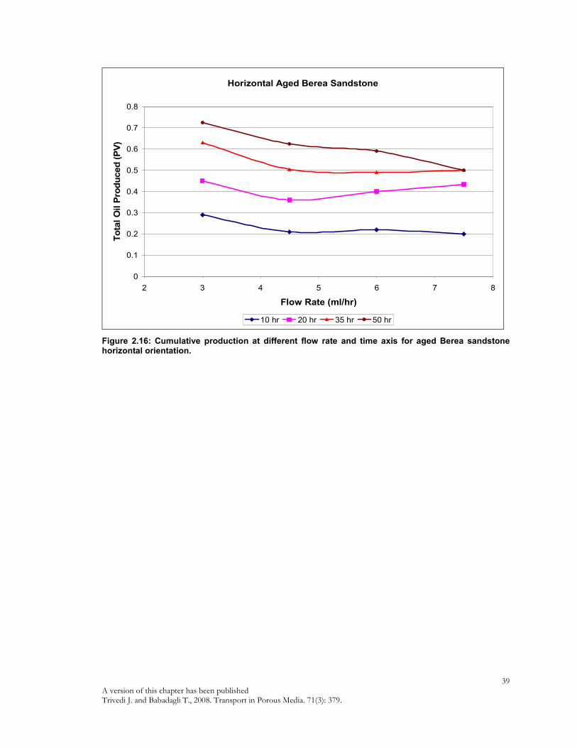
39 A version of this chapter has been published Trivedi J. and Babadagli T., 2008. Transport in Porous Media. 71(3): 379.
Horizontal Aged Berea Sandstone
0
0.1
0.2
0.3
0.4
0.5
0.6
0.7
0.8
2 3 4 5 6 7 8
Flow Rate (ml/hr)
To
tal O
il P
rod
uced
(P
V)
10 hr 20 hr 35 hr 50 hr
Figure 2.16: Cumulative production at different flow rate and time axis for aged Berea sandstone horizontal orientation.

A version of this chapter has been published Trivedi J. and Babadagli T., 2008 (In Press). Chemical Eng. J. doi:10.1016/j.cej.2008.05.032. 40
3 EXPERIMENTAL AND NUMERICAL MODELING OF THE MASS
TRANSFER BETWEEN ROCK MATRIX AND FRACTURE
3.1 Introduction
The target oil in naturally fractured reservoirs (NFR) exists in rock matrix. During the
injection of tertiary recovery materials that are miscible with matrix oil, i.e., hydrocarbon
solvents, alcohols, CO2, N2 etc., fracture network creates the path for the injected solvent to
bypass and leave the unwept oil zones in the matrix. Significant amount of oil can be
recovered from this upswept bypassed zone by maximizing the subsequent crossflow or
mass transfer between fracture and media. Likewise, when greenhouse gases (CO2, pure or
in the form of flue gas) is injected into NFRs, the matrix part could be a proper storage
environment and the transfer of the injected gas to matrix needs to be well understood for
the determination of the process efficiency. The same process is encountered in the
transportation of contaminants and waste material in NFRs.
In general four factors contribute to crossflow/mass transfer: (a) Pressure, (b) gravity, (3)
dispersion/diffusion, and (d) capillary drive. When the bypassed fluid and displacement
fluids are First Contact Miscible (FCM), there is no capillary crossflow. When the fluids are
Multi Contact Miscible (MCM) or immiscible, there could be a certain degree of capillary-
driven crossflow. Burger et al. (Burger et al., 1996; Burger and Mohanty, 1997) found that
capillary driven crossflow does not contribute significantly to mass transfer in near-miscible
hydrocarbon floods. The other three forces play a critical role in the mass transfer between
matrix and fracture and need to be well understood in terms of the effective parameters and
efficiency of the process.
Previously we had performed experiments to clarify the effective parameters on the mass
transfer during solvent injection into fractured systems (Trivedi and Babadagli, 2006). In
this study, the critical rate was defined as the maximum rate beyond which no change in the
ratio of matrix recovery to injected solvent is obtained by increasing rate. As the injection
rate is increased, the injected fluid flowing in the fracture would yield an early breakthrough
A version of this chapter has been published Trivedi J. and Babadagli T., 2008 (In Press). Chemical Eng. J. doi:10.1016/j.cej.2008.05.032. 41
without spending enough time to contact with the matrix. Hence, increasing rates may result
in a faster recovery but higher amount of solvent is needed due to weaker mass transfer
interaction to cause oil production from matrix. This results in an inefficient use of solvent.
Therefore, slower rates are desirable for a better interaction and stronger mass transfer
yielding higher matrix oil recovery to solvent injected ratio. This, however, reduces the
recovery time. Thus, the definition of critical rate is an important issue and the rate depends
on rock and fluid characteristics. The concept of critical velocity was first introduced by
Thompson and Mungan (1969). They compared displacement velocity to critical velocity
(VC) and showed its effect on recovery efficiency. Firoozabadi and Markeset (1994) showed
that the capillary pressure contrast between matrix and fracture could be the major driving
force. Further, they studied the effect of matrix/fracture configuration and fracture aperture
on first contact miscible efficiency.
Advanced visualization studies were also conducted to understand the physics of matrix-
fracture interaction. Part (1993) studied the formation of drying patterns assuming only
capillary forces and neglecting viscous effects. It was the first attempt to theoretically
characterize drying patterns in porous media as well. Computational (Zakirov et al., 1991;
Jensen et al., 1992) and experimental (Lenormand, 1998; Hunjun Li et al., 2000) studies on
the interaction of matrix and fracture for different types of fluids were also reported.
The diffusion process and correlations of the capillary pressure with variation of interfacial
tension were also investigated (Morel et al., 1993; Hu et al., 1991; Gabitto, 1998). Morel et
al. (1993) performed diffusion experiments with chalk and studied the effect of initial gas
saturation. The diffusion/stripping process in fractured media was well described by Saidi
(1987). Recently, there has been success in determining diffusion coefficients between two
miscible fluid systems (Yang and Gu, 2006; Civan and Rasmussen, 2002; Raizi, 1996; Stubos
and Poulou, 1999) but the process is totally different within the fractured porous media,
affected by many parameters such as, matrix properties, condition at the boundaries, fracture
geometry and flow conditions.
The presence of water affects the pore-scale distribution of hydrocarbon phases Pandey and
Orr al., 1990, Mohanty and Salter, 1982). Connectivity and tortuosity of the pore structure
influences the effective diffusivity and the relative permeability of each hydrocarbon phase.
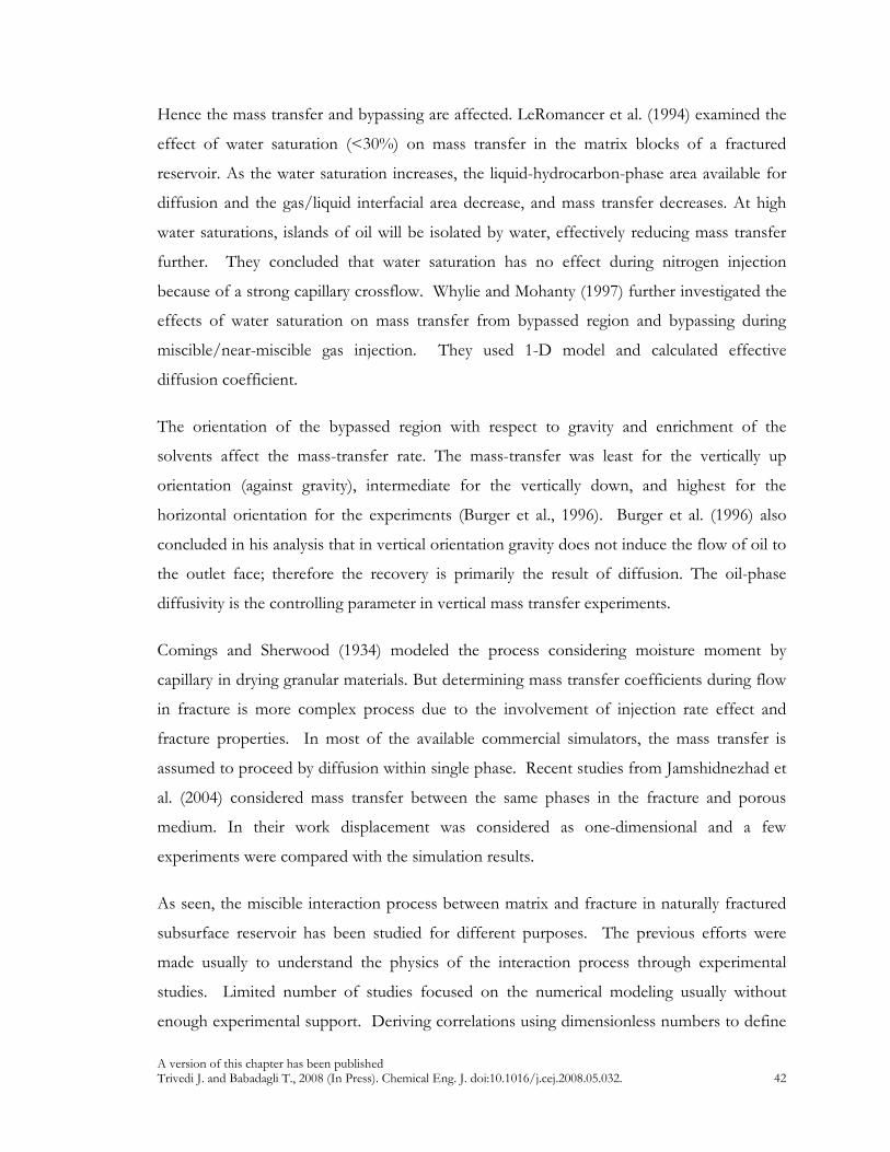
A version of this chapter has been published Trivedi J. and Babadagli T., 2008 (In Press). Chemical Eng. J. doi:10.1016/j.cej.2008.05.032. 42
Hence the mass transfer and bypassing are affected. LeRomancer et al. (1994) examined the
effect of water saturation (<30%) on mass transfer in the matrix blocks of a fractured
reservoir. As the water saturation increases, the liquid-hydrocarbon-phase area available for
diffusion and the gas/liquid interfacial area decrease, and mass transfer decreases. At high
water saturations, islands of oil will be isolated by water, effectively reducing mass transfer
further. They concluded that water saturation has no effect during nitrogen injection
because of a strong capillary crossflow. Whylie and Mohanty (1997) further investigated the
effects of water saturation on mass transfer from bypassed region and bypassing during
miscible/near-miscible gas injection. They used 1-D model and calculated effective
diffusion coefficient.
The orientation of the bypassed region with respect to gravity and enrichment of the
solvents affect the mass-transfer rate. The mass-transfer was least for the vertically up
orientation (against gravity), intermediate for the vertically down, and highest for the
horizontal orientation for the experiments (Burger et al., 1996). Burger et al. (1996) also
concluded in his analysis that in vertical orientation gravity does not induce the flow of oil to
the outlet face; therefore the recovery is primarily the result of diffusion. The oil-phase
diffusivity is the controlling parameter in vertical mass transfer experiments.
Comings and Sherwood (1934) modeled the process considering moisture moment by
capillary in drying granular materials. But determining mass transfer coefficients during flow
in fracture is more complex process due to the involvement of injection rate effect and
fracture properties. In most of the available commercial simulators, the mass transfer is
assumed to proceed by diffusion within single phase. Recent studies from Jamshidnezhad et
al. (2004) considered mass transfer between the same phases in the fracture and porous
medium. In their work displacement was considered as one-dimensional and a few
experiments were compared with the simulation results.
As seen, the miscible interaction process between matrix and fracture in naturally fractured
subsurface reservoir has been studied for different purposes. The previous efforts were
made usually to understand the physics of the interaction process through experimental
studies. Limited number of studies focused on the numerical modeling usually without
enough experimental support. Deriving correlations using dimensionless numbers to define

A version of this chapter has been published Trivedi J. and Babadagli T., 2008 (In Press). Chemical Eng. J. doi:10.1016/j.cej.2008.05.032. 43
matrix-fracture interaction terms is a critical task and that requires a combination of
experimental and simulation work. Though much effort was devoted in defining the
immiscible matrix-fracture interaction through dimensionless terms, less attention has been
given to modeling miscible interaction, especially using controllable parameters such as
injection rate and fluid characteristics. Also in simulation of the matrix-fracture fracture
miscible interaction processes, 2- or 3-D models have to be considered due to transverse
mass transfer to and from the fracture and longitudinal diffusion/dispersion within the
matrix and fracture individually. The understanding of the qualitative nature of the physics
behind the matrix-fracture interaction process and quantitative representation of the
controlling transfer parameters are the objectives of this paper and this was achieved
through a series of experimental and numerical simulation works.
3.2 Experimental Study
Experiments were performed to study and analyze the process of diffusion and dispersion
during flow of solvent into the fracture adjacent to the oil saturated matrix qualitatively with
change in length, solute type (hence the viscosity and density) and aging time with oil in the
fractured porous media. These parameters affect the various forces, viscous and diffusion in
particular, and alter the amount of oil produced and solvent diffused into the matrix with
amount of solvent injected over the period of solvent injection process. Experimental
observations will be useful in comparing and matching the results from the numerical
simulations. Experimental analysis coupled with the numerical modeling will also be used to
define and formulate critical parameters controlling the matrix-fracture interaction/transfer,
which are not practically obtainable through direct experimental measurements or
computations. To simplify the understanding of diffusion drive mechanism, we used first
contact miscible (FCM) case and neglected capillary-driven crossflow. All the experiments
were performed at room temperature and pressure to nullify the crossflow/mass transfer
due to pressure drive.

A version of this chapter has been published Trivedi J. and Babadagli T., 2008 (In Press). Chemical Eng. J. doi:10.1016/j.cej.2008.05.032. 44
3.2.1 Procedure
Cylindrical plugs were cut from 20 inches long cylindrical rods of Berea sandstone (k= 500
md; φ = 0.21) and Indiana limestone (k= 15 md; φ = 0.11) to 6 inches in length and 2
inches in diameter. Then, the samples were fully saturated with different solute under
constant vacuum for 48 hours using a vacuum pump. The saturated cores were cut into two
pieces through the center in the direction of longitudinal axis for the purpose of creating a
fracture. These pieces were held together using heat-shrinkable rubber sleeves.
The fractured core was then placed into Plexiglas holder and the annular space was filled
with silicon to ensure no flow to the annulus between the core and core holder. The solvent
was injected at constant rate from the center of the core and production line was placed at
the center of other end. Injection and production were maintained only through the fracture
while the flow into matrix was only through diffusion/mass transfer.
Flow through fractures was considered in several studies. There are three common ways of
injection: (a) Injection through matrix and production through matrix, while the fracture was
located in the middle of the two matrix blocks, (b) Injection through fracture and produce
through fracture, while there is only one (or two) matrix block adjacent to fracture, and (c)
Injection through circular annular acting as a fracture. In our experiments, we applied the
injection scheme as defined in option (b) considering the fact that the flow will be controlled
by high permeability fractures.
Some experiments were also performed with aged samples. In those cases cores were aged
for a period of one month. Effect of solute viscosity and density were analyzed by using
different solute types (mineral oil, heavy mineral oil, and kerosene).
The samples collected at the production end were analyzed using refractometer. Using the
calibration curve from the known percentage of mixture, refractive index (RI) values were
converted to obtain relative proportions in the production mixture. All the experiments were
performed at room temperature.

A version of this chapter has been published Trivedi J. and Babadagli T., 2008 (In Press). Chemical Eng. J. doi:10.1016/j.cej.2008.05.032. 45
Core preparation and experimental set-up are shown in Figures 3.1 and 3.2, respectively.
The properties of fluids used are given in Table 3.1. Detailed outline of experiments
performed is listed in Table 3.2.
Figure 3.1(a): Core cutting and fracture preparation.
Figure 3.1(b): Core holder design.
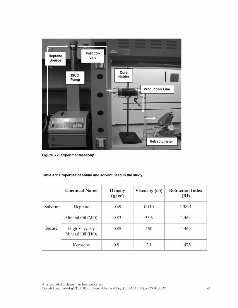
A version of this chapter has been published Trivedi J. and Babadagli T., 2008 (In Press). Chemical Eng. J. doi:10.1016/j.cej.2008.05.032. 46
Figure 3.2: Experimental set-up.
Table 3.1: Properties of solute and solvent used in the study.
Chemical Name Density (g/cc)
Viscosity (cp) Refraction Index (RI)
Solvent Heptane 0.69 0.410 1.3891
Mineral Oil (MO) 0.83 33.5 1.469
High Viscosity Mineral Oil (HO)
0.85 150 1.469
Solute
Kerosene 0.81 2.1 1.475

A version of this chapter has been published Trivedi J. and Babadagli T., 2008 (In Press). Chemical Eng. J. doi:10.1016/j.cej.2008.05.032. 47
Table 3.2: Details of experiments performed.
Case Core Type Angle (Deg)
Solute Type
Flow rate (ml/hr)
Matrix length (inches)
Aged
BSH-3 Sandstone 0 MO 3 6 No
BSH-6 Sandstone 0 MO 6 6 No
BSH-9 Sandstone 0 MO 9 6 No
BHA-3 Sandstone 0 MO 3 6 Yes
BHA-4.5 Sandstone 0 MO 4.5 6 Yes
BHA-6 Sandstone 0 MO 6 6 Yes
BHA-9 Sandstone 0 MO 9 6 Yes
BSK-3K Sandstone 0 Kerosene 3 6 No
BSK-6K Sandstone 0 Kerosene 6 6 No
BSV-3 Sandstone 90 MO 3 6 No
BSV-6 Sandstone 90 MO 6 6 No
HO-3 Sandstone 0 HO 3 6 No
HO-6 Sandstone 0 HO 6 6 No
HO-3 (3”) Sandstone 0 HO 3 3 No
HO-6 (3”) Sandstone 0 HO 6 3 No
HOA-3 Sandstone 0 HO 3 6 Yes
HOA-6 Sandstone 0 HO 6 6 Yes
ILH-3 Limestone 0 MO 3 6 No
ILH-6 Limestone 0 MO 6 6 No
H – Horizontal
V – Vertical
A – Aged over period of 1 month
MO – Mineral Oil
HO – High Viscosity Oil

A version of this chapter has been published Trivedi J. and Babadagli T., 2008 (In Press). Chemical Eng. J. doi:10.1016/j.cej.2008.05.032. 48
3.3 Experimental Observations
We used the plot of total solvent injection (as pore volume) vs. total oil (solute) recovered
(as pore volume) to represent the results. The recovery of solute (oil) in y-axis corresponds
to solvent concentration in the system. Because our main target was oil recovery in this
particular study, we preferred to use solute recovered in y-axis rather than solvent
concentration.
The diffusion dominant displacement front progresses slower when injecting solvent at a
lower rate for all three solutes (oils) (Figure 3.3). Although the solute recovery rates are
slower compared to that of higher rate solvent injection, the final recoveries are higher for
the lower rates. It was observed that the initial phase of the recovery curves are dominated
by displacement or viscous forces and the diffusion comes into picture at later stage. Such
phenomena can be detected at the point when recovery curve of BHS-3 overpasses that of
BHS-6 as marked by an arrow in Figure 3.3.
0
0.1
0.2
0.3
0.4
0.5
0.6
0.7
0.8
0.9
1
0 1 2 3 4 5 6 7
To
tal S
olu
te R
ec
ove
red
(P
ore
Vo
lum
e)
Total Solvent Injected (Pore Volume)
BSH-3 BSH-6 BSH - 3K BSH - 6K HO-3 HO-6
Figure 3.3: Solute recoveries during solvent diffusion for different oil types.

A version of this chapter has been published Trivedi J. and Babadagli T., 2008 (In Press). Chemical Eng. J. doi:10.1016/j.cej.2008.05.032. 49
Different solute types, i.e. different densities and viscosities, may take part in the diffusion
process between matrix and fracture. Some experiments were conducted to elaborate the
range of viscosity and density of solute used. We used high viscosity mineral oil and
kerosene for this purpose. Though the ultimate recoveries are lower for heptane diffusing
into high viscosity mineral oil saturated sandstone, the crossover of lower rate injection case
(HO-3) to higher rate injection case (HO-6) was evident (Figure 3.3). Interestingly, it
occurred after certain amount of pore volume solvent injected (or time). In case of kerosene,
we were not able to capture this point. It possibly occurred either at very early stage of the
process or did not ever happen. The lower-rate-diffusive-transfer dominates the solute
production throughout the process. Based on these observations, one can conclude that
density difference controls the process rather than the viscosity difference.
In contrast to the horizontal case where the effect of different flow rates was significant on
ultimate recovery, the ultimate recoveries were similar during solvent diffusion at different
rates in the vertically oriented sandstone (Figure 3.4). However, solute recovery trends were
in agreement with those of horizontal cases. It is worth noting that the BV-3 case
overpasses the BV-6 case at around 40% of solute production. This turning point is higher
than the point where BHS-3 overpasses the BHS-6. The total amounts of solute produced
were also higher with almost similar amount of solvent required to reach the plateau of
ultimate recovery, which makes a strong point of gravity influence.

A version of this chapter has been published Trivedi J. and Babadagli T., 2008 (In Press). Chemical Eng. J. doi:10.1016/j.cej.2008.05.032. 50
0
0.1
0.2
0.3
0.4
0.5
0.6
0.7
0.8
0.9
1
0 1 2 3 4 5 6 7
To
tal S
olu
te R
ec
ove
red
(P
ore
Vo
lum
e)
Total Solvent Injected (Pore Volume)
BSH-3 BSH-6 BV-3 BV-6
Figure 3.4: Solute recoveries during solvent diffusion for horizontal and vertical cases.
The role of porosity and permeability was proved to be significant when similar injection and
experimental conditions were applied for mineral oil saturated Berea sandstone and Indiana
limestone (Figure 3.5). The ultimate recovery from the limestone sample is almost half of
the recovery observed in the sandstone cores. The trend was very much alike of sandstones
where slower rate process overpasses the higher rate process at the same point of recovery.
Noticeably this transition took place at nearly 35% oil production, just a bit higher than that
of horizontal and vertical sandstone cases (30%). This point comes much later stage of time
compared to that in sandstone, meaning that the poor porosity and permeability of the
medium yield less efficient process.
Core aging affects the recovery trends. The recovery rate of mineral oil is slower and the
ultimate recovery is lower for the aged Berea sandstones compared to those of non-aged
samples. Figure 3.6 points out the influence of aging on miscible flood efficiency. The
comparison of such effect on recovery curves is illustrated using the cases of 3 ml/hr and 6
ml/hr flow rates for non-aged mineral oil saturated Berea sandstones and aged one (for a

A version of this chapter has been published Trivedi J. and Babadagli T., 2008 (In Press). Chemical Eng. J. doi:10.1016/j.cej.2008.05.032. 51
period of one month). No significant difference in terms of ultimate recovery was observed
between aged and non-aged samples for heavy-mineral oil (Figure 3.7). The amount of pore
volume injected for obtaining ultimate recovery was also found unchanged with marginal
difference compared to that of non-aged-viscous-oil-sandstone cases.
0
0.1
0.2
0.3
0.4
0.5
0.6
0.7
0.8
0.9
1
0 1 2 3 4 5 6 7
To
tal S
olu
te R
ec
ove
red
(P
ore
Vo
lum
e)
Total Solvent Injected (Pore Volume)
BSH-3 BSH-6 IH-3 IH-6
Figure 3.5: Solute recoveries during solvent diffusion comparing Berea sandstone and Indiana limestone cores.

A version of this chapter has been published Trivedi J. and Babadagli T., 2008 (In Press). Chemical Eng. J. doi:10.1016/j.cej.2008.05.032. 52
0
0.1
0.2
0.3
0.4
0.5
0.6
0.7
0.8
0.9
1
0 1 2 3 4 5 6 7
To
tal S
olu
te R
ec
ove
red
(P
ore
Vo
lum
e)
Total Solvent Injected (Pore Volume)
BSH-3 BSH-6 BHA-3 BHA-6
Figure 3.6: Comparison of the solute recoveries during solvent diffusion for the aged and non-aged samples.
0
0.1
0.2
0.3
0.4
0.5
0.6
0.7
0.8
0.9
1
0 1 2 3 4 5 6 7
To
tal S
olu
te R
ec
ove
red
(P
ore
Vo
lum
e)
Total Solvent Injected (Pore Volume)
HO-3 HO-6 HOA-3 HOA-6
Figure 3.7: Solute recoveries during solvent diffusion from high viscosity mineral oil aged and non-aged core samples.

A version of this chapter has been published Trivedi J. and Babadagli T., 2008 (In Press). Chemical Eng. J. doi:10.1016/j.cej.2008.05.032. 53
0
0.1
0.2
0.3
0.4
0.5
0.6
0.7
0.8
0 1 2 3 4 5 6
To
tal S
olu
te R
ec
ove
red
(P
ore
Vo
lum
e)
Total Solvent Injected (Pore Volume)
HO-3 (3") HO-6 (3") HO-3 (6") HO-6 (6")
Figure 3.8: Solute recoveries during solvent diffusion comparing 3” and 6” longer samples.
When the size of the core was changed from 6 inch to 3 inch (Figure 3.8), no significant
effect was observed between the ultimate recoveries of the flow rate of 3 ml/hr and 6 ml/hr
cases. But, more solvent needs to be injected to reach the same ultimate recovery in case of
shorter samples, implying that the recovery rate is lower. Solvent does not have enough time
to contact with the rock matrix to diffuse into the matrix to sweep out the solute before it
breaks through for the shorter samples. Hence, the length of the matrix size in determining
the efficient transfer conditions is also important.
3.4 Modeling of Fracture-Matrix Transfer Process
Fracture-matrix transfer process was modeled numerically and presented in the form of
dimensionless groups to analyze the effects of different parameters quantitatively. The
process experimentally analyzed in the previous section was simulated using finite element
modeling with the governing advection-convection equations and the Darcy equation. Only

A version of this chapter has been published Trivedi J. and Babadagli T., 2008 (In Press). Chemical Eng. J. doi:10.1016/j.cej.2008.05.032. 54
parameters other than those unavailable from the laboratory scale experiments are
diffusion/dispersion coefficients and mass transfer coefficients in the matrix as well as in the
fracture. These parameters were obtained through matching the numerical modeling results
to their experimental equivalents and then they were correlated to fluid-rock properties and
flow velocity.
3.4.1 Analogy between Monolith Catalysts (Reactor) and Matrix-Fracture
Systems
Monolithic catalysts have gained recent interest for reducing pollution (Cybulski and Moulin,
1998) due to simultaneous advantages of very low pressure drop, short diffusion resistance,
excellent mass transfer and high surface to volume ratio. They are also widely used in
selective catalytic reduction of NOx, hydrogenations of liquid phase, power generation using
gas turbines (Cybulski and Moulin, 1994; Forzatti, 2001).
Monolithic catalysts/reactors (Figure 3.9) consist of a matrix of uniformly aligned parallel
channels. The diameter of the channel ranges from 0.5 to 10 mm and length can be up to 1
meter long. These channels are fabricated on either ceramic or metallic supports called
substrates. On the walls of the channels a catalytic active layer (a porous layer), 10 to 200 µm
thick, can be applied. It is commonly called as washcoat. The flow is laminar in monolithic
reactor for most of the applications with the Reynolds number typically in the range 10-
1000. The reactants in the fluid phase are transported to the surface of the catalyst by
convection and from the surface of the catalyst to the active sites of the catalyst by diffusion.
The reactants react on the active catalysts sites which results in release or absorption of heat.
The presence of catalytic reactions at the wall of the channel acts as a source or sink, which
imposes temperature or concentration gradients in the radial directions.
The magnitude of radial gradients depends on the relative rates of heat and mass transfer
and chemical reaction. There are two important types of potential mass transfer limitation in
these reactors. The first is diffusion limitation in the washcoat owing to fast reaction. The
rate of reaction is controlled by the intrinsic kinetics only and the reactor is said to be in
kinetically controlled regime. If the rate of diffusion is lower than the intrinsic rate of
reaction, the bulk and surface conditions are different. In the extreme case, the catalyst
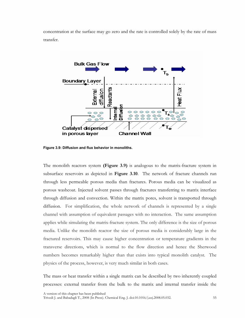
A version of this chapter has been published Trivedi J. and Babadagli T., 2008 (In Press). Chemical Eng. J. doi:10.1016/j.cej.2008.05.032. 55
concentration at the surface may go zero and the rate is controlled solely by the rate of mass
transfer.
Figure 3.9: Diffusion and flux behavior in monoliths.
The monolith reactors system (Figure 3.9) is analogous to the matrix-fracture system in
subsurface reservoirs as depicted in Figure 3.10. The network of fracture channels run
through less permeable porous media than fractures. Porous media can be visualized as
porous washcoat. Injected solvent passes through fractures transferring to matrix interface
through diffusion and convection. Within the matrix pores, solvent is transported through
diffusion. For simplification, the whole network of channels is represented by a single
channel with assumption of equivalent passages with no interaction. The same assumption
applies while simulating the matrix-fracture system. The only difference is the size of porous
media. Unlike the monolith reactor the size of porous media is considerably large in the
fractured reservoirs. This may cause higher concentration or temperature gradients in the
transverse directions, which is normal to the flow direction and hence the Sherwood
numbers becomes remarkably higher than that exists into typical monolith catalyst. The
physics of the process, however, is very much similar in both cases.
The mass or heat transfer within a single matrix can be described by two inherently coupled
processes: external transfer from the bulk to the matrix and internal transfer inside the

A version of this chapter has been published Trivedi J. and Babadagli T., 2008 (In Press). Chemical Eng. J. doi:10.1016/j.cej.2008.05.032. 56
porous matrix. Hence, the steady-state behavior of a single matrix can be mathematically
described by convection – diffusion equation in the fluid phase coupled with the diffusion–
reaction equation within the porous media involving more than one spatial dimension similar
to the single monolith channel reactor.
The shape of the washcoat geometry has large influence on the final conversion of reactants
and mass transfer rate because of their small size (µm scale). While the matrix assumed here
is of significantly larger size (cm scale) and considered rectangular shape. The effect of
matrix shape is not the scope of this research and has to be focused separately.
Figure 3.10: Diffusion and flux in matrix-fracture system.
3.4.2 Mathematical Model Formulation
The assumptions in the derivation of the equations are as follows:
• All fractures of the system are equivalent with uniform flow distribution and
represent the network of fractures by a single straight channel.
• The oil is assumed to be dispersed uniformly within the porous matrix.

A version of this chapter has been published Trivedi J. and Babadagli T., 2008 (In Press). Chemical Eng. J. doi:10.1016/j.cej.2008.05.032. 57
• In this analysis, we do not impose any restriction on the geometric shape of the
fracture, except that the cross section of the fracture is invariant with the axial
position.
• The flow is laminar and fully developed.
• The aspect ratio of the channel is assumed to be small; that is, the hydraulic diameter
is much smaller than the length of the fracture (which is true for most of the
practical applications). This assumption justifies the use of fully developed velocity
profile within the channel and also leads to the simplification of negligible axial
diffusion in both fluid phase and matrix compared to the convective transport rate.
• The flow in the fracture is assumed isothermal.
• Solvent flows only through fractures; there is no flow in the matrix surrounding
fracture.
• The variations of physical properties (such as density, viscosity, diffusivities, and so
on) and velocity with temperature and compositions are neglected.
Figure 3.11(a): Geometrical representation of matrix-fracture system used in this study (not to scale).
Figure 3.11(a) represents the matrix-fracture system (length = l and radius = 2r) with inlet,
outlet as well as the boundary conditions. The pore space of the matrix is initially filled with
a displaced fluid (CM = 1) and is flooded with a displacing fluid (CF = 1) from one side x = 0
at the center, where fracture (half aperture = b) is located. The x-axis is the principle flow
C = C0
y
x
l
r b
Matrix
Matrix
Fracture
0,0 21 =∂
∂=
∂
∂
y
CM
y
CM
0
,0
2
1
=∂
∂
=∂
∂
x
CM
x
CM
0
,0
2
1
=∂
∂
=∂
∂
x
CF
x
CF
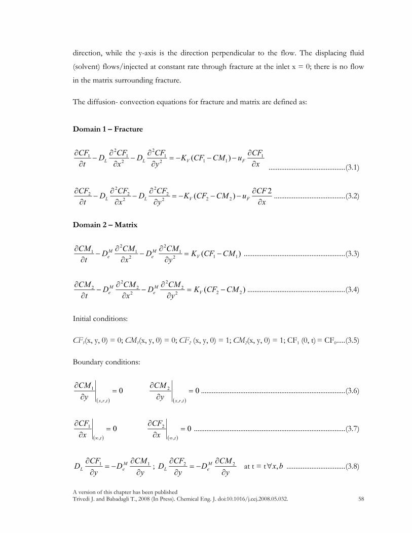
A version of this chapter has been published Trivedi J. and Babadagli T., 2008 (In Press). Chemical Eng. J. doi:10.1016/j.cej.2008.05.032. 58
direction, while the y-axis is the direction perpendicular to the flow. The displacing fluid
(solvent) flows/injected at constant rate through fracture at the inlet x = 0; there is no flow
in the matrix surrounding fracture.
The diffusion- convection equations for fracture and matrix are defined as:
Domain 1 – Fracture
x
CFuCMCFK
y
CFD
x
CFD
t
CFFVLL ∂
∂−−−=
∂∂
−∂
∂−
∂∂ 1
112
1
2
2
1
2
1 )(
...........................................(3.1)
x
CFuCMCFK
y
CFD
x
CFD
t
CFFVLL ∂
∂−−−=
∂∂
−∂
∂−
∂∂ 2
)( 222
2
2
2
2
2
2 ........................................(3.2)
Domain 2 – Matrix
)( 112
1
2
2
1
2
1 CMCFKy
CMD
x
CMD
t
CMV
M
e
M
e −=∂
∂−
∂∂
−∂
∂.........................................................(3.3)
)( 222
2
2
2
2
2
2 CMCFKy
CMD
x
CMD
t
CMV
M
e
M
e −=∂
∂−
∂∂
−∂
∂.......................................................(3.4)
Initial conditions:
CF1(x, y, 0) = 0; CM1(x, y, 0) = 0; CF2 (x, y, 0) = 1; CM2(x, y, 0) = 1; CF1 (0, t) = CF0.....(3.5)
Boundary conditions:
( )
0,,
1 =∂
∂
trxy
CM
( )
0,,
2 =∂
∂
trxy
CM.................................................................................(3.6)
( )0
,
1 =∂
∂
∞ tx
CF
( )0
,
2 =∂
∂
∞ tx
CF.....................................................................................(3.7)
y
CMD
y
CFD M
eL ∂
∂−=
∂
∂ 11 ; y
CMD
y
CFD M
eL ∂
∂−=
∂
∂ 22 at t = t bx,∀ .................................(3.8)

A version of this chapter has been published Trivedi J. and Babadagli T., 2008 (In Press). Chemical Eng. J. doi:10.1016/j.cej.2008.05.032. 59
We used Finite Element Method (FEM) to solve the partial differential equation using
COMSOL multiphysic (2006). The finite element method approximates a PDE problem
with a problem that has a finite number of unknown parameters. The advantages of FEM
are the ease of handling complex geometries, straightforward implementation of non-
uniform meshes and the simple incorporation of flux boundary conditions. Galerkin method
is used to solve the partial differential equations.
The system is described by Eqs. (3.1) through (3.4), with the initial and boundary conditions
given in Eqs. (3.5) through (3.8). The grid size in the fracture is maintained constant while
the grid size varies in the matrix. Transient analysis with time dependent solver (direct
(Spooles) linear system solver) is used. The Spooles linear solver makes use of the symmetry
in the diffusion equation and saves memory. A second order in space and time discretization
is adopted with an implicit time stepping to achieve accurate results. The temporal
simulations with increasing time steps starting with a small time step are made. The
simulation results were compared with the results of experimental performed earlier. From
the numeric simulations, values of Kv and DeM were obtained. In fact, they are the two
critical parameters controlling the matrix-fracture interaction and functions of several
different flow, fluids, fracture, and matrix properties. All other parameters were
experimentally available, measurable, or computable. Comparison of simulated and
experimental results is shown for two different cases in Figure 3.11(b).
Note that the early time behavior (initial straight line portion before the curvature) was
observed to be dominated by the Kv and the later part by the DeM. The early time behavior is
not controlled by the DeM. Therefore, the solution of the equation is assumed to be unique.

A version of this chapter has been published Trivedi J. and Babadagli T., 2008 (In Press). Chemical Eng. J. doi:10.1016/j.cej.2008.05.032. 60
Figure 3.11(b): Simulation match with the experimental results of solute (mineral oil) concentration (C2) change for two different rates on aged Berea sandstone cores.
3.4.3 Dispersion and Diffusion
Miscible recovery is the process in which solvent and solute are completely miscible with
each other either first-contact or multi-contact. The concentration changes from that of
solute to solvent inside the porous media till the equilibrium reaches. Due to miscible nature
of the process (no interfacial tension), in such process there is no existence of capillary or
inter-phase forces. Theoretically complete sweep is possible and 100% recovery of solute can
be achieved at the equilibrium stage. The driving forces are molecular diffusion and
convection.
During the flow through porous media, the additional mixing caused by uneven flow or
concentration gradient is called dispersion. It results from the different paths and speeds and
the consequent range of transit times available to tracer particles convected across a

A version of this chapter has been published Trivedi J. and Babadagli T., 2008 (In Press). Chemical Eng. J. doi:10.1016/j.cej.2008.05.032. 61
permeable medium. Dispersive mixing is a resultant of molecular diffusion and mechanical
dispersion. Perkins and Johnston (1963) have provided an analysis of the dispersion
phenomena and correlations for two types of dispersion; (1) longitudinal direction, and (2)
transverse to the direction of gross fluid movement. Both, having different magnitude, have
to be considered separately. Dispersive mixing plays important role in determining how
much solvent will dissolve/mix with solute to promote miscibility. Molecular diffusion will
cause mixing along the interface. The net result will be a mixed zone growing at a more rapid
rate than would obtain from diffusion alone. Diffusion is a special case of dispersion and a
result of concentration gradient, with or without the presence of the velocity field (Bear,
1988; Sahimi et al., 1982).
Gillham and Cherry (1982) defined the hydrodynamic dispersion coefficient as the sum of
coefficient of mechanical dispersion (Dmech) and the effective diffusion coefficient in the
porous media (Deff). The hydrodynamic dispersion coefficient is also referred as dispersion-
diffusion coefficient (DL).
effmechL DDD += .......................................................................................................................(3.9)
The mechanical dispersion is proportional to the average linearized pore-water velocity (V)
and the dispersivity (α) (Bear, 1979; Freeze and Cherry, 1979). The effective diffusion
coefficient is related to diffusion coefficient in free solution and tortuosity.
Taylor (1953) showed that in case of substantial diffusion perpendicular to the average fluid
velocity, the dispersion coefficient in the tube would be proportional to the square of the
average fluid velocity. Later, Horne and Rodriguez (1983) concluded that in the diffusion
dominated system, the dispersion coefficient in the single, straight, parallel plate fracture will
be proportional to the square of the fluid velocity. Keller et al. (1999) showed that dispersion
coefficient and velocity has linear relationship, where DL α V. Bear (1979) suggested that
the relation between dispersion coefficient and the average fluid velocity would be DL = α *
Vn. The range of the n value is limited to 1.0 ≤ n ≤ 2.0.
From the findings of Ippolite et al. (1984) and Roux et al. (1998), it is known that the
dispersion coefficient in the variable aperture fracture is the sum of molecular diffusion,
Taylor dispersion and microscopic dispersion.

A version of this chapter has been published Trivedi J. and Babadagli T., 2008 (In Press). Chemical Eng. J. doi:10.1016/j.cej.2008.05.032. 62
The Peclet number Pe for the flow in fracture is defined as;
mD
bVPe
*= ................................................................................................................................. (3.10)
where V is average fluid velocity in the fracture, b is the fracture aperture and Dm is the
molecular diffusion coefficient.
Dronfield and Silliman (1993) conducted transport experiments in sand-roughened analog
fracture and came up with a relation as DL α Pe1.4. He also suggested that the power term to
be 2 for parallel plate fracture and 1.3 to 1.4 for rough fractures. Detwiler et al. (2000)
studied the effect of Pe on DL using experiments and numerical results. His investigations
were in accordance with that of earlier from Ippolite et al (1984) and Roux et al. (1998).
Molecular diffusion dominates within the regime of Pe<<1. The Taylor dispersion and
microscopic dispersion are related to Pe. The Taylor dispersion is proportional to Pe2 while
microscopic dispersion is proportional to Pe. Detwiller et al. (2000) showed quadratic
relation from the result of Roux et al. (1998) in the form of a first-order approximation of
the total non-dimensional longitudinal dispersion coefficient:
ταα ++= )()( 2 PePeD
DmacroTaylor
m
L ..................................................................................... (3.11)
They further mentioned that for typical Pe ranges,τ (tortuosity for fracture) can be
neglected.
The Taylor dispersion coefficient defined for parallel plate fracture is: (Taylor, 1953; Aris,
1956; Fischer et al., 1979)
m
TaylorLD
bVD
22
,210
1= ............................................................................................................... (3.12)
2
22,
210
1
mm
TaylorL
D
bV
D
D= ............................................................................................................... (3.13)

A version of this chapter has been published Trivedi J. and Babadagli T., 2008 (In Press). Chemical Eng. J. doi:10.1016/j.cej.2008.05.032. 63
2
, )(210
PeD
D mTaylorL ∗= ............................................................................................................. (3.14)
In our case, we assumed DL α (Pe)1.5, an average value of Taylor and microscopic
dispersions, and used this calculated value for the dispersion coefficient in fracture. The
value of Dm in our set of experiments will be the mutual diffusion coefficient of heptane and
particular oil type. It is 3.2x10⁻⁹ m2/s and 3x10⁻⁸ m2/s for heptane-mineral oil and heptane-
kerosene, respectively.
3.5 Mass Transfer Rate Constant and Effective Diffusion into Porous
Matrix
In simple terms, mass transfer is moving of fluid material from one point to another. For
porous media it is the getting the material into and out of pores. Also for reactive process,
the speed at which a chemical reaction proceeds, in terms of amount of product formed or
amount of reactant consumed is also important. When there is no reaction, transfer rate is
mostly due to diffusion and mixing. This transfer rate between two fluid pairs, solvent and
solute, is presented by mass transfer rate constant (Kv). The increase of Kv indicates better
mixing of solvent and solute, which results in faster approach to equilibrium conditions.
Figure 3.12 clearly suggests that KV is related to velocity, solvent-solute properties, and
matrix properties as well as aging. Increase of velocity results into rapid circulation,
enhanced mixing and better mass transfer. It is also evident that with the same type of cores
and aging time, the increase in KV is controlled mainly by the velocity (Figure 3.12). As the
velocity increases, the rate constant value increases and the values vary from each other with
considerable margin.

A version of this chapter has been published Trivedi J. and Babadagli T., 2008 (In Press). Chemical Eng. J. doi:10.1016/j.cej.2008.05.032. 64
y = 0.5132x - 0.0054
y = 0.0922x + 0.0001
y = 0.7739x - 0.0094
0
0.005
0.01
0.015
0.02
0.025
0.01 0.015 0.02 0.025 0.03 0.035 0.04
Velocity (m/s)
Kv
Aged Berea Unaged Indiana Unaged Berea
Linear (Aged Berea) Linear (Unaged Indiana) Linear (Unaged Berea)
Figure 3.12: Mass transfer rate constant with velocity.
Different amount of solute recoveries were observed when cores were aged for different
periods of time after complete saturation (Figures 3.6 and 3.7). Though there is no water
present in core samples, this can be interpreted as wettability change. To quantify the effect
of aging time (or wettability change), we used spontaneous water imbibition data presented
by Hatiboglu and Babadagli (2004) and Trivedi and Babadagli (2008a) and on the same core
and oil types based on Handy’s approach (1960).
tSAP
Qw
wwC
w
=
µφκ 2
2 2.......................................................................................................... (3.15)
The initial slop of the straight line from Q2 against time were measured and normalized
against the highest slope to obtain the Pc (known as effective capillary pressure). The
changing slope reflects changing wettability caused by the aging as all other rock and fluid
properties remained the same as observed by Trivedi and Babadagli (2008a).
The capillary pressures obtained from the experimental results of Hatiboglu and Babadagli
(2004) and Trivedi and Babadagli (2008a) were normalized based on the capillary pressure of

A version of this chapter has been published Trivedi J. and Babadagli T., 2008 (In Press). Chemical Eng. J. doi:10.1016/j.cej.2008.05.032. 65
kerosene and multiplied with viscosity ratio of solvent to solute to get wettability factor
Trivedi and Babadagli (2008a). To incorporate the effect of solute viscosity we defined the
following dimensionless term (wettability factor, W factor).
=
1
2
µµ
CK
C
factorP
PW ............................................................................................................. (3.16)
Pc is obtained for each oil and rock type using Eq. 15 and PCK is the Pc value for kerosene,
which gives the highest slope due to its strong imbibition into matrix driven by its low
viscosity.
To quantify the transfer rate constant for different wettability and porosity cores, it was
represented as a function of velocity, wettability factor (Wfactor), porosity of matrix, viscosity
and density ratio of solute and solvent.
= −
1
2
06.0
1
29.015.0 **)(*)(*ρρ
µµ
φFactorV WVK .................................................................. (3.17)
Figure 3.13: Comparison of the Kv (s
-1) values obtained through the numerical simulation and the
ones obtained from Equation (3.17).
0
0.001
0.002
0.003
0.004
0.005
0.006
0.007
0.008
0.009
0.01
0 0.001 0.002 0.003 0.004 0.005 0.006 0.007 0.008 0.009 0.01
Kv - Calculated value (S-1)
Kv v
alu
e -
used
fo
r sim
ula
tio
n m
atc
h (
S-1
)
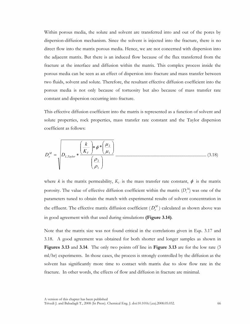
A version of this chapter has been published Trivedi J. and Babadagli T., 2008 (In Press). Chemical Eng. J. doi:10.1016/j.cej.2008.05.032. 66
Within porous media, the solute and solvent are transferred into and out of the pores by
dispersion-diffusion mechanism. Since the solvent is injected into the fracture, there is no
direct flow into the matrix porous media. Hence, we are not concerned with dispersion into
the adjacent matrix. But there is an induced flow because of the flux transferred from the
fracture at the interface and diffusion within the matrix. This complex process inside the
porous media can be seen as an effect of dispersion into fracture and mass transfer between
two fluids, solvent and solute. Therefore, the resultant effective diffusion coefficient into the
porous media is not only because of tortuosity but also because of mass transfer rate
constant and dispersion occurring into fracture.
This effective diffusion coefficient into the matrix is represented as a function of solvent and
solute properties, rock properties, mass transfer rate constant and the Taylor dispersion
coefficient as follows:
∗
∗=
1
2
1
2
,
*
ρρ
µµ
φV
TaylorL
M
e
K
k
DD .................................................................................... (3.18)
where k is the matrix permeability, KV is the mass transfer rate constant, φ is the matrix
porosity. The value of effective diffusion coefficient within the matrix (DeM) was one of the
parameters tuned to obtain the match with experimental results of solvent concentration in
the effluent. The effective matrix diffusion coefficient ( M
eD ) calculated as shown above was
in good agreement with that used during simulations (Figure 3.14).
Note that the matrix size was not found critical in the correlations given in Eqs. 3.17 and
3.18. A good agreement was obtained for both shorter and longer samples as shown in
Figures 3.13 and 3.14. The only two points off line in Figure 3.13 are for the low rate (3
ml/hr) experiments. In those cases, the process is strongly controlled by the diffusion as the
solvent has significantly more time to contact with matrix due to slow flow rate in the
fracture. In other words, the effects of flow and diffusion in fracture are minimal.

A version of this chapter has been published Trivedi J. and Babadagli T., 2008 (In Press). Chemical Eng. J. doi:10.1016/j.cej.2008.05.032. 67
R2 = 0.9796
0.00E+00
1.00E-08
2.00E-08
3.00E-08
4.00E-08
5.00E-08
6.00E-08
7.00E-08
8.00E-08
0.00E+00 1.00E-08 2.00E-08 3.00E-08 4.00E-08 5.00E-08 6.00E-08 7.00E-08
DeM value - used for simulation match (m
2/s)
DeM -
Calc
ula
ted
valu
e (
m2/s
)
Figure 3.14: Comparison of DeM
values used for the simulation matches with the ones obtained from Equation (3.18).
Figure 3.15: Concentration-time curves for matrix-fracture transfer at low and high rates.
Time
Solute Concentration
Pore Surface
Solute Concentration
Time
Pore Surface
Kv, DL
Kv, DLDe
M
DeM
Fracture
Fracture
Pores
Pores
Initial
Initial
• Low velocity
• DL is low, Less dominating
(first period)
• Kv low
• High velocity
• DL is High, More dominating
(first period)
• Kv High

A version of this chapter has been published Trivedi J. and Babadagli T., 2008 (In Press). Chemical Eng. J. doi:10.1016/j.cej.2008.05.032. 68
In our process, mass-transfer occurs in two different ways. One is in the fracture and it takes
place between fluid mixtures until the oil in the fracture is exhausted. This process is
controlled dominated by Kv and DL. The second one is in the matrix pores and controls the
remaining part of the process. This part is governed by Kv and M
eD . This fact is well justified
in the experimental results when the higher rate solute recovery curve dominates in the
earlier period of time during which the essential solute fracture has been recovered. At later
stages, dominated by M
eD , the lower rate solute recovery curve overpasses the one with the
higher rate suggesting the influence of pore diffusion. This process was schematically
presented as the concentration-time curve in Figure 3.15.
3.6 Conclusions
1. The experimental results indicated that the recovery through the fracture is
dominated by the Peclet number (dispersion effect) and mass transfer rate constant
( VK ). Hence, at the earlier stage of the production life (when the fracture oil
recovery is effective) higher rate solvent injection should be preferred.
2. Considering overall effect and assuming the solute inside the matrix pores is larger in
amount compared to that in the fracture, the effective diffusion coefficient (DeM) is
the major controlling parameter and slower rate solvent injection with more
retention time for effective diffusive flux to transfer from matrix yields better
recovery.
3. The porous media aged over a period of time behaved different than that of non-
aged one depending on the solute properties. The wettability factor presented here
and further used in the study proved handy tool for inclusion of aging effect.
4. Length of the matrix being one of the important parameter because of the solvent
breakthrough was noticed during experiments. Shorter cores, having less time for
solvent to diffuse in transverse direction into porous matrix, showed lower solute

A version of this chapter has been published Trivedi J. and Babadagli T., 2008 (In Press). Chemical Eng. J. doi:10.1016/j.cej.2008.05.032. 69
recovery in a given time and rate compared to the longer ones. This drives to the
importance of fracture spacing and matrix size in field applications.
5. We, however, did not observe significant effect of matrix size on the mass transfer
rate constant ( VK ) and effective diffusion coefficient in matrix (DeM).
6. The mass transfer rate and effective matrix diffusion coefficient were found to be
linearly dependent on the average fluid velocity in fracture and also affected by
wettability as well as rock properties.
7. VK and DeM , not available from any means of laboratory experiments, can be easily
computed for miscible solvent processes in fractured porous media using the
correlations provided here with fairly good amount of accuracy.

A version of this chapter has been published Trivedi J. and Babadagli T., 2008 (In Press). Env. Sci. and Tech. 70
4 EFFICIENCY ANALYSIS OF GREENHOUSE GAS SEQUESTRATION
DURING MISCIBLE CO2 INJECTION IN FRACTURED OIL RESERVOIRS
4.1 Introduction
One of the viable ways to sequester CO2 is to inject it into partially depleted oil reservoirs as
the cost of the sequestration process will be reduced by additional oil recovery. Co-
optimization of the process, however, is needed and this requires the manipulation of
reservoir conditions and associated factors/parameters that will lead to the best outcome of
the process. The criteria for CO2 use in enhanced oil recovery applications are well defined
(Taber et al., 1997a & 1997b). CO2 injection for enhanced oil recovery is applicable to a
wide range of reservoir types including naturally fractured ones. It is critically important to
test those types of reservoir for the suitability to storage as well. Several studies listed the
reservoir screening criteria for CO2 sequestration in geological environments (Bachu, 2002;
Kovscek, 2002; Jessen et al., 2005). Some of them (Kovscek, 2002; Jessen et al., 2005)
scrutinized the conditions for CO2 storage during enhanced oil recovery (EOR) applications
based on static reservoir conditions and oil/injectant properties. More investigation,
especially parametric analysis, is needed for dynamic conditions. This approach will
eventually lead to define the conditions for an efficient application of CO2 injection for sake
of oil recovery and storage.
We propose a parametric analysis using dimensionless groups to define the conditions for
efficiency of the process in this study. Similar analyses were proposed before for enhanced
oil recovery by miscible injection into non-fractured medium. Scaling of miscible and
immiscible processes using inspectorial analysis also led to better understanding of the
process based on the dimensionless groups associated (Gharbi et al., 1998; Gharbi, 2002;
Kulkarni and Rao, 2006; Wood et al., 2006; Grattoni et al., 2001). Kulkarni and Rao (2006)
presented the effect of major dimensionless groups on the final recovery based on various
miscible and immiscible gas assisted gravity drainage field data and laboratory experimental
data. Wood et al. (2006) derived dimensionless groups for tertiary EOR using CO2 flooding

A version of this chapter has been published Trivedi J. and Babadagli T., 2008 (In Press). Env. Sci. and Tech. 71
in water flooded reservoirs and presented a screening model for EOR and storage in the
Gulf Coast reservoirs. Yet, less has been listed about fractured reservoirs especially with the
flow conditions taken into consideration. In order to test the efficiency of such process,
new dimensionless groups need to be defined. This requires substantial amount of
laboratory experiments and analytical/numerical analysis of the process. The analysis using
the dimensionless groups (obtained from parameters affecting the process) will lead to the
better understanding of the efficiency of CO2 injection process for enhanced oil recovery
and storage in naturally fractured reservoirs.
4.2 Background
Previously we had performed experiments to clarify the effective parameters on the mass
transfer during solvent injection into fractured systems (Trivedi and Babadagli 2006). The
work was mainly focused on generalizing the effects of flow rate, matrix, fracture and fluid
properties, and gravity to obtain a diffusion driven matrix-fracture transfer function and to
propose a critical injection rate for an efficient miscible displacement. We had defined
dimensionless fracture-matrix index (FDI) as a performance indicator. The FDI
(om
sf
Dk
fvk
ρ
ρθ
**
*)(**) is the ratio of viscous terms effective in the fracture (v is the
volumetric injection rate of the diffusing phase, )(θf is the function of wettability, and kf is
fracture permeability) and the diffusive matrix-fracture interaction term effective in the
matrix (km is matrix permeability, D is the diffusion co-efficient between oil and solvent).
ρο and ρs and are the oil and solvent densities, respectively. This term was correlated to the
ratio of total oil produced to total solvent injected. Further, we extended the study with
additional experiments to account for the effect of oil viscosity and matrix length (Trivedi
and Babadagli, 2008a). To simplify the understanding of diffusion drive mechanism we used
first contact miscible solvent-solute pairs and neglected capillary-driven crossflow. Heptane
was used as a solvent to mimic the miscibility behavior of CO2 with oil phase as a commonly
encountered process during enhanced oil recovery applications.
The model consists of a core with a single artificial fracture. We used different flow rates of
3ml/hr, 6ml/hr and 9 ml/hr for the horizontal experiments, and 1 ml/hr, 3 ml/hr and 6

A version of this chapter has been published Trivedi J. and Babadagli T., 2008 (In Press). Env. Sci. and Tech. 72
ml/hr for the vertical experiments. Rock types used were Berea sandstone (k= 500 md; =
0.21) and a few Indiana limestone (k= 15 md; = 0.11) samples. Three different types of oil,
namely, kerosene (2.1 cp viscosity and 0.81 g/cc density) mineral oil (33.5 cp viscosity and
0.83 g/cc density), and heavy mineral oil (150 cp viscosity and 0.85 g/cc density), were used.
Also a few experiments were performed with Berea sandstone aged over longer period of
time after saturating with oil to see the effect of aging time that alters the wettability of the
rock sample. All the experiments were performed at room temperature and pressure to
nullify the crossflow/mass transfer due to pressure drive. For details about the experimental
study and the results, readers are referred to the relevant publication (Trivedi and Babadagli,
2008a).
In the succeeding study, we modeled the experiments using finite element (Trivedi and
Babadagli, 2008b) and obtained the process parameters governing the convection-diffusion
equation. Result of few of the experiments in Figure 4.2(a) while the matches for the
experimental and simulation results of oil (solute) produced against time are shown in
Figure 4.2(b). The values of diffusion coefficients and rate of mass transfer constants
obtained from the simulation results are used in this paper. In this paper, we focused on the
efficiency of oil recovery and storage processes and formulated it using dimensionless
groups and the term called global effectiveness factor.
4.3 Dimensionless Parameters and the Effectiveness Factor for Matrix-
Fracture Interaction by Diffusion during Injection of a Miscible Phase
In addition to diffusive resistance due to matrix, strong concentration gradients traverse to
the direction of flow may occur in the fracture-matrix system. These gradients arise as a
combination of the laminar channel flow in fracture and high rates of reaction at the wall of
matrix. Under these conditions the concentration at the matrix-fracture interface may be
significantly lower than the average concentration in the bulk fluid (the fluid-solid interface
may be significantly lower than). These concentration values are used to calculate the well-
known Sherwood number:
( ) RrAWA r
C
CC
RSh
=∂∂
−><=
2..................................................................................................(4.1a)

A version of this chapter has been published Trivedi J. and Babadagli T., 2008 (In Press). Env. Sci. and Tech. 73
where,
∫
∫ ∂
>=<R
z
R
Az
A
rdrrv
rrrCrv
C
0
0
)(
)()(
...................................................................................................... (4.1b)
The Sherwood number (Sh) is a function of axial position z and varies along the length of
the channel (fracture) as the concentration profile develops. Mass transfer coefficient or Sh
has a higher value where the concentration boundary layer is developing. It decreases along
the length of the channel approaching an asymptotic value Sh∞ as z approaches the
concentration entry length. The asymptotic value corresponds to the fully developed
concentration profile. In our simulations, we calculated the value of Sh at the exit or
production end at the end of the production life.
In addition to the equations listed above, we used some dimensionless terms and numbers as
given in right column of Table 4.1 in developing the global effectiveness factor. The Biot
number (Bim) is a ratio of convective to diffusive mass transfer. For the same characteristic
length and effective diffusion coefficient, the value of Km, mass transfer coefficient, is
indicative of convective to diffusive transfer. It is noted that, as the flow rate increases, the
value of Km and hence the value of the Biot number increases, which indicates the reduction
of diffusive transfer. From the value of the Sherwood number, mass-transfer coefficients
and the Biot numbers were calculated. For this purpose, the Sherwood number is obtained
from Eqs. (4.1-a & 4.1-b). Then, the Km, mass transfer coefficient, is obtained using the
following form of the Sherwood number:
L
hm
D
dKSh = .............................................................................................................................. (4.2-a)
Once the Km term is found, the Biot number is obtained using the following equation as
given also in Table 4.1:
M
TM
L
TFm
mt
t
D
LKBi == ............................................................................................................... (2-b)

A version of this chapter has been published Trivedi J. and Babadagli T., 2008 (In Press). Env. Sci. and Tech. 74
Another dimensionless term used in this analysis is the Thiele modulus, Lφ (see Table 4.1).
It provides a convenient measure of the importance of diffusion on the apparent conversion
rates. The Thiele modulus is a square root ratio of transverse diffusion time for matrix ( TMt )
to the reaction time ( Rt ). When the diffusion is slow (i.e., Lφ >>1), transport limitations
make the measured overall reaction rates slow compared to the intrinsic reaction rates.
The local Damkohler number ( LDa ) is the same as surface Thiele modulus ( 2
Sφ ) and it is
presented as:
L
VTFTM
SLD
KLLDa == 2φ ..........................................................................................................(4.3)
If the Thiele modulus is less than one, it indicates that diffusion does not play an important
role in overall reaction rate. The reaction kinetics for all the experiments performed here fall
well into the diffusion limited region (>1).
The Thiele modulus is useful in assessing the relative importance of diffusion but a more
direct indication of the degree to which diffusion, matrix dimensions and shape influence the
overall reaction rate is the effectiveness factor. For simple kinetics, the local effectiveness
factor depends on the local Thiele modulus. The generic solution for the effectiveness factor
can be approximated in one dimension using the analytical solution for an isothermal flat
plate (Froment and Bischoff, 1990):
( )L
LL φ
φη
tanh= .............................................................................................................................(4.4)
where Lη is defined as local effectiveness factor.
The effectiveness factor of unity indicates that diffusion is not important, whilst a value less
than one indicates that diffusion limitation is occurring. The effectiveness factor can exceed
unity in non-isothermal cases and complex kinetics.
For first order isothermal systems, the global ( Gη ) and local ( Lη ) effectiveness factors are
related by,

A version of this chapter has been published Trivedi J. and Babadagli T., 2008 (In Press). Env. Sci. and Tech. 75
m
L
LG Bi
211 φ
ηη+= ..........................................................................................................................(4.5)
As explained before, the Biot number is obtained using the Eqs. 4.1 through 4.2-a. The Lη
is obtained from Eq. 4.4 using φL which is given in Table 4.1. Trivedi and Babadagli (2008b)
obtained KV by matching the experimental results to the solution of the diffusion-
convection equations for fracture and matrix. They also derived an equation for the KV as
functions of phase densities and viscosities, porosity, wettability factor (given in Eq. 4.6
below), and velocity of the solvent injected in the fracture.
The effectiveness factor decreases as the thickness of the porous media increases. This is
due to higher mass transfer resistance inside the porous media. The concentration gradients
are much higher in fluid phase (from center of fracture to boundary between matrix and
fracture) than inside of the matrix (from boundary of matrix and fracture to matrix outer
wall). This indicates that the overall reaction rate is mostly limited by interphase diffusion.
Small values of η (< 0.01) indicate a fast intrinsic reaction rate and severe diffusive
limitations to mass transfer. The slightly larger effectiveness factor (and thus smaller) can be
attributed in part to faster diffusion of reactant species within the system.
When the global effectiveness factor is plotted against the ratio of Total Solute Produced
(TSP) and Total Solvent Injected (TSI) (Figure 4.3), it shows an increasing trend and very
good match with power law fit for all experimental points. The slower rate causes more time
for solvent to diffuse into matrix saturated with solute (oil). This results in lower gradient in
the transverse direction and lower values of mass transfer coefficient as well as lower
Sherwood number. This eventually leads to higher effectiveness factor. The higher rate
processes work the other way and results into lower effectiveness factor. If the purpose of
the injection is purely enhanced oil recovery, it is desired to maximize the recovery with
minimized injected solvent. The maximum (TSP/TSI) occurred around the value 0.22 to
0.25 of global effectiveness factor in our study.
In case of the injection of (miscible) greenhouse gases such as CO2 (or flue gas) or
contaminant transportation, the injected material is desired to be stored in the matrix of

A version of this chapter has been published Trivedi J. and Babadagli T., 2008 (In Press). Env. Sci. and Tech. 76
reservoir instead of being transported through fracture network. Therefore, the process
needs also to be evaluated in terms of the amount stored in the rock matrix. It is noticeable
that a similar trend was observed when effectiveness was plotted against the ratio of Total
Solvent Stored (TSS) and TSI (Figure 4.4). As similar to Figure 4.3, the power-law
behavior was evident. The value of global effectiveness factor here was also in a range of
0.22 to 0.25 for maximization of (TSS/TSI).
4.4 Effective Parameters and Efficiency Correlations
We went one step further and correlated the effective parameters to two different efficiency
indicators; (TSP/TSI) and (TSS/TSI) for generalization purposes. In this exercise we
considered fluid density, fluid viscosity, porosity of the matrix, solvent injection rate,
wettability of the rock material, matrix size, diffusion coefficient and mass transfer rate. The
final equations were presented in terms of dimensionless groups and parameters.
In chapter 3, we had quantified the effect of aging time and defined the following
dimensionless term (wettability factor, W factor).
=
1
2
µµ
CK
C
factorP
PW .................................................................................................................(4.6)
Pc is an “effective capillary pressure” representing the wettability of the sample. The PCK is
the Pc value for kerosene, which is the lightest oil we used in the experiments and represents
the most water wet case due to its strong imbibition into matrix driven by its low viscosity.
Therefore, the (Pc) term is normalized as to the kerosene having unity for this oil type and
lower values for the other (heavier) oil samples. Details on the derivation and use of Eq. 4.6
can be found in chapter 3. It is important to note that though there is no water phase
present in our experiments of first-contact miscible flooding, a difference in oil recovery was
noticed for core samples saturated with mineral oil over different periods of time. It is
believed that this was mainly due to the nature of oil (existence of polar groups) and its
interaction with the rock surface causing changes in the pore structure or surface
characteristics (desorption, acidic effect etc.). To quantify this effect the term Wfactor is
introduced.

A version of this chapter has been published Trivedi J. and Babadagli T., 2008 (In Press). Env. Sci. and Tech. 77
We also included the Reynolds number (Re) and Peclet number (Pe), besides the global
effectiveness factor and wettability factor and applied multivariable regression analysis to
obtain a relationship between the efficiency indicators [(TSP) / (TSI) and (TSS) / (TSI)] and
dimensionless groups described above.
The following equations show those relationships:
03.075.0009.015.0 )()()((Re))/()( −− ∗∗∗= factorG WPeTSITSP η .................................................(4.7)
03.06.009.004.0 )()()((Re))/()( −∗∗∗= factorG WPeTSITSS η ...............................................(4.8)
Figures 4.5 and 4.6 display the comparison of the experimental values of the efficiency
indicators and calculated values using Eqs. 4.7 and 4.8, respectively. Figure 4.7 shows %
error lines in the (TOP/TSI) predicated results with the one obtained from experiments. All
the points are within the range of 20% error except two points at very low TOP/TSI values.
Similarly in (TSS/TSI) values shows less than 20% prediction error, except one point shown
by red circles. Considering 10% experimental error, the predicted values fall very much into
the reliable range.
Total solute produced per total solvent injected is critical in enhanced oil recovery and this
ratio defines the efficiency of the process. The effect of diffusion has been included in
effectiveness number and the rate of mass transfer constant directly relates to velocity. Thus,
the two major parameters driving the flow dynamics, diffusion coefficient and velocity, are
incorporated in a single dimensionless number – the effectiveness number. The Peclet
number has negligible influence while the Reynolds number has inverse relation but
influence is still very less compared to effectiveness factor and these influences are only
because of parameters other than diffusion coefficient and velocity. The Peclet number and
Reynolds number effect have been included in effectiveness factor and therefore they have
relatively very low impact on the TOP/TSI and TSS/TSI. The controls the efficiency of the
process as can be inferred from the correlation given in Eq. 4.7 and is related to the
Sherwood number and the mass transfer Biot number as described earlier.

A version of this chapter has been published Trivedi J. and Babadagli T., 2008 (In Press). Env. Sci. and Tech. 78
Total solvent stored in the matrix per total solvent injected is critical in greenhouse gas
sequestration and groundwater contamination (or waste disposal). In this case, Eq. 4.8
defines the efficiency of the process.
Noticeably, the global effective factor has the greatest influence among all. Though the
power terms of Wfactor, Re and Pe weigh low comparably, they are someway affecting the final
result.
4.5 Summary and Discussion
The global effectiveness factor, defined as functions of the mass transfer Biot number and
the Sherwood number, is the major governing parameter in obtaining the optimal value of
the solute produced and solvent stored. Incorporation of different parameters evaluated
into dimensionless numbers has led us to obtain an optimal value of effectiveness factor
which maximizes the ratio of TSP/TSI as well as TSS/TSI. This effectiveness factor is in the
range of 0.22 to 0.25.
The net effect of various dimensionless numbers associated with the process such as, the
Reynolds, Peclet, and Sherwood numbers and wettability factor, has been represented in
form of empirical equation for maximizing TSP/TSI as well as TSS/TSI. Given the fluid
pairs, reservoir properties, flow condition and diffusion/mass transfer parameters (KV and
DeM) calculated from simulations or empirical equation (see Trivedi and Babadagli 2008b for
the correlations for these two values); one can easily check the efficiency of the process
using correlations in Eq. 4.7 and Eq. 4.8. Though the effectiveness factor and equations may
vary for different case of particular solvent or tracer and solute or water/oil, they depict the
ease of efficiency checking tool.
The correlations presented here could also be tested with different solvent and solute pairs.
The experiments were conducted at the atmospheric conditions; results may differ with
application of pressure drive. In this work, we have not varied the matrix size. The optimal
height of the matrix for effective solvent transfer could be studied separately. Only a few
experiments were done with limestone. A wider range of porosity/permeability could also
be tested.

A version of this chapter has been published Trivedi J. and Babadagli T., 2008 (In Press). Env. Sci. and Tech. 79
Table 4.1. Time-scales and dimensionless number associated with our physics similar to that of monolith (Bhattacharya et al. 2004).
Convection time
><=
u
LtC
Biot number
M
TM
L
TFm
mt
t
D
LKBi ==
Transverse diffusion
time into fracture L
TFTF
D
Lt
2
= Sherwood number
L
hm
D
dKSh =
Transverse diffusion
time into matrix M
e
TMTM
D
Lt
2
= Reynolds number
µ
ρ hVd=Re
Reaction (Mixing) time
V
RK
t1
= Peclet number
mD
bVPe =
Mass transfer time into
matrix TFm
TMM
LK
Lt
2
=
Local Thiele
modulus R
TM
M
e
VTML
t
t
D
KL ==φ
(first order)
Figure 4.1(a): Core cutting/fracture preparation and core holder assembly
Matrix
Fracture

A version of this chapter has been published Trivedi J. and Babadagli T., 2008 (In Press). Env. Sci. and Tech. 80
Solvent Injection
Oil + Solvent
Production
Teflon heat shrinkable
tube (black)
Plexi glass core holder
Figure 4.1(b): Core holder design
0
0.1
0.2
0.3
0.4
0.5
0.6
0.7
0.8
0.9
1
0 1 2 3 4 5 6 7
Total Solvent Injected (Pore Volume)
To
tal S
olu
te R
ec
ov
ere
d (
Po
re V
olu
me
)
Aged Berea (Mineral Oil) : 3 ml/hr
Aged Berea (Mineral Oil) : 6 ml/hr
Berea (Kerosene) : 3 ml/hr
Berea (Kerosene) : 6 ml/hr
Figure 4.2(a): Recovery of solute (oil) with injection of miscible solvent (heptane)

A version of this chapter has been published Trivedi J. and Babadagli T., 2008 (In Press). Env. Sci. and Tech. 81
0
10
20
30
40
50
60
70
80
90
100
0 5 10 15 20 25 30 35 40 45 50 55 60 65 70 75 80
Time (hr)
Oil
Cu
t %
Aged Berea (Mineral Oil) : 3 ml/hr
Aged Berea (Mineral Oil):
6 ml/hr
Berea (Kerosene) : 3 ml/hr
Berea (Kerosene) : 3 ml/hr
Solvent Injection
Fractured Core Saturated with
OilOil + Solvent
Production
Figure 4.2(b): Simulation match (solid lines) with experimental results (symbols)
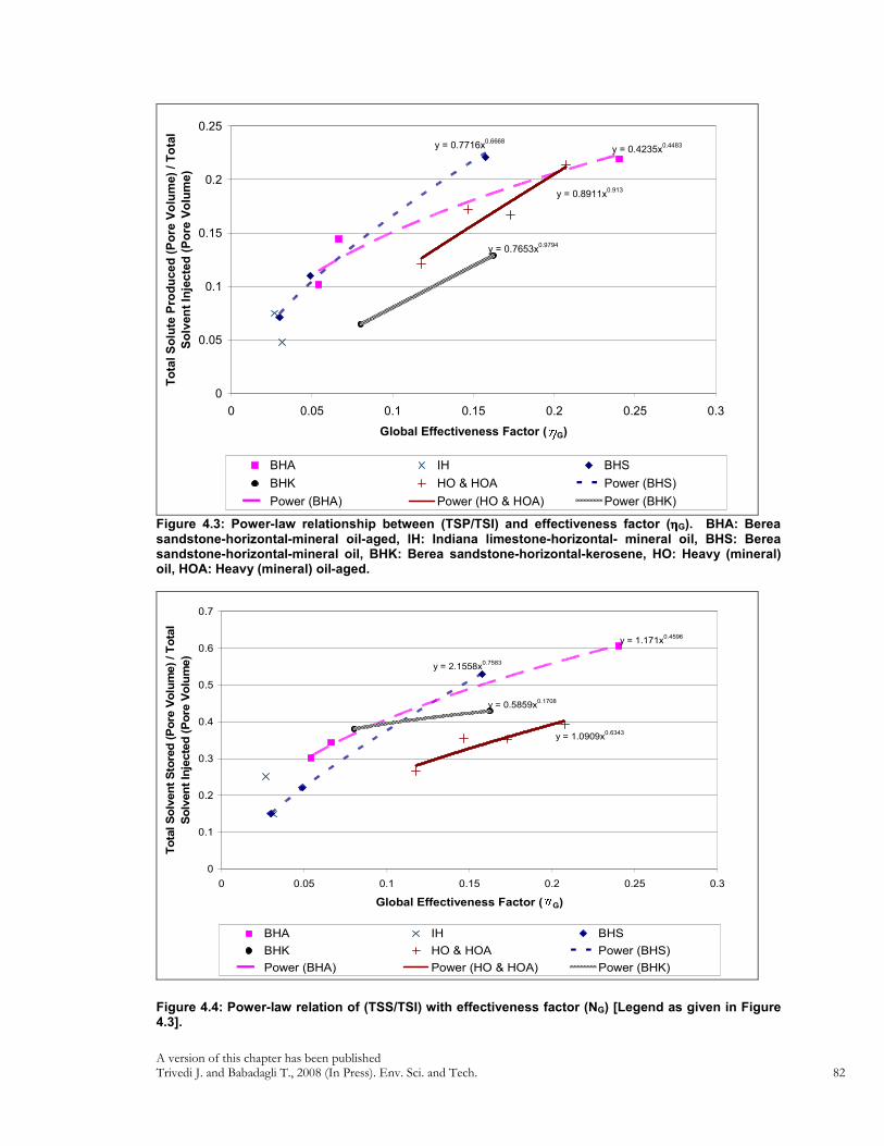
A version of this chapter has been published Trivedi J. and Babadagli T., 2008 (In Press). Env. Sci. and Tech. 82
y = 0.7716x0.6668
y = 0.4235x0.4483
y = 0.8911x0.913
y = 0.7653x0.9794
0
0.05
0.1
0.15
0.2
0.25
0 0.05 0.1 0.15 0.2 0.25 0.3
Global Effectiveness Factor ( G)
To
tal
So
lute
Pro
du
ce
d (
Po
re V
olu
me)
/ T
ota
l
So
lven
t In
jec
ted
(P
ore
Vo
lum
e)
BHA IH BHS
BHK HO & HOA Power (BHS)
Power (BHA) Power (HO & HOA) Power (BHK)
Figure 4.3: Power-law relationship between (TSP/TSI) and effectiveness factor (ηηηηG). BHA: Berea sandstone-horizontal-mineral oil-aged, IH: Indiana limestone-horizontal- mineral oil, BHS: Berea sandstone-horizontal-mineral oil, BHK: Berea sandstone-horizontal-kerosene, HO: Heavy (mineral) oil, HOA: Heavy (mineral) oil-aged.
y = 2.1558x0.7583
y = 1.171x0.4596
y = 1.0909x0.6343
y = 0.5859x0.1708
0
0.1
0.2
0.3
0.4
0.5
0.6
0.7
0 0.05 0.1 0.15 0.2 0.25 0.3
Global Effectiveness Factor ( G)
To
tal S
olv
en
t S
tore
d (
Po
re V
olu
me)
/ T
ota
l
So
lven
t In
jecte
d (
Po
re V
olu
me)
BHA IH BHS
BHK HO & HOA Power (BHS)
Power (BHA) Power (HO & HOA) Power (BHK)
Figure 4.4: Power-law relation of (TSS/TSI) with effectiveness factor (NG) [Legend as given in Figure 4.3].

A version of this chapter has been published Trivedi J. and Babadagli T., 2008 (In Press). Env. Sci. and Tech. 83
y = 0.956xR² = 0.884
0
0.05
0.1
0.15
0.2
0.25
0 0.05 0.1 0.15 0.2 0.25
(TO
P)
/ (T
SI)
Ca
lcu
late
d R
es
ult
s
(TOP) / (TSI) Experimental Results
Figure 4.5: Comparison of (TSP/TSI) experimental value and the one obtained from Equation (4.7) [% error showing 10, 20 & 30 % error in predicted values]
y = 0.975xR² = 0.895
0
0.1
0.2
0.3
0.4
0.5
0.6
0.7
0 0.1 0.2 0.3 0.4 0.5 0.6 0.7
(TSS) / (TSI) Calculated Results
(TSS) / (TSI) Experimental Results
Figure 4.6: Comparison of (TSS/TSI) experimental value and the one obtained from Equation (4.8) [% error showing 10, 20 & 30 % error in predicted values]

A version of this chapter has been published Trivedi J.J. and Babadagli T., 2008 (In Press). J. Pet. Sci. Eng. doi:10.1016/j.petrol.2008.03.001. 84
5 SCALING MISCIBLE DISPLACEMENT IN FRACTURED POROUS MEDIA
USING DIMENSIONLESS GROUPS
5.1 Background on Scaling Process
Scaling is a procedure of extrapolation of results obtained at one scale to another, usually
from a small-scale laboratory observation to a large-scale process. Two different methods for
obtaining dimensionless numbers can be found in the literature, Dimensional Analysis (DA)
and Inspectional Analysis (IA).
5.2 Dimensional Analysis (DA)
The DA determines the minimum number and form of scaling groups based on the primary
dimensions of any physical system (Fox and McDonald, 1998). The dimensionless groups
will not predict the physical behavior of the system only but these groups can also be joined
together to be easily interpreted physically. The experimental validation for the final form of
physically meaningful dimensionless group has also been recommended (Fox and
McDonald, 1998). The DA method does not require that the process being modeled be
expressed by equations rather it is based on the knowledge of the pertinent variables
affecting the process.
Historical developments in the field of fluid mechanics and dynamics point to dimensionless
numbers as a mean of comparison. Two succinct and apparently different methods for
obtaining dimensionless numbers can be found in the general fluid flow literature. General
fluid dynamics literature (Johnson, 1998; Fox and McDonald, 1998) suggest DA, whereas
petroleum related literature relies more on IA (Shook et al., 1992)
5.2.1 Inspectional Analysis (IA)
Dimensionless numbers obtained through the IA are generally considered to be more useful
(Craig et al., 1957; Shook et al., 1992). The IA is the extension of the DA, where a final

A version of this chapter has been published Trivedi J.J. and Babadagli T., 2008 (In Press). J. Pet. Sci. Eng. doi:10.1016/j.petrol.2008.03.001. 85
dimensionless formulation is tested against the variables from which it has been developed.
Unlike the DA approach, the IA is based on the set of differential equations that governs the
process of interest with the initial and boundary conditions into dimensionless forms. The
flow equations included in the analysis improve the description of the reservoir behavior.
Because the flow equations neither alter the number of primary dimensions nor introduce
new parameters to the system, the DA still holds. The primary goal of the IA on the
expanded set of equations is to introduce the necessary boundary conditions. Boundary
conditions can be introduced through the process of transformation from dimensional to
dimensionless space or through later rearrangement of already developed dimensionless
equations.
Both methods have certain advantages and disadvantages. The availability of the
mathematical equations representing the process is essential in the IA. As the IA is based on
the existing differential equation with acting boundary, it is a simpler and preferred method
in petroleum engineering related literature.
Scaling of miscible and immiscible processes using inspectorial analysis also have led to
better understanding of the process based on the dimensionless groups associated (Gharbi et
al., 1998; Gharbi, 2002; Kulkarni and Rao, 2006a; Wood et al., 2006; Grattoni et al., 2001).
Grattoni et al (1998) defined a new dimensionless group combining the effects of gravity and
viscous forces to capillary forces. This group showed a linear relationship with the total
recovery for all the scenarios tested. Kulkarni and Rao (2006a) presented the effect of major
dimensionless groups on the final recovery based on various miscible and immiscible gas
assisted gravity drainage field data and laboratory experimental data. Wood et al. (2006)
derived dimensionless groups for tertiary enhanced oil recovery (EOR) using CO2 flooding
in waterflooded reservoirs and presented a screening model for EOR and storage in Gulf
Coast reservoirs. Yet, less has been listed about fractured reservoirs especially with the flow
conditions taken into consideration. Previously, we proposed a group, FDI (Fracture
Diffusion Index), as a ratio of viscous forces in the fracture and diffusion forces in the
matrix (Trivedi and Babadagli, 2006) using the analogy to capillary imbibition controlled
immiscible displacement in fractured porous medium. In this study, we derived the groups
affecting the miscible process and proposed a new dimensionless number with its physical
significance towards the efficient recovery process.
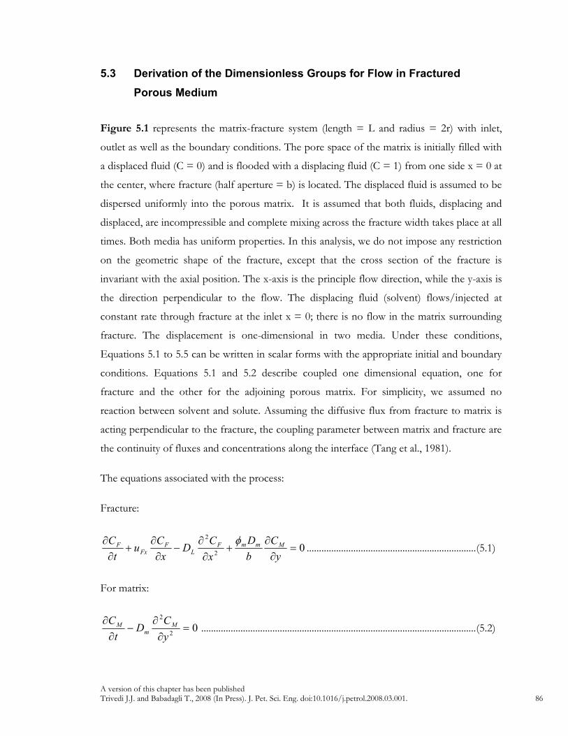
A version of this chapter has been published Trivedi J.J. and Babadagli T., 2008 (In Press). J. Pet. Sci. Eng. doi:10.1016/j.petrol.2008.03.001. 86
5.3 Derivation of the Dimensionless Groups for Flow in Fractured
Porous Medium
Figure 5.1 represents the matrix-fracture system (length = L and radius = 2r) with inlet,
outlet as well as the boundary conditions. The pore space of the matrix is initially filled with
a displaced fluid (C = 0) and is flooded with a displacing fluid (C = 1) from one side x = 0 at
the center, where fracture (half aperture = b) is located. The displaced fluid is assumed to be
dispersed uniformly into the porous matrix. It is assumed that both fluids, displacing and
displaced, are incompressible and complete mixing across the fracture width takes place at all
times. Both media has uniform properties. In this analysis, we do not impose any restriction
on the geometric shape of the fracture, except that the cross section of the fracture is
invariant with the axial position. The x-axis is the principle flow direction, while the y-axis is
the direction perpendicular to the flow. The displacing fluid (solvent) flows/injected at
constant rate through fracture at the inlet x = 0; there is no flow in the matrix surrounding
fracture. The displacement is one-dimensional in two media. Under these conditions,
Equations 5.1 to 5.5 can be written in scalar forms with the appropriate initial and boundary
conditions. Equations 5.1 and 5.2 describe coupled one dimensional equation, one for
fracture and the other for the adjoining porous matrix. For simplicity, we assumed no
reaction between solvent and solute. Assuming the diffusive flux from fracture to matrix is
acting perpendicular to the fracture, the coupling parameter between matrix and fracture are
the continuity of fluxes and concentrations along the interface (Tang et al., 1981).
The equations associated with the process:
Fracture:
02
2
=∂
∂+
∂
∂−
∂
∂+
∂
∂
y
C
b
D
x
CD
x
Cu
t
C MmmFL
FFx
F φ.....................................................................(5.1)
For matrix:
02
2
=∂
∂−
∂
∂
y
CD
t
C Mm
M ................................................................................................................(5.2)

A version of this chapter has been published Trivedi J.J. and Babadagli T., 2008 (In Press). J. Pet. Sci. Eng. doi:10.1016/j.petrol.2008.03.001. 87
+
∂
∂−= g
x
Pku F
F
F
FFX ρ
µ.........................................................................................................(5.3)
CF = 0 at t = 0 yx,∀ ..................................................................................................................(5.4)
uFY = 0 at y = 0 tx,∀ ..................................................................................................................(5.5)
uFY = 0 at y = b tx,∀ ..................................................................................................................(5.6)
∫ =b
TFX udyub
0
1At x=0 .............................................................................................................(5.7)
)( ybgPP mwfF −+= ρ at x=L.................................................................................................(5.8)
Here CF and CM are the concentrations of solute in fracture and matrix, respectively, (M/L3).
2b is the constant fracture aperture (L), r is the half fracture spacing (L), DL represents the
coefficient of hydrodynamic dispersion in the fracture (L2/T), Dm is the effective molecular
diffusion coefficient in the matrix (L2/T), which includes the effect of tortuosity. The
dependent and independent variables associated with the process are tabulated with their
respective symbols and dimensions in Table 5.1.

A version of this chapter has been published Trivedi J.J. and Babadagli T., 2008 (In Press). J. Pet. Sci. Eng. doi:10.1016/j.petrol.2008.03.001. 88
Table 5.1: Dependent and independent variables, symbols and their dimensions.
Dependent and
Independent Variables
Symbols Dimensions Dependent and
Independent Variables
Symbols Dimensions
Porosity (Fracture)
ØF M0L0T0 Porosity (Matrix)
ØM M0L0T0
Velocity uT M0L1T-1 Length of Fracture
L M0L1T0
Permeability (Fracture)
KF M0L2T0 Permeability (Matrix)
KM M0L2T0
Solvent viscosity
µs M1L-1T-1 Oil viscosity µo M1L-1T-1
Solvent density
ρs M1L-3T0 Oil density ρo M1L-3T0
Amount of solvent injected (Pore volume)
QI M0L0T0 Amount of solute produced (Pore volume)
QP M0L0T0
Fracture width b M0L1T0 Matrix width r M0L1T0
Diffusion Coefficient
Deff M0L2T-1 Dispersion Coefficient
DL M0L2T-1
Viscosity difference
∆µ M1L-1T-1 Density difference
∆ρ M1L-3T0
Gravity force g M0L1T-2
In this process, we will study the ratio of total oil produced and total solvent injected as the
efficiency indication parameter. Hence, our goal is to find the dimensionless group which
affects the objective function given below and maximize it.
),,,,,,,,,,,,,,,,()/( gDDrbLvKKfQQ LeffOSOSTMFMFIP ρµρρµµφφ ∆∆= .............(5.9)
With some simplifications,
The fluid densities and viscosities may be appropriately grouped together.

A version of this chapter has been published Trivedi J.J. and Babadagli T., 2008 (In Press). J. Pet. Sci. Eng. doi:10.1016/j.petrol.2008.03.001. 89
Since the solvent is injected into the fracture, the Darcy flow equation applies only to flow in
fracture. Hence, the permeability of the matrix does not play a role into the set of equations
representing the system.
∆∆= g
D
D
r
L
b
LvKfQQ
eff
L
SSS
O
S
OTF
M
FIP ,,,,,,,,,,)/(
ρρ
µµ
ρρ
µµ
φφ
...................................... (5.10)
This expression has no unique form. We have used the IA method to identify/derive the
dimensionless groups associated with the process. The procedure of IA is presented in
Appendix. Since the IA is a parameter rather than dimensions procedure, it can produce
dependent dimensionless scaling groups. To remediate, Shook et al (1992) proposed writing
the dimensional matrix for dimensionless groups in a form. They used linear (affine)
transformations, which works well if the grouping and elimination of translation factors is
physically meaningful. The eight dimensionless scaling groups obtained after applying this
procedure are shown in the first column of Table 5.2. These scaling groups can be reduced
further to obtain a set of independent dimensionless groups. The minimum numbers of
independent scaling groups are equal to the rank of the non-square coefficient matrix. This
method of minimizing the number of dimensionless scaling groups was suggested by Shook
et al (1992). Logarithm of the eight groups originally obtained, shown in the first column of
Table 5.1, are taken to make them linear. The rank of the resultant coefficient matrix is
determined by the method of elementary row operations. Further reducing the groups and
then exponentiation, the remaining dimensionless scaling groups are shown in second
column of Table 5.2.

A version of this chapter has been published Trivedi J.J. and Babadagli T., 2008 (In Press). J. Pet. Sci. Eng. doi:10.1016/j.petrol.2008.03.001. 90
Table 5.2: Dimensionless groups derived using the Inspectorial Analysis.
Dimensionless groups after IA
Dimensionless groups minimized (suggested by Shook et al., (1992))
T
L
Lu
D
m
L
D
D = (Dispersion diffusion ratio)
T
mm
bru
LDφ
L
rmφ = (1/aspect ratio for matrix)
T
m
ur
LD2
T
m
bu
D = (1/Pe)
0µµS
0µµS = (1/M) = (1/Mobility factor)
∆
T
F
u
gk
0µρ
∆
0ρρ
= Density Number
T
F
u
gk
0
0
µρ
∆
T
F
u
gk
0µρ
= Gravity Number
Lu
gbk
T
F
0
0
µρ
L
b = (1/Aspect ratio for fracture)
∆Lu
gbk
T
F
0µρ
= FgM
eff
LIP Ar,,MArPe
D
DfQQ ,,,,,,)/( ρ ................................................................ (5.11)
5.4 New Dimensionless Number
None of the scaling groups individually can define the efficiency of the process of interest.
Hence a new dimensionless group combining varying strength of all forces acting as
different dimensionless groups during the process is necessary.
We propose here a new group, Matrix-Fracture Diffusion Number, (NM-FD), by inverse
multiplication of (G2), (G3) and (G6).

A version of this chapter has been published Trivedi J.J. and Babadagli T., 2008 (In Press). J. Pet. Sci. Eng. doi:10.1016/j.petrol.2008.03.001. 91
(1/NM-FD) =
∆
T
F
u
gk
0µρ
T
m
bu
D
L
rmφ.................................................................................. (5.12)
Since,
( )22
22,
210
1
210
1Pe
D
bu
D
D
m
T
m
TaylorL == ......................................................................................... (5.13)
The group (G1) is also indirectly incorporated in the expression 12.
(1/NM-FD) = M
m
T
mF
ArPe
,g
L
r
bu
gDk 12
0
=
∆ φµ
ρ...................................................................... (5.14)
(NM-FD) = ,g
ArPe
r
L
gDk
bu M
mmF
T *2
0 =
∆ φρµ
........................................................................... (5.15)
5.4.1 Similarity and Comparison with the Immiscible Process
Similar dimensionless groups were introduced using different techniques before for different
purposes. Stubos and Poulou (1999) introduced a modified diffusive capillary number by
taking the ratio of diffusion to capillary gradient driven rates. Their work mainly focused on
drying of porous media with existence of two-phase.
D
ml
oeleffCa
k
CCD≡
−
φρσ
µ
**
)(**................................................................................................... (5.16)
Babadagli and Ershaghi (1993) proposed a fracture capillary number (Nf,Ca) as the ratio of
viscous to capillary forces for immiscible displacement in fractured systems. The fracture
capillary number is a ratio of viscous forces active in fracture to the capillary forces active in
matrix:
max,
,*
**
cm
wTf
CafPk
Vk,
µ= ........................................................................................................... (5.17)

A version of this chapter has been published Trivedi J.J. and Babadagli T., 2008 (In Press). J. Pet. Sci. Eng. doi:10.1016/j.petrol.2008.03.001. 92
The derivation of Eq. 5.17 is based on the viscous forces effective in fractures and capillary
forces in matrix. This ratio is given by
))()(*(
))()()()((
max, dydxPk
bdxdyV
cm
wT µ ............................................................................................................. (17-a)
Where, dx and dy are fracture and matrix dimensions and b is the fracture width. Eq. 5.17
was obtained by replacing the term (b) by fk.
In a different study, Babadagli (2002) also showed a relationship between capillary imbibition
recoveries while there is a constant rate flow in the fracture using a scaling group where he
included the length of the matrix. This group was derived using Handy’s equation (Handy,
1960) and the final form was
2
,
2
*
*
x
y
meffc
wT
L
L
kP
V µ................................................................................................................... (5.18)
The expression for the (NM-FD) proposed here (Eq. 5.15) is similar to Eq. 5.18 and also to
some extent to fracture capillary number, Nf,Ca (Eq. 5.17), where the capillary forces are
replaced by diffusive forces in the matrix with addition of gravity factor.
5.5 Validation of Proposed Group
5.5.1 Experiments
To validate the applicability of the new group proposed and its physical significance as well
as its behavior, we preformed first contact miscible core scale experiments using heptane as
solvent and mineral oil as solute. The process mimics miscible CO2 injection in naturally
fractured reservoirs. To analyze the effects of viscosity and density of the solute, we
conducted some experiments with kerosene. Rock types used were Berea sandstone and
Indiana limestone.

A version of this chapter has been published Trivedi J.J. and Babadagli T., 2008 (In Press). J. Pet. Sci. Eng. doi:10.1016/j.petrol.2008.03.001. 93
The procedure of the experimentation is as follows.
• The cores (6 inches in length and 2 inches in diameter) were cut into two pieces
through the center in direction of longitudinal axis for the purpose of creating a
fracture.
• The cut cores were weighed and fully saturated with oil under constant vacuum using
vacuum pump for 48-72 hours to achieve maximum saturation. For aged
experiments the saturation was time was over a period of a month.
• The weight of the cores after saturation was measured. Porosity was measured from
the weight difference before and after saturation.
• The saturated two pieces were held together using heat-shrinkable rubber sleeves.
• The fractured core then placed into a plexiglas holder and the annular space was
filled with silicon to ensure no flow to the annulus between the core and core holder.
• Solvent was injected at constant flow rates of 3ml/hr, 6ml/hr and 9 ml/hr for the
horizontal experiments, and 1 ml/hr, 3 ml/hr and 6 ml/hr for the vertical
experiments from the center of the core holder. The production lines were also
placed at the center at the other end.
• The samples collected at the production end were analyzed using bench-type
refractometer.
The experimental set-up is shown in Figure 5.2. The details of experiments performed are
shown in Table 5.3 with particular fluid type and rock properties used while the fluid
properties are shown in Table 5.4.

A version of this chapter has been published Trivedi J.J. and Babadagli T., 2008 (In Press). J. Pet. Sci. Eng. doi:10.1016/j.petrol.2008.03.001. 94
Table 5.3: Experiments performed.
Case Core
Type
ØM Solute
(oil)
Type
Flow
rate
(ml/hr)
L
(inches)
Aged Orientation
1 Sandstone 21% MO 3 6 No Horizontal
2 Sandstone 21% MO 6 6 No Horizontal
3 Sandstone 21% MO 9 6 No Horizontal
4 Sandstone 21% MO 3 6 Yes Horizontal
5 Sandstone 21% MO 4.5 6 Yes Horizontal
6 Sandstone 21% MO 6 6 Yes Horizontal
7 Sandstone 21% MO 9 6 Yes Horizontal
8 Sandstone 21% Kerosene 3 6 No Horizontal
9 Sandstone 21% Kerosene 6 6 No Horizontal
10 Sandstone 21% MO 1 6 No Vertical
11 Sandstone 21% MO 3 6 No Vertical
12 Limestone 11% MO 3 6 No Horizontal
13 Limestone 11% MO 6 6 No Horizontal
Table 5.4: Properties of solvent and solute used in experiments
Chemical Name Density
(g/cc)
Viscosity (cp) Refraction Index
(RI)
Solvent Heptane 0.68 0.410 1.3891
Mineral Oil (MO) 0.79 33.5 1.469
Solute Kerosene 0.81 2.1 1.475
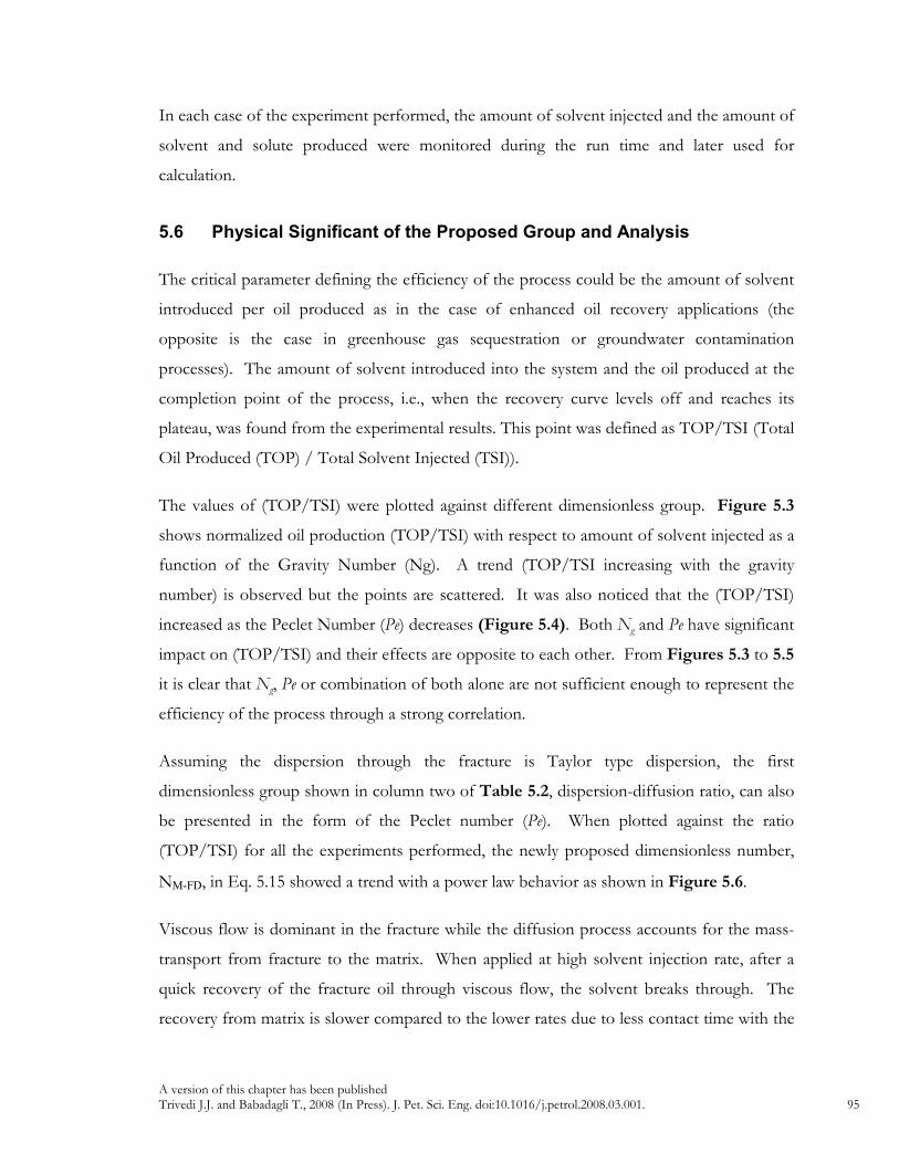
A version of this chapter has been published Trivedi J.J. and Babadagli T., 2008 (In Press). J. Pet. Sci. Eng. doi:10.1016/j.petrol.2008.03.001. 95
In each case of the experiment performed, the amount of solvent injected and the amount of
solvent and solute produced were monitored during the run time and later used for
calculation.
5.6 Physical Significant of the Proposed Group and Analysis
The critical parameter defining the efficiency of the process could be the amount of solvent
introduced per oil produced as in the case of enhanced oil recovery applications (the
opposite is the case in greenhouse gas sequestration or groundwater contamination
processes). The amount of solvent introduced into the system and the oil produced at the
completion point of the process, i.e., when the recovery curve levels off and reaches its
plateau, was found from the experimental results. This point was defined as TOP/TSI (Total
Oil Produced (TOP) / Total Solvent Injected (TSI)).
The values of (TOP/TSI) were plotted against different dimensionless group. Figure 5.3
shows normalized oil production (TOP/TSI) with respect to amount of solvent injected as a
function of the Gravity Number (Ng). A trend (TOP/TSI increasing with the gravity
number) is observed but the points are scattered. It was also noticed that the (TOP/TSI)
increased as the Peclet Number (Pe) decreases (Figure 5.4). Both Ng and Pe have significant
impact on (TOP/TSI) and their effects are opposite to each other. From Figures 5.3 to 5.5
it is clear that Ng, Pe or combination of both alone are not sufficient enough to represent the
efficiency of the process through a strong correlation.
Assuming the dispersion through the fracture is Taylor type dispersion, the first
dimensionless group shown in column two of Table 5.2, dispersion-diffusion ratio, can also
be presented in the form of the Peclet number (Pe). When plotted against the ratio
(TOP/TSI) for all the experiments performed, the newly proposed dimensionless number,
NM-FD, in Eq. 5.15 showed a trend with a power law behavior as shown in Figure 5.6.
Viscous flow is dominant in the fracture while the diffusion process accounts for the mass-
transport from fracture to the matrix. When applied at high solvent injection rate, after a
quick recovery of the fracture oil through viscous flow, the solvent breaks through. The
recovery from matrix is slower compared to the lower rates due to less contact time with the
A version of this chapter has been published Trivedi J.J. and Babadagli T., 2008 (In Press). J. Pet. Sci. Eng. doi:10.1016/j.petrol.2008.03.001. 96
matrix in order for the diffusion into matrix to take place. This yields a higher (NM-FD). In
the case of lower injection rates, the diffusion dominates the recovery resulting in lower (NM-
FD). Hence, higher NM-FD indicates a faster recovery with more solvent injection. On the
other hand, a low value of the (NM-FD) is an indication of slow but more efficient recovery,
i.e., less solvent injection is required. This might even yield higher ultimate recoveries from
the matrix compared to the extremely high injection rate cases. Hence, one needs to define
a critical rate or critical NM-FD as a more universal indicator of the efficiency of the process.
One can observe a characteristic trend of (NM-FD) change with (TOP/TSI) in Figure 5.6.
When the injection rate reaches a certain value, flow is only through the fracture and not
enough residing time is allowed for an effective diffusional matrix-fracture interaction. This
rate yields a progressing flat line parallel to x-axis, almost constant (TOP/TSI) with
increasing (NM-FD). This NM-FD value is called critical point and beyond this point, the
diffusional recovery in a fractured porous media can be considered as an inefficient process.
The critical NM-FD was found to be between 2E+07 to 3.5 E+07.
Previously we have proposed a similar group (Trivedi and Babadagli, 2006), Fracture
Diffusion Index (FDI), without any DA or IA study and found to be very much alike the
group defined here:
FDI = om
sf
Dk
fvk
ρ
ρθ
**
*)(** .................................................................................................... (5.19)
where v is the volumetric injection rate of the diffusing phase and D is the diffusion co-
efficient between oil and solvent. )(θf is the wettability indicator.
The FDI was presented as the ratio of viscous force acting into fracture and diffusion force
into matrix which has matrix permeability term (km). The main difference between NF-MD and
the FDI is the velocity terms [(uT)2 term in NF-MD instead of v in the FDI and the absence of
km in the NF-MD. It is interesting to note that the Darcy equation has been applied only to
fracture, when assuming no flow into the matrix. Due to this, the final groups derived from
the IA do not have matrix permeability term. Matrix porosity is present in the group given in
G2 and has significant impact on analysis of the process. For comparison purpose we have

A version of this chapter has been published Trivedi J.J. and Babadagli T., 2008 (In Press). J. Pet. Sci. Eng. doi:10.1016/j.petrol.2008.03.001. 97
plotted the FDI against (TOP/TSI) in Figure 5.7. The critical FDI for the same set of
experiments is between 6.5 E+14 to 9 E+14. Both groups have power law behavior against
(TOP/TSI) with a good match and can be used in determining the efficiency of the process.
Importance of matrix permeability in the effectiveness of the diffusional matrix-fracture
interaction needs more physical tests.
5.7 Concluding Remarks
If the amount of oil produced per amount of solvent injected is the critical efficiency
parameter, one can define a critical rate. We proposed a more universal approach and
derived a new dimensionless group, NM-FD, to analyze the efficiency of the process. The
critical NM-FD was found to be between 2 E+07 and 3.5 E+07. Within this range, the
process is called efficient from the recovery/solvent injection and recovery time points of
view. If it is less than 2 E+07, the process is effective for the amount of oil produced but
not very efficient in terms of time. This approach for efficiency evaluation is also useful in
greenhouse gas sequestration and groundwater contamination practices. Those processes
target to maximize the storage of injected material in the matrix and this requires an effective
matrix-fracture transfer due to diffusion. This could be controlled by the rate that would be
determined by matrix properties.
Figure 5.1 Geometrical representation of matrix-fracture system used in this study.
C = C0
y
x 0=
∂∂
x
C
L
r
0'=
∂∂
y
C
0'=
∂∂
x
C
b

A version of this chapter has been published Trivedi J.J. and Babadagli T., 2008 (In Press). J. Pet. Sci. Eng. doi:10.1016/j.petrol.2008.03.001. 98
Figure 5.2: Experimental set-up
0
0.05
0.1
0.15
0.2
0.25
0.3
0.35
0.4
0.45
0.00E+00 5.00E-03 1.00E-02 1.50E-02 2.00E-02 2.50E-02
Ng
To
tal
Oil
Pro
du
ced
(P
V)
/ T
ota
l S
olv
en
t
Inje
cte
d (
PV
)
Figure 5.3: Normalized oil production with respect to amount of solvent injected as a function of the gravity number (Ng).

A version of this chapter has been published Trivedi J.J. and Babadagli T., 2008 (In Press). J. Pet. Sci. Eng. doi:10.1016/j.petrol.2008.03.001. 99
0
0.05
0.1
0.15
0.2
0.25
0.3
0.35
0.4
0.45
0.00E+00 1.00E+03 2.00E+03 3.00E+03 4.00E+03 5.00E+03 6.00E+03
Pe
To
tal O
il P
rod
uced
(P
V)
/ T
ota
l S
olv
en
t
Inje
cte
d (
PV
)
Figure 5.4: Normalized oil production with respect to amount of solvent injected as a function of the Peclet number (Pe).
0
0.05
0.1
0.15
0.2
0.25
0.3
0.35
0.4
0.45
0.00E+00 5.00E+05 1.00E+06 1.50E+06 2.00E+06 2.50E+06 3.00E+06
(1/Ng)*Pe
To
tal
Oil
Pro
du
ce
d (
PV
) /
To
tal
So
lve
nt
Inje
cte
d (
PV
)
Figure 5.5: Normalized oil production with respect to amount of solvent injected as a function of (Peclet Number/Gravity Number).

A version of this chapter has been published Trivedi J.J. and Babadagli T., 2008 (In Press). J. Pet. Sci. Eng. doi:10.1016/j.petrol.2008.03.001. 100
R2 = 0.8247
0
0.05
0.1
0.15
0.2
0.25
0.3
0.35
0.4
0.45
0.5
0.E+00 2.E+07 4.E+07 6.E+07 8.E+07 1.E+08 1.E+08 1.E+08 2.E+08
Matrix-Fracture Diffusion Group (NM-FD)
To
tal O
il P
rod
uced
(P
V)
/ T
ota
l S
olv
en
t In
jecte
d
(PV
)
Figure 5.6: Normalized oil production with respect to amount of solvent injected as a function of
Matrix-Fracture Diffusion Group (NM-FD).
R2 = 0.9093
0
0.1
0.2
0.3
0.4
0.5
0.6
0.00E+00 5.00E+14 1.00E+15 1.50E+15 2.00E+15 2.50E+15 3.00E+15 3.50E+15
FDI
To
tal
Oil P
rod
uced
(P
V)
/ T
ota
l S
olv
en
t In
jecte
d
(PV
)
Figure 5.7: Normalized oil production with respect to amount of solvent injected as a function of Fracture Diffusion Index (FDI).

A version of this chapter has been published Trivedi J.J. and Babadagli T., 2008. # 2008-092, 59th Ann. Tech. Meeting, CIPC/SPE GTS, Calgary.17-19 June. 101
6 EXPERIMENTAL INVESTIGATIONS ON THE FLOW DYNAMICS AND
ABANDONMENT PRESSURE FOR CO2 SEQUESTRATION AND
INCREMENTAL OIL RECOVERY IN FRACTURED RESERVOIRS: THE
MIDALE FIELD CASE
6.1 Introduction
Very limited number of experimental work has been reported in context to oil recovery from
naturally fractured reservoir using carbon dioxide as a solvent, and of these, sequestration
related ones are even less. With the success of miscible flooding in different ongoing
projects, researchers and industry have come together to focus on sequestration as well
recently. Studies performed in these contexts are summarized below:
• Karimaie et al. (2007) performed experiments for secondary and tertiary injection of
CO2 and N2 in a fractured carbonate rock. In their work, 2 mm gap between core cylinder
and core was used as a fracture while the core acted as a matrix. They used binary mixture of
C1-C7 at 170 bar and 85 0C as solute. Gas was injected at 5 cc/min into the fracture to drain
the oil (in secondary injection) or water (in tertiary injection) and then reduced to 1 cc/min.
Within 10 hrs of secondary CO2 injection, 75% of oil was recovered while it took 400 hrs
(~17days) to recover 15% of oil using secondary N2.
• Darvish et al. (2006a; 2006b) used 96.6 mm long and 46 mm in diameter (4 mD,
44%) chalk cores. After saturating the core with live oil at 300 bar and 130 0C, CO2 was
injected at 5.6 cc/min to displace the oil from the fracture and then the rate was reduced to
1 cc/min.
• Chakravarthy et al. (2006) used WAG and polymer gels to delay the breakthrough
during CO2 injection into fractured cores. They studied immiscible condition and used Berea
cores (D = 2.5 cm (1 inch); L = 10 cm (3.9 inches)). They injected CO2 continuously at 0.03
cc/min and 0.1 cc/min and compared core flooding experiments with continuous CO2

A version of this chapter has been published Trivedi J.J. and Babadagli T., 2008. # 2008-092, 59th Ann. Tech. Meeting, CIPC/SPE GTS, Calgary.17-19 June. 102
injection, viscosified water injection followed by CO2, and gel injection into fractured Berea
sandstone.
• Muralidharan et al. (2004) conducted experimental and simulation studies to
investigate the effect of different stress conditions (overburden pressure) on fracture/matrix
permeability and fracture width. They concluded that during constant injection average
fracture permeability decreased about 91% and the average mean fracture aperture decreased
about 71% while increasing overburden pressure from 500 psi to 1500 psi.
• Torabi and Asghari (2007) studied CO2 huff-and-puff performance on two Berea
sandstone cores (k = 100 md and 1000 md; L = 30.48 cm; D = 5.08 cm). CO2 was injected
into 0.5 cm annular space between core and core holder acting as a fracture. In their
experiments, they injected CO2 at six different pressure steps of constant pressure into
saturated core. It followed by production at atmospheric pressure for 24 hours and
removing CO2/flash fluid from the top. Each step was continued until production ceases.
No consideration was taken for sequestration. They observed drastic increase in the recovery
factor from immiscible to near miscible/miscible conditions.
• Asghari and Torabi (2007) performed gravity drainage experiments in sandstone core
samples with fracture at the annular space and concluded that miscibility can increase the
production substantially. One of their findings was that the recovery may decrease far above
the miscibility. Injection and production was not at controlled rate, hence sudden increase or
decrease in pressure may affect the results when comparing and also sequestration cannot be
accomplished.
All these works used standard sandstone samples, usually Berea sandstone. Studies using -
fractured- carbonate rocks or low permeable matrix are very rare (Karimaie et al., 2007;
Darvish et al., 2006a & 2006b; Chakravarthy et al., 2006). Moreover, most of the works
presented above focused on the enhanced oil recovery aspect rather than the CO2
sequestration. Keeping in mind that sequestration during enhanced oil recovery experiments
at high pressure reservoir conditions on fractured cores are involved in numerous
difficulties, solution to this kind of problems was sought using simulation studies. Due to
the limitations of simulators to describe matrix-fracture transfer functions and multiphase
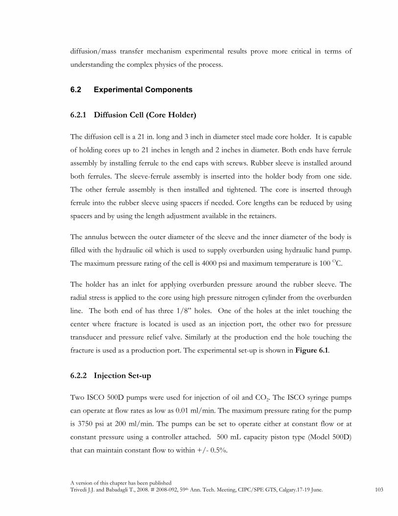
A version of this chapter has been published Trivedi J.J. and Babadagli T., 2008. # 2008-092, 59th Ann. Tech. Meeting, CIPC/SPE GTS, Calgary.17-19 June. 103
diffusion/mass transfer mechanism experimental results prove more critical in terms of
understanding the complex physics of the process.
6.2 Experimental Components
6.2.1 Diffusion Cell (Core Holder)
The diffusion cell is a 21 in. long and 3 inch in diameter steel made core holder. It is capable
of holding cores up to 21 inches in length and 2 inches in diameter. Both ends have ferrule
assembly by installing ferrule to the end caps with screws. Rubber sleeve is installed around
both ferrules. The sleeve-ferrule assembly is inserted into the holder body from one side.
The other ferrule assembly is then installed and tightened. The core is inserted through
ferrule into the rubber sleeve using spacers if needed. Core lengths can be reduced by using
spacers and by using the length adjustment available in the retainers.
The annulus between the outer diameter of the sleeve and the inner diameter of the body is
filled with the hydraulic oil which is used to supply overburden using hydraulic hand pump.
The maximum pressure rating of the cell is 4000 psi and maximum temperature is 100 OC.
The holder has an inlet for applying overburden pressure around the rubber sleeve. The
radial stress is applied to the core using high pressure nitrogen cylinder from the overburden
line. The both end of has three 1/8” holes. One of the holes at the inlet touching the
center where fracture is located is used as an injection port, the other two for pressure
transducer and pressure relief valve. Similarly at the production end the hole touching the
fracture is used as a production port. The experimental set-up is shown in Figure 6.1.
6.2.2 Injection Set-up
Two ISCO 500D pumps were used for injection of oil and CO2. The ISCO syringe pumps
can operate at flow rates as low as 0.01 ml/min. The maximum pressure rating for the pump
is 3750 psi at 200 ml/min. The pumps can be set to operate either at constant flow or at
constant pressure using a controller attached. 500 mL capacity piston type (Model 500D)
that can maintain constant flow to within +/- 0.5%.

A version of this chapter has been published Trivedi J.J. and Babadagli T., 2008. # 2008-092, 59th Ann. Tech. Meeting, CIPC/SPE GTS, Calgary.17-19 June. 104
The liquid CO2 cylinder has pressure only 850 psi. The accumulator of the pump has a
capacity of only 508 ml. Therefore, every time after the refill, the syringe pumps were used
to increase the pressure up to the desired level. N2 cylinder supplying constant pressure
using high pressure regulator at the overburden line is used to apply the loads and stresses.
In some experiments water using ISCO pump was used to supply overburden pressure.
ISCO pumps are connected to RS-232 serial interface for controlling and operating
parameters using the LabVIEW program.
6.2.3 Production System
6.2.3.1 Back Pressure Regulator
A KPB series medium to high pressure piston-sensing back pressure regulator provided by
Swagelok was used. The regulator was connected to the production line to maintain the
system pressure. It provided back-pressure control in gas/liquid application.
6.2.3.2 Separator
A separator is used for oil and gas separation coming through the backpressure regulator.
6.2.3.3 Flow Meter
A volume/mass flow meter was attached to the top of the separator.
6.2.4 Data Acquisition System (DAQ)
Data acquisition from the thermocouples and pressure transducers is performed using the
National Instruments cDAQ-9172 module equipped with NI Bus 9211 and 9215, which is
connected to a host PC. The LabVIEW software is used to monitor the entire process and
perform the appropriate programs for I/O applications.
All the necessary data, as listed below, are collected using this system:
• The flow rate, volume remaining and pump pressure signals output from the ISCO
pump controller,

A version of this chapter has been published Trivedi J.J. and Babadagli T., 2008. # 2008-092, 59th Ann. Tech. Meeting, CIPC/SPE GTS, Calgary.17-19 June. 105
• Digital scale value and weight of oil production data with time. The time steps can be
varied for frequent data collection at the early stage of experiments,
• CO2 mass flow, volume flow, temperature and pressure data,
• Pressure data through transducers attached to the two ends of the core holder.
6.2.5 Core Properties and Core Preparation
Cores were cut through the center in direction of longitudinal axis using the special saw
(Figure 6.2). The cut cores were weighted and placed in a desiccator filled with oil. The
desiccator was connected to a vacuum pump. The core was saturated under constant
vacuum for 48 hours. The weight of the core after saturation was measured. Porosity of the
matrix was calculated from the difference in the weight of saturated and unsaturated core.
The porosity of Berea sandstone cores ranges from 19 to 21 %. The porosity of Midale
cores ranges from 27 to 31 %. The average permeabilities are 500 mD and 10 mD for Berea
sandstones and the Midale sample, respectively.
The Midale reservoir is described by two distinct layers: (1) the Marly (upper layers) and (2)
the Vuggy (lower layers) zones. The upper layers consist of micro-crystalline dolomite while
the lower layers consist of micro to coarsely crystalline fragmental limestone. The zones are
separated by a thinner, tighter carbonate zone permeable to vertical fluid flow.
The core used in this experiment was selected from the Marly zone (between the depth of
1422.81m and 1424.57m) which contains highly porous crystalline dolomitic mudstones and
wackestones. The fracture intensity in the Vuggy intershoal is higher than that of the
overlying Marly. The Vuggy shoal is the least fractured. In a separate set of experiment, a
core from the caprock was taken and tested for its breakthrough capacity.
6.3 Experimental Procedure
The following steps were followed for preparation to CO2 flooding:
• Core was cut and dried in the oven to remove the water content. Before this, the
Midale cores were subjected to a cleaning process using the Soxhlet device.
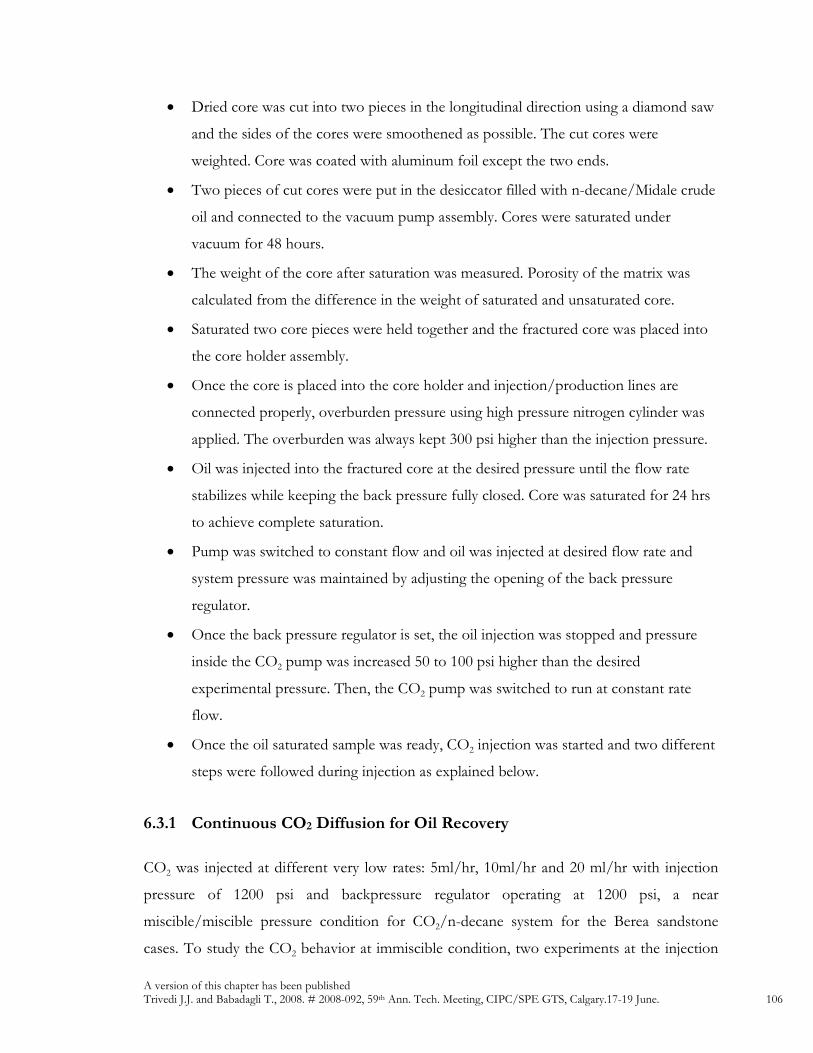
A version of this chapter has been published Trivedi J.J. and Babadagli T., 2008. # 2008-092, 59th Ann. Tech. Meeting, CIPC/SPE GTS, Calgary.17-19 June. 106
• Dried core was cut into two pieces in the longitudinal direction using a diamond saw
and the sides of the cores were smoothened as possible. The cut cores were
weighted. Core was coated with aluminum foil except the two ends.
• Two pieces of cut cores were put in the desiccator filled with n-decane/Midale crude
oil and connected to the vacuum pump assembly. Cores were saturated under
vacuum for 48 hours.
• The weight of the core after saturation was measured. Porosity of the matrix was
calculated from the difference in the weight of saturated and unsaturated core.
• Saturated two core pieces were held together and the fractured core was placed into
the core holder assembly.
• Once the core is placed into the core holder and injection/production lines are
connected properly, overburden pressure using high pressure nitrogen cylinder was
applied. The overburden was always kept 300 psi higher than the injection pressure.
• Oil was injected into the fractured core at the desired pressure until the flow rate
stabilizes while keeping the back pressure fully closed. Core was saturated for 24 hrs
to achieve complete saturation.
• Pump was switched to constant flow and oil was injected at desired flow rate and
system pressure was maintained by adjusting the opening of the back pressure
regulator.
• Once the back pressure regulator is set, the oil injection was stopped and pressure
inside the CO2 pump was increased 50 to 100 psi higher than the desired
experimental pressure. Then, the CO2 pump was switched to run at constant rate
flow.
• Once the oil saturated sample was ready, CO2 injection was started and two different
steps were followed during injection as explained below.
6.3.1 Continuous CO2 Diffusion for Oil Recovery
CO2 was injected at different very low rates: 5ml/hr, 10ml/hr and 20 ml/hr with injection
pressure of 1200 psi and backpressure regulator operating at 1200 psi, a near
miscible/miscible pressure condition for CO2/n-decane system for the Berea sandstone
cases. To study the CO2 behavior at immiscible condition, two experiments at the injection

A version of this chapter has been published Trivedi J.J. and Babadagli T., 2008. # 2008-092, 59th Ann. Tech. Meeting, CIPC/SPE GTS, Calgary.17-19 June. 107
rate of 5ml/hr and 10 ml/hr were carried out at 950 psi core pressure by keeping initial
injection pressure and backpressure regulator at 950 psi. Another pressure, 1400 psi, was
selected to obtain fully miscible displacement and compare the results with other two cases.
At 1400 psi, one CO2 injection rate (10 ml/hr) was tested. For the Midale core experiment,
injection was carried out at 10 ml/hr rate while keeping the core pressure 950 psi. This
represents a pressure slightly below the miscibility pressure. The system was continuously
supplied with constant overburden pressure of 1500 psi using water injection using ISCO
pump in all the experiments. Pressure variations and amount of oil/gas production were
closely monitored and logged during the experiment run.
6.3.2 Blow Down
After the continuous injection was stopped, the production valve at the bottom of the core-
holder and the backpressure valve were closed. The system was totally shut-down for 36 hrs.
During this period CO2 and oil diffusion and back diffusion took place. Change in pressure
at the injection/production ends was monitored. After 36 hrs, production valve and back
pressure was opened to produce CO2 and oil. Production continues until the pressure inside
the core lowers to 250 psi. The shut-down and pressure blow down cycle was then repeated
for every 250 psi pressure steps. The amount of oil and CO2 production were measured at
every pressure steps to determine the CO2 sequestration capacity at particular pressure and
ultimate oil recovered after the blow down.
6.4 Effect of Rate – Existence of Critical Rate
Many researchers showed the importance of critical rate on the oil recovery process during
gas and liquid injection. Slobod and Howlett (1964) and Thompson and Mungan (1969)
showed that the critical velocity defines the fingering behavior in displacement of more
viscous and denser fluid in a miscible process. If the density difference is lower, increase in
rate will allow more viscous force domination which leads to viscous fingering. Higher the
density difference, higher the gravity force. Hence, higher density difference will cause the
CO2 flow to the path of least resistance through the fracture to the production end.

A version of this chapter has been published Trivedi J.J. and Babadagli T., 2008. # 2008-092, 59th Ann. Tech. Meeting, CIPC/SPE GTS, Calgary.17-19 June. 108
Mahmoud (2006) and Wood et al. (2006) showed that the presence of vertical fracture
improved the oil recovery through immiscible gas assisted gravity drainage (GAGD)
compared to the unfractured counterpart. Gas will try to stay on the top and expand
laterally. They also mentioned that if the gravity force loses its dominance to viscous forces
then adverse effect of fractures can be observed.
The effect of rate or definition of critical rate on fracture reservoirs is different. Higher rates
causes early breakthrough through fractures without enough contact with matrix in order for
the diffusion between matrix and fracture to occur (Trivedi and Babadagli, 2008a & 2008c;
Babadagli, 2000).
There is always an existence of critical injection rate for optimal recovery in the fractured
reservoirs. Maintaining the same pressure condition in the reservoir by adjusting the
backpressure regulator and injecting CO2 at different rates of 5 ml/hr, 10 ml/hr and 20
ml/hr (Figure 6.3) shows the importance of knowing the critical rate before the start of
CO2-EOR project. 5ml/hr injection in Exp-2 is proven to be very slow and the recovery is
extremely low. 20 ml/hr injection rate (Exp-6) causes an early breakthrough (Figure 6.4) of
CO2. Dispersion driven flow in the fracture and mass transfer between matrix and fracture
driven by diffusion are the two major governing mechanism of oil recovery during the CO2
injection into fracture-matrix system. Flux transfer may also governed by flow into the
fracture. 5ml/hr is too slow causing an ineffective dispersion in fracture. The diffusive
transfer to matrix is effective due to delayed breakthrough in the fracture but the process is
too slow and therefore assumed to be inefficient in terms of oil recovery. On the other
hand, 20ml/hr is proved to be more efficient for recovery compared to 5ml/hr despite early
breakthrough and high CO2 production. The intermediate rate of 10ml/hr injection resulted
in even higher recovery compared to 20ml/hr, and hence suggesting the occurrence of
critical injection rate. Looking at the results of storage in Figure 6.5, again 10 ml/hr
showed maximum storage scenario followed by the 5ml/hr and 20 ml/hr cases. These
experimental results have triggered the need of a new rate dependent transfer function which
can define the critical rate for enhanced oil recovery as well as sequestration (Trivedi and
Babadagli, 2008a & 2008c; Babadagli, 2000).

A version of this chapter has been published Trivedi J.J. and Babadagli T., 2008. # 2008-092, 59th Ann. Tech. Meeting, CIPC/SPE GTS, Calgary.17-19 June. 109
6.5 Sequestration – Time and Economical Aspects
It is well understood that greenhouse gas sequestration with EOR is one of the viable
choices for cost effective solution. In early stages of the production, the EOR aspect of the
process is more critical than sequestration. When CO2 flooding is continued for long time
and eventually the oil cut has gone extremely low values, most of the injected CO2 is
recycled or reservoir pressure is reduced for additional recovery by pressure depletion (blow-
down period). The time when continuous CO2 flooding should be stopped and determining
the minimum reservoir abandonment pressure are the two important aspects of the process
in terms of optimal economical balance between oil recovery and amount of CO2
sequestered.
Figure 6.6 represents the amount sequestered with time during continuous injection of CO2.
The shapes of the curves follow similar kind of trends in all the experiments with 10ml/hr
injection. Two distinct slopes can be seen. Initially the storage is almost following a 45o line,
suggesting almost all the injected CO2 is being stored. The start of second line slope suggests
the major breakthrough of CO2. With the increase in reservoir pressure the amount of
sequestered CO2 also increases due to CO2 compressibility. At the same time, the volume of
CO2 produced also goes high with higher reservoir pressure, which causes the higher CO2
handling and recycling cost. The rate also impacts the sequestration and production volume.
Comparing the Exp-2, Exp-4 and Exp-6, one may observe that the CO2 sequestered
increases for 5 ml/hr to 10 ml/hr rate cases with increase in injection rate while maintaining
the same reservoir pressure. But further increase in injection rate, 20 ml/hr, has caused
lowest amount sequestered and highest production of CO2 compared to other two cases.
6.6 Effect of Miscibility – Sequestration and EOR
The miscibility pressure between the CO2 and n-decane is ~1200 psi at the room
temperature. CO2 was injected at constant rate with maintaining different miscibility
conditions: immiscible (~950 psi), near miscible (~1175-1225 psi) and above miscible
(~1400 psi). Injecting at a same rate and at these three different pressure condition yields
different results for EOR and sequestration. As seen in Figure 6.3, during the continuous
CO2 injection period with rate at 10 ml/hr the recoveries of immiscible, near miscible and

A version of this chapter has been published Trivedi J.J. and Babadagli T., 2008. # 2008-092, 59th Ann. Tech. Meeting, CIPC/SPE GTS, Calgary.17-19 June. 110
above miscible conditions are 47%, 67% and 60%, respectively. Increasing the pressure
above a point is not beneficial to incremental oil recovery and near miscible injection proved
to be more useful. Increase in pressure causes variation in density as well as in viscosity of
the CO2 which plays a critical role when flow is through the fracture. Figures 6.4 and
Figure 6.5 present the amount of CO2 produced and amount of CO2 stored, respectively,
against total CO2 injected. The higher the pressure above the miscible pressure, the higher
the amount of CO2 produced and CO2 sequestered.
6.7 Rock Type – Sandstone and Limestone
Though the porosity of Midale and Berea sandstones are very high, the permeability
variation can cause major impact on recovery and sequestration. Oil recovery from the
selected Marly zone core is ~ 23%, lower than from sandstone with similar injection and
pressure condition (Figure 6.3) at the end of continuous injection period. Note that oil
types are different in Berea sandstone and Midale core cases as well even though they were
both light oils (Table 6.1). Amount of sequestered and produced gas is, however, very
much equal to that of sandstone counterpart results in Figures 6.4 and Figure 6.5 despite
the differences in oil and rock type. After nearly 5 hrs of injection into the Midale core, the
produced amount of CO2 was at very high rate and oil cut went very low. Hence the
continuous injection of CO2 was carried out for shorter time for the Midale case compared
to the Berea sandstone cases (~18 hrs).
6.8 Blow Down – Sequestration and EOR
After the continuous injection period, the production and injection valves were closed for
about 36 hrs for each experiment. The peak incremental oil production was noticed right
after the blow down to 750 psi followed by shutdown period and the amount of produced
oil varied for each experiment (Figure 6.3). With the CO2 injection rate of 10 ml/hr at
different miscibility conditions, the maximum oil production during the first blow down was
noticed for ~950 psi reservoir pressure which is just below the minimum miscibility pressure
of CO2 – n-decane system. Recoveries during the first blow down became lower with
increasing pressure (increasing miscibility). For the Midale case, recovery after the first shut

A version of this chapter has been published Trivedi J.J. and Babadagli T., 2008. # 2008-092, 59th Ann. Tech. Meeting, CIPC/SPE GTS, Calgary.17-19 June. 111
down period increased from 23 % to 41% (Figure 6.3). In the Berea sandstone counterpart
case (Exp-5), the oil recovery increased significantly from 47 % to 80 % during the first blow
down cycle. This could be attributed to oil characteristics mainly. The permeability effect
was considered to be secondary importance.
It is quite noticeable that for each experimental run, the oil production increased to
significant amounts during the blow down to 750 psi after the first shut down period of 36
hrs. This could be a very vital issue in terms of oil recovery obtained mainly by gravity
drainage. During the subsequent blow down cycles oil production was not quite significant.
6.9 Critical Observations
Due to the early breakthrough of CO2 through fracture, oil was not swept well in the matrix
around the production end, compared to the matrix near the injection end. After finishing
the Exp-4, cores were visually inspected. Yellowish dark color identified the unrecovered oil
zones. It clearly showed that the most of the oil was swept near the production part and at
the injection end unswept zones were visible in the cross-section. This difference is due to
the fact that a great portion of oil was recovered during the shut-in and blow down period.
During shut-in, because of gravity, the lateral migration of CO2 inside the matrix near to the
production zone is more compared to the migration at the top of the matrix. The
mechanism clearly suggesting the huff-and-puff application would be useful to recover
unswept oil after continuous CO2 flooding even though this may not be ideal for
sequestration. More experimental support is required to justify the choice of huff-and-puff
after continuous flooding with CO2.
Density was (measured during the experiments and at the end) not changed during the
experiments with CO2-decane system, being a single component. Realistically a change in
density with CO2 is expected with the crude oil because of different CO2 dissolution rate
with different components; this was observed with CO2-Midale oil system.
When the injection of CO2 was stopped, the pressure decrease inside the core was observed.
Interestingly the pressure decreased up to a certain value in all the experiments. The change
in pressure with time was plotted for the three experiments (Exps. 4, 5, and 6) in Figure 6.7.

A version of this chapter has been published Trivedi J.J. and Babadagli T., 2008. # 2008-092, 59th Ann. Tech. Meeting, CIPC/SPE GTS, Calgary.17-19 June. 112
To understand the reasons of this strange behavior and avoid any thoughts of leakage or
adsorption, the shutdown period was kept ~92 hrs during the case-6. It is evident from
Figure 6.7 that the decrease in pressure reached to a certain value and then it was stabilized.
This pressure is around 860 psi at the experimental temperature. This is believed to be due
to phase change mechanism. Looking at the CO2 phase diagram, this point follows the
sublimation line, a line between liquid and gas phase. At this point liquid requires a large
volume change to do the phase change. Hence, the pressure tends to stabilize to reach the
equilibrium. Given the change in pressure by external means, the CO2 inside the core will be
changing the phase hence the properties of CO2 will change very abruptly and may affect the
recovery as well as storage process in the subsequent blow down periods.
If the reservoir temperature is higher, this phase change pressure also increases. The CO2
expands/diffuse inside the pores after the oil production. Also it can be seen as lost of
miscible region, where CO2 diffuses as a separate phase than oil inside the reservoir. This
enhances the oil production during the first blow down as discussed earlier. In this process
of migration mainly due to diffusion inside the matrix and convective mass transfer between
fracture-matrix, a state of dynamic equilibrium is reached and pressure tends to stabilize.
During the blow down period this aspect also needs to be taken care of.
In the case of Midale core (Exp-7), the pressure reduction (stabilized at ~915 psi) and the
CO2 diffusion during the first shut down period was less due to carbonate nature of the rock
and much denser oil type. Comparing the Exp-5 and Exp-7, where the only difference is oil
and rock type while injection pressure and rate are same, CO2 has to diffuse into much
tighter rock and more denser as well as viscous oil. This resulted into lower recovery during
the first blow down cycle to 750 psi compared to that of the Berea counterpart (Exp-5) as
discussed earlier and shown in Figure 6.3.
6.10 Cap Rock Sealing
In a separate set of experiment, oven dried cap rock core was placed inside the core holder.
The overburden was applied using water line. CO2 was continuously injected with constant
pressure injection at different pressure steps. Once a test pressure is reached, injection valve

A version of this chapter has been published Trivedi J.J. and Babadagli T., 2008. # 2008-092, 59th Ann. Tech. Meeting, CIPC/SPE GTS, Calgary.17-19 June. 113
was closed and CO2 production at the other end was monitored. The injection was done
from the bottom of the core against the gravity to mimic the real field situation. For the next
step pressure was increased 50 psi higher. Change in pressure at both the ends was
monitored closely. The change in pressure at the production end suggests the overcoming of
capillary pressure forces and causing the breakthrough. This pressure was noted in between
1650 psi to 1700 psi (Figure 6.8). Interestingly, Li et al. (2005) reported similar values of
sealing pressure capacity for Weyburn field (~ 1400 psi to 1700 psi). In their study, the cap
rock was first saturated with water and then the capillary pressure using CO2 was measured.
The effect of variable water saturation on cap rock sealing pressure was beyond the scope of
the present paper. It should be emphasized that this pressure range is around the miscibility
pressure and therefore, the pressure applied in the field.
6.11 Conclusions and Remarks
Critical rate is one of the important factors to be considered while designing an EOR and
sequestration project. 10 ml/hr has proven to be the most effective continuous injection rate
into fractured sandstones. For sequestration, 10 ml/hr was also observed as the critical rate
yielding the maximum storage. Maintaining near miscible pressure conditions is the most
effective for incremental oil recovery. Going beyond the near miscible pressure condition is
proven to be beneficial for sequestration purpose but can cause reduction in production.
Blow down for additional recovery at the end of the CO2 injection project life, can increase
the recovery by 10% up to a certain pressure (~750 psi here). Going below this pressure will
affect sequestration adversely without much benefit of recovering oil. CO2 phase
behavior/change during the project is very crucial and should be studied carefully with
density and viscosity change into consideration. The reservoirs with lower temperature can
also be targeted for sequestration and EOR. Recovery from the Midale carbonate was only
23 % but after a first cycle of blow down it reached 41 % due to CO2 diffusion and gravity
drainage. The storage capacity of the Midale carbonate was, however, almost half then that
of the sandstone rock while maintaining other operational parameter similar.
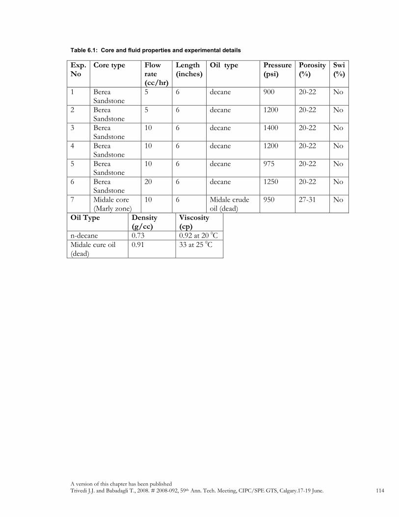
A version of this chapter has been published Trivedi J.J. and Babadagli T., 2008. # 2008-092, 59th Ann. Tech. Meeting, CIPC/SPE GTS, Calgary.17-19 June. 114
Table 6.1: Core and fluid properties and experimental details
Exp. No
Core type Flow rate (cc/hr)
Length (inches)
Oil type Pressure (psi)
Porosity (%)
Swi (%)
1 Berea Sandstone
5 6 decane 900 20-22 No
2 Berea Sandstone
5 6 decane 1200 20-22 No
3 Berea Sandstone
10 6 decane 1400 20-22 No
4 Berea Sandstone
10 6 decane 1200 20-22 No
5 Berea Sandstone
10 6 decane 975 20-22 No
6 Berea Sandstone
20 6 decane 1250 20-22 No
7 Midale core (Marly zone)
10 6 Midale crude oil (dead)
950 27-31 No
Oil Type Density (g/cc)
Viscosity (cp)
n-decane 0.73 0.92 at 20 0C Midale cure oil (dead)
0.91 33 at 25 0C
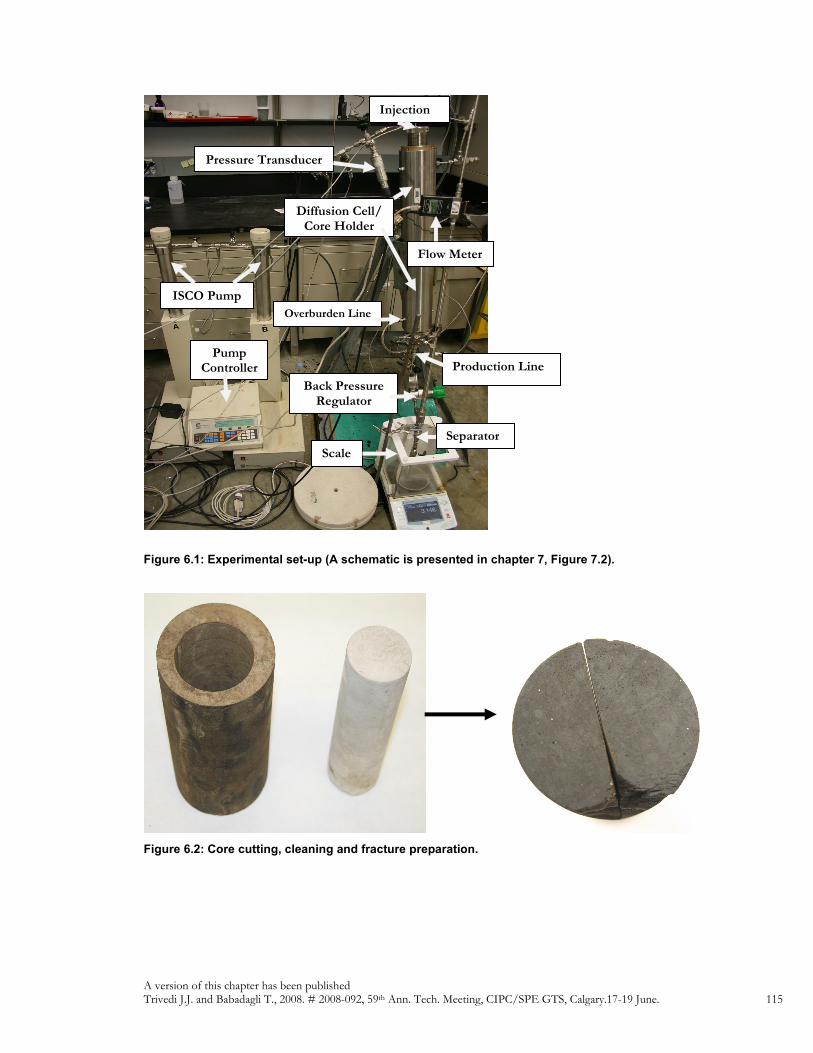
A version of this chapter has been published Trivedi J.J. and Babadagli T., 2008. # 2008-092, 59th Ann. Tech. Meeting, CIPC/SPE GTS, Calgary.17-19 June. 115
Figure 6.1: Experimental set-up (A schematic is presented in chapter 7, Figure 7.2).
Figure 6.2: Core cutting, cleaning and fracture preparation.
ISCO Pump
Diffusion Cell/ Core Holder
Scale
Back Pressure Regulator
Flow Meter
Separator
Pressure Transducer
Injection
Overburden Line
Pump Controller Production Line

A version of this chapter has been published Trivedi J.J. and Babadagli T., 2008. # 2008-092, 59th Ann. Tech. Meeting, CIPC/SPE GTS, Calgary.17-19 June. 116
Time (hr)
0 20 40 60 80 100 120 140 160
Oil Produced (% PV)
0
20
40
60
80
100
CO2 rate = 5 ml/hr (950 psi)
CO2 rate = 5 ml/hr (1200 psi)
CO2 rate = 10 ml/hr (950 psi)
CO2 rate = 10 ml/hr (1200 psi)
CO2 rate = 10 ml/hr (1400 psi)
CO2 rate = 20 ml/hr : (1250 psi)
Midale : CO2 rate = 10 ml/hr (950psi)
Figure 6.3: Oil production for different rates and pressures.
First shut down
Second shut down (~750 psi) Third shut down
Midale core

A version of this chapter has been published Trivedi J.J. and Babadagli T., 2008. # 2008-092, 59th Ann. Tech. Meeting, CIPC/SPE GTS, Calgary.17-19 June. 117
CO2 Injected (SCC)
0 10000 20000 30000 40000 50000 60000
CO2 Produced (SCC)
0
10000
20000
30000
40000
CO2 rate = 5 m l/hr (950 psi)
CO2 rate = 5 m l/hr (1200 psi)
CO2 rate = 10 m l.hr (950 psi)
CO2 rate = 10 m l/hr (1200 psi)
CO2 rate = 10 m l/hr (1400 psi)
CO2 rate = 20 m l/hr (1250 psi)
Midale: CO2 rate = 10 m l/hr (950 psi)
Figure 6.4: CO2 produced per amount of CO2 injected for different rates and pressures.
CO2 Injected (SCC)
0 20000 40000 60000
CO
2 S
tore
d (
SC
C)
0
10000
20000
30000
40000
CO2 rate = 5 m l/hr (950 psi)
CO2 rate = 5 m l/hr (1200 psi)
CO2 rate = 10 m l/hr (950 psi)
CO2 rate = 10 m l.hr (1200 psi)
CO2 rate = 10 m l/hr (1400 psi)
CO2 rate = 20 m l/hr (1250 psi)
M idale: CO2 rate = 10 m l/hr (950 psi)
Figure 6.5: CO2 stored per amount of CO2 injected for different rates and pressures.

A version of this chapter has been published Trivedi J.J. and Babadagli T., 2008. # 2008-092, 59th Ann. Tech. Meeting, CIPC/SPE GTS, Calgary.17-19 June. 118
Time (hr)
0 10 20 30 40 50
CO2 Stored (SCC)
0
10000
20000
30000
40000
50000CO2 rate = 5 ml/hr (950 psi)
CO2 rate = 5 ml/hr (1200 psi)
CO2 rate = 10 ml/hr (950 psi)
CO2 rate = 10 ml/hr (1200 psi)
CO2 rate = 10 ml/hr (1400 psi)
CO2 rate = 20 ml/hr (1250 psi)
Midale: CO2 rate = 10 ml/hr (950 psi)
Figure 6.6: CO2 stored with time for different rates and pressures.
Time (Hr)
0 50 100 150 200 250
Pressure (Psi)
0
200
400
600
800
1000
1200
1400
1600
CO2 rate: 20 ml/hr (950 psi
CO2 rate : 10 ml/hr (950 psi)
CO2 rate :10 ml/hr (1200 psi)
Midale Core: CO2 rate = 10 ml/hr (950 psi)
Figure 6.7: Core pressure change against time for four different cases.
First shut down
First shut down
Pressure decrease
during first shut
down
Pressure stabilization
Blow down start
Third shut down
Midale core
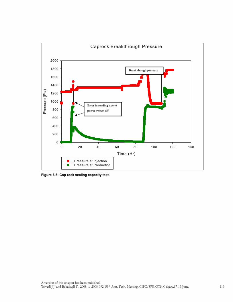
A version of this chapter has been published Trivedi J.J. and Babadagli T., 2008. # 2008-092, 59th Ann. Tech. Meeting, CIPC/SPE GTS, Calgary.17-19 June. 119
Caprock Breakthrough Pressure
Time (Hr)
0 20 40 60 80 100 120 140
Pressure (Psi)
0
200
400
600
800
1000
1200
1400
1600
1800
2000
Pressure at Injection
Pressure at Production
Figure 6.8: Cap rock sealing capacity test.
Break though pressure
Error in reading due to
power switch off

A version of this paper has been published Trivedi J.J and Babadagli T. 2008. SPE 117606. SPE Eastern Regional/AAPG Eastern Section Joint Meeting Pittsburgh.11–15 October 2008. 120
7 EXPERIMENTAL ANALYSIS OF CO2 SEQUESTRATION EFFICIENCY
DURING OIL RECOVERY IN NATURALLY FRACTURED RESERVOIRS
7.1 Overview
In the previous chapter, we dealt with different recovery and sequestration aspects during
continuous injection and consecutive blow down periods. In this chapter, we analyzed the
recovery mechanisms during continuous injection and soaking (towards huff-n-puff) of the
previous experimental results given in Chapter 6 with an additional experiment on the
Midale field core and crude oil.
7.2 Introduction
Although there exists considerable amount of experimental work on modeling matrix-
fracture interaction using first contact miscible solvents to mimic fully miscible CO2
injection (Burger and Mohanty, 1997; Burger et al., 1996; Gabitto, 1998; Firoozabadi and
Markeset, 1994; Trivedi and Babadagli, 2008a), experimental studies using CO2 as solvent are
limited. Mostly Berea sandstones are used in these researches because of their readily
availability, ease of cleaning and homogeneous structures. Studies using fractured carbonate
rocks or low permeable matrix are rare (Karimaie et al., 2007; Darvish et al., 2006a and
2006b). In one of its kind experimental work, Chakravarthy et al. (2006) used polymer gels
to show the effect of delayed breakthrough during immiscible CO2 injection into fractured
Berea cores. Improved recovery was observed during huff-and-puff performance in miscible
range over immiscible injection of CO2 (Asghari and Torabi, 2007; Torabi and Asghari,
2007). Because of the complexity and duration involved into the diffusion experiments as
well as limitations of simulators to precisely predict the multiphase diffusion/mass transfer
functions, the previous attempts to understand the physical mechanism are highly valuable.
None of these works, however, considered the sequestration aspect during EOR. In the first
part of this chapter, we performed dynamic diffusion experiments to show that oil recovery
from the matrix can be enhanced as well as greenhouse gas storage can be accomplished by

A version of this paper has been published Trivedi J.J and Babadagli T. 2008. SPE 117606. SPE Eastern Regional/AAPG Eastern Section Joint Meeting Pittsburgh.11–15 October 2008. 121
optimizing flow dynamics. In the second part, we provided a quantitative analysis showing
the efficiency limits of the process.
7.2.1 Importance/Role of Diffusivity in Miscible and Immiscible Matrix-
Fracture Transfer Process
Different miscible injection processes using carbon dioxide, nitrogen, flue gas, natural gas, or
other hydrocarbon gases such as methane, ethane, propane and butane as solvent were
tested for the purpose of enhanced oil/gas recovery. One of the most important issues in
common is that they all dissolve into the oil phase by diffusion mechanism. The efficiency
of the mixing or dissolving is typically measured or characterized by a mutual diffusion
coefficient of solvent into the oil phase. Solute transport in rough fractures is controlled by
diffusion as well as advective processes. The fracture dispersion coefficient and effective
matrix diffusion coefficient are the most important parameters for matrix oil recovery. In
fractured porous media, the matrix diffusion is of primary importance in the processes such
as geological disposal of nuclear waste, contaminant transport during ground water
contamination, enhanced oil recovery in naturally fractured reservoirs and greenhouse gas
sequestration in fractured geological formations.
Experimental methods to measure diffusivity could be direct or indirect. Direct method is
the one which requires the compositional analysis of the diffusing species while the indirect
method involves in measuring the parameters affected by diffusion such as volume change,
pressure variation or solute volatization. As reported in literature, direct methods are time
consuming and expensive (Sigmund, 1976; Upreti and Mehrotra, 2002). Recently, several
studies reported new approaches for indirect method (Upreti and Mehrotra, 2002; Riazi,
1996; Tharanivasan et al., 2004; Zhang et al., 2000; Sheikha et al., 2005). These methods
typically measure the change in pressure due to gas diffusion into liquid. Most of the
research works until now did not consider the flow (or hydrodynamics) in the porous media
while calculating the diffusion coefficient. In this study we obtained diffusion coefficients by
simulating and matching the CO2 gas injection into oil saturated fractured porous media

A version of this paper has been published Trivedi J.J and Babadagli T. 2008. SPE 117606. SPE Eastern Regional/AAPG Eastern Section Joint Meeting Pittsburgh.11–15 October 2008. 122
experimental results. Diffusion/dispersion into fractured porous media was then quantified
by newly defined dimensionless groups.
7.3 Experimental Components
7.3.1 Core Properties and Core Preparation
Cores were cut through the center in the direction of longitudinal axis using the special saw
(Figure 7.1). The cores were then weighted and placed in a desiccator filled with oil. The
desiccator was connected to a vacuum pump. The core was saturated under constant
vacuum for 48 hours. The weight of the core after saturation was measured. Porosity of the
matrix was calculated from the difference in the weight of saturated and unsaturated core.
The porosity of Berea sandstone cores ranges from 19 to 21 %. The porosity of Midale
cores ranges from 27 to 31 %. The average permeabilities are 500 mD and 10 mD for Berea
sandstones and the Midale sample, respectively.
7.3.2 Diffusion Cell (Core Holder)
The diffusion cell is a 21 in. long and 3 inch in diameter steel made core holder. It is capable
of holding cores up to 21 inches in length and 2 inches in diameter. Both ends have ferrule
assembly by installing ferrule to the end caps with screws. The rubber sleeve is installed
around both ferrules. The sleeve-ferrule assembly is inserted into the holder body from one
side. The other ferrule assembly is then installed and tightened. The core is inserted through
ferrule into the rubber sleeve using spacers if needed. Core lengths can be reduced by using
spacers and by using the length adjustment available in the retainers.
The annulus between the outer diameter of the sleeve and the inner diameter of the body is
filled with the hydraulic oil which is used to supply overburden using hydraulic hand pump.
The maximum pressure rating of the cell is 4000 psi and maximum temperature is 100 0C.
The holder has an inlet for applying overburden pressure around the rubber sleeve. The
radial stress is applied to the core using high pressure nitrogen cylinder from the overburden
line. The both end of has three 1/8” holes. One of the holes at the inlet touching the
center where fracture is located is used as an injection port, the other two for pressure

A version of this paper has been published Trivedi J.J and Babadagli T. 2008. SPE 117606. SPE Eastern Regional/AAPG Eastern Section Joint Meeting Pittsburgh.11–15 October 2008. 123
transducer and pressure relief valve. Similarly at the production end the hole touching the
fracture is used as a production port. The experimental set-up is shown in Figure 7.2.
7.3.3 Injection Set-up
Two ISCO 500D pumps were used for injection of oil and CO2. The ISCO syringe pumps
can operate at flow rates as low as 0.01 ml/min. The maximum pressure rating for the pump
is 3750 psi at 200 ml/min. The pumps can be set to operate either at constant flow or at
constant pressure using a controller attached. 500 mL capacity piston type (Model 500D)
that can maintain constant flow to within +/- 0.5%. The liquid CO2 cylinder has pressure
only 850 psi. The accumulator of the pump has a capacity of only 508 ml. Therefore, every
time after the refill, the syringe pumps were used to increase the pressure up to the desired
level. N2 cylinder supplying constant pressure using high pressure regulator at the
overburden line is used to apply the loads and stresses. In some experiments water using
ISCO pump was used to supply overburden pressure. ISCO pumps are connected to RS-232
serial interface for controlling and operating parameters using the LabVIEW program.
7.3.4 Production System
Production unit is comprised of a back pressure regulator, a custom made separator and a
flow meter unit. A KPB series medium to high pressure piston-sensing back pressure
regulator provided by Swagelok was used. The regulator is connected to the production line
coming out at bottom of the core holder. By closing and opening of the regulator knob
desired pressure inside the core holder was maintained. A separator is connected to back
pressure regulator for oil and gas separation coming through the backpressure regulator.
Separated oil is collected into a graduated cylinder on an electric balance while the amount of
gas coming out was passed through a volume/mass flow meter.
7.3.5 Data Acquisition System (DAQ)
Data acquisition from the thermocouples and pressure transducers is performed using the
National Instruments DAQ-9172 module equipped with NI Bus 9211 and 9215, which is
connected to a host PC. The LabVIEW software is used to monitor the entire process and

A version of this paper has been published Trivedi J.J and Babadagli T. 2008. SPE 117606. SPE Eastern Regional/AAPG Eastern Section Joint Meeting Pittsburgh.11–15 October 2008. 124
perform the appropriate programs for I/O applications. All the necessary data, as listed
below, are collected using this system. ISCO pumps and weight balance are connected
through RS-232 serial interface for controlling and operating parameters using the
LabVIEW program, while the flow meter is connected through s-video to RS-232 convertor
interface. The flow rate, amount of volume injected and pump pressure data from the ISCO
pump, gas mass/volume flow from the flow meter, pressure data through transducers
connected at the injection and production line and weight data from the electric balance are
collected at different time steps using LabVIEW program.
7.4 Experimental Procedure
The cores were cut and dried in the oven to remove the water content. Before this, the
Midale cores were subjected to a cleaning process using the Soxhlet device. Dried core was
cut into two pieces in the longitudinal direction using a diamond saw and the sides of the
cores were smoothened. The cut cores were weighted and coated with aluminum foil except
the two ends. Two pieces of cut cores were put in the desiccator filled with n-decane/Midale
crude oil and connected to the vacuum pump assembly. Cores were saturated under vacuum
for 48 hours. The weight of the core after saturation was measured. Porosity of the matrix
was calculated from the difference in the weight of saturated and unsaturated core. Saturated
two core pieces were held together and the fractured core was placed into the core holder
assembly. Once the prepared core is placed into the core holder and injection/production
lines are connected properly, overburden pressure using high pressure nitrogen cylinder was
applied. The overburden was always kept 300 psi higher than the injection pressure. Oil was
injected into the fractured core at the desired pressure until the flow rate stabilizes while
keeping the back pressure fully closed. Core was saturated for 24 hrs to achieve complete
saturation. The pump was switched to constant flow and oil was injected at desired flow
rate and system pressure was maintained by adjusting the opening of the back pressure
regulator. Once the back pressure regulator is set, the oil injection was stopped and pressure
inside the CO2 pump was increased 50 to 100 psi higher than the desired experimental
pressure. Then, the CO2 pump was switched to run at constant rate flow.

A version of this paper has been published Trivedi J.J and Babadagli T. 2008. SPE 117606. SPE Eastern Regional/AAPG Eastern Section Joint Meeting Pittsburgh.11–15 October 2008. 125
In one of the Midale core experiments, sudden change in pressure was observed while
injecting oil into the core situated in the core assembly as discussed earlier. Hence core was
removed from the holder before even starting the CO2 injection and we found the core
completely crushed into pieces. Upon repetition of the same problem, we modified the
design using a lead metal cover jacket surrounding the core and only exposing the fracture
portion. The overburden and core pressure was increased simultaneously so that the core
was not exposed to sudden pressure change.
7.4.1 Continuous CO2 Diffusion for Oil Recovery
CO2 was injected at different very low rates: 5ml/hr, 10ml/hr and 20 ml/hr with an injection
pressure of 1200 psi and backpressure regulator operating at 1200 psi, a near
miscible/miscible pressure condition for CO2/n-decane system for the Berea sandstone
cases. To study the CO2 behavior at immiscible condition, one experiment at the injection
rate of 5ml/hr and was carried out at 950 psi core pressure by keeping initial injection
pressure and backpressure regulator at 950 psi. Another pressure, 1400 psi, was selected to
obtain fully miscible (above miscible) displacement and compare the results with other two
cases. At 1400 psi, one CO2 injection rate (10 ml/hr) was tested. For the Midale core
experiments, injection was carried out at 10 ml/hr rate while keeping the core pressure 950
psi and 1700 psi in two different cases. At 950 psi, Midale crude oil is immiscible with CO2
while at 1700 psi it is at near miscible condition. The system was continuously supplied with
constant overburden pressure of 1500 psi using water injection using ISCO pump in all the
experiments except in case-8 where overburden was maintained at 1850 psi. Pressure
variations and amount of oil/gas production were closely monitored and logged during the
experiment run.
7.4.2 Blow Down
After the continuous injection was stopped, the production valve at the bottom of the core-
holder and the backpressure valve were closed. The system was fully shut-down for 36 hrs.
During this period CO2 and oil diffusion and back diffusion took place. Change in pressure
at the injection/production ends was monitored. After 36 hrs, production valve and back
pressure was opened to produce CO2 and oil. Production continues until the pressure inside

A version of this paper has been published Trivedi J.J and Babadagli T. 2008. SPE 117606. SPE Eastern Regional/AAPG Eastern Section Joint Meeting Pittsburgh.11–15 October 2008. 126
the core lowers to 250 psi. The shut-down and pressure blow down cycle was then repeated
for every 250 psi pressure steps. The amount of oil and CO2 production were measured at
every pressure steps to determine the CO2 sequestration capacity at particular pressure and
ultimate oil recovered after the blow down.
7.5 Experimental Results and Discussion
Figures 7.3 and 7.4 show the amount of oil produced with respect to the reservoir (core)
pressure during the project life. It can be seen that the production trend for all cases of
injection follows modified hyperbolic relationship (y0 + a*P/ (b + P)) with the core
pressure. As seen from the graphical representation of oil recovery with blow-down
pressure, most of the oil is produced during the first cycle of blowdown period up to 750
psi. For Cases 7 and 8, where CO2 was injected at 10 ml/hr into Midale core saturated with
Midale oil at pressure 950 psi and 1700 psi respectively, the recovery increased until the
pressure reduction reaches 400 psi, which is lower than the Berea sandstones. The pressure
stabilization for Case 8 was around 1100 psi during shut down higher than Berea. After the
first blowdown, the recovery at 800-700 psi for the Cases 7 and 8 are almost the same even
though, at the end of during continuous injection, 1700 psi initial pressure (case 8) showed
~8% higher recovery with less amount of CO2 PV injection.
The normalized recovery factor (R.F. = % Recovery / PV Inj) based on per volume of CO2
injected was presented in Figures 7.9 and 7.10. It is a log-log representation of R.F. with
PV of CO2 injected during the continuous injection period. The Cases 5 and 6 follow a
similar trend and are parallel in nature. But 20 ml/hr injection rate has a higher R.F. value.
Here the difference in initial injection pressure does not have much difference in values
hence difficult to reach any sound conclusion. But in Figure 7.8, where initial injection
pressure are 950 psi and 1700 psi, the difference in the R.F. clearly suggests the miscible
process having advantage over immiscible case. After ~0.3 PV of CO2 injection, the R.F.
for both cases approaches to the same value. Hence, further continuations of miscible
process can impair the economics of the project due to high compression cost of CO2 to
achieve miscible condition. At this point switching to maintaining lower pressure would be
more economical.

A version of this paper has been published Trivedi J.J and Babadagli T. 2008. SPE 117606. SPE Eastern Regional/AAPG Eastern Section Joint Meeting Pittsburgh.11–15 October 2008. 127
To check the viability of storage during pressure reduction for oil production, we showed
the results of CO2 production at different pressures in Figures 7.5 and 7.6. CO2 storage at
different pressures for the same cases is given in Figures 7.7 and 7.8 after the continuous
injection was stopped. Up to 600 psi, it follows a linear trend of CO2 storage reduction but
below 600 psi the storage drops drastically. The trend of CO2 storage with blowdown
pressure for the Midale cores initially saturated with dead Midale crude oil is also shown in
Figure 7.8. The detailed results and discussion of the experiments are presented in another
study (Trivedi and Babadagli, 2008e).
When a non-equilibrium gas comes in contact with a liquid phase in a constant volume and
constant temperature system, the system will approach to a new equilibrium state with
changed pressure and temperature condition governed by diffusion process. The time
required to reach this new equilibrium condition depends on the diffusion coefficient of the
gas into the liquid phase, matrix properties (mainly width). The amount of gas transferred
into the oil phase depends on gas solubility while the transfer rate is governed by diffusion
coefficient. During the continuous injection of CO2 into oil saturated porous media,
injection was stopped when the oil production was very low compared to gas production.
At this stage, the phase at the injection and production ports located at the centre of the core
where the fracture is lying was occupied mainly by CO2. During the shutdown period after
the continuous injection was stopped caused a drop in pressure. As shown in Figure 7.11,
during shutdown the pressure declined and reached a stable value, a point of quasi-
equilibrium. This clearly suggests the diffusion of CO2 into the hydrocarbon phase. During
this period, mobilization of heavier hydrocarbon component of the oil occurs. This
phenomenon is due to increased extraction/condensation, a result of diffusion and
solubilization.
The pressure decay behavior was observed and used by many authors (Upreti and Mehrotra,
2002; Riazi, 1996; Tharanivasan et al., 2004; Zhang et al., 2000; Sheikha et al., 2005; Fjelde et
al., 2008) to calculate solvent gas/CO2 diffusivity into heavy oil/bitumen as well as into light
hydrocarbons. In this method, more commonly known as pressure decay method, two pairs
of fluids are place in a closed chamber (Sapphire cell) at test conditions and pressure
response of the constant volume system are modeled by applying appropriate boundary
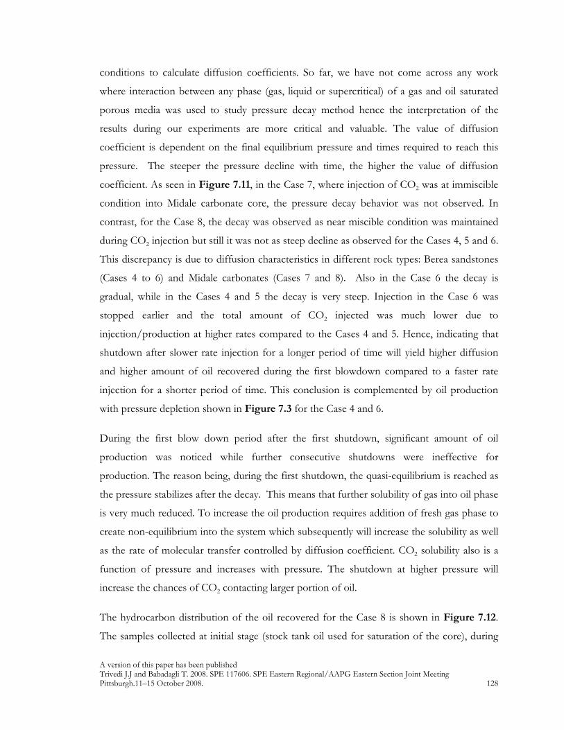
A version of this paper has been published Trivedi J.J and Babadagli T. 2008. SPE 117606. SPE Eastern Regional/AAPG Eastern Section Joint Meeting Pittsburgh.11–15 October 2008. 128
conditions to calculate diffusion coefficients. So far, we have not come across any work
where interaction between any phase (gas, liquid or supercritical) of a gas and oil saturated
porous media was used to study pressure decay method hence the interpretation of the
results during our experiments are more critical and valuable. The value of diffusion
coefficient is dependent on the final equilibrium pressure and times required to reach this
pressure. The steeper the pressure decline with time, the higher the value of diffusion
coefficient. As seen in Figure 7.11, in the Case 7, where injection of CO2 was at immiscible
condition into Midale carbonate core, the pressure decay behavior was not observed. In
contrast, for the Case 8, the decay was observed as near miscible condition was maintained
during CO2 injection but still it was not as steep decline as observed for the Cases 4, 5 and 6.
This discrepancy is due to diffusion characteristics in different rock types: Berea sandstones
(Cases 4 to 6) and Midale carbonates (Cases 7 and 8). Also in the Case 6 the decay is
gradual, while in the Cases 4 and 5 the decay is very steep. Injection in the Case 6 was
stopped earlier and the total amount of CO2 injected was much lower due to
injection/production at higher rates compared to the Cases 4 and 5. Hence, indicating that
shutdown after slower rate injection for a longer period of time will yield higher diffusion
and higher amount of oil recovered during the first blowdown compared to a faster rate
injection for a shorter period of time. This conclusion is complemented by oil production
with pressure depletion shown in Figure 7.3 for the Case 4 and 6.
During the first blow down period after the first shutdown, significant amount of oil
production was noticed while further consecutive shutdowns were ineffective for
production. The reason being, during the first shutdown, the quasi-equilibrium is reached as
the pressure stabilizes after the decay. This means that further solubility of gas into oil phase
is very much reduced. To increase the oil production requires addition of fresh gas phase to
create non-equilibrium into the system which subsequently will increase the solubility as well
as the rate of molecular transfer controlled by diffusion coefficient. CO2 solubility also is a
function of pressure and increases with pressure. The shutdown at higher pressure will
increase the chances of CO2 contacting larger portion of oil.
The hydrocarbon distribution of the oil recovered for the Case 8 is shown in Figure 7.12.
The samples collected at initial stage (stock tank oil used for saturation of the core), during

A version of this paper has been published Trivedi J.J and Babadagli T. 2008. SPE 117606. SPE Eastern Regional/AAPG Eastern Section Joint Meeting Pittsburgh.11–15 October 2008. 129
continuous injection, during the first blowdown followed by quasi-equilibrium during first
shutdown and during the last cycle of blowdown were analyzed using GC-MS for carbon
distribution and are presented here. Maintaining near miscible condition and injecting at
continuous rate, oil swelling and extraction capacity of CO2 increased. Recovery is also
governed by the extraction process during the development of miscibility. While in the
shutdown period, as the pressure decreases, condensation due to lose of miscibility occurs.
The heavier carbon components dissolve in the CO2 rich phase inside the matrix. Thus, it
creates a middle phase and recovery of heavier component increases. As shown in Figure
7.12, during this period, C14-C17 as well as C18-C22 recovery was increased almost 13%
and C22+ recovery increased by ~9%. Interestingly, there were almost zero C10-
components in the production. This emphasizes the role of density and gravity during
quasi-equilibrium. Until the pressure reduces to the stabilization point (quasi-equilibrium),
condensation and diffusion are the major driving mechanisms. After that, oil recovery is due
to mobilization of oil inside the fracture due to pressure reduction which is very low in
percentage amount and also lighter in hydrocarbon enrichment compared to the one
obtained during the quasi-equilibrium state. The carbon distribution found was similar to the
initial stock tank oil but still somewhat higher in heavier hydrocarbons. Below 600 psi, CO2
is in a gas phase and further decrease in pressure only results in gas production.
7.6 Matrix-Fracture Diffusion Simulation
Fracture-matrix transfer process was modeled numerically and presented in the form of
dimensionless groups to analyze the effects of different parameters quantitatively. The
process experimentally analyzed in the previous section was simulated using finite element
modeling with the governing advection-convection equations and the Darcy equation. Only
parameters other than those unavailable from the laboratory scale experiments are the
diffusion/dispersion coefficients and mass transfer coefficients in the matrix and fracture.
These parameters were obtained through matching the numerical modeling results to their
experimental equivalents and then they were correlated to fluid-rock properties and flow
velocity.

A version of this paper has been published Trivedi J.J and Babadagli T. 2008. SPE 117606. SPE Eastern Regional/AAPG Eastern Section Joint Meeting Pittsburgh.11–15 October 2008. 130
Figure 7.1 presents the matrix-fracture system (length = L and radius = 2r) with inlet, outlet
as well as the boundary conditions. The x-axis is the principle flow direction, while the y-axis
is the direction perpendicular to the flow. The pore space of the matrix is initially filled with
oil (C = 0) and is flooded with a CO2 (C = 1) from one side x = 0 at the center, where
fracture (half aperture = b) is located. The oil is assumed to be dispersed uniformly into the
porous matrix. It is assumed that both fluids, displacing and displaced, are incompressible
and complete mixing across the fracture width takes place at all times. Both media has
uniform properties. In this analysis, we do not impose any restriction on the geometric shape
of the fracture, except that the cross section of the fracture is invariant with the axial
position. The displacing fluid (CO2) flows/injected at constant rate through fracture at the
inlet x = 0; there is no flow in the matrix surrounding fracture. Under these conditions,
Equations governing the system are shown below with the appropriate initial and boundary
conditions. Assuming the diffusive flux from fracture to matrix is acting perpendicular to the
fracture, the coupling parameter between matrix and fracture are the continuity of fluxes and
concentrations along the interface (Tang et al., 1981).
The dead volume of the oil in the injection and production line have been subtracted from
the final experimental results and then used for simulation of flow and diffusion behavior
only inside the porous media. During the closing and opening of BPR valve the pressure
fluctuation in a range of +/- 20 psi occurs. This fluctuation has been neglected while the
performing simulation and flow at the bottom exit at the fracture has assumed to be
regulated by constant outlet pressure.
Domain 1 – Fracture
x
CFu
y
CFD
x
CFD
t
CFFLL ∂
∂−=
∂∂
−∂
∂−
∂∂ 1
2
1
2
2
1
2
1
.........................................................................(7.1)
x
CFu
y
CFD
x
CFD
t
CFFLL ∂
∂−=
∂∂
−∂
∂−
∂∂ 2
2
2
2
2
2
2
2
.........................................................................(7.2)

A version of this paper has been published Trivedi J.J and Babadagli T. 2008. SPE 117606. SPE Eastern Regional/AAPG Eastern Section Joint Meeting Pittsburgh.11–15 October 2008. 131
Domain 2 – Matrix
02
1
2
2
1
2
1 =∂
∂−
∂∂
−∂
∂y
CMD
x
CMD
t
CMee
.......................................................................................(7.3)
02
2
2
2
2
2
2 =∂
∂−
∂∂
−∂
∂y
CMD
x
CMD
t
CMee
......................................................................................(7.4)
Initial conditions:
CF1(x, y, 0) = 0; CM1(x, y, 0) = 0; CF2 (x, y, 0) = 1; CM2(x, y, 0) = 1; CF1 (0, t) = CF0 .....
.........................................................................................................................................................(7.5)
Boundary conditions:
( )
0,,
1 =∂
∂
trxy
CM
( )
0,,
2 =∂
∂
trxy
CM
....................................................................................(7.6)
( )0
,
1 =∂
∂
∞ tx
CF
( )0
,
2 =∂
∂
∞ tx
CF
.......................................................................................(7.7)
y
CMD
y
CFD eL ∂
∂−=
∂∂ 11 ;
y
CMD
y
CFD eL ∂
∂−=
∂∂ 22 at t = t bx,∀ ....................................(7.8)
The simulation results were compared with the results of experimental performed earlier.
Through matching the experimental results with the numerical ones, the values of DL and De
were obtained.
7.7 Correlation for CO2 Sequestration and Oil Production
In previous attempts, different studies derived dimensionless groups to represent the
efficiency of the immiscible or miscible EOR processes. Mostly all of them were for
homogeneous systems and only a few focused on heterogeneous reservoirs. Gharbi et al.
(1998) and Gharbi (2002) used inspection analysis to investigate the miscible displacement in

A version of this paper has been published Trivedi J.J and Babadagli T. 2008. SPE 117606. SPE Eastern Regional/AAPG Eastern Section Joint Meeting Pittsburgh.11–15 October 2008. 132
homogeneous porous media. Grattoni et al. (2001) defined a new dimensionless group
combining the effects of gravity; viscous and capillary forces which showed a linear
relationship with the total recovery. For the application of the dimensionless groups,
Kulkarni and Rao (2006) presented the effect of major dimensionless groups on the final
recovery based on various miscible and immiscible gas assisted gravity drainage field data
and laboratory experimental data. In another study (Wood et al. 2006) dimensionless groups
were derived for tertiary enhanced oil recovery (EOR) using CO2 flooding in waterflooded
reservoirs and presented a screening model for EOR and storage in Gulf Coast reservoirs.
For transfer in fractured porous media a dimensionless group, FDI (Fracture Diffusion
Index), was proposed (Trivedi and Babadagli, 2006) as a ratio of viscous forces in the
fracture and diffusion forces in the matrix using the analogy to capillary imbibition
controlled immiscible displacement in fractured porous medium. In a recent attempt, Trivedi
and Babadagli (2008d) derived a new dimensionless group with its physical significance
towards the efficiency of miscible recovery process into fractured porous media. In the
present analysis, we used the same group – Matrix-Fracture Diffusion group (N M-FD) – for
our experimental results to analyze the efficiency. (N M-FD) is defined as follws:
(NM-FD) =
g,
MArPe
rm
L
mgDFk
bTu *2
0 =∆
φρ
µ
where,
m
T
D
buPe
*= ;
∆=
T
Fg
u
gk,
0µρ
;
=
r
LAr
m
M φ
The TOP/TSI (total oil produced / total solvent injected) ratio is of particular interest when
it comes to optimization and the critical rate determination. In previous attempts,
dimensionless numbers (empirical and derived) were correlated to TOP/TSI and also with
TSS/TSI using the experimental results for solvent injection (Babadagli and Trivedi, 2006
and 2008a). They used the first contact miscible solvent to mimic the CO2 injection process
whereas we used the results of CO2/oil experiments performed in this study for the same
type of analyses. Well known dimensionless numbers, Peclet number (Pe), gravity number
(Ng) and matrix-fracture diffusion group (N M-FD) for different experiments condcuted in this

A version of this paper has been published Trivedi J.J and Babadagli T. 2008. SPE 117606. SPE Eastern Regional/AAPG Eastern Section Joint Meeting Pittsburgh.11–15 October 2008. 133
study, are shown in Table 7.3. We also included the results from Trivedi and Babadagli
(2008a) (Cases 8, 9, and 10) and Firoozabadi and Markeset (1994) (Cases 11, 12, and 13)
which were performed under similar experimental conditions but different solvent/solute
pairs. As presented in Figure 7.13, N M-FD shows a power law relation with high accuracy
with the TOP/TSI values for all experiments. In many enhanced oil recovery processes the
time to reach the ultimate recovery could be more critical compared to the amount of
solvent injected while sometimes the compression cost associated with the amount of CO2
injected could be important considering overall economics of the project. Higher N M-FD
indicates a faster recovery with more solvent injection. On the other hand, a low value of the
N M-FD is an indication of slow but higher normalized recovery due to less amount of total
solvent injected. The process having too low N M-FD also cannot be considered as the best
scenario because of extremely slow nature of the process. The optimal/critical value of N M-
FD group would be the one which is time effective as well as effective in terms of amount of
solvent injected or produced minimization and define the critical rate. The critical N M-FD
value found here is between 3.5 E+3 to 1 E+4.
7.8 Conclusions
The heavier hydrocarbon components recovery is increased by a large fraction during
shutdown after continuous injection of CO2. The shutdown after slower rate injection for a
longer period of time yielded higher diffusion and higher amount of oil recovered during
first blowdown compared to faster injection rate case for a shorter period of time. The
pressure decay during this shutdown period gives a measure of diffusion as well as recovery
enhancement phenomenon in fractured porous media. During the project life blowing down
reservoir for an economic benefit of oil recovery is not viable after a particular pressure stage
and that pressure was found to be around 600-700 psi for Berea sandstone and 400 psi for
Midale carbonate cores. Similarly, while considering greenhouse gas sequestration same
pressure was proved to be the bottom limit to exceed for viable range.
Understanding of diffusion/dispersion phenomenon into the matrix-fracture system and its
quantification were achieved using successful simulation match of very slow rate CO2
injection into oil saturated fractured porous media experimental results. Efficiency of the

A version of this paper has been published Trivedi J.J and Babadagli T. 2008. SPE 117606. SPE Eastern Regional/AAPG Eastern Section Joint Meeting Pittsburgh.11–15 October 2008. 134
miscible gravity drainage process in the fractured porous media can be generalized using a
dimensionless group N M-FD. The critical value of dimensionless matrix-fracture diffusion
group was found to be in a range of 3.5 E+3 to 1 E+4.
Table 7.1: Experiments details
Case No
Core type Flow rate (cc/hr)
Length (inches)
Oil type Pressure (psi)
Porosity (%)
1 Berea Sandstone 5 6 decane 950 20-22
2 Berea Sandstone 5 6 decane 1200 20-22
3 Berea Sandstone 10 6 decane 1400 20-22
4 Berea Sandstone 5-10 6 decane 1250 20-22
5 Berea Sandstone 10 6 decane 1000 20-22
6 Berea Sandstone 20 6 decane 1250 20-22
7 Midale core (Marly zone)
10 6 Midale crude oil (dead)
950 27-31
8 Midale core (Marly zone)
10 6 Midale crude oil (dead)
1700 27-31
Table 7.2: Hyperbolic behavior for oil recovery during production life
Case No y0 a b R2
1 61.99 4.99 -1059 0.9985
2 41.68 3.488 -1357 1
3 74 12.66 -1989 0.9832
4 85.98 13.89 -1488 0.9949
5 90.74 10.45 -1997 0.9729
6 44.32 7.748 -1849 0.9989
7 48.13 10.53 -1379 0.9316
8 52.28 17.23 -2420 0.8361

A version of this paper has been published Trivedi J.J and Babadagli T. 2008. SPE 117606. SPE Eastern Regional/AAPG Eastern Section Joint Meeting Pittsburgh.11–15 October 2008. 135
Table 7.3: Dimensionless numbers and TOP/TSI predicted values using NM-FD.
No qi (ml/hr) Pressure
(psi)
Pe Ng NM-FD TOP/TSI
(predicted)
TOP/TSI
(Experimental)
1 5 1250 300 3.9636 2149.6187 0.55 0.5825
2 10 1250 600 1.7341 9826.8282 0.3707 0.3656
3 20 1250 1200 0.9909 34393.899 0.2676 0.2842
4 10 950 1714.286 0.6606 73701.212 0.219 0.22
5 10 1350 150 0.4955 8598.4747 0.384 0.3645
6 10 1200 800 0.6606 34393.899 0.268 0.314
7 10 1700 240 1.6515 3852.1167 0.47 0.39
8 1 15 62.1055 1.6765 1068.912 0.659 0.62
9 3 15 186.3165 0.5588 9620.206 0.372 0.334
10 6 15 372.6329 0.2794 38480.82 0.259 0.23
11 0.0026087
(velocity)
15 80.8697 2.3891 418.542 0.842 0.98
12 0.01435
(velocity)
15 81.7739 0.4343 2328.069 0.539 0.51
13 0.04348
(velocity)
15 82.184 0.1433 7089.021 0.403 0.383

A version of this paper has been published Trivedi J.J and Babadagli T. 2008. SPE 117606. SPE Eastern Regional/AAPG Eastern Section Joint Meeting Pittsburgh.11–15 October 2008. 136
Figure 7.1: Core Preparation.
I-1
Pump Controller
Oil injection pump
CO2 injection pump
Pressure
Transducer
Over burden pump
Over burden line
Pressure
Transducer
Wet test meter
Pressure
Transducer
Back Pressure
Regulator
Electric
Balance
Data
Acquisition System
Core Holder /
Diffusion Cell
Figure 7.2: Experimental Setup (Photo of the set-up is shown in Figure 6.1).

A version of this paper has been published Trivedi J.J and Babadagli T. 2008. SPE 117606. SPE Eastern Regional/AAPG Eastern Section Joint Meeting Pittsburgh.11–15 October 2008. 137
Pressure (psi)
0200400600800100012001400
Oil Recovery (%)
0
20
40
60
80
Case-1
Case-2
Case-3
Case-4
Case-5
Case-6
Figure 7.3: Oil recovery with the pressure blowdown for Berea sandstone.
Pressure (psi)
0500100015002000
Oil Recovery (%)
0
10
20
30
40
50
60
Case-7
Case-8
Figure 7.4: Oil recovery with the pressure blowdown for Midale carbonate.

A version of this paper has been published Trivedi J.J and Babadagli T. 2008. SPE 117606. SPE Eastern Regional/AAPG Eastern Section Joint Meeting Pittsburgh.11–15 October 2008. 138
Pressure (psi)
0200400600800100012001400
CO2 Produced (SCC)
1e+3
1e+4
1e+5
Case-1
Case-2
Case-3
Case-4
Case-5
Case-6
Figure 7.5: CO2 production with the pressure blowdown for Berea sandstone.
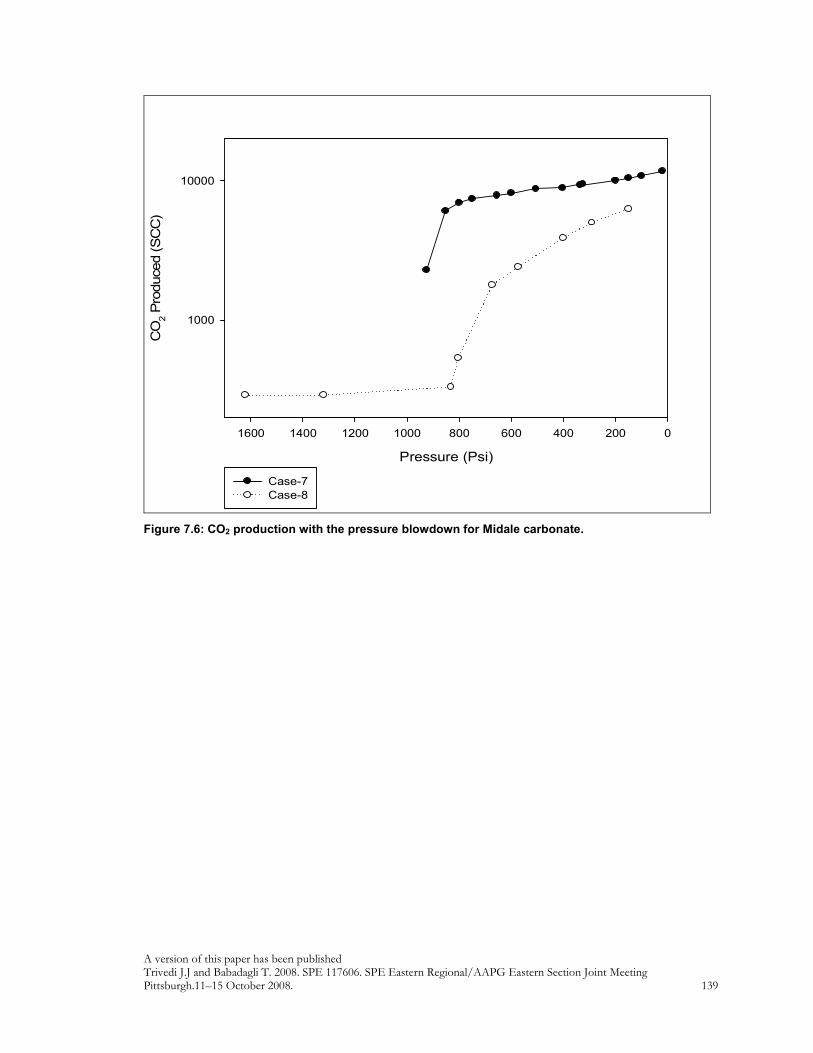
A version of this paper has been published Trivedi J.J and Babadagli T. 2008. SPE 117606. SPE Eastern Regional/AAPG Eastern Section Joint Meeting Pittsburgh.11–15 October 2008. 139
Pressure (Psi)
02004006008001000120014001600
CO2 Produced (SCC)
1000
10000
Case-7
Case-8
Figure 7.6: CO2 production with the pressure blowdown for Midale carbonate.

A version of this paper has been published Trivedi J.J and Babadagli T. 2008. SPE 117606. SPE Eastern Regional/AAPG Eastern Section Joint Meeting Pittsburgh.11–15 October 2008. 140
Pressure (Psi)
0 200 400 600 800 1000 1200
CO2 Storage (SCC)
1000
10000
Case-1
Case-2
Case-3
Case-4
Case-5
Case-6
Figure 7.7: CO2 storage with the pressure blowdown for Berea sandstone.

A version of this paper has been published Trivedi J.J and Babadagli T. 2008. SPE 117606. SPE Eastern Regional/AAPG Eastern Section Joint Meeting Pittsburgh.11–15 October 2008. 141
Pressure (Psi)
0 200 400 600 800 1000 1200 1400 1600 1800
CO2 Storage (SCC)
1000
10000
Case-7
Case-8
Figure 7.8: CO2 storage with the pressure blowdown for Midale carbonate.

A version of this paper has been published Trivedi J.J and Babadagli T. 2008. SPE 117606. SPE Eastern Regional/AAPG Eastern Section Joint Meeting Pittsburgh.11–15 October 2008. 142
CO2 Injected (PV )
0.01 0.1 1
Recovery (%PV) / CO2 Injected (PV)
10
100
1000
Case-3
Case-4
Case-5
Case-6
Figure 7.9: Normalized recovery factor with the CO2 PV injected for Berea sandstone.
CO2 Injected (PV )
0.01 0.1 1
Recovery (%PV) / CO2 Injected (PV)
10
100
1000
Case-7
Case-8
Figure 7.10: Normalized recovery factor with the CO2 PV injected for Midale carbonate.

A version of this paper has been published Trivedi J.J and Babadagli T. 2008. SPE 117606. SPE Eastern Regional/AAPG Eastern Section Joint Meeting Pittsburgh.11–15 October 2008. 143
Time (Hr)
0 20 40 60 80 100 120
Pressure (Psi)
800
1000
1200
1400
1600
1800Case-4
Case-5
Case-6
Case-7
Case-8
Figure 7.11: Pressure decay and attainment of quasi-equilibrium behavior.
0
5
10
15
20
25
30
35
% R
eco
ve
red
Initial Continuous Injection 1st blowdown (after quasi-equilibrium) Last blowdown
Figure 7.12: Hydrocarbon recovery distribution for the Case-8 at different stages of the production
life.
Start of Pressure decay (Injection stopped)

A version of this paper has been published Trivedi J.J and Babadagli T. 2008. SPE 117606. SPE Eastern Regional/AAPG Eastern Section Joint Meeting Pittsburgh.11–15 October 2008. 144
y = 4.046x-0.26
R² = 0.938
0
0.1
0.2
0.3
0.4
0.5
0.6
0.7
0.8
0.9
1
0.E+00 1.E+04 2.E+04 3.E+04 4.E+04 5.E+04 6.E+04 7.E+04 8.E+04
To
tal O
il P
rod
uc
ed
(P
V) / T
ota
l S
olv
en
t In
jec
ted
(P
V)
Matrix-Fracture Diffusion Group (N (M-FD)
Current work Firoozabadi and Markeset (1994)
Trivedi and Babadagli (2008a) Power (Current work)
Figure 7.13: (TOP/TSI) with matrix-fracture diffusion group (NM-FD).
145
8 ANALYSIS OF OBSERVATIONS ON THE MECHANICS OF MISCIBLE
GRAVITY DRAINAGE IN FRACTURED SYSTEMS
8.1 Problem Statement
• The understanding of gravity drainage mechanism in fractured systems is still below
par. Hence, the modeling of the process is a challenge yet and more attempts are
needed towards the clarifications on the physics of the process for accuracy.
• Injected gas flowing in fracture could be in equilibrium or non-equilibrium with the
oil phase in porous matrix. Depending on that the recovery mechanism varies quite
significantly.
• Moreover, the heterogeneity or presence of fracture adds more dimensions to the
difficulty level of the problem.
• The mechanistic difference between gravity stable gas injection and gravity drainage
for non-equilibrium gas (special consideration of CO2) is not studied thoroughly.
• The detailed literature review on the failure of most of the existing models to
differentiate the drainage and displacement mechanisms is studied by Kulkarni et al.
(2006). Three different mechanisms hypothesized by them for gravity drainage have
very limited experimental support in the literature to the best of our knowledge.
• Only attempts to describe the miscible gravity drainage mechanism in NFRs clearly
were done by Alavian and Whitson (2005), Darvish et al. (2004) and by Verlaan and
Boerrigter (2006) in a simulation study as well as experimental study from Schechter
and Guo (1996).
• When the non-equilibrium gas like CO2 is injected into matrix-fracture system,
mechanisms like molecular diffusion, dispersion mixing, swelling, IFT reduction,

146
viscous displacement, CO2 solubility effect and properties of fracture as well as
matrix may play important role other than the three described by Kulkarni et al.
• The mechanisms may vary depending on the well configuration (location), i.e.,
injection and production wells located in the fracture or in the matrix.
8.2 Mechanisms: Miscible Gravity Drainage in NFRs
In the experimental study, it was observed that oil produced at different time have different
composition than the original oil suggesting the existence of extraction process
simultaneously acting with other mechanism. If no extraction has taken place or the oil is
only displaced (miscibly or immiscibly), then wt% or the components should remain
constant (in terms of normalized concentration it should remain about 1). When a
component is preferentially extracted, a change in wt % should be observed; its increase
means higher extraction of that particular component (increase in normalized concentration
above 1).
1) Drainage in fracture:
At the initial period the composition change was not observed, indicating the recovery
from the fracture before much of the CO2 diffuses into the core. This period is dominant by
pure drainage from the fracture. The recovery during this period is affected by flow rate,
injection pressure (initial pressure) and density difference.
2) Induced drainage and extraction in matrix with forced drainage in fracture:
In this phase, the oil produced has higher percentage of medium components. The
governing mechanism is extraction of oil (swelling due to CO2-oil contact) and reduction in
IFT caused by lateral diffusion of CO2 and then driven by free fall gravity drainage within
matrix and forced drainage in fracture. The oil components that vaporized to the gas phase
are transported to the fracture by molecular diffusion due to compositional difference
between gas in the fracture and in the matrix. The diffusion is the limiting mechanism here.
3) Extraction of heavier hydrocarbon with forced drainage in fracture:

147
As the diffusion coefficients of heavier components are comparatively higher, a
preferential extraction occurs. At this level the heavier components are extracted.
8.3 Soaking: Improving Extraction Mechanism
If continued long enough, a point will be reached during the second phase at which the
recovery becomes uneconomical and there still exists high amount of oil saturation in the
matrix to be recovered. To recover this oil, more and more CO2 needs to be injected but a
great portion of it will be quickly produced without producing economical matrix oil making
the project inefficient. To enhance the recovery, we propose a new approach. During the
late 2nd stage and at the start of 3rd stage when the CO2 recycling cost begins to increase and
oil cut goes down, a soaking of injected CO2 until this point can increase the recovery. This
will allow the third level of recovery mechanism to become effective and heavier
components can be preferentially extracted. During soaking, the governing mechanism is
extraction and “free fall gravity drainage” (process believed to occur in NFRs after depleting
all oil in the fractures or there exists only injected gas in the fractures -Schechter and Guo,
1996).
As shown by Darvish et al. (2004), when the gas saturation in the matrix increases, the oil
viscosity drastically increases. During the soaking period when the gas saturation of the
matrix increases, oil mobility reduces to very low due to increase in viscosity. This is
extraction mechanism where heavier components of residual oil vaporize into the gas phase.
This fact has been verified by chromatographic analysis.
Time to reach gas saturation its maximum value and benefit from the recovery by extraction
in NFRs could require great amount of time and CO2 injection as well as recycling
depending on the matrix size. This may not be economical in most of the cases. To
overcome this problem, we suggest that soaking period would help to gain the recovery
through extraction. The length of the soaking period should be limited until the pressure of
the closed system (non-equilibrium gas and porous media containing residual oil) reaches a
quasi-equilibrium stage.

148
8.4 Effect of Diffusion/Dispersion and Injection Rate
Diffusion of solvent from the fracture to matrix creates a zone of mixing inside the matrix.
The mixing increases with time. In this mixed zone, the oil viscosity and density are reduced.
To understand the effect of lateral transfer and diffusion in gravity drainage, first contact
miscible experiments were performed as given in Chapter 2. This neglects the effects of
compositional change (hence extraction) due to solvent of solute with two distinct
components (heptane and mineral oil) as well as capillary and IFT change (both are zero due
to first contact miscible nature). The results presented in our previous work shows the oil
production rate does not drop drastically supporting the hypothesis, simulation results and
experimental trends of previous researches differentiating the drainage and displacement
mechanisms. Some of the conclusions gave insights into the importance of lateral flow and
diffusion flow:
• When compared with horizontal displacement with vertical drainage, the presence of
gravity effect was evident. The effect of gravity was more profound when the rate
was higher.
• At early stage, when less amount of solvent is present, the governing mechanism in
the process is viscous displacement resulting most recovery from fracture and is
higher for higher injection rate.
• The recovery curve at lower solvent injection rate overpasses the one at higher
solvent injection rate after a certain amount of solvent injected indicating slower the
rate is being more towards free fall drainage into the matrix.
• At high rates, mixing of oil and solvent is higher, resulting in lower viscosity and
density in the mixing zone. The mixing zone increases with time and so does the
gravity drainage rate. These observations were made by Verlaan and Boerrigter
(2006) in their simulation study giving justification to the higher production recovery
obtained at higher rate injection with same amount of solvent injected compared to
lower rates.

149
• The mixing zone moves faster with higher injection rate as “fresh solvent” is present
in the fracture zone to diffuse into matrix. Subsequently, the drainage rate in the
matrix and the rate of oil (solute) drained out to fracture increases (due to the
difference of drainage rate between mixing zone and oil zone). This is purely driven
by diffusion due to concentration gradient.
• With the increase of injection rate, bypassing of oil zone, i.e. matrix, is more
pronounced and this results in lower ultimate recovery. Oil trapping increases as the
injection rate and thereby the gravitational force increase. The forced gravity
drainage becomes unstable as the injection rate increases. This conclusion was also
supported by forced gravity drainage experiments in fractured system by Dastyari et
al. (2005). They performed forced drainage experiments using glass micromodels
with immiscible pair of fluids. This gives justification to the conclusion that the
slower injection rate though resulting slower ultimate recovery but efficient for
ultimate recovery.

150
9 CONTRIBUTIONS AND RECOMMENDATIONS
9.1 Contributions and Conclusions
9.1.1 First Contact Miscible Experiments
• Dominance of the phase diffusion into matrix through fracture over viscous flow in
the fracture was shown in this study. Though the higher solvent injection rate yields
high production rate of oil in the initial period of the project life, considering the
long run, the low rate solvent injection strategy is the best with most of the
production contribution from matrix through the diffusion process. Solvent injected
at lower rate has more time to diffuse into matrix in transverse direction before it
breaks through, hence results in higher ultimate recovery than that of higher rate
solvent injection strategy.
• With some water existing in the rock from previous waterflooding, one can still
obtain oil recovery from matrix by the diffusion process. Note that the ultimate
recovery obtained from the waterflooding followed by the solvent diffusion process
would be much lower than the cases with solvent diffusion only.
• The efficiency of the process was investigated using two different parameters. When
the amount of oil produced per time is the critical efficiency parameter, a rate of 6
ml/hr was found to be the optimal rate for almost all the cases except less water-wet
samples. This approach for efficiency analysis is useful for enhanced oil recovery
applications.
• In this study, we have not varied two critical parameters; the size of the matrix
(length or width) and oil type (mainly for viscosity variation). Further attempts were
made in subsequent studies where the process has been theoretically modeled using

151
the experimental observations and considering those parameters (Trivedi and
Babadagli, 2007a-b).
9.1.2 Scaling of Matrix-Fracture Miscible Process and Critical Rate
Definition
• If the amount of oil produced per amount of solvent injected is the critical efficiency
parameter, one can define a critical rate.
• Inspectorial Analysis (IA) was applied on governing equations representing miscible
matrix-fracture interaction when solvent is injected into oil saturated porous matrix.
Seven different independent dimensionless groups were derived by applying linear
(affine) transformation to the groups obtained by IA.
• The critical parameter defining the efficiency of the process could be the amount of
solvent introduced per oil produced as in the case of enhanced oil recovery
applications (the opposite is the case in greenhouse gas sequestration or groundwater
contamination processes). None of the scaling groups individually can define the
efficiency of the process of interest (Total Oil Produced (TOP) / Total Solvent
Injected (TSI)) ratio obtained from miscible experiments. Hence a new
dimensionless group combining varying strength of all forces acting as different
dimensionless groups during the process was proposed.
• Higher NM-FD indicates a faster recovery with more solvent injection. On the other
hand, a low value of the (NM-FD) is an indication of slow but more efficient recovery,
i.e., less solvent injection is required. This might even yield higher ultimate
recoveries from the matrix compared to the extremely high injection rate cases.
• This approach for efficiency evaluation is also useful in greenhouse gas sequestration
and groundwater contamination practices. Those processes target to maximize the
storage of injected material in the matrix and this requires an effective matrix-
152
fracture transfer due to diffusion. This could be controlled by the rate that would be
determined by matrix properties.
9.1.3 Simulation of Matrix-Fracture Process
• The experimental results indicated that the recovery through the fracture (less
contribution from matrix) is dominated by the Peclet number (dispersion effect) and
mass transfer rate constant (Kv). Hence, at the earlier stage of the production life
(when the fracture oil recovery is effective) higher rate solvent injection should be
preferred.
• Considering overall effect and assuming the solute inside the matrix pores is larger in
amount compared to that in the fracture, the effective diffusion coefficient (DeM) is
the major controlling parameter and slower rate solvent injection with more
retention time for effective diffusive flux to transfer from matrix yields efficient
recovery.
• The porous media aged over a period of time behaved different than that of non-
aged one depending on the solute properties. The wettability factor presented here
and further used in the study proved handy tool for inclusion of aging effect.
• Length of the matrix being one of the important parameter because of the solvent
breakthrough was noticed during experiments. The shorter cores, having less time
for solvent to diffuse in transverse direction into porous matrix, showed lower solute
recovery in a given time and rate compared to the longer ones. We, however, did
not observe significant effect of matrix size on the mass transfer rate constant (Kv )
and effective diffusion coefficient in matrix (DeM).

153
• The mass transfer rate and effective matrix diffusion coefficient were found to be
linearly dependent on the average fluid velocity through fracture and also affected by
wettability as well as rock properties.
• Kv and DeM, not available from any means of laboratory experiments, can be easily
computed for miscible solvent processes in fractured porous media using the
correlations provided here with fairly good amount of accuracy.
9.1.4 Multi-Contact CO2 Experiments
• Critical rate is one of the important factors to be considered while designing an EOR
and sequestration project.
• Maintaining near miscible pressure conditions is the most effective for incremental
oil recovery. Going beyond the near miscible pressure condition is proven to be
beneficial for sequestration purpose but can cause reduction in production.
• The reservoirs with lower temperature can also be targeted for sequestration and
EOR.
• The oil recovery from the Midale carbonate cores was only 23 % but after a first
cycle of blow down it reached 41 % due to CO2 diffusion and gravity drainage. The
storage capacity of the Midale carbonate was, however, almost half than that of the
sandstone rock while maintaining other operational parameter similar.
• The pressure decay during this shutdown (soaking) period gives a measure of
diffusion as well as recovery enhancement phenomenon in fractured porous media.

154
• The recovery of heavier hydrocarbon components is increased by a large fraction
during shutdown (soaking) after continuous injection of CO2. The shutdown after a
relatively slow injection rate for a longer period of time yielded higher diffusion and
higher amount of oil recovered during the first blowdown compared to faster
injection rate case for a shorter period of time.
• Blow down for additional recovery at the end of the CO2 injection project life, can
increase the recovery by 10% up to a certain pressure (~750 psi here). Going below
this pressure will affect sequestration adversely without much benefit of recovering
oil. CO2 phase behavior/change during the project is very crucial and should be
studied carefully with density and viscosity change into consideration.
• During the project life blowing down reservoir for an economic benefit of oil
recovery is not viable after a particular pressure stage and that pressure was found to
be around 600-700 psi for Berea sandstone and 400 psi for the Midale carbonate
cores. Similarly, while considering greenhouse gas sequestration, the same pressure
was proved to be the bottom limit not to exceed the viable range.
• “Huff and Puff” after continuous injection could prove very effective for EOR in
fractured reservoirs. The Huff cycle should be at miscible/near miscible condition
followed by a shutdown (soaking) until the quasi-equilibrium is reached and then a
Puff cycle. The Puff cycle should only be limited to pressure reduction until ~600 psi
and then followed by and Huff cycle to again reach miscible pressure.
• Understanding of diffusion/dispersion phenomenon into the matrix-fracture system
and its quantification were achieved using successful simulation match of very slow
rate CO2 injection into oil saturated fractured porous media experimental results.
Efficiency of the miscible gravity drainage process in fractured porous media can be
generalized using a dimensionless group NM-FD.

155
• The multicontact miscible diffusion at reservoir temperature and pressure is more
complex. This case requires more effort and could be critical especially in the CO2
injection for EOR and sequestration.
9.2 Recommendations for Future Research
• To predict the efficiency of EOR and sequestration we proposed a critical value of
matrix-fracture diffusion group which contains the Peclet and gravity number. More
experimental data with a wider range of porosity and permeability, wider scales of
viscosity and more oil wet systems for the validation will be ideal for necessary
modification in matrix-fracture diffusion group and its use as a transfer functions or
as a critical injection rate determination purpose.
• Current reservoir simulation tools consider matrix-fracture interaction to some
extent. The phenomenon observed in experiments such as pressure decay to reach
quasi-equilibrium and extraction of heavier components during shutdown cannot be
dealt easily with current forms of commercial reservoir simulation tools.
Modifications such as diffusion coefficient as a function of concentration and
pressure conditions also non-equilibrium boundary concepts should be incorporated.
• A micro-model and glass bead model with sandstone and carbonate replicas for
miscible CO2 diffusion and oil swelling behavior at reservoir condition should be
tested. The visual and quantitative results will lead to better understating of lighter
and heavier component phase diffusion and are necessary to solidify the implicative
conclusive statement.
• “Huff and Puff” after continuous injection could prove very effective for EOR in
fractured reservoirs. The “Huff” cycle should be at miscible/near miscible condition
followed by a shutdown until the quasi-equilibrium is reached and then a “Puff”
cycle should be implemented. The “Puff” cycle should only be limited to pressure

156
reduction till 600-500 psi and then followed by “Huff” cycle to again reach miscible
pressure. Further analysis for optimal application schemes for the “Huff” and
“Puff” process is needed.
• Since CO2 was able to recover heavier hydrocarbon components of the crude oil,
CO2 in conjunction with steam injection should be tested in heavy oil NFRs for
EOR and CO2 sequestration.

157
10 NOMENCLATURE
Chapter - 3
A = Total area for the core, m2
2b = Fracture aperture, m
CF = Concentration in fracture, fraction
CM = Concentration in matrix, fraction
Dm = Mutual diffusion coefficient, m2/s
DL = Effective dispersion coefficient in fracture, m2/s
DeM = Effective diffusion coefficient in matrix for matrix-fracture system, m2/s
Deff = Effective diffusion coefficient, m2/s
Dmech = Mechanical dispersion coefficient, m2/s
g = gravitational force, m/s2
VK = Mass transfer rate constant, s-1
N = Flux
P = Pressure, N/m2
Pe = Peclet number, Dimensionless
SQ = Source term,
Q = Amount imbibed, m3

158
r = Half fracture spacing, m
S = Saturation, fraction
t = time, s
V = Average fluid velocity in the fracture, m/s
factorW = Wettability factor, Dimensionless
x = coordinate direction along the fracture, m
y = coordinate direction normal to the fracture, m
Greek Letters
κ = Permeability, m2
fρ = Density, kg/m3
µ = Viscosity, kg/m.s
Subscripts
1 = Solvent
2 = Solute
h = Hydraulic
m = Mass transfer
M = Matrix
F = Fracture
R = Reaction
C = Convection

159
S = Surface
C = Capillary
K = Kerosene
W = Water
-------------------------------
Chapter - 4
b = Fracture width, m
Bim = Biot number, Dimensionless
>< AC = Cup-mixing concentration (transverse averaged concentration weighted with
respect to the normalized longitudinal velocity, fraction
AWC = Circumferentially averaged concentration at the fluid-solid interface, fraction
Da = Damkohler number, Dimensionless
DL = Effective dispersion coefficient in fracture, m2/s
DeM = Effective diffusion coefficient in matrix for matrix-fracture system, m2/s
VK = Mass transfer rate constant, s-1
mK = mass-transfer coefficient between bulk fluid phase and matrix fluid phase, m/s.
L = Characteristic length, m
P = Pressure, N/m2
Pe = Peclet number, Dimensionless

160
R = Core radius, m
Re = Reynolds number, Dimensionless
Sh = Sherwood number, Dimensionless
t = time, s (Defined in Table 4.1)
v = Average fluid velocity in the fracture, m/s
factorW = Wettability factor, Dimensionless
Greek Letters
ρ = Density, kg/m3
µ = Viscosity, kg/m.s
φ = Thiele modulus, Dimensionless
η = Effectiveness factor, Dimensionless
Subscript
1 = Solvent
2 = Solute
∞ = Asymptotic Value
C = Capillary
G = Global
K = Kerosene
L = Local
r = radial direction

161
z = transverse direction
-----------------------------
Chapter - 5
b = Fracture width m,
Ce = Concentration at equilibrium
DL = Effective dispersion coefficient in fracture m2/s,
DeM = Effective diffusion coefficient in matrix for matrix-fracture system m2/s,
FDI = Fracture diffusion index, dimensionless,
g = Gravity force m/s,
kf = Fracture permeability m2,
km = Matrix permeability m2,
L = Length of Fracture m,
Lx = Matrix size in x direction m,
Ly = Matrix size in y direction m,
Nf,Ca = Facture capillary number, dimensionless
effcP , = Effective capillary pressure, dimensionless,
max,cP = Maximum capillary pressure value (Pc at Swi=0), dimensionless,
QI = Amount of solvent injected (Pore volume)
QP = Amount of solute produced (Pore volume)
r = Matrix width m,

162
uT = Flow velocity m/s,
Symbols
wµ = Viscosity of water, cp,
σ = Interfacial tension, N/m,
sρ = Density of injected (solvent) phase, kg/m3,
oρ = Density of displaced (oil) phase, kg/m3,
ØF = Porosity (Fracture)
ØM = Porosity (matrix)
µs = Solvent viscosity, kg/m.s,
µo = Solute viscosity, kg/m.s,
∆µ = Viscosity difference, kg/m.s,
∆ρ = Density difference, kg/m3
-----------------------------
Chapter - 7
b = Fracture width m,
DL = Effective dispersion coefficient in fracture m2/s,
De = Effective diffusion coefficient in matrix for matrix-fracture system m2/s,
g = Gravity force m/s,
kf = Fracture permeability m2,
km = Matrix permeability m2,

163
L = Length of Fracture m,
Lx = Matrix size in x direction m,
Ly = Matrix size in y direction m,
r = Matrix width m,
uT = Flow velocity m/s,
Symbols
sρ = Density of injected (solvent) phase, kg/m3,
oρ = Density of displaced (oil) phase, kg/m3,
ØF = Porosity (Fracture)
ØM = Porosity (matrix)
µs = Solvent viscosity, kg/m.s,
µo = Solute viscosity, kg/m.s,
∆µ = Viscosity difference, kg/m.s,
∆ρ = Density difference, kg/m3

164
11 APPENDIX
Fracture:
02
2
=∂
∂+
∂
∂−
∂
∂+
∂
∂
y
C
b
D
x
CD
x
Cu
t
C MmmFL
FFx
F φ ................................................................ (10.1)
For matrix:
02
2
=∂
∂−
∂
∂
y
CD
t
C Mm
M ............................................................................................................. (10.2)
+
∂
∂−= g
x
Pku F
F
F
FFX ρ
µ...................................................................................................... (10.3)
C = 0 at t = 0 yx,∀ .......................................................................................................... (10.4)
uy = 0 at y = 0 tx,∀ ............................................................................................................ (10.5)
uy = 0 at y = b tx,∀ ............................................................................................................. (10.6)
∫ =b
TFX udyub
0
1 At x=0........................................................................................................ (10.7)
)( ybgPP mwfF −+= ρ at x=L.............................................................................................. (10.8)
Dimensionless variables for non-dimensionalizing the above equations related to our system
are as follows:
( )*2*
1 XXXx D += .................................................................................................................... (10.9)

165
( )*2*
1 yyyy D += (Within fracture) ....................................................................................... (10.10)
( )*2*
1 YYYy D += (Within matrix) ......................................................................................... (10.11)
( )*2*
1 tttt D += ........................................................................................................................... (10.12)
)( *
2
*
1 FFDFF CCCC += ........................................................................................................... (10.13)
)( *
2
*
1 MMDMM CCCC += ........................................................................................................ (10.14)
)( *
2
*
1 FXFXDFXFx uuuu += ........................................................................................................ (10.15)
)( *
2
*
1 FFDFF PPPP += ............................................................................................................... (10.16)
Using these dimensionless variables (Equations 10.9 to 10.16) the advection-convection
equation (Eq. 10.1) for fracture can be written as:
0)(
)(*
1
*
1
2
2
2*
1
*
1
*
1
*
1*
2
*
1*
1
*
1 =∂
∂
+
∂
∂
−
∂
∂
++
∂
∂
D
MDMmm
D
FDFL
D
FDFFXFXDFX
D
FDF
Y
C
Y
CD
X
C
X
CD
X
C
X
Cuuu
t
C
t
Cφ
................................................................................................................................................... (10.1A)
02
2
=∂
∂
+
∂
∂
−
∂
∂
+
∂
∂
+
∂
∂
D
MD
D
FD
D
FD
D
FDFXD
D
FD
Y
C
X
C
X
C
X
Cu
t
C*
1
*
1mm
2*
1
*
1L
*
1
*
FX2
*
1
*
1
*
FX1
*
1
Y
tDφ
)(X
tD
X
ut
X
ut
....................................................................................................................................................(10.1B)
Using these dimensionless variables (Equations 9 to 16) the advection-convection equation
(Eq. 2) for matrix can be written as:
02
2
=∂
∂
−
∂
∂
D
MD
D
MD
Y
C
t
C2*
1
*
1m
)(Y
tD.............................................................................................. (10.2A)

166
Similarly, using the dimensionless variables in Equations 10.9 to 10.16, one can present
Equations 10.3 to 10.8 in the dimensionless form:
( ) ( )[ ] ( )
∆+++
∂
∂
−++=+
−gCCC
X
P
X
PCCCkuuu FFDF
D
FDF
SFFDFFFXFXDFX ρρµµµ )()( *
2
*
10*
1
*
11
0
*
2
*
10
*
2
*
1
................................................................................................................................................... (10.3A)
1−
+
+
−
−=
*
F1F
0
*
FX1
*
1
*
F1F
*
FX1
*
1
*
F2
*
F1F
S
*
FX1
*
1
*
F1
*
F1F
0
*
FX1
*
1
*
F1
Pk
µuX
Pk
∆µuXC
Pk
µuXC
Pk
µuXCDFXD Cu
−
+
+
+
∂
∂*
FX1
*
FX2
*
F1
*
F2
*
1
*
F1
*
10
*
F1
*
F1
*
1
u
u
P
C∆ρgX
P
gXρ
P
C∆ρgXD
D
XD CX
P............(10.3B)
0)( *
2
*
1 =+ FFDF CCC at 0*
2
*
1 =+ ttt D DD yX ,∀ ........................................................ (10.4A)
−=
*
F1
*
F2
C
CFDC at
−=
*
1
*
2
t
tDt DD yX ,∀ ........................................................(10.4B)
0)( *
2
*
1 =+ FyFyDFy uuu at 0*
2
*
1 =+ yyy D DD tX ,∀ .............................................. (10.5A)
−=
*
Fy1
*
Fy2
u
uFyDu at
−=
*
1
*
2
y
yDy DD tX ,∀ ..............................................(10.5B)
0)( *
2
*
1 =+ FyFyDFy uuu at byyy D =+ *
2
*
1 DD tX ,∀ ....................... (10.6A)
−=
*
Fy1
*
Fy2
u
uFyDu at
−=
*
1
*
2
y
ybDy DD tX ,∀ ........................(10.6B)
( )∫−
=+
*1
*2 /)(
0
*
2
*
1
*
1yyb
TDFXFXDFX udYuuub
y at ( ) 0*
2
*
1 =+ XXX D Dt∀ .......... (10.7A)
∫−
=
+
*1
0
)/yy(b
*
FX1
*
1
T
*
FX1
*
FX2*2
uy
bu
u
uDFXD dyu at
−=
*
1
*
2
X
XDX Dt∀ ..................(10.7B)

167
( ) ( )( )
−−
+
∆++=+ ∫
−*
2
*
1
/)(
0
*
2
*
1
*
10
*
2
*
1
*1
*2
)( yyybgdYuuub
yPPPP D
yyb
DFXFXDFXwfFFDF ρρ
at ( ) LXXX D =+ *
2
*
1 ; ( ) byyy D ≤+≤ *
2
*
10 .......................... (10.8A)
at
−=
*
1
*
2
X
XLDX ;
−≤≤
−
*
1
*
2
*
1
*
2
y
yb
y
yDy ..............(10.8B)
Table 10.1: The unique dimensionless group from the above equations (marked as bold letters)
*
1
*
1
*
1
X
ut FX
*
1
0
*
1
*
1
FF
FX
Pk
uX µ
−
*
FX1
*
FX2
u
u
*
1
*
2
*
1
X
ut FX
∆*
1
*
1
*
1
F
F
P
CgXρ
−
*
1
*
2
y
y
2*
1
*
1
)(X
tDL
*
1
*
10
FP
gXρ
−*
1
*
2
y
yb
*
1
*
1
Y
tDmmφ
∆*
1
*
2
*
1
F
F
P
CgXρ
*
1
*
1 FX
T
uy
bu
2*
1
*
1
)(Y
tDm
*
1
*
2
FX
FX
u
u
−
*
1
*
2
X
X
*
1
0
*
1
*
1
*
1
FF
FXF
Pk
uXC µ
−
*
F1
*
F2
C
C
−*
1
*
2
F
Fwf
P
PP
*
1
*
1
*
1
*
1
FF
SFXF
Pk
uXC µ
−
*
1
*
2
t
t
−*
1
*
2
X
XL
∆*
1
*
1
*
1
*
2
FF
FXF
Pk
uXC µ
−
*
Fy1
*
Fy2
u
u

168
For eliminating extra dimensionless group from these 23 groups obtained from above
equations, the arbitrary scale factors being 0 and 1 can be assigned:
Hence, setting;
∆*
1
*
1
*
1
*
2
FF
FXF
Pk
uXC µ=0 ;
*
1
*
2
FX
FX
u
u=0 ; 0
*
1
*
2 =
F
F
C
C
0*
1
*
2 =
t
t ; 0
*
1
*
2 =
X
X ; 0
*
1
*
2 =
−
F
Fwf
P
PP
and,
1*
1 =FC ; 1*
1 =MC ; 1*
1
*
2 =
−
X
XL ; 1
*
1
*
1
*
1 =
X
ut FX ;
1*
1
0
*
1
*
1
*
1 =
FF
FXF
Pk
uXC µ ; 1
*
1
0
*
1
*
1 =
FF
FX
Pk
uX µ ; 1
*
1
*
1
=
FX
T
uY
bu ; 1
*
1
*
2 =
−
y
yb
We obtain the scale factors:
LX =*
1 ;
=
Tu
Lt *1 ;
=
F
T
Fk
LuP 0*
1
µ ;
TFX uu =*
1 ; by =*
1
Thus, the Equations (10.1B), (10.2B), (10.3B), (10.4B) and (10.5B) can be reduced to
following dimensionless equations:

169
02
2
=∂
∂
+
∂
∂
−
∂
∂+
∂
∂
D
MD
T
mmF
T
L
D
FDFxD
D
FD
Y
C
bru
LD
x
C
Lu
D
x
Cu
t
C φ...........................................(10.1C)
02
2
2=
∂
∂
−
∂
∂
D
MD
T
m
D
MD
Y
C
ur
LD
t
C................................................................................................(10.2C)
+
∆+
∂
∂
+
−−=
−
T
F
D
T
F
D
FD
D
S
FXDu
gkC
u
gk
X
PCu
0
0
0
1
0
11µ
ρµ
ρµµ
............................(10.3C)
0=FDC at 0=Dt DD yX ,∀ ..................................................(10.4C)
0=FyDu at 0=Dy DD tX ,∀ ....................................................(10.5C)
0=FyDu at 1=Dy DD tX ,∀ ....................................................(10.6C)
( )∫ =1
01DFXD dyu at 0=DX Dt∀ ...........................................................(10.7C)
( )DDFXD
T
F
T
FFD ydyu
Lu
gbk
Lu
gbkP −
∆+
= ∫ 1
1
000
0
µρ
µρ
at XD = 1, 10 ≤≤ Dy ......(10.8C)
The dimensionless groups from the above equations (10.1C to 10.5C) are:
T
L
Lu
D
........................................................................................................................................(G’-1)
T
mm
bru
LDφ
...................................................................................................................................(G’-2)
T
m
ur
LD2
...................................................................................................................................... (G’-3)
0µµS ......................................................................................................................................... (G’-4)

170
∆
T
F
u
gk
0µρ
.................................................................................................................................. (G’-5)
T
F
u
gk
0
0
µρ
...................................................................................................................................(G’-6)
Lu
gbk
T
F
0
0
µρ
..................................................................................................................................(G’-7)
∆Lu
gbk
T
F
0µρ
.................................................................................................................................(G’-8)
The coefficient matrix of these groups:
0111010100110
1101010100110
1101010000100
0111010000100
0000110000000
0000002010110
0000001111110
0000000000111
0
−−−
−−−
−−
−−
−
−
−−−
−−
∆ oFSmmTL gkrbDuLD ρρµµφ
Dimensionless scaling groups can be reduced to using the raw elimination method on
coefficient matrix:

171
0000000100010
0111010000100
1010000000000
0000110000000
0000000110100
0000001001010
0000000010001
0
−
−−
−
−
−−
−
−
∆ oFSmmTL gkrbDuLD ρρµµφ
Hence we obtain the final dimensionless groups as;
m
L
D
D = (Dispersion diffusion ratio)..................................................................................... (G1)
L
rmφ = (1/aspect ratio for matrix) ....................................................................................... (G2)
T
m
bu
D = (1/Pe) .......................................................................................................................... (G3)
0µµS = (1/M) = (1/Mobility factor) ..................................................................................... (G4)
∆
0ρρ
= Density Number ........................................................................................................ (G5)
∆
T
F
u
gk
0µρ
= Gravity Number .................................................................................................. (G6)
L
b = (1/Aspect ratio for fracture)........................................................................................ (G7)
172
12 BIBLIOGRAPHY
Aris R., 1956. On dispersion of a solute in a fluid flowing through a tube. Proc. R. Soc.
London A. 235 (1200): 66.
Alavian S. A. and Whitson C. H., 2005. CO2 IOR Potential in Naturally Fractured Haft Kel
Field, Iran. IPTC 10641, International Petroleum Technology Conference. Doha, Qatar.
November.
Asghari K. and Torabi F., 2007. Experimental Study of Extent and Rate of Gravity Drainage
of Oil From Matrix into Fractures in Presence of Miscible and Immiscible CO2. Paper 2007-
120, 58th Annual Technical Meeting, Canadian International Petroleum Conference, Calgary,
AB, Canada, 12-14 June.
Babadagli T. and Ershaghi I., 1993. Improved Modeling of Oil/Water Flow in Naturally
Fractured Reservoirs Using Effective Fracture Relative Permeabilities. SPE 26076, SPE
Western Regional Meet., Anchorage, Alaska, May 26-28.
Babadagli T. and Zeidani K., 2004. Evaluation of Matrix-Fracture Imbibition Transfer
Functions for Different Types of Oil, Rock and Aqueous Phases. SPE 89450, paper
presented at the 14th SPE/DOE Symposium on Improved Oil Recovery, Tulsa, OK, April.
Babadagli T., 2000. Efficiency of Capillary Imbibition Dominated Displacement of Non-
Wetting Phase by Wetting Phase in Fractured Porous Media. Transport in Porous Media. 40:
323.
Babadagli T., 2002. Scaling capillary imbibition during static thermal and dynamic fracture
flow conditions. J. Pet. Sci. Eng. 33: 223.

173
Babadagli T., Hatiboglu C. U. and Hamida T., 2005. Evaluation of Matrix-Transfer
Functions for Counter-Current Capillary Imbibition. SPE 92111, SPE Asia Pacific Oil &
Gas Conference and Exhibition, Jakarta, Indonesia, April.
Bachu S., 2002. Sequestration of CO2 in Geological Media: Criteria and Approach for Site
Selection in Response to Climate Change. Energy Convers. Manag. 41: 953.
Bear J., 1988. Dynamics of fluids in porous media. New York: Dover Publications Inc.
Bear J., 1979. Hydraulics of groundwater. McGraw Hill.
Bhattacharya M., Harold M. P. and Balakotaiah V., 2000. Mass-transfer coefficients in
washcoated monoliths. AICHE J. 50: 2939.
Burger J. E., Springate G. and Mohanty K. K., 1996. Experiments on Bypassing during Gas
Floods in Heterogeneous Porous Media. SPERE. 11 (2): 109.
Burger J.E. and Mohanty K. K., 1997. Mass transfer from bypassed zones during gas
injection. SPERE. 12 (2): 124.
Chakravarthy D., Muralidaharan V., Putra E., Hidayati D. T. and Schechter D. S., 2006.
Mitigating Oil Bypassed in Fractured Cores During CO2 Flooding Using WAG and Polymer
Gel Injections. SPE 97228, SPE/DOE Symposium on Improved Oil Recovery, Tulsa, OK,
USA, 22-26 April.
Civan F. and Rasmussen M. L., 2002. Improved measurement of gas diffusivity for miscible
gas flooding under nonequilibrium and equilibrium conditions. SPE 75135, SPE/DOE
Improved Oil Recovery Symposium. Tulsa, OK. April.
Civan F. and Rasmussen M. L., 2005. Determination of Parameters for Matrix-Fracture
Transfer Functions From Laboratory Data. SPE 94267, SPE Production & Operation
Symposium, Oklahoma City, OK, April.

174
Comings F. W. and Sherwood T. K., 1934. The drying of solids, moisture movement by
capillarity in drying granular materials. Ind. & Eng. Chemistry. 26: 1096.
Correa A. C. F. and Firoozabadi A., 1996. Concept of Gravity Drainage in Layered Porous
Media. SPEJ. March. 101-111.
COMSOL. 2006. COMSOL Multiphysics; 3.2 ed. Stockholm, Sweden.
Cybulski A. and Moulin J. A., 1994. Monoliths in Heterogeneous Catalysis. Catal. Rev. Sci.
Eng. 36: 179.
Cybulski A. and Moulin J. A., 1998. Structured catalysis and reactors. New York: Marcel
Dekker.
Darvish G. R., Lindeberg E., Holt T., Utne S. A. and Kleppe J., 2006a. Reservoir-Condition
Laboratory Experiments of CO2 Injection into Fractured Cores. SPE 99650, SPE
Europe/EAGE Annual Conference and Exhibition, Vienna, Austria, 12-15 June.
Darvish G. R., Lindeberg E., Holt T. and Utne S. A., 2006b. Reservoir-Condition
Laboratory Experiments of CO2 Injection into Fractured Cores. SPE 99649, SPE
Europe/EAGE Annual Conference and Exhibition, Vienna, Austria, 12-15 June.
Da Silva F. L. and Belery P., 1989. Molecular Diffusion in Naturally Fractured Reservoirs: A
Decisive Recovery Mechanism. SPE 19672, 64th SPE Fall Meeting, San Antonio, TX,
October.
Dastyari A., Bashukooh B., Shariatpanahi S. F., Haghighi M. and Sahimi M., 2005.
Visualization of Gravity Drainage in a Fractured System During Gas Injection Using Glass
Micromodel. SPE 93673, 14th SPE Middle East Oil & Gas Conference, Behrain. March.
Dindoruk B. and Firoozabadi A., 1997. Crossflow in Fractured/Layered Media
Incorporating Gravity, Viscous, and Phase Behavior Effects. SPEJ. June. 120-135.

175
Dronfield D. G. and Silliman S. E., 1993. Velocity dependence of dispersion for transport
through a single fracture of variable roughness. Water Resour. Res. 29(10): 3477.
Detwiler R. L., Rajaram H. and Glass R. J., 2000. Solute transport in variable-aperture
fractures: an investigation of the relative importance of Taylor dispersion and
macrodispersion. Water Resour. Res. 36(7): 1611.
Firoozabadi A. and Markeset T. I., 1994. Miscible Displacement in Fractured Porous Media:
Part I – Experiments. SPE 27743, SPE/DOE 9th Symposium on Improved Oil Recovery,
Tulsa, OK. April.
Fischer H. B., List E. J., Koh R. C. Y., Imberger J. and Brooks N. H., 1979. Mixing in Inland
and Coastal Waters. Academic, San Diego, Calif.
Fjelde I., Zuta J. and Duyilemi O. V., 2008. Oil Recovery from Matrix during CO2-Foam
Flooding of Fractured Carbonate Oil Reservoirs. SPE 113880, SPE Europec/EAGE Annual
Conference and Exhibition, Rome, Italy, 9-12 June.
Forzatti P., 2001. Present Status and Perspectives in de-NOx SCR Analysis. Appl. Catal. A.
Gen. 222: 221.
Fox R. W. and McDonlad T. A., 1998. Introduction to Fluid Mechanics. John Willey & Sons
Canada, Ltd.
Freeze R. A. and Cherry J. A., 1979. Groundwater. Prentice- Hall, Englewood Cliffs, NJ.
Froment G. F. and Bischoff K. B., 1990. Chemical reactor analysis and design (2nd Edition)
Wiley, New York.
Gabitto J. F., 1998. Matrix-fracture mass transfer. SPE 39702, paper presented at SPE/DOE
Improved Oil Recovery Symposium. Tulsa, OK. April.
176
Gharbi R., Peters E. and Elkamel A., 1998. Scaling Miscible Fluid Displacement in Porous
Media. Energy & Fuels. 12: 801.
Gharbi R., 2002. Dimensionally Scaled Miscible Displacement in Heterogeneous Permeable
Media. Transport in Porous Media. 48: 271.
Ghorayeb K. and Firoozabadi A., 2000. Numerical Study of Natural Convection and
Diffusion in Fractured Porous Media. SPEJ. 5 (1):12.
Grattoni C. A., Jing X. D. and Dawe R. A., 2001. Dimensionless Groups for Three-Phase
Gravity Drainage Flow in Porous Media. Journal of Petroleum Science and Engineering. 29:
53.
Gillham R. and Cerry J.A., 1982. Contaminant migration in saturated unconsolidated
geologic deposits. In Recent trends in hydrogeology. Edited by T. N. Narasimhan.
Geological Society of America, Special Paper 189, 3:1-62.
Handy L., 1960. Determination of effective capillary pressure for porous media from
imbibition data. AIME Trans. 219: 75.
Hatiboglu C. U. and Babadagli T., 2004. Experimental analysis of primary and secondary oil
recovery from matrix by counter-current diffusion and spontaneous imbibition. SPE 90312,
SPE Annual Technical Conference and Exhibition. Houston, TX. September.
Hatiboglu C. U. and Babadagli T., 2006. Primary and Secondary Oil Recovery from
Different Rocks by Countercurrent Diffusion and Spontaneous Imbibition. SPE 94120,
SPE/DOE Symposium on Improved Oil Recovery, Tulsa, OK, April.
Horne R. N. and Rodriguez F., 1983. Dispersion in tracer flow in fractured geothermal
systems. Geophys. Res. Let. 10 (4): 289.
177
Hu H., Whitson C. H. and Ai Y., 1991. A study of recovery mechanisms in a nitrogen
diffusion Experiment. SPE 21893, unsolicited paper available in Society of Petroleum
Engineers e-library.
Hujun Li., Putra E., Schechter D. S. and Grigg R. B., 2000. Experimental investigation of
CO2 gravity drainage in a fractured system. SPE 64510, SPE Asia Pacific Oil & Gas
Conference and Exhibition. Brisbane, Australia. October.
Ippolito I., Daccord G., Hinch E. J. and Hulin. J. P., 1984. Echo tracer dispersion in model
fractures with a rectangular geometry. J. Contam. Hydrol. 16 (1): 87.
Jamshidnezhad M., Montazer-Rahmati M. and Sajjadian V. A., 2004. Theoretical and
experimental investigations of miscible displacement in fractured porous media. Transport in
Porous Media. 57 (1): 59.
Jessen K., Kovscek A. R. and Orr F. M., 2005. Increasing CO2 Storage in Oil Recovery.
Energy Convers. Mgmt. 46: 293.
Jensen T. B., Sharma M. P., Harris H. G. and Whitman D. L., 1992. Numerical investigations
of steam and hot-water flooding in fractured porous media. SPE 24172, paper presented at
the SPE/DOE 8th Symposium on Enhanced Oil Recovery. Tulsa, OK. April.
Johnson R. W., 1998. The Handbook of Fluid Dynamics. CRC Press.
Karimaie H., Darvish G. R., Lindeberg E. and Torsaeter O., 2007. Experimental
Investigation of Secondary and Tertiary Gas Injection in Fractured Carbonate Rock. SPE
107187, SPE Europe/EAGE Annual Conference and Exhibition, London, UK, 11-14 June.
Keller A. A., Roberts P. V., Martin M. J., 1999. Effect of fracture aperture variations on the
dispersion of solutes. Water Resour. Res. 35(1): 55.
Kovscek A. R., 2002. Screening Criteria for CO2 Storage in Oil Reservoir. Petroleum
Science and Technology. 20 (7-8): 841.

178
Kulkarni M. M. and Rao D. N., 2006a. Characterization of Operative Mechanisms in Gravity
Drainage Field Projects through Dimensionless Analysis. SPE 103230, SPE Annual
Technical Conference and Exhibition, San Antonio, TX. September.
Kulkarni M. M. and Rao D. N., 2006a. Analytical Modeling of the Forced Gravity Drainage
GAGD Process. AIChE paper # 72361, AIChE Annual Meeting. San Francisco, CA.
November.
LaBolle E. M., Quastel J., Fogg G. E. and Gravner J., 2000. Diffusion Processes in
Composite Porous Media and their Numerical Integration by Random Walks: Generalized
Stochastic Differential Equations with Discontinuous Coefficients. Water Resources
Research. 36: 651.
Lenormand R., Le Romancer J. F., Le Gallo Y. and Bourbiaux B., 1998. Modeling the
Diffusion Flux Between Matrix and Fissure in a Fissured Reservoir. SPE 49007, SPE Annual
Technical Conference and Exhibition, New Orleans, LA, September.
Le Romancer J. F., Defives D. F., and Fernandes G., 1994. Mechanism of oil recovery by gas
diffusion in fractured reservoir in presence of water. SPE 27746, SPE/DOE 9th Symposium
on Improved Oil Recovery, Tulsa, OK. April.
Li S., Dong M., Li Z., Huang S., Qing H. and Nickel E., 2005. Gas Breakthrough Pressure
for Hydrocarbon Reservoir Seal Rocks: Implication for Security of Long-term CO2 Storage
in the Weyburn Field. Geofluids. 5: 326-334.
Mohanty K. K and Salter S. J., 1982. Multiphase flow in porous media: II- pore-level
modeling. SPE 11018, SPE Annual Technical Conference and Exhibition. New Orleans.
September.
Mahmoud N.N., 2006. Demonstration and Performance Characterization of the Gas
Assisted Gravity Drainage (GAGD) Process using A Visual Model. Thesis, Louisiana State
University.
179
Morel D. D., Bourbiaux B., Latil M. and Thiebot B., 1993. Diffusion effects in gas flooded
light oil fractured reservoirs. SPE-Adv. Tech. Series. 1 (2): 100-109.
Muralidharan V., Putra E. and Schechter D. S., 2004. Experimental and Simulation Analysis
of Fractured Reservoir Experiencing Different Stress Conditions. Paper 2004-229, 55th
Annual Technical Meeting, Canadian International Petroleum Conference, Calgary, Canada,
June 8-10.
Pande K. K. and Orr F. M. Jr., 1990. Analytical computation of breakthrough recovery for
CO2 floods in layered reservoirs. SPE 20177, unsolicited paper available in Society of
Petroleum Engineers e-library.
Part M., 1993. Percolation model of drying under isothermal conditions in porous media.
Int. J. Multiphase Flow. 19: 693.
Perkins T. K and Johnston O. C., 1963. A review of diffusion and dispersion in porous
media. SPEJ. 3(4):70, Trans. AIME. 228 (1): 70.
Rangel-German E. R. and Kovscek A. R., 2000. Matrix-Fracture Interaction in Single Matrix
Blocks. Proceedings of 25th Workshop on Geothermal Reservoir Engineering. January.
Riazi M. R., 1996. A New Method for Experimental Measurement of Diffusion Coefficients
in Reservoir Fluids. J. Pet. Sci. Eng. 14 (3-4): 235.
Roux S., Plouraboue F. and Hulin J. P., 1998. Tracer dispersion in rough open cracks. Trans.
Porous Media. 32 (1): 97.
Saidi A. M., 1987. Reservoir Engineering of Fractured Reservoir. Total Edition Press.
Sahimi M., Heiba A. A., Hughes B. D., Davis H. T. and Scriven L. E., 1982. Dispersion in
flow through porous media. SPE 10969, SPE Annual Technical Conference and Exhibition.
New Orleans. September.
180
Schechter D. S. and Guo B., 1996. Mathematical Modeling of Gravity Drainage after Gas
Injection into Fractured Reservoirs. SPE 35170, SPE Improved Oil Recovery Symposium.
Tulsa, OK. April.
Sheikha H., Pooladi-Darvish M. and Mehrotra A. K., 2005. Development of Graphical
Methods for Estimating the Diffusivity Coefficient of Gases in Bitumen from Pressure-
Decay Data. Energy & Fuels. 19 (5): 2041.
Shook M., Li D. and Lake L. W., 1992. Scaling immiscible flow through permeable media by
inspectional analysis. In-Situ 4: 311.
Sigmund P.M., 1976. Prediction of Molecular Diffusion at Reservoir Conditions: Part I.
Measurement and Prediction of Binary Dense Gas Diffusion Coefficients. J. Can. Pet. Tech.
15: 48– 57.
Slobod R. L. and Howlett W. E., 1964. The Effect o Gravity Segregation in Studies of
Miscible Displacement in Vertical Unconsolidated Porous Media. SPEJ. :1-8.
Stubos A. K. and Poulou S., 1999. Oil recovery potential from fractured reservoirs by mass
transfer processes. SPE 56415, SPE Annual Technical Conference and Exhibition. Houston,
TX. October.
Taber J. J., Martin F. D. and Seright R. S., 1997a. EOR Screening Criteria Revisited-Part 1:
Introduction to Screening Criteria and Enhanced Recovery Field Projects. SPE Res. Eng.
189.
Taber J. J., Martin F. D. and Seright R. S., 1997b. EOR Screening Criteria Revisited-Part 2:
Applications and Impact of Oil Process. SPE Res. Eng. 199.
Tang D. H., Frind E. O. and Sudicky E. A., 1981. Contaminant Transport in Fractured
Porous Media: Analytical Solution for a Single Fracture. Water Resour. Res. 17: 555.

181
Taylor G., 1953. Dispersion of soluble matter in solvent flowing slowly through a tube. Proc.
R. Soc. A. 219 (1137):186.
Tharanivasan A. K., Yang C. and Gu Y., 2004. Comparison of Three Different Interface
Mass Transfer Models Used in the Experimental Measurement of Solvent Diffusivity in
Heavy Oil. J. Pet. Sci. Eng. 44 (3-4): 269.
Thompson J. L. and Mungan N., 1969. A laboratory study of gravity drainage in fractured
systems under miscible conditions. SPEJ. June. 247.
Torabi F. and Asghari K., 2007. Performance of CO2 Huff-and-Puff Process in Fractured
Media (Experimental Results). Paper 2007-119, 58th Annual Technical Meeting, Canadian
International Petroleum Conference, Calgary, AB, Canada, 12-14 June.
Trivedi J. J. and Babadagli T., 2006. Efficiency of Miscible Displacement in Fractured
Porous Media. SPE 100411, SPE Western Regional/AAPG Pacific Section/GSA
Cordilleran Section Joint Meeting. Anchorage, Alaska, 8-10 May.
Trivedi J. and Babadagli T., 2008a. Efficiency of Diffusion Controlled Miscible
Displacement in Fractured Porous Media. Transport in Porous Media. 71(3): 379.
Trivedi J. and Babadagli T., 2008b. Experiment and Numerical Modeling of the Mass
Transfer between Rock Matrix and Fracture. Chemical Eng. J. doi:10.1016/j.cej.2008.05.032.
Trivedi J. and Babadagli T., 2008c. Efficiency Analysis of Greenhouse Gas Sequestration
during Miscible CO2 Injection into Fractured Oil Reservoirs. Accepted for publication in
Env. Sci. and Tech.
Trivedi J. and Babadagli T., 2008d. Scaling Miscible Displacement in Fractured Porous
Media Using Dimensionless Groups. J. Pet. Sci. Eng. doi:10.1016/j.petrol.2008.03.001.
Trivedi J. J. and Babadagli T., 2008e. Experimental Investigations on the Flow Dynamics
and Abandonment Pressure for CO2 Sequestration and Incremental Oil Recovery in

182
Fractured Reservoirs: The Midale Field Case. Paper 2008-092, 59th Annual Technical
Meeting, CIPC/SPE Gas Technology Symposium, Calgary, Alberta, Canada, 17-19 June.
Upreti S. R. and Mehrotra A. K., 2002. Diffusivity of CO2, CH4, C2H6, and N2 in Athabasca
bitumen. Can. J. Chem. Eng. 80: 116.
Verlaan M. and Boerrigter P., 2006. Miscible Gas/Oil Gravity Drainage. SPE 103990, 1st
International Oil Conference and Exhibition in Mexico. Cancun, Mexico. September.
Wood D. J., Lake L. W. and Johns R. T., 2006. A Screening Model for CO2 Flooding and
Storage in Gulf Coast Reservoirs Based on Dimensionless Groups. SPE 10021, SPE/DOE
Symposium Improved Oil Recovery, Tulsa, OK. April.
Wylie P. and Mohanty K. K., 1997. Effect of Water saturation on oil recovery by near-
miscible gas injection. SPERE. 12 (4): 264.
Yang C. and Gu Y., 2006. A new method of measuring solvent diffusivity in heavy oil by
dynamic pendant drop shape analysis (DPDSA). SPEJ. 11 (1): 48.
Zakirov S. N., Shandrygin A. N. and Segin T. N., 1991. Miscible displacement of fluids
within fractured porous reservoirs. SPE 22942, 66th SPE Annual Technical Conference and
Exhibition. Dallas, TX. October.
Zhang Y. P., Hyndman C. L. and Maini B. B., 2000. Measurement of Gas Diffusivity in
Heavy Oils. J. Pet. Sci. Eng. 25 (1-2): 37.
![GROUPE NORDIK TO BUILD SPA IN HARMONY-PRESS RELEASE 2[1]€¦ · WELLNESS SPA IN VISIONARY MASTER-PLANNED COMMUNITY OF HARMONY, ALBERTA. HARMONY NEWS RELEASE FEBRUARY 18, 2020 Page](https://img.pdfslide.us/doc/110x75/5f923d8c2fee1c308a71c9f7/groupe-nordik-to-build-spa-in-harmony-press-release-21-wellness-spa-in-visionary.jpg)


![February 2007 Newsletter ALBERTA 1. OIL SANDS Vol um e2,Is ... › PDF › February[1].Newsletter.pdf · GSI Japan, 1 -11 -2 Yayoi, Utsunomiya, Tochigi, Japan Tel./Fax. 011 (81) 28-638-4155](https://img.pdfslide.us/doc/110x75/5f12ccc4481841757a36ff67/february-2007-newsletter-alberta-1-oil-sands-vol-um-e2is-a-pdf-a-february1newsletterpdf.jpg)