Embed Size (px)
Citation preview
University of Alberta
The Singular Spectrum Analysis method and its application to seismic datadenoising and reconstruction
by
Vicente E. Oropeza
A thesis submitted to the Faculty of Graduate Studies and Researchin partial fulfillment of the requirements for the degree of
Master of Sciencein
Geophysics
Department of Physics
c©Vicente E. OropezaFall 2010
Edmonton, Alberta
Permission is hereby granted to the University of Alberta Libraries to reproduce single copies of this thesisand to lend or sell such copies for private, scholarly or scientific research purposes only. Where the thesis is
converted to, or otherwise made available in digital form, the University of Alberta will advise potentialusers of the thesis of these terms.
The author reserves all other publication and other rights in association with the copyright in the thesis and,except as herein before provided, neither the thesis nor any substantial portion thereof may be printed or
otherwise reproduced in any material form whatsoever without the author’s prior written permission.
Examining Committee
Dr. Mauricio D. Sacchi, Physics
Dr. Vadim Kravchinsky, Physics
Dr. Mirko Van Der Baan, Physics
Dr. Sergiy Vorobyov, Electrical and Computer Engineering
Abstract
Attenuating random and coherent noise is an important part of seismic data processing.
Successful removal results in an enhanced image of the subsurface geology, which facilitate
economical decisions in hydrocarbon exploration. This motivates the search for new and
more efficient techniques for noise removal. The main goal of this thesis is to present
an overview of the Singular Spectrum Analysis (SSA) technique, studying its potential
application to seismic data processing.
An overview of the application of SSA for time series analysis is presented. Subsequently, its
applications for random and coherenet noise attenuation, expansion to multiple dimensions,
and for the recovery of unrecorded seismograms are described. To improve the performance
of SSA, a faster implementation via a randomized singular value decomposition is proposed.
Results obtained in this work show that SSA is a versatile method for both random and
coherent noise attenuation, as well as for the recovery of missing traces.

To my family...
Acknowledgements
In first place I want to thank my supervisor, Dr. Mauricio Sacchi. He gave me the toolsand support to succeed in this degree. He motivated me to report my results and togetherwe presented parts of this work in many conferences. Thanks for your patience and encour-agement.
Special thanks to the members of my examining committee for their valuable suggestionsto improve this work.
I wish to thank the sponsors of the SAIG group for their economical support during thisresearch. Special thanks to David Mackidd (ENCANA) for providing the data set to testthe interpolation algorithm.
I also want to thank my family. My mother, Maria E Bacci, have been a great supportduring this journey. She encouraged me to travel to Canada to pursue this degree andhelped me in every detail I needed. My father, Pedro V Oropeza, also gave me his supportand help to achieve this goal. I wish to thank my siblings, Paula and Juan, for being therefor me when I needed.
I wish to thank my colleagues from the SAIG group, specially Dr. Sam Kaplan and DaveBonar for their help in reviewing my works and for providing me with valuable advises.I also wish to thank Dr. Mostafa Naghizadeh, Nadia Kreimer, Ismael Vera and AmsaluAnagaw for their advises and help when writing the codes for this work and for valuablediscussion on this topic.
Finally I wish to thank the friends I made in Canada, and specially in the InternationalHouse Residence, for their support and company. Special thanks to Alanna Tomich, AlastairFraser and Christa Jette who helped me to improve my writing.
Contents
1 Introduction 1
1.1 Background . . . . . . . . . . . . . . . . . . . . . . . . . . . . . . . . . . . . . 1
1.2 Noise attenuation methods . . . . . . . . . . . . . . . . . . . . . . . . . . . . 3
1.3 Organization of the thesis . . . . . . . . . . . . . . . . . . . . . . . . . . . . . 5
2 SSA for time series analysis 7
2.1 Background . . . . . . . . . . . . . . . . . . . . . . . . . . . . . . . . . . . . . 7
2.2 Preliminaries . . . . . . . . . . . . . . . . . . . . . . . . . . . . . . . . . . . . 9
2.3 Singular Spectrum Analysis in 1-D time series . . . . . . . . . . . . . . . . . . 11
2.4 Examples . . . . . . . . . . . . . . . . . . . . . . . . . . . . . . . . . . . . . . 15
3 SSA for noise attenuation in seismic records 20
3.1 Backgound . . . . . . . . . . . . . . . . . . . . . . . . . . . . . . . . . . . . . 20
3.2 Singular Spectrum Analysis in seismic data processing . . . . . . . . . . . . . 21
3.3 2-Dimensional Multichannel Singular Spectrum Analysis (2-D MSSA) . . . . 26
3.4 N-Dimensional Multichannel Singular Spectrum Analysis (N-D MSSA) . . . . 30
3.5 Results and Discussion . . . . . . . . . . . . . . . . . . . . . . . . . . . . . . . 32
3.5.1 SSA . . . . . . . . . . . . . . . . . . . . . . . . . . . . . . . . . . . . . 32
3.5.2 2-D MSSA . . . . . . . . . . . . . . . . . . . . . . . . . . . . . . . . . 37
3.6 Summary . . . . . . . . . . . . . . . . . . . . . . . . . . . . . . . . . . . . . . 42
4 Fast application of MSSA by randomization 43
4.1 Motivation and Background . . . . . . . . . . . . . . . . . . . . . . . . . . . . 43
4.2 Five step algorithm for Random SVD . . . . . . . . . . . . . . . . . . . . . . 45
4.3 Methodology . . . . . . . . . . . . . . . . . . . . . . . . . . . . . . . . . . . . 46
4.4 Results and Discussion . . . . . . . . . . . . . . . . . . . . . . . . . . . . . . . 47
4.5 Summary . . . . . . . . . . . . . . . . . . . . . . . . . . . . . . . . . . . . . . 49
5 Interpolation using MSSA 51
5.1 Background . . . . . . . . . . . . . . . . . . . . . . . . . . . . . . . . . . . . . 51
5.2 Application . . . . . . . . . . . . . . . . . . . . . . . . . . . . . . . . . . . . . 52
5.3 Results and Discussion . . . . . . . . . . . . . . . . . . . . . . . . . . . . . . . 54
5.3.1 Synthetic data Example . . . . . . . . . . . . . . . . . . . . . . . . . . 54
5.3.2 Real Data Example . . . . . . . . . . . . . . . . . . . . . . . . . . . . 56
5.4 Summary . . . . . . . . . . . . . . . . . . . . . . . . . . . . . . . . . . . . . . 60
6 SSA applied to ground roll attenuation 61
6.1 Introduction . . . . . . . . . . . . . . . . . . . . . . . . . . . . . . . . . . . . . 61
6.2 Theory . . . . . . . . . . . . . . . . . . . . . . . . . . . . . . . . . . . . . . . . 63
6.3 Methodology . . . . . . . . . . . . . . . . . . . . . . . . . . . . . . . . . . . . 69
6.4 Results and Discussion . . . . . . . . . . . . . . . . . . . . . . . . . . . . . . . 70
6.4.1 Synthetic Data . . . . . . . . . . . . . . . . . . . . . . . . . . . . . . . 70
6.4.2 Real Data . . . . . . . . . . . . . . . . . . . . . . . . . . . . . . . . . . 71
6.5 Summary . . . . . . . . . . . . . . . . . . . . . . . . . . . . . . . . . . . . . . 72
7 Conclusions and Recommendations 74
7.1 Future Work . . . . . . . . . . . . . . . . . . . . . . . . . . . . . . . . . . . . 79
Bibliography 80
Appendices
A SSA Library in Matlab 87

List of Tables
4.1 Computing times and S/N ratio for noise attenuation of different sizes ofdata windows (Nx×Ny). SVD means the application of multichannel Singu-lar Spectrum Analysis (MSSA) denoising using the standard Singular ValueDecomposition. R-SVD are results for the randomized SVD algorithm de-scribed in the text. . . . . . . . . . . . . . . . . . . . . . . . . . . . . . . . . . 47
6.1 Table summarizing the conditions to separate two events using SSA . . . . . 69
A.1 Table presenting the codes developed in this thesis for the application of SSA. 87
List of Figures
1.1 Features of a seismic record. . . . . . . . . . . . . . . . . . . . . . . . . . . . . 2
2.1 Singular Spectrum for a) cosine function with no noise and b) cosine functionin presence of noise. . . . . . . . . . . . . . . . . . . . . . . . . . . . . . . . . 15
2.2 Decomposition of a noisy cosine function in its singular-spetrum. . . . . . . . 16
2.3 Result from filtering the noisy cosine function using SSA. a) Cosine functionwith no noise, represents the expected solution. b) Cosine function contam-inated with random noise. c) Result of filtering using SSA. The decrease inamplitude in the solution is due to the large amount of noise in the data. . . 17
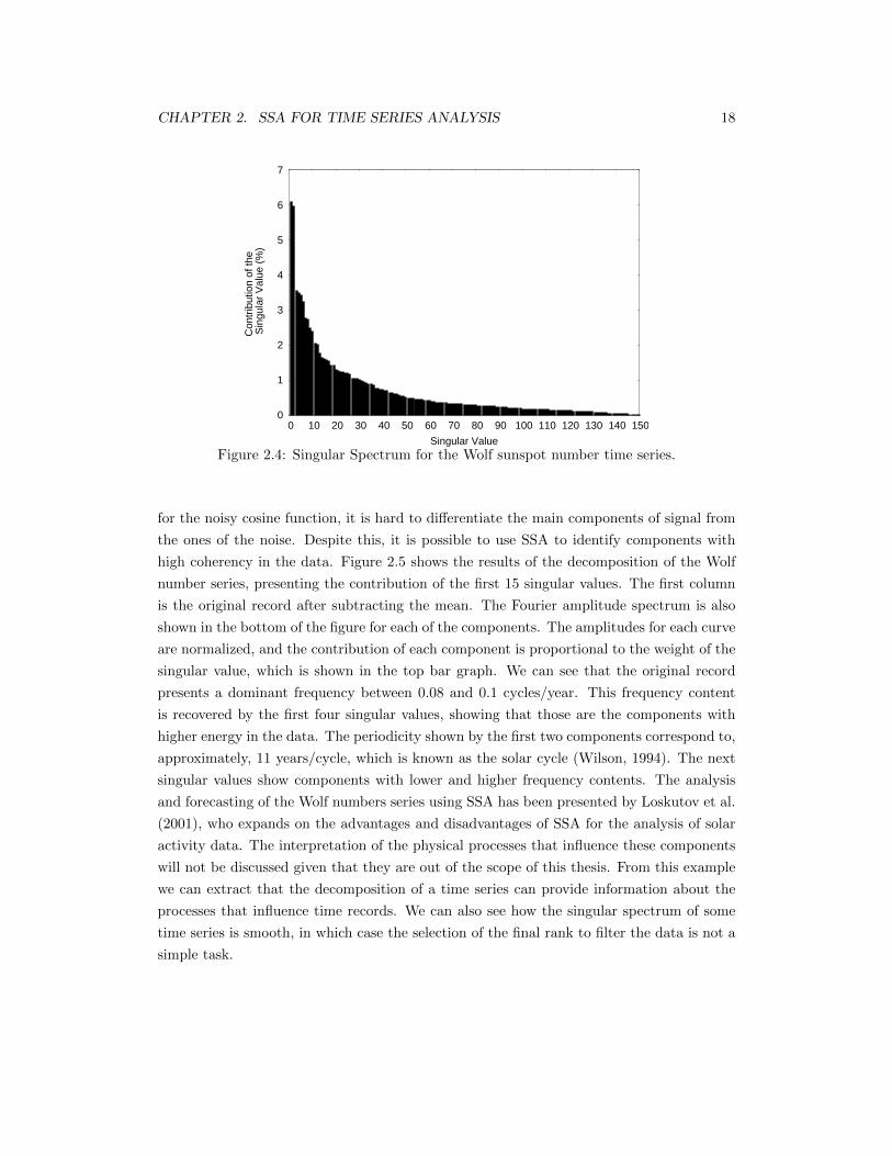
2.4 Singular Spectrum for the Wolf sunspot number time series. . . . . . . . . . . 18
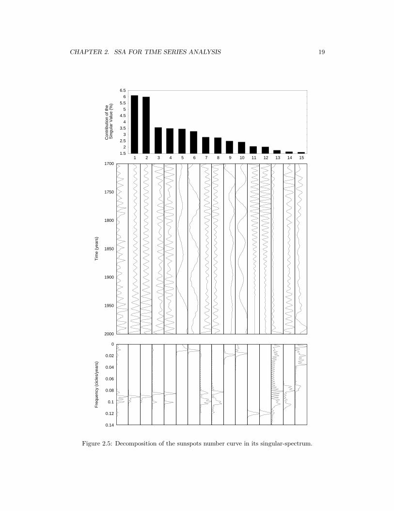
2.5 Decomposition of the sunspots number curve in its singular-spectrum. . . . . 19
3.1 Example of a 2-D waveform with constant dip. . . . . . . . . . . . . . . . . . 22
3.2 Example of one frequency slice organized as a matrix from a 3-D record toperform 2-D MSSA. . . . . . . . . . . . . . . . . . . . . . . . . . . . . . . . . 27
3.3 Construction of a Block Hankel matrix. . . . . . . . . . . . . . . . . . . . . . 28
3.4 Application of SSA on a noiseless record. a) f −x deconvolution filtering. b)SSA filtering using one frequency at a time. c) Original data prior to noisecontamination. d), e) Difference between the filtered data and the noise-freedata. . . . . . . . . . . . . . . . . . . . . . . . . . . . . . . . . . . . . . . . . . 33
3.5 Singular Values for the noiseless data. . . . . . . . . . . . . . . . . . . . . . . 33
3.6 Application of SSA on a record contaminated with random noise. a) f − xdeconvolution filtering. b) SSA filtering using one frequency at a time. c)Noisy input data. d), e) Noise estimators for a) and b). f) Original data priorto noise contamination. g), h) Difference between the filtered data and thenoise-free data. . . . . . . . . . . . . . . . . . . . . . . . . . . . . . . . . . . . 34
3.7 Singular Values for the data contaminated by random noise. . . . . . . . . . . 35
3.8 Results using windows in space on hyperbolic events: a) f − x deconvolutionfiltering. b) SSA filtering using one frequency at the time. c) Noisy inputdata. d), e) Noise estimators for a) and b). f) Original data prior to noisecontamination. g), h) Difference between the filtered data and the noise-freedata. . . . . . . . . . . . . . . . . . . . . . . . . . . . . . . . . . . . . . . . . . 36
3.9 Results of the application of f−x deconvolution and SSA to a stacked sectionwith random noise. a) Initial data. b) Random noise attenuation using f −xdeconvolution. c) Noise attenuation via SSA. . . . . . . . . . . . . . . . . . . 38
3.10 Data in the Black box of Figure 3.9. . . . . . . . . . . . . . . . . . . . . . . . 38
3.11 Noise attenuation using 2-D MSSA. a) Input data. b) Noiseless data repre-senting the expected solution. c) Noise attenuation applying f − x decon-volution. d) Noise attenuation applying SSA. e) Noise attenuation applying2-D MSSA. . . . . . . . . . . . . . . . . . . . . . . . . . . . . . . . . . . . . . 39
3.12 Slice in the y = 50 m of figure 3.11. a) Input data. b) Noise attenuationby using f − x deconvolution. c) Noise attenuation using SSA. d) Noiseattenuation using 2-D MSSA. e) Noiseless data representing the expectedsolution. f), g) and h) are the result of the subtraction of filter results (b), c)and d)) from the noiseless data (e)), respectively. . . . . . . . . . . . . . . . . 40
3.13 Slice in the x = 30 m of figure 3.11. a) Input data. b) Noise attenuationby using f − x deconvolution. c) Noise attenuation using SSA. d) Noiseattenuation using 2-D MSSA. e) Noiseless data representing the expectedsolution. f), g) and h) are the result of the subtraction of filter results (b), c)and d)) from the noiseless data (e)), respectively. . . . . . . . . . . . . . . . . 41
4.1 Plot showing the increments of the computational time vs. the number ofcolumns of the Hankel matrix (m). . . . . . . . . . . . . . . . . . . . . . . . . 48
4.2 Plot showing the Signal to Noise ratio depending on the number of columnsof the Hankel matrix (m). . . . . . . . . . . . . . . . . . . . . . . . . . . . . . 48
4.3 Slice in x = 31 for the data with size 61 × 61. a) Initial noisy data. b)Result using the traditional SVD. c), d) and e) Results using the randomSVD algorithm with i = 1, i = 2 and i = 3 respectively. f) Noiseless data(d0). g), h) i) and j) are the subtraction of f) from b), c), d) and e) respectively. 49
4.4 Slice in y = 31 for the 61 × 61 data. a) Initial noisy data. b) Result usingthe traditional SVD. c), d) and e) Results using the random SVD algorithmwith i = 1, i = 2 and i = 3 respectively. f) Noiseless data (d0). g), h) i) andj) are the subtraction of f) from b), c), d) and e) respectively. . . . . . . . . . 50
5.1 Interpolation of a noiseless synthetic example cube presenting 3 events. xand y are the two spatial dimensions. a) Initial data. b) Data decimated bythe operator T . It presents 58% of random missing traces. c) Result of theinterpolation using MSSA. d) Difference between the result (c) and the initialdata (a). . . . . . . . . . . . . . . . . . . . . . . . . . . . . . . . . . . . . . . . 55
5.2 Slice in y = 10 of the noiseless synthetic example for data interpolation.a) Initial data. b) Data decimated by the operator T . c) Result of theinterpolation using MSSA. d) Difference between (a) and (c). . . . . . . . . . 55
5.3 Interpolation of a synthetic example cube presenting 3 events and contami-nated with random noise. x and y are the two spatial dimensions. a) Initialdata. b) Data decimated by the operator T . It presents 58% of random miss-ing traces. c) Result of the interpolation using MSSA. d) Difference betweenthe result (c) and the initial data (a). . . . . . . . . . . . . . . . . . . . . . . 56
5.4 Slice in y = 10 of the synthetic example contaminated with random noise fordata interpolation. a) initial data. b) Data decimated by the operator T . c)Result of the interpolation using MSSA. d) Difference between (a) and (c). . 57
5.5 Initial distribution of offsets in each CDP. . . . . . . . . . . . . . . . . . . . . 57
5.6 Offsets regularized on a desired grid. Cells showing a star contain a trace,while the empty ones present missing traces. . . . . . . . . . . . . . . . . . . . 58
5.7 Computational times for the use of SVD and R-SVD in the rank-reductionstep of the MSSA algorithm . . . . . . . . . . . . . . . . . . . . . . . . . . . . 58
5.8 Interpolation of a real cube of 15 CDP gathers regularized on a desired grid.a) Initial data after regularization. b) Interpolated data using the iterativeMSSA algorithm applying the traditional SVD algorithm for the rank reduc-tion step. c) Interpolated data using the iterative MSSA algorithm with theR-SVD technique. . . . . . . . . . . . . . . . . . . . . . . . . . . . . . . . . . 59
5.9 Slice on CDP= 11 of the real cube interpolation example. a) initial data af-ter regularization. b) Interpolated data using the iterative MSSA algorithmapplying the traditional SVD algorithm for the rank reduction step. c) Inter-polated data using the iterative MSSA algorithm with the R-SVD technique. 60
6.1 Same amplitude and different velocities. . . . . . . . . . . . . . . . . . . . . . 65
6.2 Result for case 1. a) Input data. b) Event recovered by the first singularvalue. c) Event recovered by the second singular value. Both waves have thesame projection over the first two singular vectors, so they cannot be separated. 65
6.3 Same amplitudes and similar velocities. . . . . . . . . . . . . . . . . . . . . . 66
6.4 Result for case 2. a) Input data. b) Event recovered by the first singularvalue. c) Event recovered by the second singular value. Both events arepartially recovered by the largest singular vector while some amplitudes arerecovered by the second largest singular vector. The two events cannot beseparated. . . . . . . . . . . . . . . . . . . . . . . . . . . . . . . . . . . . . . . 66
6.5 Different amplitudes and different velocities. . . . . . . . . . . . . . . . . . . . 67
6.6 Result for case 3. a) Input data. b) Event recovered by the first singularvalue. c) Event recovered by the second singular value. Each singular vectorrepresent each event, meaning that the events can be separated. . . . . . . . . 67
6.7 Different amplitudes and similar velocities. . . . . . . . . . . . . . . . . . . . 68
6.8 Result for case 4. a) Input data. b) Event recovered by the first singular value.c) Event recovered by the second singular value. One event is completelyrecovered by the first singular vector while the second event is recovered byboth singular vectors. In this case the events cannot be separated. . . . . . . 68
6.9 Application of a low-pass filter, with a trapezoidal window of 0-3-19-22 Hz toa synthetic record. (a) Initial data with two events. (b) Low frequency eventrepresenting the GR. (c) High frequency event representing the reflection. (d)GR recovered using a low-pass filter. (e) Filtered data from the subtractionof (d) from (a). (f) Amplitude spectrum of (a). (g) Amplitude spectrum of(b) and (c). (h) Amplitude spectrum of (d) and (e). It is evident that lowfrequency content from the high frequency signal was recovered in (d) andfiltered in (e). It is also evident in (h) that the signal (e) loses frequencycontent. . . . . . . . . . . . . . . . . . . . . . . . . . . . . . . . . . . . . . . . 71
6.10 Application of SSA to the result of the low-pass filter. Same notation as figure6.9. In here (d) is the GR recovered from the first eigenimage of SSA and (e)is the filtered data which results from the subtraction of (d) from (a). We cansee here that there are no components of the signal in the recovered section(d). It is also evident in (h) that the signal (e) maintains its frequency content. 72
6.11 Application of SSA for GR filtering on a real record. (a) Original Data (b)Recovered GR. (c) Filtered Data resulting from subtracting (b) from (a). d)GR attenuation using an f − k filter for comparison. This figure presentsthe result of the application SSA to a real section. We can observe that theamount of signal present in (b) is very small. (c) Represents an improvementin its signal to noise ratio, while most of the low frequencies of the signal havebeen retained. Also, the amount of GR attenuated by SSA is larger that theone attenuated by the f − k filter. . . . . . . . . . . . . . . . . . . . . . . . . 73

List of symbols and abbreviations
[ ]H Hermitian or conjugate transpose of a matrix, page 10
[ ]T Transpose of a matrix, page 12
A Average on the anti-diagonals operator, page 14
M Hankelization operator, page 12
λ Discrete eigen-value of a squared matrix, page 9
O Order of magnitude, page 46
ω Temporal frequency, page 22
σ Discrete singular-value of a matrix, page 13
i Imaginary unit i =√−1, page 22
f − x Frequency-Space domain, page 3
ffinal Final frequency to analyze in the SSA process, page 53
finit Initial frequency to analyze in the SSA process, page 53
i Power iteration variable set by the user in the randomized algorithm for rank reduc-tion, page 46
K Number of lagged vectors in a Hankel matrix, page 12
k Final rank of a matrix (related to the number of events in a seismic record), page13
L Length of the lagged vectors, page 12
l Oversampling integer for the randomized rank reduction algorithm, page 45
li Lagged vectors from a time series, page 12
Lx Length of the lagged vectors in the x dimension. This parameter also controls thedimensions of the Hankel matrix, page 24
m Number of columns of a matrix, page 10
xiii
n Number of rows of a matrix, page 10
Nx Number of space samples in the data, page 24
p Ray parameter representing the dip of a 2-D waveform, page 22
s(t) 1-D time series, page 11
S(x, ω) 2D waveform in the f − x domain, page 22
s(x, t) 2D waveform with constant dip, page 21
S(x, y, ω) 3-D waveform in the f − x domain, page 29
s(x, y, t) 3-D waveform with constant dip, page 29
sk Time series recovered from the rank reduced Hankel matrix by averaging along theanti-diagonals, page 14
t time, page 22
t− x Time-Space domain, page 3
w(t) Pulse or Wavelet, page 22
x Space in the x dimension, page 22
y Space in the y dimension, page 29
Λ Diagonal matrix containing the eigen-values of a square matrix, page 10
Σ Diagonal matrix containing the singular values of a matrix, organized in descendingorder, page 10
Σk Matrix presenting zeros in all but the first k elements of the diagonal matrix Σ, page11
C Example of a Hermitian matrix, page 10
M Hankel Matrix, page 12
Mk Rank reduced Hankel matrix to rank k, page 14
Sω Spatial array of a given frequency ω, page 24
U Squared unitary matrix presenting the eigen-vectors of XXH , page 10
Uk Matrix presenting the first k columns of U, page 11
UkUHk Rank reduction operator, page 11
V Squared unitary matrix presenting the eigen-vectors of XHX, page 10
Vk Matrix presenting the first k columns of V, page 11
Wi(x) Waveform that represents each individual event i in a seismic record, page 63
X General matrix representing a group of data measurements, page 9
I Matrix presenting ones in all its cells, page 53
T Operator that identifies the presence of traces on the data, page 53
Sω Filtered version of Sω after averaging over the anti-diagonals, page 26
Mk Randomized approximation to the rank k Hankel matrix Mk, page 45
CDP Common Depth Point, page 6
CMP Common Midpoint, page 1
GR Ground Roll, page 61
LMO Linear Move-out, page 70
MSSA Multichannel Singular Spectrum Analysis, page 5
NMO Normal Move-out, page 1
POCS Projection onto convex sets, page 6
R-SVD Randomized SVD, page 6
SSA Singular Spectrum Analysis, page 3
SVD Singular Value Decomposition, page 4
CHAPTER 1
Introduction
1.1 Background
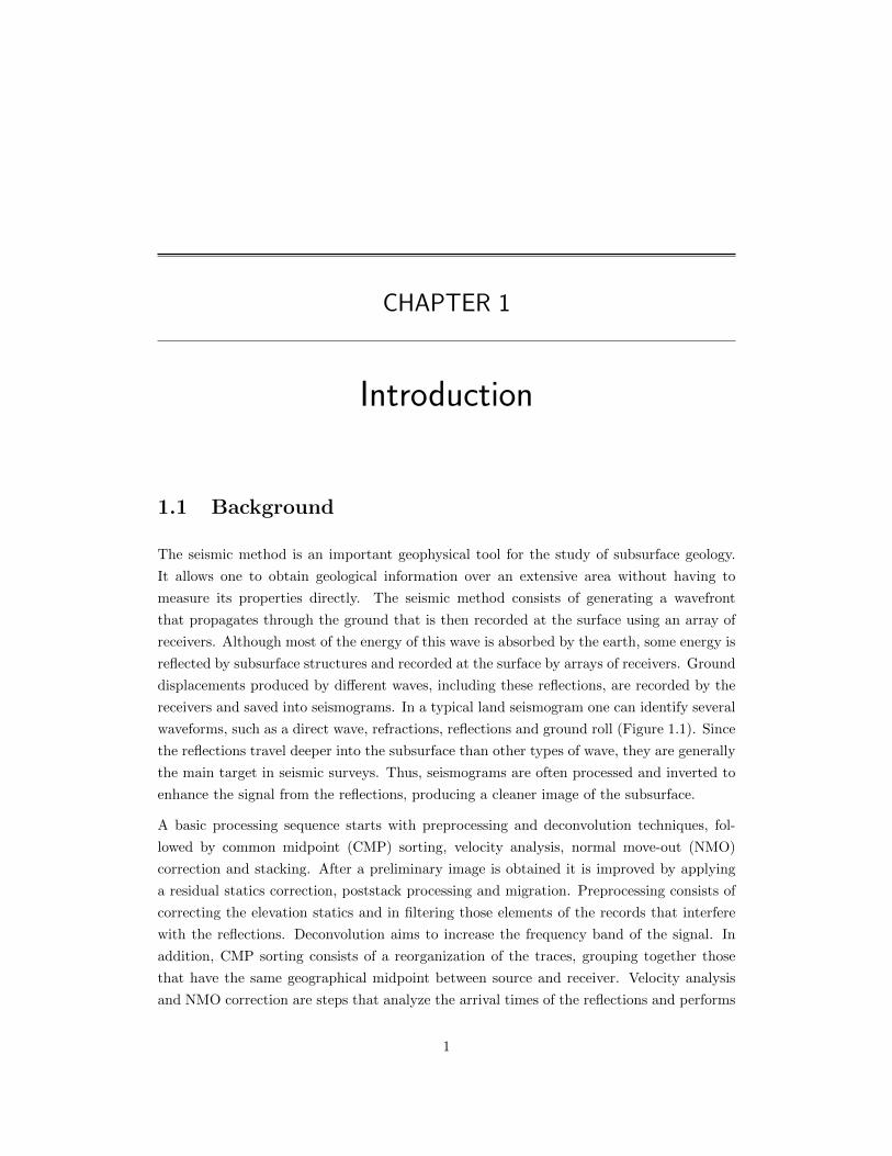
The seismic method is an important geophysical tool for the study of subsurface geology.
It allows one to obtain geological information over an extensive area without having to
measure its properties directly. The seismic method consists of generating a wavefront
that propagates through the ground that is then recorded at the surface using an array of
receivers. Although most of the energy of this wave is absorbed by the earth, some energy is
reflected by subsurface structures and recorded at the surface by arrays of receivers. Ground
displacements produced by different waves, including these reflections, are recorded by the
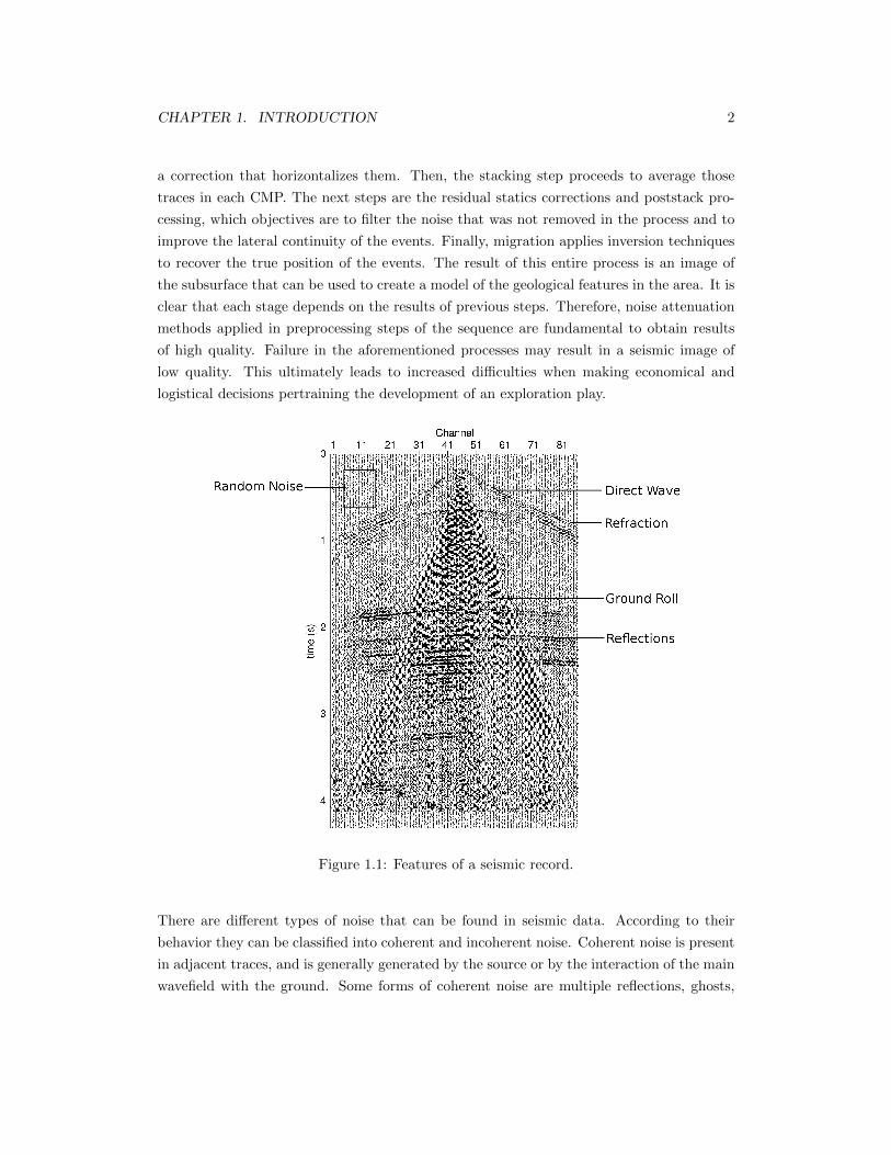
receivers and saved into seismograms. In a typical land seismogram one can identify several
waveforms, such as a direct wave, refractions, reflections and ground roll (Figure 1.1). Since
the reflections travel deeper into the subsurface than other types of wave, they are generally
the main target in seismic surveys. Thus, seismograms are often processed and inverted to
enhance the signal from the reflections, producing a cleaner image of the subsurface.
A basic processing sequence starts with preprocessing and deconvolution techniques, fol-
lowed by common midpoint (CMP) sorting, velocity analysis, normal move-out (NMO)
correction and stacking. After a preliminary image is obtained it is improved by applying
a residual statics correction, poststack processing and migration. Preprocessing consists of
correcting the elevation statics and in filtering those elements of the records that interfere
with the reflections. Deconvolution aims to increase the frequency band of the signal. In
addition, CMP sorting consists of a reorganization of the traces, grouping together those
that have the same geographical midpoint between source and receiver. Velocity analysis
and NMO correction are steps that analyze the arrival times of the reflections and performs
1
CHAPTER 1. INTRODUCTION 2
a correction that horizontalizes them. Then, the stacking step proceeds to average those
traces in each CMP. The next steps are the residual statics corrections and poststack pro-
cessing, which objectives are to filter the noise that was not removed in the process and to
improve the lateral continuity of the events. Finally, migration applies inversion techniques
to recover the true position of the events. The result of this entire process is an image of
the subsurface that can be used to create a model of the geological features in the area. It is
clear that each stage depends on the results of previous steps. Therefore, noise attenuation
methods applied in preprocessing steps of the sequence are fundamental to obtain results
of high quality. Failure in the aforementioned processes may result in a seismic image of
low quality. This ultimately leads to increased difficulties when making economical and
logistical decisions pertraining the development of an exploration play.
Figure 1.1: Features of a seismic record.
There are different types of noise that can be found in seismic data. According to their
behavior they can be classified into coherent and incoherent noise. Coherent noise is present
in adjacent traces, and is generally generated by the source or by the interaction of the main
wavefield with the ground. Some forms of coherent noise are multiple reflections, ghosts,
CHAPTER 1. INTRODUCTION 3
ground roll, air wave, etc. The incoherent noise, also called random noise, is recorded by
each receiver independently, meaning it does not correlate between adjacent channels. The
latter can be produced by environmental factors, such as the wind moving vegetation in
the survey area. The vibrations produced by the external factors are recorded by nearby
receivers. Given that the energy of these waves is very small, they are only detected by
nearby channels, making this noise incoherent. Any other perturbation in the surroundings
of a receiver can also generate random noise.
The main objective of this thesis is to study the application of a rank reduction method,
called Singular Spectrum Analysis (SSA), for the attenuation of random noise and ground
roll. The results obtained from the application of this method show a significant improve-
ment in the noise reduction compared with traditional techniques. In the next section I will
review some of the traditional techniques for noise reduction, which leads to the motivation
of this work.
1.2 Noise attenuation methods
The attenuation of random and coherent noise in seismic records is an important subject in
seismic data processing. In general, random noise is attenuated in the CMP stacking step of
processing, but in many cases noise is not completely removed by stacking. Classical meth-
ods for random noise attenuation exploit the predictability of the seismic signal in small
spatio-temporal windows. An example of the aforementioned concepts is the f − x decon-
volution (Canales, 1984), which takes advantage of the properties of the signal in the f − xdomain. In this domain, the signal is predictable as a function of the space. Random noise is
attenuated by applying a complex Wiener prediction filter that exploits this predictability
(Gulunay, 1986). Variations of f − x deconvolution are focused in improving the design
of the filter. For example, Sacchi and Kuehl (2001) introduced an autoregressive/moving-
average (ARMA) model to represent the signal. Nevertheless, those methods take advantage
of the same properties of the signal in the f − x domain. Another example of a method
that exploit the predictability of the signal is the t − x prediction error filter (Abma and
Claerbout, 1995), which works in the time-space domain by applying a single prediction
filter using a conjugate gradient method. Although it is important for noise reduction tech-
niques to be able to significantly attenuate the noise, it is also important to produce outputs
with minimal signal distortion. This condition is only met in f − x deconvolution for low
and medium levels of noise. The signal distortion can be high in low signal-to-noise-ratio
situations (Harris and White, 1997; Gulunay, 2000).
Another category of methods rely on rank reduction techniques to decompose a window of
seismic data in coherent and incoherent components (Ulrych et al., 1999). Examples in this
CHAPTER 1. INTRODUCTION 4
category are abundant in the geophysical literature. Freire and Ulrych (1988), for instance,
proposed to carry out rank reduction of seismic images in the t − x domain via the so-
called eigen-image decomposition. This approach takes advantage of the linear dependency
between traces, so it works well for horizontal events. Chiu and Howell (2008) and Cary
and Zhang (2009) extended this idea for the elimination of ground roll. For this purpose the
offending event (ground roll) is flattened via a linear moveout (LMO) correction, and then
modelled using the eigen-image method to be finally subtracted from the initial data. The
eigen-image method is also connected to the Karhunen-Loeve transform (KL) and principal
component analysis (PCA) methods (Freire and Ulrych, 1988). The KL transform has been
applied by Jones and Levy (1987), Marchisio et al. (1988) and Al-Yahya (1991) for signal-
to-noise ratio enhancement in seismic records. KL transform and PCA are similar methods
that use Singular Value Decomposition (SVD) for their applications and are sometimes used
as equivalent. The main differences between these two methods are compiled by Gerbrands
(1981). In general, rank reduction methods that are applied in the time-space domain, are
unsuccessful in identifying dipping events.
A rank reduction method that is independent of dip, and therefore, does not require flat-
tening, has been proposed by Mari and Glangeaud (1990). This method is called Spectral
Matrix Filtering; it was presented as an alternative to separate up-going and down-going
waves in VSP records. This method operates in the f − x domain and requires the eigen-
decomposition of the spectral matrix of the data. These techniques have been expanded
also to several dimensions of seismic data. Trickett (2003) proposed the application of an
eigen-image filter that works in the f − xy domain, reducing the rank of the spatial matrix
in each frequency. The latter is called f − xy eigenimage noise suppression. Although this
filter performs in multiple dimensions, the improvement of the signal-to-noise ratio of the
results is low compared to other techniques. Other rank reduction methods for noise filtering
apply a reorganization of the rows or columns of the data matrix to improve the coherency
of the signal. One of these methods is the truncated SVD, which works in time slices of a
stacked data cube by rearranging its columns into a Hankel matrix to suppress acquisition
footprints and random noise on stacked data (Al-Bannagi et al., 2005).
Although rank reduction methods have been used in seismic data processing for many years,
there is a method that has been recently attracting attention. This method is SSA (Vautard
et al., 1992), which is the main topic of this thesis. SSA arises from the decomposition of
time series in the study of dynamical systems (Broomhead and King, 1986). It has been
well studied in many fields, like climatic series analysis (Vautard and Ghil, 1989; Ghil
et al., 2002), astronomy (Auvergne, 1988; Varadi et al., 1999) and medicine (Mineva and
Popivanov, 1996; Aydin et al., 2009), but it is subjected to ongoing research in seismic data
processing. SSA works in the f − x domain and consists of reorganizing spatial data into
a Hankel matrix. Reducing the rank of this Hankel matrix can reduce the random noise in
CHAPTER 1. INTRODUCTION 5
the record without distorting the signal. The latter provides a significant advantage over
traditional noise attenuation techniques like f −x deconvolution. The SSA method has also
been called Cadzow filtering (Trickett, 2008) or the Caterpillar method (Golyandina et al.,
2001). All this techniques are equivalent, but they arise from different fields. For instance,
the Cadzow method was proposed as a general framework for denoising images (Cadzow,
1988), and the Caterpillar method also arises from time series analysis (Nekrutkin, 1996).
Research in the application of this method for random noise attenuation has been published
by Trickett (2008), Sacchi (2009) and Trickett and Burroughs (2009).
This thesis presents an overview of SSA, beginning with an explanation of its origins for
time series analysis. The application of SSA for random noise attenuation is then explained
in detail, including its expansion to multiple dimensions. A main drawback of SSA is that
it can be significantly slow compared to other seismic attenuation methods. To solve this,
I propose the introduction of a randomized algorithm for rank reduction, developed by
Rokhlin et al. (2009), which decreases the amount of computations required by SSA. In
addition to random noise attenuation, I will also investigate two different applications for
SSA. In particular, an iterative algorithm to recover missing traces in an irregularly sampled
data set is proposed. Another application is the use of SSA to attenuate ground roll, which
takes advantage of the capacity of SSA to separate different events. With this work I aim
to generate a compilation of applications of SSA for seismic data processing, which can be
used as a base to more specialized seismic data processing studies.
1.3 Organization of the thesis
This thesis is organized as follows:
• Chapter 2 expands on the origins of SSA as a time series analysis technique. It
explains the steps for the application of SSA in the analysis of dynamical components
of a time series, signal detrending and noise attenuation. This chapter presents an
example of the application of SSA for noise attenuation, by recovering a sinusoidal
curve contaminated with noise. It also shows the application of SSA to decompose the
Wolf sunspots number curve into its singular spectrum, which can provide information
of the processes that control the data. The interpretation of these components in not
discussed here, limiting the explanation to the application of SSA.
• Chapter 3 shows the application of SSA for random noise attenuation of seismic
records. This chapter also introduces the expansion of SSA to multiple dimensions
called Multichannel Singular Spectrum Analysis (MSSA). This expansion is explained
for 2-D MSSA and N-D MSSA. Several examples of SSA are presented where random
CHAPTER 1. INTRODUCTION 6
noise is attenuated. Examples include synthetic gathers with linear and hyperbolic
events, as well as real post-stack gathers. Examples of MSSA are limited to the 2-
Dimensional case, in which the random noise of a synthetic cube with linear events is
attenuated.
• Chapter 4 presents the application of a new rank reduction algorithm to the SSA tech-
nique. This algorithm is a randomized SVD (R-SVD) that generates an approximation
to the rank reduced matrix required by SSA. The randomized algorithm requires a
significantly lower amount of calculations compared with the traditional SVD algo-
rithm. Examples in this chapter show the results from the application of MSSA using
SVD and R-SVD in the rank reduction step. The amount of time required by each
process is also shown. The results of this test show that the application of the R-SVD
algorithm in MSSA decreases by 50% the running time of the method.
• Chapter 5 explores the use of SSA for seismic data interpolation. The algorithm of
MSSA is changed to work recursively, performing several iterations. In each iteration
the missing traces of the input data are replaced by the traces recovered by MSSA. Af-
ter a limited number of iterations the signal is reconstructed. This iterative algorithm
is similar to an algorithm called Projection onto convex sets (POCS). The example in
this chapter consists on a real Common Depth point (CDP) gather which offsets are
not regular. The data are regularized into a desired grid and the cells with missing
traces are recovered using the iterative MSSA algorithm. Although this is the only
example of MSSA applied to real data, it shows how the application of MSSA can
recover missing data and, at the same time, can attenuate random noise.
• Chapter 6 presents a different approach for the application of SSA. It expands on the
use of SSA for ground roll attenuation. The principles of this technique are based on
the property of SSA to identify different linear events when one of the first singular
values is recovered independently. This separation can only take place under certain
conditions, which are explained in detail. A synthetic example shows the separation of
two events, one of which presents a significantly lower frequency and different velocity
than the other. The difference in frequency and velocity simulates ground roll and
reflections. A second example applies this technique to a real shot gather that presents
a strong ground roll. The results show that signal separation using SSA is successful
in attenuating ground roll having low effect on the reflections.
• Chapter 7 presents the conclusions and recommendations for further work.
CHAPTER 2
Singular Spectrum Analysis in the study
of time series
2.1 Background
SSA is a model free technique that arises from the research of alternative tools for 1-D time
series analysis. It results from the analysis of the singular spectrum of a trajectory matrix
constructed from the time series of interest. Early applications of SSA are focused on the
analysis of dynamical systems. It is used to identify degrees of freedom in time series, and
this way, find the main physical processes present in the data. An important contribution to
the development of SSA was made by Broomhead and King (1986), who used the method of
delays proposed by Takens (1981) to study dynamical systems using multivariate statistical
analysis. Independently, Fraedrich (1986) also applied SSA to the dimensional analysis of
paleoclimatic marine records. SSA is studied more in depth by Vautard et al. (1992), who
presents it as a tool for the analysis of short, noisy and chaotic signals. They investigate four
major problems that arise from the application of SSA. These problems are: how parameters
like the embedding dimension influences the analysis, what is the level of robustness and
statistical confidence of the results, the possible applications in the identification of noise
and how to interpret the information given by each singular component. The basic aspects
of SSA are compiled and explained in books from Elsner and Tsonis (1996) and Golyandina
et al. (2001), which complement the information with different examples and applications.
SSA is a common tool in climatic series analysis. Vautard and Ghil (1989) and Yiou et al.
(1996) used this technique to study the main oscillations in paleoclimatic records, identi-
fying the amount of degrees of freedom in the data. It was also used to study baroclinic
7
CHAPTER 2. SSA FOR TIME SERIES ANALYSIS 8
processes (Read, 1992). Even though SSA has been mostly applied in meteorological stud-
ies, other disciplines have found it useful. In astronomy, for example, it have been applied
for phase space reconstruction of pulsating stars (Auvergne, 1988) and for the detection of
low-amplitude solar oscillations (Varadi et al., 1999). In medicine, it has proven useful in
decomposing data from electroencephalograms, to analyze the preparation time before a
voluntary movement (Mineva and Popivanov, 1996) or to support clinical findings in insom-
nia (Aydin et al., 2009). It has even been used for time series forecast by Danilov (1997) and
Golyandina et al. (2001). In economy, it has been used for the analysis and forecasting of
time series like daily exchange rate (Hassani et al., 2010) or the agricultural crop yield, milk
production and purchase, number of road traffic accidents, etc (Polukoshko and Hofmanis,
2009).
The application of SSA can be expanded to multiple time series simultaneously. This is called
multivariate or multichannel singular spectrum analysis (MSSA) which was first applied by
Read (1993). The difference with SSA is that the trajectory matrix includes information
from all the time series analyzed. In his study, Read (1993) applies MSSA to phase analysis
of time dependent experimental temperature measurements taken simultaneously. Again,
the main application for this technique is to study climatic records. Plaut and Vautard
(1994) uses this technique to study climatic low frequency oscillations in mid latitudes on
the northern hemisphere. It is applied to study the variations in the tropical Pacific climate
(Hsieh and Wu, 2002) and is included in a review of the application of spectral methods to
climatic data presented by Ghil et al. (2002). In a different approach, MSSA is also applied
to signal reconstruction and forecasting of time series (Golyandina and Stepanov, 2005) and
for the filtering of digital terrain models (Golyandina et al., 2007).
Together with the application of SSA in the study of dynamical systems, it is found useful
for noise attenuation in time series. This is carried on by recovering an inferior number
of singular values after the decomposition of the data. This property was observed by
Broomhead and King (1986) and is implemented in many studies. It has been said that
SSA is more powerful as a denoising technique than as a tool for dynamical analysis (Mees
et al., 1987; Palus and Dvorak, 1987). The main challenge in the use of SSA for noise
attenuation arises from the selection of the number of singular values that recover the data.
The answer to this depends on how correlated are the signal and the noise. In general, the
signal is believed to be represented by the largest singular values (Elsner and Tsonis, 1996),
but this can change when the noise is not white or the signal-to-noise ratio is too low. Most
of the papers that treat the application of SSA to dynamical systems also expand on its
application for noise removal. Works that investigate less subjective ways to use SSA for
the attenuation of noise in time series are carried on by Hansen and Jensen (1987); Allen
and Smith (1997) and Varadi et al. (1999).
CHAPTER 2. SSA FOR TIME SERIES ANALYSIS 9
The application of SSA consists of four main steps. The first step is the embedding of the
time series, which consists of organizing its entries in a trajectory matrix. The second step
is the decomposition of this matrix in its singular spectrum by using SVD. The third step
consists of the application of a rank reduction to the trajectory matrix by recovering fewer
amounts of singular values from the decomposition. Finally, the time series is recovered from
the rank reduced trajectory matrix. This chapter presents the basic theory behind SSA,
emphasizing in its application for decomposing and denoising time series. Further details
on the four main steps for the application of SSA are presented, together with examples
that demonstrate its effectiveness in extracting main oscillations and increasing the signal-
to-noise ratio of the data. A particular approach to MSSA will be done in Chapter 3, where
it will be used for the attenuation of random noise in seismic records.
2.2 Preliminaries
Many rank reduction methods rely on the application of the SVD technique to calculate the
rank reduced matrix. Before explaining the application of SSA to time series and seismic
record denoising it is necessary to understand the rank reduction process. In this section
the process of rank reduction using SVD will be expanded.
A group of data measurements can be viewed as a matrix X. For example, 1-D time series
can be represented as a matrix X by computing its autocorrelation matrix or by embedding
its components. In seismic surveys, the columns of a seismic section may represent traces and
the rows time samples of each trace. Seismic data in other domains can also be represented
as a matrix. For example, in the f − x domain the columns of the matrix X represent each
trace, but the rows represent frequency samples. Methods for noise attenuation rely on the
rank reduction of the data matrix by applying a SVD. Reducing the rank of this matrices
allows to identify coherent and incoherent components in the data. SVD consists basically
of the decomposition of the matrix X into a weighted sum of orthogonal rank one matrices,
called eigenimages of X (Ulrych et al., 1999). I will first introduce the SVD decomposition
method, followed by its application for rank reduction of a matrix.
Singular Value Decomposition (SVD)
The SVD arises from the problem in linear algebra of finding the eigenvalues and eigenvectors
of a matrix. Assuming a matrix C that is Hermitian of size m ×m, and a vector x which
elements are not all zero, then the eigenvalues of C are the ones that satisfy :
Cx = λx , (2.1)
CHAPTER 2. SSA FOR TIME SERIES ANALYSIS 10
and the vectors x are the eigenvectors of C. The number of non-zero eigenvalues of C
represents its rank. Now, expanding this operation to matrix decomposition, the Hermitian
matrix C can be represented by an arrangement of it eigenvalues and eigenvectors as:
C = UΛUH , (2.2)
where the columns of U are the eigenvectors of C, Λ is a diagonal matrix containing the
eigenvalues of C organized in descending order, and [ ]H denotes the Hermitian or conjugate
transpose of the matrix (Manning et al., 2009). Now, given that the previous decomposition
is restrained for squared matrices, a different approach has to be made to decompose a
rectangular matrix.
Let X be an m × n matrix, with m ≥ n and rank r ≤ n. The rank of a matrix is the
number of linearly independent rows or columns, therefore, the maximum rank of a matrix
is equivalent to rank(X) ≤ min{m,n} (Manning et al., 2009). The application of SVD
consists of decomposing this matrix as:
X = UΣVH , (2.3)
where U is the matrix whose columns are the eigenvectors of XXH , V is the matrix whose
columns are the eigenvectors of XHX and Σ is a diagonal matrix containing the singular
values of X. The singular values of X are obtained from the eigenvalues of XXH as Σ =√
Λ.
We can relate equations 2.2 and 2.3 by assuming C = XXH , which leads to:
C = XXH = UΣVH VΣUH = UΣ2UH = UΛUH . (2.4)
The same operation can be applied by assuming C = XHX. This leads to XHX = VΣ2VH .
With these operations it is clear how the singular values and singular vectors of X are related
to the eigenvalues and eigenvectors of XXH and XHX.
Rank reduction
The main characteristic of a low-rank matrix is that its elements are not independent from
each other. Because of this, the problem of approximating one matrix by another, with
lower rank, cannot be formulated in a straightforward manner, as a least-squares problem
(Eckart and Young, 1936). Instead of a least-square inversion, one can use SVD to calculate
the low rank approximation of a matrix.
CHAPTER 2. SSA FOR TIME SERIES ANALYSIS 11
Let X be a m× n matrix, subject to m ≥ n and with rank r ≤ n. Let k be a real number
such as k < r. The low rank approximation problem consist of finding a m× n matrix Xk,
whose rank is at most k, which minimizes the Frobenius norm of the difference X − Xk
(Manning et al., 2009). This is equivalent to:
‖X−Xk‖F =
√√√√ m∑i=1
n∑j=1
|xij − xij |2 . (2.5)
Eckart and Young (1936) found that this problem has a unique solution and that it can be
solved by using SVD. The following steps lead to the solution of the rank approximation
problem:
1. Decompose the initial matrix X by using equation 2.3, meaning X = UΣVH .
2. Replace by zero all but the first k elements of the diagonal matrix Σ to obtain the
matrix Σk .
3. The resulting rank reduced matrix is obtain by Xk = UΣkVH
This process is equivalent to replacing by zero all but the first k columns of U and V and
all but the first k elements of Σk and then to apply Xk = UkΣkVHk . The computation
of the rank reduced matrix Xk can also be calculated in a more efficient way by using the
principal eigenvectors of XXH , maintaining m ≥ n, as (Freire and Ulrych, 1988):
Xk = UkUHk X . (2.6)
The latter allow to define the operator UkUHk to apply the rank reduction process. The
recovered matrix Xk is at most rank k, and it leads to the lowest possible Frobenius norm
of X−Xk.
We have seen how the process of rank reduction can be completed by the use of SVD. With
this information it is possible to understand the principles that lay behind the rank reduction
techniques for noise attenuation. These concepts are fundamental in the application of SSA.
2.3 Singular Spectrum Analysis in 1-D time series
Let s(t) = (s1, s2, ..., sN ) be a time dependent signal, where N is the number of samples
of the data. This signal is the product of a series of dynamic processes that controls the
measured quantity plus noise. The application of SSA to the time series s(t) is performed
as follows:
CHAPTER 2. SSA FOR TIME SERIES ANALYSIS 12
Embedding
SSA consists of the decomposition of the time series in its singular spectrum. This decom-
position is applied to multidimensional series. It is possible to go from a one-dimensional
space to a multidimensional space by using the process of embedding. This consists of de-
composing the time series in a sequence of lagged vectors, which arises from the method
of delays (Broomhead and King, 1986). Now, let L be the length for these lagged vectors
having 1 < L < N , which is also called the embedding dimension (Elsner and Tsonis, 1996).
The number of lagged vectors will depend on the embedding dimension as K = N − L+ 1.
Each lagged vector will have the form:
li = (si, si+1, ..., si+L−1)T 1 ≤ i ≤ K , (2.7)
where [ ]T denotes the transpose of a matrix. The matrix that is built from the organization
of the lagged vectors as M = (l1, l2, ..., lK) is called the trajectory matrix. The resulting
trajectory matrix M is:
M =
s1 s2 · · · sK
s2 s3 · · · sK+1
......
. . ....
sL sL+1 · · · sN
. (2.8)
The main characteristics of this matrix is Mij = si+j+1, where 1 ≤ i ≤ K and 1 ≤ j ≤L . This means that the anti-diagonals of the matrix present the same values, and are
symmetrical around the main diagonal. The behavior of this trajectory matrix is that of
a Hankel matrix. The process of embedding can be summarized as M = M s(t), where
M is the Hankelization operator. The embedding dimension L is the main parameter to
select during the embedding step. Elsner and Tsonis (1996) suggests that the results from
the application of SSA are not significantly sensitive to the value of L as long as N is
considerably larger than L, recommending the use of L = N/4. The selection of small
values of L has the advantage of increasing the confidence in the results when the objective
of the analysis present high frequencies. Other authors have said that L has to be sufficiently
large so that the main behavior of the time series to analyze is content in each lagged vector
(Golyandina et al., 2001). These statements show that selecting the embedding parameter
involves a tradeoff between the amount of information in each vector and the confidence of
the results. In the end, it is clear that this parameter can be adjusted depending on the
objective of the study.
CHAPTER 2. SSA FOR TIME SERIES ANALYSIS 13
Singular Value Decomposition
This step consists in the decomposition of the trajectory matrix by using SVD. As explained
in the previous section, SVD is a decomposition of the form:
M =
r∑i=1
√λiuivi , (2.9)
where λi is the ith eigenvalue of MMH , r is the rank of M and ui and vi are the ith
eigenvectors of MMH and MHM. In general, σi =√λi is called the singular value of the
matrix M. Expression 2.9 can be converted to matrix notation as:
M = UΣVH , (2.10)
where Σ is the diagonal matrix containing all the singular values in descending order and
U and V are the matrices containing the set of orthonormal vectors ui and vi respectively.
Given that the eigenvectors of M arise from the autocorrelation matrix MMH , the com-
ponents that present the most coherency in the data will be weighted by singular values
with higher values. This way, the decomposition of the trajectory matrix in its singular
spectrum is very useful to identify trends in the data. Also, given that the signal in the
time series is correlated between time lagged windows, it will be represented by the largest
singular values. Because of this, singular values with less weight can be identified as noise,
making possible the use of this tool in denoising the time series. It is useful to present the
singular spectrum of the data as a graphical representation of the singular values of the
matrix M. To easily visualize the contribution of each singular value, it is convenient to
graph the percentage of each value compared to the sum of all the singular values.
Rank Reduction
Whatever the objective of the application of SSA is, the rank reduction of the trajectory
matrix has to be applied. The rank reduction process was explained in the previous section.
When analyzing the dynamical components of the time series, different singular values can be
grouped to recover physical behaviors identified in the decomposition. For noise reduction,
the rank that represents most of the signal has to be identified before the rank reduction
step. In general, the process consists in recovering a small subset of singular values compared
to the full rank of the trajectory matrix. Let k be the desired rank for the trajectory matrix,
this can be obtained by doing:
Mk = UkΣkVTk , (2.11)
CHAPTER 2. SSA FOR TIME SERIES ANALYSIS 14
where Mk is the recovered rank-reduced trajectory matrix. The recovered matrix is rank =
k and presents the lowest possible Frobenius norm.
Diagonal averaging
If the recovered matrix Mk is a Hankel form, then the recovery of the time series can be
done by just selecting the values in the anti-diagonals of Mk . In other words, being sk the
desired recovered time series after the rank reduction of the trajectory matrix, the element
n of this time series will be recovered by all the elements Mk(i, j) along the secondary
diagonal, being (i, j) such that i+ j − 1 = n.
Regretfully, this situation rarely happens in practice. In case that the Hankel form is not
preserved in the rank-reduced result, the process of recovering the time signal sk is by
averaging in the anti-diagonals of Mk. Golyandina et al. (2001) introduces an operator
that is helpful to describe the diagonal averaging of the recovered matrix. To simplify the
explanation let’s assume that L ≤ K. The case where K ≤ L is similar, but applying the
operator to MTk . Now, the operator works as follows: let i+ j − 1 = n and N = L+K − 1,
then the element n of sk is
sk(n) =
1
n
n∑l=1
Mk(l, n− l − 1) for 1 ≤ n ≤ L
1
L
L∑l=1
Mk(l, n− l − 1) for L+ 1 ≤ n ≤ K
1
K + L− n
L∑l=n−K+1
Mk(l, n− l − 1) for K + 1 ≤ n ≤ N
. (2.12)
The latter can be summarized as sk = AMk, where A is the averaging over the anti-diagonals
operator described by equation 2.12. This operation retrieves the component of the initial
time series s that was recovered after the rank reduction of the trajectory matrix.
We have seen the main four steps to compute SSA on time series signals. The interpretation
of the reconstructed components using different singular values is a topic that has been object
of extensive research. For further information in the use of SSA in time series the books
from Elsner and Tsonis (1996) and Golyandina et al. (2001) are recommended, which gives
more details on the use of this technique. However, some examples will be presented at
the end of this chapter, where the use of SSA for decomposition and noise attenuation are
tested.
CHAPTER 2. SSA FOR TIME SERIES ANALYSIS 15
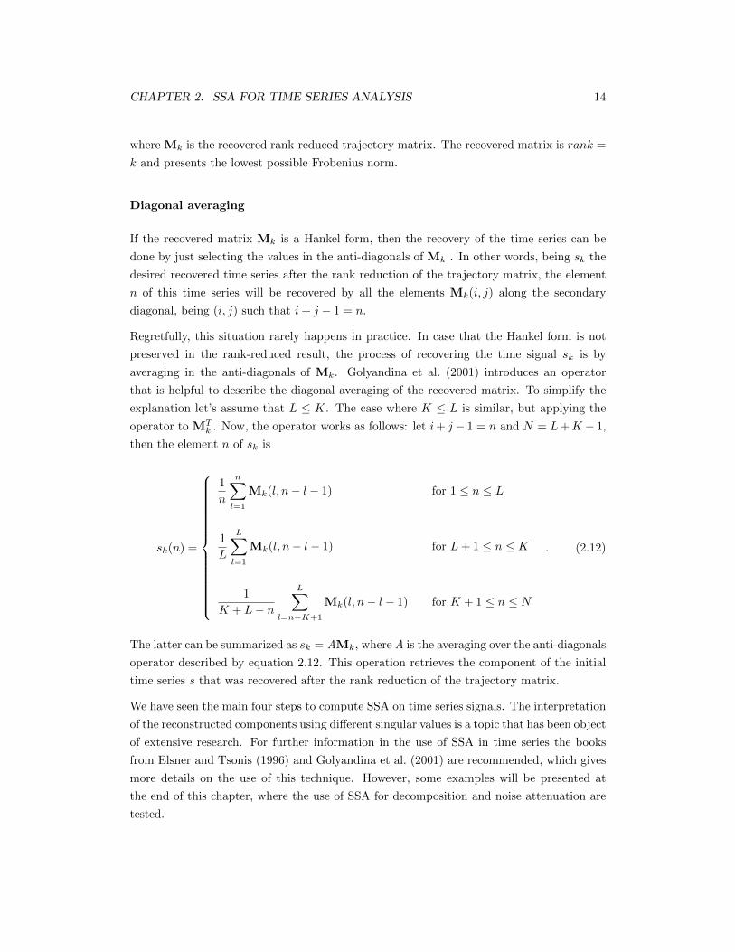
2.4 Examples
To test the SSA algorithm for time series analysis I will present first the decomposition of a
simple cosine function s(t) = cos(2πωt+φ), being the temporal frequency ω = 0.1 rad/s and
the phase φ = 0.2 rad. This function was contaminated with random noise with a variance
of 0.5 and zero mean. Given that a cosine function can be represented by the sum of two
exponentials as cos(θ) = 12 (e+iθ+e−iθ), this function is expected to have two representations
with high correlation in the singular spectrum. The reason for this is explained in chapter
3.2. SSA was applied by following the four steps previously presented. The embedding
dimension used to form the trajectory matrix was L = N/4, mostly because we know that
there are enough cycles in this time window to perform a successful analysis. This test was
repeated for L = N/3 and L = N/2, with very similar results.
0
10
20
30
40
50
60
2 4 6 8 10 12 14 16 18 20 22 24 26
Con
trib
utio
n of
the
Sin
gula
r V
alue
(%
)
Singular Value
a)
0
2
4
6
8
10
12
14
16
18
2 4 6 8 10 12 14 16 18 20 22 24 26
Singular Value
b)
Figure 2.1: Singular Spectrum for a) cosine function with no noise and b) cosinefunction in presence of noise.
The step of decomposing the signal using SVD is applied to the initial cosine function and
to the one contaminated with noise. Figure 2.1a) shows the singular spectrum for the initial
case with no noise and figure 2.1b) shows the singular spectrum for the noisy one. Notice that
the initial cosine function is represented by two singular values, confirming the assumption
previously made. In the presence of noise, the number of singular values different from zero
increases. It is possible to observe that the first two singular values are the ones with higher
energy. In general, it is possible to differentiate between the singular values that represent
the signal by looking for an abrupt change on the contribution of each of them. Even if we
do not have a priori information about these data, it is possible to conclude that the first
two singular values represent the main oscillatory components of the signal, and the rest of
them represent the noise.
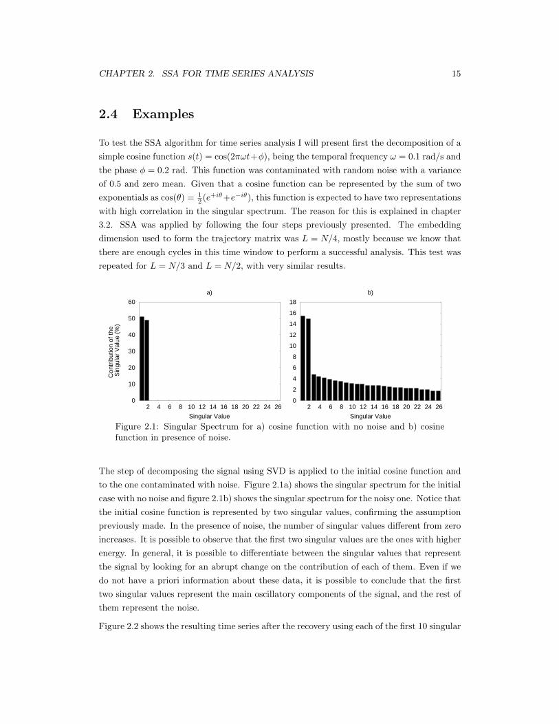
Figure 2.2 shows the resulting time series after the recovery using each of the first 10 singular
CHAPTER 2. SSA FOR TIME SERIES ANALYSIS 16
3
6
9
12
15
18
Contr
ibution o
f th
e
Sin
gula
r V
alu
e (
%)
0
10
20
30
40
50
60
70
80
90
100
Tim
e (
s)
Original Noisy 1 2 3 4 5 6 7 8 9 10
0
0.1
0.2
0.3
0.4
0.5
Fre
quency (
Hz)
Figure 2.2: Decomposition of a noisy cosine function in its singular-spetrum.
values separately. The first two columns present the original signal and the noisy one, to
which SSA was applied. The amplitudes of each curve are normalized, but its contribution
to the curve is proportional to the amplitude of its associate singular value, showed in the
bar diagram. The graphic at the bottom shows the Fourier amplitude spectrum of each
curve. In this exercise one observes the behaviour of the individual data components. The
interpretation of the singular spectrum is not always easy. Sometimes there is no abrupt
change in the amplitude of the singular values. In this case the selection of the final rank of
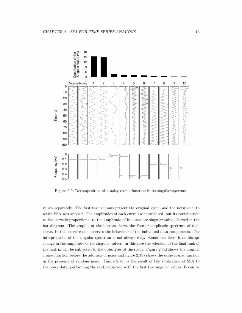
the matrix will be subjected to the objectives of the study. Figure 2.3a) shows the original
cosine function before the addition of noise and figure 2.3b) shows the same cosine function
in the presence of random noise. Figure 2.3c) is the result of the application of SSA to
the noisy data, performing the rank reduction with the first two singular values. It can be
CHAPTER 2. SSA FOR TIME SERIES ANALYSIS 17
observed that the process was successful in removing the noise, also attenuating slightly the
amplitudes of the result, compared to the original one. This example shows how SSA can
be a powerful tool for noise removal in time series analysis.
-1
0
1
0 10 20 30 40 50 60 70 80 90 100
Time (s)
c)
-1
0
1
Am
plit
ude
b)
-1
0
1a)
Figure 2.3: Result from filtering the noisy cosine function using SSA. a) Cosinefunction with no noise, represents the expected solution. b) Cosine function con-taminated with random noise. c) Result of filtering using SSA. The decrease inamplitude in the solution is due to the large amount of noise in the data.
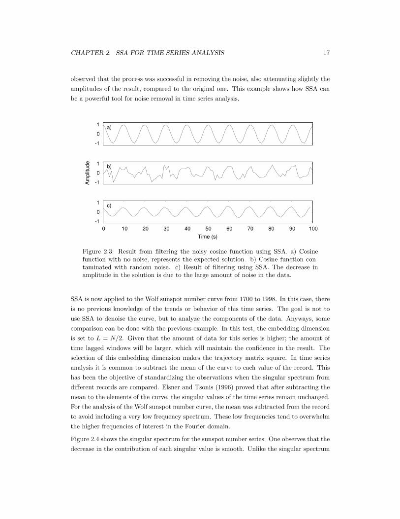
SSA is now applied to the Wolf sunspot number curve from 1700 to 1998. In this case, there
is no previous knowledge of the trends or behavior of this time series. The goal is not to
use SSA to denoise the curve, but to analyze the components of the data. Anyways, some
comparison can be done with the previous example. In this test, the embedding dimension
is set to L = N/2. Given that the amount of data for this series is higher; the amount of
time lagged windows will be larger, which will maintain the confidence in the result. The
selection of this embedding dimension makes the trajectory matrix square. In time series
analysis it is common to subtract the mean of the curve to each value of the record. This
has been the objective of standardizing the observations when the singular spectrum from
different records are compared. Elsner and Tsonis (1996) proved that after subtracting the
mean to the elements of the curve, the singular values of the time series remain unchanged.
For the analysis of the Wolf sunspot number curve, the mean was subtracted from the record
to avoid including a very low frequency spectrum. These low frequencies tend to overwhelm
the higher frequencies of interest in the Fourier domain.
Figure 2.4 shows the singular spectrum for the sunspot number series. One observes that the
decrease in the contribution of each singular value is smooth. Unlike the singular spectrum
CHAPTER 2. SSA FOR TIME SERIES ANALYSIS 18
0
1
2
3
4
5
6
7
0 10 20 30 40 50 60 70 80 90 100 110 120 130 140 150
Con
trib
utio
n of
the
Sin
gula
r V
alue
(%
)
Singular ValueFigure 2.4: Singular Spectrum for the Wolf sunspot number time series.
for the noisy cosine function, it is hard to differentiate the main components of signal from
the ones of the noise. Despite this, it is possible to use SSA to identify components with
high coherency in the data. Figure 2.5 shows the results of the decomposition of the Wolf
number series, presenting the contribution of the first 15 singular values. The first column
is the original record after subtracting the mean. The Fourier amplitude spectrum is also
shown in the bottom of the figure for each of the components. The amplitudes for each curve
are normalized, and the contribution of each component is proportional to the weight of the
singular value, which is shown in the top bar graph. We can see that the original record
presents a dominant frequency between 0.08 and 0.1 cycles/year. This frequency content
is recovered by the first four singular values, showing that those are the components with
higher energy in the data. The periodicity shown by the first two components correspond to,
approximately, 11 years/cycle, which is known as the solar cycle (Wilson, 1994). The next
singular values show components with lower and higher frequency contents. The analysis
and forecasting of the Wolf numbers series using SSA has been presented by Loskutov et al.
(2001), who expands on the advantages and disadvantages of SSA for the analysis of solar
activity data. The interpretation of the physical processes that influence these components
will not be discussed given that they are out of the scope of this thesis. From this example
we can extract that the decomposition of a time series can provide information about the
processes that influence time records. We can also see how the singular spectrum of some
time series is smooth, in which case the selection of the final rank to filter the data is not a
simple task.
CHAPTER 2. SSA FOR TIME SERIES ANALYSIS 19
1.5
2
2.5
3
3.5
4
4.5
5
5.5
6
6.5
1 2 3 4 5 6 7 8 9 10 11 12 13 14 15
Con
trib
utio
n of
the
Sin
gula
r V
alue
(%
)
1700
1750
1800
1850
1900
1950
2000
Tim
e (y
ears
)
0
0.02
0.04
0.06
0.08
0.1
0.12
0.14
Fre
quen
cy (
cicl
es/y
ears
)
Figure 2.5: Decomposition of the sunspots number curve in its singular-spectrum.
CHAPTER 3
Singular Spectrum Analysis for noise
attenuation in seismic records
3.1 Backgound
This chapter presents the use of SSA for random noise filtering in pre-stack and post-stack
seismic data. Although the application of SSA in time series analysis has been studied for a
long time, its use in seismic data processing is rather recent. Trickett (2002) introduced the
use of a rank reduction method called f − x eigenimage filter, which is based in the work
of Cadzow (1988). Trickett (2008) suggested that the method should be called Cadzow
filtering, in honor to the author from whom they based the technique. The application of
the Cadzow method is documented in Trickett and Burroughs (2009). The Cadzow method
and SSA are equivalent, but they arise from different fields of study. We have seen that
SSA was developed for the analysis of time series, while the Cadzow method was proposed
as a technique for the denoising of images (Cadzow, 1988). The relationship between the
Cadzow method and SSA is presented by Sacchi (2009), who denominated the technique as
f − x SSA.
Filtering random noise in seismic records involve the application of SSA in the f−x domain
(Trickett, 2008; Sacchi, 2009). In the first part of this chapter, SSA is applied to one single
frequency at the time, assuming it as a vector that varies in space. The methodology applied
here is analogous to the time series examples shown in chapter 2. The results from the noise
attenuation achieved by SSA are compared with those from using f −x deconvolution. The
latter is the standard technique for random noise attenuation. Although the results show
20
CHAPTER 3. SSA FOR NOISE ATTENUATION IN SEISMIC RECORDS 21
no evidence of a significant improvement on the amount of noise attenuated by SSA over
the f − x deconvolution, it does a better task in preserving the signal.
A significant improvement on the application of SSA for random noise attenuation arises
from its expansion to multiple dimensions, which is called MSSA. This chapter describes the
process of expanding SSA for the analysis of a 3-D seismic data set, which involves the appli-
cation of MSSA in two dimensions (2-D MSSA). MSSA is also applied in the f −x domain.
The main difference between SSA and 2-D MSSA is that the two spatial dimensions of a
3-D seismic record are used simultaneously for the analysis. An example of the application
of 2-D MSSA is presented. The latter shows that this expansion improves significantly the
attenuation of random noise. The results from 2-D MSSA are compared with those from
applying f − x deconvolution and SSA. The expansion to MSSA is then generalized to N
dimensions (N-D MSSA). Although the theory behind N-D MSSA is explained here, it was
not tested with synthetic or real examples. The design of an example applying MSSA to
more than two dimensions is beyond the scope of this thesis, and it is strongly recommended
for future research.
3.2 Singular Spectrum Analysis in seismic data process-
ing
The application of SSA in seismic data processing is similar to the one applied for the
analysis of time series. The main difference is that SSA is applied in the f − x domain of
the seismic records. Instead of using a temporal vector as input for the analysis, it uses a
spatial vector. Therefore, two extra steps have to be added to the SSA application sequence
described in chapter 2. These steps consist of converting the input data from the t − x
domain to the f − x domain and back. The application of SSA for the attenuation of
random noise in seismic records is performed as follows:
Application of a Fourier transform to each channel:
We start our discussion by considering a 2-D waveform with constant dip. The latter is
analogous to a single event in a seismic section. For simplicity, one can imagine a portion of
a seismic waveform seen in a small window of analysis. This waveform can be represented
as:
s(x, t) = w(t− px) , (3.1)
CHAPTER 3. SSA FOR NOISE ATTENUATION IN SEISMIC RECORDS 22
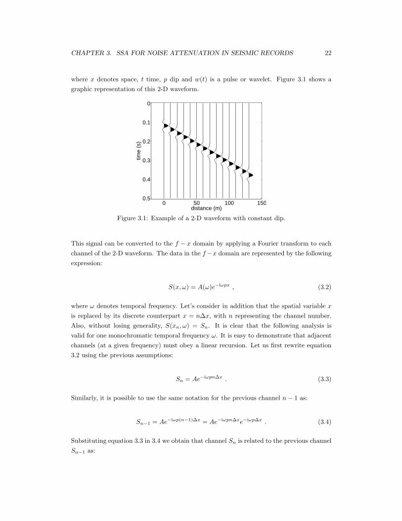
where x denotes space, t time, p dip and w(t) is a pulse or wavelet. Figure 3.1 shows a
graphic representation of this 2-D waveform.
0 50 100 150
0
0.1
0.2
0.3
0.4
0.5
Example of a 2−D waveform with constant dip
distance (m)
time
(s)
Figure 3.1: Example of a 2-D waveform with constant dip.
This signal can be converted to the f − x domain by applying a Fourier transform to each
channel of the 2-D waveform. The data in the f−x domain are represented by the following
expression:
S(x, ω) = A(ω)e−iωpx , (3.2)
where ω denotes temporal frequency. Let’s consider in addition that the spatial variable x
is replaced by its discrete counterpart x = n∆x, with n representing the channel number.
Also, without losing generality, S(xn, ω) = Sn. It is clear that the following analysis is
valid for one monochromatic temporal frequency ω. It is easy to demonstrate that adjacent
channels (at a given frequency) must obey a linear recursion. Let us first rewrite equation
3.2 using the previous assumptions:
Sn = Ae−iωpn∆x . (3.3)
Similarly, it is possible to use the same notation for the previous channel n− 1 as:
Sn−1 = Ae−iωp(n−1)∆x = Ae−iωpn∆xe−iωp∆x . (3.4)
Substituting equation 3.3 in 3.4 we obtain that channel Sn is related to the previous channel
Sn−1 as:
CHAPTER 3. SSA FOR NOISE ATTENUATION IN SEISMIC RECORDS 23
Sn = PSn−1 , (3.5)
where P = eiωp∆x.
It is possible to demonstrate that multiple 2-D waveforms also obey a linear recursion at
a given frequency. For example, a record presenting two 2-D waveforms with different dips
can be represented in the f − x domain as:
Sn = A1e−iξ1n +A2e
−iξ2n = S(1)n + S(2)
n , (3.6)
where Ak are the amplitudes for each event k, and ξk = ωpk∆x, being pk the dip of each
event. It is clear that if the dips of each event are different, then ξ1 6= ξ2. In a similar way
as in equation 3.4, one can represent the two previous channels n− 1 and n− 2 as:
Sn−1 = A1e−iξ1(n−1) +A2e
−iξ2(n−1)
Sn−2 = A1e−iξ1(n−2) +A2e
−iξ2(n−2) .(3.7)
Using equation 3.5 one can form the following system of equations:
a)
b)
c)
Sn = S
(1)n + S
(2)n
Sn−1 = a1S(1)n + a2S
(2)n
Sn−2 = a21S
(1)n + a2
2S(2)n
. (3.8)
where ak = e−iωpk∆x. The solution to this system of equations can be obtained by organizing
equations 3.8a) and 3.8b) in their matrix form:
[Sn−1
Sn−2
]=
[a1 a2
a21 a2
2
] [S
(1)n
S(2)n
]. (3.9)
Since ξ1 6= ξ2 the matrix
[a1 a2
a21 a2
2
]is invertible, so the solution for this system is
S(1)n = αSn−1 + βSn−2
S(2)n = γSn−1 + νSn−2 .
(3.10)
Finally, substituting equation 3.10 in equation 3.8a) we obtain the linear relationship be-
tween Sn, Sn−1 and Sn−2, which is
Sn = P1Sn−1 + P2Sn−2 . (3.11)
CHAPTER 3. SSA FOR NOISE ATTENUATION IN SEISMIC RECORDS 24
This relationship shows the linear recursion between adjacent channels in the presence of
two events. It is possible to expand this relation for k events. It is also important to mention
that this recursion is the basis for f − x deconvolution and represents the predictability of
the signal in the f − x domain (Sacchi and Kuehl, 2001; Ulrych and Sacchi, 2005). This
predictability is the key element in the success of SSA for random noise attenuation.
Embedding of each frequency into a Hankel matrix:
Let Sω = [S1, S2, S3, ..., SNx ]T be a spatial vector of a given frequency ω from the f − xdomain. Here Nx represents the number of space samples of the data. This spatial vector
Sω is analogous to the time series analyzed in chapter 2, but in this case it components are
complex numbers. We apply SSA using four steps similar to the ones described in chapter
2. The spatial vector Sω is embedded into a Hankel matrix of the form:
M =
S1 S2 · · · SKx
S2 S3 · · · SKx+1
......
. . ....
SLxSLx+1 · · · SNx
, (3.12)
where the length of the lagged vectors Lx is the parameter that controls the matrix dimen-
sions. Building a square Hankel matrix is a common strategy when SSA is applied to seismic
records (Trickett, 2008). The latter can be achieved by setting the lagged vectors length as
Lx = floor(Nx/2) + 1. By doing this, the number of columns in the Hankel matrix would
be Kx = Nx −Lx + 1. Expression 3.5 imposes a linear relationship between the columns of
the Hankel matrix M as:
M =
S1 PS1 · · · PKx−1S1
S2 PS2 · · · PKx−1S2
......
. . ....
SLx PSLx · · · PKx−1SLx
. (3.13)
It is easy to observe that for a simple f − x signal, the Hankel matrix reduces to a matrix
with rank = 1. It is clear that in the presence of uncorrelated noise the rank of the matrix
will increase. If the record contains two events, equation 3.11 shows that all the columns of
the matrix M are linear combinations of the first two columns
CHAPTER 3. SSA FOR NOISE ATTENUATION IN SEISMIC RECORDS 25
M =
S1 S2 P1S2 + P2S1 · · · P1Sn−1 + P2Sn−2
S2 S3 P1S3 + P2S2 · · · P1Sn−1 + P2Sn−2
......
.... . .
...
SLxSLx+1 P1SLx+1 + P2SLx
· · · P1Sn−1 + P2Sn−2
. (3.14)
For the superposition of k events with constant dip, one can show that the Hankel matrix
is rank = k. This means that, by knowing the number of events contained in the initial
data set, one can know the minimum rank of the matrix that represents all the events. As
a consequence, the selection of the final rank of the matrix is not subjective, representing
an advantage over the application of SSA in time series analysis, and over many other rank
reduction methods for noise attenuation in seismic records. Rank reduction via the Singular
Value Decomposition (SVD) of M can be used to capture the singular-vectors that model
the signal.
Decomposition of the Hankel matrix using Singular Value Decomposition (SVD):
The singular value decomposition of M is given by:
M = UΣVH , (3.15)
where:
U = eigenvectors of MMH
V = eigenvectors of MHM
Σ = singular values of M in descending order.
This process has been developed in chapters 2, so no further explanation is needed.
Rank Reduction of the Hankel matrix:
The noise in the data (Sω) can be removed by using a low-rank reconstruction of the matrix
M. As seen in chapter 2, the rank reduction of the Hankel matrix can be obtained by
recovering a subset of its singular values as:
Mk = UkΣkVHk , (3.16)
where Σk indicates the diagonal matrix containing the first k largest singular values of M.
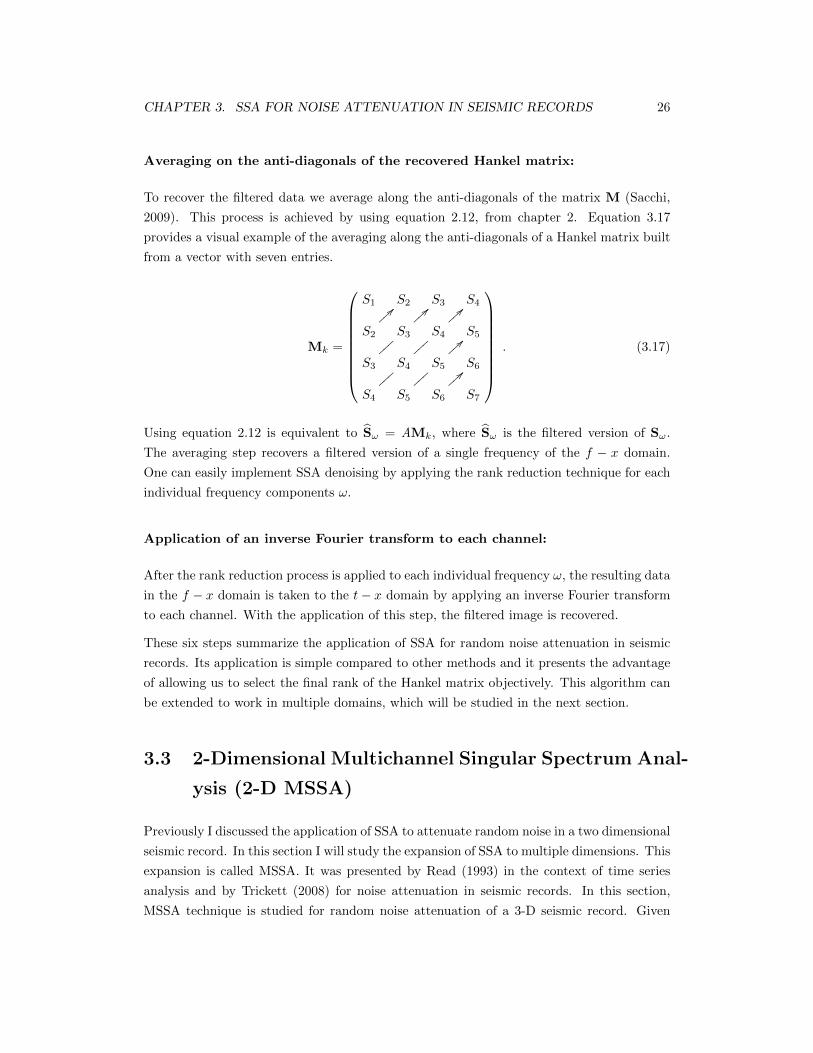
CHAPTER 3. SSA FOR NOISE ATTENUATION IN SEISMIC RECORDS 26
Averaging on the anti-diagonals of the recovered Hankel matrix:
To recover the filtered data we average along the anti-diagonals of the matrix M (Sacchi,
2009). This process is achieved by using equation 2.12, from chapter 2. Equation 3.17
provides a visual example of the averaging along the anti-diagonals of a Hankel matrix built
from a vector with seven entries.
Mk =
S1 S2 S3 S4
S2
>>|||S3
>>|||S4
>>|||S5
S3
|||S4
|||S5
>>|||S6
S4
|||S5
|||S6
>>|||S7
. (3.17)
Using equation 2.12 is equivalent to Sω = AMk, where Sω is the filtered version of Sω.
The averaging step recovers a filtered version of a single frequency of the f − x domain.
One can easily implement SSA denoising by applying the rank reduction technique for each
individual frequency components ω.
Application of an inverse Fourier transform to each channel:
After the rank reduction process is applied to each individual frequency ω, the resulting data
in the f − x domain is taken to the t− x domain by applying an inverse Fourier transform
to each channel. With the application of this step, the filtered image is recovered.
These six steps summarize the application of SSA for random noise attenuation in seismic
records. Its application is simple compared to other methods and it presents the advantage
of allowing us to select the final rank of the Hankel matrix objectively. This algorithm can
be extended to work in multiple domains, which will be studied in the next section.
3.3 2-Dimensional Multichannel Singular Spectrum Anal-
ysis (2-D MSSA)
Previously I discussed the application of SSA to attenuate random noise in a two dimensional
seismic record. In this section I will study the expansion of SSA to multiple dimensions. This
expansion is called MSSA. It was presented by Read (1993) in the context of time series
analysis and by Trickett (2008) for noise attenuation in seismic records. In this section,
MSSA technique is studied for random noise attenuation of a 3-D seismic record. Given
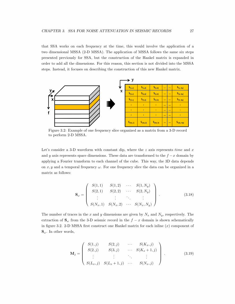
CHAPTER 3. SSA FOR NOISE ATTENUATION IN SEISMIC RECORDS 27
that SSA works on each frequency at the time, this would involve the application of a
two dimensional MSSA (2-D MSSA). The application of MSSA follows the same six steps
presented previously for SSA, but the construction of the Hankel matrix is expanded in
order to add all the dimensions. For this reason, this section is not divided into the MSSA
steps. Instead, it focuses on describing the construction of this new Hankel matrix.
Figure 3.2: Example of one frequency slice organized as a matrix from a 3-D recordto perform 2-D MSSA.
Let’s consider a 3-D waveform with constant dip, where the z axis represents time and x
and y axis represents space dimensions. These data are transformed to the f −x domain by
applying a Fourier transform to each channel of the cube. This way, the 3D data depends
on x, y and a temporal frequency ω. For one frequency slice the data can be organized in a
matrix as follows:
Sω =
S(1, 1) S(1, 2) · · · S(1, Ny)
S(2, 1) S(2, 2) · · · S(2, Ny)...
.... . .
...
S(Nx, 1) S(Nx, 2) · · · S(Nx, Ny)
. (3.18)
The number of traces in the x and y dimensions are given by Nx and Ny, respectively. The
extraction of Sω from the 3-D seismic record in the f − x domain is shown schematically
in figure 3.2. 2-D MSSA first construct one Hankel matrix for each inline (x) component of
Sω. In other words,
Mj =
S(1, j) S(2, j) · · · S(Kx, j)
S(2, j) S(3, j) · · · S(Kx + 1, j)...
.... . .
...
S(Lx, j) S(Lx + 1, j) · · · S(Nx, j)
. (3.19)
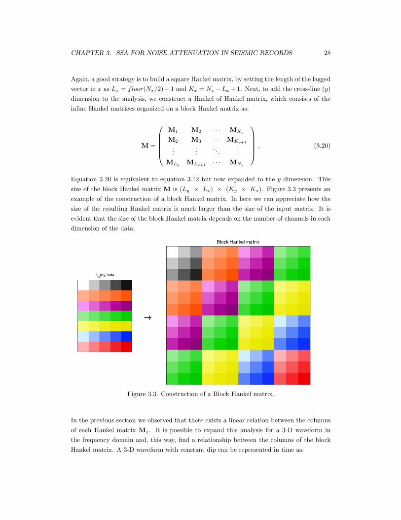
CHAPTER 3. SSA FOR NOISE ATTENUATION IN SEISMIC RECORDS 28
Again, a good strategy is to build a square Hankel matrix, by setting the length of the lagged
vector in x as Lx = floor(Nx/2) + 1 and Kx = Nx−Lx + 1. Next, to add the cross-line (y)
dimension to the analysis, we construct a Hankel of Hankel matrix, which consists of the
inline Hankel matrices organized on a block Hankel matrix as:
M =
M1 M2 · · · MKy
M2 M3 · · · MKy+1
......
. . ....
MLyMLy+1
· · · MNy
. (3.20)
Equation 3.20 is equivalent to equation 3.12 but now expanded to the y dimension. This
size of the block Hankel matrix M is (Ly × Lx) × (Ky × Kx). Figure 3.3 presents an
example of the construction of a block Hankel matrix. In here we can appreciate how the
size of the resulting Hankel matrix is much larger than the size of the input matrix. It is
evident that the size of the block Hankel matrix depends on the number of channels in each
dimension of the data.
−→−→−→
Figure 3.3: Construction of a Block Hankel matrix.
In the previous section we observed that there exists a linear relation between the columns
of each Hankel matrix Mj . It is possible to expand this analysis for a 3-D waveform in
the frequency domain and, this way, find a relationship between the columns of the block
Hankel matrix. A 3-D waveform with constant dip can be represented in time as:
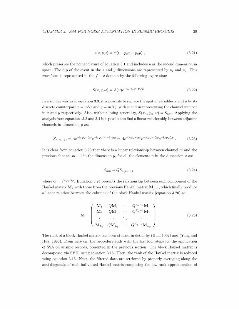
CHAPTER 3. SSA FOR NOISE ATTENUATION IN SEISMIC RECORDS 29
s(x, y, t) = w(t− pxx− pyy) , (3.21)
which preserves the nomenclature of equation 3.1 and includes y as the second dimension in
space. The dip of the event in the x and y dimensions are represented by px and py. This
waveform is represented in the f − x domain by the following expression:
S(x, y, ω) = A(ω)e−iω(pxx+pyy) . (3.22)
In a similar way as in equation 3.3, it is possible to replace the spatial variables x and y by its
discrete counterpart x = n∆x and y = m∆y, with n and m representing the channel number
in x and y respectively. Also, without losing generality, S(xn, ym, ω) = Snm. Applying the
analysis from equations 3.3 and 3.4 it is possible to find a linear relationship between adjacent
channels in dimension y as:
Sn(m−1) = Ae−iωpxn∆xe−iωpy(m−1)∆y = Ae−iωpxn∆xe−iωpym∆ye−iωpy∆y . (3.23)
It is clear from equation 3.23 that there is a linear relationship between channel m and the
previous channel m− 1 in the dimension y, for all the elements n in the dimension x as:
Snm = QSn(m−1) , (3.24)
where Q = eiωpy∆y. Equation 3.24 presents the relationship between each component of the
Hankel matrix Mj with those from the previous Hankel matrix Mj−1, which finally produce
a linear relation between the columns of the block Hankel matrix (equation 3.20) as:
M =
M1 QM1 · · · QKy−1M1
M2 QM2 · · · QKy−1M2
......
. . ....
MLyQMLy
· · · QKy−1MLy
. (3.25)
The rank of a block Hankel matrix has been studied in detail by (Hua, 1992) and (Yang and
Hua, 1996). From here on, the procedure ends with the last four steps for the application
of SSA on seismic records, presented in the previous section. The block Hankel matrix is
decomposed via SVD, using equation 3.15. Then, the rank of the Hankel matrix is reduced
using equation 3.16. Next, the filtered data are retrieved by properly averaging along the
anti-diagonals of each individual Hankel matrix composing the low-rank approximation of
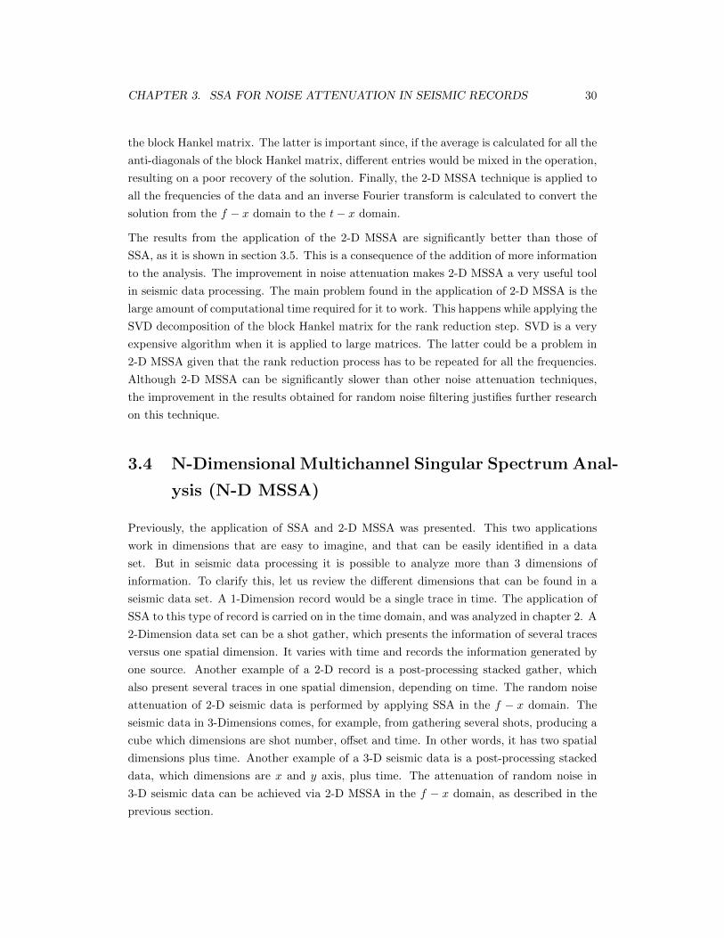
CHAPTER 3. SSA FOR NOISE ATTENUATION IN SEISMIC RECORDS 30
the block Hankel matrix. The latter is important since, if the average is calculated for all the
anti-diagonals of the block Hankel matrix, different entries would be mixed in the operation,
resulting on a poor recovery of the solution. Finally, the 2-D MSSA technique is applied to
all the frequencies of the data and an inverse Fourier transform is calculated to convert the
solution from the f − x domain to the t− x domain.
The results from the application of the 2-D MSSA are significantly better than those of
SSA, as it is shown in section 3.5. This is a consequence of the addition of more information
to the analysis. The improvement in noise attenuation makes 2-D MSSA a very useful tool
in seismic data processing. The main problem found in the application of 2-D MSSA is the
large amount of computational time required for it to work. This happens while applying the
SVD decomposition of the block Hankel matrix for the rank reduction step. SVD is a very
expensive algorithm when it is applied to large matrices. The latter could be a problem in
2-D MSSA given that the rank reduction process has to be repeated for all the frequencies.
Although 2-D MSSA can be significantly slower than other noise attenuation techniques,
the improvement in the results obtained for random noise filtering justifies further research
on this technique.
3.4 N-Dimensional Multichannel Singular Spectrum Anal-
ysis (N-D MSSA)
Previously, the application of SSA and 2-D MSSA was presented. This two applications
work in dimensions that are easy to imagine, and that can be easily identified in a data
set. But in seismic data processing it is possible to analyze more than 3 dimensions of
information. To clarify this, let us review the different dimensions that can be found in a
seismic data set. A 1-Dimension record would be a single trace in time. The application of
SSA to this type of record is carried on in the time domain, and was analyzed in chapter 2. A
2-Dimension data set can be a shot gather, which presents the information of several traces
versus one spatial dimension. It varies with time and records the information generated by
one source. Another example of a 2-D record is a post-processing stacked gather, which
also present several traces in one spatial dimension, depending on time. The random noise
attenuation of 2-D seismic data is performed by applying SSA in the f − x domain. The
seismic data in 3-Dimensions comes, for example, from gathering several shots, producing a
cube which dimensions are shot number, offset and time. In other words, it has two spatial
dimensions plus time. Another example of a 3-D seismic data is a post-processing stacked
data, which dimensions are x and y axis, plus time. The attenuation of random noise in
3-D seismic data can be achieved via 2-D MSSA in the f − x domain, as described in the
previous section.
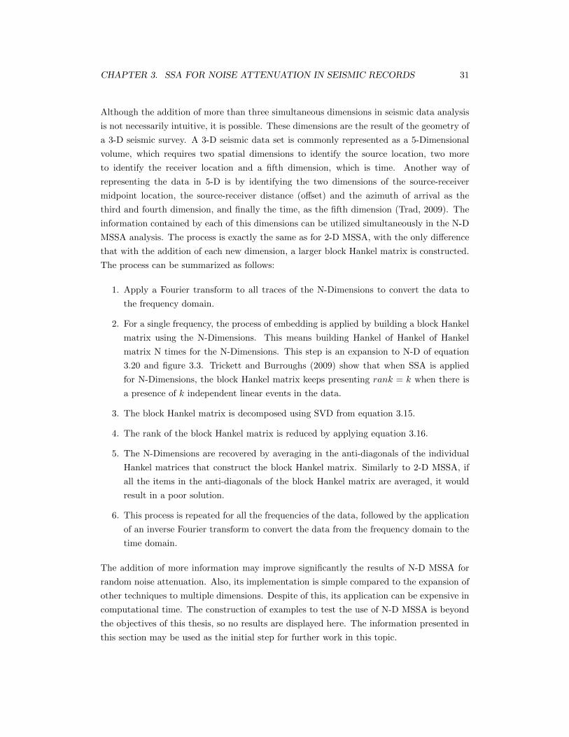
CHAPTER 3. SSA FOR NOISE ATTENUATION IN SEISMIC RECORDS 31
Although the addition of more than three simultaneous dimensions in seismic data analysis
is not necessarily intuitive, it is possible. These dimensions are the result of the geometry of
a 3-D seismic survey. A 3-D seismic data set is commonly represented as a 5-Dimensional
volume, which requires two spatial dimensions to identify the source location, two more
to identify the receiver location and a fifth dimension, which is time. Another way of
representing the data in 5-D is by identifying the two dimensions of the source-receiver
midpoint location, the source-receiver distance (offset) and the azimuth of arrival as the
third and fourth dimension, and finally the time, as the fifth dimension (Trad, 2009). The
information contained by each of this dimensions can be utilized simultaneously in the N-D
MSSA analysis. The process is exactly the same as for 2-D MSSA, with the only difference
that with the addition of each new dimension, a larger block Hankel matrix is constructed.
The process can be summarized as follows:
1. Apply a Fourier transform to all traces of the N-Dimensions to convert the data to
the frequency domain.
2. For a single frequency, the process of embedding is applied by building a block Hankel
matrix using the N-Dimensions. This means building Hankel of Hankel of Hankel
matrix N times for the N-Dimensions. This step is an expansion to N-D of equation
3.20 and figure 3.3. Trickett and Burroughs (2009) show that when SSA is applied
for N-Dimensions, the block Hankel matrix keeps presenting rank = k when there is
a presence of k independent linear events in the data.
3. The block Hankel matrix is decomposed using SVD from equation 3.15.
4. The rank of the block Hankel matrix is reduced by applying equation 3.16.
5. The N-Dimensions are recovered by averaging in the anti-diagonals of the individual
Hankel matrices that construct the block Hankel matrix. Similarly to 2-D MSSA, if
all the items in the anti-diagonals of the block Hankel matrix are averaged, it would
result in a poor solution.
6. This process is repeated for all the frequencies of the data, followed by the application
of an inverse Fourier transform to convert the data from the frequency domain to the
time domain.
The addition of more information may improve significantly the results of N-D MSSA for
random noise attenuation. Also, its implementation is simple compared to the expansion of
other techniques to multiple dimensions. Despite of this, its application can be expensive in
computational time. The construction of examples to test the use of N-D MSSA is beyond
the objectives of this thesis, so no results are displayed here. The information presented in
this section may be used as the initial step for further work in this topic.
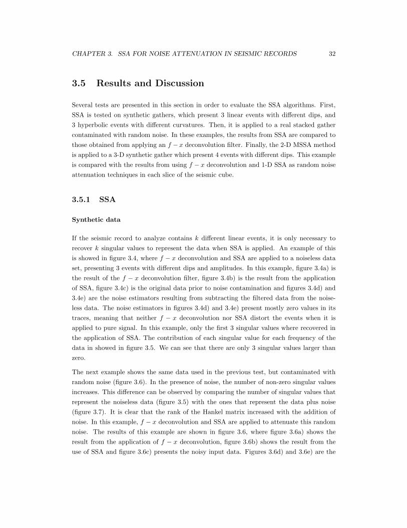
CHAPTER 3. SSA FOR NOISE ATTENUATION IN SEISMIC RECORDS 32
3.5 Results and Discussion
Several tests are presented in this section in order to evaluate the SSA algorithms. First,
SSA is tested on synthetic gathers, which present 3 linear events with different dips, and
3 hyperbolic events with different curvatures. Then, it is applied to a real stacked gather
contaminated with random noise. In these examples, the results from SSA are compared to
those obtained from applying an f − x deconvolution filter. Finally, the 2-D MSSA method
is applied to a 3-D synthetic gather which present 4 events with different dips. This example
is compared with the results from using f − x deconvolution and 1-D SSA as random noise
attenuation techniques in each slice of the seismic cube.
3.5.1 SSA
Synthetic data
If the seismic record to analyze contains k different linear events, it is only necessary to
recover k singular values to represent the data when SSA is applied. An example of this
is showed in figure 3.4, where f − x deconvolution and SSA are applied to a noiseless data
set, presenting 3 events with different dips and amplitudes. In this example, figure 3.4a) is
the result of the f − x deconvolution filter, figure 3.4b) is the result from the application
of SSA, figure 3.4c) is the original data prior to noise contamination and figures 3.4d) and
3.4e) are the noise estimators resulting from subtracting the filtered data from the noise-
less data. The noise estimators in figures 3.4d) and 3.4e) present mostly zero values in its
traces, meaning that neither f − x deconvolution nor SSA distort the events when it is
applied to pure signal. In this example, only the first 3 singular values where recovered in
the application of SSA. The contribution of each singular value for each frequency of the
data in showed in figure 3.5. We can see that there are only 3 singular values larger than
zero.
The next example shows the same data used in the previous test, but contaminated with
random noise (figure 3.6). In the presence of noise, the number of non-zero singular values
increases. This difference can be observed by comparing the number of singular values that
represent the noiseless data (figure 3.5) with the ones that represent the data plus noise
(figure 3.7). It is clear that the rank of the Hankel matrix increased with the addition of
noise. In this example, f − x deconvolution and SSA are applied to attenuate this random
noise. The results of this example are shown in figure 3.6, where figure 3.6a) shows the
result from the application of f − x deconvolution, figure 3.6b) shows the result from the
use of SSA and figure 3.6c) presents the noisy input data. Figures 3.6d) and 3.6e) are the
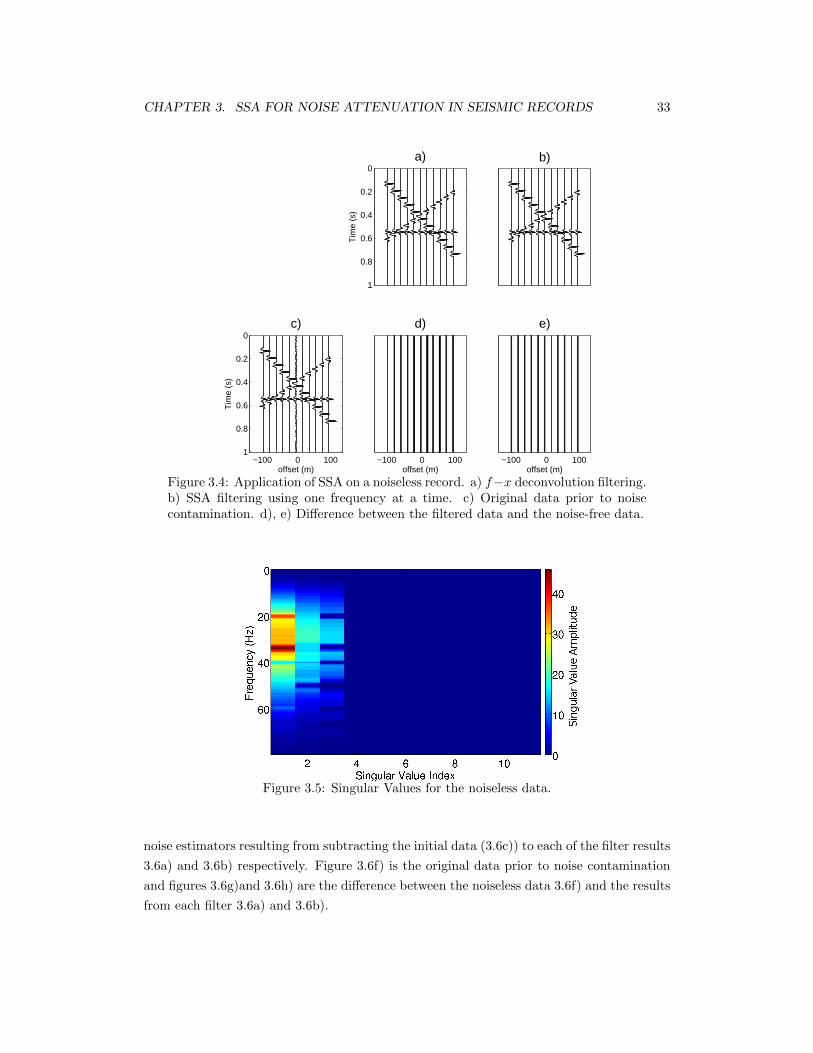
CHAPTER 3. SSA FOR NOISE ATTENUATION IN SEISMIC RECORDS 33
0
0.2
0.4
0.6
0.8
1
a)
Tim
e (s
)
b)
−100 0 100
0
0.2
0.4
0.6
0.8
1
Tim
e (s
)
offset (m)
c)
−100 0 100
d)
offset (m)−100 0 100
e)
offset (m)
Figure 3.4: Application of SSA on a noiseless record. a) f−x deconvolution filtering.b) SSA filtering using one frequency at a time. c) Original data prior to noisecontamination. d), e) Difference between the filtered data and the noise-free data.
Figure 3.5: Singular Values for the noiseless data.
noise estimators resulting from subtracting the initial data (3.6c)) to each of the filter results
3.6a) and 3.6b) respectively. Figure 3.6f) is the original data prior to noise contamination
and figures 3.6g)and 3.6h) are the difference between the noiseless data 3.6f) and the results
from each filter 3.6a) and 3.6b).
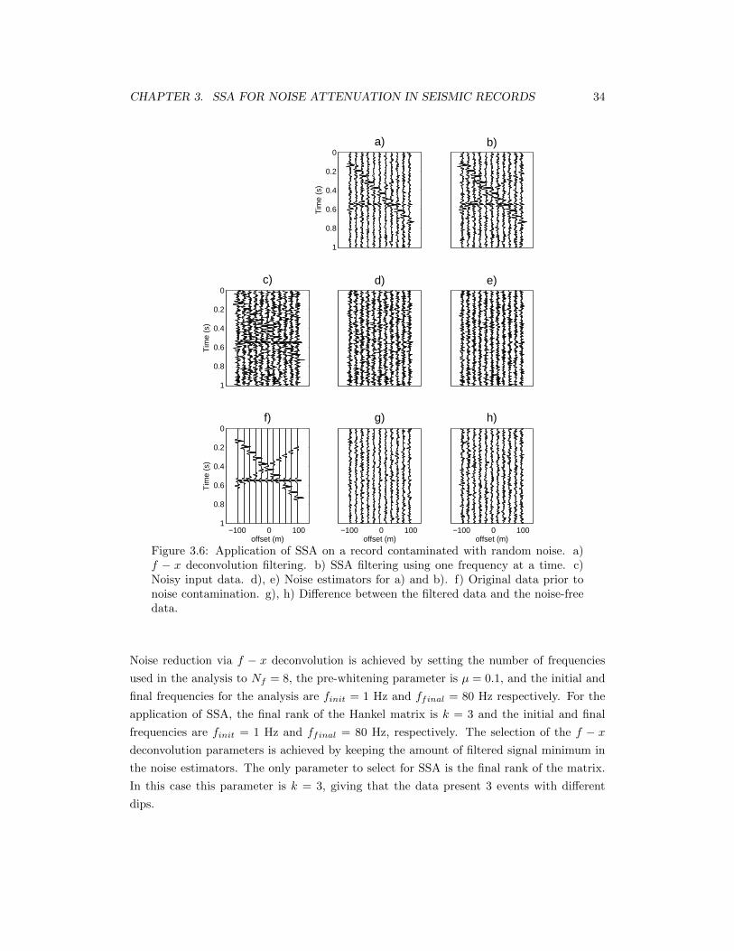
CHAPTER 3. SSA FOR NOISE ATTENUATION IN SEISMIC RECORDS 34
0
0.2
0.4
0.6
0.8
1
a)
Tim
e (s
)
b)
0
0.2
0.4
0.6
0.8
1
Tim
e (s
)
c) d) e)
−100 0 100
0
0.2
0.4
0.6
0.8
1
f)
Tim
e (s
)
offset (m)−100 0 100
g)
offset (m)−100 0 100
h)
offset (m)
Figure 3.6: Application of SSA on a record contaminated with random noise. a)f − x deconvolution filtering. b) SSA filtering using one frequency at a time. c)Noisy input data. d), e) Noise estimators for a) and b). f) Original data prior tonoise contamination. g), h) Difference between the filtered data and the noise-freedata.
Noise reduction via f − x deconvolution is achieved by setting the number of frequencies
used in the analysis to Nf = 8, the pre-whitening parameter is µ = 0.1, and the initial and
final frequencies for the analysis are finit = 1 Hz and ffinal = 80 Hz respectively. For the
application of SSA, the final rank of the Hankel matrix is k = 3 and the initial and final
frequencies are finit = 1 Hz and ffinal = 80 Hz, respectively. The selection of the f − xdeconvolution parameters is achieved by keeping the amount of filtered signal minimum in
the noise estimators. The only parameter to select for SSA is the final rank of the matrix.
In this case this parameter is k = 3, giving that the data present 3 events with different
dips.
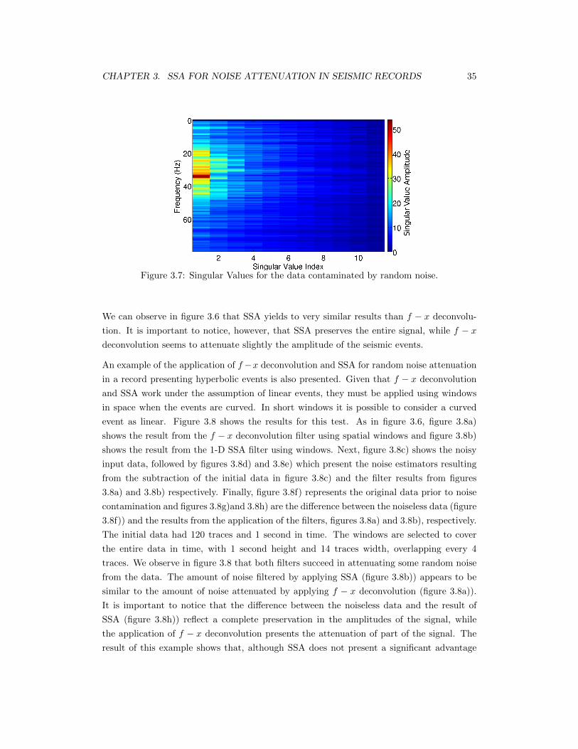
CHAPTER 3. SSA FOR NOISE ATTENUATION IN SEISMIC RECORDS 35
Figure 3.7: Singular Values for the data contaminated by random noise.
We can observe in figure 3.6 that SSA yields to very similar results than f − x deconvolu-
tion. It is important to notice, however, that SSA preserves the entire signal, while f − xdeconvolution seems to attenuate slightly the amplitude of the seismic events.
An example of the application of f−x deconvolution and SSA for random noise attenuation
in a record presenting hyperbolic events is also presented. Given that f − x deconvolution
and SSA work under the assumption of linear events, they must be applied using windows
in space when the events are curved. In short windows it is possible to consider a curved
event as linear. Figure 3.8 shows the results for this test. As in figure 3.6, figure 3.8a)
shows the result from the f − x deconvolution filter using spatial windows and figure 3.8b)
shows the result from the 1-D SSA filter using windows. Next, figure 3.8c) shows the noisy
input data, followed by figures 3.8d) and 3.8e) which present the noise estimators resulting
from the subtraction of the initial data in figure 3.8c) and the filter results from figures
3.8a) and 3.8b) respectively. Finally, figure 3.8f) represents the original data prior to noise
contamination and figures 3.8g)and 3.8h) are the difference between the noiseless data (figure
3.8f)) and the results from the application of the filters, figures 3.8a) and 3.8b), respectively.
The initial data had 120 traces and 1 second in time. The windows are selected to cover
the entire data in time, with 1 second height and 14 traces width, overlapping every 4
traces. We observe in figure 3.8 that both filters succeed in attenuating some random noise
from the data. The amount of noise filtered by applying SSA (figure 3.8b)) appears to be
similar to the amount of noise attenuated by applying f − x deconvolution (figure 3.8a)).
It is important to notice that the difference between the noiseless data and the result of
SSA (figure 3.8h)) reflect a complete preservation in the amplitudes of the signal, while
the application of f − x deconvolution presents the attenuation of part of the signal. The
result of this example shows that, although SSA does not present a significant advantage
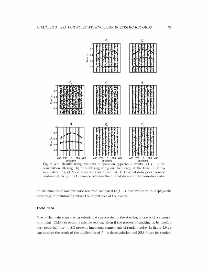
CHAPTER 3. SSA FOR NOISE ATTENUATION IN SEISMIC RECORDS 36
0
0.2
0.4
0.6
0.8
1
a)
Tim
e (s
)
b)
0
0.2
0.4
0.6
0.8
1
Tim
e (s
)
c) d) e)
−400 −200 0 200 400
0
0.2
0.4
0.6
0.8
1
f)
Tim
e (s
)
offset (m)−400 −200 0 200 400
g)
offset (m)−400 −200 0 200 400
h)
offset (m)
Figure 3.8: Results using windows in space on hyperbolic events: a) f − x de-convolution filtering. b) SSA filtering using one frequency at the time. c) Noisyinput data. d), e) Noise estimators for a) and b). f) Original data prior to noisecontamination. g), h) Difference between the filtered data and the noise-free data.
on the amount of random noise removed compared to f − x deconvolution, it displays the
advantage of maintaining intact the amplitudes of the events.
Field data
One of the main steps during seismic data processing is the stacking of traces of a common
mid-point (CMP) to obtain a seismic section. Even if the process of stacking is, by itself, a
very powerful filter, it still presents important components of random noise. In figure 3.9 we
can observe the result of the application of f − x deconvolution and SSA filters for random
CHAPTER 3. SSA FOR NOISE ATTENUATION IN SEISMIC RECORDS 37
noise attenuation of an stacked gather, constructed from real data. In here, figure 3.9 a)
shows the initial noisy gather, while figure 3.9 b) presents the result after f−x deconvolution
and figure 3.9 c) shows the result after applying SSA. If the events of the stacked data are
linear, SSA and f − x deconvolution can be applied in the whole record. However, if the
events present some curvature, or the stacked record is large, it is recommended to apply
the filters using windows in space. This is the case for this example, where the size of the
record demanded the use of spatial intervals of analysis.
Both methods are applied on overlaying windows of data. The latter aims to denoise sections
that present similar characteristics. The record presents 500 traces and 2.2 seconds in total.
The window size is 8 traces, overlapping 10 traces, for a total of 28 traces in space by
0.260 seconds with an overlapping of 0.08 seconds, for a total of 0.420 seconds in time. The
parameters for the application of f − x deconvolution are selected in order to minimize
the amount of signal attenuated by it. The best filtering using f − x deconvolution for this
example requires a number of frequencies of Nf = 4, a pre-whitening parameter of µ = 0.001
and an initial and final frequencies of finit = 1Hz and ffinal = 100Hz respectively. All the
events in each overlapping window have very similar dips, so they are recovered by the same
singular value. Because of this, the final rank of the Hankel matrices in the application
of SSA was set to k = 1. The analysis of SSA was carried on between the frequencies
finit = 1Hz and ffinal = 80Hz.
The results of this test show that SSA attenuates a similar amount of noise than f − x
deconvolution. This is consistent with the results from the linear synthetic results. To
better appreciate the behavior of these filters, figure 3.10 shows a zoom in the black box of
figure 3.9. We can observe that both filters attenuate part of the noise, being the results
very similar. We can also see that the noise estimator does not present coherent events
attenuated by the filters.
3.5.2 2-D MSSA
Synthetic data
The next example shows the expansion of SSA to 2-D MSSA, which involves the analysis
of two spatial dimensions simultaneously. The input data is a synthetic 3-D seismic cube,
presenting 4 linear events in the x and y dimensions and which is contaminated with random
noise. The objective of this test is to compare the advantages in noise attenuation of 2-D
MSSA over one dimensional noise attenuation methods, such as f − x deconvolution and
SSA.
The results from the application of the noise attenuation techniques to the input record are
presented in figure 3.11. We can observe the initial data contaminated with noise (figure
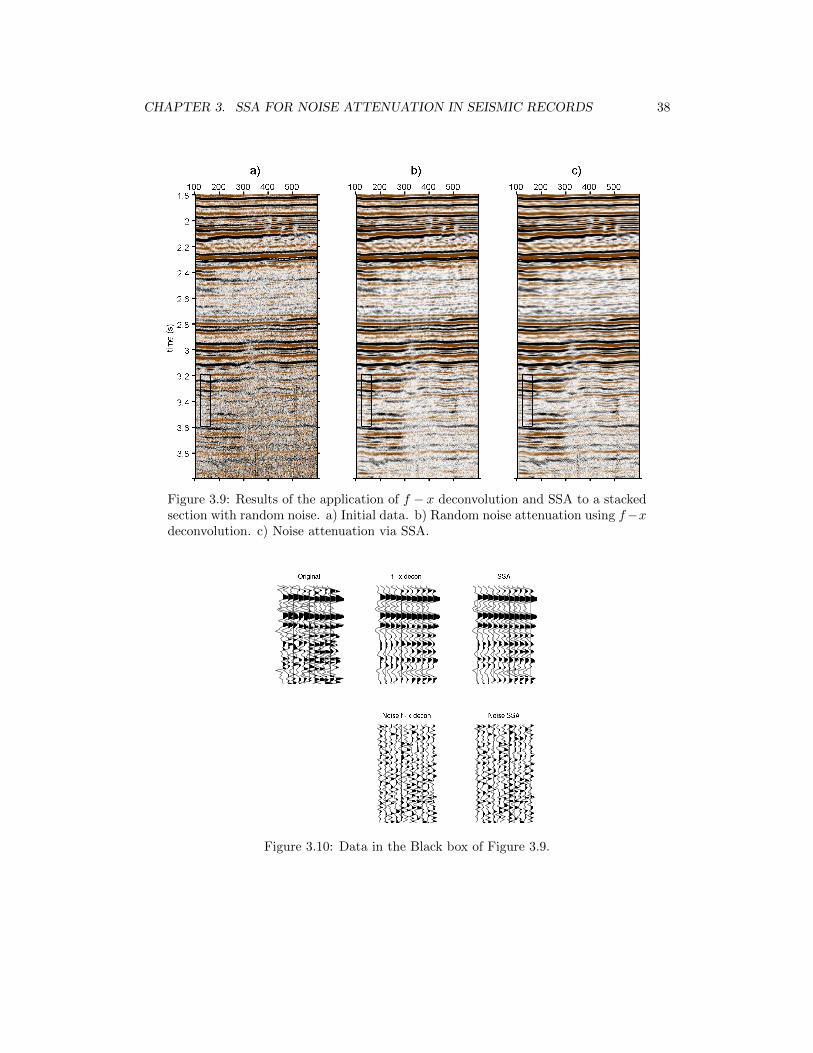
CHAPTER 3. SSA FOR NOISE ATTENUATION IN SEISMIC RECORDS 38
Figure 3.9: Results of the application of f − x deconvolution and SSA to a stackedsection with random noise. a) Initial data. b) Random noise attenuation using f−xdeconvolution. c) Noise attenuation via SSA.
Figure 3.10: Data in the Black box of Figure 3.9.
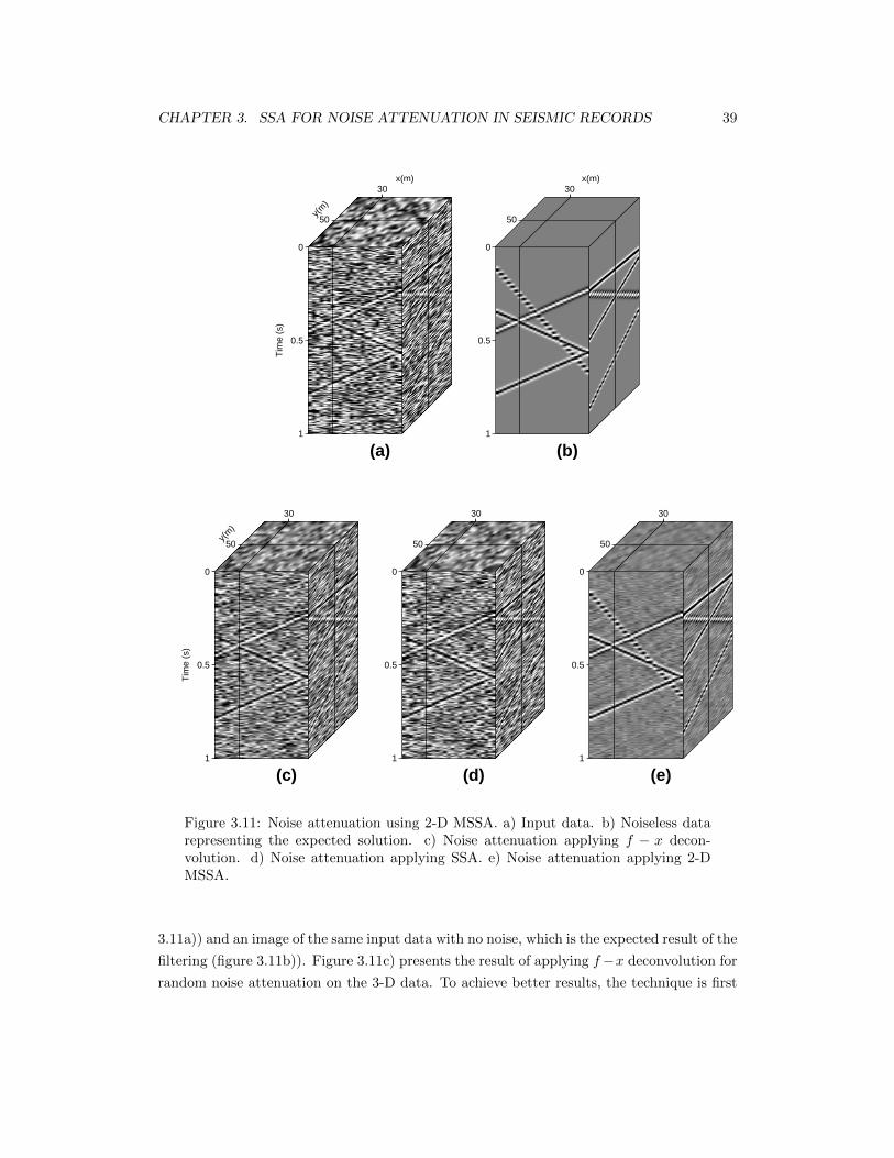
CHAPTER 3. SSA FOR NOISE ATTENUATION IN SEISMIC RECORDS 39
0
0.5
1
Tim
e (s
)
30x(m)
50y(
m)
(a)
0
0.5
1
30x(m)
50
(b)
0
0.5
1
Tim
e (s
)
30
50y(
m)
(c)
0
0.5
1
30
50
(d)
0
0.5
1
30
50
(e)
Figure 3.11: Noise attenuation using 2-D MSSA. a) Input data. b) Noiseless datarepresenting the expected solution. c) Noise attenuation applying f − x decon-volution. d) Noise attenuation applying SSA. e) Noise attenuation applying 2-DMSSA.
3.11a)) and an image of the same input data with no noise, which is the expected result of the
filtering (figure 3.11b)). Figure 3.11c) presents the result of applying f−x deconvolution for
random noise attenuation on the 3-D data. To achieve better results, the technique is first
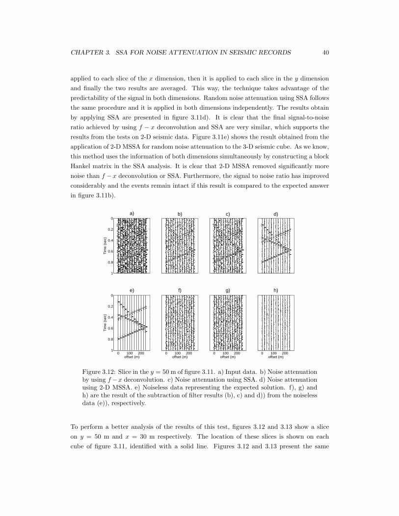
CHAPTER 3. SSA FOR NOISE ATTENUATION IN SEISMIC RECORDS 40
applied to each slice of the x dimension, then it is applied to each slice in the y dimension
and finally the two results are averaged. This way, the technique takes advantage of the
predictability of the signal in both dimensions. Random noise attenuation using SSA follows
the same procedure and it is applied in both dimensions independently. The results obtain
by applying SSA are presented in figure 3.11d). It is clear that the final signal-to-noise
ratio achieved by using f − x deconvolution and SSA are very similar, which supports the
results from the tests on 2-D seismic data. Figure 3.11e) shows the result obtained from the
application of 2-D MSSA for random noise attenuation to the 3-D seismic cube. As we know,
this method uses the information of both dimensions simultaneously by constructing a block
Hankel matrix in the SSA analysis. It is clear that 2-D MSSA removed significantly more
noise than f −x deconvolution or SSA. Furthermore, the signal to noise ratio has improved
considerably and the events remain intact if this result is compared to the expected answer
in figure 3.11b).
0
0.2
0.4
0.6
0.8
1
a)
Tim
e (s
ec)
b) c) d)
0 100 200
0
0.2
0.4
0.6
0.8
1
e)
offset (m)
Tim
e (s
ec)
0 100 200
f)
offset (m)0 100 200
g)
offset (m)0 100 200
h)
offset (m)
Figure 3.12: Slice in the y = 50 m of figure 3.11. a) Input data. b) Noise attenuationby using f −x deconvolution. c) Noise attenuation using SSA. d) Noise attenuationusing 2-D MSSA. e) Noiseless data representing the expected solution. f), g) andh) are the result of the subtraction of filter results (b), c) and d)) from the noiselessdata (e)), respectively.
To perform a better analysis of the results of this test, figures 3.12 and 3.13 show a slice
on y = 50 m and x = 30 m respectively. The location of these slices is shown on each
cube of figure 3.11, identified with a solid line. Figures 3.12 and 3.13 present the same
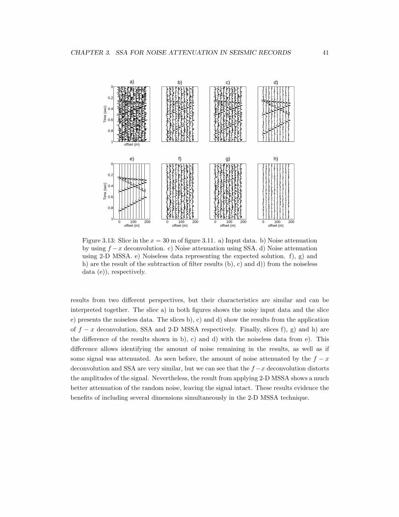
CHAPTER 3. SSA FOR NOISE ATTENUATION IN SEISMIC RECORDS 41
0
0.2
0.4
0.6
0.8
1
a)
offset (m)
Tim
e (s
ec)
b) c) d)
0 100 200
0
0.2
0.4
0.6
0.8
1
e)
offset (m)
Tim
e (s
ec)
0 100 200
f)
offset (m)0 100 200
g)
offset (m)0 100 200
h)
offset (m)
Figure 3.13: Slice in the x = 30 m of figure 3.11. a) Input data. b) Noise attenuationby using f −x deconvolution. c) Noise attenuation using SSA. d) Noise attenuationusing 2-D MSSA. e) Noiseless data representing the expected solution. f), g) andh) are the result of the subtraction of filter results (b), c) and d)) from the noiselessdata (e)), respectively.
results from two different perspectives, but their characteristics are similar and can be
interpreted together. The slice a) in both figures shows the noisy input data and the slice
e) presents the noiseless data. The slices b), c) and d) show the results from the application
of f − x deconvolution, SSA and 2-D MSSA respectively. Finally, slices f), g) and h) are
the difference of the results shown in b), c) and d) with the noiseless data from e). This
difference allows identifying the amount of noise remaining in the results, as well as if
some signal was attenuated. As seen before, the amount of noise attenuated by the f − xdeconvolution and SSA are very similar, but we can see that the f−x deconvolution distorts
the amplitudes of the signal. Nevertheless, the result from applying 2-D MSSA shows a much
better attenuation of the random noise, leaving the signal intact. These results evidence the
benefits of including several dimensions simultaneously in the 2-D MSSA technique.
CHAPTER 3. SSA FOR NOISE ATTENUATION IN SEISMIC RECORDS 42
3.6 Summary
In this chapter, SSA was expanded for the attenuation of random noise in seismic records.
For this, it was necessary to apply SSA to each frequency, requiring two extra steps in its
application to convert the data. The six steps to apply SSA in the f − x domain were
described, together with an explanation of the selection of the final rank of the Hankel
matrices. SSA was tested in two synthetic records contaminated with random noise and
presenting linear and hyperbolic events. Its results were compared to the one from applying
f − x deconvolution, which is a traditional technique for random noise attenuation. The
amount of noise attenuated by SSA showed to be similar to results obtained from applying
f − x deconvolution. Nevertheless, f − x deconvolution appeared to distort slightly the
amplitudes of the events, while SSA maintained the signal untouched.
The expansion of SSA to multiple dimensions was also covered, which was called MSSA.
The application of this expansion was explained by adding two dimensions simultaneously
(2-D MSSA) and then generalized to N dimensions (N-D MSSA). An example was presented
testing the application of 2-D MSSA for random noise attenuation. This example compared
the results of 2-D MSSA with the ones of applying f − x deconvolution and SSA. Noise
attenuation using 2-D MSSA showed to improve significantly the signal-to-noise ratio of a
3-D seismic record contaminated with noise, outperforming f−x deconvolution or SSA. The
expansion to N-D MSSA was not tested giving that it is beyond the scope of this thesis.
For the rest of this thesis MSSA will refer to 2-D MSSA.
CHAPTER 4
Fast application of Multichannel Singular
Spectrum Analysis by randomization
4.1 Motivation and Background
The application of MSSA yield to very promising results for random noise attenuation. Its
simplicity when extended to several dimensions also gives a large advantage over traditional
noise attenuation techniques. What makes the method less attractive is the amount of
computations and running time necessary for its application. It is very slow when applied
to large matrices. This increase on time happens in the rank reduction step (during the
application of the SVD). The running time of the SVD algorithm increases very fast for
large matrices. When MSSA is applied, the number of elements in the Hankel matrix of
one frequency increases rapidly with the addition of channels in each dimension. Giving
that SSA is applied to one frequency at the time, the running time will be multiplied by the
amount of frequencies in the analysis, adding substantially to the total cost of the method.
This limits the amount of information that can be included in the analysis and motivates
the research of faster and accurate algorithms for rank reduction.
Rank reduction techniques are used in multiple disciplines, giving that large matrices with
low rank appear in many scientific fields. Aiming to solve some of these problems, many
authors have proposed different mathematical methods which present fewer amounts of
operation and preserves accuracy over the traditional SVD algorithm. These algorithms
are general, since they are designed to work in many different problems, no matter the
scientific area. One of these techniques is the pivoted QR factorization, which consists
43
CHAPTER 4. FAST APPLICATION OF MSSA BY RANDOMIZATION 44
in the decomposition of the initial matrix M in a orthonormal matrix Q and an upper
triangular matrix R (Gu and Eisenstat, 1996). This decomposition was introduced by Golub
(1965) and some of its algorithms have been compiled by Golub and Van Loan (1996). This
technique is fast compared to the traditional SVD algorithm, but its accuracy depends on
how quickly the singular spectrum decays (Rokhlin et al., 2009). However, we have seen
that in the presence of noise the singular spectrum has a smooth decay, which can make
the QR factorization not suitable for MSSA. Another technique for rank reduction is the
Lanczos Method, which involves a partial tridiagonalization of the initial matrix (Golub and
Van Loan, 1996). This method has been applied by Trickett (2003) to accelerate the rank
reduction of an eigenimage noise attenuation technique. Although the Lanczos algorithm is
effective in reducing the computational time of the SVD, it can be delicate to implement and,
like the QR factorization, its accuracy is subjected to how smooth the singular spectrum of
the matrix is (Halko et al., 2009).
A relatively new approach to the rank reduction problem is the application of randomized
algorithms. The goal of these techniques is to use a subset of the initial matrix to calculate
the SVD on a smaller number of elements than if the whole matrix was used (Drinea et al.,
2001). In general, all randomized algorithms follow the same basic steps (Halko et al., 2009):
1. Apply a preprocessing to the initial matrix.
2. Use random techniques to take random samples from the data.
3. Apply a post-processing to the random samples to obtain the final low rank approxi-
mation.
It is believed that the initial steps on randomized algorithms where presented by Papadim-
itriou et al. (1998), with its application to latent semantic indexing (LSI) (Halko et al.,
2009). Works on structured dimension reduction of matrices, presented by Martinsson et al.
(2006), Sarlos (2006) and Rudelson and Vershynin (2007), among others, set the foundations
for low-rank approximation algorithms. These algorithms have been developed by Woolfe
et al. (2008), Liberty et al. (2007) and Rokhlin et al. (2009). A recent review and expansion
of these techniques have been presented by Halko et al. (2009), where they explain in simple
terms the process of rank reduction via randomization.
In this chapter we propose the use of an algorithm based on the work of Rokhlin et al. (2009).
Overall, this process entails computing the SVD of randomly compressed data matrices. The
advantage of this algorithm arises from adding a power iteration to the dimension reduction
step, which improves its performance. In essence, the algorithm replaces performing the
SVD of large matrices by the application of the SVD on two reduced matrices. The latter
leads to an algorithm that is well suited for denosing problems where one makes extensive
CHAPTER 4. FAST APPLICATION OF MSSA BY RANDOMIZATION 45
use of the SVD. This is often used when noise attenuation is applied to a large number
of overlapping spatio-temporal windows. Bear in mind that the acceleration strategies for
computing the SVD that are proposed here are applicable to any rank reduction filtering
method. I show here how this novel technique on rank reduction improves the efficiency of
MSSA by preserving the quality of the results.
4.2 Five step algorithm for Random SVD
The randomized algorithm studied by Rokhlin et al. (2009) is summarized as follows. Let
M be a complex m× n block Hankel matrix, where m ≤ n. Let Mk be the rank k desired
approximation to the original matrix M . In addition, l is an oversampling integer where
l > k and l ≤ m − k. Rokhlin et al. (2009) recommend l ≥ 2k. It can be shown that the
first k singular values and singular vectors of M can be approximated from the SVD of the
smaller matrix P = R [M MH ]iM, where R(l×m) is a matrix of independent and identically
distributed (i.i.d) Gaussian numbers with zero mean and unitary variance. The process
requires the following algorithm (Liberty et al., 2007; Rokhlin et al., 2009)
1. Compute P(l×n) = R(l×m)[M(m×n) MH(n×m)]
i M(m×n) .
2. Use the SVD of the reduced matrix PH(n×l) to obtain
PH(n×l) = Q(n×n)ρ(n×l)L
H(l×l) .
3. Use the first k columns of Q to compute
S(m×k) = M(m×n)Q(n×k) .
4. Form the SVD of the matrix S
S(m×k) = U(m×m)Σ(m×k)T(k×k) .
5. Compute the product
V(n×k) = Q(n×k)T(k×k) .
Then,
Mk (m×n) = U(m×m)ΣΣΣ(m×k)VH(k×n) . (4.1)
The rank-k matrix Mk satisfy the condition,
∥∥∥M− Mk
∥∥∥2≤ Cm1/(4i+2)σk+1 , (4.2)
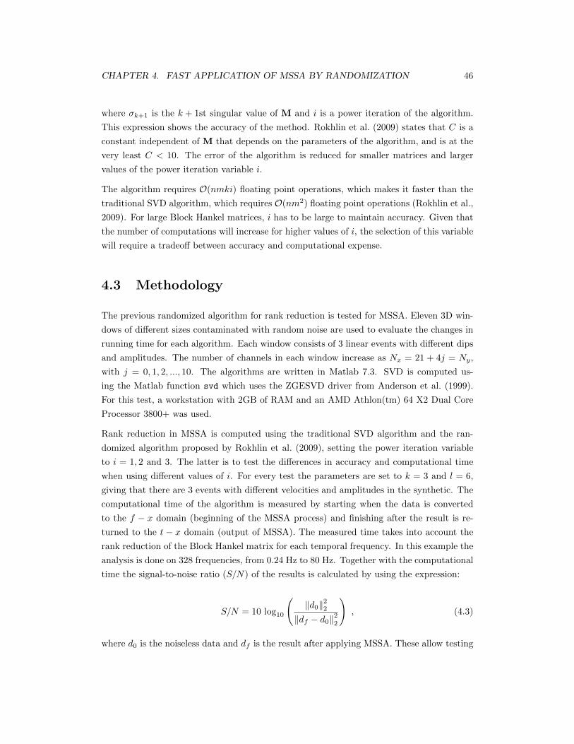
CHAPTER 4. FAST APPLICATION OF MSSA BY RANDOMIZATION 46
where σk+1 is the k + 1st singular value of M and i is a power iteration of the algorithm.
This expression shows the accuracy of the method. Rokhlin et al. (2009) states that C is a
constant independent of M that depends on the parameters of the algorithm, and is at the
very least C < 10. The error of the algorithm is reduced for smaller matrices and larger
values of the power iteration variable i.
The algorithm requires O(nmki) floating point operations, which makes it faster than the
traditional SVD algorithm, which requires O(nm2) floating point operations (Rokhlin et al.,
2009). For large Block Hankel matrices, i has to be large to maintain accuracy. Given that
the number of computations will increase for higher values of i, the selection of this variable
will require a tradeoff between accuracy and computational expense.
4.3 Methodology
The previous randomized algorithm for rank reduction is tested for MSSA. Eleven 3D win-
dows of different sizes contaminated with random noise are used to evaluate the changes in
running time for each algorithm. Each window consists of 3 linear events with different dips
and amplitudes. The number of channels in each window increase as Nx = 21 + 4j = Ny,
with j = 0, 1, 2, ..., 10. The algorithms are written in Matlab 7.3. SVD is computed us-
ing the Matlab function svd which uses the ZGESVD driver from Anderson et al. (1999).
For this test, a workstation with 2GB of RAM and an AMD Athlon(tm) 64 X2 Dual Core
Processor 3800+ was used.
Rank reduction in MSSA is computed using the traditional SVD algorithm and the ran-
domized algorithm proposed by Rokhlin et al. (2009), setting the power iteration variable
to i = 1, 2 and 3. The latter is to test the differences in accuracy and computational time
when using different values of i. For every test the parameters are set to k = 3 and l = 6,
giving that there are 3 events with different velocities and amplitudes in the synthetic. The
computational time of the algorithm is measured by starting when the data is converted
to the f − x domain (beginning of the MSSA process) and finishing after the result is re-
turned to the t − x domain (output of MSSA). The measured time takes into account the
rank reduction of the Block Hankel matrix for each temporal frequency. In this example the
analysis is done on 328 frequencies, from 0.24 Hz to 80 Hz. Together with the computational
time the signal-to-noise ratio (S/N) of the results is calculated by using the expression:
S/N = 10 log10
(‖d0‖22
‖df − d0‖22
), (4.3)
where d0 is the noiseless data and df is the result after applying MSSA. These allow testing
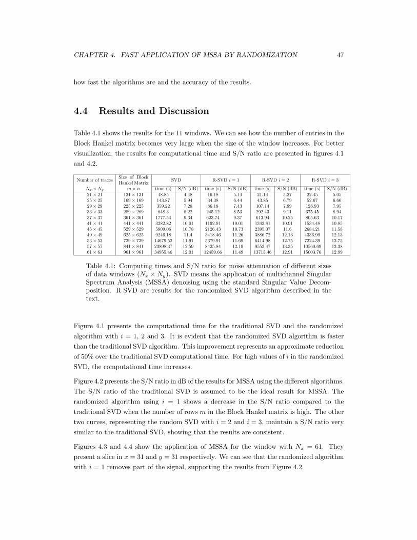
CHAPTER 4. FAST APPLICATION OF MSSA BY RANDOMIZATION 47
how fast the algorithms are and the accuracy of the results.
4.4 Results and Discussion
Table 4.1 shows the results for the 11 windows. We can see how the number of entries in the
Block Hankel matrix becomes very large when the size of the window increases. For better
visualization, the results for computational time and S/N ratio are presented in figures 4.1
and 4.2.
Number of tracesSize of BlockHankel Matrix
SVD R-SVD i = 1 R-SVD i = 2 R-SVD i = 3
Nx ×Ny m× n time (s) S/N (dB) time (s) S/N (dB) time (s) S/N (dB) time (s) S/N (dB)
21× 21 121× 121 48.85 4.48 16.18 5.14 21.14 5.27 22.45 5.0525× 25 169× 169 143.87 5.94 34.38 6.44 43.85 6.79 52.67 6.6629× 29 225× 225 359.22 7.28 86.18 7.43 107.14 7.99 128.93 7.9533× 33 289× 289 848.3 8.22 245.12 8.53 292.43 9.11 375.45 8.9437× 37 361× 361 1777.54 9.34 623.74 9.37 613.94 10.25 805.63 10.1741× 41 441× 441 3282.82 10.01 1192.91 10.01 1343.81 10.91 1534.48 10.8545× 45 529× 529 5809.06 10.78 2126.43 10.73 2395.07 11.6 2684.21 11.5849× 49 625× 625 9246.18 11.4 3418.46 11.26 3886.72 12.13 4336.99 12.1353× 53 729× 729 14679.52 11.91 5379.91 11.69 6414.98 12.75 7224.39 12.7557× 57 841× 841 23898.37 12.59 8425.84 12.19 9553.47 13.35 10560.69 13.3861× 61 961× 961 34955.46 12.01 12459.66 11.49 13715.46 12.91 15003.76 12.99
Table 4.1: Computing times and S/N ratio for noise attenuation of different sizesof data windows (Nx ×Ny). SVD means the application of multichannel SingularSpectrum Analysis (MSSA) denoising using the standard Singular Value Decom-position. R-SVD are results for the randomized SVD algorithm described in thetext.
Figure 4.1 presents the computational time for the traditional SVD and the randomized
algorithm with i = 1, 2 and 3. It is evident that the randomized SVD algorithm is faster
than the traditional SVD algorithm. This improvement represents an approximate reduction
of 50% over the traditional SVD computational time. For high values of i in the randomized
SVD, the computational time increases.
Figure 4.2 presents the S/N ratio in dB of the results for MSSA using the different algorithms.
The S/N ratio of the traditional SVD is assumed to be the ideal result for MSSA. The
randomized algorithm using i = 1 shows a decrease in the S/N ratio compared to the
traditional SVD when the number of rows m in the Block Hankel matrix is high. The other
two curves, representing the random SVD with i = 2 and i = 3, maintain a S/N ratio very
similar to the traditional SVD, showing that the results are consistent.
Figures 4.3 and 4.4 show the application of MSSA for the window with Nx = 61. They
present a slice in x = 31 and y = 31 respectively. We can see that the randomized algorithm
with i = 1 removes part of the signal, supporting the results from Figure 4.2.
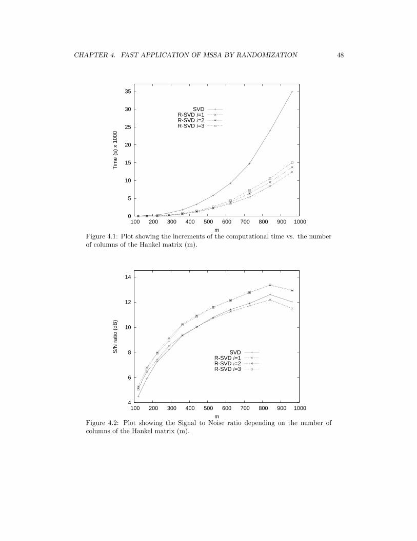
CHAPTER 4. FAST APPLICATION OF MSSA BY RANDOMIZATION 48
0
5
10
15
20
25
30
35
100 200 300 400 500 600 700 800 900 1000
Tim
e (s
) x
1000
m
SVDR-SVD i=1R-SVD i=2R-SVD i=3
Figure 4.1: Plot showing the increments of the computational time vs. the numberof columns of the Hankel matrix (m).
4
6
8
10
12
14
100 200 300 400 500 600 700 800 900 1000
S/N
rat
io (
dB)
m
SVDR-SVD i=1R-SVD i=2R-SVD i=3
Figure 4.2: Plot showing the Signal to Noise ratio depending on the number ofcolumns of the Hankel matrix (m).
CHAPTER 4. FAST APPLICATION OF MSSA BY RANDOMIZATION 49
0
0.5
1
Tim
e (s
)31
x (m)
31y (m
)
(a)
0
0.5
1
Tim
e (s
)
31x (m)
31y (m
)
(f)
0
0.2
0.4
0.6
0.8
1
1.2
(b)T
ime
(sec
)
(c) (d) (e)
0 100 200
0
0.2
0.4
0.6
0.8
1
1.2
(g)
Tim
e (s
ec)
offset (m)0 100 200
(h)offset (m)
0 100 200
(i)offset (m)
0 100 200
(j)offset (m)
Figure 4.3: Slice in x = 31 for the data with size 61 × 61. a) Initial noisy data.b) Result using the traditional SVD. c), d) and e) Results using the random SVDalgorithm with i = 1, i = 2 and i = 3 respectively. f) Noiseless data (d0). g), h) i)and j) are the subtraction of f) from b), c), d) and e) respectively.
4.5 Summary
The application of rank-reduction denoising is limited by the computational cost of tradi-
tional SVD algorithms. The application of a randomized SVD algorithm to improve the
computational time of MSSA was presented. The results show that the randomized SVD
yields an approximately 50% gain in efficiency over the traditional SVD. The accuracy of
the randomized algorithm depends on the size of the block Hankel matrix (m) and on the
selection of the parameter i. The use of larger values of i improves the accuracy of the
randomized SVD but increases the number of calculations. Because of this, the selection of
the parameter i is a tradeoff between accuracy and speed. Alternatively, one can increase
the final rank of MSSA leaving i = 1. By doing this some amount of noise will be recovered,
but no signal will be filtered. In this case, we can achieve good accuracy for the MSSA
result maintaining a lower amount of calculations.
Overall, this algorithm has proved successful in accelerating MSSA. It is clear that the use
of the randomized SVD can be applicable to any rank reduction filtering method. Impor-
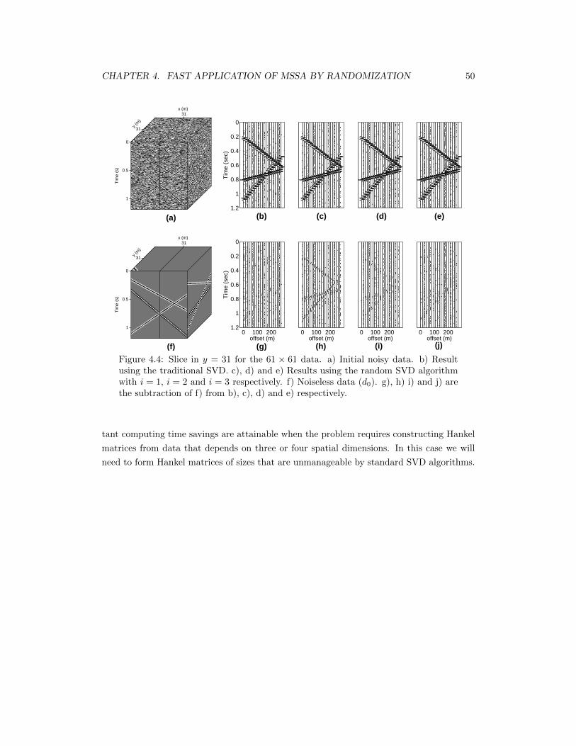
CHAPTER 4. FAST APPLICATION OF MSSA BY RANDOMIZATION 50
0
0.5
1
Tim
e (s
)31
x (m)
31y (m
)
(a)
0
0.5
1
Tim
e (s
)
31x (m)
31y (m
)
(f)
0
0.2
0.4
0.6
0.8
1
1.2
(b)T
ime
(sec
)(c) (d) (e)
0 100 200
0
0.2
0.4
0.6
0.8
1
1.2
(g)
Tim
e (s
ec)
offset (m)0 100 200
(h)offset (m)
0 100 200
(i)offset (m)
0 100 200
(j)offset (m)
Figure 4.4: Slice in y = 31 for the 61 × 61 data. a) Initial noisy data. b) Resultusing the traditional SVD. c), d) and e) Results using the random SVD algorithmwith i = 1, i = 2 and i = 3 respectively. f) Noiseless data (d0). g), h) i) and j) arethe subtraction of f) from b), c), d) and e) respectively.
tant computing time savings are attainable when the problem requires constructing Hankel
matrices from data that depends on three or four spatial dimensions. In this case we will
need to form Hankel matrices of sizes that are unmanageable by standard SVD algorithms.
CHAPTER 5
Interpolation Using Multichannel
Singular Spectrum Analysis
5.1 Background
Seismic data acquisition consists in generating a wave field in the surface of a survey area
and then in extracting the information that is reflected from the subsurface geology. The
information is recorded by receivers placed at the land surface. This means that the infor-
mation coming from the reflections will be recorded at discrete points in the space. Although
seismic surveys are designed to maintain a regular grid of sources and receivers, this will
rarely happen due to logistic or economical constrains. Because of this, seismic data may
be irregularly sampled in space or presenting gaps where no traces are recorded. Many seis-
mic processing tools for noise attenuation or imaging require the input data to be sampled
regularly in space to work properly. Different techniques have been developed to regularize
data and to recover missing traces. These techniques commonly require the conversion of
the data into different domains by using methods like the Fourier transform (Liu and Sac-
chi, 2004), Radon transform (Trad et al., 2002) or the Curvelet transform (Herrmann and
Hennenfent, 2008). One of the methods that interpolate traces in the Fourier domain is the
one developed by Spitz (1991) and expanded by Porsani (1999) and Naghizadeh and Sacchi
(2010), which applies a prediction error filter in the f −x domain of the data. This method
is very powerful when interpolating undersampled and aliased data in a regular grid; but
interpolating traces in an irregular pattern can be more difficult (Abma and Kabir, 2006).
An application that aims to solve the interpolation of missing traces in an irregular pattern
was developed by Abma and Kabir (2006). They apply an iterative method that consists
51
CHAPTER 5. INTERPOLATION USING MSSA 52
in thresholding the frequency spectrum after a 2D Fourier transform. Subsequently, they
replace the recovered traces in the original gather to perform the analysis again. After some
iterations, the traces would be recovered. The amount of missing traces and the differences
in amplitudes of the events control the number of iterations to recover the events with the
correct amplitude. This algorithm is called Projection onto convex sets (POCS) and was
developed by Youla and Webb (1982) for image restoration problems.
The objective of this chapter is to study the application of MSSA to interpolate missing
traces in an irregular pattern. Just like the interpolation method developed by Spitz (1991),
MSSA works in the f − x domain of the data, but instead of performing a prediction
error filter, it relies in the rank reduction of Hankel matrices. The process is improved by
using the POCS algorithm applied by Abma and Kabir (2006), and instead of thresholding
the frequency spectrum we apply MSSA. This chapter aims mainly in understanding the
processes that allow MSSA to interpolate seismic data and looks to be a guideline on how to
apply it. Our results are not compared with results of other interpolators. This comparison
is strongly recommended for future research in SSA.
5.2 Application
The process of interpolating and recovering missing traces in seismic record using MSSA is
the same as filtering random noise. In fact, both processes can be carried out simultaneously.
As discussed in chapter 3, the application of SSA to filter random noise in seismic records
consists in six steps that are:
1. Fourier transform to take the data to the f − x domain
2. Embedding of each frequency into a Hankel matrix
3. Decomposition in its singular spectrum via SVD
4. Rank reduction of the Hankel matrix
5. Averaging in the Hankel matrix anti-diagonals
6. Inverse Fourier transform to return to the time domain.
A noise free record with a single linear event will lead to a Hankel matrix with rank one.
Similarly, a number of k linear events with different apparent velocities will result in a
Hankel matrix with rank k (see equation 3.13). In the presence of noise the rank of the
Hankel matrix will increase. The rank reduction step of SSA aims to filter random noise
CHAPTER 5. INTERPOLATION USING MSSA 53
by recovering a Hankel matrix with the rank that represents the events contained in the
record. This procedure is still valid in the presence of missing traces, as long as they are in
a regular grid. The missing samples will be treated as noise by SSA, and the rank reduction
step will recover some of the amplitudes expected on these missing traces. This allows SSA
to be a powerful interpolator that can be easily extended to several dimensions.
Missing traces in a seismic record are characterized by presenting zeros in all its samples.
When transformed to the f−x domain, these missing traces still present zero values in each
frequency. These samples become part of the Hankel matrix after the embedding step. In
the presence of missing samples, the rank of the Hankel matrix increases. This is analogous
with the case where random noise contaminates the record. The rank reduction process will
approximate the Hankel matrix to the expected low-rank matrix that represents the signal
with no gaps. With this, the missing samples are replaced by the value that generates the
best low-rank approximation to the Hankel matrix. Given that this process is repeated for
a range of frequencies, the missing traces will recover part of its amplitude spectrum. After
one iteration, linear events are interpolated through the missing traces, but they will present
lower amplitudes compared to the original events.
To recover the right amplitude for the interpolated traces, it is possible to apply the POCS
algorithm utilized by Abma and Kabir (2006). This iterative algorithm is applied in the f−xdomain and works using SSA or MSSA. For SSA the input data is a vector and for MSSA
the input data is a matrix of a single frequency. The following description of the algorithm
assumes a 2-D input data S. Initially, an operator T is created to identify the presence of
traces on the spatial position (i, j) of the data, being T (i , j ) = 1 in the cells that present
a trace and T (i , j ) = 0 in the cell where there are missing traces. The application of the
operator T to the data S produces the observed data Sobs. In other words, T � S = Sobs.
It is evident that T � Sobs = Sobs. The difference between an operator I with ones in every
cell (i, j), meaning I = ones(dimT ), and T result in an operator that identify the spatial
position of the missing traces. This operator is used to extract the recovered traces after
one iteration, and to place them in the original input data. Then MSSA is applied again.
The POCS algorithm used to interpolate data using MSSA can be summarized as follows:
for p = 1 : Niter
for f = finit : ffinal
Sp(f) = Sobs(f) + (I − T ) � A[UkUTk H (Sp−1(f))]
end
end ,
(5.1)
where finit and ffinal are the initial and final frequencies to analyze in the MSSA process, H
is the Hankelization operator, UkUTk is the rank reduction operator and A is the averaging
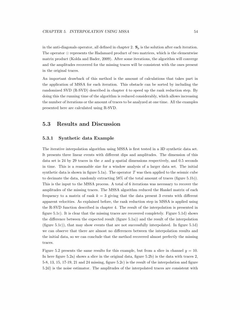
CHAPTER 5. INTERPOLATION USING MSSA 54
in the anti-diagonals operator, all defined in chapter 2. Sp is the solution after each iteration.
The operator � represents the Hadamard product of two matrices, which is the elementwise
matrix product (Kolda and Bader, 2009). After some iterations, the algorithm will converge
and the amplitudes recovered for the missing traces will be consistent with the ones present
in the original traces.
An important drawback of this method is the amount of calculations that takes part in
the application of MSSA for each iteration. This obstacle can be sorted by including the
randomized SVD (R-SVD) described in chapter 4 to speed up the rank reduction step. By
doing this the running time of the algorithm is reduced considerably, which allows increasing
the number of iterations or the amount of traces to be analyzed at one time. All the examples
presented here are calculated using R-SVD.
5.3 Results and Discussion
5.3.1 Synthetic data Example
The iterative interpolation algorithm using MSSA is first tested in a 3D synthetic data set.
It presents three linear events with different dips and amplitudes. The dimension of this
data set is 24 by 29 traces in the x and y spatial dimensions respectively, and 0.5 seconds
in time. This is a reasonable size for a window analysis of a larger data set. The initial
synthetic data is shown in figure 5.1a). The operator T was then applied to the seismic cube
to decimate the data, randomly extracting 58% of the total amount of traces (figure 5.1b)).
This is the input to the MSSA process. A total of 6 iterations was necessary to recover the
amplitudes of the missing traces. The MSSA algorithm reduced the Hankel matrix of each
frequency to a matrix of rank k = 3 giving that the data present 3 events with different
apparent velocities. As explained before, the rank reduction step in MSSA is applied using
the R-SVD function described in chapter 4. The result of the interpolation is presented in
figure 5.1c). It is clear that the missing traces are recovered completely. Figure 5.1d) shows
the difference between the expected result (figure 5.1a)) and the result of the interpolation
(figure 5.1c)), that may show events that are not successfully interpolated. In figure 5.1d)
we can observe that there are almost no differences between the interpolation results and
the initial data, so we can conclude that the method recovered almost perfectly the missing
traces.
Figure 5.2 presents the same results for this example, but from a slice in channel y = 10.
In here figure 5.2a) shows a slice in the original data, figure 5.2b) is the data with traces 2,
5-8, 13, 15, 17-19, 21 and 24 missing, figure 5.2c) is the result of the interpolation and figure
5.2d) is the noise estimator. The amplitudes of the interpolated traces are consistent with
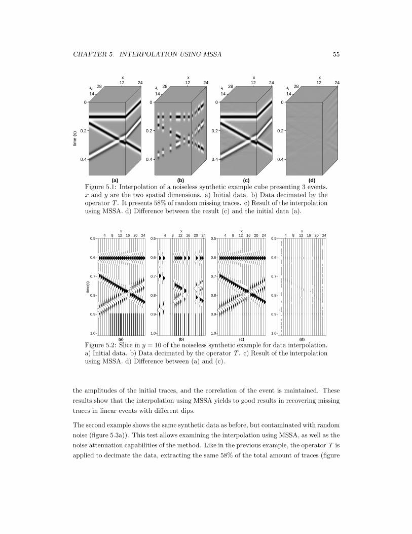
CHAPTER 5. INTERPOLATION USING MSSA 55
0
0.2
0.4
time
(s)
12 24x
14
28y
(a)
0
0.2
0.4
12 24x
14
28y
(b)
0
0.2
0.4
12 24x
14
28y
(c)
0
0.2
0.4
12 24x
14
28y
(d)Figure 5.1: Interpolation of a noiseless synthetic example cube presenting 3 events.x and y are the two spatial dimensions. a) Initial data. b) Data decimated by theoperator T . It presents 58% of random missing traces. c) Result of the interpolationusing MSSA. d) Difference between the result (c) and the initial data (a).
0.5
0.6
0.7
0.8
0.9
1.0
time(
s)
4 8 12 16 20 24x
(a)
0.5
0.6
0.7
0.8
0.9
1.0
4 8 12 16 20 24x
(b)
0.5
0.6
0.7
0.8
0.9
1.0
4 8 12 16 20 24x
(c)
0.5
0.6
0.7
0.8
0.9
1.0
4 8 12 16 20 24x
(d)
Figure 5.2: Slice in y = 10 of the noiseless synthetic example for data interpolation.a) Initial data. b) Data decimated by the operator T . c) Result of the interpolationusing MSSA. d) Difference between (a) and (c).
the amplitudes of the initial traces, and the correlation of the event is maintained. These
results show that the interpolation using MSSA yields to good results in recovering missing
traces in linear events with different dips.
The second example shows the same synthetic data as before, but contaminated with random
noise (figure 5.3a)). This test allows examining the interpolation using MSSA, as well as the
noise attenuation capabilities of the method. Like in the previous example, the operator T is
applied to decimate the data, extracting the same 58% of the total amount of traces (figure
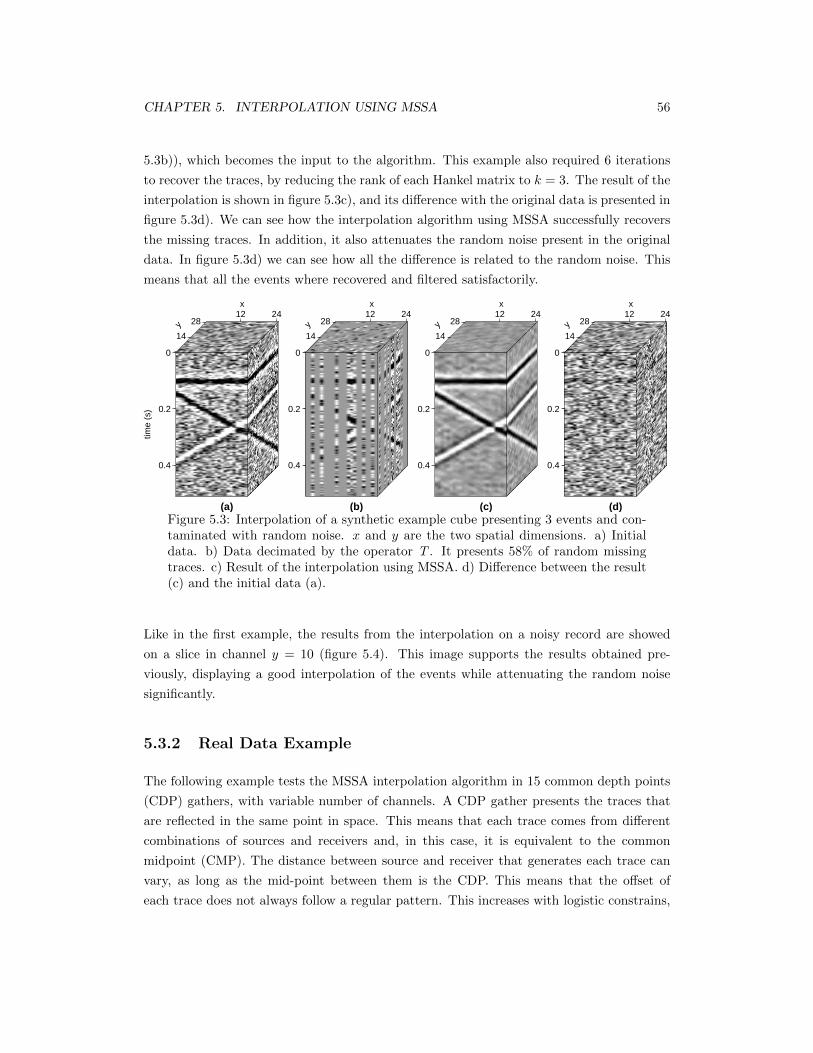
CHAPTER 5. INTERPOLATION USING MSSA 56
5.3b)), which becomes the input to the algorithm. This example also required 6 iterations
to recover the traces, by reducing the rank of each Hankel matrix to k = 3. The result of the
interpolation is shown in figure 5.3c), and its difference with the original data is presented in
figure 5.3d). We can see how the interpolation algorithm using MSSA successfully recovers
the missing traces. In addition, it also attenuates the random noise present in the original
data. In figure 5.3d) we can see how all the difference is related to the random noise. This
means that all the events where recovered and filtered satisfactorily.
0
0.2
0.4
time
(s)
12 24x
14
28y
(a)
0
0.2
0.4
12 24x
14
28y
(b)
0
0.2
0.4
12 24x
14
28y
(c)
0
0.2
0.4
12 24x
14
28y
(d)Figure 5.3: Interpolation of a synthetic example cube presenting 3 events and con-taminated with random noise. x and y are the two spatial dimensions. a) Initialdata. b) Data decimated by the operator T . It presents 58% of random missingtraces. c) Result of the interpolation using MSSA. d) Difference between the result(c) and the initial data (a).
Like in the first example, the results from the interpolation on a noisy record are showed
on a slice in channel y = 10 (figure 5.4). This image supports the results obtained pre-
viously, displaying a good interpolation of the events while attenuating the random noise
significantly.
5.3.2 Real Data Example
The following example tests the MSSA interpolation algorithm in 15 common depth points
(CDP) gathers, with variable number of channels. A CDP gather presents the traces that
are reflected in the same point in space. This means that each trace comes from different
combinations of sources and receivers and, in this case, it is equivalent to the common
midpoint (CMP). The distance between source and receiver that generates each trace can
vary, as long as the mid-point between them is the CDP. This means that the offset of
each trace does not always follow a regular pattern. This increases with logistic constrains,
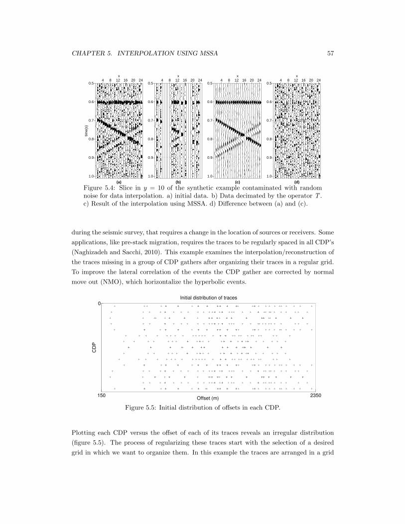
CHAPTER 5. INTERPOLATION USING MSSA 57
0.5
0.6
0.7
0.8
0.9
1.0
time(
s)
4 8 12 16 20 24x
(a)
0.5
0.6
0.7
0.8
0.9
1.0
4 8 12 16 20 24x
(b)
0.5
0.6
0.7
0.8
0.9
1.0
4 8 12 16 20 24x
(c)
0.5
0.6
0.7
0.8
0.9
1.0
4 8 12 16 20 24x
(d)
Figure 5.4: Slice in y = 10 of the synthetic example contaminated with randomnoise for data interpolation. a) initial data. b) Data decimated by the operator T .c) Result of the interpolation using MSSA. d) Difference between (a) and (c).
during the seismic survey, that requires a change in the location of sources or receivers. Some
applications, like pre-stack migration, requires the traces to be regularly spaced in all CDP’s
(Naghizadeh and Sacchi, 2010). This example examines the interpolation/reconstruction of
the traces missing in a group of CDP gathers after organizing their traces in a regular grid.
To improve the lateral correlation of the events the CDP gather are corrected by normal
move out (NMO), which horizontalize the hyperbolic events.
150 2350
0Initial distribution of traces
Offset (m)
CDP
Figure 5.5: Initial distribution of offsets in each CDP.
Plotting each CDP versus the offset of each of its traces reveals an irregular distribution
(figure 5.5). The process of regularizing these traces start with the selection of a desired
grid in which we want to organize them. In this example the traces are arranged in a grid
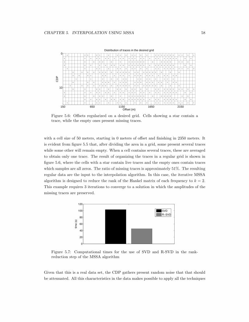
CHAPTER 5. INTERPOLATION USING MSSA 58
150 650 1150 1650 2150
0
10
Distribution of traces in the desired grid
Offset (m)
CD
P
Figure 5.6: Offsets regularized on a desired grid. Cells showing a star contain atrace, while the empty ones present missing traces.
with a cell size of 50 meters, starting in 0 meters of offset and finishing in 2350 meters. It
is evident from figure 5.5 that, after dividing the area in a grid, some present several traces
while some other will remain empty. When a cell contains several traces, these are averaged
to obtain only one trace. The result of organizing the traces in a regular grid is shown in
figure 5.6, where the cells with a star contain live traces and the empty ones contain traces
which samples are all zeros. The ratio of missing traces is approximately 51%. The resulting
regular data are the input to the interpolation algorithm. In this case, the iterative MSSA
algorithm is designed to reduce the rank of the Hankel matrix of each frequency to k = 2.
This example requires 3 iterations to converge to a solution in which the amplitudes of the
missing traces are preserved.
0
20
40
60
80
100
120
time
(s)
Times in seconds for MSSA using SVD and R−SVD
SVDR−SVD
Figure 5.7: Computational times for the use of SVD and R-SVD in the rank-reduction step of the MSSA algorithm
Given that this is a real data set, the CDP gathers present random noise that that should
be attenuated. All this characteristics in the data makes possible to apply all the techniques
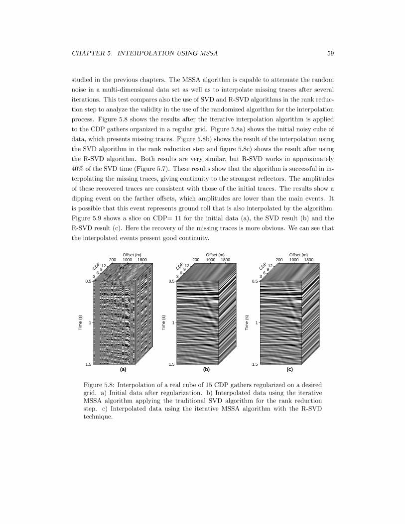
CHAPTER 5. INTERPOLATION USING MSSA 59
studied in the previous chapters. The MSSA algorithm is capable to attenuate the random
noise in a multi-dimensional data set as well as to interpolate missing traces after several
iterations. This test compares also the use of SVD and R-SVD algorithms in the rank reduc-
tion step to analyze the validity in the use of the randomized algorithm for the interpolation
process. Figure 5.8 shows the results after the iterative interpolation algorithm is applied
to the CDP gathers organized in a regular grid. Figure 5.8a) shows the initial noisy cube of
data, which presents missing traces. Figure 5.8b) shows the result of the interpolation using
the SVD algorithm in the rank reduction step and figure 5.8c) shows the result after using
the R-SVD algorithm. Both results are very similar, but R-SVD works in approximately
40% of the SVD time (Figure 5.7). These results show that the algorithm is successful in in-
terpolating the missing traces, giving continuity to the strongest reflectors. The amplitudes
of these recovered traces are consistent with those of the initial traces. The results show a
dipping event on the farther offsets, which amplitudes are lower than the main events. It
is possible that this event represents ground roll that is also interpolated by the algorithm.
Figure 5.9 shows a slice on CDP= 11 for the initial data (a), the SVD result (b) and the
R-SVD result (c). Here the recovery of the missing traces is more obvious. We can see that
the interpolated events present good continuity.
0.5
1
1.5
Tim
e (s
)
200 1000 1800Offset (m)
36
912
CDP
(a)
0.5
1
1.5
Tim
e (s
)
200 1000 1800Offset (m)
36
912
CDP
(b)
0.5
1
1.5
Tim
e (s
)
200 1000 1800Offset (m)
36
912
CDP
(c)
Figure 5.8: Interpolation of a real cube of 15 CDP gathers regularized on a desiredgrid. a) Initial data after regularization. b) Interpolated data using the iterativeMSSA algorithm applying the traditional SVD algorithm for the rank reductionstep. c) Interpolated data using the iterative MSSA algorithm with the R-SVDtechnique.
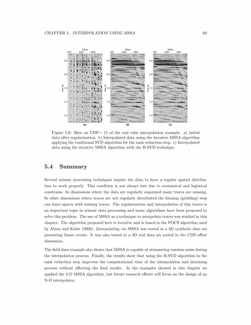
CHAPTER 5. INTERPOLATION USING MSSA 60
0.6
0.8
1.0
1.2
1.4
time
(s)
200 1000 1800Offset
(a)
0.6
0.8
1.0
1.2
1.4
time
(s)
200 1000 1800Offset
(b)
0.6
0.8
1.0
1.2
1.4
time
(s)
200 1000 1800Offset
(c)
Figure 5.9: Slice on CDP= 11 of the real cube interpolation example. a) initialdata after regularization. b) Interpolated data using the iterative MSSA algorithmapplying the traditional SVD algorithm for the rank reduction step. c) Interpolateddata using the iterative MSSA algorithm with the R-SVD technique.
5.4 Summary
Several seismic processing techniques require the data to have a regular spatial distribu-
tion to work properly. This condition is not always met due to economical and logistical
constrains. In dimensions where the data are regularly organized many traces are missing.
In other dimensions where traces are not regularly distributed the binning (gridding) step
can leave spaces with missing traces. The regularization and interpolation of this traces is
an important topic in seismic data processing and many algorithms have been proposed to
solve this problem. The use of MSSA as a technique to interpolate traces was studied in this
chapter. The algorithm proposed here is iterative and is based in the POCS algorithm used
by Abma and Kabir (2006). Interpolating via MSSA was tested in a 3D synthetic data set
presenting linear events. It was also tested in a 3D real data set sorted in the CDP-offset
dimension.
The field data example also shows that MSSA is capable of attenuating random noise during
the interpolation process. Finally, the results show that using the R-SVD algorithm in the
rank reduction step improves the computational time of the interpolation and denoising
process without affecting the final results. In the examples showed in this chapter we
applied the 2-D MSSA algorithm, but future research efforts will focus on the design of an
N-D interpolator.
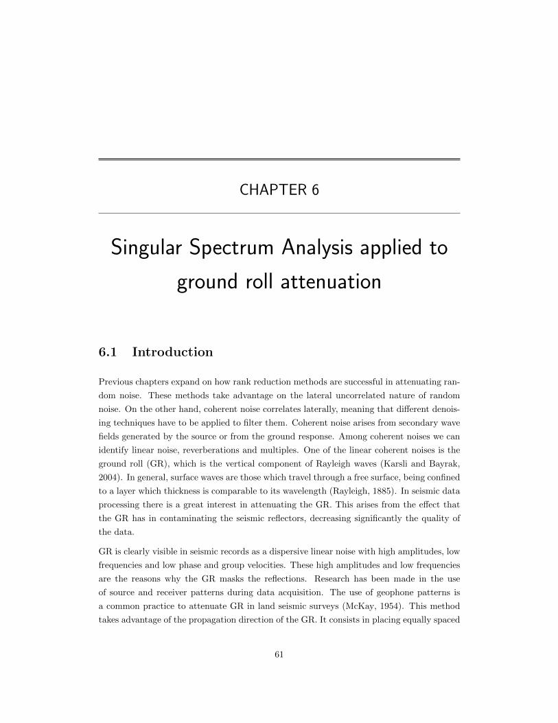
CHAPTER 6
Singular Spectrum Analysis applied to
ground roll attenuation
6.1 Introduction
Previous chapters expand on how rank reduction methods are successful in attenuating ran-
dom noise. These methods take advantage on the lateral uncorrelated nature of random
noise. On the other hand, coherent noise correlates laterally, meaning that different denois-
ing techniques have to be applied to filter them. Coherent noise arises from secondary wave
fields generated by the source or from the ground response. Among coherent noises we can
identify linear noise, reverberations and multiples. One of the linear coherent noises is the
ground roll (GR), which is the vertical component of Rayleigh waves (Karsli and Bayrak,
2004). In general, surface waves are those which travel through a free surface, being confined
to a layer which thickness is comparable to its wavelength (Rayleigh, 1885). In seismic data
processing there is a great interest in attenuating the GR. This arises from the effect that
the GR has in contaminating the seismic reflectors, decreasing significantly the quality of
the data.
GR is clearly visible in seismic records as a dispersive linear noise with high amplitudes, low
frequencies and low phase and group velocities. These high amplitudes and low frequencies
are the reasons why the GR masks the reflections. Research has been made in the use
of source and receiver patterns during data acquisition. The use of geophone patterns is
a common practice to attenuate GR in land seismic surveys (McKay, 1954). This method
takes advantage of the propagation direction of the GR. It consists in placing equally spaced
61
CHAPTER 6. SSA APPLIED TO GROUND ROLL ATTENUATION 62
receivers, aligned with the source, in a distance related to the wave length of the GR. The
reflections are expected to arrive vertically to each array, registering the same arrival time
for each of the receivers. Since the GR travels along the surface, each geophone will record
different amplitudes. The information from each receiver is then averaged. Giving that the
total length of the array is a multiple of the wave length of the GR, the latter is attenuated
after the averaging of the data recorded by each geophone. Unfortunately, this method only
filters specific wave numbers, depending on the length of the geophone array. Early studies
also expand on the use of source patterns to cancel the amplitudes of the ground roll, either
by using pattern of shot holes (McKay, 1954) or by designing different sweeps and cross-
correlation methods when using Vibroseis (Coruh and Constain, 1983). Application of GR
attenuation techniques during data acquisition is limited. It may decrease the resolution
of the signal when the source and receiver arrays overlap (Coruh and Constain, 1983) or
attenuate shallow reflectors that do not arrive vertically to the receiver arrays (Knapp, 1986).
This makes necessary the application of different techniques during the data processing.
Classical methods exploit the spatial and frequency differences between the GR and the
reflections. Filtering the data in the f − k domain is of common use to attenuate the
ground roll (March and Bailey, 1983; Duncan and Beresford, 1994). This method consists
in applying a 2-D Fourier transformation in time and space to map linear events in the f−kdomain. The low frequency and low wavenumber characteristics of the GR can be identified
in this domain. Thus a rejecting window can be designed to filter the GR (Yilmaz, 2001).
The use of an f −k filter has the drawback of distorting the signal wavelets and introducing
artifacts to the record. Another common way to filter GR, mostly during fast track data
processing, is by the use of a low pass filter. The method starts with the application of
the Fourier transform to each trace of the data to obtain its amplitude spectrum. A filter
window is then applied to the low frequencies that represent the GR. The low frequency noise
is recovered by applying the inverse Fourier transform. The recovered low frequency gather
containing the GR is then subtracted from the original data. This method is successful
when the main frequencies of the ground roll are very different from those of the signal.
When the frequencies of the ground roll and the reflections overlap, the use of a low pass
filter also eliminates low frequencies from the reflections. In this case the method becomes
less effective.
This chapter expands on the use of SSA to improve the results from the application of a
low pass filter during the GR attenuation process. The low frequency data recovered from
the application of a low pass filter is decomposed into its singular spectrum by using SSA
in the f − x domain. The same methodology used in chapter 3 is applied to build a Hankel
matrix for each frequency. We then recover the signal using the subset of singular values that
model only the GR. By doing this, the final low frequency gather that is subtracted from the
original data will contain only the GR, solving the problem of eliminating low frequencies
CHAPTER 6. SSA APPLIED TO GROUND ROLL ATTENUATION 63
in the reflections. A similar method has been applied with the name of Spectral Matrix
Decomposition. This technique differentiate events by decomposing the covariance matrix
of a single frequency of the f − x domain, while SSA does it on a Hankel matrix of each
frequency. Mari and Glangeaud (1990) used Spectral Matrix Decomposition to differentiate
arrivals in Vertical Seismic Profiles (VSP).
6.2 Theory
Previous chapters showed that linear events in a seismic section could be recovered by the
retrieval of a subset of its singular values after SSA. When dealing with random noise, this
operation takes advantage of the incoherency of the noise between traces. In general, the
first singular values will represent the signal and the amount of noise removed will depend
on how many singular values are recovered. The minimum singular values to ensure that
all the linear events are recovered are the same as the number of events with different
dips present in the record. In the case of coherent noise attenuation the situation is more
complex. In this case, the event that we wish to retain and the event that is considered noise
are recovered by the first few singular values. The problem is to know if different singular
values recover different events. If they do so, it is also important to find out which singular
value represents each event. Analyzing how the events are projected over the orthonormal
basis generated by the singular vectors holds the answer to this query.
In chapter 3 we showed that SSA is applied in the frequency domain of the data, which is
shown in equation 3.2 for a single event. When more than one event is present, the data in
the frequency domain can be written as
S(x) =k∑i=1
Wi(x) + N(x) , (6.1)
where S(x) = [S1, S2, ..., SNx]T is the data, Wi(x) = [W1,W2, ...,WNx
]T is the waveform
that represents each event i and N(x) = [N1, N2, ..., NNx]T is the noise. k is the number of
events present in the data and x = 1, 2, 3, ..., Nx, being Nx the number of channels in the
space dimension. This expression is valid for each frequency ω. The next step is to build a
trajectory matrix from S(x). Up to here, SSA follows the same methodology as the Spectral
Matrix filtering proposed by Mari and Glangeaud (1990). The main difference between the
two methods is that SSA performs a SVD over a trajectory matrix built from Sω(x) and
Spectral Matrix Filtering decomposes the covariance matrix SSH , where H denotes the
conjugate transpose. Mari and Glangeaud (1990) uses the inner product of two events given
by:
CHAPTER 6. SSA APPLIED TO GROUND ROLL ATTENUATION 64
< W1,W2 >= WH1 W2 , (6.2)
to determine when two events are orthogonal. Two vectors can only be represented by
two different singular values if they are orthogonal. Mari and Glangeaud (1990) explain
the separation performed by the Spectral Matrix Filtering by analyzing the inner product
between each S(x) vector of each event. Since SSA decomposes a Hankel matrix, the internal
product has to be calculated between the lagged vectors of each event. It is possible to show
that when two S(x) vectors from two different events are orthogonal, the lagged vectors for
the same two events are orthogonal too. This is explained because, as shown in equation
3.5, in the presence of a single event the rank of the Hankel matrix is 1, and its column
vectors are parallel to each other, and therefore, they are parallel to the S(x) of such
event. We can understand from this that all the lagged vectors from a single event will
be projected over the same singular vectors. Given that the SVD decomposes the Hankel
matrix into its orthonormal basis, it is clear that for each event to be reconstructed by a
different singular values, these events have to be orthogonal between each other. It is evident
that the number of events to reconstruct has to be lower than the embedding dimension
L, named in chapter 2, given that this is the maximum number of singular vectors that
represent the data. By computing the inner product between two lagged vectors from the
Hankel matrix of two different events, it is possible to know if they are orthonormal. To do
so, it is necessary to normalize each vector and perform equation 6.2. If the inner product
is near one (< l1, l2 >≈ 1) the lagged vectors are almost parallel, if the inner product is
near zero (< l1, l2 >≈ 0) then the lagged vectors are close to be orthogonal. Given that all
the lagged vectors for each event are parallel, if this condition applies to one pair of lagged
vectors; it will apply for all the combinations between them. It is important to remember
that the orthogonality between the two events is related to its dip and consequently to its
velocity, so if the velocities of the events are similar, the lagged vectors are parallel, and if
they are different the lagged vectors will be close to orthogonal. Also the amplitude of each
event controls if the events can be separated or not in a different way than its orthogonality.
Taking as a reference the results from Mari and Glangeaud (1990), we can summarize the
conditions in which the amplitude of the events and their orthogonality allows them to be
separated:
1. Same Amplitude and Different Velocities (< l1, l2 >= 0) :
The first possible condition is when the events present the same amplitudes for all the
frequencies, and when their velocities are different, making the lagged vectors between
both events at every frequency orthogonal. This means that the inner product between
two lagged vectors must be close to zero (< l1, l2 >= 0). Giving that none of the
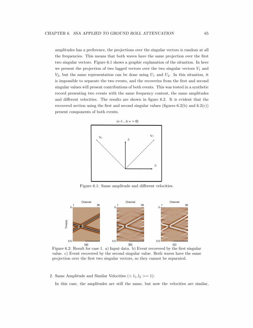
CHAPTER 6. SSA APPLIED TO GROUND ROLL ATTENUATION 65
amplitudes has a preference, the projections over the singular vectors is random at all
the frequencies. This means that both waves have the same projection over the first
two singular vectors. Figure 6.1 shows a graphic explanation of the situation. In here
we present the projection of two lagged vectors over the two singular vectors V1 and
V2, but the same representation can be done using U1 and U2. In this situation, it
is impossible to separate the two events, and the recoveries from the first and second
singular values will present contributions of both events. This was tested in a synthetic
record presenting two events with the same frequency content, the same amplitudes
and different velocities. The results are shown in figure 6.2. It is evident that the
recovered section using the first and second singular values (figures 6.2(b) and 6.2(c))
present components of both events.
V1V2
l1
l2
Same Amplitudes and Different Velocity (< l1 , l2 > � 0)
Figure 6.1: Same amplitude and different velocities.
0
0.5
Tim
e(s
)
1 36Channel
(a)
0
0.5
1 36Channel
(b)
0
0.5
1 36Channel
(c)
Figure 6.2: Result for case 1. a) Input data. b) Event recovered by the first singularvalue. c) Event recovered by the second singular value. Both waves have the sameprojection over the first two singular vectors, so they cannot be separated.
2. Same Amplitude and Similar Velocities (< l1, l2 >= 1):
In this case, the amplitudes are still the same, but now the velocities are similar,
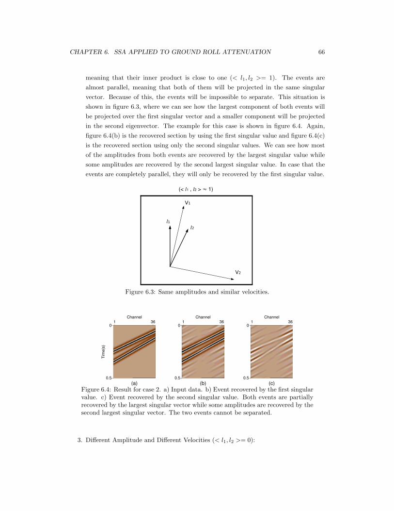
CHAPTER 6. SSA APPLIED TO GROUND ROLL ATTENUATION 66
meaning that their inner product is close to one (< l1, l2 >= 1). The events are
almost parallel, meaning that both of them will be projected in the same singular
vector. Because of this, the events will be impossible to separate. This situation is
shown in figure 6.3, where we can see how the largest component of both events will
be projected over the first singular vector and a smaller component will be projected
in the second eigenvector. The example for this case is shown in figure 6.4. Again,
figure 6.4(b) is the recovered section by using the first singular value and figure 6.4(c)
is the recovered section using only the second singular values. We can see how most
of the amplitudes from both events are recovered by the largest singular value while
some amplitudes are recovered by the second largest singular value. In case that the
events are completely parallel, they will only be recovered by the first singular value.
��
��
l�l�
Same Amplitudes and Similar Velocity (< l1 , l2 > � 1)
Figure 6.3: Same amplitudes and similar velocities.
0
0.5
Tim
e(s
)
1 36Channel
(a)
0
0.5
1 36Channel
(b)
0
0.5
1 36Channel
(c)
Figure 6.4: Result for case 2. a) Input data. b) Event recovered by the first singularvalue. c) Event recovered by the second singular value. Both events are partiallyrecovered by the largest singular vector while some amplitudes are recovered by thesecond largest singular vector. The two events cannot be separated.
3. Different Amplitude and Different Velocities (< l1, l2 >= 0):
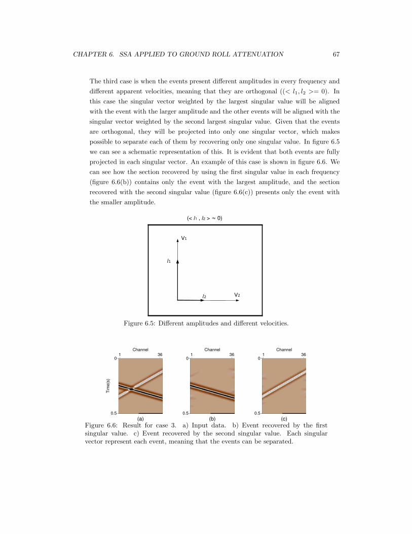
CHAPTER 6. SSA APPLIED TO GROUND ROLL ATTENUATION 67
The third case is when the events present different amplitudes in every frequency and
different apparent velocities, meaning that they are orthogonal ((< l1, l2 >= 0). In
this case the singular vector weighted by the largest singular value will be aligned
with the event with the larger amplitude and the other events will be aligned with the
singular vector weighted by the second largest singular value. Given that the events
are orthogonal, they will be projected into only one singular vector, which makes
possible to separate each of them by recovering only one singular value. In figure 6.5
we can see a schematic representation of this. It is evident that both events are fully
projected in each singular vector. An example of this case is shown in figure 6.6. We
can see how the section recovered by using the first singular value in each frequency
(figure 6.6(b)) contains only the event with the largest amplitude, and the section
recovered with the second singular value (figure 6.6(c)) presents only the event with
the smaller amplitude.
��
��
l�
l�
Different Amplitudes and Different Velocity (< l1 , l2 > � 0)
Figure 6.5: Different amplitudes and different velocities.
0
0.5
Tim
e(s
)
1 36Channel
(a)
0
0.5
1 36Channel
(b)
0
0.5
1 36Channel
(c)
Figure 6.6: Result for case 3. a) Input data. b) Event recovered by the firstsingular value. c) Event recovered by the second singular value. Each singularvector represent each event, meaning that the events can be separated.
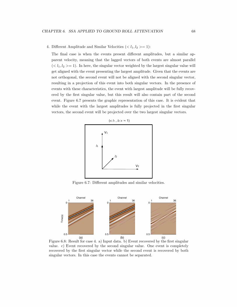
CHAPTER 6. SSA APPLIED TO GROUND ROLL ATTENUATION 68
4. Different Amplitude and Similar Velocities (< l1, l2 >= 1):
The final case is when the events present different amplitudes, but a similar ap-
parent velocity, meaning that the lagged vectors of both events are almost parallel
(< l1, l2 >= 1). In here, the singular vector weighted by the largest singular value will
get aligned with the event presenting the largest amplitude. Given that the events are
not orthogonal, the second event will not be aligned with the second singular vector,
resulting in a projection of this event into both singular vectors. In the presence of
events with these characteristics, the event with largest amplitude will be fully recov-
ered by the first singular value, but this result will also contain part of the second
event. Figure 6.7 presents the graphic representation of this case. It is evident that
while the event with the largest amplitudes is fully projected in the first singular
vectors, the second event will be projected over the two largest singular vectors.
Different Amplitude and Similar Velocity (< l1 , l2 > � 1)
��
��
l�
l�
Figure 6.7: Different amplitudes and similar velocities.
0
0.5
Tim
e(s
)
1 36Channel
(a)
0
0.5
1 36Channel
(b)
0
0.5
1 36Channel
(c)
Figure 6.8: Result for case 4. a) Input data. b) Event recovered by the first singularvalue. c) Event recovered by the second singular value. One event is completelyrecovered by the first singular vector while the second event is recovered by bothsingular vectors. In this case the events cannot be separated.
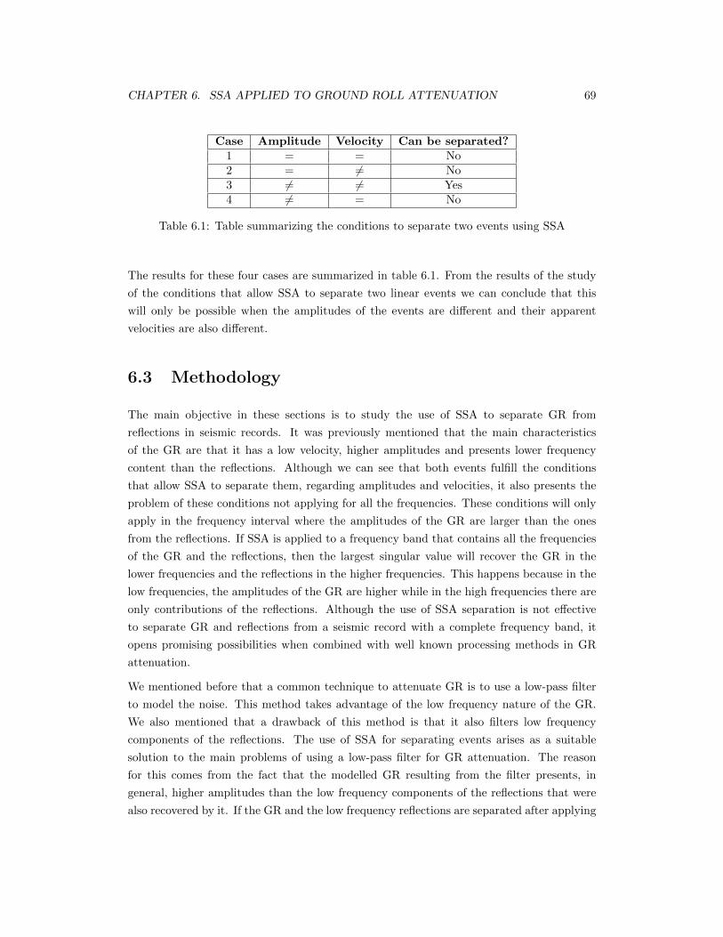
CHAPTER 6. SSA APPLIED TO GROUND ROLL ATTENUATION 69
Case Amplitude Velocity Can be separated?1 = = No2 = 6= No3 6= 6= Yes4 6= = No
Table 6.1: Table summarizing the conditions to separate two events using SSA
The results for these four cases are summarized in table 6.1. From the results of the study
of the conditions that allow SSA to separate two linear events we can conclude that this
will only be possible when the amplitudes of the events are different and their apparent
velocities are also different.
6.3 Methodology
The main objective in these sections is to study the use of SSA to separate GR from
reflections in seismic records. It was previously mentioned that the main characteristics
of the GR are that it has a low velocity, higher amplitudes and presents lower frequency
content than the reflections. Although we can see that both events fulfill the conditions
that allow SSA to separate them, regarding amplitudes and velocities, it also presents the
problem of these conditions not applying for all the frequencies. These conditions will only
apply in the frequency interval where the amplitudes of the GR are larger than the ones
from the reflections. If SSA is applied to a frequency band that contains all the frequencies
of the GR and the reflections, then the largest singular value will recover the GR in the
lower frequencies and the reflections in the higher frequencies. This happens because in the
low frequencies, the amplitudes of the GR are higher while in the high frequencies there are
only contributions of the reflections. Although the use of SSA separation is not effective
to separate GR and reflections from a seismic record with a complete frequency band, it
opens promising possibilities when combined with well known processing methods in GR
attenuation.
We mentioned before that a common technique to attenuate GR is to use a low-pass filter
to model the noise. This method takes advantage of the low frequency nature of the GR.
We also mentioned that a drawback of this method is that it also filters low frequency
components of the reflections. The use of SSA for separating events arises as a suitable
solution to the main problems of using a low-pass filter for GR attenuation. The reason
for this comes from the fact that the modelled GR resulting from the filter presents, in
general, higher amplitudes than the low frequency components of the reflections that were
also recovered by it. If the GR and the low frequency reflections are separated after applying
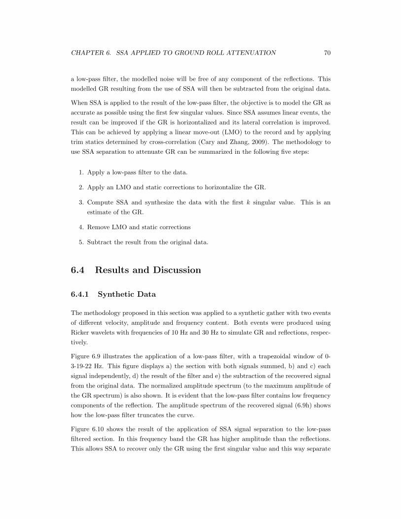
CHAPTER 6. SSA APPLIED TO GROUND ROLL ATTENUATION 70
a low-pass filter, the modelled noise will be free of any component of the reflections. This
modelled GR resulting from the use of SSA will then be subtracted from the original data.
When SSA is applied to the result of the low-pass filter, the objective is to model the GR as
accurate as possible using the first few singular values. Since SSA assumes linear events, the
result can be improved if the GR is horizontalized and its lateral correlation is improved.
This can be achieved by applying a linear move-out (LMO) to the record and by applying
trim statics determined by cross-correlation (Cary and Zhang, 2009). The methodology to
use SSA separation to attenuate GR can be summarized in the following five steps:
1. Apply a low-pass filter to the data.
2. Apply an LMO and static corrections to horizontalize the GR.
3. Compute SSA and synthesize the data with the first k singular value. This is an
estimate of the GR.
4. Remove LMO and static corrections
5. Subtract the result from the original data.
6.4 Results and Discussion
6.4.1 Synthetic Data
The methodology proposed in this section was applied to a synthetic gather with two events
of different velocity, amplitude and frequency content. Both events were produced using
Ricker wavelets with frequencies of 10 Hz and 30 Hz to simulate GR and reflections, respec-
tively.
Figure 6.9 illustrates the application of a low-pass filter, with a trapezoidal window of 0-
3-19-22 Hz. This figure displays a) the section with both signals summed, b) and c) each
signal independently, d) the result of the filter and e) the subtraction of the recovered signal
from the original data. The normalized amplitude spectrum (to the maximum amplitude of
the GR spectrum) is also shown. It is evident that the low-pass filter contains low frequency
components of the reflection. The amplitude spectrum of the recovered signal (6.9h) shows
how the low-pass filter truncates the curve.
Figure 6.10 shows the result of the application of SSA signal separation to the low-pass
filtered section. In this frequency band the GR has higher amplitude than the reflections.
This allows SSA to recover only the GR using the first singular value and this way separate
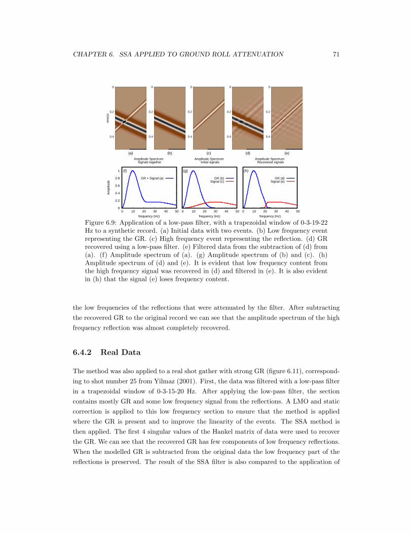
CHAPTER 6. SSA APPLIED TO GROUND ROLL ATTENUATION 71
0
0.2
0.4
time(
s)
(a)
0
0.2
0.4
(b)
0
0.2
0.4
(c)
0
0.2
0.4
(d)
0
0.2
0.4
(e)
0
0.2
0.4
0.6
0.8
1
0 10 20 30 40 50
Am
plitu
de
frequency (Hz)
Amplitude Spectrum Signals together
(f)
GR + Signal (a)
0 10 20 30 40 50
frequency (Hz)
Amplitude Spectrum Initial signals
(g)
GR (b)Signal (c)
0 10 20 30 40 50
frequency (Hz)
Amplitude Spectrum Recovered signals
(h)
GR (d)Signal (e)
Figure 6.9: Application of a low-pass filter, with a trapezoidal window of 0-3-19-22Hz to a synthetic record. (a) Initial data with two events. (b) Low frequency eventrepresenting the GR. (c) High frequency event representing the reflection. (d) GRrecovered using a low-pass filter. (e) Filtered data from the subtraction of (d) from(a). (f) Amplitude spectrum of (a). (g) Amplitude spectrum of (b) and (c). (h)Amplitude spectrum of (d) and (e). It is evident that low frequency content fromthe high frequency signal was recovered in (d) and filtered in (e). It is also evidentin (h) that the signal (e) loses frequency content.
the low frequencies of the reflections that were attenuated by the filter. After subtracting
the recovered GR to the original record we can see that the amplitude spectrum of the high
frequency reflection was almost completely recovered.
6.4.2 Real Data
The method was also applied to a real shot gather with strong GR (figure 6.11), correspond-
ing to shot number 25 from Yilmaz (2001). First, the data was filtered with a low-pass filter
in a trapezoidal window of 0-3-15-20 Hz. After applying the low-pass filter, the section
contains mostly GR and some low frequency signal from the reflections. A LMO and static
correction is applied to this low frequency section to ensure that the method is applied
where the GR is present and to improve the linearity of the events. The SSA method is
then applied. The first 4 singular values of the Hankel matrix of data were used to recover
the GR. We can see that the recovered GR has few components of low frequency reflections.
When the modelled GR is subtracted from the original data the low frequency part of the
reflections is preserved. The result of the SSA filter is also compared to the application of
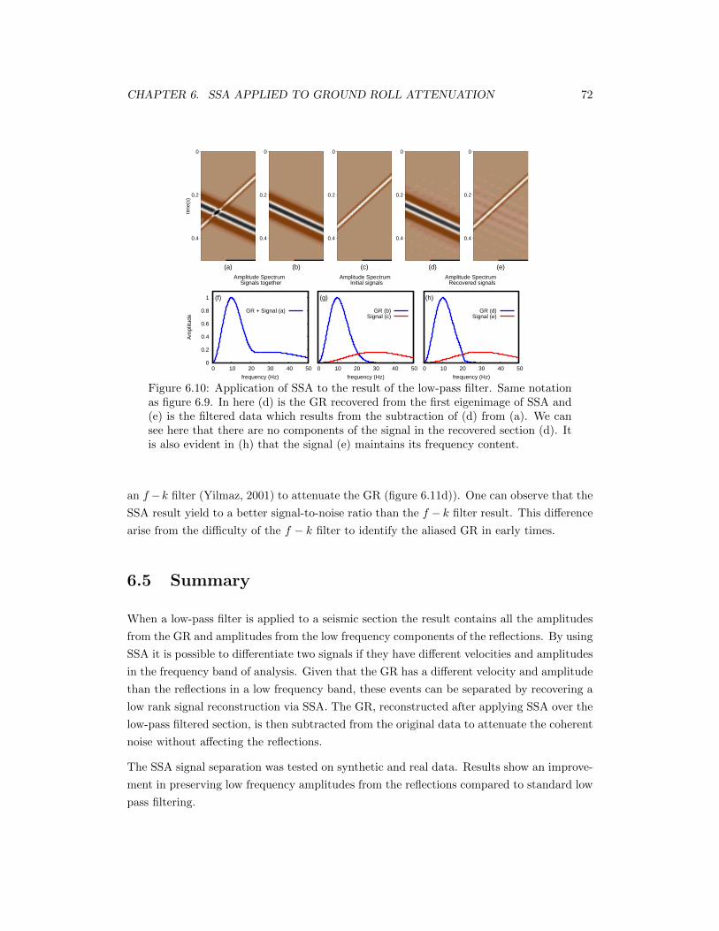
CHAPTER 6. SSA APPLIED TO GROUND ROLL ATTENUATION 72
0
0.2
0.4
time(
s)
(a)
0
0.2
0.4
(b)
0
0.2
0.4
(c)
0
0.2
0.4
(d)
0
0.2
0.4
(e)
0
0.2
0.4
0.6
0.8
1
0 10 20 30 40 50
Am
plitu
de
frequency (Hz)
Amplitude Spectrum Signals together
(f)
GR + Signal (a)
0 10 20 30 40 50
frequency (Hz)
Amplitude Spectrum Initial signals
(g)
GR (b)Signal (c)
0 10 20 30 40 50
frequency (Hz)
Amplitude Spectrum Recovered signals
(h)
GR (d)Signal (e)
Figure 6.10: Application of SSA to the result of the low-pass filter. Same notationas figure 6.9. In here (d) is the GR recovered from the first eigenimage of SSA and(e) is the filtered data which results from the subtraction of (d) from (a). We cansee here that there are no components of the signal in the recovered section (d). Itis also evident in (h) that the signal (e) maintains its frequency content.
an f −k filter (Yilmaz, 2001) to attenuate the GR (figure 6.11d)). One can observe that the
SSA result yield to a better signal-to-noise ratio than the f − k filter result. This difference
arise from the difficulty of the f − k filter to identify the aliased GR in early times.
6.5 Summary
When a low-pass filter is applied to a seismic section the result contains all the amplitudes
from the GR and amplitudes from the low frequency components of the reflections. By using
SSA it is possible to differentiate two signals if they have different velocities and amplitudes
in the frequency band of analysis. Given that the GR has a different velocity and amplitude
than the reflections in a low frequency band, these events can be separated by recovering a
low rank signal reconstruction via SSA. The GR, reconstructed after applying SSA over the
low-pass filtered section, is then subtracted from the original data to attenuate the coherent
noise without affecting the reflections.
The SSA signal separation was tested on synthetic and real data. Results show an improve-
ment in preserving low frequency amplitudes from the reflections compared to standard low
pass filtering.
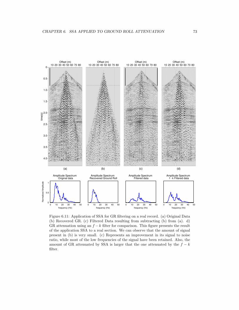
CHAPTER 6. SSA APPLIED TO GROUND ROLL ATTENUATION 73
0
0.5
1.0
1.5
2.0
2.5
3.0
3.5
4.0
tim
e(s
)
10 20 30 40 50 60 70 80Offset (m)
(a)
10 20 30 40 50 60 70 80Offset (m)
(b)
10 20 30 40 50 60 70 80Offset (m)
(c)
10 20 30 40 50 60 70 80Offset (m)
(d)
0
0.5
1
0 10 20 30 40 50
No
rma
lize
d A
mp
litu
de
frequency (Hz)
Amplitude Spectrum Original data
0 10 20 30 40 50
frequency (Hz)
Amplitude Spectrum Recovered Ground Roll
0 10 20 30 40 50
frequency (Hz)
Amplitude Spectrum Filtered data
0 10 20 30 40 50
frequency (Hz)
Amplitude Spectrum f - k Filtered data
Figure 6.11: Application of SSA for GR filtering on a real record. (a) Original Data(b) Recovered GR. (c) Filtered Data resulting from subtracting (b) from (a). d)GR attenuation using an f − k filter for comparison. This figure presents the resultof the application SSA to a real section. We can observe that the amount of signalpresent in (b) is very small. (c) Represents an improvement in its signal to noiseratio, while most of the low frequencies of the signal have been retained. Also, theamount of GR attenuated by SSA is larger that the one attenuated by the f − kfilter.
CHAPTER 7
Conclusions and Recommendations
The importance of attenuating different types of noise in seismic processing is of constant
interest in the field of geophysics. This thesis has studied the applications of a rank reduc-
tion technique called Singular Spectrum Analysis (SSA) for coherent and incoherent noise
attenuation. The main goal was to present an overview of this technique, studying its origins
and its further applications for seismic data processing, to finally evaluate the possibility of
using SSA as an alternative method in seismic noise attenuation. In addition, this thesis
has presented an acceleration method for computing the SSA and M-SSA filter based on the
randomized SVD. Another novel contribution is the iterative algorithm proposed for data
regularization/interpolation and the application of SSA to the coherent noise suppression
(ground roll elimination).
SSA has its origins in the field of time series analysis for the study dynamical systems. An
overview of these applications was shown in chapter 2. In this chapter, SSA was shown to
work in four steps:
1. Embedding of the input data. This step consisted of dividing the time series into a
series of lagged windows. These vectors were then organized to form a Hankel matrix.
2. Decomposition of the Hankel matrix into its singular spectrum using Singular Value
Decomposition (SVD).
3. Application of a rank reduction of the Hankel matrix. This was achieved by recovering
a subset of its singular values.
4. Retrieval of the resulting time series by averaging on the anti-diagonals of the rank
reduced Hankel matrix.
74
CHAPTER 7. CONCLUSIONS AND RECOMMENDATIONS 75
Although the intention of this chapter was to introduce the early stages of SSA, it can ulti-
mately be used as a reference by different science fields. Emphasis was placed on the use of
SSA for time series decomposition and noise attenuation. Despite the decomposition of time
series using SSA is an important field of study, the interpretation of the data components
depends on the objectives of the study. For this reason, this decomposition was only de-
scribed, without examining its meaning. Despite this, the examples and references provided
can indeed orient an interested reader to the application of SSA for the decomposition of
time series. Noise attenuation using SSA was also reviewed and an example was presented,
demonstrating its function. In fact, the noise attenuation property of SSA was the main
topic of interest in this thesis and was then applied for seismic data processing.
Chapters 3, 4, 5 studied different applications of SSA related to noise suppression and signal
reconstruction in seismic processing. In chapter 3 the application of SSA for random noise
attenuation was introduced. This technique was applied in the f − x domain and took
advantage of the same signal predictability as f − x deconvolution. The application of SSA
in this case was similar to the one applied in the analysis of time series, but it required
two extra steps to transform the method to the f − x domain and then back into the t− xdomain. The basic steps for the application of SSA for random noise attenuation on 2-D
seismic records were summarized as follows:
1. Application of a Fourier transform to each channel. This converted the data from the
t− x domain to the f − x domain.
2. Given that the reflections could be predicted in each frequency, the process of em-
bedding was applied for each frequency unit. This process was analogous to SSA in
time series analysis, but in this case the data consisted of each frequency depending
on space. For each frequency one Hankel matrix was built.
3. The Hankel matrix obtained from the embedding of each frequency was decomposed
using SVD.
4. The rank of the Hankel matrix was reduced by recovering only a subset of the singular
values.
5. The data were recovered by applying an averaging on the anti-diagonals of each Hankel
matrix.
6. After all the frequencies went through the rank reduction process; they were converted
back to the t− x domain, where the filtered image was obtained.
In general, rank reduction methods present the problem of selecting the appropriate final
rank that would lead to satisfactory results. Chapter 3 showed that the selection of the
CHAPTER 7. CONCLUSIONS AND RECOMMENDATIONS 76
final rank for the Hankel matrix, in each frequency, depended on the amount of events
with different apparent velocities and amplitudes. This represents a significant advantage
of SSA over other rank reduction methods. The use of SSA for random noise attenuation
was tested on 2-D synthetic and real seismic data. Furthermore, pre-stack and post-stack
data was included. These examples compared the results of SSA with the results of f − xdeconvolution. The first example applied SSA and f−x deconvolution on a synthetic gather
with linear events and no random noise. Results from this example showed that no signal is
affected under these conditions. In addition , chapter 3 presented two examples that applied
SSA and f − x deconvolution to synthetic data contaminated by random noise, in addition
to, linear and hyperbolic events respectively. Giving that SSA assumes linear events in
the data, the example presenting hyperbolic events had to be applied using overlapping
windows. Although none of these examples showed a significant difference in the amount of
noise attenuated by either of the methods, it was observed that f −x deconvolution filtered
also part of the signal while SSA was successful in preserving it untouched.
An advantage of SSA over other noise attenuation methods is that it can be easily expanded
to allow for the use of information from several dimensions of a seismic record. This expan-
sion is called Multichannel Singular Spectrum Analysis (MSSA). MSSA was described in
chapter 3, and subjected to further research in chapters 4 and 5. The extension of SSA into
MSSA is carried out by building a Hankel matrix of each column vector in one dimension.
Next, these Hankel matrices were organized as a block Hankel matrix. In other words, SSA
was expanded by building a Hankel matrix of Hankel matrices in the embedding step. If
the initial data had two spatial dimensions plus time, the technique was considered to be
a 2-D MSSA. If the initial data had more than three spatial dimensions plus time, it was
considered an N-D MSSA. Chapter 3 expanded on the application of 2-D MSSA, which
was tested with a synthetic example. The theory behind N-D MSSA was also treated in
chapter 3, but its practical applications and examples were beyond the objective of this
work. The synthetic example showed in chapter 3 demonstrating random noise attenuation
using MSSA showed a significant improvement over SSA and f − x deconvolution. The
amount of noise filtered by MSSA was larger than the other two methods, while the signal
remained untouched. The simplicity of this expansion to multiple dimensions and the great
improvement produced by it for noise attenuation makes MSSA an important alternative
for the attenuation of random noise in seismic records.
MSSA presented a disadvantage compared to other methods of noise attenuation, like f −xdeconvolution, which was the large amount of computations required for its applications.
This occurred because the block Hankel matrix built in the embedding step increased its
size significantly when very few channels were added to the initial data. Given that the
SVD was very slow while decomposing large matrices, the rank reduction of a block Hankel
matrix took a significant time to run. A solution to this problem was showed in chapter
CHAPTER 7. CONCLUSIONS AND RECOMMENDATIONS 77
4 by proposing the application of a randomized algorithm to perform the rank reduction
step. This algorithm was proposed by Rokhlin et al. (2009) and consisted of reducing the
size of the matrix by means of a randomization process and then of applying two SVD op-
erations. Given that the two SVD operations were applied to smaller matrices the amount
of computations decreased significantly. This new algorithm for MSSA using randomized
SVD (R-SVD) was tested in several 3-D synthetic records with different sizes and contam-
inated with random noise. The results showed that the use of R-SVD in MSSA improved
its running time by 50%. It was also seen that the outcome of the randomized algorithm
lead to results that correctly approximated those obtained by utilizing the traditional SVD
algorithm. With this reduction in its running time, MSSA becomes a more useful tool in
seismic data processing.
The main challenge of testing MSSA for random noise attenuation in real 3-D seismic records
was that it required the data to be regularly sampled in space. This rarely happens in pre-
stack data given that economical and logistical constrains require the displacement of sources
and receivers. If the data was organized into a regular grid, some cells did not contain traces.
When MSSA was applied over a regularly sampled record, which presented missing traces,
it was seen that it could recover part of the amplitudes of the lost signal. Therefore, chapter
5 studied the use of MSSA for the interpolation of missing traces in seismic records. Given
that MSSA only recovered a portion of the missing amplitudes when it was applied once,
an iterative algorithm was proposed. The latter worked by extracting the recovered traces
from one iteration of MSSA and then placing them into the input data of the next iteration.
The interpolation using MSSA was tested in a synthetic cube with random missing traces
and no added noise, resulting in a very accurate recovery of the missing traces. A second
example showed the same synthetic data, but this time contaminated with random noise.
The technique was successful to recover the missing traces and to reduce the amount of
random noise. Finally, MSSA was applied to a set of 15 CDP gathers whose offsets where
irregularly spread. This offsets where regularized into a desired grid, leaving some missing
traces. The interpolation using MSSA recovered successfully the missing traces of each CDP.
It also attenuated random noise present in the record. In addition, MSSA was applied using
the SVD and R-SVD algorithms, providing new evidence of the improvement in running
time given by the randomized method.
Chapter 6 introduced a different approach for SSA application. The goal was to attenuate
ground roll by separating it from the reflections. For this, a property of SSA that allowed,
under certain conditions, to represent different events by recovering individual singular
values was studied. This separation was shown to be only possible when the apparent
velocity and the amplitudes of the events where different. The separation of ground roll
from signal was carried on in a low frequency band, given that in this interval the ground
roll presents larger amplitudes than the reflections. The method was tested in a synthetic
CHAPTER 7. CONCLUSIONS AND RECOMMENDATIONS 78
example, showing that two signals with different frequency content can be separated. It was
then applied to a real shot gather, proving to be successful in attenuating the ground roll
without affecting the reflections in a significant way. This results shows that SSA can be a
very flexible method that can be used for different applications in seismic data processing.
This thesis provided a complete summary of the applications of SSA and MSSA for noise
attenuation and data interpolation of seismic records. SSA was shown to be a valid alterna-
tive over the use of f − x deconvolution for random noise attenuation. Also, the simplicity
of the expansion of SSA into MSSA made the method easy to apply in several dimensions,
improving the quality of the results. Problems of large computational times where solved by
applying an R-SVD algorithm, which made possible the use of MSSA on larger sets of data.
Furthermore, it was shown that applying MSSA in real data made possible the attenuation
of random noise, together with the recovery of missing traces. Finally, SSA was applied to
attenuate ground roll in seismic shot gather. After analyzing all the applications of SSA
for seismic data processing, it is possible to conclude that this method has the potential
to become a tool of common use in traditional processing sequences, presenting a good
alternative to conventional methods of noise attenuation.
In this thesis I have presented the following:
• A review of the application of SSA for time series analysis, that is helpful to understand
SSA and as a reference for future work.
• The connection of Cadzow method with SSA and the relationship between both tech-
niques. The latter is useful to understand the background of both techniques and their
equivalency.
• The predictability of the signal in the f − x domain and why the Hankel matrix is
rank k in the presence of k events. This helps to understand why SSA is successful in
attenuating noise, as well as its advantages and disadvantages.
• The application of a randomized algorithm for rank reduction, which decreases the
computational time of SSA.
• The application of a method similar to Projection onto convex sets (POCS) that
applies SSA iteratively to recover missing traces in seismic records.
• The use of SSA as a technique to separate individual events, which can be applied for
ground roll attenuation.
CHAPTER 7. CONCLUSIONS AND RECOMMENDATIONS 79
7.1 Future Work
Although this thesis introduced most of the applications of SSA to seismic data processing,
some of them can be expanded and improved. For instance, the decomposition of time
series using SSA can help to understand the processes that influenced the data. Paleocli-
matic records, for example, can be analyzed using this technique (Vautard and Ghil, 1989).
Chapter 2 can be used as a starting point for someone interested in applying SSA for the
analysis of time series.
It is reasonable to think that if MSSA is extended to more than two dimensions the results
would improve. Given that this expansion to N-D MSSA was not tested in this thesis, it can
be an interesting topic of further research. This includes its application for random noise
attenuation and seismic data interpolation.
Finally, it is evident that the Hankel matrix and the block Hankel matrix present very
obvious symmetries. These symmetries can be used to design a rank reduction algorithm
that does not need to go over all the elements of the matrix. Such algorithm would require
a smaller amount of computations than the traditional SVD algorithm or R-SVD. This
would ultimately make MSSA significantly faster to apply, allowing it to work on very large
records.
Bibliography
Abma, R. and J. Claerbout. “Lateral prediction for noise attenuation by tlx and f − x
techniques.” Geophysics 60 (1995): 1887–1896.
Abma, R. and N. Kabir. “Seismic trace interpolation using half-space prediction filters.”
Geophysics 71 (2006): 91–97.
Al-Bannagi, M.S., K. Fang, P.G. Kelamis, and G.S. Douglass. “Acquisition footprint sup-
pression via the truncated SVD technique: Case studies from Saudi Arabia.” The Leading
Edge 24 (2005): 832–834.
Al-Yahya, K. “Application of the partial Karhunen-Loeve transform to suppress random
noise in seismic sections.” Geophysical Prospecting 39 (1991): 77–93.
Allen, M.R. and L.A. Smith. “Optimal filtering in singular spectrum analysis.” Physics
Letters 234 (1997): 419–428.
Anderson, E., Z. Bai, C. Bischof, S. Blackford, J. Demmel, J. Dongarra, J. Du Croz,
A. Greenbaum, S. Hammarling, A. McKenney, and D. Sorensen. LAPACK User’s Guide.
http://www.netlib.org/lapack/lug/lapack lug.html, August 1999.
Auvergne, M. “Singular value analysis applied to phase space reconstruction of pulsating
stars.” Astronomy and Astrophysics 204 (1988): 341–348.
Aydin, S., H.M. Saraoglu, and S. Kara. “Singular Spectrum Analysis of Sleep EEG in
Insomnia.” Journal of Medical Systems (September 2009).
Broomhead, D.S. and G.P. King. “Extracting Qualitative Dynamics from Experimental
Data.” Physica D 20 (1986): 217–236.
Cadzow, J.A. “Signal Enhancement - A Composite Property Mapping Algorithm.” IEEE
Trans. on Acoustics, Speech and Signal Processing 36 (1988): 49–62.
Canales, L.L. “Random Noise Reduction.” SEG Expanded Abstracts 3 (1984): 525–527.
80
BIBLIOGRAPHY 81
Cary, P.W. and C. Zhang. “Ground roll attenuation with adaptive eigenimage filtering.”
SEG Expanded Abstracts 28 (2009): 3302–3306.
Chiu, S.K. and J.E. Howell. “Attenuation of coherent noise using localized-adaptive eigen-
image filter.” SEG Expanded Abstracts 27 (2008): 2541–2545.
Coruh, C. and J.K. Constain. “Noise attenuation by Vibroseis whitening (VSW) processing.”
Geophysics 48 (1983): 543–554.
Danilov, D.L. “Principal Components in Time Series Forecast.” Journal of Computational
and Graphical Statistics 6 (1997): 112–121.
Drinea, E., P. Drineas, and P. Huggins. “A randomized Singular Value Decomposition
algorithm for image processing applications.” Panhellenic Conference on Informatics
(PCI). 2001, 279.
Duncan, G. and G. Beresford. “Slowness adaptive f − k filtering of prestack seismic data.”
Geophysics 59 (1994): 140–147.
Eckart, C. and G. Young. “The approximation of one matrix by another of lower rank.”
Psychometrika 1 (1936): 211–218.
Elsner, J.B. and A.A. Tsonis. Singular Spectrum Analysis: A New Tool in Time Series
Analysis. Plenum Press, New York, 1996.
Fraedrich, K. “Estimating the Dimensions of Weather and Climate Attractors.” Journal of
the Atmospheric Sciences 43 (1986): 419–432.
Freire, S.L.M. and T.J. Ulrych. “Application of Singular Value Decomposition to vertical
seismic profiling.” Geophysics 53 (1988): 778–785.
Gerbrands, J.J. “On the relationships between SVD, KLT and PCA.” Pattern recognition
14 (1981): 375–381.
Ghil, M., M.R. Allen, M.D. Dettinger, K. Ide, D. Kondrashov, M.E. Mann, A.W. Robertson,
A. Saunders, Y. Tian, F. Varadi, and P. Yiou. “Advance Spectral Methods for Climatic
time series.” Reviews of Geophysics 40 (2002): 1–41.
Golub, G. “Numerical Methods for Solving Linear Least Squares Problems.” Numerische
Mathematik 7 (1965): 206–216.
Golub, G. and C.F. Van Loan. Matrix Computations. Third edition. The Jhans Hopkins
University Press, 1996.
Golyandina, N., V. Nekrutkin, and A. Zhigljavsky. Analysis of time series structure: SSA
and related techniques. Chapman & Hall/CRC, Boca Raton, Fla, 2001.
BIBLIOGRAPHY 82
Golyandina, N. E. and D. Stepanov. “SSA-based approaches to analysis and forecast of mul-
tidimensional time series.” Proceedings of the 5th St Petersburg Workshop on Simulation.
2005.
Golyandina, N.E., K.D. Usevich, and I.V. Florinsky. “Filtering of Digital Terrain Models
by Two-Dimesional Singular Spectrum Analysis.” International Journal of Ecology &
Development 8 (2007): 81–94.
Gu, M. and S.C. Eisenstat. “Efficient algorithms for computing a strong rank-revealing QR
factorization.” SIAM J. ScI. COMPUT 17 (1996): 848–869.
Gulunay, N. “FXDECON and complex Weiener prediction filter.” SEG Expanded Abstracts
5 (1986): 279–281.
Gulunay, N. “Noncausal spatial prediction filtering for random noise reduction on 3-D
poststack data.” Geophysics 65 (2000): 1641–1653.
Halko, N., P.G. Martinson, and J.A. Tropp. “Finding structure with randomness: Stochastic
algorithms for constructing approximate matrix decompositions.” ACM Report 2009-05
(September 2009).
Hansen, C. and S.H. Jensen. “Filter Model of Reduced-Rank Noise Reduction.” Lecture
Notes In Computer Science, Proceedings of the Third International Workshop on Applied
Parallel Computing, Industrial Computation and Optimization. Springer-Verlag, 1987,
379–387.
Harris, P.E. and R.E. White. “Improving the performance of f − x prediction filtering at
low signal-to-noise ratios.” Geophysical Prospecting 45 (1997): 269–302.
Hassani, H., A.S. Soofi, and A.A. Zhigljavsky. “Predicting daily exchange rate with singular
spectrum analysis.” Nonlinear Analysis: Real World Applications 11 (2010): 2023 – 2034.
Herrmann, F.J. and G. Hennenfent. “Non-parametric seismic data recovery with curvelet
frames.” Geophysical Journal International 173 (2008): 233–248.
Hsieh, W.W. and A. Wu. “Nonlinear multichannel singular spectrum analysis of the tropical
Pacific climate variability using a neural network approach.” Journal of Geophysical
Research 107 (2002).
Hua, Y. “Estimating two-dimensional frequencies by matrix enhancement and matrix pen-
cil.” IEEE Transactions on Signal Processing 40 (1992): 2267–2280.
Jones, I.F. and S. Levy. “Signal to noise ratio enhancement in multichannel seismic data
via the Karhunen-Loeve transform.” Geophysical Prospecting 35 (1987): 12–32.
BIBLIOGRAPHY 83
Karsli, H. and Y. Bayrak. “Using the Wiener-Levinson algorithm to suppress ground-roll.”
Journal of Applied Geophysics 55 (2004): 187–197.
Knapp, R.W. “Geophone differencing to attenuate horizontally propagating noise.” Geo-
physics 51 (1986): 1753–1759.
Kolda, T.G. and B.W. Bader. “Tensor Decompositions and Applications.” SIAM Rev. 51
(2009): 455–500.
Liberty, E., F. Woolfe, P. Martinsson, V. Rokhlin, and M. Tygerts. “Randomized algorithms
for the low-rank approximation of matrices.” PNAS 104 (2007): 20167–20172.
Liu, B. and M.D. Sacchi. “Minimum weighted norm interpolation of seismic records.”
Geophysics 69 (2004): 1560–1568.
Loskutov, A.Y., I.A. Istomin, O.L. Kotlyarov, and K.M. Kuzanyan. “A study of the regu-
larities in solar magnetic activity by singular spectral analysis.” Astronomy Letters 27
(2001): 745–753.
Manning, C.D., P. Raghavan, and H. Schutze. An introduction to information retrieval.
Cambridge University Press, 2009.
March, D.W. and A.D. Bailey. “A review of the two-dimensional transform and its use in
seismic processing.” First Break 1 (1983): 9–21.
Marchisio, G.B., J.V. Pendrel, and B.W. Mattocks. “Applications of full and partial
Karhunene-Loeve transformation to Geophysical Image Enhancement.” 58th Ann. In-
tertat. Mtg., Soc. Expl. Geophys., Expanded Abstracts. 1988, 1266–1269.
Mari, J.L. and F. Glangeaud. “Spectral matrix filtering applied to VSP processing.” Revue
de LInstitut Francais du Petrole 45 (1990): 417–433.
Martinsson, P.G., V.Rokhlin, and M. Tygert. A randomized algorithm for the approximation
of matrices. Technical Report 1316, Computer Science Department, Yale University, New
Haven, CT, 2006.
McKay, A.E. “Review of pattern shooting.” Geophysics 19 (1954): 420–437.
Mees, A.I., P.E. Rapp, and L.S. Jennings. “Singular Value Decomposition and embedding
dimension.” Physical Reveiew A 36 (1987): 340–346.
Mineva, A. and D. Popivanov. “Method for single-trial readiness potential identification,
based on singular spectrum analysis.” Journal of Neuroscience Methods 68 (1996): 91–99.
Naghizadeh, M. and M.D. Sacchi. “Robust reconstruction of aliased data using autoregres-
sive spectral estimates.” Geophysical Prospecting (2010): 1365–2478.
BIBLIOGRAPHY 84
Nekrutkin, V. “Theoretical properties of the ”Caterpillar” method of time series analysis.”
Signal Processing Workshop on Statistical Signal and Array Processing, IEEE 0 (1996):
395.
Palus, M. and I. Dvorak. “Singular-value decomposition in attractor reconstruction: pitfalls
and precautions.” Physica D 55 (1987): 221–234.
Papadimitriou, C.H., H. Tamaki, P. Raghavan, and S. Vempala. “Latent semantic indexing:
a probabilistic analysis.” PODS ’98: Proceedings of the seventeenth ACM SIGACT-
SIGMOD-SIGART symposium on Principles of database systems. New York, NY, USA:
ACM, 1998, 159–168.
Plaut, G. and R. Vautard. “Spells of Low-Frequency oscillations and weather regimes in
the northern hemisphere.” Journal of the atmospheric sciences 51 (1994): 210–236.
Polukoshko, S. and J. Hofmanis. “Use of CATERPILLAR - SSA method for analysis and
forecasting of industrial and economic indicators.” Proceedings of the 7th International
Scientific and Practical Conference. 2009, 241–248.
Porsani, M.J. “Seismic trace interpolation using half-space prediction filters.” Geophysics
64 (1999): 1461–1467.
Rayleigh, L. “On waves propagated along the plane surfaces of an elastic solid.” Proc.
London Math. Soc 17 (1885): 4–11.
Read, P.L. “Applications of singular systems analysis to ’Baroclinic chaos’.” Physica D 58
(1992): 455–468.
Read, P.L. “Phase portrait reconstruction using multivariate singular systems analysis.”
Physica D 69 (1993): 353–365.
Rokhlin, V., A. Szlam, and M. Tygert. “A randomized algorithm for principal component
analysis.” SIAM J. Matrix Anal. Appl. 31 (2009): 1100–1124.
Rudelson, M. and R. Vershynin. “Sampling from large matrices: An approach through
geometric functional analysis.” J. ACM 54 (2007): 21.
Sacchi, M.D. “FX Singular Spectrum Analysis.” CSPG CSEG CWLS Convention (2009):
392–395.
Sacchi, M.D. and H. Kuehl. “ARMA Formulation of FX Prediction Error Filters and
Projection Filters.” Journal of Seismic Exploration 9 (2001): 185–197.
Sarlos, T. “Improved Approximation Algorithms for Large Matrices via Random Projec-
tions.” FOCS ’06: Proceedings of the 47th Annual IEEE Symposium on Foundations of
Computer Science. Washington, DC, USA: IEEE Computer Society, 2006, 143–152.
BIBLIOGRAPHY 85
Spitz, S. “Seismic trace interpolation in the F-X domain.” Geophysics 56 (1991): 785–794.
Takens, F. “Detecting strange attractors in turbulence.” Lecture Notes in Mathematics 898
(1981): 366–381.
Trad, D. “Five-dimensional interpolation: Recovering from acquisition constraints.” Geo-
physics 74 (2009): V123–V132.
Trad, D.O., T.J. Ulrych, and M.D. Sacchi. “Accurate interpolation with high-resolution
time-variant Radon transforms.” Geophysics 67 (2002): 644–656.
Trickett, S. “F-x eigen noise suppression.” CSEG National Conv., Expanded Abstracts.
2002.
Trickett, S. “F-xy cadzow noise suppression.” CSPG CSEG CWLS Convention (2008):
303–306.
Trickett, S. and L. Burroughs. “Prestack Rank-Reduction-Based Noise Suppresion.”
Recorder 34 (2009): 3193–3196.
Trickett, S.R. “F-xy eigenimage noise suppression.” Geophysics 68 (2003): 751–759.
Ulrych, T.J. and M. Sacchi. Information-based inversion and processing with applications.
Elsevier, 2005.
Ulrych, T.J., M.D. Sacchi, and S.L.M. Freire. “Eigenimages processing of seismic sections..”
Covariance Analysis for Seismic Signal Processing. Ed. R.L. Kirlin and W.J. Done. So-
ciety of Exploration Geophysicists, 1999. chapter 12.
Varadi, F., J.M. Pap, R.K. Ulrich, L. Bertello, and C.J.Henney. “Searching for signal in
noise by random-lag Singular Spectrum Analysis.” The Astrophysical Journal 526 (1999):
1052–1061.
Vautard, R. and M. Ghil. “Singular Spectrum Analysis in non linear dynamics, with appli-
cations to paleoclimatic time series.” Physica D 35 (1989): 395–424.
Vautard, R., P. Yiou, and M. Ghil. “Singular-spectrum analysis: A toolkit for short, noisy
chaotic signals.” Physica D 58 (1992): 95–126.
Wilson, P.R. Solar and stellar activity cycles. Cambridge University Press, 1994.
Woolfe, F., E. Liberty, V. Rokhlin, and M. Tygert. “A fast randomized algorithm for the
approximation of matrices.” Applied and Computational Harmonic Analysis 25 (2008):
335 – 366.
BIBLIOGRAPHY 86
Yang, H.H. and Y. Hua. “On rank of block Hankel matrix for 2-D frequency detection and
estimation.” IEEE Transactions on Signal Processing 44 (1996): 1046–1048.
Yilmaz, O. Seismic data analysis. Volume 1 . Society of Exploration Geophysicists, Tulsa,
Oklahoma, 2001.
Yiou, P., E. Baert, and M.F. Loutre. “Spectral analysis of climate data.” Surveys in
Geophysics 17 (1996): 619–663.
Youla, D.C. and H. Webb. “Image Restoration by the Method of Convex Projections: Part
1 Theory.” IEEE Transactions on Medical Imaging 1 (Oct 1982): 81–94.
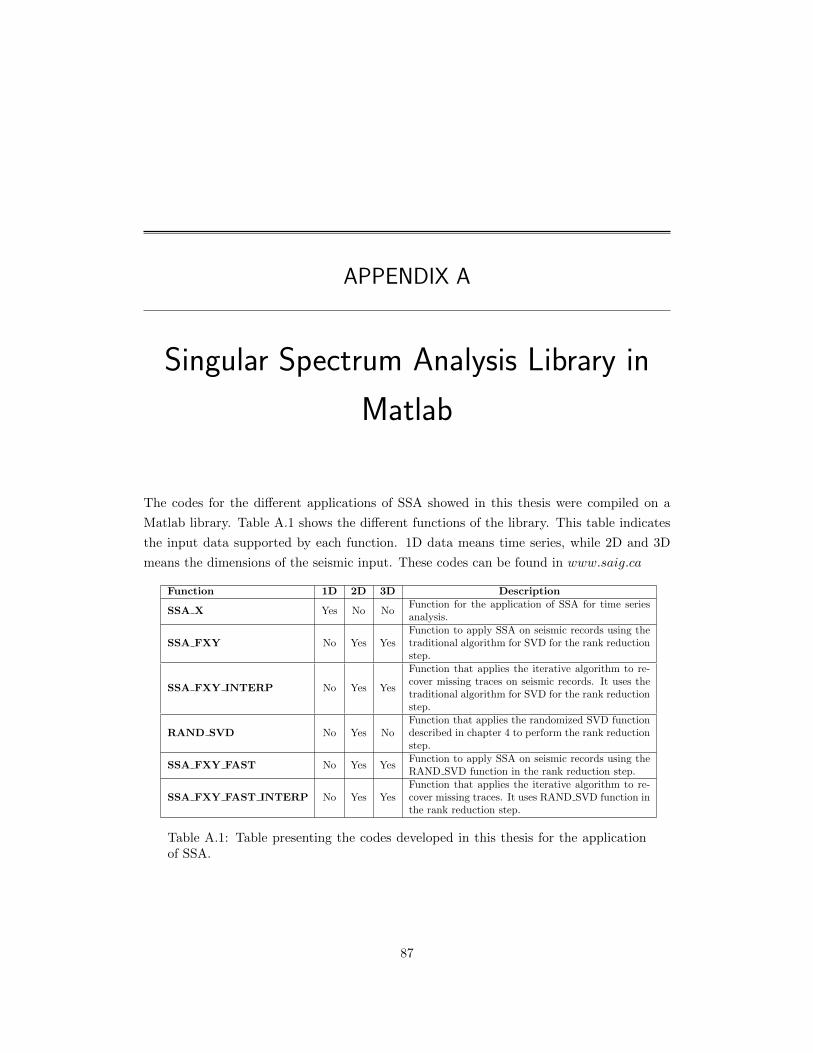
APPENDIX A
Singular Spectrum Analysis Library in
Matlab
The codes for the different applications of SSA showed in this thesis were compiled on a
Matlab library. Table A.1 shows the different functions of the library. This table indicates
the input data supported by each function. 1D data means time series, while 2D and 3D
means the dimensions of the seismic input. These codes can be found in www.saig.ca
Function 1D 2D 3D Description
SSA X Yes No NoFunction for the application of SSA for time seriesanalysis.
SSA FXY No Yes YesFunction to apply SSA on seismic records using thetraditional algorithm for SVD for the rank reductionstep.
SSA FXY INTERP No Yes Yes
Function that applies the iterative algorithm to re-cover missing traces on seismic records. It uses thetraditional algorithm for SVD for the rank reductionstep.
RAND SVD No Yes NoFunction that applies the randomized SVD functiondescribed in chapter 4 to perform the rank reductionstep.
SSA FXY FAST No Yes YesFunction to apply SSA on seismic records using theRAND SVD function in the rank reduction step.
SSA FXY FAST INTERP No Yes YesFunction that applies the iterative algorithm to re-cover missing traces. It uses RAND SVD function inthe rank reduction step.
Table A.1: Table presenting the codes developed in this thesis for the applicationof SSA.
87