THE EFFICIENCY OF THE OIL FUTURES MARKETS:INFORMATION, PRICE DISCOVERY AND LONG MEMORY

SAADA ABBA ABDULLAHI

A Thesis Submitted to the University of Abertay Dundee for the award of

the Degree of Doctor of Philosophy

UNIVERSITY

Dundee Business School

September

2012

THE EFFICIENCY OF THE OIL FUTURES MARKETS:INFORMATION, PRICE DISCOVERY AND LONG MEMORY

SAADA ABBA ABDULLAHI

A Thesis Submitted to the University of Abertay Dundee for the

award of the Degree of Doctor of Philosophy

Dundee Business School

University of Abertay Dundee

September

Dedication

To my son Mohammed Hassan Hassan

1

Acknowledgement

First, I would like to thank Almighty God, for providing me with different

opportunities and progress throughout my life. My great gratitude also goes to

my supervisors Prof. Reza Kouhy, Prof. Heather Tarbert and Dr. Zahid

Mohammad for their support, guidance and constructive comments in the process

of writing this thesis. I also want to express my appreciation to Dr. Kazem

Falahati (External examiner) and Prof. Mohamed Branine (Internal examiner) for

their contributions and comments.

My deepest thanks go to my parents for their love, care and support which make

me what I am today. I am grateful to my husband Hassan for his patience and

contributions, and my son Mohammed for using his time to study. Many thanks

go to my brothers (Dr. Nuraddeen, Hassan, Nasiru and Shamsuddeen) and sisters

(Fatima, Sadiya, Husna and Faiza) for their unconditional support,

encouragement and always being there for me.

I want to thank the Petroleum Technology Development Fund (PTDF) Nigeria

for funding this research. I am grateful to the efforts of AGM Galadima (PTDF),

Kabash Katsina, Dr. Labaran Lawal and Ibrahim Adam. Many thanks go to

Svetlana Maslyuk and Russell Smyth for the data they provide me with. I also

like to acknowledge my employers, Kano University of Science and Technology

(KUST) Wudil who provide me with the fellowship to pursue this study. Finally,

I take the responsibility of any remaining errors and weakness in this thesis.

Saada Abba Abdullahi

11

Declaration

I, Saada A. Abdullahi hereby certify that this thesis has been written by me, that

it is the record of work carried out by me and that it has not been submitted in

any previous application for a higher degree.

Signature of candidate. Date 13-

Certiflcation

I certify that this thesis is the true and accurate version as approve by the examiners, and that all relevant ordinance and regulations have been fulfilled.

m

Abstract

This thesis investigates the efficiency of the crude oil futures markets by addressing four important issues using different theoretical and methodological perspectives. Data of different frequencies was employed in the analysis covering the period 2000 to 2011. First, the short and long term efficiency is examined by testing the unbiasedness of the oil futures price in predicting the expected spot price using the Johansen (1988) and the Engle-Granger (1987) cointegration tests, and the Error Correction Model (ECM). The results suggest that the oil futures markets are unbiased in the long term but not in the short term, and the inefficiency is not caused by the time-varying risk premium. The results also show that the oil futures market are unbiased in the multi-contract and multi-market framework but not in all maturities. Second, the price discovery relationship between the oil spot and futures markets and across contract is investigated by employing the Vector Error Correction Model (VECM), Gonzalo-Granger (1995) common factor weight approach and the Garbade-Silber (1983) short run dynamic model. Empirical results indicate that price discovery is initiated in the futures market because it impounds more information than the spot market. However, the results of the cross-contract analysis show that the three-month futures contract leads one-month contract in price discovery while the relationship changes in the short term. Third, the price change and trading volume relationship is examined in the oil futures markets using the generalized method of moments (GMM), Granger causality test, impulse response function and variance decomposition approaches. The findings reject the postulation of a positive relationship between price change and trading volume, suggesting that they are not driven by the same information. Additionally, the results suggest that trading volume cannot predict price changes in all the oil markets. Lastly, this thesis investigates long memory in the oil futures return using the GARCH models, and the results indicate that both the short and long memory models support predictability in returns which violates the weak form efficient hypothesis. In sum, the findings provide new evidence on the informational efficiency of the international oil futures markets, which have significant implications for hedgers, speculators, financial analysts and policymakers. The thesis recommends that market participants and regulators should look at various aspects of these markets for effective strategies and policy implementation.

IV

Table of Content

Dedication...............................................................................................................i

Acknowledgement................................................................................................. iiDeclaration............................................................................................................iii

Certification.......................................................................................................... iii

Abstract.................................................................................................................iv

List of Tables...................................................................................................... viii

List of Figures........................................................................................................x

List of Abbreviations.............................................................................................xiCHAPTER ONE: INTRODUCTION.................................................................... 1

CHAPTER TWO: BACKGROUND LITERATURE ON THE INTERNATIONAL OIL MARKET......................................................................7

2.1 Introduction..................................................................................................7

2.2 History of the Oil Industry...........................................................................9

2.3 Oil Production, Major Oil Companies and Producer Nations.................... 12

2.4 Oil Prices, OPEC and the Market.............................................................. 17

2.5 The International Oil Markets....................................................................25

2.6 Summary and Conclusion..........................................................................32

CHAPTER THREE: THE SHORT-TERM AND LONG-TERM EFFICIENCY OF THE OIL FUTURES MARKETS.................................................................33

3.1 Introduction................................................................................................33

3.2 Literature Review....................................................................................... 37

3.3 Theoretical Framework of Market Efficiency............................................57

3.4 Empirical Methodology.............................................................................63

3.4.1 Unit Root Test.....................................................................................64

3.4.2 Cointegration Test...............................................................................67

3.4.3 Error Correction Model Approach......................................................71

3.5 Data and its Properties...............................................................................72

3.6 Empirical Results.......................................................................................76

3.6.1 Unit Root Test.....................................................................................77

3.6.2 Test of Long-term Efficiency..............................................................80

3.6.3 Test of Short-Term Efficiency............................................................85

3.6.4 Test of Multi-contract Efficiency........................................................89

v

3.6.5 Test of Multi-market Efficiency 92

3.7 Summary and Conclusion........................................................................94

CHAPTER FOUR: PRICE DISCOVERY IN THE OIL FUTURES MARKETS .............................................................................................................................. 97

4.1 Introduction................................................................................................97

4.2 Literature Review..................................................................................... 101

4.3 Theoretical Framework of Price Discovery............................................. 117

4.4 Empirical Methodology........................................................................... 118

4.4.1 Vector Error Correction Approach................................................... 119

4.4.2 Gonzalo-Granger Common Factor Weights Approach.................... 120

4.4.3 Garbade-Silber Short Run Dynamic Approach............................... 122

4.5 Data and its Properties............................................................................. 124

4.6 Empirical Results..................................................................................... 1274.7 Summary and Conclusion........................................................................ 139

CHAPTER FIVE: PRICE CHANGE AND TRADING VOLUME RELATIONSHIP IN THE OIL FUTURES MARKETS.................................. 143

5.1 Introduction.............................................................................................. 143

5.2 Literature Review..................................................................................... 146

5.3 Theoretical Framework of Price-Volume Relationship........................... 162

5.4 Empirical Methodology........................................................................... 167

5.4.1 Generalized Method of Moments..................................................... 167

5.4.2 Linear Granger Causality Test.......................................................... 169

5.4.3 Impulse Response Function.............................................................. 170

5.4.4 Variance Decomposition Analysis.................................................... 171

5.5 Data and its Properties............................................................................. 172

5.6 Empirical Results..................................................................................... 174

5.7 Summary and Conclusion........................................................................ 185

CHAPTER SIX: LONG MEMORY IN OIL FUTURES MARKETS.............. 187

6.1 Introduction.............................................................................................. 187

6.2 Literature Review..................................................................................... 190

6.3 Theoretical Background of Long Memory Models.................................210

6.4 Empirical Methodology...........................................................................212

6.4.1 GARCH Model............................................................................... 212

vi

6.4.2 EGARCH Model 213

6.4.3 APARCH Model...............................................................................213

6.4.4 FIGARCH Model..............................................................................214

6.4.5 FffiGARCH Model...........................................................................215

6.4.6 FIAPARCH Model...........................................................................215

6.4.7 HYGARCH Model...........................................................................216

6.5 Data and its Properties.............................................................................216

6.6 Empirical Results.....................................................................................220

6.7 Summary and Conclusion........................................................................234CHAPTER SEVEN: SUMMARY AND CONCLUSION................................238

7.1 Summary of Results.................................................................................238

7.2 Reconsideration of the Research Objectives............................................239

7.3 Contributions and Policy Implications.....................................................242

7.4 Limitations of the thesis and Recommendations for Future Research....245BIBLIOGRAPHY..............................................................................................247

vii

List of Tables

Table 3.1 Summary of Previous Results on Market Efficiency in the Oil Futures Market........................................................................................................................... 46

Table 3.2 Summary of Previous Results on Market Efficiency in the Non-Oil Commodity Futures Markets........................................................................................ 54

Table 3.3 Descriptive Statistics for Crude Oil Prices.................................................. 73

Table 3.4 Unit Root Test............................................................................................... 78

Table 3.5 Engle and Granger Cointegration Test for Long term Efficiency................ 81

Table 3.6 Johansen Cointegration Test for Long term Efficiency................................ 82

Table 3.7 Johansen Cointegration Restriction Test for Long-term Efficiency............. 82

Table 3.8 Error Correction Model Test for Short-Term Efficiency with Constant Risk Premium................................................................................................................ 86

Table 3.9 Error Correction Model Test for Short-Term Efficiency with Time- varying Risk Premium.................................................................................................. 88

Table 3.10 Johansen Cointegration Test for Multi-contract Efficiency........................ 90

Table 3.11 Johansen Cointegration Restriction Test for Multi-contract Efficiency....91

Table 3.12 Johansen Cointegration Test for Multi-market Efficiency......................... 93

Table 3.13 Johansen Cointegration Restriction Test for Multi-market Efficiency...... 93

Table 4.1 Summary of Previous Results on Price Discovery in the Oil Future Markets.........................................................................................................................108

Table 4.2 Summary of Previous Results on Price Discovery in the Non-Oil Commodity Future Markets.........................................................................................115

Table 4.3 Descriptive Statistics for Crude Oil Prices..................................................125

Table 4.4 Unit Root Test..............................................................................................129

Table 4.5 Johansen Cointegration Test........................................................................131

Table 4.6 Estimated Results of the VECM Approach.................................................133

Table 4.7 Estimated Results of the Common Factor Weights.....................................135

Table 4.8 Estimated Results of the Garbade-Silber Approach....................................138

viii

Table 5.1 Summary of Previous Results on Price-Volume Relationship in the Oil Futures Market.............................................................................................................152

Table 5.2 Summary of Previous Results on Price-Volume Relationship in the Non-Oil Commodity Futures Markets.........................................................................160

Table 5.3 Descriptive Statistics for Crude Oil returns and Trading Volume.............173

Table 5.4 Unit Root Test..............................................................................................176

Table 5.5 Estimated Results of the Generalized Method of Moments........................177

Table 5.6 Estimated Results of the Granger Causality Test....................................... 179

Table 5.7 Estimated Results of the Variance Decomposition Analysis...................... 184

Table 6.1 Summary of Previous Results on Long Memory in the Oil Futures Market......................................................................................................................... 200

Table 6.2 Summary of Previous Results on Long memory in the Non-oil Commodity Futures Markets...................................................................................... 208

Table 6.3 Descriptive Statistics for Crude Oil futures returns.................................... 217

Table 6.4 Unit Root Test............................................................................................. 221

Table 6.5 Estimated Results of the GARCH Model................................................... 228

Table 6.6 Estimated Results of the EG ARCH Model................................................. 229

Table 6.7 Estimated Results of the APARCH Model................................................. 230

Table 6.8 Estimated Results of the FIG ARCH Model................................................ 231

Table 6.9 Estimated Results of the FIEGARCH Model............................................. 232

Table 6.10 Estimated Results of the FLAP ARCH Model...........................................233

Table 6.11 Estimated Results of the HYGARCH Model...........................................234

ix

List of Figures

Figurel.l: The Structure of Thesis...............................................................................xiii

Figure 2. 1: Crude Oil Prices 1861-2011...................................................................... 25

Figure 3.1: Monthly Spot and Futures Prices for WTI and Brent, January 2000 - May 2011...................................................................................................................... 75

Figure 4.1: Daily Spot and Futures Prices for WTI and Brent, January 2000 -May 2011.....................................................................................................................127

Figure 5.1: Daily WTI and Brent Returns and Trading Volume, January 2008- May 2011 .....................................................................................................................174

Figure 5.2: Impulse Response Function for the WTI Returns and TradingVolume.........................................................................................................................182

Figure 5.3: Impulse Response Function for the Brent Returns and TradingVolume.........................................................................................................................183

Figure 6.1: Daily WTI and Brent Crude Oil Prices and Returns, January 2000- May 2011 .................................................................................................................... 219

x

List of Abbreviations

ADF Augmented Dickey-Fuller Unit Root Test

AIC Akaike Information Criterion

ARCH Autoregressive Conditional Heteroskedasticity Model

APARCH Asymmetric Power Autoregressive Conditional Heteroskedasticity Model

API The American Petroleum Institute scale for measuring the specific gravity of crude oil

BP British Petroleum Company

CFW Common Factor Weight Approach

DF Dickey-Fuller Unit Root Test

DGP Data Generating Process

DME Dubai Mercantile Exchange

ECM Error Correction Model

EIA Energy Information Administration U.S

EMH Efficient Market Hypothesis

EGARCH Exponential GARCH Model

FLAP ARCH Fractional Integrated APARCH Model

FIEGARCH Fractional Integrated EGARCH Model

FIGARCH Fractionally Integrated GARCH Model

FPE Final Prediction Error Criterion

GARCH Generalized Autoregressive Conditional Heteroskedasticity Model

GARCH-M-ECM GARCH in Mean Error Correction Model

GMM Generalized Method of Moments Approach

GS Garbade-Silber Short -Run Dynamic Model

HYGARCH Hyperbolic GARCH Model

ICE London Intercontinental Exchange

xi

1(d) Integrated of Order d

IGARCH Integrated GARCH Model

IS Information Share Approach

IPE London International Petroleum Exchange

IV Instrumental Variable

JB Jarque-Bera Normality Test

KPSS Kwiatkowski, Phillips, Schmidt and Shin Unit Root Test

LR Log Likelihood Ratio Test

MDH Mixture of Distribution Hypothesis

NYMEX New York Mercantile Exchange

OLS Ordinary Least Squares Method

OPEC Organization of Petroleum Exporting Countries

PT The Permanent-Transitory Component

PP Phillips-Perrons Unit Root Test

SIC Schwartz Information Criterion

SIMEX Singapore International Monetary Exchange

VAR Vector Autoregressive Model

VECM Vector Error Correction Model

WTI West Texas Intermediate Crude oil

WTRG’s West Texas Research Group

ZA Zivot-Andrew Unit Root Test

Figurel.l: The Structure of Thesis

xm

CHAPTER ONE

Introduction

Crude oil has been one of the most important global and actively traded

commodities since the mid-1950s, and changes in its prices have strong influence

on the economy at international, national and local levels. A large number of

empirical literature have documented the impact of high and volatile oil prices on

macroeconomic variables such as economic growth (Cologni and Manera, 2009),

investment (Chen et al , 2007), inflation (Hahn, 2003; Yang et al, 2004),

commodity markets (Chaudhuri, 2001) and the global financial markets (Cheong,

2009) and even (the likelihood of) recession (Hamilton, 1983). On another front,

fluctuation in oil prices may affect hedging decisions, or distort relative prices

and the optimal allocation of resources (Elder and Serletis, 2008). Prolonged

volatility in oil prices can also expose market participants to high risk and to

heavy losses in turn (Cheong, 2009). Moreover, substantial fluctuation in oil

prices can give potential opportunities to exploit arbitrage gain.

However, despite policies and strategies implemented to improve price stability,

the international crude oil market has faced higher price volatility in recent years.

This volatility has been caused by many factors, including changes in supply and

demand, transaction costs and reserves (Pindyck, 2001). Other factors, such as

low spare capacity, weakness of the US dollar, geopolitical concerns,

competition, speculative activities, military conflict, natural disasters and OPEC

decisions have also contributed to the rise in prices (Berkmen et al, 2005; Charles

and Dame, 2009; Cheong, 2009). Recently, the unrest caused by the so-called

Arab spring has also driven prices up (WTRG's, 2012). Since the year 2000,

1

when oil was sold at an average of $25.21 per barrel, prices have been steadily

increasing, reaching $28.20 in 2002, $46 in 2004 and $71.81 by 2006. They

reached the highest price ever-$145 per barrel in July 2008, from where they

declined to $33 in December 2008; in 2009 they began at $45 and stood at an

average of $70-$80 per barrel until late 2010. Prices then rose sharply to $113.93

in late April 2011, before decreasing to approximately $97 per barrel by

December 2011. This was followed by an increase again in 2012, rising to above

$100 per barrel in February 2012. Such volatility in oil prices indicates the

possibility of the existence of market inefficiency.

According to Fama (1970), an efficient oil futures market is that in which prices

fully reflect all relevant and available information, so that arbitrage opportunities

cannot be exploited consistently. The futures market for oil was established since

the early 1980s to allow market participants to hedge the high risk and

uncertainty in oil prices due to the unreliable spot market (Foster, 1994). This

market allows speculators willing to accept risk to trade oil futures in order to

profit while consumers, producers, distributors and other economic bodies use

the futures price in making their investment decisions. Today, the oil futures

markets trade more than 80 per cent of the world’s crude oil production and also

make significant contribution in determining oil prices. Therefore knowledge of

whether or not these markets are operating efficiently is crucial particularly with

continuous price fluctuation because it can assist investors and market

participants in making effective investment decisions, as well as portfolio risk

management. Moreover, it can guide energy policymakers to adopt the most

appropriate policies and strategies for both the oil industry and the global

2

economy. Despite the extensive research in this area, most of the existing

literature has focused on the performance of the US West Texas Intermediate

(WTI) oil market, the world’s most actively traded crude oil futures contract.

However, others such as the UK Brent Blend and Dubai Fateh have received less

attention, and need to be investigated in order to increase a better understanding

of the international oil futures markets.

This thesis contributes to the literature by examining the performance of the

international crude oil markets: the West Texas Intermediate and Brent crude oil

futures markets. The UK Brent Blend is the world’s second marker crude, used

to set the price of more than 70% of world crude oils and its market trades the

second most-active oil futures contracts. These two markets have therefore been

selected because they trade the world’s benchmark crude oils and their spot and

futures markets are well-established. Furthermore, this thesis employs recent

advances in econometric methodology, and the data used covers the period of

recent oil price increases.

The broad objective of the thesis is to examine the efficiency of the crude oil

futures markets during the period from January 2000 to May 2011. In doing so,

the thesis has four specific objectives, which are:

• To examine the short term and long term efficiency of the oil futures

markets.

• To investigate price discovery in the oil futures markets.

3

• To examine the price change and trading volume relationship in the oil

futures markets.

• To investigate the long memory properties of the oil futures markets.

Although these objectives are based on different theoretical perspectives and

methodological approaches, they are each concerned with the markets’

informational efficiency. These issues and their individual contributions,

literature review, methodology and results are discussed in separate chapters.

This chapter provide a brief discussion on the findings and the structure of the

thesis.

The structure of this thesis is as follows. Chapter two discusses the background

literature on the oil industry and its international oil market, providing an

understanding of the history of oil and the role played by different economic

bodies in the development of the modem oil industry. The chapter discusses the

growth and development of the oil spot and futures markets.

Chapter three examines the efficiency of the crude oil futures markets in the

short- and long-term by testing the unbiasedness hypothesis; that is, the

assumptions of risk neutrality and rational expectations of the market

participants. This chapter further investigates the multi-market and multi-contract

efficient hypothesis in the crude oil futures markets. Long-term efficiency is

investigated using Johansen (1988) and the Engle-Granger (1987) cointegration

tests, while short-term efficiency is investigated using the Error Correction

Model (ECM), allowing for existence of a constant and a time-varying risk

4

premium. The data used in this chapter are monthly closing spot and futures

prices at one, two and three-months contract to maturities during the sample

period from January 2000 to May 2011; the results indicates that the WTI crude

oil futures market is weak form efficient within one and three-month maturities

in the long term, while the Brent market is only weak form efficient at one-

month maturity. The short-term efficiency test indicates that both markets are

weak form inefficient, and specifically that the time-varying risk premium is not

the cause of the inefficiency in all markets. Furthermore, the empirical evidence

show that both the multi-contract and multi-market efficiency test provides

mixed conclusion on the semi-strong efficient hypothesis across the markets and

maturities.

Chapter four studies the price discovery between the crude oil spot and futures

markets and across the futures contracts using three standard models: the Vector

Error Correction Model (VECM), Gonzalo-Granger (1995) common factor

weight approach and the Garbade-Silber (1983) short run dynamic model. The

data analysed are daily closing spot and futures prices at one- and three-month

contracts from January 2000 to May 2011. The empirical results show that the

process of price discovery occurs in the WTI and Brent futures markets in all the

maturities. The results of the cross-contract analysis indicate that the three-month

futures contract leads the one-month futures contract in price discovery in all

markets; however, in the short term, the relationship changes with one-month

contract dominating the process.

Chapter five analyses the price change and trading volume relationship in the oil

futures markets using the generalized method of moments (GMM), Granger

5

causality test, impulse response function and variance decomposition approaches.

This chapter used data for daily futures prices and their corresponding trading

volumes for one-month over the period from January 2008 to May 2011. The

results rejects the assumption of a positive contemporaneous relationship

between trading volume and price change in both the WTI and Brent markets,

which contrasts with the mixture of distribution hypothesis. Moreover, the results

show that neither trading volume nor returns have the power to predict the other

in all markets, which rejects the sequential arrival hypothesis and the noise trader

model but supports the market efficient hypothesis.

Chapter six investigates long memory in the oil futures prices using the GARCH-

class models. The data used in the analysis are daily closing futures prices at one-

and three-month contracts to maturities from January 2000 to May 2011.

Empirical results from the long memory models show that FIGARCH,

FIEGARCH, FLAP ARCH and HYGARCH support the presence of a high degree

of persistence, which decays at a slow hyperbolic rate in the WTI and Brent

returns at the different maturities. Additionally, the results of the short memory

models, GARCH, EGARCH and APARCH, also confirm that the returns exhibit

predictability component which violates market efficiency.

Chapter seven summarizes and concludes the findings of this thesis, discusses the

policy implications of the research and also offers suggestions for future work.

6

CHAPTER TWO

Background Literature on the International Oil Market

2.1 Introduction

This chapter provides a brief discussion on the oil industry and its international

market. The chapter enables the reader to understand the history of oil, oil

production, oil pricing, and the spot and futures markets for oil. This chapter

discusses the role and contribution made by different economic bodies to the

development of the modem oil industry. Overall, this chapter aims to increase

understanding of the oil industry in general and the development of the oil

futures market in particular.

The international oil market plays a significant role in global economic

development, particularly considering the increase in the importance of oil, of

which global consumption has reached approximately 85.6 million barrels a day

(EIA, 2009). Oil contributes to the social, economic and political activities of

almost any country, and given its importance, changes in oil price have economic

impact on both exporting and importing oil countries (Moosa, 1995). Empirical

evidence has revealed that higher oil prices may cause transfer of income from

oil consumers to the producer; unemployment; high cost of production; a

decrease in consumer confidence; a reduction in investment, and inflation to oil

importing countries (Nandha and Faff, 2008). For the oil exporting countries,

decrease in oil prices may create serious budgetary problems (Abosedra and

Baghestani, 2004), while high oil prices can lead to Dutch Disease syndrome

7

through an increase in inflation, appreciation in the real exchange rate, and

decrease in the manufacturing output and employment (Mohammadi, 2011).

Since the First World War, oil has become a commodity of strategic interest and

of high importance especially to industrialized countries whose economic

activities and progress heavily dependent on oil. Due to these the international oil

market has been experiencing high fluctuations in prices caused by factors such

as war, geopolitics, and supply and demand constraints, among others. Such

volatility makes the spot market for oil to be unreliable because markets

participants are exposed to high risk and uncertainty. As a result, the futures

market for oil was introduced to serve as an effective instrument for hedging and

speculating on oil prices.

This chapter is organised as follows. Section 2.2 provides a brief review of the

history of oil industry. The section discusses the development of the oil industry,

from its origins to the modem era. Section 2.3 deals with oil production,

multinational firms and producer nations. In this section the contribution to

world oil production of the major oil companies (the Seven Sisters), independent

oil companies and producer nations are discussed. Section 2.4 covers oil prices,

OPEC and the market. This section aims to provide an understanding of different

events that have affected oil prices and the international oil market and it also

explores the role played by the Organization of Petroleum Exporting Countries

(OPEC) in influencing oil prices. Section 2.5 examines the international oil

markets, dealing with the growth of the spot market for oil, and the subsequent

8

establishment and development of the oil futures market. Section 2.6 summarize

and conclude the chapter.

2.2 History of the Oil Industry

The history of the oil industry can be traced as far back as the period before the

industrial revolution. During this era, oil was one of the important commodities

required for economic activity. In the West, where it was found in spring and

salt wells around oil creeks in North Western Pennsylvania, USA, it was called

“Rock oil”, and was used for medicinal purposes. The rock oil was supplied in

small quantities and obtained using traditional methods, such as skimming or

soaked in rags and blankets in oil water (Yergin, 2008). In the Middle Eastern

countries, oil was obtained - as it had been since 3000 BC - through natural

seepage of asphalt bitumen, sourced from mountain cracks in what was once

Mesopotamia. In this area, oil was used for medicinal poultices and in making

weapons and mastic in construction (Giebelhaus, 2004). Although there was

only a small market for oil, it was the most highly traded commodity and

integrated the people around the area (Giebelhaus, 2004).

As the global population began to grow, the demand for oil outstripped the

available supply and as a result, in the West investigation into the other

properties of rock oil began. In 1850, George Bissell discovered that rock oil

could be used as an illuminative substance. In early 1854, an American named

Professor Silliman who was hired by Bissell and other group of businessmen

further investigated the properties of rock oil and found that it could serve as an

illuminative and lubricating substance (Yergin, 2008). Following his successful

9

experiment, Silliman, along with other investors, formed the Pennsylvanian Rock

Oil Company in the United States. At the same time, a small oil industry had

already been formed in the Eastern European region where cheaper refined

kerosene for lamps was being traded in areas such as Galicia and Romania

(Yergin, 2008). Until 1859, these areas had sourced their illuminate from animal

and vegetable origins, as well as other petrochemicals; this changed with the

discovery, by Dr. Abraham Gesner, of a means to produce kerosene from coal.

By the year 1858, the demand for illuminate had also outstripped supply, while

rapid industrial growth further increased demand for oil. As results, another oil

company was established, the Seneca Oil Company, with the aim of finding oil

in large quantities. On 27th August, 1859, Edwin L. Drake, who had been hired

by Seneca, discovered oil at approximately 69ft in Titusville, Pennsylvania. As a

consequence, the business expanded and oil production in Pennsylvania

increased from about 450,000 barrels per day in 1860 to 3 million barrels in 1862

(Yergin, 2008). This rapid growth of the industry was caused by factors such as

free entry and exit into the business, the use of small capital and traditional

techniques, lack of geological knowledge of oil exploration, expectation of high

return and the Pennsylvanian law of capture that gave the owner of the land the

right to drill oil without restrictions (Giebelhaus, 2004; Yergin, 2008; Eden,

1981).

In 1865, John D. Rockefeller, a twenty-six-year-old American, joined the

business after winning an auction from his partner Maurice Clark in Cleveland,

Ohio. This event marked the beginning of the modem oil industry. Rockefeller

first started as a refiner, but within five years he had become the world leader in

10

oil refining. By the late 1860s, the oil industry had grown to the extent that

increased competition and overproduction had pushed it into depression. As a

response, Rockefeller and five other major oil producers met and formed the

Standard Oil Company on 10th January 1870. The goal of Standard Oil was to

regulate oil prices and therefore protect the industry from further depression. By

1871, production had increased to about 4.8 million barrels a day, which led to

the establishment of a formal exchange in Titusville where oil could be traded in

three possible ways: either on a regular basis, where the transaction took place

within ten days; spot sales, where the oil was traded for immediate delivery; or

future sales, where oil was traded at a certain quantity and for delivery at a

particular period of time (Yergin, 2008). By the year 1883, Standard Oil had

expanded so dramatically that the company now owned the pipelines through

which oil was extracted from the Eastern United States (Sampson, 1988).

Standard Oil later formed a partnership with the railroad committee, with the

result that by the end of the 1870s, Standard Oil had become the leader in the oil

industry, and had acquired almost all the refineries in the United States. In 1879

it produced more than 90% of the oil supply in the USA (Eden, 1981) and by

1900 about 86% of crude oil production and 82% of refining capacity was under

their control, and also produced about 85% of all the gasoline and kerosene that

was sold in the United States (Giebelhaus, 2004).

Despite the fact that oil was discovered in other areas of the country and new oil

companies had entered into the business, the Standard Oil Company still

dominated oil production, refining, marketing and price setting, and this would

continue until 1911, when antitrust legislation, in order to break the company’s

11

monopoly, forced Standard Oil to separate into a number of subsidiaries. Among

the 38 companies in the group only three - Exxon (formerly Esso or, Standard

Oil of New Jersey), Social Standard of California and Mobil (Standard of New

York) - expanded and together with four other companies - two from the

southern US (Gulf and Texaco) and two from Europe (Shell and British

Petroleum) - became the world’s major oil companies (Eden, 1981). These seven

companies, known as the “Seven Sisters”, later dominated and made significant

contributions to the development of the modern oil industry.

2.3 Oil Production, Major Oil Companies and Producer Nations

The major oil companies, or “Seven Sisters”, are multinational oil companies

that once controlled and dominated the world oil production. Prior to 1920s, the

majors operated separately, but by the end of 1930s, they had become highly

integrated both vertically and horizontally which enabled them to take control of

the global oil market (Penrose, 1968), in part because they supplied more than

80% of the world’s oil. Until the end of the First World War, the majors had

owned and controlled oil production in their own geographical locations. During

the war, oil became a necessity because for a country to survive it had to depend

on oil (Sampson, 1988). As a result, the oil producer nations had a significant

advantage over the non-producer nations, because oil became a sign of status,

prestige, power and also a weapon for the countries that produced it. It was not

surprising, then, that following the war, the most powerful countries’ interest in

controlling the world’s major oil producing areas rose noticeably; this interest

naturally focused on the Middle East, because the area was said to have the

world’s largest oil reserves. Britain was the first to start exploration in Iraq once

12

called Mesopotamia, followed by France in Baghdad, while later supply

shortages in the United States shifted the interest of the Americans towards

taking control of Middle Eastern production. The presence of these three

developed countries in the same area led to intense competition and conflict

between them as each wanted to acquire the largest share and control production.

Thus, oil production in the Middle East came under the control and therefore the

countries of the majors (Yergin, 2008).

On the other side, the idea of oil equalling power, and the high profit earned by

the major oil companies prompted the producer nations to seek nationalization.

It also led to the emergence of new oil companies outside the Seven Sisters. By

the mid-1920s, a move towards nationalization of oil production had begun in

Mexico, the second largest oil producer nation, when the union of oil workers

went on strike demanding higher wages; yet due to the United States’

intervention to protect their own companies it was unsuccessful. However, the

emergence of the new companies and producer nations reduced the dominant

power and share of the majors in the international market because oil was being

produced and sold at a cheaper price. By 1927, there was an increased flow of

cheaper oil from the Soviet Union and other countries such as Venezuela and

Rumania, as well as the Middle East region, which caused overproduction,

intense competition and increased cost of investment in the oil industry (Yergin,

2008). These industry problems led the major oil companies to establish two

different agreements in 1928. The first was the Red Line Agreement, signed

between America, France and the Anglo-Dutch Oil Company under which the

major oil companies were restricted from operating independently around the

13

Persian Gulf region. The second was the Achnacarry Agreement (Global

Agreement) signed between the three major oil companies of Jersey, Anglo-

Persian and Shell and the parent governments of Kuwait and Saudi Arabia. The

agreement forced the three major oil companies operating in the areas to have a

unified oil price.However, these measures gave the new independent oil

companies the opportunity to fix their own oil price above that of the majors so

that they could beat the market and acquire a larger share. As a result of this,

certain of the majors violated the agreements and sold outside the agreed price in

order to maintain their position in the industry. By 1929, the increase in

competition between the independent and major companies, together with the

discovery of oil in new fields, brought an end to the global agreement.

In the early 1930s, three of the major oil companies (Jersey, Shell and Anglo-

Persian) established another local agreement under which the companies would

have equal control and shares in the European markets. Yet the agreement failed

because of an increased supply from new producer countries (Yergin, 2008).

Again in the mid-1930s, the major oil companies signed the Blue Line

Agreement which gave them equal share and control over production in Bahrain,

Kuwait and Saudi Arabia. Furthermore, the As-Is (Global Agreement) was re­

established in 1934 based on Dutch principles, but was only effective for a

limited time and finally collapsed with the coming of the Second World War.

After the Second World War, the producer nations’ interest in nationalization

increased, as they felt that the majors had an advantage over them. In 1938, the

government of Mexico forced the operating oil companies to nationalize because

of their failure to improve the welfare of their workers (Eden, 1981). In the same

14

year, Venezuela, a country in which oil accounted for more than 60% of the

national income, increased the royalty payments of the major companies

operating in the country (Eden, 1981). In other places the oil producing

countries imposed different measures and restrictions on the oil companies so as

to regulate their operations, while in some areas, the majors were forced to form

cartels with the domestic oil companies, or to divide their market share with the

government of the producer states.

The measures taken by these countries began to weaken their relationship with

the major oil companies, and in addition gave the new oil companies a greater

chance of survival, and acquire larger share in the global oil market.

Furthermore, the relationship between the majors and the producer nations had

changed; the producer nations now viewed the activities of the majors as

exploitative, both retarding economic development and creating political tension

(Yergin, 2008). In contrast, the majors felt they should have control of oil

exploration because they had been responsible for the economic progress of these

nations and, in addition to investing huge amounts of capital, had taken all the

risk in production (Yergin, 2008). In March 1943, Venezuela announced a

petroleum law called the Fifty-Fifty (50/50) Agreement, under which the oil

companies and the Venezuelan government had an equal share in oil profits

(Eden, 1981). This agreement forced the oil companies to sell at fixed prices

rather than at their so-called “posted price” which was based on how the oil

companies sold their oil (Sampson, 1988). The same agreement was established

in Saudi Arabia on 30th December, 1950. In the year this agreement was formed,

the royalties paid by the major companies to the government of Saudi Arabia

15

increased from $6 million to $110 million (Yergin, 2008). By the mid-1950s, the

“fifty-fifty agreement” had reached other Arab nations; it was implemented in

Iraq in 1952 and then spread to the rest of the world. Despite the fact that the

fifty-fifty agreements gave the governments of the producer nations more power

over their oil industry, the majors’ share in oil production of non-communist

areas outside the United States alone was still more than 70 percent in the 1950s

(Adelman, 1972). The fifty-fifty agreement continued until 1957 when the Saudi

Arabian government signed the “fifty-six-forty-four” (56/44) agreement with

Japan. After a year Iran entered into a 75/25 agreement with Italy. However, the

fifty-fifty agreement was later changed to posted price due to a problem with the

calculations involved (Cremer and Salehi-Isfahani, 1991). The posted price was

based on the cost of production and tax paid by the major oil companies to the

governments of producer countries (Eden, 1981).

By the end of the 1950s, increased competition between the newcomers and the

majors, alongside the plentiful supply of cheap oil from the Soviet Union, had

caused a fall in oil prices. As a result, the major oil companies decided to cut

their posted prices so that they could survive the competition. In February 1959,

British Petroleum cut their oil price by almost 10%, from $2.04 to $1.84

(Giebelhaus, 2004). On 9th August 1960, Standard Oil of New Jersey also cut

their posted price by almost 14 cents per barrel, which reduced about 7% of the

Middle Eastern crude oil (Yergin, 2008). These cuts in oil price subsequently

caused a serious reduction in the revenues of the producer nations. As a

consequence, the five major oil exporting countries (Kuwait, Saudi Arabia,

Venezuela, Iran and Iraq) met in Baghdad on 14th September 1960, and formed

16

the Organization of Petroleum Exporting Countries (OPEC). Between them,

these countries supply the global economy with more than 80% of the world’s

crude oil production. The goal of the organization was to restore the price of oil

and protect it from further cuts by the major oil companies; it also aimed to

protect the revenues of its member countries. It quickly grew as other oil

producer nations, such as Libya, Qatar, Indonesia, Abu-Dhabi, Algeria, Nigeria,

Angola, Gabon and Ecuador, applied for membership and was accepted.

However, the Organization currently consists of 12 Member Countries because

Gabon withdraws its membership in 1995 and Indonesia on hold from January

2009.

2.4 Oil Prices, OPEC and the Market

Since the initial development of the oil industry, the global oil price has been

controlled by a number of different economic bodies. In the nineteenth centuries,

oil prices were set by the Rockefeller Standard Oil Trust; from the 1930s the

government of the United States, breaking the agreement, gave the Texas

Railroad Commission the right to control oil production and price. By the 1940s,

the price of oil was under the control of the major oil companies (the Seven

Sisters). The majors set prices based on what was known as the “Gulf Plus”: the

price paid in the Gulf of Mexico, plus the cost of transporting it to the point of

consumption (Chalabi, 2004). This changed to the posted price in the 1950s due

to the emergence of new, independent oil companies and oil producer nations. In

1960, OPEC was formed to restore the falling price of oil and to protect the

revenues of its member countries; OPEC oil price is based on the maker crude

(Saudi Arab Light) for which the members agreed to sell their oil. Although

17

OPEC does not set the world oil price, its posted price does influence the price of

oil because the majors, independent oil firms and non-OPEC producer nations fix

their price by looking at the OPEC basket price. Apart from this the organization

also makes a significant contribution in regulating the global oil price. During its

early years, OPEC was unable to achieve any of its set goals because the major

oil companies still owned the concessionaries; furthermore, the increased supply

of oil from new producer countries and the import quotas imposed in the United

States to protect its domestic producers during the period reduced the power of

OPEC to compete in the world oil market. Cremer and Salehi-Isfahani (1991)

point out that oil prices reached their lowest point of approximately $1.29 per

barrel in 1969, and therefore, despite the fact that OPEC members produced 90%

of globally traded oil, the major companies still controlled about 92% of their

production (Foster, 1994).

In spite of this, in its early years OPEC succeeded in shaping the structure of the

oil industry in different ways first, OPEC protected oil prices from high volatility

and further cuts by the majors. Secondly, the governments of the producer

nations were able to participate in oil production and price setting. Thirdly, the

organization was able to restructure the tax system in such a way that the taxes

paid to producer nations by the operating oil companies were in line with those

of the Gulf of Mexico (Chalabi, 2004). These measures helped the major oil

companies to maintain their dominant position in the industry and also reduced

competition and the ability of the independent oil companies to increase their

market share. Thus, between 1960 and 1966 the share of the major oil

companies rose from 72% to 76% in the upstream operation, and from 53% to

18

61% in the downstream operation (Chalabi, 2004). In June 1966, OPEC

announced a “Declaratory Statement of Petroleum Policy” by member countries.

This marked the first step in giving the organization the rights to fix oil prices

independently and to engage in concession agreements with the majors. This

policy therefore shifted the attention of the majors to Africa where oil had

already been discovered in some areas such as the Sahara in Algeria and the

Niger Delta in Nigeria in 1956 and at Zelten in Libya in April 1959 in an attempt

to diversify their production. Before the year 1970, the supply of crude oil from

these countries, and Libya in particular, had led to a dramatic change in the

global oil market. Libyan oil had the advantage of being of high quality,

containing less sulphur compared to that of the Persian Gulf, and Libya itself is

comparatively close to Europe. In 1969, Libya supplied one quarter of the oil

consumed in Western Europe (Sampson, 1988). Between 1960 and 1969,

overproduction from Libya caused a drop in world oil prices by more than 22%

per barrel (Yergin, 2008). Additionally, the majority of Libyan production was

supplied by independent oil companies outside the majors. By the end of 1969,

the rise to power of Colonel Qaddafi increased the posted price of Libyan oil,

and the share of the government in oil production from 50% to 55%. During this

period the world oil prices reached $3 per barrel which is a decline of more than

$19 per barrel and $14 per barrel from 1958.

In January 1971, the major oil companies agreed to negotiate price setting with

OPEC for the first time in order to break competition with the new oil companies

and producer nations; however, the Shah of Iran refused the agreement because

he wanted a concession only between the oil companies and the oil price of the

19

Persian Gulf. As the pressure mounted, on 14th February 1971 OPEC delegates

met with the members of the major oil companies in Tehran, and agreed an

increase in their oil price of $0.35 and a tax ratio of about 5% (Chalabi, 2004).

In April of the same year, OPEC announced the Tripoli agreement under which

the posted price of oil for OPEC members in the Mediterranean countries (Saudi

Arabia, Libya, Iraq and Algeria) was increased by 90% (Yergin, 2008). After

these agreements were established the price of oil was stable at $3 per barrel until

the outbreak of war in Vietnam. Although their involvement in South-East Asia

was to prove disastrous for the United States, it did succeed in effectively

“colonizing” other nations, resulting in its position as one of the two

“superpowers”. The influence of America meant that Britain had to stop oil

exploration in the Middle East; the removal of British influence allowed

independence but also gave way, in turn, to the insecurity and geopolitics of the

Middle Eastern region. At the same time, there was worsening conflict between

the Shah of Iran and Saudi Arabia over who should lead the Persian Gulf region

and the devaluation of American dollar also caused great turmoil in the oil

industry.

In mid-September of 1973, OPEC met in Vienna to renegotiate the Tehran and

Tripoli agreement because they realized that the major companies were profiting

at their expense. The negotiation was not successful because OPEC wanted a

100% increase in oil prices, and the major companies would agree to only a 15%

increase (Eden, 1981). At the time of this re-negotiation, the Yom Kippur war

then broke out between an Arab coalition and Israel, alongside war between

Egypt and Syria. The conflict between the Arabs and Israeli had escalated;

20

Israel’s support from the United States and the Netherlands prompted other Arab

countries to use their oil as a weapon to protect and support those they saw as

their brothers. On 16th October, OPEC members from the Persian Gulf met in

Kuwait and unilaterally increased the posted price of oil to $5.40 barrel - an

increase of about 70% (Eden, 1981). OPEC members and the Arab countries,

with the exception of Iraq, also made the decision to cut oil production by 5%

each month to the United States and Netherlands, as well as to any country which

supported Israel, until the conflict was resolved. On 18th October, Saudi Arabia

announced a 10% cut in oil production to the United States and Netherlands. This

unprecedented embargo had a huge impact on the oil industry in particular and

the world economy in general, especially in the industrialized countries. It also

led to shortages of oil and a doubling of its price (Sampson, 1988). With no sign

of an end to the war, OPEC members met again in Tehran and agreed to raise the

posted price of oil to $11.65 (Yergin, 2008). This gave the Shah of Iran, whose

interest lay in having control over the oil production of the Persian Gulf, the

opportunity to increase Iranian oil prices from $5.40 to $10.85 per barrel

(Chalabi, 2004). These two phenomena raised the world price of oil to $12 per

barrel in 1973 and, in turn, led to the first price shock in the oil industry.

As a consequence, the European countries decided to move to support OPEC and

the Arab countries, in order to protect their economies from further disruption.

On the other side, the oil consumer countries began to adopt different measures

and to establish energy policies that would reduce oil consumption. Yet in June

1979, when the global economy had barely recovered from the first oil price

shock, another tremendous rise in oil prices occurred. The second oil price shock

21

was caused by the ascension to power of Ayatollah Khomein in Iran, and the

Iranian oil workers’ strike. As a consequence, the world oil production reduces

by more than 4 million barrels per day as Iranian oil supply was limited to

internal consumption until March 1979. This event increased the world oil price

from $14 to about $30 per barrel and production reduce by about 10 percent. No

sooner had the Iranian production was cut, Saudi Arabia increased production

from 8.5 million to 10.5 million barrels per day which reduce the posted price to

$24 per barrel; in January 1980 it lowered its daily production ceiling to 8.5

million barrels. In mid-September 1980, OPEC members met in Algeria and

agreed to cut production in order to restore oil prices; on 22nd September, as

OPEC members were meeting again in Vienna to negotiate, the Qudisiyya war

broke out between Iran and Iraq. This reduced global oil production by about 4

million barrels a day and increased oil prices to $42 per barrel. During the war

Saudi Arabia increased its supply, and its oil price to about $34 per barrel, while

non-OPEC members were selling at less than $30 per barrel in order to capture

the market. In October 1981, OPEC members met with Saudi Arabia in an

attempt to unify their oil prices, but the meeting was not fruitful because of the

failure of the OPEC members to agree concessions. OPEC members agreed to a

fixed price of $36 per barrel while Saudi Arabia agreed on $32 per barrel.

By 1983, oil production from the non-OPEC countries was higher than that of the

OPEC members, and there was increasing competition in the global oil market.

In February 1983, Britain cut the price of North Sea oil from $33 to $30 per

barrel, an action which had a serious economic effect on OPEC members,

especially those countries whose oil was of the same quality as that of the North

22

Sea. In March 1983, OPEC also cut its oil price and production from $34 to $29,

and agreed on a quota system to protect its members (Aarts, 1999). However,

increased production from non-OPEC members had, in 1984, reduced the market

share of OPEC by more than 30% from its peak in the 1970s (Aarts, 1999) and as

a result, some of the OPEC members violated their quotas and sold their oil at a

lower price. In 1985, Saudi Arabia initiated a new oil policy outside OPEC, the

focus of which was to restore market share rather than price stability. Suddenly,

the price of oil from the United States rose dramatically to $31 per barrel while

that of the world oil market crashed to less than $10 per barrel - causing the third

oil price shock. By 1986, OPEC’s posted price of oil had fallen from $30 to less

than $5 per barrel, with that of Saudi Arabia reaching about $8 per barrel; as a

result, the global oil price declined to less than $10 per barrel. In 1987, OPEC

decided to adopt Saudi Arabia’s pricing policy and introduced a new quota

system in 1990. As a consequence of this new policy, OPEC’s oil price rose to

$15 and $22 per barrel in September and December of 1987 respectively (Treat,

2004) while during the same period the world oil price stood at approximately

$18 to $20 per barrel. However, with the growth of the oil futures market, oil

price came under the control of the market forces of supply and demand and

OPEC therefore began to base the posted price of their oil on the total quantity of

the global supply and demand for oil.

Oil prices remained stable throughout 1990 until Iraq invaded Kuwait in January

1991, which caused an increase in the price of oil from $26 per barrel to $30 per

barrel in the same month. Following Iraq’s defeat by the United States and its

allies, the oil price stood at $18 and $22 per barrel, although it had declined to

23

about $10 in 1998. Prices began to rise to their previous levels and had reached

more than $28 by the end of 1999. This changed after the attacks on Washington

and New York by Al-Qaida on September 11th 2001, which was followed by the

outbreak of war between the United States - which aimed to remove President

Saddam Hussein - and Iraq, in March 2003. These two events caused the new oil

price shock in the oil industry. During this period, oil prices rose from $25 per

barrel to $50, and reached $70 between 2001 and 2005. Oil price continue to

increase and reached about $90 per barrel in 2007 and it highest ever at $145 per

barrel in July 2008 from where it again declined to $30 in the same year. This

decline pushed the global economy into recession. Since then oil prices have

been highly volatile, particularly when compared to events that affected the

market before the twentieth century. Oil price began at $70 in 2009 and reached

$80 per barrel 2010. The political unset in Arab countries increase the price of

crude oil prices to $125 in early 2011 and slightly decline to about $111.1 in

December 2011. Some of the factors that contributed to the current oil price

increase include weak dollar condition; low spear capacity, rapid economic

growth and increase consumption in Asia, military conflict, geopolitical concerns

and the U.S refinery problems (WTRG’s, 2010). Figure 2.1 shows the

fluctuations and events that affected the world crude oil prices from 1861 to

2011.

24

'rfam Klppurwar

■ $ 2011 1861-1944 US average.■ S money of the day 1945-1983 Arabian Light posted at Ras Tanura.

1984-2011 Brerrt dated.

Figure 2.1: Crude Oil Prices 1861-2011

Source: BP Statistical Review 2012

2.5 The International Oil Markets

The international oil market is comprised of the spot and the futures markets for

oil. The spot market for oil deals with short-term contracts where oil is traded

for immediate delivery of not more than ten days. On the other hand, the futures

market for oil deals with long term contracts where oil is traded at a specific

market price for delivery at specific future period from fifteen days long to

months and up to a year. Historically, oil has been produced, refined and sold in

the international market by the major oil companies in the spot market under

short term contracts since the 1960s. However, the spot market trading had been

25

relatively small - accounting for not more than 3 to 5 percent of international

traded oil (Gulen, 1998). During this period, oil was traded only to local and

regional markets because of the high cost of delivery (Adelman and Lynch,

2004); this continued until the 1970s, when the new independent oil companies

emerged and began to engage in oil refining. These independent oil companies

do not participate in oil production but buy, process and sell their oil to

consumers on the spot to make immediate profit (Claudy, 1986). Furthermore,

the nationalization of OPEC and non-OPEC countries also contributed to spot

market activities, while increased production from the new oil companies and

producer nations enlarged the size of the spot market. It also weakened the ties of

the major oil companies in both upstream and downstream operations of the

industry (Claudy, 1986).

By the early 1980s, spot market trading had increased, and accounted for almost

10 per cent of the international oil trade. Yet participation in spot market trading

was still very small, until after the second oil price shock. In 1983, the

disruptions in the oil industry and nationalization in Nigeria and other OPEC

countries led British Petroleum (BP) to engage in spot market trading (Yergin,

2008). BP began buying and selling oil in large quantities and at a lower cost

than its major partners, which prompted the other major oil companies to also

start participating in spot market trading. Between the early and mid -1980s, the

volume of crude oil traded in the spot market increased from 50% to 65%

respectively (Foster, 1994). Before the year 1986, more than half of the

internationally traded crude oil was sold in the spot market and the major oil

companies had acquired almost 30% to 50% share in oil supply (Yergins, 2008).

26

Oil was traded in the spot market at five major centres: the Gulf of Mexico,

North-West Europe, the Mediterranean, the Caribbean and Singapore (Claudy,

1986). The Gulf of Mexico, based out of Houston, is the world’s largest crude oil

spot market and is supplied by South America, the United Kingdom and Nigeria,

while North-West Europe, based on the cargo market and located out of London,

is supplied primarily by gasoline from the USSR. The Mediterranean, based on

Italy’s west coast, is supplied by local refineries from the west Italian coast and

Islands. The Caribbean is the smallest and least active spot market, supplying the

United States with gasoline and fuel oil, and Singapore is the fastest growing and

supplies oil to South East Asia, Japan and the Persian Gulf (see Claudy, 1986).

Although spot market trading has grown very fast, on the other hand it has led to

increase in the oil price volatility and consequently exposes the weakness of the

market because participants are faced with high risks and uncertainty (Foster,

1994). As a result the oil companies and independent refiners have developed

various measures aimed at stabilizing the fluctuation in crude oil prices. Spot

market trading also shifted to an informal forward market where oil was traded

for 30 days, and then 60 days and then 90 days (Treat, 2004). However, the

forward market was inefficient because it was unable to provide the market

participants with the available information regarding market conditions and

(Foster, 1994) as result of this ineffectiveness; the futures market for oil was

introduced to serve as a more effective tool for hedging on oil prices. The high

fluctuation in spot oil prices and the need for hedgers to minimize risk and

reduce uncertainty led oil to begin trading in the futures market over long term

27

contracts1. The crude oil futures market aim was to serve the functions of price

discovery, risk management and speculative opportunity. Prior to the lunch of oil

contract in the New York Mercantile Exchange (NYMEX), and until the late

1950s, the market engaged in trading agricultural commodities on term contract.

This changed in 1960 when financial instruments were introduced. In 1978, the

deregulation of the heating oil prices led NYMEX to introduced heating oil

futures contract No.2 and fuel-oil contract No.6. In their early stages, the markets

for these crude oils were very small with only a few contracts traded per day. By

the end of 1984, trading in heating oil alone had risen to about 20,000 lots a day

with open interest of around 37,000 marks (Claudy, 1986). This success together

with increased uncertainty and high risk in the spot market trading led NYMEX

to introduce gasoline contract in 1982.

In 1983, NYMEX introduce the crude oil contract based on West Texas

Intermediate. In the year the WTI contract was established the Chicago Board of

Trade (CBT) introduced contracts for unleaded gasoline and crude oil based on

light Louisiana sweet. However, the markets for the contracts were not able to

survive, the exception being West Texas Intermediate crude oil. Before the end

of 1983, the NYMEX crude oil contract had attracted more than 80 per cent of

the fifty largest oil companies and almost all the major oil exporting and

importing countries to future trading. In April 1981, the London International

Petroleum Exchange (IPE) launched the gasoline contract and North Sea crude.

It introduced the Brent Blend contract in November of 1983 and the unleaded

gasoline contract in January of 1992. However, the Brent contract was not

1 Long term contract is when oil is traded at a specific market price for delivery at specific future period from fifteen days long to months and up to a year.

28

successful because of delivery problems. After some modifications the Brent

contract was re-launched on 23rd June 1988. This was due to mounting pressure

and the failure of the market participants to accept West Texas Intermediate as

the only hedging instrument (Claudy, 1986). After several years of re­

establishment the Brent futures contract has made remarkable progress, and the

volume of the Brent contract traded has increased to approximately $100 billion

per day.

This rapid growth of the futures market led the Singapore International Monetary

Exchange (SIMEX) to establish futures contracts for Dubai sour crude oil in

February 1989 and Gas oil in June 1991. On June 2002, E-mini futures contract

on natural gas and light sweet crude oil were lunched by NYMEX and Chicago

Mercantile Exchange (CME). These markets are less half the size of their regular

futures markets and are traded electronically through CME and their goal was to

cater for investors that cannot participate in regular futures trading (Tse, 2005).

In August 2004, the Shanghai Futures Exchange (SHFE) also lunched the

China’s fuel oil futures contract due to the increased fluctuation in oil prices and

demand for fuel in China (Chen, 2009). Again, the high volatility in oil prices

and need for pricing benchmark crude for the Asian countries which import oil

from the Middle East, the Oman crude oil futures market was launched by Dubai

Mercantile Exchange (DME) in June 2007. This was because the bulk of the

Middle Eastern oil is comprised of sour and heavy crude, therefore the WTI and

Brent futures markets would not serve as effective pricing instruments (Fattouh,

2008). The New York Mercantile Exchange (NYMEX), the International

Petroleum Exchange (IPE), the Singapore International Monetary Exchange

29

(SIMEX), the Shanghai Futures Exchange (SHFE) and the Dubai Mercantile

Exchange (DME) are the known established oil futures markets. These markets

use a variety of instruments in futures trading. Although these crude oil futures

markets are related, they each operate independently from one another, which

make them to operate efficiently. NYMEX is by far the largest and its light sweet

oil contract (West Texas Intermediate) is one of the world’s largest traded

commodities. The West Texas Intermediate is located in the United States, it has

an API gravity of 39.6 degree and contain about 0.24 percent of sulphur. These

two properties make it to be light sweet crude oil and have a very good quality.

In 1991, NYMEX traded energy futures at the rate of 160 million barrels per day

(Roeber, 1993). By 2007, the volume of crude oil traded in NYMEX has reached

about 1 billion barrel per day and continue to increase.

The London International Petroleum Exchange (IPE) is the second largest futures

exchange because of its deals with the world’s most highly traded crude oil

contract (Brent). Brent crude oil also serves as a leading global benchmark for

Atlantic Basin crude oils and low sulphur crude, particularly grades produced

from Nigeria and Angola, as well as Louisiana light sweet from the Gulf coast,

and West Texas Intermediate from the United States. Brent crude oil is located in

the North Sea in UK and has an API gravity of 38.3 degree and contains 0.37 per

cent of sulphur. Brent also has a good quality but is not as light and sweet as

WTI. In 1991, the IPE energy futures trading rose to about 45 million barrels per

day. During this period NYMEX and IPE traded crude oil at a volume almost

three times the world oil consumption (Roeber, 1993). By the year 2000, the

volume of energy futures traded in IPE has reached 1,778,142 million per barrel.

30

It further increased to 199,328,366 million in 2005 and reached 199,328,366

million per barrel in December 2010 with Brent crude accounting for almost 50%

of the total volume in each of the years (ICE, 2011). In early 2000s, the London

International Petroleum Exchange (IPE) was changed to Intercontinental

Exchange (ICE). The Shanghai Futures Exchange is the third largest and its fuel

oil contract has attracted many investors. The monthly trading volume of this

contract has increase from 34523 Lot in 2004 to 84305 in 2007, and suddenly

declined to 46629 in 2008 (Chen, 2009). By mid-2009, the volume of this

contract traded has increased to 6.8 trillion Yuan which make it the third largest

energy futures contract in the world. Moreover, despite the global financial crisis

and the disruptions in the international oil market this futures contract has been

successful, thus indicating the effectiveness of the control mechanisms that

operates in this market.

Finally, SIMEX and DME are the smallest crude oil futures markets ever. The

SIMEX oil futures contract was able to survive for only a few years and

collapsed around 1992, due to problems with both delivery and financial

instruments. While, the DME is still in operation but has the lowest contract

volume. In December 2007, the volume of its contract increased to 27,000 with

physical delivery of more than 6,000 (Fattouh, 2008). However, this does not

guarantee that the DME futures market will survive in the long term and

(Fattouh, 2008) stated that for it to survive and perform its function of price

discovery and risk management required the liquidity of the market to increase.

31

2.6 Summary and Conclusion

This chapter provides background introduction on the oil industry and the

development of the oil futures markets. It can be seen that throughout the history,

the oil industry has experience disruptions and high volatility in prices caused by

different events. The crude oil prices have also been controlled by different

economic bodies until the establishment of the futures market for oil, which was

the most remarkable change that the oil industry has ever experienced in its

history. First, this market serves the functions of risk management, thereby

allowing the hedgers to reduce their risk and the uncertainty of price changes.

Second, it allows free competition between the oil companies, independent oil

refiners, trading companies and producer nations. Third, it provides consumers,

producers, distributors and investors with information on oil prices. Finally, it

provides speculators the opportunities to make arbitrage profit. This thesis

explores the informational efficiency of the crude oil futures markets using

different theoretical and methodological approaches.

32

CHAPTER THREE

The Short-Term and Long-Term Efficiency of the Oil Futures Markets

3.1 Introduction

In recent years, the high volatility in oil prices has attracted the attention of

market participants, researchers and policy makers regarding the efficiency of the

crude oil futures markets. Market efficiency, or the efficient market hypothesis,

refers to the conditions where asset prices fully reflect available and relevant

information (Fama, 1970). In an efficient market, neither undervalued nor

overvalued assets are traded, and the assets price serves as appropriate tool that

can help in capital budgeting and resources allocation (Ortiz-Cruz, 2011; El Hedi

Arouri et al, 2010)2. Fama (1970) also divide the efficient market hypothesis into

three types based on the information set Q: weak-form, semi-strong and strong-

form efficiency. The weak-form efficient hypothesis requires that the asset price

should reflect all available information, including past price information; the

semi-strong efficient hypothesis asserts that asset price should reflect all publicly

available information (e.g. annual reports, announcement on stock splits, interest

rates and inflation), and, strong-form efficiency requires that the asset price

should reflect private information preventing even stockholders from using

inside information to exploit market opportunities.

In the futures market, efficiency refers to the condition where the current futures

price responds instantaneously to any information, making it an unbiased

predictor of the future spot price. This notion refers to the unbiasedness or simple

2 Market efficiency implies that resources are allocated effectively; therefore market participants cannot trade “undervalued stock “in order to beat the market opportunities.

33

efficiency hypothesis used to test whether the futures market is information

efficient (Hansen and Hodrick, 1980). The unbiasedness hypothesis is based on

two assumptions: first, that market participants are risk neutral, implying that risk

premium does not exists in the futures market, and second, that market

participants make rational use of all available information about market

conditions. These two assumptions form the joint hypothesis of the futures

market efficiency test for risk neutral people. If the joint hypothesis of risk

neutrality and rational expectation holds, then the futures market will be

efficient, and the reverse is the case of market inefficiency which may lead to

one of the following conclusions: (1) inefficiency may exist in the market; (2) the

futures market may be efficient but the forecast is biased due to a constant risk

premium; or (3) the futures price may be inefficient because a time varying risk

premium prevails in the market (McKenzie and Holt, 2002). It can also mean that

there are no homogenous expectations.

The objective of this chapter is to examine the short and long term efficiency in' i

the crude oil futures markets by testing the unbiasedness hypothesis . Although

there is considerable research in this area, there is no clear consensus as to

whether the futures market is efficient or not (see Mamatzakis and Remoundos,

2010; Charles and Dame, 2009; Maslyuk and Smyth, 2008; Switzer and El-

Khuory, 2007; Giilen, 1998; Moosa and Al-Loughani, 1994 and Serletis and

Banack, 1990). However, majority of these studies have concentrated on the

efficiency of the West Texas Intermediary crude oil futures market. Previous 3

3 Short term efficiency refers to the condition where the current future price is an unbiased predictor of the expected sport price within period of intraday to a week depending on the maturity of the contract. On the other hands long term efficiency is where the current future market price is an unbiased predictor of the expected sport price within period of a week to maturity of the futures contract.

34

research has also been devoted to testing for long-term efficiency; rather less

attention has been paid to the market’s short-term dynamics. Furthermore, past

studies were concerned with the weak-form efficiency and have also ignored the

possibility of the existence of a risk premium, while evidence has shown that risk

averse investors may bias the futures market (Beck, 1993). This chapter

addresses four important research questions: Are the WTI and Brent crude oil

futures markets efficient in the long term? Are these markets efficient in the short

term? Do time-varying risk premium exists in these markets? Are these oil

futures markets multi-market and multi-contract efficient4? Finally, are these

markets efficient in different maturities? In this chapter, the thesis contributes to

the knowledge and understanding of the efficiency in the crude oil futures

markets in the following ways:

1. It investigates the unbiasedness hypothesis in two benchmark crude oil

futures markets: West Texas Intermediate and Brent crude oil.

Knowledge on the behaviour of different crude oil futures markets

provides new insight into the efficiency of the international oil markets.

2. It examines the short- and long-term efficiency of the crude oil futures

markets, but different from the previous studies, the analysis allows for a

constant and a time varying risk premium. The Engle-Granger (1987) and

the Johansen and Juselius (1988) cointegration tests are applied to test the

long-term efficiency, while the Error Correction Model (ECM) is used to

explore the short-term dynamics.

4 Multi-contract efficiency is the market condition where the current futures price is an unbiased predictor of the expected spot price with the addition of another contract from the same market. The multi-market efficiency is the market condition where the current futures contract prices is an unbiased predictor of the expected spot price with addition of another contract from different market.

35

3. It also examines the multi-contract and multi-market efficiency

hypothesis, which, to the best of my knowledge no previous study has

done. As Otto (2011) pointed out, the multi-market and multi-contract

perspective would provide additional information about market efficiency

because investors take into account these interrelationships before making

investment decisions.

4. It differs from previous studies as this chapter tests both the weak-form

and semi-strong form efficient hypothesis in the oil markets at different

maturities.

5. It provides new evidence on the unbiasedness behaviour of the crude oil

futures markets using a data set that covers the most recent fluctuations in

oil prices between January 2000 and May 2011.

The chapter is structured as follows: Section 3.2 summarises the relevant

empirical literature on the efficiency of both these markets and other non-oil

commodities in order to ensure a better understanding of previous studies’

findings. Section 3.3 discusses the theoretical framework, providing an

understanding of the theoretical basis of the efficiency of the futures market.

Section 3.4 discusses the methods employed, while section 3.5 discusses the

sources and type of data. Section 3.6 presents the empirical results that were

obtained from the analysis and the final section 3.7 summarise the findings and

presents conclusions.

36

3.2 Literature Review

There is considerable literature that investigates the efficiency of the oil futures

markets using the unbiasedness hypothesis, and what has been done has offered

mixed conclusions. This section is divided into two parts. The first part discusses

the literature on the oil futures market, while the second explores the literature on

non-oil commodity futures markets where the same theoretical and

methodological approach has been applied, in order to have a greater

understanding of the area.

3.2.1 The Oil Futures Market

Among the first studies to investigate the unbiasedness hypothesis; that is, the

joint assumptions of risk neutrality ( a = 0) and rational expectations (/? = 1) of

the market participants in the oil futures market by applying the cointegration

approach is Serletis and Banack (1990). The authors investigated the efficiency

of three petroleum futures contracts traded in the NYMEX: crude oil, heating oil

and unleaded gasoline using the Engle-Granger cointegration test. The data used

in their analysis were daily spot and second-month futures contracts and they

used the spot month futures as proxy for current spot prices while the second-

month futures were used as current futures prices. The results show that the

prices are cointegrated in all the three oil markets; the coefficients of a and /?

were nearly 0 and 1, respectively. From this the authors conclude that there is

strong evidence of market efficiency in NYMEX petroleum futures contracts.

However, they failed to examine the joint restriction hypothesis test

( a = 0 and p - 1) which is the sufficient condition for market efficiency. Again,

the analysis in this study was based on the Engle-Granger cointegration test,

37

known to have less power in efficiency testing. Crowder and Hamed (1993),

continuing the research in this field, examined the simple efficiency and arbitrage

equilibrium hypotheses in the NYMEXWTI crude oil futures market by

employing the Johansen cointegration test, to avoid the weakness of the Engle-

Granger approach. The authors argued that the rejection of the simple efficient

hypothesis does not imply that risk premium prevails in the market, but instead

results from the need for compensation by investors for the risk they have taken.

Using monthly futures price, spot price and US 3-month interest rate, they found

that the oil prices are cointegrated. Furthermore, they could not reject the null of

the joint restriction hypothesis test ( a = 0,/? = l) and therefore support the

unbiasedness hypothesis in the WTI market. They also found that the arbitrage

equilibrium hypothesis is rejected because the returns on risk-free rate are not

equal to the returns on speculation which violates the semi-strong form efficient

hypothesis. According to the authors opinion these is caused either from lack of

interest on the risk-free returns that can be earn by traders or there is

cointegration between the unobserved convenient yield and the risk-free rate.

In their study, Moosa and Al-Loughani (1994) tested the speculative efficient

hypothesis in the WTI market using monthly spot and futures prices at three and

six- month contracts. The authors argued against the ideas of Crowder and

Hamed (1993), as they proposed that the unbiasedness hypothesis is rejected may

be because of the irrational expectations of participants or a time varying

premium exists in the market. However, they pointed out that the former is

difficult to test without survey data and there is a lack of theoretical support

regarding assumptions that market participants can differ, so as a result they

38

focused on investigating the existence of the time varying risk premium. To

avoid the problem of data overlapping, they favour the Engle-Granger

cointegration test based on Phillips and Ouliaris’ residual tests, rather than the

Johansen cointegration approach, because the latter is based on VAR dynamics.

In testing efficiency they addressed three important issues: firstly, whether the

expected spot price can be predicted with current futures price; secondly,

whether it can provide good prediction for the spot price and finally, the

existence or absence of a time-varying risk premium. They found that prices are

cointegrated, supporting the first condition for market efficiency. Their results

also show that the joint restriction hypothesis is rejected; implying that the

expected spot prices can be predicted using the futures price at the different

maturities. Finally, by applying the ARCH model, they established presence of a

time-varying risk premium. According to the authors, the rejection of the

unbiasedness hypothesis was because of the varying risk premium, but they also

cautioned that the results cannot be generalized for all energy products and

suggests that it should be compared with that obtained from other oil markets.

In contrast to these previous studies, Foster (1994) investigated the unbiasedness

hypothesis among international oil markets in order to reach a generalized

conclusion on oil futures market efficiency. The author tested the unbiasedness

hypothesis in two benchmark crude oil futures markets: WTI and Brent crude, as

well as examining the short-term efficiency using the error correction model. The

data are monthly spot and futures prices at one, two- and three-month contracts

to maturities. Using the Johansen cointegration test the results show

cointegration between the prices in all, except Brent market at three-month

contracts; likewise, the joint restriction hypothesis test was rejected only in Brent

39

at one and three-month maturities. In the short-term analysis, the results only

support the unbiasedness hypothesis for WTI one-month contracts, while Brent

was inefficient in all the maturities. The author presents a number of interesting

findings: first, that market efficiency varies in the short- and long-term, and

across maturities. Secondly, the international oil futures markets behave

differently; as he points out, the WTI futures market is more efficient because its

size and trading volume is larger than that of the Brent market. He concludes that

only the WTI futures market is long-term efficient, and both are short-term

inefficient. However, a criticism that can be made of this study is that Foster does

not go further in testing the reasons for the rejection of the unbiasedness

hypothesis, unlike previous studies Moosa and Al-Loughani (1994) and Crowder

and Hamed (1993), which have shown the possibility of a time-varying risk

premium.

Gulen (1998) extended previous studies and re-examined the simple efficient

hypothesis in the NYMEXWTI monthly spot and futures prices for 1, 3 and 6-

month contracts. His study is based on the Engle-Granger approach and the

Perron (1989) ADF unit root test that accounts for the existence of structural

changes. The author argued that the use of conventional unit root tests is

inappropriate and will produce spurious results when dealing with oil price

series. He examined three different types of relationship in the oil price series:

spot-contract, spot-futures and spot-contract-futures. He chose February 1986 as

the period when the largest structural changes occurred. He found that the oil

prices are cointegrated and the joint restriction of a - Oand p = 1 holds in the

three maturities. Furthermore, the results indicate that the posted prices have less

40

power in explaining the expected spot prices. He observed that the difference

between his results and that of Moosa and Al-Loughani (1994) was that he

account for structural changes and the data covers a longer period. Peroni and

McNown (1998) applied the informative and non-informative tests to

NYMEXWTI crude oil, heating oil and unleaded gasoline, again using monthly

data. The results of the informative test based on the Phillips-Lorenten

cointegration estimate support the unbiasedness hypothesis in all three oil futures

markets. However, the results of the non-informative test indicate that while the

markets for unleaded gasoline and heating oil are predictable, the WTI market is

not. Observing that, after correcting for the specification of the model, the result

of the data generating process shows efficiency in all three futures markets, they

further examined the predictability of the forecast error and found that the semi­

strong form efficient hypothesis is supported in unleaded gasoline and heating oil

markets while only the weak-form efficient hypothesis hold in the WTI crude oil.

They then argued that the mixed conclusions on the oil futures efficiency were

due to the use of different approaches, and suggested that the stochastic

properties of the variables should be accounted for as part of a valid test of

market efficiency.

Kellard et al (1999), building on the literature of market efficiency, developed a

measure of relative efficiency for the commodity futures markets. The authors

argued that previous studies are concerned with either market efficiency or

inefficiency, but have failed to look at the degree to which the efficiency exists.

They pointed out that the test for market efficiency would not provide exact

information regarding market inefficiencies because the former has different

41

ranges. Using monthly data for two oil (Brent crude and gas oil) and four non-oil

commodity futures markets, they found that in the Brent market the prices are

cointegrated and the joint restriction hypothesis could not be rejected in the long­

term. To measure the relative efficiency, they used the quasi-error correction

model based on a 28-day and 56-day forecast horizon, and consequently found

that the unbiasedness hypothesis cannot be supported in the short term, thus

confirming market inefficiency. They concluded that the oil futures markets are

long-term efficient, but arbitrage possibilities exist in the short run. However,

they fail to detail reasons for this short-term inefficiency.

Abosedra (2005) re-examined the simple efficient hypothesis in the

NYMEXWTI crude oil futures market, using the ordinary least square and

Phillips and Lorentan cointegration tests; in contrast to previous studies, the

monthly spot and futures prices are proxies of their average daily prices. The

empirical results indicate that cointegration exist between the prices and the joint

restriction hypothesis of {a,/3 = 0,1) cannot be rejected in both models, and

therefore the future spot price cannot be predicted with the current futures price,

supporting the weak-form efficient hypothesis. He also examined the

predictability of the forecasting error in order to establish whether lagged futures

prices can improve univariate forecast. The results show that past information on

the univariate forecast cannot improve the futures market forecast, while the

lagged futures price can be used to improve the univariate forecast, leading him

to conclude that the univariate forecast is weakly efficient while the futures

market forecast is semi-strong form efficient. Additionally, Switzer and El-

Khoury (2007) tested the unbiasedness hypothesis in NYMEX light sweet using

42

daily and monthly data during the period of extreme conditional volatility. They

employed the Fama (1984) regression approach and the Johansen (1988)

cointegration test and found that in the Fama approach the results support the

unbiasedness hypothesis and the presence of risk premium. These results are also

confirmed by the Johansen cointegration, which supports the weak-form efficient

hypothesis in the long term for all the frequencies. Their study also examined

hedging effectiveness. Thus, both Kellard et al (1999), Abosedra (2005) and

Switzer and El-Khoury (2007) studies have the limitation of restricting their

analysis to only weak form efficiency test.

Shuping et al (2007), using a modified model, examined the simple efficiency in

the NYMEXWTI, heating oil and unleaded gasoline futures markets. They

introduced convenience yield and risk premium as lagged spot prices in the

analysis, arguing that risk premium exists only in spot markets because only

small portion is provided by investors to the total margin when trading futures

contracts. The data used in their analysis were monthly spot prices, futures prices

and interest rates, and by applying the Engle-Granger test, the results in the WTI

market support the existence of cointegration between the variables. However,

they observed that the joint hypothesis of simple efficiency test does not hold,

implying that the market is biased in the long term. According to the author the

unbiasedness hypothesis is rejected because of the presence of a risk premium. In

order to confirm their results they further divided the study into three sub­

periods, leading them to observe that the hypotheses of simple efficiency and

arbitrage equilibrium do not hold in the first stage, while only simple efficiency

holds in the second and the third stage supported both hypotheses. They therefore

concluded weak-form efficiency in the second stage and semi-strong efficient in

43

the third. Maslyuk and Smyth (2009) also applied the Gregory and Hansen

cointegration test to daily spot and futures prices at one and three-month

contracts for the WTI and Brent crude oil markets, and the results indicates that

the oil prices are cointegrated in all maturities, thus supporting the weak-form

efficient hypothesis in both markets in the long run. But they also do not go

further to investigate the joint restriction of the market efficiency test.

Extending previous work, Kawamoto and Hamori (2010) considered the

efficiency of the NYMEXWTI futures market in the short- and long-term within

8 different contracts, allowing the risk premium to vary in the short-term

dynamic analysis. They argued that market participants may be risk-averse which

leads to bias in the futures markets. By employing the Stock and Watson

dynamic OLS approach and GARCH-M error correction model their results

indicate the following: first, that all the prices are cointegrated within the

maturities and the joint hypothesis test cannot be rejected except at one and two-

month maturities. They also observed that when the hypothesis {/3 = 1) is tested

separately the null could not be rejected in the 8 maturities, and finally, they

found that the estimates of the short term efficiency test using the GARCH-M

error correction model fail to reject the joint hypothesis in all the maturities. It is

clear from the findings that weak-form efficiency holds in the market in both the

short-and long-term, and, furthermore, the results do not support that the risk

premium is time varying in all the maturities, in contrast to the research of

Moosa and Al-Loughani (1994). Finally, Lee and Zeng (2012) applied the

quantile cointegration regression to investigate the efficiency of NYMEXWTI

under the expectation and no arbitrage rule hypotheses. They used monthly

44

interest rate, spot and futures prices at 1 to 4-month contracts. First, the results

indicate that the spot and futures prices at three-month and four-month contract

shows that quantile cointegration exist between the prices. They observed that

the joint restriction of the expectation hypothesis test does not hold except at

one-month contract, implying that the market is inefficient in the rest of the three

maturities in the long term. According to the author the hypothesis is rejected

because the futures contract with longer maturity impound less information than

short term contract. In contrast, the results of the no arbitrage rule do not support

the effect of quantile cointegration in all contracts and also the joint restriction

hypothesis indicates market efficiency except at four-month maturities.

45

Table 3.1 Summary of Previous Results on Market Efficiency in the Oil Futures Market

Author(s) and Year Data and Market Methods Results

Serletis & Banack (1990)

WTI monthly spot and futures prices for 1-month contract from 1983-1988 Engel-Granger cointegration test Weak-form efficient in the long term.

Crowder & Hamed (1993)

WTI monthly spot price, 1-month futures contract price and interest rate from 1983-1996 Johansen cointegration test

Weak-form efficient but not semi-strong form efficient in the long term.

Moosa & Al-Ghouni (1994)

WTI monthly spot and futures prices for 3 and 6- month contracts from 1986-1990 Engel-Granger cointegration test

Weak form inefficient in the long term in all maturities and there is evidence of a time varying risk premium.

Foster (1994)

WTI and Brent monthly spot and futures prices for 1,2 and 3-month contracts from 1983-1993 Johansen cointegration test/ ECM

WTI is weak-form efficient at 1-month maturity while Brent market is inefficient all maturities in the long term. Both markets are also short term inefficient.

Gulen (1998)

WTI monthly spot and futures prices for 1, 3 and 6-month contracts from 1983-1996 Engel-Granger cointegration test

Weak-form efficient in the long term in all maturities.

Peroni & McNown (1998)

WTI monthly spot and futures prices for 1-month contract from1979-1996

Phillips-Lorenten cointegration test/Ordinary Least Square

Weak-form efficient but not semi-strong form efficient in the long term.

46

Kellard et al (1999)

Brent monthly spot and futures prices for 1-month contract from 1991-1996 Johansen cointegration test

Weak-form efficient in the long term but not in the short term.

Abodesra (2005)

WTI monthly spot and futures prices for 1-month from 1991- 2002

Phillips-Lorenten cointegration test

Weak-form and semi-strong efficient in the long term.

Switzer & El-Khoury(2007)

WTI daily and monthly spot and futures for 1-month contract from 1986-2005

Fama regression approach and Johansen cointegration test Weak-form efficient in the long term.

Shuping et al (2007)

WTI monthly spot price, 1-month futures price and interest rate from 1986 to 2004 Engle-Granger cointegration test

WTI is inefficient in the first stage, weak form efficient in the second stage and also semi-strong form efficient in the third stage.

Masyluk & Smyth (2009)

WTI and Brent daily and monthly spot and futures prices for 1 and 3- month contracts from 1991-2008

Gregory-Hansen cointegration test

All markets are weak-form efficient in the long term.

Kawomoto & Hamori (2010)

WTI monthly spot and futures prices for 1 to 8-month contracts from 1991-2008

Dynamic Ordinary Least Square and GARCH-M-ECM

Weak-form efficient in both the long term and short-term within the maturities and there is no evidence of time varying risk premium.

Lee and Zeng (2012)

WTI monthly spot price, 1 to 4- month futures contract prices and interest rate from 1986 to 2009 Quantile cointegration regression

Weak-form efficient at only one-month contract in the long term.

47

Table 3.1 presents a summary of the results obtained from these previous studies, from

which it can be seen that most of these studies support the unbiasedness hypothesis in

the long term while few fail to reject it in the short term. Most of these studies used

monthly data, especially for one-month futures contracts, in their analyses and have

been conducted on weak-form efficiency in the WTI crude oil futures market in the

long-term. Finally, it can be observed that majority of these studies failed to take into

account the possibility that the oil futures market can comprise of participants that may

demand a risk premium; which can also be time varying.

3.2.2 The Non-oil Commodity Futures Markets

This section reviews the relevant empirical literature examining the unbiasedness

hypothesis in the non-oil commodity futures market, in order to demonstrate

knowledge of the area. It also helps in understanding what other markets have found in

relation to market efficiency. In metal commodities, Chowdhury (1991) tested the

simple efficient hypothesis in the futures market for four nonferrous metals (copper,

lead, tin and zinc) using the Engle-Granger approach. The data employed were

monthly average spot and three-month futures contract prices. The author argued that

most of the previous studies rejected the market efficient hypothesis because they do

not account for the stochastic properties of the time series. The empirical results show

cointegration between the spot and futures prices, with the exception of the copper

market, and rejected the joint restriction hypothesis test of {a, = 0,1) in all markets,

suggesting market inefficiency. His analysis supports the view that the presence of

long run relationship between the spot and futures prices does not imply market

efficiency. Chowdhury further applied the cointegration test to examine the multi­

market efficient hypothesis and found long run relationship between the spot and

48

futures prices for different metals. These results imply that the price of each market can

help predict the other, confirming the rejection of the efficient market hypothesis

between the markets. Building on previous studies, Chow (2001) examined the

efficiency of four precious metal (gold, silver, palladium and platinum) futures

markets, accounting for the existence of a risk premium. The author conducted his

analysis employing the Phillips and Ouliaris cointegration test using monthly spot

price, futures prices and interest rates (used as proxy to the risk premium). The results

indicated that the prices in each market are cointegrated; however, the joint restriction

test rejects market efficiency in the gold and platinum markets. Furthermore, the author

developed a model for testing multi-market efficiency extending the unbiasedness

hypothesis. In contrast with Chowdhury (1991), his investigation of the multi-market

efficiency between the silver and gold futures markets resulted in the conclusion that

the prices of the different markets do not form cointegration relationship, consistent

with the semi-strong form hypothesis. To confirm the findings, the author tested the

joint restriction hypothesis on the cointegrating vectors, with identical results, as well

as investigating efficiency in the cost-of carry framework, where he found consistent

estimates.

Additionally, Kenourgies and Samitas (2004) examined the efficiency in copper

market using daily spot and futures prices for three- and fifteen-month contracts. They

conducted their analysis using Johansen’s cointegration test and error correction

model. The results were consistent with Chowdhury (1991), in that they rejected the

unbiasedness hypothesis in both the short- and long-term for all the maturities,

resulting in the conclusion that a positive time-varying risk premium may be the

caused for the rejection of the simple efficient hypothesis. However, they do not test

whether the risk premium exists and varies over time. Otto (2011) took a different

49

perspective in his study of the speculative efficiency in the metals futures market, from

a multi-contract and multi-market framework. Relying on the ARMA procedure, he

used monthly spot and futures prices for copper, nickel, aluminium, tin, zinc and lead

three-month and fifteen-month contracts. The author argued that the study of metal

futures markets’ efficiency should focus on the multi-market perspective because

market participants base their trading decisions on the interrelation of different

markets. In contrast to Chowdhury (1991) and Kenourgies and Samitas (2004), he

found that all markets with the exception of tin fail to reject the unbiasedness

hypothesis in single-market analysis, suggesting that the different strategies

implemented have improved the metal markets’ efficiency. He also found that the

unbiasedness hypothesis is rejected in both the multi-contract and multi-market

analyses, with the exception of aluminium and lead at three-month contracts. The

author’s conclusions, that the metal markets are neither multi-contract nor multi­

market efficient, are consistent with Chowdhury (1991), although he studied different

sample periods.

In the agricultural market, Yang and Leatham (1998) investigated market efficiency

across the US grains market for wheat, com, oat, and soybeans using Johansen’s

cointegration test. They argued that the existence of cointegration among the grain spot

prices violates the weak-form efficient hypothesis and found that the spot prices for the

different grains are not cointegrated in both the bivariate and multivariate analysis, thus

supporting that all the commodity markets are efficient but without testing the joint

restriction of the unbiasedness hypothesis. They suggest that little arbitrage profit can

be exploited across the grain markets. In contrast, McKenzie et al (2002) examined the

short-term and long-term unbiasedness in US rice futures market using two-month spot

and daily futures price for 6 different maturities, where they found the all the prices are

50

cointegrated although the joint hypothesis test was rejected in all maturities. However,

they also observed that when the hypothesis is tested separately, P=1 could not be

rejected in all maturities, leading them to suggest that either the market exhibits some

degree of inefficiency, or the risk premium is not constant. The results of the short­

term efficiency test support the unbiasedness hypothesis in all maturities and therefore

they re-estimated the ECM by allowing for a risk premium. They found that the results

confirm the presence of long- term inefficiency. They also applied the ARIMA and

Random walk models but the results continued to support the weak form efficiency and

so they suggest that, given the nature of the sample size, the market is efficient in both

the short- and long-term.

Mckenzie and Holt (2002) extended this work by developing the GARCH-M-ECM

model which allows a non-linear and time-varying risk premium in the regression

equation and applying this model to examine the unbiasedness hypothesis in four

agricultural commodity futures markets. The empirical results show that all the

commodities spot and future prices are cointegrated and also fail to reject the joint

hypothesis in all the commodity markets. However, the results of the short-term

efficiency test using standard (ECM) contrast with those of McKenzie et al (2002),

while those of the GARCH-M-ECM model confirm the inefficiency. Their analysis

does not support the existence of the time varying risk premium, except in two

commodities markets. In a similar vein, He and Holt (2004) also tested the

unbiasedness hypothesis in three commodity futures markets, in this case for softwood

lumber, Northern bleached softwood Kraft and oriented strand board, using the

GARCH-M-ECM. They applied the Johansen cointegration test and weekly future and

three-months-five-days average futures prices for the nearby contract as a proxy to spot

prices. As well as supporting the unbiasedness hypothesis in all three commodity

51

markets, their analysis also found that the time-varying risk premium is insignificant in

explaining market inefficiency, but the presence of volatility affects all commodities

markets. They suggest that the persistence of the GARCH effect plays a significant

role in explaining changes in spot prices over time and should be considered when

testing market efficiency.

In the financial market, Chan et al (1992) examined the efficiency of daily futures

prices for the British pound, Japanese yen, Deutschemark and Swiss franc foreign

exchange markets. By using the unit root test, they found weak form efficiency in all

the markets. They also found that the pairwise cointegration test rejected market

efficiency, apart from in Deutschemark and Swiss franc futures, while the higher order

system ADF cointegration test rejected the hypothesis that the foreign exchange

markets are multi-market efficient in the long run. However, their findings are

unreliable because the unit root test was used to support the weak form efficient

hypothesis. Crowder and Phengis (2003) investigated the simple efficient hypothesis

in S&P 500 and Nikkie 225 using daily spot and futures prices, favouring the Hodgson

adaptive estimator against the Johansen cointegration tests because they argued that the

former takes into account the underlying error distribution. They found that the prices

are cointegrated but the joint hypothesis of the unbiasedness test is rejected in both

markets. The authors noted that the estimates of the Johansen test are even closer to

unity than the Hodgson test and therefore their study was inconclusive on the

efficiency of the two index markets. Laws and Thompson (2004) also studied short

term and long term efficiency in the Eurodollar, short sterling and yen foreign

exchange markets using the Johansen cointegration test. The data used in their analysis

were three-month spot interest rates and daily futures price for one-, two- and three-

month contracts. They found that all the prices were cointegrated, with the exception of

52

three-month Eurodollar and dollar/yen, but the joint hypothesis is rejected in all the

futures markets. Furthermore, in the short-term analysis only sterling contracts at one

and two months are unbiased. They support market efficiency in all three foreign

exchange futures markets, even though the results are ambiguous. An important

finding of this study is that the foreign exchange markets behave differently and across

maturity, findings similar to those of Foster (1994) in oil markets. A short-coming of

the study is that it fails to account for the possibility that the risk premium can change

over time, which may be the reason for the rejection of the joint hypothesis.

In contrast to previous studies, Villanueva (2007) applied the Gregory and Hansen

cointegration test to examine efficiency of the Deutschemark, yen and pound sterling

foreign exchange futures markets. His study utilized monthly spot and forward rates.

The empirical results indicate the existence of cointegration in all markets and that the

coefficients of the residuals, slope and trend were stationary centred to zero, cross zero

and more frequency, and had less persistence than no breaks. The author also found

that the short-run unbiasedness held strongly although not over the entire sample

periods. He further argued that the lack of uniform results on the foreign exchange

market efficiency was due to structural breaks, rather than fractional integration relied

upon by the previous studies, but he failed to test the joint restriction hypothesis

implied by the simple efficiency test.

53

Table 3.2 Summary of Previous Results on Market Efficiency in the Non-Oil Commodity Futures Markets

Author(s) and Year Data and Market Methods Results

Chowdhury (1991)

Four metals: copper, lead, zinc and tin monthly spot and futures prices for 1- month contract from 1971-1988 Engel-Granger cointegration test

All the markets reject the weak-form efficient and multi-market efficient hypotheses in the long term.

Chan et al (1992)

Four currencies: British pound, Japanese yen, Deutschemark and Swiss franc daily aggregate futures prices from 1977 to 1987

Phillips-Perron unit root test and Engle-Granger cointegration test

All the markets are weak form efficient but reject the multimarket efficient hypothesis in the long term.

Yang and Leatham (1995)

Four US grains: wheat, com, oat and soybean daily spot prices from 1992 to 1995 Johansen cointegration test

All the markets are weak-form efficient in the long term.

Chow (2001)

Four precious metals: gold, platinum, silver and palladium monthly spot and futures prices from 1970-2000

Phillips-Ouliaris cointegration test

The market for platinum and gold are weak form inefficient, while the silver and gold markets are multimarket efficient.

Kenourgies & Samitas (2004)

Copper spot and futures prices for 3 and 15-month contracts from 1989- 2000

Johansen cointegration test/ ECM

Weak form inefficient in both the short term and long term.

Mekenzie et al (2002)US rice daily spot and futures for 1-6 month contracts from 1986-1999

Johansen cointegration test/ ECM Weak-form efficient in the long-term and

54

short-term inefficient in all maturities.

Mekenzie & Holt (2002)

Four agriculture: live cattle, hogs, com and soybean meal monthly spot and futures prices for 1-month contracts from 1959-2000

Johansen cointegration test/ GQARCH-M-ECM

All the markets are weak-form efficient in the long term, inefficient in the short term except live cattle and time-varying risk premium exist in cattle and hog futures markets.

He & Holt (2004)

Three wood: soft lumber, Northern bleached softwood Kraft and oriented strand board weekly spot and futures prices for 1-month contract from 1997- 2001

Johansen cointegration test/ GARCH-M-ECM

All the markets are inefficient in both the long term and short term and there is no evidence of time-varying risk premium.

Crowder & Phengis (2003)

S&P and Nikkei index daily spot and futures prices for 1-month contract from 1997-2003

Johansen cointegration/Hodgson estimator

All the two markets are weak-form inefficient in the long term.

Law & Thompson (2004)

Three currencies: Eurodollar, short sterling and yen daily spot and futures prices for 1, 2 and 3 month contracts from 1987-2000

Johansen cointegration test/ECM

There is mixed conclusion on weak-form efficiency among the markets in both short-term and long-term.

Villanueva (2007)

Three currencies: deutschemark, yen and pound sterling daily spot and futures prices for 1 and 3-month contracts from 1991-2008

Gregory-Hansen cointegration test

All the markets are weak-form efficient in the long term

ARIMA procedure

55

Otto (2011) Six metals: copper, nickel, aluminium, All the markets are weak form efficienttin, zinc and lead monthly average except one and they are neither multi-spot and futures prices for 3 and 15- contract nor multi-markets efficient in themonth contracts from 1991 to 2008 long term.

56

The above review provides an insight into the efficiency of the oil and non-oil

commodities futures markets. Table 3.2 reports the results obtained from previous

research in non-oil commodity markets. Overall, however, reviewing the existing

literature in both the oil and non-oil commodity futures markets indicates a lack of

consensus on market efficiency. There are a number of general similarities in these

studies: first, the cointegration approach was applied to test the unbiasedness

hypothesis in the long-term, while the error correction model was employed in the

short-term analysis. Second, the studies concentrated on testing the weak-form

efficient hypothesis in the long-term. Third, they used data for monthly observation

and finally, they neglect the possibility of the existence of the risk premium. On the

other hand, the major difference between these studies is that in non-oil markets,

market efficiency is investigated from multi-contract and multi-market perspectives.

In this chapter, the thesis adds to the literature by investigating the short- and long­

term efficiency in the West Texas Intermediate (NYMEX) and Brent (ICE) crude oil

futures markets, using recent data from 2000 to 2011. The short-term efficiency is

also examined by assuming the risk premium to be constant and time-varying in the

oil futures markets, and this chapter also tests the multi-market and multi-contract

efficient hypothesis among the crude oil futures markets.

3.3 Theoretical Framework of Market Efficiency

In theory, market efficiency refers to the condition where a price incorporates

available information so that resources are allocated effectively. There are different

views regarding market efficiency (see Samuelson, 1965; Robert, 1959; Fama, 1965,

1970), but the most widely accepted is the Efficient Market Hypothesis (EHM)

proposed by Fama in 1970. The Efficient Market Hypothesis argues that the asset

57

price Pt at any given time t should react instantaneously to the arrival of the new

information set £2,. This new information should be independent of any past

information making the market unpredictable. If asset price Pt adjusts slowly to new

information set £2,, inefficiency may exist in the market because rational investors can

use this as an opportunity to make profit above average returns consistently. Lo

(2007) described the concept of informational efficiency in the following terms: “the

more efficient the market, the more random the sequence of price changes generated

by such a market, and the most efficient market of all is the one in which price change

is completely random and unpredictable”.

The Efficiency market hypothesis requires the current futures price Ft to be

“martingale” with respect to any information set £2f available on expected spot

price St at a given maturity time t . This means that the current futures price must be

an unbiased predictor of the expected spot price at any given timer; otherwise the

market will be inefficient. This relationship refers to the simple efficiency or

unbiasedness hypothesis that was used to test the efficiency in commodities futures

markets. The unbiasedness hypothesis can be expressed as:

£ (s ,)= iv , (3-1)

where St is the expected spot price at t and Ft__{ is the futures price for contract

at time t — 1 maturity at time t . Equation (3.1) shows that the current futures price will

equal the expected spot prices of a contract at maturity if the market participants are

risk neutral. Assuming rational expectation in the market, we obtain:

58

5, = E ( s , /n , _,)+£, (3.2)

where Qr_, is the total available information set at time t -1 and e t is the error for

rational expectation. If equation (3.1) and (3.2) are combined we obtain:

St =Ft_1+et (3.3)

The above equation forms the basis for testing the unbiasedness relationship between

the spot and the futures prices. The relationship can be expressed in linear regression

form as:

St - a + p F t_ l +£t (3.4)

where St is the expected spot price at timer, Ft_x is the futures price for contract

at time t - 1 maturity at time t , a is the constant risk premium, /? is the rational

expectation of the market participants and e t is the disturbance term which

incorporates all available information about the futures contract at timer. Equation

(3.4) is the general and valid model used to investigate the unbiasedness hypothesis of

the commodity futures market. The model is tested using the natural logarithm of the

spot and futures prices (see Serletis and Banack, 1990; Chowdhury, 1991; Foster,

1994; Villanueva, 2007; Switzer and El-Khuory, 2007). Yet the futures market would

not be efficient unless equation (3.4) satisfies the following two conditions: The first

is the necessary condition, requiring the current futures price and expected spot price

for any given contract to have a long run equilibrium relationship5. Hence, both prices

move together in the long term, implying that they are cointegrated. The second is the

5 The long run equilibrium means that the prices attained optimal position and do not move far from each other so that investors would obtain normal profit.

59

sufficient condition, which requires the joint restriction hypothesis of the coefficients

of the risk premium to be equal to zero ( a = 0) and rational expectation to be unity

( p = 1). If the null hypothesis of the joint restriction a = 0 and p = 1 is rejected, the

futures market may be biased in the long term. The techniques used to examine the

long term efficiency of the futures market are the ordinary least square regression

(OLS) or the cointegration test. Earlier studies applied the ordinary least square

regression to test equation (3.4) because it provides a simple way of testing efficiency

where the spot price is regress on the lag of the futures price, and then testing the joint

restrictions for a = 0 and /3 = 1 using the Wald test. However, the OLS approach was

found to yield inconsistent results for the joint hypothesis of a = 0 and f t = 1 because

its T- test and F - test do not follow a standard normal distribution process (Haigh,

1998)6. Due to these limitations more recent studies have employed the cointegration

test (see Moosa and Al-Loughani, 1994; Giilen, 1998; Kellard et al., 1999; Shuping et

al., 2007; Switzer and El-Khuory, 2007) which deals with non-stationary series and is

more powerful in examining the long-run relationship between economic variables.

Consequently this chapter uses Engle-Granger and Johansen’s cointegration

approaches.

Nevertheless, previous studies on commodity markets have found that the presence of

long-term efficiency cannot confirm that the futures market is overall efficient,

because there is strong evidence that the market may be biased in the short term (see

Foster, 1994; McKenzie and Holt, 2002; Laws and Thompson, 2004; Kenourgies &

Samitas, 2004; Kawomoto & Hamori, 2010) . To understand the overall efficiency of

6 Nelson and Plosner (1982) show that the used of standard statistical techniques that assume a stationary model will lead to an invalid inference because the stochastic trend affects the modelling of the economic relationships.

60

the crude oil futures market, it is important to examine both short-term and long-term

efficiency. The latter is tested with Beck’s (1994) error correction model approach

(ECM), based on equation (3.4) which can be specified as:

AS, = a 0 + /?AFm + £ A AS,_, + £ - p[SM + <5F,_2 ] + £ (3.5)i=l ;=1

where or0 is the constant term, AFM is the changes in futures price at time t - 1 ,

ASt_. is changes in spot price, AFt_t is the changes in futures price, [St_j + SFt_2 ] is the

error correction term, and £t is the disturbance term. The parameters /?,/!,, , p are

to be estimated while k and l are the number of lags. Cointegration exists if the

coefficient p is greater than zero because the spot prices react to movement from the

long-run equilibrium position. Beck (1994) showed that the unbiasedness of the

futures market can be tested by imposing the restrictions: p = 1, p = 1 and^ = yi = 0

on equation (3.5)7. The coefficients \ and yi are expected to be zero because the

current futures and spot prices should incorporate all historical information. The

parameter /3 is expected to be nonzero because new information is expected to affect

changes in both spot and futures prices (see Beck, 1994). The condition

p = 1,/? = land/l. = y ;= 0 implies that the futures market will be unbiased and

efficient. On the other hand, the condition p < 1, p = 0 and A. * y-pt 0 implies that the

futures price is biased and inefficient. Kawamoto and Hamori (2010) have pointed out

that testing equations (3.4) and (3.5) would provide a more strong result regarding the

efficient market hypothesis, while Mckenzie and Holt (2002) proposed GARCH-in-

7 If we imposed the restrictions = y{ = 0 on equation (3.5) we obtain:

A St =a0- p[St. - 1 + ^ - 2 ]+P&F,- 4 + £ . Again if the restrictions p = 1 and = 1 are imposed

the equilibrium condition for the spot and futures prices is attained: St = Ft

61

mean error correction model by extending Beck’s (1994) model, which allows the

risk premium to be time varying. They argued that their model has three important

advantages over Beck: first, it assumes that the risk premium is time varying in the

market; second, the conditional variance of spot price changes accounts for both the

linear and non-linear changes, and third, they stated that when the data is

characterized by GARCH process the model provides better estimates than OLS.

Their model can be specified as follows:

ASt = a Q + PAFt_x + ]JT A ^ t - i + 2 + ^ t - i ] + + £, (3.6a)i=i /=i

£, = et ^ t , et ~ IN (0,1)

r s s s

K = w + X rh -i+ H anelj + Y ,aie<-i+ 'Z a#e- ie-k (3-6b)i=l j =1 7=1 j* k

where ht represents the changes in the conditional variance of the spot price for

period t and 0-yJfy denotes the time-varying risk premium. As with Beck (1994), the

short-term unbiasedness is tested by imposing the joint restrictions p = 1, p = 1,

\ ~ Y i = ^ 0 ~ 0 in equation (3.6a). Following both studies this chapter tests

long-term efficiency using equation (3.4), and short-term efficiency with equations

(3.5) and (3.6). However, the tests discussed above provide evidence for the weak-

form efficient hypothesis; Granger (1986) argued that the existence of cointegration

between the prices of two different speculative markets (or a multi-market) implies

inefficiency because past information about their forecast errors can help predict each

other. Following this Chowdhury (1991), Chan et al (1992), Chow (2001) among

others investigated the multi-market efficient hypothesis. Extending Granger (1986),

62

Chow (2001) argued that the multi-market efficiency test can be used as a semi-strong

form hypothesis test, which can be express as in equation (3.4):

(3.7)

where i , j represents market i and j , respectively. represents market i

expected spot price at time f +1 Ft[t+{ and F/J+l represents the futures price contract

for i and j that matures at timet + l , respectively. As in equation 3.4, market

efficiency requires the joint restriction hypothesis of /?, = 1 and p 2 = 0 to hold. This

chapter extend this analysis to a multi-contract framework where i , j can also

represent contract a,b as follows:

s t+i = Po + P\ Fu+1 + Pi-Fb,t+i + £ t (3.8)

where a,b represents contract a and b, respectively. S°+l is the expected spot price

for a contract at time t + l , Ftat+l is the futures price for contract a that matures at time

' + 1 and Ftbt+l is the futures price for contract b that matures at time t + 1. The joint

restriction = 1 and /?2 = 0 is imposed so that the futures price for a contract is

unbiased predictor of its expected spot price with the addition of another futures

contract price. Equation (3.7) and (3.8) are used to examine the multi-market and

multi-contract efficiency in the crude oil futures markets to test for the semi-strong

form efficient hypothesis.

3.4 Empirical Methodology

This section briefly examined the econometric techniques used in the data analysis.

These techniques include the unit root tests (with and without structural break), the

63

cointegration test and the error correction model (ECM). Firstly, the unit root test and

its use in determining the stochastic properties of the oil price series is discuss.

Secondly, the use of the cointegration tests to investigate the long run relationship

between the crude oil spot and futures prices are considered, and finally, the

application of error correction model tests in determining the crude oil spot and

futures prices in the short run is discussed.

3.4.1 Unit Root Test

The unit root test is the econometric technique used to investigate whether the time

series is stationary or otherwise. It is important when dealing with time series analysis

to understand the stochastic properties (order of integration) of a series because it can

strongly influence its behaviour (Brooks, 2008). There are a large number of unit root

tests with different power and functions, but in this chapter the three most common

tests, along with one with structural break test, have been chosen in order to ensure

the robustness of the results. These unit root tests include the Augmented Dickey and

Fuller test (1979), the Phillips-Perron (1988), the Kwiatkowski, Phillips, Schmidt and

Shin (1992) and the Zivot and Andrews (1992) test. First, the Dickey and Fuller

(1979) unit root test examines the null hypothesis Ha yx = 1 that the series x t is non-

stationary against Hi: 7 i< l and that the series is stationary in the following

regression equation8.

Axt = + £t (3-9)

8 Dickey and Fuller test the null hypothesis Hq: OC — 1 in the model xt = CXXt x + £ . If we rearrange

the model by subtracting X t_x from each side in order to make it easier to compute we obtain:

Axt =yxt + £t , where y — C tx — 1 , the test for (Xx = 1 is the same as the test for y — 0.

64

The Dickey and Fuller (DF) tests examine the presence of the unit root test in

equation (3.9) by allowing for an intercept, intercept and deterministic trends and

none. However, the test statistics of the Dickey Fuller test do not follow the standard

t-distribution and the critical values are obtained from simulation (Brooks, 2008); as a

result, the Augmented Dickey and Fuller test (ADF), which uses the lag of the

dependent variable Ax, to make sure that e is not autocorrelated, was introduced

The ADF tests also examine the null hypothesis y - 0 with an intercept, intercept and

deterministic trend, or none in equation (3.10). Phillips and Perron (PP) (1988) also

developed a more comprehensive alternative unit root test that uses non-parametric

adjustment for higher order serial correlation. The Phillips-Perron method is an

extension of the Augmented Dickey Fuller test where the t-ratio of y coefficient is

modified to prevent serial correlation in affecting the asymptotic distribution of the

test statistic (Agung, 2009). It also assumes that the error term is weakly dependent

and heterogeneously distributed. Both the ADF and PP tests yield the same

conclusions and have low power especially when the process is stationary but with a

root close to the non-stationary boundary (Xu, 2009). Kwiatkowski, Phillips, Schmidt

and Shin (KPSS) (1992) proposed an alternative test of the unit root that assumes the

time series to be trend stationary under the null, as:

where x t represents a random walk and et represents a stationary process. The

KPSS test investigates the null hypothesis H0: = 0, that the variance of x t is

stationary against the alternative Hi: <7̂ > 0, that xfis not stationary. The main

(3.10)i=i

x = x ,+ £ (3.11)

65

limitation of these standard unit root tests discussed is that the presence of structural

changes in the time series data is not accounted. To overcome this problem is to

perform the unit root test that deals with structural break. Zivot and Andrews (1992),

building on Perron’s (1989) procedure, proposed a unit root test that accounts for one

change in the intercept (model A), one change in the slope of the trend (model B) and

one change in both intercept and trend function (model C)9. The endogenous break in

the test can be written in three forms:

k

Model A: Ayt = ji + ftt +6DUt + ccyt_x + ̂ cy.Ayt_j + etj= i

(3.12a)

k

Model B: Ay=ju + ftt + p T t + ayt_x + + etj= i

(3.12b)

k

Model C: Ay=ju + ftt + 0DUt + }DTt + ocyt_x + ^ c j Ayt_j + et (3.12c)j =1

where Ay, is the change is the series, // is the intercept, ftt is the slope of the

trend, DU is the dummy for the intercept, DT is the dummy for trend, yM is value

of the series at time t — 1, Ay . is the changes in the series up to period j, k is the

number of lags determined for each possible breakpoint, et is the error term and TB is

the chosen break date10. This procedure investigates the null hypothesis H0: a - 0,

implying that the series yt contain a unit root and excludes any structural breakpoint

9 Enders (1995) showed that when conducting a unit root test care should be taken due to the possibility of structural change because (Perron, 1989) when a time series contains structural breaks the various Dickey-Fuller and Phillip-Perron unit root test statistics will be biased by supporting non-stationarity.

10 The Zivot and Andrews test assumes that D U t =1 if t> T B, 0 otherwise and D T = t — TB

iit >Tb< 0 otherwise.

66

against alternative H i:# >1, meaning that the y t is a trend stationary process with

one break that take place at unknown period (see Zivot and Andrews, 1992).

3.4.2 Cointegration Test

This chapter applied the Engle-Granger (1987) and the Johansen (1988) cointegration

approaches to examine long run relationship between the oil spot and futures prices11.

These cointegration tests, discussed below, were selected because evidence from

existing literature has shown that they are powerful in studying the futures market

efficiency.

3.4.2.1 The Engle- Granger Cointegration Test

Engle and Granger (1987) proposed that when two or more variables are non-

stationary, for example the spot (S t ) and futures prices ( Ft) are both 1(1), then their

linear combination Z t = St - aFt will be 1(0). The Engle and Granger cointegration

approach can be explain in the following regression equation:

St = cc + pFt_x + £t (3.13)

where St is the spot price at time t andFf l is the futures price for contract at

time t -1 maturity at time t . The cointegration test is a two-step procedure. First, the

11 When two or more non-stationary variables are estimated using the regression analysis, we will have the non-dynamic version of spurious regression. Granger and Newbold (1974) shows that such a regression will produce parameters that is highly statistically significant even if there is no relationship among the variables. However, the alternative of using the difference form of the time series will be undesirable because it only models the short-run relationship of the variables. In this case, the cointegration techniques will provide an alternative method for examining the relationship between variables in both the short-run and long-run. Cointegration means that if two variables are non- stationary together they form a stable linear combination, even if they deviate from each other in the short run.

67

variable S t is regressed on Ft . Second, the unit root test can be used to examine the

hypothesis H 0 :£t = 7(1) (containing a unit root and therefore non-stationary) against

the alternative H l \£ t = 1(0) (not containing a unit root and therefore stationary).

Accordingly, rejecting the null hypothesis of the test implies that the prices are

cointegrated and therefore there is long run relationship between them.

3.4.2.2 The Johansen Cointegration Test

Johansen (1988) introduced a cointegration test based on a maximum likelihood

estimator. The Johansen procedure has advantage over the Engle- Granger approach

because it allows for testing of long-term equilibrium and short-term dynamic

relationships among variables. It also allows for testing restrictions on the coefficients

of the cointegrating vectors using the likelihood ratio test. Generally, the Johansen

cointegration approach is a multivariate generalization of the Augmented Dickey-

Fuller test, based on vector auto regression framework (VAR). The model can be

written in levels as follows:

p

x t = ju+ + e t (3.14)(=i

where xt is the Nxl vector of 1(1) variables, IIis the N x N matrix parameter,//

is a vector of constant and £t is a vector of mean-zero error with covariance matrix A .

Johansen (1991) states that the term// contains information on component of xt ,

that is, whether it has a constant or linear trend. Johansen and Juselius (1990) suggest

that equation (3.14) can be expanded by examining the cointegrating matrix in order

to give its equivalent error correction representation as follows:

68

(3.15)p - 1

Ax, = /U+ +Ux,_p +e,1=1

where T = (-1 + F^ + II2 + ........ I I ; ) and (i = 1,2.......... p - 1)

From equation (3.15) all the variables in difference form contain short-run

information and those in levels contain long-run information. The coefficient n is the

only source of long-run information and therefore represents the stationary linear

combination of the 1(1) variable. If the long run equilibrium is attained, Axt_p and et

will be zero. The Johansen procedure centres on the examination of the rank of the

n matrix. The rank of n ranges from G to zero and takes three possible forms: (a) If

rank 11= 0, then the variables in x t are not cointegrated, (b) If rank II = G, then the

variables in x t are not cointegrated, (c) If 0 < rank II < G, then the variables in x t are

cointegrated. The rank of matrix II indicates whether cointegration exists between

the variables in x t 12. The Johansen procedure allows further testing for restrictions on

12 The rank II is equal to its characteristic roots (Eigen value) which are different from zero (Brooks, 2008). The order of the characteristic roots is represented by X such that Xl > X2 > .......> Xg ; if the

rank of n is zero its characteristic roots will also be zero and vice versa. The Johansen approach offers two test statistics for cointegration. However, in the test statistics, ln (l — X) is used instead of X , but the two carry the same value. The approach offers the following test statistics for calculating cointegration:

A r a Ce ( r ) = - T f d H l ~ i )

i= r+1

Xma(r,r + \) = - T m - t « )

where r is the number of cointegration that exist between the variables, X is the estimated

value of the characteristic root and T = number of variables. The first formula for Xtrace investigates

the null hypothesis that (r) is less than or equal to the number of cointegrating vectors from the

estimated equation against the alternative of more than (r ) cointegrating vectors. The second formula

for X ^ tests the null hypothesis that (r) is equals to the number of cointegrating vectors from the

estimated equation against the alternative of (r + 1) (see Enders, 1995). The test statistics are estimated

69

the cointegrating vectors. In order to do this, Johansen shows that the II matrix can

be decomposed into two matrices a andp , each with the dimension( n x r ) , where

r is the rank of IT.

n = a 0 (3.16)

where p represents the matrix of the cointegrating vectors and the matrix a is

that of the error correction term (or speed of adjustment coefficient). However, the

parameters of P and a cannot be identified; only their spanned space can be

determined in the n matrix. The space spanned for the coefficient p is the row space

and the coefficient a is the column space (Johansen, 1991). This procedure tests the

hypothesis of whether the non-stationary variables in x t together form a linear

combination relationship 0 X t . The restriction can be tested by imposing a given

value on either a or P coefficient. Given that p X t is defined as:

0 X t = 0 (3.17)

where X t = (St, Ft ,1) and 0 = ( l~ P ,-a ) . To test for market efficiency the

restriction 0 - (1,—1,0) is imposed, normalizing the variable S t to unity and give the

joint restriction of a = 0 and P = 1. The test statistic is asymptotically j 2 distributed

and the number of restrictions imposed on the parameters is equal to the degrees of

freedom (Enders, 1995). Johansen proposed the following test statistic for testing

restriction:

by critical values given by Johansen and Juselius (1990). If the null hypothesis of A ,tra ce and /lmax is

rejected, there is no cointegration between the variables in X t .

70

~ x 2{ri) (3.18)

where the characteristic roots of the restricted and unrestricted models are

*represented by A i and A t , respectively, and n is the number of restrictions. The

restriction will be binding when the calculated value of the x 2 table is greater than

the test statistics (see Brooks, 2008; Enders, 1995; Lutkepohl and Kratzig, 2004).

3.4.3 Error Correction Model Approach

The error correction model (ECM) was developed by Granger (1981), which, Engle

and Granger (1987) then connected to their test for cointegration. The authors

proposed that when two or more variables that are I (1) have a linear combination,

their short-run dynamic equilibrium relationship can be estimated with the error

correction model . The error correction model measures how much disequilibrium is

eliminated in each period until the variables reach their long-run equilibrium value.

To describe how the mechanism works and assuming our variables St and Ft in

equation (3.13) are cointegrated, their error correction model can be specified as:

AS, = a 0 + p[S,_t + <Sv2 ]+ /3A F ,+ £ A, A + £ r,AF,_, + f (3.19)i=l i=l

where e t is the stationary disturbance term with mean equals to zero, and

is the error correction term measuring the rate of convergence to long­

term equilibrium position. The coefficient p will be greater than zero if the variables

are cointegrated and less than zero if otherwise. 13

13 This implies that if two non-stationary variables are cointegrated they must have an error correction model.

71

3.5 Data and its Properties

The data used to examine the efficiency of the crude oil futures markets are West

Texas Intermediary and Brent monthly crude oil spot and futures prices for one, two

and three-month contracts to maturities. These two benchmark crudes were chosen

because they are the world’s most liquid and heavily traded crude oils, and also have

well established spot and futures markets (Maslyuk and Smyth, 2009). WTI futures

contract is traded in the New York Mercantile Exchange (NYMEX), while the

London Intercontinental Exchange (ICE) traded Brent futures contract. Data for WTI

were obtained from the Energy Information Administration and NYMEX, while that

of Brent were sourced from the Data Stream. The data covers the sample period from

January 2, 2000 to May 15, 2011. Data for both WTI and Brent have been adjusted

for weekends and holidays. A total number of 136 observations are obtained in each

crude oil market; all the price series are transformed into natural logarithm forms to

reduce the problem of heteroskedasticity and to obtain consistent estimates.

The futures price is the closing price of a particular contract thirty days before the end

day of its trading (see Crowder and Hamed, 1993). Trading for the WTI crude oil

futures contract ends on the third business day before the 25th calendar day of the

month and therefore if the day is a non-business day then trading on that contract ends

on the third business day before the one preceding it. For the Brent contract, trading

ends on the business day preceding the 15th calendar day of the month and if it is a

non-business day then trading ends on the business day before that day. Both WTI

and Brent futures contracts are delivered one month prior to their maturity day. The

expected spot price of a particular futures contract is its closing cash price on its last

trading day. Following Crowder and Hamed (1993), and Kawamoto and Hamori

72

(2010) and others the closing futures price of every month is used as a proxy to the

expected spot price. This chapter uses the closing futures price for one-month as

expected spot price for one-month futures contract because it has zero maturity and

two-month futures contract price is used as the expected spot price for three-month

futures contract. The futures price rather than the spot price are used because they

provide more information about market behaviour. This chapter used the following

notations: WTI-S1, WTI-S3 to denote WTI expected spot prices for one-and three-

month contract and WTI-C1, WTI-C3 are futures prices at one- and three-month

maturities, respectively, while for the Brent market, Brent-Sl, Brent-S3, Brent-Cl,

Brent-C3 are used to denote Brent crude oil spot and futures prices for one-and three-

month maturities, respectively.

Table 3.3 Descriptive Statistics for Crude Oil Prices

Statistic WTI-S1 WTI-C1 WTI-S3 WTI-C3Maximum 4.9025 4.8980 4.9017 4.9036Minimum 2.8920 2.9653 2.9811 2.9907Mean 3.8889 3.8901 3.8930 3.8931Std.Deviation 0.49165 0.4907 0.4979 0.5055Kurtosis 1.9427 1.8426 1.7752 1.7201Skewness 0.0289 0.0187 -0.005 -0.0208Jarque-Bera prob 6.353(0.0) 7.599(0.0) 8.502(0.0) 9.293(0.0)

Statistic Brent-Sl Brent-Cl Brent-S3 Brent-C3Maximum 4.9589 4.9404 4.9459 4.9507Minimum 2.9199 2.9518 2.9585 2.9575Mean 3.8531 3.8715 3.8723 3.8723Std.Deviation 0.5102 0.5262 0.5326 0.5392Kurtosis 1.8342 1.7320 1.6948 1.6602Skewness 0.0432 0.0211 0.0036 -0.0115Jarque-Bera prob 7.743(0.0) 9.121(0.0) 9.654(0.0) 10.18(0.0)

Note: Figures in brackets are probability values for the normality test.

73

Pric

es($

) P r

ic e s

($)

wn-s wn-ci

74

B rent-S B r e n t-C l

Brent-C2 Brent-C3

Figure 3.1: Monthly Spot and Futures Prices for WTI and Brent, January 2000 - May 2011

75

Table 3.3 reports the summary statistics of the monthly spot and futures prices for

WTI and Brent markets. This reports the mean, maximum, minimum, standard

deviation, skewness; Kurtosis and Jarque-Bera probability and shows that WTI and

Brent have similar features in all maturities. The mean is higher than the standard

deviation in each price series; the prices in both markets also increase in longer

futures contracts. Almost all the prices show evidence of positive skewness, and

Kurtosis is lower than 3. The Jarque-Bera test shows that the oil prices reject the

normality test at 5% significant level. Fig 1 plots the monthly spot and futures prices

for one and three-month contracts to maturities from January 2000 to May 2011,

showing that the prices series in all markets are characterised with upward and

downward trends. The prices are also highly volatile and move in the same direction,

indicating that the crude oil futures markets respond to new information

simultaneously at almost the same time. The plots suggest that all the oil price series

might have one or more structural breaks over the sample period.

3.6 Empirical Results

This section applies the econometrics methodologies discussed in section (3.4). First,

the unit root test is used to examine the properties of the crude oil spot and futures

prices. Second, the Engle-Granger cointegration test is apply to investigate the long

run relationship between the crude oil spot and futures prices, then the Wald test is

used to estimate the joint restriction hypothesis implied by the long-term efficiency

test. Third, long-term efficiency is re-examined with the Johansen approach. Fourth,

an error correction model for each market is constructed using their spot and futures

prices, then restrictions are imposed to examine the short-term efficiency in each

market with and without a time varying risk premium. Finally, the Johansen

76

cointegration approach is employ to test the multi-contract and multi-markets efficient

hypothesis in these oil markets.

3.6.1 Unit Root Test

This chapter used four unit root tests to examine the properties of the oil spot and

futures prices series: the Augmented Dickey-Fuller; Phillips-Perron, Kwiatkowski,

Phillips, Schmidt and Shin, and Zivot and Andrews. The results of the first three tests

are presented in Table 3.4. Both were undertaken using two specifications: with

constant and with constant and trend. The Schwarz Information Criterion (SIC) is

used to choose the order of the estimated auto-regression for the ADF, while the PP

and KPSS tests are selected with Bartlett kernel. The ADF and PP tests results for the

two specifications show that all the price series contain a unit root at both 5%

significant levels, implying that the series are non-stationary. However, the results

also indicate that each of the price series is stationary in their first difference,

suggesting that they are integrated of order 1 and they are all I (1). On the other hand,

the KPSS test show that each of the oil price series rejects non stationarity in both

specifications.

To confirm the results the Zivot and Andrews (1992) unit root test, which allows for

an unknown structural break in the slope and intercept, is carried out (Model C). The

results of this unit root test reports that the spot and futures prices in all markets are

non-stationary at the 5% level, suggesting that they all have a unit root as in Panel C

of Table 3.4. However, the results indicate that the oil prices reject a unit root in their

first difference; they are I (1). The Zivot-Andrews test also identifies the single period

in which the most substantial changes (structural break) occur in the prices series over

77

the sample period. The break date for each time series is reported in panel C. For the

WTI crude oil market, the break point occurred in August 2008, with the exception of

the spot price which shows July 2008. In the Brent market, the results show July 2008

apart from the spot price which indicates September 2008. It can be concluded that

July 2008 has the most significant break in both markets because when estimating an

endogenous break point the tests may not show the exact date of an event (Maslyuk

and Smyth, 2008). This coincides with the period when oil prices increased to $145

per barrel, from which point they had crashed to $33 by December 2008. In sum, the

four different unit root tests support non-stationarity in all the oil price series.

Table 3.4 Unit Root Test

Panel A. Unit root test with intercept

Variables ADF PP KPSS

(i) (ii) (i) (ii) (i) (ii)WTI-S1 -1.116 -11.05* -1.268 -11.07* 1.237* 0.042

WTI-C1 -1.059 -8.786* -1.129 -8.756* 1.260* 0.042

WTI-S3 -0.982 -8.750* -1.047 -8.727* 1.278* 0.043

WTI-C3 -0.949 -8.589* -1.001 -8.568* 1.290* 0.043

Brent-S 1 -1.091 -11.99* 1.070 -11.99* 1.274* 0.042

Brent-Cl -0.785 -9.690* -0.757 -9.680* 1.296* 0.059

Brent-S3 -0.788 -9.250* -0.732 -9.254* 1.304* 0.058

Brent-C3 -0.773 -9.078* -0.710 -9.083* 1.310* 0.058

Note: * denote statistical significance at the 5% level. The specifications (i) and (ii) represent leveland first difference of the unit root test, respectively.

78

Panel B. Unit root with constant and trend

Variables ADF PP KPSS

(i) (ii) (i) (ii) (i) (ii)

WTI-S1 -2.719 -11.02* -3.096

*oH1 0.122* 0.037

WTI-C1 -2.937 -8.766* -2.791 -8.736* 0.129* 0.039

WTI-S3 -2.842 -8.728* -2.691 -8.705* 0.137* 0.042

WTI-C3 -2.795 -8.566* -2.621 -8.544* 0.141* 0.042

Brent-S 1 -2.820 -11.96* -3.001 -11.96* 0.128* 0.037

Brent-Cl -2.870 -9.681* -2.686 -9.671* 0.133* 0.047

Brent-S 3 -2.817 -9.238* -2.604 -9.240* 0.138* 0.049

Brent-C3 -2.748 -9.062* -2.536 -9.067* 0.142* 0.050Note: * denote statistical significance at the 5% level. The specifications (i) and (ii) represent level andfirst difference of the unit root test, respectively.

Panel C. The Zivot and Andrews’s unit root test

Variables T-statistics (i) Break date T-statistics (ii) Break date

WTI-S1 -5.341 2008M10 -7.514* 2008M07

WTI-C1 -5.011 2008M10 -9.594* 2008M08

WTI-S3 -4.732 2008M10 -9.625* 2008M08

WTI-C3 -4.568 2008M10 -9.492* 2008M08

Brent-S 1 -4.498 2008M11 -12.958* 2008M09

Brent-Cl -4.682 2008M10 -10.653* 2008M07

Brent-S3 -4.526 2008M10 -10.251* 2008M07

Brent-C3 -4.375 2008M10 -10.119* 2008M07Note: * and ** denote significance at the 1% and 5% levels. The asymptotic critical values for model Care:-5.57(1%), -5.08(5%) and -4.82(10%). The specifications (i) and (ii) represent the t- statistics in level and first difference of the unit root test, respectively.

79

3.6.2 Test of Long-term Efficiency

Given that the spot and futures prices in both the WTI and Brent crude oil markets

have a unit root, they are I (1); the long term efficiency is then investigated in these

markets. First, the Engle and Granger (1987) cointegration test is applied to examine

market efficiency in each of the crude oil futures markets; Table 3.5 reports the results

of this approach. The results indicate that the prices of the two crude oil futures

markets are cointegrated at different maturities, and the residuals were not different

from white noise. These suggest that there is long run relationship between the spot

and futures prices in both markets, thus the prices move together in the long term even

if they deviate in the short run. The results show that the coefficients for a and p are

nearly 0 and 1, respectively, in each market at different maturities.

The joint restrictions hypothesis of or = 0 and P = \ is then examine using the Wald

test in each market. Table 3.5 presents the results of the joint restriction tests. The

estimated results indicate that the WTI and Brent markets do not reject the joint

restriction test at the 1% significant level, meaning that the futures price in each of the

oil markets is unbiased within the maturities. These results suggest that the current

future price can predict the expected spot price and arbitrage opportunities do not

exist between the two markets, findings which are consistent with Serletis and Banack

(1990), Gulen (1998) and Peroni and McNown (1998) who have examined the WTI

market. However, they contrast with Moosa and Al-Loughani (1994), who found that

the WTI market was inefficient at the different maturities. Overall, these analyses

provide evidence that support the unbiasedness and weak-form efficient hypothesis in

both the WTI and Brent crude oil markets in the long term.

80

Table 3.5 Engle and Granger Cointegration Test for Long term Efficiency

DependentVariable a p DF-test a ii © n

0.089 0.979 -8.560* 0.842WTI-C1 (1.087) (46.95) (0.000) (0.433)

0.109 0.975 -8.321* 2.597WTI-C3 (1.924) (67.32) (0.000) (0.078)

0.126 0.966 -12.48* 4.180Brent-Cl (2.542) (75.82) (0.000) (0.017)

0.092 0.979 -8.781* 2.146Brent-C3 (1.591) (66.81) (0.000) (0.121)

Note: * and ** indicate that the null hypothesis is rejected at the 1% and 5% significance levels. CX and (3 denote the coefficients of the OLS estimates of equation (3.4) and the numbers in parentheses below are their t-ratios. DF is a test of the unit root for the OLS estimates and its p-values shown below in parentheses. CC = 0 , /? = 1 is the joint hypothesis and p-values shown below in parentheses.

Although there is a large body of literature that has investigated the efficiency of the

commodity markets using the Engle and Granger cointegration test, this approach has

been proven to have some limitations. First, the approach assumes that the

cointegrating vector is unique (Foster, 1994). Second, the intercept (a) and slope

(y3) coefficients which form the basis of the efficiency testing cannot provide a strong

statistical inference (Haigh, 1998) because the T and F- statistics used to estimate the

parameters are not normally distributed, which may lead to incorrect hypothesis

testing. Finally, the method relies on two steps; therefore errors that occur in the first

step are transferred to the analysis in the second step (Enders, 1995). These

drawbacks give the Engle and Granger approach less power in testing market

efficiency.

81

Table 3.6 Johansen Cointegration Test for Long term Efficiency

VariablesX trace

r=0X trace

r<l)uMax

r=0X Max

r<l

23.74* 0.586 23.15* 0.586WTI-S1 vs WTI-C1 [15.49] [3.841] [14.26] [3.841]

17.88* 1.022 16.86* 1.022WTI-S3 vs WTI-C3 [15.49] [3.841] [14.26] [3.841]

14.75* 0.356 14.39* 0.356Brent-Sl vs -Brent-Cl [15.49] [3.841] [14.26] [3.841]

25.30* 0.718 24.59* 0.718Brent-S3 vs Brent-C3 [15.49] [3.841] [3.841] [3.841]

Note: * indicates that the null hypothesis is rejected at 5% level of significance. The critical values at 5% level are taken from X trace and X max tables, MacKinnon-Haug-Michelis (1999) and are shown in parentheses below the test statistics.

Table 3.7 Johansen Cointegration Restriction Test for Long-term Efficiency

VariablesRestricted

log-likelihood LR -statistics a ii o IIWTI-S1 vs WTI-C1 384.89 4.368 0.037

WTI-S3 vs WTI-C3 636.94 5.820 0.016

Brent-Sl vs -Brent-Cl 306.08 4.362 0.037

Brent-S3 vs Brent-C3 638.59 13.21 0.000*Note: * indicates that the null hypothesis is rejected at the 1% significance level. The null hypothesis of (X = 0, /3 = 1 and their p-values are shown in this table. The likelihood ratio test

2statistics for the various restrictions is shown and has ax distribution with the degree of freedom equal to the number of restrictions placed on the parameters.

The Johansen (1988) cointegration approach is therefore applied to re-examine the oil

futures markets efficiency because it provide solutions to some of these problems.

(This approach and its advantages were discussed in section 3.4.2.2). It is conducted

with an intercept and no trend specified for the cointegrating equations. The optimal

82

lag lengths of the VAR specification range from one to six lags, and in each case are

selected by Akaike Information criterion (AIC), Sequential Modified LR statistics

(LR) and Final Prediction Error (FPE) criterions14, except Brent one-month which is

not selected by second criterion. Table 3.6 reported the results of the Johansen

cointegration test. The estimates of the trace and maximum eigen value statistics

indicate that the spot and futures prices are cointegrated in both the WTI and Brent

crude oil markets at the different maturities. These results illustrate that the spot and

futures price series have a long-run relationship in both markets at different maturities

and thus support the Engle-Granger approach. The second condition for market

efficiency is then investigated by testing the joint hypothesis restrictions of risk

neutrality and rational expectation implied on the coefficients a and f t in equation

(3.4). The test is undertaken using the Johansen likelihood ratio test statistic. Table

3.7 shows that the WTI market cannot reject the joint hypothesis of the market

efficiency test in all maturities, confirming the Engle-Granger approach. These results

show that the futures price is an unbiased predictor of the expected spot price at the

different contracts, findings consistent with Crowder and Hamed (1993), Abosedra

(2005) and Switzer and El-Khoury (2007) at one-month maturity, and with Foster

(1994) and Kawamoto and Hamori (2010) at three-month maturity.

For the Brent market, Table 3.7 reports that the null of the joint restriction test cannot

be rejected at the 1% significant level at only one-month maturity. In contrast to

Engle-Granger approach, Brent market fails the test of the weak-form efficiency at

three-month maturity. These results show that the three-month futures price is biased

14 These different criterions are used to select the optimal lag length of the VAR.

83

predictor of the future spot price in the long term and therefore arbitrage can be

exploited. These findings are consistent with Kellard et al(1999) at one- month

maturity and Foster (1994) at three-month contract. The results of the long term

efficiency test using the Johansen approach show that each of the crude oil futures

market supports the unbiasedness hypothesis, except Brent at three-month maturity.

These results are consistent with the previous studies that cointegration between the

spot and three-month futures contract prices does not imply efficiency because the

Brent market fails the test of the joint restriction hypothesis at this maturity. Hence,

the thesis supports the results of the Johansen cointegration test in the Brent market at

three-month contract given its power over the Engle-Granger approach.

The implications of the results are firstly, that market participants can benefit more

from investment diversification across the markets at one month contract and across

the contracts in the WTI, but not in the Brent market because the efficiency in this

market varies in different maturities. Secondly, hedgers can minimise unsystematic

risk by trading in the WTI and Brent markets in all and at one-month contracts,

respectively, because these futures prices contain all available information about

market conditions. Therefore hedgers can avoid adopting expensive hedging

strategies, since the markets operate efficiently at these maturities. Thirdly,

speculative opportunities can be exploited in the Brent market at three-month contract

because the market is inefficient and thus by using past information about futures

prices speculators can generate excess returns. Finally, the analysis of long-term

efficiency supports the weak-form efficient market hypothesis in each market except

Brent at three-month maturity.

84

3.6.3 Test of Short-Term Efficiency

To understand the overall efficiency of these markets, the third condition for market

efficiency requires the futures price to be unbiased in the short term. In this section,

the short-term efficiency of the oil futures markets is examined using the error

correction model. At first, the crude oil futures markets efficiency is estimated in the

short-term using the standard ECM as specified in equation (3.5). The standard error

correction model for each market was estimated with zero to three lags of the spot and

futures prices. However, following Engle-Granger (1987) only the lags with

significant coefficients are used in the analysis. The results of the diagnostic test on

the residuals, conducted using the Ljung-Box Q-statistics with up to 36 lags, indicate

no evidence of autocorrelation in both markets at different maturities. Table 3.8

presents the results of the short-term efficiency test, assuming a constant risk

premium; panel A reports the estimated parameters of the error correction model. The

estimated results of the error correction coefficients are significant in all the markets,

implying that there is co-movement between their spot and futures prices in the long

term. The second lagged futures price is also significant in these markets, indicating

that the futures price adjust instantaneously to the long-run equilibrium position.

Furthermore, the results show the significant of the coefficients of the lagged spot and

futures prices in each case except for the WTI at one-month contracts. These results

indicate that information about past spot and futures prices for the different maturities

in each market are reflected in the current futures price.

The results of the joint restriction hypothesis for short-term efficiency using the Wald

test are reported in Panel B and indicate that the WTI and Brent oil markets reject the

unbiasedness hypothesis in the short-term at the different maturities, as can be seen

85

from their p-value of (0.00). However, when the restrictions are tested individually

the hypothesis P = 1 is cannot be rejected in each market at the 5% significant level,

suggesting that the futures markets are unbiased in all maturities. Both markets fail

the weak-form efficiency test in the short term because the individual hypothesis test

on the error correction coefficient is rejected in each case, implying that they do not

converge together. The results show that futures price is biased predictor of the future

spot price in each market in the short term. The results are consistent with Foster

(1994) in both markets, but contradict Kawomato and Hamori (2010) for the WTI

market in all the maturities.

Table 3.8 Error Correction Model Test for Short-Term Efficiency with ConstantRisk Premium

Panel A. Estimated Coefficients for the ECM with Constant Risk Premium

Coefficients WTI-C1 WTI-C3 Brent-Cl Brent-C3

-1.168 -1.017 -1.165 -0.968

P (-4.212) (2.629) (8.804) (2.055)

0.967 1.916 0.894 1.253p (3.439) (1.733) (11.23) (2.586)

0.446 -0.604 0.108 1.498

(2.061) (0.564) (1.101) (1.156)

0.273 0.118 -0.124 -1.502Yi (2.259) (1.293) (1.342) (1.115)

Note: t-statistics are shown in parentheses below the parameters.

86

Panel B. Estimates of the Joint Restriction Hypothesis Test with Constant RiskPremium

Coefficients WTI-C1 WTI-C3 Brent-Cl Brent-C3

H 0 : p = 1 61.14 27.18 267.6 104.7(0.000)* (0.000)* (0.000)* (0.000)*

0.014 0.687 1.769 0.273

II (0.906) (0.409) (0.186) (0.273)

4.249 0.317 1.212 1.338

II o (0.041) (0.573) (0.273) (0.250)

5.105 1.673 1.710 1.242

oII£5 (0.026) (0.198) (0.182) (0.267)

H . = p = = 112.2 107.3 146.9 17.45

oIIII (0.000)* (0.000)* (0.000)* (0.000)*

Note: * Indicates reject the null at 5% significance level; p-values are shown in parentheses below the F-test statistics; H0: p = 1,/? = 1, yi = =0 are Wald test for short-term market

unbiasedness and efficiency with associated p-values shown in parentheses.

Since all the crude oil futures markets reject the unbiasedness hypothesis in the short

run, the efficiency of the oil futures markets is re-examined with error correction

model that allow the risk premium to be time-varying as specified in equation (3.6).

Table 3.9 reports the estimated coefficients of the error correction model and the joint

restrictions test, assuming that the risk premium is time-varying. The results of the

estimated coefficients in panel A are consistent with the previous analysis in all the oil

markets at the different maturities and support the rejection of the unbiasedness

hypothesis in both markets in the short run. Additionally, the estimated coefficient of

the lagged spot and futures prices in the error correction model are similar in each

market with that in panel A, 3.8 in values and significant in all maturities. The results

in panel B also show that the coefficient of the time-varying risk premium is

insignificant in the markets within the maturities, suggesting that the change in the

87

risk premium over time is not the cause of inefficiency. The joint restriction

hypothesis of short-term efficiency test is also rejected at 1% significant level in the

markets, confirming that the futures prices are biased in both the WTI and Brent

markets, and therefore implying market inefficiency. In summary, the analysis of the

short-term efficiency indicates that both WTI and Brent crude oil futures reject the

weak-form efficient hypothesis in all the maturities with or without the existence of

risk premium. The implication of the findings is that arbitrage profit can be exploited

in all the markets at the different maturities in the short run. Secondly, investors who

hold positions in oil futures for the short term would not profit because at this stage

the market faces high risk. Finally, investment diversification would be ineffective

across the contracts because the markets do not incorporate all the necessary

information in these maturities.

Table 3.9 Error Correction Model Test for Short-Term Efficiency with Time-

varying Risk Premium

Panel A. Estimated Coefficients for the ECM with Time-varying Risk Premium

Coefficients WTI-Cl WTI-C3 Brent-Cl Brent-C3-1.311 -1.459 -1.164 -1.309

P (-4.301) (2.966) (-8.752) (-1.866)1.061 2.311 0.893 1.601

p (3.620) (2.037) (11.13) (2.229)

0.510 -0.562 0.108 1.530A, (2.369) (-0.528) (1.095) (1.178)

0.288 0.137 -0.124 -1.533Yi (2.369) (1.489) (1.334) (-1.133)

-0.106 -0.158 -0.014 -0.619e (-1.125) (1.445) (0.200) (-0.657)

Note: t-statistics are shown in parentheses below the parameters.

88

Panel B. Estimates of the Joint Restriction Hypothesis Test with Time-varying

Risk Premium

Parameters WTI-C1 WTI-C3 Brent-Cl Brent-C3

H n : p = 1 57.51 24.99 264.7 10.84(0.000)* (0.000)* (0.000)* (0.001)*

II 0.044 1.336 1.788 0.700(0.835) (0.250) (0.184) (0.404)

: ua ii o

5.214 0.279 1.200 1.387(0.024)

5.612

(0.599)

2.217

(0.275)

1.778

(0.241)1.285

oII (0.019) (0.139) (0.185) (0.259)

n 0 - .e = o1.266 2.088 0.040 0.432

(0.263) (0.151) (0.842) (0.512)

H „ = p = = 90.18 86.95 116.5 83.50OIIII (0.000)* (0.000)* (0.000)* (0.000)*Note: P-values are shown in parentheses below the F-test statistics; * Indicates reject the null at 5%significance level, t f : p = \,/3 = 1, yi; = A- = 0 and 6 = Oare Wald test for short-term market

unbiasedness and associated p-values are shown in parentheses below t-statistics.

3.6.4 Test of Multi-contract Efficiency

In this section, the multi-contract efficient hypothesis is examined to test whether

different oil contract are biased predictor of each other in the long term. As discussed

earlier, the multi-contract (or multi-market) efficiency test can also be used to provide

evidence for the semi-strong form efficiency test in the crude oil futures markets. The

tests is conducted using Johansen’s cointegration procedure; the optimal lag lengths

of the VAR specification range from one to five lags, and in each case are selected by

Akaike Information Criterion (AIC). Table 3.10 presents the results of the multi­

contract analysis and shows that the null hypothesis of no cointegration between spot,

one-month and three-month futures prices is rejected both by the trace and maximal

eigenvalue statistics at the 5% level in all markets. However, the results indicate that

89

the hypothesis of that is at least one cointegrating vector between the prices cannot be

rejected in both markets. The results show that the spot, one-month and three-month

contract futures prices in each market move together, implying that past forecast error

across contracts can be used to predict errors of each other in the long run. Table 3.11

reports the results of the joint restriction (/^ = l,/?2 = 0) for the multi-contract

efficiency. The results show that the hypothesis cannot be rejected at the 1%

significant level in the WTI and Brent markets in the analysis for one-month contract.

For the three-month contract, the markets reject the joint restriction test at the 1%

level indicating that with the addition of one-month futures price, the expected spot

price can be predicted with this price in all markets. The findings suggest that the two

crude oil markets support the multi-contract efficient hypothesis at only one-month

maturity in the long term. Therefore, the co-movement between the spot and three-

month futures prices at one-month maturity does not have any significant impact on

each other, and in line with (Chow 2001) it can be spurious.

Table 3.10 Johansen Cointegration Test for Multi-contract Efficiency

Dependent variableX trace

r=0X trace

r<lX Max

r=0X Ma x

r<l

WTI-S1,WTI-C1 and WTI-C3 64.43**[29.71]

15.85[15.49]

48.58**[21.13]

15.43[14.26]

WTI-S3, WTI-C3 and WTI-C1 64.11**[29.71]

17.56[15.49]

46.56**[21.13]

16.58[14.26]

Brent-Sl, Brent-Cl and Brent-C3 81.74**[29.71]

22.49[15.49]

59.25**[21.13]

21.73[14.26]

Brent-S3, Brent-C3 and Brent-Cl 88.81**[29.71]

25.53[15.49]

63.28**[21.13]

24.97[14.26]

Note: * and ** indicate that the null hypothesis is rejected at 1% and 5% significance levels, respectively. The critical values at 5% level are taken from X trace and X max tables, MacKinnon- Haug-Michelis (1999) and are shown in parentheses below the test statistics.

90

Table 3.11 Johansen Cointegration Restriction Test for Multi-contract Efficiency

Dependent variableRestricted

log-likelihood LR -statistics

oll«_tsi

HIIOWTI-S1,WTI-C1 and WTI-C3 783.35 0.396 0.529

WTI-S3, WTI-C3 and WTI-C1 1133.1 22.95 0.000*

Brent-Sl, Brent-Cl and Brent-C3 694.94 5.215 0.022

Brent-S3, Brent-C3 and Brent-Cl 1143.5 38.29 0.000*Note: * indicates that the null hypothesis is rejected at the 1% significance level. H0 : J3{ = \,/32 = 0 , is nullof the joint restriction hypothesis of the multi-contract efficiency test.

When compared with Table 3.7 in page 82, the results also provide evidence that a

market which is weak form inefficient cannot be semi-strong form efficient as in the

case of Brent market at three-month maturity. Again, it can be seen that with addition

of one-month contract, WTI market reject the efficient market hypothesis at three-

month maturity in this frame work. Thus, both crude oil markets reject the semi­

strong form efficient hypothesis at three-month maturity in the multi-contract

framework. The implication of the results is that arbitrage opportunities can be

exploited by speculating in three-month contract and in fact, the increase in

speculative activities in this contract may be the reason for the markets’ inefficiency.

Another reason is that may be market participant prefer to trade oil at one-month

contract which make it more liquid and therefore speculators used this price to predict

the three-month contract. Finally, portfolio diversification across the two contracts in

either market would not reduce price risk because efficiency varies across maturities.

91

3.6.5 Test of Multi-market Efficiency

Turning to the multi-market analysis, the results of the test using the Johansen’s

cointegration procedure for each oil market is reported in Table 3.12. The optimal lag

lengths of the VAR specification range from one to seven lags, and in each case are

selected by Akaike Information Criterion (AIC). The results of the trace and maximal

Eigenvalue statistics show rejection of the null hypothesis of no cointegration

between the spot and one-month futures prices at the 5% significance level in each oil

market. Instead, the results indicate that there is at least one cointegrating vector

between the prices in each case. These results are identical in case of analysis for

three-month maturity in all the oil markets. These results show that there is

cointegration between the spot and futures prices at the different maturity in all

markets, implying they form long run relationship. The results suggest that past

information about futures prices of the different markets can provide good forecasts

for each other’s movement in the long run which violates the efficient market

hypothesis following Granger (1969).

On the other hand, the results of the joint restriction hypothesis (J3{ - 1,/?2 = 0) for

the multi-market efficiency test reported in Table 3.13 indicates that WTI market is

unbiased at three-month maturity at the 5% level, while within one-month the market

can be predicted using information about Brent futures price of the same maturity. For

the Brent market, the results cannot reject the joint restriction test at the 1% level of

significant within one- and three-month maturities, respectively, implying that futures

price is unbiased in all maturities even with addition of WTI futures price in all

maturities.

92

Table 3.12 Johansen Cointegration Test for Multi-market Efficiency

VariablesX trace

r=0X trace

r<lX Max

r=0X Max

r<l

WTI-S1,WTI-C1 and Brent-Cl 65.45**[24.28]

9.147[12.32]

56.31**[17.71]

7.554[11.22]

WTI-S3, WTI-C3 and Brent-C3 36.92**[29.71]

10.49[15.49]

26.43**[21.13]

9.775[14.26]

Brent-Sl, Brent-Cl and WTI-C1 96.01**[35.19]

19.43[20.26]

76.58**[22.21]

17.47[15.89]

Brent-S3, Brent-C3 and WTI-C3 56.21**[29.71]

22.49[15.49]

33.72**[21.13]

21.79[14.26]

Note: * and ** indicate that the null hypothesis is rejected at 1% and 5 % significance levels, respectively. The critical values at 5% level are taken from X trace and X max tables, MacKinnon-Haug-Michelis (1999) and are shown in parentheses below the test statistics. H 0 : = l , / 3 2 = 0 ,is null of the joint restriction hypothesis of the multi-contract efficiency test.

Table 3.13 Johansen Cointegration Restriction Test for Multi-market Efficiency

Dependent variableRestricted

log-likelihood LR -statistics ff0 = A = i . A = oWTI-S1, WTI-C1 and Brent-C 1 783.35 0.396 0.000*

WTI-S3, WTI-C3 and Brent-C3 1133.1 22.95 0.121

Brent-Sl, Brent-Cl and Brent-C3 694.94 5.215 0.017

Brent-S3, Brent-C3 and Brent-Cl 1143.5 38.29 0.226Note: * indicates that the null hypothesis is rejected at the 1% significance level. H 0 : f $ x = \ , f i 2 = 0 , is

the null of the joint restriction hypothesis of the multi-contract efficiency test. The likelihood ratio test

statistics for the various restrictions is shown and has a x distribution with the degree of freedom equal to the number of restrictions placed on the parameters.

It can be seen that while Brent market support the multi-market efficient hypothesis in

all the maturities, WTI reject market efficiency at one-month maturity. The results

suggest that WTI market is semi-strong form efficient at three-month maturity while

93

Brent in all maturities, results which contradict the multi-contract analysis. The

implication of the findings is that there is strong evidence to suggest that speculators

can exploit arbitrage profit by trading across the two oil markets by using Brent

futures price to forecast WTI at one-month maturity. Another point is that hedger who

trades in oil futures would reduce their risk by portfolio diversification across the two

markets because the Brent market indicates efficiency in all the maturity. Overall, it is

clear that the oil futures markets support the multi-market and multi-contract efficient

hypothesis but not in all maturities.

3.7 Summary and Conclusion

This chapter examined the long-term and short-term efficiency in the WTI and Brent

crude oil futures markets. The data used in analysis are monthly spot and futures

prices at one, two- and three-month contracts to maturities from January 2000 to

March 2011, a period of recent fluctuations in crude oil prices. This chapter applies

the Engle-Granger and Johansen cointegration tests to investigate long-term

efficiency, while the error correction model (ECM) is utilized to test for short-term

efficiency; market efficiency is estimated allowing the risk premium to be constant

and time varying. The multi-market and multi-contract efficiency are also investigated

as evidence for semi-strong form efficient hypothesis.

Empirical results support the weak form efficient hypothesis in both the WTI and

Brent oil markets in the long term. The results from the Engle-Granger and Johansen

cointegration test are contradictory: both methods indicate the presence of

cointegration relationship between the spot and futures prices at different contracts in

the long-term but the results of the joint restriction hypothesis test are rejected by the

94

Johansen test in the Brent market at three-month contracts to maturity. Given that the

Johansen approach is more powerful, the thesis supports the unbiasedness hypothesis

in Brent at only one-month maturity and specifically the rejection of the joint

restriction hypothesis in this market at three-month maturity which proves that the

existence of cointegration does not imply efficiency. The results therefore suggest that

the WTI at one- and three-month contract futures price are unbiased in the long term.

In the Brent markets, the results show weak form efficiency at only one-month

contract. The analysis provides evidence that the WTI market is more efficient in the

long term, possibly because the NYMEXWTI futures market is more liquid and has a

larger trading volume attracting more investors. In the short-term, the results reject the

unbiasedness hypothesis in all the markets at the different maturities, and in

particular, the markets reject the weak-form efficient hypothesis test with and without

the existence of a time varying risk premium. Interestingly, it appears from the

research that both markets indicate that the short term inefficiency was not caused by

the time-varying risk premium. These results support the usefulness of the futures

price in predicting the expected spot price in all the markets at different maturities.

While this contradicts Kawomoto and Hamori (2010) in the WTI market in all the

maturities, it is consistent with Foster (1994) in both markets within the maturities but

in the absence of risk premium (see Table 3.1). The results suggest that arbitrage

opportunities can be exploited in all the oil markets in the short term.

Furthermore, the results of the multi-market and multi-contract analyses show mixed

conclusions. First, the two crude oil futures markets support the multi-contract

hypothesis at one-month but not at three-month contract, suggesting that the markets

are semi-strong form efficient in the long term and contradicting Peroni and

95

Me Known (1998) and Crowder and Hamed (1993) while being consistent with

Abodesra (2005) and Shuping et al (2007), who used a different approach in the WTI

market. These suggest that hedgers should be concerned with one-month contracts

because they will reduce price risk, while speculative activities will be profitable at

three-month maturity in both markets. The results of the multi-market analysis

support efficient market hypothesis in WTI at three-month while Brent in all the

maturities, implying that information about the futures price of the latter can help

predict the former at one-month contract in the WTI market. These findings suggest

that portfolio diversification would be profitable across the markets particularly at

three-month contract because at the one-month contract the WTI market fails the

efficiency test.

This chapter concludes that both the WTI and Brent crude oil futures markets are

weak form efficiency in the long term, and inefficient in the short term within the

maturities. It is observed that the time varying risk premium is not responsible for the

inefficiencies in all markets. The multi-contract analysis supports semi-strong form

efficiency in all the markets at only one-month contract while the multi-market test

indicates efficiency in all except WTI at one-month maturity. Thus, it can be

suggested that the prices of these markets (and contracts) are tied together, and

therefore in line with Otto (2011), hedgers and speculators should take the interaction

of these markets (and contracts) into account in order to have efficient strategies.

Finally, policy makers should focus not only on single-market (or contract) analysis

but also considered these interactions when developing measures that aims to increase

the efficiency of the international oil futures markets.

96

CHAPTER FOUR

Price Discovery in the Oil Futures Markets

4.1 Introduction

The primary role of the oil futures market is to serve as an efficient mechanism for

price discovery and risk management. Price discovery can be defined as the use of

futures market price to determine the expected spot price (Working, 1948; Schroeder

and Goodwin, 1991; Yang and Zhou, 2010) and is also interpreted as the process

through which markets which trade closely related commodities incorporate all

necessary information in order to reach equilibrium price (Schreiber and Schwartz,

1986; Arto, 2009). For these reasons producers, marketing and processing firms all

use spot and futures prices when making consumption, production and inventory

decisions (Figuerola-Ferretti and Gonzalo, 2010), and moreover, these prices also

provide traders, investors, hedgers and speculators with information about the market

condition. Therefore the degree to which the oil futures market performs its price

discovery function is of crucial importance to both market participants and policy

makers.

The price discovery process depends on the relationship between the spot and futures

prices; this shows how fast each market responds to new information and thus

influences price change in another market. The price discovery process can be

generally described in two ways: first, if the spot and future prices respond to new

pricing information simultaneously, then neither the spot nor the futures market

dominates the price discovery process. This implies that both markets make an equal

contribution to the process of price discovery, and arbitrage opportunities cannot be

97

exploited. Second, if either market responds to new pricing information first, that

market dominates the other in price discovery, implying that arbitrage may exist from

the deviation of the two prices before they reach their long-run equilibrium position.

In general, price dominance does not exist in perfectly integrated market (Foster,

1994).

However, most empirical studies in this area support the theory that the futures market

dominates the price discovery process (Moosa, 2002; Schwarz and Szakmary 1994,

Traub; Rosenberg, 2009; Figuerola-Ferretti and Gonzalo, 2010; Huang et al., 2009),

arguing that it has lower transaction costs and flexibility of short selling (Bekiros and

Diks, 2008), relatively less friction and is more liquid compared to the spot market

(Foster, 1994). Opponents of this view have demonstrated that the lower transaction

costs of the futures market may lead to high speculation, which in turn causes

deviation between the spot and futures prices (Ng and Pirrong, 1996)15. As identified

by Moosa (1996, cited in Bekiros and Diks, 2008), due to unreliable futures prices

arbitrageurs and speculators will react to this difference by shifting their interest to

spot market trading. The spot market therefore impounds new information faster than

the futures market.

Many studies have examined price discovery in the crude oil market using different

methodologies, data sets and time frames, yet there is no clear consensus as to which

market lead the price discovery process. However, most of these studies examine

15 This action will allow the spot market to acquire more information and therefore dominate in price discovery (Moosa, 1996).

98

price discovery using the lead-lag return regression approach16 17; Hasbrouck (1995)

argued that the limitation of these type of models is that they have been misspecified

because they assume convergent representations in situations where they do not even

exist. More recent studies in this field are now examining price discovery from the

microstructure perspective, using as their main methodologies the Hasbrouck (1995)

information share and the Gonzalo and Granger (1995) common factor weight

approaches. The two approaches are built on the vector error correction model and

assume that prices have a common factor (implicit price) which influences changes in

the price of all markets (Baillie et al., 2002). The Hasbrouck approach measures price

discovery from the proportion of innovation that each market contributes to the

variance of the common factor, while the Gonzalo-Granger measures the contribution

of each market to the common factor. Initially, the approaches were introduced to

examine the contribution to price discovery for a single security traded in multiple

markets ; recent empirical evidence, however, supports the effectiveness of this

method in investigating price discovery in commodity futures markets (see Figuerola-

Ferretti and Gonzalo, 2010; Fricke and Menkhoff, 2010; Chen and Gau, 2010).

The objective of this chapter is to examine price discovery in the West Texas

Intermediate and Brent crude oil futures markets. Kaufmann and Ullman (2009)

pointed out that knowledge of how the oil markets incorporate information is

important because it can help in understanding some of the causes of recent

16 See for example Quan (1992), Silvapulle and Moosa (1999), and Moosa (2002).

17 For more discussion on this see Hasbrouck (1995).

99

fluctuations in oil prices18 and that furthermore, with the continuous rise in prices,

investors want to know whether the crude oil futures markets are performing their

price discovery function. At the same time, it is also very important for policy­

making, as alternative strategies may be introduced to improve the performance of the

crude oil markets. This chapter addresses four important research questions: Do WTI

and Brent crude oil futures markets perform their price discovery role in the long

term? Do these markets perform their price discovery role in the short term? Do

futures contracts of different maturity lead each other in the price discovery process in

these markets? Finally, do the international crude oil futures markets share a similar

pattern in performing their price discovery role? This chapter also contributes to the

existing literature on price discovery as follows:

1. It provides a broad analysis of price discovery in the WTI and Brent crude oil

futures markets. Despite the fact that Brent Blend is the second world marker

crude, few studies have examined the price discovery function of this contract

and therefore it is important to establish if these two contracts exhibit similar

characteristics in term of price discovery, because market participants want

alternatives for risk diversification.

2. It also examines price discovery in these futures markets across different

maturities. Although this has been examined in previous studies, only

Hammaudeh et al (2003) and Kim (2010) have investigated price discovery in

the WTI across different contracts, and there is no study of this kind in the

Brent market. Hammaudeh et al (2003) pointed out that, when compared with

trading in the long term on the spot contract alone, cross-contract analysis

18 For instance, when the futures market impounds new pricing information first, speculation may be the driving factor, while the spot market possesses more information when market fundamentals are the cause (Kaufmann and Ullman, 2009).

1 0 0

provides investors with information on whether trading in different maturities

of the same underlying asset adds more diversification benefits.

3. It used three standard measures to investigate price discovery in the crude oil

futures markets: the vector error correction model (VECM), the Gonzalo-

Granger common factor weight and the Garbade-Silber dynamic approach.

To my knowledge there is no study that has been conducted in the Brent

market using the second model.

4. Finally, it provides new insights on price discovery in the international crude

oil futures markets over the period of recent fluctuations in prices, based on

the above contributions.

The remainder of the chapter is organized as follows. Section 4.2 provides a brief

review of the literature on price discovery between the two different markets, as well

as that on price discovery in the non-oil commodity futures markets. Section 4.3

presents theoretical framework of price discovery relationship between the oil spot

and futures markets, while section 4.4 discusses the empirical methodology used to

investigate price discovery in these markets. Section 4.5 describes the data used to

analyse price discovery; empirical results and discussion are provided in section 4.6,

and section 4.7 summarizes and presents the conclusions drawn from the findings of

this chapter.

4.2 Literature Review

This section, which is divided into two parts, reviews related empirical studies that

investigate the contribution to price discovery of the oil spot and futures markets. Part

one reviews the empirical studies concerned with price discovery (or price

1 0 1

dominance) in the oil market, and the second part reviews relevant studies on price

discovery in other commodity futures markets in order to shed more light on the area.

4.2.1 The Oil Futures Market

Several studies have investigated price discovery in the crude oil futures market with

a view to establishing whether or not the market performs its function. Silvapulle and

Moosa (1991) using the linear and non-linear causality test, and daily spot and futures

prices at one-, three- and six-month contracts examine price discovery in the WTI

crude oil market. Before conducting the causality test, the authors carried out the

cointegration test and found that all the prices contain a unit root and are not

cointegrated, with the exception of contracts at three-months maturity: as a result the

authors limit their analysis to three-month futures contracts. The result of the linear

causality test indicates that the spot prices is cause by futures prices, while the non­

linear causality test indicate strong evidence in support of bi-directional causality

between the two oil prices in price discovery process. They observed that after

accounting for the presence of the ARCH effect, the non-linear causality test shows

non-linear non-bi-direction causality between the oil spot to futures prices. Without

considering the volatility persistence in the price series, the presence of bi-directional

non-linear causality will be supported; the authors also note that the simple volatility

effect associated with information flow may cause non-linear causality or lead to

spurious causality. They argued that the real price discovery relationship between the

spot and future prices cannot be captured with low frequency data and conclude that

both markets perform the price discovery role in the WTI market. In contrast to their

work, Quan (1992) applied monthly data to analysed the role of the WTI crude oil

futures market in price discovery using the Granger causality and Garbade- Silber

1 0 2

approach. He argued that the study of price discovery should be based on a two-step

testing procedure: first, establishing whether the spot and futures prices have

cointegration relationship, and secondly, testing the causal relationship between the

prices. Data for the study are spot and futures prices at one-, three-, six- and nine-

month contracts. He found that the prices are cointegrated and the spot price leads

price discovery in all the contracts under investigation; furthermore, the results of the

Garbade-Silber approach and error correction model also confirmed this. He

concludes that because the spot and the futures markets converge quickly, market

participants do not observe the difference and therefore assume that they move

together in the long term.

Extending on Quan’s study, Schwarz and Szakmary (1994) examine price discovery

in energy commodities - specifically, crude oil, unleaded gasoline, heating oil futures

markets. In the WTI crude oil market, the estimated results of the Granger causality

and Garbade-Silber approach indicate that the futures market leads price discovery,

contradicting Quan (1992). Schwarz and Szakmary argued that the monthly data on

which Quan’s analysis is based cannot capture the dynamic relationship that may exist

within a short interval of time, and also suggest that if the contribution made by the

futures market in the process of price formation is insignificant, this raises the

question of why the market for petroleum is unique and still exists. Building on the

literature, Foster (1996) developed a generalized dominance model to study price

discovery in the Brent and West Texas Intermediate crude oil futures markets. His

model analyses price discovery within a time-varying framework and examine daily

data that covers the period before and after the Persian Gulf War from 1990 to 1991.

The results show that price is discovered in the futures market during the pre-conflict

103

era, but in the post-conflict the nature of the relationship changes, with the spot

market weakly dominating price discovery in all markets. The author suggests that

because of the high fluctuations in oil prices during the study period the pattern of the

dominance relationship should not be considered as permanent. He also reports that

the dominance relationship between the markets can be explain in terms of investors’

behaviour and the type of information that enters into the oil markets, and therefore

concludes that generalizations should not be made even if the futures market performs

its price discovery role.

Moosa (2002) re-investigated the role of the WTI crude oil futures market in price

discovery and risk transfer using the Garbade-Silber model. Following Foster (1994),

he estimated the model using the seemingly unrelated time series equation in order to

allow time varying in the coefficients of the regression equation, arguing that, due to

the non-stationarity of the variables and assumption that the regression coefficients

are fixed, the estimates of the OLS method can be bias. In contrast to Silvapulle and

Moosa (1999), Moosa found that the share of the futures markets in price formation is

higher than the spot market. He reports that the two markets do not converge quickly

because they react to new information with one day interval. Bekiros and Diks (2008)

examined price discovery relationship in WTI daily spot and futures prices at one,

two, three and four months to maturity, using the linear and non-linear causality tests

and dividing the study into two sample periods from 1991-1999 and 1999-2007. They

found evidence of strong linear causality between the prices in either direction in the

vector error correction model, while the five-variate implementation showed

unidirectional causality in all contracts and for both subsamples. However, the non­

linear causality test indicates non-linear bi-directional causality from spot to futures in

104

the first sample, and unidirectional causality in the second sample. As a consequence

of these mixed results the authors conducted VECM filtering and found that the linear

causal relationship had disappeared, while the non-linear test continued to show bi­

directional causality in the first sample. Finally, they also accounted for the volatility

effect to see whether the results changed, finding non-linear bi-directional causality

still exists in the second sample while the linear causality test indicate support for bi­

directional causality from oil spot to futures prices. They reported that when new

information flows into the market, participants filter it according to their position, and

as a result, there may be bi-directional causality from spot to futures and vice-versa.

In line with Silvapulle and Moosa (1991) they concluded that the spot market also

make an equal contribution to the process of price discovery.

In a similar vein, Huang et al (2009), using the Granger causality test, and

multivariate threshold autoregressive model, studied the relationship between the WTI

spot and futures prices in the short run. In order to account for the most important

events that affect world oil prices, data for the study covered 1986 to 2007. Contrary

to the work of Bekiros and Diks (2008), both the linear and non-linear causality tests

indicate that the futures market leads price discovery over the whole sample. When

they divided the data into three sample periods - 1990, the most volatile period, a

relatively stable period, and 2001, the major volatile period - the results still support

that the dominant role of the futures market in price formation is higher in all the

subsamples, except the linear model in the first sample. Differing from previous

studies, Lean, McAleer and Wong (2010) investigated price dominance from

investors’ perspectives. In their study, price discovery is assumed to depend on the

behaviour of investors who based on the type of information they assimilate about the

105

market condition, switch their assets between the spot and futures markets. They

applied the mean-variance and the stochastic dominance approach to analyse the

relationship between daily data for closing spot and futures prices at one to four-

month contracts in the WTI market: their results indicate that both markets play the

price discovery role consistent with Silvapulle and Moosa (1999) and Bekiros and

Diks (2008). They observed that even after dividing the study period into three

subsamples the results are still consistent and also found that if price dominance is

investigated using portfolio diversification both markets contribute to the process.

Other studies have investigated price discovery across different maturities.

Hammoudeh et al (2003) studied whether investment in different contracts or markets

reduces price risk or increases benefits among three energy products: crude oil,

gasoline and heating oil exchange within and outside the United States. They applied

the error correction and GARCH models to daily spot and futures prices at one- and

three-month contracts, and found that in the WTI market, one-month futures lead spot

and three-month futures, while the same contributions was make by the markets in

price discovery among the gasoline and heating oil markets. They therefore suggest

that the WTI one-month contract should be the main focused of investors and traders

because is more efficient. Kim (2010), expanding the previous researches, proposed

the Adjustment share approach which can be used to examine price discovery for non-

unitary cointegrating vectors. He uses five different approaches to investigate this

across the WTI daily spot and futures prices for one to four-month contracts and

found mixed results across the models: the Garbade-Silber and Price discovery

efficiency loss methods indicate that the spot markets perform the price discovery role

in the different maturities while the common share approach shows that the futures

106

market dominates at one-month maturity. Furthermore, the Hasbrouck approach

reveals contradictory results in different maturities while the Adjustment share

approach support that futures with longer maturities perform the highest role in price

discovery. The author argues that the mixed findings was because the models based

on permanent shock, and those on structural shock offer a different conclusion

because each takes different factors into account, leading him to conclude that price

discovery varies across the measures of analysis. Table 4.1 discussed the summary of

previous findings on price discovery in the oil futures markets.

107

Table 4.1 Summary of Previous Results on Price Discovery in the Oil Future Markets

Author(s) and Year Data and Market Methods Results

Silvapulle & Moosa (1991)

WTI daily spot and futures prices at 1, 3 and 6-month contracts from 1985 to 1996

Linear and non-linear Granger causality tests

Futures and spot markets make equal contribution to price discovery.

Quan (1992)

WTI monthly spot and futures prices at 1, 3,6 and 9-month contract from 1984 to 1989

Linear Granger causality and Garbade-Silber approach Spot market leads price discovery.

Swchwatz & Szakmary (1994)WTI daily spot and 1- month futures prices from 1984 to 1991

Linear Granger causality and Garbade-Silber approach Futures market leads price discovery.

Foster (1996)

WTI and Brent daily spot and futures at 1-month from 1990 to 1991 Generalize dominance model

Futures market leads price discovery before the Gulf War, while the relationship changes with spot been the price leader after the War.

Moosa (2002)

WTI daily spot and futures prices at 1-month contract from 1985 to 1999 Garbade-Silber approach Futures market leads price discovery.

Hammoudeh et al (2003)

WTI daily spot and futures prices at 1, and 3-month contracts from 1986-2001

Error correction and GARCH models

Futures contract for one-months leads three- month and spot in price discovery process.

108

Bekiros & Diks(2008)

WTI daily spot and futures prices at 1, 2, 3 and 4-month contract from 1991 to 1999

Linear and non-Linear causality tests

Futures and spot markets play equal role in the process of price discovery.

Nung-Hung et al (2009)WTI daily spot and 1-month futures prices from 1991 to 2007 Linear Granger causality test Futures market leads price discovery.

Lean et al (2010)

WTI daily spot and futures prices at 1 , 2, and 3 month contracts from 1986 to 2008

Mean variance and Stochastic dominance approach

Futures and spot markets make an equal contribution in price discovery in all maturities.

Kim (2011)

WTI daily spot and futures prices at 1, 2, 3, and 4-month contracts from 1986 to 2010

Garbade-Silber (GS), Common factor weight (CFW), Information share (IS), Adjustment share (AS) & price discovery efficiency loss (PDLE) approaches

Spot market leads price discovery in all maturities in the GS and PDEL while the CFW show that the futures market at one- month maturity. Hasbrouck model show contradictory results across the maturities and AS support that futures contract with longer maturity leads price discovery.

109

Form the above review, it can be seen that most of the previous studies support the

hypothesis that the futures market leads price discovery in the crude oil markets. They

also applied either the Granger causality or the Garbade-Silber approach, and that they

have focused primarily on the WTI futures market and the price discovery role of the

spot and futures markets. Finally, most of these studies have utilized daily data because

it is believed to capture all the available information that flows into the market.

4.2.2 The Non-oil Commodity Futures Markets

This section reviews previous studies on other commodity markets, in order to develop

a deeper understanding of the area. The bulk of earlier studies in this area have

focused on price discovery in agricultural commodities because they have well-

established futures markets, some of which have been in operation since the 18th

century. Ollermann et al (1989) applied the Granger causality test and the Garbade-

Silber model to study price discovery in the US feeder cattle market, using as data

daily spot and futures prices over two periods, from 1979 to 1982 and from 1983 to

1986, in order to capture the structural changes in the market. They found that the

feeder futures led price discovery in both periods, but the dominance was stronger in

the first subperiod and very weak in the second. These results are confirmed by the

Garbade-Silber model. Oellermann et al conclude that the role of futures market in

price discovery is greater because market participants use the futures prices in

decision-making, given the low cost of obtaining information. In a similar vein,

Schroeder and Goodwin (1991) applied the Garbade-Silber approach to examined the

short-term dominance in the US live hog spot and futures markets. They found that live

hog futures market leads price discovery with approximately 65% of new information

over the fifteen year period; they noted that the magnitude of the dominance changes

110

over the years and no general trend was discovered over the time period. They also

observe that if the study is divided into subperiods, the spot market dominate the

process in five out of the fifteen years. As results they suggest that the live hog spot

market leads price discovery and this occurs during large cash movements that are not

necessarily known in the futures market. In contrast to previous studies, Liu and An

(2011) applied the M-GARCH and information share approach to investigate price

discovery in the markets for Chinese soybean and copper futures. They found that the

share of the futures market in price formation is higher in all the commodities and also

observed that the contribution of the soybean futures in the process of price discovery

is larger than that of copper. This study also examined information transmission

between these commodity markets and the US.

In the financial markets, Abhyankar (1998) investigated the UK stock index futures

market using minute-by-minute spot prices and intraday futures at one to four different

maturities in 1992. He found that both the linear and non-linear causality tests support

that the index futures market perform the function of price discovery, and that after

volatility filtering the non-linear causality test indicates non-linear causality running

from futures to spot price, leading the author to conclude that price discovery is carried

in the futures market. Rosenberg and Traub (2007) studied short- and long-term price

discovery in four currencies futures markets, namely, pound, euro, yen and

deutschemark. Using as data daily prices for three-month periods in 1996 and in 2006

and the correlation analysis, they found that futures returns led price discovery by up to

twelve minutes in 1996, while in 2006 the relationship changed, with spot return

leading futures return for all the markets. The author pointed out that the change in the

pattern of dominance may be due to changes in the market structure which allow spot

111

traders to have more information on market conditions. He found that in the long term

both the Hasbrouck information share and Gonzalo-Granger approach support the

theory that the futures market dominated in 1996, with more than 75% information,

while the spot market dominated in 2006 in all the currency markets. He concludes that

the higher level of transparency in the futures market leads to its key role in price

discovery. The problem with this finding is that it cannot be generalized because the

sample covers short time period. In line with the previous study, Mizrach and Neely

(2008) applied the Hasbrouck information share and Harris-Mclnish-Wood permanent-

transitory weight measures to examine price discovery in the US treasury futures

market. They used daily closing spot and futures prices at on-the-run two-year, five-

year and ten-year notes. The results indicate that more than 50% of the new pricing

information is contributed by the futures market in all except two-year notes, where

spot market trading is more active. They show that the growth of the bond futures

market around 1996 increased its information share, while the spot market responded

less to new information during its period of high volatility.

Theissen (2010) using the Hasbrouck information share and the Gonzalo-Granger

common factor weight approach analysed the contribution of the German index futures

market in price discovery. He used high frequency data for fifteen-second interval

prices and quote midpoints of the thirty most liquid German stocks futures; in contrast

to previous studies in these markets, he found that the role played by the futures market

in this process is greater, with approximately 93% and 72% of information share and

common factor weight, respectively. The author suggest that the dominant role of the

futures market occurs when arbitrage prevails in the market but that the spot market

adjusts rather quickly to the future market when the deviation between them is large.

1 1 2

Building on these previous studies, Chen and Gau (2010) re-examined price discovery

around new macroeconomic announcements in the European and Japanese foreign

exchange futures markets. Their analysis was carried out with the Hasbrouck

information share and the Gonzalo-Granger common factor weight approach and they

found strong evidence that support the spot market leading price discovery in euro and

yen foreign exchange, both with and without a macroeconomic announcement. Their

results are consistent with those of Rosenberg and Traub (2007) and Cabrera et al

(2009), who argued that even though the futures market contributes more during

macroeconomic announcements, it is because rational investors who are well informed

about the market conditions prefer to trade during this period in order to exploit

leverage benefits.

Fricke and Menkhoff (2010) analysed the contribution of the ten-year European bond

futures markets to German sovereign debt versus two futures contracts for two years

and five years maturity. They found that the ten-year bond accounts for 60% of the

information share but there are many days when the two other contracts impound more

information. The results remain the same when price discovery is re-examined under a

macroeconomic announcement, leading them to conclude that although the ten-year

bond is the most important contract it does not dominate price discovery in the

European bond futures market. Furthermore, most of the studies on metal commodities

also support that the futures markets leads price discovery. For example, Pavaburt and

Chaihetphon (2010) investigated price discovery in futures market for Indian gold

using the VECM. The short-term dynamic analysis shows that changes in futures

return do not influence changes in past spot returns, while changes in previous futures

prices have significant influence on spot returns. They also found that the long term

113

price discovery is performed by futures market; these results were consistent when

they investigated dominance in the Indian gold mini futures contract. Figuerola-Ferretti

and Gonzalo (2010), building on the Garbade-Silber model, developed an equilibrium

model of commodity spot and futures prices to examine whether the U.S metals futures

markets carry out their price discovery function. However, in contrast to the Garbade-

Silber model, they assumed that the elasticity of arbitrage service is finite and the

existence of endogenous convenient yield. Their study used daily spot and fifteen-

month forward prices for aluminium, copper, lead, zinc and neon, and found that the

futures market perform the price discovery function, except in the lead and copper

commodity markets; they also observed that the process of price formation occurred in

all the commodities that have highly liquid futures markets. In line with most studies

they generalized their conclusion showing that the futures market is the price leader.

Table 4.2 presents a summary of the results obtained from this review of non-oil

commodity futures markets.

114

Table 4.2 Summary of Previous Results on Price Discovery in the Non-Oil Commodity Future Markets

Author(s) and Year Data and Market Methods Results

Ollermann et al (1989)US feeder cattle daily spot and futures prices from 1979 to 1986

Linear Granger causality and Garbade-Silber approaches

Futures market leads price discovery in all the periods, but the dominance was stronger in the first subperiod and very weak in the second subperiod.

Schroeder& Goodwin (1991)US live Hog daily spot and futures prices from 1975 to 1989 Garbade-Silber approach Futures market leads price discovery.

Abyankar (1998)

UK stock index minute-by-minute spot and futures for at 1 to 4-month maturities for 1992

Linear and non-linear Granger causality test

Futures market leads price discovery in all maturities.

Rosenberg & Traub (2007)

Four currencies: euro, pound, yen and deutschemark foreign exchange daily spot and futures prices for markets in 1996 and 2006

Gonzalo-Granger common factor weight and information share approach

Futures market dominates in 1996 in both the short term and long term while the relationship changes with spot market been the price leader in 2006 in both markets.

Mizrach & Neely (2008)

US treasury bond daily spot and futures prices for 2, 5 and 10 years from 1995 to 2001

Hasbrouck information share and Harris-Mclnish-Wood permanent transitory weight measures Futures market leads price discovery.

Theissen (2010)

German stocks index 15 second interval and quote mid-points of 30 spot and futures prices for the year

Hasbrouck information share and Gonzalo-Granger approach. Futures market leads price discovery.

115

1991

Chen & Gau (2010)

Two currencies: euro and Japanese yen foreign exchange intraday spot and futures prices from 2004 to 2005

Hasbrouck information share and Gonzalo-Granger approach

Spot market leads price discovery in all the markets.

Frick & Menkhoff (2010)European bond daily futures prices for 2, 5 and 10 years from 2004 to 2007

Hasbrouck information share and Gonzalo-Granger approach

Futures markets for all the contracts play important role in price discovery.

Pavaburt & Chaihetphon (2010)

Indian Gold daily spot and futures prices from 2003 to 2007 Vector error correction model Futures market leads price discovery.

Figuerola-Ferretti and Gonzalo (2010)

Five UK non-ferrous metals: aluminium, lead, zinc, copper and neon daily spot and 15- month futures prices from 1989 to 2006

Equilibrium model of commodity spot and futures prices

Futures market leads price discovery in all the markets except copper.

Lin & An (2011)

Chinese soybean and copper daily spot and futures prices from 2004 to 2009

M-GARCH and Information share approach

Futures market leads price discovery in all markets.

116

The review shows that the studies in both the oil and non-oil commodity markets

are similar, in that they concentrated on price discovery between the spot and

futures markets at either one or more maturities. They also examine price

discovery using daily data, and apply the Granger causality approach. Their

results support that the function of price discovery is carried out by the futures

market. However, in contrast to the studies of oil, the recent studies in the non-oil

commodity markets are more concerned with microstructure models, especially

the common factor weight and information share approach. In addition, studies

of non-oil commodity markets use high frequency data such as tick-by-tick,

intraday and minute-by-minute to examine price discovery.

4.3 Theoretical Framework of Price Discovery

In theory, the futures and spot prices reflect the same commodity, so their prices

are expected to react simultaneously to new information (Bekiros and Diks,

2008) and therefore in perfectly integrated market neither market leads the

process of price discovery (Foster, 1994). Although market conditions such as

noise trading, investors psychology and market frictions may sometimes cause

deviations between the prices (Kurov and Lasser, 2004), such differences should

not allow for arbitrage. The spot and futures prices relationship was initially

described in the cost-of-carry model which considered the futures price to have a

fair value (Working 1948), a model which can be expressed in the following

form:

F, = (4 .1 )

117

where Ft represents the futures price of a contract at period t , S t represents

the spot price at period t , r represents the risk free interest rate, w represents the

storage cost, 5 represents the convenient yield in case of commodity, the maturity

period T represents the futures contract while T-t denotes the period at which the

contract matures. In this model, the futures contract price that matures at time t

should equal the spot price at timer plus the storage cost (or holding the spot

position less the convenient yield). The model argues that at the time of maturity

of the futures contract the storage cost of carrying a security is expected to be

zero so that the spot and futures prices are equated; otherwise opportunities for

arbitrage would prevail in the market19. Most studies of price discovery in

commodity futures have used the cost-of-carry model; however, this approach is

rarely applied to the oil market due to the difficulty in testing convenient yield

and storage costs (Switzer and El-Khuory, 2007). As a consequence, studies in

the oil futures market have employed either a modification of the cost-of-carry

model such as the Garbade and Silber (1983) approach, or have used the Granger

causality approach. In this chapter, price discovery is also examined using the

Gonzalo-Granger common factor weight, discussed in the next section.

4.4 Empirical Methodology

This chapter provide explanation of the standard econometric approaches that

will be used to examine price discovery in the crude oil markets: the Vector Error

Correction Model (VECM), Gonzalo-Granger common factor weights (CFW)

19 Equation 4.1 is called the equilibrium and no arbitrage position; at this point neither the seller nor buyer of futures will earn an above-average profit.

118

and Garbade and Silber short-run dynamic model (GS) approaches. These

measures are briefly discussed below.

4.4.1 Vector Error Correction Approach

Engle and Granger (1987) proposed the error correction approach which can

estimate the short-term deviations between the futures and spot prices changes

(arbitrage) to the long-run equilibrium position20. Continuous arbitrage moves

the two prices together in the long term. The error correction relationship

between the prices can be described in the following equation:

AS, = S0 + £ A, AS,_, + £ S2 AFW + a s (S,_, - F_,)+ e„/=1 (=1

Ic kAF, = A. + z A + Z AAFm + a , (S,_, - FM ) + e„ (4.2)

£=1 1=1

where ASt and AFt are the spot and futures prices changes, respectively.

a s and a f are the error correction terms (speed of adjustment coefficient) for the

spot and futures prices and e st and e fi are the residuals, respectively. Therefore

the error correction term can be used to estimate each markets contribution to

price discovery (see Cabrera et al, 2009; Eun and Sabherwal, 2003). For instance,

the spot market is the price leader if a s is insignificant while a f is positive and

significant, whereas, the futures market is the price leader if a f is insignificant

and a s is significant and negative. When a s and a f have correct signs and are

both significant, then neither market leads. Rather, the market with smaller value

of the adjustment coefficient (in absolute value) is the price leader because that

20 The deviation between the spot and the futures prices is the arbitrage relationship.

119

market impounds more information and therefore adjusts faster to the long-run

equilibrium position. Among others, Cabrera et al (2009), Schlusche (2009),

Floras (2009) and Thiessin (2010) have estimated price discovery using this

approach. This chapter also used equation (4.2) to examined price discovery

across different crude oil futures contracts.

4.4.2 Gonzalo-Granger Common Factor Weights Approach

Gonzalo and Granger (1995) built this model based on the work of Schwarz and

Szakmary (1994). It assumes that when two non-stationary variables together

form a linear combination, there must be a common factor which results in them

being cointegrated . The model assumes that the common factor of the price Pt

in equation (4.3) can be divided into a permanent component f t and a transitory

component z t - The permanent-transitory (PT) process can be described as

follows:

P t= A J t + A2zt (4.3)

where f t is the vector of common factor and z, is error correction vector

which are both linear combinations of price Pt . /, = a '± Pt and z t = P ' Pt , P ' is

the cointegrating vectors and is a vector. Gonzalo and Granger pointed out

that one can identified the common factor weight by imposing that in the long

run the error correction term does not cause the common factor. The PT

decomposition suggests that the weight of each market in the permanent 21

21 Granger and Gonzalo (1995) shows that the common factor is unobservable and form a linear combination among 1(1) variables.

120

component determines its share in price discovery, which can be calculated as

follows:

.n (4.4)

where a u is the i th element of a'± and can be negative. The value of CFWi

shows market i contribution to price discovery (Figuerola-Ferretti and Gonzalo,

2010)22. Baillie et al (2002) argued that because the error correction vector is

related to the coefficient a L in orthogonal form, then a LX - a 2 anda L2 = - a x,

where a f and a s are the adjustment coefficients for the futures and spot

markets, respectively. The ratio of the error correction term a = ( s , f ) indicates

the contribution of each market in price discovery (Schlusche, 2009; Chen and

Gau, 2010; Theissen, 2010). The market that contributes more to price discovery

adjusts faster to the long-run equilibrium price and thus each market contribution

is determined by the value of its common factor weights. For example, the

futures market leads in price formation when CFWf > CFWS and the reverse is

the case when the spot market dominates the process. Both CFWf and CFWS

will be 0.5 when the two markets make an equal contribution to price discovery.

22 Equation (4.4) is related to Granger and Gonzalo’s permanent component where higher (lower) values of the common share are the same with higher (lower) contribution of a variable to the common factor (Yang et al, 2010).

the common factor of two variables with unitary cointegrating vector J3 = ( 1 - 1)

can easily be computed from equation (4.2) as follows:

121

4.4.3 Garbade-Silber Short Run Dynamic Approach

Garbade and Silber (1983) proposed the simultaneous price dynamic model,

based on elasticity of supply of arbitrage services. In this model, the proportion

contributed by a market in price formation can be measured from the share of its

adjustment coefficient in the error correction model, and that this contribution is

determines by the number of its participants23. Garbade and Silber (GS) model

show that the market with the largest number of participants impounds new

information faster, and therefore leads the price discovery process. The matrix

form of the GS model can be described as follows24:

StFt

i-P. P,P f * “ P f

(4.10)

where St represents the spot price at time t and Ft represents the futures

contract price at time t . The parameters f i s and reflect the current price of

each market that is influenced by the past price changes in the other market. The

Garbade-Silber model includes the constant term a s and a f to reflect the secular

price trends and any persistence disparity between the futures and spot prices that

results from changes in the quotations. From equation (4.10) changes in price for

each market depend on the amount of mispricing (FM - St_{) that occurs

between the markets, and the price discovery role is performed by the market in

23 According to Garbade and Silber (1983) the number of participants determines the sizes of the

market.

24 The Garbade- Silber model can be estimated via ordinary least square as:' S , - s ' a s

i +

e , s= +

. - P f .f t - F,-l . _a f_ _£ ' f_

122

which the mispricing begins (Schwarz and Szakmary, 1994). Garbade and Silber

proposed that the spot and futures markets share in price discovery is measured

by the ratio 0 + P f ; where 6 must be positive and sum to one25 26. When

the coefficient p f = 0, the ratio would be unity and the futures market perform

price discovery, in this case the spot market become the pure satellite because it

received new pricing information from the futures market. Whereas, if the

coefficient f i s = 0 , the ratio will be zero and; therefore the reverse is the case,

with the futures market becoming the pure satellite of the spot market. However,

if 6 has its value between 1 and 0, a bi-directional (feedback effect) relationship

would exist between the markets in price discovery. Furthermore, Garbade and

Silber also proposed that the mispricing ( Ft_x - S t_x) between the markets in

equation (4.10) can be solved to estimate the role of the futures market in risk

transfer:

Ft - S t - a + S(Ft_x - St_x) + et (4.11)

where a = a f - a s, S = 1 - p f - p s and et = e t f —et s . The coefficient S is the

magnitude at which the spot and futures prices adjust to long run equilibrium,

and has an inverse relationship with the supply of arbitrage services (Schwartz

and Sazkmary, 1994) . If the value of the coefficient is lower the convergence

25 0X + 02 =1

26 Arbitrage service refers to any activity that allows the spot and futures price to serve as close substitutes for each other (see Schwartz and Sazkmary, 1994).

123

between the two prices occurs more rapidly because small proportion of the price

27difference on day t -1 persists on day t and vice versa .

4.5 Data and its Properties

This chapter employs daily closing prices for West Texas Intermediate and Brent

crude oil spot and futures at one and three-month contracts to maturities. WTI

futures contract are traded in the New York Mercantile Exchange (NYMEX)

while Brent futures contract are traded in the Intercontinental Exchange (ICE).

Both contracts serve as world benchmarks used in oil pricing and also determine

other commodity prices. Daily data is used to fully capture the information flow

that brought about innovation in prices during the study period, which the low-

frequency monthly data cannot do. The data series covers the sample period

from January 2, 2000 to May 15, 2011: those for West Texas Intermediate are

source from the U.S Energy Information Administration. Brent prices from

January 2000 to November 2008 are sourced from Maslyuk and Smyth (2008),

while those from December 2008 to May 2011 are obtained from the Data

stream. NYMEX WTI contracts are traded from 09:45 EST (14:45 GMT) to

14:30 EST (20:10 GMT) while spot market close at 18:00. Brent futures were

initially traded in the International Petroleum Exchange (IPE) until April 2005,

when it became electronic trading in ICE London. The IPE trades Brent

contracts from 10:02 GMT to 20:13 GMT while ICE trades start at 01:00 GMT

(23.00 on Sundays) to 23:00 GMT and the spot market close trading at 18:30. All

the contracts prices are in dollars and cents per barrel in both markets. To deal 27

27 Moosa (2002) pointed out that if the coefficient is estimated for daily data, it means that for short-run periods there is no high correlation among daily price change and the conclusion may be different in the case of monthly or quarterly data.

124

with the problem of nonsynchronous trading between the spot and futures

markets caused by day effect this chapter uses the matching process to adjust for

public holidays and other non-trading days, and thus observations with missing

information are deleted in all the oil price series. A total number of 2838

observations are obtained for each of the oil prices series, all of which are then

transformed into natural logarithm form to reduce the problem of

heteroskedascity. This chapter used the following notations: WTI-S, WTI-Cland

WTI-C3 to denote WTI spot and futures prices at one- and three-month

maturities, respectively, while for the Brent market, Brent-S, Brent-Cl and

Brent-C3 are used to denote spot and futures prices for one and three-month

maturities, respectively.

Table 4.3 Descriptive Statistics for Crude Oil Prices

Variables Mean Median Max Min

WTI-S 3.8939 3.9718 4.9789 2.8622

WTI-C1 3.9019 3.9896 4.9787 2.8593

WTI-C3 3.8880 3.9833 4.9845 2.8937

Brent-S 3.8695 3.9533 4.9695 2.804Brent-Cl 3.8650 3.9469 4.9842 2.8724Brent-C3 3.8648 3.9665 4.9908 2.8628

Variables Std.Dev Skewness KurtosisJarque-

Bera-prob

WTI-S 0.4905 0.0124 1.8643 152.6(0.0)WTI-C1 0.4942 -0.0136 1.8422 158.6(0.0)

WTI-C3 0.5022 0.0004 1.7471 185.6(0.0)

Brent-S 0.5206 0.0026 1.7778 176.6(0.0)Brent-Cl 0.5184 0.0451 1.7676 180.5(0.0)Brent-C3 0.5305 0.0210 1.7010 199.7(0.0)

Note: Figure in brackets is the probabilities for the normality test.

125

Table 4.3 presents the descriptive statistics of the crude oil prices. The sample

means are almost the same in all markets, but higher in the WTI at one-month

maturity. The standard deviation of the three-month futures contract is the largest

in both markets and those for futures increase with maturity. Furthermore, with

the exception of WTI at one-month futures contract, the results show evidence of

positive skewness, and kurtosis is less in all prices. The Jarque-Bera test shows

that the hypothesis of normality is rejected in all the oil prices, indicating that the

crude oil prices are not normally distributed. Figure 4.1 plots the daily data for

WTI and Brent spot and futures prices at different maturities and shows that all

the price series are highly volatile and exhibit a mixed trend. All prices show

similar upward and downward trend, implying that they respond to the same

shock. The plot also shows that the oil prices exhibits one or more structural

breaks.

WTI-S WTI-C1

126

WTI-C3 Brent-S

Brent-Cl Brent-C3

Figure 4.1: Daily Spot and Futures Prices for WTI and Brent, January 2000 - May 2011

4.6 Empirical Results

This section presents the results obtained from the data analysis. First, the

properties of the oil prices are examined using the unit root test; second, the

127

Johansen (1988) and Johansen and Juselius (1990) approach is employed to

estimate whether there is cointegration relationship among the prices. Third, the

vector error correction model (VECM) and the Gonzalo-Granger (1995) common

factor weights are used to examine price discovery in the long term, and finally,

the short-term relationship is examined using the Garbade-Silber (1983)

approach.

4.6.1 Unit Root Test

The unit root test is used to verify the properties of the oil price series. This

chapter applied four types of unit root tests: the Augmented Dickey Fuller

(ADF), Phillips-Perron (PP), Kwiatkowski, Phillips, Schmidt and Shin (KPSS)

and the Zivot-Andrews (ZA) unit root tests. These are conducted using two

specifications: with constant and with constant and trend in the oil price series.

The optimal lag length for the ADF test is selected by the Schwartz information

criterion (SIC) while the PP and KPSS test were chosen based on Bartlett kernel.

The results are reported in Table 4.4, where panels A and B present the results of

the tests with constant and with constant and trend, respectively. The results of

the Augmented Dickey Fuller and Phillips-Perron tests indicate that each of the

oil price have a unit root for the specifications. However, all prices series appear

to be stationary I (0) in difference. The Kwiatkowski, Phillips, Schmidt and Shin

also support stationary series in each of the price series, and the results are

confirmed by the Zivot and Andrew unit root test reported in Panel C. The Zivot

and Andrews test also identified the month of July 2008 as the break point

period, coinciding with the period when oil reached $145 per barrel prior to its

128

crash to $33 in December of the same year. All the unit root tests therefore show

non-stationarity in all the crude oil price series.

Table 4.4 Unit Root Test

Panel A: Unit root test with intercept

Variables ADF PP KPSS

(i) (ii) (i) (ii) (i) (ii)

WTI-S -1.368 -55.22* -1.232 -55.49* 5.463* 0.039

WTI-C1 -1.272 -54.32* -1.172 -54.49* 5.633* 0.040

WTI-C3 -1.216 -52.63* -1.220 -52.63* 5.509* 0.042

Brent-S -1.023 -52.84* -1.031 -52.85* 5.742* 0.040

Brent-C 1 -0.983 -55.41* -0.910 -55.40* 5.570* 0.050

Brent-C3 -0.876 -56.04* -0.899 -56.01* 5.661* 0.052

Note: * denotes statistical significance at the 5 % level. The specifications (i) and (ii) represent the levelsand first difference of the unit root test, respectively.

Panel B: Unit root tests with constant and trend

Variables ADF PP KPSS

(i) (ii) (i) (ii) (i) (ii)

WTI-S -2.857 -55.21* -2.666 -55.48* 0.432* 0.040

WTI-C1 -2.775 -54.31* -2.637 -54.48* 0.447* 0.041

WTI-C3 -2.482 -52.63* -2.544 -52.62* 0.487* 0.042

Brent-S -2.710 -52.84* -2.758 -52.84* 0.443* 0.038

Brent-C 1 -2.544 -55.40* -2.512 -55.39* 0.440* 0.046

Brent-C3 -2.203 -56.03* -2.276 -56.00* 0.479* 0.052Note: * denotes statistical significance at the 5 % level. The specifications (i) and (ii) represent levels and first difference of the unit root test, respectively.

129

Panel C: Zivot and Andrew unit root test

Variables T-statistics (i) Break date T-statistics (ii) Break date

WTI-S -4.906 23/09/2008 -25.001** 15/07/2008

WTI-C1 -4.684 23/09/2008 -24.992** 15/07/2008

WTI-C3 -4.726 29/09/2008 -24.559** 15/07/2008

Brent-S -4.462 29/09/2008 -53.002** 14/07/2008

Brent-Cl -4.524 26/09/2008 -55.618** 7/07/2008

Brent-C3 -4.339 29/09/2008 -24.330** 15/07/2008Note: * and ** denote significance at the 1% and 5% levels. The asymptotic critical values for model C are:-5.57(l%), -5.08(5%) and -4.82(10%). The specifications (i) and (ii) represent the t-statistics in level and first difference of the unit root test, respectively.

4.6.2 Cointegration Test

This section investigate whether the oil prices are cointegrated, meaning that they

have one common stochastic trend. Having I (1) price series, the Johansen

cointegration approach described in chapter 3, section 3.4 is used to determine

whether there is long run relationship among the crude oil futures and spot

prices, and the different futures contract prices series. First, a VAR at level is

run to determine the lag length. The optimal lag lengths ranges between one and

six lags for all prices and were selected by the Akaike information criterion

(AIC) and Schwartz information criterion (SIC). Table 4.5 presents the results

for the Johansen cointegration test and shows that for both markets the trace and

maximum eigenvalues tests indicate that the spot and futures prices are

cointegrated at the 5% significant level. The results support the work of

Kaufmann and Ullman (2009), Sivapulle and Moosa (1991) and Bekiros and

Diks (2008) in the WTI market, and are consistent with Foster (1996) in the

130

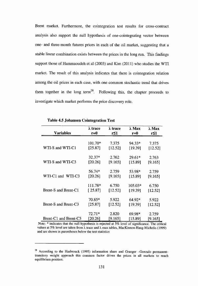
Brent market. Furthermore, the cointegration test results for cross-contract

analysis also support the null hypothesis of one-cointegrating vector between

one- and three-month futures prices in each of the oil market, suggesting that a

stable linear combination exists between the prices in the long run. This findings

support those of Hammaoudeh et al (2003) and Kim (2011) who studies the WTI

market. The result of this analysis indicates that there is cointegration relation

among the oil prices in each case, with one common stochastic trend that drives

them together in the long term28. Following this, the chapter proceeds to

investigate which market performs the price discovery role.

Table 4.5 Johansen Cointegration Test

VariablesX trace

r=0X trace

r<lX Max

r=0>uMax

r<l

WTI-S and WTI-C1101.70*[25.87]

7.375[12.52]

94.33*[19.39]

7.375[12.52]

WTI-S and WTI-C332.37*[20.26]

2.762[9.165]

29.61*[15.89]

2.763[9.165]

WTI-C1 and WTI-C356.74*[20.26]

2.759[9.165]

53.98*[15.89]

2.759[9.165]

Brent-S and Brent-Cl111.78* [ 25.87]

6.750[12.52]

105.03*[19.39]

6.750[12.52]

Brent-S and Brent-C370.85*[25.87]

5.922[12.52]

64.92*[19.39]

5.922[12.52]

Brent-Cl andBrent-C372.71*[20.26]

2.820[9.165]

69.98*[15.89]

2.759[9.165]

Note: * indicates that the null hypothesis is rejected at 5% level of significance. The critical values at 5% level are taken from X trace and X max tables, MacKinnon-Haug-Michelis (1999) and are shown in parentheses below the test statistics

28 According to the Hasbrouck (1995) information share and Granger -Gonzalo permanent- transitory weight approach this common factor drives the prices in all markets to reach equilibrium position.

131

4.6.3 Vector Error Correction Approach

Table 4.6 presents the estimated results of the error-correction model for both

crude oil markets. In the WTI market, the estimated value for the error correction

term coefficients on the spot market is negative and significant, while for the

futures market it is positive but insignificant in all markets at different maturities.

These results suggest that the futures market responds first to new information on

price in all maturities. The Brent market also provides similar results; error

correction coefficient for the futures market is insignificant and positive while

that of the spot market has the correct sign in all maturities. These results

indicate unidirectional causality from futures to spot market in the oil markets at

the different maturities. When the absolute value of the error correction terms are

compared the results clearly show that the futures market coefficient is lower,

implying that the futures prices adjust faster to the long-run equilibrium error.

The findings suggest that the futures market impound more information and

therefore leads price discovery in both markets at the different maturities.

The results of the cross-contract analysis for both markets are also presented in

Table 4.6. The results show that the estimated value of the error correction

coefficients on the one-month futures contract are negative and significant, while

for the three-month futures contract they are positive but insignificant at the 5%

level in each of the crude oil markets. This result indicates unidirectional

causality from three-month futures contract to one-month futures and not vice-

versa, suggesting that the three-month futures contract leads price discovery by

incorporating new pricing information more and that investors should therefore

focus on this contract in order to minimize risk. Finally, it is clear that all the

132

crude oil futures markets perform their price discovery function in all maturities

but are more efficient at three-month maturity.

Table 4.6 Estimated Results of the YECM Approach

Variables___________ VECM____________ Lags

' A W T I-S N yA W T I-C \J

-0.0522[-2.695] 0.0133[ 0.739] 3

' A W T I - S N ^AWTI - C ij

-0.0397[-2.314] 0.0025[0.164] 8

' A w n - e x '

AWTI - C3y-0.0299[-2.513] 0.0049[0.437] 1

B re n t-S Brent - C \y

-0.0661[-4.271] 0.0567[ 1.990] 2

rA B ren t-S VABrent - C3

-0.0453 [-3.967] 0.0161[1.477] 3

f ABrent - C lN kABrent - C3

-0.6413[-3.360]0.0126[0.707] 4

Note: t- statistics is shown in parenthesis besides the error correction coefficients. The lag lengths are selected by Akaike information criterion (AIC) and Schwartz information criterion (SIC).

4.6.4 Common Factor Weight Approach

The estimated results from the common factor weights are presented in Table

4.7. Following the approach of Baillie et al (2002), these results were obtained

from the error correction coefficients as discussed earlier and reported in Table

4.6. In the West Texas Intermediate crude oil market, the results indicate that the

spot market contributes 20% to the common factor, while the futures market at

one-month maturity contributes 79% to the process of price discovery. The

133

results also indicate that the common factor weight is 5% for the spot and 94%

for the futures markets at three-month maturity. In line with the error correction

model, the results suggest that the futures market leads the process of price

discovery by incorporating more information in all the maturities, and thus

support that the futures market performs price discovery function. The finding

confirms research by Kim (2010) who, using data for longer period from 1989 to

2010, reports the common factor weight of 82% and 1.1% at one and three-

month maturity, respectively.

For the Brent market, the spot market has the common factor weights of 46% and

54% for the futures market at one-month maturity, indicating that the futures

market leads price discovery, whereas in the second case, the futures market has

even higher common factor weight of 74% at three-month maturity, while for the

spot market it is 26%. In common with the WTI market, these results show that

new pricing information is incorporated more by the futures market and therefore

plays the price discovery role in all the maturities. One important finding is that

all the markets show that futures market at longer maturity (three-month)

contributes more, suggesting that the longer the futures contract to its maturity,

the more the market impounds new pricing information and the less contribution

the spot market make in the process of price discovery. Therefore speculative

opportunities cannot be exploited in the WTI and Brent market in the long term

due to market efficiency.

134

Table 4.7 Estimated Results of the Common Factor Weights

Variables Common Factor Weight CFW)

WTI-S 0.2032WTI-C1 0.7968

WTI-S 0.0590WTI-C3 0.9407

WTI-C1 0.140WTI-C3 0.859

Brent-S 0.4617Brent-Cl 0.5382

Brent-S 0.2622Brent-C3 0.7378

Brent-Cl 0.0193Brent-C3 0.9807

Note: The common factor weight (CFW) for the futures and spot markets are

calculated as CFWf = and CFWf = - a

respectively.

Table 4.7 presents the estimated results obtained from the cross-contract analysis.

For the WTI market, the common factor weight for the one-month contract is

14% while for the three-month contract it is 85%, a finding consistent with that

of Kim (2010). In the Brent market, the contribution of the three-month contract

is much larger at 98%, while the one-month contract contributes only 2%. These

results suggest that the three-month futures contract plays the price discovery

function in both markets. Another interesting finding is that all the markets

provide strong evidence that supports the contribution of three-month futures

contract to price discovery, and it can also be seen that the two oil markets have

similar characteristics in both the single and cross-market analysis in the long

term. In summary, and in line with the majority of previous studies, all the results

135

from the two models support the hypothesis that the leading role is perform by

the futures market in price discovery in the two crude oil markets over the study

period. Therefore, the crude oil futures markets perform their price discovery

function and are efficient in the long term. However, the results also provide

strong evidence that three-month contracts leads one-month contracts in all

markets and thus investors should focus on the former because the futures

markets performance is more efficient at this maturity. The implication of the

results is that hedgers would benefit because the markets are able to impound the

new pricing information and therefore reduce the unsystematic risk in the

different maturities. More so, portfolio diversification would be effective across

the oil markets, however, speculative opportunities can be exploited in the two

oil markets because the three-month contract leads the one-month contract in the

price discovery process.

4.6.6 Garbade-Silber Approach

Table 4.8 reports the results for the Garbade-Silber (GS) short-run dynamic

model, estimated using the regression approach. The GS model shows that the

value of 6 = + p f , will be higher and less than 0.5 when the futures and

spot market leads price discovery process, respectively. The Ljung-Box

diagnostic Q statistics indicate that the residuals in the regression equations are

not autocorrelated up to 36 lags in all the crude oil markets. In panel A, the

estimated results show that p s and p f are significant and positive in both the

WTI and Brent markets at one- and three-month contracts to maturities, implying

that the spot and futures prices respond to new pricing information

136

simultaneously. The measure of price discovery is then estimated in order to

determine the price leader. The estimated value of 0 is 0.68 and 0.73 for WTI at

one- and three-month futures contracts, respectively. The results reports that the

values are 0.55 and 0.66 in the Brent market at one- and three-month futures

contract, which implies that the futures market dominates price discovery process

with approximately 55% to 73% between the WTI and Brent markets across the

different maturities. It is clear from the results that both futures markets perform

their price discovery role in all the maturities. When the results are compared

with previous studies the estimates are a little higher than the value obtained by

Quan (1992), who reported 0.52 and 0.70 for WTI at one-and three-month

futures contracts, respectively. Schwarz and Szakmary (1994) reported the value

of 0.55 while Moosa (2002) reported 0.60 at one-month contracts. However, the

results contradict those of Kim (2010) who reported 0.17 and 0.87 at one-month

and three-month contracts, respectively, yet the difference in the value of 9 is

not surprising given the differences in the period of study.

The estimates of the coefficient 8 show that between the futures and spot prices

there is significant mispricing, extending to the next trading day in both markets.

The results indicate that the value of 8 is 0.91 and 0.93 in the WTI market at

one- and three-month contracts respectively. In the Brent, the values of 8 are

0.83 and 0.91 at one- and three-month contracts. These results imply that

approximately 10 to 17% of the mispricing ranging between the two markets

disappears the next trading day. The results also suggest that supply of arbitrage

is less at three-month contracts to maturity in both markets, suggesting that price

convergence between the prices takes place during small time interval in all

137

markets. The findings are in line with those of Quan (1992) and Schwarz and

Szakmary (1994) who studied the WTI market.

Table 4.8 Estimated Results of the Garbade-Silber Approach

Panel: A Ps p f e 8

0.062** 0.029**WTI-S and WTI-C1 [3.419] [1.730] 0.680 0.91

0.051** 0.019*WTI-S and WTI-C3 [3.470] [1.435] 0.733 0.93

0.095** 0.079**Brent-S and Brent-Cl [7.548] [6.305] 0.546 0.83

0.060** 0.030**Brent-S and Brent-C3 [5.554] [3.106] 0.664 0.91

Panel: B Px P i e 8

0.027** 0.003WTI-C1 and WTI-C3 [2.389] [0.277] 0.838 0.97

0.088** 0.017Brent-Cl andBrent-C3 [5.507] [1.183] 0.900 0.91

Note: The coefficients Ps and P f are error correction terms for spot and futures market,

respectively. Also, the coefficients f3{ and /?2 are error correction terms for futures contract at one and three-month, respectively. Garbade and Silber approach assumes the error correction

coefficients to be positive. The measure + ( 5 / , value greater than 0.5 shows that

futures market dominates in price discovery process. The coefficient 8 measures the mispricing between the markets. The values in parentheses beside the parameters are the t-statistics and asterisk (*) and (**) indicate significance at the 1% and 5% level.

Table 4.8 also reports the estimates of the cross-contract analysis for both

markets in Panel B. The estimated values of /?, for both markets are positive

and significant, suggesting that the one-month contract impounds new pricing

information more. However, the estimates of p 2 are positive but insignificant,

138

suggesting that there is little feedback of new pricing information between the

one- and three-month contracts in all markets. The value of Vindicates 0.83 and

0.90 for the WTI and Brent markets at one-month contracts, and suggests that the

one-month contract leads the three-month contract in the process of price

discovery. The results contradict that of the common factor weight analysis in

both markets, consistent with Kim (2010) who reported 0.88 in the WTI market.

Furthermore, the estimates of 8 in the WTI and Brent markets are 0.97 and 0.91

respectively, indicating that about 9% of the mispricing between two contracts is

transferred to the next trading day and thus supply of arbitrage between the two

contracts lasts over a short time in all markets. The results show that the futures

market leads price discovery in the two crude oil markets and also support that

one-month futures contracts leads three-month contracts in the process of price

discovery in all the markets in the short term. The implication of the findings is

that there is strong evidence that hedging would be effective because the oil

markets minimise the high risk associated with oil prices and portfolio

diversification across the two markets would be profitable because they are all

efficient within the maturity. However, in contrast to the long term analysis the

results show that the one-month contract dominates the three-month contract

suggesting that both markets are more efficient in the former and thus short term

investors should be concerned with this contract.

4.7 Summary and Conclusion

This chapter has investigated the price discovery relationship between the crude

oil spot and futures markets. It analyses the contribution to price discovery of the

West Texas Intermediate and Brent crude oil markets using daily data from

139

January 2000 to May 2011, and extends previous studies on price discovery as it

examines the process of price discovery across different contracts, with a view to

establishing which market (or contract) is more efficient and reducing price risk

in international oil markets. The chapter also investigates price discovery using

three different measures: the error correction approach, the common factor

weight approach and the Garbade and Silber approach. This chapter is

significant because the contribution of the futures market to price formation

determines whether the market performs its price discovery role or otherwise and

the results have important implications for investors, speculators and policy

makers.

Empirical results provide strong evidence which show that the futures markets

perform the price discovery role in the international oil markets. The results

show that the spot and futures prices as well as the futures prices of different

maturities are cointegrated, as reported by the Johansen cointegration test in all

the oil markets. These results suggest that the prices move together in the long

term, implying that they have the ability to predict each other and violating the

weak form efficient hypothesis. Using the error correction approach and common

factor weight approach, the results indicate that the futures market contributes

more to price discovery in both markets at different maturities. These also

suggest that the futures price impounds new pricing information more than the

spot price in all the oil markets, which shows that market participants prefer to

use futures prices to trade crude oil in the international market. Further, the

results show that all the oil markets support that the contribution of the futures

market to price discovery is greater at three-month contracts to maturity. This is

140

confirmed by the cross-contract analysis which shows that the three-month

contract leads the one-month contract in price discovery in both markets. In

particular, these findings demonstrate that the crude oil futures market is more

efficient at three-month maturity. The results of the Garbade-Silber approach

indicate that new pricing information is reflected first in the futures market in

both WTI and Brent markets at one and three-month maturities; however, in

contrast with the other approaches, the results suggest that the one-month

contract leads three-month contracts in the price discovery process in all the

crude oil futures markets in the short term. The implication of these findings is

that speculative opportunities cannot be exploited in both oil markets, especially

at three-month maturity, because arbitrage does not exist. Again, portfolio

diversification across the markets would be effective in the long term because

they all reduce price risk in all the maturities. However, for cross-contract

investment, investors should focus on three-month contracts because both

markets are more efficient at this maturity in the long term.

In conclusion, the results from this chapter support the theory that the WTI and

Brent crude oil futures markets perform their price discovery function in both the

short and long term at different maturities. The cross-contract analysis suggests

that the three-month oil futures contract plays the price discovery role in all the

crude oil markets in the long term, while the one month futures contract

dominates price discovery in the short term. Furthermore, the two crude oil

markets have similar patterns because in both markets, the futures prices

impound new information faster at the different maturities in the short and long

141

term. Finally, the crude oil futures markets perform their price discovery

functions, supporting the market efficiency.

142

CHAPTER FIVE

Price change and Trading Volume Relationship in the Oil Futures Markets

5.1 Introduction

Price and trading volume are the key factors determining the behaviour of the

futures market and are important because they are both influenced by the same

fundamental: arrival of new information. Sierimo (2002) pointed out that the

changes in price represent how the market values new information while the

changes in trading volume represent how investors value the new information.

Furthermore, empirical evidence revealed that trading volume reflects the nature

of information that flows into the market; low trading volume implies high price

volatility and less market liquidity, while high trading volume leads to low price

volatility and high liquidity (Floros and Vougas, 2007; Bhar and Malliaris,

1998). The relationship between trading volume and price changes has important

implications for market participants and regulators.

Several studies have identified the advantages of research into the price change

and trading volume relationship. First, the price-volume relationship can provide

information about market structures (Karpoff, 1987). Second, the same

relationship suggests whether technical or fundamental analysis should be used

in developing trading strategies (Moosa and Silvapulle, 2000), and thirdly,

determines the success or otherwise of futures contracts (Bhar and Hamori,

2004). Fourth, it can help understand the informational efficiency of the futures

market because the ability of trading volume to forecast futures price changes

implies market inefficiency (Lua and Go, 2012; Kocagil and Shachmurove,

143

1998; Foster, 1995). Finally, the relationship provides hedger, speculators, policy

makers and other participants’ information on futures market condition (Fujihara

and Mougoue, 1997; Bhar and Hamori, 2005).

The research in this area is centred on three important yet conflicting models: the

mixture of distribution hypothesis, the sequential arrival of information

hypothesis and the noise trader model. The Mixture of Distribution Hypothesis

(MDH) postulates that the trading volume and price changes relationship is

positive. The model’s supporters: Tauchen and Pitts (1983), Harris (1986),

Karpoff (1987), Epps and Epps (1976) and Clark (1973) hypothesized that

market participants respond to new information simultaneously and therefore

neither price change nor trading volume can cause the other in any direction. In

contrast, the Sequential Arrival of Information Hypothesis postulates that market

participant’s responds to new information sequentially and that past values of

prices and trading volume can predict each other, or in other words, bi­

directional causality exist between them. This model has received support from

Copeland (1976) and Jenning et al (1981), among others. Finally, De Long et al

(1990) developed the Noise Trader Model which asserts that the price change

and trading volume relationship depend on noise trader’s action that is not based

on any economic fundamentals. The model argues that the noise traders’

behaviour of using past information about price changes to make investment

decisions explain the positive causal relationship between trading volume and

price change in either direction.

144

The objective of this chapter is to examine the trading volume and price change

relationship in the crude oil futures market in order to determine the market

efficiency. In doing so, this chapter seeks to addresses two important questions:

first, whether there is positive relationship between trading volume and price,

and second, whether trading volume contains important information that can

predict the crude oil futures price. This chapter contributes to the limited studies

on the trading volume and price change relationship in oil futures markets in two

ways.

• It extends the work of previous studies which focused on the West Texas

Intermediate oil futures market, by exploring the price and trading

volume relationship in the Brent crude oil futures market. To my

knowledge except Foster (1995) there is no study that investigates the

forecast ability of trading volume to price changes in Brent market. This

study has important implication because market participants want

alternatives for risk diversification and regulators need to know the

effectiveness or otherwise of their policies on the international oil market.

• It provides new evidence using updated data that captures the recent

period of high volatility in crude oil prices and also employs the impulse

response function and variance decomposition analysis.

This chapter is organized as follows. Section 5.2 reviews the literature on the

relationship between trading volume and price change in oil futures markets. In

this section literature on this relationship in non-oil futures markets are reviewed

to have better understanding of the area. Section 5.3 presents theoretical models

on the trading volume and price change relationship. Section 5.4 provides brief

145

discussion on the methodology used in the analysis. Section 5.5 describes the

data used in the chapter. Section 5.6 presents the empirical results of relationship

between price change and trading volume and, Section 5.7 concludes the major

findings.

5.2 Literature Review

This section review relevant empirical studies that examine the relationship

between price and trading volume in commodity futures markets. Despite the

significant of the relationship between trading volume and price changes,

research in this area has been abundant in the oil futures markets29. This section

is divided into two parts. Part one reviews available literature on trading volume

and price changes relationship in the oil futures markets. The second part

explored the relevant studies that have been conducted in other commodity

markets in order to shed more light in the area.

5.3.1 The Oil Futures Market

A limited number of studies have been conducted on the price change and

trading volume relationship in the oil futures markets; among the first was that

conducted by Foster in 1995 who apply the GARCH and Generalized Method of

Moment (GMM) to examine the trading volume and price changes relation in the

crude oil futures markets for WTI and Brent. For the analysis, he utilized daily

closing futures prices with their corresponding trading volumes during the period

from January 1990 to June 1994. A second sample for WTI, covering the period

29 There is limited literature on price and trading volume relationship in the oil futures markets may be because of the problem in accessing the trading volume.

146

January 1984 to June 1988, was also investigated in order to find the maturity

effect of trading volume and price relationship. Empirical results from the

GARCH model indicate that trading volume cannot serve as an important tool for

measuring the new information that enters into both markets and furthermore, the

GMM model shows that price variability and trading volume relationship is

positive except of the WTI market in the first period supporting the mixture of

distribution hypothesis. Foster claims that in the mid-1980s the WTI market may

have been affected by factors such as liquidity or a problem of efficiency at its

early stage of development. He also found that price variability can be predicted

with information on past trading volume in both markets, yet he argued that this

finding do not provide support for the sequential arrival hypothesis nor does it

contradict the mixture of distribution hypothesis; rather, it results from pricing

inefficiency. Finally, he concluded that the inefficiencies result from the traders

or market agents’ behaviour as they use past information about trading volume to

predict market conditions.

Fujihara and Mougoue (1997) employed the Granger causality test to examine

the price variability and trading volume relationship in the US petroleum futures

market for unleaded gasoline, heating oil, crude oil within the linear and non­

linear framework. The analysis was conducted with daily closing futures prices

and their corresponding trading volume for each commodity. In the WTI market,

the linear causality test shows that lagged trading volume does not cause price

changes, while the non-linear causality test indicates bi-directional causality.

They observed that this result remains consistent even after accounting for

presence of ARCH effect in both the returns and trading volume series; to

147

confirm their results they divide the study into different sub-samples, but the

results for both tests are still consistent. The authors confirmed that the WTI

futures market is inefficient since past volume can be used to forecast current

price movement, and suggest that the inefficiency may be caused by two reasons:

first, investors set their prices based on the behaviour of others, and second,

investors used past information about trading volume to measure futures market

expectations.

Additionally, Kocagil and Shachmurove (1998) analysed the contemporaneous

and inter-temporal causality between WTI futures price and trading volume,

using both rate of return and absolute return as proxy to price changes. The

authors addressed three important issues: whether information flow in the futures

market supports the mixture or sequential information hypothesis; whether the

price-trading volume relationship is symmetric, and whether lagged trading

volume predicts future price changes. Applying the VAR framework, their

results provide interesting evidence. First, they show that trading volume is

positively correlated with absolute return, but not with rate of return, which

supports the mixture of distribution hypothesis. They also found bi-directional

causality between absolute return and trading volume, implying that they can

both predict each other which support the sequential informational arrival

hypothesis. They observed that the inter-temporal causality test indicate that

lagged trading volume does not cause return in the crude oil futures market.

However, when they re-examined their analysis using the variance

decomposition approach the results show that the variance of trading volume is

influence by absolute returns, leading them to conclude that the time interval is

148

important in explaining the trading volume and returns relationship and that the

crude oil market is inefficient during period of the study. Moosa and Silvapulle

(2000) examined the trading volume and price relationship in the WTI market

using linear and non-linear causality tests, and daily data for three and six-month

futures contracts to maturities. In order to capture the volatile period they carried

out their analysis using data over the whole sample and different sub-sample

periods, pointing out that the reason for using different futures contracts is to find

the maturity effect between price change and trading volume. They also

conducted their analysis using absolute and difference price series as a proxy to

price changes. In contrast to the results of Fujihara and Mougoue (1997), they

found that the linear causality test indicates that trading volume does not cause to

price changes, except in the second sample period. However, the non-linear

causality confirmed the existence of bi-directional causality running between

trading volume and price change. They found that the results remained consistent

even after volatility filtering, and suggest that the price and trading volume

relationship has a maturity effect which reflects liquidity. They concluded that

their findings were inconsistent with market efficiency, but support both the

noise trading model and sequential information arrival hypothesis.

Moosa et al (2003), continuing the research in this field, investigated the

temporal asymmetry causality between price change and trading volume in the

WTI market. They employed the Granger causality test and the data used for

their analysis are daily trading volume and futures prices at three and six month

contracts. The findings showed that the symmetry model demonstrated that

futures price leads trading volume in all the contracts, suggesting that both

149

positive and negative price change leads trading volume while only negative

change in trading volume leads price changes. The asymmetric model indicates

that both trading volume and price changes leads the other in all the maturities,

and specifically, the results support asymmetric relationship because negative

changes in price and trading volumes have more powerful impact than positive

changes in explaining each other. The authors suggested that their findings

specifically provide an important explanation as to why traders’ behaviour in

relation to price changes and trading volume causes the demand function in the

bear market to be steeper than in the bull markets. They argued that their results

support the noise trader model but rejects the mixture of distribution hypothesis.

Bhar and Hamori (2005) employed the augmented AR-GARCH model to

investigate information dependence and causal relationship between trading

volume and price change in the WTI market, using daily data in their analysis.

They found that price changes is not caused by trading volume, indicating that

past information on volume will not be helpful in forecasting future returns a

result that contrast most of the previous studies. However, they also observed

that returns leads trading volume with a lag of 15 and 9 days, which according to

the authors provides mild evidence in support of noise trading activities. They

pointed out that their analysis disagree with the idea of controlling the volatility

of price as a way of improving the performance of the oil futures markets

because past information about volume cannot assist speculators in forecasting

prices and thus, in contrast to Fujihara and Mougoue (1997) and Moosa and

Silvapulle (2000) they reports that the WTI crude oil futures market is price

efficient. Table 5.1 summarizes the findings obtained from the above review,

150

from which it is clear that conclusions on the relationship between price changes

and trading volume are mixed.

151

Table 5.1 Summary of Previous Results on Price-Volume Relationship in the Oil Futures Market

Author (s) and Years Data and Market Methods Results

Foster (1995)

WTI and Brent daily futures price and trading volume from 1990 to 1994

GARCH and Generalized method of moments

Positive relationship and unidirectional causality between trading volume and price change.

Fujihara and Mougoue (1997)WTI daily futures price and trading volume from 1984 to 1993

Linear & non-linear causality tests

No linear causality but bi-directional non-linear causality between trading volume and price change.

Kocagil and Shachmurove (1998)WTI daily futures price and trading volume from 1980 to 1995

Linear causality test and variance decomposition analysis

The contemporaneous test indicates positive correlation and bi-directional causality between oil price and trading volume. The intertemporal causality test also rejects the MDH.

Moosa and Silvapulle (2000)WTI daily futures price and trading volume from 1985 to 1996

Linear and non-linear causality tests

Linear unidirectional causality and non­linear bi-directional causality from trading volume to price.

Moosa et al (2002)WTI daily futures price and trading volume from 1985 to 1996

Linear and non-linear causality tests

Bi-directional causality between trading volume and price change.

Bhar and Hamori (2000)WTI daily futures price and trading volume from 1990 to 2000 AR-GARCH model

Unidirectional causality from price to trading volume and not vice-versa.

152

From the review it can be seen that the common factor across the research is that

it has been devoted to the WTI crude oil futures market, has employed daily data

and was undertaken using either the GARCH or Granger causality approach.

Moreover, most of the previous studies have shown that the relationship between

volume and price changes is positive, which support the mixture of distribution

hypothesis; however, there is controversy on the lead-lag relationship between

these variables. Not all studies show that both trading volume and price changes

can cause each other in support of the sequential information arrival hypotheses

and market inefficiency.

5.3.2 The Non-Oil Commodity Futures Markets

In this section, the relevant studies on the price change and volume relationship

in non-oil commodity futures markets are reviewed in order to build knowledge

of the area. Cornell (1981), using daily data, examined the trading volume and

price relationship in eighteen commodities futures markets including four metals,

thirteen agriculture and treasury bills. The author used the standard deviation of

the log price and daily change in average volume as proxy to price change and

trading volume respectively, with two leads and lags for each commodity. He

found not only the evidence of positive relationship but also that change in price

leads trading volume for fourteen commodities while for the remaining four, the

reverse is true. Therefore, it is clear that the analysis supports the mixture of

distribution hypothesis by demonstrating that the price change and trading

volume relationship is positive. Finally, the lead and lag relationship confirmed

the existence of market efficiency in almost all the commodity futures markets

because past futures prices cannot be predicted with information on trading153

volume. Malliaris and Urraitai (1998) further analysed price change and volume

relationship for six agricultural commodities futures markets, namely com,

soybean, wheat, oats, soybean meal and soybean oil, using a dynamic model

which assumes that trading volume and future price follows a non-stationary

process with trend. The model tests three important hypotheses, although only

the first two are related to the present work: that both price and volume are non-

stationary process and are interrelated, and that cointegration relationship exists

between return and trading volume. Data for the analysis is daily and, employing

both the Engle-Granger and Johansen cointegration tests, the results indicate that

trading volume and price are cointegrated in all commodity markets. When the

error correction model test was applied to analyse the short-term and long-term

dynamic relationship between trading volume and price changes bi-directional

causality was found from trading volume to price changes, supporting the

sequential arrival hypothesis in all the markets in the long ran. However, they

found that price changes cause trading volume in com, soybeans and soybean

meal while the rest of the commodity markets indicate weaker causality in the

short ran, suggesting that speculative activities will be profitable in the long

term.

Wang and Yau (2000) examined the price change and volume relationship in

four foreign exchange commodity futures markets, namely S&P 500,

Deutschmark, gold and silver using daily data and the Generalized Methods of

Moment. They found that trading volume had a positive significant relationship

with price change, while price change indicated a negative significant

relationship with lagged trading volume in all markets. Their results stand in

154

contrast to the mixture of distribution hypothesis in all markets and neither do

they support the market efficient hypothesis because futures price change can be

predicted with past information about trading volume. Additionally, using the

ordinary least square regression the results were confirmed but shown to

underestimate the coefficients in all markets. Building on previous work, Ciner

(2002) studied the price change and volume relationship in futures market for

three commodities, namely, gold, platinum and rubber traded in the Tokyo

Commodity Exchange, using daily data. The study applied the linear and non­

linear Granger causality tests, and GMM approach. The GMM results suggest

that return and trading volume have positive relationship, consistent with the

mixture of distribution hypothesis. Furthermore, the linear causality test indicates

that trading volume is caused by returns in all except gold futures, while the non­

linear causality test indicates bi-directional causality between them. Ciner

observed that when the ARCH effect is accounted for in all the prices, the bi­

directional causality disappears but unidirectional causality still exists from

return to volume, confirming the mixture of distribution hypothesis which lead

the author to argue that trading volume provides market participants with

information about the level of price changes but not the direction of the price

changes, which in turn supports the market efficient hypothesis.

In a similar vein, Bhar and Hamouri (2004), employing daily data, re-investigate

the relationship between change in U.S gold futures price and trading volume

using the Granger causality test. They found strong evidence of positive

relationship between price and trading volume, consistent with the mixture of

distribution hypothesis, as well as mild bidirectional causality from price change

155

to trading volume which shows weaker evidence for the sequential information

arrival hypothesis. They noted that the information that flows between price

change and trading volume has an impact on price movement in the gold market

and concluded that the reason their results contrast with those from the

agriculture and crude oil markets is due to the nature of gold, especially the way

investments are made when the market underperforms. Gianfreda (2010) also

applied the GARCH model to examine the relationship between change in

European electricity spot price and trading volume for Germany, France, Spain,

Italy and the Netherlands; the empirical results indicate significant but negative

relationship between spot price change and volume in all markets except for the

Netherlands, where volume and price change show positive relationship.

Gianfreda pointed out that price change and trading volume can have positive or

negative relationship, depending on the market structure and suggested that in the

first case past information on trading volume can help reduce the next day price

volatility in the three electricity markets, while in the second case there is

optimal production in the market30.

In the foreign exchange market, McGowan and Muhammad (2004) analysed the

dynamics of trading volume and price change relationship for the spot and next

month contracts in the Malaysian stock index futures using daily data. They

employed the vector error correction model to investigate the relationship over

four sub-periods in order to find the variation; a cointegration relationship was

shown to exist between both the spot and next month contracts trading volume

30 The market is not operating with excess capacity.

156

and returns. These results show that trading volume cause price change in all the

sub-periods for all contracts and suggest that speculators and hedgers can use the

information on the price-trading volume relationship to make investment

decisions in both markets. Floras and Vougas (2007) then employed the GARCH

and Generalized Method of Moments methods to investigate return and volume

relationship in Greek stock index futures market for FTSE/ASE Mid-40 index

and FTSE/ASE-20 index. Taking their data for the analysis from daily futures

price changes and trading volume, the empirical results of the GARCH model

indicate that trading volume is positive and significant in explaining price change

in the FTSE/ASE-20 index while the GMM estimation shows a significant but

negative relationship between lagged trading volume and absolute return. The

results for the FTSE/ASE Mid-40 also indicate an insignificant relationship

between returns and trading volume in both models. In line with Foster (1995),

they conclude that the results of Greek index futures market for FTSE/ASE-20

indicate that both the volume of trade and price changes are not driven by the

same fundamentals and that market participant’s use trading volume to measure

price variability.

Cheng and Ying (2009) investigated the hourly price and trading volume

relationship in mini-TAIFEX futures market. They argued that the trading

volume and price relationship of financial products cannot be explained by a

single model and as a result, they applied the vector error correction model and

Granger causality approach. First, the vector error correction model shows the

existence of cointegration and significant positive relationship between changes

in hourly price and volume of trade. In contrast to Floras and Vougas (2007),

157

their results clearly show that these variables are influenced by information

arrival, confirming the MDH. Secondly, the causality test indicate that both price

and trading volume lead each other which supports the sequential arrival

hypothesis, leading to their suggestion that hedge effectiveness can be increased

in the short run by using past information regarding futures prices to forecast

trading volume, and vice-versa. Summarizing, they provide strong support for

rejecting the efficient market hypothesis in the TAIFEX futures market.

In their study, Mougoue and Aggarwal (2011) using daily data examines the

relationship between currency futures price change and trading volume for the

US dollar, British pound, Japanese yen and the Canadian dollar. Applying the

Generalized Method of Moment, they found a negative but significant

relationship between change in price and trading volume in all the currencies,

which reject the mixture of distribution hypothesis. They also investigate the

linear and non-linear dynamics between trading volume and price changes; both

tests provide strong evidence of bi-directional causality from trading volume and

returns in all the currency markets, violating market efficiency but supporting the

sequential arrival hypothesis. Their results contrast with those of Bhar and

Malliaris (1998) who studied the same markets during the period from May 1972

to November 1994. Lau and Go (2012) adopt the AR-GARCH model process to

examine the trading volume and returns relationship in Malaysian options and

foreign exchange futures. The cross-correlation analysis indicate causality from

lag one of trading volume to returns, implying that changes in trading volume for

the previous day may induce a positive or negative change in the next day’s

price. They also found that when the augmented AR-GARCH model is applied

158

the dependence causality from the trading volume to return disappears. They

suggest that their findings, which contrast with those of McGowan and

Muhammad (2004), support that the Malaysian futures market comprised of

investors with noise-trading behaviour. The findings of this study are similar

with those of Bhar and Malliaris (1998) although they relate to different foreign

exchange markets.

159

Table 5.2 Summary of Previous Results on Price-Volume Relationship in the Non-Oil Commodity Futures Markets

Author (s) and Years Data and Market Methods Results

Cornell (1981)

US 12 agriculture, 4 metals and 1 financial commodities daily futures prices and trading volume from 1968 to 1974 Ordinary Least Square Regression

Positive relationship but absence of causality between trading volume and returns.

Malliaris and Urruitai (1998)

US 6 agricultural commodities daily futures prices and trading volume from 1980 to 1995

Correlation and Linear causality tests

Positive correlation and bi-directional causality between trading volume and price.

Wang and Yau (2000)

US 2 metals and 2 foreign exchange commodities daily futures prices and trading volume from 1990 to 1994 Generalized Method of Moments

Positive correlation and unidirectional causality from trading volume to price in almost all the markets.

Ciner (2002)

Tokyo daily prices and trading volume for 2 metals and 1 wood in futures markets from 1990 to 1994

GMM, Linear and non-linear causality tests

Positive relationship and unidirectional causality from price to trading volume in all the markets.

Bhar and Hamouri (2004)

US gold daily futures price and trading volume from 1990 to 2000 Linear Granger causality test

Positive relationship and mild bi­directional causality from price change to trading volume.

McGowan and MuhammadMalaysian stock index daily futures price and trading volume

Vector Error Correction Model Positive relationship and unidirectional causality from trading volume to

160

(2004) from 1997 to 2003 returns.

Floros and Vougas (2007)

Greek FTSE/ASE Mid-20 and FTSE/ASE Mid-40 stock Index daily futures prices and trading volume from 1997 to 2001 GARCH/GMM models

No relationship between returns and trading volume in FTSE/ASE Mid-40 while negative significant relationship exists in FTSE/ASE Mid-20.

Cheng and Ying (2009)

Mini-TAIFEX index daily futures price and trading volume from 2006 to 2007 VECM

Positive relationship and bidirectional causality between price and volume.

Gianfreda (2010)

Daily prices and trading volume for 4 different countries electricity spot markets GARCH model

Negative relationship between prices and trading volume in three markets while other indicates positive relationship.

Mougoue and Aggarwal (2011)

Six foreign currencies daily futures prices and trading volume from 1977 to 2009

GMM and Linear Granger causality tests

Negative relationship between price and volume, and also bidirectional causality in all markets.

Lau and Gau (2012)

Malaysian options and foreign exchange daily futures price and trading volume from 1995 to 2009 AR-GARCH model

No causality between trading volume and returns.

161

Table 5.2 summarizes the findings obtained from the review on the price-volume

relationship in non-oil commodity futures markets. In general, it can be seen that

the studies in both oil and non-oil commodity futures market employed either the

GMM or Granger causality approach and that furthermore, they used daily data

in their analysis because it has been proven to capture all the available

information. They also provide mixed conclusions on the price and volume

relationship by supporting or rejecting the market efficient hypothesis.

5.3 Theoretical Framework of Price-Volume Relationship

The price changes and trading volume relationship was originally described in

the theory of demand and supply. This theory assumes that a change in price will

lead to a change in demand, in turn causing a shift to a new equilibrium position.

Accordingly, an increase in price will lead to a decrease in demand, and a

simultaneous increase in trading volume and vice-versa no matter the direction of

the change (Moosa and Silvapulle 2000). Building on this, a number of different

theories have been proposed to offer an explanation on the relationship between

price changes and trading volume, the common once are the mixture of

distribution hypothesis, the sequential arrival of information hypothesis and the

noise trader model. However, conflicting views persist because while some

studies provide support for the mixture of distribution hypothesis, pointing out

that the trading volume and price changes relationship is positive and they cannot

predict each other in line with the efficient market hypothesis; other studies

support the sequential arrival hypothesis or the noise trader model, which shows

162

that both trading volume and price changes can cause each other, thus violating

market efficiency.

5.2.1 The Mixture of Distribution Hypothesis

Clark (1973) developed the mixture of distribution hypothesis (MDH), built upon

the assumption of stochastic dependence between changes in price and volume of

trade with the rate of information arrival as the mixing variable. The model

postulates that the rate of daily price change and trading volume at any given

interval of time is independent and identically distributed, which implies that

successive price change and trading volume on individual trades are uncorrelated

and follow a random walk process. The model hypothesized that the stock

market is always comprised of traders with different expectations regarding

prices and that information flows into the market at varying rates; therefore, price

change and trading volume depend on the nature and reaction of traders to new

information. When all traders receive high quality information at the same time

or information is received only by inside traders, an increase in price change will

lead to high trading volume and vice-versa. In this framework, trading volume

serves as a measure of changes in price. Hence, the total number of increments in

daily changes in price and volume of trade that occur in the market each day is

equal to the daily change in volume and price that occurs in that particular day:

this implies that trading volume and price changes are positively correlated.

Epps and Epps (1976) further extend Clark’s model by assuming a simultaneous

response of both trading volume and price changes to new information. Their

model postulates that stochastic dependence exists between change in price and

163

change in trading volume from one transaction to the next and thus with arrival

of new information, an increase in excess demand will shift the equilibrium price

position in the market. As result, those traders whose null price is above the

equilibrium price purchase more from those with a null price below the

equilibrium point and accordingly, the rates at which the two traders negotiate on

the new price re-establishes another equilibrium price in the market. This process

demonstrate that there is positive relationship between trading volume and price

changes because the percentage of trading volume in each transaction depends on

how traders disagree when they change their null price due to new information.

Tauchen and Pitts (1983) and Harris (1986) also improved on the model of

mixture of distribution hypothesis. Both models are based on two important

assumptions: first, that trading volume and price change are jointly independent

and identically distributed with finite variance. Second, the number of new

information flows into the market in each day is not constant. These authors

showed that each day market passes through different equilibrium positions as

traders try to adjust their null prices in line with the new information they

receive, and therefore the proportion of daily changes in price and volume of

trade can be determined by the amount of news that enters into the market. The

models assume that trading volume and price changes are stochastically

independent from each other. In their framework daily trading volume and

changes in price reflect the amount or level of news that the market generated

from each number of transactions in that day. The implication of these models is

that they assume that there is positive relationship between changes in price and

164

trading volume, and also trading volume cannot predict price changes which

support the efficient market hypothesis.

5.2.2 The Sequential Information Arrival Hypothesis

Copeland (1976) developed the sequential information hypothesis based on the

assumption that trader receive market information individually in sequential and

random form. The model postulates that a market passes through different

equilibrium positions, but at the initial equilibrium position all traders acquire the

same information. However, when new information arrives in the market each

individual trader responds and changes his level of demand based on the nature

of information flow, behaviour which induces a shift in their respective demand

curves up to the point all the traders assimilate that particular information, when

a new equilibrium position is re-established. At this point, the traders have the

same information and their respective demand curves are identical. Copeland

also describes his model by assuming that the traders with new information are

either optimists or pessimists: when new information flows each optimist shifts

his demand curve upwards, while the pessimist shifts his downwards. The model

asserts that price changes that take place from initial equilibrium to successive

equilibrium positions are known with certainty and trading volume depends on

both the value of new information and the percentage of traders (optimistic or

pessimistic) in the market. Thus, both trading volume and price change are

considered as random variables because the market passes through successive

equilibrium positions in order to adjust, suggesting that the two variables have

positive relationship. The model assumes that future price changes can be

predicted with lagged trading volume and that future trading volume can be

165

predicted with lagged price change. Most importantly this model shows that

trading volume and absolute price changes lead each other and that, furthermore,

future price changes can be predicted with information on trading volume, thus

providing evidence of market inefficiency.

5.2.3 The Noise Trader Model

De Long et al (1990) developed a model which shows that the noise traders’

activities caused the positive relationship between trading volume and price

change. The model assumes that since the noise traders’ do not based there

activities on any economic variables, in the short term they drive the price away

from its fundamental value, thereby causing a temporary mispricing. However, in

the long term the absences of transitory components drive market prices back to

their mean values. The model assumes that for each transaction the market passes

through four periods. Again, the market consists of three types of traders:

positive feedback traders, informed rational speculators and passive investors. In

period 0, there are no activities in the market and the price is set at its initial

fundamentals. When rational speculators receive new information, or any signal

about the market, they buy more stock today with the expectation of selling

tomorrow, while on the other hand, the positive feedback investors respond to

this news by buying more tomorrow at the current market price which the

rational speculators are selling to make a profit. These activities drive the market

price higher in period 1 and 2 up to the point when the market is stabilized, and

then the price adjusts back to its fundamental values in the long term or period 3.

The model shows that the activities of the positive feedback investors cause the

relationship between changes in price and volume of trade to be positive because

166

they use past price changes in order to make a profit tomorrow and therefore

price changes are determined by the level at which the noise traders buy or sell

stock in the market. The important implication of the noise trader’s model is that

the positive feedback trading strategies led the price changes and trading volume

to have a positive relationship.

5.4 Empirical Methodology

This section briefly discusses the econometric techniques used in the data

analysis. Firstly, the generalized method of moment (GMM) applied to estimate

the relationship between price changes and trading volume is discussed.

Secondly, the vector autoregressive model and its application in testing price and

trading volume relationship via the linear Granger causality test are considered,

and finally, the use of impulse response function and variance decomposition

analysis in investigating the trading volume and price changes relationship are

discussed. This chapter chooses these techniques because empirical evidence

from previous studies has shown that they are powerful in estimating relationship

among macroeconomic variables.

5.4.1 Generalized Method of Moments

The generalized method of moments developed by Hansen (1982) is a

simultaneous regression approach used in time series analysis that is robust to

heteroskedasticity and autocorrelation in the residuals. According to Hansen, this

approach is efficient, consistent and asymptotically normal compared to other

standard estimators because it does not account for any information aside those

167

in the moment conditions. It also deals with the problem of simultaneity bias in

modelling returns and trading volume relationship (Foster, 1995; Lee and Rui,

2002; Mougoue and Aggarwal, 2011). Following Foster (1995), Ciner (2002)

and Floros and Vougas (2007) this chapter used the lagged values of trading

volume and price change (returns) as an instrumental variable (IV) estimator31.

The model can be estimated using the following structural equation:

Rt = a 0 + a lVt + a 2Rt_x+ JuRt

Vt =b0 + bxRt +b2Vt_l +Mv,t (5-1)

where Rt is returns, Vt is trading volume, Rt_x is the lagged returns, VM is

the lagged trading volume and f iR t,juVt are error terms. The parameters/?, and

Vt are endogenous variables which cannot be estimated using the ordinary least

square approach because it will yield inconsistent results since the variables are

correlated with their respective error terms (Ciner, 2002). The relationship

between trading volume and returns can be determines by significance of the

coefficients a x and bx in equation (5.1). When botha x and bx are significant it

implies that trading volume and returns are related. Hansen (1982) also proposed

the used of the J-statistics to find the validity of the model whether it is properly

identify or over-identify.

31 Ciner (2002) and Floros and Vougas (2007) pointed out that the instrumental variables deal with the simultaneity bias while GMM controls the problem of heteroskedasticity in the system.

168

5.4.2 Linear Granger Causality Test

Granger (1969) proposed the causality test to determine whether a time series

variable can improve the forecast performance of another variable. Granger

argued that when two or more variables are cointegrated casualty most exist

between them in a least one direction, and it may occur even if the variables are

otherwise . The following VAR model can be used to describe the causality

relationship between trading volume and returns:

n m

R t ~ a \ + X P i V t-1 + X Y j R t - j + e \i=\ y=l (5.2)

n m

V ,= a 2+ '£ O iRl-l + 'Z SiV.- i+ e 2,i=1 j=1 (5.3)

where, Rt_xis lagged returns and VM is trading volume, <?lfand e2t are

assume to be uncorrelated error terms with zero mean and constants variance.

The parameters f3i and 6? are estimated. Granger causality (1969) approach test

the hypothesis H 0 : /?. = 0 that Vt does not linear Granger cause Rt . Likewise,

when H 0 : 9i = 0 then Rt does not linear Granger cause Vt . Granger suggests that

when the lagged values of Vt are significant in explaining Rt , Vt Granger-cause 32

32 The Granger causality test determines the ability of the variables in the VAR system to predictive each other in the long term. For example, in a VAR of two variables y t and x t , their

causal relationship can take three forms: (1) either y t causes x t , or x t causes y t (unidirectional

causality) (2) both y t and x t cause each other (bi-directional causality) (3) y t and X t do not

cause each other (Independent variables). The causal relationship can be linear or non-linear depending on the relationship among the variables in the VAR (For more explanation on the VAR model see Sims, 1980).

169

Rt and there exists unidirectional causality from trading volume to returns.

When lagged values of Rt are significant in explaining Vt , there is unidirectional

causality from returns to trading volume. Finally, when lagged return and trading

volume are significant in each other’s equation, there is bidirectional causality,

while the insignificants of the variables in explaining each other implies no

causality among them (they are independent). The standard joint F- test is used to

examine the Granger causality in a VAR system (see Brooks, 2008; Enders,

1995; Asteriou and Hall, 2007).

5.4.3 Impulse Response Function

Sims (1980) developed the impulse response function to trace responses of all the

variables in VAR system to shocks on any of the variables33. The impulse

response function not only provides understanding of the impact of shocks on

variables but show how long the effect persists, its size and direction. The

impulse response of price changes (returns) and trading volume can be drive

from equation (5.2) and (5.3) as follows:

Rf ~ X! tP lli^ R t-i X! P u i ^ R t - ii= o i - o (5 .4 )

V =2>21 , £ v , - , + 2 > » . e v,-j/=0 (-0 (5.5)

33 Brooks, 2008 pointed out that a VAR system of n variables will produce an impulse response of n2.

170

The coefficient fa can be used to produce the effect of eRt and evt on the whole

time paths of the variables; Rt and Vt . The four elements fa are impact multiplier

and the coefficient 012(O)is the effect of a one unit change in £vt on Rt . The

element fax{ 1) and fa2{l) are the responses of unit changes in £R[_i and £vt_{ on Rt

over a period. Updating by one period shows that fax{\) and 012(l)also

represents the effect of unit change in £Rt and £vtonR t+l. The four coefficients

^n (O,012(O,021(O and (f>22(i)are the impulse responses (Enders, 1995).

5.4.4 Variance Decomposition Analysis

The variance decomposition is an extension of the impulse response function

which gives the proportion of movement in a variable that is cause from its own

shock and shocks on other variables in the VAR system (Sim, 1980). The

variance decomposition can be calculated as follows34:

<J2R,n= a2R[{(f)ii(0)2 + 0n (l)2 + ......+ (/>u ( n - 1)2] +<t2[(0i2(O)2 +fa2(l)2 + ...... + fa2{ n - 1)2] (5 6)

The variance decomposition can be explained from the impulse response

equations. The variable Rt is exogenous in the system when a shocks on

£vt cannot explain its forecast error variance. Likewise, the variable Rt is said to

34 The n-step ahead forecast error of p t+n will be:

R t+n ~ E R t+n = (011 ( 0 ) £ R ,t+n + 011 ^ € R ,t+n + ....... + 011 ( n ~ ^ ) £ R ,t+l ) +

(012 (0)£V;f+n +012(1)£’v,,+„ + ......+ 012('1 -I )f v>f+1)

171

be endogenous in the system when shocks onevt explain most of its forecast error

variance and the same applied to trading volume (see Enders, 1995; Lutkepohl

and Kratzig, 2004).

5.5 Data and its Properties

This chapter used data for West Texas Intermediate and Brent crude oil daily

closing futures price and their corresponding trading volumes. Data for WTI

futures prices was sourced from the Energy Information Administration U.S,

while Brent futures prices and all the trading volumes were obtained from the

DataStream International. This chapter choose WTI and Brent crude oil markets

because in terms of oil commodities, these contracts have the world largest

trading volumes and active futures markets. The data for both markets starts from

3 January 2008 and end on 5 May 2011 a total number of 835 observations. The

data covers only three years period because of the problem with accessing Brent

trading volumes before 2008. All the oil futures price series are converted into

log returns series calculated as rt = log( p t / p t_x) x 100, where rt is the futures

return, p t is the current futures price and p t_{ is lagged futures price for one

period. The log returns is therefore used as proxy to price change following

previous studies. The following notations: WTI-retums, WTI-volume, Brent-

returns and Brent-volume are used in this chapter to denote WTI and Brent price

changes and trading volumes, respectively. Table 5.3 presents the summary

statistics for the daily trading volumes and oil futures returns. This reports the

mean, maximum, minimum, standard deviation, skewness; kurtosis and Jarque-

Bera probability for each of the oil futures returns and trading volume. The

172

sample mean are higher for the trading volume than for rate of returns in all

markets. The standard deviation for the WTI and Brent returns is 3.1123 and

2.7532, respectively, greater than for trading volume in both markets. The results

indicate that all the variables are negatively skewed except WTI-retum, implying

that they are characterised with fatter tail than the normal distribution. The

variables also show excess kurtosis, they are all greater than 3 indicating that

they are leptokurtic. The Jarque-Bera test indicates that the trading volume and

returns series reject the normality hypothesis in all the markets. Figure 5.1 plots

the trading volume and futures returns series for WTI and Brent crude oil. It can

be seen that the variables returns to their mean values, implying that they are

stationary.

Table 5.3 Descriptive Statistics for Crude Oil returns and Trading Volume

Variables Mean Median Max Min

WTI-retums 0.0009 0.0235 16.410 -13.065

WTI-volume 12.090 12.092 13.061 9.8431

Brent-returns 0.0153 0.0361 12.707 -10.946

Brent-volume 12.568 12.578 13.581 9.6040

Variables Std.Dev Skewness KurtosisJarque-

Bera prob

WTI-retums 3.1123 0.2211 6.9558 547.94(0.0)

WTI-volume 0.3319 -0.7678 6.4071 483.01(0.0)

Brent-retums 2.7532 -0.0818 5.9025 292.27(0.0)

Brent-volume 0.3988 -1.6983 11.985 3190.1(0.0)Figure in brackets are the probabilities for the normality test.

173

W TI-retum s W TI-volume

Brent-returns Brent-volume

Figure 5.1: Daily WTI and Brent Returns and Trading Volume, January 2008-

May 2011

5.6 Empirical Results

This section provides the empirical evidence obtained by applying the

econometric methods discussed to analyse the data. First, unit root tests are used174

to examine the order of integration in the crude oil price change and trading

volume for each market. Second, the Generalized Method of Moments (GMM)

approach is employed to estimate the relationship between trading volume and

price change. Third, the Granger causality test within the VAR framework is also

applied to investigate the relationship. Finally, the impulse response and variance

decomposition analysis are used to estimate the response of the trading volume

and price change to shock from each other.

5.6.1 Unit Root Test

The unit root test is applied to examine the properties of the oil futures returns

and trading volume series. This chapter use three different unit root tests; the

Augmented Dickey Fuller (ADF), Phillips-Perron (PP), and Kwiatkowski, and

Phillips and Schmidt and Shin (KPSS) unit root tests. The tests are conducted by

allowing for deterministic trend and constant, and with constant only in the

regression specification. The optimal lag length for the ADF test is selected by

the Schwartz information criterion (SIC) while that of the PP and KPSS tests

were selected by Bartlett kernel. Table 5.4 reports that the results of the ADF and

PP tests indicate that both the oil futures returns and trading volume reject the

null hypothesis, implying that the variables are stationary. These results are

confirmed by the KPSS test which supports nonstationarity in the levels of all the

trading volume and oil futures return series. All the tests results are identical in

with constant as well as with constant and trend. It is clear that the returns and

trading volume for both the WTI and Brent crude oil futures are stationary I (0).

175

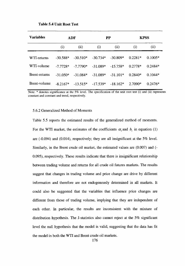
Table 5.4 Unit Root Test

Variables ADF PP KPSS

(i) (ii) (i) (ii) (i) (ii)

WTI-retums -30.588* -30.510* -30.734* -30.809* 0.2281* 0.1005*

WTI-volume -7.7728* -7.7790* -31.089* -■15.758* 0.2778* 0.2484*

Brent-retums -31.050* -31.084* -31.089* --31.101* 0.2840* 0.1044*

Brent-volume -8.2167* -13.515* -17.539* --18.162* 2.7090* 0.2476*

Note: * denotes significance at the 5 % level. The specification of the unit root test (i) and (ii) representsconstant and constant and trend, respectively.

5.6.2 Generalized Method of Moments

Table 5.5 reports the estimated results of the generalized method of moments.

For the WTI market, the estimates of the coefficients a { and b{ in equation (1)

are (-0.094) and (0.014), respectively; they are all insignificant at the 5% level.

Similarly, in the Brent crude oil market, the estimated values are (0.007) and (-

0.095), respectively. These results indicate that there is insignificant relationship

between trading volume and returns for all crude oil futures markets. The results

suggest that changes in trading volume and price change are drive by different

information and therefore are not endogenously determined in all markets. It

could also be suggested that the variables that influence price changes are

different from those of trading volume, implying that they are independent of

each other. In particular, the results are inconsistent with the mixture of

distribution hypothesis. The J-statistics also cannot reject at the 5% significant

level the null hypothesis that the model is valid, suggesting that the data has fit

the model in both the WTI and Brent crude oil markets.176

Table 5.5 Estimated Results of the Generalized Method of Moments

Coefficients WTI BRENT

1.134(0.133) -0.065(-0.016)

-0.094(-0.132) 0.007(0.014)

-0.066(-1.535) -0.083(-2.249)*

J-statistics 7.41E-42* 3.68E-42*K 4.702(8.846)* 5.654(7.349)*

b, 0.014(0.316) -0.095(-1.040)

b2 0.611(13.91)* 0.550(8.981)*

J-statistics 0.000* 3.79E-40*Note: * denotes significance at the 5 % level. The t-statistics are shown in

parentheses beside the coefficient estimate. The J-statistics test that the null hypothesis that the model is valid and are shown in parentheses below the estimated equations.

The results contradict previous studies by Kocagil and Shachmurove (1998),

who concluded that the relationship between WTI oil futures price change and

trading volume is positive. On the other hand, the findings are in line with those

of Foster (1995), who found an insignificant relationship between these variables

in his sub-sample analysis during the period 1984 to 1988 but contrast his results

of the whole sample analysis in both markets. The findings can be explains in

two ways: First, the difference of this analysis with the previous study may be

because the factors that cause the price changes are different over the study

periods. Second, the results can also suggest that the policies introduced to

regulate daily price changes would have been effective in controlling the trading

volume to responding to such movements and thus, the variables are independent

177

of each other. Overall, the results reject the mixture of distribution hypothesis in

both markets.

5.6.3 Linear Granger Causality Test

Table 5.6 presents the estimated results obtained from the Granger causality test.

Before testing the relationship between price changes and trading volume in the

oil futures markets the VAR model specified in equation (5.2) and (5.3) is first

estimated. Since the trading volume and returns series for all the markets are

stationary I (0), the unrestricted VAR in levels was estimated. The optimal lag

lengths in the VAR are selected by Akaike Information Criterion (AIC). The

estimated results cannot reject the null hypothesis of trading volume does not

cause price change in the WTI market, implying that past values of trading

volume cannot assist in predicting oil futures return; likewise, the null hypothesis

of trading volume is not cause by return cannot be rejected. Similarly, the results

for the Brent market also show that both the null hypothesis of trading volume

and returns does not causes the other cannot be rejected at the 1% level of

significant. The findings suggest that lagged trading volume does not contain any

important information that will be helpful in predicting futures returns, and the

analysis supports Clark’s (1973) mixture of distribution hypothesis, which put

forward that neither trading volume nor return can cause the other in the crude oil

futures markets.

178

Table 5.6 Estimated Results of the Granger Causality Test

Null Hypothesis Hn: F-statistics P-values Lags

WTI-volume does not cause WTI-retums 0.031* 0.861 1

WTI-retums does not cause WTI-volume 0.092** 0.761 1

Brent-volume does not cause Brent-returns 7.325** 0.120 4

Brent-returns does not cause Brent-volume 4.383** 0.357 4

Note: Lag lengths are selected based on Akaike Information Criterion (AIC) and Swartz Information Criterion (SIC). The F-statistics and P-values are shown in parenthesis. * and ** denotes in significance at 1% and 5 % levels.

However, it contradicts the sequential arrival hypothesis suggesting bi­

directional causality between trading volume and futures return, consistent with

Foster (1995) and Bhar and Hamori’s (2005) who studied the WTI market. The

findings are also in contrasts to those of Fujihara and Mougoue (1997) and

Moosa and Silvapulle (2000) whose studies cover the period 1986 to 1996, all of

which support either bi-directional or unidirectional causality between trading

volume and returns in the oil futures market. Furthermore, the results reject the

noise trader model in all the crude oil markets, contradicting Bhar and Hamori’s

(2005) who found mild evidence of noise trading activity in the WTI market.

Therefore, the analysis is in support of the market efficient hypothesis because

lagged trading volume does not contain any important information that will be

helpful in predicting future returns in all oil futures markets and thus speculators

and rational investors cannot use information about trading volume to forecast

returns. Finally, the evidence of market efficiency indicates that portfolio

179

diversification and hedging activities will be profitable across these two crude oil

futures markets.

5.6.4 Impulse Response Function and Variance Decomposition Analysis

The dynamic relationship between crude oil futures trading volume and returns is

further reinvestigated in the crude oil futures markets with the impulse response

function and variance decomposition analysis. Figures 5.2 and 5.3 illustrate the

impulse response function analyses for the WTI and Brent crude oil futures

return and their trading volume, respectively: figure 5.2 for the WTI market

indicates the insignificant impact of shock in trading volume on returns and the

results show that shock in returns cannot have any significant effect on changing

trading volume. In the Brent crude oil market, the results reported in figure 5.3

shows that shock in trading volume is insignificant in changing futures returns;

on the other hand, shock to futures returns has insignificant effect on trading

volume. These results suggest that past information about trading volume cannot

be useful in predicting returns in either the WTI or Brent markets, but that shock

on trading volume and returns are important in explaining movement in

themselves in all markets. The variance decomposition shows the percentage

movement of returns that can be explained by shock on trading volume; Table

5.7 reports the results of the generalised forecast error variance decomposition

for the WTI and Brent markets over the period of one, five and ten years. For the

WTI market, the results reported in panel A indicate the negligible impact of

trading volume on crude oil futures returns from the first to the ten year period,

implying that volume does not make a significant contribution to the forecast

variance of return. Likewise, the results in panel B for the Brent crude oil market

180

shows that trading volume does not contribute in explaining movement in

returns. Yet conversely, the results in panels A and B show that both crude oil

futures trading volume and returns are explained by movement in their own

shocks. The findings suggest that trading volume has an insignificant

contribution in forecasting returns in all the crude oil futures markets and again

confirm that there is no causal relationship between them in all markets. In

summary, the results support the analysis using the unbiasedness hypothesis and

price discovery that the WTI and Brent crude oil futures markets are efficient at

one-month maturity in the long term.

181

Response to Cholesky One S.D. Innovations ± 2 S.E.

Response of WTI-retums to WTI-retums Response of WTI-retums to WTI-volume

4-,----------------------------------------

3 -

2 -

1 -

Response of WTI-volume to WTI-retums

,3-r-------------------------------------------------------------------------------------------------

.2 -

— i-------1-------- 1--------1------- 1------- 1--------1--------1------- 1—1 2 3 4 5 6 7 8 9 10

Response of WTI-volume to WTI-volume

Figure 5.2: Impulse Response Function for the WTI Returns and Trading Volume

1 8 2

Response to Cholesky One S.D. Innovations + 2 S.E.

Response of Brent-returns to Brent-returns Response of Brent-returns to Brent-volume

Response of Brent-volume to Brent-returns Response of Brent-volume to Brent-volume

Figure 5.3: Impulse Response Function for the Brent Returns and Trading Volume

1 8 3

Table 5.7 Estimated Results of the Variance Decomposition Analysis

Panel A: Dependent variable WTI-returns Dependent variable WTI-volume

Lag Standard error Volume Returns Lag Standard error Volume Returns

1 3.110820 0.000000 100.0000 1 0.263711 99.85819 0.141807

5 3.117684 0.003379 99.99662 5 0.331813 99.80165 0.198355

10 3.117685 0.003437 99.99656 10 0.333003 99.80104 0.198964

Panel B: Dependent variable Brent-returns Dependent variable Brent-volume

Lag Standard error Volume Returns Lag Standard error Volume Returns

1 2.744223 0.000000 100.0000 1 0.327310 99.85699 0.143014

5 2.770853 0.904728 99.09527 5 0.386201 99.53177 0.468230

10 2.771236 0.927999 99.07200 10 0.399753 99.46731 0.532690

184

5.7 Summary and Conclusion

This chapter has examined the relationship between trading volume and price

change in the West Texas Intermediate and Brent crude oil futures markets from

January 2008 to May 2011, one of the most volatile periods in the history of oil

prices. It addresses the issue of whether information regarding trading volume

contributes to forecasting the magnitude of price change in the markets, an

important issue due to the ability of trading volume to predict futures price

change, thus implying market inefficiency because futures prices do not

corporate all available information. It also examines whether contemporaneous

relationship exists between price change and trading volume in the oil futures

markets. This chapter contributes to the limited literature by examining the

returns and volume relationship in the international oil futures markets, providing

findings useful to investors, speculators and policy makers who are all concerned

with the predictability of oil futures prices.

The empirical results show that there is no positive relationship between trading

volume and price change in all the crude oil markets, suggesting that trading

volume and price change are not driven by the same information flow which

contradicts the mixture of distribution hypothesis. The results of the Granger

causality test between trading volume and price change support the weak form

efficiency in all markets. These results indicate that there is no causality from

trading volume and price change, implying that trading volume cannot provide

information that can be used in predicting futures returns in all the markets, as

well as showing that there is no causality from returns to trading volume and

therefore contradicting the sequential arrival hypothesis and noise trader model.185

The results of the variance decomposition and impulse response analyses also

confirms that trading volume does not contribute to explaining movement in

prices in both markets. The implication of these results is that the two crude oil

futures markets are information efficient because trading volume cannot be

utilised in predicting oil price changes in both markets and therefore, hedging

activities will be profitable while speculative opportunities cannot be exploited.

In particular, the results show that investors would benefit from portfolio

diversification across the markets, findings which also support the view of Bhar

and Hamori (2005) who argued that the idea of regulating price fluctuation in

order to reduce the ability of trading volume to cause changes in return is not of

concern in the oil futures market.

This chapter concludes that the results support the efficient market hypothesis in

the WTI and Brent crude oil futures markets because trading volume cannot give

information that can be used to improve the short term forecast of oil returns in

all markets. The results also neither support the mixture of distribution

hypothesis because there is no positive relationship between price change and

trading volume, nor agree with the sequential arrival of information because no

causal relationship exists between the two variables in either direction. The

results also reject the noise trader model in all markets because returns cannot

predict trading volume. Finally, this chapter suggests that empirical analysis of

the relationship between price change and trade volume in international oil

markets is significant because information that can be useful in predicting prices

may flow within the markets.

186

CHAPTER SIX

Long Memory in Oil Futures Markets

6.1 Introduction

As among the world’s important strategic commodities, and due to the

vulnerability of the global economy to its price changes, investigating the

dynamic behaviour in oil price returns and volatility is crucial. Long memory is a

special form of non-linear dynamics where a time series has non-linear

dependence in its first and second moments and between distant observations,

and a predictable component that increases its forecast ability (Elder and Serletis,or

2008; Thupayagale, 2010) . It also means that a time series displays slow decay

in its autocorrelation functions (Mazaheri, 1998; Belkhouja and Boutahary,

2011) and explains the dynamic correlation structure of a time series at long lags

(Barkoulas et al, 1997; Floras, 2009). Conversely, short memory explains the

low autocorrelation in a time series which is insignificant at long lags (Barkoulas

et al, 1997; Jin and Frechette, 2004). Consequently, the existence of long

memory in oil futures price is inconsistent with efficient market hypothesis

because its autocorrelation dies slowly and therefore past information on prices

can be useful in predicting future returns.

Research in this area has utilised several statistical techniques to examine long

memory in crude oil prices. These techniques include the detrended fluctuation

analysis (DFA); rescale analysis (R/S), wavelets estimator, state space model and 35

35 Elder and Serletis (2008) show that the presences of long memory in a price series explain whether shocks decay slowly or rapidly.

187

GARCH models. However, there is no clear consensus on which method

performs best. Among the most widely used is the Generalized Autoregressive

Conditional Heteroskedasticity (GARCH) model. A number of studies supports

this in modelling and forecasting crude oil price volatility (Mohammadi and Su,

2010; Cheong, 2009; Agnolucci, 2009; Narayan and Narayan, 2007 and

Sadorsky, 2006). On the other hand, some studies have argued that the GARCH

model captures only short term persistence (or short memory) in volatility (Wei

et al, 2010; Kang et al, 2009, Tabak and Cajueiro, 2007). Further extending this

work, fractional integrated models such as the fractional integrated GARCH

(FIG ARCH); fractional integrated EG ARCH (FIEGARCH); fractional integrated

APARCH (FLAPARCH) and hyperbolic GARCH (HYGARCH) were introduced

to deal with long memory properties in time series. Recent empirical evidence

has shown that these models can capture well non-linear dependence in crude oil

prices (see Cheong, 2009; Mohammadi and Su, 2010; Wang et al, 2010;

Belkhouja and Boutahary, 2011; Wei et al, 2010).

The objective of this chapter is to investigate long memory in crude oil futures

prices as an alternative to testing market efficiency. It addresses three important

questions: Are the oil futures prices characterized by long memory properties, as

documented by previous studies such as Tabak and Cajueiro (2007), Wang et al

(2010), Cunado (2010) and Arouri et al (2011)? Do the oil futures prices display

a similar pattern across contracts? Do oil futures prices display a similar pattern

across international oil markets? This chapter contributes to the literature in the

following ways:

188

1. It investigates long memory in the West Texas Intermediate and UK

Brent markets to understand whether oil prices exhibit a similar pattern

across international oil markets, unlike previous studies which have

focused mainly on the WTI. To my knowledge only Tabak and Cajueiro

(2007) investigated long memory in the Brent oil futures market.

2. In contrast, this chapter examines long memory in crude oil futures prices

across maturities; previous studies have been concerned only with the

spot or futures prices for one-month contract. It is clear that futures

contracts for different maturities can exhibit dissimilar patterns because

they are traded for delivery on different dates.

3. It uses seven different GARCH-type models which include: GARCH,

EGARCH, APARCH, FIGARCH, FLAP ARCH, FIEGARCH and

HYGARCH to test long-term dependence in international crude oil

futures prices, in order to arrive at a strong statistical inference.

4. The analysis uses data covering eleven years of high turmoil in crude oil

prices from 2000 to 2011.

The chapter is structured as follows: Section 6.2 summarises the relevant

empirical literature on the long memory behaviour in the oil futures markets. It

also reviewed the literature in non-oil commodities to have insight on the

findings of other markets. Section 6.3 discusses the theoretical background of

long memory models in time series. Section 6.4 discusses the different methods

employed in this chapter. Section 6.5 discusses the sources, type and properties

189

of data used for this chapter. Section 6.6 presents the empirical results that were

obtained from the analysis. Section 6.7 summarises and concludes the findings.

6.2 Literature Review

This section will review the relevant empirical literature on long memory in oil

and non-oil commodity futures prices, in line with the context of the efficient

market hypothesis, and provides insight into the differing methodologies, data

frequency and findings of previous studies on the subject. This section first

explores the literature on the oil futures markets, followed by the non-oil

commodity futures markets.

6.2.1 The Oil Futures Markets

Research on long memory in oil markets has been the subject of much concern in

recent years, particularly due to the high volatility of oil prices. Among the

studies that have contributed to this area are Alvarez-Ramirez et al (2002), who

examined long term dependence in daily crude oil spot prices for WTI, Brent and

Dubai markets. The authors divided the data into three sub-periods covering

important events that affected world oil prices. Applying the Multifractal Hurst

analysis, they found that all markets exhibit persistence, with Hurst value more

than 0.5 in each series; they also found that Dubai and Brent crude oil prices

have a similar pattern in long memory behaviour. They observed that when the

analysis is conducted under a different time scale WTI show less persistence in

the short-run comparison to other crudes, but that the three crude oil prices

display similar patterns in medium and long-run time scales. They concluded that

190

the crude oil prices have long memory behaviour which contradicts the efficient

market hypothesis. Tabak and Cajueiro (2007) investigated long memory in the

WTI and Brent crude oil futures prices and volatility, using the rescaled range

hurt analysis (R/S), based on shuffling procedure, in order to deal with the

problem of short-term autocorrelation. The study focused was to determine

whether the deregulation of the crude oil futures markets of the 1990s has

improved the efficiency of these markets compared to the 1980s, a more

regulated period. By employing daily data, they found that the oil prices followed

a long memory process. They also found that in the 1980s the values of the Hurst

exponents were higher in both markets, implying that they were more efficient in

the deregulated period. In the second case, the results indicate high persistency in

price volatility, but WTI prices show more persistence than Brent, leading the

authors to conclude that the GARCH and E-GARCH models would be mis-

specified in this second case. They believed that the movement of the WTI oil

markets towards efficiency was caused by the new policies that were introduced

to improve the North American energy industry efficiency during the period.

Alvarez-Ramirez et al (2008) extended previous research by re-examining the

presence of long memory and convergence of the WTI, Brent and Dubai crude

oil markets towards efficiency using daily spot prices. They carried out their

study with their rescaled analysis based on the Detrended fluctuation approach.

The empirical results indicate that all the oil prices possess long memory in short

horizon less than 1 month because their autocorrelation dissipates at a slow

hyperbolic rate, consistent with Alvarez-Ramirez et al (2002). They observed

that when the analysis is conducted over 30 days the results show that the191

autocorrelation is reduced, implying that the oil markets efficiency have increase

over time. An interesting finding of this study is that short-term inefficiency

appears to prevail in the markets for an approximately 1.85-year cycle before the

market converges toward efficiency, allowing the conclusion that the markets are

short-term inefficient but move towards efficiency in the long term, and also

confirming the results of Tabak and Cajueiro (2007).

Additionally, Elder and Serletis (2008) tested the long term dependence

behaviour in the volatility of the energy prices for NYMEX crude oil, gasoline,

heating oil, natural gas and propane futures markets by employing the semi-

parametric wavelet-based estimator. Their analysis contrasts the previous studies

because is based on monthly futures prices. They found that the energy prices

display anti-persistence in long memory and predictability in mean, and found

that even if the estimation window is increased to 0.5, the energy price series

show evidence of anti-persistence with only propane showing infinite

persistence. In line with other research, they concluded that all the energy price

series show long term dependence, implying market inefficiency. Kang et al

(2009), building on the literature, applied the GARCH models to investigate long

memory in WTI, Brent and Dubai daily crude oil spot price volatility. First, they

used the rescale analysis; their results showed that the level of the spot returns

display long memory while volatility reveals high persistent. Second, the results

of the GARCH models indicate that the GARCH and IGARCH models were

mis-specified, as suggested by Tabak and Cajueiro (2007). However, the

CGARCH shows a high degree of persistence in the long-run and in the short-run

there is weaker volatility, while the FIGARCH model indicates persistence of192

long memory in all prices, leading Kang et al to suggest that the GARCH model

is less efficient compared to the FIGARCH and CGARCH models when

modelling oil prices’ volatility. In a similar vein, Cheong (2009) applied the

ARCH-type models in examining long memory in time-varying volatility in daily

WTI and Brent crude oil spot prices. He also examined various stylized facts,

such as asymmetric effect, volatility clustering and heavy tail innovations. The

results indicate that the volatility in the oil price exhibits high persistence in long

memory in both markets, and also found that WTI oil price show longer

persistence than Brent. Again, it was observed that WTI markets show no sign of

the leverage effect while the Brent market does, with the conclusion that the

slow decay in prices may result from two factors: First, market participants

behave differently as a consequence of the way they interpret the same

information; and second, the different responses of the market participants to

new information results in the market encountering dissimilar volatilities which

in turn lead to slow decay in the crude oil market volatility.

Furthermore, Ayadi et al (2009) in his work studied the presence of long term

dependence in Nigerian Forcados oil prices using detrended fluctuation analysis

and weekly spot prices, they found that the oil price series are characterized by a

long lasting autocorrelation structure, implying that the prices follow a non-linear

process. In their analysis, these results provide evidence of anti-persistence in

long memory of the oil prices. However, the results using the ARM A model

show that a low price level can be followed by a high price level and vice-versa,

and they suggest both that past price trends may change in the long term and that

the impact of shocks on oil prices tends to disappear in the long term, again193

consistent with Alvarez-Ramirez et al (2008) and Tabak and Cajueiro (2007).

Arouri (2010) examine the properties of weekly spot prices of four GCC crude

oil markets: Saudi Arabia, Qatar, Kuwait and the UAE using a model that is

time-varying with GARCH properties. The empirical results show that all prices

exhibit short-term autocorrelation in their returns, becoming more significant by

the end of the study period, once more consistent with Elder and Serletis (2008)

and Alvarez-Ramirez et al (2008). However, they found that the results do not

support the existence of high persistence in oil price returns volatility. They

suggest that during the 1990s the markets were weakly efficient and show no

sign of becoming efficient in the long run, and concluded that the reasons for

efficiency were associated with the cut in oil production quotas by OPEC and the

sharp drop in crude oil prices caused by the Asian crisis, while the inefficiency

resulted from a boom in the international oil markets.

Gu et al (2010) re-examined the dynamic behaviour of WTI and Brent crude oil

daily spot prices over a sample period from 1987 to 2008, in order to find

whether the international oil markets operate efficiently during the Gulf War. By

employing the multifractal detrended fluctuation analysis, their results indicate

that the oil prices are characterised by high persistence in the short-term and

weaker anti-persistence in long-term. They also observed that when the data is

divided into three subsamples the results show that the Gulf War did not change

the time scale of returns in either market; however, the results also indicate that

the Brent market shows more persistency, implying that here the impact of the

Gulf War was greater. They also pointed out that the pattern of the long memory

behaviour in the oil markets can be described as caused by factors such as194

deregulation rather than only persistency, and concluded that the international oil

markets are more efficient in the long term. Mohammadi and Su (2010), further

building on the literature, re-investigated the long term dependence in crude oil

prices of eleven markets, including oil-producers and oil-consumer countries, by

employing four GARCH-class models. They conducted their analysis using

weekly spot prices and the empirical results from all models support the

existence of time-varying volatility in oil prices, implying that they follow a long

memory process. They observed that the FIG ARCH model performs weakly in

all except one crude oil market, contradicting Kang et al (2009), and therefore

they suggest that the autocorrelation in oil price volatility dies quickly as in the

GARCH model, and not taking the form of the FIGARCH model. In their study

to investigate market efficiency in WTI daily futures prices,

Wang and Liu (2010) applied the multiscale analysis based on detrended

fluctuation analysis. They found that the WTI market exhibits long memory

persistence in the short term and anti-persistency in the medium term, while

inconsistent results were obtained in the long-term. They observed that the oil

price moves gradually from short-term inefficiency to long-term efficiency,

consistent with the results of Tabak and Cajueiro (2007) and Alvarez-Ramirez et

al (2008), but in contrast to Arouri (2010). According to the authors, the WTI

market has developed over a long time period under unstable condition, and from

this they drew the conclusion that the long-term dynamics are influenced by

demand and supply factors, while outside factors are responsible for the short­

term behaviour of the market. In the same year Wang et al (2010) re-examined

long range dependence in daily spot and futures prices volatility for WTI by195

employing the detrended fluctuation analysis (DFA), GARCH class models and

rescale analysis (R/S). Their work aimed to find whether the GARCH model can

well capture the autocorrelation in the oil price volatility, and they found

evidence supporting that all the oil prices exhibits long term dependence. They

found that the DFA and R/S indicate that a moderate persistence exists in the

short-term scale, while in the long term there is a strong degree of long memory.

They also pointed out that the difference in the level of long memory between the

two time scales results from the diversification of investment across different

trading horizons. To examine the performance of the GARCH-class models they

divided the data into four non-overlapping subperiods and the results support

long memory behaviour in oil prices over a period longer than one year; but, the

results also show that the models are mis-specified when the time scale is less

than a year. Overall, their analysis supports the findings of Mohammadi and Su

(2010) who reports that long memory can be well capture by the GARCH-class

models in the long term.

In contrast to other studies, Cunado et al (2010) examined the properties of the

energy futures markets returns and volatility, and specifically for NYMEX WTI,

heating oil, gasoline and propane, using the nonparametric, semi-parametric and

parametric procedures; the data used were daily futures prices at one and four

month contracts. They found that all the energy futures prices returns were not

long memory process at the different maturities, and also found that when the

absolute returns are proxy to volatility the results indicate support of long

memory in energy prices, with WTI having higher persistence within the

maturities. Power and Turvey (2010) also investigated long-range dependence in196

four energy (WTI crude oil, heating oil and natural gas) and eleven storable and

non-storable agricultural commodities using daily data. By applying the wavelets

estimator, it can be shown that the crude oil prices have a constant memory

parameter over the sample period. They noted that the major difference between

the results of the agricultural and energy commodities is that the former are

characterized by seasonal consumption while the latter are characterized by

seasonal production. In a similar vein, Fernandez (2010) examined long memory

in WTI and nineteen other DJ-AIG commodity futures indices, using daily

observations and five different methodologies: namely, the wavelets estimator,

the periodogram regression-based method, the Geweke and Porter-Hudak’s

approach and quasi-maximum likelihood. According to the author, when the

properties of an assets returns indicate anti-persistence or persistence, it means

that they over- or under-reaction to the new information about market price,

which is against the efficient market hypothesis in the weak-form. For the WTI

returns, the results indicate that the five methods support either anti-persistence

or persistence of long term dependence and the author also observed strong

evidence of larger persistence in absolute returns, consistent with previous

findings. He concluded that market participants can use non-linear models to

improve their short term forecast for WTI because of market inefficiency.

Belkhouja and Boutahary (2011) introduced a GARCH model that allows time-

varying in the conditional variance (TV-FIGARCH) to test volatility in crude oil

prices, accounting for structural breaks and long term dependence in the

conditional variance process. They argued that the long memory component in

the FIGARCH model may not necessarily capture the persistence that is caused197

by structural changes. Using daily data for spot prices of the WTI and S&P 500

index, they found that oil prices in the WTI market were highly volatile in the

beginning and second half of the sample period but declined by the intermediate

period. They also found that absolute returns in WTI display slow decay,

representing long memory, and that it has four structural breaks consistent with

the crisis that affected the global oil markets. They noted that the FIGARCH

model performs better than the time-varying model in explaining long range

dependence, but the out of sample forecast supports the TV-FIGARCH model,

suggesting that absolute returns are better examined by models that account for

both structural changes and long memory.

Wang et al (2011) examined autocorrelation and cross-correlation in WTI daily

spot and futures prices using detrended fluctuation analysis (DFA) and detrended

fluctuation cross correlation analysis (DFCC). The results indicate anti­

persistence in the returns under a year, while neither autocorrelation nor cross­

correlation exist in time scales longer than a year; they also found that the

autocorrelation is less than cross-correlation in a short time scale. Summarizing

their results, it is clear that the WTI market become more efficient in the long

term, supporting previous studies that applied a similar approach. They suggest

that traditional hedging strategies will be ineffective because of the strong cross­

correlation in the oil price returns. Hou and Suardi (2011) also contribute to the

literature by examining long memory in WTI and Brent daily spot prices

volatility using the parametric and nonparametric GARCH models. The model

measures the unobserved diffusion process in returns using additive functions of

lagged innovation and volatilities. The results indicate persistence in oil prices,198

and that models with long-range dependence are statistically significant in the

markets. In contrast to Mohammadi and Su (2010), the results support the

hypothesis that the FIGARCH model performs better than others in modelling

long memory consistent with Kang et al (2009). They observed that the non-

parametric GARCH model fails to capture long memory in the oil returns prices,

but in the out of sample analysis, the results indicate its improved forecast ability

over the parametric GARCH models. They suggest the use of nonparametric

GARCH models as an alternative in studying crude oil price volatility.

Finally, Arouri et al (2012) reinvestigated the significance of structural breaks

and long-term dependence in modelling daily energy spot and futures prices

volatility for NYMEX WTI crude oil, gasoline and heating oil at one and two-

month contracts to maturities, using the GARCH-type models. They found that

all the oil prices follow a long memory process, and observed that, after

accounting for the possible structural breaks; the degree of persistency in

volatility is reduced, implying that the GARCH model does not account for the

possible structural changes that occurred in the price series. The results also

show that the FIGARCH model performs well in modelling the long memory

properties of the oil prices. Next, they conducted the out of sample forecast

using other models, such as the Guassian semiparametric, Geweke and Porter-

Hudak and Exact maximum likelihood tests. They found that the results of the

FIGARCH model with a break explain long memory in oil prices volatility better

than the other model in the existence of structural changes.

199

Table 6.1 Summary of Previous Results on Long Memory in the Oil Futures Market

Author (s) and Years Data and Market Methods Results

Alvarez-Ramirez et al (2002)WTI, Brent, and Dubai daily spot prices from 1981 to 2002 Multifractal analysis

Long memory exists in all the prices in the long term and less persistence in the short term.

Tabak and Cajueiro (2007)WTI and Brent daily futures prices from 1983 to 2004 Rescaled Range analysis (R/S)

Long memory exists in all the prices.

Alvarez-Ramirez et al (2008)WTI, Brent and Dubai daily spot prices from 1987 to 2007 Rescaled Range analysis (R/S)

Long memory exists in the short term horizon less than one month and the markets moves towards efficiency in the long term.

Elders and Serletis (2008)WTI monthly spot price from 1994 to 2005 Wavelet Estimator

The price show anti-persistence in the long term.

Kang et al (2009)WTI, Brent and Dubai daily spot prices from 1992 to 2006 GARCH-class models Long memory exists in all prices.

Cheong(2009)WTI and Brent daily spot prices from 1993 to 2008 GARCH- class models

Long memory persists in all prices but WTI show high degree of persistence than Brent.

Ayadi et al (2009)Nigerian Farcados weekly spot price from 1978 to 2007 Detrended fluctuation analysis

Long memory exists in the price but disappears in the long run.

Arouri (2010)Four GCC daily spot prices State space model / Kalman filter Long memory exists with no

200

from 1997 to 2010 with GARCH effects evidence of converging towards efficiency in the long term.

Gui et al (2010)WTI and Brent daily spot prices from 1987 to 2008

Multifractal Detrended fluctuation analysis

Evidence of high persistence in the short-term and weaker anti­persistence in long-term. The Brent market also shows high persistence than WTI.

Mohammadi and Su (2010)

Weekly data for eleven oil­importing and exporting- countries from 1997 to 2008 GARCH-class models

Long term dependence present in all prices.

Wang et al (2010)WTI daily spot price from 1990 to 2009

Multiscaled detrended fluctuation analysis (MDFA)

Long memory in WTI price but die in the long run.

Wang et al (2010)WTI daily spot and futures prices from 1990 to 2009

MDFA, GARCH models and R/S analysis

Long term dependence exists in all the prices.

Cunado et al (2010)

WTI daily futures prices at one and four month contracts from 1983 to 2008

Nonparametric, semi-parametric and parametric procedures Long memory present in WTI price.

Power and Turvey (2010)WTI daily spot price from 1990 to 2008 Wavelet estimator Long memory exists in WTI price.

Fernandez (2010)WTI daily spot price from 1991 to 2008

Wavelets, periodogram regression, Geweke-Porter-Hudak’s and quasi maximum likelihood

Evidence of high degree of persistence in absolute returns.

Belkhouja and Boutahary WTI daily spot price fromTV- FIGARCH model Long memory exists in WTI price.

201

(2011) 1990 to 1999

Wang etal (2011)WTI daily spot price from 1990 to 2010

Detrended fluctuation analysis (DFA) and detrended fluctuation cross correlation analysis (DFCC)

Presence of long memory in WTI price in period less than a year and the market move towards efficiency in the long term.

Hou and Suardi (2011)WTI and Brent daily spot prices from 1992 to 2010

The parametric and nonparametric GARCH models

Long term dependence exists in all the oil prices.

Arouri et al (2012)

WTI daily spot and futures prices at 1 and 2 maturities 1986 to 2007 GARCH-type models Long memory exists in all prices.

202

To summarise, the above review shows that long memory in oil prices has been

studied extensively. Table 6.1 presents a summary of previous findings in the oil

markets. It is clear that crude oil prices are characterised by long-term

dependence, violating the argument of the weak form efficient hypothesis

because past returns can be used to forecast current future prices. Secondly, the

majority of the research show that the long-term dependence in oil prices is

driven by factors such as the activities of different groups of agents operating in

the oil markets, the way in which these agents perceive new information, and

supply and demand factors, among others. Third, most studies are devoted to

the oil spot market and NYMEX WTI futures market at one month contracts.

Finally, research in this field employs a variety of models, techniques and data

for different frequencies to test long-term dependence in oil prices.

6.2.2 The Non-oil Commodity Markets

In this section, the literature on long memory in the non-oil commodity markets

is reviewed to enable a better understanding of the area. In their study, Fang et al

(1994) examined long-term dependence in five currency (British pound, Japanese

yen, German mark and Swiss franc) futures markets using the Geweke-Porter-

Hudak (GPH) semi-non parametric procedure and data are daily closing prices.

Before conducting their analysis they first applied the autoregressive models and

ARCH model to test the price series properties, and found that the futures returns

indicate no significant autocorrelation but do reveal the presence of

heteroskedasticity in each of the prices. As a result, they suggest that the test for

fractional process should account for heteroskedasticity in order to arrive at more

reliable estimates. Their analysis with GPH provides support that all the currency203

futures prices except the British pound show long-range dependence fractional

process, and therefore they suggest that currency futures prices exhibit long-term

dependence. In a similar vein, Barkoulas et al (1997) investigated long memory

in twenty-one commodity markets including agriculture, metals, petroleum and

the UNTCAD index by applying the Geweke and Porter-Hudex; the data for their

analysis included monthly spot prices. The authors argued for the use of monthly

observations because they can provide information about the long memory

behaviour of commodity prices in both the short- and long-term. They found that

six of the commodities’ returns display long memory, while the others displayed

different patterns even though the PP and KPSS unit root tests indicate that they

are non-stationary process. These results are further confirmed by the ARMA

model and consequently the authors suggested the use of different methods in

testing long memory in commodity prices in order to arrive at a strong inference.

They also suggested that the idea of taking the difference of the data series may

not be the best way of modelling the commodity price behaviour, as according to

the authors’ view, long memory in spot prices implies that the market

inefficiency may represent the fundamental factors underlying the prices, which

can be attributed by commodity market processes with long-term dependence.

Extending the previous work, Panas (2001) tested long memory in six metals:

lead, aluminium, tin, copper, zinc and nickel, traded on the London metals

exchange. By applying the rescaled range analysis and daily futures prices, the

results support the existence of long-range dependence in all the metals futures

returns series. Furthermore, the results obtained using modified R/S analysis

also indicates that the commodities, with the exception of aluminium, have a204

short memory structure. To confirm their results they applied the autoregressive

fractionally integrated moving average model (ARFIMA) and found that the

returns of lead and nickel provided evidence for short-term memory, aluminium

and copper showed long memory while zinc and tin possessed anti-persistent

process. They interpret this as strong evidence of long-range dependence in

aluminium and copper, consistent with Barkoulas et al (1997) and concluded that

the metals futures markets are weak form efficient, although this does not hold

for all commodities. In contrast, Jin and Frechette (2004) contributed to the

literature by applying the FIGARCH model to investigate short memory and long

memory in the agricultural futures markets. They conducted their analysis using

daily closing futures prices for 14 commodities including meats, soft

commodities and grains, calculating the return series by dividing the settlement

prices with their lag values. The log returns were assumed to be zero in order to

produce valid results regarding price volatility. They found that all the

agricultural commodities display long-term memory, results confirmed by the

modified rescale analysis, which shows that the prices disconfirm the weak form

efficient hypothesis. They suggested that the FIGARCH model performs better

than the GARCH model in explaining long-term memory in all except one

commodity futures market.

Elders and Jin (2007) continued research in this area by re-examining long-range

dependence in 14 agricultural commodity futures returns volatility, using the

wavelet estimator. They modelled volatility using compounded daily returns

calculated by taking the difference of the current price and previous period. They

found that the predictability of the conditional mean is not consistent with the205

conditional volatility specification, and thus constructs volatility using absolute

returns. The findings showed that some of the commodity futures returns are

volatile but all display a high degree of persistence (long memory) in the returns

series. Elders and Jin also applied the GARCH, FIGARCH and GPH: the results

were consistent with Jin and Frechette (2004) and Barkoulas et al (1997).

Additionally, Bailie et al (2007) estimated the long memory in six US

commodities: com, soybeans, cattle, hogs, gasoline and gold futures returns

volatility, applying the FIGARCH and semi parametric Local Whittles (LW)

estimation to daily and intraday high frequency observations. They argued that

the presence of long memory in data for different frequencies implies that the

series are self-similar and provide more consistent estimates; in particular, their

results support that the commodities display long memory in their returns

volatility at both frequencies, however, the estimated value of the intraday

returns is little higher than that of daily returns. The semi-parametric Local

Whittles (LW) estimation was then applied to absolute returns and the results

indicate that both the daily and intraday returns exhibits long memory features,

leading to the conclusion that the finding of long memory in different sampling

frequencies implies long-term dependence is inherent in the features of the

commodity returns and does not arise from shocks or regime shifts.

Floras (2009) using the ARFIMA models investigated long memory in monthly

spot prices for fifteen EU milk prices. The empirical results support the existence

of long-range dependence in prices for twelve out of fifteen European countries,

implying that shock persists over a long time period, making them predictable,

results consistent with Bailie et al (2007) and others. Floras also found that the206

persistence in long memory is larger in the countries with high milk

consumption, and he concluded that the market for EU milk is inefficient

because past information on prices can be used in making future decisions.

Tansuchat et al (2009) also studied long-term dependence in sixteen agricultural

commodity futures markets returns using the seven different GARCH models.

By employing daily futures prices, they discovered that almost all of these prices

are characterised by long term dependence. In line with Jin and Frechette (2004),

the results indicate that the FIGARCH and FIEGARCH models out-performed

the traditional GARCH and EGARCH models in explaining long memory

behaviour in oil price.

Arouri et al (2012), further building on the literature, investigated the long term

dependence and structural breaks in the metal markets by employing the

parametric and non-parametric models. They conducted their analysis using daily

spot and three-month futures prices for four metals including: silver, gold,

platinum and palladium. The results show that both the returns and volatility of

all the metals display long memory, results confirmed by the ARFIMA-GARCH

model, which shows that the prices disconfirm the weak form efficient

hypothesis. They also found that even after accounting for the structural changes

in the prices, the results still confirm persistence in these markets. They suggest

that the conditional returns volatility of these markets can best be described by

long term dependence rather than structural breaks.

207

Table 6.2 Summary of Previous Results on Long memory in the Non-oil Commodity Futures Markets

Author(s) and Years Data and Market Methods Results

Fang et al (1994)

Four currencies: British pound, German mark, Japanese yen and Swiss franc daily futures prices from 1982 to 1991

Geweke-Porter-Hudak semi parametric method

Long memory exists in all the currencies prices.

Barkoulas et al (1997)21 commodity markets monthly futures prices from 1960 to 1994

Geweke-Porter-Hudak semi parametric method

Long memory exists in all the commodity prices.

Panas(2001)

Six metals: aluminium, copper, lead, tin, nickel and zinc daily futures prices from 1989 to 2000 Rescaled Range analysis

Two of the metals exhibit short- memory, two shows anti-persistence and two indicates long memory.

Jin and Frechette (2004)Seven US grains daily futures prices from 1994 to 2003 FIGARCH model

All the prices display long term dependence.

Elders and Jin (2007)

US 14 agricultural commodity daily futures prices from 1980 to 1990 Wavelet estimator

All the prices show high degree of persistence.

Bailie et al (2007)

Six commodities daily and intraday futures prices from 1980 to 1990

FIGARCH models and semi- parametric local Whittles estimator

Long memory exists in all the commodities prices.

Floros et al (2009) Fifteen European countries Milk monthly spot prices from 2001 to

ARFIMA model Long memory in all the prices but the countries with high consumption

208

2008 indicates more persistence.

Arouri et al (2012)

Four metals silver, gold, platinum and palladium daily spot and three-month futures prices from 1999 to 2011

Geweke-Porter-Hudak semi parametric method, Robinson Hendry method, Sowell maximum likelihood test, ARFIMA-FIGARCH model.

All the prices possess long memory process.

209

Overall, Table 6.2 shows how long memory was investigated in a variety of

commodity markets. In general, both the oil and non-oil commodity markets show

evidence of long memory in either their absolute returns or volatility, results which

oppose the weak form efficient market hypothesis. Moreover, these studies examine

long memory using both the same techniques and data for the same frequencies. It is

clear that there is no single model that has been agreed to best capture long memory

in commodity prices.

6.3 Theoretical Background of Long Memory Models

Most economic and financial theories postulate that the price of an asset is expected

to exhibit long-range dependence rather than to follow a random walk process36.

Long memory in time series was first investigated by Hurst (1951), a hydrologist

who analysed 600 years of data on the annual minimum flow of the Nile. In his work

Granger (1966) also showed that the majority of economic variables have “typical

spectral shape”; because of their low-frequency component the long term fluctuation

decreases smoothly over a longer period37. Maldelbort and Wallis (1968) named this

feature the “Joseph Effect”, based on an Old Testament prophet who foretold that

Egypt would experience seven years of plenty after seven years of famine. They

argued that “a long period of unusual (high or low) participation can be extremely

long”. Therefore, long memory describes the low power in time series, such that

correlation of information disappears over a long-term period. In line with these

36 Foo (2009) shows that stock prices follow a Brownian process where prices change randomly and are independent from each other.

37 “The law of typical spectral shape states that the long-term fluctuations in economic variables, if decomposed into frequency components, are such that the amplitudes of the components decrease smoothly with decreasing periods” (see Granger, 1966).

210

arguments, many studies have introduced different procedures that can be applied to

examine long memory (persistence) in financial time series, among which are the

fractional integrated models (see Maldelbort 1971; Granger and Joyeux, 1980;

Hosking, 1981). Fractional integration can be defined as a condition where a time

series is assumed to be either stationary (integrated of order zero) or non-stationary

(integrated of order one) (Elder and Jin, 2007). The presence of fractal structure in an

asset price indicates that the series is characterised by irregular cyclical changes and

long term dependence (Elder and Jin, 2007). Thupayagale (2010) also argued that a

time series with fractional integrated processes display persistent, mean reversion

and therefore differs from non-stationary and stationary processes. Hence, a

stationary time series rt display long memory when its autocorrelation functions is

non-negative and decay at slow hyperbolic rate, so that

Pk ~ c k 2d- 1

where p k is the autocorrelation function, A: is the number of lag which is

infinite, cis a constant and d is the parameter that captures the long memory

properties in the time series. In contrast, the autocorrelation function of stationary

time series takes the form p k ~ |<J|*, where |<£| < 1 so that the persistence dissipates at

a fast exponential rate (Tansuchat et al, 2009). The more recent fractional integrated

models such as the FIGARCH, FIEGARCH, FIAPARCH and HYGARCH

developed to capture volatility in conditional variance assumed that rt is a long

memory process when 0 < d < 1. Following Thupayagale (2010), Foo (2009) among

others this chapter investigates the Efficient Market Hypothesis by testing both the

211

short and long memory behaviour of the crude oil futures returns using fractional

integration methods.

6.4 Empirical Methodology

6.4.1 GARCH Model

The generalized autoregressive conditional heteroskedasticity (GARCH) model was

introduced by Bollerslev (1986) as an extension of ARCH model where the current

conditional variance depend on its own lagged values and the variance includes both

autoregressive and moving average elements. Also, the autocorrelation in volatility

(long memory) disappear at slow exponential rate. The GARCH (1,1) model for the

oil futures returns can be written as follows:

rt= M t+£t

where, £t ly /t ~ iid N{0,<Jt)

(6. 1)

O-2, = W+ / ? < , + « £ , (62)

where ^represents the dependent variable which is returns, jut is the conditional

mean, e t is the error term which is assume to have zero mean, constant variance and

independently distributed, y/ capture all information at time t - 1, of is the

conditional variance, to is the unconditional mean value which is constant, a]_x is

the GARCH term which capture information on the past forecast error variance,

e]_x is the ARCH term which capture information on volatility from the past period.

Bollerslev (1986) shows that the parameters a and p are expected to be positive

212

with the restrictions co > 0, a > 0, p > 0 to ensure positive conditional variance. The

sum of the parameters a + p measures the persistence of shock on volatility. If the

parameter a + p > 1, shock to volatility would be unstable while a + P = 1 imply that

volatility is permanent and unconditional variance is infinite representing the

Integrated GARCH model (IGARCH) (see Thupayagale, 2010). However, the

IGARCH model does not fit in modelling long memory because shock on volatility

never dies out (Kang et al, 2009).

6.4.2 EGARCH Model

The exponential GARCH (EGARCH) model was proposed by Nelson (1996) in

order to account for the asymmetric response of the conditional variance to both

positive and negative shocks. This model also assumes non-negativity in the

parameters of the conditional volatility. The conditional variance of the EGARCH (1,

1) model takes the following form:

where, y is the parameter that captures the asymmetric effect of shock to

conditional variance. The model becomes GARCH (1, 1) wheny - 0 , y < 0 implies

that positive shock leads to less volatility than negative shock while y > 0 is the

reverse condition of high volatility than negative shock (Mohammadi and Su, 2011).

6.4.3 APARCH Model

The asymmetric power autoregressive conditional heteroskedasticity (APARCH)

(6.3)

model was developed by Ding et al (1993) to capture asymmetric effect of shock to213

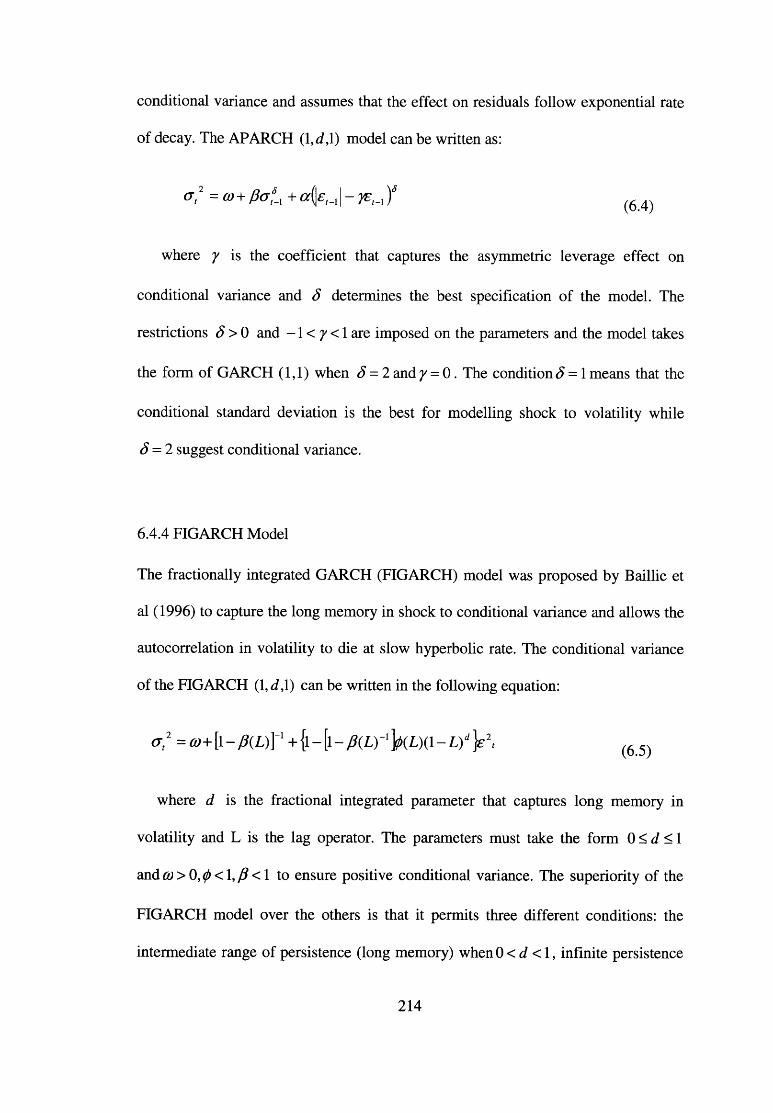
conditional variance and assumes that the effect on residuals follow exponential rate

of decay. The APARCH (l,d,l) model can be written as:

a ,2 = co + P a l , + a(\el (6.4)

where y is the coefficient that captures the asymmetric leverage effect on

conditional variance and 8 determines the best specification of the model. The

restrictions 8 > 0 and -1 < y < 1 are imposed on the parameters and the model takes

the form of GARCH (1,1) when 8 = 2 and y = 0. The condition 8 = 1 means that the

conditional standard deviation is the best for modelling shock to volatility while

8 = 2 suggest conditional variance.

6.4.4 FIGARCH Model

The fractionally integrated GARCH (FIGARCH) model was proposed by Baillie et

al (1996) to capture the long memory in shock to conditional variance and allows the

autocorrelation in volatility to die at slow hyperbolic rate. The conditional variance

of the FIGARCH can be written in the following equation:

where d is the fractional integrated parameter that captures long memory in

volatility and L is the lag operator. The parameters must take the form 0 < d < 1

and co > 0,0 < 1,/? < 1 to ensure positive conditional variance. The superiority of the

FIGARCH model over the others is that it permits three different conditions: the

intermediate range of persistence (long memory) when 0 < d < 1, infinite persistence

2 = «+[l - + {l - [l - P(L)-' \>(L)(\- L)d y , (6.5)

214

when d = 1 and geometric decay when d >138. Bailie et al (1996) suggest that this

model is strictly stationary process whenO < d < 1.

6.4.5 FIEGARCH Model

The fractional integrated EGARCH (FIEGARCH) model was introduced by

Bollerslev and Mikkelsen (1996) an extension of the EGARCH to capture both

asymmetric response of shock and long memory in the conditional variance. In this

model the parameters of the conditional variance can be negative not as in the case of

FIG ARCH model. The conditional variance of the FIEGARCH model can be written

as:

liu r ,2 = a + m ~ ' ^ - L ) - d[\ + W(L)\g,(zl-i ) ( 6 6 )

where d is the long memory parameter. The model becomes EGARCH

whend=0, stationary when d < 0.5 andgr <°o and d < 1 means that shock on

conditional volatility decay at slow hyperbolic rate.

6.4.6 FIAPARCH Model

The fractional integrated APARCH (FIAPARCH) model of Tse (1998) was proposed

to capture the long memory persistence and asymmetric effect of shock on

conditional volatility. The FIAPARCH also permits the effects on the residuals to

follow a long memory process. The FIAPARCH (1, d,l) model can be written as:

38 Mohammadi and Su (2010) show that the condition when d = 1 and d = 0 implies existence of short memory and long memory in the conditional volatility, respectively.

215

(6.7)a ,2 = 0) + [1 - p ( L ) \ ' + {l - [l - /?(!)-' \>(L)( 1 - L)" )je, | - je, )*

where 0 < d <1 ,co> 0,S > 0 ,(p ,fi<1 and -1 < y < 1. The parameter d captures

the long memory properties. The FIAPARCH model becomes APARCH model

when d = 0 and FIGARCH when 6 = 2 and y = 0.

6.4.7 HYGARCH Model

Davidson (2004) developed the hyperbolic GARCH (HYGARCH) model as an

extension to the FIGARCH is more powerful in investigating long memory in

conditional variance. Davidson argued that FIGARCH model is more of a “knife-

edge-nonstationary” class because it account for restriction that is applied to models

of level. The length of long memory increases here as d approaches zero. The

conditional variance of the HYGARCH model can be written as:

<T,2 =a>+[l-P(L)Y + {l-[l-at.)-1 k w + *)[((!-•£->" - i)k 2< (6 8)

where the parameters restriction 0 < d < \,O )> 0 ,k > 0 ,(p ,j3 < l are expected. The

HYGARCH model becomes GARCH whend = 0, FIGARCH when/: = 1, IGARCH

when d = 1 and/: = 1, nonstationary k > 1 and stationary k < l(see Davidson 2004).

6.5 Data and its Properties

This chapter used daily closing futures prices for West Texas Intermediate and Brent

crude oil at one and three-month contracts to maturities. Data for WTI were sourced

from the Energy Information Administration U.S, while that of Brent were obtained

from the Data Stream and Maslyuk and Smyth (2008). Both WTI and Brent oil216

futures prices are in US dollars per barrel. The data used starts from 3 January 2000

and ends 5 May 2011, a total number of 2838 observations for the price series in

each market. The sample used covers some of the important events that influence

recent fluctuation in oil price. First, the period of high volatility that followed the

September 11, 2001 events. Second, the period before and after Iraqi war between

2003 and 2005. Third, period during which oil price reached highest level ever $145

per barrel in 2008 and finally, period of political instability and unrest in Arab

countries in 2011. All the oil futures price series are converted into log returns series

calculated as rt =log{pt l /?M)xl00, where rt is the futures return, p t is the current

futures price and p tA is lagged futures price for one period as in Kang et al (2009)

Mohammadi and Su (2010) and Wang et al (2010). Following Bailie et al, 2007, this

chapter used absolute returns instead of squared returns to model long memory in oil

prices because it can provide strong inference on the autocorrelation structures of

returns volatility. This chapter used the following notations: WTI-C1, WTI-C3,

Brent-Cl and Brent-C3 to denote WTI and Brent futures prices at one and three-

month contract, respectively.

Table 6.3 Descriptive Statistics for Crude Oil futures returns

Statistics WTI-C1 WTI-C3 Brent-Cl Brent-C3Mean 0.047958 0.050543 0.052725 0.055144

Maximum 14.54637 13.54551 18.12974 12.70660

Minimum -16.54451 -12.7431 -16.83201 -13.07298

Std. Dev. 2.442167 2.321836 -2.137847 2.164592

Skewness -0.368575 -0.124603 -0.204659 -0.251373

KurtosisJarque-Bera Prob

6.2605681320.9(0.0)

6.8271061738.7(0.0)

7.0647131972.8(0.0)

6.1084381172.0(0.0)

Note: Figures in brackets are probability values for the normality test.217

R e t u r n s

wn-ci wn-c3

P ri c e s ( $ )

P r i c e s ($ )ro co co cnb o h o o> o b o h o

WTI-Cl WTI-G

B r e n t-C l Bren t-C 3

^ Brent-03

Figure 6.1: Daily WTI and Brent Crude Oil Prices and Returns, January 2000- May 2011

219

Table 6.3 presents the descriptive statistics for daily oil futures returns. This reports

the mean, maximum, minimum, standard deviation, skewness; Kurtosis and Jarque-

Bera probability for each of the oil futures returns. The results show that the crude oil

markets have mean lower than the standard deviation but that of Brent is higher in all

maturities. All the crude oil futures returns series have high kurtosis greater than 3,

implying that they are leptokurtic. The returns series show negative skewness,

suggesting that the markets are characterised with fatter tail than the normal

distribution. Also, the oil prices exhibits longer left tail, indicating that the oil

markets experience heavy losses during the study period. For the normality test, the

Jarque-Bera probability test indicates that all the oil futures returns are not normally

distributed. Figure 6.1 plots the daily crude oil futures prices and returns series. The

plot illustrate that the two oil markets experience high fluctuation and jumps

particularly in the years 2008 and 2011. Their returns series also appears to revert to

their mean, implying that they may possess long memory properties.

6.6 Empirical Results

This section provides analysis of the results obtained using the different techniques

discussed in the previous section. First, the stochastic properties of the daily crude oil

futures returns are determine using the unit root test (see chapter 3 for explanation of

the unit root tests). Secondly, the generalized conditional heteroskedasticity models

are used to examine whether the oil futures returns have evidence of long memory

properties.

220

6.6.1 Unit root tests

Two unit root tests are used to examine the order of integration of the oil futures

prices series: the Augmented Dickey-Fuller and Kwiatkowski, Phillips, Schmidt and

Shin. Table 6.4 reports the results of the unit root tests undertaken using two

different specifications: with constant and with constant and trend. The optimal lag

length for the ADF and KPSS is selected by the Schwarz Information Criterion (SIC)

and Bartlett kernel, respectively. The ADF tests for the two specifications show that

all the return series do not contain a unit root, implying that they are stationary. The

KPSS test results also show that the oil returns are non-stationary series at the 5%

significant level in both specifications. Both unit root tests therefore indicate that all

the oil returns series can be used in analysis without any further transformation.

Table 6.4 Unit Root Test

Variables ADF KPSS

(i) (ii) (i) (ii)

WTI-C1 -54.32* -54.31* 0.040* 0.041*

WTI-C3 -52.63* -52.63* 0.042* 0.042*

Brent-Cl -55.41* -55.40* 0.050* 0.046*

Brent-C3 -56.04* -56.03* 0.052* 0.052*

Note: * denotes significance at the 5% level. The specification of the unit root test (i) and (ii) represents constant and constant and trend, respectively.

6.6.2 Results of the GARCH Model

Since the descriptive statistics of the crude oil futures returns series indicates

evidence of non-normality, this chapter proceed to estimate the seven different

GARCH models discussed in section 5.4. The results of the conditional mean and

221

variance equations for the WTI and Brent crude oil markets estimated from these

models, along with their diagnostic tests, are reported in Table for each model. Table

6.5 reports that the estimated results obtained from the GARCH (1, 1) model show

that the parameters for the conditional variance equation a and /? are significant

and positive in the two crude oil markets at the different contracts, results which

indicate that the model observes positive constraint restrictions. The estimates of the

measure of persistence parameter a + {3 are approximately the same and very close

to unity in all the markets within the maturities. In the WTI market, the results

demonstrate that the values are 0.985 and 0.977 at one and three-month contracts,

respectively. Similarly, in the Brent market the results show the value of 0.988 and

0.980 in the maturities respectively. These findings show that the crude oil futures

markets exhibit high persistence in their returns which suggest long memory, results

consistent with those of Arouri et al (2012) and Wang et al (2010) who studied the

WTI futures market. It can be seen that the oil futures returns possess long memory

even though the autocorrelation disappears at a slow exponential rate over time.

Table 6.5 also reported that the results of the diagnostic tests using the Box-piers test

and ARCH test show the absences of serial correlation and heteroskedasticity in the

WTI and Brent markets at the different maturities, respectively.

6.6.3 Results of the EGARCH Model

Table 6.6 presents the estimated results of the EGARCH model for the crude oil

futures markets. The estimates of the conditional variance equation indicate that a

and J3 are significant at the 5% level and there sum a + J3 is greater than unity in

both WTI and Brent markets at the different maturities. The values reported are

222

between 1.128 and 1.493 across the markets and maturities, implying permanent

persistence in the returns series and supporting Wang et al (2010), who studied WTI

at one-month contract. At the same time, this results means that the EGARCH have

taken the form of IGARCH model (Wang, 2003). The results show that the

coefficient of asymmetry, y , are different from zero and significant with values

between 0.103 and 0.191 across the markets and maturities, implying that the

response of the oil futures price returns to positive shock is followed by high

volatility than negative shock of the same amount. The results therefore support the

presence of asymmetric leverage effect and long memory in the WTI and Brent

markets. The results of the diagnostic tests using the Box-piers test on the

standardized residual show no serial correlation and the ARCH test also reject

heteroskedasticity in both markets at the different maturities.

6.6.4 Results of the APARCH Model

Table 6.7 reports the results of the APARCH model for the crude oil futures markets.

The results indicate that the estimates of the power parameter 8 which select the

best specification for modelling oil futures returns for the WTI market are 1.249 and

1.283, while in the Brent market the values reported are higher, with 8 equalling

1.687 and 1.452 at one and three-month contract, respectively. These results cannot

reject the null hypothesis of 8 = 1 at the 5% significant level in all the markets,

suggesting that their returns are better investigated with conditional standard

deviation which supports the presence of long memory. Furthermore, the results

indicate that the estimates of the asymmetric parameter y are between 0.316 and

0.939 across the markets and maturities. These results provide strong evidence of a

leverage effect in the WTI and Brent market and thus supporting the EGARCH223

model. The results of the diagnostic tests using the Box-piers test on the standardized

residual reject serial correlation and the ARCH test also reject heteroskedasticity in

both WTI and Brent markets at the different maturities.

6.6.5 Results of the FIGARCH Model

Table 6.8 reports the results of the FIGARCH model for the crude oil futures

markets. The estimated results show that the values of the parameters for the

conditional variance equation are all significant and positive, indicating that the

model observes its positive constraint restrictions in all the markets. The estimates of

the long memory parameters d show that the fractional integrated coefficient is

different from zero and significant in all markets. In the WTI market, the values are

0.408 and 0.406 at one and three-month contract respectively, results consistent with

Arouri et al (2012) and Wang et al (2010). In the Brent market, the results reported

that the long memory parameter show the values of 0.474 and 0.372 at one and three-

month contract respectively. These suggest that the crude oil futures returns for both

markets have long memory in their conditional volatility at the different maturities,

which is against the efficient market hypothesis in the weak form. The results also

fail to support the hypothesis of d = 0 and d = 1, implying that the FIGARCH model

does not reduce to either the IGARCH or GARCH model in both markets. The

results support Tabak and Cajueiro (2007) and Cunado et al (2010) that reported long

memory in these markets using a different approach and thus show that previous

information about oil futures price can help predict future returns in the WTI and

Brent markets. The Box-piers diagnostic test on the standardized residual show no

serial correlation and the ARCH test also reject heteroskedasticity in all markets

within the maturities.

224

6.6.6 Results of the FffiGARCH Model

Table 6.9 presents the results of the FIEGARCH model estimated for the WTI and

Brent crude oil futures markets. The results indicate that the asymmetric parameter y

is significant and non-zero in all the markets supporting the EGARCH and APARCH

models. The estimated values are between 0.201 and 0.216 across the markets and

maturities, suggesting that the response of the oil futures returns to positive shock is

followed by high volatility than negative shock of the same amount. The results also

show that the values of the d parameter for long memory vary between 0.576 and

0.728 across the two oil markets and maturities, indicating that the oil futures returns

have autocorrelation which disappears at a slow rate. However, the results show that

the WTI market has larger persistence than Brent at one-month contract consistent

with Tabak and Cajueiro (2007), while the reverse is the case at three-month

contract. The results indicate that the returns for both markets can be predictable

using their past values which support the FIGARCH model. The diagnostic tests

using the Box-piers test on the standardized residual reject serial correlation and the

ARCH test reject heteroskedasticity in the WTI and Brent markets at the different

maturities.

6.6.7 Results of the FLAP ARCH Model

The results of the FLAP ARCH model for the crude oil futures markets are reported in

Table 6.10. The estimated results show that the value of the power parameter 8

which chooses the best specification for modelling oil futures returns are

approximately the same with that of the APARCH model in the two oil markets. The

results reports that the values are between 1.241 and 1.707 across the markets and

maturities which reject the null hypothesis of 8 = 1 in the markets, suggesting that225

returns are better investigated with conditional standard deviation. The findings are

consistent with Ding et al (1993) who show that such case provides evidence that the

returns possess long memory because the correlation between the squared returns is

less than absolute returns. The results also indicate that the long memory parameter d

has the values between 0.398 and 0.512 across the markets and maturities, implying

that the crude oil futures returns are predictable which reject the efficient market

hypothesis. These suggest that portfolio diversification across the two markets and

within the maturities would not be profitable because they all exhibit similar features.

The results of the diagnostic tests using the Box-piers test on the standardized

residual reject serial correlation and the ARCH test reject heteroskedasticity in both

the WTI and Brent markets at the different maturities.

6.6.8 Results of the HYGARCH Model

The estimated results of the HYGARCH model for the crude oil futures markets are

presented in Table 6.11. The results indicate that the coefficient of the long memory

parameters d is different from zero and significant in all the markets within the

maturities. The estimated values reported are 0.569 and 0.955 in the WTI market

while for Brent are 0.626 and 0.599 at one-month and three-month contract

respectively. These results indicate that the crude oil futures returns have long

memory in their autocorrelation which disappear slowing over time in all the markets

and maturities. Although to my knowledge there is no study that applied the

HYGARCH model to crude oil futures markets, the findings are similar with those of

Hou and Saurdi (2011) and Wei et al (2010) in the oil spot market. These results

support the FIGARCH, FLAP ARCH and FIEGARCH model that the crude oil

futures returns possess long memory behaviour in all the markets. These suggest that

226

the markets will have low returns in the long term because their future prices are

predictable and as a result, speculators profit more because they can take advantage

of market opportunities. Thus, both the WTI and Brent markets have a similar pattern

of long-term dependence in their returns, proving weak form inefficiency in the long

term. Lastly, the results of the diagnostic test using the Box-piers test and ARCH test

for serial correlation conducted confirm the fitness of the model. The Box-piers tests

show that the standardised residuals of the crude oil futures prices are not serially

correlated in all markets and maturities. The ARCH test also on the standardised

residuals for the 10th order serial correlation indicate that the oil prices are

homoskedastic in the two markets at the 1% level; results which suggest the absence

of serial correlation on the residuals of the two crude oil futures return series.

227

Table 6.5 Estimated Results of the GARCH Model

WTI-C1 WTI-C3 Brent-Cl Brent-C3

0.094** 0.100* 0.108* 0.104*M (0.041) (0.039) (0.039) (0.036)

0.090** 0.110* 0.067* 0.083*CO (0.050) (0.043) (0.029) (0.040)

0.053* 0.059* 0.050* 0.050*a (0.019) (0.016) (0.012) (0.015)

p0.932* 0.918* 0.938* 0.930*(0.025) (0.022) (0.015) (0.022)

a + p 0.985 0.977 0.988 0.980

15.64 22.02 25.93 17.28Q(20) [0.739] [0.339] [0.168] [0.635]

0.650 1.020 1.600 0.999ARCH(10) [0.772] [0.423] [0.100] [0.442]

Log(L) -6358.7 -6114.3 -6243.9 -5974.7Note: Figures in bracket are the standard errors in parenthesis below the parameters. Q (20) is the Box- piers test Q-statistics of order 20 for the standardised residuals. ARCH (10) is the t-statistics of the homoscedasticity test with 10 lags. P-values are reported in the square bracket. Significant at 1%, 5% and 10% level are represented by *, **, *** respectively. Log (L) represents the logarithm maximum likelihood function.

228

Table 6.6 Estimated Results of the EG ARCH Model

WTI-C1 WTI-C3 Brent-Cl Brent-C3

0.068* 0.084* 0.094* 0.095*(0.019) (0.036) (0.039) (0.035)

1.837** 1.416** 1.802* 1.546*00 (0.147) (0.148) (0.165) (0.134)

-0.356** -0.509** 0.143** -0.507**a (0.206) (0.120) (0.582) (0.120)

00.983*** 0.989*** 0.985*** 0.986***(0.008) (0.004) (0.006) (0.006)

0.191** 0.183* 0.103** 0.187*7 (0.050) (0.036) (0.052) (0.046)

a + ft 1.339 1.493 1.128 1.493

15.94 22.41 24.94 17.37Q(20) [0.720] [0.319] [0.204] [0.629]

0.653 0.700 1.631 0.791ARCH(10) [0.769] [0.724] [0.092] [0.637]

Log(L) -6359 -6082.6 -6254.4 -5974.2Note: Figures in bracket are the standard errors in parenthesis below the parameters. Q (20) is the Box-piers test Q-statistics of order 20 for the standardised residuals. ARCH (10) is the t-statistics of the homoscedasticity test with 10 lags. P-values are reported in the square bracket. Significant at 1%, 5% and 10% level are represented by *, ** and ***, respectively. Log (L) represents the logarithm maximum likelihood function.

229

Table 6.7 Estimated Results of the APARCH Model

WTI-C1 WTI-C3 Brent-Cl Brent-C3

0.066* 0.059* 0.094* 0.085*M (0.041) (0.041) (0.040) (0.037)

0.052* 0.057** 0.054* 0.054*CD (0.027) (0.024) (0.029) (0.037)

0.051** 0.052* 0.050* 0.049*a (0.209) (0.015) (0.014) (0.016)

0.933* 0.934* 0.942* 0.939*p (0.023) (0.017) (0.015) (0.022)

0.316** 0.501** 0.124** 0.257**7 (0.190) (0.195) (0.135) (0.241)

1.249** 1.283** 1.687** 1.452**S (0.385) (0.321) (0.475) (0.583)

15.94 21.19 26.06 17.63Q(20) [0.720] [0.386] [0.164] [0.612]

0.653 1.418 1.673 1.271ARCH(10) [0.769] [0.166] [0.081] [0.241]

Log(L) -6359 -6101.5 -6242.5 -5971.4Note: Figures in bracket are the standard errors in parenthesis below the parameters. Q (20) is the Box-

piers test Q-statistics of order 20 for the standardised residuals. ARCH (10) is the t-statistics of the homoscedasticity test with 10 lags. P-values are reported in the square bracket. Significant at 1 % , 5 % and 10% level are represented by *, ** and ***, respectively. Log (L) represents the logarithm maximum likelihood function.

230

Table 6.8 Estimated Results of the FIG ARCH Model

WTI-C1 WTI-C3 Brent-Cl Brent-C3

0.105* 0.110* 0.115* 0.113*f t (0.041) (0.038) (0.039) (0.035)

0.187** 0.142** 0.112** 0.159**O) (0.107) (0.086) (0.057) (0.093)

p0.649** 0.689** 0.716** 0.660**(0.100) (0.094) (0.075) (0.089)

0.408** 0.406** 0.474** 0.372**d (0.091) (0.108) (0.104) (0.091)

0.324** 0.387** 0.311** 0.373**<p (0.083) (0.065) (0.068) (0.070)

15.70 21.82 24.69 17.23Q(20) [0.735] [0.351] [0.214] [0.638]

0.340 0.336 1.160 0.630ARCH(10) [0.970] [0.972] [0.312] [0.789]

Log(L) -6245.4 -6115.5 -6245.4 -5975.7Note: Figures in bracket are the standard errors in parenthesis below the parameters. Q (20) is the Box- piers test Q-statistics of order 20 for the standardised residuals. ARCH (10) is the t-statistics of the homoscedasticity test with 10 lags. P-values are reported in the square bracket. Significant at 1%, 5% and 10% level are represented by *, ** and ***, respectively. Log (L) represents the logarithm maximum likelihood function.

231

Table 6.9 Estimated Results of the FIEGARCH Model

WTI-C1 WTI-C3 Brent-Cl Brent-C3

M0.082**(0.038)

0.075**(0.033)

0.095* (0.0 4)

0.108*(0.030)

CO

2.140*(0.321)

1.796*(0.332)

2.013*(0.336)

1.646*(0.321)

p-0.617*(0.152)

-0.579**(0.274)

0.783*(0.295)

-0.628*(0.227)

y0.216*(0.041)

0.206*(0.036)

0.108**(0.053)

0.201*(0.036)

d0.728*(0.053)

0.704*(0.054)

0.576*(0.183)

0.710*(0.062)

<p0.380**(0.190)

0.410*(0.229)

0.303(0.784)

0.380(0.274)

Q(20)14.97

[0.778]21.35

[0.377]26.06

[0.164]18.64

[0.545]

ARCH(10)0.516

[0.880]0.590

[0.823]1.405

[0.171]0.768

[0.660]

Log(L) -6353.3 -6106.4 -6252.5 -5974.1Note: Figures in bracket are the standard errors in parenthesis below the parameters. Q (20) is the Box- piers test Q-statistics of order 20 for the standardised residuals. ARCH (10) is the t-statistics of the homoscedasticity test with 10 lags. P-values are reported in the square bracket. Significant at 1%, 5% and 10% level are represented by *, ** and ***, respectively. Log (L) represents the logarithm maximum likelihood function.

232

Table 6.10 Estimated Results of the FIAPARCH Model

WTI-C1 WTI-C3 Brent-Cl Brent-C3

M0.074**(0.053)

0.067**(0.038)

0.107*(0.031)

0.093*(0.037)

CO

0.181**(0.067)

0.161**(0.051)

0.151**(0.064)

0.182**(0.080)

p0.706**(0.086)

0.721**(0.063)

0.734**(0.082)

0.693**(0.092)

y0.312**(0.199)

0.509**(0.223)

0.072**(0.095)

0.279**(0.223)

81.252**(0.361)

1.241**(0.264)

1.707**(0.244)

L 4 4 4 * *

(0.387)

d0.487**(0.101)

0.415**(0.094)

0.512**(0.124)

0.398**(0.107)

<P0.318**(0.075)

0.417**(0.065)

0.293**(0.079)

0.398**(0.107)

Q(20)15.30

[0.759]21.34

[0.377]24.96

[0.203]17.86

[0.597]

ARCH(10)0.506

[0.887]0.453

[0.920]1.140

[0.327]0.566

[0.843]

Log(L) -6350.6 -6099.3 -6243.9 -5970.4Note: Figures in bracket are the standard errors in parenthesis below the parameters. Q (20) is the Box-piers test Q-statistics of order 20 for the standardised residuals. ARCH (10) is the t-statistics of the homoscedasticity test with 10 lags. P-values are reported in the square bracket. Significant at 1%, 5% and 10% level are represented by *, ** and ***, respectively. Log (L) represents the logarithm maximum likelihood function.

233

Table 6.11 Estimated Results of the HYGARCH Model

WTI-C1 WTI-C3 Brent-Cl Brent-C3

0.105** 0.106* 0.116* 0.114*M (0.041) (0.038) (0.030) (0.035)

0.310** 0.099 0.202** 0.276**Q) (0.147) (0.080) (0.098) (0.122)

0.712* 0.921* 0.769* 0.735*P (0.114) (0.060) (0.111) (0.097)

0.569* 0.955* 0.626* 0.599**d (0.144) (0.136) (0.196) (0.149)

0.261* 0.092 0.238* 0.271*<P (0.068) (0.100) (0.095) (0.080)

16.15 22.16 26.06 16.91Q(20) [0.707] [0.332] [0.164] [0.659]

0.349 0.342 1.141 0.534ARCH(10) [0.967] [0.970] [0.327] [0.867]

Log(L) -6357.6 -6110.5 -6244.1 -5972.9Note: Figures in bracket are the standard errors in parenthesis below the parameters. Q (20) is the Box-piers test Q-statistics of order 20 for the standardised residuals. ARCH (10) is the t-statistics of the homoscedasticity test with 10 lags. P-values are reported in the square bracket. Significant at 1 % , 5 % and 10% level are represented by *, ** and ***, respectively. Log (L) represents the logarithm maximum likelihood function.

6.7 Summary and Conclusion

This chapter has examined long-term dependence in the West Texas Intermediate

and Brent crude oil futures markets, using daily data from January 2000 to May

2011. It contributes to the existing literature by investigating long memory in

different crude oil futures markets within maturities and also addresses the

asymmetric leverage effect in their oil futures returns volatility. Theoretically, it is

argued that evidence of long memory in asset prices means that past information can234

be used to forecast returns, an indication of market inefficiency in the weak form.

GARCH class-models that account for short- and long-term persistence in prices

were applied to model the behaviour of the crude oil futures returns. The results of

this chapter have several implications because policy makers want better knowledge

on the informational efficiency of oil futures prices and furthermore, investors want

to know whether portfolio diversification across different crude oil markets or

maturities reduces investment risk and uncertainty.

Empirical results show that the fractional integrated GARCH models - the

FIG ARCH, FIEGARCH, FLAP ARCH and HYGARCH model which captures long

memory in conditional volatility - indicates high persistence, with the parameter d

being significant in both the WTI and Brent crude oil markets at different maturities.

The results suggest that returns volatility in the two crude oil markets have long

memory behaviour, contrary to the weak form efficient hypothesis. The results are

consistent with Tabak and Cajueiro (2007), Cunado et al (2010), Wang et al (2010)

and Arouri (2012) (see Table 6.1). They further indicate that the short memory

models, GARCH, EGARCH and APARCH, also confirm the presence of a high

degree of persistence in all the crude oil futures returns, which dies at an exponential

rate at the different maturities. The results, consistent with that of Wang et al (2010)

and Arouri (2012), support the hypothesis that returns can be predicted using past

information, which implies that the oil prices do not incorporate all the necessary

information in both markets at different maturities. Lastly, the results also show that

the results of the asymmetric models (the EGARCH, APARCH, FIEGARCH and

FLAP ARCH models) provide evidence of a leverage effect in the WTI and Brent

market at different maturities. These findings suggest that the response to good news

235

(positive shock) of oil futures prices in both markets is followed by higher volatility

than bad news (negative shock) of the same degree, results consistent with those of

Cheong (2009), Wei et al (2010) and Hou and Suardi (2011) in the oil spot markets.

The major implication of the results is that investors would not profit more from

portfolio diversification across the two oil markets and within the maturities because,

even though WTI shows larger persistence than Brent, they all exhibit similar

features. Furthermore, speculative activities will be profitable because past

information can be used to help exploit arbitrage opportunities in both the short and

long term. It can be suggest, based on the results that the long-term dependence in

the crude oil prices may be caused by a number of reasons: first, there may be an

increase in investment, based on past information about prices that is attributed to

high expectations of future returns. Second, it may be that the investors respond

sequentially to the arrival of new information, causing time-varying dependence in

oil prices because each takes decisions based entirely on his own perception. Thirdly,

the high fluctuation in oil prices may have increased uncertainty in the mind of the

market participants, leading them to shift their investment to the spot market; as a

result the oil futures prices are determined from spot prices.

The results from this chapter lead us to conclude that the WTI and Brent crude oil

futures prices show higher persistence and exhibit long memory properties in all

maturities, which reveal that although WTI shows larger persistence than Brent in all

the maturities, the international oil futures markets have a similar pattern.

Additionally, the results indicate that the WTI and Brent oil spot and futures prices

exhibit similar pattern in term of long term dependence. The findings show that the

236

markets violate the weak form efficient hypothesis within the maturities in the long

term.

237

CHAPTER SEVEN

Summary and Conclusion

7.1 Summary of Results

Oil prices have been highly volatile since the price shock of the 1970s and the oil

futures market was established during the 1980s as a mechanism for price discovery

and risk management as a consequence of the high risk and uncertainty which

continues to surround them. However, the price of oil has continued to increase and

during the last decade it became even more volatile, which may result in market

inefficiency. Evidence of inefficiency in the futures market implies that hedging and

portfolio diversification would be ineffective, while speculative and arbitrage

opportunities can be exploited. The broad objective of this thesis is to examine the

performance of the WTI and Brent crude oil futures markets by addressing four

important issues: firstly, the unbiasedness of the oil futures markets; the price

discovery of the oil futures markets; the price change and trading volume

relationship in the oil futures markets, and finally the long memory properties of the

oil futures markets. The thesis applies different methodological approaches and data

of different frequencies in the analysis covering the period 2000 to 2011 (with the

exception of the third case, which begins from 2008). Its findings have significant

implications for hedgers, speculators, regulators, financial analysts and

policymakers.

The empirical results show that the oil futures markets are unbiased in the long term,

the markets perform their price discovery and risk management functions and their

trading volume cannot help to improve the short term forecast of future returns

238

supporting market efficiency. However, the result also indicates strong evidence of

short term inefficiency and the multi-market and multi-contract efficiency are not

supported in the markets at all maturities. Moreover, the findings show evidence of

long memory in the oil futures prices returns. Overall, the results support the

efficiency of the oil futures markets; however, it cannot be generalized because the

markets also show sign of inefficiencies in the short term. The thesis therefore

concludes that the efficiency of the oil futures markets varies across maturities,

framework and models.

7.2 Reconsideration of the Research Objectives

This thesis adds to the understanding of the performance of the crude oil futures

markets by examining four important objectives as specified in chapter one. The

results obtained provide strong evidence which proofs that these objectives have

been met. Firstly, the short- and long-term efficiency of the crude oil futures markets

is examined by testing the unbiasedness hypothesis; that is, whether the price of

crude oil futures has the ability to predict the expected spot price. It also investigates

the multi-market and multi-contract efficiency as evidence for the semi-strong form

efficient hypothesis. The findings suggest that the crude oil futures price is unbiased

in predicting the expected spot price in both the WTI and Brent markets in all and

one-month maturity, respectively, indicating that they are weak form efficient in the

long term. The results are not surprising because the WTI market has more liquidity

and a larger trading volume, attracting more investors and thus increasing its

efficiency. Additionally, the results support the theory that the existence of co­

integration between the spot and futures prices does not imply market efficiency as

seen in the case of the Brent market at three-month contracts. The results also239

indicate that the oil markets reject the unbiasedness hypothesis in the short term

within the maturities. In particular, it is found that the presence or absence of a time-

varying risk premium does not contribute to the short term inefficiencies because it is

insignificant in explaining the predictive power of the futures price regarding the

expected spot price. Finally, in the multi-contract analysis, the results indicate that

the crude oil markets support the efficient market hypothesis at one-month maturity,

while that of the multi- market analysis shows only three-month contract in the WTI

market. The results obtained indicate that objective one was met.

Secondly, the thesis examines the price discovery relationship between the crude oil

spot and futures markets and across contracts, with a view to establishing which

market or contract is more efficient and reducing price risk in the international oil

markets. The main finding is that the empirical results indicate that the futures

markets react first to new pricing information in all the maturities in both the short

and long term. The results also suggest that the contribution to price discovery is

greater at three-month contracts to maturity in all the markets. Furthermore, the

results of the cross-contract analysis show that new pricing information is reflected

first in the three-month contract in the long term while the one-month contract

dominates price discovery process in the short term and in all the markets. These

results also confirm that the three-month contract impounds more information than

the one-month contract in price discovery in the long term. The results indicate that

objective two was achieved.

Thirdly, the thesis examines the dynamic relationship between price changes and

trading volume in the crude oil futures markets. The result indicates that both the oil

240

futures markets reject positive relationship between price change and trading volume

over the sample period. These results suggest that trading volume and returns are not

driven by an exogenous variable, information flow, contradicting the mixture of

distribution hypothesis. The results regarding the ability of the trading volume to

forecast returns indicate that the two variables cannot provide useful information that

can assist in one predicting the other. This suggests that there is no causality from

returns to trading volume, therefore contradicting the noise trader model and the

sequential arrival hypothesis which argues bi-directional causality between the

variables. The findings provide strong evidence which shows that neither the positive

nor causal relationship exists between price changes and trading volume in the oil

futures markets. The results show that objective three was met.

Lastly, the thesis investigates the long memory properties of the crude oil futures

markets. The results presented shows that the fractional integrated GARCH models

indicate that the crude oil futures markets returns are characterised by long memory

properties, with the parameter d being significant in both the crude oil markets at

different maturities. The results suggest that the oil futures returns have predictability

components because their autocorrelation dissipates at a slow hyperbolic rate. The

results of the short memory models also confirm the presence of a high degree of

persistence in oil returns, rejecting the weak form efficient hypothesis. More so, the

results indicate the presence of an asymmetric leverage effect in the crude oil futures

markets returns at different maturities, suggesting that the response of oil futures

prices to positive shock in both markets is followed by higher volatility than its

response to negative shock of the same degree. The findings indicate that the

241

international crude oil futures markets exhibit long range dependence in their returns

volatility at different maturities. The results show that objective four was achieved.

7.3 Contributions and Policy Implications

This thesis contributes to knowledge on the efficiency of the oil futures markets in

the following ways: First, the thesis provide evidence on the short term efficiency of

the oil futures markets allowing for a constant and a time varying risk premium, and

also investigates the multi-market and multi-contract efficient hypothesis which to

the best of my knowledge no previous study has done. The results suggest that both

the long-term and short-term efficiency of the oil markets should be considered when

developing strategies and policies because this will provide insight into their overall

efficiency. Focusing on long-term efficiency alone may result in the introduction of

ineffective measures as evidence has shown that the oil markets are inefficient in the

short-term. Again, the interest in controlling the existence of risk premium between

spot and futures prices will have an insignificant impact on the reduction of market

inefficiencies, and therefore factors like high speculation, investor’s behaviour and

other market fundamentals, among others, should be taken into account in

policymaking. It is also suggested that policymaking and research conducted in this

area should not be restricted to the weak-form efficiency of the markets, because the

results from the multi-market and multi-contract analyses clearly indicate that

rational investors can use other information to exploit arbitrage opportunities across

contracts and markets. As a result, measures that would reduce the forecast ability of

futures prices using any outside information are needed to improve the performance

of these markets. Moreover, the interaction of the international oil markets (or

242

contracts) should be taken into account in decision-making for sound policies and

portfolio management strategies, and in line with this there is a need to increase the

collective efficiency of both the crude oil futures markets and contracts.

Furthermore, the thesis extends the previous studies that focus on price discovery

between the spot and futures markets as it provides new insight on price discovery in

the international oil markets across maturities. The result suggests that market

participants prefer to use futures prices to trade crude oil in the international market,

which results in them impounding more information than spot prices. The results also

indicate that the futures contracts for different maturities do not respond to new

information instantaneously because the three-month contract dominates price

discovery in the long term and the relationship changes in the short term with one

month dominating the process. This suggests that investors should focus on three-

month contracts because the markets are more efficient at this maturity in the long

term. The thesis suggest the need for strategies and policies that would ensure

instantaneous response of crude oil futures contracts to new information flow in

order to control the dominant role of different contracts in the process of price

formation and increase market efficiency. Regulators concerned with market

integration should also understand that policies designed to reduce the high price risk

in the futures market will be inappropriate in the spot markets because they do not

impound new information at the same time.

Another contribution of this thesis is that it increase understanding of the price

change and trading volume relationship in the oil futures markets, an important area

previously ignored in the literature. Despite the fact that oil futures contract is the

243

world’s largest traded commodities and oil prices have been highly volatile, there is

little evidence on this relationship which focus mainly on the WTI market. The

results provide evidence that daily price movement and trading volume do not

respond to the same information flow and therefore the measures that control price

volatility may not have impact on volume of trade as shown in chapter five. Thus, the

strategies that focus on regulating trading volume should be introduced in order to

have fruitful outcomes. Moreover, traders and investors who participate in oil futures

should not base their decisions on past trading volume because it will lead to profit

loss; the results also have implications for market efficiency as past information

cannot assist speculators in forecasting futures returns in all the markets.

Finally, the thesis provide new evidence on long memory in the international oil

futures markets across maturities using the GARCH models which to the best of my

knowledge there is no study of this kind, with implications for portfolio

diversification and policymaking. The results suggest that the international oil

markets are characterized with high persistence in long memory at different

maturities a feature similar to that of the spot prices. Specifically, the thesis

recommends the need for effective strategies that would prevent sequential arrival of

news across the oil markets and maturities, in order to avoid long term dependence of

information. More importantly, there is also a need to control the correlation of

information regarding oil prices over different time periods. Finally, policy makers

and regulators should investigate different issues when considering policy analysis in

order to understand the behaviour of these markets and help develop sound measures

and strategies for the oil markets and the global economy.

244

7.4 Limitations of the thesis and Recommendations for Future Research

There are some limitations and recommendations of this thesis which needs to be

acknowledged. First, the short term and long term efficiency in the oil markets is

tested using the sample data for ten year period and the existence of time-varying

risk premium is considered only in the short term which limits the generalization of

the findings. Future studies could therefore investigate the short- and long-term

efficiency using data for longer period, and could also account for the existence of

time-varying risk premium in the long term. Future research might investigate the

multi-market and multi-contract efficient hypotheses in these markets in the short

term; the results may be different from those of the long-term analysis because

efficiency may vary across the markets and maturities. The semi-strong form

efficiency test can also be conducted using macroeconomic variables such as GDP,

foreign exchange, interest rates and stock indexes among others, because they have a

significant impact on oil prices.

Another weakness is that the thesis analysed price discovery in the oil markets using

models that account for transitory shock while results may be different with those

that consider permanent shock. Future studies should investigate price discovery

using structural measures such as the Price Discovery Efficiency Loss (PDEL) and

the Adjustment Share Approach recently developed by Yan and Zivot (2010) and

Kim (2011), respectively. These measures model how fast the market adjusts to

permanent shock in the long run. Research could also be conducted on price

discovery in the oil markets around transitory factors such as macroeconomic

announcements, volatility, liquidity, and so on, because they can drive price

dominance between the spot and futures markets.245

Additionally, the thesis investigates price-volume relationship in oil markets only at

one-month futures contract to maturity using data for two years. It is suggested that

the future study should investigate this relationship across maturities and markets to

help understand whether the relationship between the variables is still the same in

different contracts. Another proposal is that price change and trading volume

relationship be examine using alternative, more advanced models such as the

dynamic correlation analysis (DCC) or smooth transition regression which may

provide new evidence.

Lastly, the long memory in the oil returns is modelled in this thesis using the

GARCH models without accounting for structural breaks as some researchers, such

as Thupayagale (2010), have argued that it may lead to spurious results. A significant

recommendation for future study is to examine long memory in oil futures markets

across maturities by accounting for the existence of structural breaks. It would also

be interesting to investigate long memory in the crude oil futures markets across

maturities with other approaches such as the Multifractal detrended fluctuation

analysis and rescaled analysis and so on, because they consider time-scaling in order

to confirm the findings.

246

BIBLIOGRAPHY

Aarts, P. 1999. The Arabs oil weapon: A one shot edition?: Emirates Centre for Strategic Studies and Research

Abhyankar, A. 1998. Linear and nonlinear Granger causality: Evidence from the U.K. stock index futures market. The Journal o f Futures Markets. 18(5):519-540.

Abosedra and Baghestani. 2004. On the predictive accuracy of crude oil futures prices. Energy Policy. 32(12): pp.1389-1393.

Abosedra, S. 2005. Futures versus univariate forecast of crude oil prices. OPEC Financial Review, pp.232-241.

Adelman, M. A. 1972. The world petroleum markets. Baltimore and London: Johns Hopkins University Press

Adelman, M. A. and Lynch, M. C. 2004. Markets for petroleum. In: C. J. Cleveland, ed. Encyclopedis o f Energy. Boston: Elsevier academic press, pp. 809-823.

Administration, U. S. E. I. 2011. Today in Energy. Available from: http://www.eia.gov/ [Accessed 1/11/2011].

Afshin, H. 2009. Asymmetry in retail gasoline and crude oil price movements in the United States: An application of hidden cointegration technique. Energy Economics. 31(3): pp.395-402.

Agnolucci, P. 2009. Volatility in crude oil futures: A comparison of the predictive ability of GARCH and implied volatility models. Energy Economics. 31(2): pp.3lb- 321.

Agung, I. G. N. 2009. Time series data analysis using eviews. Singapore: John Wiley and Sons (Asia) Ltd.

A1 Janabi, M. A. M., Hatemi-J, A. and Irandoust, M. 2010. An empirical investigation of the informational efficiency of the GCC equity markets: Evidence from bootstrap simulation. International Review o f Financial Analysis. 19(1): pp.47- 54.

Alizadeh, A. H. and Nomikos, N. K. 2004. Cost of carry, causality and arbitrage between oil futures and tanker freight markets. Transportation Research Part E: Logistics and Transportation Review. 40(4): pp.297-316.

Aloui, C. and Mabrouk, S. 2010. Value-at-risk estimations of energy commodities via long-memory, asymmetry and fat-tailed GARCH models. Energy Policy. 38(5): pp.2326-2339.

247

Alvarez-Ramirez, J., Alvarez, J. and Rodriguez, E. 2008. Short-term predictability of crude oil markets: A detrended fluctuation analysis approach. Energy Economics. 30(5): pp.2645-2656.

Alvarez-Ramirez, J., Alvarez, J. and Solis, R. 2010. Crude oil market efficiency and modelling: Insights from the multiscaling autocorrelation pattern. Energy Economics. 32(5): pp.993-1000.

Alvarez-Ramirez, J., et al. 2002. Multifractal hurst analysis of crude oil prices. PhysicaA: Statistical Mechanics and its Applications. 313(3—4): pp.651-670.

Amano, R. A. and van Norden, S. 1998. Oil prices and the rise and fall of the US real exchange rate. Journal o f International Money and Finance. 17(2): pp.299-316.

Andersen, T. G., et al. 2007. Real-time price discovery in global stock, bond and foreign exchange markets. Journal o f International Economics. 73(2): pp.251-277.

Antonio, S. 1998. Information transmission and causality in the Italian Treasury bond market. Journal o f Empirical Finance. 5(4): pp.361-384.

Arouri, M. E. H., Jawadi, F. and Nguyen, D. K. 2012. Nonlinearities in carbon spot- futures price relationships during Phase II of the EU ETS. Economic Modelling. 1(0).

Arouri, M. E. H., et al. 2011. Forecasting the conditional volatility of oil spot and futures prices with structural breaks and long memory models. Energy Economics. 34(1): pp.283-293.

Ayadi, O. F., Williams, J. and Hyman, L. M. 2009. Fractional dynamic behaviour in Forcados oil price series: An application of detrended fluctuation analysis. Energy fo r Sustainable Development. 13(1): pp. 11-17.

Baillie, R. T., Bollerslev, T. and Mikkelsen, H. O. 1996. Fractionally integrated generalized autoregressive conditional heteroskedasticity. Journal o f Econometrics. 74(1): pp.3-30.

Baillie, R. T., et al. 2002. Price discovery and common factor models. Journal o f Financial Markets. 5(3): pp.309-321.

Baillie, R. T., et al. 2007. Long memory models for daily and high frequency commodity futures returns. Journal o f Futures Markets. 27(7): pp.643-668.

Baneijee, A. and Urga, G. 2005. Modelling structural breaks, long memory and stock market volatility: an overview. Journal o f Econometrics. 129(1-2): pp.1-34.

Barkoulas, J., Labys, W. C. and Onochie, J. 1997. Fractional dynamics in international commodity prices. Journal o f Futures Markets. 17(2): pp. 161-189.

Beck, S. 1993. Test of the intertemporal hedging model. The Journal o f Futures Markets. 13 pp.223-360.

248

Beck, S. E. 1994. Cointegration and market efficiency in commodities futures markets. Applied Economics. 26 pp.249-257.

Bekiros, S. D. and Diks, C. G. H. 2008. The relationship between crude oil spot and futures prices: Cointegration, linear and nonlinear causality. Energy Economics. 30(5): pp.2673-2685.

Belkhouja, M. and Boutahary, M. 2011. Modelling volatility with time-varying FIGARCH models. Economic Modelling. 28(3): pp.761-1454.

Bhar R and S, H. 2004. Information flow between price changes and volume in gold futures contracts. International Journal o f Business and Economics. 3(1): pp.45-56.

Bhar, R. and Hamori, S. 2005. Causality in variance and the type of traders in crude oil futures. Energy Economics. 27(3): pp.527-539.

Bhar, R. and Malliaris, A. 1998. Volume and volatility in foreign currency futures markets. Review o f Quantitative Finance and Accounting. 10(3): pp.285-302.

Bollerslev, T. 1986. Generalized autoregressive conditional heteroskedasticity. Journal o f Econometrics. 31 pp.307-327.

Bopp, A. E. and Sitzer, S. 1988. On the efficiency of futures markets: Another View. Energy Economics. 10(3): pp. 199-205.

Botterud, A., Kristiansen, T. and flic, M. D. 2010. The relationship between spot and futures prices in the Nord Pool electricity market. Energy Economics. 32(5): pp.967- 978.

Brooks, C. 2008. Introductory econometrics time fo r finance. 2nd ed. New York: Cambridge University Press

Brunetti, C. and Gilbert, C. L. 2000. Bivariate FIGARCH and fractional cointegration. Journal o f Empirical Finance. 7(5): pp.509-530.

Cabrera, J., Wang, T. and Yang, J. 2009. Do futures leads price discovery in electronic foreign exchange markets? The Journal o f Futures Markets. 29(2): pp. 137-156.

Carl B. McGowan, J. and Muhammad, J. 2004. The price-volume relationship of the Malaysian stock index futures market. Journal o f Finance and Accountancy, pp.1-15.

Cetin, C. 2002. Information content of volume: An investigation of Tokyo commodity futures markets. Pacific-Basin Finance Journal. 10(2): pp.201-215.

Chalabi, F. J. 2004. OPEC History Of. In: C. J. Cutler, ed. Encyclopedia o f Energy. Elsevier Academic Press, pp. 753-765.

249

Chan, K. C., Gup, B. E. and Pan, K. S. 1989. Multi-market efficiency and cointegration: An application to foreign exchange currency futures markets. Working paper. No. 195.

Chan, K. C., Gup, B. E. and Pan, K. S. 1992. Market efficiency and cointegration test for foreign currency futures markets. Environmental Economics. 2(1): pp.79-89.

Charles, A. and Dame, O. 2009. The efficiency of the crude oil futures markets: Evidence from variance ratio tests. Energy Policy. 37 pp.4267-4272.

Chauduri, K. 2001. Long- ran prices of primary commodities and oil prices. Applied Economics. 38 pp.531-538.

Chen, R. and Zheng, Z.-l. 2008. Unbiased estimation, price discovery, and market efficiency: Futures prices and spot prices. Systems Engineering - Theory & Practice.28(8): pp.2-11.

Chen, S.-S. and Chen, H.-C. 2007. Oil prices and real exchange rates. Energy Economics. 29(3): pp.390-404.

Chen, Y.-L. and Gau, Y.-F. 2010. News announcements and price discovery in foreign exchange spot and futures markets. Journal o f Banking & Finance. 34(7): pp. 1628-1636.

Cheng, H.-M. and Ying, K.-C. 2009. The causality of hourly price-volume relationship: An empirical study of mini Taiwan exchange futures. Expert Systems with Applications. 36(3, Part 1): pp.4896-4899.

Cheong, C. W. 2008. Time-varying volatility in Malaysian stock exchange: An empirical study using multiple-volatility-shift fractionally integrated model. Physica A: Statistical Mechanics and its Applications. 387(4): pp.889-898.

Cheong, C. W. 2009. Modelling and forecasting crude oil markets using ARCH-type models. Energy Policy. 37 pp.2346-2355.

Chin Wen, C. 2011. Parametric and non-parametric approaches in evaluating martingale hypothesis of energy spot markets. Mathematical and Computer Modelling. 54(5-6): pp. 1499-1509.Choi, K., Yu, W.-C. and Zivot, E. 2010. Long memory versus structural breaks in modelling and forecasting realized volatility. Journal o f International Money and Finance. 29(5): pp.857-875.

Chow, Y.-F. 2001. Arbitrage, risk premium, and cointegration tests of the efficiency of futures markets. Journal o f Business Finance & Accounting. 28(5-6): pp.693-713.

Chowdhury, A. R. 1991. Futures market efficiency: Evidence from cointegration tests. The Journal o f Futures Markets. 11 pp.577-589.

250

Chu, Q. C., Hsieh, W.-l. G. and Tse, Y. 1999. Price discovery on the S&P 500 index markets: An analysis of spot index, index futures, and SPDRs. International Review o f Financial Analysis. 8(1): pp.21-34.

Clark, P. K. 1973. A subordinated stochastic process model with finite variance for speculative prices. Econometrica. 41(1): pp.135-155.

Claudy, S. 1986. Trading in oil futures. England: Woodhead-Faul Kner Limited

Coakley, J., Dollery, J. and Kellard, N. 2011. Long memory and structural breaks in commodity futures markets. Journal o f Futures Markets. 31(11): pp.1076-1113.

Cologni, A. and Manera, M. 2008. Oil prices, inflation and interest rates in a structural cointegrated VAR model for the G-7 countries. Energy Economics. 30(3): pp.856-888.

Cologni, A. and Manera, M. 2009. The asymmetric effects of oil shocks on output growth: A Markov-Switching analysis for the G-7 countries. Economic Modelling. 26(1): pp.1-29.

Copeland, T. E. 1976. A model of asset trading under the assumption of sequential information arrival. The Journal o f Finance. 31(4): pp.l 149-1168.

Corazza, M., Malliaris, A. G. and Nardelli, C. 1997. Searching for fractal structure in agricultural futures markets. Journal o f Futures Markets. 17(4): pp.433-473.

Cornell, B. 1981. The relationship between volume and price variability in futures markets. The Journal o f Futures Markets. 1 pp.303-316.

Crato, N. and Ray, B. K. 2000. Memory in returns and volatilities of futures' contracts. Journal o f Futures Markets. 20(6): pp.525-543.

Crowder, W. J. and Hamed, A. 1993. A cointegration test for oil futures market efficiency. The Journal o f Futures Markets. 13(8): pp.933-941.

Crowder, W. J. and Phengpis, C. 2003. Testing futures market efficiency using adaptive estimation. Working Paper.

Cunado, J., Gil-Alana, L. A. and Perez de Gracia, F. 2010. Persistence in some energy futures markets. Journal o f Futures Markets. 30(5): pp.490-507.

Cunado, J. and Perez de Gracia, F. 2005. Oil prices, economic activity and inflation: evidence for some Asian countries. The Quarterly Review o f Economics and Finance. 45(1): pp.65-83.

Davidson, J. 2004. Moment and memory properties of linear conditional heteroscedasticity models, and a new model. Journal o f Business & Economic Statistics. 22(1): pp. 16-29.

251

De Long, J. B., et al. 1990. Noise trader risk in financial markets. Journal o f Political Economy. 98(4): pp.703-738.

deB. Harris, F. H., Mclnish, T. H. and Wood, R. A. 2002. Security price adjustment across exchanges: An investigation of common factor components for Dow stocks. Journal o f Financial Markets. 5(3): pp.277-308.

Demirer, R. and Kutan, A. M. 2010. The behavior of crude oil spot and futures prices around OPEC and SPR announcements: An event study perspective. Energy Economics. 32(6): pp. 1467-1476.

Dickey, D. A. and Fuller, W. A. 1979. Distribution of the estimators for autoregression time series with a unit root. Journal o f the American Statistical Association. 74 pp.427-431.

Dickey, D. A. and Fuller, W. A. 1981. Likelihood ratio statistics for autoregressive time series with a unit root. Econometrica. 49 pp. 1057-1072.

Ding, L. and Vo, M. 2012. Exchange rates and oil prices: A multivariate stochastic volatility analysis. The Quarterly Review o f Economics and Finance. 52(1): pp.15- 37.

Ding, Z., Granger, C. W. J. and Engle, R. F. 1993. A long memory property of stock market returns and a new model. Journal o f Empirical Finance. 1(1): pp.83-106.

DiSario, R., et al. 2008. Long memory in the volatility of an emerging equity market: The case of Turkey. Journal o f International Financial Markets, Institutions and Money. 18(4): pp.305-312.

Du, W. and Wang, H. H. 2004. Price behavior in China's wheat futures market. China Economic Review. 15(2): pp.215-229.

Du, X., Yu, C. L. and Hayes, D. J. 2011. Speculation and volatility spillover in the crude oil and agricultural commodity markets: A Bayesian analysis. Energy Economics. 33(3): pp.497-503.

Eden, e. a. 1981. Energy economics: Growth, resources and policies. New York: Cambridge University Press

El Hedi Arouri, M., Huong Dinh, T. and Khuong Nguyen, D. 2010. Time-varying predictability in crude-oil markets: The case of GCC countries. Energy Policy. 38(8): pp.4371-4380.

El Hedi Arouri, M., Jouini, J. and Nguyen, D. K. 2011. Volatility spillovers between oil prices and stock sector returns: Implications for portfolio management. Journal o f International Money and Finance. 30(7): pp. 1387-1405.

Elder, J. and Jin, H. J. 2007. Long memory in commodity futures volatility: A wavelet perspective. Journal o f Futures Markets. 27(5): pp.411-437.

252

Elder, J., Miao, H. and Ramchander, S. 2012. Impact of macroeconomic news on metal futures. Journal o f Banking & Finance. 36(1): pp.51-65.

Elder, J. and Serletis, A. 2008. Long memory in energy futures prices. Review o f Financial Economics. 17(2): pp. 146-155.

Elroy, D. and Massoud, M. 2000. Market efficiency. The Current States o f Business Disciplines. 3 pp.959-970.

Enders, W. 1995. Applied Econometrics Time Series. Canada: John Wiley and Sons

Engle, R. F. 1982. Autoregressive conditional heteroskedasticity with estimates of the variance of the United Kingdom inflation. Econometrica. 50 pp.987-1007.

Engle, R. F. and Bollerslev, T. 1986. Modelling the persistence of conditional variances. Economic Reviews. 5 pp.1-50.

Engle, R. F. and Granger, C. W. J. 1987. Cointegration and error correction: Representation, estimation and testing. Econometrica. 55 pp.251-276.

Engle, R. F., Lilien, D. M. and Robins, R. P. 1987. Estimating time varying risk premia in the term structure: The ARCH-M model. Econometrica. 85 pp.391-407.

Epps, T. W. and Epps, M. L. 1976. The stochastic dependence of security price changes and transaction volumes: Implications for the mixture-of-distributions hypothesis. Econometrica. 44(2): pp.305-321.

Eun, C. S., & Sabherwal, S. 2003. Cross-border listings and price discovery: Evidence from U.S.-listed Canadian stocks. Journal o f Finance. 58 pp.549-575.

Fama, E. 1965. The behaviour of stock prices. Journal o f Business, pp.34-105.

Fama, E. 1970. Efficient capital market. Journal o f Finance, pp.383-417.

Fama, E. F. 1984. Forward and spot exchange rates. Journal o f Monetary Economics. 14 pp.319-338.

Fan, Y., Liang, Q. and Wei, Y.-M. 2008. A generalized pattern matching approach for multi-step prediction of crude oil price. Energy Economics. 30(3): pp.889-904.

Fang, H., .Lai, K. S. and Lai, M. 1994. Fractional structure in currency futures price dynamics. The Journal o f Futures Markets. 14(2): pp.169-181.

Fattouh, B. 2008. Prospect of the DME Oman crude oil futures market contract. Oxford Energy Comment.

Fattouh, B. 2010. Price formation in oil markets: Some lessons from 2009. Oxford Energy Comment.

253

Feng-bin, L., et al. 2008. Information spillovers among international crude oil markets — An empirical analysis based on CCF method and ECM. Systems Engineering - Theory &amp; Practice. 28(3): pp.25-34.

Fereidun, F. 1990. Oil prices in the short, medium and long-term. Energy Policy. 18(1): pp.66-71.

Fernandez, V. 2010. Commodity futures and market efficiency: A fractional integrated approach. Resources Policy. 35(4): pp.276-282.

Figuerola-Ferretti, I. and Gilbert, C. L. 2008. Commonality in the LME aluminium and copper volatility processes through a FIG ARCH lens. Journal o f Futures Markets. 28(10): pp.935-962.

Figuerola-Ferretti, I. and Gonzalo, J. 2010. Modelling and measuring price discovery in commodity markets. Journal o f Econometrics. 158(1): pp.95-107.

Floros, C. 2009. Long memory in milk prices: Evidence from EU-15. International Journal o f Applied Economics. 6(2): pp. 10-12.

Floros, C. 2009. Price discovery in the South African stock index futures market. International Research Journal o f Finance and Economics.(34): pp. 148-158.

Floros, C. and Vougas, D. V. 2007. Trading volume and returns relationship in Greek stock index futures market: GARCH vs. GMM. International Research Journal o f Finance and Economics.(12): pp.98-115.

Fong, W. M. and See, K. H. 2002. A Markov switching model of the conditional volatility of crude oil futures prices. Energy Economics. 24(1): pp.71-95.

Foo, D. A. C. 2009. Modelling market memory as potential indicators of market informational efficiency, 18th World IMACS / MODSIM Congress, Australia. pp.1307-1313.

Foster, A. 1995. Volume-volatility relationship for crude oil futures markets. The Journal o f Futures Markets. 8(15): pp.929-951.

Foster, A. J. 1994. Information, volatility and price discovery in the oil futures markets. University of Brunei.

Foster, A. J. 1996. Price discovery in oil markets: A time varying analysis of the 1990-1991 Gulf conflict. Energy Economics. 18(3): pp.231-246.

Frank, W. 2005. A finite sample correction for the variance of linear efficient two- step GMM estimators. Journal o f Econometrics. 126(1): pp.25-51.

Fricke, C. and Menkhoff, L. 2010. Does the "Bund" dominate price discovery in Euro bond futures? Examining information shares. Journal o f Banking & Finance. 35 pp. 1057-1072.

254

Fujihara, R. A. and Mougoue, M. 1997. An examination of linear and nonlinear causal relationships between price variability and volume in petroleum futures markets. The Journal o f Futures Markets. 17(4): pp.385-416.

Fung, H.-G., “Wilson” Liu, Q. and Tse, Y. 2010. The information flow and market efficiency between the U.S. and Chinese aluminium and copper futures markets. Journal o f Futures Markets. 30(12): pp. 1192-1209.

Garbade, K. D. and Silber, W. L. 1983. Price movements and price discovery in futures and cash markets. The Review o f Economics and Statistics. 65(2): pp.289- 297.

Gebre-Mariam, Y. K. 2011. Testing for unit roots, causality, cointegration, and efficiency: The case of the northwest US natural gas market. Energy. 36(5): pp.3489- 3500.

Geoffrey Booth, G. and Ciner, C. 1997. International transmission on information in com futures markets. Journal o f Multinational Financial Management. 7(3): pp.175- 187.

Gianfreda, A. 2010. Volatility and volume effects in European electricity spot markets. Economic Notes. 39(1-2): pp.47-63.

Giebelhaus, A. W. 2004. Oil industry, history of. In: C. J. Cleveland, ed. Encyclopedia o f Energy. Boston: Elsevier Academic Press, pp. 649-660.

Gonzalo, J. and Granger, C. 1995. Estimation of common long-memory components in cointegrated systems. Journal o f Business & Economic Statistics. 13(1): pp.27-35.

Granger, Clive W.J. 1966. The Typical Spectral Shape of an Economic Variable. Econometrica. 34(1): pp. 150-161.

Granger, C. 1969. Investigating causal relationship by econometric models and cross-spectral methods. Econometrica. 37 pp.424-438.

Granger, C. W. J. 1981. Some properties of time series data and their use in econometrics model specification. Journal o f Econometrics. 16 pp. 121-130.

Granger, C. W. J. 1986. Development in the Study of Cointegrated Economics Variables. Oxford Bulletin O f Economics and Statistics. 48(3). 213-228.

Granger, C. W. J. and Newbold, P. 1974. Spurious regression in econometrics. Journal o f Econometrics. 2 pp. 111-120.

Granger, C. W.J. and Joyeux, R. 1980. An Introduction to Long-Memory Time Series Models and Fractional Differencing. Journal o f Time Series Analysis. 1 pp.15- 29.

255

Gregory, A. W. and Hansen, B. E. 1996. Residual- based tests for cointegration in models with regime shifts. Journal o f Econometrics. 70 pp.99-126.

Gu, G.-F., Chen, W. and Zhou, W.-X. 2008. Empirical distributions of Chinese stock returns at different microscopic timescales. Physica A: Statistical Mechanics and its Applications. 387(23): pp.495-502.

Gu, R., Chen, H. and Wang, Y. 2010. Multifractal analysis on international crude oil markets based on the multifractal detrended fluctuation analysis. Physica A: Statistical Mechanics and its Applications. 389(14): pp.2805-2815.

Giilen, S. G. 1998. Efficiency in the crude oil futures market. Journal o f Energy Finance & Development. 3(1): pp.13-21.

Haigh, M. S. 1998. Cointegration analysis of unbiased expectations in the BIFFEX freight futures markets. Americal Agricultural Economics Association Annual Conference Working Paper.

Hallam, D. 1990. Econometric modelling o f agricultural commodity markets. London: Routledge.

Hamilton, J. D. 1983. Oil and the Macroeconomy since World War H Journal o f Political Economy. 91 pp.228-248.

Hammoudeh, S., Li, H. and Jeon, B. 2003. Causality and volatility spillovers among petroleum prices of WTI, gasoline and heating oil in different locations. The North American Journal o f Economics and Finance. 14(1): pp.89-114.

Hahn, E. 2003. Pass through of external shocks to Euro Area inflation. European Central Bank working paper series. No 243.

Hanabusa, K. 2009. Causality relationship between the price of oil and economic growth in Japan. Energy Policy. 37(5): pp. 1953-1957.

Hansen, L. P. 1982. Large sample properties of generalized method of moments estimators. Econometrica. 50(4): pp. 1029-1054.

Hansen, L.P., and Hodrick, R.J. 1980. Forward Exchange Rates as Optimal Predictors of Futures Spot Rates: An Econometric Analysis. Journal o f Political Economy. 88(5): pp. 829-853.

Happonin, J. 2009. A review of factors determining crude oil prices. Discussion Paper. Heisinki School of Economics.

Harris, F. H. d., Mclnish, T. H. and Wood, R. A. 2002. Common factor components versus information shares: a reply. Journal o f Financial Markets. 5(3): pp.341-348.

256

Harris, L. 1986. A transaction data study of weekly and intradaily patterns in stock returns. Journal o f Financial Economics. 16(1): pp.99-117.

Hasbrouck, J. 1995. One security, many markets: Determining the contributions to price discovery. The Journal o f Finance. 50(4): pp.l 175-1199.

He, L.-Y. and Chen, S.-P. 2010. Are crude oil markets multifractal? Evidence from MF-DFA and MF-SSA perspectives. Physica A: Statistical Mechanics and its Applications. 389(16): pp.3218-3229.

He, L.-Y., Fan, Y. and Wei, Y.-M. 2009. Impact of speculator's expectations of returns and time scales of investment on crude oil price behaviors. Energy Economics. 31(1): pp.77-84.

He, Y., et al. 2009. Price discovery in the round-the-clock U.S. Treasury market. Journal o f Financial Intermediation. 18(3): pp.464-490.

Herbert, J. H. 1995. Trading volume, maturity and natural gas futures price volatility. Energy Economics. 17(4): pp.293-299.

Herbert, J. H. and Kreil, E. 1996. US natural gas markets : How efficient are they? Energy Policy. 24(1): pp.1-5.

Hiemstra, C. and Jones, J. D. 1994. Testing for linear and nonlinear Granger causality in the stock price-volume relation. Journal o f finance. 49 pp. 1639-1664.

Hiemstra, C. and Jones, J. D. 1997. Another look at long memory in common stock returns. Journal o f Empirical Finance. 4(4): pp.373-401.Holt, M. and A, M. 2002. Market efficiency in agricultural futures markets. Applied Economics, pp. 1519-1532.

Horsnell, P. and Mabro, R. 1993. Oil markets and prices: The Brent market and formation o f world oil prices. Oxford: Oxford University Press

Hosking, J.R.M. 1981. Fractional Differencing. Biometrika. 1. pp. 165-76.

Hou, A. and Suardi, S. 2012. A nonparametric GARCH model of crude oil price return volatility. Energy Economics. 34(2): pp.618-626.

Howe, J. S., Martin, D. W. and Wood, B. G. 1999. Much to do about nothing: Long­term memory in Pacific Rim equity markets. International Review o f Financial Analysis. 8(2): pp.l39-151.

Huang, B.-N., Yang, C. W. and Hwang, M. J. 2009. The dynamics of a nonlinear relationship between crude oil spot and futures prices: A multivariate threshold regression approach. Energy Economics. 31(1): pp.91-98.

Huang, Y. and Guo, F. 2007. The role of oil price shocks on China's real exchange rate. China Economic Review. 18(4): pp.403-416.

257

Huisman, R. 2009. An introduction to model fo r the energy markets: The thinking behind econometric technique and their application. Houston, London: Risk Books

Humpe, A. 2008. Macroeconomic variables and the stock market: An empirical comparison of the US and Japan. PhD thesis, University of St. Andrews.

Hung, S.-Y., Liang, T.-P. and Victor Wei-Chi, L. 1996. Integrating arbitrage pricing theory and artificial neural networks to support portfolio management. Decision Support Systems. 18(34): pp.301-316.

Hurst, H.E. 1951. Long-term Storage Capacity of Reservoirs. Transactions o f the American Society o f Civil Engineers. 116 pp. 770-799.

Hyun-Joung. 2008. A long memory conditional variance model for international grains markets. Journal o f Rural Development. 31(2): pp.81-103.

Jamdee, S. and Los, C. A. 2007. Long memory options: LM evidence and simulations. Research in International Business and Finance. 21(2): pp.260-280.

Jennings, R., Starks, L. and Fellingham, J. 1981. An equilibrium model of asset trading with sequential information arrival. Journal o f Finance. 36 pp. 143-162.

Jiang, J. and Sun, T. 2011. Volatility spillover effects between Shanghai and Hong Kong stock markets. Energy Procedia. 13(0): pp. 1307-1314.

Jiang, Z.-Q. and Zhou, W.-X. 2008. Multifractal analysis of Chinese stock volatilities based on the partition function approach. Physica A: Statistical Mechanics and its Applications. 387(20): pp.4881-4888.

Jin, H. J. and Frechette, D. L. 2004. Fractional integration in agricultural futures price volatilities. American Journal o f Agricultural Economics. 86(2): pp.432-443.

Jin, X., XiaowenLin, S. and Tamvakis, M. 2011. Volatility transmission and volatility impulse response functions in crude oil markets. Energy Economics. 34(6): pp. 1742-2260.

Johansen, S. 1988. Statistical analysis of cointegration vector. Journal o f Economics Dynamics and Control, pp.31-54.

Johansen, S. 1991. Estimation and hypothesis testing of cointegration vector in Guassian vector autoregressive models. Econometrica. 59 pp. 1551-1580.

Johensen, S. and Julius, K. 1990. Maximum likelihood estimation and inference on cointegration with application to the demand for money. Oxford Bulletin and Statistics pp. 169-210.

Hui, B. 2011. Price dynamics and speculators in crude oil futures market. S ys tem sE n g in ee rin g P ro c e d ia . 2(0): pp. 114-121.

258

Jong, F. d. 2001. Measures of contributions to price discovery. Tinbergen Institute Discussion Paper, T I2001-114/2

Kaminski, V. 2004. Managing energy price risk: The new challenges and solutions. 3rd ed. London: Risk Books

Kang, S. H., Cheong, C. and Yoon, S.-M. 2010. Long memory volatility in Chinese stock markets. Physica A: Statistical Mechanics and its Applications. 389(7): pp. 1425-1433.

Kang, S. H., Kang, S.-M. and Yoon, S.-M. 2009. Forecasting volatility of crude oil markets. Energy Economics. 31(1): pp.119-125.

Kang, S. H. and Yoon, S.-M. 2008. Long memory features in the high frequency data of the Korean stock market. Physica A: Statistical Mechanics and its Applications. 387(21): pp.5189-5196.

Kao, C.-W. and Wan, J.-Y. 2009. Information transmission and market interactions across the Atlantic an empirical study on the natural gas market. Energy Economics. 31(1): pp.152-161.

Karpoff, J. M. 1987. The relation between price changes and trading volume: A survey. Journal o f Financial and Quantitative Analysis. 22(01): pp. 109-126.

Kasman, A., Kasman, S. and Torun, E. 2009. Dual long memory property in returns and volatility: Evidence from the CEE countries' stock markets. Emerging Markets Review. 10(2): pp.122-139.

Kaufmann, R. K. and Ullman, B. 2009. Oil prices, speculation, and fundamentals: Interpreting causal relations among spot and futures prices. Energy Economics. 31(4): pp.550-558.

Kawamoto, K. and Hamori, S. 2010. Market efficiency among futures with different maturities: Evidence from the crude oil futures market. Journal o f Futures Markets. 31(5): pp.487-501.

Kellard, N., et al. 1999. The relative efficiency of commodity futures markets. The Journal o f Futures Markets. 19 pp.413-432.

Keynes, M. J. 1930. A treatise on money. London: Macmillian

Kim, C.-H. 2011. Price discovery in crude oil prices. SSRN eLibrary.

Kocagil, A. E. and Shachmurove, Y. 1998. Return-volume dynamics in futures markets. The Journal o f Futures Markets. 18(4): pp.399-426.

John, B. 2007. Oil spills on other commodities. R e so u rc e s P o lic y . 32(3): pp. 126-134.

259

Kuang-Liang, C. 2012. Volatility regimes, asymmetric basis effects and forecasting performance: An empirical investigation of the WTI crude oil futures market. Energy Economics. 34(1): pp.294-306.

Kurov, A. and Lasser, D. J. 2004. Price discovery in regular and Emini futures markets. Journal o f Financial and Quantitative Analysis. 39 pp.365-384.

Kwiatkwoski, D., et al. 1992. Testing the null hypothesis of stationarity against the alternative of a unit root: How sure are we that economic time series have a unit root? Journal o f Econometrics. 54 pp. 159-178.

Lanza, A., Manera, M. and McAleer, M. 2006. Modelling dynamic conditional correlations in WTI oil forward and futures returns. Finance Research Letters. 3(2): pp. 114-132.

Larsson, K. and Nossman, M. 2011. Jumps and stochastic volatility in oil prices: Time series evidence. Energy Economics. In Press, Corrected Proof.

Lau, W.-Y. and Go, Y.-H. 2012. Information flow between return and trading volume in Malaysian futures market. African Journal o f Business Management. 6(1).

Laws, J. and Thompson, J. 2004. The efficiency of financial futures markets: Tests of prediction accuracy. European Journal o f Operational Research. 155(2): pp.284- 298.

Lean, H. H., McAleer, M. and Wong, W.-K. 2010. Market efficiency of oil spot and futures: A mean-variance and stochastic dominance approach. Energy Economics. 32(5): pp.979-986.

Lean, H. H. and Smyth, R. 2009. Long memory in US disaggregated petroleum consumption: Evidence from univariate and multivariate LM tests for fractional integration. Energy Policy. 37(8): pp.3205-3211.

Lee, C.-C. and Zeng, J.-H. 2011. Revisiting the relationship between spot and futures oil prices: Evidence from quantile cointegrating regression. Energy Economics. 33(5): pp. 924-935.

Lee, J. and Strazicich, M. C. 2003. Minimum langrange multiplier unit root test with two structural breaks. Review o f Economics and Statistics. 85 pp. 1082-1089.Liao, H.-C., Lee, Y.-H. and Suen, Y.-B. 2008. Electronic trading system and returns volatility in the oil futures market. Energy Economics. 30(5): pp.2636-2644.

Lien, D. and Shrestha, K. 2009. A new information share measure. Journal o f Futures Markets. 29(4): pp.377-395.

Lien, D. and Yang, L. 2008. Asymmetric effect of basis on dynamic futures hedging: Empirical evidence from commodity markets. Journal o f Banking & Finance. 32(2): pp. 187-198.

260

Lien, D. and Yang, L. 2008. Hedging with Chinese metal futures. Global Finance Journal. 19(2): pp.123-138.

Lin, S. X. and Tamvakis, M. N. 2004. Effects of NYMEX trading on IPE Brent Crude futures markets: a duration analysis. Energy Policy. 32(1): pp.77-82.

Liu, L. and Wan, J. 2011. A study of correlations between crude oil spot and futures markets: A rolling sample test. Physica A: Statistical Mechanics and its Applications. 390(21-22): pp.3754-3766.

Liu, Q. and An, Y. 2011. Information transmission in informationally linked markets: Evidence from US and Chinese commodity futures markets. Journal o f International Money and Finance. 30(5): pp.778-795.

Lizardo, R. s. A. and Mollick, A. V. 2010. Oil price fluctuations and U.S. dollar exchange rates. Energy Economics. 32(2): pp.399-408.Lo. A. W. 2007. Efficient Market Hypothesis. Available from : http://web.mit.edu/alo/www/Papers/EMH Final.pdf [Accessed 10/7/ 2011].

Luis A, G.-A. 2001. A fractionally integrated model with a mean shift for the US and the UK real oil prices. Economic Modelling. 18(4): pp.643-658.

Luo, B., Sun, L. and Mweene, R. 2005. The evolvement and relevant factors of price discovery: A case study of cross-listed stocks in China. Expert Systems with Applications. 29(2): pp.463-471.

Lutkepohl, H. 2004. Vector Autoregressive and Vector error correction model. In: Helmut Lutkephol & Kratzi, M. (eds.) Applied time series econometric. Cambridge: Cambridge University Press

Lux, T. and Kaizoji, T. 2007. Forecasting volatility and volume in the Tokyo stock market: Long memory, fractality and regime switching. Journal o f Economic Dynamics and Control. 31(6): pp. 1808-1843.

Malliaris, A. G. and Urrutia, J. L. 1998. Volume and price relationships: Hypotheses and testing for agricultural futures. Journal o f Futures Markets. 18(1): pp.53-72.

Mamatzakis, E. and Remoundos, P. 2011. Testing for adjustment costs and regime shifts in Brent crude futures market. Economic Modelling. In Press, Corrected Proof.

Mandelbrot, B.B. and J.W. van Ness. 1968. Fractional Brownian Motions, Fractional Noises and Applications: Parts 1, 2, 3. SIAM Review. 10(40). pp. 422-37.

Manfredo, M. R. and Sanders, D. R. 2008. Price discovery in a private cash forward market for lumber. Journal o f Forest Economics. 14(1): pp.73-89.

Martens, M. and Zein, J. 2004. Predicting financial volatility: High-frequency time- series forecasts vis-a-vis implied volatility. Journal o f Futures Markets. 24(11): pp. 1005-1028.

261

Martikainen, T. and Puttonen, V. 1994. International price discovery in Finnish stock index futures and cash markets. Journal o f Banking & Finance. 18(5): pp.809-822.

Maslyuk, S. and Smyth, R. 2008. Unit root properties of crude oil spot and futures prices. Energy Policy. 36(7): pp.2591-2600.

Maslyuk, S. and Smyth, R. 2009. Cointegration between oil spot and future prices of the same and different grades in the presence of structural change. Energy Policy. 37(5): pp.1687-1693.

Mazaheri, A. ed. 1998. Essays in petroleum futures market, convenient yield and long memory. (Department of Economics). University of Toronto.

McKenzie, A. M. and Holt, M. T. 2002. Market efficiency in agricultural futures markets. Applied Economics. 34 pp. 1519-1532.

McKenzie, M., et al. 2002. Unbiasedness and market efficiency tests of the US rice futures market. Review o f Agricultural Economics. 24(2): pp.474-493.Medlock, K. B. and Jaffe, A. M. 2009. Who Is the Oil Futures Market and How it Changed?\ James A Baker III Institute for Public Policy Rice University

Ming, L. 2000. Modelling long memory in stock market volatility. Journal o f Econometrics. 99(1): pp. 139-171.

Mizrach, B. and Neely, C. 2008. The transition to electronic communications networks in the secondary treasury market. Federal Reserve Bank o f St. Louis Review 88(6): pp. 527-541.

Mizrach, B. and Neely, C. J. 2008. Information shares in the US Treasury market. Journal o f Banking & Finance. 32(7): pp. 1221-1233.

Mohammadi, H. and Su, L. 2010. International evidence on crude oil price dynamics: Applications of ARIMA-GARCH models. Energy Economics. 32(5): pp. 1001-1008.

Moosa, I. A. 2002. Price discovery and risk transfer in the crude oil futures market: Some structural time series evidence. Economic Notes. 31(1): pp. 155-165.

Moosa, I. A. and Al-Loughani, N. E. 1994. Unbiasedness and time varying risk premia in the crude oil futures market. Energy Economics. 16(2): pp.99-105.

Moosa, I. A. and Silvapulle, P. 2000. The price-volume relationship in the crude oil futures market: Some results based on linear and nonlinear causality testing. International Review o f Economics & Finance. 9(1): pp.l 1-30.

Moosa, I. A., Silvapulle, P. and Silvapulle, M. 2003. Testing for temporal asymmetry in the price-volume relationship. Bulletin o f Economic Research. 55 pp.373-389.

262

Mougoue, M. and Aggarwal, R. 2011. Trading volume and exchange rate volatility: Evidence for the sequential arrival of information hypothesis. Journal o f Banking & Finance. 35(10): pp.2690-2703.

Nam, S. O., et al. 2006. An empirical analysis of the price discovery and the pricing bias in the KOSPI 200 stock index derivatives markets. International Review o f Financial Analysis. 15(4-5): pp.398-414.

Nandha, M. and Faff, R. 2008. Does oil move equity prices. Energy Economics. 30 pp.986-997.

Narayan, P. K. and Narayan, S. 2007. Modelling oil price volatility. Energy Policy. 35(12): pp.6549-6553.

Narayan, P. K., Narayan, S. and Popp, S. 2011. Investigating price clustering in the oil futures market. Applied Energy. 88(1): pp.397-402.

Narayan, P. K., Narayan, S. and Zheng, X. 2010. Gold and oil futures markets: Are markets efficient? Applied Energy. 87(10): pp.3299-3303.

Natanelov, V., et al. 2011. Is there co-movement of agricultural commodities futures prices and crude oil? Energy Policy. 39(9): pp.4971-4984.

Nazlioglu, S. and Soytas, U. 2011. World oil prices and agricultural commodity prices: Evidence from an emerging market. Energy Economics. 33(3): pp.488-496.

Nelson, C. R. and Plosser, C. I. 1982. Trends and random walks in macroeconomic time series: Some evidence and implication. Journal o f Monetary Economics. 10 pp. 139-162.

Nelson, D. B. 1991. Conditional heteroskedasticity in asset returns: A new approach. Econometrica. 59(2): pp.347-370.

Ng, V. K. and Pirrong, S. C. 1996. Price dynamics in refined petroleum spot and futures markets. Journal o f Empirical Finance. 2(4): pp.359-388.

Nilsson, M. 2007. Is the oil market efficient? A cointegration study of spot and futures prices. Mid Sweden University. Working Paper.

Nomikos, N. K. and Pouliasis, P. K. 2011. Forecasting petroleum futures markets volatility: The role of regimes and market conditions. Energy Economics. 33(2): pp.321-337.

Nowak, S., et al. 2011. Macroeconomic fundamentals, price discovery, and volatility dynamics in emerging bond markets. Journal o f Banking & Finance. 35(10): pp.2584-2597.

Ollermann, C. M., Brorsen, B.W. and Farris, P.L. 1989. Price discovery for feeder cattle. The Journal o f Futures Markets. 9 pp.l 13-121.

263

Ortiz-Cruz, A., et al. 2011. Efficiency of crude oil markets: Evidences from informational entropy analysis. Energy Policy. 41(0): pp.365-373.

Osier, C. L., Mende, A. and Menkhoff, L. 2011. Price discovery in currency markets. Journal o f International Money and Finance. 30(8): pp. 1696-1718.

Otto, S. 2011. A speculative efficiency analysis of the London metal exchange in a multi-contract framework. International Journal o f Economics and Finance. 3(1).

Panas, E. 2001. Long memory and chaotic models of prices on the London metal exchange. Resources Policy. 27(4): pp.235-246.

Park, J. and Ratti, R. A. 2008. Oil price shocks and stock markets in the U.S. and 13 European countries. Energy Economics. 30(5): pp.2587-2608.Park, J. and Ratti, R. A. 2008. Oil price shocks and stock markets in the U.S. and 13 European countries. Energy Economics. 30(5): pp.2587-2608.

Pavabutr, P. and Chaihetphon, P. 2010. Price discovery in the Indian gold futures market. Journal o f Economics and Finance. 34(4): pp.455-467.

Peroni, E. and McNown, R. 1998. Non informative and informative test of efficiency in three energy future market. Journal o f Futures Market, pp.939-964.

Perron, P. 1989. The great crash, the oil price shock and the unit root hypothesis. Econometrica. pp. 1361-1401.

Perry, S. 1999. Oil price shocks and stock market activity. Energy Economics. 21(5): pp.449-469.

Phillip, P. and Perron, P. 1988. Testing for a unit root test in time series regression. Biometrica. pp.335-460.

Phillips, A. W. 1957. Stabilization policy and time forms of lagged responses. Economic Journal. 67 pp.265-277.

Pindyck, R. S. 1991. The long run evolution of energy prices. Energy Journal. 20 pp.1-27.

Pindyck, R. S. 2001. The dynamics of commodity spot and futures markets: A primer. Energy Journal. 22 pp.1-29.

Power, G. J. and Turvey, C. G. 2010. Long-range dependence in the volatility of commodity futures prices: Wavelet-based evidence. Physica A: Statistical Mechanics and its Applications. 389(1): pp.79-90.

Quan, J. 1992. Two-step testing procedure for price discovery role of futures prices. The Journal o f Futures Markets. 12(2): pp.139-149.

264

Ray, B. K. and Tsay, R. S. 2000. Long range dependence in daily stock volatilities. Journal o f Business and Economics Statistics. 18(2): pp.254-262.

Ripple, R. D. and Moosa, I. A. 2009. The effect of maturity, trading volume, and open interest on crude oil futures price range-based volatility. Global Finance Journal. 20(3): pp.209-219.

Robert, H. 1959. Stock market patterns and financial analysis: Methodological suggestion. Journal o f finance. 44 pp.1-10.

Roeber, J. 1993. The evolution o f the oil markets: Trading instruments and their role in oil price formation. 1st ed. Washington: The Royal Institute of International Affairs

Rose, A. K. and Selody, J. G. 1984. Exchange market efficiency: A semi-strong test using multiple markets and daily data. The Review o f Economics and Statistics. 66(4): pp.669-672.

Rosenberg, J. V. and Traub, L. G. 2009. Price discovery in the foreign currency futures and spot markets. The Journal o f Derivatives. 17(2): pp.7-25.

Rowland, C. and Hann, D. 1987. The economics o f North Sea oil taxation. London: Macmillan

Sadorsky, P. 2006. Modelling and forecasting petroleum futures volatility. Energy Economics. 28(4): pp.467-488.

Sampson, A. 1975. The Seven sisters- the great oil companies and the world they made. London: Hodder and Stoughton

Sampson, A. 1988. The Seven sisters. 1st ed. Great Britain: Hodder and Stoughton Limited

Samuelson, P. 1965. Proof that properly anticipated prices fluctuates randomly. Industrial Management. 6 pp.41-49.

Schlusche, B. 2009. Price formation in spot and futures market: Exchange traded funds vs index futures. The Journal o f Derivatives. 17(2): p.2009.

Schreiber, P. S., and Robert A. Schwartz. 1986. Price discovery in securities markets. Journal o f Portfolio Management. 12 pp.43-48.

Schroeder, T. C. and Goodwin, B. K. 1991. Price discovery and cointegration for live hogs. Journal o f Futures Markets. 11(6): pp.685-696.

Schubert, S. F. and Turnovsky, S. J. 2011. The impact of oil prices on an oil­importing developing economy. Journal o f Development Economics. 94(1): pp.18- 29.

265

Schwarz, T. V. and Szakmary, A. C. 1994. Price discovery in petroleum markets: Arbitrage, cointegration and time interval analysis. The Journal o f Futures Markets. 14(2): pp. 147-167.

Sen, A. 2003. On unit root tests when the alternative is a trend-break stationary process. Journal o f Business and Economics Statistics. 21 pp. 174-185.

Serletis, A. and Banack, D. 1990. Market efficiency and cointegration: An application to petroluem markets. Review o f Futures Markets, New Series. 9 pp.372- 380.

Shambora, W. E. and Rossiter, R. 2007. Are there exploitable inefficiencies in the futures market for oil? Energy Economics. 29(1): pp. 18-27Sharma, N. ed. 1998. Forecasting oil price volatility. Virginia Polytechnic Institute and State University.

Shiu-Sheng, C. 2009. Oil price pass-through into inflation. Energy Economics. 31(1): pp.126-133.

Shuping, W., Jianping, L. and Shulin, Z. 2007. An analysis about markets efficiency in international petroleum markets: Evidence from three oil commodities. In: S. Y. e. al, ed. Lecture notes in computer science, pp. 992-999.

Sierimo, C. ed. 2002. Testing the efficient market hypothesis of the Helsinki stock exchange: Further empirical evidence based on nonlinear models. (Department of Economics). University of Helsinki.

Silvapulle, P. and Moosa, I. A. 1999. The relationship between spot and futures prices: Evidence from the crude oil market. The Journal o f Futures Markets. 19 pp.175-193.

Sims, C. 1980. Macroeconomics and reality. Econometrica. 48 pp.1-48.

Souza, S. R., Tabak, B. M. and Cajueiro, D. O. 2008. Long memory testing for Fed Funds futures contracts. Journal o f Banking and Finance. 37(1): pp.180-186.

Speight, A. E. H., McMillan, D. G. and Gwilym, O. 2000. Intra-day volatility components in FTSE-100 stock index futures. Journal o f Futures Markets. 20(5): pp.425-444.

Switzer, L. N. and El-Khuory, M. 2007. Extreme volatility speculative efficiency, and the hedging effectiveness of the oil futures markets. The Journal o f Futures Markets. 27 pp.61-84.

Tabak, B. M. and Cajueiro, D. O. 2007. Are the crude oil markets becoming weakly efficient over time? A test for time-varying long-range dependence in prices and volatility. Energy Economics. 29(1): pp.28-36.

266

Tang, T.-L. and Shieh, S.-J. 2006. Long memory in stock index futures markets: A value-at-risk approach. Physica A: Statistical Mechanics and its Applications. 366(0): pp.437-448.

Tansuchat, R., Chang, C.-L. and McAleer, M. 2009. Modelling long memory volatility in agricultural commodity futures returns. C A R F W o r k i n g P a p e r .

Tauchen, G. E. and Pitts, M. 1983. The price variability -volume relationship on speculative markets. Econometrica. 51(2).

Theissen, E. 2011. Price discovery in spot and futures markets: A reconsideration. CFR-Working Paper No. 09-17.

Thupayagale, P. ed. 2010. Essays in long memory: evidence from African stock markets. University of St.Andrews.

Thurlin, A. ed. 2009. Essays on market microstructure: price discovery and informed trading. (Department of Finanace and Economics). Hanken School of Economics, Helsinki, Finland.

Tonn, V. L., Li, H. C. and McCarthy, J. 2010. Wavelet domain correlation between the futures prices of natural gas and oil. The Quarterly Review o f Economics and Finance. 50(4): pp.408-414.

Treat, J. E. 2004. Energy futures and options. Encyclopedia o f Energy Elsevier Inc. 2(2004): pp.403-415.

Tsay, R. S. 2002. Analysis o f financial time series. Canada: John Wiley and Sons.Inc

Tse, Y. and Booth, G. G. 1996. Common volatility and volatility spillovers between U.S. and Eurodollar interest rates: Evidence from the futures market. Journal o f Economics and Business. 48(3): pp.299-312.

Tse, Y. and Martinez, V. 2007. Price discovery and informational efficiency of international iShares funds. Global Finance Journal. 18(1): pp.1-15.

Tse, Y. and Xiang, J. 2005. Market quality and price discovery: Introduction of the E-mini energy futures. Global Finance Journal. 16(2): pp. 164-179.

Tse, Y. K. 1998. The conditional heteroscedasticity of the yen-dollar exchange rate. Journal o f Applied Econometrics. 13(1): pp.49-55.

Turner, L. 1980. Oil companies in the international system. London: George Allen and Unwin Limited

Uri, N. D. 1996. Crude-oil price volatility and agricultural employment in the USA. Applied Energy. 54(4): pp.355-373.

267

Veld-Merkoulova, Y. V. 2003. Price limits in futures markets: Effects on the price discovery process and volatility. International Review o f Financial Analysis. 12(3): pp.311-328.

Villanueva, O. M. 2007. Spot-forward cointegration, structural breaks and FX market unbiasedness. Journal o f International Financial Markets, Institution and Money. 17 pp.58-78.

Vo, M. T. 2009. Regime-switching stochastic volatility: Evidence from the crude oil market. Energy Economics. 31(5): pp.779-788.

Voituriez, T. 2001. What explains price volatility changes in commodity markets? Answers from the world palm-oil market. Agricultural Economics. 25(2-3): pp.295- 301.

Wan, J.-Y. and Kao, C.-W. 2009. Price discovery in Taiwan's foreign exchange market. Journal o f International Financial Markets, Institutions and Money. 19(1): pp.77-93.

Wang, G. H. K. and Yau, J. 2000. Trading volume, bid-ask spread, and price volatility in futures markets. Journal o f Futures Markets. 20(10): pp.943-970.

Wang, T., Wu, J. and Yang, J. 2008. Realized volatility and correlation in energy futures markets. Journal o f Futures Markets. 28(10): pp.993-1011.

Wang, T. and Yang, J. 2010. Nonlinearity and intraday efficiency tests on energy futures markets. Energy Economics. 32(2): pp.496-503.

Wang, Y. and Liu, L. 2010. Is WTI crude oil market becoming weakly efficient over time?: New evidence from multiscale analysis based on detrended fluctuation analysis. Energy Economics. 32(5): pp.987-992.

Wang, Y., Wei, Y. and Wu, C. 2010. Auto-correlated behavior of WTI crude oil volatilities: A multiscale perspective. Physica A: Statistical Mechanics and its Applications. 389(24): pp.5759-5768.

Wang, Y., Wei, Y. and Wu, C. 2011. Detrended fluctuation analysis on spot and futures markets of West Texas Intermediate crude oil. Physica A: Statistical Mechanics and its Applications. 390(5): pp.864-875.

Wang, Y. and Wu, C. 2012. What can we learn from the history of gasoline crack spreads?: Long memory, structural breaks and modelling implications. Economic Modelling. 29(2): pp.349-360.

Wang, Y., Wu, C. and Wei, Y. 2011. Can GARCH-class models capture long memory in WTI crude oil markets? Economic Modelling. 28(3): pp.921-927.

268

Watkins, C. and McAleer, M. 2002. Cointegration analysis of metal futures. Mathematics and Computer in Simulation 59 pp.207-221.

Watkins, C. and McAleer, M. 2002. Modelling time-varying volatility in non-ferrous metals markets. Department of Economics, University of Western Australia. Working Paper.

Wei, Y. 2012. Forecasting volatility of fuel oil futures in China: GARCH-type, SV or realized volatility models? Physica A: Statistical Mechanics and its Applications.(0).

Wei, Y., Wang, Y. and Huang, D. 2010. Forecasting crude oil market volatility: Further evidence using GARCH-class models. Energy Economics. 32(6): pp.1477- 1484.

Working, H. 1948. Theory of the inverse carrying charge in futures markets. Journal o f Farm Economics. 30 pp.1-28.

WRTG, E. 2012. Oil Prices History and Analysis. Available from: http://www.wtrg.com/prices.htm [Accessed 20/2/2012].

Wu, M.-H. and Ni, Y.-S. 2011. The effects of oil prices on inflation, interest rates and money. Energy. 36(7): pp.4158-4164.

Wu, P.-T. and Shieh, S.-J. 2007. Value-at-Risk analysis for long-term interest rate futures: Fat-tail and long memory in return innovations. Journal o f Empirical Finance. 14(2): pp.248-259.

Xu, B. and Ouenniche, J. 2012. A data envelopment analysis-based framework for the relative performance evaluation of competing crude oil prices' volatility forecasting models. Energy Economics. 34(2): pp.576-583.

Xu, J. 2009. The impact of trading cost and exchange rate volatility on bilateral trade: A case study of developed countries and Asia developing countries. PhD thesis, University of Birmingham.

Yan, B. and Zivot, E. 2007. The dynamics of price discovery. Department of Economics, University of Washington, Febuary 2007. Working Paper.

Yang, J. and Leatham, D. J. 1998. Market efficiency of US grain markets: Application of cointegration tests. Agribusiness. Vol. 14 (2): pp. 107-112.

Yang, J., Guo, H. and Wang, Z. 2004. International Transmission of Inflation among G-7 Countries: A Data-Determined VAR Analysis. The Federal Reserve Bank o f St. Louis Working Paper Series. 2004-028B

Yang, J., Yang, Z. and Zhou, Y. 2010. Intraday price discovery and volatility transmission in stock index and stock index futures markets: Evidence from China. The Journal o f Futures Markets. 00(00): pp.1-23.

269

Yergin, D. 2008. The Price: The epic quest fo r oil, money and power. New York: Free Press

Yiuman, T. 1998. International transmission of information: evidence from the Euroyen and Eurodollar futures markets. Journal o f International Money and Finance. 17(6): pp.909-929.

Young Wook, H. 2005. Long memory volatility dependency, temporal aggregation and the Korean currency crisis: the role of a high frequency Korean won (KRW)-US dollar ($) exchange rate. Japan and the World Economy. 17(1): pp.97-109.

Yulia V, V.-M. 2003. Price limits in futures markets: Effects on the price discovery process and volatility. International Review o f Financial Analysis. 12(3): pp.311- 328.

Zhang, Y.-J. and Wei, Y.-M. 2010. The crude oil market and the gold market: Evidence for cointegration, causality and price discovery. Resources Policy. 35(3): pp.168-177.

Zhong, M., Darrat, A. F. and Otero, R. 2004. Price discovery and volatility spillovers in index futures markets: Some evidence from Mexico. Journal o f Banking & Finance. 28(12): pp.3037-3054.

Zivot, E. and Andrews, D. 1992. Further evidence from the great crash, the oil price shock and the unit root hypothesis. Journal o f Business and Economic Statistics. pp.251-270.

270