promoting access to White Rose research papers

White Rose Research Online

Universities of Leeds, Sheffield and York http://eprints.whiterose.ac.uk/

This is an author produced version of a paper published in Geophysical & Astrophysical Fluid Dynamics. White Rose Research Online URL for this paper: http://eprints.whiterose.ac.uk/4729/

Published paper Sreenivasan, B. and Gubbins, D. (2008) Dynamos with weakly convecting outer layers: implications for core-mantle boundary interaction. Geophysical & Astrophysical Fluid Dynamics, 102 (4). pp. 395-407.

eprints@whiterose.ac.uk

Dynamos with weakly convecting outer layers:

implications for core-mantle boundary interaction

BINOD SREENIVASAN1 and DAVID GUBBINS

School of Earth and Environment, University of Leeds, Leeds LS2 9JT, United Kingdom

(Received 1 May 2007; in final form 5 October 2007 )

Abstract

Convection in the Earth’s core is driven much harder at the bottom than the

top. This is partly because the adiabatic gradient steepens towards the top, partly

because the spherical geometry means the area involved increases towards the top,

and partly because compositional convection is driven by light material released

at the lower boundary and remixed uniformly throughout the outer core, provid-

ing a volumetric sink of buoyancy. We have therefore investigated dynamo action

of thermal convection in a Boussinesq fluid contained within a rotating spherical

shell driven by a combination of bottom and internal heating or cooling. We first

apply a homogeneous temperature on the outer boundary in order to explore the

effects of heat sinks on dynamo action; we then impose an inhomogeneous tempera-

ture proportional to a single spherical harmonic Y 22

in order to explore core-mantle

interactions. With homogeneous boundary conditions and moderate Rayleigh num-

bers, a heat sink reduces the generated magnetic field appreciably; the magnetic

1Corresponding author; e-mail: earbs@earth.leeds.ac.uk

1

Reynolds number remains high because the dominant toroidal component of flow

is not reduced significantly. The dipolar structure of the field becomes more pro-

nounced as found by previous authors. Increasing the Rayleigh number yields a

regime in which convection inside the tangent cylinder is strongly affected by the

magnetic field. With inhomogeneous boundary conditions a heat sink promotes

boundary effects and locking of the magnetic field to boundary anomalies. We show

that boundary locking is inhibited by advection of heat in the outer regions. With

uniform heating the boundary effects are only significant at low Rayleigh num-

bers, when dynamo action is only possible for artificially low magnetic diffusivity.

With heat sinks the boundary effects remain significant at higher Rayleigh numbers

provided the convection remains weak or the fluid is stably stratified at the top.

Dynamo action is driven by vigorous convection at depth while boundary thermal

anomalies dominate in the upper regions. This is a likely regime for the Earth’s

core.

Keywords: Geodynamo, core-mantle interaction, Earth’s core, heat sink.

1 Background

In two earlier papers, hereafter referred to as I (Gubbins et al. 2007) and II (Willis et al.

2007), we have explored dynamo action in a fluid contained within a rotating, spherical

annulus and cooled by imposing a laterally varying heat flux on the outer boundary. Of

particular interest is the regime in which the fluid flow and magnetic field become locked

to the boundary anomalies because this can explain the observation of the four relatively

stationary main concentrations of flux seen on the surface of the Earth’s core. Both papers

used the pattern of seismic shear wave velocity at the base of the Earth’s mantle for the

heat flow boundary condition, in common with several previous studies (Glatzmaier et al.

1999, Bloxham 2000, Olson and Christensen 2002, Christensen and Olson 2003). Paper I

found a near-steady solution with surface magnetic flux concentrated into four main lobes

2

located very close to those in the Earth. Paper II explored the parameter ranges required

to produce quasi-steady solutions locked to the boundary. Factors controlling locking

are the congruence of length scales, where the underlying convection with homogeneous

boundary conditions must have length scales comparable to those of the inhomogeneous

boundary conditions, and the state of convection in the fluid core, which must be such

that thermal diffusion is effective in allowing the boundary anomalies to diffuse into the

core and organize the internal flow. The latter required turbulent thermal diffusivity to

be one order of magnitude higher than the magnetic diffusivity, which is unrealistic for

the Earth. In this paper, therefore, we explore another regime that allows penetration of

boundary inhomogeneities into the upper regions of the fluid core – we change the basic

heating mode to produce vigorous convection at depth, but much reduced convection, or

even stable stratification, in the upper core. This approach reduces the Peclet number in

the upper regions without altering the deep convection significantly, thereby promoting

boundary effects.

Several arguments have been put forward for the existence of weakened convection or a

stratified layer at the top of the Earth’s outer core. Fearn and Loper (1981) suggested that

light elements could rise through the core and accumulate in a thin layer beneath the core-

mantle boundary (CMB). Gubbins et al. (1982) discussed the possibility of a thermally

stratified layer developing over time as the Earth cooled. Another possible mechanism is

an inward flux of buoyancy across the CMB (e.g. Lister and Buffett 1995, Olson 2000).

Braginsky (1993) introduced a theory of the dynamics in a stratified upper core that he

called the “hidden ocean of the core” and developed it in subsequent papers (Braginsky

1998, 1999, 2000). In a recent paper, Anufriev et al. (2005) consider the situation whereby

the heat flux is superadiabatic at the inner core boundary (ICB) but subadiabatic at the

CMB, which could have a significant effect on dynamo models. Stratification also eases

problems with the Earth’s thermal history. The adiabat is steep and the core loses heat

rapidly simply by cooling down the adiabat, so rapidly in fact that the inner core is thought

3

to have formed just 1 Gyr ago (Labrosse et al. 1997, Nimmo et al. 2004). Compositional

convection plays an important, if not dominant, role in supplying buoyancy to drive the

dynamo. The core might be thermally stable yet still convect vigorously all the way to the

top, with compositional buoyancy maintaining mixing against the thermal stratification

(Loper 1978).

The standard model of core convection assumes a cooling core that freezes at the ICB,

releasing a light component of the liquid that rises. The light component is usually as-

sumed to become mixed throughout the outer core, contributing to a slow secular decrease

in its density. The equations are the same for compositional convection as for thermal

convection, the only difference being in the diffusivity; double-diffusive effects have not

been observed and are too exotic to have attracted much interest at this primitive stage

of the theory. The counterpart of heat conduction down the adiabat is barodiffusion of

the light component down the pressure gradient, which may be significant (Braginsky

1963), but composition becomes well mixed by convection so there is no equivalent to the

adiabatic temperature gradient.

Here we adopt a model of thermal, Boussinesq convection, but use the standard core

model to guide our choice of buoyancy sources. The Boussinesq temperature equation

governs fluctuations about a basic temperature profile comprising the steady-state con-

duction solution minus the adiabat. This profile may well have a negative gradient for

temperatures appropriate to the Earth’s core, corresponding to heat sinks in the Boussi-

nesq model. In reality there are no heat sinks in the core; they arise in the heat equation

as a result of a subadiabatic conduction profile. In the special case when the adiabat has

a quadratic form, which is a fair match to recent estimates of the adiabat (e.g. Gubbins

et al. 2004), the equivalent heat sink is uniform – in general the adiabat will correspond

to a radially dependent heat sink. The real heat sources, from radioactivity and secular

cooling, must be added to this in the Boussinesq heat equation.

The mix of compositional and thermal buoyancy also provides a mix of sources at the

4

bottom (latent heat of freezing and release of light material at the ICB), internal heating

(specific heat of cooling and radiogenic isotopes in the core), and heat sinks (subadiabatic

regions and re-mixing of light material throughout the liquid core). We therefore adopt a

simple basic temperature profile that includes both uniform internal heating (or cooling)

and bottom heating, and retain the freedom to vary the relative importance of each.

We make two further simplifications over the model in Papers I and II. First, we

replace the “tomographic” boundary condition based on seismic shear wave velocity with

its dominant spherical harmonic Y 2c2

(e.g. Sarson et al. 1997). This function has minima

around the great circle φ = ±π/2, mimicking the cold lower mantle beneath the Pacific

rim where geomagnetic flux is concentrated. The effects of this simpler geometry should

be easier to interpret. Secondly we use a temperature rather than a heat flux boundary

condition. This simplifies interpretation because, with heat flux boundary conditions,

the length scales of convection at the moderate Ekman numbers conveniently accessible

numerically are a very sensitive function of the Ekman number (Gibbons et al. 2007),

making it difficult to judge in advance whether or not a particular dynamo is likely to

lock. With temperature boundary conditions the length scale dependence on the Ekman

number is monotonic near onset of convection.

The paper is organized as follows. In the next section, we present the governing

equations and parameters. In section 3 we present dynamo solutions with homogeneous

boundary conditions and explore their dependence on the relevant governing parameters.

In section 4 we include the inhomogeneous boundary condition and study regimes in which

these dynamos lock. In both sections a comparative study is made of dynamos with weak

and strong convection beneath the outer boundary. The paper concludes with a summary

of results and consequences for geodynamo studies.

5

2 Governing equations and parameters

Consider an electrically conducting, Boussinesq fluid between two concentric, co-rotating

spherical surfaces. The radius ratio ri/ro is 0.35. The temperatures of the inner and outer

boundaries are kept fixed; otherwise the mathematical formulation of the problem and its

numerical solution are as described in Paper II. The time-dependent MHD equations for

the velocity u, the magnetic field B and the temperature T are

EPm−1

(∂u

∂t+ (u · ∇)u

)

+ 2ez × u = −∇p + Rar

roPm Pr−1T

+ (∇× B) × B + E∇2u, (1)

∂B

∂t= ∇× (u × B) + ∇2B, (2)

∂T

∂t+ (u · ∇)T = Pm Pr−1 ∇2T + QD, (3)

∇ · u = ∇ · B = 0. (4)

The dimensionless groups in the above equations are the Ekman number, E = ν/ΩL2, the

Prandtl number, Pr = ν/κ, the ‘modified’ Rayleigh number, Ra = gα∆TbL/Ωκ, and the

magnetic Prandtl number, Pm = ν/η. We shall refer to the product PmPr−1 = q = κ/η

as the Roberts number, a measure of the strength of thermal diffusion relative to magnetic

diffusion in the model. The uniform heat source (sink) density is represented by QD in (3).

In the above expressions, L is the gap-width of the spherical shell, ∆Tb is the temperature

difference across the layer from basal heating, ν is the kinematic viscosity, κ is the thermal

diffusivity and η is the magnetic diffusivity. The unit of length is L and of time L2/η. No-

slip, electrically insulating boundaries are used as they permit comparison of our results

with several previously published calculations.

We use three intrinsic dimensionless parameters. As velocity is scaled by η/L, the

dimensionless mean velocity, uL/η, gives the magnetic Reynolds number, Rm. Magnetic

field is measured in units of (ρΩµη)1/2, ρ being the density and µ the permeability of free

space. The Elsasser number is therefore the square of the mean dimensionless magnetic

6

field, B. As the competition between advection and thermal diffusion is expected to play

a role in core-boundary coupling, the Peclet number, Pe = uL/κ is introduced as another

intrinsic parameter in the model. The dimensionless kinetic and magnetic energies are

given by

Ek =1

2

∫

u2dV, Em =Pm

2E

∫

B2dV ;

both are scaled up to their true value when multiplied by ρη2/L2.

The basic state temperature profile has the form

T0(r) = −1

2βir

2 +βb

r; βi = QD/3q, (5)

where βi and βb are constants representing intrinsic and basal heating respectively. In

our study, βb is kept fixed at riro so that the temperature difference from basal heating,

∆Tb is unity in dimensionless units. The desired intrinsic heating (cooling) is obtained by

varying βi in the model. Following the definition of the Rayleigh number, Ra, based on

∆Tb, we define an independent Rayleigh number, Rai, based on the temperature difference

corresponding to internal heating (cooling):

Rai =gα∆TiL

Ωκ, (6)

where ∆Ti = (QD/6q) (r2

o − r2

i ). Note that Rai would be negative for a volumetric heat

sink.

The total temperature, T , is expressed as the sum of the basic temperature and a

fluctuating component:

T (r, θ, φ, t) = T0(r) + T1(r, θ, φ, t).

Subtracting T0(r) from T in equation (3) leaves an equation for the temperature perturba-

tion T1 with no heat source term. Inhomogeneous temperature outer boundary conditions

are introduced in section 4. The temperature perturbation T1 is then decomposed into a

homogeneous part, Θ and a fixed inhomogeneous part, f such that

T1 = Θ(r, θ, φ, t) + fY 2c2

(θ, φ). (7)

7

where Y 2c2

is a Schmidt-normalised spherical harmonic with maxima at φ = 0,±π and

minima at φ = ±π/2 and f is the amplitude of the inhomogeneity. Since temperature

is kept fixed at both boundaries in this study, Θ(ri) = Θ(ro) = 0. To quantify the

inhomogeneity at the outer boundary, another Rayleigh number, RaH , is defined based

on the maximum (peak-to-peak) temperature variation at the outer boundary, ∆TH .

The Rayleigh number Ra is varied between approximately 10 and 20 times its critical

value for the onset of nonmagnetic convection. This is one order of magnitude higher than

the Rayleigh numbers considered in Papers I & II. For the parameter ranges considered

in the next two sections, the maximum spherical harmonic degree must be at least 60 and

60−80 grid points are used in the radial direction. All calculations reported in this paper

have been performed at E = 10−4.

3 Dynamo action with homogeneous boundary con-

ditions

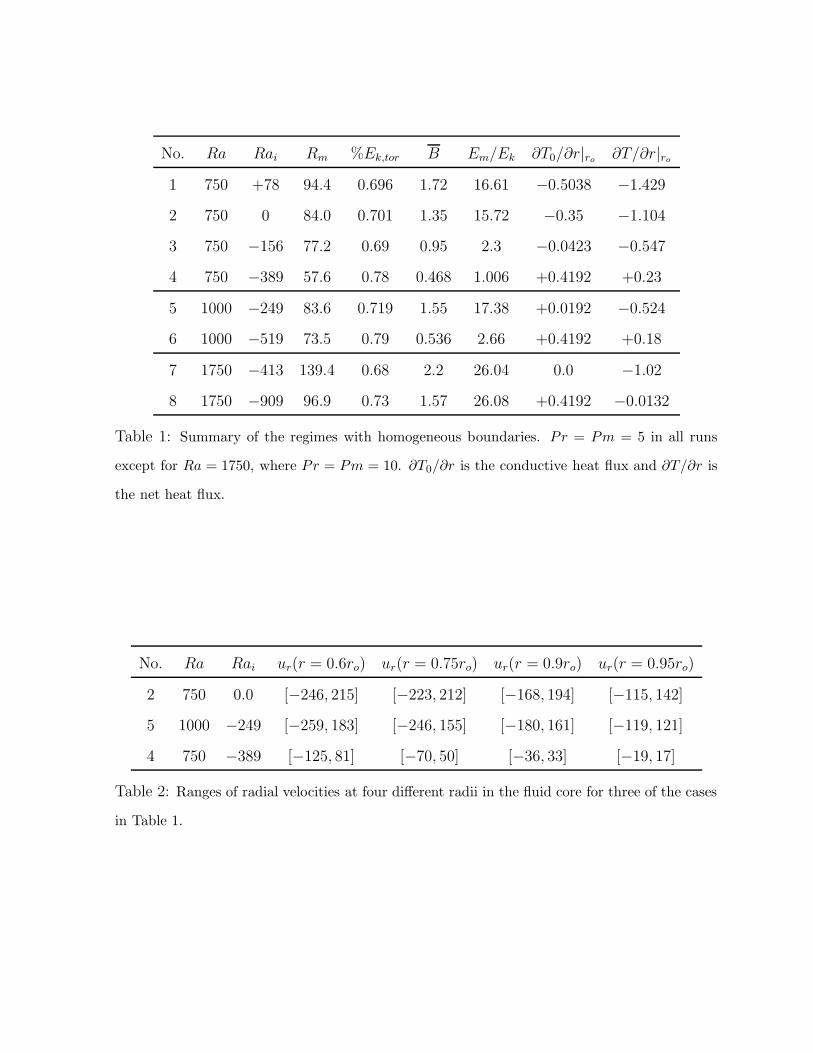
A summary of the results with homogeneous boundaries are given in table 1. For Rayleigh

numbers of Ra = 750 and 1000, a heat sink decreases Rm only slightly but the average

magnetic field (B, obtained from the magnetic energy in the spherical shell) registers a

sharp decrease. For a strong heat sink (Rai = −519), the poloidal kinetic energy decreases

but the toroidal energy does not; approximately 80% of the kinetic energy is contained in

the toroidal component (table 1). The decrease in Rm is due to the fall in poloidal velocity;

note that ur is very small in the outer periphery of the spherical shell in figure 2(b) (also

see table 2). Convection is shut down in the outer regions and this is reflected in the

overall magnetic field generated in the shell. The ratio of magnetic to kinetic energies

decreases to unity as Rai is reduced. Reducing Rai further results in failure of dynamo

action.

8

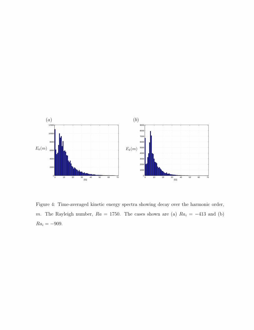
Increasing the Rayleigh number to a higher value (Ra = 1750) gives rise to additional

effects that are not observed at moderate Rayleigh numbers – the buoyancy forces now

are large enough to generate a large-scale zonal motion, whereby the m = 0 mode is

strong in the kinetic energy spectrum; see figure 4(a). From figure 4(b) we note that the

heat sink acts in two ways: (i) to reduce energy in the m = 0 mode and (ii) to damp

out energy contained in high azimuthal wave modes (small scales). The latter effect is

also present at moderate Rayleigh numbers (Ra = 750) as is clear from a comparison of

two cases given in figures 2(a,b). Hence the fall in kinetic energy (and Rm) caused by the

heat sink is greater at high Rayleigh numbers than at low or moderate Rayleigh numbers.

Consequently, the ratio of magnetic to kinetic energies is not affected much (see table 1,

cases 7 & 8).

Cases 2 & 5 in table 1 are equivalent in the sense that, the magnetic Reynolds number,

the mean magnetic field and the energy contained in the toroidal component are all

approximately the same. This is not surprising if we note that the sum of the Rayleigh

numbers based on basal heating and internal cooling, Ra + Rai, is approximately the

same for the two cases. The main difference between these two states is in the heat flux

at the outer boundary: in case 5 the heat flux is lower due to the presence of the heat

sink. From table 2 we see that the reduced heat flux at the outer boundary has a small

but finite effect on the radial velocity distribution in the fluid core, the upwelling velocity

in the outer regions being lower and of the same order of magnitude as the downwelling

velocity. When the effect of the heat sink is dominant (case 4, table 2), the radial velocity

decreases to a low value with increasing radius.

Separating the kinetic and magnetic energies into parts symmetric and antisymmet-

ric about the equator shows that the solution becomes progressively symmetric as Rai

decreases and for the minimum values the solution has near-perfect symmetry about the

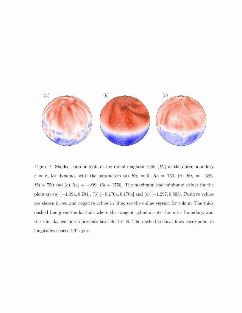
equator. Furthermore, as Rai is reduced, the field structure is a stable dipole [figure 1(b)],

qualitatively similar to the results of Kutzner and Christensen (2002), who used volumet-

9

ric heat sinks to mimic chemical convection in their dynamo. (See Wicht and Olson (2004)

and Christensen (2006) for further examples of the application of heat sinks in chemical

convection.)

Figure 1(a) shows reverse-flux patches (of sign opposite to that of the main dipole

field) at low latitudes. These are common in many geodynamo simulations (also see

Olson et al. 1999, Sreenivasan and Jones 2006b), but they are absent from the runs with

an imposed heat sink: for the lowest Rai these flux patches are eliminated totally from

the outer boundary [figure 1(b)]. From figure 2(c) we see discontinuities in the toroidal

magnetic field in regions of strong downwelling. Bφ is twisted by the shear ∂ur/∂φ to give

a negative Br above the equatorial plane [figure 2(d)], but the phenomenon now occurs

deep within the shell and hence is not visible on the outer boundary.

A strong heat sink also changes the mode of convection in the tangent cylinder – the

imaginary cylinder touching the inner core boundary and parallel to the Earth’s rotation

axis. Flow dominated by a strong upwelling plume as in figure 3(a) (called the magnetic

mode, see Sreenivasan and Jones 2006a) changes to a regime where there are several thin,

weak upwellings [the viscous mode; see figure 3(b)]. As convection is damped out, the

maximum Elsasser number within the tangent cylinder falls below the value required for

the magnetic mode of convection. The expulsion of magnetic flux and the formation

of reverse flux patches in the tangent cylinder requires the strong upwellings that we

associate with the magnetic mode. However, in case 8 the convection within the tangent

cylinder is again strong enough to excite the magnetic mode [figure 3(c)]. Here we have

a regime wherein convection is vigorous in the bulk of the fluid but weak enough in the

outer regions to preclude the occurrence of reverse flux patches near the equatorial plane

[see figure 1(c)]. We note from table 1 that the heat flux at the outer boundary is very

small in this regime.

10

4 Dynamo action with inhomogeneous boundary con-

ditions: locking

Now consider the same problem as in the previous section but with the temperature

outer boundary condition of the form T (ro) = fY 2

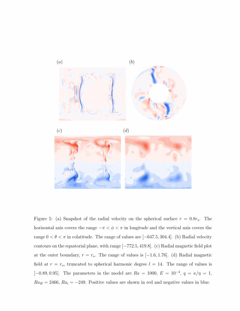
2(θ, φ). Figure 5 gives the velocity and

magnetic field plots for case 1, table 3. The parameters for this run are Ra = 1000,

Rai = −249. When the temperature inhomogeneity is small there is no perceivable

effect on the dynamo and multi-columnar convection is dominant. With RaH ≈ 2500

convection is organized into two strong downwellings beneath regions of low temperature

[see figures 5(a,b)]. These two downwellings remain close to the same longitude during

one run. Although the magnitude of the magnetic field fluctuates with time, the four-

lobed structure of the radial magnetic field as seen in figures 5(c) and (d) is preserved

at approximately the same longitude throughout the run. As the kinetic and magnetic

energy spectra decay by three orders of magnitude in our calculations, the small-scale

structures in figures 5(a) and (c) are well-resolved parts of the solution. Case 2 (Ra =

1750, Rai = −909, RaH ≈ 3000) has strong convection that gives rise to weak or even

reversed flux patches in both hemispheres. Despite the chaotic nature of the solution, the

magnetic field shows the m = 2 pattern of the inhomogeneity. The magnetic Reynolds

number and Elsasser number (B2

) of this dynamo are comparable to those in case 1.

As Rai is increased to zero and positive values, the outer surface temperature in

the dynamo progressively decreases, the mean heat flux at the boundary increases, and

convection decouples from the boundary temperature variations. For Rai = +78 (i.e. with

a heat source rather than a heat sink), dipolar solutions were obtained with RaH = 0

but the behaviour is different for RaH ∼ 800: the dipolar structure of the magnetic field

breaks down into a chaotic state. The magnetic energy decreases to only a fraction of the

kinetic energy (case 3, table 3). This regime is reminiscent of the low Pr = Pm regime of

Sreenivasan and Jones (2006b) where the Lorentz forces do not play a significant part in

11

the force balance. Runs at higher values of Ra or Rai were not attempted as they would

produce only non-dipolar dynamos.

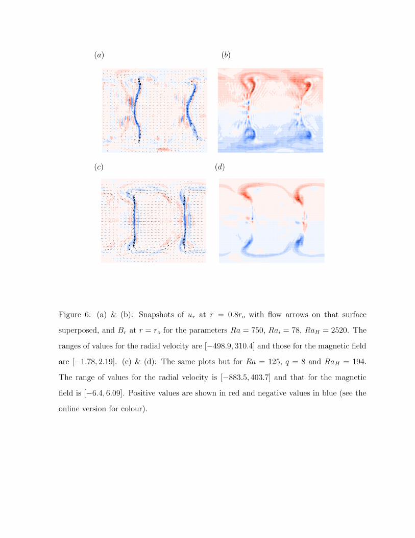
We explore two ways to force a locked solution when convection is strong: (i) to

increase RaH , keeping q = κ/η equal to unity and (ii) to decrease Ra and increase q. The

first option (case 4 in table 3) is effective in forcing two strong downwellings, producing

a strong dipolar magnetic field as shown in figures 6(a,b). However, prograde (eastward)

thermal winds beneath the boundary tend to tilt the fluid columns and, at higher values

of RaH , destroy both the columnar convection and the dynamo. A similar effect was

observed with Y 2

2and Y 0

2heat flow patterns by Olson and Christensen (2002). This

places an upper limit on the useable value of RaH . When stronger heat sources are

present it becomes more difficult to produce locked dynamos by increasing RaH as the

regime narrows down. However, increasing q to 8 [option (ii) above; see case 5 in table 3

and figures 6(c,d)] and lowering Ra to 125 restores the solution with quasi-stationary

flux lobes. This result is significant because it indicates that the key to obtaining locked

solutions is to create a regime where external thermal perturbations can penetrate into

the interior of the fluid. The requires a small Peclet number, uL/κ, which is 38 for case

5 compared with 213 for case 1.

5 Discussion

We have obtained dynamo solutions where convection is weakened in the upper regions of

the fluid by a basic state temperature distribution that incorporates both boundary heat

flux and uniform internal cooling. This regime cannot be obtained by merely reducing

the Rayleigh number in a model with only uniform internal heating and does not preclude

strong convection from occurring lower down in the fluid. Models with moderate Rayleigh

numbers and strong heat sinks (case 4 of table 1) give rise to severe thermal stratification

with net heat flux into the outer boundary. The temperature gradient changes sign at

12

r = 1.183; the surface heat flux is still inwards but is less than that for the basic state

(table 1), indicating that convection still occurs throughout the fluid. The equivalent

situation in the Earth’s core would be a conduction profile that becomes subadiabatic

800 km below the CMB and a positive, but subadiabatic heat flow out of the core. The

magnetic energy is considerably attenuated and the dynamos are stable and dipolar. Here

we have shown that such models support strong thermal boundary coupling even when

q = κ/η ∼ 1.

Papers I and II used uniform internal heating, which meant the heat flux was highest

at the top. This forced vigorous advection of heat near the upper boundary, which

swamped any influence of the lateral variations of heat flux on the boundary except at

small Rayleigh number. This entailed weak convective velocities everywhere, producing

a small magnetic Reynolds number and little hope of dynamo action unless the magnetic

diffusivity was reduced, which in terms of dimensionless parameters meant, inevitably,

a large q. Molecular values for the core suggest q ≈ 10−6, but this is irrelevant for the

type of turbulence expected in the core. Turbulence is usually assumed to equalise the

diffusivities, making q ≈ 1, but large q of order 10 is unreasonable. In this paper we

obviate the need for large q by introducing heat sinks that reduce the advection of heat

near the upper boundary, allowing lateral heat flux variations at the boundary to influence

the deeper convection and produce locking at higher Rayleigh number. These heat sinks

are eminently realistic for modelling the core for two reasons. First, convection is driven

only by the superadiabatic temperature gradient, which is weakened towards the CMB

by the steepening of the adiabatic gradient. Secondly, compositional convection, which

provides most of the buoyancy in the core, is fed from the bottom in the form of light

material released on freezing of the liquid and is remixed uniformly throughout the outer

core.

The solutions obtained here are more mobile than the case with the largest inhomo-

geneity in Paper I and are not as well locked. They are no less geophysically relevant for

13

this because the geomagnetic field is also mobile. Surface fields are dominated by 4 main

lobes that move irregularly a small distance from the mean position of the locked solu-

tions. A preliminary exploration into lower Ekman numbers (∼ 10−5) suggests locking

continues to occur at high Rayleigh numbers when heat sinks are present.

6 Acknowledgements

This work was supported by NERC Consortium Grant Deep Earth Systems O/2001/00668

and Grant F/00 122/AD from the Leverhulme Trust. The computations were performed

on the White Rose Grid Cluster at Leeds University.

References

Anufriev, A. P., Jones, C. A., and Soward, A. M., The Boussinesq and anelastic liquid

approximation for convection in the Earth’s core. Phys. Earth Planet. Inter., 2005, 152,

163–190.

Bloxham, J., The effect of thermal core-mantle interactions on the paleomagnetic secular

variation. Phil. Trans. Roy. Soc. London Ser. A, 2000, 358, 1171–1179.

Braginsky, S. I., Structure of the F layer and reasons for convection in the Earth’s core.

Dokl. Akad. Nauk. SSSR Engl. Trans., 1963, 149, 1311–1314.

Braginsky, S. I., MAC-oscillations of the hidden ocean of the core. J. Geomagn. Geoelectr.,

1993, 45, 1517–1538.

Braginsky, S. I., Magnetic Rossby waves in the stratified ocean of the core, and topo-

graphic core-mantle coupling. Earth Planets Space, 1998, 50, 641–649.

14

Braginsky, S. I., Dynamics of the stably stratified ocean at the top of the core. Phys.

Earth Planet. Inter., 1999, 111, 21–934.

Braginsky, S. I., Effect of the stratified ocean of the core upon the Chandler wobble. Phys.

Earth Planet. Inter., 2000, 118, 195–203.

Christensen, U. R., A deep dynamo generating mercury’s magnetic field. Nature, 2006,

444, 1056–1058.

Christensen, U. R. and Olson, P., Secular variation in numerical geodynamo models with

lateral variations of boundary heat flow. Phys. Earth Planet. Inter., 2003, 138, 39–54.

Fearn, D. R. and Loper, D. E., Compositional convection and stratification of Earth’s

core. Nature, 1981, 289, 393–394.

Gibbons, S. J., Gubbins, D., and Zhang, K., Convection in a rotating spherical fluid

shells with inhomogeneous heat flux at the outer boundary. Geophys. Astrophys. Fluid

Dynam., 2007, p. in press.

Glatzmaier, G. A., Coe, R. S., Hongre, L., and Roberts, P. H., The role of the Earth’s

mantle in controlling the frequency of geomagnetic reversals. Nature, 1999, 401, 885–

890.

Gubbins, D., Thomson, C. J., and Whaler, K. A., Stable regions in the Earth’s liquid

core. Geophys. J. R. Astron. Soc., 1982, 68, 241–251.

Gubbins, D., Alfe, D., Masters, T. G., Price, D., and Gillan, M., Gross thermodynamics

of 2-component core convection. Geophys. J. Int., 2004, 157, 1407–1414.

Gubbins, D., Willis, A. P., and Sreenivasan, B., Correlation of Earth’s magnetic field

with lower mantle thermal and seismic structure. Phys. Earth Planet. Inter., 2007,

162, 256–260.

15

Kutzner, C. and Christensen, U., From stable dipolar towards reversing numerical dy-

namos. Phys. Earth Planet. Inter., 2002, 131, 29–45.

Labrosse, S., Poirier, J.-P., and Mouel, J.-L. L., On cooling of the Earth’s core. Phys.

Earth Planet. Inter., 1997, 99, 1–17.

Lister, J. R. and Buffett, B. A., The strength and efficiency of thermal and compositional

convection in the geodynamo. Phys. Earth Planet. Inter., 1995, 91, 17–30.

Loper, D. E., Some thermal consequences of a gravitationally powered dynamo. J. Geo-

phys. Res., 1978, 83, 5961–5970.

Nimmo, F., Price, G., Brodholt, J., and Gubbins, D., The influence of potassium on core

and geodynamo evolution. Geophys. J. Int., 2004, 156, 1407–1414.

Olson, P., Thermal interaction of the core and mantle. In: Earth’s Core and Lower Mantle,

C. Jones, A. Soward, and K. Zhang (Eds), pp. 1–38, 2000 (London: Taylor and Francis).

Olson, P. and Christensen, U. R., The time-averaged magnetic field in numerical dynamos

with non-uniform boundary heat flow. Geophys. J. Int., 2002, 151, 809–823.

Olson, P., Christensen, U., and Glatzmaier, G., Numerical modeling of the geodynamo:

mechanisms of field generation and equilibration. J. Geophys. Res., 1999, 104, 10,383–

10,404.

Sarson, G. R., Jones, C. A., and Longbottom, A. W., The influence of boundary region

heterogeneities on the geodynamo. Phys. Earth Planet. Inter., 1997, 101, 13–32.

Sreenivasan, B. and Jones, C. A., Azimuthal winds, convection and dynamo action in

the polar regions of planetary cores. Geophys. Astrophys. Fluid Dynam., 2006, 100,

319–339.

16

Sreenivasan, B. and Jones, C. A., The role of inertia in the evolution of spherical dynamos.

Geophys. J. Int., 2006, 164, 467–476.

Wicht, J. and Olson, P., A detailed study of the polarity reversal mechanism in a numerical

dynamo model. Geochem. Geophys. Geosyst., 2004, 5, Q03H10.

Willis, A. P., Sreenivasan, B., and Gubbins, D., Thermal core-mantle interaction: explor-

ing regimes for ‘locked’ dynamo action. Phys. Earth Planet. Inter., 2007, 165, 83–92.

17

No. Ra Rai Rm %Ek,tor B Em/Ek ∂T0/∂r|ro∂T/∂r|ro

1 750 +78 94.4 0.696 1.72 16.61 −0.5038 −1.429

2 750 0 84.0 0.701 1.35 15.72 −0.35 −1.104

3 750 −156 77.2 0.69 0.95 2.3 −0.0423 −0.547

4 750 −389 57.6 0.78 0.468 1.006 +0.4192 +0.23

5 1000 −249 83.6 0.719 1.55 17.38 +0.0192 −0.524

6 1000 −519 73.5 0.79 0.536 2.66 +0.4192 +0.18

7 1750 −413 139.4 0.68 2.2 26.04 0.0 −1.02

8 1750 −909 96.9 0.73 1.57 26.08 +0.4192 −0.0132

Table 1: Summary of the regimes with homogeneous boundaries. Pr = Pm = 5 in all runs

except for Ra = 1750, where Pr = Pm = 10. ∂T0/∂r is the conductive heat flux and ∂T/∂r is

the net heat flux.

No. Ra Rai ur(r = 0.6ro) ur(r = 0.75ro) ur(r = 0.9ro) ur(r = 0.95ro)

2 750 0.0 [−246, 215] [−223, 212] [−168, 194] [−115, 142]

5 1000 −249 [−259, 183] [−246, 155] [−180, 161] [−119, 121]

4 750 −389 [−125, 81] [−70, 50] [−36, 33] [−19, 17]

Table 2: Ranges of radial velocities at four different radii in the fluid core for three of the cases

in Table 1.

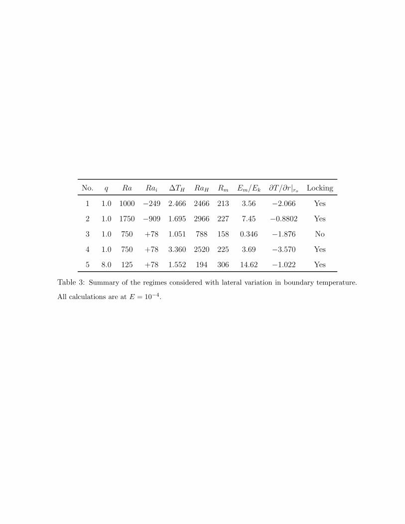
No. q Ra Rai ∆TH RaH Rm Em/Ek ∂T/∂r|roLocking

1 1.0 1000 −249 2.466 2466 213 3.56 −2.066 Yes

2 1.0 1750 −909 1.695 2966 227 7.45 −0.8802 Yes

3 1.0 750 +78 1.051 788 158 0.346 −1.876 No

4 1.0 750 +78 3.360 2520 225 3.69 −3.570 Yes

5 8.0 125 +78 1.552 194 306 14.62 −1.022 Yes

Table 3: Summary of the regimes considered with lateral variation in boundary temperature.

All calculations are at E = 10−4.

(a) (b) (c)

Figure 1: Shaded contour plots of the radial magnetic field (Br) at the outer boundary

r = ro for dynamos with the parameters (a) Rai = 0, Ra = 750, (b) Rai = −389,

Ra = 750 and (c) Rai = −909, Ra = 1750. The maximum and minimum values for the

plots are (a) [−1.094, 0.794], (b) [−0.1704, 0.1704] and (c) [−1.297, 0.803]. Positive values

are shown in red and negative values in blue; see the online version for colour. The thick

dashed line gives the latitude where the tangent cylinder cuts the outer boundary, and

the thin dashed line represents latitude 45 N. The dashed vertical lines correspond to

longitudes spaced 90 apart.

(a) (b)

(c) (d)

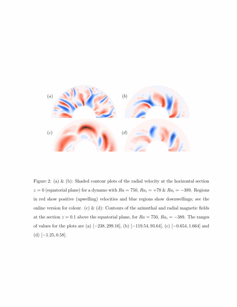
Figure 2: (a) & (b): Shaded contour plots of the radial velocity at the horizontal section

z = 0 (equatorial plane) for a dynamo with Ra = 750, Rai = +78 & Rai = −389. Regions

in red show positive (upwelling) velocities and blue regions show downwellings; see the

online version for colour. (c) & (d): Contours of the azimuthal and radial magnetic fields

at the section z = 0.1 above the equatorial plane, for Ra = 750, Rai = −389. The ranges

of values for the plots are (a) [−238, 299.16], (b) [−119.54, 93.64], (c) [−0.654, 1.664] and

(d) [−1.25, 0.58].

(a) (b) (c)

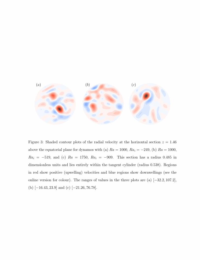
Figure 3: Shaded contour plots of the radial velocity at the horizontal section z = 1.46

above the equatorial plane for dynamos with (a) Ra = 1000, Rai = −249, (b) Ra = 1000,

Rai = −519, and (c) Ra = 1750, Rai = −909. This section has a radius 0.485 in

dimensionless units and lies entirely within the tangent cylinder (radius 0.538). Regions

in red show positive (upwelling) velocities and blue regions show downwellings (see the

online version for colour). The ranges of values in the three plots are (a) [−32.2, 107.2],

(b) [−16.43, 23.9] and (c) [−21.26, 76.78].

0 10 20 30 40 50 60 700

2000

4000

6000

8000

10000

12000

PSfrag replacements

m

Ek(m)

0 10 20 30 40 50 60 700

1000

2000

3000

4000

5000

6000

7000

8000

9000

PSfrag replacements

m

Ek(m)

(a) (b)

Figure 4: Time-averaged kinetic energy spectra showing decay over the harmonic order,

m. The Rayleigh number, Ra = 1750. The cases shown are (a) Rai = −413 and (b)

Rai = −909.

(a) (b)

(c) (d)

Figure 5: (a) Snapshot of the radial velocity on the spherical surface r = 0.8ro. The

horizontal axis covers the range −π < φ < π in longitude and the vertical axis covers the

range 0 < θ < π in colatitude. The range of values are [−647.5, 304.4]. (b) Radial velocity

contours on the equatorial plane, with range [−772.5, 419.8]. (c) Radial magnetic field plot

at the outer boundary, r = ro. The range of values is [−1.6, 1.76]. (d) Radial magnetic

field at r = ro, truncated to spherical harmonic degree l = 14. The range of values is

[−0.89, 0.95]. The parameters in the model are Ra = 1000, E = 10−4, q = κ/η = 1,

RaH = 2466, Rai = −249. Positive values are shown in red and negative values in blue.

(a) (b)

(c) (d)

Figure 6: (a) & (b): Snapshots of ur at r = 0.8ro with flow arrows on that surface

superposed, and Br at r = ro for the parameters Ra = 750, Rai = 78, RaH = 2520. The

ranges of values for the radial velocity are [−498.9, 310.4] and those for the magnetic field

are [−1.78, 2.19]. (c) & (d): The same plots but for Ra = 125, q = 8 and RaH = 194.

The range of values for the radial velocity is [−883.5, 403.7] and that for the magnetic

field is [−6.4, 6.09]. Positive values are shown in red and negative values in blue (see the

online version for colour).