Embed Size (px)
Citation preview
85
Journal of ICT, 15, No. 2 (December) 2016, pp: 85–116
APPENDIX: Visualising the Data Dispersion of Six Financial Ratios using Box Plots
INTELLIGENT COOPERATIVE WEB CACHING POLICIES FOR MEDIA OBJECTS BASED ON J48 DECISION TREE AND NAÏVE BAYES SUPERVISED MACHINE LEARNING ALGORITHMS IN
STRUCTURED PEER-TO-PEER SYSTEMS
Hamidah Ibrahim, Waheed Yasin, Nur Izura Udzir & Nor Asilah Wati Abdul Hamid
Universiti Putra Malaysia, Malaysia
[email protected];[email protected];[email protected];[email protected]
ABSTRACT
Web caching plays a key role in delivering web items to end users in World Wide Web (WWW). On the other hand, cache size is considered as a limitation of web caching. Furthermore, retrieving the same media object from the origin server many times consumes the network bandwidth. Furthermore, full caching for media objects is not a practical solution and consumes cache storage in keeping few media objects because of its limited capacity. Moreover, traditional web caching policies such as Least Recently Used (LRU), Least Frequently Used (LFU), and Greedy Dual Size (GDS) suffer from caching pollution (i.e. media objects that are stored in the cache are not frequently visited which negatively affects on the performance of web proxy caching). In this work, intelligent cooperative web caching approaches based on J48 decision tree and Naïve Bayes (NB) supervised machine learning algorithms are presented. The proposed approaches take the advantages of structured peer-to-peer systems where the contents of peers’ caches are shared using Distributed Hash Table (DHT) in order to enhance the performance of the web caching policy. The performance of the proposed approaches is evaluated by running a trace-driven simulation on a dataset that is collected from IRCache network. The results demonstrate that the new proposed policies improve the performance of traditional web caching policies that are LRU, LFU, and GDS in terms of Hit
http
://jic
t.uum
.edu
.my
Journal of ICT, 15, No. 2 (December) 2016, pp: 85–116
86
Ratio (HR) and Byte Hit Ratio (BHR). Moreover, the results are compared to the most relevant and state-of-the-art web proxy caching policies.
Keywords: Web Caching, Machine Learning Algorithms, Peer-to-Peer Systems.
INTRODUCTION
Web caching is a technique where local copies of web page are stored in places close to the end-users. Web caches are used to improve the performance of the World Wide Web (WWW) (Yasin et al., 2014a). Many benefits can be gained from caching such as improving the hit rates, alleviating loads on origin servers, and reducing network traffic. However, due to cache size limitations, new approaches are required to improve the cache efficiency (Ali et al., 2012b). On the other hand, traditional web caching algorithms such as Least Recently Used (LRU), Least Frequently Used (LFU), and Greedy Dual Size (GDS) suffer from caching pollution where the most popular media objects get the most requests, while a large portion of media objects that are stored in the cache are not frequently visited (Koskela et al., 2003; Arlitt et al., 2000).
Cache replacement is the core of web caching which is the procedure that has to be taken when the cache is full while there are web objects to be cached. Thus, it is common that a web caching policy is defined according to the cache replacement algorithm which is used by this web caching policy. This work presents new policies based on machine learning algorithms and sharing information about peers caches’ contents in order to enhance traditional web caching policies that are LRU, LFU, and GDS.
Many variants of LRU, LFU, and GDS have been presented in the literature (Stefan & Böszörmenyi, 2003) such as SVM-LRU, NB-LRU, LFU-Aging (Ali et al., 2012a; Ali et al., 2012b), and Least Frequently Used with Dynamic Aging (LFU-DA) (ElAarag, 2013; Zink & Shenoy, 2005).
Cooperative web caching is a way of sharing web contents in a peer-to-peer system based on supervised machine learning algorithms. The proposed policies take the advantages of structured peer-to-peer systems where peers’ caches contents are shared using Distributed Hash Table (DHT). Therefore, it improves the performance of web caching policies (Hara et al., 2010).
In this work, two supervised machine learning algorithms are adopted that are: Naïve Bayes (NB) classifier and J48 decision tree classifier. They are popular supervised machine learning algorithms that have been applied successfully
http
://jic
t.uum
.edu
.my
87
Journal of ICT, 15, No. 2 (December) 2016, pp: 85–116
in many domains (Ali et al., 2011; Sulaiman et al., 2008). In this work, NB and J48 classifiers are incorporated effectively with traditional web caching policies (Ali et al., 2012a).
The aim of this work is to present intelligent cooperative web caching policies that have better performance in terms of Hit Ratio (HR) and Byte Hit Ratio (BHR) based on NB and J48 supervised machine learning algorithms in peer-to-peer systems. A trace-driven simulation is carried out to evaluate the performance of the proposed policies. Furthermore, the results are compared to traditional and state-of-the-art web proxy caching policies.
In the works of Yasin et al. (2014a) and Yasin et al. (2014b), we have presented a brief description of the proposed policies for intelligent cooperative web caching policies for media objects based on J48 decision tree supervised machine learning algorithms in structured peer-to-peer systems, while; this paper gives a full explanation for them.
LITERATURE REVIEW
In the work of Xu et al.’s (2010), a study on media caching for peer-to-peer systems has been conducted which verified that peer-to-peer media queries can be answered from the cache. Furthermore, a peer-to-peer live streaming caching algorithm which is based on Sliding Window (SLW) has been proposed. It predicts and caches popular media objects according to the measured distribution. The proposed algorithm has been evaluated and compared to conventional caching strategies. A trace-driven simulation has been performed to evaluate the proposed approach. The results showed that the SLW algorithm performed close to an optimal algorithm which has full knowledge of future requests. This idea motivates us to build our policies based on peer-to-peer systems in delivering cached media objects to end-users where the traffic load is alleviated and the access latency is minimized.
In the work of Sripanidkulchai and Zhang (2005), an algorithm called interest-based shortcuts has been proposed based on Gnutella peer-to-peer system (Yasin et al., 2011). This algorithm takes into account peers’ interests where media objects are organized logically according to their interests over the existing network. Gnutella is a structured peer-to-peer system which uses query flooding that is considered as a limitation because it consumes the bandwidth of the network. Furthermore, it is not scalable. Interest-based shortcuts approach assumes a peer which has a media object that other peers
http
://jic
t.uum
.edu
.my
Journal of ICT, 15, No. 2 (December) 2016, pp: 85–116
88
are interested in which may also have other media objects that they are also interested in. In the case of a cache miss, the request is forwarded to another peer that has the same interests. Thus, the overhead and network traffic is reduced. The logs file has been collected from Carnegie Mellon University (CMU) web cache. A trace-driven simulation has been carried to evaluate the performance of the proposed approach. In this work, we take the advantages of structured peer-to-peer systems. However, we adopt Chord protocol which has been presented in the work of Tracey Ho et al. (2006) because it is more scalable. Moreover, less overhead and network traffic are required.
Media objects caching improves the performance of media streams systems in terms of delivery time. Media objects have some characteristics that have to be considered when a caching algorithm is to be performed. In the work of Yasin et al. (2013), an overview of media streams caching in peer-to-peer systems has been presented, where the characteristics of media objects have been listed. In this work, we focus on media objects caching because there is no need to consider the characteristics of consistency where web objects are updated. Media objects usually follow the Write-Once-Read-Many (WORM) principle, which makes cache consistency issues more resilient. On the other hand, unlike other web objects that might be delivered with a resilient time tolerance, time characterizes media objects delivery and it is considered as a key point which plays a role in the Quality of Service (QoS) that determines the level of end-user’s satisfaction.
On the other hand, a key point of our approaches is to apply NB and J48 machine learning algorithms. In the works of Ali et al. (2012a) and Ali et al. (2012b), new approaches based on machine learning techniques have been proposed to improve the performance of conventional cache replacement strategies. Three machine learning techniques have been adopted that are Support Vector Machine (SVM), NB, and C4.5. The machine learning techniques are intelligently incorporated with conventional web caching techniques that are LRU, GDS, Greedy-Dual-Size-Frequency (GDSF), and Dynamic Aging (DA). These approaches depend on the capability of SVM, NB and C4.5 to learn from proxy log files and predict the class of web objects that would be revisited. The proposed approaches have been evaluated by trace-driven simulation and compared to the most relevant web caching policies. The simulation results showed that the proposed approaches improved the performance in terms of HR and BHR of the traditional policies on a range of datasets that have been collected from IRCache network. More details about IRCache network are available on http://www.ircache.net. Also, the proposed approaches can alleviate the cache pollution because they can
http
://jic
t.uum
.edu
.my
89
Journal of ICT, 15, No. 2 (December) 2016, pp: 85–116
store the desired web objects and remove the unwanted web objects. Thus, they can optimize the cache usage appropriately and maximize the cache hits that lead in reducing the loads on the origin servers. Therefore, the proposed approaches can reduce costs for accessing the origin servers. This can reduce the network bandwidth that is used by the clients and Internet network traffic. Moreover, the latency of delivering web objects can be reduced accordingly.
However, these approaches have some disadvantages that appear in the additional computational overhead which is required for the target outputs preparation of the training phase when looking for future requests. In our work, we compare our proposed policies to the policies that have been presented in the works of Ali et al. (2012a) and Ali et al. (2012b).
Back Propagation Neural Network (BPNN) has been used in Neural Network Proxy Cache Replacement (NNPCR) in the work of Cobb and ElAarag (2008) and NNPCR-2 in the work of ElAarag and Romano (2009) for making cache replacement decisions in web caching policies where the web object is replaced based on the rating returned by BPNN. The network is a two-hidden layer feed-forward artificial neural network which belongs to the Multilayer Perceptron (MLP) model. NNPCR and NNPCR-2 have benefited from the advantages of neural networks’ properties mainly universal approximation and generalization. They are implemented in the Squid Proxy Cache version 3.1 to see their fair against the existing strategies implemented in Squid. The neural networks created by NNPCR and NNPCR-2 are able to classify training and testing sets with Correct Classification Ratio (CCR) values that indicate effective generalization. The trace files used for datasets have been collected from the IRCache network and have been cleaned before feeding them through the neural network. However, one of their disadvantages appears in the performance of BPNN which is influenced by the optimal selection of the network topology and its parameters. Furthermore, the learning process of BPNN is time consuming. Also, BPNN does not take into account the cost in replacement decisions. On the other hand, NB and J48 achieved a better accuracy and are much faster than BPNN.
In the work of Ali and Shamsuddin (2009), an Adaptive Neuro-Fuzzy Inference System (ANFIS) has been used to predict web objects that could be revisited again. The proposed approach assumed the splitting client-side of web cache into two caches that are short-term cache and long-term cache. The short-term cache is used to store web objects that are visited less than a threshold value, while long-term cache is used to store web objects that exceed this value. The LRU web caching policy is used to remove web objects when the short-term
http
://jic
t.uum
.edu
.my
Journal of ICT, 15, No. 2 (December) 2016, pp: 85–116
90
cache is full. However, when the long-term cache is full, neuro-fuzzy system is employed to classify web objects into cacheable or uncacheable object. The old uncacheable web objects are selected to be removed from the long-term cache. Consequently, the cache pollution is alleviated and the cache space is utilized effectively. The proposed approach was evaluated by trace-driven simulation and compared to the most relevant web caching policies. The simulation results showed that the proposed method improves the performance in terms of HR, while, the performance in terms of BHR was not good enough because the proposed method did not take into account the cost and size of the predicted objects in cache replacement decisions. Moreover, it requires a long time and extra overheads for the training process. Furthermore, division of cache into two segments makes storing and organization of the web objects more complicated, especially with large web objects. On the other hand, NB and J48 achieved a better accuracy and are much faster than ANFIS.
MLP model is one of the popular neural network models. The MLP is a nonlinear model which its architecture consists of a description of the number of layers it has, the number of neurons in each layer, the activation function of each layer, and how the layers are connected to each other. In the work of Koskela et al. (2003), MLP model is used in web proxy caching by predicting the class of web object depending on the syntactic features of the HTML structure of a document and the HTTP responses of a server. Then, the class value is integrated with LRU to select web objects that have to be removed from the cache in order to optimize the web cache. Thus, it is called Least Recently Used Class (LRU-C). The trace logs file was obtained from the Finnish University and Research Network (FUNET) web cache. The experimental results showed that the proposed approach accomplished some improvements compared to the most relevant web caching policies in terms of web cache size. However, this approach ignored the frequency factor in web cache replacement decisions. On the other hand, it relies on some factors that do not have a direct affect on the performance of web caching. Furthermore, training phase consumes long time and requires extra computational overhead. Moreover, MLP model is more complex than NB and J48 classifiers that are adopted in our approaches.
PROPOSED APPROACHES
The proposed approaches take the advantages of both client-server and peer-to-peer systems where peers’ caches contents are shared in order to enhance the performance of the web caching policy. There are two different ways for configuring a peer-to-peer system that are unstructured peer-to-peer system
http
://jic
t.uum
.edu
.my
91
Journal of ICT, 15, No. 2 (December) 2016, pp: 85–116
and structured peer-to-peer system (Xu et al., 2010; Yasin et al., 2011; Yasin et al., 2013). In this work, a structured peer-to-peer system is adopted where a pre-existing infrastructure such as having access points is required. Moreover, each peer keeps track of resources obtainable by its neighbours. Thus, fewer messages are needed for answering queries. Furthermore, structured peer-to-peer systems provide both low latency and load balancing. In this work, the Chord protocol which was presented in the work of Tracey Ho et al. (2006) is adopted for the structured peer-to-peer system. Chord is based on DHT in which hash functions are used to map peers and shared content references. The signaling overhead that is generated between peers is ignored because it does not have a big affect in terms of performance (Hara et al., 2010).
On the other hand, the core of the proposed approaches is to predict the class of the media object whether it will be revisited or not. Then, the class of the object is integrated with cooperative web caching policies to determine which object to be removed from the proxy cache when it is full. In this work, two supervised machine learning algorithms are implemented to classify objects in order to cope with the problem of web caching pollution that are: NB classifier and J48 decision tree classifier. They are popular supervised machine learning algorithms that have been applied successfully in many domains. Thus, media objects should be cached or replaced according to the best use of available cache space which improves hit rates, alleviates loads on the origin servers, and reduces network traffic. In this section, we present NB and J48 classifiers in details and how we integrate them in the proposed approaches.
Intelligent Cooperative Web Caching Policies for Media Objects Based on NB Classifier
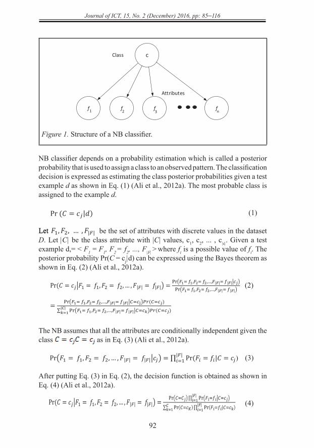
Bayesian networks are supervised learning algorithms that have large popularity in several fields such as medical, military, control, forecasting, modeling, computer science, and statistics (Darwiche, 2010; de Melo & Sanchez, 2008; Goubanova & King, 2008; Shafaatunnur et al., 2012). NB classifier is a Bayesian network that has been applied successfully in many fields. Furthermore, NB is considered as a simple classifier due to independent assumptions among features. Moreover, it is more effective compared to other more sophisticated classifiers such as Support Vector Machine (SVM) (Chen & Hsieh, 2006). Thus, NB classifier is popular in solving various classification problems (Fan et al., 2009; Lu, Chiang et al., 2010).
In NB classifier, all attributes are assumed to be conditionally independent given the class label. The structure of the NB is illustrated in Figure 1. The term naïve comes from the independent assumption between attributes which ignores any correlation among them (Friedman et al., 1997).
http
://jic
t.uum
.edu
.my
Journal of ICT, 15, No. 2 (December) 2016, pp: 85–116
92
Figure 1. Structure of a NB classifier.
NB classifier depends on a probability estimation which is called a posterior probability that is used to assign a class to an observed pattern. The classification decision is expressed as estimating the class posterior probabilities given a test example d as shown in Eq. (1) (Ali et al., 2012a). The most probable class is assigned to the example d.
(1)
Let be the set of attributes with discrete values in the dataset D. Let |C| be the class attribute with |C| values, c1, c2, ... , c|c|. Given a test example d,= < F1 = F1, F2 = f2, ..., F|F| > where fi is a possible value of fi. The posterior probability Pr(C = cj|d) can be expressed using the Bayes theorem as shown in Eq. (2) (Ali et al., 2012a). (2)
The NB assumes that all the attributes are conditionally independent given the class as in Eq. (3) (Ali et al., 2012a).
(3)
After putting Eq. (3) in Eq. (2), the decision function is obtained as shown in Eq. (4) (Ali et al., 2012a).
(4)
c
f f f f
Class
1 2 3 n
Attributes
Pr (𝐶𝐶 = 𝑐𝑐𝑗𝑗|𝑑𝑑) (1)
Let 𝐹𝐹1,𝐹𝐹2, … ,𝐹𝐹|𝐹𝐹| be the set of attributes with discrete values in the dataset D. Let C be the class
attribute with |C| values, 𝑐𝑐1, 𝑐𝑐2, ... , 𝑐𝑐|𝐶𝐶|. Given a test example 𝑑𝑑 =< 𝐹𝐹1 = 𝑓𝑓1,𝐹𝐹2 = 𝑓𝑓2, … ,𝐹𝐹|𝐹𝐹| =
𝑓𝑓|𝐹𝐹| >, where 𝑓𝑓𝑖𝑖 is a possible value of 𝐹𝐹𝑖𝑖. The posterior probability Pr(𝐶𝐶 = 𝑐𝑐𝑗𝑗|𝑑𝑑) can be expressed
using the Bayes theorem as shown in Eq. (2) (Ali et al., 2012a).
Pr(𝐶𝐶 = 𝑐𝑐𝑗𝑗|𝐹𝐹1 = 𝑓𝑓1,𝐹𝐹2 = 𝑓𝑓2, … ,𝐹𝐹|𝐹𝐹| = 𝑓𝑓|𝐹𝐹|) = Pr(𝐹𝐹1= 𝑓𝑓1,𝐹𝐹2= 𝑓𝑓2,…,𝐹𝐹|𝐹𝐹|= 𝑓𝑓|𝐹𝐹||𝑐𝑐𝑗𝑗)Pr(𝐹𝐹1= 𝑓𝑓1,𝐹𝐹2= 𝑓𝑓2,…,𝐹𝐹|𝐹𝐹|= 𝑓𝑓|𝐹𝐹|)
= Pr(𝐹𝐹1= 𝑓𝑓1,𝐹𝐹2= 𝑓𝑓2,…,𝐹𝐹|𝐹𝐹|= 𝑓𝑓|𝐹𝐹||𝐶𝐶=𝑐𝑐j)𝑃𝑃𝑃𝑃 (𝐶𝐶=𝑐𝑐𝑗𝑗)∑ Pr(𝐹𝐹1= 𝑓𝑓1,𝐹𝐹2= 𝑓𝑓2,…,𝐹𝐹|𝐹𝐹|= 𝑓𝑓|𝐹𝐹||𝐶𝐶=𝑐𝑐𝑘𝑘)𝑃𝑃𝑃𝑃 (𝐶𝐶=𝑐𝑐𝑗𝑗)|𝐶𝐶|𝑘𝑘=1
(2)
Pr(𝐹𝐹1 = 𝑓𝑓1,𝐹𝐹2 = 𝑓𝑓2, … ,𝐹𝐹|𝐹𝐹| = 𝑓𝑓|𝐹𝐹||𝑐𝑐𝑗𝑗) = ∏ Pr (𝐹𝐹𝑖𝑖|𝐹𝐹|𝑖𝑖=1 = 𝑓𝑓𝑖𝑖|𝐶𝐶 = 𝑐𝑐𝑗𝑗) (3)
Pr(𝐶𝐶 = 𝑐𝑐𝑗𝑗|𝐹𝐹1 = 𝑓𝑓1,𝐹𝐹2 = 𝑓𝑓2, … ,𝐹𝐹|𝐹𝐹| = 𝑓𝑓|𝐹𝐹|) = Pr(𝐶𝐶=𝐶𝐶𝑗𝑗)∏ Pr(𝐹𝐹𝑖𝑖=𝑓𝑓𝑖𝑖|𝐶𝐶=𝑐𝑐𝑗𝑗)|𝐹𝐹|𝑖𝑖=1
∑ Pr(𝐶𝐶=𝑐𝑐𝐾𝐾)∏ Pr(𝐹𝐹𝑖𝑖=𝑓𝑓𝑖𝑖|𝐶𝐶=𝑐𝑐𝑘𝑘)|𝐹𝐹|𝑖𝑖=1
𝐶𝐶𝑘𝑘=1
(4)
𝑐𝑐 = 𝑎𝑎𝑎𝑎𝑎𝑎max𝑐𝑐𝑗𝑗 Pr (𝐶𝐶 = 𝑐𝑐𝑗𝑗)∏ Pr (𝐹𝐹𝑖𝑖|𝐹𝐹|𝑖𝑖=1 = 𝑓𝑓𝑖𝑖|𝐶𝐶 = 𝑐𝑐𝑗𝑗) (5)
In the training phase of NB classifier, it is only required to estimate the prior probabilities Pr (𝐶𝐶 = 𝑐𝑐𝑗𝑗)
and the conditional probabilities Pr (𝐹𝐹𝑖𝑖 = 𝑓𝑓𝑖𝑖|𝐶𝐶 = 𝑐𝑐𝑗𝑗) from the proxy training dataset using Eq. (6) (Ali
et al., 2012a) and Eq. (7) (Ali et al., 2012a).
Pr(𝐶𝐶 = 𝑐𝑐𝑗𝑗) = No.ofexamples of class 𝑐𝑐𝑗𝑗Total No.of examples (6)
Pr(𝐹𝐹𝑖𝑖 = 𝑓𝑓𝑖𝑖|𝐶𝐶 = 𝑐𝑐𝑗𝑗) = 𝑁𝑁𝑁𝑁.𝑁𝑁𝑓𝑓 𝑒𝑒𝑒𝑒𝑒𝑒𝑒𝑒𝑒𝑒𝑒𝑒𝑒𝑒𝑒𝑒 𝑤𝑤𝑖𝑖𝑤𝑤ℎ 𝐹𝐹𝑖𝑖=𝑓𝑓𝑖𝑖 𝑒𝑒𝑎𝑎𝑎𝑎 𝑐𝑐𝑒𝑒𝑒𝑒𝑒𝑒𝑒𝑒 𝑐𝑐𝑗𝑗𝑁𝑁𝑁𝑁.𝑁𝑁𝑓𝑓𝑒𝑒𝑒𝑒𝑒𝑒𝑒𝑒𝑒𝑒𝑒𝑒𝑒𝑒𝑒𝑒 𝑁𝑁𝑓𝑓 𝑐𝑐𝑒𝑒𝑒𝑒𝑒𝑒𝑒𝑒 𝑐𝑐𝑗𝑗
(7)
Gain(𝑆𝑆,𝐴𝐴) = Entropy (𝑆𝑆,𝐴𝐴) − ∑ |𝑆𝑆𝑣𝑣||𝑆𝑆|𝑣𝑣=Value(𝐴𝐴) Entropy (𝑆𝑆𝑣𝑣) (8)
Entropy(𝑆𝑆) = −∑ Pr(𝑐𝑐𝑗𝑗) 𝑙𝑙𝑙𝑙𝑎𝑎2Pr (𝑐𝑐𝑗𝑗)|𝐶𝐶|𝑗𝑗=1 (9)
http
://jic
t.uum
.edu
.my
93
Journal of ICT, 15, No. 2 (December) 2016, pp: 85–116
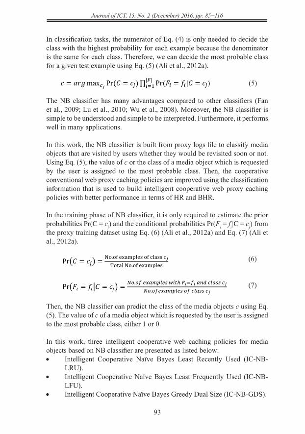
In classification tasks, the numerator of Eq. (4) is only needed to decide the class with the highest probability for each example because the denominator is the same for each class. Therefore, we can decide the most probable class for a given test example using Eq. (5) (Ali et al., 2012a).
(5)
The NB classifier has many advantages compared to other classifiers (Fan et al., 2009; Lu et al., 2010; Wu et al., 2008). Moreover, the NB classifier is simple to be understood and simple to be interpreted. Furthermore, it performs well in many applications.
In this work, the NB classifier is built from proxy logs file to classify media objects that are visited by users whether they would be revisited soon or not. Using Eq. (5), the value of c or the class of a media object which is requested by the user is assigned to the most probable class. Then, the cooperative conventional web proxy caching policies are improved using the classification information that is used to build intelligent cooperative web proxy caching policies with better performance in terms of HR and BHR.
In the training phase of NB classifier, it is only required to estimate the prior probabilities Pr(C = cj) and the conditional probabilities Pr(Fi = fi|C = cj) from the proxy training dataset using Eq. (6) (Ali et al., 2012a) and Eq. (7) (Ali et al., 2012a).
(6)
(7)
Then, the NB classifier can predict the class of the media objects c using Eq. (5). The value of c of a media object which is requested by the user is assigned to the most probable class, either 1 or 0.
In this work, three intelligent cooperative web caching policies for media objects based on NB classifier are presented as listed below:• Intelligent Cooperative Naïve Bayes Least Recently Used (IC-NB-
LRU).• Intelligent Cooperative Naïve Bayes Least Frequently Used (IC-NB-
LFU).• Intelligent Cooperative Naïve Bayes Greedy Dual Size (IC-NB-GDS).
Pr (𝐶𝐶 = 𝑐𝑐𝑗𝑗|𝑑𝑑) (1)
Let 𝐹𝐹1,𝐹𝐹2, … ,𝐹𝐹|𝐹𝐹| be the set of attributes with discrete values in the dataset D. Let C be the class
attribute with |C| values, 𝑐𝑐1, 𝑐𝑐2, ... , 𝑐𝑐|𝐶𝐶|. Given a test example 𝑑𝑑 =< 𝐹𝐹1 = 𝑓𝑓1,𝐹𝐹2 = 𝑓𝑓2, … ,𝐹𝐹|𝐹𝐹| =
𝑓𝑓|𝐹𝐹| >, where 𝑓𝑓𝑖𝑖 is a possible value of 𝐹𝐹𝑖𝑖. The posterior probability Pr(𝐶𝐶 = 𝑐𝑐𝑗𝑗|𝑑𝑑) can be expressed
using the Bayes theorem as shown in Eq. (2) (Ali et al., 2012a).
Pr(𝐶𝐶 = 𝑐𝑐𝑗𝑗|𝐹𝐹1 = 𝑓𝑓1,𝐹𝐹2 = 𝑓𝑓2, … ,𝐹𝐹|𝐹𝐹| = 𝑓𝑓|𝐹𝐹|) = Pr(𝐹𝐹1= 𝑓𝑓1,𝐹𝐹2= 𝑓𝑓2,…,𝐹𝐹|𝐹𝐹|= 𝑓𝑓|𝐹𝐹||𝑐𝑐𝑗𝑗)Pr(𝐹𝐹1= 𝑓𝑓1,𝐹𝐹2= 𝑓𝑓2,…,𝐹𝐹|𝐹𝐹|= 𝑓𝑓|𝐹𝐹|)
= Pr(𝐹𝐹1= 𝑓𝑓1,𝐹𝐹2= 𝑓𝑓2,…,𝐹𝐹|𝐹𝐹|= 𝑓𝑓|𝐹𝐹||𝐶𝐶=𝑐𝑐j)𝑃𝑃𝑃𝑃 (𝐶𝐶=𝑐𝑐𝑗𝑗)∑ Pr(𝐹𝐹1= 𝑓𝑓1,𝐹𝐹2= 𝑓𝑓2,…,𝐹𝐹|𝐹𝐹|= 𝑓𝑓|𝐹𝐹||𝐶𝐶=𝑐𝑐𝑘𝑘)𝑃𝑃𝑃𝑃 (𝐶𝐶=𝑐𝑐𝑗𝑗)|𝐶𝐶|𝑘𝑘=1
(2)
Pr(𝐹𝐹1 = 𝑓𝑓1,𝐹𝐹2 = 𝑓𝑓2, … ,𝐹𝐹|𝐹𝐹| = 𝑓𝑓|𝐹𝐹||𝑐𝑐𝑗𝑗) = ∏ Pr (𝐹𝐹𝑖𝑖|𝐹𝐹|𝑖𝑖=1 = 𝑓𝑓𝑖𝑖|𝐶𝐶 = 𝑐𝑐𝑗𝑗) (3)
Pr(𝐶𝐶 = 𝑐𝑐𝑗𝑗|𝐹𝐹1 = 𝑓𝑓1,𝐹𝐹2 = 𝑓𝑓2, … ,𝐹𝐹|𝐹𝐹| = 𝑓𝑓|𝐹𝐹|) = Pr(𝐶𝐶=𝐶𝐶𝑗𝑗)∏ Pr(𝐹𝐹𝑖𝑖=𝑓𝑓𝑖𝑖|𝐶𝐶=𝑐𝑐𝑗𝑗)|𝐹𝐹|𝑖𝑖=1
∑ Pr(𝐶𝐶=𝑐𝑐𝐾𝐾)∏ Pr(𝐹𝐹𝑖𝑖=𝑓𝑓𝑖𝑖|𝐶𝐶=𝑐𝑐𝑘𝑘)|𝐹𝐹|𝑖𝑖=1
𝐶𝐶𝑘𝑘=1
(4)
𝑐𝑐 = 𝑎𝑎𝑎𝑎𝑎𝑎max𝑐𝑐𝑗𝑗 Pr (𝐶𝐶 = 𝑐𝑐𝑗𝑗)∏ Pr (𝐹𝐹𝑖𝑖|𝐹𝐹|𝑖𝑖=1 = 𝑓𝑓𝑖𝑖|𝐶𝐶 = 𝑐𝑐𝑗𝑗) (5)
In the training phase of NB classifier, it is only required to estimate the prior probabilities Pr (𝐶𝐶 = 𝑐𝑐𝑗𝑗)
and the conditional probabilities Pr (𝐹𝐹𝑖𝑖 = 𝑓𝑓𝑖𝑖|𝐶𝐶 = 𝑐𝑐𝑗𝑗) from the proxy training dataset using Eq. (6) (Ali
et al., 2012a) and Eq. (7) (Ali et al., 2012a).
Pr(𝐶𝐶 = 𝑐𝑐𝑗𝑗) = No.ofexamples of class 𝑐𝑐𝑗𝑗Total No.of examples (6)
Pr(𝐹𝐹𝑖𝑖 = 𝑓𝑓𝑖𝑖|𝐶𝐶 = 𝑐𝑐𝑗𝑗) = 𝑁𝑁𝑁𝑁.𝑁𝑁𝑓𝑓 𝑒𝑒𝑒𝑒𝑒𝑒𝑒𝑒𝑒𝑒𝑒𝑒𝑒𝑒𝑒𝑒 𝑤𝑤𝑖𝑖𝑤𝑤ℎ 𝐹𝐹𝑖𝑖=𝑓𝑓𝑖𝑖 𝑒𝑒𝑎𝑎𝑎𝑎 𝑐𝑐𝑒𝑒𝑒𝑒𝑒𝑒𝑒𝑒 𝑐𝑐𝑗𝑗𝑁𝑁𝑁𝑁.𝑁𝑁𝑓𝑓𝑒𝑒𝑒𝑒𝑒𝑒𝑒𝑒𝑒𝑒𝑒𝑒𝑒𝑒𝑒𝑒 𝑁𝑁𝑓𝑓 𝑐𝑐𝑒𝑒𝑒𝑒𝑒𝑒𝑒𝑒 𝑐𝑐𝑗𝑗
(7)
Gain(𝑆𝑆,𝐴𝐴) = Entropy (𝑆𝑆,𝐴𝐴) − ∑ |𝑆𝑆𝑣𝑣||𝑆𝑆|𝑣𝑣=Value(𝐴𝐴) Entropy (𝑆𝑆𝑣𝑣) (8)
Entropy(𝑆𝑆) = −∑ Pr(𝑐𝑐𝑗𝑗) 𝑙𝑙𝑙𝑙𝑎𝑎2Pr (𝑐𝑐𝑗𝑗)|𝐶𝐶|𝑗𝑗=1 (9)
Pr(𝐶𝐶 = 𝑐𝑐𝑗𝑗) = No.of examples of class 𝑐𝑐𝑗𝑗Total No.of examples (6)
http
://jic
t.uum
.edu
.my

Journal of ICT, 15, No. 2 (December) 2016, pp: 85–116
94
IC-NB-LRU. The proposed IC-NB-LRU approach works as follows: assume we have a media object g that is the least recently used and its class is 1 which means it will be revisited. However, a media objet k has the same priority and its class is 0 which means will not be revisited. In this case, the cache manager will choose object k as a victim to be removed from the cache.
As a result, the proposed IC-NB-LRU approach can efficiently remove unwanted media objects to provide space for new ones. Thus, cache pollution is reduced and the available cache space is utilized effectively. Consequently, the HR and BHR can be improved by using the proposed IC-NB-LRU approach.
IC-NB-LFU. The LFU web caching policy suffers from cache pollution. Thus, it might keep media objects in the cache, while they are not going to be revisited in the future. In IC-NB-LFU, the NB classifier is integrated with cooperative LFU to utilize the cache.
Assume we have a media object g that has the lowest priority which means it is the least frequently used and its class is 1. However, a media object k has the same priority and its class is 0. In this case, the cache manager will choose object k to be removed from the cache. Consequently, IC-NB-LFU approach improves the performance in terms of HR and BHR.
IC-NB-GDS. The GDS web caching policy has been proposed as an extension of SIZE web caching policy in order to avoid cache pollution. GDS takes into account the size, recency, and the cost to fetch the media object. In IC-NB-GDS, assume we have a media object g which is chosen by normal GDS to be removed from the cache and its class is 1. On the other hand, object k has the same priority and its class is 0. IC-NB-GDS will choose the media object k to be removed from the cache. Consequently, the proposed IC-NB-GDS approach improves the performance in terms of HR and BHR.
Intelligent Cooperative Web Caching Policies for Media Objects Based on J48 Classifier
Decision tree is a popular supervised machine learning algorithm which has a large popularity in several fields such as medical, marketing, finance, and computer science. It is simple and easy to be understood. C4.5 is an algorithm which is used to generate a decision tree that has been developed by Quinlan (1993). J48 classifier is a Java implementation of the C4.5 algorithm in Weka data mining tool. More details about Weka are available on http://www.cs.waikato.ac.nz/ml/weka/s. In this work, J48 is used to build the decision tree.
http
://jic
t.uum
.edu
.my

95
Journal of ICT, 15, No. 2 (December) 2016, pp: 85–116
The J48 classifier is used to decide the target value of a new sample based on different attribute values of the available data. The internal nodes of the decision tree indicate the different attributes; while the branches between the nodes refer to the possible values of these attributes. Furthermore, the terminal nodes (leafs) indicate the classification of the target. The attribute to be predicted is called the dependent variable, because its value depends on all the other attributes’ values. These attributes are called the independent variables (Yasin et al., 2014b).
The J48 classifier implements C4.5 algorithm for generating a pruned or unpruned C4.5 decision tree. The decision trees created by J48 classifier can be used for classification. The J48 classifier creates decision trees from a set of labeled training data using the idea of information entropy. Each attribute of the data might be used to make a decision by dividing the data into smaller subsets. The J48 examines the normalized information gain which results from choosing an attribute for dividing the data. The attribute with the highest normalized information gain is used to make a decision. Then the J48 is repeated on smaller subsets. Dividing procedure stops when all instances in a subset belong to the same class. Finally, a leaf node is created to choose that class in the decision tree. On the other hand, it might happen that features do not give any information gain. In this case the J48 classifier creates a decision node higher up in the decision tree using the expected value of the class.
The J48 classifier can handle continuous and discrete attributes. Also, it can handle training data with missing attribute values and attributes with differing costs. Moreover, it provides pruning option for trees after creation.
In the J48 classifier, Information Gain and Information Gain Ratio are the impurity functions that are used for attributes’ selection. The Information Gain is computed using Eq. (8) (Ali et al., 2012b). Gain(S, A) of an attribute A, relative to a collection of instances S, where Value(A) is the set of all possible values for attribute A, and is the subset of S for which attribute A has value v.
(8)
Entropy(S) is defined as Eq. (9) (Ali et al., 2012b):
(9)
Pr (𝐶𝐶 = 𝑐𝑐𝑗𝑗|𝑑𝑑) (1)
Let 𝐹𝐹1,𝐹𝐹2, … ,𝐹𝐹|𝐹𝐹| be the set of attributes with discrete values in the dataset D. Let C be the class
attribute with |C| values, 𝑐𝑐1, 𝑐𝑐2, ... , 𝑐𝑐|𝐶𝐶|. Given a test example 𝑑𝑑 =< 𝐹𝐹1 = 𝑓𝑓1,𝐹𝐹2 = 𝑓𝑓2, … ,𝐹𝐹|𝐹𝐹| =
𝑓𝑓|𝐹𝐹| >, where 𝑓𝑓𝑖𝑖 is a possible value of 𝐹𝐹𝑖𝑖. The posterior probability Pr(𝐶𝐶 = 𝑐𝑐𝑗𝑗|𝑑𝑑) can be expressed
using the Bayes theorem as shown in Eq. (2) (Ali et al., 2012a).
Pr(𝐶𝐶 = 𝑐𝑐𝑗𝑗|𝐹𝐹1 = 𝑓𝑓1,𝐹𝐹2 = 𝑓𝑓2, … ,𝐹𝐹|𝐹𝐹| = 𝑓𝑓|𝐹𝐹|) = Pr(𝐹𝐹1= 𝑓𝑓1,𝐹𝐹2= 𝑓𝑓2,…,𝐹𝐹|𝐹𝐹|= 𝑓𝑓|𝐹𝐹||𝑐𝑐𝑗𝑗)Pr(𝐹𝐹1= 𝑓𝑓1,𝐹𝐹2= 𝑓𝑓2,…,𝐹𝐹|𝐹𝐹|= 𝑓𝑓|𝐹𝐹|)
= Pr(𝐹𝐹1= 𝑓𝑓1,𝐹𝐹2= 𝑓𝑓2,…,𝐹𝐹|𝐹𝐹|= 𝑓𝑓|𝐹𝐹||𝐶𝐶=𝑐𝑐j)𝑃𝑃𝑃𝑃 (𝐶𝐶=𝑐𝑐𝑗𝑗)∑ Pr(𝐹𝐹1= 𝑓𝑓1,𝐹𝐹2= 𝑓𝑓2,…,𝐹𝐹|𝐹𝐹|= 𝑓𝑓|𝐹𝐹||𝐶𝐶=𝑐𝑐𝑘𝑘)𝑃𝑃𝑃𝑃 (𝐶𝐶=𝑐𝑐𝑗𝑗)|𝐶𝐶|𝑘𝑘=1
(2)
Pr(𝐹𝐹1 = 𝑓𝑓1,𝐹𝐹2 = 𝑓𝑓2, … ,𝐹𝐹|𝐹𝐹| = 𝑓𝑓|𝐹𝐹||𝑐𝑐𝑗𝑗) = ∏ Pr (𝐹𝐹𝑖𝑖|𝐹𝐹|𝑖𝑖=1 = 𝑓𝑓𝑖𝑖|𝐶𝐶 = 𝑐𝑐𝑗𝑗) (3)
Pr(𝐶𝐶 = 𝑐𝑐𝑗𝑗|𝐹𝐹1 = 𝑓𝑓1,𝐹𝐹2 = 𝑓𝑓2, … ,𝐹𝐹|𝐹𝐹| = 𝑓𝑓|𝐹𝐹|) = Pr(𝐶𝐶=𝐶𝐶𝑗𝑗)∏ Pr(𝐹𝐹𝑖𝑖=𝑓𝑓𝑖𝑖|𝐶𝐶=𝑐𝑐𝑗𝑗)|𝐹𝐹|𝑖𝑖=1
∑ Pr(𝐶𝐶=𝑐𝑐𝐾𝐾)∏ Pr(𝐹𝐹𝑖𝑖=𝑓𝑓𝑖𝑖|𝐶𝐶=𝑐𝑐𝑘𝑘)|𝐹𝐹|𝑖𝑖=1
𝐶𝐶𝑘𝑘=1
(4)
𝑐𝑐 = 𝑎𝑎𝑎𝑎𝑎𝑎max𝑐𝑐𝑗𝑗 Pr (𝐶𝐶 = 𝑐𝑐𝑗𝑗)∏ Pr (𝐹𝐹𝑖𝑖|𝐹𝐹|𝑖𝑖=1 = 𝑓𝑓𝑖𝑖|𝐶𝐶 = 𝑐𝑐𝑗𝑗) (5)
In the training phase of NB classifier, it is only required to estimate the prior probabilities Pr (𝐶𝐶 = 𝑐𝑐𝑗𝑗)
and the conditional probabilities Pr (𝐹𝐹𝑖𝑖 = 𝑓𝑓𝑖𝑖|𝐶𝐶 = 𝑐𝑐𝑗𝑗) from the proxy training dataset using Eq. (6) (Ali
et al., 2012a) and Eq. (7) (Ali et al., 2012a).
Pr(𝐶𝐶 = 𝑐𝑐𝑗𝑗) = No.ofexamples of class 𝑐𝑐𝑗𝑗Total No.of examples (6)
Pr(𝐹𝐹𝑖𝑖 = 𝑓𝑓𝑖𝑖|𝐶𝐶 = 𝑐𝑐𝑗𝑗) = 𝑁𝑁𝑁𝑁.𝑁𝑁𝑓𝑓 𝑒𝑒𝑒𝑒𝑒𝑒𝑒𝑒𝑒𝑒𝑒𝑒𝑒𝑒𝑒𝑒 𝑤𝑤𝑖𝑖𝑤𝑤ℎ 𝐹𝐹𝑖𝑖=𝑓𝑓𝑖𝑖 𝑒𝑒𝑎𝑎𝑎𝑎 𝑐𝑐𝑒𝑒𝑒𝑒𝑒𝑒𝑒𝑒 𝑐𝑐𝑗𝑗𝑁𝑁𝑁𝑁.𝑁𝑁𝑓𝑓𝑒𝑒𝑒𝑒𝑒𝑒𝑒𝑒𝑒𝑒𝑒𝑒𝑒𝑒𝑒𝑒 𝑁𝑁𝑓𝑓 𝑐𝑐𝑒𝑒𝑒𝑒𝑒𝑒𝑒𝑒 𝑐𝑐𝑗𝑗
(7)
Gain(𝑆𝑆,𝐴𝐴) = Entropy (𝑆𝑆,𝐴𝐴) − ∑ |𝑆𝑆𝑣𝑣||𝑆𝑆|𝑣𝑣=Value(𝐴𝐴) Entropy (𝑆𝑆𝑣𝑣) (8)
Entropy(𝑆𝑆) = −∑ Pr(𝑐𝑐𝑗𝑗) 𝑙𝑙𝑙𝑙𝑎𝑎2Pr (𝑐𝑐𝑗𝑗)|𝐶𝐶|𝑗𝑗=1 (9)
http
://jic
t.uum
.edu
.my
Journal of ICT, 15, No. 2 (December) 2016, pp: 85–116
96
where |C| is the number of classes. In this work, we have two classes as defined in Eq. (10)
(10)
and Pr( ) indicates the probability of class in S. Pr( ) refers to the number of instances of class in S divided by the total number of instances in S. The first part on the right hand side of Eq. (10) (Ali et al., 2012b) indicates the Entropy of the original collection S; while, the second part is the expected value of the Entropy after S is partitioned using attribute A.
Eq. (11) (Ali et al., 2012b) is used to calculate the Information Gain Ratio that is used as the impurity function for attributes’ selection.
(11)
where Split information(S, A) is computed using Eq. (12) (Ali et al., 2012b):
(12) where Si through Sk are the k subsets of instances that are gathered from partitioning S by the k-values of attribute A. On the other hand, Split Information is actually the Entropy of S with respect to attribute A values.
In this work, three intelligent cooperative web caching policies for media objects based on J48 classifier are presented as listed below:• Intelligent Cooperative J48 Least Recently Used (IC-J48-LRU).• Intelligent Cooperative J48 Least Frequently Used (IC-J48-LFU).• Intelligent Cooperative J48 Greedy Dual Size (IC-J48-GDS).
IC-J48-LRU. The proposed IC-J48-LRU approach works same as IC-NB-LRU approach; however, J48 classifier is applied to generate the decision tree which is created using the data that are extracted from proxy log file. In the decision tree, the leaf node represents the class of the target which is either 1 that means the object will be revisited or 0 otherwise. The predicted class is integrated with the cooperative LRU web caching policy in order to enhance the performance in terms of HR and BHR.
𝑐𝑐 = {1, 𝑖𝑖𝑖𝑖 𝑡𝑡ℎ𝑒𝑒 𝑚𝑚𝑒𝑒𝑚𝑚𝑖𝑖𝑚𝑚 𝑜𝑜𝑜𝑜𝑜𝑜𝑒𝑒𝑐𝑐𝑡𝑡 𝑤𝑤𝑜𝑜𝑤𝑤𝑤𝑤𝑚𝑚 𝑜𝑜𝑒𝑒 𝑟𝑟𝑒𝑒𝑟𝑟𝑖𝑖𝑟𝑟𝑡𝑡𝑒𝑒𝑚𝑚0, 𝑜𝑜𝑡𝑡ℎ𝑒𝑒𝑟𝑟𝑤𝑤𝑖𝑖𝑟𝑟𝑒𝑒 (10)
Gain Ratio(𝑆𝑆,𝐴𝐴) = Gain(𝑆𝑆,𝐴𝐴)Split Information (𝑆𝑆,𝐴𝐴) (11)
Split Information(𝑆𝑆,𝐴𝐴) = −∑ |𝑆𝑆𝑖𝑖||𝑆𝑆| log2
|𝑆𝑆𝑖𝑖||𝑆𝑆|
𝑘𝑘𝑖𝑖=1 (12)
𝐻𝐻𝐻𝐻 = ∑ 𝑥𝑥𝑖𝑖𝑁𝑁𝑖𝑖=1𝑁𝑁 (13)
𝐵𝐵𝐻𝐻𝐻𝐻 = ∑ 𝑆𝑆𝑖𝑖𝑥𝑥𝑖𝑖𝑁𝑁𝑖𝑖=1∑ 𝑆𝑆𝑖𝑖𝑁𝑁𝑖𝑖=1
(14)
http
://jic
t.uum
.edu
.my
97
Journal of ICT, 15, No. 2 (December) 2016, pp: 85–116
IC-J48-LFU. The proposed IC-J48-LFU approach works same as IC-NB-LFU; however, J48 classifier is used to generate the tree and leafs represent the class of the target. The IC-J48-LFU approach improves the performance in terms of HR and BHR.
IC-J48-GDS. The proposed IC-J48-GDS approach works same as IC-NB-GDS approach; however, J48 classifier is used to generate the tree which is created using the data that are extracted from proxy log file. In the J48 tree, the leaf node represents the class of the target which is either 1 that means the object will be revisited or 0 otherwise. The predicted class is integrated with the cooperative GDS web caching policy in order to enhance the performance in terms of HR and BHR.
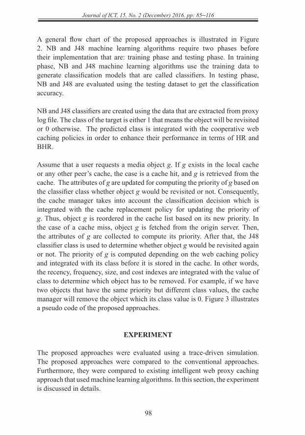
Figure 2. A general flow chart of the proposed intelligent cooperative web proxy caching approaches.
Start
User requests a media object g
Is g in the local cache?
Is g in any peer’s cache?
Cache miss
Cache miss
No
No
Fetch g from server
Cache hit
Yes
Store g in the cache
Is the space in cache enough?
Compute g priority based on classification decision
Yes
Retrieve g from the cache
Update g attributes
Update cache manager
End
Yes
Remove an object according to caching
policy with lowest priority
Cache hit
No
http
://jic
t.uum
.edu
.my
Journal of ICT, 15, No. 2 (December) 2016, pp: 85–116
98
A general flow chart of the proposed approaches is illustrated in Figure 2. NB and J48 machine learning algorithms require two phases before their implementation that are: training phase and testing phase. In training phase, NB and J48 machine learning algorithms use the training data to generate classification models that are called classifiers. In testing phase, NB and J48 are evaluated using the testing dataset to get the classification accuracy.
NB and J48 classifiers are created using the data that are extracted from proxy log file. The class of the target is either 1 that means the object will be revisited or 0 otherwise. The predicted class is integrated with the cooperative web caching policies in order to enhance their performance in terms of HR and BHR.
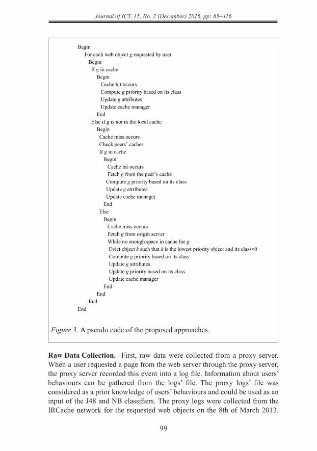
Assume that a user requests a media object g. If g exists in the local cache or any other peer’s cache, the case is a cache hit, and g is retrieved from the cache. The attributes of g are updated for computing the priority of g based on the classifier class whether object g would be revisited or not. Consequently, the cache manager takes into account the classification decision which is integrated with the cache replacement policy for updating the priority of g. Thus, object g is reordered in the cache list based on its new priority. In the case of a cache miss, object g is fetched from the origin server. Then, the attributes of g are collected to compute its priority. After that, the J48 classifier class is used to determine whether object g would be revisited again or not. The priority of g is computed depending on the web caching policy and integrated with its class before it is stored in the cache. In other words, the recency, frequency, size, and cost indexes are integrated with the value of class to determine which object has to be removed. For example, if we have two objects that have the same priority but different class values, the cache manager will remove the object which its class value is 0. Figure 3 illustrates a pseudo code of the proposed approaches.
EXPERIMENT
The proposed approaches were evaluated using a trace-driven simulation. The proposed approaches were compared to the conventional approaches. Furthermore, they were compared to existing intelligent web proxy caching approach that used machine learning algorithms. In this section, the experiment is discussed in details.
http
://jic
t.uum
.edu
.my
99
Journal of ICT, 15, No. 2 (December) 2016, pp: 85–116
Figure 3. A pseudo code of the proposed approaches.
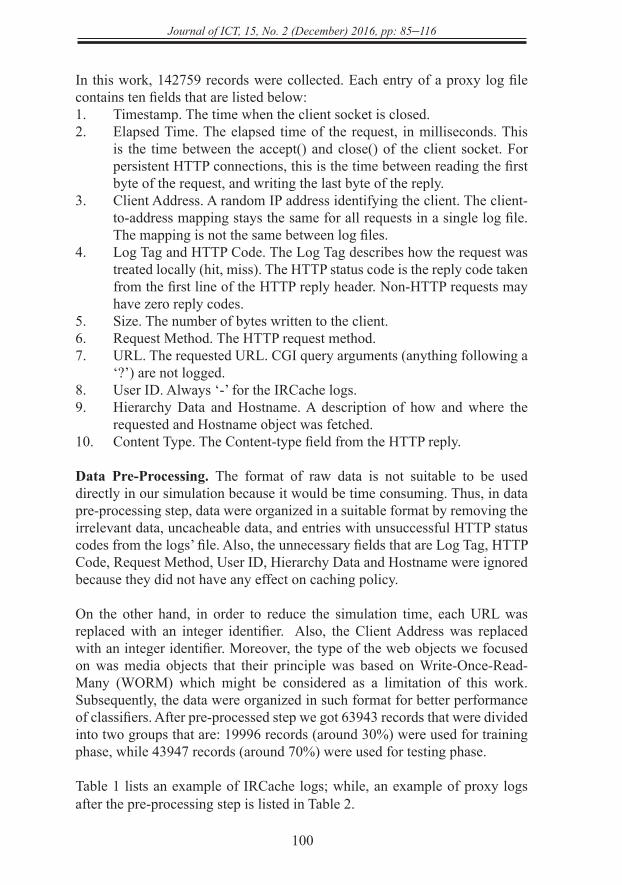
Raw Data Collection. First, raw data were collected from a proxy server. When a user requested a page from the web server through the proxy server, the proxy server recorded this event into a log file. Information about users’ behaviours can be gathered from the logs’ file. The proxy logs’ file was considered as a prior knowledge of users’ behaviours and could be used as an input of the J48 and NB classifiers. The proxy logs were collected from the IRCache network for the requested web objects on the 8th of March 2013.
17
Figure 3. A pseudo code of the proposed approaches
Raw Data Collection. First, raw data were collected from a proxy server. When a user requested a
page from the web server through the proxy server, the proxy server recorded this event into a log file.
Information about users’ behaviours can be gathered from the logs’ file. The proxy logs’ file was
considered as a prior knowledge of users’ behaviours and could be used as an input of the J48 and NB
classifiers. The proxy logs were collected from the IRCache network for the requested web objects on
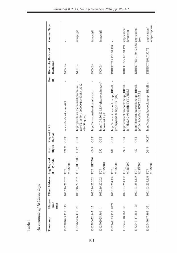
the 8th of March 2013. In this work, 142759 records were collected. Each entry of a proxy log file
contains ten fields that are listed below:
1. Timestamp. The time when the client socket is closed.
Begin For each web object g requested by user Begin If g in cache Begin Cache hit occurs Compute g priority based on its class Update g attributes Update cache manager End Else if g is not in the local cache Begin Cache miss occurs Check peers’ caches If g in cache Begin Cache hit occurs Fetch g from the peer’s cache Compute g priority based on its class Update g attributes Update cache manager End Else Begin Cache miss occurs Fetch g from origin server While no enough space in cache for g Evict object k such that k is the lowest priority object and its class=0 Compute g priority based on its class Update g attributes Update g priority based on its class Update cache manager End End End End
http
://jic
t.uum
.edu
.my
Journal of ICT, 15, No. 2 (December) 2016, pp: 85–116
100
In this work, 142759 records were collected. Each entry of a proxy log file contains ten fields that are listed below:1. Timestamp. The time when the client socket is closed.2. Elapsed Time. The elapsed time of the request, in milliseconds. This
is the time between the accept() and close() of the client socket. For persistent HTTP connections, this is the time between reading the first byte of the request, and writing the last byte of the reply.
3. Client Address. A random IP address identifying the client. The client-to-address mapping stays the same for all requests in a single log file. The mapping is not the same between log files.
4. Log Tag and HTTP Code. The Log Tag describes how the request was treated locally (hit, miss). The HTTP status code is the reply code taken from the first line of the HTTP reply header. Non-HTTP requests may have zero reply codes.
5. Size. The number of bytes written to the client.6. Request Method. The HTTP request method.7. URL. The requested URL. CGI query arguments (anything following a
‘?’) are not logged.8. User ID. Always ‘-’ for the IRCache logs.9. Hierarchy Data and Hostname. A description of how and where the
requested and Hostname object was fetched.10. Content Type. The Content-type field from the HTTP reply.
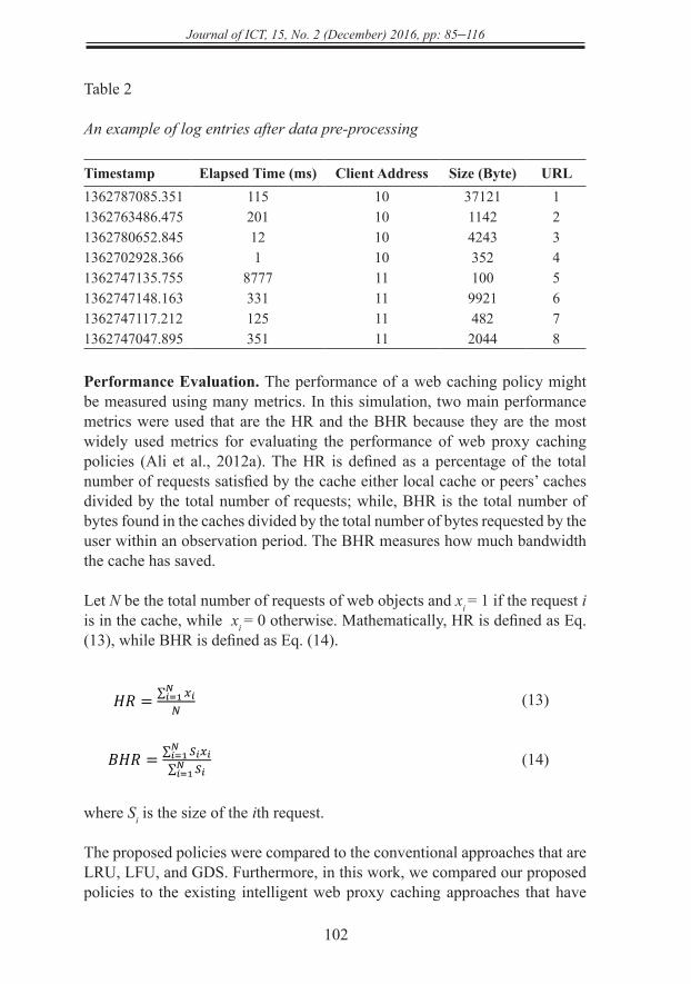
Data Pre-Processing. The format of raw data is not suitable to be used directly in our simulation because it would be time consuming. Thus, in data pre-processing step, data were organized in a suitable format by removing the irrelevant data, uncacheable data, and entries with unsuccessful HTTP status codes from the logs’ file. Also, the unnecessary fields that are Log Tag, HTTP Code, Request Method, User ID, Hierarchy Data and Hostname were ignored because they did not have any effect on caching policy.
On the other hand, in order to reduce the simulation time, each URL was replaced with an integer identifier. Also, the Client Address was replaced with an integer identifier. Moreover, the type of the web objects we focused on was media objects that their principle was based on Write-Once-Read-Many (WORM) which might be considered as a limitation of this work. Subsequently, the data were organized in such format for better performance of classifiers. After pre-processed step we got 63943 records that were divided into two groups that are: 19996 records (around 30%) were used for training phase, while 43947 records (around 70%) were used for testing phase.
Table 1 lists an example of IRCache logs; while, an example of proxy logs after the pre-processing step is listed in Table 2.
http
://jic
t.uum
.edu
.my
101
Journal of ICT, 15, No. 2 (December) 2016, pp: 85–116
Tabl
e 1
An e
xam
ple
of IR
Cac
he lo
gs
Tim
esta
mp
Ela
psed
Ti
me
(ms)
Clie
nt A
ddre
ssL
og T
ag a
nd
HT
TP
Cod
eSi
ze
(Byt
e)R
eque
st
Met
hod
UR
LU
ser
IDH
iera
rchy
Dat
a an
d H
ostn
ame
Con
tent
Typ
e
1362
7870
85.3
5111
510
3.21
6.22
.202
TCP_
MIS
S/20
037
121
GET
ww
w.fa
cebo
ok.c
om:4
43-
NO
NE/
--
1362
7634
86.4
7520
110
3.21
6.22
.202
TCP_
HIT
/200
1142
GET
http
://pr
ofile
.ak.
fbcd
n.ne
t/hpr
ofile
-ak-
ash4
/211
679_
1000
0091
8440
883_
3312
4740
0_q.
jpg
-N
ON
E/-
imag
e/gi
f
1362
7806
52.8
4512
103.
216.
22.2
02TC
P_H
IT/5
0442
43G
ETht
tp://
ww
w.m
sftn
csi.c
om/n
csi.t
xt-
NO
NE/
-im
age/
gif
1362
7029
28.3
661
103.
216.
22.2
02TC
P_M
ISS/
404
352
GET
http
://17
4.36
.231
.13/
rela
xmov
s/im
ages
/bo
okm
ark1
.gif
-N
ON
E/-
imag
e/gi
f
1362
7471
35.7
5587
7710
7.10
3.25
4.13
8TC
P_M
ISS/
000
100
GET
http
://co
nnec
t.fac
eboo
k.ne
t/pt_
BR
/all.
js?[
2qsy
6Xx3
albp
gkU
txT.
jiN]
-D
IREC
T/75
.126
.60.
194
-
1362
7471
48.1
6333
110
7.10
3.25
4.13
8TC
P_M
ISS/
200
9921
GET
http
://co
nnec
t.fac
eboo
k.ne
t/pt_
BR
/all.
js?[
3ks2
AC
i99u
bzH
oEY
EU5E
sL]
-D
IREC
T/75
.126
.60.
194
appl
icat
ion/
java
scrip
t
1362
7471
17.2
1212
510
7.10
3.25
4.13
8TC
P_M
ISS/
200
482
GET
http
://co
nnec
t.fac
eboo
k.ne
t/pt_
BR
/all.
js?[
0vl8
zXzO
eHj3
ZW5.
1Bf2
.L]
-D
IREC
T/18
4.17
0.12
8.58
appl
icat
ion/
json
1362
7470
47.8
9535
110
7.10
3.25
4.13
8TC
P_M
ISS/
200
2044
POST
http
://co
nnec
t.fac
eboo
k.ne
t/pt_
BR
/all.
js-
DIR
ECT/
199.
7.57
.72
appl
icat
ion/
ocsp
-res
pons
e
http
://jic
t.uum
.edu
.my
Journal of ICT, 15, No. 2 (December) 2016, pp: 85–116
102
Table 2
An example of log entries after data pre-processing
Timestamp Elapsed Time (ms) Client Address Size (Byte) URL1362787085.351 115 10 37121 11362763486.475 201 10 1142 21362780652.845 12 10 4243 31362702928.366 1 10 352 41362747135.755 8777 11 100 51362747148.163 331 11 9921 61362747117.212 125 11 482 71362747047.895 351 11 2044 8
Performance Evaluation. The performance of a web caching policy might be measured using many metrics. In this simulation, two main performance metrics were used that are the HR and the BHR because they are the most widely used metrics for evaluating the performance of web proxy caching policies (Ali et al., 2012a). The HR is defined as a percentage of the total number of requests satisfied by the cache either local cache or peers’ caches divided by the total number of requests; while, BHR is the total number of bytes found in the caches divided by the total number of bytes requested by the user within an observation period. The BHR measures how much bandwidth the cache has saved.
Let N be the total number of requests of web objects and xi = 1 if the request i is in the cache, while xi = 0 otherwise. Mathematically, HR is defined as Eq. (13), while BHR is defined as Eq. (14).
(13)
(14)
where Si is the size of the ith request.
The proposed policies were compared to the conventional approaches that are LRU, LFU, and GDS. Furthermore, in this work, we compared our proposed policies to the existing intelligent web proxy caching approaches that have
𝑐𝑐 = {1, 𝑖𝑖𝑖𝑖 𝑡𝑡ℎ𝑒𝑒 𝑚𝑚𝑒𝑒𝑚𝑚𝑖𝑖𝑚𝑚 𝑜𝑜𝑜𝑜𝑜𝑜𝑒𝑒𝑐𝑐𝑡𝑡 𝑤𝑤𝑜𝑜𝑤𝑤𝑤𝑤𝑚𝑚 𝑜𝑜𝑒𝑒 𝑟𝑟𝑒𝑒𝑟𝑟𝑖𝑖𝑟𝑟𝑡𝑡𝑒𝑒𝑚𝑚0, 𝑜𝑜𝑡𝑡ℎ𝑒𝑒𝑟𝑟𝑤𝑤𝑖𝑖𝑟𝑟𝑒𝑒 (10)
Gain Ratio(𝑆𝑆,𝐴𝐴) = Gain(𝑆𝑆,𝐴𝐴)Split Information (𝑆𝑆,𝐴𝐴) (11)
Split Information(𝑆𝑆,𝐴𝐴) = −∑ |𝑆𝑆𝑖𝑖||𝑆𝑆| log2
|𝑆𝑆𝑖𝑖||𝑆𝑆|
𝑘𝑘𝑖𝑖=1 (12)
𝐻𝐻𝐻𝐻 = ∑ 𝑥𝑥𝑖𝑖𝑁𝑁𝑖𝑖=1𝑁𝑁 (13)
𝐵𝐵𝐻𝐻𝐻𝐻 = ∑ 𝑆𝑆𝑖𝑖𝑥𝑥𝑖𝑖𝑁𝑁𝑖𝑖=1∑ 𝑆𝑆𝑖𝑖𝑁𝑁𝑖𝑖=1
(14)
http
://jic
t.uum
.edu
.my
103
Journal of ICT, 15, No. 2 (December) 2016, pp: 85–116
been presented in the works of Ali et al. (2012a) and Ali et al. (2012b), where C4.5-LRU, C4.5-LFU, C4.5-GDS intelligent web caching approaches have been proposed based on C4.5 decision tree supervised machine learning algorithm; while, NB-LRU, NB-LFU, NB-GDS intelligent web caching approaches have been proposed based on NB supervised machine learning algorithm.
RESULTS AND DISCUSSION
In this section, the results that are gathered from running the simulation are presented and they are discussed in details.
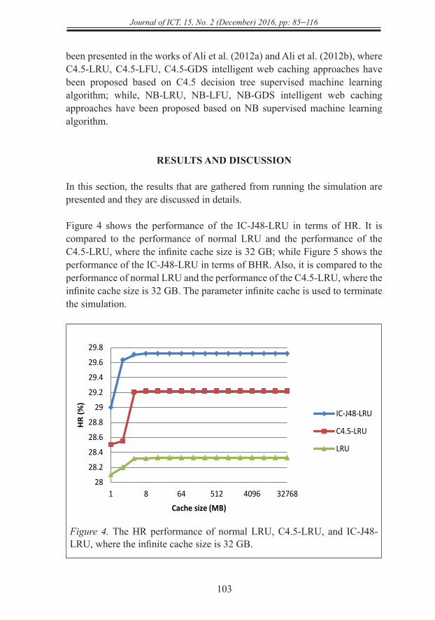
Figure 4 shows the performance of the IC-J48-LRU in terms of HR. It is compared to the performance of normal LRU and the performance of the C4.5-LRU, where the infinite cache size is 32 GB; while Figure 5 shows the performance of the IC-J48-LRU in terms of BHR. Also, it is compared to the performance of normal LRU and the performance of the C4.5-LRU, where the infinite cache size is 32 GB. The parameter infinite cache is used to terminate the simulation.
Figure 4. The HR performance of normal LRU, C4.5-LRU, and IC-J48-LRU, where the infinite cache size is 32 GB.
21
Figure 4 shows the performance of the IC-J48-LRU in terms of HR. It is compared to the performance
of normal LRU and the performance of the C4.5-LRU, where the infinite cache size is 32 GB; while
Figure 5 shows the performance of the IC-J48-LRU in terms of BHR. Also, it is compared to the
performance of normal LRU and the performance of the C4.5-LRU, where the infinite cache size is
32 GB. The parameter infinite cache is used to terminate the simulation.
Figure 4. The HR performance of normal LRU, C4.5-LRU, and IC-J48-LRU, where the infinite cache size is 32 GB
Figure 5. The BHR performance of normal LRU, C4.5-LRU, and IC-J48-LRU, where the infinite cache size is 32 GB
Figure 6 shows the performance of the IC-J48-LFU in terms of HR. It is compared to the performance
of normal LFU and the performance of the C4.5-LFU, where the infinite cache size is 32 GB; while
28
28.2
28.4
28.6
28.8
29
29.2
29.4
29.6
29.8
1 8 64 512 4096 32768
HR
(%)
Cache size (MB)
IC-J48-LRU
C4.5-LRU
LRU
26.5
27
27.5
28
28.5
29
29.5
1 8 64 512 4096 32768
BHR
(%)
Cache size (MB)
IC-J48-LRU
C4.5-LRU
LRU
http
://jic
t.uum
.edu
.my
Journal of ICT, 15, No. 2 (December) 2016, pp: 85–116
104
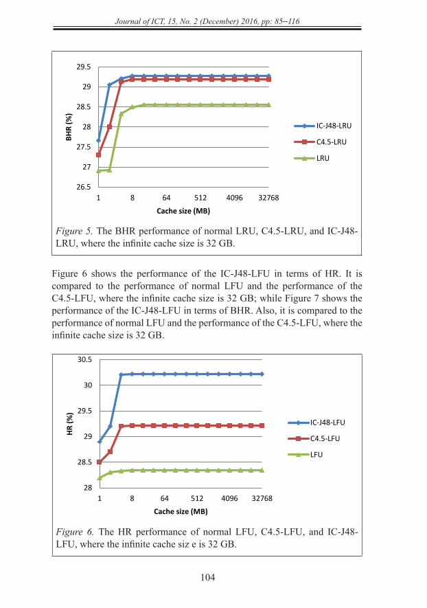
Figure 5. The BHR performance of normal LRU, C4.5-LRU, and IC-J48-LRU, where the infinite cache size is 32 GB.
Figure 6 shows the performance of the IC-J48-LFU in terms of HR. It is compared to the performance of normal LFU and the performance of the C4.5-LFU, where the infinite cache size is 32 GB; while Figure 7 shows the performance of the IC-J48-LFU in terms of BHR. Also, it is compared to the performance of normal LFU and the performance of the C4.5-LFU, where the infinite cache size is 32 GB.
Figure 6. The HR performance of normal LFU, C4.5-LFU, and IC-J48-LFU, where the infinite cache siz e is 32 GB.
21
Figure 4 shows the performance of the IC-J48-LRU in terms of HR. It is compared to the performance
of normal LRU and the performance of the C4.5-LRU, where the infinite cache size is 32 GB; while
Figure 5 shows the performance of the IC-J48-LRU in terms of BHR. Also, it is compared to the
performance of normal LRU and the performance of the C4.5-LRU, where the infinite cache size is
32 GB. The parameter infinite cache is used to terminate the simulation.
Figure 4. The HR performance of normal LRU, C4.5-LRU, and IC-J48-LRU, where the infinite cache size is 32 GB
Figure 5. The BHR performance of normal LRU, C4.5-LRU, and IC-J48-LRU, where the infinite cache size is 32 GB
Figure 6 shows the performance of the IC-J48-LFU in terms of HR. It is compared to the performance
of normal LFU and the performance of the C4.5-LFU, where the infinite cache size is 32 GB; while
28
28.2
28.4
28.6
28.8
29
29.2
29.4
29.6
29.8
1 8 64 512 4096 32768
HR
(%)
Cache size (MB)
IC-J48-LRU
C4.5-LRU
LRU
26.5
27
27.5
28
28.5
29
29.5
1 8 64 512 4096 32768
BHR
(%)
Cache size (MB)
IC-J48-LRU
C4.5-LRU
LRU
22
Figure 7 shows the performance of the IC-J48-LFU in terms of BHR. Also, it is compared to the
performance of normal LFU and the performance of the C4.5-LFU, where the infinite cache size is 32
GB.
Figure 6. The HR performance of normal LFU, C4.5-LFU, and IC-J48-LFU, where the infinite cache size is 32 GB
Figure 7. The BHR performance of normal LFU, C4.5-LFU, and IC-J48-LFU, where the infinite cache size is 32 GB
Figure 8 shows the performance of the IC-J48-GDS in terms of HR. It is compared to the performance
of normal GDS and the performance of the C4.5-GDS, where the infinite cache size is 32 GB; while
Figure 9 shows the performance of the IC-J48-GDS in terms of BHR. Also, it is compared to the
performance of normal GDS and the performance of the C4.5-GDS, where the infinite cache size is
32 GB.
28
28.5
29
29.5
30
30.5
1 8 64 512 4096 32768
HR (%
)
Cache size (MB)
IC-J48-LFU
C4.5-LFU
LFU
26.5
27
27.5
28
28.5
29
29.5
1 8 64 512 4096 32768
BHR
(%)
Cache size (MB)
IC-J48-LFU
C4.5-LFU
LFU
http
://jic
t.uum
.edu
.my
105
Journal of ICT, 15, No. 2 (December) 2016, pp: 85–116
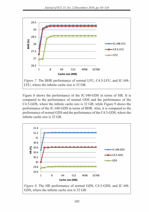
Figure 7. The BHR performance of normal LFU, C4.5-LFU, and IC-J48-LFU, where the infinite cache size is 32 GB.
Figure 8 shows the performance of the IC-J48-GDS in terms of HR. It is compared to the performance of normal GDS and the performance of the C4.5-GDS, where the infinite cache size is 32 GB; while Figure 9 shows the performance of the IC-J48-GDS in terms of BHR. Also, it is compared to the performance of normal GDS and the performance of the C4.5-GDS, where the infinite cache size is 32 GB.
Figure 8. The HR performance of normal GDS, C4.5-GDS, and IC-J48-GDS, where the infinite cache size is 32 GB.
22
Figure 7 shows the performance of the IC-J48-LFU in terms of BHR. Also, it is compared to the
performance of normal LFU and the performance of the C4.5-LFU, where the infinite cache size is 32
GB.
Figure 6. The HR performance of normal LFU, C4.5-LFU, and IC-J48-LFU, where the infinite cache size is 32 GB
Figure 7. The BHR performance of normal LFU, C4.5-LFU, and IC-J48-LFU, where the infinite cache size is 32 GB
Figure 8 shows the performance of the IC-J48-GDS in terms of HR. It is compared to the performance
of normal GDS and the performance of the C4.5-GDS, where the infinite cache size is 32 GB; while
Figure 9 shows the performance of the IC-J48-GDS in terms of BHR. Also, it is compared to the
performance of normal GDS and the performance of the C4.5-GDS, where the infinite cache size is
32 GB.
28
28.5
29
29.5
30
30.5
1 8 64 512 4096 32768
HR (%
)
Cache size (MB)
IC-J48-LFU
C4.5-LFU
LFU
26.5
27
27.5
28
28.5
29
29.5
1 8 64 512 4096 32768
BHR
(%)
Cache size (MB)
IC-J48-LFU
C4.5-LFU
LFU
23
Figure 8. The HR performance of normal GDS, C4.5-GDS, and IC-J48-GDS, where the infinite cache size is 32 GB
Figure 9. The BHR performance of normal GDS, C4.5-GDS, and IC-J48-GDS, where the infinite cache size is 32 GB
Figure 10 shows the performance of IC-NB-LRU in terms of HR. It is compared to the performance
of normal LRU and the performance of NB-LRU, where the infinite cache size is 32 GB; while Figure
11 shows the performance of IC-NB-LRU in terms of BHR. Also, it is compared to the performance
of normal LRU and the performance of NB-LRU, where the infinite cache size is 32 GB.
29.6
29.8
30
30.2
30.4
30.6
30.8
31
31.2
31.4
1 8 64 512 4096 32768
HR (%
)
Cache size (MB)
IC-J48-GDS
C4.5-GDS
GDS
27
27.5
28
28.5
29
29.5
1 8 64 512 4096 32768
BHR
(%)
Cache size (MB)
IC-J48-GDS
C4.5-GDS
GDS
http
://jic
t.uum
.edu
.my
Journal of ICT, 15, No. 2 (December) 2016, pp: 85–116
106
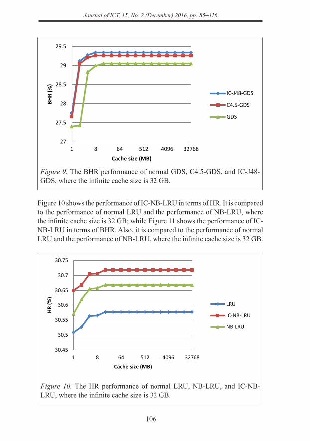
Figure 9. The BHR performance of normal GDS, C4.5-GDS, and IC-J48-GDS, where the infinite cache size is 32 GB.
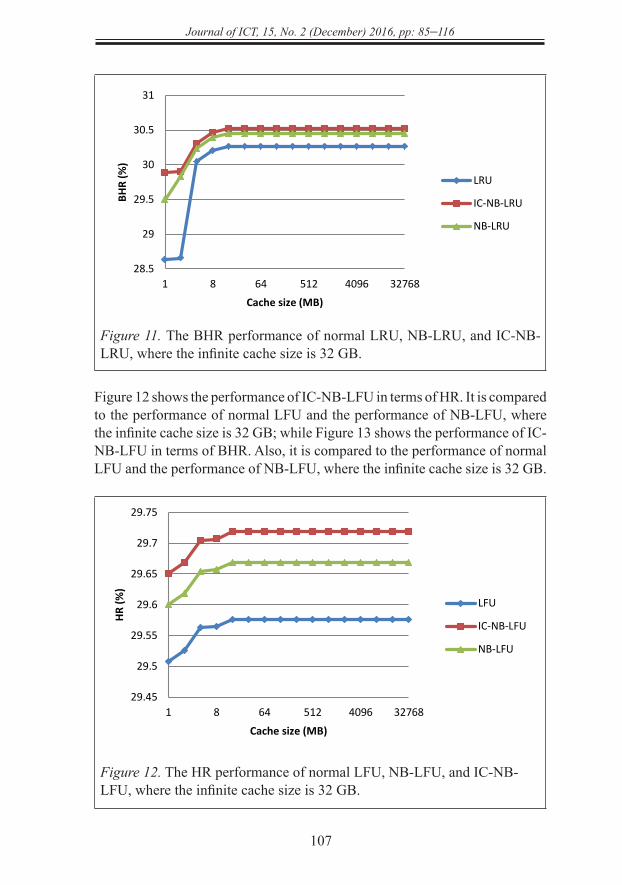
Figure 10 shows the performance of IC-NB-LRU in terms of HR. It is compared to the performance of normal LRU and the performance of NB-LRU, where the infinite cache size is 32 GB; while Figure 11 shows the performance of IC-NB-LRU in terms of BHR. Also, it is compared to the performance of normal LRU and the performance of NB-LRU, where the infinite cache size is 32 GB.
Figure 10. The HR performance of normal LRU, NB-LRU, and IC-NB-LRU, where the infinite cache size is 32 GB.
23
Figure 8. The HR performance of normal GDS, C4.5-GDS, and IC-J48-GDS, where the infinite cache size is 32 GB
Figure 9. The BHR performance of normal GDS, C4.5-GDS, and IC-J48-GDS, where the infinite cache size is 32 GB
Figure 10 shows the performance of IC-NB-LRU in terms of HR. It is compared to the performance
of normal LRU and the performance of NB-LRU, where the infinite cache size is 32 GB; while Figure
11 shows the performance of IC-NB-LRU in terms of BHR. Also, it is compared to the performance
of normal LRU and the performance of NB-LRU, where the infinite cache size is 32 GB.
29.6
29.8
30
30.2
30.4
30.6
30.8
31
31.2
31.4
1 8 64 512 4096 32768
HR (%
)
Cache size (MB)
IC-J48-GDS
C4.5-GDS
GDS
27
27.5
28
28.5
29
29.5
1 8 64 512 4096 32768
BHR
(%)
Cache size (MB)
IC-J48-GDS
C4.5-GDS
GDS
24
Figure 10. The HR performance of normal LRU, NB-LRU, and IC-NB-LRU, where the infinite cache size is 32 GB
Figure 11. The BHR performance of normal LRU, NB-LRU, and IC-NB-LRU, where the infinite cache size is 32 GB
Figure 12 shows the performance of IC-NB-LFU in terms of HR. It is compared to the performance of
normal LFU and the performance of NB-LFU, where the infinite cache size is 32 GB; while Figure 13
shows the performance of IC-NB-LFU in terms of BHR. Also, it is compared to the performance of
normal LFU and the performance of NB-LFU, where the infinite cache size is 32 GB.
30.45
30.5
30.55
30.6
30.65
30.7
30.75
1 8 64 512 4096 32768
HR (%
)
Cache size (MB)
LRU
IC-NB-LRU
NB-LRU
28.5
29
29.5
30
30.5
31
1 8 64 512 4096 32768
BHR
(%)
Cache size (MB)
LRU
IC-NB-LRU
NB-LRU
http
://jic
t.uum
.edu
.my
107
Journal of ICT, 15, No. 2 (December) 2016, pp: 85–116
Figure 11. The BHR performance of normal LRU, NB-LRU, and IC-NB-LRU, where the infinite cache size is 32 GB.
Figure 12 shows the performance of IC-NB-LFU in terms of HR. It is compared to the performance of normal LFU and the performance of NB-LFU, where the infinite cache size is 32 GB; while Figure 13 shows the performance of IC-NB-LFU in terms of BHR. Also, it is compared to the performance of normal LFU and the performance of NB-LFU, where the infinite cache size is 32 GB.
Figure 12. The HR performance of normal LFU, NB-LFU, and IC-NB-LFU, where the infinite cache size is 32 GB.
24
Figure 10. The HR performance of normal LRU, NB-LRU, and IC-NB-LRU, where the infinite cache size is 32 GB
Figure 11. The BHR performance of normal LRU, NB-LRU, and IC-NB-LRU, where the infinite cache size is 32 GB
Figure 12 shows the performance of IC-NB-LFU in terms of HR. It is compared to the performance of
normal LFU and the performance of NB-LFU, where the infinite cache size is 32 GB; while Figure 13
shows the performance of IC-NB-LFU in terms of BHR. Also, it is compared to the performance of
normal LFU and the performance of NB-LFU, where the infinite cache size is 32 GB.
30.45
30.5
30.55
30.6
30.65
30.7
30.75
1 8 64 512 4096 32768
HR (%
)
Cache size (MB)
LRU
IC-NB-LRU
NB-LRU
28.5
29
29.5
30
30.5
31
1 8 64 512 4096 32768
BHR
(%)
Cache size (MB)
LRU
IC-NB-LRU
NB-LRU
25
Figure 12. The HR performance of normal LFU, NB-LFU, and IC-NB-LFU, where the infinite cache size is 32 GB
Figure 13. The BHR performance of normal LFU, NB-LFU, and IC-NB-LFU, where the infinite cache size is 32 GB
Figure 14 shows the performance of IC-NB-GDS in terms of HR. It is compared to the performance
of normal GDS and the performance of NB-GDS, where the infinite cache size is 32 GB; while Figure
15 shows the performance of IC-NB-GDS in terms of BHR. Also, it is compared to the performance
of normal GDS and the performance of NB-GDS, where the infinite cache size is 32 GB.
29.45
29.5
29.55
29.6
29.65
29.7
29.75
1 8 64 512 4096 32768
HR (%
)
Cache size (MB)
LFU
IC-NB-LFU
NB-LFU
27.427.627.8
2828.228.428.628.8
2929.229.429.6
1 8 64 512 4096 32768
BHR
(%)
Cache size (MB)
LFU
IC-NB-LFU
NB-LFU
http
://jic
t.uum
.edu
.my
Journal of ICT, 15, No. 2 (December) 2016, pp: 85–116
108
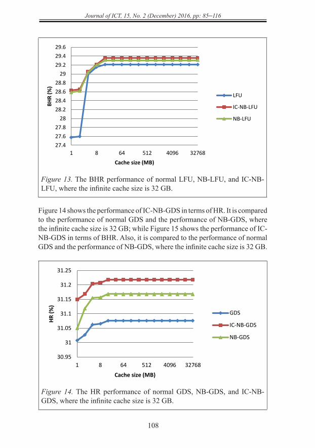
Figure 13. The BHR performance of normal LFU, NB-LFU, and IC-NB-LFU, where the infinite cache size is 32 GB.
Figure 14 shows the performance of IC-NB-GDS in terms of HR. It is compared to the performance of normal GDS and the performance of NB-GDS, where the infinite cache size is 32 GB; while Figure 15 shows the performance of IC-NB-GDS in terms of BHR. Also, it is compared to the performance of normal GDS and the performance of NB-GDS, where the infinite cache size is 32 GB.
Figure 14. The HR performance of normal GDS, NB-GDS, and IC-NB-GDS, where the infinite cache size is 32 GB.
25
Figure 12. The HR performance of normal LFU, NB-LFU, and IC-NB-LFU, where the infinite cache size is 32 GB
Figure 13. The BHR performance of normal LFU, NB-LFU, and IC-NB-LFU, where the infinite cache size is 32 GB
Figure 14 shows the performance of IC-NB-GDS in terms of HR. It is compared to the performance
of normal GDS and the performance of NB-GDS, where the infinite cache size is 32 GB; while Figure
15 shows the performance of IC-NB-GDS in terms of BHR. Also, it is compared to the performance
of normal GDS and the performance of NB-GDS, where the infinite cache size is 32 GB.
29.45
29.5
29.55
29.6
29.65
29.7
29.75
1 8 64 512 4096 32768
HR (%
)
Cache size (MB)
LFU
IC-NB-LFU
NB-LFU
27.427.627.8
2828.228.428.628.8
2929.229.429.6
1 8 64 512 4096 32768
BHR
(%)
Cache size (MB)
LFU
IC-NB-LFU
NB-LFU
26
Figure 14. The HR performance of normal GDS, NB-GDS, and IC-NB-GDS, where the infinite cache size is 32 GB
Figure 15. The BHR performance of normal GDS, NB-GDS, and IC-NB-GDS, where the infinite cache size is 32 GB
Referring to Figure 4, it can be observed that IC-J48-LRU performs better than LRU and C4.5-LRU
in terms of HR. For example, the HR of IC-J48-LRU is around 29% when the cache size is 1 MB;
while the HR of LRU is around 28.1% and the HR of C4.5-LRU is around 28.5% for the same cache
size.
Referring to Figure 5, it can be observed that IC-J48-LRU performs better than LRU in terms of BHR.
For example, the BHR of IC-J48-LRU is around 29.27% when the cache size is 64 MB; while the
BHR of LRU is around 28.56% and the BHR of C4.5-LRU is around 29.19% for the same cache size.
This is mainly due to the capability of IC-J48-LRU approach for storing the preferred media objects
30.95
31
31.05
31.1
31.15
31.2
31.25
1 8 64 512 4096 32768
HR (%
)
Cache size (MB)
GDS
IC-NB-GDS
NB-GDS
28.5
29
29.5
30
30.5
31
31.5
1 8 64 512 4096 32768
HR (%
)
Cache size (MB)
GDS
IC-NB-GDS
NB-GDS
http
://jic
t.uum
.edu
.my
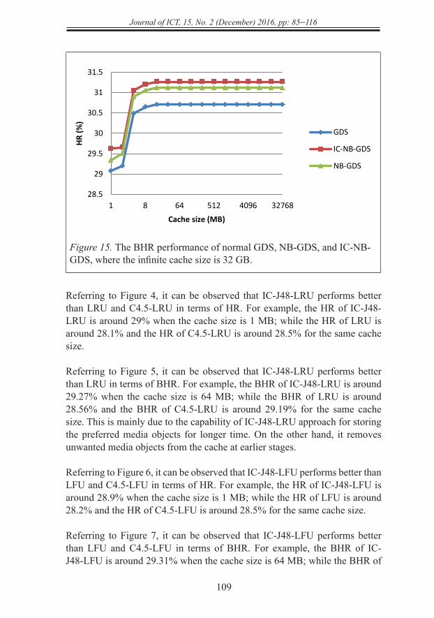
109
Journal of ICT, 15, No. 2 (December) 2016, pp: 85–116
Figure 15. The BHR performance of normal GDS, NB-GDS, and IC-NB-GDS, where the infinite cache size is 32 GB.
Referring to Figure 4, it can be observed that IC-J48-LRU performs better than LRU and C4.5-LRU in terms of HR. For example, the HR of IC-J48-LRU is around 29% when the cache size is 1 MB; while the HR of LRU is around 28.1% and the HR of C4.5-LRU is around 28.5% for the same cache size.
Referring to Figure 5, it can be observed that IC-J48-LRU performs better than LRU in terms of BHR. For example, the BHR of IC-J48-LRU is around 29.27% when the cache size is 64 MB; while the BHR of LRU is around 28.56% and the BHR of C4.5-LRU is around 29.19% for the same cache size. This is mainly due to the capability of IC-J48-LRU approach for storing the preferred media objects for longer time. On the other hand, it removes unwanted media objects from the cache at earlier stages.
Referring to Figure 6, it can be observed that IC-J48-LFU performs better than LFU and C4.5-LFU in terms of HR. For example, the HR of IC-J48-LFU is around 28.9% when the cache size is 1 MB; while the HR of LFU is around 28.2% and the HR of C4.5-LFU is around 28.5% for the same cache size.
Referring to Figure 7, it can be observed that IC-J48-LFU performs better than LFU and C4.5-LFU in terms of BHR. For example, the BHR of IC-J48-LFU is around 29.31% when the cache size is 64 MB; while the BHR of
26
Figure 14. The HR performance of normal GDS, NB-GDS, and IC-NB-GDS, where the infinite cache size is 32 GB
Figure 15. The BHR performance of normal GDS, NB-GDS, and IC-NB-GDS, where the infinite cache size is 32 GB
Referring to Figure 4, it can be observed that IC-J48-LRU performs better than LRU and C4.5-LRU
in terms of HR. For example, the HR of IC-J48-LRU is around 29% when the cache size is 1 MB;
while the HR of LRU is around 28.1% and the HR of C4.5-LRU is around 28.5% for the same cache
size.
Referring to Figure 5, it can be observed that IC-J48-LRU performs better than LRU in terms of BHR.
For example, the BHR of IC-J48-LRU is around 29.27% when the cache size is 64 MB; while the
BHR of LRU is around 28.56% and the BHR of C4.5-LRU is around 29.19% for the same cache size.
This is mainly due to the capability of IC-J48-LRU approach for storing the preferred media objects
30.95
31
31.05
31.1
31.15
31.2
31.25
1 8 64 512 4096 32768
HR (%
)
Cache size (MB)
GDS
IC-NB-GDS
NB-GDS
28.5
29
29.5
30
30.5
31
31.5
1 8 64 512 4096 32768
HR (%
)
Cache size (MB)
GDS
IC-NB-GDS
NB-GDS
http
://jic
t.uum
.edu
.my
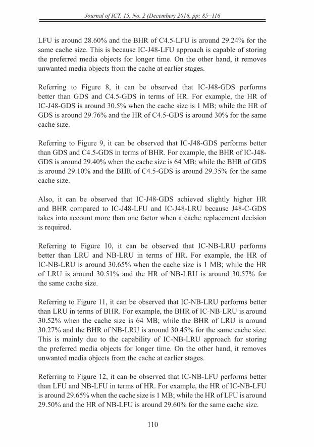
Journal of ICT, 15, No. 2 (December) 2016, pp: 85–116
110
LFU is around 28.60% and the BHR of C4.5-LFU is around 29.24% for the same cache size. This is because IC-J48-LFU approach is capable of storing the preferred media objects for longer time. On the other hand, it removes unwanted media objects from the cache at earlier stages.
Referring to Figure 8, it can be observed that IC-J48-GDS performs better than GDS and C4.5-GDS in terms of HR. For example, the HR of IC-J48-GDS is around 30.5% when the cache size is 1 MB; while the HR of GDS is around 29.76% and the HR of C4.5-GDS is around 30% for the same cache size.
Referring to Figure 9, it can be observed that IC-J48-GDS performs better than GDS and C4.5-GDS in terms of BHR. For example, the BHR of IC-J48-GDS is around 29.40% when the cache size is 64 MB; while the BHR of GDS is around 29.10% and the BHR of C4.5-GDS is around 29.35% for the same cache size.
Also, it can be observed that IC-J48-GDS achieved slightly higher HR and BHR compared to IC-J48-LFU and IC-J48-LRU because J48-C-GDS takes into account more than one factor when a cache replacement decision is required.
Referring to Figure 10, it can be observed that IC-NB-LRU performs better than LRU and NB-LRU in terms of HR. For example, the HR of IC-NB-LRU is around 30.65% when the cache size is 1 MB; while the HR of LRU is around 30.51% and the HR of NB-LRU is around 30.57% for the same cache size.
Referring to Figure 11, it can be observed that IC-NB-LRU performs better than LRU in terms of BHR. For example, the BHR of IC-NB-LRU is around 30.52% when the cache size is 64 MB; while the BHR of LRU is around 30.27% and the BHR of NB-LRU is around 30.45% for the same cache size. This is mainly due to the capability of IC-NB-LRU approach for storing the preferred media objects for longer time. On the other hand, it removes unwanted media objects from the cache at earlier stages.
Referring to Figure 12, it can be observed that IC-NB-LFU performs better than LFU and NB-LFU in terms of HR. For example, the HR of IC-NB-LFU is around 29.65% when the cache size is 1 MB; while the HR of LFU is around 29.50% and the HR of NB-LFU is around 29.60% for the same cache size.
http
://jic
t.uum
.edu
.my
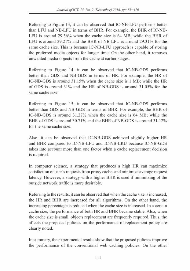
111
Journal of ICT, 15, No. 2 (December) 2016, pp: 85–116
Referring to Figure 13, it can be observed that IC-NB-LFU performs better than LFU and NB-LFU in terms of BHR. For example, the BHR of IC-NB-LFU is around 29.36% when the cache size is 64 MB; while the BHR of LFU is around 29.21% and the BHR of NB-LFU is around 29.31% for the same cache size. This is because IC-NB-LFU approach is capable of storing the preferred media objects for longer time. On the other hand, it removes unwanted media objects from the cache at earlier stages.
Referring to Figure 14, it can be observed that IC-NB-GDS performs better than GDS and NB-GDS in terms of HR. For example, the HR of IC-NB-GDS is around 31.15% when the cache size is 1 MB; while the HR of GDS is around 31% and the HR of NB-GDS is around 31.05% for the same cache size.
Referring to Figure 15, it can be observed that IC-NB-GDS performs better than GDS and NB-GDS in terms of BHR. For example, the BHR of IC-NB-GDS is around 31.27% when the cache size is 64 MB; while the BHR of GDS is around 30.71% and the BHR of NB-GDS is around 31.12% for the same cache size.
Also, it can be observed that IC-NB-GDS achieved slightly higher HR and BHR compared to IC-NB-LFU and IC-NB-LRU because IC-NB-GDS takes into account more than one factor when a cache replacement decision is required.
In computer science, a strategy that produces a high HR can maximize satisfaction of user’s requests from proxy cache, and minimize average request latency. However, a strategy with a higher BHR is used if minimizing of the outside network traffic is more desirable.
Referring to the results, it can be observed that when the cache size is increased, the HR and BHR are increased for all algorithms. On the other hand, the increasing percentage is reduced when the cache size is increased. In a certain cache size, the performance of both HR and BHR became stable. Also, when the cache size is small, objects replacement are frequently required. Thus, the affects the proposed policies on the performance of replacement policy are clearly noted.
In summary, the experimental results show that the proposed policies improve the performance of the conventional web caching policies. On the other
http
://jic
t.uum
.edu
.my
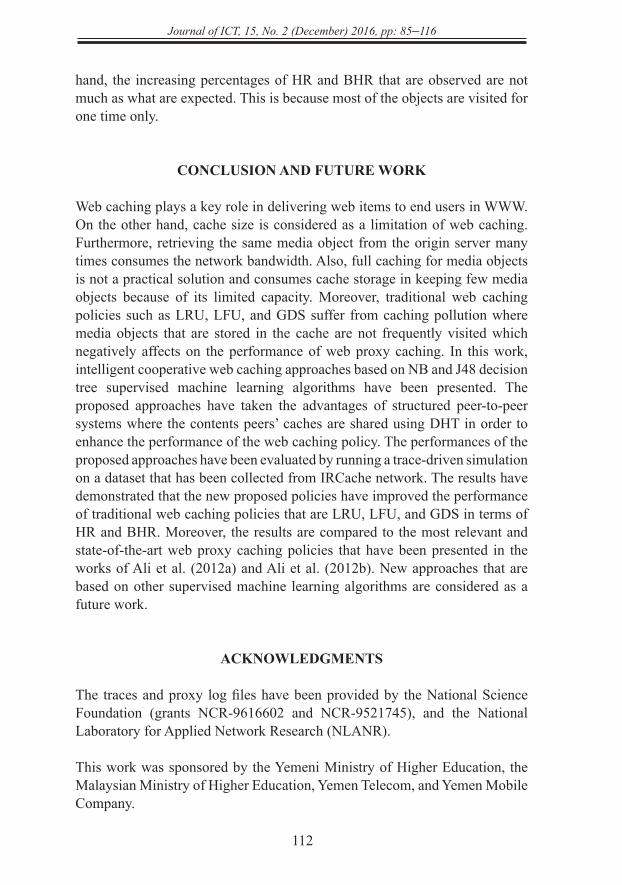
Journal of ICT, 15, No. 2 (December) 2016, pp: 85–116
112
hand, the increasing percentages of HR and BHR that are observed are not much as what are expected. This is because most of the objects are visited for one time only.
CONCLUSION AND FUTURE WORK
Web caching plays a key role in delivering web items to end users in WWW. On the other hand, cache size is considered as a limitation of web caching. Furthermore, retrieving the same media object from the origin server many times consumes the network bandwidth. Also, full caching for media objects is not a practical solution and consumes cache storage in keeping few media objects because of its limited capacity. Moreover, traditional web caching policies such as LRU, LFU, and GDS suffer from caching pollution where media objects that are stored in the cache are not frequently visited which negatively affects on the performance of web proxy caching. In this work, intelligent cooperative web caching approaches based on NB and J48 decision tree supervised machine learning algorithms have been presented. The proposed approaches have taken the advantages of structured peer-to-peer systems where the contents peers’ caches are shared using DHT in order to enhance the performance of the web caching policy. The performances of the proposed approaches have been evaluated by running a trace-driven simulation on a dataset that has been collected from IRCache network. The results have demonstrated that the new proposed policies have improved the performance of traditional web caching policies that are LRU, LFU, and GDS in terms of HR and BHR. Moreover, the results are compared to the most relevant and state-of-the-art web proxy caching policies that have been presented in the works of Ali et al. (2012a) and Ali et al. (2012b). New approaches that are based on other supervised machine learning algorithms are considered as a future work.
ACKNOWLEDGMENTS
The traces and proxy log files have been provided by the National Science Foundation (grants NCR-9616602 and NCR-9521745), and the National Laboratory for Applied Network Research (NLANR).
This work was sponsored by the Yemeni Ministry of Higher Education, the Malaysian Ministry of Higher Education, Yemen Telecom, and Yemen Mobile Company.
http
://jic
t.uum
.edu
.my
113
Journal of ICT, 15, No. 2 (December) 2016, pp: 85–116
REFERENCES
Ali, W., Shamsuddin, S. M., & Ismail, A. S. (2011). Patterns analysis and classification for web proxy cache. Proceedings of the 11th International Conference on Hybrid Intelligent Systems (HIS), Malacca, Malaysia. 97-102. doi:10.1109/HIS.2011.6122087
Ali, W., Shamsuddin, S. M., & Ismail, A. S. (2012a). Intelligent naïve bayes-based approaches for web proxy caching. Knowledge-Based Systems, 31(0), 162-175. doi:10.1016/j.knosys.2012.02.015”
Ali, W., Shamsuddin, S. M., & Ismail, A. S. (2012b). Intelligent web proxy caching approaches based on machine learning techniques. Decision Support Systems, 53(3), 565-579. doi:10.1016/j.dss.2012.04.011”
Ali, W., & Shamsuddin, S. (2009). Intelligent client-side web caching scheme based on least recently used algorithm and neuro-fuzzy system. In W. Yu, H. He & N. Zhang (Eds.), (pp. 70-79) Springer Berlin Heidelberg. doi:10.1007/978-3-642-01510-6_9
Arlitt, M., Cherkasova, L., Dilley, J., Friedrich, R., & Jin, T. (2000). Evaluating content management techniques for web proxy caches. ACM SIGMETRICS Performance Evaluation Review, 27(4), 3-11. doi:10.1145/346000.346003
Chen, R., & Hsieh, C. (2006). Web page classification based on a support vector machine using a weighted vote schema. Expert Systems with Applications, 31(2), 427-435. doi:10.1016/j.eswa.2005.09.079
Cobb, J., & ElAarag, H. (2008). Web proxy cache replacement scheme based on back-propagation neural network. Journal of Systems and Software, 81(9), 1539-1558. doi:10.1016/j.jss.2007.10.024
Darwiche, A. (2010). Bayesian networks. Communications of the ACM, 53(12), 80-90. doi:10.1145/1859204.1859227
de Melo, A. C. V., & Sanchez, A. J. (2008). Software maintenance project delays prediction using bayesian networks. Expert Systems with Applications, 34(2), 908-919. doi:10.1016/j.eswa.2006.10.040
http
://jic
t.uum
.edu
.my
Journal of ICT, 15, No. 2 (December) 2016, pp: 85–116
114
ElAarag, H., & Romano, S. (2009). Training of NNPCR-2: An improved neural network proxy cache replacement strategy. Proceedings of the International Symposium on Performance Evaluation of Computer & Telecommunication Systems (SPECTS 2009) , Istanbul, Turkey. , 41 260-267. doi:978-1-4244-4165-5
ElAarag, H. (2013). A quantitative study of web cache replacement strategies using simulation. (pp. 17-60) Springer London. doi:10.1007/978-1-4471-4893-7_4
Fan, L., Poh, K., & Zhou, P. (2009). A sequential feature extraction approach for naïve bayes classification of microarray data. Expert Systems with Applications, 36(6), 9919-9923. doi:10.1016/j.eswa.2009.01.075
Friedman, N., Geiger, D., & Goldszmidt, M. (1997). Bayesian network classifiers. Machine Learning, 29(2-3), 131-163. doi:10.1023/A:1007465528199
Goubanova, O., & King, S. (2008). Bayesian networks for phone duration prediction. Speech Communication, 50(4), 301-311. doi:10.1016/j.specom.2007.10.002
Hara, T., Maeda, K., Ishi, Y., Uchida, W., & Nishio, S. (2010). Cooperative caching by clients constructing a peer-to-peer network for push-based broadcast. Data & Knowledge Engineering, 69(2), 229-247. doi:10.1016/j.datak.2009.10.011
Koskela, T., Heikkonen, J., & Kaski, K. (2003). Web cache optimization with nonlinear model using object features. Computer Networks, 43(6), 805-817. doi:10.1016/S1389-1286(03)00334-7
Lu, S., Chiang, D., Keh, H., & Huang, H. (2010). Chinese text classification by the naïve bayes classifier and the associative classifier with multiple confidence threshold values. Knowledge-Based Systems, 23(6), 598-604. doi:10.1016/j.knosys.2010.04.004
Quinlan, J. R. (1993). C4.5: Programs for machine learning. San Francisco, CA, USA: Morgan Kaufmann Publishers Inc.
Shafaatunnur, H., Tan Swee, Q., & Siti Mariyam, S. (2012). Artificial fish swarm for multilayer network learning in classification problems. Journal of Information and Communication Technology, 11, 37-53.
http
://jic
t.uum
.edu
.my
115
Journal of ICT, 15, No. 2 (December) 2016, pp: 85–116
Sripanidkulchai, K., & Zhang, H. (2005). Content location in peer-to-peer systems: Exploiting locality. In X. Tang, J. Xu, S. T. Chanson & Y. Zhang (Eds.), Web content delivery (pp. 73-97) Springer US. doi:10.1007/0-387-27727-7_4
Stefan Podlipnig & Laszlo Böszörmenyi (2003). A survey of web cache replacement strategies. ACM Computing Surveys, 35(4), 374-398. doi:10.1145/954339.954341
Sulaiman, S., Shamsuddin, S. M., Forkan, F., & Abraham, A. (2008). Intelligent web caching using neurocomputing and particle swarm optimization algorithm. Proceedings of the Second Asia International Conference on Modeling & Simulation (AICMS 08), Kuala Lumpur, Malaysia. 642-647. doi:10.1109/AMS.2008.40
Tracey Ho, Medard, M., Koetter, R., Karger, D. R., Effros, M., Jun Shi, & Leong, B. (2006). A random linear network coding approach to multicast. IEEE Transactions on Information Theory, 52(10), 4413-4430. doi:10.1109/TIT.2006.881746
Wu, X., Kumar, V., Ross Quinlan, J., Ghosh, J., Yang, Q., Motoda, H., & Steinberg, D. (2008). Top 10 algorithms in data mining. Knowledge and Information Systems, 14(1), 1-37. doi:10.1007/s10115-007-0114-2
Xu, K., Zhang, M., Liu, J., Qin, Z., & Ye, M. (2010). Proxy caching for peer-to-peer live streaming. Computer Networks, 54(7), 1229-1241. doi:10.1016/j.comnet.2009.11.013
Yasin, W., Ibrahim, H., Hamid, N. A. W. A., & Udzir, N. I. (2011). A systematic review of file sharing in mobile devices using peer-to-peer systems. Computer and Information Science, 4(1), 28-41.
Yasin, W., Ibrahim, H., Hamid, N. A. W. A., & Udzir, N. I. (2013). An overview of media streams caching in peer-to-peer systems. The Computer Journal, 57, 1167-1177. doi:10.1093/comjnl/bxt054
Yasin, W., Ibrahim, H., Hamid, N. A. W. A., & Udzir, N. I. (2014a). Intelligent cooperative web caching policies for media objects based on decision tree supervised machine learning algorithm. Proceedings of the Malaysian National Conference on Databases 2014 (MANCOD 14), Selangor D.E., Malaysia. 69-74.
http
://jic
t.uum
.edu
.my

Journal of ICT, 15, No. 2 (December) 2016, pp: 85–116
116
Yasin, W., Ibrahim, H., Hamid, N. A. W. A., & Udzir, N. I. (2014b). Intelligent cooperative web caching policies for media objects based on J48 classifier. Proceedings of the 16th International Conference on Information Integration and Web-Based Applications & Services (iiWAS2014), Hanoi, Vietnam. 262-269. doi:10.1145/2684200.2684299
Zink, M., & Shenoy, P. (2005). Caching and distribution issues for streaming content distribution networks. In Y. Zhang, X. Tang, J. Xu & S. T. Chanson (Eds.), Web content delivery (pp. 246-263) Springer US. doi:10.1007/0-387-27727-7_11
http
://jic
t.uum
.edu
.my