UNIVERSITI PUTRA MALAYSIA A CLASS OF DIAGONALLY ...psasir.upm.edu.my/7547/1/ABS_---__FS_2009_29.pdf · penghampiran songsangan Hessian permulaan merupakan matriks identiti, suatu

UNIVERSITI PUTRA MALAYSIA

A CLASS OF DIAGONALLY PRECONDITIONED LIMITED MEMORY QUASI-NEWTON METHODS FOR LARGE-SCALE UNCONSTRAINED

OPTIMIZATION

CHEN CHUEI YEE

FS 2009 29

A CLASS OF DIAGONALLY PRECONDITIONED

LIMITED MEMORY QUASI-NEWTON

METHODS FOR LARGE-SCALE

UNCONSTRAINED OPTIMIZATION

CHEN CHUEI YEE

MASTER OF SCIENCE

UNIVERSITI PUTRA MALAYSIA

2009

A CLASS OF DIAGONALLY PRECONDITIONED LIMITED MEMORY

QUASI-NEWTON METHODS FOR LARGE-SCALE

UNCONSTRAINED OPTIMIZATION

By

CHEN CHUEI YEE

Thesis Submitted to the School of Graduate Studies, Universiti Putra Malaysia,

in Fulfilment of the Requirements for the Degree of Master of Science

September 2009

ii

Abstract of thesis presented to the Senate of Universiti Putra Malaysia

in fulfilment of the requirement for the degree of Master of Science

A CLASS OF DIAGONALLY PRECONDITIONED

LIMITED MEMORY QUASI-NEWTON METHODS FOR

LARGE-SCALE UNCONSTRAINED OPTIMIZATION

By

CHEN CHUEI YEE

September 2009

Chairman: Leong Wah June, PhD

Faculty: Science

The focus of this thesis is to diagonally precondition on the limited memory quasi-

Newton method for large scale unconstrained optimization problem. Particularly, the

centre of discussion is on diagonally preconditioned limited memory Broyden-

Fletcher-Goldfarb-Shanno (L-BFGS) method.

L-BFGS method has been widely used in large scale unconstrained optimization due

to its effectiveness. However, a major drawback of the L-BFGS method is that it can

be very slow on certain type of problems. Scaling and preconditioning have been

used to boost the performance of the L-BFGS method.

In this study, a class of diagonally preconditioned L-BFGS method will be proposed.

Contrary to the standard L-BFGS method where its initial inverse Hessian

iii

approximation is the identity matrix, a class of diagonal preconditioners has been

derived based upon the weak-quasi-Newton relation with an additional parameter.

Choosing different parameters leads the research to some well-known diagonal

updating formulae which enable the R-linear convergent for the L-BFGS method.

Numerical experiments were performed on a set of large scale unconstrained

minimization problem to examine the impact of each choice of parameter. The

computational results suggest that the proposed diagonally preconditioned L-BFGS

methods outperform the standard L-BFGS method without any preconditioning.

Finally, we discuss on the impact of the diagonal preconditioners on the L-BFGS

method as compared to the standard L-BFGS method in terms of the number of

iterations, the number of function/gradient evaluations and the CPU time in second.

iv

Abstrak tesis yang dikemukakan kepada Senat Universiti Putra Malaysia

sebagai memenuhi keperluan untuk ijazah Sarjana Sains

SUATU KAEDAH KELAS KUASI-NEWTON INGATAN TERHAD

DENGAN PRAPENSYARAT PEPENJURU BAGI

PENGOPTIMUMAN TAK BERKEKANGAN BERSKALA BESAR

Oleh

CHEN CHUEI YEE

September 2009

Pengerusi: Leong Wah June, PhD

Fakulti: Sains

Tumpuan tesis ini adalah mencari prapensyarat pepenjuru untuk kaedah kuasi-

Newton ingatan terhad bagi menyelesaikan masalah pengoptimuman tak

berkekangan berskala besar. Khususnya, tumpuan perbincangan adalah kepada

kaedah Broyden-Fletcher-Goldfarb-Shanno ingatan terhad (L-BFGS) dengan

prapensyarat pepenjuru.

Kaedah L-BFGS telah digunakan secara meluas dalam pengoptimuman tak

berkekangan berskala besar disebabkan oleh keberkesanannya. Walau

bagaimanapun, satu kelemahan utama kaedah L-BFGS adalah ia boleh menjadi

perlahan bagi sesetengah masalah. Penskalaan dan prapensyarat telah digunakan

untuk meningkatkan prestasi kaedah L-BFGS.

v

Dalam kajian ini, beberapa cara telah diperiksa untuk menprasyarat kaedah L-BFGS

secara pepenjuru. Bertentangan dengan kaedah L-BFGS yang piawai di mana

penghampiran songsangan Hessian permulaan merupakan matriks identiti, suatu

kelas prapensyarat pepenjuru telah diperolehi berdasarkan kepada hubungan kuasi-

Newton lemah dengan satu parameter tambahan. Pemilihan parameter yang

berlainan dalam penyelidikan ini membawa kepada beberapa formula kemaskini

secara pepenjuru yang terkemuka dan juga mengekalkan penumpuan R-linear.

Ujikaji berangka telah dijalankan ke atas satu set masalah peminimuman tak

berkekangan berskala besar untuk mengkaji impak setiap pilihan parameter.

Keputusan pengiraan mencadangkan bahawa kaedah L-BFGS berprapensyarat

pepenjuru adalah lebih baik daripada kaedah L-BFGS tanpa sebarang prapensyarat.

Akhirnya, kami membincangkan tentang impak setiap prapensyarat pepenjuru

kepada kaedah L-BFGS dengan perbandingan kepada kaedah L-BFGS piawai.

Lanjutan bagi penyelidikan masa depan juga diberi.

vi

ACKNOWLEDGEMENT

First and foremost, thank God for His blessing and wisdom.

I would like to thank and express my gratitude to my supervisor, Dr. Leong Wah

June, for his guidance and patience throughout the period of this degree. He has

indeed given me a lot of insights on this research and did a thorough checking on my

thesis.

Apart from that, I would like to express my thanks towards my supervisory

committee members, Professor Dr. Malik B. Hj. Abu Hassan and Associate

Professor Dr. Fudziah Ismail, for willing to be part of the committee and for their

advice throughout the period of my study.

My appreciation also goes to my family members who have always been there for

me. Their endurance and love keeps me moving forward all the time. Not forgetting

are my beloved friends and colleagues who have offered advices whenever I need

one. No word can express my deepest gratitude at the moment.

vii

I certify that a Thesis Examination Committee has met on 29 September 2009 to

conduct the final examination of Chen Chuei Yee on her thesis entitled “A Class of

Diagonally Preconditioned Limited Memory Quasi-Newton Methods for Large-

Scale Unconstrained Optimization” in accordance with the Universities and

University Colleges Act 1971 and the Constitution of the Universiti Putra Malaysia

[P.U.(A) 106] 15 March 1998. The Committee recommends that the student be

awarded the Master of Science.

Members of the Examination Committee were as follows:

Isa Daud, PhD

Associate Professor

Faculty of Science

Universiti Putra Malaysia

(Chairman)

Lee Lai Soon, PhD

Lecturer

Faculty of Science


(Internal Examiner)

Mansor Monsi, PhD

Lecturer

Faculty of Science


(Internal Examiner)

Mustafa Mamat, PhD

Lecturer

Faculty of Science and Techonology

Universiti Malaysia Terengganu

(External Examiner)

BUJANG BIN KIM KUAT, Phd

Professor and Deputy Dean

School of Graduate Studies


Date: 15 October 2009

viii

This thesis was submitted to the Senate of Universiti Putra Malaysia and has been

accepted as fulfilment of the requirement for the degree of Master of Science. The

members of the Supervisory Committee were as follows:

Leong Wah June, PhD

Faculty of Science


(Chairman)

Malik Hj. Abu Hassan, PhD

Professor

Faculty of Science


(Member)

Fudziah Ismail, PhD

Associate Professor

Faculty of Science


(Member)

___________

HASANAH MOHD GHAZALI, PhD

Professor and Dean

School of Graduate Studies


Date: 16 November 2009

ix

DECLARATION

I declare that the thesis is my original work except for quotations and citations which

have been duly acknowledged. I also declare that it has not been previously, and is

not concurrently, submitted for any other degree at Universiti Putra Malaysia or any

other institution.

CHEN CHUEI YEE

Date: 08 February 2010

x

TABLE OF CONTENTS

Page

ABSTRACT ii

ABSTRAK iv

ACKNOWLEDGEMENTS vi

APPROVAL vii

DECLARATION ix

LIST OF TABLES xii

LIST OF FIGURES xiv

LIST OF ABBREVIATIONS xv

CHAPTER

1 INTRODUCTION

1.1 Preliminaries

1.2 Optimization Problem

1.3 Functions and Derivatives

1.4 Convexity

1.5 An Overview of the Thesis

1

1

2

4

10

18

2 QUASI-NEWTON METHODS

2.1 An Overview of Newton’s Method

2.2 Quasi-Newton Methods

2.2.1 Introduction

2.2.2 Approximating the Inverse Hessian

2.2.3 Family of Quasi-Newton Methods

2.3 Summary

19

19

25

25

27

30

45

3 LIMITED MEMORY QUASI-NEWTON METHODS

3.1 Introduction

3.2 Limit Memory BFGS (L-BFGS) Method

3.3 Other Limited Memory Quasi-Newton Methods

3.3.1 Limited Memory Symmetric Rank One (L-SR1)

Method

3.3.2 Limited Memory Broyden Family

3.3.3 Limited Memory DFP (L-DFP)Method

3.4 Summary

47

47

50

54

54

56

57

59

4 DIAGONAL PRECONDITIONERS FOR LIMITED

MEMORY QUASI-NEWTON METHODS

4.1 Quasi-Newton Relation and Diagonal Updating

4.2 Diagonal Preconditioners for Limited Memory Quasi-

61

61

68

xi

Newton Methods

4.3 A Class of Positive Definite Diagonal Preconditioners for

L-BFGS Method

75

5 CONVERGENCE ANALYSIS

5.1 Introduction

5.2 Convergence Analysis

5.3 Conclusion

78

78

79

82

6 COMPUTATIONAL RESULTS AND DISCUSSION

6.1 Computational Experiments

6.2 Computational Results and Discussion

83

83

86

7 CONCLUSION AND FUTURE WORKS

7.1 Conclusion

7.2 Future Works

116

116

117

REFERENCES 119

APPENDICES 122

BIODATA OF STUDENT 185

xii

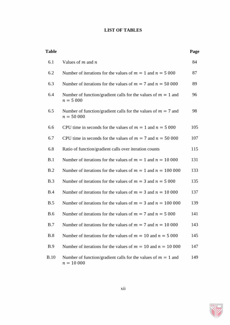
LIST OF TABLES

Table Page

6.1 Values of 𝑚 and 𝑛 84

6.2 Number of iterations for the values of 𝑚 = 1 and 𝑛 = 5 000 87

6.3 Number of iterations for the values of 𝑚 = 7 and 𝑛 = 50 000 89

6.4 Number of function/gradient calls for the values of 𝑚 = 1 and

𝑛 = 5 000

96

6.5 Number of function/gradient calls for the values of 𝑚 = 7 and

𝑛 = 50 000

98

6.6 CPU time in seconds for the values of 𝑚 = 1 and 𝑛 = 5 000 105

6.7 CPU time in seconds for the values of 𝑚 = 7 and 𝑛 = 50 000 107

6.8 Ratio of function/gradient calls over iteration counts 115

B.1 Number of iterations for the values of 𝑚 = 1 and 𝑛 = 10 000 131









B.10 Number of function/gradient calls for the values of 𝑚 = 1 and

𝑛 = 10 000

149

xiii


𝑛 = 100 000

151


𝑛 = 5 000

153


𝑛 = 10 000

155


𝑛 = 100 000

157


𝑛 = 5 000

159


𝑛 = 10 000

161


𝑛 = 5 000

163


𝑛 = 10 000

165

B.19 CPU time in seconds for the values of 𝑚 = 1 and 𝑛 = 10 000 167









xiv

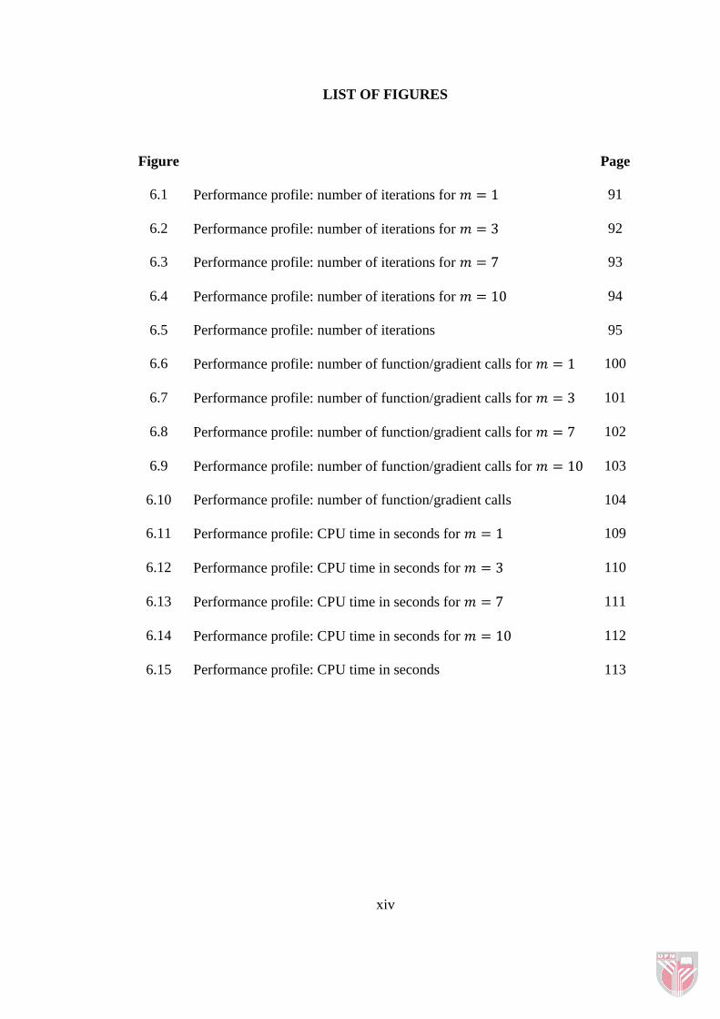
LIST OF FIGURES

Figure Page

6.1 Performance profile: number of iterations for 𝑚 = 1 91




6.5 Performance profile: number of iterations 95

6.6 Performance profile: number of function/gradient calls for 𝑚 = 1 100




6.10 Performance profile: number of function/gradient calls 104

6.11 Performance profile: CPU time in seconds for 𝑚 = 1 109




6.15 Performance profile: CPU time in seconds 113

xv

LIST OF ABBREVIATIONS

Abbreviation Description

𝑥 real-valued vectors where

𝑥 = 𝑥1,𝑥2 ,… , 𝑥𝑛 𝑇

𝑓 𝑥 or 𝑓 function of 𝑥

𝑅 set of real numbers

𝑅𝑛 set of 𝑛 dimensional real-valued vectors

∇𝑓 𝑥 or 𝑔 𝑥 first derivative of 𝑓 𝑥 where

𝛻𝑓 𝑥 = 𝑔 𝑥 = 𝜕𝑓

𝜕𝑥1,𝜕𝑓

𝜕𝑥2,⋯ ,

𝜕𝑓

𝜕𝑥𝑛 𝑇

.

∇2𝑓 𝑥 or 𝐺 𝑥 second derivative of 𝑓 𝑥 , called the Hessian, where

𝐺 𝑥 = ∇2𝑓 𝑥 =

𝜕2𝑓 𝑥

𝜕𝑥12

𝜕2𝑓 𝑥

𝜕𝑥1𝜕𝑥2⋯

𝜕2𝑓 𝑥

𝜕𝑥1𝜕𝑥𝑛

𝜕2𝑓 𝑥

𝜕𝑥2𝜕𝑥1

𝜕2𝑓 𝑥

𝜕𝑥22 ⋯

𝜕2𝑓 𝑥


⋮ ⋮ ⋱ ⋮𝜕2𝑓 𝑥

𝜕𝑥𝑛𝜕𝑥1

𝜕2𝑓 𝑥

𝜕𝑥𝑛𝜕𝑥2⋯

𝜕2𝑓 𝑥

𝜕𝑥𝑛2

.

𝐼 identity matrix

𝑦𝑘 the difference between 𝑔𝑘+1 and 𝑔𝑘 where

𝑦𝑘 = 𝑔𝑘+1 − 𝑔𝑘

𝑠𝑘 the difference between 𝑥𝑘+1 and 𝑥𝑘 where

𝑠𝑘 = 𝑥𝑘+1 − 𝑥𝑘

𝐵𝑘 approximation of the Hessian

𝐻𝑘 approximation of the inverse Hessian

𝑡𝑟 trace operator

FONC First-Order Necessary Condition

SONC Second-Order Necessary Condition

SOSC Second-Order Sufficient Condition

BFGS Broyden-Fletcher-Goldfarb-Shanno

L-BFGS limited memory Broyden-Fletcher-Goldfarb-Shanno

DFP Davidon-Fletcher-Powell

xvi

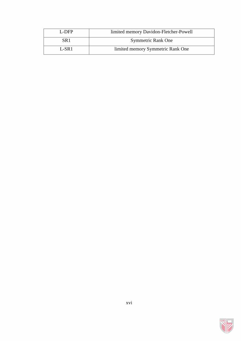
L-DFP limited memory Davidon-Fletcher-Powell

SR1 Symmetric Rank One

L-SR1 limited memory Symmetric Rank One

CHAPTER 1

INTRODUCTION

1.1 Preliminaries

Optimization, a subject in applied mathematics, is a fascinating blend of heuristics

and rigour, of theory and experiment. It is normally studied as a branch of

mathematics and yet it has vast applications in almost every branch of science and

technology such as engineering, economics, science and military. Optimization is

recognized as the science of determining the optimal or best solutions to certain

mathematically defined problems. As optimization as a whole, it is the central to any

problem involving decision making by which the optimal solutions to the problems

can be found from various schemes.

One of the well-known methods in optimization is the Newton’s method. However,

the evaluation of the Hessian matrix or its inverse is considered to be impractical and

costly. Moreover, convergence to a solution cannot be guaranteed from an arbitrary

initial point for a general nonlinear objective functions. With this, the quasi-Newton

methods came to rise by which the Hessian matrix (or its inverse) of the function to

be minimized need not be computed. A number of algorithms have been proposed

under the quasi-Newton scheme.

Since the origin of limited memory methods in 1977, many attentions have been

given to limited memory quasi-Newton methods for solving large scale

2

unconstrained optimization problems. Despite the fact that the limited memory

methods are often very effective, they can be slow and have limited accuracy,

especially for ill-conditioned problem. It is well-known that the limited-memory

methods can be greatly accelerated by preconditioning on the initial inverse Hessian

approximation.

The centre of this research revolves around solving large scale unconstrained

minimization problems using limited memory quasi-Newton methods. Particularly,

we focus on solving the problems by diagonally preconditioning on the limited

memory Broyden-Fletcher-Goldfarb-Shanno (L-BFGS) method.

Before we begin with the main idea of this research, it is more appropriate to look at

the mathematical background of an optimization problem first. Note that the

mathematical background discussed in this chapter can be found in Gill et al. (1981),

Fletcher (2004), Nocedal and Wright (2006) and Chong and Żak (2008). Additional

information on this chapter can be obtained in those references too.

1.2 Optimization Problem

We consider the optimization problem

minimize 𝑓 𝑥

subject to 𝑥 ∈ Ω (1.1)

3

where 𝑓:𝑅𝑛 → 𝑅 is the objective/cost function, the vector 𝑥 = 𝑥1, 𝑥2,… , 𝑥𝑛 𝑇 ∈ 𝑅𝑛

is a n-vector of independent variables and the set Ω ⊂ 𝑅𝑛 is the constraint/feasible

set.

If Ω = 𝑅𝑛 , the optimization problem is regarded as unconstrained optimization

problem by which we

minimize 𝑓 𝑥

subject to 𝑥 ∈ 𝑅𝑛 . (1.2)

The problem of maximizing f is the same as minimizing –f since there is no loss of

generality.

A constrained optimization problem can be written as

minimize 𝑓 𝑥

subject to 𝑐𝑖 ≥ 0, 𝑖 = 1, 2,… ,𝑘,

𝑐𝑖 = 0, 𝑖 = 𝑘 + 1,𝑘 + 2,… ,𝑚.

(1.3)

If the objective function and the constraint functions are in the form of linear

functions, the problem is regarded as linear programming. Otherwise, the problem

becomes a nonlinear programming problem.

Following, we shall discuss on the mathematical background of large scale

unconstrained optimization. Since we aim to solve minimization problems, it is

necessary to include the definitions of types of minimizer.

4

Definition 1.1: Suppose that 𝑓:𝑅𝑛 → 𝑅 is a real-valued function defined on some set

Ω ⊂ 𝑅𝑛 . A point 𝑥∗ ∈ Ω is a local minimizer of f over Ω if there exists 휀 > 0 such

that 𝑓 𝑥 ≥ 𝑓 𝑥∗ for all 𝑥 ∈ Ω\ 𝑥∗ and 𝑥 − 𝑥∗ < 휀.


Ω ⊂ 𝑅𝑛 . A point 𝑥∗ ∈ Ω is a strict local minimizer of f over Ω if there exists 휀 > 0

such that 𝑓 𝑥 > 𝑓 𝑥∗ for all 𝑥 ∈ Ω\ 𝑥∗ and 𝑥 − 𝑥∗ < 휀.


Ω ⊂ 𝑅𝑛 . A point 𝑥∗ ∈ Ω is a global minimizer of 𝑓over Ω if 𝑓 𝑥 ≥ 𝑓 𝑥∗ for all

𝑥 ∈ Ω\ 𝑥∗ .

1.3 Functions and Derivatives

A function 𝑓:𝑅𝑛 → 𝑅 is said to be continuously differentiable at 𝑥 ∈ 𝑅𝑛 , if 𝜕𝑓 𝑥

𝜕𝑥𝑖

exists and is continuous for 𝑖 = 1, 2,… , 𝑛. The gradient of f at x is given by

∇𝑓 𝑥 = 𝜕𝑓

𝜕𝑥1,𝜕𝑓

𝜕𝑥2,⋯ ,

𝜕𝑓

𝜕𝑥𝑛 𝑇

. (1.4)

A function 𝑓:Ω → 𝑅𝑛 , Ω ∈ 𝑅𝑛 , is said to be continuously differentiable on Ω if it is

differentiable on Ω, and the components of f have continuous partial derivatives. It is

5

denoted by 𝑓 ∈ 𝒞1 . It will be denoted as 𝑓 ∈ 𝒞𝑝 if the components of f have

continuous partial derivatives of order p.

A function 𝑓:𝑅𝑛 → 𝑅 is said to be twice continuously differentiable at 𝑥 ∈ 𝑅𝑛 , if

𝜕2𝑓 𝑥

𝜕𝑥𝑖𝜕𝑥𝑗 exists and is continuous for 𝑖 = 1, 2,… ,𝑛. The second derivative of 𝑓 𝑥 is

written as

𝐺 𝑥 = ∇2𝑓 𝑥 =

𝜕2𝑓 𝑥

𝜕𝑥12

𝜕2𝑓 𝑥

𝜕𝑥1𝜕𝑥2⋯

𝜕2𝑓 𝑥


𝜕2𝑓 𝑥

𝜕𝑥2𝜕𝑥1

𝜕2𝑓 𝑥

𝜕𝑥22 ⋯

𝜕2𝑓 𝑥


⋮ ⋮ ⋱ ⋮𝜕2𝑓 𝑥

𝜕𝑥𝑛𝜕𝑥1

𝜕2𝑓 𝑥

𝜕𝑥𝑛𝜕𝑥2⋯

𝜕2𝑓 𝑥

𝜕𝑥𝑛2

. (1.5)

The matrix 𝐺 𝑥 is called the Hessian matrix of the function 𝑓:𝑅𝑛 → 𝑅 at x and it is

an 𝑛 × 𝑛 symmetric matrix if 𝑓 is continuous.

Definition 1.4: A vector 𝑑 ∈ 𝑅𝑛 , 𝑑 ≠ 0, is a feasible direction at 𝑥 ∈ Ω if there

exists 𝛼0 > 0 such that 𝑥 + 𝛼𝑑 ∈ Ω for all 𝛼 ∈ 0,𝛼0 .

Let 𝑓:𝑅𝑛 → 𝑅 be a real-valued function and let 𝑑 be a feasible direction at 𝑥 ∈ Ω,

the directional derivative of 𝑥 in the direction of 𝑑 is denoted by

𝜕𝑓 𝑥

𝜕𝑑= lim𝛼→0

𝑓 𝑥+𝛼𝑑 −𝑓 𝑥

𝛼= ∇𝑓 𝑥 𝑇𝑑. (1.6)

6

Suppose that 𝑥 and 𝑑 are given, then 𝑓 𝑥 + 𝛼𝑑 is a function of 𝛼 and

𝜕𝑓 𝑥

𝜕𝑑= 𝜕

𝜕𝛼𝑓 𝑥 + 𝛼𝑑

𝛼=0. (1.7)

By the chain rule,

𝜕𝑓 𝑥

𝜕𝑑= 𝜕

𝜕𝛼𝑓 𝑥 + 𝛼𝑑

𝛼=0= ∇𝑓 𝑥 𝑇𝑑 = ∇𝑓 𝑥 ,𝑑 = 𝑑𝑇∇𝑓 𝑥 . (1.8)

In short, if 𝑑 = 1 which means 𝑑 is a unit vector, then 𝜕𝑓 𝑥

𝜕𝑑 or ∇𝑓 𝑥 ,𝑑 is the

rate of increase of 𝑓 at the point 𝑥 in the direction 𝑑.

Following, we will discuss on the first order conditions of functions. Let 𝑓:𝑅𝑛 → 𝑅

be a continuously differentiable function defined on 𝑅𝑛 .

Theorem 1.1 First-Order Necessary Condition (FONC):

Let Ω be a subset of 𝑅𝑛 and 𝑓 ∈ 𝒞1 a real-valued function on Ω. If 𝑥∗ is a local

minimizer of f over Ω, then for any feasible direction d at 𝑥∗, we have

𝑑𝑇∇𝑓 𝑥∗ ≥ 0. (1.9)

Proof.

Define

𝑥 𝛼 = 𝑥∗ + 𝛼𝑑, 𝑥 𝛼 ∈ Ω. (1.10)

7

If 𝛼 = 0, it is clear that 𝑥 0 = 𝑥∗. The composite function is defined as:

𝜙 𝛼 = 𝑓 𝑥 𝛼 . (1.11)

By Taylor’s theorem,

𝑓 𝑥∗ + 𝛼𝑑 − 𝑓 𝑥∗ = 𝜙 𝛼 − 𝜙 0

= 𝜙′ 0 𝛼 + 𝑜 𝛼

= 𝛼𝑑𝑇∇𝑓 𝑥 0 + 𝑜 𝛼 ,

(1.12)

where 𝛼 ≥ 0.

Thus if 𝜙 𝛼 ≥ 𝜙 0 , that is

𝑓 𝑥∗ + 𝛼𝑑 − 𝑓 𝑥∗ ≥ 0,

𝑓 𝑥∗ + 𝛼𝑑 ≥ 𝑓 𝑥∗ , (1.13)

for sufficiently small values of 𝛼 > 0, then we must have 𝑑𝑇∇𝑓 𝑥∗ ≥ 0. ∎

Corollary 1.1 Interior Case:

Let Ω be a subset of 𝑅𝑛 and 𝑓 ∈ 𝒞1 a real-valued function on Ω. If 𝑥∗ is a local

minimizer of f over Ω and if 𝑥∗ is an interior point of Ω, then

∇𝑓 𝑥∗ = 0. (1.14)

Proof.

Suppose that f has a local minimizer 𝑥∗ that is an interior point of Ω. Because 𝑥∗ is

an interior point of Ω, the set of feasible directions at 𝑥∗ is the whole of 𝑅𝑛 . Thus, for

any 𝑑 ∈ 𝑅𝑛 , 𝑑𝑇∇𝑓 𝑥∗ ≥ 0 and −𝑑𝑇∇𝑓 𝑥∗ ≥ 0 . Hence, 𝑑𝑇∇𝑓 𝑥∗ = 0 for all

𝑑 ∈ 𝑅𝑛 , which implies that ∇𝑓 𝑥∗ = 0. ∎

Documents

UNIVERSITI PUTRA MALAYSIA A CLASS OF DIAGONALLY ...psasir.upm.edu.my/7547/1/ABS_---__FS_2009_29.pdf · penghampiran songsangan Hessian permulaan merupakan matriks identiti, suatu