Embed Size (px)
Citation preview

Universiteit Leiden
ICT in Business
Exploring the Relationship between Football Players’
Performance and Their Market Value Name: Miao He Student-no: S1372734 Date: 25/07/2015 1st supervisor: Ricardo Cachucho 2nd supervisor: Prof. Dr. Aske Plaat MASTER'S THESIS Leiden Institute of Advanced Computer Science (LIACS) Leiden University Niels Bohrweg 1 2333 CA Leiden The Netherlands
Abstract
A lot of money is involved with the transfers of top players in the big European football
leagues. For various reasons, obtaining a good economic valuation of football players
throughout the year is valuable, in other words, not only when a player has just been
transferred. The good performance of a player has a positive impact on his club’s income.
Furthermore, it is relevant to consider how the market value of a player relates to the
performance of that player. Both these factors again depend on the various parameters of
the player, that might be gleaned from various public sources on the web. In this paper, I
demonstrate how market value and performance of La Liga (the Spanish League) players
can be modeled using extensive public data sources. According to the results of my
model, some players are overvalued or undervalued by the market. In addition, the
reasons for these exceptions have been studied.
i

Acknowledgments
First of all, I would like to thank my first supervisor, Ricardo Cachucho, for his valuable
guidance, support and recommendations during my master thesis, unconditionally
support me when I feel depressed and uneasy with my thesis. And my second Reader,
Professor Dr. Aske Plaat, for assisting me in the initial phase of the master thesis and
useful suggestions in the end.
In addition, I would like to thank my colleagues from ICT in Business. I really like and
will miss studying and working together. Especially, I want to thank the girls - Huihang
He, Huan Tan, Yaxin Zhang, Lijin Zheng - for your accompany and treat me as a family
here. Also, I want to thank Yaxin Zhang for helping me with the thesis writing.
Last but not least, I would like to thank my family in China for their unconditionally
supporting. They always encourage me when I have hard time. Without them I cannot
get though this big challenge in my master.
ii

Contents
Abstract i
Acknowledgments ii
Contents iii
List of figures vi
List of tables vii
1 Introduction 1
1.1 Background . . . . . . . . . . . . . . . . . . . . . . . . . . . . . . . . . . . 1
1.2 Research Questions . . . . . . . . . . . . . . . . . . . . . . . . . . . . . . . 2
1.3 Research Contribution . . . . . . . . . . . . . . . . . . . . . . . . . . . . . 2
1.4 Research Scope . . . . . . . . . . . . . . . . . . . . . . . . . . . . . . . . . 3
1.5 Research Methods . . . . . . . . . . . . . . . . . . . . . . . . . . . . . . . . 3
1.6 Thesis Outline . . . . . . . . . . . . . . . . . . . . . . . . . . . . . . . . . . 5
2 Problem Statement 7
2.1 Problem Definition . . . . . . . . . . . . . . . . . . . . . . . . . . . . . . . 7
2.2 Research Question . . . . . . . . . . . . . . . . . . . . . . . . . . . . . . . 9
2.3 Prior Research . . . . . . . . . . . . . . . . . . . . . . . . . . . . . . . . . 10
2.3.1 Market Value . . . . . . . . . . . . . . . . . . . . . . . . . . . . . . 10
2.3.2 Performance . . . . . . . . . . . . . . . . . . . . . . . . . . . . . . . 11
3 Data 13
3.1 Data Collection . . . . . . . . . . . . . . . . . . . . . . . . . . . . . . . . . 13
3.1.1 Data Source . . . . . . . . . . . . . . . . . . . . . . . . . . . . . . . 13
3.1.2 Data gathering method . . . . . . . . . . . . . . . . . . . . . . . . . 14
iii

Contents
3.1.3 Data gathering-Start with la Liga . . . . . . . . . . . . . . . . . . . 15
3.2 Data Preparation . . . . . . . . . . . . . . . . . . . . . . . . . . . . . . . . 16
3.2.1 Data Merge . . . . . . . . . . . . . . . . . . . . . . . . . . . . . . . 17
3.2.2 Data Normalization . . . . . . . . . . . . . . . . . . . . . . . . . . . 18
3.2.3 Dealing with missing values . . . . . . . . . . . . . . . . . . . . . . 18
3.2.4 Type convert . . . . . . . . . . . . . . . . . . . . . . . . . . . . . . 19
3.3 Data Set . . . . . . . . . . . . . . . . . . . . . . . . . . . . . . . . . . . . . 19
4 General Model for Real Value 20
4.1 Model Preparation . . . . . . . . . . . . . . . . . . . . . . . . . . . . . . . 20
4.1.1 Machine Learning Method . . . . . . . . . . . . . . . . . . . . . . . 20
4.1.2 Proxy Value . . . . . . . . . . . . . . . . . . . . . . . . . . . . . . . 21
4.1.3 Variable Selection . . . . . . . . . . . . . . . . . . . . . . . . . . . . 22
4.2 Choose Suitable Regression Model . . . . . . . . . . . . . . . . . . . . . . . 23
4.2.1 Regression Tree . . . . . . . . . . . . . . . . . . . . . . . . . . . . . 23
4.2.2 LASSO . . . . . . . . . . . . . . . . . . . . . . . . . . . . . . . . . 25
4.3 Apply Lasso Model in R . . . . . . . . . . . . . . . . . . . . . . . . . . . . 26
4.3.1 Model Implementation . . . . . . . . . . . . . . . . . . . . . . . . . 26
4.3.2 Proper Model . . . . . . . . . . . . . . . . . . . . . . . . . . . . . . 26
5 Market Value 28
5.1 LASSO Real Market Value Model . . . . . . . . . . . . . . . . . . . . . . . 28
5.1.1 Lambda.min model . . . . . . . . . . . . . . . . . . . . . . . . . . . 28
5.1.2 Lambda.1se model . . . . . . . . . . . . . . . . . . . . . . . . . . . 29
5.1.3 Proper Model . . . . . . . . . . . . . . . . . . . . . . . . . . . . . . 29
5.2 Market Value Statistic Description . . . . . . . . . . . . . . . . . . . . . . 31
5.2.1 Relationship between market value and general features . . . . . . . 32
5.2.2 Re-category Positions . . . . . . . . . . . . . . . . . . . . . . . . . . 34
6 Performance Analysis 37
6.1 LASSO Real Performance Model for Strikers . . . . . . . . . . . . . . . . . 37
6.2 Models for Goalkeepers, Defenders, Midfielders . . . . . . . . . . . . . . . . 40
6.2.1 Whoscored’s Rating as the Target . . . . . . . . . . . . . . . . . . . 40
6.2.2 LASSO Models . . . . . . . . . . . . . . . . . . . . . . . . . . . . . 41
6.2.3 Performance Analysis . . . . . . . . . . . . . . . . . . . . . . . . . . 42
iv

Contents
7 Market Value vs Performance 45
7.1 Cross Market Value and Performance . . . . . . . . . . . . . . . . . . . . . 45
7.1.1 Pre-study . . . . . . . . . . . . . . . . . . . . . . . . . . . . . . . . 45
7.1.2 Market Value Defined by Performance . . . . . . . . . . . . . . . . 46
7.2 Value Results observations by Positions . . . . . . . . . . . . . . . . . . . . 49
7.2.1 Value Result versus Characteristics and careers . . . . . . . . . . . 49
7.2.2 Analysis for improperly valued players . . . . . . . . . . . . . . . . 52
7.2.3 Study for Goalkeepers . . . . . . . . . . . . . . . . . . . . . . . . . 53
7.3 Underlying Reasons . . . . . . . . . . . . . . . . . . . . . . . . . . . . . . . 54
7.3.1 General Reasons . . . . . . . . . . . . . . . . . . . . . . . . . . . . 54
7.3.2 Superstar Players . . . . . . . . . . . . . . . . . . . . . . . . . . . . 55
7.3.3 Nationality . . . . . . . . . . . . . . . . . . . . . . . . . . . . . . . 56
7.3.4 Clubs . . . . . . . . . . . . . . . . . . . . . . . . . . . . . . . . . . 57
8 Conclusion 58
8.1 Conclusions . . . . . . . . . . . . . . . . . . . . . . . . . . . . . . . . . . . 58
8.2 Research limitations . . . . . . . . . . . . . . . . . . . . . . . . . . . . . . 60
8.3 Future Study . . . . . . . . . . . . . . . . . . . . . . . . . . . . . . . . . . 60
A Variable Explanation 66
B R code 69
B.1 Data Preparation . . . . . . . . . . . . . . . . . . . . . . . . . . . . . . . . 69
B.1.1 Preprocesing . . . . . . . . . . . . . . . . . . . . . . . . . . . . . . . 69
B.1.2 Data Match . . . . . . . . . . . . . . . . . . . . . . . . . . . . . . . 71
B.2 LASSO in R . . . . . . . . . . . . . . . . . . . . . . . . . . . . . . . . . . . 72
C Intermediate Results 73
C.1 Defenders Predicted Logarithm of Market Value . . . . . . . . . . . . . . . 73
v

List of Figures
1.1 Research Techniques . . . . . . . . . . . . . . . . . . . . . . . . . . . . . . 4
1.2 Data Mining Process . . . . . . . . . . . . . . . . . . . . . . . . . . . . . . 5
3.1 Research Techniques . . . . . . . . . . . . . . . . . . . . . . . . . . . . . . 16
4.1 Comparisson between real and proxy variables for Market value and perfor-
mace assessment of footbal players. . . . . . . . . . . . . . . . . . . . . . . 21
4.2 Covanriance of all the Variables . . . . . . . . . . . . . . . . . . . . . . . . 22
4.3 Real Market Value by Regression Tree . . . . . . . . . . . . . . . . . . . . 24
5.1 LASSO regression for real market value prediction . . . . . . . . . . . . . . 30
5.2 Histogram of football player’s real market value . . . . . . . . . . . . . . . 31
5.3 Relationship between market value and numerical general features . . . . . 33
5.4 Histogram of football player’s real market value by positions . . . . . . . . 34
5.5 Left Wings and Right Wings Market Value Distribution . . . . . . . . . . . 35
6.1 FIFA Ballon d’Or winners by position . . . . . . . . . . . . . . . . . . . . . 38
6.2 General Distribution of strikers’ Performance Prediction . . . . . . . . . . 39
6.3 Relation between WhoScored Rating and Voting. . . . . . . . . . . . . . . 40
6.4 General Distribution of Players Performance Prediction with WhoScored’s
Rating . . . . . . . . . . . . . . . . . . . . . . . . . . . . . . . . . . . . . . 44
7.1 Relation Between Market Value and Strikers Performance Assessments. . . 46
7.2 Relation between logarithm market value and performance assessments. . . 47
7.3 Relation between market value and strikers characteristics and career. . . . 50
7.4 Relation between market value and midfielders characteristics and career. . 51
7.5 Relation between market value and defenders characteristics and career. . . 52
7.6 Factors Regression Tree for Goal Keepers’ Market Value . . . . . . . . . . 54
vi

List of Tables
5.1 Lambda.min Model for Real Market Value Summary . . . . . . . . . . . . 29
6.1 central tendency of strikers ’ Performance Prediction . . . . . . . . . . . . . 39
6.2 central tendency of Players’ Performance Prediction . . . . . . . . . . . . . 43
7.1 Overvalued Players . . . . . . . . . . . . . . . . . . . . . . . . . . . . . . . 53
7.2 Undervalued Players . . . . . . . . . . . . . . . . . . . . . . . . . . . . . . 53
8.1 Overvalued Players . . . . . . . . . . . . . . . . . . . . . . . . . . . . . . . 59
A.1 Variable Explanations . . . . . . . . . . . . . . . . . . . . . . . . . . . . . 68
vii

1Introduction
1.1 Background
European football is the most popular sport in the world [17]. The football clubs in
Europe acquire or sell players at a very high transfer fee compared to other countries
(e.g. U.S.) [56]. According to accounting’s point of view [3], football players’ market
value is considered to be the most expensive asset for the club’s balance sheet. The
performance of a player will affect the club’s income [23], therefore clubs are willing to
spend more money on acquiring good players. The transfer fee of football players are
getting higher and higher each year [53]. The UEFA (Union of European Football
Associations) Financial Fair Play Regulations[54] were recently implemented strictly, and
the break-even assessment was first made during season 2013/14. The motive of this
regulation is to prevent professional football clubs from getting into financial problems by
spending more than what they earn, which might threaten their long-term survival. Its
implementation will definitely affect the behavior of clubs in the transfer market.
Nowadays, spending money on overvalued players not only wastes club’s money, but also
is against UEFA’s regulations. It becomes more critical to value football player properly
for clubs. Bosman’s ruling [4] in 1995 determined a free transfer right within the EU
when a player’s contract ends, making it even more important for players and agents to
1

Chapter 1. Introduction
know the suitable value. Therefore, the goal of this research is to study the relationship
between the market value and the performance of players.
1.2 Research Questions
The main research question is:
What is the relationship between football players’ performance and their
market value?
In order to answer the main question, the sub-questions are:
• What is a football player’s market value?
• How can the real market value of a football player be determined?
• What are the performance factors?
• How can a football player’s performance be evaluated?
• Why are some of the players improperly valued?
1.3 Research Contribution
Incomplete dataset model Not every player has been transferred or is judged by
experts. It is impossible to collect market value and assess the performance of all the
players. However, there are proxy values (Market Value from Transfer Market1, Rating
from Whoscored.2) available for all the players. They are the results of some certain
mathematics models which are inaccessible to this research. As a result, the designed
model in this research has been built for predicting all the players’ real values with the
help of proxy values.
More variables introduced Most of previous research is based on the old identified
characteristics (total goals, assists, save, etc.) which are very classical indicators for
analyzing performance used by media. That is because they are very representative, but
this is also the result of the previous undeveloped technology in collecting matches
performance data. Since nowadays more detailed data have been collected by advanced
technology, this research can be feed by these detailed performance indicators.
1http://www.transfermarkt.co.uk/wettbewerbe/national2http://www.whoscored.com/AboutUs
2

Chapter 1. Introduction
Proposed key performance indicators(KPIs) As more performance variables have
been introduced, the complexity of the model will be extremely high. In the literature,
there are few quantitative researches on getting the performance indicators. In this paper
however, a quantitative research method has been conducted to explore the KPIs for each
position. As a quantitative method can reduce the bias caused by people, it is adopted in
this research.
The relationship of market value and performance The general relationship
between players’ market value and performance have been analyzed. In addition, the
factors which make the players improperly valued have been revealed as well.
1.4 Research Scope
Opta has collected data from more than 200 professional leagues3 running in diverse
economic environment. Due to the diversity, the distribution of their market data are
quite different, e.g. the mean value of each league. As time frame of this study, I have
gathered and prepared data only for the Spanish League La Liga in the first half4 of
season 2014/2015.
In this paper, the player’s performance is defined as the overall performance of the
player in the selected matches, contrary to the previous definition as physical or
psychological test results.
1.5 Research Methods
The research problem is proposed and defined based on the literature review. In addition,
personal observations on soccer matches also play a part in coming up with a research
problem. After the problem is well defined, this research is conducted by a deductive
research approach associated with a quantitative analysis to test the hypothesis[20].
Furthermore, the market value should follow the trend of performance and the exceptions
of the market value should have some specific reasons.
Literature review is conducted throughout the whole research process. In other words,
at each step of the research, the literature review has been carried out for the study of
each subtopic. The literature review process is following Mark Saunders et.al [45]
3Opta is a performance data provide. According to my email conversations with Opta sales, I got whatprofessional leagues data they have.
4With the spring transfer window passed, there is no more transfers in this season.
3

Chapter 1. Introduction
guidelines. The following key words have been generated: sports data mining, football
player, market value, transfer fee, transfer market, performance analysis, athletes
performance assessment, etc.. Google scholar[25] is used as the specific search engine for
literature review. The literature has been selected before being applied to this research.
Various researches have been conducted in American football, basketball, baseball and
hockey, and the most famous research is from Billy Bean [28]. He has defined the process
of constructing operational definitions within performance analysis and used them with
large objective databases. It helps him to recruit players more efficiently and
economically, hence achieve success far in excess of the expectation of his club’s financial
standing. Billy’s success has shown data mining is very useful in the sports area and it
can be probably extended to other sports. Added by the fact that there are very limited
researches on European football, data mining is the research method for this thesis.
Various research techniques have been applied in this research. Figure 1.1 shows
detailed steps of the techniques.
Figure 1.1: Research Techniques
Firstly, the research questions are identified, data sources found out and data observed.
Secondly, the data mining technology is selected, on which the model is built. The proper
model should be sufficient to solve the problem and consistent to the common sense.
Thirdly, the explanations and illustrations are presented. Finally, the conclusion is drawn
from the overall process and results.
The adopted tool for this research is R. It [51] is a system for statistics which provides
4

Chapter 1. Introduction
a programming language for computation, high level graphics, interfaces to other
languages and debugging facilities.
1.6 Thesis Outline
The thesis is structured by following the Cross Industry Standard Process for Data
Mining [46], and the details are as shown below. (Figure 1.2).
Figure 1.2: Data Mining Process
Chapter 2 - Problem Statement is the starting point of this research. It describes how
this research topic comes out and what the specific concepts are defined in this research.
Chapter 3 - Data Preparation is based on the results from Chapter 2. It shows how
data have been collected and pre-processed.
Chapter 4 - General Model for Real Value determines the proper machine learning tool
and builds the suitable model for predicting incomplete data set.
5

Chapter 1. Introduction
Chapter 5 - Market Value and Chapter 6 - Performance Analysis use the model from
Chapter 4 to predict the appropriate economic market value of football players and their
performance. These two chapters use different parameters to apply to the model.
Chapter 7 - Market Value vs Performance has crossed the football player market value
and his performance. Also, their general relationship and the other factors have been
discussed.
Chapter 8 - Conclusion concludes this research and mentions the direction of future
study.
6

2Problem Statement
The research question has been defined based on the results of literature review and
personal observations, which leads to the definition of key concepts - market value and
performance.
2.1 Problem Definition
Matheson’s survey of literature in 2003 says that football (or soccer) is undoubtedly
considered to be the world’s most popular sport [32]. Hundreds of millions of players
worldwide have registered with FIFA (Federation Internationale de Football
Association)[16]. Especially, it is the national sport in Latin America, Africa, and most of
the countries in Europe. Also, football participation is catching up rapidly in other
countries.
Besides playing football for interests or exercise, some people are professional
footballers. They can make money by playing in the matches or from endorsements and
so on. Successful players or clubs are supported by their fans all over the world, even in
the places where very few people actually play football themselves. For instance, in
China, more than 1 million users perform actively on Soccer Hupu1, which is just one of
1http://bbs.hupu.com/
7

Chapter 2. Problem Statement
the famous online football forums in Chinese.
In the same survey of Matheson[32], there is an evidence that football has tremendous
economic value which has subsequently attracted much attentions from economists.
There are various economic studies on football, like studies on gambling, the labour
market of football, econometric analysis of football attendance, etc. [13].
Each piece of player’s transfer news has drawn the attention of media, and transfer fee
records are reported much higher than previous years. I have looked up the statistics of
historical transfer records and there are some interesting findings by only looking at the
simple ranking of top 100 transfers in the world [57]. The transfer fee indeed increased a
lot in recent years, and highest record ”transfer fee” in 2013 is double that in 2008.
Particularly, nine out of top ten most expensive transfers in the history happened in
recent five years. Generally, the purchasing clubs of these records are clubs in European
countries.
According to Forbes 2015 [35], the current value of top clubs is estimated to be billions
of dollars, all of which are from the top five Europe Leagues. They are Premier
(England), la Liga (Spain), Serie A (Italy), Bundesliga (Germany), Ligue 1 (France).
Additionally, Deloitte’s report [21] showed that the top 20 most valuable clubs are in the
top five most valuable leagues in the world.
Football clubs in Europe are much maturer than those in other continents, as
Deloitte’s report stated [21]:
”While the potential for growth in markets outside the ‘core’ European markets
remains substantial, the pace of growth at clubs across the ‘big five’ leagues makes it
difficult to see an increase in Money League entrants from outside these leagues in the
near future unless they achieve transformational uplifts in their domestic broadcast
deals.”
The scope of this study is focus on these top five leagues in the world, as players in the
following part are all registered in these leagues.
Furthermore, the fans group of European football clubs are very global. According to
Forbes[35], Manchester United, which is a famous club of English premier league, has
over 600 million followers worldwide. According to the statistic from Hupu2, the clubs
supported by Chinese football fans are all on the most valuable clubs’ list, e.g. Real
Madrid which has more than 70, 000 supporters on this website.
It is important to realize that not all of these players who have been transferred at a
very high fee, have sufficient performance in terms of the money. The most illustrative
example is Fernando Torres in 2011. He was transferred from Liverpool to Chelsea at
2http://bbs.hupu.com/9456602.html
8
Chapter 2. Problem Statement
£50 million, which broke the British transfer record in January 2011. However, the
performance of Torres was not worth his prohibitive transfer fee paid by Chelsea. This
transfer is regarded as one of the worst transfers in the world by media (Daily Mail3,
Independent4, ESPN5, etc).
The player’s performance is very important to a team’s success, which results in the
income for the team. A player with high performance deserves a high market value,
because he can bring more money to the team. According the case of Torres, it is
reasonable to assume that there are some low performers overvalued and waste team
much money, while some others may be undervalued. The hypothesis is based on this,
which turns out to be
A player’s market market is supposed to be in line with his performance. There might
be some exceptions due to other market value related factors.
2.2 Research Question
External Factors Which Affect Market Value European football has received less
attention from sports data mining, unlike the ‘big four’ American team sports (football,
basketball, baseball and (ice) hockey), for which there are various data mining studies.
No extensive scientific research on analyzing the relationship between market value and
players’ performance has been done. However, sports articles have stated some factors
with the limited reason from football experts (football players, coaches, sports journalists,
etc.). The following items are the summary of the most common factors from them:
• Squad Status, if this player is a Captain
• Age of players
• Performance Talent
• League Factors
• Image Rights for example Beckham
• Iconic Status for example Ronaldo
3http://www.dailymail.co.uk/sport/football/article-3145665/Chelsea-transfers-10-best-10-worst-Premier-League-signings.
html4http://www.independent.co.uk/sport/football/news-and-comment/
the-worst-ever-january-transfer-signings-including-fernando-torres-andy-carroll-and-eric-djembadjemba-1858589.
html5http://en.espn.co.uk/football/sport/story/233413.html
9
Chapter 2. Problem Statement
Narrow down research scope and define research questions Due to the
researcher’s lack of practical experience on football and connections with football experts,
as well as time frame of this research, the qualitative part for modeling market value is
not included in this research. After basing the market value model on player performance,
the other factors can be figured out by studying the variance of the designed model and
the player’s real market value. Research on players’ performance analysis does not require
practical experience, as what Peter Brand has done with baseball [28]. He can find
something through out the data and build mathematics model and provide suggestions
about finding true baseball diamonds in the rough. My research is conducting the similar
approach as Money Ball, to find rules for performance and market market value from the
data and present the crossed results. In the end, my research topic is defined as:
”What is the relationship between a football player’s market value and his
performance?”.
2.3 Prior Research
Regarding to the research topic, the definitions of a player’s Market Value and
Performance should be clarified and quantified.
2.3.1 Market Value
Market value is represented by Transfer Fee From the accounting point of view
[3], football players are intangible assets for a club. In Europe, players are bought or sold
for a cash “transfer fee” unlike the wage system of players in the U.S NBA. The football
players’ market value is considered to be the transfer fee of football player.
Transfer Transfer fee is introduced by a player’s transfer. A transfer is the action
taken when a player under contract moves between clubs in professional football leagues.
This results in the player’s registration transfer from one association football club to
another. The transfer fee is the money the purchasing club pays to the player’s previous
club. The player can only be transferred when the transfer window is open and in
accordance with the rules set by the governing organizations.
Transfer window is the period when players can be transferred from one club to
another and ended with players registering in new clubs via FIFA. It opens twice every
year - the winter transfer (Lasting less than 4 weeks) and the summer transfer (Lasting
less than 12 weeks) - and is decided by the national associations themselves [16].
10

Chapter 2. Problem Statement
A good example of a famous transfer rule is the Bosman Ruling. This rule gave the
right to Bosman and all other EU football players to a free transfer at the end of their
contracts. However, the provision is that they transfer from a club in one EU Association
to a club in another EU Association[4]. Before the issue of Bosman Ruling, even if the
contracts had expired, some clubs still had the power to prevent players from joining a
club in another country.
A transfer is the action taken under contract moves, so contract length is verdict to
players’ market value after Bosman Ruling. Amir et.al [3] found that market values are
positively and significantly associated with investment in player contracts length. Feess’s
[15] study found that the significance of long-term effect makes the average contract
length higher now, thereby leading to a dramatic increase in transfer fees.
2.3.2 Performance
Define Performance When one speaks of performance, most previous researches have
focused on factors which would make a difference in the future. Rampinini [40] believes
football is a complex sport which requires the repetition of many disparate actions to
assess the physical prowess of players and is very critical the potential performance of
players. Krustrup et al.,2006 [26] tested that the mean blood have been observed with
individual values above 12 mmol during soccer games, while lactate concentrations of
2–10 mmol under normal condition. William [41] stated that cognition and perception
skills are essential determinants to the playing ability when players are confronted with a
complex and rapidly changing environment.
The motive for buyer is to acquire a new player to help team to succeed in terms of
positions in the League, the champions [9]. In other words, the high transfer fee reflect
the new clubs’ expectation on the transferred player’s high performance to help the team
to win more games. As the performance data come from matches which are the most
relevant to the market value, the performance in this research can be quantified.
Therefore, the performance data in the match are the indicators for the performance
analysis. For example, if a player cannot handle his anxiety in the match very well, he
will not probably perform well in that game. As a result, this player’s performance data
will not be good.
Performance Assessment Some papers or media have chosen the best presentable
variable by positions to value the player. Brandes [8] measures performance only by the
commonly used categories as goals of strikers and assists of midfielders. In addition,
11
Chapter 2. Problem Statement
Spanish Leagues la Liga use the total saves to rank the goalkeeper6. Unlike the winning
points in tennis, football goals are not only from good shots by players, but also it is the
result of strong team work. Assessing players with only one most representative
performance indicator is an unfair evaluation system, because the passes and other
movements are also contribute to the goal. However, with the help of developed video
analysis technology, more detailed performance data can be collected which can be
included in performance analysis. A fair performance evaluation model should be built
with turning the detailed data into assessment results for players’ performance.
Evaluating players is quite subjective in soccer. Different people will use different
metrics to evaluate for good performance and good players [24]. There are some qualify
research on KPIs (Key Performance Indicators) by various positions, such as Hughes et.al
have interviewed experts for acquiring the performance indicators by position[24, 12].
However, it need still to find the performance assessment indicator by having the KPIs,
because their relationship still needs to be studied.
There is a possible way to discovered this problem by asking football experts to rank
players. The number of the interviewed experts should be enough and the experts should
have different backgrounds and experience. The final ranking is taken all the experts
opinion, which can decrease the bias created by few people. A lot of organization has
conducted survey with similar idea by asking the experts to vote for the best players, e.g.
FIFA selects the world footballer every year. The votes can be the performance
assessment indicator, because a good player will get more votes from the experts.
6http://www.ligabbva.com/4067_estadisticas/index.html
12

3Data
3.1 Data Collection
According to the research question and prior researches, the goal of this research in terms
of modeling is to cross examine the performance with the market value in euro amount.
The required data should cover these three aspects: the players’ basic information
(Name, Team, Age, Height, Weight, etc.), market information (transfer fee, former team,
the length of the contract, when comes to the team, etc.) and match performance
information (on ground time, the actions of the balls, fouls, scores, etc.).
3.1.1 Data Source
The first challenge was to get easy access to the required data in tabular format. I have
inquired a lot of online football database webmasters for free data sample. However, due
to its high commercial value, there is no free data set available. Most of these websites
are buying data from OPTA which is the biggest football data provider and they are
using their technology to collect data with the same definitions and same standard for
different leagues 1. Their classic data are detailed into each touch of the ball for each
1http://www.optasports.com/en/about/who-we-are/about-opta.aspx
13

Chapter 3. Data
player (shots, passes, key passes, assists, through balls, etc.), which are the ideal data for
required performance information. According to OPTA’s sales2, a classic data set for
only one historic season just for Premier League is charged at £1750, VAT exclusive and
with a significant academic discount. Due to the budget of this research, other methods
have been be applied to find the data source.
After an extensive online search and the literature reference tracking [37, 27], I have
found the following four useful public tabular data sources, from which the complete data
set could be collected. They are Transfer Market3, WhoScored 4, European football
database 5 and Guardian 6.
The market data were from Transfer Market, a website to discuss and learn the latest
news from the world of football. In the website, there are transfer news, rumors and also
statistics on the market value, e.g. the length of contract, the former clubs.
Transfer fee was gathered from the European Football Database, which is a web
database that presents all transfer news in tabular form, by league. It includes basic
information of the transferred player and participating clubs in the transfer.
The performance data of the players were collected from the website WhoScored,
which has detailed statistics for the top five leagues in Europe accumulated at different
scales (powered by OPTA). Details of the offensive, defensive, and pass data have been
collected from this website. The chosen performance data were accumulated by each 90
minutes, because it is a normalized version of those data are comparable among players.
As for the real performance assessment indicator, the votes organized by media group -
the Guardian were considered, which gathers all the relevant information (name, team,
the total votes of player, etc.). The voters consist of sports journalist and the football
players themselves. There are 73 judges from 28 nations voting and the more votes a
football player gets, the better performance the player has.
3.1.2 Data gathering method
The data of these four data sources present in different formats. I have conducted
different methods for downloading the data set.
2I have email conversations with OPTA’s sales.3http://www.transfermarkt.co.uk/wettbewerbe/national4http://www.whoscored.com/AboutUs5http://www.footballdatabase.eu6http://www.theguardian.com/football/2014/dec/21/how-the-guardian-ranked-the-2014-worlds-top-
100-footballers
14

Chapter 3. Data
Web Query Web queries have been conducted for getting data from Transfer Market
and Football Database.eu. The data on these two websites rely heavily on front-end
formatting, which means we can identify tables with HTML tag. For example transfer
table on Football Database.eu. is identified with HTML < /table >. Excel web queries
[14] can download the tables from these websites directly to the excel sheet by
recognizing these HTML tags.
Download Votes on Guardian Media is in an excel file. It can be downloaded directly
and easily transferred into ”.csv” format which can me processed in R.
Manual Work The performance data from Whoscoard is downloaded by hand. The
data are stored in the back-end database which I have no access to, and it is also
impossible to scrape data from the web front-end. The only way to get the performance
data are to copy and paste the pages manually to the excel sheet.
3.1.3 Data gathering-Start with la Liga
The original research scope was the top five most valuable leagues, but there is a big
challenge to collecting performance data. Due to the incomparable pace (the same
number of match played in the league) between different leagues, it is impossible to
collect consistence data in a short time. In addition, copying and pasting multiple tables
on different web pages are very intensive manual tasks, which make collecting harder.
The Reason for Choosing la Liga The Spanish league la Liga7 is chosen to be the
starting point. La Liga ranks 2nd out of the most valuable markets in the world by
Forbes [35]. Especially, Real Madrid is the most valuable club in the world, which is from
La liga.
In addition, at the first half of season 2014/20158, la Liga teams’ performance ranking
is the most in line with the teams’ market value among the top five leagues. The team’s
performance ranking is the ranking of the team by the accumulated points of its league’s
competition. The total number of players is different between teams, so the comparable
market value of the team (MV) is are the average market value by players, which is
MV = Team′sTotalMarketV alue/NumbersofP layers
7http://www.ligabbva.com/8This research started in January, which is in the middle of leagues competition. The data was collected
after the winter transfer window closed, which means the market value is the latest
15

Chapter 3. Data
The market value data for the team are from Transfer Market. The team’s ranking come
from the official website of each league. According to Figure3.1, la Liga (the red line)
shows the best fit on the team performance and team’s market value in February 2015.
5 10 15 20
Clubs' Ranking
Mar
ket V
alue
per
per
son
by C
lubs
Premier
La.Liga
Serie.A
X1.Bundesliga
Ligue.1
Figure 3.1: Research Techniques
3.2 Data Preparation
Data preparation is essential for data mining, as Zhang et al.[62] have stressed the
importance of data preparation in these three aspects: (1) the data is impure in real
world; (2) it requires quality data in high-performance mining systems; and (3)
high-quality patterns are based on the high quality data. In my case, the collected data
set are from four data sources with different formats and there are a lot of missing
variables. Thus, before data mining, the data preprocessing has been conducted.
Encoding Some of the files present garbled characters because they are encoding in
different format. In order to prevent this situation in the final results, all files have been
dealt (open, salve,etc) with UTF – 8 formatting.
16

Chapter 3. Data
3.2.1 Data Merge
Record Linkage The collected data are from four sources, which result in four tables.
In order to facilitate the data mining process in this research, the collected data was
merged into one data set. This is a record linkage[59] task of finding out the complete
information of players in different tables referring. The player’s name is considered to be
the record, as it is the shared item among all these four data sources. The next task is to
choose the right algorithm to match record automatically.
Match Preparation The noise in the collected data has been removed, e.g. the
missing observations from Transfer Market and duplicate records from Whoscored.
Players’ name are presented quite differently between these tables, e.g. Messi’s names
is present in Transfer Market as ”Lionel Messi”, while in Whoscored as ”Lionel Messi27,
AM(CR),FW”. As players’ names from Whoscored are presented with other information,
it is required to extract them from this attribute. By observing the attribute, it is found
that the field before the first comma is the combination of name and age. Every player’s
age is with two characters because no player is younger than 10 and older than 99 in la
Liga. As long as the name and age field is extracted, the names can be got by erasing the
last two characters, which is easily to be done with R. It is not hard to pick up that field.
In particular, the unlist() function in R can produce a vector which contains all the
atomic components occurring in the name. The separation can be identified by commas.
Match Algorithm Matching is necessary to get a cohesive picture especially when this
research is extended to more leagues. Distance calculating is chosen as the match
algorithm.
• Step 1: Choose the representative variables
• Step 2: Choose the distance
• Step 3: Calculate and compare the distance
The basic information of player is chosen as the representative variables: name, team
and age.
Jaro-Winker distance is the chosen distance metric for matching algorithm, given its
ability to deal with the approximate match. The Jaro distance is defined as 3.1
1− 1
3(w1m
|a|+w2m
|b|+w3m− t
m) (3.1)
17
Chapter 3. Data
|a| indicates the number of characters in a, |b| indicates the number of characters in b, m
is the number of character matches and t is the number of transpositions of matching
characters. The wi are weights associated with the characters in a, characters in b and
with transpositions. [34]
The best match is the least sum of the distance for name(dn), team(dt) and age(da),
which is in Formula 3.2:
min(dn+ dt+ da)ij (3.2)
The above steps can be done with the help of R package stringdist [55]. After getting
the matching result, I did the final check and adjusted the unmatched items by hand.
The amount of remaining unmatched data set is quite small, which is 29 and it is less
than 10% of the whole data set. The data preparation will be more time consuming than
data mining [61]. As data match is not the priority of this research and the time frame
does not allow me to spend much time on this section, the accuracy of the matching
result is larger than 90%, which is sufficient enough to this research.
3.2.2 Data Normalization
The objective functions will not work properly if there is no normalization[18]. e.g. in
classification, if one of the features has a broad range of values, the distance between
clusters will be affected by this particular feature. Therefore, in order to prevent this
error, the range of all features should be normalized in to the same scale.
Furthermore, gradient descent runs much faster with applying feature scaling than
without it [22]. The chosen machine learning method is LASSO, and a gradient descent
algorithm is proposed to implement LASSO in R ’glment’ package [48]. The motivation
of using LASSO will be described in the next chapter (Chapter 4).
The numerical data are re-scaling from 0 to 1 by applying the following formula [18]:
X ′i =Xi −Xmin
Xmax −Xmin
X ′i is the scaled result of Xi, which is one of the X. Xmin is the smallest number of the
X. Xmax is the biggest number of X.
3.2.3 Dealing with missing values
There are a lot of missing values on performance information, which is a problem for the
mining process because the common statistical methods and software presume that all
variables in a specified model are measured for all cases. The methods to deal with
18

Chapter 3. Data
missing value are known as listwise deletion or complete case analysis [2]. The default
method for virtually all statistical software is listwise deletion [2], which is simple to
delete cases with any missing data on the variables of interest.
Since every observation has missing values, the default method - delete observations
with missing values - of the software cannot be used. The missing value in this case are
”not missing not at random (NMAR)” [2], which is generated by the difference of players’
position. For example, only goalkeepers have the performance data on savings which
presents ”NA” for other positions. The performance data are the accumulated counts for
the specific movements. When a player does not have that specific movement, it is
recorded as 0. All the performance missing data have been convert into number 0.
3.2.4 Type convert
As umerical data are easily to be manipulated by the software and machine learning
method, the following variables will be convert into the numerical type.
The variable contract length and in the team since have been converted from date to
the numeric, which in terms of the year. The contract end dates are all on June 30, while
in the team since varies by players. However, the specific date is not important, so there
is no need to put it as the type date. The convert rules are as follows:
Contact Length = Contract Until Y ear − 2015
Y ears in the Team = 2015− Y ear of in the team since
Market value has been converted from character to the numeric, by converting the text
form of describing number into the mathematical form, e.g. set 1 million to 1,000,000.
3.3 Data Set
The required data have been collected and organized, which resulted in a table with 103
variables. On one hand, there are five nominal variables and 98 numerical variables. On
the other hand, there are 16 variables for basic information and market information. The
performance data is collected with details, so there are 87 variables for player
performance. All of the performance data have been accumulated within 90 minutes. The
details of each variable described in Appendix A.
19

4General Model for Real Value
As stated in the previous chapter, the transfer fee is the market value of football players
and the voting result is considered as the players’ performance indicator. There are 381
players in la Liga. Not every player has been transferred this season and only top players
are on the candidate list of the voting, which are only 33 and 40 players for both subsets.
As a result, there is a need to predict the market value and performance indicators for all
the players, because this research’s scope is for all the players in la Liga.
4.1 Model Preparation
Before modeling the complete list for players’ real market value and performance, the
machine learning method has been adopted and the relationship between variables been
studied.
4.1.1 Machine Learning Method
Depending on whether a target variable exists, not exists, or incompletely exists, there
are three machine learning approaches: supervised, unsupervised, and semi-supervised
learning [33]. Nevertheless, the target list of the data set is incomplete, it seems proper
for semi-supervised learning. In reality, I have decided to start the research in the
20

Chapter 4. General Model for Real Value
supervised setting because there is a baseline needed. In addition, there are proxy values
exist for both sides. The cross result is good between real and proxy variables. Moreover,
the target values - Transfer Fee and Votes - are numerical. Hence, the regression model is
the suitable machine learning tool for the research.
4.1.2 Proxy Value
Besides the incomplete list for real market and performance indicators, proxy variables for
them have been collected. Market value1 is a model built by Transfer Market to predict
the transfer fee if the player is transferred at this moment, which is adjusted every year.
Rating2 is based on WhoScored’s statistical algorithm, which is calculated live during the
game. The ratings are scaled from 0-10(10=best). They are based on the models which is
not accessible and their relationships with the real value are not revealed as well.
The relations between the proxy values and the real values have been studied. The
differences of real value and proxy value have been plotted in Figure4.1, and proxy
market value is related to transfer fee. For market value model, the proxy market value
can work as independent variables together with other variables to predict the dependent
variable. The performance’s Q-Q plot failed to tell the relationship between rating and
votes. Therefore, rating will not be considered as the dependent variable.
0 10000 20000 30000 40000 50000 60000
020
000
4000
060
000
8000
0
Market value from Transfer Market(in 1000 euro)
14/1
5 P
laye
rs' T
rans
fer
fee
(in 1
000
euro
)
(a) Q-Q plot comparing transfer fees and marketvalue from Transfermarket
0 500 1000 1500 2000 2500 3000
6.5
7.0
7.5
8.0
8.5
Votes of best players by experts
Ran
king
from
Who
scor
ed
(b) Q-Q plot comparing votes FIFA Ballon d’Orand WhoScored rating
Figure 4.1: Comparisson between real and proxy variables for Market value and performaceassessment of footbal players.
1http://www.transfermarkt.co.uk/jumplist/startseite/wettbewerb/ES12http://www.whoscored.com/Statistics
21

Chapter 4. General Model for Real Value
4.1.3 Variable Selection
Covariance Covariance test was conducted to study the relationship between all the
numerical variables in the data set. A positive covariance would indicate a positive linear
relationship between the variables, and vice verse. The covariance value[36] for the whole
data set is calculated according to formula 4.1, and the result is coded by color in Figure
4.2.
cov(X, Y ) =n∑
i=1
(xi − x)(yi − y)
n(4.1)
The bright yellow represents a positive linear relationship and the blue stands for a
negative linear relationship. The strong linear relationships between variables are in
bright colours, and the fade colour zones represent the variables that are independent.
According to Figure 4.2, a lot of variables have dependent relationships between each
other.
In.the.team.sinceContract.untilMarket.valueTransfer.FeeRatingAgeCMKGAppsMinsTotalTacklesDribbledPastTotalAttemptedTacklesInterceptionFouledFoulsYellowRedCaughtOffsideClerancesShotsBlockedCrossesBlockedPassesBlockedSavesSixYardBoxPenaltyAreaOutOfBoxShorts.in.ZonesOutOfBox.1SixYardBox.1PenaltyArea.1SituationOpenPlayCounterSetPiecePenaltyTakenAccuracyOffTargetOnPostOnTargetBlockedBody.PartsRightFootLeftFootHeadOtherZone.of.GoalsSixYardBox.2PenaltyArea.2OutOfBox.2SituationsOpenPlay.1Counter.1SetPiece.1PenaltyScoredOwnNormalBody.Parts.1RightFoot.1LeftFoot.1Head.1Other.1UnsuccessfulSuccessfulDribbleTotalUnsuccessfulTouchesDispossessedAerialWonLostLength.of.PassesAccLBInAccLBAccSPInAccSPAccCrInAccCrAccCrnInAccCrnAccFrKInAccFrKKey.Passes.LengthLongShortCrossCornerThroughballFreekickThrowinOther.2Cross.1Corner.1Throughball.1Freekick.1Throwin.1Other.3Assists
In.the.team.sinceContract.untilMarket.valueTransfer.FeeRatingAgeCMKGAppsMinsTotalTacklesDribbledPastTotalAttemptedTacklesInterceptionFouledFoulsYellowRedCaughtOffsideClerancesShotsBlockedCrossesBlockedPassesBlockedSavesSixYardBoxPenaltyAreaOutOfBoxShorts.in.ZonesOutOfBox.1SixYardBox.1PenaltyArea.1SituationOpenPlayCounterSetPiecePenaltyTakenAccuracyOffTargetOnPostOnTargetBlockedBody.PartsRightFootLeftFootHeadOtherZone.of.GoalsSixYardBox.2PenaltyArea.2OutOfBox.2SituationsOpenPlay.1Counter.1SetPiece.1PenaltyScoredOwnNormalBody.Parts.1RightFoot.1LeftFoot.1Head.1Other.1UnsuccessfulSuccessfulDribbleTotalUnsuccessfulTouchesDispossessedAerialWonLostLength.of.PassesAccLBInAccLBAccSPInAccSPAccCrInAccCrAccCrnInAccCrnAccFrKInAccFrKKey.Passes.LengthLongShortCrossCornerThroughballFreekickThrowinOther.2Cross.1Corner.1Throughball.1Freekick.1Throwin.1Other.3Assists
−1.0
−0.5
0.0
0.5
1.0
Figure 4.2: Covanriance of all the Variables
Variable Selection It is necessary to conduct the variable selection due to the high
covariance between variables. High covariance between variables will cause collinearity
22

Chapter 4. General Model for Real Value
because too many variables are trying to do the same job [22]. The model will be
complex and the response time will be longer due to the redundant variables. It also
against the principle of Occam’s Razor [7] that is the simplest is the best out of the
several plausible explanations for a phenomenon.
In addition, due to the lack of observations, the extra variables will add noise to the
prediction of the real market value [22]. The models will be built with 33 observations for
market value and 40 for performance, but the numbers of the variables are 100 and 87
respectively. This is because the performance-related variables were included to model
the market value, but not the other way around. The rationale behind this decision is
that performance cannot be influenced by economical variables.
4.2 Choose Suitable Regression Model
Problem Statement The main task is to find a good regression model with variable
selection for Market Value and Performance. More formally, it is assumed that a wide
data set with both performance and/or economic related variables, as well as an
evaluation function (R2) can evaluate the quality of the model, with respect to the target
variables (real Market Value and Performance). The task is to find good models such
that:
• The score of R2 is high, where 0 ≤ R2 ≤ 1.
• The complexity of the model (number of variables) is low.
• The models are interpretable for further analysis.
4.2.1 Regression Tree
The data set for estimating Market Value has both numeric and nominal independent
variables. Most of the regression algorithms have a common constraint that the
independent variables must be numerical. Previous research emphasized the impacts of
these non-numerical variables on players’ market value. Rottenberg [44] stated that
dis-economies of scale set in when the difference between teams becomes too great, as
rich teams will prefer winning by close margins to winning by great margins. The
required model is the one which can deal with nominal variables. Friedman et al [18] has
stated that trees can naturally handle data of “mixed” type, be good at handling of
missing values, be able to deal with irrelevant inputs. Thereupon, the regression tree was
firstly applied.
23

Chapter 4. General Model for Real Value
In order to estimate players’ market value, a regression tree is built in R with all the
variables, including the non-numeric ones (team, nationality, etc). The mechanism of
implantation this tree is stated in R ”tree” package [42]: ”A tree is grown by binary
recursive partitioning using the response in the specified formula and choosing splits from
the terms of the right-hand-side”. Additionally, the most representative variables for
market value can be selected out. The explanation of the result is [42]: ”The variables
are divided into X < a and X > a; the levels of an unordered factor are divided into two
non-empty groups. The split which maximizes the reduction in impurity is chosen, the
data set split and the process repeated. Splitting continues until the terminal nodes are
too small or too few to be split”.
Figure 4.3 shows the regression trees for predicting real market value. Due to the high
correlation between proxy market value and transfer fee, only the proxy market value has
been used when applied regression tree with all the variables (Figure 4.3 (a) ). In order
to find out other significant variables, another regression tree has been built with all the
variables excluding the proxy market value (Figure 4.3 (b)).
(a) Real Market Value Tree with Transfer Mar-ket’s Market Value
(b) Real Market Value Tree without TransferMarket’s Market Value
Figure 4.3: Real Market Value by Regression Tree
The task is to predict the real market value with all the representative variable, but
the result of regression tree fails to do that. That’s because of the tree model’s own
drawbacks. Friedman said that their ability to extract linear combinations of features
and its predictive power are very poor[18]. Nevertheless, the experts believe that Team,
Nationality and Clubs have huge impact on players’ market value. The significant
variables selected by regression tree are numerical ones. Hence, it is reasonable to apply
another regression model which can perform predicting well, leaving these nominal
variables out.
24

Chapter 4. General Model for Real Value
4.2.2 LASSO
Least Squared Methods There are many regression methods for prediction, and least
squared is the most common method among these. This method [1] is a procedure of
determining the best fit line to data. The best fitting is reached when the least square of
the difference between target value and predict value appears, which equals to formula
4.2.
min(S) =n∑
i=1
(yi − f(xi, β))2 (4.2)
yi is the target value and f(xi, β) is the predict target value.
There are more variables than observations in the sub data set which have real values
of Performance and Market Value. This makes it impossible to apply least squared
methods [50] and avoiding over-fitting becomes a real challenge. Moreover, some
variables that are correlated with each other. As a a result, the required regression
technique can carry out feature selection, and LASSO is recently widely used[52].
LASSO “LASSO” is actually an acronym for Least Absolute Selection and Shrinkage
Operator. The whole selected variables have been shrunken by setting some coefficients to
0[52]. It tries to retain the good features of both subset selection and ridge regression3.
By comparing the ordinary linear regression model, LASSO has generated the best
optimal model by taking number of the variables and the error of the model into
consideration with the help of introducing a criterion. This criterion is subject to a
soft-thresholding which would affect the total number of coefficients, and it could be
decided by the audience.
LASSO Feature Selection Mechanism LASSO can have better prediction error
than linear regression in different scenarios, depending on the choice of threshold.
LASSO estimates are defined as the formula 4.3
(α, β) = arg minN∑i=1
(yi − α−∑j
βjxij)2subject to
∑j
|βj| ≤ t (4.3)
The tuning parameter is t ≥ 0, which is the threshold mentioned before. For all t, the
solution for α is α = y. [52] The bigger t is, the more variables will be included.
3Subset selection and ridge regression are two standard techniques for improving the ordinary leastsquare prediction.Both techniques have their own drawbacks
25

Chapter 4. General Model for Real Value
4.3 Apply Lasso Model in R
4.3.1 Model Implementation
In the R package Glmnet, the algorithm of applying LASSO uses cyclical coordinate
descent in a path-wise fashion. [48] λ is introduced by transferring the problem into the
Lagrangian formulation 4.4
λPα(β) = λ(αP∑i=1
|βi|+1
2(1− α)
P∑i=1
β2i ) (4.4)
It is able to perform variable selection in the linear model and it can have better accuracy
than linear regression in a variety of scenarios, depending on the choice of lambda (λ). As
λ increases, more coefficients will be zero which means fewer variables are selected and
more shrinkage is employed among the non-zero coefficients. With a bound on the sum of
the absolute values of the coefficients, it minimizes the usual sum of squared errors.
Fit the model The generalized linear models have been fitted with penalized
maximum likelihood. The regularization path is computed for the LASSO or elastic net
penalty at a grid of values for the regularization parameter λ. It can deal with all shapes
of data, including very large sparse data matrices, which also fits nonlinear
models(logistic, Poisson etc) besides linear model. [19]
4.3.2 Proper Model
cross validation Using cross-validation (CV), a suitable value for λ can be chosen.
CV[18] is a generally appropriate way to predict the performance of a model on a
validation set using computation in place of mathematical analysis. In ”R” Package
Glment [19], k-fold CV is included in this package for helping decide the suitable λ. The
mechanism of k-fold CV is as follows. The data set is divided into k subsets. One of the
k subsets used as the test set and the other k − 1 subsets put together to form a training
set. The predicted models are generated by the training set with the test set’s inputs.
The errors it makes are accumulated as before to give the mean absolute test set error,
which is used to evaluate the model. The process has been repeated k times with
different test sets. The variance of the resulting estimate is reduced as k increasing [18].
Two significant λs have been proposed within Glment Package with CV. The λmin
option refers to value of λ at the lowest CV error, which is the best model to be
considered. Sometimes λmin might cause over-fitting, because the error at this value is
26

Chapter 4. General Model for Real Value
the average of the errors over the k folds. The second option offered by Glmnet is to use
λ1se. This λ ensures the largest pruning of variables while keeping the minimum standard
error, thus creating simpler models. The most suitable threshold is normally between
λmin and λ1se subject to other conditions.
Prediction After chosen the right λ, the coefficients of the regression model can be
decided with the specific λ. The unknown target can be calculated by applying the
decided coefficients.
27
5Market Value
5.1 LASSO Real Market Value Model
Because the data set for training the real market value is very small, the k should be
small enough to avoid over fitting. The k value for k− fold CV is chosen to be 3 which is
the smallest choice for k in Package Glment.
In order to find out the suitable LASSO model for the market value, I have tried
different λ values. The chosen model is based on the following criteria: the CV error, the
complexity of the model, and the common sense.
5.1.1 Lambda.min model
As is stated in last chapter, λ.min determines the model with the model of least mean
squared value. It is ideal to start with this model, which is:
M = −1, 453.19+1.01·Market.value−5, 536.44·OnPost−103, 099.55·Corner.1+9, 514.54·Assists
The predicted real market with λ.min model central tendency table (Table 5.1) shows
that the first quarter of the predicted result is negative. In the other word, at least 1/4 of
the predictions have negative value. After counting for all the players, there are 142
28

Chapter 5. Market Value
negative values out of the 381 predicted real market value.
Min. 1st Qu. Median Mean 3rd Qu. Max.-82,710 -1,434 1,428 4,736 6,617 136,900
Table 5.1: Lambda.min Model for Real Market Value Summary
The negative value means that selling club sells its player for free, and they will give
money to the buying club. It is extremely weird and against our common sense that
customer getting extra money by taking free product. In addition, there is no trade like
this in the transfer records of la Liga in recently five years1. Therefore, λ.min model is
not the suitable model.
5.1.2 Lambda.1se model
Model built with the significant λ - λ1se is:
M = 231.26 + 0.89 ·Market.value
For λ1se model, the coefficient and interception are positive. In that case, the prediction
of the real value will be positive. Nevertheless, this model has solved the problem caused
by λmin model. As it is too restrictive by only introducing one variable, the λ1se model is
considered to be the bottom-line, if there is no better one.
5.1.3 Proper Model
The proper λ must be between λ1se and λmin. According to the models figure(Figure
5.1), for the interval [λ1se, λmin], the mean-squared error will be smaller when λ is closer
to λmin (Left black line in the figure).
1In addition, I cannot find any transfer records like this, since the complete transfer records can onlydate back to last 5 years.
29

Chapter 5. Market Value
Figure 5.1: LASSO regression for real market value prediction
By taking all practical concerns above into consideration, the criteria for suitable
model are: min(λmin-λ) subject to all the predict market values are positive.
The method of finding this value is to traverse the different λ values from λmin to λ1se
and predict the model. The experiment stopped when there is no negative market value
been predicted.
Based on the above criteria, the threshold is set when λ = 3247.0. It is the closest
model to the best which will never cause negative prediction market value. The red line
in Figure 5.1 is the chosen model. It is in the interval of the best model and simple
model. The model is:
M = 231.26 + 0.89 ·Market.value+ 2723.26 · Assists (5.1)
Lockhart et.al said ”The usual constructs like p-values,confidence intervals, etc., do not
exist for lasso estimate” [30]. As a result, the p-value for the lasso model of market value
cannot be provided. However, there is another statistic significant value - devianceratio
which is the fraction of (null) deviance explained[19]. For the proper model, this ratio is
83.4%, which means the chosen variables can explain 83.4% of the data.
30

Chapter 5. Market Value
5.2 Market Value Statistic Description
The market value2 has been collected by applying the suitable model (Formula 5.1) to all
the players. Figure 5.2 shows the market value varies from players, which is almost in
normal distribution with a peak skewed to the right. The mass of the distribution is
concentrated on the left of the figure with the longer right tail [47]. The players with
market value distributed on the long tail are the super star players in the league, e.g. Leo
Messi, Cristiano Ronaldo.
The threshold for distinguishing star player and average player is at 20 Million Euro,
which is the start of the right long tail in Figure 5.2. Only 27 out of 381 players in la
Liga has the market value higher than 20 Million Euro. The ratio for the total market
value of 27 stars and the total market value of rest average players is 77.9%, but the total
number of players in later group is 13 times more than the former one. In addition, the
highest market value of player is more than five times higher than the threshold.
Predict Real Market Value in 1000 euro
Fre
quen
cy
0 20000 40000 60000 80000 100000 120000
020
4060
8010
0
Figure 5.2: Histogram of football player’s real market value
2If there is no other explanation, market value in the following pages refers to the real market value Igot by appplying LASSO model.
31

Chapter 5. Market Value
5.2.1 Relationship between market value and general features
Market Value versus Numerical Variables. In Chapter 2, I have stated players’
market value is in relation to players’ personal profiles (like age) or market information
(e.g. contract duration) from experts’ perspective. I have crossed the numerical variables
with market value separately in the scatter figure. However, these variables have not
created significant difference to market value with large volumes (Figure 5.3). e.g. Age,
when a player is younger than 20 or older than 33, their market value is significant lower
than other ages. However, the number of players in these groups is less than 5% of the
whole group of players, which is not sufficient to prove Age is the differentiation variable.
32

Chapter 5. Market Value
Mar
ket.v
alue
05
1015
2025
3035
6070
8090
060000
0515
In.th
e.te
am.s
ince
Con
trac
t.unt
il
024
2030
Age
CM
165185
607590
KG
040
000
1000
000
12
34
516
518
019
55
1020
515
App
s
Fig
ure
5.3:
Rel
atio
nsh
ipb
etw
een
mar
ket
valu
ean
dnum
eric
alge
ner
alfe
ature
s
33

Chapter 5. Market Value
Market Value versus Nominal Variables. The data set is divided into subgroups
by the nominal variable. Because of the right long tail distribution of players’ market
value, the mean value is heavily influenced by outlying measurements. The median value
is always representative of the centre of the data distribution. Hence, median value is the
representative for all subgroups.
Market Value versus Position The median of the football players market value
shows that there are significant market value difference between football player caused by
their positions (Figure 5.4). The players in the strikers positions have the highest market
value, while the goalkeepers lowest. The general rule is the market value will increase as
the player’s position moves forward.
K LB CB RB AM RM DM CF RW CM SS LW
Med
ian
mar
ket v
alue
of e
ach
posi
tion
010
0020
0030
0040
00
Figure 5.4: Histogram of football player’s real market value by positions
5.2.2 Re-category Positions
The left wings and right wings are the strikers on different side of the play ground. It is
very weird that left wings has higher market value than the right wings in Figure 5.4. I
was wondering what makes them such big difference and whether there is a real reason
behind.
34

Chapter 5. Market Value
I have looked into the left wings and right wings by plotting the distribution diagram
for them. Figure 5.5, shows that the left wings and right wings fit almost the same curve.
The total number of the players and the central tendency of these two positions are
different, which leads to huge difference on their medians.0
2000
040
000
6000
080
000
1000
0012
0000
Mar
ket V
alue
in 1
000
euro
020
000
4000
060
000
8000
010
0000
1200
00
Figure 5.5: Left Wings and Right Wings Market Value Distribution
KS test In statistics, the KS test (Kolmogorov–Smirnov test) is a nonparametric test
which can compare the distribution of two samples. It provides a mean of testing
whether a set of observations are from some completely specified continuous distribution.
[29] KS test has two major advantages[31]:
• The validity of KS test is good with small sample sizes.
• It doesn’t depend on the distribution of sample data.
p-value is the significant value in KS test, and normally the threshold for this value is
0.05. When p < 0.05, the hypothesis has been rejected and the distributions of the
sample data are not the same; when p > 0.05, we cannot say the sample data distribute
differently. High value of p (1 is the highest value) means the big chance of these two
data sets have the same distribution.
The data size of these two positions are 27 and 31, which are all small sample sizes.
The distributions of these two samples are still unknown. When the data set is large, the
35

Chapter 5. Market Value
distributions of these two data sets can be considered to be the continuous distributions,
and the distribution functions are LW(mv) and RW(mv). KS test is taken to check
whether there is any difference on the distribution of left wings and right wings. The
hypothesis for this test is:
H0 : LW (mv) = RW (mv)
The KS-test has been taken in R [10], and the p-value of KS test for left wings and
right wings is 0.88. The hypothesis cannot be rejected, which can prove that the left
wings and right wings have the same distribution.
For the rest positions, not all of them have significant differences as that between each
other like left wings and right wings. The 12 positions have been composed into four
significant different categories based on the background knowledge of football, which will
be tested in the following paragraph. They are goalkeepers(goalkeeper), defenders (centre
back, left back, right back), midfielders (attacking midfield, right midfield, defensive
midfield, central midfield),strikers (centre forward, right wing, secondary striker, left
wing).
KS-test has been taken to test whether there are significant differences between and
within the these categories. When considering the market value between the four
categories (e.g. test goalkeeper and left wings), all the p < 0.001 which indicates a very
significant difference between the four positions. Furthermore, when comparing the
market value between specific sub-categories within each group (e.g. comparing various
types of defenders amongst each other), the p-values are all larger 0.8, which suggest it
make sense to group such very similar sub-categories.
36

6Performance Analysis
In Section 2.3.2, the performance analysis should be separated by positions has been
explained. The data set has classified positions into 12 categories, however, this
classification is too specific. Especially, most players have played in more than one
position. Moreover, the whole pool of the data is very small. If subgroups were made into
12 groups, the size of these subgroups would be too small for each subgroup.
Players were classified by positions into goalkeepers, defenders, midfielders or strikers
from a market value perspective in Section 5.2.2. Also, they are the same categories
suggested by Hugh et.al [24], who have carried on a technical analysis of playing positions
within elite level international soccer at the European Championships 2004. Therefore,
also from literature review perspective, the subgroups for performance analysis are
justified.
6.1 LASSO Real Performance Model for Strikers
I have attempted to model the performance over the entire set of players, but failed to
find satisfactory results, due to the variance of performance per position. The strikers
tend to get votes and be selected out due to the bias of voting system. FIFA World
Player of the Year (since a few years called the Ballon d’Or) is evaluated with the same
37

Chapter 6. Performance Analysis
voting mechanism as mentioned in Chapter 3. Moreover, the result of FIFA’s1 ranking is
the same as the voting I have used in this research. Although strikers only represent 30%
of all players, they appear as winners of the FIFA World Player of the Year in 17 out of
24 years.(Figure 6.1) No goalkeeper has ever won the prize. Therefore, I also failed to
find an adequate LASSO model for goalkeepers, defenders, midfileders.
Forward MiddleField Back
17
6
1
Positions
Win
ners
Cou
nts
by P
ositi
ons
05
1015
20
Figure 6.1: FIFA Ballon d’Or winners by position
Only occurring on the strikers specifically, it becomes possible to model their
performance. In this case, I used LASSO to train the strikers with 5-fold cross validation.
The threshold for the proper model is λmin. The KPIs for strikers have been selected as
follows. A good player should have more:
- Shots and Goals in Penalty area (SP&GP );
- Shots on Target (ST );
- Goals from out of Box (GB);
- Dribble successfully (D);
- Assists total (A);
but less:
- Few Fouls (F );
1FIFA website.
38

Chapter 6. Performance Analysis
The model for strikers is shown in Formula 6.1.
P = 0.28−0.073 ·F +0.06 ·SP +0.04 ·ST +0.02 ·GP +0.05 ·GB+0.02 ·D+0.08 ·A (6.1)
The final step is applying this model to predict all the strikers. The result of the
prediction is strikers ’ performance indicator, which is from -0.22 to 1.02. A player with
good performance will be assigned a high score. As is shown in Figure 6.2, The general
distribution of strikers ’ performance is almost the same as the normal distribution.
Players prediction votes
Fre
quen
cy
−0.5 0.0 0.5 1.0 1.5
05
1015
2025
3035
Figure 6.2: General Distribution of strikers’ Performance Prediction
From the distribution diagram and the central tendency (Table 6.1) of performance,
the top players have much higher performance scores than average players. The difference
between the Max and the 3rd Quarter is bigger than the that between the 3rd Quarter
and the Min. It means some strikers performed much better than the rest of the players.
Min. 1st Qu. Median Mean 3rd Qu. Max.-0.22 0.20 0.27 0.28 0.36 1.02
Table 6.1: central tendency of strikers ’ Performance Prediction
39

Chapter 6. Performance Analysis
6.2 Models for Goalkeepers, Defenders, Midfielders
6.2.1 Whoscored’s Rating as the Target
Except the votes, Whoscored’s rating is considered to be the closet value for the players’
performance(3.1.1). However, the relationship between rating and votes by experts is still
unclear from Q-Q plot in Figure 4.1.
Because strikers are favoured by votes, other positions have very few players on the
voting list. This cannot justify the relationship between votes and rating for all the
players. In order to prove my hypothesis, I have crossed rating and votes twice. The first
time is for all the players and the second time is only for strikers. Furthermore, I have
also analyzed the statistic results of them.
The result of crossing rating with votes for all the players and strikers is in Figure 6.3.
It is hard to tell a linear relationship due to the fact that most of the observations are
around 0 (a). However, an obvious linear relationship appears between rating and votes
for strikers in the Figure 6.3 (b).
0 500 1000 1500 2000 2500 3000
6.5
7.0
7.5
8.0
8.5
Votes of best players by experts
Ran
king
from
Who
scor
ed
(a) For all the voted players
0 500 1000 1500 2000 2500 3000
7.0
7.5
8.0
8.5
Votes of best players by experts
Ran
king
from
Who
scor
ed
(b) For voted Strikers
Figure 6.3: Relation between WhoScored Rating and Voting.
F-test F-test[18] is a common test for comparing statistical models which have been
fitted to a data set. The purpose of this test is to identify the best fiting model. The
p-value is smaller than the significant value in the system (0.05) for both models, which
means there is a relationship between votes and rating for all the players [60].
Multiple R-squared [60] R-squared value represents how well the data fit for the
crossed model, which ranges from 0 to 1. The high R-squared value(bigger than 0.8) can
be considered as the ranking in lines with votes. The low R-squared value (smaller than
40

Chapter 6. Performance Analysis
0.6) means the two variables cannot represent each other. The multiple R-squared for
only crossed strikers is 0.8036, however it is 0.5623 of crossing for all the players [18].
According to the above statistic test results, there is a linear relationship between
strikers ’ votes and rating. It means rating is able to represent the performance for
strikers. Thus, rating can be considered as the performance indicators for other positions.
6.2.2 LASSO Models
Rating is the target value of LASSO models for goalkeepers, defenders and midfielders.
And the same training processes for the strikers have been conducted for these three
positions. I used LASSO to train the model with five-fold cross validation. The threshold
for the proper model is λmin.
The KPIs for players and the performance prediction model have been studied as
follows.
Goalkeepers The goalkeepers are responsible for preventing to goal, as a result, a good
goalkeepers should have more:
- Save in penalty area (SP );
- Fouled (F );
- Successful dribbled pass (S)
- In accurate block (In)
but less:
- Dribbled past (DP );
- Interception (I);
- Accurate free kicks (AF )
It indicates that good goalkeepers should stick to their role, while the other actions
may distract them. The SP is the determinant variable for goalkeepers, and the top
goalkeepers tend to have more saves in penalty area. The model for goalkeepers is as
shown in Formula 6.2.
P = 6.53− 0.04 ·DP − 0.06 · I + 0.01 ·F + 0.17 ·SP + 0.03 ·S + 0.01 · In− 0.1 ·AF (6.2)
Defenders The defenders are responsible for preventing the opposite players close to
their box, as a result, a good defenders should have more:
- Interceptions (I);
- Shots blocked (SB);
- Short on target (ST );
41

Chapter 6. Performance Analysis
- Accurate long balls (AL);
- Accurate short passes (AS);
- Total long passes (L).
but less:
- Fouls (F );
- yellow cards (Y );
These KPIs indicate that the block and pass techniques are very critical for the
defenders. In addition, the fouls and yellow cards will create bad influence on the
defenders performance, which should be avoided in the matches. The model for defenders
is shown in Formula 6.3.
P = 6.82+0.04·I−0.04·F−0.01·Y +0.02·SB+0.07·ST+0.02·AL+0.04·AS+0.01·L (6.3)
Midfielders The midfileders are responsible for organizing offense and defense, as a
result, a good midfileders should have more:
- Interceptions (I);
- Goals in the zone (GZ);
- Goals by head (GH);
- Aerial won (W );
- Length of passes (LP );
- Accurate free kicks (AK);
- Other assists (OS)
but less: - Unsuccessful touches of ball (UT )
The indicators - Situation goals and goals by body parts - have slightly positive
influence on the player’s performance, because the coefficients of these variables are
smaller than e−14, which are not taken into the model. However, if the midfileders have
more UT , the performance of these players will be lower than other players, because they
are wasting chances. The model for defenders is shown in Formula 6.4.
P = 6.72+0.03·I+0.11·GZ+0.003·GH−0.03·UT+0.004·W+0.05·LP+0.02·AK+0.03·OS(6.4)
6.2.3 Performance Analysis
After applying these prediction models to the rest of the players by positions, the
predicted ratings have been collected, which serve as the performance assessment
benchmark. The higher rating score means the better performance of a player. The
42
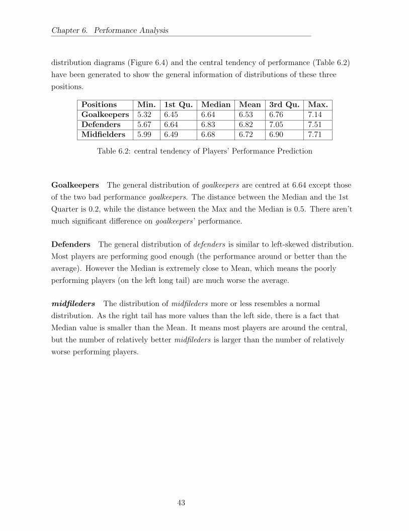
Chapter 6. Performance Analysis
distribution diagrams (Figure 6.4) and the central tendency of performance (Table 6.2)
have been generated to show the general information of distributions of these three
positions.
Positions Min. 1st Qu. Median Mean 3rd Qu. Max.Goalkeepers 5.32 6.45 6.64 6.53 6.76 7.14Defenders 5.67 6.64 6.83 6.82 7.05 7.51Midfielders 5.99 6.49 6.68 6.72 6.90 7.71
Table 6.2: central tendency of Players’ Performance Prediction
Goalkeepers The general distribution of goalkeepers are centred at 6.64 except those
of the two bad performance goalkeepers. The distance between the Median and the 1st
Quarter is 0.2, while the distance between the Max and the Median is 0.5. There aren’t
much significant difference on goalkeepers ’ performance.
Defenders The general distribution of defenders is similar to left-skewed distribution.
Most players are performing good enough (the performance around or better than the
average). However the Median is extremely close to Mean, which means the poorly
performing players (on the left long tail) are much worse the average.
midfileders The distribution of midfileders more or less resembles a normal
distribution. As the right tail has more values than the left side, there is a fact that
Median value is smaller than the Mean. It means most players are around the central,
but the number of relatively better midfileders is larger than the number of relatively
worse performing players.
43

Chapter 6. Performance Analysis
Player Predict Performance
Fre
quen
cy
5.0 5.5 6.0 6.5 7.0 7.5
02
46
810
12
(a) Goalkeepers
Player Predict Performance
Fre
quen
cy
5.5 6.0 6.5 7.0 7.5 8.0
05
1015
2025
30
(b) Defenders
Player Predict Performance
Fre
quen
cy
5.5 6.0 6.5 7.0 7.5 8.0
05
1015
2025
(c) Midfielders
Figure 6.4: General Distribution of Players Performance Prediction with WhoScored’sRating
44

7Market Value vs Performance
Since the predictions of market value and performance assessments of players have been
got, the relation between them can be studied. There are significant differences between
the positions, so the relation study is also conducted in different positions.
7.1 Cross Market Value and Performance
In pre-study, the proper parameters for cross model have been defined. Accordingly,
based on the cross model result, whether a player is proper valued or not can be defined.
7.1.1 Pre-study
The pre-study started from one position — strikers. The crossed result for strikers is in
(Figure 7.1). The over-all trend of market value follows the trend of performance. The
better performance a player has, the higher the market value will be. Apart from the
super star players with a very clear linear relationship, most of the players are centred to
very low value. It seems that market value has an exponential relationship with the
strikers performance. The market value has been plotted in logarithm scale in the right
figure.
45

Chapter 7. Market Value vs Performance
−0.2 0.0 0.2 0.4 0.6 0.8 1.0
020
000
4000
060
000
8000
010
0000
1200
00
Performance Indicators
Mar
ket v
alue
in 1
000
euro
(a) Relation between Market Value and Perfor-mance
−0.2 0.0 0.2 0.4 0.6 0.8 1.0
Performance Indicators
Mar
ket v
alue
in 1
000
euro
1200
1200
012
0000
(b) Logarithm Relation between Market Valueand Performance
Figure 7.1: Relation Between Market Value and Strikers Performance Assessments.
The red line is the simple linear regression fitting[58] and the purple line is polynomial
fitting with local regression model by R [11]. It is obvious in Figure 7.1 that the
polynomial fitting is the better one for strikers. In addition, on a logarithm scale, the
polynomial fitting looks like a linear curve (straight line).
The rest of the positions showed the similar plotting results as the strikers. Hence, the
parameters for building relationship model are the logarithm of market value and the
performance indicator.
7.1.2 Market Value Defined by Performance
The process of defining economic market value result is as follows.
Step 1: Fit the data. ln of market value is mapped to y-axis, and performance
indicators x-axis. Each player is visualized as a small circle in Figure 7.2. After that, the
crossed data have been fitted by the linear (red line) and polynomial (purple line) model.
46

Chapter 7. Market Value vs Performance
−0.2 0.0 0.2 0.4 0.6 0.8 1.0
67
89
1011
PlayerPfor
ln o
f Mar
ket v
alue
(a) Strikers
6.0 6.5 7.0 7.5
67
89
1011
Performance Indicators
ln o
f Mar
ket v
alue
(b) Midfielders
6.0 6.5 7.0 7.5
67
89
10
Performance Indicators
ln o
f Mar
ket v
alue
(c) Defenders
5.5 6.0 6.5 7.0
6.0
6.5
7.0
7.5
8.0
8.5
9.0
Performance Indicators
ln o
f Mar
ket v
alue
(d) Goalkeepers
Figure 7.2: Relation between logarithm market value and performance assessments.
Step 2: Choose the proper model. The objective of this research is to study the
general relationship between market value and performance. Hence, there is no need for a
precise prediction for the market value based on the performance. The complexity of the
linear model is much lower than that of the polynomial model. According to Occam’s
Razor principle[7], the linear model will be the first choice, as long as its grouping for
overvalued, propervalued, and undervalued is reasonable.
Step 3: Apply the chosen model. The estimated logarithm of market value (M)
based on performance is predicted by the chosen model. The difference between it and
the logarithm of market value (M) has been calculated as ∆ = ln(M)− ln(M). The
smaller the ∆ is, the more better the player’s market value matches his performance.
47

Chapter 7. Market Value vs Performance
Step 4: Determine the threshold. The threshold is to determine how the system
tolerate ∆. The value result for players is defined with formular 7.1:overvalued, ∆ > 0.8
undervalued, ∆ < −0.8
propervalued, −0.8 ≤ ∆ ≤ 0.8
(7.1)
Next, the above steps have been applied for each position.
Strikers The linear model and polynomial model have almost the same division on
whether a player is correctly valued. In this case, the linear relationship is considered to
be the model of the proper market value regarding to the predicted performance of
football players. The model for strikers is Formula 7.2.
ln(Ms) = 7.11 + 4.41 · Ps (7.2)
Midfielders Due to the same reason as strikers, the linear model is chosen to be the
best model for midfielders, which is Formula 7.3.
ln(Mm) = −1.81 + 1.49 · Pm (7.3)
Defenders All of the high performance defenders have been overvalued with linear
model. It means that the chosen model failed to describe the relationship. Therefore, the
polynomial model is considered as the best model in this case.
Unfortunately, the LOESS function does not produce the regression function. That is
because LOESS is a non-parametric method which couldn’t expressed as a simple
equation. The model for defenders cannot be written into an equation, but the function
is not very important in this case. However, the R package stats for LOESS can predict
the result of the polynomial model [39]. The reslut of predicted logarithm of market
value by R is in Appendix C.1.
Goalkeepers The distribution of goalkeepers ’ performance and market value is very
random, and both models failed to find their relationship. Some goalkeepers have the
same market value with a big difference on performance, while others have the same
performance with a big difference on market value.
48

Chapter 7. Market Value vs Performance
7.2 Value Results observations by Positions
The value results (i.e. overvalued, propervalued, undervalued) can be marked after
comparing their ∆s to the threshold in 7.1 for strikers, midfielders and defenders. Due to
the random relationship between performance and market value, the goal keepers will be
studied with another approach.
7.2.1 Value Result versus Characteristics and careers
In this section, the value result will be studied by analyzing market value together with
players’ characteristics and career details by positions. There seems to be a ceiling for
market value, where the top performing players have similar market values but very
different performance ratings. The following figures have revealed some additional factors
which have impact on players market value. In these figures, the value results have been
coded by colours, which are blue (overvalued players), red (propervalued players), green
(undervalued players).
49

Chapter 7. Market Value vs Performance
Strikers Figure 7.3 has revealed that the improperly valued strikers have the special
values in age, appearance minutes, contract duration and years stayed in the team.
Age
Mar
ket v
alue
0
20000
40000
60000
80000
100000
20 25 30
(a) Market Value and Age
Players' appearance minutes
Mar
ket v
alue
0
20000
40000
60000
80000
100000
0 5 10 15 20
(b) Market Value and Appearance Minutes
contract length in years
Mar
ket v
alue
0
20000
40000
60000
80000
100000
0 1 2 3 4 5
(c) Market Value and Contract Duration
Years in the team
Mar
ket v
alue
0
20000
40000
60000
80000
100000
0 2 4 6 8 10
(d) Market Value and Years for the team
Figure 7.3: Relation between market value and strikers characteristics and career.
50

Chapter 7. Market Value vs Performance
Midfielders Figure 7.4 has revealed that the improperly valued midfielders have the
special values in age, appearance minutes, and contract duration.
Age
Mar
ket v
alue
0
10000
20000
30000
40000
50000
20 25 30 35
(a) Market Value and Age
Players' appearance minutes
Mar
ket v
alue
0
10000
20000
30000
40000
50000
0 5 10 15 20
(b) Market Value and Appearance Minutes
contract length in years
Mar
ket v
alue
0
10000
20000
30000
40000
50000
0 1 2 3 4 5
(c) Market Value and Contract Duration
Figure 7.4: Relation between market value and midfielders characteristics and career.
51

Chapter 7. Market Value vs Performance
Defenders Unlike the other two positions, the players with highest value have been
properly valued for defenders. Figure 7.5 has revealed that the improperly valued
defenders have the special values in age, appearance minutes, contract duration and
years stayed in the team.
Age
Mar
ket v
alue
0
10000
20000
30000
40000
20 25 30 35
(a) Market Value and Age
Players' appearance minutesM
arke
t val
ue
0
10000
20000
30000
40000
5 10 15 20
(b) Market Value and Appearance Minutes
contract length in years
Mar
ket v
alue
0
10000
20000
30000
40000
0 1 2 3 4 5
(c) Market Value and Contract Duration
Years in the team
Mar
ket v
alue
0
10000
20000
30000
40000
0 5 10 15
(d) Market Value and Years for the team
Figure 7.5: Relation between market value and defenders characteristics and career.
7.2.2 Analysis for improperly valued players
Strikers, Midfielders, Defenders There are general factors related to the improper
valued players: Players’ age (Age), the contract left for the player (Con), the years
players have played for this club (YinT), the ratio of international players and local
players (InvsLo), the number of the players from the top 5 club of the League1 (Clubs),
and the number of the players from the world top clubs2 (PreC). These factors should be
1The top five clubs in la Liga:Real Madrid, FC Barcelona, Atletico de Madrid, Valencia CF, Sevilla FC2The world top clubs are performances well in matches and generate a lot revenue all around the world
e.g. Bayern Munich[21]
52

Chapter 7. Market Value vs Performance
compared with total number of players for this position in the league (PinL) and total
number of overvalued players for this position (Player) for analysis.
The specific figures of each factor are stated by positions in Table 7.1 and Table7.2,
which are separated by overvalued and undervalued players.
Positions PinL Player Age Con YinT InvsLo Clubs PreCStrikers 111 23 23− 30 > 3 - 14/9 19 18Midfielders 109 20 22− 31 > 3 - 8/12 18 10Defenders 128 19 19− 32 2-5 1-5 13/6 16 10
Table 7.1: Overvalued Players
Positions PinL Player Age Con YinT InvsLo Clubs PreCStrikers 111 15 < 23 > 30 < 3 < 3 3/12 0 1Midfielders 109 16 22− 36 < 2 - 8/12 0 1Defenders 128 17 18− 38 < 2 1− 7 8/9 1 0
Table 7.2: Undervalued Players
7.2.3 Study for Goalkeepers
Since there is no specific relationship between market value and their performance, I
applied the regression tree for goalkeepers (Figure 7.6). Market value is considered as the
target and all of the rest factors are the independent variables. The variables from
regression tree result are regarded as the dominant factors to goalkeepers market value.
The appearance is the most important factor for the goalkeepers. Only when the
goalkeeper has appearance minutes ≥ 17.5, their market value is in relation with their
performance. Only less than 1/3 of the goalkeepers ’s market value depend on their
performance. For the rest of the goalkeepers, age and weight are the two key indicators.
And there is no literature that shows the relationship between the weight and the
goalkeepers performance.
53

Chapter 7. Market Value vs Performance
|
Apps < 17.5
Age < 28.5
KG < 82.5
Rating < 6.745
2860.0 1250.0
883.8
3244.0 6700.0
Figure 7.6: Factors Regression Tree for Goal Keepers’ Market Value
7.3 Underlying Reasons
Besides the general reasons for the players and clubs, e.g. ages and contracts, there are
some other factors effecting players’ market value besides footballer themselves, which are
super star atmosphere, nationality, club and previous, which have affected players market
value.
7.3.1 General Reasons
For all the positions but goalkeepers, the older players are most likely to be undervalued.
Though the undervalued players in midfielders and defenders are distributed to all the
age groups, the distributions of these players are much more intense for players older
than 31 years. Young players also tend to be undervalued. Market value shows the
potential performance of the player in the future, however the expectation for the old
players is very low because the physical performance will get poorer as the age grow.
The overvalued players always have more playing minutes and a longer contract length.
The club knows the player very well and can value him properly. The expectation for the
players has shown in their contract length which also affects on their market value. On
the contrary, the remaining contract length for undervalued players is very short. On one
54

Chapter 7. Market Value vs Performance
hand, when the club does not value a player, the player will not get more appearance
opportunity and the club does not want to keep this player. On the other hand, when the
club values a player, they prefer to make the player play for them for more years. When a
player stays in a team more than 7 years, he is not likely to be improperly valued.
7.3.2 Superstar Players
Superstars Almost all of the overvalued players have very high performance, but the
marginal contribution of their performance is lower than their market value. These
players are the superstars in the media, e.g. Neymar da Silva, Luis Suarez. Why do these
super stars been overvalued?
Rosen [43] who is regarded as the founder of economics superstar player has defined
superstars as ”the relatively small numbers of people who earn enormous amounts of
money and dominate the activities in which they engage”. The superstars have the
overvalued atmosphere are most due to the marketing value. Normally, high-performance
players also bring revenues to the clubs in terms of publicity and merchandise sales.
Attracting Fans Rosen [43] indicates that stars play an important role in promoting
fan interest. In 2004, the report [49] from SportFive has stated that 69% of the European
soccer fans think that their identification with and affiliation to a team largely depends
on the particular players the team engages. The gate revenues can be increased by a
star’s talent superiority or a star’s popularity [6].
According to Rosen [43], audience want to see their favoured players in the ceteris
paribus. For example, the movement of the passes are very attractive to the spectators,
but these will not be shown in the performance data.
Level of Matches The superstars tend to have longer appearance time than other
players. Especially in the big events, the success of tournaments such as the UEFA Cup,
the Champions League and the FIFA World Cup, coaches rely more on the stars. Good
performance in these important matches is more valuable than that in ordinary matches.
Players will be favoured by fans and coaches immediately if they have one key
performance indicator in these matches. For example Mario Gotze[16] had the final goal
in 2014 FIFA World Cup final, which helped the Germany be the champion of and world
and made him famous in the world. Consequently, his market value is the second highest
among all the German players. However, a lot of players have three goals in matches
cannot be known by the public. Even though the overall performance statistics of super
stars may not as good as some average players, they tend to shine in important matches.
55

Chapter 7. Market Value vs Performance
7.3.3 Nationality
In la Liga, around 58% of the overvalued players are international players, and it is more
than that ratio for the whole league. In addition, the international players have a smaller
ratio(37%) of undervalued players. Spending money on foreign players brings several
extra benefits besides their contribution to win the games as discussed below.
Dramatic Fans Increase Most stars only have loyal local attraction[8], but superstars
have fans both domestically and abroad. For example, Leo Messi and Cristiano Ronaldo
have fans all over the world. Players from the same place tend to have the same fans
group, for instance Spanish players are most likely to be favoured by Spanish people. If
the player A is already a team member, the fans will not increase much if the team buys
player B who is from the same place as A. Bringing in an international player can
dramatically increase the fans’ number due to different fans group. For example, Neymar
helps Barcelona to gain more fans from Brazil.
Other Revenues Acquiring an international player can help the club to earn extra
money besides revenue from tickets. The most important one is revenue from the TV
rights. The international player can bring more living chances for the club. Before Sun
transferred to PSV, there was no Dutch football league’s living match and reports in
Chinese media. However, there is more living matches or news for PSV than Real Madrid
in Chinese media when Sun was in the PSV. The price of TV rights for Premier League
games is extremely high due to the influx of foreign players. Sky Sports and BT Live
spending a record £3 billion on TV rights from 2013− 16, which gives each Premier
league club an extra £60 million every year[38].
There are also some intangible benefits created by the international transfer that
creates revenue. The club will be more famous in the player’s home country because of
the transferred international player. It can be regarded as a free advertise for the club to
foreign land. The transfer of Sun made PSV famous in China, most Chinese people only
know PSV other than Ajax. The club products (e.g. the suits) will have more sales and
will be easily sponsored by foreign companies.
More Appearance Another possible reason why the international players are easily
overvalued is the statistic bias. The statistics of performance is averaged by 90 minutes.
The international players have more appearances and movements than local players.
Mohr et al.[5] have found that international players performed 28% more high-intensity
running (2.43 vs.1.90 km) and 58% more sprinting (650 vs. 410 m) than the local
56

Chapter 7. Market Value vs Performance
professional players in the same league. Due to longer appearance time than other
players, the average of their performance data is relatively low.
7.3.4 Clubs
All the records of the transfer fee happened in the richest clubs [57]. It seems these clubs
have created the inflation of football player market value.
Existing Clubs More than 85% of overvalued players are playing in the richest clubs,
while none of undervalued player are working for these clubs except one defender
Fernando Navarro from Sevilla.
These clubs have a better ability to increase their financial budget, which enables them
to pay the high transfer fee and salary to the superstars. They have generated more
revenue from match day including ticket and corporate hospitality sales.
Their TV rights are distributed to more countries and the content covers domestic
leagues, cups and European club competitions. In addition, their commercial sources
(e.g. sponsorship, merchandising and other commercial operations) are much more than
the rest of the clubs.
These clubs have money to buy a lot of stars all over the world. With many stars in
the same team, even a superstar player couldn’t have much chance to play in the match
as well. For example, in 2006-2007, Micheal Owen had very short appearance time. Even
though he is worth to his market value, he couldn’t have much performance data. Even a
super star performs well enough, there is like to be someone else in the same team plays
better than him. He will get less attention by teammates, coach or fans than he should
have got.
Previous Clubs There is also a finding on previous clubs of the improperly valued
players. Most of the overvalued players are transferred from the world most valuable
teams, while only one the undervalued players is transferred from top clubs in the world,
that is Wellington Silva from Arsenal FC. According to the previous clubs, the inflation
of the riches clubs also happens in their second team, e.g. midfielders are more from
Barcelona B.
Dismissing the contract with players in the top clubs cost more than the rest clubs.
The buyer clubs have to pay more to buy the players’ remaining contract. [9] That’s why
most overvalued players are from the riches clubs.
57

8Conclusion
In this chapter, the research conclusion will be presented first. And the limitations of this
research will be pointed out. At last, the suggestions for the future study will be given.
8.1 Conclusions
The performance of players are related to the income of the team as stated in Chapter 2.
Especially under the newly regulations of UEFA, the clubs should spend money wisely.
The correct evaluation of players is more important than that of previous years.
Player performance data are hard to acquire and have high commercial value.
Therefore, it is difficult to obtain useful data for this research. This research was
conducted under a lot of pre-studies on finding out the available useful data source.
Record linkage has been used to merge the data from different data sources. The transfer
fee is considered as the market value of a player and the votes by experts are as the
players’ performance assessment.
Real value model As is mentioned in Chapter 4, the target data voting and transfer
fee are insufficient. LASSO models have been trained to get the complete list for these
two values. Since the transfer fee has a relationship with the market value from Transfer
58

Chapter 8. Conclusion
Market, the real market model is based on that variable, which is formula 8.1
M = 231.26 + 0.89 ·Market.value+ 2723.26 · Assists (8.1)
The players’ performance is not in line with the proxy value rating from Whoscored.
The reason is the basis of the voting, which favours the strikers. The real performance
model was only trained for the forward players which is formula 8.2.
P = 0.28−0.073 ·F +0.06 ·SP +0.04 ·ST +0.02 ·GP +0.05 ·GB+0.02 ·D+0.08 ·A (8.2)
Performance KPIs by positions The performance KPIs have been selected with the
LASSO feature selection by positions in Table 8.1. The indicators with ‘-’ in the front
have a negative impact on the performance. The observations from the table are as
follows. There is a significant difference in the performance indicators between positions.
The same indicators create different impacts on positions. For example, more Interception
is a plus for midfielders and defenders while it makes the goalkeepers performance worse.
Strikers Midfielders Defenders GoalkeepersShots in penalty area Interception Shots blocked Saves in penalty areaGoals in penalty area Goals in the zone Shot on Target FouledShots on target Goals by head Interceptions Dribbled passGoals from out of box Aerial won Accurate long balls inaccurate blockDribble successfully Length of passes Accurate short passes -Accurate free kickAssists total Accurate free kicks Long passes -Interception-Fouls Other assists -Fouls -Dribbled past
-Unsuccessful touches -Yellow cards
Table 8.1: Overvalued Players
Market value/performance cross results By studying the Spanish league la Liga,
the market value is majorly based on the performance of players. The general
relationship of market value and performance has been studied. In general, a football
player’s market value is in a logitism relationship with his performance. As long as a
player’s performance improves a little, the market value of this player will be multiplied.
The international, young and old players are easily to be improperly valued. The rich
clubs tend to overvalue their players, which also affects the market value of their previous
players. In addition, the improperly valued players have a significant difference in
appearance time and contract length when compared to other players.
59

Chapter 8. Conclusion
8.2 Research limitations
Due to the difficulty of collecting data, this research is conducted with insufficient data.
There is only a half season of one league’s data which is very limited. Also, the ranking
of the club in Section3.1.3 is only for the middle season, the sequence is changed at the
end of the season.
The performance and market value use supervised learning to predict the unknown
variable. Because of the bias of voting system, among the performance models for all
positions, only that of strikers is available.
This research is only studied within la Liga. It does not take the leagues differences
into consideration. The model has not been verified in different leagues yet. As a result,
it cannot represent all the leagues.
Soccer is a highly interactive game based on the combination of complementary player
skills. The combination of the players was not taken into consideration in this research.
This will result in the inaccuracy prediction on players’ performance.
8.3 Future Study
This model is built for evaluating market value of all the players of la Liga based on their
performance. Furthermore, the method could be applied to other leagues. As for the
performance, the operational model at this point only applies to strikers. This can be
extended to other positions if a unique model is created for performance across different
leagues. As part of future work, I would like to scale up the project to all European
leagues.
Even all leagues are covered, this project will keep on dealing with incomplete data
because not all players are valued every year (by being transferred), neither are all
players’ performance evaluated by the voting system. In the future, the semi-supervised
methods are considered to solve the tasks of Performance and Market Value estimation.
Finally, the voting system to assess performance is biased towards strikers and well
performing players. Hence, there is need to explore other data mining techniques that
account for this problem, e.g. an Elo Rating model can be created to evaluate the
performance of football players across positions and leagues.
60

Bibliography
[1] Herve Abdi. The method of least squares. Encyclopedia of Measurement and
Statistics. CA, USA: Thousand Oaks, 2007.
[2] Paul D Allison. Missing data, volume 136. Sage publications, 2001.
[3] Eli Amir and Gilad Livne. Accounting, valuation and duration of football player
contracts. Journal of Business Finance & Accounting, 32(3-4):549–586, 2005.
[4] Peter Antonioni and John Cubbin. The bosman ruling and the emergence of a single
market in soccer talent. European Journal of Law and Economics, 9(2):157–173,
2000.
[5] Jens Bangsbo and Magni Mohr. Variations in running speeds and recovery time
after a sprint during top-class soccer matches: 472 board# 63 2: 00 pm-3: 30 pm.
Medicine & Science in Sports & Exercise, 37(5):S87, 2005.
[6] David J Berri, Martin B Schmidt, and Stacey L Brook. Stars at the gate the impact
of star power on nba gate revenues. Journal of Sports Economics, 5(1):33–50, 2004.
[7] Anselm Blumer, Andrzej Ehrenfeucht, David Haussler, and Manfred K Warmuth.
Occam’s razor. Information processing letters, 24(6):377–380, 1987.
[8] Leif Brandes, Egon Franck, and Stephan Nuesch. Local heroes and superstars: An
empirical analysis of star attraction in german soccer. Journal of Sports Economics,
2007.
[9] Fiona Carmichael and Dennis Thomas. Bargaining in the transfer market: theory
and evidence. Applied Economics, 25(12):1467–1476, 1993.
[10] Luis Carvalho and Maintainer Luis Carvalho. Package ‘kolmim’. 2015.
61

Bibliography
[11] William S Cleveland, Eric Grosse, and William M Shyu. Local regression models.
Statistical models in S, pages 309–376, 1992.
[12] V Di Salvo, R Baron, H Tschan, FJ Calderon Montero, N Bachl, and F Pigozzi.
Performance characteristics according to playing position in elite soccer.
International journal of sports medicine, 28(3):222, 2007.
[13] Stephen Dobson and John Goddard. The economics of football. Cambridge
University Press, 2011.
[14] Mark Dodge and Craig Stinson. Microsoft office excel 2007 inside out. Microsoft
Press, 2007.
[15] Eberhard Feess and GERD MUHLHEUßER. Economic consequences of transfer fee
regulations in european football. European Journal of Law and Economics,
13(3):221–237, 2002.
[16] FIFA. Regulations on the status and transfer of players.
http://www.fifa.com/mm/document/affederation/administration/
regulations_on_the_status_and_transfer_of_players_en_33410.pdf, October
2003.
[17] Bernd Frick. The football players’labor market: Empirical evidence from the major
european leagues. Scottish Journal of Political Economy, 54(3):422–446, 2007.
[18] Jerome Friedman, Trevor Hastie, and Robert Tibshirani. The elements of statistical
learning, volume 1. Springer series in statistics Springer, Berlin, 2001.
[19] Jerome Friedman, Trevor Hastie, and Robert Tibshirani. Regularization paths for
generalized linear models via coordinate descent. Journal of Statistical Software,
33(1):1–22, 2010.
[20] Pervez N Ghauri and Kjell Grønhaug. Research methods in business studies: A
practical guide. Pearson Education, 2005.
[21] Deloitte Business group. Football money league.
https://www2.deloitte.com/content/dam/Deloitte/uk/Documents/
sports-business-group/deloitte-football-money-league-2015.PDF, January
2015.
[22] Isabelle Guyon and Andre Elisseeff. An introduction to variable and feature
selection. The Journal of Machine Learning Research, 3:1157–1182, 2003.
62

Bibliography
[23] Stephen Hall, Stefan Szymanski, and Andrew S Zimbalist. Testing causality between
team performance and payroll the cases of major league baseball and english soccer.
Journal of Sports Economics, 3(2):149–168, 2002.
[24] Michael David Hughes, Tim Caudrelier, Nic James, Athalie Redwood-Brown, Ian
Donnelly, Anthony Kirkbride, and Christophe Duschesne. Moneyball and soccer-an
analysis of the key performance indicators of elite male soccer players by position.
2012.
[25] Google Inc. Google scholar, 2015.
[26] Peter Krustrup, Magni Mohr, Adam Steensberg, Jesper Bencke, Michael Kjær, and
Jens Bangsbo. Muscle and blood metabolites during a soccer game: implications for
sprint performance. Medicine and science in sports and exercise, 38(6):1165–1174,
2006.
[27] Gunjan Kumar. Machine learning for soccer analytics. 2013.
[28] Michael Lewis. Moneyball: The art of winning an unfair game. New York: W.W.
Norton., 2003.
[29] Hubert W Lilliefors. On the kolmogorov-smirnov test for normality with mean and
variance unknown. Journal of the American Statistical Association, 62(318):399–402,
1967.
[30] Richard Lockhart, Jonathan Taylor, Ryan J Tibshirani, and Robert Tibshirani. A
significance test for the lasso. Annals of statistics, 42(2):413, 2014.
[31] Frank J Massey Jr. The kolmogorov-smirnov test for goodness of fit. Journal of the
American statistical Association, 46(253):68–78, 1951.
[32] Victor A. Matheson. European football: a survey of the literature. Mimeo,
Department of Economics, Williams College., 2003.
[33] Mehryar Mohri, Afshin Rostamizadeh, and Ameet Talwalkar. Foundations of
machine learning. MIT press, 2012.
[34] Gonzalo Navarro. A guided tour to approximate string matching. ACM computing
surveys (CSUR), 33(1):31–88, 2001.
[35] The Business of Soccer. Forbes Magazine. Soccer team values, 2015.
63

Bibliography
[36] K Ohta. Hierarchical theory of selection: the covariance formula of selection and its
application. Bulletin of the Biometrical Society of Japan, 4:25–33, 1983.
[37] Vladan Pavlovic, Srecko Milacic, and Isidora Ljumovic. Controversies about the
accounting treatment of transfer fee in the football industry1. Management, page 70,
2014.
[38] Huffington Post. Sky sports and bt sport secure premiere league tv rights for
combined £5.136 billion, 2015.
[39] R Core Team. R: A Language and Environment for Statistical Computing. R
Foundation for Statistical Computing, Vienna, Austria, 2013. ISBN 3-900051-07-0.
[40] Ermanno Rampinini, David Bishop, SM Marcora, D Ferrari Bravo, R Sassi, and
FM Impellizzeri. Validity of simple field tests as indicators of match-related physical
performance in top-level professional soccer players. International journal of sports
medicine, 28(3):228, 2007.
[41] Thomas Reilly, A Mark Williams, Alan Nevill, and Andy Franks. A
multidisciplinary approach to talent identification in soccer. Journal of sports
sciences, 18(9):695–702, 2000.
[42] Brian Ripley. Classification and regression trees. R package version, pages 1–0, 2005.
[43] Sherwin Rosen. The economics of superstars. The American economic review, pages
845–858, 1981.
[44] Simon Rottenberg et al. Resource allocation and income distribution in professional
team sports. Journal of Sports Economics, 1(1):11–20, 2000.
[45] Mark NK Saunders, Mark Saunders, Philip Lewis, and Adrian Thornhill. Research
methods for business students, 5/e. Pearson Education India, 2011.
[46] Colin Shearer. The crisp-dm model: the new blueprint for data mining. Journal of
data warehousing, 5(4):13–22, 2000.
[47] David J Sheskin. Handbook of parametric and nonparametric statistical procedures.
crc Press, 2003.
[48] Noah Simon, Jerome Friedman, Trevor Hastie, Rob Tibshirani, et al. Regularization
paths for cox’s proportional hazards model via coordinate descent. Journal of
statistical software, 39(5):1–13, 2011.
64

Bibliography
[49] Sportfive. European football 2004, 2004.
[50] Victoria Stodden. Model selection when the number of variables exceeds the number
of observations. PhD thesis, Stanford University, 2006.
[51] R Core Team. R language definition, 2000.
[52] Robert Tibshirani. Regression shrinkage and selection via the lasso. Journal of the
Royal Statistical Society. Series B (Methodological), pages 267–288, 1996.
[53] Paul Tomkins, Graeme Riley, and Gary Fulcher. Pay As You Play: The True Price
of Success in the Premier League Era. GPRF Publishing., 2010.
[54] UEFA. Financial fair play. http://www.uefa.org/protecting-the-game/
club-licensing-and-financial-fair-play/, February 2014.
[55] Mark PJ Van der Loo. The stringdist package for approximate string matching. The
R, 2014.
[56] Kevin Whitehead. The impact of european football player transfers on share price.
2014.
[57] Wikipedia. List of most expensive association football transfers, 2015.
[58] GN Wilkinson and CE Rogers. Symbolic description of factorial models for analysis
of variance. Applied Statistics, pages 392–399, 1973.
[59] William E Winkler. Overview of record linkage and current research directions. In
Bureau of the Census. Citeseer, 2006.
[60] Yi Xue and Liping Chen. Statistic model and r software, 2007.
[61] Xiaowei Yan, Chengqi Zhang, and Shichao Zhang. Toward databases mining:
Pre-processing collected data. Applied Artificial Intelligence, 17(5-6):545–561, 2003.
[62] Shichao Zhang, Chengqi Zhang, and Qiang Yang. Data preparation for data mining.
Applied Artificial Intelligence, 17(5-6):375–381, 2003.
65

AVariable Explanation
Variables ExplanationTeam Player’s teamPlayer Player’s namePosition Player’s positionAge Player’sageNat. Player’s nationalitySecond.Nat. Player’s second nationalityFoot Player’s usually foot playIn.the.team.since Player’s start date of the teambefore For which team player has played beforeContract.until when will the player’s contract endMarket.value Player’s market value from Transfer MarketRating Player’s rating score by WhoScoredCM Player’s heightKG Player’s weightApps AppearanceMins The total minutes played for this seasonTotalTackles Total tackles per 90 minutesDribbledPast Total dribbled past per 90 minutesTotalAttemptedTackles Total attempted tackles per 90 minutesInterception Total interception per 90 minutes
66

Appendix A. Variable Explanation
Variables ExplanationFouled Total being fouled times per 90 minutesFouls Total fouls per 90 minutesYellow Total yellow cards per 90 minutesRed Total red cards per 90 minutesCaughtOffside Total caught off side per 90 minutesClerances Total clerances per 90 minutesShotsBlocked Total shots blocked per 90 minutesCrossesBlocked Total crosses blocked per 90 minutesPassesBlocked Total passes blocked per 90 minutesSaves Total saves per 90 minutesSixYardBox Saves in six yard box per 90 minutesPenaltyArea Saves in penalty area per 90 minutesOutOfBox Saves out of box per 90 minutesShot.in.Zones Shots in Zones per 90 minutesOutOfBox.1 Shot out of Box per 90 minutesSixYardBox.1 Shot within six yard box per 90 minutesPenaltyArea.1 Shot in the penalty area per 90 minutesSituation Situation Shot per 90 minutesOpenPlay Shot Open play per 90 minutesCounter Counter Shot per 90 minutesSetPiece Set Piece Shot per 90 minutesPenaltyTaken Penalty Shot per 90 minutesAccuracy Shot accuracy per 90 minutesOffTarget Shot off target per 90 minutesOnPost Shot on post per 90 minutesOnTarget Shot on target per 90 minutesBlocked Shot blocked per 90 minutesBody.Parts Body Parts Shot per 90 minutesRightFoot Right foot Shot per 90 minutesLeftFoot Left foot Shot per 90 minutesHead Head Shot per 90 minutesOther Other Shot per 90 minutesZone.of.Goals Goals from zones per 90 minutesSixYardBox.2 Goals from six yard box per 90 minutesPenaltyArea.2 Goals from penalty area per 90 minutesOutOfBox.2 Goals from out of box per 90 minutesSituations Situation goals per 90 minutesOpenPlay.1 Open play goals per 90 minutesCounter.1 Counter goals per 90 minutesSetPiece.1 Set piece goals per 90 minutesPenaltyScored Penalty scored per 90 minutesOwn Own goals per 90 minutesNormal Normal goals per 90 minutes
67

Appendix A. Variable Explanation
Variables ExplanationBody.Parts.1 Goal by body parts per 90 minutesRightFoot.1 Goals by right foot per 90 minutesLeftFoot.1 Goals by left foot per 90 minutesHead.1 Goals by head per 90 minutesOther.1 Goals by other parts per 90 minutesUnsuccessful Dribble unsuccessful per 90 minutesSuccessful Dribble successful per 90 minutesDribbleTotal Dribble total per 90 minutesUnsuccessfulTouches Possession loss unsuccessful touches per 90 minutesDispossessed Possession loss dispossessed per 90 minutesAerial Total aerial per 90 minutesWon Aerial won per 90 minutesLost Aerial lost per 90 minutesLength.of.Passes Total passes per 90 minutesAccLB Accurate long balls per 90 minutesInAccLB Inaccurate long balls per 90 minutesAccSP Accurate short passes per 90 minutesInAccSP Inaccurate short passes per 90 minutesAccCr Accurate cross passes per 90 minutesInAccCr Inaccurate cross passes per 90 minutesAccCrn Accurate corner passes per 90 minutesInAccCrn Inaccurate corner passes per 90 minutesAccFrK Accurate freekicks per 90 minutesInAccFrK Inaccurate freekicks per 90 minutesKey.Passes.Length Total key passes per 90 minutesLong Total key long passes per 90 minutesShort Total key short passes per 90 minutesCross Total key cross passes per 90 minutesCorner Total key corner passes per 90 minutesThroughball Total key through ball per 90 minutesFreekick Total key free kick per 90 minutesThrowin Total key throw in per 90 minutesOther.2 Total key other passes per 90 minutesCross.1 Corner assists per 90 minutesCorner.1 Corner assists per 90 minutesThroughball.1 Throughball assists per 90 minutesFreekick.1 Free kick assists per 90 minutesThrowin.1 Thrownin assists per 90 minutesOther.3 Other assists per 90 minutesAssists Assists total per 90 minutes
Table A.1: Variable Explanations
68

BR code
In this part, part of Key Process of R code have been provided.
B.1 Data Preparation
B.1.1 Preprocesing
# erase l a s t reccord from Transfer Market ( empty l i n e )
dataTF <− dataTF[−nrow( dataTF ) , ]
# erase a l l d u p l i c a t e reccords from WhoScored
dataWS <− unique (dataWS)
# Change Contract . u n t i l to numeric
for ( i in 1 :nrow(TF)){t e s t<−TF$Contract . u n t i l [ i ]
t e s t <− unlist ( s t r sp l i t ( t e s t , sp l i t=”” ) )
i f ( length ( t e s t )<10)
{
69

Appendix B. R code
TF$Contract . u n t i l [ i ]<−0
} else {TF$Contract . u n t i l [ i ] <− as . numeric ( as . numeric ( paste ( t e s t [ 7 ] , t e s t [ 8 ] , t e s t [ 9 ] , t e s t [ 1 0 ] , sep=””))−2015)
}}
TF$Contract . u n t i l <− as . numeric (TF$Contract . u n t i l )
# Change in the team s i n c e i n t o years
for ( i in 1 :nrow(TF)){t e s t<−TF$In . the . team . s i n c e [ i ]
t e s t <− unlist ( s t r sp l i t ( t e s t , sp l i t=”−” ) )
i f ( length ( t e s t )<3)
{TF$In . the . team . s i n c e [ i ]<−0
} else {num <− as . numeric(15−as . numeric ( t e s t [ 3 ] ) )
i f (num<0 )
{num<−num+100
}TF$In . the . team . s i n c e [ i ]<−num
}}
TF$In . the . team . s i n c e <− as . numeric (TF$In . the . team . s i n c e )
# Convert Market Value i n t o numbers
for ( j in 1 :nrow( MergeMatrix ) ) {t e s t <− MergeMatrix$Market . va lue [ j ]
num <− unlist ( s t r sp l i t ( t e s t , sp l i t=” ” ) ) [ 1 ]
un i t <− unlist ( s t r sp l i t ( t e s t , sp l i t=” ” ) ) [ 2 ]
num <− unlist ( s t r sp l i t (num, sp l i t=” , ” ) )
i f ( i s . na(num [ 2 ] ) ) {num<−num [ 1 ]
} else {num<−paste (num [ 1 ] , num [ 2 ] , sep=”” )
}
70

Appendix B. R code
num <− as . numeric (num)
amatch ( unit , ” Mi l l . ” )
i f ( i s . na( amatch ( unit , ” Mi l l . ” ) ) ) {MergeMatrix$Market . va lue [ j ]<−num
} else {MergeMatrix$Market . va lue [ j ]<−num∗10
}}
MergeMatrix$Market . va lue <−as . numeric ( MergeMatrix$Market . va lue )
#Erase the NA Market Value p l a y e r
MergeMatrix <− MergeMatrix [−which( i s . na( MergeMatrix$Market . va lue ) ) , ]
# Deal ing wi th Missing Value
TF[ i s . na(TF) ]<−0
B.1.2 Data Match
output <− matrix (nrow=nrow(dataWS ) , ncol=3, dimnames=l i s t ( c ( ) , c ( ”aindexWS” , ” minTotalDist ” , ”aindexTF” ) ) )
j=1
for ( j in 1 :nrow(dataWS)){aDistName <− s t r i n g d i s t (dataWS$Name [ j ] , dataTF$Player , method=”jw” )
aDistTeam <− s t r i n g d i s t (dataWS$Team [ j ] , dataTF$Team, method=”jw” )
aDistAge <− s t r i n g d i s t (dataWS$Age [ j ] , dataTF$Age , method=”jw” )
aDistHeight <− s t r i n g d i s t (dataWS$CM[ j ] , dataTF$Height , method=”jw” )
Tota lDist <− aDistName + aDistTeam + aDistAge + aDistHeight
minDist <− min( Tota lDist )
aIndex <− which( Tota lDist == minDist )
output [ j , 1 ] <− j
output [ j , 2 ] <− minDist
output [ j , 3 ] <− aIndex
}summary( RightMatch )
# Evaluate the matching r e s l u t
RightMatch <− vector (mode=” i n t e g e r ” , length=nrow( DIndex ) )
for ( j in 1 :nrow( DIndex ) ){
71

Appendix B. R code
i f ( length (na . omit ( DIndex [ j , 2 ] ) ) == 0 | length (na . omit ( output [ j , 3 ] ) ) == 0)
next
i f ( DIndex [ j ,1]== output [ j , 1 ] & DIndex [ j ,2]== output [ j , 3 ] ) {RightMatch [ j ] <− 1
}}summary( RightMatch ) [ [ 4 ] ] /(1−summary( DIndex [ , 2 ] ) [ [ 7 ] ] /nrow(dataWS ) )
nrow( dataTF )
#s o r t the data by d i s t a n c e
output [ sort . l i s t ( output [ , 2 ] ) , ]
B.2 LASSO in R
Take the forward players’ performance training as an example
# Use the package ” glment ”
l ibrary ( ”glmnet” )
# Train LASSO model wi th 5 f o l d e r s c r o s s v a l i d a t i o n
c v f i t = cv . glmnet (x , y , n f o l d s =5)
# Plot a l l t he mean squared e r r o r s wi th f o r a l l the f i t t i n g
plot ( c v f i t )
# Get the c o e f f i c i e n t wi th the proper lambda v a l u e
Coef<− coef ( c v f i t , s = 0 .081740)
Coef [ ( which( Coef [ , 1 ] != 0 ) ) , ]
72

CIntermediate Results
C.1 Defenders Predicted Logarithm of Market Value
x<−as . numeric ( Player$Rating )
y<−log ( Player$Market . va lue ) # A c c t u a l l y i t i s ln , not l o g
f i t<− l o e s s ( y˜x )
premv <− as . data . frame ( predict ( f i t , i n t e r v a l = ” p r e d i c t i o n ” ) )
# premv Resu l t i s
predict ( f i t , i n t e r v a l = ” p r e d i c t i o n ” )
1 7.637719
2 7.683803
3 7.729092
4 7.692301
5 7.752875
6 7.884957
7 8.247011
8 7.675055
9 8.223610
73

Appendix C. Intermediate Results
10 7.590636
11 7.276625
12 7.812882
13 8.118786
14 7.967009
15 8.344933
16 7.276625
17 7.666961
18 7.571646
19 7.766630
20 8.091007
21 7.904617
22 8.648674
23 7.904617
24 9.591489
25 8.579214
26 8.425293
27 8.837744
28 9.432839
29 9.646156
30 8.223610
31 7.613014
32 7.988835
33 7.945675
34 7.709607
35 7.660412
36 7.729092
37 7.740314
38 7.829851
39 8.344933
40 8.091007
41 7.452000
42 7.598582
43 7.700814
44 8.037117
45 8.319634
74
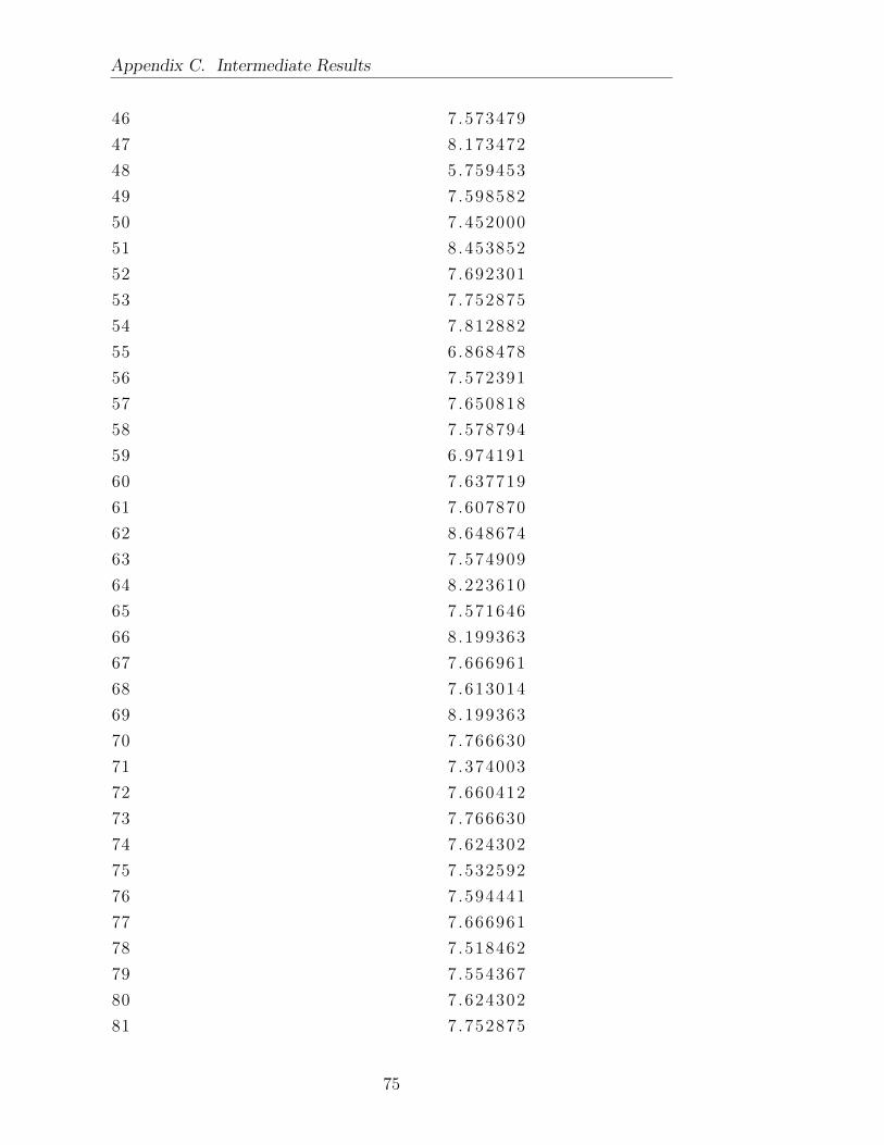
Appendix C. Intermediate Results
46 7.573479
47 8.173472
48 5.759453
49 7.598582
50 7.452000
51 8.453852
52 7.692301
53 7.752875
54 7.812882
55 6.868478
56 7.572391
57 7.650818
58 7.578794
59 6.974191
60 7.637719
61 7.607870
62 8.648674
63 7.574909
64 8.223610
65 7.571646
66 8.199363
67 7.666961
68 7.613014
69 8.199363
70 7.766630
71 7.374003
72 7.660412
73 7.766630
74 7.624302
75 7.532592
76 7.594441
77 7.666961
78 7.518462
79 7.554367
80 7.624302
81 7.752875
75

Appendix C. Intermediate Results
82 7.573479
83 7.647207
84 7.647207
85 7.924867
86 7.847542
87 7.781239
88 7.666961
89 7.239863
90 7.634060
91 7.603059
92 7.647207
93 7.629683
94 7.700814
95 8.270758
96 7.473687
97 9.701714
98 8.247011
99 9.484831
100 8.012021
101 10.178366
102 7.692301
103 8.247011
104 8.223610
105 8.063615
106 7.692301
107 7.569416
108 8.012021
109 8.319634
110 7.847542
111 7.752875
112 7.532592
113 9.048897
114 8.370919
115 7.554367
116 8.012021
117 7.718945
76

Appendix C. Intermediate Results
118 8.684724
119 7.675055
120 9.815510
121 8.453852
122 8.199363
123 8.798165
124 7.576681
125 8.397677
126 8.798165
127 9.093784
128 8.425293
77