Embed Size (px)
Citation preview

Université Libre de BruxellesInstitut de Recherches Interdisciplinaires et de Développements en Intelligence Artificielle
Ant Colony Optimization under
Uncertainty
Prasanna BALAPRAKASH
IRIDIA – Technical Report Series
Technical Report No.
TR/IRIDIA/2005-028
November 2005

IRIDIA – Technical Report SeriesISSN 1781-3794
Published by:
IRIDIA, Institut de Recherches Interdisciplinaires
et de Developpements en Intelligence Artificielle
Universite Libre de Bruxelles
Av F. D. Roosevelt 50, CP 194/61050 Bruxelles, Belgium
Technical report number TR/IRIDIA/2005-028
The information provided is the sole responsibility of the authors and does not necessarilyreflect the opinion of the members of IRIDIA. The authors take full responsability forany copyright breaches that may result from publication of this paper in the IRIDIA –Technical Report Series. IRIDIA is not responsible for any use that might be made ofdata appearing in this publication.

Universite Libre de BruxellesFaculte des Sciences AppliqueesIRIDIA - Institut de Recherches Interdisciplinaireset de Developpements en Intelligence Artificielle
Ant Colony Optimization
under Uncertainty
Sampling and Racing Techniques for the
Probabilistic Traveling Salesman Problems
Prasanna BALAPRAKASH
Directeur de Memoire:
Prof. Marco DORIGO
Co-promoteur de Memoire:
Dr. Mauro BIRATTARI
Memoire presentee en vue de l’obtention du Diplome d’Etudes Approfondies en SciencesAppliquees
Annee Academique 2004/2005


Abstract
The goal of the thesis is to study the behavior of the ant colony optimization metaheuristic underuncertain conditions. We choose the probabilistic traveling salesman problem (PTSP) asa test-bed amongst stochastic optimization problems, in much the same way as the traveling
salesman problem (TSP) has been considered a standard amongst deterministic optimizationproblems. Given a set of cities and the cost of travel between each pair of them, the goal of theTSP is to find the cheapest way of visiting all of the cities and returning to the starting point.This is a computationally hard problem to solve and called as NP-hard problem. Ant colonyoptimization metaheuristic is one of the successful techniques to find the nearly optimal solutionfor this class of problems. The PTSP is a variant of TSP in which each city only needs to bevisited with certain probability. To solve this problem, one first decides upon the order in whichthe cities are to be visited: the ’a priori ’ tour. Subsequently, it is revealed which cities need tobe visited, and those which need to be skipped, generating in this way an ’a posteriori tour ’. Theobjective is to choose an a priori tour which minimizes the expected length of the a posterioritour. This is again a NP-hard problem.
In this thesis, we present a new approach to compute a good solution for PTSP based onsampling and racing techniques. The accuracy of our approach is experimentally evaluated andcompared against the standard ant colony optimization metaheuristic.
i

ii

Dedicated to my beloved parents and sisters.....
iii

iv

Statement
This research work has been supported by COMP2SYS, a Marie Curie Early Stage ResearchTraining Site funded by the European Community’s Sixth Framework Programme under contractnumber MEST-CT-2004-505079.
The information provided is the sole responsibility of the author and does not reflect the Com-munity’s opinion. The Community is not responsible for any use that might be made of dataappearing in this publication.
This work is an original research and has been done in collaboration with the researchers ofthe COMP2SYS project. A part of this work has already been published in Sixth MetaheuristicsInternational Conference 2005. (Birattari et al. [19]).
The source code of pACS algorithm is developed by Bianchi et al. [13]. It is made available bythe authors for the comparative analysis and we would like to express our sincere thanks to them.
Figure 3.1 presented in Chapter 3 is taken from Birattari et al. [18] and Birattari [17]. It is usedin this thesis with kind permission of the author.
v

vi

Acknowledgments
I wish to express my gratitude to my supervisor, Prof. Marco Dorigo, for the opportunity to workin an environment where I had all the necessary and even more. His confidence in me, his patienceand his precision have been essential factors to the success of this research. In this context mygratitude goes also to Prof. Hugues Bersini, the director of IRIDIA.
Special thanks to my co-supervisor Dr. Mauro Birattari, for his constant encouragement withbrainstorming sessions, his great help in clarifying and synthesizing the results of this work, andthe fruitful collaboration we had throughout the project. Without his priceless advice, I wouldnot have been able to reach this point.
I’m in debt with people in IRIDIA who always created the atmosphere that was both scientifi-cally productive and socially relaxed: Carlotta Piscopo, Elio Tuci, Christos Ampatzis, AlexandreCampo, Anders Christensen, Roderich Groß, Thomas Halva Labella, Max Manfrin, Colin Molter,Shervin Nouyan, Rehan O’Grady, Christophe Philemotte, Utku Salihoglu, Pierre Sener, KrzysztofSocha, Vito Trianni, Paola Pellegrini, Bruno Marchal, Fransisco Santos and Tom Lenaerts.
I wish to express, my sincerest gratitude to my father Balaprakash, mother Sakunthala whogave me everything in life and always supported my studies. I am very much indebted to mybeloved sisters Siva Sankari and Deepa Aishwarya for their love, affection and care. I would alsolike to thank my friends Karthik, Lakshmi and Jagadesh for their support and help during thesepast few years.
Last but not least, I wish to thank Arthi who always prays for my success though she is notwith me.
This work was supported by the COMP2SYS, a Marie Curie Early Stage Research Training Sitefunded by the the European Commission.
vii

viii

Contents
Abstract i
Statement v
Acknowledgments vii
Contents ix
List of Figures xi
List of Algorithms xv
1 Introduction 1Goals of the Thesis . . . . . . . . . . . . . . . . . . . . . . . . . . . . . . . . . . . . . . . 2Original Contributions . . . . . . . . . . . . . . . . . . . . . . . . . . . . . . . . . . . . . 3Structure of the Thesis . . . . . . . . . . . . . . . . . . . . . . . . . . . . . . . . . . . . . 3
2 Background and State of the Art 52.1 Problem Definition . . . . . . . . . . . . . . . . . . . . . . . . . . . . . . . . . . . . 5
2.1.1 Probabilistic Traveling Salesman Problem . . . . . . . . . . . . . . . . . . . 72.2 State-of-the-Art Approaches . . . . . . . . . . . . . . . . . . . . . . . . . . . . . . . 11
2.2.1 Metaheuristic Approaches . . . . . . . . . . . . . . . . . . . . . . . . . . . . 112.2.2 Mathematical Approaches . . . . . . . . . . . . . . . . . . . . . . . . . . . . 21
3 Proposed Approach 233.1 ACO/F-Race Algorithm . . . . . . . . . . . . . . . . . . . . . . . . . . . . . . . . . 23
3.1.1 Solution Methodology . . . . . . . . . . . . . . . . . . . . . . . . . . . . . . 263.2 Local Search Methodology . . . . . . . . . . . . . . . . . . . . . . . . . . . . . . . . 28
4 Experiments and Results 394.1 Experimental Framework . . . . . . . . . . . . . . . . . . . . . . . . . . . . . . . . 39
4.1.1 Experiments on Solution Techniques . . . . . . . . . . . . . . . . . . . . . . 424.1.2 Experiments on Local Search techniques . . . . . . . . . . . . . . . . . . . . 51
5 Conclusion and Future Work 67
Bibliography 71
ix

x

List of Figures
2.1 First step in the a priori optimization: The a priori tour of a PTSP instance (whichcontains six cites) that visits all the cities once and only once. . . . . . . . . . . . . 8
2.2 Second step in the a priori optimization: The a posteriori tour (thick line) in whichcities of the PTSP will be visited in the same order as they appear in the a prioritour (dotted line) by skipping the cities that are not a part of the random scenario S 8
2.3 The main means used by ants to form and maintain the line is a pheromone trail.Ants deposit a certain amount of pheromone while walking, and each ant prob-abilistically prefers to follow a direction rich in pheromone rather than a poorerone. An obstacle in the ant’s path which leads to two paths, a longer and a shorterbetween nest and food. . . . . . . . . . . . . . . . . . . . . . . . . . . . . . . . . . . 12
2.4 Ants which are just in front of the obstacle cannot continue to follow the pheromonetrail and therefore they have to choose between turning right or left. Therefore,they randomly choose both longer and shorter paths. The pheromone intensitystarts to increase more in the shorter path . . . . . . . . . . . . . . . . . . . . . . . 13
2.5 Due to the positive feedback process, very soon all the ants will choose the shorterpath which contains higher pheromone intensity than the longer one. . . . . . . . . 13
3.1 A visual representation of the amount of computation needed by brute force (rect-angle comprised by dashed line) and racing approach(shadowed area). . . . . . . . 25
3.2 The a priori tour of a PTSP visiting all the cities once and only once. The edges(ui, uj) and (uk, ul) are selected for the 2-opt move. . . . . . . . . . . . . . . . . . 30
3.3 The modified a priori tour of a PTSP visiting all the cities once and only once.The edges (ui, uj) and (uk, ul) are modified as (ui, uk) and (uj , ul) with 2-opt move 31
3.4 The a posteriori tour of a PTSP visiting the cities in the same order as modified apriori tour when the city ui doesn’t need to be visited. . . . . . . . . . . . . . . . 32
3.5 The a posteriori tour of a PTSP visiting the cities in the same order as modified apriori tour when the city uj doesn’t need to be visited. . . . . . . . . . . . . . . . 32
3.6 The a posteriori tour of a PTSP visiting the cities in the same order as modified apriori tour when the city uk doesn’t need to be visited. . . . . . . . . . . . . . . . 33
3.7 The a posteriori tour of a PTSP visiting the cities in the same order as modified apriori tour when the city ul doesn’t need to be visited. . . . . . . . . . . . . . . . 33
3.8 The modified a priori tour of a PTSP visiting all the cities once and only once.The edges (ui, uj), (uk, ul) and (ul, ulnext
) are modified as (ui, ul), (ul, uj) and(uk, ulnext
) by 2.5-opt move which inserts the city ul between ui and uj . . . . . . 37
4.1 Experimental results for the stochasticity on the uniformly distributed and clus-tered homogeneous PTSP instances. The x-axis denotes the probability that thecities require being visited in the homogeneous PTSP. The y-axis represents thenormalized standard deviation, that is, the standard deviation divided by mean,for the the a posteriori tour length computed on 300 random scenarios sampledaccording to the corresponding x-axis probability. . . . . . . . . . . . . . . . . . . . 43
xi
4.2 Experimental results on the uniformly distributed homogeneous PTSP. The plotrepresents the expected length of the a posteriori tour obtained by ACO/F-Race,S-ACO and ACO-1 for the computational time of 60 seconds. . . . . . . . . . . . . 45
4.3 Experimental results on the uniformly distributed homogeneous PTSP. The plotrepresents the expected length of the a posteriori tour obtained by ACO/F-Raceand S-ACO normalized by the one obtained by ACO-1 for the computational timeof 60 seconds. . . . . . . . . . . . . . . . . . . . . . . . . . . . . . . . . . . . . . . . 45
4.4 Experimental results on the uniformly distributed homogeneous PTSP. The plotrepresents the expected length of the a posteriori tour obtained by ACO/F-Race,S-ACO and ACO-1 for the computational time of 120 seconds. . . . . . . . . . . . 48
4.5 Experimental results on the uniformly distributed homogeneous PTSP. The plotrepresents the expected length of the a posteriori tour obtained by ACO/F-Raceand S-ACO normalized by the one obtained by ACO-1 for the computational timeof 120 seconds. . . . . . . . . . . . . . . . . . . . . . . . . . . . . . . . . . . . . . . 48
4.6 Experimental results on the clustered homogeneous PTSP. The plot represents theexpected length of the a posteriori tour obtained by ACO/F-Race, S-ACO andACO-1 for the computational time of 60 seconds. . . . . . . . . . . . . . . . . . . . 49
4.7 Experimental results on the clustered homogeneous PTSP. The plot represents theexpected length of the a posteriori tour obtained by ACO/F-Race and S-ACOnormalized by the one obtained by ACO-1 for the computational time of 60 seconds. 49
4.8 Experimental results on the clustered homogeneous PTSP. The plot represents theexpected length of the a posteriori tour obtained by ACO/F-Race, S-ACO andACO-1 for the computational time of 120 seconds. . . . . . . . . . . . . . . . . . . 50
4.9 Experimental results on the clustered homogeneous PTSP. The plot represents theexpected length of the a posteriori tour obtained by ACO/F-Race and S-ACOnormalized by the one obtained by ACO-1 for the computational time of 120 seconds. 50
4.10 Experimental results on the uniformly distributed homogeneous PTSP. The plotrepresents the expected length of the a posteriori tour obtained by ACO/F-Race,ACO/F-Race empirical 2-opt and ACO/F-Race empirical 2.5-opt for the computa-tional time of 60 seconds. . . . . . . . . . . . . . . . . . . . . . . . . . . . . . . . . 52
4.11 Experimental results on the uniformly distributed homogeneous PTSP. The plotrepresents the expected length of the a posteriori tour obtained by ACO/F-Raceempirical 2-opt and ACO/F-Race empirical 2.5-opt normalized by the one obtainedby ACO/F-Race for the computational time of 60 seconds. . . . . . . . . . . . . . . 52
4.12 Experimental results on the uniformly distributed homogeneous PTSP. The plotrepresents the expected length of the a posteriori tour obtained by ACO/F-Race,ACO/F-Race empirical 2-opt and ACO/F-Race empirical 2.5-opt for the computa-tional time of 120 seconds. . . . . . . . . . . . . . . . . . . . . . . . . . . . . . . . . 54
4.13 Experimental results on the uniformly distributed homogeneous PTSP. The plotrepresents the expected length of the a posteriori tour obtained by ACO/F-Raceempirical 2-opt and ACO/F-Race empirical 2.5-opt normalized by the one obtainedby ACO/F-Race for the computational time of 120 seconds. . . . . . . . . . . . . . 54
4.14 Experimental results on the clustered homogeneous PTSP. The plot represents theexpected length of the a posteriori tour obtained by ACO/F-Race, ACO/F-Raceempirical 2-opt and ACO/F-Race empirical 2.5-opt for the computational time of60 seconds. . . . . . . . . . . . . . . . . . . . . . . . . . . . . . . . . . . . . . . . . 57
4.15 Experimental results on the clustered homogeneous PTSP. The plot represents theexpected length of the a posteriori tour obtained by ACO/F-Race empirical 2-optand ACO/F-Race empirical 2.5-opt normalized by the one obtained by ACO/F-Race for the computational time of 60 seconds. . . . . . . . . . . . . . . . . . . . . 57
4.16 Experimental results on the clustered homogeneous PTSP. The plot represents theexpected length of the a posteriori tour obtained by ACO/F-Race, ACO/F-Raceempirical 2-opt and ACO/F-Race empirical 2.5-opt for the computational time of120 seconds. . . . . . . . . . . . . . . . . . . . . . . . . . . . . . . . . . . . . . . . . 58
xii

4.17 Experimental results on the uniformly distributed homogeneous PTSP. The plotrepresents the expected length of the a posteriori tour obtained by ACO/F-Raceempirical 2-opt and ACO/F-Race empirical 2.5-opt normalized by the one obtainedby ACO/F-Race for the computational time of 120 seconds. . . . . . . . . . . . . . 58
4.18 Experimental results on the uniformly distributed homogeneous PTSP. The plotrepresents the expected length of the a posteriori tour obtained by ACO/F-Raceempirical 2-opt, ACO/F-Race empirical 2.5-opt and pACS 1-shift for the compu-tational time of 60 seconds. . . . . . . . . . . . . . . . . . . . . . . . . . . . . . . . 61
4.19 Experimental results on the uniformly distributed homogeneous PTSP. The plotrepresents the expected length of the a posteriori tour obtained by ACO/F-Raceempirical 2-opt and pACS 1-shift normalized by the one obtained by ACO/F-Raceempirical 2.5-opt for the computational time of 60 seconds. . . . . . . . . . . . . . 61
4.20 Experimental results on the uniformly distributed homogeneous PTSP. The plotrepresents the expected length of the a posteriori tour obtained by ACO/F-Raceempirical 2-opt, ACO/F-Race empirical 2.5-opt and pACS 1-shift for the compu-tational time of 120 seconds. . . . . . . . . . . . . . . . . . . . . . . . . . . . . . . 62
4.21 Experimental results on the uniformly distributed homogeneous PTSP. The plotrepresents the expected length of the a posteriori tour obtained by ACO/F-Raceempirical 2-opt and pACS 1-shift normalized by the one obtained by ACO/F-Raceempirical 2.5-opt for the computational time of 120 seconds. . . . . . . . . . . . . . 62
4.22 Experimental results on the clustered homogeneous PTSP. The plot represents theexpected length of the a posteriori tour obtained by ACO/F-Race empirical 2-opt,ACO/F-Race empirical 2.5-opt and pACS 1-shift for the computational time of 60seconds. . . . . . . . . . . . . . . . . . . . . . . . . . . . . . . . . . . . . . . . . . . 63
4.23 Experimental results on the clustered homogeneous PTSP. The plot represents theexpected length of the a posteriori tour obtained by ACO/F-Race empirical 2-optand pACS 1-shift normalized by the one obtained by ACO/F-Race empirical 2.5-optfor the computational time of 60 seconds. . . . . . . . . . . . . . . . . . . . . . . . 63
4.24 Experimental results on the clustered homogeneous PTSP. The plot represents theexpected length of the a posteriori tour obtained by ACO/F-Race empirical 2-opt,ACO/F-Race empirical 2.5-opt and pACS 1-shift for the computational time of 120seconds. . . . . . . . . . . . . . . . . . . . . . . . . . . . . . . . . . . . . . . . . . . 64
4.25 Experimental results on the clustered homogeneous PTSP. The plot represents theexpected length of the a posteriori tour obtained by ACO/F-Race empirical 2-optand pACS 1-shift normalized by the one obtained by ACO/F-Race empirical 2.5-optfor the computational time of 120 seconds. . . . . . . . . . . . . . . . . . . . . . . . 64
xiii

xiv

List of Algorithms
1 Ant Colony Optimization Framework . . . . . . . . . . . . . . . . . . . . . . . . . . 142 Simulation based Ant Colony Optimization . . . . . . . . . . . . . . . . . . . . . . 183 Stochastic Simulated Annealing . . . . . . . . . . . . . . . . . . . . . . . . . . . . . 194 Genetic Algorithms for Noisy Environments . . . . . . . . . . . . . . . . . . . . . . 215 ACO/F-Race Algorithm . . . . . . . . . . . . . . . . . . . . . . . . . . . . . . . . . 266 Racing Function . . . . . . . . . . . . . . . . . . . . . . . . . . . . . . . . . . . . . 277 Empirical 2-opt local search . . . . . . . . . . . . . . . . . . . . . . . . . . . . . . . 348 Emprical 2.5-opt local search . . . . . . . . . . . . . . . . . . . . . . . . . . . . . . 369 Nearest Neighbor . . . . . . . . . . . . . . . . . . . . . . . . . . . . . . . . . . . . . 4210 Nearest Insertion . . . . . . . . . . . . . . . . . . . . . . . . . . . . . . . . . . . . . 4211 Furthest Insertion . . . . . . . . . . . . . . . . . . . . . . . . . . . . . . . . . . . . 42
xv

xvi

Chapter 1
Introduction
Science and technology have changed every aspect of life and society and provided significantbenefits to the day to day life. They have also created new issues for the society due to theirapplication and the level of sophistication they have brought. In many cases these scientific andtechnological advances hold the advantage of positive applications for the benefit of humankind. Aslong as there have been people, there has been technology. Indeed, the techniques of creating andshaping tools from stones and wood to hunt animals are taken as the chief evidence of the beginningof human culture. On the whole, technology has been a powerful force in the development ofcivilization and has a very close link with science. Technology, like language, rituals, commerce,and arts, is an intrinsic part of a cultural system and it both shapes and reflects the system’s values.In today’s world, technology is a complex social network that includes not only research, design,and crafts but also finance, manufacturing, management, labor, marketing, and maintenance.
In the broadest sense, technology extends our abilities to change the world: to cut, shape, orput together materials; to move things from one place to another; to reach farther with our hands,voices, and senses. We use technology to change the world to suit us better. The changes mayrelate to survival needs such as food, shelter, or defense, or they may relate to human aspirationssuch as knowledge, art, or control. But the results of changing the world are often complex,uncertain and not completely predictable. They can include unexpected benefits, unexpectedcosts, and unexpected risks any of which may fall on different social groups at different times.
By ‘uncertain’ knowledge, let me explain, I do not mean merely to distinguish what isknown for certain from what is only probable. The game of roulette is not subject, inthis sense, to uncertainty...The sense in which I am using the term is that in whichthe prospect of a European war is uncertain, or the price of copper and the rate ofinterest twenty years hence...About these matters there is no scientific basis on whichto form any calculable probability whatever. We simply do not know. - (J.M. Keynes,1883-1946, a revolutionary economist)
Anticipating, modelling and understanding the effects of uncertainty is therefore important forexploiting the benefits and capabilities of the technology. In the ever changing world, the onlycertainty is uncertainty. Reasoning based on probability and statistics gives modern societies theability to cope with uncertainty. It has astonishing power to improve decision-making accuracyand to test new ideas.
The last two decades have seen numerous advancement in humans ability to solve large-scaleproblems with computers. Though a number of factors led to this impressive progress, the mostimportant one is the advancement in the hardware and software technology. The computingpower has been growing exponentially in the last decade in terms of processor speed and memory.
1

2 CHAPTER 1. INTRODUCTION
This increase in the power of hardware has subsequently facilitated the development of increas-ingly sophisticated software for large scale problems. Combinatorial optimization problems are aprominent class of such large scale problems. They are conceptually easy to model and challeng-ing to solve in practice. Due to the importance of combinatorial optimization problems for thescientific as well as the industrial world, the number of researchers in this field is growing day byday. Further, the concept of cluster and parallel computing has allowed researchers to gain morein the optimization efforts.
While much research work has been made in finding exact solutions to some combinatorial op-timization problems, using techniques such as dynamic programming, cutting planes, and branchand cut methods, many hard combinatorial problems are yet to be solved exactly and require goodheuristic methods. In practice we are often solving models that are approximate representation ofreality: reaching “optimal solutions” in many cases doesn’t have any meaning. The goal of heuris-tic methods for combinatorial optimization is to quickly produce good-quality solutions, withoutnecessarily providing any guarantee of their optimality. Metaheuristics are high level proceduresthat coordinate simple heuristics, such as local search, to find solutions that are of better qualitythan those found by the simple heuristics without any such procedure. The term metaheuristicsrefers to the class of algorithms that can find good enough solutions in a reasonably short compu-tational time and limited resources. Modern metaheuristics include simulated annealing [65, 23],genetic algorithms [57], tabu search [47], GRASP (greedy randomized adaptive search procedure)[40, 41], ant colony optimization [31, 32], variable neighborhood search [54], and their hybrids. Inmany practical problems they have proved to be effective and efficient approaches, being portableand adaptable to accommodate variations in problem structure and in the objectives consideredfor the evaluation of solutions. For all these reasons, metaheuristics have probably been one ofthe most promising research topics in optimization for the last two decades.
The need for efficient algorithms became evident as people attempted to solve large instancesof complex problems on computers. This spawned extensive research in several fields of computerscience; the problems in these fields experienced world-wide popularity not only because they havean enormous number of applications in computer, communications, and industrial engineering, butalso because they have supplied an ideal proving ground for new algorithmic techniques. Nature-inspired computing is the set of computing techniques that are inspired by natural process. Theremarkable growth of computing power over the last decades have made the computer a fantastictool to cope with complexity. The emergence of nature inspired computing is one of the mostamazing achievements of the researches. Ant colony optimization [31, 32] inspired by foragingbehavior of ants, genetic algorithms [57] inspired by biology, simulated annealing [65, 23] inspiredby physics are some of the well known computational techniques inspired by nature.
This thesis addresses a specific family of combinatorial optimization problems which includesprobabilistic elements in the problem definition to describe the uncertainty associated with theproblem itself. For the applications such as strategic planning for collection and distributionservices, communication and transportation systems, job scheduling, organizational structuresetc., the probabilistic nature of the models are very attractive as a abstraction of real worldsystems. Another peculiarity of the thesis is the use of nature inspired computation, ant colonyoptimization metaheuristic to attack the combinatorial optimization problems under uncertainty.
Goals of the Thesis
The traveling salesman problem (TSP) is a basic version of a combinatorial optimizationproblems. Ant colony optimization metaheuristics, a nature inspired computational technique, isone of the successfully applied techniques to find a good enough solution for the TSP in a rea-sonably short computational time. The probabilistic traveling salesman problem (PTSP)is a variant of the TSP under uncertain conditions. The first goal of the thesis is to analyze

3
the possibility of tackling the PTSP by treating it as TSP with ant colony optimization. Moreprecisely, we experimentally evaluate the influence of the probabilistic nature of the problems onquality of the solutions found by ant colony optimization algorithms. The motivation behind thisgoal is to study portability, adaptability and robustness of the optimal solution of the determin-istic case for the probabilistic scenario. The second goal is to develop an ant colony optimizationalgorithm based on probabilistic and statistical techniques to find a good solution to the PTSP.The motivation behind the design of new algorithm is to compute a better quality solution to theproblems in which the influence of randomness is of major importance.
Original Contributions
The original contributions are:
• In previous research works (Birattari [17], Birattari et al. [18]), the F-Race algorithm issuccessfully employed to tune the metaheuristic algorithms. In this thesis, we show that theF-Race algorithm can be profitably combined with ACO for developing an algorithm thatfinds good quality solutions to the combinatorial optimization problems under uncertainty.ACO/F-Race algorithm for optimization under uncertainty (Birattari et al. [19]) has beenpresented at the Sixth Metaheuristics International Conference 2005.
• pACS [13], the state-of-the-art ACO algorithm designed to solve the PTSP, is based onmathematical approximations whereas the proposed ACO/F-Race approach is based on em-pirical estimation. This thesis describes an experimental evaluation method to compare theempirical estimation against mathematical approximation techniques for the PTSP.
• Local search methods are used in general to improve the solution found by ACO algorithms.The state-of-the-art local search methods for the PTSP are based on mathematical approxi-mation [8, 12]. This thesis describes a local search for the PTSP which is based on empiricalestimation. This thesis also proposes a comparative analysis of these two approaches.
Structure of the Thesis
The rest of the thesis is organized as follows. Chapter 2 is divided into two sections and will presentthe background required to understand the entire thesis. The first section defines the problem,its formal notation and informal explanation to understand the complexity and the nature ofthe problem which is going to be tackled by this thesis. The second section of this chapter willexplain the state-of-the-art methodologies to solve the problem under consideration. Ant colonyoptimization is described in detail, whereas other methodologies will be briefly explained for thesake of completeness. Chapter 3 discusses the proposed approach, the original element of thethesis. This chapter is also divided into two sections where the first section presents the algorithmand the second section explains the local search for the proposed approach. Chapter 4 presentssome computational experiments and results. The experimental framework and the criterions foranalyzing the results of the proposed approach are described in the first section of this chapter.The second section presents the results with interpretation. Chapter 5 concludes the thesis with abrief summary followed by some suggestions to improve the proposed approach and some directionsfor the future research work.

4 CHAPTER 1. INTRODUCTION

Chapter 2
Background and State of the Art
This chapter is composed of two parts: Section 2.1 provides the background knowledge aboutcombinatorial optimization problems. In specific, we describe the probabilistic traveling salesmanproblem, its formulation, complexity and literature review in subsection 2.1.1. Section 2.2 de-scribes the state-of-the-art solution techniques for the probabilistic traveling salesman problem.We present them in two subsections. Subsection 2.2.1 describes metaheuristics. In particular,we focus on the ant colony optimization metaheuristic and on its stochastic variants with higherimportance. Subsection 2.2.2 gives a bird’s eye view of the popular exact solution techniques.
2.1 Problem Definition
Combinatorial optimization (CO) problems describe the optimal allocation of limited re-sources to meet desired objectives when the values of some or all of the resources are restrictedby constraints. Constraints on basic resources, such as labor, cost, energy, or distance, restrictthe possible alternatives that are considered feasible. The versatility of the CO model stems fromthe fact that in many practical problems, activities and resources, such as machines, airplanesand people, are indivisible. Also, many problems have only a finite number of alternative choicesand consequently they can appropriately be formulated as combinatorial optimization problems.Combinatorial optimization models are used in planning where some or all of the decisions cantake on only a finite number of alternative possibilities. In most such problems, there are manypossible alternatives to consider and one overall goal determines which of these alternatives isbest. For example, an airline company needs to determine crew schedules which minimize thetotal operating cost; as another example, consider the design of flexible production plant in amanufacturing industry to handle the dynamic needs of the market. Therefore, in day-to-day’schanging and competitive industrial world, the difference between using a quickly derived solu-tion and using sophisticated mathematical models to find an optimal solution can determine thesuccess and failure of the enterprizes.
CO is a process of finding one or more optimal solutions in a well defined problem solution space.Such problems occur in almost all fields of management (e.g. commerce, production, scheduling,inventory control and layout), as well as in many engineering disciplines (e.g. optimal design ofwaterways or bridges, VLSI-circuitry design and testing, the layout of circuits to minimize the areadedicated to wires, design and analysis of data networks, logistics of electrical power generationand transport, the scheduling of lines in flexible manufacturing facilities).
Computational Complexity
Computational complexity (or complexity theory) is a central subfield of the theoretical founda-tions of computer science. It is concerned with the study of the intrinsic complexity of computa-tional tasks. This study tends to aim at generality; it focuses on computational time and considers
5

6 CHAPTER 2. BACKGROUND AND STATE OF THE ART
the effect of limiting it on the class of problems that can be solved. It also tends to asymptotic:studying the complexity as the size of data grows. Another related subfield deals with the designand analysis of algorithms for specific (classes of) computational problems that arise in a varietyof areas of mathematics, science and engineering. In general, computational complexity studies:
• the efficiency of algorithms
• the inherent “difficulty” of problems of practical and/or theoretical importance
A decision problem is a problem that takes an input and requires either YES or NO as output.If there is an algorithm which is able to produce the correct answer for any input of length n inat most nk steps, where k is some constant independent of the input, then the problem can besolved in polynomial time and are grouped as P class.
Now consider an algorithm A(w,C) which takes two arguments: input w of length n to thedecision problem, and another input C which is an information required to verify a positive answer,such that A produces a YES/NO answer in at most nk steps. Then we say that the problem canbe solved in non-deterministic polynomial time and are called as NP class. For example, we mightask whether 69799 is a multiple of any integers between 1 and 250. The answer is YES, thoughit would take a fair amount of computational time. On the other hand, if someone claims thatthe answer is YES because 223 is a divisor of 69799, then we can quickly check that with a singledivision. Verifying that a number is a divisor is much easier than finding the divisor in the firstplace.
NP-complete problems are the most difficult problems in NP, in the sense that they are theones most likely not to be in P. A decision problem is NP-complete if it is in NP and everyother problem in NP is reducible to it. The reduction here refers to the transformation of oneproblem into another problem in a polynomial time. One example of an NP-complete problem isthe subset sum problem which can be stated in the following way: given a finite set of integers,determine whether any non-empty subset of them sums to zero. A supposed answer is very easyto verify for correctness, but no one knows a significantly faster way to solve the problem than totry every single possible subset, which is computationally expensive.
The term NP-hard refers to any problem that is at least as hard as any problem in NP. Thus,the NP-complete problems are precisely the intersection of the class of NP-hard problems withthe class NP. Any problem that involves the identification of an optimal solution from a welldefined large solution space is known as an optimization problem. In computational complexity,optimization problems whose decision versions are NP-complete are NP-hard, since solving theoptimization version is at least as hard as solving the decision version. A substantial treatment ofthis topic was presented in [45].
Formal Definition
According to Papadimitriou and Steiglitz [80], a CO problem P = (S, f) is an optimizationproblem in which a finite set of solutions and the search space S are given along with an objectivefunction f : S → <+ that assigns a positive cost to each solution s in the search space S. Thegoal is to find a solution of minimal cost.1 The practical importance of CO problems attractedmany researchers over time and led to the development of different algorithms to tackle them. Itis interesting to note that all these algorithms falls into one of the two classes:
• Complete algorithms : Complete algorithms are guaranteed to find for every finite sizeinstance of a CO problem a minimum cost value [80, 77].
1Note that minimizing over an objective function f is the same as maximizing over −f . Therefore, every COproblem can be described as a minimization problem.

2.1. PROBLEM DEFINITION 7
• Approximate algorithms: However, for CO problems that are NP-hard, no polynomial timealgorithm exists, assuming that P 6= NP [45]. The amount of time that an exact algorithmtakes is likely to be so long that it might be too long for all practical purposes. Theapproximate algorithms find good enough solution in a reasonable amount of time. Thekey idea behind this technique is to sacrifice the quality of the solution for a tractablerunning time.
2.1.1 Probabilistic Traveling Salesman Problem
We adopt the probabilistic traveling salesman problem (PTSP) as a test-bed amongststochastic optimization problems, in much the same way as the traveling salesman problem
(TSP) has been considered a standard amongst deterministic optimization problems. PTSP is themost fundamental stochastic routing problem that is available in the literature [60]. Given a set ofcities and the cost of travel between each pair of them, the goal of the TSP is to find the cheapestway of visiting all of the cities and returning to the starting point. However, it is certainly notobvious how to use this data to plan the cheapest route. PTSP, as the name reveals, is a variantof TSP to optimization in the face of unknown data. Whereas all of the cities in the TSP must bevisited once and only once, in the PTSP each city only needs to be visited with some probability.For example, consider a PTSP through a set of n cities. On any given scenario of the problemonly k out of n cities have to be visited. This can be denoted by the subset S where | S | =k. (i.e)on any given day, the salesman may have to visit only a subset S that contains k cities. Therefore,there exist 2n possible scenarios for the problem.2
The most obvious approach in dealing with such cases is to attempt to solve optimally or re-optimize every potential scenarios of the PTSP. Though re-optimization technique is trivial, it aimsto solve exponentially many scenarios of a NP-hard problem. Moreover, in many applications itis necessary to find a solution to each new scenario quickly but without extra computation andextra resources. A well known approach to tackle this situation is a priori optimization or skippingstrategy introduced by Jaillet [61]. In PTSP, a tour which visits all the cities is called as an apriori tour. The | S | = k cities of the PTSP will be visited in the same order as they appear inthe a priori tour by skipping the cities that are not a part of S: constructing in this way the aposteriori tour. Therefore, the problem of finding an a priori tour which minimizes the expectedvalue of the a posteriori tour length is defined as PTSP [62]. The expected value is computed overall possible scenarios S1, S2 . . . S2n . Figure 2.1 shows one of such possible a priori tour of thePTSP. The a posteriori tour follows the a priori tour by skipping the cites that are not a part ofcurrent scenario is shown in Figure 2.2.
From the a priori optimization perspective, the formal notation of PTSP can be derived as:
• G = (N,A), complete weighted graph
• N , the set of nodes in G representing cities
• pi, the probability associated with the node i ∈ N
• A, the set of arcs connecting the nodes in N
• dij , the weight associated with arcs, that is, the distance between cities i, j ∈ N3
• S1, S2 . . . S2n , the set of all possible scenarios.
2For example consider 2 cities n1 n2 PTSP. The set of possible scenarios is {(),(n1),(n2),(n1,n2) } that has 22
cardinality.3For symmetric PTSP dij=dij but in asymmetric PTSP, at least one arc (i, j) depend on the direction (i.e)
dij 6= dij

8 CHAPTER 2. BACKGROUND AND STATE OF THE ART
Figure 2.1: First step in the a priori optimization: The a priori tour of a PTSP instance (whichcontains six cites) that visits all the cities once and only once.
Figure 2.2: Second step in the a priori optimization: The a posteriori tour (thick line) in whichcities of the PTSP will be visited in the same order as they appear in the a priori tour (dottedline) by skipping the cities that are not a part of the random scenario S

2.1. PROBLEM DEFINITION 9
The goal is to find the a priori tour of the graph that minimizes the expected value of the aposteriori tour length. The most recent and comprehensive literature review about the PTSP andits solution techniques is presented by Campbell [21] where she describes the aggregation approachto solve PTSP. The rest of this section summarizes the history of PTSP and its solution techniquesfrom [21].
In 1985, Patrick Jaillet first made an exhaustive study of the PTSP in his dissertation [60].His work attested interesting properties of optimal PTSP tours. Later in [61], he provided aformulation for the expected value of the a posteriori tour and established the relationship betweenoptimal PTSP and TSP solutions. Most of the Jaillets results discussed PTSP with homogeneousprobabilities.
Berman and Simchi-Levi [6] studied instances of the PTSP with heterogeneous probabilities.They established the lower bound for the PTSP instances. They also explained the potentialitiesof using a branch-and-bound algorithm to find an optimal a priori tour but without any compu-tational results. Therefore, it is hard to observe quantitative relationship between the solutionand the instance. Furthermore, the nature of the proposed approach paralyzes its application andgenerality to large problem instances.
For what concerns the thesis, it is important to observe the work of Rossi and Gavioli [86].They proposed an approximation algorithm based on nearest neighbor techniques. The expectedcosts of the resulting solutions are compared with those found using the basic TSP approximationalgorithms. The results of computational experiments conclude that it is necessary to employtechniques specifically developed for the PTSP if the number of cities is greater than 50 and theprobability of each city requiring a visit is less than 60%.
Bertsimas focussed on a series of other probabilistic combinatorial optimization problems, suchas the probabilistic minimum spanning tree and vehicle routing problems in his dissertation [8] andrelated papers [7, 9, 10]. Inspired by Jaillets work, he generalized the computational techniques ofthe approximation algorithms for the deterministic problems to the probabilistic context, includingthe spacefilling curve approach for the TSP to the PTSP.
Bertsimas and Howell [9] investigated the potentialities of applying TSP approximation algo-rithm for solving the PTSP. They proposed an algorithm based on spacefilling curve approach[4] to construct an initial solution and local search to improve the computed solution. The 2-optand 1-shift techniques developed for the TSP in [68] are extended to compute the change in theobjective function in an expected value sense. Notwithstanding some approximation errors [15]in the generalization, improvement based on expected value becomes more significant as the sizeof the problem becomes large. They also found that expected value based local improvement isparticularly important when the probability values associated with the cities are significantly lessthan 1 as proposed by Rossi and Gavoli [86]
The sampling approach for solving PTSP was proposed by Bertsimas et al. [11]. They comparedthe objective values obtained from the a priori tour and sampling techniques. While the formeris computed from the TSP approximate algorithm and improved with local search, the later isderived by averaging the results obtained from a sampling of realizations. The experimental resultsshow that there is no significant difference in the solution quality but the computational time ofthe a priori approach is lesser than sampling techniques.
When instances of larger sizes must be optimized, or a large sequence of instances must be opti-mized, exact algorithms are no longer practical. The next best choice, then, is to use approximatemethods that find near-optimal tours quickly. These are known as heuristic algorithms. Meta-heuristic algorithms [46] guide the heuristic algorithms to find high quality near optimal solutions
10 CHAPTER 2. BACKGROUND AND STATE OF THE ART
in a reasonable computational time. Evolutionary algorithm [38], stochastic annealing approach[53] , and ant colony metaheuristics [13] [52] provide a robust and effective optimization techniquesto solve PTSP.
The PTSP has a wide range of applications because it is close to some important real worldproblems such as routing problems like dynamic vehicle routing with stochastic demands [14],communication network and protocol design [3].
Cost Function Estimation
Optimization problems require finding the minimum or maximum (depending on the problem)of a mathematical expression known as the objective function. The objective function involves anumber of variables. The goal of optimization is to find values for these constituent variables thatminimize or maximize the objective function. In the context of cost minimization and revenuemaximization, it is known as cost function and value function respectively. Robbins and Munro [85]gave the first formal idea of optimizing the stochastic problems by stochastic approximation. Theformal description of the cost function of the CO problems under uncertainty can be representedas follows:
• s, a solution in the set of feasible solution S
• ω which describes the influence of the uncertainty associated with the solution s
• f(s, ω), the cost function which depends on s and ω
• E, the mathematical expectation
• The goal is, Minimize F (s) = E[f(s, ω)] subject to s ∈ S
In the context of PTSP, a feasible solution s represents an a priori tour visiting once and onlyonce all the cities. The set S contains all the feasible a priori tours. The variable ω determinesthe cities to be included in the tour. The function f(s, ω) is the tour length of the a posterioritour. The goal of the optimal solution in PTSP is to choose an a priori tour from the set S whichminimizes the expected value of the a posteriori tour length f(s, ω).
One attempt to solve the PTSP using an exact method was taken by Laporte et al. [66] whointroduced the use of integer stochastic programming. This study was severely limited in thesize of problem attempted and the stochastic programming algorithm failed to solve the PTSP oncertain occasions. Thus the quality of the results is not very high. On the other hand, the empiricalestimation approach is employed to solve PTSP. The main advantage of the estimation approachover the one based on mathematical approximation is generality: Indeed, a sample estimate of theexpected cost of a given solution can be simply obtained by averaging a number of realizationsof the cost itself. Further, computing a profitable approximation is a problem-specific issue andrequires a deep understanding of the underlying probabilistic model. In the empirical estimationapproach to stochastic combinatorial optimization, the expectation F (s) of the cost f(s, ω) for agiven solution s is estimated on the basis of a sample f(s, ω1), f(s, ω2),..., f(s, ωN ) obtained fromN independently extracted realizations of the random variable ω:
ε(F (s)) =1
N
N∑
v=1
f(s, ωv) (2.1)
Clearly, ε(F (s)) is an unbiased estimator of F (s).

2.2. STATE-OF-THE-ART APPROACHES 11
2.2 State-of-the-Art Approaches
Due to the economical importance and scientific challenge of the PTSP, several algorithms weredevised for their solution. The choice of the exact or approximate algorithms is decided by thepractical problems and their time constraints. In the following sections we describe both of thembriefly but a substantial treatment is given to ant colony optimization metaheuristics which servesas a background for the approach described in Chapter 3.
2.2.1 Metaheuristic Approaches
The field of metaheuristics for the application to combinatorial optimization problems is an in-teresting and rapidly growing field of research. This is due to the importance of combinatorialoptimization problems for the scientific as well as the industrial world. The term metaheuristic isderived from two Greek words. Heuristic, which derives from the verb heurısco (ευρισκω) whichmeans “to search”, and meta (µετα), stands for “beyond, on a higher level”. The term meta-heuristic, first proposed by Glover [46], has been used in the literature with different meanings.Only in the last years some researcher have proposed a general definition [79, 95]. We can cite forexample the one given by Stutzle [90]:
Metaheuristics are typically high-level strategies which guide an underlying, more prob-lem specific heuristic, to increase their performance. The main goal is to avoid thedisadvantages of iterative improvement and, in particular, multiple descent by allow-ing the local search to escape from local optima. This is achieved by either allowingworsening moves or generating new starting solutions for the local search in a more“intelligent” way than just providing random initial solutions. Many of the methodscan be interpreted as introducing a bias such that high quality solutions are producedquickly. This bias can be of various forms and can be cast as descent bias (based onthe objective function), memory bias (based on previously made decisions) or experi-ence bias (based on prior performance). Many of the metaheuristic approaches relyon probabilistic decisions made during the search. But, the main difference to purerandom search is that in metaheuristic algorithms randomness is not used blindly butin an intelligent, biased form.
A simple and precise definition is given by Metaheuristics Network4 which states that:
A metaheuristic is a set of concepts that can be used to define heuristic methods that canbe applied to a wide set of different problems. In other words, a metaheuristic can beseen as a general algorithmic framework which can be applied to different optimizationproblems with relatively few modifications to make them adapted to a specific problem.
Blum and Roli [20] presented a series of characteristic properties of metaheuristics. We summarizethem as follows:
• Metaheuristics are strategies that “guide” the search process. Their goal is to efficientlyexplore the search space in order to find (near-)optimal solutions.
• Metaheuristics may incorporate mechanisms to avoid getting trapped in confined areas ofthe search space.
• The basic concepts of metaheuristics can be described on an abstract level (i.e., not tied toa specific problem).
• Metaheuristics often use the experience gained in previous searches (memory) to guide newsearches.
4Metaheuristics Network was a European Union research project whose main scientific goal is to improve the
understanding of metaheuristics work through theoretical and experimental research. www.metaheuristics.org

12 CHAPTER 2. BACKGROUND AND STATE OF THE ART
Figure 2.3: The main means used by ants to form and maintain the line is a pheromone trail.Ants deposit a certain amount of pheromone while walking, and each ant probabilistically prefersto follow a direction rich in pheromone rather than a poorer one. An obstacle in the ant’s pathwhich leads to two paths, a longer and a shorter between nest and food.
• Metaheuristics may make use of domain-specific knowledge in the form of heuristics thatare controlled by the upper level strategy. Those strategies must be chosen in such a wayto balance dynamically the exploitation of previously gained experience, called intensifica-tion, and the exploration of the search space, called diversification. This balancement isnecessary, on one side, to quickly identify region in the search space where good solutionsare, on the other side, to not loose to much time in searching inside regions that have alreadybeen explored or that seem not to have good solutions.
Ant Colony Optimization
Ant colony optimization(ACO) is one of the latest metaheuristic developed to tackle CO prob-lems. ACO technique was introduced by Dorigo [31]. Henceforth, the number of applicationsand researchers using this methodology are increasing day by day. In this section we present thedescription of ACO framework given by Dorigo and Caro [32].
The computational model of ACO was inspired by the foraging behavior of ants. This behavioras described by Deneubourg et al. [30] enables ants to find shortest paths between food sourcesand their nest. As soon as an ant finds a source of food, the former evaluates the source quantityand quality and carries some food sample to the nest. While returning back, the ant depositsa chemical substance called pheromone on the ground. This pheromone serves to attract otherants to follow the same path. Clearly, the ants taking shorter path will return back to the nestsooner than the ants taking the longer path. Henceforth the concentration of the pheromone onthe shorter path increases faster than the longer paths. The higher the pheromone intensity, thehigher will be the probability that the following ants take the respective (shorter) path. Althoughleaving the pheromone trails by an ant on the path while returning to the nest seems to be aprimitive behavior, a colony of ants engaging in this primitive behavior will emerge as a source ofcollective intelligence [36]. This intelligent behavior of ant colonies is the inspiration for artificialant colonies which are developed to tackle CO problems.
For illustration, let us consider Figure 2.3 that sketches an obstacle in the ant’s path. Obviously,it forms two paths, a longer and a shorter between nest and food. Figure 2.4 shows the ants willtake randomly both longer and shorter paths. Clearly, the pheromone intensity increases more inthe shorter path. As a consequence, after some time all the ants will take the shorter path whichis shown in Figure 2.5.
ACO algorithm incorporates artificial ants that follow the artificial pheromone trails representedby a parameterized probabilistic model termed as the pheromone model. The pheromone model

2.2. STATE-OF-THE-ART APPROACHES 13
Figure 2.4: Ants which are just in front of the obstacle cannot continue to follow the pheromonetrail and therefore they have to choose between turning right or left. Therefore, they randomlychoose both longer and shorter paths. The pheromone intensity starts to increase more in theshorter path
Figure 2.5: Due to the positive feedback process, very soon all the ants will choose the shorterpath which contains higher pheromone intensity than the longer one.

14 CHAPTER 2. BACKGROUND AND STATE OF THE ART
consists of a set of model parameters whose values are called the pheromone values. The interestingelement of the ACO algorithm is the probabilistic construction of solutions using the pheromonevalues. The motivations behind this solution construction techniques are:
• To generate a solution using the pheromone model from a large solution space which containssolutions of different quality.
• To narrow the search towards the high quality solutions in the solution space by updatingthe pheromone values with the solutions that were constructed in earlier iterations.
More in general, ACO is a constructive technique that aims to improve the solution after eachiteration. The framework of the ACO metaheuristic for CO presented by Dorigo and Stutzle [34]is shown in Algorithm 1.
Algorithm 1 Ant Colony Optimization Framework
input: an instance x of a CO problemwhile termination conditions not met do
ScheduleActivitiesSolutionConstructionWithAnts()PheromoneUpdate()DaemonActions()
end ScheduleActivitiessbest ← best solution in the population of solutions
end whileoutput: sbest, “candidate” to optimal solution for x
Clearly, the three key algorithmic components are grouped under the ScheduleActivities con-struct. This framework also provides more flexibility to the designer with respect to schedulingand synchronization. More precisely, there is no restriction for parallel and independent or syn-chronization methodology for the execution.
SolutionConstructionWithAnts(): ACO, as a constructive heuristic, assembles solutions assequences of solution components taken from a finite set C = {c1, · · · , cn}. For the TSP thesesolution components are referred as cities. A starting point in the solution construction step isan empty partial solution sp =<>. Now, we will describe the solution construction phase withthe first ACO algorithm called Ant System [35],[31]. Initially, m artificial ants are placed onrandomly chosen cities. At each construction step, each ant constructs the solution by using aprobabilistic action choice rule called random proportional rule, to decide which city to visit next.More precisely, the probability with which ant k, currently at city i, chooses to go to city j isgiven by Equation:
pkij =
ταij · η
βij
∑
l∈Nki
ταil · η
βil
, if j ∈ Nki (2.2)
where, ηij is known as the the heuristic information which is inversely proportional to the distancedij of current city i and the next city j and τij refers to pheromone trails of the biological metaphorthat judge the the desirability of visiting city j from city i. Dorigo and Stutzle [34] proposed toset ηij = 1/dij . The solution construction mechanism, at each construction step, add a feasiblesolution component from the set Nk
i ⊆ C \ sp to the current partial solution sp. Intuitively, Nki is
the feasible neighborhood of ant k when being at city i, that is, the set of cities that ant k has notvisited yet. It is interesting to note the dependency of the solution construction with respect topositive parameters α and β. The search is intensified towards the already found solutions whenthe α value is higher, whereas the search is diversified in the solution space to explore the newsolution with the lower counterpart. On the other hand, when the β value is higher, the solution

2.2. STATE-OF-THE-ART APPROACHES 15
component from N(ik) which has the lower heuristic value (nearest neighbor) will be selected asthe next solution component and viceversa.
PheromoneUpdate(): There are several types of pheromone updates employed in ACO algo-rithms. However the basic ingredient is the same. Similar to the biological metaphor, pheromoneupdate incorporates two elements:
• pheromone evaporation, which uniformly decreases all the pheromone values. Henceforththis process implements a useful form of forgetting. As a consequence, the search process isdiversified in the solution space favoring the exploration of new areas.
• pheromone deposit: one or more solutions from the current and/or from earlier iterationsare used to increase the values of pheromone trail parameters on solution components thatare part of these solutions.
The Ant System [35],[31] uses the following pheromone update rule called AS-update.
τij ← (1 − ρ) · τij + ρ ·∑
{s∈Giter |ci∈s}
F (s), ∀(i, j) ∈ C (2.3)
where Giter is the set of solutions that were generated in the current iteration. Furthermore,ρ ∈ (0, 1] is a parameter called evaporation rate, and F : G → <+ is a function such thatf(s) < f(s′) ⇒ F (s) ≥ F (s′),∀s 6= s′ ∈ G. F (·) is commonly called the quality function. Inthe first work [35],[31] the update rule in the Equation 2.3 was defined without multiplying thepheromone by ρ in the second additive factor. Only afterwards (for example in [33]) this was oftendone. However, as ρ is a constant, it does not paralyze the qualitative behavior of the algorithm.
DaemonActions(): Daemon actions refers to the execution of actions which has to take placecentrally. For example, the constructed solution is improved by applying local search. As a anotherexample, the daemon may decide to deposit extra pheromone on the solution components thatbelong to the best solution found so far.
Several types of pheromone update procedures are available in practice which aim at the in-tensification or the diversification of the search process and they differ in the way they updatethe pheromone values. Explaining each flavor is beyond the scope of the thesis. However, it isworthwhile to mention some of the ACO variants: Ant Colony System (ACS)[33], MAX −MINAnt System (MMAS) [91], Elitist Ant System [35][33]. In the following sections we present theACO algorithms which are proposed to solve the PTSP.
Explicit Objective Function based Ant Colony System
Bianchi et al. [13] first proposed the potentialities of ACO algorithms for the PTSP. This approachexploits an explicit formula for the calculation of expectation of the objective function. Let the setV denotes cities in the a priori tour and S be the subset of cities whose a posteriori tour lengthis Lλ(S). We can denote p(S) as the probability that the subset of cities S will require a visit.In this context, the objective function or the expected length of the a posteriori tour E[Lλ] isaveraged over all possible a posteriori tour lengths. Jaillet [60] proposed a closed form expressionto compute the objective function:
E[Lλ] =∑
S⊆V
p(S)Lλ(S) (2.4)
An arc (i, j) is actually used only when nodes i and j need to be visited by skipping the nodesi + 1, i + 2, ..., j − 1. This event occurs with the probability given by Equation 2.5
p(i, j) = pipj
j−1∏
k=i+1
(1 − pk) (2.5)

16 CHAPTER 2. BACKGROUND AND STATE OF THE ART
Therefore,
p(S) =∏
iεS
pi
∏
iεV −S
(1 − pi) (2.6)
When the a priori tour is adapted by skipping a set of cities which do not require a visit,the objective function can be derived as shown in Equation 2.7 [60] in which dij denotes thedistance between two cities i and j. In other words, the number of skipping nodes represented by|i + 1, i + 2, ..., j − 1| ranges from 0, 1, 2....n − 2.
E[Lλ] =n
∑
i=1
n∑
j=i+1
dijpipj
j−1∏
k=i+1
(1 − pk) +n
∑
i=1
i−1∑
j=1
dijpipj
j−1∏
k=i+1
(1 − pk)
j−1∏
l=1
(1 − pl) (2.7)
For a homogeneous PTSP where all cities have same probability, the Equation 2.7 becomessimple as shown below [13]:
E[Lλ] = p2n−2∑
r=0
(1 − p)rL(r)λ (2.8)
where, L(r)λ =
∑n
j=1 d(j, (j + 1 + r) mod n) is the sum of the distances between each city and its
(r + 1)th following city in the a priori tour.
The ACS algorithm was introduced as an improved version of AS to harness a better perfor-mance. Bianchi et al. [13] developed a modified version of ant colony system (ACS) [33] calledprobabilistic ant colony system (pACS) to tackle homogeneous PTSP that takes the PTSP objectivefunction in Equation 2.8 while selecting the best solution at each iteration. More precisely, for eachant’s a priori tour, E[Lλ] is computed using the Equation 2.8. The a priori tour with minimumE[Lλ] and the corresponding ant is selected as the iteration-best solution and the iteration-bestant respectively for the current iteration. The interesting elements which makes the pACS differfrom AS are as follows:
• A variant of the Equation 2.2 called pseudo-random-proportional rule is used in pACS toperform the construction steps.
j =
{
argmaxlεNki{τil[η]β} if q ≤ q0,
J Otherwise(2.9)
where q is uniformly distributed in the interval [0,1], q0 is a parameter such that [0 ≤ q0 ≤ 1]and J is a random variable whose value is returned by the Equation 2.2. Therefore, withprobability q0 the ant chooses the best city according to the pheromone trail and the distancebetween cities, whereas with probability 1 − q0 exploration of search space is achieved.
• The search process during the solution construction is diversified by immediately decreas-ing the pheromone value τij when the ants move from city i to city j. This is given byEquation 2.10
τij ← (1 − ξ) · τij + ξ · τij , (2.10)
where ξ, 0 < ξ < 1, and τij are parameters. Dorigo and Stutzle [34] recommended to setτ0=1/Cnn, where n is the number of cities and Cnn is the length of the nearest neighbortour.

2.2. STATE-OF-THE-ART APPROACHES 17
• The components of the best-so-far solution are only allowed to update the pheromone. Thesame holds true concerning the pheromone evaporation. Therefore the Equation 2.3 becomes,
τij ← (1 − ρ) · τij + ρ · τij , ∀(i, j) ∈ sbest (2.11)
where sbest represents the iteration-best tour whose objective function has minimum expectedlength.
Now we summarize the results and the significance of this approach. In the experimentalsection, Bianchi et al. [13] presented the comparative analysis of the pACS against ACS whenapplied to homogenous PTSP with respect to solution quality. The results showed that the smallerthe value of probabilities associated with each city in the PTSP, the higher the solution qualityof pACS compared to ACS. For the probability values closer to 1, ACS performs better. Thereason for these observations is explained with respect to time complexity of the algorithms. Thetime complexity of one iteration in both the algorithms is O(n2) but constant of proportionalityis higher in pACS. Furthermore, in each iteration the evaluation of best solution takes O(n2) inpACS because of expensive computation in objective function whereas in ACS it is O(n). Whenp is near to 1, a good solution to the TSP is also a good solution to the PTSP. As a consequence,ACS, which can perform more iterations than pACS for a same amount of computational time,has a better solution quality. They also concluded that pACS cannot be easily generalized toheterogenous PTSP as the equation for calculating the objective function becomes complex.
Simulation based Ant Colony Optimization
The stochastic combinatorial optimization problem needs not to be essentially different from thatof a deterministic problem when the objective function can be represented as an explicit math-ematical expression (for example the Equation 2.8) or at least be easily computed numerically[52]. In such case, it is possible to formulate the stochastic problems as the representation of theexpected objective function and to solve them with deterministic exact or approximate optimi-zation algorithms. In most cases, it is only possible to determine the estimates of the expectedobjective function by means of sampling or simulation. Moreover this is the key element in thearea of simulation optimization, which has been a topic of interesting and challenging research forseveral decades. A substantial treatment of this topic and the key features have been describedby Fu [44]. In pACS [13], an explicit formula for the expectation of the objective function value isknown for the PTSP, so the chosen solution technique cannot be generalized to problems wheresampling is necessary to obtain estimates of this expectation. Gutjahr [52] proposed a generalpurpose, simulation based ACO algorithm called S-ACO for solving stochastic combinatorial op-timization problems. The theoretical convergence of S-ACO to the global optimum solution hasbeen described in [51]. Without the loss of generality S-ACO can be employed to solve PTSP.The pseudo code of the S-ACO algorithm is given in Algorithm 2.
The algorithm starts with the initialization of the pheromone values such that the pheromonevalues for all arcs in PTSP is set to unity. The important and interesting elements which make thedifference between AS and S-ACO are the sampling/simulation and pheromone update procedures.Once the ants finished constructing the a priori tour with random proportional rule, a randomscenario ω is generated according to the probability pi associated with each city in the PTSP.Intuitively, the algorithm generates a random number x for each city in the interval [0,1] to decidea city to be included in the ω. In other words, if pi ≤ x then the city is included otherwise it isexcluded. Afterwards, the a posteriori tour length for each a priori tour is computed using therandom scenario ω. The ant whose a posteriori tour length is minimum will be considered as theiteration best ant and the corresponding a priori tour is considered as the iteration-best solutions. Gutjahr [52] also experimented with several random scenarios to select the iteration best antbut this methodology increased the runtime without improving the solution quality.

18 CHAPTER 2. BACKGROUND AND STATE OF THE ART
Algorithm 2 Simulation based Ant Colony Optimization
input: an instance C of a PTSP problemset τij ← 1 for all (i,j)for round r = 1, 2, 3..... do
for ant σ = 1, 2, 3.....m doplace the ant in a random city ichoose the next city by random proportional rule until all the cities were included in thetour
end forBased on one random scenario ω select the best tour s from m antsif (r = 1) then
set sbest ← selse
Based on Nm random scenarios ωv, compute a sample estimate
ε(F (s) − F (sbest)) =1
Nm
Nm∑
v=1
f(s, ωv) − f(sbest, ωv)
if ε(F (s) − F (sbest)) < 0 thensbest ← s;
end ifend ifevaporation: set τij ← 1 − ρ∀(i, j) ;best-so-far pheromone update: set τij ← τij + c1,∀(i, j) ∈ sbest;iteration best pheromone update: set τij ← τij + c2,∀(i, j) ∈ s;
end for
For the first iteration, the iteration-best solution is also considered as the best-so-far solution.But for the subsequent iterations, it is not possible anymore to decide deterministically whether aiteration-best solution s is better than the solution currently considered as the best so far solutionsbest. After the iteration-best solution s has been determined, it is compared with the solutionconsidered currently as the best-so-far solution sbest using sampling/simulation technique. Intu-itively, the algorithm generates Nm iteration specific scenarios5 and for each of them it computesthe a posteriori tour length for both s and sbest. Only afterwards, the solution with least averageis considered as the sbest. The larger the Nm, the higher the precision of the decision will be.The number of random scenarios grows linearly with the number of iterations r and Gutjahr [52]proposed to set Nm = 50 + (0.0001.n2).r where n is the number of cities in the PTSP.
In contrast to AS algorithm, only the solutions s and sbest are allowed to update the pheromone.The parameters c1 > 0 and c2 > 0 in the algorithm determine the amount of pheromone incrementon the best-so-far tour and iteration-best tour respectively. Experiments in [52] showed that c2
should be chosen small compared to c1, but a small positive c2 produced better results than settingc2 = 0.
Stochastic Simulated Annealing
Simulated annealing (SA) is one of the oldest metaheuristics and one of the first algorithmsthat had an explicit strategy to escape from local minima. The history of this algorithm datesback to 1953 with statistical mechanics (Metropolis algorithm [72]). The original idea of SA wasinspired by physics, in specific, the annealing process of metal and glass, which assume a lowenergy configuration when cooled with an appropriate cooling schedule. SA was first presented as
5For the next iteration, new scenarios will be drawn.

2.2. STATE-OF-THE-ART APPROACHES 19
a search algorithm for CO problems in Kirkpatrick et al. [65] and Cerny [23]. In order to avoidgetting trapped in local minima, the fundamental idea is to allow moves to solutions with objectivefunction values that are worse than the objective function value of the current solution. Such akind of move is often called an uphill-move. For the deterministic CO, at each iteration a solutions′ ∈ N (s) is randomly chosen. If s′ is better than s (i.e., has a lower objective function value),then s′ is accepted as new current solution. For the stochastic CO problems, the evaluation of theobjective function is done by sampling [53]. In other words, accepting a best solution needs theevaluation of Nm random scenarios. Otherwise, if the move from s to s′ is an uphill-move, s′ isaccepted with a probability which is a function of a temperature parameter Tk and f(s′) − f(s).Usually this probability is computed by following the Boltzmann distribution:
p(s′|Tk, s) = e−
f(s′)−f(s)Tk . (2.12)
The search process described by SA is a markov process [37], as it follows a trajectory in the statespace in which the next state is chosen depending only on the current state. Therefore in principle,SA is memory-less. However, the use of memory can be beneficial for SA approaches (as proposedin Chardaire et al. [24]). The algorithmic framework of stochastic SA is described in Algorithm 3.
Algorithm 3 Stochastic Simulated Annealing
input: an instance C of a PTSP problems ← GenerateInitialSolution()k ← 0Tk ← SetInitialTemperature()while termination conditions not met do
s′ ← PickNeighborAtRandom(N (x))Based on Nm random scenarios ωv, compute a sample estimate
ε(F (s) − F (s′)) =1
Nm
Nm∑
v=1
f(s, ωv) − f(s′, ωv)
if ε(F (s) − F (s′)) < 0 thens ← s′;
elseaccept s′ as new solution with probability p(s′|Tk, s)
end ifAdaptTemperature(Tk)
end whilesbest ← soutput: sbest, “candidate” to optimal solution for C
GenerateInitialSolution(): The algorithm starts with an initial solution which is generatedin a random or a heuristic way.
SetInitialTemperature(): The initial value of the temperature is set in such a way that itfavors uphill-move at the start of the algorithm.
AdaptTemperature(Tk): The temperature Tk is changed at each iteration according to a coolingscheme. The cooling scheme determines the value of Tk at each iteration k. The choice of anappropriate cooling scheme plays an important role in the performance of the algorithm. Theprobability of accepting the worsening solutions should be high during the initial iterations tofavor the uphill-moves. Afterwards, this probability should be gradually decreased during thesearch.
Aarts et al. [1] verified the theoretical results with non-homogeneous markov chains which statesthat under certain conditions on the cooling schedule, the algorithm converges in probability to

20 CHAPTER 2. BACKGROUND AND STATE OF THE ART
a global minimum for k → ∞. A particular cooling scheme that fulfills the hypothesis for theconvergence to guarantee the optimal solution is the one that follows a logarithmic law. Therefore,Tk is determined as Tk ← r
log k+c(where c is a constant). Typically, the cooling schemes which
satisfies the logarithmic law will be too slow for the practical purposes. Therefore, a faster coolingscheme is adopted in practice. One of the most popular ones follows a geometric law: Tk ←α × Tk−1, where α ∈ (0, 1), which corresponds to an exponentially decay of the temperature.
The cooling scheme can be used for balancing between diversification and intensification. Forexample, at the beginning of the search, Tk might be constant or linearly decreasing in order tosample the search space; then, Tk might follow a rule such as the geometric one in order to makethe algorithm converge to a local minimum at the end of the search. The cooling scheme and theinitial temperature should be adapted to the particular problem instance considered, since thecost of escaping form local minima depends on the structure of the search landscape. A simpleway of empirically determining the starting temperature T0 is to initially sample the search spacewith a random walk to roughly evaluate the average and the variance of objective function values.Based on the samples, the starting temperature can be fixed to favor the uphill-moves. Referenceof successful applications of SA can be found in Fleischer [39], Ingber [59], Aarts et al. [1].
Genetic Algorithms for Noisy Function
Genetic algorithms was first introduced by Holland [57]. They falls under the computationalalgorithms called evolutionary computation (EC). EC algorithms can be characterized as compu-tational models of evolutionary process that take inspiration from the natural selection. At eachiteration, a number of operators is applied to the individuals of the current population to generatethe individuals of the population of the next generation (iteration). EC algorithms use opera-tors called recombination or crossover to recombine two or more individuals to produce new ones.They also use mutation or modification operators which cause a self-adaptation of individuals.The driving force in evolutionary algorithms is the selection of individuals based on their fitness(which can be based on the objective function or some other kind of quality measure). Individ-uals with a higher fitness have a higher probability to be chosen as members of the populationof the next iteration (or as parents for the generation of new individuals). This corresponds tothe principle of survival of the fittest in natural evolution. It is the capability of the nature toadapt to a changing environment, which gave the inspiration for EC algorithms. Other classesof EC includes evolutionary programming (EP) as introduced by Fogel [43], Fogel et al. [42],evolutionary strategies (ES) proposed by Rechenberg [83]. Hertz and Kobler [56] give a goodoverview of the different components of EC algorithms and of the possibilities to define them.In the context of stochastic CO problems, Fitzpatrick and Grefenstette [38] proposed the geneticalgorithms based on sampling techniques. Without loss of generality, we can use this approach toPTSP. Algorithm 4 shows the basic structure of stochastic genetic algorithms.
In this algorithm, P denotes the population of individuals. A population of offsprings is gener-ated by the application of recombination and mutation operators and the individuals for the nextpopulation are selected from the union of the old population and the offspring population. Themain features of the Genetic Algorithm are:
Description of the individuals: GA works with populations of individuals. These individualsare not necessarily solutions to the considered instance. They may be partial solutions, orsets of solutions. Most commonly used individuals in TSP is the representation of solutionsas bit-strings or as permutations of number of cities n. Furthermore, individuals are calledgenotypes, whereas the solutions that are encoded by individuals are called phenotypes.Radcliffe [82] proposed various representation schemes for different types of problems.
Evolution process: The algorithm has to choose which individuals will enter the population ofthe next iteration. This is done by a selection scheme. In PTSP, the performance of eachcandidate solution is computed by estimating the performance via sampling techniques.

2.2. STATE-OF-THE-ART APPROACHES 21
Algorithm 4 Genetic Algorithms for Noisy Environments
input: an instance C of a PTSP problems ← GenerateInitialPopulation()Evaluate(s)while termination conditions not met do
s′ ← Recombine(s)s′′ ← Mutate(s′)Based on Nm random scenarios ωv, compute a sample estimate
ε(F (s′) − F (s′′)) =1
Nm
Nm∑
v=1
f(s′, ωv) − f(s′′, ωv)
if ε(F (s′) − F (s′′)) < 0 thenEvaluate(s′′)P ← Select(s′′, s′)
end ifsbest ← best solution in s
end whileoutput: sbest, “candidate” to optimal solution for C
Neighborhood function: This function defines the rule for recombination. A neighborhoodfunction NEC : I → 2I assigns to each individual i ∈ I a set of individuals NEC(i) ⊆ Iwhose members are permitted to act as recombination partners for i to create offspring.
Information sources: The most common form of information sources to create offsprings (i.e.,new individuals) is a two-parent crossover. Muhlenbein and Voigt [76] and Syswerda [93]proposed various methodologies to generate the next population.
Intensification and Diversification: EC algorithms that apply a local search to each individualof a population to intensify the search process are often called as Memetic Algorithms [75].On the other hand, the search process is diversified by using a mutation operator. DeJong[29], Cavicchio [22], Goldberg and Richardson [48] and Mahfoud [69] present a substantialexplanations for intensification and diversification nature of genetic algorithms.
2.2.2 Mathematical Approaches
In this section we present a brief description of the most widely used mathematical solutiontechniques for the PTSP. In the following section, we limit ourselves to the very basic conceptscharacterizing each technique without entering into the explanations. Therefore, the goal of thissub-section is to give a overview of the state-of-the-art exact solution techniques.
Sample Average Approximation
The sample average approximation (SAA) [27] is an approach for solving stochastic optimizationproblems by using monte carlo simulation. In this technique the expected objective function of thestochastic problem is approximated by a sample average estimate derived from a random sample.The resulting sample average approximating problem is then solved by deterministic optimizationtechniques such as branch and cut [94]. The process is repeated with different samples to obtaincandidate solutions along with statistical estimates of the variations in the optimal solutions.
Variable Sample Random Search Methods
Verweij et al. [94] proposed the application of a certain class of Monte Carlo methods to solvestochastic CO problems. In particular, they studied variable-sample techniques, in which the

22 CHAPTER 2. BACKGROUND AND STATE OF THE ART
objective function is replaced, at each iteration, by a sample average approximation. They alsoprovided general results on the schedule of sample sizes, under which variable-sample methodsyield consistent estimators as well as bounds on the estimation error. The work illustrate theseideas by studying a modification of the well-known pure random search method and adaptingthe variable-sample scheme to show the convergence of the algorithm. In pure random searchalgorithms, the randomness is not used blindly but in an intelligent, biased form.
Stochastic Branch and Bound Method
The main idea of the stochastic branch and bound method is to iteratively execute three operations:
• partitioning a large solution S space into smaller subsets S1, S2, S3,..., Sn
• stochastic estimation of the objective function within the subsets
• removal of some subsets
If the branch-and-bound works well, most of the Si will be eliminated. At the next step,partition is done to the remaining Si and the algorithm is repeated. A stochastic version of thebranch and bound method is proposed for solving stochastic global optimization problems byNorkin et al. [78]. The method, instead of deterministic bounds, uses stochastic upper and lowerestimates of the optimal value of subproblems, to guide the partitioning process. The authors alsoprove the convergence of this method. Methods for constructing random bounds for stochasticglobal optimization problems are also discussed in this work.
Stochastic Ruler Method
Yan and Mukai [97] described the stochastic ruler (SR) method that is related to, but differentfrom the SA method. While the objective value at a new solution candidate is compared withthat of the current solution candidate in SA, the objective value at a new solution candidate iscompared against a probabilistic ruler in the SR method, where the ruler range covers the rangeof the observed objective function values. The convergence is shown to be global. Alrefaei andAndradottir [2] proposed another method based on a modification of the SR method. The newalgorithm uses a finite number of random scenarios for each iteration whereas the SR method usesan increasing sequence of scenarios per iteration.
Nested Partition Method
The nested partition (NP) algorithm is a new optimization algorithm that is based on the conceptof adaptive sampling. The NP algorithm steers the sampling effort toward a decreasing searchspace until the search space is indivisible. The algorithm partitions the solution feasible regioninto subregions where it samples each subregion and chooses the best promising subregion topartition further. Regions not belonging to the most promising subregion are aggregated into asurrounding subregion which is also sampled. The algorithm moves back to a larger subregion ifthe surrounding subregion is found to be more promising. It is shown in [87] that this algorithmforms a markov chain and would recognize the global optimum solution that forms an absorbingstate and never leaves this state. Making a correct move, between the different transient statesuntil being absorbed in the global optimum solution state, depends on lots of factors such as thepartitioning scheme and the quality of the samples [88].

Chapter 3
Proposed Approach
This chapter is exclusively dedicated to the description of the ACO/F-Race algorithm. Section3.1 starts with a technical overview of the general racing approach. Subsection 3.1.1 describes theACO/F-Race solution technique to solve the PTSP. The introductory part of this chapter and thedescription of ACO and its variant S-ACO from the previous chapter will provide sufficient back-ground to understand the proposed approach. Therefore, this subsection doesn’t reprise the ACOconcepts but concentrates on the description of adopting F-Race in the ACO framework to tacklePTSP. Furthermore, for the sake of clarity and illustration, we focus on the homogeneous versionof PTSP. Without loss of generality, all the algorithms proposed in this section can be adapted toheterogenous PTSP. Section 3.2 describes the computational procedures to improve the solutionfound by the ACO/F-Race. We propose two local search algorithms for PTSP called empirical2-opt and empirical 2.5-opt inspired by 2-opt and 2.5-opt local search algorithms designed to solvethe TSP.
3.1 ACO/F-Race Algorithm
The family of racing approaches is inspired by the algorithm Hoeffding race introduced by Maronand Moore [71] for solving the model selection problem in machine learning. The problem of modelselection can be thought of as trying to find the best student in a classroom using a series of tests.This problem, in different flavors, occurs repeatedly in the field of machine learning [73]. Thereare several ways to determine the solution to this problem as proposed by Weiss and Kulikowski[96]. The key idea behind Hoeffding race can be explained in the following way: All the studentsin the class are evaluated with the first set of tests at once. After a small number of tests, wecan distinguish the best students, that is, those with the higher grades, from those with the lowergrades. Using statistical bounds, the students whose grades are significantly worse than the bestones are discarded and not considered anymore for the further tests. Depending on the feedbackfrom several evaluations, more students can be differentiated and eliminated. Quite similarly,the racing algorithm concentrates the computational effort on the best models by discarding theinaccurate models by not testing them unnecessarily.
In the context of metaheuristics, racing algorithms are designed to select the best performingsettings of the parameter values [18], [17]. The solution quality of ACO and other metaheuristicsis susceptible to the stochastic nature of the algorithms. Moreover, it is also depends on the valuesassigned to the parameters in the algorithm. Given a set of parameters and some instances of aCO problem, the racing procedure computes the best parameter configuration for the given COproblem in a limited amount of time. For example, let us consider the S-ACO [52] describedin Chapter 2. Let us also consider a scenario in which we need to find the best parameterssetting for this algorithm where each parameter has several values such as α ∈ {1,1.25,1.5,2}, β∈ {0,1,3,5}, ρ ∈ {0.6,0.7,0.8,0.9}, c1 ∈ {0,0.005,0.002 } and c2 ∈ {0,0.1,0.2,0.3}. Clearly, each
23
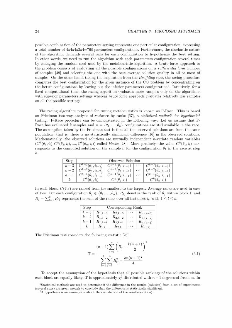
24 CHAPTER 3. PROPOSED APPROACH
possible combination of the parameters setting represents one particular configuration, expressinga total number of 4x4x4x3x4=768 parameters configurations. Furthermore, the stochastic natureof the algorithm demands several runs for each configuration to hypothesize the best setting.In other words, we need to run the algorithm with each parameters configuration several timesby changing the random seed used by the metaheuristic algorithm. A brute force approach tothe problem consists of evaluating all the possible configurations on a sufficiently large numberof samples [49] and selecting the one with the best average solution quality in all or most ofsamples. On the other hand, taking the inspiration from the Hoeffding race, the racing procedurecomputes the best configuration for the given instance of the CO problem by concentrating onthe better configurations by leaving out the inferior parameters configurations. Intuitively, for afixed computational time, the racing algorithm evaluates more samples only on the algorithmswith superior parameters settings whereas brute force approach evaluates relatively less sampleson all the possible settings.
The racing algorithm proposed for tuning metaheuristics is known as F-Race. This is basedon Friedman two-way analysis of variance by ranks [67], a statistical method1 for hypothesis2
testing. F-Race procedure can be demonstrated in the following way: Let us assume that F-Race has evaluated k samples and n = {θ1, ...., θn} configurations are still available in the race.The assumption taken by the Friedman test is that all the observed solutions are from the samepopulation, that is, there is no statistically significant difference [16] in the observed solutions.Mathematically, the observed solutions are mutually independent n-variate random variables(Ck(θ1, il), C
k(θ2, il), ...., Ck(θn, il)) called blocks [28]. More precisely, the value Ck(θ1, il) cor-
responds to the computed solution on the sample il for the configuration θ1 in the race at stepk.
Step Observed Solutionk − 3 Ck−3(θ1, il−3) Ck−3(θ2, il−3) · · · Ck−3(θn, il−3)k − 2 Ck−2(θ1, il−2) Ck−2(θ2, il−2) · · · Ck−2(θn, il−2)k − 1 Ck−1(θ1, il−1) Ck−1(θ2, il−1) · · · Ck−1(θn, il−1)
k Ck(θ1, il) Ck(θ2, il) · · · Ck(θn, il)
In each block, C(θ, i) are ranked from the smallest to the largest. Average ranks are used in caseof ties. For each configuration θj ∈ {θ1, ...., θn}, Rlj denotes the rank of θj within block l, and
Rj =∑k
l=1 Rlj represents the sum of the ranks over all instances il, with 1 ≤ l ≤ k.
Step Corresponding Rankk − 3 R1,k−3 R2,k−3 · · · Rn,(k−3)
k − 2 R1,k−2 R2,k−2 · · · Rn,(k−2)
k − 1 R1,k−1 R2,k−1 · · · Rn,(k−1)
k R1,k R2,k · · · Rn,(k)
The Friedman test considers the following statistic [26].
T =
(n − 1)
n∑
j=1
(
Rj −k(n + 1)
2
)2
k∑
l=1
n∑
j=1
R2lj −
kn(n + 1)2
4
(3.1)
To accept the assumption of the hypothesis that all possible rankings of the solutions withineach block are equally likely, T is approximately χ2 distributed with n− 1 degrees of freedom. In
1Statistical methods are used to determine if the difference in the results (solution) from a set of experiments(several runs) are great enough to conclude that the difference is statistically significant.
2A hypothesis is an assumption about the distribution of the results(solution).

3.1. ACO/F-RACE ALGORITHM 25
Θ
i
Figure 3.1: A visual representation of the amount of computation needed by brute force (rectanglecomprised by dashed line) and racing approach(shadowed area).
F-Race, if the hypothesis is accepted at step k, then all the configurations from step k are allowedto race for the next step k +1. On the other hand, if the observed T exceeds the 1−α quantile ofsuch distribution, the hypothesis is rejected. As a consequence, at the approximate level α, thereis a possibility of dropping at least a configuration θj from {θ1, ...., θn} which shows statisticallysignificant difference from the other configurations.
Next step after rejecting the hypothesis is to identify which configuration has to be dropped fromfurther racing. For this reason, pairwise comparison between individual candidates is performed.The candidates θj and θh are considered different if:
| Rj − Rh |√
2k(1− Tk(n−1)
)(P
kl=1
P
nj=1 R2
lj−
kn(n+1)2
4 )
(k−1)(n−1)
> t1 − α/2 (3.2)
where t1−α/2 is the 1−α/2 quantile of the student’s t distribution. Therefore in F-Race, rejectionof hypothesis is followed by pairwise comparisons which are executed between the best candidateand each other one. All the candidates, whose ranks are significantly worse than the best, at stepk, are discarded and will not appear in the next step k + 1.
The ranking of the quantiles C(θ, i) plays the vital role for the efficient computation of the bestconfiguration by F-Race approach [18] [17] in the following way:
• Nonparametric nature: Nonparametric tests are powerful in detecting population differenceswhen certain assumptions are not satisfied. On the other hand, if we consider the parametrictests, for example, t test assumes the values from each sample should come from a normaldistribution. Central limit theorem states that when the samples are very large, then thesample means will follow the normal distribution even if the respective variable is not nor-mally distributed in the observation. Hence, the parametric methods like t test are morepowerful and appropriate for large samples. The smaller the sample size, the lesser will bethe ability of t test to detect the differences. The striking feature of the nonparametric testis that it doesn’t requires the hypothesis formulation and thus they are distribution-free.Further it is appropriate when the sample sizes are small. In F-Race, the number of candi-dates is reduced as soon as possible and the further evaluations take place only on a small

26 CHAPTER 3. PROPOSED APPROACH
number of surviving candidates. Therefore, we cannot use parametric tests and we have toadopt nonparametric tests. More debates, discussions and facts about nonparametric andparametric methods were presented in Larson [67].
• Blocking design: Blocking design reduces the variability due to a known source of variation.Given a set of configuration for the stochastic algorithms such as metaheuristic algorithmsand treating them with several different samples results in a large variation in the solutionquality. Blocking is an efficient way of normalizing the solution quality observed on severaldifferent samples [28]. Therefore, the ranking of different configurations within each sampleeliminates the risk of sample’s influence in the accepting or rejecting a configuration.
Notwithstanding the inspiration from a number of machine learning algorithms such as Maron[70], Gratch et al. [50], Chien et al. [25], Moore and Lee [74], F-Race is the first racing algorithmto implement blocking through ranking and to adopt the Friedman test as the aggregate test [49]over all candidates, to be performed prior to any pairwise test. By means of F-Race, Birattariet al. [18] first proposed the formal definition for the problem of tuning metaheuristics from amachine learning perspective. A substantial explanation of the topic is given in Birattari [17].
3.1.1 Solution Methodology
ACO/F-Race algorithm, we propose in this thesis, is inspired by S-ACO [52] and F-Race [18]approaches. In this algorithm, F-Race is used in an original way as a component of the ACOalgorithm. Similar to S-ACO, the proposed approach uses empirical estimation for tackling COproblems under uncertainty. Without loss of generality, ACO/F-Race can be adopted to solve thePTSP, in specific, to optimize the expected length of the a posteriori tour. The pseudo-code ofthe ACO/F-Race is presented in Algorithm 5.
Algorithm 5 ACO/F-Race Algorithm
input: an instance C of a PTSP problemset τij ← 1 for all (i,j)for round r = 1, 2, 3..... do
for ant σ = 1, 2, 3.....m doplace the ant in a random city ichoose the next city by random proportional rule until all the cities were included in thetour
end forif (r = 1) then
Based on Nm random scenarios ωv, race m ant’s tour sm
sbest ← F-Race(Nm, sm)
elseBased on Nm random scenarios ωv, race m ant’s tour sm with best-so-far ant’s tour sbest
sbest ← F-Race(Nm, sm ∪ sbest)
end ifevaporation: set τij ← (1 − ρ)τij∀(i, j) ;best-so-far pheromone update: set τij ← τij + c1,∀(i, j) ∈ sbest;iteration-best pheromone update: set τij ← τij + c2,∀(i, j) ∈ sbest;
end for
Clearly, the algorithm reveals that most of the components are similar to S-ACO. Typically,the algorithm starts by initializing the pheromone on each arcs (i, j) of the PTSP to unity. Sub-sequently, the iterative ContructSolution phase of the ACO/F-Race starts. The iteration begins

3.1. ACO/F-RACE ALGORITHM 27
by placing m ants randomly on the cities of the PTSP. Each ant construct the a priori tour ac-cording to the random proportional rule given by Equation 3.3 (which is same as the Equation2.2). Therefore, an ant k, currently at city i moves to the city j probabilistically using Equation3.3, where Nk
i is the set of all cities yet to be visited by the ant k.
pkij =
ταij · η
βij
∑
l∈Nki
ταil · η
βil
, if j ∈ Nki (3.3)
Once m ants finished constructing their respective a priori tour, the original element of theproposed approach, F-Race algorithm starts. During the first iteration, the function F-Raceevaluates and compares m ants a priori tour to select the iteration-best solution. Since there isno best-so-far tour at the first iteration, the selected iteration-best solution is also considered asthe best-so-far solution. From the subsequent iterations, the function F-Race evaluates m ant’ssolution together with the best-so-far solution.
Now we describe the way in which the F-Race approach is adopted as a component for selectingthe best-so-far solution. As described earlier, once the ants constructed the tour, it’s a prioritours are then passed to the function F-Race as described in Algorithm 6. In S-ACO, the value
Algorithm 6 Racing Function
Function F-Race(Nm,Θ)M ← 2 ∗ Nm{/*stopping criteria for each iteration in ACO/F-RACE */}evaluated-candidates ← 0 {/* number of evaluated candidates */}steps ← 0{/* number of steps performed */}while (evaluated-candidates+surviving-candidates) ≤ M do
steps ← steps + 1surviving-candidates ← | Θ |{/* number of surviving candidates */}generate a random scenario ωfor each a priori tour θi ∈ Θ do
compute the a posteriori tour θi by skipping strategyend forevaluated-candidates ← evaluated-candidates+surviving-candidatesif (Failed Significance Friedman(steps, θ1 · · · θ|Θ|) then
Θ ← Θ \ pairwise(θi ∈ Θ)end if
end whilereturn θbest from surviving candidates of the set Θ
of Nm determines the number of random scenarios to be evaluated for each iteration to select thebest-so-far solution. At each iteration (except first iteration), the iteration-best and best-so-farsolution is evaluated on Nm random scenarios. As a consequence, the number of evaluations inS-ACO is twice that of Nm. In order to make a fair experimental evaluation and comparison ofACO/F-Race with S-ACO, we have adopted the same number of evaluations in the later as thatof the former. Therefore, the termination condition of the F-Race function is set such that thenumber of evaluations should reach twice the value of Nm. Until this termination condition isencountered, at each step, a new step specific random scenario ω is generated according to theprobability pi associated with each city i in the PTSP. This ω is used for evaluating the solutionwhich are still in the race. Intuitively, at each step, a posteriori tour length θi is computed foreach a priori tour θi ∈ Θ (the set Θ contains the surviving ant’s solution) with ω (cities to bevisited in the a posteriori tour) using skipping strategy.
Without loss of generality, the racing approach designed for tuning metaheuristic algorithms canbe employed to discard the ants with inferior solutions. The function (Failed Significance Friedman(steps, θ1 · · · θ|Θ

28 CHAPTER 3. PROPOSED APPROACH
test for the failure of the hypothesis using Friedman-two-way analysis of variance by ranks. Moreprecisely, at each step, the a posteriori tour length of the surviving ants Θ referred as θ1 · · · θ|Θ|
is tested for the statistically significant difference by computing T using the Equation 3.1. As aconsequence of such difference, the next step is to discard some ants from the race with the func-tion pairwise(θi ∈ Θ). Using the Equation 3.2, this function removes the ants whose solution’srank are significantly worse than the rank of best ant’s solution. Racing of solutions stops whenthe termination condition becomes true. The a priori tour that wins the race is returned as theθbest to the main algorithm.
The solution that wins the race is employed for updating the pheromone and stored as thebest-so-far solution for the next iteration of the algorithm. Since the best-so-far solution fromthe previous iteration has to compete with the solutions generated at the current iteration, theconcept of iteration-best solution doesn’t occur in ACO/F-Race. Although the concept of iteration-best pheromone update doesn’t have any sense in ACO/F-Race, a fair experimental comparisonwith S-ACO requires it. Therefore, the best-so-far solution is used as the candidate for updatingpheromone both in the best-so-far and the iteration-best pheromone updates.
The significant difference between S-ACO and ACO/F-Race lies in the technique used to selectthe iteration-best tour for each iteration. In S-ACO, the solutions produced at a given iterationare compared on the basis of a single scenario ω to select the iteration-best tour. On the basis oflarger sample size Nm, whose size is computed dynamically, the iteration-best tour is comparedwith best-so-far tour in the algorithm. The tour with least expected a posteriori tour lengthamong two solutions is selected and stored as the new best-so-far tour for future comparisonsand to update the pheromone matrix for the global pheromone update phase. More precisely,S-ACO exploits sampling techniques and parametric test whereas ACO/F-Race uses F-Race, analgorithm originally developed for tuning metaheuristics based on nonparametric tests. Althoughit is not necessary to have iteration-best pheromone update phase and large sample size, ACO/F-Race solution construction and pheromone update were implemented as described in [52] for theexperimental comparison.
3.2 Local Search Methodology
Metaheuristic algorithms frequently encounter a sequence of states in which it is impossible toimprove the solution quality by itself. Notwithstanding this inadequacy, various research workson metaheuristics tell us that a promising approach to extract high-quality solutions is to couple alocal search mechanism within the metaheuristics framework. Local search algorithms operate onthe solutions found by metaheuristics by introducing some modification to obtain locally optimalsolutions [92]. Furthermore, the consideration of local search algorithm as a stand alone solutiontechnique for CO problems suffers from the problem of finding good starting solutions. Therefore,the key idea of coupling metaheuristic algorithms with local search algorithms can be explained inthe following way: On the one hand, the metaheuristic algorithms provide a high quality startingsolutions. On the other hand, local search algorithms operate on these quality solutions to providea higher quality solutions.
ACO framework has the flexibility of coupling local search in the definition. Once ants completetheir solution construction phase, the local search algorithms are allowed to refine their solutionsto yield a higher quality solutions. Afterwards, the pheromones are updated on the arcs withrespect to the improved solutions found by local search procedures. With various experimentalevidence, Dorigo and Stutzle [34] proposed that combining the ant’s solution construction phasewith the local search procedures is a promising approach and there is a very high possibility andprobability that the local search procedures can improve the solution constructed by the ants.

3.2. LOCAL SEARCH METHODOLOGY 29
Fortunately enough, the number of possible choices when combining the local search with ACOalgorithms is quite large [34]. Notwithstanding these possibilities, it is very important to under-stand the fundamental nature of local search procedure concerning effectiveness and efficiency.Most of the local search procedures demand high computational time to refine the solutions.Therefore, the decision is up to the algorithm designer to choose, for a given computation time,a frequent refining local search algorithm that slightly improves the solution quality of the initialsolutions, or a less frequent, slow and effective local search algorithm that significantly improvesthe solution quality.
The number of ants, the necessity to use heuristic information, parameter settings and whichant(s) should be allowed to improve their solutions by a local search are some of the major elementsto be set before adopting a particular local search algorithm in the ACO framework. Most effectiveand recommended local search in ACO algorithms is best-so-far solution refinement [34]. It is alsointeresting to know whether ACO algorithm with a best parameter setting will remain best afteradding the local search.
Local search algorithms for the TSP are based on the k-exchange neighborhood relation, inwhich candidate solutions s and s′ are direct neighbors if and only if, s′ can be obtained from sby deleting a set of k edges and rewiring the resulting fragments into a complete tour by insertinga different set of k edges [92]. Within the ACO framework, the local search techniques such as2-opt, 2.5-opt and 3-opt [92] are used quite often in TSP to improve the solution found by ants.All three implementations exploit three standard speedup techniques: use of nearest neighbor listof limited length, the use of a fixed radius nearest-neighbor search, and the use of don’t look bits.These techniques increases the computation time sub-quadratically, that is, O(n2) where n is thesize of the instance. Large number of speed up techniques and its substantial explanation can befound in Bentley [5], Johnson and McGeoch [63] and Reinelt [84].
A quick and straightforward implementation [92] of a k-exchange iterative improvement algo-rithm considers, in each step, all possible combinations for the k edges to be deleted and replaced.After deleting k edges from a given candidate solution s, the number of ways in which the resultingfragments can be reconnected into a candidate solution different from s depends on k; For k = 2,after deleting two edges (ui, uj) and (uk, ul), the only way to reconnect the two partial tours intoa different complete tour is by introducing the edges (ui, uk) and (ul, uj). It is interesting to notethat after a 2-exchange move, one of the two partial tours is reversed.
Candidates for k-exchange moves can be identified quickly using the speed up techniques. Forexample, to enable an efficient access to the cities in the given tour that are connected to a givencity ui by edges with shorter distance can be achieved in the form of a list of neighboring citiesuk that is sorted according to the distance in ascending order. By using such candidate list for allthe cities in the TSP, nearest neighbor search can be performed very efficiently. The use of listsfor 2-opt often leads to improvement in the quality of the local optima found by these algorithms.Recommended value for the number of neighbors ranges from 10 to 40 [92]. Full candidate list foreach city incorporating all the n − 1 other cities in the TSP requires O(n2log n) computationaltime and O(n2) memory. Therefore, to reduce memory requirements, it is often desirable to usefixed length nearest neighbor list. As a consequence, the tours obtained from 2-opt using nearestneighbor list are no longer guaranteed to be locally optimal, because some improving moves maybe missed. Alternative approachs to construct nearest neighbor lists were proposed by Pecknyand Miller [81], Helsgaum [55].
Empirical 2-opt local search for PTSP
Bertsimas [8] first introduced the local search algorithms based on mathematical approximations,for CO problems under uncertainty known as 2-p-opt and 1-shift algorithms. Bianchi et al. [15]

30 CHAPTER 3. PROPOSED APPROACH
Figure 3.2: The a priori tour of a PTSP visiting all the cities once and only once. The edges(ui, uj) and (uk, ul) are selected for the 2-opt move.
and Bianchi and Campbell [12] extended the 2-p-opt and 1-shift algorithms to the PTSP. Thelocal search algorithm we propose in this thesis, empirical 2-opt local search for PTSP, is based onthe 2-opt local search in best-so-far solution using nearest neighbor list as the speed up technique.This technique, to the best of our knowledge, is the first local search for the PTSP which usesempirical estimation.
Before entering into the algorithmic details, it is important to understand the meaning of so-lution quality improvement in the context of TSP and PTSP. In the TSP, the improvement isstraightforward, in the sense that the improvement can be calculated directly. Intuitively, if weconsider the 2-opt move between the edges (ui, uj) and (uk, ul) of the TSP, the only possiblerefinement is (ui, uk) and (ul, uj). Therefore, the improvement in the solution quality 4 is consid-ered as the difference between the length of the solution components after and before 2-opt moveas shown in Equation 3.4:
4 = (d[ui][uk] + d[ul][uj ]) − (d[ui][uj ] + d[uk][ul]) (3.4)
where, d[ui][uk], d[ul][uj ], d[ui][uj ], d[uk][ul] represents the distance between the respectivecities in the TSP. The solution quality is said to be improved when 4 < 0 and viceversa. On theother hand, for the PTSP, the 2-opt move in the best-so-far solution is considered as an improvedmove only when it reduces the expected length of the a posteriori tour with respect to the set ofall random scenarios ωv. Therefore, in ACO/F-Race algorithm, to compute the improvement fora 2-opt move, it is customary to remember the random scenarios ωv which are evaluated to selectthe best-so-far solution for a given iteration.
In the context of PTSP, it should be noted that since the edges (ui, uj) and (uk, ul) for 2-optmove are selected from the a priori solution, there are possibilities that the cities ui, uj , uk, ul
may not occur in the random scenarios ωv. A straight forward approach which re-computes thea posteriori tour length for each random scenario doesn’t needs to consider this issue. But thisre-computation increases the total computational time especially when the number of randomscenarios is large. This case is trivial when the number of iteration increases. Therefore, wepropose a simple way of computing the improvement similar to the Equation 3.4. For illustration,consider the best-so-far solution as shown in Figure 3.2. Assume that the edges (ui, uj) and

3.2. LOCAL SEARCH METHODOLOGY 31
Figure 3.3: The modified a priori tour of a PTSP visiting all the cities once and only once. Theedges (ui, uj) and (uk, ul) are modified as (ui, uk) and (uj , ul) with 2-opt move
(uk, ul) in the best-so-far solution are selected for 2-opt move. As a consequence, the new tourwith interchanged edges (ui, uk) and (ul, uj) is shown in Figure 3.3. Now we have to compute theimprovement measure 4ωc
, for each random scenario ωc ∈ ωv. We can use the same Equation3.4 to compute 4ωc
, when all the cities in the selected edges for 2-opt move are included in arandom scenario ωc. On the other hand, let us consider a case when the city ui is not included inthe random scenario ωc. In such scenario, we have to find the previous city uprev which has to bevisited before visiting ui in the modified a priori solution. Intuitively, in the modified a posterioritour, the city uprev is visited followed by visiting the city uk by skipping the city ui as shown inFigure 3.4. Therefore, the 2-opt improvement measure 4ωc
for the random scenario ωc can bederived as:
4ωc= (d[uprev][uk] + d[ul][uj ]) − (d[uprev][uj ] + d[uk][ul]) (3.5)
Similar argument can be made when the random scenario doesn’t contain uj as shown in Figure3.5. Equation for this case is given as:
4ωc= (d[ui][uk] + d[ul][uprev]) − (d[ui][uprev] + d[uk][ul]) (3.6)
For the random scenario that doesn’t have cities uk or ul, the equation can be derived by findingthe next city to be visited from uk or ul in the modified solution. The scenarios without uk andul are shown in Figures 3.6 and 3.7 respectively. Equations for both the cases are established as:
4ωc= (d[ui][unext] + d[ul][uj ]) − (d[ui][uj ] + d[unext][ul]) (3.7)
4ωc= (d[ui][uk] + d[unext][uj ]) − (d[ui][uj ] + d[uk][unext]) (3.8)
The total improvement measure is the average of all improvement measure computed for eachscenario ωc ∈ ωv. This is represented as:
4ωv=
1
v
v∑
c=1
4ωc(3.9)
Therefore, after the 2-opt move, the solution quality is considered to be improved when 4ωv< 0
and viceversa.

32 CHAPTER 3. PROPOSED APPROACH
Figure 3.4: The a posteriori tour of a PTSP visiting the cities in the same order as modified apriori tour when the city ui doesn’t need to be visited.
Figure 3.5: The a posteriori tour of a PTSP visiting the cities in the same order as modified apriori tour when the city uj doesn’t need to be visited.

3.2. LOCAL SEARCH METHODOLOGY 33
Figure 3.6: The a posteriori tour of a PTSP visiting the cities in the same order as modified apriori tour when the city uk doesn’t need to be visited.
Figure 3.7: The a posteriori tour of a PTSP visiting the cities in the same order as modified apriori tour when the city ul doesn’t need to be visited.

34 CHAPTER 3. PROPOSED APPROACH
Algorithm 7 Empirical 2-opt local search
Function empirical 2-opt local search(ωv,sbest){function pick edge random() randomly select an edge for the 2-opt move}(ui, uj) ← pick edge random()(uk, ul) ← pick edge random() {function excahnge edge() makes the 2-opt move in sbest}s′best ←exchange edge((ui, uj), (uk, ul))for each random scenario ωc ∈ ωv do
if ui ∈ ωc thenfirst edge first ← ui
elsefirst edge first ← previous city(ui, s
′best)
end ifif uj ∈ ωc then
first edge second ← uj
elsefirst edge second ← previous city(uj , s
′best)
end ifif uk ∈ ωc then
second edge first ← uk
elsesecond edge first ← next city(uk, s′best)
end ifif ul ∈ ωc then
second edge second ← ul
elsesecond edge second ← next city(ul, s
′best)
end if4ωc
← (d[first edge first][second edge first]+d[first edge second][second edge second]) -(d[first edge first][first edge second]+d[second edge first][second edge second])
end for
4ωv=
1
v
v∑
c=1
4ωc
if 4ωv< 0 then
sbest ← s′best
end ifreturn sbest

3.2. LOCAL SEARCH METHODOLOGY 35
The pseudo code for the empirical 2-opt local search is presented in Algorithm 7. Once thebest-so-far solution is computed by the racing approach in ACO/F-Race algorithm, the 2-opt localsearch is employed to refine the solution.
The local search algorithm needs the best-so-far solution sbest and the set of all random sce-narios ωv used for selecting the best-so-far solution from the F-Race algorithm. The 2-opt localsearch procedure starts by selecting two edges (ui, uj),(uk, ul) at random by using the functionpick edge random() from the nearest neighbor list. It is customary to remember the selected listof edges to avoid selecting same edge more than once. The function exchange edge applies the2-opt move between the edges to yield a modified solution s′best. It is followed by evaluating theimprovement measure for each random scenario ωc ∈ ωv. According to the cities that need to bevisited in the random scenario, the improvement measure 4ωc
is computed as illustrated earlierwith the Figures 3.4, 3.5, 3.6, 3.7. Given a random scenario ωc, the functions previous city() andnext city() are used to find the previous city and the next city in the modified a priori tour s′best
when the given city doesn’t requires a visit in ωc. The improvement measure 4ωcis computed
for each random scenario. Followed by these evaluations, the average improvement 4ωvis calcu-
lated. Inexpensive computational time for 2-opt local search gives the flexibility to have severalrefinements of best-so-far solution before updating the pheromone. In our case, we employed the2-opt local search repeatedly as long as the quality of the modified solution improves. Finally, theempirical 2-opt local search algorithm returns the modified solution as sbest to the ACO/F-Racealgorithm which is then used as the candidate for updating the pheromone.
Empirical 2.5-opt local search for PTSP
In this section, we present empirical 2.5-opt local search procedure for the PTSP based on empiricalestimation and inspired by the 2.5-opt local search procedure of TSP [92]. Let us consider thatthe algorithm wants to make a 2.5-opt move between the edges (ui, uj) and (uk, ul). It first checks2-opt move between edges for the improvement. If it is not fruitful then it will explore the nextimprovement by inserting the city ul between ui and uj . It is interesting to note that, in 2.5-optmove none of the partial tour will be reversed. Obviously, the additional refinement phase in2.5-opt move requires extra computing time when compared to 2-opt move. Notwithstanding thecomputational overhead, the experimental evidence of Bentley [5] shows that the amount of extracomputational time is small and it leads to significantly better solution quality with respect to2-opt local search in the TSP. A substantial explanations for 2.5-opt can be found in Stutzle andHoos [92], Dorigo and Stutzle [34].
In the context of 2.5-opt move, the only possible refinement is inserting the city ul between thecities ui and uj . As a consequence, the edge starting from the city uk is rewired to the city ulnext
which has to be visited after visiting the city ul. Figure 3.8 shows the re-fragmentation procedureof the 2.5-opt move for the same a priori solution sketched in the Figure 3.2. The improvementin the solution quality is estimated by Equation 3.10 similar to the 2-opt move.
4 = (d[ui][ul] + d[ul][uj ] + d[uk][ulnext]) − (d[ui][uj ] + d[uk][ul] + d[ul][ulnext
]) (3.10)
Considering different random scenarios and the cities to be visited in each of those randomscenarios, the improvement measure 4ωc
is computed. The pseudo code for empirical 2.5-opt isshown in Algorithm 8. The algorithm first checks for 2-opt improvement, failure of which leads to2.5-opt move. The function excahnge edge2.5() makes the 2.5-opt re-fragmentation in the solutionas illustrated in the Figure 3.8. The functions which are used in empirical 2-opt local search suchas previous city() and next city() can be used for 2.5-opt move without any modifications. Theprocedures for selecting the city and computing the improvement measure were same as that ofthe empirical 2-opt algorithm.

36 CHAPTER 3. PROPOSED APPROACH
Algorithm 8 Emprical 2.5-opt local search
Function empirical 2.5-opt local search(ωv,sbest)Perform the same operations as explained in the empirical 2-opt algorithmIf the empirical 2-opt move doesn’t show any improvement then start the 2.5-opt move in sbest
{function excahnge edge2.5() makes the 2.5-opt move in sbest}s′best ←exchange edge2.5 ((ui, uj), (uk, ul))for each random scenario ωc ∈ ωv do
if ui ∈ ωc thenfirst edge first ← ui
elsefirst edge first ← previous city(ui, s
′best)
end ifif uj ∈ ωc then
first edge second ← uj
elsefirst edge second ← previous city(uj , s
′best)
end ifif uk ∈ ωc then
second edge first ← uk
elsesecond edge first ← next city(uk, s′best)
end ifif ul ∈ ωc then
second edge second ← ul
elsesecond edge second ← next city(ul, s
′best)
end ifif ulnext
∈ ωc thensecond edge second next ← ulnext
elsesecond edge second next ← next city(ulnext
, s′best)end if4ωc
← (d[first edge first][second edge second]+d[second edge second][first edge second]+d[second edge first][second edge second next]) -(d[first edge first][first edge second]+d[second edge first][second edged[second edge second][second edge second next])
end for
4ωv=
1
v
v∑
c=1
4ωc
if 4ωv< 0 then
sbest ← s′best
end ifreturn sbest
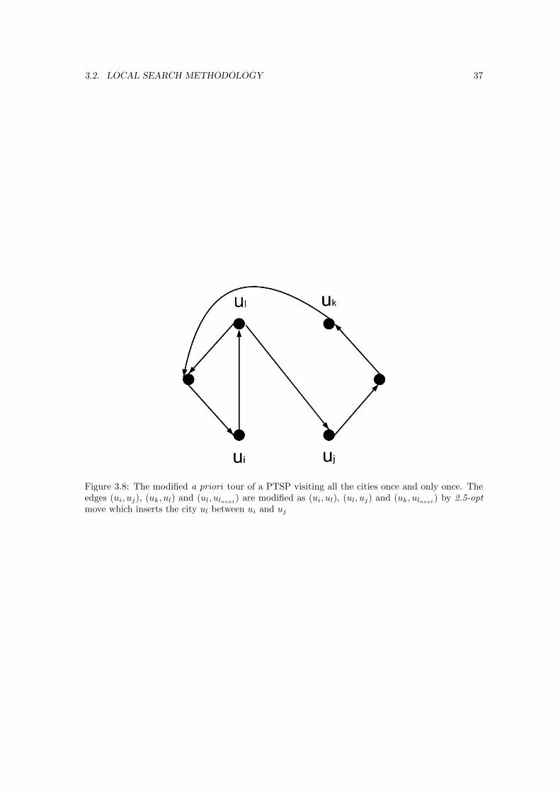
3.2. LOCAL SEARCH METHODOLOGY 37
Figure 3.8: The modified a priori tour of a PTSP visiting all the cities once and only once. Theedges (ui, uj), (uk, ul) and (ul, ulnext
) are modified as (ui, ul), (ul, uj) and (uk, ulnext) by 2.5-opt
move which inserts the city ul between ui and uj

38 CHAPTER 3. PROPOSED APPROACH

Chapter 4
Experiments and Results
In this chapter we discuss the results of the experiments we conducted using the ACO/F-Racealgorithm and empirical local search algorithms. Section 4.1 describes the experimental set-up,the problem sets, the hardware and software specifications and the output metrics for the exper-imental evaluations. Subsection 4.1.1 presents the experimental results concerning the behaviorof ACO under uncertain conditions. More precisely, the computational experiments include thecomparative study of the state-of-the-art ACO algorithms for solving PTSP such as explicit objec-tive function based ACS (pACS) [13], simulation based ACO (S-ACO) [52] against the proposedACO/F-Race approach. The next subsection 4.1.2 describes the results for empirical 2-opt and2.5-opt local search algorithms. We show how the empirical 2-opt and 2.5-opt improves the so-lution quality of ACO/F-Race. We also present a set of preliminary results in which we comparethe performance of empirical local search approaches against 1-shift local search [15, 8], the state-of-the-art local search methodology for solving PTSP.
4.1 Experimental Framework
The primary goal of this thesis is to study the behavior of the ACO algorithms under uncertainconditions. More precisely, we are interested in evaluating the solution quality of the ACO al-gorithm which solves PTSP as TSP. In this context, we fixed Ant System [31] as the standardACO algorithm with a slight modification, that is, the objective function is estimated on the basisof a single random scenario which is freshly sampled at each iteration of the algorithm. It is astandard practice to justify the proposal of a new algorithm by comparison of the new algorithmwith the current state-of-the-art algorithm. The proposed algorithm, ACO/F-Race, based on thesampling and racing approach is inspired by S-ACO [52] which is based on the sampling technique.Quite naturally, it is more meaningful to compare the solution quality of the two algorithms tojustify the significance of the proposed approach. The proposed empirical estimation approach isstill relatively unstudied. We would, nevertheless like to make the first step towards the compara-tive study of ACO/F-Race with pACS [13] which is based on mathematical approximation and thestate-of-the-art ACO algorithm designed to solve PTSP. In this thesis, we restrict our experimentsto ACO. Henceforth we use the following notation.
Algorithm NotationAnt System ACO-1Simulation based ACO algorithm S-ACORacing and Sampling ACO algorithm ACO/F-RaceExplicit objective function based ACS pACS
We use a standard benchmark to evaluate the quality of the algorithms. TSPLIB is one of thestandard benchmarks with a library of sample instances for the TSP from various sources such
39

40 CHAPTER 4. EXPERIMENTS AND RESULTS
as cities in a country, drilling holes in a printed circuit board etc. These instances can be furthersubdivided into cases where the nodes are uniformly distributed and the cases where they areclustered. There are no standard benchmark for the PTSP. To gain some standardization, wecarried out the experiments with the TSP instances. We used the TSP instances generated by theDIMACS [64]1 TSP generator. We are also interested in analyzing how the performance of thealgorithm varies in terms of the organization of the nodes in the instances. In this context, wefollowed the experimental setup of Bertsimas and Howell [9]: case in which nodes are uniformlydistributed and case in which nodes are clustered. For each case, we consider 100 TSP instancesof 300 cities. From each TSP instance, we obtain 21 homogeneous PTSP instances by letting theprobability associated with each city be {0,0.05,0.10,· · · ,0.95,1.0}. This resulted in 4200 PTSPinstances for the experimental evaluation.
After the selection of the problem, we fixed the computational time for the algorithms as pro-posed by Dorigo and Stutzle [34]. They compared various ACO algorithms to solve TSP instancesfrom TSPLIB involving 198 and 783 cities using 100 seconds and 10000 seconds as the compu-tational time respectively. Therefore, we allowed 120 seconds for each algorithm as the amountof computational time. It is interesting to see the quality of the solutions at the half way of thisrunning time. For this purpose, we have also recorded the solution quality of the algorithms at 60seconds.
The primary motivation behind this experimental study was to compare the evaluation pro-cedure based on F-Race with the one proposed in S-ACO. Therefore, the algorithms were notfine-tuned, and the parameters adopted are those suggested by Gutjahr [52] for S-ACO. Thismight possibly introduce a bias in favor of S-ACO. In future, we will adopt F-Race approach [18]for tuning the algorithms.
Parameter Notation ValueNumber of ants σ 25Pheromone exponent α 1.0Heuristic exponent β 2.0Pheromone evaporation factor ρ 0.01best-so-far update constant c1 0.04iteration-best update constant c2 0.00Number of nearest neighbors in tour construction nn 25
Empirical Analysis of the Solution Quality
The goal of the optimal solution of the PTSP is to choose an a priori tour which minimizes theexpected value of the a posteriori tour length. The a priori tour computed by each algorithmon each instance were then evaluated on 300 freshly generated random scenarios to compute theexpected value of the a posteriori tour length. The random scenarios are sampled according tothe probability associated with the instance.
The Computing Environment
The experiments presented in this chapter were performed on the cluster of personal computerscalled Polyphemus which is available at IRIDIA, Universite Libre de Bruxells. More precisely,we used a group of clients composed of 16 nodes and each node features 2 AMD OpteronTM244.All the nodes run the GNU/Linux operating system as distributed by Debian. All the algorithmsmentioned in this chapter were implemented in C language based on the source code of Stutzle
1DIMACS is a academic competition that aims create a reproducible picture of the state of the art in the areaof TSP heuristics (their effectiveness, their robustness, their scalability, etc.)

4.1. EXPERIMENTAL FRAMEWORK 41
[89]2 except pACS algorithm [13] which is implemented in C++. The source code was compiled forexecution on Polyphemus using gcc, the GNU Compiler Collection of the Free Software Foundation,versions 3.2 and 3.3. The graphs and plots shown in this section were produced with the Rpackage3.
Interpreting Tables and Graphs
For every class of instances and then for the entire set of instances we verify if differences in cost ofthe solutions found by the algorithms are statistically significant. We use the Pairwise Wilcoxonrank sum test [26] with p-values4 adjustment method by Holm [58]. In the tables associated tothe graphics we report for every pair of algorithms (r, c) the p-values for the null hypothesis: “Thedistributions of the solutions generated by A and by B are the same”.
The significance level with which we reject the null hypothesis is 0.99. The p-values smallerthan 0.01 are sufficient to reject the null hypothesis in favor of the alternate hypothesis. The tablefeatures the names of the algorithms under consideration on its row (r) and column (c). A numberless than 0.01 as an entry in (r,c) represents the condition that the observed performance of thealgorithms r and c has a sufficient statistical difference to reject the null hypothesis at a confidencelevel of at least 99%. The symbol * as an entry in (r,c) of the table refers to the condition that thealgorithms are same r=c whereas - as an entry in (r,c) represents that the comparison is alreadymade in the form of (c,r).
We represent the performance of the algorithms in x-y plots and present them in two forms foreach case: the absolute performance graph and its corresponding relative performance graph. Inthe absolute performance graph, the x-axis denotes the probability that the cities require beingvisited in the PTSP and the y-axis represents the expected value of the a posteriori tour lengthaveraged over 100 PTSP instances. The large scale of the y-axis makes the visualization of thedifference in the solution quality difficult. The next graph illustrates the relative difference in thesolution quality of the algorithms by taking a single algorithm as a normalized reference.
Analysis of Stochasticity
The stochasticity of the homogeneous PTSP can be measured with other simple heuristics. In thiscontext, the term stochasticity refers to the variance associated with the a posteriori tour length ofthe PTSP. For illustration, consider a straight forward and simple heuristic algorithm that findsthe a priori tour for the PTSP by treating it as TSP. It is possible to measure the quality ofthe solution with respect to the influence of the stochasticity in the following way: The solutionscomputed by each algorithm on a given PTSP were evaluated on a number of random scenariosto compute the a posteriori tour length associated with each random scenario. The mean andvariance of the a posteriori tour length over the set of all random scenarios under considerationdescribe the stochasticity associated with the problem. More precisely, the larger the variance,the higher the stochasticity associated with the problem and viceversa.
In order to determine the stochastic nature of the problem, we test the homogeneous PTSPproblems with simple heuristics such as Nearest Neighbor, Nearest Insertion and Furthest Insertionheuristics. The Nearest Neighbor algorithm (see Algorithm 9) always visits the nearest city
2This software package provides an implementation of various ACO algorithms applied to the TSP. The ACOalgorithms implemented are Ant System, Elitist Ant System, MAX-MIN Ant System, Rank-based version of AntSystem, Best-Worst Ant System, and Ant Colony System.
3R is a language and environment for statistical computing and graphics. It provides a wide variety of statistical(linear and nonlinear modelling, classical statistical tests, time-series analysis, classification, clustering, ...) andgraphical techniques, and is highly extensible. It is also available as Free Software under the terms of the FreeSoftware Foundation’s GNU General Public License in source code form.
4The p-value of a test is the probability of obtaining a value more extreme than the one that is obtained, in thedirection of the alternate hypothesis, if the null hypothesis is true.

42 CHAPTER 4. EXPERIMENTS AND RESULTS
whereas other algorithms first find a tour on small subset of cities, and then extends this tourby inserting the remaining cities one after the other until all the cities have been inserted. Moreprecisely, the Nearest Insertion approach (see Algorithm 10), from all cities yet to be visited,chooses a city whose insertion causes the lowest increase in the length of the tour. On the otherhand, the Furthest Insertion approach (see Algorithm 11) inserts a city whose minimal distanceto the visiting city is maximal. The idea behind this strategy is to fix the overall layout of the tourin the first few iterations of the insertion process. These algorithms are simple in conception andimplementation. Figure 4.1 visualizes the stochasticity associated with the uniformly distributedand clustered homogeneous PTSP instances. The x-axis denotes the probability that the citiesrequire being visited in the homogeneous PTSP. The y-axis represents the normalized standarddeviation, that is, the standard deviation divided by the mean, for the a posteriori tour lengthcomputed on 300 random scenarios sampled according to the corresponding x-axis probability.
Algorithm 9 Nearest Neighbor
1. Select a random city2. Select the nearest unvisited city and go there3. Repeat step 2 until no more cities remain4. Return to the first city
Algorithm 10 Nearest Insertion
1. Select the shortest edge and make a sub tour of it2. Select the city not in the sub tour having the shortest distance to any one of the cities in thesub tour3. Find the edge in the sub tour such that the cost of inserting the selected city between theedge’s cities will be minimal4. Repeat step 2 until no more cites remain
Algorithm 11 Furthest Insertion
1. Select the longest edge and make a sub tour of it2. Select the city not in the sub tour having the farthest distance to any one of the cities in thesub tour3. Find the edge in the sub tour such that the cost of inserting the selected city between theedge’s cities will be minimal4. Repeat step 2 until no more cities remain
From the results, we infer that the variance of the a posteriori tour length computed for thehomogeneous PTSP is less for the probability values close to 1. This indicates that in these cases,most of the cites in the PTSP need to be visited in all the sampled random scenarios. On the otherhand, as the probability decreases, the number of cities that need to be visited in the generatedrandom scenarios also decreases. As a consequence, the lesser the probability, the higher thevariance of the a posteriori tour length. Therefore, we informally conclude that by decreasing theprobability values associated with each city, the stochasticity of the homogeneous PTSP increases.These results form the basis for other experiments described in the rest of this chapter.
4.1.1 Experiments on Solution Techniques
In this subsection, we present the computational results which describe the behavior of several ACOversions under uncertainty. Figures 4.2, 4.3 describe the absolute and the relative performanceof the algorithms in terms of solution quality for the computational time of 60 seconds. Thevalues in the y-axis denote the expected value of the a posteriori tour length averaged over

4.1. EXPERIMENTAL FRAMEWORK 43
0.0 0.2 0.4 0.6 0.8 1.0
0.0
50
.10
0.1
50
.20
Instance class: uh Instance size: 300
Probability
No
rma
lize
d s
tan
da
rd d
evi
atio
n
Nearest neighborFarthest insertionNearest insertion
0.0 0.2 0.4 0.6 0.8 1.0
0.1
50
.20
0.2
5
Instance class: ch Instance size: 300
Probability
No
rma
lize
d s
tan
da
rd d
evi
atio
n
Nearest neighborFarthest insertionNearest insertion
Figure 4.1: Experimental results for the stochasticity on the uniformly distributed and clusteredhomogeneous PTSP instances. The x-axis denotes the probability that the cities require beingvisited in the homogeneous PTSP. The y-axis represents the normalized standard deviation, thatis, the standard deviation divided by mean, for the the a posteriori tour length computed on 300random scenarios sampled according to the corresponding x-axis probability.

44 CHAPTER 4. EXPERIMENTS AND RESULTS
Table 4.1: The Wilcoxon paired test and p-values for the null hypothesis: The distributions of thesolutions are the same for uniformly distributed homogeneous PTSP for the computational timeof 60 seconds. The significance level with which we reject the null hypothesis is 0.99. p-valuessmaller than 0.01 are sufficient to reject the null hypothesis. The quantities under analysis are theexpected length of the a posteriori tour obtained by ACO/F-Race, S-ACO and ACO-1.
Probability=0.25 pACS ACO/F-Race SACO ACO-1pACS * < 2.2e − 16 < 2.2e − 16 < 2.2e − 16ACO/F-Race - * < 2.2e − 16 < 2.2e − 16SACO - - * < 2.2e − 16
Probability=0.5 pACS ACO/F-Race SACO ACO-1pACS * < 2.2e − 16 < 2.2e − 16 < 2.2e − 16ACO/F-Race - * < 2.2e − 16 1SACO - - * 1
Probability=0.75 pACS ACO/F-Race SACO ACO-1pACS * < 2.2e − 16 < 2.2e − 16 1ACO/F-Race - * < 2.2e − 16 1SACO - - * 1
Probability=1.0 pACS ACO/F-Race SACO ACO-1pACS * < 2.2e − 16 < 2.2e − 16 < 2.2e − 16ACO/F-Race - * < 2.2e − 16 1SACO - - * 1
100 homogeneous PTSP instances of 300 uniformly distributed cities. The values in the x-axisrepresent the corresponding probability that the cities require being visited in the homogeneousPTSP. Table 4.1 summarize the statistical significance for the observation, that is, the p-valuesfor the Wilcoxon paired rank test for the probabilities {0.25, 0.50, 0.75, 1.0} that the cities requirebeing visited in the PTSP.
From Figure 4.3, we can observe that the solution quality computed by ACO-1 is better thanS-ACO and ACO/F-Race for the probability range greater than 0.4, that is, when the varianceof the a posteriori tour length is small. This means that an algorithm designed to solve TSP isbetter than one specifically developed for PTSP. This confirms the results of the research workestablished by Rossi and Gavioli [86]. This is easily explained: Using large number of randomscenarios for selecting the best-so-far solution is simply a waste of time when the variance of theobjective function is very small.
On the other hand, for the probability range less than 0.4, the problem becomes more stochastic.Therefore, the best-so-far solution obtained using large number of samples plays a significant role.The rationale behind this technique is that unfortunate modifications to the pheromone matrixthat can be caused by sampling an atypical random scenario at a given iteration, will not have alarge impact on the overall result and will be corrected in following iterations. The risk we runby following a single sample strategy, in ACO-1, is that we might sample a particularly atypicalrandom scenario which provides a misleading selection of the solutions. As a consequence, ACO/F-Race and S-ACO obtain better results than ACO-1. We can justify our observation with Table4.3. The p value associated with ACO/F-Race(row) Vs. ACO-1(column) and S-ACO(row) Vs.ACO-1(column) is < 2.2e−16 for the probability range 0.0 to 0.4 and it becomes 1 for probabilityrange 0.5 to 1.0 which refers to the condition that ACO-1 obtain better results than ACO/F-Raceand S-ACO.
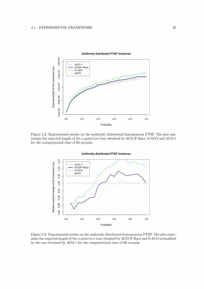
4.1. EXPERIMENTAL FRAMEWORK 45
0.0 0.2 0.4 0.6 0.8 1.0
0.0e
+00
5.0e
+06
1.0e
+07
1.5e
+07
2.0e
+07
Uniformly distributed PTSP instances
Probability
Exp
ecte
d le
ngth
of t
he a
pos
terio
ri to
ur
ACO−1ACO/F−RaceS−ACOpACS
Figure 4.2: Experimental results on the uniformly distributed homogeneous PTSP. The plot rep-resents the expected length of the a posteriori tour obtained by ACO/F-Race, S-ACO and ACO-1for the computational time of 60 seconds.
0.0 0.2 0.4 0.6 0.8 1.0
0.80
0.85
0.90
0.95
1.00
1.05
1.10
1.15
Uniformly distributed PTSP instances
Probability
Rel
ativ
e ex
pect
ed le
ngth
of t
he a
pos
terio
ri to
ur ACO−1ACO/F−RaceS−ACOpACS
Figure 4.3: Experimental results on the uniformly distributed homogeneous PTSP. The plot repre-sents the expected length of the a posteriori tour obtained by ACO/F-Race and S-ACO normalizedby the one obtained by ACO-1 for the computational time of 60 seconds.

46 CHAPTER 4. EXPERIMENTS AND RESULTS
Another important observation concerning the results is the performance of the ACO/F-Race.Throughout the whole range of probabilities, the solution quality computed by ACO/F-Race issignificantly better than S-ACO. Therefore, we infer that the nonparametric evaluation methodadapted by ACO/F-Race computes better solution than parametric S-ACO. Notwithstanding thesame number of evaluations, the S-ACO selects the iteration-best solution based on a single randomscenario whereas ACO/F-Race use the racing approach to evaluate all the solutions obtained ateach iteration. As a consequence, while selecting the iteration-best solution, the probability ofneglecting a good solution is very high in S-ACO by sampling an atypical random scenario. InTable 4.1, for the entire probability range, the p value of the Wilcoxon test associated with ACO/F-Race(row) Vs. S-ACO(column) is < 2.2e−16. To ensure ACO/F-Race is significantly better thanS-ACO it is enough to have the p value < 0.01.
Further insight into the results revels that pACS performs better than ACO/F-Race and S-ACO.The statistical significance for this observation is shown in Table 4.1. The p-value is < 2.2e − 16for all the probabilities in pACS(row) Vs. ACO/F-Race(column). The same holds true for pACS(row) Vs. S-ACO (column). It should be noted that pACS is fine tuned for parameter configurationand it exploits the pseudo random proportional rule5 in the solution construction process. On theother hand, ACO/F-Race and S-ACO are not tuned for the parameter and employ the randomproportional rule6. It is known in the literature [34] that an ACO algorithm which employs pseudorandom proportional rule computes better solution than one which uses random proportional rule.Therefore, pACS computes better solution than ACO/F-Race and S-ACO. The primary goal ofthis experiment was to compare the evaluation procedure based on F-Race with the one proposedin S-ACO. For this reason, solution construction (with random proportional rule) was implementedas described in S-ACO [52]. In future, we will combine F-Race with better performing ACO.
Figure 4.5 shows the results obtained for the uniformly distributed homogeneous PTSP for thecomputational time of 120 seconds. We can observe a similar behavior to the results obtainedfor the computational time of 60 seconds. The interesting element to observe from these resultsis that the difference in the relative performance among different algorithms becomes less withrespect to the relative performance at 60 seconds. This behavior can be justified with the propertyof convergence in solution of ACO. It is a state of the algorithm that keeps on generating the sameoptimal solution. ACO-F/Race and pACS reach this optimal solution in shorter computationaltime due to the improved technique which they adopt to select the iteration-best solution. On theother hand, ACO-1 and S-ACO attain this state by reaping the benefits of higher computationaltime. The statistical significance for this observation is given in Table 4.2.
The experimental evaluations for the homogeneous PTSP with clustered cities, for the compu-tational time of 60 and 120 seconds are shown in Figures 4.7 and 4.9 respectively. The Wilcoxonpaired test and the p values are summarized in Tables 4.3 and 4.4. From the results, we observethat the behavior of the algorithms do not change significantly with the clustered distribution.Therefore, the arguments and justifications which are explained for the uniformly distributed citiescan be adapted to the clustered PTSP.
5See Equation 2.9 described in page 186See Equation 2.2 described in page 15

4.1. EXPERIMENTAL FRAMEWORK 47
Table 4.2: The Wilcoxon paired test and p-values for the null hypothesis: The distributions of thesolutions are the same for uniformly distributed homogeneous PTSP for the computational timeof 120 seconds. The significance level with which we reject the null hypothesis is 0.99. p-valuessmaller than 0.01 are sufficient to reject the null hypothesis. The quantities under analysis are theexpected length of the a posteriori tour obtained by ACO/F-Race, S-ACO and ACO-1.
Probability=0.25 pACS ACO/F-Race SACO ACO-1pACS * < 2.2e − 16 < 2.2e − 16 < 2.2e − 16ACO/F-Race - * < 2.2e − 16 < 2.2e − 16SACO - - * < 2.2e − 16
Probability=0.5 pACS ACO/F-Race SACO ACO-1pACS * < 2.2e − 16 < 2.2e − 16 0.8757ACO/F-Race - * < 2.2e − 16 1SACO - - * 1
Probability=0.75 pACS ACO/F-Race SACO ACO-1pACS * < 2.2e − 16 < 2.2e − 16 0.9583ACO/F-Race - * < 2.2e − 16 1SACO - - * 1
Probability=1.0 pACS ACO/F-Race SACO ACO-1pACS * < 2.2e − 16 < 2.2e − 16 < 2.2e − 16ACO/F-Race - * < 2.2e − 16 1SACO - - * 1
Table 4.3: The Wilcoxon paired test and p-values for the null hypothesis: The distributions of thesolutions are the same for clustered homogeneous PTSP for the computational time of 60 seconds.The significance level with which we reject the null hypothesis is 0.99. p-values smaller than 0.01are sufficient to reject the null hypothesis. The quantities under analysis are the expected lengthof the a posteriori tour obtained by ACO/F-Race, S-ACO and ACO-1.
Probability=0.25 pACS ACO/F-Race SACO ACO-1pACS * < 2.2e − 16 < 2.2e − 16 < 2.2e − 16ACO/F-Race * - < 2.2e − 16 < 2.2e − 16SACO - - * < 2.2e − 16
Probability=0.5 pACS ACO/F-Race SACO ACO-1pACS * < 2.2e − 16 < 2.2e − 16 < 2.2e − 16ACO/F-Race * - < 2.2e − 16 < 2.2e − 16SACO - - * 1
Probability=0.75 pACS ACO/F-Race SACO ACO-1pACS * < 2.2e − 16 < 2.2e − 16 1ACO/F-Race * - < 2.2e − 16 1SACO - - * 1
Probability=1.0 pACS ACO/F-Race SACO ACO-1pACS * < 2.2e − 16 < 2.2e − 16 < 2.2e − 16ACO/F-Race * - < 2.2e − 16 < 2.2e − 16SACO - - * 1

48 CHAPTER 4. EXPERIMENTS AND RESULTS
0.0 0.2 0.4 0.6 0.8 1.0
0.0e
+00
5.0e
+06
1.0e
+07
1.5e
+07
2.0e
+07
Uniformly distributed PTSP instances
Probability
Exp
ecte
d le
ngth
of t
he a
pos
terio
ri to
ur
ACO−1ACO/F−RaceS−ACOpACS
Figure 4.4: Experimental results on the uniformly distributed homogeneous PTSP. The plot rep-resents the expected length of the a posteriori tour obtained by ACO/F-Race, S-ACO and ACO-1for the computational time of 120 seconds.
0.0 0.2 0.4 0.6 0.8 1.0
0.80
0.85
0.90
0.95
1.00
1.05
1.10
1.15
Uniformly distributed PTSP instances
Probability
Rel
ativ
e ex
pect
ed le
ngth
of t
he a
pos
terio
ri to
ur ACO−1ACO/F−RaceS−ACOpACS
Figure 4.5: Experimental results on the uniformly distributed homogeneous PTSP. The plot repre-sents the expected length of the a posteriori tour obtained by ACO/F-Race and S-ACO normalizedby the one obtained by ACO-1 for the computational time of 120 seconds.

4.1. EXPERIMENTAL FRAMEWORK 49
0.0 0.2 0.4 0.6 0.8 1.0
0e+
002e
+06
4e+
066e
+06
8e+
061e
+07
Clustered PTSP instances
Probability
Exp
ecte
d le
ngth
of t
he a
pos
terio
ri to
ur
ACO−1ACO/F−RaceS−ACOpACS
Figure 4.6: Experimental results on the clustered homogeneous PTSP. The plot represents theexpected length of the a posteriori tour obtained by ACO/F-Race, S-ACO and ACO-1 for thecomputational time of 60 seconds.
0.0 0.2 0.4 0.6 0.8 1.0
0.80
0.85
0.90
0.95
1.00
1.05
1.10
1.15
Clustered PTSP instances
Probability
Rel
ativ
e ex
pect
ed le
ngth
of t
he a
pos
terio
ri to
ur ACO−1ACO/F−RaceS−ACOpACS
Figure 4.7: Experimental results on the clustered homogeneous PTSP. The plot represents theexpected length of the a posteriori tour obtained by ACO/F-Race and S-ACO normalized by theone obtained by ACO-1 for the computational time of 60 seconds.
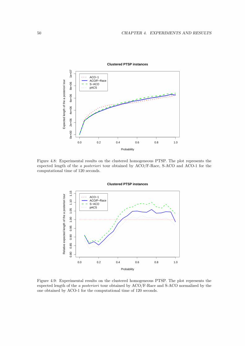
50 CHAPTER 4. EXPERIMENTS AND RESULTS
0.0 0.2 0.4 0.6 0.8 1.0
0e+
002e
+06
4e+
066e
+06
8e+
061e
+07
Clustered PTSP instances
Probability
Exp
ecte
d le
ngth
of t
he a
pos
terio
ri to
ur
ACO−1ACO/F−RaceS−ACOpACS
Figure 4.8: Experimental results on the clustered homogeneous PTSP. The plot represents theexpected length of the a posteriori tour obtained by ACO/F-Race, S-ACO and ACO-1 for thecomputational time of 120 seconds.
0.0 0.2 0.4 0.6 0.8 1.0
0.80
0.85
0.90
0.95
1.00
1.05
1.10
1.15
Clustered PTSP instances
Probability
Rel
ativ
e ex
pect
ed le
ngth
of t
he a
pos
terio
ri to
ur ACO−1ACO/F−RaceS−ACOpACS
Figure 4.9: Experimental results on the clustered homogeneous PTSP. The plot represents theexpected length of the a posteriori tour obtained by ACO/F-Race and S-ACO normalized by theone obtained by ACO-1 for the computational time of 120 seconds.

4.1. EXPERIMENTAL FRAMEWORK 51
Table 4.4: The Wilcoxon paired test and p-values for the null hypothesis: The distributions of thesolutions are the same for clustered homogeneous PTSP for the computational time of 120 seconds.The significance level with which we reject the null hypothesis is 0.99. p-values smaller than 0.01are sufficient to reject the null hypothesis. The quantities under analysis are the expected lengthof the a posteriori tour obtained by ACO/F-Race, S-ACO and ACO-1.
Probability=0.25 pACS ACO/F-Race SACO ACO-1pACS * < 2.2e − 16 < 2.2e − 16 < 2.2e − 16ACO/F-Race - * < 2.2e − 16 < 2.2e − 16SACO - - * < 2.2e − 16
Probability=0.5 pACS ACO/F-Race SACO ACO-1pACS * < 2.2e − 16 < 2.2e − 16 1ACO/F-Race - * < 2.2e − 16 1SACO - - * 1
Probability=0.75 pACS ACO/F-Race SACO ACO-1pACS * < 2.2e − 16 < 2.2e − 16 1ACO/F-Race - * < 2.2e − 16 1SACO - - * 1
Probability=1.0 pACS ACO/F-Race SACO ACO-1pACS * < 2.2e − 16 < 2.2e − 16 < 2.2e − 16ACO/F-Race - * < 2.2e − 16 < 2.2e − 16SACO - - * 1
4.1.2 Experiments on Local Search techniques
This subsection describes the potentialities of the empirical 2-opt and 2.5-opt local search pro-cedures proposed in this thesis. More precisely, we will present the computational experimentsto illustrate the phenomenon and the significance of the empirical local search techniques whenapplied to ACO/F-Race. The second part of this subsection describes some preliminary exper-imental results in which we compare our local search techniques with the state-of-the-art localsearch approach.
Effectiveness of the empirical local search algorithms
We followed the same experimental methodology with respect to the problem type and the com-putational time as explained in the previous section. We examined the solution refinement phe-nomenon of the proposed local search approach by solving the PTSP with three different algo-rithms:
• ACO/F-Race
• ACO/F-Race with empirical 2-opt local search
• ACO/F-Race with empirical 2.5-opt local search
For the homogeneous PTSP that contains uniformly distributed cites, Figures 4.10, 4.11 describesthe absolute and the relative performance of the algorithms for the computational time of 60seconds. Table 4.5 summarize the p-values for the Wilcoxon paired rank test to show the statisticalsignificance for the experimental observations.

52 CHAPTER 4. EXPERIMENTS AND RESULTS
0.0 0.2 0.4 0.6 0.8 1.0
0.0e
+00
5.0e
+06
1.0e
+07
1.5e
+07
2.0e
+07
Uniformly distributed PTSP instances
Probability
Exp
ecte
d le
ngth
of t
he a
pos
terio
ri to
ur
ACO/F−RaceACO/F−Race 2−optACO/F−Race 2.5 opt
Figure 4.10: Experimental results on the uniformly distributed homogeneous PTSP. The plotrepresents the expected length of the a posteriori tour obtained by ACO/F-Race, ACO/F-Raceempirical 2-opt and ACO/F-Race empirical 2.5-opt for the computational time of 60 seconds.
0.0 0.2 0.4 0.6 0.8 1.0
0.80
0.85
0.90
0.95
1.00
1.05
1.10
1.15
Uniformly distributed PTSP instances
Probability
Rel
ativ
e ex
pect
ed le
ngth
of t
he a
pos
terio
ri to
ur ACO/F−RaceACO/F−Race 2−optACO/F−Race 2.5 opt
Figure 4.11: Experimental results on the uniformly distributed homogeneous PTSP. The plotrepresents the expected length of the a posteriori tour obtained by ACO/F-Race empirical 2-opt and ACO/F-Race empirical 2.5-opt normalized by the one obtained by ACO/F-Race for thecomputational time of 60 seconds.

4.1. EXPERIMENTAL FRAMEWORK 53
Table 4.5: The Wilcoxon paired test and p-values for the null hypothesis: The distributions of thesolutions are the same for uniformly distributed homogeneous PTSP for the computational timeof 60 seconds. The significance level with which we reject the null hypothesis is 0.99. p-valuessmaller than 0.01 are sufficient to reject the null hypothesis. The quantities under analysis are theexpected length of the a posteriori tour obtained by ACO/F-Race, ACO/F-Race empirical 2-optand ACO/F-Race empirical 2.5-opt.
Probability=0.25 ACO/F-Race 2.5-opt ACO/F-Race 2-opt ACO/F-RaceACO/F-Race 2.5-opt * < 2.2e − 16 < 2.2e − 16ACO/F-Race 2-opt - * < 2.2e − 16
Probability=0.50 ACO/F-Race 2.5-opt ACO/F-Race 2-opt ACO/F-RaceACO/F-Race 2.5-opt * < 2.2e − 16 < 2.2e − 16ACO/F-Race 2-opt - * < 2.2e − 16
Probability=0.75 ACO/F-Race 2.5-opt ACO/F-Race 2-opt ACO/F-RaceACO/F-Race 2.5-opt * < 2.2e − 16 < 2.2e − 16ACO/F-Race 2-opt - * < 2.2e − 16
Probability=1.0 ACO/F-Race 2.5-opt ACO/F-Race 2-opt ACO/F-RaceACO/F-Race 2.5-opt * < 2.2e − 16 < 2.2e − 16ACO/F-Race 2-opt - * < 2.2e − 16
The results from Figure 4.11 clearly show that the empirical 2-opt and 2.5-opt significantlyincrease the quality of the solution computed by the ACO/F-Race for all the probability values.This is easily explained: The empirical 2-opt local search approach evaluates the improvement inthe expected length of the a posteriori tour that results from reversing the tour between each pairof nodes. The empirical 2.5-opt local search computes the improvement by removing each city fromits current position in the tour and inserting it at all other points in the tour. As a consequence,the newly computed solution is always better. Table 4.5 provides statistical significance for theobservation.
Further insight into the results reveals that the solution quality of empirical 2.5-opt is signif-icantly better than empirical 2-opt for probabilities greater than 0.1. The superior performanceof the empirical 2.5-opt local search can be justified by the technique employed for the solutionrefinement. For the same set of nearest neighbors, the 2.5-opt chooses the best swap when com-pared to 2-opt [92]. The same argument holds true for the empirical local search too. But thepoor performance of 2.5-opt for the probabilities from 0.0 to 0.1 is surprising. Here the problembecomes highly stochastic. In 2.5-opt, the search for the best swap with very few cities usinglarge number of samples results in a waste of computational time. On the other hand, 2-opt movecontributes this extra time to the ACO/F-Race to perform more iterations which results in betterquality solutions.
Another interesting observation from this result is the difference in the relative performanceof the algorithms. The relative difference of solutions computed by local search versions of theACO/F-Race (with respect to ACO/F-Race) decreases with the increase of the probability associ-ated with the homogeneous PTSP. For highly stochastic problems, using large samples to estimatethe improvement measure enables empirical local search to compute better quality solutions. It issimply a waste of time when the problem is less stochastic.
Figures 4.12, 4.13 show the results obtained for the uniformly distributed cities in the homo-geneous PTSP for the computational time of 120 seconds. Table 4.6 lists the p-values for the

54 CHAPTER 4. EXPERIMENTS AND RESULTS
0.0 0.2 0.4 0.6 0.8 1.0
0.0e
+00
5.0e
+06
1.0e
+07
1.5e
+07
2.0e
+07
Uniformly distributed PTSP instances
Probability
Exp
ecte
d le
ngth
of t
he a
pos
terio
ri to
ur
ACO/F−RaceACO/F−Race 2−optACO/F−Race 2.5 opt
Figure 4.12: Experimental results on the uniformly distributed homogeneous PTSP. The plotrepresents the expected length of the a posteriori tour obtained by ACO/F-Race, ACO/F-Raceempirical 2-opt and ACO/F-Race empirical 2.5-opt for the computational time of 120 seconds.
0.0 0.2 0.4 0.6 0.8 1.0
0.80
0.85
0.90
0.95
1.00
1.05
1.10
1.15
Uniformly distributed PTSP instances
Probability
Rel
ativ
e ex
pect
ed le
ngth
of t
he a
pos
terio
ri to
ur ACO/F−RaceACO/F−Race 2−optACO/F−Race 2.5 opt
Figure 4.13: Experimental results on the uniformly distributed homogeneous PTSP. The plotrepresents the expected length of the a posteriori tour obtained by ACO/F-Race empirical 2-opt and ACO/F-Race empirical 2.5-opt normalized by the one obtained by ACO/F-Race for thecomputational time of 120 seconds.

4.1. EXPERIMENTAL FRAMEWORK 55
Table 4.6: The Wilcoxon paired test and p-values for the null hypothesis: The distributions of thesolutions are the same for uniformly distributed homogeneous PTSP for the computational timeof 120 seconds. The significance level with which we reject the null hypothesis is 0.99. p-valuessmaller than 0.01 are sufficient to reject the null hypothesis. The quantities under analysis are theexpected length of the a posteriori tour obtained by ACO/F-Race, ACO/F-Race empirical 2-optand ACO/F-Race empirical 2.5-opt.
Probability=0.25 ACO/F-Race 2.5-opt ACO/F-Race 2-opt ACO/F-RaceACO/F-Race 2.5-opt * < 2.2e − 16 < 2.2e − 16ACO/F-Race 2-opt - * < 2.2e − 16
Probability=0.50 ACO/F-Race 2.5-opt ACO/F-Race 2-opt ACO/F-RaceACO/F-Race 2.5-opt * < 2.2e − 16 < 2.2e − 16ACO/F-Race 2-opt - * < 2.2e − 16
Probability=0.75 ACO/F-Race 2.5-opt ACO/F-Race 2-opt ACO/F-RaceACO/F-Race 2.5-opt * < 2.2e − 16 < 2.2e − 16ACO/F-Race 2-opt - * < 2.2e − 16
Probability=1.0 ACO/F-Race 2.5-opt ACO/F-Race 2-opt ACO/F-RaceACO/F-Race 2.5-opt * < 2.2e − 16 < 2.2e − 16ACO/F-Race 2-opt - * < 2.2e − 16
Wilcoxon paired rank test for this observation. The only difference that can be found in Fig-ure 4.13 is that the difference in relative performance among different algorithms becomes lesswith respect to the relative performance at 60 seconds due to the property of convergence in thesolution.
The experimental evaluations for the homogeneous PTSP with clustered cities, for the compu-tational time of 60 and 120 seconds are shown in Figures 4.14, 4.15 and 4.16, 4.17 respectively.The Wilcoxon paired test and the p values are summarized in Tables 4.7 and 4.8. The behav-ior of the algorithms is similar to the uniformly distributed instances. Therefore, the argumentsand justifications which are explained for the uniformly distributed cities can be adapted to theclustered PTSP.
Preliminary Results Towards the State-of-the-Art Perspective
In this subsection, we present the results of the computational experiments which compare theACO/F-Race empirical 2-opt and 2.5-opt local search against pACS 1-shift local search algorithm.The 1-shift local search is a solution improvement technique that computes the improvementmeasure using mathematical approximation by removing each city from its current position in thetour and inserting it at all other points in the tour (in the same way as that of 2.5-opt move).The experimental setup was same as stated before.
The absolute and relative behavior of the algorithms, on the uniformly distributed instances,for the computational time of 60 seconds, are shown in Figures 4.18 and 4.19 respectively. Table4.9 contains the p values of the Wilcoxon paired test for the observation.

56 CHAPTER 4. EXPERIMENTS AND RESULTS
Table 4.7: The Wilcoxon paired test and p-values for the null hypothesis: The distributions of thesolutions are the same for clustered homogeneous PTSP for the computational time of 60 seconds.The significance level with which we reject the null hypothesis is 0.99. p-values smaller than 0.01are sufficient to reject the null hypothesis. The quantities under analysis are the expected length ofthe a posteriori tour obtained by ACO/F-Race, ACO/F-Race empirical 2-opt and ACO/F-Raceempirical 2.5-opt.
Probability=0.25 ACO/F-Race 2.5-opt ACO/F-Race 2-opt ACO/F-RaceACO/F-Race 2.5-opt * < 2.2e − 16 < 2.2e − 16ACO/F-Race 2-opt - * < 2.2e − 16
Probability=0.50 ACO/F-Race 2.5-opt ACO/F-Race 2-opt ACO/F-RaceACO/F-Race 2.5-opt * < 2.2e − 16 < 2.2e − 16ACO/F-Race 2-opt - * < 2.2e − 16
Probability=0.75 ACO/F-Race 2.5-opt ACO/F-Race 2-opt ACO/F-RaceACO/F-Race 2.5-opt * < 2.2e − 16 < 2.2e − 16ACO/F-Race 2-opt - * < 2.2e − 16
Probability=1.0 ACO/F-Race 2.5-opt ACO/F-Race 2-opt ACO/F-RaceACO/F-Race 2.5-opt * < 2.2e − 16 < 2.2e − 16ACO/F-Race 2-opt - * < 2.2e − 16
Table 4.8: The Wilcoxon paired test and p-values for the null hypothesis: The distributions of thesolutions are the same for clustered homogeneous PTSP for the computational time of 120 seconds.The significance level with which we reject the null hypothesis is 0.99. p-values smaller than 0.01are sufficient to reject the null hypothesis. The quantities under analysis are the expected length ofthe a posteriori tour obtained by ACO/F-Race, ACO/F-Race empirical 2-opt and ACO/F-Raceempirical 2.5-opt.
Probability=0.25 ACO/F-Race 2.5-opt ACO/F-Race 2-opt ACO/F-RaceACO/F-Race 2.5-opt * < 2.2e − 16 < 2.2e − 16ACO/F-Race 2-opt - * < 2.2e − 16
Probability=0.50 ACO/F-Race 2.5-opt ACO/F-Race 2-opt ACO/F-RaceACO/F-Race 2.5-opt * < 2.2e − 16 < 2.2e − 16ACO/F-Race 2-opt - * < 2.2e − 16
Probability=0.75 ACO/F-Race 2.5-opt ACO/F-Race 2-opt ACO/F-RaceACO/F-Race 2.5-opt * < 2.2e − 16 < 2.2e − 16ACO/F-Race 2-opt - * < 2.2e − 16
Probability=1.0 ACO/F-Race 2.5-opt ACO/F-Race 2-opt ACO/F-RaceACO/F-Race 2.5-opt * < 2.2e − 16 < 2.2e − 16ACO/F-Race 2-opt - * < 2.2e − 16

4.1. EXPERIMENTAL FRAMEWORK 57
0.0 0.2 0.4 0.6 0.8 1.0
0e+
002e
+06
4e+
066e
+06
8e+
061e
+07
Clustered PTSP instances
Probability
Exp
ecte
d le
ngth
of t
he a
pos
terio
ri to
ur
ACO/F−RaceACO/F−Race 2−optACO/F−Race 2.5 opt
Figure 4.14: Experimental results on the clustered homogeneous PTSP. The plot represents theexpected length of the a posteriori tour obtained by ACO/F-Race, ACO/F-Race empirical 2-optand ACO/F-Race empirical 2.5-opt for the computational time of 60 seconds.
0.0 0.2 0.4 0.6 0.8 1.0
0.80
0.85
0.90
0.95
1.00
1.05
1.10
1.15
Clustered PTSP instances
Probability
Rel
ativ
e ex
pect
ed le
ngth
of t
he a
pos
terio
ri to
ur ACO/F−RaceACO/F−Race 2−optACO/F−Race 2.5 opt
Figure 4.15: Experimental results on the clustered homogeneous PTSP. The plot represents theexpected length of the a posteriori tour obtained by ACO/F-Race empirical 2-opt and ACO/F-Race empirical 2.5-opt normalized by the one obtained by ACO/F-Race for the computationaltime of 60 seconds.

58 CHAPTER 4. EXPERIMENTS AND RESULTS
0.0 0.2 0.4 0.6 0.8 1.0
0e+
002e
+06
4e+
066e
+06
8e+
061e
+07
Clustered PTSP instances
Probability
Exp
ecte
d le
ngth
of t
he a
pos
terio
ri to
ur
ACO/F−RaceACO/F−Race 2−optACO/F−Race 2.5 opt
Figure 4.16: Experimental results on the clustered homogeneous PTSP. The plot represents theexpected length of the a posteriori tour obtained by ACO/F-Race, ACO/F-Race empirical 2-optand ACO/F-Race empirical 2.5-opt for the computational time of 120 seconds.
0.0 0.2 0.4 0.6 0.8 1.0
0.80
0.85
0.90
0.95
1.00
1.05
1.10
1.15
Clustered PTSP instances
Probability
Rel
ativ
e ex
pect
ed le
ngth
of t
he a
pos
terio
ri to
ur ACO/F−RaceACO/F−Race 2−optACO/F−Race 2.5 opt
Figure 4.17: Experimental results on the uniformly distributed homogeneous PTSP. The plotrepresents the expected length of the a posteriori tour obtained by ACO/F-Race empirical 2-opt and ACO/F-Race empirical 2.5-opt normalized by the one obtained by ACO/F-Race for thecomputational time of 120 seconds.
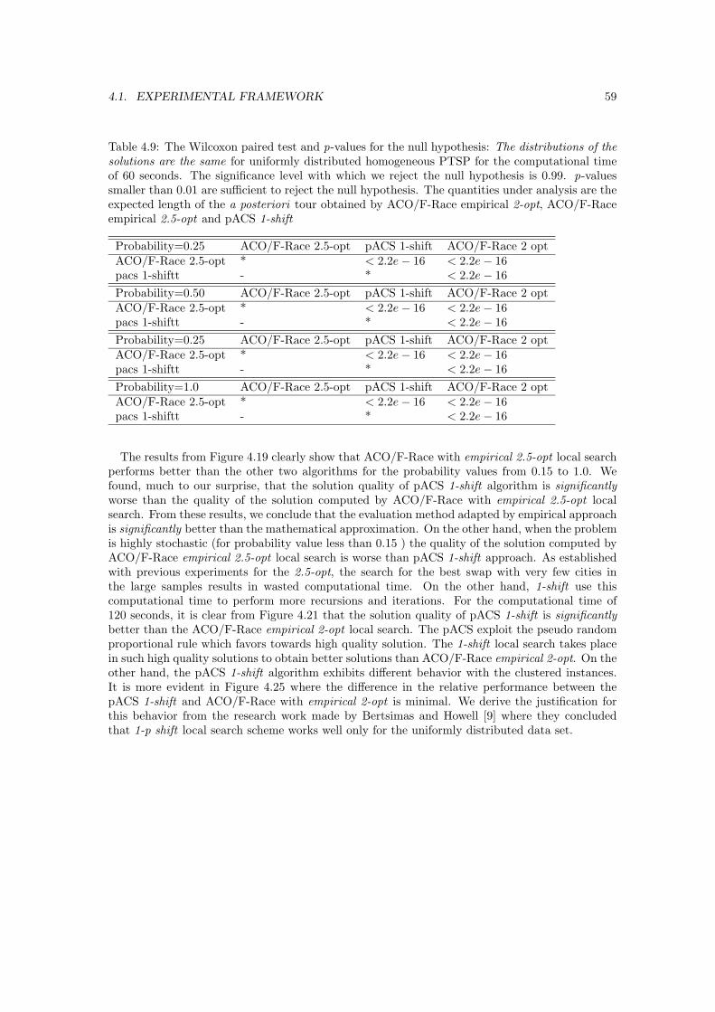
4.1. EXPERIMENTAL FRAMEWORK 59
Table 4.9: The Wilcoxon paired test and p-values for the null hypothesis: The distributions of thesolutions are the same for uniformly distributed homogeneous PTSP for the computational timeof 60 seconds. The significance level with which we reject the null hypothesis is 0.99. p-valuessmaller than 0.01 are sufficient to reject the null hypothesis. The quantities under analysis are theexpected length of the a posteriori tour obtained by ACO/F-Race empirical 2-opt, ACO/F-Raceempirical 2.5-opt and pACS 1-shift
Probability=0.25 ACO/F-Race 2.5-opt pACS 1-shift ACO/F-Race 2 optACO/F-Race 2.5-opt * < 2.2e − 16 < 2.2e − 16pacs 1-shiftt - * < 2.2e − 16
Probability=0.50 ACO/F-Race 2.5-opt pACS 1-shift ACO/F-Race 2 optACO/F-Race 2.5-opt * < 2.2e − 16 < 2.2e − 16pacs 1-shiftt - * < 2.2e − 16
Probability=0.25 ACO/F-Race 2.5-opt pACS 1-shift ACO/F-Race 2 optACO/F-Race 2.5-opt * < 2.2e − 16 < 2.2e − 16pacs 1-shiftt - * < 2.2e − 16
Probability=1.0 ACO/F-Race 2.5-opt pACS 1-shift ACO/F-Race 2 optACO/F-Race 2.5-opt * < 2.2e − 16 < 2.2e − 16pacs 1-shiftt - * < 2.2e − 16
The results from Figure 4.19 clearly show that ACO/F-Race with empirical 2.5-opt local searchperforms better than the other two algorithms for the probability values from 0.15 to 1.0. Wefound, much to our surprise, that the solution quality of pACS 1-shift algorithm is significantlyworse than the quality of the solution computed by ACO/F-Race with empirical 2.5-opt localsearch. From these results, we conclude that the evaluation method adapted by empirical approachis significantly better than the mathematical approximation. On the other hand, when the problemis highly stochastic (for probability value less than 0.15 ) the quality of the solution computed byACO/F-Race empirical 2.5-opt local search is worse than pACS 1-shift approach. As establishedwith previous experiments for the 2.5-opt, the search for the best swap with very few cities inthe large samples results in wasted computational time. On the other hand, 1-shift use thiscomputational time to perform more recursions and iterations. For the computational time of120 seconds, it is clear from Figure 4.21 that the solution quality of pACS 1-shift is significantlybetter than the ACO/F-Race empirical 2-opt local search. The pACS exploit the pseudo randomproportional rule which favors towards high quality solution. The 1-shift local search takes placein such high quality solutions to obtain better solutions than ACO/F-Race empirical 2-opt. On theother hand, the pACS 1-shift algorithm exhibits different behavior with the clustered instances.It is more evident in Figure 4.25 where the difference in the relative performance between thepACS 1-shift and ACO/F-Race with empirical 2-opt is minimal. We derive the justification forthis behavior from the research work made by Bertsimas and Howell [9] where they concludedthat 1-p shift local search scheme works well only for the uniformly distributed data set.

60 CHAPTER 4. EXPERIMENTS AND RESULTS
Table 4.10: The Wilcoxon paired test and p-values for the null hypothesis: The distributions of thesolutions are the same for uniformly distributed homogeneous PTSP for the computational timeof 120 seconds. The significance level with which we reject the null hypothesis is 0.99. p-valuessmaller than 0.01 are sufficient to reject the null hypothesis. The quantities under analysis are theexpected length of the a posteriori tour obtained by ACO/F-Race empirical 2-opt, ACO/F-Raceempirical 2.5-opt and pACS 1-shift
Probability=0.25 ACO/F-Race 2.5-opt pACS 1-shift ACO/F-Race 2 optACO/F-Race 2.5-opt * < 2.2e − 16 < 2.2e − 16pacs 1-shiftt - * < 2.2e − 16
Probability=0.50 ACO/F-Race 2.5-opt pACS 1-shift ACO/F-Race 2 optACO/F-Race 2.5-opt * < 2.2e − 16 < 2.2e − 16pacs 1-shiftt - * < 2.2e − 16
Probability=0.25 ACO/F-Race 2.5-opt pACS 1-shift ACO/F-Race 2 optACO/F-Race 2.5-opt * < 2.2e − 16 < 2.2e − 16pacs 1-shiftt - * < 2.2e − 16
Probability=1.0 ACO/F-Race 2.5-opt pACS 1-shift ACO/F-Race 2 optACO/F-Race 2.5-opt * < 2.2e − 16 < 2.2e − 16pacs 1-shiftt - * < 2.2e − 16
Table 4.11: The Wilcoxon paired test and p-values for the null hypothesis: The distributions of thesolutions are the same for clustered homogeneous PTSP for the computational time of 60 seconds.The significance level with which we reject the null hypothesis is 0.99. p-values smaller than 0.01are sufficient to reject the null hypothesis. The quantities under analysis are the expected lengthof the a posteriori tour obtained by ACO/F-Race empirical 2-opt, ACO/F-Race empirical 2.5-optand pACS 1-shift
Probability=0.25 ACO/F-Race 2.5-opt pACS 1-shift ACO/F-Race 2 optACO/F-Race 2.5-opt * < 2.2e − 16 < 2.2e − 16pacs 1-shiftt - * < 2.2e − 16
Probability=0.50 ACO/F-Race 2.5-opt pACS 1-shift ACO/F-Race 2 optACO/F-Race 2.5-opt * < 2.2e − 16 < 2.2e − 16pacs 1-shiftt - * < 2.2e − 16
Probability=0.25 ACO/F-Race 2.5-opt pACS 1-shift ACO/F-Race 2 optACO/F-Race 2.5-opt * < 2.2e − 16 < 2.2e − 16pacs 1-shiftt - * < 2.2e − 16
Probability=1.0 ACO/F-Race 2.5-opt pACS 1-shift ACO/F-Race 2 optACO/F-Race 2.5-opt * < 2.2e − 16 < 2.2e − 16pacs 1-shiftt - * < 2.2e − 16

4.1. EXPERIMENTAL FRAMEWORK 61
0.0 0.2 0.4 0.6 0.8 1.0
0.0e
+00
5.0e
+06
1.0e
+07
1.5e
+07
2.0e
+07
Uniformly distributed PTSP instances
Probability
Exp
ecte
d le
ngth
of t
he a
pos
terio
ri to
ur
ACO/F−Race 2−optACO/F−Race 2.5−optpACS 1−shift
Figure 4.18: Experimental results on the uniformly distributed homogeneous PTSP. The plotrepresents the expected length of the a posteriori tour obtained by ACO/F-Race empirical 2-opt,ACO/F-Race empirical 2.5-opt and pACS 1-shift for the computational time of 60 seconds.
0.0 0.2 0.4 0.6 0.8 1.0
0.80
0.85
0.90
0.95
1.00
1.05
1.10
1.15
Uniformly distributed PTSP instances
Probability
Rel
ativ
e ex
pect
ed le
ngth
of t
he a
pos
terio
ri to
ur ACO/F−Race 2−optACO/F−Race 2.5−optpACS 1−shift
Figure 4.19: Experimental results on the uniformly distributed homogeneous PTSP. The plotrepresents the expected length of the a posteriori tour obtained by ACO/F-Race empirical 2-opt and pACS 1-shift normalized by the one obtained by ACO/F-Race empirical 2.5-opt for thecomputational time of 60 seconds.

62 CHAPTER 4. EXPERIMENTS AND RESULTS
0.0 0.2 0.4 0.6 0.8 1.0
0.0e
+00
5.0e
+06
1.0e
+07
1.5e
+07
2.0e
+07
Uniformly distributed PTSP instances
Probability
Exp
ecte
d le
ngth
of t
he a
pos
terio
ri to
ur
ACO/F−Race 2−optACO/F−Race 2.5−optpACS 1−shift
Figure 4.20: Experimental results on the uniformly distributed homogeneous PTSP. The plotrepresents the expected length of the a posteriori tour obtained by ACO/F-Race empirical 2-opt,ACO/F-Race empirical 2.5-opt and pACS 1-shift for the computational time of 120 seconds.
0.0 0.2 0.4 0.6 0.8 1.0
0.80
0.85
0.90
0.95
1.00
1.05
1.10
1.15
Uniformly distributed PTSP instances
Probability
Rel
ativ
e ex
pect
ed le
ngth
of t
he a
pos
terio
ri to
ur ACO/F−Race 2−optACO/F−Race 2.5−optpACS 1−shift
Figure 4.21: Experimental results on the uniformly distributed homogeneous PTSP. The plotrepresents the expected length of the a posteriori tour obtained by ACO/F-Race empirical 2-opt and pACS 1-shift normalized by the one obtained by ACO/F-Race empirical 2.5-opt for thecomputational time of 120 seconds.
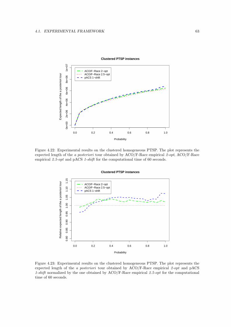
4.1. EXPERIMENTAL FRAMEWORK 63
0.0 0.2 0.4 0.6 0.8 1.0
0e+
002e
+06
4e+
066e
+06
8e+
061e
+07
Clustered PTSP instances
Probability
Exp
ecte
d le
ngth
of t
he a
pos
terio
ri to
ur
ACO/F−Race 2−optACO/F−Race 2.5−optpACS 1−shift
Figure 4.22: Experimental results on the clustered homogeneous PTSP. The plot represents theexpected length of the a posteriori tour obtained by ACO/F-Race empirical 2-opt, ACO/F-Raceempirical 2.5-opt and pACS 1-shift for the computational time of 60 seconds.
0.0 0.2 0.4 0.6 0.8 1.0
0.80
0.85
0.90
0.95
1.00
1.05
1.10
1.15
Clustered PTSP instances
Probability
Rel
ativ
e ex
pect
ed le
ngth
of t
he a
pos
terio
ri to
ur ACO/F−Race 2−optACO/F−Race 2.5−optpACS 1−shift
Figure 4.23: Experimental results on the clustered homogeneous PTSP. The plot represents theexpected length of the a posteriori tour obtained by ACO/F-Race empirical 2-opt and pACS1-shift normalized by the one obtained by ACO/F-Race empirical 2.5-opt for the computationaltime of 60 seconds.

64 CHAPTER 4. EXPERIMENTS AND RESULTS
0.0 0.2 0.4 0.6 0.8 1.0
0e+
002e
+06
4e+
066e
+06
8e+
061e
+07
Clustered PTSP instances
Probability
Exp
ecte
d le
ngth
of t
he a
pos
terio
ri to
ur
ACO/F−Race 2−optACO/F−Race 2.5−optpACS 1−shift
Figure 4.24: Experimental results on the clustered homogeneous PTSP. The plot represents theexpected length of the a posteriori tour obtained by ACO/F-Race empirical 2-opt, ACO/F-Raceempirical 2.5-opt and pACS 1-shift for the computational time of 120 seconds.
0.0 0.2 0.4 0.6 0.8 1.0
0.80
0.85
0.90
0.95
1.00
1.05
1.10
1.15
Clustered PTSP instances
Probability
Rel
ativ
e ex
pect
ed le
ngth
of t
he a
pos
terio
ri to
ur ACO/F−Race 2−optACO/F−Race 2.5−optpACS 1−shift
Figure 4.25: Experimental results on the clustered homogeneous PTSP. The plot represents theexpected length of the a posteriori tour obtained by ACO/F-Race empirical 2-opt and pACS1-shift normalized by the one obtained by ACO/F-Race empirical 2.5-opt for the computationaltime of 120 seconds.

4.1. EXPERIMENTAL FRAMEWORK 65
Table 4.12: The Wilcoxon paired test and p-values for the null hypothesis: The distributions of thesolutions are the same for clustered homogeneous PTSP for the computational time of 120 seconds.The significance level with which we reject the null hypothesis is 0.99. p-values smaller than 0.01are sufficient to reject the null hypothesis. The quantities under analysis are the expected lengthof the a posteriori tour obtained by ACO/F-Race empirical 2-opt, ACO/F-Race empirical 2.5-optand pACS 1-shift
Probability=0.25 ACO/F-Race 2.5-opt pACS 1-shift ACO/F-Race 2 optACO/F-Race 2.5-opt * < 2.2e − 16 < 2.2e − 16pacs 1-shiftt - * < 2.2e − 16
Probability=0.50 ACO/F-Race 2.5-opt pACS 1-shift ACO/F-Race 2 optACO/F-Race 2.5-opt * < 2.2e − 16 < 2.2e − 16pacs 1-shiftt - * < 2.2e − 16
Probability=0.25 ACO/F-Race 2.5-opt pACS 1-shift ACO/F-Race 2 optACO/F-Race 2.5-opt * < 2.2e − 16 < 2.2e − 16pacs 1-shiftt - * < 2.2e − 16
Probability=1.0 ACO/F-Race 2.5-opt pACS 1-shift ACO/F-Race 2 optACO/F-Race 2.5-opt * < 2.2e − 16 < 2.2e − 16pacs 1-shiftt - * < 2.2e − 16

66 CHAPTER 4. EXPERIMENTS AND RESULTS

Chapter 5
Conclusion and Future Work
This chapter presents the summary of the thesis with the contribution of the proposed approachfollowed by the conclusion of the thesis, suggestions for the improvement and future work.
Summary
In a large number of real-world combinatorial optimization problems, the objective function isaffected by uncertainty. In order to tackle these problems, it is customary to resort to a proba-bilistic model of the value of each feasible solution. In other words, a setting is considered in whichthe cost of each solution is a random variable, and the goal is to find the solution that minimizessome statistics of the latter. For a number of practical and theoretical reasons, it is customaryto optimize with respect to the expectation. For a given probabilistic model, the expectationcan always be computed but this typically involves particularly complex analytical manipulationsand computationally expensive procedures. Two alternatives have been discussed in the litera-ture: analytical approximation and empirical estimation. While the former explicitly relies onthe underlying probabilistic model for approximating the expectation, the latter estimates theexpectation through sampling or simulation. Computing a profitable approximation is a problemspecific issue and requires a deep understanding of the underlying probabilistic model. The mainadvantage of the estimation approach over the one based on approximation is generality: Indeed,a sample estimate of the expected cost of a given solution can be simply obtained by averaging anumber of realizations of the cost itself.
We adopted the probabilistic traveling salesman problem (PTSP) as a test-bed forstochastic optimization problems, in much the same way as the traveling salesman problem
(TSP) has been considered a standard amongst deterministic optimization problems.
Metaheuristics is a general algorithmic framework to solve different optimization problems.They compute fairly good solution in a reasonable amount of computational time. Ant colonyoptimization is a metaheuristic which takes inspiration from foraging behavior of ant colonies.
We have developed a computational technique called ACO/F-Race algorithm for tackling highlystochastic PTSP. The proposed approach is inspired by S-ACO [52] and F-Race [18, 17]. Theformer is an ACO algorithm based on simulation/sampling techniques to tackle the stochasticoptimization problems and the later is an algorithmic framework originally developed for tuningmetaheuristics. F-Race is itself inspired by a class of racing algorithms proposed in the machinelearning literature for tackling model selection problem. The peculiarity of the F-Race approachcompared to other racing algorithms is the adoption of the Friedman two-way analysis of varianceby ranks, a nonparametric statistical test that appears particularly suitable for the highly stochasticPTSP.
67
68 CHAPTER 5. CONCLUSION AND FUTURE WORK
In general, ACO algorithms frequently encounter a sequence of states in which it is impossibleto improve the solution quality by itself. Local search algorithms improve the solutions computedby ACO by introducing some modifications [92]. The state-of-the-art local search procedures forPTSP such as 1-shift and 2-p-opt local search are based on complex mathematical approxima-tions. We proposed empirical 2-opt and empirical 2.5-opt for PTSP inspired by 2-opt and 2.5-optlocal search algorithms which are explicitly designed to solve TSP. We derived computationallyinexpensive equations to compute the improvement in the objective function for the proposedimprovement techniques. As a consequence, the solution computed by ACO/F-Race algorithm issubjected to several refinements in a short computational time to obtain a high quality solution.
Conclusion
The experimental results proposed in the subsection 4.1.1 confirm the generality of the approachproposed in Gutjahr [52]. More precisely, from the computational experiments, we conclude thatit is important to use an ACO technique specifically developed for PTSP when the probabilityassociated with each city in the PTSP is significantly less than 1. This confirms the resultsestablished by Rossi and Gavioli [86] and Bertsimas and Howell [9]. In the experimental analysisproposed in the subsection 4.1.1, the goal was to compare the evaluation procedure based on F-Race with the one proposed in S-ACO [52] and with the trivial one based on a single sample ACO-1.For this reason, solution construction and pheromone update were implemented as described in[52]. As a consequence, ACO/F-Race exhibits inferior solution quality than the state-of-the-artpACS algorithm [13]. On the other hand, ACO/F-Race computes significantly better solutionsthan S-ACO by reaping the benefits of the nonparametric selection phenomenon of the F-Raceapproach. The general conclusions that we can draw from these results are:
• ACO/F-Race algorithm is extremely useful when the stochasticity associated with the PTSPis significantly large as suggested by Rossi and Gavioli [86].
• We propose to use ACO algorithms designed for TSP to solve PTSP when the stochasticityassociated with the problem is small. This is because the computational time is wasted bythe evaluation method adopted by ACO/F-Race (which results in inferior solution quality).
The experimental results on the proposed local search procedures such as empirical 2-opt andempirical 2.5-opt reveal that the solution computed by ACO/F-Race can be significantly improvedby coupling it with the empirical local search. The inexpensive computational time of the proposedimprovement procedures enables ACO/F-Race to have several refinements to produce significantlyhigh quality solutions. The results from the preliminary experiments with the state-of-the-art localsearch procedure indicate that the empirical estimation based evaluation method is more profitablethan mathematical approximation. Therefore, in the context of PTSP, we conclude the following:
• ACO/F-Race can be employed to identify good quality solutions in the search space. Theempirical local search techniques operate on these solutions to compute significantly betterquality solutions.
• Local search approach which uses empirical estimation can obtain better solutions thanmathematical approximation.
Finally, We conclude that the ACO/F-Race algorithm and the empirical estimation based localsearch can be profitably adopted for computing high quality solutions in the framework of appli-cations of ant colony optimization to combinatorial optimization problems under uncertainty.
Original Contributions
The original contributions of this DEA thesis are:

69
• We proposed the ACO/F-Race algorithm inspired by F-Race [18, 17] and S-ACO [52] asthe computational technique for computing quality solutions in the framework of ant colonyoptimization algorithms when applied to combinatorial optimization problems under un-certainty. More precisely, the novelty of the proposed technique lies in the nonparametricapproach for selecting the best-so-far ant, that is, the ant that is appointed for updatingthe pheromone matrix. In contrast, S-ACO employ the parametric procedure for the same.ACO/F-Race algorithm for optimization under uncertainty (Birattari et al. [19]) has beenpresented at the Sixth Metaheuristics International Conference 2005.
• pACS [13], the state-of-the-art ACO algorithm designed to solve the PTSP, is based onmathematical approximations whereas the proposed ACO/F-Race approach is based on em-pirical estimation. This thesis described an experimental evaluation method to analyze theempirical estimation against mathematical approximation techniques.
• Local search methods are used in general to improve the solution found by ACO algorithms.The state-of-the-art local search methods for the PTSP are based on mathematical approxi-mations and recursions [8, 12]. In this thesis, we proposed empirical 2-opt and 2.5-opt localsearch for the PTSP which is based on empirical estimation. This approach, to the best ofour knowledge, is the first local search technique that uses empirical estimation to computethe objective function. This thesis also proposed a comparative analysis of the estimationapproach against mathematical approximation.
Future work
Further research is needed for properly assessing the quality of ACO/F-Race. We plan to studythe behavior of ACO/F-Race on non-homogeneous problems. We intend to enrich the solutionconstruction phase of the ACO/F-Race by exploring other possibilities, such as construction andupdate as defined in MAX −MIN ant system [91].
In the context of local search techniques, we are currently developing empirical 3-opt for PTSPinspired by the 3-opt local search for TSP [92]. Preliminary experiments with this local searchtechnique indicate that significant improvements in the solution quality can be attained with theproposed approach.
We plan to design a unified framework which contains the ACO/F-Race algorithm enriched byempirical estimation based local search procedures such as empirical 2-opt, 2.5-opt and 3-opt localsearch procedures.
Applications to other problems, in particular of the vehicle routing class, will be considered,too.

70 CHAPTER 5. CONCLUSION AND FUTURE WORK

Bibliography
[1] E.H.L. Aarts, J.H.M. Korst, and P.J.M. vanLaarhoven. Simulated Annealing. In Local Searchin Combinatorial Optimization, pages 91–120. John Wiley & Sons, Chichester, UK, 1997.
[2] M.H. Alrefaei and S. Andradottir. A modification of the stochastic ruler method for discretestochastic optimization. European Journal of Operational Research, 133:160–182, 2001.
[3] R.C. Ball, T.M Fink, and N.E Bowler. Stochastic Annealing. Accepted in Physical Reviewletter and unpublished. Available from:http://arXiv.org/abs/cond-mat/0301179, 2002.
[4] J.J. Bartholdi and L.K. Platzman. An O(n log n) planar travelling salesman heuristic basedon spacefilling curves. Operations Research Letters, 1:121–125, 1982.
[5] J. L. Bentley. Fast algorithms for geometric traveling salesman problems. ORSA Journal onComputing, 4(4):387–411, 1992.
[6] O. Berman and D. Simchi-Levi. Finding optimal a priori tour and location of travelingsalesman with nonhomogenous customers. Trasnportation Science, 22:148–154, 1988.
[7] D. Bertsimas. A vehicle routing problem with stochastic demand. Operations Research, 40:574–585, 1992.
[8] D. Bertsimas. Probabilistic Combinatorial Optimization Problems. PhD thesis, MIT, Cam-bridge, MA, 1988.
[9] D. Bertsimas and L. Howell. Further results on the probabilitsic traveling salesman problem.European Journal of Operations Research, 65:68–95, 1993.
[10] D. Bertsimas, P. Jaillet, and A. Odoni. A priori optimization. Operations Research, 38:1019–1033, 1990.
[11] D. Bertsimas, P. Chervi, and M. Peterson. Computational approaches to stochastic routingproblems. Transportation Science, 29:342–352, 1995.
[12] L. Bianchi and A. Campbell. Extension of the 2-p-opt and 1-shift algorithms to the hetero-geneous probabilistic traveling salesman problem. Technical report, IDSIA, 2004.
[13] L. Bianchi, L. Gambardella, and M. Dorigo. Solving the homogeneous probabilistic travellingsalesman problem by the ACO metaheuristic. In G. Di Caro M. Dorigo and M. Sampels,editors, ANTS-III, volume 2463 of LNCS, pages 176–187, Berlin, Germany, 2002. Springer-Verlag.
[14] L. Bianchi, M. Birattari, M. Chiarandini, M. Manfrin, M. Mastrolilli, L. Paquete, O. Rossi-Doria, and T. Schiavinotto. Metaheuristics for the vehicle routing problem with stochasticdemands. In X. Yao, E. Burke, J. A. Lozano, J. Smith, J. J. Merelo-Guervos, J. A. Bullinaria,J. Rowe, P. Tino, A. Kaban, and H.-P. Schwefel, editors, Parallel Problem Solving fromNature, 8th International Conference, PPSN VIII, volume 3242 of LNCS, pages 450–460,Berlin, Germany, 2004. Springer-Verlag.
71

72 BIBLIOGRAPHY
[15] L. Bianchi, J. Knowles, and N. Bowler. Local search for the probabilistic traveling salesmanproblem: Correction to the 2-p-opt and 1-shift algorithms. European Journal of OperationalResearch, 162:206–219, 2005.
[16] P. Billingsley. Probability and Measure. John Wiley & Sons, New York, NY, USA, secondedition, 1986.
[17] M. Birattari. The Problem of Tuning Metaheuristics as Seen from a Machine Learning Per-spective. PhD thesis, Universite Libre de Bruxelles, Brussels, Belgium, 2004.
[18] M. Birattari, T. Stutzle, L. Paquete, and K. Varrentrapp. A racing algorithm for configuringmetaheuristics. In W. B. Langdon, E. Cantu-Paz, K. Mathias, R. Roy, D. Davis, R. Poli,K. Balakrishnan, V. Honavar, G. Rudolph, J. Wegener, L. Bull, M. A. Potter, A. C. Schultz,J. F. Miller, E. Burke, and N. Jonoska, editors, Proceedings of the Genetic and EvolutionaryComputation Conference, pages 11–18, San Francisco, CA, USA, 2002. Morgan Kaufmann.
[19] M. Birattari, P. Balaprakash, and M. Dorigo. ACO/F-Race: Ant colony optimization andracing techniques for combinatorial optimization under uncertainty. In R. F. Hartl, editor,MIC 2005: The 6th Metaheuristics International Conference, Vienna, Austria, 2005.
[20] C. Blum and A. Roli. Metaheuristics in combinatorial optimization: Overview and conceptualcomparison. ACM Computing Surveys, 35(3):268–308, 2003.
[21] A. M. Campbell. Aggregation for the probabilistic traveling salesman problem. Unpublished,Available from:http://www.myweb.uiowa.edu/acampbll/aggregation, 2004.
[22] D.J. Cavicchio. Adaptive search using simulated evolution. PhD thesis, University of Michigan,Ann Arbor, MI, 1970.
[23] V. Cerny. A thermodynamical approach to the traveling salesman problem: an efficientsimulation algorithm. Journal of Optimization Theory and Applications, 45(1):41–51, 1985.
[24] P. Chardaire, J.L. Lutton, and A. Sutter. Thermostatical persistency: a powerful improvingconcept for simulated annealing algorithms. European Journal of Operational Research, 86:565–579, 1995.
[25] S. Chien, J. Gratch, and M. Burl. On the efficient allocation of resources for hypothesisevaluation: A statistical approach. IEEE Transactions on Pattern Analysis and MachineIntelligence, 17(7):652–665, 1995.
[26] W. J. Conover. Practical Nonparametric Statistics. John Wiley & Sons, New York, NY, USA,third edition, 1999.
[27] T. Homem de Mello. Variable sample methods for stochastic optimization. ACM Trans. onModelling and Computer Simulation, 13:108–133, 2003.
[28] A. Dean and D. Voss. Design and Analysis of Experiments. Springer-Verlag, New York, NY,USA, 1999.
[29] K.A. DeJong. An Analysis of the Behavior of a Class of Genetic Adaptive Systems. PhDthesis, University of Michigan, Ann Arbor, MI, 1975.
[30] J.-L. Deneubourg, S. Aron, S. Goss, and J.-M. Pasteels. The self-organizing exploratorypattern of the argentine ant. Journal of Insect Behaviour, 3:159–168, 1990.
[31] M. Dorigo. Ottimizzazione, apprendimento automatico, ed algoritmi basati su metafora nat-urale. PhD thesis, Politecnico di Milano, Milan, Italy, 1992.

BIBLIOGRAPHY 73
[32] M. Dorigo and G. Di Caro. The Ant Colony Optimization meta-heuristic. In D. Corne,M. Dorigo, and F. Glover, editors, New Ideas in Optimization, pages 11–32. McGraw-Hill,London, UK, 1999.
[33] M. Dorigo and L.M. Gambardella. Ant Colony System: A cooperative learning approachto the travelling salesman problem. IEEE Transactions on Evolutionary Computation, 1(1):53–66, April 1997.
[34] M. Dorigo and T. Stutzle. Ant Colony Optimization. MIT Press, Cambridge, MA, 2004.
[35] M. Dorigo, V. Maniezzo, and A. Colorni. Ant System: Optimization by a colony of cooper-ating agents. IEEE Transactions on Systems, Man, and Cybernetics – Part B, 26(1):29–41,1996.
[36] M. Dorigo, E. Bonabeau, and G. Theraulaz. Ant algorithms and stigmergy. Future GenerationComputer Systems, 16(8):851–871, 2000.
[37] W. Feller. An introduction to Probability Theory and its Applications. John Wiley & Sons,New York, NY, 1968.
[38] J.M. Fitzpatrick and J.J. Grefenstette. Genetic algorithms in noisy environments. MachineLearning, 3:101–120, 1998.
[39] M. Fleischer. Simulated Annealing: past, present and future. In C. Alexopoulos, K. Kang,W. R. Lilegdon, and G. Goldsam, editors, Proceedings of the 1995 Winter Simulation Con-ference, pages 155–161, 1995.
[40] T. A. Foe and M.G.C. Resende. A probabilisitc heuristic for a computationally difficult setcovering problem. Operations Research Letters, 8:67–71, 1989.
[41] T. A. Foe and M.G.C. Resende. Greedy randomized adaptive search procedures. Jouranl ofGlobal Optimization, 6:109–133, 1995.
[42] L. J. Fogel, A. J. Owens, and M. J. Walsh. Artificial Intelligence through Simulated Evolution.John Wiley & Sons, New York, NY, 1966.
[43] L.J. Fogel. Toward inductive inference automata. In Proceedings of the International Feder-ation for Information Processing Congress, pages 395–399, Munich, Germany, 1962.
[44] M. Fu. Optimization for simulation: theory vs practice. INFORMS Journal on Computing,14:192–215, 2002.
[45] M.R. Garey and D.S. Johnson. Computers and Intractability. A guide to the Theory of NP-Completeness. W.H. Freeman and Company, New York, NY, USA, 1979.
[46] F. Glover. Heuristics for integer programming using surrogate constraints. Decision Sciences,8:156–166, 1977.
[47] F. Glover and M. Laguna. Tabu Search. Kluwer Academic Publishers, Norwell, MA, secondedition, 1997.
[48] D.E. Goldberg and J. Richardson. Genetic algorithms with sharing for multimodal functionoptimization. In J. J. Grefenstette, editor, Genetic Algorithms and their Applications, pages41–49. Lawrence Erlbaum Associates, Hillsdale, NJ, 1987.
[49] P. I. Good. Resampling Methods. Birkhauser, Boston, MA, USA, second edition, 2001.
[50] J. Gratch, S. Chien, and G. DeJong. Learning search control knowledge for deep space networkscheduling. In Proceedings of the Tenth International Conference on Machine Learning, pages135–142, San Francisco, CA, USA, 1993. Morgan Kaufmann.

74 BIBLIOGRAPHY
[51] W.J. Gutjahr. A converging ACO algorithm for stochastic combinatorial optimization. InA.Albrecht and K.steinhofl, editors, Stochastic Algorithms: Foundations and Applications,volume 2827, pages 10–25. SAGA 2003, LNCS, 2003.
[52] W.J. Gutjahr. S-ACO: An ant based approach to combinatorial optimization under uncer-tainity. In M. Dorigo, M. Birattari, C. Blum, L. M. Gambardella, F. Mondada, and T. Stutzle,editors, ANTS-IV, volume 3172 of LNCS, pages 238–249, Berlin, Germany, 2004. Springer-Verlag.
[53] W.J. Gutjahr and G. Pflug. Simulated Annealing for Noisy Cost Functions. Journal of GlobalOptimization, 8:1–13, 1996.
[54] P. Hansen and N. Mladenovic. An introduction to variable neighborhood search. In S. Voss,S. Martello, I. H. Osman, and C. Roucairol, editors, Meta-Heuristics: Advances and Trendsin Local Search Paradigms for Optimization, pages 433–458. Kluwer Academic Publisher,Boston, MA, USA, 1999.
[55] K. Helsgaum. An effective implementation of the lin-kernighan traveling salesman heuristic.European Journal of Operational Research, 126:106–130, 2000.
[56] A. Hertz and D. Kobler. A framework for the description of evolutionary algorithms. EuropeanJournal of Operational Research, 126:1–12, 2000.
[57] J.H. Holland. Adaptation in natural artificial systems. University of Michigan Press, AnnArbor, MI, 1975.
[58] S. Holm. A simple sequentially rejective multiple test procedure. Scandinavian Journal ofStatistics, 6:65–70, 1979.
[59] L. Ingber. Adaptive simulated annealing (asa): Lessons learned. Control and Cybernetics- Special Issue on Simulated Annealing Applied to Combinatorial Optimization, 25(1):33–54,1996.
[60] P. Jaillet. Probabilistic Traveling Salesman Problems. PhD thesis, MIT, Cambridge, MA,1985.
[61] P. Jaillet. A priori solution of a travelling salesman problem in which a random subset of thecustomers are visited. Operations Research, 36(6):929–936, 1988.
[62] P. Jaillet and A. Odoni. The probabilistic vehicle routing problems. In B. L. Golden and A. A.Assad, editors, Vehicle Routing: Methods and Studies. Elsevier, Amsterdam, The Nether-lands, 1988.
[63] D. S. Johnson and L. A. McGeoch. The travelling salesman problem: A case study in localoptimization. In E. H. L. Aarts and J. K. Lenstra, editors, Local Search in CombinatorialOptimization, pages 215–310. John Wiley & Sons, Chichester, United Kingdom, 1997.
[64] D. S. Johnson, L. A. McGeoch, C. Rego, and F. Glover. 8th DIMACS implementationchallenge, 2001.
[65] S. Kirkpatrick, C.D. Gelatt, and M.P. Vecchi. Optimization by simulated annealing. Science,220(4598):671–680, 1983.
[66] G. Laporte, F.V. Louveaux, and H. Mercure. A priori optimization of the probabilistictraveling salesman problem. Operations Research,, 42:543–549, 1994.
[67] H. Larson. Introduction to Probability Theory and Statistical Inference. John Wiley & Sons,New York, NY, USA, 1982.

BIBLIOGRAPHY 75
[68] S. Lin. Computer solution of the travelling salesman problem. Bell System Technical Journal,44:2245–2269, 1965.
[69] S.W. Mahfoud. Niching Methods for Genetic Algorithms. PhD thesis, University of Illinoisat Urbana-Champaign, Urbana, IL, 1995.
[70] O. Maron. Hoeffding races, model selection for mri classification. Master’s thesis, Dept. ofElectrical and Computer science, MIT, 1994.
[71] O. Maron and A.W. Moore. Hoeffding races: Accelerating model selection search for classi-fication and function approximation. In J. D. Cowan, G. Tesauro, and J. Alspector, editors,Advances in Neural Information Processing Systems, volume 6, pages 59–66, San Francisco,CA, USA, 1994. Morgan Kaufmann.
[72] N. Metropolis, A. Rosenbluth, M. Rosenbluth, A.Teller, and E.Teller. Equation of statecalculations by fast computing machines. Journal of Chemical Physics, 21:1087–1092, 1953.
[73] T. M. Mitchell. Machine Learning. McGraw-Hill, New York, NY, USA, 1997.
[74] A.W. Moore and M.S. Lee. Efficient algorithms for minimizing cross validation error. InProceedings of the Eleventh International Conference on Machine Learning, pages 190–198,San Francisco, CA, USA, 1994. Morgan Kaufmann.
[75] P. Moscatos. On evolution, search, optimization, genetic algorithms and martial arts: Towardsmemetic algorithms. Technical Report Caltech Concurrent Computation Program, Report.826, California Institute of Technology, Pasadena, CA, 1989.
[76] H. Muhlenbein and H.-M. Voigt. Gene pool recombination in genetic algorithms. In I. H.Osman and J. P. Kelly, editors, Proceedings of the Metaheuristics Conference, Norwell, MA,1995. Kluwer Academic Publishers.
[77] G.I. Nemhauser and A.L. Wolsey. Integer and Combinatorial Optimization. John Wiley &Sons, New York, NY, 1988.
[78] V. I. Norkin, Y. M. Ermoliev, and A. Ruszczynski. On optimal allocation of indivisibles underuncertainity. Operations Research, 46:381–395, 1998.
[79] I. Osman and G. Laporte. Metaheuristics: A Bibliography. Annals of Operations Research,63:513–623, 1996.
[80] C.H. Papadimitriou and K. Steiglitz. Combinatorial Optimization - Algorithms and Complex-ity. Dover Publications, Inc., New York, NY, 1982.
[81] J.F. Peckny and D.L. Miller. A staged primal-dual algorithm for finding a minimum costperfect two-matching in an undirected graph. ORSA Journal on Computing, 6:68–81, 1994.
[82] N.J. Radcliffe. Formal analysis and random respectful recombination. In Proceedings of theFourth International Conference on Genetic Algorithms, ICGA 1991, pages 222–229, SanMateo, CA, 1991. Morgan Kaufmann Publishers.
[83] I. Rechenberg. Evolution strategy: Optimization of technical systems by means of biologicalevolution. Fromman-Holzboog, Stuttgart, Germany, 1973.
[84] G. Reinelt. The Traveling Salesman: Computational Solutions for TSP Applications, volume840 of LNCS. Springer-Verlag, Berlin, Germany, 1994.
[85] H. Robbins and S. Munro. A stochastic approximation method. Annals of MathematicalStatistics, 22:400–407, 1951.
76 BIBLIOGRAPHY
[86] F. Rossi and I. Gavioli. Aspects of heuristic methods in the probabilisitc traveling salesmanproblem. In Advanced School on Stochastics in Combinatorial Optimization, pages 214–227.World Scientific, 1987.
[87] L. Shi and S. Olafsson. Nested partition method for global optimization. Operations Research,48:390–407, 2000.
[88] L. Shi and S. Olafsson. New parallel randomized algorithms for the traveling salesman prob-lem. Computers & Operations Research, 26:371–394, 1999.
[89] T. Stutzle. ACOTSP software package provides an implementation of various ant colonyoptimization (ACO) algorithms applied to the symmetric traveling salesman problem (TSP).the ACO algorithms implemented are ant system, elitist ant system, max-min ant system,rank-based version of ant system, best-worst ant system, and ant colony system., 2002.
[90] T. Stutzle. Local Search Algorithms for Combinatorial Problems - Analysis, Algorithms andNew Applications. PhD thesis, Technische Universitat Darmstadt, Darmstadt, Germany,1998. Published in 1999 - Infix, Sankt Augustin, Germany - volume 220 of DISKI.
[91] T. Stutzle and H. Hoos. MAX–MIN Ant System. Future Generation Computer System,16(8):889–914, 2000.
[92] T. Stutzle and H. Hoos. Stochastic Local Search: Foundations and Applications. MorganKaufmann, 2005.
[93] G. Syswerda. Simulated crossover in genetic algorithms. In Proceedings of the second work-shop on Foundations of Genetic Algorithms, pages 239–255, San Mateo, CA, 1993. MorganKaufmann Publishers.
[94] B. Verweij, S. Ahmed, A. J. Kleywegt, G. Nemhauser, and A. Shapiro. The sample aver-age approximation method applied to stochastic routing problems: A computational study.Computational Optimization and Applications, 24:289–333, 2002.
[95] S. Voss, S. Martello, I. Osman, and C. Roucairol. Meta-Heuristics - Advances and Trends inLocal Search Paradigms for Optimization. Kluwer Academic Publishers, Boston, MA, 1999.
[96] S.M Weiss and C. Kulikowski. Computer systems that learn Classification and predictionmethods from statistics neural nets machine learning and expert systems. Morgan Kaufmann,1991.
[97] D. Yan and H. Mukai. Stochastic discrete optimization. SIAM Journal on Control andOptimization, 30:594–612, 1992.