Embed Size (px)
Citation preview

UNIVERSITAT POLITÈCNICA DE CATALUNYA
PhD Thesis
Acoustic Event Detection and Classification
Author: Andriy Temko Advisor: Dr. Climent Nadeu
Thesis Committee: Chair: Dr. José B. Mariño, UPC Member: Dr. Javier Hernando, UPC Member: Dr. Dan Ellis, Columbia University Member: Dr. Xavier Serra, Universitat Pompeu Fabra Member: Dr. José C. Segura, Universidad de Granada
Speech Processing Group
Department of Signal Theory and Communications Universitat Politècnica de Catalunya
Barcelona, December 2007

ii

iii
Моїй сім'ї,

iv

Abstract
v
Abstract
The human activity that takes place in meeting-rooms or class-rooms is reflected in a rich variety of
acoustic events, either produced by the human body or by objects handled by humans, so the deter-
mination of both the identity of sounds and their position in time may help to detect and describe
that human activity. Additionally, detection of sounds other than speech may be useful to enhance
the robustness of speech technologies like automatic speech recognition.
Automatic detection and classification of acoustic events is the objective of this thesis work. It
aims at processing the acoustic signals collected by distant microphones in meeting-room or class-
room environments to convert them into symbolic descriptions corresponding to a listener's percep-
tion of the different sound events that are present in the signals and their sources.
First of all, the task of acoustic event classification is faced using Support Vector Machine
(SVM) classifiers, which are motivated by the scarcity of training data. A confusion-matrix-based
variable-feature-set clustering scheme is developed for the multiclass recognition problem, and
tested on the gathered database. With it, a higher classification rate than the GMM-based technique
is obtained, arriving to a large relative average error reduction with respect to the best result from
the conventional binary tree scheme. Moreover, several ways to extend SVMs to sequence process-
ing are compared, in an attempt to avoid the drawback of SVMs when dealing with audio data, i.e.
their restriction to work with fixed-length vectors, observing that the dynamic time warping kernels
work well for sounds that show a temporal structure. Furthermore, concepts and tools from the fuzzy
theory are used to investigate, first, the importance of and degree of interaction among features, and
second, ways to fuse the outputs of several classification systems. The developed AEC systems are
tested also by participating in several international evaluations from 2004 to 2006, and the results
are reported.
The second main contribution of this thesis work is the development of systems for detection of
acoustic events. The detection problem is more complex since it includes both classification and
determination of the time intervals where the sound takes place. Two system versions are developed
and tested on the datasets of the two CLEAR international evaluation campaigns in 2006 and 2007.
Two kinds of databases are used: two databases of isolated acoustic events, and a database of
interactive seminars containing a significant number of acoustic events of interest. Our developed
systems, which consist of SVM-based classification within a sliding window plus post-processing,
were the only submissions not using HMMs, and each of them obtained competitive results in the
corresponding evaluation.

vi
Speech activity detection was also pursued in this thesis since, in fact, it is a –especially impor-
tant – particular case of acoustic event detection. An enhanced SVM training approach for the
speech activity detection task is developed, mainly to cope with the problem of dataset reduction.
The resulting SVM-based system is tested with several NIST Rich Transcription (RT) evaluation
datasets, and it shows better scores than our GMM-based system, which ranked among the best
systems in the RT06 evaluation.
Finally, it is worth mentioning a few side outcomes from this thesis work. As it has been carried
out in the framework of the CHIL EU project, the author has been responsible for the organization
of the above mentioned international evaluations in acoustic event classification and detection,
taking a leading role in the specification of acoustic event classes, databases, and evaluation proto-
cols, and, especially, in the proposal and implementation of the various metrics that have been used.
Moreover, the detection systems have been implemented in the UPC’s smart-room and work in real
time for purposes of testing and demonstration.
Resum
vii
Resum
L’activitat humana que té lloc en sales de reunions o aules d’ensenyament es veu reflectida en una rica
varietat d’events acústics, ja siguin produïts pel cos humà o per objectes que les persones manegen. Per
això, la determinació de la identitat dels sons i de la seva posició temporal pot ajudar a detectar i a
descriure l’activitat humana que té lloc en la sala. A més a més, la detecció de sons diferents de la veu
pot ajudar a millorar la robustes de tecnologies de la parla com el reconeixement automàtica a
condicions de treball adverses.
L’objectiu d’aquesta tesi és la detecció i classificació automàtica d’events acústics. Es tracta de
processar els senyals acústics recollits per micròfons distants en sales de reunions o aules per tal de
convertir-los en descripcions simbòliques que es corresponguin amb la percepció que un oient tindria
dels diversos events sonors continguts en els senyals i de les seves fonts.
En primer lloc, s’encara la tasca de classificació automàtica d’events acústics amb classificadors
de màquines de vectors suport (Support Vector Machines (SVM)), elecció motivada per l’escassetat de
dades d’entrenament. Per al problema de reconeixement multiclasse es desenvolupa un esquema
d’agrupament automàtic amb conjunt de característiques variable i basat en matrius de confusió.
Realitzant proves amb la base de dades recollida, aquest classificador obté uns millors resultats que la
tècnica basada en models de barreges de Gaussianes (Gaussian Mixture Models (GMM)), i
aconsegueix una reducció relativa de l’error mitjà elevada en comparació amb el millor resultat
obtingut amb l’esquema convencional basat en arbre binari.
Continuant amb el problema de classificació, es comparen unes quantes maneres alternatives
d’estendre els SVM al processament de seqüències, en un intent d’evitar l’inconvenient de treballar
amb vectors de longitud fixa que presenten els SVM quan han de tractar dades d’àudio. En aquestes
proves s’observa que els nuclis de deformació temporal dinàmica funcionen bé amb sons que presenten
una estructura temporal. A més a més, s’usen conceptes i eines manllevats de la teoria de lògica difusa
per investigar, d’una banda, la importància de cada una de les característiques i el grau d’interacció
entre elles, i d’altra banda, tot cercant l’augment de la taxa de classificació, s’investiga la fusió de les
sortides de diversos sistemes de classificació. Els sistemes de classificació d’events acústics
desenvolupats s’han testejat també mitjançant la participació en unes quantes avaluacions d’àmbit
internacional, entre els anys 2004 i 2006.
La segona principal contribució d’aquest treball de tesi consisteix en el desenvolupament de
sistemes de detecció d’events acústics. El problema de la detecció és més complex, ja que inclou tant la
classificació dels sons com la determinació dels intervals temporals on tenen lloc. Es desenvolupen

viii
dues versions del sistema i es proven amb els conjunts de dades de les dues campanyes d’avaluació
internacional CLEAR que van tenir lloc els anys 2006 i 2007, fent-se servir dos tipus de bases de
dades: dues bases d’events acústics aïllats, i una base d’enregistraments de seminaris interactius, les
quals contenen un nombre relativament elevat d’ocurrències dels events acústics especificats. Els
sistemes desenvolupats, que consisteixen en l’ús de classificadors basats en SVM que operen dins
d’una finestra lliscant més un post-processament, van ser els únics presentats a les avaluacions
esmentades que no es basaven en models de Markov ocults (Hidden Markov Models) i cada un d’ells
va obtenir resultats competitius en la corresponent avaluació.
La detecció d’activitat oral és un altre dels objectius d’aquest treball de tesi, pel fet de ser un cas
particular de detecció d’events acústics especialment important. Es desenvolupa una tècnica de millora
de l’entrenament dels SVM per fer front a la necessitat de reducció de l’enorme conjunt de dades
existents. El sistema resultant, basat en SVM, és testejat amb uns quants conjunts de dades de
l’avaluació NIST RT (Rich Transcription), on mostra puntuacions millors que les del sistema basat en
GMM, malgrat que aquest darrer va quedar entre els primers en l’avaluació NIST RT de 2006.
Per acabar, val la pena esmentar alguns resultats col·laterals d’aquest treball de tesi. Com que s’ha
dut a terme en l’entorn del projecte europeu CHIL, l’autor ha estat responsable de l’organització de les
avaluacions internacionals de classificació i detecció d’events acústics abans esmentades, liderant
l’especificació de les classes d’events, les bases de dades, els protocols d’avaluació i, especialment,
proposant i implementant les diverses mètriques utilitzades. A més a més, els sistemes de detecció
s’han implementat en la sala intel·ligent de la UPC, on funcionen en temps real a efectes de test i
demostració.
Thanks to…
ix
Thanks to…
Щиро дякую (ukr)…
…first and foremost, Climent Nadeu, my advisor, whose extremely experienced and very kind way
to provide guidance has been converting any research work into pleasure during the period of my PhD
studying. His ongoing encouragements in my work have strongly motivated me. I want to thank him
very much also for helping me in improving my writing skills. I feel very fortunate and grateful to have
Climent as a mentor and a friend.
…Enric Monte, whose contribution to my formation can not be overestimated. His intuitive man-
ner to explain things has not only made me refresh my skills in philosophy but also helped me find
answers to many questions especially in the beginning when it was most important.
…Dušan Macho for his support and advices during the years of my PhD studying. He was the only
Slavic soul in the group when I arrived. For many people in the group he served as an example of a
researcher to follow; and I’m not an exception.
…signal processing group for the created fruitful atmosphere where I grew up as a researcher. I
appreciate the help of, and interactions with, many past and present group members, including (but not
exclusively) Javier Hernando, Antonio Bonafonte, Jan Anguita, Marta Casar, Frank Diehl, Adrià de
Gispert, Javier Pérez, Xavi Anguera. Special thanks go to the “habitants” of 120: Jaume Padrell, Pere
Pujol, Alberto Abad, Jordi Adell, Jordi Luque, Pablo Daniel Agüero, Helenca Duxans, Xavi Giró,
Christian Canton, Enric Calvo.
…Alex Waibel who was the originator and leader of the CHIL project in which I was lucky to par-
ticipate. I would like to thank Rainer Stiefelhagen who was the general coordinator of the CHIL project
and the coordinator of the evaluations on behalf of the CHIL project. In the very beginning of the
project I had to believe that the area of AED would be accepted in research community. Among others,
I’m especially grateful to Maurizio Omologo for his interest and support of the task. I also want to
thank Gerasimos Potamianos who was responsible for the work-package where AED belonged to.
Special thanks go to Josep Casas who was coordinating the CHIL project here at the UPC. His brilliant
organization abilities made possible a successful contribution of our research groups to the CHIL
project, something that is enforced by the fact that the UPC was one of the main partners in the project.
I wish to thank Joachim Neumann for his help to integrate the AED technology into real life services in
the UPC smart-room. Also, ELDA must be acknowledged for transcribing acoustic events and for
assisting in the selection of evaluation data; in particular, Djamel Mostefa and Nicolas Moreau are
thanked. Finally, I would like to express my gratitude to the CHIL partners that provided the evaluation

x
seminar databases and also to all the participants in the evaluations for their interest and their contribu-
tions. I’m especially grateful to Rob Malkin and Christian Zieger for valuable research collaboration.
... Joan Isaac Biel and Carlos Segura for their help in making a demo of the developed AED tech-
nology. Without the work of Joan Isaac the demo would not be possible. I was pleased to be
collaborating with him. I wish to thank again Carlos Segura who helped a lot to develop the UPC
isolated acoustic event database.
…SAMOVA group of IRIT centre for their kind hospitality during my stay in Toulouse. I’m grate-
ful to Khalid Daoudi for the interesting meetings and fruitful discussions. I would like to thank also
Eduardo Sánchez-Soto for his help.
…José Mariño Acebal for his call for a PhD student that finally resulted in four wonderful years
past in Barcelona.
…finally and above all, my lovely parents, my brother Yevgenij, my friends Zurab and Fakhri, and
my girlfriend Anya, whose continuous support and great interest let me feel at home being far away
from it.

Contents
xi
Contents CHAPTER 1. INTRODUCTION 1
1.1 THESIS OVERVIEW AND MOTIVATION 1 1.2 THESIS OBJECTIVES 2 1.3 THESIS OUTLINE 4
CHAPTER 2. STATE OF THE ART 5 2.1 CHAPTER OVERVIEW 5 2.2 SOUNDS TAXONOMY 6 2.3 APPLICATIONS OF AUDIO RECOGNITION 9
2.3.1 Audio indexing and retrieval 9 2.3.2 Audio recognition for a given environment 10 2.3.3 Recognition of generic sounds 12 2.3.4 Classification of acoustic environments 14
2.4 TYPES OF FEATURES 15 2.5 AUDIO CLASSIFICATION ALGORITHMS 17 2.6 AUDIO DETECTION ALGORITHMS 18
2.6.1 Detection-by-classification 18 2.6.2 Detection-and-classification 19
2.7 CHAPTER SUMMARY 21 CHAPTER 3. BASIC CLASSIFICATION TECHNIQUES 23
3.1 CHAPTER OVERVIEW 23 3.2 SUPPORT VECTOR MACHINES 24
3.2.1 Introduction 24 3.2.2 Construction of SVM 24 3.2.3 Generalization error and SVM 29 3.2.4 Summary on SVM 32
3.3 GAUSSIAN MIXTURE MODELS 34 3.4 FUZZY INTEGRAL AND FUZZY MEASURE 35 3.5 CHAPTER SUMMARY 39
CHAPTER 4. ACOUSTIC EVENTS CLASSIFICATION 41 4.1 CHAPTER OVERVIEW 41 4.2 AUDIO FEATURES 42 4.3 CLASSIFICATION OF ACOUSTIC EVENTS USING SVM-BASED CLUSTERING SCHEMES 45
4.3.1 Introduction 45 4.3.2 Database 46 4.3.3 Features extraction 47 4.3.4 Classification techniques 48 4.3.5 Experiments 49 4.3.6 Conclusion 60
4.4 COMPARISON OF SEQUENCE DISCRIMINANT SUPPORT VECTOR MACHINES FOR ACOUSTIC EVENT CLASSIFICATION 61
4.4.1 Introduction 61 4.4.2 SVM-based sequence discriminant techniques 62 4.4.3 Experiments and discussion 64

xii
4.4.4 Conclusions 68 4.5 FUZZY INTEGRAL BASED INFORMATION FUSION FOR CLASSIFICATION OF HIGHLY CONFUSABLE NON-SPEECH SOUNDS 69
4.5.1 Introduction 69 4.5.2 Fuzzy measure learning 70 4.5.3 Feature extraction 71 4.5.4 Experiments and discussion 72 4.5.5 Conclusion 80
4.6 CHAPTER SUMMARY 81 CHAPTER 5. ACOUSTIC EVENT DETECTION 83
5.1 CHAPTER OVERVIEW 83 5.2 ACOUSTIC EVENT DETECTION SYSTEMS 84
5.2.1 Acoustic event detection and acoustic event classification systems 2006 84 5.2.2 Acoustic event detection system 2007 85
5.3 CHAPTER SUMMARY 90 CHAPTER 6. PARTICIPATION IN INTERNATIONAL EVALUATIONS 91
6.1 CHAPTER OVERVIEW 91 6.2 CHIL DRY-RUN EVALUATIONS 2004 92
6.2.1 Introduction 92 6.2.2 Database & evaluation setup 92 6.2.3 Developed systems 94 6.2.4 Results and discussion 94 6.2.5 Conclusions 96
6.3 CHIL EVALUATIONS 2005 97 6.3.1 Introduction 97 6.3.2 Database & evaluation setup 97 6.3.3 Developed systems 100 6.3.4 Results and discussion 100 6.3.5 Conclusions 101
6.4 CLASSIFICATION OF EVENTS, ACTIVITIES AND RELATIONSHIPS – CLEAR'06 EVALUATION AND WORKSHOP 102
6.4.1 Introduction 102 6.4.2 Evaluation setup 103 6.4.3 Acoustic event detection and classification systems 107 6.4.4 Results and discussion 107 6.4.5 Conclusions 108
6.5 CLASSIFICATION OF EVENTS, ACTIVITIES AND RELATIONSHIPS – CLEAR'07 EVALUATION AND WORKSHOP 109
6.5.1 Introduction 109 6.5.2 Evaluation setup 109 6.5.3 Acoustic event detection system 113 6.5.4 Results and discussion 113 6.5.5 Conclusions 114
6.6 CHAPTER SUMMARY 115 CHAPTER 7. SPEECH ACTIVITY DETECTION 117
7.1 CHAPTER OVERVIEW 117

Contents
xiii
7.2 ENHANCED SVM TRAINING FOR ROBUST SPEECH ACTIVITY DETECTION 118 7.2.1 Introduction 118 7.2.2 Databases 119 7.2.3 Features 120 7.2.4 Metrics 120 7.2.5 SVM-based speech activity detector 121 7.2.6 Experiments 123 7.2.7 Conclusions 126
7.3 SAD EVALUATION IN NIST RICH TRANSCRIPTION EVALUATIONS 2006 -2007 127 7.3.1 Introduction 127 7.3.2 SAD systems overview and results on referenced datasets 127 7.3.3 Conclusions 128
7.4 CHAPTER SUMMARY 129 CHAPTER 8. UPC’S SMART-ROOM ACTIVITIES 131
8.1 CHAPTER OVERVIEW 131 8.2 CHIL PROJECT 132 8.3 UPC’S SMART-ROOM 134 8.4 RECORDINGS OF THE DATABASES IN THE SMART-ROOM 136 8.5 ACOUSTIC EVENT DETECTION COMPONENT IMPLEMENTATION 137 8.6 ACOUSTIC EVENT DETECTION DEMONSTRATIONS 139
8.6.1 Acoustic event detection and acoustic source localization demo 139 8.6.2 Acoustic event detection in CHIL mockup demo 141 8.6.3 Acoustic event detection and 3D virtual smart-room demo 143
8.7 CHAPTER SUMMARY 145 CHAPTER 9. CONCLUSIONS AND FUTURE WORK 147
9.1 SUMMARY OF CONCLUSIONS 147 9.2 FUTURE WORK 151
9.2.1 Feature extraction and selection 151 9.2.2 Sequence-discriminative SVM 151 9.2.3 Acoustic event detection in real environments 152 9.2.4 Fuzzy integral fusion for multi-microphone AED 153 9.2.5 Acoustic source localization for AED 153 9.2.6 Speech activity detection 153
APPENDIX A. UPC-TALP DATABASE OF ISOLATED MEETING-ROOM ACOUSTIC EVENTS 155 APPENDIX B. GUIDELINES FOR HAVING ACOUSTIC EVENTS WITHIN THE 2006 CHIL INTERACTIVE MEETING RECORDINGS 161 OWN PUBLICATIONS 165 BIBLIOGRAPHY 167

xiv
List of Acronyms
AE(s) Acoustic Event(s) AEC Acoustic Event Classification AED Acoustic Event Detection ANN(s) Artificial Neural Network(s) ASL Acoustic Source Localization ASR Automatic Speech Recognition CASA Computational Auditory Scene Analysis BIC Bayesian Information Criteria CHIL Computer in the Human Interaction Loop CLEAR Classification of Event, Activities, and Relationships CV Cross Validation DAG Directed Acyclic Graphs DFT Discrete Fourier Transform DP Decision Profile DT(s) Decision Tree(s) DTW Dynamic Time Warping EM Expectation-Maximization ERM Empirical Risk Minimization FBE Filter Bank Energies FF(BE) Frequency Filtered (Band Energies) FFT Fast Fourier Transform FI Fuzzy Integral FM(s) Fuzzy Measure(s) GMM(s) Gaussian Mixture Model(s) GUI Graphic User Interface HMM(s) Hidden Markov Model(s) ICA Independent Component Analysis LDA Linear Discriminant Analysis LPC Linear Prediction Coefficients MFCC Mel-Frequency Cepstral Coefficients NIST National Institute of Standards and Technology PCA Principal Component Analysis PSVM Proximal Support Vector Machines RBF Radial Basis Function RT Rich Transcription SAD Speech Activity Detection SNR Signal-to-Noise Ratio SRM Structural Risk Minimization SV(s) Support Vector(s) SVM(s) Support Vector Machine(s) VC Vapnik-Chervonenkis dimension VQ Vector Quantization WAM Weighted Arithmetical Mean

List of Figures
xv
List of Figures
Figure 2.2.1. Sound taxonomy proposed in [Ger03b]..........................................................................7
Figure 2.2.2. Sound taxonomy proposed in [Cas02]............................................................................8
Figure 2.2.3. CHIL acoustic sound taxonomy ......................................................................................8
Figure 2.2.4. CHIL meeting-room semantic sound taxonomy..............................................................8
Figure 2.6.1. Detection-by-classification ...........................................................................................18
Figure 3.2.1. Two-class linear classification. The support vectors are indicated with crosses.........25
Figure 3.2.2. Four points in two dimensions shattered by axis-aligned rectangles...........................30
Figure 3.2.3. Graphical depiction of the SRM principle. A set of functions f are decomposed into a
nested sequence of subsets S of increasing size and capacity. ......................................32
Figure 3.4.1. Lattice representation of fuzzy measure for 4 information sources..............................37
Figure 4.3.1. Binary tree structure for eight classes. Every test pattern enters each binary
classifier, and the chosen class is tested in an upper level until the top of the tree is
reached. The numbers 1–8 encode the classes. The figure shows a particular
example, where class 1 is the class chosen by the classification scheme. .....................50
Figure 4.3.2. Percentage of classification rate for the SVM-based binary tree classifier and the
GMM classifier on the defined feature sets. ..................................................................50
Figure 4.3.3. Dependence of performance of classifying “liquid_pouring”, “sneeze” and “sniff”
upon the feature sets using SVMs. .................................................................................51
Figure 4.3.4. Clustering algorithm based on an exhaustive search and using a set of estimated
confusion matrices. ........................................................................................................52
Figure 4.3.5. Normal and restricted clustering schemes for SVM classifiers ....................................56
Figure 4.3.6. Distribution of the errors along the tree path for SVM-N, GMM-N, SVM-R and
GMM-R. A darker cell means a larger error.................................................................57
Figure 4.3.7. Restricted clustering tree based on SVM. The numbers in the nodes are the ordinal
numbers of the 15 SVM classifiers, and the bold numbers between each pair of
clusters denote the best separating feature sets.............................................................60
Figure 4.4.1. Classification accuracy for the 8 techniques ................................................................65
Figure 4.4.2. Dependence of the performance of the Fisher score kernel, likelihood ratio kernel
and GMM on the number of Gaussians (log2Ng)..........................................................66
Figure 4.4.3. Comparison results for the classes “music” (7) and “sneeze” (13) ............................68
Figure 4.4.4. Comparison results for the classes “pen writing” (10) and “liquid pouring” (11).....68

xvi
Figure 4.5.1. Fusion at the feature level (a) and at the decision level (b)..........................................69
Figure 4.5.2. Sample spectrograms of acoustic events from ..............................................................73
Figure 4.5.3. Recall measure for the 10 SVM systems running on each feature type, the
combination of the 10 features at the feature-level with SVM, and the fusion on the
decision-level with WAM and FI operators. ..................................................................76
Figure 4.5.4. Importance of features extracted from FM. Dashed line shows the average
importance level. ............................................................................................................77
Figure 4.5.5. Interaction of features extracted from FM....................................................................77
Figure 5.2.1. UPC acoustic event detection system 2006...................................................................85
Figure 5.2.2. The block-scheme of the developed AED system 2007 .................................................86
Figure 5.2.3. Frame log-energy histograms calculated over the whole seminar signal ....................87
Figure 5.2.4. One microphone AED system........................................................................................88
Figure 5.2.5. The choice of the microphones for the UPC’s smart-room ..........................................89
Figure 6.4.1. From reference transcription with overlapping of level 2 to reference single-level
transcription.................................................................................................................106
Figure 7.2.1. Geometrical interpretation of PSVM ..........................................................................122
Figure 8.5.1. SmartAudio map that corresponds to the AED system ...............................................138
Figure 8.6.1. The developed GUI for demonstration of AED and ASL functionalities (“laugh” is
being produced) ...........................................................................................................140
Figure 8.6.2. The two screens of the GUI: real-time video (a) and the graphical representation of
the AED and ASL functionality (“keyboard typing” is being produced) ....................140
Figure 8.6.3. The Talking Head is a mean of demonstrating the context awareness given by
perceptual components ................................................................................................142
Figure 8.6.4. Screenshot of the Field Journalist’s laptop ................................................................143
Figure 8.6.5. A snapshot that shows the built virtual UPC’s smart-room .......................................144
Figure A. 1. Microphone and camera positioning in the UPC’s smart-room..................................156
Figure A. 2. Configuration & orientation of the T-shaped microphone clusters .............................156
Figure A. 3. Graphical illustration of participants’ positions..........................................................157
Figure A.4. Selected channels of Mark III array, distance between them and symbolic grouping
into clusters ..................................................................................................................159

List of Tables
xvii
List of Tables
Table 4.3.1. The sixteen acoustical events considered in our database, including number of
samples and their sources (I means Internet) ................................................................46
Table 4.3.2. Feature sets that were used in this work, the way they were constructed from the
basic acoustic features, and their size. d and dd denote first and second time
derivatives, respectively, E means frame energy, and “+” means concatenation of
features...........................................................................................................................48
Table 4.3.3. Performances of variable-feature-set and fixed-feature-set classifiers using different
adaptations of the regularization parameters for the SVM classifiers. -N and -R,
denote normal and restricted clustering scheme, respectively. Standard deviations
estimated over 20 repetitions are denoted with ± σ.......................................................56
Table 4.3.4. Confusion measure Sn (multiplied by 100), best separating feature set, and
percentage distribution of the classification error (for the best results in Table 4.3.3)
along the 15 nodes (depicted in Figure 4.3.5 for SVM) for both normal and restricted
clustering, and for the variable-features-set SVM classifier and the GMM classifier. .57
Table 4.3.5. Confusion matrix corresponding to the best results (88.29 %) ......................................59
Table 4.5.1. Sound classes and number of samples per class ............................................................72
Table 4.5.2. FI result for individual, semi-shared and shared fuzzy measure....................................74
Table 4.5.3. Comparison of individual recall scores for each class...................................................76
Table 4.5.4. Classification results using feature selection based on FM ...........................................78
Table 4.5.5. Individual performance of SVM, HMM on FFBE with and without time derivatives,
and FI fusion..................................................................................................................79
Table 6.2.1. Evaluated acoustic event classes ....................................................................................93
Table 6.2.2. Results of the dry-run evaluations on AEC.....................................................................95
Table 6.3.1. Annotated semantic classes ............................................................................................98
Table 6.3.2. Evaluated acoustic classes .............................................................................................99
Table 6.3.3. Semantic acoustic mapping ............................................................................................99
Table 6.3.4. Results of the AEC evaluations 2005............................................................................100
Table 6.4.1. Number of events for the UPC and ITC databases of isolated acoustic events, and the
UPC interactive seminar .............................................................................................104
Table 6.4.2. Obtained single-level reference transcription and a list of events to detect ................106
Table 6.4.3. Error rate (in %) for acoustic event classification and detection tasks .......................108
xviii
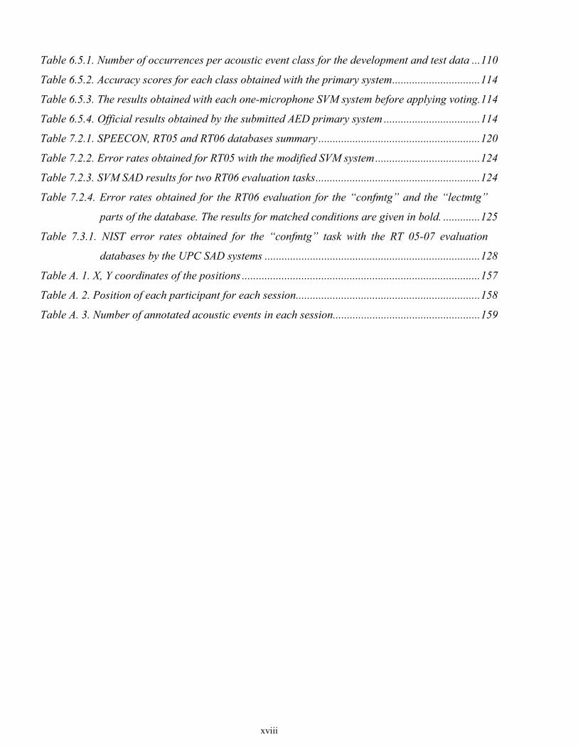
Table 6.5.1. Number of occurrences per acoustic event class for the development and test data ...110
Table 6.5.2. Accuracy scores for each class obtained with the primary system...............................114
Table 6.5.3. The results obtained with each one-microphone SVM system before applying voting.114
Table 6.5.4. Official results obtained by the submitted AED primary system ..................................114
Table 7.2.1. SPEECON, RT05 and RT06 databases summary.........................................................120
Table 7.2.2. Error rates obtained for RT05 with the modified SVM system.....................................124
Table 7.2.3. SVM SAD results for two RT06 evaluation tasks..........................................................124
Table 7.2.4. Error rates obtained for the RT06 evaluation for the “confmtg” and the “lectmtg”
parts of the database. The results for matched conditions are given in bold. .............125
Table 7.3.1. NIST error rates obtained for the “confmtg” task with the RT 05-07 evaluation
databases by the UPC SAD systems ............................................................................128
Table A. 1. X, Y coordinates of the positions ....................................................................................157
Table A. 2. Position of each participant for each session.................................................................158
Table A. 3. Number of annotated acoustic events in each session....................................................159

Chapter 1. Introduction
1
Chapter 1. Introduction
1.1 Thesis Overview and Motivation
Activity detection and description is a key functionality of perceptually aware interfaces working in
collaborative human communication environments like meeting-rooms or classrooms. In the context of
person-machine communication, computers involved in human communication activities have to be
designed to have minimal possible awareness from the users. Consequently, there is a need of percep-
tual user interfaces which, besides being multimodal and robust, use unobtrusive sensors. One example
of new challenging multimodal research efforts is the development of smart-rooms. A smart-room is a
closed space equipped with multiple microphones and cameras, and several functionalities, which are
designed to assist and complement human activities. In the case of the audio processing, some of the
technologies that may be involved are speech activity detection, automatic speech recognition, speaker
identification and verification, and speaker localization.
Indeed, speech usually is the most informative acoustic event, but other kind of sounds may also
carry useful information. Since in such types of environments the human activity is reflected in a rich
variety of acoustic events, either produced by the human body or by objects handled by humans,
detection and classification of acoustic events may help to detect and describe human activity. For
example: clapping or laughing inside a speech, a strong yawn in the middle of a lecture, a chair moving
or door slam when the meeting has just started. Additionally, the robustness of automatic speech
recognition systems may be increased if such non-speech acoustic events are previously detected and
identified.
The main goal of this thesis work is detection and classification of meeting-room acoustic events,
namely Acoustic Event Detection/Classification (AED/C). AED/C is a recent discipline belonging to
the area of computational auditory scene analysis [WB06] that consists of processing acoustic signals
and converting them into symbolic descriptions corresponding to a listener's perception of the different
sound events that are present in the signals and their sources.

1.2. Thesis Objectives
2
1.2 Thesis Objectives
The primary objective of this PhD thesis is the development of systems for acoustic event detection
and classification. As required in any pattern recognition task, the thesis work focuses on algorithms
for both feature extraction and classification. The developed systems are tested through the partici-
pation in international evaluations in the framework of the project Computers in the Human
Interaction Loop (CHIL). A secondary objective of the thesis is to design and implement a system of
acoustic event detection that provides in real time semantic content to specific services defined in
CHIL.
Investigation of different types of features is an important point of any classification system.
The relevance of conventional sets of features that are widely used in speech processing applications
will be addressed. Several basic feature sets will be compared and investigated to find the most
appropriate set of features. Apart from the features used in speech processing, there exist a number
of features that have a more perceptually-oriented profile. The usefulness of the perceptual features
will be investigated in terms of individual feature importance and degree of interaction.
A large part of the work has to be concerned with the problem of acoustic event classification
(AEC), since detection also requires classification. Due to the problem of scarcity of data in the
available corpus, the development of classification algorithms that can tackle this problem is crucial
and necessary. Recently, the Support Vector Machine (SVM) paradigm has proved highly success-
ful in a number of classification tasks. As a classifier that discriminates the data by creating
boundaries between classes rather than estimating class conditional densities, it may need consid-
erably less data to perform accurate classification. For this reason the SVM classifier is initially
chosen in this thesis as the main classification technique, and it is compared to Gaussian mixture
models in a series of tests. As the developed algorithm may benefit from using the temporal evolu-
tion of the acoustic events, several techniques for sequential processing will be compared. The thesis
will also explore the combination of several information sources in order to capture the interdepend-
encies among them.
Applications in real meeting-room environments require facing the acoustic event detection
(AED) problem. For that purpose, it is necessary to produce a database with a sufficient number of
acoustic events of interest. The database can be used as a training material and as a testing material
to evaluate the algorithm performance for AED. Besides, participation in the international evaluation
campaigns is a good way for evaluating and comparing the various approaches submitted by the
participants. Indeed, those evaluations have to be organized and coordinated, and appropriate

Chapter 1. Introduction
3
metrics and evaluation tools for AED have to be developed. Moreover, the AED systems will be
implemented in the UPC’s smart-room and work in real time for purposes of testing and demonstra-
tion.

1.3. Thesis Outline
4
1.3 Thesis Outline
The thesis is organized as follows. Chapter 2 presents state of the art in the area of general audio
recognition, discussing the schemes for sound organization, presenting a literature review from the
application point of view, and reporting the features, classification and detection techniques that
have been used so far for acoustic event detection and classification.
Chapter 3 reports the work done in the area of acoustic event classification and presents the a
novel SVM-based classification technique. Moreover, several advanced classification techniques are
compared in that chapter including those SVM-based techniques which can model the time dynam-
ics of sounds. Importance and interaction of various perceptual features are investigated in the
framework of fusion several information sources using fuzzy theory and concepts.
Chapter 5 describes a few new systems for acoustic event detection developed in this thesis. Re-
sults, obtained with the above-mentioned systems of AEC and AED in several international
evaluations, are reported in Chapter 6.
Chapter 7 considers the particular problem of speech activity detection and the way SVM clas-
sifier is applied to this problem. Results obtained with the international evaluation datasets are
reported and compared with the previously developed detectors.
The activities on AED, which were carried out in the UPC’s smart-room, are described in Chap-
ter 8: database recordings, implementation of the AED system in real time, development of demos.
Chapter 9 concludes the work. The main achievements are summarised in this chapter. Several
promising future directions are highlighted.

Chapter 2. State of the Art
5
Chapter 2. State of the Art
2.1 Chapter Overview
In this chapter the current state of the art in the area of Acoustic Event Detection and Classification
(AED/C) is presented.
The remaining sections of this chapter are organized as follows. In Section 2.2 the schemes for
sound organization are discussed. Section 2.3 presents a literature review from the application point of
view, while Sections 2.4, 2.5, and 2.6 discuss features, classification and detection techniques that have
been used so far for AED/C.

2.2. Sounds Taxonomy
6
2.2 Sounds Taxonomy
The research on sound classification has usually been carried out so far for a limited number of
classes, like speech/music [PRO02] [MP04] [And04], music/song [Ger03a], or music/speech/other,
where “other” is any kind of environmental sounds [LZJ02]. In the last years, however, the interest
in AED/C has been significantly increased. The area of AED/C can be structured by different
semantic levels. It can be the classification of events specific to a certain environment, classification
of sounds specific to a given activity, generic sound classification, etc. In all the cases, there exist a
large number of sounds and it is necessary to limit the number of classes considered. That is the
reason why authors usually try to provide a sound taxonomy. The development of the sound taxon-
omy helps to better understand the data domain [Ger03b], and increase the accuracy and speed of
classification [Cow04]. One example of a general sound taxonomy has been first presented in
[Ger03b] and can be seen in Figure 2.2.1. It divides sounds firstly into hearable and non-hearable.
Then the hearable part is further divided into noise, natural sound, artificial sounds, speech and
music. An example of a standard taxonomy suitable for text-based query applications, such as
WWW search engines, or any processing tool that uses text fields, was used in [Cas02] and it is
presented in Figure 2.2.2. It is less general than the previous one as it is fitted to a given task. A
sound taxonomy scheme for environmental sound classification can be found in [Cow04]. Because
of the uncountable number of classes for a general environment, the author has proposed the taxon-
omy based on the physical states of sounding objects (solid, liquid, gas) and the possible interaction
of objects (solid-solid, solid-liquid, etc). A scheme proposed in [AN00] has been based on the nature
of sound sources. Firstly, the sources are divided into continuous and changing. Semantic classes
appear at the next level.
Clearly, the conception of sound taxonomy is subjective and it strongly depends on the chosen
classification domain. In the framework of the CHIL project [CHI] it has been decided that for the
chosen meeting-room environment it is reasonable to have an acoustic sound taxonomy for general
sound description and a semantic sound taxonomy for a specific task. The proposed acoustic scheme
is shown in Figure 2.2.3. Actually, almost any type of sounds can be referred to one of the proposed
groups according to its acoustical property. On the contrary, the semantic scheme that is presented in
Figure 2.2.4 is very specific to the CHIL meeting-room scenario. Additionally, with two sound
taxonomies (acoustic and semantic) it is possible to cope with situations when the produced event
does not match any semantic label but can be identified acoustically.

Chapter 2. State of the Art
7
Figure 2.2.1. Sound taxonomy proposed in [Ger03b]
Music Type Culture Genre
Composer Performer
Content Chord pattern
Melody Notes
Music
Sounds
Hearable Sounds
Non Hearable Soundss
Natural Sounds
Artificial Sounds
Speech Noise
Colour White Pink Brown …
Perceptual Features
Objects Animals Vegetables Minerals Atmosphere …
Interactions
Source
Objects Vehicles Buildings Tools … Interactions
Intent
Language
Speaker Speaker
Emotion
Content Sentences
Number of instruments
Instrument Family Type
Individual

2.2. Sounds Taxonomy
8
Figure 2.2.2. Sound taxonomy proposed in [Cas02]
Figure 2.2.3. CHIL acoustic sound taxonomy
Figure 2.2.4. CHIL meeting-room semantic sound taxonomy
Continuous tone Continuous non-tone
Non-repetitive non-continuous
Regular repetitive non-continuous
Sound
Irregular repetitive non-continuous
Other
Breathes Laughter Throat/cough Disagreement Whisper Mouth (generic) …
Human vocal tract non-speech noises
Clapping Beep Chair moving Door slams Footsteps Key jingling Music (radio, handy) …
Non-speech environ-ment noises
Sound
Speech noises
Repetitions Corrections False starts Mispronunciation …
General Taxonomy Speech Male
Female
Impacts Glass smash
GunShots Explosions Foley Music
Animals
Strings
WoodWinds
Brass Percussion
Violin Cello Guitar Trumpet Piano
English Horn
Alto Flute
Dog Barks Birds
Laughter Applause Shoes Telephones
Footstep Squeak

Chapter 2. State of the Art
9
2.3 Applications of Audio Recognition
2.3.1 Audio indexing and retrieval
A lot of applications of audio recognition are related to audio indexing and retrieval. In [Sla02a], the
authors have considered the problem of animal sound classification for the purposes of semantic-
audio retrieval. The semantic and acoustic spaces are clustered and the probability linkage between
the resulting models is established. The acoustic clustering has been done using Mel-Frequency
Cepstral Coefficients (MFCC) [RJ93] and an agglomerative clustering algorithm with Gaussian
Mixture models (GMM) [RJ93] to represent each cluster. The same authors proposed another
solution for the same domain task in [Sla02b]. In that paper, mixture-of-probability experts have
been used to learn the association between acoustic and semantic spaces. A similar approach for
sounds retrieval made according to their nature (changing vs. continuous) is implemented in
[AN00].
The system for content-based classification, search, and retrieval of audio has been proposed in
[WBK+96]. It was one of the earliest in the domain of audio classification, and it has been patented
as a “Muscle Fish” system. The authors have discussed how several perceptual features fit to the
task of sound classification and retrieval. The classification itself was based on the Euclidian dis-
tance between feature vectors that consisted of mean, variance and autocorrelation coefficient at a
small lag over the features computed by frame analysis. The investigation of feature importance was
also performed. Several practical applications for similar systems were given as examples.
In [GL03], the similar task with the same database has been more efficiently solved by using a
binary tree scheme with Support Vector Machine (SVM) [DHS00] as a node. Retrieval has been
done based on the distance-from-boundary conception. An improvement in comparison to the
previous work has been obtained with concatenation of cepstral and perceptual features and SVM
classification.
In [APA05], the authors have applied two classification techniques (SVM and GMM) to audio
indexing. They have performed a discrimination of “speech” and “music” in radio programs and a
discrimination of environmental sounds (“laughter” and “applause”) in TV broadcasts.
In [CLH05], the unsupervised approach for discovering and categorizing semantic content in a
composite audio stream has been developed. Firstly, the authors have performed spectral clustering
in order to discover natural semantic sound clusters in the analyzed data stream. The auditory scenes
are categorized then in terms of the extracted audio elements.

2.3. Applications of Audio Recognition
10
2.3.2 Audio recognition for a given environment
Recently, a huge interest has arisen in the area of detecting and classifying sounds which are specific
to a given environment. Such environments can be lectures or meeting rooms, clinics or hospitals,
sport stadiums or natural parks, kitchens or coffer shops, etc. In [KE04], the authors have considered
the detection of “laughter” in meetings with SVM. In their experiments, MFCC features outperform
the proposed spatial features and modulation spectrum features. No significant gain in the perform-
ance has been reported from combination of the examined features. Also the first six cepstral
coefficients have been reported to provide the most information for classification.
In [KE03], the detection of an emphasis for the purpose of characterization of meeting re-
cordings has been proposed. The approach uses only pitch information to identify the utterances of
interest.
Apart from the meeting environments, sound classification is performed in environments related
to the medicine. In [BHM+04], authors have used a classification system to analyze the sound of
drills in the context of spine surgery. To facilitate the work of surgeon maintain the same accuracy,
the system gives information about the density of the bones using the results of the sound analysis.
Several features like zero crossing rate, median frequency, sub-band energies, as well as MFCC and
pitch have been used with Artificial Neural Networks (ANN) [DHS00], SVM and Hidden Markov
Models (HMM) [RJ93] classifiers.
A smart audio sensor for a telemonitoring system in telemedicine has been developed in
[VIB+03a]. That sensor is equipped with microphones in order to detect a sound event (an abnormal
noise or a call for help). Comparison of Linear Prediction Coefficients (LPC), MFCC along with
their combination with time-derivatives and some perceptual features has been considered. The
same authors have proposed the technique based on transient models and wavelet coefficient tree to
classify the sounds for clinic telesurvey purposes in [VIS04]. The paper discusses the sound analysis
of patient activity, psychology and possible stress situations. Among other classification models,
GMM has been chosen as the least complex one. Bayesian Information Criteria (BIC) has been used
to find the optimal number of Gaussians. In [VIB+03b], the classification of sounds in different
Signal-to-Noise Ratios (SNR) for the medical telemonitoring has been investigated.
Baseball, golf and soccer games have been viewed a unified framework for sport highlight ex-
traction in [XRD+03]. The authors have compared MPEG-7 spectral vectors and MFCC features.
MPEG-7 feature extraction mainly consists of a Normalized Audio Spectrum Envelope (NASE),
basis decomposition algorithm (e.g. Singular Value Decomposition or Independent Component

Chapter 2. State of the Art
11
Analysis (ICA) [DHS00]), and a spectrum basis projection, obtained by multiplying the NASE with
a set of extracted basis functions. HMMs with entropy prior and maximum likelihood training
algorithms have been used as classifiers. The authors have obtained promising results using chosen
pre- and post-processing techniques and exploiting general sports knowledge.
In [HMS05], the authors report an experiment with an acoustic surveillance system comprised
of a computer and microphone situated in a typical office environment. The system continuously
analyzes the acoustic activity at the recording site, and using a set of low-level acoustic features the
system is able to separate all interesting events in an unsupervised manner.
The work presented in [CER05] deals with audio events detection in noisy homeland environ-
ments for a homeland security. The performance of a GMM-based shot detection system was
improved by considering the hierarchical approach.
The acoustic event recognition for four different environments - kitchen, workshop (mainte-
nance), office and outdoors – has been applied in [SLP+03]. The paper discusses a prototype of a
sound recognition system focused on an ultra low power hardware implementation in a button-like
miniature form. The implementation and evaluation of the final version of the prototype are per-
formed in [SLT04]. In those papers, the authors have used FFT features and compared a k-nearest
centre classifier with a k-nearest neighbour classifier. To preserve the low energy consume of the
proposed technique, while maintaining high accuracy, several feature combinations as well as
feature selection and feature relevance extraction algorithms have been tested. The paper also
discusses the trade-off between computational cost and recognition rate, analyses the signal intensity
for two microphones recognition system, and estimates the complexity of different parts of the
whole system.
Recognition of sounds related to the bathroom environment has been done in [JJK+05]. The
system is designed to recognize and classify different activities of daily living occurring within a
bathroom based on sound. It uses an HMM classifier and MFCC features. Preliminary results
showed high average accuracy.
In [RD06], the authors have defined the conception of the background and the foreground
sounds. It is done by tracking the generative process that consists of detecting and adapting to
changes in the underlying generative process. The proposed approach for the adaptive background
modelling was applied to detection of suspicious sounds in an elevator environment.
In [SKI07], an unsupervised algorithm for audio segmentation is proposed and applied to the
database of meeting-room isolated acoustic events produced in the CHIL project (see Appendix A).

2.3. Applications of Audio Recognition
12
It is compared to the BIC algorithm and the better results are obtained. The algorithm is based on a
modification of the Expectation-Maximization algorithm.
In [Luk04], the authors have considered human activity detection in public places mainly by
concentrating on coffee shop activity detection. The main priority of the final system has been
defined as a real time or close-to-real time functionality for the activity detection module, and
dealing with both single speaker acoustic events and a whole auditory scene. A wide range of
features and two distinct classifiers (k-nearest neighbours and GMM) have been compared. The
research done on auditory scene analysis has been reported as probably the most interesting and the
most valuable for the project.
2.3.3 Recognition of generic sounds
The group of works presented in this subsection deals with detection and classification of generic
sounds that are not related to any specific environment. In [Ell01], the author compare two different
approaches to alarm sound detection and classification, namely: ANN and a technique specifically
designed to exploit the structure of alarm sounds and minimize the influence of background noise.
The usefulness of a set of general characteristics in different types of noises has been investigated on
a collected small database of alarm sounds.
The commercial removal system for personal video recorders has been considered in
[GMR+04]. In the paper, the authors have applied k-means clustering to assign a chosen audio
segment with commercial or program label. Unlike other existing systems, they make no assumption
about program content resulting to the content-adaptive method.
Bird species sound recognition has been performed in [Har03]. The authors have investigated
recognition of a limited set of bird species by comparing sinusoidal representations of isolated
syllables assuming that a large number of songbird syllables can be approximated as amplitude-and-
frequency-varying brief sinusoidal pulses.
Jingle detection and classification has been done in [PO04]. A sequence of spectral vectors is
used to represent each key jingle event. Some heuristic classification procedures are then applied to
the obtained event “signature”.
In [NNM+03] the authors have tackled the problem of classifying many types of isolated envi-
ronmental sounds that had been collected in an anechoic room, the RWCP (Real World Computing
Partnership) sound scene database [NHA+00]. Along with finding the identity of the tested sounds,
their main goal was to improve the robustness of an ASR system, so they have used HMMs and
worked in the context of speech recognition.

Chapter 2. State of the Art
13
In [CS02], the authors have compared the performance of speech recognition techniques applied
to the task of non-speech environmental sound recognition. The Learning Vector Quantization
(LVQ) and ANN have been used. The same authors in [CS03] have presented the results of a
comparative study of several classification techniques, which are typically used in speech/speaker
recognition and musical instrument recognition, applied to the environmental sound identification.
They have found also that conventional “winners” in the speech/speaker recognition are either not
suitable or performs not so good as other techniques in the environment sound recognition.
This work in [AMK06] presents a hierarchical approach of audio based event detection for sur-
veillance. A given audio frame is firstly classified as vocal or non-vocal, and then further classified
as normal and excited. The approach is based on a GMM classifier and LPC features.
In [Cow04], a system of non-speech environmental sound classification for autonomous surveil-
lance has been discussed. Features based on a wavelet transformation and MFCC features performed
the best.
The comparison of MFCC and Mpeg7 features as well as analysis of the latter has been done in
[KBS04]. The authors have evaluated also three approaches of feature selection (feature space
reduction): Principal Component Analysis (PCA) [DHS00], ICA, and non-negative matrix factoriza-
tion. The features are fed to a continuous HMM classifier. From analysis of efficiency, it is
concluded that MFCC features yield better performance in comparison with MPEG-7 features in the
general sound recognition under some practical constraints. Nevertheless, the best results have been
obtained with PCA applied to Mpeg7 features. The same authors in [KMS04] have compared one-
level and hierarchical classification strategies based on a HMM and ICA-pre-processed Mpeg7
features. The best results have been obtained by “hierarchical structure with hints” that implies the
usage of some auxiliary information about the task domain.
In [RAS04], a comparison of MFCC and proposed Noise-Robust Auditory Features (NRAF)
has been done for a four class audio classification problem. Motivated by the fact that MFCCs do
not perform so well in the presence of noise, a viable alternative in the form of NRAF was proposed.
GMMs have been used for classification. The proposed alternative has been also conditioned by a
need to have a low-power autonomous classification system.
A multi-class audio classification system has been proposed in [HKS05]. The authors have cre-
ated SOLAR: Sound Object Localization and Retrieval in Complex Audio Environments system
based on frequency band energy based features (band-width, peaks, loudness, etc) and AdaBoost for
boosting several decision trees. Due to the diversity of sounds, the cascade of classifier is reported to
recover special types of errors made in previous classification steps.

2.3. Applications of Audio Recognition
14
In [SN07], the authors have focused on the problem of discriminating between machine-
generated and natural noise sources. A bio-inspired tensor representation of audio that models the
processing at the primary auditory cortex is used for feature extraction. Comparing with MFCC
features, better performance has been obtained using the cortical representation.
2.3.4 Classification of acoustic environments
On the contrary to the above-mentioned works where authors recognize sounds specific to a chosen
environment, the authors in [EL04] have investigated the problem of recognizing environments
specific to a set of sounds. They have performed personal audio archiving using environment as a
clustering criteria. The author have tried to facilitate user’s access to the requested information by
segmenting the audio stream into 16 environment classes like “street”, “restaurant”, “class”, “li-
brary”, “campus”, etc. Spectral clustering of a feature set consisting of bark-scaled frequency
energies and spectral entropy has been performed.
An HMM-based classification of different listening environments, like speech in quiet, speech
in traffic, and speech in babble, for the purposes of hearing aids has been presented in [Nor04]. The
work also investigates the robustness of the classification at a variety of SNR. In [Buc02], the work
for hearing aids deals with the problems of how to increase the performance of automatic and robust
classification of five types of sounds by using the information of the detected acoustic environments.
In [MSM03] [SMR05] the authors have proposed an approach of rapid recognition of an envi-
ronmental noise, minimizing the computation cost by usage of adaptive learning and easy training
based on HMMs. The system can rapidly recognize 12 types of environments by classifying 3-
second segments.
An HMM-based system for classification of 24 everyday audio contexts (street, road, nature,
market, etc) has been proposed in [EPT+06]. In that work, computational efficiency of the devel-
oped recognition methods have been evaluated. In comparison with a human ability, the proposed
system has obtained comparative results. Slight increase in recognition accuracy has been obtained
by using PCA or ICA transformation applied to MFCC features.

Chapter 2. State of the Art
15
2.4 Types of Features
Lots of works on audio recognition have been devoted to the feature extraction block. Good features
simplify the design of a classifier whereas features with little discriminating power can hardly be
compensated with any classifier. A long list of features has been investigated, ranging from standard
ASR features to new application-driven perceptual features.
As ASR features are well-known, they have been very popular in audio recognition tasks.
MFCC features have been used in a number of works [Sla02a] [Sla02b] [CLH05] [NNM+03]
[Cow04] [APA05].
Nevertheless, in many cases the best performance may be obtained by concatenation of percep-
tual and conventional ASR features as it has been done in [GL03] [BHM+04] [CER05].
Comparison of MPEG-7 spectral vectors and MFCC features has been done in [KBS04] and
[XRD+03]. In [RAS04] the authors have tested MFCC features and proposed new noise-robust
auditory features. Wavelet dispersion feature vectors have been used in [KZD02]. The comparison
of LPC, MFCC, and their combination with time-derivatives and some perceptual features has been
done in [VIB+03a].
The content of the perceptual set of feature differs from application to application. Here we
mention some of the perceptual features that can be found in the literature:
• Distance to voicing [BBW+03] is an estimation of the voicing level profile of the wave-
form. Regions above a given threshold are marked as voices. The distance to voicing is
defined as the distance between the current frame and the closest voiced frame. A dis-
tance of zero indicates that the frame is a voiced frame. A large distance hints that the
frame is probably a non-speech since human speech typically does not contain long
segments with no voicing.
• Frame energy [BBW+03] [SPP99] [ZK01] [GL03] is a total energy of a current frame.
• The silence ratio [GL03] is the number of silent frames divided by total number of
frames.
• The pitched ratio [GL03] is the number of pitched frames divided by total number of
frames.
• Spectral tilt [BBW+03] is defined as a ratio of high- to low-frequency energies. Frica-
tives typically display a larger spectral tilt than steady-state noises such as car noise.
• Sub-band energies [SPP99] [GL03] the log FBE of some number of chosen subbands.

2.4. Types of Features
16
• Zero-crossing rate ([SPP99] [Ger03b]) is defined as the number of zero crossing in a
frame.
• High zero-crossing rate ratio (HZCRR) [LZJ02] is defined as a ratio of the number of
frames whose ZCR is above 1.5 fold average zero-crossing rate in one-second window.
• Low Short-Time Energy Ratio [LZJ02] is defined as a ratio of the number of frames
whose STE are less than 0.5 times of average short time energy in a one-second.
• Spectrum Flux [LZJ02] [LLZ03] is defined as a (squared) difference of the spectra be-
tween two adjacent frames.
• Band Periodicity [LZJ02] [LLZ03] is defined as the periodicity of each sub-band de-
rived by sub-band correlation analysis.
• Noise Frame Ratio [LZJ02] is defined as a ratio of noise frames in a given audio clip.
• Fundamental frequency [GL03] [ZK01] is the lowest frequency in a harmonic series.
• Spectral centroid [LZJ02] is a centroid of the (linear) spectrum. It is a measure of the
spectral “brightness”.
• Spectral roll-off [LZJ02] is the 95th percentile of the spectral energy distribution. It is a
measure of the “skewness” of the spectral shape.
• Spectral bandwidth [LZJ02] is a measure of spreading of the spectrum around the spec-
tral centroid.
• Modulation spectrum [KE04] [SA02] is characterization of the time-varying behaviour
of the signal.
Because of a large number of possible features several works have studied feature selection
techniques. In [SLP+03] [SLT04] a selection of FFT features has been carried out based on rele-
vance estimation algorithms. Three approaches of feature selection (feature space reduction),
namely PCA, ICA, and non-negative matrix factorization, have been evaluated in [KBS04]
[EPT+06].

Chapter 2. State of the Art
17
2.5 Audio Classification Algorithms
Any recognition task requires a classification. The task of classification is to provide a label for an
unseen input pattern. However, as it was mentioned in the previous subsection, a poor feature process-
ing can hardly be compensated by a good classification.
One of the very first works on audio classification has used a minimum distance classification
model - simple distance-based classifier with the Euclidian distance between extracted features
[WBK+96]. The minimum distance classifiers choose a class according to the closest training sample.
Little more complex algorithms pick k-nearest neighbours to an unknown input and then choose the
class that is most often picked. In that case classification gets very complex with a lot of training data,
as one must measure a distance to all training samples. Performing clustering and storing only centres
of the clusters (class prototypes) can improve computational efficiency. Mentioned algorithms and
related optimization steps for audio classification have been reviewed in [SLP+03] [SLT04] [Luk04]
[GMR+04].
A rule-based classification algorithm that initially also relies on good feature extraction has been
used in [PO04]. In that work several task-specific features have been proposed with a set of heuristic
classification rules.
Among other classification paradigms a way to classify audio data is to use already developed and
well-tested speech recognition algorithms. In ASR usually GMMs or HMMs are used. They are well
suited to work with time series data, may use information included in the temporal evolution of an
audio signal. A lot of audio recognition works have exploited the mentioned techniques. GMMs have
been used in [Sla02a] [Sla02b] [AN00] [VIB+03a] [VIS04] [VIB+03b] [Luk04] [RAS04] and HMMs
in [BHM+04] [XRD+03] [KE04] [NHA+00] [KMS04] [Nor04] [MSM03] [SMR05].
In [CS03] the comparison of ASR techniques for the task of the environmental sound recognition
has been performed. The conclusion was that conventional ASR techniques are not that suited for the
general task of audio recognition. Instead of using generative classification models like GMM, dis-
criminative classification models have been used in a number of works, like ANN in [BHM+04]
[Ell01] [KZD02], VQ in [CS02], decision trees in [HKS05], SVM in [GL03] [KE04] [BHM+04]
[LLZ03] [APA05].

2.6. Audio Detection Algorithms
18
2.6 Audio Detection Algorithms
It is necessary to mention that detection is only involved in those tasks that deal with continuous
audio and not with events that have been already extracted. Indeed, the audio detection can be
performed in two different ways. The first one consists of detection of a sound endpoints and then
classification of the end-pointed segment. Hereafter we refer to it as detection-and-classification.
The second one detects by classifying the consecutive audio segments. We refer to it as detection-
by-classification.
2.6.1 Detection-by-classification
Most papers give preference to the detection-by-classification due to its natural simplicity. In that
way, the detection task converts to the classification task. The problem consists of the choice of a
window length. The detection itself is carried on by assigning a segment with a label given by the
classification when applied to that segment (Figure 2.6.1). The number of works that use this
strategy is by far larger than the number of works that perform detection and then classification.
Clearly, the window length is an arbitrary value. For “laughter” detection it may be one second
[KE04] [APA05], for “music” a window of several seconds may be chosen [KZD02]. Depending on
the task domain, the length of a segment usually goes from half a second up to several minutes
[KE04] [BHM+04] [SLP+03] [SLT04] [NHA+00] [And04] [Ell01] [KZD02] [GMR+04] [DL04]
[HKS05].
Although the scheme can be soundly applied only to signals where the main part is stationary
this type of detection has been successfully applied to impulse-like sounds in [Ell01] and [HKS05].
Consequently, knowledge of task domain may have a great impact upon the accuracy of chosen
detection scheme. The choice of the length and the shift of the sliding window becomes very impor-
. . .C L A S S I F I C A T I O N
w i n d o w l e n g t h
s h i f t
Figure 2.6.1. Detection-by-classification

Chapter 2. State of the Art
19
tant. Moreover, a kind of a compromise between temporal resolutions of the decision-making and
implied computational cost has to be found. The influence of the window length on the classification
results has been reviewed in [KBS04] and the reasons for the chosen detection strategy have been
investigated in [HKS05].
An important aspect of the detection-by-classification strategy is the application of some post-
processing techniques. As even an appropriate window length and shift cannot naturally satisfy all
acoustical requirements of a signal, a certain smoothing of results is necessary. Under the assump-
tion that it is improbable that sound types change suddenly or frequently in an arbitrary way, a
smoothing of the final segmentation of an audio sequence can be applied. For instance, the sequence
labelled as “Music-Music-Speech-Music-Music” may be smoothed to “all-Music” sequence. The
rules usually are highly heuristic. Smoothing applied to silence /speech /music /environment seg-
mentation in [LZJ02] can serve as an example.
Another aspect in the detection-by-classification strategy is a usage of a classifier that has its
own segmentation algorithm inside. As an example, HMMs borrowed from speech/speaker recogni-
tion sphere has been successfully used in [XRD+03] [Nor04] [KMS04] [KBS04]. The difference
with above-mentioned methods is that it has no constant window length for decision-making as it
classifies by accumulating probabilities. In that case the limitation of the technique is that HMM
accurate modelling requires relatively large amount of data.
2.6.2 Detection-and-classification
An interesting strategy appears to be detection and then classification of the segment bounded by
detection algorithm. It should be noted that resulting temporal segmentation does not try to interpret
the data but in case the classes under review consist of both stationary and impulse-like sounds both
affected by background noise the detection algorithms become quite challenging.
Thus, in [Pfe01] the approach based upon exploration of relative silences has been proposed. A
relative silence has been considered as a pause between important foreground sounds. However, the
approach has been mainly designed for spoken words extraction. As an example a reporter speech
on the background crowd noise was considered.
A large number of papers in detection-and-classification deal with metric-based detection tech-
niques. In that sense segmentation refers to the process of breaking audio into time segments based
on what could be called “texture” of sound [TC99]. A sliding window goes through the signal and a
certain similarity measure between adjacent regions is calculated and compared to the chosen
threshold. This way no classification decision is made, instead, a segment boundary is claimed to be

2.6. Audio Detection Algorithms
20
detected when the metric value exceeds the threshold. As a similarity measure distance measures
such as Euclidian distance [WBK+96] [PO04], Mahalanobis distance [TC99], Kullback-Leibler
[CTK+03], Bhattacharyya [PCC01] have been used. An important issue is the usage of the self-
adapting threshold and other heuristics. For instance, in [TC99] the peaks of the derivative of
Mahalanobis distance correspond to texture changes and are used to automatically determine
segmentation boundaries; or in [PO04] only candidates that have a value less than half of the mean
of the values in the window are considered. The distance-based methods have some advantages and
disadvantages. Low computational cost and real time processing possibility from one side and
difficult choice of a threshold and a relatively long window required from the other side. Moreover
to apply some of the distance-based similarity measure the assumption that the features follow some
distribution (usually Gaussian) is done.
To overcome some of the above-mentioned disadvantages, similarity measures that are not
based on distances have been used in [VIB+03b] [VIB+03a]. In those papers, the authors have used
two metrics: cross-correlation and energy spline interpolation. In the first one, maximum value of
cross-correlation has been taken as a measure of similarity between two adjacent windows. For the
energy prediction-based method, ten previous values of energy have been used to predict the next
one using spline interpolation. The authors have investigated the behaviour of the detection tech-
niques in artificial and real environmental noises with different SNR.
On the other hand the model-based algorithms like BIC do not need any threshold and can be
applied directly to audio streams [CW03] [CW04] [EL04]. However they also have disadvantages as
a relatively high computational cost and a need for long windows that is bearable for stationary
sounds and not suitable for impulse-like sounds. For the latter, the technique based on median-filter
is proposed in [DBA+00]. The signal energy is estimated for every successive time block. Then, the
obtained energy sequence is median-filtered, and the output of the filter is subtracted from the
energy resulting in a new sequence which being normalized emphasizes the relevant energy pulses.
A very interesting method for detection of both stationary and impulse-like sounds has been
proposed in [VIB+03b] where six techniques for sound detection have been compared. The discrete
wavelet transform has been applied to extract high order wavelet coefficients that are reported to
detect impulsive sounds almost clearly. The method is shown to outperform two methods based on
median-filtering, simple energy-variance-based method, and the cross-correlation and spline interpo-
lation for energy prediction methods for different noises with several SNR conditions tested. The
above-mentioned method has been modified in [VIS04] [VIS+05] where the authors have used
transient models based on dyadic trees of wavelet coefficients.

Chapter 2. State of the Art
21
2.7 Chapter Summary
In this chapter we have quickly reviewed the work done so far in the area of acoustic event classifi-
cation and acoustic event detection. Firstly, the main schemes for sound semantic organization have
been discussed. Also, a literature review from the application point of view has been presented,
where the application domain has been subdivided into audio indexing and retrieval, sound recogni-
tion for a given environment, recognition of generic sounds, and classification of acoustic
environments. Then, the features and classification techniques that have been used in the area of
audio recognition have been discussed. Finally, detection techniques, subdivided into detection-by-
classification and detection-and-classification, have been explained, and the relevant reported works
have been presented.

22

Chapter 3. Basic Pattern Recognition Techniques
23
Chapter 3. Basic Pattern Recognition Techniques
3.1 Chapter Overview
Three basic classification techniques are considered in this work: Support Vector Machine (SVM),
Gaussian Mixture Model (GMM), and Fuzzy Integral (FI). In this section, the above-mentioned tech-
niques will be presented.
Firstly, the basic theory of SVM will be given in Section 3.2. Specifically, the construction of
SVM will be overviewed in Subsection 3.2.2. Subsection 3.2.3 will discuss the generalization proper-
ties of SVM. Finally, the main advantages and disadvantages of SVM will be highlighted in Subsection
3.2.4.
The very basics of GMM will be given in Section 3.3.
The basic theory of the FI and Fuzzy Measure (FM) that are used to fuse various information
sources in the way to benefit from the interactions between them will be presented in Section 3.4.

3.2. Support Vector Machines
24
3.2 Support Vector Machines
3.2.1 Introduction
The SVM is a discriminative model classification technique that mainly relies on two assumptions.
First, transforming data into a high-dimensional space may convert complex classification problems
(with complex decision surfaces) into simpler problems that can use linear discriminant functions.
Second, SVMs are based on using only those training patterns that are near the decision surface
assuming they provide the most useful information for classification. In this section the basic theory
of SVM will be given. Firstly, the construction of an SVM classifier will be presented in Subsection
3.2.2. Subsection 3.2.3 gives the basics of Structural Risk Minimization (SRM) and its connection to
the SVM classifier. The outline of the main advantages and disadvantages of SVM concludes the
section in Subsection 3.2.4.
3.2.2 Construction of SVM
Let us assume a typical two-class problem in which the training patterns (vectors) nix ℜ∈ are
linearly separable, as in [Bur98], where the decision surface used to classify a pattern as belonging
to one of the two classes is the hyperplane H0 (Figure 3.2.1). If x is an arbitrary vector ( nx ℜ∈ ), we
define
bxwxf +⋅=)( (3.2.1)
where nw ℜ∈ and )(⋅ denotes the dot product. H0 is the region of vectors x which verify the equa-
tion 0)( =xf [SS02], and H1 and H-1 are two hyperplanes parallel to H0, and defined by 1)( =xf
and 1)( −=xf , respectively. The distance separating the H1 and H-1 hyperplanes is
w2 (3.2.2)
and it is called margin. The margin must be maximal in order to obtain a classifier that is not much
adapted to the training data, i.e. with good generalization characteristics. As we will see, the deci-
sion hyperplane H0 directly depends on vectors closest to the two parallel hyperplanes H1 and H2,
which are called support vectors.
Consider a set of training data vectors ,,,...1n
iL xxxX ℜ∈= and a set of corresponding la-
bels 1,1,,...1 −∈= iL yyyY . We consider that the vectors are optimally separated by the

Chapter 3. Basic Pattern Recognition Techniques
25
hyperplane H0 if they are classified without error and the margin is maximal. In order to be correctly
classified, the vectors must verify
11)( +=+≥ ii yforxf (3.2.3)
11)( −=−≤ ii yforxf
Or, more concisely,
. ,1)( ixfy ii ∀≥ (3.2.4)
Thus the problem of finding the SVM classifying function H0 can be stated as follows:
minimize 2
21 w (3.2.5)
subject to . ,1)( ixfy ii ∀≥
This is called the primal optimization problem [Bur98] [SS02] [MMR+01]. In order to solve it,
we form the following Lagrange function
∑=
−−=L
iiii xfywbwL
1
2 ]1)([21),( α (3.2.6)
where the Lagrange multipliers αi verify
. ,0 ii ∀≥α (3.2.7)
Figure 3.2.1. Two-class linear classification. The support vectors are indicated with crosses
1H
1−H0H
Separating hyperplane
w

3.2. Support Vector Machines
26
The Lagrangian L(w,b) must be minimized with respect to w and b, so its gradient must vanish,
i.e.
0),(,0),( =∂∂=
∂∂ bwL
wbwL
b (3.2.8)
From the two above equations, it follows, respectively, that
01
=∑=
i
L
ii yα (3.2.9)
and ii
L
ii xyw ∑
=
=1
α (3.2.10)
Substituting the conditions (3.2.9) and (3.2.10) into the Lagrangian (3.2.6), we arrive at the so-
called dual optimization problem:
maximize ∑∑∑= ==
−L
ijijij
L
ji
L
ii xxyy
1 11
·21 ααα (3.2.11)
subject to 01
=∑=
i
L
ii yα and ii ∀≥ ,0α
The dual optimization problem is a (convex [Ber90]) quadratic programming problem that can
be efficiently solved with a number of mathematical algorithms [Ber95]. In our work we use the
decomposition method with conventional modifications [MMR+01].
Data observed in real conditions are frequently affected by outliers. Sometimes they are caused
by noisy measurements. If the outliers are taken into account, the margin of separation decreases so
the solution does not generalize so well, and the data patterns may no longer be linearly separable.
To account for the presence of outliers, we can soften the decision boundaries by introducing a slack
positive variable ξi for each training vector [SS02]. Thus, we can modify the equations (3.2.3) in the
following way:
11' +=−+≥+ iii yforbxw ξ (3.2.12)
11' −=+−≤+ iii yforbxw ξ
Obviously, if we take ξi large enough, the constraints (3.2.12) will be met for all i. To avoid the
trivial solution of large ξi , we introduce a penalization cost in the objective function in (3.2.5), and
thus the primal optimization formulation becomes:

Chapter 3. Basic Pattern Recognition Techniques
27
minimize )21(
1
2 ∑=
+L
iiCw ξ (3.2.13)
subject to , ,1)'( ibxwy iii ∀−≥+ ξ
where C is a positive regularization constant which controls the degree of penalization of the slack
variables ξi, so that, when C increases, fewer training errors are permitted, though the generalization
capacity may degrade. The resulting classifier is usually called soft margin classifier. If C = ∞, no
value for ξi except 0 is allowed; it is the so-called hard margin SVM case.
The formulation (3.2.13) leads to the same dual problem as in (3.2.11) but changing the positiv-
ity constraints on iα by the constraints Ci ≤≤ α0 . Thus, it can be shown that the optimal solution
has to fulfil the following conditions (known as Karush-Kuhn-Tucker optimality conditions)
[MMR+01]:
01)(0 =≥⇒= iiii andxfy ξα (3.2.14)
01)(0 ==⇒<< iiii andxfyC ξα (3.2.15)
01)( >≤⇒= iiii andxfyC ξα (3.2.16)
The above equations reveal one of the most important features of SVM: since most patterns lie
outside the margin area, their optimal αi’s are zero (equation (3.2.14)). Only those training patterns
xi which lie on the margin surface (equation (3.2.15)) or inside the margin area (equation (3.2.16))
have non-zero αi, and they are named support vectors. Consequently, the classification problem
consists of assigning to any input vector x one of the two classes according to the sign of
,)(1∑
=
+⋅=M
jjjj bxxyxf α (3.2.17)
being M the number of support vectors. The fact that the support vectors are a small part of the
training data set makes the SVM implementation practical for large data sets [MMR+01].
In real situations, the distribution of the data among the classes is often not uniform, so some
classes are statistically under-represented with respect to other classes. To cope with this problem in
the two-class SVM formulation, we can introduce different cost functions for positively- and
negatively-labelled points in order to have asymmetric soft margins, so that the class with smaller
data size obtains a larger margin [VCC99]. Consequently, the conventional soft margin approach
can be generalized as

3.2. Support Vector Machines
28
minimize )21(
1:1:
2 ∑∑=
+−=
− ++ii yi
iyi
i CCw ξξ (3.2.18)
subject to . ,1)'( ibxwy iii ∀−≥+ ξ
As the formulation (3.2.18) suggests, when C+ increases, the number of allowed training errors
from positively-labelled data decreases, but at the expenses of increasing the allowed number of
training errors from the negatively-labelled data. And the opposite occurs when C- increases.
The resulting dual problem has the same Lagrangian as in (11), but the positivity constraints on
iα now become:
+≤≤ Ciα0 for 1+=iy (3.2.19)
−≤≤ Ciα0 for 1−=iy
For a non-linearly separable classification problem we have first to map the data onto a higher
dimensional (possibly infinite) feature space where the data are linearly separable. Accordingly, the
Lagrangian of the dual optimization problem (3.2.11) must be changed to
∑∑∑= ==
⋅−L
ijijij
L
ji
L
ii xxyy
1 11)()(
21 φφααα (3.2.20)
Notice the input vectors are involved in the expression through a kernel function
),()(),( jiji xxxxK φφ ⋅= (3.2.21)
which can be thought as a non-linear similarity measure between two datapoints. According to the
Mercer’s theorem [GR79], any (semi) positive definite symmetric function can be regarded as a
kernel function, that is, as a dot product in some space, so we will look for (semi) positive definite
symmetric functions that imply a data transformation to a new space where the classes can be
linearly separated. Note that there is no need to know the mapping function φ explicitly, but only
the kernel ),( ji xxK .
The most often used kernel functions in SVM applications are the following two:
Radial Basis Function (RBF):σxx
exxK jiji
2/),(
2−−
= (3.2.22)
Polynomial: djiji xxxxK )(),( ⋅= (3.2.23)

Chapter 3. Basic Pattern Recognition Techniques
29
Thus, from equation (3.2.17) and the kernel concept, it follows that the two-class classification
process with a SVM consists of assigning a positive/negative label to each input vector x through the
following equation:
)),(sgn()(1∑
=
+=M
jjjj bxxKyxy α (3.2.24)
being M the number of support vectors.
3.2.3 Generalization error and SVM
As it was said in the previous subsection the SVM problem is to find a hyperplane that separates the
data. It is obvious that the problem is ill-posed as many of such hyperplanes exist. As a criterion of
optimality, the hyperplane that gives the maximal margin to the nearest datapoints is chosen. Here
we will shortly summarize how that maximal margin principle that is used in SVM is connected to
SRM and thus to the generalization problem.
Consider a same set of training data vectors niL xxxX ℜ∈= ,,...1 and a set of corresponding
labels 1,1,,...1 −∈= iL yyyY . Further, assume that the samples are all drawn i.i.d. (independent
and identically distributed) from an unknown but fixed probability distribution P(x, y). If a unit loss
is defined for a misclassified point, and a zero loss for a correctly-classified point, we can define the
empirical risk as a measure of average absolute error (L1 norm) on the training data:
∑=
−=m
iiiemp yxf
mR
1)),((1)( θθ (3.2.25)
where the ),( θixf is the class label predicted for the i-th training sample by the machine learning
algorithm which may be parameterized by a set of adjustable parameters denoted by θ . It is clear
that different values of θ generate different learning functions f. The empirical risk minimization
(ERM) principle is widely used in current learning algorithms. The least squares method in the
problem of regression estimation or the maximum likelihood method in the problem of density
estimation are realizations of the ERM principle for specific loss functions [Vap99].
The danger for the researcher that arises from using the ERM principle is that )(θempR can be as
low as desired for the arbitrarily-chosen parameters θ of the function f. Let’s assume a learning
algorithm that can memorize all training points. Obviously, it will obtain 0% error on training data
but will not generalize on test data. The actual risk, also called generalization error, which is the

3.2. Support Vector Machines
30
mean of the error rate on the unknown entire distribution P(x, y) can be found by integrating over
the entire distribution, that is:
∫ −= ),()),(()( yxdPyxfR iiactual θθ (3.2.26)
Although the law of large number [SS02] states that with ∞→m
actualemp RR → (3.2.27)
it does not imply the optimal results in the limit of the infinite sample size as the law of large
numbers is not uniform over the whole set of functions f that the learning machine can implement
[Vap99].
Statistical learning theory or Vapnik – Chervonenkis (VC) theory shows that it is imperative to
restrict the set of functions from which f is chosen to one that has a capacity suitable for the amount
of training data. By capacity the authors (V.C.) mean an index or a number that measures the
flexibility that a function has. For example, intuitively, a quadratic function is more flexible than a
linear function; therefore it should have a higher capacity. The best-known capacity concept from
VC theory is the VC dimension. It was introduced in [VC71] to measure the capacity of a hypothe-
sis space. The m datapoints can be labelled in 2m different ways as positives or negatives. It means
that 2m learning problems can be defined. If for any i-th problem we can find a hypothesis Hi that
separates the positive examples from the negative, H is said to shatter (separate) m datapoints. The
maximum number of datapoints that can be shattered by H is called the VC dimension of H and is
Figure 3.2.2. Four points in two dimensions shattered by axis-aligned rectangles

Chapter 3. Basic Pattern Recognition Techniques
31
denoted as h. Consider the following example. In Figure 3.2.2 we see how four points in a two-
dimensional space can be shattered by an axis-aligned rectangle for any possible labelling of the
four points (the trivial cases are not plotted). Thus, the VC dimension of the hypothesis class of axis-
aligned rectangles in a two-dimensional space is 4. Note that it is enough that we find a case of four
points that can be shattered; it is not necessary that any four points can be shattered. For example,
four points placed in a line can not be shattered by rectangles. However, for five points placed
anywhere in two dimensions we can not find such a set of rectangles that is able to separate the
positive and the negative examples for all possible labellings [Alp04].
It was shown in [Vap79] that for a whole set of functions f with known VC dimension h an up-
per bound for the value of actual risk given the empirical risk can be derived. For a given ( ]1,0∈η ,
with probability of at least η−1 the following bound holds:
mhmhRR empactual
)4/ln()1)/2(ln()()( ηθθ −++≤ (3.2.28)
From [3.2.28] it comes that generalization error relates the number of examples (m), the training set
error ( )(θempR ) and the VC dimension (h). The right side of the equation (3.2.28) is called structural
risk (or functional risk). The expression (3.2.28) can be understood intuitively as follows. As it was
said above, the ERM criterion may lead to overfitting. That is why the second term – capacity – is
added. We can expect that the capacity term gets larger if we increase the VC dimension (h), and in
the same time the empirical error will decrease. On the other hand the capacity term gets smaller as
we increase the number of training datapoints (m), because the learning functions f get better con-
strained by data and in the same time empirical error will increase. Conceptually, the expression
(3.2.28) is shown in Figure 3.2.3.
Recall from the previous subsection that one of the optimization criteria of SVM is to maximize
the margin by minimizing its norm ||w||:
w2=∆ (3.2.29)
One can show [SS02] that the VC dimension h is bounded:
12
2
+∆
< rh (3.2.30)
where r indicates the radius of the minimal sphere containing all datapoints. It is obvious from
(3.2.30) that maximizing the margin we minimize the VC dimension h and thus the capacity term of

3.2. Support Vector Machines
32
the expression (3.2.28). Now the equation (3.2.5) can be reformulated as: to minimize the capacity
term of the expression (3.2.28) with the restriction to correctly classify all datapoints. It justifies that
the hyperplane with the largest margin of separation is the optimal hyperplane in the framework of
the VC-dimension-based risk bounds [Zha01].
3.2.4 Summary on SVM
The key advantages of SVM can be outlined in the following way:
• The control on capacity is obtained by maximizing the margin inspired by SRM.
• The absence of local minima that comes from convexity [Ber90] of the quadratic optimiza-
tion problem.
• The dual formulation that enables the usage of kernels. The kernel function represents a
computational shortcut because we never explicitly have to evaluate the feature map in the
high dimensional feature space. The number of operations required is not necessarily propor-
tional to the number of features. The kernel defines a similarity measure between two
datapoints and thus allows us to incorporate our prior knowledge of the problem.
Figure 3.2.3. Graphical depiction of the SRM principle. A set of functions f are decomposed into a nested sequence of subsets S of increasing size and capacity.
Bound on test error
capacity term
training error
error
h
underfitting overfitting
structure . . . ⊂ ⊂ . . . Sn-1 Sn Sn+1

Chapter 3. Basic Pattern Recognition Techniques
33
• The sparseness of the solution. Only a small part of data is preserved.
The main disadvantages are:
• The choice of the kernel is crucial for the success of all kernel algorithms because the kernel
constitutes prior knowledge that is available about a task.
• The selection of the kernel function parameters and the parameter C that controls slack vari-
ables.
• Both training and testing speed and size of the high algorithmic complexity and extensive
memory requirements of the required quadratic programming in large-scale tasks.
• The disability of SVM to deal with non-static data (dynamic data, sequences)
• A lack of optimal design for multiclass SVM classifiers.

3.3. Gaussian Mixture Models
34
3.3 Gaussian Mixture Models
Gaussian mixture models are quite popular in speech and speaker recognition. In the design step, we
have to find the probability density functions that most likely have generated the training patterns of
each of the classes, assuming that they can be modelled by mixtures of Gaussians.
In the GMM, the likelihood function is defined as
∑=
Σ=P
iiii xNwxp
1),;()( µ (3.3.1)
where P is the number of Gaussians, the weights wi verify
∑=
=P
iiw
11 and iwi ∀≥ ,0 (3.3.2)
and ),;( ΣµxN denotes the multivariate Gaussian distribution
−Σ−−
Σ=Σ −Τ )()(
21exp
)2(
1),;( 1
2
µµπ
µ xxxN x (3.3.3)
being µ the mean vector and Σ the covariance matrix (often considered diagonal). As the goal is to
maximize the likelihood (ML), the parameters of the GMM ( iiiw Σ and ,,µ ) are obtained via the
Expectation-Maximization (EM) algorithm [RJ93]. Unlike SVM, which is a two-class classifier,
GMM-based classifiers can handle an arbitrary number of classes. The GMM-ML classifier belongs
to the group of generative classifiers, unlike SVM, which is a discriminative classifier. Due to this
different approach, GMM generally needs a larger training set than SVM and so it is usually consid-
ered more complex [DHS00].
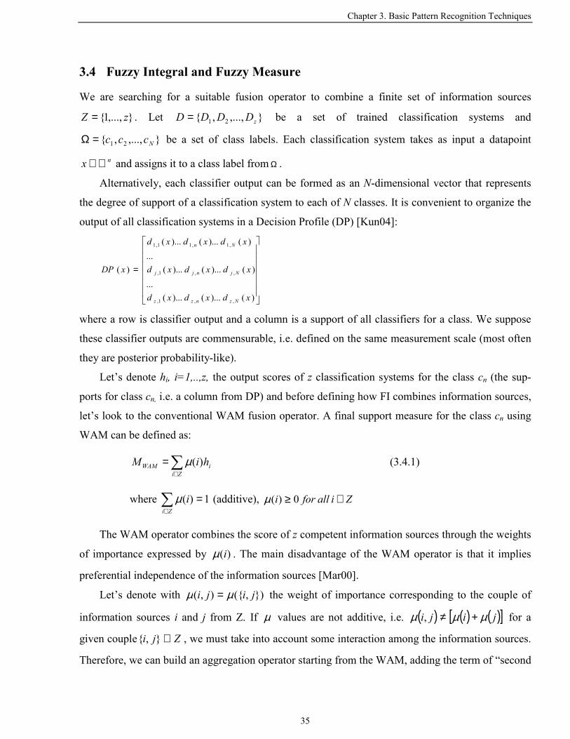
Chapter 3. Basic Pattern Recognition Techniques
35
3.4 Fuzzy Integral and Fuzzy Measure
We are searching for a suitable fusion operator to combine a finite set of information sources
,...,1 zZ = . Let ,...,, 21 zDDDD = be a set of trained classification systems and
,...,, 21 Nccc=Ω be a set of class labels. Each classification system takes as input a datapoint
nx ℜ∈ and assigns it to a class label from Ω .
Alternatively, each classifier output can be formed as an N-dimensional vector that represents
the degree of support of a classification system to each of N classes. It is convenient to organize the
output of all classification systems in a Decision Profile (DP) [Kun04]:
=
)()...()...(...
)()...()...(...
)()...()...(
)(
,,1,
,,1,
,1,11,1
xdxdxd
xdxdxd
xdxdxd
xDP
Nznzz
Njnjj
Nn
where a row is classifier output and a column is a support of all classifiers for a class. We suppose
these classifier outputs are commensurable, i.e. defined on the same measurement scale (most often
they are posterior probability-like).
Let’s denote hi, i=1,..,z, the output scores of z classification systems for the class cn (the sup-
ports for class cn, i.e. a column from DP) and before defining how FI combines information sources,
let’s look to the conventional WAM fusion operator. A final support measure for the class cn using
WAM can be defined as:
∑∈
=Zi
iWAM hiM )(µ (3.4.1)
where ∑∈
=Zi
i 1)(µ (additive), Ziallfori ∈≥ 0)(µ
The WAM operator combines the score of z competent information sources through the weights
of importance expressed by )(iµ . The main disadvantage of the WAM operator is that it implies
preferential independence of the information sources [Mar00].
Let’s denote with ),(),( jiji µµ = the weight of importance corresponding to the couple of
information sources i and j from Z. If µ values are not additive, i.e. ( ) ( ) ( )[ ]jiji µµµ +≠, for a
given couple Zji ⊆, , we must take into account some interaction among the information sources.
Therefore, we can build an aggregation operator starting from the WAM, adding the term of “second

3.4. Fuzzy Integral and Fuzzy Measure
36
order” that involves the corrective coefficients ( ) ( ) ( )[ ]jiji µµµ +−, , then the term of “third order”,
etc. In this way, we arrive to the definition of the FI: assuming the sequence hi, i=1,..,z, is ordered in
such a way that zhh ≤≤ ...1 , the Choquet fuzzy integral [Kun03] [Gra95a] [Gra04] can be computed
as
( ) ( )[ ]∑=
+−=z
iiFI hzizihM
1,...,1,...,),( µµµ (3.4.2)
where 0ø)()1( ==+ µµ z . )(Sµ can be viewed as a weight related to a subset S of the set Z of
information sources. It is called fuzzy measure and has to meet the following conditions:
1)( 0,ø)( == Zµµ , Boundary
)( )( TSTS µµ ≤⇒⊆ , Monotonicity
where ZTS ⊆, .
To illustrate the FI, let us consider a case of two information sources with outputs h1 and h2, and
assume that h1<h2. Consequently, we have corrective coefficients of the second order only:
( ) ( ) ( )[ ]212,1 µµµ +− . According to (3.4.2), FI is computed as
( ) ( )[ ] ( ) 21 222,1),( hhhM FI µµµµ +−= (3.4.3)
which, after a slight manipulation, results in
( ) ( ) ( )( )[ ] ( ) ( ) 211 21122,1),( hhhhM FI µµµµµµ +++−= (3.4.4)
where the first term corresponds to the “second order” correction mentioned above.
For Z information sources there are a total of 2Z FM parameters that can be arranged in a lattice
with the usual ordering of real numbers [CG03]. The lattice representation shows the monotonicity
of the FM and particular values involved in the FI calculation. An example of lattice representation
of FM defined for 4 information sources is shown on Figure 3.4.1. The lattice consists of Z+1 layers
with each node representing a particular subset of Z. Two nodes in adjacent layers are connected
only if there are set-inclusion relationships between the two subsets of Z whose measures they
represent. The red line on the Figure 3.4.1 shows the values used for the FI calculation given the
following ordering of classifiers’ scores: h1<h4<h2<h3.

Chapter 3. Basic Pattern Recognition Techniques
37
Indeed, the large flexibility of the FI aggregation operator is due to the use of FM that can
model interaction among criteria. And although the FM )(iµ provides an initial view about the
importance of information source i, all possible subsets of Z that include that information source
should be analysed to give a final score. For instance, we may have 0)( =iµ , suggesting that ele-
ment i, Ti ∉ , is not important; but if, at the same time, )()( TiT µµ >>∪ , this actually indicates i is
an important element for the decision. For calculating the importance of the information source i,
the Shapley score [Gra95a] [Mar00] is used. It is defined as:
)]()([!
!)!1(),(
\TiT
ZTTZ
iiZT
µµµφ −∪−−
= ∑⊆
(3.4.5)
Generally, (3.4.5) calculates a weighted average value of the marginal contribution
)()( TiT µµ −∪ of the element i over all possible combinations. It can be easily shown that the
information source importance sums to one.
Another interesting concept is interaction among information sources. As long as the FM is not
additive, there exists some correlation among information sources. When )()(),( jiji µµµ +< the
information sources i and j express negative synergy and can be considered redundant. On the
contrary, when )()(),( jiji µµµ +> , the information sources i and j are complementary and express
positive synergy. For calculating the interaction indices, instead of the marginal contribution of
element i in (3.4.5), the contribution of a pair of information sources i and j is defined as the differ-
Figure 3.4.1. Lattice representation of fuzzy measure for 4 information sources.
µ1234
µ0
µ1 µ2 µ3 µ4
µ123 µ124 µ134 µ234
µ12 µ13 µ14 µ23 µ24 µ34

3.4. Fuzzy Integral and Fuzzy Measure
38
ence between the marginal contribution of the pair and the addition of the two individual marginal
contributions [Mar00], or equivalently:
)()()(),())(( , TjTiTjiTTji µµµµµ +∪−∪−∪=∆ (3.4.6)
and the interaction indices are calculated as:
)])(()!1(
!)!2(),;( ,
,\T
ZTTZ
jiI jijiZT
µµ ∆−−−
= ∑⊆
(3.4.7)
We can see the index is positive as long as i and j are negatively correlated (complementary)
and negative when i and j are positively correlated (competitive).
As was mentioned in [Mar00], FI has very good properties for aggregation: it is continuous,
non-decreasing, ranges between a minimum and a maximum value, and coincides with WAM
(discrete Lebesgue integral) as long as the FM is additive. Actually, it was shown in [Mar00] that
the ordered weighted average, the WAM, and the partial minimum and maximum operators are all
particular cases of FI with special FM. In fact, FI can be seen as a compromise between the evidence
expressed by the outputs of the classification systems and the competence represented by the FM’s
knowledge of how the different information sources interact [Kun03].
As the FM is a generalization of a probability measure, we can calculate a measure of uncer-
tainty associated to FM analogously to the way the entropy is computed from the probability
[Mar02], that is:
[ ]∑ ∑= ⊆
−∪=z
i iZTT TiTgH
1 \)()()( µµγµ (3.4.7)
where !/!)!1( ZTTZT −−=γ , xxxg ln)( −= , and 00ln0 = by convention.
When normalized by Zln , )(µH measures the extent to which the information sources are be-
ing used in calculating the aggregation value of ),( hM FI µ . When that entropy measure is close to
1, all criteria are used almost equally; when it is close to 0, the FI concentrates almost on only one
criterion [KMR02].

Chapter 3. Basic Pattern Recognition Techniques
39
3.5 Chapter Summary
In this chapter the basic theory of 3 techniques, support vector machines, Gaussian mixture models, and
fuzzy integral, used in the work, has been given.
Firstly, the construction of SVM classifier has been presented followed by the basic notion of the
structural risk minimization theory and its connection to the SVM classifier. The main advantages and
disadvantages of SVM have been mentioned and discussed.
The GMM classifier is used in the work mostly for comparison purposes. In this chapter the basis
of GMM has been presented and the detailed information has been referenced.
General information on information fusion and the fundamentals of fuzzy integral and fuzzy meas-
ure theory has been also given in this chapter. The FI is used to fuse various information sources in
order to capture and benefit from the information about importance and interaction among the informa-
tion sources.

40

Chapter 4. Acoustic Events Classification
41
Chapter 4. Acoustic Events Classification
4.1 Chapter Overview
Acoustic events produced in controlled environments may carry information useful for perceptually
aware interfaces. In this chapter we focus on the problem of classifying meeting-room acoustic events.
In Section 4.2, we define the features that will be used throughout the work.
Section 4.3 presents 16 types of events and gathered sound database. Then, several classifiers
based on Support Vector Machines (SVM) are developed using confusion matrix based clustering
schemes to deal with the multi-class problem. Also, several sets of acoustic features are defined and
used in the classification tests. In the experiments, the developed SVM-based classifiers are compared
with an already reported binary tree scheme and with their correlative Gaussian mixture model (GMM)
classifiers.
SVM are discriminant classifiers, but they cannot easily deal with the dynamic time structure of
sounds, since they are constrained to work with fixed-length vectors. Several methods that adapt SVM
to sequence processing have been reported in the literature. In Section 4.4, they are reviewed and
applied to the classification of the 16 types of sounds from the meeting room environment.
Fuzzy Integral (FI) is a meaningful formalism for combining classifier outputs that can capture in-
teractions among the various sources of information. In Section 4.5, fusion of different information
sources with the FI, and the associated Fuzzy Measure (FM), is applied to the problem of classifying a
small set of highly confusable human non-speech sounds.

4.2. Audio Features
42
4.2 Audio Features
We use the following notation in feature definition:
s(n) – signal value at the time index n;
N – frame length;
f(i), a(i) – frequency value at the frequency bin i and the corresponding Discrete Fourier Trans-
form (DFT) amplitude, respectively;
x(k), y(k) – value of mel-scaled logarithmic filter-bank energy at the sub-band frequency index k
corresponding to the current and previous frame, respectively;
The following types of frame-level acoustic features with the number of features per frame in
parenthesis are investigated in this thesis:
Zero crossing rate (1). It measures the number of zero crossings of the waveform within a frame
and is calculated as:
( ) ( ) ∑−
=
<−=1
001
N
nnsnsIZCR (4.2.1)
where the indicator function IA is 1 if its argument A is true and 0 otherwise.
Short-time energy (1). Total signal energy in a frame calculated as:
( ) ( )∑−
=
=1
0
N
nnsnsSTE (4.2.2)
Fundamental frequency (1). A simple cepstrum-based method was used to determine the pitch in
the range [70, 500] Hz [Nol67]. When the signal is unvoiced, a zero value is used.
Sub-band log energies (4). The 4 sub-bands are equally distributed along the 20 mel-scaled FBEs
(5 per sub-band). The energy of each sub-band is calculated as:
( ) ( ) 3,...,0for 15
5== ∑
−+
=jkxjSBE
Nj
jk
(4.2.3)
where N=5 is the number of log FBEs per sub-band.
Sub-band log energy distribution (4). Percentage distribution of the total log frame energy among
the above-defined 4 sub-bands.
Sub-band log energy correlations (4). This new type of feature is a measure of correlation of log
FBEs between two adjacent frames and within each of the above defined 4 sub-bands. It is com-

Chapter 4. Acoustic Events Classification
43
puted as the maximum absolute value of the cross-correlation function between the two sequences
x(k) and y(k):
( )( ) ( )( ) ( ) ( )( )[ ]
( ) ( )( ) ( ) ( )( )
3,...,0for
max15
5
215
5
2
15
5
=
−−−
−−⋅−=
∑∑
∑−+
=
−+
=
−+
=
j
jmydkyjmxkx
jmydkyjmxkxabsjSBC
Nj
jk
Nj
jk
Nj
jk
d (4.2.4)
where mx(j) and my(j) are the means of the corresponding sub-band spectra, d=0,1…,N-1 are mel-
scaled sub-band frequency delays, and N=5 is the number of log FBEs per sub-band.
Sub-band log energy time differences (4). It measures the changes of spectra in time and is
calculated as difference of log energies between two adjacent frames for the above defined 4 sub-
bands:
( ) ( ) ( )( ) 3,...,0for 15
5=−= ∑
−+
=jkykxjSBD
Nj
jk
(4.2.5)
where N=5 is the number of log FBEs per sub-band.
Spectral centroid (1). The centroid is a measure of the spectral “brightness” of the spectral frame
and is defined as the linear average frequency weighted by DFT amplitudes, divided by the sum of
the amplitudes:
∑∑
∀
∀=
i
i
ia
iaifCE
)(
)()( (4.2.6)
Spectral roll-off (1). It is a measure of the skewness of the spectral shape and is defined as a
frequency bin fc below which the c percentage of the spectral amplitudes is concentrated (in our case
c=95):
∑∑∀=
=i
f
i
iaciac
)(100
)(0
(4.2.7)
Spectral bandwidth (1). A measure of spreading of the spectrum around the spectral centroid:
∑∑
∀
∀−
=
i
i
ia
iaCEifBW
)(
)())((
2
22
(4.2.8)

4.2. Audio Features
44
where CE is the spectral centroid of the frame.
We will call the above-mentioned features as perceptual throughout the work, since it has a
more perceptually-oriented profile than the conventional features taken from ASR. The ASR fea-
tures used in the work are:
Cepstral coefficients (12) - 12 mel-frequency cepstral coefficients (MFCC) are computed for each
frame using 20 mel-scaled spectral bands. The zero-th cepstral coefficient was removed, but the
frame energy was added to the set.
FF-based spectral parameters (13) - parameters based on filtering the frequency sequence of log
FBEs (FFBE) [NHG95] [NMH01]. We have used the usual second-order filter H(z)=z-z-1, which
implies subtraction of the log FBEs of the two adjacent bands. Before filtering, the sequence of log
FBEs along frequency is extended with one zero at each side. In this way, the first and last parame-
ters actually are the energies of the second and the second last sub-bands. That is the reason why the
frame energy was not used with these features.

Chapter 4. Acoustic Events Classification
45
4.3 Classification of Acoustic Events Using SVM-Based Clustering Schemes
4.3.1 Introduction
In this section we focus on acoustic events that may take place in meeting-rooms or classrooms and
on the preliminary task of classifying isolated sounds. The number of sounds encountered in such
environments may be large, but in this initial work we have chosen 16 different acoustic events,
including speech and music, and a database has been defined for training and testing. While in
[NNM+03] the authors looked at the problem from the point of view of speech recognition, applying
the usual ASR strategy (cepstral features, classifier based on Hidden Markov Models (HMM) and
GMM)), in our work we consider, develop and compare several feature sets and classification
techniques, aiming at finding the ones which are most appropriate for the problem we are dealing
with. In this way, not only the parameters that are used in speech recognition to model the short-time
spectral envelope of the signals and its time derivatives are considered, but also other perceptual
features which may be more fitted to non-speech sounds. Moreover, HMMs require relatively large
amount of data to accurately train the models, something that is not realistic in our task, since there
are not many collections of meeting recordings and the number of samples of some type of sounds
that can be found in them is small.
Recently, the Support Vector Machine (SVM) paradigm has proved highly successful in a num-
ber of classification tasks. As a classifier that discriminates the data by creating boundaries between
classes rather than estimating class conditional densities, it may need considerably less data to
perform accurate classification. In fact, SVMs have already been used for audio classification
[GL03] and segmentation [LLZ03]. In this work we use SVM classifiers and compare them with
GMM classifiers.
As SVMs are binary classifiers, some type of strategy must be employed to extend them to the
multi-class problem. In [GL03], the authors used the binary tree classification scheme to cope with
several classes. That approach requires a relatively high number of classifiers and classification
steps, and the number of classes has to be a power of 2 to get the most benefit from the technique.
There are other ways of applying SVMs to the multi-class problem; see [HL02] for a comparison of
different methods of multi-class SVM classification. In our work, we propose and develop several
variants of a tree clustering technique. Relying on a given set of confusion matrices, that technique
chooses the most discriminative partition and feature set at each step of classification, and, unlike
the binary tree, works for any number of classes.

4.3. Classification of Acoustic Events Using SVM-Based Clustering Schemes
46
Comparative tests have been carried out using the two basic classifiers (GMM and SVM) and a
number of classification schemes (binary tree and several clustering alternatives). The effects of
using two different regularization parameters of the SVM classifiers to compensate data unbalance,
and a confusion matrix based modification of those parameters are also investigated in this work.
The section is organized as follows. In Subsection 4.3.2 we present the database of gathered
sounds. Subsection 4.3.3 describes the features and explains the construction of feature sets. The
classification techniques are overviewed in Subsection 4.3.4. The experiments and a discussion of
the results are presented in Subsection 4.3.5. Finally, conclusions are given in Subsection 4.3.6.
4.3.2 Database
The first problem we had to face when trying to develop a system for classifying acoustic events
which take place in a meeting-room environment was the lack of data. As mentioned above, there
exists a relatively large database of sounds, the RWCP sound scene database, but only a small part
of the sounds included in that database can be considered as usual or at least possible in a meeting
room.
The second column of Table 4.3.1 shows the sixteen categories of sounds that were chosen. As
can be seen in the third column, only four of them belong to the RWCP database. The other sounds
Table 4.3.1. The sixteen acoustical events considered in our database, includ-ing number of samples and their sources (I means Internet)
Event Source Number 1 Chair moving I 12 2 Clapping RWCP + I 100+7 3 Cough I 47 4 Door slam I 80 5 Keyboard I 45 6 Laughter I 26 7 Music I 38 8 Paper crumple RWCP 100 9 Paper tear RWCP 100 10 Pen/pencil handwriting I 30 11 Liquid pouring I 40 12 Puncher/Stapler RWCP 200 13 Sneeze I 40 14 Sniffing I 13 15 Speech ShATR 52 16 Yawn I 12

Chapter 4. Acoustic Events Classification
47
have been found in a large number of websites, except the speech sounds, which were taken from
the ShATR Multiple Simultaneous Speaker Corpus [ShA] and include short fragments from both
close-talk and omnidirectional microphones. The number of samples is 100 or larger for the sounds
taken from the RWCP database, but it is much smaller for a few classes. As shown in the fourth
column of Table 4.3.1, chair moving and yawn events have only 12 samples in the database. The
whole database amounts 53 min of audio (942 files).
Indeed both the diversity in the number of samples per class and the small number of samples
for some sounds are a challenge for the classifier. And, the fact that sounds were taken from differ-
ent sources makes the task even more complicated due to the presence of several (at times even
unknown) environments and recording conditions.
4.3.3 Features extraction
The signals from all the sounds in the database presented above were downsampled to 8kHz,
normalized to be in the range [-1 1], and partitioned in frames using: frame length=128, overlapping
of 50%, and a Hamming window. The silence portions of the signals were removed using an energy
threshold.
Three basic types of acoustic feature were considered in this work. Two of them are spectrum
envelope representations used in speech/speaker recognition, namely the typical MFCC plus the
frame energy [RJ93], and the recently introduced FFBE [NHG95]. Like in speech recognition, they
will be considered either alone or together with their first and second time derivatives (the so-called
delta and delta-delta features) [RJ93]. We consider both types of features because we want to
compare their discriminative capability in this application. The third type of features is a small set
which includes perceptual features which are not considered in the above feature sets and may be
more adequate for some kind of sounds (fundamental frequency and zero crossing rate), and also a
reduced representation of the spectral envelope and its time evolution.
Thus, the acoustic features considered in this work are defined in the following way:
1. Perceptual features
• Short time signal energy
• Sub-band energies
• Spectral flux
• Zero-crossing rate
• Fundamental frequency
2. Cepstral coefficients

4.3. Classification of Acoustic Events Using SVM-Based Clustering Schemes
48
3. FF-based spectral parameters
The three above defined types of acoustic features were combined to build the 9 different fea-
ture sets shown in Table 4.3.2 which are considered in the experiments reported in Subsection 4.3.5.
The mean and standard deviation of those features, estimated by averaging over the whole acoustic
event signal, were taken for classification, thus forming one final statistical feature vector per audio
event with a number of elements which doubles the length of the acoustic feature set.
4.3.4 Classification techniques
Two basic classification techniques are considered in this work: SVM and GMM. The former is
based on decision surfaces, and the latter models data with probability distributions.
As SVM is a binary classifier, we cannot employ it directly in our acoustic event classification
problem, since we have a set of 16 classes. In the literature, several methods of extending from
binary classifiers to multi-class classifiers can be found: one against all, one against one,
DAGSVM, ECOC,… (see [HL02] [RK04] for a comparison). In our experiments, we first use the
scheme proposed in [GL03], namely a binary tree with a SVM at each node. A disadvantage of the
binary tree approach is that the number of classes has to be a power of two, otherwise the tree is
unbalanced and some classes are more likely to be chosen than others. The alternative that is pro-
posed in Subsection 4.3.5 is based on a decision tree that uses a specific feature set at each node, and
it is trained with a clustering technique from a given set of confusion matrices. In this way, it uses
the most discriminative feature set at each step of classification and works for any number of
Table 4.3.2. Feature sets that were used in this work, the way they were constructed from the basic acoustic features, and their size. d and dd denote first and second time derivatives, respectively, E means frame energy, and “+” means concatena-tion of features.
Feature set Content Size 1 Perc Perceptual features 11 2 Ceps+der E+MFCC+d+dd 39 3 Ceps E+MFCC 13 4 FF+der FFBE+d+dd 39 5 FF FF 13 6 Perc+ceps+der “Perc”+“Ceps+der” 50 7 Perc+ceps “Perc” + “Ceps” 24 8 Perc+FF+der “Perc” + “FF+der” 50 9 Perc+FF “Perc” + “FF” 24

Chapter 4. Acoustic Events Classification
49
classes. The effect of a confusion matrix based modification of the generalization parameters C+ and
C- of the SVM classifier is also presented in Subsection 4.3.5.
4.3.5 Experiments
Several experiments were carried out to assess the classification performance of the selected feature
sets and the classification systems, either based on SVM or GMM. To perform the evaluation, the
acoustic event samples were randomly permuted within each class and indexed, so odd index
numbers were assigned to training and even index numbers to testing. Also, 20 permutations were
used in each experiment. Because of unevenness in the number of representatives of the various
classes, the overall performance is computed as an average of the individual class performances.
As preliminary tests with the SVM classifier showed a superiority of the Radial Basis Function
(RBF) kernel over the polynomial one, only the former was used in the evaluation. There are two
main parameters (hyperparameters) that are to be specified using SVMs: σ from the RBF kernel and
the regularization parameter C presented in Chapter 3. Regarding the setting of σ, 5-fold cross-
validation [Bur98] was applied. After that kernel parameter is found, the whole training set is used
again to generate the final classifier.
4.3.5.1 Binary tree scheme
First of all, a binary tree with a SVM at each node was applied to our acoustic event classification
problem. Figure 4.3.1 illustrates how the classifier works. In our implementation, the classes in the
bottom level are ordered randomly. In [GL03], each SVM was trained using C=200; in our work, we
chose C=1, since this value yielded better results in the experiments, a fact that may indicate that our
data are more noisy (contains more outliers) than data used in [GL03].
This SVM-based classification system was compared with a GMM classifier. The latter has one
model per class and, for every test pattern, the model with maximal likelihood is chosen. Both a
fixed and a variable number of Gaussians per class were tried; the best accuracy was achieved by
using a variable number that depends on the amount of data per class.
Figure 4.3.2 shows results for both classifiers. The best feature set in combination with the
GMM classifier was the set number 9 (Perc + FF), with recognition rate 78,9%, whereas for the
SVM classifier was the set number 8 (Perc + FF + der), with 82,9% recognition rate. Note that, in
our experiments, the SVM approach shows a higher performance than the GMM one across all types
of feature sets.

4.3. Classification of Acoustic Events Using SVM-Based Clustering Schemes
50
4.3.5.2 Confusion matrix based clustering scheme
We have developed a tree clustering algorithm which makes use of confusion matrices, one for each
feature set. They are obtained from the experiments reported in the last section, by averaging over
the 20 permutations, and normalizing their elements so that each row adds up 1. Those confusion
matrices are used to find the best way of splitting the classes at a given node into two clusters with
the least mutual confusion. As we have a relatively small number of classes, we can perform ex-
1
6 3 1
6
7
8 7 6 5 4 3 2 1
SVMs
Classes
1
Figure 4.3.1. Binary tree structure for eight classes. Every test pattern enters each binary classifier, and the chosen class is tested in an upper level until the top of the tree is reached. The numbers 1–8 encode the classes. The figure shows a particular example, where class 1 is the class chosen by the classification scheme.
82.9
78.87
0
10
20
30
40
50
60
70
80
90
1 2 3 4 5 6 7 8 9feature set
AC
C
%
SVM
GMM
Figure 4.3.2. Percentage of classification rate for the SVM-based binary tree classifier and the GMM classifier on the defined feature sets.

Chapter 4. Acoustic Events Classification
51
haustive search and get the global minimum. For the sake of homogeneity, we use confusion matri-
ces obtained by SVM classifiers for SVM clustering, and GMM matrices for GMM clustering.
As our database contains a large variety of sounds, the feature set that gets the largest classifica-
tion rate for a given class is not necessarily the best one for a different class. This fact is illustrated
in Figure 4.3.3, where the three considered classes (liquid pouring, sneezing and sniffing) show their
performance peaks at different feature sets and none of the sets is the 8th, the one that yields the best
overall performance. Therefore, it is reasonable to assume that the performance can improve by
using a specific feature set to discriminate within each pair of classes or groups of classes.
The clustering algorithm that selects a specific feature set for each tree node will be presented in
the next section. The simpler case that uses the same feature set at every node is also considered in
the experiments. We refer to them, respectively, as variable-feature-set and fixed-feature-set cluster-
ing schemes. In the following, we will present the former clustering algorithm since the latter is a
particular case of it.
The variable-feature-set clustering algorithm
The algorithm for clustering with a variable-feature-set approach is formally described in Figure
4.3.4. At the first step, all possible combinations of grouping 16 classes into two clusters (i.e.
grouping 6 and 10, 8 and 8, etc) are searched over the available 9 confusions matrices that corre-
0102030405060708090
100
1 2 3 4 5 6 7 8 9feature set
AC
C
%
liquid
sneeze
sniff
Figure 4.3.3. Dependence of performance of classifying “liquid_pouring”, “sneeze” and “sniff” upon the feature sets using SVMs.

4.3. Classification of Acoustic Events Using SVM-Based Clustering Schemes
52
spond to the 9 considered feature sets. For example, for the SVM clustering, we found that the 16
classes were best separated choosing the clusters C1=9 and C2=1, 2, 3, 4, 5, 6, 7, 8, 10, 11, 12,
13, 14, 15, 16, and the 6th feature set. That process is carried out until we have single event clus-
ters. Note in the expression of mnkS , from Figure 4.3.4 that the confusion measures k
ije are
normalized by the corresponding accuracies kiie to cope with the dispersion of performance rates
among the classes. Regarding the GMM classifier, the algorithm also groups the classes into two
clusters, but in this case two models are generated at each step, one for each cluster.
1. Initialize N=16.
2. For n=1…N/2 a. Determine M combinations of grouping N classes into two clus-
ters C1 and C2 containing n and N-n classes, respectively. b. For m=1…M
i. Having the m-th grouping combination, look up at each confusion matrix and measure how much are C1 and C2 confused for each feature set k, by computing
∑∑==
+=
21
1121
, 1 C
jkjj
kji
kii
kij
C
i
mnk e
eee
CCS
where kije denotes the i,j-th element of the k-th confusion
matrix, and |C1| and |C2| are the number of classes (cardi-nalities) of the two clusters.
ii. Find the minimum confusion measure over all feature sets )( min mn,
k, SBkmn =
c. Find the minimum confusion measure over all grouping combi-nations for the current number of classes at each cluster
)(B min mn,mnT =
3. Find the minimum confusion measure over all possible numbers of classes at each cluster
)( min nnTR =
4. Repeat steps 2-3 for each node of growing tree, initializing N with N-n for the right branch and N with n for the left one, until N=1 is reached.
Figure 4.3.4. Clustering algorithm based on an exhaustive search and using a set of estimated confusion matrices.

Chapter 4. Acoustic Events Classification
53
The above clustering technique is intended for a relatively small number of classes, as in our
acoustic event classification task. When the number of classes is large either agglomerative hierar-
chical clustering or divisive hierarchical clustering [Voo86] can be used if they are modified to
handle several feature sets while searching; however, they do not guarantee to reach the global
minimum.
Dealing with the data unbalance problem
In our experiments, we have tried several ways of alleviating the problem of having a too much
different amount of training data between the two clusters at a given tree node. A straightforward
way of tackling that problem which has been considered in the experiments consists of restricting
the exhaustive search in Figure 4.3.4 to look for an equal number of classes at each cluster, i.e.
having only the index value n=N/2 at step 2 of the algorithm. That solution is no longer optimal in
terms of the tree structure, but the involved SVMs will work with more balanced data. Hereafter, we
will refer to it as restricted clustering. Figure 4.3.5 shows the trees obtained by the normal (unre-
stricted) and restricted clustering algorithms in the SVM case. Note that the two trees show a very
different structure, but they have the same number of nodes (N-1), that is the same number of trained
SVM classifiers. Indeed, the restricted tree shows a balanced structure, whereas, as it can be ob-
served in Figure 4.3.5, in the normal clustering case we mostly have only one class separated on
each clustering step. Actually, there is only one case where there are two classes grouped in the
smaller cluster, which corresponds to classes 11 and 12. We have observed that the amount of
confusions between both classes is a large portion of the total error for class 11. Regarding the
GMM-based techniques, since each class model is trained without using information about the other
classes it is not so much influenced by the problem of data unbalance. However, we will also
consider both clustering schemes for the GMM case. The resulting schemes are similar to those in
Figure 4.3.5.
The alternative way of coping with data unbalance used in our experiments (already mentioned
in Subsection 3.2.2) is to introduce different regularization parameters for positively- and nega-
tively-labelled training samples. Additionally, since a measure of confusions at each tree node can
be obtained as a byproduct of the clustering algorithm, we have used these estimated measures to
adapt the regularization parameters. The greater the confusion is, the larger the error should be
allowed during training, and so the smaller the regularization parameters should be. Consequently,
we force those parameters to be inversely proportional to the confusion measures. Indeed, we have a
∞ value at the beginning for normal clustering since the confusion at this step is 0. Note from

4.3. Classification of Acoustic Events Using SVM-Based Clustering Schemes
54
Figure 4.3.4 that if the performance of a class for a given feature set were 0 ( 0=kiie ), the value of
mnkS , would be ∞ . In order to decrease the contribution of that possible zeroth performance of a class
to the computation of the confusion measures of the whole cluster, we substitute zero by a small
value. In our algorithm, we use 0.001.
Three different methods of using and computing the regularization parameters in the SVM-
based classifiers are considered in this work, along with the baseline method that uses only a con-
stant parameter C=K. They are defined in the following, denoting by nS the confusion measure at
the n-th classification step:
1) Only one regularization parameter C computed as
nSKC 1= . (4.3.1)
2) Two different parameters C+ and C-, defined such that
+
−+ =
AAKC
−
+− =
AAKC (4.3.2)
where A+ and A- are the number of positive and negative training samples, respectively. In this way,
the training errors of the two classes contribute equally to the cost of misclassification.
3) The effect of doing both adaptations simultaneously, namely,
nn SAAKC
SAAKC 1 ,1
−
+−
+
−+ == (4.3.3)
In our tests, K was set to value 10 since it gave the best performance for the baseline method with
constant C.
4.3.5.3 Results and discussion
Table 4.3.3 shows classification performance for GMM and SVM classifiers using either a variable-
or a fixed-feature-set approach, and either normal (N) or restricted (R) clustering. The table also
shows the standard deviation for each experiment, estimated over the 20 repetitions. The first
column of results corresponds to C=K=10, and the other 3 columns correspond, respectively, to the
three above-mentioned methods of computing the regularization parameters in the SVM cases. Note
that SVM performs consistently better than GMM, and with SVM the highest accuracies are ob-
tained using the third method.

Chapter 4. Acoustic Events Classification
55
The column C=K in Table 4.3.3 shows that, without any adaptation, SVM-based restricted clus-
tering performs equally well as normal clustering (and better than the binary tree scheme). In that
table, we can notice that SVM-N takes advantage of using different C values for each class accord-
ing to the simple equation of proportionality, since the training set sizes are largely spread across
classes in our database. And SVM-R does not take any advantage due presumably to the balancing
average implied by the half-to-half constraint. Additionally, as we can see from Table 4.3.3, intro-
ducing prior knowledge (about confusions) with the generalization parameter C (method 1) does not
have a positive influence on the classification performance, while introducing it along with different
C values for positive and negative classes (method 3) leads to an improvement for both types of
clustering trees. The gain in performance, however, is not much significant, so there is a need to
have a more sophisticated algorithm of introducing prior knowledge about confusions in the regu-
larization parameters. In restricted clustering we can obtain only the global minimum of error within
the constraint that is why the final performance of the SVM-R technique is worse than that of the
normal one (Table 4.3.3, method 3). We can also observe that normal clustering seems to perform
slightly better than restricted clustering for GMM.
Notice in Table 4.3.3 how the results for SVM fixed-feature-set clustering show just a slightly
worse performance with respect to the variable-feature-set ones. This can be explained in the
following way. On the one hand, for fixed-feature-set clustering, the chosen feature set is the one
which yielded the best results in the previous experiments with binary tree, i.e. the 8th, which
includes all kind of features: perceptual, envelope representation and time derivatives. On the other
hand, the SVM classifier has somehow a built-in feature selection process. In fact, as it implicitly
works with features in a transformed domain, if the kernel and the hyperparameters are appropri-
ately chosen (so that good results are obtained), its transformation may imply emphasizing those
features that are crucial for a good classification. That is why for the SVM classifier no feature
selection technique leads to a huge classification improvement [WMC+00]. Moreover, using real-
world data, it was shown in [WMC+00] that the best feature set was the one that included all types
of features. Additional evidence from our experiments is given by the fact that the difference in
performance between fixed- and variable-feature-set is more noticeable for the GMM classifiers
than for the SVM ones. Nevertheless, in spite of that kind of “implicit feature selection” process in
SVM classifiers, and the fact that a fixed-feature-set scheme requires less computation, the variable-
feature-set scheme may still be advantageous for the SVM case. In fact, apart from offering some
information about the acoustical properties of the chosen classes, the variable-feature-set scheme

4.3. Classification of Acoustic Events Using SVM-Based Clustering Schemes
56
Figure 4.3.5. Normal and restricted clustering schemes for SVM classifiers
Table 4.3.3. Performances of variable-feature-set and fixed-feature-set classifiers using different adaptations of the regularization parameters for the SVM classifiers. -N and -R, denote normal and restricted clustering scheme, respectively. Standard deviations estimated over 20 repetitions are denoted with ± σ.
C=K Method 1 Method 2 Method 3 SVM-N variable 84.67 ± 2.5 84.05 ± 1.7 86.71 ± 1.4 88.29 ± 2.1 SVM-R variable 84.72 ± 2.6 84.88 ± 2.7 84.95 ± 2.2 87.20 ± 1.5 GMM-N variable 83.6 ± 2.2 GMM-R variable 82.15 ± 2.3 SVM-N fixed 84.6 ± 1.9 84.4 ± 1.6 86.6 ± 3.0 87.10 ± 1.8 SVM-R fixed 84.6 ± 2.7 83.8 ± 1.2 84.4 ± 2.3 87.06 ± 1.8 GMM-N fixed 81.2 ± 2.3 GMM-R fixed 80.7 ± 2.4
Table 4.3.4. Confusion measure Sn (multiplied by 100), best separating feature set, and percent-age distribution of the classification error (for the best results in Table 4.3.3) along the 15 nodes (depicted in Figure 4.3.5 for SVM) for both normal and restricted clustering, and for the vari-able-features-set SVM classifier and the GMM classifier.
1 2 3 4 5 6 7 8 9 10 11 12 13 14 15 Confusion 0 0.01 0.03 0.07 0.78 0.82 0.83 0.98 3.90 1.27 1.57 2.57 8.44 15.00 46.88Features 6 3 6 7 7 8 3 7 5 9 5 3 6 4 9 SVM-N
Error 0.78 1.97 0 0 7.65 15.42 2.19 6.30 4.47 4.38 6.64 19.63 18.93 6.23 5.39 Confusion 0.41 2.15 0.04 0.15 15.74 1.74 0 0 4.41 46.88 2.23 3.31 0 0 0 Features 7 9 7 8 6 9 6 5 5 4 8 8 3 1 1 SVM-R
Error 23.59 12.35 1.14 0.69 23.1 6.01 0.46 9.12 5.32 4.76 6.51 1.29 3.95 1.20 0.53
Confusion 0.01 0.1 0.18 0.22 0.28 0.74 1.10 1.14 2.41 3.77 3.00 7.55 13.76 29.86 55.07Features 6 9 9 3 7 7 9 5 9 4 5 7 1 6 1 GMM-N
Error 0.07 1.00 3.46 2.91 2.19 6.55 6.89 5.94 8.33 10.63 6.11 5.28 14.61 14.60 11.42Confusion 0.53 5.59 0.10 15.60 1.92 0.58 0 12.03 55.07 0.81 6.84 0.77 0.92 0 0.1 Features 9 6 7 6 8 3 1 1 1 5 5 7 7 1 6 GMM-R
Error 25.35 24.27 3.27 15.43 3.23 3.18 0 3.18 9.50 2.63 7.18 0.51 1.83 0.38 0.07
1 2
3 4
5 6
7 8
9 1011
12 13
14
15
8 15 7 5 10 12 11 1 9 2 4 14 13 6 3 16 1
3
4 2 14 3 16 6 12 10 11 7 13 5 8 9 15
1
2
4 5 6 7
15 14 13 1211109 8

Chapter 4. Acoustic Events Classification
57
Figure 4.3.6. Distribution of the errors along the tree path for SVM-N, GMM-N, SVM-R and GMM-R. A darker cell means a larger error.
obviously shows a smaller restriction bias than that of the fixed-feature-set clustering, thus resulting
in a smaller inductive bias and a presumable higher overall accuracy [LYC02].
The proposed clustering schemes (both normal and restricted) show two computational advan-
tages in front of the binary tree classifier. First, the required number of trained SVM is N-1, where N
is the number of classes, while for the binary tree (N-1)N/2 trained SVM are needed. Second, the
proposed schemes involve a smaller number of classification steps, 4 for restricted clustering, and
between 1 and 14, depending on the input pattern, for normal clustering in our case (see Figure
4.3.5), whereas the binary tree requires 15. However, the proposed variable-feature-set scheme has
an obvious disadvantage: with our choice of feature sets (see Table 4.3.2) up to 9 feature sets can be
involved in testing, 7 in our case (numbers 3 4 5 6 7 8 9).
From Table 4.3.4 we can extract some observations concerning the feature sets. Looking at bold
numbers in the SVM case of Table 4.3.4, which correspond to a confusion measure larger than 10, it
seems that the best separating feature sets for the most confused classes mostly are FFBE-based
features (sets 4,5,8,9), while observing the italic numbers, which correspond to a confusion measure
smaller than 1, it appears that the for the least confused classes the best separating feature sets are

4.3. Classification of Acoustic Events Using SVM-Based Clustering Schemes
58
MFCC-based (sets 2,3,6,7). This fact may indicate that the FFBE-based features are more discrimi-
native than the MFCC features for highly overlapped data distributions, while MFCC features
appear to show the best performance when there is a clearer separation between classes. However,
for the most confused classes in the GMM case (see bold numbers in the GMM part of Table 4.3.4)
the average best feature set is the one we have called perceptual set. This may be due to the rela-
tively low size of that feature set, which facilitates the estimation problem.
Note in Table 4.3.4 that for normal clustering the largest errors are more located towards the
end of the tree path while for restricted clustering they are towards the beginning. This effect, which
is also illustrated in Figure 4.3.6, can be expected for the normal clustering technique, due to the
way the clustering algorithm in Figure 4.3.4 works. Apparently, the restrictions applied by restricted
clustering make the largest errors are placed at the beginning. That information can be useful to
improve classification by boosting, since the most erroneous steps generally contain rare class data
and boosting the SVM that deal with rare categories has been shown to improve general perform-
ance in [LYC02].
Table 4.3.5 shows the confusion matrix corresponding to the best results. The resulting classifi-
cation rates for the various types of sounds are diverse due to both the acoustic nature of sounds and
the unevenness of the number of samples in the database. Notice that the sounds we could name
human vocal-tract non-speech (HVTNS) sounds (numbers 3, 6, 13, 14, and 16) account for a large
relative amount of confusions, since they only are 5/16 of the total number of classes and contribute
with 69.7% of the total error. The only other sound with more than 10% error is number 11. In
average, the HVTNS classes have a small number of samples in the database, but there are other
sounds with similar number of samples (like chair moving), which do not show such a high error.
Furthermore, the HVTNS sounds are mainly confused among themselves (the average for the 5
classes is 73.96%). Actually, although the proposed clustering schemes are based on acoustic
features, some clusters can be interpreted from a semantic point of view, that is according to their
source identity; e.g. the shaded cluster in contains “cough”, “laughter”, “sneeze”, and “yawn”,
sounds which belong to that HVTNS set.

Chapter 4. Acoustic Events Classification
59
Table 4.3.5. Confusion matrix corresponding to the best results (88.29 %) 1 2 3 4 5 6 7 8 9 10 11 12 13 14 15 16
1 96.67 0 0 0 0 1.67 0 0 0 0 0 0 0 0 0 1.672 0 96.79 0 0.19 0.57 0.19 0 0 0.57 0 0 0.38 1.13 0.19 0 0 3 0 0.43 88.70 2.61 0 5.22 0 0 0 0 0 0.43 2.61 0 0 0 4 0 0.75 0.50 96.50 0 0.75 0 0 0.50 0 0.50 0 0.50 0 0 0 5 0 0 0 2.27 87.73 3.64 0 0 0 0 2.27 3.18 0.91 0 0 0 6 0.77 0 26.92 3.85 0 48.46 0 0 0 9.23 0 0 10.00 0.77 0 0 7 0 0 0 0 0 0 100 0 0 0 0 0 0 0 0 0 8 0 0.20 0 0.40 0 0 0 98.8 0.20 0 0 0.2 0.20 0 0 0 9 0 0 0 0 0 0 0 0.2 99.80 0 0 0 0 0 0 0 10 0 0 1.33 1.33 0 3.33 0 0 0 92.67 0 0 1.33 0 0 0 11 0 0 0 2.00 1.50 1.00 0 2.5 0 3.50 77.00 10.0 2.50 0 0 0 12 0 1.30 0 0 0 0.60 0 0.2 0 0 0.10 97.2 0.60 0 0 0 13 0 0.50 14.50 0 0 8.00 0 0 0 0.50 2.50 0 74 0 0 0 14 0 5.00 5.00 0 0 0 0 0 0 6.67 0 0 6.67 76.67 0 0 15 0 0 0 0 0 0 0 0 0 0 0 0 0 0 100 0 16 0 0 11.67 0 0 3.33 0 0 0 1.67 0 0 1.67 0 0 81.67
Figure 4.3.7. Restricted clustering tree based on SVM. The numbers in the nodes are the ordinal numbers of the 15 SVM classifiers, and the bold numbers between each pair of clusters denote the best separating feature sets.
4.3. Classification of Acoustic Events Using SVM-Based Clustering Schemes
60
4.3.6 Conclusion
The work in the section is a preliminary attempt to deal with the problem of classifying acoustic
events that occur in a meeting-room environment. A preliminary small database has been defined,
and several feature sets and classification techniques have been tested with it. In our tests, the SVM-
based techniques show a higher classification capability than the GMM-based techniques, and the
best results were consistently obtained with a confusion matrix based variable-feature-set clustering
scheme, arriving with SVM to a 88.29 % classification rate, which implies a 31.5% relative average
error reduction with respect to the best result from the conventional binary tree scheme. That good
performance is mostly attributable to the presented clustering technique, and to the fact that SVM
provides the user with the ability to introduce knowledge about data unbalance and class confusions.

Chapter 4. Acoustic Events Classification
61
4.4 Comparison of Sequence Discriminant Support Vector Machines for Acoustic Event Classification
4.4.1 Introduction
A drawback of SVMs when dealing with audio data is their restriction to work with fixed-length
vectors. Both in the kernel evaluation and in the simple input space dot product, the units under
processing are vectors of constant size. However, when working with audio signals, although each
signal frame is converted into a feature vector of a given size, the whole acoustic event is repre-
sented by a sequence of feature vectors, which shows variable length. In order to apply a SVM to
this kind of data, one needs either to somehow normalize the size of the sequence of input space
feature vectors or to find a suitable kernel function that can deal with sequential data.
Several methods have been explored to adapt SVMs to sequence processing [Die02]. The most
common approach is to extract some statistical parameters from the sequence of vectors and thus
transform the problem into that of fixed-length vector spaces. For example, the mean and the
standard deviation of the features extracted from every frame of an audio clip were taken as feature
vector for audio analysis in [GL03]. Despite the good results we obtained using this approach for
acoustic event classification in Section 4.3, when frame-level features are transformed into statistical
event-level features there exist an unavoidable loss of information.
In the work reported in this section, we aim at using SVMs for AEC but preserving the informa-
tion contained in the sequentiality of data, i.e. the temporal structure of the acoustic events. For that
purpose, after choosing a set of meaningful reported techniques, we have compared their perform-
ance in the framework of our meeting-room AEC task. The fact that the used set of acoustic event
types includes time structured sounds (e.g. music) but also sounds whose time evolution is not
relevant (e.g. liquid pouring), allows us to investigate the appropriateness of the various techniques
to classify the different types of sounds.
While in our previous work we tested several feature sets and several multi-class schemes for
SVM, here we use only the best feature set from Section 4.3 and a Directed Acyclic Graph (DAG)
[PCS00] classification scheme. Moreover, the influence of the generative model parameters’ estima-
tion error on the Fisher score derivative is investigated.
The section is organized as follows: Subsection 4.4.2 quickly reviews the SVM-based methods
used in the work, Subsection 4.4.3 presents experimental results and discussions, and Subsection
4.4.4 concludes the work.

4.4. Comparison of Sequence Discriminant Support Vector Machines for Acoustic Event Classification
62
4.4.2 SVM-based sequence discriminant techniques
We have chosen three different SVM kernels techniques that make use of dynamic time warping
(DTW), namely: dynamic time-alignment kernel (DTAK) [SNN01], Gaussian dynamic time warp-
ing (GDTW) kernel [BHB02], and the recent polynomial dynamic time warping kernel (PolyDTW)
[WC05]. Additionally, we included in the comparison the Fisher score kernel [JH99] and the Fisher-
ratio kernel [WR05] [SG02], which aim at using generative model classifiers like GMM in the
discriminative framework, and have been applied for speech/speaker recognition using SVM
[WR05] [SG02]. On the other hand, among the algorithms reported in the literature that normalize
the size of the vector sequences [ASS04], we have chosen the simple outerproduct of trajectory
matrix method, which was the winner in [ASS04]. As references for comparison, we also use a
standard GMM classifier, and an SVM classifier with statistical event-level features. Besides,
several promising sequential kernels like GMM SuperVector kernel [CSR+06] or Incomplete
Cholesky Decomposition Sequence Kernel [LDB06] were not used in the work as they appeared a
little after the work was done.
4.4.2.1 Fisher kernel
Fisher kernel is one of the most successful approaches that enable SVM to classify whole sequences.
Inspired by using statistical modelling method, Fisher kernel recently has become very popular in
the areas that involve time-series recognition. The generalized idea of Fisher kernel the score-space
kernel was applied to speech recognition in [SG02]. Modification of likelihood score space kernel
(i.e. Fisher kernel) known as likelihood ratio score-space kernel has shown comparative results in
the sphere of speaker verification [WR05].
The idea of Fisher kernel includes in mapping the variable length sequence to a single point in
fixed-dimension space, the so-called score-space. To perform such a mapping, Fisher kernel applies
the first derivative operator to the likelihood score of the generative model. Given an input sequence
X, and a model M, parameterized by θ, the Fisher score is defined as
( ) ( )θψ θ ,log MXPXfisher ∇= (4.4.1)
The Fisher score can be interpreted in the following way. When a generative model is trained by
ML (maximum likelihood) criterion, it uses the same set of derivatives to compute how close it is to
the local extreme. Another motivation of using Fisher score is that the gradient of the log-likelihood
can capture the generative process of the whole sequence better than just a posterior probability.
Furthermore, in [JH99] it was shown that, under the condition that the class variable is a latent

Chapter 4. Acoustic Events Classification
63
variable in the probability model, the learning machines, that use Fisher kernel, are asymptotically at
least as good as making decision based on the generative model itself (maximum a posteriori). In
[JH99] applied to bio-sequences recognition Fisher kernel performed significantly better than
HMM.
4.4.2.2 Outerproduct of trajectory matrix
The time analysis of the data gives a sequence of l-dimensional parametric vectors. The sequence is
considered as a trajectory in the l-dimensional space. If we define the l-by-m trajectory matrix as X
= [x1,x2, …xm], the outerproduct matrix Z [ASS04] is defined as
Z=XTX (4.4.2)
Thus the outerproduct matrix Z is l-by-l and no longer depends on the length of the sequence.
The vectorized outerproduct thus can feed the SVM classifier directly. It is obvious that this method
explicitly considers sequence duration information. Despite the simplicity of the given approach, it
showed considerably better results than Compaction and Elongation method in the task of spoken
letters recognition [ASS04].
4.4.2.3 Gaussian dynamic time warping (GDTW)
This approach as well as a previous one does not assume a model for the generative class condi-
tional densities. The GDTW [BHB02] method addresses the problem of variable length sequences
classification by introducing the DTW technique to SVM kernel. Recalling the standard RBF kernel
for SVM
( )2exp),( RTRTK −−= γ (4.4.3)
where T, R denote two patterns to compare. As mentioned in Subsection 4.4.1, if the two patterns
are sequences of different length, they cannot be compared in the kernel evaluation directly. An
obvious modification of (4.4.3) is to substitute the squared Euclidian distance computation with the
equivalent that can cope with temporally distorted variable length sequences. Thus, in [BHB02]
GDTW kernel was defined as
( )( )RTDRTK ,exp),( γ−= (4.4.4)
where ( )RTD , is a DTW distance between sequences T and R.
The proposed method was successfully applied to handwriting recognition and showed com-
parative and at times superior results to HMM and MLP in [BHB02].

4.4. Comparison of Sequence Discriminant Support Vector Machines for Acoustic Event Classification
64
4.4.2.4 Dynamic time alignment kernel (DTAK)
The approach proposed in [SNN01] also deals with DTW. Instead of substituting the Euclidian
distance in Gaussian kernel (4.2.3) by DTW distance, it substitutes the Euclidian distance in defini-
tion of DTW local distance by a kernel.
( ) ( ) ( )∑=
==N
nnRnT
rtkN
RTDRTK1
)()(,1,, φφφ (4.4.5)
where k(.) is a kernel function that can be either a simple dot product or any conventional SVM
kernel and Ф is the optimal DTW path. Actually, DTAK performs DTW in the feature space. Unlike
the original DTW, which finds the optimal path that minimizes the accumulated distance/distortion,
the DTAK algorithm maximizes the similarity. In the task of phoneme recognition, the proposed
DTAK method outperformed HMM with a small or medium amount of training data and it got
comparable results with a larger dataset [SNN01].
4.4.2.5 Polynomial dynamic time warping (PolyDTW)
The method shares the same idea of performing DTW in transformed feature space. After spherical
normalization [WR05] each vector t of a sequence is projected onto the sphere surface as
+=
ααt
tt
22
1ˆ (4.4.6)
Then the arcos of the dot product between normalized vectors can be taken as a local distance
for DTW. Thus, the kernel is given as
( ) ( )
⋅= ∑=
N
nnRnT
m rtN
RTK1
)()(ˆˆarccos1cos, φφ (4.4.7)
This method has been successfully applied to the task with high intra-class variation such as dy-
sarthric speech recognition and showed superior results to HMM [WC05].
4.4.3 Experiments and discussion
4.4.3.1 Experimental setup
Our previous efforts in Section 4.3 were focused on developing a variable-feature-set clustering
scheme and using SVM with statistical event-level features. In this work, for simplicity, we use
DAG [PCS00] multi-class scheme, and only one feature set, the one that showed best results in
Section 4.3, namely, a concatenation of perceptual features (ZCR, Spectral Flux, etc) and frequency

Chapter 4. Acoustic Events Classification
65
filtering features [NHG95] (plus their first and second derivatives). The number of features per
frame is 50 and there is a frame each 10ms.
In all the experiments we use the databases of acoustic events described in Subsection 4.3.2.
The database contains the 16 classes of meeting-room acoustic events that are summarized in Table
4.3.1.
For the outerproduct, DTAK, and GDTW methods we use a Gaussian kernel, and a 5-fold
cross-validation on the training database was applied to find the optimal kernel parameter. The
techniques that exploit DTW required some optimization steps to be feasible in practice (beam
search strategy, kernel caching). For PolyDTW, a polynomial of third degree was chosen with α=1,
as suggested in [WC05]. Also, we chose the linear SVM kernel for the Fisher score and the likeli-
hood ratio methods, since it performed better than RBF.
The mean of individual class accuracies was chosen as a metric as in Section 4.3.
4.4.3.2 Comparison results
Figure 4.4.1 shows the results of the 8 considered techniques when applied to the database of
acoustic events. The best average result is obtained with the Fisher kernel, 88.13%, and it is fol-
lowed by the results from PolyDTW, likelihood ratio kernel and GMM. All mentioned results are
better than 83.1%, the score of the non-sequential SVM technique that uses statistical event-level
features (SVM stat). A similar result was observed in Section 4.3 using a binary tree instead of a
DAG scheme: 82.9%.
88.13
84.32
77.36 77.13 76.21
84.46 84.2283.1
7072747678808284868890
Fisher
LikeR
atio
Outer
pr
GDTWDTAK
PolyDTW
GMM
SVM st
at
Figure 4.4.1. Classification accuracy for the 8 techniques

4.4. Comparison of Sequence Discriminant Support Vector Machines for Acoustic Event Classification
66
It is also worth noticing that the result with the Fisher kernel (88.13%) is comparable to the best
result in Section 4.3 using non-sequential SVM techniques: 88.29%. However, the latter result was
obtained by using a variable-feature-set clustering, a classification scheme that is more developed
than DAG, and by using the most discriminative feature set on each step of classification.
4.4.3.3 Influence of the number of Gaussians on the derivatives of the generative model
Interesting enough that the best results for GMM were obtained with 8 Gaussians, while for Fisher
kernel the appropriate generative model that leaded to the best performance was 1-Gaussian GMM.
Figure 4.4.2 shows the dependence of performance of Fisher kernel, Likelihood ratio kernel and
GMM on the number of Gaussians. As can be seen from Figure 4.4.2 there is an apparent inconsis-
tency in the results, in the sense that the recognition rate improves in the case of the GMM classifier
as the number of Gaussians increases, but at the same time, the results degrade in the case of the
Fisher kernel. There is a two-fold explanation of this phenomenon. The first is related to the fact that
the likelihood of the observation given the model is computed by means of a linear combination of
Gaussians. The weight of each Gaussian is proportional to the number of samples that are assigned
to it. Therefore, the parameters estimated with a small number of samples (i.e. that have a higher
estimation error), have a lower influence in the likelihood. In the case of the Fisher score, the
derivative of the likelihood with respect to each parameter inherits the estimation error, and it is not
concealed, as it is the case of the GMM. Furthermore this effect is augmented by the fact that the
dimensionality of the Fisher kernel increases proportionally to the number of Gaussians, and the
0 1 2 3 4 60
65
70
75
80
85
90
GMM
Likelihood Ratio
Fisher score
Figure 4.4.2. Dependence of the performance of the Fisher score kernel, likelihood ratio kernel and GMM on the number of Gaussians (log2Ng)

Chapter 4. Acoustic Events Classification
67
number of noisy coordinates can be majority [TKM03]. The second explanation uses the concept of
sensitivity, which is the percentage change of a function for a given percentage change of one of the
parameters:
dxxdf
xfx
xxxfxfS )(
)(/)(/)(
≈∆
∆= (4.4.8)
We computed the sensitivity of the likelihood of a GMM, and the Fisher kernel associated to the
GMM. The resulting expressions are highly complicated. Nevertheless, simulations for one Gaus-
sian confirmed that the sensitivities to the mean and the weight of each Gaussian are similar for both
GMM and Fisher kernel, but the sensitivity to the variance is at least three times higher in the case
of the Fisher kernel.
4.4.3.4 Dependence of the classifier performance on the temporal structure of the acoustic event signals
The signals to be classified are quite heterogeneous, and have different temporal structures. There-
fore, as was expected the performance of each classifier was biased to a given subset of the classes.
For instance the DTW based classifiers behaved better with signals such as “music”, or “sneeze”,
while classifiers that did not take into account the temporal structure of the signal did better with
other signals that did not have that structure, such as “pen writing” or “liquid pouring”. Ranking
eight classifiers for a given class (giving the score 1 to the best one and 8 to the worst one) these
properties can be summarized in Figure 4.4.3 and Figure 4.4.4, where we compare the 8 classifiers
for above-mentioned pairs of classes.
In Figure 4.4.3 it can be seen that in the case of “music” and “sneeze” the best classifiers, i.e.
highest ranking and recognition rate, are DTW-based such as GDTW, PolyDTW and DTAK. While
the classifiers that do not take into account the temporal structure, give inferior results. In Figure
4.4.4 the ranking of classifiers is opposite, and the classifiers that specifically dismiss the temporal
order fare better; the highest ranking corresponds to the GMM, and the Fisher Ratio. Another
general feature that was detected, and that is reflected in these figures, is that there are signals that
are easier to classify. It can be seen that systematically the results for a given class are better than for
the others consistently for all the 8 classifiers, i.e. the distribution of the results for all classification
systems are separated, although the order of the systems can be different for each signal.
As a general summary, we can assert that there was a correlation between the classes and the
classifiers, which is masked in the mean values presented in Figure 4.4.1. For both types of signals,

4.4. Comparison of Sequence Discriminant Support Vector Machines for Acoustic Event Classification
68
with time structure or without it, the overall best accuracy with Fisher kernel is usually in the middle
offering a good balance between the two groups of classes.
4.4.4 Conclusions
Several methods that adapt SVMs to sequence processing have been reviewed and applied to the
classification of sounds from the meeting room environment. We have seen that the dynamic time
warping kernels work well for sounds that show a temporal structure, but due to the presence of
less-time-structured sounds in the database the best average score is obtained with the Fisher kernel.
Moreover, only one Gaussian is used in that method due to its high sensitivity to the variance
parameters as a consequence of the scarcity of data. On the other hand, the observed bias of the
classifiers to specific types of classes is a good condition for a successful application of fusion
techniques.
70 75 80 85 90 95 100
8
7
6
5
4
3
2
1
←7 Outpr
←13 Outpr
←7 Gdtw
←13 Gdtw
←7 Dtak
←13 Dtak
←7 PolyDTW ←13 PolyDTW ←7 Fisher
←13 Fisher ←7 Fisher Ratio
←13 Fisher Ratio
←7 GMM
←13 GMM ←7 SVMStat
←13 SVMStat
Recognition Rate, %
Ran
k
Figure 4.4.3. Comparison results for the classes “music” (7) and
“sneeze” (13)
60 65 70 75 80 85 90 95 100
8
7
6
5
4
3
2
1
←11 Outpr
←10 Outpr ←11 Gdtw
←10 Gdtw ←11 Dtak
←10 Dtak
←11 PolyDTW ←10 PolyDTW
←11 Fisher
←10 Fisher
←11 Fisher Ratio ←10 Fisher Ratio
←11 GMM ←10 GMM
←11 SVMStat
←10 SVMStat
Recognition Rate, %
Ran
k
Figure 4.4.4. Comparison results for the classes “pen writing” (10) and
“liquid pouring” (11)

Chapter 4. Acoustic Events Classification
69
4.5 Fuzzy Integral Based Information Fusion for Classification of Highly Confusable Non-Speech Sounds
4.5.1 Introduction
A rich variety of information sources is obtained in this work by extracting a set of ten different
kinds of features and using them as inputs of ten different SVM classifiers, whose outputs are
combined to give a final classification score. Besides the above-mentioned fusion of information
sources at the decision level, and for clarity purposes, we also consider information fusion at the
feature level, i.e. an early integration of information sources, and will be carried out by the SVM.
These two kinds of fusion are depicted in Figure 4.5.1.
Usual combinations of classifier outputs like sum, product, max, min, weighted arithmetical
mean (WAM), etc [Kun03], assume that each output represents an independent source of informa-
tion that can be treated separately. Often, this is not the case, and an approach that considers the
interactions among the classifier outputs is needed. Over the past several years there have been a
number of successful applications of the FI [Kun03] [Sug74] in decision-making and pattern recog-
nition using multiple information sources (e.g. [Gra95a] [CG03] [Gra95b]). FI is a meaningful
formalism for combining classifier outputs which can capture interactions among the various
sources of information. Moreover, the FM, which is associated with the FI, furnishes a measure of
importance for each subset of information sources, allowing feature selection and giving a valuable
insight into the classification problem itself.
Both feature-level fusion and decision-level fusion are compared in our AEC experiments. As a
default classifier we use the SVM classifier, which helps to overcome the problem of the high-
dimensionality [WCC+04] of the input feature space.
Figure 4.5.1. Fusion at the feature level (a) and at the decision level (b).
Out 1
Event hypothesis
Feat 1
.. .
Feat 2
Feat N
Out 2
Out N
Event hypothesis
Feat 1
. . . Feat N
Feat 2
(a) (b)
Classifier 1
Classifier 2
Classifier N
Classifier
FI

4.5. Fuzzy Integral Based Information Fusion for Classification of Highly Confusable Non-Speech Sounds
70
In this section, we focus on the classification of a particular type of acoustic events, a set of five
human vocal-tract non-speech sounds (cough, laughter, sneeze, sniff and yawn), which were found
responsible for a large part of errors in the classification of meeting-room acoustic events in Section
4.3. In fact, those sounds contributed with 70% of the total classification error, in spite of accounting
only for 30% of the acoustic events included in the testing database. Additionally, it was observed in
Section 4.3 that those human non-speech sounds were mainly confused among themselves. Using
the same small database and keeping SVM as the basic classifier, the work presented in this section
is intended to reduce the classification error rate of the above mentioned set of highly confusable
human non-speech sounds by turning to the fusion of different information sources that in our case
consists of the combination of classifier outputs.
Finally, as the FI aggregation may be appropriate when the feature-level fusion is difficult (e.g.
due to the different nature of the involved features), or when it is beneficial to preserve the applica-
tion or technique dependency (e.g. when fusing well established feature-classifier configurations),
we have also conducted experiments to combine HMM that use frame-level features with the SVM
using signal-level features, and have witnessed an additional improvement. As smart-rooms are
usually equipped with a network of microphones and video cameras that provide multimodal
information, fusion of information with the FI may find a useful application in such a framework.
The rest of the section is organized as follows: Subsection 4.5.2 gives the details of the FM
learning algorithm. Audio features investigated in this work are presented in Subsection 4.5.3.
Subsection 4.5.4 presents the experiments and discussion. Finally, conclusions are given in Subsec-
tion 4.5.5.
4.5.2 Fuzzy measure learning
From Section 3.4 it is obvious that FI completely relies on the FM. The better the FM describes the
real competence and interaction among all classification systems, the more accurate results can be
expected. There are two methods of calculating the FM known to the authors (if it is not provided by
an expert knowledge): one based on fuzzy densities [Kun03], and the other based on learning the
FM from training data [CG03] [Gra95b]. In our work, we have used the latter method: a supervised,
gradient-based algorithm of learning the FM, with additional steps for smoothing the unmodified
nodes:
Step 1. Initialize the FM to the equilibrium state Zi /1)( =µ , where Z is the number of information
sources and FM is additive, i.e. )()(),( jiji µµµ +=
Step 2. For a data point x with label cn

Chapter 4. Acoustic Events Classification
71
Step 2.1. Obtain the DP(x) and calculate the FIs Mn for each of N classes (i.e. for each col-
umn of the DP).
Step 2.2. Calculate the error for each of N classes: εn = cn - Mn, where cn is one for the cor-
rect class and zeros for the others.
Step 2.3. For each of N classes, update the FM µ values that were used in the calculation of
Mn (e.g. in Figure 3.4.1, those that are on the red line, i.e. µ234, µ23 and µ3) using the
formula derived from a mean-squared-error criterion [CG03]. Note that for each
class the order of classifiers may differ, what implies that different µ values are
used for the calculation of Mn.
Step 2.4. Verify the monotonicity condition for the µ values that were used in the calculation
of Mn.
Step 3. Due to the scarcity of data, verify the monotonicity condition of the unmodified µ values and
smooth their values. The smoothing is based on the average values of the upper and lower
neighbours of the current node.
For the detailed description of the algorithm and exact parameter update equations refer to
[CG03] [Gra95b].
4.5.3 Feature extraction
Although the best feature sets for AEC in Section 4.3 consisted of combinations of features used in
automatic speech recognition and other perceptual features, in the current work we only focus on the
latter, since their contribution to vocal-tract sounds is not so well-established. 10 types of features
were chosen with a substantial degree of redundancy in order to use FM to find out their relative
importance and their degree of interaction. The following types of frame-level acoustic features with
the number of features in parenthesis are investigated in this thesis:
1. Zero crossing rate (1)
2. Short-time energy (1)
3. Fundamental frequency (1)
4. Sub-band log energies (4)
5. Sub-band log energy distribution (4)
6. Sub-band log energy correlations (4)
7. Sub-band log energy time differences (4)
8. Spectral centroid (1)
9. Spectral roll-off (1)

4.5. Fuzzy Integral Based Information Fusion for Classification of Highly Confusable Non-Speech Sounds
72
10. Spectral bandwidth (1)
Therefore, 22 acoustical measures are extracted from each frame, using 16ms/8ms frame
length/shift. Then, from the whole time sequence of each acoustical measure in an event, four
statistical parameters are computed: mean, standard deviation, autocorrelation coefficient at the
second lag, and entropy. Those four statistical values per acoustical measure are used to represent
the whole acoustic event.
4.5.4 Experiments and discussion
4.5.4.1 Experimental setup
Database
Due to the lack of an acceptable corpus, the acoustic event database used in this work has been
assembled using different sources. Part of the database was taken from the seminar recordings
employed within the CHIL project [EVA]. The other part has been found in a large number of
Internet websites.
All sounds were down-sampled to 8 kHz. The fact that the acoustic events were taken from dif-
ferent sources makes the classification task more complicated due to the presence of several
(sometimes unknown) environments and recording conditions. Table 4.5.1 shows the five acoustic
classes considered in this work and Figure 4.5.2 shows their sample spectrograms. Notice that each
realization of “cough” and “sniff” (there are two in the depicted time interval) shows a rather
stationary behaviour, and “laughter” is almost periodic. Conversely, both “sneeze” and “yawn” have
more spectral change. Actually, the “sneeze” sound results from the concatenation of two very
different waveforms, and the “yawn” sound shows a decreasing pitch in its first segment.
There is a high variation in the number of samples per class, which represents an additional dif-
ficulty. In order to achieve a reasonable testing scenario, the data has been approximately equally
split into the training and testing parts in such a way that there was the same number of representa-
Table 4.5.1. Sound classes and number of samples per class
Event NumberA Cough & Throat 119 B Laughter 37 C Sneeze 40 D Sniff 37 E Yawn 12

Chapter 4. Acoustic Events Classification
73
tives from the two data sources in the training and testing part. 10 runs were done in all the experi-
ments.
SVM setup
The training data for each binary SVM classifier were firstly normalized anisotropicly to be in the
range from –1 to 1, and the obtained normalizing template was then applied also to the testing data
that are fed to that classifier. In the experiments with the SVM we used the Gaussian kernel. Leave-
one-out cross validation [SS02] was applied to search for the optimal kernel parameter σ. To cope
with the data imbalance we introduce different generalization parameters (C+ and C-) for positively-
and negatively-labelled training samples: +
−+ =
AAKC ,
−
+− =
AAKC where A+ and A- are the number
of positive and negative training samples, respectively. In this way, the training errors of the two
classes contribute equally to the cost of misclassification (see Section 4.3). K was set to value 10 for
all experiments as it was done in Section 4.3. MAX WINS (pairwise majority voting) [HL02]
scheme was used to extend the SVM to the task of classifying several classes. The softmax function
Cough
0
2000
4000
Laughter
0
2000
4000
Sneeze
0
2000
4000
Yawn0
2000
4000
Time (s)0 0.2 0.4 0.6 0.8 1 1.2 1.4
0
2000
4000
Sniff
Fre
quen
cy (H
z)
Figure 4.5.2. Sample spectrograms of acoustic events from
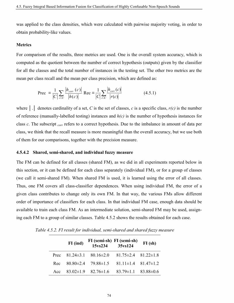
4.5. Fuzzy Integral Based Information Fusion for Classification of Highly Confusable Non-Speech Sounds
74
was applied to the class densities, which were calculated with pairwise majority voting, in order to
obtain probability-like values.
Metrics
For comparison of the results, three metrics are used. One is the overall system accuracy, which is
computed as the quotient between the number of correct hypothesis (outputs) given by the classifier
for all the classes and the total number of instances in the testing set. The other two metrics are the
mean per class recall and the mean per class precision, which are defined as:
∑∈
=Cc
corr
chch
C )()(1Prec ∑
∈=
Cc
corr
crch
C )()(1Rec (4.5.1)
where . denotes cardinality of a set, C is the set of classes, c is a specific class, r(c) is the number
of reference (manually-labelled testing) instances and h(c) is the number of hypothesis instances for
class c. The subscript corr refers to a correct hypothesis. Due to the imbalance in amount of data per
class, we think that the recall measure is more meaningful than the overall accuracy, but we use both
of them for our comparisons, together with the precision measure.
4.5.4.2 Shared, semi-shared, and individual fuzzy measure
The FM can be defined for all classes (shared FM), as we did in all experiments reported below in
this section, or it can be defined for each class separately (individual FM), or for a group of classes
(we call it semi-shared FM). When shared FM is used, it is learned using the error of all classes.
Thus, one FM covers all class-classifier dependences. When using individual FM, the error of a
given class contributes to change only its own FM. In that way, the various FMs allow different
order of importance of classifiers for each class. In that individual FM case, enough data should be
available to train each class FM. As an intermediate solution, semi-shared FM may be used, assign-
ing each FM to a group of similar classes. Table 4.5.2 shows the results obtained for each case.
Table 4.5.2. FI result for individual, semi-shared and shared fuzzy measure
FI (ind) FI (semi-sh)15vs234
FI (semi-sh) 35vs124 FI (sh)
Prec 81.24±3.1 80.16±2.0 81.75±2.4 81.22±1.8
Rec 80.80±2.4 79.88±1.5 81.11±1.4 81.47±1.2
Acc 83.02±1.9 82.76±1.6 83.79±1.1 83.88±0.6

Chapter 4. Acoustic Events Classification
75
As it can be seen from Table 4.5.2 shared, semi-shared and individual FMs show similar results,
although shared FM is preferable than individual FM in our case when a small database is available,
due to slightly better average recall and lower standard deviation of the results. Columns 2 and 3
show that, when using semi-shared FM, one should define FM for a meaningful group of classes, as
done in column 3 when classes are grouped into two sets (3-5 and 1-2-4) according to the degree of
non-stationarity of the corresponding types of sounds. On the contrary, in column 2, classes are
divided simply to have an equal amount of data for each group, and the fusion performance is lower.
4.5.4.3 Feature and decision level information fusion
In this section, the two ways of information fusion mentioned in the Introduction are compared. For
the feature-level fusion (see Figure 4.5.1 (a)), all ten types of features were used to feed the input of
one SVM classifier. For the decision-level fusion (see Figure 4.5.1 (b)), ten independent SVM-based
classifiers were trained, one for each feature type. The ten input criteria, represented by these ten
classifiers, were then combined by WAM operator and FI with learned shared FM. For the weights
in WAM operator we use uniform class noise model with the weights computed as
ii Ei
Eii EE −−= 1)1(µ where Ei is the training error of class ci [Kun04].
As we can see from Figure 4.5.3, all fusion approaches show a strong improvement in compari-
son to the SVM with the best single feature type (number 4). As expected, feeding all the features to
the SVM classifier increased significantly the performance (SVM, 10 feature types). Interestingly
enough, the fusion at the decision-level by FI showed comparable results to the powerful SVM
classifier, which uses all the features. To gain an insight into the way FI works, we compare in Table
4.5.3 the individual recall score of the best feature type (column 2) for a given class, and the FI score
(column 3) for the same class. Notice that, for the most represented class (A), the FI performance is
lower, whereas for two less represented classes (C and D) it is higher. As the FM was trained using
the errors of the particular classes as cost functions, we observe that, at the expense of accepting
more errors for the most represented classes, the FI can recover a few errors for infrequent classes
and thus obtain higher recall.
However, the accuracy and precision measures for both FI and WAM were slightly worse than
that of the SVM: Accuracy=83.9 and Precision=81.2 for FI, versus Accuracy=84.8 and Preci-
sion=84.5 for SVM. Notice also that FI fusion has approximately a 10 times higher computation cost
than SVM feature-level fusion (10 independent SVM classifiers vs. one), and therefore the latter
would seem preferable in this case.

4.5. Fuzzy Integral Based Information Fusion for Classification of Highly Confusable Non-Speech Sounds
76
4.5.4.4 Feature ranking and selection
An information source consists of two parts: a classifier and a set of features. When using the same
classifier for each information source, we can interpret the FM as the importance of features for the
given classification task and we can use it for feature ranking and selection.
The information about both the importance of each feature type and the interaction among dif-
ferent feature types can be extracted applying the Shapley score to the FM. Using this approach,
Figure 4.5.4 shows that in our case the new feature type 6 (SBE correlations) is the most important
followed by feature type 7 (SBE time difference). As both feature types measure the changes of the
spectral envelope along the time, we can conclude that that information is of high importance. The
only other feature type with importance score above the average is number 4 (SBE). Interestingly
that although the new feature type described in Section 4.2 has the highest overall importance,
individual accuracy is only around 50% as it can be seen from Figure 4.5.4. We also observed that
without calculating the maximum absolute value in (4.2.4) the new feature individual accuracy
increases to around 63% while the fusion result decreases to 79.4 %.
Figure 4.5.3. Recall measure for the 10 SVM systems running on each feature type, the combination of the 10 features at the feature-level with SVM, and the fusion on the decision-level with WAM and FI operators.
Table 4.5.3. Comparison of individual recall scores for each class
Class Best score FI A(119) 0.85 0.81 B(37) 0.61 0.61 C(40) 0.95 1.00 D(37) 0.77 1.00 E(12) 0.67 0.67

Chapter 4. Acoustic Events Classification
77
On the other hand, Figure 4.5.5 shows the interaction among the feature types in our task; it can
be seen that feature types 6 (SBE time correlation) and 7 (SBE time difference) express a negative
interaction, which coincide with their similar character. As an extreme case, the light cell (4,5) has a
large negative value and thus indicates a high competitiveness (redundancy) of the mentioned
feature types. Therefore it would be better to consider only one of the two feature types. Actually,
feature type 4 (SBE) and the feature type 5 (SBE Distribution) become roughly the same feature
after using the SVM normalization. In a similar way, as feature types 1 (ZCR) and 8 (Sp. Centroid)
are both targeting the “main” frequency, their cell is also rather light. Also, from the two lighter
cells in the bottom of the Figure 4.5.5, one can conclude that feature type 9 is redundant if feature
types 8 and 10 are considered. On the contrary, feature types 4 and 6, or 4 and 7, or 4 and 10 seem to
be highly complementary, and thus are preferable to be considered together.
In the following AEC tests, we use the information from Figure 4.5.4 and Figure 4.5.5 to per-
form the feature selection. In the first test, we select the 5 best feature types according to the
Figure 4.5.4. Importance of features extracted from FM.
Dashed line shows the average importance level.
Figure 4.5.5. Interaction of features extracted from FM.

4.5. Fuzzy Integral Based Information Fusion for Classification of Highly Confusable Non-Speech Sounds
78
individual feature type importance (Method 1), while to select the 5 best features in the second test,
both the individual feature type importance and the interaction indices are used (Method 2, see
[MZ99] for a detailed description). The selected features are then fed to the SVM classifier.
The performance of the SVM with all features is considered as a baseline in this part. It can be
seen from the results in Table 4.5.4 that Method 1 did not lead to a better performance, while
Method 2 obtained a slight improvement over the baseline.
The last column in Table 4.5.4 shows that the FI scores resulting from using the feature types
chosen by Method 2 are clearly worse than the SVM ones. Notice that, although apparently FI
should benefit from a feature selection based on FM, the 5 features have been selected according to
a FM computed from 10 information sources, while FI scores in Table 4.5.4 result from a different
FM, since it has been trained using only data corresponding to the 5 selected features.
Note that the recall score in the last column of Table 4.5.4 is much lower than the one shown in
Figure 4.5.3 (and last column in Table 4.5.2) for the FI technique when using the whole set of
features, in spite of the fact that FI technique apparently should benefit from a feature selection
based on FM. There are two reasons for this behaviour. First, the 5 features have been selected
according to a FM computed from 10 information sources, while FI scores in Table 4.5.4 result from
a different FM, since it has been trained using only data corresponding to the 5 selected features.
The second reason is based on the measure of uncertainty defined by (3.4.7). As it was mentioned in
Section 3.4, if that entropy measure is close to 1 almost all information sources are equally used. In
fact, for the 10 features case, it is 0.86, meaning that to achieve the results shown in Figure 4.5.3, the
FI operator uses in average 8-9 out of 10 information sources, so preserving only 50% of all features
is not sufficient.
Table 4.5.4. Classification results using feature selection based on FM
Support Vector Machines FI
Baseline Method 1 Method 2
Features 10 (all) 5(1,4,6,7,10) 5(4,6,7,8,10) Method 2
Prec 84.50±2.1 82.76±1.3 86.14±1.7 81.74±2.4 Rec 80.98±1.1 75.31±2.1 80.14±1.6 74.79±2.5 Acc 84.83±2.3 83.97±2.2 85.86±1.4 83.79±1.6

Chapter 4. Acoustic Events Classification
79
4.5.4.5 Fusion of different classifiers using FI
In previous subsections we showed that the FI decision-level fusion obtains comparative results to
the feature-level fusion using the SVM classifier. Indeed, from the computational cost point of view
the feature-level fusion is preferred. However, when the resulting feature space has a too high
dimensionality or when features are conveyed by different data types (strings, matrices, etc) the
feature-level fusion is not an option.
On the other hand, it may be beneficial to combine the outputs of different well-established
classification configurations for a given task; for example, the output of a SVM classifier which is
discriminative but uses features from the whole signal with the output of a HMM generative classi-
fier which considers time localized features. Based on that, we have tested with the FI formalism the
combination of a SVM classifier that uses statistical (event-level) features with a HMM classifier
that uses acoustic (frame-level) features. In these experiments, the best 5 feature types selected in
the previous subsection by Method 2 are used with the SVM classifier. For HMM, we use a standard
configuration coming from speech recognition: a 3 state left-to-right continuous density HMM
model per class, with 8 Gaussians per state, and 13 frequency-filtered filter-bank energies (FFBE)
[NHG95] as features.
The first four columns in Table 4.5.5 show the performance of the SVM classifier and several
HMM classifiers, where ∆FFBE means the time derivatives of FFBE features [NMH01]. HMM-
∆FFBE gives low performance because the time derivatives only carry information about dynamics
of sound but lack the basic static representation of the audio signal. The low score resulting from the
HMM classifier when it uses as features both FFBE and their time derivatives (fourth column in
Table 4.5.5), indicates that the amount of data we use is not enough to train the 26-dimensional
vector data properly. Then, we decided to fuse the outputs of the previous classifiers: SVM, HMM-
FFBE and HMM-∆FFBE. From the second last column of Table 4.5.5 an improvement can be
observed by FI fusion of the SVM and HMM-FFBE outputs. A further improvement is obtained by
Table 4.5.5. Individual performance of SVM, HMM on FFBE with and without time derivatives, and FI fusion
SVM (1)
HMM-FFBE (2)
HMM-∆FFBE(3)
HMM-FFBE+∆FFBE FI(1,2) FI (1,2,3)
Prec 86.14±1.7 69.28±3.5 51.06±4.7 66.70±3.2 88.23±1.8 89.47±1.9 Rec 80.14±1.6 67.36±2.7 60.73±3.8 59.31±2.5 81.43±1.5 82.43±1.0 Acc 85.86±1.4 84.48±2.1 52.59±4.6 79.17±2.6 87.07±2.2 87.93±1.8
4.5. Fuzzy Integral Based Information Fusion for Classification of Highly Confusable Non-Speech Sounds
80
fusion of the SVM output with two information sources that separately give much lower individual
performances, but use different features, as it is shown in the last column of Table 4.5.5.
Note from Figure 4.5.3 that a much higher improvement was observed by fusing a larger num-
ber of information sources (10). Actually, the higher is the number of information sources the larger
is the degree of interaction between them, and thus the better is the performance expected from the
FI with an appropriately-learned FM. However, the difficulty of learning FM increases with the
number of information sources. From our experience in this work, we would suggest to apply the FI
formalism to fuse a number of information sources between 3 and 10.
4.5.5 Conclusion
In this work, we have carried out a preliminary investigation about the fusion of a relatively large
number of information sources with the FI approach. We have shown an improvement over the
baseline SVM approach in the task of classifying a small set of human vocal-tract non-speech
sounds. By interpreting an information source as a specific combination of a classifier and a set of
features, we have been able to carry out different types of tests.
In the experiments, fusion of several information sources with the FI formalism has shown a
significant improvement with respect to the best single information source. Moreover, the FI deci-
sion-level fusion approach has shown comparable results to the high-performing SVM feature-level
fusion. The experimental work has also indicated that the FI may be a good choice when feature-
level fusion is not an option.
We have also observed that the importance and the degree of interaction among the various fea-
ture types given by the FM can be used for feature selection, and it gives a valuable insight into the
problem.

Chapter 4. Acoustic Events Classification
81
4.6 Chapter Summary
The problem of classifying a set meeting-room acoustic events has been tackled in this chapter. A
database has been defined and a set of experiments has been carried out.
Firstly, a confusion matrix based variable-feature-set clustering algorithm based on SVM classifier
has been developed and applied to the problem. A 31.5% relative average error reduction with respect
to the conventional binary tree scheme has been achieved.
Various sequential kernels have been tried to adapt the SVM classifier to sequence processing. The
results of comparison has shown that using dynamic kernels a better performance can be obtained for
sounds with a temporal structure; however the worse results on less-time-structured sounds and high
computational cost of sequential kernels make their usefulness low at present.
Finally, fusion of several information sources with the FI formalism has been performed and has
shown a significant improvement with respect to the best single information source. It has also been
observed that the importance and the degree of interaction among the various feature types given by the
FM can be used for feature selection, and it gives a valuable insight into the problem.

82

Chapter 5. Acoustic Event Detection
83
Chapter 5. Acoustic Event Detection
5.1 Chapter Overview
In the previous chapter the work done on classification of acoustic events was reported. More complex
is the problem of Acoustic Event Detection, which purpose is to determine the presence of a given
acoustic event of interest.
In this chapter we describe the AED systems developed at the UPC and submitted to the CLEAR
evaluations that were carried out in March 2006 and March 2007, respectively. The system of year
2006, which is explained in Subsection 5.2.1, is based on two steps: performing silence/non-silence
segmentation and then classification of non-silence portions by SVM classifiers. A set of features
described in Section 4.3 is used. The system of year 2007, which is explained in Section 5.2.2, merges
the two steps (segmentation and classification) and is also based on SVM classifiers. Besides, accord-
ing to the importance and degree of interaction shown in Section 4.5, several features are selected and
added to the set of features used in the AED system 2006 and one feature is eliminated. Additionally,
multi-microphone decision fusion is added to the AED system 2007.
The acoustic event classification system used for evaluations 2006 is also explained in this chapter
in Section 5.2.1.
As the systems have only been evaluated through participation in the international evaluation cam-
paigns, the results are not presented in this chapter but in the next one.

5.2. Acoustic Event Detection systems
84
5.2 Acoustic Event Detection systems
5.2.1 Acoustic event detection and acoustic event classification systems 2006
5.2.1.1 General description
The systems are based on SVM. A DAG [PCS00] multi-classification scheme was chosen to extend
the SVM binary classifier to the multi-classification problem. 5-fold cross-validation [SS02] on the
training data was applied to find the optimal SVM hyper parameters that were σ for the chosen
Gaussian kernel, and C, a parameter that controls the amount of data allowed to be misclassified
during the training procedure. In all the experiments the third channel of the Mark III microphone
array was used.
Firstly, the sound is downsampled from the initial 44 kHz sampling rate to 22 kHz, and framed
(frame length = 25 ms, overlapping 50%, Hamming window). For each frame, the set of spectral
parameters that showed the best results in Section 4.3 was extracted. It consists of the concatenation
of two types of parameters: 1) 16 Frequency-Filtered (FF) log filter-bank energies [NHG95] taken
from ASR, and 2) a set of other perceptual parameters: zero-crossing rate, short time energy, 4 sub-
band energies, spectral flux calculated for each of the defined subbands, and pitch. The first and
second time derivatives were also calculated for the FF parameters. In total, a vector of 59 compo-
nents is build to represent each frame.
5.2.1.2 AEC system
The mean, standard deviation, entropy and autocorrelation coefficient of the parameter vectors were
computed along the whole event signal thus forming one vector per audio event with 4x59 elements.
Then, that vector of statistical features was used to feed the SVM classifier, which was trained on
the training set of the two databases of isolated acoustic events. The resulting system was used to
test both UPC and ITC databases of isolated acoustic events, which are described in Chapter 6, so
neither features nor system adaptation related to a specific database were applied.
5.2.1.3 AED system
The scheme of the AED system is shown in Figure 5.2.1. Using a sliding window of one second
with a 100 ms shift, a vector of 4x59 statistical features was extracted like in the AEC system
described in the last subsection for each position of the window (every 100 ms).
The statistical feature vector is then fed to an SVM-based silence/non-silence classifier trained
on silence and non-silence segments of the two isolated acoustic events databases. At the output, a

Chapter 5. Acoustic Event Detection
85
binary sequence of decisions is obtained. A median-filter of size 17 is applied to eliminate too short
silences or non-silences.
Then, the SVM-based event classifier is applied to each detected non-silence segment. The
event classifier was trained on a parameters extracted from a sliding window with 100 ms shift
applied to each event in the way that the first and the last windows still include more than 50% of
the event content. The event classifier is trained on both isolated acoustic events and seminar
databases to classify a set of 12 defined acoustical classes, plus classes “speech” and “unknown”. A
sequence of decisions made on a 1-second window every 100 ms is obtained within the non-silence
segment. That sequence is smoothed by assigning to the current decision point the label that is most
frequent in a string of five decision points around the current one. Also, a confidence measure is
calculated for each point as the quotient between the number of times that the chosen label appears
in the string and the number of labels in the string (5).
The sequence of decisions from the non-silence segment is then processed again to get the de-
tected events. In that step, only the events that have their length equal or larger than the average
event length are kept, and the number of events kept in the non-silence segment is forced to be lower
than a number which is proportional to the length of the segment. The average length of the events is
estimated from the training and development databases. Finally, if the average of the above-
mentioned computed confidences in a detected event is less than a threshold, the hypothesized event
is marked as “unknown”; otherwise, it maintains the assigned label.
5.2.2 Acoustic event detection system 2007
The general scheme of the proposed system for AED is shown in Figure 5.2.2. Firstly, in the data
pre-processing step, the signals are normalized based on the histograms of the signal energy. Then, a
Figure 5.2.1. UPC acoustic event detection system 2006
SVM silence / non-silence
segmentation Feature extraction
SVM classification
Segmentation step
Classification step
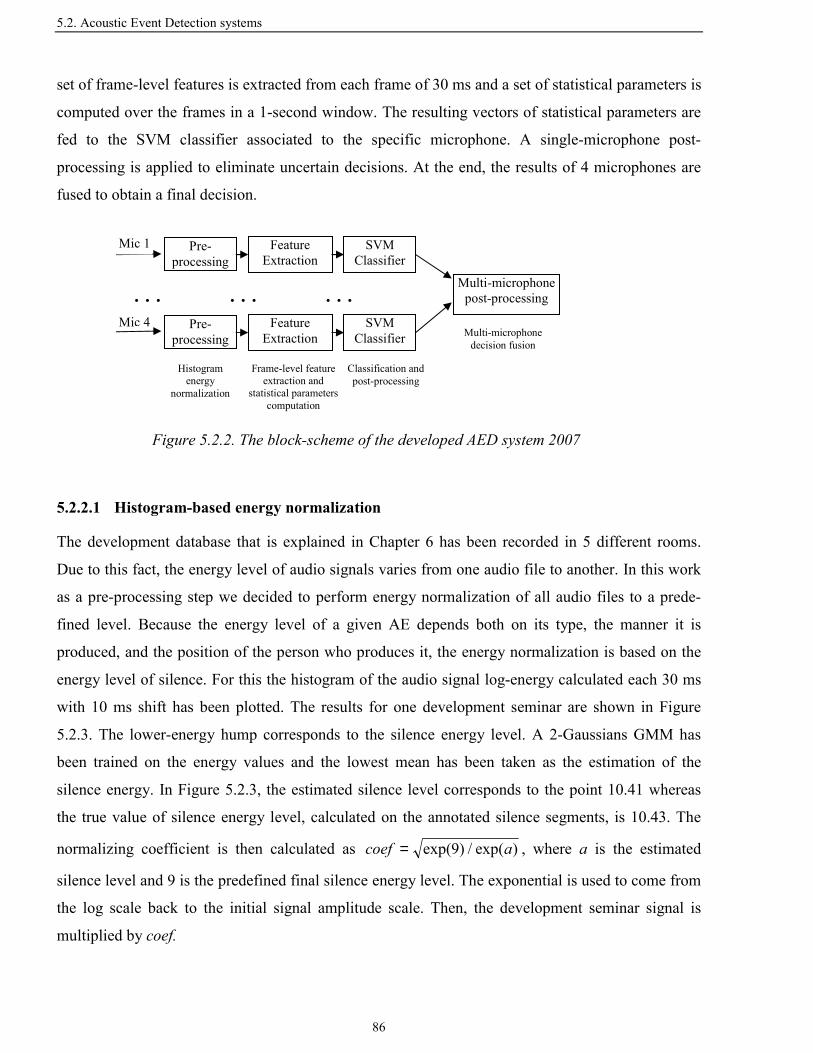
5.2. Acoustic Event Detection systems
86
set of frame-level features is extracted from each frame of 30 ms and a set of statistical parameters is
computed over the frames in a 1-second window. The resulting vectors of statistical parameters are
fed to the SVM classifier associated to the specific microphone. A single-microphone post-
processing is applied to eliminate uncertain decisions. At the end, the results of 4 microphones are
fused to obtain a final decision.
5.2.2.1 Histogram-based energy normalization
The development database that is explained in Chapter 6 has been recorded in 5 different rooms.
Due to this fact, the energy level of audio signals varies from one audio file to another. In this work
as a pre-processing step we decided to perform energy normalization of all audio files to a prede-
fined level. Because the energy level of a given AE depends both on its type, the manner it is
produced, and the position of the person who produces it, the energy normalization is based on the
energy level of silence. For this the histogram of the audio signal log-energy calculated each 30 ms
with 10 ms shift has been plotted. The results for one development seminar are shown in Figure
5.2.3. The lower-energy hump corresponds to the silence energy level. A 2-Gaussians GMM has
been trained on the energy values and the lowest mean has been taken as the estimation of the
silence energy. In Figure 5.2.3, the estimated silence level corresponds to the point 10.41 whereas
the true value of silence energy level, calculated on the annotated silence segments, is 10.43. The
normalizing coefficient is then calculated as )exp(/)9exp( acoef = , where a is the estimated
silence level and 9 is the predefined final silence energy level. The exponential is used to come from
the log scale back to the initial signal amplitude scale. Then, the development seminar signal is
multiplied by coef.
Figure 5.2.2. The block-scheme of the developed AED system 2007
Pre-processing
Feature Extraction
SVM Classifier
Mic 1
: : :
Histogram energy
normalization
Frame-level feature extraction and
statistical parameters computation
Classification and post-processing
Multi-microphone decision fusion
Mic 4 Pre-processing
Feature Extraction
SVM Classifier
Multi-microphonepost-processing : : : : : :

Chapter 5. Acoustic Event Detection
87
5.2.2.2 Feature extraction
The sound signal is down-sampled to 16 kHz, and framed (frame length/shift is 30/10 ms, a Ham-
ming window is used). For each frame, a set of spectral parameters has been extracted. It consists of
the concatenation of two types of parameters (see Section 4.2): 1) 16 FFBE along with the first and
the second time derivatives, and 2) a set of the following parameters: zero-crossing rate, short time
energy, 4 sub-band energies, spectral flux, calculated for each of the defined sub-bands. Addition-
ally, according the importance and degree of interaction shown in see Section 4.5, two features are
added, namely, spectral centroid, and spectral bandwidth, and pitch is eliminated. In total, a vector
of 60 components is built to represent each frame. The mean and the standard deviation parameters
have been computed over all frames in a 1-second window with a 200ms shift, thus forming one
vector of 120 elements.
5.2.2.3 One-microphone SVM system
For AED, SVM classifiers [SS02] have been implemented. They have been trained using the
isolated AEs from the two DBs of IAE explained in Chapter 6, along with segments from the
development data seminars that include both isolated AEs and AEs overlapped with speech. The
segments that contain the overlapping of two or more AEs with or without speech are not used. In
both training and testing processes, a vector of 120 statistical parameters has been computed from
each 1-second window. The 1 vs. 1 multiclass strategy has been chosen to classify among 14 classes
that include “Speech”, “Unknown”, and the 12 evaluated classes of AEs. Besides, “Silence” vs.
“Non-silence” SVM classifier has been trained where “Non-silence” class includes all 14 classes. In
that case, in order to decrease the number of training vectors and make training feasible, the dataset
reduction technique described in following section of this chapter has been applied.
The testing stage scheme is shown in Figure 5.2.4. An input vector of statistical components
computed over the frames from a 1-second window is firstly fed to the “Silence” vs. “Non-silence”
6 8 10 12 14 16 180
500
1000
1500
Figure 5.2.3. Frame log-energy histograms calculated over the whole
seminar signal
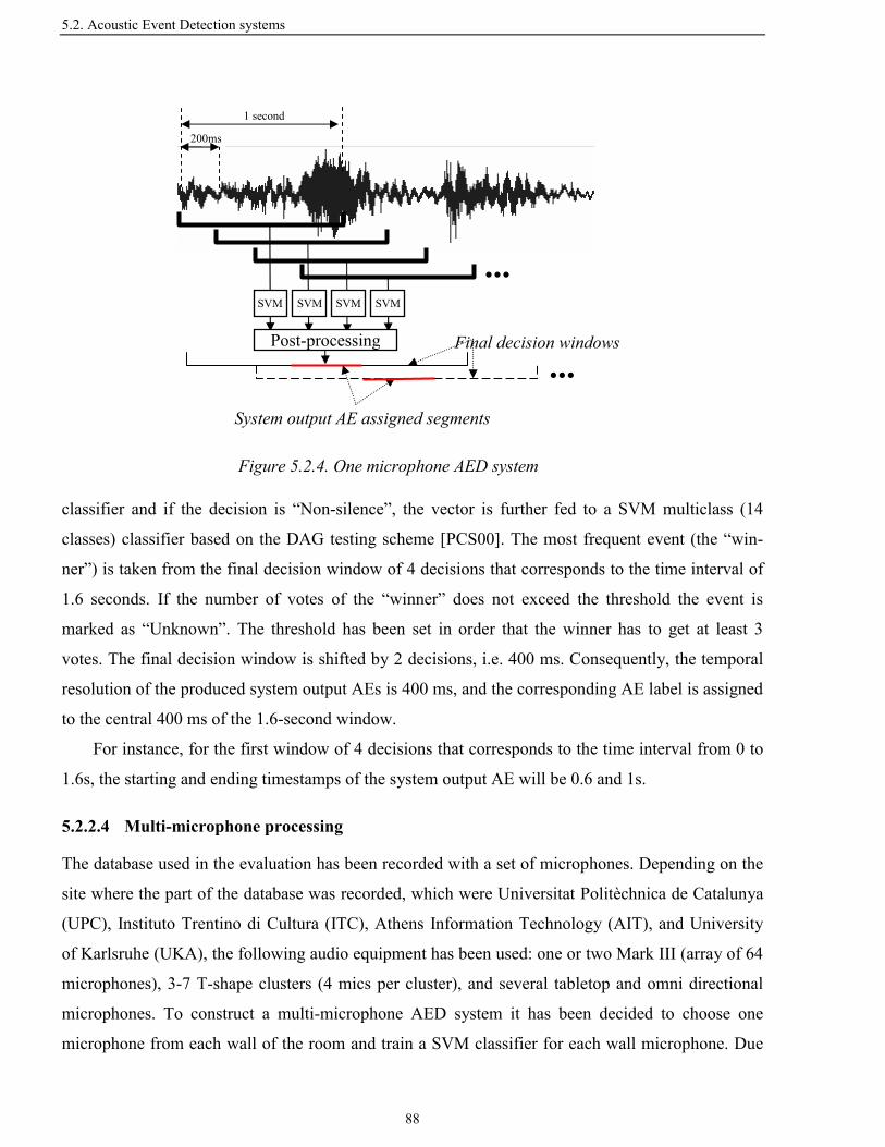
5.2. Acoustic Event Detection systems
88
classifier and if the decision is “Non-silence”, the vector is further fed to a SVM multiclass (14
classes) classifier based on the DAG testing scheme [PCS00]. The most frequent event (the “win-
ner”) is taken from the final decision window of 4 decisions that corresponds to the time interval of
1.6 seconds. If the number of votes of the “winner” does not exceed the threshold the event is
marked as “Unknown”. The threshold has been set in order that the winner has to get at least 3
votes. The final decision window is shifted by 2 decisions, i.e. 400 ms. Consequently, the temporal
resolution of the produced system output AEs is 400 ms, and the corresponding AE label is assigned
to the central 400 ms of the 1.6-second window.
For instance, for the first window of 4 decisions that corresponds to the time interval from 0 to
1.6s, the starting and ending timestamps of the system output AE will be 0.6 and 1s.
5.2.2.4 Multi-microphone processing
The database used in the evaluation has been recorded with a set of microphones. Depending on the
site where the part of the database was recorded, which were Universitat Politèchnica de Catalunya
(UPC), Instituto Trentino di Cultura (ITC), Athens Information Technology (AIT), and University
of Karlsruhe (UKA), the following audio equipment has been used: one or two Mark III (array of 64
microphones), 3-7 T-shape clusters (4 mics per cluster), and several tabletop and omni directional
microphones. To construct a multi-microphone AED system it has been decided to choose one
microphone from each wall of the room and train a SVM classifier for each wall microphone. Due
Figure 5.2.4. One microphone AED system
...
System output AE assigned segments
...
1 second
200ms
SVM
Final decision windows
SVM SVM SVM
Post-processing

Chapter 5. Acoustic Event Detection
89
to the different configuration of the rooms where the development and testing data have been
recorded and due to different numbering of the microphones, a mapping of the microphones across
the sites has been performed. The Mark III microphone array has been chosen as the fixed point. For
the remaining walls the T-shape cluster microphones have been chosen. An example of choice of the
cluster microphones for the UPC’s smart-room is shown in Figure 5.2.5. The following microphone
numbers have been chosen 1-5-9, 6-1-25, 1-5-9, 1-5-9 for the AIT/ITC/UKA/UPC smart-rooms,
respectively. For instance, one SVM has been trained on audio signals from microphones 1, 6, 1, 1
taken from AIT/ITC/UKA/UPC, respectively. For the Mark III array the 3rd microphone has been
chosen across all sites.
For multi-microphone decision fusion, the voting scheme has been used. The AE label with the
largest number of votes is sent to the system output. In case of draw the event is chosen randomly.
Figure 5.2.5. The choice of the microphones for the UPC’s smart-room
0102
03
04
07
05
0608
0910
11
12
MkIII 001
· · ·
MkIII_064
MkIII 003

5.3. Chapter Summary
90
5.3 Chapter Summary
In the current chapter the AED/C systems developed at UPC for the international evaluations of
years 2006 and 2007 have been presented. The features and classifiers have been described. As the
systems have only been evaluated through participation in the international evaluation campaigns,
the results have not been presented in this chapter but will be reported in the next one.

Chapter 6. Participation in International Evaluations
91
Chapter 6. Participation in International Evaluations
6.1 Chapter Overview
The chapter reviews the results obtained with the developed systems for Acoustic Event Classification
(AEC) and Acoustic Event Detection (AED).
Section 6.2 presents the results of the very first dry-run evaluation on AEC. The definition of the
task, metrics and a set of meeting-room acoustic events are given. Then the results of the AEC system
are presented and discussed.
The modifications of the first AEC task definitions and the evaluation setup of the second interna-
tional evaluation on AEC are presented in Section 6.3. New metrics are defined and the results of the
new systems tested on both the previous and the new databases are reported.
In Section 6.4, we present the results of the AED and AEC evaluations carried out in February
2006 by the three participant partners from the CHIL project. The primary evaluation task was AED of
the testing portions of the isolated sound databases and seminar recordings produced in CHIL. Addi-
tionally, a secondary AEC evaluation task was designed using only the isolated sound databases. The
set of meeting-room acoustic event classes and the metrics were agreed by the three partners and
ELDA was in charge of the scoring task.
Next, the AED system developed at the UPC and its results in the CLEAR evaluations carried out
in March 2007 are reported in Section 6.5. The system is based on SVM classifiers and multi-
microphone decision fusion. Also, the current evaluation setup and, in particular, the two new metrics
used in this evaluation are presented.

6.2. CHIL Dry-Run Evaluations 2004
92
6.2 CHIL Dry-Run Evaluations 2004
6.2.1 Introduction
The CHIL-sponsored dry-run evaluations were carried on in spring 2004. The presented technolo-
gies were: ASR – Automatic Speech Recognition, SAD – Speech Activity Detection, Speaker ID –
Speaker Identification, ASL – Acoustic Speaker Localization, and AEC – Acoustic Event Classifi-
cation.
Crucial to the goal of the CHIL project is the ability to determine human context from auditory
or visual cues in the environment. Toward this end, systems to identify common acoustic events in
the first CHIL scenario seminars were developed and evaluated. In this section we describe the first
evaluations that were carried out for the task of AEC.
The section is organized as follows. In Subsection 6.2.2 we present the database of gathered
sounds and the evaluation setup with metrics. The classification techniques are overviewed in
Subsection 6.2.3. The experiments and discussion of the results are presented in Subsection 6.2.4.
Finally, conclusions are given in Subsection 6.2.5.
6.2.2 Database & evaluation setup
The evaluation used CHIL seminar data collected at Universität Karlsruhe in 2003. The seminar
database consists of seven technical seminars. The natural meeting-room settings were designed
without planning acoustic events.
Audio was collected with a combination of microphones. The 3rd channel of a wall-mounted 64-
microphone array (MarkIII array) was used for the AEC evaluation. The data were transcribed with
36 noise classes. Over 2800 individual noise instances were collected. These instances were tran-
scribed with tight temporal bounds, allowing to perform an isolated-sound test.
The sound classes that were transcribed are presented in Table 6.2.1. Additionally, Table 6.2.1
shows number of sound instances that appeared in training and testing data. From all the acoustic
classes the ones that had more than 8 instances for both training and testing were chosen. The
dropped acoustic classes are shown in grey in Table 6.2.1.

Chapter 6. Participation in International Evaluations
93
The dry-run evaluation had two participants: Interactive System Laboratories from Carnegie
Mellon University (ISL-CMU) [Mal06] and our TALP research group from UPC. In this corpus, we
found 25 classes suitable for use in the evaluation: breathing, bang, bump, click, conversation (i.e.
background speech between two parties which is not part of the seminar interaction), cough, paper
crumple, door, exhale, footsteps, inhale, metal, microphone, chair moving, pen, pop, electrical noise,
silence, lip smack, snap, speech, squeak, tap, throat clear, and typing. This set was ad hoc in the
sense that we did not know a priori what kinds of sounds would be present in the database; hence
Table 6.2.1. Evaluated acoustic event classes
Name Train Test Comments Breath 24 33 Bang 2 6 Bump 59 79 Chair moving 5 1 A chair being moved Click 34 48 Conv 8 4 Conversation (simultaneous speech) Cough 4 10 Crump 3 6 Paper crumple Door 11 8 Door slams E 11 8 Expiration Fan 0 3 Foot 3 10 Steps I 288 267 Inspiration Keyb 83 76 Keyboard typing Knock 1 0 Door/table knock Laugh 1 1 Metal 3 7 Metallic noise Mic 15 14 Microphone noise Mn 4 2 An unidentified mouth noise Mov 8 27 Movement, someone moving N 1 3 Generic noise Pen 2 10 Pen, pencil, whiteboard-pen writing Pop 5 6 Punch 0 1 Puncher & stapler Rattle 1 1 Shh 24 17 Steady environmental noise Silence 715 630 Smack 19 15 Smack, pressing the lips together Snap 8 12 Sniff 4 2 Speech 1309 1209 Squeak 10 14 Tap 10 5 Throat 10 4 Throat noise Wh 2 0 Whistle Whir 2 5 Whirring

6.2. CHIL Dry-Run Evaluations 2004
94
we relied on transcriber’s judgment to select the noise set. This decision resulted in a large amount
of class overlap (e.g. “bang” and “bump”), but it was important to determine which classes were
actually present in quantity.
The dry run data consisted of isolated sound segments only. There were 2805 total segments,
which we divided into training (1425 segments) and evaluation sets (1380) at random.
Accuracy and recall were used as metrics in the evaluations. The former is defined as the num-
ber of correctly classified acoustic events divided by the total number of acoustic events. Recall is
defined as a mean of the individual class recalls calculated as the number of correctly-classified
events of a particular class divided by the number of events of that class.
6.2.3 Developed systems
In the evaluations we used the front-end described in Subsection 4.3.3. Namely, the signals from all
the sounds in the database presented above were downsampled to 8kHz, normalized to be in the
range [-1 1], and partitioned in frames using: frame length=128, overlapping of 50%, and a Ham-
ming window. The silence portions of the signals were removed using an energy threshold. We
tested all 9 acoustic feature sets presented in the Subsection 4.3.3, specifically, a set of perceptual
features (Perc), a set of cepstral coefficients (MFCC), a set of frequency-filtered features (FF), and
combinations of the formers. The mean, standard deviation of those features, estimated by averaging
over the whole acoustic event signal, were taken for classification, thus forming one final statistical
feature vector per audio event with a number of elements which doubles the length of the acoustic
feature set. Besides, along with the mean and standard deviation we decided to calculate the autocor-
relation coefficient at the second lag and the entropy, to compare the results with and without the
last two statistical parameters.
GMM and SVM classifier were used as alternative back-ends of the developed systems. Both
classifiers were compared across all available feature sets. For the SVM case, we used the binary
tree scheme that is explained in Subsection 4.3.5.1.
6.2.4 Results and discussion
The best results were obtained using the 3rd feature set (E + MFCC) for GMM and the 8th for SVM
(Perc + FF + ∆FF + ∆∆FF). Interestingly enough, that the best results with GMM were obtained
with mean and standard deviation of the 3rd feature set while, in the case of SVM, the set of mean,
standard deviation, autocorrelation coefficient at the second lag, and entropy calculated over the 8th

Chapter 6. Participation in International Evaluations
95
feature set showed the best performance. The best GMM and SVM results are summarized in Table
6.2.2.
As it can be seen from Table 6.2.2, the worst (at times 0%) performance is obtained for the
classes with small number of acoustic event instances for training, like “bang”, “crump”, “foot”.
Also we can see from Table 6.2.2, that for most classes, SVM shows better performance than GMM,
finally achieving better accuracy and recall. Additionally, Table 6.2.2 shows the baseline recall and
accuracy calculated as if the system always guesses the most frequent class i.e. “speech” in our case.
As it can be seen, the accuracy of GMM is even worse than that of the baseline; however the GMM
recall is much higher. SVM system clearly outperforms the baseline for both metrics.
The accuracy metric is affected by the imbalance of the number of instances per acoustic event
Table 6.2.2. Results of the dry-run evaluations on AEC
Recall for Each Class (%) Event GMM SVM
b 10.61 3.03 bang 0 0 bump 22.78 41.77 click 19.57 30.43 conv 25.00 0 cough 15.00 40.00 crump 0 0 door 50.00 62.50
e 25.00 0 foot 0 0
i 52.81 74.00 keyb 37.50 60.53 metal 0 0 mic 3.57 7.14 mov 1.85 0 pen 0 0 pop 0 0 shh 8.82 17.65
silence 56.20 58.00 smack 13.33 26.67 snap 12.50 0
speech 96.00 100.00 squeak 21.43 7.14
tap 0 0 throat 62.50 75.00
Baseline (Recall) 4.0
Baseline (Accuracy) 47.8 Recall 21.38 24.15
Accuracy 47.4 55.1

6.2. CHIL Dry-Run Evaluations 2004
96
classes, so that the good performance shown for “speech” class contributed significantly to the
accuracy metric.
It is worth to note that the low system performance is attributable to the noisy conditions of the
recorded seminars (far-field microphone, reverberation, etc). Besides, the annotation of acoustic
events describes them from a semantic point of view while acoustically most of classes are similar
(“bump” and “bang”, “shh” and “silence”, etc.). Additionally, the high number of acoustic classes
made it rather difficult to correctly transcribe the seminars, resulting in a number of outliers.
6.2.5 Conclusions
The first official evaluation of acoustic event classification was carried out in 2004 and has been
described in this section. In that pioneering work, the set of meeting room acoustic events has been
defined based on the number of acoustic event instances and the metric has been agreed by the
participants. Previously developed systems have been applied to the AEC task and comparative
results have been obtained.

Chapter 6. Participation in International Evaluations
97
6.3 CHIL Evaluations 2005
6.3.1 Introduction
The first year of the CHIL project concluded with the CHIL evaluation campaign in January 2005,
followed by the first CHIL evaluation workshop, which took place in Athens on 20th and 21st of
January 2005.
During this campaign, 12 technological components were evaluated: 5 vision technologies (face
detection, visual person tracking, visual speaker identification, head pose estimation, and hand
tracking); 6 sound and speech technologies (close-talking automatic speech recognition, far-field
automatic speech recognition, acoustic person tracking, acoustic speaker identification, speech
activity detection, acoustic scene analysis; and 1 contents processing technology (automatic summa-
rization). AEC, along with acoustic environment classification, were considered subtasks of the
acoustic scene analysis task.
As it was mentioned the goal of the AEC efforts in the CHIL project is to provide situation
awareness to smart CHIL spaces by monitoring ambient audio. Many events which carry semantic
relevance to scene understanding cannot be detected by visual analysis, but are relatively easy to
detect with auditory analysis. Some of these events are speech-related and can thus be handled by
SAD or ASR systems. Many others, however, are not speech-related and must be dealt with sepa-
rately. Examples of these types of events include applause, doors opening and closing, knocking on
doors, telephones ringing, music, and electrical noise characteristic of some piece of office equip-
ment like a printer or fax machine. The CHIL AEC task was conceived to reliably classify sounds
like these, along with speech and other human noises.
The section is organized as follows. In Subsection 6.3.2 we present the database of gathered
sounds and the evaluation setup with metrics. The classification techniques are overviewed in
Subsection 6.3.3. The experiments and discussion of the results are presented in Subsection 6.3.4.
Finally, conclusions are given in Subsection 6.3.5.
6.3.2 Database & evaluation setup
ISL-CMU and UPC were also the only participants in the AEC evaluation 2005. For this evaluation,
we worked to limit the number of classes to those which were both easy for transcribers to identify
and semantically relevant to the CHIL task. However, as we wished to retain a label for every sound
in the corpus, whether it was easily identifiable or not, we split the label set into two types, semantic
labels and acoustic labels. Semantic labels correspond to specific named sounds with CHIL rele-

6.3. CHIL Evaluations 2005CHIL Evaluations 2005
98
vance; e.g. doors slamming, speech, etc. The semantic classes that were annotated are presented in
Table 6.3.1. In total there are 8 human noises and 13 environmental noises. Based on the availability
of samples per class, the following 15 semantic classes were finally chosen for evaluation: breath-
ing, chair moving, click, door, footsteps, laughter, mouth noise, papers, silence, speech, throat,
typing, and electrical noise.
Acoustic labels correspond to unnamed sounds which are either unidentifiable or have no CHIL
relevance. The acoustic labels use names describing both tonal and rhythmic features of a sound.
The set of acoustic-labelled sounds consists of continuous non-tonal sounds, continuous tonal
sounds, single non-continuous sounds, non-continuous sounds repeated in a regular pattern, non-
continuous sounds repeated in an irregular pattern, and other noises. Table 6.3.2 shows the acoustic
classes used in the evaluations.
Table 6.3.1. Annotated semantic classes
Class Description
Human Noises [b] Breathe (in general, when it is not possible to be more precise) [lgh] Speaker laughing [thr] Throat noise /Cough [tsk] Willful noise made to express one’s disagreement: “tsk tsk tsk…” [conv] Whisper or conversation in the background [mn] Generic mouth noise (including smacks) [snif] Sniffing [sp] Speech segment Non-speech, environment noises [app] Hand clapping, audience applauding [beep] Some device beeping [click] Click [chr] A chair being moved [door] A door opening, closing, slamming or grating [fst] Footsteps [key] Keys jiggling or being knocked on a surface. [mus] Some music, e.g. radio or mobile phone [pap] The noise of some action done with paper sheets [sil] Silence (more or less, event if there is a background noise global
to the recording) [typ] Someone typing on a keyboard [unk] Unknown [whir] Some kind of electrical whirring

Chapter 6. Participation in International Evaluations
99
It was decided to perform two independent evaluations: acoustic and semantic. For acoustic
evaluation, all semantically-labelled classes were mapped to the corresponding acoustic classes. The
mapping is shown in the Table 6.3.3.
Like in the dry-run, the AEC evaluation set consisted of isolated sounds only, collected in
seminars at Universität Karlsruhe. The data were split into a training set, a development test set, and
an evaluation set. There were 7092 total segments; 3039 were used for training (1946 speech, 333
breath, 333 silence, 232 unk, 44 footsteps, 24 throat, 16 click, 15 paper…), 2949 for development
testing (749 speech, 183 unk, 139 silence, 9 throat, 9 breath, 7 typing…), and 1104 for evaluation
(2084 speech, 348 silence, 274 unk, 123 breath, 30 throat, 25 footsteps, 18 chair…).
The far-field microphone, that was the 4th channel of MarkIII microphone array, was used in the
entire evaluation. Participants were permitted to use for system training only the data distributed for
this evaluation and identified as training data. No other data were allowed for training purposes,
though development data may be used for strobe testing and cross-validation.
For measuring the performance, the error rate metric was exploited. It is defined as 1 – accu-
racy. The accuracy is calculated as the number of correctly classified acoustic events divided by the
total number of acoustic events.
Table 6.3.2. Evaluated acoustic classes
Class Description [c-t] Continuous tone [c-nt] Continuous sound without tone [nc-s] Single non-continuous sound [nc-xreg] Regular repetitive non-continuous sound [nc-xirr] Irregular repetitive non-continuous sound [n] Generic noise, all other kinds of sounds
Table 6.3.3. Semantic acoustic mapping
Semantic label Acoustic label [lgh], [sp] c-t
[b], [snif], [pap], [whir], [thr] c-nt [click], [chr], [door], [mn] nc-s
[fst] nc-xreg [typ] nc-xirr

6.3. CHIL Evaluations 2005CHIL Evaluations 2005
100
6.3.3 Developed systems
In the AEC evaluation 2005, we used an SVM-based variable-feature-set clustering approach, i.e. an
enhanced version of the dry-run SVM binary tree scheme system. The idea is to choose the most
appropriate feature sets on each step of classification. The hierarchical structure of the final system
is constructed based on the confusion matrices obtained from initial experiments. The system is
described in details in Subsection 4.3.
As feature sets, various perceptual and conventional spectral representations of the signal were
used. The experiments in the dry-run evaluations explained above showed that SVM obtained better
results with two additional statistical parameters – autocorrelation and entropy. Thus, instead of only
mean and standard deviation, both the mean, standard deviation, autocorrelation coefficient at the
second lag, and entropy were calculated from the whole event.
6.3.4 Results and discussion
The results of the evaluations were presented at the HSCMA’05 workshop in March 2005
[MMT+05] and are shown in Table 6.3.4. As it can be seen from Table 6.3.4 the proposed confu-
sion-matrix-based SVM clustering approach improves the results obtained with the SVM binary tree
on the dry-run evaluation database. Additionally, Table 6.3.4 shows the baseline error rate calcu-
lated as if the system always guesses the most frequent class i.e. “speech” in case of semantic set
and “continuous tone” in case of acoustic set. The obtained results are clearly better than the base-
line.
The AEC evaluation 2005 was unfortunately suffering from problems of corpus. Transcription
mistakes were still quite frequent; hence, the labels were not as reliable as they could have been.
Further, the corpus was extremely unbalanced; a large majority of the segments were made up of
speech. Many interesting classes had only a few examples in the training or test sets, and hence were
not well-modelled by our systems.
Table 6.3.4. Results of the AEC evaluations 2005
Dry-run database 2005 year database Dry-run systems 2005 year SVM system
GMM SVM 2005 year
SVM system Acoustic set Semantic set Error rate 52.6% 44.9% 37.1% 22.11% 18.51% Baseline Error rate 52.2% 29.3% 29.4%

Chapter 6. Participation in International Evaluations
101
6.3.5 Conclusions
The 2005 CHIL evaluation of acoustic event classification has been carried out and described in this
section. The set of meeting room acoustic events has been defined. Along with a semantic AEC, an
acoustic AEC task has been proposed and performed. An appropriate mapping between the semantic
set and the acoustic set of acoustic events has been established. The developed SVM-based variable-
feature-set clustering scheme presented in Subsection 4.3.5.2 has been applied to the AEC task. The
results of the 2004 AEC evaluations have been improved and comparative results for the new
database of 2005 have been obtained. For the future, it was decided to limit to a group of events
relevant to actual CHIL services. For the purpose of measuring the performance of AEC, the largely
prevailing “speech” class was proposed to be eliminated from scoring. Besides, we planned to move
from classification to detection of a limited number of transcribable acoustic events like doors,
applause, laughing, etc. In order to have a sufficient number of non-speech acoustic events, intro-
ducing the scenario of the recordings is crucial.

6.4. Classification of Events, Activities and Relationships – CLEAR'06 Evaluation and Workshop
102
6.4 Classification of Events, Activities and Relationships – CLEAR'06 Evaluation and Workshop
6.4.1 Introduction
The spring 2006 CLEAR evaluation and workshop was an international effort to evaluate systems
that are designed to analyze people, their identities, activities, interactions and relationships in
human-human interaction scenarios, as well as related scenarios. CLEAR was meant to bring
together projects and researchers working on related technologies in order to establish a common
international evaluation campaign in this field. The CLEAR 2006 evaluation was supported by the
European Integrated project CHIL, the US ARDA VACE program, and the NIST.
The tasks to be addressed in CLEAR 2006 were the following: Person Tracking (2D and 3D,
audio-only, video-only, and multimodal), Face Tracking, Head Pose Estimation (2D, 3D), Person
Identification (audio-only, video-only, and multimodal), Acoustic Event Detection and Classifica-
tion (AED/C). These tasks were conducted on various multimodal data sets collected in lecture and
meetings domains, as well as on broadcast news data.
The results of the evaluations were presented during the CLEAR 2006 evaluation workshop
held on April 6-7, in Southampton, UK. The CLEAR 2006 post-workshop proceedings are available
under the Springer LNCS book series: LNCS 4122: Multimodal Technologies for Perception of
Humans.
In this section, we present the results of the AED/C CLEAR evaluations carried out by three
participants UPC, CMU and Instituto Trentino di Cultura (ITC). The primary evaluation task was
AED of the testing portions of the two isolated sound databases (from ITC and UPC) and 4 UPC’s
seminar recordings produced in CHIL. Additionally, a secondary AEC evaluation task was designed
using only the isolated sound databases and it is also included in this report. All the participants
agreed the set of acoustic classes a priori before recording the databases. A common metrics was
also developed at the UPC and agreed with the other partners. ELDA was in charge of the scoring
task.
The section is organized as follows: Subsection 6.4.2 gives the experimental setup. Specifically,
the databases used in the evaluations are described in Subsection 6.4.2.1, while the evaluation
scenario and metrics are given in Subsection 6.4.2.2 and 6.4.2.3, respectively. Subsection 6.4.3
reviews the systems used by each of the AED/C evaluation participants. The results obtained by the
detection and classification systems in the CLEAR evaluations are shown and discussed in Subsec-
tion 6.4.4. Conclusions are presented in Subsection 6.4.5.

Chapter 6. Participation in International Evaluations
103
6.4.2 Evaluation setup
6.4.2.1 Databases
The conducted experiments were carried out on 2 different kinds of databases, namely: 2 databases
of isolated acoustic events recorded at the UPC and ITC, and 5 interactive seminars recorded at the
UPC.
The two former databases contain a set of isolated acoustic events that occur in a meeting room
environment and were recorded specially for the CHIL AED/C task. The recorded sounds do not
have temporal overlapping and no interfering noises were present in the room.
The UPC database of isolated acoustic events (see Appendix A for the detailed description) was
recorded using 84 microphones, namely, Mark III (array of 64 microphones), three T-shape clusters
(4 mics per cluster), 4 tabletop directional, and 4 omni-directional microphones. The database
consists of 13 semantic classes plus “unknown”. Approximately 60 sounds per each of the sound
classes were recorded as shown in Table 6.4.1. Ten people participated in recordings: 5 men and 5
women. There are 3 sessions per each participant. At each session, the participant took a different
place in the room out of 7 fixed different positions.
The ITC database of isolated acoustic events [ZO05] was recorded with 32 microphones. They
were mounted in 7 T-shaped arrays (composed by 4 microphones each one) plus there were 4 table
microphones. The database contains 16 semantic classes of events. Approximately 50 sounds per
almost each of the sound classes were recorded as shown in Table 6.4.1. 9 people participated at the
recordings. For each experiment 4 positions in the room were located. People swapped their posi-
tions after every session. During each session every person reproduced a complete set of acoustic
events.
Additionally, the AED techniques were applied to the database of the interactive seminars
[CS04] recorded at the UPC. 5 interactive seminars have been collected. The difference with two
previous databases of isolated acoustic events is that seminars consist of real environment events
that may have temporal overlapping with speech and/or other acoustic events. Each seminar consists
of a presentation of 10-20 minutes to a group of 3-5 attendees in a meeting room. During and after
the presentation there are questions from the attendees with answers from the presenter. There is
also activity in terms of people entering/leaving the room, opening and closing the door, standing up
and going to the screen, some discussion among the attendees, coffee breaks, etc. The databases was
recorded using 88 different sensors that include 3 4-microphoned T-shaped arrays, 1 64-microphone

6.4. Classification of Events, Activities and Relationships – CLEAR'06 Evaluation and Workshop
104
Mark III array, 4 omni-directional table-top microphones, 4 directional table-top microphones, and 4
close-talk microphones. The number of events of one of the seminars is summarized in Table 6.4.1.
6.4.2.2 Evaluation scenario
The AED/C evaluation is done on 12 semantic classes that are defined as:
• Knock (door, table) [kn]
• Door slam [ds]
• Steps [st]
• Chair moving [cm]
• Spoon (cup jingle) [cl]
• Paper wrapping [pw]
• Key jingle [kj]
• Keyboard typing [kt]
• Phone ringing/Music [pr]
• Applause [ap]
Table 6.4.1. Number of events for the UPC and ITC databases of isolated acoustic events, and the UPC interactive seminar
Number of events Event type UPC-
isolated ITC-
isolated UPC-
seminar Door knock 50 47 4 Door open 60 49 7 Door slam 61 51 7 Steps 73 50 43 Chair moving 76 47 26 Spoon/cup jingle 64 48 15 Paper work 84 48 21 Key jingle 65 48 2 Keyboard typing 66 48 14 Phone ring 116 89 6 Applause 60 12 2 Cough 65 48 5 Laugh 64 48 8 Unknown 126 12 Mimo pen buzz 48 Falling object 48 Phone vibration 13 Speech 169

Chapter 6. Participation in International Evaluations
105
• Cough [co]
• Laugh [la]
Also there are two other possible events that are present but are not evaluated
• Speech [sp]
• Unknown [un]
Actually, the databases of isolated acoustic events contain more semantic classes than the above-
proposed list as shown in Table 6.4.1. For that reason, the classes that are out of the scope of the
current AED/C evaluation were marked as “unknown”.
Two main series of experiments are performed: AED and AEC. AED was done in both isolated
and real environment conditions. For the task of AEC and isolated AED the databases of isolated
acoustic events were split into training and testing parts, namely, for the UPC database sessions 1
and 2 were used for training and session 3 for testing; for the ITC database sessions 1-3 were used
for training and session 4 for testing. For the task of AED in real environment all databases of
isolated acoustic events and one of five seminars were allowed to use for training and developing,
while for testing a 5-minute extract from each of the remaining 4 seminars was proposed forming in
total 4 five-minute segments. The selection of extracted parts was done by ELDA.
The primary evaluation task was defined as AED evaluated on both the isolated databases and
the seminars.
6.4.2.3 Metric
As it was mentioned above, the acoustic events that happen in real environment may have temporal
overlapping. The appropriate metric was developed to score the system outputs. It consists of two
steps: projecting all levels of overlapping events into a single-level reference transcription and
comparing a hypothesized transcription with the single level reference transcription.
For instance, let’s suppose we have a reference that contain overlapping of level 2 and can be
represented as shown in Figure 6.4.1 and
REF_1: _la_kt_
REF_2: _co_ds_cl_la_
where REF_1 and REF_2 model two overlapping acoustic event sequences. Then we can form the
single-level reference transcription and a list of events to detect as shown in Table 6.4.2.
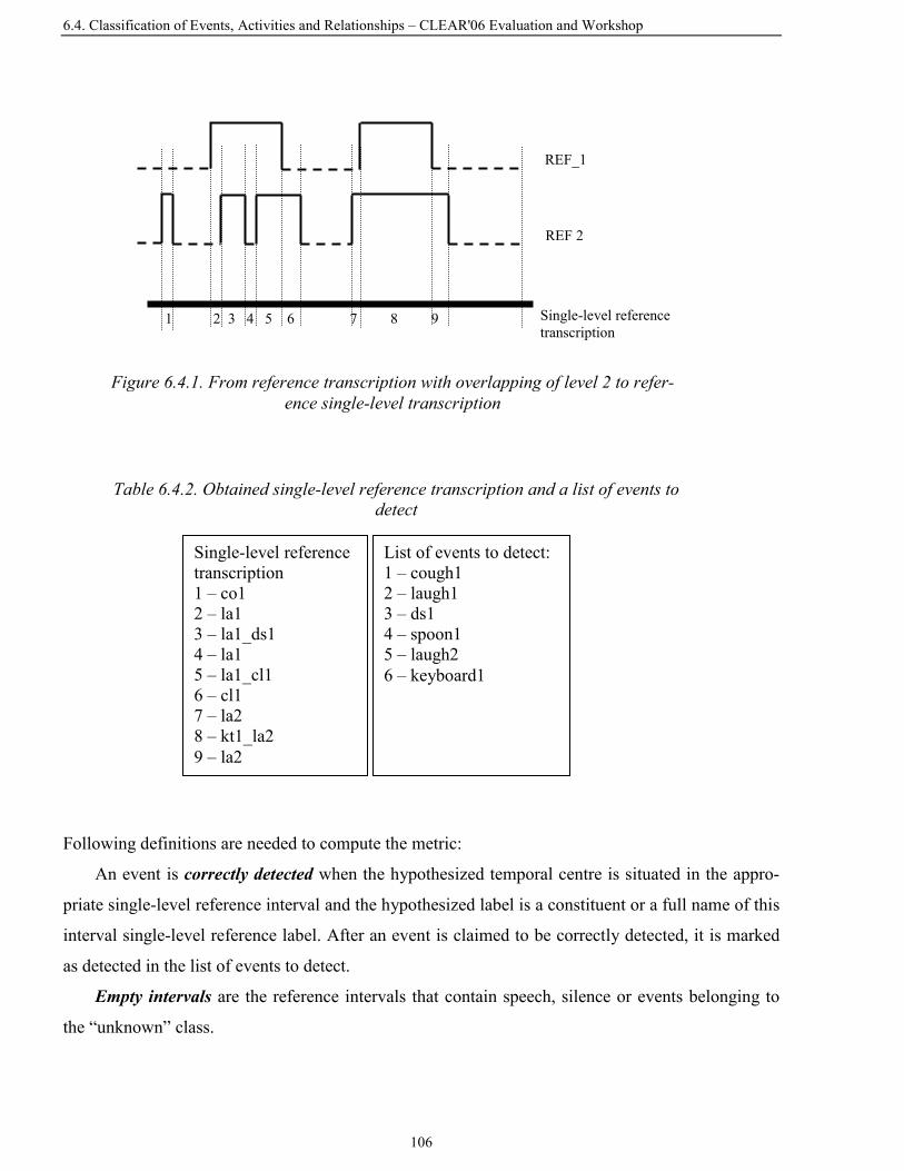
6.4. Classification of Events, Activities and Relationships – CLEAR'06 Evaluation and Workshop
106
Following definitions are needed to compute the metric:
An event is correctly detected when the hypothesized temporal centre is situated in the appro-
priate single-level reference interval and the hypothesized label is a constituent or a full name of this
interval single-level reference label. After an event is claimed to be correctly detected, it is marked
as detected in the list of events to detect.
Empty intervals are the reference intervals that contain speech, silence or events belonging to
the “unknown” class.
Figure 6.4.1. From reference transcription with overlapping of level 2 to refer-ence single-level transcription
Table 6.4.2. Obtained single-level reference transcription and a list of events to detect
Single-level reference transcription
1 2 3 4 5 6 7 8 9
REF_1
REF 2
Single-level reference transcription 1 – co1 2 – la1 3 – la1_ds1 4 – la1 5 – la1_cl1 6 – cl1 7 – la2 8 – kt1_la2 9 – la2
List of events to detect: 1 – cough1 2 – laugh1 3 – ds1 4 – spoon1 5 – laugh2 6 – keyboard1

Chapter 6. Participation in International Evaluations
107
A substitution error occurs when the temporal centre of the hypothesized event is situated in
the appropriate single-level reference interval and the label of the hypothesized event is not constitu-
ent or the full name of the label of that single-level reference interval.
An insertion error occurs when the temporal centre of the hypothesised event is not situated in
any of the single-level reference intervals (i.e. are situated in empty intervals)
A deletion error occurs when there is an event in the list of events to detect that is not marked
as detected.
Finally, Acoustic Event Error Rate (AEER) is computed as
AEER= (D+I+S)/N * 100
where N is the number of events to detect, D – deletions, I – insertions, and S – substitutions.
6.4.3 Acoustic event detection and classification systems
The system of AED and AEC are explained in Subsection 5.2.1. Briefly, for classification, a vector
of statistical parameters that include mean, standard deviation, autocorrelation and entropy is
calculated from the frame-level acoustic features of the whole event, and fed to the SVM-based
event classifier (system UPC-C). For detection, a vector of statistical parameters is calculated from a
sliding window and then fed to an SVM-based silence/non-silence classifier to perform the segmen-
tation step. The silence/non-silence classifier is trained on silence and non-silence segments of the
two isolated acoustic events databases. At the output, a binary sequence of decisions is obtained.
After a post-processing of the sequence the SVM-based event classifier, which is trained on the
events taken from both two isolated acoustic event databases and development seminars, is applied
to each detected non-silence segment. After smoothing a final decision is made (system UPC-D).
6.4.4 Results and discussion
Table 6.4.3 shows classification error rates obtained using the classification system described above.
The UPC system used one set of models for the both testing databases. In fact, the SVM-based
system obtained best error rate among all the participants despite the fact that database-specific
systems were not used for SVM.
In the detection task we took and approach of first performing segmentation and then classifica-
tion. Table 6.4.3 shows detection error rates for the two isolated event databases and the interactive
seminar database. Although our system achieved the best results among all submitted systems in
classification, in detection the results are much worse. If we add up the results obtained for the
detection task for both isolated and seminar conditions the error rate of 69.6% is calculated. Al-

6.4. Classification of Events, Activities and Relationships – CLEAR'06 Evaluation and Workshop
108
though there might be a number of reasons to explain the bad performance of the AED-D system we
conjecture that the initial segmentation step is the main cause of the lower overall detection per-
formance. Further investigation is needed in the direction of the approach to see whether it can
outperform the well-established scheme that is used in ASR. Besides, it can be seen from the Table
6.4.3, the error rates increase significantly for the UPC seminar database, although being the lowest
among all submitted systems. One of possible reasons of such a bad performance is that it is difficult
to detect low-energy acoustic classes that overlap with speech, such as e.g. “chair moving”, “steps”,
“keyboard typing”, and “paper work”. Actually, these classes cover the majority of the events in the
UPC seminars and probably they are the cause of the bad results we obtained in the seminar task. A
usage of multiple microphones might be helpful in this case.
6.4.5 Conclusions
The presented work has focused on the CLEAR evaluation tasks concerning the detection and
classification of acoustic events that may happen in a lecture/meeting room environment. In this
context, we have evaluated two different tasks, acoustic event classification and acoustic event
detection, AED being the primary objective of the evaluation. Two kinds of databases have been
used: two databases of isolated acoustic events and a database of interactive seminars containing a
significant number of acoustic events of interest.
Preliminary detection and classification systems have been presented. Our system is based on
the SVM discriminative approach and uses FF features and four kinds of perceptual features. In the
classification task, the UPC SVM-based system showed the best performance over all participants.
In the detection task, first performing segmentation and then classification showed worse perform-
ance than merging the segmentation and classification in one step as performed by the Viterbi search
in the state-of-the-art ASR systems.
Table 6.4.3. Error rate (in %) for acoustic event classification and detection tasks
SystemsDatabases UPC-C UPC-D
ITC isolated DB 4.1 64.6 UPC isolated DB 5.8 58.9 UPC seminars DB 97.1
Chapter 6. Participation in International Evaluations
109
6.5 Classification of Events, Activities and Relationships – CLEAR'07 Evaluation and Workshop
6.5.1 Introduction
After the AED evaluation within the CLEAR evaluation campaign 2006, explained in the previous
section, organized by the CHIL project, several modifications have been introduced into the task for
the CLEAR evaluation campaign 2007. The old metric has been substituted by two new metrics:
Accuracy and Error Rate, which are based, respectively, on precision/recall and on a temporal
measure of detection error. Additionally, AED is performed only in seminar conditions, where the
AEs are often overlapped with speech and/or other AEs. The definition of the classes of AEs is kept.
Six participants submitted their systems for CLEAR 2007, namely: Athens Information Tech-
nology (AIT), Institute for Infocomm Research (IIR), Foundation Bruno Kessler (IRST), Tampere
University of Technology (TUT), University of Illinois (UIUC), Technical University of Catalonia
(UPC).
The results of the evaluations were presented during the CLEAR 2007 evaluation workshop
held on May 9-10, in Baltimore, USA. The CLEAR 2007 post-workshop proceedings will soon be
available under the Springer LNCS book series: Multimodal Technologies for Perception of Hu-
mans.
In this section, after presenting the current evaluation setup and, in particular, the two new met-
rics used in this evaluation, we describe the AED system developed at the UPC and submitted to the
CLEAR evaluations carried out in March 2007 along with its results.
The section is organized as follows. In Subsection 6.5.2 the evaluation setup is presented. Spe-
cifically, the definition of the task is given in Subsection 6.5.2.1. Subsection 6.5.2.2 describes the
databases assigned to development and testing. Metrics are given in Subsection 6.5.2.3, and Subsec-
tion 6.5.2.4 states the main evaluation conditions. The short overview of the proposed system is
given in Subsection 6.5.3. The results obtained by the detection system in the CLEAR evaluations
are shown and discussed in Subsection 6.5.4. Conclusions are presented in Subsection 0.
6.5.2 Evaluation setup
6.5.2.1 Acoustic event classes
The AED evaluation use the same 12 semantic classes, i.e. types of AEs, used in the past evaluations
CLEAR 2006. The semantic classes with the corresponding annotation label are shown in black in

6.5. Classification of Events, Activities and Relationships – CLEAR'07 Evaluation and Workshop
110
the first column of Table 6.5.1. Apart from the 12 evaluated classes, there are 3 other possible events
shown in grey in Table 6.5.1 which are not evaluated.
6.5.2.2 Databases
The database used in the CLEAR evaluation campaign 2007 consists of 25 interactive seminars of
approximately 30 min long each that have been recorded by AIT, ITC, IBM, UKA, and UPC in their
smart-rooms.
Five interactive seminars (one from each site) were assigned for system development. Along
with the seminar recordings, the databases of isolated AEs recorded at UPC (Appendix A) and ITC
[ZO05] have been used for development.
The development database details in terms of the number of occurrences per AE class are
shown in Table 6.5.1. In total, development data consists of 7495 seconds, where 16% of total time
is AEs, 13% is silence, and 81% is “Speech” and “Unknown” classes.
The remaining interactive seminars have been conditionally decomposed into 5 types of acous-
tic scenes: “beginning”, “meeting”, “coffee break”, “question/answers”, and “end”. After observing
the “richness” of each acoustic scene type in terms of AEs, 20 5-minute segments have been ex-
tracted by ELDA maximizing the AE time and number of occurrences per AE class. The details of
Table 6.5.1. Number of occurrences per acoustic event class for the development and test data
Number of Occurrences Development Test Event Type
UPC iso ITC iso Seminars Seminars Door knock [kn] 50 47 82 153
Door open/slam [ds] 120 100 73 76 Steps [st] 73 50 72 498
Chair moving [cm] 76 47 238 226 Spoon/cup jingle [cl] 64 48 28 28
Paper work [pw] 84 48 130 88 Key jingle [kj] 65 48 22 32
Keyboard typing [kt] 66 48 72 105 Phone ring [pr] 116 89 21 25 Applause [ap] 60 12 8 13
Cough [co] 65 48 54 36 Laugh [la] 64 48 37 154
Unknown [un] 126 - 301 559 Speech [sp] - 1224 1239 Silence Not annotated explicitly

Chapter 6. Participation in International Evaluations
111
the testing database are given in Table 6.5.1. In total, the test data consist of 6001 seconds, where
36% are AE time, 11% are silence, and 78% are “Speech” and “Unknown” classes. Noticeably,
during about 64% of time, the AEs are overlapped with “Speech” and during 3% they are over-
lapped with other AEs. In terms of AE occurrences, more than 65% of the existing 1434 AEs are
partially or completely overlapped with “Speech” and/or other AEs
6.5.2.3 Metrics
Two metrics have been developed at the UPC, with the agreement of the other participating partners
which are involved in CHIL: an F-score measure of detection accuracy (which combines recall and
precision), and an error rate measure that focuses more on the accuracy of the endpoints of each
detected AE. They have been used separately in the evaluations, and will be called, respectively,
AED-ACC and AED-ER.
AED-ACC
The aim of this metric is to score detection of all instances of what is considered as a relevant AE.
With this metric it is not important to reach a good temporal coincidence of the reference and system
output timestamps of the AEs but to detect their instances. It is oriented to applications like real-time
services for smart-rooms, audio-based surveillance, etc. AED-ACC is defined as the F-score (the
harmonic mean between precision and recall):
RecallPrecision*Recall*PrecisionACCAED
++=− 2
2 *)1(β
β ,
where
AEsoutputsystemallofnumberAEsoutputsystemcorrectofnumberPrecision =
AEsreferenceallofnumberAEsreferenceecteddetcorrectlyofnumbercallRe =
and β is a weighting factor that balances precision and recall. In this evaluation the factor β has been
set to 1. A system output AE is considered correct or correctly produced either if there exist at least
one reference AE whose temporal centre is situated between the timestamps of the system output
AE and the labels of the system output AE and the reference AE are the same, or if the temporal
centre of the system output AE lies between the timestamps of at least one reference AE and the
labels of the system output AE and the reference AE are the same. A reference AE is considered
correctly detected either if there exist at least one system output AE whose temporal centre is

6.5. Classification of Events, Activities and Relationships – CLEAR'07 Evaluation and Workshop
112
situated between the timestamps of the reference AE and the labels of the system output AE and the
reference AE are the same, or if the temporal centre of the reference AE lies between the timestamps
of at least one system output AE and the labels of the system output AE and the reference AE are
the same.
AED-ER
For some applications it is necessary to have a good temporal resolution of the detected AEs. The
aim of this metric is to score AED as a task of general audio segmentation. Possible applications can
be content-based audio indexing/retrieval, meeting stage detection, etc.
In order to define AED-ER, the NIST metric for speaker diarization [Spr06] has been adapted to
the task of AED. The audio data is divided into adjacent segments, whose borders coincide with the
points whether either a reference AE or a system output AE starts or stops, so that, along a given
segment, the number of reference AEs and the number of system output AEs do not change.
The AED-ER score is computed as the fraction of time, including regions of overlapping, in
which a system output AE is not attributed correctly to a reference AE, in the following way:
( ) ( ) ( )( )
( ) ( ) ∑
∑ −
=−
segall
REF
segall
correctSYSREF
segNsegdur
segNNNsegdur
ERAED*
max* ,
where, for each segment seg:
dur(seg): duration of seg
NREF (seg): number of reference AEs in seg
NSYS (seg): number of system output AEs in seg
Ncorrect (seg): number of reference AEs in seg which correspond to system output AEs in seg
Notice that an overlapping region may contribute with several errors. Also, “Silence” is not ex-
plicitly transcribed, but is counted in the context of this metric as an AE.
The numerator of the AED-ER expression includes the substitution time, that corresponds to the
wrong AE detection, the deletion time (missed AEs), and the insertion time (AE false alarms).
Only the 12 above-mentioned evaluated classes can cause errors. For example, if the reference
label is “Speech” and the system output is “Unknown”, there is no error; however if the system
output is one of the 12 classes, it will be counted as an error (insertion). Similarly, if the reference is
one of the 12 classes and the system output is “Speech”, it will be also counted as an error (dele-
tion).

Chapter 6. Participation in International Evaluations
113
6.5.2.4 Evaluation scenario
In order to have systems comparable across sites, a set of evaluation conditions were defined:
- The evaluated system must be applied to the whole CLEAR 2007 test DB.
- Only primary systems are submitted to compete.
- The evaluated systems must use only audio signals, though they can use any number of micro-
phones.
6.5.3 Acoustic event detection system
The system of AED is described in Subsection 5.2.2. In a nutshell, on the data pre-processing step,
the signals are normalized based on the histograms of the signal energy. Then, a set of frame-level
features is extracted from each frame of 30ms and a set of statistical parameters is computed over
the frames in a 1-second window. The resulting vectors of statistical parameters are fed to the SVM
classifier associated to the specific microphone. A single-microphone post-processing is applied to
eliminate uncertain decisions. At the end, the results of 4 microphones are fused to obtain a final
decision.
6.5.4 Results and discussion
The results obtained with the primary system submitted to the evaluation are shown in Table 6.5.2.
Along with the main metrics, accuracy and error rate, the intermediate values are also given. They
are precision and recall for accuracy, and DEL (deletions), INS (insertions), and SUB (substitutions)
for error rate. A contrast system has been also submitted, showing little worse results than the
primary system: ACC=23, ER=141.57. The difference between the primary and contrast system is
that for multi-microphone fusion the former uses voting among the “winners” of the one-
microphone systems while the contrast system performs voting adding up the confidences of the
“winners” calculated as the number of times the “winner” is found in the 4-decision window.
Table 6.5.3 shows the results of each one-microphone SVM system before applying the voting
decision. Actually, the final results of the multi-microphone system shown in Table 6.5.2 are worse
that the results of the one-microphone SVM system obtained on the 3rd microphones of MarkIII
array (Mic4). This fact may indicate that simple fusion methods, i.e. voting, do not work properly
when the scores of the various systems differ significantly.
The individual class accuracies are shown in Table 6.5.4. Interestingly enough, we have ob-
served that the low accuracy and high error rate are mostly attributable to the bad recognition of the
class “steps”, which occurs more than 40% of all AE time.

6.5. Classification of Events, Activities and Relationships – CLEAR'07 Evaluation and Workshop
114
Besides, more than 76% of all error time occurs in the segments where AEs are overlapped with
speech and/or other AEs. If the overlapped segments were not scored, the error rate of the primary
submitted system would be 32.33%.
6.5.5 Conclusions
The presented work focuses on the CLEAR evaluation task concerning the detection of acoustic
events that may happen in a lecture/meeting room environment. The evaluation has been performed
on the database of interactive seminars that have been recorded in different smart-rooms and contain
a significant number of acoustic events of interest. Two different metrics have been proposed and
implemented. One is based on the precision and recall of the detection of the AEs as semantic
instances, and the other is based on a more time-based error. Although the proposed system, which
was the only submission not using HMM, ranked the second among 6 participants, there is still a big
room for improvement.
Table 6.5.2. Official results obtained by the submitted AED primary system
Accuracy (%) (Precision / Recall )
Error Rate (%) (DEL/INS/SUB)
23.0 (19 / 29)
136.69 (50.3 / 57.1 / 29.3)
Table 6.5.3. The results obtained with each one-microphone SVM system before applying voting
Mic1 Mic2 Mic3 Mic4 Accuracy (%)
(Precision / Recall ) 20.5
(17/27) 22.6
(19/28) 19.9
(15/29) 26.8
(34/22) Error Rate (%)
(DEL/INS/SUB) 145
(51/64/30) 136
(54/55/27) 155
(46/74/34)98
(69/13/16)
Table 6.5.4. Accuracy scores for each class obtained with the primary system
ap = 0.81 cl = 0.29 cm = 0.22 co = 0.19 ds = 0.42 kj = 0.18 kn = 0.05 kt = 0.08 la = 0.38 pr = 0.28 pw = 0.12 st = 0.16

Chapter 6. Participation in International Evaluations
115
6.6 Chapter Summary
The results of the systems developed for acoustic event classification and acoustic event detection
international evaluation campaigns have been presented in this chapter. The evaluation setups that
include the evaluation databases, metrics and evaluation rules have been also reviewed.
The first CHIL evaluations on the recent discipline of AEC have been carried out in 2004. The se-
mantic set of meeting room acoustic events was defined based on the number of acoustic event
instances and the metric was agreed. Initial systems for the task were developed and compared among
the participants.
In the next evaluation in 2005 both a semantic AEC and an acoustic AEC tasks were proposed and
performed. An appropriate mapping between the semantic set and the acoustic set of acoustic events
was established. The previously developed SVM-based variable-feature-set clustering scheme was
applied to the AEC task. The results of the 2004 AEC evaluations were improved and comparative
results for the new database of 2005 were obtained.
The CLEAR evaluation tasks in 2006 concerned the detection and classification of acoustic events
that may happen in a lecture/meeting room environment. In this context, two different tasks were
evaluated, AEC and AED, AED being the primary objective of the evaluation. Two kinds of databases
were used: two databases of isolated acoustic events and a database of interactive seminars containing a
significant number of acoustic events of interest. A preliminary detection system and its results were
presented.
The CLEAR evaluations 2007 were performed on the database of interactive seminars. Two dif-
ferent metrics were proposed and implemented. The proposed SVM-based system ranked among the
best being the only submission not using HMMs. However the results indicate there is still a big room
for improvement.

116

Chapter 7. Speech Activity Detection
117
Chapter 7. Speech Activity Detection
7.1 Chapter Overview
Speech Activity Detection (SAD) is a key objective in speech-related technologies. Although speech
usually is the most informative acoustic event, other kind of sounds may also carry useful information.
Detection of speech may be seen as a subtask of the general sound detection task. And, conversely, a
set of acoustic events may be considered as a refinement of the non-speech class in SAD. In this
chapter, work done on SAD is described.
An enhanced version of the training stage of a SAD system based on the SVM classifier is pre-
sented in Section 7.2, and its performance is tested with the Rich Transcription 2005 (RT05) and RT06
evaluation tasks. A fast algorithm of data reduction based on proximal SVM is developed and, further-
more, the specific characteristics of the metric used in the US National Institute of Standards and
Technology (NIST) SAD evaluations are taken into account during training.
In Section 7.3, we summarize the systems developed in our lab in last years and the results ob-
tained with them in the previous NIST RT SAD evaluations, and also present the SAD results that have
been obtained for the last RT-07 evaluation with the developed SVM-based system within the Speaker
Diarization task performed on conference meetings.

7.2. Enhanced SVM Training For Robust Speech Activity Detection
118
7.2 Enhanced SVM Training For Robust Speech Activity Detection
7.2.1 Introduction
In smart-room environments, the availability of a robust SAD system is a basic requirement. Detect-
ing the presence of speech is a key objective in speech-related technologies. In fact, the use of SAD
usually allows an increase of recognition rate in automatic speech or speaker recognition, and it is
also required in both speech/speaker recognition and speech coding to save computational resources
(and batteries) in the devices where the processing of non-speech events is not needed.
In the previous work done at our lab [PMN05], a SAD algorithm was developed and compared
with other reported techniques using a subset of the SPEECON database. The SAD system was
based on a decision tree classifier and FFBE. That system was posteriorly improved by adding two
additional features (measures of energy dynamics at low and high frequencies) [MNT06], and by
developing two alternative classifiers based, respectively, on GMM [MNT06] and SVM [SS02].
Here only the SVM-based SAD system will be described.
A set of several hundred of thousand of examples is a usual amount of data for classical audio
and speech processing techniques that involve GMM. However, it is an enormous number of feature
vectors to be used for a usual SVM training process and hardly makes such training feasible in
practice. A number of methods of dataset reduction for SVM have been recently proposed. In
[LZL03], a speech / non-speech classification with SVM has been done by changing from frame-
based to segment-based decisions and computing mean and deviation of all feature vectors inside
the chosen segment. The proposed method, however, results in a temporal resolution decrease of the
SAD system and thus is better suited to audio indexing (for what it was actually designed) than to
SAD. In [RYG+06], SVMs have been also applied to the SAD problem using a training set that
consists of an arbitrarily chosen small portion of the whole database (12 utterances out of 4914). In
[ZJZ+06], a method based on regression trees has been proposed to reduce the available dataset for
audio classification, and a cross-training method has been exploited in [BBW04]. Unfortunately,
none the above mentioned methods is suitable for our SAD task, either because they show a small
ratio of data reduction or they have been applied to relatively small datasets on which it was possible
to train a classical SVM. Active learning literature [TK01] propose several alternatives to deal with
moderately large databases, however they involve continuous retraining that with accurate sub-
sampling strategy and large initial dataset becomes computationally very expensive.

Chapter 7. Speech Activity Detection
119
In this work, the usual training algorithm of the SVM classifier has been enhanced in order to
cope with that problem of dataset reduction, proposing a fast algorithm based on Proximal SVM
(PSVM) [FM01]. Besides that, the SVM learning process has been adjusted in order to take into
account the specific characteristics of the metric used in the NIST RT evaluations. The resulting
SVM SAD system has been tested with the RT06 data, and it has shown better scores than the
GMM-based system which, submitted by the authors, ranked among the best systems in the RT06
evaluation.
The whole chapter is organized as follows. The databases are described in Subsection 7.2.2. The
features used by the SAD system are explained in Subsection 0. Subsection 7.2.4 gives the metrics,
and Subsection 7.2.5 provides with the detailed description of the developed system. The experi-
mental results and discussion are proposed in Subsection 7.2.6. Finally, Subsection 7.2.7 concludes
the work.
7.2.2 Databases
Several databases have been used in this work. A subset of the Spanish SPEECON database, already
used in [PMN05] [MNT06], was used for classifier training. The single distant microphone evalua-
tion database from the RT05 “conference room” meeting task was used for development in the first
stage and for training in the second one. It contains 10 extracts from 10 English language meetings
recorded at 5 different sites. Each extract is about 12 minutes long. The proportion of speech / non-
speech is highly unbalanced: approximately 90% of the whole signal is speech.
For testing, we have used the RT06 dataset that consists of two kinds of data, conference meet-
ings (“confmtg”) and lecture meetings (“lectmtg”). The “confmtg” dataset is similar to the
previously described RT05 data. The “lectmtg” data were collected from lectures and interactive
seminars across the smart-rooms of different CHIL (Computers in the Human Interaction Loop)
project partners.
SPEECON and the RT data are similar in the sense that they are recorded in closed environ-
ments using far-field microphones, thus the recordings have a relatively low SNR due to
reverberation and environmental noise. However, there are some differences that should be men-
tioned: different speech and non-speech proportion and also the fact that the main attention of a
speaker in SPEECON was the recording itself, while in the RT databases the recording was secon-
dary. As a consequence, the RT databases are more spontaneous, speakers speak not necessarily
heading the microphone, and the data contain overlapped speech. Other features of the databases
used in the work are presented in Table 7.2.1.

7.2. Enhanced SVM Training For Robust Speech Activity Detection
120
7.2.3 Features
The same feature set from [MNT06] was used. The first part of it extracts information about the
spectral shape of the acoustic signal in a frame. It is based on Linear Discriminant Analysis (LDA)
of FF parameters [PMN05]. The size of the FF representation (16FF+16∆FF+16∆∆FF+∆E=49) is
reduced to a single scalar measure by applying LDA. The second part of the feature set focuses more
on the dynamics of the signal along the time observing low- and high-frequency spectral compo-
nents [MNT06].
The contextual information is involved in several ways. First, before applying the LDA trans-
form, the current delta and delta-delta features involve an interval of 50 and 70 ms, respectively, in
their calculation. Next, for the representation of the current frame, eight LDA measures are selected
from a time window spanning the interval of 310 ms around the current frame. Finally, low and high
frequency dynamics involve a smoothed derivative calculation that uses 130 ms interval.
The first and the second part of the feature set form a vector of 10 components. Additionally,
for RT06 evaluation task, a cross-frequency energy dynamic feature, which is obtained as a combi-
nation of low and high frequency dynamics and was also introduced in [MNT06], is added to the
final feature vector.
7.2.4 Metrics
As a primary metric we use the one defined for the SAD task in the NIST RT evaluation. It is
defined as the ratio of the duration of incorrect decisions to the duration of all speech segments in
reference. We denote this metric as NIST metric in our results.
Notice that the NIST metric depends strongly on the prior distribution of speech and non-speech
in the test database. For example, a system that achieves a 5% error rate at speech portions and a 5%
error rate at non-speech portions, would result in very different NIST error rates for test databases
with different proportion of speech and non-speech segments; in the case of 90-to-10% ratio of
Table 7.2.1. SPEECON, RT05 and RT06 databases summary
Database SPEECON RT05 RT06 Language Spanish English English
Type Single utterances Conference Conference &
Lecture
Microphone 2-3 m in front of a speaker On the table On the table
Signal 16kHz, 16b 16kHz, 16b 16kHz, 16b

Chapter 7. Speech Activity Detection
121
speech-to-non-speech the NIST error rate is 5.6%, while in the case of 50-to-50% ratio it is 10%.
Due to this fact we also report three metrics that are used for the CHIL project SAD evaluations:
Mismatch Rate (MR), Speech Detection Error Rate (SDER), and Non-Speech Detection Error Rate
(NDER) defined as:
MR = duration of incorrect decisions / duration of all utterances
SDER = duration of incorrect decisions at speech segments / duration of speech segments
NDER = duration of incorrect decisions at non-speech segments / duration of non-speech seg-
ments
7.2.5 SVM-based speech activity detector
A set of several hundreds of thousand of feature vectors hardly makes SVM training process feasible
in practice. Alternative methods should be effectively applied to reduce the amount of data. In
[MNT06] a hard data reduction was imposed by randomly selecting 20 thousand examples where
the two classes of interest are equally represented. In this section we propose two modifications of
the SVM training process that aim to improve SAD performance of the SVM classifier from
[MNT06]. We use the same pre-processing steps. The training data are firstly normalized anisot-
ropicly to be in the range from –1 to 1, and the obtained normalizing template was then applied also
to the testing dataset. In all experiments the Gaussian kernel is used. To train the system the
SVMlight software [SVM] was used.
7.2.5.1 Dataset reduction by PSVM
Proximal Support Vector Machine (PSVM) has been recently introduced in [FM01] as a result of the
substitution of the inequality constraint of a classical SVM yi(wxi+b)≥1 by the equality constraint
yi(wxi+b)=1, where yi stands for a label of a vector xi, w is the norm of the separating hyperplane H0,
and b is the scalar bias of the hyperplane H0 .
This simple modification significantly changes the nature of the optimization problem. Unlike
conventional SVM, PSVM solves a single square system of linear equations and thus it is very fast
to train. As a consequence, it turns out that it is possible to obtain an explicit exact solution to the
optimization problem [FM01].
Figure 7.2.1 shows a geometrical interpretation of the change. H-1 and H1 planes do not bound
the negatively- and the positively-labelled data anymore, but can be viewed as “proximal” planes
around which the points of each class are clustered and between which the separating hyperplane H0
lies.

7.2. Enhanced SVM Training For Robust Speech Activity Detection
122
In the nonlinear case of PSVM (we use a Gaussian kernel) the concept of Support Vectors
(SVs) (Figure 7.2.1, in grey) disappears as the separating hyperplane depends on all data. In that
way, all training data must be preserved for the testing stage.
Our proposed algorithm of dataset reduction consists of the following steps:
Step 1. Divide all the data into chunks of 1000 samples per chunk.
Step 2. Train a PSVM on each chunk performing 5-fold cross-validation (CV) to obtain the
optimal kernel parameter and the C parameter that controls the training error.
Step 3. Apply an appropriate threshold to select a pre-defined number of chunks with the
highest CV accuracy
Step4. Train a classical SVM on the amount of data selected in Step 3.
The proposed approach is in fact similar to Vector Quantization (VQ) used for dataset reduction
for SVM in [LCC04]. With Step 2 some kind of clustering is performed, and Step 3 chooses the data
that corresponds to the most separable clusters. However, unlike VQ, SVs, which are obtained with
the proposed algorithm in Step 4, are taken from the initial data. Besides, additional homogeneity is
achieved because the PSVM data clustering is performed in the transformed feature spaces with the
transformation functions that correspond to the Gaussian kernel and the same kernel type is applied
to the chosen data in Step 4. Additionally, as it will be shown in the experimental part, the proposed
algorithm gives flexibility to select an efficient dataset for different levels of difficulty of the tested
databases.
Figure 7.2.1. Geometrical interpretation of PSVM
H-1
Classical SVM PSVM
H1 H-1 H1 Separating
hyperplane H0 Separating
hyperplane H0

Chapter 7. Speech Activity Detection
123
7.2.5.2 Adjustment to NIST metric
The second modification makes use of the knowledge of the specific NIST metric during the train-
ing phase. As it has been mentioned in Subsection 7.2.4, NIST metrics depends on the prior
distribution of speech and non-speech in the test database. For this reason, if we want to improve the
NIST scores we should penalize the errors from the speech class more than those from the non-
speech class. That is possible for a discriminative classifier as SVM in the training stage by intro-
ducing different costs for the two classes. In that way, the separating hyperplane H0 will no longer
lie exactly in the middle of the H-1 and H1 hyperplanes (Figure 7.2.1). In our case the SVMlight
coefficient j was fixed to 10.
For a GMM classifier, however, it is possible to favour one of the classes only in the testing
stage as it was done in [MNT06]. In that work the final decision was made from the condition
αp1(x)-(1-α)p2(x) > 0, where α is a balancing factor, p1(x) and p2(x) are the likelihoods calculated
with non-speech and speech GMMs, respectively. When positive, a non-speech label is assigned. α
was fixed to 0.4. Although it was not done in this work, it is worth to mention that favouring a class
in the testing stage could be done for SVM in a similar way through the bias b of the separating
hyperplane.
7.2.6 Experiments
7.2.6.1 RT05 results
For the RT05 evaluation, the SPEECON database was used for training and development as it was
done in [MNT06].
For SVM training we select the same number of data: 20 chunks = 20 thousand samples. Table
7.2.2 shows results of the RT05 evaluation with the SVM system, modified according to Subsec-
tions 7.2.5.1 and 7.2.5.2, along with the ones obtained with the best SVM and GMM systems in
[MNT06].
From Table 7.2.2 we observe that, as it can be expected after the second modification, the
NDER score has increased but the SDER score, which has the major influence on the NIST meas-
ure, has strongly decreased. In consequence, after both modifications, the NIST error for the
modified SVM system decreases from 11.45% to 8.03%, showing comparable results to the best
GMM system.
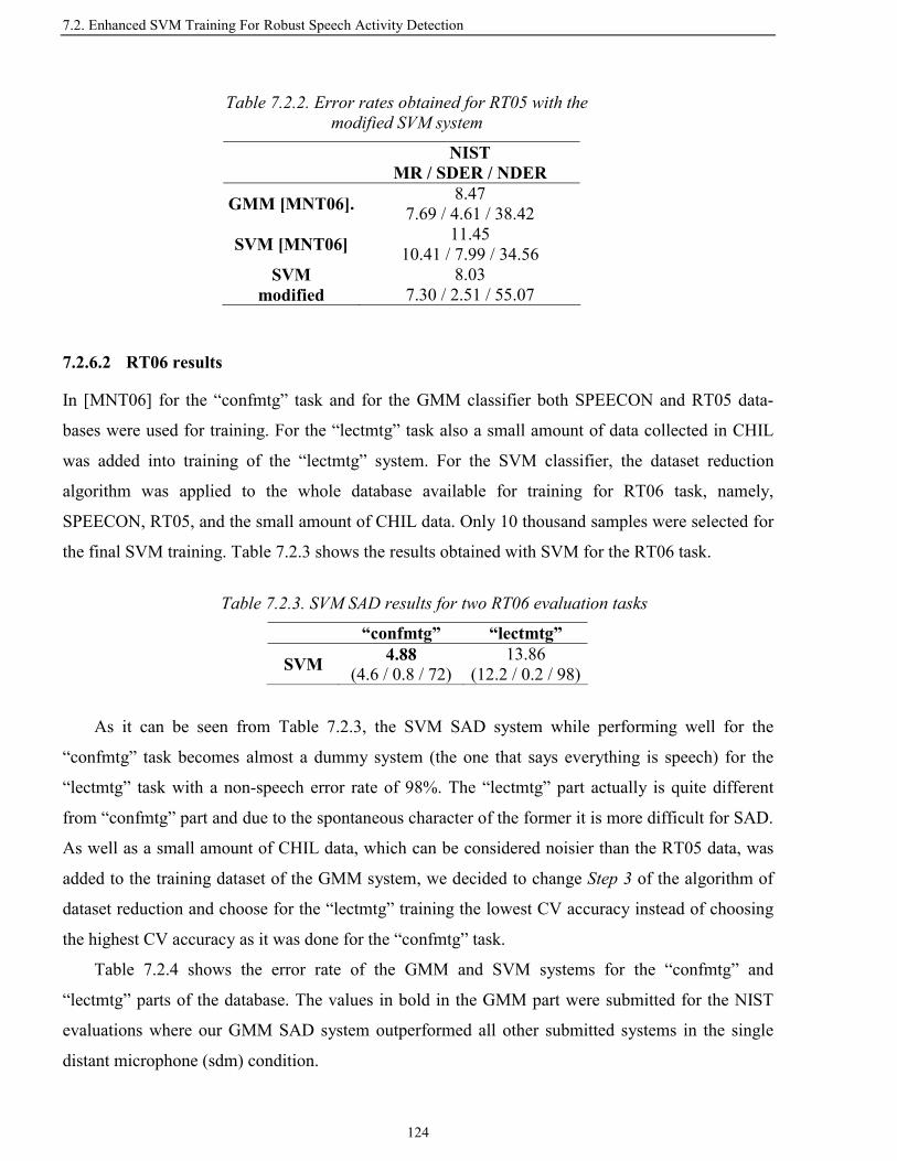
7.2. Enhanced SVM Training For Robust Speech Activity Detection
124
7.2.6.2 RT06 results
In [MNT06] for the “confmtg” task and for the GMM classifier both SPEECON and RT05 data-
bases were used for training. For the “lectmtg” task also a small amount of data collected in CHIL
was added into training of the “lectmtg” system. For the SVM classifier, the dataset reduction
algorithm was applied to the whole database available for training for RT06 task, namely,
SPEECON, RT05, and the small amount of CHIL data. Only 10 thousand samples were selected for
the final SVM training. Table 7.2.3 shows the results obtained with SVM for the RT06 task.
As it can be seen from Table 7.2.3, the SVM SAD system while performing well for the
“confmtg” task becomes almost a dummy system (the one that says everything is speech) for the
“lectmtg” task with a non-speech error rate of 98%. The “lectmtg” part actually is quite different
from “confmtg” part and due to the spontaneous character of the former it is more difficult for SAD.
As well as a small amount of CHIL data, which can be considered noisier than the RT05 data, was
added to the training dataset of the GMM system, we decided to change Step 3 of the algorithm of
dataset reduction and choose for the “lectmtg” training the lowest CV accuracy instead of choosing
the highest CV accuracy as it was done for the “confmtg” task.
Table 7.2.4 shows the error rate of the GMM and SVM systems for the “confmtg” and
“lectmtg” parts of the database. The values in bold in the GMM part were submitted for the NIST
evaluations where our GMM SAD system outperformed all other submitted systems in the single
distant microphone (sdm) condition.
Table 7.2.2. Error rates obtained for RT05 with the modified SVM system
NIST MR / SDER / NDER
GMM [MNT06]. 8.47 7.69 / 4.61 / 38.42
SVM [MNT06] 11.45 10.41 / 7.99 / 34.56
SVM modified
8.03 7.30 / 2.51 / 55.07
Table 7.2.3. SVM SAD results for two RT06 evaluation tasks
“confmtg” “lectmtg”
SVM 4.88 (4.6 / 0.8 / 72)
13.86 (12.2 / 0.2 / 98)

Chapter 7. Speech Activity Detection
125
The diagonal elements of the SVM part show lower error rates than the diagonal elements of the
GMM part. That indicates that the proposed algorithm managed to select the appropriate 10000
samples out of the whole training database available that consists of more than 1.5 million examples.
From Table 7.2.4 we observe that for the “lectmtg” case the change of Step 3 of the proposed
algorithm has an intermediate influence. Chunks with the lowest CV accuracy, which contain less
separable data, are more important for the final classical SVM training in Step 4 for the given
subtask.
Notice that the NIST evaluation scenario allows having an independent system for each subtask
so the comparison conditions for the GMM and for the SVM are the same.
On the other hand, the off-diagonal elements of the GMM part from the Table 7.2.4 show lower
error rates than the off-diagonal elements of the SVM part. That can be either an indication that the
GMM is not so sensitive to the mismatch between the training and testing databases or can be the
result of the fact that GMM used much larger amount of data for training.
Actually, the off-diagonal elements are not considered in NIST but here we include them to
show the behaviour of the GMM and SVM classifiers for the case when the characteristics of the
training and testing databases do not match.
Note that, for comparison with GMM, the feature extraction process was left unchanged. Actu-
ally, taking one LDA measure and reducing the dimension of the final feature vectors can be
beneficial for a generative model classifier as GMM since it means decreasing the difficulty of the
estimation problem [DHS00] but in this way one of the main advantages of SVM classifiers – to
make use of a much larger feature set – is not exploited. To check it we made a straightforward
experiment. Instead of taking 1 LDA measure we decided to preserve 4 LDA measures for each
Table 7.2.4. Error rates obtained for the RT06 evaluation for the “confmtg” and the “lectmtg” parts of the database. The results for matched conditions
are given in bold.
NIST MR / SDER / NDER
SVM GMM Test
Train confmtg lectmtg confmtg lectmtg
confmtg 4.88 (4.6 / 0.8 / 72)
13.86 (12.2 / 0.2 / 98)
5.45 (5.1 / 3.1 / 41.4)
11.71 (10.3 / 0.1 / 83)
lectmtg 11.84 (11.2 / 11 / 14)
6.16 (5.4 / 1.4 / 33)
9.54 (9 / 8.2 / 22.4)
7.1 (6.2 / 0.4 / 48)

7.2. Enhanced SVM Training For Robust Speech Activity Detection
126
frame, thus multiplying the total number of feature in a vector approximately by 4 (the 3 features
based on energy dynamics remain the same). We tested it on the “lectmtg” task and observed an
improvement of the error rate from 6.16% to 4.51% (the best GMM results were 7.1%). In conse-
quence, further work should be done to design the front-end that can better fit the capacity of the
SVM classifier.
7.2.7 Conclusions
The presented work is oriented towards robust SVM-based speech activity detection systems for
smart-room environments.
Two modifications of the usual training algorithm of the SVM-based classifier presented in
[MNT06] have been developed in order to cope with two problems of that classifier in our applica-
tion: the very large amount of training data and the particular characteristics of the NIST metric.
With those two modifications, the SVM system has reduced the error rate on the RT05 database
from 11.45% to 8.03%, score comparable to the best GMM score of 8.47%. With the RT06 SAD
evaluation task, the modified SVM system has achieved an error reduction with respect to the GMM
system from 5.45% to 4.88% for the “confmtg” task, and from 7.1% to 6.16% for the “lectmtg” task.
Additionally, the error rate for “lectmtg” task has been further decreased to 4.51% by preserving 4
LDA measures.

Chapter 7. Speech Activity Detection
127
7.3 SAD Evaluation in NIST Rich Transcription Evaluations 2006 -2007
7.3.1 Introduction
The Rich Transcription 2006-2007 spring meeting recognition evaluation were the fourth and fifth
NIST sponsored evaluation of speech technologies within the meeting domain. The evaluations are
related to the CLEAR evaluations since both are concerned with multimodal signals and sensor
fusion experiments in the meeting domain.
The RT-06 evaluation included three meeting domain tasks in the evaluation: Speech-To-Text
(STT), diarization “who spoke when” (SPKR also known as “Speaker Diarization”), and SAD. The
RT-07 evaluation dropped the task of the SAD however the task of speaker diarization needs SAD
as a component of the system.
In Section 7.2 we already presented the results obtained by the proposed SVM-based SAD sys-
tem for the RT-05 and RT-06 SAD evaluations. In this section we summarize the results of the
previous RT SAD evaluations and also present the SAD results that were obtained for the last RT-07
evaluation within the speaker diarization task performed on conference meetings [LAT+07].
7.3.2 SAD systems overview and results on referenced datasets
In this subsection we present the results of the last SAD systems developed in our lab and tested in
various RT evaluations conducted in the conference room environment. Table 7.3.1 shows the NIST
metric error rates obtained by three UPC’s systems on the RT datasets. The system based on the
Decision Tree (DT) classifier with the basic feature set that consists of the Frequency-Filtering-and-
Linear-Discriminant-Analysis-extracted features (FF-LDA) was developed by J. Padrell et. al. in
[PMN05] where on Speecon and SpeechDat databases it showed better results in comparison to the
commercial GSM cell-phone standard SAD system and two SAD systems taken from the ETSI
Advanced Front-End standard for noisy speech recognition [ETS02]. D. Macho et. al. in [MNT06]
proposed three new energy dynamics features in addition to the basic FF-LDA feature set and
substituted the DT classifier by the GMM classifier. The proposed GMM-based system showed
better performance than DT-based system on RT-05 dataset in the tested sdm condition as it can be
seen from Table 7.3.1. Besides, the GMM-based SAD system has been submitted to the RT-06
evaluation and outperformed all other submitted systems in sdm subtask in both the “lectmtg” and
“confmtg” conditions. The proposed SVM-based SAD system substitutes the GMM classifier by
SVM and proposes the solutions to the problems that appear when applying SVM to the SAD task.
As it can be seen from Table 7.3.1, the SVM-based SAD system showed better results than the

7.3. SAD Evaluation in NIST Rich Transcription Evaluations 2006 -2007
128
GMM system on the RT-05 and RT-06 datasets. Additionally, Table 7.3.1 shows the results ob-
tained with the proposed SVM-based system on the RT-07 sdm. The result obtained on a signal
enhanced by beamforming signals from the multiple distant microphones (mdm) is also presented in
Table 7.3.1.
7.3.3 Conclusions
In this section, the results obtained with the NIST RT evaluation datasets by the SAD systems
developed in our lab have been shortly overviewed. The comparison has shown that the recently
developed SVM-based SAD system performed better than both the GMM and the DT-based systems
on the tested RT datasets. Additionally, the error rates produced with the proposed SVM-based SAD
system on the last RT-07 evaluation dataset have been presented.
Table 7.3.1. NIST error rates obtained for the “confmtg” task with the RT 05-07 evaluation databases by the UPC SAD systems.
RT-05 sdm
RT-06 sdm
RT-07 sdm
RT-07 mdm
SVM 8.03 4.88 7.03 4.72 GMM 8.47 5.45 - -
DT 11.54 - - -
Chapter 7. Speech Activity Detection
129
7.4 Chapter Summary
An enhanced version of the training stage of the SVM-based SAD system has been presented. It
consists of a fast algorithm of data reduction and an adjustment to the specific characteristics of the
metric used in the NIST SAD evaluations has been presented. Tested with the RT06 data, the resulting
SVM SAD system has shown better scores than the best GMM-based system developed by the authors
and submitted to the past RT06 evaluation.
The results obtained on the NIST RT evaluation datasets by the SAD systems developed in last
years in our lab have been shortly overviewed showing better performance obtained by the developed
SVM-based SAD system.

130

Chapter 8. UPC’s Smart-Room Activities
131
Chapter 8. UPC’s Smart-Room Activities
8.1 Chapter Overview
In this chapter the activities concerning Acoustic Event Detection (AED) in the UPC’s smart-room
are described.
The remaining sections are organized as follows. In Section 8.2, a brief description of the Com-
puter in the Human Interaction Loop (CHIL) project is proposed. The smart-room built at UPC in
the framework of CHIL project is described in Section 8.3. Section 8.4 presents the information
concerning the recording of the database of isolated acoustic events and the recording of seminars
that were used in the CLEAR evaluation campaign on AED. Section 8.5 gives basic information on
the implementation of the AED component in the smart-room. Finally, three different demos devel-
oped in the UPC’s smart-room, in which the implemented AED component has participated, are
presented in Section 8.6.

8.2. CHIL Project
132
8.2 CHIL Project
The project CHIL [CHI] is an Integrated Project (IP 506909) funded by the European Union under
its 6th framework program. The project started on January 1st, 2004 and has a planned duration of
three years.
The CHIL team is a consortium of internationally renowned research labs in Europe and the
US, who collaborate to bring friendlier and more helpful computing services to society. Rather than
requiring user attention to operate machines, CHIL services attempt to understand human activities
and interactions to provide helpful services implicitly and unobtrusively.
Considerable human attention is expended in operating and attending to computers, and humans
are forced to spend precious time on fighting technological artefacts, rather than on human interac-
tion and communication. CHIL aims to radically change the way we use computers. Rather than
expecting a human to attend to technology, CHIL attempts to develop computer assistants that
attend to human activities, interactions, and intentions. Instead of reacting only to explicit user
requests, such assistants proactively provide services by observing the implicit human request or
need, much like a personal butler would. To achieve this goal, machines must understand the human
context and activities better; they must adapt to and learn from the humans’ interests, activities,
goals and aspirations. This requires machines to better perceive and understand all the human
communication signals including speech, facial expressions, attention, emotion, gestures, and many
more.
Based on the perception and understanding of human activities and social context, a new type of
context aware and proactive services can be developed. Within the years of the CHIL project, four
instantiations of such CHIL services have been implemented:
• The connector: This service attempts to connect people at the best time by the best media,
whenever it is most opportune to connect them. In lieu of leaving streams of voice messages
and playing phone tag, the Connector tracks and knows its masters’ activities, preoccupa-
tions and their relative social relationships and mediates a proper connection at the right time
between them.
• The memory jog: This is a personal assistant that helps its human user remember and retrieve
needed facts about the world and people around him/her. By recognizing people, spaces and
activities around its master, the memory jog can retrieve names and affiliations of other
members in a group. It provides past records of previous encounters and interactions, and re-
trieves information relevant to the meeting.

Chapter 8. UPC’s Smart-Room Activities
133
• Socially supportive workspaces: This service supports human gathering. It offers meeting
assistants that track and summarize human interactions in lectures, meetings and office inter-
actions, and provide automatic minutes and create browseable records of past events.
• The attention cockpit: This agent tracks the attention of an audience and provides feedback
to a lecturer or speaker.
CHIL represents a vision of the future - a new approach to more supportive and less burden-
some computing and communication services. The research consortium includes 15 leading research
laboratories from 9 countries representing today’s state of the art in multimodal and perceptual user
interface technologies in European Union and the US. The team sets out to study the technical,
social and ethical questions that will enable this next generation of computing in a responsible
manner.
The CHIL results are disseminated and made available to a wide community of interested par-
ties.

8.3. UPC’s Smart-Room
134
8.3 UPC’s Smart-Room
The UPC has built the smart-room – a room equipped with multiple cameras and microphones – in
order to investigate the video and audio perception of the computer systems. The main objective is
to make the computer systems be aware of the activity that is going on in the room and to stop them
being only the tools from which the humans can only obtain help as a reaction to the very special
request. If computers know the environment they can interact with us in the same manner we
interact with each other. The technologies of the perceptual interface have to enable computers help
us with their information services better do our everyday work.
The smart-room is an intelligent space designed as a meeting-room with a table in the centre
and chairs around it. The configuration of the UPC’s smart-room can be found in Appendix A.
Among others, there are several audio-visual sensors (cameras and microphones), synchronization
and acquisition equipments, working computers, and a video projector. The smart-room is the
indispensable installation for the UPC research groups that work on multimodal interfaces. The
acquired audio-visual signals allow both developing the technologies of audio and video analysis
and making demos that can offer specific services in the configuration of meeting rooms or teaching
rooms.
The UPC’s smart-room forms the part of the CHIL project, described in the previous subsec-
tion, along with other 15 participants, universities, and research groups from Europe and the United
States.
The speech-related technologies like speech recognition are the fundamentals of the analysis of
the human activity in the smart-rooms. At present, robust speech recognition systems are investi-
gated that use a signal from a far-field microphone in order to avoid bothering people wear cables or
close-talk microphones. On the other hand, the video technologies analyze the presence, localization
and movements of the peoples, face recognition, gesture detection, postures and attention tracking,
in order to classify the events, activities, and relationships. The detection technologies, classification
and recognition based on multiple sensors, like audio and visual localization, person identification
based on speech and face, activity detection based on acoustics or images, can increase the robust-
ness of existing systems.
As a practical examples consider a meeting room. Imagine that you come late to the meeting.
The system of perceptual analysis recognized who spoke and what was when you were absent.
Then, when you joined the meeting, the system proposed you the summary of what was said during
the time when you was absent. In order to achieve the objective the system had to: 1) localize the

Chapter 8. UPC’s Smart-Room Activities
135
speakers, 2) focus the acoustics of the room to obtain the signal cleaned from noises and interfer-
ences of the far-field microphone, 3) identify the interval when something was said, 4) process the
signal with a speech recognizer to generate the transcription of what was said, 5) finally, process the
transcription to generate the summary.
With respect to the video analysis, the extraction of the data about the position, activity or ges-
tures in the scene allow to obtain high level semantic information like knowing whether the person
is sitting or standing, if the person makes a voting gesture (a hand picked up), etc. Besides, the
UPC’s smart-room allows reconstructing the virtual 3D scene from the images of multiple cameras
that will be described in Subsection 8.6.3.

8.4. Recordings of the Databases in the Smart-Room
136
8.4 Recordings of the Databases in the Smart-Room
To work in real environments acoustic event detection problem has to be faced. For the purposes of
AED a database of isolated acoustic events has been designed and collected at the UPC, which will
be publicly disseminated by the European Language Resources Association. This database has been
used as a training material and as a testing material to evaluate the algorithm performance for
AED/C as it has been reported in Chapter 6. Along with other databases, it has been used in the
international CLEAR evaluation campaigns that have taken place in spring 2006 and spring 2007,
where the AED/C evaluation task has been coordinated by our UPC's group, which has defined the
AED metrics and developed the corresponding evaluation tools. The details on the database of
isolated acoustic events are given in Appendix A. Apart from the database of isolated acoustic
events, UPC contributed to the seminar recordings that were also used as a part of the development
and testing datasets in the international evaluation campaigns. In order to increase the number of
acoustic events in the recorded seminars, a list of suggestions was produced and disseminated
among the partners that contributed to the recorded database. The suggestions include instructions
on how to introduce acoustic events into the seminars in a natural and unobtrusive way. The details
of the instructions as well as a trade-off between the naturalness of the seminar recordings and AE
recordings are discussed in Appendix B.

Chapter 8. UPC’s Smart-Room Activities
137
8.5 Acoustic Event Detection Component Implementation
Our system, which is described in Section 6.5, is written in C++ programming language and is a part
of the smartAudio++ software package developed at UPC which includes other audio technology
components (such as speech activity detection, acoustic source localization, and speaker identifica-
tion) for the purpose of real-time activity detection and observation in the smart-room environment.
The software architecture chosen in the UPC’s smart-room is based on NIST smartflow system
[NIS] and KSC socket messaging system. The lower level of the software architecture consists of
the video and audio sensors. The signal capture software is implemented as smartflow clients in the
computers with the corresponding acquisition hardware. The resulting data streams are transferred
as smartflow flows into other computers that can either pre-process the data streams or directly
analyze the raw data streams (as in the case of the speech activity detection audio technology).
Smartflow also provides a mechanism to dynamically decide on which computer in the local area
network a specific technology should run. The KSC message server and the KSC client library allow
sending results of data analysis asynchronously.
Figure 8.5.1 shows the smartAudio map that corresponds to the AED system described in Sub-
section 6.5.3. The map shows the needed smartflow clients and the interconnections among them.
Firstly, a audio signal from cluster microphones and the MarkIII microphone array are captured with
data acquisition clients RMEAlsaCapBlock and UPCMarkIIICapturev0.1, respectively. Three
cluster microphones (one from each cluster) and the 3rd channel of the MarkIII are extracted with the
RMEChannelExtractors and the MarkIIIChannelExtractor, respectively. Then, with the Resample-
Clients the signals are downsampled to 16 kHz. Feature extraction and SVM-based sliding window
classification are performed for each channel with the AEDOnLine client, and the fusion of deci-
sions is applied with the AEDFusion client. Depending on the demo, in which the AED perceptual
component is involved, there can be clients shared among several perceptual components, for
instance data acquisition or resample clients, and clients responsible for results visualization.

8.5. Acoustic Event Detection Component Implementation
138
Figure 8.5.1. SmartAudio map that corresponds to the AED system

Chapter 8. UPC’s Smart-Room Activities
139
8.6 Acoustic Event Detection Demonstrations
8.6.1 Acoustic event detection and acoustic source localization demo
Acoustic event detection and acoustic source localization (ASL) are two of the functionalities
implemented in the UPC’s smart-room.
A Graphic User Interface (GUI) that shows both functionalities working together has been de-
veloped and it is currently running in real time in the smart-room. It is used to test the technologies
and to demonstrate them. A video has been recorded with the output of the GUI during a session
lasting about 2', where four people in the room speak, are silent, or make one of the 12 meeting-
room sounds defined in CHIL and a few others1. The 12 defined sounds, ordered according to time
of occurrence in the session, are: knock (door), door slam (door open, door close), steps, chair
moving, spoon clings (cup jingle), paper wrapping, key jingle, keyboard typing, phone ringing,
applause, cough and laugh. The screenshot of the GUI is given in Figure 8.6.1 when a laugh sound
is produced.
There are two screens in the GUI output as it is shown in Figure 8.6.2. One corresponds to the
real video captured from one of the cameras installed in the UPC’s smart-room, and the other is a
graphical representation of the output of the two technologies. The video has not been edited at all,
and it shows what can be seen in the room in real time.
The two functionalities are simply juxtaposed in the GUI, so e.g. it may happen that the AED
output is correct but the output of acoustic source localization is not, so showing the right event in a
wrong place. There is some clutter noise in the localization output due to the fact that the algorithm
allows sudden changes of position and no other information has been used for smoothing the output
position during an event.
The AED technology includes an “unknown” output, symbolized with “?”. There are two dif-
ferent situations when the “unknown” label may appear. Firstly and most frequently, it appears
when the AED algorithm does not have enough confidence to assign a detected non-silent event to
one of the above-mentioned 12 classes. Secondly, the “unknown” label is produced when an out-of-
list acoustic event is detected.
1 The video is downloadable from http://gps-tsc.upc.es/veu/personal/temko/presents/AEDLdemo_UPC.avi

8.6. Acoustic Event Detection Demonstrations
140
Figure 8.6.1. The developed GUI for demonstration of AED and ASL functionalities (“laugh” is being produced)
(a) (b)
Figure 8.6.2. The two screens of the GUI: real-time video (a) and the graphical representation of the AED and ASL functionality (“keyboard typing” is being produced)

Chapter 8. UPC’s Smart-Room Activities
141
8.6.2 Acoustic event detection in CHIL mockup demo
The aim of the mockup demonstration [CN07] designed at UPC is to gain context awareness in the
context of the CHIL memory jog assistant. It is achieved by means of detection of people, objects,
events, and situations in the interaction scene. The information needed to build the relevant context
awareness stems from the analysis of the signals acquired in real-time from a collection of sensors.
Specifically, the memory jog service developed at UPC focuses at providing information to a group
of newspaper journalists gathered together in the CHIL smart-room. Figure 8.6.4 shows the screen-
shot of the journalist’s laptop. In the lower right part of the Figure 8.6.4, the Skype-based bi-
directional audio communication allows talking to the journalists in the room. The upper right shows
the real-time video stream from one of the cameras of the meeting room. An automatic cameraman
is choosing the optimal camera from five possible angles. This decision is based on the location of
the last acoustic event and smoothed by a hysteresis to avoid rapid camera-changes. The real-time
video streaming also displays annotations in the form of subtitles that explain the situation, e.g.,
“people enter”, “interaction with ASR”, “sound of keys”, “front page published”, “The meeting has
started”. On the left side of the screen, a graphical user interface allows the field journalist of add a
piece of news (a test and an image) to the decision GUI of the journalists in the room. Within ten
minutes the front page of tomorrow’s edition of their newspaper has to be decoded. One of the most
outstanding means of the memory jog to interact with the journalists is a talking head shown in
Figure 8.6.3 that not only informs the journalists about available resources, and points out events
such as the arrival of a latecomer or news being contributed by remote colleagues, but also facili-
tates information requests from the journalists in a human-like interface based on automatic speech
recognition technologies.
In the service implemented at the UPC’s smart-room, context awareness consists of knowledge
about the number of persons in the room, their identification, position in the room and their orienta-
tion. Objects in the room and acoustic events also add to the context awareness. It is worth to
mention that when humans experience the computer-driven service like the Memory Jog, another
subjective bias naturally arises: unexpected actions of the service triggered by a false-positive
detection of one of the technologies turn out to be far more annoying than a service not provided due
to false-negative detection. Due to that fact, only acoustic events that can be reliably detected are
chosen: door knock, door opening/closing, speech, applause, and key jingles.
Perceptual components are computing modules that analyze the signals provided by the network
of sensors in order to detect and classify objects of interest, persons and events adding information

8.6. Acoustic Event Detection Demonstrations
142
to context awareness. In total 8 perceptual components which are based on around 42 smart-flow
clients, are integrated into the single application called central logic. The combination of video-
based and audio-based systems allows the system to gain a basic understanding of what happens in
the smart-room. Among others it is possible to do the following:
a) A person of interest (e.g. the latecomer) can be tracked in the room. This location is used to
direct the talking head and an automatic cameraman to his current position.
b) The position of all participants can be used to guesstimate changes of the state of the session,
e.g. between the states “people enter”, “meeting starts” or “coffee break”.
c) The position and identity of sudden acoustic event can be determined. The automatic cam-
eraman has been configured to capture these events by choosing the camera that is positioned
furthest from the location of the acoustic event.
d) In the current implementation of the context awareness, the detection of a latecomer is based
on a multitude of criteria amongst which the first two depend on the person and object tracking:
increase of the number of person, appearing of a new object close to the door, detection of the
acoustic signal of a door-knock, a door-slam or steps close to the door.
e) Person identification is performed based on face ID and speaker ID technologies.
f) The dialogue system allows a human-like verbal interaction with the memory jog system. It is
based on two components: a commercially available 2D animation of a talking head and an ASR
based dialogue system that utilizes the HTK recognizer [You93].
g) Interactive behaviour of the talking head depending on an acoustic event detected, like an ut-
terance “Don’t forget your keys!” when “key jingle” is detected or exclamation “Great! Well done!”
when “applause” is detected.
Figure 8.6.3. The talking head is a mean of demonstrating the context awareness given by perceptual components

Chapter 8. UPC’s Smart-Room Activities
143
Figure 8.6.4. Screenshot of the field journalist’s laptop
8.6.3 Acoustic event detection and 3D virtual smart-room demo
The last demo is developed to demonstrate the UPC’s smart-room remotely. The functionalities that
are currently involved in the demonstration are the 3D person tracking, ASL, and AED.
The virtual 3D scene is reconstructed from the images of multiple cameras in the smart-room.
Figure 8.6.5 shows the developed 3D visualizer. Specifically, it shows one detected person sitting,
and the other passing in the room. “Steps” are detected with the AED and localized in space with the
ASL. The text label “steps” is assigned to the place where the event happens. Additionally, the small
screen at the lower left corner shows the corresponding real video.

8.6. Acoustic Event Detection Demonstrations
144
Figure 8.6.5. A snapshot that shows the built virtual UPC’s smart-room

Chapter 8. UPC’s Smart-Room Activities
145
8.7 Chapter Summary
In this chapter the activities concerning Acoustic Event Detection (AED) in the UPC’s smart-room
have been described.
A brief description of the CHIL project has been proposed and the main objectives have been high-
lighted. The smart-room built at UPC in the framework of CHIL project has been described. The basic
information concerning the recording of the database of isolated acoustic events and the recording of
seminars that were used in the CLEAR evaluation campaign on AED has been reported. The imple-
mentation of AED component has been reviewed. Finally, three different demos developed in the
UPC’s smart-room and in which the implemented AED component participated have been presented.
Specifically, the demo of AED and acoustic source localization with a cartoon animation, the role of
AED in the versatile mockup demo, and the 3D demonstration of the UPC’s virtual smart-room using
the 3D person tracking, acoustic source localization, and AED, have been described.

146

Chapter 9. Conclusions and Future Work
147
Chapter 9. Conclusions and Future Work
9.1 Summary of Conclusions
This thesis is a pioneering work in the area of audio classification that, by focusing on the acoustic
events which are naturally produced in a meeting-room environment, ranges from classification of
previously segmented acoustic events to detection of acoustic events in seminar sessions, and its
real-time implementation in the smart-room of the UPC. SVM classifier is chosen as a basic classi-
fication technique in this thesis.
The first main contribution of this thesis is an attempt to deal with the problem of classifying
acoustic events. When trying to deal with the problem of acoustic event classification in the frame-
work of the CHIL project [CHI], we soon noticed that reported works are scarce. Actually,
classification of sounds has usually been carried out so far to segment digital audio streams using a
limited number of categories, like music/speech/silence/environmental sound. We have focused on
acoustic events that may take place in meeting-rooms or classrooms and on the preliminary task of
classifying isolated sounds. The number of sounds encountered in such environments may be large,
but in the initial work we have chosen 16 different acoustic events, including speech and music, and
a database has been defined for training and testing. Several feature sets and classification tech-
niques have been tested with it. In our tests, the SVM-based techniques show a higher classification
capability than the GMM-based techniques, and the best results were consistently obtained with a
confusion matrix based variable-feature-set clustering scheme. With it, a large relative average error
reduction with respect to the best result from the SVM conventional binary tree scheme has been
obtained. That good performance is mostly attributable to the proposed clustering technique, and to
the fact that SVM provides the user with the ability to introduce knowledge about data unbalance
and class confusions.
A drawback of SVMs when dealing with audio data is their restriction to work with fixed-
length vectors. Both in the kernel evaluation and in the simple input space dot product, the units
under processing are vectors of constant size. However, when working with audio signals, although
each signal frame is converted into a feature vector of a given size, the whole acoustic event is
represented by a sequence of feature vectors, which shows variable length. In order to apply an
SVM to this kind of data, one needs either to normalize somehow the size of the sequence of input
space feature vectors or to find a suitable kernel function that can deal with sequential data.
Several methods that adapt SVMs to sequence processing have been reviewed and applied to the
classification of sounds from the meeting room environment. We have seen that the dynamic time

9.1. Summary of Conclusions
148
warping kernels work well for sounds that show a temporal structure, but due to the presence of
less-time-structured sounds in the database the best average score is obtained with the Fisher kernel.
Moreover, only one Gaussian is used in that method due to its high sensitivity to the variance
parameters as a consequence of the scarcity of data.
Usual combinations of classifier outputs like sum, product, max, min, weighted arithmetical
mean, assume that each output represents an independent source of information that can be treated
separately. Often, this is not the case, and an approach that considers the interactions among the
classifier outputs is needed. Fuzzy integral fusion can capture interactions among the various
sources of information. Moreover, the fuzzy measure, which is associated with the fuzzy integral,
furnishes a measure of importance for each subset of information sources, allowing feature selection
and giving a valuable insight into the classification problem itself. Experiments with fuzzy integral
have been carried out with a set of five human vocal-tract non-speech sounds (cough, laughter,
sneeze, sniff and yawn) which was found responsible for a large part of errors in the classification of
meeting-room acoustic events. Ten types of features were chosen with a substantial degree of
redundancy in order to use the fuzzy measure to find out their relative importance and their degree
of interaction.
In the experiments, a system which fuses several information sources with the fuzzy integral
formalism has shown a significant improvement with respect to the best single information source.
Moreover, the fuzzy integral decision-level fusion approach has shown comparable results to the
high-performing SVM feature-level fusion. Finally, the experimental work also indicates that the
fuzzy integral may be a good choice when feature-level fusion is not an option e.g. when the feature-
level fusion is difficult (e.g. due to the different nature of the involved features), or when it is
beneficial to preserve the application or technique dependency (e.g. when fusing well-established
feature-classifier configurations). For that purpose we have also conducted experiments to combine
hidden Markov models that use frame-level features with the SVM using signal-level features, and
have witnessed an additional improvement.
Systems of acoustic event classification developed in this thesis have participated in the dry-run
evaluation on acoustic event classification in 2004, in the first official evaluation on acoustic event
classification in 2005, and in the international CLEAR evaluation campaign in 2006. In all those
evaluations, the system ranked among the best, and, in the last one, outperformed the other two
submitted systems.
The second main contribution of this thesis is the development of systems for detection of
acoustic events. AED is more complex than AEC since it includes both classification and determi-
Chapter 9. Conclusions and Future Work
149
nation of the time intervals where the sound takes place. Two acoustic event detection systems were
developed at the UPC for CLEAR evaluations.
The first system has participated in the CLEAR 2006 evaluation tasks concerning the detection
of acoustic events that may happen in a lecture/meeting room environment. Two kinds of databases
have been used: two databases of isolated acoustic events, and a database of interactive seminars
containing a significant number of acoustic events of interest.
The system of year 2006 was based on two steps: performing silence/non-silence segmentation
and then classification of non-silence portions. Our system was based on an SVM discriminative
approach and used frequency filtering features and four types of perceptual features. The detection
results indicated that first doing segmentation and then classification performs worse than merging
both segmentation and classification in one step, as it is performed by Viterbi search in the state-of-
the-art ASR systems that have been developed for many years and therefore can be considered as a
challenging reference for other presented approaches/systems in the acoustic event detection task
like our SVM-based system.
The next AED system has participated in the CLEAR 2007 evaluation. The evaluation has been
performed with the database of interactive seminars that has been recorded at different smart-rooms
and contains a significant number of acoustic events of interest. Two different metrics have been
proposed and implemented. One is based on precision and recall of the detection of the AEs as
semantic instances, and the other is more time. The system of 2007 merges the two steps (segmenta-
tion and classification) and is also based on SVM classifiers. Each sliding window is classified with
SVM classifiers and a post-processing is applied to the sequence of decisions. According to the
importance and degree of interaction of features from the work with the fuzzy integral, several
features were added to the set of features used in the AED system 2006 and one feature was elimi-
nated. Additionally, multi-microphone decision fusion was introduced into the AED system 2007.
The proposed system, which was the only submission not using HMM, ranked the second out of six
participants.
A work oriented towards robust SVM-based SAD for smart-room environments has also been
carried out. A set of several hundred of thousand of samples is a usual amount of data for classical
audio and speech processing techniques that involve GMM. However, it is an enormous number of
feature vectors to be used for a usual SVM training process and hardly makes such training feasible
in practice. In this thesis, the usual training algorithm of the SVM classifier has been enhanced in
order to cope with that problem of dataset reduction, proposing a fast algorithm based on Proximal
SVM. Besides that, the SVM learning process has been adjusted in order to take into account the

9.1. Summary of Conclusions
150
specific characteristics of the metric used in the NIST RT evaluations. The resulting SVM SAD
system has been tested with the RT06 data, and it has shown better scores than our GMM-based
system which was submitted to the RT06 evaluations and ranked the first among all submitted
systems in single distant microphone condition.
This thesis has proactively contributed to provide the tools and resources that make the research
possible, including: recordings and labelling of the databases, providing support to worldwide open
competitions organized in CHIL, the organization of AED/C evaluations, definition of classes,
evaluation scenarios and conditions, databases, etc. The metrics were changing starting from the
first evaluations in 2004. Finally, after almost four years of task evolution, two grounded metrics
have been proposed, agreed, and used in the last CLEAR evaluation campaign. The evaluation plans
as well as other coordinating activities have been reflected in several CHIL deliverables, revised
implementation plans, and UPC internal reports.
Another contribution of this thesis is the real-time implementation of the developed AED and
SAD systems. The system based on four extracted LDA measures and SVM classifier has been used
in UPC’s smart-room for real-time SAD. A GUI that shows AED and acoustic source localization
functionalities working together has been developed and it is currently running in real time in the
smart-room. It is used to test the technologies and to demonstrate them. A video has been recorded
with the output of the GUI during a session lasting about 2', where four people in the room speak,
are silent, or make one of the 12 meeting-room sounds defined in CHIL and a few others. Besides,
the developed real-time AED component contributed to two more demonstrations of technologies
and services developed within CHIL project.

Chapter 9. Conclusions and Future Work
151
9.2 Future Work
From the work done in this thesis a set of problems and limitations have been detected and should
be faced in future. In this subsection we will critically summarize the drawbacks of the techniques
that were developed and used throughout the work, and also propose a few envisaged research lines
that seem promising.
9.2.1 Feature extraction and selection
In this thesis work several feature sets have been used for the AEC task. In Section 4.5, a set of what
we called perceptual features was investigated and one new feature was proposed. For the feature
selection, the importance and interaction indices were calculated with FI. However, we concentrated
on the interrelations inside the perceptual set of features and so did not calculate the interaction
between the conventional ASR feature set and the perceptual features. We think it can be useful to
group all perceptual and conventional ASR features into several acoustic groups according to the
way each feature describes an audio signal. In this way, we plan to investigate the importance of and
interactions among the mentioned groups of features in order to see which combinations of groups
may be beneficial for audio processing.
The normalization of the acoustic features to make different instances of a given event appear as
similar as possible is also an important problem in classification and detection of acoustic events.
More time should be also spent on the low-level features to try to ensure good generalization across
different channel characteristics.
When applying SVM in our work we used statistical parameters like mean and variance, or
mean, variance, autocorrelation, and entropy in order to transform the frame-level features into
segment-level features. Indeed, the performed averaging over frames results in a huge loss of
information. Alternative approaches can be envisaged like the recently proposed GMM SuperVector
kernel [CSR+06] where the final vector is constructed from the parameters of GMMs trained on
every segment of an audio signal.
9.2.2 Sequence-discriminative SVM
The ability to model dynamics of the observed data is one of the major characteristics of the state-
of-the-art HMM techniques in speech and audio processing, and it is a big advantage over static
classification techniques like SVM classifiers. However, the good performance of SVM for several
classification tasks and its excellent theoretical background stimulate the research community to

9.2. Future Work
152
keep looking for ways to enable SVM to work with variable-length sequences. In our work in
Section 4.4, we compared several sequential kernels for the task of AEC. The experiments were
performed on a small database and it would be interesting to see if the same conclusions can be
drawn from much larger databases. Besides, the observed bias of classifiers in our results with
sequential kernels to specific types of AE classes is a good basis for a successful application of
fusion techniques. On the other hand, the efficient way to introduce the dynamics of the sequences
into the kernel is still an open research area.
9.2.3 Acoustic event detection in real environments
Detection of acoustic events appeared to be a very interesting and difficult task. The initial works
carried out in this direction in this thesis and the results obtained within the international evaluation
campaigns showed that, although the proposed system, which was the only submission not using
HMM, ranked among the best, there is still a big room for improvement.
The biggest problem in real environment AED is overlappings – i.e. temporal intervals where
the AE of interest is overlapped with speech and/or other AEs. It was found that the overlapping
segments account for more than 70% of errors produced by every submitted system. The problem of
overlapping of different speakers has been addressed since the NIST RT-07 [Spr06] evaluation
campaign where the tasks (e.g. Speaker Diarization) have been evaluated on overlapped segments as
well. Actually, the problem of acoustic overlappings is closely related to the “cocktail-party”
problem [Bre90] [WB06]. In the latter, however, one usually tries to separate one speech source
from others. Conversely, in our application we would like to separate acoustic events from speech.
Conceptually, the problem of overlapping can be addressed at different system levels. At the signal
level, it can be dealt with source separation techniques like ICA. The overlapping problem can be
addressed at the level of models by modelling also the possible combination of sounds by classifiers.
Finally, at the level of decision, different weights can be assigned within the multi-microphone
system architecture to particular microphones. In the latter case the main assumption is that the
audio sources (in our case, speech and acoustic events) are well separated in space, and an acoustic
event of interest can be the most powerful signal in some microphone. Future work will be devoted
to search a better way to deal with overlapping sounds.
Additional improvement is expected by integrating the developed variable-feature-set clustering
scheme (see Section 4.3) into the AED system.

Chapter 9. Conclusions and Future Work
153
Multimodal AED is another approach from which a performance improvement can be expected.
Some sounds can be detected by video technologies, e.g. “steps” can be assumed when detecting an
object moving around the smart-room, etc.
The choice of the system structure is also very important. In fact, none of the AED systems pre-
sented to the evaluations was built as a set of isolated detectors. That is, there were no systems
which intended to detect one particular sound. This approach can be addressed in future.
When an SVM-based AED/C system is trained, it would be interesting to be able to adapt it to a
new environment keeping the same acoustic event classes. For this it is necessary either to design a
mechanism of online learning or perform an adaptation of the learnt SVM classifier to new envi-
ronmental acoustics similar to MAP or MLLR adaptation for GMM. Some works on the former
approach can be found in the literature [DC03] while the latter is still an open question.
Detection of higher-level semantics like the stage of a meetings based on the statistics of occur-
rences of AEs is an interesting topic and deserves attention. For example, detection of frequent
cup/spoon jingles may indicate that the meeting is in its “coffee break” stage, etc.
9.2.4 Fuzzy integral fusion for multi-microphone AED
A few information sources were fused in our work with the FI formalism. The use of semi-shared
and individual FMs is a promising approach. Unfortunately, we were not able to explore it more due
to the scarcity of the data in the evaluation corpus. Future work will also be devoted to the applica-
tion of the FI to multi-microphone classification and detection of acoustic events with a much larger
dataset recorded in meeting rooms (see Section 6.5). Also, a further improvement can come from the
fact that signals captured from microphones placed at different positions in the room may carry
different information about the acoustic events taking place in it.
9.2.5 Acoustic source localization for AED
Combination with other audio technologies can be very beneficial for AED. For instance, based on
the position of the localized audio source and its orientation, different weights can be efficiently
assigned to the microphones in the smart-room to increase the performance of AED.
9.2.6 Speech activity detection
The work concerning SAD presented in this thesis mostly intended to show how SVM can be
efficiently applied to the SAD task. In Chapter 7, it was shown that the proposed SVM-based SAD
system showed results which were competitive and at times significantly superior to GMM and
9.2. Future Work
154
decision tree classifiers. As it was reported in Chapter 7, making use of a much longer feature set by
preserving 4 LDA measures for each frame improved the error rate for SVM. Further work should
be done to design the front-end that can better fit the capacity of the SVM classifier.
The system based on four extracted LDA measures and an SVM classifier has been used in the
UPC’s smart-room for real-time SAD. However, although the algorithm has shown a very good
performance in the offline tests, as reported in Chapter 7, in the online tests it produces lots of
confusion of speech with high-energy acoustic events (cough, door slam, etc). In fact, we also tried
the GMM method but it performed badly either. Actually, although most existing SAD methods are
energy based as usual testing datasets designed for the SAD task do not have a rich variety of
acoustic events, but just speech and silence, the Speech vs. Non-Speech task becomes a Silence vs.
Non-Silence task. Again, this fact shows that AED and SAD are two interlaced problems which
require a common solution when working in real seminar environments. Further investigation will
be devoted to a closer integration of both technologies.

Appendix A. UPC-TALP Database of Isolated Meeting-Room Acoustic Events
155
Appendix A. UPC-TALP Database of Isolated Meeting-Room Acoustic Events
Introduction
This database contains a set of isolated acoustic events that occur in a meeting room environment
and were recorded for the CHIL Acoustic Event Detection (AED) task. The recorded sounds do not
have temporal overlapping. The database can be used as a training material for AED technologies as
well as for testing AED algorithms in quite environments without temporal sound overlapping.
Description of the acoustic events
For recording, we used the same list of sounds that was defined in CHIL with conventional labels,
except for “door slam” that was further divided into “door open” and “door close”:
Acoustic event Label
Knock (door, table) kn
Door open do
Door close dc
Steps st
Chair moving cm
Spoon (cup jingle) cl
Paper work (listing, wrapping) pw
Key jingle kj
Keyboard typing kt
Phone ringing/Music pr
Applause ap
Cough co
Laugh la
Unknown un
Description of the recording setup
The whole database was recorded using the following audio equipment: Mark III (array of 64
microphones), three T-shape clusters (4 mics per cluster), 4 tabletop and 4 omni directional micro-

156
phones. In total 64+12+8=84 microphones. The positions of the microphones in the UPC CHIL -
room are described in Figure A.1. Figure A.2 describes the configuration of the T-shaped clusters.
Data was recorded at 44.1 kHz, 24-bit precision, and then converted to 16-bit Raw Little-Endian
format. All the channels were synchronized. During all the recordings two-three additional people
were inside the room for a more realistic scenario.2
2 Video data was also acquired simultaneously to audio data.
Figure A.1. Microphone and camera positioning in the UPC’s smart-room
Figure A. 2. Configuration & orientation of the T-shaped microphone clusters
Cam5
Cam6
Cam8 zenithal
cam
Cam2
Cam1
Cam3
Cam4
5.245 m
3.966 m
PTZ Cam
Hammer_xx
Ham
mer_xx
01 02
03
04
07
05
06
08
09
10
11
12
Hammer_13 to Hammer_20
MkIII_001
. . . . . .
MkIII_064
x
y Hammer XX

Appendix A. UPC-TALP Database of Isolated Meeting-Room Acoustic Events
157
Description of the recorded database
Approximately 60 sounds per each of the sound classes were recorded. Ten people participated in
recordings: 5 men and 5 women. There are 3 sessions per each participant. At each session, the
participant took a different place in the room out of 7 fixed different positions that are marked in
Figure A.3. The exact coordinates of the positions are given in Table A.1. Participant positions for
each session are shown in Table A.2.
Table A.1. X, Y coordinates of the positions
Position X (meters) Y(meters)
P1 1.28 1.58 P2 1.28 2.40 P3 1.28 3.05 P4 2.28 3.53 P5 3.03 3.05 P6 3.03 2.40 P7 2.19 1.26
Figure A.3. Graphical illustration of participants’ positions
y
5.245 m
3.966 m
P3. . . . . .
x
P2P1
P7
P6 P5

158
During each session a person had to produce a complete set of sounds two times. A script indi-
cating the order of events to be produced was given to each participant. Almost each event was
followed and preceded by a pause of several seconds. All sounds were produced individually, except
“applause” and several “laugh” that were produced by the people that were inside the room alto-
gether
Annotation of the database
The annotation was done manually by listening at signals from a single channel (the 3rd channel
from Mark III microphone array). The following criterion was used during the annotation. If an
event of class X includes a pause of minimum 300ms and both parts of the event, the one before the
pause and the one after the pause, can be (subjectively) assigned a label X, then the event is anno-
tated as two separated events of class X. If either the pause length is less than 300ms or the
first/second part of the event is not recognizable without hearing the other part, the whole event is
marked as only one event of class X. That kind of events only occurs for classes “cough”, “laugh”,
and “phone ring”.
Contents of the distributed database
The database that is distributed in 3 DVDs contains signals corresponding to 23 audio channels and
the corresponding labels. The 23 audio channels correspond to: 12 microphones of the 3 T-shaped
clusters, 4 tabletop omni directional microphones, and 7 channels of the Mark III array: 3rd, 13th
23rd, 33rd and 43rd, 53rd, and 63rd. The 7 mics from the array can be viewed as three clusters, as
shown in Figure A.4.
Table A. 2. Position of each participant for each session
Session 1 Session 2 Session 3
UPC_AE01(m) P2 P7 P3 UPC_AE02(m) P4 P6 P1 UPC_AE03(m) P4 P5 P6 UPC_AE04(m) P2 P7 P3 UPC_AE05(f) P4 P5 P1 UPC_AE06(f) P4 P2 P3 UPC_AE07(f) P7 P6 P5 UPC_AE08(m) P1 P4 P5 UPC_AE09(f) P2 P3 P7 UPC_AE10(f) P1 P6 P3

Appendix A. UPC-TALP Database of Isolated Meeting-Room Acoustic Events
159
The splitting of the data for purposes of training and testing can be based on either participants
or sessions. To produce the DVDs, we chose the latter option, so the database is distributed on three
DVDs each one containing one session. Table A.3 shows the distribution of the audio material
among the three sessions.
The name of a signal file is raw_K_44100_16b_upc_aeM_N.raw, where K is the number of the
microphone, 44100 is the sampling frequency, 16 is the number of bits per sample, M is the person
number (from 01 to 10), and N is the session number (from 1 to 3). There is a different number
ordering for the Mark III microphones and the other microphones (T-shaped clusters and tabletop
omni directional microphones). The former ones are ordered from 001 to 064 (although only 7 of
them are included), and the latter from 001 to 016, according to the ordering indicated in Figure A.1.
Figure A. 4. Selected channels of Mark III array, distance between them and symbolic grouping into clusters
Table A. 3 Number of annotated acoustic events in each session
Event type Session 1 Session 2 Session 3
kn 15 18 17 do 20 20 20 dc 20 21 20 st 28 24 21 cm 23 28 25 cl 23 21 20 pw 31 29 24 kj 21 21 23 kt 21 25 20 pr 37 36 43 ap 20 20 20 co 22 22 21 la 22 21 21 un 38 46 42
... ... 20cm
... ... 20cm
33 43 53 63 23 13 3
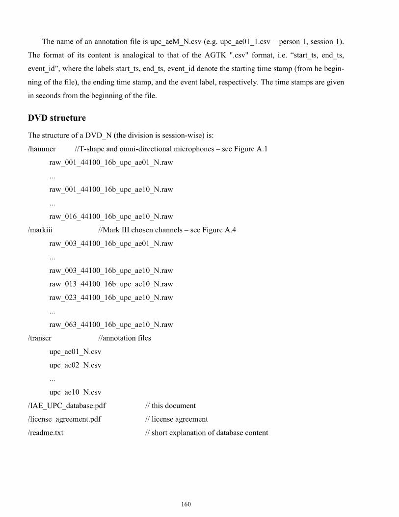
160
The name of an annotation file is upc_aeM_N.csv (e.g. upc_ae01_1.csv – person 1, session 1).
The format of its content is analogical to that of the AGTK ".csv" format, i.e. “start_ts, end_ts,
event_id”, where the labels start_ts, end_ts, event_id denote the starting time stamp (from he begin-
ning of the file), the ending time stamp, and the event label, respectively. The time stamps are given
in seconds from the beginning of the file.
DVD structure
The structure of a DVD_N (the division is session-wise) is:
/hammer //T-shape and omni-directional microphones – see Figure A.1
raw_001_44100_16b_upc_ae01_N.raw
...
raw_001_44100_16b_upc_ae10_N.raw
...
raw_016_44100_16b_upc_ae10_N.raw
/markiii //Mark III chosen channels – see Figure A.4
raw_003_44100_16b_upc_ae01_N.raw
...
raw_003_44100_16b_upc_ae10_N.raw
raw_013_44100_16b_upc_ae10_N.raw
raw_023_44100_16b_upc_ae10_N.raw
...
raw_063_44100_16b_upc_ae10_N.raw
/transcr //annotation files
upc_ae01_N.csv
upc_ae02_N.csv
...
upc_ae10_N.csv
/IAE_UPC_database.pdf // this document
/license_agreement.pdf // license agreement
/readme.txt // short explanation of database content

Appendix B. Guidelines for Having Acoustic Events within the 2006 CHIL Interactive Meeting Recordings
161
Appendix B. Guidelines for Having Acoustic Events within the 2006 CHIL Interactive Meeting Recordings
In order to evaluate properly the AE detection systems, a sufficient number of acoustic events (AE)
must appear in the recordings. Ideally, they should appear in a natural way inside the meetings, but
as the duration of meetings is limited, the number of occurrences of some events would not be large
enough. However, forcing the recording of a given number of AE per meeting may cause some lack
of naturalness, which should be avoided. On the other hand, if AE are produced outside the meeting,
they may suffer of lack of naturalness. Consequently, there is a tradeoff between “natural meeting
recordings” and “natural AE recordings”.
We consider that an hybrid approach may be adequate: as many AE as possible are recorded
during the main part of the interactive meeting, and the remaining ones are recorded in a short time
interval at the end of the meeting. Each site may find its own concrete way of dealing with it;
anyway, we give some guidelines in the following.
Types of acoustic events
The whole set of acoustic events of interest include 12 events that can be tentatively divided into
two sets:
AE1) Those which can be produced more or less naturally within a recorded meeting:
• Door knock
• Door slam
• Steps
• Chair moving
• Applause
• Keyboard typing
AE2) Those which are more difficult to be produced naturally, at least in a sufficient number:
• Paper work (listing, wrapping)
• Phone ringing/Music
• Spoon/cup jingle
• Key jingle
• Cough
• Laugh

162
Inclusion of AE within the interactive meeting scenario
1. Try to produce sounds included in set AE1 within the meeting in a natural way. For that:
a. each participant knocks the door before entering the CHIL room, closes it once is in-
side walk to the chair and seat (enter one by one);
b. at the end, each participant leaves the room separately and produces a door slam;
c. have somebody taking notes of the meeting on a laptop not far from a microphone;
d. clap after each (short) presentation;
e. etc.
2. If appropriate, try to include also sounds from AE2. For example:
a. call a participant on the phone from outside the smart-room;
b. distribute handouts of the presentations among the participants so that they may look
and take notes on them;
c. etc.
3. Remind the participants about all these sounds just before the recording starts.
4. It helps to have a person (or two) which are responsible for either doing the noises or re-
minding it to the other participants: starts to clap, typewrites, etc.
Production of the remaining AE after the interactive meeting scenario
AE from the set AE2 (and those from AE1 which have not been produced within the interactive
meeting) can be produced purposefully at the end of the interactive meeting. For that:
1. At least two people should be performing in order to have some overlapped events and, spe-
cially, AE overlapped with speech.
2. They can either stay in the room after the other participants have left or re-enter.
3. It is recommended that they are doing a natural activity like:
a. Coffee break (drinking coffee/tea, moving around the room, commenting the meet-
ing, laughing, etc)
b. Clear up the room (moving chairs, picking papers up, putting keys away, etc)
c. Any other activity that does not break the semantic integrity of the meeting scenario.
For example: one person, who is drinking, makes a question to another (who may be
one of the presenters), they walk to the whiteboard and the latter answers the question
writing on it.

Appendix B. Guidelines for Having Acoustic Events within the 2006 CHIL Interactive Meeting Recordings
163
Number of AE per interactive meeting of approximately half an hour
The recommended minimum number of sounds from AE2 per interactive meeting is 5, but indeed a
larger number is preferable.

164

Own Publications
165
Own publications
• A. Temko, D. Macho, C. Nadeu, “Fuzzy Integral Based Information Fusion for Classifica-tion of Highly Confusable Non-Speech Sounds”, Pattern Recognition, in print, Elsevier
• A. Temko, C. Nadeu, J-I. Biel, “Acoustic Event Detection: SVM-based System and Evalua-
tion Setup in CLEAR'07”, CLEAR 2007 Evaluation Campaign and Workshop, Baltimore MD, USA, May 2007, to appear in LNCS, Springer.
• J. Luque, X. Anguera, A. Temko, J. Hernando, “Speaker Diarization for Conference Room:
The UPC RT07s Evaluation System”, NIST 2007 Rich Transcription Meeting Recognition Evaluations, Baltimore MD, USA, May 2007, to appear in LNCS, Springer.
• M. Farrús, P. Ejarque, A. Temko, J. Hernando, “Histogram Equalization in SVM Multimodal
Person Verification”, IAPR/IEEE International Conference on Biometrics, ICB'07, Seoul, Ko-rea, August 2007.
• A. Temko, D. Macho, C. Nadeu, “Enhanced SVM Training for Robust Speech Activity
Detection”, IEEE International Conference on Acoustics, Speech, and Signal Processing, ICASSP'07, Honolulu, Hawaii, USA, April 2007.
• A. Temko, R. Malkin, C. Zieger, D. Macho, C. Nadeu, M. Omologo, “Acoustic Event Detec-
tion and Classification in Smart-Room Environment: Evaluation of CHIL Project Systems”, The IV Biennial Workshop on Speech Technology, Zaragoza, Spain, November 2006.
• D. Macho, A. Temko, C. Nadeu, “Systems for Robust Speech Activity Detection and Their
Results with the RT05 and RT06 Evaluation Tests”, The IV Biennial Workshop on Speech Technology, Zaragoza, Spain, November 2006.
• A. Temko, R. Malkin, C. Zieger, D. Macho, C. Nadeu, M. Omologo, “CLEAR Evaluation of
Acoustic Event Detection and Classification systems”, CLEAR 2006 Evaluation Campaign and Workshop, Southampton, UK, April 2006, LNCS, Vol. 4122, pp. 311-322, Springer, January 2007.
• D. Macho, C. Nadeu, A. Temko, “Robust Speech Activity Detection in Interactive Smart-
Room Environment”, 3rd Joint Workshop on Multimodal Interaction and Related Machine Learning Algorithms, Washington DC, USA, May 2006, LNCS, Vol. 4299, pp. 236-247, Springer, 2007.
• A. Temko, E. Monte, C. Nadeu, “Comparison of Sequence Discriminant Support Vector
Machines For Acoustic Event Classification”, IEEE International Conference on Acoustics, Speech, and Signal Processing, ICASSP'06, Toulouse, France, May 2006.
• A. Temko, C. Nadeu, “Classification of Acoustic Events using SVM-based Clustering
Schemes”, Pattern Recognition, Vol. 39, Issue 4, pp. 682-694, Elsevier, April 2006.

166
• R. Malkin, D. Macho, A. Temko, C. Nadeu, “First Evaluation of Acoustic Event Classifica-tion Systems in CHIL Project”, Joint Workshop on Hands-Free Speech Communication and Microphone Array, HSCMA'05, New Jersey, USA, March 2005.
• A. Temko, C. Nadeu, “Classification of Meeting-Room Acoustic Events with Support Vector
Machines and Variable-Feature-Set Clustering”, IEEE International Conference on Acous-tics, Speech, and Signal Processing, ICASSP 2005, pp. 505-508, Philadelphia, USA, March 2005.
• A. Temko, D. Macho, C. Nadeu, “Improving the Performance of Acoustic Event Classifica-
tion by Selecting and Combining Information Sources using the Fuzzy Integral”, 2nd Joint Workshop on Multimodal Interaction and Related Machine Learning Algorithms, Edinburgh, UK, July 2005, LNCS, Vol. 3869, pp. 357-368, Springer, February 2006.
• A. Temko, D. Macho, C. Nadeu, “Selection of Features and Combination of Classifiers using
a Fuzzy Approach for Acoustic Event Classification”, European Conference on Speech Communication and Technology, Interspeech 2005, pp. 2989-2992, Lisbon, Portugal, September 2005.

Bibliography
167
Bibliography
[Alp04] E. Alpaydin, Introduction to Machine Learning, MIT Press, 2004. [AMK06] P. Atrey, N. Maddage, M. Kankanhalli, “Audio Based Event Detection for Multimedia
Surveillance”, in Proc. IEEE International Conference on Acoustics, Speech, and Sig-nal Processing, 2006.
[AN00] M. Abe, M. Nishiguchi, “Content-Based Classification of Audio Signals Using Source and Structure Modelling”, in Proc. IEEE Pacific Conference on Multimedia, pp. 280-283, 2000.
[And04] T. Anderson, Audio Classification and Content Description, MSc Thesis, Luleå University of Technology, Luleå , Sweden, 2004.
[APA05] J. Arias, J. Pinquier, R. André-Obrecht, “Evaluation of classification techniques for audio indexing”, in Proc. European Signal Processing Conference, 2005.
[Aro50] N. Aronszajn, “Theory of Reproducing Kernels”, Transactions of the American Mathematical Society, Vol. 68, no. 3, pp. 337-404, 1950.
[ASS04] R. Anita, D. Satish, C. Sekhar, “Outerproduct of trajectory matrix for acoustic model-ling using support vector machines”, in Proc. IEEE International Workshop on Machine Learning for Signal Processing, 2004.
[BBW+03] F. Beaufays, D. Boies, M. Weintraub, Z. Zhu, “Using speech/non-speech detection to bias recognition search on noisy date”, in Proc. IEEE International Conference on Acoustics, Speech, and Signal Processing, 2003.
[BBW04] G. Bakr, L. Bottou, J. Weston, “Breaking SVM Complexity with Cross-Training”, in Proc. Advances in Neural Information Processing Systems, Vol. 17, pp. 81-88, 2004.
[Ber95] D. Bersekas, Nonlinear programming, Athena Scientific, 1995. [Ber90] M. Berger, “Convexity”, The American Mathematical Monthly, Vol. 97, no. 8 pp. 650-
678, 1990. [BHB02] C. Bahlmann, B. Haasdonk, H. Burkhardt, “On-line Handwriting Recognition using
Support Vector Machines - A kernel approach”, In Proc. International Workshop on Frontiers in Handwriting Recognition, 2002.
[BHM+04] I. Boesnach, M. Hahn, J. Moldenhauer, T. Beth, U. Spetzger, “Analysis of Drill Sound in Spine Surgery”, in Proc. International Workshop on Medical Robotics, Navigation and Visualization, pp. 11-12, 2004.
[Bre90] A. Bregman, Auditory Scene Analysis. MIT Press, Cambridge, 1990. [Buc02] M. Büchler, Algorithms for Sound Classification in Hearing Instruments, PhD Thesis,
Swiss Federal Institute of technology, Zurich, Switzerland, 2002. [Bur98] C. Burges, “A tutorial on support vector machines for pattern recognition”, Data
Mining Knowledge Discovery, Vol. 2, no. 2, Kluwer, pp. 955–975, 1998. [Cas02] M. Casey, “Sound Classification and Similarity Tools”, Introduction to MPEG-7:
Multimedia Content Description Language, J. Wiley, 2002. [CER05] C. Clavel, T. Ehrette, G. Richard, “Events Detection for an Audio-Based Surveillance
System”, in Proc. IEEE International Conference on Multimedia and Expo, 2005. [CG03] S. Chang and S. Greenberg, “Syllable-proximity evaluation in automatic speech
recognition using fuzzy measures and a fuzzy integral”, in Proc. IEEE Fuzzy Systems conference, pp. 828- 833, 2003.
[CHI] CHIL - Computers in the Human Interaction Loop, http://chil.server.de/ [CLH05] R. Cai, L. Lu A. Hanjalic, “Unsupervised content discovery in composite audio”, in
Proc. ACM International Conference on Multimedia, pp. 628-637, 2005.

168
[CN07] J. Casas, J. Neumann, “Context Awareness triggered by Multiple Perceptual Analyz-ers”, to appear in Emerging Artificial Intelligence Applications in Computer Engineering, IOS Press, 2007.
[Cow04] M. Cowling, Non-Speech Environmental Sound Classification System for Autonomous Surveillance, PhD Thesis, Griffith University, Australia, 2004.
[CS02] M. Cowling, R. Sitte, “Analysis of speech Recognition Techniques for use in a Non-Speech Sound Recognition System”, in Proc. International Symposium on Digital Signal Processing for Communication Systems, 2002.
[CS03] M. Cowling, R. Sitte, “Comparison of techniques for environmental sound recogni-tion”, Pattern Recognition Letters, Vol. 24, no. 15, pp. 2895-2907, 2003.
[CS04] J. Casas, R. Stiefelhagen, “Multi-camera/multi-microphone system design for con-tinuous room monitoring,” CHIL-WP4-D4.1-V2.1-2004-07-08-CO, CHIL Consortium Deliverable D4.1, July 2004.
[CSR+06] W. Campbell, D. Sturim, D Reynolds, A. Solomonoff, “SVM Based Speaker Verifica-tion using a GMM Supervector Kernel and NAP Variability Compensation”, in Proc. IEEE International Conference on Acoustics, Speech, and Signal Processing, 2006.
[CSW+06] R. Collobert, F. Sinz, J. Weston, L. Bottou, “Trading convexity for scalability”, in Proc. International Conference on Machine Learning, 2006.
[CTK+03] Y. Cao, W. Tavanapong, K. Kim, J. Oh, “Audio-Assisted Scene Segmentation for Story Browsing”, in Proc. International Conference on Imaging and Video Retrieval, pp. 446-455, 2003.
[CW03] S. Cheng, H. Wang, “A Sequential Metric-based Audio Segmentation Method via The Bayesian Information Criterion”, in Proc. European Speech Processing Conference, 2003.
[CW04] S. Cheng, H. Wang, “METRIC-SEQDAC: A Hybrid Approach for Audio Segmenta-tion” in Proc. International Conference on Spoken Language Processing, 2004.
[DBA+00] A. Dufaux, L. Besacier, M. Ansorge, F. Pellandini, “Automatic sound detection and recognition for noisy environment ", in Proc. European Signal Processing Confer-ence, 2000.
[Die02] T. Dietterich, “Machine Learning for Sequential Data: A Review”, LNCS, Vol. 2396, pp 15-30, Springer, 2002.
[DC03] C. Diehl, G. Cauwenberghs, “SVM incremental learning, adaptation and optimiza-tion”, in Proc. International Joint Conference on Neural Networks, 2003.
[DHS00] R. Duda, P. Hart, D. Stork, Pattern Classification, (2nd Edition), Wiley-Interscience, 2000.
[DL04] P. Doets, R. Lagendijk, “Stochastic Model of a Robust Audio Fingerprinting System”, in Proc. International Symposium on Music Information Retrieval, 2004.
[RD06] R. Radhakrishnan, A. Divakaran, “Generative Process Tracking for Audio Analysis”, in Proc. IEEE International Conference on Acoustics, Speech, and Signal Processing, 2006.
[EL04] D. Ellis, K. Lee, “Minimal-Impact Audio-Based Personal Archives”, in Proc. ACM workshop on Continuous Archiving and Recording of Personal Experiences, 2004.
[Ell01] D. Ellis, “Detecting Alarm Sounds”, in Proc. Workshop on Consistent and Reliable Acoustic Cues, 2001.
[EPT+06] A. Eronen, V. Peltonen, J. Tuomi, A. Klapuri, S. Fagerlund, T. Sorsa, G. Lorho, and J. Huopaniemi, “Audio-Based Context Recognition”, IEEE Transactions on Audio, Speech, and Language Processing, Vol. 14, no. 1, 2006.
[ETS02] ETSI ES 202 050 Ver. 1.1.1, “Speech Processing, Transmission and Quality Aspects (STQ); Distributed speech recognition; Advanced feature extraction algorithm”, 2002.

Bibliography
169
[EVA] “Evaluation Packages for the First CHIL Evaluation Campaign”, CHIL project Deliverable D7.4, downloadable from http://chil.server.de/servlet/is/2712/, 2005.
[FM01] G. Fung, O. Mangasarian, “Proximal Support Vector Machine Classifiers”, in Proc. ACM SIGKDD International Conference on Knowledge Discovery and Data Mining, pp. 77-86, 2001.
[Ger03a] D. Gerhard, “Silence as a Cue to Rhythm in the Analysis of Speech and Song”, Journal of the Canadian Acoustical Association, Vol. 31, no. 3, pp. 22-23, 2003.
[Ger03b] D. Gerhard, “Audio Signal Classification: History and Current Techniques”, Technical Report TR-CS 2003-07, 2003.
[GL03] G. Guo, Z. Li, “Content-based Audio Classification and Retrieval using Support Vector Machines”, IEEE Transactions on Neural Networks, Vol. 14, pp. 209-215, January, 2003.
[GL94] J. Gauvain, C. Lee, “Maximum a Posteriori Estimation for Multivariate Gaussian Mixture Observations of Markov Chains”, IEEE Transactions on Speech and Audio Processing, Vol. 2, no. 2, pp. 291-298, 1994.
[GMR+04] K. Goh, K. Miyahara, R. Radhakrishan, Z. Xiong, A. Divakaran, “Audio-Visual Event Detection Based on Mining of Semantic Audio-Visual Labels”, in Proc. SPIE Confer-ence on Storage and Retrieval for Multimedia Databases, pp. 292-299, 2004.
[GR79] I. Gradshteyn, I. Ryzhik, Tables of Integrals, Series, and Products, 5th ed., Academic Press, 1979.
[Gra04] M. Grabisch, “The Choquet integral as a linear interpolator”, in Proc. International Conference on Information Processing and Management of Uncertainty in Knowl-edge-Based Systems, pp. 373-378, 2004.
[Gra95a] M. Grabisch, “Fuzzy integral in multi-criteria decision-making”, Fuzzy Sets & Sys-tems, Vol. 69, pp. 279-298, 1995.
[Gra95b] M. Grabisch, “A new algorithm for identifying fuzzy measures and its application to pattern recognition”, in Proc. IEEE International Conference on Fuzzy Systems, pp.145-50, 1995.
[Har03] A.Härmä, “Automatic recognition of bird species based on sinusoidal modeling of syllables”, in Proc. IEEE International Conference on Acoustics, Speech, and Signal Processing, 2003.
[HKS05] D. Hoiem, Y. Ke, and R. Sukthankar, “SOLAR: Sound Object Localization and Retrieval in Complex Audio Environments”, in Proc. IEEE International Conference on Acoustics, Speech, and Signal Processing, 2005.
[HL02] C. Hsu, C. Lin, “A Comparison of Methods for Multi-class Support Vector Ma-chines”, IEEE Transactions on Neural Networks, Vol. 13, pp. 415-425, 2002.
[HMS05] A. Härmä, M. McKinney, J. Skowronek, “Automatic surveillance of the acoustic activity in our living environment”, in Proc. International Conference on Multimedia and Expo, 2005
[JH99] T. Jaakkola, D. Haussler, “Exploiting generative models in discriminative classifiers”, in Proc. Advances in Neural Information Processing Systems, Vol. 2, pp.487-493, 1999.
[JJK+05] C. Jianfeng, Z. Jianmin, A. Kam, L. Shue, “An automatic acoustic bathroom monitor-ing system”, in Proc. IEEE International Symposium on Circuits and Systems, 2005.
[KBS04] H. Kim, J. Burred, T. Sikora, “How efficient is MPEG-7 for General Sound Recogni-tion”, in Proc. International AES Conference Metadata for Audio, pp. 17-19, 2004.
[KE03] L. Kennedy, D. Ellis, “Pitch-based emphasis detection for characterization of meeting recordings”, In Proc. IEEE workshop on Automatic Speech Recognition and Under-standing, 2003.

170
[KE04] L. Kennedy, D. Ellis, “Laughter Detection in Meetings”, NIST Meeting Recognition Workshop, in Proc. IEEE International Conference on Acoustics, Speech, and Signal Processing, 2004.
[KMR02] I. Kojadinovic, J. Marichal, M. Roubens, “An axiomatic approach to the definition of the entropy of a discrete Choquet capacity”, in Proc. International Conference on In-formation Processing and Management of Uncertainty in Knowledge-Based Systems, pp. 763–768, 2002.
[KMS04] H. Kim, N. Moreau, T. Sikora, “Audio Classification Based on MPEG-7 Spectral Basis Representations”, IEEE Transactions on Circuits and Systems for Video Tech-nology, Special Issue on Audio and Video Analysis for Multimedia Interactive services, Vol. 14, no. 5, pp. 716-725, 2004.
[Kun03] L. Kuncheva, “’Fuzzy’ vs ‘Non-fuzzy’ in combining classifiers designed by boosting”, IEEE Transactions on Fuzzy Systems, Vol. 11, no. 6, pp. 729-741, 2003.
[Kun04] L. Kuncheva, Combining Pattern Classifiers, John Wiley & Sons, Inc, 2004. [KZD02] B. Kostek, P. Zwan, M. Dziubinski, “Statistical Analysis of Musical Sound Features
Derived from Wavelet Representation”, Audio Engineering Society, 2002. [LAT+07] J. Luque, X. Anguera, A. Temko, J. Hernando, “Speaker Diarization for Conference
Room: The UPC RT07s Evaluation System”, NIST 2007 Rich Transcription Meeting Recognition Evaluations, Baltimore MD, USA, May 2007, to appear in LNCS.
[LCC04] G. Lebrun, C. Charrier, H. Cardot, “SVM Training Time Reduction using Vector Quantization”, in Proc. International Conference on Pattern Recognition, Vol. 1, pp. 160-163, 2004.
[LDB06] J. Louradour, K. Daoudi, F. Bach “SVM Speaker Verification using an Incomplete Cholesky Decomposition Sequence Kernel”, in Proc. Odyssey: The Speaker and Lan-guage Recognition Workshop, 2006.
[LLZ03] L. Lu, S. Li, and H. Zhang, “Content-based Audio Classification and Segmentation by Using Support Vector Machines”, ACM Multimedia Systems Journal, Vol. 8, no. 6, pp. 482-492, 2003.
[Luk04] B. Lukic, Activity Detection in Public Spaces, M.Sc. Thesis, Royal Institute of Tech-nology, Stockholm, Sweden, 2004.
[LYC02] Y. Liu Y. Yang, J. Carbonell, “Boosting to correct inductive bias in text classifica-tion”, in Proc. International Conference on Information and Knowledge Management, pp. 348 – 355, 2002.
[LZJ02] L. Lu, H. Zhang, H. Jiang, “Content Analysis for Audio Classification and Segmenta-tion”, IEEE Transactions on Speech and Audio Processing, Vol. 10, no. 7, pp. 504-516, 2002.
[LZL03] L. Lu, H. Zhang, S. Li, “Content-based Audio Classification and Segmentation by Using Support Vector Machines”, ACM Multimedia Systems, Vol. 8, no. 6, pp. 482-492, 2003.
[Mal06] R. Malkin, Machine Listening for Context-Aware Computing, PhD Thesis, Carnegie Mellon University, 2006.
[Mar00] J. Marichal, “Behavioral analysis of aggregation in multicriteria decision aid, Prefer-ences and Decisions under Incomplete Knowledge”, Studies in Fuzziness and Soft Computing, Vol. 51, pp. 153-178, Physica-Verlag, Heidelberg, 2000.
[Mar02] J. Marichal, “Entropy of discrete Choquet capacities”, European Journal of Opera-tional Research, Vol. 137, no. 3, pp. 612-624, 2002.
[MMR+01] K. Müller, S. Mika, G. Rätsch, K. Tsuda, and B. Schölkopf, “An Introduction to Kernel-Based Learning Algorithms”, IEEE Transactions on Neural Networks, Vol. 12, pp. 181-202, 2001.
Bibliography
171
[MMT+05] R. Malkin, D. Macho, A. Temko, C. Nadeu, “First Evaluation of Acoustic Event Classification Systems in CHIL Project”, in Proc. Joint Workshop on Hands-Free Speech Communication and Microphone Array, 2005.
[MNT06] D. Macho, C. Nadeu, A. Temko, “Robust Speech Activity Detection in Interactive Smart-Room Environment”, LNCS, Vol. 4299, pp. 236-247, Springer, 2007.
[MP04] J. Mauclair, J. Pinquier “Fusion of descriptors for speech / music classification”, in Proc. European Signal Processing Conference, 2004.
[MSM03] L. Ma, D. Smith, B. Milner, “Context awareness using environmental noise classifica-tion”, in Proc. European Speech Processing Conference, pp. 2237-2240, 2003.
[MZ99] L. Mikenina, H. Zimmermann, “Improved feature selection and classification by the 2-additive fuzzy measure”, Fuzzy Sets and Systems, Vol. 107, no. 2, pp. 197-218, 1999.
[NIS] NIST Smart Flow System: http://www.nist.gov/smartspace/nsfs.html [NHA+00] S. Nakamura, K. Hiyane, F. Asano, T. Nishiura, and T. Yamada, “Acoustical Sound
Database in Real Environments for Sound Scene Understanding and Hands-Free Speech Recognition”, in Proc. International Conference on Language Resources & Evaluation, 2000.
[NHG95] C. Nadeu, J. Hernando, and M. Gorricho “On the decorrelation of filter-bank energies in speech recognition”, in Proc. European Speech Processing Conference, pp. 1381-1384, 1995.
[NMH01] C. Nadeu, D. Macho, J. Hernando, “Frequency and time filtering of filter-bank energies for robust HMM speech recognition”, Speech Communication, Vol. 34, pp. 93-114, 2001.
[NNM+03] T. Nishiura, S. Nakamura, K. Miki, K. Shikano, “Environmental Sound Source Identification Based on Hidden Markov Model for Robust Speech Recognition”, in Proc. European Speech Processing Conference, pp. 2157-2160, 2003.
[Nol67] A. Noll, “Cepstrum Pitch Determination”, Journal of the Acoustical Society of Amer-ica, Vol. 41, no. 2, pp. 293-309, 1967.
[Nor04] P. Nordqvist, Sound Classification in Hearing Instruments, PhD Thesis, Royal Insti-tute of Technology, Stockholm, Sweden, 2004.
[PAA04] J. Pinquier, J. Arias, and R. André-Obrecht, “Audio Classification by Search of Primary Components”, in Proc. International Workshop on Image, Video and Audio Retrieval and Mining, 2004.
[PCC01] O. Pietquin, L. Couvreur, P. Couvreur, “Applied Clustering for Automatic Speaker-Based Segmentation of Audio Material”, Belgian Journal of Operations Research, Statistics and Computer Science, Vol. 41, 2001.
[PCS00] J. Platt, N. Cristianini, J. Shawe-Taylor, “Large Margin DAGs for Multiclass Classifi-cation”, in Proc. Advances in Neural Information Processing Systems 12, pp. 547-553, 2000.
[Pfe01] S. Pfeiffer, “Pause concepts for audio segmentation at different semantic levels”, in Proc. ACM International Conference on Multimedia, pp.187-193, 2001.
[PMN05] J. Padrell, D. Macho, C. Nadeu, “Robust Speech Activity Detection Using LDA Applied to FF Parameters”, Proc. IEEE International Conference on Acoustics, Speech, and Signal Processing, 2005.
[PO04] J. Pinquier, R. André-Obrecht, “Jingle detection and identification in audio docu-ments”, Proc. IEEE International Conference on Acoustics, Speech, and Signal Processing, 2004.
[PRO02] J. Pinquier, J. Rouas, R. André-Obrecht, “Robust Speech / Music Classification in Audio Documents“, in Proc. International Conference Spoken Language Processing, pp. 2005-2008, 2002.

172
[RAS04] S. Ravindran, D. Anderson, M. Slaney, “Low Power Audio Classification for Ubiqui-tous Sensor Networks”, in Proc. IEEE International Conference on Acoustics, Speech, and Signal Processing, 2004.
[RJ93] L. Rabiner, B.H. Juang, Fundamentals of Speech Recognition, Prentice Hall, 1993. [RK04] R. Rifkin, A. Klautau, “In Defense of One-Vs-All Classification”, Journal of Machine
Learning Research, Vol. 5, pp.101-141, 2004. [Rob83] H. Robbins, “Some Thoughts on empirical Bayes Estimation”, The Annals of Statis-
tics, Vol. 11, no. 3, pp. 713-723, 1983. [RYG+06] J. Ramirez, P. Yelamos, J. Gorriz, C. Puntonet, J. Segura, “SVM-Enabled Voice
Activity Detection”, LNCS, Vol. 3972, pp. 676-681, Springer, 2006. [SA02] S. Sukittanon, L. Atlas, “Modulation Frequency Features for Audio Fingerprinting”, in
Proc. IEEE International Conference on Acoustics, Speech, and Signal Processing, pp.1173-1176, 2002.
[SAH+07] C. Segura, A. Abad, J. Hernando, C. Nadeu, “Multispeaker Localization and Tracking in Intelligent Environments”, CLEAR'07 Evaluation Campaign and Workshop, Balti-more MD, USA, May 2007, to appear in LNCS.
[SG02] N. Smith, M. Gales, “Using SVMs and Discriminative Models for Speech Recogni-tion”, in Proc. IEEE International Conference on Acoustics, Speech, and Signal Processing, pp. 77-80, 2002.
[SG84] L. Shapley, B. Grofman, “Optimizing group judgmental accuracy in the presence of interdependencies”, Public Choice, 1984.
[ShA] ShATR Multiple Simultaneous Speaker Corpus, http://www.dcs.shef.ac.uk/research/groups/spandh/projects/shatrweb/index.html
[SKI07] T. Sainath, D. Kanevsky, G. Iyengar, “Unsupervised Audio Segmentation using Extended Baum-Welch Transformations”, in Proc. IEEE International Conference on Acoustics, Speech, and Signal Processing, 2007.
[Sla02a] M. Slaney, “Semantic–Audio Retrieval”, in Proc. IEEE International Conference on Acoustics, Speech, and Signal Processing, 2002.
[Sla02b] M. Slaney, “Mixtures of Probability Experts for Audio Retrieval and Indexing”, in Proc. IEEE International Conference on Multimedia and Expo, 2002.
[SLP+03] M. Stäger, P. Lukowicz, N. Perera, T. von Büren, G. Tröster, T. Starner, “Sound Button: Design of a Low Power Wearable Audio Classification System”, in Proc. IEEE International Symposium on Wearable Computers, pp. 12-17, 2003.
[SMR05] D. Smith, L. Ma, Nick Ryan, “Acoustic environment as an indicator of social and physical context”, Personal and Ubiquitous Computing, 2005.
[SN07] S. Sundaram, S. Narayanan, “Discriminating Two Types of Noise Sources using Cortical Representation and Dimension Reduction Technique”, in Proc. IEEE Interna-tional Conference on Acoustics, Speech, and Signal Processing, 2007.
[SNN01] H. Shimodaira, K. Noma, M. Nakai, “Dynamic Time-Alignment Kernel in Support Vector Machine”, in Proc. Advances in Neural Information Processing Systems, 14, Vol. 2, pp. 921-928, 2001.
[SPP99] S. Srinivasan, D. Petkovic, and D. Ponceleon, “Towards Robust Features for Classify-ing Audio in the CueVideo System”, in Proc. ACM International Conference on Multimedia, pp. 393-400, 1999.
[Spr06] “Spring 2007 (RT-07) Rich Transcription Meeting Recognition Evaluation Plan”, NIST, December, 2006.
[SS02] B. Schölkopf, A. Smola, Learning with Kernels, MIT Press, Cambridge, MA, 2002.

Bibliography
173
[SLT04] M. Stäger, P. Lukowicz, G. Tröster, “Implementation and Evaluation of a Low-Power Sound-Based User Activity Recognition System”, in Proc. IEEE International Sympo-sium on Wearable Computers, pp. 138-141, 2004.
[Sug74] M. Sugeno, Theory of fuzzy integrals and its applications, PhD thesis, Tokyo Institute of Technology, 1974.
[SVM] SVMlight: http://svmlight.joachims.org/. [TC99] G. Tzanetakis, P. Cook, “Multi-Feature Audio Segmentation for Browsing and
Annotation,” in Proc. IEEE Workshop on Applications of Signal Processing to Audio and Acoustics, 1999.
[TK01] S. Tong, D. Koller, “Support Vector Machine Active Learning with Applications to Text Classification”, Journal of Machine Learning Research, Vol. 2, pp. 45-66, 2001.
[TKM03] K. Tsuda, M. Kawanabe, K. Müller, “Clustering with the fisher score”, in Proc. Advances in Neural Information Processing Systems, 15, pp. 729-736, 2003.
[Vap79] V. Vapnik, “Estimation of dependences based on empirical data”, Nauka [in Russian], Moscow, 1979.
[Vap95] V. Vapnik, The Nature of Statistical Learning Theory, Springer, New York, 1995. [Vap99] V. Vapnik, “An overview of statistical learning theory”, IEEE Transactions on Neural
Networks, Vol. 10, no. 5, 1999. [VC71] V. Vapnik, A. Chervonenkis, “On the uniform convergence of relative frequencies of
events to their probabilities”, Theory of Probability and its Applications, Vol. 16, no. 2, pp. 264-280, 1971.
[VCC99] K. Veropoulos, C. Campbell, N. Cristianini, “Controlling the Sensitivity of Support Vector Machines”, in Proc. International Joint Conference on Artificial Intelligence, pp. 55-60, 1999.
[VIB+03a] M. Vacher, D. Istrate, L. Besacier, E. Castelli, J. Serignat, “Smart audio sensor for telemedicine”, in Proc. Smart Object Conference, 2003.
[VIB+03b] M. Vacher, D. Istrate, L. Besacier, J. Serignat, E. Castelli, “Life Sounds Extraction and Classification in Noisy Environment”, in Proc. IASTED International Conference on Signal & Image Processing, 2003.
[VIS04] M. Vacher, D. Istrate and J. Serignat , “Sound Detection and Classification through Transient Models using Wavelet Coefficient Trees”, in Proc. European Signal Proc-essing Conference, pp. 1171-1174, 2004.
[VIS+05] M. Vacher, D. Istrate, J.F. Serignat and N. Gac, “Detection and Speech/Sound Seg-mentation in a Smart Room Environment”, in Proc. International Conference on Speech Technology and Human - Computer Dialogue, 2005.
[Voo86] E. Voorhees, “Implementing Agglomerative Hierarchical Clustering Algorithms for use in Document Retrieval”, Information Processing and Management, Vol. 22, pp. 465-476, 1986.
[WB06] D. Wang, G. Brown, Computational Auditory Scene Analysis: Principles, Algorithms and Applications, Wiley-IEEE Press, 2006.
[WBK+96] E. Wold, T. Blum, D. Keislar, J. Wheaton, “Content-Based Classification, Search, and Retrieval of Audio”, in Proc. IEEE Multimedia, Vol. 3, no. 3, pp. 27-36, 1996.
[WC05] V. Wan, J. Carmichael, “Polynomial Dynamic Time Warping Kernel Support Vector Machines for Dysarthric Speech Recognition with Sparse Training Data”, in Proc. In-terspeech, pp. 3321-3324, 2005.
[WCC+04] Y. Wu, E. Chang, K. Chang, J Smith., “Optimal Multimodal Fusion for Multimedia Data Analysis”, in Proc. ACM International Conference on Multimedia, pp. 572-579, 2004.

174
[WMC+00] J. Weston, S. Mukherjee, O. Chapelle, M. Pontil, T. Poggio, and V. Vapnik, “Feature Selection for SVMs”, in Proc. Advances in Neural Information Processing Systems, 2000.
[WR05] V. Wan, S. Renals, “Speaker Verification using Sequence Discriminant Support Vector Machines”, IEEE Transactions on Speech and Audio Processing, Vol. 13, no. 2, pp. 203-210, 2005.
[XRD+03] Z. Xiong, R. Radhakrishnan, A. Divakaran, T. Huang, “Audio Events Detection Based Highlights Extraction from Baseball, Golf and Soccer Games in a Unified Frame-work”, in Proc. IEEE International Conference on Multimedia and Expo, pp. 401-404, 2003.
[You93] S.J. Young, “The HTK Hidden Markov Model Toolkit: Design and Philosophy”, Technical Report 152, Cambridge University Engineering Dept, Speech Group, 1993.
[Zha01] B. Zhang, “Is the Maximal Margin Hyperplane Special in a Feature Space”, Hewlett Packard report, 2001.
[ZJZ+06] S. Zhang, H. Jiang, S. Zhang, B. Xu, “Fast SVM Training based on the Choice of Effective Samples for Audio Classification”, in Proc. Interspeech, 2006.
[ZK01] T. Zhang, C. Kuo, “Audio content analysis for on-line audiovisual data segmentation”, IEEE Transactions on Speech and Audio Processing, Vol. 9, no. 4, pp. 441-457, 2001.
[ZO05] C. Zieger, M. Omologo, “Acoustic Event Detection - ITC-irst AED database”, Internal ITC report, 2005.