Embed Size (px)
Citation preview
UNIVERSITAT POLITECNICA DECATALUNYA (UPC) - BARCELONATECH,
POLYTECHNIC OF TURIN
Facultat d’Informatica de Barcelona (FIB)
Final Master Thesis
Software Defined Radio overCUDA
Integration of GNU Radio framework with GPGPU
Supervisorsprof. Jose Ramon Herreroprof. Bartolomeo Montrucchio
Marco Ribero
October 2015
i
Summary
Software Defined Radio (SDR) is a wireless communication system in whichcomponents of transmitters and receivers are mostly implemented by software(filters, mixers, modulators).
Thanks to this approach, is possible to implement a single universal radiotransceiver, capable of multi-mode and multi-standard wireless communica-tions.
These capabilities are very useful for researchers and radio amateur, whocan now avoid to buy lot of different transceivers. Commercial equipment getadvantages because is possible to adopt a simpler hardware, offering at sametime a wide support to different protocols. Existing SDR frameworks usuallyrely on CPUs or FPGAs.
In last years a new powerful processing platform gain attention: the Gen-eral Purpose GPU implemented on almost every graphic cards. The goal ofthis project is to allow users to move some operations into the graphic card,taking advantage of both processors, CPU and GPGPU.
ii
Acknowledgements
First and foremost I offer my sincerest gratitude to my supervisors, Jose-Ramon Herrero and Bartolomeo Montrucchio, who have supported me throughmy thesis with their patience and knowledge. I would like to thank users ofGNU Radio forums, which solved lot of my doubts Finally, I must thankmy family and my friends for helping and encouraging me during the entirethesis.
Contents
1 Software Defined Radio 11.0.1 Cognitive Radio . . . . . . . . . . . . . . . . . . . . . . 2
1.1 GNU Radio . . . . . . . . . . . . . . . . . . . . . . . . . . . . 21.2 Hardware . . . . . . . . . . . . . . . . . . . . . . . . . . . . . 4
1.2.1 USRP . . . . . . . . . . . . . . . . . . . . . . . . . . . 41.2.2 UHD . . . . . . . . . . . . . . . . . . . . . . . . . . . . 51.2.3 RTL-SDR . . . . . . . . . . . . . . . . . . . . . . . . . 5
2 CUDA 72.1 GPGPU . . . . . . . . . . . . . . . . . . . . . . . . . . . . . . 72.2 Consideration about CUDA architecture . . . . . . . . . . . . 8
2.2.1 Execution . . . . . . . . . . . . . . . . . . . . . . . . . 92.2.2 Memory . . . . . . . . . . . . . . . . . . . . . . . . . . 102.2.3 Concurrency and synchronization . . . . . . . . . . . . 12
3 SDR with CUDA 153.1 State of art and objectives . . . . . . . . . . . . . . . . . . . . 153.2 Architectural choices . . . . . . . . . . . . . . . . . . . . . . . 16
3.2.1 Memory . . . . . . . . . . . . . . . . . . . . . . . . . . 163.2.2 Execution and synchronization . . . . . . . . . . . . . . 18
4 Implementation of common parts 214.1 Tagged streams . . . . . . . . . . . . . . . . . . . . . . . . . . 21
4.1.1 Usage of reference counters . . . . . . . . . . . . . . . . 224.1.2 Considerations about allocation . . . . . . . . . . . . . 244.1.3 Allocation . . . . . . . . . . . . . . . . . . . . . . . . . 24
4.2 Memory allocator . . . . . . . . . . . . . . . . . . . . . . . . . 254.2.1 Structure . . . . . . . . . . . . . . . . . . . . . . . . . 26
iii
iv CONTENTS
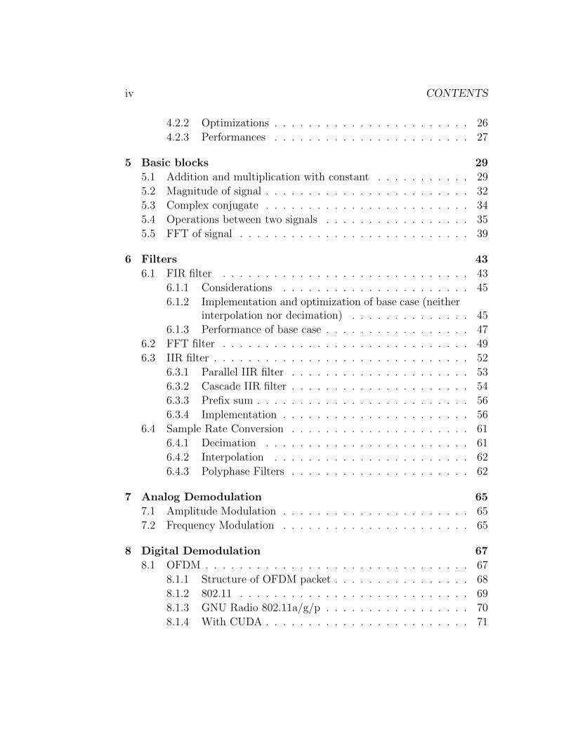
4.2.2 Optimizations . . . . . . . . . . . . . . . . . . . . . . . 26
4.2.3 Performances . . . . . . . . . . . . . . . . . . . . . . . 27
5 Basic blocks 29
5.1 Addition and multiplication with constant . . . . . . . . . . . 29
5.2 Magnitude of signal . . . . . . . . . . . . . . . . . . . . . . . . 32
5.3 Complex conjugate . . . . . . . . . . . . . . . . . . . . . . . . 34
5.4 Operations between two signals . . . . . . . . . . . . . . . . . 35
5.5 FFT of signal . . . . . . . . . . . . . . . . . . . . . . . . . . . 39
6 Filters 43
6.1 FIR filter . . . . . . . . . . . . . . . . . . . . . . . . . . . . . 43
6.1.1 Considerations . . . . . . . . . . . . . . . . . . . . . . 45
6.1.2 Implementation and optimization of base case (neitherinterpolation nor decimation) . . . . . . . . . . . . . . 45
6.1.3 Performance of base case . . . . . . . . . . . . . . . . . 47
6.2 FFT filter . . . . . . . . . . . . . . . . . . . . . . . . . . . . . 49
6.3 IIR filter . . . . . . . . . . . . . . . . . . . . . . . . . . . . . . 52
6.3.1 Parallel IIR filter . . . . . . . . . . . . . . . . . . . . . 53
6.3.2 Cascade IIR filter . . . . . . . . . . . . . . . . . . . . . 54
6.3.3 Prefix sum . . . . . . . . . . . . . . . . . . . . . . . . . 56
6.3.4 Implementation . . . . . . . . . . . . . . . . . . . . . . 56
6.4 Sample Rate Conversion . . . . . . . . . . . . . . . . . . . . . 61
6.4.1 Decimation . . . . . . . . . . . . . . . . . . . . . . . . 61
6.4.2 Interpolation . . . . . . . . . . . . . . . . . . . . . . . 62
6.4.3 Polyphase Filters . . . . . . . . . . . . . . . . . . . . . 62
7 Analog Demodulation 65
7.1 Amplitude Modulation . . . . . . . . . . . . . . . . . . . . . . 65
7.2 Frequency Modulation . . . . . . . . . . . . . . . . . . . . . . 65
8 Digital Demodulation 67
8.1 OFDM . . . . . . . . . . . . . . . . . . . . . . . . . . . . . . . 67
8.1.1 Structure of OFDM packet . . . . . . . . . . . . . . . . 68
8.1.2 802.11 . . . . . . . . . . . . . . . . . . . . . . . . . . . 69
8.1.3 GNU Radio 802.11a/g/p . . . . . . . . . . . . . . . . . 70
8.1.4 With CUDA . . . . . . . . . . . . . . . . . . . . . . . . 71
CONTENTS v
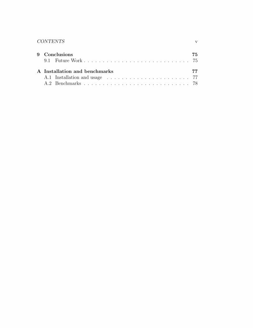
9 Conclusions 759.1 Future Work . . . . . . . . . . . . . . . . . . . . . . . . . . . . 75
A Installation and benchmarks 77A.1 Installation and usage . . . . . . . . . . . . . . . . . . . . . . 77A.2 Benchmarks . . . . . . . . . . . . . . . . . . . . . . . . . . . . 78

vi CONTENTS
Chapter 1
Software Defined Radio
Software Defined Radio is an evolving technology in which a big portion ofradio hardware is substituted with software modules.
The term software radio was firstly coined in the 1984 by E-System for aprototype, but we need to wait until 1991 in order to see a military programwhich specifically requires a radio with the physical layer implemented insoftware. The goal of this DARPA’s project was to have a radio capable tosupport ten different radio protocols and operate in any frequency between2 MHz and 2 GHz. In addition, it had to have the capacity to support newprotocols and modulations.
Next year was published the first paper about this topic,”Software Radio:Survey, Critical Analysis and Future Directions” [1]. In the following yearsthe civil interest grow considerably, bringing to the birth of some frameworkwhich can automatically generate code for SDR platforms. The most famousare provided by MathWorks and GNU Radio[2].
The adoption of SDR technology removes the development gap amongdifferent technologies and protocols, lowering the research and developmentcost and time.
For the users’ perspective, SDR terminal means a single device for mul-tiple protocols and standards, allowing customization and insertion of newfeatures/services with a simple software upgrade. In this way the lifetime ofthe terminal is stretched. Hardware bugs are less frequents (because the HWpart is more essential and can be tested deeply) and they can be partiallymasked by software.
1
2 CHAPTER 1. SOFTWARE DEFINED RADIO
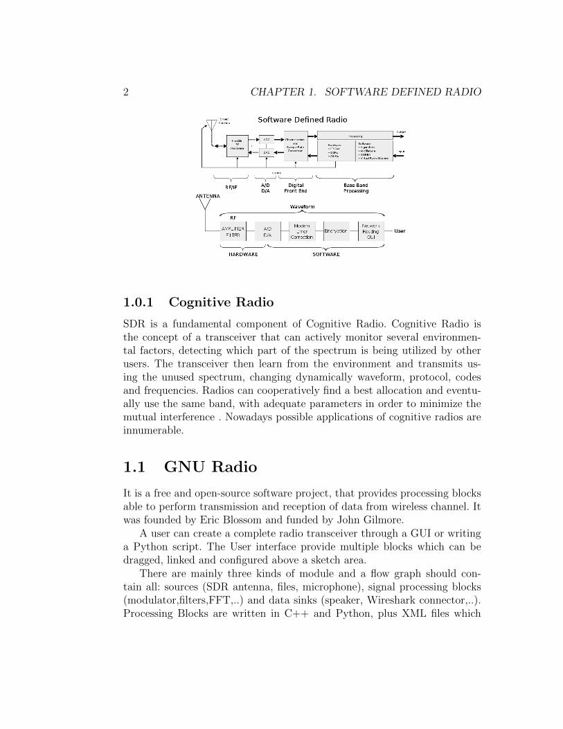
1.0.1 Cognitive Radio
SDR is a fundamental component of Cognitive Radio. Cognitive Radio isthe concept of a transceiver that can actively monitor several environmen-tal factors, detecting which part of the spectrum is being utilized by otherusers. The transceiver then learn from the environment and transmits us-ing the unused spectrum, changing dynamically waveform, protocol, codesand frequencies. Radios can cooperatively find a best allocation and eventu-ally use the same band, with adequate parameters in order to minimize themutual interference . Nowadays possible applications of cognitive radios areinnumerable.
1.1 GNU Radio
It is a free and open-source software project, that provides processing blocksable to perform transmission and reception of data from wireless channel. Itwas founded by Eric Blossom and funded by John Gilmore.
A user can create a complete radio transceiver through a GUI or writinga Python script. The User interface provide multiple blocks which can bedragged, linked and configured above a sketch area.
There are mainly three kinds of module and a flow graph should con-tain all: sources (SDR antenna, files, microphone), signal processing blocks(modulator,filters,FFT,..) and data sinks (speaker, Wireshark connector,..).Processing Blocks are written in C++ and Python, plus XML files which
1.1. GNU RADIO 3
describe their GUI interface. The presence of C++ aids the user to obtainhigh performance above more compute intensive paths, taking advantage ofprocessor extensions like vector operations.
GNU Radio make an extensive usage of a library called Volk, which im-plements vector extensions. For each method exposed, are available differentimplementation. Benchmarks are executed in order to understand which in-struction is the best choice in different scenario, taking into account size,memory alignment, etc..
The presence of Python allows the user to write code at higher level, in-terconnecting various basic components. C++ blocks are visible from Pythonthanks to a wrapping system based on SWIG
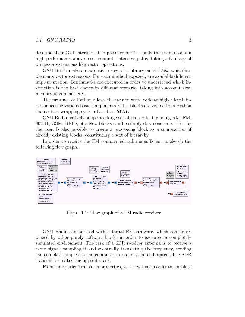
GNU Radio natively support a large set of protocols, including AM, FM,802.11, GSM, RFID, etc. New blocks can be simply download or written bythe user. Is also possible to create a processing block as a composition ofalready existing blocks, constituting a sort of hierarchy.
In order to receive the FM commercial radio is sufficient to sketch thefollowing flow graph.
Figure 1.1: Flow graph of a FM radio receiver
GNU Radio can be used with external RF hardware, which can be re-placed by other purely software blocks in order to executed a completelysimulated environment. The task of a SDR receiver antenna is to receive aradio signal, sampling it and eventually translating the frequency, sendingthe complex samples to the computer in order to be elaborated. The SDRtransmitter makes the opposite task.
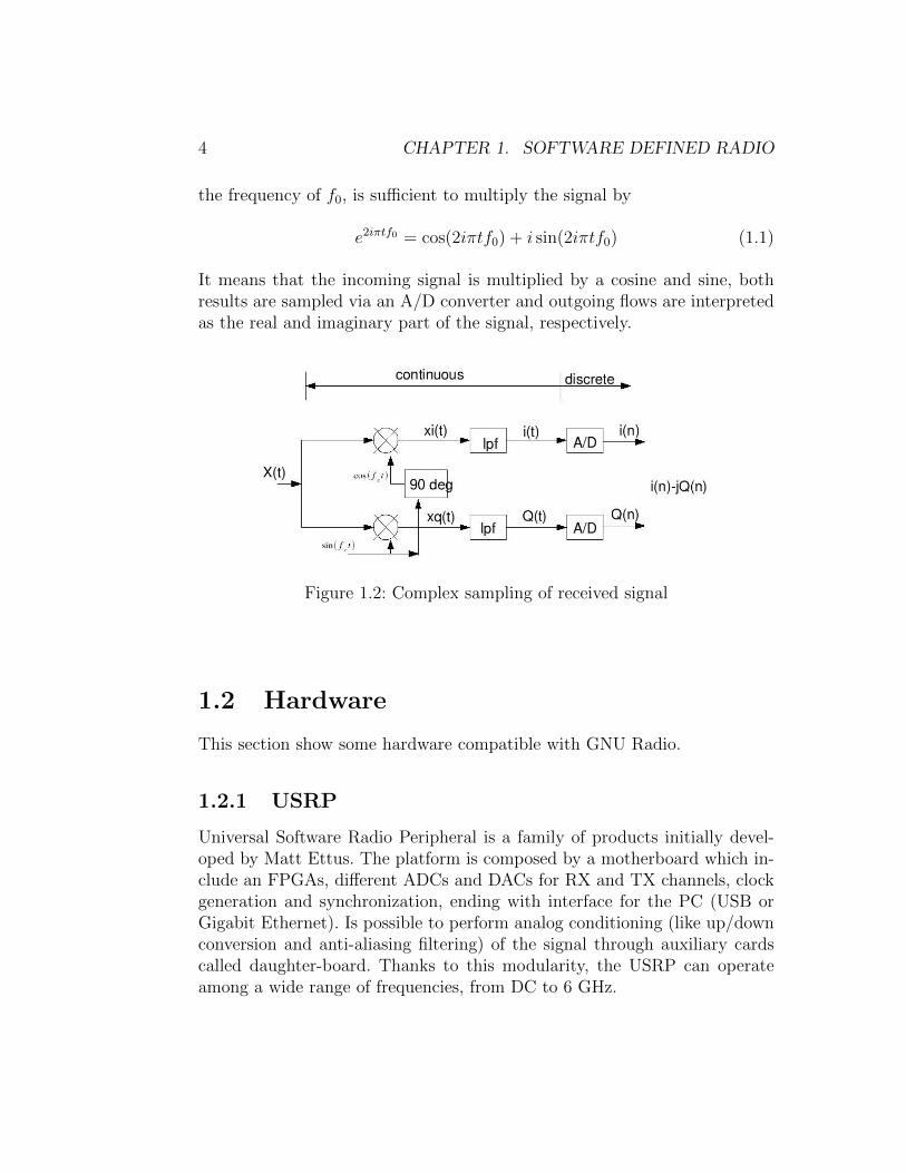
From the Fourier Transform properties, we know that in order to translate
4 CHAPTER 1. SOFTWARE DEFINED RADIO
the frequency of f0, is sufficient to multiply the signal by
e2iπtf0 = cos(2iπtf0) + i sin(2iπtf0) (1.1)
It means that the incoming signal is multiplied by a cosine and sine, bothresults are sampled via an A/D converter and outgoing flows are interpretedas the real and imaginary part of the signal, respectively.
Figure 1.2: Complex sampling of received signal
1.2 Hardware
This section show some hardware compatible with GNU Radio.
1.2.1 USRP
Universal Software Radio Peripheral is a family of products initially devel-oped by Matt Ettus. The platform is composed by a motherboard which in-clude an FPGAs, different ADCs and DACs for RX and TX channels, clockgeneration and synchronization, ending with interface for the PC (USB orGigabit Ethernet). Is possible to perform analog conditioning (like up/downconversion and anti-aliasing filtering) of the signal through auxiliary cardscalled daughter-board. Thanks to this modularity, the USRP can operateamong a wide range of frequencies, from DC to 6 GHz.
1.2. HARDWARE 5
The board is capable to digitize signals with a rate of 64 MSamples/swith a precision of 12 bit. Is also capable to emit 128 MSamples/s with aprecision of 14 bit.
The presence of FPGA permits the usage of the board in standalonemode, nevertheless is possible to perform distribute the execution of codebetween internal FPGA and CPU of a PC connected via USB (or GigabitEthernet). This card has good characteristics, but the price is in the order ofthousands of euro. In addition, the FPGA has a finite computational power,therefore in some scenario would be great to offload the execution on otherdevices (like GPU).
The interface between USRP and final PC is called UHD.
1.2.2 UHD
UHD is a short for USRP Hardware Driver. It provides an homogeneous in-terface for all USRP products, is compatible with major OS (Linux, Windowsand Mac) and is supported by several framework. Most important are GNURadio, MATLAB, Simulink and LabVIEW, in any case are exposed APIsaccessible from all products with native support for C++.
1.2.3 RTL-SDR
Few years ago Eric Fry discovered that some cheap DVB-T dongles offersdirect access to samples captured by antenna, at the desired frequency andwithout additional elaboration. With 20 eis possible to buy a dongle (basedon Realtek RTL2832U) able to receive almost every frequency between 22and 2200 MHz , with little variation according to the model and some dis-continuity near frequency multiple of internal local oscillator.
The sampling can be performed at a maximum rate of 2.56 MSamples/swith complex samples of 8 bit. Are available higher value of sample rate, butthey can loss samples.
Initially were implemented programs able to basic tasks, like receive FMcommercial radio on Linux or save samples into files, for a successive elabora-tion with Octave or MATLAB. Subsequently was implemented a GNU Radioblock able to handle these device and make available samples for successiveelaboration, directly inside the framework.
With a radio receiver with limited characteristic is still possible to performinteresting jobs, like receive audio signals, capture low rate data transmis-
6 CHAPTER 1. SOFTWARE DEFINED RADIO
sions, sniff radio remote controllers and telemetry, capture NOAA weathersatellite images and detect pulsars (another limitation is given by the an-tenna).
Chapter 2
CUDA
CUDA, which is a short of Compute Unified Device Architecture, is a parallelcomputing architecture developed by NVIDIA for massively parallel high-performance computing, exploiting the power of GPGPU.
2.1 GPGPU
General Purpose GPU is an evolution of graphics processing unit (GPU),originally developed for computer graphics, able to perform elaborate a widerset of applications, usually handled by CPU.
The CPU was initially developed with an architecture for sequential oper-ations. It uses a sophisticated control logic in order to manage the executionof different instructions out-of-order with multiple function units, still main-taining the appearance of a sequential execution. It also adopts large cachesin order to minimize the bottleneck caused by the RAM.
Conversely, the main goal of GPU was to execute large amount of floating-point operations in order to perform graphic applications. It is composed byseveral processing units (up to hundreds at least), each one with a simplerimplementation and lower frequency respect to CPU.
In the first period, the behaviour of these units was hardwired for graph-ical operations, allowing the programmer to use only languages as OpenGLand DirectX.
In last years the interest about general computation performed by GPUgrown significantly, leading to a new architecture: General Processing GPU.These graphic cards are able to handle hundreds of threads together, with
7
8 CHAPTER 2. CUDA
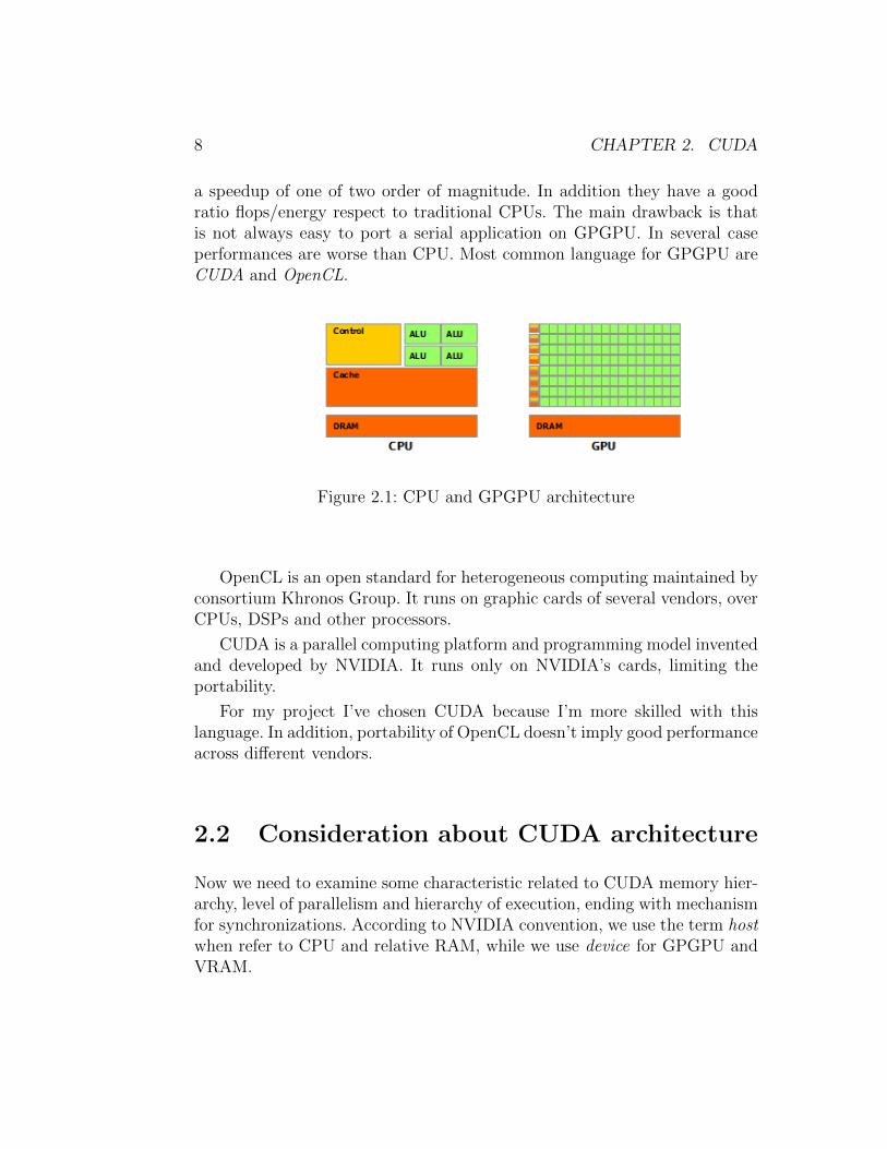
a speedup of one of two order of magnitude. In addition they have a goodratio flops/energy respect to traditional CPUs. The main drawback is thatis not always easy to port a serial application on GPGPU. In several caseperformances are worse than CPU. Most common language for GPGPU areCUDA and OpenCL.
Figure 2.1: CPU and GPGPU architecture
OpenCL is an open standard for heterogeneous computing maintained byconsortium Khronos Group. It runs on graphic cards of several vendors, overCPUs, DSPs and other processors.
CUDA is a parallel computing platform and programming model inventedand developed by NVIDIA. It runs only on NVIDIA’s cards, limiting theportability.
For my project I’ve chosen CUDA because I’m more skilled with thislanguage. In addition, portability of OpenCL doesn’t imply good performanceacross different vendors.
2.2 Consideration about CUDA architecture
Now we need to examine some characteristic related to CUDA memory hier-archy, level of parallelism and hierarchy of execution, ending with mechanismfor synchronizations. According to NVIDIA convention, we use the term hostwhen refer to CPU and relative RAM, while we use device for GPGPU andVRAM.
2.2. CONSIDERATION ABOUT CUDA ARCHITECTURE 9
2.2.1 Execution
The programmer writes functions, called kernel, which are executed N timesin parallel when launched, by N different CUDA threads. Is defined an hier-archy among computation elements.
The lower level is the thread, which execute an instance of the kernel, ischaracterized by a unique ID within its thread block and own a small set ofprivate registers. Thread is executed by a Streaming Processor (SP), whichcontain an ALU, a Floating Point Unit and other functional units.
The middle level is the block, which is a set of concurrently executingthreads that can cooperate among themselves through synchronizations andshared memory. A thread block is characterized by a block ID within itsgrid. Threads of the same block are executed on the same Streaming Mul-tiprocessor (SM) for the entire execution. SM is a SIMT (Single InstructionMultiple Threads) processor which manages and executes threads in groupsof 32 parallel threads, called warp. Every SM is composed by multiple Stream-ing Processor and Special Function Units (SFU, deputed for functions liketrigonometric). Actually each block can contain a maximum of 1024 threads.
The higher level is the grid, which is the set of all blocks created bya kernel launch, eventually executed on different SM. They are executedindependently, the communication can happen only through global memory,that we’ll see later.
Is important to remark that threads of same warp execute same instruc-tion ”simultaneously”. If one or more threads executes conditional code thatdiffer in code path from other threads in the warp, these different executionpaths are effectively serialized, as the threads need to wait for each other.This phenomenon is referred as thread divergence and dramatically worsenperformances.
A GPGPU can manage more threads (and blocks) than available SPs (andSMs). Only some warps (and block) are active and a fast context switchinghappen every time there is a stall due to operand not ready.
A common metric of utilization is occupancy, which is the ratio of thenumber of active warps per multiprocessor to the maximum number of warpsthat can be active on the multiprocessor at once. There is a finite memoryinside the multiprocessor, so higher occupancy implies less registers for eachthread. When the kernel is memory bounded (access to global off-chip mem-ory) a good approach is to have high occupancy, because in this way thelatency can be hidden switching to other warps, exploiting the Thread Level
10 CHAPTER 2. CUDA
Parallelism (TLP). The drawback of this method is that it aggravate registerpressure.
Another way to increase parallelism is given by Instruction Level Paral-lelism [3]. This strategy can be applied with a low occupancy, which impliesmore registers available for each thread. Programmer must write kernel codewhich is not stalled waiting data from (immediately) previous instructionslike arithmetic and memory transfer (e.g. loop unrolling). Another advantageof this technique is that shared communications can be reduced, because noweach thread elaborate more items. This is good, because memory access tolocal memory is (usually) faster than shared memory, improving the finalspeedup.
2.2.2 Memory
During execution, CUDA threads can access data from multiple memoryspaces.
Threads own a private local memory, which is stored in register (accessin few cycles, but limited space) or in global memory (off-chip, high latency).
Thread blocks have a shared memory visible to all threads of the sameblock. This is the main method used for communication inside block andaccesses are 3-6 times slower than local register (it depends on architecture).Another way would be the usage of shuffle instructions, unfortunately theyare not supported by my graphic card. The shared memory is divided intoequally-sized memory modules, called banks, which can be accessed simul-taneously. If a memory request (usually launched by a warp) contains twoor more addresses of the same bank, a bank conflict occurs. In this case therequest is split, slowing down performances.
Threads can also perform read/write operations on global memory, whichis hosted outside the chip (this won’t be true with next architecture Pascal)and survive across different kernel calls. This storage has a capacity in orderof gigabytes, but the latency is hundred of times higher than on-chip registers,also bandwidth is slower than storages previously analyzed.
Every access is performed with memory transactions with a width of 32-,64- or 128-bytes. For this reason is important that all threads of the samewarp access to aligned and adjacent memory location, otherwise memoryaccess is serialized into multiple memory transactions. The access is calledcoalesced when this rule apply.
Another bottleneck is given by partition camping [4]: as shared memory,
2.2. CONSIDERATION ABOUT CUDA ARCHITECTURE 11
also global memory is divided into memory banks (with a size bigger thanshared). When different warps access to the same bank, accesses are serializedslowing down the execution. This limitation was almost solved for Fermi andnewer architectures.
Two other kind of memory are texture and constant. The former is usefulin graphics application because allow the programmer to use floating pointindices over matrices, performing an efficient interpolation across adjacentcells. The latter allow an efficient access to constant memory, but loads mustbe relatively small and must be accessed uniformly for good performance (Allthreads of a warp should access the same location, otherwise a serializationwill be performed). Both kind of memory are hosted on global memory, withon-chip caches for last used values. I’ve decided to don’t use constant memorybecause its size is very small and it would be shared by different GNU Radioblocks.
Inside the chip there is a L2 cache for the global memory, which is almosttransparent to programmer (is possible to use PTX instructions in order tointeract with it, as also with L1). It is visible by all SMs into the chip and ituses a LRU policy. This memory is also used to perform
Each SM has an own L1 cache, which is stored on the same memoryportion of shared memory (on newer architectures is possible to choose howsplit this space). According to the architecture, this cache is used for allaccesses to global memory or only for register spilling.
Last architectures provide an efficient mechanism for constant memory,called read-only data cache. It can be enabled by compiler over standardpointers pointers when certain conditions are met, like the usage of modifiersconst and restrict . It uses a separate cache with a separate memory pipe(to global memory) and with relaxed memory coalescing rules. The usageof this feature can improve the performance of bandwidth-limited kernels,because data cache can be much larger and can be accessed in a non-uniformpattern respect to standard constant memory.
CUDA kernels can access directly to host memory regions when the allo-cated RAM is pinned (guarantee that the memory page is not flushed ontohard disk) and mapped into device address space. This feature is called Uni-fied Virtual Address space (UVA).
From CUDA 6 this feature was extended with Unified Memory, whicheliminates the need of explicit data movement between host and device mem-ory. Memory regions are automatically migrated where they needed (alsoacross different devices in multi GPU configurations), facilitating the pro-
12 CHAPTER 2. CUDA
gramming and maintainability. Actually a clever ”manual” management ismuch more efficient than this mechanism, so I didn’t use this feature in myproject.
Operations
Main operation is the memory copy between host memory (RAM) and globalmemory (cudaMemcpy and cudaMemcpyAsync). Surely the bandwidth is up-per bounded by PCIe bus. Another limit is given by the kind of allocationin host memory. If the memory region is pinned (page-locked), the allocationcannot be swap onto secondary storage and the the copy is performed di-rectly by the DMA. Otherwise the host need to perform an additional copybetween the host memory and an internal host-pinned memory, halving thebandwidth.
Recent architectures contain one or more copy engine, which allow thecontemporary data transfer and execution of independent kernel.
Memory copy between host pinned memory and global memory can alsobe performed writing an adequate kernel. Choosing a clever occupancy andILP is possible to reach same performance of the CUDA memory copy func-tion (from my experiments), where the bandwidth is limited by PCIe bus.
CUDA provides a function for memory initialization, called cudaMemset,which allows the user to fill/initialize an array. The curios fact is that thisoperation doesn’t fulfill the bandwidth. Is more efficient to write a smallkernel in order to perform the initialization. The CUDA API is used wherethe initialization is performed only once, at start-up.
2.2.3 Concurrency and synchronization
Scheduling of kernels
An important concept in CUDA is stream. It is a sequence of operationsthat are executed sequentially, while commands of different streams may beexecuted out of order and concurrently. Kernel calls and memory copy arealways associated to a stream, implicitly or explicitly. Example of explicitusage of stream are CUDA functions that contain async in the name, likecudaMemcpyAsync.
A particular case is the default stream, which issues next operations whenall previous commands from any streams (of current threads or all threads)
2.2. CONSIDERATION ABOUT CUDA ARCHITECTURE 13
are terminated. This is used as implicit stream. The host code can pause untilprevious command in the stream are executed, providing an useful mechanismof synchronization.
An interesting object is event, which monitors the device’s progress aswell as perform accurate timining. Events are inserted into a specific stream(may be the default stream) and are recorded when all previous commandin the queue are executed. Host code can query their status in order to knowthe progress, is also possible to suspend host execution until a given event isrecorded. Streams can be paused until a certain event is reached, providingan useful mechanism to wait the availability of all inputs before a kernelexecution.
Combining streams and events, is possible to express a direct acyclic graphof dependencies. If a stream A should wait that stream B reach a given point,is sufficient to create an event associate at this spot and pause the executionof A until the event is recorded. The graph is acyclic because is not possible topause a stream waiting for an event not still created when CUDA schedule it(from host side). In this case the execution continue ignoring the conditionalpausing.
Warp execution
Threads of same warp execute simultaneously and CUDA provides somemechanism for synchronization across warps.
There is a basic barrier synchronization for warps of same block throughthe function syncthreads(), that pause thread execution until all warps (ofblock) reach the barrier. This is a rigid mechanism, because in lot of caseis undesirable to wait every threads. This happens each time the functionis called inside a branch imposing a more complex code to the programmer.The barrier also strongly limits application where each warp takes a differentexecution path (warp specialization)
The ”assembler” of CUDA offers a more flexible mechanism inside theblock , called named barriers . Are available 16 barriers and the syncthreads()is built on it, using two of them. There are two methods, one signal the ar-rival of a warp to a given barrier (without stop), while the other stop thewarp until a certain number of warps has signaled its arrival to the barrier.Using two barriers, is possible to implement a producer-consume paradigmover different warps.
This feature is exploited by CudaDMA [5] library, which provides an
14 CHAPTER 2. CUDA
higher level approach (respect to manual handling of PTX code) for executeasynchronous memory operation. Warps are split in compute and memorygroups, one performs elaboration and ask to load new data, while the otherperform memory global operations. This can be very efficient when the mem-ory pattern is not sequential.
Is not available a function for synchronization across threads of differentkernel. Researcher suggest some approach like memory spinning, but is notguarantee that they work in every conditions. The scheduling is not pre-dictable or the same for all architecture, so a code that perfectly work in onegraphics card, cause deadlock on another.
Chapter 3
SDR with CUDA
3.1 State of art and objectives
The usage of software defined radio could require an huge computationalpower during elaboration, which can be speed up thanks to the usage ofGPGPU.
Actually there are some implementations of radio processing blocks whichtake advantage of GPGPU capabilities.
Gr-theano[6] is a module of GNU Radio which uses a Python library,called theano[7][8], strictly integrated with Numpy. Currently this module isable to perform FFT, FIR filtering and can be used to model the fading.
Gr-fosphor is a block which shows a waterfall diagram of the input, usingOpenCL in order to compute the spectral components and OpenGL for thevisualization.
Some years ago was also available an experimental library called gr-gpu.The author was not satisfied about its performances and removed it fromrepositories. I was not able to find the source code.
Another useful example is an implementation of LTE receiver [9] overGPGPU. Their research was more focused on turbo decoder, their imple-mentation takes globally few milliseconds for each data frame sent/received,being able to work in real-time.
The problem is that previous implementation, although they provide goodperformance, are very specific for a specific target and are not able to providea flexible framework, losing the wide approach given by SDR.
The goal of this thesis is to extend GNU Radio in order to allow users to
15
16 CHAPTER 3. SDR WITH CUDA
build flow graph composed by CUDA blocks, finding and minimizing bottle-necks. The porting will cover all the main blocks,so mathematical operationbetween flows, low-pass/high-pass/band-pass filters, IIR filters, FFTs andFFT filters, ending with OFDM.
The final user should be able to use these blocks without an additionalknowledge. The unique suggestion is to avoid the insertion of CPU GNURadio blocks between GPU blocks.
For compatibility reason I’ve decided to don’t make a customized ver-sion of GNU Radio, instead I’ve created a module which contain all blocksand management. This module can be imported in every installation whichsupport CUDA, immediately after can be used joined with other blocks. Forsake of simplicity this framework won’t be compatible with CUDA devicecharacterized by a compute capability less than 2.0. Older architectures arevery limited, in addition its support is ended with CUDA 7.0.
In this thesis I start showing the common part used by all my blocks(management of memory, execution, etc.) followed by choices in the designof single blocks.
3.2 Architectural choices
3.2.1 Memory
The management of memory is always a problem: each transfer between hostand device is expensive in terms of bandwidth and latency. For instance thecomputation of FFT over the CUDA device can be very profitable, but partof the gain would be lost if the FFT size is small, the input and output mustbe transferred from/to host memory and a low latency is required.
Is mandatory to minimize transfers between device and host memory.Ideally there is only one transfer host-to-device at the beginning of the flowgraph (e.g. incoming data from antenna) and a device-to-host copy at theend.
Now we examine requirement of GNU Radio blocks in terms of commu-nication buffer between adjacent blocks. In a data-link between to attachedblocks, we call top the source of data and bottom the sink of data flow. Weknow that some block has a simple relation 1:1 between incoming and out-coming data, while other has N:1 (decimation) or 1:N (interpolation), whereN is previously know. Where are rarely case in which N is not previously
3.2. ARCHITECTURAL CHOICES 17
know (e.g. frame detector) because it depends on incoming data and the sizemust be returned from device, but we can manage this case separately. Inaddition some blocks has special needs, like know previous inputs(history)for blocks like FIR filter, in other case is necessary to know previous out-puts (e.g. IIR filter). It is also recommendable to don’t invoke a kernel overa small task, otherwise overhead due to invocation would be greater thancomputational time. A first approach would be the usage of a circular bufferallocated in device memory at start-up. It satisfies some requirement, but thecode would become complex when we try to use the same buffer as input forone block, and both input/output for another blocks. In addition, it wouldimpossible to make a clever usage of CUDA events in order to manage aproducer-consumer pattern on the device.
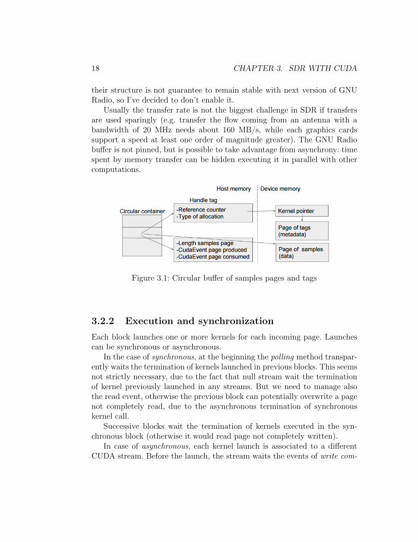
A good trade off would be the usage of a circular buffer of pages, whereeach pages is an area in device memory with a dimension of some Kilobytesor Megabytes. The number of pages and the dimension of each would be atradeoff between latency and execution time. Each page is associated to twoevents: one is registered when the write operation (by the producer) on therelative page is finished, while the other is registered when the read (fromconsumer) is terminated.
At the beginning (in the constructor), each blocks declare its preferenceof incoming and outcoming links, like minimum and maximum number ofitems per page, which multiple should be the number of items in the page,maintain the previous page as history. This strategy aims to improve memoryusage.
Each block must perform, for each invocation, a method called pollingwhich internally manages the initially handshake and each time performsdifferent checks.
All information about current written/read page and its length are con-tained in host memory, because the CPU knows and uses these information(e.g. when is necessary to split a kernel call in two separate execution, dueto end of page of output). Lot of blocks have the dimension of output pre-dictable from the input size, so it can calculated by host, avoiding expensivememory transfers.
There are two GNU Radio blocks for the memory transfer between RAMand memory device. They perform a series of cudaMemcpyAsync betweenGNU Radio buffer and CUDA buffer. Unfortunately the host buffer is notpinned, so we cannot avoid the double-copy, halving performances. In anycase is possible to use cudaHostRegister in order to pin these buffers, but
18 CHAPTER 3. SDR WITH CUDA
their structure is not guarantee to remain stable with next version of GNURadio, so I’ve decided to don’t enable it.
Usually the transfer rate is not the biggest challenge in SDR if transfersare used sparingly (e.g. transfer the flow coming from an antenna with abandwidth of 20 MHz needs about 160 MB/s, while each graphics cardssupport a speed at least one order of magnitude greater). The GNU Radiobuffer is not pinned, but is possible to take advantage from asynchrony: timespent by memory transfer can be hidden executing it in parallel with othercomputations.
Figure 3.1: Circular buffer of samples pages and tags
3.2.2 Execution and synchronization
Each block launches one or more kernels for each incoming page. Launchescan be synchronous or asynchronous.
In the case of synchronous, at the beginning the polling method transpar-ently waits the termination of kernels launched in previous blocks. This seemsnot strictly necessary, due to the fact that null stream wait the terminationof kernel previously launched in any streams. But we need to manage alsothe read event, otherwise the previous block can potentially overwrite a pagenot completely read, due to the asynchronous termination of synchronouskernel call.
Successive blocks wait the termination of kernels executed in the syn-chronous block (otherwise it would read page not completely written).
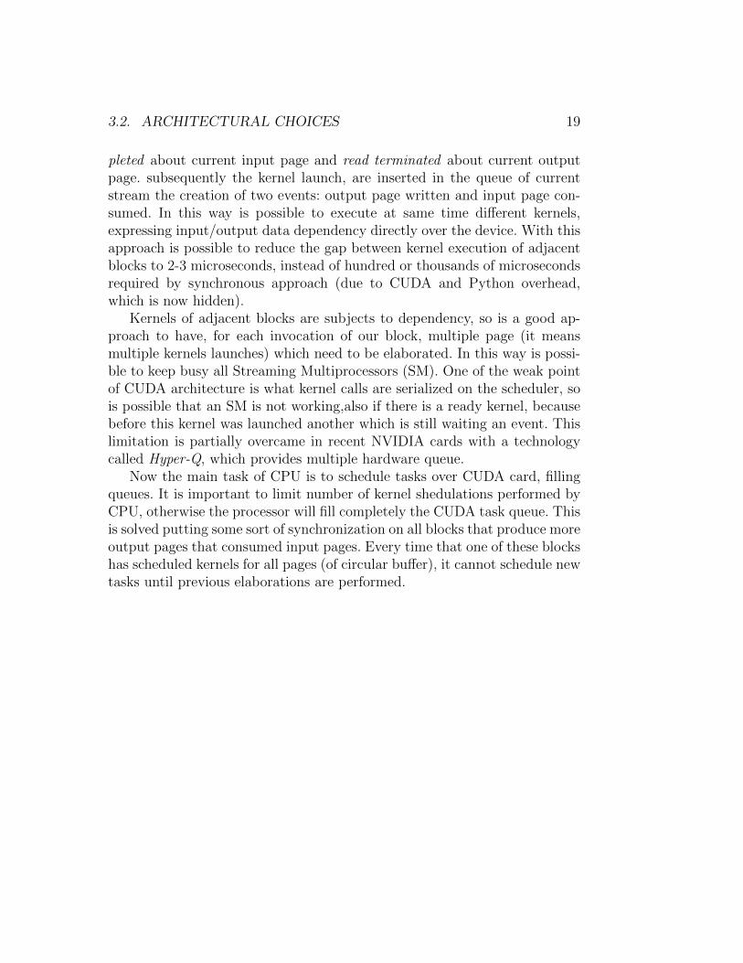
In case of asynchronous, each kernel launch is associated to a differentCUDA stream. Before the launch, the stream waits the events of write com-
3.2. ARCHITECTURAL CHOICES 19
pleted about current input page and read terminated about current outputpage. subsequently the kernel launch, are inserted in the queue of currentstream the creation of two events: output page written and input page con-sumed. In this way is possible to execute at same time different kernels,expressing input/output data dependency directly over the device. With thisapproach is possible to reduce the gap between kernel execution of adjacentblocks to 2-3 microseconds, instead of hundred or thousands of microsecondsrequired by synchronous approach (due to CUDA and Python overhead,which is now hidden).
Kernels of adjacent blocks are subjects to dependency, so is a good ap-proach to have, for each invocation of our block, multiple page (it meansmultiple kernels launches) which need to be elaborated. In this way is possi-ble to keep busy all Streaming Multiprocessors (SM). One of the weak pointof CUDA architecture is what kernel calls are serialized on the scheduler, sois possible that an SM is not working,also if there is a ready kernel, becausebefore this kernel was launched another which is still waiting an event. Thislimitation is partially overcame in recent NVIDIA cards with a technologycalled Hyper-Q, which provides multiple hardware queue.
Now the main task of CPU is to schedule tasks over CUDA card, fillingqueues. It is important to limit number of kernel shedulations performed byCPU, otherwise the processor will fill completely the CUDA task queue. Thisis solved putting some sort of synchronization on all blocks that produce moreoutput pages that consumed input pages. Every time that one of these blockshas scheduled kernels for all pages (of circular buffer), it cannot schedule newtasks until previous elaborations are performed.

20 CHAPTER 3. SDR WITH CUDA
Chapter 4
Implementation of commonparts
4.1 Tagged streams
GNU Radio was originally developed as a streaming system, where data flowbetween consecutive GNU Radio blocks is treated as a stream of numbers.They represent samples provided by antenna, inputs for the audio sink, etc.
This basic model doesn’t provide features like control and meta data overthe data flow. In different scenario would be useful to associate meta data tothese values, like time stamp of receipt, frequency, beginning of a new packet(in OFDM transmission).
In order to satisfy these requirement, GNU Radio provides a feature calledstream tags. This is an additional data stream that works synchronously withthe main data stream. Tags are generated by specific blocks, are associatedto specific samples and can follow the same flow of the main data flow. Eachblocks can propagate, ignore, modify or add tags.
Each tag is characterized by a key-value pair, both fields are PMTs (Poly-morphic Types). PMT is usually used to carry numbers and strings, but italso support dictionaries, tuples, vectors of PMTs and other types.
In practice, only strings and numbers (integer, float, complex) are usedas PMT, so I’ve implemented these cases.
In addition, the management of textual keys in parallel can be a bottle-neck. For this reason, textual keys which are treated by blocks on GPGPU aretransparently converted to numerical constant during the memory transfer
21
22 CHAPTER 4. IMPLEMENTATION OF COMMON PARTS
between host and device (and vice versa). Other textual keys can be managedas bunch of bytes, because are meaningless for blocks executed over GPGPU.
Blocks can ignore tags, forward them directly (e.g start of frame) or mod-ify them. Lot of blocks don’t use tags, but eventually propagate them. Givena page of samples to a GNU Radio blocks, is not predictable the number thenumber of tags that will be produced by the block itself: it is known from thekernel function only during the execution. In addition, we’d like to maintainthe asynchronous kernel execution for performance reason.
In a typical case the block at the beginning of flow graph produces tags,which are propagated and consumed only at the end of the chain. A situationlike this is not rare. For this reason is not good to use an approach similar tothe main data stream between consecutive blocks (a circular buffer of pages),because in the worst scenario we would have tons of avoidable memory copies.
A better approach would be to ”allocate” a memory region each timethat is necessary to associate tags to some samples. For sake of simplicity,all tags of samples contained in the same page (referring to buffer of maindata stream) are maintained in the same memory region, which we call tagpage. So each page of circular buffer is eventually associated to a different tagpage. The forward is performed simply by propagating the pointer to the nextGNU Radio block. What happen then a block needs to modify/add/deletesome tags?
Before to think how to implement this situation, is better to consideranother scenario.
4.1.1 Usage of reference counters
Is possible that a block propagates incoming tags to multiple output, then ispreferable to avoid additional memory copies (due to bifurcations).
It seems obvious the usage of reference counter for each tag page, whichare incremented each time that a tag page is propagated to multiple outputs.
When a tag page is modified, a new tag page is created and is propagatedto next blocks, while the reference counter of source tag page is decremented.
In this way, there are no problems if a block in a branch modify the tagpage shared with another branch. The unique case in which is not requiredto create a new page is when the reference counter is equal to 1, but usuallyperformed operations are add and delete tags. It means that in lot of case isrequired a different size for the tag page, so an allocation would be necessary.
4.1. TAGGED STREAMS 23
Each time that a tag page is not propagated by a block, the relativecounter is decremented. When it reaches zero, the tag page can be deallo-cated.
Because kernels are executed asynchronously, is necessary to wait thekernel termination before to decrement the counter. This requirement can beaccomplished in different way.
• CudaStreamAddCallback called after the invocation of CUDA kernel,performing the decrement of counter
• Create an event when the kernel terminate. Probe sometimes eventshappened (tag page is consumed) and decrement relative counters.
The first approach has some limitations, like the callback method cannotcontain CUDA calls (like cudaFree) otherwise in some situation a deadlockcan happen. The execution of the callback method is expensive (about 15microseconds on my platform) and prevents the occupation of all streamingmultiprocessor (because there is a sort of synchronization between devicecode and host code).
The latter consist of create a CUDA event after the termination of CUDAkernel with cudaEventCreateWithFlags (in order to don’t save timing infor-mation, which slowdown the execution) and cudaEventRecord. SometimescudaEventQuery is called in order to test which events are happened, inorder to know which tag page can be deallocated (or reference counter decre-mented). This approach allow to call CUDA API during deallocation, likecudaFree, because is not a callback method like the previous. Are used threeNvidia call, cudaEventCreateWithFlags, cudaEventRecord and cudaEvent-Query, which take between 0.5 and 1 microseconds each, with an overalloverhead between 2 and 3 microseconds. This implementation would be fasterthan CudaStreamAddCallback, but it can be improved.
Is not mandatory that the reference counter is decremented immediatelyafter the execution of kernel which consume the page. In addition, we knowthat all CUDA calls executed on the same stream are performed sequentially.In order to decrease perceived overhead due to CUDA API calls, we can usea time-space tradeoff: record (and create) an event every N CUDA kerneltermination (over the same stream). In this way, the overhead is reducedby a factor N, increasing the number of tag page which are not anymorereferenced, but are still in memory.
24 CHAPTER 4. IMPLEMENTATION OF COMMON PARTS
4.1.2 Considerations about allocation
In some case the size of tag page is predictable by the host before the kernellaunch, e.g. during the copy of samples between host memory and devicememory.
In other scenarios the number of tags is know only during the execution ofCUDA kernel, for instance when the kernel detect the beginning of packets.
The problem is which allocator use in order to create memory regionsover device memory.
Adopt only an host malloc is not easily implementable with asynchronouscall, because after the kernel execution (which produce tags) would be nec-essary to allocate a memory region and copy tags inside. Is not possibleto call asynchronously a cudaMalloc (inside a CudaStreamAddCallback), soa customized allocator would be necessary. The usage of callback is also anightmare for performance.
Is not a good idea to adopt only a device malloc, because in scenariolike move data flow (of GNU Radio flow graph) from CPU to GPU sizes areknown by CPU (because its copying tags from RAM).
Is better to allow the user to use both. Each tag page is referenced by an”handle”. It is composed by a reference counter, a flag which indicate the usedallocator and a pointer to device memory (allocated by host). This pointerrefers to a small memory portion, what we call kernel pointer, containingonly the address of the tag page (on device memory). Kernel pointer can bewritten by host and device without problems about performance. kernel callsneed only to access to this pointer, without interact with host memory. Atthe same time, the host code only need to propagate handles between GNURadio blocks, also when the tag page is NOT still allocated.
4.1.3 Allocation
Because for each page could be necessary to allocate space for tags, invoca-tion of allocation and deallocation in memory can happen often, that inducea significant bottleneck. There are different kind of allocation on device mem-ory:
• Fixed size by host
• Flexible size by host
4.2. MEMORY ALLOCATOR 25
• Flexible size by device
The former usually doesn’t involve big chunks of memory and is used espe-cially for allocate kernel pointer. An approach would be to allocate at thebeginning a big chunk of memory, splitting it and putting pointers into a freelist. Malloc is performed by taking (and removing) a pointer from this list,while the free is performed by inserting the pointer inside the list.
Memory allocation by host with flexible size can be easily performedby cudaMalloc, while the free can be executed via cudaFree in some lazyway (callback cannot be used). The allocation of one million of region withthe size of one pointer takes about 10 seconds, it means 10 microsecondsfor each allocation. The cudaFree takes other 6 microseconds, plus a bigdrawback: this function waits the termination of previous calls executed ondevice, impeding the asynchronous paradigm. In the next section we explorea customized allocator.
For the last case (allocation from device), are available the CUDA mal-loc() and free() methods. Their performance are acceptable when they areused sporadically and not concurrently from different threads. Are availablespecific allocators like Halloc[10] with high performances, but they’re de-signed for small allocations. In my project, allocations performed by deviceare minimized.
4.2 Memory allocator
In our implementation there are lot of device memory allocation/deallocationperformed by the host. As seen previously, these API calls are expensive interms of performance. For this reason, it would be great to use a customizedallocator which manages device memory and makes few interactions withCUDA allocator.
There are different types of allocator: in my implementation I’ve chosena memory pool which offer only memory regions with size power of two,because is simple and faster compared to other approaches. The maximuminternal fragmentation will be not bigger than the space required by the user.In addition, are available additional sizes which accommodate objects largelyused, like kernel pointers.
Another requirement is that calls to allocator are thread safe, becauseeach GNU Radio block can work in a different threads. Usually memory
26 CHAPTER 4. IMPLEMENTATION OF COMMON PARTS
allocated by a block will be deallocated by another block, then would bepreferable to share freed allocation among all threads.
4.2.1 Structure
Each GNU Radio block instantiate a set of Allocator object (one for eachsize). These objects contain a set of free allocations. All malloc/free oper-ations take/insert pointers in this set. When the cardinality of the array islower/bigger than certain thresholds, a subset of pointers is taken/movedfrom another object, called GlobalAllocator. It is a templated singleton,where the parameter is the size of memory region. It means that there is aunique global object for each size, uniqueness that is guarantee by a c++11construct. It shares a set of free region with local allocator, allocating newspace when necessary.
4.2.2 Optimizations
There are different C++ data structures which can host the set of pointers.The more suitable are vector, list and deque. I’ve tried all three approach,but the first is always faster, also with GlobalAllocator which need to copysome hundred of pointers each time. I’ve also tried a mixed approach: localallocators work with vector of free portions, while global allocator keep a listof vectors. In this way, for each interaction with a local allocator, an item ofthe list (vector of pointers) is inserted/removed. This approach tend to beslower than the simple vector.
Is mandatory to guarantee multi threading, while at the same time isdesirable to minimize its cost. It would be great to minimize temp spentinside locked sections. Methods malloc and free of global allocator(whichwork on vectors of pointers) are protected by a lock guard, according toRAII paradigm (Resource Acquisition Is Initialization). This mechanism isprovided by Boost and by c++11 standard libraries. Boost is faster on mymachine, in any case the price paid for critical section is distributed amongmultiple allocations.
Each local allocator keeps two vectors of free allocations, operations areperformed above one, called active. When the active vector contains morepointers than a given constant, vectors are swapped. When both sets arefull, one of them is passed to global allocator, while the other become theactive set. This transfer of items (pointers) and the opposite operation (get
4.2. MEMORY ALLOCATOR 27
allocations from global allocator) are performed using the move construct ofc++11, which move the ownership of an object. In this way is not performeda useless copy of objects (during the passage of arguments) which are demol-ished immediately after. The compiler can also get more advantage respectto the usage of references.
4.2.3 Performances
Sizes of memory pools used by local and global allocators can be changedeasily. In my implementation, I’ve chosen for the global pool a minimumsize of 4096 items, while local pools are between 512 and 1024. I’ve triedto executed for 100 000 times a set of 10 000 allocations followed by theirdeallocations (but performed from a different local allocator). In this waylocal allocators need to interact often with global allocator.
The whole execution for one billion of allocation/deallocation takes be-tween 5.6 and 5.7. It means that in average a pair allocation/deallocationtakes less than 6 nanoseconds, much better than microseconds required byCUDA allocator.

28 CHAPTER 4. IMPLEMENTATION OF COMMON PARTS
Chapter 5
Basic blocks
Is important to give the opportunity to perform basic tasks as mathematicaloperation over signals. GNU Radio provides blocks for each operation, allimplemented using the most appropriate CPU vector extension.
I’ve written an implementation for addition and multiplication(signal-tosignal and signal-to-constant), division and amplitude of complex number.We can expect tasks memory bounded, with a short kernel duration.
5.1 Addition and multiplication with constant
Implementation and behaviour of these blocks is expected to be similar.Where don’t specify, I speak about summation between complex numbersand each input page has a size of 4 millions of samples (MSamples).
The kernel of the naive implementation takes about 6.8 ms for each exe-cution, with the best combination blockDim and gridDim, with an occupancyof 100%. In this case, accesses performed by a single thread are strided withsize of grid. Adding a pragma unroll above the loop decrease performances.
For complex numbers, an idea can be to use even threads for real parts andodd threads for imaginary parts, with manual overlapping in order to executethe same number of operations (for iteration) of previous implementation.According to profiling, kernel execution become slower.
Computing two items for each iteration with a manual unrolling of twooperation (with size blockDim inside the loop), is possible to terminate theexecution in 3.2 ms (occupancy 85%), doubling performance also thanks tobetter locality. According to the profiler, global bandwidth is near the limit
29
30 CHAPTER 5. BASIC BLOCKS
(>24GB/s), but there is an unbalance of 30% between global loads and stores.
It seems natural to improve locality by splitting the input page in gridDimparts. Global bandwidth is slightly smaller (25GB/s) than the device limit,with a good balance between reads and writes, but surprisingly the timeexecution doubles.
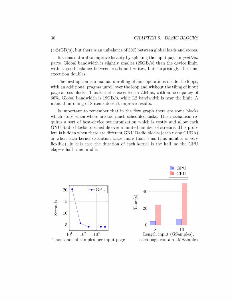
The best option is a manual unrolling of four operations inside the loops,with an additional pragma unroll over the loop and without the tiling of inputpage across blocks. This kernel is executed in 2.64ms, with an occupancy of66%. Global bandwidth is 19GB/s, while L2 bandwidth is near the limit. Amanual unrolling of 8 items doesn’t improve results.
Is important to remember that in the flow graph there are some blockswhich stops when where are too much scheduled tasks. This mechanism re-quires a sort of host-device synchronization which is costly and allow eachGNU Radio blocks to schedule over a limited number of streams. This prob-lem is hidden when there are different GNU Radio blocks (each using CUDA)or when each kernel execution takes more than 5 ms (this number is veryflexible). In this case the duration of each kernel is the half, so the GPUelapses half time in idle.
101 102 103
5
10
15
20
Thousands of samples per input page
Sec
onds
GPU
8 160
20
40
Length input (GSamples),each page contain 4MSamples
Tim
e(s)
GPUCPU
5.1. ADDITION AND MULTIPLICATION WITH CONSTANT 31
Length input page Length input Time16k 8G 20.3s64k 8G 5.6s256k 8G 4.14s2M 8G 4.13s4M 8G 4.06sCPU 8G 24.7s4M 16G 6.91sCPU 16G 49.4s
The bar chart considers input pages of 4 MSamples and is noticeable aspeed up of 6-7 times for complex addition (respect to CPU). There is anexception for input pages with small size (16 thousands of samples). In thiscase, most time is spent in idle. In a real scenario this rarely happens, becausethere are also other blocks filling CUDA queues.
The naive implementation of multiplication requires 11 register for threadand has an occupancy of 100%. The elaboration of 8 billion of samples takes7.1 seconds (7.5ms each kernel execution).
I’ve performed experiment similar to addition and the best implemen-tation is the same again, manual unrolling with stride access of blockDiminside the iteration and blockDim*gridDim between iterations. Each threadsoccupies 27 registers and the occupancy decrease to 66%. The execution timeover the same previous elaboration takes 4.85s (with manual unrolling of 4items) with a speedup of 46%.
Using a manual unrolling of 8 samples improve slightly the execution, go-ing down to 4.18s (+16%), while the execution of single kernel is acceleratedby 31%.
Below are shown results for complex multiplication by constant.
32 CHAPTER 5. BASIC BLOCKS
4 80
50
100
150
Length input (GSamples)
Tim
e(s)
GPUCPU
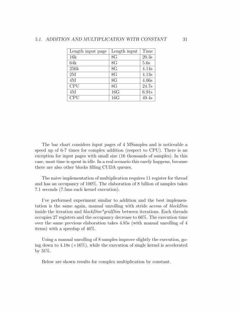
Length input page Length input Time4M 4G 2.75sCPU 4G 71.3s16k 8G 28.2s64k 8G 7.51s256k 8G 4.21s2M 8G 4.20s4M 8G 4.18sCPU 8G 143s8M 16G 7.23s
In this scenario the GPU strongly dominates, reaching a speedup of 34x.
Is mandatory to keep in mind that complex multiplications can exploitbetter Instruction Level Parallelism. With 16 billions of floats, CPU takes69.8s and GPU 5.86s, with a gain of 12x. Similar situation happens withintegers, with a speedup of 11 times.
5.2 Magnitude of signal
A common task in DSP is to get the magnitude of a complex signal. GNURadio provides two blocks, one calculate the normal magnitude, while theother emits squared magnitude.
5.2. MAGNITUDE OF SIGNAL 33
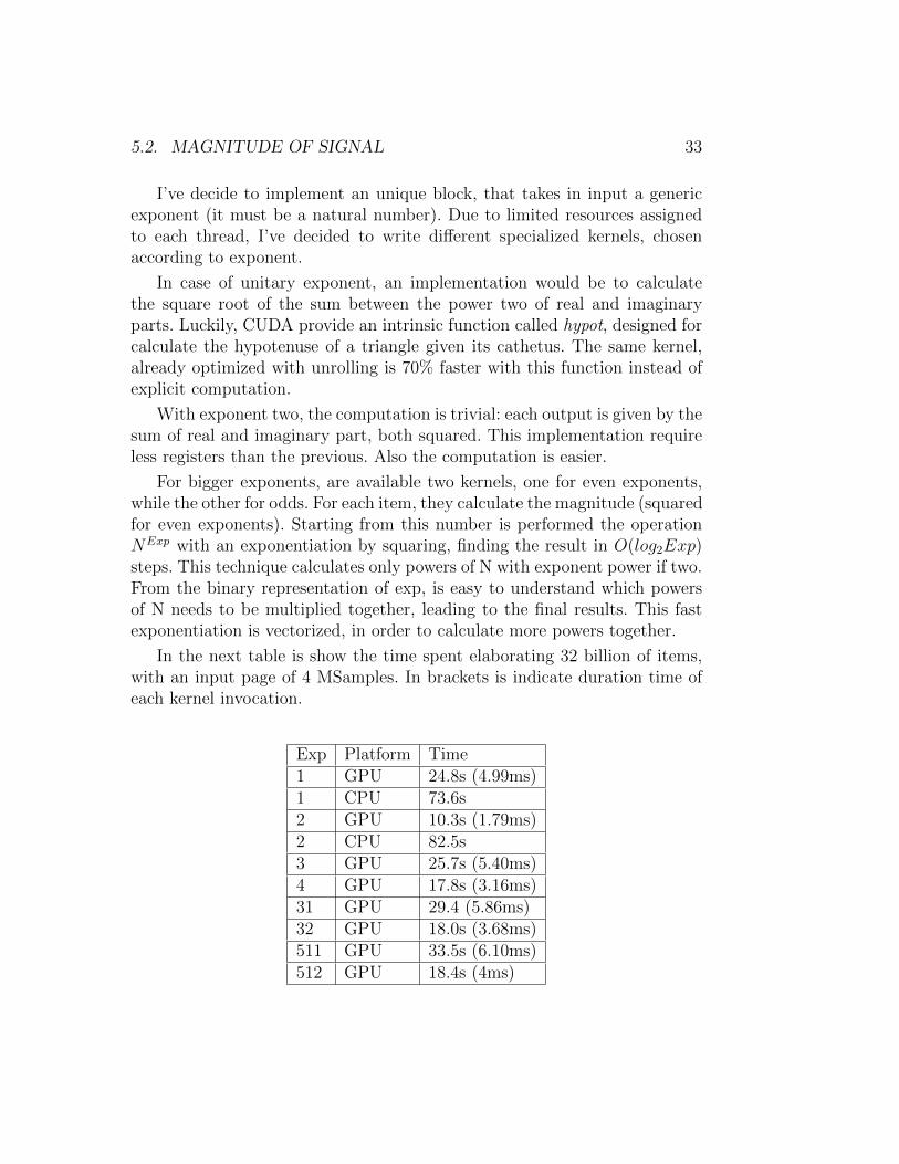
I’ve decide to implement an unique block, that takes in input a genericexponent (it must be a natural number). Due to limited resources assignedto each thread, I’ve decided to write different specialized kernels, chosenaccording to exponent.
In case of unitary exponent, an implementation would be to calculatethe square root of the sum between the power two of real and imaginaryparts. Luckily, CUDA provide an intrinsic function called hypot, designed forcalculate the hypotenuse of a triangle given its cathetus. The same kernel,already optimized with unrolling is 70% faster with this function instead ofexplicit computation.
With exponent two, the computation is trivial: each output is given by thesum of real and imaginary part, both squared. This implementation requireless registers than the previous. Also the computation is easier.
For bigger exponents, are available two kernels, one for even exponents,while the other for odds. For each item, they calculate the magnitude (squaredfor even exponents). Starting from this number is performed the operationNExp with an exponentiation by squaring, finding the result in O(log2Exp)steps. This technique calculates only powers of N with exponent power if two.From the binary representation of exp, is easy to understand which powersof N needs to be multiplied together, leading to the final results. This fastexponentiation is vectorized, in order to calculate more powers together.
In the next table is show the time spent elaborating 32 billion of items,with an input page of 4 MSamples. In brackets is indicate duration time ofeach kernel invocation.
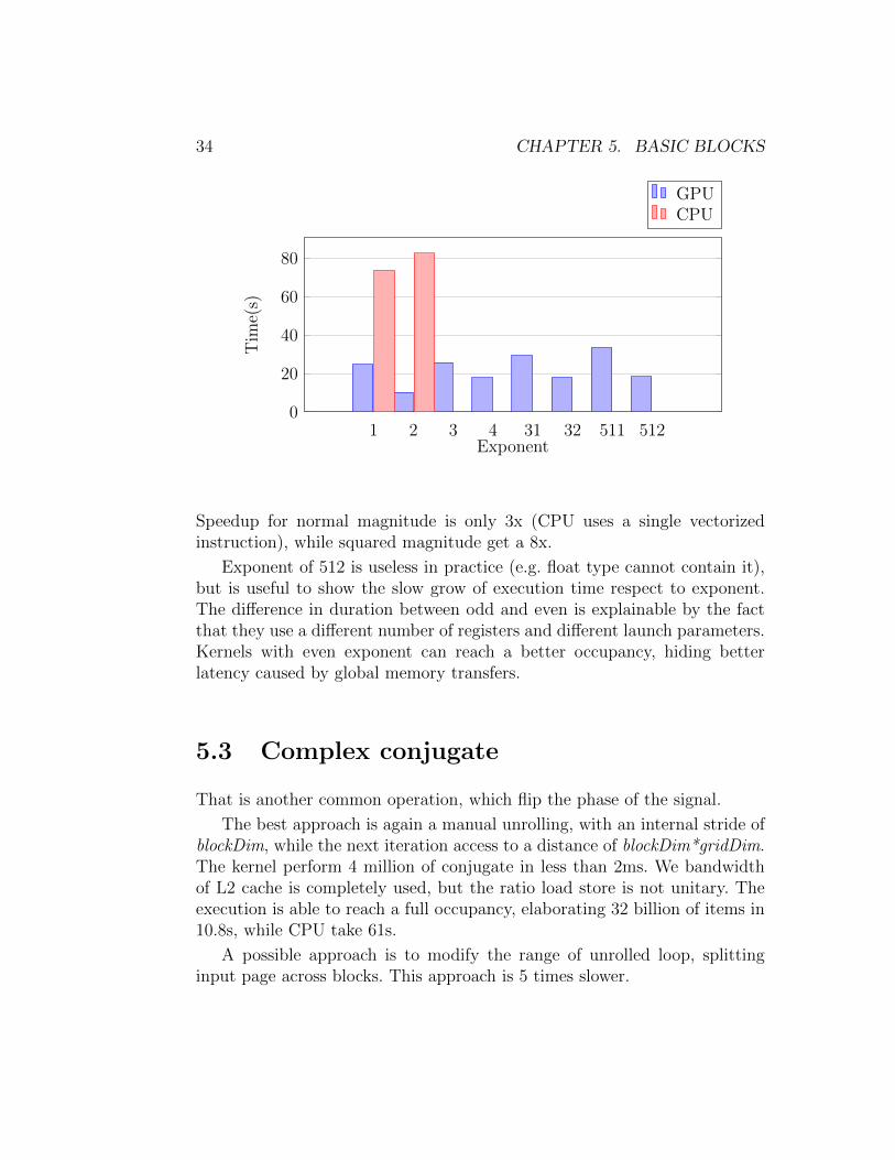
Exp Platform Time1 GPU 24.8s (4.99ms)1 CPU 73.6s2 GPU 10.3s (1.79ms)2 CPU 82.5s3 GPU 25.7s (5.40ms)4 GPU 17.8s (3.16ms)31 GPU 29.4 (5.86ms)32 GPU 18.0s (3.68ms)511 GPU 33.5s (6.10ms)512 GPU 18.4s (4ms)
34 CHAPTER 5. BASIC BLOCKS
1 2 3 4 31 32 511 5120
20
40
60
80
Exponent
Tim
e(s)
GPUCPU
Speedup for normal magnitude is only 3x (CPU uses a single vectorizedinstruction), while squared magnitude get a 8x.
Exponent of 512 is useless in practice (e.g. float type cannot contain it),but is useful to show the slow grow of execution time respect to exponent.The difference in duration between odd and even is explainable by the factthat they use a different number of registers and different launch parameters.Kernels with even exponent can reach a better occupancy, hiding betterlatency caused by global memory transfers.
5.3 Complex conjugate
That is another common operation, which flip the phase of the signal.
The best approach is again a manual unrolling, with an internal stride ofblockDim, while the next iteration access to a distance of blockDim*gridDim.The kernel perform 4 million of conjugate in less than 2ms. We bandwidthof L2 cache is completely used, but the ratio load store is not unitary. Theexecution is able to reach a full occupancy, elaborating 32 billion of items in10.8s, while CPU take 61s.
A possible approach is to modify the range of unrolled loop, splittinginput page across blocks. This approach is 5 times slower.
5.4. OPERATIONS BETWEEN TWO SIGNALS 35
5.4 Operations between two signals
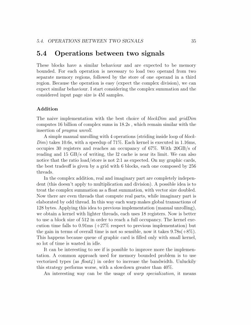
These blocks have a similar behaviour and are expected to be memorybounded. For each operation is necessary to load two operand from twoseparate memory regions, followed by the store of one operand in a thirdregion. Because the operation is easy (expect the complex division), we canexpect similar behaviour. I start considering the complex summation and theconsidered input page size is 4M samples.
Addition
The naive implementation with the best choice of blockDim and gridDimcomputes 16 billion of complex sums in 18.2s , which remain similar with theinsertion of pragma unroll.
A simple manual unrolling with 4 operations (striding inside loop of block-Dim) takes 10.6s, with a speedup of 71%. Each kernel is executed in 1.16ms,occupies 30 registers and reaches an occupancy of 67%. With 20GB/s ofreading and 15 GB/s of writing, the l2 cache is near its limit. We can alsonotice that the ratio load/store is not 2:1 as expected. On my graphic cards,the best tradeoff is given by a grid with 6 blocks, each one composed by 256threads.
In the complex addition, real and imaginary part are completely indepen-dent (this doesn’t apply to multiplication and division). A possible idea is totreat the complex summation as a float summation, with vector size doubled.Now there are even threads that compute real parts, while imaginary part iselaborated by odd thread. In this way each warp makes global transactions of128 bytes. Applying this idea to previous implementation (manual unrolling),we obtain a kernel with lighter threads, each uses 18 registers. Now is betterto use a block size of 512 in order to reach a full occupancy. The kernel exe-cution time falls to 0.91ms (+27% respect to previous implementation) butthe gain in terms of overall time is not so sensible, now it takes 9.78s(+8%).This happens because queue of graphic card is filled only with small kernel,so lot of time is wasted in idle.
It can be interesting to see if is possible to improve more the implemen-tation. A common approach used for memory bounded problem is to usevectorized types (as float4 ) in order to increase the bandwidth. Unluckilythis strategy performs worse, with a slowdown greater than 40%.
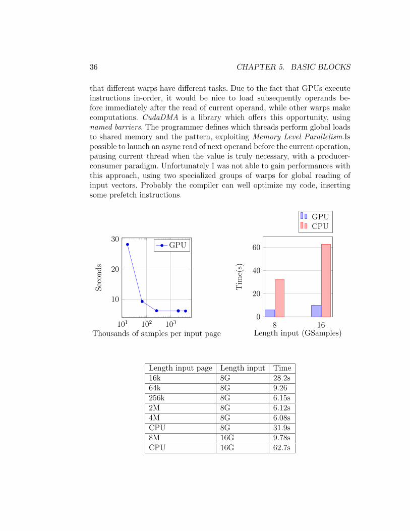
An interesting way can be the usage of warp specialization, it means
36 CHAPTER 5. BASIC BLOCKS
that different warps have different tasks. Due to the fact that GPUs executeinstructions in-order, it would be nice to load subsequently operands be-fore immediately after the read of current operand, while other warps makecomputations. CudaDMA is a library which offers this opportunity, usingnamed barriers. The programmer defines which threads perform global loadsto shared memory and the pattern, exploiting Memory Level Parallelism.Ispossible to launch an async read of next operand before the current operation,pausing current thread when the value is truly necessary, with a producer-consumer paradigm. Unfortunately I was not able to gain performances withthis approach, using two specialized groups of warps for global reading ofinput vectors. Probably the compiler can well optimize my code, insertingsome prefetch instructions.
101 102 103
10
20
30
Thousands of samples per input page
Sec
onds
GPU
8 160
20
40
60
Length input (GSamples)
Tim
e(s)
GPUCPU
Length input page Length input Time16k 8G 28.2s64k 8G 9.26256k 8G 6.15s2M 8G 6.12s4M 8G 6.08sCPU 8G 31.9s8M 16G 9.78sCPU 16G 62.7s
5.4. OPERATIONS BETWEEN TWO SIGNALS 37
Complex addition has a speedup of 5-6 times, mainly bounded by memorybandwidth.
Multiplication
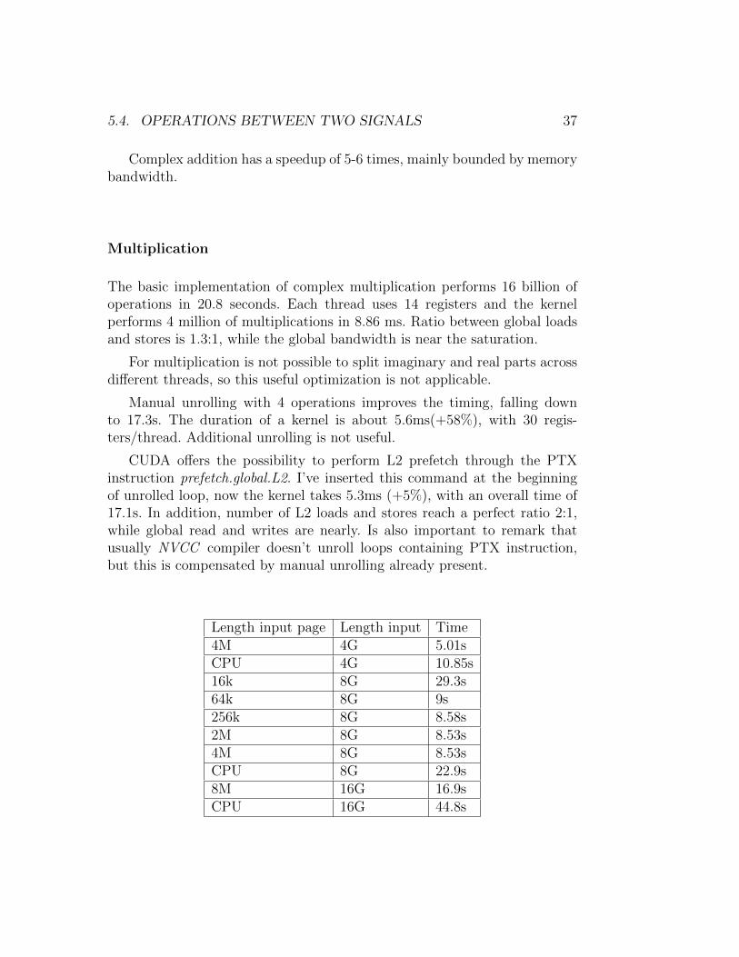
The basic implementation of complex multiplication performs 16 billion ofoperations in 20.8 seconds. Each thread uses 14 registers and the kernelperforms 4 million of multiplications in 8.86 ms. Ratio between global loadsand stores is 1.3:1, while the global bandwidth is near the saturation.
For multiplication is not possible to split imaginary and real parts acrossdifferent threads, so this useful optimization is not applicable.
Manual unrolling with 4 operations improves the timing, falling downto 17.3s. The duration of a kernel is about 5.6ms(+58%), with 30 regis-ters/thread. Additional unrolling is not useful.
CUDA offers the possibility to perform L2 prefetch through the PTXinstruction prefetch.global.L2. I’ve inserted this command at the beginningof unrolled loop, now the kernel takes 5.3ms (+5%), with an overall time of17.1s. In addition, number of L2 loads and stores reach a perfect ratio 2:1,while global read and writes are nearly. Is also important to remark thatusually NVCC compiler doesn’t unroll loops containing PTX instruction,but this is compensated by manual unrolling already present.
Length input page Length input Time4M 4G 5.01sCPU 4G 10.85s16k 8G 29.3s64k 8G 9s256k 8G 8.58s2M 8G 8.53s4M 8G 8.53sCPU 8G 22.9s8M 16G 16.9sCPU 16G 44.8s
38 CHAPTER 5. BASIC BLOCKS
4 8 160
20
40
Length input (GSamples)
Tim
e(s)
GPUCPU
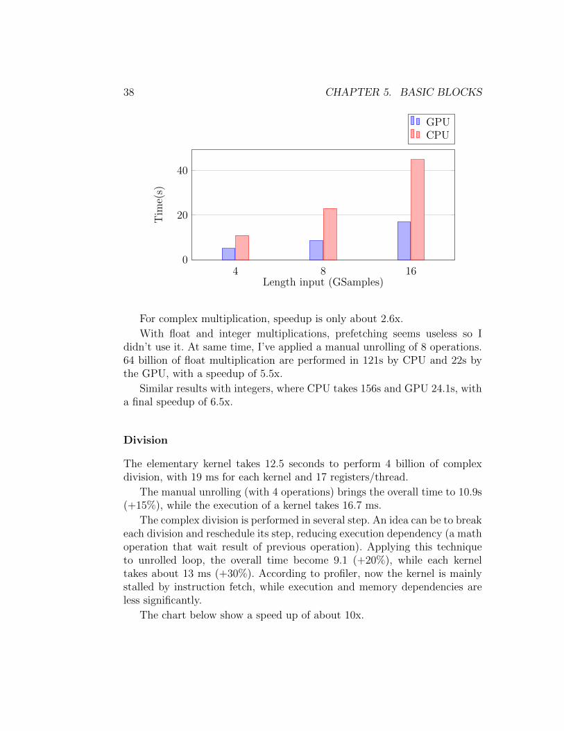
For complex multiplication, speedup is only about 2.6x.
With float and integer multiplications, prefetching seems useless so Ididn’t use it. At same time, I’ve applied a manual unrolling of 8 operations.64 billion of float multiplication are performed in 121s by CPU and 22s bythe GPU, with a speedup of 5.5x.
Similar results with integers, where CPU takes 156s and GPU 24.1s, witha final speedup of 6.5x.
Division
The elementary kernel takes 12.5 seconds to perform 4 billion of complexdivision, with 19 ms for each kernel and 17 registers/thread.
The manual unrolling (with 4 operations) brings the overall time to 10.9s(+15%), while the execution of a kernel takes 16.7 ms.
The complex division is performed in several step. An idea can be to breakeach division and reschedule its step, reducing execution dependency (a mathoperation that wait result of previous operation). Applying this techniqueto unrolled loop, the overall time become 9.1 (+20%), while each kerneltakes about 13 ms (+30%). According to profiler, now the kernel is mainlystalled by instruction fetch, while execution and memory dependencies areless significantly.
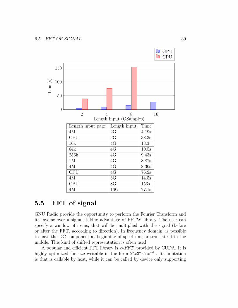
The chart below show a speed up of about 10x.
5.5. FFT OF SIGNAL 39
2 4 8 160
50
100
150
Length input (GSamples)
Tim
e(s)
GPUCPU
Length input page Length input Time4M 2G 4.19sCPU 2G 38.3s16k 4G 18.364k 4G 10.5s256k 4G 9.43s1M 4G 8.87s4M 4G 8.36sCPU 4G 76.2s4M 8G 14.5sCPU 8G 153s4M 16G 27.1s
5.5 FFT of signal
GNU Radio provide the opportunity to perform the Fourier Transform andits inverse over a signal, taking advantage of FFTW library. The user canspecify a window of items, that will be multiplied with the signal (beforeor after the FFT, according to direction). In frequency domain, is possibleto have the DC component at beginning of spectrum, or translate it in themiddle. This kind of shifted representation is often used.
A popular and efficient FFT library is cuFFT, provided by CUDA. It ishighly optimized for size writable in the form 2ax3bx5cx7d . Its limitationis that is callable by host, while it can be called by device only supporting
40 CHAPTER 5. BASIC BLOCKS
dynamic parallelism (a kernel launch another kernel), that is not the case ofmy graphic card.
Consequently for each elaboration can be necessary to call a maximumof three different kind of kernels. The first and the last eventually performa multiplication with the window and a shift of spectral component, they’recalled once for each input page. The middle kernel is the execution of FFT,called one or more time.
Calls to cuFFT can be asynchronous, which fits with the approach of myframework.
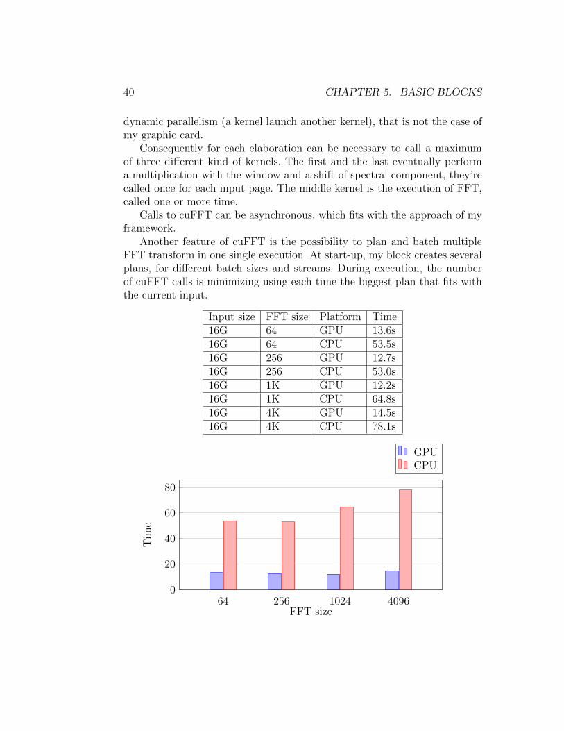
Another feature of cuFFT is the possibility to plan and batch multipleFFT transform in one single execution. At start-up, my block creates severalplans, for different batch sizes and streams. During execution, the numberof cuFFT calls is minimizing using each time the biggest plan that fits withthe current input.
Input size FFT size Platform Time16G 64 GPU 13.6s16G 64 CPU 53.5s16G 256 GPU 12.7s16G 256 CPU 53.0s16G 1K GPU 12.2s16G 1K CPU 64.8s16G 4K GPU 14.5s16G 4K CPU 78.1s
64 256 1024 40960
20
40
60
80
FFT size
Tim
e
GPUCPU

5.5. FFT OF SIGNAL 41
The speedup given by GPU is about 3x for FFT with small size, growingwith the size and overcoming an acceleration of 5x with bigger transforms.

42 CHAPTER 5. BASIC BLOCKS
Chapter 6
Filters
Filtering of digitized data is one of the most important and older disciplinein Digital Signal Processing. The main goal is to reduce some spectral com-ponents.
6.1 FIR filter
One of the traditional linear filter is called FIR, a short for Finite ImpulseResponse. From the name is obviously the fact that a finite input producesa finite output (it doesn’t contain feedbacks able to propagate indefinitelythe power). Each output samples can be seen as a weighted sum of lasts Ninputs, where N is called the order of the filter. Weights are called taps and
compose the impulse response. y[n] =N∑i=0
ak ∗ x[n− k]
Fir filters expose following properties:
• They are BIBO stable, it means that a bounded input produces abounded output.
• Is easy to design linear phase filters, useful in several applications.
• Rounding errors are not infinitely propagated, because there is not arecursive structure which propagates them.
Most common types of filters are: low-pass, high-pass, stop-band andpass-band. Generally they are described by these parameters:
• Pass-band
43
44 CHAPTER 6. FILTERS
• Stop-band
• Transition band
• Pass-band ripple
• Stop-band ripple
• Frequency of sampling
• Decimation/Interpolation factor
A common design method is called Window Design Method. The convo-lution can be seen as a multiplication in frequency domain between inputsand taps, so taps can be easily designed in frequency domain.
Taps are then converted in time domain via inverse fast Fourier transform.In lot of applications the number of taps is not so big, so is more performantthe convolution respect to the execution of two series of FFT, for this reasonFIR filters work in time domain. Another case in which FIR beats FFT iswith high rates of decimation (or interpolation). With FIR is possible to applydecimation during filtering (avoiding useless calculus), while with FFT thedecimation must be applied after the Fourier Transform. The same appliesfor interpolation.
The discrete convolution works on finite inputs (and outputs), it is equiv-alent to say that the impulse response is multiplied in time domain, whichmeans that there is a convolution in frequency domain between desired out-put and sync functions. This can be described as a FIR filter where the setof taps is convoluted with a sync, causing ripples. In order to overcome withthis problem, taps are designed with one of the following windows function:
• Blackman
• Kaiser
• Hamming
• Rectangular
6.1. FIR FILTER 45
6.1.1 Considerations
As said before, FIR filter perform a convolution between two vectors, inputsamples and taps. There are different scenarios, so is necessary to implementdifferent specializations of device code. A basic approach is to have eachthread associated to a different output item (plus eventual global load/store).
One variable is the order of the filter. With few thousands of taps, theycan be stored in shared memory or constant memory. Usually FIR filters canbe designed with shorter taps, so this is the case more optimized. Bigger set oftaps are supported for compatibility, but they are not well optimized. Thereare two ways to store taps: shared memory and constant. The latter optionseem to be the best, but it is not completely true. A limitation of constantmemory is its size (64 KB), which must be distributed across all kernels.Moreover, according to the documentation, requests to constant memory aresplit into as many separate requests as there are different memory addressesin the initial request. Because is not guarantee that threads of same warpwill access to the same taps at the same time, I’ve chosen shared memory asstorage for taps.
Another case is when the number of threads is bigger than the numberof expected outputs. This happens especially with decimation (e.g. an out-put items is produced every 50 inputs). In this case is better to split thecomputation of an output item among multiple threads.
6.1.2 Implementation and optimization of base case(neither interpolation nor decimation)
The GNU Radio FIR filter works with different types (float,complex, short,..)and I preserve this compatibility. For this reason I’ve written a templatelibrary which facilitates mathematical operations between different types.The compiler will instantiate multiple specializations for each kernel, one foreach triple type input, type taps and type output.
Items of input and taps vector can be loaded once (inside shared/localmemory) and used for multiple operations. For this reason we can predictthat the elaboration is compute bounded. It means that we won’t focus onhigh occupancy, but we will exploit Instruction Level Parallelism.
Shared memory is very limited, so I’ve declared two shared array of about2048 items in order to store slices of input and taps. Each thread loadsone input from global memory (coalesced access), waits other threads and
46 CHAPTER 6. FILTERS
performs a dot product between taps vector and previous inputs, calculatingan output sample and storing it.
I’ve tried several optimization. A common approach is to avoid bankconflicts over shared memory, adding an adequate padding to indices. Becausethe dot product is computed over shared arrays (it’s an inner loop), thismodification could have a significant impact. unexpectedly this techniqueslow down the execution, about 10% when applied to taps shared vector andmore than 75% when applied to input shared vector. This is because usuallytaps are accessed in broadcast mode, the size is small and easily cacheable.The padding inhibits an easy prediction by cache mechanisms. Also for inputshared vector there is a similar problem: in basic implementation, during dotproduct each thread reads the sample which was read by preceding threads inprevious iteration. Probably the compiler can manage very well this memorypattern, while the insertion of pads breaks some optimizations (it would beinteresting the usage of shuffle instructions on newer architectures). I’ve triedto apply again these techniques after other optimizations, without gettingimprovements.
Another common practice is loop unrolling. There are two nested loops,the outer which load items from global vectors and the inner which computedot products. The choice fall obviously on the inner loop. The simple usageof # pragma unroll doesn’t give any sensible speedup (less than 5%). Abetter approach is a manual unrolling, elaborating four pairs input sample-tap every iteration and using different accumulators (in order to don’t havedependencies between operations inside the same iteration). In this way ispossible to obtain a time speedup greater than 10%.
About the inner loop of dot product, the index of one vector is computedas modulo of its length (it acts as a circular vector) while the other vectoris treaty as a simple linear array. Due to manual loop unrolling, there arefour modulo operations for each iteration. Because the length is a powerof two, the modulo operation can be optimized by compiler as a bitwiseoperation (in theory this is a very fast operation). According to compiler,these instructions have a sensible impact. In order to minimize it, the circularvector is stretched in order to contain a copy of firsts elements at the end.Now indices inside the inner loop don’t need a modulo operation and memoryaccesses are easily optimizable, because are always sequential (inside theloop). This optimization give a speedup of 25% on overall time.
Each kernel invocation instantiate one or more blocks, according to di-mension of input. For few thousands of inputs, is counterproductive to split
6.1. FIR FILTER 47
the incoming array into different chunks.According to different parameters (like dimension of input, taps and type
of data) is chosen a different kernel.
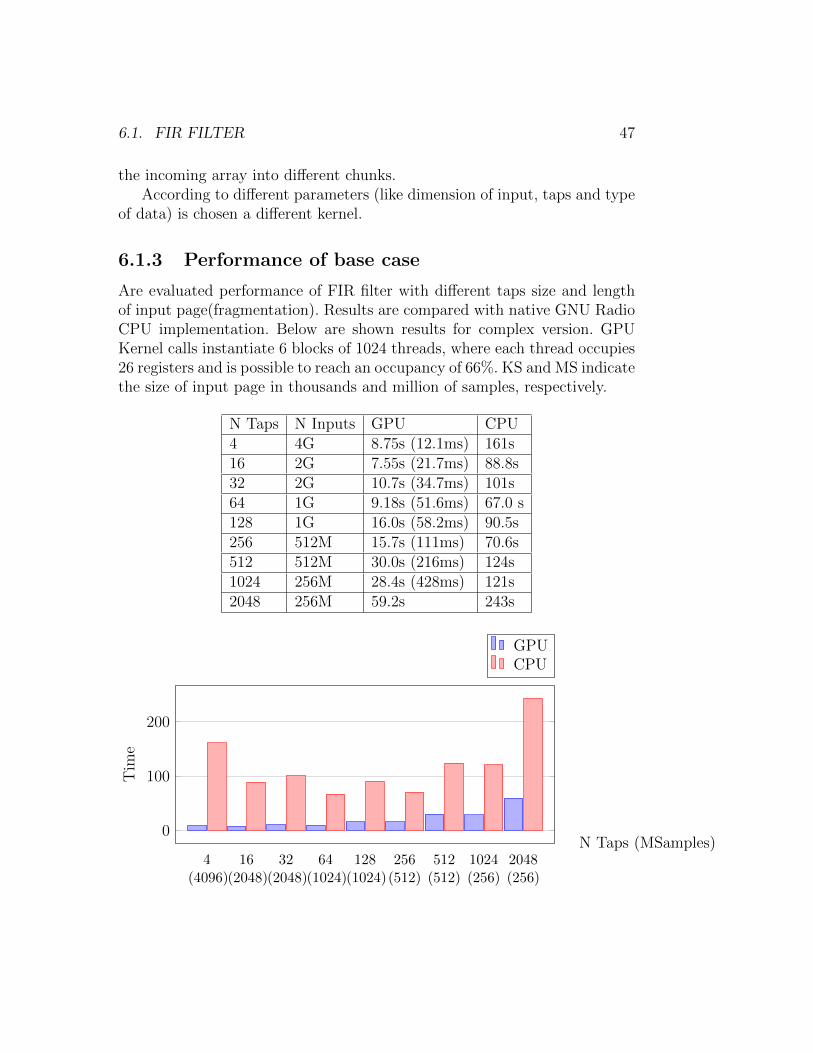
6.1.3 Performance of base case
Are evaluated performance of FIR filter with different taps size and lengthof input page(fragmentation). Results are compared with native GNU RadioCPU implementation. Below are shown results for complex version. GPUKernel calls instantiate 6 blocks of 1024 threads, where each thread occupies26 registers and is possible to reach an occupancy of 66%. KS and MS indicatethe size of input page in thousands and million of samples, respectively.
N Taps N Inputs GPU CPU4 4G 8.75s (12.1ms) 161s16 2G 7.55s (21.7ms) 88.8s32 2G 10.7s (34.7ms) 101s64 1G 9.18s (51.6ms) 67.0 s128 1G 16.0s (58.2ms) 90.5s256 512M 15.7s (111ms) 70.6s512 512M 30.0s (216ms) 124s1024 256M 28.4s (428ms) 121s2048 256M 59.2s 243s
4(4096)
16(2048)
32(2048)
64(1024)
128(1024)
256(512)
512(512)
1024(256)
2048(256)
0
100
200
N Taps (MSamples)
Tim
e
GPUCPU
48 CHAPTER 6. FILTERS
The time in bracket is the execution time of a single kernel call, invocatedover an input page of 4 million of samples.
The table shows a speedup greater than 18x for small set of taps, whichremains above 10x for windows shorter than 32 taps. For larger number, thespeedup fall to 4x for windows larger than 64 taps.
This happen because the CPU version uses intensively a library calledVolk for vector operations, which exploits extensions like SSE and AVX.During the installation of GNU Radio, is performed a benchmark in order tounderstand which is the best implementation for each operation and align-ment. Therefore large dot products are mainly executed by the most efficientparallel instruction, with aligned access.
I’ve also tried different sizes of input pages, ranging from 64K samplesto 16M samples. In theory, a greater number implies better performance,because each invocation elaborates more data (minimizing number of kernellaunches). In the table below, KS and MS refer to thousands and millions ofsamples, respectively.
N Taps N Inputs 64KS 256KS 1MS 4MS 8MS4 4G 99.7s 27.6s 8.75 8.45s64 1G 348s 120s 32.6s 9.18s 9.2s1024 64M 108.2s 86.5s 32.1s 17.4s 17.3s
From the table we can deduce that is better to avoid small chunks of inputs,because the slowdown would be significantly. A good tradeoff is the usageof input page with 4 million of items. This choice is not always practicable:for instance when there are lot of blocks that use a similar size, the memoryspace can be a problem ( remember that each block manages a buffer ofpages). Another unfavourable scenario is when is mandatory to have a lowlatency, because a bigger kernel execution implies more latency.
In the previous trial, each kernel call is usually launched on a variablenumber of blocks. This is because the usage of multiple block with smallinput size is counterproductive. Each blocks need also to read a portion ofglobal data used by previous block (history of filter). So more blocks impliesmore repeated readings.
-
6.2. FFT FILTER 49
6.2 FFT filter
As mentioned before, FIR filters can be described as a convolution betweentwo functions, the set of inputs and taps.
For convolution between large sets, can be more convenient the usage ofFast Transform
Y = X ∗ TAPS ⇔ Y = IFFT (FFT (X)FFT (TAPS)) (6.1)
Given a filter with Q taps, the input will be split into vectors of lengthM (arbitrary choice), each one with an additional padding of Q-1 reaching asize of L=Q+M-1 (otherwise it would be a circular convolution). For perfor-mance’s reason, L will be a power of two.
Taps’ vector is stretched to L items, inserting zeros at the end. Nowthese vectors (strip of inputs and taps) are transformed into Fourier domain,multiplied together, ending with an Inverse Fourier Transform and discardinga portion of result(the padding of length Q-1).
When there are multiple strips of input, the result will be aliased. In orderto avoid this phenomena, two techniques are available.
Overlap-and-save
For each strip of input, the first part is filled with Q-1 items from previousinput vector(its last part). FFT, multiplication and IFFT are performed asbefore, but for each output vector are discarded firsts Q-1 items.
Overlap-and-add
For each strip of input, the last part is filled with Q-1 zeros. FFT, multiplica-tion and IFFT are performed as before, but for each output vector, the lastpart (of Q-1 items) is summed with the first portion of next output vector.
These methods are expected to have similar performances. I’ve chosen thefirst, because it requires only a mechanism of history on the input (alreadyavailable). The latter would need to pass a state (given by last Q-1 outputs)between to execution, preventing the parallel execution of different set ofinputs (in different streams).
At the beginning, different configuration for the cuFFT library are per-formed, in addition taps are transformed into frequency domain.
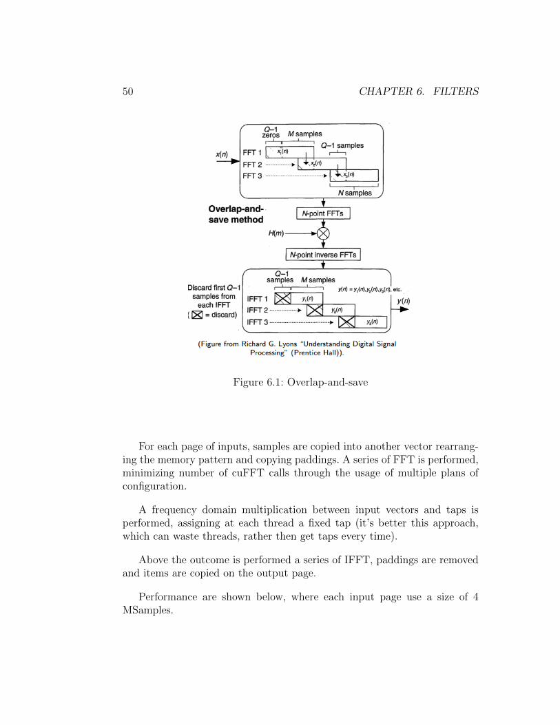
50 CHAPTER 6. FILTERS
Figure 6.1: Overlap-and-save
For each page of inputs, samples are copied into another vector rearrang-ing the memory pattern and copying paddings. A series of FFT is performed,minimizing number of cuFFT calls through the usage of multiple plans ofconfiguration.
A frequency domain multiplication between input vectors and taps isperformed, assigning at each thread a fixed tap (it’s better this approach,which can waste threads, rather then get taps every time).
Above the outcome is performed a series of IFFT, paddings are removedand items are copied on the output page.
Performance are shown below, where each input page use a size of 4MSamples.
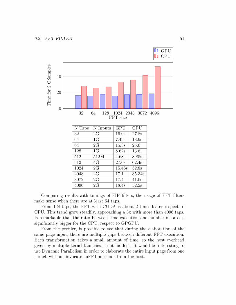
6.2. FFT FILTER 51
32 64 128 1024 2048 3072 40960
20
40
FFT size
Tim
efo
r2
GSam
ple
sGPUCPU
N Taps N Inputs GPU CPU32 2G 16.0s 27.8s64 1G 7.49s 13.9s64 2G 15.3s 25.6128 1G 8.62s 13.6512 512M 4.68s 8.85s512 4G 27.0s 62.4s1024 2G 15.45s 32.8s2048 2G 17.1 35.34s3072 2G 17.4 41.0s4096 2G 18.4s 52.2s
Comparing results with timings of FIR filters, the usage of FFT filtersmake sense when there are at least 64 taps.
From 128 taps, the FFT with CUDA is about 2 times faster respect toCPU. This trend grow steadily, approaching a 3x with more than 4096 taps.Is remarkable that the ratio between time execution and number of taps issignificantly bigger for the CPU, respect to GPGPU.
From the profiler, is possible to see that during the elaboration of thesame page input, there are multiple gaps between different FFT execution.Each transformation takes a small amount of time, so the host overheadgiven by multiple kernel launches is not hidden . It would be interesting touse Dynamic Parallelism in order to elaborate the entire input page from onekernel, without invocate cuFFT methods from the host.
52 CHAPTER 6. FILTERS
Due to the presence of FFT and IFFT, it would be interesting to performthe Fourier Transform removing a step of bit-reversal permutation (a com-mon part of Cooley–Tukey’s algorithm). An appropriate permutation wouldbe performed over taps’ vector, avoiding some operations during filtering.Unfortunately this experiment would require to implement a very efficientFFT library, able to compete with cuFFT.
6.3 IIR filter
One of the challenge in parallel implementation is the construction of IIRfilters. They are described with the following formula:
y[n] =M∑k=0
ak ∗ x[n− k]−M∑k=1
bk ∗ y[n− k] (6.2)
This is a recurrence equation, which is easily implementable over a CPU.I’ve decided to implement this filter in order to gain some performance andavoid expensive device-host memory transfer (IIR filter are often present inSDR chains).
The presence of memory cause some advantages and drawbacks
• Efficiency: these filters require far less multiplication respect to a FIRwith same frequency response. In a serial implementation, it meansthat is possible to elaborate signals with higher sample rate.
• A better frequency response, comparing with FIR.
• Instability: the perturbation of an input can, depending to filter design,bring the output in a unstable region and oscillate forever.
• IIR filters are less easy to design, compared to FIR.
• Is not easy to get a linear phase response.
The formula which describe IIR filters is not easily parallelizable, due torecurrence.
We are managing discrete-time signal, so is possible to use the z transformwhich is a sort of equivalent of Laplace transform in discrete-time.
Two useful properties are:
6.3. IIR FILTER 53
• Linearity:
y[n] = a · x[n] + b · s[n]⇔ Y (z) = a ·X(z) + b · S(z) (6.3)
• Time-shifting:
y[n] = x[n− k]⇔ Y (z) = z−k ·X(z) (6.4)
In z-domain , the formula
y[n] =M∑k=0
ak ∗ x[n− k]−M∑k=1
bk · y[n− k] (6.5)
become
b0 · Y (z) =M∑k=0
ak · z−k ·X(z)−M∑k=1
bk · z−k · Y (z) (6.6)
where the variable b0 = 1. Now we can collect variables X and Y, yielding to
(M∑k=0
bk · z−k) · Y (z) = (M∑k=0
ak · z−k) ·X(z) (6.7)
The transfer function is
Y (z)
X(z)=a0 + a1 · z−1 + a2 · z−2...am · z−m
b0 + b1 · z−1 + b2 · z−2...bm · z−m(6.8)
Factorizing the two polynomials, we obtain
Y (z)
X(z)=
(z−1 − z0)(z−1 − z1)..(z−1 − zm)
(z−1 − p0)(z−1 − P − 1)..(z−1 − pm)=
(z−1 − z0)(z−1 − z1)..(z−1 − zm)
(z−1 − p0)(z−1 − P − 1)..(z−1 − pm)(6.9)
There are mainly two approach for implement it, parallel and cascade IIRfilter.
6.3.1 Parallel IIR filter
According to decomposition in residues, is possible to dissociate a genericdivision of two polynomials into a sum of simple fractions, where each fractionhas a denominator of first degree. The transfer function becomes
Y (z)
X(z)= q +
noz−1 − p0
+n1
z−1 − p1..+
nmz−1 − pm
(6.10)
54 CHAPTER 6. FILTERS
. It means that is possible to take the input, process it with different transferfunctions obtaining multiple Yi(z), at the end Y (z) will be the sum of allYi(z). The function
Yi(z)
X(z)=
niz−1 − pi
(6.11)
can be written as
Yi(z)(z−1 − pi) = X(z) · ni ⇒ Yi(z) =X(z) · ni − Y (z) · z−1
−pi(6.12)
. In time-domain it becomes yi[t] = x[t]·ni−y[t−1]−pi which is easily implementable.
For sake of simplicity we rewrite we previous formula as yi[t] = a · x[t] + b ·x[t− 1] = a · x[t] + b · (a · x[t− 1] + b · y[t− 2]). We can expand the formulauntil we reach x[0], by the way this equation can be seen as a prefix sum.
This kind of addition is also called cumulative sum and is easily imple-mentable in serial way. The parallelized version is more sophisticated andmay be not liner.
The problem of this approach is that it doesn’t provide a good stability:according to the order of summation of results coming from different blocks,the result can vary heavily. For instance, if we have three blocks, where twoof them are exposing the same big number, with opposite sign, while a thirdis outputting a small value, the final result can become zero or the correctvalue according to the order of summation.
Another case happens when two conjugate poles(zeros) are fixed near theunit circle: considered alone, they are near the instability region. But theoverall transfer function can be completely stable.
6.3.2 Cascade IIR filter
In this approach, the formula
Y (z)
X(z)=
(z−1 − z0)(z−1 − z1)..(z−1 − zm)
(z−1 − p0)(z−1 − P − 1)..(z−1 − pm)(6.13)
is rewritten as
Y (z)
X(z)=
(z−1 − z0)(z−1 − z1)(z−1 − p0)(z−1 − p1)
· .. · (z−1 − zm−1)(z−1 − zm)
(z−1 − pm−1)(z−1 − pm)(6.14)
6.3. IIR FILTER 55
The latter can be interpreted as a cascade of blocks, where the output ofeach become the input for the next. A generic block can now be expressed as
Yi(z)
Xi(z)=
(z−1 − z0)(z−1 − z1)(z−1 − p0)(z−1 − p1)
⇒
⇒ Yi(z) · (z−1 − p0)(z−1 − p1) = Xi(z) · (z−1 − z0)(z−1 − z1)⇒⇒ Yi(z) · (p0 · p1 − (p0 + p1)z
−1 + z−2) = Xi(z) · (z0 · z1 − (z0 + z1)z−1 + z−2)
(6.15).That equation, in time-domain can be expressed as
yi[n](p0·p1)−yi[n−1](p0+p1)+yi[n−2] = xi[n](z0·z1)−xi[n−1](z0+z1)+xi[n−2](6.16)
. For simplicity, we rewrite it as
yi[n] = a0 ·xi[n]+a1 ·xi[n−1]+a2 ·xi[n−2]+b1 ·yi[n−1]+b2 ·yi[n−2] (6.17)
. Now we have a recurrence equation of second order,which is not easy tothreat with prefix sum. We can introduce the usage of vectors and matrices.We now assign
Yi[k] = (yi[k · 2] yi[k · 2 + 1]) (6.18)
Xi[k] = (xi[k · 2− 2] xi[k · 2− 1] xi[k · 2] xi[k · 2 + 1]) (6.19)
We’d like to have a formula like Yi[k] = Xi[k] ·Ai + Yi−1[k] ·Bi. We knowthat
yi[k · 2] = a0 · xi[k · 2] + a1 · xi[k ∗ 2− 1] + a2 · xi[k · 2− 2]+
b1 · yi[k · 2− 1] + b2 · yi[k · 2− 2](6.20)
The formula for yi[k ·2+1] is similar, but we can expand the term yi[k ·2−1]in order to avoid a dependence, as follow
yi[k · 2 + 1] = a0 · xi[k · 2 + 1] + a1 · xi[k · 2] + a2 · xi[k · 2− 1] + b1 · (a0 · xi[k · 2]+
+ a1 · xi[k · 2− 1] + a2 · xi[k · 2− 2] + b1 · yi[k · 2− 1] + b2 · yi[k · 2− 2]) + b2 · yi[k · 2− 1](6.21)
From here we can write the matrix
Bi = (b2 b1 · b2b1 b21 + b2
) Ai = (
a2 b1 · a2a1 b1 · a1 + a2a0 b1 · a0 + a10 a0
) (6.22)
.
56 CHAPTER 6. FILTERS
6.3.3 Prefix sum
The prefix sum of a given sequence X = x0, x1, x2.. is another sequenceY = y0, y1, y2.. where each term is given by the sequence of previous items inX. There are two kinds of summation, exclusive and inclusive.
In the first case, the generic term yi is given by the summation of previousitems in X, while in the last summation is also included xi.Their output isthe same, expect for a shift by one position. The input page can be split inseveral chunks and a prefix sum performed on each.
A basic parallel summation
A first implementation is to perform log2N iterations, where at the genericith step each of lasts N-2i is summed with the item present 2i positions before.This algorithm has a complexity of O(N logN).
A more advanced approach
Is possible to perform a parallel prefix sum in O(n) step, treating the in-put vector as a balanced binary tree. Items can be treated as leafs, but forperformance reason the entire tree is contained in vector. The algorithm iscomposed by two phases, up-sweep and down-sweep.
On the first step, starting from the leafs, each node is replaced by thesum of its children.
The second phase begin form the top descending to leafs. For each node,the value of right child is adjusted with the value contained in the left child.
Recurrence equation of first order can be implemented as prefix sum,multiplicating value of left child by backward tap (power to the distancebetween children) before merging it with right child.
Is also possible to implement second order equation thinking in term ofmatrices (e.g. grouping input into vectors of 2 items).
6.3.4 Implementation
In the native CPU implementation, there are two GNU Radio blocks: oneprovides an IIR filter with one pole, while the other allow the user to gener-ically write forward and backward taps (they are coefficient which multiplyinput and output samples in the recurrence equation, respectively. I’ve alsodecide to implement two blocks.
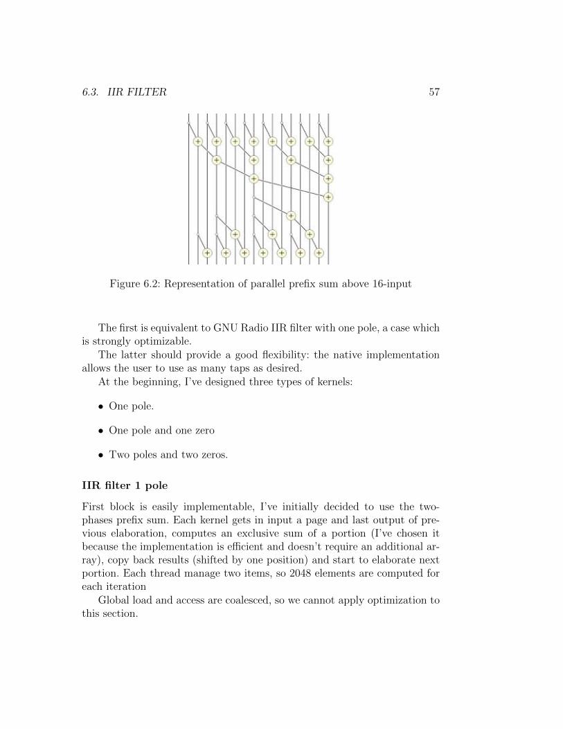
6.3. IIR FILTER 57
Figure 6.2: Representation of parallel prefix sum above 16-input
The first is equivalent to GNU Radio IIR filter with one pole, a case whichis strongly optimizable.
The latter should provide a good flexibility: the native implementationallows the user to use as many taps as desired.
At the beginning, I’ve designed three types of kernels:
• One pole.
• One pole and one zero
• Two poles and two zeros.
IIR filter 1 pole
First block is easily implementable, I’ve initially decided to use the two-phases prefix sum. Each kernel gets in input a page and last output of pre-vious elaboration, computes an exclusive sum of a portion (I’ve chosen itbecause the implementation is efficient and doesn’t require an additional ar-ray), copy back results (shifted by one position) and start to elaborate nextportion. Each thread manage two items, so 2048 elements are computed foreach iteration
Global load and access are coalesced, so we cannot apply optimization tothis section.
58 CHAPTER 6. FILTERS
The prefix sum makes an intensive use of shared memory, with stridedaccesses not easily predictable by the compiler. A good strategy can be theinsertion of paddings in shared memory, in order to reduce bank conflicts.This approach give good results, with a speedup of 40%.
Another optimization is given by manual unrolling (which permits toremove some syncthreads()).
Unluckily this implementation is much slower than CPU, like more than4 times.
A faster implementation is the naive algorithm, with complete unrolling(and without useless synchronization intra-warp). Although is less efficient(interms of complexity) than the previous adopted, the maximum number ofstep performed by one thread is the half (depth is logN instead of 2logN).
Balance tree would be efficient with much more items, but is upperbounded by shared memory size (or global memory bandwidth). In aver-age requires less work for each threads, but they spend a lot of time in idle,waiting computation of leading threads.
With naive approach, the IIR filter with complex input/output and realtaps (GNU Radio block with one pole doesn’t provide complex taps) takes18.5s elaborating 8 billion of items with CPU, while GPU needs 26.9s. Theslowdown is 1.45, what can be acceptable when IIR filter is not the moreexpensive block of a flow graph.
Is possible to reduce this gap using more CUDA blocks in parallel: eachone computes prefix sum on a portion of input, after waits the output ofprevious chunk performed by another Streaming Multiprocessor, adjustingthe current output. I decided to don’t make this optimization for differentreasons. First of all, the gain cannot be noticeable because different CUDAblocks perform two series of global reads and writes instead of one. In ad-dition, it would be necessary some sort of synchronization between CUDAblocks, not available in standard API. There are different research and re-sults about it, but they are not generic and is not difficult to have paradoxicalsituation in which the usage of multiple SM leads to a slowdown.
IIR filter with multiple zeros and poles
My first approach was to implement a generic filter as a cascade of filterswith one or two poles(and zeros), where a single kernel invocation call themsequential on he entire input page. This approach would require to the userto write directly zeros and poles instead of taps, that is not usually a problem
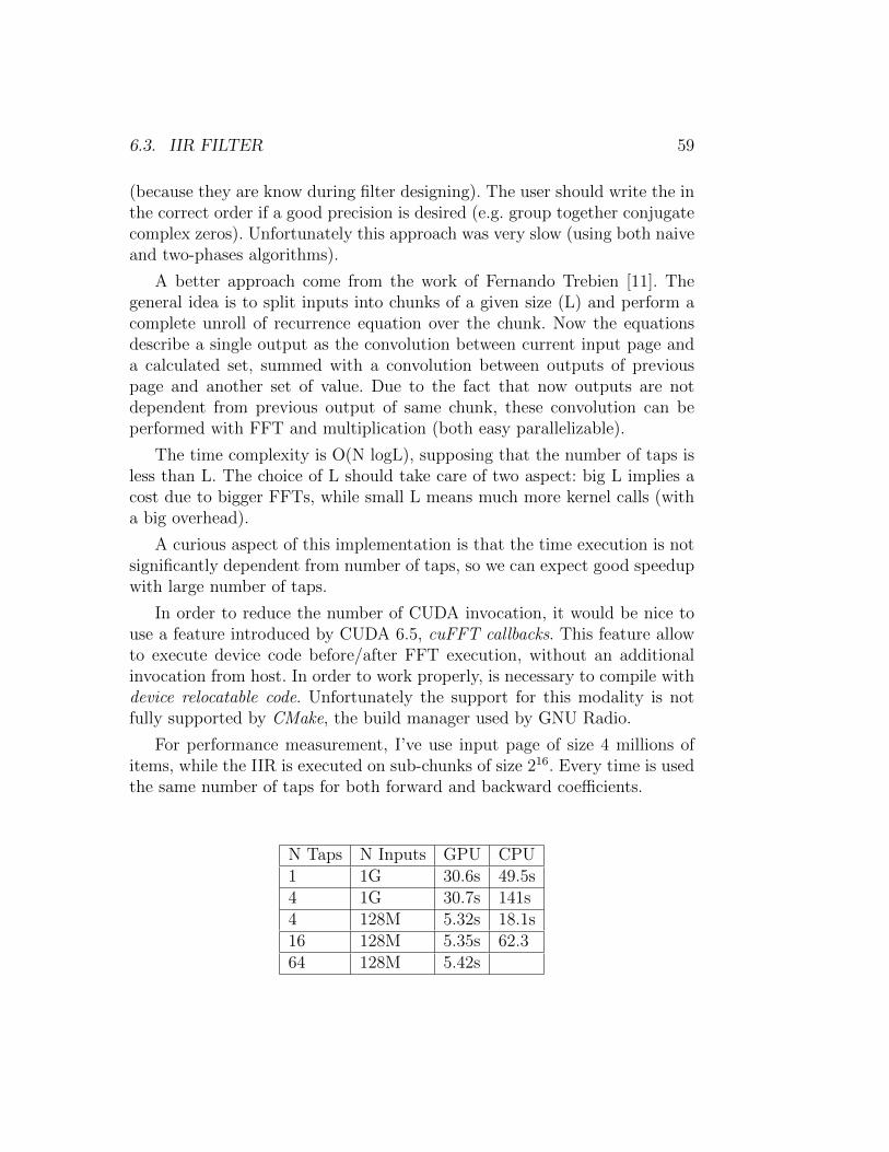
6.3. IIR FILTER 59
(because they are know during filter designing). The user should write the inthe correct order if a good precision is desired (e.g. group together conjugatecomplex zeros). Unfortunately this approach was very slow (using both naiveand two-phases algorithms).
A better approach come from the work of Fernando Trebien [11]. Thegeneral idea is to split inputs into chunks of a given size (L) and perform acomplete unroll of recurrence equation over the chunk. Now the equationsdescribe a single output as the convolution between current input page anda calculated set, summed with a convolution between outputs of previouspage and another set of value. Due to the fact that now outputs are notdependent from previous output of same chunk, these convolution can beperformed with FFT and multiplication (both easy parallelizable).
The time complexity is O(N logL), supposing that the number of taps isless than L. The choice of L should take care of two aspect: big L implies acost due to bigger FFTs, while small L means much more kernel calls (witha big overhead).
A curious aspect of this implementation is that the time execution is notsignificantly dependent from number of taps, so we can expect good speedupwith large number of taps.
In order to reduce the number of CUDA invocation, it would be nice touse a feature introduced by CUDA 6.5, cuFFT callbacks. This feature allowto execute device code before/after FFT execution, without an additionalinvocation from host. In order to work properly, is necessary to compile withdevice relocatable code. Unfortunately the support for this modality is notfully supported by CMake, the build manager used by GNU Radio.
For performance measurement, I’ve use input page of size 4 millions ofitems, while the IIR is executed on sub-chunks of size 216. Every time is usedthe same number of taps for both forward and backward coefficients.
N Taps N Inputs GPU CPU1 1G 30.6s 49.5s4 1G 30.7s 141s4 128M 5.32s 18.1s16 128M 5.35s 62.364 128M 5.42s
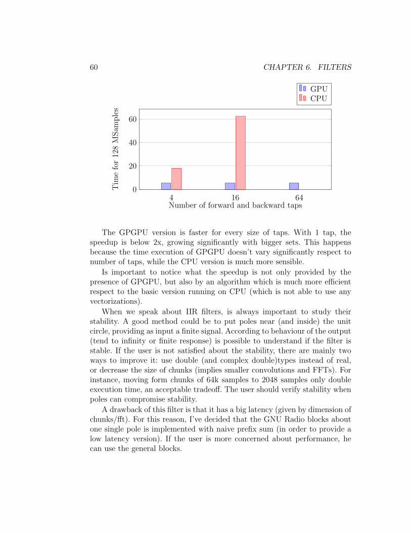
60 CHAPTER 6. FILTERS
4 16 640
20
40
60
Number of forward and backward taps
Tim
efo
r12
8M
Sam
ple
s
GPUCPU
The GPGPU version is faster for every size of taps. With 1 tap, thespeedup is below 2x, growing significantly with bigger sets. This happensbecause the time execution of GPGPU doesn’t vary significantly respect tonumber of taps, while the CPU version is much more sensible.
Is important to notice what the speedup is not only provided by thepresence of GPGPU, but also by an algorithm which is much more efficientrespect to the basic version running on CPU (which is not able to use anyvectorizations).
When we speak about IIR filters, is always important to study theirstability. A good method could be to put poles near (and inside) the unitcircle, providing as input a finite signal. According to behaviour of the output(tend to infinity or finite response) is possible to understand if the filter isstable. If the user is not satisfied about the stability, there are mainly twoways to improve it: use double (and complex double)types instead of real,or decrease the size of chunks (implies smaller convolutions and FFTs). Forinstance, moving form chunks of 64k samples to 2048 samples only doubleexecution time, an acceptable tradeoff. The user should verify stability whenpoles can compromise stability.
A drawback of this filter is that it has a big latency (given by dimension ofchunks/fft). For this reason, I’ve decided that the GNU Radio blocks aboutone single pole is implemented with naive prefix sum (in order to provide alow latency version). If the user is more concerned about performance, hecan use the general blocks.
6.4. SAMPLE RATE CONVERSION 61
6.4 Sample Rate Conversion
Conversion is the process of changing the sample rate of a discrete time-domain signal. It has different application, e.g. when two systems work withdifferent frequencies or the signal need to be elaborated by a narrowed filter.Main common conversions are decimation and interpolation. Next are shownblocks which work with integer factors. Is possible to perform a conversionwith rational factor using both blocks with integer factors. For instance aconversion from 100 kHz to 44 kHz can be performed with an interpolationby 11 followed by a decimation by 25.
6.4.1 Decimation
It is the process of reducing the sampling rate of a signal by a factor M, calleddecimation factor. This block can be seen as low-pass filtering followed by adown sampler, which consider only one output every M. The implementedlow-pass filter is a FIR and must have a cutoff frequency less than half ofoutcoming sample rate. In this way, components with higher frequency don’tcause aliasing.
Instead of apply the filter to every input sequence and discard lot ofoutputs (sampling), is better to consider only sequences which will producea valid output. In this way is possible to save lot of computation (like Mtimes).
Another aspect is that in lot of scenario the decimation factor is not sosmall. The filter tap length is about
AttdB22 ∗ (fstop − fpass)/fsamplerateinit (6.23)
where Att is the attenuation in transition band, expressed in dB. A big Mimplies a small transition band compared to initial sample rate. A filter withthese characteristics needs a large set of taps, which slow down the speedof signal processing. In this case is better to design a two-stage decimation,composed by two decimators in cascade, with factors M1 and M2. According
to [12] , a good choice for M1 is 2M ∗ 1−√MF/(2−F )
2−F (M+1). F = fstop−fpass
fstopand
M2=M/M1
62 CHAPTER 6. FILTERS
6.4.2 Interpolation
The interpolation convert a sampling rate fold to a new sequence with samplerate L ∗ fold. It is executed in two steps, the first consist to insert L-1 zeroeseach samples, while the second phase is a low-pass filter. The insertion of nullsamples doesn’t modify the frequency shape of the signal (while is changedthe scale). After that is necessary to use a low-pass filter, because the newband contains multiple replicas (images) of original signal.
Instead of insert zeroes and multiply them with taps, is better to splittaps in different disjoint sets (with as many sets as L). Each set contain tapswhich are not multiplied by zero when calculating one of L output samples.This is solved with polyphase filters.
Also for interpolators is valid the same consideration done about decima-tion: with big factor is better to use two-stage interpolators.
6.4.3 Polyphase Filters
These two kind of sample rate conversion can be performed by a filter calledpolyphase [13].
Initially are calculated taps H for low pass FIR filter as usually. Given adecimator/interpolator with factor M (or L), taps are split into M(L) differentsub-filters(as FIR filter), where the i-th sub-filter contain taps hi,hM+i,h2M+i.
For a decimator, each sub-filter takes interleaved inputs (with the samepattern for taps) and results of sub-filters are summed into a unique output(so, one output every L inputs). After what, each sub-filter progress of oneinput(so,M position globally)
In the interpolator, all sub-filters operate one same set of inputs (whichare now read sequentially, not interleaved). Each sub-filter produce a separateoutput for the same set in input. After what, all sub-filters advance of oneposition.
Summarizing, decimators distribute the input across different sub-filters,while their output is merged. Conversely, interpolator provide the same inputto all sub-filters, while their output is separated.
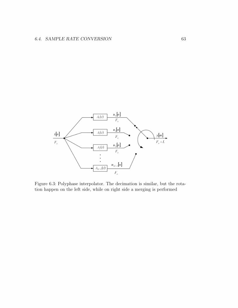
6.4. SAMPLE RATE CONVERSION 63
Figure 6.3: Polyphase interpolator. The decimation is similar, but the rota-tion happen on the left side, while on right side a merging is performed

64 CHAPTER 6. FILTERS
Chapter 7
Analog Demodulation
In lot of scenarios, signals are not directly transmitted in base band, butare conveyed inside another periodic waveform signal that can be physicallytransmitted (called carrier signal). The modulation consist of varying one ormore properties of this carrier, according to information to be transmitted.When the carrier is modulated with an analog signal, an analog modulationis performed. More common modulations are AM and FM.
7.1 Amplitude Modulation
AM is a signal with the amplitude (signal strength) of the carrier wave lin-early modulated, according to the data to be transmitted. The AM Demod-ulation is relatively simple to implement. First of all, the band which containthe signal is filtered, removing foreigners components. For each (complex)sample the magnitude is computed. After that a constant value is subtractedfrom (real) magnitudes, removing the amplitude of the carrier signal. Theoutcoming signal contain modulations of both information and carry signal.Because the frequency of carry signal is higher than carried information, issufficient to perform a low pass filtering.
7.2 Frequency Modulation
The FM is another type of modulated signal. Frequency Modulation signalsconvey information on the carrier wave by varying its instant frequency, while
65
66 CHAPTER 7. ANALOG DEMODULATION
amplitude remain constant. This approach is usually much robust againstnoise respect to AM.
The first step is to select only the band containing the signal, using alow-pass filter (supposing that the receiver is centered over the signal).
Sequentially a quadrature demodulation is performed. This operationemit for each input sample the difference (in phase) between the currentinput and the previous. A method could be to compute the phase of bothinputs, performing after the difference. Usually trigonometric operations arevery expensive, so is better to use another approach: perform a multiplicationbetween current item and conjugate complex of previous item, calculating thearc tangent of the result. This operation make sense: the phase of the productis equal to the difference of phases of two samples.
After this operation, the output is down sampled to the same samplerate of audio card and is put into the audio sink block, reproducing theaudio through speakers.
Chapter 8
Digital Demodulation
8.1 OFDM
Orthogonal frequency-division multiplexing is a modulation format that islargely used in recently wireless standards, like 802.11a/b/g, LTE, WiMAXand DVB-T. It divides the assigned band of frequency into N-orthogonal sub-carriers, transmitting an high data rate stream by splitting it in small flows,one for each sub-carriers. Each chunk of these flow is encoded separately, according to some modulation already available (BSK,QAM16,QAM256).Outputs of modulators become the input of a subsequent IFFT blocks, whichproduces symbols in time-domain. So we have a transmission with low baudrate (number of symbols/second) and an high bit rate.
This modulation offer different advantages:
• Resilience to interference: Many interferences are bandwidth-limited,so they don’t affect all the sub-carriers
• Robust against inter-symbol interference: Each subchannel adopt a lowbaud rate. In order to contrast effects of multi-path, an interval guardis inserted between consecutive symbols (produced by IFFT)
• Simpler channel equalization: Is not easy to apply equalization to awide band channel, especially when channel response is not the sameabove the entire band. With sub-channels it becomes easier.
• Efficiency of spectrum: using sub-carriers close-spaced it exploit a bet-ter efficiency compared to other solutions. The usage of FFT avoid
67
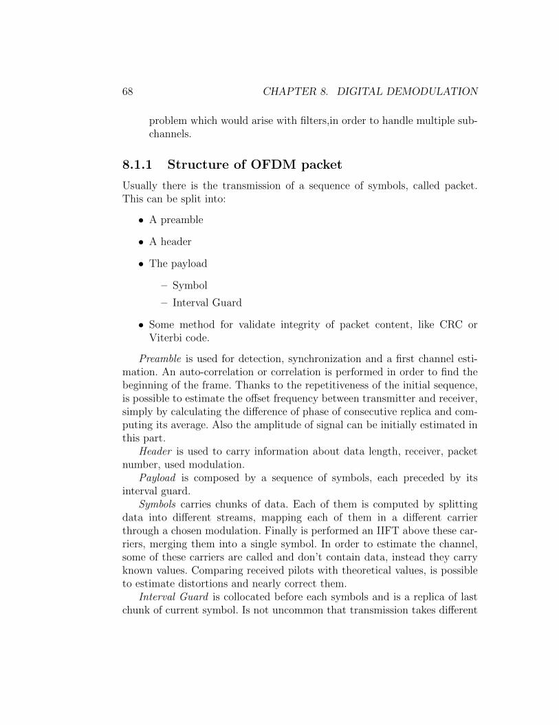
68 CHAPTER 8. DIGITAL DEMODULATION
problem which would arise with filters,in order to handle multiple sub-channels.
8.1.1 Structure of OFDM packet
Usually there is the transmission of a sequence of symbols, called packet.This can be split into:
• A preamble
• A header
• The payload
– Symbol
– Interval Guard
• Some method for validate integrity of packet content, like CRC orViterbi code.
Preamble is used for detection, synchronization and a first channel esti-mation. An auto-correlation or correlation is performed in order to find thebeginning of the frame. Thanks to the repetitiveness of the initial sequence,is possible to estimate the offset frequency between transmitter and receiver,simply by calculating the difference of phase of consecutive replica and com-puting its average. Also the amplitude of signal can be initially estimated inthis part.
Header is used to carry information about data length, receiver, packetnumber, used modulation.
Payload is composed by a sequence of symbols, each preceded by itsinterval guard.
Symbols carries chunks of data. Each of them is computed by splittingdata into different streams, mapping each of them in a different carrierthrough a chosen modulation. Finally is performed an IIFT above these car-riers, merging them into a single symbol. In order to estimate the channel,some of these carriers are called and don’t contain data, instead they carryknown values. Comparing received pilots with theoretical values, is possibleto estimate distortions and nearly correct them.
Interval Guard is collocated before each symbols and is a replica of lastchunk of current symbol. Is not uncommon that transmission takes different
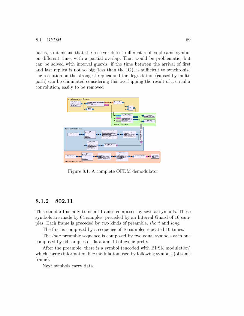
8.1. OFDM 69
paths, so it means that the receiver detect different replica of same symbolon different time, with a partial overlap. That would be problematic, butcan be solved with interval guards: if the time between the arrival of firstand last replica is not so big (less than the IG), is sufficient to synchronizethe reception on the strongest replica and the degradation (caused by multi-path) can be eliminated considering this overlapping the result of a circularconvolution, easily to be removed
Figure 8.1: A complete OFDM demodulator
8.1.2 802.11
This standard usually transmit frames composed by several symbols. Thesesymbols are made by 64 samples, preceded by an Interval Guard of 16 sam-ples. Each frame is preceded by two kinds of preamble, short and long.
The first is composed by a sequence of 16 samples repeated 10 times.
The long preamble sequence is composed by two equal symbols each onecomposed by 64 samples of data and 16 of cyclic prefix.
After the preamble, there is a symbol (encoded with BPSK modulation)which carries information like modulation used by following symbols (of sameframe).
Next symbols carry data.
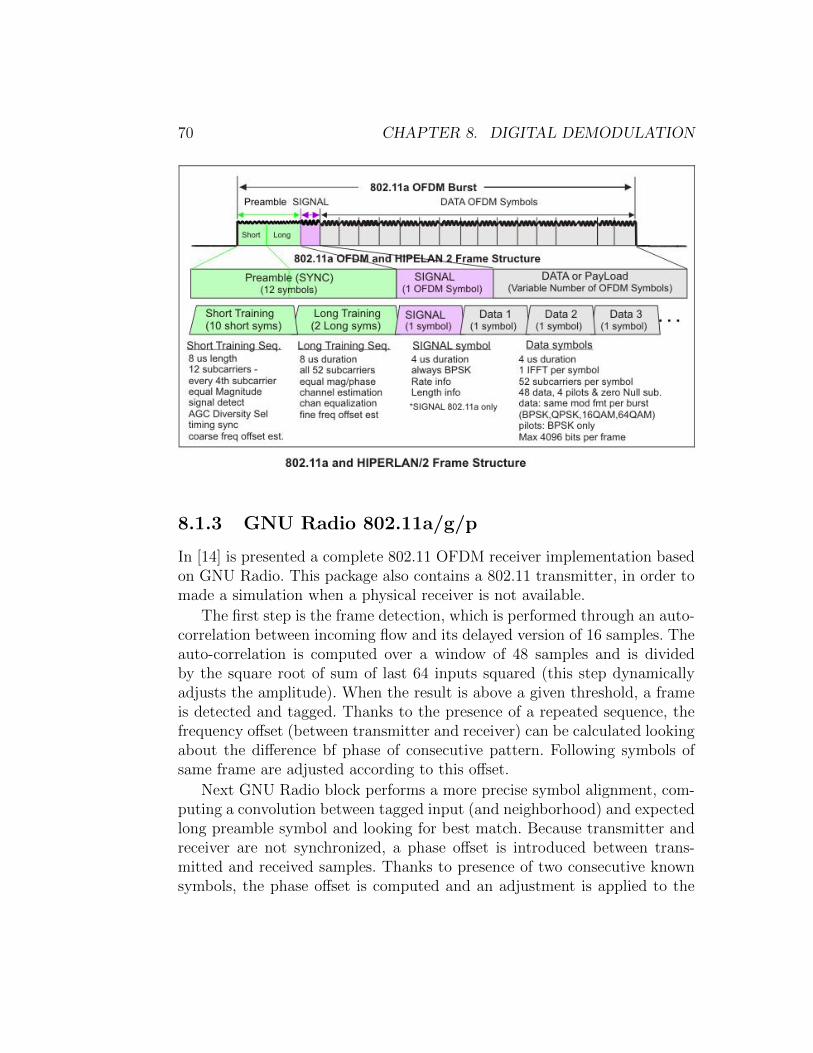
70 CHAPTER 8. DIGITAL DEMODULATION
8.1.3 GNU Radio 802.11a/g/p
In [14] is presented a complete 802.11 OFDM receiver implementation basedon GNU Radio. This package also contains a 802.11 transmitter, in order tomade a simulation when a physical receiver is not available.
The first step is the frame detection, which is performed through an auto-correlation between incoming flow and its delayed version of 16 samples. Theauto-correlation is computed over a window of 48 samples and is dividedby the square root of sum of last 64 inputs squared (this step dynamicallyadjusts the amplitude). When the result is above a given threshold, a frameis detected and tagged. Thanks to the presence of a repeated sequence, thefrequency offset (between transmitter and receiver) can be calculated lookingabout the difference bf phase of consecutive pattern. Following symbols ofsame frame are adjusted according to this offset.
Next GNU Radio block performs a more precise symbol alignment, com-puting a convolution between tagged input (and neighborhood) and expectedlong preamble symbol and looking for best match. Because transmitter andreceiver are not synchronized, a phase offset is introduced between trans-mitted and received samples. Thanks to presence of two consecutive knownsymbols, the phase offset is computed and an adjustment is applied to the
8.1. OFDM 71
frame using linear regression.
An FFT with size 64 is computed over symbols (from time samples to sub-carriers) and frequencies are changed, moving DC in the center of spectrum.
The channel is estimated looking about pilot sub-carriers (they have pre-determined values), then outgoing sub-carriers are adjusted, using a linearinterpolation of these estimated offsets.
Afterward samples are decoded, punctured and convolutional decoded,descrambled and converted into MAC format. These steps are not consider,because an external library is used (IT++) and they are less parallelizable.
8.1.4 With CUDA
I’ve tried to implement two blocks, the first performs steps before the FFT,while the other execute FFT and equalization (from channel estimation).
Frame detection and offset correction
The auto-correlation can be described as a moving sum with a window of 48value (each value is the multiplication between one input and the conjugateof input that precede by 16 positions). It can be implemented with a prefixsum, where each auto-correlation is given by the difference of two values(results of prefix sum) distanced by 48 positions.
A similar strategy is applicable to the moving average of squared value(for amplitude adjusting).
In Bloessl’s implementation a sample is marked as START OF FRAMEwhen is preceded by a given number of auto-correlations above a threshold, inaddition it should be a minimum distance between two START OF FRAME.For each samples with associated a big auto-correlation, is set a bit in anarray, where each position correspond to one sample.
After that each thread (linked with a samples candidate to be the startof frame) counts how many bits are set between its position and previousclear bit. In this way candidates are reduced, afterward is performed a checkabout distance between starts of frame. Therefore is adjusted the frequencyoffset for all samples, performing a phase offset (based on detected frequencyoffset and distance from first sample of frame).
Now is possible to execute a precise alignment making a correlation be-tween first part of each frame and the known long preamble sequence.
72 CHAPTER 8. DIGITAL DEMODULATION
The host must wait the end of kernel execution, in order to know thenumber of samples (number of samples of one frame is upper bounded, othervalues are noise and are discarded).
FFT and following steps
The other block performs FFT and equalization. Fast Fourier is performedas in previous blocks, followed by a channel estimation and equalization ofsymbols using linear interpolation. Each kernel modifies tag page (number ofsub-carrier of each symbol is reduced, after the removal of pilot sub-carriers)and the number of outputs is not predictable by host code, so a synchroniza-tion is mandatory.
In addition, a input page can contain symbols of a frame started one ormore page before, so is not sufficient to read tag page associated to previousinput page. The general case require to pass an history between subsequentlykernel launches, impeding concurrent execution of kernel above different in-put pages.
Performances
Unfortunately, both blocks are slower than their CPU counterpart, betweenthree and nine times.
The first block essentially compute a moving average, a task which is eas-ily processed by CPU (while is not so efficient on GPGPU due to limitationalready seen on IIR filters, like limited shared memory because all computedvalues must be accessible for next instructions). The expensive correlationbetween input and known long preamble sequence is done only for few sam-ples every frame. The GPGPU would be convenient for a frame detectorthat uses only the expensive correlation, because it acts like a FIR/FFT fil-ter. Can be convenient to execute frame detection for newer protocols basedon MIMO, because it is more compute intensive an parallelizable.
The second block computes lot of small FFT (one for each symbol), fol-lowed by few computations, lot of memory transfers and a host synchroniza-tion. GPGPU would be better with more refined equalizations, which requiremuch more computations.
It would be interesting the usage of dynamic parallelism: write a kernelthat makes frame detection (over short preamble), launch FFT in order tomake frame alignment (correlation between input and known long preamble
8.1. OFDM 73
sequence), followed by FFT over symbols and equalization. In this way isstrongly reduced the number of synchronization between host and device (inwhich the host waits the number of element produced by device).
In literature are available CUDA implementation of convolutional de-coder, so it would be possible to move also this part over GPGPU.
I’ve found a paper[15] about a 802.11 receiver implemented over CUDAthat claims to have good performance. Unlucky I didn’t find neither sourcecode nor citations in other papers.

74 CHAPTER 8. DIGITAL DEMODULATION
Chapter 9
Conclusions
It is clear that GPGPU can provide a good speedup for Digital Signal Pro-cessing, ranging from 2x to more than 10x, according to the task executed.
It is also obviously that is better to perform several GNU Radio con-secutive blocks on graphic cards, in order to minimize host-device memorytransfer. For this reason can be acceptable to run a GNU Radio block overGPGPU when it’s slower than its CPU counterpart, if adjacent GNU Radioblocks are executed over graphic card.
The goal of this thesis is not to show that is better to use GPGPU insteadof CPU, but that is possible to obtain a good speedup moving some portionof GNU Radio flow graph over GPGPU, exploiting all available processors.
All benchmarks are executed over input page with size 4 million of sam-ples. This is a good tradeoff between memory allocated (for internal buffers)and number of CUDA invocations. According to sample rate and latencydesired, the user would prefer another value.
In a ideal case, the CUDA command queue always contain some readykernel, in this case the delay between two kernel execution is about fewmicrosecond(or less, when launched by different threads).
9.1 Future Work
Thanks to features offered by lasts CUDA cards, are possible different im-provements.
HyperQ enqueue CUDA kernels in different hardware queue, avoidingtons of false dependencies, caused by the order in which kernels (of different
75
76 CHAPTER 9. CONCLUSIONS
streams) are queued.Dynamic parallelism allows to launch CUDA kernels from other kernels.
It become possible to launch only one kernel every one (or more) input page.This kernel can call cuFFT functions without the interaction of the host. Inaddition, a big kernel can be split into a kernel with high register pressureand another lighter.
Run time compilation allows the user to create, compile and execute de-vice code at run time. Some GNU Radio blocks (e.g. with a ratio 1:1 betweeninput/output) can propagate its kernel code to neighbors. Some GNU Radioblocks would collect device code of different block, merging them togetherand compile as a unique kernel, fusing execution of adjacent blocks. In thisway can be reduced kernel invocations and global memory transfers (it be-come possible to pass data through shared memory).
In [16] is showed a FFT that claims to be faster than cuFFT. This isreached running benchmarks able to locate bottleneck of each graphic card,information useful for a good scheduling of FFT (e.g. radix chosen, number ofthreads and blocks,in-place transform). It could be interesting to substitutecuFFT with this library. The drawback is that initial benchmarks take lot oftime
Appendix A
Installation and benchmarks
A.1 Installation and usage
Over a PC with GNU Radio already installed, is possible to add my libraryin few steps.
First of all, the library must be copied on the local hard-disk. In the libfolder, is better to modify the file CMakeLists.txt, updating arch and codecompilation flags with version of current graphic card. Is possible to changeparameters like number of supported streams, max dimension of buffers andothers editing files lib/cuda structures.cc and lib/blocks comm.cc.
After that, is necessary to follow the same procedure used in order toinstall GNU Radio out of tree modules. From the top folder, is sufficient torun these commands:
mkdir build && cd build && cmake .. && make -j && sudo make install&& sudo ldconfig
At the end, is mandatory to restart GNU Radio, if it was open duringcompilation/linking.
All GNU Radio blocks developed during my project can be found underthe category CUDA, with the same name of their counterparts created forCPU. When the user design its flowchart, he must handle manually host-device memory transfers, inserting blocks Memory CPU to GPGPU andMemory GPGPU to CPU where appropriate.
About Memory CPU to GPGPU, is possible to suggest a minimum lengthof pages issued and a mandatory divisor of the length. This is for performancereason: when the user indicates as divisor the minimum common multiple of
77
78 APPENDIX A. INSTALLATION AND BENCHMARKS
FFT sizes and decimations of following blocks, situations like output samplesdepending from two input pages are reduced.
A.2 Benchmarks
Measurement are performed on my laptop, composed by an Intel i7-2670QM(2.2GHz), 12 GB RAM DDR3 and a GT-540M graphic card (Fermi architec-ture 2.1, two Streaming Multiprocessors with 96 threads, 2 GB RAM DDR3).
The system operative installed is Linux Mint 17.1, while the used versionof CUDA Toolkit is 7.0.
Time is measured with time command, considering a GNU Radio execu-tion on single thread (obtainable exporting the variable GR SCHEDULER=STSbefore the execution.
NVIDIA Visual Profiler was used in order to find bottlenecks and performoptimizations.
Due to the fact that running time is not usually dependent from input butonly its length, I’ve developed some GNU Radio blocks which simply changecounters of input/output samples, in order to keep busy profiled blocks (bothCPU and GPGPU version). Is also possible (for GPU version) to randomlyinitialize pages at the beginning, in order to graphically study behaviour offilters.
Bibliography
[1] J. Mitola III, “Software radios: Survey, critical evaluation and futuredirections,” Aerospace and Electronic Systems Magazine, IEEE, vol. 8,no. 4, pp. 25–36, 1993.
[2] “GNU Radio website.” http://www.gnuradio.org. Accessed: 2015-06-20.
[3] V. Volkov, “Better performance at lower occupancy,” 2010.
[4] A. M. Aji, M. Daga, and W.-c. Feng, “Bounding the effect of partitioncamping in gpu kernels,” 2011.
[5] M. Bauer, H. Cook, and B. Khailany, “Cudadma: optimizing gpu mem-ory bandwidth via warp specialization,” in Proceedings of 2011 Interna-tional Conference for High Performance Computing, Networking, Stor-age and Analysis, p. 12, ACM, 2011.
[6] “Gr-theano repository.” https://github.com/osh/gr-theano. Ac-cessed: 2015-06-22.
[7] F. Bastien, P. Lamblin, R. Pascanu, J. Bergstra, I. Goodfellow, A. Berg-eron, N. Bouchard, D. Warde-Farley, and Y. Bengio, “Theano: new fea-tures and speed improvements,” Nov. 23 2012. Comment: Presented atthe Deep Learning Workshop, NIPS 2012.
[8] F. Bastien, P. Lamblin, R. Pascanu, J. Bergstra, I. J. Goodfellow,A. Bergeron, N. Bouchard, D. Warde-Farley, and Y. Bengio, “Theano:new features and speed improvements,” CoRR, vol. abs/1211.5590, 2012.
[9] S. Bang, C. Ahn, Y. Jin, S. Choi, J. Glossner, and S. Ahn, “Implemen-tation of LTE system on an SDR platform using CUDA and UHD,”Analog Integr. Circuits Signal Process., vol. 78, pp. 599–610, Mar. 2014.
79
80 BIBLIOGRAPHY
[10] “Halloc repository.” http://github.com/canonizer/halloc. Ac-cessed: 2015-06-20.
[11] F. Trebien, “An efficient gpu-based implementation of recursive linearfilters and its application to realistic real-time re-synthesis for interactivevirtual worlds,” 2009.
[12] R. E. Crochiere and L. R. Rabiner, “Optimum fir digital filter imple-mentations for decimation, interpolation, and narrow-band filtering,”Acoustics, Speech and Signal Processing, IEEE Transactions on, vol. 23,no. 5, pp. 444–456, 1975.
[13] R. G. Lyons, Understanding digital signal processing. Pearson Educa-tion, 2010.
[14] B. Bloessl, M. Segata, C. Sommer, and F. Dressler, “An ieee 802.11a/g/p ofdm receiver for gnu radio,” in Proceedings of the second work-shop on Software radio implementation forum, pp. 9–16, ACM, 2013.
[15] K. Li, M. Wu, G. Wang, and J. R. Cavallaro, “A high performancegpu-based software-defined basestation,”
[16] Y. Dotsenko, S. S. Baghsorkhi, B. Lloyd, and N. K. Govindaraju, “Auto-tuning of fast fourier transform on graphics processors,” in ACM SIG-PLAN Notices, vol. 46, pp. 257–266, ACM, 2011.


![Curriculum Vitæ - UPC Universitat Politècnica de Catalunyajordicf/CV.pdf · Co-advised with Sachin S. Sapatnekar. PhD thesis. Universitat Polit`ecnica de Catalunya, May 2017. [2]](https://img.pdfslide.us/doc/110x75/5afd20d67f8b9a864d8d0f11/curriculum-vit-upc-universitat-politcnica-de-catalunya-jordicfcvpdfco-advised.jpg)