Universitat Augsburg

Audio Brush:

Editing Audio in the Spectrogram

C. G. v. d. Boogaart, R. Lienhart

Report 2005-10 Juni 2005revised Oktober 2005

Institut fur InformatikD-86135 Augsburg

Copyright c© C. G. v. d. Boogaart, R. LienhartInstitut fur InformatikUniversitat AugsburgD–86135 Augsburg, Germanyhttp://www.Informatik.Uni-Augsburg.DE— all rights reserved —

Audio Brush:Editing Audio in the Spectrogram

C. G. v. d. Boogaart, R. LienhartMultimedia Computing Lab

University of Augsburg86159 Augsburg, Germany

{boogaart,lienhart}@informatik.uni-augsburg.de

ABSTRACTA tool for editing audio signals in the spectrogram is pre-sented. It allows manipulating the spectrogram of a signalat any chosen time-frequency resolution directly and to re-construct the edited signal in HiFi quality – a capability thatis usually not possible with the Fourier or wavelet transfor-mation. Image processing and computer vision methods areapplied to the spectrogram in order to identify, separate,eliminate and/or modify audio objects visually. As spec-trograms give descriptive information about the sound, thistool allows editing audio in a “what you see is what youhear” style. This is enabled by a thorough investigation andexploitation of Gabor analysis and synthesis. We furtherpropose to use a kind of zooming, as in visual painting tools,which results in a change of time and frequency resolution,and can be adapted for the task at hand. Results on apply-ing this tool to erasing audio objects such as whistles, music,clapping and alike in audio tracks are presented. Hence au-dio objects are automatically identified as visual objects inthe spectrogram and eliminated therein. The cleaned signalis then reconstructed from the spectrogram in HiFi quality.

1. INTRODUCTIONHearing, analyzing and evaluating sounds is possible for

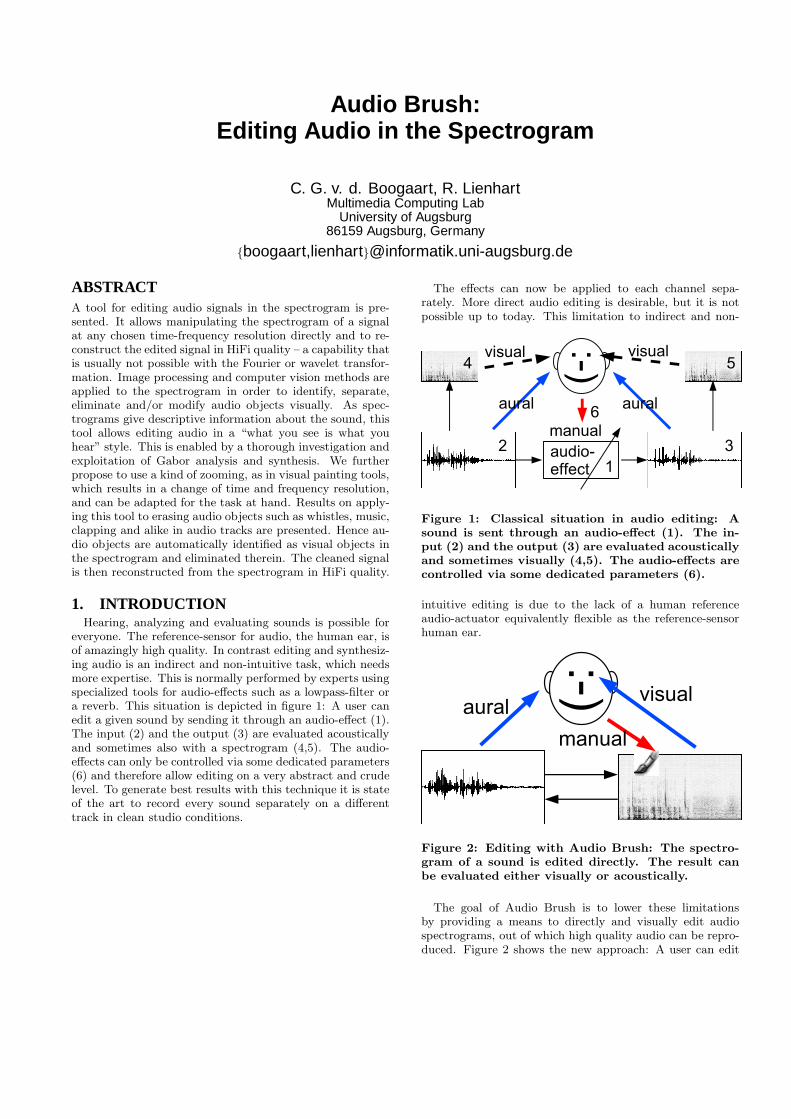
everyone. The reference-sensor for audio, the human ear, isof amazingly high quality. In contrast editing and synthesiz-ing audio is an indirect and non-intuitive task, which needsmore expertise. This is normally performed by experts usingspecialized tools for audio-effects such as a lowpass-filter ora reverb. This situation is depicted in figure 1: A user canedit a given sound by sending it through an audio-effect (1).The input (2) and the output (3) are evaluated acousticallyand sometimes also with a spectrogram (4,5). The audio-effects can only be controlled via some dedicated parameters(6) and therefore allow editing on a very abstract and crudelevel. To generate best results with this technique it is stateof the art to record every sound separately on a differenttrack in clean studio conditions.

The effects can now be applied to each channel sepa-rately. More direct audio editing is desirable, but it is notpossible up to today. This limitation to indirect and non-

Figure 1: Classical situation in audio editing: Asound is sent through an audio-effect (1). The in-put (2) and the output (3) are evaluated acousticallyand sometimes visually (4,5). The audio-effects arecontrolled via some dedicated parameters (6).

intuitive editing is due to the lack of a human referenceaudio-actuator equivalently flexible as the reference-sensorhuman ear.

Figure 2: Editing with Audio Brush: The spectro-gram of a sound is edited directly. The result canbe evaluated either visually or acoustically.

The goal of Audio Brush is to lower these limitationsby providing a means to directly and visually edit audiospectrograms, out of which high quality audio can be repro-duced. Figure 2 shows the new approach: A user can edit

the spectrogram of a sound directly. The result can be eval-uated either visually or acoustically resulting in a shorterclosed loop for editing and evaluation. This has several ad-vantages:

1. A spectrogram is a very good representation of anaudio-signal. Often speech-experts are able to readtext out of speech-spectrograms. In our approach, thespectrogram is used as representation of both, the orig-inal and the recreated audio-signal, which both can berepresented visually and acoustically. It therefore nar-rows the gap between hearing and editing audio.

2. Audio is transient. It is emitted by a source througha dynamic process, travels through air and is receivedby the human ear. It cannot be held for investigationat a given time moment and frequency band. Thislimitation is overcome by representing the audio sig-nal as a spectrogram. The spectrogram can be studiedin detail and edited appropriately before inverse trans-forming it back into the dynamic audio domain.

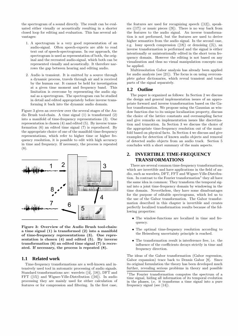
Figure 3 gives an overview over the several stages of the Au-dio Brush tool-chain. A time signal (1) is transformed (2)into a manifold of time-frequency representations (3). Onerepresentation is chosen (4) and edited (5). By inverse trans-formation (6) an edited time signal (7) is reproduced. Bythe appropriate choice of one of the manifold time-frequencyrepresentations, which refer to higher time or higher fre-quency resolution, it is possible to edit with high accuracyin time and frequency. If necessary, the process is repeated(8).

Figure 3: Overview of the Audio Brush tool-chain:a time signal (1) is transformed (2) into a manifoldof time-frequency representations (3). One repre-sentation is chosen (4) and edited (5). By inversetransformation (6) an edited time signal (7) is recre-ated. If necessary, the process is repeated (8).

1.1 Related workTime-frequency transformations are a well-known and in-

tensively used tool in automatic processing of audio signals.Standard transformations are: wavelets ([4], [18]), DFT andFFT ([15]) and Wigner-Ville-Distribution ([16]). In audioprocessing they are mainly used for either calculation offeatures or for compression and filtering. In the first case,

the features are used for recognizing speech ([12]), speak-ers ([17]) or music pieces ([9]). There is no way back fromthe features to the audio signal. An inverse transforma-tion is not performed, but the features are used to derivehigher semantics from the audio signal. In the second case,e.g. lossy speech compression ([18]) or denoising ([5]), aninverse transformation is performed and the signal is eitherintentionally or unintentionally edited in the short term fre-quency domain. However the editing is not based on anyvisualization and thus no visual manipulation concepts canbe applied.

Multiresolution Gabor analysis has already been appliedfor audio analysis (see [21]). The focus is on using overcom-plete gabor dictionaries, which reveal transient and tonalparts of the signal separately.

1.2 OutlineThe paper is organized as follows: In Section 2 we discuss

the design and general implementation issues of an appro-priate forward and inverse transformation based on the Ga-bor transformation. We propose using the Gaussian as win-dow function due to its unique localization property, discussthe choice of the lattice constants and oversampling factorand give remarks on implementation issues like discretiza-tion and truncation. In Section 3 we discuss the choice ofthe appropriate time-frequency resolution out of the mani-fold based on physical facts. In Section 4 we discuss and giveexamples for detection of known audio objects and removalof detected audio objects from an audio track. Section 5concludes with a short summary of the main aspects.

2. INVERTIBLE TIME-FREQUENCYTRANSFORMATIONS

There are several common time-frequency transformations,which are invertible and have applications in the field of au-dio, such as wavelets, DFT, FFT and Wigner-Ville-Distribu-tion. In contrast to the Fourier transformation1 they all havethe same idea in common: They transform the temporal sig-nal into a joint time-frequency domain by windowing in thetime domain. Nevertheless, they have some disadvantagesfor the purpose of editable spectrograms, which led us tothe use of the Gabor transformation. The Gabor transfor-mation described in this chapter is invertible and createsperfectly localized transformation results because of the fol-lowing properties:

• The window-functions are localized in time and fre-quency.

• The optimal time-frequency resolution according tothe Heisenberg uncertainty principle is reached.

• The transformation result is interference free, i.e. theinfluence of the coefficients decays strictly in time andfrequency direction.

The ideas of the Gabor transformation (Gabor regression,Gabor expansion) trace back to Dennis Gabor [8]. Sinceits original formulation the theory has been developed muchfurther, revealing serious problems in theory and possible

1The Fourier transformation computes the spectrum of atime signal, hiding all information of its temporal evolutionin the phases, i.e. it transforms a time signal into a purefrequency signal (see [14]).

solutions to deal with them. The major results can be foundin [6] and [7].

2.1 Fundamentals of the Gabor transforma-tion

As the Gabor transformation is its discretized version, westart our discussion with the windowed or short time Fouriertransformation (STFT). It was developed to overcome thelack of time localization of the Fourier transformation. TheSTFT is defined as follows: A time function x(t) is splitin the time-frequency domain into X(t, f) by the use of awindowing function w(t):

X(t, f) =

+∞Z

−∞

x(τ )w∗(τ − t)e−j2πfτ dτ . (1)

This is the inner product of the temporal signal x(t) witha modulated (by e−j2πft) and time shifted, conjugate com-plex window function w(t). The inner product measures thesimilarity of the signal to the so called prototype functionw∗(τ − t)e−j2πfτ ([18]). To get the local properties of x(t)the window w(t) has to be chosen appropriately to be lo-calized in time and frequency. An inverse transformationreconstructs the signal and is given by the formula ([1]):

x(t)

+∞Z

−∞

|w(t)|2 dt =

+∞Z

−∞

+∞Z

−∞

X(τ, f)w(τ − t)ej2πft dτdf . (2)

For use in digital signal processing formulas (1) and (2) haveto be discretized, using sums instead of integrals and sums offinite length. This is discussed under the term Gabor trans-formation. The Gabor transformation is defined as follows:From a single prototype or window function g(t), which islocalized in time and frequency, a Gabor system gna,mb(t)is derived by time shift and frequency shift as follows (see[19]):

gna,mb(t) = e2πjmbtg(t − na), n, m ∈ Z, a, b ∈ R, (3)

The time frequency plane is then covered by a lattice oflocal functions with the lattice constants a time shift andb frequency shift. The Gabor transformation is calculatedas sampled STFT of x(t) (see [6]). With the Gabor systemgna,mb(t) this can be expressed as follows:

cnm = X(na, mb) =

+∞Z

−∞

x(t)g∗

na,mb(t) dt. (4)

cnm are called the Gabor coefficients of x(t). The inversetransformation or reconstruction recreates the signal x(t)from its Gabor coefficients. This inverse transformation iscalled Gabor expansion and is calculated with the windowfunction γ(t), which is called dual window of g(t) and whichdepends on g(t) and on the lattice constants a and b. TheGabor system γna,mb(t) of γ(t) is also defined as:

γna,mb(t) = e2πjmbtγ(t − na), n, m ∈ Z, a, b ∈ R, (5)

The inverse transformation is then defined as follows (see[1]):

x(t)∞

X

k=−∞

|γ(ka)|2 =∞

X

n=−∞

∞X

m=−∞

cnmγna,mb(t). (6)

The role of analysis and synthesis window is interchangeable.As already mentioned, the window function g(t) has to

be localized in time and frequency. The same is necessaryfor the dual window γ(t). The theory of the Gabor trans-formation led to the result, that the window functions g(t)and γ(t) and the lattice constants a and b must fulfill cer-tain requirements in order to assure the invertibility. Thisis discussed further in the following two sections.

2.2 Choice of the window functionWe start with the choice of the window function. The lo-

calization in time and frequency has to be discussed in thecontext of the uncertainty principle of Heisenberg. It saysthat the product of the time duration ∆t of a window func-tion and its frequency extent ∆f has a total lower limit. If∆t and ∆f are defined as standard deviation of the windowfunction and its Fourier transformation respectively, this canbe expressed with the following inequality (see [18]):

∆t∆f ≥ 1

4π. (7)

The “=” is only reached for the Gaussian as window function(see e.g. [20]):

g(t) =1

p

2πσ2t

e−

1

2

t2

σ2t . (8)

Its Fourier transformation has the same Gaussian shape asthe time function itself:

G(f) =1

q

2πσ2f

e−

1

2

f2

σ2

f . (9)

With ∆t and ∆f defined as standard deviation of the timefunction and its Fourier transformation respectively (∆t =σt, ∆f = σf ) and formula (7) for the “=” we get:

σf =1

4πσt

. (10)

A Gaussian window has the following properties:

• Minimal extent in the time frequency plane accordingto the Heisenberg uncertainty principle.

• Localized shape, i.e. only one local and global maxi-mum and strict decay in time and frequency direction.

This localization properties are of essential importance foraudio processing, in general and audio editing, in specific,because the reference sensor, the human ear itself has a timefrequency resolution, which closely reaches the physical limitexpressed in the Heisenberg principle (see [2]). It is further-more capable of adapting its time-frequency resolution inaccordance to the Heisenberg principle. The Gaussian aswindow function leads to Gabor coefficients, which have thebest localized influence possible according to the Heisenbergprinciple. As the Gabor coefficients represent the signal sim-ilar or better localized in time and frequency as the humanear, it is possible to avoid perceivable artefacts introducedthrough editing. The meaning of the Heisenberg principlefor Audio Brush is discussed further in chapter 3.

2.3 Choice of dual window function, latticeconstants and oversampling factor

With the choice of the window-function, it is still an openissue, which dual window-function γ(t) and lattice constants

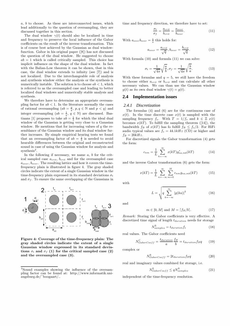
a, b to choose. As these are interconnected issues, whichlead additionally to the question of oversampling, they arediscussed together in this section.

The dual window γ(t) should also be localized in timeand frequency to preserve the local influence of the Gaborcoefficients on the result of the inverse transformation. Thisis of course best achieved by the Gaussian as dual window-function. Gabor in his original paper ([8]) has not discussedthe question of the dual window. He suggested to chooseab = 1 which is called critically sampled. This choice hasimplicit influence on the shape of the dual window. In factwith the Balian-Low theorem it can be shown, that in thiscase, the dual window extends to infinity (see [7]) and isnot localized. Due to the interchangeable role of analysisand synthesis window either the analysis or the synthesis isnumerically instable. The solution is to choose ab < 1, whichis referred to as the oversampled case and leading to betterlocalized dual windows and numerically stable analysis andsynthesis.

We therefore have to determine an appropriate oversam-pling factor for ab < 1. In the literature normally the casesof rational oversampling (ab = p

q, p, q ∈ N and p < q) and

integer oversampling (ab = 1

q, q ∈ N) are discussed. Bas-

tiaans [1] proposes to take ab = 1

3for which the ideal dual

window of the Gaussian is getting very close to a Gaussianwindow. He mentions that for increasing values of q the re-semblance of the Gaussian window and its dual window fur-ther increases. By simple empirical hearing tests we foundthat an oversampling factor of ab = 1

5is needed to avoid

hearable differences between the original and reconstructedsound in case of using the Gaussian window for analysis andsynthesis2.

In the following if necessary, we name a, b for the crit-ical sampled case acrit, bcrit and for the oversampled caseaover, bover. The resulting lattice and how it covers the time-frequency plain is illustrated in figure 4. The gray shadedcircles indicate the extent of a single Gaussian window in thetime-frequency plain expressed in its standard deviations σt

and σf . To ensure the same overlapping of the Gaussians in

Figure 4: Coverage of the time-frequency plain: Thegray shaded circles indicate the extent of a singleGaussian window expressed in its standard devia-tions σt and σf (1) for the critical sampled case (2)and the oversampled case (3).

2Sound examples showing the influence of the oversam-pling factor can be found at: http://www.informatik.uni-augsburg.de/˜boogaart/..

time and frequency direction, we therefore have to set:

σt

σf

=acrit

bcrit

=aover

bover

. (11)

With aoverbover = 1

qthis holds for:

aover =acrit√

q, bover =

bcrit√q

. (12)

With formula (10) and formula (11) we can solve:

σt =1√4π

r

a

b, σf =

1√4π

r

b

a. (13)

With these formulas and q = 5, we still have the freedomto choose either acrit or bcrit and can calculate all othernecessary values. We can than use the Gaussian windowg(t) as its own dual window γ(t) = g(t).

2.4 Implementation issues

2.4.1 DiscretizationThe formulas (4) and (6) are for the continuous case of

x(t). In the time discrete case x(t) is sampled with thesampling frequency fs. With T = 1/fs and k ∈ Z x(t)becomes x(kT ). To fulfill the sampling theorem ([14]), thebandwidth fB of x(kT ) has fo fulfill fB ≤ fs/2. For HiFiaudio typical values are fs = 44.1kHz (CD) or higher andfB = 20kHz.

For discretized signals the Gabor transformation (4) getsthe form:

cnm =1

L

∞X

k=−∞

x(kT )g∗

na,mb(kT ) (14)

and the inverse Gabor transformation (6) gets the form:

x(kT ) =1

L

∞X

n=−∞

MX

m=0

cnmgna,mb(kT ) (15)

with

L =

v

u

u

tq

∞X

k=−∞

|g(ka)|2 (16)

and

m ∈ [0, M ] and M = ⌈fB/b⌉. (17)

Remark: Storing the Gabor coefficients is very effective. Adiscretized time signal of length tduration needs for storage

NR

samples = tdurationfs (18)

real values. The Gabor coefficients need

NC

GaborCoeff =tduration

a

fB

b= tdurationfBq (19)

complex or

NR

GaborCoeff = 2tdurationfBq (20)

real and imaginary values combined for storage, i.e.

NR

GaborCoeff ≤ qNR

samples (21)

independent of the time-frequency resolution.

2.4.2 TruncationThe formulas (14) and (15) still use a sum over infinite

time. To implement them a truncation of the sum is neces-sary, which corresponds to a truncation of the windows. Tofind an appropriate truncation we have chosen the way ofsimple empirical listening tests again, with the goal to get areproduced sound with no hearable difference from the orig-inal sound. The decline D of the Gaussian window from themaximum to the cut is expressed in dB:

D = 20logg(0)

g(tcut)dB. (22)

For a given D we get with (8):

tcut =

r

2ln“

10D20

”

σt. (23)

The digital implemental form of the Gabor transformationis then:

cnm =1

L

NX

k=−N

x(kT )g∗

na,mb(kT ) (24)

and the inverse:

x(kT ) =1

L

NX

n=−N

MX

m=0

cnmgna,mb(kT ) (25)

with:

L =

v

u

u

tqN

X

k=−N

|g(ka)|2 (26)

and

N = tcutfs =tcut

T, m ∈ [0, M ]andM = ⌈fB/bover⌉. (27)

In our implementation high values for D (up to 200dB) havebeen tested in 10dB increments, but values of D ≥ 30dBhave shown to be completely sufficient for high quality au-dio3.

3. TIME-FREQUENCY ZOOMING

3.1 Time-frequency resolutionAs mentioned in section 2.2, the human ear usually adapts

its current time-frequency resolution to the current contentof the signal according to the Heisenberg uncertainty princi-ple. It is therefore advantageous also to adapt the resolutionof our transformation to the current editing task.

3.1.1 Heisenberg Uncertainty PrincipleWe already applied the Heisenberg uncertainty principle

to the functions of the window (see section 2.2) and the dualwindow (see section 2.3). It also holds for the function ofthe signal, which of course in general has a resolution worsethan the theoretical limit.

As the Gabor transformation is a discretized version ofthe STFT, we can discuss the continuous case of the STFT.

3Sound examples showing the influence of the trun-cation of the Gaussian window can be found at:http://www.informatik.uni-augsburg.de/˜boogaart/.

The STFT (see eq. (1)) can be expressed as a convolutionof signal x(t) with h∗(−t, f) = w∗(−t)e−j2πft:

X(t, f) = x(t) ∗ h∗(−t, f) =

Z

+∞

−∞

x(τ )h∗(−(t − τ ), f) dτ .

(28)This is similar to adding the variances of two statisticallyindependent random variables X and Y , which form a newrandom variable Z = X + Y . Their probability densityfunctions are also convolved and the variance of Z is thengiven by (see [10]):

σ2Z = σ2

X + σ2Y . (29)

Therefore the time and frequency variances of a signal anda window are added in the form:

σ2ttransformation

= σ2tsignal

+ σ2twindow

, (30)

σ2ftransformation

= σ2fsignal

+ σ2fwindow

. (31)

Consequently the achievable accuracy of editing a given sig-nal is given by the superposition of the signal’s and window’suncertainty. As time and frequency resolution are intercon-nected, one has to give up time resolution in order to im-prove the frequency resolution and vice versa. Choosing anadapted window length allows locally to minimize the influ-ence of the window on the representation of a signal in thespectrogram.

3.1.2 Multiwindow AnalysisWith the choices of chapter 2 (g(t) = γ(t) gaussian, p = 1,

q = 5, D = 30dB), we can still choose the frequency shiftbcrit resulting in a time shift acrit = 1

bcritor vice versa.

This is equivalent to choosing an adapted window length.Different choices lead to different time frequency represen-tations of the same signal in the 3D-space with the axes t, fand e.g. bcrit. However, the same signal is represented andthus this space is overcomplete: different characteristics ofthe signal are revealed in different layers with constant bcrit.The properties of this space can be clarified by the extremesof bcrit:

For bcrit → ∞: The window g(t) becomes the Dirac im-pulse and the Gabor transformation becomes the timesignal itself.

For bcrit = 0: The window becomes g(t) = const. losing itswindowing properties and the Gabor transformationbecomes the Fourier transformation.

It is therefore proposed to calculate the Gabor transforma-tion of an audio signal with different choices of bcrit and toperform the respective editing task in the layer bcrit = const.which allows the best accuracy for the current task. Thiscan be understood as zooming, which allows to increase theresolution of the representation of a signal either in time orin frequency. As result of the Heisenberg uncertainty prin-ciple, the resolution of the other domain always decreases.

3.2 ExampleFigure 5 shows a typical spectrogram of a speech signal.

The spectrogram is calculated with bcrit = 64Hz, which re-sults with bover = 28.6Hz in roughly 699 frequency bandsin the range from 0 Hz to 20 kHz. Figure 6 for comparison

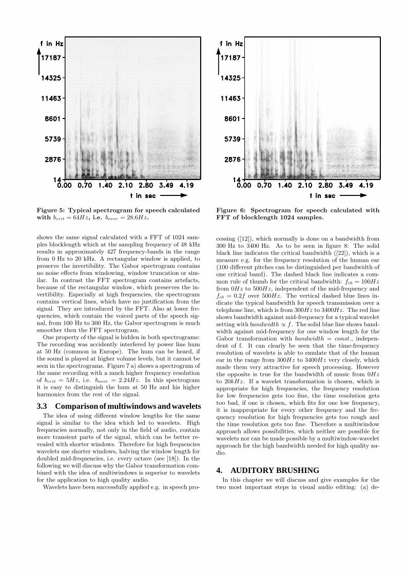
Figure 5: Typical spectrogram for speech calculatedwith bcrit = 64Hz, i.e. bover = 28.6Hz.

shows the same signal calculated with a FFT of 1024 sam-ples blocklength which at the sampling frequency of 48 kHzresults in approximately 427 frequency-bands in the rangefrom 0 Hz to 20 kHz. A rectangular window is applied, topreserve the invertibility. The Gabor spectrogram containsno noise effects from windowing, window truncation or sim-ilar. In contrast the FFT spectrogram contains artefacts,because of the rectangular window, which preserves the in-vertibility. Especially at high frequencies, the spectrogramcontains vertical lines, which have no justification from thesignal. They are introduced by the FFT. Also at lower fre-quencies, which contain the voiced parts of the speech sig-nal, from 100 Hz to 300 Hz, the Gabor spectrogram is muchsmoother then the FFT spectrogram.

One property of the signal is hidden in both spectrograms:The recording was accidently interfered by power line humat 50 Hz (common in Europe). The hum can be heard, ifthe sound is played at higher volume levels, but it cannot beseen in the spectrograms. Figure 7 a) shows a spectrogram ofthe same recording with a much higher frequency resolutionof bcrit = 5Hz, i.e. bover = 2.24Hz. In this spectrogramit is easy to distinguish the hum at 50 Hz and his higherharmonics from the rest of the signal.

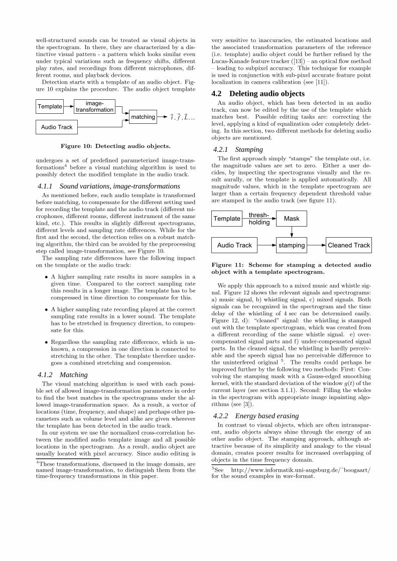
3.3 Comparison of multiwindows and waveletsThe idea of using different window lengths for the same

signal is similar to the idea which led to wavelets. Highfrequencies normally, not only in the field of audio, containmore transient parts of the signal, which can be better re-vealed with shorter windows. Therefore for high frequencieswavelets use shorter windows, halving the window length fordoubled mid-frequencies, i.e. every octave (see [18]). In thefollowing we will discuss why the Gabor transformation com-bined with the idea of multiwindows is superior to waveletsfor the application to high quality audio.

Wavelets have been successfully applied e.g. in speech pro-

Figure 6: Spectrogram for speech calculated withFFT of blocklength 1024 samples.

cessing ([12]), which normally is done on a bandwidth from300 Hz to 3400 Hz. As to be seen in figure 8: The solidblack line indicates the critical bandwidth ([22]), which is ameasure e.g. for the frequency resolution of the human ear(100 different pitches can be distinguished per bandwidth ofone critical band). The dashed black line indicates a com-mon rule of thumb for the critical bandwidth: fcb = 100Hzfrom 0Hz to 500Hz, independent of the mid-frequency andfcb = 0.2f over 500Hz. The vertical dashed blue lines in-dicate the typical bandwidth for speech transmission over atelephone line, which is from 300Hz to 3400Hz. The red lineshows bandwidth against mid-frequency for a typical waveletsetting with bandwidth ∝ f . The solid blue line shows band-width against mid-frequency for one window length for theGabor transformation with bandwidth = const., indepen-dent of f. It can clearly be seen that the time-frequencyresolution of wavelets is able to emulate that of the humanear in the range from 300Hz to 3400Hz very closely, whichmade them very attractive for speech processing. Howeverthe opposite is true for the bandwidth of music from 0Hzto 20kHz. If a wavelet transformation is chosen, which isappropriate for high frequencies, the frequency resolutionfor low frequencies gets too fine, the time resolution getstoo bad, if one is chosen, which fits for one low frequency,it is inappropriate for every other frequency and the fre-quency resolution for high frequencies gets too rough andthe time resolution gets too fine. Therefore a multiwindowapproach allows possibilities, which neither are possible forwavelets nor can be made possible by a multiwindow-waveletapproach for the high bandwidth needed for high quality au-dio.

4. AUDITORY BRUSHINGIn this chapter we will discuss and give examples for the

two most important steps in visual audio editing: (a) de-

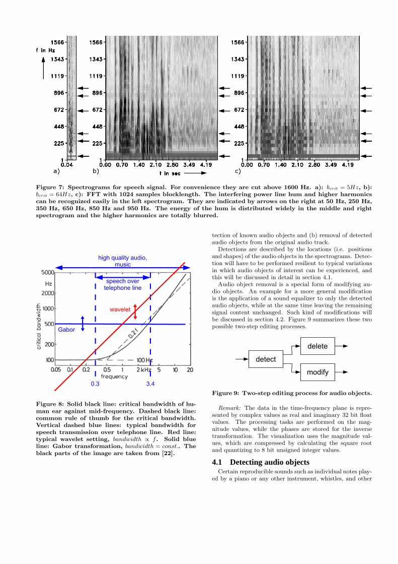
Figure 7: Spectrograms for speech signal. For convenience they are cut above 1600 Hz. a): bcrit = 5Hz, b):bcrit = 64Hz, c): FFT with 1024 samples blocklength. The interfering power line hum and higher harmonicscan be recognized easily in the left spectrogram. They are indicated by arrows on the right at 50 Hz, 250 Hz,350 Hz, 650 Hz, 850 Hz and 950 Hz. The energy of the hum is distributed widely in the middle and rightspectrogram and the higher harmonics are totally blurred.

Figure 8: Solid black line: critical bandwidth of hu-man ear against mid-frequency. Dashed black line:common rule of thumb for the critical bandwidth.Vertical dashed blue lines: typical bandwidth forspeech transmission over telephone line. Red line:typical wavelet setting, bandwidth ∝ f . Solid blueline: Gabor transformation, bandwidth = const.. Theblack parts of the image are taken from [22].

tection of known audio objects and (b) removal of detectedaudio objects from the original audio track.

Detections are described by the locations (i.e. positionsand shapes) of the audio objects in the spectrograms. Detec-tion will have to be performed resilient to typical variationsin which audio objects of interest can be experienced, andthis will be discussed in detail in section 4.1.

Audio object removal is a special form of modifying au-dio objects. An example for a more general modificationis the application of a sound equalizer to only the detectedaudio objects, while at the same time leaving the remainingsignal content unchanged. Such kind of modifications willbe discussed in section 4.2. Figure 9 summarizes these twopossible two-step editing processes.

Figure 9: Two-step editing process for audio objects.

Remark: The data in the time-frequency plane is repre-sented by complex values as real and imaginary 32 bit floatvalues. The processing tasks are performed on the mag-nitude values, while the phases are stored for the inversetransformation. The visualization uses the magnitude val-ues, which are compressed by calculating the square rootand quantizing to 8 bit unsigned integer values.

4.1 Detecting audio objectsCertain reproducible sounds such as individual notes play-

ed by a piano or any other instrument, whistles, and other

well-structured sounds can be treated as visual objects inthe spectrogram. In there, they are characterized by a dis-tinctive visual pattern - a pattern which looks similar evenunder typical variations such as frequency shifts, differentplay rates, and recordings from different microphones, dif-ferent rooms, and playback devices.

Detection starts with a template of an audio object. Fig-ure 10 explains the procedure. The audio object template

Figure 10: Detecting audio objects.

undergoes a set of predefined parameterized image-trans-formations4 before a visual matching algorithm is used topossibly detect the modified template in the audio track.

4.1.1 Sound variations, image-transformationsAs mentioned before, each audio template is transformed

before matching, to compensate for the different setting usedfor recording the template and the audio track (different mi-crophones, different rooms, different instrument of the samekind, etc.). This results in slightly different spectrograms,different levels and sampling rate differences. While for thefirst and the second, the detection relies on a robust match-ing algorithm, the third can be avoided by the preprocessingstep called image-transformation, see Figure 10.

The sampling rate differences have the following impacton the template or the audio track:

• A higher sampling rate results in more samples in agiven time. Compared to the correct sampling ratethis results in a longer image. The template has to becompressed in time direction to compensate for this.

• A higher sampling rate recording played at the correctsampling rate results in a lower sound. The templatehas to be stretched in frequency direction, to compen-sate for this.

• Regardless the sampling rate difference, which is un-known, a compression in one direction is connected tostretching in the other. The template therefore under-goes a combined stretching and compression.

4.1.2 MatchingThe visual matching algorithm is used with each possi-

ble set of allowed image-transformation parameters in orderto find the best matches in the spectrograms under the al-lowed image-transformation space. As a result, a vector oflocations (time, frequency, and shape) and perhaps other pa-rameters such as volume level and alike are given whereverthe template has been detected in the audio track.

In our system we use the normalized cross-correlation be-tween the modified audio template image and all possiblelocations in the spectrogram. As a result, audio object areusually located with pixel accuracy. Since audio editing is

4These transformations, discussed in the image domain, arenamed image-transformation, to distinguish them from thetime-frequency transformations in this paper.

very sensitive to inaccuracies, the estimated locations andthe associated transformation parameters of the reference(i.e. template) audio object could be further refined by theLucas-Kanade feature tracker ([13]) – an optical flow method– leading to subpixel accuracy. This technique for exampleis used in conjunction with sub-pixel accurate feature pointlocalization in camera calibration (see [11]).

4.2 Deleting audio objectsAn audio object, which has been detected in an audio

track, can now be edited by the use of the template whichmatches best. Possible editing tasks are: correcting thelevel, applying a kind of equalization oder completely delet-ing. In this section, two different methods for deleting audioobjects are mentioned.

4.2.1 StampingThe first approach simply “stamps” the template out, i.e.

the magnitude values are set to zero. Either a user de-cides, by inspecting the spectrograms visually and the re-sult aurally, or the template is applied automatically. Allmagnitude values, which in the template spectrogram arelarger than a certain frequency dependent threshold valueare stamped in the audio track (see figure 11).

Figure 11: Scheme for stamping a detected audioobject with a template spectrogram.

We apply this approach to a mixed music and whistle sig-nal. Figure 12 shows the relevant signals and spectrograms:a) music signal, b) whistling signal, c) mixed signals. Bothsignals can be recognized in the spectrogram and the timedelay of the whistling of 4 sec can be determined easily.Figure 12, d): “cleaned” signal: the whistling is stampedout with the template spectrogram, which was created froma different recording of the same whistle signal. e) over-compensated signal parts and f) under-compensated signalparts. In the cleaned signal, the whistling is hardly perceiv-able and the speech signal has no perceivable difference tothe uninterfered original 5. The results could perhaps beimproved further by the following two methods: First: Con-volving the stamping mask with a Gauss-edged smoothingkernel, with the standard deviation of the window g(t) of thecurrent layer (see section 3.1.1). Second: Filling the wholesin the spectrogram with appropriate image inpainting algo-rithms (see [3]).

4.2.2 Energy based erasingIn contrast to visual objects, which are often intranspar-

ent, audio objects always shine through the energy of another audio object. The stamping approach, although at-tractive because of its simplicity and analogy to the visualdomain, creates poorer results for increased overlapping ofobjects in the time frequency domain.

5See http://www.informatik.uni-augsburg.de/˜boogaart/for the sound examples in wav-format.

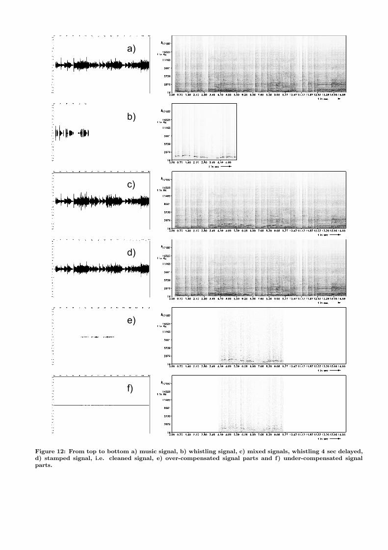
Figure 12: From top to bottom a) music signal, b) whistling signal, c) mixed signals, whistling 4 sec delayed,d) stamped signal, i.e. cleaned signal, e) over-compensated signal parts and f) under-compensated signalparts.

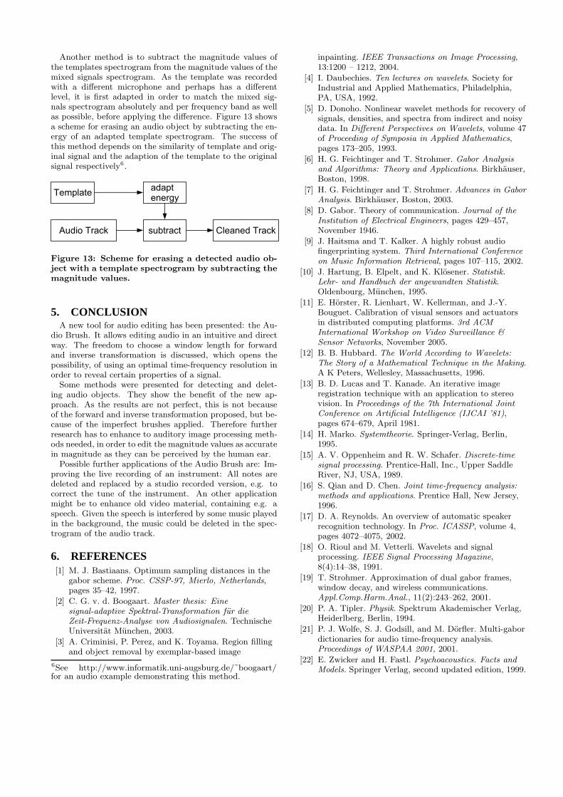
Another method is to subtract the magnitude values ofthe templates spectrogram from the magnitude values of themixed signals spectrogram. As the template was recordedwith a different microphone and perhaps has a differentlevel, it is first adapted in order to match the mixed sig-nals spectrogram absolutely and per frequency band as wellas possible, before applying the difference. Figure 13 showsa scheme for erasing an audio object by subtracting the en-ergy of an adapted template spectrogram. The success ofthis method depends on the similarity of template and orig-inal signal and the adaption of the template to the originalsignal respectively6.

Figure 13: Scheme for erasing a detected audio ob-ject with a template spectrogram by subtracting themagnitude values.

5. CONCLUSIONA new tool for audio editing has been presented: the Au-

dio Brush. It allows editing audio in an intuitive and directway. The freedom to choose a window length for forwardand inverse transformation is discussed, which opens thepossibility, of using an optimal time-frequency resolution inorder to reveal certain properties of a signal.

Some methods were presented for detecting and delet-ing audio objects. They show the benefit of the new ap-proach. As the results are not perfect, this is not becauseof the forward and inverse transformation proposed, but be-cause of the imperfect brushes applied. Therefore furtherresearch has to enhance to auditory image processing meth-ods needed, in order to edit the magnitude values as accuratein magnitude as they can be perceived by the human ear.

Possible further applications of the Audio Brush are: Im-proving the live recording of an instrument: All notes aredeleted and replaced by a studio recorded version, e.g. tocorrect the tune of the instrument. An other applicationmight be to enhance old video material, containing e.g. aspeech. Given the speech is interfered by some music playedin the background, the music could be deleted in the spec-trogram of the audio track.

6. REFERENCES[1] M. J. Bastiaans. Optimum sampling distances in the

gabor scheme. Proc. CSSP-97, Mierlo, Netherlands,pages 35–42, 1997.

[2] C. G. v. d. Boogaart. Master thesis: Einesignal-adaptive Spektral-Transformation fur dieZeit-Frequenz-Analyse von Audiosignalen. TechnischeUniversitat Munchen, 2003.

[3] A. Criminisi, P. Perez, and K. Toyama. Region fillingand object removal by exemplar-based image

6See http://www.informatik.uni-augsburg.de/˜boogaart/for an audio example demonstrating this method.

inpainting. IEEE Transactions on Image Processing,13:1200 – 1212, 2004.

[4] I. Daubechies. Ten lectures on wavelets. Society forIndustrial and Applied Mathematics, Philadelphia,PA, USA, 1992.

[5] D. Donoho. Nonlinear wavelet methods for recovery ofsignals, densities, and spectra from indirect and noisydata. In Different Perspectives on Wavelets, volume 47of Proceeding of Symposia in Applied Mathematics,pages 173–205, 1993.

[6] H. G. Feichtinger and T. Strohmer. Gabor Analysisand Algorithms: Theory and Applications. Birkhauser,Boston, 1998.

[7] H. G. Feichtinger and T. Strohmer. Advances in GaborAnalysis. Birkhauser, Boston, 2003.

[8] D. Gabor. Theory of communication. Journal of theInstitution of Electrical Engineers, pages 429–457,November 1946.

[9] J. Haitsma and T. Kalker. A highly robust audiofingerprinting system. Third International Conferenceon Music Information Retrieval, pages 107–115, 2002.

[10] J. Hartung, B. Elpelt, and K. Klosener. Statistik.Lehr- und Handbuch der angewandten Statistik.Oldenbourg, Munchen, 1995.

[11] E. Horster, R. Lienhart, W. Kellerman, and J.-Y.Bouguet. Calibration of visual sensors and actuatorsin distributed computing platforms. 3rd ACMInternational Workshop on Video Surveillance &Sensor Networks, November 2005.

[12] B. B. Hubbard. The World According to Wavelets:The Story of a Mathematical Technique in the Making.A K Peters, Wellesley, Massachusetts, 1996.

[13] B. D. Lucas and T. Kanade. An iterative imageregistration technique with an application to stereovision. In Proceedings of the 7th International JointConference on Artificial Intelligence (IJCAI ’81),pages 674–679, April 1981.

[14] H. Marko. Systemtheorie. Springer-Verlag, Berlin,1995.

[15] A. V. Oppenheim and R. W. Schafer. Discrete-timesignal processing. Prentice-Hall, Inc., Upper SaddleRiver, NJ, USA, 1989.

[16] S. Qian and D. Chen. Joint time-frequency analysis:methods and applications. Prentice Hall, New Jersey,1996.

[17] D. A. Reynolds. An overview of automatic speakerrecognition technology. In Proc. ICASSP, volume 4,pages 4072–4075, 2002.

[18] O. Rioul and M. Vetterli. Wavelets and signalprocessing. IEEE Signal Processing Magazine,8(4):14–38, 1991.

[19] T. Strohmer. Approximation of dual gabor frames,window decay, and wireless communications.Appl.Comp.Harm.Anal., 11(2):243–262, 2001.

[20] P. A. Tipler. Physik. Spektrum Akademischer Verlag,Heiderlberg, Berlin, 1994.

[21] P. J. Wolfe, S. J. Godsill, and M. Dorfler. Multi-gabordictionaries for audio time-frequency analysis.Proceedings of WASPAA 2001, 2001.

[22] E. Zwicker and H. Fastl. Psychoacoustics. Facts andModels. Springer Verlag, second updated edition, 1999.